Embed Size (px)
Citation preview
NASA Contractor Report 3 640
Aeroelastic Loads Prediction for an Arrow Wing
Task I - Evaluation of R. P. White’s Method
Christopher J. Borland
CONTRACT NASI-15678 MARCH 1983
25th Anniversary 1958-1983
TECH LIBRARY KAFB, NM
. -..._ ..I OOb2l,80 ---.‘--’
NASA Contractor Report 3 640
Aeroelastic Loads Prediction for an Arrow Wing
Task I - Evaluation of R. P. White’s Method
Christopher J. Borland Boeing Conzmercial Airplane Company Seattle, Washington
Prepared for Langley Research Center under Contract NAS I- 15 6 7 8
MSA National Aeronautics and Space Administration
Scientific and Technical Information Branch
1983

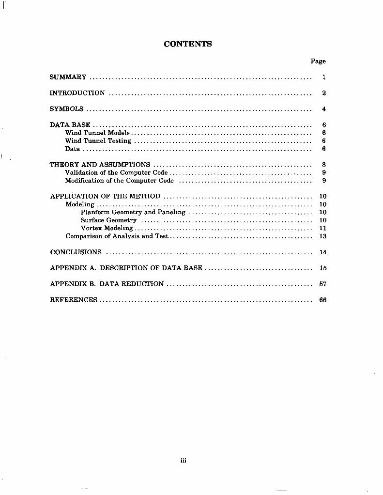
CONTENTS
Page
SUMMARY ......................................................................
INTRODUCTION ................................................................
SYMBOLS .......................................................................
DATA BASE ..................................................................... Wind Tunnel Models ......................................................... Wind Tunnel Testing ........................................................ Data ........................................................................
THEORY AND ASSUMPTIONS .................................................. Validation of the Computer Code ............................................. Modification of the Computer Code ..........................................
APPLICATION OF THE METHOD ............................................... Modeling ....................................................................
Planform Geometry and Paneling ....................................... Surface Geometry ...................................................... Vortex Modeling ........................................................
Comparison of Analysis and Test. ............................................
CONCLUSIONS .................................................................
APPENDIX A. DESCRIPTION OF DATA BASE ..................................
APPENDIX B. DATA REDUCTION ..............................................
REFERENCES ...................................................................
1
2
4
6 6 6 6
8 9 9
10 10 10 10 11 13
14
15
57
66
. . . lu
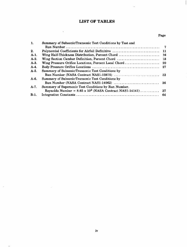
LIST OF TABLES
1.
2. A-l. A-2. A-3. A-4. A-5.
A-6.
A-7.
B-l.
Page
Summary of SubsoniwTransonic Test Conditions by Test and RunNumber ............................................................ 7
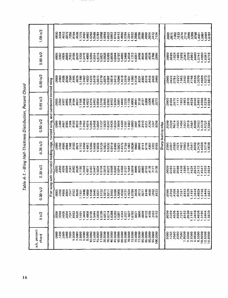
Polynomial Coefficients for Airfoil Definitive .............................. 11 Wing Half-Thickness Distribution, Percent Chord .......................... 16 Wing Section Camber Definition, Percent Chord ........................... 18 Wing Pressure Orifice Locations, Percent Local Chord ...................... 20 Body Pressure Orifice Locations ........................................... 27 Summary of Subsonic/Transonic Test Conditions by
Run Number (NASA Contract NASl-12875) ............................. 33 Summary of Subsonic/Transonic Test Conditions by
Run Number (NASA Contract NASl-14962) ............................. 36 Summary of Supersonic Test Conditions by Run Number.
Reynolds Number = 8.65 x lo6 (NASA Contract NASl-14141) ............ 37 IntegrationConstants.. ................................................... 64
iv
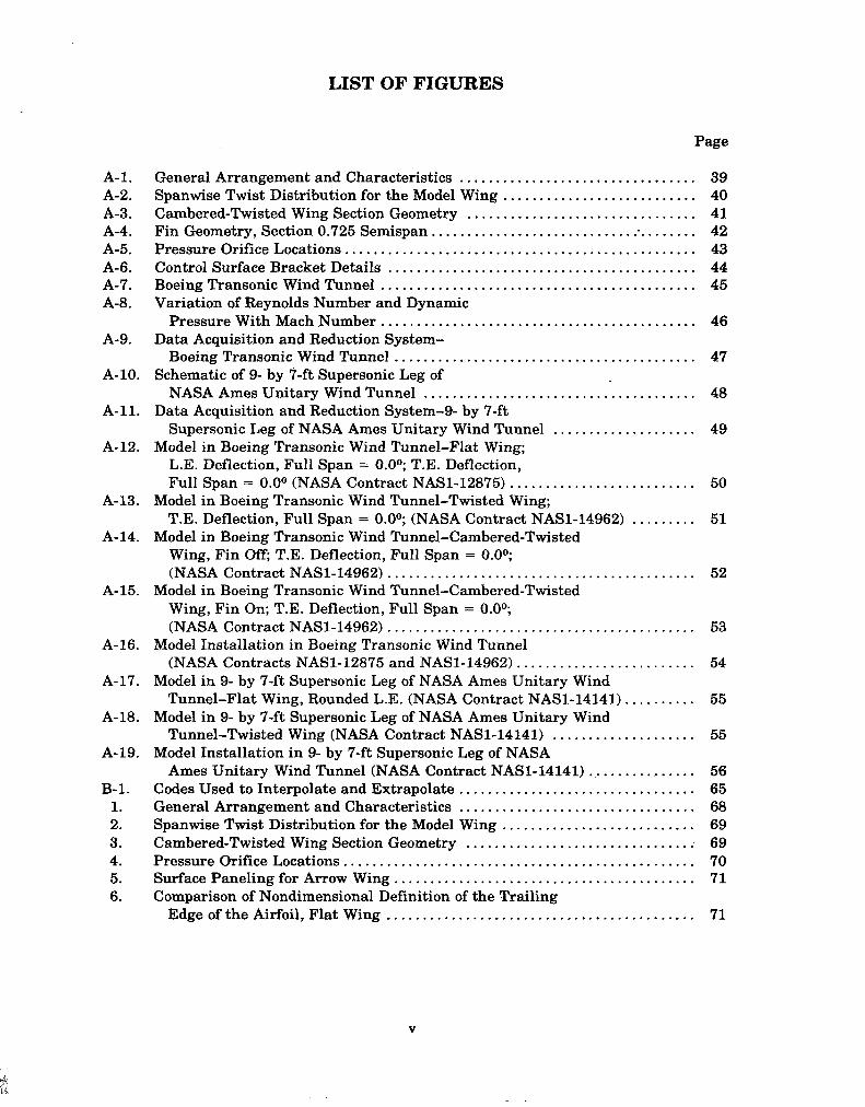
LIST OF FIGURES
Page
A-l. A-2. A-3. A-4. A-5. A-6. A-7. A-8.
A-9.
A-10.
A-11.
A-12.
A-13.
A-14.
A-15.
A-16.
A-17.
A-18.
A-19.
B-l. 1. 2. 3. 4. 5. 6.
General Arrangement and Characteristics ................................. 39 Spanwise Twist Distribution for the Model Wing ........................... 40 Cambered-Twisted Wing Section Geometry ................................ 41 Fin Geometry, Section 0.725 Semispan ...................................... 42 Pressure Orifice Locations ................................................. 43 Control Surface Bracket Details ........................................... 44 Boeing Transonic Wind Tunnel ............................................ 45 Variation of Reynolds Number and Dynamic
Pressure With Mach Number ............................................ 46 Data Acquisition and Reduction System-
Boeing Transonic Wind Tunnel .......................................... 47 Schematic of 9- by i-ft Supersonic Leg of
NASA Ames Unitary Wind Tunnel ...................................... 48 Data Acquisition and Reduction System-g- by 7-ft
Supersonic Leg of NASA Ames Unitary Wind Tunnel .................... 49 Model in Boeing Transonic Wind Tunnel-Flat Wing;
L.E. Deflection, Full Span = O.OO; T.E. Deflection, Full Span = O.O” (NASA Contract NASl-12875) .......................... 50
Model in Boeing Transonic Wind Tunnel-Twisted Wing; T.E. Deflection, Full Span = O.O”; (NASA Contract NASl-14962) ......... 51
Model in Boeing Transonic Wind Tunnel-Cambered-Twisted Wing, Fin Off; T.E. Deflection, Full Span = O.OO; (NASA Contract NASl-14962) ........................................... 52
Model in Boeing Transonic Wind Tunnel-Cambered-Twisted Wing, Fin On; T.E. Deflection, Full Span = O.OO; (NASA Contract NASl-14962) ........................................... 53
Model Installation in Boeing Transonic Wind Tunnel (NASA Contracts NASl-12875 and NASl-14962). ........................ 54
Model in 9- by 7-ft Supersonic Leg of NASA Ames Unitary Wind Tunnel-Flat Wing, Rounded L.E. (NASA Contract NASl-14141). ......... 55
Model in 9- by 7-ft Supersonic Leg of NASA Ames Unitary Wind Tunnel-Twisted Wing (NASA Contract NASl-14141) .................... 55
Model Installation in 9- by 7-ft Supersonic Leg of NASA Ames Unitary Wind Tunnel (NASA Contract NASl-14141) ................. 56
Codes Used to Interpolate and Extrapolate ................................. 65 General Arrangement and Characteristics ................................. 68 Spanwise Twist Distribution for the Model Wing ........................... 69 Cambered-Twisted Wing Section Geometry ................................ 69 Pressure Orifice Locations ................................................. 70 Surface Paneling for Arrow Wing .......................................... 71 Comparison of Nondimensional Definition of the Trailing
Edge of the Airfoil, Flat Wing ........................................... 71
V
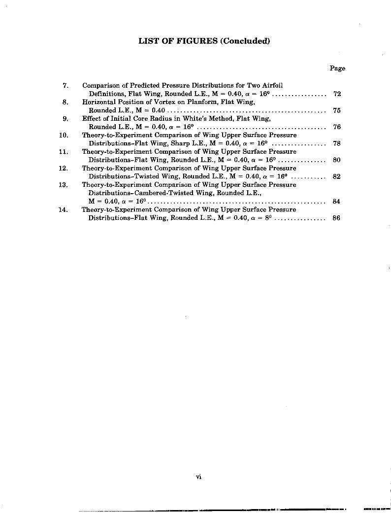
LIST OF FIGURES (Concluded)
Page
7.
8.
9.
10.
11.
12.
13.
14.
Comparison of Predicted Pressure Distributions for Two Airfoil Definitions, Flat Wing, Rounded L.E., M = 0.40, OL = 16O . . . . . . . . . . . . . . . . . 72
Horizontal Position of Vortex on Planform, Flat Wing, Rounded L.E., M = 0.40 . . . . . . . . . . . . . . . . . . . . . . . . . . . . . . . . . . . . . . . . . . . . . . . . . 75
Effect of Initial Core Radius in White’s Method, Flat Wing, Rounded L.E., M = 0.40, (Y = 16O . . . . . . . . . . . . . . . . . . . . . . . . . . . . . . . . . . . . . . . . 76
Theory-to-Experiment Comparison of Wing Upper Surface Pressure Distributions-Flat Wing, Sharp L.E., M = 0.40, cr = 16O . . . . . . . . . . . . . . . . . 78
Theory-to-Experiment Comparison of Wing Upper Surface Pressure Distributions-Flat Wing, Rounded L.E., M = 0.40, (Y = 16O . . . . . . . . . . . . . . . 80
Theory-to-Experiment Comparison of Wing Upper Surface Pressure Distributions-Twisted Wing, Rounded L.E., M = 0.40, cy = 16O . . . . . . . . . . . 82
Theory-to-Experiment Comparison of Wing Upper Surface Pressure Distributions-Cambered-Twisted Wing, Rounded L.E., M = 0.40,(~ = 16O....................................................... 84
Theory-to-Experiment Comparison of Wing Upper Surface Pressure Distributions-Flat Wing, Rounded L.E., M = 0.40, (Y = 8O . . . . . . . . . . . . . . . . 86
SUMMARY
The accurate prediction of loads on flexible, low aspect-ratio wings is critical to the design of reliable and efficient aircraft. The conditions for structural design frequently involve nonlinear aerodynamics.
Under previous NASA contracts (NASl-12875, NASl-14141, and NASl-14962) a large experimental data base for three wing shapes was obtained, and .linear theoretical methods were evaluated. The current contract, NASl-15678, extends the evaluation of state-of-the-art theoretical predictive methods to two separated-flow computer programs and also evaluates a semi-empirical method for incorporating the experimentally measured separated-flow effects into a linear aeroelastic analysis.
The resultant three tasks have been documented separately. This volume describes the evaluation of R. P. White’s (RASA Division of Systems Research Laboratories) separated-flow method (Task I). The evaluation of The Boeing Company’s Three-Dimensional Leading-Edge Vortex (LEV) code (Task III) is presented in NASA CR-3642. The development and evaluation of a semi-empirical method to predict pressure distributions on a deformed wing by using an experimental data base (Task II) is described in NASA CR-3641.
The method of R. P. White was developed for moderately swept wings with multiple, constant-strength vortex systems. The flow on the highly swept wing used in this evaluation is characterized by a single vortex system of continuously varying strength. The data comparisons, as currently formulated, show that this method does not predict the pressure distribution on this highly swept wing.
INTRODUCTION
Accurate analytical techniques for the prediction of the magnitude and distribution of aeroelastic loads are required in order to achieve an optimum design of the structure of large flexible aircraft. Uncertainties in the characteristics of loads may result in an improper accounting for aeroelastic effects, leading to understrength or overweight designs and. unacceptable fatigue life. In addition, the correct prediction of load distribution and the resultant structural deformation is essential to the determination of the aircraft stability and control characteristics, control power requirements, and flutter boundaries. The alternative to using satisfactory analytical techniques is the increased use of expensive, time-consuming wind tunnel testing for each aircraft configuration.
The problem of accurate load prediction becomes particularly acute for aircraft with low aspect-ratio wings where critical design conditions occur in the transonic speed regime. In this region, at typical design angles of attack, the flow is generally nonlinear - mixed flow, embedded shocks, separation, and vortex flow.
A program was started in 1974 to systematically obtain experimental pressure data for an arrow wing throughout the subsonic, transonic, and low supersonic Mach numbers. This program was comprised of three NASA contracts: NASl-12875, NASl-14141, and NASl-14962 (documented in refs. 1 through 12). As the specific objective was to understand the change in load with aeroelastic deformation, three wing shapes were tested - all with the same planform and thickness distribution. The first wing was flat (no camber or twist); the second has a spanwise twist (typical of aeroelastic deformation) but no camber; and the third has the same twist with camber superimposed.
In addition to the creation of a data base, which is useful for evaluating aeroelastic effects, a second objective was to evaluate state-of-the-art theoretical methods that might be used for this purpose. Primarily these methods were linear. The evaluations showed that linear theories are adequate at low angles of attack typical of cruise conditions and are basically capable of predicting loading changes due to smooth changes in wing shape at these low angles. However, at the higher angles of attack typical of structural design conditions, these methods are not useful because the flow is nonlinear due to leading-edge separation of the flow. The limited comparisons that were made with advanced separated-flow methods indicated some hope even though the aerodynamic panel model available at that time was very crude (only a few panels to represent the camber surface).
The current evaluation of methods for predicting pressure distributions when the flow is separated is divided into three tasks. Two currently available computer codes were evaluated in Tasks I and III, and an approach involving semi-empirical corrections to linear theory was investigated in Task II. The three tasks are essentially independent efforts and are documented separately: Task I, an evaluaton of R. P. White’s computer code in this document; Task II, the development and evaluation of a semi-empirical method in NASA CR-3641; and Task III, an evaluation of Boeing’s Three-Dimensional Leading-Edge Vortex computer code in NASA CR-3642.
2
The computer code ‘evaluated in Task I is the method of R. P. White of the RASA Division of Systems Research Laboratories, which models the vortex as a concentrated region of vorticity over the wing, and adds the results of this phenomenon to that of the linearized flow over a thin wing. The NASA arrow-wing configuration data base described above was used for this evaluation to determine the possible applicability of this method to the prediction of aeroelastic loads on highly swept wings. The following are discussed: theoretical basis of White’s method; implementation of the method in a computer code; modeling of the arrow wing for analysis by the method; comparisons of calculated and experimental data; and the results of the evaluation.
3

SYMBOLS
b
BL
C
E, M.A.C.
CB
CC
cc
CM
c In
C m.25c
CN
crl
%
D
M
MS
Ps
Pt
q
S
Sh
vco
wing span, cm
buttock line, cm; distance outboard from model plane of symmetry
section chord length, cm
mean aerodynamic chord length, cm
surface bending moment coefficient referenced to yref, positive wingtip up
surface chord force coefficient; positive aft
section chord force coefficient; positive aft
surface pitching moment coefficient, referenced to 0.25 M.A.C.; positive leading edge up
section pitching moment coefficient referenced to section leading edge; positive leading edge up
section pitching moment coefficient referenced to section 0.25~; positive leading edge up
surface normal force coefficient; positive up
section normal force coefficient; positive up
pressure coefficient = measured pressure - reference pressure q
body diameter, cm
Mach number
model station, cm; measured aft along the body centerline from the nose
static pressure, kN/m2
total pressure, kN/m2
dynamic pressure, kN/m2
reference area used for surface coefficients, cm2
area of streamwise strip associated with a pressure station, cm2; used in summation of section force coefficients (app. B)
free stream velocity
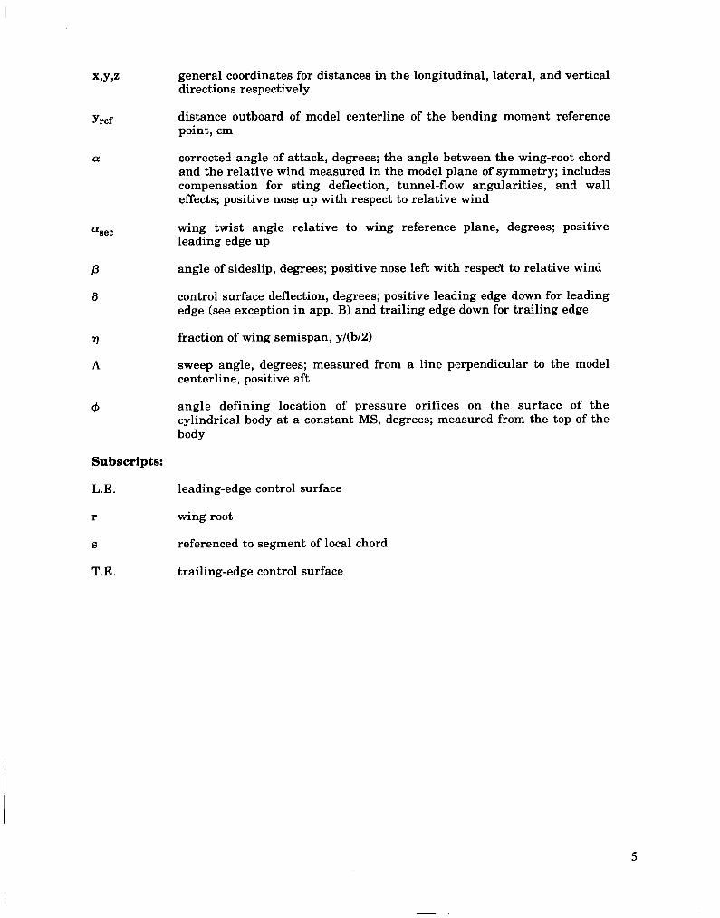
X,Y,Z general coordinates for distances in the longitudinal, lateral, and vertical directions respectively
Yref distance outboard of model centerline of the bending moment reference point, cm
ct! corrected angle of attack, degrees; the angle between the wing-root chord and the relative wind measured in the model plane of symmetry; includes compensation for sting deflection, tunnel-flow angularities, and wall effects; positive nose up with respect to relative wind
%ec wing twist angle relative to wing reference plane, degrees; positive leading edge up
P angle of sideslip, degrees; positive nose left with respect to relative wind
6 control surface deflection, degrees; positive leading edge down for leading edge (see exception in app. B) and trailing edge down for trailing edge
7) fraction of wing semispan, y/(b/2)
A sweep angle, degrees; measured from a line perpendicular to the model centerline, positive aft
angle defining location of pressure orifices on the surface of the cylindrical body at a constant MS, degrees; measured from the top of the body
Subscripts:
L.E. leading-edge control surface
r
S
wing root
referenced to segment of local chord
T.E. trailing-edge control surface
DATA BASE
The data obtained, both experimental and theoretical, have been presented in several papers (refs. 1 through 3) and are presented in more detail in numerous NASA reports (refs. 4 through 12).
WIND TUNNEL MODELS
The configuration chosen for this study was a thin, low aspect-ratio, highly swept wing mounted below the centerline of a high fineness-ratio body. The general arrangement and characteristics of the model are shown in figure 1. Two complete wings were constructed for contract NASl-12875, one with no camber or twist and one with no camber but with a spanwise twist variation. A third wing with camber and twist was constructed for c6ntract NASl-14962. Deflectable control surfaces were available on all three of these wings.
The three wings, body, and fin used to create this data base are described in detail in appendix A. The wings all have the same planform, thickness distribution, and placement of orifices. The twisted wing and the cambered-twisted wing have the same twist, i.e., the coordinates of the leading edges and trailing edges of the two wings are the same. This twist distribution is shown in figure 2. Sections at the root, midspan, and tip of the cambered-twisted wing (fig. 3) show not only the camber but the position of the sections of the cambered-twisted wing and the twisted wing, relative to the wing reference plane (flat wing). The flat wing had a sharp leading-edge segment in addition to the rounded leading-edge segment common to all three wings.
The capability to measure the detailed load distribution on the wing and body of this configuration was provided by distributing 300 pressure orifices on the model. Each wing had 217 pressure orifices equally divided into seven streamwise sections on the left half. Orifices were located on both the top and bottom surfaces at the chordwise locations shown in figure 4. Pressure orifices were located on the body in five streamwise rows of- 15 orifices each. An additional eight orifices in the area of the wing-body junction made a total of 83 orifices on the left side of the body.
WIND TUNNEL TESTING
The experimental data used in this study were obtained in the Boeing Transonic Wind Tunnel (BTWT) under NASA contracts NASH-12875 and NAS1;14962. A description of the tunnel and tests are in appendix A. The current study was limited to the wings that had both leading-edge and trailing-edge control surfaces undeflected. Table 1 shows a summary of these data.
DATA
The measured pressures were edited, as necessary, to account for plugged or leaking orifices or missing data points. The pressure coefficients were then integrated, as described in appendix B, to obtain streamwise section coefficients and total surface coefficients. When pressure coefficients were required at points other than where measured, a linear interpolation was used.
6
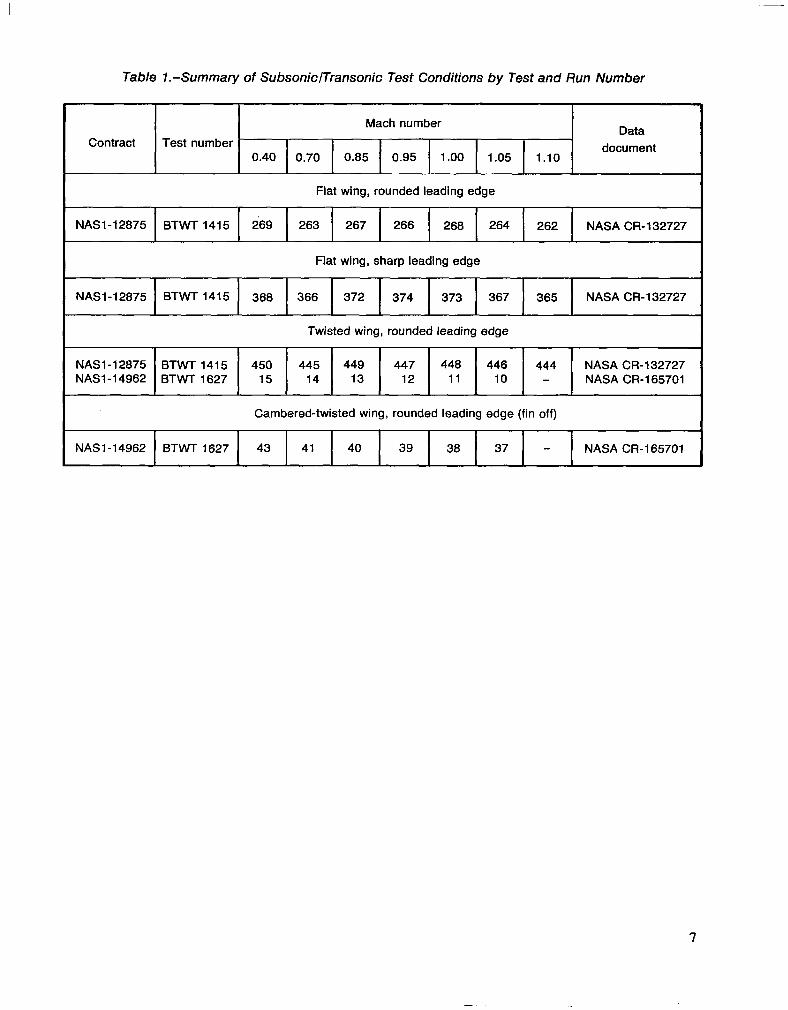
Table l.-Summary of SubsoniclTransonic Test Conditions by Test and Run Number
Mach number Data
Contract Test number document 0.40 0.70 0.85 0.95 1 .oo 1.05 1.10
Fiat wing, rounded leading edge
NASI-12875 BTWT 1415 289 283 287 288 288 284 282 NASA CR-1 32727
Flat wing, sharp leading edge
NASI-12875 BTWT 1415 388 386 372 374 373 367 365 NASA CR-1 32727
Twisted wing, rounded leading edge
NASI-12875 BTWT 1415 450 445 449 447 448 446 444 NASA CR-l 32727 NASI-14962 BTWT 1627 15 14 13 12 11 10 - NASA CR-l 65701
Cambered-twisted wing, rounded leading edge (fin off)
NASI-14962 BTWT 1627 43 41 40 39 38 37 - NASA CR-l 65701
7
THEORY AND ASSUMPTIONS
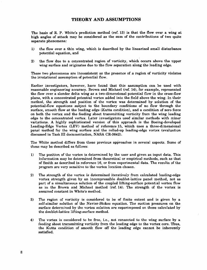
The basis of R. P. White’s prediction method (ref. 13) is that the flow over a wing at high angles of attack may be considered as the sum of the contributions of two quite separate phenomena:
1) the flow over a thin wing, which is described by the linearized small disturbance potential equation, and
2) the flow due to a concentrated region of vorticity, which occurs above the upper wing surface and originates due to the flow separation along the leading edge.
These two phenomena are inconsistent as the presence of a region of vorticity violates the irrotational assumption of potential flow.
Earlier investigators, however, have found that this assumption can be used with reasonable engineering accuracy. Brown and Michael (ref. 14), for example, represented the flow over a slender delta wing as a two-dimensional potential flow in the cross-flow plane, with a concentrated potential vortex added into the field above the wing. In their method, the strength and position of the vortex was determined by solution of the potential-flow equations subject to the boundary conditions of no flow through the surface, smooth flow at the leading edge (Kutta condition), and a condition of zero force on both the vortex and the feeding sheet transmitting vorticity from the wing leading edge to the concentrated vortex. Later investigators used similar methods with minor variations. A highly sophisticated version of this approach is the Boeing-developed Leading-Edge Vortex (LEV) method of reference 15, which uses a three-dimensional panel method for the wing surface and the rolled-up leading-edge vortex (evaluation discussed in Task III documentation, NASA CR-3642).
The White method differs from these previous approaches in several aspects. Some of these may be described as follows:
1)
2)
3)
4)
The position of the vortex is determined by the user and given as input data. This information may be determined from theoretical or empirical methods, such as that of Smith as described in reference 16, or from experimental data. The results of the program are very sensitive to the vortex location chosen.
The strength of the vortex is determined iteratively from calculated leading-edge vortex strength given by an incompressible doublet-lattice panel method, not as part of a simultaneous solution of the coupled lifting-surface potential vortex flow as in the Brown and Michael method (ref. 14). The strength of the vortex is assumed constant in White’s method.
The region of vorticity is considered to be of finite extent and is given by a self-similar solution of the Navier-Stokes equation. The suction pressures on the surface determined by the vortex solution are superimposed on those calculated by the doublet-lattice lifting-surface method.
The vortex is’considered to be free, i.e., not connected to the wing surface by a feeding sheet transmitting vorticity from the leading edge to the vortex core. Thus, the Kutta condition of smooth flow off the leading edge cannot be inherently satisfied.
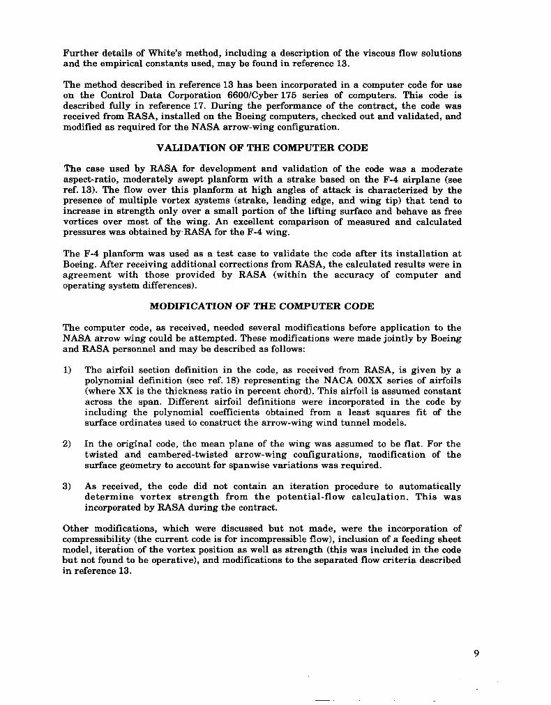
Further details of White’s method, including a description of the viscous flow solutions and the empirical constants used, may be found in reference 13.
The method described in reference 13 has been incorporated in a computer code for use on the Control Data Corporation 6600/Cyber 175 series of computers. This code is described fully in reference 17. During the performance of the contract, the code was received from RASA, installed on the Boeing computers, checked out and validated, and modified as required for the NASA arrow-wing configuration.
VALIDATION OF THE COMPUTER CODE
The case used by RASA for development and validation of the code was a moderate aspect-ratio, moderately swept planform with a strake based on the F-4 airplane (see ref. 13). The flow over this planform at high angles of attack is characterized by the presence of multiple vortex systems (strake, leading edge, and wing tip) that tend to increase in strength only over a small portion of the lifting surface and behave as free vortices over most of the wing. An excellent comparison of measured and calculated pressures was obtained by.RASA for the F-4 wing.
The F-4 planform was used as a test case to validate the code after its installation at Boeing. After receiving additional corrections from RASA, the calculated results were in agreement with those provided by RASA (within the accuracy of computer and operating system differences).
MODIFICATION OF THE COMPUTER CODE
The computer code, as received, needed several modifications before application to the NASA arrow wing could be attempted. These modifications were made jointly by Boeing and RASA personnel and may be described as follows:
1) The airfoil section definition in the code, as received from RASA, is given by a polynomial definition (see ref. 18) representing the NACA OOXX series of airfoils (where XX is the thickness ratio in percent chord). This airfoil is assumed constant across the span. Different airfoil definitions were incorporated in the code by including the polynomial coefficients obtained from a least squares fit of the surface ordinates used to construct the arrow-wing wind tunnel models.
2) In the original code, the mean plane of the wing was assumed to be flat. For the twisted and cambered-twisted arrow-wing configurations, modification of the surface geometry to account for spanwise variations was required.
3) As received, the code did not contain an iteration procedure to automatically determine vortex strength from the potential-flow calculation. This was incorporated by RASA during the contract.
Other modifications, which were discussed but not made, were the incorporation of compressibility (the current code is for incompressible flow), inclusion of a feeding sheet model, iteration of the vortex position as well as strength (this was included in the code but not found to be operative), and modifications to the separated flow criteria described in reference 13.
9
APPLICATION OF THE METHOD
After installation and validation of the code, the NASA arrow-wing configuration was modeled for input to the program. The cases that were run for comparison with the experiment consisted of the flat, twisted, and cambered-twisted wings at a Mach number of 0.40 and an angle of attack of 16O. In addition, the flat wing was run at an angle of attack of 8O. The results of these cases and the comparison with experimental data are described in this section.
MODELING
The modeling consists of three general parts. The procedure for this modeling, along with the difficulties that were encountered, are described.
PLANFORM GEOMETRY AND PANELING
Surface paneling of the wing is required for implementation of the doublet-lattice method for the linear part of the flow. Paneling in the code is either manual (user input of constant percent chord (x/c) and constant fraction of semispan (y/(b/2)) locations for the panel edges) or automatic (a standard set of nondimensional paneling). The automatic option was used for the arrow wing. Figure 5 shows the paneling used. The code assumes the paneling is the same for the upper and lower surfaces of the wing.
SURFACE GEOMETRY
In the White method, the boundary condition of no flow through the surface is specified on the actual airfoil surface. It is, therefore, necessary to provide an accurate representation of the surface thickness, camber, and twist distributions. In the original code, an NACA OOXX series airfoil was used with the surface shape represented by the polynomial description given in reference 18. The wing was assumed to be symmetric about the mean plane, i.e., no twist or camber. In order to represent the various configurations of the NASA arrow wing, development of new surface representations and modifications to the code were required.
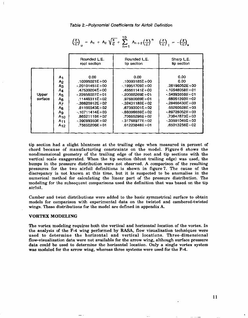
The polynominal coefficients to represent the thickness of these airfoils (with both rounded and sharp leading edges) were obtained with a least squares fit of the surface coordinates of the airfoil (z/c versus x/c). Table 2 shows the form of the polynomial used to fit the geometry and the coefficients obtained. These coefficients were used to define surface geometry and slope in White’s code. A comparison of the forward portions of the rounded- and sharp-airfoil sections, as used, are shown in figure 4.
The nondimensional airfoil sections also varied as a function of span because the trailing edge is a constant 0.0254 cm (0.01 in.) thick due to manufacturing constraints on the models. It was assumed for purposes of incorporating the geometry in White’s code that a constant spanwise section could be used. This assumption caused some difficulty as the answers varied greatly, depending on whether the root section or tip section was chosen as representative.
The root section, which has a relatively sharp trailing edge, was originally used to define the airfoil. This gave large bumps in the pressure distribution near the trailing edge, which were not observed in the experimental data. As previously mentioned, the
10
Upper surface
Al A2 A3 A4 As A6 A7 A8 4 A10 AII A12
Table 2. -Polynomial Coefficients for Airfoil Definition
2 0 Fu= AI + AZ I& g, An+z(-$)” (-), = -($),
Rounded L.E. root section
0.00 .I0095021 E+OO
-.20101451E+00 .47539204E+OO
-.22656037E+Ol .11448311E+02
-.38620912E+O2 .81190343E+02
-.10711414E+03 .86521116E+02
-.39099350E+02 .75650206E+Ol
Rounded L.E. tip section
0.00 .10093185E+00
-.19951709E+00 .45661141E+OO
-.20088269E+Ol .97680669E+Ol
-.32431182E+02 .67393001 E+02
-.88096659E+02 .70665296E +02
-.31768977E+02 .61223848E+Ol
Sharp L.E. tip section
0.00 0.00
.26196052E+OO -.10548058E+Ol -.54993659E+Ol .68051393E+02
-.28466430E+03 .65260528E+03
-.89728052E+03 .73847873E+03
-.33591049E+03 .65013256E+02
tip section had a slight bluntness at the trailing edge when measured in percent of chord because of manufacturing constraints on the model. Figure 6 shows the nondimensional geometry of the trailing edge of the root and tip sections with the vertical scale exaggerated. When the tip section (blunt trailing edge) was used, the bumps in the pressure distribution were not observed. A comparison of the resulting pressures for the two airfoil definitions is shown in figure 7. The cause of the discrepancy is not known at this time, but it is suspected to be anomalies in the numerical method for calculating the linear part of the pressure distribution. The modeling for the subsequent comparisons used the definition that was based on the tip airfoil.
Camber and twist distributions were added to the basic symmetrical surface to obtain models for comparison with experimental data on the twisted and cambered-twisted wings. These distributions for the model are defined in appendix A.
VORTEX MODELING
The vortex modeling requires both the vertical and horizontal location of the vortex. In the analysis of the F-4 wing performed by RASA, flow visualization techniques were used to determine the horizontal and vertical locations. Three-dimensional flow-visualization data were not available for the arrow wing, although surface pressure data could be used to determine the horizontal location. Only a single vortex system was modeled for the arrow wing, whereas three systems were used for the F-4.
11
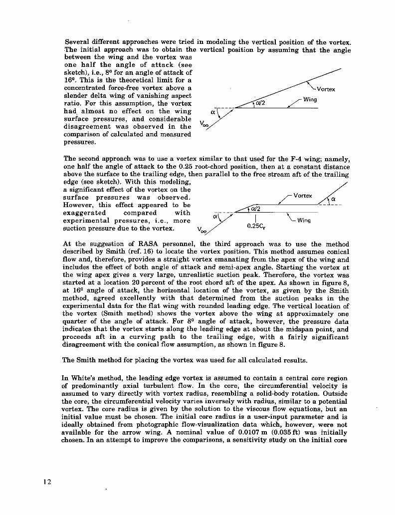
Several different approaches were tried in modeling the vertical position of the vortex. .The initial approach was to obtain the vertical position by assuming that the angle between the wing and the vortex was one half the angle of attack (see sketch), i.e., 8O for an angle of attack of 16O. This is the theoretical limit for a concentrated force-free vortex above a slender delta wing of vanishing aspect ratio. For this assumption, the vortex had. almost no effect on the wing surface pressures, and considerable v disagreement was observed in the comparison of calculated and measured pressures.
The second approach was to use a vortex similar to that used for the F-4 wing; namely, one half the angle of attack to the 0.25 root-chord position, then at a constant distance above the surface to the trailing edge, then parallel to the free stream aft of the trailing edge (see sketch). With this modeling, a significant effect of the vortex on the surface pressures was observed. However, this effect appeared to be exaggerated compared with experimental pressures, i.e., more suction pressure due to the vortex.
7A$g
“00 0.25C,
At the suggestion of RASA personnel, the third approach was to use the method described by Smith (ref. 16) to locate the vortex position. This method assumes conical flow and, therefore, provides a straight vortex emanating from the apex of the wing and includes the effect of both angle of attack and semi-apex angle. Starting the vortex at the wing apex gives a very large, unrealistic suction peak. Therefore, the vortex was started at a location 20 percent of the root chord aft of the apex. As shown in figure 8, at 16O angle of attack, the horizontal location of the vortex, as given by the Smith method, agreed excellently with that determined from the suction peaks in the experimental data for the flat wing with rounded leading edge. The vertical location of the vortex (Smith method) shows the vortex above the wing at approximately one quarter of the angle of attack. For 8O angle of attack, however, the pressure data indicates that the vortex starts along the leading edge at about the midspan point, and proceeds aft in a curving path to the trailing edge, with a fairly significant disagreement with the conical flow assumption, as shown in figure 8.
The Smith method for placing the vortex was used for all calculated results.
In White’s method, the leading edge vortex is assumed to contain a central core region of predominantly axial turbulent flow. In the core, the circumferential velocity is assumed to vary directly with vortex radius, resembling a solid-body rotation. Outside the core, the circumferential velocity varies inversely with radius, similar to a potential vortex. The core radius is given by the solution to the viscous flow equations, but an initial value must be chosen. The initial core radius is a user-input parameter and is ideally obtained from photographic flow-visualization data which, however, were not available for the arrow wing. A nominal value of 0.0107 m (0.035 ft) was initially chosen. In an attempt to improve the comparisons, a sensitivity study on the initial core
12
radius was performed. Higher and lower values of 0.0427 m (0.140 ft) and 0.0030 m (0.01 ft) were tried. A comparison of the calculated pressures for these three values is shown in figure 9. It may be seen that no consistent trend in the pressures can be observed due to this change in core radius, therefore, the initial core radius of 0.0107 m (0.035 ft) was used for the study.
COMPARISON OF ANALYSIS AND TEST
Calculations on the arrow-wing configuration were performed using White’s code, modified to account for the exact surface geometry. Since the code was limited to incompressible flow, the results are compared to experimental data at a Mach number of 0.40, the lowest Mach number tested. Most of the calculations were done for an angle of attack of 16O. Some calculations were later performed at about 8O.
Chordwise pressure distributions on the arrow wing were measured at seven spanwise locations: y/(b/2) = 0.09, 0.20, 0.35, 0.50, 0.65, 0.80, and 0.93. The code, as written, evaluates pressures at y/(b/2) = 0.01 and at each increment of 0.02 across the wing. This difference in fraction of semispan of 0.01, where it occurs, was assumed negligible in comparing calculated and experimental pressures.
Figures- 10 through’ 13 show a comparison of calculated and experimental data at 16O angle of attack. Figure 10 shows the calculated and measured upper-surface pressure coefficients for the flat wing with sharp leading edge. The pressure distribution is not predicted accurately and is not adequate for design loads. The calculated pressure distributions show “humps,” which may be interpreted as the effect of vortex suction. At one section (y/(b/2) = 0.201, the comparison of theoretical and experimental pressures shows fairly good agreement; unfortunately, this appears to be merely fortuitous. The vortex effect is far more pronounced in the experimental data, particularly at midspan (y/(b/2) = 0.35 and 0.501, where the values of the theoretical data are much lower than the experimental. On the outboard wing (y/(b/2) = 0.65, 0.80, and 0.93), the experimental data indicate that the flow is separated, i.e., the pressure level is nearly constant without significant pressure recovery near the trailing edge. The calculated values, on the other hand, are typical of classical linear theory, with high suction pressures near the leading edge and recovery to static pressure near the trailing edge.
White’s method contains a “separated-flow criteria” for determining whether, at any point on the wing, separation has occurred. A section was assumed to be stalled if the net aerodynamic angle of attack (the geometric angle of attack minus the induced angle) was greater than an empirically defined angle. Considerable effort on this separated flow criteria failed to reproduce the experimentally observed behavior. It would appear, therefore, that significant difficulties in modeling the vortex flow remain in the code. Similar observations can be made for the flat, twisted, and cambered-twisted wings with the rounded leading edge, shown in figures 11 through 13.
A comparison of experimental and calculated data for the flat wing with rounded leading edge at 8O angle of attack is shown in figure 14. The comparison at 80 is better than that at 16O, probably because at 8O the vortex is present only over the outboard portion of the wing (fig. 81, and it is weaker as well. This is consistent with the observed difficulties in predicting the effect of the vortex. Since at 8O angle of attack the flow is predominately potential, the vortex would be expected to have a smaller effect on the lifting-surface pressure relative to the linear portion predicted by the doublet-lattice method at 8O than at 16O angle of attack.
13
CONCLUSIONS
White’s method has been evaluated for its applicability to the calculation of surface pressures that are due to separated vortex flow on a highly swept configuration using a variety of surface shapes. The shapes are those that would be typical of the deformed geometry of a low aspect-ratio wing under aeroelastic load.
From the comparisons of experimental and calculated surface pressures, it does not appear that the method is capable of accurate predictions of pressure with the modeling that is available in the code. The method was developed for applicability to less highly swept wings with multiple vortex systems. These vortices were not characterized by the continuous variation of vortex strength that is typical of highly swept configurations. Furthermore, the method is highly sensitive to the placement of the vortex in the flow field. Although this information could be made available from wind tunnel tests for an undeformed wing, the use of the method in an aeroelastic solution would require that the solution be capable of predicting changes in the vortex position in response to surface geometric changes due to aeroelastic deformation.
It cannot be recommended, therefore, that the method be considered further for incorporation in an aeroelastic analysis unless significant changes are made to:
0 the assumptions used in modeling the vortex system, especially to allow changes in vortex strength,
0 the solution procedure to allow the vortex to be properly repositioned automatically as part of the solution, and
0 include the effects of compressibility.
Boeing Commercial Airplane Company P. 0. Box 3707
Seattle, Washington 98124 May 1982
14
APPENDIX A
DESCRIPTION OF DATA BASE
WIND TUNNEL MODELS
The configuration chosen for this study was a thin, low aspect-ratio, highly swept wing mounted below the centerline of a high fineness-ratio body. The general arrangement and characteristics of the model are shown in figure A-1. Two complete wings were constructed for contract NASH-12875, one with no camber or twist and one with no camber but with a spanwise twist variation. A third wing with camber and twist was constructed for contract NASH-14962. Deflectable control surfaces were available on all three of these wings.
FLAT WING
The mean surface of the flat wing is the Wing reference plane. The ,nondimensional wing thickness distributions (shown in table A-l) deviate slightly from a constant for all streamwise sections to satisfy a manufacturing requirement for a finite thickness of 0.0254 cm (0.01 in.) at the trailing edge. The wing was designed with a full-span, 25-percent chord, trailing-edge control surface. Sets of fixed angle brackets allowed streamwise deflections of &4.1°, ?8.3O, _ +17.7”, and ?30.2O, as well as O.O”. A removable full-span leading-edge control surface (15 percent of streamwise chord) could be placed in an undeflected position and also drooped 5.1° and 12.8O with fixed angle brackets. Both the leading- and trailing-edge control surfaces extended from the side of the body (0.087 b/2) to the wingtip and were split near midspan (0.570 b/2). The inboard and outboard portions of the control surfaces were able to be deflected separately and were rotated about points in the wing reference plane. An additional leading-edge control surface for this wing was constructed with a sharp (20° included angle) leading edge to examine the effects of leading-edge shape. The surface ordinates and slopes of this leading-edge segment were continuous with those of the flat wing at the leading-edge hingeline (table A-l). The sharp leading edge was smoothly faired from 0.180 b/2 into the fixed portion of the rounded leading edge at 0.090 b/2.
TWISTED WING
The mean surface of the twisted wing was generated by rotating the streamwise section chord lines about the 75-percent local chord points (trailing-edge control surface hingeline). The spanwise variation of twist is shown in figure A-2. The hingeline was straight and located in the wing reference plane at its inboard end (0.087 b/2) and 2.261 cm (0.890 in.) above the wing reference plane at the wingtip. The airfoil thickness distribution (table A-l) and the trailing-edge control surface location and available deflections were identical to those of the flat wing.
CAMBERED-TWISTED WING
The mean surface of the cambered-twisted wing was generated by superimposing a camber on the twisted-wing definition but keeping the coordinates of the leading edge and trailing edge of the cambered-twisted wing the same as those of the twisted wing.
15
Tabl
e A-
I.-W
ing
Hal
f-Thi
ckne
ss
Dis
tribu
tion,
Pe
rcen
t C
hord
C/C
, per
cent
ch
ord
0 b/
2 0.
09
b/2
0.20
b/
2 0.
35
b/2
0.50
b/
2 0.
65
b/2
0.80
b/
2 0.
93 b
/2
1.00
b/2
.ooo
o .o
ooo
.ooo
o .o
ooo
.ooo
o .o
ooo
.ocl
oo
.ooo
o .o
ooo
.ooo
o .1
250
.335
9 .3
359
.335
9 .3
359
.336
0 .3
360
.336
0 .3
362
.336
4 .2
500
.450
6 .4
506
.450
6 .4
506
.450
7 .4
507
.450
8 .4
509
.451
2 .5
000
.606
4 .6
064
.606
4 .6
064
.606
5 .6
065
.606
6 .6
068
.607
2 .7
500
.724
7 .7
247
.724
7 .7
248
.724
8 .7
249
.725
0 .7
253
.725
8 1.
0000
.8
182
.818
2 .8
182
.818
3 .8
183
.818
4 .8
185
.818
8 .8
194
1.50
00
.952
0 .9
520
.952
0 .9
521
.952
2 .9
523
.952
5 .9
530
.953
8 2.
5000
1.
1191
1.
1191
1.
1192
1.
1192
1.
1194
1.
1195
1.
1199
1.
1206
1.
1219
5.
0000
1.
3448
1.
3448
1.
3449
1.
3450
1.
3453
1.
3456
1.
3462
1.
3475
1.
3497
8.
5000
1.
4809
1.
4809
1.
4811
1.
4813
1.
4816
1.
4822
1.
4832
1.
4855
1.
4892
10
.000
0 1.
5195
1.
5196
1.
5197
1.
5200
1.
5204
1.
5210
1.
5222
1.
5250
1.
5293
12
.500
0 1.
5444
1.
5445
1.
5447
1.
5450
1.
5456
1.
5463
1.
5479
1.
5514
1.
5568
15
.000
0 1.
5630
1.
5631
1.
5634
1.
5638
1.
5644
1.
5654
1.
5673
1.
5715
1.
5781
17
.500
0 1.
5720
1.
5722
1.
5724
1.
5729
1.
5737
1.
5748
1.
5770
1.
5821
1.
5898
20
.000
0 1.
5813
1.
5815
1.
5818
1.
5823
1.
5832
1.
5845
1.
5871
1.
5929
1.
6018
30
.000
0 1.
6214
1.
6217
1.
6222
1.
6230
1.
6242
1.
6262
1.
6301
1.
6389
1.
6522
40
.000
0 1.
6398
1.
6402
1.
6408
1.
6419
1.
6435
1.
6462
1.
6514
1.
6630
1.
6807
45
.000
0 1.
6282
1.
6286
1.
6293
1.
6305
1.
6324
1.
6354
1.
6413
1.
6544
1.
6742
50
.000
0 1.
5901
1.
5906
1.
5914
1.
5927
1.
5948
1.
5981
1.
6046
1.
6192
1.
6412
60
.000
0 1.
4344
1.
4350
1.
4359
1.
4375
1.
4400
1.
4440
1.
4518
1.
4692
1.
4956
65
.000
0 1.
3121
1.
3127
1.
3137
1.
3155
1.
3181
1.
3225
1.
3310
1.
3498
1.
3 78
4 70
.000
0 1.
1627
1.
1634
1.
1644
1.
1663
1.
1692
1.
1739
1.
1831
1.
2034
1.
2341
72
.500
0 1.
0792
1.
0799
1.
0810
1.
0830
1.
0860
1.
0908
1.
1003
1.
1213
1.
1532
75
.000
0 .9
921
.992
8 .9
940
.996
0 .9
991
1.00
41
1.01
39
1.03
57
1.06
86
77.5
000
.900
6 .9
013
.902
5 .9
046
.907
8 .9
129
.923
1 .9
456
.979
6 80
.000
0 .8
069
.8O
JJ
.808
9 .8
111
.814
3 .8
197
.830
2 .8
534
.888
5 85
.000
0 .6
132
.614
0 .6
153
.617
6 .6
211
.626
8 .6
379
.662
6 .6
999
90.0
000
.415
6 .4
165
.417
8 .4
203
,424
O
.430
0 .4
418
.467
9 .5
074
95.0
000
.215
3 .2
162
.217
J .2
202
.224
1 .2
305
.243
0 .2
706
.312
2 10
0.00
00
.011
3 .0
123
.013
8 .0
165
.020
6 .0
273
.040
5 .0
695
.113
4
Shar
p le
adin
g ed
ge
.ooo
o .1
250
.250
0 .5
000
.750
0 1 .
oooo
1.
5000
2.
5000
5.
0000
8.
5000
10
.000
0 12
.500
0 15
.000
0 I .o
ooo
.ooo
o .o
ooo
.ooo
o .o
ooo
.ooo
o .3
359
.335
9 .0
293
.030
7 .0
329
.036
4 .4
506
.450
6 .0
557
.058
0 .0
614
.067
0 .6
064
.606
4 .0
998
.102
1 .1
055
.llll
.724
7 .7
247
.143
9 .1
462
.149
6 .1
552
.818
2 .8
182
.188
0 .1
903
.193
J .1
993
.952
0 .9
520
.276
1 .2
784
.281
8 .2
875
1.11
91
1.11
91
.452
4 .4
547
.458
1 .4
638
1.34
48
1.34
48
.893
3 .8
956
.899
0 .9
046
1.48
09
1.48
09
1.34
13
1.34
29
1.34
53
1.34
93
1.51
95
1.51
96
1.45
47
1.45
59
1.45
78
1.46
09
1.54
44
1.54
45
1.52
03
1.52
10
1.52
21
1.52
38
1.56
30
1.56
31
1.56
34
1.56
38
1 1.
5644
1
1.56
54
.ooo
o .o
ooo
.ooo
o .0
433
.058
5 .0
815
.078
1 .1
024
.139
2 .1
222
.146
5 .1
833
.166
3 .1
906
.227
4 .2
103
.234
7 .2
715
.298
5 .3
229
.359
6 .4
748
.4
992
.535
9 .9
156
.940
0 .9
768
1.35
70
1.37
41
1.40
01
1.46
69
1.48
03
1.50
07
1.52
72
1.53
47
1.56
73
1 1.
5715
1.
5461
1.
5781
Flat
win
! /it
h ro
unde
d le
adin
g ed
ge, t
wis
ted
win
g,
and
cam
bere
d-tw
iste
d w
ing
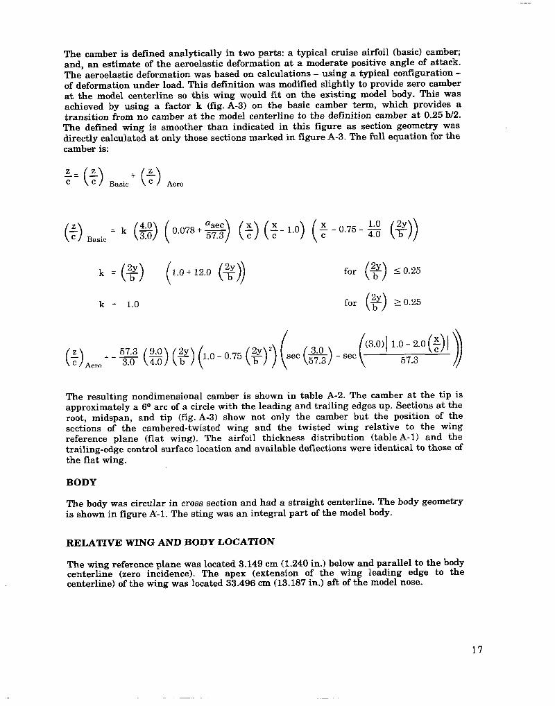
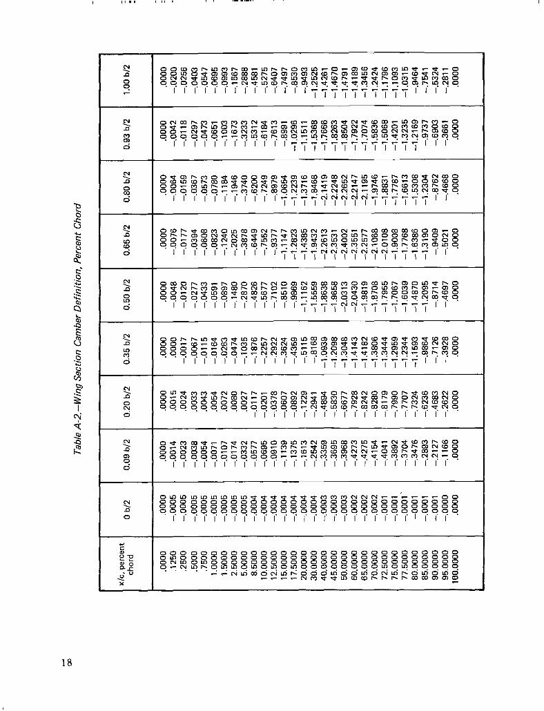
The camber is defined analytically in two parts: a typical cruise airfoil (basic) camber; and, an estimate of the aeroelastic deformation at a moderate positive angle of attack. The aeroelastic deformation was based on calculations - using a typical configuration - of deformation under load. This definition was modified slightly to provide zero camber at the model centerline so this wing would fit on the existing model body. This was achieved by using a factor k (fig. A-3) on the basic camber term, which provides a transition from no camber at the model centerline to the definition camber at 0.25 b/2. The defined wing is smoother than indicated in this figure as section geometry was directly calculated at only those sections marked in figure A-3. The full equation for the camber is:
z
0 c Basic 0.078+%) (:) (:-1.0) (:-0.75-g ($))
k = (T) (Lo+ 12.0 (+))
k = 1.0 for L 0.25
Z 0 c Aero =-gf (E) ($) (Lo-o.75
The resulting nondimensional camber is shown in table A-2. The camber at the tip is approximately a 6O arc of a circle with the leading and trailing edges up. Sections at the root, midspan, and tip (fig. A-3) show not only the camber but the position of the sections of the cambered-twisted wing and the twisted wing relative to the wing reference plane (flat wing). The airfoil thickness distribution (table A-l) and the trailing-edge control surface location and available deflections were identical to those of the flat wing.
BODY
The body was circular in cross section and had a straight centerline. The body geometry is shown in figure A-l. The sting was an integral part of the model body.
RELATIVE WING AND BODY LOCATION
The wing reference plane was located 3.149 cm (1.240 in.) below and parallel to the body centerline (zero incidence). The apex (extension of the wing leading edge to the centerline) of the wing was located 33.496 cm (13.187 in.) aft of the model nose.
17
Tabl
e A-
2.-W
ing
Sect
ion
Cam
ber
Def
initi
on,
Perc
ent
Cho
rd
c/c,
per
cent
ch
ord
0 b/
2
.ooo
o .o
ooo
.125
0 -.0
005
.250
0 -.0
005
.500
0 -.0
005
.750
0 -.0
005
1 .oo
oo
-.000
5 1.
5000
-.0
005
2.50
00
-.000
5 5.
0000
-.0
005
8.50
00
-.000
4 10
.000
0 -.0
004
12.5
000
-.000
4 15
.000
0 -.0
004
17.5
000
-.000
4 20
.000
0 -.0
004
30.0
000
-.000
4 40
.000
0 -.0
003
45.0
000
-.000
3 50
.000
0 -.0
003
60.0
000
-.000
2 65
.000
0 -.0
002
70.0
000
-.000
2 72
.500
0 -.O
OO
l 75
.000
0 -.O
OO
l 77
.500
0 -.O
OO
l‘ 80
.000
0 -0
001
85.0
000
-.OO
Ol
90.0
000
-.OO
Ol
95.0
000
-.ooo
o 10
0.00
00
.ooo
o
0.09
b/2
0.
20
b/2
0.35
b/
2 0.
50 b
/2
0.65
b/2
0.
80 b
/2
0.93
b/2
1.
00 b
/2
.ooo
o .o
ooo
.ooo
o .o
ooo
.ooo
o .o
ooo
.ooo
o .o
ooo
-.001
4 .0
015
.ooo
o -.0
048
-.007
6 -.0
064
-.004
2 -.0
200
-.002
3 .0
024
-.001
7 -.0
120
-.017
7 -.0
159
-.011
8 -.0
256
-.003
8 .0
033
-.006
7 -.0
277
-.039
4 -.0
367
-.029
7 -.0
403
-.005
4 .0
043
-.011
5 -.0
433
-.060
8 -.0
573
-.047
3 -.0
547
-.007
1 .0
054
-.016
4 -.0
591
-.082
3 -.0
780
-.065
1 -.0
695
-.010
7 .0
072
-.026
3 -.0
897
-.I24
0 -.1
184
-.100
3 -.0
993
-.017
4 .0
080
-.047
4 -.1
480
-.202
5 -.1
946
-.I67
3 -.1
567
-.033
2 .0
027
-.103
5 -.2
870
-.387
8 -.3
740
-.323
3 -.2
888
-.057
7 -.0
117
-.187
6 -.4
826
-.644
9 -.6
200
-.531
2 -.4
581
-.069
5 -.0
201
-.225
7 -.5
677
-.755
2 -.7
249
-.618
4 -.5
275
-.091
0 -.0
378
-.292
2 -.7
102
-.937
7 -.8
979
-.761
3 -.6
407
-.I13
9 -.0
607
-.362
4 -.8
510
-1.1
147
-1.0
654
-.899
1 -.7
497
-.137
5 -.0
892
-.435
9 -.9
869
-1.2
823
-1.2
239
-1.0
296
-.853
0 -.1
613
-.122
9 -.5
115
-1.1
162
-1.4
385
-1.3
716
-1.1
511
-.949
3 -.2
542
-.294
1 -.8
168
-1.5
559
-1.9
432
-1.8
468
-1.5
368
-1.2
525
-.335
9 -.4
894
-1.0
939
-1.8
638
-2.2
613
-2.1
419
-1.7
666
-1.4
261
-.369
5 -.5
830
-1.2
098
-1.9
658
-2.3
531
-2.2
248
-1.8
263
-1.4
670
-.396
8 -.6
677
-1.3
048
-2.0
313
-2.4
002
-2.2
652
-1.8
504
-1.4
791
-.427
3 -.
7928
-1
.414
3 -2
.043
0 -2
.355
1 -2
.214
7 -1
.792
2 -1
.418
9 -.4
275
-.824
2 -1
.418
2 -1
.981
9 -2
.257
7 -2
.119
5 -1
.707
4 -1
.345
6 -.4
154
-.828
0 -1
.380
6 -1
.870
8 -2
.106
8 -1
.974
6 -1
.583
6 -1
.242
4 -.4
041
-.817
9 -1
.344
4 -1
.795
5 -2
.010
8 -1
.883
1 -1
.506
8 -1
.179
6 -.3
892
-.799
0 -1
.295
9 -1
.706
7 -1
.900
8 -1
.778
7 -1
.420
1 -1
.109
3 -.3
704
-.770
7 -1
.234
4 -1
.603
9 -1
.776
8 -1
.661
3 -1
.323
5 -1
.031
5 -.3
476
-.732
4 -1
.159
3 -1
.487
0 -1
.638
6 -1
.530
8 -1
.216
9 -.9
464
-.289
3 -.6
236
-.986
4 -1
.209
5 -1
.319
0 -1
.230
4 -.9
737
-.754
1 -.2
127
-.468
3 -.7
126
-.871
4 -.9
409
-.876
2 -.6
903
-.532
4 -.I
166
-.262
2 -.3
928
-.469
7 -.5
021
-.466
8 -.3
661
-.281
1 .o
ooo
.ooo
o .o
ooo
.ooo
o .o
ooo
.ooo
o .o
ooo
.ooo
o
WING FIN
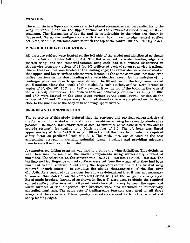
The wing fin is a 3-percent biconvex airfoil placed streamwise and perpendicular to the wing reference plane on the upper surface of the cambered-twisted wing at 0.725 semispan. The dimensions of the fin and its relationship to the wing are shown in figure A-4. To obtain configurations with the outboard trailing-edge control surface deflected, the fin is extended down to touch the top of the control surface. (See fig. A-4.)
PRESSURE ORIFICE LOCATIONS
All pressure orifices were located on the left side of the model and distributed as shown in figure A-5 and tables A-3 and A-4. The flat wing with rounded leading edge, the twisted wing, and the cambered-twisted wing each had 214 orifices distributed in streamwise pressure stations of 31 (or 30) orifices at each of seven spanwise locations. One of these orifices was located at the leading edge; the remainder were distributed so that upper- and lower-surface orifices were located at the same chordwise locations. The orifice locations on the sharp leading edge were identical except for the omission of the leading-edge orifice at each spanwise station. The 83 orifices on the body were located at 15 stations along the length of the model. At each station, orifices were located at angles of O”, 45O, 90°, 135O, and 180° measured from the top of the body. In the area of the wing-body intersection, the orifices that are nominally identified as being at 1350 and 180° were located on the wing lower surface at the same lateral location as the orifices at 45O and O”, respectively. Eight additional orifices were placed on the body, close to the juncture of the body with the wing upper surface.
DESIGN AND CONSTRUCTION
The objectives of this study dictated that the contours and physical characteristics of the flat wing, the twisted wing, and the cambered-twisted wing be as nearly identical as possible. The model was constructed of steel to minimize aeroelastic deflections and to provide strength for testing to a Mach number of 3.0. The aft body was flared approximately 4O from 194.310 cm (76.500 in.) aft of the nose to provide the required safety factor on predicted loads (fig. A-l). The model size was selected as the best compromise between minimizing potential tunnel blockage and providing adequate room to install orifices in the model.
A computerized lofting program was used to provide the wing definition. This definition was then used to machine the model components using numerically controlled machines. The tolerance on the contour was +0.1524, -0.0 mm (+0.006, -0.0 in.). The leading- and trailing-edge control surfaces were cut from the wings after they had been machined to final contour. A cut along the 15-percent chord line of the twisted wing removed enough material to simulate the elastic characteristics of the flat wing (fig. A-6). As a result of the previous tests it was determined that it was not necessary to remove this material on the cambered-twisted wing as the wings were very rigid. Fixed angle brackets (arranged as shown in fig. A-6) were used to obtain the required control surface deflections with all pivot points located midway between the upper and lower surfaces at the hingelines. The brackets were also machined on numerically controlled machines. The same sets of trailing-edge brackets were used on all three wings, and the same sets of leading-edge brackets were used for both the rounded and sharp leading edges.
19
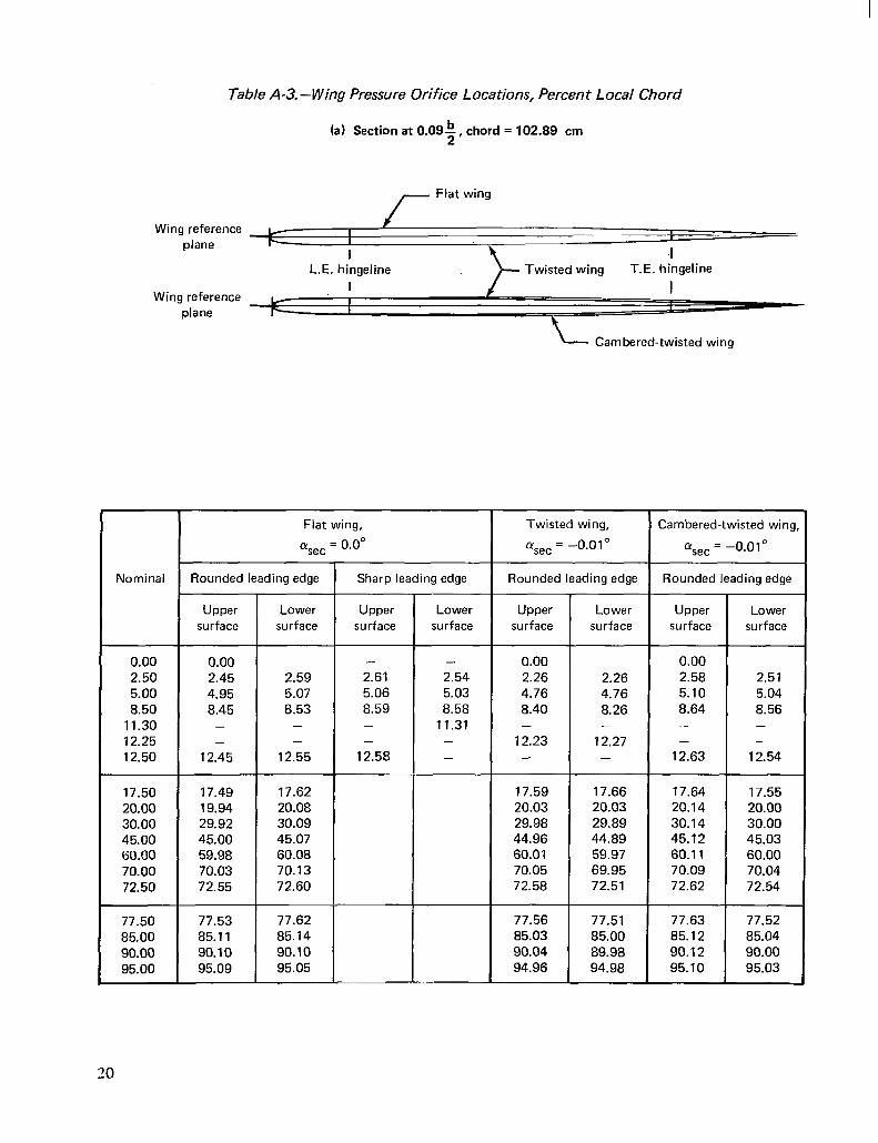
Table A-3. -Wing Pressure Orifice locations, Percent Local Chord
(a) Section at O.O9b, chord = 102.89 cm 2
Flat wing
Wing reference w I I- plane r
-I L.E. hingeline T.E. hingeline
Wing reference plane
Cambered-twisted wing
Nominal t
0.00 2.50 5.00 8.50
11.30 12.25 12.50
0.00 2.45 4.95 8.45
-
2.59 5.07 8.53
- - -
12.45 12.55
17.50 17.49 17.62 20.00 19.94 20.08 30.00 29.92 30.09 45.00 45.00 45.07 60.00 59.98 60.08 70.00 70.03 70.13 72.50 72.55 72.60
77.50 77.53 77.62 85.00 85.11 85.14 90.00 90.10 90.10 95.00 95.09 95.05
Flat wing, asec = 0.0”
Rounded leading edge
Upper surface
Lower surface
T Sharp leading edge
Upper surface
- 2.61 5.06 8.59 - -
12.58
Lower surface
- 2.54 5.03 8.58
11.31 - -
-
t
Twisted wing,
%iec = -O.O1°
Rounded leading edge
Upper surface
Lower surface
Upper surface
Lower surface
0.00 2.26 4.76 8.40 -
12.23
2.26 4.76 8.26 -
12.27 -
0.00 2.58 5.10 8.64 -
2.51 5.04 8.56 -
- - 12.63 12.54
17.59 17.66 17.64 17.55 20.03 20.03 20.14 20.00 29.98 29.89 30.14 30.00 44.96 44.89 45.12 45.03 60.01 59.97 60.11 60.00 70.05 69.95 70.09 70.04 72.58 72.51 72.62 72.54
77.56 77.51 77.63 77.52 85.03 85.00 85.12 85.04 90.04 89.98 90.12 90.00 94.96 94.98 95.10 95.03
Cambered-twisted wing
CY set = -O.OlO
Rounded leading edge
20
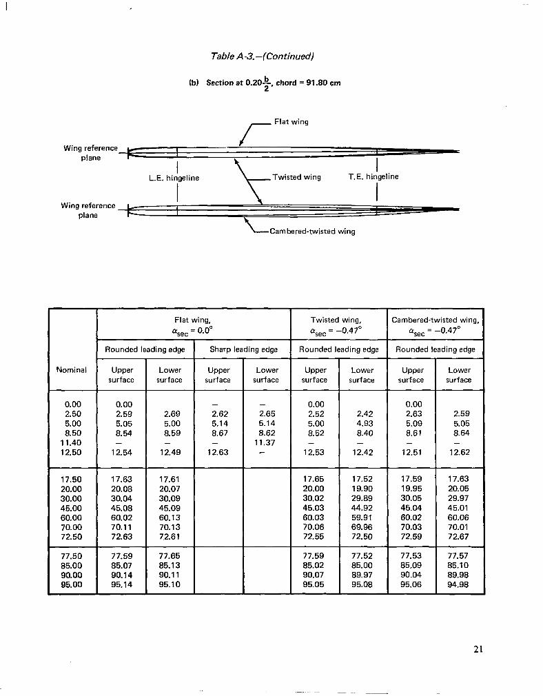
Table A -3. -(Con timed)
(b) Section at 0.20$-, chord = 91.80 cm
L.E. hingeline
Cambered-twisted wing
Nominal
0.00 2.50 5.00 8.50
11.40 12.50
17.50 17.63 17.61 17.65 17.52 17.59 17.63 20.00 20.08 20.07 20.00 19.90 19.95 20.05 30.00 30.04 30.09 30.02 29.89 30.05 29.97 45.00 45.08 45.09 45.03 44.92 45.04 45.01 60.00 60.02 60.13 60.03 59.91 60.02 60.06 70.00 70.11 70.13 70.06 69.96 70.03 70.01 72.50 72.63 7.2.61 72.55 72.50 72.59 72.67
77.50 77.59 77.65 77.59 77.52 77.53 77.57 85.00 85.07 85.13 85.02 85.00 85.09 85.10 90.00 90.14 90.11 90.07 89.97 90.04 89.98 95.00 95.14 95.10 95.05 95.08 95.06 94.98
Flat wing, (Ysec = o.o”
Rounded leading edge
Upper surface
Lower surface
0.00 2.59 5.05 8.54
2.69 5.00 8.59
- - 12.54 12.49
r Sharp leading edge
Upper surface
- 2.62 5.14 8.67 -
12.63
Lower surface
- 2.65 5.14 8.62
11.37 -
Twisted wing,
%ec = -0.47”
Rounded leading edge
Upper surface
Lower surface
Upper surface
Lower surface
0.00 2.52 5.00 8.52
2.42 4.93 8.40
0.00 2.63 5.09 8.61
2.59 5.05 6.64
- - - - 12.53 12.42 12.51 12.62
Cambered-twisted wing, a set = -0.47”
Rounded leading edge
21
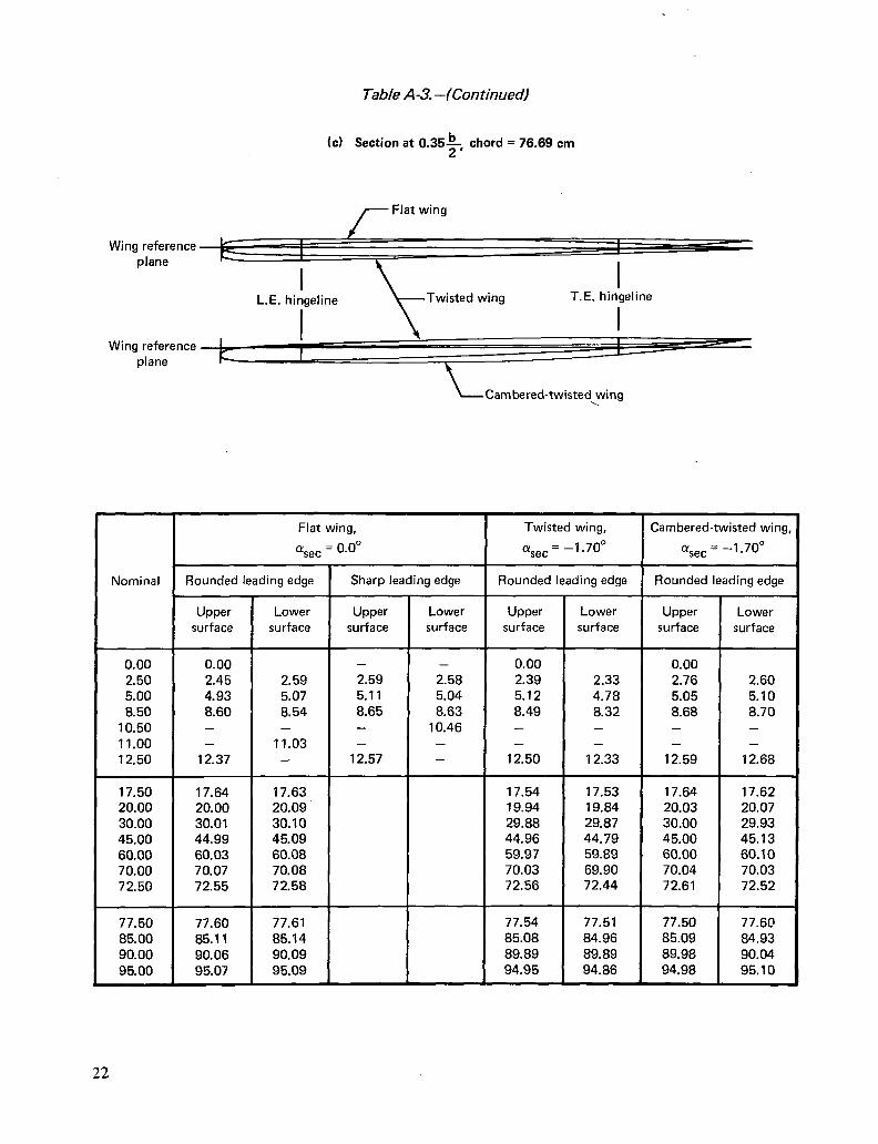
Table A-3.-(Continued)
(c) Section at 0.35$, chord = 76.69 cm
Wing reference plane
L.E. hingeline
I
Twisted wing T.E. hingeline
I
Wing reference plane
L-Cambered-twisted,wing
I Twisted wing,
%ec = -1 .70°
Cambered-twisted wing,
%ec = -1.70”
Flat wing,
asec = 0.0”
Nominal Rounded leading edge I Sharp leading edge Rounded leading edge Rounded leading edge
Lower surface
Upper surface
Lower surface
Upper I
Lower surface surface
Upper surface
Lower surface
Upper surface
0.00 2.50 5.00 8.50
10.50 ! 1.00 12.50
0.00 2.45 4.93 8.60 - -
12.37
- 2.59 5.11 8.65
- 2.58 5.04 8.63
10.46
0.00 2.39 5.12 8.49
2.33 4.78 8.32 -
0.00 2.76 5.05 8.68 -
- - 12.33 12.59
2.59 5.07 8.54 -
11.03 -
2.60 5.10 8.70 - -
12.68
- - -
12.57 - -
12.50 -
17.50 17.64 17.63 20.00 20.00 20.09 30.00 30.01 30.10 45.00 44.99 45.09 60.00 60.03 60.08 70.00 70.07 70.08 72.50 72.55 72.58
17.54 17.53 17.64 17.62 19.94 19.84 20.03 20.07 29.88 29.87 30.00 29.93 44.96 44.79 45.00 45.13 59.97 59.89 60.00 60.10 70.03 69.90 70.04 70.03 72.56 72.44 72.61 72.52
77.54 77.51
-T-
85.08 84.96 89.89 89.89 94.95 94.86
77.50 77.60 85.09 84.93 89.98 90.04 94.98 95.10
77.50 85.00 90.00 95.00
22
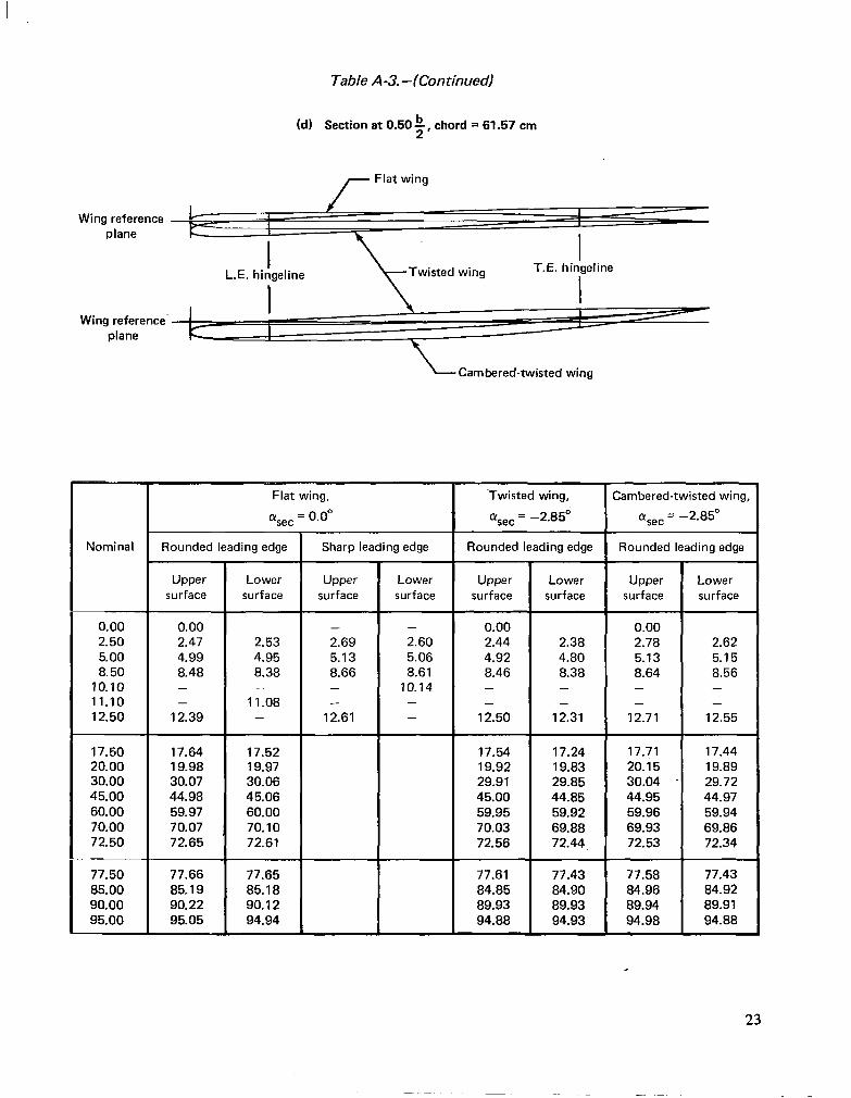
Table A-3. -(Con timed)
(d) Section at 0.50 k, chord = 61.57 cm
/- Flat wing
Wing reference plane
L.E. hingeline T.E. hingeline
Wing reference’ plane
L Cambered-twisted wing
11.08 - - - - - - 12.50 12.39 - 12.61 - 12.50 12.31 12.71 12.55
17.50 17.64 17.52 17.54 17.24 17.71 17.44 20.00 19.98 19.97 19.92 19.83 20.15 19.89 30.00 30.07 30.06 29.91 29.85 30.04 . 29.72 45.00 44.98 45.06 45.00 44.85 44.95 44.97 60.00 59.97 60.00 59.95 59.92 59.96 59.94 70.00 70.07 70.10 70.03 69.88 69.93 69.86 72.50 72.65 72.61 72.56 72.44 72.53 72.34
77.50 77.66 77.65 77.61 77.43 77.58 77.43 85.00 85.19 85.18 84.85 84.90 84.96 84.92 90.00 90.22 90.12 89.93 89.93 89.94 89.91 95.00 95.05 94.94 94.88 94.93 94.98 94.88
23
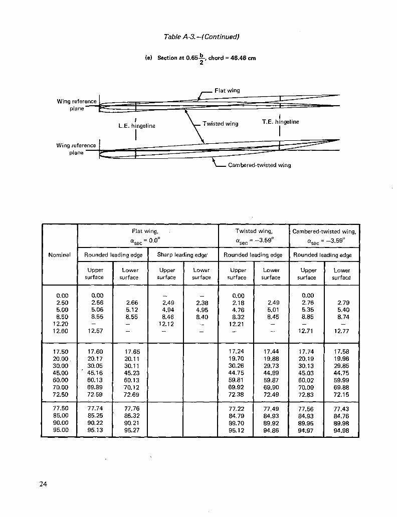
Table A-3. -(Continued)
(e) Section at 0.655, chord = 46.46 cm
T.E. hingeline
Cambered-twisted wing
Flat wing,
cYsec = 0.0”
Twisted wing, Cambered-twisted wing,
I ci set = -3.59O I %ec = -3.59O
Nominal I Rounded leading edge I Sharp leading edge’ I Rounded leading edge I Rounded leading edge
0.00 2.50 5.00 8.50
12.20 12.60
17.50 17.60 17.65 17.24 17.24 17.44 17.44 17.74 17.74 17.58 20.00. 20.17 20.11 19.70 19.70 19.88 19.88 20.19 20.19 19.96 30.00 30.05 30.11 30.26 30.26 29.73 29.73 30.13 30.13 29.85 45.00 45.16 45.23 44.75 44.75 44.89 44.89 45.03 45.03 44.75 60.00 60.13 60.13 59.81 59.81 59.87 59.87 60.02 60.02 59.99 70.00 69.89 70.12 69.92 69.92 69.90 69.90 70.09 70.09 69.88 72.50 72.59 72.69 72.38 72.38 72.49 72.49 72.83 72.83 72.15
Upper surface
0.00 2.56 5.06 8.55 -
12.57
Lower surface
2.66 5.12 8.55 -
Upper surface
- 2.49 4.94 8.46
12.12
- - 2.38 2.38 4.95 4.95 8.40 8.40
- -
77.50 77.74 77.76 77.22 77.49 77.56 77.43 85.00 85.25 85.32 84.79 84.93 84.93 84.76 90.00 90.22 90.21 89.70 89.92 89.95 89.98 95.00 95.13 95.27 95.12 94.86 94.97 94.98
0.00 0.00 2.18 2.18 4.76 4.76 8.32 8.32
12.21 12.21 - -
2.49 2.49 5.01 5.01 8.45 8.45
- -
0.00 0.00 2.76 2.76 5.35 5.35 8.85 8.85 - -
12.71 12.71
Lower surface
2.79 5.40 8.74
- 12.77
24
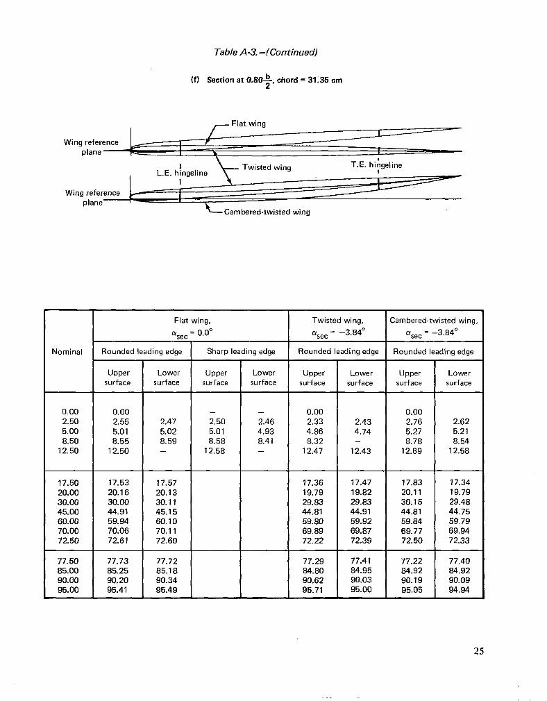
Table A-3. -(Continued)
(f) Section at 0.80*, chord = 31.35 cm
Cambered-twisted wing
Nominal
Flat wing, Twisted wing, Cambered-twisted wing,
CY set = 0.0” %ec = -3.84O %ec = -3.84’
Rounded leading edge Sharp leading edge Rounded leading edge Rounded leading edge
Upper Lower Upper Lower Upper Lower Upper Lower surface surface surface surface surface surface surface surface
0.00 0.00 - - 0.00 0.00 2.50 2.55 2.47 2.50 2.46 2.33 2.43 2.76 2.62 5.00 5.01 5.02 5.01 4.93 4.86 4.74 5.27 5.21 8.50 8.55 8.59 8.58 8.41 8.32 - 8.78 8.54
12.50 12.50 - 12.58 - 12.47 12.43 12.69 12.58
17.50 17.53 17.57 17.36 17.47 17.83 17.34 20.00 20.16 20.13 19.79 19.82 20.11 19.79 30.00 30.00 30.11 29.83 29.83 30.15 29.48 45.00 44.91 45.15 44.81 44.91 44.81 44.75 60.00 59.94 60.10 59.80 59.92 59.84 59.79 70.00 70.06 70.11 69.89 69.87 69.77 69.94 72.50 72.61 72.60 72.22 72.39 72.50 72.33
77.50 77.73 77.72 77.29 77.41 77.22 77.40 85.00 85.25 85.18 84.80 84.95 84.92 84.92 90.00 90.20 90.34 90.62 90.03 90.19 90.09 95.00 95.41 95.49 95.71 95.00 95.05 94.94
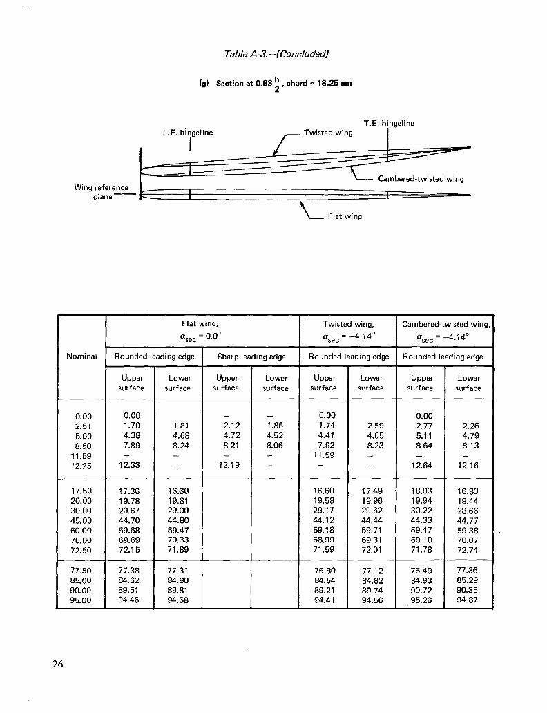
Table A-3. -(Concluded)
(g) Se&on at 0.93-$, chord = 18.25 cm
T.E. hingeline
Cambered-twisted wing Wing reference
plane I I
+ -
Flat wing
Nominal r 0.00 2.51 5.00 8.50
11.59 12.25
17.50 17.36 16.60 16.60 17.49 18.03 16.83 20.00 19.78 19.81 19.58 19.96 19.94 19.44 30.00 29.67 29.00 29.17 29.62 30.22 28.66 45.00 44.70 44.80 44.12 44.44 44.33 44.77 60.00 59.68 59.47 59.18 59.71 59.47 59.38 70.00 69.69 70.33 68.99 69.31 69.10 70.07 72.50 72.15 71.89 71.59 72.01 71.78 72.74
77.50 77.38 77.31 76.80 77.12 76.49 77.36 85.00 84.62 84.90 84.54 84.82 84.93 85.29 90.00 89.51 89.81 89.21. 89.74 90.72 90.35 95.00 94.46 94.68 94.41 94.56 95.26 94.87
Flat wing, Twisted wing, ffsec = 0.0” %.ec = -4.14O
Rounded leading edge
Upper surface
0.00 1.70 4.38 7.89 -
12.33
Lower surf ace
1.81 4.68 8.24 - -
T Sharp leading edge
Upper surface
- 2.12 4.72 8.21 -
12.19
Lower surface
- 1.86 4.52 8.06 - -
t
Lower surface
Rounded leading edge
Upper surf ace
0.00 1.74 4.41 7.92
11.59
2.59 4.65 8.23 -
- -
Cambered-twisted wing,
%ec = -4.14O
Rounded leading edge
Upper surface
Lower surface
0.00 2.77 5.11 8.64
2.26 4.79 8.13
- - 12.64 12.16
26
#J
a -
- -
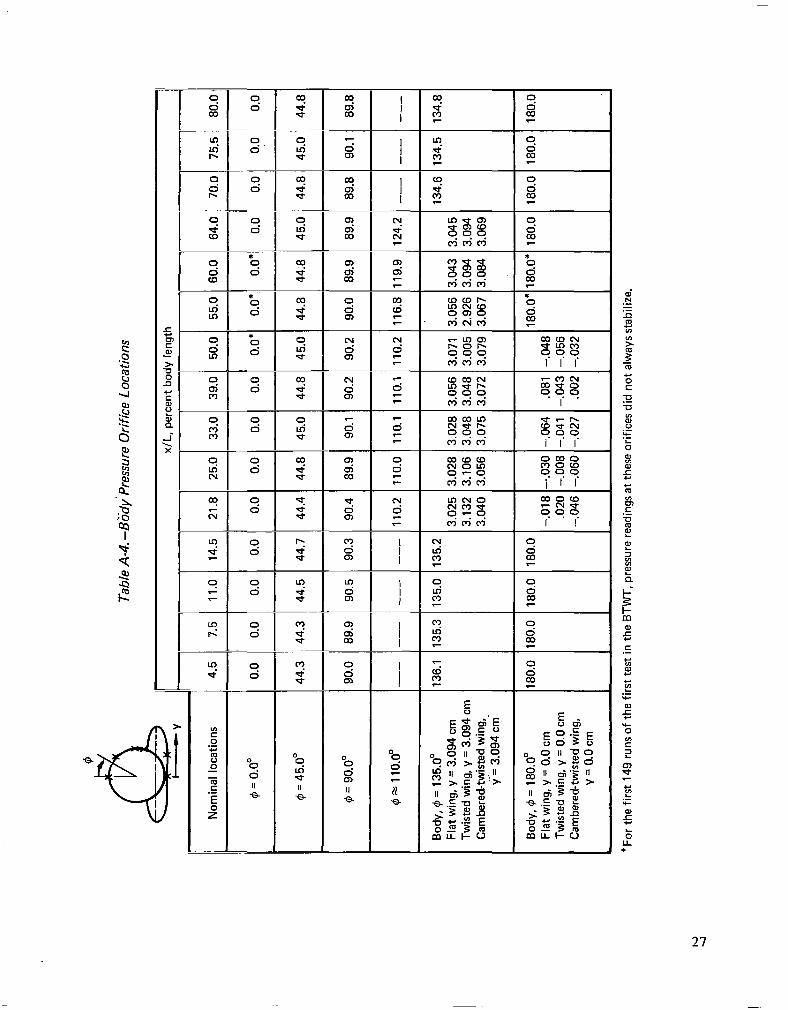
Tabl
e A-
4.-B
iddy
Pr
essu
re O
rific
e Lo
catio
ns
Ii-
x/L,
pe
rcen
t bo
dy l
engt
h -Y
8O.t
Nom
inal
lo
catio
ns
4.5
7.5
11.0
14
.5
60.0
64
.0
70.0
21
.8
25.0
0.0
44.4
0.0
44.8
0.0
0.0
0.0
0.0
0.0”
0.
0”
0.0’
0;
o
44.3
44
.5
44.7
44
.8
I 45
.0
1 44
.8
44.8
45
.0
44.8
44
.1
89.9
90
.5
90.3
90
.4
89.9
90
.1
90.2
90
.2
90.0
89
.9
89.9
89
.8
90.1
89
.t
110.
2 11
0.0
110.
1 11
0.1
110.
2 11
6.8
119.
9 12
4.2
135.
3 13
5.0
135.
2 13
4.6
134.
5 13
4.t
3.02
5 3.
028
3.02
8 3.
056
3.07
1 3.
056
3.04
3 3.
045
3.13
2 3.
106
3.04
8 3.
048
3.00
5 2.
926
3.09
4 3.
094
3.04
0 3.
056
3.07
5 3.
072
3.07
9 3.
067
3.08
4 3.
069
180.
0 18
0.0
180.
0 -.0
18
-.030
-.0
64
.081
.0
20
-.008
-.0
41
-.043
-.0
46
-.060
-.0
27
.002
180.
0’
180.
0 18
0.0
180.
0 18
O.f
@ =
0.0”
0.
0
44.3
@
= 45
.0”
9 =
90.0
° 90
.0
d =
110.
0”
Body
, @
J = 13
5.0’
Fl
at w
ing,
y =
3.0
94 c
m
Twis
ted
win
g, y
= 3
.094
cm
C
ambe
red-
twis
ted
win
g,
. . y =
3.09
4 cm
-
136.
*For
th
e fir
st
149
runs
of
the
first
te
st i
n th
e BT
WT,
pr
essu
re r
eadi
ngs
at t
hese
orif
ices
di
d no
t al
way
s st
abiliz
e.
Body
, #
= 18
0.0’
Fl
at w
ing,
y =
0.0
cm
Tw
iste
d w
ing,
y =
0.0
cm
C
ambe
red-
twis
ted
win
g,
y =
0.0
cm
180.
0
Pressure tubing used in this model was 1.016 mm (0.040 in.) o.d. Monel with a 0.1524 mm (0.006 in.) wall thickness. The major channels for wing pressure tubing were machined into the surface. The detailed grooves required to route tubing from the orifices to these channels were cut by hand. The pressure orifices were installed normal to and flush with the local surface. After installation of the pressure tubing, the grooves were filled with solder and brought back to contour by hand-filing to match templates prepared by numerically controlled machining.
Quick disconnects were used at the wing-body junction to reduce the time required for installing a different wing. Unfortunately, by the time the cambered-twisted wing was installed in the test section, one quick-disconnect block had become worn out due to the two previous tests and model checkout. The connection did not seal properly and measurements at a series of orifices (x/c from 0.125 through 0.600) on the lower surface at 0.80 b/2 were not sufficiently accurate to be used. Data values to be used in the integration were obtained by linear spanwise interpolation between adjacent sections.
The tubing for body pressure orifices was run through the hollow center of the model body rather than running it in grooves in the outside contour. Tubing from all the orifices was routed through the hollow body to the scanivalves located in the body nose. Wiring from the scanivalves was routed through the body to the sting.
The nose portion of the body was removable to provide access to the fifteen 24-position scanivalves. Figure A-l shows the aft body location of the strain gages that were used to measure normal force and pitching moment.
PRESSURE INSTRUMENTATION
The model was instrumented with fifteen 24-position scanivalves. Each scanivalve contained a 103.42-kNlm2 (X-psi) differential Statham, variable resistance, unbonded strain gage transducer. These transducers are calibrated against a high accuracy standard and, if placed in a temperature-controlled environment, will read within an accuracy of 0.1 percent of full scale. The transducers were located inside the model and subjected to large temperature excursions. During testing in the Boeing Transonic Wind Tunnel (BTWT), temperatures recorded at the scanivalves indicated that the accuracy of the readout was 0.75 percent of full-scale capability based on the calibration data. For tests in the 9- by 7-ft supersonic leg of the NASA Ames Unitary Wind Tunnel, the accuracy of pressure measurements was better than +0.3 percent, based on the maximum temperature measured in the test section.
During the first test in the BTWT (NASl-12875), two problems were encountered. For the first 149 runs, the data filter for one of the scanivalves was inadvertently set at too low of a cutoff frequency. This caused a lag that affected five body pressure measurements, which produced a maximum error of approximately 0.684 kNlm2 (0.1 psi) at an angle of attack of 16O and M = 0.95. Table A-4 identifies the specific data affected. During the first half (approximately) of the test, the scanivalve that -recorded lower surface pressures between the hingelines for the sections at 2y/b = 0.09, 0.20, 0.35, and 0.50 was intermittent at an angle of attack of 16O. This problem was eventually traced to an electrical problem in the strut. Rather than sacrifice all of these data, the incorrect measurements were replaced by extrapolating the data from angles of attack of 12O and 14O.
28
In the second test in the BTWT (NAS1:14962), damage to one of the quick disconnects for the wing caused the loss of measurements at a series of orifices (x/c from 0.125 through 0.600) on the lower surface at 0.80 b/2. Replacement values were obtained by a linear-spanwise interpolation between the adjacent sections.
WIND TUNNEL FACILITIES AND CAPABILITIES
The majority of testing (NASA contracts NASl-12875 and NASl-14962) of this model was conducted in the Boeing Transonic Wind Tunnel (BTWT). There was also limited testing (NASA contract NASl-14141) of the flat and twisted wings in the 9- by 7-ft supersonic leg of the NASA Ames Unitary Wind Tunnel. These two facilities are described in some detail.
BOEING TRANSONIC WIND TUNNEL (BTWT)
The BTWT is a continuous-flow, closed-circuit, single-return facility with an operating range of Mach number from 0.0 to nearly- 1.1. The test section is 2.438 by 3.658 by 4.420 m (8 by 12 by 14.5 ft) with 11.0 percent of the wall area in slots.
The tunnel layout is shown in figure A-7. The tunnel stagnation pressure is atmospheric with a total temperature range of 300 K to 356 K (540° to 640° R). The variation with Mach number of Reynolds number based on the mean aerodynamic chord (M.A.C.) of this model is shown in figure A-8., which also shows the variation of dynamic pressure with Mach number. The 26 856-kW (36 OOO-hp) wound-rotor induction motor in tandem with a 13 428-kW (18 OOO-hp) synchronous motor provides the power to drive a 7.315-m (24-ft) diameter fan up to a maximum speed of 470 rpm. The fan is made up of a 5.486-m ‘(18-ft) diameter hub with 72 fixed-pitch fiberglass blades 0.914 m (36 in.) long in two stages and directs circuit air through two stages of 67 hollow steel stators.
Data System
The BTWT data system provides the capabilities of real-time test data acquisition, feedback control computation, and display. The data system consists of an Astrodata acquisition subsystem and a computing subsystem that uses a Xerox data system (XDS 9300) digital computer. The Astrodata system acquires signals from the sensors, conditions them, and passes them directly to the computer. Test data (averaged from as many as 256 samples per test point) are recorded on a rapid-access data drum. As final computations are performed, selected on-line displays are provided on analog X-Y plotters and teletypewriters. Real-time computations and displays are performed every 200 milliseconds for control and test monitoring functions. Any test data may be retrieved from rapid-access drum storage and displayed on an oscilloscope. On-line programs also provide for the preparation of magnetic tapes for plotting or interfacing with off-line programs. Figure A-9 is .a schematic of the data acquisition and reduction system.
Mach Number
Mach number in the BTWT is referenced to the horizontal and lateral center of the test section at tunnel station- 1000, which was the pitch point of this model (40-percent M.A.C.).
29
The pressures used in determining the Mach number, ps, and pt are measured through permanently positioned sensors. Static pressure ps is measured by a’ 103.42-kN/m2 -(15-psi) absolute transducer. A 103.42~kN/m2 I15psi) differential transducer is used to obtain total pressure by measuring (pt-ps). These transducers are temperature compensated in addition to being in a fI.llO C (?2O F) environment. Transducer performance is checked periodically, and both the static and differential transducers have shown a maximum deviation of kO.02 percent of full scale.
The static pressure tap is located out of the test section above the ceiling in the pressure cap plenum. A correction is made to adjust this static pressure reading to the measured test-section-centerline static pressure determined during calibrations at station 1000. The tunnel total pressure is obtained from a total pressure probe mounted near the tunnel ceiling in the bellmouth throat (fig. A-7).
Signals from the pressure sensors are fed to the XDS 9300 computer. The XDS system computes and updates the Mach display five times per second. Accounting for the entire system, calculated Mach number is accurate within kO.002. Data are recorded only when the tunnel is within a preselected Mach tolerance. For this test, a tolerance of 20.003 was used.
Dynamic Pressure
The dynamic pressure q is computed from the Mach number and the corrected static pressure. The estimated tolerance on dynamic pressure is +95.8 N/m2 (k2.0 psf).
Angle of Attack
The angle of attack of the reference point (0.25 M.A.C. for this model) for a sting-mounted model is a combination of the input angle measured at the base of the sting and several incremental corrections. The input angle of attack is determined by an encoder mounted in the strut. This angle is accurate within +O.O2O. This angle is then modified by the effects of sting deflection, up-flow, and wall corrections.
Sting deflections due to load were determined during the calibrations of the strain gages, which are mounted on the integral sting body of the model. These deflections are known within +O.O2O. The corrections for sting deflection are based on the normal force and pitching moment loads obtained during wind-on data acquisition. The sting deflection was taken into account when setting test angles of attack, to minimize the variation in final angle of attack for the various model configurations. The strain gages attached to the sting body of this model have an estimated accuracy of 25 percent of full-scale reading. This means that the sting deflections based on maximum model loads were known within +O.llO.
During run 55 of the second test in the BTWT, the wiring for the pitching moment gage broke, affecting both the normal force and pitching moment measurements and, therefore, the calculation of sting deflection under load. For the remainder of that test, the model angle was set using the angle of attack as determined by the encoder for the most similar previously run configuration. After the test, the normal force and pitching moment obtained by integrating the pressure data were used to correct the final angle of attack. To verify this procedure, a comparison of these two methods was made using data obtained prior to run 55; the results matched within ?O.OlO.
30
Up-flow corrections were made based on data obtained from upright and inverted runs on a calibration model of similar span. These corrections were less than 0.2O. It is generally accepted that the up-flow values are known within 20.050.
A correction to model angle was made for the effect of lift interference for ll-percent slotted walls. The lift interference is a function of the ratio of model-to-test section size, test section shape, CN, and wall geometry. For CN = 1.0, this correction is on the order of -0.48O. Due to the limited amount of experimental substantiation, the wall correction could be in error by +20 percent.
NASA AMES UNITARY WIND TUNNEL, 9- BY 7-FT SUPERSONIC LEG
The 9- by 7-ft supersonic leg of the NASA Ames Unitary Wind Tunnel is a continuous-flow, closed-return, variable-density facility with an operating range of Mach number from 1.54 to 2.50. (A schematic is shown in fig. A-10.) The tunnel is equipped with an asymmetrical sliding-block nozzle and a flexible upper plate; variation of the test section Mach number is achieved by translating, in the streamwise direction, the fixed-contour block that forms the floor of the nozzle. For this test, the Reynolds number was selected as 8.65 by 106 based on the mean aerodynamic chord (3 of this model. The test section is 2.74 by 2.13 by 5.49 m (9 by 7 by 18oft).
The tunnel air is driven by an 11-stage axial-flow compressor that is powered by four variable-speed, wound-rotor induction motors with a combined output of 134 280 kW (180 000 hp). Four 850 m3 (30 000 ft3) spherical storage tanks provide dry air for tunnel pressurization. The temperature is controlled by aftercooling.
Data System
The data acquisition system is comprised of a Beckman 210 analog-digital recorder and a minicomputer. Output from the Beckman 210 is converted to an acceptable format and transmitted by the minicomputer to an IBM 360 computer, which is located in the AMES Research Center central computer facility for the processing and preparation of final data. This flow is illustrated in figure A-11.
Angle of Attack
The angle of attack of the reference point (0.25 M.A.C. for this model) for a sting-mounted model is a combination of the input angle at the base of the sting and an increment due to sting deflection. The input angle of attack at the base of the sting is accurate within 0.02O.
Sting deflections due to load were determined during the calibration of the strain gages mounted on the integral sting body of the model. The corrections for sting deflection are based on the normal force and pitching moment loads obtained during wind-on data acquisition. The sting deflection was taken into account when setting test angles of attack to minimize the variation in final angle of attack for the various model configurations. Only a crude calibration of the normal force and pitching moment gages was obtained since the force and pitching moment measurements were used primarily for calculating sting deflection. Comparison with the integrated pressure results indicates that both force and moment measurements may be about 10 percent low, which could yield a maximum error in final angle of attack of O.lO.
31
TESTS AND DATA ACQUISITION
BOEING TRANSONIC WIND TUNNEL (BTWT)
Tests
As previously stated, tests were conducted in the BTWT under two NASA contracts. Table A-5 shows the 54 configurations that were tested under contract NAS1;12875. The 12 configurations tested under contract NAS1;14962 are shown in table A-6. Two of the configurations were included in both tests to ensure that data from the two tests are consistent. Photographs of some of the configurations are shown in figures A-12 through A-15; a diagram of the model installation in the BTWT is shown in figure A-16.
Pressure and total force data were obtained at Mach numbers of 0.40, 0.85, 0.95, and 1.05 for all configurations and at Mach numbers of 0.70; 1.00, and- I.11 for selected configurations. Test angles of attack were from -8O to +16O in 2O increments, however, not all angles of attack were included for all configurations and/or Mach numbers. Tables A-5 and A-6 show the run numbers for each Mach number and configuration for which these data were obtained.
During the first test, wingtip deflection pictures were taken for representative configurations at three Mach numbers to evaluate the stiffness of the wing. These were compared to wind-off reference pictures to determine the relative deflection and twist. Configurations included the flat and twisted wings, and trailing-edge control surfaces deflected +30.2O, O.O”, and -17.7O. Whereas the tip did deflect (less than 2 cm), the change in incidence was negligible even at M =- 1.05; and, due to model flexibility, no corrections to the data were required.
Data Repeatability
Comparisons of data from both tests (NASA CR-165701), show that the data are within the tolerances expected for repeat runs during a single test. Therefore, data from both tests are compared without regard to the test in which the data were obtained.
Data Acquisition and Initial Processing
The pressure data were recorded through the use of fifteen 24-position scanivalves located in the fore body of the model. Pressure transducers in the scanivalves measured the differential pressure between the local surface pressures and tunnel total pressure. Signals from the scanivalves, force and moment data, tunnel parameters, and model attitude angle were recorded on the Astrodata system and reduced using the XDS 9300 computer.
NASA AMES UNITARY WIND TUNNEL, 9- BY 7-FT SUPERSONIC LEG
Tests
Table A-7 lists the- 13 configurations that were tested. Photographs of two of these are shown in figures A-17 and Ai18; a diagram of the model installation in the test section is shown in figure A-19. Pressure and total force data were obtained at Mach numbers of 1.70, 2.10 and 2.50 for all configurations. Table A-7 shows the run numbers for each Mach number and configuration for which these data were obtained. Test angles of attack were from -8O to -f- 14O in 2O increments and + 15O.
32
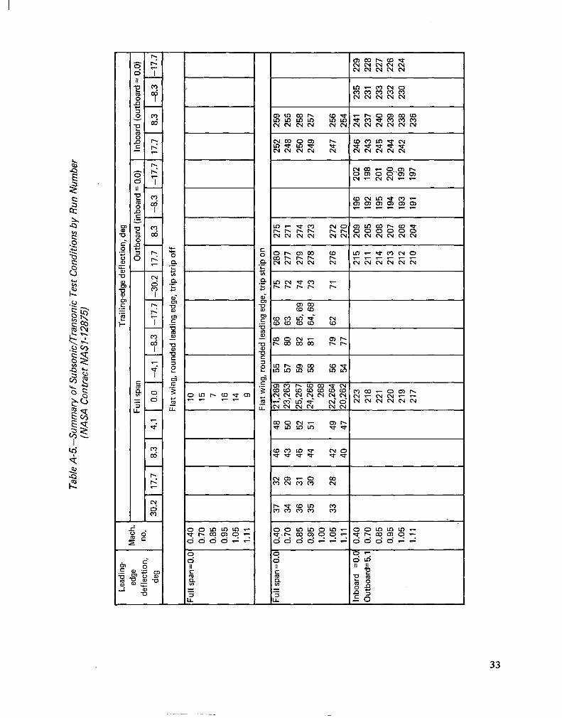
Tabl
e A-
5.-S
umm
ary
of S
ubso
nic/
Tran
soni
c Te
st C
ondi
tions
by
R
un N
umbe
r (N
ASA
Con
tract
N
ASI-
1287
5)
Lead
ing
Trai
ling-
edge
de
flect
ion,
deg
edge
M
ach.
de
flect
ion,
no
. Fu
ll sp
an
Out
boar
d (in
boar
d =
0.0)
In
boar
d (o
utbo
ard
= 0.
0)
deg
30.2
17
.7
8.3
4.1
0.0
-4.1
-8
.3
-17.
7 -3
0.2
17.7
8.
3 -8
.3
-17.
7 17
.7
8.3
-8.3
-1
7.7
Flat
win
g, r
ound
ed
lead
ing
edge
, trip
st
rip o
ff
Fulls
pan=
O.O
0.
40
10
0.70
15
0.
85
7 0.
95
16
1.05
14
1.
11
9
I Fl
at w
ing,
ro
unde
d le
adin
g ed
ge, t
rip
strip
on
I Fu
llspa
n=O
.O
0.40
o.
io
0.85
0.
95
1.00
1.
05
1.11
In
boar
d =O
.O
0.40
O
utbo
ard'
=5.1
0.
70
0.85
0.
95
1.05
1.
11
37
32
46
34
29
43
36
31
45
35
30
44
33
28
42
40
48
21,2
69
55
48
21,2
69
55
50
23,2
63
57
50
23,2
63
57
52
25,2
67
59
52
25,2
67
59
7 7 51
51
24,2
66
58
24,2
66
58
268
268
49
22,2
64
56
49
22,2
64
56
47
20.2
62
54
47
20.2
62
54
78 78
80
80
82
82
81
81
79
79
77
77
223
223
215
218
218
211
221
221
214
220
220
213
219
219
212
217
217
210
66
75
280
63
72
277
65,6
9 74
27
9 64
,68
73
278
62
71
276
275
252
259
271
248
255
274
250
258
273
249
257
272
270
209
196
205
192
208
195
207
194
206
193
204
191
247
202
246
198
243
201
245
200
244
199
242
197
256
254
241
237
240
239
238
236
235
229
231
228
233
227
232
226
230
224
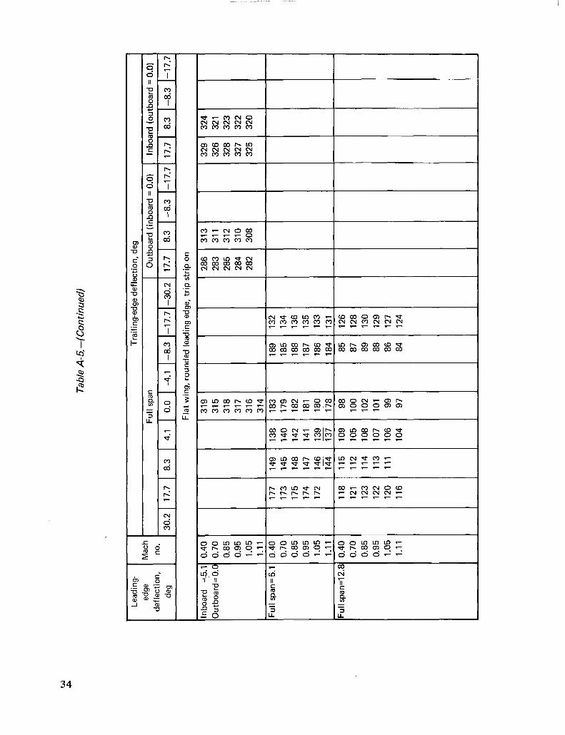
Tabl
e A-
5. -
(Con
tinue
d)
Lead
ing-
Tr
ailin
g-ed
ge
defle
ctio
n,
deg
edge
M
ach
defle
ctio
n,
no.
Full
span
O
utbo
ard
(inbo
ard
= 0.
0)
Inbo
ard
(out
boar
d =
0.0)
deg
30.2
17
.7
8.3
4.1
0.0
-4.1
-8
.3
-17.
7 -3
0.2
17.7
a.
3 -8
.3
-17.
7 17
.7
a.3
-8.3
-1
7.7
Inbo
ard
=.5.
1 0.
40
Inbo
ard
=.5.
1 0.
40
Out
boar
d=O
.O
0.70
O
utbo
ard=
O.O
0.
70
0.85
0.
85
0.95
0.
95
1.05
1.
05
1.11
1.
11
Full
span
=5.1
0.
40
Full
span
=5.1
0.
40
0.70
0.
70
0.85
0.
85
0.95
0.
95
1.05
1.
05
1.11
1.
11
Fulls
pan=
12.8
0.
40
Fulls
pan=
12.8
0.
40
0.70
0.
70
0.85
0.
85
0.95
0.
95
1.05
1.
05
1.11
1.
11
Flat
win
g,
roun
ded
lead
ing
edge
, tri
p st
rip
on
319
286
315
283
318
285
317
284
316
282
314
177
149
138
183
is9
132
173
145
140
179
185
134
175
148
142
is2
188
136
174
147
141
181
is7
135
172
146
139
180
186
133
1 14
4 13
7 ii8
18
4 13
1
118
B 11
5 10
9 98
85
12
6 12
1 11
2 10
5 10
0 87
12
8 12
3 11
4 10
8 10
2 89
13
0 12
2 11
3 10
7 10
1 88
12
9 12
0 11
1 10
6 99
86
12
7 11
6 10
4 97
84
12
4
313
329
324
311
326
321
312
328
323
310
327
322
308
325
320
.
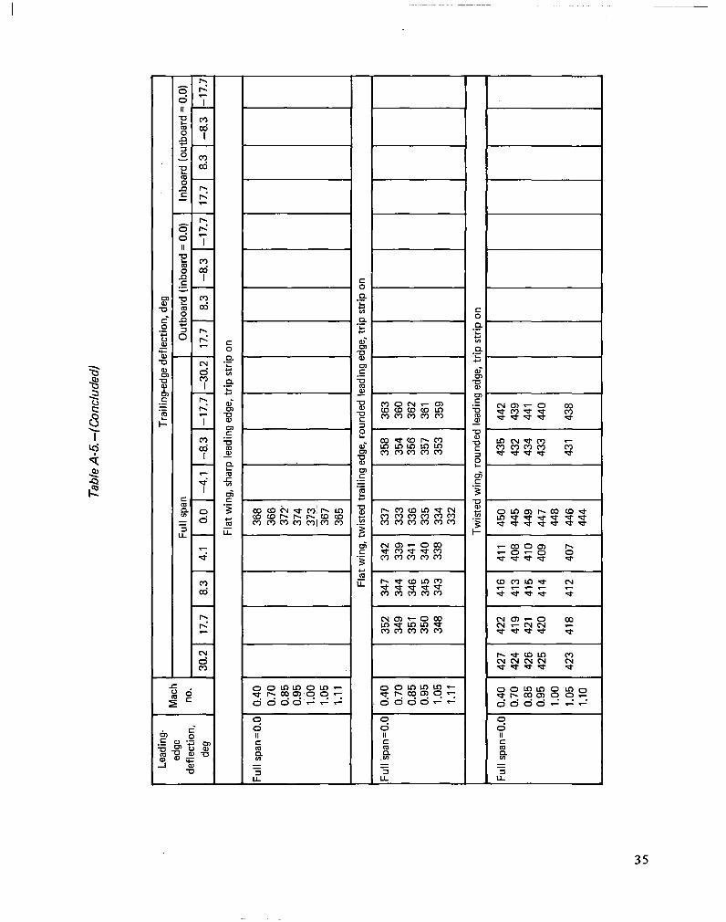
Tabl
e A-
5. -
(Con
clud
ed)
Lead
ing-
ed
ge
Mac
h
defle
ctio
n,
no.
dw
I
Trai
ling-
edge
de
flect
ion,
de
g
Full
span
O
utbo
ard
(inbo
ard
= 0.
0)
Inbo
ard
(out
boar
d =
0.0)
30.2
17
.7
8.3
4.1
0.0
-4.1
-8
.3
-17.
7 -3
0.2
17.7
a.
3 -8
.3
-17.
7 17
.7
a.3
-8.3
I Fl
at w
ing,
sha
rp l
eadi
ng e
dge,
trip
st
rip o
n
Full
span
=O.O
0.
40
368
0.70
36
6 0.
85
372’
0.
95
374
1.00
37
3 1.
05
367
1.11
36
5
Flat
win
g, t
wis
ted
trailin
g ed
ge, r
ound
ed
lead
ing
edge
, trip
st
rip o
n
Full
span
=O.O
0.
40
352
347
342
337
358
363
0.70
34
9 34
4 33
9 33
3 35
4 36
0 0.
85
351
346
341
336
356
362
0.95
35
0 34
5 34
0 33
5 35
7 36
1 1.
05
348
343
338
334
353
359
1.11
33
2
Full
span
=O.O
0.
40
427
422
0.70
42
4 41
9 0.
85
426
421
0.95
42
5 42
0 1.
00
1.05
42
3 41
8 1.
10
416
413
415
414
412
Twis
ted
win
g, r
ound
ed
lead
ing
edge
, I :ri
l p st
rip o
n
411
450
408
445
410
449
409
447
448
407
446
444
435
442
432
439
434
441
433
440
431
438
I I
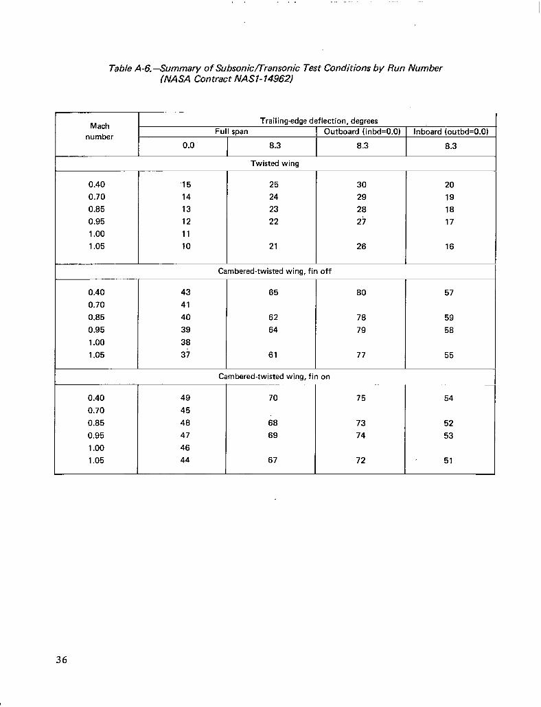
Table A-6.-Summary of Subsonic/Transonic Test Conditions by Run Number (NASA Contract NASl- 14962)
Mach number
Trailing-edge deflection, degrees Full span Outboard (inbd=O.O) Inboard (outbd=O.O)
0.0 8.3 8.3 8.3
Twisted wing
0.40 ‘15 25 30 20
0.70 14 24 29 19 0.85 13 23 28 18 0.95 12 22 27 17 1 .oo 11
1.05 10 21 26 16
Cambered-twisted wing, fin off
0.40 43 0.70 41
0.85 40
0.95 39 1 .oo 38
1.05 37
65
62
64
61
Cambered-twisted wing, fin on
80 57
78 59
79 58
77 55
-.
0.40 49 70 75 54 0.70 45
0.85 48 68 73 52
0.95 47 69 74 53 1 .oo 46
1.05 44 67 72 51
36
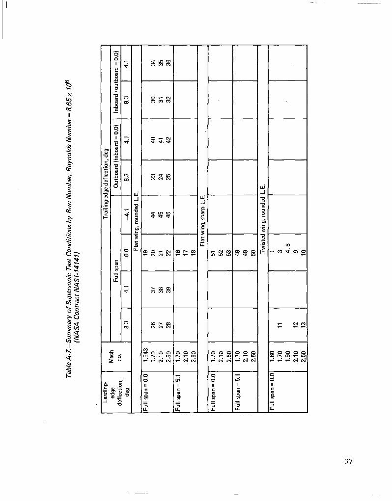
Tabl
e A-
7.-S
umm
ary
of S
uper
soni
c Te
st C
ondi
tions
by
Run
Num
ber.
Rey
nold
s N
umbe
r =
8.65
x
10s
(NAS
A C
ontra
ct
NAS
l-141
41)
Lead
ing
edge
de
flect
ion,
de
s
Mac
h no
. 8.
3
Trai
ling-
edge
de
flect
ion,
de
g
Full
span
O
utbo
ard
(inbo
ard
= 0.
0)
Inbo
ard
(out
boar
d =
0.0)
4.1
0.0
-4.1
8.
3 I
4.1
8.3
I 4.
1
I Fl
at w
ine.
ro
unde
d L.
E.
I
Full
span
= 0
.0
1.54
3 19
1.
70
26
37
20
44
23
40
30
34
2.10
27
38
21
45
24
41
31
35
2.
50
28
39
22
46
25
42
32
36
.Ful
l sp
an =
5.1
1.
70
16
2.10
17
2.
50
18
I Fl
at w
ing,
sha
rp L
. E.
I Fu
ll sp
an =
0.0
1.
70
51
2.10
52
2.
50
53
Full
span
= 5
.1
1.70
48
2.
10
49
2.50
50
I Tw
iste
d w
ing,
rou
nded
L.
E.
I Fu
ll sp
an =
0.0
1.
60
1 1.
70
11
3 1.
90
4,6
2.10
12
9
2.50
13
10
Data Acquisition and Initial Processing
The pressure data were recorded through the use of fifteen 24-position scanivalves located in the fore body of the model. Pressure transducers in the scanivalves measured the differential pressure between the local surface pressures and a known reference pressure. Signals from the scanivalves, force and moment data, tunnel parameters, and model attitude angle were recorded on the Beckman 210 analog-digital recorder and reduced by the Ames staff.
TRIP STRIP
A trip strip of no. 60 Carborundum grit was used throughout the tests with the exception of one series. On the body, the trip strip was 0.32 cm (0.125 in.) wide and placed 2.54 cm (1 in.) from the nose. On the wing, it was 0.32 cm (0.125 in.) wide from the side of body to the midspan control surface break (0.57 b/2), and tapered to 0.16 cm (0.0625 in.) wide at the wingtip. On the upper surface of the wing, the trip strip was placed at 15-percent chord; and, on the lower surface, it was placed just aft of the location of the leading-edge control surface brackets on the flat wing (see fig. A-6). Density of the grit was 4 to 5 grains per quarter-inch (6 to 8 grains per cm) of trip strip length.
FINAL DATA
Final data (pressure coefficients, tunnel parameters, and model attitude) were merged on magnetic tapes with appropriate configuration and test point identification for integration and plotting of these data.
A detailed description of the data editing and integration procedure are included in appendix B.
38
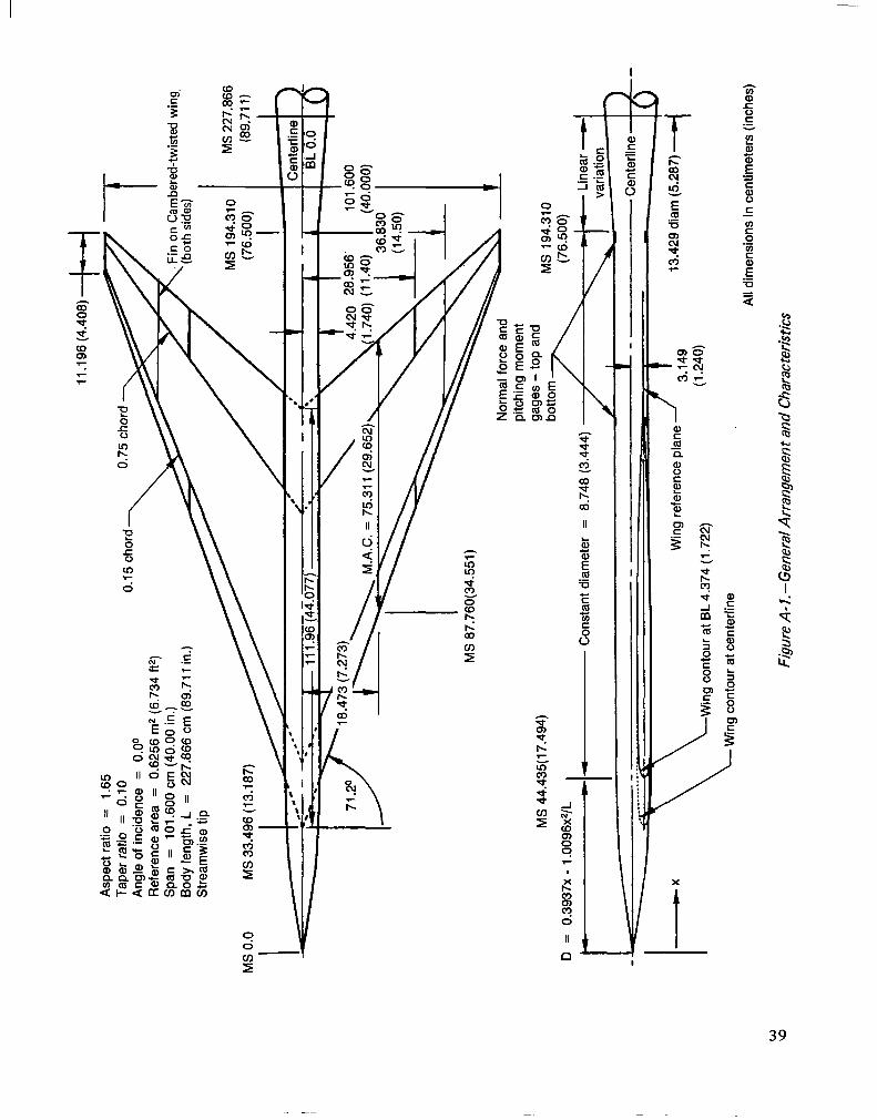
11.1
96
(4.4
08)
-+j
Aspe
ct
ratio
=
1.65
Ta
per
ratio
=
0.10
An
gle
of i
ncid
ence
=
O.O
” R
efer
ence
ar
ea
= 0.
6256
m
2 (6
.734
ft*
) Sp
an
= 10
1.60
0 cm
(40
.00
in.)
Body
le
ngth
, L
= 22
7.86
6 cm
(89
.711
in
.) St
ream
wis
e tip
-7
(d
oth
side
s)
Fm o
n C
ambe
red-
twis
ted
win
g,
0.75
cho
rd
-,
/ /
MS
194.
310
MS
227.
866
MS
0.0
MS
33.4
96
(13.
187)
I- -*
- e-
-
/ /,
(76.
500)
(8
9.71
1)
I I
/ I
I b
-- -.
- . .
. -s
:
111.
9~~4
z.07
7)
6 I
- .
I -1
8.47
3 (7
.273
) 10
1.60
0 (4
0.00
0)
1 7,
.20/
’ -
Nor
mal
fo
rce
and
t
MS
87.7
60(3
4.55
1)
MS
44.4
35(
17.4
94)
D
= 0.
3937
x -
1.00
96x2
/L
Con
stan
t di
amet
er
= 8.
748
(3.4
44)
pitc
hing
m
omen
t ga
ges
- to
p an
d
botto
m
7l
MS
194.
310
(76.
500)
Win
g re
fere
nce
plan
e
Win
g co
ntou
r at
BL
4.37
4 (1
.722
)
Win
g co
ntou
r at
cen
terli
ne
(1.2
40)
13.4
29
diam
(5.
287)
All
dim
ensi
ons
in c
entim
eter
s (in
ches
)
Figu
re
A - 1
. - G
ener
al A
rrang
emen
t a
nd C
hara
cter
istic
s
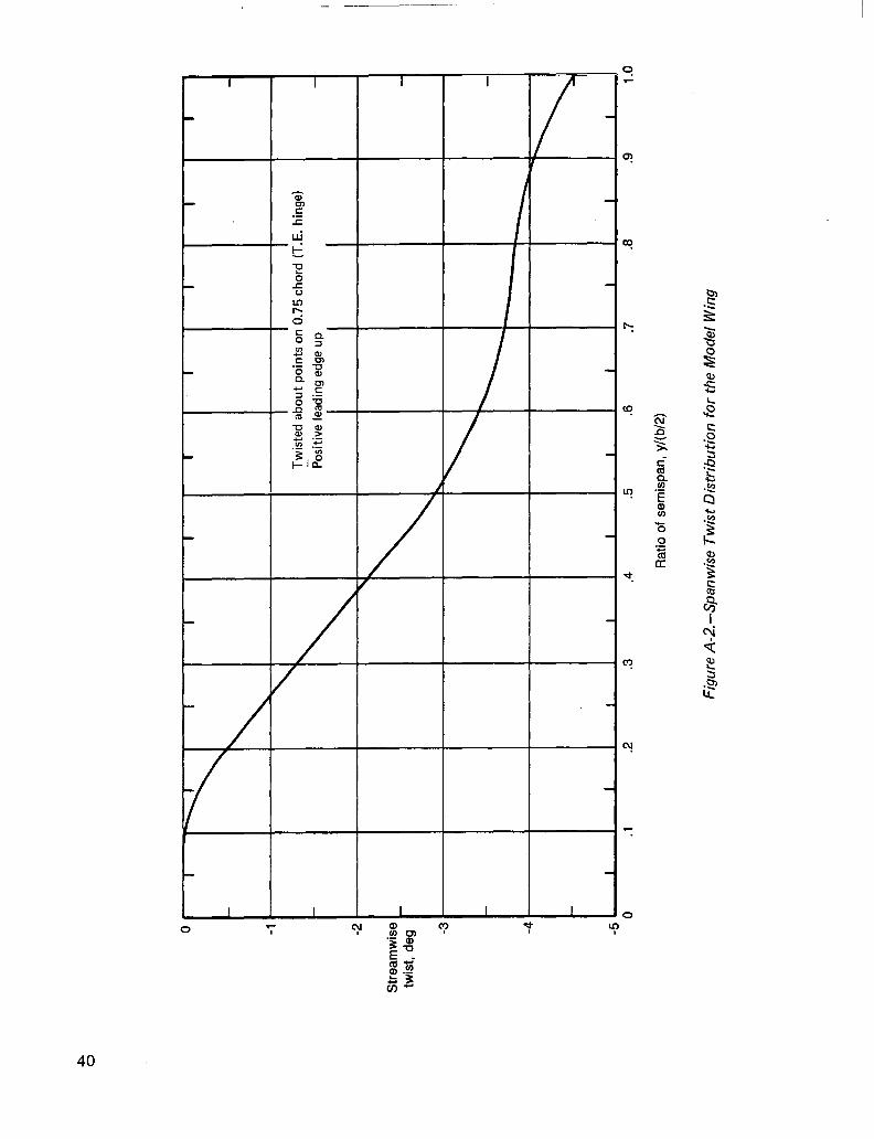
P 0
0 -1
-2
Stre
amw
ise
twis
t, de
g -3
-4
-5
I I
I I
.2
.3
.4
.5
.6
.7
.8
.9
1.0
Rat
io
of s
emis
pan,
y/
(b/2
)
I I
I I
I
I - Tw
iste
d ab
out
poin
ts
on 0
.75
chor
d (T
.E.
hing
e)
Posi
tive
lead
ing
edge
up
0 .l
Figu
re
A-2.
-Spa
nwis
e Tw
ist
Dis
tribu
tion
for
the
Mod
el
Win
g
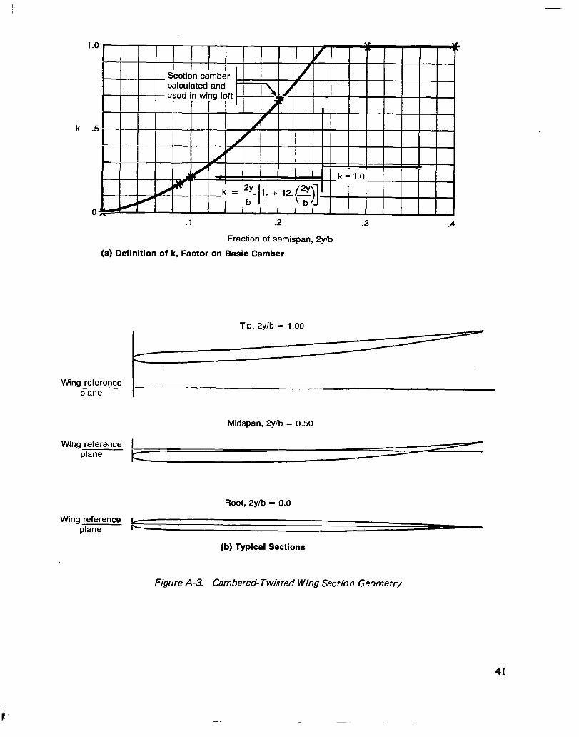
k .5
Section camber calculated and used in wing loft
”
1 I T
l II 0 L I I I I I I I ’ ~J’J I I _-
.1 .2
Fraction of semispan, 2ylb
(a) Definition of k, Factor on Basic Camber
Tip, 2y/b = 1.00
Wing reference plane I
-.
Midspan, 2ylb = 0.50
Wing reference plane
Root, 2ylb = 0.0
Wing reference k plane Ic .-
(b) Typical Sections
Figure A-3.-Cambered-Twisted Wing Section Geometry
41
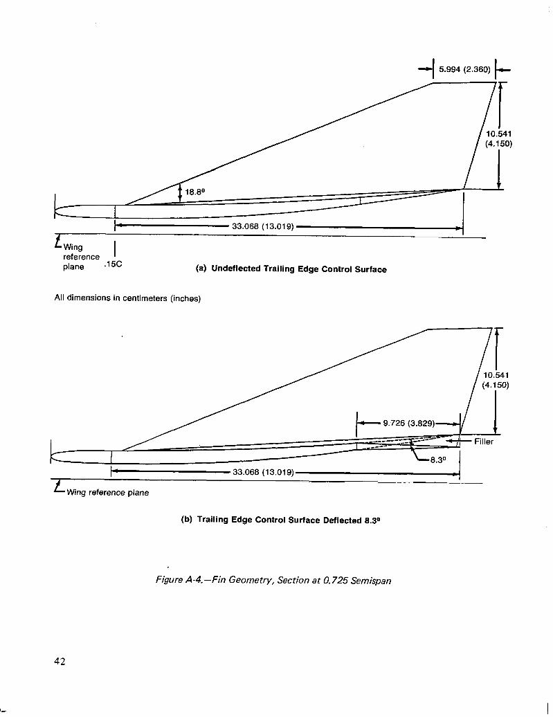
-I 5.994 (2.360) I-
plane (a) Undeflected Trailing Edge Control Surface
All dimensions in centimeters (inches)
I-- 33.068 (13.019)-d
Wing reference plane
(b) Trailing Edge Control Surface Deflected 8.30
Figure A-4. -Fin Geometry, Section at 0.725 Semispan
42
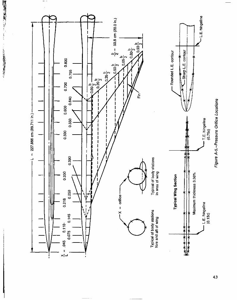
d L
= 22
7.86
6 cm
(89
.711
in
.) =-
I
II I
I I
I II
I I
I I I I\
,218
0.
330
0.25
0 0.
390
0.55
0 0.
640
WI
0.75
5
I .
6X
= or
ifice
yO
,
Typi
cal
of b
ody
stat
ions
Ty
pica
l of
bod
y st
atio
ns
fore
an
d af
t of
win
g in
are
a of
win
g
Typi
cal
Win
g Se
ctio
n
Max
imum
th
ickn
ess
3.36
%
L.E.
hin
gelin
e (0
.15c
) T.
E.
hing
elin
e (0
.75c
)
Rou
nded
L.
E. c
onto
ur
Figu
re
A-5.
-Pre
ssur
e O
rific
e Lo
catio
ns
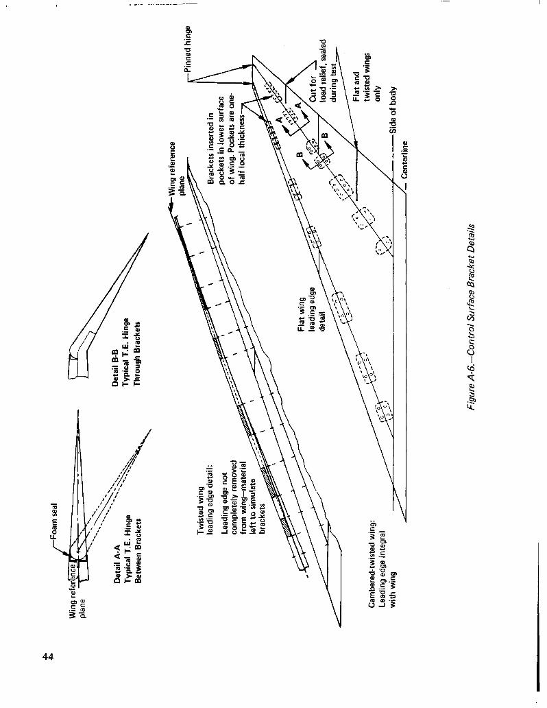
rFoa
m
seal
Det
ail
A-A
Typi
cal
T.E.
H
inge
Be
twee
n Br
acke
ts
Det
ail
B-B
Typi
cal
T.E.
tii
nge
Thro
ugh
Brac
kets
Twis
ted
win
g le
adin
g ed
ge d
etai
l:
Lead
ing
edge
not
co
mpl
etel
y re
mov
ed
from
w
ing-
mat
eria
l
Brac
kets
in
serte
d in
po
cket
s in
low
er
surfa
ce
of w
ing.
Po
cket
s ar
e on
e-
half
loca
l th
ickn
ess
Cam
bere
d-tw
iste
d w
ing:
Le
adin
g ed
ge in
tegr
al
with
w
ing
/ --S
ide
of b
ody
/I-
Cen
terli
ne
Figu
re
A-6.
-Con
trol
Surfa
ce
Brac
ket
Det
ails
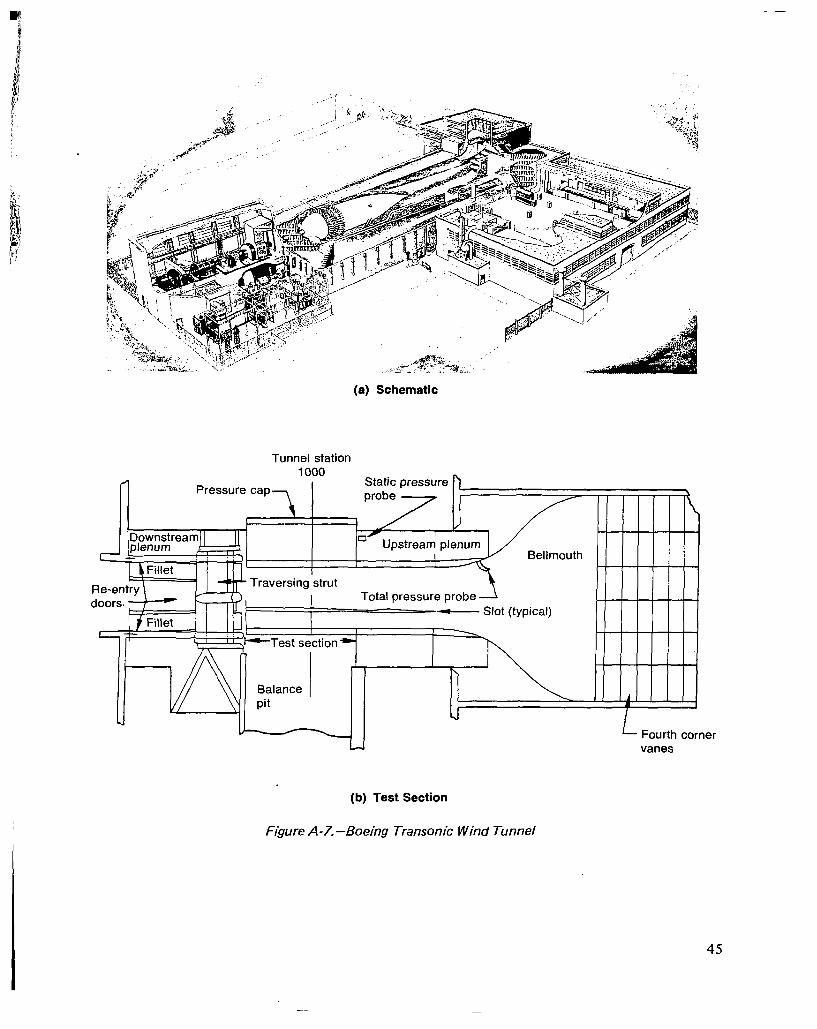
(a) Schematic
Tunnel station
II I I Y / II 1-I --
‘:-, _ xa, ’ ravers’ng;trut imi Total vssur.,,,,,?t (typical) *Test section -
L Fourth corner vanes
(b) Test Section
Figure A-7.-Boeing Transonic Wind Tunnel
45
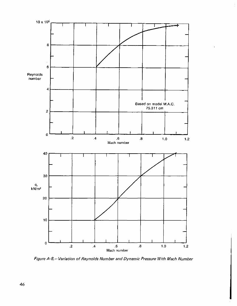
Reynolds number
I
4,
Based on model M.A.C. 75.311 cm
.6
40
30
20
10
0
7--
.2
Mach number
.6 Mach number
.8 1.0 1.2
Figure A-8.- Variation of Reynolds Number and Dynamic Pressure With Mach Number
46
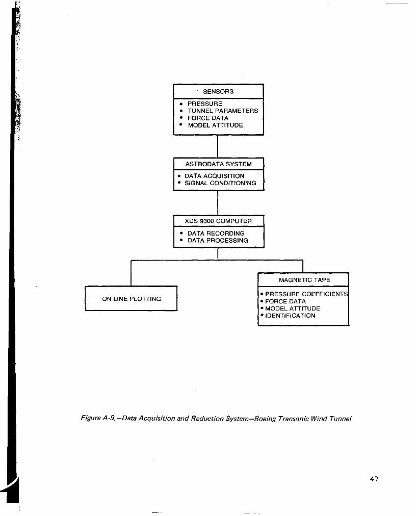
SENSORS
. PRESSURE l TUNNEL PARAMETERS l FORCE DATA . MODEL ATTITUDE
I ASTRODATA SYSTEM I
l DATA ACQUISITION l SIGNAL CONDITIONING
1 XDS 9300 COMPUTER
I l DATA RECORDING l DATA PROCESSING I
I ON LINE PLOTTING I
MAGNETIC TAPE
. PRESSURE COEFFICIENT l FORCE DATA l MODEL AlTITUDE l IDENTIFICATION
Figure A-9.-Data Acquisition and Reduction System-Boeing Transonic Wind Tunnel
47
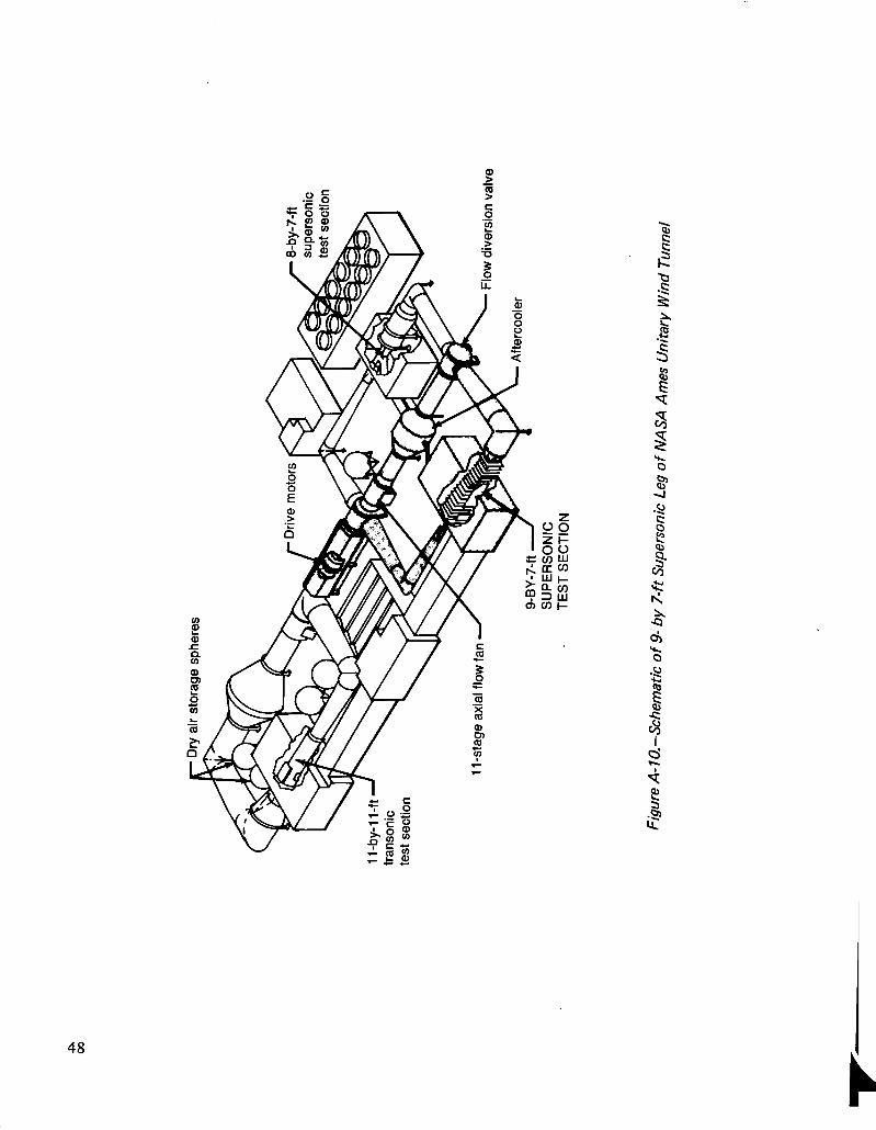
air
stor
age
sphe
res
test
se
ctio
n
11 -s
tage
ax
ial
flow
fan
Fl
ow
dive
rsio
n va
lve
SUPE
RSO
NIC
TE
ST
SEC
TIO
N
Figu
re
A- I
O.-S
chem
atic
of
9-
by
7-ft
Supe
rson
ic
Leg
of N
ASA
Ames
U
nita
ry
Win
d Tu
nnel
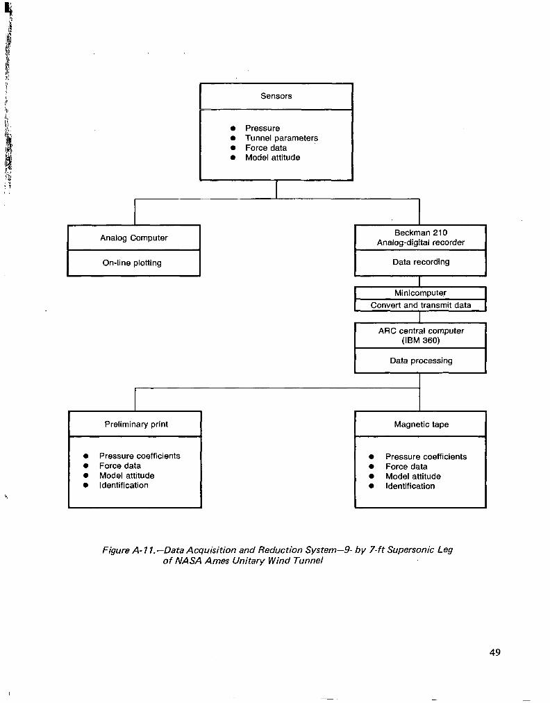
Sensors
0 Pressure 0 Tunnel parameters 0 Force data 0 Model attitude
Analog Computer Beckman 210
Analog-digital recorder
On-line plotting Data recording
I I Minicomputer I
Convert and transmit data I
I Data processing I
Preliminary print Magnetic tape
0 Pressure coefficients 0 Pressure coefficients 0 Force data 0 Force data 0 Model attitude 0 Model attitude 0 Identification 0 Identification
Figure A- Il.-Data Acquisition and Reduction System-.9- by 7-ft Supersonic Leg of NASA Ames Unitary Wind Tunnel
49
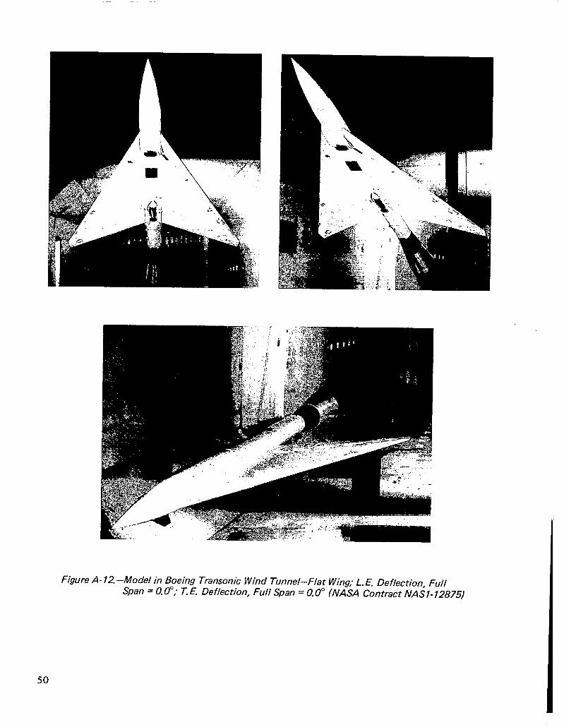
Figure A- 12. -Model in Boeing Transonic Wind Tunnel-Flat Wing; L. E. Deflection, Full Span = 0.0”; T. E. Deflection, Full Span = 0.0” (NASA Contract NASH- 12875)
50
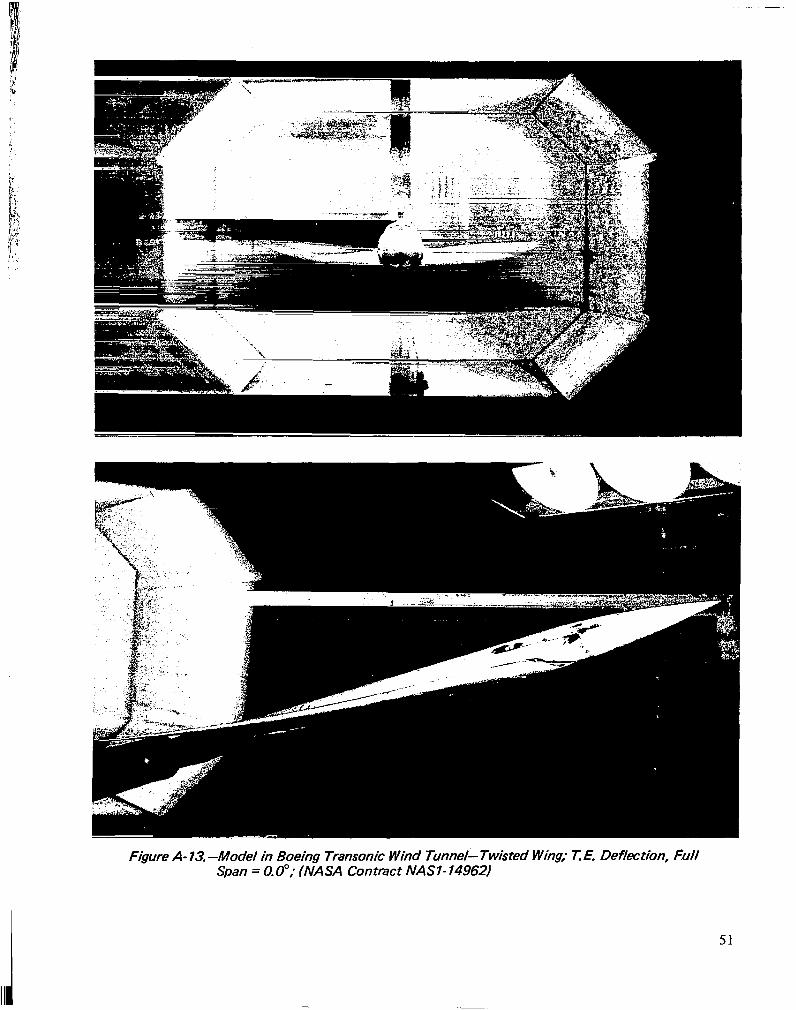
/. . (,
Figure A- 73. -Model in Boeing Transonic Wind Tunnel- Twisted Wing; T. E. Deflection, Full Span = 0.0”; (NASA Contract NASI- 149621
51
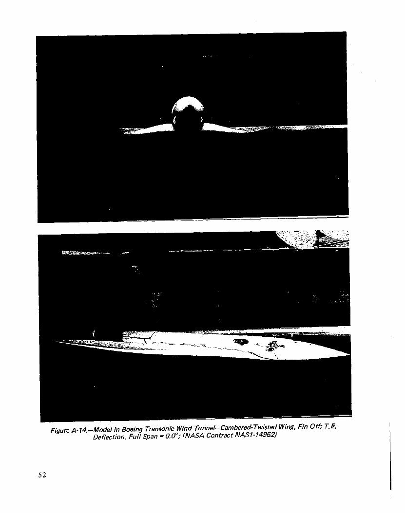
52
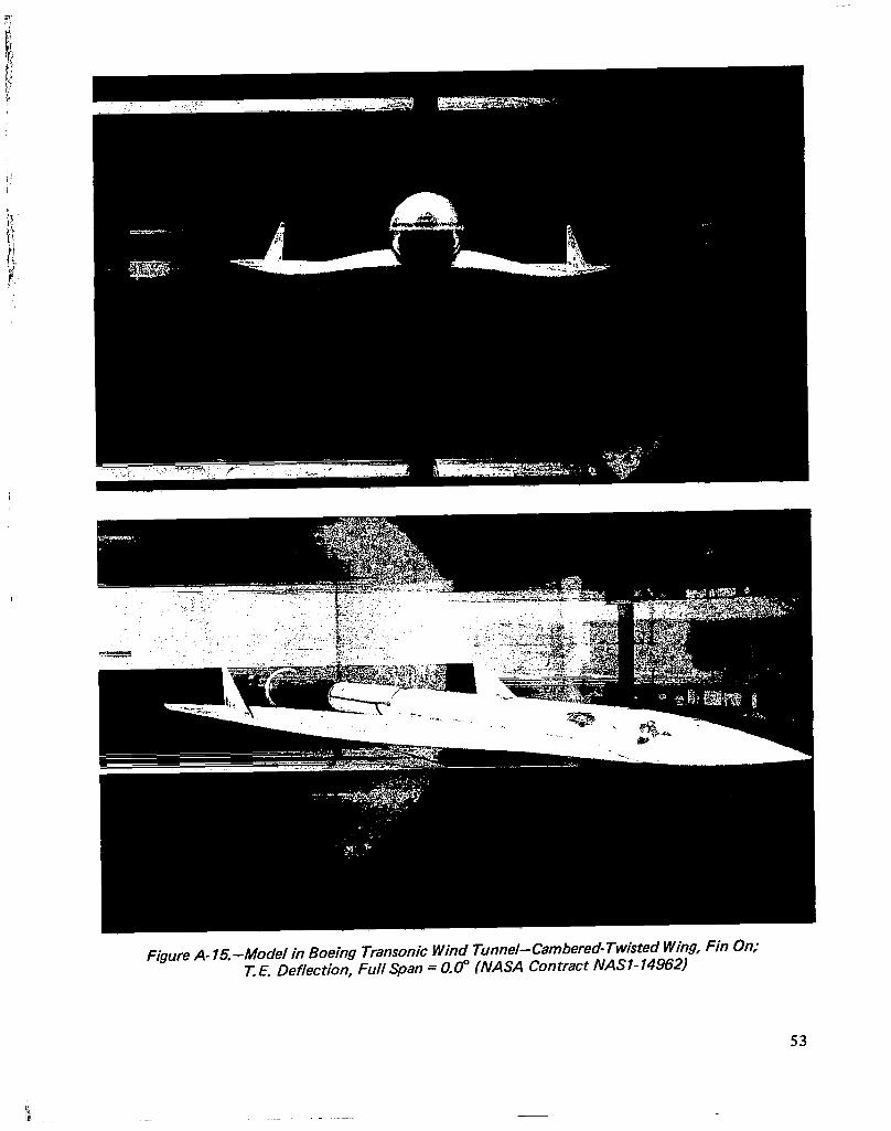
Figure A- 16.-Model in Boeing Transonic Wind Tunnel-Cambered-Twisted Wing, Fin On; T. E. Deflection, Full Span = 0.0” (NASA Contract NASI- 14962)
53
.
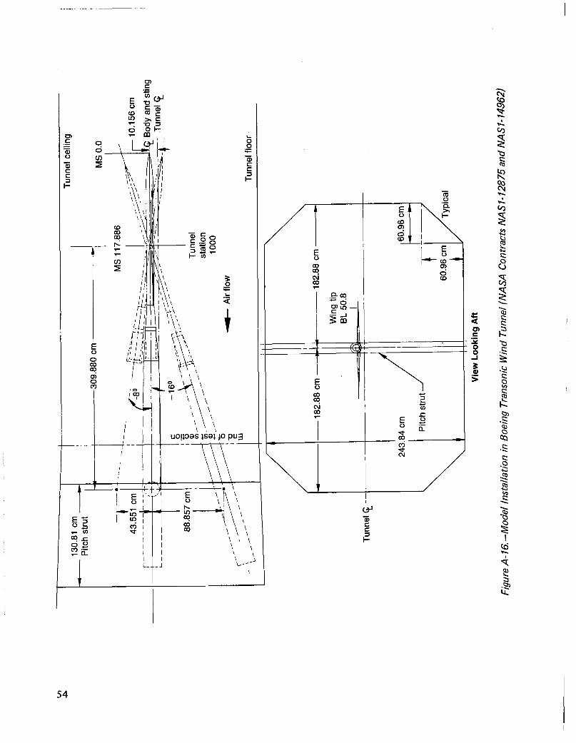
- 13
0.81
cm
-
Pitc
h st
rut
t
7 -j
43.5
51
cm
r-----
----
y+
--l
- $.
L----
---
--
f 88
.857
cm
1
Tunn
el
$-
I Tu
nnel
ce
iling
+309
.880
cm
--
--(
MS
0.0
,
MS
117.
886
Tunn
el
stat
ion
1000
w
Air
flow
Tunn
el
floor
- -
182.
88
cm
t- -
182.
88
cm A
243.
84
cm
I Pi
tch
stru
t /
60.9
6 cn
n t--
c
-t-- t
60.9
6 cm
t
View
Lo
okin
g Af
t
Figu
re
A-16
.-Mod
el
Inst
alla
tion
in B
oein
g Tr
anso
nic
Win
d Tu
nnel
(N
ASA
Con
tract
s N
ASI-
1287
5 an
d N
ASl-
1496
2)
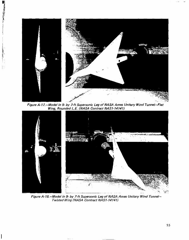
Figure A-17.-Model in 9- by 7-ft Supersonic Leg of NASA Ames Unitary Wind Tunnel-Flat Wina. Rounded L. E. (NASA Contract NASI- 74 74 II
Figure A- 18.~Model in 9- by 7-ft Supersonic Leg of NASA Ames Unitary Wind Tunnel- Twisted Wing (NASA Contract NASl- 14 14 7)
55
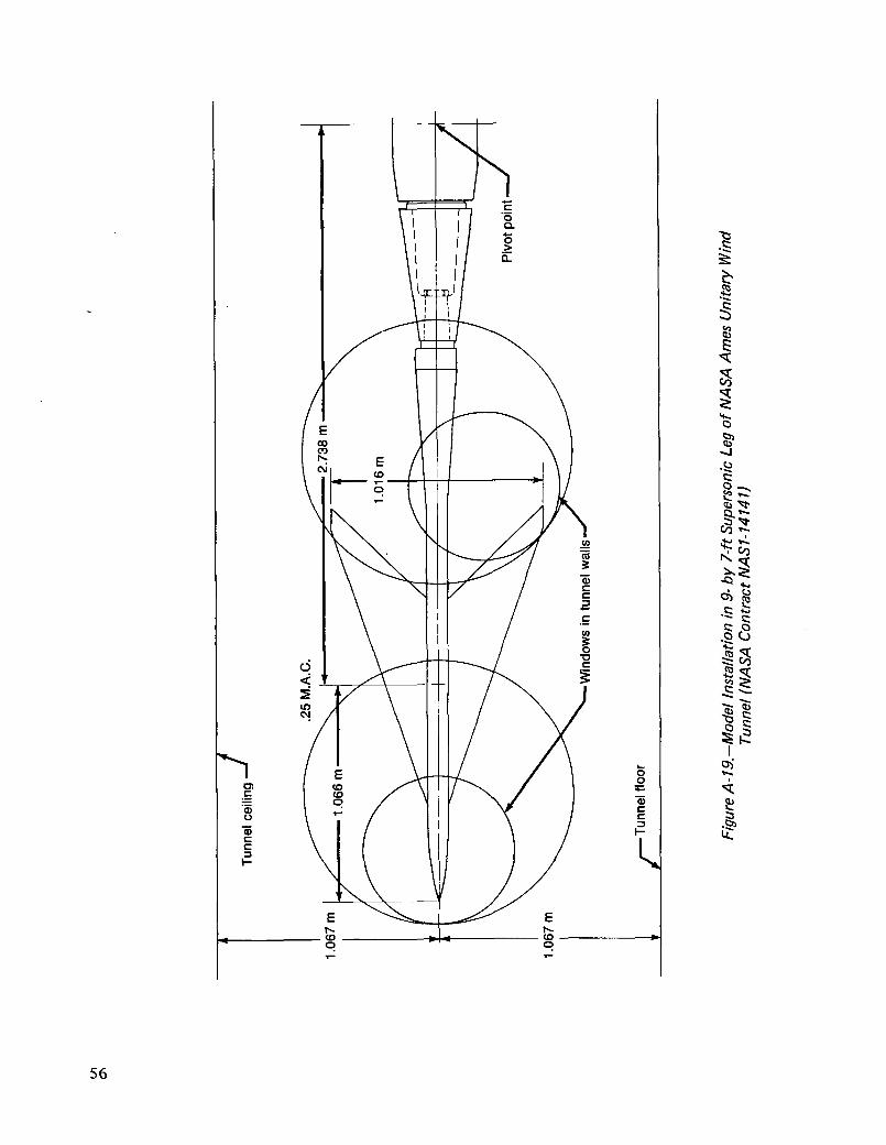
I ---
LWin
dow
s in
tun
nel
wal
ls -
/ -
Tunn
el
floor
Figu
re
A-19
.~M
odel
In
stal
latio
n in
9-
by
7-ft
Supe
rson
ic
Leg
of N
ASA
Ames
U
nita
ry
Win
d Tu
nnel
(N
ASA
Con
tract
N
ASl-
14 1
4 1)
APPENDIX B
DATA REDUCTION
DATA EDITING
There were some cases encountered with these data where the methods of data editing available within the integration programs were not adequate. Because the plotting program assumes that the geometry is the same for all configurations, and the chordwise location of orifices on the various model parts was not absolutely identical, points were added as required. Therefore, some interpolations or extrapolations using selected orifices were done before the integration program was used. The row of orifices on the body at the wing-body intersection was extended in front of the wing and aft of the wing by interpolating between the orifices located at 90° and 135O.
Some specific problems with the data acquisition systems required the replacement of some data for parts of tests. These are identified in appendix A.
Several methods were introduced into the integration program to replace or add data points to account for:
- Plugged or leaking orifices, or bad data points
Extrapolating the data to leading and trailing edges
- Hingeline discontinuities in the pressure data
These procedures were selected by code for each point. The codes are described in the following list and are illustrated in figure B-l. An additional use of these codes is to ensure that only measured pressure data (CODE, = 0) are identified with symbols on the plots. The subscript i identifies the position of the point from the leading edge of the upper or lower surface of the section.
IF CODE, = 0, use pressure as entered on tape (measured pressure)
= 20, use as entered on tape (previously replaced value)
= 1, interpolate from adjacent points
= 2, extrapolate from two preceding points
= 3, extrapolate from two following points
= 4, set equal to preceding point
= 5, set equal to following point
= 6, interpolate using points (i-2) and (i + 1)
= 7, interpolate using points (i-l) and (i+2)
57
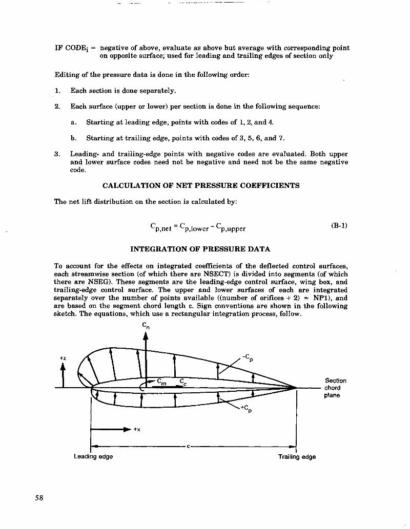
IF CODEi = negative of above, evaluate as above but average with corresponding point on opposite surface; used for leading and trailing edges of section only
Editing of the pressure data is done in the following order:
1. Each section is done separately.
2. Each surface (upper or lower) per section is done in the following sequence:
a. Starting at leading edge, points with codes of 1,2, and 4.
b. Starting at trailing edge, points with codes of 3, 5, 6, and 7.
3. Leading- and trailing-edge points with negative codes are evaluated. Both upper and lower surface codes need not be negative and need not be the same negative code.
CALCULATION OF NET PRESSURE COEFFICIENTS
The net lift distribution on the section is calculated by:
cp,net = cp,lower - cp,upper (B-1)
INTEGRATION OF PRESSURE DATA
To account for the effects on integrated coefficients of the deflected control surfaces, each streamwise section (of which there are NSECT) is divided into segments (of which there are NSEG). These segments are the leading-edge control surface, wing box, and trailing-edge control surface. The upper and lower surfaces of each are integrated separately over the number of points available ((number of orifices + 2) = NPl), and are based on the segment chord length c. Sign conventions are shown in the following sketch. The equations, which use a rectangular integration process, follow.
Section chord plane
I- -1 Leading edge Trailing edge
58
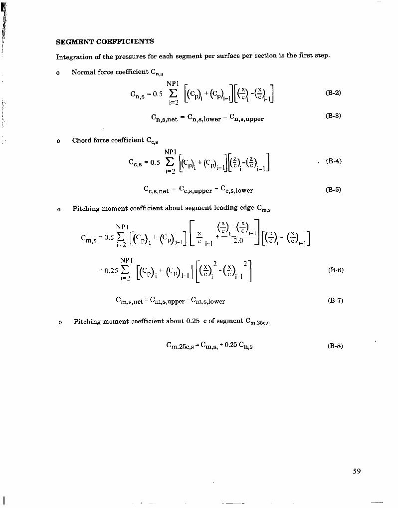
SEGMENT COEFFICIENTS
Integration of the pressures for each segment per surface per section is the first step.
0
Normal force coefficient C,,,
Cn,s = o.5 NC [(‘p)i + (‘p)i-l][(+\ -(:)-I] i=*
C n,s,net =c n,s,lower -c n,wpper
Chord force coefficient C,,,
Cc,’ = o’5 ~~’ [(Cdi + (‘p)i_ 13[(F)i-(~)i_il
C c,s,net =c wwper -c c,s,lower
Pitching moment coefficient about segment leading edge C,,,
NPI
‘m,s= o’5 F2 [(‘P)i + (‘P)j-I]
= o.25 ~’ [(‘p)i + (‘P)i-*] [(~)i* -(q-~*] C m,s,net = Cm,s,upper -C m,s,lower
Pitching moment coefficient about 0.25 c of segment Cm.~5c,s
C m.25c,s = Cm,s, + o.25 Cn,s
(B-2)
(B-3)
. (B-4)
(B-5)
(B-6)
(B-7)
(B-8)
59
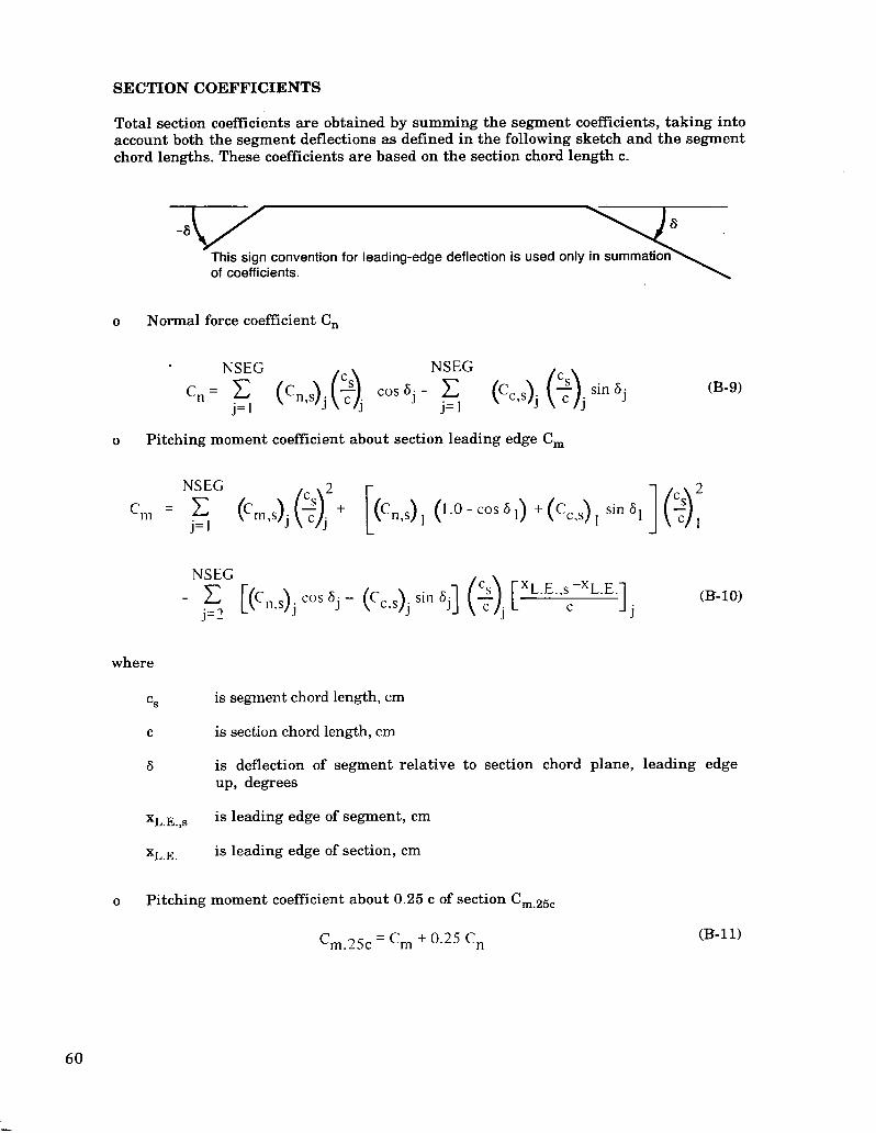
SECTION COEFFICIENTS
Total section coefficients are obtained by summing the segment coefficients, taking into account both the segment deflections as defined in the following sketch and the segment chord lengths. These coefficients are based on the section chord length c.
This sign convention for leading-edge deflection is used only of coefficients.
0 Normal force coefficient C,
C, = ‘$JG (C~,S)~ ($)j cos ‘j -NEG ('C,S)j (2)j sin "j (B-9)
0 Pitching moment coefficient about section leading edge C,
‘*, = ~~” (‘“l,S>j (~),~ + [(‘n,S) 1 (’ ‘O - ‘OS ’ 1) + (Cc,,) 1 sin ‘I ] ~):
NSEG
COS “j - (Ccqs)j sin ~j] (+)j [ XL-E.‘~XL.E.] j (B-10)
where
Cs
C
6
is segment chord length, cm
is section chord length, cm
is deflection of segment relative to section chord plane, leading edge up, degrees
XL.E.,s is leading edge of segment, cm
XL.E. is leading edge of section, cm
0 Pitching moment coefficient about 0.25 c of section Cm.25c
C m 35c = Cm + 0.25 C, .- (B-11)
60
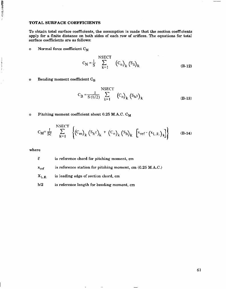
TOTAL SURFACE COEFFICIENTS
To obtain total surface coefficients, the assumption is made that the section coefficients apply for a finite distance on both sides of each row of orifices. The equations for total surface coefficients are as follows:
0 Normal force coefficient CN
i NSECT s i cN=$
0 Bending moment coeffkient C,
NSECT
(B-12)
(B-13)
0 Pitching moment coefficient about 0.25 M.A.C. CM
* CM’ E NT {(‘rn)k (‘h’)h + (‘n)k (‘h)k krcf- (‘~.h.)dJ (B-14)
where
c
Xref
xL.E.
b/2
is reference chord for pitching moment, cm
is reference station for pitching moment, cm (0.25 M.A.C.)
is leading edge of section chord, cm
is reference length for bending moment, cm
61
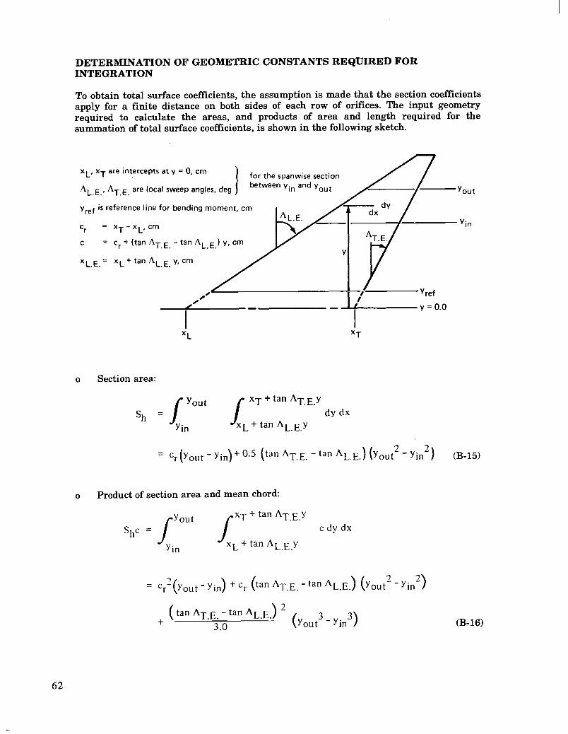
DETERMINATION OF GEOMETRIC CONSTANTS REQUIRED FOR INTEGRATION
To obtain total surface coefficients, the assumption is made that the section coefficients apply for a finite distance on both sides of each row of orifices. The input geometry required to calculate the areas, and products of area and length required for the summation of total surface coefficients, is shown in the following sketch.
XL, XT are intercepts at y = 0, cm for the spanwise section
AL E., AT E. are local sweep angles, deg between yin and yout nwise section n and Yout
A Yout L.L. I .L. - -I Yout
yref is reference line for bending moment, cm
‘r = xT-xL, cm I L I Y
-I.+/ Yin Yin
C = cr + (tan AT.E. - tan
xL.~. = XL + tan AL.~. Y, cm
0’ /
1’ yref
//- -
I I I
y = 0.0
0 Section area:
= ‘r Yollt ( - yin~ + 0.5 (tall AT.E. - tan ‘LE.1 (Yout* - Yin*) (B-15)
0 Product of section area and mean chord:
7 = cl-- Yout ( - Yin) + cr (tan *T.E. - tan ‘L.E.) (Yout* - Yin2)
( tan ‘T.E. - tan AL.E. ) 2 + ( Yout 3 3.0 - Yin3 > (B-16)
62
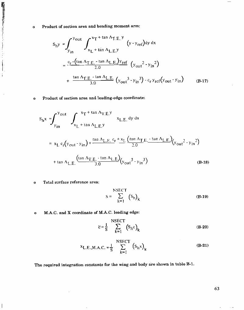
0 Product of section area and bending moment arm:
Shy =I’““’ JI:f:,“,;;-y (Y %,f)dY dx
m . .
c~ -(tan *T.E. - tan *L.E. > Yref =
2.0 ( Yout * - Yin* >
+ tan AT-E. - tan AL.E.
3.0 Yout 3 - Yin3) - cy Yref(Yout - Yin) (B-17)
0 Product of section area and leading-edge coordinate:
Shx ;/6’““’ lL ::,: 1: ::“v XL-E. dY dx
In . .
tan AL E. c,. + XL .
(tan *T.E. - ta” ‘L.E.) 2 _ y, r! 2.0 Yo1,t In
tall + tall AL-E.
AT.E. - tan AL.E,. > 3 3 3.0 Yout - Yin > (B- 18)
0 Total surface reference area:
NSECT
s = c (‘h)k k=l
0 M.A.C. and X coordinate of M.A.C. leading edge:
NSECT c=-
; & (shc)k
XL.E.,M.A.C. =+
(B-19)
(B-20)
(B-21)
The required integration constants for the wing and body are shown in table B-l.
63
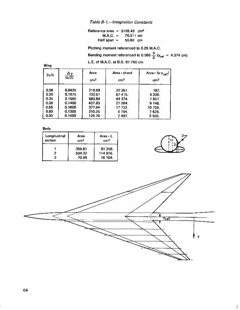
Table B-I.-Integration Constants
Reference area = 3128.45 cm2 MAC. = 75.311 cm
Half span = 50.80 cm
Pitching moment referenced to 0.25 M.A.C.
Bending moment referenced to 0.088 $ (yref = 4.374 cm)
L.E. of M.A.C. at B.S. 87.780 cm Wing
I
2y/b A!- (b/2)
0.0425 219.69 22 357. 167. 0.1575 733.51 67 415. 4 206. 0.1500 580.54 44 374. 7 857. 0.1400 437.93 27 084. 9 748. 0.1600 377.64 17 722. 10 729. 0.1300 210.35 6 794. 7 528. 0.1400 129.79 2 487. 5 505.
Area
cm2
1 1 I -
64
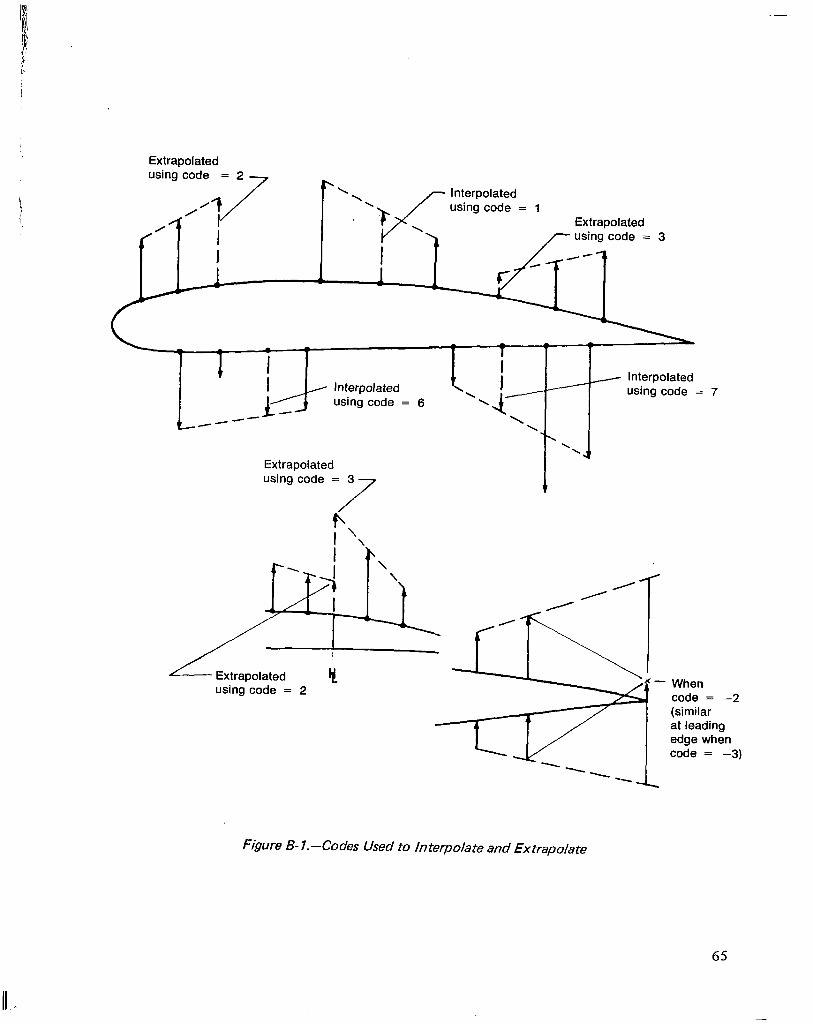
Extrapolated using code = 2
using code = 1 Extrapolated using code = 3
using code = 6
y Interpolated using code = 7
\ \
Extrapolated using code = 3
7 / I ‘N-4
When code = -2 (similar at leading edge when code = -3)
Figure B-I.-Codes Used to Jntetpolate and Extraoolate
65
REFERENCES
1. Manro, Marjorie E.; Tinoco, Edward N.; Bobbitt, Percy J.; and Rogers, John T.: Comparisons of Theoretical and Experimental Pressure Distributions on an Arrow-Wing Configuration at Transonic Speeds. Aerodynamic Analyses Requiring Advanced Compilters - Part II, NASA SP-347,1975, pp. 1141-1188.
2. Manro, M. E.; Bobbitt, P. J.; and Rogers, J. T.: Comparisons of Theoretical and Experimental Pressure Distributions on an Arrow-Wing Configuration at Subsonic, Transonic, and Supersonic Speeds. Prediction of Aerodynamic Loading. AGARD CP-204, Feb. 1977, pp. 11-l - 11-14.
3. Bobbitt, Percy J.; and Manro, Marjorie E.: Theoretical and Experimental Pressure Distributions for a 71.2O Swept Arrow-Wing Configuration at Subsonic, Transonic, and Supersonic Speeds. Proceedings of the SCAR Conference - Part 1, NASA CP-001 [1977’i,pp. 85-122.
4. Manro, Marjorie E.; Manning, Kenneth J. R.; Hallstaff, Thomas H.; and Rogers, John T.: Transonic Pressure Measurements and Comparison of Theory to Experiment for an Arrow-Wing Configuration - Summary Report. NASA CR-2610,1976.
5. Manro, Marjorie E.; Manning, Kenneth J. R.; Hallstaff, Thomas H.; and Rogers, John T.: Transonic Pressure Measurements and Comparison of Theory to Experiment for an Arrow-Wing Configuration, Volume I: Experimental Data Report - Base Configuration and Effects of Wing Twist and Leading-Edge Configuration. NASA CR-132727,1975.
6. Manro, Marjorie E.; Manning, Kenneth J. R.; Hallstaff, Thomas H.; and Rogers, John T.: Transonic Pressure Measurements and Comparison of Theory to Experiment for an Arrow-Wing Configuration, Volume II: Experimental Data Report - Effects of Control Surface Deflection. NASA CR-132728,1975.
7. Manro, Marjorie E.; Manning, Kenneth J. R.; Hallstaff, Thomas H.; and Rogers, John T.: Transonic Pressure Measurements and Comparison of Theory to Experiment for an Arrow-Wing Configuration, Volume III: Data Report - Comparison of Attached Flow Theories to Experiment. NASA CR-132729, 1975.
8. Manro, M. E.: Supersonic Pressure Measurements and Comparison of Theory to Experiment for an Arrow-Wing Configuration. NASA CR-145046,1976.
9. Manro, Marjorie E.: Transonic Pressure Measurements and Comparison of Theory to Experiment for Three Arrow-Wing Configurations - Summary Report. NASA CR-3434,1982.
10. Manro, Marjorie E.: Transonic Pressure Measurements and Comparisons of Theory to Experiment for Three Arrow-Wing Configurations, Volume I: Experimental Data Report - Basic Data and Effect of Wing Shape. NASA CR-165701,198l.
66
11. Manro, Marjorie E.: Transonic Pressure Measurements and Comparisons of Theory to Experiment for Three Arrow-Wing Configurations, Volume II: Experimental Data Report - Effect of Trailing-Edge Control Surface Deflection and a Wing Fin. NASA CR-165702,198l.
12. Manro, Marjorie E.: Transonic Pressure Measurements and Comparisons of Theory to Experiment for Three Arrow-Wing Configurations, Volume III: Data Report - Comparison of Attached-Flow Theories to Experiment. NASA CR-165703,198l.
13. White, R. P., Jr.; Gangwani, S. T.; and Janaki Ram, D. S.: A Theoretical and Experimental Investigation of Vortex Flow Control for High Lift Generation. Office of Naval Research Report ONR-CR212-223-4, December 1977.
14. Brown, Clinton E.; and Michael, William H., Jr.: On Slender Delta Wings With Leading-Edge Separation. NACA TN 3430, April 1955.
15. Johnson, F. T.; Lu, P; Brune, G. W.; Weber, J. A.; and Rubbert, P. E.: An Improved Method for the Prediction of Completely Three-Dimensional Aerodynamic Load Distributions of Configurations With Leading Edge Vortex Separation. AIAA Paper 76-417, AIAA 9th Fluid and Plasma Dynamics Conference, July 1976.
16. Smith, J. N. B.: Inviscid Fluid Models, Based on Rolled-Up Vortex Sheets, for Three-Dimensional Separation at High Reynolds Numbers. AGARD Lecture Series No. 94 on Three-Dimensional and Unsteady Separation at High Reynolds Numbers, February, 1978.
17. Samant, S. S.; and Janaki Ram, D. S.: Documentation of Computer Codes for Predicting the Lift of Low Aspect-Ratio Wings With Attached Vortex Flows. RASA/SRL Report No. 14-78-04, December, 1978.
18. Abbott, I. H.; and Von Doenhoff, A. E.: Theory of Wing Sections. New York, Dover Publications, Inc., 1959.
67
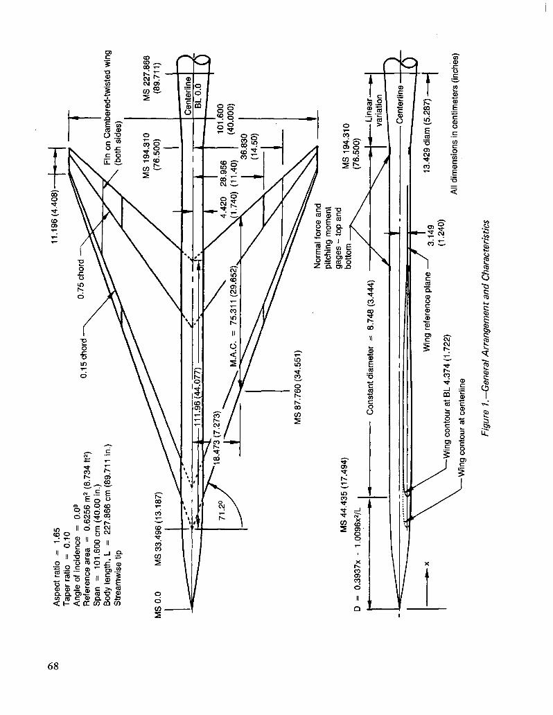
Aspe
ct
ratio
=
1.65
11
.196
(4
.408
) -+
+
Tape
r ra
tio
= 0.
10
Angl
e of
inc
iden
ce
= 0.
00
Ref
eren
ce
area
=
0.62
56
m2
(6.7
34
ft*)
Span
=
101.
600
cm (
40.0
0 in
.) Bo
dy
leng
th,
L =
227.
866
cm (
89.7
11
in.)
Stre
amw
ise
tip
I I
0.15
cho
rd
-\ o.
75 “
O-/7
7
Fin
on C
ambe
red-
twis
ted
win
g
MS
194.
310
MS
227.
866
MS
0.0
MS
33.4
96
(13.
187)
(8
9.71
1)
I I
J ,
MS
44.4
35
(17.
494)
D
= 0.
3937
x -
1.00
96x2
/L
,
I Cen
terli
ne
I -
.
I 4.42
0 28
.956
10
1.60
0 Ii
7All\
If4
Al-0
(40.
000)
MS
87.7
60
(34.
551)
Nor
mal
fo
rce
and
pitc
hing
m
omen
t ga
ges
- to
p an
d
botto
m
7-l
MS
194.
310
(76.
500)
Con
stan
t di
amet
er
= 8.
748
(3.4
44)
Win
g re
fere
nce
plan
e
Win
g co
ntou
r at
BL
4.37
4 (1
.722
)
Win
g co
ntou
r at
cen
terli
ne
13.4
29
diam
(5
.287
)
All
dim
ensi
ons
in c
entim
eter
s (in
ches
)
Figu
re
1. -G
ener
al
Arra
ngem
ent
and
Cha
ract
eris
tics
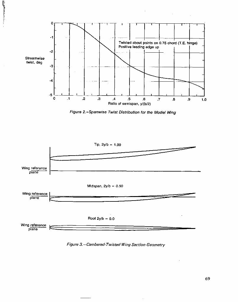
0
-1
-2
Streamwise twist, deg
-3
-4
-5
1--
\ \
1 ~~
Twisted about points on 0.75 chord (T.E. hinge) Positive leading edge up
\
-L I I
0 .l .2 .3 .4 .5 .6 .7 .8 .9 1.0 Ratio of semispan, y/(b/2)
Figure P.-Spanwise Twist Distribution for the Model Wing
Tip, 2y/b = 1.00
Wing reference plane I
Midspan, 2ylb = 0.50
Wing reference plane
Wing reference w plane rc
Root 2y/b = 0.0
Figure 3. -Cambered-Twisted Wing Section Geometry
69
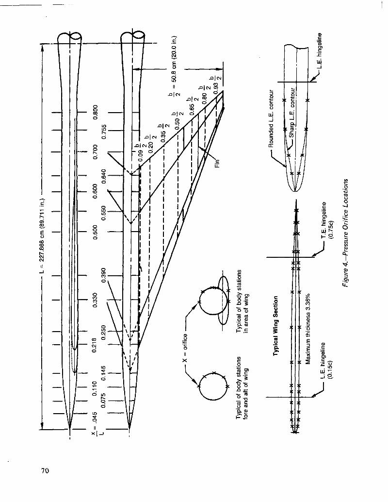
L =
227.
866
cm (
89.7
11
in.)
‘I I
x=
.045
0.
110
0.21
8 0.
330
20.0
in.
)
Typi
cal
of b
ody
stat
ions
Ty
pica
l of
bod
y st
atio
ns
fore
and
aft
of w
ing
in a
rea
of w
ing
Typi
cal
Win
g Se
ctio
n r
Rou
nded
L.
E.
cont
our
--)tx
)c
-::
-Jex
x-
x ;i
JI
:
Max
imum
th
ickn
ess
3.36
%
L.E.
hi
ngel
ine
(0.1
5c)
T.E.
hi
ngel
ine
(0.7
5c)
Figu
re
4.-P
ress
ure
Orif
ice
Loca
tions
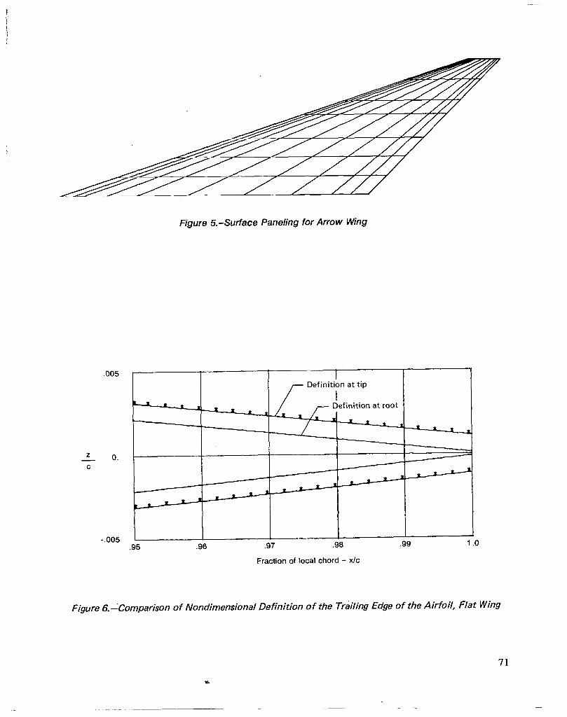
Figure 5.-Surface Paneling for Arrow Wing
,005
Z - 0.
C
-.005
Definition at tip
I 1 .95 .96 .97 .96 .99 1 .o
Fraction of local chord - X/C
Figure 6. -Comparison of Nondimensional Definition of the Trailing Edge of the Airfoil, Fiat Wing
71
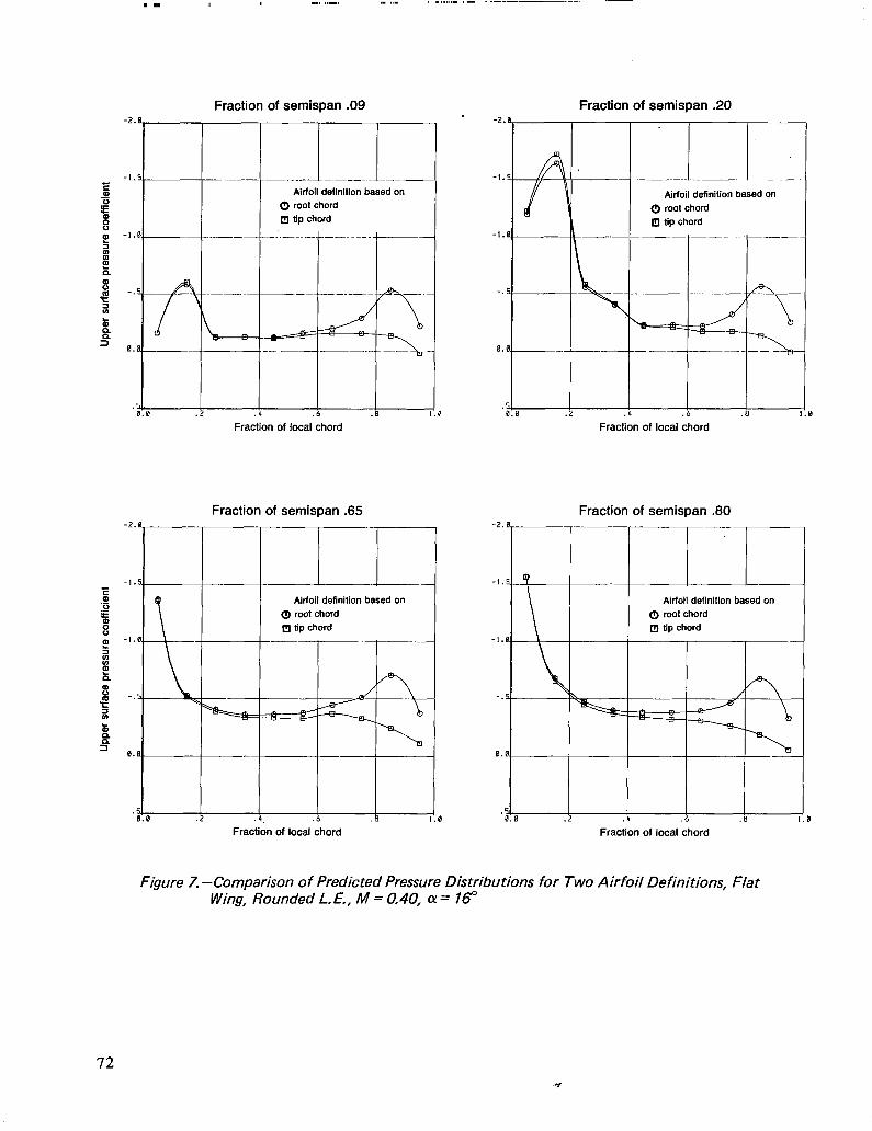
Fraction of semispan .09 Fraction of semispan .20
-1.5. - ..----______ E a Airfoil definition based on Airfoil definition based on g root chord $
Q tip chord
4. .0.0 .4 .6 .8
Fraction of local chord Fraction of local chord
Fraction of semispan .65
Airfoil definition based on
I 2 .4 .6 B I
Fraction of local chord
Fraction of semispan .60
Fraction of local chord
Airfoil definition based on
j \ / / %%:zd
Figure 7. -Comparison of Predicted Pressure Distributions for Two Airfoil Definitions, Fiat Wing, Rounded 1. E., M = 0.40, CV= 16”
72
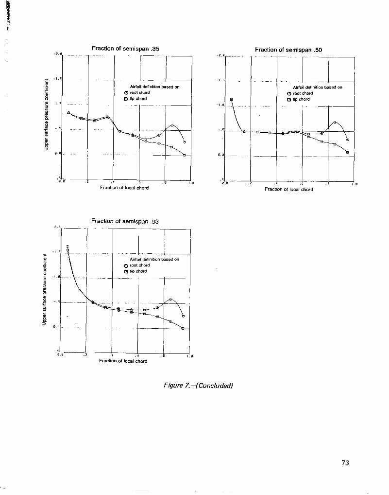
Fraction of semispan .35 Fraction of semispan .50
Airfoil definition based on Q root chord [II tlp chord .-
.=--K
Fraction of local chord .B
Fraction of semispan .93
Airfoil definition based on
I.0
1 .4
Airfoil definition based on 0 root chord [II tip chord
Fraction of local chord
Fraction of local chord
Figure 7. -(Concluded)
73

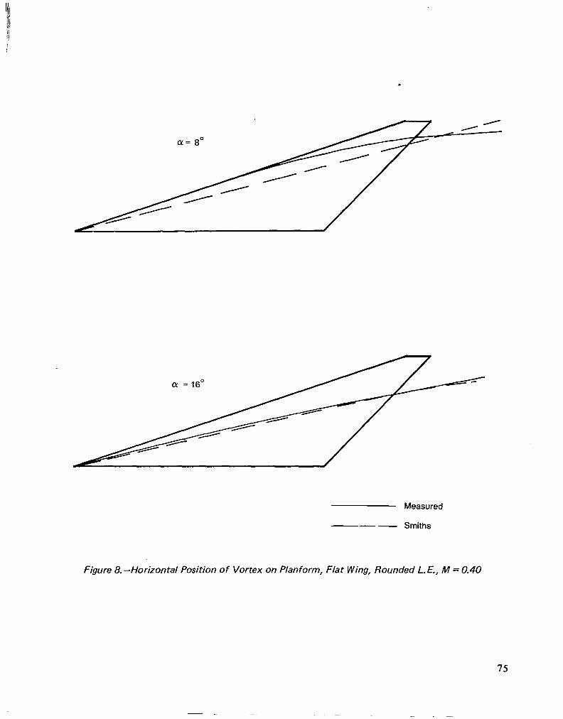
Measured
--- Smiths
Figure 8.-Horizontal Position of Vortex on Planform, Flat Wing, Rounded 1. E., M = 0.40
75
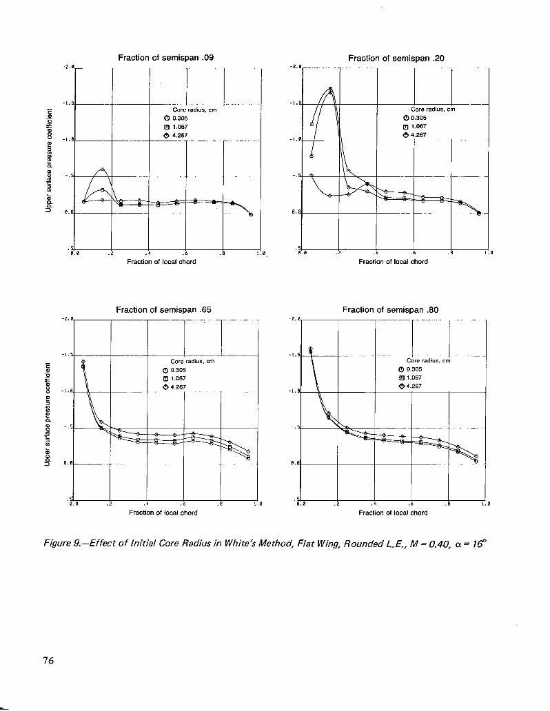
Fraction of semispan .09 Fraction of semispan .20
-““~ !.
l.S-
n-
. . _
l.R-
L ‘0.0
.E
.I
Core radius, cm
I [I) 1.067
.2 .4 .6
Fraction of local chord
Fraction of semispan .65
1 -- .b
Core radius, cm Q 0.305 Q 1.067 0 4.267
I
.6
Fraction of local chord Fraction of local chord
.-
110
Core radius, Q 0.305 Q 1.067
-1.n \ @ 4.267 II I
-2.
-I.
-I.
-.
0.
Fraction of local chord
Fraction of semispan .80
r- --- ..‘- Li Core radius, cm
Q 0.305 izI 1.067 0 4.267
Figure 9.-Effect of Initial Core Radius in White’s Method, Flat Wing, Rounded L.E., M = 0.40, (Y= 16”
76
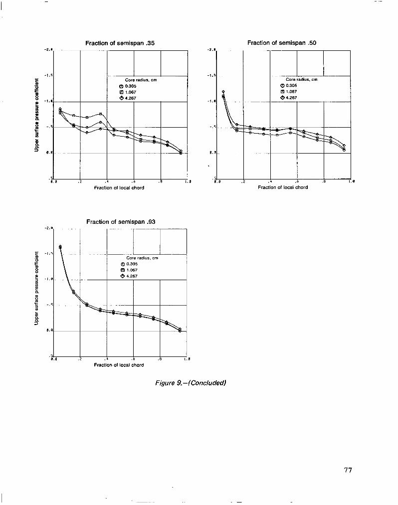
Fraction of semispan .35 Fraction of semispan .50
Cl 1.067 @ 4.267
Fraction of local chord Fraction of local chord
Fraction of semispan .93
Q 0.305 1 Cl 1.067
I I .4 .6 I Fraction of local chord
Core radius. cm Q 0.305 @I 1.067 @ 4.267
Figure 9. -(Concluded)
77
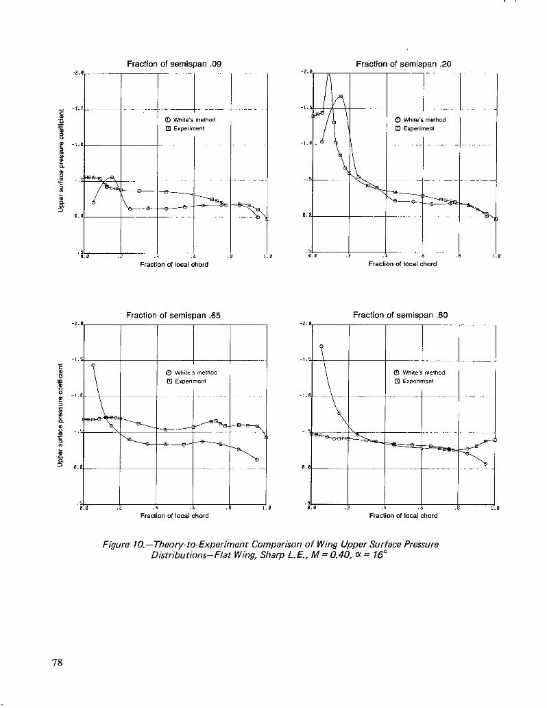
Fraction of semispan .09
Fraction of local chord Fraction of local chord
Fraction of semiwan .65
I I 1 I .4 .b .B
Fraction of local chord
Fraction of semispan .20
0 White’s method
Fraction of semispan .80
Fraction of local chord
Figure 10. -Theory- to-Experiment Comparison of Wing Upper Surface Pressure Distributions-Flat Wing, Sharp 1. E., M = 0.40, (Y = 76”
78
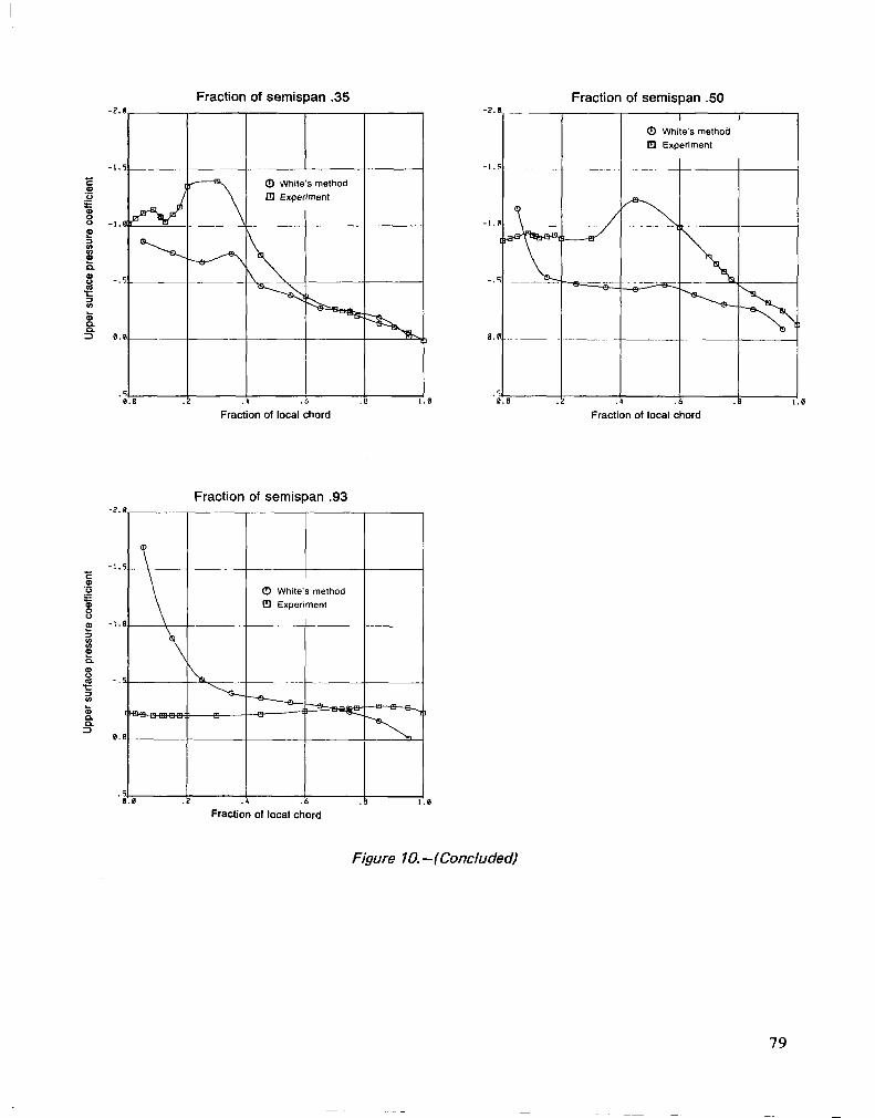
Fraction of semispan .35
Fraction of local chord
Fraction of semispan .93
-2.
-I.
-I.
-.
0.
I.0
Fraction of semispan .50 I I
0 White’s method
Cl Experiment
Fraction of local chord
Figure IO.-(Concluded)
Fraction of local chord
79
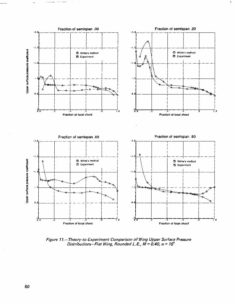
__ . . . - -.--
Fraction of semispan .09 -2. -2.
-1. -1. -I. -I. -. -.
Fraction of local chord Fraction of local chord
Fraction of semispan .65 Fraction of semispan .80
Fraction of l&al chord Fraction of local chord
Fraction of semispan .20 -2.
-I.
-1.
-.
8.
Figure 7 1. -Theory- to-Experiment Comparison of Wing Upper Surface Pressure Distributions- Flat Wing, Rounded 1. E., M = 0.40, Q! = 16”
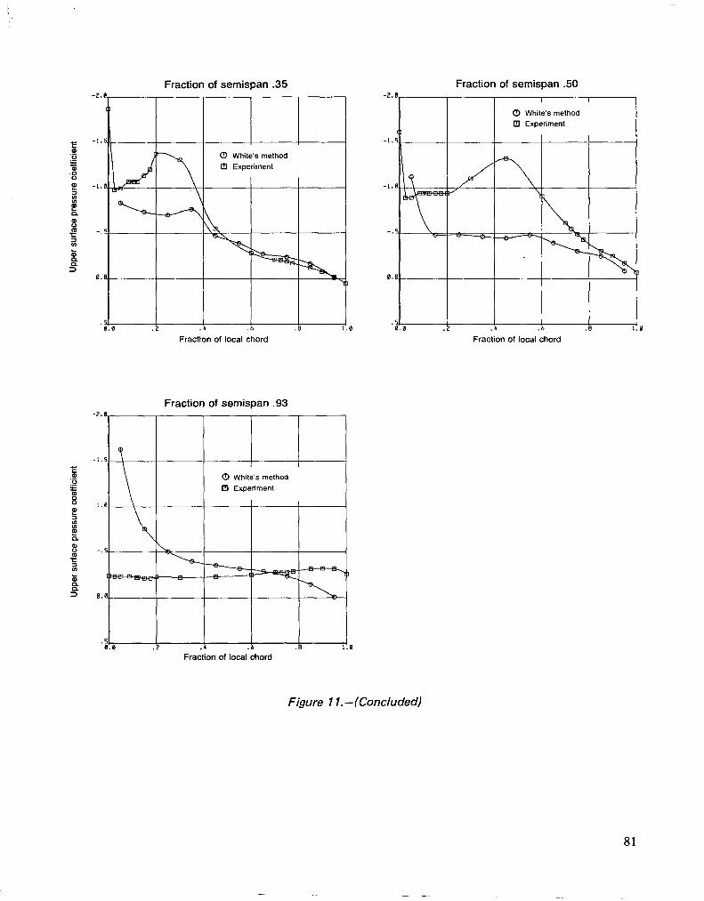
Fraction of semispan .35 Fraction of semispan 50
0 White’s method fl Experiment
Fraction of local chord
Fraction of semispan .93
I I 0 White’s method
I I I I .4 .6 I.0 Fraction of local chord
Fraction of local chord
Figure 1 I.-(Concluded)
81
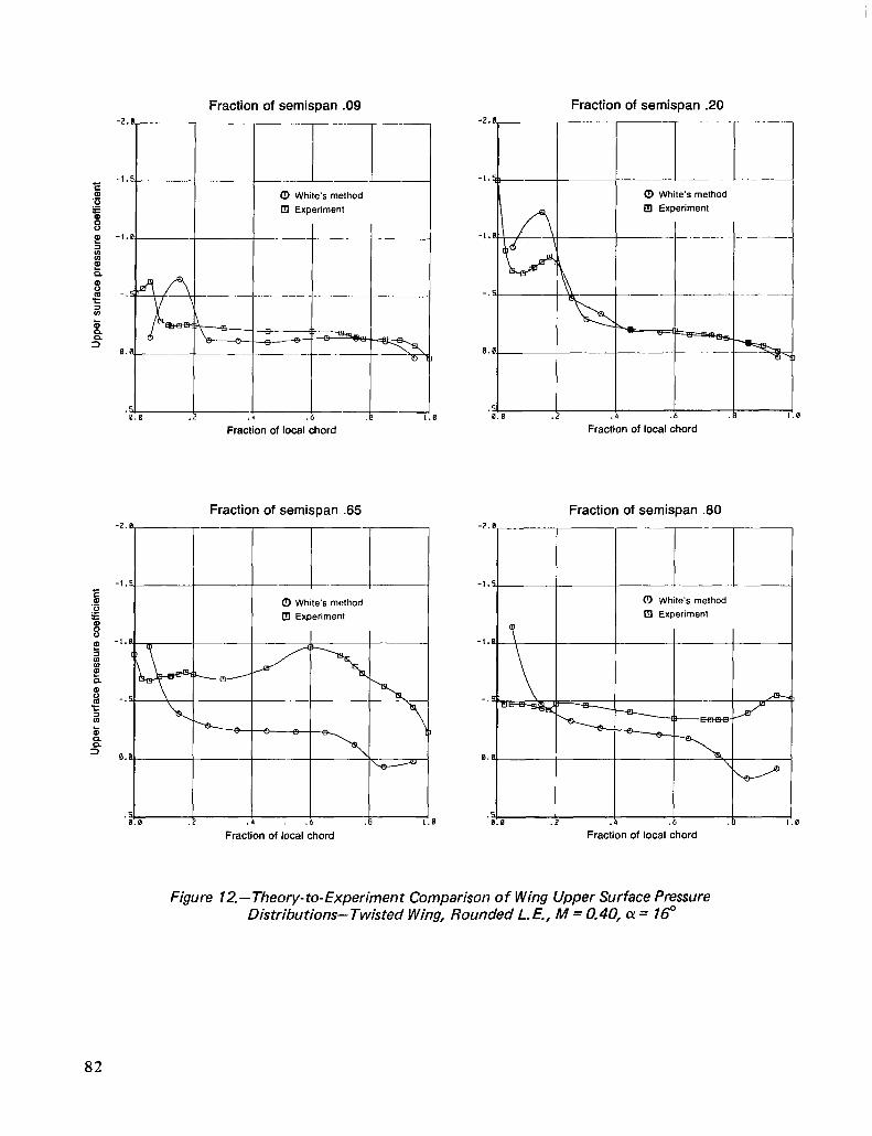
Fraction of semispan .09 Fraction of semispan .20
0 White: method
I I I I I I .--4-J .* .6 I.0
Fraction of local chord
Fraction of semispan .65
1 0 White’s method
I I I I I I 5/I
‘0.0 .4 .b .8 I.0 Fraction of local chord
Fraction of semispan .60
-I.
-.
0.
.x 2 .4 .6 b 1.0
Fraction of local chord
-ltmTF4 51
‘0:0 I ! ! I
.4 .6 I.0 Fraction of local chord
Figure 12. -Theory- to-Experiment Comparison of Wing Upper Surface Pressure Distributions- Twisted Wing, Rounded I!.. E., M = 0.40, Q! = 16”
82
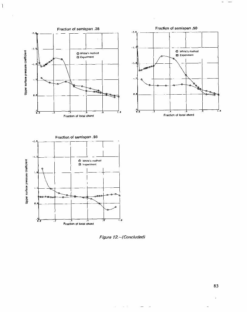
Fraction of semispan .35 Fraction of semispan .50
@J White’s method
.- Fraction of local chord
Fraction of semispan .93
-2.I
Fraction of local chord
1 0 White’s method I
I I I U I I
.5 0.0 2 ., .6 b I.0
Fraction of local chord
Figure 12. -/Concluded)
83
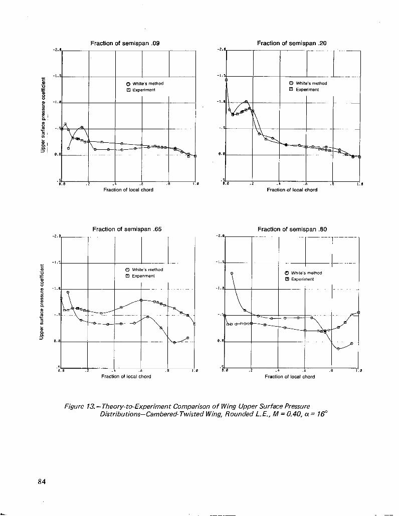
Fraction of semispan .09 Fraction of semispan .20 -2.
-I.
-I.
-.
0.
0 Fraction of local chord Fraction of local chord
Fraction of semispan .65 Fraction of semispan .80
0 White’s method 0 White’s method
Fraction of local chord Fraction of local chord Fraction of local chord
-2.
-1.
-I. -I.
-. -.
0. 0.
.3.0 .4 .6 1.0 0
Figure 13. -Theory- to-Experiment Comparison of Wing Upper Surface Pressure Distributions-Cambered-Twisted Wing, Rounded L. E., M = 0.40, cy = 16”
84
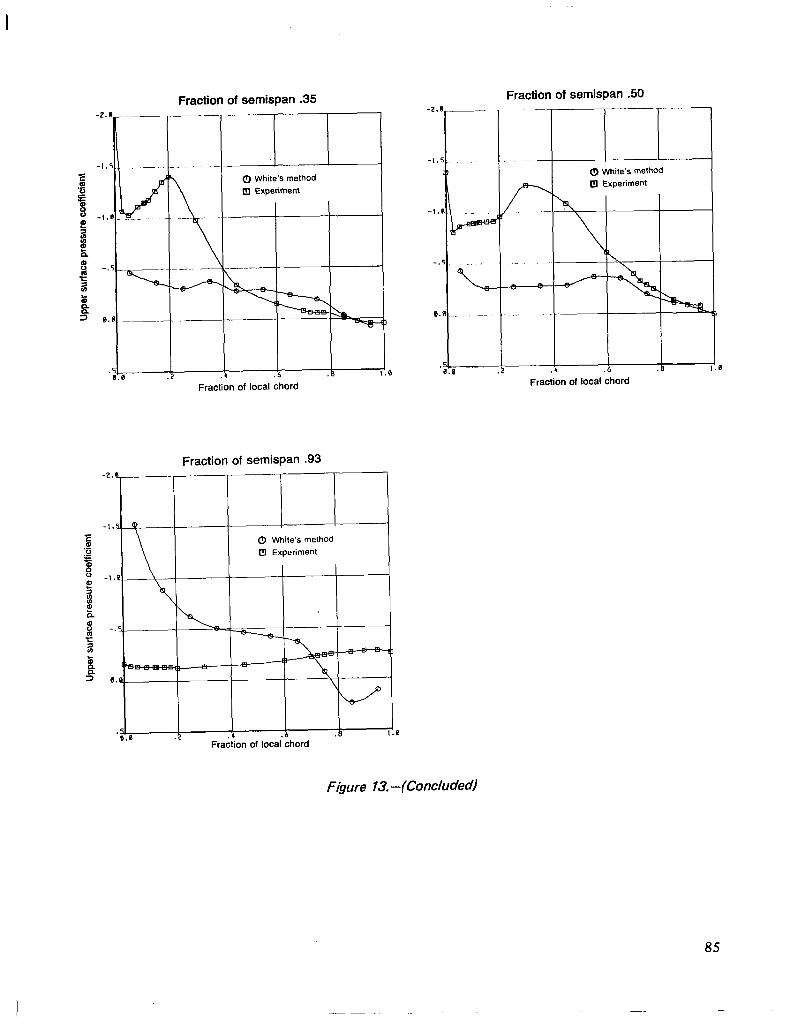
Fraction of semispan .50 Fraction of semispan .35
Fraction of local chord
0 White’s method
Fraction of semispan .93
0 White’s method
Fraction of local chord
.0 5l I I I I I
‘0:e .2 .a .6 I.0 Fraction of local chord
F&ure 13.4Concluded
85
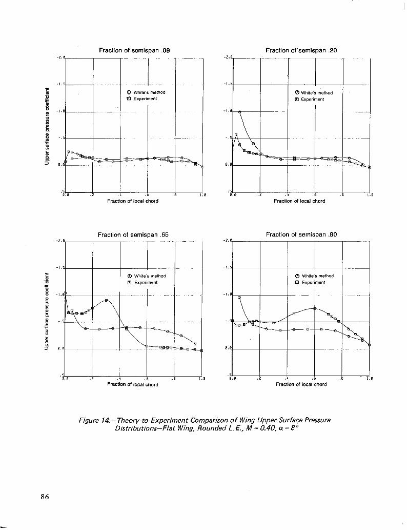
Fraction of‘semispan .09 Fraction of semispan .20 -2.0.
I I .2 .4 .6 110
Fraction of local chord
Fraction of semispan .65 Fraction of semiwan .80
0 White’s method 0 White’s method
E (I1 Experiment (I1 Experiment
E -I.
7 I h 8 -.
7
Fraction of lo.cal chord Fraction of local chord
.- -
-f,
i-. 0
0 White’s method
I I
(I1 Experiment
I
2 .4 .6 .B IL0
Fraction of local chord
Figure 14. -Theory- to-Experiment Comparison of Wing Upper Surface Pressure Distributions-Flat Wing, Rounded L. E., M = 0.40, CY = 8”
86
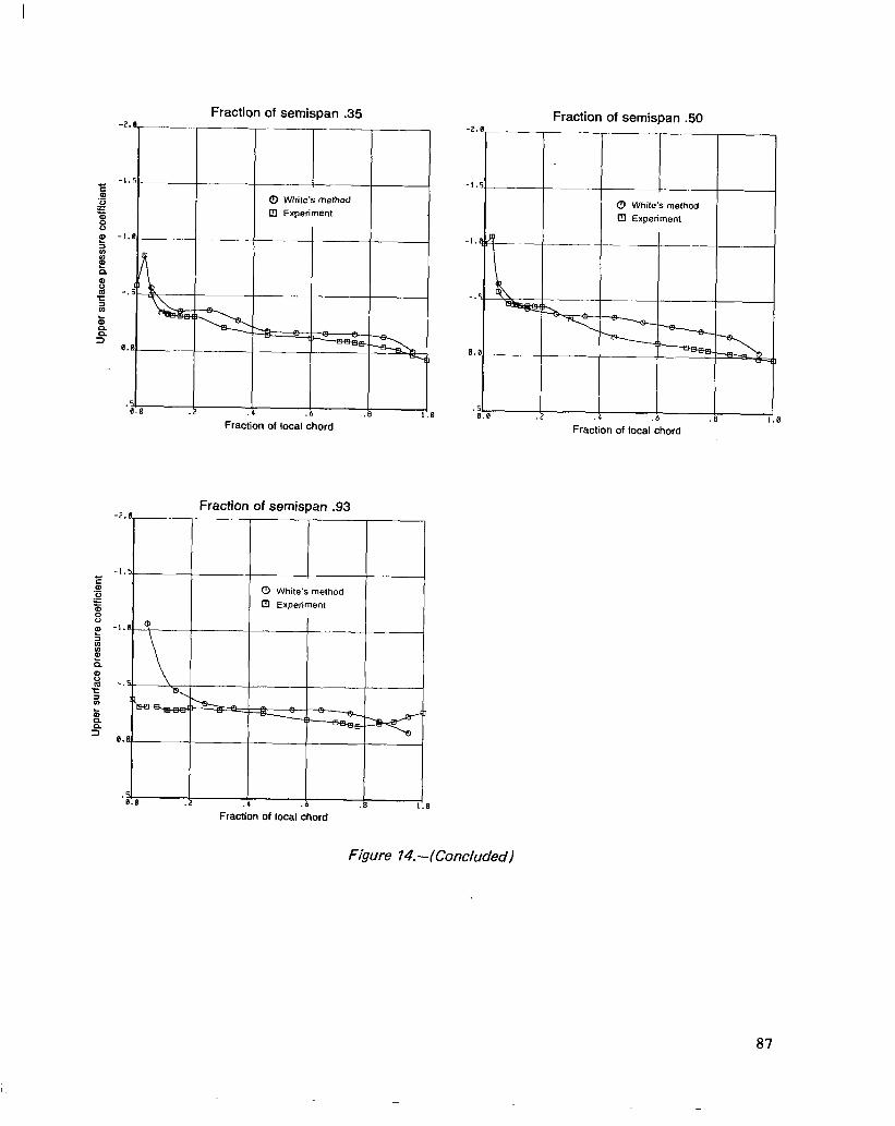
Fraction of semispan .35 Fraction of semispan .35
.2 .4 .b I I.0
Fraction of local chord Fraction of local chord
Fraction of semisDan .50 Fraction of semispan .50
cl White3 method
.4 .6 Fraction of local chord Fraction of local chord
-2. 4 Fraction of semispan .93 , , Fraction, of semisrn .93 ,
0 0 White’s method White’s method
0 0 Fraction of local chord Fraction of local chord
Figure 14.-(Concluded) Figure 14.-(Concluded)
87
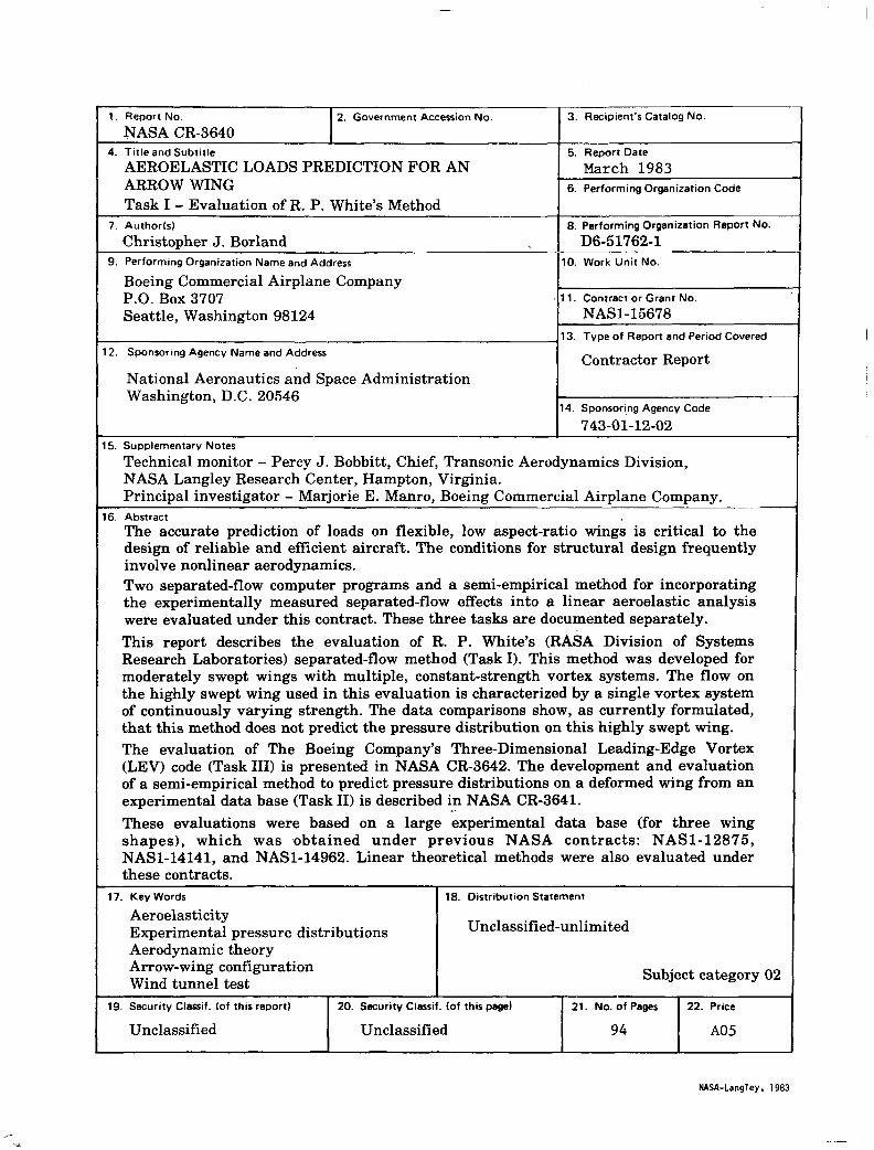
-
1. Report No. 2. Government Accession No.
NASA CR-3640 4. Title and Subtitle
AEROELASTIC LOADS PREDICTION FOR AN ARROW WING Task I - Evaluation of R. P. White’s Method
3. Recipient’s Catalog No.
5. Report Date
March 1983 6. Performing Organization Code
7. Author(s)
Christopher J. Borland 9. Performing Organization Name and Address
Boeing Commercial Airplane Company P.O. Box 3707 Seattle, Washington 98124
12. Sponsoring Agency Name and Address
8. Performing Organization Report NO.
\ -fjzEJh---~
NASl-15678 I 13. Type of Report and Period Covered
Contractor Report National Aeronautics and Space Administration Washington, D.C. 20546
14. Sponsor!ng Agency Code
743-01-12-02 I5 Supplementary Notes
Technical monitor - Percy J. Bobbitt, Chief, Transonic Aerodynamics Division, NASA Langley Research Center, Hampton, Virginia. Principal investigator - Marjorie E. Manro, Boeing Commercial Airplane Company.
-.- 16. Abstract
The accurate prediction of loads on flexible, low aspect-ratio wings is critical to the design of reliable and efficient aircraft. The conditions for structural design frequently involve nonlinear aerodynamics. Two separated-flow computer programs and a semi-empirical method for incorporating the experimentally measured separated-flow effects into a linear aeroelastic analysis were evaluated under this contract. These three tasks are documented separately. This report describes the evaluation of R. P. White’s (RASA Division of Systems Research Laboratories) separated-flow method (Task I). This method was developed for moderately swept wings with multiple, constant-strength vortex systems. The flow on the highly swept wing used in this evaluation is characterized by a single vortex system of continuously varying strength. The data comparisons show, as currently formulated, that this method does not predict the pressure distribution on this highly swept wing. The evaluation of The Boeing Company’s Three-Dimensional Leading-Edge Vortex (LEV) code (Task III) is presented in NASA CR-3642. The development and evaluation of a semi-empirical method to predict pressure distributions on a deformed wing from an experimental data base (Task II) is described in NASA CR-3641. ,- These evaluations were based on a large experimental data base (for three wing shapes), which was obtained under previous NASA contracts: NASl-12875, NASl-14141, and NASl-14962. Linear theoretical methods were also evaluated under these contracts.
17. Key Words 18. Distribution Statement
Aeroelasticity Experimental pressure distributions Unclassified-unlimited
Aerodynamic theory Arrow-wing configuration Wind tunnel test
Subject category 02
19. Security Classif. tof this report) 20. Security Classif. (of this page) 21. No. of Pages 22. Price
Unclassified Unclassified 94 A05
HASA-Langley, 1983