Embed Size (px)
Citation preview
Aerodynamic Design of an Aspirated
Counter-Rotating Compressor
by
Jody Kirchner
B.A.Sc (Mechanical Eng), University of British Columbia (2000)
Submitted to the Department of Aeronautics and Astronauticsin partial fulfillment of the requirements for the degree of
Master of Science
at the
MASSACHUSETTS INSTITUTE OF TECHNOLOGY
June 2002
@ Massachusetts Institute of Technology 2002. All rights reserved.
A uthor ................. ...............Dep$rtrent of Aeronautics and Astronautics
May 1, 2002
Certified by...Jack L. Kerrebrock
Professor Emeritus of Aeronautics and AstronauticsThesis Supervisor
Accepted by............. ...Wallace E. Vander Velde
Professor of Aeronautics and AstronauticsChair, Committee on Graduate Students
MASSACHUSETTS iNSTITUTEOF TECHNOLOGY
AEROAUG 1 3 2002
I I M'" M"' A V'% lr-ir%

2

Aerodynamic Design of an Aspirated Counter-Rotating
Compressor
by
Jody Kirchner
Submitted to the Department of Aeronautics and Astronauticson May 1, 2002, in partial fulfillment of the
requirements for the degree ofMaster of Science
Abstract
A primary goal in compressor design for jet engines is the reduction of size and weight.This can be achieved by increasing the work output per stage, thereby reducing therequired number of stages. In this thesis, the aerodynamic design of a high speedcompressor that produces a pressure ratio of 9.1:1 in only two stages (rather thanthe typical six or seven) is presented. This is accomplished by employing bladeaspiration in conjunction with rotor counter-rotation. Aspiration has been shown tomake feasible significantly increased blade loading and counter-rotation provides ameans of taking full advantage of this potential throughout a multistage compressor.
The aspirated counter-rotating compressor was designed using a one-dimensionalstage analysis program coupled with an axisymmetric throughflow code and a quasi-three-dimensional cascade code for blade design. The design of each stage focussedon maximising pressure ratio within diffusion factor and relative inlet Mach number(i.e. shock loss) constraints. The exit angle of the first stator was optimised tomaximise the pressure ratio of the counter-rotating (second) rotor. The blade designcode MISES allowed for each feature of the blade sections, including aspiration, to beprecisely designed for the predicted conditions. To improve the process of designingblades with MISES, extensive analysis of previously designed high-speed aspiratedblades was performed to identify the relationships between various blade features.
Thesis Supervisor: Jack L. KerrebrockTitle: Professor Emeritus of Aeronautics and Astronautics
3

4
Acknowledgments
I would like to thank my advisor Professor Jack Kerrebrock for suggesting this project,
providing guidance while giving me space to figure things out on my own, and, perhaps
most importantly, keeping me excited about the project along the way.
I would also like to thank Ali Merchant for providing supervision and for putting
up with my struggles with all the CFD programs. Also, thanks for writing an excellent
PhD thesis which was an invaluable reference for this work. Thanks to Brian Schuler
for teaching me how to use MISES and for providing assistance along the way.
Finally, a very special thanks to all the friends I have made at MIT who have
helped make this a great experience.
5

6
Contents
1 Introduction
1.1 Motivation and Background . . . . . . . . . . . . . . . . . . . . . . .
1.2 O bjectives . . . . . . . . . . . . . . . . . . . . . . . . . . . . . . . . .
1.3 O utline. . . . . . . . . . . . . . . . . . . . . . . . . . . . . . . . . . .
2 Compressor Theory
2.1 Stage A nalysis . . . . . . . . . . . . . . . . . . . . . . . . . . . . . . .
2.2 Dimensionless Parameters . . . . . . . . . . . . . . . . . . . . . . . .
2.3 Losses ....... ...................................
2.3.1 V iscous Losses . . . . . . . . . . . . . . . . . . . . . . . . . . .
2.3.2 Shock Losses . . . . . . . . . . . . . . . . . . . . . . . . . . .
2.4 A spiration . . . . . . . . . . . . . . . . . . . . . . . . . . . . . . . . .
3 Design Methodology and 0
3.1 Design Process . . . . . .
3.2 Goals and Constraints . .
4 Stage and Flowpath Design
4.1 Stage Analysis . . . . . . .
4.1.1 Work Distribution
4.1.2 Interstage Swirl . .
4.1.3 Geometry . . . . .
4.2 Flowpath Generation . . .
bjectives
. . . . . . . . . . . . . . . . . . . . . . . .
. . . . . . . . . . . . . . . . . . . . . . . .
7
13
13
17
17
19
19
21
22
23
24
25
29
29
31
33
33
34
34
36
37
4.3 Throughflow Analysis . . . . . . . . . . . . . . . . . . . . . . . . . . . 38
4.3.1 Code Description . . . . . . . . . . . . . . . . . . . . . . . . . 39
4.3.2 Results . . . . . . . . . . . . . . . . . . . . . . . . . . . . . . . 40
4.4 Design Summary . . . . . . . . . . . . . . . . . . . . . . . . . . . . . 41
5 Blade Design 45
5.1 Code Description . . . . . . . . . . . . . . . . . . . . . . . . . . . . . 45
5.2 Design Process . . . . . . . . . . . . . . . . . . . . . . . . . . . . . . 47
5.3 Blade Features . . . . . . . . . . . . . . . . . . . . . . . . . . . . . . 51
5.3.1 Incidence . . . . . . . . . . . . . . . . . . . . . . . . . . . . . 52
5.3.2 Camber Distribution . . . . . . . . . . . . . . . . . . . . . . . 54
5.3.3 Thickness Distribution . . . . . . . . . . . . . . . . . . . . . . 56
5.3.4 Leading Edge . . . . . . . . . . . . . . . . . . . . . . . . . . . 58
5.3.5 Trailing Edge . . . . . . . . . . . . . . . . . . . . . . . . . . . 59
5.3.6 Aspiration . . . . . . . . . . . . . . . . . . . . . . . . . . . . . 60
5.4 Final Blade Designs. . . . . . . . . . . . . . . . . . . . . . . . . . . . 61
5.4.1 Stage 1. . . . . . . . . . . . . . . . . . . . . . . . . . . . . . . 61
5.4.2 Stage 2. . . . . . . . . . . . . . . . . . . . . . . . . . . . . . . 67
5.4.3 Summary . . . . . . . . . . . . . . . . . . . . . . . . . . . . . 72
6 Conclusion 75
6.1 Compressor Design Summary . . . . . . . . . . . . . . . . . . . . . . 75
6.2 Concluding Remarks on Design Process . . . . . . . . . . . . . . . . . 76
6.3 Future W ork . . . . . . . . . . . . . . . . . . . . . . . . . . . . . . . . 77
A 25% and 75% Span Blade Sections 83
8
List of Figures
1-1 Work output of counter-rotating relative to conventional compressor
1-2 Conventional modern engine and conceptual engine with aspirated
counter-rotating compressor (adapted from Reference [8]) . . . . . . .
2-1 Compressor stage nomenclature . . . . . . . . . . .
2-2 Correlation of diffusion factor and loss parameter .
2-3 Variation of entropy rise due to shock loss with inlet
2-4 Suction slot (adapted from Reference [18]) . . . . .
2-5 Effect of aspiration on a blade boundary layer [18] .
3-1 Compressor design process . . . . . . . . . . . . . .
4-1 Variation of rotor 2 diffusion factor with inlet swirl
4-2 Stator 1 exit angle distribution . . . . . . . . . . .
4-3 Flowpath and blades . . . . . . . . . . . . . . . . .
4-4 Throughflow pressure contours . . . . . . . . . . . .
4-5 Velocity triangles . . . . . . . . . . . . . . . . . . .
5-1
5-2
5-3
5-4
5-5
5-6
5-7
Mach number
15
16
20
24
26
. . . . . . . . . 27
. . . . . . . . . 27
. . . . . . . . . 30
. . . . . . . . . 35
. . . . . . . . . 36
. . . . . . . . . 38
. . . . . . . . . 41
. . . . . . . . . 42
Blade section design flowchart . . . . . . . . . . . . . . . . . .
Blade pressure distribution design templates . . . . . . . . . .
Correction of blade surface bump . . . . . . . . . . . . . . . .
Impact of blade surface bump on inviscid pressure distribution
Blade section parameters . . . . . . . . . . . . . . . . . . . . .
Stagger angle versus turning angle . . . . . . . . . . . . . . . .
Maximum camber versus turning angle . . . . . . . . . . . . .
. . . . 48
. . . . 49
. . . . 50
50
51
54
55
9
5-8 Typical rotor camber di
5-9 Maximum thickness ver
5-10 Leading edge radius ver
5-11 Diverging trailing edge
5-12
5-13
5-14
5-15
5-16
5-17
5-18
5-19
5-20
5-21
5-22
5-23
5-24
5-25
A-i
A-2
A-3
A-4
A-5
A-6
A-7
A-8
hape
hap
stributions . . . . . . .
sus inlet Mach number
sus inlet Mach number
paraete.........
..pramte.........
..............
parameter . . . . . . .
..............
e parameter . . . . . . .
..............
..............
. . . . . . . . . . . . . .
. . . . . . . . . . . . . .
10
Rotor 1 hub . ...
Rotor 1 50% span .
Rotor 1 50% span s
Rotor 1 tip . . . .
Stator 1 hub . ...
Stator 1 50% span
Stator 1 50% span s
Stator 1 tip . . . .
Rotor 2 hub . ...
Rotor 2 50% span .
Rotor 2 tip . . . .
Stator 2 hub . ...
Stator 2 50% span
Stator 2 tip . . . .
Rotor 1 25% Span .
Rotor 1 75% Span .
Stator 1 25% Span
Stator 1 75% Span
Rotor 2 25% Span.
Rotor 2 75% Span.
Stator 2 25% Span
Stator 2 75% Span
56
58
59
60
62
63
63
64
65
66
66
67
68
69
70
71
72
72
83
84
84
85
85
86
86
87

List of Tables
3.1 Design goals and constraints . . . . . . . . . . . . . . . . . . . . . . . 31
4.1 Stage design results . . . . . . . . . . . . . . . . . . . . . . . . . . . . 43
5.1 M ISES design results . . . . . . . . . . . . . . . . . . . . . . . . . . . 73
11

12
Chapter 1
Introduction
1.1 Motivation and Background
A driving force in compressor design is the desire to achieve a high pressure ratio and
efficiency while maintaining or decreasing the size (particularly length) and weight of
the compressor. It is also beneficial to reduce the number of parts, especially blades
which are expensive to produce and maintain. To this end it is necessary to develop
means of improving the performance of individual compressor stages so that fewer
stages are required for a given application.
The pressure ratio attainable in a compressor stage has traditionally been limited
by viscous effects on the blades, in particular flow separation. However, recent work
by Kerrebrock and others has shown that removing a portion of the boundary layer
fluid from the blade surface through aspiration can delay separation and allow for
significantly increased blade loading (see for example [11], [12]). This in turn reduces
the number of stages required to obtain the desired compressor pressure ratio. A
low-speed compressor stage employing aspiration has been built and tested success-
fully [18, 21] and a high-speed stage has been designed and is under construction for
testing [18]. With aspiration shown to be viable way of raising the loading limits of
blades, it is an opportune time to consider means of taking advantage of the ability
to do more work with each stage.
A conventional compressor stage consists of a rotating blade row, or rotor, and a
13
stationary blade row, or stator. The rotor does work on the fluid given by
WR = w(r 2v 2 - riV) (1.1)
where w is the angular velocity and rv is the angular momentum per unit mass (also
called swirl) at the inlet (1) and exit (2). The stator converts some fraction of the
rotor work into a static pressure rise. Equation 1.1 shows that there are two ways
to increase the work of a stage: increase the tip speed and increase the change in
swirl or turning. However, tip speed in modern compressors is limited by structural
constraints, so increased turning must be considered as a means to obtain any increase
in work.
There is a wide range of design options to choose from in selecting the swirl at the
inlet to the rotor, riv1 , but in modern high-work compressors the stators typically
remove all of the swirl from the upstream rotors, so that the flow entering each rotor
is axial (rivi = 0). Even with advances in blade design, there is a limit on how far
the rotor can turn the flow from the axial direction and, therefore, how much work
it can do on the flow. However, if the flow entering the rotor has swirl against the
direction of rotation (riv < 0), for the same rotor exit angle the amount of work
is increased. This can be achieved throughout a multistage compressor by reducing
the turning of the stators (or removing the stators altogether) and alternating the
direction of rotation of the spools. This is termed counter-rotation.
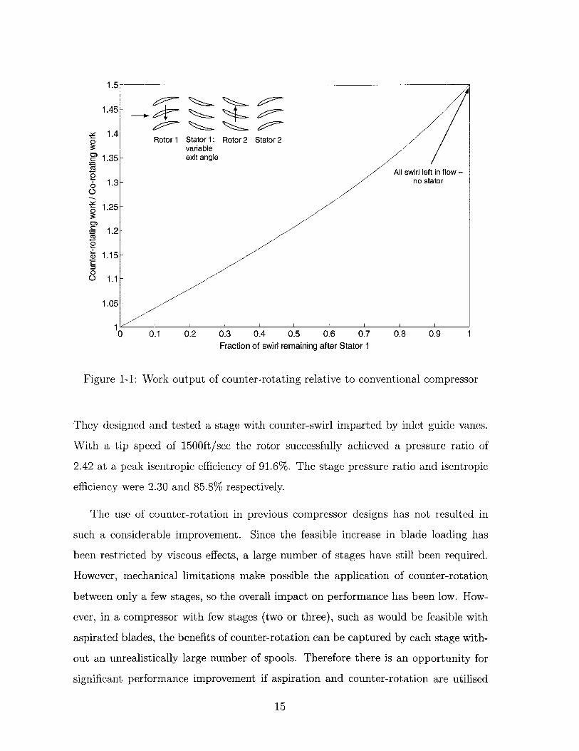
Figure 1-1 shows the ratio of the ideal work output of a simple two-stage counter-
rotating compressor to that of a conventional two-stage compressor given by
Wcounter _ wr(vc - Vb)counter - 1 +-tan
WeO wr(ve - Vb)cO 2
where a is the exit angle of the first stator for the counter-rotating configuration.
Geometrically, the configurations are identical except for the exit angle of the first
stator which is zero for the conventional configuration and varies for the counter-
rotating configuration. This simple analysis shows that a significant increase in work
is possible with counter-rotation.
A more extensive assessment of the performance improvement possible for a single
compressor stage with inlet counter-swirl was made by Law and Wennstrom [14].
14
1.5
1.45-
-~1.4-
1 Rotor 1 Stator 1: Rotor 2 Stator 2variable
. 1.35- exit angle
- All swirl left in flow -2 1.3 no stator
1.25-
1.2-0
1.15-
0o 1.1
1.05-
10 0.1 0.2 0.3 0.4 0.5 0.6 0.7 0.8 0.9 1
Fraction of swirl remaining after Stator 1
Figure 1-1: Work output of counter-rotating relative to conventional compressor
They designed and tested a stage with counter-swirl imparted by inlet guide vanes.
With a tip speed of 1500ft/sec the rotor successfully achieved a pressure ratio of
2.42 at a peak isentropic efficiency of 91.6%. The stage pressure ratio and isentropic
efficiency were 2.30 and 85.8% respectively.
The use of counter-rotation in previous compressor designs has not resulted in
such a considerable improvement. Since the feasible increase in blade loading has
been restricted by viscous effects, a large number of stages have still been required.
However, mechanical limitations make possible the application of counter-rotation
between only a few stages, so the overall impact on performance has been low. How-
ever, in a compressor with few stages (two or three), such as would be feasible with
aspirated blades, the benefits of counter-rotation can be captured by each stage with-
out an unrealistically large number of spools. Therefore there is an opportunity for
significant performance improvement if aspiration and counter-rotation are utilised
15
together.
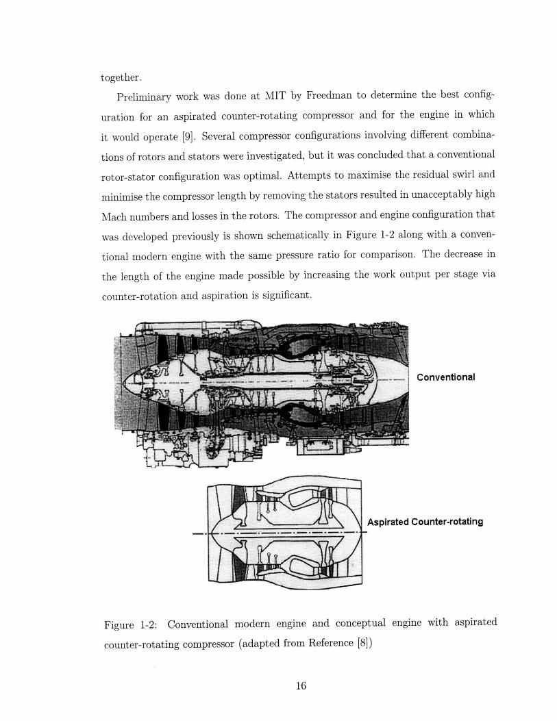
Preliminary work was done at MIT by Freedman to determine the best config-
uration for an aspirated counter-rotating compressor and for the engine in which
it would operate [9]. Several compressor configurations involving different combina-
tions of rotors and stators were investigated, but it was concluded that a conventional
rotor-stator configuration was optimal. Attempts to maximise the residual swirl and
minimise the compressor length by removing the stators resulted in unacceptably high
Mach numbers and losses in the rotors. The compressor and engine configuration that
was developed previously is shown schematically in Figure 1-2 along with a conven-
tional modern engine with the same pressure ratio for comparison. The decrease in
the length of the engine made possible by increasing the work output per stage via
counter-rotation and aspiration is significant.
Conventional
Aspirated Counter-rotating
Figure 1-2: Conventional modern engine and conceptual engine with aspirated
counter-rotating compressor (adapted from Reference [8])
16
1.2 Objectives
The purpose of this work was to continue with the development of the multi-stage
aspirated counter-rotating compressor discussed in Section 1.1. More specifically, the
primary goal was to produce a detailed aerodynamic design of a two-stage compressor
to be tested in the Blowdown Compressor facility at MIT. These tests will be used
to assess the validity of the aspirated counter-rotating concept for use in practical
applications.
Although other applications are possible, it is presently thought that an aspirated
counter-rotating compressor would be ideal for use as a core compressor in a long
range supersonic cruise aircraft. This is mainly because such aircraft are especially
sensitive to weight. This foreseen application provided the basis for many of the
parameters of the current design.
1.3 Outline
The body of this thesis details the steps and results of the compressor design. Chapter
2 provides a theoretical background for the work, including the important parameters
and equations for the stage analysis and evaluation of losses and aspiration. The steps
of the design process as well as the goals and constraints are presented in Chapter 3.
Chapter 4 discusses the design of the compressor stages and the flowpath including the
work distribution and geometry choices. The results of a computational throughflow
analysis are also presented in this chapter. Chapter 5 describes the design of the blade
sections using a quasi-three-dimensional turbomachinery cascade code and presents
the final blade designs. Finally, Chapter 6 provides some conclusions, including a
summary of the compressor design as well as a discussion of future work.
17

18
Chapter 2
Compressor Theory
2.1 Stage Analysis
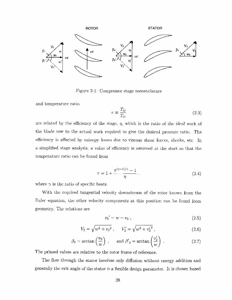
In a one-dimensional compressor stage analysis, the flow through a blade row (rotor
and stator) is described by the changes in velocity components as shown in Figure 2-1.
The components shown as solid vectors represent absolute velocities and those shown
as dotted vectors represent velocities relative to the rotating frame of reference of the
rotor. The conditions at the stage inlet (denoted with the subscript 1) are known
either from the compressor inlet conditions (for the first stage) or the upstream stage
exit conditions (for subsequent stages). To simplify the analysis, it is often assumed
that the axial velocity, w, is constant, although in reality it will fluctuate across the
blade rows.
The change in tangential velocity, v, across the rotor can be related to the stag-
nation temperature, T, rise by the Euler equation
C,(T2- Tti) = w(r 2v 2 - riv1 ) (2.1)
where w is the rotational speed, r is the radius, and c, is the specific heat at constant
pressure. In the design problem considered here, the stagnation temperature change
is fixed by the desired pressure ratio and the required tangential velocity change must
be found. The pressure ratio= - (2.2)
Pt1
19.
ROTOR STATOR
v V2 V3P3i Vcr V2~
W r w2 v or W3owr j3/ V2
Figure 2-1: Compressor stage nomenclature
and temperature ratio
T - - (2.3)T
are related by the efficiency of the stage, TI, which is the ratio of the ideal work of
the blade row to the actual work required to give the desired pressure ratio. The
efficiency is affected by entropy losses due to viscous shear forces, shocks, etc. In
a simplified stage analysis, a value of efficiency is assumed at the start so that the
temperature ratio can be found from
T = 1 + (2.4)
where -y is the ratio of specific heats.
With the required tangential velocity downstream of the rotor known from the
Euler equation, the other velocity components at this position can be found from
geometry. The relations are
V2 = W - V2 (2.5)
V2 /= w 2 +v 22 , V2'= W2+4 , (2.6)
V2V2 V2+ V
02 = arctan , and #'2 = arctan ). (2.7)
The primed values are relative to the rotor frame of reference.
The flow through the stator involves only diffusion without energy addition and
generally the exit angle of the stator is a flexible design parameter. It is chosen based
20
on the inlet flow desired for the downstream component, within the aerodynamic
constraints of the blade (for example, the separation characteristics). Once the stator
exit angle is chosen, the velocity components at that position can be found from
V 3 = wtan/33 , and (2.8)
V = w 2 +v 32 . (2.9)
Generally, it is useful to represent the velocities through the compressor as Mach
numbers given by
M=- . (2.10)a
The quantity a is the local speed of sound
V2
a = RT = yR (T - 2p(2.11)
where R is the specific gas constant, and T is the static temperature.
For a counter-rotating compressor stage, the analysis is the same as that for a
conventional stage except that the tip speed used in the Euler equation is negative.
When determining the velocity components geometrically, care must be taken to use
tangent and sine functions rather than cosine so that the negative relative velocities
are preserved.
2.2 Dimensionless Parameters
From the quantities obtained in the stage analysis, several useful dimensionless pa-
rameters can be defined, in addition to the pressure and temperature ratios. These
dimensionless parameters are useful in summarising a compressor design since val-
ues for different compressors can be compared more directly than can dimensional
parameters.
The work done across the stage, cAT, and the rotor speed, wr, are combined to
give the stage loading coefficient which is a measure of the fraction of blade energy
transferred to the fluid
w=)2 . (2.12)(Wr)2
21
The axial velocity, w, and the rotor speed are combined to give the flow coefficient
w=_ .(2.13)
The absolute value of the rotational speed is used here so that the flow coefficient will
be positive for the counter-rotating rotor. The distribution of loading in the stage is
represented by the degree of reaction which is the ratio of the static enthalpy, cT,
rise in the rotor to that in the stage
RC = T T (2.14)T3 - T1
The fractional change in axial velocity through a blade row is termed the axial velocity
ratio
AVR = . (2.15)W1
This value is important to blade boundary layer behaviour which depends heavily
on whether the flow is accelerating (AVR > 1) or decelerating (AVR < 1). In the
stage analysis described in Section 2.1, the axial velocity ratio will be equal to one
(since axial velocity is assumed constant), but this will not in general be the case.
For flow in which large density changes occur, such as in high-speed compressors, a
more useful parameter is the axial velocity density ratio
AVDR - P (2.16)p1w1
which represents the streamtube contraction or expansion through the blade row.
2.3 Losses
In low-speed compressors the most significant source of loss is viscous shear on the
blades. However, for high-speed compressors, such as that considered here, shock
losses can be up to seven or eight times larger than viscous losses (as seen with the
aspirated blades designed by Merchant [18]). Therefore, an accurate model for both
types of loss is important. More minor sources of loss such as tip leakage losses and
possible shroud losses are not considered here.
22
To avoid results that are dependant on the frame of reference (moving for the
rotor and stationary for the stator), the losses are presented in terms of the resulting
entropy increase in the flow, As [10]. The entropy rises due to each component of loss
for the rotor and stator can be added to give the total entropy increase for the stage.
The entropy rise and temperature ratio of the stage give the adiabatic efficiency
res* 0 /cP - 1T-=l .(2.17)
2.3.1 Viscous Losses
Viscous losses in cascades are represented by a non-dimensional pressure loss coeffi-
cientA = . (2.18)
Pt - P1
Analysis of cascade data by Lieblein [15] lead to a correlation between the loss coeffi-
cient and the now widely used diffusion factor which is a measure of the deceleration
of the flow through the blade passages. The diffusion factor is given by
D = 1 V2 + |v2 - v 1 (2.19)V1 2-Vi
where the subscript 1 represents relative inlet flow and the subscript 2 represents
relative exit flow. The solidity of the cascade, o, is the ratio of the chord length
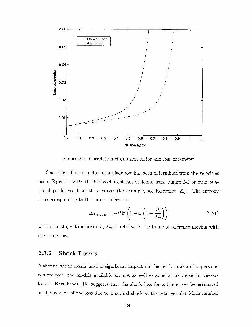
to the blade spacing. Figure 2-2 shows the Lieblein correlation between the loss
parameter which is a function of the loss coefficient and the diffusion factor
W 2cos c f (D) . (2.20)cs1 2o-
For low diffusion factors (below about 0.45) the viscous loss is almost constant, but
above this value the loss increases rapidly due to boundary layer separation. For this
reason, conventional blades are generally limited to diffusion factors well below 0.5.
Adding aspiration to blades reduces the boundary layer thickness. Therefore, it is
possible to go to higher diffusion factors before approaching separation and incurring
a rapid increase in loss. Schuler [21] presents a correlation between the diffusion
factor and the loss parameter for aspirated blades, similar to Lieblein's correlation
for conventional blades. This is also shown in Figure 2-2.
23
0 0.1 0.2 0.3 0.4 0.5 0.6
Diffusion factor
0.7 0.8 0.9 1
Figure 2-2: Correlation of diffusion factor and loss parameter
Once the diffusion factor for a blade row has been determined from
using Equation 2.19, the loss coefficient can be found from Figure 2-2
tionships derived from these curves (for example, see Reference [21]).
rise corresponding to the loss coefficient is
the velocities
or from rela-
The entropy
a~sviscous = -R In 1 - D 1 - P))(2.21)
where the stagnation pressure, P'2, is relative to the frame of reference moving with
the blade row.
2.3.2 Shock Losses
Although shock losses have a significant impact on the performance of supersonic
compressors, the models available are not as well established as those for viscous
losses. Kerrebrock [10] suggests that the shock loss for a blade row be estimated
as the average of the loss due to a normal shock at the relative inlet Mach number
24
0.06
0.05
0.04
0.03
EDa
0-
-J
Conventional- - Aspirated
-/
0.02
0.01
01.1
'
and the loss due to a normal shock at the suction surface impingement location Mach
number. Experimental data has shown that the actual shock losses in rotors are lower
than predicted by this method, so it provides a conservative estimate.
The blade relative Mach number will be known from the stage analysis, but the
shock impingement Mach number must be estimated since the position of the shock
will not generally be known at this point in the design. Based on aspirated blades
designed by Merchant, Schuler [21] presents an equation to estimate the shock im-
pingement Mach number,
Mimp = 1.225Mre. (2.22)
With the Mach numbers known, the corresponding entropy rise through the shock is
27) 2 2+ (7y - 1)M 2 '\ 27) 2"/.XSshock cpn I + (M2 - 1) -Rln I + (M2 _ 1)
7+ 1(7y + 1) M2 7+ 1(2.23)
The average of the entropy rises at the two Mach numbers provides the entropy rise
for the blade row.
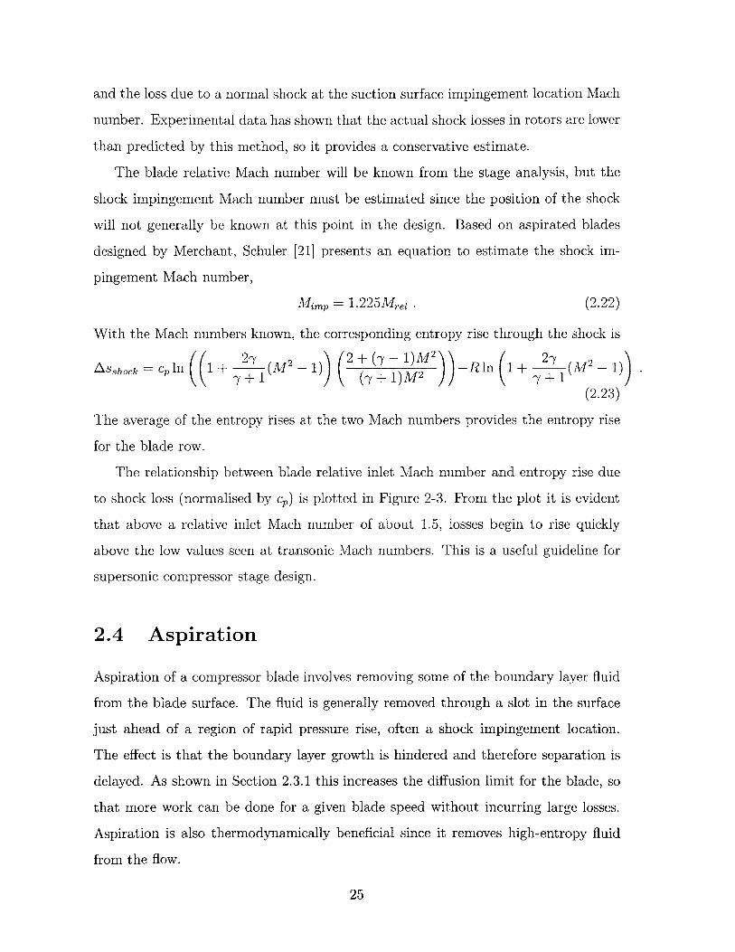
The relationship between blade relative inlet Mach number and entropy rise due
to shock loss (normalised by c,) is plotted in Figure 2-3. From the plot it is evident
that above a relative inlet Mach number of about 1.5, losses begin to rise quickly
above the low values seen at transonic Mach numbers. This is a useful guideline for
supersonic compressor stage design.
2.4 Aspiration
Aspiration of a compressor blade involves removing some of the boundary layer fluid
from the blade surface. The fluid is generally removed through a slot in the surface
just ahead of a region of rapid pressure rise, often a shock impingement location.
The effect is that the boundary layer growth is hindered and therefore separation is
delayed. As shown in Section 2.3.1 this increases the diffusion limit for the blade, so
that more work can be done for a given blade speed without incurring large losses.
Aspiration is also thermodynamically beneficial since it removes high-entropy fluid
from the flow.
25
0.12
c-
Cj)
0.06-C.0
0.04-
0.02-
00.8 1 1.2 1.4 1.6 1.8 2
Inlet relative Mach number
Figure 2-3: Variation of entropy rise due to shock loss with inlet Mach number
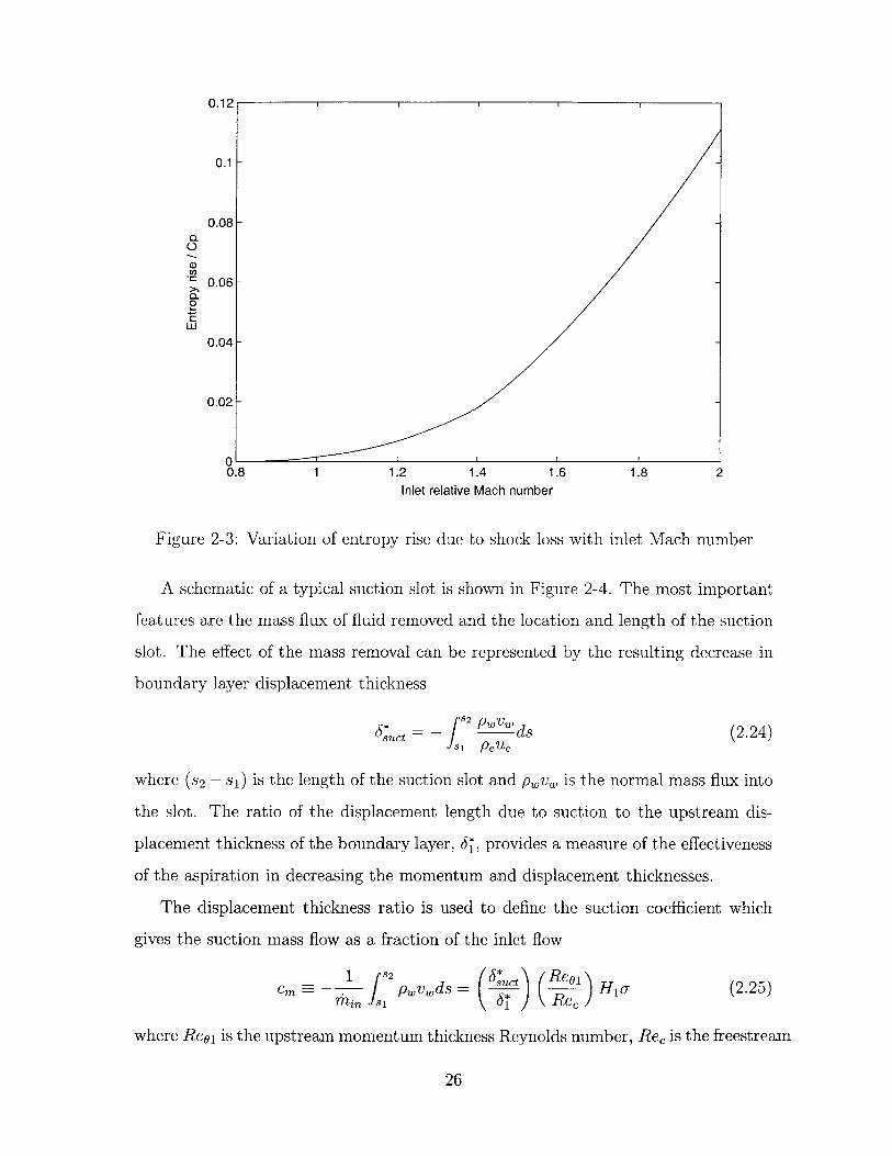
A schematic of a typical suction slot is shown in Figure 2-4. The most important
features are the mass flux of fluid removed and the location and length of the suction
slot. The effect of the mass removal can be represented by the resulting decrease in
boundary layer displacement thickness
f82
6d*,t = - pwvw ds (2.24)isi Peue
where (s2 - si) is the length of the suction slot and pwVw is the normal mass flux into
the slot. The ratio of the displacement length due to suction to the upstream dis-
placement thickness of the boundary layer, 6*, provides a measure of the effectiveness
of the aspiration in decreasing the momentum and displacement thicknesses.
The displacement thickness ratio is used to define the suction coefficient which
gives the suction mass flow as a fraction of the inlet flow
1 fs2 = * Reol 1,mj5 /1o Re (2.25)
where Reo1 is the upstream momentum thickness Reynolds number, Rec is the freestream
26
Mn
'++
Figure 2-4: Suction slot (adapted from Reference [18])
Reynolds number based on chord length, H1 is the boundary layer shape parameter,
and o is the solidity of the blade row [18].
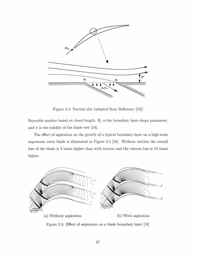
The effect of aspiration on the growth of a typical boundary layer on a high-work
supersonic rotor blade is illustrated in Figure 2-5 [18]. Without suction the overall
loss of the blade is 3 times higher than with suction and the viscous loss is 10 times
higher.
C~ .0255
(a) Without aspiration (b) With aspiration
Figure 2-5: Effect of aspiration on a blade boundary layer [18]
27

28
Chapter 3
Design Methodology and
Objectives
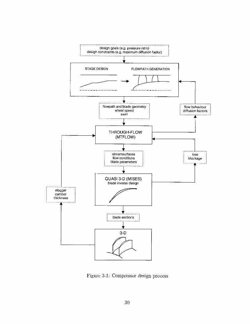
3.1 Design Process
The design process followed in this work was adapted from that used by Merchant [18]
to design low- and high-speed aspirated compressor stages. The process is outlined
schematically in Figure 3-1.
Given a set of goals and constraints for the compressor, the first step in the design
process is to determine the required flow properties upstream and downstream of each
stage, including the flow angles and velocities. From this information the flowpath
and axial blade geometry can be generated. The geometry and the parameters from
the stage design are then input to an axisymmetric throughflow solver which provides
more detailed aerodynamic information. The throughflow solver also outputs the data
required for the quasi-three-dimensional design of the blades which is performed in the
next step. Finally a complete three-dimensional analysis of the design is performed.
After each step, the new (and presumably improved) information gained is input to
the previous step to refine the design. This leads to an iterative process for which
the final goal is agreement between the results from each analysis and satisfaction
of the constraints of the problem. This thesis carries the design only through the
quasi-three-dimensional design phase.
29
design goals (e.g. pressure ratio)design constraints (e.g. maximum diffusion factor)
STAGE DESIGN FLOWPATH GENERATION
flowpath and blade geometrywheel speed
swirl
THROUGH-FLOW(MTFLOW)
flow behaviourdiffusion factors
1"q
streamsurfaces,flow conditions
blade parameters
QUASI 3-D (MISES)blade inverse design
blade sections
Figure 3-1: Compressor design process
30
lossblockage
staggercamber
thickness.. ..... ....
3-D
3.2 Goals and Constraints
The main goal of this work was to design a compressor that will be used in experiments
to assess the use of counter-rotation together with aspiration. Based on this intended
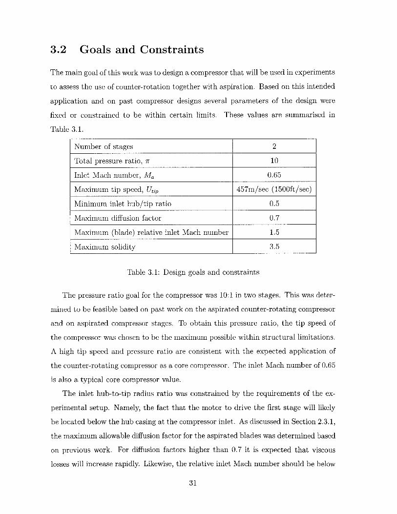
application and on past compressor designs several parameters of the design were
fixed or constrained to be within certain limits. These values are summarised in
Table 3.1.
Number of stages 2
Total pressure ratio, 7r 10
Inlet Mach number, Ma 0.65
Maximum tip speed, Utip 457m/sec (1500ft/sec)
Minimum inlet hub/tip ratio 0.5
Maximum diffusion factor 0.7
Maximum (blade) relative inlet Mach number 1.5
Maximum solidity 3.5
Table 3.1: Design goals and constraints
The pressure ratio goal for the compressor was 10:1 in two stages. This was deter-
mined to be feasible based on past work on the aspirated counter-rotating compressor
and on aspirated compressor stages. To obtain this pressure ratio, the tip speed of
the compressor was chosen to be the maximum possible within structural limitations.
A high tip speed and pressure ratio are consistent with the expected application of
the counter-rotating compressor as a core compressor. The inlet Mach number of 0.65
is also a typical core compressor value.
The inlet hub-to-tip radius ratio was constrained by the requirements of the ex-
perimental setup. Namely, the fact that the motor to drive the first stage will likely
be located below the hub casing at the compressor inlet. As discussed in Section 2.3.1,
the maximum allowable diffusion factor for the aspirated blades was determined based
on previous work. For diffusion factors higher than 0.7 it is expected that viscous
losses will increase rapidly. Likewise, the relative inlet Mach number should be below
31

1.5 to avoid large shock losses. Finally, the maximum solidity requirement exists to
limit the number of blades required and help avoid blockage problems. The value of
3.5 was chosen based on past experience and is at the high end of the typical range
so as to help keep diffusion losses low.
32
Chapter 4
Stage and Flowpath Design
The first step in the design process was to quantify the properties of each stage,
including the geometry, flow angles, Mach numbers, and losses, based on the given
values and constraints. Many of the design variables were unconstrained so some
investigation of previous designs and experimentation was required to find the best
combination of parameters. Once the stage properties were fixed, the flowpath was
generated and a throughflow CFD code was used to analyse the design. This process
was repeated until the throughflow results were acceptable.
4.1 Stage Analysis
To design the stages, a simple stage analysis program was developed with the proce-
dure described in Section 2.1 implemented at three spanwise locations: hub, mean,
and tip. Radial equilibrium was assumed. The diffusion factors and viscous and shock
losses were also computed using the models discussed in Section 2.3. This program
facilitated the relatively quick investigation of many design alternatives and hence
allowed for some rudimentary design optimization. The primary metric used to de-
termine the best design at this step was the distribution of diffusion factors. However,
consideration was also given to the relative Mach numbers entering the blade rows,
since shock losses were expected to be significant.
33
4.1.1 Work Distribution
A primary goal of the stage design was to fix the pressure ratio or work division for the
stages. For ease of design, the pressure ratio of the first stage was chosen to match that
of the high-speed aspirated stage designed by Merchant [18]. The design of this stage,
including the blade sections, has been completed successfully. The pressure ratio of
the second stage was then fixed by the overall compressor requirement. The required
pressure ratios of the rotors were initially estimated using an assumed pressure ratio
for the stators. This was revised when more accurate values were available from the
throughflow analysis.
4.1.2 Interstage Swirl
The swirl distribution (rv) at the exit of the first stator is critical to the design since it
directly determines the usefulness of the counter-rotation. However, determining the
optimum distribution was not straightforward as several competing design variables
are influenced by the swirl, including the diffusion factors at several locations. Clearly,
maximizing the swirl entering the second stage maximizes the benefit of counter-
rotation. The pressure ratio of the second rotor can be increased while decreasing
the diffusion factors of both stators. However, the residual swirl increases the relative
Mach number entering the second rotor, thereby increasing the shock losses. The
swirl also increases the reaction of the second stage meaning that the rotor shares
a larger burden in producing the enthalpy rise in the stage. The diffusion factor of
the second rotor is affected by the swirl as well, but the relationship is relatively
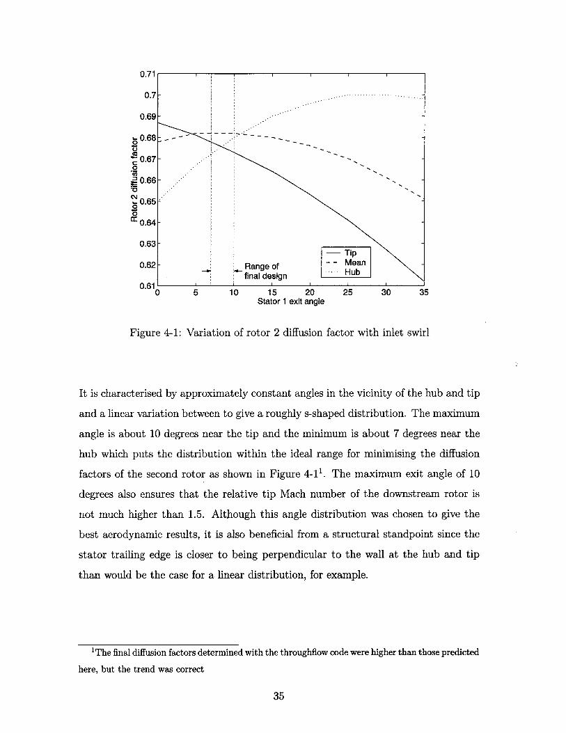
complicated as it depends on the radial location. This is illustrated in Figure 4-1.
A preliminary investigation of the effects of the stator swirl distribution (as dis-
cussed above) was completed with the stage analysis program. However, there were
secondary effects of the distribution that were only evident in the throughflow so-
lution. These effects were more complicated and not easy to quantify. Therefore,
iteration on this feature of the design using the throughflow code was necessary.
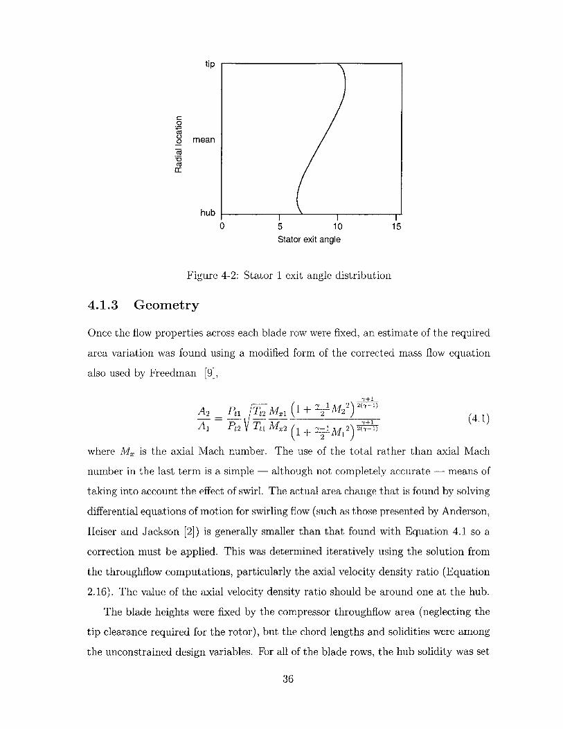
The stator swirl distribution that was selected is shown graphically in Figure 4-2.
34
-00
0
0.64
0.63 -
0.62 -Range offinal design~-~---Hu
0.610 5 10 15 20 25 30 35
Stator 1 exit angle
Figure 4-1: Variation of rotor 2 diffusion factor with inlet swirl
It is characterised by approximately constant angles in the vicinity of the hub and tip
and a linear variation between to give a roughly s-shaped distribution. The maximum
angle is about 10 degrees near the tip and the minimum is about 7 degrees near the
hub which puts the distribution within the ideal range for minimising the diffusion
factors of the second rotor as shown in Figure 4-1. The maximum exit angle of 10
degrees also ensures that the relative tip Mach number of the downstream rotor is
not much higher than 1.5. Although this angle distribution was chosen to give the
best aerodynamic results, it is also beneficial from a structural standpoint since the
stator trailing edge is closer to being perpendicular to the wall at the hub and tip
than would be the case for a linear distribution, for example.
The final diffusion factors determnined with the throughilow code were higher than those predicted
here, but the trend was correct
35
tip
04uCo,8 mean
CE
hub0 5 10 15
Stator exit angle
Figure 4-2: Stator 1 exit angle distribution
4.1.3 Geometry
Once the flow properties across each blade row were fixed, an estimate of the required
area variation was found using a modified form of the corrected mass flow equation
also used by Freedman [9],
A2. PtI T 2 MX1 (I + y M2) 2(y-1)(41- = - -(4.1)
A1 Pt 2 Ta Mx2 (1 + 2 IM 12) 2(y-1)
where Mx is the axial Mach number. The use of the total rather than axial Mach
number in the last term is a simple - although not completely accurate - means of
taking into account the effect of swirl. The actual area change that is found by solving
differential equations of motion for swirling flow (such as those presented by Anderson,
Heiser and Jackson [2]) is generally smaller than that found with Equation 4.1 so a
correction must be applied. This was determined iteratively using the solution from
the throughflow computations, particularly the axial velocity density ratio (Equation
2.16). The value of the axial velocity density ratio should be around one at the hub.
The blade heights were fixed by the compressor throughflow area (neglecting the
tip clearance required for the rotor), but the chord lengths and solidities were among
the unconstrained design variables. For all of the blade rows, the hub solidity was set
36
close to the maximum allowable value to keep the diffusion factors low. Approximately
constant chord lengths were used for all blade rows to maximize the solidities away
from the hub. The values of the chord lengths were determined from the aspect ratios.
These were chosen based on other modern high-speed core compressor designs.
4.2 Flowpath Generation
The large pressure ratios across each stage in this design necessitate area contractions
that are much larger than typically seen in axial compressors. This made the flowpath
design particularly challenging. Frequently, axial compressors are designed with a
constant tip radius which means only the hub is contoured to achieve the required area
variation. This minimizes the turning required for a given rate of rotation (because
the radii are kept high) and helps keep the losses low. Also, the possibility of the
rotor hitting the tip casing during forward-backward vibration is virtually eliminated.
However, if the required area contractions are large a constant tip radius leads to a
very convoluted profile at the hub. This can adversely affect the flow behavior and
increase the structural complexity. Also, there is some benefit to decreasing the tip
radius in that it accelerates the flow at the tip and decreases the diffusion factors
there. Therefore, for this design a linearly decreasing tip radius was used. The angle
of the tip casing relative to the rotational axis is about 3".
Approximate radial coordinates for the hub were determined from the required
area (found using Equation 4.1) upstream and downstream of each blade row. Axial
coordinates were determined by taking axial projections of the blades and assuming a
blade row separation distance of one-quarter of the maximum chord length of the up-
stream blade as suggested by Mattingly [16]. The cubic spline package in MATLAB 2
was used to interpolate between the hub points and generate a smooth flowpath. A
major objective in this process was to avoid sharp curves so as to reduce the pos-
sibility of flow separation and minimize the pressure gradients caused by streamline
curvature. Across the rotors the hub was constrained to be linear to avoid mechan-
2See MATLAB documentation at www.mathworks.com
37
ical complexity. The linear tip radius decrease lead to a hub ramp angle at the first
rotor of about 30'. For the subsequent blade rows, the hub ramp angle decreases
approximately linearly.
After the flowpath was initially generated, it was optimised using the results of
the throughflow computations (discussed in the next section). This primarily involved
further smoothing of the hub profile and small area changes based on the computed
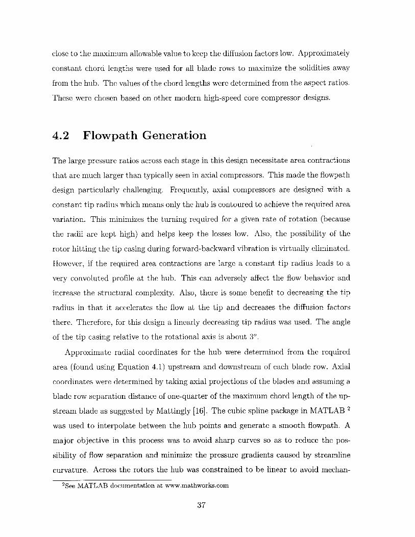
axial velocity density ratios. The final flowpath with the axial blade projections is
shown in Figure 4-3.
3*
STATOR 2
STATOR 1
300
ROTOR 1
Figure 4-3: Flowpath and blades
4.3 Throughflow Analysis
To obtain more accurate estimates for the compressor performance (and improve
the design where necessary), the results of the stage design were analysed with a
throughflow CFD code. This code was also used to generate the input files for the
blade design.
38

4.3.1 Code Description
The throughflow analysis was performed with MTFLOW, an axisymmetric code de-
veloped at MIT by Drela [5]. MTFLOW solves the Euler equations on a streamline
grid taking into account the effects of swirl, loss generation, and blockage which are
input as spanwise distributions. End wall boundary layers, spanwise mixing, and
non-axisymmetric effects are not modelled in the code.
For reference, the 3-D Euler equations in vector form are
80 oP a 85+ + + = pQ (4.2)
where U is the state vector, F, G, and H are the flux vectors in the x, y, and x
directions respectively, and Q is the source term for centrifugal and Coriolis forces,
/ \
/Pu
pu 2 + P
pu~v
Puw
u(pE +p)/
I,
p
pu
pv
pw
pEI
p~vPYLV
pv H-
pvw
v(pE +p)/
(4.3)
/pw
paw
pvw
pw2 + p
w(pE + p) j
, (4.4)
/
In these vectors, E is the total rotary
0
0
Q2 y - 2Qw
Q 2 z + 2Qv
0
internal energy given by
,1(22 12E = e+ 1- (U2+ V2 + 2 2) r2
2 2
39
(4.5)
(4.6)
\
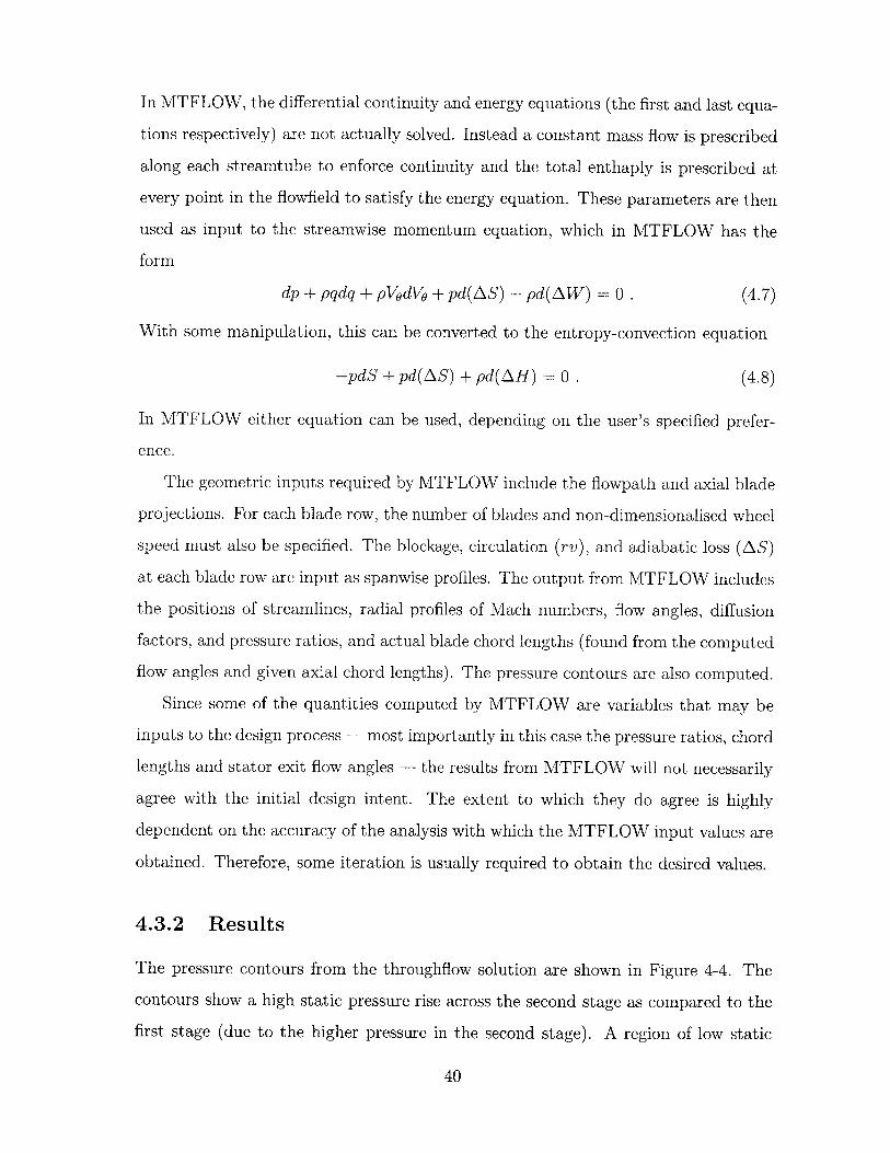
In MTFLOW, the differential continuity and energy equations (the first and last equa-
tions respectively) are not actually solved. Instead a constant mass flow is prescribed
along each streamtube to enforce continuity and the total enthaply is prescribed at
every point in the flowfield to satisfy the energy equation. These parameters are then
used as input to the streamwise momentum equation, which in MTFLOW has the
form
dp + pqdq + pVodVo + pd(ZAS) - pd(AW) = 0 . (4.7)
With some manipulation, this can be converted to the entropy-convection equation
-pdS + pd(LAS) + pd(AH) = 0 . (4.8)
In MTFLOW either equation can be used, depending on the user's specified prefer-
ence.
The geometric inputs required by MTFLOW include the flowpath and axial blade
projections. For each blade row, the number of blades and non-dimensionalised wheel
speed must also be specified. The blockage, circulation (rv), and adiabatic loss (AS)
at each blade row are input as spanwise profiles. The output from MTFLOW includes
the positions of streamlines, radial profiles of Mach numbers, flow angles, diffusion
factors, and pressure ratios, and actual blade chord lengths (found from the computed
flow angles and given axial chord lengths). The pressure contours are also computed.
Since some of the quantities computed by MTFLOW are variables that may be
inputs to the design process - most importantly in this case the pressure ratios, chord
lengths and stator exit flow angles - the results from MTFLOW will not necessarily
agree with the initial design intent. The extent to which they do agree is highly
dependent on the accuracy of the analysis with which the MTFLOW input values are
obtained. Therefore, some iteration is usually required to obtain the desired values.
4.3.2 Results
The pressure contours from the throughflow solution are shown in Figure 4-4. The
contours show a high static pressure rise across the second stage as compared to the
first stage (due to the higher pressure in the second stage). A region of low static
40
pressure rise can be seen near the hub of the first stage from rotor mid-chord to stator
mid-chord, similar to that seen in Merchant's high-speed aspirated compressor [18].
This is due to the low reaction at the hub. This phenomenon is not seen in the second
stage which has less spanwise variation in reaction.
Figure 4-4: Throughflow pressure contours
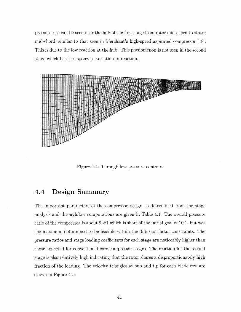
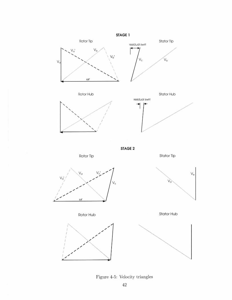
4.4 Design Summary
The important parameters of the compressor design as determined from the stage
analysis and throughflow computations are given in Table 4.1. The overall pressure
ratio of the compressor is about 9.2:1 which is short of the initial goal of 10:1, but was
the maximum determined to be feasible within the diffusion factor constraints. The
pressure ratios and stage loading coefficients for each stage are noticeably higher than
those expected for conventional core compressor stages. The reaction for the second
stage is also relatively high indicating that the rotor shares a disproportionately high
fraction of the loading. The velocity triangles at hub and tip for each blade row are
shown in Figure 4-5.
41
STAGE 1
Rotor Tip Stator Tipresidual swirl
V ' NVb'VN*
Va
r
Rotor Hub Stator Hub
residual swirl
NN
STAGE 2
Rotor Tip Stator Tip
%d c, Veor
Roor HuNtto u
Figure -5:VVd - --- - - V
- wr
Rotor Hub Stator Hub
/e
Figure 4-5: Velocity triangles
42
Table 4.1: Stage design results
43
Stage 1 Stage 2
Tip speed 457 m/sec -457 m/sec
Rotor pressure ratio 3.60 2.75
Stage pressure ratio 3.40 2.70
Estimated (average) efficiency 93% 95%
Meanline reaction 0.58 0.72
Flow coefficient 0.58 0.5
Stage loading coefficient 0.70 0.77
Rotor hub solidity 3.5 3.5
Stator hub solidity 3.0 3.0
Inlet corrected mass flow 212 kg/sec - M 2
Inlet hub/tip radius ratio 0.5
Outlet hub/tip radius ratio 0.92
Length/inlet radius ratio 1.13

44
Chapter 5
Blade Design
The blade design process involved first designing two-dimensional sections and then
stacking the sections radially to produce a three-dimensional blade shape. The blade
sections were designed with a turbomachinery cascade code using data extracted
from the throughflow solution. This included streamline radii, inlet and outlet flow
conditions, chord length, and pitch. In the process of designing the blade sections,
an attempt was made to reduce the complexity and difficulty of high-speed aspirated
blade design by analysing the relationships between features of previously designed
blades.
5.1 Code Description
The blade design code used was MISES, a quasi-three-dimensional turbomachinery
cascade solver developed at MIT by Drela et al [7, 25]. In MISES, the flow field is
divided into a viscous region, extending from the body surface to a height equal to
the displacement thickness of the boundary layer, and an inviscid region outside of
this. In the viscous region, the flow is modelled by a two-equation integral boundary
layer formulation. In the inviscid region, the flow is governed by the 3-D Euler equa-
tions (given in Equations 4.2 to 4.5) projected onto an axisymmetric streamsurface
of varying radius and thickness. As with MTFLOW, either the standard momentum
equation (4.7) or the entropy convection equation (4.8) can be solved depending on
45

the user's specification. The viscous and inviscid equations are coupled in MISES via
the edge velocity and displacement thickness to yield a system of non-linear equations
which are solved simultaneously.
In addition to blade analysis, MISES has inverse-design capabilities. Both mixed-
inverse and modal-inverse methods are available, but the former was used in this
work. In mixed-inverse design, the desired pressure distribution over a segment of
the blade is prescribed by modifying the distribution for a seed geometry. MISES
then perturbs the seed geometry at each point to achieve the specified pressure. The
camber and thickness of the blade can be preserved during inverse design if desired.
The geometric inputs required for MISES include the blade coordinates and pitch
and the radius and thickness of the stream surface on which the blade-to-blade flow is
computed. The latter is provided by the throughflow code. The input flow conditions
required depend on the boundary conditions imposed and can vary as the calculation
proceeds. All of the relevant parameters, including the inlet and outlet Mach numbers,
flow angles, and pressures are provided by the throughflow code. For the high-speed
blades designed in this work, the boundary conditions generally imposed were the inlet
Mach number and pressure, the so-called leading edge Kutta condition (for blades
with non-sharp leading edges), the trailing edge Kutta condition and either the inlet
flow slope or the exit pressure.
Given the above boundary conditions, the outputs from MISES include cascade
exit quantities such as the Mach number, flow angle, and pressure. The viscous and
shock losses and the diffusion factor for the blade section are also computed.
In the version of MISES used for this work, the boundary layer formulation in-
cludes a suction model. The required inputs to this model are the suction coefficient,
Cm (given by equation 2.25), and the location and length of the suction slot. When
suction is applied it decreases the boundary layer displacement thickness, so it appears
as a negative displacement of the streamline at the edge of the viscous layer.
46
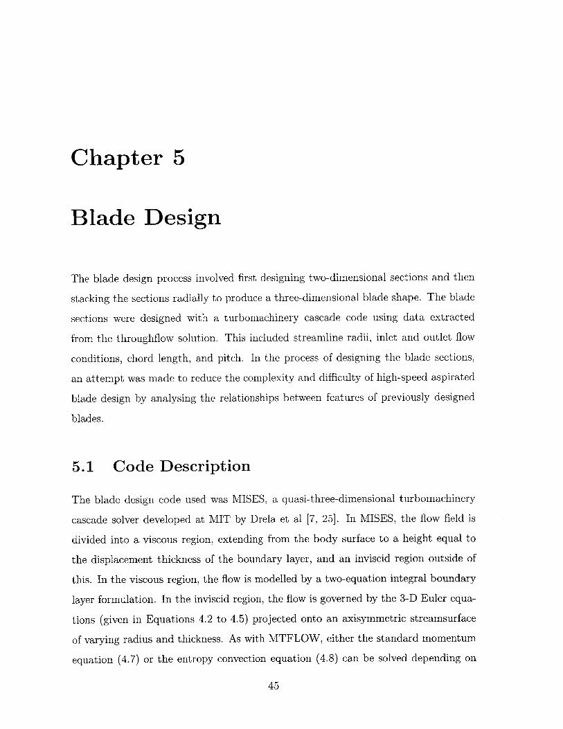
5.2 Design Process
The design process for a blade section is broken up into an inviscid design (represented
in MISES by setting the Reynolds number equal to zero) and a viscous design. The
steps followed to design the blades in this work are outlined as a flowchart in Figure
5-1.
The process begins with a seed geometry that is generally a previous design that
has similar turning (defined as the difference between the exit and inlet flow angles)
and inlet Mach number to the present design. A suitable inviscid design is then
found by alternately modifying the geometry manually and using the inverse design
capabilities of MISES. Often a slightly increased back pressure is imposed during this
phase of the design to simulate the effects of viscosity, particularly the deviation of
the flow at the blade trailing edge.
For the inviscid design, the geometry modification generally involves choosing
the maximum camber to produce the required turning and setting the maximum
thickness location based on the shock impingement point. The leading edge radius
is chosen according to the inlet Mach number. The stagger angle required to achieve
the desired incidence is also found. The choice of these parameters will be discussed
in more detail in Section 5.3. The manual geometry modification is performed with
XFOIL, an inviscid airfoil design and analysis program developed by Drela [4].
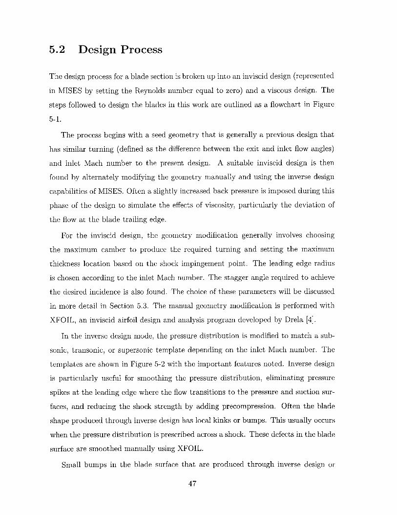
In the inverse design mode, the pressure distribution is modified to match a sub-
sonic, transonic, or supersonic template depending on the inlet Mach number. The
templates are shown in Figure 5-2 with the important features noted. Inverse design
is particularly useful for smoothing the pressure distribution, eliminating pressure
spikes at the leading edge where the flow transitions to the pressure and suction sur-
faces, and reducing the shock strength by adding precompression. Often the blade
shape produced through inverse design has local kinks or bumps. This usually occurs
when the pressure distribution is prescribed across a shock. These defects in the blade
surface are smoothed manually using XFOIL.
Small bumps in the blade surface that are produced through inverse design or
47
modification of maximum
edge
blade smoothing
tinverse design
no
modification of blade shapeand trailing edge
modification of maximumcamber and thickness,
tagger, trailing edge shape
Figure 5-1: Blade section design flowchart
48
cp
mild pressure gradient. ..... ................................. . ......... r i (M 1so nic (M=1)
No x/c uniform loading
(a) Subsonic
cp smooth deceleration; cp mild precompression
no shock shock
mild pressure gra<
acceleration at
N x/c diverging trailing edge 0 x/c mild pressure gradient
(b) Transonic (c) Supersonic
Figure 5-2: Blade pressure distribution design templates
49
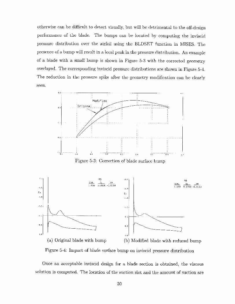
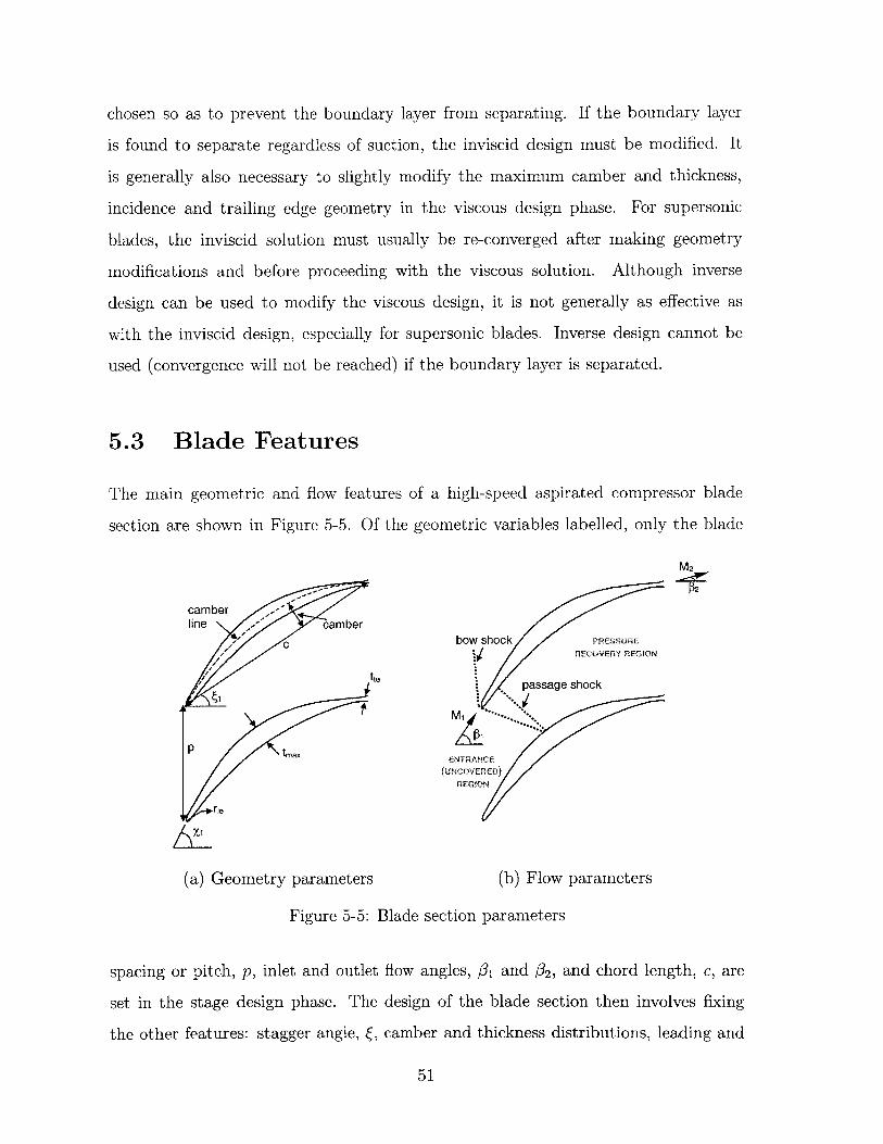
otherwise can be difficult to detect visually, but will be detrimental to the off-design
performance of the blade. The bumps can be located by computing the inviscid
pressure distribution over the airfoil using the BLDSET function in MISES. The
presence of a bump will result in a local peak in the pressure distribution. An example
of a blade with a small bump is shown in Figure 5-3 with the corrected geometry
overlayed. The corresponding inviscid pressure distributions are shown in Figure 5-4.
The reduction in the pressure spike after the geometry modification can be clearly
seen.
3,
Modif ied
Original
0.0 0.0 0.3 0.4 0.5
Figure 5-3: Correction of blade surface bump
RSSINL 0L CM
1.1430 0.2800 -0.0166
-2.0
-1.s
CP
-1.0
-0.5
0.0 -
0.5
1.0
(a) Original blade with bump
Figure 5-4: Impact of blade surface
R5
SINL CL CM1.1430 0.2799 -0.0163
(b) Modified blade with reduced bump
bump on inviscid pressure distribution
Once an acceptable inviscid design for a blade section is obtained, the viscous
solution is computed. The location of the suction slot and the amount of suction are
50
05
0.2
0.!1
0.
0. 1 j
-2.0
-1.s
CP
-1.0
-0.5
0.0
0.5
1.01
0.
.......... - ......... ............
chosen so as to prevent the boundary layer from separating. If the boundary layer
is found to separate regardless of suction, the inviscid design must be modified. It
is generally also necessary to slightly modify the maximum camber and thickness,
incidence and trailing edge geometry in the viscous design phase. For supersonic
blades, the inviscid solution must usually be re-converged after making geometry
modifications and before proceeding with the viscous solution. Although inverse
design can be used to modify the viscous design, it is not generally as effective as
with the inviscid design, especially for supersonic blades. Inverse design cannot be
used (convergence will not be reached) if the boundary layer is separated.
5.3 Blade Features
The main geometric and flow features of a high-speed aspirated compressor blade
section are shown in Figure 5-5. Of the geometric variables labelled, only the blade
P2
(a) Geometry parameters (b) Flow parameters
Figure 5-5: Blade section parameters
spacing or pitch, p, inlet and outlet flow angles, #1 and /32, and chord length, c, are
set in the stage design phase. The design of the blade section then involves fixing
the other features: stagger angle, , camber and thickness distributions, leading and
51
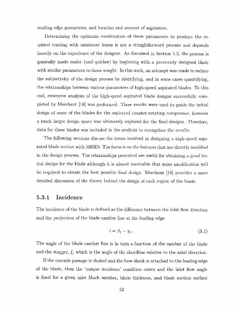
trailing edge geometries, and location and amount of aspiration.
Determining the optimum combination of these parameters to produce the re-
quired turning with minimum losses is not a straightforward process and depends
heavily on the experience of the designer. As discussed in Section 5.2, the process is
generally made easier (and quicker) by beginning with a previously designed blade
with similar parameters to those sought. In this work, an attempt was made to reduce
the subjectivity of the design process by identifying, and in some cases quantifying,
the relationships between various parameters of high-speed aspirated blades. To this
end, extensive analysis of the high-speed aspirated blade designs successfully com-
pleted by Merchant [18] was performed. These results were used to guide the initial
design of some of the blades for the aspirated counter-rotating compressor, however
a much larger design space was ultimately explored for the final designs. Therefore,
data for these blades was included in the analysis to strengthen the results.
The following sections discuss the issues involved in designing a high-speed aspi-
rated blade section with MISES. The focus is on the features that are directly modified
in the design process. The relationships presented are useful for obtaining a good ini-
tial design for the blade although it is almost inevitable that some modification will
be required to obtain the best possible final design. Merchant [18] provides a more
detailed discussion of the theory behind the design of each region of the blade.
5.3.1 Incidence
The incidence of the blade is defined as the difference between the inlet flow direction
and the projection of the blade camber line at the leading edge
i = 1-Xi (5.1)
The angle of the blade camber line is in turn a function of the camber of the blade
and the stagger, , which is the angle of the chordline relative to the axial direction.
If the cascade passage is choked and the bow shock is attached to the leading edge
of the blade, then the 'unique incidence' condition exists and the inlet flow angle
is fixed for a given inlet Mach number, blade thickness, and blade suction surface
52
angle. As described by Cumpsty [3], the 'unique incidence' inlet flow angle can be
found from continuity and the Prandtl-Meyer relation applied along a characteristic
extending from far upstream to the point, e, on the blade where the expansion wave
from the leading edge of the adjacent blade intersects the suction surface,
1 + V (M) = c + v (Me) . (5.2)
To design blades with 'unique incidence' using MISES the cascade exit pressure is
constrained and the leading edge geometry and stagger are chosen such that the
calculated inlet flow angle matches that provided by the throughflow solution.
For most of the high-speed aspirated blades, the bow shock is actually slightly
detached from the leading edge and some spillage of flow between cascade passages
is possible. Therefore, the 'unique incidence' flow angle need not be matched exactly
(it should be close, however, to keep mass flow capacity and efficiency high). There
is also a computational advantage to constraining the inlet flow angle in MISES (to
match the throughflow value) rather than the exit pressure and then choosing the
leading edge geometry and stagger angle based on other criteria. In particular, it is
desirable to minimize spikes in the pressure distribution on the suction and pressure
sides of the blade at the leading edge and to reduce the leading edge shock loss (these
properties are also affected by the leading edge geometry which will be discussed
in Section 5.3.4). It was found in this work that using these criteria gives a blade
design for which the 'unique incidence' flow angle matches the angle provided by the
throughflow code very closely. This was confirmed by re-computing the flow over a
completed blade without the inlet flow angle constrained.
With the leading edge geometry and camber angle fixed by other design consider-
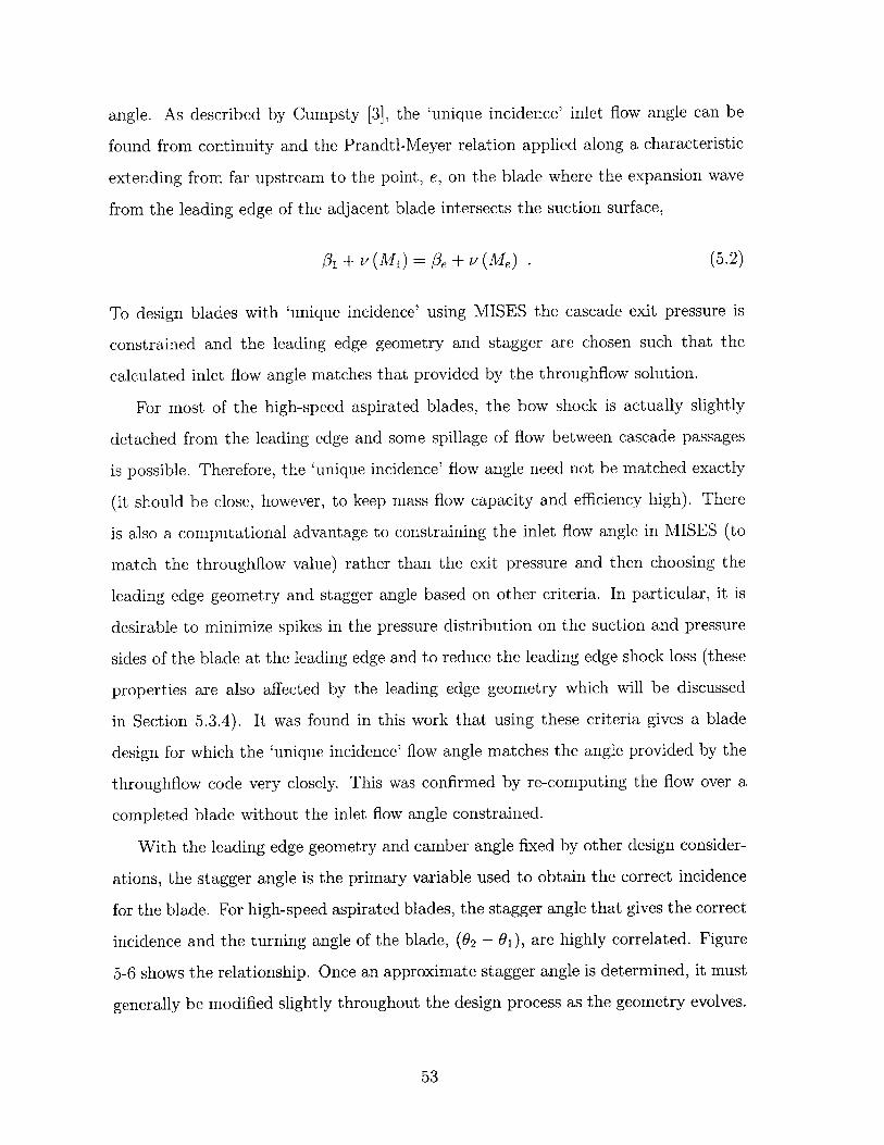
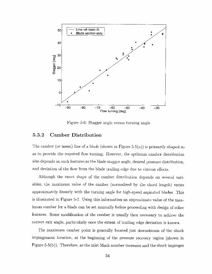
ations, the stagger angle is the primary variable used to obtain the correct incidence
for the blade. For high-speed aspirated blades, the stagger angle that gives the correct
incidence and the turning angle of the blade, (02 - 01), are highly correlated. Figure
5-6 shows the relationship. Once an approximate stagger angle is determined, it must
generally be modified slightly throughout the design process as the geometry evolves.
53
50
40- *
* *
20 - **
***
U)
10-
**
-10-90 -80 -70 -60 -50 -40 -30
Flow turning [deg]
Figure 5-6: Stagger angle versus turning angle
5.3.2 Camber Distribution
The camber (or mean) line of a blade (shown in Figure 5-5(a)) is primarily shaped so
as to provide the required flow turning. However, the optimum camber distribution
also depends on such features as the blade stagger angle, desired pressure distribution,
and deviation of the flow from the blade trailing edge due to viscous effects.
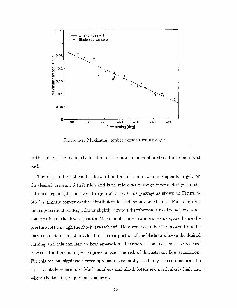
Although the exact shape of the camber distribution depends on several vari-
ables, the maximum value of the camber (normalized by the chord length) varies
approximately linearly with the turning angle for high-speed aspirated blades. This
is illustrated in Figure 5-7. Using this information an approximate value of the max-
imum camber for a blade can be set manually before proceeding with design of other
features. Some modification of the camber is usually then necessary to achieve the
correct exit angle, particularly once the extent of trailing edge deviation is known.
The maximum camber point is generally located just downstream of the shock
impingement location, at the beginning of the pressure recovery region (shown in
Figure 5-5(b)). Therefore, as the inlet Mach number increases and the shock impinges
54
0.35
Line-of-best-fit* Blade section data
0.3-
0V 0.25-0
> 0.2-E0z
E 0.15-E
0.1-
0.05-
-90 -80 -70 -60 -50 -40 -30Flow turning [deg]
Figure 5-7: Maximum camber versus turning angle
further aft on the blade, the location of the maximum camber should also be moved
back.
The distribution of camber forward and aft of the maximum depends largely on
the desired pressure distribution and is therefore set through inverse design. In the
entrance region (the uncovered region of the cascade passage as shown in Figure 5-
5(b)), a slightly convex camber distribution is used for subsonic blades. For supersonic
and supercritical blades, a flat or slightly concave distribution is used to achieve some
compression of the flow so that the Mach number upstream of the shock, and hence the
pressure loss through the shock, are reduced. However, as camber is removed from the
entrance region it must be added to the rear portion of the blade to achieve the desired
turning and this can lead to flow separation. Therefore, a balance must be reached
between the. benefit of precompression and the risk of downstream flow separation.
For this reason, significant precompression is generally used only for sections near the
tip of a blade where inlet Mach numbers and shock losses are particularly high and
where the turning requirement is lower.
55
0.4
0.3 -'02 M = 0.78
0
0.2- M =1.30
0.1-
00 0.1 0.2 0.3 0.4 0.5 0.6 0.7 0.8 0.9 1
x/c
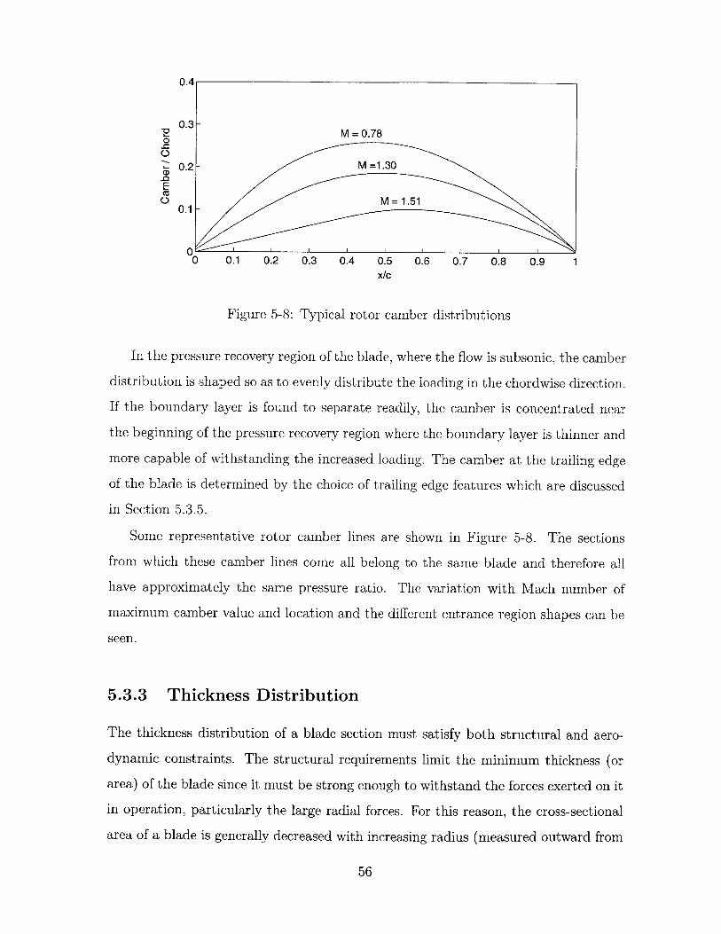
Figure 5-8: Typical rotor camber distributions
In the pressure recovery region of the blade, where the flow is subsonic, the camber
distribution is shaped so as to evenly distribute the loading in the chordwise direction.
If the boundary layer is found to separate readily, the camber is concentrated near
the beginning of the pressure recovery region where the boundary layer is thinner and
more capable of withstanding the increased loading. The camber at the trailing edge
of the blade is determined by the choice of trailing edge features which are discussed
in Section 5.3.5.
Some representative rotor camber lines are shown in Figure 5-8. The sections
from which these camber lines come all belong to the same blade and therefore all
have approximately the same pressure ratio. The variation with Mach number of
maximum camber value and location and the different entrance region shapes can be
seen.
5.3.3 Thickness Distribution
The thickness distribution of a blade section must satisfy both structural and aero-
dynamic constraints. The structural requirements limit the minimum thickness (or
area) of the blade since it must be strong enough to withstand the forces exerted on it
in operation, particularly the large radial forces. For this reason, the cross-sectional
area of a blade is generally decreased with increasing radius (measured outward from
56
the hub) so that the sections near the hub are able to support those near the tip. For
constant-chord blades (such as those considered here), this means that the thickness
is decreased with radius. The suction passage requirements also limit the minimum
thickness of aspirated blades. Currently this requirement can only be estimated based
on the low-speed aspirated stage that has been built and tested [21].
For satisfactory aerodynamic performance, the maximum thickness of the blade,
which governs the size of the throat in the cascade passage, must be small enough
to ensure that the required mass flow can be passed through the blade row. The
approximate throat area needed, At, can be determined from the area ratio required
for 'started' supersonic flow, At/Ai , where A2 is the cascade inlet area. For two-
dimensional flow this is calculated from the pressure change across the shock (ne-
glecting the effect of the boundary layer thickness). The throat area is also affected
by the choice of solidity and stagger.
For high-speed aspirated blades, the areas of the sections are decreased approx-
imately linearly with increasing radius while taking into account the constraints on
maximum and minimum thicknesses described above, particularly the ability to pass
the design mass flow. The maximum thicknesses for several sections of three high-
speed aspirated blade rows (two rotors and a stator) are plotted in Figure 5-9 to show
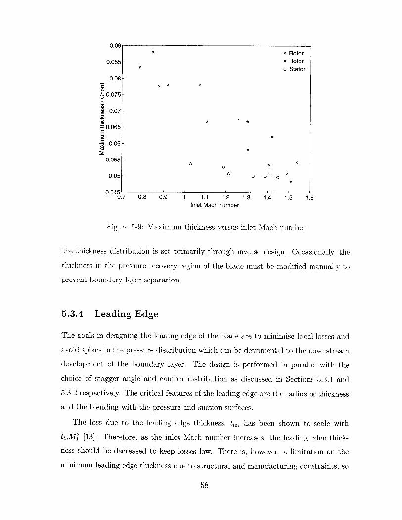
the typical values.
The location of maximum thickness is critical to the aerodynamic performance of
the blade section since it influences where the cascade passage shock (shown in Fig-
ure 5-5(b)) is located. At the design point, the passage shock and bow shock should
coalesce so that the boundary layer does not have to withstand two shock impinge-
ment points and the length of the subsonic pressure recovery region of the blade is
maximised. This condition is achieved by placing the maximum thickness point just
upstream of the bow shock impingement location. If the maximum thickness is aft of
this point then the passage shock will move downstream. On the other hand, if the
maximum thickness is forward of this point, the throat area will be decreased and
the cascade may not pass the desired mass flow.
Away from the leading and trailing edges and the maximum thickness location,
57
0.09* Rotor
0.085 - Rotoro Stator
0.08x*x
0.00.075 -
U
.C
, 0.065-E
0.06 -
0.055 x
0.05- 0 0 00 *
0.0450.7 0.8 0.9 1 1.1 1.2 1.3 1.4 1.5 1.6
Inlet Mach number
Figure 5-9: Maximum thickness versus inlet Mach number
the thickness distribution is set primarily through inverse design. Occasionally, the
thickness in the pressure recovery region of the blade must be modified manually to
prevent boundary layer separation.
5.3.4 Leading Edge
The goals in designing the leading edge of the blade are to minimise local losses and
avoid spikes in the pressure distribution which can be detrimental to the downstream
development of the boundary layer. The design is performed in parallel with the
choice of stagger angle and camber distribution as discussed in Sections 5.3.1 and
5.3.2 respectively. The critical features of the leading edge are the radius or thickness
and the blending with the pressure and suction surfaces.
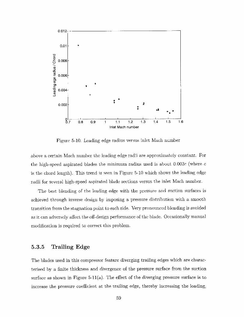
The loss due to the leading edge thickness, tie, has been shown to scale with
tieM2 [13]. Therefore, as the inlet Mach number increases, the leading edge thick-
ness should be decreased to keep losses low. There is, however, a limitation on the
minimum leading edge thickness due to structural and manufacturing constraints, so
58
0.012
0.01- *
00.008-
U 0.006-
.3 **0 0.004-CUa)
0.002-4
0 ' ' '
0.7 0.8 0.9 1 1.1 1.2 1.3 1.4 1.5 1.6Inlet Mach number
Figure 5-10: Leading edge radius versus inlet Mach number
above a certain Mach number the leading edge radii are approximately constant. For
the high-speed aspirated blades the minimum radius used is about 0.002c (where c
is the chord length). This trend is seen in Figure 5-10 which shows the leading edge
radii for several high-speed aspirated blade sections versus the inlet Mach number.
The best blending of the leading edge with the pressure and suction surfaces is
achieved through inverse design by imposing a pressure distribution with a smooth
transition from the stagnation point to each side. Very pronounced blending is avoided
as it can adversely affect the off-design performance of the blade. Occasionally manual
modification is required to correct this problem.
5.3.5 Trailing Edge
The blades used in this compressor feature diverging trailing edges which are charac-
terised by a finite thickness and divergence of the pressure surface from the suction
surface as shown in Figure 5-11(a). The effect of the diverging pressure surface is to
increase the pressure coefficient at the trailing edge, thereby increasing the loading,
59
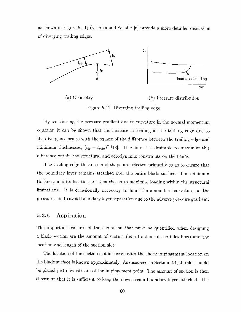
as shown in Figure 5-11(b). Drela and Schafer [6] provide a more detailed discussion
of diverging trailing edges.
cpte
tmin
Increased loading
x/c
(a) Geometry (b) Pressure distribution
Figure 5-11: Diverging trailing edge
By considering the pressure gradient due to curvature in the normal momentum
equation it can be shown that the increase in loading at the trailing edge due to
the divergence scales with the square of the difference between the trailing edge and
minimum thicknesses, (tte - tmin) 2 [18]. Therefore it is desirable to maximize this
difference within the structural and aerodynamic constraints on the blade.
The trailing edge thickness and shape are selected primarily so as to ensure that
the boundary layer remains attached over the entire blade surface. The minimum
thickness and its location are then chosen to maximise loading within the structural
limitations. It is occasionally necessary to limit the amount of curvature on the
pressure side to avoid boundary layer separation due to the adverse pressure gradient.
5.3.6 Aspiration
The important features of the aspiration that must be quantified when designing
a blade section are the amount of suction (as a fraction of the inlet flow) and the
location and length of the suction slot.
The location of the suction slot is chosen after the shock impingement location on
the blade surface is known approximately. As discussed in Section 2.4, the slot should
be placed just downstream of the impingement point. The amount of suction is then
chosen so that it is sufficient to keep the downstream boundary layer attached. The
60
suction coefficients required for high-speed aspirated blades have varied from about
0.5 percent to a maximum of about 2 percent (required at the tip sections of the rotor
blades). Often some iteration between the location and amount of suction is required
since the suction can cause the shock impingement location to move slightly.
When choosing the location and amount of suction it is useful to consider the
development along the blade surface of the boundary layer shape parameter given by
6*H - (5.3)
where P* is the boundary layer thickness and 0 is the momentum thickness. The shape
parameter is computed by MISES and gives an indication of how close the boundary
layer is to separation at each point. As a general rule it is desirable to keep the shape
parameter well below 4 for laminar flow and 3 for turbulent flow.
For all of the high-speed aspirated blades designed to-date, a suction slot length
of 0.02c (where c is the blade section chord length) has been used. This was found to
be optimal on the basis of Merchant's work [18].
5.4 Final Blade Designs
The hub, 50% span, and tip section designs for each blade row are presented in the
following sections. For each section the blade shape, surface isentropic Mach number
distribution, and pressure contours are shown. The shape parameter distributions for
two sections are shown to illustrate the effect of aspiration on boundary layer growth.
25% and 75% span sections were also designed for each blade row. The plots for these
sections are included in Appendix A.
5.4.1 Stage 1
Rotor Hub
The Mach number distribution and pressure contours for the rotor hub section of the
first stage are shown in Figure 5-12. The total pressure ratio of this section is 3.56.
This is lower than the throughflow value of 3.6, but it was not possible to increase
61
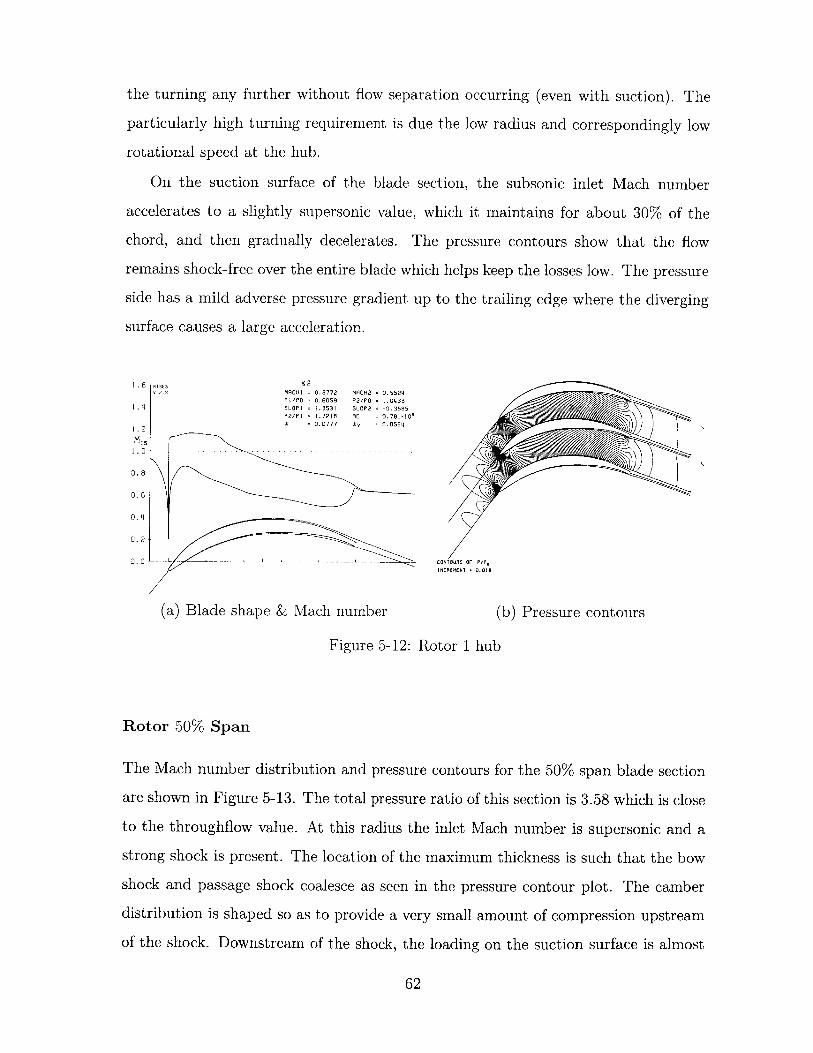
the turning any further without flow separation occurring (even with suction). The
particularly high turning requirement is due the low radius and correspondingly low
rotational speed at the hub.
On the suction surface of the blade section, the subsonic inlet Mach number
accelerates to a slightly supersonic value, which it maintains for about 30% of the
chord, and then gradually decelerates. The pressure contours show that the flow
remains shock-free over the entire blade which helps keep the losses low. The pressure
side has a mild adverse pressure gradient up to the trailing edge where the diverging
surface causes a large acceleration.
2.3 MACH] 0.8772 MACH2 = 0.5524P1/PS 0.6059 P2/PO 1.0433
1 .4 SLOPI =1.3531 SLOP2 -0.3885P2/PI 1.7218 RE 0.781,106U 0.0777 89 = 0.0554
1.
0.
0.2
0.0 --- - - - - --- -- CONTOURS OF P/PoINCREMENT - 0.018
(a) Blade shape & Mach number (b) Pressure contours
Figure 5-12: Rotor 1 hub
Rotor 50% Span
The Mach number distribution and pressure contours for the 50% span blade section
are shown in Figure 5-13. The total pressure ratio of this section is 3.58 which is close
to the throughflow value. At this radius the inlet Mach number is supersonic and a
strong shock is present. The location of the maximum thickness is such that the bow
shock and passage shock coalesce as seen in the pressure contour plot. The camber
distribution is shaped so as to provide a very small amount of compression upstream
of the shock. Downstream of the shock, the loading on the suction surface is almost
62
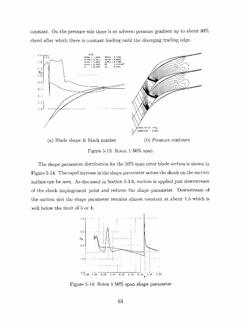
constant. On the pressure side there is an adverse pressure gradient up to about 30%
chord after which there is constant loading until the diverging trailing edge.
1.-6 M ISES :510
2. 3 MRCHI = 1.2598 MACH2 = 0.5192P1/PO - 0.3810 P2/PO = 0.8825
1 .4 DLOF: = .6507 SLOP2 = 0.1780P2/P = .13 RE =102106
1.2
MIS1 . 0 -- --- -- - - -- - -- -- - -- - - -- - - - -
D.8
0.6
0.14
0.2
ONT0URS OF P/P0
INCREMENT = 0.025
(a) Blade shape & Mach number (b) Pressure contours
Figure 5-13: Rotor 1 50% span
The shape parameter distribution for the 50% span rotor blade section is shown in
Figure 5-14. The rapid increase in the shape parameter across the shock on the suction
surface can be seen. As discussed in Section 5.3.6, suction is applied just downstream
of the shock impingement point and reduces the shape parameter. Downstream of
the suction slot the shape parameter remains almost constant at about 1.5 which is
well below the limit of 3 or 4.
4.0
3.0
H -
2.0
1.0
0.0-0.08 0.00 0.08 0.16 0.24 0.32 0.40 0.48 0.56
Figure 5-14: Rotor 1 50% span shape parameter
63
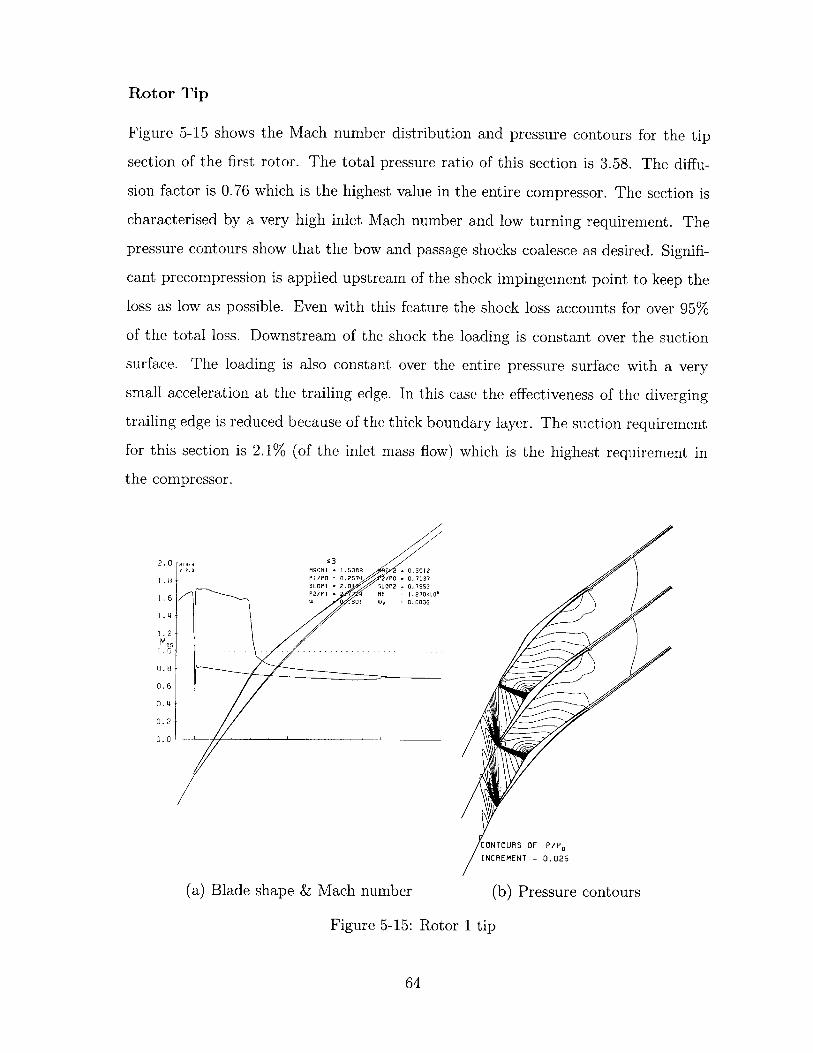
Rotor Tip
Figure 5-15 shows the Mach number distribution and pressure contours for the tip
section of the first rotor. The total pressure ratio of this section is 3.58. The diffu-
sion factor is 0.76 which is the highest value in the entire compressor. The section is
characterised by a very high inlet Mach number and low turning requirement. The
pressure contours show that the bow and passage shocks coalesce as desired. Signifi-
cant precompression is applied upstream of the shock impingement point to keep the
loss as low as possible. Even with this feature the shock loss accounts for over 95%
of the total loss. Downstream of the shock the loading is constant over the suction
surface. The loading is also constant over the entire pressure surface with a very
small acceleration at the trailing edge. In this case the effectiveness of the diverging
trailing edge is reduced because of the thick boundary layer. The suction requirement
for this section is 2.1% (of the inlet mass flow) which is the highest requirement in
the compressor.
2.0 -misEs2.3 MRCII = 1.5389 - 0.5012
1.8 P s/PO = 0.2574 /P 0. 7137SLOPI = 2.0 SLOP? = 0.7953
1.6 0 00
1.4
1.2MIS
1 . 0 ----------- -- - ------ - - ---- --- - - - --- --
0.8
0.6
0. 4
0.2
0.0
CONTOURS OF P/PoINCREMENT = 0.025
(a) Blade shape & Mach number
Figure 5-15:
(b) Pressure contours
Rotor 1 tip
64
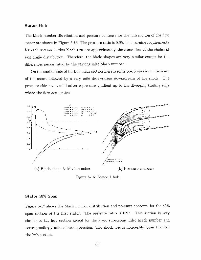
Stator Hub
The Mach number distribution and pressure contours for the hub section of the first
stator are shown in Figure 5-16. The pressure ratio is 0.95. The turning requirements
for each section in this blade row are approximately the same due to the choice of
exit angle distribution. Therefore, the blade shapes are very similar except for the
differences necessitated by the varying inlet Mach number.
On the suction side of the hub blade section there is some precompression upstream
of the shock followed by a very mild deceleration downstream of the shock. The
pressure side has a mild adverse pressure gradient up to the diverging trailing edge
where the flow accelerates.
1. 6 M ISES I1
2.3 MACHI 1.2653 MACH2 = 0.5172P1/PG 0.3782 P2/PH = 0.7870
1. 4 SLOP 2 1.5272 SLOP2 = 0.1333P2/P 2.0808 RE = 1.501-101w 0.0893 WV = 0.0248
0 . 81 .0 6 - ----- --- ~-------------- -
DA.
0.2
0.0
ONTOURS OF P/P,INCREMENT - 0.010
(a) Blade shape & Mach number (b) Pressure contours
Figure 5-16: Stator 1 hub
Stator 50% Span
Figure 5-17 shows the Mach number distribution and pressure contours for the 50%
span section of the first stator. The pressure ratio is 0.97. This section is very
similar to the hub section except for the lower supersonic inlet Mach number and
correspondingly milder precompression. The shock loss is noticeably lower than for
the hub section.
65
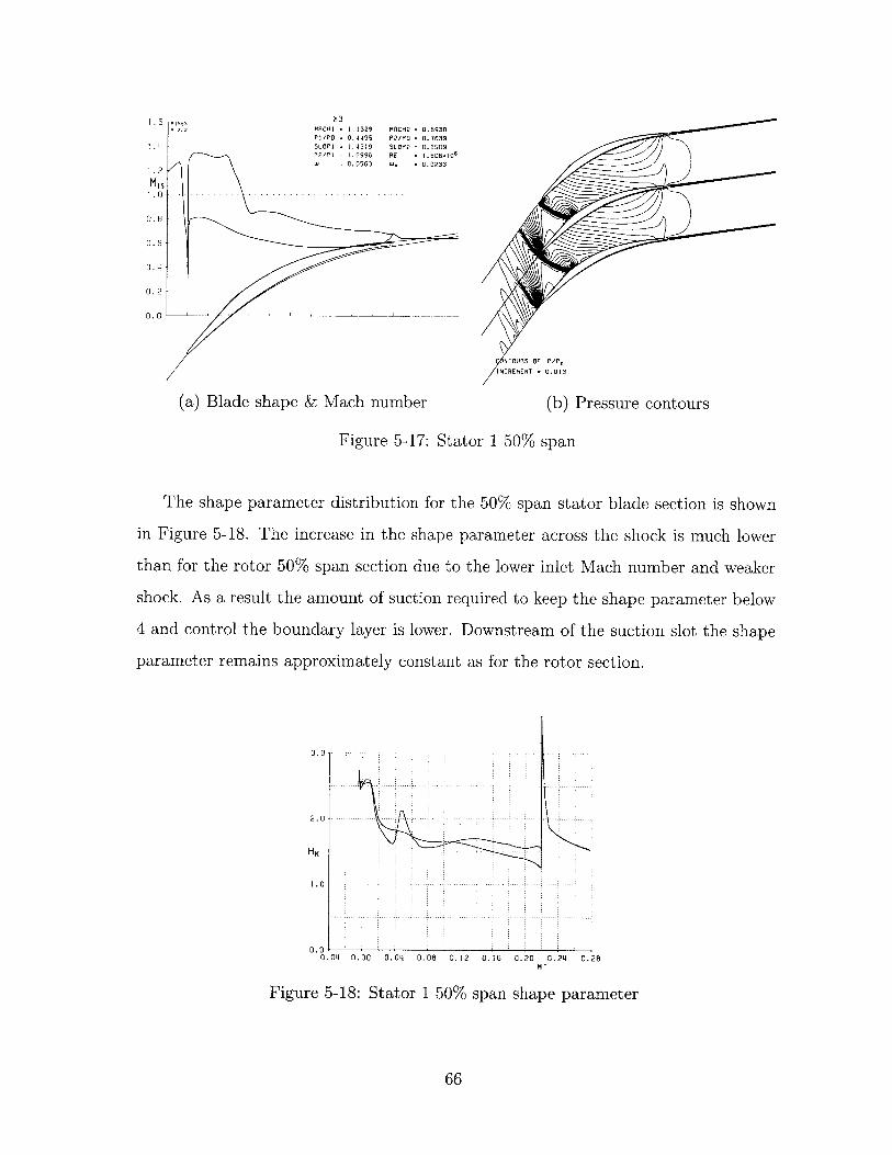
1.6 M15ES32.3 MACH1 v 1.1329 MACH2 = 0.5930
P1/PO = 0.4495 P2/P0 = 0.76391. U SLOP) = 1.4319 SLOP2 = 0.2509
P2/PI = 1.6996 RE = 1.506-106W = 0.0563 Wy 0.0233
1 .2
MIS
0.8
0. 2
0. 0
NT01URS OF P/Ps
INCREMENT = 0.013
(a) Blade shape & Mach number (b) Pressure contours
Figure 5-17: Stator 1 50% span
The shape parameter distribution for the 50% span stator blade section is shown
in Figure 5-18. The increase in the shape parameter across the shock is much lower
than for the rotor 50% span section due to the lower inlet Mach number and weaker
shock. As a result the amount of suction required to keep the shape parameter below
4 and control the boundary layer is lower. Downstream of the suction slot the shape
parameter remains approximately constant as for the rotor section.
3.0
2.0
HK
1. 0 -- --
0.01-0.04 0.00 0.04 0.08 0.12 0.16 0.20 0.24 0.28
Figure 5-18: Stator 1 50% span shape parameter
66
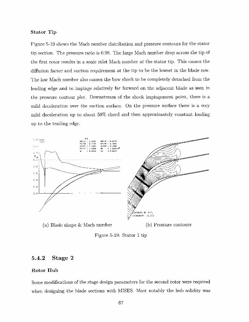
Stator Tip
Figure 5-19 shows the Mach number distribution and pressure contours for the stator
tip section. The pressure ratio is 0.98. The large Mach number drop across the tip of
the first rotor results in a sonic inlet Mach number at the stator tip. This causes the
diffusion factor and suction requirement at the tip to be the lowest in the blade row.
The low Mach number also causes the bow shock to be completely detached from the
leading edge and to impinge relatively far forward on the adjacent blade as seen in
the pressure contour plot. Downstream of the shock impingement point, there is a
mild deceleration over the suction surface. On the pressure surface there is a very
mild deceleration up to about 50% chord and then approximately constant loading
up to the trailing edge.
1.3 MISES 2t41 .3 MACHI = 1.0231 MACH2 = 0.6070
PI/E 0 =0.5142 P2/PO = 0.7644
1.4 S . 62 SLP2 = 0.959P2/PI *4B66 RE = 14.28x10⁶
W 0.0405 HR - 0.03271.2
MIS1 . 0 -- ------------ --------- --- - - - - - - - - -- --- - -- - - -- - - ---
0.8
0.6
0.4
0.2
0.0
ONTOURS OF P/P,INCREMENT = 0.013
(a) Blade shape & Mach number (b) Pressure contours
Figure 5-19: Stator 1 tip
5.4.2 Stage 2
Rotor Hub
Some modifications of the stage design parameters for the second rotor were required
when designing the blade sections with MISES. Most notably the hub solidity was
67
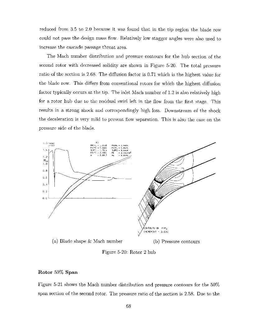
reduced from 3.5 to 2.0 because it was found that in the tip region the blade row
could not pass the design mass flow. Relatively low stagger angles were also used to
increase the cascade passage throat area.
The Mach number distribution and pressure contours for the hub section of the
second rotor with decreased solidity are shown in Figure 5-20. The total pressure
ratio of the section is 2.68. The diffusion factor is 0.71 which is the highest value for
the blade row. This differs from conventional rotors for which the highest diffusion
factor typically occurs at the tip. The inlet Mach number of 1.2 is also relatively high
for a rotor hub due to the residual swirl left in the flow from the first stage. This
results in a strong shock and correspondingly high loss. Downstream of the shock
the deceleration is very mild to prevent flow separation. This is also the case on the
pressure side of the blade.
1.86 misEs :5
2.3 MRCH1 1.2195 MRCH2 = 0.4635P1/P0 0.4020 P2/PO = 0.8465
1 .4 SLOP - 1.7614 SLOP2 = 0.q428P2/Pl =2.1061 HE = 2.190x106
= 0.0917 wy = 0.0084
1.0
0.8
0.6
0.11
0.2
0.0
ONTOURS OF P/PoINCREMENT = 0.025
(a) Blade shape & Mach number (b) Pressure contours
Figure 5-20: Rotor 2 hub
Rotor 50% Span
Figure 5-21 shows the Mach number distribution and pressure contours for the 50%
span section of the second rotor. The pressure ratio of the section is 2.58. Due to the
68
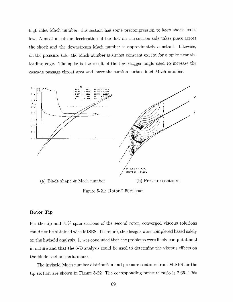
high inlet Mach number, this section has some precompression to keep shock losses
low. Almost all of the deceleration of the flow on the suction side takes place across
the shock and the downstream Mach number is approximately constant. Likewise,
on the pressure side, the Mach number is almost constant except for a spike near the
leading edge. The spike is the result of the low stagger angle used to increase the
cascade passage throat area and lower the suction surface inlet Mach number.
ONTOURS OF P/PoINCREMENT = 0.025
(a) Blade shape & Mach number (b) Pressure contours
Figure 5-21: Rotor 2 50% span
Rotor Tip
For the tip and 75% span sections of the second rotor, converged viscous solutions
could not be obtained with MISES. Therefore, the designs were completed based solely
on the inviscid analysis. It was concluded that the problems were likely computational
in nature and that the 3-D analysis could be used to determine the viscous effects on
the blade section performance.
The inviscid Mach number distribution and pressure contours from MISES for the
tip section are shown in Figure 5-22. The corresponding pressure ratio is 2.65. This
69
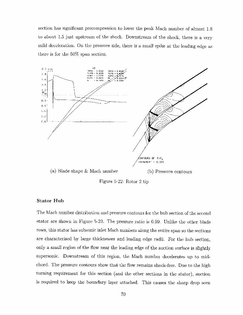
section has significant precompression to lower the peak Mach number of almost 1.8
to about 1.5 just upstream of the shock. Downstream of the shock, there is a very
mild deceleration. On the pressure side, there is a small spike at the leading edge as
there is for the 50% span section.
ONTOURS OF P/P0INCREMENT = 0.025
(a) Blade shape & Mach number (b) Pressure contours
Figure 5-22: Rotor 2 tip
Stator Hub
The Mach number distribution and pressure contours for the hub section of the second
stator are shown in Figure 5-23. The pressure ratio is 0.99. Unlike the other blade
rows, this stator has subsonic inlet Mach numbers along the entire span so the sections
are characterised by large thicknesses and leading edge radii. For the hub section,
only a small region of the flow near the leading edge of the suction surface is slightly
supersonic. Downstream of this region, the Mach number decelerates up to mid-
chord. The pressure contours show that the flow remains shock-free. Due to the high
turning requirement for this section (and the other sections in the stator), suction
is required to keep the boundary layer attached. This causes the sharp drop seen
70
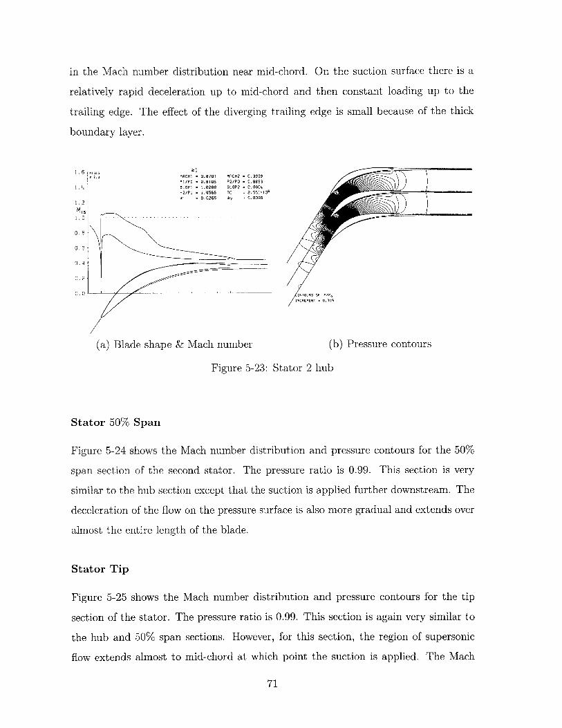
in the Mach number distribution near mid-chord. On the suction surface there is a
relatively rapid deceleration up to mid-chord and then constant loading up to the
trailing edge. The effect of the diverging trailing edge is small because of the thick
boundary layer.
1. 6 MISESMACHI = 0.8701 MCH2 0.3939
P1/P2 = 0.6105 P2/P 0.8893
1.14 SLOP: = 1.628B SLOP2 = 0.0004P2/PI = '.5566 BE =2.551.106'W 0.0265 w)y = 0.039B
1.2
1 . 0 - -- - - - - - - - - -- - - -- - - - -- ---- - - -
0. 8
0.6
0.4
0.2
0. 0 0510090 OP P/P
INCREMENT = ODDOS
(a) Blade shape & Mach number (b) Pressure contours
Figure 5-23: Stator 2 hub
Stator 50% Span
Figure 5-24 shows the Mach number distribution and pressure contours for the 50%
span section of the second stator. The pressure ratio is 0.99. This section is very
similar to the hub section except that the suction is applied further downstream. The
deceleration of the flow on the pressure surface is also more gradual and extends over
almost the entire length of the blade.
Stator Tip
Figure 5-25 shows the Mach number distribution and pressure contours for the tip
section of the stator. The pressure ratio is 0.99. This section is again very similar to
the hub and 50% span sections. However, for this section, the region of supersonic
flow extends almost to mid-chord at which point the suction is applied. The Mach
71
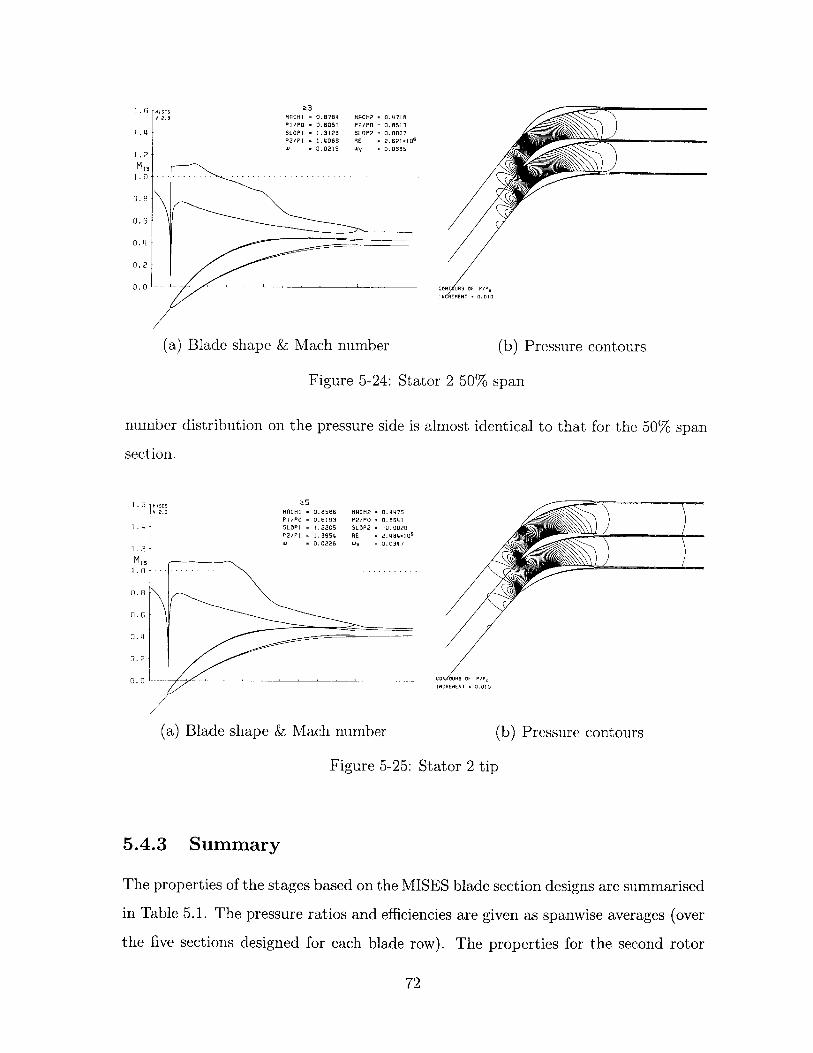
MACHI = 0.8784P1/PO = 0.6051SLOPI = 1.3123P2/PI = 1.4069W = 0.0215
MACH2 = 0.4718P2/PO = 0.8513SLOP2 = 0.0007RE = 2.621=106ov = 0.0335
1 . 4
1.2
1.0
D. 8
0. 6
0.2
0.0
-a - - -shap- -- M c -n --
(a) Blade shape &Mach number (b) Pressure contours
Figure 5-24: Stator 2 50% span
number distribution on the pressure side is almost identical to that for the 50% span
section.
MACHI = 0.8566 MACH2 = 0.4475P1/PO = 0.6193 P2/PO = 0.8641SLOPI = 1.2205 SLOP2 = -0.0020P2/PI = 1.3954 RE = 2.484x10⁶W = 0.0226 Wv = 0.0347
COM/rURS OF P/P0INCREMENT - 0.010
(a) Blade shape & Mach number (b) Pressure contours
Figure 5-25: Stator 2 tip
5.4.3 Summary
The properties of the stages based on the MISES blade section designs are summarised
in Table 5.1. The pressure ratios and efficiencies are given as spanwise averages (over
the five sections designed for each blade row). The properties for the second rotor
72
1.6 2 mISES
4S OF P/P0
1. 4
1.2
1 .
0. 8
0. 6
0. L4
0. 2
0. 0
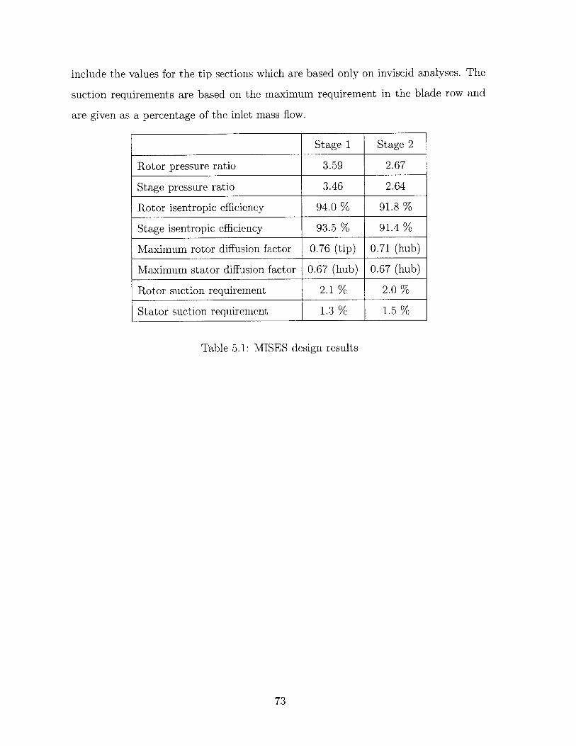
include the values for the tip sections which are based only on inviscid analyses. The
suction requirements are based on the maximum requirement in the blade row and
are given as a percentage of the inlet mass flow.
Table 5.1: MISES design results
73
Stage 1 Stage 2
Rotor pressure ratio 3.59 2.67
Stage pressure ratio 3.46 2.64
Rotor isentropic efficiency 94.0 % 91.8 %
Stage isentropic efficiency 93.5 % 91.4 %
Maximum rotor diffusion factor 0.76 (tip) 0.71 (hub)
Maximum stator diffusion factor 0.67 (hub) 0.67 (hub)
Rotor suction requirement 2.1 % 2.0 %
Stator suction requirement 1.3 % 1.5 %

74
Chapter 6
Conclusion
A quasi-three-dimensional, MISES-based design of a two-stage aspirated counter-
rotating compressor has been completed. The combination of aspiration and counter-
rotation enables both stages to produce pressure ratios much higher than those pos-
sible in conventional compressors with comparable tip speeds. For comparison the
design pressure ratio of the two-stage compressor is approximately equivalent to that
of a six- or seven-stage conventional high speed compressor. Therefore, if the aspi-
rated counter-rotating compressor could be successfully integrated in a gas turbine
engine it would lead to a significantly smaller and lighter device.
6.1 Compressor Design Summary
The (absolute) tip speed chosen for both rotors was 457m/s (1500ft/s) which is typical
of high-speed compressors. The blade rows were designed to produce optimal pressure
distributions within diffusion factor and inlet Mach number constraints. For the aspi-
rated blades, the diffusion factor limit is about 0.7, as opposed to 0.5 for conventional
blades. The Mach number limit was chosen to be around 1.5 to avoid large losses.
This is important for high speed aspirated blades for which the shock losses can be
up to 7 to 8 times larger than the viscous losses. The exit angle from the first stator
was optimised to maximise the pressure ratio of the downstream (counter-rotating)
rotor within the given constraints.
75
The initial flowpath shape was generated from a meanline analysis and then re-
fined using the results of axisymmetric throughflow computations. The most dis-
tinctive feature of the flowpath is the large contractions across the rotors which is
necessitated by the high pressure ratios. The blade sections were designed with the
quasi-three-dimensional cascade code MISES which allowed for precise design of each
blade feature to match the flow conditions. MISES was also used to determine the
optimum aspiration scheme for each blade section.
The overall pressure ratio of the final (MISES) design is about 9.1:1 (3.46:1 in
stage 1 and 2.64:1 in stage 2). The maximum diffusion factor in the compressor is
0.75 at the tip of the first rotor. This section also has the highest suction requirement
which is 2.1%. The maximum relative inlet Mach number is about 1.53 and occurs
at the tip sections of both rotors.
6.2 Concluding Remarks on Design Process
Several important issues were addressed in the process of designing the aspirated
counter-rotating compressor. These are significant to the design of high-speed as-
pirated stages and may prove significant to the design of other high-work stages as
well. It was found in general that there is a high potential for complicated interaction
between design features and aerodynamic behaviour. In this design, for example, the
exit angle of the first stator and the diffusion factor of the downstream rotor exhibit
a highly nonlinear interaction. This makes an iterative design process such as that
used here (and by Merchant [18]) critical to obtaining a good final design.
A more specific issue addressed in the design process was that shock losses are as
important as viscous losses (if not more so) to the efficiency of a high-speed aspirated
stage. This dictates that equal attention should be paid to the relative inlet Mach
numbers and diffusion factors of the blades in the stage design process. In some cases,
it will be the Mach number and not the diffusion factor that will limit the design
of a particular compressor feature. This is a notable difference from conventional
compressors which have lower diffusion factor limits.
76
Given the large pressure ratios across high-work compressor stages, flowpath con-
traction also becomes an issue. This can significantly impact the performance of the
compressor and poses a unique design challenge. In this design, it was necessary
to depart from the common practice of holding the tip radius constant through the
compressor and a great deal of effort was required to obtain a sufficiently smooth
hub profile. A detailed throughflow analysis provides invaluable information on the
impacts of flowpath shape on aerodynamic behaviour.
Design of blade sections for high-speed aspirated stages also involves some chal-
lenges. In particular, there is a strong interrelation between blade features which
necessitates an iterative design process (generally involving many iterations). The
features of the blades also differ in many respects from those of conventional blades.
Despite this, some correlations between certain features of high-speed aspirated blades
and some design trends were identified in this work. These are useful for obtaining a
good starting point for the design of a blade section, so that ultimately fewer iterations
are required to reach an optimal design.
6.3 Future Work
The next step in the process of designing the aspirated counter-rotating compressor
will be to complete the three-dimensional computational aerodynamic analysis. This
will provide information on the effects of tip clearance flows, radial transport, and
mixing between blade rows and on the ability of the compressor to pass the design
mass flow among other things. Based on this information, some modification of the
design will likely be necessary. Three-dimensional computational analysis of such
a high-performance compressor is, however, not straightforward. Initial attempts to
complete such an analysis encountered several difficulties. It appears that very careful
attention must be paid to the abilities of the computational tools and to the procedure
used to carry out the computations.
Once the design of the compressor has been satisfactorily completed (including all
relevant structural analysis), the next step will be to build and test the device. As
77
mentioned previously the compressor could be tested in the Blowdown Compressor
facility at MIT. Since this facility has been used in the past to test only single-stage,
comparatively low-speed compressors, some issues with the setup would need to be
addressed. Perhaps one of the most important is the accommodation of the second,
counter-rotating stage. This would involve (among other things) lengthening the test
section and adding a motor to drive the second rotor.
In order to integrate the aspirated counter-rotating compressor in an actual gas
turbine engine, some redesign of other engine components will also be necessary. Most
notably a counter-rotating turbine will be required to drive the compressor. Prelimi-
nary investigation of such a turbine showed that it will benefit aerodynamically from
the counter-rotation (as the compressor does) and should be capable of producing the
required power in few stages. This provides an additional contribution to the overall
goal of producing a smaller, lighter engine.
78
Bibliography
[1] J.D. Anderson. Modern Compressible Flow. McGraw-Hill, 1990.
[2] L.R. Anderson, W.H. Heiser, and J.C. Jackson. Axisymmetric one-dimensional
compressible flow - theory and applications. Journal of Applied Mechanics, pages
917-923, December 1970.
[3] N.A. Cumpsty. Compressor Aerodynamics. Addison Wesley Longman, 1989.
[4] M. Drela. Xfoil: An analysis and design system for low reynolds number airfoils.
In Low Reynolds Number Aerodynamics, T.J. Mueller, editor, June 1989.
[5] M. Drela. A user's guide to MTFLOW 1.2, November 1997.
[6] M. Drela and M. Schafer. Experimental and computational investigation of di-
vergant trailing edges. Technical Report CFDL TR-91-3, MIT CFD Laboratory,
1991.
[7] M. Drela and H.H. Youngren. A user's guide to MISES 2.53, December 1998.
[8] A. Epstein. 16.511 course notes. Department of Aeronautics and Astronautics,
Massachusetts Institute of Technology, Fall 2000.
[9] J.H. Freedman. Design of a multi-spool, high-speed, counter-rotating, aspirated
compressor. Master's thesis, Massachusetts Institute of Technology, 2000.
[10] J.L. Kerrebrock. Aircraft Engines and Gas Turbines. MIT Press, Cambridge,
1996.
79
[11] J.L. Kerrebrock, M. Drela, A.A. Merchant, and B.J. Schuler. A family of designs
for aspirated compressors. Technical Report 98-GT196, ASME, 1998.
[12] J.L. Kerrebrock, D.P. Reijnen, W.S.Ziminsky, and L.M. Smilg. Aspirated com-
pressors. Technical Report 97-GT525, ASME, 1997.
[13] C.C. Koch and L.H. Smith Jr. Loss sources and magnitudes in axial-flow com-
pressors. Journal of Engineering for Power, pages 411-424, July 1976.
[14] C.H. Law and A.J. Wennerstrom. Performance of two transonic compressor
rotors incorporating inlet counterswirl. Journal of Turbomachinery, 109:142-
148, January 1987.
[15] S. Lieblein, F.C. Schwenk, and F.L. Broderick. Diffusion factor for estimat-
ing losses and limiting blade loadings in axial flow compressor blade elements.
Technical Report RME53DO1, NACA, 1953.
[16] J.D. Mattingly. Elements of Gas Turbine Propulsion. McGraw-Hill, 1996.
[17] A.A. Merchant. Design and analysis of supercritical airfoils with boundary layer
suction. Master's thesis, Massachusetts Institute of Technology, 1996.
[18] A.A. Merchant. Design and Analysis of Axial Aspirated Compressor Stages. PhD
thesis, Massachusetts Institute of Technology, 1999.
[19] D.P. Reijnen. Experimental Study of Boundary Leyer Suction in a Transonic
Compressor. PhD thesis, Massachusetts Institute of Technology, 1997.
[20] E.J. Sabel and A. Sabatiuk. Turbojet engine development: Design of phase 1
compressor. Technical Report 501, Curtis-Wright Corporation, 1957.
[21] B.J. Schuler. Experimental Investigation of an Aspirated Fan Stage. PhD thesis,
Massachusetts Institute of Technology, 2001.
[22] B.J. Schuler, J.L. Kerrebrock, A.A. Merchant, and M. Drela. Design, analysis,
fabrication and test of an aspirated fan stage. Technical Report 2000-GT618,
ASME, 2000.
80
[23] A.J. Wennerstrom. Design of critical compressor stages. In Transonic Compres-
sors, Volume 2, von Karman Institute Lecture Series 1988-03, 1988.
[24] A.J. Wennerstrom. Highly loaded axial flow compressors: History and current
developments. Journal of Turbomachinery, pages 567-578, October 1990.
[25] H.H. Youngren and M. Drela. Viscous/inviscid method for preliminary design of
transonic cascades. Technical Report 91-2364, AIAA, 1991.
81

82
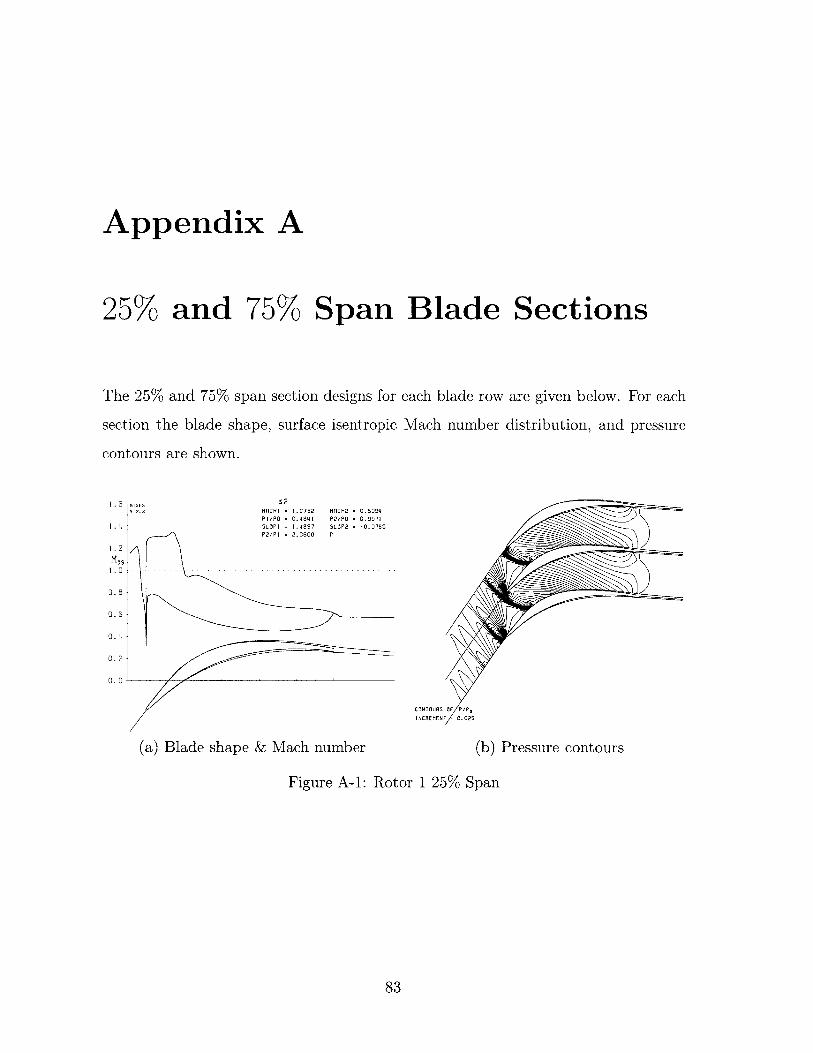
Appendix A
25% and 75% Span Blade Sections
The 25% and 75% span section designs for each blade row are given below. For each
section the blade shape, surface isentropic Mach number distribution, and pressure
contours are shown.
1 .4
1.2
MIS1.0
0.8
0.6
0.4i
0.2
0.0
s52MCHI -. 0732 SCL2 0.5096PI/PO 0.4841 P2/PD 0.99715LOPI -1.4897 SLOP2 -- 0.07 60P2/P 1 2.0600 F'
CONTOURS
025
(a) Blade shape & Mach number (b) Pressure contours
Figure A-1: Rotor 1 25% Span
83
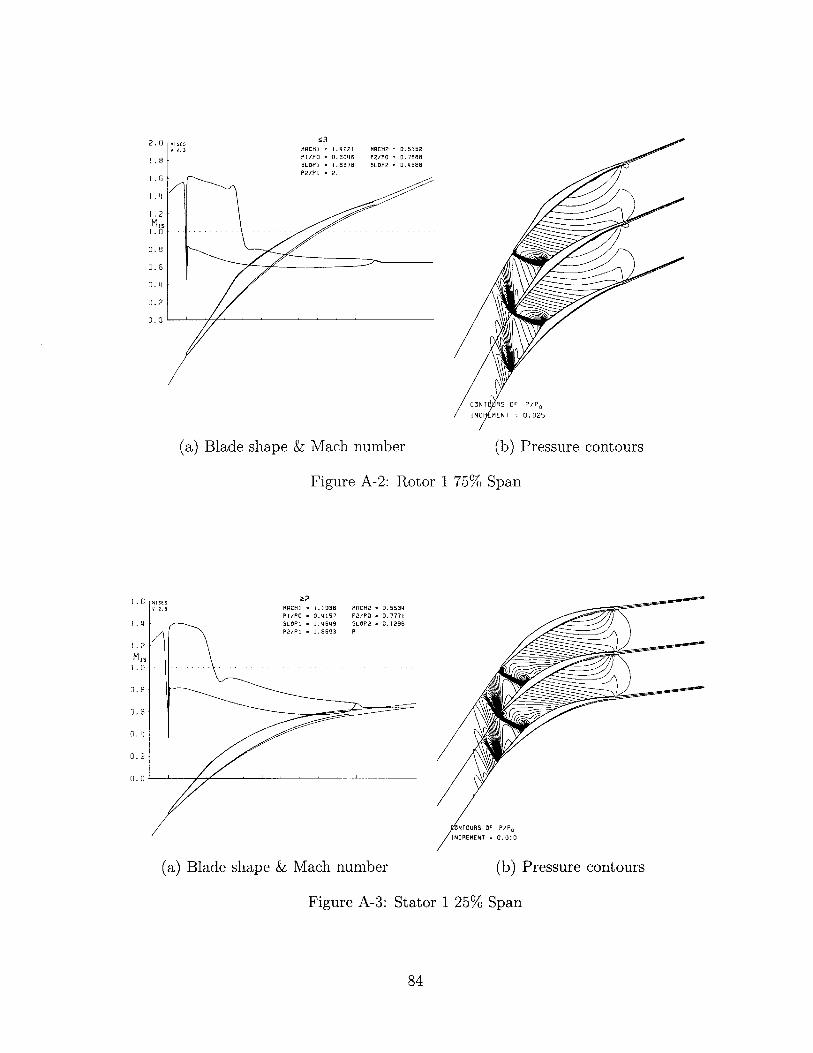
(a) Blade shape & Mach number (b) Pressure contours
Figure A-2: Rotor 1 75% Span
a2MACH1 = 1.1938P1/PO = 0.4157SLOPN = 1.4649P2/P1 = 1.8693
1.6 MISESv 2 .3
1.4
1.2MS
1.0
0.8
0.6
0. 4i
0.2
0.0 - -
MACH2 = 0.5534P2/PO = 0.7771SLOP2 = 0.1296R
P/PO
0.010
(a) Blade shape & Mach number (b) Pressure contours
Figure A-3: Stator 1 25% Span
84
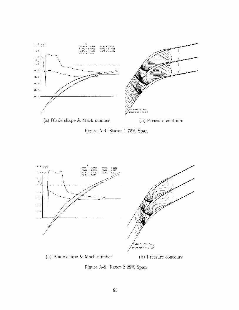
1.6
1.4
1.2
MS1.0
0.8
0.6
0. 4
0.2
0.0
Z4MACHI = 1.0864 MACH2 = 0.6230PI/PO = 0.4763 P2/PD = 0.7503SLOPI = 1.4620 SLODP2 = 0.2084P2/P1 = 1.57
ZONTOURS OF P/P0INCREMENT = 0.012
(a) Blade shape & Mach number (b) Pressure contours
Figure A-4: Stator 1 75% Span
1.6
1.4
1.2
MIS1.0
0.8
0.6
0. 4
0.2
0. 0
INCREMENT = 0.025
(a) Blade shape & Mach number (b) Pressure contours
Figure A-5: Rotor 2 25% Span
85
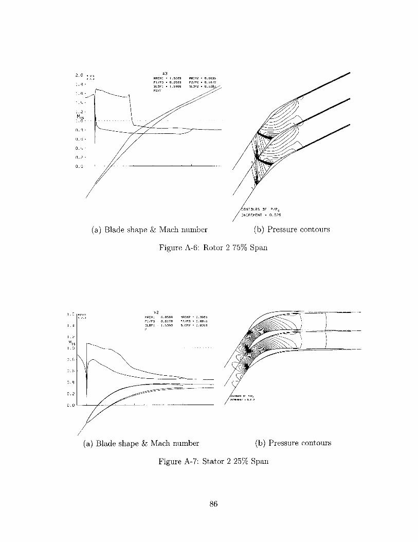
INCREMENT = 0.025
(a) Blade shape & Mach number (b) Pressure contours
Figure A-6: Rotor 2 75% Span
2MACHI = 0.8589 MRCH2 = 0.3965P1/PO = 0.6178 P2/PO = 0.8875SLOPI 1.5393 SLOP2 0.0058P,
(a) Blade shape & Mach number (b) Pressure contours
Figure A-7: Stator 2 25% Span
86
1.6
1 . 4
1.2
MS1.0
0. 8
0. 6
0. 4
0.2
0.0
IF P/P.
- 0.012
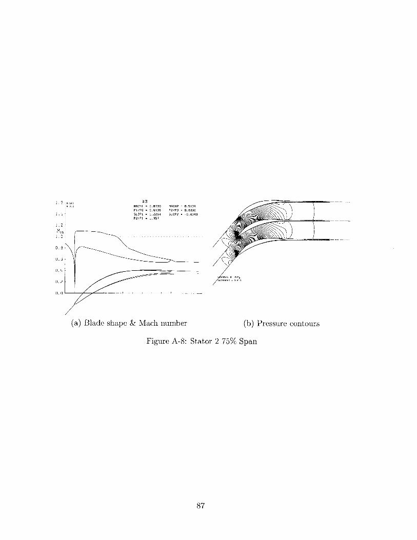
1.6
1. 14
1.2
MIS1.0
0.8
23MRCHI = 0.8700PI/PO = 0.6105SLOP1 = 1.2254P2/Pl = 1.357
MACH2 0.5109P2/PD = 0.8290SLOP2 = -0.0043
0.6
0. 4
(a) Blade shape & Mach number (b) Pressure contours
Figure A-8: Stator 2 75% Span
87