Embed Size (px)
Citation preview

Ae/APh/CE/ME 101 Notes
Bradford Sturtevant
Hans W. Liepmann Professor of Aeronautics
Graduate Aeronautical Laboratories
California Institute of Technology
April 23, 2001
1

Ae101 Notes
Contents
1 The Conservation Equations in Integral Form 1
1.1 Material Volume V ∗ (Surface S∗) . . . . . . . . . . . . . . . . . . . . . . . . . . . . . . . . . 1
1.1.1 Variables and dimensions . . . . . . . . . . . . . . . . . . . . . . . . . . . . . . . . . 2
1.2 Reynolds Transport Theorem . . . . . . . . . . . . . . . . . . . . . . . . . . . . . . . . . . . 2
1.3 Moving (Non-Material) Control Volume V (Surface S, s 6= u) . . . . . . . . . . . . . . . . . 3
1.4 Fixed Control Volume . . . . . . . . . . . . . . . . . . . . . . . . . . . . . . . . . . . . . . . 3
1.5 Scaling: Non-dimensional numbers . . . . . . . . . . . . . . . . . . . . . . . . . . . . . . . . 3
1.6 Control Volume Analysis – Mass and Momentum . . . . . . . . . . . . . . . . . . . . . . . . 5
1.7 The Stress Tensor . . . . . . . . . . . . . . . . . . . . . . . . . . . . . . . . . . . . . . . . . 7
1.8 The Flux of Momentum Tensor ρ u u . . . . . . . . . . . . . . . . . . . . . . . . . . . . . . . 9
1.9 Summary of Equations . . . . . . . . . . . . . . . . . . . . . . . . . . . . . . . . . . . . . . . 9
2 The Equations of Motion in Differential Form 10
2.1 The Divergence Theorem . . . . . . . . . . . . . . . . . . . . . . . . . . . . . . . . . . . . . 10
2.2 The Equations of Motion . . . . . . . . . . . . . . . . . . . . . . . . . . . . . . . . . . . . . 10
2.3 The Convective Derivative . . . . . . . . . . . . . . . . . . . . . . . . . . . . . . . . . . . . . 11
2.4 Convective Form of the Equations of Motion . . . . . . . . . . . . . . . . . . . . . . . . . . 12
2.5 Alternative Forms of the Conservation Equations . . . . . . . . . . . . . . . . . . . . . . . . 12
2.5.1 Mechanical Energy Equation . . . . . . . . . . . . . . . . . . . . . . . . . . . . . . . 12
2.5.2 Internal Energy Equation . . . . . . . . . . . . . . . . . . . . . . . . . . . . . . . . . 13
2.5.3 Equation for Total Enthalpy – The Bernoulli Equation . . . . . . . . . . . . . . . . . 13
2.5.4 Entropy Equation . . . . . . . . . . . . . . . . . . . . . . . . . . . . . . . . . . . . . 14
2.6 Control Volume Analysis – Energy . . . . . . . . . . . . . . . . . . . . . . . . . . . . . . . . 16
2.7 The Rate of Deformation Tensor and Vorticity . . . . . . . . . . . . . . . . . . . . . . . . . 17
2.8 Vorticity . . . . . . . . . . . . . . . . . . . . . . . . . . . . . . . . . . . . . . . . . . . . . . . 17
2.8.1 The vorticity equation . . . . . . . . . . . . . . . . . . . . . . . . . . . . . . . . . . . 18
3 Viscous Stresses and Heat Flux 20
3.1 Newtonian fluid . . . . . . . . . . . . . . . . . . . . . . . . . . . . . . . . . . . . . . . . . . . 20
3.2 Bulk viscosity . . . . . . . . . . . . . . . . . . . . . . . . . . . . . . . . . . . . . . . . . . . . 20

Ae/APh/CE/ME 101 Notes
3.3 Heat flux vector (Fourier’s law) . . . . . . . . . . . . . . . . . . . . . . . . . . . . . . . . . . 21
3.4 The Equations of Motion - Newtonian Fluid . . . . . . . . . . . . . . . . . . . . . . . . . . . 21
3.4.1 Vorticity equation - Isothermal fluid . . . . . . . . . . . . . . . . . . . . . . . . . . . 22
3.4.2 Constant viscosity and heat conductivity . . . . . . . . . . . . . . . . . . . . . . . . 22
3.5 Crocco’s Theorem . . . . . . . . . . . . . . . . . . . . . . . . . . . . . . . . . . . . . . . . . 22
3.6 Incompressible fluid . . . . . . . . . . . . . . . . . . . . . . . . . . . . . . . . . . . . . . . . 23
4 Summary: Other Forms of the Equations of Motion 24
4.1 Cartesian Tensor Notation . . . . . . . . . . . . . . . . . . . . . . . . . . . . . . . . . . . . . 24
4.2 2 Dimensional Plane Flow: Cartesian Coordinates . . . . . . . . . . . . . . . . . . . . . . . 24
4.3 Cylindrical Coordinates . . . . . . . . . . . . . . . . . . . . . . . . . . . . . . . . . . . . . . 24
4.4 2 Dimensional Axisymmetric Flow: Cylindrical Polar Coordinates . . . . . . . . . . . . . . 25
4.5 2 Dimensional Flow: Spherical Polar Coordinates . . . . . . . . . . . . . . . . . . . . . . . . 26
4.5.1 Stream Function . . . . . . . . . . . . . . . . . . . . . . . . . . . . . . . . . . . . . . 26
5 Dimensions 27
5.1 Some derived dimensional units . . . . . . . . . . . . . . . . . . . . . . . . . . . . . . . . . . 27
5.2 Conventional Dimensionless Numbers . . . . . . . . . . . . . . . . . . . . . . . . . . . . . . 27
5.3 Parameters for Air and Water . . . . . . . . . . . . . . . . . . . . . . . . . . . . . . . . . . . 27
6 Thermodynamics 28
6.1 Thermodynamic potentials and fundamental relations . . . . . . . . . . . . . . . . . . . . . 28
6.2 Maxwell relations . . . . . . . . . . . . . . . . . . . . . . . . . . . . . . . . . . . . . . . . . . 28
6.3 Reciprocity relations and the equations of state . . . . . . . . . . . . . . . . . . . . . . . . . 29
6.4 Various defined quantities . . . . . . . . . . . . . . . . . . . . . . . . . . . . . . . . . . . . . 30
6.5 Perfect Gas Equations of State . . . . . . . . . . . . . . . . . . . . . . . . . . . . . . . . . . 31
7 Quasi-onedimensional flow 33
7.1 The Euler equations . . . . . . . . . . . . . . . . . . . . . . . . . . . . . . . . . . . . . . . . 34
7.2 Steady flow . . . . . . . . . . . . . . . . . . . . . . . . . . . . . . . . . . . . . . . . . . . . . 34
7.2.1 Quasi-1D Steady Euler flow . . . . . . . . . . . . . . . . . . . . . . . . . . . . . . . . 35
7.3 Constant β (or Γ) fluid . . . . . . . . . . . . . . . . . . . . . . . . . . . . . . . . . . . . . . . 37
7.4 Perfect Gas . . . . . . . . . . . . . . . . . . . . . . . . . . . . . . . . . . . . . . . . . . . . . 38
iii April 23, 2001

Ae/APh/CE/ME 101 Notes
8 Normal Shock Waves 40
8.1 Steady Frame . . . . . . . . . . . . . . . . . . . . . . . . . . . . . . . . . . . . . . . . . . . . 40
8.1.1 Calculating Shock Conditions for Real Fluids . . . . . . . . . . . . . . . . . . . . . . 41
8.1.2 Expansion about the upstream state (weak shocks) . . . . . . . . . . . . . . . . . . . 41
8.1.3 Perfect gas . . . . . . . . . . . . . . . . . . . . . . . . . . . . . . . . . . . . . . . . . 42
8.2 Nonsteady Frame . . . . . . . . . . . . . . . . . . . . . . . . . . . . . . . . . . . . . . . . . . 45
8.2.1 Reflected shock waves . . . . . . . . . . . . . . . . . . . . . . . . . . . . . . . . . . . 46
9 Frictional Flow – Fanno Flow 48
9.1 dh/dv and tangency . . . . . . . . . . . . . . . . . . . . . . . . . . . . . . . . . . . . . . . . 49
9.2 Curvature of the isentropes in the h-v plane . . . . . . . . . . . . . . . . . . . . . . . . . . . 49
9.3 Entropy . . . . . . . . . . . . . . . . . . . . . . . . . . . . . . . . . . . . . . . . . . . . . . . 49
10 Flow with Heat Addition – Rayleigh Flow 51
10.1 Tangency . . . . . . . . . . . . . . . . . . . . . . . . . . . . . . . . . . . . . . . . . . . . . . 51
10.2 Entropy . . . . . . . . . . . . . . . . . . . . . . . . . . . . . . . . . . . . . . . . . . . . . . . 52
10.3 The Mollier Diagram . . . . . . . . . . . . . . . . . . . . . . . . . . . . . . . . . . . . . . . . 52
11 Detonation Waves in One Dimension 54
11.1 2-γ model of detonation waves . . . . . . . . . . . . . . . . . . . . . . . . . . . . . . . . . . 55
11.2 Equations in the steady frame . . . . . . . . . . . . . . . . . . . . . . . . . . . . . . . . . . . 56
12 Nonsteady Flows 58
12.1 One-dimensional inviscid nonheatconducting flow . . . . . . . . . . . . . . . . . . . . . . . . 58
12.2 Homentropic flow . . . . . . . . . . . . . . . . . . . . . . . . . . . . . . . . . . . . . . . . . . 59
12.3 Simple waves . . . . . . . . . . . . . . . . . . . . . . . . . . . . . . . . . . . . . . . . . . . . 59
12.4 Perfect gas . . . . . . . . . . . . . . . . . . . . . . . . . . . . . . . . . . . . . . . . . . . . . 60
12.4.1 Simple Waves . . . . . . . . . . . . . . . . . . . . . . . . . . . . . . . . . . . . . . . . 60
12.4.2 Centered Waves . . . . . . . . . . . . . . . . . . . . . . . . . . . . . . . . . . . . . . 61
12.4.3 Complete expansion . . . . . . . . . . . . . . . . . . . . . . . . . . . . . . . . . . . . 63
12.5 Wave interactions – The shock-tube equation . . . . . . . . . . . . . . . . . . . . . . . . . . 63
13 Steady Two-Dimensional Flow 66
13.1 Oblique shock waves . . . . . . . . . . . . . . . . . . . . . . . . . . . . . . . . . . . . . . . . 66
iv April 23, 2001

Ae/APh/CE/ME 101 Notes
13.2 Weak shocks . . . . . . . . . . . . . . . . . . . . . . . . . . . . . . . . . . . . . . . . . . . . 68
13.3 Continuous flows – Prandtl-Meyer expansion . . . . . . . . . . . . . . . . . . . . . . . . . . 70
13.4 The hodograph . . . . . . . . . . . . . . . . . . . . . . . . . . . . . . . . . . . . . . . . . . . 71
13.5 Wave interactions . . . . . . . . . . . . . . . . . . . . . . . . . . . . . . . . . . . . . . . . . . 73
13.6 Natural Coordinates . . . . . . . . . . . . . . . . . . . . . . . . . . . . . . . . . . . . . . . . 74
13.7 The Equations in Characteristic Form . . . . . . . . . . . . . . . . . . . . . . . . . . . . . . 76
13.7.1 The Method of Characteristics . . . . . . . . . . . . . . . . . . . . . . . . . . . . . . 77
14 Acoustics 78
14.1 Plane Waves I . . . . . . . . . . . . . . . . . . . . . . . . . . . . . . . . . . . . . . . . . . . . 78
14.2 Acoustics in multi dimensions . . . . . . . . . . . . . . . . . . . . . . . . . . . . . . . . . . . 79
14.3 Plane waves II . . . . . . . . . . . . . . . . . . . . . . . . . . . . . . . . . . . . . . . . . . . 80
14.4 Refraction . . . . . . . . . . . . . . . . . . . . . . . . . . . . . . . . . . . . . . . . . . . . . . 82
14.5 Spherical waves . . . . . . . . . . . . . . . . . . . . . . . . . . . . . . . . . . . . . . . . . . . 83
14.6 Cylindrical waves . . . . . . . . . . . . . . . . . . . . . . . . . . . . . . . . . . . . . . . . . . 85
14.7 General acoustic field from superposition of sources . . . . . . . . . . . . . . . . . . . . . . . 87
14.7.1 Impulsive point source. . . . . . . . . . . . . . . . . . . . . . . . . . . . . . . . . . . 87
14.7.2 General solution obtained from a distribution of impulsive point sources . . . . . . . 88
14.7.3 Harmonic point source. . . . . . . . . . . . . . . . . . . . . . . . . . . . . . . . . . . 88
14.7.4 General solution for harmonic waves . . . . . . . . . . . . . . . . . . . . . . . . . . . 89
14.8 Harmonic dipoles and quadrupoles . . . . . . . . . . . . . . . . . . . . . . . . . . . . . . . . 89
14.8.1 Dipole source . . . . . . . . . . . . . . . . . . . . . . . . . . . . . . . . . . . . . . . . 89
14.8.2 Quadrupole source . . . . . . . . . . . . . . . . . . . . . . . . . . . . . . . . . . . . . 90
14.9 Radiation from a plane . . . . . . . . . . . . . . . . . . . . . . . . . . . . . . . . . . . . . . . 91
14.10Aero-acoustics . . . . . . . . . . . . . . . . . . . . . . . . . . . . . . . . . . . . . . . . . . . 93
14.10.1Scaling of jet noise . . . . . . . . . . . . . . . . . . . . . . . . . . . . . . . . . . . . . 94
14.11Geometrical acoustics . . . . . . . . . . . . . . . . . . . . . . . . . . . . . . . . . . . . . . . 95
15 Potential Flow 100
15.1 Bernoulli equation for nonsteady flow . . . . . . . . . . . . . . . . . . . . . . . . . . . . . . 100
15.2 The potential equation . . . . . . . . . . . . . . . . . . . . . . . . . . . . . . . . . . . . . . . 100
15.3 Small disturbance theory . . . . . . . . . . . . . . . . . . . . . . . . . . . . . . . . . . . . . 102
15.3.1 Energy equation for steady flow . . . . . . . . . . . . . . . . . . . . . . . . . . . . . . 102
v April 23, 2001

Ae/APh/CE/ME 101 Notes
15.3.2 The potential equation . . . . . . . . . . . . . . . . . . . . . . . . . . . . . . . . . . . 102
15.3.3 Pressures. . . . . . . . . . . . . . . . . . . . . . . . . . . . . . . . . . . . . . . . . . . 103
15.3.4 Boundary conditions – body. . . . . . . . . . . . . . . . . . . . . . . . . . . . . . . . 104
15.3.5 Solution – Plane slender body . . . . . . . . . . . . . . . . . . . . . . . . . . . . . . . 104
15.3.6 Solution – Slender body of revolution . . . . . . . . . . . . . . . . . . . . . . . . . . 107
15.4 Similarity rules for compressible flow . . . . . . . . . . . . . . . . . . . . . . . . . . . . . . . 110
15.4.1 Plane flow – subsonic case . . . . . . . . . . . . . . . . . . . . . . . . . . . . . . . . . 110
15.4.2 Supersonic flow . . . . . . . . . . . . . . . . . . . . . . . . . . . . . . . . . . . . . . . 111
15.4.3 Axisymmetric flow – subsonic case . . . . . . . . . . . . . . . . . . . . . . . . . . . . 111
16 Incompressible Flow 113
16.1 The stream function . . . . . . . . . . . . . . . . . . . . . . . . . . . . . . . . . . . . . . . . 114
16.2 Complex notation for plane flow . . . . . . . . . . . . . . . . . . . . . . . . . . . . . . . . . 117
16.3 Flows with volume sources . . . . . . . . . . . . . . . . . . . . . . . . . . . . . . . . . . . . . 117
16.4 Flows with sources of vorticity . . . . . . . . . . . . . . . . . . . . . . . . . . . . . . . . . . 120
16.4.1 Helmholtz vortex theorems . . . . . . . . . . . . . . . . . . . . . . . . . . . . . . . . 120
16.4.2 Biot-Savart Law . . . . . . . . . . . . . . . . . . . . . . . . . . . . . . . . . . . . . . 121
16.4.3 General vortex sheet – Lift . . . . . . . . . . . . . . . . . . . . . . . . . . . . . . . . 123
16.5 Uniform flow, (x, y) . . . . . . . . . . . . . . . . . . . . . . . . . . . . . . . . . . . . . . . . . 125
16.6 Flow over a lifting cylinder . . . . . . . . . . . . . . . . . . . . . . . . . . . . . . . . . . . . 125
16.7 The Kutta condition . . . . . . . . . . . . . . . . . . . . . . . . . . . . . . . . . . . . . . . . 129
17 Airfoil theory 131
17.1 Flat plate airfoil . . . . . . . . . . . . . . . . . . . . . . . . . . . . . . . . . . . . . . . . . . 131
17.2 The Joukowski Transformation . . . . . . . . . . . . . . . . . . . . . . . . . . . . . . . . . . 134
18 Wing Theory 138
18.1 Induced Drag . . . . . . . . . . . . . . . . . . . . . . . . . . . . . . . . . . . . . . . . . . . . 139
18.2 Control Volume Analysis of the Forces on a Wing . . . . . . . . . . . . . . . . . . . . . . . . 140
18.3 Pressures . . . . . . . . . . . . . . . . . . . . . . . . . . . . . . . . . . . . . . . . . . . . . . 141
18.4 Lift . . . . . . . . . . . . . . . . . . . . . . . . . . . . . . . . . . . . . . . . . . . . . . . . . . 141
18.5 Drag . . . . . . . . . . . . . . . . . . . . . . . . . . . . . . . . . . . . . . . . . . . . . . . . . 142
18.6 Constant Downwash . . . . . . . . . . . . . . . . . . . . . . . . . . . . . . . . . . . . . . . . 142
vi April 23, 2001

Ae/APh/CE/ME 101 Notes
18.7 Vortex Distribution and Circulation on the Wing . . . . . . . . . . . . . . . . . . . . . . . . 143
18.8 Spanwise Loading – Planform . . . . . . . . . . . . . . . . . . . . . . . . . . . . . . . . . . . 144
19 Parallel Viscous Flows 146
19.1 Viscous waves . . . . . . . . . . . . . . . . . . . . . . . . . . . . . . . . . . . . . . . . . . . . 146
19.2 Rayleigh problem . . . . . . . . . . . . . . . . . . . . . . . . . . . . . . . . . . . . . . . . . . 148
19.3 Flows with Heat Transfer; Couette flow . . . . . . . . . . . . . . . . . . . . . . . . . . . . . 149
19.4 Poiseuille flow . . . . . . . . . . . . . . . . . . . . . . . . . . . . . . . . . . . . . . . . . . . . 150
20 Thin-Layer Flows 153
20.1 Round Laminar Jet . . . . . . . . . . . . . . . . . . . . . . . . . . . . . . . . . . . . . . . . . 155
20.1.1 Integral relations . . . . . . . . . . . . . . . . . . . . . . . . . . . . . . . . . . . . . . 156
20.1.2 Scaling . . . . . . . . . . . . . . . . . . . . . . . . . . . . . . . . . . . . . . . . . . . 157
20.1.3 Similarity. . . . . . . . . . . . . . . . . . . . . . . . . . . . . . . . . . . . . . . . . . . 158
20.1.4 Point source of momentum . . . . . . . . . . . . . . . . . . . . . . . . . . . . . . . . 159
20.2 Plane Laminar Wake . . . . . . . . . . . . . . . . . . . . . . . . . . . . . . . . . . . . . . . . 160
20.2.1 Drag. . . . . . . . . . . . . . . . . . . . . . . . . . . . . . . . . . . . . . . . . . . . . 161
20.2.2 Similarity. . . . . . . . . . . . . . . . . . . . . . . . . . . . . . . . . . . . . . . . . . . 161
20.3 Boundary Layers . . . . . . . . . . . . . . . . . . . . . . . . . . . . . . . . . . . . . . . . . . 163
20.3.1 Integral relations . . . . . . . . . . . . . . . . . . . . . . . . . . . . . . . . . . . . . . 163
20.3.2 Wall Fluxes . . . . . . . . . . . . . . . . . . . . . . . . . . . . . . . . . . . . . . . . . 166
20.3.3 Energy equation . . . . . . . . . . . . . . . . . . . . . . . . . . . . . . . . . . . . . . 167
20.3.4 Lighthill’s formula . . . . . . . . . . . . . . . . . . . . . . . . . . . . . . . . . . . . . 169
20.3.5 Flat-plate boundary layer . . . . . . . . . . . . . . . . . . . . . . . . . . . . . . . . . 170
20.3.6 Boundary Layers on Curved Bodies . . . . . . . . . . . . . . . . . . . . . . . . . . . 173
21 Turbulent boundary layers 174
22 Low Reynolds Number Flow 179
22.1 Stokes flow – Creeping flow . . . . . . . . . . . . . . . . . . . . . . . . . . . . . . . . . . . . 179
22.2 The Oseen equations . . . . . . . . . . . . . . . . . . . . . . . . . . . . . . . . . . . . . . . . 184
22.3 Drag at higher Reynolds numbers – D vs. Re. . . . . . . . . . . . . . . . . . . . . . . . . . . 185
22.4 Lubrication theory . . . . . . . . . . . . . . . . . . . . . . . . . . . . . . . . . . . . . . . . . 185
vii April 23, 2001

Ae/APh/CE/ME 101 Notes
23 Turbulence 189
23.1 Reynolds Averaging . . . . . . . . . . . . . . . . . . . . . . . . . . . . . . . . . . . . . . . . 189
23.2 Closure – Turbulence Models . . . . . . . . . . . . . . . . . . . . . . . . . . . . . . . . . . . 191
23.2.1 Eddy Viscosity Model. . . . . . . . . . . . . . . . . . . . . . . . . . . . . . . . . . . . 191
23.2.2 Prandtl’s Mixing Length Theory. . . . . . . . . . . . . . . . . . . . . . . . . . . . . . 191
23.2.3 Other closure schemes . . . . . . . . . . . . . . . . . . . . . . . . . . . . . . . . . . . 192
23.3 Turbulent Scales . . . . . . . . . . . . . . . . . . . . . . . . . . . . . . . . . . . . . . . . . . 193
24 Buoyancy Effects 194
24.1 Hydostatic compressible gas . . . . . . . . . . . . . . . . . . . . . . . . . . . . . . . . . . . . 194
24.2 Boussinesq approximation (Spiegel &Veronis (1960)) . . . . . . . . . . . . . . . . . . . . . . 195
24.2.1 Equation of State . . . . . . . . . . . . . . . . . . . . . . . . . . . . . . . . . . . . . . 196
24.2.2 Continuity Equation . . . . . . . . . . . . . . . . . . . . . . . . . . . . . . . . . . . . 196
24.2.3 Momentum Equation . . . . . . . . . . . . . . . . . . . . . . . . . . . . . . . . . . . . 197
24.2.4 Energy equation . . . . . . . . . . . . . . . . . . . . . . . . . . . . . . . . . . . . . . 197
24.3 Axisymmetric Buoyant Plumes . . . . . . . . . . . . . . . . . . . . . . . . . . . . . . . . . . 198
24.3.1 Laminar Plumes . . . . . . . . . . . . . . . . . . . . . . . . . . . . . . . . . . . . . . 198
24.3.2 Buoyancy driven by density variations (e.g., concentration) . . . . . . . . . . . . . . 202
24.3.3 Laminar plumes in stratified atmospheres (Morton (1967)) . . . . . . . . . . . . . . 202
24.3.4 Approximate Integral Method . . . . . . . . . . . . . . . . . . . . . . . . . . . . . . . 203
24.4 Turbulent Plumes (Morton et al. (1956)) . . . . . . . . . . . . . . . . . . . . . . . . . . . . . 204
24.4.1 Uniform atmosphere . . . . . . . . . . . . . . . . . . . . . . . . . . . . . . . . . . . . 205
24.4.2 Nonuniform atmosphere . . . . . . . . . . . . . . . . . . . . . . . . . . . . . . . . . . 206
24.5 Stratified Flows . . . . . . . . . . . . . . . . . . . . . . . . . . . . . . . . . . . . . . . . . . . 206
24.5.1 Shallow water waves . . . . . . . . . . . . . . . . . . . . . . . . . . . . . . . . . . . . 206
24.6 Small Amplitude Motions . . . . . . . . . . . . . . . . . . . . . . . . . . . . . . . . . . . . . 208
24.7 Hydraulic Jump . . . . . . . . . . . . . . . . . . . . . . . . . . . . . . . . . . . . . . . . . . . 208
24.8 Flows With No Losses . . . . . . . . . . . . . . . . . . . . . . . . . . . . . . . . . . . . . . . 209
24.8.1 Steady flow . . . . . . . . . . . . . . . . . . . . . . . . . . . . . . . . . . . . . . . . . 209
25 Rotating Flows 212
25.1 Coordinate Systems . . . . . . . . . . . . . . . . . . . . . . . . . . . . . . . . . . . . . . . . 212
25.2 Momentum equation . . . . . . . . . . . . . . . . . . . . . . . . . . . . . . . . . . . . . . . . 214
viii April 23, 2001

Ae/APh/CE/ME 101 Notes
25.3 Vorticity equation . . . . . . . . . . . . . . . . . . . . . . . . . . . . . . . . . . . . . . . . . 214
25.3.1 Potential vorticity . . . . . . . . . . . . . . . . . . . . . . . . . . . . . . . . . . . . . 214
25.4 Small Rossby number . . . . . . . . . . . . . . . . . . . . . . . . . . . . . . . . . . . . . . . 215
25.5 Taylor-Proudman Theorem . . . . . . . . . . . . . . . . . . . . . . . . . . . . . . . . . . . . 216
25.6 Geostrophic Motion . . . . . . . . . . . . . . . . . . . . . . . . . . . . . . . . . . . . . . . . 216
26 References 219
ix April 23, 2001

Ae/APh/CE/ME 101 Notes
1 The Conservation Equations in Integral Form
Inertial frame of reference.
1.1 Material Volume V ∗ (Surface S∗)
Figure 1. Notation for a material volume
Mass :d
dt
∫V ∗
ρ dV = 0
Momentum :d
dt
∫V ∗
ρ u dV =∫
V ∗ρB dV +
∫S∗
F dS
Energy :d
dt
∫V ∗
ρ
(e +
u2
2
)dV =
∫V ∗
ρB · u dV +∫
S∗F · u dS −
∫S∗
q · n dS +∫
V ∗ρQ dV
Entropy :d
dt
∫V ∗
ρs dV +∫
S∗
q
T· n dS −
∫V ∗
ρQ
TdV ≥ 0
(1.1)
These equations are forms of the conservation of mass, Newton’s laws of motion, the first law of thermo-dynamics and the second law of thermodynamics, respectively.

Ae/APh/CE/ME 101 Notes
1.1.1 Variables and dimensions
The units of every term in each of these equations are as follows,
Mass :MT
Momentum :MLT2
= F
Energy :ML2
T3
Entropy :ML2
T3θ
(1.2)
Thus the units of B are acceleration, and of F are pressure. The units of q are energy per unit area perunit time. In particular,
ρ density ML3 u velocity L
T
B specific body forceLT2 F traction force
MLT2
e specific internal energyL2
T2 q heat flux vectorMT3
(wattsm2
)s specific entropy
L2
θT2 Q specific volumetric energy additionL2
T3
1.2 Reynolds Transport Theorem
For a control volume V moving relative to material (Surface S, s 6= u), the Reynolds Transport Theoremis
d
dt
∫V
f dV =∫
V
∂f
∂tdV +
∫S
f s · n dS , (1.3)
where s = velocity of surface S. In general, the conservation laws are of the form
d
dt
∫V ∗
f dV =∫
V ∗g dV +
∫S∗
h dS , (1.4)
which, using Eq. 1.3, is ∫V ∗
∂f
∂tdV +
∫S∗
fu · n dS =∫
V ∗g dV +
∫S∗
h dS , (1.5)
Taking V ∗ and V to instantaneously coincide and adding Eqs. 1.3 and 1.5,
d
dt
∫V
f dV +∫
Sf(u − s) · n dS =
∫V
g dV +∫
Sh dS (1.6)
2 April 23, 2001

Ae/APh/CE/ME 101 Notes
1.3 Moving (Non-Material) Control Volume V (Surface S, s 6= u)
Mass :d
dt
∫V
ρ dV +∫
Sρ(u − s) · n dS = 0
Momentum :d
dt
∫V
ρ u dV +∫
Sρu (u − s) · n dS =
∫V
ρB dV +∫
SF dS
Energy :d
dt
∫V
ρ
(e +
u2
2
)dV +
∫S
ρ
(e +
u2
2
)(u − s) · n dS =∫
VρB · u dV +
∫S
F · u dS −∫
Sq · n dS
(1.7)
1.4 Fixed Control Volume V (Surface S, s = 0)
Mass :d
dt
∫V
ρ dV +∫
Sρu · n dS = 0
Momentum :d
dt
∫V
ρ u dV +∫
Sρu u · n dS =
∫V
ρB dV +∫
SF dS
Energy :d
dt
∫V
ρ
(e +
u2
2
)dV +
∫S
ρ
(e +
u2
2
)u · n dS =∫
VρB · u dV +
∫S
F · u dS −∫
Sq · n dS
Entropy :d
dt
∫V
ρs dV +∫
Sρs u · n dS +
∫S
q
T· n dS −
∫V
ρQ
TdV ≥ 0
(1.8)
1.5 Scaling: Non-dimensional numbers
It is useful to be able to compare the magnitude of terms in an equation. This is done by scaling. Becauseof the equality expressed by an equation, at least two terms must be of the same order of magnitude (unlessthere is only one term, in which case it is trivially equal to zero). The order of magnitude of the size ofterms in Eqs. 1.8 are expressed by characteristic quantities (L, T, ρ, U, etc). The body force term isscaled by the acceleration of gravity g. The traction force has a pressure contribution which scales withpressure changes ∆p through the flow, and a viscous contribution scaled by µU
L , where µ is a viscosity andthe scaling is patterned after the Newtonian viscous shear model. In the energy equation the characteristicinternal energy is denoted by e, which in turn is scaled by a specific heat cp and temperature θ and alsoan acoustic speed squared c2,
e ∼ cpθ ∼ c2 . (1.9)
The heat flux is modeled by the Fourier heat conduction law, k θL , where k is the thermal conductivity.
The equations of motion then suggest the following balances:
Mass :ρL3
T︸︷︷︸1
ρUL2︸ ︷︷ ︸2
= 0
21
=UT
L
(1.10)
3 April 23, 2001

Ae/APh/CE/ME 101 Notes
Momentum :ρUL3
T︸ ︷︷ ︸3
ρU2L2︸ ︷︷ ︸4
= ρgL3︸ ︷︷ ︸5
∆pL2︸ ︷︷ ︸6
µUL︸ ︷︷ ︸7
45
=U2
gL= Fr
47
=UL
ν= Re
Re · 57
=Re2
Fr=
gL3
ν2= Gr
(1.11)
Energy :ρeL3
T︸ ︷︷ ︸8
ρU2L3
T︸ ︷︷ ︸9
ρeUL2︸ ︷︷ ︸10
ρU3L2︸ ︷︷ ︸11
= ρgUL3︸ ︷︷ ︸12
∆pUL2︸ ︷︷ ︸13
µU2L︸ ︷︷ ︸14
kθL︸︷︷︸15
89
=e
U2
gases∼ 1M2
1415
=µU2
kθ∼ Pr
U2
e
1015
=ρeUL
kθ∼ UL
κ= Pe = RePr ,
(1.12)
where we have takene ∼ cp θ ; ν =
µ
ρ; κ =
k
cpρ; Pr =
ν
κ(1.13)
The pressure may balance with one other term. For example,
64
=∆p
ρU2
gases∼ ∆ρ
ρ
1M2
65
=∆p
ρgL
67
=∆p L
µU
(1.14)
ρU2 is the dynamic pressure, ρgL is the hydrostatic pressure and µU/L is the viscous pressure drop. Fromthe last, it follows that viscous drag must be of order µUL.
We have not accounted for the fact that the fluid may be a mixture of substances, the conservation ofeach one of which may have to be accounted for. In this case each component satisfies an equation likethe first of Eqs. 1.1, say, for its concentration C (same units as ρ), except that there will be source termson the right hand side. Chemical reactions cause volumetric changes and diffusion causes flux across theboundaries,
d
dt
∫V ∗
C dV =∫
V ∗Ckc dV +
∫S∗
Cud dS , (1.15)
4 April 23, 2001

Ae/APh/CE/ME 101 Notes
where kc is the chemical reaction rate with units 1/T, and ud is the diffusive flux velocity. The latter ismodeled to order of magnitude by (see Fick’s Law)
Cud = DC
L, (1.16)
where D is the diffusion coefficient, [D] = L2/T. This leads to two more nondimensional numbers,
Le =D
κ(1.17)
Sc =ν
D. (1.18)
1.6 Control Volume Analysis – Mass and Momentum
In this section we illustrate how the above ideas can be used to solve even rather difficult problems.Usually, the control volume boundary in internal (channel) flows is placed at locations where the flowconditions can be assumed uniform, so the surface integrals reduce to algebraic expressions.
The rocket equation. A rocket accelerates vertically upward in a vertical gravitational field. We write theequations of motion in the inertial frame fixed with the earth (Fig. 2). In that coordinate system the fluid
Figure 2. Schematic of a rocket moving parallel to the gravity vector
velocity is u and the velocity of the control volume is s, while the velocity relative to the rocket is v. Thatis,
v = u − s . (1.19)
The integral equation for the conservation of mass is
d
dt
∫V
ρ dV = −∫
Se
ρ(u − s) · n dS . (1.20)
Defining the total mass of the rocket M , and evaluating the integrals gives
dM
dt= −ρeveSe , (1.21)
5 April 23, 2001

Ae/APh/CE/ME 101 Notes
where Se is the nozzle exit area.
The momentum equation is
d
dt
∫V
ρu dV +∫
Se
ρu(u − s) · n dS =∫
Vρg dV +
∫S
F dS (1.22)
By symmetry the net contribution from the pressure acting on the solid body to the last term is a verticalforce downward of magnitude p0Se. Writing the equation for the vertical momentum, and splitting thefirst term into the momenta of the masses moving (combustion products) and fixed (e.g., the unburnedpropellant) with respect to the rocket casing, respectively,
d
dt
∫Vfix
(ρs)fix dV +d
dt
∫Vmove
(ρv)move dV + ρe(ve + s)veSe = −Mg + (pe − p0)Se − D , (1.23)
where D is the contribution of the vicous traction forces. Throughout most of the trajectory the momentumof the gases in the rocket chamber and nozzle (the second term) is small compared to the momentum ofthe solid components of the rocket. With the definition of M ,
dMs
dt− M(ve + s) = −Mg + (pe − p0)Se − D . (1.24)
Partially differentiating the fist term and cancelling results in the so-called rocket equation
MdU
dt= Mve − Mg − (p0 − pe)Se − D . (1.25)
The thrust is defined byT ≡ Mve . (1.26)
Optimal performance results when the exit pressure is matched to the ambient, pe = p0, typically athigh altutude. At sea level (p0 > pe), there is a performance penalty. At very high altitude, where theatmosphere is rarefied,
MdU
dt= T − Mg + peSe . (1.27)
Losses at area changes in pipes – pressure recovery. Control surface analysis can be used to analyze theeffects of losses on pressure recovery across a sudden enlargement of a pipe in the flow of an incompressiblefluid, as shown in Fig. 3. It is assumed that the incoming stream is uniform and the control volume is long
Figure 3. Control surface for area expansion in a pipe
enough that the flow across station 1 is also uniform. For simplicity, viscous forces are neglected. The flowis steady. That means that, though there may be large fluctuations internally, the flows in and out are
6 April 23, 2001

Ae/APh/CE/ME 101 Notes
steady, so the integral quantities do not vary in time, d/dt = 0. It will emerge that one further piece ofinformation is required to close the problem. We use the fact that the fluid by the vertical section at thearea change can communicate very well with the region on the left (1), so the pressure pb on the verticalsection at the area change is constant and equal to p1.
The control volume is fixed, so the mass equation gives that
u2A2 = u1A1 . (1.28)
The flow slows down. The integral momentum equation in the horizontal direction states that the changeof momentum flux between 1 and 2, ρu2
2A2 − ρu21A1, is balanced by the pressure forces acting in the
downstream direction. Using the continuity equation and pb = p1,
ρu2A2(u2 − u1) = p1A1 + p1(A2 − A1) − p2A2 . (1.29)
Thus the pressure increase is
p2 − p1 = ρu2(u1 − u2) ,
Cp = 2A1
A2
(1 − A1
A2
) (1.30)
where Cp ≡ (p2 − p1)/12ρu2
1.
If the area change were very gradual, so there were no losses, the flow would satisfy the Bernoulliequation, p + 1
2ρu2 = const, with the result
Cp = 1 −(
A1
A2
)2
(1.31)
These two results are compared in Fig. 4. The estimate based on pb = p1 gives considerably lower pressurerecovery, but they both agree for very small changes of area, where in any case the process is nearly ideal.
1.7 The Stress Tensor
The force F depends on the orientation of the surface S. This means that in order to express the force,we need 3 components for each component of the outward normal, i.e., a tensor of rank 2, called the stresstensor σ (see figure, drawn for 2 dimensions). In terms of the stress tensor the traction force is expressed
F = σ n ; Fi = σij nj (Cartesian tensor notation) (1.32)
Splitting the Stress Tensor:The concept of the stress tensor is very general, and applies to all substances. The stress and strain δ
experienced by a general substance can be thought of as divided into two parts
σ = σelastic + σplastic
cold part+ fluid-like+thermal part memory, hysteresis
δ = δelastic + δplastic .
(1.33)
7 April 23, 2001

Ae/APh/CE/ME 101 Notes
Figure 4. Comparison of Bernoulli flow with model flow with losses
Figure 5. Components of the stress in 2D
We consider only the simplest fluids and solids at stresses greater than about 1 Mbar = 100 GPa, in whichcase the stress can be split into the isotropic normal contribution which is finite when there is no motion(the pressure p), and a viscous contribution (the viscous stress tensor τ).
σ = −pI + τ ; σij = −p δij + τij , (1.34)
where δij is the Kronecker delta; δij =
1 if i = j0 if i 6= j
. Here, the pressure is taken to be the thermodynamic
pressure, i.e., it is a thermal quantity. The traction force is thus expressed in terms of the stress tensor as
F = −pn + τn ; Fi = −pni + τijnj . (1.35)
8 April 23, 2001

Ae/APh/CE/ME 101 Notes
1.8 The Flux of Momentum Tensor ρ uu
Where a vector multiplies a scalar dot product in the equations, it can be replaced by a tensor multi-plying a vector, as justified by the Catresian tensor form. For example,
ρu (u · n) = (ρu u)n ; ρui (ujnj) = (ρuiuj) nj (1.36)
1.9 Summary of Equations
Thus, summarizing for a stationary control volume (s = 0),
Mass :d
dt
∫V
ρ dV +∫
Sρ u · n dS = 0
Momentum :d
dt
∫V
ρ u dV +∫
S(ρuu)n dS = −
∫S
p n dS +∫
VρB dV +
∫S
τ n dS
Energy :d
dt
∫V
ρ
(e +
u2
2
)dV +
∫S
ρ
(e +
u2
2
)u · n dS =
−∫
Spu · n dS +
∫V
ρB · u dV +∫
Sτu · n dS −
∫S
q · n dS +∫
VρQ dV
Entropy :d
dt
∫V
ρs dV +∫
Sρs u · n dS +
∫S
q
T· n dS −
∫V
ρQ
TdV ≥ 0
(1.37)
9 April 23, 2001

Ae/APh/CE/ME 101 Notes
2 The Equations of Motion in Differential Form
The surface integrals in the conservation equations (Eqs. 1.8) can be transformed to volume integralsby using the Divergence (Gauss’) Theorem. Then the limit lim
V →0can be taken, with some corresponding
constraints, to transform the equations into differential form.
2.1 The Divergence Theorem
The definition of the divergence is, for any “density” variable,
∇ · f = limV →0
1V
∫S
fn dS (2.1)
This forms the basis for the Divergence Theorem,∫S
fn dS =∫
V∇ · f dV (2.2)
f can be a scalar, vector or tensor, because any operation on a vector f can be written in terms of theequivalent skew-symmetric tensor
f =
0 −f3 f2
f3 0 −f1
−f2 f1 0
. (2.3)
Writing the various surface integrals that appear in the equations of motion in terms of the divergencetheorem illustrates how it applies to scalars, vectors and tensors:
I.∫S ρu · n dS =
∫V ∇ · (ρu) dV
II.∫S ρu(u · n) dS =
∫S(ρuu)n dS =
∫V ∇ · (ρuu) dV
III.∫S F dS =
∫S σn dS =
∫V ∇ · σ dV
IV.∫S F · u dS =
∫S(σn) · u dS =
∫S(σu) · n dS =
∫V ∇ · (σu) dV
V.∫S q · n dS =
∫V ∇ · q dV .
(2.4)
2.2 The Equations of Motion
Eqs. 2.4 transform the equations of motion to a form which contains only volume integrals. Then, withthe definition of the partial with respect to time,
∂f
∂t≡ lim
V →0
1V
d
dt
∫V
f dV , (2.5)
10 April 23, 2001

Ae/APh/CE/ME 101 Notes
we can take the limit V → 0, yielding the equations of motion in differential form.
Mass :∂ρ
∂t+ ∇ · ρu = 0
∂ρ
∂t+
∂ρuj
∂xj= 0
Momentum :∂ρu
∂t+ ∇ · (ρu u) = ρB + ∇ · σ
∂ρui
∂t+
∂ρuiuj
∂xj= ρBi +
∂σij
∂xj
Energy :∂ρ
(e + u2
2
)∂t
+ ∇ · ρ(
e +u2
2
)u = ρB · u + ∇ · (σu) −∇ · q + ρ Q
∂ρ(e + u2
2
)∂t
+∂ρ
(e + u2
2
)uj
∂xj= ρBjuj +
∂σijui
∂xj− ∂qj
∂xj+ ρ Q
(2.6)
Splitting the stress tensor according to Eq. 1.34 and using ∇ · (pI) = ∇p , i.e.,∂pδij
∂xj=
∂p
∂xj, gives for the
momentum and energy equations
∂ρu
∂t+ ∇ · (ρu u) = −∇p + ρB + ∇ · τ (2.7)
∂ρui
∂t+
∂ρuiuj
∂xj= − ∂p
∂xi+ ρBi +
∂τij
∂xj
∂ρ(e + u2
2
)∂t
+ ∇ · ρ(
e +u2
2
)u = −∇ · (pu) + ρB · u + ∇ · (τu) −∇ · q + ρ Q (2.8)
∂ρ(e + u2
2
)∂t
+∂ρ
(e + u2
2
)uj
∂xj= −∂pui
∂xi+ ρBjuj +
∂τijui
∂xj− ∂qj
∂xj+ ρ Q
2.3 The Convective Derivative
The convective derivative expresses the changes in time of a density quantity f following a fluid particle.The location x(ξ, t) of any fluid particle at time t in a given flow is uniquely defined by its initial position
ξ and t. The local velocity at the point is u =∂x(ξ,t)
∂t . Thus, the convective derivative of f is
Df
Dt≡ ∂f(x(ξ, t), t)
∂t=
∂f
∂t+
∂f
∂x
∂x
∂t=
∂f
∂t+ u ∇f
Df
Dt= uj
∂f
∂xj.
(2.9)
For scalars:Df
Dt=
∂f
∂t+ u · ∇f ;
Df
Dt=
∂f
∂t+ uj
∂f
∂xj(2.10)
For vectors:Df
Dt=
∂f
∂t+ u ∇f ;
Dfi
Dt=
∂fi
∂t+ uj
∂fi
∂xj(2.11)
11 April 23, 2001

Ae/APh/CE/ME 101 Notes
The latter is usually expressed with the vector notation
Df
Dt=
∂f
∂t+ (u · ∇) f (2.12)
The convective derivative (sometimes called substantial or total derivative) expresses how quantities changefollowing a fluid particle, i.e., along a streamline.
2.4 Convective Form of the Equations of Motion
A new form of the continuity equation is obtained by partially differentiating it and using Eq. 2.9,
Dρ
Dt+ ρ∇ · u = 0
Dρ
Dt+ ρ
∂uj
∂xj= 0
(2.13)
This expresses the fact that, necessarily, any change of fluid density in a fluid particle must be accompaniedby a divergence of the velocity field. In a flowing incompressible fluid the velocity is divergence free,
Dρ
Dt= 0 ; ∇ · u = 0 . (2.14)
A further operation on the convective derivative is necessary to treat the remaining equations of motion.Multiplying Eq. 2.9 by ρ and adding the continuity equation times f (= 0) gives
ρDf
Dt=
∂ρf
∂t+ ∇ · (ρuf) ; ρ
Df
Dt=
∂ρf
∂t+ ∇ · (ρu f) . (2.15)
This directly transforms the LHS of the momentum, energy and entropy equations to convective form.
ρDu
Dt= −∇p + ρB + ∇ · τ (2.16)
ρDui
Dt= − ∂p
∂xi+ ρBi +
∂τij
∂xj
ρD
(e + u2
2
)Dt
= −∇ · pu + ρB · u + ∇ · (τu − q) + ρ Q (2.17)
ρD
(e +
ujuj
2
)Dt
= −∂puj
∂xj+ ρBjuj +
∂
∂xj
(τijui − qj
)+ ρ Q
ρDs
Dt+ ∇ ·
( q
T
)− ρ
Q
T≥ 0 (2.18)
ρDs
Dt+
∂qj/T
∂xj− ρ
Q
T≥ 0
2.5 Alternative Forms of the Conservation Equations
2.5.1 Mechanical Energy Equation
The mechanical energy equation is derived by dotting the momentum equation into u.
ρDu2
2
Dt= −∇p · u + ρB · u + (∇ · τ) · u (2.19)
12 April 23, 2001

Ae/APh/CE/ME 101 Notes
2.5.2 Internal Energy Equation
The internal energy equation is derived by subtracting the mechanical energy equation (2.19) from theenergy equation (2.17).
ρDe
Dt= −p∇ · u + Φ −∇ · q + ρ Q (2.20)
Φ ≡ τ ∇u
∇u is the velocity gradient tensor, which, for example, appears in the definition 2.9 of Du/Dt, and Φ isthe dissipation. Eq. 2.20 is valid even when body forces B are present.
2.5.3 Equation for Total Enthalpy – The Bernoulli Equation
Other forms of the energy equation can be derived by substituting
−∇p · u = −Dp
Dt+
∂p
∂t(2.21)
and, from Eq. 2.13,
−p∇ · u =p
ρ
Dρ
Dt, (2.22)
and combining into D(p/ρ)/Dt. Similarly, for body forces that are conservative, that is, work done by theforce on a body is independent of path, a potential G can be defined such that
ρB · u = −ρ∇G · u = −ρDG
Dt+ ρ
∂G
∂t. (2.23)
We take ∂G/∂t = 0 (neglect gravity waves).
In the total energy equation Eq. 2.17, letting h = e + p/ρ gives
ρD
(h + u2
2 + G)
Dt=
∂p
∂t+ ∇ · (τu − q) + ρQ . (2.24)
For steady flow (∂/∂t = 0), and if the fluid is inviscid and nonheatconducting,
D(h + u2
2 + G)Dt
= Q , (2.25)
and for Q = 0,
h +u2
2+ G ≡ H = const along a streamline. (2.26)
This is the form of the Bernoulli equation for steady compressible flow. In this sense the Bernoulli “con-stant” H is a generalized total enthalpy. The potential G includes the effects of gravity and rotation.For incompressible flow, by Eq. 2.20 De/Dt = 0. Therefore,
p + 12ρu2 + ρG = const along a streamline, (2.27)
the incompressible form of the Bernoulli equation for steady flow. Here the Bernoulli equation has beenderived from the enrgy equation. Later, in the Crocco Theorem (Eq. 3.21) we will see how it also comesfrom the momentum equation, establishing a connection between vorticity and entropy.
13 April 23, 2001
Ae/APh/CE/ME 101 Notes
2.5.4 Entropy Equation
The internal energy equation Eq. 2.20 provides a form independent of the body forces, since they onlyincrease mechanical energy. Using the relation (2.21) gives immediately
ρ
(De
Dt+ p
D1/ρ
Dt
)= Φ −∇ · q + ρ Q . (2.28)
With the thermodynamic identity
T ds = de + p d1ρ
, (2.29)
(2.28) becomes
ρTDs
Dt= Φ −∇ · q + ρ Q . (2.30)
This equation is valid even when body forces B are present, because they do not serve to increase theentropy. In order for it to be consistent with the second law Eq. 2.18, it must be that Φ − q
T∇T > 0. We
will come back to this question later.
Gases: The potential temperature. From thermodynamics, variations of the entropy can be expressed interms of p and T , i.e., s(p, T ),
ds =(
∂s
∂T
)p
dT +(
∂s
∂p
)T
dp . (2.31)
Using cp ≡ T (∂s/∂T )p and the Maxwell relation(∂s
∂p
)T
= −(
∂v
∂T
)p
= −αv , (2.32)
derived from the differential dg = v dp− s dT of the Gibbs free energy, g = h− Ts, where α is the thermalcoefficient of expansion, gives
ds =cp
TdT − α
ρdp , (2.33)
ords
cp=
dT
T− αp
cpρ
dp
p. (2.34)
For a perfect gas, α = 1/T and p = ρRT , so
αp
cpρ=
γ − 1γ
, (2.35)
where γ = cp/cv = const. Thus the logarithmic derivatives in Eq. 2.34 combine to form the potentialtemperature θ,
ds
cp=
dθ
θ, (2.36)
where
θ ≡(
p
p0
)− γ−1γ
T , (2.37)
with the result thatθ
θ0= e
s−s0cp . (2.38)
14 April 23, 2001

Ae/APh/CE/ME 101 Notes
So the potential temperature is really just the entropy. θ is the temperature which a fluid particle, initiallyat T , aquires when the pressure changes from p to p0 isentropically. Correspondingly, there is the potentialdensity,
ρθ ≡(
p
p0
)− 1γ
ρ . (2.39)
In terms of θ the entropy equation (2.30) becomes
Dθ
Dt=
θ
cpT
(Φρ− 1
ρ∇ · q + Q
). (2.40)
As would be expected from the definition of θ, it changes along a particle path only if entropy-alteringprocesses, indicated on the right hand side, are active. In particular, the potential temperature of a fluidparticle is constant in an isentropic flow.
A stationary atmosphere (u = 0), for which the z-momentum equation gives
dp
dz= ρ g , (2.41)
gives for the temperature gradient (2.34)
1T
dT
dz=
γ − 1γ
1p
dp
dz= −γ − 1
γ
ρg
p. (2.42)
That is, (dT
dz
)ad
= − g
cp. (2.43)
This is so-called the adiabatic lapse rate for a stationary atmosphere. It describes the temperatures acquiredby the reversible adiabatic (isentropic) motion of a fluid particle. Such a motion is used to test the stabilityof an atmosphere. If such a fluid particle finds itself at the same density as its surroundings, then theatmospher is neutrally stable. If, upon being elevated, it finds itself lighter than the surroundings becausedT/dz > (dT/dz)ad then the atmosphere is unstable, while if it is heavier because dT/dz < (dT/dz)ad, theatmosphere is stable. In summary, if dθ/dz = 0 the atmosphere is neutrally stable.
Temperature energy equation. Now, finally, an equation can be derived for how the temperature varies ina flow. From Eq. 2.34, the entropy equation Eq. 2.30 can be written
ρcpDT
Dt= αT
Dp
Dt+ Φ −∇ · q + ρ Q . (2.44)
The energy equation for liquids. With the flow of liquids at modest velocities the changes of entropy(density) by heating
(∂s∂T
)pdT may be large compared to the changes due to dynamical changes of pressure(
∂s∂p
)T
dp. That is,
αTDp
Dt¿ ρcp
DT
Dt. (2.45)
With ∆p ∼ ρU2, and to order of magnitude ∆T ∼ T , the condition becomes
αU2
cp= αT
U2
cpT¿ 1 . (2.46)
15 April 23, 2001

Ae/APh/CE/ME 101 Notes
For water, this requires that U ¿ 2000 m/s. Then, changes of density are due to heating, that is ρ = ρ(T ),and the energy equation becomes
DT
Dt=
1cp
(Φρ− 1
ρ∇ · q + Q
), (2.47)
orDρ
Dt= −αρ0
cp
(Φρ− 1
ρ∇ · q + Q
). (2.48)
For constant α, ρ(T ) is given by the familiar formula
ρ
ρ0= 1 − α(T − T0) , (2.49)
but, near 4C in water, α actually changes sign.
Again, note that all these equations apply when there are body forces, even though they don’t appearin these forms.
2.6 Control Volume Analysis – Energy
A global form of Bernoulli’s equation can be derived by control-volume analysis of the energy equation,Eq. 1.37. Consider a volume V contained in surface S (see Fig. 6) containing a steady flow subject todrag elements D, heat addition Q from the external system, work W powered from an external source,and a body force g which can be expressed in terms of a potential −g = −∇G. One effect of viscosity,
Figure 6. Schematic diagram of possible processes affecting energy in a control volume.
namely the no-slip boundary condition at solid surfaces, is explicitly invoked. This “lumped parameter”approach is used to simplify an otherwise complicated problem. All of the viscous and pressure tractionforces on fixed surfaces which depend on the configuration of the flow, and thus on its detailed solution, arerepresented by D, which we won’t calculate, but assume is given. Those acting on moving surfices, whichdo work, are represented by W , which we won’t calculate, but assume is given. Energy addition by heatflux accross boundaries and by volumetric heat addition are represented by Q, also assumed given. Thedrag contribution D disappears from the energy equation because of the no-slip condition. This meansthat the only surviving surface area term on the right hand side of Eq. 1.37 is the contribution of pressureon surfaces S1,2. Similarly, the lhs has nonzero velocity contributions only from S1,2. Thus, the energyequation is ∫
S1,2
ρ
(e +
u2
2
)u · n dS = −
∫S1,2
pu · n dS −∫
V∇G · ρu dV + W + Q . (2.50)
16 April 23, 2001

Ae/APh/CE/ME 101 Notes
Now, ∇G · ρu = ∇ · (ρGu) − G∇ · ρu, and the continuity equation for steady flow says that ∇ · ρu = 0everywhere in the volume. The consequence of the resulting form of the body-force term is that the volumeintegral can be converted to a surface integral by the divergence theorem. Thus, grouping terms,∫
S1,2
ρ
(e +
u2
2+
p
ρ+ G
)u · n dS = W + Q . (2.51)
Defining the control volume so that flow quantities are uniform across S1,2 gives
M
[h +
u2
2+ G
]2
1
= W + Q , (2.52)
where M ≡ ρ2u2S2 = ρ1u1S1 and [ ]21 ≡ ( )2−( )1. This is a general form of the energy equation. It yieldsan integral form of the Bernoulli Equation when W = Q = 0. Subject to the assumptions made here,the actual Bernoulli Equation, as derived earlier, may be obtained by letting the control volume become astream tube.
2.7 The Rate of Deformation Tensor and Vorticity
∂ui
∂xj︸︷︷︸velocitygradienttensor
=12
(∂ui
∂xj+
∂uj
∂xi
)︸ ︷︷ ︸
rate of deformation tensor
+12
(∂ui
∂xj− ∂uj
∂xi
)︸ ︷︷ ︸vorticity tensor
≡ 12εij + 1
2ωij
=12
ε11 ε12 ε13
ε12 ε22 ε23
ε13 ε23 ε33
+12
0 ω12 ω13
−ω12 0 ω23
−ω13 −ω23 0
(2.53)
=12
2∂u
∂x
∂u
∂y+
∂v
∂x
∂u
∂z+
∂w
∂x∂v
∂x+
∂u
∂y2∂v
∂y
∂v
∂z+
∂v
∂y∂w
∂x+
∂u
∂z
∂w
∂y+
∂v
∂z2∂w
∂z
+12
0
∂u
∂y− ∂v
∂x
∂u
∂z− ∂w
∂x∂v
∂x− ∂u
∂y0
∂v
∂z− ∂w
∂y∂w
∂x− ∂u
∂z
∂w
∂y− ∂v
∂z0
∇u = 12 defu + 1
2 ω
2.8 Vorticity
A second order skew symmetric tensor has 3 independent components and so represents a vector inthree dimensions. In particular, the vorticity vector ω is defined by
ω1 = ω32 ; ω2 = ω13 ; ω3 = ω21 . (2.54)
17 April 23, 2001

Ae/APh/CE/ME 101 Notes
That is,
ωij = −εijk ωk ; ωi = −12εijk ωjk = −1
2εijk
(∂uj
∂xk− ∂uk
∂xj
), (2.55)
where εijk is the permutation operator1. From the last relation,
ω =(
∂w
∂y− ∂v
∂z
)ex +
(∂u
∂z+
∂w
∂x
)ey +
(∂v
∂x− ∂u
∂y
)ez =
∣∣∣∣∣∣∣∣∣∣ex ey ez
∂
∂x
∂
∂y
∂
∂z
u v w
∣∣∣∣∣∣∣∣∣∣= curl u (2.56)
Thus the vorticity vector ω is normal to the velocity u. In view of the second of Eqs. 2.55,
ωi = εijk∂uk
∂xj. (2.57)
As we will see later, because∇ · (∇× u) = ∇ · ω = 0 (2.58)
there is no such thing as a point source of vorticity.
2.8.1 The vorticity equation
The vorticity equation is derived by taking the curl of the momentum equation, Eq. 2.16. First, theconvective derivative is modified by using the vector identity
u · ∇u = (∇× u) × u + ∇u2
2, (2.59)
so,∂u
∂t+ u · ∇u =
∂u
∂t+ ∇u2
2+ ω × u (2.60)
When the curl is taken and the identities curl grad = 0, div curl = 0 and
∇× (u × v) = (v · ∇)u − v∇ · u + u∇ · v − (u · ∇)v (2.61)
are used, the result is
∂ω
∂t+ (u · ∇)ω + ω(∇ · u) − (ω · ∇)u = (2.62)
Dω
Dt+ ω(∇ · u) − (ω · ∇)u = −∇×
(1ρ∇p
)+ ∇×
(1ρ∇ · τ
)Now, rewriting in terms of the specific vorticity, ξ = ω/ρ
ρDξ
Dt+ ξ
Dρ
Dt+ ρ ξ(∇ · u) − (ω · ∇)u = −∇×
(1ρ∇p
)+ ∇×
(1ρ∇ · τ
)(2.63)
1 εijk =
0 if 2 of the indices (ijk) are equal1 if (ijk) is an even permutation of (123)
−1 if (ijk) is an odd permutation of (123). The cross product is given by (a × b)i = εijkajbk.
Vector identities are easily proven in this notation, with the help of the identity εijkεilm = δjlδkm − δjmδkl.
18 April 23, 2001

Ae/APh/CE/ME 101 Notes
Using the continuity equation and expanding the pressure and viscous terms leads finally to
ρDω/ρ
Dt= ω · ∇u︸ ︷︷ ︸
vortexstretching
−(∇1
ρ
)×∇p︸ ︷︷ ︸
baroclinicgeneration
+1ρ∇×∇ · τ︸ ︷︷ ︸viscousdecay
+(∇1
ρ
)×∇ · τ︸ ︷︷ ︸
variable densityviscous decay
. (2.64)
With dh = T ds + 1ρ dp, the baroclinic generation term can be written in alternative form,
−(∇1
ρ
)×∇p = −∇×
(1ρ∇p
)= ∇× (T∇s) = ∇T ×∇s , (2.65)
so
ρDω/ρ
Dt= ω · ∇u + ∇T ×∇s + ∇×
(1ρ∇ · τ
). (2.66)
For an inviscid, constant-density fluid,
Dω
Dt= ω · ∇u Helmholtz Equation (2.67)
In 2D flow there are no velocity gradients parallel to the vorticity vector, so there is no vortex stretching,and
Dω
Dt= 0 . (2.68)
19 April 23, 2001

Ae/APh/CE/ME 101 Notes
3 Viscous Stresses and Heat Flux
3.1 Newtonian fluid
In establishing a constitutive law relating stress to strain, it is first hypothesized that the viscousstress τ depends on changes of velocity. The simplest Gallilean invariant measure of changes is ∇u. TheNewtonian approximation is that the relationship is linear,
τij = µijkl∂uk
∂xl
= µijkl(εkl + ωkl) ,
(3.1)
where µijkl are the (89) viscosity coefficients. The complexity of the material properties is drasticallyreduced when the fluid behaves isotropically (there is no preferred direction), i.e., both the stress and thestrain are isotropic. Therefore, necessarily so is µijkl. The basic isotropic tensor is the Kronecker delta, soa 4th-order isotropic tensor can be constructed from products of pairs of deltas,
µijkl = µ1 δijδkl + µ2 δikδjl + µ3 δilδjk . (3.2)
So the 89 coefficients are reduced to 3! There are many non-isotropic fluids, so beware. However, τ issymmetric, so, from Eq. 3.1 µijkl is symmetric in (i, j). Thus,
µijkl = µ1 δijδkl + 2µ2 δikδjl . (3.3)
Furthermore, from this result it can be seen that µijkl is also symmetric in (k, l), which eliminates the ωkl
term, which is antisymmetric, from Eq. 3.1. Thus,
τij = µ1 δijδkl εkl + 2µ2 δikδjl εkl
= µ1δij εkk + 2µ2 εij .(3.4)
εkk is 2∂uk∂xk
, so we redefine the two viscosities (µ1, µ2) → (λ, µ), such that
τij = λ∂uk
∂xkδij + µ
(∂ui
∂xj+
∂uj
∂xi
)τ = λ ∇ · u I + µ def u
Φ = τ ∇u = 12 τε
(3.5)
The last equality is true because the stress tensor is symmetric. λ is called the compressive viscosity andµ the shear viscosity, but note that there are not only shear stress terms but also normal-stress terms indefu. The compressive viscosity has effect only in compressible flow.
3.2 Bulk viscosity
The average normal viscous stress is given by the 1/3 of the trace of the stress tensor.(Note: δii = 3.)
τii = (3λ + 2µ)∂ui
∂xi(3.6)
20 April 23, 2001

Ae/APh/CE/ME 101 Notes
The average stress is taken to be proportional to the bulk viscosity
tr τ
3= η ∇ · u (3.7)
η = λ +23µ (3.8)
so,
τ = η∇ · u I + µ(defu − 23∇ · u)
τij = η∂uk
∂xkδij + µ
(∂ui
∂xj+
∂uj
∂xi− 2
3∂uk
∂xkδij
) (3.9)
3.3 Heat flux vector (Fourier’s law)
q = −k ∇T (3.10)
3.4 The Equations of Motion - Newtonian Fluid
In the equations of motion ∇ · τ becomes
∇ · τ = ∇(λ ∇ · u) + ∇ · (µ defu) , (3.11)
so
Momentum : ρDu
Dt= −∇p + ρB + ∇(λ ∇ · u) + ∇ · (µ defu)
ρDui
Dt= − ∂p
∂xi+ ρBi +
∂
∂xi
(λ
∂uk
∂xk
)+
∂
∂xj
[µ
(∂ui
∂xj+
∂uj
∂xi
)] (3.12)
Energy : ρDe
Dt= −p∇ · u + Φ + ∇ · (k∇T )
Φ = λ(∇ · u)2 +µ
2(defu)2
ρDe
Dt= −p
∂uj
∂xj+ Φ +
∂
∂xjk
∂T
∂xj
Φ = λ∂uk
∂xkδij
∂ui
∂xj+ µ
(∂ui
∂xj+
∂uj
∂xi
)∂ui
∂xj
=(
η − 23µ
) (∂uj
∂xj
)2
+µ
2
(∂ui
∂xj+
∂uj
∂xi
)2
=14
[(η − 2
3µ
)ε2ii + 2µ ε2ij
]
(3.13)
From Eq. 2.44,
ρ cpDT
Dt= αT
Dp
Dt+ Φ + ∇ · (k∇T ) (3.14)
21 April 23, 2001

Ae/APh/CE/ME 101 Notes
3.4.1 Vorticity equation - Isothermal fluid
If the temperature is constant p = p(ρ), so the pressure and density gradients are parallel. This iscalled barotropic flow. It holds when any single thermodynamic variable is constant throughout. An addedside benefit of the isothermal case is that µ(T ) = const. Then Eq. 2.64 becomes
ρDω/ρ
Dt= ω · ∇u + ν∇× (∇ · defu) + µ∇1
ρ×∇ · defu + λ∇1
ρ×∇(∇ · u) , (3.15)
where ν = µ/ρ is the kinematic viscosity and the fact that curl grad = 0 has been used. From the vectoridentity curl div def = div grad curl,
ρDω/ρ
Dt= ω · ∇u + ν ∇2ω + µ∇1
ρ×∇ · defu + λ∇1
ρ×∇(∇ · u) , (3.16)
The last 3 terms are all second order derivatives and so act to diffuse vorticity. This can be most easilyseen in constant-density, two-dimensional plane flow, where there are no velocity gradients parallel to thevorticity and so there is no vortex stretching, and where the density gradient terms vanish,
Dω
Dt= ν ∇2ω . (3.17)
Viscosity is a “diffusion coefficient” that diffuses vorticity. In order to preclude pathological behavioroverall diffusion must be down the vorticity gradient. In the simple case where there is only one diffusiveterm (Eq. 3.17) the viscosity had better be positive to insure this, µ > 0.
3.4.2 Constant viscosity and heat conductivity
For constant viscosity and heat conductivity, from Eq. 3.12, since ∇ · defu = ∇(∇ · u) + ∇2u
∇ · τ = (λ + µ)∇(∇ · u) + µ∇2u , (3.18)
so,Du
Dt= −1
ρ∇p + B + ν ∇2u +
(η
ρ+ 1
3ν
)∇(∇ · u) . (3.19)
From Eq. 2.44
ρ cpDT
Dt= αT
Dp
Dt+ Φ + k∇2T ; Φ = τ · ∇u (3.20)
3.5 Crocco’s Theorem
Another form of the momentum equation Eq. 2.16 can be derived by using the modified form ofthe convective derivative given in Eq. 2.60. Using the form (3.11) for ∇ · τ , and taking B = −∇G,dh = T ds + 1
ρ dp and λ = η − 23µ gives
ρ
(∂u
∂t+ ω × u + ∇H
)= ρT ∇s + ∇ [(
η − 23µ
) ∇ · u]+ ∇ · (µ defu) (3.21)
where H was defined in Eq. 2.26. For steady, inviscid flow
ω × u + ∇H = T ∇s . (3.22)
22 April 23, 2001

Ae/APh/CE/ME 101 Notes
a. If s = constant everywhere (homentropic), then H = constant everywhere if
ω × u = 0 . (3.23)
In this case either the flow must be irrotational (ω = 0) or ω and u must be parallel, which is a verylimited class of flows called Beltrami flow.
b. On the other hand, if the flow is irrotational, then
∇H = T ∇s . (3.24)
While Eq. 2.25 deals with behavior along a streamline, these results apply throughout the flow, andare valid in general for steady inviscid irrotational flow.
For constant viscosity, using the form (3.18) for ∇ · τ permits use of the vector identity
∇2u = ∇(∇ · u) −∇× ω , (3.25)
to give∂u
∂t+ ω × u + ∇H = T ∇s +
(η
ρ+ 4
3ν
)∇(∇ · u) − ν∇× ω . (3.26)
In irrotational flow only the dilatational contributions to viscous stress act. Note that nowhere in thisparagraph has constant density been assumed.
3.6 Incompressible fluid
Dρ/Dt = 0 and α = 0:
∇ · u = 0 (3.27)
ρDu
Dt= −∇p + ρB + µ∇2u (3.28)
ρ cpDT
Dt= Φ + k∇2T ; Φ = τ · ∇u (3.29)
Again, with the vector identities Eqs. 3.25 and 2.59, and taking B = −∇G, another form of the momentumequation is
∂u
∂t+ ω × u + ∇H = −ν∇× ω , (3.30)
where H now is of the incompressible form
H =u2
2+
p
ρ+ G (3.31)
and the ρ has been brought inside the ∇p because it is constant. Compare with Eqs. 3.26 and 2.27.
For irrotational flow (ω = 0), this is the Bernoulli equation for nonsteady incompressible flow.
The term u × ω in the momentum equation is analogous to the Coriolis force and is related to theso-called Magnus effect, in which a normal velocity imposed upon a vortex line is resisted by a force, the“lift”. On airfoils this is the Kutta-Joukowski theorem.
23 April 23, 2001

Ae/APh/CE/ME 101 Notes
4 Summary: Other Forms of the Equations of Motion
4.1 Cartesian Tensor Notation
Momentum equation.
ρ∂ui
∂t+ ρuj
∂ui
∂xj= − ∂p
∂xi+
∂
∂xi
(η − 2
3µ
)∂uj
∂xj+
∂
∂xjµ
(∂ui
∂xj+
∂uj
∂xi
)(4.1)
Energy Equation.
ρ cp
(∂T
∂t+ uj
∂T
∂xj
)= αT
Dp
Dt+ Φ +
∂
∂xjk
∂T
∂xj(4.2)
Φ =(
η − 23µ
) (∂uj
∂xj
)2
+ µ
(∂ui
∂xj+
∂uj
∂xi
)∂ui
∂xj(4.3)
4.2 2 Dimensional Plane Flow: Cartesian Coordinates
Continuity equation:∂ρu
∂x+
∂ρv
∂y= 0 (4.4)
x-momentum equation:
ρ∂u
∂t+ ρu
∂u
∂x+ ρv
∂u
∂y= −∂p
∂x+
∂
∂x
(η − 2
3µ
) (∂u
∂x+
∂v
∂y
)+ 2
∂
∂x
(µ
∂u
∂x
)+
∂
∂yµ
(∂u
∂y+
∂v
∂x
)(4.5)
y-momentum equation:
ρ∂v
∂t+ ρu
∂v
∂x+ ρv
∂v
∂y= −∂p
∂y+
∂
∂y
(η − 2
3µ
) (∂u
∂x+
∂v
∂y
)+ 2
∂
∂y
(µ
∂v
∂y
)+
∂
∂xµ
(∂u
∂y+
∂v
∂x
)(4.6)
Energy equation:
ρ cp
(∂T
∂t+ u
∂T
∂x+ v
∂T
∂y
)= αT
(∂p
∂t+ u
∂p
∂x+ v
∂p
∂y
)+ Φ +
∂
∂x
(k∂T
∂x
)+
∂
∂y
(k∂T
∂y
)(4.7)
Φ =(
η − 23µ
) (∂u
∂x+
∂v
∂y
)2
+ µ
[2
(∂u
∂x
)2
+ 2(
∂v
∂y
)2
+(
∂u
∂y+
∂v
∂x
)2](4.8)
4.3 Cylindrical Coordinates
(r, θ)(u, v) ( ∂∂z = 0)
Continuity equation:∂ρ
∂t+
1r
∂ ρur
∂r+
1r
∂ ρv
∂θ= 0 (4.9)
r-momentum equation:
ρ
(Du
Dt− v2
r
)= −∂p
∂r+
1r
∂ rτrr
∂r+
1r
∂τrθ
∂θ− τθθ
r(4.10)
θ-momentum equation:
ρ
(Dv
Dt+
uv
r
)= −1
r
∂p
∂θ+
1r2
∂ r2τrθ
∂r+
∂τθθ
∂θ(4.11)
24 April 23, 2001

Ae/APh/CE/ME 101 Notes
τrr = 2µ∂u
∂r+ η∇ · u (4.12)
τrθ = µ
(1r
∂u
∂θ+ r
∂v/r
∂r
)(4.13)
τθθ = 2µ(
1r
∂v
∂θ+
u
r
)+ η∇ · u (4.14)
∇ · u =1r
∂ru
∂r+
1r
∂v
∂θ(4.15)
D
Dt=
∂
∂t+ u
∂
∂r+
v
r
∂
∂θ(4.16)
Energy equation:
ρcvDT
Dt= −p
(1r
∂ru
∂r+
1r
∂v
∂θ
)+ Φ +
1r
∂
∂r
(kr
∂T
∂r
)+
1r2
∂
∂θ
(k∂T
∂θ
)(4.17)
Φ =14
(η − 2
3µ
)(∇ · u)2 + 2µ
[(∂u
∂r
)2
+12
(1r
∂u
∂θ+ r
∂
∂r
v
r
)2
+(
1r
∂v
∂θ+
u
r
)2]
(4.18)
4.4 2 Dimensional Axisymmetric Flow: Cylindrical Polar Coordinates
(z, r)(u, v) ( ∂∂θ = 0)
Continuity equation:∂ρ
∂t+
∂ρu
∂z+
1r
∂ ρvr
∂r= 0 (4.19)
z-momentum equation:
ρDu
Dt= −∂p
∂z+
∂τzz
∂z+
1r
∂ rτzr
∂r(4.20)
r-momentum equation:
ρDv
Dt= −∂p
∂r+
1r
∂ rτrr
∂r+
∂τzz
∂z(4.21)
τzz = 2µ∂u
∂z+ η∇ · u (4.22)
τrr = 2µ∂v
∂r+ η∇ · u (4.23)
τrz = µ
(∂u
∂r+
∂v
∂z
)(4.24)
∇ · u =∂u
∂z+
1r
∂ rv
∂r(4.25)
D
Dt=
∂
∂t+ u
∂
∂z+ v
∂
∂r(4.26)
Energy equation:
ρcvDT
Dt= −p
(∂u
∂z+
1r
∂rv
∂r
)+ Φ +
∂
∂z
(k∂T
∂z
)+
1r
∂
∂r
(kr
∂T
∂r
)(4.27)
Φ =14
(η − 2
3µ
)(∇ · u)2 + 2µ
[(∂u
∂z
)2
+12
(∂u
∂z+
∂v
∂r
)2
+(
∂v
∂r
)2]
(4.28)
Vorticity:
∇× u = ωθ =∂v
∂z− ∂u
∂r(4.29)
25 April 23, 2001

Ae/APh/CE/ME 101 Notes
4.5 2 Dimensional Flow: Spherical Polar Coordinates
(r, φ)(u, v) ( ∂∂θ = 0)
r-momentum equation:
ρ
(Du
Dt− v2
r
)= −∂p
∂r+
1r2
∂
∂r
(r2τrr
)+
1r sin φ
∂
∂φ(τrφ sinφ) − τφφ
r(4.30)
φ-momentum equation:
ρ
(Dv
Dt+
uv
r
)= −∂p
∂φ+
1r2
∂
∂r
(r2τrφ
)+
1r sin φ
∂
∂φ(τφφ sinφ) +
τrφ
r(4.31)
τrr = 2µ∂u
∂r+ η∇ · u (4.32)
τφφ = 2µ
(1r
∂v
∂φ+
u
r
)+ η∇ · u (4.33)
τrφ = µ
(1r
∂u
∂φ+ r
∂
∂r
v
r
)(4.34)
∇ · u =1r2
∂ r2u
∂r+
1r sinφ
∂
∂φ(v sinφ) (4.35)
D
Dt=
∂
∂t+ u
∂
∂r+
v
r
∂
∂φ(4.36)
Vorticity:
∇× u = ωθ =1r
∂rv
∂r− 1
r
∂u
∂φ(4.37)
4.5.1 Stream Function
u =1
r2 sinφ
∂Ψ∂φ
, v = − 1r sinφ
∂Ψ∂r
(4.38)
26 April 23, 2001

Ae/APh/CE/ME 101 Notes
5 Dimensions
L length meter (m)M mass kilogram (kg)T time second (s)θ temperature Kelvin (K)I current Ampere (A)
5.1 Some derived dimensional units
force Newton (N) MLT−2
pressure Pascal (Pa) ML−1T−2
bar = 105 Paenergy Joule (J) ML2T−2
frequency Hertz (Hz) T−1
power Watt (W) ML2T−3
viscosity (µ) Pa s ML−1T−1
5.2 Conventional Dimensionless Numbers
Reynolds Re ρUL/µ
Mach Ma U/c
Prandtl Pr µcP /k = ν/κ
Strouhal St fL/U
Knudsen Kn Λ/L
Peclet Pe UL/κ
Schmidt Sc ν/D
Lewis Le D/κ
Rayleigh RagL3
νκ
Reference conditions: U , velocity; µ, vicosity; D, mass diffusivity; k, thermal conductivity; L, length scale;f , frequency; c, sound speed; Λ, mean free path; cP , specific heat at constant pressure.
5.3 Parameters for Air and Water
Values given for nominal standard conditions 20 C and 1 bar.
Air Waterdynamic viscosity µ (kg/ms) 1.8×10⁻⁵ 1.00×10⁻³
kinematic viscosity ν (m2/s) 1.5×10⁻⁵ 1.0×10⁻⁶
thermal conductivity k (W/mK) 2.54×10⁻² 0.589thermal diffusivity κ (m2/s) 2.1×10⁻⁵ 1.4×10⁻⁷
specific heat cp (J/kgK) 1004. 4182.sound speed c (m/s) 343.3 1484density ρ (kg/m3) 1.2 998.gas constant R (m2/s2K) 287 462.thermal expansion α (K−1) 3.3×10⁻⁴ 2.1×10⁻⁴
isentropic compressibility κs (Pa−1) 7.01×10⁻⁶ 4.5×10⁻¹⁰
Prandtl number Pr .72 7.1Fundamental derivative Γ 1.205 4.4ratio of specific heats γ 1.4 1.007Gruneisen coefficient G 0.40 0.11
27 April 23, 2001

Ae/APh/CE/ME 101 Notes
6 Thermodynamics
6.1 Thermodynamic potentials and fundamental relations
The first thermodynamic potential derives from the first law
dq = de + dw
= de + p dv(6.1)
and the definition of entropydq = T ds , (6.2)
namely,
energy e(s, v)
de = T ds − p dv (6.3)(∂e
∂s
)v
= T ;(
∂e
∂v
)s
= −p (6.4)
Then, others follow from the definitions of new state variables,
enthalpy, h(s, p) = e + pv
dh = T ds + v dp (6.5)(∂h
∂s
)p
= T ;(
∂h
∂p
)s
= v (6.6)
Helmholtz free energy, f(T, v) = e − Ts
df = −s dT − p dv (6.7)(∂f
∂T
)v
= −s ;(
∂f
∂v
)T
= −p (6.8)
Gibbs free energy, g(T, p) = h − Ts
dg = −s dT + v dp (6.9)(∂g
∂T
)p
= −s ;(
∂g
∂p
)T
= v (6.10)
6.2 Maxwell relations
(∂T
∂v
)s
= −(
∂p
∂s
)v
(6.11)(∂T
∂p
)s
=(
∂v
∂s
)p
(6.12)(∂s
∂v
)T
=(
∂p
∂T
)v
(6.13)(∂s
∂p
)T
= −(
∂v
∂T
)p
(6.14)
28 April 23, 2001

Ae/APh/CE/ME 101 Notes
Thermodynamic differentials:Given that f(x, y, z) = 0, then
x(y, z) : dx =(
∂x
∂y
)z
dy +(
∂x
∂z
)y
dz (6.15)
y(x, z) : dy =(
∂y
∂x
)z
dx +(
∂y
∂z
)x
dz (6.16)
Eliminating dy,
dx
(1 −
(∂x
∂y
)z
(∂y
∂x
)z
)= dz
((∂x
∂z
)y
+(
∂x
∂y
)z
(∂y
∂z
)x
)(6.17)
so (∂x
∂y
)z
=1(
∂y∂x
)z
(6.18)
(∂x
∂z
)y
= −(
∂x
∂y
)z
(∂y
∂z
)x
(6.19)
6.3 Reciprocity relations and the equations of state
The thermal equation of state is a relation fnc(p, v, T ) = 0. The caloric equation of state is a relationfnc(e, v, T ) = 0 or fnc(h, p, T ) = 0. From the thermodynamic identity Eq. 6.5,
ds =1T
dh − v
Tdp . (6.20)
Considering h to be h(p, T ), expanding the differential dh in terms of partials and substituting, gives
ds =1T
(∂h
∂T
)p
dT +1T
[(∂h
∂p
)T
− v
]dp . (6.21)
Now, treating s(p, T ) and expanding, we can identify(∂s
∂T
)p
=1T
(∂h
∂T
)p
(6.22)(∂s
∂p
)T
=1T
[(∂h
∂p
)T
− v
]. (6.23)
Performing the same steps on Eq. 6.3 with e(v, T ), s(v, T ) gives(∂s
∂T
)v
=1T
(∂e
∂T
)v
(6.24)(∂s
∂v
)T
=1T
[(∂e
∂v
)T
+ p
]. (6.25)
Eqs. 6.22 – 6.25 are the reciprocity relations. Cross differentiating the LHS of Eqs. 6.22 and 6.23 andEqs. 6.24 and 6.25, respectively, permits the elimination of s, resulting in relations between the thermaland caloric equations of state, (
∂h
∂p
)T
= v − T
(∂v
∂T
)p
(6.26)(∂e
∂v
)T
= T
(∂p
∂T
)v
− p (6.27)
29 April 23, 2001

Ae/APh/CE/ME 101 Notes
Given an empirical determination of the (p, v, T ) behavior of a substance, these equations permit theconstruction of the caloric EOS by integration along appropriate paths.
6.4 Various defined quantities
The specific heat is defined as
c ≡ dq
dt. (6.28)
At constant pressure,
cp = T
(∂s
∂T
)p
=(
∂h
∂T
)p
. (6.29)
where Eq. 6.5 has been used for for the second step. Similarly,
cv = T
(∂s
∂T
)v
=(
∂e
∂T
)v
. (6.30)
Thus,
specific heat at constant volume cv ≡(
∂e
∂T
)v
(6.31)
specific heat at constant pressure cp ≡(
∂h
∂T
)p
(6.32)
ratio of specific heats γ ≡ cp
cv(6.33)
sound speed c ≡√(
∂p
∂ρ
)s
(6.34)
coefficient of thermal expansion α ≡ 1v
(∂v
∂T
)p
(6.35)
isothermal compressibility kT ≡ −1v
(∂v
∂p
)T
(6.36)
isentropic compressibility ks ≡ −1v
(∂v
∂p
)s
=1
ρa2(6.37)
Specific heat relationships
kT = γks or(
∂p
∂v
)s
= γ
(∂p
∂v
)T
(6.38)
cp − cv = −T
(∂p
∂v
)T
(∂v
∂T
)2
p
(6.39)
Sound speed (squared)
a2 ≡(
∂p
∂ρ
)s
(6.40)
= −v2
(∂p
∂v
)s
(6.41)
=v
ks(6.42)
= γv
kT(6.43)
30 April 23, 2001

Ae/APh/CE/ME 101 Notes
Fundamental derivative
Γ ≡ v3
2a2
(∂2p
∂v2
)s
(6.44)
=a4
2v3
(∂2v
∂p2
)s
(6.45)
= 1 +ρ
2a2
(∂2p
∂ρ2
)s
(6.46)
= 1 +ρ
a
(∂a
∂ρ
)s
=ρ
a
(∂ρa
∂ρ
)s
(6.47)
= 1 + ρa
(∂a
∂p
)s
(6.48)
=12
(v2
a2
(∂2h
∂v2
)s
+ 1)
(6.49)
≡ β + 1 (6.50)
Gruneisen Coefficient
G ≡ v
(∂p
∂e
)v
(6.51)
=v
T
(∂p
∂s
)v
(6.52)
= − v
T
(∂T
∂v
)s
(6.53)
=vα
cpks=
αa2
cp(6.54)
=vα
cvkT(6.55)
6.5 Perfect Gas Equations of State
Thermally perfect gas:p = ρ RT (6.56)
Calorically perfect gas:cp, cv = const (6.57)
so,
γ =cp
cv= const (6.58)
R = cp − cv = const (6.59)
Therefore,
h = cp T + const (6.60)
e = cv + const (6.61)
31 April 23, 2001

Ae/APh/CE/ME 101 Notes
Entropy:
ds =de + p dv
T= cv
dT
T+ R
dv
v(6.62)
s − s0 = cv lnT
T0+ R ln
v
v0, (6.63)
and, from the dh identity,
s − s0 = cp lnT
T0− R ln
p
p0. (6.64)
For constant entropydT
T= −R
cv
dv
v=
R
cp
dp
p, (6.65)
sodp
p= γ
dρ
ρ; p ∼ ργ (6.66)
Canonical Equation of StateFrom the last equation
s ∼ cp ln(
T p− R
cp
)(6.67)
es
cp ∼ T p− R
cp (6.68)
Withh = cp T (6.69)
we get
h(s, p) = const cp es
cp pRcp (6.70)
e(s, v) = const cv es
cv vRcv (6.71)
Other equations (∂p
∂ρ
)s
= γ
(∂p
∂ρ
)T
= γRT (6.72)
a2 = γRT = γp
ρ(6.73)
Γ =γ + 1
2; β =
γ − 12
(6.74)
G = γ − 1 . (6.75)
32 April 23, 2001

Ae/APh/CE/ME 101 Notes
7 Quasi-onedimensional flow
The quasi-1D model is a useful approximation for describing many fluid flows. The flow is taken to be“mostly” in the x direction, and gradients in the y direction are assumed much smaller than those in thex direction. A control volume is shown in Fig. 7. A is the cross-sectional area and S is the area of the
Figure 7. Control volume for quasi-1D flow.
control volume. Tx is the viscous traction force, and Q is the energy loss per unit area per unit time.
The equations ared
dt
∫V
ρ dV − ρ1u1A1 + ρ2u2A2 = 0 (7.1)
d
dt
∫V
ρu dV − ρ1u21A1 + ρ2u
22A2 = p1A1 − p2A2 +
∫p dA + TxdS (7.2)
d
dt
∫V
ρ
(e +
u2
2
)dV − ρ1
(e1 +
u21
2
)u1A1 + ρ2
(e2 +
u22
2
)u2A2 = p1u1A1 − p2u2A2 −
∫Q dS (7.3)
From the definitions of the areas,
dV = A dx (7.4)
dS = P dx (7.5)
dA =dA
dxdx , (7.6)
where P is the perimeter of the channel. To get the equations in differential form the volume is shrunk ina limiting process to the one shown hatched. The various integrals and differences become,∫
f dV −→ f dV = fA dx (7.7)
d
dt
∫f dV −→ ∂
∂fAt dx (7.8)
f2 − f1 −→ df =∂f
∂xdx (7.9)∫
f dA −→ fdA
dxdx (7.10)∫
f dS −→ f P dx , (7.11)
33 April 23, 2001

Ae/APh/CE/ME 101 Notes
with the result∂ρA
∂t+
∂ρuA
∂x= 0 (7.12)
∂ρuA
∂t+
∂ρu2A
∂x+
∂pA
∂x− p
dA
dx= PTx (7.13)
∂ρ(e + u2
2
)A
∂t+
∂ρ(e + u2
2
)uA
∂x+
∂puA
∂x= −QP (7.14)
Differentiate the nonsteady and convective terms on the left hand side of all equations and use the continuityequation in the momentum and energy equations. But, first, in the energy equation combine the pua termwith the first x derivative, setting ht = e + p/rho + u2/2, and arrange to get the same form in thetime derivative by adding and subtracting A∂p/∂t. Further, assume that the area does not vary in time,A = A(x). Then, there results,
∂ρ
∂t+
∂ρu
∂x= −ρu
A
dA
dx(7.15)
Du
Dt=
∂u
∂t+ u
∂u
∂x= −1
ρ
∂p
∂x+ f (7.16)
Dht
Dt=
∂ht
∂t+ u
∂ht
∂x=
1ρ
∂p
∂t− QP
ρA, (7.17)
where f = PTx/ρA is the friction force per unit mass.
These equations apply to general substances. The continuity equation now contains a source term,induced by changes of area.
7.1 The Euler equations
Strictly 1D flow (dA/dx = 0) with f = Q = 0 is governed by Euler’s equations for an inviscid,nonheatconducting fluid in 1D flow. In convective form,
∂ρ
∂t+
∂ρu
∂x= 0 (7.18)
Du
Dt= −1
ρ
∂p
∂x(7.19)
Dht
Dt=
1ρ
∂p
∂t. (7.20)
7.2 Steady flow
dρuA
dx= 0 (7.21)
udu
dx+
1ρ
dp
dx= f (7.22)
dh
dx+ u
du
dx= −q , (7.23)
where q = PQ/ρuA, the energy loss per unit mass per unit length of channel.
34 April 23, 2001
Ae/APh/CE/ME 101 Notes
7.2.1 Quasi-1D Steady Euler flow
f = q = 0.
d(ρuA) = 0 (7.24)
dp + ρu du = 0 (7.25)
dh + u du = 0 (7.26)
ds = 0 . (7.27)
The continuity and energy equations integrate immediately
ρuA = m = const (7.28)
h +u2
2= ht = const , (7.29)
but the momentum equation doesn’t. Note that the energy integral is actually more general than this andapplies in the steady flow of an inviscid nonheatconducting fluid in any dimensionality along a streamline(Eq. 2.26).
The momentum equation saysdp = −ρu du , (7.30)
so ρu is a form of impedance.
WithTds = dh − 1
ρdp (7.31)
and Eq. 7.25, Eq. 7.26 givesds = 0, (7.32)
so Euler flow is isentropic. Then, the definition (∂p/∂ρ)s = a2 gives
dp = a2 dρ . (7.33)
Using this in the momentum equation gives
dρ
ρ= −M2 du
u(7.34)
Dependence on the area is introduced by considering the continuity equation. Differentiating the continuityequation logarithmically and eliminating ρ from Eq. 7.34 yields,
du
u=
1M2 − 1
dA
A. (7.35)
This shows that in subsonic flow a fluid acclerates in a converging channel, while in supersonic flow itaccelerates in a diverging channel.
The material property β is (Eq. 6.50) (∂a
∂p
)s
≡ β
ρa. (7.36)
35 April 23, 2001

Ae/APh/CE/ME 101 Notes
Thus,da
a= β
dp
ρa2= β
dρ
ρ. (7.37)
Then, from the momentum equation, for this isentropic flow
da
a= −β M2 du
u. (7.38)
Note the significance of β = 0. From the logarithmic differentiation of the definition of Mach number,there results,
dM
M= (1 + βM2)
du
u(7.39)
and, with (7.35),dA
A=
M2 − 11 + βM2
dM
M=
M2 − 1ΓM2 − (M2 − 1)
dM
M. (7.40)
With monatonically changing M , dA must change sign at M = 1. Whether A is minimum or maximumdepends on the derivative of Eq. 7.40 at M = 1,
1A
(d2A
dx2
)M=1
=2Γ
(dM
dx
)2
, (7.41)
where Γ = β + 1 is the “fundamental derivative” (Eq. 6.44). Thus, whether the throat is convergent ordivergent depends on the sign of Γ.
Eq. 7.40 can be used in the above relations to show how (u, ρ, h) depend on M ,
du
u=
11 + βM2
dM
M(7.42)
dρ
ρ= − M2
1 + βM2
dM
M(7.43)
dh
2(h − ht)=
11 + βM2
dM
M, (7.44)
where the last expression is obtained from the energy equation
dh = −u du = −u2 du
u= 2(h − ht)
du
u, (7.45)
where ht = h + u2/2. Also, from dh = T ds + v dp we have(∂h
∂p
)s
=1ρ
, (7.46)
so, from the definition of β,
dh =1β
a da (7.47)
36 April 23, 2001

Ae/APh/CE/ME 101 Notes
7.3 Constant β (or Γ) fluid
So far, differential relations have been written for a general fluid in terms of the material properties β
and Γ. If they are constant, the equations may be integrated. This approximation holds for local regionsin p-v space far from a zero of Γ. Integrating Eq. 7.47 gives,
a2 = 2βh , (7.48)
which may be compared to a2 = γRT for a perfect gas.
With constant β, Eq. 7.37 integrates to give
a
at=
(ρ
ρt
)β
, (7.49)
Eq. 7.43 to giveρt
ρ=
(1 + βM2
) 12β , (7.50)
and Eq. 7.40 to give (A
A∗
)2
=1
M2
(1 + βM2
1 + β
) 1+ββ
. (7.51)
With Eq. 7.49,at
a=
(1 + βM2
) 12 , (7.52)
and with Eq. 7.48,ht
h= 1 + βM2 . (7.53)
Finally, we get the pressure from the definition of sound speed,
dp
ρta2t
=ρa2
ρta2t
dρ
ρ. (7.54)
Substituting Eq. 7.43 and integrating gives
p − pt
ρta2t
=1
2β + 1
(1 + βM2
)− 2β+12β − 1
(7.55)
If outside of the region −12 < β < 0 where the exponent (2β + 1)/2β is negative, we require that
limM→+∞ p = 0, then from that limit Eq. 7.55 gives
pt =1
2β + 1ρta
2t , (7.56)
so,pt
p=
(1 + βM2
) 2β+12β (7.57)
37 April 23, 2001

Ae/APh/CE/ME 101 Notes
7.4 Perfect Gas
Relations for Quasi-1D flow of a perfect gas are directly obtained by substituting β = (γ − 1)/2,
ht
h= 1 +
γ − 12
M2 . (7.58)
at
a=
(1 +
γ − 12
M2
) 12
, (7.59)
ρt
ρ=
(1 +
γ − 12
M2
) 1γ−1
, (7.60)
pt
p=
(1 +
γ − 12
M2
) γγ−1
(7.61)
u
at=
u
a
a
at=
M2
1 + γ−12 M2
12
(7.62)
A
A∗ =1M
2
γ + 1
(1 +
γ − 12
M2
) γ+12(γ−1)
. (7.63)
For high Mach number flow (M −→ ∞) and fixed stagnation conditions,
h, a, ρ, p −→ 0 (7.64)
u −→√
2γ − 1
at =√
2 ht ≡ um (7.65)
A
A∗ −→ ∞ (7.66)
At sonic conditions (M = 1),ht
h∗ =γ + 1
2(7.67)
at
a∗=
(γ + 1
2
) 12
(7.68)
ρt
ρ∗=
(γ + 1
2
) 1γ−1
(7.69)
pt
p∗=
(γ + 1
2
) γγ−1
= 1.893 =1
0.528for γ =
75
(7.70)
u∗
at=
a∗
at=
√2
γ + 1< 1 (7.71)
um =√
γ + 1γ − 1
a∗ (7.72)
m∗ = ρ∗ u∗ A∗ =(
2γ + 1
) γ+12(γ−1)
ρt at A∗ (7.73)
38 April 23, 2001

Ae/APh/CE/ME 101 Notes
From Eqs. 7.59and 7.68,a∗
a=
[1 +
γ − 1γ + 1
(M2 − 1)] 1
2
. (7.74)
Dynamic pressure.
q ≡ 12
ρ u2 (7.75)
=γ
2M2 p , (7.76)
q
pt=
γ
2M2
(1 +
γ − 12
M2
)− γγ−1
(7.77)
Note:p + q
pt=
1 + γ2M2(
1 + γ−12 M2
) γγ−1
6= 1 (7.78)
Fig. 8 shows the progression A−→B−→C that takes place as the exit pressure pe is decreased, starting
Figure 8. Pressure profiles in compressible channel flow as the exit pressure is reduced.
at pe = pt, with pt held constant. Condition B is called the shock-in-nozzle configuration.
39 April 23, 2001

Ae/APh/CE/ME 101 Notes
8 Normal Shock Waves
8.1 Steady Frame
Constant area, adiabatic, frictionless flow.Shock waves are discontinuities, so we must use an integral formulation to see how they behave. Thecontrol volume shown in Fig. 9 yields the following equations for the conservation of mass, momentum,
Figure 9. Control volume for calculating the shock jump conditions.
energy and entropy,
ρ2 u2 = ρ1 u1 = m (8.1)
p2 − p1 = ρ1 u21 − ρ2 u2
2 (8.2)
h2 − h1 =u2
1
2− u2
2
2(8.3)
s2 − s1 > 0 (8.4)
Other forms of the continuity equation are
∆u
u1= −∆ρ
ρ2=
∆v
v1. (8.5)
Combining mass and momentum,
p2 − p1 = ρ1 u1(u1 − u2) (8.6)
∆p = −m ∆u . (8.7)
The following useful forms result,
∆p
∆ρ= u1 u2 (8.8)
∆p
∆v= −m2 (8.9)
∆p∆v = −(∆u)2 , (8.10)
Compare Eq. 8.9 with (∂p
∂v
)s
= −ρ2 a2 (8.11)
Combining with the energy equation gives,
∆h = v∆p (8.12)
∆e = −p∆v , (8.13)
40 April 23, 2001

Ae/APh/CE/ME 101 Notes
where ( ) ≡ [( )2 + ( )1]/2. Compare with (∂h
∂p
)s
= v (8.14)(∂e
∂p
)s
= −p (8.15)
Fig. 10 shows the graphical interpretation of some of these results. The chord between the upstream and
Figure 10. Graphical interpretation of the shock jump conditions.
downstream states is known as the Rayleigh Line.
8.1.1 Calculating Shock Conditions for Real Fluids
Useful forms of the equations for use in iterative numerical calculations on substances with complexequations of state are,
p2 = p1 + ρ1u1
(1 − ρ1
ρ2
)(8.16)
h2 = h1 +u2
1
2
[1 −
(ρ1
ρ2
)2]
. (8.17)
The approach is to guess ρ1/ρ2, calculate p2 and h2 and then calculate a new value of ρ1/ρ2 from theequations of state.
8.1.2 Expansion about the upstream state (weak shocks)
General fluid.An important constraint on the entropy can be obtained by expanding
∆e = −p∆v = −∆p
2∆v − p1∆v (8.18)
about the upstream state ( )1. Taking e(s, v),
∆e =(
∂e
∂v
)s
∆v +(
∂2e
∂v2
)s
∆v2
2+
(∂3e
∂v3
)s
∆v3
6+ · · · +
(∂e
∂s
)v
∆s + · · · (8.19)
41 April 23, 2001

Ae/APh/CE/ME 101 Notes
= −p∆v −(
∂p
∂v
)s
∆v2
2−
(∂2p
∂v2
)s
∆v3
6+ T∆s , (8.20)
the substitutions for the thermodynamic derivatives being derived from Eq. 6.3. Similarly, with p(s, v),
∆p =(
∂p
∂v
)s
∆v +(
∂2p
∂v2
)s
∆v2
2+ · · · , (8.21)
so,∆p
2∆v =
(∂p
∂v
)s
∆v2
2+
(∂2p
∂v2
)s
∆v3
4. (8.22)
Using Eqs. 8.20 and 8.22 in 8.18 yields
T∆s = − 112
(∂2p
∂v2
)s
∆v3 + · · · . (8.23)
Therefore,
T1∆s = − Γ1
6a2
1
∆v3
v31
. (8.24)
The entropy increase is third order in the shock strength. For Γ > 0 (“normal” fluids) the second lawrequires that shock waves be compression shocks, for Γ < 0, expansion shocks.
With this information, we can now qualitatively construct the locus of downstream states ©2 for shocks,known as the shock adiabat, or the Hugoniot. The shock adiabat has the same slope and curvature as theisentrope through the upstream state ©1 . When isentropes are concave up (normal fluids), the Hugoniotnear the upstream state (weak shocks) must also be concave up, and vice versa. Fig. 11 shows how theHugoniot looks compared to the isentropes and the Rayleigh line for 4 different cases, depending on thesigns of Γ (Eq. 6.44) and G (Eq. 6.52).
8.1.3 Perfect gas
For a perfect gas the enthalpy h in terms of p and v is
h =γ
γ − 1pv , (8.25)
so eliminating h from Eq. 8.12 gives the Hugoniot explicity,
p2
p1=
γ + 1γ − 1
− v2
v1
γ + 1γ − 1
v2
v1− 1
(8.26)
Fig. 12 shows its behavior. Note the intercept vint = (γ + 1)/(γ − 1) on the x-axis and the asymptotevmin = (γ − 1)/(γ + 1) for large p2/p1. The isentrope, p ∼ v−γ , through (1,1) is the long-dashed line.
Another form of (8.26) is
∆v
v1= −
2∆pp1
2γ + (γ + 1)∆p
p1
, (8.27)
which, with∆p
p1= −γ M2
1
∆v
v1, (8.28)
42 April 23, 2001

Ae/APh/CE/ME 101 Notes
Figure 11. Qualitative behavior of the shock adiabat for general fluids.
Figure 12. The shock Hugoniot for a perfect gas.
givesp2
p1= 1 +
2γ
γ + 1(M2
1 − 1) (8.29)
From the other equations of this section, there follows a series of relations for the important parameters
43 April 23, 2001

Ae/APh/CE/ME 101 Notes
for perfect gases in terms of M21 ,
∆u
a1= − 2
γ + 1M2
1 − 1M1
(8.30)
ρ2
ρ1=
M21
1 + γ−1γ+1(M2
1 − 1)(8.31)
h2
h1=
T2
T1= 1 +
2(γ − 1)(γ + 1)2
(M21 − 1)(1 + γM2
1 )M2
1
(8.32)
M22 =
1 + γ−1γ+1(M2
1 − 1)
1 + 2γγ+1(M2
1 − 1)(8.33)
For strong shocks (M21 À 1),
p2
p1−→ 2γ
γ + 1M2
1 (8.34)
u2
a1−→ γ − 1
γ + 1M1 (8.35)
ρ2
ρ1−→ γ + 1
γ − 1(8.36)
h2
h1−→ 2γ(γ − 1)
(γ + 1)2M2
1 (8.37)
M22 −→ γ − 1
2γ(8.38)
For weak shocks (M21 − 1 ¿ 1),
∆p
p1=
2γ
γ + 1(M2
1 − 1) (8.39)
∆u
a1= − 2
γ + 1(M2
1 − 1) (8.40)
∆ρ
ρ1=
2γ + 1
(M21 − 1) (8.41)
∆T
T1=
2(γ − 1)γ + 1
(M21 − 1) (8.42)
1 − M22 = M2
1 − 1 (8.43)
Prandtl’s relation. For a perfect gas
h =a2
γ − 1. (8.44)
Thus the energy equation can be written
u21
2+
a21
γ − 1=
u22
2+
a22
γ − 1= ht . (8.45)
Withht
h∗ =γ + 1
2and
h∗
a∗2=
1γ − 1
, (8.46)
44 April 23, 2001

Ae/APh/CE/ME 101 Notes
ht can be written
ht =γ + 1
2(γ − 1)a∗2 . (8.47)
Thusa2
1 =γ + 1
2a∗2 − γ − 1
2u2
1
a22 =
γ + 12
a∗2 − γ − 12
u22 .
(8.48)
Here ( )∗ is the fictitious state that is arrived at by compressing (expanding) state 1 (2) isentropically tosonic conditions. The momentum equation
p2 − p1 = ρ1u21 − ρ2u
22 (8.49)
can be rewritten
u1 − u2 =p2
ρ2u2− p1
ρ1u1=
a22
γu2− a2
1
γu1(8.50)
Substituting (8.48) into (8.50) gives, after cancelation,
u1 u2 = a∗2 (8.51)
For weak shock waves, a∗ is very close to a1 = a2, so the left hand side must be also. Thus weak shocksmove at the speed of sound and in the limit are acoustic waves. It follows that for shocks of finite strength,one of the velocities must be supersonic and the other must be subsonic. For perfect gases we have seen thatonly compression shocks satisfy the second law, so u1 is supersonic and u2 is subsonic. It can be shownthat the supersonic-subsonic relation is required by basic considerations of causality, for all materials.
8.2 Nonsteady Frame
General fluid.’Til now, we have treated shocks in a steady frame. However, by a Galilean transformation the shock jumpconditions can be expressed in a general, nonsteady frame. The conserved velocities are:
1. ∆u the change of fluid (particle) velocity across the shock.
2. uS the velocity of the shock relative to the fluid ahead.
The correspondence between the notation in the two frames is:
Steady Nonsteadyu1 uS
u1 − u2 ∆u
For the “shock-tube” frame, in which the fluid ahead of the shock is at rest (see Fig. 13), ∆u = u2.Convenient forms of the equations of motion for a general nonsteady frame are,
∆u
uS=
∆ρ
ρ2= −∆v
v1; (∆u)2 = −∆p ∆v (8.52)
∆p = ρ1uS ∆u (8.53)
∆h = v ∆p , (8.54)
where ( )1 and ( )2 refer to the thermodynamic states ahead of and behind the wave, respectively.
45 April 23, 2001

Ae/APh/CE/ME 101 Notes
8.2.1 Reflected shock waves
When a shock reflects from the solid end of a tube, the interaction is shown in space-time in Fig. 13.The important result implied by the boundary condition u5 = 0 imposed by the presence of the wall is
Figure 13. Schematic of a shock wave reflecting from a solid wall
that the fluid velocity jump across both waves is the same, ∆uR = ∆uS = u2. For the incident wave, fromEq. 8.52,
u2
uS=
ρ2 − ρ1
ρ2(8.55)
and for the reflected waveu2
uR + u2=
ρ5 − ρ2
ρ5. (8.56)
From the last equation, we get uR in terms of the unknown ρ5,
uR =u2
ρ5
ρ2− 1
. (8.57)
From the momentum equation for the reflected shock
p5 − p2 = ρ2(uR + u2)u2 (8.58)
Using continuity,
p5 = p2 +ρ5 u2
2ρ5
ρ2− 1
, (8.59)
and, from the energy equation,
h5 − h2 =v2 + v5
2(p5 − p2) (8.60)
=ρ5 + ρ2
2ρ2
u22
ρ5
ρ2− 1
, (8.61)
so,
h5 = h2 +u2
2
2
ρ5
ρ2+ 1
ρ5
ρ2− 1
(8.62)
These relations can be used to calculate the reflected shock jump conditions for any equation of state.
46 April 23, 2001

Ae/APh/CE/ME 101 Notes
Perfect gas. From the last form of Eq. 8.52 a p-v relation can be derived,
(p5 − p2)(v5 − v2) = (p2 − p1)(v2 − v1) , (8.63)
or, in terms of pressure ratios PR = p5/p2 and PS = p2/p1,
(PR − 1)∆vR
v2=
(PS − 1)∆vS
v1
PS
(∆vS
v1+ 1
) , (8.64)
with the introduction of obvious temporary notation. With use of Eq. 8.27 ∆v for both the incident andreflected waves can be eliminated to yield a remarkably simple relationship between pressure ratios,
p5
p2=
(3γ − 1)p2
p1− (γ − 1)
(γ − 1)p2
p1+ (γ + 1)
. (8.65)
Other simple results include
M21R − 1M1R
=a1
a2
M2S − 1MS
(8.66)
uR + u2
uS= M−2
S
p2
p1(8.67)
p5 − p2
p2= γ
ρ2 − ρ1
ρ1(8.68)
uS − u2
a2=
a2
uS + uR(8.69)
uR
a1=
1 + 2γ−1γ+1(M2
S − 1)
MS(8.70)
p5 − p1
p1= 2
p2 − p1
p1
1 +(
12 + γ−1
γ+1
)(M2
S − 1)
1 + γ−1γ+1(M2
S − 1)(8.71)
T5 − T1
T1= 4
γ − 1γ + 1
M2S − 1MS
[1 +
(12
+γ − 1γ + 1
)(M2
S − 1)]
(8.72)
where M1R = (uR + u2)/a2.
47 April 23, 2001
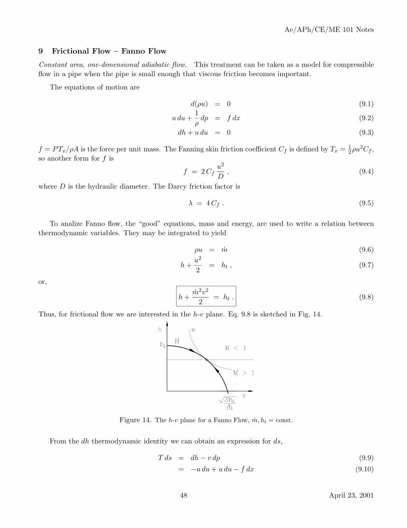
Ae/APh/CE/ME 101 Notes
9 Frictional Flow – Fanno Flow
Constant area, one-dimensional adiabatic flow. This treatment can be taken as a model for compressibleflow in a pipe when the pipe is small enough that viscous friction becomes important.
The equations of motion are
d(ρu) = 0 (9.1)
u du +1ρ
dp = f dx (9.2)
dh + u du = 0 (9.3)
f = PTx/ρA is the force per unit mass. The Fanning skin friction coefficient Cf is defined by Tx = 12ρu2Cf ,
so another form for f is
f = 2 Cfu2
D, (9.4)
where D is the hydraulic diameter. The Darcy friction factor is
λ = 4 Cf . (9.5)
To analize Fanno flow, the “good” equations, mass and energy, are used to write a relation betweenthermodynamic variables. They may be integrated to yield
ρu = m (9.6)
h +u2
2= ht , (9.7)
or,
h +m2v2
2= ht . (9.8)
Thus, for frictional flow we are interested in the h-v plane. Eq. 9.8 is sketched in Fig. 14.
Figure 14. The h-v plane for a Fanno Flow, m, ht = const.
From the dh thermodynamic identity we can obtain an expression for ds,
T ds = dh − v dp (9.9)
= −u du + u du − f dx (9.10)
48 April 23, 2001

Ae/APh/CE/ME 101 Notes
The second law says that the entropy must increase. Therefore,
ds
dx= − f
T≥ 0 . (9.11)
Thus, f < 0 . In order to satisfy the 2nd law, the traction force must act as a drag.
9.1 dh/dv and tangency
Combining the continuity and energy equation gives a relation for dh/dv, the slope of the Fanno processon the h-v plane.
du
u=
dv
v(9.12)
dh = −u2 du
u, (9.13)
so,dh
dv= −u2
v. (9.14)
Compare with (∂h
∂v
)s
=(
∂h
∂p
)s
(∂p
∂v
)s
= −a2
v. (9.15)
Thus, if an isentrope is tangent to h(v) for a Fanno flow, as indicated in Fig. 14. the flow must be sonicthere. This point is indicated by the star in Fig. 14.
9.2 Curvature of the isentropes in the h-v plane
The criterion for isentrope curvature is of course different in (h, v) than in (p, v),(∂2h
∂v2
)s
=∂
∂v
(v
∂p
∂v
)(9.16)
=(
∂p
∂v
)s
+ v
(∂2p
∂v2
)s
. (9.17)
Therefore,
v2
2a2
(∂2h
∂v2
)s
=v3
2a2
(∂2p
∂v2
)s
− 12
(9.18)
= Γ − 12
(9.19)
= β +12
. (9.20)
Thus, the isentrope shown in Fig. 14 is for Γ > 12 . A straight-line isentrope tangent at ∗ would have Γ = 1
2 .
9.3 Entropy
In order to see what direction the flow moves with positive dx on the h-v plane, we obtain a relevantexpression for the entropy and use the 2nd law. From
T ds = dh + v dp (9.21)
49 April 23, 2001

Ae/APh/CE/ME 101 Notes
and
dp =(
∂p
∂v
)s
dv +(
∂p
∂s
)v
ds (9.22)
we get [T + v
(∂p
∂s
)v
]ds = −(u2 − a2)
dv
v. (9.23)
With (∂p
∂s
)v
= −(
∂p
∂v
)s
(∂v
∂T
)v
(∂T
∂s
)p
(9.24)
=T
v
αa2
cp=
T
vG , (9.25)
where G is the Gruneisen parameter, (9.23) becomes
T ds = −u2 − a2
1 + G
dv
v(9.26)
Thus, for α > 0, in order to have ds/dx > 0 in the subsonic region dv > 0, and in the supersonic regiondv < 0. This result is indicated schematically in Fig. 14 by the arrows. Friction in a pipe flow forces theflow toward choking, either from the subsonic or the supersonic side.
50 April 23, 2001

Ae/APh/CE/ME 101 Notes
10 Flow with Heat Addition – Rayleigh Flow
Constant area, one-dimensional frictionless nonadiabatic flow.Now the equations of motion are
d(ρu) = 0 (10.1)
u du +1ρ
dp = 0 (10.2)
dh + u du = −q dx (10.3)
q = PQ/ρuA is the heat lost per unit mass per unit length of channel. The Stanton number St is definedby
St ≡ − Q
ρuh=
Aq
hP=
D
4hq , (10.4)
where, again, D is the hydraulic diameter.
The “good” equations are now mass and momentum. Integrating,
ρu = m ; u = m v (10.5)
(ρu)u + p = I , (10.6)
sop = I − m2 v . (10.7)
The Rayleigh flow executes a straight line in the p-v plane, the Rayleigh line, indicated in Fig. 15.
Figure 15. p-v plane for a Rayleigh process
10.1 Tangency
Differential relations given by continuity and momentum are
du
u= −dρ
ρ(10.8)
dp = −ρu1 du
u. (10.9)
Therefore,dp
dρ= u2 ;
dp
dv= −u2
v2(10.10)
51 April 23, 2001

Ae/APh/CE/ME 101 Notes
Compare with (∂p
∂ρ
)s
= a2 . (10.11)
Thus, again, where an isentrope is tangent to the Rayleigh line, there is a sonic point, indicated by the ∗.
10.2 Entropy
Taking s(p, v),
ds =(
∂s
∂p
)v
dp +(
∂s
∂v
)p
dv . (10.12)
With the chain rule for (∂s/∂p)v, dp/dv = −u2/v2 and (∂p/∂v)s = −a2/v2, we get
ds = −(
∂s
∂v
)p
(M2 − 1) dv . (10.13)
Now (∂s
∂v
)p
=(
∂s
∂T
)p
(∂T
∂v
)p
=cp
αvT, (10.14)
so finally
T ds =a2 − u2
G
dv
v. (10.15)
Increasing entropy causes the flow to progress in the direction on the p-v plane indicated by the arrows.That is, increasing entropy tends to choke a nonadiabtic pipe flow.
Whether the entropy is actually increasing or decreasing in the flow direction is determined by the signof the heat flow in this problem. We have
T ds = dh − v dp = −q dx (10.16)ds
dx= − q
T. (10.17)
With heat addition (q < 0), ds/dx > 0, and vice versa. As with friction, heat addition tends to choke aflow in a pipe.
10.3 The Mollier Diagram
Both Fanno flow and Rayleigh flow flow toward a maximum entropy in (h, s) space (see Fig. 16).
Figure 16. Rayleigh process on a Mollier Diagram
52 April 23, 2001

Ae/APh/CE/ME 101 Notes
However, in a Rayleigh process there may also be a maximum in enthalpy. From the energy and massequations,
dh = −u du − q dx (10.18)
= −u2 dv
v− q dx (10.19)
Substituting from Eq. 10.15,
dh = u2 αT
cp
ds
M2 − 1− q dx (10.20)
With α > 0, for large enough heat addition (q < 0), or M close enough to unity, dh > 0. At the maximum,dh/ds = 0; after a little algebra,
M2 =1
1 + a2αcp
. (10.21)
For a perfect gas, α = 1/T , so the enthalpy is maximum at
M2 =1γ
. (10.22)
53 April 23, 2001

Ae/APh/CE/ME 101 Notes
11 Detonation Waves in One Dimension
Detonation waves are driven by the release of chemical energy in a combustion process at a sharp front.They move supersonically into a combustible mixture and self ignite. As a consequence, the uspstreamsubstance is thermodynamically distinct from the combustion products downstream, so the Hugoniot doesnot pass smoothly through the initial point. The two possible cases are shown in the sketch. Note that
by Eq. 8.9 the cross-hatched portion of the Hugoniot is not possible. The equations of motion for thisdiscontinuity are Eqs. 8.52 – 8.54. Here we consider the case when the Hugoniot falls above the initialstate.
It is useful to study differential changes of the downstream state. Differentiating the momentumequation Eq. 8.9,
dp2
∆p− dv2
∆v= 2
dm
m, (11.1)
or,dm
dv=
m
2∆p
(dp2
dv2− ∆p
∆v
). (11.2)
This shows that a tangency condition may arise; namely, the Rayleigh line may be tangent to the Hugoniot,at which point the mass flux is stationary, dm = 0. This is shown on the sketch below.
54 April 23, 2001

Ae/APh/CE/ME 101 Notes
Differentiating the energy equation Eq. 8.54 and using it again to eliminate ∆h,
dh2 = v dp2 +∆p
2dv2 . (11.3)
Substituting this into the dh2 thermodynamic identity gives
T2ds2
dv2=
∆v
2
(∆p
∆v− dp2
dv2
). (11.4)
Therefore, at the same tangency the entropy is stationary, so the isentrope is also tangent there! Aconsequence of this fact is that the downstream flow is sonic relative to the wave; in the steady frame,
∆p
∆v= −u2
2
v22
;(
∂p
∂v
)s
= −a22
v22
, (11.5)
so,M2 = 1 . (11.6)
This is indicated by the ∗ on the sketch. This important state is called the Chapman-Jouget (C-J) point.
By inspecting the geometry at the point indicated by (2), it can be seen that M2 < 1 there; detonationsfalling above the ∗ are called strong detonations. Correspondingly, final states below the ∗ have supersonicdownstream states, M2 > 1, and are called weak detonations. Because of the supersonic condition theyviolate causality and are not dynamically realizable states.
Waves that expand and depressurize the flow are called deflagrations, and are not discussed here.
11.1 2-γ model of detonation waves
Perfect gas.We assume that the upstream and downstream fluids are different perfect gases, such that
h1 = cp1T1 + q ; h2 = cp2T2
p1 = ρ1R1T1 ; p2 = ρ2R2T2
cp1 =γ1
γ1 − 1R1 ; cp2 =
γ2
γ2 − 1R2 ,
(11.7)
where q is the heat of reaction. Using
h1 =γ1
γ1 − 1p1v1 + q (11.8)
h2 =γ2
γ2 − 1p2v2 (11.9)
in Eq. 8.12 in the same manner as for deriving Eq. 8.26, gives the detonation Hugoniot
p2
p1=
γ1 + 1γ1 − 1
− v2
v1+ 2γ1
q
a21
γ2 + 1γ2 − 1
v2
v1− 1
. (11.10)
Evaluating at v2/v1 = 1,p2
p1=
γ2 − 1γ1 − 1
[1 + γ1(γ1 − 1)
q
a21
](11.11)
55 April 23, 2001

Ae/APh/CE/ME 101 Notes
shows that for γ2 < γ1, which is usually the case, the Hugoniot is below the upstream state, while for q > 0,appropriate for the necessary exothermic reaction to make a detonation wave, it is above. It turns out thatwith real fuels the latter effect always dominates, i.e.,
q
a21
>γ1 − γ2
γ1(γ1 − 1)(γ2 − 1). (11.12)
11.2 Equations in the steady frame
The momentum equation Eq. 8.2 can be written
p2
(1 +
ρ2
p2u2
2
)= p1
(1 +
ρ1
p1u2
1
), (11.13)
so,p2
p1=
1 + γ1M21
1 + γ2M22
. (11.14)
The continuity equation Eq. 8.1 can be written
ρ2
p2u2 =
ρ1
p1u1
p1
p2(11.15)
γ2M22
u2=
γ1M21
u1
p1
p2, (11.16)
so,u2
u1=
v2
v1=
γ2M22
γ1M21
1 + γ1M21
1 + γ2M22
. (11.17)
The energy equation Eq. 8.3 becomes
γ2
γ1 − 1R2T2
(1 +
γ2 − 12
M22
)=
γ1
γ1 − 1R1T1
(1 +
γ1 − 12
M21
)+ q , (11.18)
so,
T2
T1=
R1
R2
γ1
γ2
γ2 − 1γ1 − 1
1 +γ1 − 1
2M2
1 + (γ1 − 1)q
a21
1 +γ2 − 1
2M2
2
(11.19)
Finally, from the thermal EOSp2
p1
v2
v1=
R2
R1
T2
T1. (11.20)
Using this to combine all the equations gives
M22
(1 +
γ2 − 12
M22
)(1 + γ2M2
2
)2 =(
γ1
γ2
)2 γ2 − 1γ1 − 1
M21
(1 +
γ1 − 12
M21 + (γ1 − 1)
q
a21
)(1 + γ1M2
1
)2 . (11.21)
This is a quadratic equation for M22 . The two real roots give the weak and strong detonation waves. A
quantitative plot of the solution for γ2 = γ1 is shown in the sketch below. The 45 line is the trivialsolution M2 = M1 and applies for q = 0. The hyperbola passing through (1,1) for q = 0 is the shock wavesolution. To the right of (1,1) in the 4th quadrant it is a compression shock (M1 > 1, M2 < 1), while to
56 April 23, 2001

Ae/APh/CE/ME 101 Notes
the left in the 2nd quadrant it is an expansion shock, impossible for these perfect gases. In the first andthird quadrants are the weak solutions, bordering on M2 = M1, and in the 2nd and 4th quadrants are thestrong solutions, bordering on the shock. In the 1st quadrant, below the 45 line q > 0 (detonation waves)and above q < 0 (refrigeration waves?), etc.
A case for γ2 < γ1 is shown in the last sketch. Note that q/a21 ' 2 gives essentially the adiabatic shock
conditions for a single-γ gas.
57 April 23, 2001

Ae/APh/CE/ME 101 Notes
12 Nonsteady Flows
12.1 One-dimensional inviscid nonheatconducting flow
Eqs. 7.18 and 7.19, withDs
Dt= 0 or
Dρ
Dt=
1a2
Dp
Dt(12.1)
(see Eq. 2.30) apply to these flows. Rewriting the continuity and momentum equations, taking the conti-nuity equation in terms of pressure,
∂p
∂t+ u
∂p
∂x+ ρa2 ∂u
∂x= 0 (12.2)
ρ∂u
∂t+ ρu
∂u
∂x+
∂p
∂x= 0 . (12.3)
Multiplying the momentum equation by a and adding and subtracting the two equations gives two moreequations, in so-called characteristic form, plus the entropy equation,[
∂
∂t+ (u ± a)
∂
∂x
]p ± ρa
[∂
∂t+ (u ± a)
∂
∂x
]u = 0 (12.4)
(∂
∂t+ u
∂
∂x
)s = 0 (12.5)
The operators in square brackets are wave operators and define curves of constant phase (α, β),
∂
∂α=
∂
∂t+ (u + a)
∂
∂x;
∂
∂x=
12a
(∂
∂α− ∂
∂β
)(12.6)
∂
∂β=
∂
∂t+ (u − a)
∂
∂x;
∂
∂t=
12a
[−(u − a)
∂
∂α+ (u + a)
∂
∂β
], (12.7)
or, with α(x, t), β(x, t) and x(α, β), t(α, β),
dα =12a
(dx − (u − a)dt) ; dx = (u + a)dα + (u − a)dβ (12.8)
dβ =12a
(−dx + (u + a)dt) ; dt = dα + dβ . (12.9)
Constant phase means
β = const alongdx
dt= u + a (12.10)
α = const alongdx
dt= u − a . (12.11)
Eqs. 12.4 and 12.5 state that
dp ± ρa du = 0 alongdx
dt= u ± a (12.12)
ds = 0 alongdx
dt= u . (12.13)
Compare Eq. 12.12 with Eq. 7.25, the momentum equation in quasi-1D steady flow. The difference betweenthe two is in the “impedance,” ρa vs. ρu. The two flows in some sense trade behavior between subsonic
58 April 23, 2001

Ae/APh/CE/ME 101 Notes
and supersonic flow. Expressed in this way, the relation between dp and du, and the geometry on whichthey occur are transparent. However, u and a are unknowns, so, though the mathematical approach togetting a solution is evident, a closed form analytical solution is not possible.
Formally integrating, ∫dp
ρa± u = P
Qalong
dx
dt= u ± a . (12.14)
P and Q are the Riemann invariants.
12.2 Homentropic flow
If the entropy is the same everywhere,s = s0 , (12.15)
then the number of variables is reduced by one, and we can write
dp
ρa=
(∂p
∂a
)s
da
ρa. (12.16)
With Eq. 6.48, Eq. 12.14 becomes∫da
Γ(a) − 1± u = P
Qalong
dx
dt= u ± a (12.17)
There are now 2 unknowns (u, a) and 2 equations.
Uniform Flow. In uniform flow the characteristics are straight, dx/dt = u ± a = const.
12.3 Simple waves
A nonuniform flow bordered on one side in (x, t) space by a uniform flow is a “simple wave.” Fig. 17shows a simple wave bordered on the left by a uniform flow, a “left-facing simple wave.” The simplifying
Figure 17. A nonsteady wave flow with unifom conditions on its left
thing here is that all of the P characteristics carry the same value of the P Riemann invariant, say, P0.Thus, ∫
da
Γ(a) − 1+ u = P0 everywhere (12.18)∫
da
Γ(a) − 1− u = Q along
dx
dt= u − a . (12.19)
59 April 23, 2001

Ae/APh/CE/ME 101 Notes
Therefore, ∫da
Γ(a) − 1=
P0 + Q
2
u =P0 − Q
2
alongdx
dt= u − a , (12.20)
which proves that
u, a = const alongdx
dt= u − a , (12.21)
in turn showing that the Q characteristics are straight lines, as shown in Fig. 17.
We have, then, that
du = ∓ da
Γ − 1; left
right facing wave (12.22)
dx
dt= u ∓ a ; Q
Pstraight characteristic (12.23)
d
(dx
dt
)= du ∓ da
= ∓ ΓΓ − 1
da
; QP
straight characteristic , (12.24)
the last expression indicating how the slope of the straight set of characteristics changes from the headto the tail of the wave. Using these relations, we can build up Table 1 to describe the behavior of allthe different cases: Cases 1 and 2 are representative of the behavior of perfect gases. In cases 3 and 4,even though the fluid is “normal,” the sound speed varies oppositely to what we are used to in fluidswith positive β; it increases in expansion waves and decreases in compression waves. Cases 2 and 3 givecompression shocks after a certain propagation distance and case 6 gives expansion shocks because of theconvergence of the characteristics.
12.4 Perfect gas
In a perfect gas Γ = (γ + 1)/2, so Eq. 12.17 can be integrated to give
a ± γ − 12
u = PQ
alongdx
dt= u ± a (12.25)
12.4.1 Simple Waves
For leftright waves propagating into a fluid at rest (u1 = 0),
a ± γ − 12
u = a1 ;1a1
dx
dt= ∓1 +
γ + 12
u
a1(12.26)
a
a1= 1 ∓ γ − 1
2u
a1=
11 ± γ−1
2 M(12.27)
T
T1=
(1 ∓ γ − 1
2u
a1
)2
=1(
1 ± γ−12 M
)2 (12.28)
60 April 23, 2001

Ae/APh/CE/ME 101 Notes
Table 1. Twelve cases for continuous nonsteady flow
dadpdρ
du d
(dx
dt
)
1. Γ > 1β > 0 < 0 < 0 (expansion) > 0
< 0> 0< 0
2. > 0 > 0 (compression) < 0> 0
< 0> 0
3. 0 < Γ < 1β < 0 < 0 > 0 (compression) < 0
> 0< 0> 0
4. > 0 < 0 (expansion) > 0< 0
> 0< 0
5. Γ < 0β < 0 < 0 > 0 (compression) < 0
> 0> 0< 0
6. > 0 < 0 (expansion) > 0< 0
< 0> 0
ρ
ρ1=
(1 ∓ γ − 1
2u
a1
) 2γ−1
=1(
1 ± γ−12 M
) 2γ−1
(12.29)
p
p1=
(1 ∓ γ − 1
2u
a1
) 2γγ−1
=1(
1 ± γ−12 M
) 2γγ−1
(12.30)
12.4.2 Centered Waves
Impulsive expansion of a fluid, e.g. by the impulsive acceleration of a piston, produces a centered wave,as in the Fig. 18. It is possible for compression waves to be centered, also. In the former case, thediscontinuity in flow properties at t = 0 immediately disintegrates and the flow becomes continuous. Theflow shown in Fig. 18 is a centered left-facing simple wave with straight Q characteristics. In centeredwaves the flow properties have a simple “conical” dependence on space and time (x, t). The equation for
61 April 23, 2001

Ae/APh/CE/ME 101 Notes
Figure 18. A left-facing centered wave
the Q characteristics isx
a1t=
u − a
a1
=2
γ − 1
(1 − γ + 1
2a
a1
)=
1 − M
1 ± γ−12 M
,
(12.31)
or,a
a1=
2γ + 1
(1 − γ − 1
2x
a1t
). (12.32)
Centered waves have the interesting property that, if the flow has a vertical characteristic through theorigin, then the flow is sonic there, u = a, a = 2/(γ + 1)a1. Thus, the time axis in a centered nonsteadywave plays the role of the throat in a quasi-1D steady flow. However because of the difference in theimpedances (see above) the flow behavior is different. For example,
Nonsteady Steady
T1
T=
(1 +
γ − 12
M
)2 Tt
T= 1 +
γ − 12
M2 .
(12.33)
In fact, since the total temperature is defined for every flow, including these nonsteady flows, we cancombine the two Eqs. 12.33 and compare the local total temperature Tt with the “reservoir temperature”T1,
Tt
T1=
1 + γ−12 M2(
1 + γ−12 M
)2 . (12.34)
This function is plotted vs. the local Mach number M in Fig. 19. For large enough M , Tt can besubstantially greater than the reservoir temperature, a useful feature of nonsteady flow resulting fromnonsteady pressure work (see Eq. 7.20).
62 April 23, 2001

Ae/APh/CE/ME 101 Notes
Figure 19. Total temperature in nonsteady flow
12.4.3 Complete expansion
If the piston recedes fast enough, the flow thermal energy can be converted entirely to kinetic energy,when a, ρ, p = 0. Then,
Nonsteady Steady
ue
a1=
2γ − 1
um
at=
√2
γ − 1.
(12.35)
ue is known as the escape velocity. The steady result shown above is Eq. 7.65, an analogous result from thesame conversion of thermal energy to kinetic energy. However, owing to the effects of nonsteady pressurework, it is not as large as for nonsteady flow.
12.5 Wave interactions – The shock-tube equation
The shock jump conditions, in particular Eq. 8.29 and Eq. 8.30, can be plotted together with thecorresponding relation for expansion waves, Eq. 12.30, in a form useful for the graphical solution of waveinteraction problems (see Fig. 20).
For example, the solution of the classic problem of gasdynamics called the shock tube problem, is shownin Fig. 21. At time t = 0 a partition dividing a high-pressure region (4, the driver) from a low pressurechamber (1, the driven section) is instantaneously removed, generating a shock wave moving to the rightand an expansion (rarefaction) wave moving to the left. The moving boundary (dashed line) between theshock-processed fluid and the expanded fluid is called a “contact surface,” and it supports no waves. Thus,p3 = p2 and u3 = u2. The solution to this problem is shown graphically in Fig. 22. The pressure betweenthe two waves is intermediate between the initial high and low pressures. The gas between is moving tothe right.
63 April 23, 2001

Ae/APh/CE/ME 101 Notes
Figure 20. ∆p/p1 vs. ∆u/a1 for shocks (∆p/p1 > 0) and for expansion waves (∆p/p1 < 0).
Figure 21. The shock-tube problem
We obtain an analytical expression for the solution as follows. Expanding the pressure ratio p4/p1,
p4
p1=
p4
p3
p3
p2
p2
p1, (12.36)
and substituting Eq. 12.30 for p3/p4, Eq. 8.29 for p2/p1, with p3 = p2 and u3 = u2, and then substitutingEq. 8.30 for u2/a1, gives
p4
p1=
1 +2γ1
γ1 + 1(M2
s − 1)(1 − γ4 − 1
γ1 + 1a1
a4
M2s − 1Ms
) 2γ4γ4−1
(12.37)
The γ’s have been subscripted to allow for the fact that different gases may initially occupy the driverand driven regions. This result shows that even with an infinite pressure ratio p4/p1 only a finite strengthshock will be generated, owing to the finite escape velocity when the driver gas has been expanded to zero
64 April 23, 2001
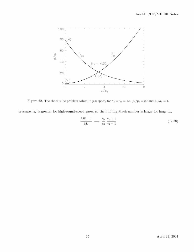
Ae/APh/CE/ME 101 Notes
Figure 22. The shock tube problem solved in p-u space, for γ1 = γ4 = 1.4, p4/p1 = 80 and a4/a1 = 4.
pressure. ue is greater for high-sound-speed gases, so the limiting Mach number is larger for large a4,
M2s − 1Ms
−→ a4
a1
γ1 + 1γ4 − 1
(12.38)
65 April 23, 2001
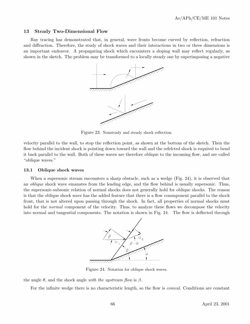
Ae/APh/CE/ME 101 Notes
13 Steady Two-Dimensional Flow
Ray tracing has demonstrated that, in general, wave fronts become curved by reflection, refractionand diffraction. Therefore, the study of shock waves and their interactions in two or three dimensions isan important endeavor. A propagating shock which encounters a sloping wall may reflect regularly, asshown in the sketch. The problem may be transformed to a locally steady one by superimposing a negative
Figure 23. Nonsteady and steady shock reflection.
velocity parallel to the wall, to stop the reflection point, as shown at the bottom of the sketch. Then theflow behind the incident shock is pointing down toward the wall and the refelcted shock is required to bendit back parallel to the wall. Both of these waves are therefore oblique to the incoming flow, and are called“oblique waves.”
13.1 Oblique shock waves
When a supersonic stream encounters a sharp obstacle, such as a wedge (Fig. 24), it is observed thatan oblique shock wave emanates from the leading edge, and the flow behind is usually supersonic. Thus,the supersonic-subsonic relation of normal shocks does not generally hold for oblique shocks. The reasonis that the oblique shock wave has the added feature that there is a flow commponent parallel to the shockfront, that is not altered upon passing through the shock. In fact, all properties of normal shocks musthold for the normal component of the velocity. Thus, to analyze these flows we decompose the velocityinto normal and tangential components. The notation is shown in Fig. 24. The flow is deflected through
Figure 24. Notation for oblique shock waves.
the angle θ, and the shock angle with the upstream flow is β.
For the infinite wedge there is no characteristic length, so the flow is conical. Conditions are constant
66 April 23, 2001

Ae/APh/CE/ME 101 Notes
along radii centered at the tip of the cone.
The preservation of the parallel flow component is expressed by
u1 cos β = u2 cos(β − θ) . (13.1)
The continuity, momentum and energy equations are Eqs. 8.1–8.3 applied to the normal component of thevelocities,
ρ1u1 sinβ = ρ2u2 sin(β − θ) (13.2)
p2 − p1 = ρ1u21 sin2 β − ρ2u
22 sin2(β − θ) (13.3)
h2 − h1 =u2
1 sin2 β
2− u2
2 sin2(β − θ)2
(13.4)
Because the equations are fundamentally the same, we can pass immediately to the perfect gas case,Eqs. 8.29, 8.31 and 8.32. Substituting the correct form for the normal component gives
p2
p1= 1 +
2γ
γ + 1(M2
1 sin2 β − 1)
ρ2
ρ1=
M21 sin2 β
1 + γ−1γ+1(M2
1 sin2 β − 1)
h2
h1= 1 +
2(γ − 1)(γ + 1)2
(M21 sin2 β − 1)(1 + γM2
1 sin2 β)M2
1 sin2 β.
(13.5)
These equations determine the unknowns p2, ρ2 and h2 in terms of the unknown β and the knowns θ, p1,ρ1 and h1. An equation for M2 is given by Eq. 13.2,
M22 sin2(β − θ) =
M21 sin2 βρ2
ρ1
p2
p1
, (13.6)
so that,
M22 sin2(β − θ) =
1 + γ−1γ+1(M2
1 sin2 β − 1)
1 + 2γγ+1 (M2
1 sin2 β − 1). (13.7)
Finally, Eq. 13.1 can be used to determine β. Dividing it into (13.2),
ρ1 tanβ = ρ2 tan(β − θ) (13.8)
and expanding the tangent of the difference between two angles gives
tan θ =1
tanβ
M21 sin2 β − 1
γ+12 M2
1 − (M21 sin2 β − 1)
. (13.9)
Eq. 13.9 shows that θ can be 0 if β = sin−1 1M1
≡ µ, the Mach angle, or β = π2 . In the latter case sin β = 1,
and all the above equations reduce to those for normal shocks (Sec. 8). θ carries the sign of β, which canbe either positive (for shocks of the + family) or negative (− family).
Fig. 25 shows the “shock polar”, p2/p1 vs. θ (the first of Eqs. 13.5 with 13.9) for several differentupstream Mach numbers M1. For given wedge angle θ there are two solutions, known as the weak
67 April 23, 2001

Ae/APh/CE/ME 101 Notes
Figure 25. The shock polar, shown for several different upstream Mach numbers M1. ∗, sonic condition.
solution and the strong solution. The asterisks mark the “sonic condition,” below which the downstreamflow is supersonic (the weak solution) and above which it is subsonic (the strong solution). Thus, forθ = 0 there is either no disturbance or a normal shock wave. There is a maximum θ, beyond which thereis no solution at all for each upstream Mach number. This is the “maximum deflection angle” or the“detachment angle,” beyond which the shock detaches from the wedge. The sonic condition happens tooccur very close to the maximum deflection angle, but not precisely at it.
When the wedge angle increases beyond the maximum deflection angle, the body becomes a bluff body,and experiments show that the fact that the body must really be of finite transverse size controls the flow.That is, there is a characteristic length, the body diameter D. The shock jumps out to a distance of orderD ahead of the body, and is normal on the axis of symmetry, the stagnation streamline, as is shown in thesketches of Fig. 26. The figure shows a compilation of shock standoff distance for several different bodyshapes (Liepmann & Roshko 1957). The standoff distance gets very large as the upstream Mach numberM1 → 1.
13.2 Weak shocks
For small θ and ∆p = p2 − p1, M21 sin2 β − 1 ¿ 1, and the shocks are weak, though the Mach number
itself might be large. Then,
sinβ =1
M1(13.10)
tanβ =1√
M21 − 1
, (13.11)
68 April 23, 2001

Ae/APh/CE/ME 101 Notes
Figure 26. Experimental measurements of shock stand off for several different body shapes, as compiled by Liepmann& Roshko (1957).
so,
θ =√
M21 − 1
2γ + 1
M21 sin2 β − 1
M21
(13.12)
∆p
p=
2γ
γ + 1(M2
1 sin2 β − 1) . (13.13)
Thus,∆p
p=
γM21√
M21 − 1
θ (13.14)
This function of M1 is large for both small and large M1, and is minimum for M1 =√
2, independent ofγ. This behavior explains why the shock polars in the above sketch first expand and then get thinner asM − 1 increases.
Another important weak shock relation is obtained from Eq. 13.1; expanding the cosine of the differenceof two angles, and using the above approximation for tanβ gives
∆u
u1= − θ√
M21 − 1
. (13.15)
69 April 23, 2001

Ae/APh/CE/ME 101 Notes
The change of Mach number can be obtained by multiplying the approximate velocity ratio by the soundspeed ratio, and substituting for the latter,
M2
M1=
a1
a2
(1 − θ√
M21 − 1
)(13.16)
a2
a1= 1 +
γ − 12
M21√
M21 − 1
θ , (13.17)
with the result∆M
M1= −
(1 +
γ − 12
M21
)θ√
M21 − 1
. (13.18)
13.3 Continuous flows – Prandtl-Meyer expansion
The weak-shock relations can be generalized to describe local changes in continuous 2-dimensionalisentropic flow. In particular, for a continuous process Eq. 13.18 can be written
dθ = −√
M2 − 11 + γ−1
2 M2
dM
M, (13.19)
and integrated to give−θ + const = ν(M) , (13.20)
where
ν(M) =√
γ + 1γ − 1
tan−1
√γ − 1γ + 1
(M2 − 1) − tan−1√
M2 − 1 (13.21)
is the Prandtl-Meyer function, shown in Fig. 27 It gives the Mach number change with the flow deflection
Figure 27. The Prandtl-Meyer Function ν(M).
angle. The thermodynamic variables follow from Eqs. 7.58–7.62. As with shock waves, the Mach numberdecreases with either increasing or decreasing θ, depending on which family of waves is present. Similarlyfor expansions. (See below.)
70 April 23, 2001

Ae/APh/CE/ME 101 Notes
Note that ν(1) = 0 and ν(∞) = π2
(√γ+1γ−1 − 1
); the maximum turning angle results from expanding
from M = 1 to M = ∞, and is predicted to be greater than 180 for γ < 5/4!
In the (p, θ) plane, Prandtl-Meyer expansion waves (∆p/p0 < 0) join smoothly with the shock polar,as shown in Fig. 28. The compressive branch (∆p/p0 > 0) falls nearly on the shock polar, for weak
Figure 28. Comparison of compression (∆p/p0 > 0) and expansion (∆p/p0 < 0) Prandtl-Meyer flows with the shockpolar for one upstream Mach number.
shocks. The Prandtl-Meyer curve with positive slope represents the positive family of waves, and the onewith negative slope the negative. Compression members of the positive family increase the flow defelctionangle, while the opposite is true of the opposite family.
13.4 The hodograph
Useful geometrical insight can be obtained by examining solutions in the hodograph plane (ux, uy).
Oblique shocks. The sketch below shows the shock polar for oblique waves. The tigonometry of the similar
triangles establishes the following relations,
u‖u1⊥
=u2y
u1 − u2x(13.22)
71 April 23, 2001

Ae/APh/CE/ME 101 Notes
u‖u1
=u2y
u1⊥ − u2⊥(13.23)
u21 = u2
1⊥ + u2‖ (13.24)
u22 = u2
2⊥ + u2‖ . (13.25)
The Prandtl relation, Eq. 8.51, was derived using the energy equation, and so doesn’t transform triviallyto the oblique flow. The energy equations Eq. 8.48 now becomes
u21⊥ +
2γ − 1
a21 = u2
2⊥ +2
γ − 1a2
2 =γ + 1γ − 1
a∗2 − u2‖ , (13.26)
with the consequence that, after incorporating the momentum equation, the Prandtl relation becomes
u1⊥ u2⊥ = a∗2 − γ − 1γ + 1
u2‖ . (13.27)
It is convenient to normalize all velocities with a∗, M∗ ≡ u/a∗, because, for example, when M → ∞,M∗ is finite,
M∗2 =M2
1 + γ−1γ+1(M2 − 1)
. (13.28)
Eliminating the perpendicular and parallel velocities from the Prandtl relation using Eqs. 13.22–13.25 givesthe shock polar in the hodograph plane,
M∗22y =
(M∗1 − u2x)2 (M∗
1 M∗2x − 1)
2γ+1 M∗2
1 − (M∗1 M∗
2x − 1). (13.29)
This result is the epicycloid curve plotted in the sketch above (for M∗1 = 2).
Prandtl-Meyer function. Written in terms of M∗, the Prandtl-Meyer function, Eq. 13.21 becomes
ν(M∗) =√
γ + 1γ − 1
tan−1
√M∗2 − 1
γ+1γ−1 − M∗2 − tan−1
√γ + 1γ − 1
√M∗2 − 1
γ+1γ−1 − M∗2 (13.30)
This function plots onto the hodograph as shown below. M∗ continuously increases from M∗ = 1 to
M → ∞ at νmax, which depends on γ. The above sketch is for γ = 1.4 and the sketch below shows thestrophoid for several values of γ. It shows turning angles greater than 180 for small γ. For flows withM1 > 1, the strophoid is rotated so that the initial M∗ coincides with the initial θ, and changes from theinitial state are then followed in the direction appropriate for compressions or expansions.
72 April 23, 2001

Ae/APh/CE/ME 101 Notes
13.5 Wave interactions
With the tools developed in this section, arbitrarily complex wave interactions can be solved. First,we treat the simplest reflection problem, the reflection of an incident oblique shock from a plane wall.Fig. 29 illustrates a quantitative case in which the upstream Mach number is M1 = 5, and θ is measuredrelative to the upstream flow direction. The lowest polar shows the incident shock, and the point
Figure 29. p-θ diagram and quantitative sketch of a regular reflection. θ1 = 17.84. β2 = 27.38. β3 = −33.88.
∆p/p1 = 5.0, θ = 17.84 depicts the downstream state, from which the reflected shock polar begins. Twosolution points are marked by the pluses. The one of interest here is the left one where the flow deflectionangle is 0.
Often the reflection is such that the point of maximum flow deflection falls to the right of the θ = 0axis, as in Fig. 30. In this case there is no solution with θ = 0. Experiments show that, in fact, Machreflection occurs, such that the solution indicated by the + is realized locally, in a configuration indicatedin the sketch on the right. The p-θ curve originationg at conditions ©1 gives the two waves 1–2 and 1–3,
73 April 23, 2001

Ae/APh/CE/ME 101 Notes
Figure 30. p-θ diagram and quantitative sketch of a Mach reflection. θ1 = 14.12. β2 = 44.18. θ2 = 3.07.β3 = −71.8. β4 = −81.1.
and the one originating at condition ©2 gives 1–4.
13.6 Natural Coordinates
We now make a slight diversion in order to simplify the general treatment of supersonic flow in twodimensions. We rederive the equations of motion in terms of motions down streamtubes, the “natural”coordinate system of Crocco. Fig. 31 shows the geometry. s is in the streamwise direction, n is normal to s.
Figure 31. Definition of the natural coordinate system
We use the notation ∆n and ∆s temporarily, and, later, pass to the limit where they become differentials.
74 April 23, 2001

Ae/APh/CE/ME 101 Notes
From the geometry of the figure (viz. dashed lines)
tan∂θ
∂n∆n
.=∂θ
∂n∆n =
∂∆n
∂s(13.31)
tan∂θ
∂s∆s
.=∂θ
∂s∆s =
∂∆s
∂n. (13.32)
By definition, since the volume is infinitesimal, the equations of quasi-onedimensional flow apply exactly.However, they must be improved to account for the fact that fluid tends to slosh outward on a curve, i.e.,they must be augmented for transverse curvature effects.
The continuity equation isρ u ∆n = const , (13.33)
which, differentiated logarithmically becomes
1ρ
∂ρ
∂s+
1u
∂u
∂s+
1∆n
∂∆n
∂s= 0 . (13.34)
Using Eq. 13.31,1ρ
∂ρ
∂s+
1u
∂u
∂s+
∂θ
∂n= 0 . (13.35)
The s-momentum equation is
ρu∂u
∂s+
∂p
∂s= 0 . (13.36)
The new equation required is derived from the fact that the infinitesimal volume of Fig. 31 is notan inertial system, but is rotating. There are no velocities in the transverse direction, so the normalmomentum equation is simply a hydrostatic force balance between a pressure gradient and a “body force”resulting from the centripetal acceleration Ω2R, where R = ∆s
∆θ is the radius of curvature. Here,
Ω =∆θ
∆t= u
∆θ
∆s−→ u
∂θ
∂s. (13.37)
The last equality is obtained by expressing ∆θ and ∆s as differentials. With reference to Eq. 2.16, then-momentum equation is
−ρΩ2R − ∂p
∂n= 0 , (13.38)
or,
ρu2 ∂θ
∂s+
∂p
∂n= 0 . (13.39)
The energy equation will give a useful condition for ensuring isentropic flow. We begin by making theminimum assumption, namely, adiabatic flow.
h +u2
2= ht(n) ; dh = dht − u du . (13.40)
75 April 23, 2001

Ae/APh/CE/ME 101 Notes
The total enthalpy can vary normal to the streamlines because of upstream conditions. The followingthermodynamic identity gives
T dS = dh − 1ρ
dp (13.41)
= dht −(
u du +1ρ
dp
). (13.42)
Decomposed into the two directions s and n, it gives,
T∂S
∂s= 0 (13.43)
T∂S
∂n= −u
(∂u
∂n− u
∂θ
∂s
)+
dht
dn, (13.44)
where in each equation the corresponding momentum equation has been used to eliminate p. This can beput in terms of vorticity ω. The vorticity can be written down from its definition, or it can be derivedfrom Kelvin’s Theorem. The circulation Γ is defined as
Γ ≡∮
u · d` =∫
Sω · dS , (13.45)
where the last equality follows from Stokes Theorem. Now, the circulation around the infinitesimal volumeof Fig. 31 has contributions from only the bottom and top legs,
Γ = u ∆s − (u +∂u
∂n∆n)(∆s +
∂∆s
∂n∆n)
=(
u∂θ
∂s− ∂u
∂n
)∆s∆n ,
(13.46)
where Eq. 13.32 has been used. Thus
ω = u∂θ
∂s− ∂u
∂n, (13.47)
so the energy equation is
T∂S
∂n= uω +
dht
dn. (13.48)
This is the inviscid 2D form of Crocco’s theorem, Eq. 3.22.
13.7 The Equations in Characteristic Form
Homentropic flow, which we consider from here on, is obtained by the assumptions ω = 0 and ht =const. The equations can be put in characteristic form in the same way as with nonsteady flow; multiplyEq. 13.35 by a2 = dp/dρ, eliminate dρ in favor of dp. However, here we prefer to write equations for (u, θ),so we eliminate p by subtracting Eq. 13.36 to obtain
(M2 − 1)1u
∂u
∂s− ∂θ
∂n= 0
∂u
∂n− u
∂θ
∂s= 0 .
(13.49)
The last equation is the irrotationality condition, ω = 0.
76 April 23, 2001

Ae/APh/CE/ME 101 Notes
These equations can be simplified by replacing u by ν(M) from Eq. 13.15,
dθ ≡ −dν(M) = −√
M2 − 1du
u(13.50)
ordν = cot µ
du
u. (13.51)
Substituting into the above equations gives
∂ν
∂s− tanµ
∂θ
∂n= 0 (13.52)
tanµ∂ν
∂n− ∂θ
∂s= 0 . (13.53)
Now they can be put directly into charcteristic form by adding and subtracting,
∂
∂s(ν ∓ θ) ± tanµ
∂
∂n(ν ∓ θ) = 0 , (13.54)
or, in words,
θ ∓ ν = PQ along
dn
ds= ± tanµ . (13.55)
13.7.1 The Method of Characteristics
These equations form the basis for numerical calculations by the method of characteristics. It can easilybe extended to non-homentropic (but isentropic) flows, with some additional computational complexity.For this purpose, the equations can at this stage be transformed from natural coordinates back into (x, y)almost trivially, simply by inspection of Fig. 31,
θ ∓ ν = PQ along
dy
dx= tan(θ ± µ) . (13.56)
77 April 23, 2001

Ae/APh/CE/ME 101 Notes
14 Acoustics
Acoustics is the small-amplitude approximation to gas-dynamics. Because entropy changes are thirdorder in shock strength, acoustic fields are isentropic.
14.1 Plane Waves I
Uni-directional propagation. One-way propagation (say, in the x-direction) can be derived from the shockrelation Eq. 8.7 by approximating the changes as differentials,
dp = ρa du , (14.1)
where ρ and a are the values for the undisturbed ambient medium. This is of course the Riemann invariantfor an infinitesimal right-facing wave.
Bidirectional propagation. The equation for general one-dimensional acoustic fields can be derived bylinearizing Eq. 12.4 with the substitution
p = p0 + p′ (14.2)
ρ = ρ0 + ρ′ (14.3)
a = a0 + a′ (14.4)
u = u′ . (14.5)
( )0 refers to the ambient medium. Dropping all but the first-order terms gives
∂p
∂t+ a0
∂p
∂x+ ρ0a0
(∂u
∂t+ a0
∂u
∂x
)= 0 (14.6)
∂p
∂t− a0
∂p
∂x− ρ0a0
(∂u
∂t− a0
∂u
∂x
)= 0 , (14.7)
where the primes have been dropped from the perturbation quantities. Adding and subtracting the twoequations recovers the original forms of the continuity and momentum equations,
∂p
∂t+ ρ0a
20
∂u
∂x= 0 (14.8)
∂p
∂x+ ρ0
∂u
∂t= 0 . (14.9)
Differentiating the first with respect to t, multiplying the second by a20 and differentiating with respect to
x, and subtracting from the first gives the wave equation
∂2p
∂t2− a2
0
∂2p
∂x2= 0 . (14.10)
Factoring the operators exhibits again the bi-directional structure of the equation,(∂
∂t+ a0
∂
∂x
) (∂
∂t− a0
∂
∂x
)p = 0 , (14.11)
the solution to which isp = f(x − a0t) + g(x + a0t) . (14.12)
In a uniform medium (a0 = const) acoustic waves propagate along straight lines dx/dt = ±a0 in (x, t).
78 April 23, 2001
Ae/APh/CE/ME 101 Notes
14.2 Acoustics in multi dimensions
The wave equation for multi-dimensional flow follows by applying the same procedure to Eqs. 2.13-2.17.The linearized continuity equation is
∂ρ′
∂t+ ρ0 ∇ · u′ = 0 , (14.13)
Substituting
a20 =
(∂p
∂ρ
)s0
(14.14)
to eliminate dρ gives∂p
∂t+ ρ0a
20 ∇ · u = 0 , (14.15)
where now the primes have been dropped. The linearized momentum equation is
ρ0∂u
∂t+ ∇p = 0 . (14.16)
Dividing Eq. 14.15 by a20, differentiating it with respect to time and subtracting ∇· times Eq. 14.16 gives
∂2p
∂t2− a2
0 ∇2p = 0 , (14.17)
the multi-dimensional version of Eq. 14.10.
Likewise, a wave equation can be derived for u. In fact, defining a velocity potential
u = ∇φ , (14.18)
the momentum equation, Eq. 14.16, becomes
∇(
ρ0∂φ
∂t+ p
)= 0 , (14.19)
which is solved by
p = −ρ0∂φ
∂t, (14.20)
where the arbitrary time function from the integration has been absorbed into φ because it doesn’t changeu = ∇φ. Conveniently, φ gives both the acoustic pressure and the acoustic velocity. Substituting Eqs. 14.18and 14.20 into Eq. 14.15 results directly in a wave equation for φ,
∂2φ
∂t2− a2
0 ∇2φ = 0 , (14.21)
Energy. To linearize Eq. 2.17 express e(s, v) and Taylor expand the perturbation,
e′ = e − e0 =(
∂e
∂v
)s0
v′ +12
(∂2e
∂v2
)s0
v′2 + · · · . (14.22)
Using Eqs. 6.4, 6.41 and
v′ =(
∂p
∂v
)s
p′ , (14.23)
79 April 23, 2001

Ae/APh/CE/ME 101 Notes
gives
e +u2
2= e0 + e′ +
u′2
2= e0 − p0v
′ +12
p′2
ρ20a
20
+u′2
2. (14.24)
With linearization, the convective derivative becomes simply the time derivative. The first term on theright of Eq. 2.17 (all the rest are zero in this inviscid theory) linearizes to p0∇ · u′ +∇ · p′u′, so the energyequation is
−p0ρ0∂v′
∂t+ ρ0
∂
∂t
(12
p′2
ρ20a
20
+u′2
2
)+ p0∇ · u′ + ∇ · p′u′ = 0 . (14.25)
Eq. 14.13 can be written
− 1v0
∂v′
∂t+ ∇ · u′ = 0 , (14.26)
so, combining with (14.25),
ρ0∂
∂t
(12
p2
ρ20a
20
+u2
2
)+ ∇ · pu = 0 , (14.27)
where now the primes have been dropped.
In a left- or right-facing wave,p = ±ρ0a0 u , (14.28)
so12
p2
ρ20a
20
=12
pu
ρ0a0=
u2
2. (14.29)
That is, the acoustic energy is equi-partitioned between potential and kinetic energy. Eq. 14.27 can thenbe written
1a0
∂pu
∂t+ ∇ · pu = 0 , (14.30)
which is an equation in conservative form,
∂
∂tdensity = ∇ · flux . (14.31)
We have,
E ≡ energy density =pu
a0
F ≡ energy flux = pu = a0 Eu
u
(14.32)
The last equality shows that acoustic energy in this non-dispersive medium is carried with the sound speeda0.
14.3 Plane waves II
For plane-waves the solution to Eq. 14.21 is
φ = f
(t − x · n
a0
)+ g
(t +
x · na0
), (14.33)
wheren =
u
u(14.34)
80 April 23, 2001

Ae/APh/CE/ME 101 Notes
is the unit vector in the direction of propagation. Thus
u = ∇φ = − 1a0
(f ′ − g′)n
p = −ρ0∂φ
∂t= −ρ0(f ′ + g′) ,
(14.35)
where here the primes denote differentiation with respect to the argument.
Harmonic plane waves. The velocity potential for harmonic plane waves is conventionally taken to be
φ = fnc(x) e−iωt . (14.36)
Then the solution, (14.33), becomes
φ =(Aeik·x + Be−ik·x
)e−iωt
= A ei(k·x−ωt) + B e−i(k·x+ωt) ,
(14.37)
where the wave vector k isk =
ω
a0n . (14.38)
Thus,
p = −ρ0∂φ
∂t= ρ0 iω
(Aeik·x + Be−ik·x
)e−iωt
u = ∇φ = ik(Aeik·x − Be−ik·x
)e−iωt .
(14.39)
As with any plane-wave field, this solution can be rewritten to show that it is a summation of a standingwave and a travelling wave, either left-facing or right-facing,
φ = 2A cos(k · x) e−iωt − (A − B) e−i(k·x+ωt) (14.40)
= 2B cos(k · x) e−iωt + (A − B) ei(k·x−ωt) (14.41)
When A = B, it is a pure standing wave.
Energy. The magnitude of the energy flux for progressive harmonic waves, say, B = 0, is
F = pu = ρ0a0 u2 = ρ0a0 k2 A2 =ρ0
a0ω2 A2 , (14.42)
where the last two equalities follow from Eq. 14.39. It follows from Eq. 14.32 that the energy density is
E =ρ0
a20
ω2 A2 . (14.43)
Measures of sound amplitude – Decibels. The sound pressure level is defined as
SPL = 20 log10
|p|2 × 10⁻⁵ Pa
, (14.44)
where the units of SPL are called deciBels (dB). Roughly speaking, 0 dB is the limit of human hearing.The particle velocity in air induced by the least audible sound (2 × 10⁻⁵ Pa) is about 4 × 10⁻⁸ m/s, andthe energy flux is approximately 10−12 w/m2. An increase of SPL by 100 dB implies an increase of rmspressure by a factor of 105, so SPL = 100 dB is p = 2 Pa, and SPL = 200 dB is p = 2 × 10⁵ Pa = 2 bar!
81 April 23, 2001

Ae/APh/CE/ME 101 Notes
14.4 Refraction
The refraction of plane waves φ = f(t − n·xa ) at a discontinuous interface is easy to work out, and
applies locally to curved waves incident on curved interfaces, so long as the interface can be taken to bediscontinuous. We take the wave incident from above (y > 0) onto an interface aligned with the x axis.The notation is defined in Fig. 32. The arrows are the normals to the phase fronts and are called rays. The
Figure 32. Refraction of plane waves.
potential function of the field in region ©1 is the superposition of the incident and reflected waves, whilein region ©2 it is just the reflected wave,
φ1 = φi + φr (14.45)
φ2 = φt , (14.46)
The boundary conditions are that the pressure and vertical component of the velocity be continuous acrossthe interface, and that the phases of φi,r,t all be equal. The phase η is
η = t − nxx + nyy
a(14.47)
= t − x sin θ ± y cos θ
a, (14.48)
where the sign expresses whether the wave is propagating in the positive or negative y direction. Thus,the phase condition at the interface is
t − x sin θi
a1= t − x sin θr
a1= t − x sin θt
a2, (14.49)
which give the familiar results
θi = θr
sin θt
a2=
sin θi
a1.
(14.50)
The last equation is Snell’s Law. Total reflection occurs when θt = π/2, i.e., when
sin θi =a1
a2< 1 ; Total reflection (14.51)
82 April 23, 2001

Ae/APh/CE/ME 101 Notes
That is, total reflection can only occur in fast-slow refraction. The velocity vtr along the interface of theintersection of a phase front with the interface is known as the trace velocity,
vtr =a1
sin θi> a1
=a2
sin θt.
(14.52)
For real wave propagation the trace velocity must be supersonic. For total reflection vtr becomes just sonicrelative to region ©2 ,
vtr = a2 ; Total reflection , (14.53)
so wave propagation does not occur below the interface.
The wave amplitudes are determined by the dynamical boundary conditions at the interface,
u2y = u1y
∂φ2
∂y=
∂φ1
∂y
φ′t
cos θt
a2= φ′
i
cos θi
a1− φ′
r
cos θr
a1
p2 = p2
ρ2∂φ2
∂t= ρ1
∂φ1
∂t
ρ2φ′t = ρ1(φ′
i + φ′r) ,
(14.54)
where the primes denote differentiation with respect to the argument. The last two equations determineφ′
r/φ′i and φ′
t/φ′i,
φ′r
φ′i
=2ρ1a2 cos θi
ρ2a2 cos θi + ρ1a1 cos θt(14.55)
φ′t
φ′i
=ρ2a2 cos θi − ρ1a1 cos θt
ρ2a2 cos θi + ρ1a1 cos θt. (14.56)
The pressures and velocities are
pr
pi=
ρ2a2 cos θi − ρ1a1 cos θt
ρ2a2 cos θi + ρ1a1 cos θt; (14.57)
pt
pi=
2ρ2a2 cos θi
ρ2a2 cos θi + ρ1a1 cos θt;
ut
ui=
2ρ1a1 cos θt
ρ2a2 cos θi + ρ1a1 cos θt(14.58)
This gives an interesting case where there is no reflected pressure field, perhaps “total refraction,”
tan2 θi =
(ρ2a2
ρ1a1
)2
− 1
1 −(
a2
a1
)2 > 0 . (14.59)
This condition can be realized in either slow-fast or fast-slow configurations, and is unique to acoustics.
14.5 Spherical waves
In spherical coordinates the wave equation is
∂2φ
∂t2− a2
0
r2
∂
∂r
(r2 ∂φ
∂r
)= 0 . (14.60)
83 April 23, 2001
Ae/APh/CE/ME 101 Notes
The substitutionφ =
κ
r(14.61)
reduces the wave equation to the one-dimensional form,
∂2κ
∂t2− a2
0
∂2κ
∂r2= 0 , (14.62)
soκ = f(r − a0t) + g(r + a0t) , (14.63)
or,
φ =f(r − a0t)
r+
g(r + a0t)r
. (14.64)
The pressure disturbance is
p = −ρ0∂φ
∂t=
ρ0a0
r(f ′ − g′) , (14.65)
and the velocity perturbation in the radial direction is
u =∂φ
∂r=
1r(f ′ + g′) − 1
r2(f + g) . (14.66)
For the important case of a wave system propagating outward from a point source, g = 0, and
p = ρ0a0f ′
r
u =f ′
r− f
r2.
(14.67)
The fact that u now has two terms distinquishes a “far field” solution, r À 0,
u =f ′
r(14.68)
p = ρ0a0 u , (14.69)
for which (14.69) implies that the behavior in the far field is plane-wave-like, and a near field solution,r ¿ a0t,
u = − f(−a0t)r2
. (14.70)
The latter can be expressed in terms of the volume flux from the origin (source strength)
Q(t) = limr→0
4πr2u = −4π f(−a0t) , (14.71)
i.e.,
f(η) = −Q
(− η
a0
)4π
; f ′(η) =Q′
(− η
a0
)4πa0
. (14.72)
84 April 23, 2001

Ae/APh/CE/ME 101 Notes
Thus, in terms of the source strength the outgoing wave is
φ(r, t) = − 14π
Q(t − r
a0
)r
p(r, t) =ρ0
4π
Q′(t − r
a0
)r
u(r, t) =14π
Q(t − r
a0
)r2
+Q′
(t − r
a0
)a0r
.
(14.73)
The important properties of this solution are,
• Q = const −→ no nonsteadiness, so no wave propagation.Incompressible, steady source.
• (a → ∞) −→ no delay, no distiction between near and far fields, i.e., no wave propagation.Incompressible, non-steady source.
• In the far field p and u are derivatives of the source strength.In the absence of attenuation, high frequencies are enhanced.Acoustics is a differentiator (analog computer).
• The source strength attenuated by 1/r2 measures the departure of the wave field from plane waves,
u(r, t) − p(r, t)ρ0a0
=Q
(t − r
a0
)4πr2
. (14.74)
Source of finite duration. (Wave system of finite spatial extent.)In this case both p and u (f and f ′) are zero ahead of and behind the wave, so the integral of f ′ (that is,p) through the wave is zero, ∫ ∞
−∞p(r, t) dt = 0 . (14.75)
The area under the positive parts of the pressure disturbance is equal to that under the negative parts,and the total impulse is zero. The implications for the damaging effect of blast waves are important.
14.6 Cylindrical waves
For cylindrical waves the wave equation is simpler,
1a2
0
∂2φ
∂t2− 1
r
∂
∂r
(r∂φ
∂r
)= 0 , (14.76)
but the solution is more complicated. It can be constructed by summing an array of spherical sources ofuniform strength q aligned along the z-axis,
φ(r, t) = − 14π
∫ ∞
−∞
q(t − R
a0
)R
dz , (14.77)
where R is the distance from a source element at point (0, 0, z) to the observer in the x-y plane,
R2 = r2 + z2 (14.78)
r2 = x2 + y2 . (14.79)
85 April 23, 2001

Ae/APh/CE/ME 101 Notes
Grouping the contributions of pairs of points symmetric about z = 0 and rewriting the integral in termsof the retarded time
τ = t − R
a0, (14.80)
such thatz2 = a2
0(t − τ)2 − r2 , (14.81)
gives
φ(r, t) = − 12π
∫ t− ra0
−∞q(τ)√
(t − τ)2 − r2
a20
dτ . (14.82)
The upper limit is the contribution from the nearest point on the z-axis (z = 0) and is retarded by thetravel time. The lower limit shows that cylindrical waves have an infinite tail, even if the source is of finiteduration. For example, if the source is only on for 0 < τ < T , then
φ(r, t) = − 12π
∫ T
0
q(τ)√(t − τ)2 − r2
a20
dτ . (14.83)
and, for large time
φ(r, t) = − 12π
∫ T0 q(τ) dτ
t(14.84)
p = − ρ0
2π
∫ T0 q(τ) dτ
t2. (14.85)
The pressure dies off only algebraically at large time.
The integral in Eq. 14.82 has the unfortunate property that the integrand blows up at the upper limit,so the singular part must be removed. This is done most easily with the transformation
τ = t − r
a0cosh σ
dτ = − r
a0sinhσ dσ
= −√
(t − τ)2 − r2
a20
dσ .
(14.86)
After switching the limits of integration the solution becomes
φ(r, t) = − 12π
∫ ∞
0q
(t − r
a0cosh σ
)dσ . (14.87)
The singularity is removed and subsequent calculations are simplified. For example, the pressure turns outto be given simply by the differential of the source strength with respect to its argument, and the velocityyields a multiplicative term which is the r-derivative of the argument in the transformed equation,
p =ρ0
2π
∫ t− ra0
−∞q′(τ) dτ√
(t − τ)2 − r2
a20
(14.88)
u =1
2πr
∫ t− ra0
−∞q′(τ)(t − τ) dτ√
(t − τ)2 − r2
a20
(14.89)
86 April 23, 2001

Ae/APh/CE/ME 101 Notes
14.7 General acoustic field from superposition of sources
Flow fields can in general be constructed by superposing distributions of point sources, such that theresult satisfies the specified initial and boundary conditions. We first consider the simple case of pointvolume sources f(r, t). To conserve mass, they must be represented in the continuity equation, Eq. 14.13.
∂ρ′
∂t+ ρ0 ∇ · u′ = ρ0 q(r, t) . (14.90)
Eliminating ρ′ from the first term with Eq. 6.40 and using the equations for (p, u) in terms of the velocitypotential, Eq. 14.35, there results a wave equation for φ,
1a2
0
∂2φ
∂t2−∇2φ = −q(r, t) , (14.91)
The solution is obtained by summing the effects observed by an observer at r of all the sources located atξ, where the separation distance is R = r − ξ,
φ(r, t) = − 14π
∫ ∞
−∞
q(ξ, t − R
a0
)R
dξ , (14.92)
(Born & Wolf, Principles of Optics, Pergammon, Ch. 2). φ is called the retarded potential.
From this solution, so-called fundamental solutions can be constructed for later superposition:
14.7.1 Impulsive point source.
An impulsive point source isq(r, t) = δ(r) δ(t) , (14.93)
where δ is the Dirac delta function. The solution g to the equation
1a2
0
∂2g
∂t2−∇2g = −δ(r) δt (14.94)
is, from Eq. 14.92,
g(r, t) = − 14π
∫ ∞
−∞
δ(ξ) δ(t − R
a0
)R
dξ (14.95)
= − 14π
δ(t − r
a0
)r
. (14.96)
g is a Green’s function. The Green’s functions are spherically symmetric, i.e., don’t depend on the directionof r.
The radial velocity induced by this source is
u =∂g
∂r=
14π
δ(t − r
a0
)r2
+δ′
(t − r
a0
)a0r
, (14.97)
87 April 23, 2001

Ae/APh/CE/ME 101 Notes
which, with2
δ′(x) = −δ(x)x
, (14.98)
gives
u =δ′
(t − r
a0
)4πa0r
. (14.99)
This equation has only one term, the 1/r term, and so exhibits far-field behavior everywhere, as would beexpected of a point source.
14.7.2 General solution obtained from a distribution of impulsive point sources
. The solution to a general source distribution f(r, t) follows from
f(r, t) = f(ξ, τ) δ(r − ξ) δ(t − τ) , (14.100)
by summing the corresponding Green’s functions, namely,
φ(r, t) =∫ ∫ ∞
−∞f(ξ, τ) g(|r − ξ|, t − τ) dξ dτ . (14.101)
Note that this is the convolution of the Green’s function with the source distribution.
14.7.3 Harmonic point source.
The harmonic point source isf(r, t) = δ(r)e−iωt , (14.102)
the Green’s function for which is, from Eq. 14.92,
g(r, t) = − 14π
∫ ∞
−∞
δ(ξ) e−iω
(t− R
a0
)R
dξ (14.103)
= − 14π
e−iω
(t− r
a0
)r
= − 14π
ei(kr−ωt)
r, (14.104)
where k is the wave number,k =
ω
a0. (14.105)
2Properties of the delta function can be proven by operating on test functions, say f(x). In this case it is convenient toexpand f(x) at the origin, f(x) = f(0) + xf ′(0) + . . ., and to consider the operation∫ ∞
−∞f(x)
δ(x)
xdx = f(0)
∫ ∞
−∞
δ(x)
xdx + f ′(0)
∫ ∞
−∞δ(x) dx + . . .
=
∫ ∞
−∞f ′(x)δ(x) dx
= f(x)δ(x)
∣∣∣∣∞−∞
−∫ ∞
−∞f(x)δ′(x) dx
The first term on the right side of the top equation is zero because δ(x)/x is an odd function, the second equation results fromthe definition
∫ ∞−∞ f(x)δ(x) dx = f(0), and the first term of the third equation is zero because δ(x) only has a contribution at
x = 0. Thus, Eq. 14.98 is proven.
88 April 23, 2001

Ae/APh/CE/ME 101 Notes
The acoustic velocity and pressure induced by the point harmonic source are
u =∂g
∂r=
14πr
(1r− ik
)ei(kr−ωt)
p = −ρo∂g
∂t= −ρ0 iω
4πrei(kr−ωt) .
(14.106)
In the far field they are,
u = − 14π
ik
rei(kr−ωt)
p = −ρ0a0
4π
ik
rei(kr−ωt)
(14.107)
so, again, nearly plane-wave behavior results,
p = ρ0a0 u . (14.108)
The acoustic energy flux is
F = |pu| =1
(4π)2ρ0a0
ω2
r2. (14.109)
14.7.4 General solution for harmonic waves
. The solution to a general source distribution,
f(r, t) = f(r) e−iωt , (14.110)
such thatf(r, t) = f(ξ) δ(r − ξ) e−iωt , (14.111)
is
φ(r, t) =∫ ∞
−∞f(ξ) g(|r − ξ|, t) dξ , (14.112)
again, the convolution of the Green’s function with the source distribution. Substituting from Eq. 14.104yields the harmonic retarded potential,
φ = − 14π
∫ ∞
−∞f(ξ)
ei(kR−ωt)
Rdξ . (14.113)
14.8 Harmonic dipoles and quadrupoles
In this section we construct higher-order singularities from simple ones.
14.8.1 Dipole source
A dipole can be constructed by superposing two point sources of equal magnitude A and opposite signseparated by an infinitesimal distance δ (Fig. 33). For this calculation they are aligned with the z-axis.The acoustic field resulting from the superposition is
φd = limδ→0
[Ag δ
2− Ag− δ
2
]δ
δ = A′ ∂g
∂z
∣∣∣0
, (14.114)
89 April 23, 2001

Ae/APh/CE/ME 101 Notes
Figure 33. Schematic diagram for the construction of a dipole oriented with the z-axis.
where, in order to get a finite dipole strength A′, the source strength must become infinite such thatAδ → A′. Writing the z derivative
∂
∂z=
z
r
∂
∂r;
z
r= cos φ , (14.115)
gives
φd = − A′
4πrik cos φ
(1 +
i
kr
)ei(kr−ωt) . (14.116)
Use of notation φ for both the velocity potential and an angle should cause no confusion because the anglealways occurs in a trigonometric function. For a dipole aligned in any arbitrary direction, A′ is assignedthat direction, and
φd = −iA′ · k4πr
(1 +
i
kr
)ei(kr−ωt) . (14.117)
In the far field
φd = − A′
4π
ik cos φ
rei(kr−ωt) , (14.118)
and
u =A′
4π
k2 cos φ
rei(kr−ωt) (14.119)
p = ρ0a0A′
4π
k2 cos φ
rei(kr−ωt) , (14.120)
showing once again the plane-wave behavior, and
F = |pu| = ρ0a0
(A′
4π
)2 k4 cos2 φ
r2. (14.121)
14.8.2 Quadrupole source
A quadrupole is constructed from two dipoles displaced, say, in the x-direction (Fig. 34).
φq = A′′ ∂φd
∂x, (14.122)
90 April 23, 2001

Ae/APh/CE/ME 101 Notes
Figure 34. Schematic diagram for the construction of a quadrupole from two dipoles displaced along the x-axis.
where A′δ → A′′. Writing∂
∂x=
x
r
∂
∂r, (14.123)
gives
φq =A′′
4πrk2 xz
r3
[1 +
3i
kr− 3
(kr)2
]e(kr−ωt) . (14.124)
Now,z
r= cos φ ;
x
R= cos θ ;
R
r= sinφ , (14.125)
so,
φ =A′′
4πr
k2
rsinφ cos φ cos θ
[1 +
3i
kr− 3
(kr)2
]e(kr−ωt) . (14.126)
14.9 Radiation from a plane
A classic problem in acoustics is the sound generated by sources in a plane, with application to loud-speakers, transducers, etc. The geometry is shown in Fig. 35. The acoustic field at the point r generatedby all the patches at ρ in the x-y plane, distance R from r, is the summation of a distribution of sphericalwaves,
φ = − 14π
e−iωt
∫f(ρ)
eikR
Rdρ . (14.127)
Now,
ρ2 = ξ2 + η2 (14.128)
r2 = x2 + y2 + z2 (14.129)
R2 = (x − ξ)2 + (y − η)2 + z2 (14.130)
= r2 + ρ2 − 2(xξ + yη) (14.131)
= r2
[1 +
ρ2
r2− 2
xξ + yη
r2
]. (14.132)
From the sketch,xξ + yη
r=
r · ρr
= sinφr · ρr
. (14.133)
91 April 23, 2001

Ae/APh/CE/ME 101 Notes
Figure 35. Geometry for radiation from a plane
For the purpose of approximating the phase kR, Eq. 14.132 is expanded as
R = r
1 +ρ2
2r2︸︷︷︸Fraunhofer
−xξ + yη
r2− 1
2
(xξ + yη
r2
)2
︸ ︷︷ ︸Fraunhofer
+ O(
ρ3
r2
)︸ ︷︷ ︸Fresnel
, (14.134)
where the underbraces denote the terms, and smaller, neglected for
Fresnel Diffraction ;kρ3
r2¿ 2π (14.135)
Fraunhofer Diffraction ;kρ2
r¿ 2π . (14.136)
In the latter approximation, using Eq. 14.133,
kR = kr − k sinφr · ρr
. (14.137)
Define the wave vectork ≡ k
R
R= k
r
r. (14.138)
It’s projection in the x-y plane is
κ = k sinφr
r, (14.139)
sokR = kr − κ · ρ . (14.140)
Thus, the Fraunhofer approximation to Eq. 14.127 is
φ = −ei(kr−ωt)
4πr
∫ ∞
−∞f(ρ) e−iκ·ρ dρ . (14.141)
92 April 23, 2001
Ae/APh/CE/ME 101 Notes
This can be simplified by recognizing that the 2D spatial Fourier Transform is
F(k) =12π
∫ ∞
−∞f(ρ) e−ik·ρ dρ , (14.142)
so
φ = −ei(kr−ωt)
2rF(κ) . (14.143)
The resulting acoustic field consists of a spherical wave with a directional dependence which dependson the source distribution in the source plane. Acoustic propagation takes the Fourier transform of thedistribution in the source plane. This result is the origin of the field called “Fourier optics.”
Acoustically compact source If the extent a of the source in the transverse plane is small, in the sensethat ka ¿ 1, then the exponential evaluates to unity and
F(k) =S
2π
1S
∫ ∞
−∞f(ρ) dρ =
fS
2π, (14.144)
where S is the surface area of the volume occupied by the source and f is the mean source strength. Thevelocity potential is
φ = −fSei(kr−ωt)
4πr. (14.145)
14.10 Aero-acoustics
Aero-acoustics is the production of noise by nonsteady fluid flow, usually turbulent flow, but alsoperiodically varying flows, etc. In the 1950’s a model equation for generation of noise by flow was derivedfrom the equations of motion by M. J. Lighthill. The advent of jet noise produced by modern jet-poweredaircraft stimulated rapid growth of the field in the 1960’s.
Allowing for mass sources in the continuity equation,
∂ρ
∂t+ ∇ · ρu = m , (14.146)
and vector forces in the inviscid momentum equation,
∂ρu
∂t+ ∇ · ρuu + ∇p = F , (14.147)
eliminating the pressure by (6.40), differentiating the continuity equation w.r.t. t, taking the divergence ofthe momentum equation, and subtracting the latter from the former, yields a wave equation for ρ,
1a2
0
∂2ρ
∂t2− ∇2ρ = − 1
a20
(−∂m
∂t+ ∇ · F −∇ · ∇ · ρuu
). (14.148)
Treating the rhs as known, Eq. 14.148 is in the form of Eq. 14.91, so the solution is formally, say, Eq. 14.112,
ρ =1a2
o
∫ ∞
−∞(−m + ∇ξ · F −∇ξ · ∇ξ · ρuu) g(|r − ξ|, t) dξ . (14.149)
The integral is over the entire source region, so if the surface containing the volume of integration is outsideall sources, then by the divergence theorem∫
g∇ · F dξ = −∫
F · ∇g dξ , (14.150)
93 April 23, 2001

Ae/APh/CE/ME 101 Notes
so the force term yields a dipole source. Similarly, the rate of strain tensor term transforms to a quadrupolesource, and so in Cartesian tensor notation
ρ =1a2
o
∫ ∞
−∞
(−mg − Fi
∂g
∂ξi+ ρuiuj
∂2g
∂ξi∂ξj
)dξ . (14.151)
This equation is suggestive, and has been the basis for 4 decades of work on aerodynamic noise. However,the approach is not unique, and other possible models have not been thoroughly investigated.
14.10.1 Scaling of jet noise
To get an idea of the velocity dependence of jet noise, we model the dilatational effect of pressureperturbations in a turbulent jet as sources of mass. Consider a subsonic turbulent jet of velocity U asshown in Fig. 36. By dimensional reasoning, in turbulent flow pressure fluctuations are of order of the
Figure 36. Model of the noise generated by a turbulent jet
turbulent energy,p′ ∼ ρ0u′2 , (14.152)
and a characteristic noise-producing scale of the turbulence is of the order of the diameter of the jet, orsmaller, say, the so-called integral scale λ ∼ D. The convection time,
τ ∼ λ
U, (14.153)
fixes a typical period of the turbulence. The dilatational effect is obtained by transforming the pressurefluctuations to density fluctuations by Eq. 6.40,
ρ′ ∼ p′
a20
∼ ρ0u′2
a20
, (14.154)
and the mass-flux fluctuation is a consequence of the density fluctuation ocurring for a time τ in a volumeλ3,
m′ ∼ ρ′λ3
τ. (14.155)
94 April 23, 2001

Ae/APh/CE/ME 101 Notes
This in turn implies a volume source strength
q ∼ m′
ρ0, (14.156)
which finally gives us the forcing function for the acoustic waves,
q ∼ u′2
a2o
λ3
τ. (14.157)
Propagation to the far field has, to order of magnitude, the effect of a point source, Eqs. 14.73, anddifferentiates the source strength. The acoustic pressure is given by the second of Eqs. 14.73, whereq′ ∼ q/τ , so
p ∼ ρ0u′2
a2o
λ3
τ2
1r
. (14.158)
The acoustic energy flux (intensity) is therefore
F = |pu| =p2
ρ0a0∼ ρ0
(u′2
)2
a50
λ6
τ4
1r2
. (14.159)
In jets, u′ ∼ U . With Eq. 14.153, the total flux integrated over the entire sphere in the far field is
F r2 ∼ ρ0λ2 U8
a50
, (14.160)
a very strong dependence on the jet velocity.
14.11 Geometrical acoustics
High-frequency limit. Geometrical acoustics is an intuitive way to treat wave-propagation in nonuniformmedia, and has application to the sonic boom problem. A plane wave in such a medium is taken to haveamplitude and phase varying slowly, that is over distances large compared to the wavelength,
φ(x, t) = A(x, t) eiΨ(x,t) , (14.161)
where Ψ is the phase function or eikonal. Over small distances and time the phase changes according tothe Taylor expansion
Ψ =∂Ψ∂x
xi +∂Ψ∂t
t . (14.162)
Comparing with Eq. 14.35 for an outgoing wave, there results
k = ∇Ψ
ω = −∂Ψ∂t
(14.163)
We consider problems in which∂ω
∂t= 0 , (14.164)
95 April 23, 2001

Ae/APh/CE/ME 101 Notes
soω = f(k, x) = a0(k, x) k . (14.165)
That is,
−∂Ψ∂t
= f(k, x) . (14.166)
Taking the gradient of (14.166) and changing the order of differentiation on the lhs,
−∂ki
∂t=
∂f
∂kj
∂ki
∂xj+
∂f
∂xi, (14.167)
where also the order of differentiation of ∂ki/∂xj has been changed because
∂kj
∂xi=
∂2Ψ∂xi∂xj
=∂2Ψ
∂xj∂xi. (14.168)
Thus, in view of Eq. 14.165,∂ki
∂t+
∂ω
∂kj
∂ki
∂xj= − ∂ω
∂xi. (14.169)
This equation is in the form of a one-way wave equation where the propagation speed is
U =∂ω
∂kj, (14.170)
the “group velocity.” That is,
dk
dt= −∇ω along
dx
dt= U =
∂ω
∂k. (14.171)
This is the ray equation, prescribing how the rays of the wavefronts are traced.
In a nondispersive medium, a0 = a0(x) and
dx
dt=
∂ω
∂k= a0(x)
k
k. (14.172)
Uniform medium In a uniform dispersive medium dispersive a0 = a0(k), so ω = f(k) and ∇ω = 0.Therefore,
dk
dt= 0 along
dx
dt=
∂ω
∂k. (14.173)
In a nondispersive medium, Eq. 14.172 holds, so
dk
dt= 0 along
dx
dt= a0
k
k. (14.174)
In a uniform nondispersive medium the rays are straight and the direction of propagation is parallel to k.
By tracing rays generated by accelerating and maneuvering aircraft according to the requirement thatthe ray angle to the flight path be π
2 − β, where β is the Mach angle, one can show how the fronts tend tofocus and form cusps at the foci. The first sketch shows the rays and one wavefront generated by an aircraftflying from left to right, initially at M = 1, and steadily accelerated until reaching the marked point with
96 April 23, 2001

Ae/APh/CE/ME 101 Notes
the emphasized ray, whereupon it maintains steady speed. A wavefront corresponding to a time near theend of the path is shown thickened. The second sketch above shows a map view of a supersonic aircraftwhich flies straight and then enters a left turn of constant radius at constant speed. Two wavefronts areshown, one half way through the maneuver and one near the end. It can be seen how the front foldstwice, the first, proceeding from the aircraft, at a circular caustic and the second not at a crossing ofrays, but owing to the fact that the post-focus wave joins with the unfocused wave from the straight-flyingpre-maneuver trajectory. At the cusp a “super-boom” occurs. The figure below shows just one of manyresults obtained in French tests of aircraft maneuvers during the 1970’s. The traces are pressure vs. timeon an array of microphones. The incident shock starts at t = 0 with an N-wave (microphone 25) and thesuperboom occurs on microphone 15. Note the change of wave form on the post-focus fold of the front.On microphones 11–14 a “rumble” in the evanescent region is seen (see below).
Non-uniform non-dispersive medium. In a non-uniform non-dispersive medium
ω(k, x) = a0(x) k (14.175)
∇ω = ∇a0 k (14.176)∂ω
∂k= a0(x)
k
k, (14.177)
sodk
dt= −k∇a0 along
dx
dt= a0
k
k. (14.178)
Stratified atmosphere. A relatively simple non-uniform medium is a stratified atmosphere, a0 = a0(y).
ω = a0(y) k (14.179)
k2 =ω2
a20(y)
= k2x + k2
y . (14.180)
Therefore, from the ray equation,dkx
dt= 0 ; kx = k sin θ = const (14.181)97 April 23, 2001

Ae/APh/CE/ME 101 Notes
Wanner et al., J. Acoust. Soc. Am., 52, 13 (1972)
ky = ±√
ω2
a20(y)
− k2x , (14.182)
where θ is the angle between the k vector and the vertical, and the rays are
dx
dt= a0(y)
kx
k(14.183)
dy
dt= a0(y)
ky
k(14.184)
or,dx
dy=
kx
ky= ±
√ω2
a20(y)k2
x
− 1 , (14.185)
The sketch shows the consequences for a point source in an atmosphere in which the sound-speed gradientpoints down vertically. The rays propagating upward have positive slope (the + sign in Eq. 14.185) andexperience a decreasing sound speed, so the slope increases. The rays propagating downward have negativeslope (the − sign in Eq. 14.185) and experience an increasing sound speed, so the slope decreases negatively,i.e., it also increases. At the minima there is the possibility that the signs change to +, in which case thebehavior is the same as in the positive half-plane (solid lines), or the sign does not change and ky becomes
98 April 23, 2001
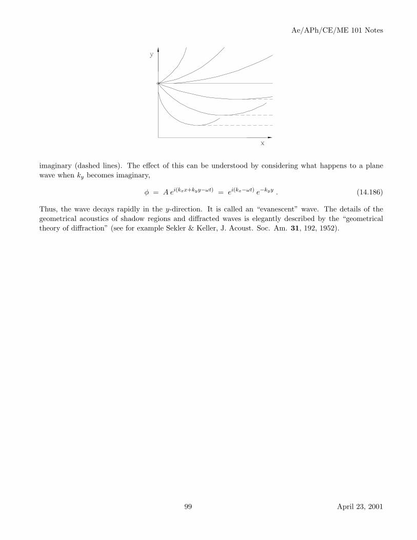
Ae/APh/CE/ME 101 Notes
imaginary (dashed lines). The effect of this can be understood by considering what happens to a planewave when ky becomes imaginary,
φ = A ei(kxx+kyy−ωt) = ei(kx−ωt) e−kyy . (14.186)
Thus, the wave decays rapidly in the y-direction. It is called an “evanescent” wave. The details of thegeometrical acoustics of shadow regions and diffracted waves is elegantly described by the “geometricaltheory of diffraction” (see for example Sekler & Keller, J. Acoust. Soc. Am. 31, 192, 1952).
99 April 23, 2001

Ae/APh/CE/ME 101 Notes
15 Potential Flow
Multi-dimensional nonsteady flow of an inviscid, non-heat conducting fluid.
15.1 Bernoulli equation for nonsteady flow
The Bernoulli equation for nonsteady flow is derived by introducing the definition of the velocitypotential, u = ∇φ into the momentum equation, Eq. 2.16,
∂∇φ
∂t+
12∇(∇φ)2 +
1ρ(p)
∇p = 0 . (15.1)
How the second term was obtained can be understood in terms of Cartesian tensor notation. It is
uj∂ui
∂xj=
∂φ
∂xj
∂2φ
∂xi∂xj(15.2)
=12
∂
∂xi
(∂φ
∂xj
∂φ
∂xj
). (15.3)
Differentiating (15.1) w.r.t. time gives
∂2∇φ
∂t2+
12
∂
∂t∇(∇φ)2 + ∇
(1ρ∇p
)= 0 , (15.4)
where the last term is obtained by partially differentiating
∂
∂t
(1ρ∇p
)=
∂1/ρ
∂p∇p
∂p
∂t+
1ρ∇∂p
∂t(15.5)
=(∇1
ρ
)∂p
∂t+
1ρ∇∂p
∂t(15.6)
= ∇(
1ρ
∂p
∂t
). (15.7)
The ∇ can be taken outside every term of (15.4) and the equation integrated w.r.t. x. The resultingarbitrary function of time is absorbed into φ. Thus
∂2φ
∂t2+
12
∂
∂t(∇φ)2 +
1ρ
∂p
∂t= 0 . (15.8)
This equation can then be integrated w.r.t. time to finally give the non-steady Bernoulli equation,
∂φ
∂t+
(∇φ)2
2+
∫dp
ρ(p)= const . (15.9)
15.2 The potential equation
The potential equation for this isentropic flow is derived from the mechanical energy equation Eq. 2.19with B = τ = 0, and Bernoulli’s equation. The pressure gradient term in (2.19) can be written as part ofa convective derivative, which can be converted to to the convective derivative of ρ by the definition of the
100 April 23, 2001
Ae/APh/CE/ME 101 Notes
sound speed,
1ρu · ∇p =
1ρ
Dp
Dt− 1
ρ
∂p
∂t(15.10)
=a2
ρ
Dρ
Dt− 1
ρ
∂p
∂t(15.11)
= −a2∇ · u − 1ρ
∂p
∂t, (15.12)
where the last equality is obtained by using the continuity equation. Thus the mechanical energy equationbecomes
∂u2/2∂t
+ u · ∇u2
2− a2∇ · u − 1
ρ
∂p
∂t= 0 . (15.13)
Eq. 15.8 is used to eliminate the pressure from Eq. 15.13, with the result
∂2φ
∂t2+
∂
∂t(∇φ)2 +
12∇φ · ∇(∇φ)2 − a2∇2φ = 0 . (15.14)
For steady flow, in terms of velocities in Cartesian tensor notation the equation is
12
uj∂u2
i
∂xj= a2 ∂ui
∂xi. (15.15)
Note that:
i. When a → ∞ the equation becomes∇2φ = 0 , (15.16)
the Laplace equation, valid for incompressible, nonsteady irrotational flow of an ideal (inviscid, non-heatconducting) fluid. The irrotationality follows from the existence of the velocity potential.
ii. For small amplitude motions, neglecting the nonlinear terms, the equation becomes
∂2φ
∂t2− a2
0 ∇2φ = 0 , (15.17)
the wave equation.
iii. The dot-product nonlinear term in Cartesian tensor notation is, from the original form of the me-chanical energy equation
12uj
∂u2i
∂xj= uiuj
∂ui
∂xj(15.18)
so in these terms for steady flow, the equation becomes
uiuj∂ui
∂xj= a2 ∂ui
∂xi. (15.19)
This form illustrates how the coefficient of the nonlinear term “balances” a2 to determine the super-sub-sonic behavior.
101 April 23, 2001

Ae/APh/CE/ME 101 Notes
15.3 Small disturbance theory
We consider steady isentropic irrotational flow of a perfect gas, with uniform inflow from the left ofvelocity U and sound speed a∞.
15.3.1 Energy equation for steady flow
In steady flow the total enthalpy is conserved,
a2 +γ − 1
2u2 = a2
∞ +γ − 1
2U2 . (15.20)
The velocity components are (U + u, v, w). Substituting,
a2 = a2∞ − γ − 1
2(2Uu − u2 − v2 − w2
). (15.21)
15.3.2 The potential equation
Using this result in Eq. 15.19 and multiplying out gives[a2∞ − γ − 1
2(2Uu − u2 − v2 − w2
)](∂u
∂x+
∂v
∂y+
∂w
∂z
)(15.22)
= (U + u)2∂u
∂x+ v2 ∂v
∂y+ w2 ∂w
∂z+ (U + u)v
(∂v
∂x+
∂u
∂y
)+ (U + u)w
(∂w
∂x+
∂u
∂z
)+ vw
(∂v
∂z+
∂w
∂y
). (15.23)
The above equations are exact. For small disturbances like those generated by slender bodies,(u, v, w) ¿ U . If we now multiply out and keep terms of O(1) (lhs) and O(u) (rhs) in the coefficients ofthe velocity derivatives, we get(
1 − M2∞
) ∂u
∂x+
∂v
∂y+
∂w
∂z= M2
∞
[(γ + 1)
u
U
∂u
∂x+ (γ − 1)
u
U
(∂v
∂y+
∂w
∂z
)(15.24)
+v
U
(∂v
∂x+
∂u
∂y
)+
w
U
(∂u
∂z+
∂w
∂x
)]. (15.25)
The terms on the rhs may become important when M∞ → 1, in particular the term in ∂u/∂x. Thus, anequation valid for subsonic, transonic or supersonic flow is(
1 − M2∞
) ∂u
∂x+
∂v
∂y+
∂w
∂z= M2
∞(γ + 1)u
U
∂u
∂x, (15.26)
or, in terms of the perturbation potential, (u, v, w) = ∇φ,
(1 − M2
∞) ∂2φ
∂x2+
∂2φ
∂y2+
∂2φ
∂z2=
M2∞(γ + 1)U
∂φ
∂x
∂2φ
∂x2. (15.27)
For subsonic and supersonic flow only,
(1 − M2
∞) ∂2φ
∂x2+
∂2φ
∂y2+
∂2φ
∂z2= 0 . (15.28)
102 April 23, 2001

Ae/APh/CE/ME 101 Notes
In cylindrical polar coordinates,where
ux =∂φ
∂x
ur =∂φ
∂r(15.29)
uθ =1r
∂φ
∂θ,
(1 − M2
∞) ∂2φ
∂x2+
1r
∂
∂r
(r∂φ
∂r
)+
1r2
∂2φ
∂θ2= 0 . (15.30)
15.3.3 Pressures.
The pressure coefficient is
Cp =p − p∞12ρ∞U2
=2
γM2∞
p − p∞p∞
, (15.31)
where the last equality holds for a perfect gas. For isentropic flow,
p
p∞=
(a
a∞
) 2γγ−1
, (15.32)
which, with Eq. 15.21, gives
p
p∞=
[1 − γ − 1
2M2
∞
(2u
U+
u2 + v2 + w2
U2
)] 2γγ−1
. (15.33)
Thus,
Cp =2
γM2∞
[1 − γ − 1
2M2
(2u
U+
u2 + v2 + w2
U2
)] γγ−1
− 1
(15.34)
From Eq. 15.21 we also have
ρ
ρ∞=
(T
t∞
) 1γ−1
=[1 − γ − 1
2(2Uu − u2 − v2 − w2
)] 1γ−1
. (15.35)
Now, for small disturbances expand to quadratic terms. After some cancellations there results
Cp = −(
2u
U+
(1 − M2
∞) u2
U2+
v2 + w2
U2
)(15.36)
ρ
ρ∞= 1 − M2
∞u
U+
v2 + w2
a2∞. (15.37)
For plane flow it suffices to take just the linear term, but for axisymmetric flow because of the fact that ur
gets very large near the axis it turns out to be necessary to include the quadratic term in ur (see below),
Planar body : Cp = −2u
U
Slender body of revolution : Cp = −2u
U− u2
r
U2
(15.38)
103 April 23, 2001

Ae/APh/CE/ME 101 Notes
15.3.4 Boundary conditions – body.
The boundary condition on the body is that the flow be tangent to the body.
Plane Flow. For an airfoil with small surface deflections
vb
U + ub=
dyb
dx, (15.39)
so approximatelyvb
U=
dyb
dx. (15.40)
For a slender body the boundary conditions can be applied at y = 0,
v(x, 0) = Ud yb(x)
dx. (15.41)
The result can be extended to nearly planar 3-dimensional flow, i.e., for a slender wing, in which case theconvention is to take y to be the spanwise coordinate and z to be vertical up,
w(x, y, 0) = U∂zb(x, y)
∂x. (15.42)
Axisymmetric Flow. Because the continuity equation must balance it implies an important scaling forur near r = 0,
1r
∂ur r
∂r∼ ∂u
∂x. (15.43)
Since the last term must be well behaved we have that
ur ∼ 1r
as r −→ 0 . (15.44)
Therefore, the boundary condition should be multiplied by r and written
(r ur)0 = URdR(x)
dx. (15.45)
15.3.5 Solution – Plane slender body
The equations are
Subsonic :(1 − M2
∞) ∂2φ
∂x2+
∂2φ
∂y2= 0
Supersonic :(M2
∞ − 1) ∂2φ
∂x2− ∂2φ
∂y2= 0
(15.46)
104 April 23, 2001

Ae/APh/CE/ME 101 Notes
Supersonic case. By comparing the last equation with Eq. 14.21 we can immediately write down thesolution from Eq. 14.33 by setting
x
a0−→
√M2∞ − 1 y ≡ λy (15.47)
t −→ x , (15.48)
i.e.,
φ = f(x −
√M2∞ − 1 y
)+ g
(x +
√M2∞ − 1 y
)(15.49)
The perturbation velocities and pressures are
u =∂φ
∂x= f ′ + g′ (15.50)
v =∂φ
∂y= −λ(f ′ − g′) (15.51)
v
U= − λ
U
(f ′ − g′
)(15.52)
Cp = −2u
U= − 2
U
(f ′ + g′
). (15.53)
Example. Diamond airfoil.The surfaces of a slender diamond airfoil at angle of attack are
Figure 37. Diamond airfoil at angle of attack
yu = 2δx
c− αx ; x <
c
2
= 2δ(1 − x
c
)− αx ; x >
c
2
yl = −2δx
c− αx ; x <
c
2
= −2δ(1 − x
c
)− αx ; x >
c
2.
(15.54)
105 April 23, 2001

Ae/APh/CE/ME 101 Notes
Thus the boundary conditions v/U = dyb/dx are as follows, and their relationship to the pressure coefficientis established through Eqs. 15.52 and 15.53,
vu
U=
dyu
dx=
2δ
c− α
−2δ
c− α
= − λ
Uf ′(x − λyu) =
λ
U
U
2Cpu
; x <c
2
; x >c
2
vl
U=
dyl
dx=
−2δ
c− α
2δ
c− α
=λ
Ug′(x − λyl) = − λ
U
U
2Cpl
; x <c
2
; x >c
2
.
(15.55)
Thus the pressure coefficients and their relations to lift and drag are
Cpu =
2λ
(2δ
c− α
)
− 2λ
(2δ
c+ α
) =−dCLu
−dCLu
=
12δc − α
dCDu
− 12δc + α
dCDu
; x <c
2
; x >c
2
Cpl =
2λ
(2δ
c+ α
)
− 2λ
(2δ
c− α
) =dCLl
dCLl
=
12δc + α
dCDl
− 12δc − α
dCDl
; x <c
2
; x >c
2
,
(15.56)
where the factors multiplying dCD are the cosecants of the angles of the surface elements, ı.e., theirprojections in the streamwise direction.
Integrating the lift we get
CLu = − 2λ
(2δ
c− α
)c
2+
2λ
(2δ
c+ α
)c
2
CLl =2λ
(2δ
c+ α
)c
2− 2
λ
(2δ
c− α
)c
2,
(15.57)
so
CL =4c
λα . (15.58)
Of course there is no lift for α = 0, and the lift is proportional to α.
The factors in(
2δc ± α
)in the drag multiply to give squares, which after multiplying out and canceling
give
CD =4c
λ
[(2δ
c
)2
+ α2
]. (15.59)
106 April 23, 2001

Ae/APh/CE/ME 101 Notes
Thus
• The drag is second order in δ.
• There is drag even for α = 0. This is “wave drag” and is a consequence of the fact that the bodymakes first order disturbances far out into the fluid.
• The “drag due to lift” is of order α2.
15.3.6 Solution – Slender body of revolution
The equations are
Subsonic :(1 − M2
∞) ∂2φ
∂x2+
1r
∂
∂r
(r∂φ
∂r
)= 0
Supersonic :(M2
∞ − 1) ∂2φ
∂x2+
1r
∂
∂r
(r∂φ
∂r
)= 0
(15.60)
By comparing these equations with Eq. 14.76 we can immediately write down the solution from Eq. 14.82by setting
r
a0−→
√M2∞ − 1 r ≡ λr ; Supersonic case
√1 − M2∞ r ≡ mr ; Subsonic case
(15.61)
t −→ x (15.62)
τ −→ ξ , (15.63)
namely,
φ(x, r) = − 12π
∫ x−λr
−∞f(ξ) dξ√
(ξ − x)2 − λ2r2; Supersonic case (15.64)
= − 14π
∫ ∞
−∞
f(ξ) dξ√(ξ − x)2 + m2r2
; Subsonic case . (15.65)
This is a solution for the velocity potential in terms of an as-yet undetermined source distribution f . Forthe subsonic case a form of Eq. 14.82 before the integration limits were changed to the semi-infinite rangeis used.
Supersonic case. This solution has the same structure as cylindrical acoustic waves, with the consequencethat there is a disturbance (wake) downstream of the body, algebraically decaying to infinity. Again,the singular behavior of the integrand at the upper limit requires that the finite part of the integrals bedetermined. We use the same transformation as in acoustics,
ξ = x − λ r cosh σ , (15.66)
107 April 23, 2001

Ae/APh/CE/ME 101 Notes
so thatλ r sinhσ =
√(ξ − x)2 − λ2r2 , (15.67)
and
d ξ = −λ r sinhσ dσ (15.68)
= −√
(ξ − x)2 − λ2r2 dσ . (15.69)
We limit the range of integration by taking the body to start at x = 0. Then the solution transforms into
φ = − 12π
∫ cosh−1 xλ r
0f(x − λ r cosh σ) dσ . (15.70)
Now differentiation to get the velocities proceeds smoothly. We take that the body is sharp at the nose,f(0) = 0, so the term from the differential at the upper limit is zero. Then,
u =∂φ
∂x= − 1
2π
∫ cosh−1 xλ r
0f ′(x − λ r cosh σ) dσ
= − 12π
∫ x−λr
0
f ′(ξ) dξ√(ξ − x)2 − λ2r2
ur ≡ v =∂φ
∂r=
12π
∫ cosh−1 xλ r
0λ cosh σf ′(x − λ r cosh σ) dσ
=1
2πr
∫ x−λr
0
(ξ − x)f ′(ξ) dξ√(ξ − x)2 − λ2r2
.
(15.71)
From the last equation it can be seen that
limr→0
2π rv = f(x) , (15.72)
so we see that the source distribution is given in terms of the boundary condition applied at r = 0,
f(x) = 2π U(rv
U
)0
. (15.73)
In view of the boundary condition Eq. 15.45, the source strength can be written in terms of the cross-sectional area S = πR2 of the body of revolution,
f(x) = UdS
dx. (15.74)
Example. Slender cone of half angle δ.For the cone,
dR
dx= δ (15.75)
dS
dx= 2πR
dR
dx= 2π δ2 x , (15.76)
108 April 23, 2001

Ae/APh/CE/ME 101 Notes
so
f(x) = 2π U δ2 x (15.77)
f ′(x) = 2π U δ2 , (15.78)
and
u
U= −δ2
∫ cosh−1 xλ r
0dσ (15.79)
= −δ2 cosh−1 x
λ r(15.80)
= −δ2 ln
(x
λ r+
√x2
λ2 r2− 1
). (15.81)
Similarly,
v
U= δ2λ
∫ cosh−1 xλ r
0cosh σ dσ (15.82)
= δ2λ√
cosh2 σ − 1∣∣∣cosh−1 x
λ r
0(15.83)
= δ2λ
√( x
λ r
)2 − 1 . (15.84)
The solutions come out in terms of the “similarity” variable x/r, because there is no characteristic lengthin this problem. All flow quantities are constant along x/r = const, rays from the origin. Clearly, theoriginal equations could have been transformed to eliminate one of the independant variables and becomeordinary differential equations for x/r and the solution obtained by solving the resulting equations. Thatis one approach for finding an exact solution to the cone problem.
Note that there is no change of flow deflection angle at the leading characteristic (v/U(x/λr = 1) = 0),in contrast to the plane-flow case. This is because of azimuthal “leakage” in the flow over a body ofrevolution.
For the flow on or near the body, where r is small, for cases in which λ is not too large (supersonic butnot hypersonic flow) x/λr À 1, and the results can be simplified. In particular, on the body x/λr = 1/λδ,so
u
U= −δ2 ln
2λδ
v
U= δ .
(15.85)
It was originally proposed that the quadratic term in Eq. 15.38 for bodies of revolution is necessary, andwe now find that because u ∼ δ2 while v ∼ δ that is indeed the case
Cp = −2u
U− v2
U2(15.86)
= δ2
(2 ln
2λδ
− 1)
. (15.87)
109 April 23, 2001

Ae/APh/CE/ME 101 Notes
15.4 Similarity rules for compressible flow
Rules can be derived for converting results from one flow to another flow over a body of the same familyof shapes at different Mach number and in a different perfect gas.
15.4.1 Plane flow – subsonic case
Consider flow 1, φ(x, y), at free-stream Mach number M1 over a body characterized by a thickness ratioτ1 yb
c= τ1 f(
x
c) . (15.88)
The equation of motion is Eq. 15.28 written for plane flow, and the boundary conditions and pressures are(∂φ
∂y
)0
= U1τ1f′(x
c
)(15.89)
Cp1 = − 2U1
(∂φ
∂x
)0
. (15.90)
Transform to flow 2, Φ(ξ, η), by
x = ξ (15.91)√1 − M2
1 y =√
1 − M22 η (15.92)
φ(x, y) = AU1
U2Φ(ξ, η) . (15.93)
The arbitrary constant on the rhs of Eq. 15.93, which arises because the differential equation is homogeneousin φ, is chosen for convenience. The equation of motion transforms to the same form
(1 − M2
2
) ∂2Φ∂x2
+∂2Φ∂y2
= 0 , (15.94)
and the boundary condition transforms to(∂φ
∂y
)0
=
√1 − M2
1
1 − M22
AU1
U2
(∂Φ∂η
)0
, (15.95)
where (∂Φ∂η
)0
= U2τ2f′(
ξ
c
). (15.96)
Thus, from Eq. 15.89 the boundary condition transforms unchanged if
τ2 = τ1
√1 − M2
2
1 − M21
1A
(15.97)
and f ′ is the same. That is, the body shapes are the same though the thickness varies. The pressurecoefficient transforms to
Cp1 = − 2U1
(∂φ
∂x
)0
= − 2U2
A
(∂Φ∂ξ
)0
. (15.98)
Comparing with Eq. 15.90 shows that
Cp2 =1A
Cp1 . (15.99)
110 April 23, 2001

Ae/APh/CE/ME 101 Notes
This scaling can be summarized in the following functional form,
Cp
A= fnc
(τ
A√
1 − M2∞
). (15.100)
A is an arbitrary parameter, various choices of which give commonly used similarity laws (see Table 3).For example, if we choose A to cancel the Mach numbers in Eq. 15.97, then we are comparing to differentflows over the same body, τ2 = τ1. The first 3 entries are known as the Prandtl-Glauert similarity laws,
Table 3. Subsonic and Supersonic Compressible Flow Similarity Laws
A
1 1 Cp = fnc
(τ√
1 − M2∞
)
21√
1 − M2∞Cp =
1√1 − M2∞
fnc (τ)
3 τ Cp = τ fnc(√
1 − M2∞)
41
1 − M2∞Cp =
11 − M2∞
fnc(τ√
1 − M2∞)
and the last is the Gothert similarity law, applicable also to bodies of revolution (see below).
15.4.2 Supersonic flow
The same derivation goes through for the suppersonic form of the potential equation. One need onlyreplace (1−M2∞) with (M2∞−1) in the results. Results valid for both cases can be written using |(M2∞−1)|.
15.4.3 Axisymmetric flow – subsonic case
The equation of motion is Eq. 15.60. In this case it is necessary to be careful to avoid any problemsthat might arise from applying the boundary condition on the axis. In fact, to get the scaling laws itis easiest to simply apply the boundary conditions exactly on the body, R/c = τ1f(x/c). This will addanother condition, which will fix A. The boundary condition is(
∂φ
∂r
)b
= U1τ1 f ′(x
c
), (15.101)
and the pressure is
Cp1 = − 2U1
(∂φ
∂x
)0
− 1U2
1
(∂φ
∂r
)2
0
. (15.102)
The transformation is
φ = AU1
U2Φ(ξ, ρ) (15.103)
111 April 23, 2001
Ae/APh/CE/ME 101 Notes
x = ξ (15.104)√1 − M2
1 r =√
1 − M22 ρ . (15.105)
The boundary condition transforms to(∂φ
∂r
)r=τ1cf(x/c)
=
√1 − M2
1
1 − M22
AU1
U2
(∂Φ∂ρ
)ρ=
√1−M2
11−M2
2τ1cf(x/c)
, (15.106)
where we require (∂Φ∂ρ
)ρ=τ2cF (ξ/c)
= U2τ2 F ′(
ξ
c
). (15.107)
In order to have the radii at which the boundary conditions are applied comparable, the bodies must beof the same family, F = f and
τ2 =
√1 − M2
1
1 − M22
τ1 . (15.108)
Substituting Eq. 15.107 into 15.106 and equating to Eq. 15.101 gives
A =
√1 − M2
2
1 − M21
. (15.109)
Thus, for axisymmetric flow the arbitrary constant is fixed by the requirement that the boundary conditionstransform. We know what the flow will be at a different Mach number only on a body whose thicknessis determined by the new M∞. Even though the pressures coefficients are given in terms of two terms,applying the transformation gives again Eq. 15.99. Thus the symmetry properties can be summarized by
Cp
(1 − M2
∞)
= fnc(√
1 − M2∞ τ)
, (15.110)
the Gothert similarity law, entry #4 in the table above.
112 April 23, 2001

Ae/APh/CE/ME 101 Notes
16 Incompressible Flow
The transition from compressible flow to incompressible flow can be derived from our previous resultsby simply taking the limit a∞ → ∞, or λ, m → 1. Here, in addition, we take a somewhat more generalpoint of view.
Fluid flow is often constructed by superposing a distribution of singularities to satisfy boundary con-ditions, or to otherwise represent in simplified form bodies or sources of vorticity. From a mathematicalpoint of view, this is because any vector field can be represented in terms of the gradient of a scalar poten-tial φ and the curl of a vector potential B; we will see that these represent volume and vorticity sources,respectively. In addition, in fluids there can exist a pure straining motion with no change of volume andno rotation, so this adds some additional flexibility in the flow which in general must be accounted for.In this chapter we construct velocity fields whose divergence and curl have specified values, and later insome examples we see how these can be translated to or from boundary conditions. Velocities ue inducedby expansion and velocities uv induced by vorticity are given by
1) ∇ · ue = f ; ∇× ue = 0 (16.1)
2) ∇ · uv = 0 ; ∇× uv = ω (16.2)
In terms of the potentials the velocities are
ue = ∇φ (16.3)
uv = ∇× B . (16.4)
The equations satisfied by φ and B are therefore
∇2φ = f (16.5)
∇×∇× B = −∇2B = ω . (16.6)
The last equality of the second equation results if ∇ · B = 0, which is valid if the velocities go to zero atinfinity and a suitable limiting procedure is adopted at boundaries (Batchelor 1967).
Now, getting back to the pure straining motion, if a velcity field u is consistent with both (16.1) and(16.2), then v = u−ue−uv must be both divergence and curl free, and so in general is the purely strainingmotion satisfying
3) ∇ · v = 0 ; ∇× v = 0 . (16.7)
Flows driven by some simple, frequently utilized singularities are given later in this chapter. Theyin turn can be used to construct more complex structures by summing two equal and opposite elementsspaced 2δ apart and then letting δ → 0. In general, the limiting process is as follows (see Fig. 38). Giventhat
φ = −A f(r) , (16.8)
summation of two such singularities gives
φ = −A [f(r − δ) − f(r + δ)] . (16.9)
Multiplying and dividing by δ and applying the limit δ → 0; Aδ → A′ gives
φ = A′ · ∇f(r) . (16.10)
This result is used below.
113 April 23, 2001

Ae/APh/CE/ME 101 Notes
Figure 38. Construction of a higher-order singularity
16.1 The stream function
The stream function identically satisfies the continuity equation, so it has important physical signifi-cance. It arises in flows which have symmetries reducing the number of independent variables from 3 to 2,so that B has only one component, perpendicular to u. That component is related to the stream functionψ. This section gives some examples. For completeness we also show the appropriate forms of the gradientof the velocity potential for obtaining the velocity components.
Cartesian coordinates (x, y, z): Plane flow; ∂∂z = 0. The vector potential is perpendicular to u, so in 2D
flow has only a z component, which we call ψ,
B = (0, 0, ψ) . (16.11)
Now from Eq. 16.4
u = i∂ψ
∂y− j
∂ψ
∂x, (16.12)
so
u =∂ψ
∂y=
∂φ
∂x
v = −∂ψ
∂x=
∂φ
∂y.
(16.13)
From Eq. 16.6, ψ satisfies a Poisson equation
∂2ψ
∂x2+
∂2ψ
∂y2= ωz , (16.14)
as does φ (Eq. 16.5)∂2φ
∂x2+
∂2φ
∂y2= f . (16.15)
Cylindrical coordinates (r, θ, z): Plane flow; ∂∂z = 0. As before,
B = (0, 0, ψ) . (16.16)
From Eq. 16.4
u = er
1r
∂ψ
∂θ− eθ
∂ψ
∂r, (16.17)
114 April 23, 2001

Ae/APh/CE/ME 101 Notes
so
ur =1r
∂ψ
∂θ=
∂φ
∂r
uθ = −∂ψ
∂r=
1r
∂φ
∂θ.
(16.18)
The corresponding Poisson equations to be solved are
∂
∂r
(r∂ψ
∂r
)+
∂
∂θ
(1r
∂ψ
∂θ
)= −ωz . (16.19)
∂
∂r
(r∂φ
∂r
)+
∂
∂θ
(1r
∂φ
∂θ
)= f . (16.20)
Cylindrical coordinates (r, θ, z): Axisymmetric flow; ∂∂θ = 0. In this case B has only a θ component which,
to insure that ψ satisfies the continuity equation, we take to be
B = (0,ψ
r, 0) . (16.21)
Thenu = −er
1r
∂ψ
∂z+ ez
1r
∂ψ
∂r, (16.22)
so
ur = −1r
∂ψ
∂z=
∂φ
∂r
uz =1r
∂ψ
∂r=
∂φ
∂z,
(16.23)
and, with the vorticity in the θ direction, ψ satisfies the equation
1r
∂
∂r
(r∂ψ/r
∂r
)+
∂2ψ/r
∂z2= −ωθ , (16.24)
and φ satisfies1r
∂
∂r
(r∂φ
∂r
)+
∂2φ
∂z2= f . (16.25)
Spherical coordinates (r, φ, θ): Axisymmetric flow; ∂∂θ = 0. Again B has only a θ component, in this case
B = (0, 0,ψ
r sinφ) . (16.26)
In this case, ψ is called the Stokes Stream Function. Then
u = er
1r2 sinφ
∂ψ
∂φ− eφ
1r sinφ
∂ψ
∂r, (16.27)
115 April 23, 2001

Ae/APh/CE/ME 101 Notes
so
ur =1
r2 sinφ
∂ψ
∂φ=
∂φ
∂r
uφ = − 1r sinφ
∂ψ
∂r=
1r
∂φ
∂φ,
(16.28)
and, again with the vorticity in the θ direction,
1r2
∂
∂r
(r2 ∂ψ/r sin φ
∂r
)+
1r2 sinφ
∂
∂φ
(sinφ
∂ψ/r sinφ
∂φ
)= −ωθ . (16.29)
while1r2
∂
∂r
(r2 ∂φ
∂r
)+
1r2 sinφ
∂
∂φ
(sinφ
∂φ
∂φ
)= −ωθ . (16.30)
Alternartively, for ψ1
sinφ
∂2ψ
∂r2+
1r2 sinφ
∂
∂φ
(sin φ
∂ψ/ sinφ
∂φ
)= −r ωθ . (16.31)
Physical interpretation of the stream function. The difference of the values of the stream function at twopoints in a flow is defined as being the volume flow between streamlines through the two points. FromFig. 39 it is seen that in a Cartesian system the incremental change of volume flux between the two points
Figure 39. Geometry for computing volume fluxes from the stream function
isdψ = −v dx + u dy (16.32)
while in a polar coordinate system it is
dψ = −uθ dr + ur r dθ (16.33)
Thus, as we have seen
Cartesian Coords Polar Coords
u =∂ψ
∂yrur =
∂ψ
∂θ(16.34)
v = −∂ψ
∂xuθ = −∂ψ
∂r. (16.35)
In the examples of simple flows given below, we derive the stream function from the velocity componentsfor the appropriate symmetry as shown above.
116 April 23, 2001

Ae/APh/CE/ME 101 Notes
16.2 Complex notation for plane flow
For plane flow, equations for the velocity components (u, v),
∂φ
∂x=
∂ψ
∂y(16.36)
∂φ
∂y= −∂ψ
∂x, (16.37)
form Cauchy Riemann conditions establishing an analytic function
F (z) = φ + i ψ (16.38)
of the complex variablez = x + i y = r eiθ , (16.39)
such that its derivativedF
dz=
∂φ
∂x+
∂ψ
∂y(16.40)
is the complex velocity w
w = u − i v . (16.41)
In the examples of simple plane (2D) flows given below, we include expressions for the complex potential.
16.3 Flows with volume sources
Eq. 16.1 with 16.3 gives∇2φe = f . (16.42)
We already have the solution for this equation by setting a0 = ∞ (k = ω = 0) in accoustics (Eq. 14.104)or m = λ = 1 in potential flow (Eq. 15.65),
φe(r) = − 14π
∫ ∞
−∞
f(ξ) dξ
R(16.43)
ue(r) = ∇φe = − 14π
∫ ∞
−∞∇ 1
Rf(ξ) dξ (16.44)
=14π
∫ ∞
−∞R
R3f(ξ) dξ , (16.45)
where R = r − ξ. This gives the irrotational velocity field resulting from a distribution of volume sources.No dilatation occurs anywhere in the field except at the singularities.
Point source (3D). f(x) = qδ(x).
φe = − q
4πr
ue =q
4π
r
r3
ψ = − q
4πcos φ .
(16.46)
This is the near-field result (since a0 = ∞) for a steady acoustic source.
117 April 23, 2001
Ae/APh/CE/ME 101 Notes
Point source (2D). 3D point sources can be distributed along a straight line (z-axis) to form a line source.R is the distance from the sourcelet at ξ = z on the z-axis to the observer at (r, θ) in the (x, y) plane,R2 = z2 + r2. Thus
ue =q
4π
∫ ∞
−∞r
R3dz (16.47)
and there results
ue =q
2π
r
r2
φe =q
2πln r
ψ =q
2πθ
F =q
2πln z .
(16.48)
Dipole (3D). Summing two equal and opposite 3D point sources by the prescription given by Eq. 16.10gives
φe =14π
µ · ∇1r
, (16.49)
or
φe = − 14π
µ · r
r3
ue =14π
(− µ
r3+ 3
µ · rr5
r)
.
(16.50)
In spherical coordinates (r, φ, θ), with the dipole oriented along the z-axis,
φ = − µ
4π
cos φ
r2
ur =µ
2π
cos φ
r3
uθ =µ
4π
sinφ
r3
ψ =µ
4π
sin2 φ
r.
(16.51)
Dipole (2D). Summing two equal and opposite 2D point sources gives by Eq. 16.10
φe = − 12π
µ · ∇ln r , (16.52)
118 April 23, 2001

Ae/APh/CE/ME 101 Notes
or
φe = − 12π
µ · r
r2
ue =12π
(− µ
r2+ 2
µ · rr4
r)
.
(16.53)
In polar coordinates (r, θ), with the dipole oriented along the x-axis,
φ = − µ
2π
cos θ
r
ur =µ
2π
cos θ
r2
uθ =µ
2π
sin θ
r2
ψ =µ
2π
sin θ
r
F = − µ
2πz.
(16.54)
If the dipole were oriented along the y-axis the complex potential would simply read
F = −iµ
2πz. (16.55)
The 2D dipole could also have been constructed by summing the stream functions of two sources,
Figure 40. Construction of a 2D dipole by superposition
ψ =q
2π(θ+ − θ−) =
q∆2π
, (16.56)
and noting from the geometry of Fig. 40 that the curves ψ = const. (∆ = const.) are circles through bothsingularities such that
sin∆ =δ
d, (16.57)
119 April 23, 2001

Ae/APh/CE/ME 101 Notes
where d is the diameter of the circle. In the limit δ → 0, we have
θ+ ≈ θ− ≡ θ (16.58)δ
sin ∆≈ r
sin θ, (16.59)
so,
ψ =µ
2π
sin θ
r(16.60)
16.4 Flows with sources of vorticity
Formally, the solution of Eq. 16.6 is
B =14π
∫ ∞
−∞
ω(ξ) dξ
R(16.61)
uv(r) = ∇× B =14π
∫ ∞
−∞∇× ω
Rdξ (16.62)
= − 14π
∫ ∞
−∞R × ω
R3dξ . (16.63)
Applying the divergence theorem shows that in fact ∇ · B = 0 if ω · n = 0 on all boundaries of the fluid.
Point sources of vorticity do not exist because ∇ · ω = 0. Thus, as with magnetic fields, one thinks interms of vortex lines or filaments, continuous lines everywhere parallel to ω. By the divergence theorem∫
ω · n dA on the area defined by any closed curve completely surrounding the same vortex lines must bethe same. The closed curves and the vortex lines form a vortex tube. By Stokes theorem∫
ω · n dA =∮
u · dl = Γ . (16.64)
These results imply the
16.4.1 Helmholtz vortex theorems
1. The strength of a vortex filament is constant along its length.
2. A vortex filament can not end in a fluid; it must extend to the boundaries of the fluid or must forma closed path.
3. For an inviscid fluid,
(a) In the absence of rotational external forces, a fluid that is initially irrotational remains irrota-tional.
(b) In the absence of rotational external forces, if the circulation around a path enclosing a definitegroup of particles is initially zero, it will remain zero.
(c) In the absence of rotational external forces, the circulation around a path that encloses a taggedgroup of elements is invariant.
120 April 23, 2001

Ae/APh/CE/ME 101 Notes
16.4.2 Biot-Savart Law
A curved vortex is a singularity formed by shrinking a vortex tube to zero diameter such that∫δξ
ω dξ = Γ δl , (16.65)
giving, from Eq. 16.63,
uv = − Γ4π
∫R × dl
R3, (16.66)
the Biot-Savart Law.
Line vortex. A line vortex (as distinct from a vortex line) is made by integrating the Biot-Savart law alonga straight line, say the z-axis. From the geometry of Fig. 41, it is seen that R × dl = rdz, R2 = r2 + z2,
Figure 41. Effect in the x-y plane of a vortex element on the z-axis
and that the induced velocity is only in the θ direction. Thus, integrating Eg. 16.66,
uθ = − Γ4π
∫ ∞
−∞r dz
(r2 + z2)3/2(16.67)
=Γ4π
z
r (r2 + z2)1/2
∣∣∣∣∣∞
−∞, (16.68)
so,
uθ =Γ
2πr
φ =Γ2π
θ
ψ = − Γ2π
ln r
F = −iΓ2π
ln z
w = −iΓ
2πz.
(16.69)
121 April 23, 2001

Ae/APh/CE/ME 101 Notes
Vortex doublet. The vortex doublet is constructed by Eq. 16.10, where say, Γδ → λ,
ψ =12π
λ · ∇ ln r , (16.70)
so,
ψ =12π
λ · rr2
. (16.71)
In polar coordinates, with the doublet aligned along the y-axis,
ψ =λ sin θ
2π r
ur =λ
2π
cos θ
r2
uθ =λ
2π
sin θ
r2
φ = − λ
2π
cos θ
r
F = − λ
2πz.
(16.72)
Note that this field is identical to that induced by a 2D dipole oriented at 90 to the vortex doublet,Eqs. 16.54.
122 April 23, 2001

Ae/APh/CE/ME 101 Notes
Infinite Vortex Sheet. An infinite vortex sheet can be constructed from the superposition of vortex linesof constant strength ω, as shown in Fig. 42. The circulation per unit length γ is defined from
Figure 42. Construction of an infinite vortex sheet by superposition
dΓ = ω · dS = ω dη dξ = γ dξ , (16.73)
where γ ≡ ω dη. At each point y > 0 the contribution to the x-component of velocity from the twosymmetric points shown is
du+ = −2y
r
dΓ2πr
= −γ
π
y dξ
r2, (16.74)
while by symmetry dv = 0. Here, r2 = y2 + ξ2. Integrating over 0 < ξ < ∞, for γ = const.,
u+ = −γ
πtan−1 ξ
y
∣∣∣∣∣∞
0
= −γ
2(16.75)
For y < 0 we get the result u− = γ/2, so across the sheet
∆u ≡ u+ − u− = −γ . (16.76)
Written in terms of the velocity potential, Eq. 16.75 is
∂φ+
∂x= −1
2dΓdx
, (16.77)
A similar relation, with a change of sign, holds for φ−, so if we take pairs of points above and below thevortex sheet
∂∆φ
∂x= −dΓ
dx, (16.78)
where ∆φ = φ+ − φ−. If the vortex sheet is of finite extent, the total circulation Γ is finite and Eq. 16.78can be integrated to yield
Γ = −∆φ . (16.79)
16.4.3 General vortex sheet – Lift
Consider a 3-D (curved) vortex sheet of circulation γ per unit length in an otherwise uniform flow withvelocity U− below the sheet. The vorticity imposes a velocity change u+ = −γ/2 on the top, and a changeu− = +γ/2 on the bottom thus causing velocity U+ on the top (see Fig. 43). All of the vectors shownin the sketch lie in the tangent plane to the sheet. To accommodate a bound vortex sheet we allow for
123 April 23, 2001

Ae/APh/CE/ME 101 Notes
Figure 43. Vector diagram for a vortex sheet with convective velocity in the plane of the sheet
forces on it, namely, a pressure difference between the top p+ and the bottom p−. The mean velocity isU = 1
2(U+ + U−).
By Bernoulli’s equation,
p0+ = p+ +12ρU2
+ ; p0− = p− +12ρU2
− , (16.80)
so,
∆p ≡ p+ − p− = ∆p0 +12ρ(U2
− − U2+) , (16.81)
where ∆p0 = p0+ − p0−. From the construction in the sketch, we have
U2− − U2
+ = −2Uu−(cos θ− − cos θ+) (16.82)
= 4Uu+ sinθ− + θ+
2sin
θ− − θ+
2(16.83)
= 2Uγ sin ψ , (16.84)
where 2ψ = θ− − θ+. Thus, from Eq. 16.81 we have the result
∆p = ∆p0 + ρ U sinψ γ , (16.85)
where U sinψ = Un is just the component of the convective velocity normal to the vorticity. We now applyEq. 16.85 to three cases:
i. Trailing vortex sheet.Typically behind a wing the flow on each side of the sheet has approximately the same total pressureso ∆p0 = 0. Since the sheet is free, it cannot support any pressure difference, so ∆p = 0. Thus,ψ = 0, so any imposed “mean flow” U is aligned with γ, and the vortex sheet does not convect.
ii. Edge of a separated flow (bubble).Dissipation acts in the recirculation region of a separated flow, so in general ∆p0 6= 0. However, sincethe sheet is free, ∆p = 0. Therefore, in this case ψ 6= 0, and the sheet is convected by the meanvelocity.
124 April 23, 2001

Ae/APh/CE/ME 101 Notes
iii. Bound vortex sheet.In this case, a force must be present, ∆p 6= 0, while for a thin wing ∆p0 ≈ 0. We are free to chooseU , and if we take it to be Un, the free stream velocity of a flow over an airfoil swept at angle ψ, then
∆p = ρUnγ . (16.86)
This is the Kutta-Joukowski Theorem for the lift force (actually the negative of lift). Whenintegrated over the entire bound vortex sheet representing an airfoil, it gives the result
L = −ρUnΓ , (16.87)
where L is the force in the positive z direction.
16.5 Uniform flow, (x, y)
Uniform flow in the x-direction with velocity U is given by,
Plane flow
φ = Ux (16.88)
ψ = Uy (16.89)
F = Uz . (16.90)
In an incompressible fluid, if a body moves with constant velocity U , and fluid particles move only as aconsequence of the body motion, then
∂
∂t= −(U · ∇) . (16.91)
Axisymmetric flow (Flow now in the z-direction.)Polar coordinates, (r, θ, z), ∂
∂θ = 0.
φ = Uz (16.92)
ψ =Ur2
2(16.93)
Spherical coordinates, (r, φ.θ), ∂∂θ = 0.
ψ =U
2r2 sin2 φ (16.94)
ur = U cos φ (16.95)
uθ = −U sinφ . (16.96)
16.6 Flow over a lifting cylinder
Uniform flow + dipole + vortex.To examine the flow over what is perhaps the simplest closed lifting body, consider the superposition of a
125 April 23, 2001

Ae/APh/CE/ME 101 Notes
uniform flow U , a dipole oriented upstream −µ, and a vortex Γ. The stream function is, from Eqs. 16.89,16.54 and 16.69,
Ψ = Ur sin θ − µ sin θ
2πr− Γ
2πln
r
a(16.97)
= Ur sin θ(1 − µ
2πUr2
)− Γ
2πln
r
a, (16.98)
where a is an arbitrary constant of integration which has been added for use in Eq. 16.100. Thus,
ur =1r
∂Ψ∂θ
= U cos θ(1 − µ
2πUr2
). (16.99)
Note that the radial velocity vanishes on a circle,
r =√
µ
2πU≡ a , (16.100)
and, since by the above choice the stream function is zero on r = a, we have derived the flow over a cylinderof radius a and circulation Γ. To summarize, the velocities in the field are
ur =1r
∂Ψ∂θ
= U cos θ
(1 − a2
r2
), (16.101)
uθ = −∂Ψ∂r
= −U sin θ
(1 +
a2
r2
)+
Γ2πr
. (16.102)
On the cylinder the tangential velocity is
uθ = −2U sin θ +Γ
2πa. (16.103)
The sense of the contributions of the first term is sketched on the left of Fig. 44 and of the second on the
Figure 44. Sense of the contributions of terms in Eq. 16.103
right. These motions move the stagnation points ur = uθ = 0 on the body. From Eq. 16.101 we see thatur = 0 when r = a or θ = ±π/2. In the first case, uθ = 0 when
sin θ = Γ/4πUa . (16.104)
Curves of constant ψ (streamlines) for one such case are shown in Fig. 45. When Γ/4πUa > 1 there is
126 April 23, 2001

Ae/APh/CE/ME 101 Notes
Figure 45. Streamlines around a circular cylinder for U = 1, µ = 3 and Γ = 5 (a = 0.691)
a problem, because sin < 1; the stagnation points move off the body and the condition θ = −π/2 holds.Then, the zero of Eq. 16.102 is at
r =Γ
4πU
1 +
√1 −
(4πUa
Γ
)2 . (16.105)
Streamlines for one such case are shown in Fig. 46.
That the lift force on the cylinder satisfies the Kutta-Joukowski Theorem (Eq. 16.87) can be verifiedby integrating the pressure acting on the cylinder using Bernoulli’s Equation:
p +ρu2
2= p∞ +
ρU2
2(16.106)
p − p∞ =ρU2
2
[1 −
( u
U
)2]
(16.107)
On the body, u = uθ(r = a), so
p − p∞ =ρU2
2
[1 − 4 sin2 θ −
(Γ
2πUa
)2
+2Γ
πUasin θ
]. (16.108)
The infinitesimal contributions to lift and drag are (Fig. 47)
dL = −(p − p∞)a sin θ dθ (16.109)
dD = −(p − p∞)a cos θ dθ (16.110)
127 April 23, 2001

Ae/APh/CE/ME 101 Notes
Figure 46. Streamlines around a circular cylinder for U = 1, µ = 3 and Γ = 9 (a = 0.691)
Figure 47. Orientation of lift and drag forces
The cosine multiplying every term in the drag formula insures that the integral from θ = 0 to 2π of eachterm is zero. In the lift formula, the only contribution comes from terms with even powers of the sine, thatis, only from the term with Γ. Integrating that term confirms that L = −ρUΓ.
This example has not addressed how the cylinder might acquire circulation. In fact, attempts to realizethis configuration, called the Flettner Rotor, have not met with total success. The key requirement is tocontrol the location of separation, a very important example of flow control. In the next section we will seehow an airfoil with a sharp trailing edge generates circulation. It then remains to calculate the circulationof a given shape airfoil. That is the subject of airfoil theory.
128 April 23, 2001

Ae/APh/CE/ME 101 Notes
16.7 The Kutta condition
1. The way in which circulation is established about airfoils to generate lift is one of the great accom-plishments of aerodynamic design, and one of the earliest successes in flow control. Of course, themagnitude of the accomplishment is somewhat mitigated by the fact that birds had developed thetechnology much earlier, and, to unlock the secret, all humans had to do was look up.
2. The Kutta condition states that the flow leaves the trailing edge of an airfoil smoothly, and that thevelocity there is finite.
3. When an inviscid irrotational fluid is set into motion, the resulting flow is irrotational.
4. Thus, the shape of a lifting body must be such that viscosity is forced to initially play a crucial role inestablishing circulation, but later, after the flow is established, the effects of viscosity should be small.
Figure 48. The consequences of adding viscous effects near a body, namely separation, to the global flow field
The left column of Fig. 48 shows three different flows as they would be established in a perfect (inviscid)fluid. They are;
1. flow over a flat plate at small incidence to the free stream,
2. flow normal to a flat plate,
3. two streams at different velocities and total pressure flowing parallel to a flat plate.
The common feature of all three flows is that the bodies have sharp edges.
In all cases there is no circulation, so both the lift and drag are zero.
Helmholtz (1868) first established that, in fact, vortex sheets trail downstream from sharp edges; thatis, that sharp edges force separation. Kutta (1902) showed that if the flow leaves the trailing edge of a wing
129 April 23, 2001

Ae/APh/CE/ME 101 Notes
smoothly i.e., if the trailing edge is sharp (the Kutta Condition), then perfect-fluid theory (potentialflow theory) can be used to calculate the lift.
The right column of Fig. 48 shows that the three flows manifest the effects of viscosity in three funda-mentally different ways.
1. In the first one, at the initial instant the plate sheds a “starting vortex” which forces the Kuttacondition on the flow. The trailing vortex sheet maintains the separation thereafter. The miracle oflift is that a starting vortex is generated of just the right strength Γ to provide the required force.
2. In flow normal to a plate a large vortex pair forms downstream of the plate and remains there forever,forcing the Kutta condition.
3. In order for the flow parallel to the plate to separate smoothly, it is necessary for vortices to becontinually shed from the plate for all time.
130 April 23, 2001

Ae/APh/CE/ME 101 Notes
17 Airfoil theory
17.1 Flat plate airfoil
The lift generated by a flat plate at angle of attack can be represented by a bound vortex sheet γ(x),subject to the Kutta condition γ(c) = 0. If the angle of attack is small the vortex sheet can to anapproximation be placed on the x-axis. The unknown vortex strength γ(x) is determined by requiring thatthe flat plate be a streamline, that is, that the velocity normal to the plate be zero. From Eq. 16.69, thetangential velocity induced by an infinitesimal element dξ at point (ξ, 0) is
duθ =γ dξ
2π√
(x − ξ)2 + y2. (17.1)
On the axis the induced velocity is vertical,
dv =γ dξ
2π(x − ξ). (17.2)
The component of the free stream normal to the plate is U sinα. Making the small angle approximation,and adding up the effects of all the elements and the free stream, we get
v =12π
∫ c
0
γ(ξ)x − ξ
dξ + Uα . (17.3)
Setting this expression to 0 to satisfy the requirement of streamline flow,
12π
∫ c
0
γ(ξ)x − ξ
dξ = −Uα . (17.4)
Integrals with singularities at x = ξ appear often in wing theory, and in such cases it should always beunderstood that reference is to the principal value.
Using the transformation
ξ =c
2(1 − cos θ) (17.5)
x =c
2(1 − cos φ) , (17.6)
Eq. 17.4 and the Kutta condition become
12π
∫ π
0
γ(θ) sin θ dθ
cos θ − cos φ= −Uα (17.7)
γ(π) = 0 . (17.8)
The distribution that satisfies Eqs. 17.7 and 17.8 is
γ(θ) = −2αU1 + cos θ
sin θ(17.9)
Proof: In order to prove Eq. 17.9 it is necessary to show that∫ π
0
1 + cos θ
cos θ − cos φdθ = π . (17.10)
131 April 23, 2001

Ae/APh/CE/ME 101 Notes
First, consider the first term,∫ π
0
dθ
cos θ − cos φ=
∫ φ−ε
0
dθ
cos θ − cos φ+
∫ π
φ+ε
dθ
cos θ − cos φ(17.11)
=1
sinφln
sin φ+θ2
sin φ−θ2
∣∣∣∣∣φ−ε
0
+1
sin φln
sin θ+φ2
sin θ−φ2
∣∣∣∣∣π
φ+ε
(17.12)
=1
sinφ
[ln sin
(φ − ε
2
)− ln sin
ε
2− ln
sin φ2
sin φ2
](17.13)
+1
sinφ
[ln
sin π+φ2
sin π−φ2
− ln sin(φ +
ε
2
)+ ln sin
ε
2
](17.14)
=1
sinφ
[ln
sin(φ − ε
2
)sin
(φ + ε
2
)]−→ 0 . (17.15)
For the second term it follows that∫ π
0
cos θ
cos θ − cos φdθ =
∫ π
0
(1 +
cos φ
cos θ − cos φ
)dθ = π . (17.16)
Therefore, Eq. 17.10 is proven.
From Eqs. 17.9 and 17.6, the vortex distribution is
γ(x) = −2Uα
√c − x
x, (17.17)
and it is seen that the vortex distribution is singular at x = 0 and is zero at x = c. Fig. 49 shows thevariation of γ(x).
Figure 49. Vortex distribution for a flate plat airfoil
i) Lift. The lift is the integral of the pressure over the body, so, from Eqs. 16.86 and 17.5
L = −∫ c
0∆p(ξ) dξ = −ρUc
2
∫ π
0γ(θ) sin θ dθ . (17.18)
132 April 23, 2001

Ae/APh/CE/ME 101 Notes
The non-dimensional lift is the section lift coefficient,
C` =L
12ρU2c
, (17.19)
soC` = −
∫ π
0
γ(θ)U
sin θ dθ . (17.20)
From Eq. 17.9, for an uncambered thin airfoil we get
C` = 2πα . (17.21)
The section lift coefficient slope isC`α = 2π . (17.22)
The lift increases linearly with angle of attack with a slope of 2π.
ii) Moment. The clockwise moment about the leading edge of the airfoil (x = 0) is the moment of thepressure on the airfoil, so from Eqs. 16.86 and 17.5
M0 =∫ c
0∆p ξ dξ =
ρUc2
4
∫ π
0γ(θ)(1 − cos θ) sin θ dθ . (17.23)
The non-dimensional moment, the sectional moment coefficient, is
Cm0 =M0
12ρU2c2
, (17.24)
so,
Cm0 =12
∫ π
0
γ(θ)U
(1 − cos θ) sin θ dθ . (17.25)
From Eq. 17.9, for an uncambered thin airfoil
Cm0 = −π
2α = −C`
4(17.26)
iii) Center of pressure. The center of pressure xc.p. is centroid of the lift distribution, and, therefore, is thepoint about which the moment is zero
M0 + L xc.p. = 0 , (17.27)
so
xc.p. = −cCm0
C`=
c
4. (17.28)
iv) Comment. Consistent with potential flow theory, we obtain a value for lift, the force perpendicular tothe free-stream direction, while the drag is zero (Fig. 50). In this case the result is remarkable because it isknown that the only force exerted on a body by an inviscid fluid is the normal pressure force P . Thus, inorder to resolve the resultant force L, there must be a thrust S
.= Lα parallel to the plate. The source ofthis force is the infinite leading edge suction pressure caused by the infinite velocity at the infinitesimallythick leading edge!
Eqs. 17.21 and 17.26 are actually good first approximations to the performance of real thin uncamberedairfoils, because by careful design of rounded leading edges it is possible to recover virtually all of theleading-edge suction.
133 April 23, 2001

Ae/APh/CE/ME 101 Notes
Figure 50. Vector diagram for the forces on a flate plate airfoil
17.2 The Joukowski Transformation
The earliest successful attempts to study airfoil sections analytically made use of the tools of complexanalysis and conformal transformations. Joukowski experimented with the transformation which maps acircle of unit radius into a straight line,
ζ = z +1z
. (17.29)
The inverse transformation is
z =ζ
2±
√ζ
2
2
− 1 . (17.30)
The scale parameter of the transformation dζ/dx = 1−1/ζ2 shows that the points ±1 map uncomformably;the unit circle maps to the line ξ = 2 cos θ, η = 0. In terms of the real and imaginary parts (ξ, η) of ζ,Eq. 17.29 is
ξ =(
r +1r
)cos θ (17.31)
η =(
r − 1r
)sin θ . (17.32)
This transformation is important because it maps the flow over a cylinder of unit radius, F (z) = U(z+1/z)into the flow over a flat plate at zero incidence F (ζ) = Uζ. The flat plate can be put at angle of attack α
by first rotating the flow over the cylinder through the angle α
ζ ′ = zeiα , (17.33)
with the result that
F (ζ ′) = U cos α
(ζ ′ +
1ζ ′
)− iU sinα
(ζ ′ − 1
ζ ′
), (17.34)
and then using the inverse transformation Eq. 17.30 to write ζ ′(ζ), to obtain
F (ζ) = U cos α ζ ∓ iU sinα√
ζ2 − 4 . (17.35)
The signs in Eq. 17.35 apply to the upper and lower surfaces, respectively. This is an extension of theresults of Sec. 17.1.
134 April 23, 2001

Ae/APh/CE/ME 101 Notes
The Joukowski transformation maps circles with r = r0 > 1 to ellipses
ξ2
(r20 + 1)2
+η2
(r20 − 1)2
=1r20
(17.36)
with foci at ξ = ±2. The sketch shows a graphical construction of the transformation. The circles ζ and
1/ζ are shown; representative points ζ (squares) and 1/ζ and the points on the ellipse to which their summaps are connected by straight-line segments. Joukowski used the fact that a short line segment through(+1, 0) maps to a fold to devise shapes with sharp trailing edges. A circle of radius larger than unitywith center at (xc, yc) which passes through the point (+1, 0) transforms to a shape which has a nearlyelliptical front edge and a sharp trailing edge. For yc = 0 the resulting airfoil is symmetric and for yc > 0it is cambered (see next sketch).
A circle with center at (0, yc) which passes through both of the points (±1, 0) transforms to a circulararc (i.e., it has two sharp ends and zero thickness; a flat plate which is bowed up) which forms the so-called ‘skeleton’ of the above airfoil. It results because of the property that the Joukowski Transformation,Eq. 17.29, has the alternative form
ζ − 2ζ + 2
=(z − 1)2
(z + 1)2. (17.37)
The skeleton is an approximation to the camber line for small (xc, yc).
The next sketch shows the graphical construction for a circle with center at (-0.1, 0.1). Lift isgenerated by by applying circulation to the cylinder and rotating the flow to satisfy the Kutta condition atthe trailing edge. When circulation is applied the stagnation point moves downward on the body (Fig. 44)to the position given by Eq. 16.104. The Kutta condition is satisfied by rotating the velocity vector counterclockwise until the rear stagnation point moves back up to the point (+1, 0). From the geometry of thesketch α = θ − φ. Therefore,
Γ = 4πUa sin(α + φ) , (17.38)
whereφ = tan−1 yc
1 − xc; a = (1 − xc) sec φ . (17.39)
From Eq. 16.87 and Eq. 17.19, we have
C` = 8πa
csin(α + φ) , (17.40)
135 April 23, 2001

Ae/APh/CE/ME 101 Notes
where, since for the transformation chosen c = 4,
a
c=
1 − xc
4sec φ . (17.41)
Using the trigonometric addition formulas gives,
C` = 2π(1 − xc)(
sinα +yc
1 − xccos α
), (17.42)
C`α = 2π(1 − xc)(
cos α − yc
1 − xcsinα
). (17.43)
In reality, lift is limited by stall, an effect of viscosity, rather than any limitations of the value of sinα inEq. 17.42 and Eq. 17.43, so it is valid to take the small angle approximation, with the result
C` = 2π(1 − xc)(
α +yc
1 − xc
),
C`α = 2π(1 − xc)(
1 − yc
1 − xcα
).
(17.44)
136 April 23, 2001
Ae/APh/CE/ME 101 Notes
Finite camber (yc 6= 0) gives a shape-dependent contribution to lift, and finite thickness (xc 6= 0) modifiesthe lift curve slope from the thin-airfoil value of 2π.
137 April 23, 2001

Ae/APh/CE/ME 101 Notes
18 Wing Theory
In this section we consider the modifications to airfoil theory that must be made to treat wings of finitespan (see Fig. 51). As with 2-dimensional sections, the Kutta condition establishes circulation around the
Figure 51. An airfoil of finite span is a wing
wing which can be represented as one or more bound vortex lines. With finite wings there is a problemwith this model, because the Helmholtz vortex theorems state that vortex lines can not end in a fluid.The bound vorticity must connect to trailing free vortices at their ends. The simplest picture is a singlehorseshoe vortex, as indicated in the Fig. 52. This model expresses the fact that the fluid on the bottom
Figure 52. A single horseshoe vortex
high-pressure surface of the wing tends to wash up to the low-pressure top surface creating vorticity in thesense shown.
The loading at any section is ∆p ∼ γ, and we expect that it must go to zero smoothly at the wing tips.Thus, a more realistic model involves a continuous distribution of infinitesimal horseshoe vortices arrangedso that the total strength is maximum at the wing centerline.
138 April 23, 2001

Ae/APh/CE/ME 101 Notes
18.1 Induced Drag
The trailing vortices of a horseshoe vortex system contain kinetic energy. Work must be done togenerate that energy, so it is reasonable to expect that drag will be connected with the kinetic energyof the wake. Treating the horseshoe vortex as a model of a finite-span wing, the downwash distributioninduced by the vortices in the plane of the wing centerspan is shown schematically by the dashed line inFig. 53. The incident flow apparent to the airfoil is inclined downward by the downwash, so the force
Figure 53. Notation for downwash and induced angle of attack
exerted by the bound vortex, which by the Kutta-Joukowski theorem is always at right angles to theincident flow, is now inclined backward. Since here we are taking Γ to be given, Fig. 53 does not show theangle of attack of the wing and other details about how Γ is generated, by the Kutta condition, etc. Thefigure is an “overlay” on such detail to show the effects of Γ. Note that
U = U ′ cos αi
w0 = U sinαi
L = L′ cos αi
D = L′ sinαi .
(18.1)
The Kutta-Joukowski Theorem (incompressible flow) now gives for the lift
L′ = −ρ∞U ′Γ , (18.2)
so,
L = −ρ∞ U ′ Γ cosαi = −ρ∞ U Γ ; ⊥ to U
D = −ρ∞ U ′ Γ sinαi = −ρ∞ w0 Γ ; ‖ to U .(18.3)
The lift remains perpendicular to the free-stream, and the drag is parallel to it. This is the induced dragDi. From the above,
Di
L=
w0
U. (18.4)
Luckily for the airframe industry, which otherwise wouldn’t exist, the drag is of smaller order than the lift.Because the fluid at the point where the lift and drag act (x = 0) sees only a semi-infinite vortex pair,while that far downstream sees an infinite one, w0 is half of the downwash far downstream, w1,
w0 =w1
2. (18.5)
The same result holds if the vorticity is distributed across the span.
Table 5 summarizes the fundamental’s that have been learned in this and the previous chapters.
139 April 23, 2001

Ae/APh/CE/ME 101 Notes
Table 5. Summary of Airfol and Wing Theories
Airfoil: α −→Kutta
Γ −→ L
D = 0(D’Alembert’s Paradox)
Wing: Γ −→Trailingvorticies
w0 −→ αi −→ L
Di
18.2 Control Volume Analysis of the Forces on a Wing
Figure 54. Control volume for calculating forces on a wing
In this section we calculate the forces acting on a wing by equating them to the momentum flux throughthe faces of a large control volume, as indicated in Fig. 54. The conservation of momentum Eq. 1.8 statesthat in steady flow the force on the airfoil (the negative of the force on the fluid) is
F = −∫S
∆p dS −∫S
ρ(U + u) (U + u) · dS , (18.6)
where the surface S includes all 6 faces of the rectangular control volume. Velocities are represented as thesum of the undisturbed free-stream velocity U , which, being constant, where it appears first in Eq. 18.6integrates out to zero, and the disturbance velocities u. The upstream plane normal to the flow direction isplaced so far upstream that there are no disturbance velocities on it. The downstream plane normal to theflow direction, called the Trefftz plane (TP), is placed so far downstream that the disturbance velocitiesare vanishingly small except in the wake, but not so far downstream that the wake deviates much fromplanar; the vortex sheet is not rolled up. This may eliminate consideration of one class of wings, deltawings, where the vortices are rolled up right over the wing. However, the analysis is sufficiently general toinclude high-speed flight, where compressibility effects may be important.
We consider a body symmetric about the x-z plane, so there are no side forces. The vertical component
140 April 23, 2001

Ae/APh/CE/ME 101 Notes
of the force in Eq. 18.6 is by definition the lift,
L = −∫
TP
ρw(U + u)︸ ︷︷ ︸x=∞
dy dz
−∞∫
−∞dx
∞∫−∞
∆p + ρw2︸ ︷︷ ︸z=±∞
dy +
∞∫−∞
ρwv︸︷︷︸y=±∞
dz
, (18.7)
where (x = ∞) indicates the TP, (y = ±∞) denotes the two side faces of the control volume, and (z = ±∞)denotes the top and bottom faces. The horizontal force is the drag,
D = −∫
TP
∆p + ρu(U + u)︸ ︷︷ ︸x=∞
dy dz (18.8)
−∞∫
−∞dx
∞∫−∞
ρuw︸︷︷︸z=±∞
dy +
∞∫−∞
ρuv︸︷︷︸y=±∞
dz
, (18.9)
We take the surfaces of the control volume to be so far away that squares of the disturbance velocities arenegligible. Furthermore, in the TP the only important disturbance velocities are those induced by the liftin the transverse direction; u is negligible. Then,
L = −∫
TP
ρUw︸︷︷︸x=∞
dy dz −∞∫
−∞dx
∞∫−∞
∆p︸︷︷︸z=±∞
dy , (18.10)
D = −∫
TP
∆p︸︷︷︸x=∞
dy dz . (18.11)
18.3 Pressures
Using the Bernoulli equation, the pressures can be represented in terms of velocities. We take the fluidto be a perfect gas, and so treat compressible flow. From Eq. 15.36
∆p = − ρ∞Uu − 12ρ∞(u2 + v2 + w2) . (18.12)
From Eq. 15.37, in the TP, where u = 0, but not (v, w), to first order
ρTP = ρ∞ . (18.13)
18.4 Lift
Substituting Eqs. 18.12 and 18.13, evaluated to first order, into Eq. 18.10, gives
L = ρ∞U
∞∫−∞
dy
−∫
TP
w︸︷︷︸x=∞
dz +
∞∫−∞
u︸︷︷︸z=±∞
dx
. (18.14)
Now, w = ∂φ/∂z and u = ∂φ/∂x, so the arguments in the last two integrals are perfect differentials.The z and x integrations are along the strip shown by dashed lines in Fig. 54. By symmetry, the only
141 April 23, 2001

Ae/APh/CE/ME 101 Notes
contribution can come from the discontinuity in φ at the wake (see Eq. 16.79). Thus, the integral in y onlyhas contributions from −b < y < b, where b is the semi-span, so
L = ρ∞U
b∫−b
TP
∆φ(y) dy . (18.15)
A major result is that both the lift (Eq. 18.15) and drag (Eq. 18.11) can be computed by considerationsin the TP only. Of course, this does not make their determination any simpler, because the configurationof the wake in the TP may not be straightforward to determine.
18.5 Drag
In the Trefftz plane streamwise perturbations u and u2 are taken to be smaller than lateral perturbationsw2 and v2. Since for drag we are concerned with second-order quantities (energy), the Bernoulli equationEq. 18.12 must be used correct to second order. Thus, as expected from the energy considerations ofSec. 18.1, the drag is a second-order quantity. Substituting Eq. 18.12 into Eq. 18.11, gives
D =12ρ∞
∫TP
(∂φ
∂y
)2
+(
∂φ
∂z
)2
︸ ︷︷ ︸x=∞
dy dz . (18.16)
Now, the further assumption that not only u = 0 but also ∂u/∂x = 0 in the TP reduces the equationsatisfied by the velocity potential for perfect-fluid flow to
∂2φ
∂y2+
∂2φ
∂z2= 0 . (18.17)
Thus, the flow in the TP is two-dimensional. Then, using Green’s Theorem to convert the surface integralto a line integral around the wake, with Eq. 18.17, gives
D =12ρ∞
∮φ
∂φ
∂nds . (18.18)
The integral is along the strip −b < y < b. Taking pairs of points at z = (0+, 0−) and the same y, gives
D =12ρ∞
b∫−b
TP
∆φ w1 dy . (18.19)
18.6 Constant Downwash
In oreder to proceed further, we consider a special case. A flat (untwisted) high-aspect-ratio wingprodueces a uniform downwash distribution w1(y) = const. Furthermore, it was shown by Munk in 1919that this case yields minimum drag, so it is an important subcase. With constant downwash, w1 in Eq. 18.19comes out of the integral, so, with Eq. 18.15,
D =12
w1
UL . (18.20)
142 April 23, 2001

Ae/APh/CE/ME 101 Notes
It remains to determine the velocity potential φ in the wake. In this case the flow in the TP looks like theflow over a flat plate at 90 incidence with a uniform vertically upward free stream velocity w1. Thus thevelocity potential can be obtained directly from results for a flat plate airfoil with U = w1 and α = π/2.
∆φ = 2w1b
√1 −
(y
b
)2. (18.21)
Substituting into Eq. 18.15 gives
L = 2ρ∞Uw1b
b∫−b
√1 −
(y
b
)2dy , (18.22)
The distribution of load on the wing is elliptic, and the total lift is
L = πρ∞Uw1b2 . (18.23)
With CL = L/12ρU2S, where S is the planform area, and AR = 4b2/S,
CL =π
2AR
w1
U(18.24)
Eliminating w1/U from Eqs. 18.24 and 18.20,
CD =1
πARC2
L (18.25)
Again, the drag is second order in the lift; a plot of CD(CL) is a concave-up parabola. Only for two-dimensional airfoils (AR → ∞) is the drag zero (d’Alembert’s Paradox). Even when the lift is negative,the drag is positive; there’s no way to avoid drag!
18.7 Vortex Distribution and Circulation on the Wing
From Eq. 16.78 we have in the Trefftz plane
∂φ+
∂y= −1
2dΓdy
= −γTP (y) , (18.26)
where Γ(y) is the total circulation of the sheet, and γTP (y) is the vorticity at point y. With Eq. 18.21 weget
γTP = 2w1y/b√
1 − (y/b)2. (18.27)
Helmholtz’ Vortex Theorems state that the trailing vortex sheet contains the same vorticity as doesthe bound vortex on the wing, so they provide the mechanism for studying more about the actual flowover the wing. This is done most directly if AR >> 1 and the wing is untwisted, because in that case itcan be assumed that the sheet is flat all the way from the wing to the TP. Then, in the TP
Γ(y) = −∆φ(y) = −2w1b
√1 −
(y
b
)2, (18.28)
and this result applies also to the wing. If we wish to apply it to the Kutta-Joukowski Theorem in orderto determine the lift, we must apply the further restriction that the fluid is incompressible.
143 April 23, 2001

Ae/APh/CE/ME 101 Notes
18.8 Spanwise Loading – Planform
The ‘section lift’ (lift per unit span) was treated in Section 17. In terms of the total lift, the sectionlift `(y) is `(y) = dL/dy. The Kutta-Joukowski theorem is
`(y) = −ρ∞ U Γ(y) = 2ρ∞Uw1b
√1 −
(y
b
)2. (18.29)
The section lift coefficient C` = l(y)/12ρU2c(y) is,
C`(y) = 4w1
U
b
c(y)
√1 −
(y
b
)2. (18.30)
Using Eq. 18.24 ro eliminate w1/U , the differential form of Eq. 18.22 is derived,
C`(y) c(y) =8b
πARCL
√1 −
(y
b
)2. (18.31)
This result exhibits the elliptic loading explicitly.
For large AR wings, the flow over the wing can be treated as locally two-dimensional, except near thetips. In that case, for a wing with no twist and with constant section parameters the section lift is constantand approximately equal to CL (see below),
C`(y) = const = CL . (18.32)
For such a wing, from Eq. 18.31 the planform is elliptic,
c(y) =8b
πAR
√1 −
(y
b
)2. (18.33)
The maximum chord cmax is at y = 0, and cmax = 8b/πAR. This rather strange looking result is aconsequence of the fact that for an elliptic wing
CD =cmax
bC2
L (18.34)
As shown in Fig. 53, the constant downwash w0 induces an angle of attack αi,
αi =w0
U=
w1
2U. (18.35)
From Eq. 18.24,
αi =CL
πAR(18.36)
Approximating the behavior of large AR wings by the linearized results of thin airfoil theory, we have
CL = C` = C`α αe , (18.37)
144 April 23, 2001

Ae/APh/CE/ME 101 Notes
where αe = α − αi. Using Eqs. 18.37 and Eq. 18.36,
α =CL
C`α
(1 +
C`α
πAR
), (18.38)
or,
CLα =C`α
1 +C`α
πAR
. (18.39)
The wing lift curve slope is less than the section lift curve slope due to the effect of finite aspect ratio. Foran uncambered thin airfoil, C`α = 2π, so
CLα
C`α
=AR
2 + AR. (18.40)
In Eq. 18.40 C`α = 2π.
145 April 23, 2001

Ae/APh/CE/ME 101 Notes
19 Parallel Viscous Flows
The equations of motion for 2D plane, incompressible flow with µ = const (and no body force) are
∂u
∂x+
∂v
∂y= 0 (19.1)
∂u
∂t+ u
∂u
∂x+ v
∂u
∂y= −1
ρ
∂p
∂x+ ν
(∂2u
∂x2+
∂2u
∂y2
)(19.2)
∂v
∂t+ u
∂v
∂x+ v
∂v
∂y= −1
ρ
∂p
∂y+ ν
(∂2v
∂x2+
∂2v
∂y2
)(19.3)
∂ω
∂t+ u
∂ω
∂x+ v
∂ω
∂y= +ν
(∂2ω
∂x2+
∂2ω
∂y2
)(19.4)
To study the basic physics of viscous flow, we first consider flows in which the velocity is in one directiononly, u(x, y, t), v = 0. From Eq. 19.1 ∂u/∂x = 0, and it follows from Eq. 19.3 that ∂p/∂y = 0
19.1 Viscous waves
Consider first a semi-infinite domain bounded by one solid surface.
Infinite flat plate oscillating parallel to itself. The plate motion is
u(x, 0, t) = u0 eint
v(x, 0, t) = 0 ,(19.5)
where in this section n is the frequency. As we will see, despite the fact that the fluid is assumed incom-pressible, this motion produces transverse waves.
In the x-momentum equation only the nonsteady term survives from the left hand side and, withconstant viscosity, the only term from µ∇2u is µ∂2u/∂y. The result is
∂u
∂t= ν
∂2u
∂y2, (19.6)
a diffusion equation. The vorticity ω = −∂u/∂y satisfies the same equation,
∂ω
∂t= ν
∂2ω
∂y2. (19.7)
We expect u = f(η)eint, where η is the “similarity variable.” Here we choose the characteristic time to bethe period of the motion, and the corresponding similarity variable to be η = y
√n/2ν. As a consequence.
the diffusion equation reduces to an o.d.e.
However, here we are trying to find waves, so we assume
u(y, t) = u0 ei(ky−nt) , (19.8)
and obtain a dispersion relation
k = ±(1 + i)√
n
2ν. (19.9)
146 April 23, 2001

Ae/APh/CE/ME 101 Notes
To exclude exponentially growing solutions we select the + sign. Thus
u = u0 e−η ei(η−nt) . (19.10)
This solution shows that the velocities die off exponentially away from the wall in distance δ =√
2ν/n
and that the phase velocity a = n/k isa =
√2νn , (19.11)
while the group velocity c = ∂n/∂k isc = 4νk = 2a . (19.12)
The vorticity isω(y, t) = −ik u(y, t) (19.13)
and the circulation isΓ =
∫ω dS = −∆x
∫∂u
∂ydy
= ∆x u(0, t)(19.14)
Γ = u0 ∆x e−int . (19.15)
Since the circulation only depends on the wall motion, it is clear that the total vorticity only changes asthe wall adds and subtracts vorticity from the fluid. The average circulation is null, because equal andopposite amounts of vorticity are added in each cycle.
A physically useful measure of the distance that the disturbance created by the plate extends into thefluid is the so-called vorticity thickness,
ω(0, t) δω(t) ≡∫ ∞
0ω(y, t) dy = −
∫ ∞
0
∂u
∂ydy (19.16)
δω = i(1 − i)√
ν
2n(19.17)
Only the magnitude of δ is of interest, so
δω =√
ν
n. (19.18)
The disturbance is confined closer to the wall as the frequency increases. Compared to the amplitude ofthe plate motion,
δω n
u0∼ 1√
Ren, (19.19)
where
Ren =u2
0
νn. (19.20)
The layer is thin when the Reynolds number is large.
147 April 23, 2001

Ae/APh/CE/ME 101 Notes
19.2 Rayleigh problem
The impulsive acceleration of a flat plate to velocity U parallel to itself in incompressible flow.
Here we take for the similarity variable
η =y
2√
νt, (19.21)
and substututeu
U= f(η) (19.22)
into the diffusion equation, giving the result
f ′′ + 2η f ′ = 0 ;f(0) = 1
f(∞) = 0(19.23)
The soution isf = erfcη , (19.24)
where erfcη = 1 − erfη, and
erfη =2√π
∫ η
0e−x2
dx . (19.25)
The vorticity is
ω = −Uf ′ 12√
νt= U
e−η2
√πνt
, (19.26)
so
ω(0, t) =U√πνt
. (19.27)
The vorticity thickness, defined in Eq. 19.16, is
δω =√
πνt . (19.28)
If we normalize δω with L = Ut, the distance the plate has traveled, then
δω
L=
1√ReL
, (19.29)
where ReL = UL/ν. The circulation is
Γ =∮
u · d` = U∆x . (19.30)
In this flow the total vorticity is constant for all time! All of the vorticity is deposited into the fluid by theplate at time t = 0 and all that happens after that is that the vorticity diffuses.
Arbitrary plate velocity. The motion induced by an arbitrary plate velocity U(t) can be built up by thesuperposition of small impulsive motions. The motion at time t resulting from one such small impulse attime τ is
du(t) = dU(τ) erfcy
2√
ν(t − τ). (19.31)
Therefore the complete flow is given by the Stieltjes integral
u(t) =∫ t
0
dU(τ)dτ
erfcy
2√
ν(t − τ)dτ . (19.32)
148 April 23, 2001

Ae/APh/CE/ME 101 Notes
19.3 Flows with Heat Transfer; Couette flow
Compressible, steady flow. (Liepmann & Roshko, 1957)In Couette flow, the fluid is driven by a top plate moving parallel to itself, while the bottom plate is atrest. Now the simplifications are great enough that problems with heat transfer can easily be solved. Fromthe problem specification, ∂/∂t = 0 and ∂/∂x = 0. The continuity equation gives ρv = const, which withthe bottom plate boundary condition, and the requirement ρ 6= 0 again gives v = 0. The y-momentumequation gives the same result for p, while the entire lhs of the x-momentum equation is now 0, so
∂τ
∂y= 0
τ = τw .(19.33)
Because the lhs is gone, the density ρ does not appear (no inertia). The velocity profile follows fromτ = µ∂u/∂y,
u(y) = τw
∫ y
0
dy
µ(T (y)), (19.34)
where T is the temperature. Compressibility in Couette flow appears only as variable viscosity µ(T ). Thevelocity profile depends on the temperature distribution, which is determined by the energy equation.
The lhs of the energy equation (Eq. 2.24) similarly goes away, so all that remains is
d
dy(τxyu − q) = 0
uτ − q = −qw .(19.35)
With τ = µ du/dy and q = −k dT/dy this becomes
du2
2
dy+
1Pr
dh
dy= −qw
µ, (19.36)
where Pr = cpµ/k and dh = cp dT have been used. This equation can be integrated providing that Pr
= const. Substituting Eq. 19.34 to eliminate the indefinite integral gives an exact integral of the energyequation
hw − h = Pr
(u2
2+
qw
τwu
). (19.37)
This is the energy integral. It relates h and u. Note that hw is the enthalpy of the fluid at the walltemperature, not the enthalpy of the wall. Assuming cp = const permits evaluation of the temperature atthe top wall, ( )∞,
Tw − T∞ =Pr
cp
(U2
2+
qw
τwU
). (19.38)
Adiabatic wall. The wall temperature required to insure qw = 0 is Tw ≡ Tr,
Tr = T∞ +Pr
2cpU2 . (19.39)
Assuming a perfect gas and using the perfect gas equation of state gives
Tr
T∞= 1 + Pr
γ − 12
M2∞ , (19.40)
149 April 23, 2001

Ae/APh/CE/ME 101 Notes
which looks something like Eq. 7.58. In fact, combining the two equations gives the recovery factor,
Tr − T∞Tt − T∞
≡ r = Pr . (19.41)
Another form of Eq. 19.38 is
Tw = Tr +qw
cpτwPr U τw , (19.42)
which relates the heat flux to the wall shear,
qw =cp(Tw − Tr)
U Prτw . (19.43)
Defining the Stanton number and skin friction coefficient
St ≡ qw
ρ∞Ucp(Tw − Tr)(19.44)
Cf ≡ τw12ρ∞U2
, (19.45)
Eq. 19.43 gives the Reynolds Analogy
St =Cf
2Pr. (19.46)
19.4 Poiseuille flow
If the two parallel plates are fixed, distance h apart, a flow can nevertheless be driven if there is apressure gradient dp/dx in the fluid. To generate a flow with positive velocity, the pressure gradient mustbe negative. The flow is assumed to be incompressible. In this parallel flow, as before, ∂/∂t = 0, ∂u/∂x = 0and ∂p/∂y = 0. In the x-momentum equation the entire lhs again goes away, and what’s left is two termson the rhs.
Channel flow – plane flow. The channel is of height 2h, and y = 0 lies at mid-channel. For constantviscosity and plane flow
0 = −dp
dx+ µ
∂2u
∂y2;
u(−h) = u(h) = 0(du
dy
)h=0
= 0 (19.47)
This equation is easily integrated to give, first, the shear stress,
τ = µdu
dy=
dp
dxy (19.48)
τw = −dp
dxh , (19.49)
where the constant of integration has been evaluated by the symmetry condition at y = 0. The shear stresson the wall determines the pressure drop in the pipe. For a control volume of length ∆x and covering0 < y < h, the above equation gives
τw ∆x = −h ∆p , (19.50)
150 April 23, 2001

Ae/APh/CE/ME 101 Notes
which is just what would be derived from the integral form of the momentum equation. For the same areathe circulation is
Γ =∫
ω dS
= −∆x
∫ h
0
du
dydy
= umax ∆x .
(19.51)
Next, the velocity profile can be calculated,
u(y) =1µ
(−dp
dx
)h2 − y2
2. (19.52)
The maximum velocity is
umax =1µ
(−dp
dx
)h2
2, (19.53)
so the wall friction and velocity profile can be expressed as
τw = 2µumax
h(19.54)
u
umax= 1 −
(y
h
)2. (19.55)
In nondimensional terms,
Cf =4
Reh, (19.56)
where here Cf ≡ 2τw/ρu2m and Reh ≡ umaxh/ν.
Pipe flow. In this case,
0 = −dp
dx+ µ
1r
∂
∂r
(r∂u
∂r
);
u(−R) = u(R) = 0(du
dr
)r=0
= 0 (19.57)
Again using the symmetry condition, one integration gives
τ = µdu
dr=
dp
dx
r
2(19.58)
τw = −dp
dx
R
2, (19.59)
and a second gives
u(r) = −dp
dx
R2 − r2
4µ. (19.60)
The skin friction coefficient is conventionally defined with u the mean velocity, and the Reynolds numberwith u and the diameter d,
Cf =τw
12ρu2
(19.61)
Re =ρud
µ. (19.62)
151 April 23, 2001

Ae/APh/CE/ME 101 Notes
The volume flux is
Q =∫ R
0
∫ 2π
0ur dr dθ (19.63)
= −dp
dx
π R4
8 µ. (19.64)
Thus the mean velocity is
u ≡ Q
πR2= −dp
dx
R2
8µ, (19.65)
soCf =
8µ
ρuR, (19.66)
Cf =16Re
. (19.67)
152 April 23, 2001
Ae/APh/CE/ME 101 Notes
20 Thin-Layer Flows
In fluid mechanics there are situations in which the effects of viscosity are confined to very thin layersadjacent to the body, and the rest of the flow is given by irrotational considerations. In this section wederive what the conditions are for thin viscous layers to occur. For simplicity we consider plane flow of anincompressible fluid. Because the layer is thin, the coordinates are set up so that the x-coordinate followsthe body surface, no matter what the body shape, and the y-coordinate is normal to the body surface. Wescale the velocities and spatial coordinates as follows,
u ∼ U v ∼ V (20.1)
x ∼ x y ∼ δ . (20.2)
If the layer is thin, then δ/x ¿ 1 . Correspondingly, the velocity V must be small, and we take V/U ∼ δ/x .
x-momentum equation. The momentum equation, and the magnitude of the various terms are givenbelow. The nonsteady term is assumed to scale with the convective ones, and the pressure is consideredlater.
ρ∂u
∂t+ ρu
∂u
∂x︸ ︷︷ ︸ρU2
x
+ ρv∂u
∂y︸ ︷︷ ︸ρUV
δ=
ρU2
x
= −∂p
∂x+ µ
(∂2u
∂x2︸ ︷︷ ︸µU
x2
+∂2u
∂y2
)︸ ︷︷ ︸µU
δ2
(20.3)
The last term on the right is much larger than the first. To balance the left side with the viscous term onthe right, it must be that
Ux
ν
(δ
x
)2
= O(1) , (20.4)
orδ
x∼ 1√
Rex¿ 1 , (20.5)
where Rex = Ux/ν. Thus the condition for thin viscous layers is Rex À 1 . The fact that Re must belarge for these flows raises a question about the uniqueness of the solutions to be obtained. Laminar flowwith thin layers holds in a limited Reynolds number regime between Stokes flow and turbulent flow.
y-momentum equation. Scaling of the y-momentum equation gives
ρ∂v
∂t+ ρu
∂v
∂x︸ ︷︷ ︸ρUV
x
+ ρv∂v
∂y︸ ︷︷ ︸ρV 2
δ=
ρUV
x
= −∂p
∂y+ µ
(∂2v
∂x2︸ ︷︷ ︸µV
x2
+∂2v
∂y2
)︸ ︷︷ ︸µV
δ2
. (20.6)
Every term in the y-momentum equation is smaller than in the x-momentum equation, so ∂p/∂y must becorrespondingly small. In this approximation, it is
∂p
∂y= 0 ; p(x) = p∞(x) . (20.7)
The pressure doesn’t vary across the layer, and is “imposed” by whatever the behavior of the outer potentialflow is. Thus, the x-momentum equation becomes, in the thin-layer approximation
ρ∂u
∂t+ ρu
∂u
∂x+ ρv
∂u
∂y= −dp∞
dx+ µ
∂2u
∂y2(20.8)
153 April 23, 2001

Ae/APh/CE/ME 101 Notes
Two important simplifications have resulted,
1. One higher order derivative has been removed, so the equations have been changed from elliptic-typeto parabolic-type, the latter having diffusion-equation behavior. Parabolic equations can be solvedby time-marching (x-marching) schemes.
2. The pressure field is now a given, not one of the unknowns.
Mechanical Energy equation.
ρ∂u2/2
∂t+ ρu
∂u2/2∂x
+ ρv∂u2/2
∂y= −u
dp∞dx
+ µu∂2u
∂y2. (20.9)
Energy equation. Thermal energy may diffuse at a different rate (k) than momentum (µ), so we allow fora separate thermal y-scale, δT . First, consider the dissipation in plane flow (Eq. 4.8),
Φ =(
η − 23µ
) (∂u
∂x︸ ︷︷ ︸µU2
x2
+∂v
∂y
)2
︸ ︷︷ ︸µV 2
δ2=
µU2
x2
+µ
[2
(∂u
∂x
)2
︸ ︷︷ ︸µU2
x2
− 2(
∂v
∂y
)2
︸ ︷︷ ︸µV 2
δ2=
µU2
x2
+(
∂u
∂y︸ ︷︷ ︸µU2
δ2
+∂v
∂x
)2]
︸ ︷︷ ︸µV 2
x2
(20.10)
The largest term is µU2/δ2, so in the thin-layer approximation
Φ = µ
(∂u
∂y
)2
. (20.11)
The energy equation (Eq. 4.7) scales as
∂T
∂t+ u
∂T
∂x︸ ︷︷ ︸UT
x
+v∂T
∂y=
αT
ρ cp
(∂p
∂t+ u
∂p
∂x+ v
∂p
∂y
)︸ ︷︷ ︸
UT
x
α
cpρx
dp∞dx
+Φ
ρ cp︸︷︷︸µU2
cpρδ2T
+κ
(∂2T
∂x2︸ ︷︷ ︸κ
T
x2
+∂2T
∂y2
)︸ ︷︷ ︸κ
T
δ2T
(20.12)
The magnitude of the pressure-work term depends on p∞(x). As before, the next to last term on the rightside is small compared to the last. In order for this equation to balance, it must be that
κ
δ2T
∼ U
x=
Ux
ν
ν
x2=
ν
δ2. (20.13)
Therefore,δT
δ∼ 1√
Pr. (20.14)
It remains to consider dissipation. The ratio of dissipation to heat conduction is
PrU2
cp∆T. (20.15)
154 April 23, 2001

Ae/APh/CE/ME 101 Notes
For low velocities the dissipation is small. That large Pr may cause an increase of dissipation is often nota consideration because Pr À 1 usually also means high viscosity and therefore low Re, so the thin-layerassumption may not be appropriate in those problems. Thus, the thin-layer form of the energy equation is
∂T
∂t+ u
∂T
∂x+ v
∂T
∂y=
αT
ρ cp
(∂p
∂t+ u
∂p
∂x+ v
∂p
∂y
)+
Φρ cp
+ κ∂2T
∂y2. (20.16)
The energy equation in terms of total enthalpy is
ρu∂ht
∂x+ ρv
∂ht
∂y=
∂
∂y(τu − q) =
∂2
∂y2
(µ
u2
2+ kT
), (20.17)
where the last equality holds, again, for constant µ and k.
20.1 Round Laminar Jet
Consider a steady round laminar jet (Fig. 55). At first we take the jet fluid to be compressible, becausegeneral results can easily be derived. Assume that the thin layer approximation holds, and that the
Figure 55. Schematic sketch of a round jet
ambient fluid is uniform, so dp∞ = const. Then the continuity equation (Eq. 4.19) is
∂ρu
∂x+
1r
∂ρvr
∂r= 0 . (20.18)
In the x-momentum equation (Eq. 4.20), the derivative of τxx is smaller in the thin layer approximationthan first term in the derivative of τrx = µ(∂u/∂r + ∂v/∂x). Thus, written in conservation form which isconvenient for integrating, the x-momentum equation is
∂ρu2
∂x+
1r
∂ρuvr
∂r=
1r
∂rτrx
∂r, (20.19)
whereτrx = µ
∂u
∂r. (20.20)
155 April 23, 2001

Ae/APh/CE/ME 101 Notes
20.1.1 Integral relations
To get the total x-momentum flux we multiply the momentum equation by 2πr dr and integrate withrespect to r from r = 0 to r = δ (Fig. 55),∫ δ(x)
0
∂ρu2
∂x2πr dr +
∫ δ(x)
0
∂ρuvr
∂r2π dr =
∫ δ(x)
0
∂rτ
∂r2π dr . (20.21)
The x-derivative can be taken outside, in accordance with the rules for partial differentiation of an integral,and the r integrations can be carried out,
d
dx
∫ δ(x)
0ρu22πr dr − (ρu22πr)δ
dδ
dx+ 2πρuvr
∣∣∣δ0
= 2πrτ∣∣∣δ0
. (20.22)
In order to evaluate the limits shown, the limit δ → ∞ is taken with the following requirements for howfast the velocity components must approach zero as r → ∞,
limr→∞ ρu2r = 0 (20.23)
limr→∞ ρuvr = 0 (20.24)
limr→∞ rτ = 0 . (20.25)
Thus, the result isdJ
dx= 0 ; J ≡ 2π
∫ δ(x)
0ρu2r dr (20.26)
So, the total momentum flux in the jet remains constant, J = const. . Note that all fluid, including theambient, is treated in this analysis; the jet extends to ∞. It does not exert a “drag” on the outer fluid, orvice versa; the momentum flux does not change.
However, there is a displacement effect; the jet entrains. This is shown by the continuity equationEq. 20.18, Integrating as before, ∫ δ(x)
0
∂ρu
∂x2πr dr +
∫ δ(x)
0
∂ρvr
∂r2π dr = 0 (20.27)
d
dx
∫ δ(x)
0ρu2πr dr − (ρu2πr)δ
dδ
dx+ 2πρvr
∣∣∣δ0
= 0 . (20.28)
In taking the limit δ → ∞, we now require
limr→∞ ρur = 0 , (20.29)
but it is not possible to constrain ρvr at r = ∞, because the mass flux in the jet can not be constant ifthe momentum flux is. Thus,
dm
dx= −2π(ρvr)∞ ; m ≡ 2π
∫ δ(x)
0
∂ρu
∂xr dr (20.30)
The jet acts like a pump, pulling in fluid from far away, and continually increasing the mass flux.
156 April 23, 2001

Ae/APh/CE/ME 101 Notes
20.1.2 Scaling
The x-dependence of the solution of the equations for a laminar jet can be deduced by scaling. Again, forthe characteristic lengths and velocities we take (x, δ) and (U, V ). From now on we consider incompressibleflow with µ = const.
From the thin-layer approximation,V
U∼ δ
x, (20.31)
which is in conformity with the scaled continuity equation, Eq. 20.18. The r-momentum equation isEq. 4.21 which scales as follows
u∂v
∂x︸︷︷︸UV
x
+ v∂v
∂r︸︷︷︸V 2
δ
= ν
[∂
∂r
(2r
∂rv
∂r
)︸ ︷︷ ︸
νV
δ2
+∂2u
∂x∂r︸ ︷︷ ︸νU
xδ
+∂2v
∂x2
]︸ ︷︷ ︸νV
x2
. (20.32)
The first and third terms on the rhs are of the same size, while the last term is smaller in the thin-layerapproximation. Equating the second term on the lhs with the first on the rhs gives
V δ
ν∼ 1 , (20.33)
while equating the first and third terms gives
δ
x∼ 1
Reδ¿ 1 , (20.34)
where Reδ = Uδ/ν. From Eq. 20.26J
ρ∼ U2δ2 , (20.35)
so, combining this result and Eq. 20.34 gives
δ ∼ νx√J/ρ
U ∼ J/ρ
νx
V ∼√
J/ρ
x
δV ∼ ν
(20.36)
The jet grows linearly with distance (in contrast to what Fig. 55 showed!), the axial velocity decreases asx−1, the transverse velocity is independent of ν, and the rate of mass entrainment (the right hand side ofEq. 20.30) is simply proportional to µ.
157 April 23, 2001

Ae/APh/CE/ME 101 Notes
20.1.3 Similarity.
Solutions to the equations of motion can be obtained by assuming a similarity form,
u
U(x)= F (η) ; η =
r
δ(x). (20.37)
U is now the maximum velocity (on the centerline). Similarity, as expressed in the above formula, ispossible, when there is no characteristic length from the geometry of the problem, for example the orificediameter. Therefore, the problem as expressed here is for a point source jet in a plane wall (point sourceof momentum). It is equivalent to a point force applied to the fluid. Put in other terms, the similaritysolution is valid far downstream of the orifice. This reduces the equations to linear o.d.e.’s, which cansolved analytically, as described by Schlichting (1955). A stream function is defined by
ψ = νx F (η) , (20.38)
resulting after an integration in an o.d.e. of the form
ηF ′′ + (F − 1)F ′ = 0 , (20.39)
which has the solution
F =η2
1 + 14η2
. (20.40)
The streamlines ψ = const are shown in Fig. 56. As a measure of the thickness of the jet the dashed linestrace approximately the points of closest approach of the streamlines to the axis of symmetry. Inside thedashed lines the streamlines diverge slightly as the jet grows. The results for the parameters discussed
Figure 56. Streamlines of a round laminar jet
158 April 23, 2001

Ae/APh/CE/ME 101 Notes
above are
δ =
√16π
3νx√J/ρ
U =38π
J/ρ
νx
m = 8π µx
dm
dx= 8π µ
(vr)∞ = −4 ν
(20.41)
The last of Eqs. 20.41 is proportional the volume entrainment rate. In fact, the pumping action of the jetis
dV
dx= 8π ν , (20.42)
independent of how large or small J is. This equation explains the extreme effectiveness of diffusion pumpsfor vacuum, which are nothing other than jets of low-vapor-pressure oil vapor. At extremely low pressure(low ρ), the volume rate is huge.
20.1.4 Point source of momentum
The above solution can be compared with another one for a point source of momentum in an infinitefluid (no wall) described by Batchelor (1973). In this case, the flow is an exact solution of the Navier-Stokes equations, and does not rely on the thin-layer approximation. Thus, in this flow the pressure variesthrough the jet. In spherical coordinates the stream function is written
ψ = rν f(ξ) , (20.43)
where ξ = cos φ, and after an integration the resulting o.d.e. is
f2 − 2(1 − ξ2)f ′ − 4ξf = 0 . (20.44)
The solution is
f(ξ) =2(1 − ξ2)1 + c − ξ
, (20.45)
where c is related to the momentum of the jet or the force applied to the fluid. The force F applied by thesingularity at the origin to fluid contained in any sphere surrounding the origin is given by the differencebetween the momentum flux out of the sphere and stresses acting on the sphere. It turns out to be givensolely in terms of c, or, equivalently, the spreading angle of the jet φ0, defined as the locus of points ofclosest approach of the streamlines to the axis of symmetry. They are related by
cos φ0 =1
1 + c. (20.46)
The force is given by
F
2πρν2=
323
cos φ0
sin2 φ0+
4cos2 φ0
ln(
1 − cos φ0
1 + cos φ0
)+
8cos φ0
. (20.47)
The streamlines are shown in Fig. 57, and the jet edge is indicated by dashed lines drawn at the angle φ0.
159 April 23, 2001

Ae/APh/CE/ME 101 Notes
Figure 57. Streamlines of a point source of momentum
20.2 Plane Laminar Wake
The wake of a body is similarly caused by the force applied by the body on the fluid, in this case thedrag D. This implies that drag can be measured by measuring the velocity profile of the wake, and viceversa, the wake profile depends on the drag. Fig. 58 shows a control volume for which surfaces 1–3 are farfrom the body. the fourth plane is a plane of symmetry, so there is no flux across it. Its (large) height is
Figure 58. Control volume for the laminar wake
h. Far away from the body the departure u′ of the velocity from U is small,
u′ = U − u ¿ U . (20.48)
160 April 23, 2001

Ae/APh/CE/ME 101 Notes
20.2.1 Drag.
There is a mass loss out of ©2, given by the difference between the fluxes through ©1 and ©3 ,
Mass Lost︸ ︷︷ ︸2
=∫ h
0ρU dy︸ ︷︷ ︸1
−∫ h
0ρ(U − u′) dy︸ ︷︷ ︸
3
(20.49)
=∫ h
0ρu′ dy︸ ︷︷ ︸3
. (20.50)
This mass flux carries its momentum ρU out ©2 . That momentum loss must balance the fluxes throughthe vertical surfaces, and half of the drag, since we are considering only the top half plane,
D
2=
∫ h
0ρU2 dy︸ ︷︷ ︸1
−∫ h
0ρUu′ dy︸ ︷︷ ︸
2
−∫ h
0ρ(U − u′)2 dy︸ ︷︷ ︸
3
(20.51)
= U
∫ h
0ρu′ dy︸ ︷︷ ︸3
. (20.52)
Taking the limit h → ∞, and accounting for both half planes,
D = U
∫ ∞
−∞ρu′ dy . (20.53)
This result holds for compressible fluids providing that the assumption of uniform flow at the boundaries(no shock waves) is satisfied. With multiplication by the appropriate (2πr)’s it holds for axisymmetric flowalso.
20.2.2 Similarity.
From now on we consider plane incompressible flow. The x-momentum equation is written under thethin-layer assumption for ©3 , where it is assumed that the free-stream fluid is uniform (p∞ = const.),
u∂u
∂x+ v
∂u
∂y= ν
∂2u
∂y2. (20.54)
Far downstream we take u = U + u′, where the velocity defect is small, u′ ¿ U , to give
U∂u′
∂x= ν
∂2u′
∂y2. (20.55)
Similarity in the form
u′ = Uf(η)δ(x)
; η =y
δ, (20.56)
is assumed, where δ is the viscous length scale
δ =√
νx
U(20.57)
161 April 23, 2001

Ae/APh/CE/ME 101 Notes
and f has the dimensions of length. The scale of the body doesn’t enter because only the far wake isbeing considered, where the body looks like a point. The unusual multiplicative factor 1/δ in Eq. 20.56 isrequired to make the drag independent of x: From Eqs. 20.53 and 20.56,
D = ρU2
∫ ∞
−∞f(η) dη , (20.58)
which, as required, is constant. The derivatives of u′ in Eq. 20.55 are obtained from the similarity formEq. 20.56 as
∂u′
∂x= U
(f
d1/δ
dx+
1δ
∂f
∂x
), (20.59)
where
d1/δ
dx= − 1
2δx(20.60)
∂f
∂x= −1
2η
x
∂f
∂η, (20.61)
so
U∂u′
∂x= − U2
2δx(f + ηf ′) (20.62)
ν∂2u
∂y2=
Uν
δ
f ′′
δ2. (20.63)
Combining and canceling gives the o.d.e.
f ′′ +η
2f ′ +
f
2= 0 , (20.64)
which can be integrated twice to give
f = Ke−η2
2 . (20.65)
Now the integral in Eq. 20.58 can be evaluated to give
K =D
2√
πρU2=
L
4√
πCD , (20.66)
where now we have introduced the length scale L of the body to define the drag coefficient,
CD ≡ D12ρU2L
. (20.67)
Finally, written out in terms of (x, y), the perturbation velocity is
u′
U=
CD
4√
π
√ReL
√L
xe−
y2U4νx . (20.68)
162 April 23, 2001

Ae/APh/CE/ME 101 Notes
Figure 59. Schematic diagram of a flat plate boundary layer
Figure 60. Thin boundary layer on a curved body
20.3 Boundary Layers
We now consider thin layers adjacent to bodies within which the effects of viscosity are confined, calledboundary layers. The simplest case is the flat plate boundary layer (see Fig. 59). For a thin flat plate,the flow far away is uniform, so p∞ = const. For a curved body, such as a cylinder or a sphere (Fig. 60),in general the pressure outside the boundary layer varies. The flow there is inviscid, and to first order isparallel, so the x-momentum equation is, in the present notation,
dp∞dx
= −ρ∞UdU
dx. (20.69)
The external pressure and velocity fields are related.
20.3.1 Integral relations
First we consider some integral properties, in particular, the behavior of the boundary-layer thickness.These analyses can be carried out for a general compressible fluid and an arbitrarily shaped body, but welimit consideration to steady flow.
Mass Thickness (Displacement Thickness)Integrating the continuity equation Eq. 4.4 from y = 0 to δ gives,
ρδvδ = −∫ δ
0
∂ρu
∂xdy . (20.70)
163 April 23, 2001

Ae/APh/CE/ME 101 Notes
Add and subtract the x derivative of ρ∞U to the integrand on the rhs,
ρδvδ =∫ δ
0
∂(ρ∞U − ρu)∂x
dy −∫ δ
0
d ρ∞U
dxdy . (20.71)
The x-derivative can be taken outside of the first term with no contribution from the derivative of theupper limit, because it has just been arranged that the integrand be zero at the upper limit as δ → ∞.The derivative in the second term on the right is not a function of y, so it integrates immediately,
ρδvδ =dρ∞Uδ∗
dx− δ
d ρ∞U
dx, (20.72)
where, taking the limit,
δ∗ =∫ ∞
0
(1 − ρu
ρ∞U
)dy . (20.73)
Now, far from the body, the fact that v∞ is not zero (the “displacement effect”) is expressed in thecontinuity equation,
d ρ∞U
dx= −
(∂ρv
∂y
)∞
. (20.74)
This allows us to simplify Eq. 20.72 by “extrapolating” ρδvδ to the wall,
ρδvδ ≡ ρ0v0 + δ
(∂ρv
∂y
)∞
. (20.75)
This, together with Eq. 20.74, transforms Eq. 20.72 to
ρ0v0 =dρ∞Uδ∗
dx. (20.76)
For the flat plate, d U/dx = 0, this becomes
v∞ = Udδ∗
dx. (20.77)
The growth of the displacement thickness measures the velocity normal to the body induced by the presenceof the boundary layer. The only effect of a thin viscous layer on the outer flow is a displacement effect.The effect of viscosity is to slightly displace the fluid outward from the body. Beyond that, there is nofriction or heating exerted on the outer flow; as we shall see, only the fluid in the boundary layer feels theeffects of friction and heating.
Momentum ThicknessThe integrated momentum equation yields a connection between the velocity profile and wall friction inboundary layers. In Eq. 20.8, written in conservation form, U is subtracted and added on the l.h.s., asfollows
∂ρu(u − U)∂x
+∂ρv(u − U)
∂y+ ρu
dU
dx= ρ∞U
dU
dx+
∂τ
∂y. (20.78)
Integrating and taking the x-derivative out, as with the continuity equation, gives
d
dx
∫ δ
0ρu(u − U) dy +
dU
dx
∫ δ
0(ρu − ρ∞U) dy = −τw . (20.79)
164 April 23, 2001

Ae/APh/CE/ME 101 Notes
Thus, taking the limit δ → ∞,dρ∞U2θ
dx+ ρ∞U
dU
dxδ∗ = τw , (20.80)
where the momentum thickness θ is
θ =∫ ∞
0
ρu
ρ∞U
(1 − u
U
)dy . (20.81)
Nondimensionalizing Eq. 20.80 by dividing through by ρ∞U2, and differentiating out the first term, gives
Cf
2=
dθ
dx+
θ
U
dU
dx
(2 +
δ∗
θ
). (20.82)
H = δ∗/θ is the “shape factor.” The skin friction at any station x can be measured by measuring andintegrating the velocity profile there. For a flat plate (dU/dx = 0), the result is
Cf
2=
dθ
dx. (20.83)
Mechanical Energy ThicknessPerforming the now-familiar operations, this time on Eq. 20.9, leads one to subtract U2 from the terms onthe left-hand side,
∂ρu(u2 − U2)∂x
+∂ρv(u2 − U2)
∂y+ ρu
dU2
dx= ρ∞u
dU2
dx+ 2u
∂τ
∂y. (20.84)
Integrating, trading derivatives in the last term on the r.h.s. by partial differentiation, and taking the limitgives
d ρ∞U3δme
dx= ρ∞U
dU2
dxδρ + δΦ , (20.85)
where integrals have been represented by some pretty non-standard “thicknesses,”
δme =∫ ∞
0
ρu
ρ∞U
(1 − u2
U2
)dy
δρ =∫ ∞
0
(ρ
ρ∞− 1
)u
Udy
δΦ =∫ ∞
0Φ dy .
(20.86)
For an incompressible fluid, δρ = 0, and δme measures the total dissipation in the boundary layer.
Energy ThicknessThe energy thickness is obtained by integrating Eq. 20.17 in its general form (first equality). Subtractinght∞ from the terms on the l.h.s. and integrating gives∫ δ
0
∂ρu(ht − ht∞)∂x
dy +dht∞dx
∫ δ
0ρu dy = −qw . (20.87)
165 April 23, 2001

Ae/APh/CE/ME 101 Notes
The second term on the l.h.s. is troublesome because it doesn’t integrate to a finite value in the limitδ → ∞. Therefore this analysis can only be carried out for dht∞/dx = 0 . In that case,
dρ∞Uht∞δht
dx= qw , (20.88)
where
δht =∫ ∞
0
ρu
ρ∞
(1 − ht
ht∞
)dy . (20.89)
20.3.2 Wall Fluxes
At the wall, the x-momentum equation gives
dp∞dx
=(
∂τ
∂y
)w
; τ = µ∂u
∂y
= µw
(∂2u
∂y2
)w
+(
∂µ
∂y
)w
(∂u
∂y
)w
.
(20.90)
Thus the curvature of the velocity profile near the wall is
µw
(∂2u
∂y2
)w
=dp∞dx
−(
∂u
∂y
)w
(∂µ
∂y
)w
. (20.91)
It is affected by both the pressure gradient and any variation of the viscosity. For a flat plate and constant-viscosity fluid, the curvature is zero. Qualitative profiles are shown in Fig. 61. Profiles with positive
Figure 61. Schematic of velocity profiles for different pressure gradients
curvature have smaller shear, exhibit an inflection point, and tend to be less stable. The limit whenthe shear goes to zero is incipient separation (reverse velocities). So-called “adverse” pressure gradients(dp∞/dx > 0) induce positive curvature. Similarly, cooling the wall for a liquid or heating the wall for agas is equivalent to an adverse pressure gradient. The subcases are indicated in the table.
Vorticity FluxThe diffusive flux of vorticity is
Fω = −ν∂ω
∂y, (20.92)
which can be seen by writing the vorticity equation Eq. 3.17 in conservation form
Dω
Dt+
∂Fω
∂y= 0 . (20.93)
166 April 23, 2001

Ae/APh/CE/ME 101 Notes
∂2u/∂y2 F−ωw τw dp∞/dx (∂µ/∂y)w Substance
> 0 < 0 low > 0 (adverse) < 0 liquid: cold wallgas: hot wall
< 0 > 0 high < 0 (favorable) > 0 liquid: hot wallgas: cold wall
In the thin layer approximation ω = −∂u/∂y and is negative in the boundary layer on the top of a body,so the flux of negative vorticity is
F−ω = −ν∂2u
∂y2. (20.94)
Near the wall, using Eq. 20.91
F−ωw = − 1ρw
dp∞dx
+1ρw
(∂u
∂y
)w
(∂µ
∂y
)w
. (20.95)
The vorticity flux behaves just the same as the curvature, except for the sign, and has been included in thetable above. For a flat plate, there is no flux of vorticity from the wall! It is all deposited at the leadingedge, and simply diffuses as the flow progresses downstream. On the other hand, a favorable pressuregradient adds further negative vorticity to the fluid in the downstream flow, while an adverse gradientadds vorticity of the opposite sign.
20.3.3 Energy equation
Flows with Heat Transfer.
The thin-layer energy equation in the form of Eq. 20.17 describes flows with heat transfer. Written inconservation form for non-constant density and viscosity, it is
∂ρuht
∂x+
∂ρvht
∂y=
∂
∂y(uτ − q) (20.96)
=∂
∂yµ
(∂u2/2
∂y+
1Pr
∂h
∂y
). (20.97)
For Pr = 1, which we henceforth assume, the equation simplifies to
∂ρuht
∂x+
∂ρvht
∂y=
∂
∂yµ
∂ht
∂y. (20.98)
Adiabatic Wall. One immediate solution of Eq. 20.98 is ht = const. A consequence from Eq. 20.17 andthe boundary conditions at y = ∞ is
uτ = q . (20.99)
Dissipation is balanced by heat flux everywhere through the boundary layer. This is the same result as inCouette flow, but that result was for any constant Pr, while here it is restricted to Pr = 1. For Pr = 1,by scaling the two layers have the same thicknes, δT = δ.
The solution obtained is
h +u2
2= hw = h∞ +
U2
2. (20.100)
167 April 23, 2001

Ae/APh/CE/ME 101 Notes
Differentiating shows that (∂h
∂y
)w
=(
cp∂T
∂y
)w
= 0 , (20.101)
that is, qw = 0 . There is no heat flux to the wall. Hence the name “adiabatic wall.” By definition, thewall temperature with qw = 0 is the recovery temperature. Tw = Tr, with the corresponding enthalpyhw = hr.
Crocco Integral. Another simple solution is ht ∼ u, that is, ht = hw + Cu, where C is a constant ofintegration. Again differentiating at y = 0(
µ∂h
∂y
)w
= Pr
(k∂T
∂y
)w
= C
(µ
∂u
∂y
)w
, (20.102)
so for Pr = 1C = −qw
τw. (20.103)
Thus, the Crocco Integral, valid for Pr = 1, is
h +u2
2= hw − qw
τwu . (20.104)
It can be verified that this solution satisfies the energy equation by substituting it into Eq. 20.98. Theresulting equation rfeduces to the momentum equation! Evaluating the Crocco Integral at y = ∞ providesanother useful relation
hw = hr +qw
τwU , (20.105)
which then suggests rewriting the Crocco Integral as
h +u2
2= hw + (hr − hw)
u
U. (20.106)
Furthermore, it givesqw = (hw − hr)
τw
U, (20.107)
which can be nondimensionalized with the Stanton number and the skin-friction coefficient to give
St =Cf
2; Pr = 1 . (20.108)
This Reynolds Analogy is the same as the one obtained for Couette flow (assuming Pr = const) in thecase Pr = 1.
An empirical relation for arbitrary Pr that is often used is (see below)
St =Cf
2 Pr23
. (20.109)
168 April 23, 2001

Ae/APh/CE/ME 101 Notes
20.3.4 Lighthill’s formula
The fact that integrals are generally insensitive to slight inaccuracies of the integrand can often beexploited to derive powerful analytical approximations to general, complex nonlinear behavior3. Theintegral of the energy equation can be used to express the dependence of the wall heat flux on the parametersof the flow under rather general circumstances. The case considered here is that studied by Liepmann (JFM3, 357 1950);
i. Pr = const 6= 1.
ii. h∞ = const, for simplicity
iii. Subsonic compressible flow; neglect dissipation, and u2/2 in ht.
iv. Variable Tw(x), ρ, µ.
Then the enrgy equation simplifies to
∂ρuh
∂x+
∂ρvh
∂y= −∂q
∂y. (20.113)
Multiplying by dy and integrating over the boundary layer, having manipulated terms to avoid problemsat the upper limit, and taking the limit δ → ∞ gives
d
dx
∫ ∞
0ρu(h − hw) dy = qw (20.114)
d
dx(ρUh∞θh) = −qw
θh =∫ ∞
0
ρu
ρ∞U
(1 − h
h∞
)dy
(20.115)
Now, the strategy is to consider the velocity profile in Eq. 20.114 to be a function of h, u(h). Thenthe integrand becomes a universal function which integrates to a constant. u(h) can be expressed withenough accuracy for substitution into the integral, which by its averaging property is insensitive to anysmall inaccuracies, by evaluating near the wall,
u =(
∂u
∂y
)w
y =τw
µwy
h − hw =(
∂h
∂y
)w
y = −cpqw
kwy
h − hw = −Prqw
τwu
(20.116)
3For example, Weyl’s method can be used to estimate the Blasius function (Sec. 20.3.5). It approximates the exact firstintegral of the Blasius equation Eq. 20.143
f ′′ = f ′′(0) exp
(−
∫ η
0
f dη
)(20.110)
by substituting a Taylor series expansion of f at the wall, f = f(0) + f ′(0) + f ′′(0)η2/2, which after satisfying the wallboundary conditions yields ∫ η
0
f dη = f ′′(0)η3
6(20.111)
with the result
f ′(η) = f ′′(0)
∫ η
0
e−f′′(0)η3
6 dη . (20.112)
169 April 23, 2001

Ae/APh/CE/ME 101 Notes
This looks like the Crocco integral without u2 terms, but with the Prandtl number. Substituting into(20.114) gives
− 1Pr
d
dx
τw
qw
∫ ∞
0ρ(h − hw)(h − h∞) dy = qw , (20.117)
which, after dividing by dh/dy = − cp
k q, becomes
1Pr
d
dx
τw
qw
∫ h∞
hw
ρµ
Pr
(h − hw)(h − h∞)q
dh = qw . (20.118)
This rewritten into the following universal form
1Pr2
d
dx
ρwµwτw(h∞ − hw)3
q2w︸ ︷︷ ︸
f(x)
∫ 1
0
ρµ
ρwµw
h−hwh∞−hw
h−hw+hw−h∞h∞−hw
q/qwd
h − hw
h∞ − hw︸ ︷︷ ︸1α
= qw , (20.119)
such that α integrates to a constant and the equation for f is
23
df32
dx=
Pr2
α
√ρwµwτw(h∞ − hw)3 . (20.120)
The equation can easily be integrated. After re-expanding the result, we get Lighthill’s formula for theheat flux
qw =(
23
) 13 √
ρwµwτw(h∞ − hw)3α
13
Pr23
(∫ x
0
√ρwµwτw(h∞ − hw)3 dx
)− 13
. (20.121)
In terms of nondimensional coefficients, where St is now conveniently normalized with (h∞ − hw),
St =qw
ρ∞U(h∞ − hw)(20.122)
it is
St =(
23α
) 13
Pr−23
√ρwµw
ρ∞µ∞Cf
2∆h
(∫ Rex
0
√ρwµw
ρ∞µ∞Cf
2∆h3 dRex
)− 13
. (20.123)
This is the Reynold’s Analogy, showing explicitly the dependence on Pr, the ρµ product, and the enthalpydifference ∆h = h∞ − hw.
20.3.5 Flat-plate boundary layer
We now seek the solution of the equations of motion for dp/dx = 0. For simplicity we assume ρ, µ
= const. (‘Compressible’ boundary layers can be treated by similar methods, and, in the case of µ ∼ T ,exactly as here.) The flow is a plane flow so the equations to be solved are
Mass :∂u
∂x+
∂v
∂y= 0 (20.124)
x−momentum : u∂u
∂x+ v
∂u
∂y= ν
∂2u
∂y2
(20.125)
170 April 23, 2001

Ae/APh/CE/ME 101 Notes
The continuity equation is satisfied by using the stream function,
u =∂ψ
∂y(20.126)
v = −∂ψ
∂x. (20.127)
The momentum equation becomes
∂ψ
∂y
∂2ψ
∂x∂y− ∂ψ
∂x
∂2ψ
∂y2= ν
∂3ψ
∂y3. (20.128)
Similarity is assumed in the form
ψ ≡ Uδ(x) f(η) (20.129)
η =y
δ(x)(20.130)
δ(x) =
√2νx
U. (20.131)
Differentiating to get u gives
u =∂ψ
∂y= U f ′ , (20.132)
or,
f ′ =u
U;
f ′(0) = 0
f ′(∞) = 1(20.133)
Other derivatives that are needed are∂
∂y=
1δ
∂
∂η(20.134)
dδ
dx=
12
δ
x(20.135)
∂η
∂x= −η
δ
dδ
dx= − η
2x(20.136)
∂ψ
∂x= U
(f
dδ
dx+ δf ′ ∂η
∂x
)(20.137)
= Uδ
2x(f − ηf ′) (20.138)
∂2ψ
∂x∂y= − U
2xηf ′′ (20.139)
∂2ψ
∂y2= U
f ′′
δ(20.140)
∂3ψ
∂y3= U
f ′′′
δ2. (20.141)
Substituting in to Eq. 20.128 gives
−Uf ′ U2x
ηf ′′ − Uδ
2x(f − ηf ′)U
f ′′
δ= νUf ′′′ U
2νx. (20.142)
171 April 23, 2001

Ae/APh/CE/ME 101 Notes
After cancelations the Blasius Equation results
f ′′′ + ff ′′ = 0 ;
f ′(0) = 0f(0) = 0f ′(∞) = 1
(20.143)
This nonlinear equation can be compared to the linear ones derived for the Rayleigh problem Eq. 19.23and the wake Eq. 20.64, which have similarities. Note that f ′′′(0) = 0; the curvature of the velocity profileat the wall is zero, as we have already seen.
The system of equations and boundary conditions comprises a two-point boundary-value problem. Itcan be solved as an initial-value problem by the shooting method, which converges by trial and error ona value f ′′(0) assuring the boundary condition at ∞. The result is f ′′(0) = 0.46952 and the solution,labeled n = 0, is shown in Fig. 62. The shear stress at the wall is given by
Figure 62. Velocity profiles for different pressure gradients
τw = µ
(∂u
∂y
)w
= µU
√U
2νxf ′′(0) . (20.144)
In terms of the skin friction coefficient, it is
Cf =τw
12ρU2
=
√2ν
Uxf ′′(0) (20.145)
Cf =0.66411√
Rex. (20.146)
172 April 23, 2001

Ae/APh/CE/ME 101 Notes
20.3.6 Boundary Layers on Curved Bodies
The x-momentum boundary-layer equation for a general body is
u∂u
∂x+ v
∂u
∂y= U
dU
dx+ ν
∂2u
∂y2. (20.147)
In terms of the stream function the momentum equation is
∂ψ
∂y
∂2ψ
∂x∂y− ∂ψ
∂x
∂2ψ
∂y2= U
dU
dx+ ν
∂3ψ
∂y3(20.148)
In order to calculate such a boundary layer it is first necessary to solve the outer potential flow anddetermine the velocity history U(x) at the surface. Simple plane flows can be solved by complex variablemapping techniques. Otherwise, CFD numerical solution methods are used. In incompressible flow astagnation point gives, U ∼ x. Incompressible flow over an infinite wedge of half angle n
n+1π gives U ∼ xn.
It turns out that the power-law behavior U ∼ xn admits similarity of the form,
ψ = U(x)δ(x) f(η) (20.149)
η =y
δ(x)(20.150)
δ(x) =
√2
n + 1νx
U(x)(20.151)
U(x) = K xn (20.152)
Substituting into the momentum equation results in the following nonlinear ordinary differential equationfor f :
f ′′′ + ff ′′ +2n
n + 1(1 − f ′2) = 0 ; Faulkner − Skan Equation (20.153)
Results:
δ(x) ∼√
νx
U(x)∼ x
1−n2 (20.154)
Cf =
√2(n + 1)
Rexf ′′(0) ∼ x−n+1
2 (20.155)
f ′′′(0) = − 2n
n + 1(20.156)
n = −0.0904 =⇒ f ′′(0) = 0 (20.157)
Velocity profiles for 3 different values of n are given in Fig. 62.
173 April 23, 2001

Ae/APh/CE/ME 101 Notes
21 Turbulent boundary layers
We describe the effort that has been made over many decades to origanize a purely emprical science,the study of incompressible turbulent boundary layers. Experiments show that the velocity profile u(y)has two regions, an inner and an outer. Fig. 63 shows the latest experimental data for the velocity profileof a pipe boundary layer measured to better than 5% accuracy over a very large range of Reynolds numberin the same facility (Zagarola et al. 1997). Data upon which earlier interpretations and evaluation of
Figure 63. Data of Zagarola et al. 1997
the coefficients to be derived are shown in Fig. 64. The variables at a given streamwise station x that
Figure 64. Compendium of early data on turbulent boundary layers
characterize the flow are:
1. the velocity profile u(y)
174 April 23, 2001

Ae/APh/CE/ME 101 Notes
2. the free-stream velocity U
3. the boundary layer thickness δ(x)4. the wall stress τw(x)5. the fluid properties ρ, η, and ν = η/ρ
6. the independent variable y.
In the inner region the velocity depends only on y the distance from the wall, the shear stress and the fluidproperties,
u = fnc(y, τw, ρ, ν) . (21.1)
In order to nondimensionalize, the characteristic velocity in the near-wall region is the friction velocity,
uτ =√
τw
ρ, (21.2)
and the corresponding length is the friction length ν/uτ . Defining
u+ =u
uτ; y+ =
yuτ
ν, (21.3)
the nondimensional form of the inner behavior is
u+ = f(y+) ; y+ −→ 0 . (21.4)
This is the Law of the Wall, which is associated with the names Prandtl, von Karman and Nikuradse, whoobtained the experimental data on which the classical form is based. Note that at the wall
u =τw
µy , (21.5)
sou+ = y+ ; y+ → 0 . (21.6)
In the outer region the effect of the wall is to cause a velocity defect, as in a wake, which does notdepend on the viscosity. The characteristic length there is the boundary layer thickness δ (R for a pipe)and we take again as the characteristic velocity uτ (u for a pipe). Thus,
U − u = fnc(y, δ, uτ ) . (21.7)
The nondimensional distance from the wall is η = y/δ, so
U − u
uτ= F (η) ;
y ∼ δy −→/ 0
(21.8)
This is the Defect Law, and is due to von Karman.
The objective is to deduce a universal law for the velocity profile in a region of overlap where bothEqs. 21.4 and 21.8 are applicable. The derivation is due to Millikan (1938). For each region there is anappropriate Reynolds number based on the boundary layer thickness,
Re+ =δuτ
ν(21.9)
Re =δU
ν, (21.10)
175 April 23, 2001

Ae/APh/CE/ME 101 Notes
so y+ and η are related byy+ =
yuτ
ν= Re+ η . (21.11)
In the overlap region, we expect
u
uτ= G
(y+, η
)= G(Re+η, η) . (21.12)
At y = δ this becomesU
uτ= G1(Re+) . (21.13)
This is an implicit equation for τw(U, δ, ρ, ν), so it is the skin friction law for turbulent boundary layers.Note that Cf = 2/G2
1. From Fig. 63 it can be seen that the overlap region is larger at higher Reynoldsnumber. In the above-defined notation, the Law of the Wall and the Defect Law become
u
uτ= f(Re+ η) ; η −→ 0 (21.14)
u
uτ= G1(Re+) − F (η) ≡ h(Re+, η) ; η −→/ 0 . (21.15)
“Overlap” implies the following equality
f(Re+η) = G1(Re+) − F (η) , (21.16)
suggesting that in some sense the variables are separable. To make this precise, differentiate f in twodifferent ways and use Eq. 21.16,
∂f
∂Re+= f ′η = G′
1
∂f
∂η= f ′Re+ = −F ′ .
(21.17)
The primes denote differentiation with respect to the arguments, which are different for each function.Solving for f ′ gives
G′1Re+︸ ︷︷ ︸
fnc(Re+)
+ = −F ′η︸ ︷︷ ︸fnc(η)
= const ≡ 1κ
. (21.18)
κ is the Karman constant. Integrating G1 and F separately in Eq. 21.18 gives
G1(Re+) =1κ
lnRe+ + C (21.19)
F (η) = −1κ
ln η + D ; η −→/ 0 , (21.20)
where C and D are constants of integration. These two equations are of completely different natures,because the first involves only constants at each x location, while the second deals with y variations.Because of that fact, C is strictly constant and the friction law Eq. 21.13 becomes
U
uτ=
1κ
lnRe+ + C . (21.21)
176 April 23, 2001

Ae/APh/CE/ME 101 Notes
On the other hand, because of the limited range of the result (21.20), D may not in general be constantfor all η, so set
D = −g∗(η) . (21.22)
Now, to determine what f and h are, we try a simple sum which will be forced to behave properly atthe wall and at the edge,
u
uτ= G(Re+η, η) = f(Re+η) + h(Re+, η) . (21.23)
That is, it is required thatlimη→0
h(Re+, η) = 0 . (21.24)
From Eqs. 21.19 and 21.20 we have for the Defect Law (Eq. 21.15)
u
uτ=
1κ
lnRe+ + C +1κ
ln η + g∗(η) (21.25)
=1κ
lnRe+η + C + g∗(η) . (21.26)
Thus, the required behavior results if we separately take f and h to be
f(Re+η) =1κ
ln Re+η + C +g∗(0) (21.27)
h(Re+, η) = g∗(η) −g∗(0) , (21.28)
where the last terms in each equation have been added and subtracted to insure Eq. 21.24. In Eq. 21.27we let E = C + g∗(0). Simplifying the results, we get
Overlapu
uτ=
1κ
lnRe+η + φ(η)
Wall u+ =1κ
ln y+ + φ(0)
FrictionU
uτ=
1κ
lnRe+ + φ(1)
OverlapU − u
uτ= −1
κln η − φ(η) + φ(1) ,
(21.29)
where φ(η) = g∗(η) − g∗(0) + E. Zagarola et al. (1997) fitted their data in the wall region to get
u+ =1
0.436ln y+ + 6.13 . (21.30)
Thus the Karman constant is κ = 0.436 . In terms of the primitive variables, the results are
Overlapu
uτ=
1κ
ln(yuτ
ν
)+ φ
(y
δ
)Wall
u
uτ=
1κ
ln(yuτ
ν
)+ φ(0)
FrictionU
uτ=
1κ
ln(
uτδ
ν
)+ φ(1)
OverlapU − u
uτ= −1
κln
(y
δ
)− φ
(y
δ
)+ φ(1) ,
(21.31)
177 April 23, 2001

Ae/APh/CE/ME 101 Notes
The thickness δ is not well defined, so it is better to express, say, the Friction Law in terms of integraldefinitions of thickness, such as the momentum thickness Θ (Coles, 1954),
Θ =∫ δ
0
u
U
(1 − u
U
)dy , (21.32)
and the displacement thickness,
δ∗ =∫ δ
o
(1 − u
U
)dy . (21.33)
ThenU − u
uτ= −1
κln
RΘ
c1 − c2(uτ/U)+ φ(1) , (21.34)
where RΘ is the Reynolds number
RΘ =UΘν
, (21.35)
and c1 and c2 are
c1 =U
uτ
δ∗
δ=
U
uτ
∫ 1
0
(1 − u
U
)dη =
∫ 1
0F (η) dη
c2 =(
U
uτ
)2 (δ∗ − Θ
δ
)=
(U
uτ
)2 ∫ 1
0
(1 − u
U
)2dη =
∫ 1
0F 2(η) dη
(21.36)
c1,2, which are functions of the unknown uτ , are evaluated from the first integral, where the experimentalprofile data are integrated using a consistent definition of the upper limit δ.
178 April 23, 2001

Ae/APh/CE/ME 101 Notes
22 Low Reynolds Number Flow
22.1 Stokes flow – Creeping flow
Low Reynolds number, incompressible flow.The Navier Stokes equation for incompressible flow (constant viscosity), Eq. 3.28, becomes in the limit oflow Re,
∇p = µ ∇u2 , (22.1)
with the continuity equation∇ · u = 0 . (22.2)
Because∇2u = ∇(∇ · u) −∇× (∇× u) , (22.3)
the momentum equation is∇p = −µ ∇× ω . (22.4)
Note that these equations do not depend on the density of the fluid. Inertia, and therefore the density, playno role in Stokes flow. Thus, if L is a characteristics size of the body, and U is the free-stream velocity, bydimensional reasoning the drag must go as
D ∝ µUL . (22.5)
Because the Laplacian is interchangable with both the grad and curl operators, when the divergence ofEq. 22.1 is taken, there results
∇2p = 0 , (22.6)
(having used ∇ · u = 0), and when the curl is taken the result is
∇2ω = 0 (22.7)
(having used curl grad = 0).
The classical solution for Stokes flow, which we now outline, is for the motion of a sphere of radius R
moving at constant velocity U in the z direction in a uniform fluid (see Fig. 65). Various derivations of thesolution can be found in standard fluid mechanics texts, such as Batchelor (1973), Landau & Lifshitz (1959)and Lamb (1945). The vorticity generated by the motion of the sphere is azimuthal, in the form of vortexrings with axes falling on the z-axis, ω = ωθ. In spherical symmetry the pressure and vorticity can beexpressed in terms of spherical harmonics, and the only one with the required symmetry about the z axisis the dipole aligned with the z axis,
p − p∞µ
= CU · rr3
. (22.8)
The vorticity is an axial vector, and the only way this can be constructed from the two polar vectorsavailable, U and r, is by crossing them,
ω = CU × r
r3. (22.9)
An axisymmetric velocity field in spherical coordinates (r, φ, θ) is expressed in terms of the Stokes StreamFunction Eq. 16.27, while the vorticity, with the symmetry ∂/∂θ = 0, is
ωθ =1r
∂rv
∂r− 1
r
∂u
∂φ. (22.10)
179 April 23, 2001

Ae/APh/CE/ME 101 Notes
Figure 65. Schematic sketch of a sphere moving at velocity U in the z-direction, with the spherical polar co-ordinatesystem defined.
Eqs. 22.9 and 22.10 give∂2ψ
∂r2+
sinφ
r2
∂
∂φ
(1
sin φ
∂ψ
∂φ
)= C
U sin2 φ
r. (22.11)
In view of the rhs, trying the solutionψ = U sin2 φ f(r) (22.12)
gives
f ′′ − 2f
r2= −C
r, (22.13)
the solution of which isf(r) =
C
2r +
L
r+ Mr2 . (22.14)
The normal-velocity boundary condition u(R) = U cos φ requires f(R) = R2/2. At r → ∞, the velocity
(stream function) is zerof
r2→ 0. These two conditions determine L and M . The no-slip tangential-velocity
condition leads to C = 32R. This immediately gives the pressure
p − p∞ = −32µR
U · rr3
, (22.15)
and the stream function is (Batchelor, 1973)
ψ =UR2 sin2 φ
4
(3
r
R− R
r
)(22.16)
Note that the stream function does not depend on µ. The streamlines at the instant the sphere is at theorigin are shown in Fig. 66. At every instant before and after, the instantaneous streamlines are different,following the body as it moves. The pathlines differ from the instantaneous streamlines, and tend to closeon themselves. The “flow” inside the sphere is of course fictitious, but interesting. The flow is symmetricfore and aft owing to the linearity. Thus, there is no “wake;” the vorticity diffuses equally in all directions.
180 April 23, 2001

Ae/APh/CE/ME 101 Notes
Figure 66. Streamlines for moving sphere in low Reynolds number (Stokes) flow.
The steady stream lines in the system in which the sphere is fixed and the velocity in the free stream isUk is shown in Fig. 67.
In the latter system the r and φ components of the velocity are (Landau & Lifshitz, 1959)
u = U cos φ
(1 − 3R
2r+
R3
2r3
)(22.17)
v = −U sinφ
(1 − 3R
4r− R3
4r3
). (22.18)
In vector notation the velocity field is given by (Lagerstrom, 1964)
u = Uk − 32
UR
rk +
UR
4∇
(R2 ∂1/r
∂z+ 3
z
r
), (22.19)
where k is the unit vector in the z-direction. The first term is the free-stream velocity. The second is theonly rotational contribution, and therefore is the only term which contributes to the viscous stress and thedrag. It gives the 1/r term in Eq. 22.17 and twice the 1/r term in Eq. 22.18. The first and third termsare irrotational.
The drag is calculated by integrating the z-component of the normal pressure and viscous stresses andthe tangential viscous forces,
D =∫
(−p cos φ + τrr cos φ − τrφ sinφ) dS . (22.20)
181 April 23, 2001

Ae/APh/CE/ME 101 Notes
Figure 67. Streamlines for fixed sphere in low Reynolds number (Stokes) flow with freestream velocity U .
It turns out that the pressure integrates out, and the viscous stresses give a force in the z direction that isat every point the same,
τw =3µU
2Rk , (22.21)
so the total drag results from simply multiplying by the surface area,
D = 6π R µ U , (22.22)
or, defining CD = D/12ρU2A, with the frontal area A = πR2,
CD =24Re
; Re =UD
ν. (22.23)
A comparison of flow visualization of a sphere moving in a tube at Re = 0.1, and the stream functionof the body-fixed system is given in Fig. 68. The streamlines near the body agree very well, but far fromthe body the constraint of the tube limits the curvature of the flow.
Stokes flow over a cylinder is impossible. Repeating the above analysis in a cylindrical polar coordinatesystem appropriate for low Reynolds number flow over a cylinder, i.e., assuming the form of the solutionanalogous to Eq. 22.12,
ψ = U sin2 φ f(r) , (22.24)
gives, instead of Eq. 22.13
f ′′ +f ′
r− f
r2= −C
r, (22.25)
182 April 23, 2001

Ae/APh/CE/ME 101 Notes
Figure 68. Calculated streamlines in Stokes flow overlaid on a streak photograph of a sphere in a tube, the latterfrom Van Dyke, 1982.
and, for the velocity field,
u = U + CU
(−1
2ln
r
R− 1
4+
R2
4r2
)+ Cr
U · 2r
r2
(1 − R2
r2
), (22.26)
where the constant C would have to be evaluated from the boundary condition at r → ∞. But this can’tbe carried out because of the logarithmic term. Thus, there is no solution for Stokes flow over a cylinder.Because the flow over a cylinder doesn’t “escape” around the ends, as with a sphere, the very large extentof the perturbation induced by Stokes flow just becomes impossibly large for a cylinder.
Integration of the forces on the body gives the drag in terms of C,
D = 2πµU C . (22.27)
Other bodies. The drag for bodies of other shapes has been calculated. For example, a disk alignedperpendicular, or parallel, to the direction of motion has drag
CD = 16 µ U R (22.28)
CD =323
µ U R , (22.29)
respectively. Thus, in creeping flow the drag does not depend much on the shape or orientation of thebody.
Balance between inertial and viscous forces. In the coordinate system in which the body is stationary, thevelocity far away from the origin can be approximated by the linearizing assumption
u = Uk + u′ , (22.30)
183 April 23, 2001

Ae/APh/CE/ME 101 Notes
where u′ ¿ U . From the solution the order of magnitude of the velocity components is
u′ ∼ UR
r. (22.31)
Thus in the solution the size of the inertial and vicous terms are
ρu · ∇u ∼ ρU · ∇u′ ∼ ρU2 R
r2(22.32)
µ∇2u′ ∼ µUR
r3, (22.33)
and their ratio isInertiaViscous
∼ Rer
R. (22.34)
This result says that in low Reynolds number flow the effect of the body is felt very far from the body,and, in fact, the solution is not uniformly valid over the entire domain. Thus, though the solution is goodclose to the body (in particular, the drag), far away it is erroneous. Corrections can be made as describedlater.
22.2 The Oseen equations
The Stokes equations are linear, and, as such, can be considered as linearizations of the Navier-Stokesequations about u = 0. An improvement can be made for the behavior in the far field if, instead, theequations are linearized about the velocity U . The resulting solution will not be as good near the body,but for low Re flow the intertial terms there will be negligible anyway. This approach also make it possible toobtain a solution for low Reynolds number flow over a cylinder, not possible in the Stokes approximation.In the system in which the sphere is moving, providing the motion is steady, Eq. 16.91 holds for thenonsteady inertial term, and the convective term is quadratic and smaller, the Oseen equations become
−ρU · ∇u = −∇p + µ∇2u . (22.35)
This equation is linear, and as yet no restrictions on Re have been made. However, a closed-form solutionis not available, and only approximate solutions for small Re can be found, which is what was desired,anyway. Because of the linearization about the free-stream velocity, the solution should not be very goodnear the body where, in fact, in the body-fixed coordinate system the velocity must go to zero. However,for low Re it turns out that the solution there is almost as good as the Stokes solution. The stream functionresulting from an analysis similar to that above for Stokes flow about a sphere is (Batchelor, 1973)
ψ = UR2
− R
4rsin2 φ +
3(1 − cos φ)Re
[1 − e−Re r
4R(1+cos φ)
], (22.36)
where Re = UD/ν. In this solution, the fore-and-aft symmetry of Stokes flow is lost, and the beginningsof a “wake” appear. The distortion of the instantaneous steamlines is shown in Fig. 69, in which a bodyis moving from right to left with velocity U . The instantaneous streamlines follow the body as it moves.Note that the fluid appears to be convecting through the body, apparently an artifact of the approximatenature of the solution near the body, where the convection isn’t quite right. In Fig. 70, a uniform velocityU from the left has been added, which fixes the sphere. In both views the “wake” on the right is seen.
The problem of computing the flow over a cylinder can now be resolved by taking the Oseen solutionfor the cylinder, which is valid far away from the body, and requiring it to match with the Stokes solution
184 April 23, 2001
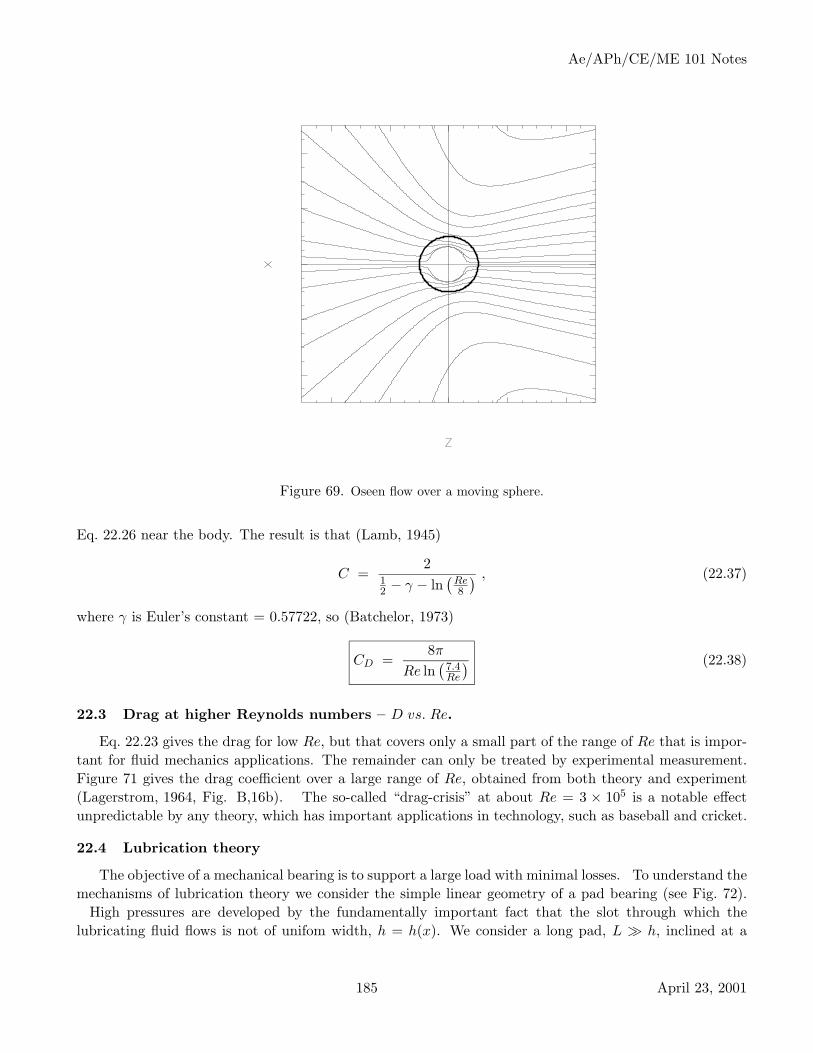
Ae/APh/CE/ME 101 Notes
Figure 69. Oseen flow over a moving sphere.
Eq. 22.26 near the body. The result is that (Lamb, 1945)
C =2
12 − γ − ln
(Re8
) , (22.37)
where γ is Euler’s constant = 0.57722, so (Batchelor, 1973)
CD =8π
Re ln(
7.4Re
) (22.38)
22.3 Drag at higher Reynolds numbers – D vs. Re.
Eq. 22.23 gives the drag for low Re, but that covers only a small part of the range of Re that is impor-tant for fluid mechanics applications. The remainder can only be treated by experimental measurement.Figure 71 gives the drag coefficient over a large range of Re, obtained from both theory and experiment(Lagerstrom, 1964, Fig. B,16b). The so-called “drag-crisis” at about Re = 3 × 10⁵ is a notable effectunpredictable by any theory, which has important applications in technology, such as baseball and cricket.
22.4 Lubrication theory
The objective of a mechanical bearing is to support a large load with minimal losses. To understand themechanisms of lubrication theory we consider the simple linear geometry of a pad bearing (see Fig. 72).
High pressures are developed by the fundamentally important fact that the slot through which thelubricating fluid flows is not of unifom width, h = h(x). We consider a long pad, L À h, inclined at a
185 April 23, 2001

Ae/APh/CE/ME 101 Notes
Figure 70. Oseen flow as seen in a body-fixed coordinate system.
Figure 71. Sphere drag over eight orders of magnitude in Reynolds Number.
small angle α ¿ 1. The combination of a moving block plus a confined channel yields a superposition of
186 April 23, 2001

Ae/APh/CE/ME 101 Notes
Figure 72. A pad bearing in plane geometry
Poiseuille and Couette flows,
u(x, y) = − 1µ
(−dp
dx
)y(h − y)
2+ U
h − y
h. (22.39)
This solution can be written in terms of the volume flux
Q =∫ h
0u dy = −dp
dx
h3
12µ+
Uh
2, (22.40)
yielding for the pressure gradient,
dp
dx(x) = 6µ
(U
h2(x)− 2Q
h3(x)
). (22.41)
Withα = −dh
dx(22.42)
the pressure integrates to
p − p1 =∫ h2
h1
dp
dx
dx
dhdh =
6µ
α
[U
(1h− 1
h1
)+ Q
(1h2
− 1h2
1
)]. (22.43)
To evaluate the load-carrying pressure that is developed in the bearing, it is necessary to complete the flowloop. The flow connects over the top where the flow area is large, so there is little resistance, and p1 = p2.Using this in Eq. 22.43 evaluated at p2 gives
Q = Uh1h2
h1 + h2. (22.44)
Substituting for Qin Eq. 22.43 gives
p − p1 =6µU
α
(h1 − h)(h − h2)h2(h1 + h2)
. (22.45)
As drawn above, h1 > h > h2, so p > p1 . But p1 = p2, so there must be a maximum pressure. FromEqs. 22.41 and 22.44, it occurs at
h =2h1h2
h1 + h2, (22.46)
187 April 23, 2001

Ae/APh/CE/ME 101 Notes
with the result
(p − p1)max =6µU
α
(h1 − h2)2
4h1h2(h1 + h2). (22.47)
An optimal bearing design generates a large bearing pressure, so in general
∆h
h1= O(1) , (22.48)
andα =
∆h
L∼ h1
L. (22.49)
Thus
∆pmax ∼ µUL
h21
. (22.50)
An effective bearing runs with large µ, U and L, and small h1. However, more important is its “efficiency,”that is the bearing load versus the frictional force. The total normal force supported is
Fn =∫ h2
h1
∆p
αdh ∼ µUL
h21
, (22.51)
while the tangential forces are of order
Ft =∫ L
0µ
du
dydx ∼ µUL
h1. (22.52)
Therefore,Tangential
Normal∼ h1 , (22.53)
so the relative frictional forces are reduced as the bearing gap is reduced. This explains why bearings mustbe machined very accurately to remove roughness and ensure that the surfaces can be very close withouttouching.
188 April 23, 2001

Ae/APh/CE/ME 101 Notes
23 Turbulence
23.1 Reynolds Averaging
In this section we discuss the equations for incompressible turbulent shear flow, for simplicity, witha steady mean flow. In an attempt to get managable equations, the flow is decomposed into mean andfluctuating components
u = u + u′ ; u′ = 0 (23.1)(∂u
∂x
)=
∂u
∂x, (23.2)
etc. We use Cartesian tensor notation.
The continuity equation is∂(ui + u′
i)∂xi
= 0 , (23.3)
which, when averaged gives∂ui
∂xi= 0 =⇒ ∂u′
i
∂xi= 0 . (23.4)
The mean and fluctuating components are separately incompressible.
The momentum equation, in conservation form, is
∂(ui + u′i)
∂t+
∂(ui + u′i)(uj + u′
j)∂xj
= −∂(p + p′)∂xi
+ ν∂2(ui + u′
i)∂xj
2. (23.5)
When averaged, the first term gives nothing, because the mean flow is steady. The second term is
∂ui uj
∂xj+
∂uiu′j
∂xj+
∂uju′i
∂xj+
∂u′iu
′j
∂xj. (23.6)
When averaged, only the first and last terms contribute. Thus, the momentum equation becomes
∂ui uj
∂xj+
∂u′iu
′j
∂xj= −1
ρ
∂p
∂xi+ ν
∂2ui
∂xj2
. (23.7)
A new term and new mechanism for momentum transport arises. When moved to the r.h.s., it becomes astress, the Reynolds stress,
τij = u′iu
′j . (23.8)
Thus, using the averaged continuity equation,
uj∂ui
∂xj= −1
ρ
∂p
∂xi− ∂u′
iu′j
∂xj+ ν
∂2ui
∂xj2
. (23.9)
u′iu
′j is an unknown quantity involving the product of velocities. An equation for the first moment of
velocity (the momentum) is expressed in in terms of an unknown second moment (velocity2). It can nowbe seen that this procedure leads to an endless chain: Each equation, when averaged, will be in terms ofunknown higher-order products. The only recourse is to at some stage make an assumption which closesthe system (or to solve the full Navier-Stokes equations from the outset!).
189 April 23, 2001

Ae/APh/CE/ME 101 Notes
A shear flow producing positive vorticity is expected to result in a positive correlation u′iu
′j , because
fluctuation flux upward v′ > 0 will carry momentum from high-velocity to low-velcocity regions, u′ > 0.This is analogous to the way molecules with random thermal velocities convect momentum in shear flowsby molecular diffusion. Splitting the ‘viscous Bernoulli equation’ (Eq. 3.30), in Cartesian tensor notationthere results,
∂ui
∂t= − ∂
∂xj
(p
ρ+
u2
2+
u′2
2
)+ εijk (uj ωk + u′
jω′k) + ν
∂2ui
∂xj2
, (23.10)
where εijk is the permutation operator, so that
εijk uj ωk = (u × ω)i . (23.11)
The cross-product terms u′jω
′k represent the cross-stream derivatives of the Reynolds stress. For example,
in 2-D flow with 3-D turbulence, they are
v′ω′z − w′ω′
y = − ∂u′v′
∂y, (23.12)
where the = means that we neglect normal stress (turbulent ‘pressure’) in favor of shear (Reynolds) stress.In 2D flow v′ω′
z could be represented in terms of a mixing length and the gradient ∂u/∂y (a ‘mixing lengththeory of vorticity transfer’, Tennekes & Lumley, p80), but w′ω′
y would have to be represented by someout-of-plane gradient, which is impossible in 2D. By differentiating the rhs of Eq. 23.12, represented interms of a mixing length, u′`∂u/∂y, it can be seen that the ω′
y term must be associated with ∂`/∂y, i.e.,with a change of scale, or vortex stretching. This is called the ‘vortex stretching force’ (because the termis on the rhs of the momentum equation!) (Tennekes & Lumley, p. 80).
Splitting Eq. 2.57 gives the turbulent vorticity equation,
uj∂ωi
∂xj= −u′
j
∂ω′i
∂xj+
12
ω′jε
′ij +
12
ωj εij + ν∂2ωi
∂xj2
(23.13)
= −∂u′jω
′i
∂xj+
∂ω′ju
′i
∂xj+
12
ωj εij + ν∂2ωi
∂xj2
, (23.14)
where the second form follows because, since (div curl) = 0, the vorticity, both mean and fluctuating, isdivergence free. The first term on the right is analogous to the Reynolds stress, and the second term is thegain of mean vorticity due to the stretching of fluctuating vorticity by fluctuating strain.
To study vorticity interactions, one needs equations equivalent to the mean and fluctuationg kineticenergy equations,
uj∂ 1
2ωi2
∂xj= − ∂ωi ω′
iu′j
∂xj︸ ︷︷ ︸transport
+ u′jω
′i
∂ωi
∂xj︸ ︷︷ ︸production
+ ωi ωjεij︸ ︷︷ ︸stretching
+ ωi ω′jε
′ij︸ ︷︷ ︸
stretching
(23.15)
+ ν∂2 1
2ωi2
∂xj2︸ ︷︷ ︸
viscoustransport
− ν
(∂ωi
∂xj
)2
︸ ︷︷ ︸viscous
dissipation
.
190 April 23, 2001

Ae/APh/CE/ME 101 Notes
uj∂ 1
2ω′i
2
∂xj= − u′
jω′i
∂ωi
∂xj︸ ︷︷ ︸production
+ − 12
∂u′jω
′i2
∂xj︸ ︷︷ ︸transport
+ ω′iω
′jε
′ij︸ ︷︷ ︸
stretching
+ ω′iω
′j εij︸ ︷︷ ︸
stretching
+ ωj ω′iε′ij︸ ︷︷ ︸
stretching
(23.16)
+ ν∂2 1
2ω′i
2
∂xj2︸ ︷︷ ︸
viscoustransport
− ν
(∂ω′
i
∂xj
)2
︸ ︷︷ ︸viscous
dissipation
.
23.2 Closure – Turbulence Models
We outline the ideas behind two historical simple models.
23.2.1 Eddy Viscosity Model.
The idea behind the eddy viscosity is that, as with molecular transport, turbulent transport is drivenby the mean velocity gradient. This was the first of many gradient-transport models. Thus, in a planeshear flow,
u′v′ = νT∂u
∂y. (23.17)
Clearly, νT must be determined empirically, and, unfortunately, it turns out to be far from constant. Forexample, it must go to zero at any wall, where (u′, v′) = 0.
23.2.2 Prandtl’s Mixing Length Theory.
Prandtl exploited the analogy between molecular and turbulent transport, representing the interactionbetween two fluid particles as the interaction between two molecules. In a plane shear flow, kinetic theorystates that a molecule moving downward one mean-free-path Λ in its thermal motion from a high-speedregion u + ∆u at y + ∆y to a low-speed region u at y transports excess momentum m∆u, where m is itsmass. The number of molecules doing so per unit time per unit area, on average, is nc/4. Thus, moleculartransport of momentum gives
τ ∼ m∆unc
4. (23.18)
The density is ρ = mn, and ∆u = Λ∂u/∂y, so
τ ∼ ρcΛ4
du
dy. (23.19)
Therefore, the molecular kinetmatic viscosity is
ν =cΛ4
. (23.20)
Note that, using the relation between collision cross section σ and Λ
Λ =1
nσ, (23.21)
191 April 23, 2001

Ae/APh/CE/ME 101 Notes
the temperature dependence of µ can be exhibited
µ ∼ mc(T )4σ(T )
. (23.22)
The application to turbulence comes in associating the vertical thermal velocity with v′ and the meanfree path with a “mixing length” l,
νT = kv′l . (23.23)
23.2.3 Other closure schemes
Another approach to closing the Reynolds averaged equations is to develop equations for higher-ordermoments, which can be used to evaluate the Reynolds stress. These equations will, in turn, have evenhigher moments, which must be modeled. The hope is that with more equations, and with models for onlyvery high order correlations, the physics might be represented more accurately. Intuitively, the idea is thatthe approximations are being pushed to smaller and smaller scales.
Some of the equations that provide fuel for this activity are given below.
Mean Kinetic Energy
ρDu2/2
Dt+ ρ uj
∂u2
∂xj=
∂
∂xj
(−puj︸ ︷︷ ︸
pressurework
+ η εijui︸ ︷︷ ︸viscous
transport
− ρ u′iu
′j ui︸ ︷︷ ︸
Reynoldsstress
transport
)− Φ︸︷︷︸
dissipation
+ ρ u′iu
′j
εij
2︸ ︷︷ ︸turbulenceproduction
(23.24)
Turbulent Kinetic Energy – Steady Flow
ρ uj∂u′2
∂xj= − ∂
∂xj
(−p′uj︸ ︷︷ ︸
pressurework
+12ρ u′
i2uj︸ ︷︷ ︸
turbulenttransport
− η u′iε′ij︸ ︷︷ ︸
viscoustransport
)− ρ u′
iu′j
εij
2︸ ︷︷ ︸turbulenceproduction
− η
2ε′ijε
′ij︸ ︷︷ ︸
viscousdissipation
(23.25)
Turbulent dissipation ≡ ε =η
2ε′ijε
′ij (23.26)
Energy Equation
∂T
∂t+ uj
∂T
∂xj= −∂u′
jT′
∂xj− κ
∂2T
∂xj2
(23.27)
qj = cpρ u′jT
′ − k∂T
∂xj(23.28)
192 April 23, 2001

Ae/APh/CE/ME 101 Notes
23.3 Turbulent Scales
The important scales of turbulence are defined in this section. Integral scale, `
(Example: transport scale transverse to the free-stream)Size of the “‘eddies,” at which turbulent convection balances inertia (`/L = u′/U).
` =1
v′2
∫ ∞
0v′(y + η) v′(y) dη (23.29)
Kolmogorov scale, µ
The smallest (rapidly adjusting) scale of turbulence, at which dissipation occurs.Dimensional analysis: 2 variables (ν, ε) to make a length (ε = turbulent dissipation; Eq. 23.26).
µ =(
ν3
ε
) 14
, (23.30)
from which,
τ =(ν
ε
) 12 (23.31)
u = (νε)14 (23.32)
Re ≡ µu
ν= 1 (23.33)
Taylor microscale, λ
Time scale of strain-rate fluctuations (τT ).Take
ε =1ρ
(η
2ε′ijε
′ij
)∼ ν
(∂u′
∂x
)2
≡ νu′2
λ2, (23.34)
where u′ is a typical velocity fluctuation scale. There is actually no reason to associate the velocity scaleu′ with ε, but the corresponding time,
τT ∼ λ
u′ , (23.35)
is well defined.
193 April 23, 2001

Ae/APh/CE/ME 101 Notes
24 Buoyancy Effects
The study of buoyancy effects often specializes to approximations more applicable to atmospheres(gases) than to oceans (liquids). Thus in this section we talk mostly about gases, but from time to timewrite equations applicable also to liquids.
24.1 Hydostatic compressible gas
In a neutrally stable atmosphere with no motion
ds
dz= 0 . (24.1)
Thus for a perfect gas,p ∼ ργ ∼ T
γγ−1 , (24.2)
or, in terms of a reference state (po, ρθ, θ),
p
po=
(ρ
ρθ
)γ
=(
T
θ
) γγ−1
. (24.3)
θ = T
(p
p0
)− γ−1γ
(24.4)
ρθ = ρ
(p
p0
)− 1γ
(24.5)
ρθ and θ are the potential density and temperature, respectively, and are the density and temperature ofthe fluid at pressure p0. In a neutrally stable atmosphere they remain constant when a fluid particle movesupward or downward (a more precise statement will be made later).
Differentiating Eqs. 24.4 and 24.5, and using the perfect gas equation of state (dρ/ρ = dp/p = −dT/T ),
dθ
θ=
dT
T− γ − 1
γ
dp
p(24.6)
dρθ
ρθ=
dρ
ρ− 1
γ
dp
p(24.7)
= −(
dT
T− γ − 1
γ
dp
p
), (24.8)
so
1θ
dθ
dz= − 1
ρθ
dρθ
dz=
1T
dT
dz− γ − 1
γ
1p
dp
dz. (24.9)
The z-momentum equation for a stationary fluid gives dp/dz = −ρg, so
1θ
dθ
dz=
1T
(dT
dz+
g
cp
). (24.10)
194 April 23, 2001

Ae/APh/CE/ME 101 Notes
For a neutrally stable atmosphere, ds/dz = dθ/dz = 0, so
dT
dz= − g
cp. (24.11)
This is the so-called adiabatic lapse rate. However, note that the stipulation was that the entropy beconstant. That is a stronger requirement than that any changes be adiabatic (no heat transferred fromoutside the system). Constant entropy means that the process be adiabatic and reversible, so the motionsintroduced to test the stability must be made reversibly.
For the neutrally stable atmosphere, the temperature profile is
T = T0 − gz
cp. (24.12)
The density profile is given by
1ρ
dρ
dz=
1γp
dp
dz= − g
γRT (z)=
g
a2, (24.13)
where a is the sound speed. The charcteristic depth a2/g is called the scale height,
Λ =a2
g. (24.14)
Small amplitude long wavelength gravity waves travel at a speed c given by Froude number based on depth(Λ) unity,
Fr =c√gΛ
=c
a= M = 1 , (24.15)
so the waves also travel at Mach 1 and are therefore also acoustic waves. Substituting the temperaturevariation Eq. 24.12 into Eq. 24.13 and integrating gives
ρ = ρ0
(gz
1 − cpT0
) 1γ−1
. (24.16)
24.2 Boussinesq approximation (Spiegel &Veronis, 1960)
The Boussinesq approximation applies to a thin layer (much thinner than the scale height of thesystem) of compressible fluid within which density fluctuations are no larger than the change of densitydue to gravitational effects. Dissipation in a gas scales as M2/Re and so is small for atmospheric motions.
The pressure, density and temperature are represented by sums of the spatial mean value, the hydro-statically varying component, and the flow-driven component,
p = p + ps(z) + p′(x, y, z, t) (24.17)
ρ = ρ + ps(z) + ρ′(x, y, z, t) (24.18)
T = T + Ts(z) + T ′(x, y, z, t) (24.19)
The scale height for each is, for example,
Λp =∣∣∣∣1p dps
dz
∣∣∣∣−1
. (24.20)
The Boussinesq approximation is:
195 April 23, 2001

Ae/APh/CE/ME 101 Notes
1. The layer thickness D is very small compared to the scale height Λ
D ¿ Λρ (24.21)D
ρ
dρs
dz¿ 1 . (24.22)
Integrating this over the layer gives for the gravitational density changes there,
∆ρs
ρ¿ 1 . (24.23)
2. The perturbation density is no larger than the gravitational changes
ρ′
ρ≤ ∆ρs
ρ. (24.24)
24.2.1 Equation of State
ρ(p, t) is expanded in a Taylor series about its mean value
ρ = ρ +(
∂ρ
∂T
)p
(T − T ) +(
∂ρ
∂p
)T
(p − p) + . . . (24.25)
= ρ[1 + kT (p − p) − α(T − T )
]+ . . . , (24.26)
where the isothermal compressibility and the coefficient of thermal expansion are
kT =1ρ
(∂ρ
∂p
)T
(24.27)
α = −1ρ
(∂ρ
∂T
)p
. (24.28)
Collecting terms of equal magnitude in the resulting equation,
1 +ρs + ρ′
ρ= 1 + kT (ps + p′) − α(Ts + T ′) , (24.29)
gives
ρs = ρ (kT ps − α Ts) (24.30)
ρ′ = ρ (kT p′ − α T ′) , (24.31)
24.2.2 Continuity Equation
The continuity equation (2.13) expands to
∂ρ′
∂t+ u · ∇(ρs + ρ′) + ρ∇ · u = 0 (24.32)(
∂∂t + u · ∇)
(ρs + ρ′)ρ
+ρ
ρ∇ · u = 0 . (24.33)
From the inequalities Eqs. 24.23 and 24.24 the first term is small, so there results
∇ · u = 0 (24.34)
196 April 23, 2001

Ae/APh/CE/ME 101 Notes
24.2.3 Momentum Equation
For no motion, the vertical component of the momentum equation is
dps
dz= −gρ − gρs . (24.35)
Thus, in the full momentum equation Eq. 3.19,
∇p = ∇ps + ∇p′ (24.36)
= −gρ − gρs + ∇p′ , (24.37)
where g points in the z-direction. Therefore,
−∇p − gρ = −∇p′ − gρ′ . (24.38)
Using Eqs. 24.34 and 24.38, the momentum equation becomes
ρDu
Dt= −∇p′ − ρ′g + µ∇2u , (24.39)
The gravity term in the momentum equation is actually of a smaller order than the others, but it mustbe kept, or there would be no buoyancy effect. It means that the acceleration of gravity is always muchlarger than the acceleration of fluid driven by gravity effects.
The vertical component of the pressure and gravity terms in Eq. 24.39 are
−1ρ
∂p′
∂z− ρ′
ρg
= −1ρ
[∂p′
∂z+ ρkT g p′
]− αg T ′ .
(24.40)
Now
ρkT g ≡ 1H
= O(
1Λρ
)(24.41)
is the inverse of a characteristic length, of the order of the scale height. Therefore,
∂p′
∂z∼ p′
DÀ p′
H, (24.42)
so the vector momentum equation reduces to
Du
Dt= −∇p′
ρ− αT ′g + ν∇2u . (24.43)
24.2.4 Energy equation
Eq. 3.13 is expanded, as above. For no flow it is
k∇2Ts + ρQs = 0 . (24.44)
Subtracting this from the full equation gives
ρcv
(∂T ′
∂t+ u · ∇T
)= −p∇ · u + k∇2T ′ + ρQ′ , (24.45)
197 April 23, 2001

Ae/APh/CE/ME 101 Notes
where Q′ = Q−Qs, and the dissipation has been neglected. From Eqs. 24.23 and 24.24 we take in the firstterm on the right p = p + ps + p′ .= p. To the same approximation, Eq. 24.31 is
ρ′ = −ρ α T ′ . (24.46)
Using that and Eq. 24.30 in 24.32 gives
p∇ · u = −pD
Dt
[kT ps − α(Ts + T ′)
]. (24.47)
Now, since ps = ps(z),Dktps
Dt= kT w
dps
dz= −kT wgρ , (24.48)
where the first approximation to Eq. 24.35 has been used for the last equality. The result is
−p∇ · u = −pD
Dt
[α(Ts + T ′)
]+ pkT wgρ , (24.49)
and Eq. 24.45 becomes
ρ
(cv +
p α
ρ
) (∂T ′
∂t+ u · ∇T
)+ pkT wgρ = k∇2T ′ + ρQ′ , (24.50)
For gases α = 1/T and kT = 1/p, so the first parentheses is cp, and the result can be written
DT ′
Dt+ w
(dTs
dz+
g
cp
)= κ∇2T ′ +
Q′
cp. (24.51)
Note that the adiabatic lapse rate emerges as an important parameter in the dynamical equations.
24.3 Axisymmetric Buoyant Plumes
The simplest plume is generated by a steady point source of heat. We analyze plumes making theBoussinesq approximation, and assuming constant transport properties, constant ambient temperatureT∞ (but at the same time neutrally buoyant atmosphere), and thin-layer approximation.
The scales of the velocity and thermal fields will in general be different, because the diffusivities ofmomentum (viscosity) and heat (conductivity) or mass (diffusion coefficient) are different. In this treatmentwe attempt to distinguish these scales as δ and δT , respectively, and also the corresponding entrainmentvelocities V and VT . The scale that is largest, δ or δT , will in general set the scale of the flow. Thus forlarge Pr (viscous liquids) the scale will be δ and for small Pr (liquid metals) the scale will be δT ,
24.3.1 Laminar Plumes
The equations of motion, and their order of magnitude scaling, are then
∂ru
∂x︸︷︷︸Ux
+∂rv
∂r︸︷︷︸Vδ
= 0 (24.52)
198 April 23, 2001

Ae/APh/CE/ME 101 Notes
u∂u
∂x︸︷︷︸U2
x
+ v∂u
∂r︸︷︷︸UVδ
= gα(T − T∞)︸ ︷︷ ︸gαT
+ν
r
∂
∂r
(r∂u
∂r
)︸ ︷︷ ︸
νUδ2
(24.53)
u∂T
∂x︸ ︷︷ ︸UTx
+ v∂T
∂r︸︷︷︸VT TδT
=κ
r
∂
∂r
(r∂T
∂r
)︸ ︷︷ ︸
κT Tδ2T
. (24.54)
x is vertical, as is the gravity vector, and r is the transverse coordinate. Note that separate lateral scales δ
and δT , and corresponding lateral velocities V and VT , have been assumed for viscous and thermal effects.The boundary conditions are
r = 0 ; v =∂
∂r= 0
r −→ ∞ ; u −→ 0T −→ T∞
(24.55)
The buoyancy flux (here the heat flux) is defined as
Q ≡∫ ∞
0ρcp(T − T∞)u 2πr dr︸ ︷︷ ︸
ρcpTUδ2T
. (24.56)
It is the constant heat input driving the plume.
The consequences of scaling are:As with jets, from the continuity equation, the thin-layer scaling,
U
x∼ V
δ; (24.57)
from the first and fourth terms in the momentum equation the requirement for high Reynolds number,
Uδ
ν∼ x
δ; (24.58)
and a new result from the gravitational term,
gαT ∼ ν2x
δ4; (24.59)
from the first and third terms in the energy equation,
δT ∼√
κx
U∼ Pr−
12 δ ; (24.60)
and from the second and third terms,
VT ∼ κ
δT∼ Pr−
12 V . (24.61)
199 April 23, 2001

Ae/APh/CE/ME 101 Notes
It is useful to simplify the bookeeping for distinguishing between the large and small Pr cases byintroducing simple interpolation formulas so only one scale need be considered. This is accomplished byinserting a factor 1 + Pr/Pr at appropriate locations.
δ ∼(
νx
U
1 + Pr
Pr
) 12
V ∼ ν
δ
1 + Pr
Pr.
(24.62)
Combining Eqs. 24.56, 24.58 and 24.60 gives
Q
cpρ∼ TUδ2
T ∼ TUδ2 1 + Pr
Pr∼ Tνx
1 + Pr
Pr. (24.63)
Thus,
T ∼ Q
cpρ ν x
Pr
1 + Pr. (24.64)
The temperature perturbation decreases as 1/x. Continuing by applying Eqs. 24.59 to 24.63,
Q
cpρ∼ ν3
gα
x2
δ4
1 + Pr
Pr, (24.65)
so
δ
x∼
(cpρ
Qα
ν3
g
1 + Pr
Pr
) 14
x− 12 . (24.66)
The plume diameter increases with the expected parabolic behavior. Now, the Grashof number is
Grx ≡ αTgx3
ν2. (24.67)
Using the scaling for T , we have, for plumes,
Grx =gαQ
cpρ
x2
ν3
Pr
1 + Pr. (24.68)
Thus, Eq. 24.66 is the same thing asδ
x∼ (Grx)−
14 . (24.69)
It remains to determine the dependence of U(x) and the momentum flux J(x),
J =∫
ρu2 2πr dr︸ ︷︷ ︸ρU2δ2
. (24.70)
Putting Eq. 24.66 in 24.58 gives
U ∼(
gαQg
cpµ
Pr
1 + Pr
) 12
. (24.71)
200 April 23, 2001

Ae/APh/CE/ME 101 Notes
The characteristic (e.g., centerline) velocity is constant. Thus, the momentum must increase as the plumegrows. Eq. 24.70 gives
J ∼(
gαQµ
cp
Pr
1 + Pr
) 12
x , (24.72)
so the momentum flux increases linearly with x.
A comparison of the behaviors of momentum-driven laminar jets and buoyancy-driven laminar plumesis given in the table below.
Plume JetConserved Q J
U
(gαQg
cpµ
Pr
1 + Pr
) 12 J/ρ
νxEntrainmentdm
dx∼ ρV δ µ
1 + Pr
Prµx
J
(gαQµ
cp
Pr
1 + Pr
) 12
x const
Q const —
Similarity.Define the similarity variable
R =r
δ(x), (24.73)
the stream functionψ(x, r) = νxf(R) , (24.74)
the nondimensional temperature
θ(R) =T − T∞
T0(x) − T∞, (24.75)
and assume the behavior of T0(x)−T∞ given in Eq. 24.64. Then the buoyancy flux becomes (see Eqs. 16.23)
Q = 2πρcp(T0(x) − T∞)νx
∫ ∞
0θf ′ dR , (24.76)
and the momentum and energy equations reduce to two coupled ordinary differential equations,
f ′′′ + (f − 1)(
f ′
R
)′+ Rθ = 0 (24.77)
(Rθ′)′ + Pr (fθ)′ = 0 . (24.78)
Since Pr = const, the energy equation can be integrated twice to give
θ(R) = e−Pr∫ R0
fR
dR . (24.79)
When this is substituted into the momentum equation there results an ordinary integro-differential equa-tion. After the solution for f is obtained, the lateral velocity is given by
v =ν
δ(x)
(f ′
2− f
R
). (24.80)
The solutions will yield the numerical constants multiplying the results of the previous section.
201 April 23, 2001

Ae/APh/CE/ME 101 Notes
24.3.2 Buoyancy driven by density variations (e.g., concentration)
Buoyancy can equally well be induced by variations of the concentration of different fluids or con-stituents. In this case transport of momentum by viscous diffusion is important as above, but replacing thesmoothing of temperature by diffusion of heat, there now arises concentration smoothing by mass diffusion.The corresponding equation to replace the energy equation is mass conservation of one of the constituents.If written in terms of the density perturbation ρ∞−ρ that equation can be written down by analogy to theenergy equation, which is what we do here. The only fundamental change is that the diffusivity changesfrom κ to D, the diffusion coefficient. The equations in conservation form are,
∂ru
∂x+
∂rv
∂r= 0 (24.81)
∂u2
∂x+
1r
∂ruv
∂r= g
ρ∞ − ρ
ρ0+
ν
r
∂
∂r
(r∂u
∂r
)(24.82)
∂(ρ∞ − ρ)u∂x
− udρ∞dx
+1r
∂r(ρ∞ − ρ)v∂r
=D
r
∂
∂r
(r∂(ρ∞ − ρ)
∂r
). (24.83)
The buoyancy flux is
F =∫ ∞
0gρ∞ − ρ
ρ0u 2πr dr (24.84)
24.3.3 Laminar plumes in stratified atmospheres (Morton 1967)
A stratified atmosphere adds sufficient complexity that similarity can no longer be expected. Thus,the problem is treated by analyzing the integrated equations of motion (see Sec. 20.1). Plumes involveboth viscous diffusion and thermal diffusion, so, as discussed in Sec. 24.3, it is necessary to account for twolateral scales, δ and δT . In this section we consider the case Pr ≥ 1, so we take δT ∼ δ/
√Pr. Multiplying
the continuity equation by r dr and integrating across the plume gives (see Eq. 20.18),
d
dx
∫ δ
0ur dr = −(rv)∞ . (24.85)
The term on the lhs can be written in terms of the stream function ψ = νx f(R), where R = r/δ,∫ δ
0ur dr = νxf∞ , (24.86)
so the entrainment is−(rv)∞ = νf∞ . (24.87)
f∞ is thought of as the entrainment coefficient.
Integrating Eq. 24.53, cast into conservation form, gives
d
dx
∫ δ
0u2r dr =
∫ δT
0gα(T − T∞)r dr . (24.88)
In the energy equation 24.54 T is the perturbation temperature, which here we write explicitly as T (x, r)−T∞(x). It is necessary to account for the fact that here the base temperature T∞(x) is a function of x;doing so, and then using the continuity equation to put in conservation form, Eq. 24.54 becomes
∂u(T − T∞)∂x
+ udT∞dx
+1r
∂rv(T − T∞)∂r
=κ
r
∂
∂r
(r∂T
∂r
). (24.89)
202 April 23, 2001

Ae/APh/CE/ME 101 Notes
In integrating this equation we adopt the case dT∞/dx = const, so it comes out of the integral of thesecond term, and Eq. 24.86 can be used. Thus,
d
dx
∫ δT
0u(T − T∞)r dr +
dT∞dx
f∞νx = 0 . (24.90)
This equation can be integrated wrt x to obtain∫ δT
0u(T − T∞)r dr =
Q
2πcpρ− dT∞
dxf∞ν
x2
2, (24.91)
where the first term on the right is the constant of integration evaluated using Eq. 24.56.
24.3.4 Approximate Integral Method
Approximate solutions to Eqs. 24.85, 24.88 and 24.91 can be obtained by assuming a form of thevelocity profile u(r) and carrying out the integrations. The simplest profile is the top-hat profile, whichgives for the differential form,
d
dx
uδ2
2= f∞ν (24.92)
d
dxu2δ2 = gα(T − T∞)δ2
T (24.93)
d
dx
u(T − T∞)δ2T
2= −dT∞
dxf∞νx , (24.94)
and after integrating wrt x,
uδ2
2= f∞νx (24.95)
d
dxu2δ2 = gα(T − T∞)
δ2
Pr(24.96)
u(T − T∞)δ2
Pr=
Q
πcpρ− dT∞
dxf∞νx2 , (24.97)
where δ2T has been replaced by δ2/Pr, i.e., Pr > 1. Substituting the third equation into the second
equation to eliminate T − T∞, using the first to eliminate δ, and multiplying by ux, gives
uxdux
dx=
gα
2f∞ν
(Q
πcpρ− dT∞
dxf∞νx2
)x , (24.98)
which integrates to
u2 = gα
(Q
2πcpρf∞ν− 1
4dT∞dx
x2
)(24.99)
This confirms that similarity is lost, but it has the interesting result that the plume stops at a finite altitudexm
xm =
(2Q
πcpρf∞ν dT∞dx
) 12
. (24.100)
u(x) then becomesu2 = u2
0
[1 − (x/xm)2
], (24.101)
203 April 23, 2001

Ae/APh/CE/ME 101 Notes
where
u0 =(
gαQ
2πf∞cpµ
) 12
(24.102)
is the constant velocity of plumes in a uniform atmosphere. Putting u(x) into the continuity equation andsolving for δ gives
δ2 = δ20
x/xm
[1 − (x/xm)2]12
;δ20
xm=
2f∞ν
u0. (24.103)
Finally, the temperature is given by
T − T∞ =12
dT∞dx
xm
(xm
2x− x
xm
)(24.104)
The behavior of these parameters is shown in Fig. 73. In the limit when the atmosphere becomes uniform,
Figure 73. Variation of the velocity, radius and temperature of a laminar plume in a stratified atmosphere
xm → ∞, and the results approach those obtained in Sec. 24.3.1.
24.4 Turbulent Plumes (Morton et al. 1956)
At high enough Reynolds numbers plumes become unstable and transition to turbulence. At veryhigh Re when the turbulence is strong molecular diffusivity is unimportant and is replaced by turbulenttransport. If an eddy viscosity model, or some other possibly more sophisticated gradient-transport model,us used, the equations integrate to give the same form as in the laminar case. In the laminar case ν andκ do not appear in the momentum and energy integral equations, only ν in the continuity equation. Withturbulence, it’s the same, so it becomes necessary to model the entrainment term.
After the same procedure as was used above is applied to Eqs. 24.81–24.84, the equations for a top-hatprofile plume are,
d uδ2
dx= −2(rv)∞ = 2αδu (24.105)
204 April 23, 2001

Ae/APh/CE/ME 101 Notes
d u2δ2
dx= g
ρ∞ − ρ
ρ0δ2 (24.106)
d (ρ∞ − ρ)uδ2
dx=
d ρ∞dx
uδ2 , (24.107)
The last equality in Eq. 24.105 is the entrainment hypothesis, namely, that (rv)∞ is proportional, withproportionality constant α, to the volume flux per unit length of the plume. This hypothesis is based ondimensional reasoning and the idea that fluid is ingested into the plume at a rate dependent on the axialvelocity.
24.4.1 Uniform atmosphere
For a uniform atmosphere the term on the right of Eq. 24.107 is zero, so
F = gρ∞ − ρ
ρ0uδ2 = const = F0 . (24.108)
Thus DefiningV = uδW = uδ2 ,
(24.109)
The continuity and momentum equations equations become
dW
dx= 2αV (24.110)
dV 2
dx=
F0
u= F0
W
V 2. (24.111)
Eliminating W from the momentum equation by differentiation gives
d2V 4
dx2= 4F0αV . (24.112)
This equation can be solved by letting v = V 4 and p = dv/dx, resulting in
dp
dx= p
dp
dv= 4F0αv
14 . (24.113)
Integrating once to get p(v) = dv/dx and again to get v(x) gives finally for V (x) (and by integration W (x))
V =(
910
F0α
) 13
x23 (24.114)
W =3α
5
(910
F0α
) 13
x53 . (24.115)
The original unknowns follow immediately
δ =3α
5x
u =53α
(910
F0α
) 13
x− 13
g′ = gρ∞ − ρ
ρ0=
5F0
3α
(910
F0α
) 13
x− 53 .
(24.116)
Because of the entrainment term, the turbulent plume behaves very differently than the laminar plume. δ
grows much more rapidly and so the velocity decreases rather than being constant.
205 April 23, 2001

Ae/APh/CE/ME 101 Notes
24.4.2 Nonuniform atmosphere
For a nonuniform atmospher there is one more unknown, F (x). The equations become
dW
dx= 2αV (24.117)
dV 2
dx=
F0
u= F0
W
V 2(24.118)
dF
dx= −WG . (24.119)
Defining the nondimensional variables
ξ = α12 F
− 14
0 G38 x (24.120)
v = F− 1
20 G
14 V (24.121)
w = α− 14 F
− 34
0 G58 W (24.122)
f =F
F0, (24.123)
the equations become
dw
dξ= v (24.124)
dv4
dξ= fw (24.125)
df
dξ= −w , (24.126)
which are in the form for numerical computaion. The numerical solution yields the behavior with ξ, andtherefore u(x), δ(x), g′(x) and F (x). The numerical value of ξm at which the velocity vanishes is also aresult of the numerical computation. The dimensional height xm of the plume is given in terms of thestrength F0 of the plume, the atmospheric lapse rate G, and a fundamental fluid mechanical property, theentrainment coefficient α. Morton et al. (1956) conducted laboratory experiments to determine α, withthe result α = 0.093. Then the computed height of the plume was found to be
xm = 3.79 F140 G− 3
8 . (24.127)
24.5 Stratified Flows
24.5.1 Shallow water waves
The theory of shallow water waves describes the motion of a stably stratified thin layer of dense fluid.“Shallow” means that the layer depth h(x, t) is small compared to the lateral scale of the flow λ. Aconsequence is that vertical accelerations must be very small
Dw
Dt= 0 . (24.128)
206 April 23, 2001

Ae/APh/CE/ME 101 Notes
Here we take the fluid to be incompressible (e.g., water), and for simplicity consider a two-dimensionalplane flow (x, z). Also, the fluid is inviscid. We first consider the simple case in which the light overlyingfluid is of zero density. Thus the equations of motion for the dense layer are
∇ · u = 0 (24.129)
ρDu
Dt= −∇p − ρg . (24.130)
or∂u
∂x+
∂w
∂z= 0 (24.131)
ρDw
Dt= −∂p
∂z− ρg (24.132)
ρDu
Dt= −∂p
∂x. (24.133)
The boundary conditions are
p = 0∂h
∂t+ u
∂h
∂x= w
z = h (24.134)
w = 0 z = 0 (24.135)
Because the layer is thin, the lhs of Eq. 24.132 is zero so the pressure is hydrostatic,
∂p
∂z= −ρg (24.136)
p(x, z, t) = ρg(h(x, t) − z) . (24.137)
Thus ∂p/∂x (and ∂p/∂y) does not depend on z, so neither does Du/Dt. We conclude that if u(x, z, t) isinitially not a function of z, then it never is, so u = u(x, t). Thus integrals of the equations over depth areeasy; they just account for variations of depth h(x, t). Consequently, to get equations for the behavior ofdepth h(x, t), we integrate the above equations. For continuity,∫ h
0
∂u
∂xdz + w
∣∣∣h0
= 0 (24.138)
∂
∂x
∫ h
0u dz − u(h)
dh
dx+ w(h) = 0 , (24.139)
so,∂uh
∂x+
∂h
∂t= 0 , (24.140)
where u is now the mean velocity, and the last term in the last equation has been obtained from theboundary conditions. Thus
∂h
∂t+
∂uh
∂x= 0 . (24.141)
The x-momentum equation is∂u
∂t+ u
∂u
∂x+ g
∂h
∂x= 0 . (24.142)
Multiplying it through by h, and using the continuity equation, puts it in conservation form
∂uh
∂t+
∂u2h
∂x+
12
∂gh2
∂x= 0 . (24.143)
207 April 23, 2001

Ae/APh/CE/ME 101 Notes
24.6 Small Amplitude Motions
Linearizing the continuity and momentum equations for small changes of depth and small velocitiesgives
∂h
∂t+ h
∂u
∂x= 0 (24.144)
∂u
∂t+ g
∂h
∂x= 0 . (24.145)
Cross differentiating and subtracting to eliminate u gives the wave equation for h
∂2h
∂t2− gh
∂2h
∂x2= 0 . (24.146)
Solutions have the formh = f(x − ct) + g(x + ct) , (24.147)
where c =√
gh is the wave speed.
24.7 Hydraulic Jump
The above equations can be directly used to describe the hydraulic jump and the dam break problem.A jump is a transition of unspecified structure between two uniform states, and so is analogous to a shockwave. The jump conditions can be derived by a) a control-volume analysis of the above equations, or b)by integrating them across the jump (wrt x). Integrating the continuity equation through the jump gives
uh = const (24.148)
and evaluating at the two uniform states (1) and (2) gives
u2h2 = u1h1 . (24.149)
Similarly, the momentum equation gives
u2h +gh2
2= const (24.150)
through the jump and thus
u22h2 +
gh22
2= u2
1h1 +gh2
1
2. (24.151)
Using the continuity equation to eliminate u2 from the momentum equation gives(h2
h1
)2
− 1 − 2u21
gh1
(1 − h2
h1
)= 0 . (24.152)
Setting F1 = u1/√
gh1, a given quantity, and H ≡ h2/h1 the unknown, gives
(H − 1)(H2 + H − 2F1) = 0 (24.153)
Beside the trivial solution H = 1, the solution is
H =√
1 + 8F1 − 12
. (24.154)
208 April 23, 2001

Ae/APh/CE/ME 101 Notes
Figure 74. Hydraulic jump
Then the downstream velocity is given by
F2
F1=
1H3
=8(√
1 + 8F1 − 1)3 . (24.155)
The variation of h2 with F1 is shown in Fig. 24.7. In this derivation, the energy equation has not beenused. In fact, the kinetic energy flux is not conserved. The fact that energy must be dissipated is shownby breaking and turbulence at the front, or, with weak waves, a system of waves that radiates downstreamfrom the front.
24.8 Flows With No Losses
To describe flows in which no losses occur (because the wave fronts are smooth) requires use of theBernoulli equation, which from Eq. 3.30, with ω = 0, is
∂u
∂t+ ∇
(u2
2+
p
ρ+ G
)= 0 . (24.156)
We have ∇G = g, so G = gz+ const. Also, for inviscid, incompressible, irrotational flow, u = ∇φ.Integrating gives
∂φ
∂t+
u2
2+
p
ρ+ gz = const . (24.157)
24.8.1 Steady flow
For steady flow the Bernoulli equation is Eq. 2.25,
u2
2+
p
ρ+ gz = H . (24.158)
209 April 23, 2001

Ae/APh/CE/ME 101 Notes
Consider a steady inflow from the left of a layer of density ρ1 = ρ0 + ρ′ and thickness h(x) which flowsover an obstacle of shape z0(x) and is overlain by a very thick stagnant layer of density ρ0 (sketch). TheBernoulli equation applied to each layer on the stream line z = h + z0 (that is, on the interface) is
p0
ρ0+ g(h + z0) = H0 (24.159)
u2
2+
p1
ρ1+ g(h + z0) = H1 . (24.160)
The continuity equation isuh = Q . (24.161)
On the interface p1 = p0. Eliminating p0 using the Bernoulli equation for the top layer, and u using thecontinuity equation gives
Q2
2gh2+ (h + z0)
(1 − ρ0
ρ1
)= H1 − ρ0
ρ1H0 . (24.162)
Dividing through by 1 − ρ0/ρ1 = ρ′/ρ1, and defining
g′ =ρ′
ρ1g , (24.163)
givesQ2
2g′h2+ h = H − z0(x) , (24.164)
where H is a redefined Bernoulli constant. The left hand side is plotted in the sketch. It can be shown thatthe minimum occurs at F = 1, and to the left is “supercritical” flow, while to the right is “subcritical.”For any given inflow condition (Q, H), where at inflow z0 = 0, the flow can be in zero or two states, shownby the square points. As the flow encounters the obstruction, z0(x) > 0, according to Eq. 24.164 the flowis driven toward critical. It can never pass critical unles just at that point the obstruction reaches itsmaximum height and begins to decrease.
210 April 23, 2001

Ae/APh/CE/ME 101 Notes
211 April 23, 2001

Ae/APh/CE/ME 101 Notes
25 Rotating Flows
25.1 Coordinate Systems
Figure 75.
We treat two coordinate systems; an inertial system (X, Y, Z) and a non-inertial system (x, y, z), whichmay be accelerating or rotating relative to the inertial system. The distance between the origin of theinertial axes and the origin of the moving, rotating system is R, and the distance between the origin of theinertial axes and a point in the rotating system distance r from its origin is s. Thus,
s = R + r , (25.1)
and, differentiating,u = U + u′ , (25.2)
where u = ds/dt, U = dR/dt, u′ = dr/dt.
Some important results are:
1. The angular velocity ω of the rotating system is unique. It is always possible to decompose anymotion into a translation plus a rotation,
ds = dR + dφ × r . (25.3)
Dividing by dt, there results
u = U + ω × r . (25.4)
The motion consists of the velocity U of the origin (center of mass) plus the rotational velocity ω × r
perpendicular to ω.
For a second rotating system ()′ with origin distance a away but the same point s, such that r = r′+a,
u = U + ω × (r′ + a) , (25.5)
212 April 23, 2001

Ae/APh/CE/ME 101 Notes
At the same time, formally,u = U ′ + ω′ × r′ . (25.6)
It follows that,
U ′ = U+ω×a (25.7)
and
ω′ = ω . (25.8)
Thus, the angular velocity is unique to each rotating system (body). Furthermore, it is always possibleto find an origin which is instantaneously fixed (or at worst translating along the axis of rotation)such that the “instantaneous axis of rotation” passes through it.
2. For a fixed point in the rotating system, dr as seen in the inertial system is nonzero only because ofrotation. Then for any vector A changing as d′A/dt in the rotating system, the changes seen in theinertial system are
dA
dt=
d′Adt
+ ω × A . (25.9)
In particular,d
drt =
d′rdt
+ Ω × r , (25.10)
or,
u = u′ + Ω × r . (25.11)
du
dt=
d′udt
+ ω × u . (25.12)
Also, for an angular velocity ω which is itself in a system rotating with angular velocity Ω,
dω
dt=
d′ωdt
+ Ω × ω . (25.13)
Substituting Eq. 25.11 into the right hand side of Eq. 25.12 and expanding gives
du
dt=
d′udt
+ 2Ω × u′︸ ︷︷ ︸Coriolis
acceleration
+ Ω × (Ω × r)︸ ︷︷ ︸centripetalacceleration
+d′Ωdt
× r .
(25.14)
In geophysics the last term is zero.The centripetal acceleration (centrifugal force) can be absorbed into the body force B.
213 April 23, 2001

Ae/APh/CE/ME 101 Notes
25.2 Momentum equation
The momentum equation was derived in an inertial system. Gradients are unchanged in a rotatingsystem. Therefore, in a rotating system,
ρ
(Du
Dt+ 2Ω × u
)= −∇p + ∇ · τ (25.15)
ρDu
Dt= −∇p − ρ 2Ω × u︸ ︷︷ ︸
Coriolisforce
+∇ · τ(25.16)
25.3 Vorticity equation
The vorticity equation was derived in an inertial system. Now,
ω︸︷︷︸absolutevorticity
= ω′︸︷︷︸relativevorticity
+ 2Ω︸︷︷︸planetaryvorticity
. (25.17)
But Dω/Dt = Dω′/Dt, so, in the rotating system (see Eq. 2.64),
ρDω′/ρ
Dt= (ω · ∇)u − ∇1
ρ×∇p + ∇×
(1ρ∇ · τ
). (25.18)
Differentiating the LHS and using the continuity equation yields another form of the vorticity equation,
Dω′
Dt= (ω · ∇) u − ω∇ · u − ∇1
ρ×∇p + ∇×
(1ρ∇ · τ
). (25.19)
25.3.1 Potential vorticity
The potential vorticity Π is defined by,
Π =ω′ + 2Ω
ρ· ∇λ , (25.20)
where λ is a scalar which may have a source Ψ,
Dλ
Dt= Ψ . (25.21)
To learn about the conservation of Π, take the dot product of ∇λ with 1/ρ times the vorticity equation(Eq. 25.18), and use the last term of the identity
ω
ρ· D∇λ
Dt=
(ω
ρ· ∇
)Dλ
Dt−
[(ω
ρ· ∇
)u
]· ∇λ (25.22)
214 April 23, 2001

Ae/APh/CE/ME 101 Notes
to substitute for the dot product of ∇λ with the vortex-stretching term on the RHS of 25.18. (Eq. 25.22can be proven by using Cartesian tensor notation.) The result is,
DΠDt
=(
ω
ρ· ∇
)Dλ
Dt− ∇λ
ρ·(∇1
ρ×∇p
)+
∇λ
ρ·(∇× 1
ρ∇ · τ
)(25.23)
The three terms on the RHS of Eq. 25.23 are zero, respectively, when
1. λ is conserved (Ψ = 0),
2. (a) the flow is barotropic, or(b) λ = fnc(p, ρ) only,
3. the fluid is inviscid.
In case 2b,
∇λ =∂λ
∂p∇p +
∂λ
∂ρ∇ρ , (25.24)
so ∇λ has no component parallel to the perpendicular of ∇p and ∇ρ.
When 1–3 hold, the potential vorticity is a conserved quantity,
DΠDt
= 0 . (25.25)
25.4 Small Rossby number
Small Rossby number Ro = U/ΩL implies that velocities induced by the applied forces are smallcompared to the rotation velocity. Thus
ω′ ¿ ω , (25.26)
so ω = Ω. The ratio of the LHS of Eq. 25.19 to the vortex stretching and tilting terms on the RHS is Ro,so for Ro ¿ 1 and E ¿ 1, where E = ν/ΩL2 is the Ekman number, Eq. 25.19 becomes
(2Ω · ∇)u − 2Ω∇ · u = ∇1ρ×∇p . (25.27)
This equation expresses a (delicate) balance between baroclinic vorticity production and vortex stretchingand tilting, and provides for the maintanance of long-lived motions which otherwise would change in timeΩ−1. In component form Eq. 25.27 is
2Ω∂u
∂z= − 1
ρ2
(∂p
∂z
∂ρ
∂y− ∂p
∂y
∂ρ
∂z
)(25.28)
2Ω∂v
∂z=
1ρ2
(∂p
∂z
∂ρ
∂x− ∂p
∂x
∂ρ
∂z
)(25.29)
2Ω(
∂u
∂x+
∂v
∂y
)=
1ρ2
(∂p
∂x
∂ρ
∂y− ∂p
∂y
∂ρ
∂x
)= 0 , (25.30)
215 April 23, 2001

Ae/APh/CE/ME 101 Notes
where a coordinate system with Ω aligned with the z-axis has been used. Eqs. 25.28–25.29 describe thethermal wind. The RHS of Eq. 25.30 is small because of the thin-layer approximation.
For low Rossby and Ekman numbers, the momentum equation (Eq. 25.16 including the body forceterm) is
ρ 2Ω × u = −∇p + ρB (25.31)
25.5 Taylor-Proudman Theorem
For constant-density flow (∇ · u = 0) Eq. 25.30 gives that
∂w
∂z= 0 . (25.32)
Thus if the flow is bounded by a solid bottom, where w = 0, then w = 0 everywhere and the flow istwo-dimensional. The result of towing a body (sphere) horizontally through the rotating fluid is a Taylorcolumn which moves along with the sphere, deflecting the fluid as though the body were a cylinder.
25.6 Geostrophic Motion
This treatment is slightly different than that carried out in class.
To get the geostrophic equations we subtract out the hydrostatic balance and make the thin layerapproximation. In the coordinate system (r, θ, φ), that is, (altitude, latitude, longitude), with velocities
Figure 76.
(w, v, u) (vertical, north-south, east-west), respectively, Eq. 25.31 written out in component form is
ρ (−2Ω v sin θ + 2Ωw cos θ) = − 1r cos θ
∂p
∂φ(25.33)
ρ 2Ω u sin θ = −1r
∂p
∂θ(25.34)
−ρ 2Ω u cos θ = −∂p
∂r− ρg . (25.35)
216 April 23, 2001

Ae/APh/CE/ME 101 Notes
With
p = ps(r) + p′(r, θ, φ) (25.36)
ρ = ρs(r) + ρ′(r, θ, φ) , (25.37)
where ()s refers to the static (no motion) case, such that
−∂ps
∂r= ρsg , (25.38)
the equations become
(ρs + ρ′) (−2Ω v sin θ + 2Ωw cos θ) = − 1r cos θ
∂p′
∂φ(25.39)
(ρs + ρ′) 2Ω u sin θ = −1r
∂p′
∂θ(25.40)
−(ρs + ρ′) 2Ω u cos θ = −∂p′
∂r− ρ′g . (25.41)
we have in the thin layer approximation, D/L ¿ 1,
w ∼ UD
l(25.42)
p′ ∼ ρ2ΩUL (25.43)∂p′
∂r∼ ρ2ΩU
L
D(25.44)
ρ′ ∼ p′
gD∼ ρ2ΩUL
gD(25.45)
ρ′
ρ∼ Ro
4Ω2L2
gD, (25.46)
so Eqs. 25.39–25.41 become,
fv =1
ρsr0 cos θ
∂p
∂φ(25.47)
fu = − 1ρsr0
∂p
∂θ(25.48)
ρg = −∂p
∂z, (25.49)
or,
uH =1
fρsk ×∇p , (25.50)
where f = 2Ω sin θ and z = r − r0. The primes have been dropped from the first two equations becauseps = ps(r).
In another form,
fv =1
r0 cos θg
(∂z
∂φ
)θ,p
(25.51)
fu = − 1r0
g
(∂z
∂θ
)φ,p
, (25.52)
217 April 23, 2001

Ae/APh/CE/ME 101 Notes
or,
uH =gk
f× (∇z)p , (25.53)
Differentiating Eqs. 25.47–25.48, gives the equations for the thermal wind in this coordinate systemand approximation,
∂v
∂z= − g
fρ r0 cos θ
(∂ρ
∂φ
)p
(25.54)
∂u
∂z=
g
fρ r0
(∂ρ
∂θ
)p
, (25.55)
or
∂uH
∂z=
gk
ρf× (∇ρ)p , (25.56)
218 April 23, 2001

Ae/APh/CE/ME 101 Notes
26 References
Batchelor, G. K., 1973 An Introduction to Fluid Dynamics, Cambridge University Press.
Coles, D. 1954 The problem of the turbulent boundary layer. J. App. Math. Phys. (ZAMP) 5, 181-203.
Lagerstrom, P.A., 1964 Laminar Flow Theory, Princeton University Press.
Lamb, H., 1945 Hydrodynamics, Dover.
Landau, L. D., Lifshitz, E. M., 1959 Fluid Mechanics, Addison-Wesley.
Liepmann, H. W., Roshko, A., 1957 Elements of Gasdynamics, Wiley.
Millikan, C. B., 1938 A critical discussion turbulent flows in channels and circular tubes. Proc. 5th Int.Cong. App. Mech., 386-392.
Morton, B. R. 1967 Entrainment models for laminar jets, plumes and wakes. Phys. Fluids 10, 2120-2127.
Morton, B. R., Taylor, G. & Turner, J. S. 1956 Turbulent Gravitational Convection from Maintainedand Instantaneous Sources. Proc. Roy. Soc. A 234, 1.
Schlichting, H., 1955 Boundary Layer Theory, McGraw-Hill.
Spiegel, Veronis, 1960 Astrophys. J. 131, 442-447.
Thompson, P.A., 1972 Compressible Fluid Dynamics, McGraw-Hill.
Van Dyke, M. 1982 An Album of Fluid Motion, Parabolic Press.
Zagarola, M. V., Perry, A. E. & Smits, A. J. 1997 Log laws or power laws: The scaling in the overlapregion. Phys. Fluids 9, 2094-2100.
219 April 23, 2001