Finance and Economics Discussion SeriesDivisions of Research & Statistics and Monetary Affairs

Federal Reserve Board, Washington, D.C.

Advertising and Risk Selection in Health Insurance Markets

Naoki Aizawa and You Suk Kim

2015-101

Please cite this paper as:Aizawa, Naoki, and You Suk Kim (2015). “Advertising and Risk Selection in Health Insur-ance Markets,” Finance and Economics Discussion Series 2015-101. Washington: Board ofGovernors of the Federal Reserve System, http://dx.doi.org/10.17016/FEDS.2015.101.

NOTE: Staff working papers in the Finance and Economics Discussion Series (FEDS) are preliminarymaterials circulated to stimulate discussion and critical comment. The analysis and conclusions set forthare those of the authors and do not indicate concurrence by other members of the research staff or theBoard of Governors. References in publications to the Finance and Economics Discussion Series (other thanacknowledgement) should be cleared with the author(s) to protect the tentative character of these papers.

Advertising and Risk Selection in HealthInsurance Markets∗

Naoki Aizawa and You Suk Kim†

November 1, 2015

Abstract

We study impacts of advertising as a channel of risk selection in Medicare Advan-tage. We show evidence that both mass and direct mail advertising are targeted to achieverisk selection. We develop and estimate an equilibrium model of Medicare Advantagewith advertising to understand its equilibrium impacts. We find that advertising attractsthe healthy more than the unhealthy. Moreover, shutting down advertising increases pre-miums by up to 40% for insurers that advertised by worsening their risk pools, whichfurther reduces the demand of the unhealthy. We argue that risk selection may makeconsumers better off by improving insurers’ risk pools.

∗The first draft of this paper (November 2013) was completed when both of the authors were at theUniversity of Pennsylvania. We are grateful to Hanming Fang, Katja Seim, Bob Town, and Ken Wolpinfor their guidance and encouragement. We also thank our conference discussant Elena Krasnokutskayafor the detailed comments and seminar participants at many places. Any remaining errors are ours.We gratefully acknowledge funding support from the Wharton Risk Center Russell Ackoff Fellowship.Kathleen Nosal kindly shared Medicare Compare Database for this paper.

†Naoki Aizawa: Department of Economics at the University of Minnesota and the Federal ReserveBank of Minneapolis, aizawa@umn.edu. You Suk Kim: Research and Statistics, the Board of Gover-nors of the Federal Reserve System, you.kim@frb.gov. The views expressed are those of the authorsand do not necessarily reflect those of the Board of Governors, the Federal Reserve System, or theFederal Reserve Bank of Minneapolis.

1 Introduction

Many Americans purchase health insurance in private markets that are largely designedby the government. These markets, including Medicare Advantage, Medicare Part D,and health insurance marketplaces, have substantially expanded over time.1 One ofthe important goals for the government in designing these markets is to provide accessto health insurance to unhealthy individuals by mitigating insurers’ risk selection (orcream-skimming), the selective enrollment of low-cost healthy individuals. In thesemarkets, private insurers are prohibited from discriminating individuals based on theirhealth risks in term of plan offering, premiums or plan benefits. Moreover, the gov-ernment uses risk adjustment, through which insurers receives a subsidy based on anenrollee’s health risk. However, the risk adjustment is still not perfect in practice, andthe incentives for risk selection still remain.

Previous empirical studies find the presence of risk selection (Kuziemko et al.,2013) and discuss how the imperfect risk adjustment system leads to an excess govern-ment expenditure by providing excessive subsidies to insurers for enrolling low-costhealthy consumers (Brown et al., 2014). However, in evaluating risk selection, little isknown about its effectiveness and its effects on equilibrium outcomes. By treating thedemands of individuals with different health risks differently, risk selection affects aninsurer’s risk pool and thereby its marginal cost. Thus, with imperfect risk adjustment,risk selection will eventually affect an insurer’s pricing. If risk selection decreases thepremium, then it may rather help unhealthy individuals purchase health insurance andimprove their welfare. Of course, overall welfare impacts depend on the possibility ofexcessive spending on risk selection (i.e., rent-seeking) due to insurers’ competitionfor attracting the healthy individuals. The quantitative significance of these issues hasnot been studied in the existing literature, as the presence of risk selection is examinedwithout using measures of risk selection tools.

In this paper, we empirically study advertising as a means of risk selection in thecontext of Medicare Advantage (MA), which offers an option for Medicare beneficia-ries to choose private coverage instead of public traditional Medicare. We focus on

1In 2014, roughly 16 million elderly individuals eligible for public insurance Medicare (Medicarebeneficiaries) were insured by private Medicare Advantage plans. Medicare Part D provides prescrip-tion drug coverage to 37 million Medicare beneficiaries only through private plans. Health insurancemarketplaces were introduced in 2014 due to the Affordable Care Act.

1

advertising for several reasons. Advertising is one of the most important marketingactivities of any company to target certain consumers. In particular, the significanceof marketing activities and advertising by insurers in the health insurance markets hasbeen pointed out in the literature (see, e.g., Cebul et al., 2011). Furthermore, advertis-ing in MA is largely unregulated, unlike the design of plan benefits. Thus, advertisingcan be much more responsive to the risk adjustment system. In this paper, we providethe first empirical analysis of equilibrium impacts of advertising on a health insurancemarket by focusing on its role as risk selection. We start our analysis by investigatingwhether MA insurers target advertising to individuals and regions where risk selectionresults in greater profits. Then we structurally estimate a model of the MA market andquantify the effects of risk selection through advertising on the market outcomes inMA such as demand, pricing, and government expenditures.

The MA market is an ideal environment in which to study risk selection for threereasons. First, an MA plan receives a subsidy called a capitation payment from the gov-ernment for an enrollee and then bears the health care costs incurred by the enrollee.Although an MA plan often charges a premium, the capitation payment accounts formost of a plan’s revenue. Moreover, the capitation payment has been known to beimperfectly adjusted to an enrollee’s health risk. Therefore, concerns for risk selec-tion in MA have arisen.2 Second, as we describe in section 2, there is variation in thecapitation payment across markets and over years, which allows us to identify how theincentive of advertising responds to changes in capitation payments and its quantitativesignificance on market outcomes. Lastly, the large size of the MA program makes it avery important market to study.

We begin our empirical analysis by providing evidence that insurance companiestarget advertising at the market level (defined as a county-year pair) and at the in-dividual level by exploiting unique data sets about mass advertising and direct mailadvertising. We obtain the data for mass advertising by insurers from 2001 to 2005from the AdSpender Database of Kantar Media, which includes advertising expendi-tures on TV, newspaper, radio, etc. The direct mail advertising data are from MintelComperemedia, which provide information on demographic characteristics of nation-ally representative households and characteristics of direct-marketing mailings they

2Note that the government has allowed capitation payments to become more risk adjusted in the past10 years. See Newhouse et al. (2012).

2

received. We first show that insurers target mass advertising at markets where riskselection (i.e. enrolling healthy individuals) in the markets is more profitable than inother markets. We also find that, within a market, direct mailings are targeted at certaintypes of individuals. Moreover, we provide evidence that the targeting of direct mail-ings responded to the introduction of a more comprehensive risk adjustment regime in2004 that changed amounts of capitation payments an MA plan receive for enrollingindividuals with different health statuses.

In order to understand the impact of advertising on market outcomes, we developand structurally estimate a consumer demand model of MA markets with advertising.Consumers make a discrete choice to enroll with one of the available MA insurersor to select traditional Medicare. The impact of advertising can differ according tothe consumer’s characteristics, including the previous insurer choice and health status,which captures the possibility that different individuals respond differently to advertis-ing. Consumer preferences for an insurer depend on characteristics such as premiumsand coverage benefits. We also allow that the consumer can face the switching costassociated with changing insurance choices, which is known to be important in thecontext of MA (see Miller (2014), Miller et al. (2014), and Nosal (2012)).3

We estimate the demand side using data on consumer characteristics and choicefrom the Medicare Current Beneficiary Survey and data on insurer characteristics fromCMS State-County-Plan (SCP) files. Estimation is by generalized method of moments,in the spirit of Berry et al. (2004). We allow for insurer-year fixed effects and countyfixed effects and use instrumental variables to account for the endogeneity of premiumsand advertising stemming from unobserved plan heterogeneity. Our estimates showthat healthier individuals are responsive to advertising, and thus, additional advertisingattracts more healthy individuals. Moreover, sizable switching costs are associatedwith changing insurers. Because of the large switching costs, advertising has greatereffects on the demand by new Medicare beneficiaries who face no switching costs.

We evaluate the importance of risk selection through advertising on consumer de-mand, pricing, and government expenditures by conducting a counterfactual experi-ment that exogenously shuts down the advertising activities. In order to investigate thesupply side responses, we estimate the supply side parameters by assuming that firms

3For works on switching cost or inertia in other health insurance markets, see Handel (2013), Hoet al. (2015), and Polyakova (2014).

3

play Bertrand Nash price competition in a differentiated goods market.4 An insurer’srevenue from an enrollee equals the sum of the premium and capitation payment forthe enrollee. The capitation payment is adjusted based on individual characteristics,but importantly, it is not perfectly adjusted based on individual health risks, makingthe insurer’s profit from an enrollee vary by individual. Thus, the optimal pricing takesinto account the effects of these choices on the plan’s composition of health risks.

We investigate the impact of shutting down advertising in two counterfactual situa-tions. In one, premiums are exogenously fixed at their baseline levels, and in the other,insurers reoptimize their premiums in a situation without any advertising. We findthat shutting down advertising lowers the overall demand for MA and that its impactis much larger for healthier consumers and new Medicare beneficiaries. Interestingly,when insurers reoptimize their premiums, the demand for MA decreases much morethan when premiums are fixed exogenously. The decrease is especially pronounced,around 10%, for individuals that newly became eligible for Medicare because they donot have switching costs. The further decline is driven by a sharp increase in premi-ums, around 40%, among insurers that had relatively large advertising expenditures.The key mechanism is that shutting down advertising makes the insurers unable to en-gage in risk selection. As fewer healthier individuals will now obtain coverage throughMA, the insurers’ risk pools will deteriorate. With imperfectly risk-adjusted capitationpayments, the change in the risk pool will increase premiums for those insurers. Atthe same time, premiums decrease for other insurers that had few or zero advertisingexpenditures, which highlights a rent-seeking aspect of risk selection: advertising im-proves an insurer’s own risk pool while it negatively affects other insurers’ risk pools.Overall, shutting down advertising increases premiums on average and decreases thedemand. Moreover, a wasteful advertising competition through insurers’ rent-seekingwas likely to be limited as most small insurers did not advertise. Thus, under an imper-fect risk adjustment system, risk selection through advertising may make consumersbetter off by lowering premiums without much inefficient spending. Although it iscommonly discussed that risk selection should be minimized, our finding suggests thatrisk selection can possibly improve the welfare.

4Because we conduct a counterfactual experiment that exogenously shuts down advertising, we areagnostic about how advertising is optimally chosen in the economy with advertising.

4

Related Literature This paper contributes to large literature empirically investigat-ing selections in insurance markets. Although the majority of the literature focus onthe consumer side selection, there are a few studies investigating risk selection by in-surers.5 Bauhoff (2012) studies risk selection in the German health insurance marketby looking at how insurers respond differently to insurance applications from regionswith different profitability levels. Kuziemko et al. (2013) study risk selection amongprivate Medicaid managed-care insurers in Texas and provide evidence that the insur-ers risk-select more profitable individuals. Brown et al. (2014) provide evidence thatinsurers engage in risk selection in MA by exploiting changes in MA risk adjustmentsystem. Although the occurrences of risk selection are well documented in the relatedworks, there is still little research on its channels. This paper adds to this literature byinvestigating the role of advertising on risk selection and its equilibrium impact.6

This paper is also related to new and growing literature studying supply-side com-petition in insurance markets. Lustig (2011) studies adverse selection and imperfectcompetition in MA, and Starc (2014) investigates the impact of pricing regulations inMedicare supplement insurance. Recently, Cabral et al. (2014), Duggan et al. (2014),and Curto et al. (2014) study the impact of capitation payments in MA markets. Es-pecially, Curto et al. (2014) use Medicare administrative records, which contain richerinformation about individual characteristics than we have available and which covermore recent years when capitation payment were adjusted more to variation in ex-pected medical expenditures. They find that healthier individuals still purchase MAand it is still profitable for insurers to attract healthy individuals. However, they alsoargue that insurers’ behaviors do not affect its risk pool. They assume that pricing is aninsurer’s only tool affecting the risk pool, and they do not find an correlation betweenan insurer’s premium and its risk pool. In this paper, we find that price sensitivity doesnot vary by individuals with different health status, consistent with theirs. However,we also find that advertising is an important channel of an insurer’s risk selection, andas long as risk adjustment is not perfect, pricing decisions substantially depend on theeffectiveness of risk selection through advertising. Therefore, our result suggests that

5See Chiappori and Salanie (2000), Finkelstein and McGarry (2006), and Fang et al. (2008) forconsumer-side selection. See Van de Ven and Ellis (2000) and Ellis and Fernandez (2013) for excellentsurveys on the concept and issue of risk selection and risk adjustment.

6See also Geruso and Layton (2015) who interestingly find that insurers manipulate reports to thegovernment about the risk types of enrollees to capitation payments.

5

evaluating the welfare impacts of risk adjustment designs requires the broader mea-surement of insurers’ risk selection tools.

Lastly, this paper is also related to the literature on advertising. Many empirical pa-pers in the literature study the channels through which advertising influences consumerdemand, that is, whether advertising gives information about a product or affects utilityfrom the product.7 More recently, researchers have studied the effects of advertising inan equilibrium framework for different contexts: Goeree (2008) for the personal com-puter market; Dubois et al. (2014) for junk food markets; and Gordon and Hartmann(2013) and Moshary (2015) for the U.S. elections. A paper that is closely related toours is Hastings et al. (2013), who also study advertising in a privatized governmentprogram (the privatized social security market in Mexico). An important differencebetween this paper and the related works on advertising is that advertising in healthinsurance markets affect the marginal cost of providing an additional insurance due tothe risk selection, through which pricing and consumer welfare are affected.

The paper is organized as follows. Section 2 describes Medicare Advantage ingreater detail. Section 3 describes the data and presents results from the preliminaryanalysis. Section 4 outlines the model, and Section 5 discusses the estimation andidentification of the model. Section 6 provides estimates of the model, and Section 7describes the results from counterfactual analyses. Section 8 concludes.

2 Background on Medicare Advantage

Medicare is a federal health insurance program for the elderly (people aged 65 andolder) and for younger people with disabilities in the United States. Before the in-troduction of Medicare Part D in 2006, which provides prescription drug coverage,Medicare had three Parts: A, B, and C. Part A is free and provides coverage for in-patient care. Part B provides insurance for outpatient care. Part C is the MedicareAdvantage program, previously known as Medicare + Choice until it was renamed in2003.8

The traditional fee-for-service Medicare comprises of Parts A and B, which reim-

7For examples, see Ackerberg (2001, 2003); Ching and Ishihara (2012); Clark et al. (2009).8Although we will focus on the period 2000–2003 for our analysis, we will refer to Medicare private

plans as Medicare Advantage plans instead of Medicare + Choice plans.

6

burse costs of medical care utilized by a beneficiary who is covered by Parts A and B.As an alternative to traditional Medicare, a Medicare beneficiary also has the option toreceive coverage from an MA plan run by a qualified private insurer. Insurers wishingto enroll Medicare beneficiaries sign contracts with the Centers for Medicare and Med-icaid Services (CMS) describing what coverage they will provide and at what costs.The companies that participate in the MA program are usually health maintenance or-ganizations (HMOs) or preferred provider organizations (PPOs), many of which havea large presence in individual or group health insurance markets, such as Blue CrossBlue Shield, Kaiser Permanente, United Healthcare and so on. They contract with theCenter for Medicare and Medicaid Services on a county-year basis and compete forbeneficiaries in each county where they operate.

The main attraction of MA plans for a consumer is that they usually offer morecomprehensive coverage and provide benefits that are not available in traditional Medi-care. For example, many MA plans offer hearing, vision, and dental benefits, whichare not covered by Parts A or B. Before the introduction of Part D, prescription drugcoverage was available in MA plans, but not in traditional Medicare. Although a ben-eficiary in traditional Medicare is able to purchase Medicare supplement insurance(known as Medigap) for more comprehensive coverage than basic Medicare Parts Aand B, the Medigap option is priced more expensively than a usual MA plan, manyof which require no premium. Therefore, MA is a relatively cheaper option for bene-ficiaries who want more comprehensive coverage than traditional Medicare offers. Inreturn for greater benefits, however, MA plans usually have restrictions on providernetworks. Moreover, MA enrollees often need a referral to receive care from special-ists. In contrast, an individual in traditional Medicare can see any provider that acceptsMedicare payments.

Previous works on MA find that healthier individuals are systematically more likelyto enroll in an MA plan.9 Risk selection was blamed for the selection pattern. MAinsurers are not allowed to charge individuals with different health statuses withina county different premiums. More importantly, capitation payments from the gov-ernment do not fully account for variation in health expenditures across individuals.Until the year 2000, adjustments to capitation payments were made based only on de-mographic information such as an enrollee’s age, gender, welfare status, institutional

9For example, see Langwell and Hadley (1989); Mello et al. (2003); Batata (2004).

7

status, and location, which accounted for only about 1% of an enrollee’s expectedhealth costs (Pope et al. 2004). During the period 2000–2003, the CMS made 10% ofcapitation payments depend on inpatient claims data using the PIP-DCG risk adjust-ment model, but the fraction of variations in expected health costs by the newer systemremained around 1.5% (Brown et al. 2014).

In 2004, the CMS introduced a more comprehensive risk adjustment model calledthe hierarchical conditional categories (HCC) model in order to reduce incentives forrisk selection. The HCC model uses inpatient and outpatient claims to predict the fol-lowing year’s medical expenditures. Based on this prediction, the CMS calculates anindividual’s risk score with a higher score for a greater expected health expenditure.And an individual’s risk score, together with the capitation benchmark for the individ-ual’s county of residence, eventually determines the amount of capitation payment anMA insurer receives for enrolling an individual. Brown et al. (2014) find that the newHCC model reduced the returns from enrolling individuals with low risk scores. Evenwith the HCC model, however, enrolling a low-risk-score individual was still moreprofitable than a high-risk-score individual. They also find that MA insurers were stillable to risk-select individuals who were healthy in dimensions that are not captured byrisk scores in the HCC model.

3 Data and Preliminary Analysis

3.1 Data

This paper combines data from multiple sources. We use the Medicare Current Ben-eficiary Survey (MCBS) for the years 2001–2005 for individual-level information onMA enrollment and demographic characteristics, including health status. Our data onmass advertising, through media such as TV, newspaper and radio by health insurers inlocal advertising markets for the years 2001–2005 were retrieved from the AdSpenderDatabase of Kantar Media, a leading market research firm. We obtain data for di-rect mail advertising for the years 2001–2005 from Mintel Comperemedia (hereafter“Mintel"). Market share data for the years 2001–2005 are taken from the CMS State-County-Plan (SCP) files, and insurers’ plan characteristics are taken from the Medicare

8

Compare databases for the years 2001–2005.10

Although we use data sets from relatively old periods, our sample periods arehighly suitable for the purposes of this paper for two reasons. First, the MCBS doesnot provide information on an individual’s choice of MA insurer from 2006 onward.Without this information, it would be difficult to identify how advertising affects thedemand of individuals with different health types. Second, the CMS introduced moresophisticated risk adjustment of capitation payments from 2004 and on, which ex-ogenously changed an MA insurer’s profits from enrolling individuals with differenthealth types. The change was likely to create incentives to target different types of con-sumers, which allows us to investigate how insurers responded to this policy change interms of the targeting of advertising.

3.1.1 Individual-Level Data

The MCBS is a survey of a nationally representative sample of Medicare beneficia-ries, which contains information for about 15,000 Medicare beneficiaries every year.The survey is a rotating panel that tracks a Medicare beneficiary for up to four years.This data set provides information on a beneficiary’s demographic information such ashealth status, age, income, education and location. An important feature of this dataset is that it is linked to Medicare administrative data, which provide information onan individual’s MA insurer choice, the amount of the capitation payment paid for anMA enrollee in the sample, and the amount of Medicare claims costs for individualsin traditional Medicare.

For our analysis, we select our sample using four criteria. First, we only keep indi-viduals who are eligible for Medicare solely because of their ages. Thus, we excludeindividuals who are younger than 65 or who are on Medicaid.11 Second, we excludeindividuals who reside in institutions such as nursing homes. We imposed the firstand second criteria because we wanted to have relatively homogeneous individuals forpredicting an amount of capitation payment for each individual. As mentioned above,the capitation payment for an individual depends on whether he is eligible for Med-icaid and whether he resides in an institution. Third, we exclude individuals whose

10We thank Kathleen Nosal for generously sharing Medicare Compare data with us.11To be precise, the first sample criterion also excludes individuals who are eligible for both Medicare

and Medicaid.

9

insurance choices last year are not available in the data.12 We have the third criterionbecause switching cost is found to be very important in the MA market. Althoughindividuals who just started to receive Medicare benefits do not have a choice madelast year, we still include these individuals in the final sample because we do not haveany missing information about them.13 Lastly, we exclude individuals from countieswhere there was no available MA insurers; these are likely to be rural counties.

3.1.2 Advertising Data

Mass Advertising AdSpender contains information on the annual expenditures ofmass advertising by health insurers in different media such as TV, newspaper, andradio in the 100 largest local advertising markets in the United States.14 A local ad-vertising market consists of a major city and its surrounding counties, and its size iscomparable to that of a Metropolitan Statistical Area (MSA).15 AdSpender catego-rizes advertising across product types whenever specific product information can bedetected in an advertisement, which allows us to isolate advertising expenditures foran insurer’s MA plan. We use the total advertising expenditure by an insurer in a localadvertising market as a measure of the insurer’s advertising activity in the market.16

Direct Mail Advertising Mintel Comperemedia (Mintel henceforth) is a databasetracking direct mail advertising in the United States. In each month, the database col-lects direct mailings from nationally representative households throughout the UnitedStates. These households are asked to collect and return mailings in the eight sectorsmonitored by Mintel, which include health insurance. The Mintel data contain infor-

12Because the MCBS is a rotating panel data set, every individual in the data set is not surveyed fromthe point at which he or she becomes eligible for Medicare. In the first year an individual is surveyedby the MCBS, we would not be able to know the individual’s choice last year, so we exclude thisobservation from our final sample. We are still able to observe which plan an individual in the MCBSfrom 2001 had in the year 2000 because we do have access to the MCBS from 2000.

13These individuals are most likely to be 65 or 66 years old when first surveyed by the MCBS.14Given the data periods of our data, the Internet was not a major channel of advertising at least for

MA insurers.15In the advertising industry, this local market is usually referred to as a Designated Media Market,

which is defined by the Nielsen Company.16We did not use advertising expenditures in different media separately since it would be difficult to

estimate the effects of advertising in different media on demand separately because of a high positivecorrelation between expenditures in different media.

10

mation on each mailing such as the advertiser and product name, which allows us totell whether a mailing is advertising an MA plan. Moreover, the data also provide in-formation of demographic characteristics of the recipient of each mailing such as agesof household heads, household income, zip code, and so on. Based on the incomemeasure provided in the Mintel data, we also created a new income variable using thefive categories that were used to create a new income variable for individuals in theMCBS. For our analysis, we excluded individuals from counties where there is no MAinsurer available. Moreover, we selected households with at least one household headwho is at least 64.17

3.1.3 Firm- and Market-Level Data

The Medicare Compare Database is released each year to inform Medicare beneficia-ries which private insurers are operating in their county, what plans they offer, andwhat benefits and costs are associated with each plan. We take a variety of plan ben-efit characteristics from the data, such as premiums, dental coverage, vision coverage,prescription drug coverage, and the copayments associated with primary care doctorvisits and specialist visits, skilled nursing facility stays, and inpatient hospital stays.

The CMS State-County-Plan (SCP) files provide the number of Medicare benefi-ciaries and number of enrollees for each MA insurer. A problem with this data set isthat although many insurers offer multiple plans in the same county, the aggregate en-rollment information is at the insurer-county-year level, not at the plan-insurer-county-year level. We deal with this issue by taking the base plan of each MA insurer as arepresentative plan because the base plan is usually the most popular. As a result, eachMA insurer will have only one representative plan available in each county in analysis.

In addition, we also use information on the county-year-level capitation bench-mark and the county-year-level per-capita Medicare reimbursement cost for individ-uals in traditional Medicare, which are available from the CMS website. The capi-tation benchmark determines the overall amount of capitation payment for enrollingan individual in a county and in a year, and the benchmark for a county-year pair isapproximately the capitation payment for an individual with the average health status

17We chose age 64 as the threshold because an individual can enroll in MA three months before theyturn 65. Thus, MA insurers are likely to send direct-marketing mail to 64-year-old individuals as wellas to older individuals.

11

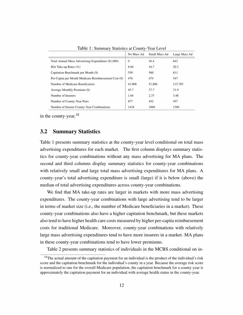
Table 1: Summary Statistics at County-Year LevelNo Mass Ad Small Mass Ad Large Mass Ad

Total Annual Mass Advertising Expenditure ($1,000) 0 36.4 642

MA Take-up Rates (%) 8.84 16.7 20.3

Capitation Benchmark per Month ($) 550 560 611

Per-Capita per Month Medicare Reimbursement Cost ($) 476 474 547

Number of Medicare Beneficiaries 41,906 51,886 115,785

Average Monthly Premium ($) 45.7 37.7 31.9

Number of Insurers 1.64 2.37 3.48

Number of County-Year Pairs 877 452 457

Number of Insurer-County-Year Combinations 1434 1069 1589

in the county-year.18

3.2 Summary Statistics

Table 1 presents summary statistics at the county-year level conditional on total massadvertising expenditures for each market. The first column displays summary statis-tics for county-year combinations without any mass advertising for MA plans. Thesecond and third columns display summary statistics for county-year combinationswith relatively small and large total mass advertising expenditures for MA plans. Acounty-year’s total advertising expenditure is small (large) if it is below (above) themedian of total advertising expenditures across county-year combinations.

We find that MA take-up rates are larger in markets with more mass advertisingexpenditures. The county-year combinations with large advertising tend to be largerin terms of market size (i.e., the number of Medicare beneficiaries in a market). Thesecounty-year combinations also have a higher capitation benchmark, but these marketsalso tend to have higher health care costs measured by higher per-capita reimbursementcosts for traditional Medicare. Moreover, county-year combinations with relativelylarge mass advertising expenditures tend to have more insurers in a market. MA plansin these county-year combinations tend to have lower premiums.

Table 2 presents summary statistics of individuals in the MCBS conditional on in-

18The actual amount of the capitation payment for an individual is the product of the individual’s riskscore and the capitation benchmark for the individual’s county in a year. Because the average risk scoreis normalized to one for the overall Medicare population, the capitation benchmark for a county-year isapproximately the capitation payment for an individual with average health status in the county-year.

12

surance status. The first and second columns present summary statistics of individualsthat chose traditional Medicare and MA, respectively. We find that a majority of indi-viduals do not switch between the traditional Medicare and MA. For those who choosethe traditional Medicare, more than 90% chose traditional Medicare last year, althoughonly 70% of overall Medicare beneficiaries chose traditional Medicare last year. Like-wise, about 85% of those who choose MA this year also chose MA last year, althoughonly 20% of the overall Medicare beneficiaries had MA last year. Also, we find thathealth and income status of MA enrollees are different from those at traditional Medi-care. We construct a binary health status, healthy or unhealthy, based on self-reportedhealth status.19 Our income measure is constructed as a five-level categorical variable,with five being the category for the highest income, based on the income variable inthe MCBS.20 We find that healthy individuals are more likely to choose MA, which isconsistent with the findings of previous research on MA, as mentioned earlier. More-over, we find that those who choose MA are more likely to have lower income and befemale, although the average ages between the two groups of individuals are not verydifferent.

Table 3 presents summary statistics from Mintel. In this data set, the unit of ob-servation is a combination of individual and month, meaning that an individual re-ceived 0.158 mailings from MA plans on average. Conditional on receiving at leastone MA-related mailing, an individual received 1.24 mailings on average. We findthat those who received mailings tend to have lower household income and also residein neighborhoods with lower average income (measured by zip-code-level).21 Thosewho received mailings tend to be older than those who did not. Moreover, individualsin markets with more Medicare beneficiaries are more likely to receive mailings.

19An individual’s health status is defined to be healthy if the self-reported health status is “Excellent,”“Very Good,” or “Good.” An individual’s health status is defined to be unhealthy if the self-reportedhealth status is “Fair” or “Poor.”

20Although MCBS income variable has eleven categories originally, we create a new variable withfive categories in order for the income measure in the MCBS to be compatible with the income mea-sure in the Mintel data. Eventually, the new income variable we create is equal to one, two, three,four, or five if an individual’s income belongs to the following five intervals, respectively: [0,15000),[15000,25000), [25000,35000), [35000,50000), and [50000,∞). Henceforth, when we refer to an indi-vidual’s income in the MCBS, we refer to the new income variable with the five categories.

21We obtain the zip-code-level mean income from the IRS,which is available atwww.irs.gov/uac/SOI-Tax-Stats-Individual-Income-Tax-Statistics-Zip-Code-Data-(SOI).

13

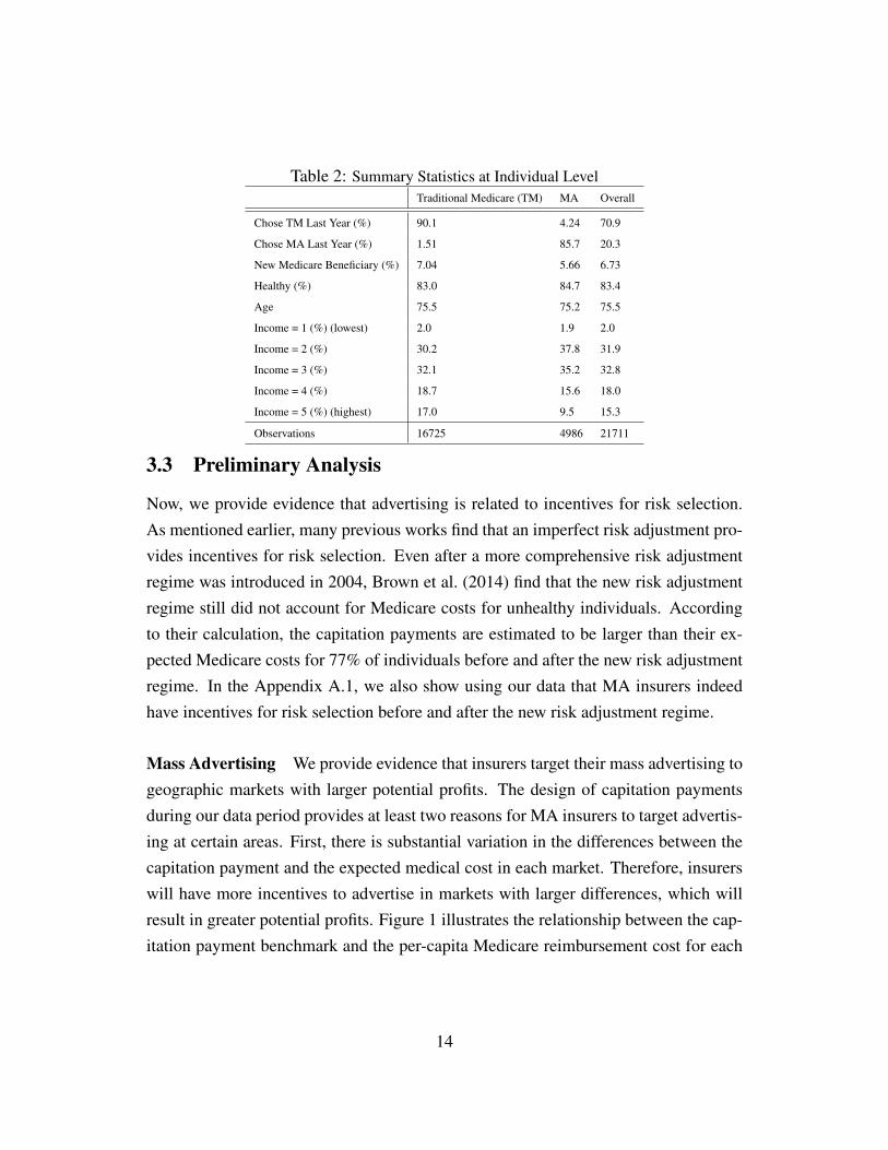
Table 2: Summary Statistics at Individual LevelTraditional Medicare (TM) MA Overall

Chose TM Last Year (%) 90.1 4.24 70.9

Chose MA Last Year (%) 1.51 85.7 20.3

New Medicare Beneficiary (%) 7.04 5.66 6.73

Healthy (%) 83.0 84.7 83.4

Age 75.5 75.2 75.5

Income = 1 (%) (lowest) 2.0 1.9 2.0

Income = 2 (%) 30.2 37.8 31.9

Income = 3 (%) 32.1 35.2 32.8

Income = 4 (%) 18.7 15.6 18.0

Income = 5 (%) (highest) 17.0 9.5 15.3

Observations 16725 4986 21711

3.3 Preliminary Analysis

Now, we provide evidence that advertising is related to incentives for risk selection.As mentioned earlier, many previous works find that an imperfect risk adjustment pro-vides incentives for risk selection. Even after a more comprehensive risk adjustmentregime was introduced in 2004, Brown et al. (2014) find that the new risk adjustmentregime still did not account for Medicare costs for unhealthy individuals. Accordingto their calculation, the capitation payments are estimated to be larger than their ex-pected Medicare costs for 77% of individuals before and after the new risk adjustmentregime. In the Appendix A.1, we also show using our data that MA insurers indeedhave incentives for risk selection before and after the new risk adjustment regime.

Mass Advertising We provide evidence that insurers target their mass advertising togeographic markets with larger potential profits. The design of capitation paymentsduring our data period provides at least two reasons for MA insurers to target advertis-ing at certain areas. First, there is substantial variation in the differences between thecapitation payment and the expected medical cost in each market. Therefore, insurerswill have more incentives to advertise in markets with larger differences, which willresult in greater potential profits. Figure 1 illustrates the relationship between the cap-itation payment benchmark and the per-capita Medicare reimbursement cost for each

14

Table 3: Mintel Summary StatsHouseholds w/o MA Mails Households w/ MA Mails Overall

Number of MA Mailings 0 1.24 0.16

Income = 1 (%) (lowest) 17.0 20.7 17.4

Income = 2 (%) 16.3 20.5 16.8

Income = 3 (%) 15.6 16.7 15.8

Income = 4 (%) 16.1 15.7 16.0

Income = 5 (%) (highest) 35.0 26.5 33.9

Zip code-Level Income ($) 48,662 47,381 48,500

Age of Female Household Head if Any 67.7 71.3 68.2

Age of Male Household Head if Any 69.4 72.5 69.8

Number of Medicare Beneficiaries (County Level) 163,725 219,626 170,849

Observations 14,515 2,120 16,635

county-year.22 Although the capitation payment and the Medicare reimbursement costare positively correlated, there is still substantial heterogeneity among capitation pay-ments conditional on per-capital Medicare costs.23

Second, risk selection is potentially more profitable in some markets than others.Differences in health care costs between healthy and unhealthy individuals will be typ-ically greater in regions where health care is more expensive.24 Then an insurer willmake a greater profit (loss) by enrolling healthy (unhealthy) individuals in a regionwith more expensive health care. Although we do not have the exact measure of healthcare prices in different regions, we have information on the per-capita Medicare reim-bursement cost of each county-year, which should reflect the health care price of eachcounty-year.25

22An important caveat is that the Medicare reimbursement cost is the health care cost only for in-dividuals who choose traditional Medicare and may imperfectly reflect an MA insurer’s expected costin each county. However, the Medicare reimbursement will still provide useful information about howhealth care costs vary across regions.

23One source of such variation is based on city size: metropolitan areas with a population of 250,000or more have receive an additional capitation payment that is approximately 10.5% of the premium,which is not available to MSAs below this threshold (Duggan et al. 2014).

24An extreme example is a hypothetical case in which a healthy individual’s cost is zero. In this case,all of the medical expenditures result from unhealthy individuals. Because healthy individuals’ healthcare cost is always zero, differences in health care costs between healthy and unhealthy individuals willbe greater in regions where health care is more expensive.

25As reported in Table 16 of the Appendix, we find that an unhealthy individual in a county-year witha greater per-capita Medicare reimbursement cost tends to incur a greater Medicare reimbursement cost,compared with a healthy individual in the same county-year.

15

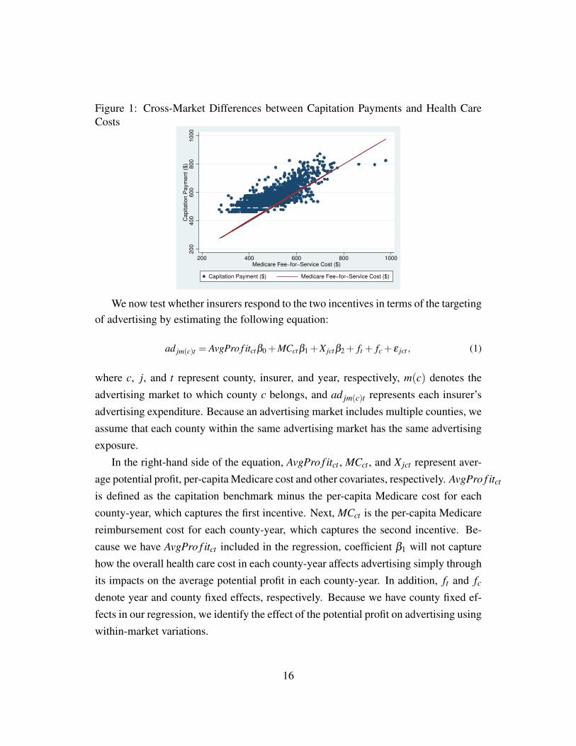
Figure 1: Cross-Market Differences between Capitation Payments and Health CareCosts

200

400

600

800

1000

Capitation P

aym

ent ($

)

200 400 600 800 1000Medicare Fee−for−Service Cost ($)

Capitation Payment ($) Medicare Fee−for−Service Cost ($)

We now test whether insurers respond to the two incentives in terms of the targetingof advertising by estimating the following equation:

ad jm(c)t = AvgPro f itctβ0 +MCctβ1 +X jctβ2 + ft + fc + ε jct , (1)

where c, j, and t represent county, insurer, and year, respectively, m(c) denotes theadvertising market to which county c belongs, and ad jm(c)t represents each insurer’sadvertising expenditure. Because an advertising market includes multiple counties, weassume that each county within the same advertising market has the same advertisingexposure.

In the right-hand side of the equation, AvgPro f itct , MCct , and X jct represent aver-age potential profit, per-capita Medicare cost and other covariates, respectively. AvgPro f itct

is defined as the capitation benchmark minus the per-capita Medicare cost for eachcounty-year, which captures the first incentive. Next, MCct is the per-capita Medicarereimbursement cost for each county-year, which captures the second incentive. Be-cause we have AvgPro f itct included in the regression, coefficient β1 will not capturehow the overall health care cost in each county-year affects advertising simply throughits impacts on the average potential profit in each county-year. In addition, ft and fc

denote year and county fixed effects, respectively. Because we have county fixed ef-fects in our regression, we identify the effect of the potential profit on advertising usingwithin-market variations.

16

Table 4: Geographical Targeting of Mass AdvertisingDependent Variable Advertising Expenditure

VARIABLES Coefficient Std. Error

Average Potential Profit (AvgPro f itc jt) 0.00123*** (0.000275)

Per-Capita Medicare Cost (MCc jt ) 0.00115*** (0.000357)

Observations 4,092Note: In order to save space, we do not report estimate for all coefficients here. Table 17 in the Appendix provide the complete

results.

Table 4 shows the regression result. We find that the estimates of the coefficientsof potential profit and per-capita Medicare costs are both positive, which is consis-tent with our hypothesis that both higher average profits and higher profitability fromhealthy individuals in each markets lead to more advertising. Although we have yet toshow direct evidence on how advertising can achieve risk selection, if insurers can at-tract healthy individuals with advertising, they will have greater incentives to advertisemore in a market where attracting a healthy individual results in greater profit. In thefollowing sections, we will provide the evidence from our structural demand modelthat advertising tends to attract healthy types more than unhealthy types.

Direct Mail Although we find evidence that mass advertising is targeted based onthe profitability of each county, insurers may further implement sophisticated targetingwithin a county. To pursue this possibility, we investigate the second measure of ad-vertising: direct mail advertising. We believe that direct mailings are very useful toolsfrom an insurer’s perspective for targeting its advertising at an individual with certaincharacteristics. Presumably, insurers often have access to the demographic character-istics of individuals who live at specific addresses or have access to information aboutthe average demographic in a small geographic area such as zip code. Therefore, theymay utilize sophisticated targeting to attract less costly customers. By using this dataset, we can gain insights into which individuals are more likely to receive advertising.

We first investigate whether the targeting of direct mailings responded to the in-troduction of the comprehensive risk adjustment in 2004. As discussed earlier, Brownet al. (2014) find that capitation payments for individuals with lower risk scores sub-stantially decreased after the new risk adjustment regime. Thus, although enrolling ahealthy individual continues to be profitable to in the new regime, profitability froman individual with a lower risk score likely decreased compared with that from an in-

17

dividual with a higher risk score. The targeting of direct mailings was then likely tochange with the introduction of the new regime.

One limitation of the Mintel data is that we do not observe health-related measuresfor individuals. Thus, we use a household’s income as a proxy for the risk scores ofthe household’s heads, which is motivated by the fact that an individual’s health andincome are highly negatively correlated. We use two different measures for income.In the first specification, we use an individual’s income reported in the Mintel data,which is a categorical variable with five categories as mentioned before. In the secondspecification, we use the average income in an individual’s zip code.

With the first specification, we run the following regression:

yit = α0+4

∑k=1

α1,k1[Iit = k]+4

∑k=1

α2,k1[t ≥Oct 2003]1[Iit = k]+Xitβ + ft + fc(i),risk(t)+εit (2)

where yit is the number of MA-related direct mailings that household i received in aparticular month-year t, Iit is a categorical variable for a household income measure,which takes a higher value if an income is higher, and 1[Iit = k] is a dummy variablethat is equal to one if Iit is equal to k. As mentioned earlier, Iit has five categories fromone to five, with a higher number assigned for a greater income. In (2), we normal-ize coefficients for the highest income to zero. That is, α1,5 = α2,5 = 0. Similarly,1[t ≥Oct, 2003] is a dummy variable that is equal to one for a time in or after October2003. We chose the beginning of the fourth quarter of 2003 as the time when the newrisk adjustment regime starts to affect an MA insurer’s targeting. Because its imple-mentation was announced in March 2003, MA insurers likely adjusted their targetingeven before the beginning of 2004. Moreover, Xit is a vector of other characteristicsof a household i, including whether there is a male or female household head, agesof male and female household heads if they exist, potential average profit as definedin equation (1) for each county-year, the number of Medicare beneficiaries in eachcounty-year, and median household income for each county-year. Next, ft representfixed effects for month-year t. In addition, fc(i),risk(t) represent fixed effects for a com-bination of household i’s county of residence and risk adjustment regime. As discussedbefore, if t < Oct 2003, then the time belongs to the old risk adjustment regime. Andif t ≥ Oct 2003, then the time belongs to the new risk adjustment regime. Thus, eachcounty has two fixed effects in this regression.

18

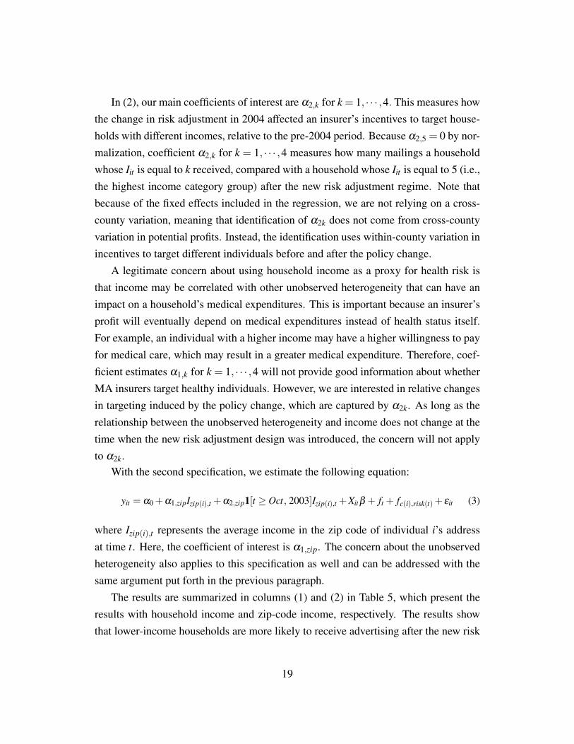
In (2), our main coefficients of interest are α2,k for k = 1, · · · ,4. This measures howthe change in risk adjustment in 2004 affected an insurer’s incentives to target house-holds with different incomes, relative to the pre-2004 period. Because α2,5 = 0 by nor-malization, coefficient α2,k for k = 1, · · · ,4 measures how many mailings a householdwhose Iit is equal to k received, compared with a household whose Iit is equal to 5 (i.e.,the highest income category group) after the new risk adjustment regime. Note thatbecause of the fixed effects included in the regression, we are not relying on a cross-county variation, meaning that identification of α2k does not come from cross-countyvariation in potential profits. Instead, the identification uses within-county variation inincentives to target different individuals before and after the policy change.

A legitimate concern about using household income as a proxy for health risk isthat income may be correlated with other unobserved heterogeneity that can have animpact on a household’s medical expenditures. This is important because an insurer’sprofit will eventually depend on medical expenditures instead of health status itself.For example, an individual with a higher income may have a higher willingness to payfor medical care, which may result in a greater medical expenditure. Therefore, coef-ficient estimates α1,k for k = 1, · · · ,4 will not provide good information about whetherMA insurers target healthy individuals. However, we are interested in relative changesin targeting induced by the policy change, which are captured by α2k. As long as therelationship between the unobserved heterogeneity and income does not change at thetime when the new risk adjustment design was introduced, the concern will not applyto α2k.

With the second specification, we estimate the following equation:

yit = α0 +α1,zipIzip(i),t +α2,zip1[t ≥ Oct, 2003]Izip(i),t +Xitβ + ft + fc(i),risk(t)+ εit (3)

where Izip(i),t represents the average income in the zip code of individual i’s addressat time t. Here, the coefficient of interest is α1,zip. The concern about the unobservedheterogeneity also applies to this specification as well and can be addressed with thesame argument put forth in the previous paragraph.

The results are summarized in columns (1) and (2) in Table 5, which present theresults with household income and zip-code income, respectively. The results showthat lower-income households are more likely to receive advertising after the new risk

19

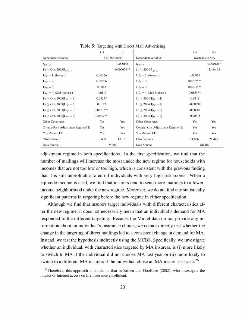
Table 5: Targeting with Direct Mail Advertising(1) (2) (3) (4)

Dependent variable: # of MA mails Dependent variable: Switches to MA

Izip(i),t -0.000105 Izip(i),t -0.000126*

1[t ≥ Oct, 2003]Izip(i),t -0.000679** 1[t ≥ 2004]Izip(i),t -2.44e-05

1[Iit = 1] (lowest ) 0.00326 1[Iit = 1] (lowest ) 0.00965

1[Iit = 2] 0.00906 1[Iit = 2] 0.0262***

1[Iit = 3] -0.00451 1[Iit = 3] 0.0223***

1[Iit = 4] (2nd highest ) -0.0117 1[Iit = 4] (2nd highest ) 0.0155**

1[t ≥ Oct, 2003]1[Iit = 1] 0.0433* 1[t ≥ 2004]1[Iit = 1] -0.0118

1[t ≥ Oct, 2003]1[Iit = 2] 0.0177 1[t ≥ 2004]1[Iit = 2] -0.00398

1[t ≥ Oct, 2003]1[Iit = 3] 0.0857*** 1[t ≥ 2004]1[Iit = 3] -0.00201

1[t ≥ Oct, 2003]1[Iit = 4] 0.0632** 1[t ≥ 2004]1[Iit = 4] -0.00315

Other Covariates Yes Yes Other Covariates Yes Yes

County-Risk Adjustment Regime FE Yes Yes County-Risk Adjustment Regime FE Yes Yes

Year-Month FE Yes Yes Year-Month FE Yes Yes

Observations 13,430 13,317 Observations 21,836 21,448

Data Source Mintel Data Source MCBS

adjustment regime in both specifications. In the first specification, we find that thenumber of mailings will increase the most under the new regime for households withincomes that are not too low or too high, which is consistent with the previous findingthat it is still unprofitable to enroll individuals with very high risk scores. When azip-code income is used, we find that insurers tend to send more mailings to a lower-income neighborhood under the new regime. Moreover, we do not find any statisticallysignificant patterns in targeting before the new regime in either specification.

Although we find that insurers target individuals with different characteristics af-ter the new regime, it does not necessarily mean that an individual’s demand for MAresponded to the different targeting. Because the Mintel data do not provide any in-formation about an individual’s insurance choice, we cannot directly test whether thechange in the targeting of direct mailings led to a consistent change in demand for MA.Instead, we test the hypothesis indirectly using the MCBS. Specifically, we investigatewhether an individual, with characteristics targeted by MA insurers, is (i) more likelyto switch to MA if the individual did not choose MA last year or (ii) more likely toswitch to a different MA insurers if the individual chose an MA insurer last year.26

26Therefore, this approach is similar to that in Brown and Goolsbee (2002), who investigate theimpact of Internet access on life insurance enrollment.

20

Now we define yit to be a dummy variable that equals one if condition (i) or (ii)is met. We run regressions similar to equations (2) and (3). Specifications (3) and (4)in Table 5 presents results from the two regressions. Note that none of the estimatedcoefficients for the interactions between incomes and the new risk adjustment regimeare statistically significant. This result implies that direct mail was not very effectivein inducing consumers to enroll in MA at least for the years considered in our analysis.Because the cost of sending direct mailings is very tiny, insurers likely responded to thechange in the risk adjustment regime, expecting that direct mailings to newly targetedindividuals will lead to a greater demand by them. Eventually, however, any changesin demand were quantitatively insignificant.

4 Demand Model

We now investigate how advertising affects consumer demand by structurally esti-mating a model of health insurance demand. Although we provided evidence for thetargeting of both direct mail and mass advertising, we only consider the impact ofmass advertising on demand. One difficulty of using the data on direct mail in thedemand analysis is that it is difficult to link the direct mail data (Mintel) to the dataon a consumer’s insurer choice (MCBS). The number of individuals in a county-yearin the Mintel data is not large enough to construct a measure of direct mails sent to acounty-year. Thus, without combined information on advertising exposure and subse-quent choice, it will be difficult to estimate the effects of direct mail on demand forMA.27 Moreover, as shown in the previous section, we do not find evidence that thechange in the targeting of direct mail led to a corresponding change in demand forMA.

As discussed in a previous section, MA insurers contract with CMS for each county(c) in each year (t). As a result, consumers in different counties and different years facedifferent choice sets. Thus, we will naturally define a market of MA as a combinationof county-year (ct). However, each advertising decision is typically made on the basisof a local advertising market (m), which contains several counties. Thus, we assume

27One possibility is to impute the number of MA mailings an individual receives using characteristicspresent in both data sets. Unless we can do the imputation precisely, the impact of imputed mailings ondemand is likely to be estimated with a substantial bias.

21

individuals in different c but in the same m are exposed to the same advertising levelby the same firm. The advertising market m, to which county c belongs, is denoted bym(c).

Each MA market (ct) has Jct MA insurers available. An individual in a marketalso has the option of choosing traditional Medicare. Thus, an individual has the totalJct + 1 options in MA market ct. An insurer j in market ct can be described by acombination of advertising (ad jm(c)t), other observed characteristics (x jct) includingpremium and plan characteristics, county fixed effect (µc), an insurer-year fixed effect(ξ jt), and an unobservable characteristic (∆ξ jct). A consumer i can be described by acombination of health status (hi), last year’s choice of insurer (di,t−1), other observedcharacteristics (cit), and a preference shock (εi jct). We will explain each insurer’s andindividual’s characteristics after we describe an individual’s utility from an insurer.

Consider an individual i living in county c and year t. Consumer i chooses to enrollwith one of the available J MA insurers in each c and t or in traditional Medicare. Weassume that consumer i, living in a county c in year t, obtains indirect utility ui jct fromMA insurer j as follows:

ui jct = ln(1+ad jm(c)t

)αi jt +x jctβit +φict1[di,t−1 6= j,di,t−1 ≥ 0]+µc +ξ jt +∆ξ jct +εi jct (4)

where

αi jt = α0 +α11[di,t−1 = j]hit +1

∑k=0

α2,k1[di,t−1 6= j,di,t−1 ≥ 0]1[hit = k];

βit = β0 +β1hit ;

φict = φ0 +φ0hit +φ1Jct +φ0J2ct .

A consumer’s outside option is to enroll in traditional Medicare, from which a con-sumer receives utility of ui0ct :

ui0ct = hitρ1 + citρ2 +φict1[di,t−1 6= 0,di,t−1 ≥ 0]+ εi0ct . (5)

Both an individual’s characteristics and an insurer’s characteristics determine ui jct .An individual’s characteristics included in ui jct are individual i’s binary health statushit that equals to one if healthy (and zero if unhealthy), last year’s insurance choicedi,t−1, and other relevant individual characteristics cit . Last year’s insurance choice

22

di,t−1 contains information about (i) whether individual i chose MA or traditionalMedicare last year and (ii) which MA insurer this individual chose if MA was cho-sen last year. In case that individual i is new to Medicare, we set di,t−1 =−1, and thus1[di,t−1 6= j,di,t−1 ≥ 0] = 0 for any j for new Medicare beneficiaries.28 Lastly, εi jct isan individual i’s preference shock for insurer j, which we assume is distributed as theType I extreme value distribution.

Each insurer has observable characteristics (ad jm(c)t and x jct), county fixed effect(µc) and an insurer-year fixed effect (ξ jt), and an unobservable characteristic (∆ξ jct).First, ad jmt denotes insurer j’s advertising expenditure in millions in advertising mar-ket m in year t.29 30 Note that the effects of advertising diminish in its expenditurebecause ad jm(c)t enters ui jct in logarithm.31 The effect of advertising on indirect util-ity ui jct is captured by αi jt , which depends on individual i’s previous insurance statusdi,t−1 and self-reported health status hit . In other words, insurer j’s advertising hasdifferent effects, depending on whether individuals chose the insurer last year andwhether an individual is healthy. Parameter α0 represents the effects of advertisingthat are independent of an individual’s characteristics. Parameter α1 represents the ef-fects of advertising for healthy consumers who chose the same insurer last year. Andα2,0 and α2,1 capture the effects of advertising on unhealthy and healthy individualsthat did not choose insurer j last year, respectively.

We distinguish the effects of advertising on individuals who chose the advertisedinsurer last year and those who did not because if advertising is informative, it willbe more effective for individuals who did not choose the insurer (Ackerberg, 2001).Informative advertising is likely to provide information about an insurer’s unobservedquality or simply the existence of the insurer in the market. Thus, it is plausible that

28We define an individual as new to Medicare if he or she has spent less than two years on Medicareas of the end of year t.

29Note that advertising affects demand through the indirect utility function in our model. Alterna-tively, one can model specific channels through which advertising affects demand: for example, a con-sumer’s awareness of a product, providing experience characteristics of product quality, or enhancingprestige or image of a product. We do not take this approach, however, because separately identifyingdifferent effects of advertising is challenging with our data.

30This specification assumes no interaction term between advertising and price. We also estimatedthe version of the model allowing those interactions and also further allow interaction with them toindividual last year’s insurance status. However, none of them are statistically significant and thereforewe decided to drop for this estimation. Estimates for the specification are available on request.

31Because ad jm(c)t is zero for many insurers, we use ln(1+ad jm(c)t

)instead of ln

(ad jm(c)t

).

23

this type of advertising will have little effects on individuals who chose the insurer lastyear. On the other hand, if advertising has prestige or image effects, then it will likelyaffect both types of individuals. Moreover, advertising can be still informative foran individual who already enrolled with the advertised insurer. Unless an individualreceives much medical care, the individual will not be able to know an insurer’s trueunobserved quality. Advertising can still provide information to such an individual.

Moreover, we allow for the possibility that advertising has a different impact de-pending on hit . If the impact of advertising depends on hit , then advertising will even-tually affect an insurer’s risk pool and thereby its cost. In this case, advertising canbe used for risk selection. In principle, there are two interpretations of the hetero-geneous impacts of advertising depending on hit : the targeting of mass advertisingat certain types of consumers and a consumer’s differential response to advertising.First, targeting refers to the possibility that an insurer targets its advertising at certainTV programs and newspapers that are more exposed to a certain health type than toanother type. Note that this kind of targeting requires an insurer to employ a moresophisticated targeting strategy than targeting certain counties. Second, a consumer’sdifferential response to advertising refers to the possibility that a certain health typeresponds to advertising more than another health type. In this case, advertising canstill affect a certain type’s demand disproportionately more even without sophisticatedtargeting. Unfortunately, we cannot clearly distinguish the two different channels be-cause we do not have information about which types of consumers were exposed to anMA insurer’s mass advertising.

However, we view that the heterogeneous impacts are likely to capture the secondmechanism for the following reasons.32 First, even without sophisticated targeting,health status itself can determine how much an individual is exposed to advertising.For example, mass advertising mostly appears on TV or in newspapers, and thosewho are able to watch TV or read newspapers are less likely to have their vision orhearing problems. We find that unhealthy individuals are more likely to have vision or

32In case that the heterogeneous impacts capture an insurer’s targeting to some extent, then a potentialproblem is that parameter αi jt is not policy-invariant for our counterfactual analysis. That is because aninsurer may target its advertising at a different health type with a counterfactual change in its incentivesto attract different health types. In our counterfactual analysis, however, we exogenously shut downadvertising in order to investigate the impact of advertising on the MA market. In this case, parameterα1,k will not play any role in this counterfactual analysis. Thus, results in our counterfactual analysiswill not depend on whether the heterogeneous impacts capture the targeting.

24

hearing problems in the MCBS, as shown in Table 18 in the Appendix.33 Moreover,among those who have such problems, unhealthy individuals are more likely to believethat their vision or hearing problems make it difficult for them to obtain informationabout Medicare, as reported in Table 18 in the Appendix.34 Thus, those who actuallyrespond to advertising will be more likely to be healthy even without sophisticatedtargeting. Second, as Fang et al. (2008) argue, a health status is highly correlatedwith cognition abilities for elderly people, which may lead to a differential response toadvertising. Third, our preliminary analysis on direct mail advertising reveals that thetargeting of advertising at certain individuals within a market was not very effective inattracting them to MA. The result indicates that targeting does not necessarily lead toan increase in demand by targeted consumers. Because targeting mass advertising atcertain individuals is plausibly more difficult than targeting via direct mail, we believethat it will be difficult for insurers to risk-select through targeting mass advertising athealthy types.

The term x jct denotes a vector of insurer j’s observed characteristics other thanadvertising, which include the premium, copayments for a variety of medical servicessuch as inpatient care and outpatient doctor visits, and variables describing whether aninsurer offers drug coverage, vision coverage, dental coverage, and so on. We definethe premium to be the amount that a consumer pays in addition to the Medicare PartB premium.35 The effects of plan characteristics on utility are potentially heteroge-neous depending on an individual’s health type. For example, an MA insurer offeringdrug coverage may be preferred by individuals who expect a large expenditure on pre-scription drugs, and a private fee-for-service MA insurer may be preferred by a certainhealth type because its provider network is not as restrictive as an HMO. We also allowfor the possibility that disutility from a premium depends on a healthy type becausedifferent health types may have different willingness to pay for MA. The heteroge-

33The Table 18 in the Appendix presents results for regressions of whether an individual has a visionor hearing problem on his health status and age.

34The Table 18 in the Appendix also presents results for regressions of whether an individual believethat his vision or hearing problems make it difficult to obtain information about Medicare on his healthstatus and age.

35When enrolling in an MA plan, an individual must pay the Medicare Part B premium as well as thepremium charged by the plan. Here we do not include Medicare Part B premium in p jct because almostall Medicare beneficiaries, who remain in traditional Medicare, enroll in Medicare Part B and pay theMedicare Part B premium.

25

neous effects are captured by parameter βit , which depends on an individual’s healthhit .36

The term φict denotes switching cost of changing insurers. Note that 1[di,t−1 6=j,di,t−1 ≥ 0] is equal to one if an individual, who is not new to Medicare, chooses adifferent plan from one chosen last year. This means that new Medicare beneficiariesdo not pay a switching cost for their initial choice of insurer. Notice that the switch-ing cost makes the impact of advertising on demand depend on di,t−1. Because newMedicare beneficiaries do not face a switching cost, advertising will have a larger ef-fect on them. We also allow for the possibility that φit is different, depending on hit

and Jct (number of available insurers in a market). We let Jct affect φict because thefunctional-form assumption for εi jct mechanically implies that an individual in a mar-ket with more insurers is more likely to switch to a different plan with all others beingequal.

The term ξ jt denotes insurer-year fixed effects that capture an insurer j’s brandeffect in year t. Moreover, µc represents county fixed effects, which capture county-specific factors that determine demand for MA in the county. An individual’s utilityalso depends on aspects of an insurer that are unobserved by researchers but observedby consumers and insurers. The term ∆ξ jct is a deviation from µc and ξ jt , and ∆ξ jct

captures unobserved characteristics and/or shocks to demand for this insurer. We as-sume that ∆ξ jct is known by consumers and insurers when they make decisions.

Lastly, we discuss the specification of utility for the outside option, which is tradi-tional Medicare. Note that the constant term for ui0ct is normalized to zero because theterm cannot be identified in a discrete choice model. All of the terms included in ui0ct

are individual characteristics such as health status, switching cost, and other charac-teristics denoted by cit , which include age, income, and interaction between year andprevious insurance status. These individual characteristics capture different utilitiesfrom the outside option for individuals with different characteristics, relative to theirutility from MA insurers in general.

36In order to reduce the number of parameters to be estimated, we do not interact every variable inx jct with health status. We select which variables to interact with health status based on the results ofthe preliminary analysis. A complete list of variables interacted with health status is reported in Table6.

26

5 Identification and Estimation

For the discussion of identification and estimation of the model, we define θ to be avector that contains all parameters in the model. For our discussion in this section, letθ ≡ (θ0,θ1), where θ0 is a collection of parameters that determine the parts of utilityindependent of individual heterogeneity and where θ1 is a collection of parameters thatdetermine preference heterogeneity resulting from individual characteristics. That is,θ0 ≡ (α0,β0), and θ1 contains all other parameters in equations (4) and (5).

Mean Utility First, we discuss the identification of parameters in θ0. The parts ofui jct in equation (4) that are independent of individual heterogeneity are usually calledmean utility δ jct . In other words,

δ jct ≡ ln(1+ad jm(c)t

)α0 + x jctβ0 +ξ jt +µc +∆ξ jct . (6)

Berry et al. (1995) show that given a value for θ1, there is a unique δ ∗jct(θ1) that ex-actly match predicted market shares to observed market shares. Then parameter θ0 isestimated using equation (6) by treating ∆ξ jct as a structural error term. A well-knownproblem regarding the identification of θ0 is that ∆ξ jct , which may capture unobservedproduct characteristics, and endogenous plan characteristics included in the model arecorrelated. This problem is a typical endogeneity problem, and then a simple ordinary-least-squared regression of δ ∗jct(θ1) on (ad jmt ,x jct) will result in inconsistent estimatesof θ0 if (ad jm(c)t ,x jct) contains endogenously chosen characteristics. We assume thatthe advertising expenditure ad jm(c)t and the premium p jct , which is a part of x jct , areendogenous variables. Although almost all of the plan characteristics are potentiallyendogenous, we assume that these characteristics are exogenous in this estimation. Acrucial reason for this decision is that the number of instruments required for consistentestimation should be at least as great as the number of endogenous variables includedin (ad jm(c)t ,x jct) . Given the large number of plan characteristics, it is extremely diffi-cult to come up with instruments for all of them.

Although the endogeneity problem challenges the identification, the fixed effectsµc and ξ jt included in δ jct is likely to control for a significant part of the unobservedheterogeneity of insurers. However, it is still possible that ∆ξ jct still contains unob-served characteristics that are varying over insurers, counties and years. A typical

27

approach to accounting for the endogeneity problem is to use instruments that are cor-related with the endogenous variables, but not with the unobservable. We use instru-ments similar to ones used by Hausman (1996) and Nevo (2001).37 In other words,we use the average advertising expenditures of the same parent companies in otheradvertising markets for ad jm(c)t and the use the average premium of the same parentcompany in other counties for p jct . The instruments capture the idea that an insurer’smarginal cost contains a component that is common to all subsidiaries of a parentcompany, which is assumed to be uncorrelated with the unobserved heterogeneity. Re-sulting moment conditions employed in the estimation are that E[∆ξ jct |Γ] = 0, whereΓ is a set of instruments that includes the aforementioned two sets of instruments aswell as x jct .

Preference Heterogeneity Important information for the identification of parame-ters for preference heterogeneity θ1 is an individual’s insurer choice from the MCBS(the individual-level data). Parameter θ1 will be identified by variation in the character-istics of insurers chosen by individuals having different characteristics. An importantparameter in θ1 are the parameters that determine the heterogeneous effect of advertis-ing depending on an individual’s health type and last year’s choice, which are α1,α2,0

and α2,1 in (4). These parameters will be identified by variation in individuals’ switch-ing patterns across health types, last year’s choices, and advertising expenditures byinsurers they are switching to.

In order to construct micro-moments for an individual’s choice and combine themwith the aggregate moments, we use the score of the log-likelihood function for achoice by an individual observed in the MCBS, as in Imbens and Lancaster (1994). Thelikelihood function for an individual’s choice is L = ∏i, j,c,t q jct(zi)

di jct , where q jct(zi)

is the probability that an individual with characteristics zi chooses an insurer jct, anddi jct is an indicator variable that equals one when individual i chooses plan jct. Thenour micro-moments are ∂ log(L)/∂θ1 = 0.

37Town and Liu (2003) also use a similar instrument in estimating a model of demand for MA plans.

28

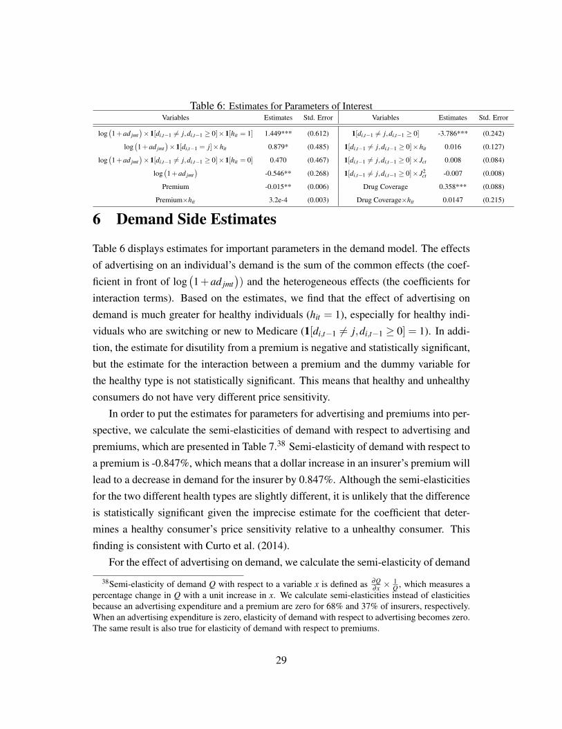
Table 6: Estimates for Parameters of InterestVariables Estimates Std. Error Variables Estimates Std. Error

log(1+ad jmt

)×1[di,t−1 6= j,di,t−1 ≥ 0]×1[hit = 1] 1.449*** (0.612) 1[di,t−1 6= j,di,t−1 ≥ 0] -3.786*** (0.242)

log(1+ad jmt

)×1[di,t−1 = j]×hit 0.879* (0.485) 1[di,t−1 6= j,di,t−1 ≥ 0]×hit 0.016 (0.127)

log(1+ad jmt

)×1[di,t−1 6= j,di,t−1 ≥ 0]×1[hit = 0] 0.470 (0.467) 1[di,t−1 6= j,di,t−1 ≥ 0]× Jct 0.008 (0.084)

log(1+ad jmt

)-0.546** (0.268) 1[di,t−1 6= j,di,t−1 ≥ 0]× J2

ct -0.007 (0.008)

Premium -0.015** (0.006) Drug Coverage 0.358*** (0.088)

Premium×hit 3.2e-4 (0.003) Drug Coverage×hit 0.0147 (0.215)

6 Demand Side Estimates

Table 6 displays estimates for important parameters in the demand model. The effectsof advertising on an individual’s demand is the sum of the common effects (the coef-ficient in front of log

(1+ad jmt

)) and the heterogeneous effects (the coefficients for

interaction terms). Based on the estimates, we find that the effect of advertising ondemand is much greater for healthy individuals (hit = 1), especially for healthy indi-viduals who are switching or new to Medicare (1[di,t−1 6= j,di,t−1 ≥ 0] = 1). In addi-tion, the estimate for disutility from a premium is negative and statistically significant,but the estimate for the interaction between a premium and the dummy variable forthe healthy type is not statistically significant. This means that healthy and unhealthyconsumers do not have very different price sensitivity.

In order to put the estimates for parameters for advertising and premiums into per-spective, we calculate the semi-elasticities of demand with respect to advertising andpremiums, which are presented in Table 7.38 Semi-elasticity of demand with respect toa premium is -0.847%, which means that a dollar increase in an insurer’s premium willlead to a decrease in demand for the insurer by 0.847%. Although the semi-elasticitiesfor the two different health types are slightly different, it is unlikely that the differenceis statistically significant given the imprecise estimate for the coefficient that deter-mines a healthy consumer’s price sensitivity relative to a unhealthy consumer. Thisfinding is consistent with Curto et al. (2014).

For the effect of advertising on demand, we calculate the semi-elasticity of demand

38Semi-elasticity of demand Q with respect to a variable x is defined as ∂Q∂x ×

1Q , which measures a

percentage change in Q with a unit increase in x. We calculate semi-elasticities instead of elasticitiesbecause an advertising expenditure and a premium are zero for 68% and 37% of insurers, respectively.When an advertising expenditure is zero, elasticity of demand with respect to advertising becomes zero.The same result is also true for elasticity of demand with respect to premiums.

29

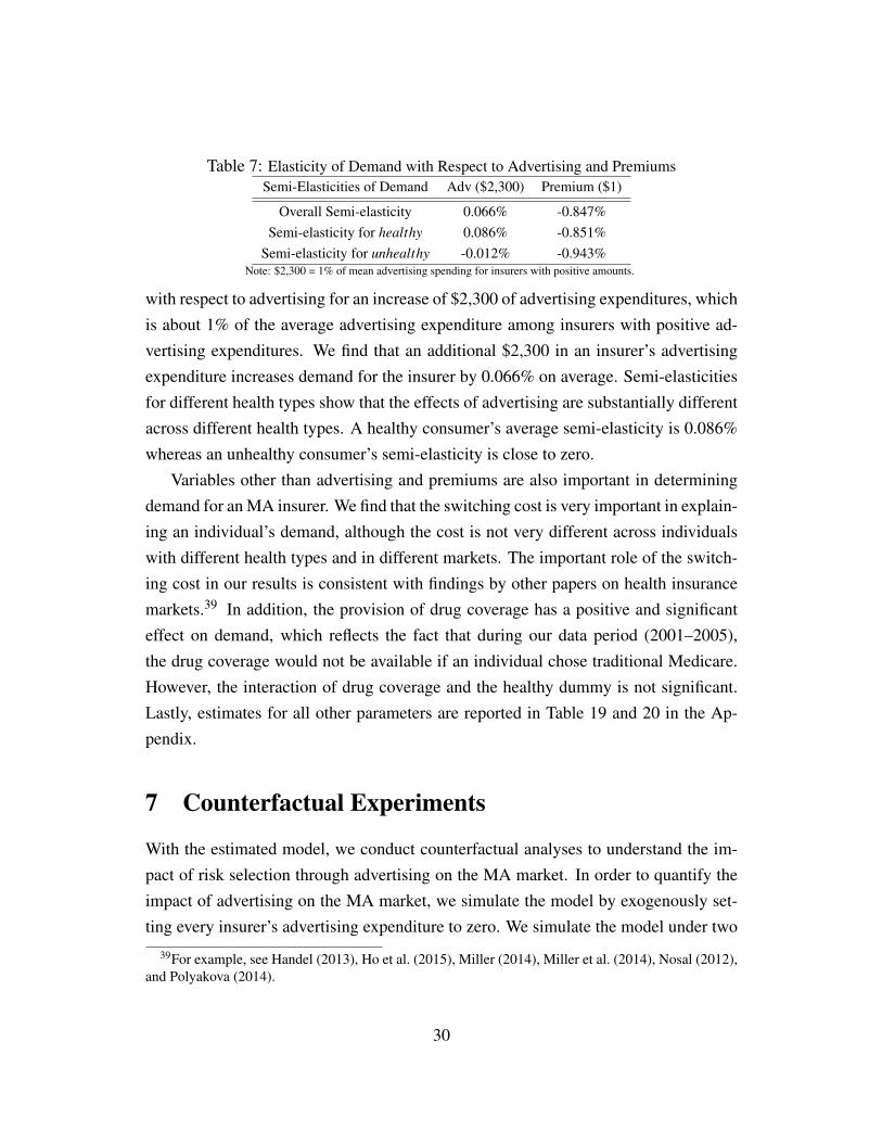
Table 7: Elasticity of Demand with Respect to Advertising and PremiumsSemi-Elasticities of Demand Adv ($2,300) Premium ($1)

Overall Semi-elasticity 0.066% -0.847%Semi-elasticity for healthy 0.086% -0.851%

Semi-elasticity for unhealthy -0.012% -0.943%Note: $2,300 = 1% of mean advertising spending for insurers with positive amounts.

with respect to advertising for an increase of $2,300 of advertising expenditures, whichis about 1% of the average advertising expenditure among insurers with positive ad-vertising expenditures. We find that an additional $2,300 in an insurer’s advertisingexpenditure increases demand for the insurer by 0.066% on average. Semi-elasticitiesfor different health types show that the effects of advertising are substantially differentacross different health types. A healthy consumer’s average semi-elasticity is 0.086%whereas an unhealthy consumer’s semi-elasticity is close to zero.

Variables other than advertising and premiums are also important in determiningdemand for an MA insurer. We find that the switching cost is very important in explain-ing an individual’s demand, although the cost is not very different across individualswith different health types and in different markets. The important role of the switch-ing cost in our results is consistent with findings by other papers on health insurancemarkets.39 In addition, the provision of drug coverage has a positive and significanteffect on demand, which reflects the fact that during our data period (2001–2005),the drug coverage would not be available if an individual chose traditional Medicare.However, the interaction of drug coverage and the healthy dummy is not significant.Lastly, estimates for all other parameters are reported in Table 19 and 20 in the Ap-pendix.

7 Counterfactual Experiments

With the estimated model, we conduct counterfactual analyses to understand the im-pact of risk selection through advertising on the MA market. In order to quantify theimpact of advertising on the MA market, we simulate the model by exogenously set-ting every insurer’s advertising expenditure to zero. We simulate the model under two

39For example, see Handel (2013), Ho et al. (2015), Miller (2014), Miller et al. (2014), Nosal (2012),and Polyakova (2014).

30

different counterfactual scenarios. In the first scenario, we assume that a premiumis fixed exogenously at its level in the baseline. In the second scenario, we assumethat insurers can reoptimize their premiums in the counterfactual environment. In thiscase, we investigate the equilibrium impact of shutting down advertising on marketoutcomes. We believe that modeling equilibrium price responses is important to betterunderstanding advertising as playing a role in risk selection and its implications forconsumer demand and ultimately welfare.

In order to obtain its impact on equilibrium, we first need to specify a model of howMA insurers choose their premiums. Therefore, we discuss the model of the supplyside before simulating our model.

7.1 Model of the Supply Side

We assume that insurers play a simultaneous game in choosing optimal pricing in eachmarket (county-year).40 When insuring an individual i with characteristic zi, insurerjct expects to incur a marginal cost c jct(zi) as follows:

c jct(zi) = Eω [m(zi,x jct ,ωi jct ;λ )]+η jct , (7)

where m(zi,x jct ,ωi jct ;λ ) is a realized reimbursement cost for an individual with char-acteristic zi who choose plan jct. The term ωi jct represents a random chock to thereimbursement cost, and λ represents parameters to be estimated. Next, η jct is ainsurer-county-year-specific shock to marginal cost that is constant across individu-als having different zi. We assume that η jct is observed by all insurers when makinga pricing decision. Note that the expected marginal cost c jct(zi) depends on the con-sumer’s characteristic zi, which includes health status. Therefore, an insurer’s costswill eventually depend on what kinds of individuals are enrolled with the insurer.

We estimate the marginal cost parameters λ using the individual-level informationfrom the MCBS on how much an individual’s MA insurer paid for the individual’smedical care in a year. Details on the exact functional form of m(zi,x jct ,ωi jct ;λ ) andestimation of λ are reported in Appendix A.2.

40Because we do not consider counterfactual situations where MA insurers re-optimize their adver-tising expenditures, we do not consider the optimal advertising decision here.

31

Insurer j’s profit from a county c in year t is given by

π jct = Mct

ˆ

zi

(p jct + cp(zi)− c jct(zi))q jct(zi)dFct(zi)−C(ad jm(c)t), (8)

where Mct is the population of those who are at least 65 years old in county c in year t,and p jct is the premium charged by insurer j in county c in year t.41 Next, cp(zi) is theexpected capitation payment for an individual having characteristics zi. We calculatecp(zi) based on the relationship between the observed amount of capitation paymentand zi in the MCBS. The details about the calculation can be found in Appendix A.1.Lastly, q jct(zi) is the probability of choosing insurer j by an individual having char-acteristics zi. Lastly, C(ad jm(c)t) denotes the advertising cost for each firm, whichcaptures both the variable and fixed costs associated with ad jct .

With the profit equation, it is clear how risk adjustment and advertising affect prof-its. With a perfect risk adjustment of capitation payment, cp(zi)− c jct(zi) is constantacross zi. In this case, a healthy individual will not cost less than an unhealthy indi-vidual, and advertising will affect an insurer’s profit just by increasing the overall de-mand for the insurer

´z q jct(zi)dFct(z). With an imperfect risk adjustment, in contrast,

cp(zi)− c jct(zi) will depend on zi and will be typically larger for healthy individuals,which is the case for the MA market. In this case, advertising affects an insurer’s profitthrough an insurer’s cost

´z c jct(zi)q jct(zi) as well as through the overall demand.

The Nash equilibrium condition for the optimal pricing game for insurers is thatinsurers’ choices maximize their profits given choices made by other insurers. Thus,we have the following condition for each p jct such that ∂π jct/∂ p jct = 0. We can solvefor η jct in a way that is similar to Berry et al. (1995). Appendix A.2 provides detailson how we solve for η jct .

41One important assumption we made is that firms are myopic. With an individual’s switching cost,an MA insurer potentially has a dynamic pricing incentive. Miller (2014) is the first attempt to estimatea model with forward-looking insurers in the MA market. One alternative is to follow the approachby Decarolis et al. (2015), who also estimate an equilibrium insurance market model with switchingcosts and myopic firms. In order to correct for possible bias resulting from ignoring dynamic pricingincentives, they do a robustness check on whether the estimates of marginal cost are biased at a certainlevel. Fully characterizing the dynamic pricing decision is a very challenging task and left to futurework.

32

Table 8: Counterfactual: Individual DemandMarkets with Small Adv Markets with Large Adv Markets with Any Ad

Health Type Baseline Partial Eq Full Eq Baseline Partial Eq Full Eq Baseline Partial Eq Full Eq

Panel 1: Consumers That Are New to Medicare: Pr(Switching to MA)

Healthy 0.177 0.175 0.171 0.228 0.205 0.199 0.208 0.193 0.188

Unhealthy 0.196 0.196 0.190 0.212 0.212 0.206 0.207 0.207 0.201

Panel 2: Consumers That Chose Traditional Medicare Last Year: Pr(Switching to MA)

Healthy 0.0170 0.0167 0.0162 0.0174 0.0151 0.0141 0.0172 0.0158 0.0150

Unhealthy 0.0148 0.0148 0.0144 0.0133 0.0133 0.0125 0.0139 0.0139 0.0133

Panel 3: Consumers That Chose a MA Plan Last Year: Pr(Switching to different MA)

Healthy 0.0368 0.0365 0.0365 0.0716 0.0679 0.0706 0.0605 0.0578 0.0597

Unhealthy 0.0351 0.0349 0.0348 0.0709 0.0667 0.0702 0.0596 0.0567 0.0591Note: Markets with Small Adv refers to a set of markets where market-level total advertising expenditures are below the median of

market-level total advertising expenditures; Markets with Large Adv refers to a set of markets where market-level total advertising

expenditures are above the median of market-level total advertising expenditures.

7.2 Simulation Results

We now evaluate the effects of shutting down advertising on the MA market undertwo different scenarios. First, we assume that a premium is fixed at its baseline levelexogenously. Second, we assume that insurers can reoptimize their premiums. Hence-forth, we will refer to the first and second counterfactual scenarios as the “Partial Eq”and the “Full Eq” counterfactual.

Table 8 summarizes the effects of shutting down advertising on a consumer’s switch-ing patterns, depending on a consumer’s insurance choice last year. For each group ofconsumers, we calculate the effects on demand separately for markets with differentlevels of advertising expenditures. First, we compare results in the baseline and thosein the counterfactual where premiums are fixed, which are presented under the columnslabeled “Partial Eq.” As expected, the probability of switching to MA will be lower inthe counterfactual situation than in the baseline, regardless of a consumer’s insurancestatus last year. Moreover, the probability of switching to MA is much greater for anew Medicare beneficiary because a new Medicare beneficiary does not face switch-ing costs. Therefore, the effect of advertising on demand is much greater for a newMedicare beneficiary in terms of an absolute change in probabilities of switching toMA. This indicates that it is important to look at flows instead of stocks in order tounderstand the effect of advertising on demand. We also find that the decrease in the

33

probabilities will be greater in markets with larger advertising expenditures. This re-sult shows that an insurer’s geographical targeting of advertising plays an importantrole in explaining cross-market differences in demand for MA.

Next, we investigate the impact of advertising on demand in the “Full Eq” counter-factual. Compared with the results in the other counterfactual situation where premi-ums are fixed, we find more substantial declines in overall probabilities of switching toMA for individuals that new to Medicare and those who chose traditional MA last year.In contrast, the probability of switching for those who chose a MA insurer last year inthe “Full Eq” counterfactual is greater, compared with the “Partial Eq” counterfactual.

In order to understand the difference between the results in the two counterfactualsituations, we analyze how new equilibrium premiums in the “Full Eq” counterfactualare different from the premiums in the baseline. Table 9 reports equilibrium premiumsand market shares in different counterfactual situations. We report the results for twogroups of insurers, depending on whether they advertise at all in the baseline economy.First, insurers with positive baseline advertising expenditures will increase premiumin the “Full Eq” counterfactual. We find that the increase in the average premiumwill be much larger in the markets with relatively large baseline advertising expendi-tures than for the markets with relatively small baseline expenditures. In the formergroup of markets, insurers with positive baseline advertising expenditure will increasemonthly premiums by about 40% from $20.6 to $28.8 (or from $247.2 to $345.6 an-nually). Such a large increase in premiums will keep individuals who did not chooseMA last year from switching to MA in the “Full Eq” counterfactual. Second, insurerswith zero baseline advertising expenditures will decease their monthly premiums byabout 19% from $18.6 to $15.0 (or from $223.2 to $180.0 annually). Because of thepremium decrease, individuals who chose MA last year will be more likely to switchto a different MA insurer in the “Full Eq” counterfactual, compared with the “PartialEq” counterfactual. Overall, the average premium across all insurers increase in bothgroup of markets. In markets with larger advertising expenditures, the average monthlypremium increases by about 11% from $19.5 to $21.6 (or from $234.0 to $259.2 annu-ally). In markets with smaller advertising expenditures, the average monthly premiumincreases by about 2% from $41.5 to $42.5 (or from $498 to $510 annually).

The changes in market shares reported in Table 9 are consistent with the changesin premiums. Compared with the predicted changes in premiums, however, market

34

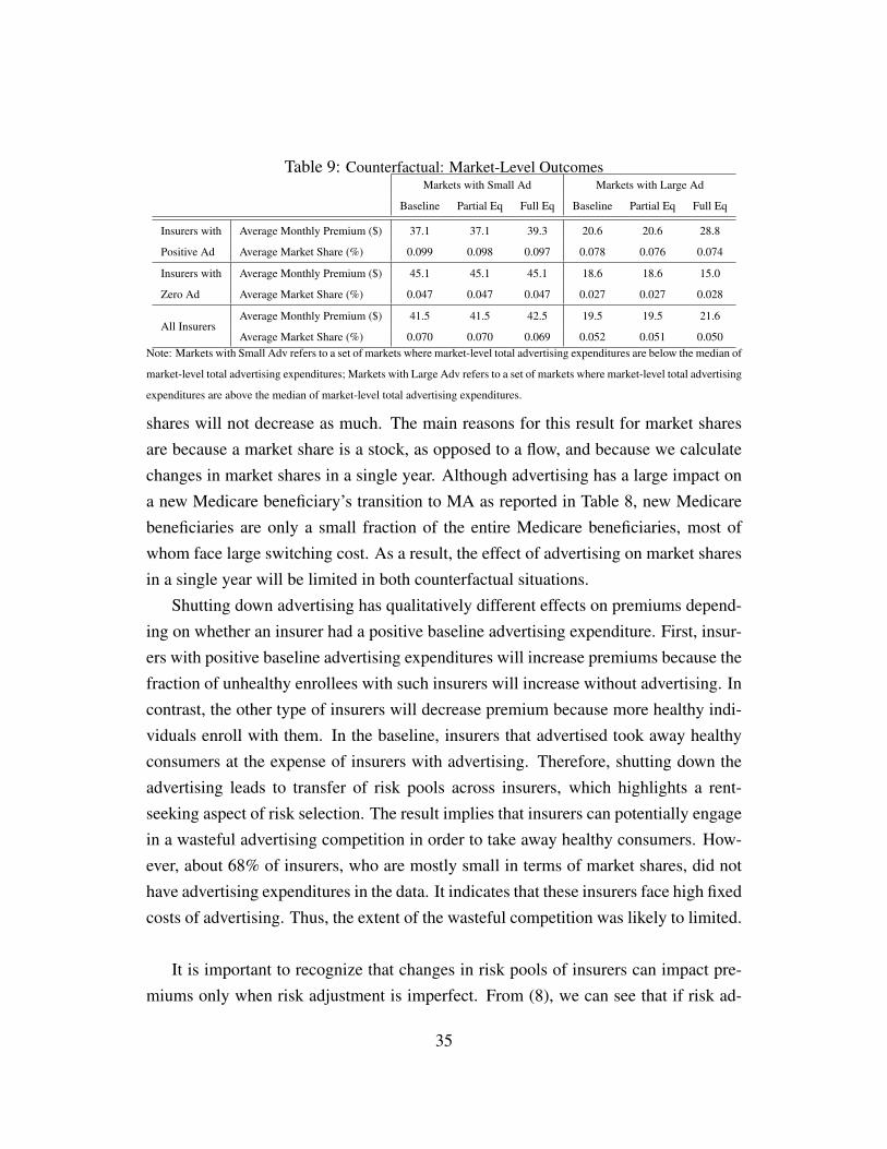
Table 9: Counterfactual: Market-Level OutcomesMarkets with Small Ad Markets with Large Ad

Baseline Partial Eq Full Eq Baseline Partial Eq Full Eq

Insurers with Average Monthly Premium ($) 37.1 37.1 39.3 20.6 20.6 28.8

Positive Ad Average Market Share (%) 0.099 0.098 0.097 0.078 0.076 0.074

Insurers with Average Monthly Premium ($) 45.1 45.1 45.1 18.6 18.6 15.0

Zero Ad Average Market Share (%) 0.047 0.047 0.047 0.027 0.027 0.028

All InsurersAverage Monthly Premium ($) 41.5 41.5 42.5 19.5 19.5 21.6

Average Market Share (%) 0.070 0.070 0.069 0.052 0.051 0.050Note: Markets with Small Adv refers to a set of markets where market-level total advertising expenditures are below the median of

market-level total advertising expenditures; Markets with Large Adv refers to a set of markets where market-level total advertising

expenditures are above the median of market-level total advertising expenditures.

shares will not decrease as much. The main reasons for this result for market sharesare because a market share is a stock, as opposed to a flow, and because we calculatechanges in market shares in a single year. Although advertising has a large impact ona new Medicare beneficiary’s transition to MA as reported in Table 8, new Medicarebeneficiaries are only a small fraction of the entire Medicare beneficiaries, most ofwhom face large switching cost. As a result, the effect of advertising on market sharesin a single year will be limited in both counterfactual situations.

Shutting down advertising has qualitatively different effects on premiums depend-ing on whether an insurer had a positive baseline advertising expenditure. First, insur-ers with positive baseline advertising expenditures will increase premiums because thefraction of unhealthy enrollees with such insurers will increase without advertising. Incontrast, the other type of insurers will decrease premium because more healthy indi-viduals enroll with them. In the baseline, insurers that advertised took away healthyconsumers at the expense of insurers with advertising. Therefore, shutting down theadvertising leads to transfer of risk pools across insurers, which highlights a rent-seeking aspect of risk selection. The result implies that insurers can potentially engagein a wasteful advertising competition in order to take away healthy consumers. How-ever, about 68% of insurers, who are mostly small in terms of market shares, did nothave advertising expenditures in the data. It indicates that these insurers face high fixedcosts of advertising. Thus, the extent of the wasteful competition was likely to limited.

It is important to recognize that changes in risk pools of insurers can impact pre-miums only when risk adjustment is imperfect. From (8), we can see that if risk ad-

35

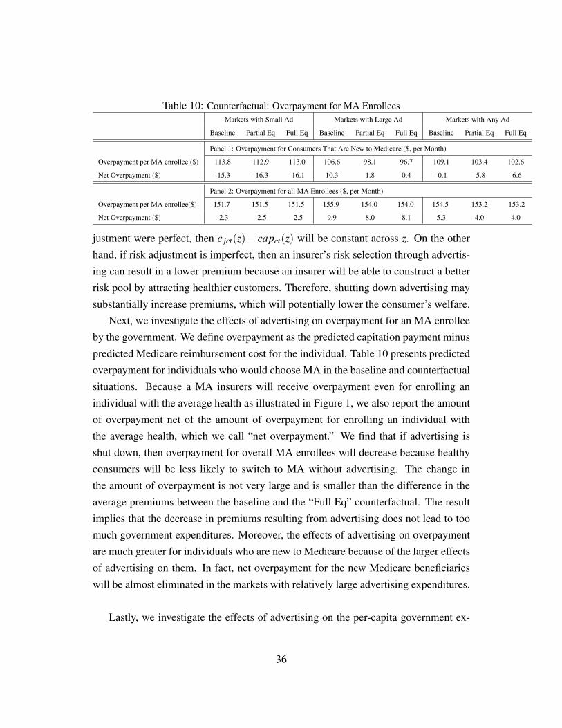
Table 10: Counterfactual: Overpayment for MA EnrolleesMarkets with Small Ad Markets with Large Ad Markets with Any Ad

Baseline Partial Eq Full Eq Baseline Partial Eq Full Eq Baseline Partial Eq Full Eq

Panel 1: Overpayment for Consumers That Are New to Medicare ($, per Month)

Overpayment per MA enrollee ($) 113.8 112.9 113.0 106.6 98.1 96.7 109.1 103.4 102.6

Net Overpayment ($) -15.3 -16.3 -16.1 10.3 1.8 0.4 -0.1 -5.8 -6.6

Panel 2: Overpayment for all MA Enrollees ($, per Month)

Overpayment per MA enrollee($) 151.7 151.5 151.5 155.9 154.0 154.0 154.5 153.2 153.2

Net Overpayment ($) -2.3 -2.5 -2.5 9.9 8.0 8.1 5.3 4.0 4.0

justment were perfect, then c jct(z)− capct(z) will be constant across z. On the otherhand, if risk adjustment is imperfect, then an insurer’s risk selection through advertis-ing can result in a lower premium because an insurer will be able to construct a betterrisk pool by attracting healthier customers. Therefore, shutting down advertising maysubstantially increase premiums, which will potentially lower the consumer’s welfare.

Next, we investigate the effects of advertising on overpayment for an MA enrolleeby the government. We define overpayment as the predicted capitation payment minuspredicted Medicare reimbursement cost for the individual. Table 10 presents predictedoverpayment for individuals who would choose MA in the baseline and counterfactualsituations. Because a MA insurers will receive overpayment even for enrolling anindividual with the average health as illustrated in Figure 1, we also report the amountof overpayment net of the amount of overpayment for enrolling an individual withthe average health, which we call “net overpayment.” We find that if advertising isshut down, then overpayment for overall MA enrollees will decrease because healthyconsumers will be less likely to switch to MA without advertising. The change inthe amount of overpayment is not very large and is smaller than the difference in theaverage premiums between the baseline and the “Full Eq” counterfactual. The resultimplies that the decrease in premiums resulting from advertising does not lead to toomuch government expenditures. Moreover, the effects of advertising on overpaymentare much greater for individuals who are new to Medicare because of the larger effectsof advertising on them. In fact, net overpayment for the new Medicare beneficiarieswill be almost eliminated in the markets with relatively large advertising expenditures.

Lastly, we investigate the effects of advertising on the per-capita government ex-

36

Table 11: Per-Capita Monthly Government Expenditures ($)Baseline Partial Eq Full Eq

Consumers That Are New to Medicare 307.4 304.9 304.2All MA Enrollees 452.6 451.8 451.5

penditure. The total government expenditure is defined as the sum of capitation pay-ments for MA enrollees and Medicare reimbursement costs for traditional Medicareenrollees. Table 11 shows that although advertising does not have a large effect for theoverall population because of switching cost, shutting down advertising will decreasethe expenditure by about 1% to $304.2 per individual per month among new Medicarebeneficiaries. We also find that the difference in government expenditures between thebaseline and the “Full Eq” counterfactual is smaller than the difference in the averagepremiums between the two situations, again implying that the decrease in premiumsresulting from advertising does not lead to too much government expenditures.

In summary, we find that advertising mainly affects the demand for consumerswho become newly eligible in Medicare, and at the same time, we find a substantialincrease in premiums. These equilibrium impacts are often ignored when researchersare interested in measuring the welfare impact of risk selection under various risk ad-justment systems, which so far emphasizes excess government expenditure due to riskselection (see Brown et al. 2014). Although a more complete welfare analysis is leftto the future work, our results highlight that it is important to endogenize and quantifythe risk selection tools of insurers in order to understand risk adjustment designs.42

8 Conclusion

This paper quantifies the impacts of advertising as risk selection on equilibrium mar-ket outcomes in MA. We first document evidence that both mass advertising and directmail advertising are targeted in order to risk-select, attracting healthier individuals. Inthe main analysis, we develop and estimate an equilibrium model of the MA marketwith advertising in order to understand the impact of advertising on consumer demand.

42An important reason we did not attempt to conduct a complete welfare analysis is that such an anal-ysis with advertising heavily depends on how we specify the way advertising affects demand. For exam-ple, informative advertising can be welfare-improving, whereas persuasive advertising can be wastefulin terms of social welfare.

37

Our estimates demonstrate that advertising has positive effects on overall demand, buta much larger effect on the demands of the healthy. Then, we conduct a counterfactualexperiment that shuts down advertising to quantitatively evaluate the importance ofrisk selection through advertising on market outcomes. We find that the equilibriumpremium increases on average up to 40% for insurers that had relatively large adver-tising expenditures, as their risk pools deteriorate. Although we find that risk selectionthrough advertising has a rent-seeking aspect, it did not likely lead to a wasteful adver-tising competition. Therefore, risk selection through advertising may make consumersbetter off by lowering premiums without much inefficient spending.

An important future work is to quantify the welfare impact of risk selection andinvestigate the optimal design of risk adjustment. The main challenge in our contextis to develop a coherent framework in which to measure the impact of advertising onconsumer welfare. This requires an explicit modeling and identification of variousmechanisms of the impact of advertising, for example informative, persuasive, andsignaling roles, which are known to be challenging. Another important avenue is toconsider other instruments for conducting risk selection. These extensions will allowus to conduct a more complete welfare assessment of risk selection.

ReferencesAckerberg, D. A., 2001. Empirically distinguishing informative and prestige effects of advertising.

RAND Journal of Economics, 316–333.

Ackerberg, D. A., 2003. Advertising, learning, and consumer choice in experience good markets: anempirical examination. International Economic Review 44 (3), 1007–1040.

Batata, A., 2004. The effect of hmos on fee-for-service health care expenditures: Evidence from medi-care revisited. Journal of health economics 23 (5), 951–963.

Bauhoff, S., 2012. Do health plans risk-select? an audit study on germany’s social health insurance.Journal of Public Economics 96 (9), 750–759.

Berry, S., Levinsohn, J., Pakes, A., 1995. Automobile prices in market equilibrium. Econometrica,841–890.

Berry, S., Levinsohn, J., Pakes, A., 2004. Differentiated products demand systems from a combinationof micro and macro data: The new car market. Journal of Political Economy 112 (1), pp. 68–105.

Brown, J., Duggan, M., Kuziemko, I., Woolston, W., 2014. How does risk selection respond to riskadjustment? new evidence from the medicare advantage program. American Economic Review104 (10), 3335–64.

38

Brown, J. R., Goolsbee, A., 2002. Does the internet make markets more competitive? evidence fromthe life insurance industry. Journal of Political Economy 110 (3), pp. 481–507.

Cabral, M., Geruso, M., Mahoney, N., 2014. Does privatized health insurance benefit patients or pro-ducers? evidence from medicare advantage. Working Paper 20470, National Bureau of EconomicResearch.

Cebul, R. D., Rebitzer, J. B., Taylor, L. J., Votruba, M. E., 2011. Unhealthy insurance markets: Searchfrictions and the cost and quality of health insurance. The American Economic Review 101 (5),1842–71.

Chiappori, P.-A., Salanie, B., 2000. Testing for asymmetric information in insurance markets. Journalof political Economy 108 (1), 56–78.

Ching, A. T., Ishihara, M., 2012. Measuring the informative and persuasive roles of detailing on pre-scribing decisions. Management Science 58 (7), 1374–1387.

Clark, C. R., Doraszelski, U., Draganska, M., 2009. The effect of advertising on brand awareness andperceived quality: An empirical investigation using panel data. Quantitative Marketing and Eco-nomics 7 (2), 207–236.

Curto, V., Einav, L., Levin, J., Bhattacharya, J., 2014. Can health insurance competition work? evidencefrom medicare advantage. Working Paper 20818, National Bureau of Economic Research.

Decarolis, F., Polyakova, M., Ryan, S. P., 2015. The welfare effects of supply-side regulations in medi-care part d. Working Paper 21298, National Bureau of Economic Research.

Dubois, P., Griffith, R., O’Connell, M., 2014. The effects of banning advertising in junk food markets.Unpublished manuscript, Toulouse School of Economics.

Duggan, M., Starc, A., Vabson, B., 2014. Who benefits when the government pays more? pass-throughin the medicare advantage program. Working Paper 19989, National Bureau of Economic Research.

Ellis, R. P., Fernandez, J. G., 2013. Risk selection, risk adjustment and choice: Concepts and lessonsfrom the americas. International Journal of Environmental Research and Public Health 10 (11), 5299–5332.

Fang, H., Keane, M. P., Silverman, D., 2008. Sources of advantageous selection: Evidence from themedigap insurance market. Journal of Political Economy 116 (2), pp. 303–350.

Finkelstein, A., McGarry, K., 2006. Multiple dimensions of private information: evidence from thelong-term care insurance market. American Economic Review 96 (4), 938–958.

Geruso, M., Layton, T., 2015. Upcoding: Evidence from medicare on squishy risk adjustment. WorkingPaper 21222, National Bureau of Economic Research.

Goeree, M. S., 2008. Limited information and advertising in the us personal computer industry. Econo-metrica 76 (5), 1017–1074.

Gordon, B. R., Hartmann, W. R., 2013. Advertising effects in presidential elections. Marketing Science32 (1), 19–35.

Handel, B. R., 2013. Adverse selection and inertia in health insurance markets: When nudging hurts.American Economic Review 103 (7), 2643–82.

39

Hastings, J. S., Hortaçsu, A., Syverson, C., 2013. Advertising and competition in privatized socialsecurity: the case of mexico.

Hausman, J. A., 1996. Valuation of new goods under perfect and imperfect competition. In: The eco-nomics of new goods. University of Chicago Press, pp. 207–248.

Ho, K., Hogan, J., Morton, F. S., 2015. The impact of consumer inattention on insurer pricing in themedicare part d program. Working Paper 21028, National Bureau of Economic Research.

Imbens, G. W., Lancaster, T., 1994. Combining micro and macro data in microeconometric models. TheReview of Economic Studies 61 (4), 655–680.

Kuziemko, I., Meckel, K., Rossin-Slater, M., 2013. Do insurers risk-select against each other? evidencefrom medicaid and implications for health reform. NBER Working Paper (w19198).

Langwell, K. M., Hadley, J. P., 1989. Evaluation of the medicare competition demonstrations. HealthCare Financing Review 11 (2), 65.

Lustig, J., 2011. Measuring welfare losses from adverse selection and imperfect competition in priva-tized medicare. Manuscript.

Mello, M. M., Stearns, S. C., Norton, E. C., Ricketts, T. C., 2003. Understanding biased selection inmedicare hmos. Health services research 38 (3), 961–992.

Miller, K., 2014. Do private medicare firms face lower costs? Unpublished manuscript, University ofMinnesota.

Miller, K., Petrin, A., Town, R., Chernew, M., 2014. Health plan changes in response to medicareadvantage payment rates. Unpublished manuscript, University of Minnesota.

Moshary, S., 2015. Price discrimination across pacs and the consequences of political advertising regu-lation. Unpublished manuscript, MIT.

Nevo, A., 2001. Measuring market power in the ready-to-eat cereal industry. Econometrica 69 (2), 307–342.

Newhouse, J. P., Price, M., Huang, J., McWilliams, J. M., Hsu, J., 2012. Steps to reduce favorablerisk selection in medicare advantage largely succeeded, boding well for health insurance exchanges.Health Affairs 31 (12), 2618–2628.

Nosal, K., 2012. Estimating switching costs for medicare advantage plans. Unpublished manuscript,University of Mannheim.

Polyakova, M., 2014. Regulation of insurance with adverse selection and switching costs: Evidencefrom medicare part d. Unpublished manuscript, Stanford University.

Pope, G. C., Kautter, J., Ellis, R. P., Ash, A. S., Ayanian, J. Z., Ingber, M. J., Levy, J. M., Robst, J.,et al., 2004. Risk adjustment of medicare capitation payments using the cms-hcc model.

Starc, A., 2014. Insurer pricing and consumer welfare: evidence from medigap. The RAND Journal ofEconomics 45 (1), 198–220.

Town, R., Liu, S., 2003. The welfare impact of medicare hmos. RAND Journal of Economics, 719–736.

Van de Ven, W. P., Ellis, R. P., 2000. Risk adjustment in competitive health plan markets. Vol. 1, Part Aof Handbook of Health Economics. Elsevier, pp. 755 – 845.

40

A Appendix

A.1 Incentives for Risk Selection

Using the data available in this paper, we investigate whether MA insurers have incen-tives to risk-select by calculating potential expected profits from enrolling a healthyand an unhealthy individual. Although recent papers make use of an individual’s riskscore (e.g., Brown et al. 2014 and Curto et al. (2014)), we do not have access to suchinformation with our data. However, the MCBS still provides useful information thatcan shed light on potential profits for insurers from enrolling individuals of differenthealth types. We make use of the two variables in the MCBS in order to calculate thepotential profits from a healthy and an unhealthy individual. First, the MCBS con-tains information on how much an MA insurer received for enrolling an individualincluded in the data. Second, we use the amount of Medicare reimbursement costs forindividuals enrolled in traditional Medicare.

A possible measure of potential profit for an individual is the difference betweenthe expected capitation payment if the individual enrolls in MA and the expected Medi-care reimbursement cost if the individual enrolls in traditional Medicare. However, animportant limitation of the two variables is that they are non-missing only for individu-als depending on their insurance choice. Therefore, we impute the expected capitationpayment and the expected Medicare reimbursement cost using their relationship withan individual’s observed characteristics, which is estimated with individuals who havenon-missing values for the two variables.

For the capitation payment, we run the following regression using information fromindividuals who enrolled in MA:

cpit = f (Ageit ,Femaleit ,Healthit ,Benchmarkcounty(i),t)β + εit , (9)

where cpit denotes the amount of the monthly capitation payment for individual i andyear t, and f (Ageit ,Femaleit ,Healthit ,Benchmarkcounty(i),t) is a function that gener-ates interactions between an individual’s age, gender, health status, and the capita-

41

tion benchmark of the individual’s county in year t (Benchmarkcounty(i),t). An indi-vidual health status Healthit is a binary variable that is equal to one if individual i ishealthy as defined when we described the MCBS in Section 2. Because of the intro-duction of the new risk adjustment regime in 2004, the relationship between cpit andf (Ageit ,Femaleit ,Healthit ,Benchmarkcounty(i),t) may have changed during the year.Thus, we run separate regressions for the years before 2004 and after 2003. The re-gression results are reported in Table 14 in the Appendix. Using the estimates, wesimulate the expected capitation payment for each individual included in the MCBS.

For the expected Medicare reimbursement cost, we run a similar regression usinginformation from individuals who enrolled in traditional Medicare:

mrit = f (Ageit ,Femaleit ,Healthit ,Costcounty(i),t)β + εit , (10)

where mrit denotes the Medicare reimbursement cost for individual i in year t averagedover twelve months, and f (Ageit ,Femaleit ,Healthit ,Costcounty(i),t) is a function thatgenerates interactions between an individual’s age, gender, health status, and per-capitaMedicare reimbursement cost in the individual’s county in year t (Costcounty(i),t). Notethat information for Costcounty(i),t does not come from the MCBS but directly from theCMS. Thus, Costcounty(i),t is the exact per-capita Medicare cost for the county in year t.The regression results are reported in Table 15 in the Appendix. Using the estimates,we simulate the expected Medicare reimbursement cost for each individual includedin the MCBS.

Once we calculate the expected capitation payment and Medicare cost for eachindividual in the MCBS, we calculate the potential profit for an MA insurer from en-rolling each individual. The potential profit πit is defined as

πit = E[cpit ]−E[mrit ].

Table 12 presents the average monthly potential profits depending on an individual’shealth status before and after the introduction of the more comprehensive risk adjust-ment regime after 2003. Note that the potential profit from a healthy individual is sub-stantially larger than that from an unhealthy individual, regardless of risk adjustmentregimes. The differences between the potential profits from a healthy and an unhealthy

42

Table 12: Incentives to Target Healthy Consumers

E[πit |Healthi = 1] ($) E[πit |Healthi = 0] ($) Difference ($)

Before 2004 214.4 -303.8 518.2After 2003 252.4 -214.2 466.6

individual are $518.2 and $466.4 before and after the new risk adjustment regime, re-spectively. Although E[πit |Healthi = 1] increased after 2003, E[πit |Healthi = 0] in-creased even more, and the difference decreased after 2003. Therefore, we find thatenrolling healthy individuals is much more profitable for MA insurers before and af-ter the new risk adjustment regime, although relative potential profits from healthyindividuals slightly decreased after 2003.

The fact that we find that enrolling healthy individuals continues to be profitableeven after 2003 may seem inconsistent with the finding that the new risk adjustmentregime substantially reduces the capitation payment to individuals with low risk scores,who are considered healthier according to the risk score system (see Table 3 in Brownet al. (2014)). However, we argue that our finding is not necessarily contradictoryto the finding by Brown et al. (2014) for two reasons. First, they also find that thenew risk adjustment regime still does not account for Medicare costs for unhealthyindividuals. In other words, the capitation payment for an individual with a lowerrisk score is still greater than the individual’s expected Medicare cost. In fact, Brownet al. (2014) find that for 77% of individuals, the capitation payments are estimated tobe larger than their expected Medicare costs before and after the new risk adjustmentregime. Because Healthit is equal to one for about 83% of individuals as shown inTable 2, it is likely that overall, healthy individuals overall continue to result in greaterprofits for MA insurers. Second, the capitation benchmark increased when the newrisk adjustment regime was introduced after 2003. As a result, the capitation paymentfor every individual increased, although the relative capitation payment changed.

43

A.2 Details on the Supply Side

A.2.1 Estimation of the Expected Health Costs

We assume that an MA enrollee’s realized health reimbursement cost for insurer jct isgiven by

ln(1+m(zi,x jct ,ωi jct ;λ )

)= ziλz + x jctλx +λwωi jct

where ωi jct is assumed to be a standard normal random variable.The realized reimbursement cost for an MA’s enrollee in a given year is available

from the MCBS Cost and Use module. Because we observed an individual’s char-acteristics zi and those of the insurer the individual chose x jct , estimating parameterλ is straightforward and can be done independently of the demand model. Table 13presents estimates for λ .

A.2.2 Solving for η jct

The profit function (8) will lead to the first order condition for the optimal pricing asfollows:

η jct =Q jct +

´zi

(p jct + cp(zi)−Eω [m(zi,x jct ,ωi jct ;λ )]

) ∂q jct(z)∂ p jct

dFct(zi)

∂Q jct∂ p jct

. (11)

Because parameter λ can be estimated outside the demand model and because both∂q jct(z)

∂ p jctand ∂Q jct

∂ p jctcan be calculated based on parameter estimates for the demand model,

η jct can be calculated using equation (11) by assuming observed premiums in the dataare at equilibrium.

44

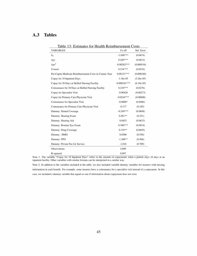
A.3 Tables

Table 13: Estimates for Health Reimbursement CostsVARIABLES Co eff Std. Error

hit -1.048*** (0.0674)

Age 0.420*** (0.0812)

Age2 -0.00262*** (0.000516)

Female 0.234*** (0.0524)

Per-Capita Medicare Reimbursement Costs in County-Year 0.00121*** (0.000240)

Copay for 10 Inpatient Days -1.36e-05 (5.26e-05)

Copay for 20 Days at Skilled Nursing Facility -0.000161*** (6.16e-05)

Coinsurance for 20 Days at Skilled Nursing Facility 0.210*** (0.0276)

Copay for Specialist Visit -0.00420 (0.00273)

Copay for Primary Care Physician Visit -0.0244*** (0.00600)

Coinsurance for Specialist Visit -0.0888* (0.0486)

Coinsurance for Primary Care Physician Visit -0.177 (0.185)

Dummy: Dental Coverage -0.249*** (0.0848)

Dummy: Hearing Exam 0.561** (0.251)

Dummy: Hearing Aid 0.0453 (0.0633)

Dummy: Routine Eye Exam 0.300*** (0.0914)

Dummy: Drug Coverage 0.154** (0.0645)

Dummy : HMO 0.0586 (0.556)

Dummy: PPO -1.388** (0.566)

Dummy: Private Fee for Service -1.016 (0.709)

Observations 4,890

R-squared 0.097Note 1: The variable “Copay for 10 Inpatient Days” refers to the amount of copayments when a patient stays 10 days at aninpatient facility. Other variables with similar formats can be interpreted in a similar way.

Note 2: In addition to the variables included in the table, we also included variable dummy variables for insurers with missing

information in each benefit. For example, some insurers have a coinsurance for a specialist visit instead of a copayment. In this

case, we included a dummy variable that equals to one if information about copayment does not exist.

45

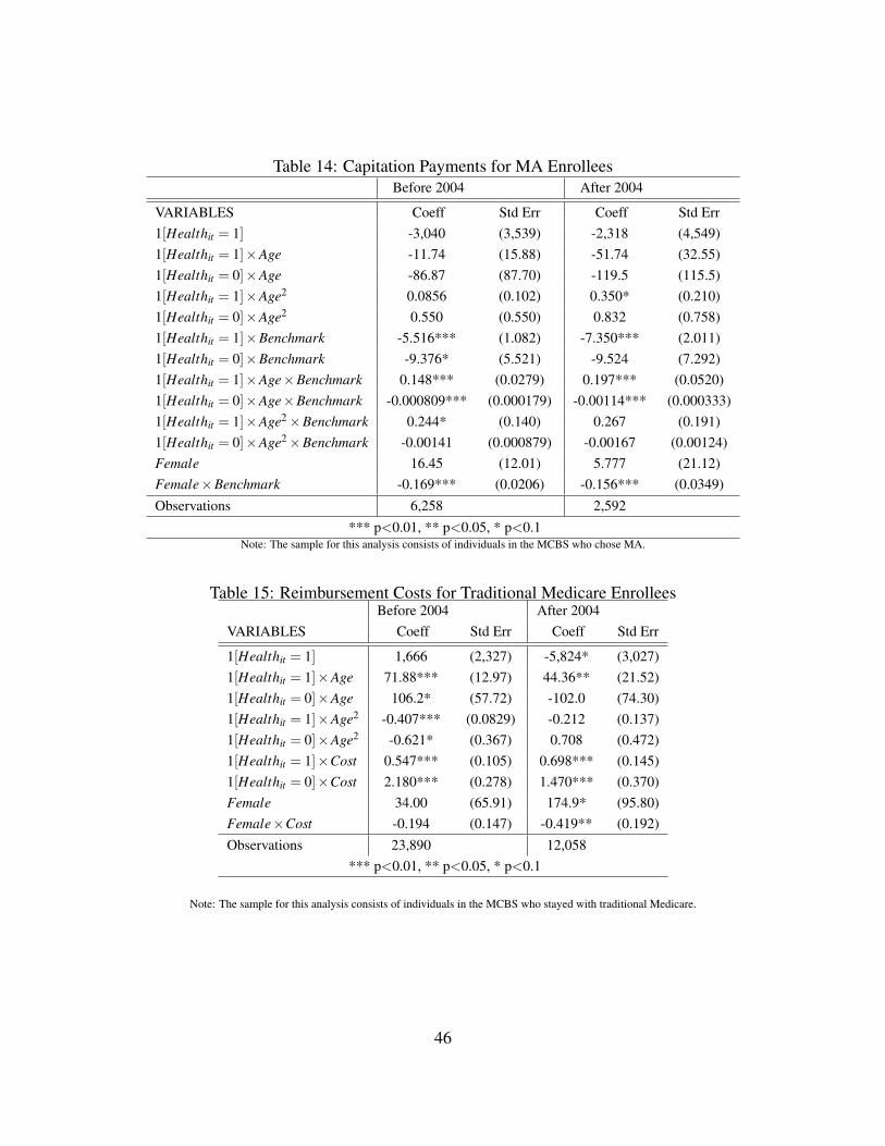
Table 14: Capitation Payments for MA EnrolleesBefore 2004 After 2004

VARIABLES Coeff Std Err Coeff Std Err1[Healthit = 1] -3,040 (3,539) -2,318 (4,549)1[Healthit = 1]×Age -11.74 (15.88) -51.74 (32.55)1[Healthit = 0]×Age -86.87 (87.70) -119.5 (115.5)1[Healthit = 1]×Age2 0.0856 (0.102) 0.350* (0.210)1[Healthit = 0]×Age2 0.550 (0.550) 0.832 (0.758)1[Healthit = 1]×Benchmark -5.516*** (1.082) -7.350*** (2.011)1[Healthit = 0]×Benchmark -9.376* (5.521) -9.524 (7.292)1[Healthit = 1]×Age×Benchmark 0.148*** (0.0279) 0.197*** (0.0520)1[Healthit = 0]×Age×Benchmark -0.000809*** (0.000179) -0.00114*** (0.000333)1[Healthit = 1]×Age2×Benchmark 0.244* (0.140) 0.267 (0.191)1[Healthit = 0]×Age2×Benchmark -0.00141 (0.000879) -0.00167 (0.00124)Female 16.45 (12.01) 5.777 (21.12)Female×Benchmark -0.169*** (0.0206) -0.156*** (0.0349)Observations 6,258 2,592

*** p<0.01, ** p<0.05, * p<0.1Note: The sample for this analysis consists of individuals in the MCBS who chose MA.

Table 15: Reimbursement Costs for Traditional Medicare EnrolleesBefore 2004 After 2004

VARIABLES Coeff Std Err Coeff Std Err

1[Healthit = 1] 1,666 (2,327) -5,824* (3,027)1[Healthit = 1]×Age 71.88*** (12.97) 44.36** (21.52)1[Healthit = 0]×Age 106.2* (57.72) -102.0 (74.30)1[Healthit = 1]×Age2 -0.407*** (0.0829) -0.212 (0.137)1[Healthit = 0]×Age2 -0.621* (0.367) 0.708 (0.472)1[Healthit = 1]×Cost 0.547*** (0.105) 0.698*** (0.145)1[Healthit = 0]×Cost 2.180*** (0.278) 1.470*** (0.370)Female 34.00 (65.91) 174.9* (95.80)Female×Cost -0.194 (0.147) -0.419** (0.192)Observations 23,890 12,058

*** p<0.01, ** p<0.05, * p<0.1

Note: The sample for this analysis consists of individuals in the MCBS who stayed with traditional Medicare.

46

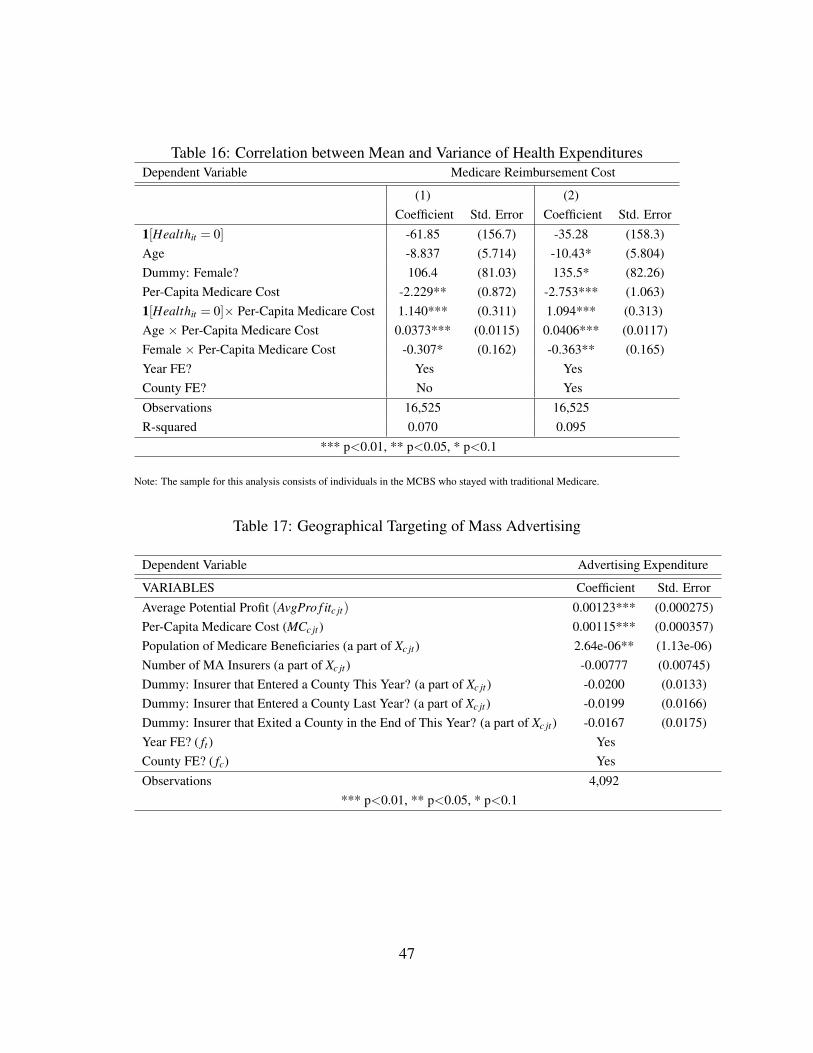
Table 16: Correlation between Mean and Variance of Health ExpendituresDependent Variable Medicare Reimbursement Cost

(1) (2)Coefficient Std. Error Coefficient Std. Error

1[Healthit = 0] -61.85 (156.7) -35.28 (158.3)Age -8.837 (5.714) -10.43* (5.804)Dummy: Female? 106.4 (81.03) 135.5* (82.26)Per-Capita Medicare Cost -2.229** (0.872) -2.753*** (1.063)1[Healthit = 0]× Per-Capita Medicare Cost 1.140*** (0.311) 1.094*** (0.313)Age × Per-Capita Medicare Cost 0.0373*** (0.0115) 0.0406*** (0.0117)Female × Per-Capita Medicare Cost -0.307* (0.162) -0.363** (0.165)Year FE? Yes YesCounty FE? No YesObservations 16,525 16,525R-squared 0.070 0.095

*** p<0.01, ** p<0.05, * p<0.1

Note: The sample for this analysis consists of individuals in the MCBS who stayed with traditional Medicare.

Table 17: Geographical Targeting of Mass Advertising

Dependent Variable Advertising Expenditure

VARIABLES Coefficient Std. ErrorAverage Potential Profit (AvgPro f itc jt) 0.00123*** (0.000275)Per-Capita Medicare Cost (MCc jt ) 0.00115*** (0.000357)Population of Medicare Beneficiaries (a part of Xc jt ) 2.64e-06** (1.13e-06)Number of MA Insurers (a part of Xc jt ) -0.00777 (0.00745)Dummy: Insurer that Entered a County This Year? (a part of Xc jt ) -0.0200 (0.0133)Dummy: Insurer that Entered a County Last Year? (a part of Xc jt ) -0.0199 (0.0166)Dummy: Insurer that Exited a County in the End of This Year? (a part of Xc jt ) -0.0167 (0.0175)Year FE? ( ft ) YesCounty FE? ( fc) YesObservations 4,092

*** p<0.01, ** p<0.05, * p<0.1

47

Tabl

e18

:Hea

lthan

dPr

oble

ms

with

Vis

ion

and

Hea

ring

Dep

ende

ntV

arV

isio

nSt

atus

1V

isio

nSt

atus

2H

eari

ngSt

atus

1H

eari

ngSt

atus

2C

oeff

Std

Err

Coe

ffSt

dE

rrC

oeff

Std

Err

Coe

ffSt

dE

rr

1[H

ealt

h it=

0]0.

203*

**(0

.014

6)0.

146*

**(0

.033

0)0.

130*

**(0

.012

9)0.

0967

***

(0.0

293)

Age

-0.0

594*

**(0

.014

5)-0

.147

***

(0.0

262)

-0.0

611*

**(0

.012

5)-0

.076

3***

(0.0

228)

Age

Squa

red

0.00

0449

***

(9.3

4e-0

5)0.

0010

4***

(0.0

0016

7)0.

0004

87**

*(8

.02e

-05)

0.00

0524

***

(0.0

0014

7)O

bser

vatio

ns21

,734

5,05

721

,811

6,32

9**

*p<

0.01

,**

p<0.

05,*

p<0.

1N

ote

1:V

isio

nSt

atus

1=

aca

tego

rica

lvar

iabl

eth

atde

scri

bes

anin

divi

dual

’sst

atus

ofvi

sion

with

ahi

gher

num

berr

epre

sent

ing

mor

ese

riou

spr

oble

ms

with

one’

svi

sion

.N

ote

2:V

isio

nSt

atus

2=

aca

tego

rica

lvar

iabl

eth

atde

scri

bes

how

diffi

cult

anin

divi

dual

tofin

dou

tabo

utM

edic

are

due

toa

prob

lem

with

visi

on.

Thi

sva

riab

leis

popu

late

don

lyfo

rin

divi

dual

sth

atin

dica

ted

that

they

had

prob

lem

sw

ithvi

sion

forV

isio

nSt

atus

1.A

ndth

isva

riab

lebe

cam

eav

aila

ble

from

2002

.

Not

e3:

Hea

ring

Stat

us1

and

2ar

ede

fined

ina

sim

ilarw

ay.A

ndH

eari

ngSt

atus

2al

sobe

cam

eav

aila

ble

from

2002

.

48

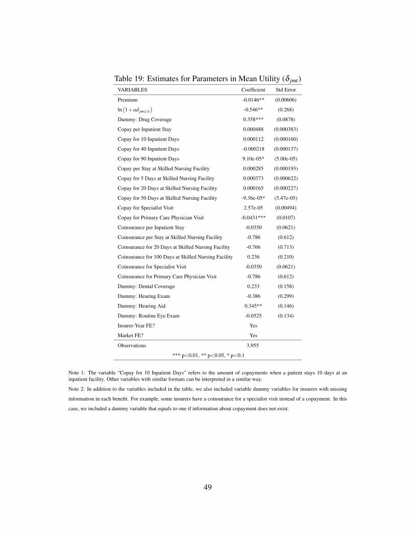
Table 19: Estimates for Parameters in Mean Utility (δ jmt)VARIABLES Coefficient Std Error

Premium -0.0146** (0.00606)

ln(1+ad jm(c)t

)-0.546** (0.268)

Dummy: Drug Coverage 0.358*** (0.0878)

Copay per Inpatient Stay 0.000488 (0.000383)

Copay for 10 Inpatient Days 0.000112 (0.000160)

Copay for 40 Inpatient Days -0.000218 (0.000137)

Copay for 90 Inpatient Days 9.10e-05* (5.00e-05)

Copay per Stay at Skilled Nursing Facility 0.000285 (0.000193)

Copay for 5 Days at Skilled Nursing Facility 0.000373 (0.000622)

Copay for 20 Days at Skilled Nursing Facility 0.000165 (0.000227)

Copay for 50 Days at Skilled Nursing Facility -9.36e-05* (5.47e-05)

Copay for Specialist Visit 2.57e-05 (0.00494)

Copay for Primary Care Physician Visit -0.0431*** (0.0107)

Coinsurance per Inpatient Stay -0.0350 (0.0621)

Coinsurance per Stay at Skilled Nursing Facility -0.786 (0.612)

Coinsurance for 20 Days at Skilled Nursing Facility -0.766 (0.713)

Coinsurance for 100 Days at Skilled Nursing Facility 0.236 (0.210)

Coinsurance for Specialist Visit -0.0350 (0.0621)

Coinsurance for Primary Care Physician Visit -0.786 (0.612)

Dummy: Dental Coverage 0.233 (0.158)

Dummy: Hearing Exam -0.386 (0.299)

Dummy: Hearing Aid 0.345** (0.146)

Dummy: Routine Eye Exam -0.0525 (0.134)

Insurer-Year FE? Yes

Market FE? Yes

Observations 3,955

*** p<0.01, ** p<0.05, * p<0.1

Note 1: The variable “Copay for 10 Inpatient Days” refers to the amount of copayments when a patient stays 10 days at aninpatient facility. Other variables with similar formats can be interpreted in a similar way.

Note 2: In addition to the variables included in the table, we also included variable dummy variables for insurers with missing

information in each benefit. For example, some insurers have a coinsurance for a specialist visit instead of a copayment. In this

case, we included a dummy variable that equals to one if information about copayment does not exist.

49

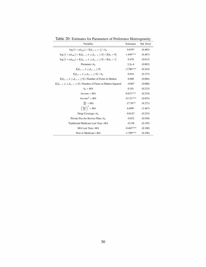
Table 20: Estimates for Parameters of Preference HeterogeneityVariables Estimates Std. Error

log(1+ad jmt

)×1[di,t−1 = j]×hit 0.879* (0.485)

log(1+ad jmt

)×1[di,t−1 6= j,di,t−1 ≥ 0]×1[hit = 0] 1.449*** (0.467)

log(1+ad jmt

)×1[di,t−1 6= j,di,t−1 ≥ 0]×1[hit = 1] 0.470 (0.612)

Premium×hit 3.2e-4 (0.003)

1[di,t−1 6= j,di,t−1 ≥ 0] -3.786*** (0.242)

1[di,t−1 6= j,di,t−1 ≥ 0]×hit 0.016 (0.127)

1[di,t−1 6= j,di,t−1 ≥ 0]×Number of Firms in Market 0.008 (0.084)

1[di,t−1 6= j,di,t−1 ≥ 0]×Number of Firms in Market Squared -0.007 (0.008)

hit ×MA 0.181 (0.215)

Income×MA 0.631*** (0.234)

Income2×MA -0.131*** (0.035)Age65 ×MA -17.76** (8.271)(

Age65

)2×MA 6.698* (3.467)

Drug Coverage×hit 0.0147 (0.215)

Private Fee-for-Service Plan×hit -0.832 (0.540)

Traditional Medicare Last Year×MA -0.338 (0.195)

MA Last Year×MA -0.463*** (0.180)

New to Medicare×MA -1.709*** (0.196)

50