Electronic copy available at: http://ssrn.com/abstract=1405014

Advertising and Firms’ Performance:

An Empirical Analysis

BY

NIKHIL GUPTA

ROLL NO. 0624

e-mail: nikhil_economics@yahoo.co.in

A DISSERTATION SUBMITTED TO DR. RUPAYAN PAL,

GOKHALE INSTITUTE OF POLITICS AND ECONOMICS (GIPE), PUNE

IN PARTIAL FULFILLMENT OF THE REQUIREMENTS FOR THE DEGREE

OF POST GRADUATION IN ECONOMICS, 2006-08

ADVISORY COMMITTEE

DR. RUPAYAN PAL

DR. J. KAJALE

DR. R. NAGARAJAN

Electronic copy available at: http://ssrn.com/abstract=1405014

2

ABSTRACT

This paper empirically examines the effect of advertisement expenditure on the firms’

performance in three industries of different nature – Automobile industry, Textiles

industry and Food industry. Taking data of all the three industries together, it is shown

that the impact of advertisement intensity on sales is positive and significant while it has

significant adverse effect on profitability. In case of automobile industry, advertisement

intensity has positive and significant effect on both the performance variables, sales and

profitability. However, in case of textiles industry and food industry, it seems that

advertisement intensity has negative and significant effect on profitability, as in case of

all three industries considered together in the analysis.

Keywords: Advertisement, Performance, Sales and Profit.

3

© copyright by

NIKHIL GUPTA

2008

4

ACKNOWLEDGEMENTS

I wish to express my sincere gratitude to Dr. Rupayan Pal for his guidance

during all phases of this dissertation. He always provided his knowledgeable

thoughts required to complete this dissertation.

In addition, special thanks are due to Dr. Rajas Parchure, Dr. Pradeep Apte

and Dr. S. Uma (Faculty, NIA) for their assistance.

5

Advertising and Firms’ Performance: An empirical analysis

Table of Contents

Abstract

Acknowledgements

Chapters

1. Introduction………………………………………………………………….9

2. Existing Literature……………………………………………………...…..15

3. Measures of Firms’ performance………………….………………...…….18

4. Definition of the variables used…………………………………..….…….21

5. Data and Descriptive Statistics……………………………………..….…..23

Industry level comparison…………………………..………….…..………26

Intra-industry level comparison…………………..……………...………..32

Firm level comparison…………………………………..………...………..34

6. Panel Data……………………………………………….…………..………38

7. Econometric Modeling……………………………….…………..…………42

Industry level modeling…………………..……………………..………….47

8. Discussion and concluding remarks...……………………………..………..56

References

6

List of Tables

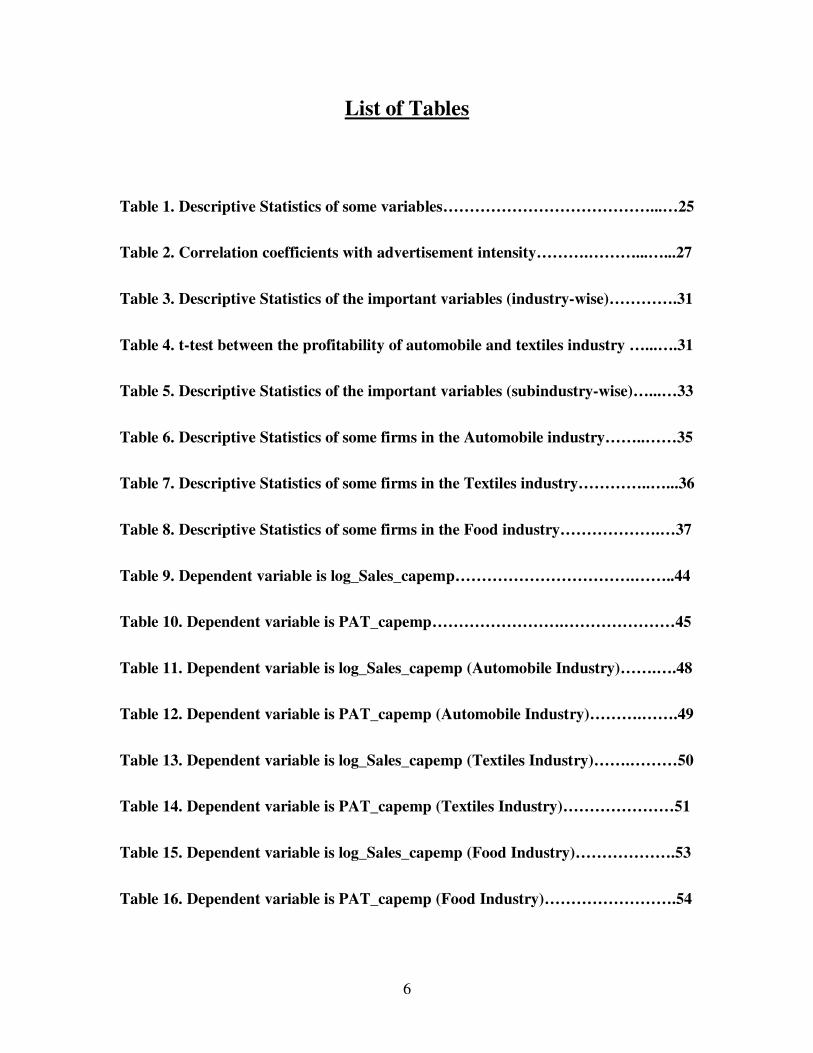
Table 1. Descriptive Statistics of some variables…………………………………...…25

Table 2. Correlation coefficients with advertisement intensity……….………...…...27

Table 3. Descriptive Statistics of the important variables (industry-wise)………….31

Table 4. t-test between the profitability of automobile and textiles industry …...….31

Table 5. Descriptive Statistics of the important variables (subindustry-wise)…...…33

Table 6. Descriptive Statistics of some firms in the Automobile industry……..……35

Table 7. Descriptive Statistics of some firms in the Textiles industry…………..…...36

Table 8. Descriptive Statistics of some firms in the Food industry……………….…37

Table 9. Dependent variable is log_Sales_capemp…………………………….……..44

Table 10. Dependent variable is PAT_capemp…………………….…………………45

Table 11. Dependent variable is log_Sales_capemp (Automobile Industry)…….….48

Table 12. Dependent variable is PAT_capemp (Automobile Industry)……….…….49

Table 13. Dependent variable is log_Sales_capemp (Textiles Industry)…….………50

Table 14. Dependent variable is PAT_capemp (Textiles Industry)…………………51

Table 15. Dependent variable is log_Sales_capemp (Food Industry)……………….53

Table 16. Dependent variable is PAT_capemp (Food Industry)…………………….54

7

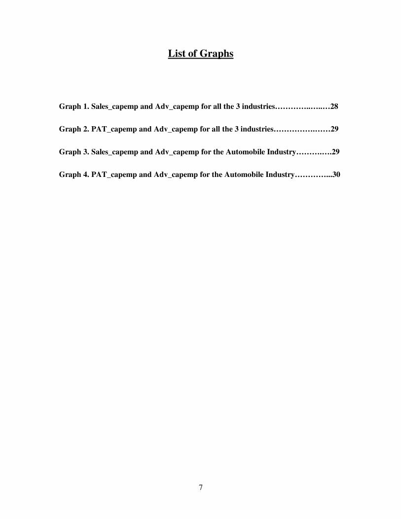
List of Graphs

Graph 1. Sales_capemp and Adv_capemp for all the 3 industries…………..…..…28

Graph 2. PAT_capemp and Adv_capemp for all the 3 industries…………….……29

Graph 3. Sales_capemp and Adv_capemp for the Automobile Industry……….….29

Graph 4. PAT_capemp and Adv_capemp for the Automobile Industry…………...30

8

“Advertising has been defined as the dissemination of information concerning an idea,

services or products to compel action in accordance with the interest of advertisers”.

M. Banerjee.

“Advertising consists of all the activities involved in presenting to a group, a non-

personal, oral or visual, openly sponsored message regarding a product or services, or

idea”.

Stanton.

“I am a part of that school, which believes, that a good advertisement is the one that

sells the products without attracting the attention to oneself. It should attract the

attention of the reader to the product. Instead of saying “what a smart advertisement”,

the reader should say “I didn’t know this before. I must try this product”.

David Ogilvy

9

1. INTRODUCTION:

The roots of the Indian advertising go back to the 18th century when hawkers called out to

the public to have a look at their wares. However, economists started to look at it as a

matter of their concern in 20th century, since earlier it was used by merchants and its

transition to the “big business” is more recent. In fact the development of transport and

communication and the liberalization of the economy have contributed to the

development of interest to this area and to the growth of this industry to attract more and

more spectators.

India, today, is regarded as the second fastest growing economy in the world, enjoying an

average growth rate of about 9.6% for the fiscal year 2006-07. With this high growth it

has become such an attractive market for the world that all producers are innovating

methods everyday to inform more and more people about their products. Consequently,

the increased competition among industrial players, the changing behavior of the Indian

consumers and an increase in the number of advertising mediums has, not surprisingly,

led to a huge amount of expenditure on advertising.

Advertising is an art used to familiarize public with the product by informing of its

description uses, its superiority over other brands, sources of its availability and price etc.

It implies the promotion of goods, services, companies and ideas with the primary

objective of creating /enhancing the demand for the product being advertised. Advertising

is not only merely propaganda but it is a paid form of communication. The advertisers

10

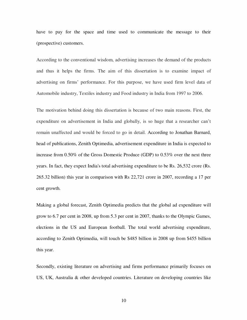
have to pay for the space and time used to communicate the message to their

(prospective) customers.

According to the conventional wisdom, advertising increases the demand of the products

and thus it helps the firms. The aim of this dissertation is to examine impact of

advertising on firms’ performance. For this purpose, we have used firm level data of

Automobile industry, Textiles industry and Food industry in India from 1997 to 2006.

The motivation behind doing this dissertation is because of two main reasons. First, the

expenditure on advertisement in India and globally, is so huge that a researcher can’t

remain unaffected and would be forced to go in detail. According to Jonathan Barnard,

head of publications, Zenith Optimedia, advertisement expenditure in India is expected to

increase from 0.50% of the Gross Domestic Produce (GDP) to 0.53% over the next three

years. In fact, they expect India's total advertising expenditure to be Rs. 26,532 crore (Rs.

265.32 billion) this year in comparison with Rs 22,721 crore in 2007, recording a 17 per

cent growth.

Making a global forecast, Zenith Optimedia predicts that the global ad expenditure will

grow to 6.7 per cent in 2008, up from 5.3 per cent in 2007, thanks to the Olympic Games,

elections in the US and European football. The total world advertising expenditure,

according to Zenith Optimedia, will touch be $485 billion in 2008 up from $455 billion

this year.

Secondly, existing literature on advertising and firms performance primarily focuses on

US, UK, Australia & other developed countries. Literature on developing countries like

11

India is very rare. We note that there is a study that analyses cross-cultural content of

advertising from the US and India (Niaz Ahmed, 2000). However, it examines the

characteristics, similarities and differences in the advertising strategies in the US and

India. It does not analyse the effects of advertisement on the performance of a firm.

According to Braithwaite (1928), advertising is a part of the total cost which is different

from the production cost as well as selling cost. It is actually that part of cost which is not

incurred in order to produce the goods or to put the goods in the market, in fact it’s that

part of the cost without which the demand curve would be too low. It is an expenditure

which is not indispensable to the marketing of the commodities, however, it is made

deliberately in order to create more demand, i.e. to shift the demand curve up or to induce

the consumers to buy more of the commodity at the given price or pay high price for the

given units of commodity purchased or may be to buy more at a higher price. However,

in modern business it is taken as a part of the selling & distribution expenses which, in

turn, increases the cost of production.

Now if advertising increases the cost for the firm, it implies that it affects many other

accounting variables of the firm, for example, the increased cost of production affects the

prices charged by the firm for its product leading to a change in the total sales of the firm

which will change the profits of the firm and thus the overall performance of the firm will

be affected. This is exactly what we will be looking ahead in this paper.

However, since it costs the firms to advertise they have an incentive to create fancy

pictures in the minds of the consumers to persuade them to purchase more commodities

so that they can cover the expenses of the advertisement from the consumer’s pocket and

12

can earn some extra profit over and above the total cost incurred including the advertising

cost. If true information is being given in the advertisement then consumer’s decision /

judgement would be based on the facts and thus would overall lead to a higher

satisfaction of the society, however, most of the times this is not the case. Thus, it is not

always necessary that the consumers respond to the advertisement by demanding more.

Though the detailed discussion of this issue is not the motivation of this paper, it is very

important to look at the ways in which consumers respond to the advertisement because

that will give us an idea of why do firms advertise?

As economists have struggled with this question, three views have emerged with each

view being associated with distinct positive and normative implications:

1.) The persuasive view - This is the most highly accepted view among the economists.

By various appeals advertisement induces the consumers to change their subjective

valuation of the commodity. It changes the consumers’ tastes and behavior in favor of

the advertised products thus, creating a spurious kind of product differentiation

leading to a less elastic demand of the advertised goods. Thus it helps the producers

to charge a higher price for their advertised commodities because the price tend to be

equal to the “true” cost of production of the commodity plus what the producer thinks

it worth to add in the way of the advertisement costs. In addition, advertisement by

the incumbent or established firms might lead to barriers to entry by making it more

difficult for the new entrants to create the reputation that the established firms have

already made and thus it becomes hard for the new entrants to find a market for their

products. These kinds of barriers can easily be found in the markets which are highly

13

concentrated or where there are economies of scale in production and/or advertising.

If this view is right then the sums spent on advertising are not on par with other costs,

and can’t be considered as part of the ordinary cost of production of the commodity.

Thus, in short, according to persuasive view, advertising leads to the anti-competitive

effects, as it has no real value but creates an artificial product differentiation to

stimulate the sales and thus, results in concentration.

2.) The informative view – This view emerged in 1960s, under the leadership of the

Chicago School. There are many markets that are characterized by imperfect

consumer information because there is considerable amount of expenditure in form of

huge search costs. Thus, consumers don’t have much information about the quality,

price, or even existence of several products. This imperfect information leads to the

market inefficiencies for which advertising acts as a solution by providing

information to the consumers. So, advertising is not a cause of the problem in fact it’s

the endogenous solution to the imperfect market. It is due to advertising that

consumers come to know about the products at a low cost. In return it makes the

demand of the existing products more elastic and thus gives new entrants an incentive

to enter the market. Therefore, it is considered to have pro-competitive effects and

hence, it is sometimes claimed that advertisement raises the standard of living and

educates the public by increasing their wants and pointing out to them the use and

desirability of the advertised commodities.

14

3.) The complementary view – Sometimes, advertising doesn’t change the preferences

of the consumers according to the persuasive view nor does it provides any new or

useful information to the consumers as said in the informative view. In fact

consumers who are induced to increase their purchase of advertised goods do so

because the marginal utility that they derive from that commodity has been raised.

That is, by advertising, advertisers try to increase the social value of the consumers

and the consumption of the products may generate higher satisfaction to the

customers in the form of the prestige that they get when they use that advertised

products.

As said, these three views are the most widely accepted views as far as the consumer’s

response to the advertising is concerned, though economists were never able to get to a

uniform result on which view is dominant or more preferable. Braithwaite (1928)

contributes significantly toward a conceptual foundation for the persuasive view. The

persuasive view of advertising is further advanced by Kaldor (1950). The formal

foundation for the information view is laid by Ozga (1960) and Stigler (1961). In Telser’s

(1964) influential effort, the theoretical and empirical foundations for the informative

view are significantly advanced. The complementary view is also associated with the

Chicago School. Important elements of this view are found in Telser’s (1964) work, but

Stigler and Becker (1977) offer a more complete statement of the central principles. Due

to shortage of time we have not done anything towards this area, however the mention of

these views was indispensable in this paper.

15

2. EXISTING LITERATURE:

A huge literature has already been devoted to the advertisement theory and much work

has been done in relation to the inter industry comparisons; however it is not recent when

the effects of advertisement was seen on an intra-industry level or firm level. Since this

paper is also on the same line, a look at the existing literature from this perspective is

essential. There are several questions that surround our mind when we start talking about

the effects of advertising like does it always lead to an increase in the sales of a firm? Is it

always profitable for the firm to advertise? If yes, then what all variables measuring the

performance of the company are getting affected due to advertising? Does advertisement

increases the demand of the whole industry as more people are aware of the product or it

just redistributes the sales among the various firms in the industry to cancel the aggregate

effect? Does it work as an informative tool for the uninformed customers or it merely

creates brand loyalty in form of less elastic demand for the advertised product due to the

conventional wisdom that only high quality goods are advertised? Some of these

questions have been investigated in details and some are still unanswered. How we will

contribute to the existing literature is by trying to look at the effects of advertisement on

the various performance measures and since much work has not been done to unfold its

effects n Indian industries, its’ not a bad idea to take this issue.

The positive relationship between the advertisement and sales are reported for the US

Auto industry by John E. Kwoka, Jr. (1993), where he showed that advertising in the auto

industry increases a car’s model sales but it is short-lived. Seldon & Doroodian (1989)

16

showed that advertising increases demand of the cigarette in the US and that health

warnings reduce the consumption of cigarettes. In fact, the interesting point he made is

that the industry reacts to the health warnings by increasing its advertising. Nerlove and

Waugh (1961) investigated the same relationship in the US orange industry by stating

that industry output must always increase with the increase in the advertisement

expenditure. While we have these papers, there are studies that reported the negative

relationship between advertisement expenditure and sales like Baltagi and Levin (1986)

used a dynamic demand for cigarettes and indicated insignificant income elasticity and

significant low price elasticity. Similar negative relationship was worked out in the US

cigarette industry by Hamilton (1962).

In addition to these findings, it was concluded that (i) rival’s advertising reduces the

effect of our own positive advertising efforts and thus the overall effect of the

advertisement on primary demand is difficult to determine and appears to vary across

industries. (ii) The industry, to some extent, believes that advertising mitigates the effects

of health warnings and thus responds to them by increasing their total advertisement

expenditures. (iii) Stronger anti smoking health warnings are considered second best to

the advertising ban.

Telser (1964) gave empirical evidence to show that there exists an inverse relationship

between the intensity of competition and the intensity of advertising. Henry Simons, one

of the major critics of advertising summed it up neatly when he wrote that “ a major

barrier to really competitive enterprises and efficient service to consumer is to be found

in advertising – in national advertising especially- and in sales organisation which cover

17

great regional or national areas.” Boulding, Lee and Staelin (1994) used longitudinal and

cross-section PIMS (Profit Impact of Market Strategies) data, in order to assess at the

business-unit level the effect of advertising on demand elasticity. They report evidence

that current advertising reduces future demand elasticity for firms that price above the

industry average.

Coming to the other aspect like whether high quality firm or low quality firm engages in

high advertising there is huge signaling literature on advertising spending. Hao Zhao

(2000) found that the high quality firm will reduce advertising spending and increase

price from their respective complete information levels. The intuition behind this is that

when information is incomplete, the high quality firm cannot exploit its advantages.

Whenever its advantages in quality or MC are lessened, a firm will want to spend less on

advertising. Nelson (1974b) explained the way in which advertising as information

operates. Manufacturers of experienced goods can increase the demand by advertising

heavily, lowering the prices and increasing the quality; however, consumers have greater

marginal revenue for search goods as compared to the experienced goods.

18

3. MEASURES OF FIRM’S PERFORMANCE:

The primary aim of this dissertation is to see the impact of advertisement expenditure on

the performance of a firm. We have seen some of the existing literature on the

advertisement effects thus; it becomes important to talk about the other side of the

discussion, namely, the performance of a company.

Measuring performance of a company is not an easy task. As industries and firms

approach the twenty-first century, they are being confronted by business environments

markedly different from those of the past.

As customers have become increasingly educated and understand their requirements

better, their expectations have increased. Competitors are becoming stronger and global

in their perspective. Technological, social, regulatory, and other types of change are, in

many cases, accelerating. To be successful in this new environment of the three C’s

customers, competitors, and change firms must adapt to the changing needs of customers

better than their competitors along such dimensions as quality, speed, flexibility, variety,

and value. They must employ their resources, including investments in new product

development, capital expenditures, and people, productively. This new environment has

given the firms an incentive to advertise heavily because in this world of infinite

products, it becomes a challenge in itself to make consumers aware of your products.

Ultimately, to increase shareholder value a firm must yield a return to its shareholders in

excess of its cost of capital.

19

Different things are advocated to measure performance in a better way. It is said that

What many firms need is a performance indicator system that focuses externally on the

business environment and its changing demands, on market/customers and competitors,

and internally on key non-financial indicators (such as market penetration, customer

satisfaction, quality, delivery, flexibility, and value) as well as more typical financial

measures (such as sales growth, profits, return on investment, and cash flows). But the

way to achieve it is still missing.

Moreover, Key Performance Indicators, also known as KPI or Key Success Indicators

(KSI), are defined to measure progress of a company towards organizational goals. But a

KPI must be measurable. For example, "Make customers happier" is not an effective KPI

without some way to measure the success of your customers. "Be the most convenient

drugstore" won't work either if there is no way to measure convenience. These are the

basic problems in following the new methods described to measure performance.

Therefore, whatever Key Performance Indicators are selected, they must reflect the

organization's goals, they must be key to its success and they must be quantifiable

(measurable). Key Performance Indicators usually are long-term considerations. The

definition of what they are and how they are measured do not change often.

Should they look at the preferences of their customers or their shareholders, as most of

the times they differ? Are they operating efficiently in terms of managing costs,

productivity etc.? Is the company strategy’s, be it market share, customer acquisition,

product/service profitability, working? All these questions, in one or the other way, give

some idea of the performance of a company. However, many of these variables are

20

subjective in nature, and thus data on them is not available. Therefore, even though one

can’t understand tennis by looking at the scoreboard, we don’t have any other option to

stick to the budget that includes various financial terms, prepared at regular intervals, to

measure actual performance of a company.

The variables that we would be using to measure the performance of a company are:

(i) The ratio of sales to capital employed (Sales_capemp);

(ii) The ratio of profit after tax (PAT) to capital employed (PAT_capemp).

21

4. DEFINITION OF THE VARIBLES USED:

1) Sales per unit of capital employed (Sales_capemp): This is one of the

endogenous or dependent variables used in this paper. It is the ratio of the net

sales to the capital employed. We have standardized sales by capital employed to

take care of the price level. But we would be using “sales” equivalent to this ratio,

to keep things simple and easy.

2) Profit after tax (PAT) per unit of capital employed (PAT_capemp): Profit

after tax (PAT) is the residual profit that is left to the shareholders of the

company, therefore, it is also known as the net profit. To make it comparable, it is

taken as per unit of capital employed. We would be using “profitability” for this

variable throughout the paper.

3) Advertisement expenditure per unit of capital employed (Adv_capemp): In

order to make comparison possible among different industries at different time

periods, we have standardized advertisement expenditure with capital employed.

It also takes care of the change in the price level. To reflect this variable, we

would use “advertisement intensity” in the paper.

4) Age: The age of the company is also taken as one of the independent variable, by

deducting year of inception form the current year, to see if profit or sales variable

get affected by the age of a firm.

22

Apart from these dependent and independent variables, we have transformed the

variables as and when necessary to take the log of some variables, lag of some variables

and the square of some variables.

23

5. DATA AND DESCRIPTIVE STATISTICS:

This analysis is based on data drawn from the CAPITALINE database published by

Centre for Monitoring Indian Economy (CMIE). The database includes detailed

accounting information compiled from the annual reports of companies. We have

analyzed data of three industries – Automobile industry, Textile industry and Food

industry. There are 12 sub-industries that we have analyzed and overall 103 companies.

In this section first we will look at the descriptive statistics of these 3 industries and will

compare them. Going further, we will compare the descriptive statistics of 12 sub-

industries and will look at the firm level comparisons as well to some extent. In between,

we will also calculate the correlation (or relationship) between the performance variables

and the advertisement variables in different industries.

It is well documented that consumer goods industry is the most heavily advertised

industry thus all the three industries we have considered are consumer goods industry.

Automobile industry is purely luxury goods industry, Food industry is purely necessary

goods industry but textiles industry is a necessary as well as luxury goods industry. In

fact, Automobile and textiles industry can be taken as a representative of durable or non-

perishable industry, while Food industry can be taken as a representative of non-durable

or perishable industry. Thus overall we are comparing the effects of advertisement on two

kinds of industries- necessary and luxury goods industry. In our data, we have 5 sub-

industries under Automobile industry, namely, LCV/HCV (5), Passenger Cars (5),

Motor/Moped (4), Scooters/3 wheelers (6) and Tractors (6), 4 sub-industries in Textiles

24

industry, namely, Denim Fabrics (5), Embroidery Fabrics (4), Hosiery/Knitwear (18) and

Readymade (6) and 3 sub-industries, namely, Large (13), Medium & Small (26) and

MNC’s (5). With the sub-industries we have given the total number of companies in

parenthesis making a total of 26 companies in Automobile industry, 33 firms in Textiles

industry and 44 firms in Food industry. We have data for 10 years for most of these

companies starting from 1997-98 to 2006-07 but for some companies it is less than 10

years, so we would be using Unbalanced Panel Data.

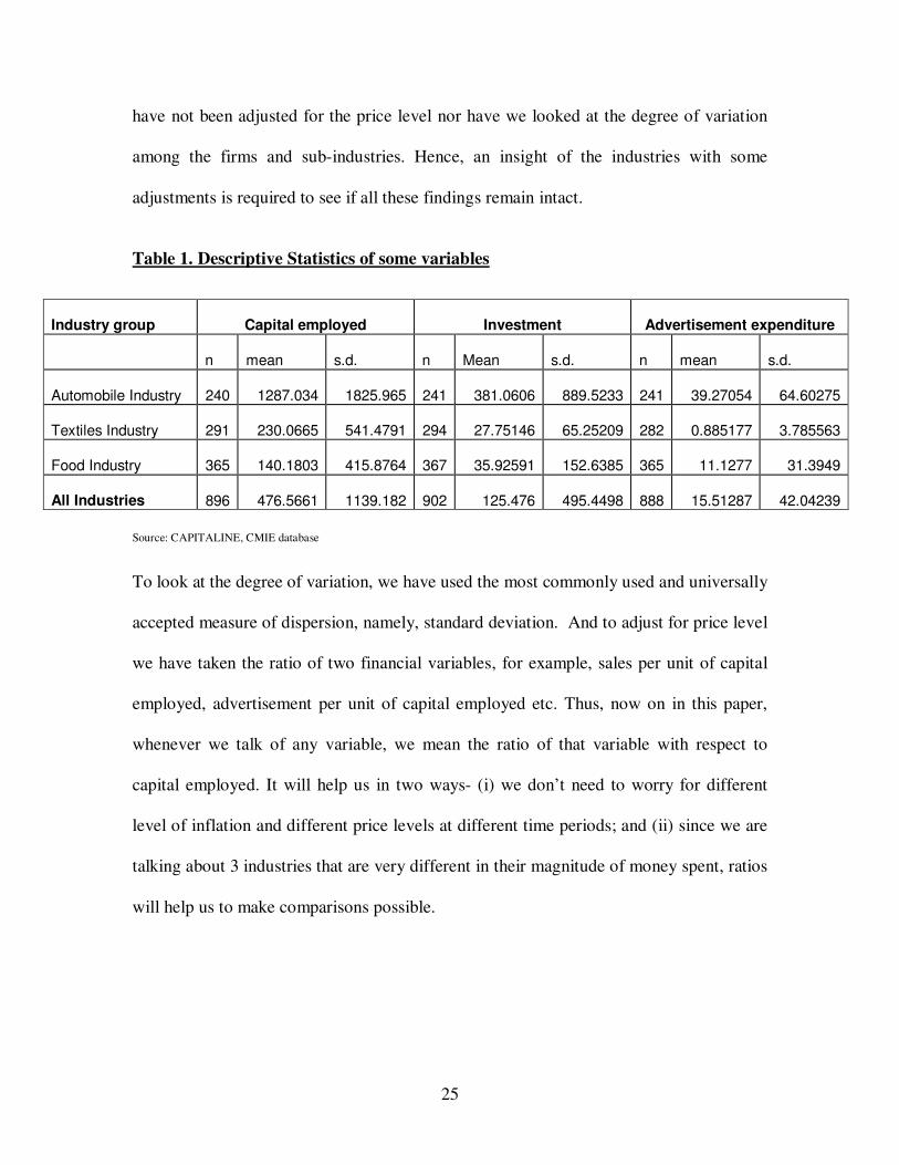
Looking generally at all the industries in one glimpse (Table 1), we find that around Rs.

15.5 crore a year on an average is spent on advertisement by these 3 industries we have

chosen, which is significant. Among them, automobile industry spends the most around

Rs. 39 crore a year while food and textiles industry spend approximately Rs. 11 crore and

Rs. 0.9 crore a year, respectively on an average. This is an interesting thing because

automobile and textiles industry, both are consumer durable goods industry, still the

difference in their advertisement expenditure is significantly large. Similarly, textiles and

food industry can be taken as necessary goods industry, still their difference is

significant. Looking at the trend in the investment & capital expenditure, where

automobile industry is the most heavily invested industry and textiles industry indulges in

least investment though food industry is also not far ahead of textiles. It is not surprising

to find that automobile industry is highly intensive in capital, spending on an average Rs.

1287 crore a year; its cost of production is also far ahead of that in either of food industry

or textiles industry since the technology that is required for automobile industry is much

innovative & expensive than in any other of the two industry. This all look pretty natural,

however not to forget that we are talking about the expenditures in absolute terms, they

25

have not been adjusted for the price level nor have we looked at the degree of variation

among the firms and sub-industries. Hence, an insight of the industries with some

adjustments is required to see if all these findings remain intact.

Table 1. Descriptive Statistics of some variables

Industry group Capital employed Investment Advertisement expenditure

n mean s.d. n Mean s.d. n mean s.d.

Automobile Industry 240 1287.034 1825.965 241 381.0606 889.5233 241 39.27054 64.60275

Textiles Industry 291 230.0665 541.4791 294 27.75146 65.25209 282 0.885177 3.785563

Food Industry 365 140.1803 415.8764 367 35.92591 152.6385 365 11.1277 31.3949

All Industries 896 476.5661 1139.182 902 125.476 495.4498 888 15.51287 42.04239

Source: CAPITALINE, CMIE database

To look at the degree of variation, we have used the most commonly used and universally

accepted measure of dispersion, namely, standard deviation. And to adjust for price level

we have taken the ratio of two financial variables, for example, sales per unit of capital

employed, advertisement per unit of capital employed etc. Thus, now on in this paper,

whenever we talk of any variable, we mean the ratio of that variable with respect to

capital employed. It will help us in two ways- (i) we don’t need to worry for different

level of inflation and different price levels at different time periods; and (ii) since we are

talking about 3 industries that are very different in their magnitude of money spent, ratios

will help us to make comparisons possible.

26

5.1 INDUSTRY LEVEL COMPARISONS:

We find that average advertisement expenditure per unit of capital employed

(Adv_capemp) is 5.00 in the automobile industry, .0.80 in the textiles industry and 6.44

in the food industry. But are they really statistically and significantly different from each

other? This is what we will find out in this section. We will compare the descriptive

statistics of some important variables at the industry level.

To answer the above question we need to find out the student’s t ratio. We calculate the t

statistic pair-wise since it’s not possible to take all the 3 industries at one time. The null

hypothesis, denoted by Ho, would be that the difference between the mean of automobile

industry and textiles industry or automobile industry and food industry or textiles

industry and food industry is zero. The alternate hypothesis, denoted by Ha, would be

whether the difference is greater than or less than zero, i.e.

Ho: mean (automobile) – mean (textiles) = 0;

and, Ha: mean (automobile) – mean (textiles) > 0;

or, mean (automobile) –mean (textiles) < 0;

We would be using one-tailed test since the alternative hypothesis is that either the

difference is greater than or less than zero. Therefore, if we reject the null hypothesis

based on the t-statistic, we can conclude that the difference between the variable of two

industries is significantly different from zero, i.e. they are not same but if we don’t reject

27

the null hypothesis, then we can say that the difference is not statistically different from

each other. As far as level of significance is concerned, by looking at the p-limit value,

we can find out the lowest level of significance at which null hypothesis can be rejected.

Though there is no hard & fast rule of what level of significance should be chosen, we

would take a difference to be significant if null hypothesis can be rejected at 10% level of

significance. We will repeat this exercise for all the variables we are taking into

consideration, first industry wise and then at the sub-industry level.

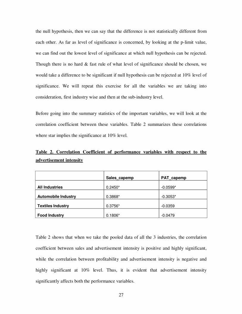
Before going into the summary statistics of the important variables, we will look at the

correlation coefficient between these variables. Table 2 summarizes these correlations

where star implies the significance at 10% level.

Table 2. Correlation Coefficient of performance variables with respect to the

advertisement intensity

Sales_capemp PAT_capemp

All Industries 0.2450* -0.0599*

Automobile Industry 0.3868* -0.3053*

Textiles Industry 0.3756* -0.0359

Food Industry 0.1806* -0.0479

Table 2 shows that when we take the pooled data of all the 3 industries, the correlation

coefficient between sales and advertisement intensity is positive and highly significant,

while the correlation between profitability and advertisement intensity is negative and

highly significant at 10% level. Thus, it is evident that advertisement intensity

significantly affects both the performance variables.

28

However, when we look at the correlation between sales and advertisement intensity

industry wise, it comes out to be positive and significant for all of them while the

correlation between profitability and advertisement is negative for all the 3 industries

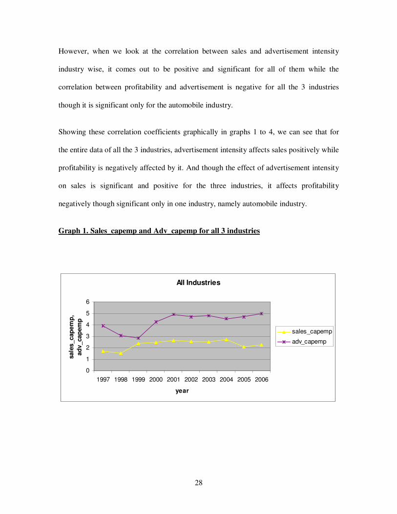
though it is significant only for the automobile industry.

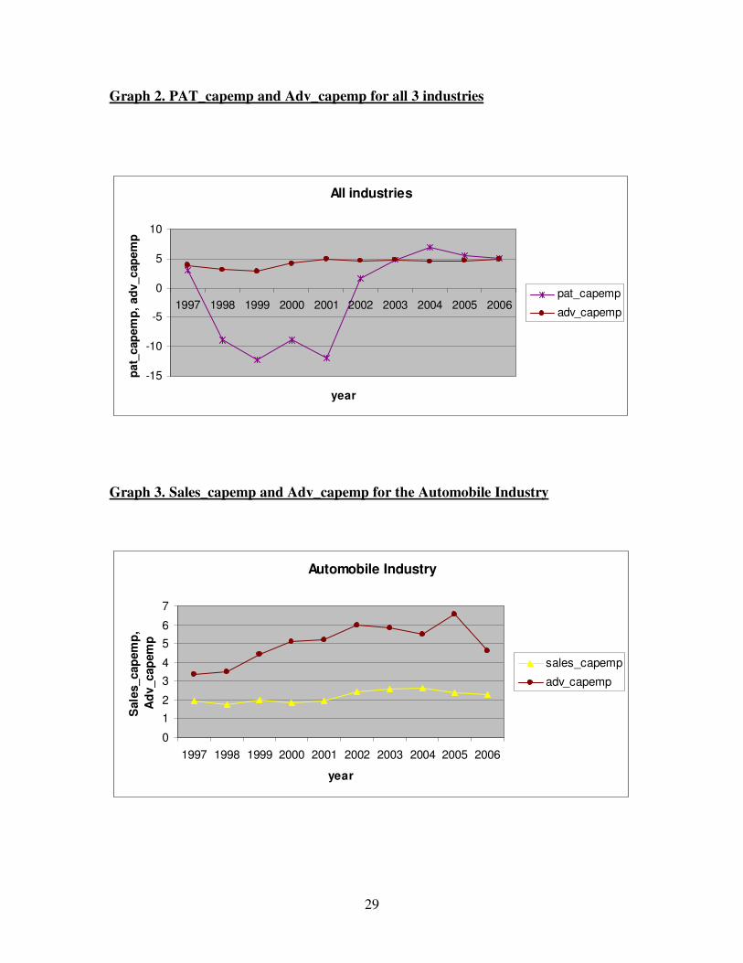
Showing these correlation coefficients graphically in graphs 1 to 4, we can see that for

the entire data of all the 3 industries, advertisement intensity affects sales positively while

profitability is negatively affected by it. And though the effect of advertisement intensity

on sales is significant and positive for the three industries, it affects profitability

negatively though significant only in one industry, namely automobile industry.

Graph 1. Sales_capemp and Adv_capemp for all 3 industries

All Industries

0

1

2

3

4

5

6

1997 1998 1999 2000 2001 2002 2003 2004 2005 2006

year

sale

s_cap

em

p,

ad

v_cap

em

p

sales_capemp

adv_capemp

29

Graph 2. PAT_capemp and Adv_capemp for all 3 industries

Graph 3. Sales_capemp and Adv_capemp for the Automobile Industry

All industries

-15

-10

-5

0

5

10

1997 1998 1999 2000 2001 2002 2003 2004 2005 2006

year

pat_

cap

em

p,

ad

v_cap

em

p

pat_capemp

adv_capemp

Automobile Industry

0

1

2

3

4

5

6

7

1997 1998 1999 2000 2001 2002 2003 2004 2005 2006

year

Sale

s_cap

em

p,

Ad

v_cap

em

p

sales_capemp

adv_capemp

30

Graph 4. PAT_capemp and Adv_capemp for the Automobile Industry

After examining of the correlation coefficients between the performance variables and

the advertisement variable, now we move our attention to the summary statistics of these

variables. Table 3 summarizes the descriptive statistics of sales, profitability and

advertisement expenditure of the entire data and the industry wise.

Sales: Comparing sales between Automobile industry and textiles industry, with null

hypothesis, Ho: diff = 0 and alternate hypothesis, Ha: diff > 0, we can reject the null

hypothesis because the p-value is 0.00 and we can conclude that the average sales is

higher in the automobile industry than the textiles industry. Similarly, Food industry

shows significantly higher sales than the other two industries. Thus, we can say that sales

are highest in the food industry as compared to the other two industries.

Automobile Industry

-10

-5

0

5

10

15

1997 1998 1999 2000 2001 2002 2003 2004 2005 2006

year

pat_

cap

em

p,

ad

v_cap

em

p

adv_capemp

pat_capemp

31

Table 3. Descriptive Statistics of the important variables (Industry-wise)

Industry group Sales_capemp PAT_capemp Adv_capemp

n mean s.d. n Mean s.d. n mean s.d.

Automobile Industry 240 2.155083 1.445626 240 0.060208 0.302618 239 5.008216 7.403163

Textiles Industry 291 0.934055 0.750828 291 -0.05333 0.738942 273 0.804797 3.692756

Food Industry 365 3.474685 5.927504 365 -0.04301 0.676555 351 6.444615 13.54939

All Industries 896 2.296083 4.025594 896 -0.01872 0.624374 863 4.262726 9.992828

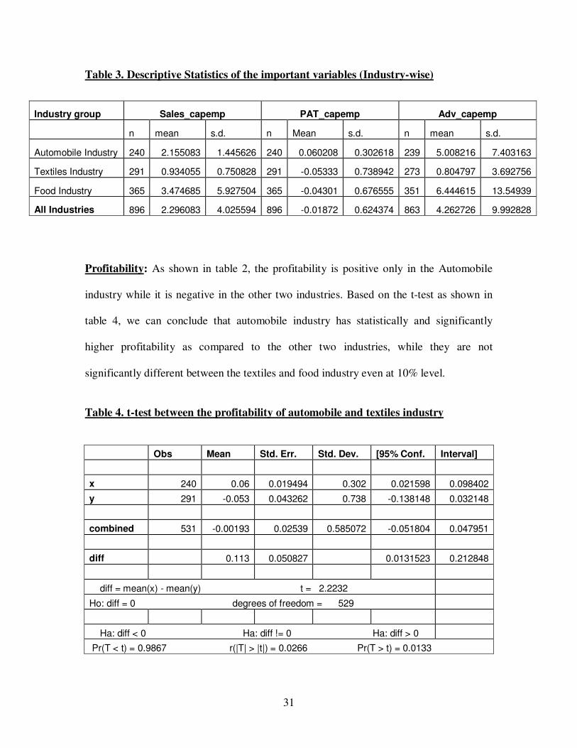
Profitability: As shown in table 2, the profitability is positive only in the Automobile

industry while it is negative in the other two industries. Based on the t-test as shown in

table 4, we can conclude that automobile industry has statistically and significantly

higher profitability as compared to the other two industries, while they are not

significantly different between the textiles and food industry even at 10% level.

Table 4. t-test between the profitability of automobile and textiles industry

Obs Mean Std. Err. Std. Dev. [95% Conf. Interval]

x 240 0.06 0.019494 0.302 0.021598 0.098402

y 291 -0.053 0.043262 0.738 -0.138148 0.032148

combined 531 -0.00193 0.02539 0.585072 -0.051804 0.047951

diff 0.113 0.050827 0.0131523 0.212848

diff = mean(x) - mean(y) t = 2.2232

Ho: diff = 0 degrees of freedom = 529

Ha: diff < 0 Ha: diff != 0 Ha: diff > 0

Pr(T < t) = 0.9867 r(|T| > |t|) = 0.0266 Pr(T > t) = 0.0133

32

Advertisement intensity: As we mentioned earlier that food industry has the highest

sales as compared to other industries, it is shown by the t-statistic that food industry

spends most on the advertisement as well. Thus, the positive and significant correlation

coefficient between sales and advertisement intensity is also understandable. Though

between automobile and textiles industry, automobile industry is the much more

advertisement intensive.

5.2 INTRA-INDUSTRY COMPARISONS:

Some of the things that we investigated and discussed so far and agreed upon now is that

food industry has statistically highest sales and spends most on the advertisement but

automobile industry have statistically and significantly highest profitability. However, in

this section we will see the differences in the sub-industries of the 3 industries in terms of

sales, profitability and advertisement intensity.

As shown in table 5, we can conclude that within the automobile industry, LCV/HCV has

the statistically highest sales using the t-statistic. Readymade sub-industry of textiles

industry has the significantly highest sales as compared to the other sub-industries of

textiles industry. Coming to the food industry, sub-industry MNC’s lead in sales.

Comparing between the sub-industries of 3 industries, MNC’s has the statistically and

significantly highest sales among all the 12 sub-industries.

33

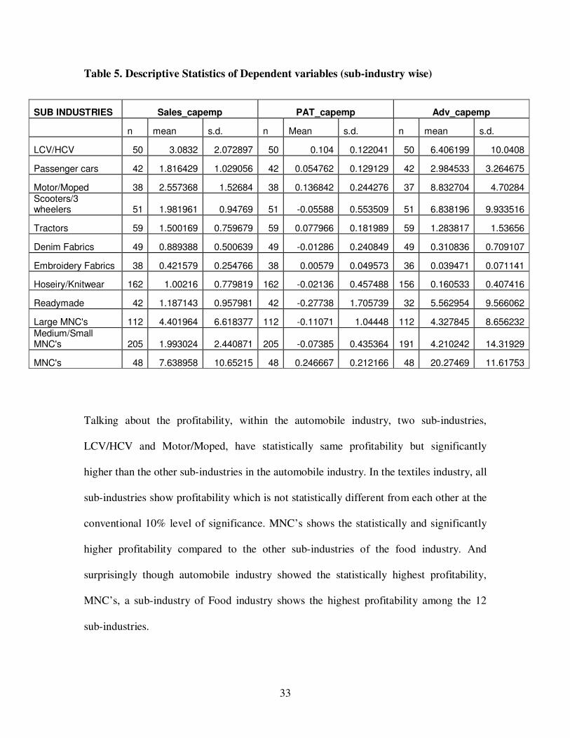
Table 5. Descriptive Statistics of Dependent variables (sub-industry wise)

SUB INDUSTRIES Sales_capemp PAT_capemp Adv_capemp

n mean s.d. n Mean s.d. n mean s.d.

LCV/HCV 50 3.0832 2.072897 50 0.104 0.122041 50 6.406199 10.0408

Passenger cars 42 1.816429 1.029056 42 0.054762 0.129129 42 2.984533 3.264675

Motor/Moped 38 2.557368 1.52684 38 0.136842 0.244276 37 8.832704 4.70284 Scooters/3 wheelers 51 1.981961 0.94769 51 -0.05588 0.553509 51 6.838196 9.933516

Tractors 59 1.500169 0.759679 59 0.077966 0.181989 59 1.283817 1.53656

Denim Fabrics 49 0.889388 0.500639 49 -0.01286 0.240849 49 0.310836 0.709107

Embroidery Fabrics 38 0.421579 0.254766 38 0.00579 0.049573 36 0.039471 0.071141

Hoseiry/Knitwear 162 1.00216 0.779819 162 -0.02136 0.457488 156 0.160533 0.407416

Readymade 42 1.187143 0.957981 42 -0.27738 1.705739 32 5.562954 9.566062

Large MNC's 112 4.401964 6.618377 112 -0.11071 1.04448 112 4.327845 8.656232

Medium/Small MNC's 205 1.993024 2.440871 205 -0.07385 0.435364 191 4.210242 14.31929

MNC's 48 7.638958 10.65215 48 0.246667 0.212166 48 20.27469 11.61753

Talking about the profitability, within the automobile industry, two sub-industries,

LCV/HCV and Motor/Moped, have statistically same profitability but significantly

higher than the other sub-industries in the automobile industry. In the textiles industry, all

sub-industries show profitability which is not statistically different from each other at the

conventional 10% level of significance. MNC’s shows the statistically and significantly

higher profitability compared to the other sub-industries of the food industry. And

surprisingly though automobile industry showed the statistically highest profitability,

MNC’s, a sub-industry of Food industry shows the highest profitability among the 12

sub-industries.

34

Coming to the independent variable, advertisement intensity within the automobile

industry, Motor/Moped and Scooters/3 wheelers spend statistically indifferent amount on

advertisement intensity, while significantly higher than the other sub-industries. Within

the textiles industry, readymade sub-industry has the significantly highest advertisement

intensity and MNC’s spends the most among the sub-industries of the food industry.

Among all the 12 sub-industries, MNC’s has the highest advertisement intensity, which is

not surprising since this sub-industry has the highest sales and profitability as well.

One more interesting thing to notice is that 9 out of 12 sub-industries (75%) show

positive and significant correlation between sales and advertisement intensity, while one

sub-industry shows negative and significant relationship. Correlation between

profitability and advertisement intensity shows really diverse picture. Overall, 5 sub-

industries show significant correlation of which 3 sub-industries show positive and 2 sub-

industries show negative correlation. Interestingly, none of the textiles sub-industry

shows significant correlation coefficient.

5.3 FIRM LEVEL COMPARISON:

To understand the high tides in the sea we need to see what’s there in the bottom. To

understand the life of a plant we need to see what’s there in the routes. Similarly, to

understand the variations in any data, we need to disaggregate it as much as possible.

Therefore, to see the reason of differences in the averages of two variables at the industry

level, we looked the differences in the averages at the sub-industry level and to see the

reason for differences in the averages at the sub-industry level, we must look at the

averages at the firm level.

35

We will cover only some companies that show interesting results and that are important

in explaining the results that we have talked about in the industry and intra-industry

comparison. First thing to note is that out of 103 companies, almost 38% of the

companies (for which data is available on these variables) show the positive and

significant correlation between Sales and advertisement intensity. While almost 25%

companies (for which data is available on these variables) show significant relationship

between profitability and advertisement intensity, of which 70% companies show

positive and merely 30% of the companies show negative relationship.

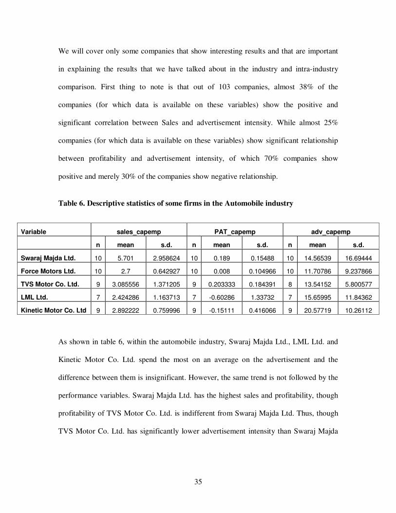
Table 6. Descriptive statistics of some firms in the Automobile industry

As shown in table 6, within the automobile industry, Swaraj Majda Ltd., LML Ltd. and

Kinetic Motor Co. Ltd. spend the most on an average on the advertisement and the

difference between them is insignificant. However, the same trend is not followed by the

performance variables. Swaraj Majda Ltd. has the highest sales and profitability, though

profitability of TVS Motor Co. Ltd. is indifferent from Swaraj Majda Ltd. Thus, though

TVS Motor Co. Ltd. has significantly lower advertisement intensity than Swaraj Majda

Variable sales_capemp PAT_capemp adv_capemp

n mean s.d. n mean s.d. n mean s.d.

Swaraj Majda Ltd. 10 5.701 2.958624 10 0.189 0.15488 10 14.56539 16.69444

Force Motors Ltd. 10 2.7 0.642927 10 0.008 0.104966 10 11.70786 9.237866

TVS Motor Co. Ltd. 9 3.085556 1.371205 9 0.203333 0.184391 8 13.54152 5.800577

LML Ltd. 7 2.424286 1.163713 7 -0.60286 1.33732 7 15.65995 11.84362

Kinetic Motor Co. Ltd 9 2.892222 0.759996 9 -0.15111 0.416066 9 20.57719 10.26112

36

Ltd., LML Ltd. and Kinetic Motor Co. Ltd., its profitability is statistically higher than

LML Ltd. and Kinetic Motor Co. Ltd.

Table 7. Descriptive statistics of some firms in the Textiles industry

In the textiles industry, Rupa & Co. Ltd. spends a significantly higher amount on

advertisement than other companies, but the difference between sales of Rupa & Co. Ltd.

and Koutons Retail India Ltd. is statistically insignificant. In fact, profitability is

significantly higher in Koutons Retail India Ltd.

Thus, two points are noteworthy here:

- Though there is a significant difference between the advertisement intensity in Rupa

& Co. Ltd. and Koutons Retail India Ltd., the difference in their sales is insignificant.

It shows that there are many other variables that affect the Sales of a firm.

- Similarly there are many other factors that affect the profitability since the company

with significantly highest advertisement expenditure doesn’t have highest

profitability.

Variable sales_capemp PAT_capemp adv_capemp

n mean s.d. n Mean s.d. n mean s.d.

K G Denim Ltd 10 1.373 0.425495 10 0.032 0.09016 10 1.057445 1.340812

T T Ltd. 10 1.988 0.69081 10 0.024 0.013499 10 1.06912 0.745266

Rupa & Co. Ltd. 6 2.405 0.252646 6 0.041667 0.004083 6 24.40983 2.919086

Koutons Retail India 6 2.288333 0.926119 6 0.093333 0.081404 6 3.191667 4.971963

Apeego Ltd. 5 0.676 0.609163 5 -2.784 4.553397 3 1.555556 2.143034

37

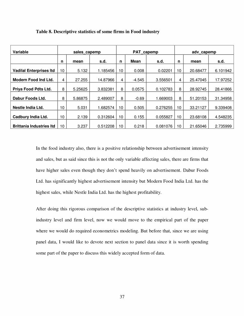
Table 8. Descriptive statistics of some firms in Food industry

Variable sales_capemp PAT_capemp adv_capemp

n mean s.d. n Mean s.d. n mean s.d.

Vadilal Enterprises ltd 10 5.132 1.185456 10 0.008 0.02201 10 20.68477 6.101942

Modern Food Ind Ltd. 4 27.255 14.87966 4 -4.545 3.556501 4 25.47045 17.97252

Priya Food Pdts Ltd. 8 5.25625 3.832381 8 0.0575 0.102783 8 28.92745 28.41866

Dabur Foods Ltd. 8 5.86875 2.489007 8 -0.69 1.669003 8 51.20153 31.34958

Nestle India Ltd. 10 5.031 1.682574 10 0.505 0.276255 10 33.21127 9.339408

Cadbury India Ltd. 10 2.139 0.312604 10 0.155 0.055827 10 23.68108 4.548235

Brittania Industries ltd 10 3.237 0.512208 10 0.218 0.081076 10 21.65046 2.735999

In the food industry also, there is a positive relationship between advertisement intensity

and sales, but as said since this is not the only variable affecting sales, there are firms that

have higher sales even though they don’t spend heavily on advertisement. Dabur Foods

Ltd. has significantly highest advertisement intensity but Modern Food India Ltd. has the

highest sales, while Nestle India Ltd. has the highest profitability.

After doing this rigorous comparison of the descriptive statistics at industry level, sub-

industry level and firm level, now we would move to the empirical part of the paper

where we would do required econometrics modeling. But before that, since we are using

panel data, I would like to devote next section to panel data since it is worth spending

some part of the paper to discuss this widely accepted form of data.

38

6. PANEL DATA

This section is heavily due to Hsiao (1988) and Gujarati (2006). A longitudinal or panel

data is one that follows a given sample of individuals over time, and thus provides

multiple observations on each individual in the sample. If each cross sectional unit has

the same number of time series observations, then such a panel (data) is called a balanced

panel. If the number of observations differs among panel members, we call such a panel

as unbalanced panel.

Panel data sets for economic research possess several major advantages over

conventional cross-sectional or time-series analysis. First, they usually give the

researcher a large number of data points, increasing the degrees of freedom and reducing

the collinearity among explanatory variables – hence improving the efficiency of the

econometric estimates. Second, and more importantly, longitudinal data allows a

researcher to analyze a number of important economic questions that can’t be addressed

using cross sectional or time series data. For instance, those economists who tend to

interpret the differences in the union or non-union workers as real believe that being a

union member enhances the chances of more wages because of their bargaining power.

On the other hand, those economists who regard union effects as illusionary tend to

believe that the changes in the wages are mainly due to the prior differences (like skill,

quality, motivation to learn etc.) in the union and non-union workers. Now, if one

believes in the former view, the coefficient of the dummy variable for union status in a

wage or earning equation is a measure of the effect of unionism. If one believes the latter

39

view, then the coefficient of the dummy variable could be simply used as a proxy for

worker’s quality. A single cross-sectional data set can’t provide a direct choice between

these two hypotheses, because the estimates are likely to reflect inter-individual

differences inherent in comparisons of different people or firms. However, if panel data

are used, one can distinguish these two hypotheses by studying the wage differential for a

worker moving from a non-union firm to a union firm or vice-versa.

Besides the advantages that panel data allow us to construct and test more complicated

behavioral models than purely cross sectional or time series data, by utilizing information

on both, the intertemporal dynamics and the individuality of the entities being invested,

one is better able to control in a more natural way for the effects of missing or

unobserved variables.

With all these benefits, there are some issues involved with panel data. The typical

assumption that economic variable y is generated by a parametric probability distribution

function identical for all individuals at all times, may not be a realistic one. Ignoring such

heterogeneity among cross sectional or time series units could lead to inconsistent or

meaningless estimates of interesting parameters.

One way to take into account the “individuality” of each cross-sectional unit is to let the

intercept vary for each unit but still assume that the slope coefficients are same across

firms. Making a model like this, in the literature, is known as the fixed effects model

(FEM). The term “fixed effects” is due to the fact that although the intercept may differ

across individuals, each individual’s intercept doesn’t vary over time; it is time invariant.

Thus we use dummy variables to estimate the fixed effects, due to which this model is

40

also known as least-squares dummy variable (LSDV) model. But if we introduce too

many dummy variables, we will lose the degrees of freedom. In fact, with so many

variables in the model, there is always the possibility of multicollinearity, which might

make the precise estimation of one or more parameters difficult. Thus, although

straightforward to apply, fixed effects modeling can be expensive in terms of degrees of

freedom.

To overcome this problem, error components model (ECM) or random effects model

(REM) was introduced. The main idea of this model is that if dummy variables are

essentially expressing the failure of including relevant explanatory variables that don’t

change overtime, then why not express this ignorance through the disturbance term. In

this, we have a common mean value for the intercept and the individual differences in the

intercept values of each cross sectional unit are reflected in the error term. Hence, in

FEM each cross-sectional unit has its own (fixed) intercept value, in REM, on the other

hand, the intercept represents the mean value of all the cross-sectional intercepts and the

error term represents the deviation of individual intercept from this mean value.

“Is there a formal test that will help us to choose between FEM and REM”? Yes, a test

was developed by Hausman in 1978. The null hypothesis underlying the Hausman test is

that the FEM and REM estimates don’t differ substantially. The test statistic developed

by Hausman has an asymptotic chi-square 2χ distribution. If the null hypothesis is

rejected, the conclusion is that REM is not appropriate and that we may be better off

using FEM, in which case statistical inferences will be conditional on the error term in

the sample.

41

Another frequently observed source of bias in both cross-sectional and panel data is that

the sample may not be randomly drawn from the population. For example, the New

Jersey negative Income tax experiment excluded all families in the geographic areas of

the experiment who had income above 1.5 times the officially defined poverty level. This

sample selection procedure introduces correlation between the right hand side variables

and the error term, which leads to the downward biased regression line. Though this

problem is not much relevant in our analysis.

42

7. ECONOMETRIC MODELING

After having some knowledge on panel data and how to estimate the panel data, now it’s

time to do some modeling to get results. In this section, we will be doing several

regressions and the performance or the dependent variables in all the regressions would

be either the logarithm of Sales (log_Sales_capemp) or profitability (PAT_capemp).

Since sales can’t be negative so, we have taken the log of it to make it normally

distributed but since profit after tax can vary from - ∞ to + ∞ , there is no need to

transform that variable.

Our main focus in the regressions would be to find the effect of advertisement intensity

on the performance variables (log_Sales_capemp and PAT_capemp). Thus, to do that, we

have transformed the explanatory variable Adv_capemp into Adv_caepmp-1, i.e. we have

taken one period lag of the advertisement effect to see if advertisement has any kind of

unutilized effects that are utilized in the future periods, known as the goodwill effects.

Apart from these two variables, we have taken the square of these two variables to see the

curvature of the advertisement expenditure.

Hence, we have five explanatory variables in all, of which four are the advertisement

variables:

1. Advertisement per unit of capital employed, Adv_capemp;

2. Log of Advertisement per unit of capital employed, Adv_capemp -1;

3. Square of Advertisement per unit of capital employed, (Adv_capemp)2;

43

4. Square of the Lag of Advertisement per unit of capital employed, (Adv_capemp -1)2;

5. Age.

We will run two regressions each taking one of the performance variables as the

dependent variable. First, we will run the regressions for the entire data and then we will

do it industry wise. Thus, we will estimate two regressions for the entire data, i.e. pooled

data of all the three industries together:

Regression 1:

log_Sales_capemp = 0α + 1α (Adv_capemp) + 2α (Adv_capemp)2 + 3α (Adv_capemp-1)

+ 4α (Adv_capemp -1)2 + 5α (Age) + 1µ

Regression 2:

PAT_capemp = 0β + 1β (Adv_capemp) + 2β (Adv_capemp)2 + 3β (Adv_capemp-1)

+ 4β (Adv_capemp -1)2 + 5β (Age) + 2µ

Now since we have taken the logarithm of the sales, such models, in the literature, are known

as semi-log models or log-lin model because only one variable (regressand in this case)

appears in the logarithmic form. Thus, in this model, the slope coefficient measures the

proportional or relative change in the regressand for a given absolute change in the value of

the regressors. However, since profit after tax (PAT) is taken in its absolute form, it is a

linear model with the usual interpretation.

Before interpreting the result, one important thing is that based on the Hausman specification

test, we have chosen the method of estimating the results – whether it is Fixed effects method

or Random effects GLS method.

44

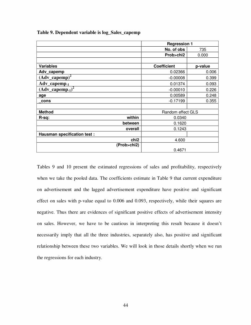
Table 9. Dependent variable is log_Sales_capemp

Regression 1

No. of obs 735

Prob>chi2 0.000

Variables Coefficient p-value

Adv_capemp 0.02366 0.006

(Adv_capemp)2 -0.00008 0.399

Adv_capemp-1 0.01374 0.093

(Adv_capemp-1)2 -0.00010 0.226

age 0.00589 0.248

_cons -0.17199 0.355

Method Random effect GLS

R-sq: within 0.0340

between 0.1620

overall 0.1243

Hausman specification test :

chi2 4.600 (Prob>chi2)

0.4671

Tables 9 and 10 present the estimated regressions of sales and profitability, respectively

when we take the pooled data. The coefficients estimate in Table 9 that current expenditure

on advertisement and the lagged advertisement expenditure have positive and significant

effect on sales with p-value equal to 0.006 and 0.093, respectively, while their squares are

negative. Thus there are evidences of significant positive effects of advertisement intensity

on sales. However, we have to be cautious in interpreting this result because it doesn’t

necessarily imply that all the three industries, separately also, has positive and significant

relationship between these two variables. We will look in those details shortly when we run

the regressions for each industry.

45

The effect of age on sales is positive but insignificant and the comparatively high

coefficient of the constant term is evident of many other variables affecting the dependent

variable.

Table 10. Dependent variable is PAT_capemp

Regression 2

No. of obs 744

Prob>chi2 0.000

Variables Coefficient p-value

Adv_capemp -0.03487 0.000

(Adv_capemp)2 0.00011 0.148

Adv_capemp-1 0.02870 0.000

(Adv_capemp-1)2 -0.00017 0.012

age 0.00344 0.255

_cons -0.12160 0.244

Method Random effect GLS

R-sq: within 0.0882

between 0.0371

overall 0.0436

Hausman specification test :

chi2 1.740 (Prob>chi2)

0.8842

This picture however is different when profitability is taken as the endogenous variable.

Table 10 shows that the effect of advertisement intensity on profitability, surprisingly, is

negative and significant while the lagged advertisement expenditure affects the

profitability positively and significantly. Thus, though current advertisement expenditure

has positive and significant effect on sales, it affects profitability negatively. Though not

very convincing, a possible explanation for this may be is that the advertisement is a kind

of addition to the total cost of production, whose return can be reaped only if with the

46

unchanged price sales are higher or if with the same sales figure, the price charged for

one unit of output is higher, however it is not necessary that advertisement leads to these

changes. Thus, profit after tax may fall if advertisement is done excessively and returns

are not according to the amount of advertisement.

Here also, the effect of age on the profitability is positive but insignificant implying that

age does not have any crucial effect on profitability or sales.

However, again one thing needs to be kept in mind is that tables 9 and 10 are results for

the pooled data of all the three industries which doesn’t imply that all the three industries

separately have the similar effects as shown in the above tables. Their effect will be

examined next but before that we should look at some interesting propositions

established:

1.) Advertisement intensity has positive and highly significant effects on Sales but it

has negative and significant effect on profitability.

2.) The effect of the one period lag of advertisement, Adv_capemp -1, is positive and

significant on both of the performance variables.

3.) The effect of age on both the performance variables is positive but insignificant.

47

7.1 INDUSTRY LEVEL MODELING:

All the above mentioned propositions are true when we pooled the entire data but now we

will split the data into three industries- Automobile industry, Textiles industry and Food

industry. It is expected to see the differences between these industries as their intensity to

advertise is entirely different. Moreover, the nature of the industries is also very different,

automobile industry is luxury goods industry, food industry is necessary goods industry

and textiles industry is a mix. Thus, it is important to look at the effect of advertisement

intensity separately on these 3 industries.

The modeling will remain same, the dependent and independent variables will remain

same, and as earlier, we will run two regressions for each industry. But the difference

would be in the data. Earlier, we combined the three industries data and run the

regressions. Now we will run the regressions for each industry separately as implied by

the subscript i in all the models: where i = 1 for automobile industry, 2 for textiles

industry and 3 for the food industry. Thus, overall we will have 2 tables for each industry

one with sales as the regressand and the other with profitability as the regressand.

Therefore, in total we will have 6 tables, 2 for each industry. Table 11 to 16 shows the

results of the industry-wise regressions.

Again we will be using the log-lin or semi-log models whenever we use sales as the

dependent variable to find the relative change and linear models when the dependent

variable is the PAT per unit of capital employed.

48

Regression 1:

(log_Sales_capemp)i = 0γ + 1γ (Adv_capemp)i + 2γ (Adv_capemp)i2 + 3γ (Adv_capemp -1)i

+ 4γ (Adv_capemp -1)i2 + 5γ (Age)i + 1µ

Regression 2:

(PAT_capemp)i = 0δ + 1δ (Adv_capemp)i + 2δ (Adv_capemp)i2 + 3δ (Adv_capemp-1)i

+ 4δ (Adv_capemp -1)i2 + 5δ (Age)i+ 4µ

Table 11 and 12 present the estimated regressions of sales and profitability in the

automobile industry. Advertisement intensity shows positive and significant impact on

sales with p-value equal to 0.022, while the effect of the lagged advertisement

expenditure is insignificant. The square of the current advertisement is negative and

significant with p-value equal to 0.033.

Table 11. Dependent variable is log_Sales_capemp (Automobile Industry)

Regression 1

No. of obs 203

Prob>chi2 0.0026

Variables Coefficient p-value

Adv_capemp 0.04935 0.022

(Adv_capemp)2 -0.00121 0.033

Adv_capemp-1 0.02028 0.321

(Adv_capemp-1)2 -0.00025 0.649

age 0.00774 0.281

_cons 0.05399 0.847

Method Random effect GLS

R-sq: within 0.0811

between 0.1258

overall 0.0841

Hausman specification test :

chi2 6.20

(Prob>chi2)

0.2875

49

The coefficient of age is positive but insignificant implying that the sales are not affected

significantly by the age of the firms.

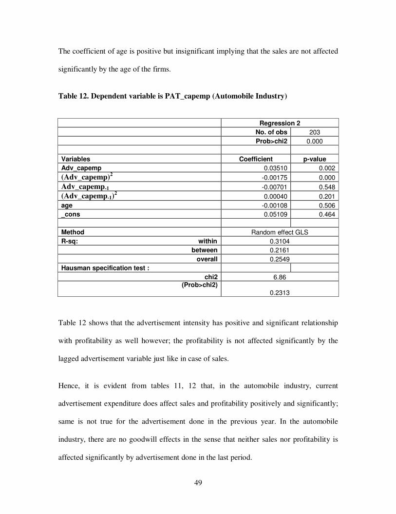
Table 12. Dependent variable is PAT_capemp (Automobile Industry)

Regression 2

No. of obs 203

Prob>chi2 0.000

Variables Coefficient p-value

Adv_capemp 0.03510 0.002

(Adv_capemp)2 -0.00175 0.000

Adv_capemp-1 -0.00701 0.548

(Adv_capemp-1)2 0.00040 0.201

age -0.00108 0.506

_cons 0.05109 0.464

Method Random effect GLS

R-sq: within 0.3104

between 0.2161

overall 0.2549

Hausman specification test :

chi2 6.86 (Prob>chi2)

0.2313

Table 12 shows that the advertisement intensity has positive and significant relationship

with profitability as well however; the profitability is not affected significantly by the

lagged advertisement variable just like in case of sales.

Hence, it is evident from tables 11, 12 that, in the automobile industry, current

advertisement expenditure does affect sales and profitability positively and significantly;

same is not true for the advertisement done in the previous year. In the automobile

industry, there are no goodwill effects in the sense that neither sales nor profitability is

affected significantly by advertisement done in the last period.

50

Thus, some propositions that can be established for the automobile industry, as far as

advertisement per unit of capital employed is concerned, from the above results are:

1. In the automobile industry, the higher the advertisement intensity is, the higher

the is the sales and profitability of a firm;

2. The effect of the lagged value of advertisement is insignificant in the automobile

industry;

3. The effect of age is positive on and negative on profitability, but insignificant in

both the cases;

Table 13. Dependent variable is log_Sales_capemp (textiles industry)

Regression 1

No. of obs 231

Prob>chi2 0.186

Variables Coefficient p-value

Adv_capemp 0.00131 0.981

(Adv_capemp)2 0.00060 0.818

Adv_capemp-1 0.12407 0.026

(Adv_capemp-1)2 -0.00348 0.149

age -0.00229 0.767

_cons -0.46465 0.038

Method Random effect GLS

R-sq: within 0.0203

between 0.1083

overall 0.0925

Hausman specification test :

chi2 0.64 (Prob>chi2)

0.9862

Having explained the results for the automobile industry (i=1), we can repeat the same

exercise for the rest of the two industries, namely Textiles and Food industry, i.e. we will

51

run the same two regressions with the subscript i=2 for the textiles industry now and i=3

for the Food industry after that.

Table 13 and 14 present the results for the textiles industry. Table 13 shows that in the

textiles industry, advertisement intensity does not have any significant effect on sales

while the effect of the lagged variable is positive and significant on sales with p-value

equal to 0.026.

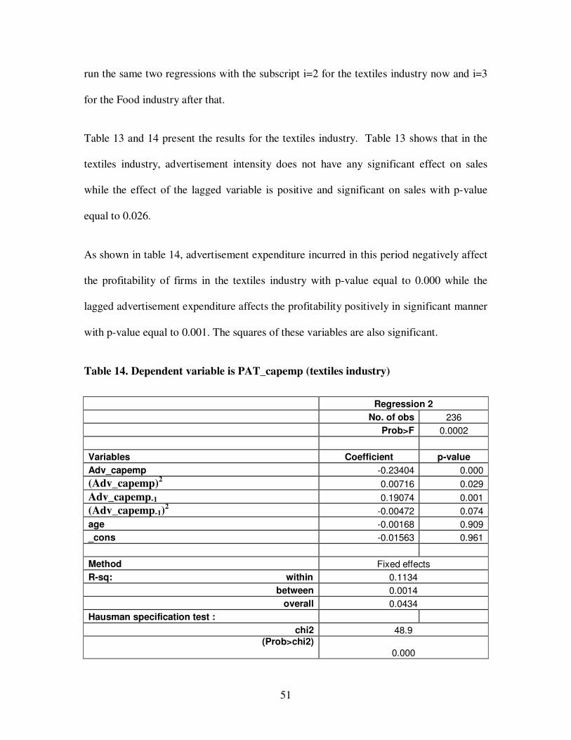
As shown in table 14, advertisement expenditure incurred in this period negatively affect

the profitability of firms in the textiles industry with p-value equal to 0.000 while the

lagged advertisement expenditure affects the profitability positively in significant manner

with p-value equal to 0.001. The squares of these variables are also significant.

Table 14. Dependent variable is PAT_capemp (textiles industry)

Regression 2

No. of obs 236

Prob>F 0.0002

Variables Coefficient p-value

Adv_capemp -0.23404 0.000

(Adv_capemp)2 0.00716 0.029

Adv_capemp-1 0.19074 0.001

(Adv_capemp-1)2 -0.00472 0.074

age -0.00168 0.909

_cons -0.01563 0.961

Method Fixed effects

R-sq: within 0.1134

between 0.0014

overall 0.0434

Hausman specification test :

chi2 48.9 (Prob>chi2)

0.000

52

Thus, textiles industry shows that though advertisement does not have any significant

effect on sales, it does have a negative and significant effect on profitability of firms in

the textiles industry. Hence, it is worth to compare the effect of advertisement intensity

on the performance of the two industries (automobile and textiles industry):

1.) The effect of advertisement intensity was significantly positive on sales of the

firms in the automobile industry and it is insignificant in the textiles industry.

2.) While the effect of advertisement intensity was positive and significant on

profitability in the automobile industry, it is negative and significant on the

profitability in the textiles industry.

3.) Unlike automobile industry, where the lagged advertisement expenditure didn’t

have any significant effect on both the performance variable, in the textiles

industry, both of the performance variables are positively affected by the lagged

advertisement expenditure.

4.) Like automobile industry, age doesn’t have any significant effect on the

performance of the firm.

Now, we move our attention to the third and last industry. So, again we will estimate two

regressions, one with each performance variable. Table 15 and 16 show the results of the

regressions estimated for sales and profitability in the food industry.

Food industry, like automobile industry, shows the positive and significant effect of

advertisement intensity on sales. The coefficient of the square of advertisement

expenditure is negative but insignificant.

53

Table 15. Dependent variable is log_Sales_capemp (Food industry)

Regression 1

No. of obs 301

Prob>chi2 0.0005

Variables Coefficient p-value

Adv_capemp 0.03738 0.003

(Adv_capemp)2 -0.00018 0.156

Adv_capemp-1 0.01033 0.369

(Adv_capemp-1)2 -0.00008 0.464

age -0.00185 0.842

_cons 0.11047 0.767

Method Random effect GLS

R-sq: within 0.0648

between 0.1148

overall 0.0978

Hausman specification test :

chi2 1.85 (Prob>chi2)

0.8689

The effect of the lagged variables of advertisement intensity is positive but insignificant,

like that in the automobile industry. Similarly, the effect of age on sales is also

insignificant.

Overall, the effect of advertisement intensity in the food industry on sales is almost

similar to that in the automobile industry; though there is difference in the magnitude of

the effects (0.049 in the automobile industry and 0.037 in the food industry) they affect

the performance in the same direction.

54

Table 16. Dependent variable is PAT_capemp (Food industry)

Regression 2

No. of obs 305

Prob>chi2 0.000

Variables Coefficient p-value

Adv_capemp -0.03904 0.000

(Adv_capemp)2 0.00017 0.027

Adv_capemp-1 0.03826 0.000

(Adv_capemp-1)2 -0.00024 0.000

age 0.00249 0.348

_cons -0.08492 0.371

Method Random effect GLS

R-sq: within 0.2199

between 0.1528

overall 0.1313

Hausman specification test :

chi2 0.11 (Prob>chi2)

0.9998

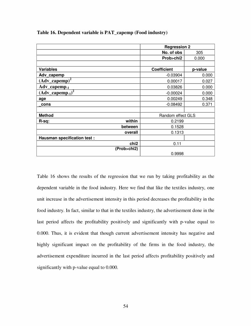
Table 16 shows the results of the regression that we run by taking profitability as the

dependent variable in the food industry. Here we find that like the textiles industry, one

unit increase in the advertisement intensity in this period decreases the profitability in the

food industry. In fact, similar to that in the textiles industry, the advertisement done in the

last period affects the profitability positively and significantly with p-value equal to

0.000. Thus, it is evident that though current advertisement intensity has negative and

highly significant impact on the profitability of the firms in the food industry, the

advertisement expenditure incurred in the last period affects profitability positively and

significantly with p-value equal to 0.000.

55

However, like other industries, age doesn’t have any significant effect on the

performance in the food industry also. The overall model is significant as shown by the p-

value of chi-square equal to 0.000.

Thus, food industry shows some mixed results of automobile and textiles industry, which

are worth noting:

1.) Like the automobile industry, the advertisement intensity positively affects the

sales, which is significant also.

2.) But the effect of advertisement intensity is negative and significant on the

profitability just like the textiles industry.

3.) Though like automobile industry, the lagged term of advertisement has

insignificant effect on the sales, the effect of lagged advertisement on

profitability is positive and significant like the textiles industry.

4.) Like the other two industries, the effect of age is insignificant on both the

performance variables in the textiles industry also.

56

8. DISCUSSION AND CONCLUDING REMARKS:

The primary aim of this dissertation was to find out the impact of advertisement on the

firms’ performance in three different industries- Automobile industry, Textiles industry

and Food industry. This paper was different in the sense that we have used three

industries of different nature and compared the effect of advertisement on them pooling

the entire data and separately as well. It is evident from the results that advertisement

certainly affects the firms depending on their nature.

When the entire data was taken, it is evident that advertisement has positive and

significant effect on sales of firms while it has significant adverse effect on profitability.

Doing the modeling industry-wise, we are convinced that there are huge differences in

the way; the advertisement affects the sales and profitability in these 3 industries.

Automobile industry shows positive impact of advertisement on sales as well as

profitability. However, the effect of advertising on profitability in food and textiles

industry seems to be negative and significant.

Due to shortage of time, I was not able to derive the demand functions for these different

industries and see if micro modeling fits in the empirical findings. This can be taken as a

task for future research for the interested candidates.

57

References:

1. Baltagi, B. H. and D. Levin (1986), “Estimating Dynamic Demand for Cigarettes

Using Panel Data: The Effects of Bootlegging, Taxation and Advertising

Reconsidered,” The Review of Economics and Statistics, 68, February, 148-55.

2. Berndt, E.R. (1991), Causality and Simultaneity between Advertising and Sales,”

appearing as Chapter 8 in E. R. Berndt (1991), The Practice of Econometrics:

Classic and Contemporary, Reading: Addison- Wesley.

3. Boulding, W., Lee, O-K., and R. Staelin (1994), “Marketing the Mix: Do

Advertising, Promotions and Sales Force Activities Lead to Differentiation?,”

4. Braithwaite, D. (1928), “The Economic Effects of Advertisement,” Economic

Journal, 38, March, 16-37.

5. Cheng Hsiao (1988), “Analysis of Panel Data,” University of Southern

California, Cambridge University Press.

6. Comanor, W. S. and T. A. Wilson (1967), “Advertising, Market Structure and

Performance,” The Review of Economics and Statistics, 49, 423-40.

7. Damodar N. Gujarati (2006), “Basic Econometrics,” United States Military

Academy, West Point, IVth edition, Tata McGraw Hill.

8. Hamilton, J. L. (1972), “The Demand for Cigarettes: Advertising, the Health

Scare, and the Cigarette Advertising Ban,” The Review of Economics and

Statistics, 54.4, November, 401-11.

9. Hausman J.A. (1978), “Specification Tests in Econometrics” Econometrica, Vol.

46 (6), November, 1251-1271.

58

10. Jayanti Sarkar and Subrata Sarkar (2008), “Debt and Corporate Governance

in emerging economies,” Economics of Transition, 16(2), 293-334.

11. Kaldor, N. V. (1950), “The Economic Aspects of Advertising,” Review of

Economic Studies, 18, February, 1-27.

12. Kwoka, Jr., J. E. (1993), “The Sales and Competitive Effects of Styling and

Advertising Practices in the U.S. Auto Industry,” The Review of Economics and

Statistics, November, 75.4, 649-56.

13. Nelson, P. (1974b), “Advertising as Information,” Journal of Political Economy,

82, August, 729-54.

14. Nerlove, M. and F. Waugh (1961), “Advertising Without Supply Control: Some

Implications of a Study of the Advertising of Oranges,” Journal of Farm

Economics, 43.4, part 1, November, 813-37.

15. Niaz Ahmed (2000), “Cross Cultural Content Analysis of Advertising from the

United States and India,” University of Southern Mississippi.

16. Ozga, S. A. (1960), “Imperfect Markets Through Lack of Knowledge,” Quarterly

Journal of Economics, 74.1, 29-52.

17. P. Rameshan (2001), “Corporate Performance during 1990s,” Productivity,

41(4), January-March, 631-641.

18. Seldon, B. J. and K. Doroodian (1989), “A Simultaneous Model of Cigarette

Advertising: Effects of Demand and Industry Response to Public Policy,” The

Review of Economics and Statistics, 71.4, November, 673-7.

19. Stigler, G. J. (1961), “The Economics of Information,” Journal of Political

Economy, 69, June, 213-25.

59

20. Sudha Sachdeva (1990), “Trends in advertising by Indian Corporate Sector”

Institute for Studies in Industrial Development.

21. Telser, L. G. (1964), “Advertising and Competition,” Journal of Political

Economy, Vol. 72, No. 6, December, 537-62.

22. Valentina G. Bruno and Stijn Claessens (2007), “Corporate Governance and

Regulation: Can there be too much of a good thing?,” World Bank Policy

Research Working Paper 4140.

23. Zhao, H. (2000), “Raising Awareness and Signaling Quality to Uninformed

Consumers: A Price Advertising Model,” Marketing Science, 19.4, Fall, 390-96.