ADVERSARY PATH ANALYSIS OF A PHYSICAL PROTECTION SYSTEM DESIGN

USING A STOCHASTIC APPROACH

A Thesis

by

YANUAR ADY SETIAWAN

Submitted to the Office of Graduate and Professional Studies of

Texas A&M University

in partial fulfillment of the requirements for the degree of

MASTER OF SCIENCE

Chair of Committee, Sunil Chirayath

Committee Members, Craig Marianno

Sergiy Butenko

Head of Department, Yassin Hassan

May 2018

Major Subject: Nuclear Engineering

Copyright 2018 Yanuar Ady Setiawan

ii

ABSTRACT

The Estimate of Adversary Sequence Interruption (EASI) model is a single path analysis

model to calculate the Probability of Interruption (PI) of a Physical Protection System (PPS) in a

facility. However, the PI value estimated by the EASI model does not have uncertainty value which

is important to represent the confidence level of the PPS’s performance. A stochastic (Monte

Carlo) approach to analyze the effectiveness of a PPS, specifically estimating the PI value and

uncertainty in the PI estimation, is implemented into the EASI model approach in a software code

developed as part of this study. The software code is tested by analyzing a hypothetical facility by

estimating PI values considering the characteristics [Probability of Detection (PD) and delay time

(td)] of the protection elements in the PPS, uncertainties in the PD and tD values, and various

adversary strategies including collusion with an insider. Sensitivity analysis of PI value with

regards to PD and td values is performed for the Most Vulnerable Path (MVP) of the facility by

considering the Critical Detection Point (CDP) of the facility’s Adversary Sequence Diagram

(ASD).

Sensitivity analysis of PI value estimation shows that the relationship between PD and PI is

linear however the relationship between td and PI is non-linear. The implementation of stochastic

(Monte Carlo) approach successfully produces PI value distribution from which the mean and

standard deviation values are estimated. The PI value is the lowest in the simulations where the

insider’s act is included, whether the insider acts on the detection or delay function or both

simultaneously. The lowest mean value of PI distribution is for the rushing strategy, among the

other adversary strategies analyzed. This is due to an unbalanced PPS design of the hypothetical

iii

facility analyzed. Frequency analysis of PI value also shows that simulations of rushing strategy

have a higher frequency of lower PI value (below 0.8) compared to the other strategies.

In conclusion, the implementation of the stochastic (Mote Carlo) method is valuable in

modeling the PD values in the EASI model, and in the estimation of PI value distribution and the

uncertainty associated, especially in modeling the adversary path including the collusion of an

insider for multi-path analysis. Frequency analysis performed on the PI values is valuable in

modifying the PPS design instead of just using the mean value of the PI distribution and its standard

deviation in the multi-path analysis.

iv

DEDICATION

This thesis is dedicated to my father, my mother, my two sisters, and especially to the God

of creation. They are the reasons I am still moving forward in this life even though I am fragile

and full of weaknesses. There are no words that can fully express my gratitude for their love, pray,

and encouragement in my life.

v

ACKNOWLEDGEMENTS

I would like to thank my committee chair, Dr. Sunil Chirayath, who has accepted me in

NSSPI from my very first day at Texas A&M University. He provides me assistance, guidance,

and support for me to learn as much as I can through many opportunities. Thank you for being

patient in helping me learn in my study and research in nuclear engineering. And thank you for all

valuable feedbacks and comments in my writing. I also want to thank my committee members, Dr.

Marianno and Dr. Butenko, for their time, feedback, and involvement in the completion of my

master’s degree. I also thank Dr. Kitcher who gave me feedback in the early phase of this research.

I also want to thank my NSSPI friends at AI 2nd floor since my first year: Athena, Linda,

Henry, Drew, Hawila, Paul, Jackson, Patrick, Rob; and those whom I hung out or traveled with:

Barbara, Katie, Ernesto, Rainbow, Logan, Robert and all the NSSPI 2017 students. I appreciate

our time and experience together. I would like to thank Gayle Rodgers who has been supporting

my administration business during my time at NSSPI, and Kelley Ragusa as the administrator of

NSSEP from which I learn things for my class and research. And last but not least in NSSPI, Dr.

Gariazzo who has been a good friend, colleague, and supporter. Thanks also go to my friends and

colleagues and the department faculty and staff for making my time at Texas A&M University a

great experience.

I want to thank my roommate, Farid Putra Bakti, and all the Indonesian students in College

Station for the warm welcome, friendship, and memorable moments in these two years. I am also

sending my gratitude to all my friends and colleague in Indonesia or abroad, for their continuous

prayers, encouragement, friendship, and love. At last, no word or poem can express my ultimate

gratitude to be born and raised by my family in Christ. Jesus blesses us all. Amen.

vi

CONTRIBUTORS AND FUNDING SOURCES

Contributors

All the work for the thesis was completed by the student, under the primary advisement of

Dr. Sunil Chirayath of the Department of Nuclear Engineering. Feedback from Dr. Marianno and

Dr. Kitcher of the Department of Nuclear Engineering and Dr. Butenko from the Department of

Industrial and Systems Engineering was valuable for the completion of the thesis. Advises from

Dr. Kitcher of the Center for Nuclear Security Science and Policy Initiatives (NSSPI) were also

essential for the thesis.

Funding Sources

Graduate study was fully sponsored by the government of Republic of Indonesia, through

the Indonesian Endowment Fund for Education (LPDP) institution under the authority of Ministry

of Finance.

vii

NOMENCLATURE

PPS Physical Protection System

PD Probability of Detection

td Delay Time

PI Probability of Interruption

PN Probability of Neutralization

PE PPS overall effectiveness

EASI Estimate of Adversary Sequence Diagram

PND Probability of Non-Detection

PNDet Probability of No Detection

PFDet Probability of First Detection

CF Correction Factor

RFT Response Force Time

PC Probability of Alarm Communication

P(R|A) Probability of Response Force Arrival

ASD Adversary Sequence Diagram

CDP Critical Detection Point

NARI Nusantara Atomic Research Institute

SNL Sandia National Laboratories

MVP Most Vulnerable Path

TR Time Remaining

viii

TABLE OF CONTENTS

Page

ABSTRACT .................................................................................................................................... ii

DEDICATION ............................................................................................................................... iv

ACKNOWLEDGEMENTS .............................................................................................................v

CONTRIBUTORS AND FUNDING SOURCES ......................................................................... vi

NOMENCLATURE ..................................................................................................................... vii

TABLE OF CONTENTS ............................................................................................................. viii

LIST OF FIGURES .........................................................................................................................x

LIST OF TABLES ....................................................................................................................... xiii

1. INTRODUCTION AND LITERATURE REVIEW................................................................1

1.1. Physical Protection System (PPS) .................................................................................. 1 1.2. Estimate of Adversary Sequence Interruption (EASI) ................................................... 3

1.3. Previous Work ................................................................................................................ 8 1.4. Objectives ..................................................................................................................... 13

1.5. Scope of Work .............................................................................................................. 13

2. DEVELOPMENT OF EASI-BASED INPUT FILE AND SOFTWARE CODE .................15

2.1. Development of Facility Design for the Input File ....................................................... 15

2.1.1. Facility Description ................................................................................................. 15 2.1.2. PPS Design of the NARI Facility ........................................................................... 16 2.1.3. Adversary Sequence Diagram (ASD) and the Input File ........................................ 20

2.2. Development of the EASI-based Software Code ......................................................... 24

2.2.1. Detection Function .................................................................................................. 25 2.2.2. Delay Function ........................................................................................................ 28 2.2.3. Response Function .................................................................................................. 30 2.2.4. Multiple Simulations ............................................................................................... 32

2.3. Probability of Detection (PD) Value Distribution ......................................................... 32

ix

3. MOST VULNERABLE PATH (MVP) AND SENSITIVITY ANALYSIS .........................35

3.1. Critical Detection Point (CDP) and Most Vulnerable Path (MVP) .............................. 35

3.1.1. Choosing Path Option with the Lowest Delay Capability for the MVP ................. 37 3.1.2. Choosing Path Option with the Lowest Detection Capability for the MVP ........... 39 3.1.3. Determining the CDP Location of the MVP........................................................... 40 3.1.4. MVP Analysis Result of the NARI Facility ........................................................... 41

3.2. Sensitivity Analysis ...................................................................................................... 44

3.2.1. Sensitivity Analysis with Regards to PD Value ....................................................... 48 3.2.2. Sensitivity Analysis with Regards to td Value ........................................................ 49

4. THE ADVERSARY PATH AND THE INSIDER’S INTERVENTION OF PPS ................51

4.1. The Adversary’s Strategy ............................................................................................. 53 4.1.1. Random Strategy ..................................................................................................... 53 4.1.2. Rushing Strategy ..................................................................................................... 54 4.1.3. Covert Strategy ....................................................................................................... 56

4.1.4. Deep Penetration Strategy....................................................................................... 58 4.1.5. MVP Strategy.......................................................................................................... 60

4.2. The Insider’s Intervention of PPS ................................................................................. 61 4.2.1. Insider’s Intervention to the Detection Function .................................................... 61 4.2.2. Insider’s Intervention to the Delay Function .......................................................... 63

4.2.3. Insider’s Intervention to the Detection and Delay Functions ................................. 66

5. RESULTS, DISCUSSION AND RECOMMENDATION ....................................................68

6. CONCLUSION ......................................................................................................................78

REFERENCES ..............................................................................................................................80

APPENDIX A COUNTRY, FACILITY, AND THREAT DESCRIPTION ................................82

APPENDIX B DEVELOPMENT OF ADVERSARY SEQUENCE DIAGRAM (ASD) OF

NARI FACILITY...........................................................................................................................86

APPENDIX C DISTRIBUTION OF DETECTION PROBABILITY VALUE OF THE NARI

FACILITY .....................................................................................................................................91

APPENDIX D SINGLE PATH EASI CALCULATION TABLE FOR SENSITVITY

ANALYSIS ....................................................................................................................................96

APPENDIX E DATA VALUE GRAPH OF SENSITIVITY ANALYSIS WITH REGARDS

TO DELAY TIME .......................................................................................................................100

APPENDIX F ADVERSARY SEQUENCE DIAGRAM AND SINGLE PATH EASI

CALCULATION TABLE OF THE COMPARISON FACILITIES ...........................................103

x

LIST OF FIGURES

Page

Figure 1. Example of a single path analysis of EASI model .......................................................... 4

Figure 2. Location of z-value in a normal distribution: (a) true cumulative td > RFT (b) true

cumulative td < RFT ........................................................................................................ 7

Figure 3. The SAVI adversary path timeline ................................................................................ 11

Figure 4. The NARI facility layout ............................................................................................... 17

Figure 5. The personnel portal room layout .................................................................................. 17

Figure 6. The main entrance room layout ..................................................................................... 18

Figure 7. The Adversary Sequence Diagram (ASD) of the NARI facility ................................... 19

Figure 8. Detection location in a path element: (a) At the beginning, the middle, and the end.

(b) At the beginning and the middle. ............................................................................. 21

Figure 9. The Microsoft Excel sheet file as the input for the software code ................................ 23

Figure 10. General flowchart of the software code ....................................................................... 24

Figure 11. Detection function calculation process flowchart ....................................................... 26

Figure 12. Sampling of PD value process flowchart ..................................................................... 27

Figure 13. Delay function calculation process flowchart ............................................................. 29

Figure 14. Response function calculation process flowchart........................................................ 31

Figure 15. Multiple simulations of PI calculation process flowchart............................................ 32

Figure 16. Distribution of PD value for the MVP for the (a) first protection layer; (b) second

protection layer; (c) third protection layer .................................................................... 33

Figure 17. Overview of MVP analysis process flowchart ............................................................ 36

Figure 18. Path selection process flowchart for the later protection layer (CDP to end) ............. 38

Figure 19. Path selection process flowchart for the earlier protection layer (start to CDP) ......... 39

Figure 20. Flowchart of the process in determining the CDP location ......................................... 40

Figure 21. The layout of the MVP route as the result of the MVP analysis ................................. 42

xi

Figure 22. The adversary timeline of the MVP ............................................................................ 42

Figure 23. Sensitivity Analysis Process Flowchart....................................................................... 45

Figure 24. Relationship of PD of the first protection layer with PI value ...................................... 46

Figure 25. Relationship of td of the ninth protection layer with PI value...................................... 47

Figure 26. Adversary path and insider’s intervention modeling process flowchart ..................... 52

Figure 27. Example of bins for random strategy path selection process ...................................... 53

Figure 28. The PI value distribution of the adversary’s random strategy simulations .................. 54

Figure 29. Example of bins for rushing strategy path selection process ...................................... 55

Figure 30. The PI value distribution of the adversary’s rushing strategy simulations .................. 56

Figure 31. Example of bins for covert strategy path selection process ........................................ 57

Figure 32. The PI value distribution of the adversary’s covert strategy simulations .................... 58

Figure 33. Flowchart of modeling the adversary’s deep penetration strategy in path selection

process ........................................................................................................................... 59

Figure 34. The PI value distribution of the adversary’s deep penetration strategy simulations ... 60

Figure 35. The PI value distribution of the adversary’s MVP strategy simulations ..................... 61

Figure 36. Flowchart of modeling the insider’s intervention of detection function of the PPS ... 62

Figure 37. The PI value distribution of the adversary’s MVP with insider’s intervention of

detection function .......................................................................................................... 63

Figure 38. Flowchart of modeling the insider’s intervention of delay function of the PPS ......... 64

Figure 39. The PI value distribution of the adversary’s MVP with insider’s intervention of

delay function ................................................................................................................ 65

Figure 40. Flowchart of modeling the insider’s intervention of detection and delay functions

of the PPS ...................................................................................................................... 66

Figure 41. The PI value distribution of the adversary’s MVP with insider’s intervention of

detection and delay functions ........................................................................................ 67

Figure 42. Frequency of PI value in five bins of MVP strategy for NARI facility ....................... 74

xii

Figure 43. Frequency of PI value in five bins of random strategy and rushing strategy for

NARI facility ................................................................................................................. 74

Figure 44. Frequency of PI value in five bins of covert strategy and deep penetration strategy

for NARI facility ........................................................................................................... 75

Figure 45. Frequency of PI value in five bins NARI facility’s MVP with various insider’s

intervention of PPS’s function ...................................................................................... 76

xiii

LIST OF TABLES

Page

Table 1. Most Vulnerable Path (MVP) of the NARI facility ........................................................ 41

Table 2. Summary of sensitivity analysis of PI with regards to PD value ..................................... 48

Table 3. Summary of sensitivity analysis of PI with regards to td value ....................................... 49

Table 4. Comparison of the initial and the distribution of PD value ............................................. 68

Table 5. Results of the sensitivity analysis ................................................................................... 69

Table 6. Results of the PI calculation simulations with combination of the adversary’s strategy

and the insider’s intervention of the NARI facility ....................................................... 71

Table 7. Results of PI calculation simulations to the improved PPS design of NARI facility ..... 73

1

1. INTRODUCTION AND LITERATURE REVIEW

Radiological and Nuclear (RN) materials present in a nuclear facility are attractive targets

for some adversaries. The intent of the adversary here is either to steal the RN materials or to

sabotage the facility itself, which can cause severe unwanted consequences. Vivid examples of

adversaries’ malicious acts involving RN materials can be found in the Incident and Trafficking

Database (ITDB) established in 1995 by the International Atomic Energy Agency (IAEA). The

ITDB information system provides data on incidents of illicit trafficking, unauthorized activities,

and events involving RN material outside of regulatory control. To prevent such malicious acts of

the adversaries, an appropriately designed and evaluated Physical Protection System (PPS) should

be installed at a nuclear facility. The IAEA has adopted a convention [1] on PPS since 1980 and

has published several guidance documents on physical protection for nuclear facilities [2]. After

the 9/11 terrorist event in 2001, the international community and the IAEA has made substantial

efforts that focused on the improvement of security of nuclear facilities.

1.1. Physical Protection System (PPS)

Physical Protection System (PPS) is a security system which integrates equipment,

procedures, and people to protect assets or facilities against theft, sabotage or another kind

malevolent adversary attack [3]. A robust PPS should have deterrence, detection, delay and

response components to defeat the success of the adversary [4]. An adversary might be a criminal,

protester, or terrorist group [5]. The adversary threat can vary based on three attributes, which are

its motivation, intention, and capability. An adversary threat spectrum is generally prepared for a

2

given nuclear facility depending on these three attributes of the adversaries who are likely to attack

the facility. The threat spectrum analysis leads to the creation of a Design Basis Threat (DBT)

document, a base on which a PPS design is made upon for a nuclear facility [6]. The insider threat

is another aspect that needs to be considered while designing a PPS. This is because of insiders

have knowledge, access, and authority, which could be misused for malicious acts including

assistance to an outside adversary.

The primary functions of a PPS are (a) provide barriers to stop the adversary intrusion, (b)

detect the adversary intrusion, (c) delay the adversary action (after the intrusion has occurred and

detected), and (d) respond to neutralize the adversary. Integration of various types of protection

elements into the PPS provides those mentioned functions. The detection protection element of a

PPS (for example, a motion sensor on a fence) is characterized quantitatively by its Probability of

Detection (PD). The detection process consists of three parts, which are intrusion sensing with the

probability of producing a signal (Ps), the probability of signal transmission as an alarm (Pt), and

the probability of accurate alarm assessment (Pa). These probability values are used to determine

PD using the relationship expressed in Equation 1.1.

𝑃𝐷 = 𝑃𝑠 × 𝑃𝑡 × 𝑃𝑎 (1.1)

The delay protection element (for example, a locked door) of a PPS provides the ability to

slow down the adversary intrusion progress towards the target, which in turn provides time for the

response force, after a genuine alarm, to interrupt the adversary before he or she reaches the target.

The capability of a delay protection element is characterized by the delay time (td) it provides.

3

The last element of the PPS is the response force, made up of trained security personnel

and the necessary equipment, such as weapons, body protection, transportation, communication,

etc. The purpose of the response force is to intercept and neutralize the intruding adversary. The

Probability of Interruption (PI) is defined as the probability that the response force can interrupt

(intercept) the adversary after a genuine intrusion detection alarm. The capability of response force

is characterized by the Probability of Neutralization (PN), which is defined as the probability that

the response force can neutralize the adversary. The product of PI and PN represents the overall

effectiveness (PE) of the PPS as shown in Equation 1.2.

𝑃𝐸 = 𝑃𝐼 × 𝑃𝑁 (1.2)

1.2. Estimate of Adversary Sequence Interruption (EASI)

Estimate of Adversary Sequence Interruption (EASI) model is used to determine the

overall Probability of Interruption (PI) value of a PPS [3]. The EASI model is based on the

assumption that the response force must be notified of the adversary’s attempt of theft or sabotage

while there is still sufficient time to interrupt and neutralize the adversary [7]. It is developed as a

single path analysis tool, in which the adversary path in the facility has been defined by the user

along with the detection, delay, and response force capability information for every protection

layer as shown in Figure 1. The EASI model has three calculation sections in general. The first

one is the detection function calculation section. The second one is the delay function calculation

section. The third one is the response function calculation section, in which the results from two

other sections are combined and used to calculate the total PI value.

4

Figure 1. Example of a single path analysis of EASI model

In the detection function calculation section, EASI model uses the PD values of each

protection layer along the adversary path. The PD values are used to calculate three other

probability values; the Probability of Non-Detection (PND), the Probability of No Detection (PNDet),

and the Probability of First Detection (PFDet). PND is the probability that the adversary is not

detected in a protection layer of interest. PNDet is the probability that there is no detection from the

first protection layer until a protection layer of interest. PFDet is the probability that the adversary’s

intrusion is detected for the first time at the corresponding protection layer of interest. PND, PNDet,

and PFDet can be expressed as shown in Equations 1.3, 1.4, and 1.5 respectively.

𝑃𝑁𝐷𝑖= 1 − 𝑃𝐷𝑖

(1.3)

𝑃𝑁𝐷𝑒𝑡𝑖= ∏ 𝑃𝑁𝐷𝑖

𝑖1 (1.4)

𝑃𝐹𝐷𝑒𝑡𝑖= 𝑃𝐷𝑖

× 𝑃𝑁𝐷𝑒𝑡𝑖−1 (1.5)

0.88Estimate of Probability of

Adversary Alarm System Response Time (in seconds)

Sequence Communication Mean Standard Deviation

Interruption 0.97 270 81

(EASI)

Delays (in seconds):

Task Description P(Detection) Location Mean: Standard Deviation

1 Penetrates the Fence (Entrance) 0.8 B 10 3.0

2 Runs through Limited Access Area 0.02 M 90 27.0

3 Penetrates Vehicle Door P9 0.5 E 30 9.0

4 Runs through Protected Area 0.02 M 90 27.0

5 Penetrates door P5 0.99 E 54 16.2

6 Runs through Plant Controlled Building 0.02 M 20 6.0

7 Penetrate door P6 0.99 E 127 38.1

8 Runs to the target 0.02 M 15 4.5

9 Sabotage 1 B 51 15.3

Probability of Interruption:

5

In the delay function calculation section, there are several delay-related values calculated

for every protection layer along the adversary path. The first value is the cumulative delay time,

which is the summation of the td values from protection layer of interest until the last protection

layer along the adversary path, as expressed by Equation 1.6. The cumulative delay time variance

of each protection layer along the adversary path is also calculated from the standard deviation

(td) of the td value, as expressed by Equation 1.7.

Detection location information indicates a Correction Factor (CF) which is used to calculate

other delay-related values, as shown in Equation 1.8. ‘B’ represents detection right at the beginning

of current protection element, ‘M’ represents the detection mid-way between current protection

element to the next, and ‘E’ represents detection very late almost at the next protection element so

that no delay time credit can be given at the current protection element. CF is used to calculate the

real amount of time along the path that needs to be spent by the adversary to go to the next

protection layer after being detected in a protection layer of interest, expressed by Equation 1.9.

This real amount of time in the path is called true delay time value, which also has an associated

true variance value as expressed in Equation 1.10. Finally, EASI model calculates the true

cumulative delay time and true cumulative variance of each protection layer along the adversary

path by using Equations 1.11 and 1.12 respectively. In Equations 1.6 through 1.12, ‘n’ represents

the total number of protection element layer of the PPS while ‘i’ is the protection layer of interest.

𝑐𝑢𝑚𝑢𝑙𝑎𝑡𝑖𝑣𝑒 𝑡𝑑𝑖= ∑ 𝑡𝑑𝑖

𝑛𝑖=𝑖 (1.6)

𝑐𝑢𝑚𝑢𝑙𝑎𝑡𝑖𝑣𝑒 𝜎2𝑡𝑑𝑖

= ∑ (𝜎𝑡𝑑𝑖)2𝑛

𝑖=𝑖 (1.7)

𝐶𝐹 {

1 𝑓𝑜𝑟 ′𝐵′

0.5 𝑓𝑜𝑟 ′𝑀′

0 𝑓𝑜𝑟 ′𝐸′

(1.8)

6

𝑡𝑟𝑢𝑒 𝑡𝑑𝑖= 𝐶𝐹 × 𝑡𝑑𝑖

(1.9)

𝑡𝑟𝑢𝑒 𝜎2𝑡𝑑𝑖

= (𝐶𝐹 × 𝜎𝑡𝑑𝑖)2 (1.10)

𝑡𝑟𝑢𝑒 𝑐𝑢𝑚𝑢𝑙𝑎𝑡𝑖𝑣𝑒 𝑡𝑑𝑖= 𝑡𝑟𝑢𝑒 𝑡𝑑𝑖

+ ∑ 𝑡𝑑𝑖

𝑛𝑖=𝑖+1 (1.11)

𝑡𝑟𝑢𝑒 𝑐𝑢𝑚𝑢𝑙𝑎𝑡𝑖𝑣𝑒 𝜎2𝑡𝑑𝑖

= 𝑡𝑟𝑢𝑒 𝜎2𝑡𝑑𝑖

+ ∑ (𝜎𝑡𝑑𝑖)2𝑛

𝑖=𝑖+1 (1.12)

In the response function calculation section, true cumulative delay time and true cumulative

delay variance values are used to calculate the z-value for each protection layer using Equation

1.13. Response Force Time (RFT) in Equation 1.13 is the cumulative time which is the sum of

alarm transmission time, alarm assessment time, alarm communication time to the response force,

the response force preparation time, the response force travel time, and the response force muster

and deployment time. RFT is the standard deviation of the RFT. The Probability of Alarm

Communication (PC) represents the probability that the assessed alarm was communicated

correctly by the alarm assessor to the response force and is assumed to be a constant for all the

detection elements in the PPS.

𝑧𝑖 =𝑥 − 𝜇

𝜎=

𝑡𝑟𝑢𝑒 𝑐𝑢𝑚𝑢𝑙𝑎𝑡𝑖𝑣𝑒 𝑡𝑑𝑖 − 𝑅𝐹𝑇

√𝑡𝑟𝑢𝑒 𝑐𝑢𝑚𝑢𝑙𝑎𝑡𝑖𝑣𝑒 𝜎2𝑡𝑑𝑖

+ 𝜎𝑅𝐹𝑇2

(1.13)

Given the response force team is alerted by the detection of the adversary’s intrusion at any

protection layer, based on the remaining cumulative delay time at that protection element to the

target, the Probability of Response Force Arrival (P(R|A)) before the adversary reach the target has

to be calculated. P(R|A) is calculated as the integration of the probability density function from -∞

7

to the z-value (Equation 1.13) of the protection layer of interest using the RFT normal distribution.

This calculation can be done by using the Norm.S.Dist function in Microsoft Excel to integrate the

probability density function from -∞ to the z-value. Figure 2a shows the location of a z-value in

which the true cumulative delay time is more than the RFT, which means that the adversary is

detected in earlier protection layer. Figure 2b shows the location of a z-value in which the true

cumulative delay time is less than the RFT, which means that the adversary is detected in later

protection layer almost at the end of the adversary’s mission. Specific Probability of Interruption

(PI) value for each protection layer is calculated by using Equation 1.14.

𝑆𝑝𝑒𝑐𝑖𝑓𝑖𝑐 𝑃𝐼𝑖= 𝑃𝐹𝐷𝑒𝑡𝑖

× 𝑃𝐶 × 𝑃(𝑅|𝐴)𝑖 (1.14)

(a) (b)

Figure 2. Location of z-value in a normal distribution: (a) true cumulative td > RFT

(b) true cumulative td < RFT

The general mathematical equation to calculate the total PI value is shown in Equation 1.15

and can be simplified as Equation 1.16. In summary, the total PI value of the PPS is the

accumulation of the specific PI values provided by every protection layer along the adversary path.

8

𝑃𝐼 = 𝑃(𝐷1) × 𝑃(𝐶1) × 𝑃(𝑅|𝐴1) + ∑ 𝑃(𝐷𝑖) × 𝑃(𝐶𝑖) × 𝑃(𝑅|𝐴𝑖) × ∏ (1 − 𝑃(𝐷𝑖))𝑖−1𝑖=1

𝑛𝑖=2 (1.15)

𝑃𝐼 = ∑ 𝑠𝑝𝑒𝑐𝑖𝑓𝑖𝑐 𝑃𝐼𝑖𝑛𝑖 (1.16)

The Probability of Neutralization (PN) is the probability that the response force successfully

neutralizes the adversary, given the interruption has been made. The Analytic System and Software

for Evaluating Safeguards and Security (ASSESS) Neutralization Model is one of the computer

code to simulate engagement between the postulated adversary and response force. It requires data

on the adversary, such as number and type of the adversary, and weapon of the adversary. It also

requires data on the response force, such as type and number of guards, and weapon owned by the

guards. A Markov Chain is constructed to determine PN as a function of successive volleys by both

sides [8].

1.3. Previous Work

The EASI model has been used in many PPS evaluations and improvement studies. A.A

Wadoud et al. used the single path EASI model to calculate the PI value for two sabotage scenarios

in a hypothetical research reactor facility [8]. The ASSESS code was used to calculate the PN value

for both scenarios to finally get the overall effectiveness (PE) of the PPS using Equation 1.2. Based

on the EASI model evaluation, they then modified the PPS design to achieve a higher and

acceptable PI value. Another PPS evaluation study has been done by O.D. Oyeyinka et al. They

used the EASI model to calculate PI value as the PPS effectiveness at a Nuclear Energy Centre

(NEC) in Nigeria [9]. They demonstrated the use of the EASI model in PPS evaluation and

performed sensitivity analysis. The EASI model was used for a single protected asset analysis, in

which the most likely adversary path for each of the three main buildings had to be determined

9

manually through the target and site assessment process and was analyzed separately. Suggested

upgrades to the security system of the facility were evaluated by calculating the improvement of

PI value in those three most likely adversary paths. Those two studies show that the EASI model

is a single path analysis model which can only analyze one adversary path scenario at a time.

Several studies also have been done to improve or to use the EASI model for insider threat

impact analysis on PPS effectiveness. Bowen Zou et al. proposed a novel method named “Estimate

and Prevention of the Insider Threats (EPIT)” to estimate insider threat behaviors and the impact

on the protection elements capability [10]. They used the Failure Mode and Effect Analysis

(FMEA) to analyze PPS protections elements failure mode while taking human factor as the main

external cause of the failure. Based on the role of staff in the PPS and the failure mode from the

FMEA, Common Cause Failure (CCF) modeling and analysis were conducted which also included

the impact of insiders to the PPS. The human factor impact to the detection and delay function of

the protection element in PPS from the CCF analysis were then used to improve the EASI approach

in the PI value calculation. Another study from M. Hawila et al. demonstrated a methodology to

evaluate the vulnerability of a PPS of a typical nuclear research reactor by considering an insider-

outsider collusion threat to sabotage the reactor pump [11]. They used the Adversary Sequence

Diagram (ASD) analysis to determine the Most Vulnerable Path (MVP) of the facility and then

used the EASI model. The insider was assumed to be able to open two doors thus decreasing the

delay time provided by these PPS protection elements along the adversary path. The PI value

substantially decreased by 29.9% in this case. In another similar work by M. Hawila and S.

Chirayath, insider-outsider collusion was assumed to sabotage a power reactor spent fuel pool [12].

The PI would drop by 16.9% if the insider opens the door with the highest delay time value and

would drop by 39.3% if the insider can open another door along the most vulnerable path. These

10

studies show that the impact of insider threat is an important aspect to be considered in developing

a methodology to evaluate the effectiveness of a PPS design.

N. Terao and M. Suzuki devised a new calculation method for three components in the

EASI model: PDi, PCi, and P(R|A)i [13]. For a specific type of sensor, such as infra-red or microwave,

they expressed the uncertainty and variability as a probability distribution. In their work,

uncertainty stands for the incompleteness of knowledge, such as failure to set condition or wrong

operation procedures, while variability stands for the fluctuations in nature, such as weather and

environmental conditions, or the presence of wild animals. PC value is expressed using a human

error probability distribution without the consideration of insider threat or sabotage possibilities.

They used Poisson distribution to represent P(R|A) instead of the normal distribution as used in the

EASI model. The PDi, PCi, and P(R|A)i values in their method are expressed in a distribution of 5,000

values each, in which generated by the Monte Carlo method. By using those various values of PD,

PC, and P(R|A) in the EASI principle, Equation 1.15 was used to get the PI value distribution.

Meanwhile, there are also various methods that have been and are being developed besides

the EASI model. One of the first developed methodologies to assess PPS vulnerabilities is the

Systematic Analysis of Vulnerability to Intrusion (SAVI). It is said that SAVI can provide

estimates of protection system effectiveness against a spectrum of outsider threats, including

collusion with an insider adversary [14]. SAVI calculates PI values of all potential paths of theft

or sabotage attempt at the target. The model consists of the following four main parts. First, a

graphic representation of the facility called the ASD. Second, a database of the component delay

and detection values. Third, a threat and response force time specification. The last part is the

algorithm to calculate the PI value of the possible adversary paths and their ranks. For a threat

including collusion with an insider, the appropriate protection element values are selected by the

11

analyst. For example, if a guard badge check is used where the guard is postulated as an insider

threat, then the probability of detection would be set as zero (PD=0). Another example is in which

the insider compromises an emergency door which has panic bars. In this example, the delay time

provided by the door should be selected as zero (td=0). This process relies on the analyst’s

understanding and assumption to postulate the insider’s act in the SAVI simulation.

The SAVI algorithm is based on the adversary path timeline from the start until the target

as shown in Figure 3. The algorithm then determines the Critical Detection Point (CDP) based on

the RFT and the delay time provided by the protection elements. The PI value is obtained by

accumulating the detection probabilities from the CDP to the off-site area. At the end of the

analysis, the SAVI code lists and ranks the first ten most vulnerable paths based on each PI value

from high to low.

Figure 3. The SAVI adversary path timeline

Systematic Analysis of Physical Protection Effectiveness (SAPE) is another method

developed in South Korea, mainly by researchers in the Korea Institute of Nonproliferation and

Control (KINAC) [15]. They also used the same EASI principle, as shown in Equation 1.15, to

12

calculate the PI value of the PPS. The difference from the EASI model is that, instead of using the

ASD, they used a 2D map of the facility. The map was then divided into a grid of small individual

meshes containing protection element information within the map. The mesh grid of the facility

map provides a bird’s eye view of the facility and the PPS elements in it. It is also representing the

relative distance between the protection elements and the adversary. The relative distance is used

to model the decrease of the protection element capability. In order to find the most vulnerable

path, a path with the lowest PI value, they used generalized A* algorithm. Moreover, SAPE also

has a sensitivity analysis on the PI value considering all protection elements along the evaluated

path, which is calculated by using Equation 1.17 below.

𝑆𝑑𝑒𝑡𝑒𝑐𝑡𝑖=

𝜕𝑃𝐼

𝜕𝑃𝐷𝑖 and 𝑆𝑑𝑒𝑙𝑎𝑦𝑖

=𝜕𝑃𝐼

𝜕𝑡𝑑𝑖 (1.17)

Based on the literature survey, there is no work cited for multi-path analysis model to

estimate uncertainty in PI value. There is also no work cited in the literature to analyze various

strategies used by the adversary, including the insider’s collusion. The work by Norichika Terao

and Mitsutoshi Suzuki shows a way to use Monte Carlo method in modeling the uncertainty of

PPS components which gives uncertainty to the PI value in the EASI model. However, Terao and

Suzuki’s study is still limited to a single path analysis and does not model various possible

adversary path in a facility and insider’s collusion. SAPE method by the KINAC is a facility-level

analysis model to calculate PI value and its sensitivity to the deviation PD and td. But it does not

yet model the various possible adversary path based on the penetration strategy nor the

involvement of the insider. Therefore, the main purpose of this study is to develop a multi-path

(facility level) analysis model to calculate PI value, which is also able to model the performance

13

uncertainty of PPS component, various adversary path based on the penetration strategy, and the

insider’s involvement in adversary’s intrusion that produce uncertainty value of the PI value.

1.4. Objectives

This study is to develop a multi-path analysis methodology to evaluate the PI value of a

PPS at a facility using a stochastic approach (Monte Carlo) instead of the deterministic approach

used in EASI model. The stochastic approach presented here can comprehensively assess the

whole Adversary Sequence Diagram (ASD) of the facility and the PPS’s protection elements

instead of limiting it to adversary’s single path analysis approach in the EASI model. The proposed

stochastic approach of evaluating PI will be able to analyze the strategic choices made by the

adversary to reach the target based on their knowledge of the facility and the security system.

These strategies include rushing strategy to the target, covert strategy, deep penetration strategy,

etc. The proposed stochastic approach is also able to model the insider’s involvement in assisting

the outsider adversary’s intrusion. At last, the stochastic approach is also applied in modeling the

performance of PD value of the PPS in PI value calculation. The aim is to obtain a more realistic

value for PI and the corresponding uncertainty value of PI. Another objective is to do a sensitivity

analysis of PI value with regards to PD and td value, to see their relationship and estimate the change

of the PI value due to a deviation of PD and td value in facility analysis.

1.5. Scope of Work

The scope of this work is limited to the evaluation of Probability of Interruption (PI) value

of the PPS, as one reflection of PPS’s effectiveness, given that the performance value of each

14

protection element is available. This work does not include the process of determining the

performance value of the protection element, such as PD and td, instead, those values from the

literature are used. Related to the response force time, it is assumed that the Probability of

Communication (PC) about the assessed alarm to the response force is the same for all of the

protection elements (PC=0.95). Evaluation of the Probability of Neutralization (PN) is not in the

scope of this work. This work expands the single path EASI model to be used in the multi-path

level of adversary path analysis by using the Monte Carlo technique, as a stochastic approach, to

obtain PI distribution values and hence the uncertainty in PI value.

This work does not include the discussion of adversary’s attributes or the probability of the

adversary attack. It does not calculate the probability of insider’s involvement or the probability

of success of insider action in helping the adversary. Instead, this work tries to model the insider’s

involvement in the moment of the adversary’s intrusion to the facility, and the effect on the PI

value. Both the attributes of the adversary and the insider have to be postulated by the user in the

stochastic approach proposed.

The method developed in this work assumes the intrusion of the adversary with or without

the insider’s help. It is not developed to measure the effectiveness of the PPS against the insider

threat alone. Furthermore, the method developed is to automatically analyze a sabotage scenario

using the user-supplied input file. The analyst has the option to analyze a theft scenario by

modifying the input file.

15

2. DEVELOPMENT OF EASI-BASED INPUT FILE AND SOFTWARE CODE

2.1. Development of Facility Design for the Input File

2.1.1. Facility Description

A hypothetical facility, named the Nusantara Atomic Research Institute (NARI), was

created for its PPS analysis, specifically for evaluating PI value. Three hypothetical facility

description documents obtained from the website of the International Training Course (ITC) on

PPS of Nuclear Facilities and Materials by Sandia National Laboratories (SNL) were used as

references to build NARI facility. The hypothetical facilities used as references were:

• The Lone Pine Nuclear Power Plant (LPNPP) [16]

• The Hypothetical Atomic Research Institute (HARI) [17]

• The Lagassi Institute of Medicine and Physics (LIMP) [18]

In short, NARI facility is the only research reactor facility owned by a hypothetical country

named the Republic of Nusantara. Since the country decided to build nuclear power plant soon,

there is a lot of joint research being conducted with faculty and students from an advanced

university nearby the NARI facility. It also gained popularity and publication in which people can

get a lot of information about NARI facility from open sources, such as newspaper, website,

science and technology magazine, and academic literature. Knowing the importance of the NARI

facility, organized crime group related to oil and gas business in the country may try to sabotage

the reactor in NARI facility, possibly by colluding with the terrorist or criminal groups who have

bad sentiments to the western countries supporting the nuclear energy program in the country. The

terrorist and criminal group in the country have criminal record which indicates that they have the

16

capability and human resources to sabotage the NARI facility. Major damage to the reactor due to

the external attack will demonstrate to the public the country’s inability to safely and securely

operate a nuclear facility while also causing a radiological hazard to the public and delaying the

country’s pursuit of nuclear energy. Appendix A provides a more detailed background of the

country, facility, and the threats.

2.1.2. PPS Design of the NARI Facility

A PPS has been implemented at the NARI facility not long after the western countries came

and assisted the country in nuclear energy research and development. Figure 4 shows the layout of

the secured facility since then. The outer fence is 2.5-m chain fence with multiple sensors. The

main gate is usually locked with a high-security padlock at night and is monitored by a surveillance

camera nearby. At night, there is a guard who usually patrols around the limited access area of the

facility.

The controlled area is surrounded by a double 2.5-m chain fence link, in which a vibration

sensor is attached to each fence. Also, between the two fences, there is an infrared sensor. Figure

5 shows the layout of the personnel portal room. Both room doors, which connect the room to the

controlled area and the limited access area, are locked and equipped with a balanced magnetic

switch (BMS). There are also 4 steel turnstiles coupled with a badge and Personal Identification

Number (PIN) system inside the personnel portal room itself. On the other side, the vehicle gate

is a double chain link gate, which is locked by a high-security padlock at night. It is also enforced

by the same infrared sensor system which serves the controlled double fences. The controlled area

is usually patrolled by two guards randomly.

17

Figure 4. The NARI facility layout

Figure 5. The personnel portal room layout

18

The building itself is built with a 20-cm thick concrete wall, which is then equipped with a

vibration sensor. The building’s main entrance room has an outer door which is equipped with a

BMS. A steel turnstile coupled with badging and PIN system is installed inside the main entrance

room for anyone to get through. The main entrance room layout is shown in Figure 6. There is also

a metal detector inside the main entrance room but is only used in the daytime for non-employee

visitors. The office rooms inside the facility building have windows which are equipped with glass

break sensor, while the door to the protected area inside the building in each office room is

equipped with position switch sensor. The central alarm station (CAS) room has windows to the

controlled area as well. The CAS room windows are equipped with glass break sensors, while the

CAS room is closed by a steel door to the protected area, which has a BMS on it. On the backside

of the facility building, there is a 30-cm concrete and steel rolling door, to enable a transport

vehicle to get into the building for the purposes bringing in any material or equipment.

Figure 6. The main entrance room layout

19

The vital area, reactor hall, is surrounded by 60-cm concrete wall equipped with the

vibration sensor as well. Personnel can get inside the vital area through the main door, which is

made of steel, or through the vehicle door. Both doors are equipped with BMS and coupled to a

badge-PIN system. At night during the maintenance period, multiple complement interior sensors

monitor the area surrounding the reactor hall and the reactor core.

Figure 7. The Adversary Sequence Diagram (ASD) of the NARI facility

20

2.1.3. Adversary Sequence Diagram (ASD) and the Input File

From the facility and layout descriptions, the Adversary Sequence Diagram (ASD) of the

facility’s PPS can be made. The ASD in Figure 7 shows all the possible path options from the off-

site area to the target for the adversary. For each path option, there are at least three pieces of

information that need to be provided. The first one is the detection probability of the protection

element in the path, commonly noted as PD with a value from 0 to 1. The second information is

the delay time provided by the protection element in the path, commonly noted as td with value in

second or minute. The third one is the location of the detection point along the delay time in the

path, either at the beginning (B), the middle (M), or the end (E). The HARI hypothetical facility

document by SNL [17] provides all PD and td values for NARI facility’s ASD. Appendix B

provides a detailed description of NARI facility’s ASD development.

Generally, in a PPS, there are multiple protection elements to detect and delay the

adversary along a path. To get the combined PD value for a path option, the PND value of each

detection element must be calculated using Equation 1.3. Then the combined PD for that path

option can be determined using Equation 2.1. As for the combined td value from several delay

elements, Equation 2.2 is used to calculate the combined td for that path option. Equations 2.3 and

2.4 show an example of calculating the combined PD value of a path option with three detection

elements.

𝑃𝐷 = 1 − (𝑃𝑁𝐷1 × 𝑃𝑁𝐷2 × 𝑃𝑁𝐷3) (2.1)

𝑡𝑑 = 𝑡𝑑1 + 𝑡𝑑2 + 𝑡𝑑3 (2.2)

𝑃𝑁𝐷 {

𝑒𝑛𝑡𝑒𝑟𝑖𝑛𝑔 𝑑𝑜𝑜𝑟 𝐵𝑀𝑆: 𝑃𝑁𝐷1= 1 − 0.8 = 0.2

𝑏𝑎𝑑𝑔𝑒 − 𝑃𝐼𝑁 𝑠𝑦𝑠𝑡𝑒𝑚: 𝑃𝑁𝐷2= 1 − 0.6 = 0.4

𝑒𝑥𝑖𝑡𝑖𝑛𝑔 𝑑𝑜𝑜𝑟 𝐵𝑀𝑆: 𝑃𝑁𝐷3= 1 − 0.8 = 0.2

(2.3)

21

𝑃𝐷 = 1 − (0.2 × 0.4 × 0.2) = 1 − 0.016 = 0.984 (2.4)

It is more complicated to estimate the location of the detection point of a path option with

three detection elements in different locations. There is no general rule to follow and it depends

on the user’s intuition. One approach is to set the location of the detection point to the device which

has the highest PD value. Another approach used in this study is a conservative approach which

sets the detection location to the last detection opportunity among those detection elements, thus,

providing the minimum true td of that path option. For example, as shown in Figure 8a, there are

three devices to detect the adversary, one at the beginning of the path, one at the middle of the

path, and one at the end of the path. Therefore, the detection location will be set as ‘E’ if the user

takes the conservative approach. Another example is if the latest 2 devices detect the adversary at

the middle of the path element, as shown in Figure 8b, then the detection location will be set as

‘M’.

Figure 8. Detection location in a path element: (a) At the beginning, the middle, and the end. (b)

At the beginning and the middle.

After the adversary sequence diagram is made, the input file for the software code can be

prepared in a Microsoft Excel sheet file as shown in Figure 9. In this EASI model, the PC value in

cell E6 of the input file is same for all detection devices. And for this hypothetical facility, the PC

22

value is set as 0.95, as most of the system operates at PC=0.95 based on the SNL’s system design

evaluations [3]. However, the hypothetical response force team is located quite far from the

facility. It takes around 11-12 minutes, 700 seconds precisely, for the postulated adequate response

force team to interrupt the adversary. As a conservative approach based on tests at SNL, the

standard deviation of the RFT can be estimated at 30% of the mean value [3].

In Figure 9, from row 10 and so on, one line represents one path option in a protection

layer. Some information to be provided for each path option are:

• PD value in column E

• 𝜎𝑃𝐷 value in column F

• Detection location in column G

• td value in column H

• 𝜎𝑡𝑑 value in column I

• Type of Delay information in column J

The type of delay component is an additional information of the delay feature of the path

element, whether an authorized access might reduce the td of the path drastically, in which td=0.

For example, the insider might leave the door and window unlocked for the adversary to get in the

facility building through the office room, which is therefore set as ‘A’ for available. Meanwhile,

the insider cannot use his access to reduce the delay time of the 60-cm vital area wall or the time

needed by the adversary to travel the area, which is therefore set as ‘NA” for not available.

In this study, it is assumed that the PD value in a path option has 10% standard deviation in

its performance. Meanwhile, the td standard deviation is 30% of the delay time mean value, due to

23

the same reason with the RFT standard deviation. Another important thing is that the user has to

precisely enter the correct number of the protection layer because the largest number entered in

Column B indicates the total number of protection layer in the PPS, which is used as an index in

the software code’s iteration.

Figure 9. The Microsoft Excel sheet file as the input for the software code

A B C D E F G H I J

2

3

4

5 Mean Standard Deviation

6 0.95 700 210

7

8

9 Layer No P(Detection) Pdet std Location Delay Time Mean Delay Time std Type of Delay

10 a Penetrate Main Gate 0.85 0.085 B 60 18.0 A

11 b Penetrate Fence 0.75 0.075 M 10 3.0 NA

12 c

13 d

14 e

15 a Run through limited access area 0.02 0.002 M 30 9.0 NA

16 b

17 c

18 d

19 e

20 a Penetrate Double Fences 0.95 0.095 M 20 6.0 NA

21 b Penetrate Vehicle Gate 0.8 0.08 M 120 36.0 A

22 c Penetrate Personnel Portal 0.98 0.098 E 48 14.4 A

23 d

24 e

25 a Run through controlled area 0.04 0.004 M 15 4.5 NA

26 b

27 c

28 d

29 e

30 a Penetrate Office Room 0.95 0.095 E 17 5.1 A

31 b Penetrate CAS Room 0.98 0.098 E 35 10.5 A

32 c Penetrate Outer Vehicle Door 0.8 0.08 E 214 64.2 A

33 d Pentrate Main Entrance 0.96 0.096 E 198 59.4 A

34 e Penetrate 20-cm Wall 0.9 0.09 M 120 36.0 NA

35 a Run through Protected Area 0.5 0.05 M 10 3.0 NA

36 b

37 c

38 d

39 e

40 a Penetrate Main Door 0.92 0.092 E 180 54.0 A

41 b Penetrate Inner Vehicle Door 0.92 0.092 E 214 64.2 A

42 c Penetrate 60-cm Wall 0.9 0.09 M 480 144.0 NA

43 d

44 e

45 a Run through vital area to target 0.9 0.09 M 5 1.5 NA

46 b

47 c

48 d

49 e

50 a Sabotage target 0.9 0.09 M 600 180.0 NA

51 b

52 c

53 d

54 e

8

9

7

6

Response Force Time (RFT)Modified EASI-Monte Carlo

Probability of

Alarm

Communication

Attempt Options Description:

1

2

3

4

5

24

2.2. Development of the EASI-based Software Code

As discussed in section 1.2, EASI model is used widely to calculate PI value of a PPS based

on the protection elements (detection and delay elements) that must be encountered by the

adversary along the path from offsite area to the target. In this study, the EASI model methodology

is modified to implement the stochastic approach of calculating the PI value from a numerous

simulation. Figure 10 shows the general flowchart of the software code developed in this study.

Figure 10. General flowchart of the software code

In the beginning, some information must be provided to the software code. They are the

name of the MS Excel input file to be analyzed (as can be seen in Figure 9), the adversary’s strategy

to be assumed in the simulation to construct the adversary path, the existence and capability of the

insider to be modeled in the simulation, the sampling process of PD value along the adversary path

in the simulation, and number of simulation to be done by the software code. The software code

then continues to analyze the PPS information from the input file to find the Most Vulnerable Path

(MVP) based on the concept of Critical Detection Point (CDP) in a one-time simulation. Also, the

software code does the sensitivity analysis of PI value with regards to PD and td value, using the

MVP as the base case scenario. Section 3 provides more detail about the MVP and sensitivity

analysis.

25

After that, the software code does numerous simulation (as indicated by the user) of multi-

path analysis. For every simulation, the software code constructs an adversary path by a stochastic

approach based on the user’s input about the adversary’s strategy. The software code also uses a

stochastic approach to model the insider’s intervention to the PPS in assisting the adversary in in

every simulation. After the adversary path and insider’s intervention have been modeled, the

software code calculates the PI value using the EASI (as explained in section 1.2), in which the PD

value of every protection layer might be sampled in a stochastic process depending on the user’s

input for the simulation. The stochastic approach in constructing the adversary path and modeling

the insider’s intervention are discussed in section 4. The implementation of EASI model to do

multiple simulations in the software code is discussed in sections 2.2.1, 2.2.2, 2.2.3, and 2.2.4. The

stochastic approach to sampling the PD of every protection layer is discussed in the last part of

section 2.2.1 and the result of that stochastic approach to sampling PD value is discussed in section

2.3.

2.2.1. Detection Function

This section shows the detection function calculation section built in the software code. As

a reminder, there are several detection-related terms in the PI calculation using EASI model. First,

the Probability of Detection (PD) of a protection layer is the probability that the adversary’s

intrusion is detected by the protection element in that protection layer, which includes the sensing,

transmitting, and assessing processes. The second one is the Probability of Non-Detection (PND)

of a protection layer. PND is the probability that the adversary’s intrusion is not detected by the

detection element in that protection layer. The third one is the Probability of No Detection (PNDet)

of a protection layer. It is the probability that the adversary’s intrusion is not detected in any

26

protection layer from the starting point until the protection layer of interest. The fourth one is the

Probability of First Detection (PFDet) of a protection layer. It is the probability that the adversary’s

intrusion is not detected in any previous protection layer but then is detected for the first time in

that protection layer of interest. The PD, PND, PNDet, PFDet values are expressed mathematically in

Equations 1.1, 1.3, 1.4, 1.5 respectively.

After the adversary path has been constructed, the software code continues with PI

calculation simulation which starts with detection function calculation. Figure 11 shows the

iteration process of the software code to calculate PND, PNDet, PFDet for every protection layer from

the first layer until the last layer.

Figure 11. Detection function calculation process flowchart

Based on the user input at the beginning of the program, the software code checks whether

the user wants to do sampling process for the PD value of the adversary path to modeling the

uncertainty and fluctuation of detection performance against the adversary’s intrusion in the

simulation. If the user indicates to not sampling the PD value, the software code calculates the PND,

27

PNDet, PFDet values based on the PD value provided by the user in the MS Excel input file. If the

user indicates to sampling the PD value, the software code checks whether the PD value of the

protection layer in that iteration is equal to 1 or not. If it is equal to 1, the software code does not

sample the PD value for that protection layer, instead, goes straight to calculate the PND, PNDet, PFDet

values based on PD=1. If the PD value of the protection layer in that iteration is not equal to 1, the

software code does sample the PD value for that protection layer through a process as shown in

Figure 12.

Figure 12. Sampling of PD value process flowchart

First, the software code checks whether the PD + 2𝜎𝑃𝐷 value of that protection layer is more

than or equal to 1. If it is more than or equal to 1, the software code reduces the 𝜎𝑃𝐷 value of that

protection layer by half until it meets the condition that PD + 2𝜎𝑃𝐷 value is less than 1. Once that

condition is met, the software code does the sampling process by generating a random number

from a normal distribution which is made of the PD value and the accepted 𝜎𝑃𝐷 value of that

protection layer. If the sampled PD value is equal or more than 1, the software code repeats the

sampling process until it meets the condition that the sampled PD value is less than one. Once the

28

sampled PD value is meet that condition, the software code goes to calculate the PND, PNDet, PFDet

values using that sampled PD value for that protection layer as shown in Figure 11.

Those two conditions (PD + 2𝜎𝑃𝐷 and the sampled PD value have to be less than 1) have to

be met to ensure that there is no PD value is equal or more than 1 for any protection layer in which

the initial PD value provided by the user is not 1. These two conditions are also keeping the mean

value of all sampled PD values from numerous simulations, to not deviate far from the initial PD

value provided by the user for that protection layer.

2.2.2. Delay Function

This section shows the delay function calculation section built in the software code. As a

reminder, there are several delay-related terms in the PI calculation using EASI model. The first

one is delay time (td), is an additional time provided by a protection element of the PPS, if the

adversary chooses a certain path in the facility where the protection element is located. Or in other

words, the amount of time needed by the adversary to overcome all protection elements in a certain

path option of the protection layer of interest.

The second term is the true delay time value, which is the product of the td and the correction

factor (CF) with regards to the detection location. It indicates the amount of time has to be spent

by the adversary after being detected for the first time in a protection layer of interest, before

entering the next protection layer. For example, if the adversary has to spend 20 seconds to unlock

the door in order to get through, thus, the td value of the door is 20 seconds. However, the detection

mechanism installed on that door is that the sensor detects the adversary after the door is unlocked

and opened. It means that the detection is made at the end of the delay mechanism, at end of the

20 seconds. That way, the true delay time of that path is 0 second since it provides no delay time

after the first detection is made in that path. In the EASI model, the detection location information

29

is simplified as occurring in 3 possible ways, as expressed in Equation 1.8. Equations 1.9 and 1.10

show how the CF affects to calculate true delay time and the true delay time variance.

The third term is the cumulative delay time. It is the total amount of delay time provided

by the PPS that has to be spent by the adversary, from the beginning of the protection layer of

interest until the adversary finishes their mission in the last protection layer. The fourth term is the

true cumulative delay time. It is the total amount of delay time provided by the PPS that has to be

spent by the adversary, from the detection location of the protection layer of interest until the

adversary finishes their mission in the last protection layer. The difference between these two terms

is due to the detection location (and its associated CF) of the protection layer of interest. Equations

1.11 and 1.12 show how the CF affects to calculate true cumulative delay time and the true

cumulative delay time variance.

Figure 13. Delay function calculation process flowchart

After the detection function calculation process, the software code continues to delay

function calculation process. Figure 13 shows the iteration process of the software code to

determine the CF of the protection layer of interest, to be used in calculating the true delay time

30

and true delay time variance, and also true cumulative delay time and true cumulative delay time

variance of the protection layer of interest in that iteration.

The iteration process of the delay function calculation is a bit different than the detection

function calculation. While the iteration of detection function calculation starts from the first

protection layer, the iteration of the delay function calculation starts from the last protection layer.

It is because to calculate true cumulative delay time of a protection layer, the cumulative delay

time of the later protection layer has to be calculated first as shown in Equation 1.11. For example,

in order to calculate the true cumulative delay time of the fifth protection layer, the cumulative

delay time (Equation 1.6) for the sixth protection layer is needed. The same thing happens for the

delay time variance value calculation.

2.2.3. Response Function

This section shows the response function calculation section built in the software code.

After the detection function and the delay function calculations, the software continues to the

response force function calculation process. As a reminder, there are several response-related

terms in the PI calculation using EASI model. The first term is the z-value, which is expressed in

Equation 1.13. In general, z-value is the location of a certain value in the normal distribution

indicated by how many standard deviations that value is from the mean of the normal distribution.

In EASI model, given that the adversary is detected for the first time in a protection layer and

based on how much time left for the adversary to complete the mission after that first detection

(true cumulative delay time), how far is that time value from the RFT mean in the RFT normal

distribution (made of RFT mean and standard deviation). The z-value is calculated for every

protection layer in EASI model.

31

The second term is the Probability of Response Force Arrival (P(R|A)) of a protection layer.

It is the probability that the response force arrived before the end of adversary’s mission, given the

first alarm of intrusion is triggered by detection in that protection layer of interest (with its true

cumulative delay time for the adversary to complete the mission). The P(R|A) value for every

protection layer is approximated by integrating the probability density function from -∞ to the z-

value of the protection layer of interest.

The third term is the specific Probability of Interruption (PI) of a protection layer. It is the

probability that the response force successfully interrupts the adversary, given the first alarm of

intrusion is triggered in that protection layer of interest (with its true cumulative delay time for the

adversary to complete the mission) and communicated to the response force. The specific PI of

every protection layer is the product of PFDet, PC, and (P(R|A)) of the protection layer of interest as

expressed by Equation 1.14. Finally, the total PI value for the whole PPS’s protection layers in the

adversary path is the summation of all specific PI values from every protection layer.

Figure 14 shows the flowchart of the software code to calculate z-value, P(R|A), and specific

PI value for every protection layer, before calculating the total PI value of that one simulation.

Figure 14. Response function calculation process flowchart

32

2.2.4. Multiple Simulations

As shown in Figure 10, the user has to provide information on how many simulations need

to be done by the software code to do the multi-path analysis. For each simulation in the multi-

path analysis, the software code does three main things as shown in Figure 15, which are the

construction of adversary path (based on adversary’s strategy), modeling the insider’s intervention

to the PPS, and PI value calculation (including the sampling process of PD values). The stochastic

approach in those three processes differentiate details of one simulation from another simulation

in the multiple simulations.

Figure 15. Multiple simulations of PI calculation process flowchart

The software code records the PI value for every simulation, along with some details for

every simulation such as the adversary path, the PD values, and the td values. The software code

calculates the mean and standard deviation value of the PI value distribution from multiple

simulations.

2.3. Probability of Detection (PD) Value Distribution

Figure 16 shows the distribution of PD value of protection layer 1, 2, and 3 from the MVP

simulation generated for a sample case. The distributions of PD value of the other protection

layers are provided in Appendix C.

33

For Figure 16a, the initial PD value is 0.75 while the standard deviation is 0.075. From the

sampling process, as explained in section 2.2.1, there are 100,000 PD values of the first protection

layer produced and used in 100,000 different MVP PI calculation simulations. The distribution in

Figure 16a has a mean value of 0.7495.

Figure 16. Distribution of PD value for the MVP for the (a) first protection layer; (b) second

protection layer; (c) third protection layer

34

For Figure 16b, the initial PD value is 0.02 while the standard deviation is 0.002. From the

sampling process, as explained in section 2.2.1, there are 100,000 PD values of the second

protection layer produced and used in 100,000 different MVP PI calculation simulations. The

distribution in Figure 16b has a mean value of 0.02.

For Figure 16c the initial PD value is 0.8 while the standard deviation is 0.08. From the

sampling process, as explained in section 2.2.1, there are 100,000 PD values of the third protection

layer produced and used in 100,000 different MVP PI calculation simulations. The distribution in

Figure 16c has a mean value of 0.7984.

From the distribution of PD value for each protection layer produced by 100,000 MVP PI

calculation simulations, it can be seen that two conditions (PD + 2𝜎𝑃𝐷 and the sampled PD value

have to be less than 1) set for the sampling process of PD value are successfully creating a

distribution of sampled PD value used numerous simulations, in which the mean value is not far

from the initial PD value inputted by the user for the corresponding protection layer.

35

3. MOST VULNERABLE PATH (MVP) AND SENSITIVITY ANALYSIS

As shown in Figure 10 that the software code does a one-time simulation to analyze the

PPS information the input file to find the MVP based on the CDP and does the sensitivity analysis

of PI value with regards to PD and td value in that MVP. This section provides discussion on how

the software code finds the MVP of the facility and does the sensitivity analysis.

3.1. Critical Detection Point (CDP) and Most Vulnerable Path (MVP)

The Most Vulnerable Path (MVP) is defined as the path to the target for which the

effectiveness of the PPS, 𝑃𝐸 = 𝑃𝐼 × 𝑃𝑁, is the lowest among all adversary paths [19]. Because the

PN value estimation is not part of the scope of this work, it is assumed that the MVP is the adversary

path which has the lowest PI value.

One most common approach to determine the MVP in EASI model is by utilizing the

concept of Critical Detection Point (CDP). CDP is defined as the last detection point in the

adversary path in which the remaining time for the adversary to complete the mission is still greater

than the time for the response force to arrive (true cumulative delay time > RFT). If the detection

is made before or at the CDP, the probability that the response force arrives before the end of

adversary’s mission is relatively higher (equal or greater than 0.5). If the detection is made after

the CDP, the probability that the response force arrive before the end of adversary’s mission is

relatively low (lower than 0.5). Therefore, the time needed by the adversary from the CDP until

the end of the mission, named as Time Remaining (TR), must be equal or more than the RFT.

36

Knowing the importance of this concept, the PPS designer should increase the delay

function capability after the CDP, while also increasing the detection function capability before

the CDP. On the other hand, the adversary might want to avoid being detected until a point, in

which the remaining time for the adversary’s fastest path to finish the mission is lower than the

time for the response force to arrive (true cumulative delay time < RFT). PPS designer and analyst

using the CDP as a reference point to determine the MVP from the ASD by choosing the path with

the lowest td value from the bottom end until the CDP of the ASD and choosing the path with the

lowest PD value from the CDP until the top end of the ASD.

Figure 17. Overview of MVP analysis process flowchart

Figure 17 shows the iteration process of the software code in analyzing the ASD to

determine the MVP and calculate the PI value of the MVP. It shows that iteration process starts

from the bottom end of the ASD towards the top end of the ASD in determining which path option

in each protection layer is a part of the MVP. In every iteration, the software code evaluates

whether the total cumulative delay time (not the true value) provided by the later protection layer

(analyzed in previous iterations) is equal or more than the RFT value. If not equal or more than

37

the RFT, the software code goes to the process of choosing the path with the lowest delay capability

of the protection layer in the present iteration (explained in section 3.1.1). If equal or more than

the RFT, the software code goes to the process of choosing the path with the lowest detection

capability of the protection layer in the present iteration (explained in section 3.1.2). After the path

option has been chosen, the software code goes to the process of determining whether the

protection layer in the present iteration is the location of the CDP or not. The software code also

calculates the total cumulative delay time provided by all protection layer that has been analyzed

by the MVP iteration process. The software code then determines whether the protection layer in

the present iteration is the last to be analyzed or not. If not, it continues to the next iteration process.

If yes, it calculates the PI value of the MVP to end the process of the MVP analysis.

3.1.1. Choosing Path Option with the Lowest Delay Capability for the MVP

Figure 18 shows the process of the software code in choosing the path with the lowest delay

capability. This process is done when analyzing protection layer from the bottom end of the ASD

until the CDP has been found and determined in the iteration process of Figure 17. The maximum

number of iteration is five since in this study the input file provides up to five path options in a

protection layer.

In the first iteration, the software code takes first path option as the ‘temporary’ chosen

path. In the next iteration, it will be compared with the second path option. The first comparison

is the true delay time value. If the true td of the second path option is lower than the true td of the

first path as the ‘temporary’ chosen path, the software code takes the second path option as the

new ‘temporary’ chosen path, replacing the first path option to be compared in the next iteration.

If the true td of the second path option is higher than the true td of the first path as the ‘temporary’

38

chosen path, the software code retains the first path option as the ‘temporary’ chosen path to be

compared in the next iteration process.

Figure 18. Path selection process flowchart for the later protection layer (CDP to end)

If the true td of the second path option is equal to the true td of the first path as the

‘temporary’ chosen path, the software code then compares the original td value of both path options

to choose the path option with the lowest original td value. If both path options have the same

original td value, the software code then compares PD value of both path options to choose path

option with the lowest PD value. If even both path options have the same PD value, the software

code retains the first path option as the ‘temporary’ chosen path to be compared in the next iteration

process. The similar comparison process is done for the rest of the iteration.

39

3.1.2. Choosing Path Option with the Lowest Detection Capability for the MVP

Figure 19 shows the process of the software code in choosing the path with the lowest

detection capability. This process is done when analyzing protection layer from when the CDP has

been found and determined in the iteration process of Figure 17, until the top end of the ASD. The

maximum number of iteration is five since in this study the input file provides up to five path

options in a protection layer.

In the first iteration, the software code takes first path option as the ‘temporary’ chosen

path. In the next iteration, it will be compared with the second path option with regards to the PD

value. If the PD of the second path option is lower than the PD of the first path as the ‘temporary’

chosen path, the software code takes the second path option as the new ‘temporary’ chosen path,

replacing the first path option to be compared in the next iteration. If the PD of the second path

option is higher than the PD of the first path as the ‘temporary’ chosen path, the software code

retains the first path option as the ‘temporary’ chosen path to be compared in the next iteration

process.

Figure 19. Path selection process flowchart for the earlier protection layer (start to CDP)

40

If both path options have the same PD value, the software code then compares true td of

both path options to choose path option with the lowest true td. If even both path options have the

same true td value, the software code retains the first path option as the ‘temporary’ chosen path

to be compared in the next iteration process. The similar comparison process is done for the rest

of the iteration.

3.1.3. Determining the CDP Location of the MVP

As can be seen from Figure 17, that after a path option has been chosen in an iteration of a

protection layer, from either the process in section 3.1.1 or section 3.1.2, the software code goes

to the process of determining whether the CDP is in the protection layer of the present iteration or

not.

Figure 20. Flowchart of the process in determining the CDP location

Figure 20 shows the flowchart of determining the CDP by the software code. The software

code adds the true td of the chosen path of the protection layer of interest in the present iteration,

with the total cumulative delay time from the previous iteration, to get the true cumulative delay

time of the protection layer (which is the remaining time for the adversary to complete the mission

given is detected in this protection layer). If only this true cumulative delay time is the first to

41

equal or larger than the RFT mean, then the corresponding protection layer is the location of the

CDP and the true cumulative delay time of that protection layer is the TR value of the CDP.

3.1.4. MVP Analysis Result of the NARI Facility

The MVP analysis of the NARI facility by the software code gives PI=0.88. The CDP of

the facility is at the sixth protection layer, which gives TR = 790 seconds until the adversary

complete the mission. Table 1 shows the path information for every protection layer in the MVP

of the NARI facility. It is seen that software code chooses the lowest PD value from the first until

sixth protection layer, then chooses the lowest td afterward. Figure 21 shows the MVP in the facility

layout.

Table 1. Most Vulnerable Path (MVP) of the NARI facility

Layer Path Option # Description PD Detection

Location

Delay Time

(Mean)

Type of

Delay

1 2 Penetrate Fence 0.75 M 10 NA

2 1 Run through limited area 0.02 M 30 NA

3 2 Penetrate Vehicle Gate 0.8 M 120 A

4 1 Run through controlled area 0.04 M 15 NA

5 3 Penetrate Vehicle Door 0.8 E 214 A

6 1 Run through protected area 0.5 M 10 NA

7 1 Penetrate Main Door 0.92 E 180 A

8 1 Run through vital area 0.9 M 5 NA

9 1 Sabotage Target 0.9 M 600 NA

42

Figure 21. The layout of the MVP route as the result of the MVP analysis

Figure 22. The adversary timeline of the MVP

43

Figure 22 shows the adversary timeline of the MVP for the NARI facility. However, the

dimension scale between those lines does not precisely show the time distance between one

protection layer to another. The upward solid line shows the cumulative delay time provided by

the PPS from the target until the protection layer of interest. The downward dashed line indicates

the true cumulative delay time from the target until the detection point protection layer of interest.

The downward dotted line shows the response force time (RFT) of the PPS.

The MVP analysis states that the CDP is the sixth layer with TR=790 seconds, although

the RFT itself is 700 seconds and falls in the bin of the seventh protection layer. However, as can

be seen in the PPS description and input file in section 2.1, all protection elements in the seventh

protection layer make detection at the end of penetration of the seventh protection layer. Thus, if

the adversary is detected by any protection element of seventh protection layer, there are only 605

seconds left before the adversary reaches the target, as shown by true cumulative delay time at

seventh protection layer in Figure 22. In that case, the response force does not have enough time

to interrupt the adversary’s intrusion. To prevent this from happening, the sixth protection layer

must be set as the CDP, as this is the last chance for the PPS to detect the adversary while the

response force still has time to interrupt the adversary’s intrusion.

If each of all the path options in the seventh protection layer makes a detection at the

beginning of the penetration of seventh protection layer, then the chosen path for seventh

protection layer will stay the same, while the CDP will be at the seventh protection layer and the

TR value is 785 seconds. That change is to fulfill the definition of CDP, as the first detection point

before any point, in which cumulative delay time is equal to the RFT. Meanwhile, if only first path

option of the seventh protection layer detects the adversary at the beginning of penetration to the

44

seventh protection layer, while the other path elements detect at the end, the software will choose

third path option due to its smaller td value compared to the td value of second path option in the

seventh layer. That will affect the cumulative delay time value from the seventh layer to the first

layer.

3.2. Sensitivity Analysis

After the MVP analysis has been done, the software code continues with sensitivity

analysis of PI with regards to the PD and td value in the MVP. Figure 23 shows the flowchart of the

sensitivity analysis process by the software code, in which the iteration starts from the first until

the last protection layer of the MVP. In every iteration process for each protection layer, there are

7 sub-iteration processes in which the first two sub-iterations are to get data points for sensitivity

with regards to PD value while the last five sub-iterations are to get data points for sensitivity with

regards to td value.

In the first sub-iteration, the software code calculates PI value for which the PD value of the

protection layer of interest in the present iteration is decreased by its 𝜎𝑃𝐷. In the second sub-

iteration, the software code calculates PI value for which PD value of the protection layer of interest

in the present iteration is increased by its 𝜎𝑃𝐷.

45

Figure 23. Sensitivity Analysis Process Flowchart

In the third sub-iteration, the software code calculates PI value for which the td value of the

protection layer of interest in the present iteration is decreased by two times its 𝜎𝑡𝑑. In the fourth

sub-iteration, the software code calculates PI value for which the td value of the protection layer of

interest in the present iteration is decreased by one times its 𝜎𝑡𝑑. In the fifth sub-iteration, the

software code calculates PI value for which the td value of the protection layer of interest in the

46

present iteration is unchanged. In the sixth sub-iteration, the software code calculates PI value for

which the td value of the protection layer of interest in the present iteration is increased by one

times its 𝜎𝑡𝑑. In the seventh sub-iteration, the software code calculates PI value for which the td

value of the protection layer of interest in the present iteration is increased by two times its 𝜎𝑡𝑑. In

the sub-iteration in which the td is changed, the 𝜎𝑡𝑑 will be adjusted (30% of td) when calculating

the PI value.

After 7 sub-iterations have been done for every protection layer iteration, the software code

continues with calculating the sensitivity of PI with regards to the PD and td value. From manual

EASI calculation with five data points for the sensitivity analysis of PI with regards to PD value, it

is found that the PD has a linear relationship with the PI value. Figure 24 shows the example of a

linear relationship between PD of first protection layer with PI value. Therefore, the software code

uses Equation 3.2 to predict how much the PI will change if there is 0.1 absolute value deviation

of PD in any protection layer.

Figure 24. Relationship of PD of the first protection layer with PI value

y = 0.1x + 0.805R² = 1

0.85

0.86

0.87

0.88

0.89

0.9

0.91

0.4 0.5 0.6 0.7 0.8 0.9 1

PI

valu

e

PD

𝑆DETECTION 1

47

𝑆𝑃𝐷= 0.1 ×

𝑃𝐼(𝑃𝐷+𝜎𝑃𝐷)−𝑃𝐼(𝑃𝐷−𝜎𝑃𝐷

)

(2×𝜎𝑃𝐷)

(3.2)

Meanwhile, from manual EASI calculation with five data points for the sensitivity analysis

of PI with regards to td value, it is found that the td has a non-linear relationship with the PI value,

especially if td value is big and comparable to the RFT. For example, Figure 25 shows the non-

linear relationship between the td of the ninth protection layer with the PI value.

Figure 25. Relationship of td of the ninth protection layer with PI value

The software cannot use the same principle as the detection case to predict the change of

PI value due to a deviation of td in any protection layer. Instead, the software code creates a

polynomial equation with a degree of 2 as exampled by Equation 3.3, then used the coefficient ‘a’

and coefficient ‘b’ in Equation 3.4 to predict how much the PI value will change if there is any 5

seconds deviation of td in the protection layer. Coefficient ‘c’ is not used because it is canceling

each other in the derivation process to find the difference of coefficient ‘y’ from different ‘x’

values.

y = -9E-07x2 + 0.0015x + 0.3023R² = 0.9921

0.5

0.6

0.7

0.8

0.9

1

0.0 200.0 400.0 600.0 800.0 1000.0 1200.0

PIV

alu

e

td

𝑆delay 9

48

y = 𝑎𝑥2 + 𝑏𝑥 + 𝑐 (3.3)

𝑆𝑡𝑑= 𝑎(10 × 𝑡𝑑 × 25) + 𝑏(5) (3.4)

3.2.1. Sensitivity Analysis with Regards to PD Value

Table 2 summarizes the result of the PI sensitivity analysis with respect to the PDs of the

detection elements in the NARI facility’s MVP (Table 1). From the sensitivity analysis, it can be

inferred that the PD in the first protection layer is one of the most sensitive points of the PPS, as it

causes a change of 0.0094 (≈0.01) to the total PI value if the PD deviates by an absolute value of

0.1. It is followed by the PD in the third protection layer, as it also causes a change of 0.0068

(≈0.01) in the total PI value if PD is deviated by an absolute value of 0.1. However, both changes

are still insignificant to the base case PI=0.88.

Table 2. Summary of sensitivity analysis of PI with regards to PD value

Base Case Probability of Interruption for MVP

PI = 0.88

Layer PI for

PD - σ

PI for

PD + σ

PI Value change

due to 0.1

deviation of PD

1 0.87 0.89 0.01

2 0.88 0.88 0.00

3 0.87 0.88 0.01

4 0.88 0.89 0.00

5 0.88 0.88 0.00

6 0.88 0.88 0.00

7 0.88 0.88 0.00

8 0.88 0.88 0.00

9 0.88 0.88 0.00

49

Appendix D provides the calculation tables which show how the PD value of a protection

layer change affects the whole PI value calculation. The calculation tables verify that the major

contribution of the total PI value comes from the specific PI value of the first and the third

protection layers as those two contribute 0.85 to the total PI value.

3.2.2. Sensitivity Analysis with Regards to td Value

Table 3 shows the PI values obtained by the software code for each protection layer, in

cases that the td is decreased by 2 𝜎𝑡𝑑, decreased by 1 𝜎𝑡𝑑

, unchanged, increased by 1 𝜎𝑡𝑑, increased

by 2 𝜎𝑡𝑑. It also shows coefficients a, b, and c of the polynomial equation degree of 2 fitted for

those five PI values for each protection layer. Appendix E provides graphs of polynomial equation

fitted for 5 data points for each NARI facility’s MVP protection layer.

Table 3. Summary of sensitivity analysis of PI with regards to td value

Layer

PI Value for different td value in protection layer

a b c

PI value

change due

to 5

seconds

deviation td – (2*σ) td – (1*σ)

td of

MVP td + (1*σ) td +(2*σ)

1 0.88 0.89 0.88 0.88 0.88 8.0E-07 0.0001 0.88 0.0006

2 0.87 0.88 0.88 0.88 0.88 -6.0E-07 0.0003 0.87 0.0012

3 0.85 0.87 0.88 0.89 0.90 -7.0E-07 0.0005 0.83 0.0015

4 0.88 0.88 0.88 0.88 0.88 -7.0E-07 0.0004 0.87 0.0018

5 0.82 0.85 0.88 0.90 0.91 -9.0E-07 0.0007 0.76 0.0017

6 0.88 0.88 0.88 0.88 0.88 -8.0E-07 0.0004 0.87 0.0020

7 0.82 0.86 0.88 0.90 0.91 -6.0E-07 0.0008 0.78 0.0020

8 0.88 0.88 0.88 0.88 0.88 -6.0E-06 0.0004 0.88 0.0021

9 0.60 0.79 0.88 0.92 0.93 -9.0E-07 0.0015 0.30 0.0022

Right end column in Table 3 shows the result of PI sensitivity analysis due to 5 seconds

deviation of any protection layer’s td value of the NARI facility’s MVP. There is a general trend

50

that the PI is more sensitive to td value change at the deeper protection layers, although there are

some anomalies in the fifth and seventh protection layer in this case. Those two layers have a

smaller PI value change than the previous protection layer because their detection locations are

located at the end of the path (see Table 1). However, all PI value changes are insignificant to the

base case PI value (0.88). It means that the NARI facility’s MVP is not sensitive to 5 seconds

deviation of any protection layer’s td value.

51

4. THE ADVERSARY PATH AND THE INSIDER’S INTERVENTION OF PPS

As shown in Figure 10, the software code does numerous simulations of multi-path analysis

based on the user’s input about the adversary’s strategy and insider’s intervention. The software

code uses stochastic (Monte Carlo) approach to construct the adversary path (and the PD values in

that path), model the insider’s intervention for every simulation, and eventually calculates the PI

value for that simulation. The software code then estimates the mean and standard deviation

values, as expressed by Equations 4.1 and 4.2 respectively, of the PI value distribution obtained

from numerous simulation.

𝜇 =1

𝑁∑ 𝑥𝑖

𝑁𝑖=1 (4.1)

𝜎 = √1

𝑁−1∑ |𝑥𝑖 − 𝜇|2𝑁

𝑖=1 (4.2)

There are five adversary’s strategies developed in the software code to be used in the

simulation, which are the random strategy, rushing strategy, covert strategy, deep penetration

strategy, and MVP strategy. These strategies are explained in sections 4.1.1, 4.1.2, 4.1.3, 4.1.4,

and 4.1.5. Those strategies are developed for multi-path analysis simulation, except the MVP

strategy in which the software code uses a single path (the result from MVP analysis) in the

simulation and only does the stochastic approach in modeling the insider’s intervention and

sampling the PD values.

There are three insider’s intervention models developed in the software code to be used in

the simulation, which are the insider’s intervention of PD, insider’s intervention of td, and insider’s

intervention of PD and td. These three models are explained in sections 4.2.1, 4.2.2, 4.2.3.

52

Figure 26 shows the general flowchart of the software code in the process of constructing

the adversary path and modeling the insider’s intervention of the PPS. It starts by evaluating the

user’s input about the adversary’s strategy. Depending on the user’s input, the software code goes

to a different algorithm for constructing the adversary path by using stochastic approach (except

the MVP strategy). The software code then continues by evaluating the user’s input about the

insider in the simulation. Depending on the user’s input, the software code goes to a different

algorithm in modeling the insider’s intervention of PPS in the adversary path by using stochastic

approach.

Figure 26. Adversary path and insider’s intervention modeling process flowchart

53

4.1. The Adversary’s Strategy

4.1.1. Random Strategy

The first adversary’s strategy developed in the software code is the random strategy. It is

an option for the user to assume that the adversary has no particular strategy in penetrating the

facility, therefore, chooses the path randomly without much consideration about the existing PPS

in the facility. This option can be used to simulate an adversary which does not have adequate

knowledge about the existing PPS when penetrating the facility, thus, makes a spontaneous path

choice based on any consideration and circumstance at the time.

Figure 27 shows the example of stochastic approach implementation in the software code,

in modeling adversary’s random strategy in choosing one path in a protection layer with three path

options. The software code generates and assigns a random number (between 0 to 1) for every path

option. The software code then normalizes those assigned numbers and create bins from 0 to 1 as

shown in Figure 27. Lastly, the software code generates another random number (between 0 to 1)

after the bins have been made. If the random number is between 0 and 0.3, the first path option is

the chosen path for that protection layer. If the random number is between 0.3 and 0.75, the second

path option is the chosen path for that protection layer. If the random number is between 0.75 and

1, the third path option is the chosen path for that protection layer. This process is being done for

each protection layer, from first to last, by the software code in adversary’s random strategy.

Figure 27. Example of bins for random strategy path selection process

54

Figure 28 shows the distribution of PI values from 100,000 simulations for the adversary’s

random strategy in penetrating the NARI facility. The distribution is a result of the multi-path

analysis, with the sampling of PD values of the constructed adversary path in each simulation,

without insider’s intervention of any PPS’s function. The mean value of the distribution is 0.86

with a standard deviation of 0.07.

Figure 28. The PI value distribution of the adversary’s random strategy simulations

4.1.2. Rushing Strategy

The second adversary’s strategy developed in the software code is the rushing strategy. It

is an option for the user to assume that the adversary, for whatever reason, disregards the detection

capability of the existing PPS. The adversary is assumed to tend to choose the faster way (path

55

option with the lower td value) in penetrating the facility. The adversary is assumed to know the

layout of the facility and understand the td value of each path option in every protection layer.

′𝑛𝑒𝑤′ = 1 − 𝑛𝑜𝑟𝑚𝑎𝑙𝑖𝑧𝑒𝑑 𝑡𝑑 (4.3)

Figure 29 shows the example of stochastic approach implementation in the software code,

in modeling adversary’s rushing strategy in choosing one path in a protection layer with three path

options. First, the software code normalizes the td value of each path option. Equation 4.3 is then

used to get a ‘new’ assigned number for every path option. Those numbers are then normalized to

be used by the software code to create bins from 0 to 1 as shown in Figure 29. By this process,

path option with a lower td value will have a wider bin, which means more preferred to be chosen

by the adversary. Lastly, the software code generates a random number (between 0 to 1) after the

bins have been made. If the generated random number is between 0 and 0.4, the first path option

is the chosen path for that protection layer. If the random number is between 0.4 and 0.65, the

second path option is the chosen path for that protection layer. If the random number is between

0.65 and 1, the third path option is the chosen path for that protection layer. This process is being

done for each protection layer, from first to last, by the software code in adversary’s rushing

strategy.

Figure 29. Example of bins for rushing strategy path selection process

56

Figure 30. The PI value distribution of the adversary’s rushing strategy simulations

Figure 30 shows the distribution of PI values from 100,000 simulations for the adversary’s

rushing strategy in penetrating the NARI facility. The distribution is a result of the multi-path

analysis, with the sampling of PD values of the constructed adversary path in each simulation,

without insider’s intervention of any PPS’s function. The mean value of the distribution is 0.83

with a standard deviation of 0.07.

4.1.3. Covert Strategy

The third adversary’s strategy developed in the software code is the covert strategy. It is

an option for the user to assume that the adversary, for whatever reason, disregards the delay

capability of the existing PPS. The adversary is assumed to tend to avoid being detected (path

57

option with the lower PD value) in penetrating the facility. The adversary is assumed to know the

layout of the facility and understand the PD value of each path option in every protection layer.

Figure 31 shows the example of stochastic approach implementation in the software code,

in modeling adversary’s covert strategy in choosing one path in a protection layer with three path

options. First, the software code uses Equation 1.3 to get the PND value for each path option. The

software code then normalizes those PND values and creates bins from 0 to 1 as shown in Figure

31. Lastly, the software code generates a random number (between 0 to 1) after the bins have been

made. If the generated random number is between 0 and 0.35, the first path option is the chosen

path for that protection layer. If the random number is between 0.35 and 0.7, the second path option

is the chosen path for that protection layer. If the random number is between 0.7 and 1, the third

path option is the chosen path for that protection layer. This process is being done for each

protection layer, from first to last, by the software code in adversary’s covert strategy.

Figure 31. Example of bins for covert strategy path selection process

Figure 32 shows the distribution of PI values from 100,000 simulations for the adversary’s

covert strategy in penetrating the NARI facility. The distribution is a result of the multi-path

analysis, the with sampling of PD values of the constructed adversary path in each simulation,

without insider’s intervention of any PPS’s function. The mean value of the distribution is 0.89

with a standard deviation of 0.05.

58

Figure 32. The PI value distribution of the adversary’s covert strategy simulations

4.1.4. Deep Penetration Strategy

The fourth adversary’s strategy developed in the software code is the deep penetration

strategy. It is an option for the user to assume that the adversary has a lot of knowledge of the

facility layout and the PPS of the facility, and understands the concept of the detection, delay, and

response functions of the PPS, as well as the CDP of the facility. Therefore, it is assumed that the

adversary tries to penetrate the facility as deep as possible by choosing path option with the lower

PD value before the CDP and choosing path option with the lower td value after the CDP.

Figure 33 shows the flowchart of the software code modeling the adversary’s deep

penetration strategy in constructing the adversary path. The software code uses the CDP resulted

from the MVP analysis as a reference protection layer. If the protection layer of interest is before

or at the CDP’s protection layer, the software code uses the algorithm of covert strategy (lower PD

value) in choosing path option in that protection layer. If the protection layer of interest is after the

59

CDP’s protection layer, the software code uses the algorithm of rushing strategy (lower td value)

in choosing path option in that protection layer. This process is being done for each protection

layer, from first to last, by the software code in adversary’s deep penetration strategy.

Figure 33. Flowchart of modeling the adversary’s deep penetration strategy in path selection

process

Figure 34 shows the distribution of PI values from 100,000 simulations for the adversary’s

deep penetration strategy in penetrating the NARI facility. The distribution is a result of the multi-

path analysis, with the sampling of PD values of the constructed adversary path in each simulation,

without insider’s intervention of any PPS’s function. The mean value of the distribution is 0.88

with a standard deviation of 0.05.

There is a sharp drop in the area between 0.91 and 0.93 in Figure 34. It is because the fact

most of the path combinations with deep penetration strategy resulted in the area around 0.87 and

around 0.94, while their PD value sampling process is rarely resulting PI value between 0.91 and

0.93. There are only few path combinations with PI value in the area between 0.91 and 0.93.

60

Figure 34. The PI value distribution of the adversary’s deep penetration strategy simulations

4.1.5. MVP Strategy

The fifth adversary’s strategy developed in the software code is the MVP strategy. It is an

option for the user to assume that the adversary has a full knowledge of the facility layout, the

PPS, and the CDP of the facility. The adversary then has chosen the MVP of the facility, as

explained in section 3.1, to be the only determined path in penetrating facility.

Figure 35 shows the distribution of PI values from 100,000 simulations for the adversary’s

random strategy in penetrating the NARI facility. The distribution is a result of the multi-path

analysis, with the sampling of PD values of the constructed adversary path in each simulation,

without insider’s intervention of any PPS’s function. The mean value of the distribution is 0.88

with a standard deviation of 0.01. Unexpectedly, random strategy and rushing strategy have a

lower PI value than deep penetration strategy and MVP strategy. This unexpected result is

discussed in section 5.

61

Figure 35. The PI value distribution of the adversary’s MVP strategy simulations

4.2. The Insider’s Intervention of PPS

As mentioned before, there are three models developed for insider’s intervention in the

software code. It is seen from Figure 26 that after the adversary path has been constructed, the

software code goes to the process of modeling the insider’s intervention. However, if the user

indicates that there is no insider in the simulation, the software code goes straight to PI calculation

after the adversary path has been constructed. The following insider’s intervention models are

based on the single path MVP simulations, as shown in section 4.1.5 to clearly show the impact of

the insider in the simulations.

4.2.1. Insider’s Intervention to the Detection Function

The first insider’s intervention model developed in the software code is the intervention of

detection function. In this model, it is assumed that the insider manages to disable detection

function at any protection layer in the constructed adversary path.

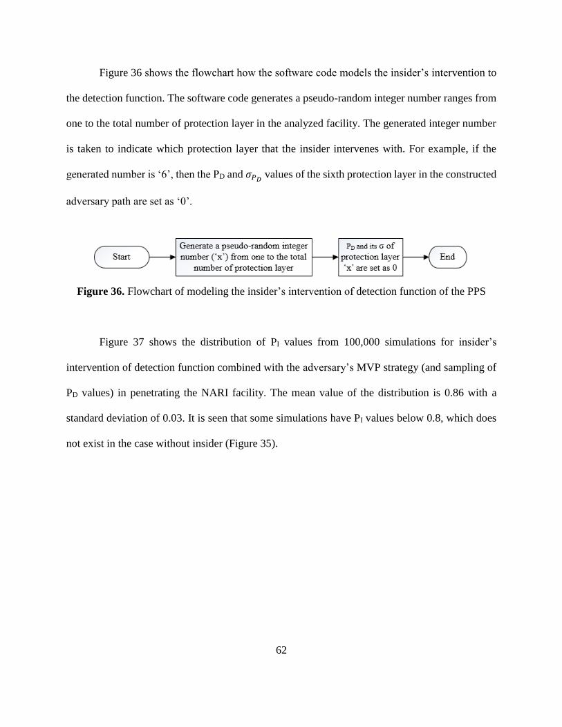
62

Figure 36 shows the flowchart how the software code models the insider’s intervention to

the detection function. The software code generates a pseudo-random integer number ranges from

one to the total number of protection layer in the analyzed facility. The generated integer number

is taken to indicate which protection layer that the insider intervenes with. For example, if the

generated number is ‘6’, then the PD and 𝜎𝑃𝐷 values of the sixth protection layer in the constructed

adversary path are set as ‘0’.

Figure 36. Flowchart of modeling the insider’s intervention of detection function of the PPS

Figure 37 shows the distribution of PI values from 100,000 simulations for insider’s

intervention of detection function combined with the adversary’s MVP strategy (and sampling of

PD values) in penetrating the NARI facility. The mean value of the distribution is 0.86 with a

standard deviation of 0.03. It is seen that some simulations have PI values below 0.8, which does

not exist in the case without insider (Figure 35).

63

Figure 37. The PI value distribution of the adversary’s MVP with insider’s intervention of

detection function

4.2.2. Insider’s Intervention to the Delay Function

The second insider’s intervention model developed in the software code is the intervention

of delay function. In this model, it is assumed that the insider manages to disable delay function at

any protection layer in the constructed adversary path, in which the delay function of that path

option is available to be reduced by the insider’s capability as indicated in the input file by the user

(Figure 9).

Figure 38 shows the flowchart how the software code models the insider’s intervention of

the delay function. The software code generates a pseudo-random integer number from one up to

the total number of protection layer in the analyzed facility. The generated integer number is taken

to indicate which protection layer that the insider intervenes with. The software code evaluates

whether the protection layer in the constructed adversary path is a path with ‘Type of Delay’

64

information ‘A’ in the input file (Figure 9). If the ‘Type of Delay’ information of that path is ‘NA’

given by the user, the software code repeats the pseudo-random integer number generating process

until it meets the condition where the variable ‘type’ of the path element is ‘A’. For example, given

the MVP of the NARI facility (Table 1) is used in the simulation. If the generated pseudo-random

integer number is ‘6’, in which the path of the sixth protection layer is an area to be traversed by

the adversary (‘Type of Delay’ is ‘NA’), then the software code has to repeat the pseudo-random

integer number generation process. If the next generated number is ‘7’, in which the path of the

seventh protection layer is a door (‘Type of Delay’ is ‘A’), then the td and 𝜎𝑡𝑑 values of the seventh

protection layer in that constructed adversary path are set as ‘0’. However, there might be a case

where the constructed adversary path has no path of protection layer with ‘Type of Delay’

information ‘A’. In that case, after a number of times of checking, the simulation continues

without reducing any td and 𝜎𝑡𝑑 value.

Figure 38. Flowchart of modeling the insider’s intervention of delay function of the PPS

Figure 39 shows the distribution of PI values from 100,000 simulations for insider’s

intervention of detection function combined with the adversary’s MVP strategy (and sampling of

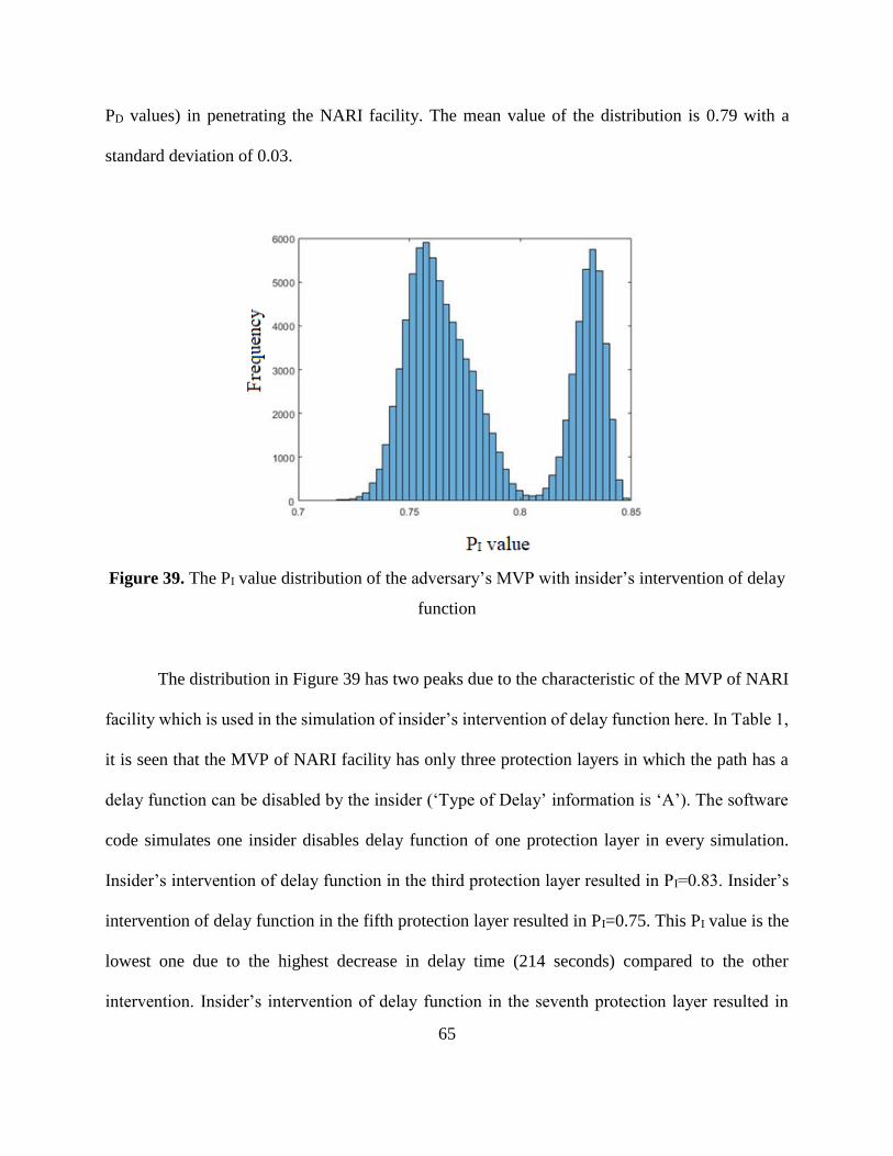
65

PD values) in penetrating the NARI facility. The mean value of the distribution is 0.79 with a

standard deviation of 0.03.

Figure 39. The PI value distribution of the adversary’s MVP with insider’s intervention of delay

function

The distribution in Figure 39 has two peaks due to the characteristic of the MVP of NARI

facility which is used in the simulation of insider’s intervention of delay function here. In Table 1,

it is seen that the MVP of NARI facility has only three protection layers in which the path has a

delay function can be disabled by the insider (‘Type of Delay’ information is ‘A’). The software

code simulates one insider disables delay function of one protection layer in every simulation.

Insider’s intervention of delay function in the third protection layer resulted in PI=0.83. Insider’s

intervention of delay function in the fifth protection layer resulted in PI=0.75. This PI value is the

lowest one due to the highest decrease in delay time (214 seconds) compared to the other

intervention. Insider’s intervention of delay function in the seventh protection layer resulted in

66

PI=0.77. The sampling of PD values in the MVP simulation gives a distribution around those three

PI values.

4.2.3. Insider’s Intervention to the Detection and Delay Functions

The third insider’s intervention model developed in the software code is the intervention

of detection and delay functions. In this model, it is assumed that the insider manages to disable

both detection and delay functions at any protection layer in the constructed adversary path, in

which the delay function of that path option is available to be reduced by the insider’s capability

as indicated in the input file by the user (Figure 9).

Figure 40. Flowchart of modeling the insider’s intervention of detection and delay functions of

the PPS

Figure 40 shows the flowchart how the software code models the insider’s intervention of

detection and delay functions. Basically, it has the similar process with the insider’s intervention

of delay function, except that the PD and 𝜎𝑃𝐷 are also set as ‘0’ beside the td and 𝜎𝑡𝑑

values.

Figure 41 shows the distribution of PI values from 100,000 simulations for insider’s

intervention of detection and delay functions combined with the adversary’s MVP strategy (and

67

sampling of PD values) in penetrating the NARI facility. The mean value of the distribution is 0.77

with a standard deviation of 0.02. It is seen that most simulations have PI values below 0.8, which

does not exist in the case without insider (Figure 35).

Figure 41. The PI value distribution of the adversary’s MVP with insider’s intervention of

detection and delay functions

68

5. RESULTS, DISCUSSION AND RECOMMENDATION

Results from the PD value distribution, and MVP and sensitivity analysis are summarized

in this section. Moreover, the discussion of results from the simulations for the adversary’s various

intrusion strategies including insider support or no support is presented in this section. This section

also provides suggestions on the improvements on calculating EASI-based PI values from a more

realistic approach.

Table 4 shows the comparison between the initial and sampled PD values for every

protection layer along the MVP constructed by the CDP approach in section 3.1. It is seen that the

distribution of sampled PD values for every path option in the protection layer does have a mean

value in the range of the initial standard deviation from initial PD value provided in the Microsoft

Excel input file.

Table 4. Comparison of the initial and the distribution of PD value

Protection

Layer Description

Initial PD

Value

Initial Standard

Deviation of PD

value

Mean Value of

Sampled PD Values

Distribution

Standard Deviation

of Sampled PD

Values Distribution

1 penetrate the fence 0.75 0.075 0.7495 0.075

2 run through limited access area 0.02 0.002 0.02 0.002

3 penetrate vehicle gate 0.8 0.08 0.7984 0.078

4 run through controlled area 0.04 0.004 0.04 0.004

5 penetrate outer vehicle door 0.8 0.08 0.7986 0.079

6 run through protected area 0.5 0.05 0.5002 0.050

7 penetrate main door 0.92 0.092 0.9201 0.023

8 run through vital area 0.9 0.09 0.8986 0.043

9 sabotage the target 0.92 0.092 0.8984 0.043

69

𝜎𝑢 = 𝑢 √(𝜎𝑥

𝑥)

2

+ (𝜎𝑦

𝑦)

2

+ ⋯ (5.1)

However, as mentioned in section 2.1. as well, the standard deviation of initial PD value in

the input file is 10% of the PD value of the path element, which usually consists of several detection

devices with different type to each other The PD for every path in this software code will be more

realistic and accurate if the PD value and its standard deviation for every detection device in the

path element modeled and calculated, as exampled by the work of Norichika Terao and Mitsutoshi

Suzuki. The combined standard deviation for the path can be calculated by Equation 5.1.

Table 5. Results of the sensitivity analysis

Protection

Layer Description

Sensitivity of 0.1

PD Deviation

Sensitivity of 5 Seconds

td Deviation

1 Penetrate the fence 0.01 0.00

2 Run through limited access area 0.00 0.00

3 Penetrate vehicle gate 0.01 0.00

4 Run through controlled area 0.00 0.00

5 Penetrate outer vehicle door 0.00 0.00

6 Run through protected area 0.00 0.00

7 Penetrate main door 0.00 0.00

8 Run through vital area 0.00 0.00

9 Sabotage the target 0.00 0.00

Table 5 summarizes the results of the PI sensitivity with regards to the PD and td values of

the NARI facility’s MVP. It can be seen that the NARI facility’s MVP is not sensitive either to the

70

fluctuation of PD performance (up to an absolute value of 0.1) or the adversary’s outperforming

the delay element (up to 5 seconds faster). There is no significant change in the total PI value due

to 0.1 absolute value change in PD value or 5 seconds change in td value in any protection layer.

As for the sensitivity due to td, it is believed that 5 seconds change is negligible to the RFT (700

seconds) in this case. However, it is found in this study that the PI value has a linear relationship

with PD value and has a non-linear relationship with the td value.

Table 6 shows the result (mean and standard deviation of PI value distribution) of 100,000

simulations for every combination of adversary’s strategy and insider’s intervention in the NARI

facility. Unexpectedly, the analysis gives that the rushing strategy approach by the adversary

results in a path with lowest PI value, followed by the random strategy as the second lowest. From

single path calculation table of adversary’s rushing strategy in Appendix D, it is seen that rushing

strategy approach drastically reduce the cumulative delay time of the adversary path, thus,

drastically reduce the z-value and the P(R|A) of protection layers, especially the first and the third

protection layers as the main contributors to the total PI value. Even though the adversary path of

rushing strategy has higher PD values, the reduction due to the decreased cumulative delay time in

the adversary path is not compensated.

In short, the PPS of the NARI facility is unbalanced. There are path options with similar

PD value but have very different td value. It makes the adversary benefits more in choosing a path

with the lowest td value, regardless of the PD value, especially from the starting point until the CDP

in penetrating the NARI facility. This means that the CDP approach to determine the MVP has

failed to find the path with the lowest PI value for the NARI facility case.

71

Table 6. Results of the PI calculation simulations with combination of the adversary’s strategy

and the insider’s intervention of the NARI facility

PI value and

standard deviation

No insider Insider intervenes PD Insider intervenes td Insider intervenes PD

and td

Random 0.86 ± 0.07 0.85 ± 0.07 0.79 ± 0.14 0.77 ± 0.11

Rushing 0.82 ± 0.07 0.82 ± 0.08 0.73 ± 0.13 0.72 ± 0.13

Covert 0.89 ± 0.05 0.88 ± 0.06 0.82 ± 0.10 0.81 ± 0.09

Deep Penetration 0.88 ± 0.05 0.87 ± 0.06 0.80 ± 0.10 0.78 ± 0.09

MVP 0.88 ± 0.01 0.86 ± 0.03 0.79 ± 0.03 0.77 ± 0.02

Another hypothetical nuclear facility case based on the work reported by Hawila et. al. [10]

is used to compare the PI value distribution obtained for NARI facility analysis presented here.

Hawila’s work analyzed a sabotage case at a nuclear power plant for which the ASD is shown in

Appendix F. By using the same CDP approach as explained at the beginning of section 3.1, the

MVP of that facility is determined and analyzed by using the single path EASI PI calculation table.

The result shows that the PI value for MVP is 0.89. Then, by using the rushing strategy of the

adversary, the PI value for the adversary path increased to 0.95. The calculation tables for this

nuclear power plant facility considering the MVP and the rushing strategy approach are provided

in Appendix F. In Hawila’s case, the CDP approach successfully produced an MVP with lower PI

value compared to the rushing strategy (0.89 vs 0.95).

It is found that the CDP approach works to find the MVP of a facility with a balanced PPS

design, in which the adversary does not have many path options with a wide range of PD and td

values. However, there might be a lot of facilities with an unbalanced PPS. Therefore, the CDP

approach cannot be bluntly applied for the analysis and finding the path with the lowest PI value.

72

In summary, from the comparison of PI value calculation of two hypothetical facilities, it can be

concluded that the software code developed in this study can provide understanding about the

balance of the PPS design.

It should be noted that the NARI facility in this study is a more open facility, with relatively

less focus on the delay function of the PPS to reduce the hindrance for the visitors, compared to

the nuclear power plant in Hawila’s study, However, if the country seriously need to secure the

facility major changes in the delay function should be done. The PPS of the NARI facility can be

strengthened by modifying the protection elements of the PPS as follows:

• For the first protection layer, substitute the fence by a 60-cm wall which can provide a

delay time of 480 seconds just like the vital area building. Equip the wall with a seismic

buried cable sensor system with PD = 0.5. As for the main gate, make it a double gate

with a high security padlock each, thus, increase td to 120 s in total.

• For the third protection layer, substitute the double fence also with a 20-cm wall with

delay time of 120 s and vibration sensor with PD = 0.9. Enhance the vehicle gate to

provide td = 214 s like the vehicle door at the entry to the vital area.

• For the fifth protection layer, substitute the window of the CAS and office rooms with

a wall as a protection element. Thus, those rooms will have the same PD and td value as

that of the building wall.

Table 7 shows the result (mean and standard deviation of PI value distribution) of 100,000

simulations for every combination of adversary’s strategy and insider’s intervention of the

improved PPS design of NARI facility. It can be noted from the PI values in Table 7 that the

improved PPS is more balanced, both the rushing and the covert strategy approaches do not result

73

in a lower mean PI value compared to the deep penetration or the MVP strategies. However, the

PPS design is still sensitive to the decrease of the delay time caused by the insider. Lowering the

RFT value is one solution to further improve the resilience of the PPS.

There is another issue if multi-path analysis is used for PPS evaluation even using a

stochastic (Monte Carlo) approach. That is the mean and standard deviation values from PI

distribution from the simulations may not lead to produce a conservative PPS design. For example,

in section 4.2.2, the mean value of the distribution is 0.79, while there are many PI values in the

distribution which is less than 0.79. For a conservative PPS design, the analyst may be interested

in the lowest PI value. Therefore, an analysis on the PI value distribution is presented next.

Table 7. Results of PI calculation simulations to the improved PPS design of NARI facility

PI Value and

Standard Deviation

No Insider Insider intervenes PD Insider intervenes td Insider intervenes PD

and td

Random 0.91 ± 0.03 0.89 ± 0.04 0.86 ± 0.07 0.84 ± 0.07

Rushing 0.91 ± 0.02 0.90 ± 0.04 0.86 ± 0.06 0.84 ± 0.06

Covert 0.90 ± 0.03 0.89 ± 0.05 0.86 ± 0.07 0.83 ± 0.07

Deep Penetration 0.90 ± 0.03 0.88 ± 0.05 0.84 ± 0.06 0.81 ± 0.06

Figure 42 shows the frequency of PI values from 100,000 simulations of the original NARI

facility’s MVP without insider’s collusion, in 5 bins of ranges where the PI values vary from 0.5

to 0.6, 0.6 to 0.7, 0.7 to 0.8, 0.8 to 0.9, 0.9 to 1. Each bin has a mean PI value. It is seen that for the

MVP base case, all the PI values are concentrated in the bin range 0.8 to 0.9, with mean value 0.88.

74

Figure 43 shows the frequency of PI value from 100,000 simulations of adversary’s random

strategy and rushing strategy in penetrating the original NARI facility without insider’s collusion.

It is seen that in the random strategy, there are around 20,000 simulations (around 20% of total

simulations) with PI values less than 0.8. In the rushing strategy, there are more than 30,000

simulations (more than 30% of total simulations) with PI value less than 0.8.

Figure 42. Frequency of PI value in five bins of MVP strategy for NARI facility

Figure 43. Frequency of PI value in five bins of random strategy and rushing strategy for NARI

facility

Figure 44 shows the frequency of PI value from 100,000 simulations of adversary’s covert

strategy and deep penetration strategy in penetrating the original NARI facility without insider’s

collusion. It is seen that in the covert strategy, there are around 5,000 simulations (5% of total

0

20000

40000

60000

80000

100000

120000

0.55 0.65 0.75 0.88 0.91

Fre

qu

en

cy

Bin's Mean PI Value

MVP Strategy

0

10000

20000

30000

40000

50000

0.55 0.69 0.76 0.86 0.92

Fre

qu

en

cy

Bin's Mean PI Value

Random Strategy

0

10000

20000

30000

40000

50000

0.55 0.69 0.75 0.86 0.92

Fre

qu

en

cy

Bin's Mean PI Value

Rushing Strategy

75

simulations) with PI value less than 0.8. In the deep penetration strategy, there are around 8,000

simulations (8% of total simulations) with PI value less than 0.8. In all of those strategies, there are

small number of simulations in which the PI value is less than 0.7.

Figure 44. Frequency of PI value in five bins of covert strategy and deep penetration strategy for

NARI facility

Figure 45 shows the frequency of PI value from 100,000 simulations of adversary’s MVP

strategy combined with insider’s intervention in penetrating the original NARI facility’s MVP.

There are a few numbers of simulation in the insider’s intervention of detection function case with

PI value less than 0.8. However, in the case of insider’s intervention of delay function, more than

half (65%) of the simulations have PI value less than 0.8. In the case of insider’s intervention of

detection and delay functions, more than 80% of the simulations have PI value less than 0.8. The

frequency analysis is valuable in the multi-path analysis from numerous simulation, rather than

just depending on the mean and standard deviation values from the distribution.

Frequency analysis in the multi-path analysis shows a drastic change of PI value

distribution in several bins due to various adversary strategies and insider’s collusion. The

adversary’s rushing strategy (in Figure 43), among other strategies, has the highest percentage of

0

10000

20000

30000

40000

50000

0.55 0.69 0.77 0.87 0.93

Fre

qu

en

cy

Bin's Mean PI Value

Covert Strategy

0

10000

20000

30000

40000

50000

60000

0.55 0.69 0.77 0.87 0.92

Fre

qu

en

cy

Bin's Mean PI Value

Deep Penetration Strategy

76

simulations resulting lower PI value (below 0.8) compared with the base case of single path MVP

(Figure 42) of the NARI facility. The insider’s intervention of detection and delay functions,

among other insider’s collusions, has the highest percentage of simulations resulting lower PI value

(below 0.8).

Figure 45. Frequency of PI value in five bins NARI facility’s MVP with various insider’s

intervention of PPS’s function

Further recommendations based on this work for the adversary path modeling is that

analyzing various adversary strategies and the insider’s malicious involvement are very important.

The hypothetical facilities used in this study are considered as simple facilities with less

complicated PPS. They do not have jump mechanism which allows the adversary to surpass one

0

20000

40000

60000

80000

100000

0.55 0.65 0.79 0.87 0.91

Fre

qu

en

cy

Bin's Mean PI Value

MVP with Insider on PD

0

20000

40000

60000

80000

0.55 0.65 0.76 0.83 0.95

Fre

qu

en

cy

Bin's Mean PI Value

MVP with Insider on Td

0

20000

40000

60000

80000

100000

0.55 0.65 0.76 0.81 0.95

Fre

qu

en

cy

Bin's Mean PI Value

MVP with Insider on PD and Td

77

or two protection layers along the path to the target. This jump strategy analysis is not a capability

of the developed software code. Also, modeling of theft-case scenario cannot be analyzed

completely by this software code. Currently, the detail of insider’s act to reduce the delay time

cannot be analyzed in the software code. There is also a room for improvement in modeling how

the insider intervenes with the protection element in a path element of the PPS, especially if the

protection element in each path option can be modeled in more detail.

78

6. CONCLUSION

A stochastic (Monte Carlo) approach developed and implemented in the Estimate of

Adversary Sequence Interruption (EASI) model as part of this study is presented. The approach is

capable of analyzing the effectiveness of a Physical Protection System (PPS) by estimating

Probability of Interruption (PI) value and the uncertainty in PI value. The implementation is done

by developing a software code. The software code is tested by analyzing a hypothetical facility by

estimating the PI values considering the characteristics [Probability of Detection (PD) and delay

time (td)] of the protection elements in the PPS, uncertainties in the PD and tD values and various

adversary strategies including collusion with an insider. Sensitivity analysis of PI value with

regards to PD and td values is performed for the Most Vulnerable Path (MVP) of the facility by

considering the Critical Detection Point (CDP) of the facility’s Adversary Sequence Diagram

(ASD).

Sensitivity analysis of PI value estimation shows that the relationship between PD and PI is

linear, however the relationship between td and PI is non-linear. The implementation of stochastic

(Monte Carlo) approach successfully produces PI value distribution from which the mean and

standard deviation values are estimated. The PI value is the lowest in the simulations where the

insider act is included, whether the insider acts on the detection or delay function or both

simultaneously. The lowest mean value of PI distribution is for the rushing strategy, among the

other adversary strategies analyzed. This is due to an unbalanced PPS design of the analyzed

hypothetical facility.

79

In addition, the multi-path analysis in this software code was complemented by a frequency

distribution analysis of PI values manually. This is needed because the mean and standard deviation

values alone could mislead the user to overlook simulations with much lower PI value than the

mean. Frequency analysis performed on the PI values is found to be valuable in modifying the PPS

design instead of just using the mean value of the PI distribution and its standard deviation in multi-

path analysis. This is because the PI value frequency distribution analysis shows a drastic change

of PI value when categorized in to several bins, especially for various adversary strategies and

insider’s collusion compared to the base case. The adversary’s rushing strategy, among other

strategies, has the highest percentage of the distribution resulting in lower PI values (below 0.8).

The insider’s intervention of detection and delay functions, among other insider’s collusions, has

the highest percentage of the distribution resulting in lower PI values (below 0.8).

The implementation of the stochastic (Mote Carlo) method is valuable in modeling the PD

values in the EASI model and in the estimation of PI value distribution and the uncertainty

associated, especially in modeling the adversary path including the collusion of an insider for

multi-path analysis. The insider collusion is found to reduce the PI value of the PPS drastically.

In the future, it is valuable to add to the software the theft and jump case scenarios. It would

be good to add to the software code an automatic analysis of the PI value frequency distribution.

Detailed modeling of detection and delay elements in a path can be a future work too.

80

REFERENCES

[1] INTERNATIONAL ATOMIC ENERGY AGENCY, “Convention on the Physical

Protection of Nuclear Material” INFCIRC/274/Rev.1, Vienna, (1980).

[2] INTERNATIONAL ATOMIC ENERGY AGENCY, “The Physical Protection of Nuclear

Material and Nuclear Facilities”, INFCIRC/225/Rev.4, Vienna, (1999).

[3] GARCIA M.L., “The Design and Evaluation of Physical Protection System”, Butterworth-

Heinemann, Burlington (2001).

[4] U.S. CONGRESS: OFFICE OF TECHNOLOGY ASSESSMENT, “Technology Against

Terrorism: Structuring Security”, OTA-ISC-511, Washington, D.C., (1992).

[5] FERGUSON C., POTTER W., “Four Faces of Nuclear Terrorism”, Center for

Nonproliferation Studies, Monterey (2004).

[6] INTERNATIONAL ATOMIC ENERGY AGENCY, “Development, Use and

Maintenance of the Design Basis Threat”, IAEA Nuclear Security Series No. 10, Vienna,

(2009)

[7] BENNET H., “EASI – An Evaluation Method for Physical Security System”, Nuclear

Materials Management, Vol. 6, No. 3, 371-379, (1977).

[8] Wadoud A.A., Adail A.S., Saleh A.A., “Physical Protection Evaluation Process for Nuclear

Facility via Sabotage Scenarios”, Alexandria Engineering Journal, 1-9, (2017).

https://doi.org/10.1016/j.aej.2017.01.045

[9] OYEYINKA O.D., DIM L.A., ECHETA M.C., KUYE A.O., “Determination of System

Effectiveness for Physical Protection System of a Nuclear Energy Centre”, Science and

Technology, Vol. 4, No. 2, 9-16, (2014).

[10] ZOU, B., YANG M., GUO J., BENJAMIN E., et al., “Insider Threats of Physical

Protection Systems in Nuclear Power Plants: Prevention and Evaluation”, Progress in

Nuclear Energy, 1-8, (2017). http://dx.doi.org/10.1016/j.pnucene.2017.08.006

[11] HAWILA M., CHIRAYATH S., CHARLTON W., “Nuclear Security Risk Evaluation

Using Adversary Pathway Analysis Methodology for an Insider-Outsider Collusion

Scenario”, INMM Annual Meeting Proceedings, Vol 56, 1-8, (2015).

[12] HAWILA, M., CHIRAYATH, S., "Nuclear Security Risk Analysis: An Insider-Outsider

Collusion Scenario," International Journal of Nuclear Security, Vol. 2, No. 2, Article 7,

(2016). http://dx.doi.org/10.7290/V7B56GNN

81

[13] TERAO N., SUZUKI M., “A Probabilistic Extension of the EASI Model”, Journal of

Physical Security, Vol. 7, No. 2, 12-29, (2014).

[14] WINBLAD A.E., “The SAVI Vulnerability Assessment Model”, INMM Annual Meeting

Proceedings, Vol. 16, 24-28, (1987).

[15] JANG S. S., KWAK S., YOO, H., KIM J., YOON W. K., “Development of a Vulnerability

Assessment Code for a Physical Protection System: Systematic Analysis of Physical

Protection Effectiveness (SAPE)”, Nuclear Engineering and Technology, Vol. 41, No. 5,

747-752, (2009).

[16] SANDIA NATIONAL LABORATORIES, “Hypothetical Facility Exercise Data:

Hypothetical Atomic Research Institute”, The Twenty-Sixth International Training Course,

Albuquerque, (2016).

[17] SANDIA NATIONAL LABORATORIES, “Hypothetical Facility Exercise Data: The

Lone Pine Nuclear Power Plant”, The Twenty-Sixth International Training Course,

Albuquerque, (2016).

[18] SANDIA NATIONAL LABORATORIES, “Hypothetical Facility Exercise Data: The

Lagassi Institute of Medicine and Physics”, The Twenty-Sixth International Training

Course, Albuquerque, (2016).

[19] SANDIA NATIONAL LABORATORIES, “20. Multipath Analysis: Outsider Analysis

with the Path Analysis (MP VEASI) Model”, The Twenty-Sixth International Training

Course, Albuquerque, (2016).

82

APPENDIX A

COUNTRY, FACILITY, AND THREAT DESCRIPTION

The NARI facility is located in the outskirt of hypothetical City, Nusa, the capital city of

the hypothetical Republic of Nusantara, a developing country in the Southeast Asia region. It is

operated by the country’s National Science and Technology Institute (NSTI) and engages in many

research activities with one of the advanced universities in the country, the University of Nusantara

(UNUS), which is also located near NARI. It has served as the country’s premier research facility

in nuclear science and technology for about 15 years. The country has decided to start the

construction of a nuclear power plant in 2025. The country has increased the amount of joint

research being conducted with the faculties and students from the UNUS. The NARI facility has

gained attention in the media. The media spotlights the facility and its research activities

frequently, since the country’s ‘go nuclear’ decision was made just before the Japanese Fukushima

Nuclear Accident in 2011. All of the NARI facility publicity given by the media, UNUS, and NSTI

have made the NARI facility and its activities transparent. People can get a lot of information about

NARI facility from open sources, such as newspaper, website, science and technology magazine,

and academic literature.

The Republic of Nusantara was well-known as an oil-exporter in the 1970s and 1980s, but

it has turned into a net oil-importer country since mid-late 1990’s to fulfill their energy needs. It

is well known that there are a lot of oil and gas businessmen and organized crime network in the

country, who were unhappy with the country’s decision to pursue nuclear energy, which threaten

their oil and gas business. There were protests happening in many occasions, such as during the

83

nuclear-related conferences and summits in the city, nuclear-related visits by researchers and

businessmen from other countries. The protesters are highly suspected to be supported by the oil

and gas businessmen and by the organized crime network. Not only nuclear energy, there were

several cases of sabotage of renewable energy installation plant, such as small to mid-level of solar

and wind farm. Sabotage mainly happened in an area which is highly dependent on oil energy.

Meanwhile, the country is also a nest of some terrorist and criminal groups. Since the

economic crisis in the late 1990s, there is no rapid economy progression that satisfies the mid to

low-income group people in the country. Those mid to low income group people showed their

dissatisfaction and opposition to the government through crime and terrorism. There have been

several major bombings in the country those took place during occasions related to western cultural

events. Apparently, the country’s main partners in the nuclear research and development are

developed western countries, considered enemies by the terrorist and criminal groups.

Since the partnership began two years ago, the western countries have funded the

implementation of a security system in the NARI facility. Based on the facility target analysis, the

highest consequence is when there is a sabotage that causes major damage to the reactor. The worst

outcome is that it may cause unacceptable radiological release. Meanwhile, as the country’s one

and only nuclear research and development facility, major damage to the facility will delay the

country’s pursuit of nuclear energy. It will also show the public of the country’s inability to safely

and securely operate a nuclear facility, given the existence of the terrorist and criminal groups in

the country. Even people who are currently pro-nuclear might oppose to the country’s plan to use

nuclear energy, due to the threat of radiological release in from a nuclear accident or sabotage.

Based on the analysis of the reactor, the fastest way to cause considerable damage to the reactor is

84

to sabotage the control rod drive bridge during the maintenance of the reactor. It will take around

10 minutes to cause the damage.

Knowing the importance of the facility for the country’s early nuclear regime, people who

oppose the plan might want to create damage to the reactor. The oil and gas businessmen and the

people from the organized crime network are among the most probable ones. In some of the cases

of renewable energy plant sabotage, the culprits have proven to be related to the oil and gas

business. Therefore, it is highly possible that the organized crime would find a way to try sabotage

the reactor in NARI facility, possibly with support from the terrorist or criminal groups. They are

assumed to have enough material and resources and from the past incidents it is clear that the

terrorist and criminal groups have the capability and human resources to do the sabotage.

The postulated threat for the NARI facility can be described as follows. The adversary’s

motivation comes from a mix of anti-western, anti-government, and anti-nuclear energy

sentiments. The adversary’s intention is to sabotage the nuclear reactor inside NARI facility. The

adversary has enough funding to acquire the required materials, tools, and human resources to

execute their sabotage plan at the NARI reactor. The adversary team, which consists of four to five

people, will all be equipped with at least one rifle and one pistol. Limited explosive materials will

be available for the adversary to penetrate one or two steel doors or concrete wall and to sabotage

the reactor. Portable mechanical tools are also possessed by the adversary team, but not high-tech

advanced tools. They communicate to each other by using the cellular phone and two-way radio

system. The adversary team has a land transportation vehicle which can only deliver the team

undetected until the offsite area just before entering the limited access area of the NARI facility.

The adversary has enough technical skill to use those materials, tools, equipment, and weapons

85

combined with stealth and force tactic. The adversary has no sophisticated cyber skills. Although

very unlikely, there is still a possibility of an insider assisting the adversary.

86

APPENDIX B

DEVELOPMENT OF ADVERSARY SEQUENCE DIAGRAM (ASD) OF NARI FACILITY

The HARI hypothetical facility document by SNL [17] provides all PD and td values to

construct the ASD of the NARI hypothetical facility. From the offsite area, there is no protection

element used to detect or to delay an adversary. Therefore, it has PD=0 value and td=0 value. For

the next step, there are two options for the adversary to enter the limited access area from the off-

site area: either through the main gate or through the fence surrounding the limited access area.

For the adversary to pass through the fence, the PD value is 0.75 since the fence is equipped with

multiple sensors. The multiple sensors might detect the adversary in the middle of action in passing

through the fence, in which case the detection location is set as ‘M’. But, it will take only

approximately 10 seconds for the adversary to pass through the fence. As for the main gate, the

adversary will take approximately 60 seconds to open or break the high security padlock. The

addition of the camera to monitor the main gate will give the PD value 0.85 in detecting the

adversary once they have arrived at the main gate to unlock the padlock, thus, the detection location

is set as ‘B’.

The average distance from the facility’s outer fence to the controlled area’s double fence

is 300 meters. It will take 30 seconds for the adversary to traverse the limited access area. A guard

patrolling in a scheduled time gives the limited access area a PD value of 0.02 and might detect the

adversary in the middle of the path. In order to get into the controlled area, the adversary has three

options. The first option is through the double fence, which has 20 seconds delay time value. Since

each fence has a vibration sensor and an infrared sensor system in between the fence, Equation 1.3

87

and Equation 2.1 are used to calculate the combined PD value of those sensors. From the reference

[17], the fence vibration sensor gives PD value 0.5 for each fence, while the exterior infrared sensor

gives PD value of 0.8. Therefore, the combined PD value of the double fence is 0.95. Those sensors

are likely to detect the adversary in the middle of the action to pass through the double fence.

Therefore, this path’s detection location is set as ‘M’. The second option to enter the controlled

area is through the vehicle gate which is locked with high security padlocks on both sides of the

gate, which give a delay time of this path element of 120 seconds. The infrared sensor used in the

double fence goes through this vehicle gate as well, which will detect the adversary in the middle

of the path element with PD value of 0.8.

The third option is to go through the personnel portal. Both doors to get in and to get out

of the personnel portal are 0.75-cm steel plate doors. Each door gives approximately 30 seconds

delay time for the postulated adversary. The steel turnstile inside the room gives an additional

delay time of 18 seconds for this path element. BMS in both doors give PD value 0.8 each, while

the badge-PIN system of the turnstile gives PD value 0.6. Therefore, the combined PD value for the

personnel portal room is 0.98, obtained by using Equations 1.3 and 2.1. Once the adversary is in

the controlled area, the adversary must take at least 15 seconds to travel before penetrating the

protected area. Two random patrol guards in the controlled area contribute to combined PD value

of 0.04 by applying Equations 1.3 and 2.1, in which the detection location is in the middle of the

adversary path in passing through the area.

In order to penetrate the protected area, the adversary has five options to get through. The

first option is through the main entrance of the building. The 10-cm wood door with metal sheeting

gives 180 seconds delay time, while the steel turnstile gives 18 seconds delay time, therefore 198

88

seconds in total. The BMS with PD=0.8 attached at the front door and the exchange badge-PIN

system at the steel turnstile with PD=0.8 contribute to PD value of 0.96 in total. The last detection

opportunity is if the adversary somehow breaks through the turnstile right before they enter the

protected area, thus, the detection location is set as ‘E’. The second option is to penetrate the

window of the office room, then break through the door. There is a glass break sensor attached to

every window with PD=0.9 and a position switch sensor attached to the door with PD=0.5. It gives

PD=0.95 in total for the office room by utilizing Equations 1.3 and 2.1. However, 5 seconds delay

time of the window and 12 seconds delay time of the wood door only give 17 seconds delay time

in total for the office room. The detection location of the office room is set as ‘E’ as the BMS of

the office door is the last detection opportunity before entering the protected area.

The third option is through the Central Alarm Station (CAS) room. The window for the

CAS room also has the glass break sensor with PD=0.9 and delay time of 5 seconds, while its door

is made of steel with a delay time of 30 seconds where the BMS with PD=0.8 is attached to. In

total, the CAS room has PD value of 0.98 and delay time of 35 seconds, and the detection location

is also set as ‘E’ with regards to the BMS at the door. The fourth option is through the outer-side

30-cm concrete and steel rolling vehicle door at the backside of the building. The outsider might

spend approximately 214 seconds to use explosives to break the lock of the door. The BMS with

PD=0.8 equipped to the door will detect the adversary once the door just before the protected area

is opened and entry is made. Thus, the detector location for this path element is set as ‘E’. The last

option is by penetrating through the building wall directly. It would take approximately 120

seconds to use explosives to break the 20-cm concrete wall and enter the protected area. However,

the building wall is equipped with a vibration sensor which has PD value of 0.9 to detect the

89

explosion vibration. Thus, the detection location is set as ‘M’. In the protected area itself, the video

motion sensor is applied in several spots insider the administration building hall with PD value of

0.5. It might detect the adversary movement in the middle of the path element. The average time

for the adversary to go through the administration hall to start penetrating the vital area is

approximately 10 seconds.

From the protected area, there are three options to get into the vital area. First option is

through inner-side vehicle door from the back of the building. The delay time provided by this

inner side door is same with the outer vehicle rolling door, 214 seconds by explosive to break the

door. But, this rolling door is equipped with a badge-PIN system with PD=0.6 and BMS with

PD=0.8. These sensors will detect the adversary after the lock is broken, and the door is opened.

These sensors give the combined PD value of 0.92 to this path element. The second option is

through the main door. It has the same detection BMS and badge-PIN system feature with the

inner-sider vehicle door which gives the combined PD of 0.92 and detection location is set as ‘E’.

However, since it is a 30-cm wooden door with metal sheeting, it has a lower delay time value,

180 seconds, for a penetration using explosives. The third option is through the vital area building

wall. It is a 60-cm concrete wall with a vibration sensor, thus, giving this path element a PD value

of 0.9, detection location set as ‘M’, and delay time of 480 seconds if the adversary uses explosives.

The vital area and the target are equipped by multiple complementary sensors with PD=0.9 for each

of them. It will take approximately not more than five seconds needed by the adversary to penetrate

the vital area to reach the target. And as stated in the target identification before, it will take

approximately 600 seconds to sabotage the control rod drive bridge until the adversary desired

level of damage. Those multiple complementary sensors in many parts of the of the vital area and

90

around the reactor most likely detect the adversary in the middle of their progress in the path

element, therefore detection location ‘M’ is given for both path elements in the ASD.

91

APPENDIX C

DISTRIBUTION OF DETECTION PROBABILITY VALUE OF THE NARI FACILITY

PD value distribution of the first protection layer

PD value distribution of the second protection layer

92

PD value distribution of the third protection layer

PD value distribution of the fourth protection layer

93

PD value distribution of the fifth protection layer

PD value distribution of the sixth protection layer

94

PD value distribution of the seventh protection layer

PD value distribution of the eighth protection layer

95

PD value distribution of the ninth protection layer

96

APPENDIX D

SINGLE PATH EASI CALCULATION TABLE FOR SENSITVITY ANALYSIS

Sensitivity Analysis due to PD change

1 RFT 700 210 0.8883

PC 0.95

LayerDetection

ProbabilityLocation

Delay

Time

Mean

Delay

Time

STD

Probability

of Detection

Probability

of No

Detection

Probability

of First

Detection

Cumulative

Delay

Time

Cumulative

Variance

True

Cumulative

Delay Time

True

Cumulative

Variance

z-value

Response

Force Arrival

Probability

Specific

Probability

of

Interruption

1 0.85 M 10 3.0 0.85 0.1500 0.8500 1184 40855.14 1179 40848.39 1.6435 0.9499 0.7670

2 0.02 M 30 9.0 0.02 0.1470 0.0030 1174 40846.14 1159 40785.39 1.5754 0.9424 0.0027

3 0.8 M 120 36.0 0.8 0.0294 0.1176 1144 40765.14 1084 39793.14 1.3258 0.9075 0.1014

4 0.04 M 15 4.5 0.04 0.0282 0.0012 1024 39469.14 1016.5 39453.953 1.0949 0.8632 0.0010

5 0.8 E 214 64.2 0.8 0.0056 0.0226 1009 39448.89 795 35327.25 0.3371 0.6320 0.0136

6 0.5 M 10 3.0 0.5 0.0028 0.0028 795 35327.25 790 35320.5 0.3194 0.6253 0.0017

7 0.92 E 180 54.0 0.92 0.0002 0.0026 785 35318.25 605 32402.25 -0.3435 0.3656 0.0009

8 0.9 M 5 1.5 0.9 0.0000 0.0002 605 32402.25 602.5 32400.563 -0.3525 0.3622 0.0001

9 0.9 M 600 180.0 0.9 0.0000 0.0000 600 32400 300 8100 -1.7508 0.0400 0.0000

Detection Delay

Probability of Interruption

Response

1 RFT 700 210 0.8811

PC 0.95

LayerDetection

ProbabilityLocation

Delay

Time

Mean

Delay

Time

STD

Probability

of Detection

Probability

of No

Detection

Probability

of First

Detection

Cumulative

Delay

Time

Cumulative

Variance

True

Cumulative

Delay Time

True

Cumulative

Variance

z-values

Response

Force Arrival

Probability

Specific

Probability

of

Interruption

1 0.75 M 10 3.0 0.75 0.2500 0.7500 1184 40855.14 1179 40848.39 1.6435 0.9499 0.6768

2 0.12 M 30 9.0 0.12 0.2200 0.0300 1174 40846.14 1159 40785.39 1.5754 0.9424 0.0269

3 0.8 M 120 36.0 0.8 0.0440 0.1760 1144 40765.14 1084 39793.14 1.3258 0.9075 0.1517

4 0.04 M 15 4.5 0.04 0.0422 0.0018 1024 39469.14 1016.5 39453.9525 1.0949 0.8632 0.0014

5 0.8 E 214 64.2 0.8 0.0084 0.0338 1009 39448.89 795 35327.25 0.3371 0.6320 0.0203

6 0.5 M 10 3.0 0.5 0.0042 0.0042 795 35327.25 790 35320.5 0.3194 0.6253 0.0025

7 0.92 E 180 54.0 0.92 0.0003 0.0039 785 35318.25 605 32402.25 -0.3435 0.3656 0.0013

8 0.9 M 5 1.5 0.9 0.0000 0.0003 605 32402.25 602.5 32400.5625 -0.3525 0.3622 0.0001

9 0.9 M 600 180.0 0.9 0.0000 0.0000 600 32400 300 8100 -1.7508 0.0400 0.0000

Detection Delay

Probability of Interruption

Response

1 RFT 700 210 0.8857

PC 0.95

LayerDetection

ProbabilityLocation

Delay

Time

Mean

Delay

Time

STD

Probability

of Detection

Probability

of No

Detection

Probability

of First

Detection

Cumulative

Delay

Time

Cumulative

Variance

True

Cumulative

Delay Time

True

Cumulative

Variance

z-values

Response

Force Arrival

Probability

Specific

Probability

of

Interruption

1 0.75 M 10 3.0 0.75 0.2500 0.7500 1184 40855.14 1179 40848.39 1.6435 0.9499 0.6768

2 0.02 M 30 9.0 0.02 0.2450 0.0050 1174 40846.14 1159 40785.39 1.5754 0.9424 0.0045

3 0.9 M 120 36.0 0.9 0.0245 0.2205 1144 40765.14 1084 39793.14 1.3258 0.9075 0.1901

4 0.04 M 15 4.5 0.04 0.0235 0.0010 1024 39469.14 1016.5 39453.9525 1.0949 0.8632 0.0008

5 0.8 E 214 64.2 0.8 0.0047 0.0188 1009 39448.89 795 35327.25 0.3371 0.6320 0.0113

6 0.5 M 10 3.0 0.5 0.0024 0.0024 795 35327.25 790 35320.5 0.3194 0.6253 0.0014

7 0.92 E 180 54.0 0.92 0.0002 0.0022 785 35318.25 605 32402.25 -0.3435 0.3656 0.0008

8 0.9 M 5 1.5 0.9 0.0000 0.0002 605 32402.25 602.5 32400.5625 -0.3525 0.3622 0.0001

9 0.9 M 600 180.0 0.9 0.0000 0.0000 600 32400 300 8100 -1.7508 0.0400 0.0000

Detection Delay

Probability of Interruption

Response

97

Sensitivity Analysis due to td change

1 RFT 700 210 0.8801

PC 0.95

LayerDetection

ProbabilityLocation

Delay

Time

Mean

Delay

Time

STD

Probability

of Detection

Probability

of No

Detection

Probability

of First

Detection

Cumulative

Delay

Time

Cumulative

Variance

True

Cumulative

Delay Time

True

Cumulative

Variance

z-values

Response

Force Arrival

Probability

Specific

Probability

of

Interruption

1 0.75 M 10 3.0 0.75 0.2500 0.7500 1184 40855.14 1179 40848.39 1.6435 0.9499 0.6768

2 0.02 M 30 9.0 0.02 0.2450 0.0050 1174 40846.14 1159 40785.39 1.5754 0.9424 0.0045

3 0.8 M 120 36.0 0.8 0.0490 0.1960 1144 40765.14 1084 39793.14 1.3258 0.9075 0.1690

4 0.14 M 15 4.5 0.14 0.0421 0.0069 1024 39469.14 1016.5 39453.9525 1.0949 0.8632 0.0056

5 0.8 E 214 64.2 0.8 0.0084 0.0337 1009 39448.89 795 35327.25 0.3371 0.6320 0.0202

6 0.5 M 10 3.0 0.5 0.0042 0.0042 795 35327.25 790 35320.5 0.3194 0.6253 0.0025

7 0.92 E 180 54.0 0.92 0.0003 0.0039 785 35318.25 605 32402.25 -0.3435 0.3656 0.0013

8 0.9 M 5 1.5 0.9 0.0000 0.0003 605 32402.25 602.5 32400.5625 -0.3525 0.3622 0.0001

9 0.9 M 600 180.0 0.9 0.0000 0.0000 600 32400 300 8100 -1.7508 0.0400 0.0000

Detection Delay

Probability of Interruption

Response

1 RFT 700 210 0.8795

PC 0.95

LayerDetection

ProbabilityLocation

Delay

Time

Mean

Delay

Time

STD

Probability

of Detection

Probability

of No

Detection

Probability

of First

Detection

Cumulative

Delay

Time

Cumulative

Variance

True

Cumulative

Delay Time

True

Cumulative

Variance

z-values

Response

Force Arrival

Probability

Specific

Probability

of

Interruption

1 0.75 M 10 3.0 0.75 0.2500 0.7500 1184 40855.14 1179 40848.39 1.6435 0.9499 0.6768

2 0.02 M 30 9.0 0.02 0.2450 0.0050 1174 40846.14 1159 40785.39 1.5754 0.9424 0.0045

3 0.8 M 120 36.0 0.8 0.0490 0.1960 1144 40765.14 1084 39793.14 1.3258 0.9075 0.1690

4 0.04 M 15 4.5 0.04 0.0470 0.0020 1024 39469.14 1016.5 39453.9525 1.0949 0.8632 0.0016

5 0.9 E 214 64.2 0.9 0.0047 0.0423 1009 39448.89 795 35327.25 0.3371 0.6320 0.0254

6 0.5 M 10 3.0 0.5 0.0024 0.0024 795 35327.25 790 35320.5 0.3194 0.6253 0.0014

7 0.92 E 180 54.0 0.92 0.0002 0.0022 785 35318.25 605 32402.25 -0.3435 0.3656 0.0008

8 0.9 M 5 1.5 0.9 0.0000 0.0002 605 32402.25 602.5 32400.5625 -0.3525 0.3622 0.0001

9 0.9 M 600 180.0 0.9 0.0000 0.0000 600 32400 300 8100 -1.7508 0.0400 0.0000

Detection Delay

Probability of Interruption

Response

1 RFT 700 210 0.8791

PC 0.95

LayerDetection

ProbabilityLocation

Delay

Time

Mean

Delay

Time

STD

Probability

of Detection

Probability

of No

Detection

Probability

of First

Detection

Cumulative

Delay

Time

Cumulative

Variance

True

Cumulative

Delay Time

True

Cumulative

Variance

z-values

Response

Force Arrival

Probability

Specific

Probability

of

Interruption

1 0.75 M 10 3.0 0.75 0.2500 0.7500 1184 40855.14 1179 40848.39 1.6435 0.9499 0.6768

2 0.02 M 30 9.0 0.02 0.2450 0.0050 1174 40846.14 1159 40785.39 1.5754 0.9424 0.0045

3 0.8 M 120 36.0 0.8 0.0490 0.1960 1144 40765.14 1084 39793.14 1.3258 0.9075 0.1690

4 0.04 M 15 4.5 0.04 0.0470 0.0020 1024 39469.14 1016.5 39453.9525 1.0949 0.8632 0.0016

5 0.8 E 214 64.2 0.8 0.0094 0.0376 1009 39448.89 795 35327.25 0.3371 0.6320 0.0226

6 0.6 M 10 3.0 0.6 0.0038 0.0056 795 35327.25 790 35320.5 0.3194 0.6253 0.0034

7 0.92 E 180 54.0 0.92 0.0003 0.0035 785 35318.25 605 32402.25 -0.3435 0.3656 0.0012

8 0.9 M 5 1.5 0.9 0.0000 0.0003 605 32402.25 602.5 32400.5625 -0.3525 0.3622 0.0001

9 0.9 M 600 180.0 0.9 0.0000 0.0000 600 32400 300 8100 -1.7508 0.0400 0.0000

Detection Delay

Probability of Interruption

Response

td1 1 RFT 700 210 0.879474154

PC 0.95

LayerDetection

ProbabilityLocation

Delay

Time

Mean

Delay

Time

STD

Probability

of Detection

Probability

of No

Detection

Probability

of First

Detection

Cumulative

Delay Time

Cumulative

Variance

True

Cumulative

Delay Time

True

Cumulative

Variance

z-value

Response

Force Arrival

Probability

Specific

Probability of

Interruption

1 0.75 M 15 4.5 0.75 0.25 0.75 1189 40866.39 1181.5 40851.2025 1.6520 0.9507 0.713049975

2 0.02 M 30 9.0 0.02 0.245 0.005 1174 40846.14 1159 40785.39 1.5754 0.9424 0.004712101

3 0.8 M 120 36.0 0.8 0.049 0.196 1144 40765.14 1084 39793.14 1.3258 0.9075 0.177878224

4 0.04 M 15 4.5 0.04 0.04704 0.00196 1024 39469.14 1016.5 39453.9525 1.0949 0.8632 0.001691928

5 0.8 E 214 64.2 0.8 0.009408 0.037632 1009 39448.89 795 35327.25 0.3371 0.6320 0.023782424

6 0.5 M 10 3.0 0.5 0.004704 0.004704 795 35327.25 790 35320.5 0.3194 0.6253 0.00294128

7 0.92 E 180 54.0 0.92 0.00037632 0.00432768 785 35318.25 605 32402.25 -0.3435 0.3656 0.0015823

8 0.9 M 5 1.5 0.9 3.7632E-05 0.00033869 605 32402.25 602.5 32400.5625 -0.3525 0.3622 0.000122682

9 0.9 M 600 180.0 0.9 3.7632E-06 3.3869E-05 600 32400 300 8100 -1.7508 0.0400 1.35456E-06

Detection Delay

Probability of Interruption

Response

98

td2 1 RFT 700 210 0.880078801

PC 0.95

LayerDetection

ProbabilityLocation

Delay

Time

Mean

Delay

Time

STD

Probability

of Detection

Probability

of No

Detection

Probability

of First

Detection

Cumulative

Delay Time

Cumulative

Variance

True

Cumulative

Delay Time

True

Cumulative

Variance

z-value

Response

Force Arrival

Probability

Specific

Probability of

Interruption

1 0.75 M 10 3.0 0.75 0.25 0.75 1189 40884.39 1184 40877.64 1.6603 0.9516 0.713681569

2 0.02 M 35 10.5 0.02 0.245 0.005 1179 40875.39 1161.5 40792.7025 1.5839 0.9434 0.004716977

3 0.8 M 120 36.0 0.8 0.049 0.196 1144 40765.14 1084 39793.14 1.3258 0.9075 0.177878224

4 0.04 M 15 4.5 0.04 0.04704 0.00196 1024 39469.14 1016.5 39453.9525 1.0949 0.8632 0.001691928

5 0.8 E 214 64.2 0.8 0.009408 0.037632 1009 39448.89 795 35327.25 0.3371 0.6320 0.023782424

6 0.5 M 10 3.0 0.5 0.004704 0.004704 795 35327.25 790 35320.5 0.3194 0.6253 0.00294128

7 0.92 E 180 54.0 0.92 0.00037632 0.00432768 785 35318.25 605 32402.25 -0.3435 0.3656 0.0015823

8 0.9 M 5 1.5 0.9 3.7632E-05 0.00033869 605 32402.25 602.5 32400.5625 -0.3525 0.3622 0.000122682

9 0.9 M 600 180.0 0.9 3.7632E-06 3.3869E-05 600 32400 300 8100 -1.7508 0.0400 1.35456E-06

Detection Delay

Probability of Interruption

Response

td3 1 RFT 700 210 0.880284263

PC 0.95

LayerDetection

ProbabilityLocation

Delay

Time

Mean

Delay

Time

STD

Probability

of Detection

Probability

of No

Detection

Probability

of First

Detection

Cumulative

Delay Time

Cumulative

Variance

True

Cumulative

Delay Time

True

Cumulative

Variance

z-value

Response

Force Arrival

Probability

Specific

Probability of

Interruption

1 0.75 M 10 3.0 0.75 0.25 0.75 1189 40965.39 1184 40958.64 1.6595 0.9515 0.713621909

2 0.02 M 30 9.0 0.02 0.245 0.005 1179 40956.39 1164 40895.64 1.5915 0.9443 0.004721284

3 0.8 M 125 37.5 0.8 0.049 0.196 1149 40875.39 1086.5 39820.7025 1.3342 0.9089 0.178149853

4 0.04 M 15 4.5 0.04 0.04704 0.00196 1024 39469.14 1016.5 39453.9525 1.0949 0.8632 0.001691928

5 0.8 E 214 64.2 0.8 0.009408 0.037632 1009 39448.89 795 35327.25 0.3371 0.6320 0.023782424

6 0.5 M 10 3.0 0.5 0.004704 0.004704 795 35327.25 790 35320.5 0.3194 0.6253 0.00294128

7 0.92 E 180 54.0 0.92 0.00037632 0.00432768 785 35318.25 605 32402.25 -0.3435 0.3656 0.0015823

8 0.9 M 5 1.5 0.9 3.7632E-05 0.00033869 605 32402.25 602.5 32400.5625 -0.3525 0.3622 0.000122682

9 0.9 M 600 180.0 0.9 3.7632E-06 3.3869E-05 600 32400 300 8100 -1.7508 0.0400 1.35456E-06

Detection Delay

Probability of Interruption

Response

td4 1 RFT 700 210 0.880618945

PC 0.95

LayerDetection

ProbabilityLocation

Delay

Time

Mean

Delay

Time

STD

Probability

of Detection

Probability

of No

Detection

Probability

of First

Detection

Cumulative

Delay Time

Cumulative

Variance

True

Cumulative

Delay Time

True

Cumulative

Variance

z-value

Response

Force Arrival

Probability

Specific

Probability of

Interruption

1 0.75 M 10 3.0 0.75 0.2500 0.7500 1189 40870.89 1184 40864.14 1.6605 0.9516 0.7137

2 0.02 M 30 9.0 0.02 0.2450 0.0050 1179 40861.89 1164 40801.14 1.5924 0.9444 0.0047

3 0.8 M 120 36.0 0.8 0.0490 0.1960 1149 40780.89 1089 39808.89 1.3429 0.9103 0.1784

4 0.04 M 20 6.0 0.04 0.0470 0.0020 1029 39484.89 1019 39457.89 1.1036 0.8651 0.0017

5 0.8 E 214 64.2 0.8 0.0094 0.0376 1009 39448.89 795 35327.25 0.3371 0.6320 0.0238

6 0.5 M 10 3.0 0.5 0.0047 0.0047 795 35327.25 790 35320.50 0.3194 0.6253 0.0029

7 0.92 E 180 54.0 0.92 0.0004 0.0043 785 35318.25 605 32402.25 -0.3435 0.3656 0.0016

8 0.9 M 5 1.5 0.9 0.0000 0.0003 605 32402.25 602.5 32400.56 -0.3525 0.3622 0.0001

9 0.9 M 600 180.0 0.9 0.0000 0.0000 600 32400 300 8100.00 -1.7508 0.0400 0.0000

Detection Delay

Probability of Interruption

Response

td5 1 RFT 700 210 0.880452523

PC 0.95

LayerDetection

ProbabilityLocation

Delay

Time

Mean

Delay

Time

STD

Probability

of Detection

Probability

of No

Detection

Probability

of First

Detection

Cumulative

Delay Time

Cumulative

Variance

True

Cumulative

Delay Time

True

Cumulative

Variance

z-value

Response

Force Arrival

Probability

Specific

Probability of

Interruption

1 0.75 M 10 3.0 0.75 0.2500 0.7500 1189 41049.99 1184 41043.24 1.6587 0.9514 0.7136

2 0.02 M 30 9.0 0.02 0.2450 0.0050 1179 41040.99 1164 40980.24 1.5908 0.9442 0.0047

3 0.8 M 120 36.0 0.8 0.0490 0.1960 1149 40959.99 1089 39987.99 1.3415 0.9101 0.1784

4 0.04 M 15 4.5 0.04 0.0470 0.0020 1029 39663.99 1021.5 39648.8025 1.1109 0.8667 0.0017

5 0.8 E 219 65.7 0.8 0.0094 0.0376 1014 39643.74 795 35327.25 0.3371 0.6320 0.0238

6 0.5 M 10 3.0 0.5 0.0047 0.0047 795 35327.25 790 35320.5 0.3194 0.6253 0.0029

7 0.92 E 180 54.0 0.92 0.0004 0.0043 785 35318.25 605 32402.25 -0.3435 0.3656 0.0016

8 0.9 M 5 1.5 0.9 0.0000 0.0003 605 32402.25 602.5 32400.5625 -0.3525 0.3622 0.0001

9 0.9 M 600 180.0 0.9 0.0000 0.0000 600 32400 300 8100 -1.7508 0.0400 0.0000

Detection Delay

Probability of Interruption

Response

99

td6 1 RFT 700 210 0.880879653

PC 0.95

LayerDetection

ProbabilityLocation

Delay

Time

Mean

Delay

Time

STD

Probability

of Detection

Probability

of No

Detection

Probability

of First

Detection

Cumulative

Delay Time

Cumulative

Variance

True

Cumulative

Delay Time

True

Cumulative

Variance

z-value

Response

Force Arrival

Probability

Specific

Probability of

Interruption

1 0.75 M 10 3.0 0.75 0.25 0.75 1189 40866.39 1184 40859.64 1.6605 0.9516 0.713694828

2 0.02 M 30 9.0 0.02 0.245 0.005 1179 40857.39 1164 40796.64 1.5925 0.9444 0.004721805

3 0.8 M 120 36.0 0.8 0.049 0.196 1149 40776.39 1089 39804.39 1.3429 0.9104 0.178429506

4 0.04 M 15 4.5 0.04 0.04704 0.00196 1029 39480.39 1021.5 39465.2025 1.1122 0.8670 0.001699253

5 0.8 E 214 64.2 0.8 0.009408 0.037632 1014 39460.14 800 35338.5 0.3548 0.6386 0.024032945

6 0.5 M 15 4.5 0.5 0.004704 0.004704 800 35338.5 792.5 35323.3125 0.3282 0.6286 0.002957067

7 0.92 E 180 54.0 0.92 0.00037632 0.00432768 785 35318.25 605 32402.25 -0.3435 0.3656 0.0015823

8 0.9 M 5 1.5 0.9 3.7632E-05 0.00033869 605 32402.25 602.5 32400.5625 -0.3525 0.3622 0.000122682

9 0.9 M 600 180.0 0.9 3.7632E-06 3.3869E-05 600 32400 300 8100 -1.7508 0.0400 1.35456E-06

Detection Delay

Probability of Interruption

Response

td7 1 RFT 700 210 0.88074435

PC 0.95

LayerDetection

ProbabilityLocation

Delay

Time

Mean

Delay

Time

STD

Probability

of Detection

Probability

of No

Detection

Probability

of First

Detection

Cumulative

Delay Time

Cumulative

Variance

True

Cumulative

Delay Time

True

Cumulative

Variance

z-value

Response

Force Arrival

Probability

Specific

Probability of

Interruption

1 0.75 M 10 3.0 0.75 0.2500 0.7500 1189 41019.39 1184 41012.64 1.6590 0.9514 0.7136

2 0.02 M 30 9.0 0.02 0.2450 0.0050 1179 41010.39 1164 40949.64 1.5910 0.9442 0.0047

3 0.8 M 120 36.0 0.8 0.0490 0.1960 1149 40929.39 1089 39957.39 1.3417 0.9102 0.1784

4 0.04 M 15 4.5 0.04 0.0470 0.0020 1029 39633.39 1021.5 39618.20 1.1111 0.8667 0.0017

5 0.8 E 214 64.2 0.8 0.0094 0.0376 1014 39613.14 800 35491.50 0.3545 0.6385 0.0240

6 0.5 M 10 3.0 0.5 0.0047 0.0047 800 35491.50 795 35484.75 0.3368 0.6318 0.0030

7 0.92 E 185 55.5 0.92 0.0004 0.0043 790 35482.50 605 32402.25 -0.3435 0.3656 0.0016

8 0.9 M 5 1.5 0.9 0.0000 0.0003 605 32402.25 602.5 32400.56 -0.3525 0.3622 0.0001

9 0.9 M 600 180.0 0.9 0.0000 0.0000 600 32400.00 300 8100.00 -1.7508 0.0400 0.0000

Detection Delay

Probability of Interruption

Response

td8 1 RFT 700 210 0.880928159

PC 0.95

LayerDetection

ProbabilityLocation

Delay

Time

Mean

Delay

Time

STD

Probability

of Detection

Probability

of No

Detection

Probability

of First

Detection

Cumulative

Delay Time

Cumulative

Variance

True

Cumulative

Delay Time

True

Cumulative

Variance

z-value

Response

Force Arrival

Probability

Specific

Probability of

Interruption

1 0.75 M 10 3.0 0.75 0.25 0.75 1189 40861.89 1184 40855.14 1.6605 0.9516 0.713698142

2 0.02 M 30 9.0 0.02 0.245 0.005 1179 40852.89 1164 40792.14 1.5925 0.9444 0.004721829

3 0.8 M 120 36.0 0.8 0.049 0.196 1149 40771.89 1089 39799.89 1.3430 0.9104 0.178430649

4 0.04 M 15 4.5 0.04 0.04704 0.00196 1029 39475.89 1021.5 39460.7025 1.1122 0.8670 0.001699266

5 0.8 E 214 64.2 0.8 0.009408 0.037632 1014 39455.64 800 35334 0.3548 0.6386 0.024033087

6 0.5 M 10 3.0 0.5 0.004704 0.004704 800 35334 795 35327.25 0.3371 0.6320 0.002972803

7 0.92 E 180 54.0 0.92 0.00037632 0.00432768 790 35325 610 32409 -0.3254 0.3724 0.001611836

8 0.9 M 10 3.0 0.9 3.7632E-05 0.00033869 610 32409 605 32402.25 -0.3435 0.3656 0.000123832

9 0.9 M 600 180.0 0.9 3.7632E-06 3.3869E-05 600 32400 300 8100 -1.7508 0.0400 1.35456E-06

Detection Delay

Probability of Interruption

Response

td9 1 RFT 700 210 0.880405708

PC 0.95

LayerDetection

ProbabilityLocation

Delay

Time

Mean

Delay

Time

STD

Probability

of Detection

Probability

of No

Detection

Probability

of First

Detection

Cumulative

Delay Time

Cumulative

Variance

True

Cumulative

Delay Time

True

Cumulative

Variance

z-value

Response

Force Arrival

Probability

Specific

Probability of

Interruption

1 0.75 M 10 3.0 0.75 0.25 0.75 1189 41397.39 1184 41390.64 1.6553 0.9511 0.713303841

2 0.02 M 30 9.0 0.02 0.245 0.005 1179 41388.39 1164 41327.64 1.5875 0.9438 0.004719012

3 0.8 M 120 36.0 0.8 0.049 0.196 1149 41307.39 1089 40335.39 1.3387 0.9097 0.178294903

4 0.04 M 15 4.5 0.04 0.04704 0.00196 1029 40011.39 1021.5 39996.2025 1.1086 0.8662 0.001697769

5 0.8 E 214 64.2 0.8 0.009408 0.037632 1014 39991.14 800 35869.5 0.3536 0.6382 0.024016308

6 0.5 M 10 3.0 0.5 0.004704 0.004704 800 35869.5 795 35862.75 0.3360 0.6315 0.002970798

7 0.92 E 180 54.0 0.92 0.00037632 0.00432768 790 35860.5 610 32944.5 -0.3242 0.3729 0.001613691

8 0.9 M 5 1.5 0.9 3.7632E-05 0.00033869 610 32944.5 607.5 32942.8125 -0.3333 0.3695 0.000125135

9 0.9 M 605 181.5 0.9 3.7632E-06 3.3869E-05 605 32942.25 302.5 8235.5625 -1.7376 0.0411 1.39352E-06

Detection Delay

Probability of Interruption

Response

100

APPENDIX E

DATA VALUE GRAPH OF SENSITIVITY ANALYSIS WITH REGARDS TO DELAY TIME

y = 8E-07x2 + 0.0001x + 0.8777R² = 0.9983

0.878

0.8785

0.879

0.8795

0.88

0.0 2.0 4.0 6.0 8.0 10.0 12.0 14.0 16.0 18.0

Pro

bab

ility

of

Inte

rru

pti

on

Delay time of the first protection layer (second)

𝑆delay 1

y = -6E-07x2 + 0.0003x + 0.8707R² = 1

0.872

0.874

0.876

0.878

0.88

0.882

0.884

0.0 10.0 20.0 30.0 40.0 50.0 60.0

Pro

bab

ility

of

Inte

rru

pti

on

Delay time of the second protection layer (second)

𝑆delay 2

y = -7E-07x2 + 0.0005x + 0.8339R² = 1

0.85

0.86

0.87

0.88

0.89

0.9

0.0 50.0 100.0 150.0 200.0 250.0Pro

bab

ility

of

Inte

rru

pti

on

Delay time of the third protection layer (second)

𝑆delay 3

101

y = -7E-07x2 + 0.0004x + 0.8732R² = 1

0.875

0.876

0.877

0.878

0.879

0.88

0.881

0.882

0.883

0.0 5.0 10.0 15.0 20.0 25.0 30.0

Pro

bab

ility

of

Inte

rru

pti

on

Delay time of the fourth protection layer (second)

𝑆delay 4

y = -9E-07x2 + 0.0007x + 0.7625R² = 0.9997

0.8

0.82

0.84

0.86

0.88

0.9

0.92

0.0 50.0 100.0 150.0 200.0 250.0 300.0 350.0 400.0

Pro

bab

ility

of

Inte

rru

pti

on

Delay time of the fifth protection layer (second)

𝑆delay 5

y = -8E-07x2 + 0.0004x + 0.8746R² = 0.9999

0.876

0.877

0.878

0.879

0.88

0.881

0.882

0.0 2.0 4.0 6.0 8.0 10.0 12.0 14.0 16.0 18.0Pro

bab

ility

of

Inte

rru

pti

on

Delay time of the sixth protection layer (second)

𝑆delay 6

102

y = -1E-06x2 + 0.0008x + 0.7755R² = 0.9999

0.82

0.84

0.86

0.88

0.9

0.92

0.0 50.0 100.0 150.0 200.0 250.0 300.0 350.0Pro

bab

ility

of

Inte

rru

pti

on

Delay time of the seventh protection layer (second)

𝑆delay 7

y = 3E-06x2 + 0.0004x + 0.8768R² = 0.9994

0.877

0.8775

0.878

0.8785

0.879

0.8795

0.88

0.8805

0.0 1.0 2.0 3.0 4.0 5.0 6.0 7.0 8.0 9.0

Pro

bab

ility

of

Inte

rru

pti

on

Delay time of the eighth protection layer (second)

𝑆delay 8

y = -9E-07x2 + 0.0015x + 0.3023R² = 0.9921

0

0.1

0.2

0.3

0.4

0.5

0.6

0.7

0.8

0.9

1

0.0 200.0 400.0 600.0 800.0 1000.0 1200.0

Pro

bab

ility

of

Inte

rru

pti

on

Delay time of the ninth protection layer (second)

𝑆delay 9

103

APPENDIX F

ADVERSARY SEQUENCE DIAGRAM AND SINGLE PATH EASI CALCULATION TABLE

OF THE COMPARISON FACILITY

EASI calculation table of the MVP strategy of comparison facility

1 RFT 270 40.24 0.8942573

PC 0.97

LayerDetection

ProbabilityLocation

Delay

Time

Mean

Delay

Time

STD

Probabilit

y of

Detection

Probability

of No

Detection

Probabilit

y of First

Detection

Cumulative

Delay Time

Cumulativ

e Variance

True

Cumulative

Delay Time

True

Cumulative

Variance

z-value

Response

Force

Arrival

Probability

Specific

Probability

of

Interruption

1 0.8 M 10 3.0 0.8 0.2 0.8 487 3552.39 482 3545.64 2.9499 0.9984 0.7987284

2 0.02 M 90 27.0 0.02 0.196 0.004 477 3543.39 432 2996.64 2.3844 0.9914 0.0039658

3 0.5 E 30 9.0 0.5 0.098 0.098 387 2814.39 357 2733.39 1.3187 0.9064 0.0888236

4 0.02 M 90 27.0 0.02 0.09604 0.00196 357 2733.39 312 2186.64 0.6808 0.7520 0.0014739

5 0.99 M 54 16.2 0.99 0.0009604 0.09508 267 2004.39 240 1807.56 -0.5125 0.3042 0.0289192

6 0.02 M 20 6.0 0.02 0.0009412 1.92E-05 213 1741.95 203 1714.95 -1.1603 0.1230 2.362E-06

7 0.99 M 127 38.1 0.99 9.412E-06 0.000932 193 1705.95 129.5 617.2425 -2.9709 0.0015 1.383E-06

8 0.02 M 15 4.5 0.02 9.224E-06 1.88E-07 66 254.34 58.5 239.1525 -4.9061 0.0000 8.743E-14

9 1 E 51 15.3 1 0 9.22E-06 51 234.09 0 0 -6.7097 0.0000 8.992E-17

Detection Delay

Probability of

Response

104

EASI calculation table of the rushing strategy of comparison facility

1 RFT 270 40.24 0.949171101

PC 0.97

Layer

Detection

Probabilit

y

Location

Delay

Time

Mean

Delay

Time STD

Probabilit

y of

Detection

Probability

of No

Detection

Probability

of First

Detection

Cumulativ

e Delay

Time

Cumulativ

e Variance

True

Cumulativ

e Delay

Time

True

Cumulativ

e Variance

z-value

Response

Force Arrival

Probability

Specific

Probability

of

Interruption

1 0.8 M 10 3.0 0.8 0.2 0.8 477 3507.39 472 3500.64 2.8231 0.9976 0.798097317

2 0.02 M 90 27.0 0.02 0.196 0.004 467 3498.39 422 2951.64 2.2482 0.9877 0.003950878

3 0.99 E 20 6.0 0.99 0.00196 0.19404 377 2769.39 357 2733.39 1.3187 0.9064 0.175870775

4 0.02 M 90 27.0 0.02 0.0019208 0.0000392 357 2733.39 312 2186.64 0.6808 0.7520 2.94785E-05

5 0.99 M 54 16.2 0.99 1.9208E-05 0.00190159 267 2004.39 240 1807.56 -0.5125 0.3042 0.000578384

6 0.02 M 20 6.0 0.02 1.8824E-05 3.8416E-07 213 1741.95 203 1714.95 -1.1603 0.1230 4.72359E-08

7 0.99 M 127 38.1 0.99 1.8824E-07 1.8636E-05 193 1705.95 129.5 617.2425 -2.9709 0.0015 2.76648E-08

8 0.02 M 15 4.5 0.02 1.8447E-07 3.7648E-09 66 254.34 58.5 239.1525 -4.9061 0.0000 1.74851E-15

9 1 E 51 15.3 1 0 1.8447E-07 51 234.09 0 0 -6.7097 0.0000 1.79834E-18

Detection Delay

Probability of Interruption

Response