1

Adversarial Search and Game Playing

Russell and Norvig, Chapter 5

http://xkcd.com/601/

Games n  Games: multi-agent environment

q  What do other agents do and how do they affect our success?

q  Cooperative vs. competitive multi-agent environments. q  Competitive multi-agent environments give rise to

adversarial search a.k.a. games n  Why study games?

q  Fun! q  They are hard q  Easy to represent and agents restricted to small

number of actions… sometimes!

2

Relation of Games to Search n  Search – no adversary

q  Solution is (heuristic) method for finding goal q  Heuristics and CSP techniques can find optimal solution q  Evaluation function: estimate of cost from start to goal through

given node q  Examples: path planning, scheduling activities

n  Games – adversary q  Solution is strategy (strategy specifies move for every possible

opponent reply). q  Time limits force approximate solutions q  Examples: chess, checkers, Othello, backgammon

3

Types of Games

4

Our focus: deterministic, turn-taking, two-player, zero-sum games of perfect information

Deterministic Chance

Perfect information

chess, go, checkers, othello

backgammon

Imperfect information

Bridge, hearts Poker, canasta, scrabble

zero-sum game: a participant's gain (or loss) is exactly balanced by the losses (or gains) of the other participant. perfect information: fully observable

Game setup

n  Two players: MAX and MIN n  MAX moves first and they take turns until the game is over. n  Games as search:

q  Initial state: e.g. starting board configuration q  Player(s): which player has the move in a state q  Action(s): set of legal moves in a state q  Result(s, a): the states resulting from a given move. q  Terminal-test(s): game over? (terminal states) q  Utility(s,p): value of terminal states, e.g., win (+1), lose (-1) and draw

(0) in chess. n  Players use search tree to determine next move.

5

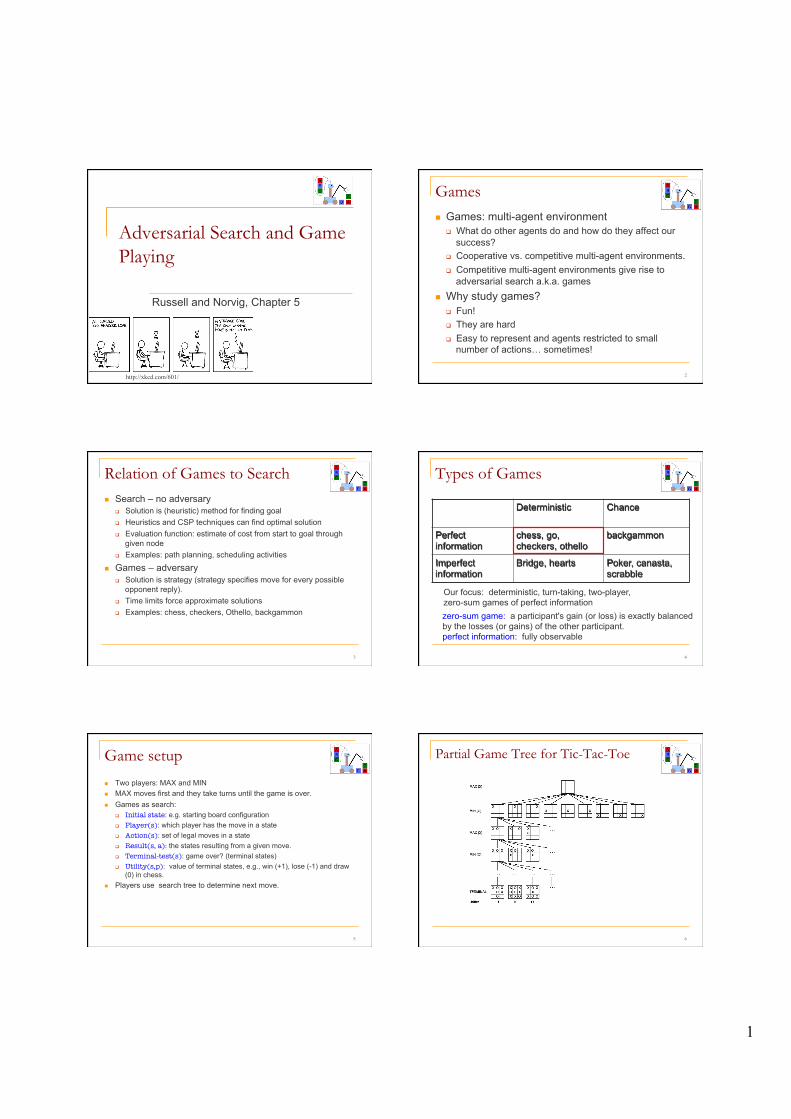
Partial Game Tree for Tic-Tac-Toe

6

2

7 http://xkcd.com/832/

The Tic-Tac-Toe Search Space

n  Is this search space a tree or graph? n  What is the minimum search depth?

n  What is the maximum search depth?

n  What is the branching factor?

Optimal strategies

n  Find the best strategy for MAX assuming an infallible MIN opponent.

n  Assumption: Both players play optimally. n  Given a game tree, the optimal strategy can be determined

by using the minimax value of each node:

MINIMAX(s)= UTILITY(s) If s is a terminal maxa ∈ Actions(s) MINIMAX(RESULT(s,a)) If PLAYER(s)=MAX mina ∈ Actions(s) MINIMAX(RESULT(s,a)) If PLAYER(s)=MIN

9

Two-Ply Game Tree

10

Definition: ply = turn of a two-player game

Two-Ply Game Tree

11

The minimax value at a min node is the minimum of backed-up values, because your opponent will do what’s best for them (and worst for you).

Two-Ply Game Tree

12

The minimax decision!

Minimax maximizes the worst-case outcome for max.

3

Minimax Algorithm

13

function MINIMAX-DECISION(state) returns an action return arg maxa ∈ Actions(s) MIN-VALUE(RESULT(state,a))

function MIN-VALUE(state) returns a utility value if TERMINAL-TEST(state) then return UTILITY(state) v ← ∞ for a in ACTIONS(state) do v ← MIN(v,MAX-VALUE(RESULT(state,a))) return v

function MAX-VALUE(state) returns a utility value if TERMINAL-TEST(state) then return UTILITY(state) v ← ∞ for each a in ACTIONS(state) do v ← MAX(v,MIN-VALUE(RESULT(state,a))) return v

Properties of Minimax

n  Minimax explores tree using DFS. n  Therefore:

q  Time complexity: O(bm) q  Space complexity: O(bm)

14

J L

Problem of minimax search

n  Number of game states is exponential in the number of moves. q  Solution: Do not examine every node q  ==> Alpha-beta pruning

n  Remove branches that do not influence final decision n  General idea: you can bracket the highest/lowest value

at a node, even before all its successors have been evaluated

15

Alpha-Beta Pruning

n  α: the highest (i.e. best for Max) value possible

n  β: the lowest (i.e. best for Min) value possible n  initially α and β are (-∞, ∞).

Alpha-Beta Example

17

[-∞, +∞]

[-∞,+∞]

Range of possible values!

Alpha-Beta Example (continued)

18

[-∞,3]

[-∞,+∞]

4

Alpha-Beta Example (continued)

19

[-∞,3]

[-∞,+∞]

Alpha-Beta Example (continued)

20

[3,+∞]

[3,3]

Alpha-Beta Example (continued)

21

[-∞,2]

[3,+∞]

[3,3]

This node is worse !for MAX

Alpha-Beta Example (continued)

22

[-∞,2]

[3,14]

[3,3] [-∞,14]

,

Alpha-Beta Example (continued)

23

[-∞,2]

[3,5]

[3,3] [-∞,5]

,

Alpha-Beta Example (continued)

24

[2,2] [-∞,2]

[3,3]

[3,3]

5

Alpha-Beta Example (continued)

25

[2,2] [-∞,2]

[3,3]

[3,3]

Alpha-Beta Algorithm

26

function ALPHA-BETA-SEARCH(state) returns an action v←MAX-VALUE(state, - ∞ , +∞) return the action in ACTIONS(state) with value v

function MAX-VALUE(state,α , β) returns a utility value if TERMINAL-TEST(state) then return UTILITY(state) v ← - ∞ for each a in ACTIONS(state) do v ← MAX(v, MIN-VALUE(RESULT(state,a), α , β)) if v ≥ β then return v α ← MAX(α ,v) return v

Alpha-Beta Algorithm

27

function MIN-VALUE(state, α , β) returns a utility value if TERMINAL-TEST(state) then return UTILITY(state) v ← + ∞ for each a in ACTIONS(state) do v ← MIN(v, MAX-VALUE(RESULT(state,a), α , β)) if v ≤ α then return v β ← MIN(β ,v) return v

Alpha-beta pruning

n  When enough is known about a node n, it can be pruned.

28

Final Comments about Alpha-Beta Pruning

n  Pruning does not affect final results n  Entire subtrees can be pruned, not just leaves. n  Good move ordering improves effectiveness of pruning n  With “perfect ordering,” time complexity is O(bm/2)

q  Effective branching factor of sqrt(b) q  Consequence: alpha-beta pruning can look twice as

deep as minimax in the same amount of time

29

Is this practical?

n  Minimax and alpha-beta pruning still have exponential complexity.

n  May be impractical within a reasonable amount of time. n  SHANNON (1950):

q  Terminate search at a lower depth q  Apply heuristic evaluation function EVAL instead of the UTILITY

function

30

6

Cutting off search

n  Change: q  if TERMINAL-TEST(state) then return UTILITY(state) into q  if CUTOFF-TEST(state,depth) then return EVAL(state)

n  Introduces a fixed-depth limit depth q  Selected so that the amount of time will not exceed what the

rules of the game allow. n  When cuttoff occurs, the evaluation is performed.

31

Heuristic EVAL

n  Idea: produce an estimate of the expected utility of the game from a given position.

n  Performance depends on quality of EVAL. n  Requirements:

q  EVAL should order terminal-nodes in the same way as UTILITY. q  Fast to Compute. q  For non-terminal states the EVAL should be strongly correlated

with the actual chance of winning.

32

Heuristic EVAL example

33

Eval(s) = w1 f1(s) + w2 f2(s) + … + wn fn(s)

Addition assumes independence

In chess: w1 material + w2 mobility + w3 king safety + w4 center control + …

How good are computers…

n  Let’s look at the state of the art computer programs that play games such as chess, checkers, othello, go…

34

Checkers

n  Chinook: the first program to win the world champion title in a competition against a human (1994)

35

Chinook n  Components of Chinook:

q  Search (variant of alpha-beta). Search space has 1020 states.

q  Evaluation function q  Endgame database (for all states with 4 vs. 4 pieces;

roughly 40 billion positions). q  Opening book - a database of opening moves

n  Chinook can determine the final result of the game within the first 10 moves.

n  Author has recently shown that several openings lead to a draw.

36

Jonathan Schaeffer, Neil Burch, Yngvi Bjornsson, Akihiro Kishimoto, Martin Muller, Rob Lake, Paul Lu and Steve Sutphen. "Checkers is Solved," Science, 2007. http://www.cs.ualberta.ca/~chinook/publications/solving_checkers.html

7

Chess

n  1997: Deep Blue wins a 6-game match against Garry Kasparov

n  Searches using iterative deepening alpha-beta; evaluation function has over 8000 features; opening book of 4000 positions; end game database.

n  FRITZ plays world champion, Vladimir Kramnik; wins 6-gam match.

37

Othello

n  The best Othello computer programs can easily defeat the best humans (e.g. Logistello, 1997).

38

Go

n  Go: humans still much better!

39

Games that include chance

n  Possible moves (5-10,5-11), (5-11,19-24),(5-10,10-16) and (5-11,11-16)

40

Games that include chance

n  Possible moves (5-10,5-11), (5-11,19-24),(5-10,10-16) and (5-11,11-16)

n  [1,1],…,[6,6] probability 1/36, all others - 1/18 n  Can not calculate definite minimax value, only expected value

41

chance nodes!

Expected minimax value EXPECTIMINIMAX(s)=

UTILITY(s) If s is a terminal maxa EXPECTIMINIMAX(RESULT(s,a)) If PLAYER(S)=MAX mina EXPECTIMINIMAX(RESULT(s,a)) If PLAYER(S)=MIN ∑r P(r) EXPECTIMINIMAX(RESULT(s,r)) If PLAYER(S)=CHANCE r is a chance event (e.g., a roll of the dice). These equations can be propagated recursively in a similar way to the MINIMAX algorithm.

42

8

TD-Gammon (Tesauro, 1994)

43

World class program based on a combination of reinforcement Learning, neural networks and alpha-beta pruning to 3 plies. Move analyses by TD-Gammon have lead to some changes in accepted strategies.

White’s turn, with a roll of 4-4

http://www.research.ibm.com/massive/tdl.html

Summary

n  Games are fun n  They illustrate several important points about AI

q  Perfection is (usually) unattainable -> approximation q  Uncertainty constrains the assignment of values to

states

44