Advantages of the flux-based interpretationof dependency length minimization

Sylvain Kahane Chunxiao YanModyco, Université Paris Nanterre & CNRS

sylvain@kahane.fr yanchunxiao@yahoo.fr

Abstract

Dependency length minimization (DLM, also called dependency distance minimization) is studiedby many authors and identified as a property of natural languages. In this paper we show that DLMcan be interpreted as the flux size minimization and study the advantages of such a view. First it al-lows us to understand why DLM is cognitively motivated and how it is related to the constraints onthe processing of sentences. Second, it opens the door to the definition of a big range of variationsof DLM, taking into account other characteristics of the flux such as nested constructions and pro-jectivity.

1 Introduction

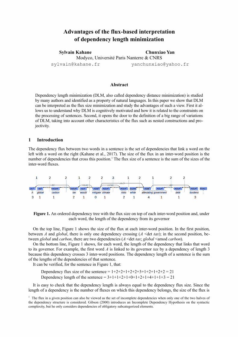
The dependency flux between two words in a sentence is the set of dependencies that link a word on theleft with a word on the right (Kahane et al., 2017). The size of the flux in an inter-word position is thenumber of dependencies that cross this position.1 The flux size of a sentence is the sum of the sizes of theinter-word fluxes.

Figure 1. An ordered dependency tree with the flux size on top of each inter-word position and, undereach word, the length of the dependency from its governor

On the top line, Figure 1 shows the size of the flux at each inter-word position. In the first position,between A and global, there is only one dependency crossing (A <det tax); in the second position, be-tween global and carbon, there are two dependencies (A <det tax; global <amod carbon).

On the bottom line, Figure 1 shows, for each word, the length of the dependency that links that wordto its governor. For example, the first word A is linked to its governor tax by a dependency of length 3because this dependency crosses 3 inter-word positions. The dependency length of a sentence is the sumof the lengths of the dependencies of that sentence.

It can be verified, for the sentence in Figure 1, that:

Dependency flux size of the sentence = 1+2+2+1+2+2+3+1+2+1+2+2 = 21Dependency length of the sentence = 3+1+1+2+1+0+1+2+1+4+1+1+3 = 21

It is easy to check that the dependency length is always equal to the dependency flux size. Since thelength of a dependency is the number of fluxes on which this dependency belongs, the size of the flux is1 The flux in a given position can also be viewed as the set of incomplete dependencies when only one of the two halves ofthe dependency structure is considered. Gibson (2000) introduces an Incomplete Dependency Hypothesis on the syntacticcomplexity, but he only considers dependencies of obligatory subcategorized elements.

the sum, on all the dependencies, of the number of fluxes they cross. In other words, these two values areequal to the number of crossings between a dependency and an inter-word position.

Several studies have studied dependency length and shown that natural languages tend to minimize it(Liu, 2008; Futrell et al., 2015). This property is called dependency length minimization (DLM) or de-pendency distance minimization (dependency lengths can be interpreted as distances between syntacti-cally related words). DLM is correlated with several properties of natural languages. For instance, thefact that dependency structures in natural languages are much less non-projective than in randomly or-dered trees can be explained by DLM (Ferrer i Cancho, 2006; Liu, 2008). It is also claimed that DLM isa factor affecting the grammar of languages and word order choices (Gildea and Temperley, 2010; Tem-perley and Gildea, 2018).

Since the dependency length is equal to the dependency flux size, by trying to minimize the lengths ofthe dependencies, we also try to minimize the sizes of the inter-word fluxes. This gives us two differentviews on DLM. The objective of this article is to show that thinking about DLM in terms of flux has sev-eral advantages. In section 2, we will show that the interpretation of DLM in terms of flux makes it pos-sible to highlight the cognitive relevance of this constraint. In section 3, we will examine other flux-based constraints related to DLM.

2 Cognitive relevancy of DLM

As we have just seen, DLM corresponds to the minimization of the flux size of the sentence and there-fore of all inter-word fluxes. However, since we know that sentences are more or less parsed as fast asthey are received by the speakers (Frazier and Fodor, 1978), we can see the flux in a given inter-wordposition as the information resulting from the portion of the sentence already analyzed that is necessaryfor its further analysis. In other words, there is an obvious link between the inter-word flux and the work-ing memory of the recipient of an utterance (as well as the producer of the utterance).

The links between syntactic complexity and working memory have often been discussed, starting withYngve (1960) and Chomsky and Miller (1963). According to Friederici (2011), “the processing of syn-tactically complex sentences requires some working memory capacity”. The founding work on limita-tions of working memory is Miller’s (1956), who defended that the span is 7 ± 2 elements; this limitationhas been updated between 3 and 5 meaningful items by Cowan's work (2001). According to Cowan(2010), “Working memory is used in mental tasks, such as language comprehension (for example, retain-ing ideas from early in a sentence to be combined with ideas later on), problem solving (in arithmetic,carry a digit from the ones to the tens column while remembering the numbers), and planning (determin-ing the best order in which to visit the bank, library, and grocery).” He adds that “There are also pro-cesses that can influence how effectively working memory is used. An important example is in the use ofattention to fill working memory with items one should be remembering.”

We think that the dependency flux in inter-word positions is a good approximation of what the recipi-ent must remember to parse the rest of the sentence. Of course, it is also possible to make a link betweenthe working memory and DLM if it is interpreted in terms of dependency length: it means that it is cog-nitively expensive to keep a dependency in working memory for a long time and that the longer a depen-dency is, the more likely it is to deteriorate in working memory (Gibson, 1998; 2000).

3 DLM-related constraints

DLM is a constraint on the size of the whole flux of a sentence and therefore a particular case of con-straints on the complexity of the flux. DLM is neither the only metrics for syntactic complexity (seeLewis (1996) for several constituency-based metrics; Berdicevskis et al. 2018), nor the only metrics onthe complexity of the flux and perhaps not the best. We will present other potentially interesting flux-based metrics.

3.1 Constraints on the size of inter-word fluxes

We have seen that the sum of the lengths of the dependencies is equal to the sum of the sizes of the inter-word fluxes. Since there are as many dependencies as there are inter-word positions in a sentence (n-1for a sentence of n words), this means that the average length of the dependencies is equal to the averagesize of the inter-word fluxes. For the entire UD database (version 2.4, 146 treebanks), this value is equal

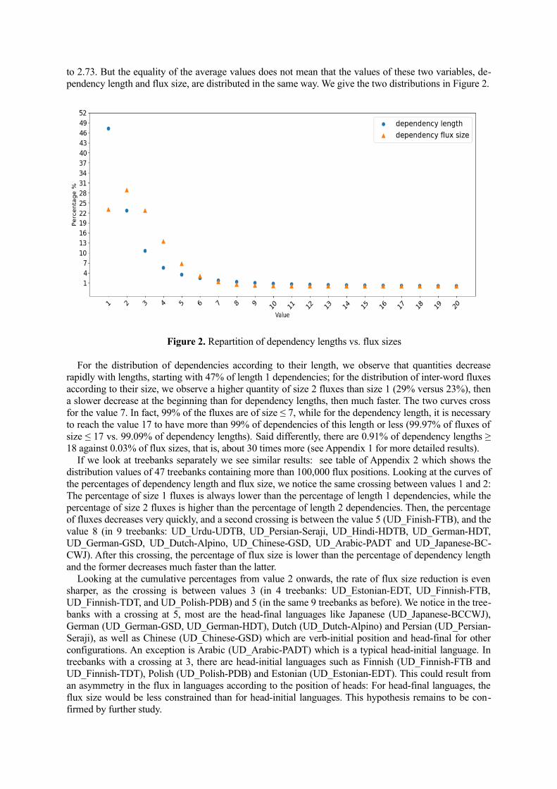
to 2.73. But the equality of the average values does not mean that the values of these two variables, de-pendency length and flux size, are distributed in the same way. We give the two distributions in Figure 2.

Figure 2. Repartition of dependency lengths vs. flux sizes

For the distribution of dependencies according to their length, we observe that quantities decreaserapidly with lengths, starting with 47% of length 1 dependencies; for the distribution of inter-word fluxesaccording to their size, we observe a higher quantity of size 2 fluxes than size 1 (29% versus 23%), thena slower decrease at the beginning than for dependency lengths, then much faster. The two curves crossfor the value 7. In fact, 99% of the fluxes are of size ≤ 7, while for the dependency length, it is necessaryto reach the value 17 to have more than 99% of dependencies of this length or less (99.97% of fluxes ofsize ≤ 17 vs. 99.09% of dependency lengths). Said differently, there are 0.91% of dependency lengths ≥18 against 0.03% of flux sizes, that is, about 30 times more (see Appendix 1 for more detailed results).

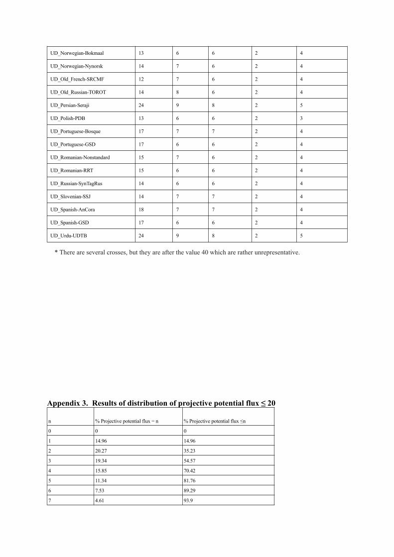
If we look at treebanks separately we see similar results: see table of Appendix 2 which shows thedistribution values of 47 treebanks containing more than 100,000 flux positions. Looking at the curves ofthe percentages of dependency length and flux size, we notice the same crossing between values 1 and 2:The percentage of size 1 fluxes is always lower than the percentage of length 1 dependencies, while thepercentage of size 2 fluxes is higher than the percentage of length 2 dependencies. Then, the percentageof fluxes decreases very quickly, and a second crossing is between the value 5 (UD_Finish-FTB), and thevalue 8 (in 9 treebanks: UD_Urdu-UDTB, UD_Persian-Seraji, UD_Hindi-HDTB, UD_German-HDT,UD_German-GSD, UD_Dutch-Alpino, UD_Chinese-GSD, UD_Arabic-PADT and UD_Japanese-BC-CWJ). After this crossing, the percentage of flux size is lower than the percentage of dependency lengthand the former decreases much faster than the latter.

Looking at the cumulative percentages from value 2 onwards, the rate of flux size reduction is evensharper, as the crossing is between values 3 (in 4 treebanks: UD_Estonian-EDT, UD_Finnish-FTB,UD_Finnish-TDT, and UD_Polish-PDB) and 5 (in the same 9 treebanks as before). We notice in the tree-banks with a crossing at 5, most are the head-final languages like Japanese (UD_Japanese-BCCWJ),German (UD_German-GSD, UD_German-HDT), Dutch (UD_Dutch-Alpino) and Persian (UD_Persian-Seraji), as well as Chinese (UD_Chinese-GSD) which are verb-initial position and head-final for otherconfigurations. An exception is Arabic (UD_Arabic-PADT) which is a typical head-initial language. Intreebanks with a crossing at 3, there are head-initial languages such as Finnish (UD_Finnish-FTB andUD_Finnish-TDT), Polish (UD_Polish-PDB) and Estonian (UD_Estonian-EDT). This could result froman asymmetry in the flux in languages according to the position of heads: For head-final languages, theflux size would be less constrained than for head-initial languages. This hypothesis remains to be con-firmed by further study.

If we look for which value n we reach the 99% of dependencies of length ≤ n, we find values rangingfrom 9 (UD_finish-FTB) to 27 (UD_Arabic-PADT). The same calculation for flux size gives values be-tween 6 (in 12 treebanks: UD_Bulgarian-BTB, UD_Czech-FicTree, UD_Finnish-FTB, UD_French-GSD, UD_Italian-ISDT, UD_Korean-Kaist, UD_Norwegian-Bokmaal, UD_Polish-PDB, UD_Por-tuguese-GSD, UD_Romanian-RRT, UD_Russian-SynTagRus, and UD_Spanish-GSD) and 11 (UD_Ja-panese-BCCWJ) (this value is a little exceptional, since the value is equal to 7 for UD_Japanese-BC-CWJ). We also find that variations in dependency length are more sensitive than those in flux size in thedifferent treebanks of a language. For example, for French, UD_French-FTB has 99% length dependen-cies ≤ 21, and UD_French-GSD has 99% length dependencies ≤ 16, while in the case of flux size, thevalues are 7 and 6 respectively.

If DLM expresses a constraint on the average value of dependency lengths and flux sizes, we see thatthere is also a fairly strong constraint on the size of each inter-word flux, whereas there is not such astrong constraint on the length of each dependency. For this reason, we postulate that DLM results moreon a constraint on flux sizes than on dependency lengths, even if it is not possible to give a precise limitto the size of individual fluxes as Kahane et al. (2017) have already shown.

3.2 Center-embedding and constraints on structured fluxes

Beyond the question of their lengths, the way the dependencies are organized plays an important role insyntactic complexity. In particular, center-embedding structures carry a computational constraint in sen-tence processing (Chomsky and Miller, 1963; Lewis, 1996; Lewis and Vasishth, 2005). It is important tonote that the complexity caused by center-embedding structures cannot be involved in DLM-based con-straints. Neurobiological studies have highlighted the independence of memory degradation related tothe length of a dependency and the computational aspect expressed by the center-embedding phenom-ena, which are located in different parts of the brain (Makuuchi et al., 2009).

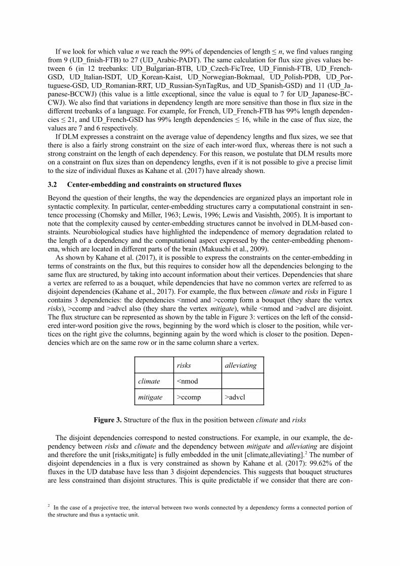
As shown by Kahane et al. (2017), it is possible to express the constraints on the center-embedding interms of constraints on the flux, but this requires to consider how all the dependencies belonging to thesame flux are structured, by taking into account information about their vertices. Dependencies that sharea vertex are referred to as a bouquet, while dependencies that have no common vertex are referred to asdisjoint dependencies (Kahane et al., 2017). For example, the flux between climate and risks in Figure 1contains 3 dependencies: the dependencies <nmod and >ccomp form a bouquet (they share the vertexrisks), >ccomp and >advcl also (they share the vertex mitigate), while <nmod and >advcl are disjoint.The flux structure can be represented as shown by the table in Figure 3: vertices on the left of the consid-ered inter-word position give the rows, beginning by the word which is closer to the position, while ver-tices on the right give the columns, beginning again by the word which is closer to the position. Depen-dencies which are on the same row or in the same column share a vertex.

risks alleviating

climate <nmod

mitigate >ccomp >advcl

Figure 3. Structure of the flux in the position between climate and risks

The disjoint dependencies correspond to nested constructions. For example, in our example, the de-pendency between risks and climate and the dependency between mitigate and alleviating are disjointand therefore the unit [risks,mitigate] is fully embedded in the unit [climate,alleviating].2 The number ofdisjoint dependencies in a flux is very constrained as shown by Kahane et al. (2017): 99.62% of thefluxes in the UD database have less than 3 disjoint dependencies. This suggests that bouquet structuresare less constrained than disjoint structures. This is quite predictable if we consider that there are con-

2 In the case of a projective tree, the interval between two words connected by a dependency forms a connected portion ofthe structure and thus a syntactic unit.

straints on working memory and that dependencies in a bouquet share more information than disjoint de-pendencies.

Note that non-projectivity can also be detected from a structured flux, if we take into account the orderin which the vertices of the dependencies of the same flux are located. We plan in our further studies tolook more precisely on the distribution of the different possible configurations of the flux.

3.3 Constraints on the potential flux

It must be remarked that we do not really know the flux when processing a sentence incrementally sincewe do not generally know which words already processed will be linked with a word not yet processed.We call potential flux in a given inter-word position the set of words before the position which are likelyto be linked to words after it. See in particular the principles of the transition-based parsing (Nivre, 2003)which consists in keeping all the words already processed and still accessible in the working memory.The largest hypothesis on the potential flux is to consider that all words before the position are accessi-ble. But clearly some words are more likely to have dependents (for instance, only content words canhave dependents in UD). It is also possible to make structural hypothesis on the potential flux. We callprojective potential flux the set of words accessible while maintaining the projectivity of the analysis. Wewill limit our study to the projective potential flux even if we are aware that, on one hand, projectivity isfar to be an absolute constraint in many languages and, in the other hand, other constraints apply on thepotential flux.

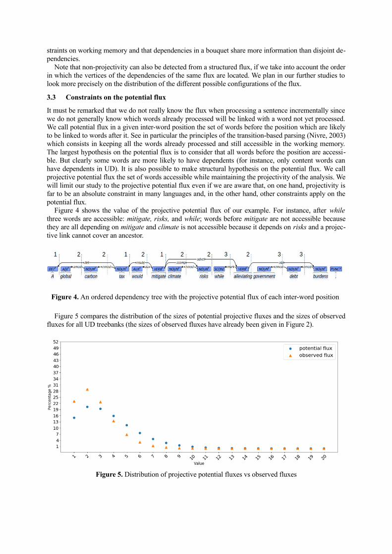
Figure 4 shows the value of the projective potential flux of our example. For instance, after whilethree words are accessible: mitigate, risks, and while; words before mitigate are not accessible becausethey are all depending on mitigate and climate is not accessible because it depends on risks and a projec-tive link cannot cover an ancestor.

Figure 4. An ordered dependency tree with the projective potential flux of each inter-word position

Figure 5 compares the distribution of the sizes of potential projective fluxes and the sizes of observedfluxes for all UD treebanks (the sizes of observed fluxes have already been given in Figure 2).

Figure 5. Distribution of projective potential fluxes vs observed fluxes

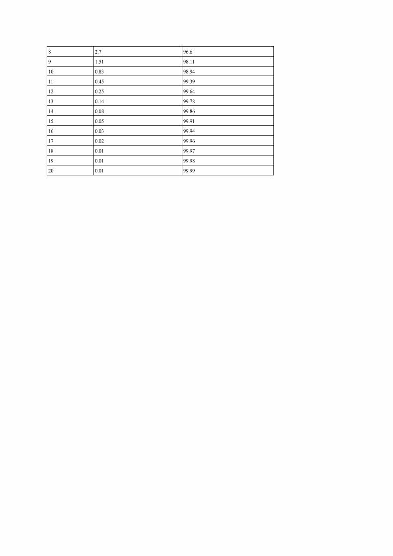
The distribution of projective potential fluxes is flatter (20% vs. 29% for size 2) with less fluxes withsizes ≤ 3 and more fluxes with sizes ≥ 4, which means that projective potential fluxes generally havegreater size than observed flux. From the size 2, the number of projective potential fluxes decreases butmore slowly than the number of observed fluxes. It is necessary to reach size 11 to have more than 99%of the potential fluxes (99.39% of the potential fluxes have a size ≤ 11) while this value is reached withsize 7 for the observed fluxes (see Appendix 3 for details).

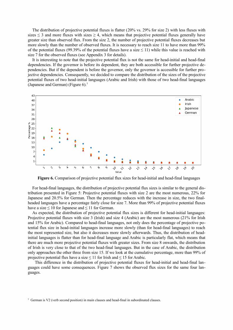
It is interesting to note that the projective potential flux is not the same for head-initial and head-finaldependencies. If the governor is before its dependent, they are both accessible for further projective de-pendencies. But if the dependent is before the governor, only the governor is accessible for further pro-jective dependencies. Consequently, we decided to compare the distribution of the sizes of the projectivepotential fluxes of two head-initial languages (Arabic and Irish) with those of two head-final languages(Japanese and German) (Figure 6).3

Figure 6. Comparison of projective potential flux sizes for head-initial and head-final languages

For head-final languages, the distribution of projective potential flux sizes is similar to the general dis-tribution presented in Figure 5: Projective potential fluxes with size 2 are the most numerous, 22% forJapanese and 20.5% for German. Then the percentage reduces with the increase in size, the two final-headed languages have a percentage fairly close for size 7. More than 99% of projective potential fluxeshave a size ≤ 10 for Japanese and ≤ 11 for German.

As expected, the distribution of projective potential flux sizes is different for head-initial languages:Projective potential fluxes with size 3 (Irish) and size 4 (Arabic) are the most numerous (21% for Irishand 15% for Arabic). Compared to head-final languages, not only does the percentage of projective po-tential flux size in head-initial languages increase more slowly (than for head-final languages) to reachthe most represented size, but also it decreases more slowly afterwards. Thus, the distribution of head-initial languages is flatter than for head-final language and Arabic is particularly flat, which means thatthere are much more projective potential fluxes with greater sizes. From size 8 onwards, the distributionof Irish is very close to that of the two head-final languages. But in the case of Arabic, the distributiononly approaches the other three from size 15. If we look at the cumulative percentage, more than 99% ofprojective potential flux have a size ≤ 11 for Irish and ≤ 15 for Arabic.

This difference in the distribution of projective potential fluxes for head-initial and head-final lan-guages could have some consequences. Figure 7 shows the observed flux sizes for the same four lan-guages.

3 German is V2 (verb second position) in main clauses and head-final in subordinated clauses.

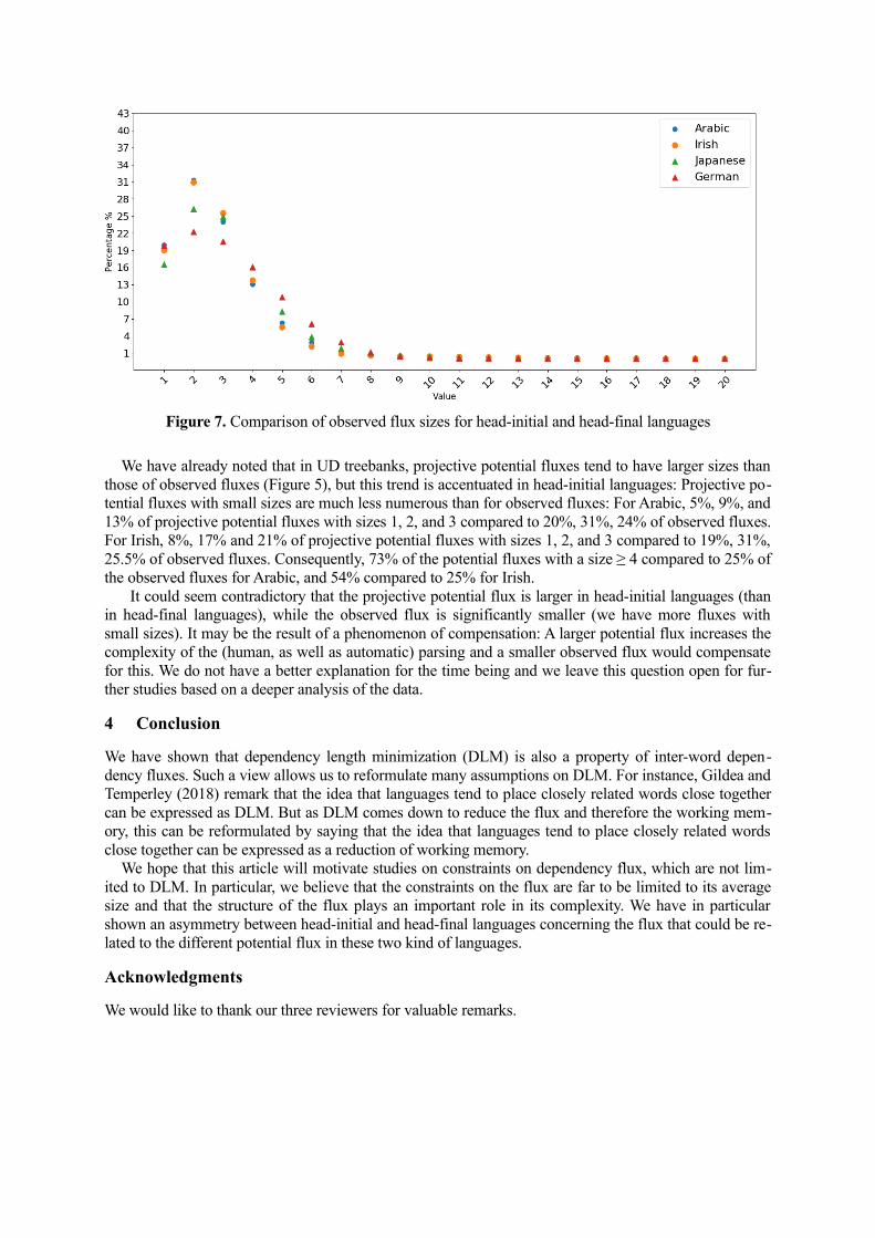
Figure 7. Comparison of observed flux sizes for head-initial and head-final languages

We have already noted that in UD treebanks, projective potential fluxes tend to have larger sizes thanthose of observed fluxes (Figure 5), but this trend is accentuated in head-initial languages: Projective po-tential fluxes with small sizes are much less numerous than for observed fluxes: For Arabic, 5%, 9%, and13% of projective potential fluxes with sizes 1, 2, and 3 compared to 20%, 31%, 24% of observed fluxes.For Irish, 8%, 17% and 21% of projective potential fluxes with sizes 1, 2, and 3 compared to 19%, 31%,25.5% of observed fluxes. Consequently, 73% of the potential fluxes with a size ≥ 4 compared to 25% ofthe observed fluxes for Arabic, and 54% compared to 25% for Irish.

It could seem contradictory that the projective potential flux is larger in head-initial languages (thanin head-final languages), while the observed flux is significantly smaller (we have more fluxes withsmall sizes). It may be the result of a phenomenon of compensation: A larger potential flux increases thecomplexity of the (human, as well as automatic) parsing and a smaller observed flux would compensatefor this. We do not have a better explanation for the time being and we leave this question open for fur-ther studies based on a deeper analysis of the data.

4 Conclusion

We have shown that dependency length minimization (DLM) is also a property of inter-word depen-dency fluxes. Such a view allows us to reformulate many assumptions on DLM. For instance, Gildea andTemperley (2018) remark that the idea that languages tend to place closely related words close togethercan be expressed as DLM. But as DLM comes down to reduce the flux and therefore the working mem-ory, this can be reformulated by saying that the idea that languages tend to place closely related wordsclose together can be expressed as a reduction of working memory.

We hope that this article will motivate studies on constraints on dependency flux, which are not lim-ited to DLM. In particular, we believe that the constraints on the flux are far to be limited to its averagesize and that the structure of the flux plays an important role in its complexity. We have in particularshown an asymmetry between head-initial and head-final languages concerning the flux that could be re-lated to the different potential flux in these two kind of languages.

Acknowledgments

We would like to thank our three reviewers for valuable remarks.

References

Berdicevskis Aleksandrs et al. 2018. Using Universal Dependencies in cross-linguistic complexity research. InProceedings of the Second Workshop on Universal Dependencies (UDW 2018), 8-17.

Ramon Ferrer i Cancho. 2006. Why do syntactic links not cross?. EPL (Europhysics Letters), 76, 1228-1234.

Nelson Cowan. 2001. The magical number 4 in short-term memory: A reconsideration of mental storage capacity.Behavioral and brain sciences, 24(1), 87-114.

Nelson Cowan. 2010. The magical mystery four: How is working memory capacity limited, and why?. Current di-rections in psychological science, 19(1), 51-57.

Angela D Friederici. 2011. The brain basis of language processing: from structure to function. Physiological re-views, 91(4), 1357-1392.

Lyn Frazier and Fodor Janet Dean. 1978. The sausage machine: A new two-stage parsing model, Cognition, 6(4),291-325.

Richard Futrell, Kyle Mahowald and Edward Gibson. 2015. Large-scale evidence of dependency length minimiza-tion in 37 languages. Proceedings of the National Academy of Sciences, 112(33), 10336-10341.

Edward Gibson. 1998. Linguistic complexity: Locality of syntactic dependencies. Cognition, 68(1), 1-76.

Edward Gibson. 2000. The dependency locality theory: A distance-based theory of linguistic complexity. Image,language, brain, 2000, 95-126.

Daniel Gildea and David Temperley. 2010. Do grammars minimize dependency length?. Cognitive Science, 34(2),286-310.

Sylvain Kahane, Alexis Nasr and Owen Rambow. 1998. Pseudo-projectivity: a polynomially parsable non-projec-tive dependency grammar. In COLING 1998 Volume 1: The 17th International Conference on ComputationalLinguistics (Vol. 1).

Sylvain Kahane, Chunxiao Yan, and Marie-Amélie Botalla. 2017. What are the limitations on the flux of syntacticdependencies? Evidence from UD treebanks. In 4th international conference on Dependency Linguistics(Depling) (pp. 73-82).

Richard L. Lewis. 1996. Interference in short-term memory: The magical number two (or three) in sentence pro-cessing. Journal of psycholinguistic research, 25(1), 93-115.

Richard L. Lewis and Shravan Vasishth. 2005. An activation‐based model of sentence processing as skilled mem-ory retrieval. Cognitive science, 29(3), 375-419.

Haitao Liu. 2008. Dependency distance as a metric of language comprehension difficulty. Journal of Cognitive Sci-ence, 9(2), 159-191.

Michiru Makuuchi et al. 2009. Segregating the core computational faculty of human language from working mem-ory. Proceedings of the National Academy of Sciences, 106(20), 8362-8367.

George A. Miller and Noam Chomsky. 1963. Finitary models of language users.

Joakim Nivre. 2003. An efficient algorithm for projective dependency parsing. In Proceedings of the Eighth Inter-national Conference on Parsing Technologies, 149-160.

Joakim Nivre. 2006. Constraints on non-projective dependency parsing. In 11th Conference of the European Chap-ter of the Association for Computational Linguistics.

Daniel D. K. Sleator and Davy Temperley. 1995. Parsing English with a link grammar. arXiv preprint cmp-lg/9508004.

David Temperley and Daniel Gildea. 2018. Minimizing syntactic dependency lengths: typological/cognitive uni-versal?. Annual Review of Linguistics, 4, 67-80.

Victor H. Yngve. 1960. A model and an hypothesis for language structure. Proceedings of the American philo-sophical society, 104(5), 444-466.

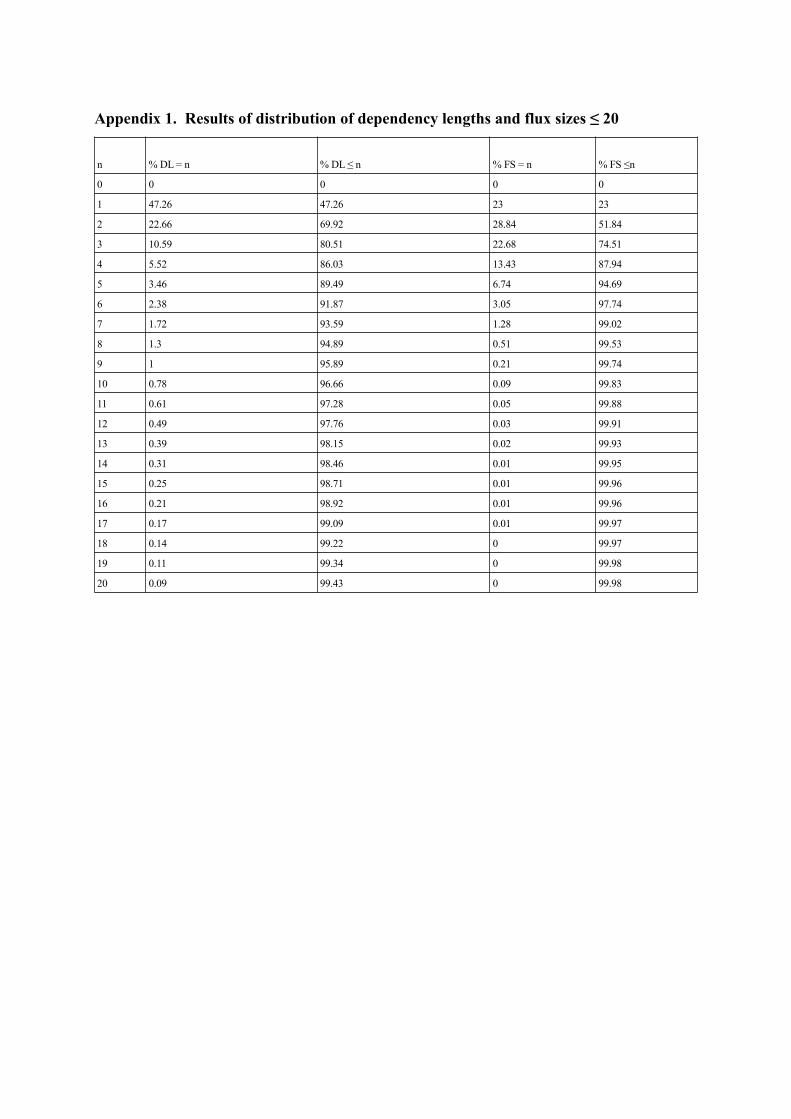
Appendix 1. Results of distribution of dependency lengths and flux sizes ≤ 20

n % DL = n % DL ≤ n % FS = n % FS ≤n

0 0 0 0 0

1 47.26 47.26 23 23

2 22.66 69.92 28.84 51.84

3 10.59 80.51 22.68 74.51

4 5.52 86.03 13.43 87.94

5 3.46 89.49 6.74 94.69

6 2.38 91.87 3.05 97.74

7 1.72 93.59 1.28 99.02

8 1.3 94.89 0.51 99.53

9 1 95.89 0.21 99.74

10 0.78 96.66 0.09 99.83

11 0.61 97.28 0.05 99.88

12 0.49 97.76 0.03 99.91

13 0.39 98.15 0.02 99.93

14 0.31 98.46 0.01 99.95

15 0.25 98.71 0.01 99.96

16 0.21 98.92 0.01 99.96

17 0.17 99.09 0.01 99.97

18 0.14 99.22 0 99.97

19 0.11 99.34 0 99.98

20 0.09 99.43 0 99.98

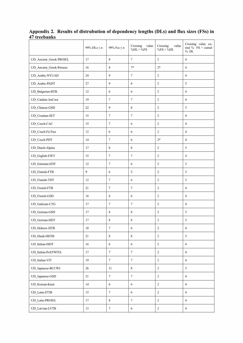
Appendix 2. Results of distrubution of dependency lengths (DLs) and flux sizes (FSs) in47 treebanks

99% DLs ≤ n 99% Fss ≤ nCrossing value%DL > %FS

Crossing value%FS > %DL

Crossing value cu-mul % FS > cumul% DL

UD_Ancient_Greek-PROIEL 17 8 7 2 4

UD_Ancient_Greek-Perseus 16 8 7* 2* 4

UD_Arabic-NYUAD 24 9 7 2 4

UD_Arabic-PADT 27 9 8 2 5

UD_Bulgarian-BTB 12 6 6 2 4

UD_Catalan-AnCora 19 7 7 2 4

UD_Chinese-GSD 22 9 8 2 5

UD_Croatian-SET 15 7 7 2 4

UD_Czech-CAC 15 7 6 2 4

UD_Czech-FicTree 12 6 6 2 4

UD_Czech-PDT 14 7 6 2* 4

UD_Dutch-Alpino 17 8 8 2 5

UD_English-EWT 15 7 7 2 4

UD_Estonian-EDT 12 7 6 2 3

UD_Finnish-FTB 9 6 5 2 3

UD_Finnish-TDT 12 7 6 2 3

UD_French-FTB 21 7 7 2 4

UD_French-GSD 16 6 6 2 4

UD_Galician-CTG 17 7 7 2 4

UD_German-GSD 17 8 8 2 5

UD_German-HDT 17 8 8 2 5

UD_Hebrew-HTB 18 7 6 2 4

UD_Hindi-HDTB 21 8 8 2 5

UD_Italian-ISDT 16 6 6 2 4

UD_Italian-PoSTWITA 17 7 7 2 4

UD_Italian-VIT 19 7 7 2 4

UD_Japanese-BCCWJ 26 11 8 2 5

UD_Japanese-GSD 21 7 7 2 4

UD_Korean-Kaist 14 6 6 2 4

UD_Latin-ITTB 15 7 6 2 4

UD_Latin-PROIEL 17 8 7 2 4

UD_Latvian-LVTB 13 7 6 2 4

UD_Norwegian-Bokmaal 13 6 6 2 4

UD_Norwegian-Nynorsk 14 7 6 2 4

UD_Old_French-SRCMF 12 7 6 2 4

UD_Old_Russian-TOROT 14 8 6 2 4

UD_Persian-Seraji 24 9 8 2 5

UD_Polish-PDB 13 6 6 2 3

UD_Portuguese-Bosque 17 7 7 2 4

UD_Portuguese-GSD 17 6 6 2 4

UD_Romanian-Nonstandard 15 7 6 2 4

UD_Romanian-RRT 15 6 6 2 4

UD_Russian-SynTagRus 14 6 6 2 4

UD_Slovenian-SSJ 14 7 7 2 4

UD_Spanish-AnCora 18 7 7 2 4

UD_Spanish-GSD 17 6 6 2 4

UD_Urdu-UDTB 24 9 8 2 5

* There are several crosses, but they are after the value 40 which are rather unrepresentative.

Appendix 3. Results of distribution of projective potential flux ≤ 20

n % Projective potential flux = n % Projective potential flux ≤n

0 0 0

1 14.96 14.96

2 20.27 35.23

3 19.34 54.57

4 15.85 70.42

5 11.34 81.76

6 7.53 89.29

7 4.61 93.9

8 2.7 96.6

9 1.51 98.11

10 0.83 98.94

11 0.45 99.39

12 0.25 99.64

13 0.14 99.78

14 0.08 99.86

15 0.05 99.91

16 0.03 99.94

17 0.02 99.96

18 0.01 99.97

19 0.01 99.98

20 0.01 99.99