Embed Size (px)
Citation preview
Advantages of Mixed-effects Regression Models(MRM; aka multilevel, hierarchical linear, linear mixed models)
1. MRM explicitly models individual change across time
2. MRM more flexible in terms of repeated measures
(a) need not have same number of obs per subject
(b) time can be continuous, rather than a fixed set of points
3. Flexible specification of the covariance structure among repeatedmeasures ⇒ methods for testing specific determinants of thisstructure
4. MRM can be extended to higher-level models ⇒ repeatedobservations within individuals within clusters
5. Generalizations for non-normal data
1
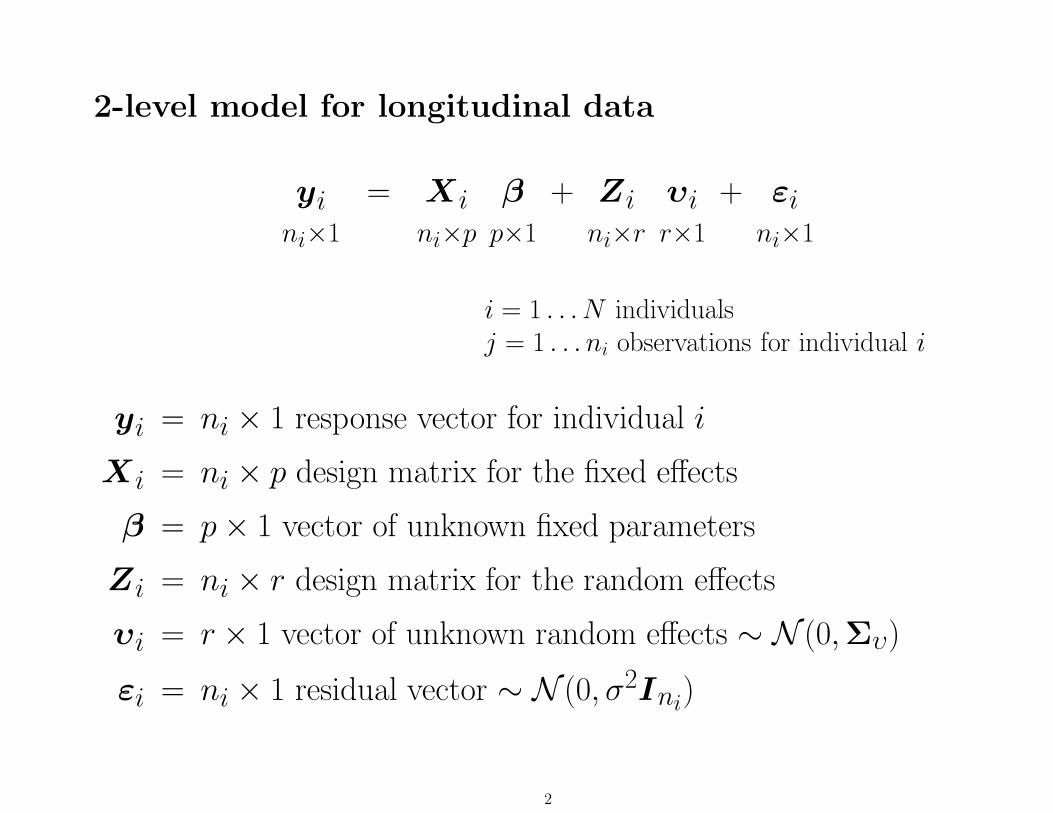
2-level model for longitudinal data
yini×1
= Xini×p
βp×1
+ Zini×r
υir×1
+ εini×1
i = 1 . . . N individualsj = 1 . . . ni observations for individual i
yi = ni × 1 response vector for individual i
Xi = ni × p design matrix for the fixed effects
β = p × 1 vector of unknown fixed parameters
Zi = ni × r design matrix for the random effects
υi = r × 1 vector of unknown random effects ∼ N (0,Συ)
εi = ni × 1 residual vector ∼ N (0, σ2Ini)
2
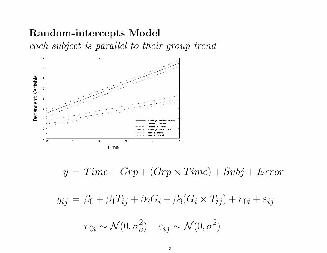
Random-intercepts Modeleach subject is parallel to their group trend
y = T ime + Grp + (Grp× T ime) + Subj + Error
yij = β0 + β1Tij + β2Gi + β3(Gi × Tij) + υ0i + εij
υ0i ∼ N (0, σ2υ) εij ∼ N (0, σ2)
3
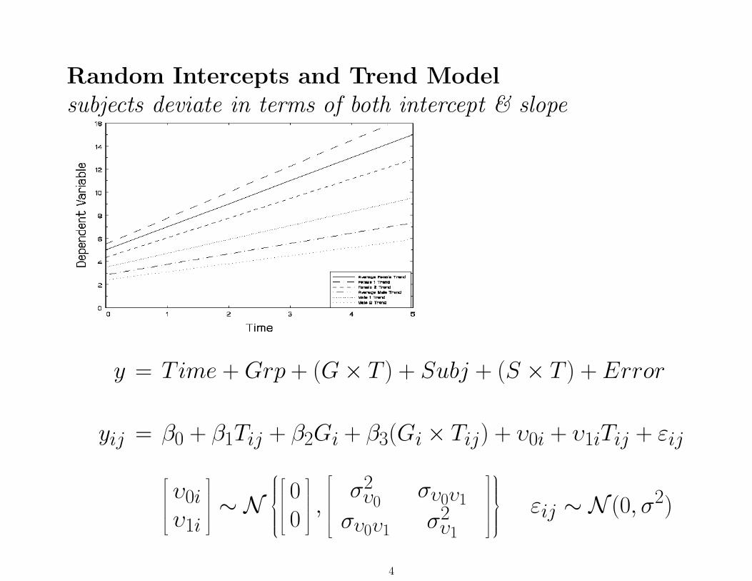
Random Intercepts and Trend Modelsubjects deviate in terms of both intercept & slope
y = T ime + Grp + (G × T ) + Subj + (S × T ) + Error
yij = β0 + β1Tij + β2Gi + β3(Gi × Tij) + υ0i + υ1iTij + εij
υ0iυ1i
∼ N
00
,
σ2υ0
συ0υ1
συ0υ1 σ2υ1
εij ∼ N (0, σ2)
4
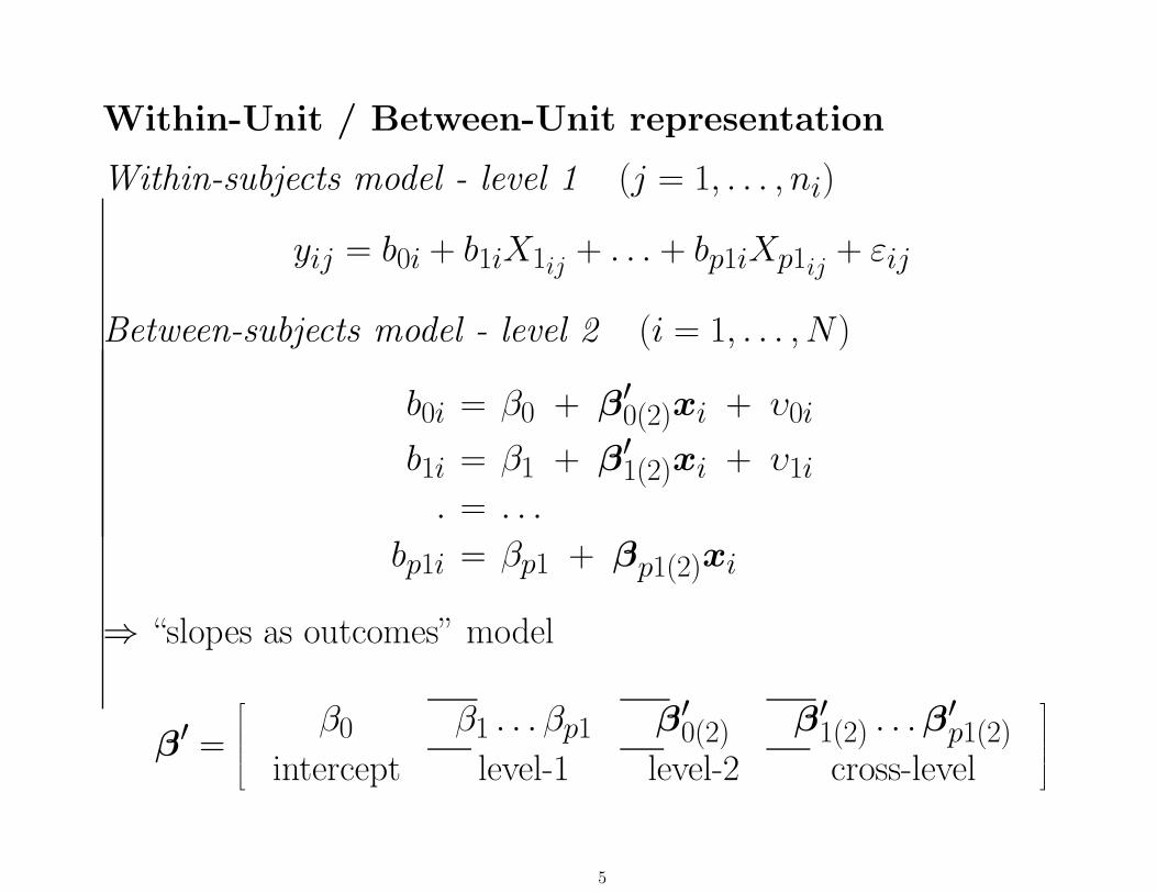
Within-Unit / Between-Unit representation
Within-subjects model - level 1 (j = 1, . . . , ni)
yij = b0i + b1iX1ij+ . . . + bp1iXp1ij
+ εij
Between-subjects model - level 2 (i = 1, . . . , N)
b0i = β0 + β′0(2)xi + υ0i
b1i = β1 + β′1(2)xi + υ1i
. = . . .
bp1i = βp1 + βp1(2)xi
⇒ “slopes as outcomes” model
β′ =
β0 β1 . . . βp1 β′0(2) β′
1(2) . . . β′p1(2)
intercept level-1 level-2 cross-level
5
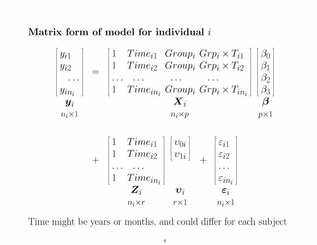
Matrix form of model for individual i
yi1yi2
. . .yini
yini×1
=
1 T imei1 Groupi Grpi × Ti11 T imei2 Groupi Grpi × Ti2. . . . . . . . . . . .1 T imeini
Groupi Grpi × Tini
Xini×p
β0β1β2β3
βp×1
+
1 T imei11 T imei2. . . . . .1 T imeini
Zini×r
υ0iυ1i
υir×1
+
εi1εi2. . .εini
εini×1
Time might be years or months, and could differ for each subject
6
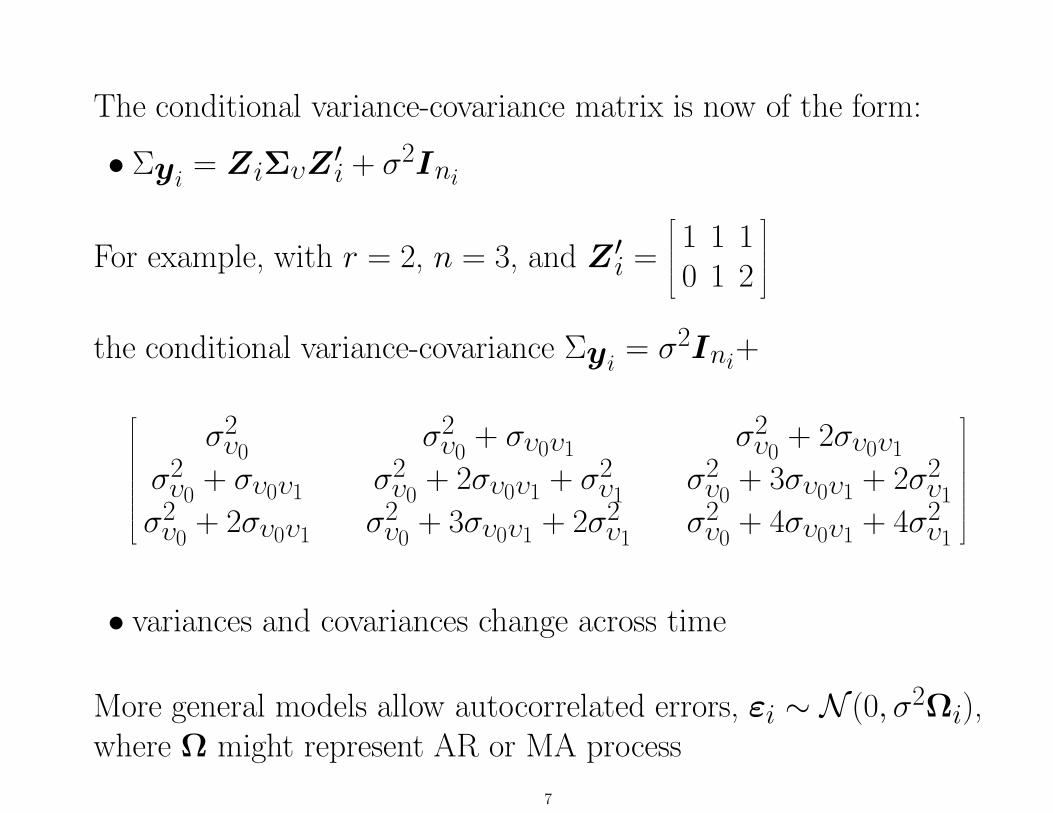
The conditional variance-covariance matrix is now of the form:
• Σyi= ZiΣυZ
′i + σ2Ini
For example, with r = 2, n = 3, and Z′i =
1 1 10 1 2
the conditional variance-covariance Σyi= σ2Ini+
σ2υ0
σ2υ0
+ συ0υ1 σ2υ0
+ 2συ0υ1
σ2υ0
+ συ0υ1 σ2υ0
+ 2συ0υ1 + σ2υ1
σ2υ0
+ 3συ0υ1 + 2σ2υ1
σ2υ0
+ 2συ0υ1 σ2υ0
+ 3συ0υ1 + 2σ2υ1
σ2υ0
+ 4συ0υ1 + 4σ2υ1
• variances and covariances change across time
More general models allow autocorrelated errors, εi ∼ N (0, σ2Ωi),where Ω might represent AR or MA process
7
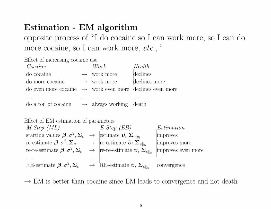
Estimation - EM algorithmopposite process of “I do cocaine so I can work more, so I can domore cocaine, so I can work more, etc., ”
Effect of increasing cocaine useCocaine Work Health
do cocaine → work more declines
do more cocaine → work more declines more
do even more cocaine → work even more declines even more
. . . . . . . . . . . .
do a ton of cocaine → always working death
Effect of EM estimation of parametersM-Step (ML) E-Step (EB) Estimation
starting values β, σ2,Συ → estimate υi Συ|yiimproves
re-estimate β, σ2,Συ → re-estimate υi Συ|yiimproves more
re-re-estimate β, σ2,Συ → re-re-estimate υi Συ|yiimproves even more
. . . . . . . . . . . .
RE-estimate β, σ2,Συ → RE-estimate υi Συ|yiconvergence
→ EM is better than cocaine since EM leads to convergence and not death
8
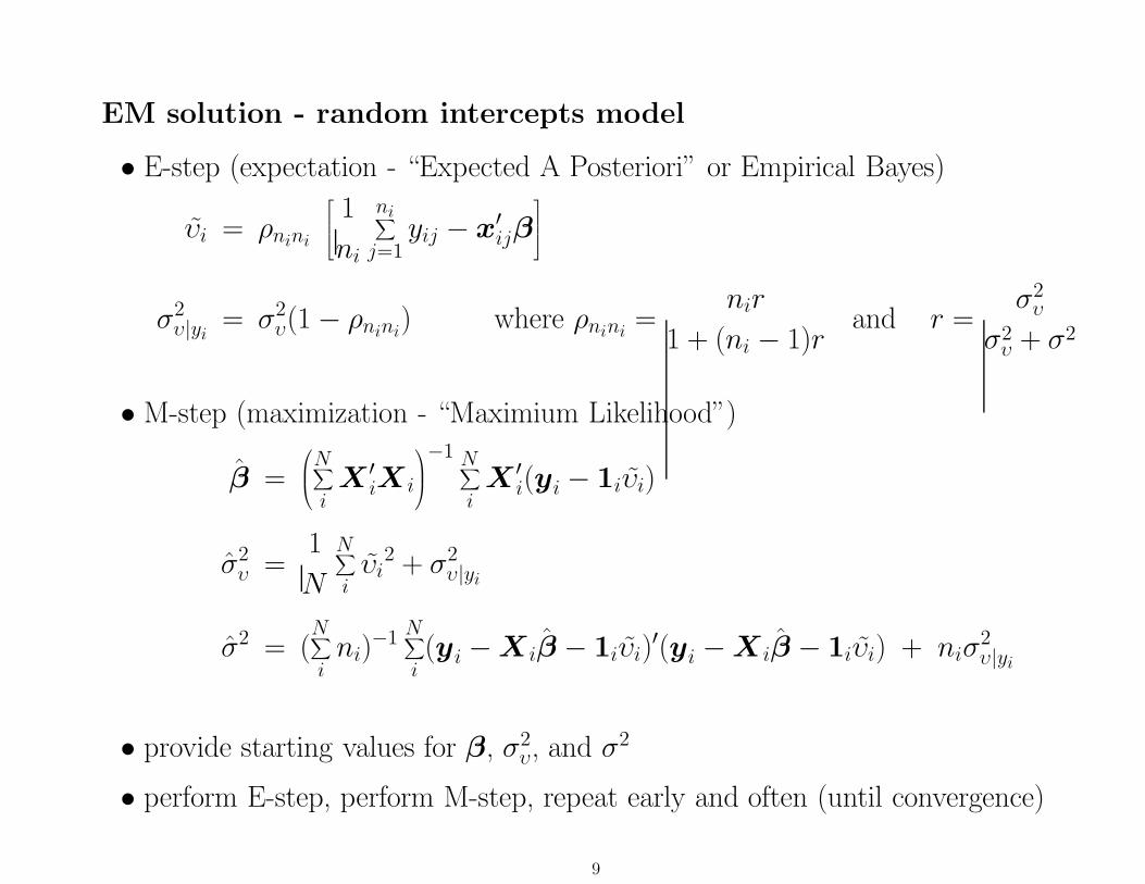
EM solution - random intercepts model
• E-step (expectation - “Expected A Posteriori” or Empirical Bayes)
υi = ρnini
1
ni
ni∑
j=1yij − x′
ijβ
σ2υ|yi
= σ2υ(1 − ρnini
) where ρnini=
nir
1 + (ni − 1)rand r =
σ2υ
σ2υ + σ2
• M-step (maximization - “Maximium Likelihood”)
β =
N∑
iX ′
iX i
−1 N∑
iX ′
i(yi − 1iυi)
σ2υ =
1
N
N∑
iυi
2 + σ2υ|yi
σ2 = (N∑
ini)
−1 N∑
i(yi − X iβ − 1iυi)
′(yi − X iβ − 1iυi) + niσ2υ|yi
• provide starting values for β, σ2υ, and σ2
• perform E-step, perform M-step, repeat early and often (until convergence)
9
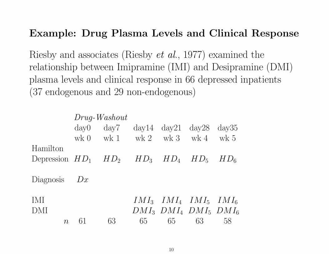
Example: Drug Plasma Levels and Clinical Response
Riesby and associates (Riesby et al., 1977) examined therelationship between Imipramine (IMI) and Desipramine (DMI)plasma levels and clinical response in 66 depressed inpatients(37 endogenous and 29 non-endogenous)
Drug-Washoutday0 day7 day14 day21 day28 day35wk 0 wk 1 wk 2 wk 3 wk 4 wk 5
HamiltonDepression HD1 HD2 HD3 HD4 HD5 HD6
Diagnosis Dx
IMI IMI3 IMI4 IMI5 IMI6
DMI DMI3 DMI4 DMI5 DMI6
n 61 63 65 65 63 58
10
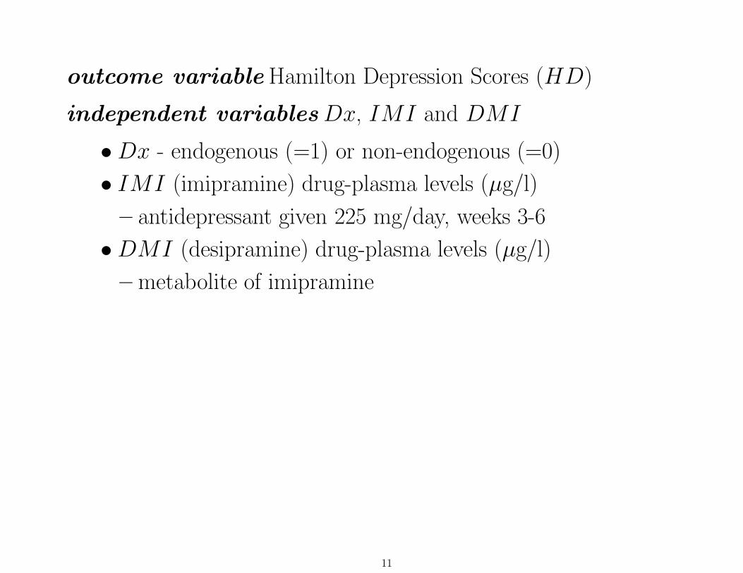
outcome variable Hamilton Depression Scores (HD)
independent variables Dx, IMI and DMI
• Dx - endogenous (=1) or non-endogenous (=0)
• IMI (imipramine) drug-plasma levels (µg/l)
– antidepressant given 225 mg/day, weeks 3-6
• DMI (desipramine) drug-plasma levels (µg/l)
– metabolite of imipramine
11
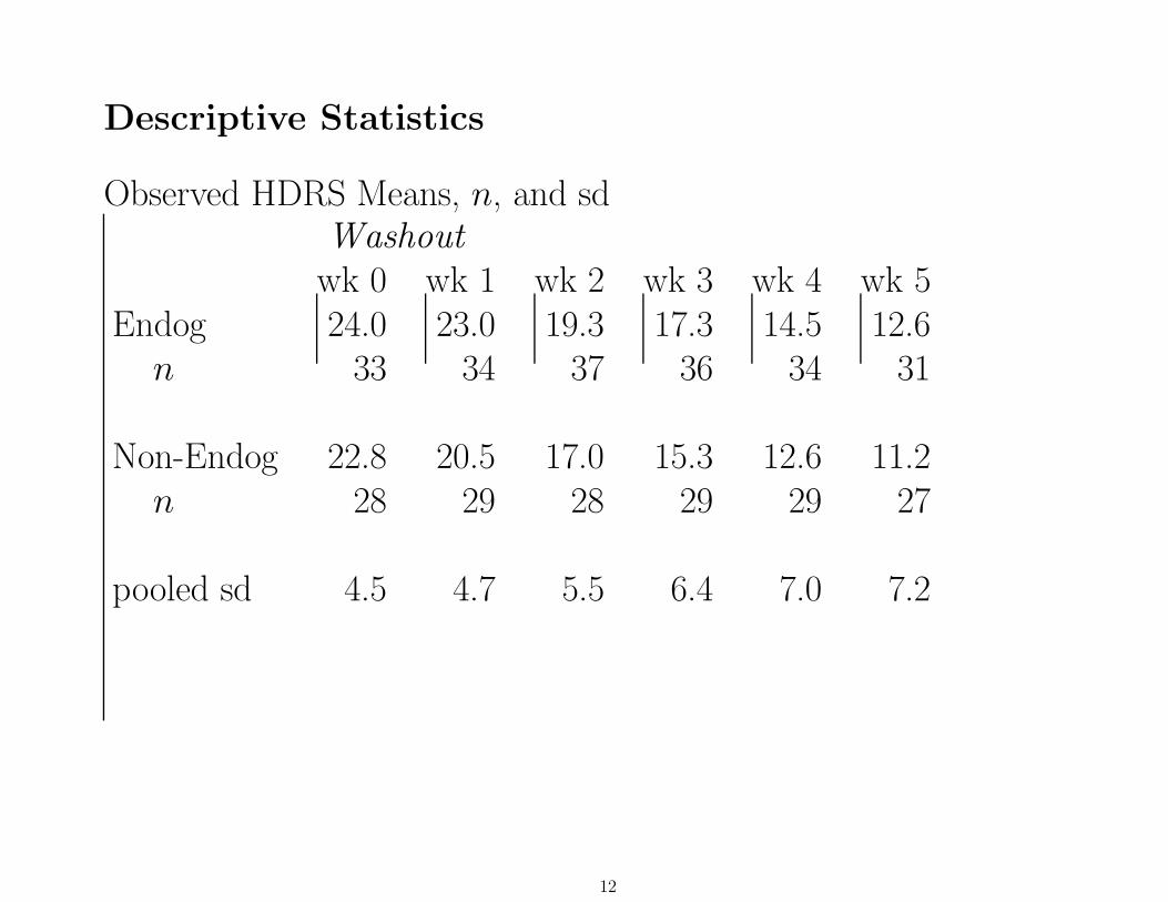
Descriptive Statistics
Observed HDRS Means, n, and sdWashoutwk 0 wk 1 wk 2 wk 3 wk 4 wk 5
Endog 24.0 23.0 19.3 17.3 14.5 12.6n 33 34 37 36 34 31
Non-Endog 22.8 20.5 17.0 15.3 12.6 11.2n 28 29 28 29 29 27
pooled sd 4.5 4.7 5.5 6.4 7.0 7.2
12
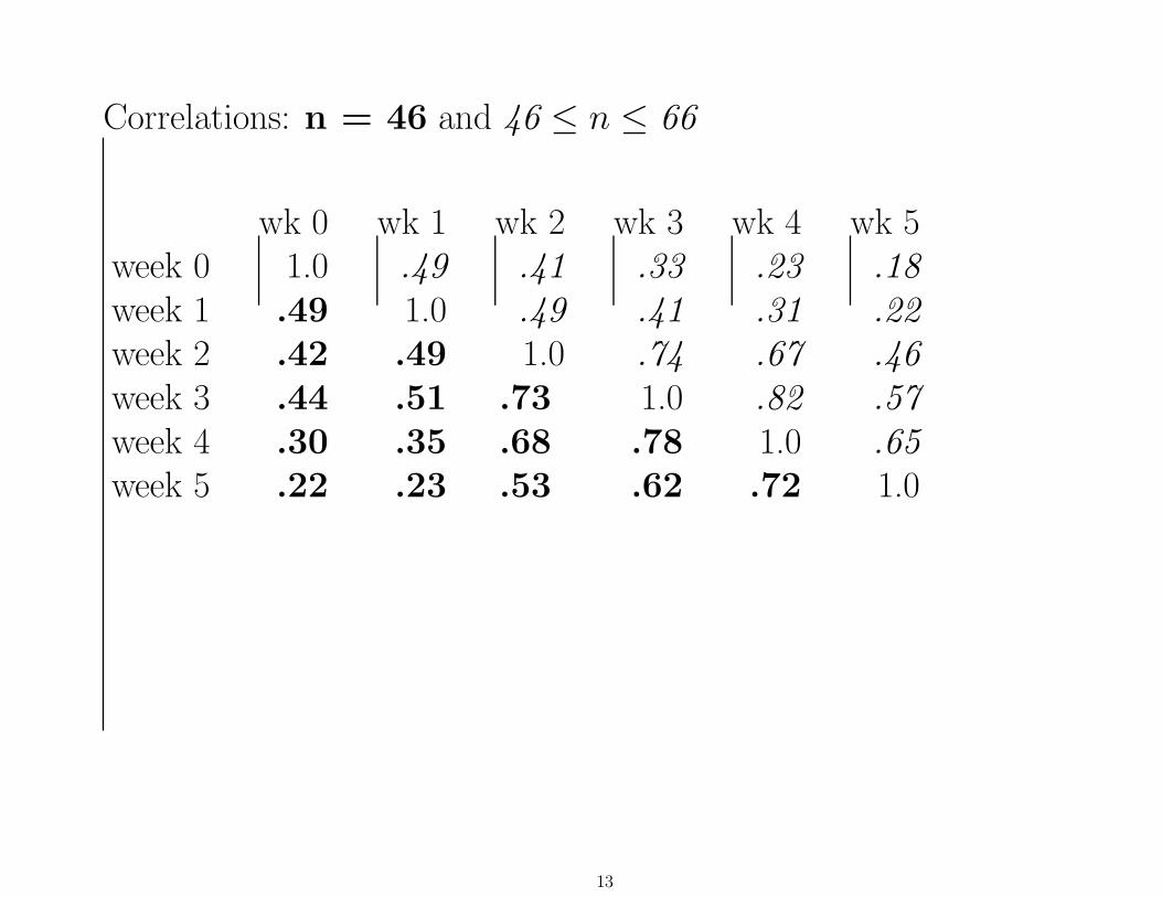
Correlations: n = 46 and 46 ≤ n ≤ 66
wk 0 wk 1 wk 2 wk 3 wk 4 wk 5week 0 1.0 .49 .41 .33 .23 .18week 1 .49 1.0 .49 .41 .31 .22week 2 .42 .49 1.0 .74 .67 .46week 3 .44 .51 .73 1.0 .82 .57week 4 .30 .35 .68 .78 1.0 .65week 5 .22 .23 .53 .62 .72 1.0
13
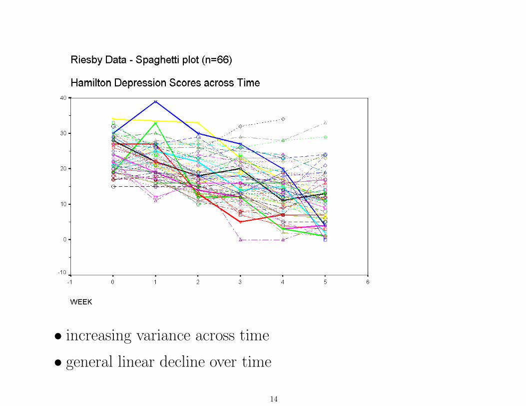
• increasing variance across time
• general linear decline over time
14
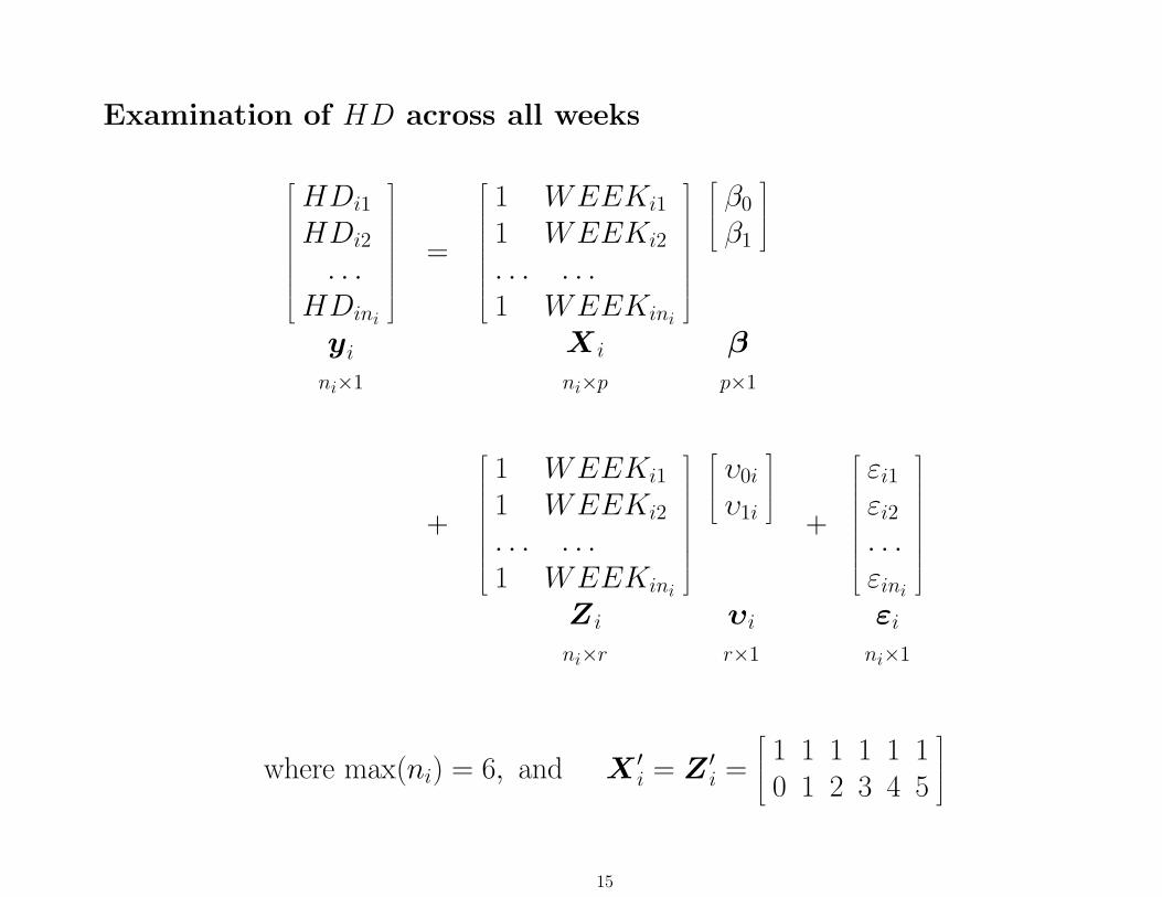
Examination of HD across all weeks
HDi1
HDi2
. . .HDini
yi
ni×1
=
1 WEEKi1
1 WEEKi2
. . . . . .1 WEEKini
X i
ni×p
β0
β1
βp×1
+
1 WEEKi1
1 WEEKi2
. . . . . .1 WEEKini
Z i
ni×r
υ0i
υ1i
υi
r×1
+
εi1
εi2
. . .εini
εi
ni×1
where max(ni) = 6, and X ′i = Z ′
i =
1 1 1 1 1 10 1 2 3 4 5
15
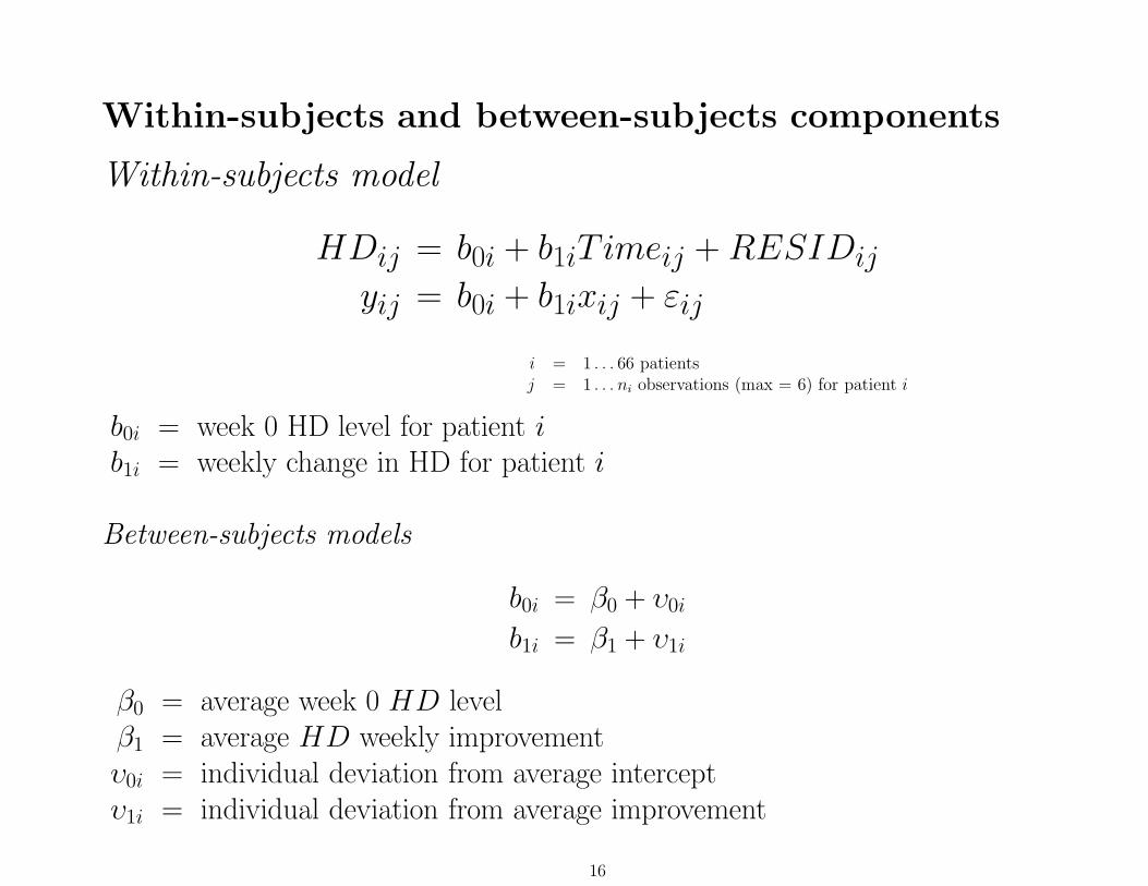
Within-subjects and between-subjects components
Within-subjects model
HDij = b0i + b1iT imeij + RESIDij
yij = b0i + b1ixij + εij
i = 1 . . . 66 patientsj = 1 . . . ni observations (max = 6) for patient i
b0i = week 0 HD level for patient ib1i = weekly change in HD for patient i
Between-subjects models
b0i = β0 + υ0i
b1i = β1 + υ1i
β0 = average week 0 HD levelβ1 = average HD weekly improvementυ0i = individual deviation from average interceptυ1i = individual deviation from average improvement
16
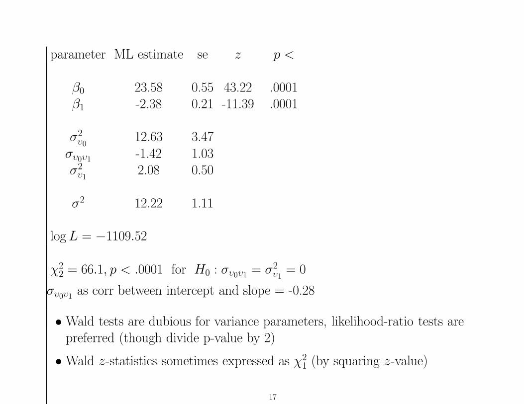
parameter ML estimate se z p <
β0 23.58 0.55 43.22 .0001β1 -2.38 0.21 -11.39 .0001
σ2υ0
12.63 3.47συ0υ1 -1.42 1.03σ2
υ12.08 0.50
σ2 12.22 1.11
log L = −1109.52
χ22 = 66.1, p < .0001 for H0 : συ0υ1 = σ2
υ1= 0
συ0υ1as corr between intercept and slope = -0.28
• Wald tests are dubious for variance parameters, likelihood-ratio tests arepreferred (though divide p-value by 2)
• Wald z-statistics sometimes expressed as χ21 (by squaring z-value)
17
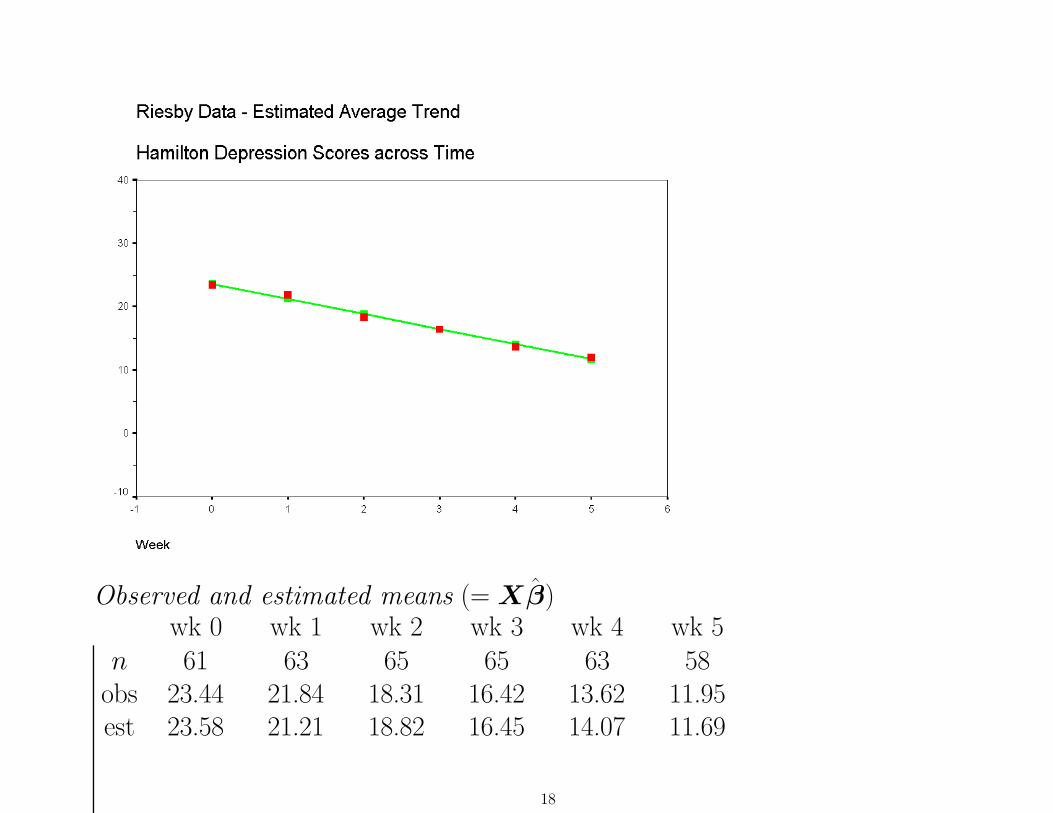
Observed and estimated means (= Xβ)wk 0 wk 1 wk 2 wk 3 wk 4 wk 5
n 61 63 65 65 63 58obs 23.44 21.84 18.31 16.42 13.62 11.95est 23.58 21.21 18.82 16.45 14.07 11.69
18
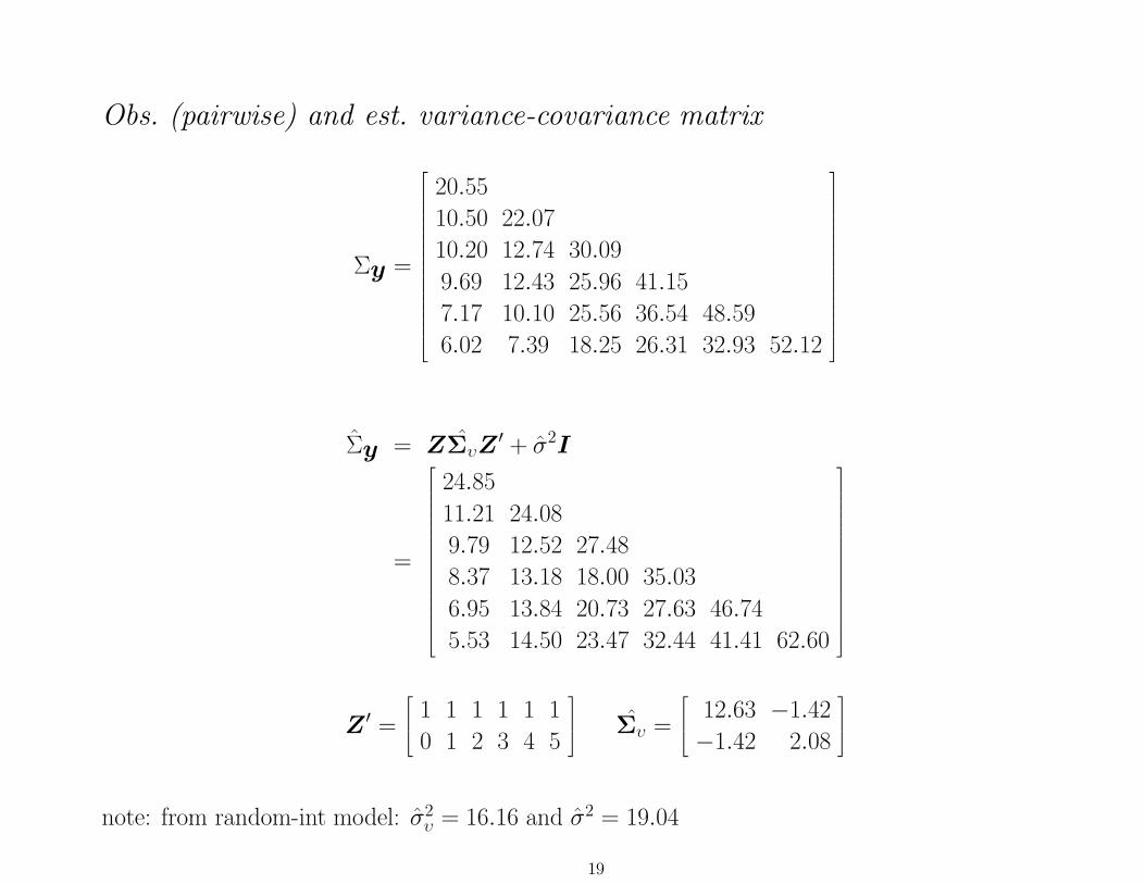
Obs. (pairwise) and est. variance-covariance matrix
Σy =
20.55
10.50 22.07
10.20 12.74 30.09
9.69 12.43 25.96 41.15
7.17 10.10 25.56 36.54 48.59
6.02 7.39 18.25 26.31 32.93 52.12
Σy = ZΣυZ′ + σ2I
=
24.85
11.21 24.08
9.79 12.52 27.48
8.37 13.18 18.00 35.03
6.95 13.84 20.73 27.63 46.74
5.53 14.50 23.47 32.44 41.41 62.60
Z ′ =
1 1 1 1 1 1
0 1 2 3 4 5
Συ =
12.63 −1.42
−1.42 2.08
note: from random-int model: σ2υ = 16.16 and σ2 = 19.04
19
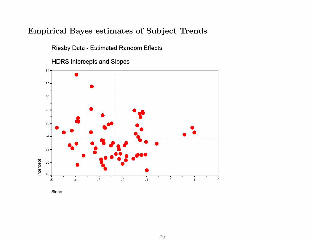
Empirical Bayes estimates of Subject Trends
20
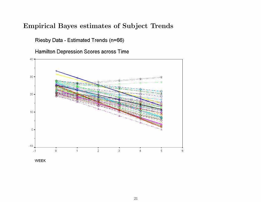
Empirical Bayes estimates of Subject Trends
21
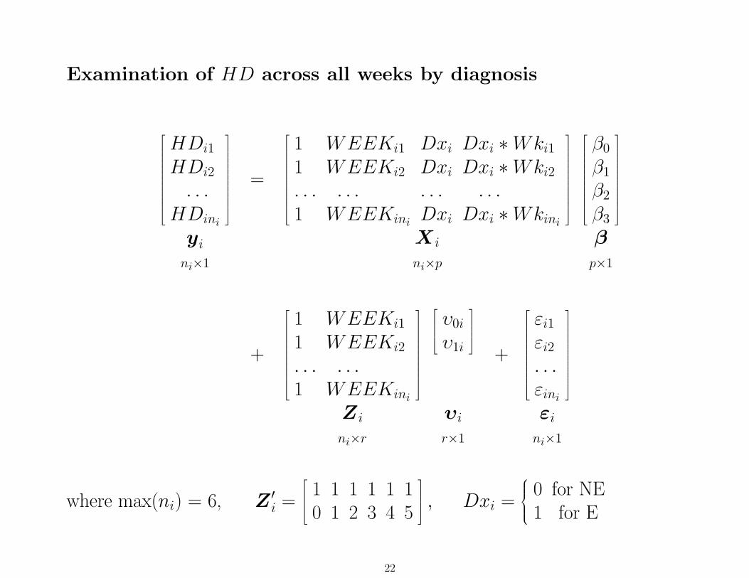
Examination of HD across all weeks by diagnosis
HDi1
HDi2
. . .HDini
yi
ni×1
=
1 WEEKi1 Dxi Dxi ∗ Wki1
1 WEEKi2 Dxi Dxi ∗ Wki2
. . . . . . . . . . . .1 WEEKini
Dxi Dxi ∗ Wkini
X i
ni×p
β0
β1
β2
β3
βp×1
+
1 WEEKi1
1 WEEKi2
. . . . . .1 WEEKini
Z i
ni×r
υ0i
υ1i
υi
r×1
+
εi1
εi2
. . .εini
εi
ni×1
where max(ni) = 6, Z ′i =
1 1 1 1 1 10 1 2 3 4 5
, Dxi =
0 for NE1 for E
22
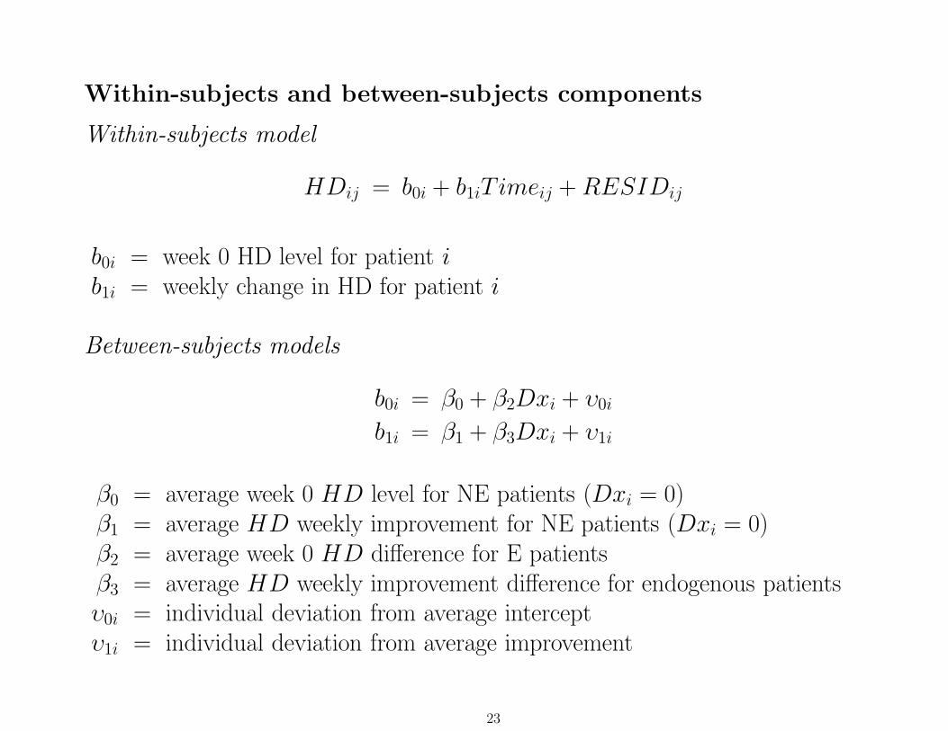
Within-subjects and between-subjects components
Within-subjects model
HDij = b0i + b1iT imeij + RESIDij
b0i = week 0 HD level for patient ib1i = weekly change in HD for patient i
Between-subjects models
b0i = β0 + β2Dxi + υ0i
b1i = β1 + β3Dxi + υ1i
β0 = average week 0 HD level for NE patients (Dxi = 0)β1 = average HD weekly improvement for NE patients (Dxi = 0)β2 = average week 0 HD difference for E patientsβ3 = average HD weekly improvement difference for endogenous patientsυ0i = individual deviation from average interceptυ1i = individual deviation from average improvement
23
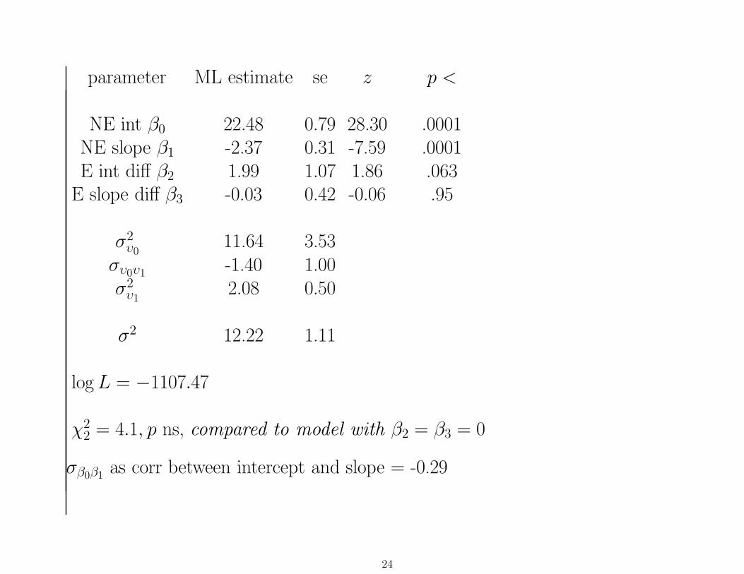
parameter ML estimate se z p <
NE int β0 22.48 0.79 28.30 .0001NE slope β1 -2.37 0.31 -7.59 .0001E int diff β2 1.99 1.07 1.86 .063
E slope diff β3 -0.03 0.42 -0.06 .95
σ2υ0
11.64 3.53συ0υ1
-1.40 1.00σ2
υ12.08 0.50
σ2 12.22 1.11
log L = −1107.47
χ22 = 4.1, p ns, compared to model with β2 = β3 = 0
σβ0β1 as corr between intercept and slope = -0.29
24
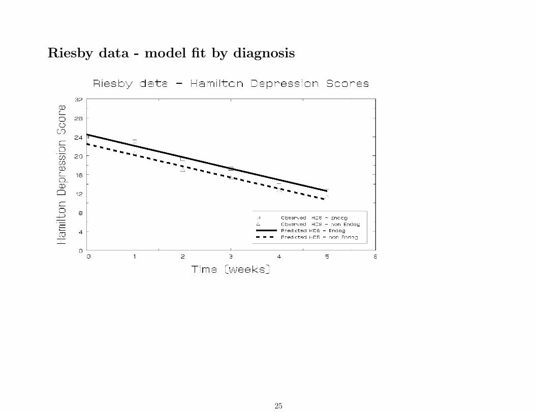
Riesby data - model fit by diagnosis
25
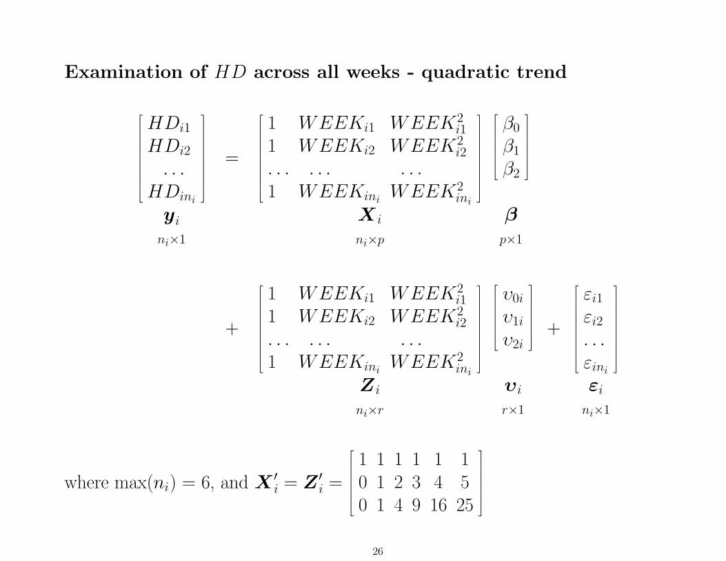
Examination of HD across all weeks - quadratic trend
HDi1
HDi2
. . .HDini
yi
ni×1
=
1 WEEKi1 WEEK2i1
1 WEEKi2 WEEK2i2
. . . . . . . . .1 WEEKini
WEEK2ini
X i
ni×p
β0
β1
β2
βp×1
+
1 WEEKi1 WEEK2i1
1 WEEKi2 WEEK2i2
. . . . . . . . .1 WEEKini
WEEK2ini
Z i
ni×r
υ0i
υ1i
υ2i
υi
r×1
+
εi1
εi2
. . .εini
εi
ni×1
where max(ni) = 6, and X ′i = Z ′
i =
1 1 1 1 1 10 1 2 3 4 50 1 4 9 16 25
26
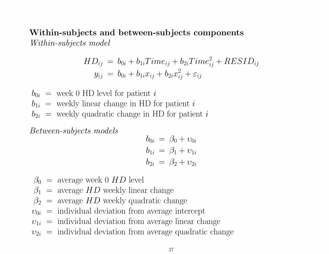
Within-subjects and between-subjects componentsWithin-subjects model
HDij = b0i + b1iT imeij + b2iT ime2ij + RESIDij
yij = b0i + b1ixij + b2ix2ij + εij
b0i = week 0 HD level for patient ib1i = weekly linear change in HD for patient ib2i = weekly quadratic change in HD for patient i
Between-subjects modelsb0i = β0 + υ0i
b1i = β1 + υ1i
b2i = β2 + υ2i
β0 = average week 0 HD levelβ1 = average HD weekly linear changeβ2 = average HD weekly quadratic changeυ0i = individual deviation from average interceptυ1i = individual deviation from average linear changeυ2i = individual deviation from average quadratic change
27
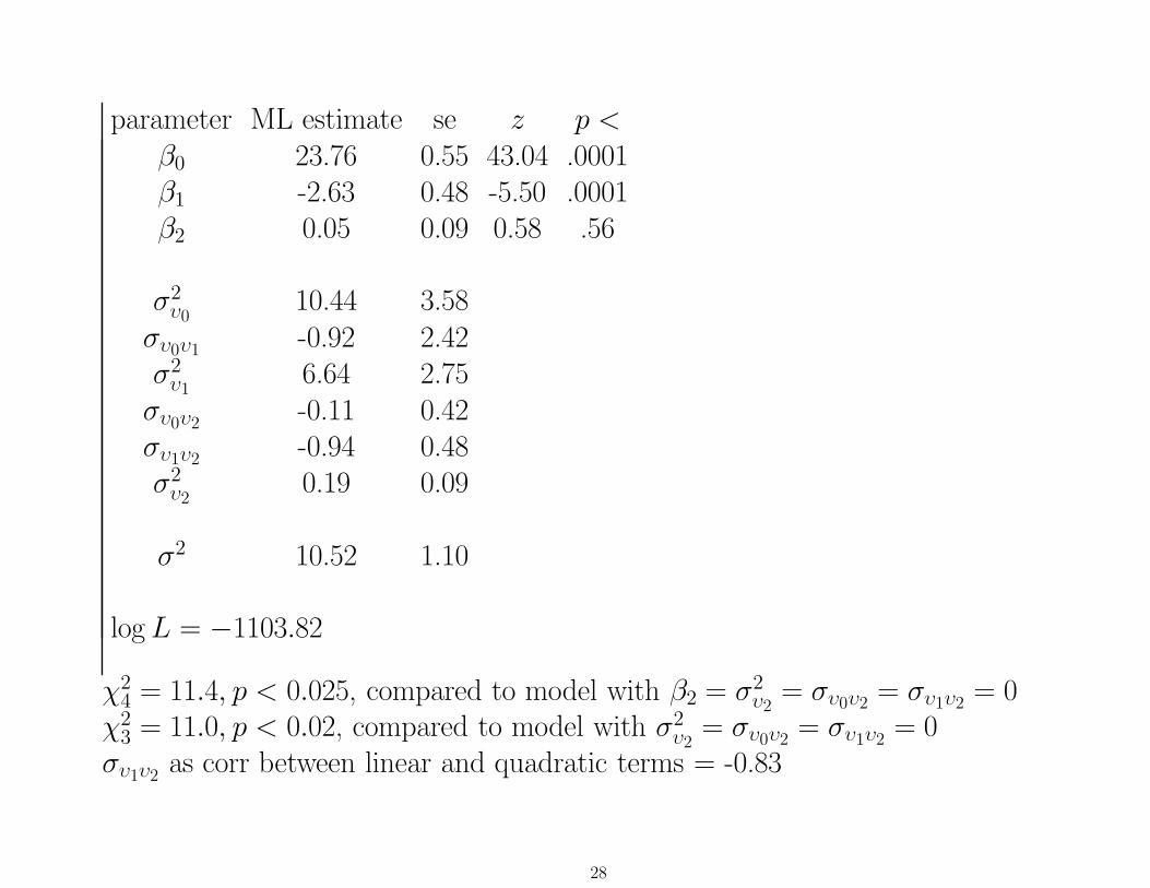
parameter ML estimate se z p <β0 23.76 0.55 43.04 .0001β1 -2.63 0.48 -5.50 .0001β2 0.05 0.09 0.58 .56
σ2υ0
10.44 3.58συ0υ1 -0.92 2.42σ2
υ16.64 2.75
συ0υ2-0.11 0.42
συ1υ2 -0.94 0.48σ2
υ20.19 0.09
σ2 10.52 1.10
log L = −1103.82
χ24 = 11.4, p < 0.025, compared to model with β2 = σ2
υ2= συ0υ2 = συ1υ2 = 0
χ23 = 11.0, p < 0.02, compared to model with σ2
υ2= συ0υ2
= συ1υ2= 0
συ1υ2as corr between linear and quadratic terms = -0.83
28
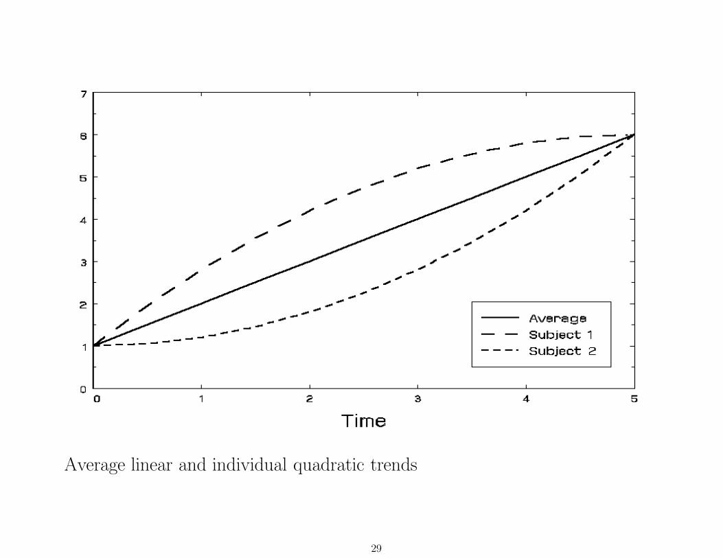
Average linear and individual quadratic trends
29
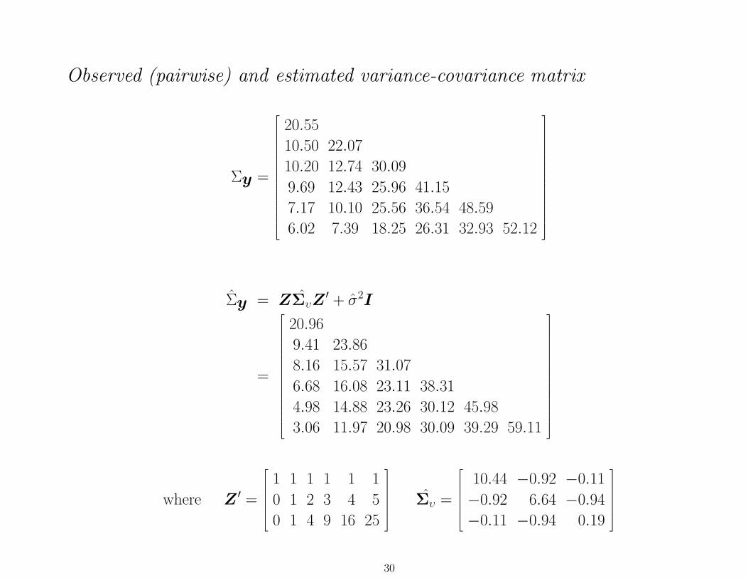
Observed (pairwise) and estimated variance-covariance matrix
Σy =
20.55
10.50 22.07
10.20 12.74 30.09
9.69 12.43 25.96 41.15
7.17 10.10 25.56 36.54 48.59
6.02 7.39 18.25 26.31 32.93 52.12
Σy = ZΣυZ′ + σ2I
=
20.96
9.41 23.86
8.16 15.57 31.07
6.68 16.08 23.11 38.31
4.98 14.88 23.26 30.12 45.98
3.06 11.97 20.98 30.09 39.29 59.11
where Z ′ =
1 1 1 1 1 1
0 1 2 3 4 5
0 1 4 9 16 25
Συ =
10.44 −0.92 −0.11
−0.92 6.64 −0.94
−0.11 −0.94 0.19
30
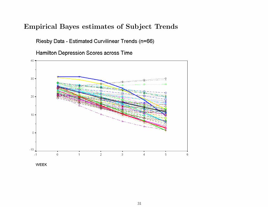
Empirical Bayes estimates of Subject Trends
31
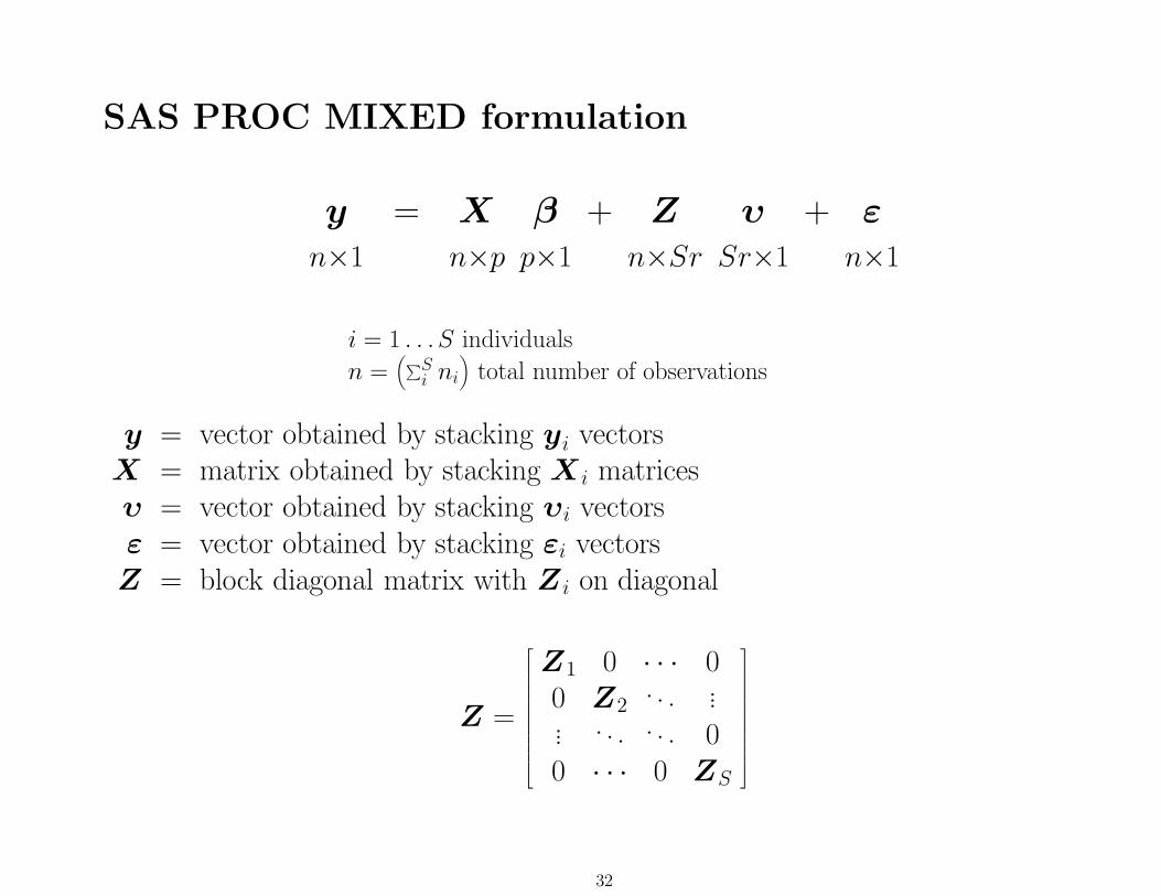
SAS PROC MIXED formulation
yn×1
= Xn×p
βp×1
+ Zn×Sr
υSr×1
+ εn×1
i = 1 . . . S individuals
n =(∑S
i ni
)total number of observations
y = vector obtained by stacking yi vectorsX = matrix obtained by stacking X i matricesυ = vector obtained by stacking υi vectorsε = vector obtained by stacking εi vectorsZ = block diagonal matrix with Z i on diagonal
Z =
Z1 0 · · · 00 Z2
. . . ...... . . . . . . 00 · · · 0 ZS
32
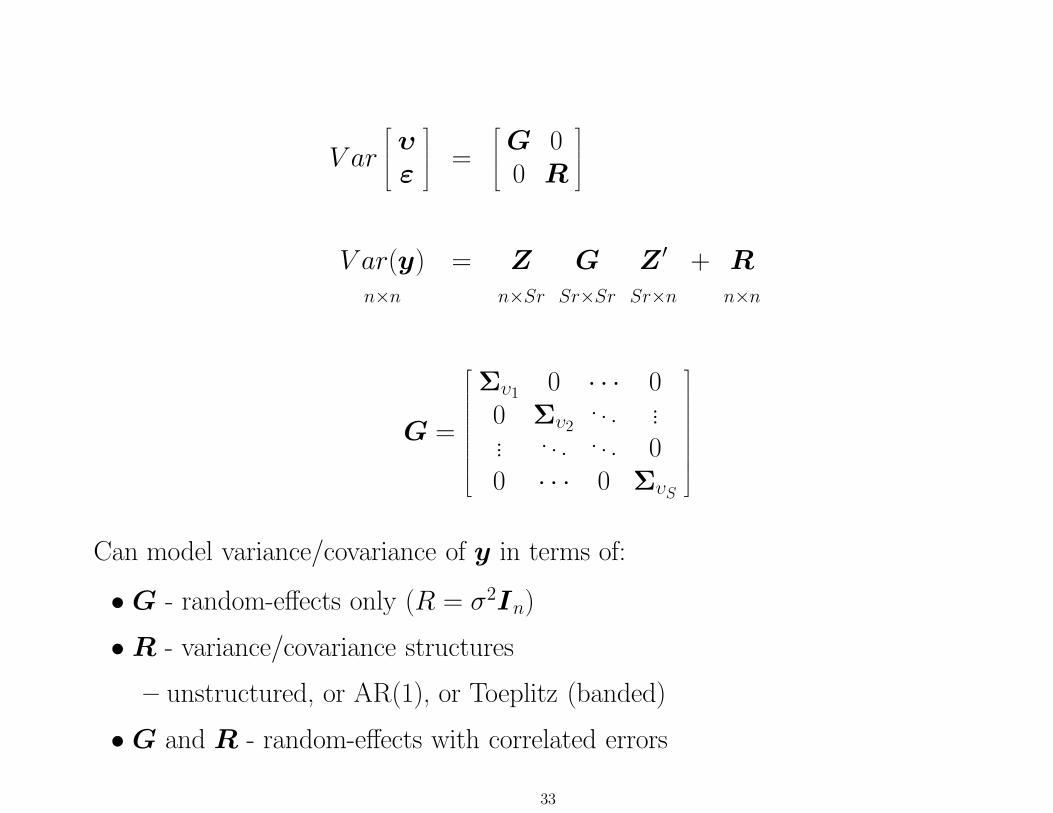
V ar
υε
=
G 00 R
V ar(y)n×n
= Zn×Sr
GSr×Sr
Z ′
Sr×n
+ Rn×n
G =
Συ1 0 · · · 00 Συ2
. . . ...... . . . . . . 00 · · · 0 ΣυS
Can model variance/covariance of y in terms of:
• G - random-effects only (R = σ2In)
• R - variance/covariance structures
– unstructured, or AR(1), or Toeplitz (banded)
• G and R - random-effects with correlated errors
33
Example 4a: Analysis of Riesby dataset using MRM. Thisexample has a few different PROC MIXED specifications, andincludes a grouping variable and curvilinear effect of time.(SAS code and output)http://tigger.uic.edu/∼hedeker/RIESBYM.txt
34
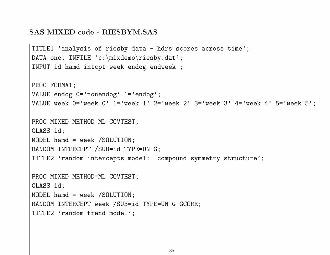
SAS MIXED code - RIESBYM.SAS
TITLE1 ’analysis of riesby data - hdrs scores across time’;
DATA one; INFILE ’c:\mixdemo\riesby.dat’;INPUT id hamd intcpt week endog endweek ;
PROC FORMAT;
VALUE endog 0=’nonendog’ 1=’endog’;
VALUE week 0=’week 0’ 1=’week 1’ 2=’week 2’ 3=’week 3’ 4=’week 4’ 5=’week 5’;
PROC MIXED METHOD=ML COVTEST;
CLASS id;
MODEL hamd = week /SOLUTION;
RANDOM INTERCEPT /SUB=id TYPE=UN G;
TITLE2 ’random intercepts model: compound symmetry structure’;
PROC MIXED METHOD=ML COVTEST;
CLASS id;
MODEL hamd = week /SOLUTION;
RANDOM INTERCEPT week /SUB=id TYPE=UN G GCORR;
TITLE2 ’random trend model’;
35
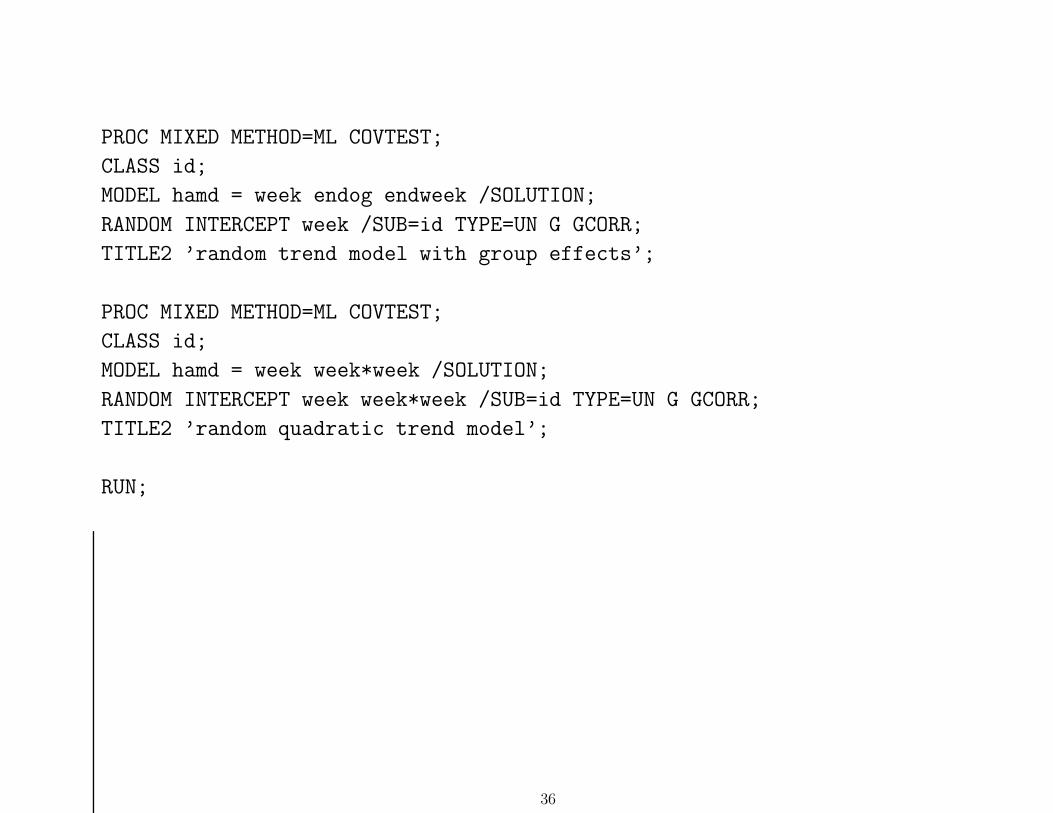
PROC MIXED METHOD=ML COVTEST;
CLASS id;
MODEL hamd = week endog endweek /SOLUTION;
RANDOM INTERCEPT week /SUB=id TYPE=UN G GCORR;
TITLE2 ’random trend model with group effects’;
PROC MIXED METHOD=ML COVTEST;
CLASS id;
MODEL hamd = week week*week /SOLUTION;
RANDOM INTERCEPT week week*week /SUB=id TYPE=UN G GCORR;
TITLE2 ’random quadratic trend model’;
RUN;
36
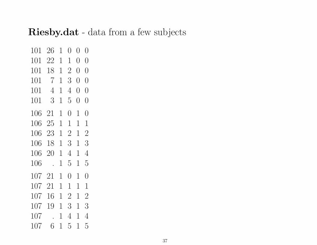
Riesby.dat - data from a few subjects
101 26 1 0 0 0101 22 1 1 0 0101 18 1 2 0 0101 7 1 3 0 0101 4 1 4 0 0101 3 1 5 0 0
106 21 1 0 1 0106 25 1 1 1 1106 23 1 2 1 2106 18 1 3 1 3106 20 1 4 1 4106 . 1 5 1 5
107 21 1 0 1 0107 21 1 1 1 1107 16 1 2 1 2107 19 1 3 1 3107 . 1 4 1 4107 6 1 5 1 5
37
Example 4b: Analysis of Riesby dataset. This handout showshow empirical Bayes estimates can be output to a dataset inorder to calculate estimated individual scores at all timepoints.(SAS code and output)http://tigger.uic.edu/∼hedeker/RIESBYM2.txt
38
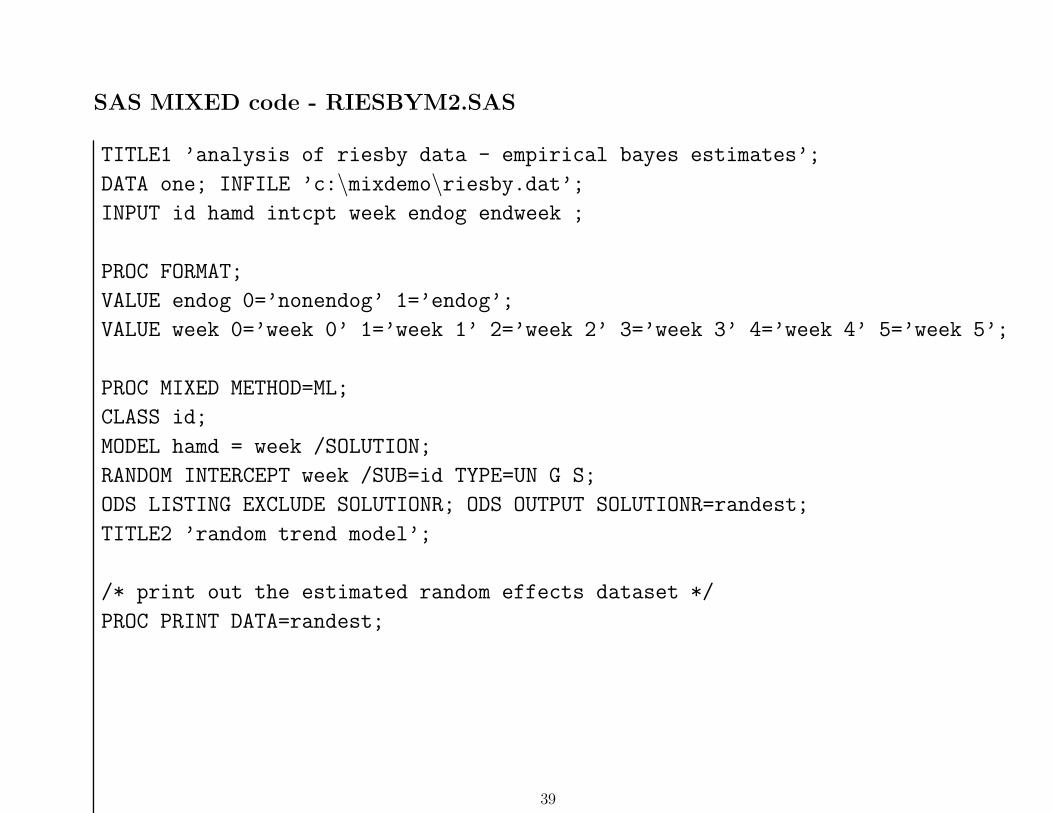
SAS MIXED code - RIESBYM2.SAS
TITLE1 ’analysis of riesby data - empirical bayes estimates’;
DATA one; INFILE ’c:\mixdemo\riesby.dat’;INPUT id hamd intcpt week endog endweek ;
PROC FORMAT;
VALUE endog 0=’nonendog’ 1=’endog’;
VALUE week 0=’week 0’ 1=’week 1’ 2=’week 2’ 3=’week 3’ 4=’week 4’ 5=’week 5’;
PROC MIXED METHOD=ML;
CLASS id;
MODEL hamd = week /SOLUTION;
RANDOM INTERCEPT week /SUB=id TYPE=UN G S;
ODS LISTING EXCLUDE SOLUTIONR; ODS OUTPUT SOLUTIONR=randest;
TITLE2 ’random trend model’;
/* print out the estimated random effects dataset */
PROC PRINT DATA=randest;
39
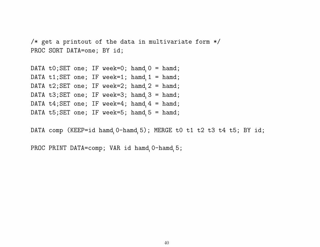
/* get a printout of the data in multivariate form */
PROC SORT DATA=one; BY id;
DATA t0;SET one; IF week=0; hamd 0 = hamd;
DATA t1;SET one; IF week=1; hamd 1 = hamd;
DATA t2;SET one; IF week=2; hamd 2 = hamd;
DATA t3;SET one; IF week=3; hamd 3 = hamd;
DATA t4;SET one; IF week=4; hamd 4 = hamd;
DATA t5;SET one; IF week=5; hamd 5 = hamd;
DATA comp (KEEP=id hamd 0-hamd 5); MERGE t0 t1 t2 t3 t4 t5; BY id;
PROC PRINT DATA=comp; VAR id hamd 0-hamd 5;
40
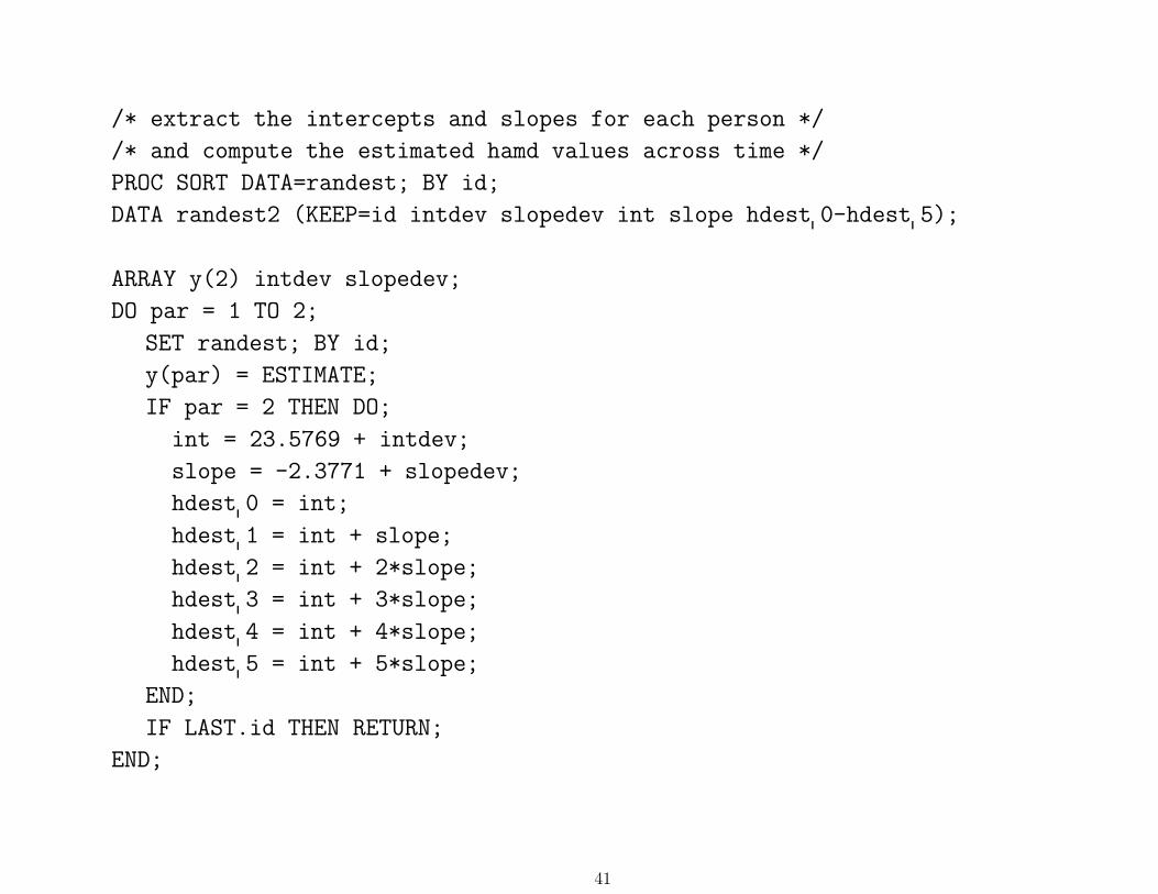
/* extract the intercepts and slopes for each person */
/* and compute the estimated hamd values across time */
PROC SORT DATA=randest; BY id;
DATA randest2 (KEEP=id intdev slopedev int slope hdest 0-hdest 5);
ARRAY y(2) intdev slopedev;
DO par = 1 TO 2;
SET randest; BY id;
y(par) = ESTIMATE;
IF par = 2 THEN DO;
int = 23.5769 + intdev;
slope = -2.3771 + slopedev;
hdest 0 = int;
hdest 1 = int + slope;
hdest 2 = int + 2*slope;
hdest 3 = int + 3*slope;
hdest 4 = int + 4*slope;
hdest 5 = int + 5*slope;
END;
IF LAST.id THEN RETURN;
END;
41
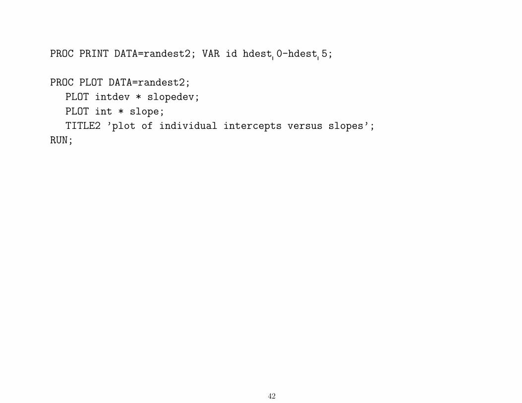
PROC PRINT DATA=randest2; VAR id hdest 0-hdest 5;
PROC PLOT DATA=randest2;
PLOT intdev * slopedev;
PLOT int * slope;
TITLE2 ’plot of individual intercepts versus slopes’;
RUN;
42
Time-varying Covariates - WS and BS effects
Section 4.5.2 in Hedeker & Gibbons (2006), Longitudinal DataAnalysis, Wiley.
43
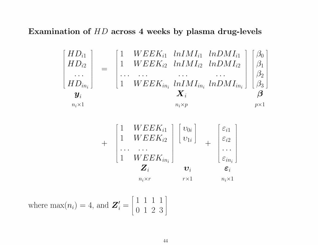
Examination of HD across 4 weeks by plasma drug-levels
HDi1
HDi2
. . .HDini
yi
ni×1
=
1 WEEKi1 lnIMIi1 lnDMIi1
1 WEEKi2 lnIMIi2 lnDMIi2
. . . . . . . . . . . .1 WEEKini
lnIMIinilnDMIini
X i
ni×p
β0
β1
β2
β3
βp×1
+
1 WEEKi1
1 WEEKi2
. . . . . .1 WEEKini
Zi
ni×r
υ0i
υ1i
υi
r×1
+
εi1
εi2
. . .εini
εi
ni×1
where max(ni) = 4, and Z ′i =
1 1 1 10 1 2 3
44
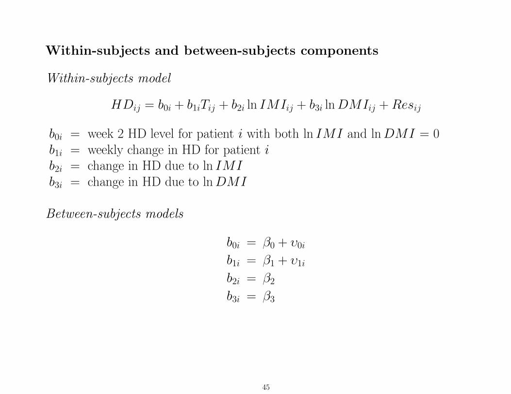
Within-subjects and between-subjects components
Within-subjects model
HDij = b0i + b1iTij + b2i ln IMIij + b3i ln DMIij + Resij
b0i = week 2 HD level for patient i with both ln IMI and ln DMI = 0b1i = weekly change in HD for patient ib2i = change in HD due to ln IMIb3i = change in HD due to ln DMI
Between-subjects models
b0i = β0 + υ0i
b1i = β1 + υ1i
b2i = β2
b3i = β3
45
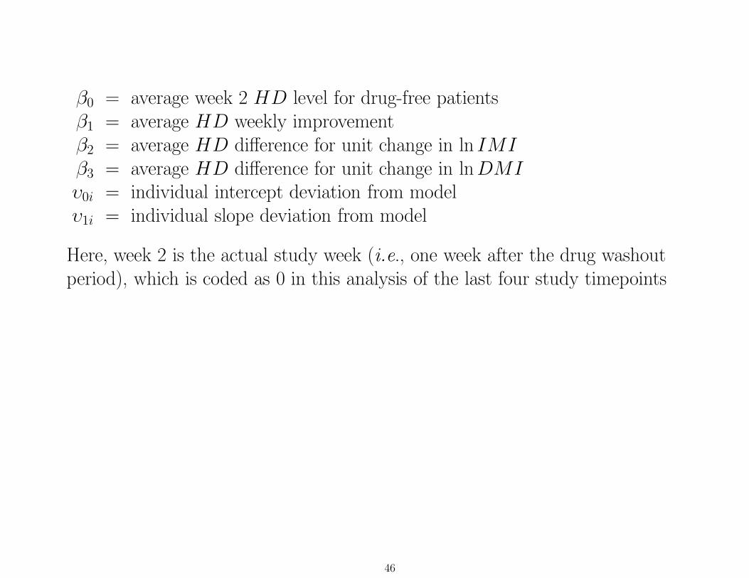
β0 = average week 2 HD level for drug-free patientsβ1 = average HD weekly improvementβ2 = average HD difference for unit change in ln IMIβ3 = average HD difference for unit change in ln DMIυ0i = individual intercept deviation from modelυ1i = individual slope deviation from model
Here, week 2 is the actual study week (i.e., one week after the drug washoutperiod), which is coded as 0 in this analysis of the last four study timepoints
46
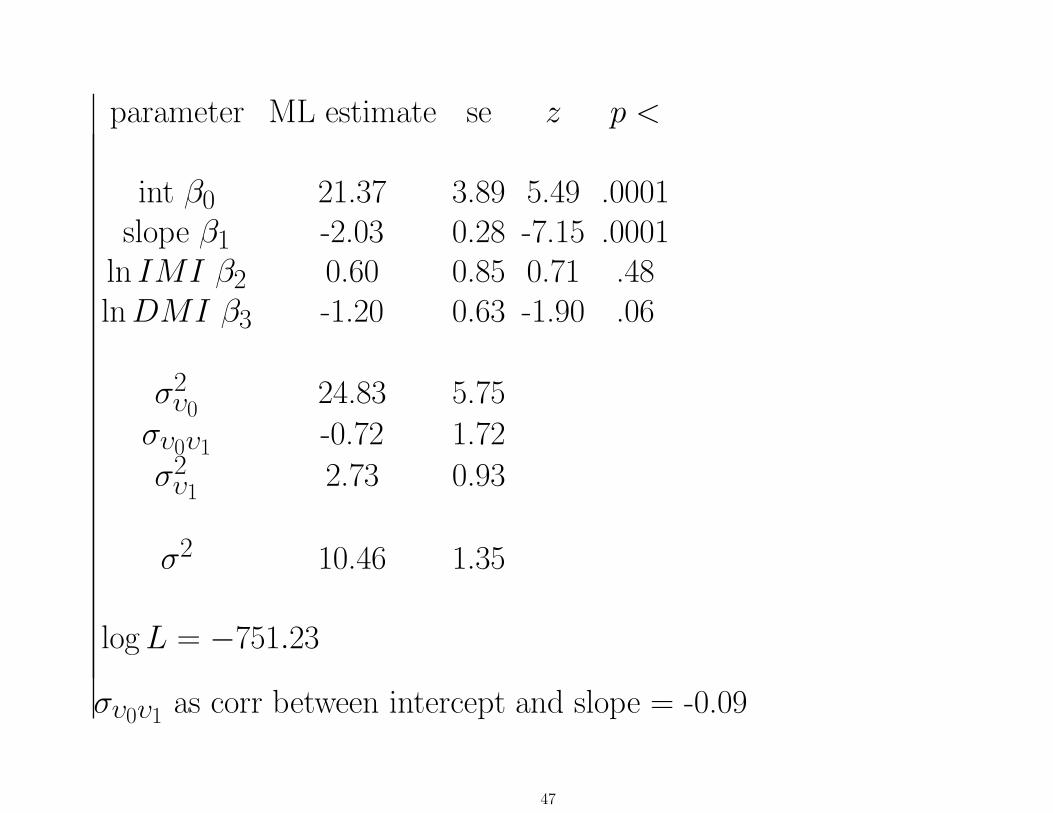
parameter ML estimate se z p <
int β0 21.37 3.89 5.49 .0001slope β1 -2.03 0.28 -7.15 .0001
ln IMI β2 0.60 0.85 0.71 .48ln DMI β3 -1.20 0.63 -1.90 .06
σ2υ0
24.83 5.75
συ0υ1 -0.72 1.72
σ2υ1
2.73 0.93
σ2 10.46 1.35
log L = −751.23
συ0υ1 as corr between intercept and slope = -0.09
47
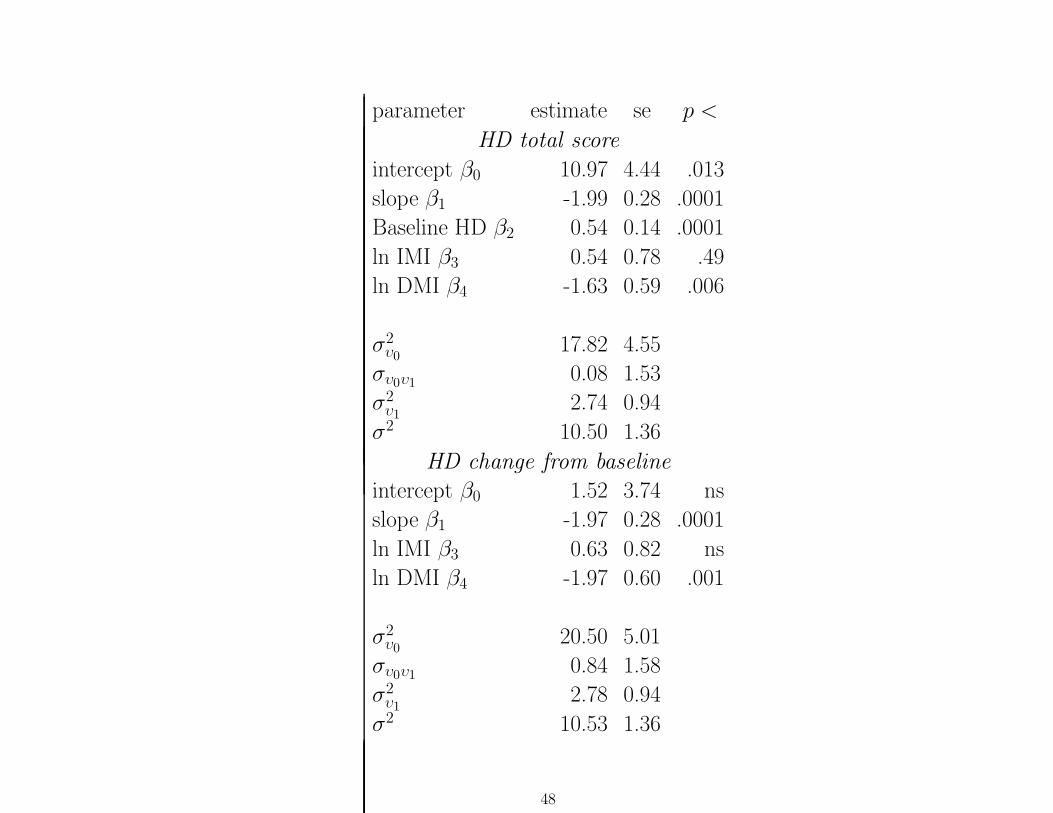
parameter estimate se p <
HD total score
intercept β0 10.97 4.44 .013
slope β1 -1.99 0.28 .0001
Baseline HD β2 0.54 0.14 .0001
ln IMI β3 0.54 0.78 .49
ln DMI β4 -1.63 0.59 .006
σ2υ0
17.82 4.55
συ0υ1 0.08 1.53
σ2υ1
2.74 0.94
σ2 10.50 1.36
HD change from baseline
intercept β0 1.52 3.74 ns
slope β1 -1.97 0.28 .0001
ln IMI β3 0.63 0.82 ns
ln DMI β4 -1.97 0.60 .001
σ2υ0
20.50 5.01
συ0υ1 0.84 1.58
σ2υ1
2.78 0.94
σ2 10.53 1.36
48
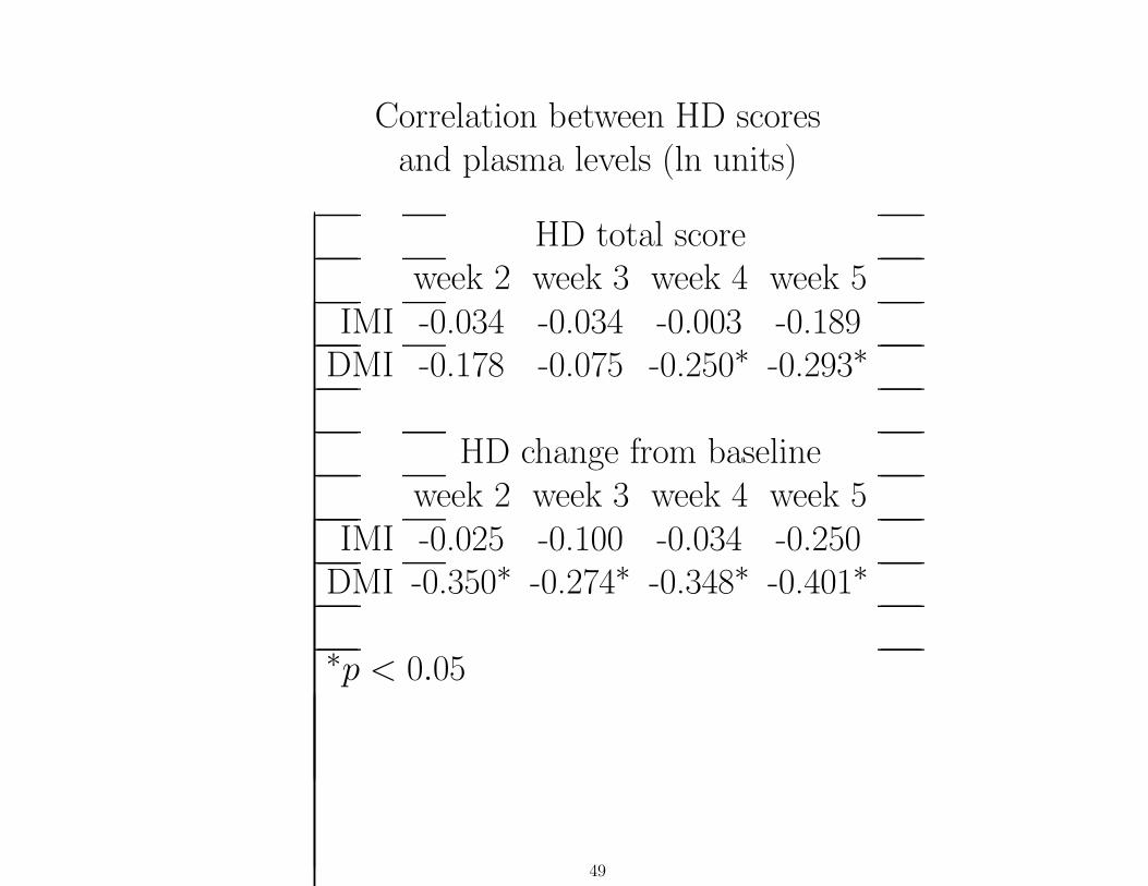
Correlation between HD scoresand plasma levels (ln units)
HD total scoreweek 2 week 3 week 4 week 5
IMI -0.034 -0.034 -0.003 -0.189DMI -0.178 -0.075 -0.250∗ -0.293∗
HD change from baselineweek 2 week 3 week 4 week 5
IMI -0.025 -0.100 -0.034 -0.250DMI -0.350∗ -0.274∗ -0.348∗ -0.401∗
∗p < 0.05
49
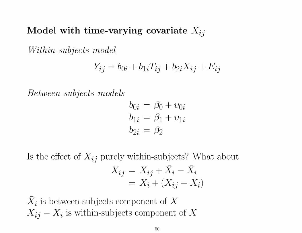
Model with time-varying covariate Xij
Within-subjects model
Yij = b0i + b1iTij + b2iXij + Eij
Between-subjects modelsb0i = β0 + υ0i
b1i = β1 + υ1i
b2i = β2
Is the effect of Xij purely within-subjects? What about
Xij = Xij + Xi − Xi
= Xi + (Xij − Xi)
Xi is between-subjects component of XXij − Xi is within-subjects component of X
50
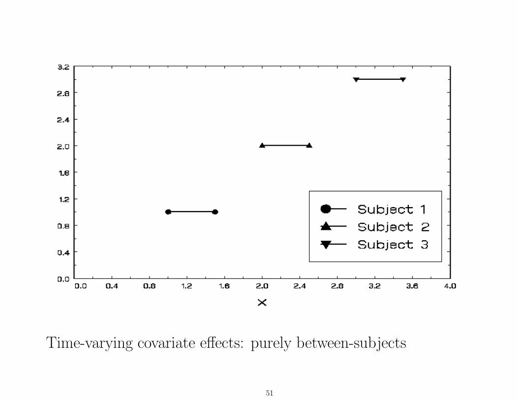
Time-varying covariate effects: purely between-subjects
51
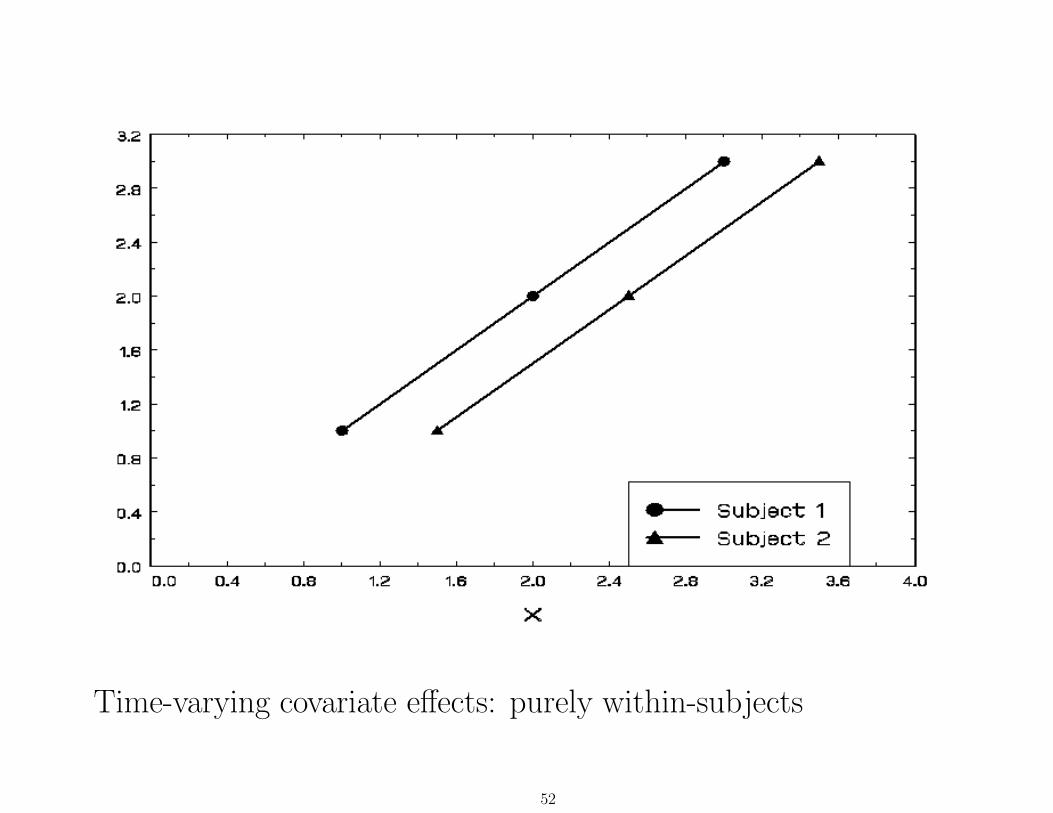
Time-varying covariate effects: purely within-subjects
52
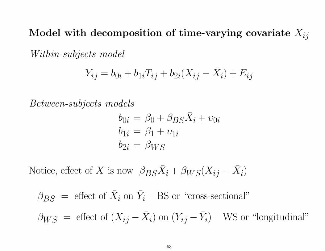
Model with decomposition of time-varying covariate Xij
Within-subjects model
Yij = b0i + b1iTij + b2i(Xij − Xi) + Eij
Between-subjects models
b0i = β0 + βBSXi + υ0i
b1i = β1 + υ1i
b2i = βWS
Notice, effect of X is now βBSXi + βWS(Xij − Xi)
βBS = effect of Xi on Yi BS or “cross-sectional”
βWS = effect of (Xij − Xi) on (Yij − Yi) WS or “longitudinal”
53
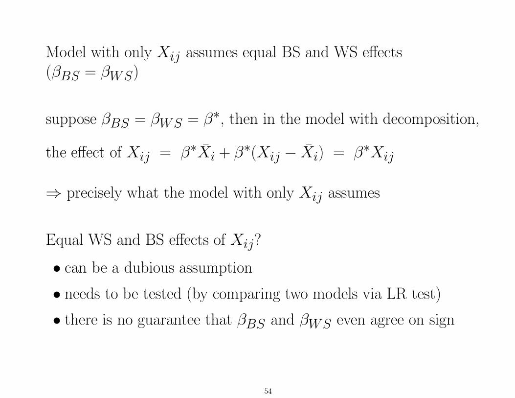
Model with only Xij assumes equal BS and WS effects(βBS = βWS)
suppose βBS = βWS = β∗, then in the model with decomposition,
the effect of Xij = β∗Xi + β∗(Xij − Xi) = β∗Xij
⇒ precisely what the model with only Xij assumes
Equal WS and BS effects of Xij?
• can be a dubious assumption
• needs to be tested (by comparing two models via LR test)
• there is no guarantee that βBS and βWS even agree on sign
54
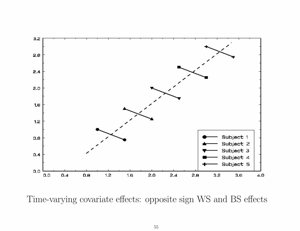
Time-varying covariate effects: opposite sign WS and BS effects
55
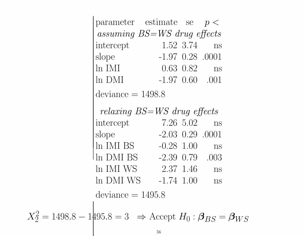
parameter estimate se p <assuming BS=WS drug effectsintercept 1.52 3.74 nsslope -1.97 0.28 .0001ln IMI 0.63 0.82 nsln DMI -1.97 0.60 .001
deviance = 1498.8
relaxing BS=WS drug effectsintercept 7.26 5.02 nsslope -2.03 0.29 .0001ln IMI BS -0.28 1.00 nsln DMI BS -2.39 0.79 .003ln IMI WS 2.37 1.46 nsln DMI WS -1.74 1.00 ns
deviance = 1495.8
X22 = 1498.8 − 1495.8 = 3 ⇒ Accept H0 : βBS = βWS
56
Example 4c: Analysis of Riesby dataset. This handout has theanalysis considering the time-varying drug plasma levels,separating the within-subjects from the between-subjects effectsfor these time-varying covariates.(SAS code and output)http://tigger.uic.edu/∼hedeker/riesbsws.txt
57
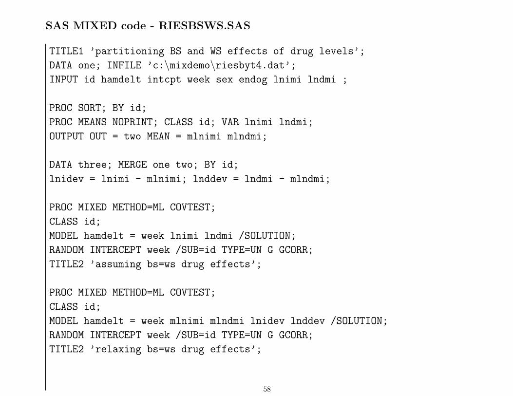
SAS MIXED code - RIESBSWS.SAS
TITLE1 ’partitioning BS and WS effects of drug levels’;
DATA one; INFILE ’c:\mixdemo\riesbyt4.dat’;INPUT id hamdelt intcpt week sex endog lnimi lndmi ;
PROC SORT; BY id;
PROC MEANS NOPRINT; CLASS id; VAR lnimi lndmi;
OUTPUT OUT = two MEAN = mlnimi mlndmi;
DATA three; MERGE one two; BY id;
lnidev = lnimi - mlnimi; lnddev = lndmi - mlndmi;
PROC MIXED METHOD=ML COVTEST;
CLASS id;
MODEL hamdelt = week lnimi lndmi /SOLUTION;
RANDOM INTERCEPT week /SUB=id TYPE=UN G GCORR;
TITLE2 ’assuming bs=ws drug effects’;
PROC MIXED METHOD=ML COVTEST;
CLASS id;
MODEL hamdelt = week mlnimi mlndmi lnidev lnddev /SOLUTION;
RANDOM INTERCEPT week /SUB=id TYPE=UN G GCORR;
TITLE2 ’relaxing bs=ws drug effects’;
58


![^JfEWS :] THE CilMOEN~MRm~](https://img.pdfslide.us/doc/110x75/61ed4499603c703d6079ce65/jfews-the-cilmoenmrm.jpg)