Research ArticleAdvancing Shannon Entropy for Measuring Diversity in Systems

R. Rajaram,1 B. Castellani,2 and A. N. Wilson3

1Department of Mathematical Sciences, Kent State University, Kent, OH, USA2Department of Sociology, Kent State University, 3300 Lake Rd. West, Ashtabula, OH, USA3School of Social and Health Sciences, Abertay University, Dundee DD1 1HG, UK

Correspondence should be addressed to R. Rajaram; rrajaram@kent.edu

Received 31 January 2017; Revised 5 April 2017; Accepted 23 April 2017; Published 24 May 2017

Academic Editor: Enzo Pasquale Scilingo

Copyright © 2017 R. Rajaram et al. This is an open access article distributed under the Creative Commons Attribution License,which permits unrestricted use, distribution, and reproduction in any medium, provided the original work is properly cited.

From economic inequality and species diversity to power laws and the analysis of multiple trends and trajectories, diversity withinsystems is a major issue for science. Part of the challenge is measuring it. Shannon entropy 𝐻 has been used to rethink diversitywithin probability distributions, based on the notion of information. However, there are two major limitations to Shannon’sapproach. First, it cannot be used to compare diversity distributions that have different levels of scale. Second, it cannot be used tocompare parts of diversity distributions to the whole. To address these limitations, we introduce a renormalization of probabilitydistributions based on the notion of case-based entropy 𝐶𝑐 as a function of the cumulative probability 𝑐. Given a probability density𝑝(𝑥), 𝐶𝑐 measures the diversity of the distribution up to a cumulative probability of 𝑐, by computing the length or support of anequivalent uniform distribution that has the same Shannon information as the conditional distribution of 𝑝𝑐(𝑥) up to cumulativeprobability 𝑐. We illustrate the utility of our approach by renormalizing and comparing three well-known energy distributionsin physics, namely, the Maxwell-Boltzmann, Bose-Einstein, and Fermi-Dirac distributions for energy of subatomic particles. Thecomparison shows that 𝐶𝑐 is a vast improvement over𝐻 as it provides a scale-free comparison of these diversity distributions andalso allows for a comparison between parts of these diversity distributions.

1. Diversity in Systems

Statistical distributions play an important role in any branchof science that studies systems comprised of many similaror identical particles, objects, or actors, whether material orimmaterial, human or nonhuman. One of the key featuresthat determines the characteristics and range of potentialbehaviors of such systems is the degree and distribution ofdiversity, that is, the extent to which the components of thesystem occupy states with similar or different features.

As Page outlined in a series of inquiries [1, 2], includ-ing The Difference and Diversity and Complexity, diversitywithin systems is an important concern for science, be itmaking sense of economic inequality, expanding the tradeportfolio of countries, measuring the collapse of speciesdiversity in various ecosystems, or determining the optimalutility/robustness of a network. However, an importantmajorchallenge in the literature on diversity and complexity, whichPage also points out [1, 2], remains: the issue ofmeasurement.

Although statistical distributions that directly reflect thespread of key parameters (such as mass, age, wealth, orenergy) provide descriptions of this diversity, it can bedifficult to compare the diversity of different distributions oreven the same distribution under different conditions, mostlybecause of differences in scales and parameters. Also, manyof the measures currently available compress diversity into asingle score or are not intuitive [1–4].

At the outset, motivated by examples of measuringdiversity in ecology and evolutionary biology from [3, 4],we sought to address these challenges. We begin with somedefinitions and a review of our previous research.

First, in terms of definitions, we follow the ecologicalliterature, defining diversity as the interplay of “richness” and“evenness” in a probability distribution. Richness refers to thenumber of different diversity types in a system. Examplesinclude (a) the different levels of household income in acity, (b) the number of different species in an ecosystem, (c)the diversity of a country’s exports, (d) the distribution of

HindawiComplexityVolume 2017, Article ID 8715605, 10 pageshttps://doi.org/10.1155/2017/8715605

2 Complexity

different nodes in a complex network, (e) the various healthtrends for a particular disease across time/space, or (f) thecultural or ethnic diversity of an organization or company. Inall such instances, the greater the number of diversity types(be these types discrete or continuous), the greater the degreeof richness in a system. In the case of the current study,for example, richness was defined as the number of differentenergy states.

In turn, evenness refers to the uniformity or “equiprob-ability” of occurrence of such states. In terms of the aboveexamples, evenness would be defined as (a) a city wherehousehold income was evenly distributed, (b) an ecosystemwhere the diversity of its species was equal in number,(c) a country with an even distribution of exports, (d) acomplex network where all nodes had the same probability ofoccurrence, (e) a disease where all possible health trends wereequiprobable, or (f) a company or organization where peopleof different cultural or ethnic backgrounds were evenlydistributed. In the case of the current study, for example,evenness was defined as the uniformity or “equiprobability”of the occurrence of all possible energy states.

More specifically, as we will see later in the paper, wedefine the diversity of a probability distribution as the numberof equivalent equiprobable types required to maintain thesame amount of Shannon entropy 𝐻 (i.e., the number ofShannon-equivalent equiprobable states). Given such a def-inition, a system with a high degree of richness and evennesswould have a higher degree of 𝐻, whereas a system with alow degree of richness and evenness would have a low degreeof 𝐻. In turn, a system with high richness but low evenness(as in the case of a skewed-right system with long tail) wouldhave a lower degree of 𝐻 than a system with high richnessand high evenness.

1.1. Purpose of the Current Study. Recently, we have intro-duced a novel approach to representing diversity within sta-tistical distributions [5, 6], which overcomes such difficultiesand allows the distribution of diversity in any given system(or cumulative portions thereof) to be directly comparedto the distribution of diversity within any other system. Ineffect, it is a renormalization that can be applied to anyprobability distribution to produce a direct representationof the distribution of diversity within that distribution.Arising from our work in the area of complex systems,the approach is based on the notion of case-based entropy,𝐶𝑐 [5]. This approach has two major advantages over theShannon Entropy 𝐻, which, as we alluded to above, is oneof the most commonly used measures of diversity withinprobability distributions and which calculates the averageamount of uncertainty (or information, depending on one’sperspective) present in a given probability distribution. First,𝐶𝑐 can be used to compare distributions that have differentlevels of scale; and, second, 𝐶𝑐 can be used to compare partsof distributions to their whole.

After developing the concept and formalism for case-based entropy for discrete distributions [5], we first applied itto compare complexity across a range of complex systems [6].In that work, we investigated a series of systems described bya variety of skewed-right probability distributions, choosing

examples that are often suggested to exhibit behaviorsindicative of complexity such as emergent collectivity, phasechanges, or tipping points. What we found was that suchsystems obeyed an apparent “limiting law of restricted diver-sity” [6], which constrains the majority of cases in thesecomplex systems to simpler types. In fact, for these typesof distribution, the distributions of diversity were foundto follow a scale-free 60/40 rule, with 60% or more ofcases belonging to the simplest 40% or less of equiprobablediversity types. This was found to be the case regardless ofwhether the original distribution fit a power law or was long-tailed, making it fundamentally distinct from the well-known(but often misunderstood) Pareto Principle [7].

In the following, we continue to explore the use of case-based entropy in comparing systems described by statisticaldistributions. However, we now go beyond our prior workin the following ways. First, we extend the formalism inorder to compute case-based entropy for continuous as wellas discrete distributions. Second, we broaden our focusfrom complexity/complex systems to diversity in any typeof statistically distributed system. That is, we start to exploredistributions of diversity for systems where richness is not afunction of the degree of complexity types.

Third, the discrete indices we used had a degree ofsubjectivity to them, for example, how should householdincome be binned and what influence does that have on thedistribution of diversity? As such, we wanted to see how well𝐶𝑐 worked for distributions where the unit of measurementwas universally agreed upon.

Fourth, we had not emphasized how 𝐶𝑐 was a majoradvance on Shannon entropy 𝐻. As known, while 𝐻 hasproven useful, it compresses itsmeasurement of diversity intoa single number; it is also nonintuitive; and, as we statedabove, it is not scale-free and therefore cannot be used tocompare the diversity of different systems; neither can it beused to compare parts of the diversity within a system to theentire system.

Hence, the purpose of the current study, as a demon-stration of the utility of 𝐶𝑐, is to renormalize and comparethree physically significant energy distributions in statisticalphysics: the energy probability density functions for systemsgoverned by Boltzmann, Bose-Einstein, and Fermi-Diracstatistics.

2. Renormalizing Probability: Case-BasedEntropy and the Distribution of Diversity

The quantity case-based entropy [5], 𝐶𝑐, renormalizes thediversity contribution of any probability distribution 𝑃(𝑥),by computing the true diversity 𝐷 of an equiprobable distri-bution (called the Shannon-equivalent uniform distribution)that has the same Shannon entropy𝐻 as 𝑃(𝑥). 𝐶𝑐 is preciselythe number of equiprobable types in the case of a discretedistribution, or the length, support, or extent of the variable inthe case of continuous distributions, which is required to keepthe value of the Shannon entropy the same across the wholeor any part of the distribution up to a cumulative probability

Complexity 3

𝑐. We choose the Shannon-equivalent uniform distributionfor two reasons:

(i) First, it is well known that, on a finite measure space,the uniform distribution maximizes entropy: that is,the uniform distribution has the maximal entropyamong all probability distributions on a set of finiteLebesgue measures [8].

(ii) Second, a Shannon-equivalent uniform distributionwill, by definition, count the number of values (orrange of values) of 𝑥 that are required to give thesame information as the original distribution 𝑃(𝑥) ifwe assume that all the values (or range of values) areequally probable.

Hence, the uniformdistribution renormalizes the effect ofvarying relative frequencies (or probabilities) of occurrenceof the values of 𝑥 without losing information (or entropy).In other words, if all choices of the random variable areequally likely, the number of values (or the length, if itis a continuous random variable) needed for the randomvariable to keep the same amount of information as the givendistribution is a measure of diversity. In a sense, each newvalue (or type) is counted as adding to the diversity, only ifthe new value has the same probability of occurrence as theexisting values. Diversity necessarily requires the values of therandom variable to be equiprobable since lower probability,for example, means that such values occur rarely in therandom variable and hence cannot be treated as equallydiverse as other values with higher probabilities. Hence,by choosing an equiprobable (or uniform) distribution fornormalization, we are counting the true diversity, that is, thenumber of equiprobable types that are required to matchthe same amount of Shannon information 𝐻 as the givendistribution.

This calculation (as we have shown elsewhere [5]) canbe done for parts of the distribution up to a cumulativeprobability of 𝑐. This means that a comparison of 𝐶𝑐 fora variety of distributions is actually a comparison of thevariation of the fraction of diversity 𝐶𝑐 contributed by valuesof the random variable up to 𝑐.

Since, regardless of the scale and units of the originaldistribution, 𝑐 and 𝐶𝑐 both vary from 0 to 1, one can plota curve for 𝐶𝑐 versus 𝑐 for multiple distributions on thesame axes. 𝐶𝑐 thus provides us with a scale-free measure tocompare distributions without omitting any of the entropyinformation, but by renormalizing the variable to one thathas equiprobable values. What is more, it also allows us tocompare different parts of the same distribution, or parts towholes. That is, we can generate a 𝐶𝑐 versus 𝑐 curve for anypart of a distribution (normalizing the probabilities to add upto 1 in that part) and compare the 𝐶𝑐 curve of the part to the𝐶𝑐 curve of the whole or another part to see if the functionaldependence of 𝐶𝑐 on 𝑐 is the same or different. In essence, 𝐶𝑐has the ability to compare distributions in a “fractal” or self-similar way.

In [5], we showed how to carry out the renormalizationfor discrete probability distributions, both mathematical andempirical. In this paper, as we stated in the Introduction, we

make the case for how 𝐶𝑐 constitutes an advance over 𝐻,in terms of providing a scale-free comparison of probabilitydistributions and also comparisons between parts of distri-butions. More importantly, we demonstrate how 𝐶𝑐 worksfor continuous distributions, by examining the Maxwell-Boltzmann, Bose-Einstein, and Fermi-Dirac distributions forenergy of subatomic particles. We begin with a more detailedreview of 𝐶𝑐.3. Case-Based Entropy of a ContinuousRandom Variable

Our impetus for making an advance over the Shannonentropy 𝐻 comes from the study of diversity in evolutionarybiology and ecology, where it is employed tomeasure the truediversity of species (types) in a given ecological system ofstudy [3, 4, 9, 10]. As we show here, it can also be used tomeasure the diversity of an arbitrary probability distributionof a continuous random variable.

Given the probability density function 𝑝(𝑥) of a randomvariable𝑥 in ameasure space𝑋, the Shannon-Weiner entropyindex𝐻 is given by

𝐻 = −∫𝑋𝑝 (𝑥) ln (𝑝 (𝑥)) 𝑑𝑥. (1)

The problem, however, with the Shannon entropy index𝐻, as we identified in our abstract and Introduction, isthat while being useful for studying the diversity of a singlesystem, it cannot be used to compare the diversity acrossprobability distributions. In other words,𝐻 is not multiplica-tive: a doubling of value for 𝐻 does not mean that the actualdiversity has doubled. To address this problem, we turned tothe true diversitymeasure 𝐷 [3, 11, 12], which gives the rangeof equiprobable values of 𝑥 that gives the same value of𝐻:

𝐷 = 𝑒𝐻. (2)

The utility of 𝐷 for comparing the diversity acrossprobability distributions is that, in𝐷, a doubling of the valuemeans that the number of equiprobable ranges of valuesof 𝑥 has doubled as well. 𝐷 calculates the range of suchequiprobable values of 𝑥 that will give the same value ofShannon entropy 𝐻 as observed in the distribution of 𝑥.We say that two probability densities 𝑝1(𝑥) and 𝑝2(x) areShannon-equivalent if they have the same value of Shannonentropy. Case-based entropy is then the range of values of𝑥 for the Shannon-equivalent uniform distribution for 𝑝(𝑥).We also note that Shannon entropy can be recomputed from𝐷 by using𝐻 = ln(𝐷).

In order to measure the distribution of diversity, wenext need to determine the fractional contribution to overalldiversity up to a cumulative probability 𝑐. In other words, weneed to be able to compute the diversity contribution 𝐷𝑐 upto a certain cumulative probability 𝑐. To do so, we replace 𝐻with𝐻𝑐, the conditional entropy, given that only the portionof the distribution up to a cumulative probability 𝑐 (denotedby𝑋𝑐) is observed with conditional probability of occurrence

4 Complexity

with density𝑝𝑐(𝑥) up to a given cumulative probability 𝑐.Thatis,

𝑝𝑐 (𝑥) = 𝑝 (𝑥)∫𝑋𝑐

𝑝 (𝑥) 𝑑𝑥 ,

𝐻𝑐 = −∫𝑋𝑐

𝑝𝑐 (𝑥) ln (𝑝𝑐 (𝑥)) ,

𝑐 = ∫𝑋𝑐

𝑝 (𝑥) 𝑑𝑥,𝐷𝑐 = 𝑒𝐻𝑐 .

(3)

The value of𝐷𝑐 for a given value of cumulative probability𝑐 is the number of Shannon-equivalent equiprobable energystates (or of values of the variable in the 𝑥-axis in general) thatare required to explain the information up to a cumulativeprobability of 𝑐 within the distribution. If 𝑐 = 1, then 𝐷𝑐 =𝐷 is the number of such Shannon-equivalent equiprobableenergy states for the entire distribution itself.

We can then simply calculate the fractional diversitycontribution or case-based entropy as

𝐶𝑐 = 𝐷𝑐𝐷 . (4)

It is at this point that the renormalization (𝐶𝑐 as a functionof 𝑐) becomes scale independent as both axes range betweenvalues of 0 and 1with the graph of𝐶𝑐 versus 𝑐 passing through(0, 0) and (1, 1). Hence, irrespective of the range and scaleof the original distributions, all distributions can be plottedon the same graph and their diversity contributions can becompared in a scale-free manner.

To check the validity of our formalism, we calculate 𝐷𝑐for the simple case of a uniform distribution given by 𝑝(𝑥) =𝜒[0,𝐿](𝑥) on the interval 𝑋 = [0, 𝐿]. Intuitively, if we choose𝑋𝑐 = [0, 𝑐], then, owing to the uniformity of the distribution,we expect 𝐷𝑐 = 𝑐 itself. In other words, the diversity ofthe part [0, 𝑐] is simply equal to 𝑐, that is, the length of theinterval [0, 𝑐], and hence the 𝐶𝑐 versus 𝑐 curve will simply bethe straight line with slope equal to 1. This can be shown asfollows:

𝑝𝑐 (𝑥) = 1𝑐 𝜒[0,𝐿] (𝑥) ,

𝐻𝑐 = −∫[0,𝑐]

1𝑐 ln(1

𝑐 ) 𝑑𝑥 = ln (𝑐) ,𝐷𝑐 = 𝑒𝐻𝑐 = 𝑒ln(𝑐) = 𝑐.

(5)

With our formulation of 𝐶𝑐 complete, we turn to theenergy distributions for particles governed by Boltzmann,Bose-Einstein, and Fermi-Dirac statistics.

4. Results

4.1. 𝐶𝑐 for the Boltzmann Distribution in One Dimension. Wefirst illustrate our renormalization by applying it to a relativelysimple case: that of an ideal gas at temperature 𝑇. The kinetic

energies 𝐸 of particles in such a gas are described by theBoltzmann distribution [8]. In one dimension, this is

𝑝𝐵,1𝐷 (𝐸) = ( 1𝑘𝐵𝑇) 𝑒−𝐸/𝑘𝐵𝑇 = 𝛽

𝑒𝛽𝐸 , (6)

where 𝑘𝐵 is the Boltzmann constant and 𝛽 = (1/𝑘𝐵𝑇).The entropy of 𝑝𝐵,1𝐷(𝐸) can be shown to be 𝐻𝐵 = 1 −

ln(𝛽), and hence the true diversity of energy in the range[0,∞) is given by

𝐷𝐵,1𝐷 = 𝑒𝐻 = 𝑒1−ln(𝛽) = 𝑒𝛽 . (7)

The cumulative probability 𝑐 from 𝐸 = 0 to 𝐸 = 𝑘 is thengiven by

𝑐 = ∫[0,𝑘]

𝑝𝐵,1𝐷 (𝐸) 𝑑𝐸 = 1 − 𝑒−𝛽𝑘. (8)

Hence, 𝑘 can be computed in terms of 𝑐 as𝑘 = − ln (1 − 𝑐)

𝛽 . (9)

Equation (9) is useful for the one-dimensional Boltzmanncase to eliminate the parameter 𝑘 altogether in (11) to obtainan explicit relationship between𝐶𝑐 and 𝑐. It is to be noted that,inmost cases, both𝐶𝑐 and 𝑐 can only be parametrically relatedthrough 𝑘. The other quantities introduced in Section 3 canthen be calculated as follows:

𝑝𝑐 (𝐸) = 𝑝𝐵,1𝐷 (𝐸)𝑐 = 𝛽𝑒−𝛽𝐸1 − 𝑒−𝛽𝑘 , (10)

𝐻𝑐 = −∫[0,𝑘]

𝛽𝑒−𝛽𝐸1 − 𝑒−𝛽𝑘 ln( 𝛽𝑒−𝛽𝐸

1 − 𝑒−𝛽𝑘)𝑑𝐸

= 1 + ln( 𝑐𝛽 (1 − 𝑐)(1−𝑐)/𝑐) ,

(11)

𝐷𝑐 = 𝑒𝐻𝑐 = 𝑒1+ln((𝑐/𝛽)(1−𝑐)(1−𝑐)/𝑐)= 𝑒

𝛽 ⋅ (𝑐 (1 − 𝑐)(1−𝑐)/𝑐) , (12)

𝐶𝑐 = 𝐷𝑐𝐷𝐵,1𝐷 = (𝑒/𝛽) ⋅ (𝑐 (1 − 𝑐)(1−𝑐)/𝑐)𝑒/𝛽

= 𝑐 (1 − 𝑐)(1−𝑐)/𝑐 .(13)

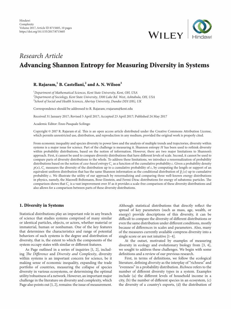
We note that, in (13), the temperature factor 𝛽 cancelsout, indicating that the distribution of diversity for anideal gas in one dimension is independent of temperature.The resulting graph of 𝐶𝑐 as a function of 𝑐 is shown inFigure 1. It is worth noting in passing that 𝐶𝑐 reaches 40%when 𝑐 ≈ 69%, indicating that approximately 69% of themolecules in the gas are contained within the lower 40% ofdiversity of energy probability states at all temperatures (here,diversity is defined as the number of equivalent equiprobableenergy states required to maintain the same amount of

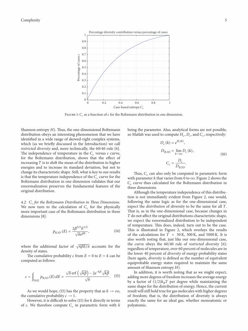
Complexity 5

Percentage diversity contribution versus percentage of cases

0.2 0.4 0.6 0.80 1

CcCase-based entropy

0

0.1

0.2

0.3

0.4

0.5

0.6

0.7

0.8

0.9

1

Perc

enta

ge o

f cas

es c

Figure 1: 𝐶𝑐 as a function of 𝑐 for the Boltzmann distribution in one dimension.

Shannon entropy𝐻). Thus, the one-dimensional Boltzmanndistribution obeys an interesting phenomenon that we haveidentified in a wide range of skewed-right complex systems,which (as we briefly discussed in the Introduction) we callrestricted diversity and, more technically, the 60/40 rule [6].The independence of temperature in the 𝐶𝑐 versus 𝑐 curve,for the Boltzmann distribution, shows that the effect ofincreasing 𝑇 is to shift the mean of the distribution to higherenergies and to increase its standard deviation, but not tochange its characteristic shape. Still, what is key to our resultsis that the temperature independence of the 𝐶𝑐 curve for theBoltzmann distribution in one dimension validates that ourrenormalization preserves the fundamental features of theoriginal distribution.

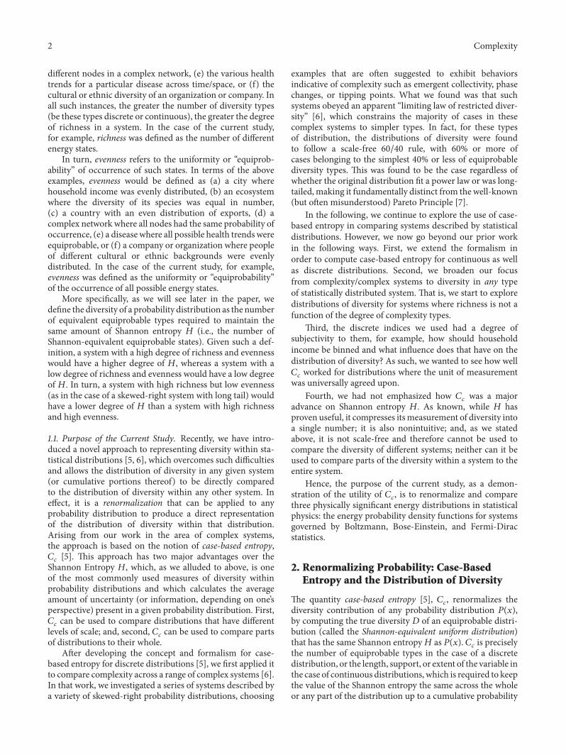
4.2. 𝐶𝑐 for the Boltzmann Distribution in Three Dimensions.We now turn to the calculation of 𝐶𝑐 for the physicallymore important case of the Boltzmann distribution in threedimensions [8]:

𝑝𝐵,3𝐷 (𝐸) = 2𝛽3/2𝐸1/2√𝜋𝑒𝛽𝐸 , (14)

where the additional factor of √4𝛽𝐸/𝜋 accounts for thedensity of states.

The cumulative probability 𝑐 from 𝐸 = 0 to 𝐸 = 𝑘 can becomputed as follows:

𝑐 = ∫[0,𝑘]

𝑝𝐵,3𝐷 (𝐸) 𝑑𝐸 = √𝜋 erf (√𝑘𝛽) − 2𝑒−𝑘𝛽√𝑘𝛽√𝜋 . (15)

As we would hope, (15) has the property that as 𝑘 → ∞,the cumulative probability 𝑐 → 1.

However, it is difficult to solve (15) for 𝑘 directly in termsof 𝑐. We therefore compute 𝐶𝑐 in parametric form with 𝑘

being the parameter. Also, analytical forms are not possible,so Matlab was used to compute𝐻𝑐,𝐷𝑐, and 𝐶𝑐, respectively:

𝐷𝑐 (𝑘) = 𝑒𝐻𝑐(𝑘),𝐷𝐵,3𝐷 = lim

𝑘→∞𝐷𝑐 (𝑘) ,

𝐶𝑐 = 𝐷𝑐𝐷𝐵,3𝐷 .(16)

Thus, 𝐶𝑐 can also only be computed in parametric formwith parameter 𝑘 that varies from 0 to∞. Figure 2 shows the𝐶𝑐 curve thus calculated for the Boltzmann distribution inthree dimensions.

Although the temperature independence of this distribu-tion is not immediately evident from Figure 2, one would,following the same logic as for the one-dimensional case,expect the distribution of diversity to be the same for all 𝑇.That is, as in the one-dimensional case, because changes in𝑇 do not affect the original distributions characteristic shape,we expect the renormalized distribution to be independentof temperature. This does, indeed, turn out to be the case.This is illustrated in Figure 2, which overlays the resultsof the calculations for 𝑇 = 50K, 500K, and 5000K. It isalso worth noting that, just like our one-dimensional case,the curve obeys the 60/40 rule of restricted diversity [6]:regardless of temperature, over 60 percent of molecules are inthe lower 40 percent of diversity of energy probability states(here again, diversity is defined as the number of equivalentequiprobable energy states required to maintain the sameamount of Shannon entropy𝐻).

In addition, it is worth noting that as we might expect,addingmore degrees of freedom increases the average energyby a factor of (1/2)𝑘𝐵𝑇 per degree while maintaining thesame shape for the distribution of energy. Hence, the currentresult will still hold true for gasmolecules with higher degreesof freedom; that is, the distribution of diversity is alwaysexactly the same for an ideal gas, whether monoatomic orpolyatomic.

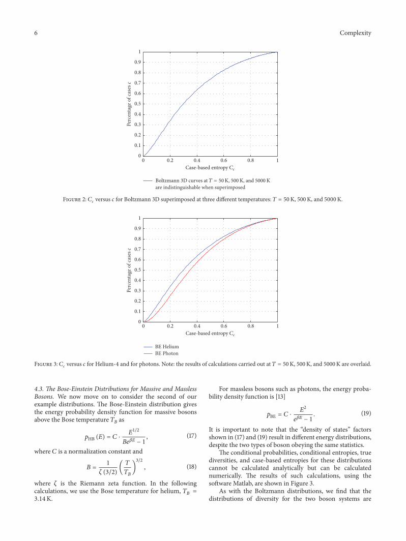
6 Complexity

are indistinguishable when superimposedBoltzmann 3D curves at T = 50K, 500 KK, and 5000

0.2 0.4 0.6 0.80 1

Case-based entropy Cc

0

0.1

0.2

0.3

0.4

0.5

0.6

0.7

0.8

0.9

1

Perc

enta

ge o

f cas

es c

Figure 2: 𝐶𝑐 versus 𝑐 for Boltzmann 3D superimposed at three different temperatures: 𝑇 = 50K, 500K, and 5000K.

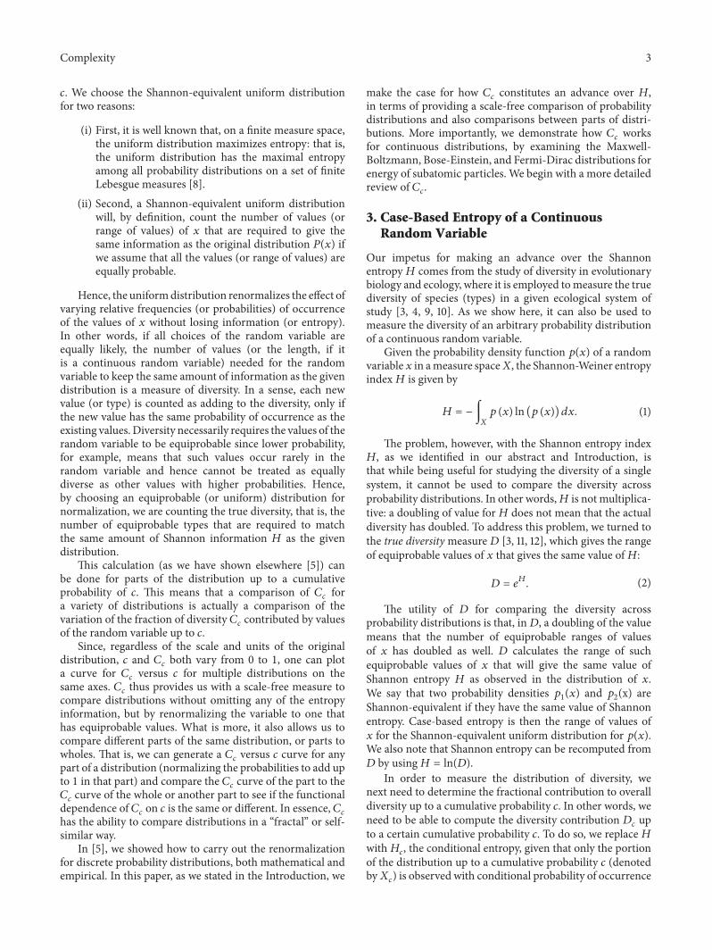
BE HeliumBE Photon

0.2 0.4 0.6 0.80 1

CcCase-based entropy

0

0.1

0.2

0.3

0.4

0.5

0.6

0.7

0.8

0.9

1

Perc

enta

ge o

f cas

es c

Figure 3: 𝐶𝑐 versus 𝑐 for Helium-4 and for photons. Note: the results of calculations carried out at 𝑇 = 50K, 500K, and 5000K are overlaid.

4.3. The Bose-Einstein Distributions for Massive and MasslessBosons. We now move on to consider the second of ourexample distributions. The Bose-Einstein distribution givesthe energy probability density function for massive bosonsabove the Bose temperature 𝑇𝐵 as

𝑝HB (𝐸) = 𝐶 ⋅ 𝐸1/2𝐵𝑒𝛽𝐸 − 1 , (17)

where 𝐶 is a normalization constant and

𝐵 = 1𝜁 (3/2) (

𝑇𝑇𝐵)3/2 , (18)

where 𝜁 is the Riemann zeta function. In the followingcalculations, we use the Bose temperature for helium, 𝑇𝐵 =3.14K.

For massless bosons such as photons, the energy proba-bility density function is [13]

𝑝BE = 𝐶 ⋅ 𝐸2𝑒𝛽𝐸 − 1 . (19)

It is important to note that the “density of states” factorsshown in (17) and (19) result in different energy distributions,despite the two types of boson obeying the same statistics.

The conditional probabilities, conditional entropies, truediversities, and case-based entropies for these distributionscannot be calculated analytically but can be calculatednumerically. The results of such calculations, using thesoftware Matlab, are shown in Figure 3.

As with the Boltzmann distributions, we find that thedistributions of diversity for the two boson systems are

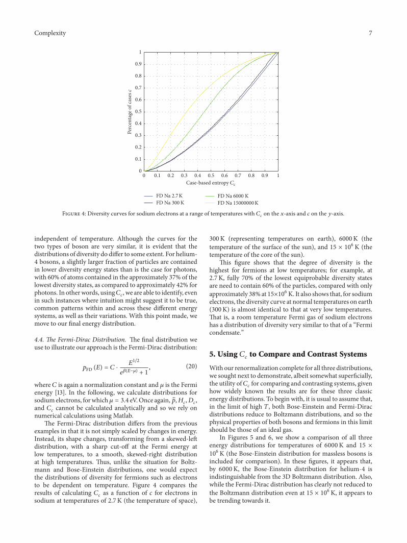
Complexity 7

FD Na 15000000 KFD Na 6000 K

FD Na 300 KFD Na 2.7 K

0

0.1

0.2

0.3

0.4

0.5

0.6

0.7

0.8

0.9

1

Perc

enta

ge o

f cas

es c

10 0.3 0.4 0.5 0.8 0.90.2 0.60.1 0.7

Case-based entropy Cc

Figure 4: Diversity curves for sodium electrons at a range of temperatures with 𝐶𝑐 on the 𝑥-axis and 𝑐 on the 𝑦-axis.

independent of temperature. Although the curves for thetwo types of boson are very similar, it is evident that thedistributions of diversity do differ to some extent. For helium-4 bosons, a slightly larger fraction of particles are containedin lower diversity energy states than is the case for photons,with 60%of atoms contained in the approximately 37%of thelowest diversity states, as compared to approximately 42% forphotons. In otherwords, using𝐶𝑐, we are able to identify, evenin such instances where intuition might suggest it to be true,common patterns within and across these different energysystems, as well as their variations. With this point made, wemove to our final energy distribution.

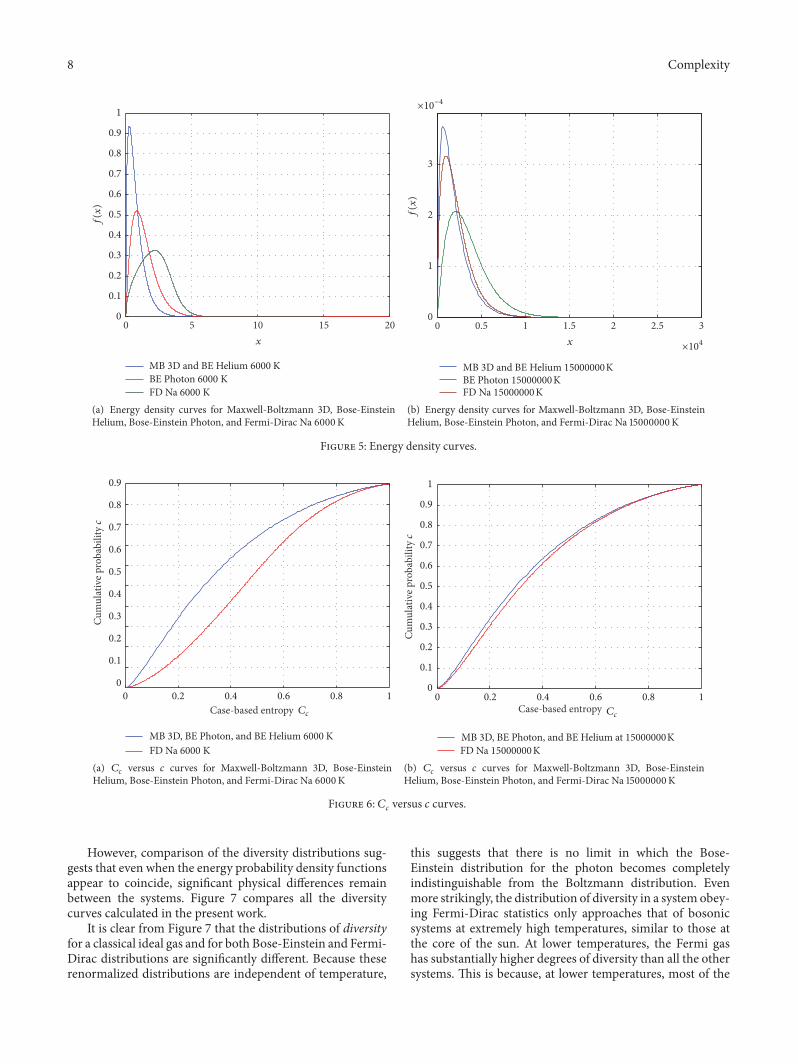
4.4. The Fermi-Dirac Distribution. The final distribution weuse to illustrate our approach is the Fermi-Dirac distribution:

𝑝FD (𝐸) = 𝐶 ⋅ 𝐸1/2𝑒𝛽(𝐸−𝜇) + 1 , (20)

where 𝐶 is again a normalization constant and 𝜇 is the Fermienergy [13]. In the following, we calculate distributions forsodiumelectrons, forwhich𝜇 = 3.4 eV.Once again,𝑝,𝐻𝑐, 𝐷𝑐,and 𝐶𝑐 cannot be calculated analytically and so we rely onnumerical calculations using Matlab.

The Fermi-Dirac distribution differs from the previousexamples in that it is not simply scaled by changes in energy.Instead, its shape changes, transforming from a skewed-leftdistribution, with a sharp cut-off at the Fermi energy atlow temperatures, to a smooth, skewed-right distributionat high temperatures. Thus, unlike the situation for Boltz-mann and Bose-Einstein distributions, one would expectthe distributions of diversity for fermions such as electronsto be dependent on temperature. Figure 4 compares theresults of calculating 𝐶𝑐 as a function of 𝑐 for electrons insodium at temperatures of 2.7K (the temperature of space),

300K (representing temperatures on earth), 6000K (thetemperature of the surface of the sun), and 15 × 106 K (thetemperature of the core of the sun).

This figure shows that the degree of diversity is thehighest for fermions at low temperatures; for example, at2.7K, fully 70% of the lowest equiprobable diversity statesare need to contain 60% of the particles, compared with onlyapproximately 38%at 15×106 K. It also shows that, for sodiumelectrons, the diversity curve at normal temperatures on earth(300K) is almost identical to that at very low temperatures.That is, a room temperature Fermi gas of sodium electronshas a distribution of diversity very similar to that of a “Fermicondensate.”

5. Using 𝐶𝑐 to Compare and Contrast Systems

With our renormalization complete for all three distributions,we sought next to demonstrate, albeit somewhat superficially,the utility of𝐶𝑐 for comparing and contrasting systems, givenhow widely known the results are for these three classicenergy distributions. To begin with, it is usual to assume that,in the limit of high 𝑇, both Bose-Einstein and Fermi-Diracdistributions reduce to Boltzmann distributions, and so thephysical properties of both bosons and fermions in this limitshould be those of an ideal gas.

In Figures 5 and 6, we show a comparison of all threeenergy distributions for temperatures of 6000K and 15 ×106 K (the Bose-Einstein distribution for massless bosons isincluded for comparison). In these figures, it appears that,by 6000K, the Bose-Einstein distribution for helium-4 isindistinguishable from the 3D Boltzmann distribution. Also,while the Fermi-Dirac distribution has clearly not reduced tothe Boltzmann distribution even at 15 × 106 K, it appears tobe trending towards it.

8 Complexity

0

0.1

0.2

0.3

0.4

0.5

f(x)

0.6

0.7

0.8

0.9

1

5 10 15 200x

FD Na 6000 KBE Photon 6000 KMB 3D and BE Helium 6000 K

(a) Energy density curves for Maxwell-Boltzmann 3D, Bose-EinsteinHelium, Bose-Einstein Photon, and Fermi-Dirac Na 6000K

×10−4

×104

0

1

2f(x)

3

0.5 1 1.5 2 2.5 30x

FD Na 15000000 KBE Photon 15000000 KMB 3D and BE Helium 15000000K

(b) Energy density curves for Maxwell-Boltzmann 3D, Bose-EinsteinHelium, Bose-Einstein Photon, and Fermi-Dirac Na 15000000K

Figure 5: Energy density curves.

0

0.1

0.2

0.3

0.4

0.5

0.6

0.7

0.8

0.9

Cum

ulat

ive p

roba

bilit

y c

0.6 0.8 10.2 0.40

Case-based entropy Cc

FD Na 6000 KMB 3D, BE Photon, and BE Helium 6000 K

(a) 𝐶𝑐 versus 𝑐 curves for Maxwell-Boltzmann 3D, Bose-EinsteinHelium, Bose-Einstein Photon, and Fermi-Dirac Na 6000K

0.2 0.4 0.6 0.80 1Case-based entropy Cc

0

0.1

0.2

0.3

0.4

0.5

0.6

0.7

0.8

0.9

1

Cum

ulat

ive p

roba

bilit

y c

FD Na 15000000 KMB 3D, BE Photon, and BE Helium at 15000000K

(b) 𝐶𝑐 versus 𝑐 curves for Maxwell-Boltzmann 3D, Bose-EinsteinHelium, Bose-Einstein Photon, and Fermi-Dirac Na 15000000K

Figure 6: 𝐶𝑐 versus 𝑐 curves.

However, comparison of the diversity distributions sug-gests that even when the energy probability density functionsappear to coincide, significant physical differences remainbetween the systems. Figure 7 compares all the diversitycurves calculated in the present work.

It is clear from Figure 7 that the distributions of diversityfor a classical ideal gas and for both Bose-Einstein and Fermi-Dirac distributions are significantly different. Because theserenormalized distributions are independent of temperature,

this suggests that there is no limit in which the Bose-Einstein distribution for the photon becomes completelyindistinguishable from the Boltzmann distribution. Evenmore strikingly, the distribution of diversity in a system obey-ing Fermi-Dirac statistics only approaches that of bosonicsystems at extremely high temperatures, similar to those atthe core of the sun. At lower temperatures, the Fermi gashas substantially higher degrees of diversity than all the othersystems. This is because, at lower temperatures, most of the

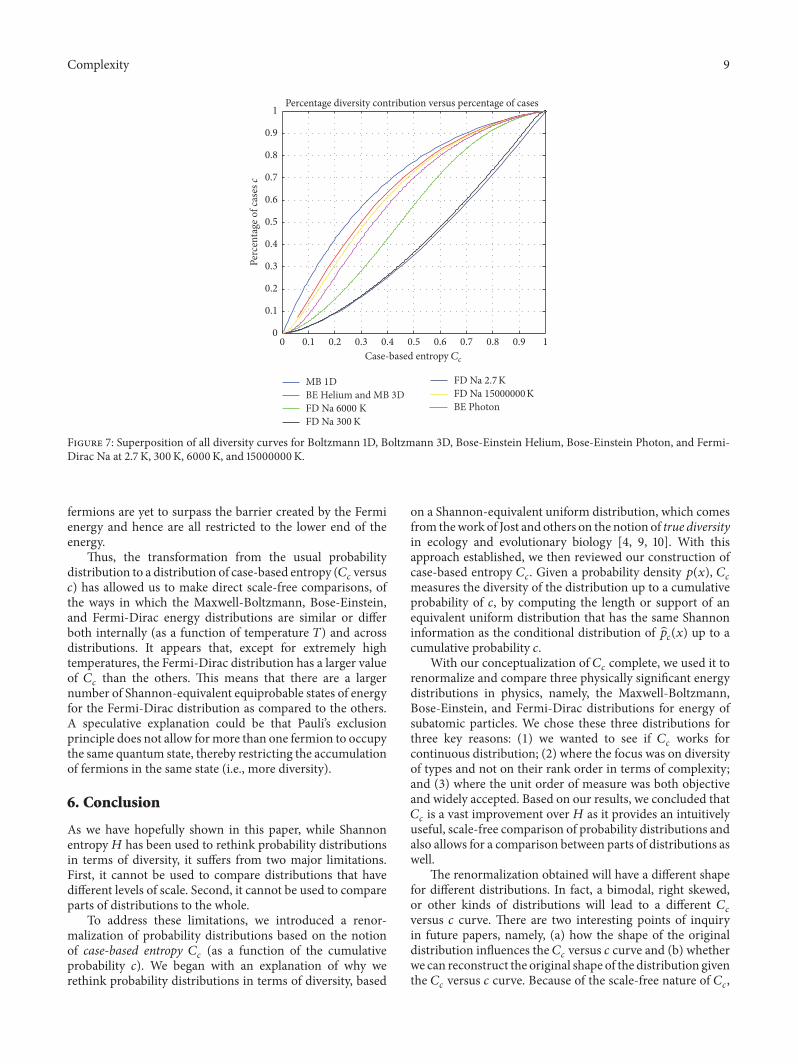
Complexity 9

MB 1DBE Helium and MB 3D

BE PhotonFD Na 15000000 KFD Na 2.7 K

FD Na 300 KFD Na 6000 K

0

0.1

0.2

0.3

0.4

0.5

0.6

0.7

0.8

0.9

1

Perc

enta

ge o

f cas

es c

10 0.3 0.4 0.5 0.6 0.7 0.8 0.90.1 0.2

Case-based entropy Cc

Percentage diversity contribution versus percentage of cases

Figure 7: Superposition of all diversity curves for Boltzmann 1D, Boltzmann 3D, Bose-Einstein Helium, Bose-Einstein Photon, and Fermi-Dirac Na at 2.7 K, 300K, 6000K, and 15000000K.

fermions are yet to surpass the barrier created by the Fermienergy and hence are all restricted to the lower end of theenergy.

Thus, the transformation from the usual probabilitydistribution to a distribution of case-based entropy (𝐶𝑐 versus𝑐) has allowed us to make direct scale-free comparisons, ofthe ways in which the Maxwell-Boltzmann, Bose-Einstein,and Fermi-Dirac energy distributions are similar or differboth internally (as a function of temperature 𝑇) and acrossdistributions. It appears that, except for extremely hightemperatures, the Fermi-Dirac distribution has a larger valueof 𝐶𝑐 than the others. This means that there are a largernumber of Shannon-equivalent equiprobable states of energyfor the Fermi-Dirac distribution as compared to the others.A speculative explanation could be that Pauli’s exclusionprinciple does not allow formore than one fermion to occupythe same quantum state, thereby restricting the accumulationof fermions in the same state (i.e., more diversity).

6. Conclusion

As we have hopefully shown in this paper, while Shannonentropy𝐻 has been used to rethink probability distributionsin terms of diversity, it suffers from two major limitations.First, it cannot be used to compare distributions that havedifferent levels of scale. Second, it cannot be used to compareparts of distributions to the whole.

To address these limitations, we introduced a renor-malization of probability distributions based on the notionof case-based entropy 𝐶𝑐 (as a function of the cumulativeprobability 𝑐). We began with an explanation of why werethink probability distributions in terms of diversity, based

on a Shannon-equivalent uniform distribution, which comesfrom thework of Jost and others on the notion of true diversityin ecology and evolutionary biology [4, 9, 10]. With thisapproach established, we then reviewed our construction ofcase-based entropy 𝐶𝑐. Given a probability density 𝑝(𝑥), 𝐶𝑐measures the diversity of the distribution up to a cumulativeprobability of 𝑐, by computing the length or support of anequivalent uniform distribution that has the same Shannoninformation as the conditional distribution of 𝑝𝑐(𝑥) up to acumulative probability 𝑐.

With our conceptualization of 𝐶𝑐 complete, we used it torenormalize and compare three physically significant energydistributions in physics, namely, the Maxwell-Boltzmann,Bose-Einstein, and Fermi-Dirac distributions for energy ofsubatomic particles. We chose these three distributions forthree key reasons: (1) we wanted to see if 𝐶𝑐 works forcontinuous distribution; (2) where the focus was on diversityof types and not on their rank order in terms of complexity;and (3) where the unit order of measure was both objectiveand widely accepted. Based on our results, we concluded that𝐶𝑐 is a vast improvement over 𝐻 as it provides an intuitivelyuseful, scale-free comparison of probability distributions andalso allows for a comparison between parts of distributions aswell.

The renormalization obtained will have a different shapefor different distributions. In fact, a bimodal, right skewed,or other kinds of distributions will lead to a different 𝐶𝑐versus 𝑐 curve. There are two interesting points of inquiryin future papers, namely, (a) how the shape of the originaldistribution influences the 𝐶𝑐 versus 𝑐 curve and (b) whetherwe can reconstruct the original shape of the distribution giventhe 𝐶𝑐 versus 𝑐 curve. Because of the scale-free nature of 𝐶𝑐,

10 Complexity

all distributions can be compared in the same plot withoutreference to their original scales. In our future work, we willendeavor to connect the shape of the 𝐶𝑐 versus 𝑐 curve to theshape of the original distribution. This will allow us to locateportions of the original distribution (irrespective of theirscale), where diversity is concentrated, and portions whereit is sparse, even though the original distributions cannotbe plotted on the same graph due to huge variation in theirscales.

Conflicts of Interest

The authors declare that there are no conflicts of interestregarding the publication of this paper.

Acknowledgments

The authors would like to thank the following colleaguesat Kent State University: (1) Dean Susan Stocker, (2) KevinAcierno and Michael Ball (Computer Services), and (3) theComplexity in Health and Infrastructure Group for theirsupport.They also wish to thank EmmaUprichard andDavidByrne and the ESRC Seminar Series on Complexity andMethod in the Social Sciences (Centre for InterdisciplinaryMethodologies, University of Warwick, UK) for the chanceto work through the initial framing of these ideas.

References

[1] S. E. Page, The Difference: How the Power of Diversity CreatesBetter Groups, Firms, Schools, and Societies, Princeton Univer-sity Press, 2008.

[2] S. E. Page,Diversity and Complexity, PrincetonUniversity Press,2008.

[3] M. O. Hill, “Diversity and evenness: a unifying notation and itsconsequences,” Ecology, vol. 54, no. 2, pp. 427–432, 1973.

[4] L. Jost, “Entropy and diversity,” Oikos, vol. 113, no. 2, pp. 363–375, 2006.

[5] R. Rajaram and B. Castellani, “An entropy based measure forcomparing distributions of complexity,” Physica A. StatisticalMechanics and Its Applications, vol. 453, pp. 35–43, 2016.

[6] B. Castellani and R. Rajaram, “Past the power law: complexsystems and the limiting law of restricted diversity,”Complexity,vol. 21, no. 2, pp. 99–112, 2016.

[7] M. E. J. Newman, “Power laws, Pareto distributions and Zipf ’slaw,” Contemporary Physics, vol. 46, no. 5, pp. 323–351, 2005.

[8] M. C. Mackey, Time’s Arrow: The Origins of ThermodynamicBehavior, Springer Verlag, Germany, 1992.

[9] T. Leinster and C. A. Cobbold, “Measuring diversity: theimportance of species similarity,” Ecology, vol. 93, no. 3, pp. 477–489, 2012.

[10] J. Beck and W. Schwanghart, “Comparing measures of speciesdiversity from incomplete inventories: an update,” Methods inEcology and Evolution, vol. 1, no. 1, pp. 38–44, 2010.

[11] R. H. Macarthur, “Patterns of species diversity,” BiologicalReviews, vol. 40, pp. 510–533, 1965.

[12] R. Peet, “The measurement of species diversity,” Annual Reviewof Ecological Systems, vol. 5, pp. 285–307, 1974.

[13] C. H. Tien and J. H. Lienhard, Statistical Thermodynamics,Hemisphere, 1979.

Submit your manuscripts athttps://www.hindawi.com

Hindawi Publishing Corporationhttp://www.hindawi.com Volume 2014

MathematicsJournal of

Hindawi Publishing Corporationhttp://www.hindawi.com Volume 2014

Mathematical Problems in Engineering

Hindawi Publishing Corporationhttp://www.hindawi.com

Differential EquationsInternational Journal of

Volume 2014

Applied MathematicsJournal of

Hindawi Publishing Corporationhttp://www.hindawi.com Volume 2014

Probability and StatisticsHindawi Publishing Corporationhttp://www.hindawi.com Volume 2014

Journal of

Hindawi Publishing Corporationhttp://www.hindawi.com Volume 2014

Mathematical PhysicsAdvances in

Complex AnalysisJournal of

Hindawi Publishing Corporationhttp://www.hindawi.com Volume 2014

OptimizationJournal of

Hindawi Publishing Corporationhttp://www.hindawi.com Volume 2014

CombinatoricsHindawi Publishing Corporationhttp://www.hindawi.com Volume 2014

International Journal of

Hindawi Publishing Corporationhttp://www.hindawi.com Volume 2014

Operations ResearchAdvances in

Journal of

Hindawi Publishing Corporationhttp://www.hindawi.com Volume 2014

Function Spaces

Abstract and Applied AnalysisHindawi Publishing Corporationhttp://www.hindawi.com Volume 2014

International Journal of Mathematics and Mathematical Sciences

Hindawi Publishing Corporationhttp://www.hindawi.com Volume 201

The Scientific World JournalHindawi Publishing Corporation http://www.hindawi.com Volume 2014

Hindawi Publishing Corporationhttp://www.hindawi.com Volume 2014

Algebra

Discrete Dynamics in Nature and Society

Hindawi Publishing Corporationhttp://www.hindawi.com Volume 2014

Hindawi Publishing Corporationhttp://www.hindawi.com Volume 2014

Decision SciencesAdvances in

Journal of

Hindawi Publishing Corporationhttp://www.hindawi.com

Volume 2014 Hindawi Publishing Corporationhttp://www.hindawi.com Volume 2014

Stochastic AnalysisInternational Journal of