Embed Size (px)
Citation preview
Faculty of Science and Technology
Department of Physics and Technology
Advancing Segmentation and Unsupervised Learning Withinthe Field of Deep Learning—Michael Kampffmeyer, UiT Machine Learning Group
A dissertation for the degree of Philosophiae Doctor — August 2018
Abstract
Due to the large improvements that deep learning basedmodels have brought to
a variety of tasks, they have in recent years received large amounts of attention.
However, these improvements are to a large extent achieved in supervised set-
tings, where labels are available, and initially focused on traditional computer
vision tasks such as visual object recognition. Specific application domains that
consider images of large size and multi-modal images, as well as applications
where labeled training data is challenging to obtain, has instead received less
attention.
This thesis aims to fill these gaps from two overall perspectives. First, we ad-
vance segmentation approaches specifically targeted towards the applications
of remote sensing and medical imaging. Second, inspired by the lack of labeled
data in many high-impact domains, such as medical imaging, we advance four
unsupervised deep learning tasks: domain adaptation, clustering, representa-
tion learning, and zero-shot learning.
The works on segmentation address the challenges of class-imbalance, missing
data-modalities and themodeling of uncertainty in remote sensing. Founded on
the idea of pixel-connectivity, we further propose a novel approach to saliency
segmentation, a common pre-processing task. We illustrate that phrasing the
problem as a connectivity prediction problem, allows us to achieve good per-
formance while keeping the model simple. Finally, connecting our work on
segmentation and unsupervised deep learning, we propose an approach to
unsupervised domain adaptation in a segmentation setting in the medical do-
main.
Besides unsupervised domain adaptation, we further propose a novel approach
to clustering based on integrating ideas from kernel methods and informa-
tion theoretic learning achieving promising results. Based on our intuition
that meaningful representations should incorporate similarities between data
points, we further propose a kernelized autoencoder. Finally, we address the
task of zero-shot learning based on improving knowledge propagation in graph
convolutional neural networks, achieving state-of-the-art performance on the
21K class ImageNet dataset.
Acknowledgements
First and foremost I would like to thank Professor Robert Jenssen for being
the best supervisor I could have asked for. Robert’s guidance and support are
what made this thesis possible and I am grateful for all the time and effort that
he spent on teaching me the ways of academia. A special thanks also to my
co-supervisor Dr. Arnt-Børre Salberg for all the insightful discussions and all
his advice.
I am grateful to Professor Eric P. Xing for giving me the opportunity to spend
10 months in his lab at Carnegie Mellon University. It was a truly inspiring and
memorable experience. I would like to thank Dr. Xiaodan Liang for mentoring
me while I was there and would like to thank everyone in the SAILING Lab, and
all the other visitors in the visitors office, for making it so enjoyable. Special
thanks to Yujia for her wonderful sense of humor and the countless meals,
which provided a nice break from work.
I would also like to express my gratitude to everyone in the Machine Learning
Group at UiT. It has been fun to see it grow from Jonas, Karl Øyvind, Sigurd,
and Filippo to so many people that I do not have space to mention them all.
Further, I am particularly grateful to all my co-authors and colleagues. It has
been amazing working with so many brilliant people and I look forward to
continuing our collaborations. I would also like to thank Filippo, Karl Øyvind,
and Einar for allowing me to distribute all my belongings in their houses while
I was at CMU.
I want to thank my committee members Associate Professor Devis Tuia, Dr.
Wojciech Samek, and Professor Fred Godtliebsen for making time to read the
thesis and attend the defense.
Special shoutout to Hansi & Family for all their dinner invitations. Building
trains with Ciljan and Otelie is a nice change of pace from busy days at the
office. Last but definitely not least, I would like to thank my family for their
continued support!
Michael Kampffmeyer
Tromsø, August 2018
Contents
Abstract i
Acknowledgements iii
List of Figures ix
List of Abbreviations xi
1 Introduction 1
1.1 Key Challenges . . . . . . . . . . . . . . . . . . . . . . . . . 2
1.2 Key Objectives . . . . . . . . . . . . . . . . . . . . . . . . . 4
1.3 Key Solutions . . . . . . . . . . . . . . . . . . . . . . . . . 5
1.4 Brief summary of papers . . . . . . . . . . . . . . . . . . . . 5
1.5 Other papers . . . . . . . . . . . . . . . . . . . . . . . . . . 8
1.6 Reading guide . . . . . . . . . . . . . . . . . . . . . . . . . 10
I Methodology and context 11
2 Deep Learning 13
2.1 Fully Connected Neural Networks . . . . . . . . . . . . . . . 15
2.2 Convolutional Neural Networks . . . . . . . . . . . . . . . . 18
2.3 Graph Convolutional Neural Networks . . . . . . . . . . . . 21
2.4 Autoencoders . . . . . . . . . . . . . . . . . . . . . . . . . 23
2.5 Generative Adversarial Networks . . . . . . . . . . . . . . . 26
3 Segmentation 29
3.1 Semantic Segmentation . . . . . . . . . . . . . . . . . . . . 29
3.2 Salient Segmentation . . . . . . . . . . . . . . . . . . . . . 32
4 Unsupervised Learning 35
4.1 Domain Adaptation . . . . . . . . . . . . . . . . . . . . . . 35
4.2 Representation Learning . . . . . . . . . . . . . . . . . . . . 37
4.3 Clustering . . . . . . . . . . . . . . . . . . . . . . . . . . . 39
v
vi CO N T E N TS
4.4 Zero-shot Learning . . . . . . . . . . . . . . . . . . . . . . . 40
5 Kernel Methods and Information Theoretic Learning 43
5.1 Kernel Methods . . . . . . . . . . . . . . . . . . . . . . . . 43
5.2 Information Theoretic Learning . . . . . . . . . . . . . . . . 45
5.2.1 Cauchy-Schwartz Divergence . . . . . . . . . . . . . 45
II Summary of research 49
6 Paper I 51
7 Paper II 53
8 Paper III 55
9 Paper IV 57
10 Paper V 59
11 Paper VI 61
12 Paper VII 63
13 Conclusion 65
13.1 Future Directions . . . . . . . . . . . . . . . . . . . . . . . 66
III Included papers 67
14 Paper I 69
15 Paper II 79
16 Paper III 91
17 Paper IV 101
18 Paper V 113
19 Paper VI 129
20 Paper VII 147
CO N T E N T S vii
Bibliography 161
List of Figures
1.1 Overview of topics addressed in Thesis. . . . . . . . . . . . . 2
1.2 Comparison of images encountered in traditional computer
vision and remote sensing. . . . . . . . . . . . . . . . . . . 3
1.3 Publication overview figure and paper hierarchy . . . . . . . 6
2.1 Illustration of a MLP. . . . . . . . . . . . . . . . . . . . . . 16
2.2 Illustration of Dropout for a MLP. . . . . . . . . . . . . . . . 17
2.3 Illustration of the convolution operation. . . . . . . . . . . . 19
2.4 Illustration of max pooling. . . . . . . . . . . . . . . . . . . 20
2.5 Illustration of a CNN. . . . . . . . . . . . . . . . . . . . . . 20
2.6 Illustration of a GCN. . . . . . . . . . . . . . . . . . . . . . 22
2.7 Illustration of a AE. . . . . . . . . . . . . . . . . . . . . . . 23
2.8 Illustration of a dAE. . . . . . . . . . . . . . . . . . . . . . . 25
2.9 Illustration of a GAN. . . . . . . . . . . . . . . . . . . . . . 27
3.1 Semantic segmentation task illustration. . . . . . . . . . . . 29
3.2 Segmentation using CNNs. . . . . . . . . . . . . . . . . . . 31
3.3 Salient segmentation task illustration. . . . . . . . . . . . . 32
4.1 Domain adaptation. . . . . . . . . . . . . . . . . . . . . . . 36
4.2 Partitional and hierarchical clustering. . . . . . . . . . . . . 40
4.3 Zero-shot learning task. . . . . . . . . . . . . . . . . . . . . 41
5.1 Linear and Kernel SVM example. . . . . . . . . . . . . . . . 44
6.1 FCN network used in Paper I . . . . . . . . . . . . . . . . . 52
7.1 Concept figure for Paper II. . . . . . . . . . . . . . . . . . . 54
8.1 Architecture figure of Paper III. . . . . . . . . . . . . . . . . 56
9.1 Concept figure of Paper IV. . . . . . . . . . . . . . . . . . . 58
10.1 Architecture figure of Paper V. . . . . . . . . . . . . . . . . 60
ix
x L I S T O F FI G U R E S
11.1 Concept figure of Paper VI. . . . . . . . . . . . . . . . . . . 62
12.1 Architecture figure of Paper VII. . . . . . . . . . . . . . . . . 64
List of Abbreviations
ADDA adversarial discriminative domain adaptation
AE Autoencoder
BM Boltzmann Machine
CAE Contractive Autoencoder
CNN Convolutional Neural Network
CS Cauchy-Schwartz
dAE Denoising Autoencoder
FCN Fully Convolutional Network
GAN Generative adversarial network
GCN Graph Convolutional Neural Network
GPU Graphics Processing Unit
KL Kullback-Leibler
MLP Multilayer Perceptron
MSE Mean Square Error
PCA Principal Component Analysis
RBM Restricted Boltzmann Machine
ReLU Rectified Linear Unit
xi
xii L I S T O F A B B R E V I AT I O N S
sAE Sparse Autoencoder
SdAE Stacked Denoising Autoencoder
SGD Stochastic Gradient Descent
SVM Support Vector Machine
VAE Variational Autoencoder
1Introduction
In the past few years, impressive results have been achieved on various
tasks using deep learning, such as for example speech recognition [Bah-
danau et al., 2016, Hinton et al., 2012], image classification [He et al., 2016,
Krizhevsky et al., 2012], object detection [Girshick, 2015, Ren et al., 2017],
image segmentation [Chen et al., 2018, He et al., 2017, Long et al., 2015a],
video analysis [Karpathy et al., 2014, Zhang et al., 2018a,b], and time-series
analysis [Bianchi et al., 2017, Chang et al., 2017]. Especially in the computer
vision domain, convolutional neural networks have revolutionized the field
and deep learning is nowadays used by many people on a daily basis [LeCun
et al., 2015]. They often outperform more traditional approaches as they do not
rely on hand-crafted features but are able to learn meaningful task-dependent
feature representations from data at the same time as they learn how to
perform the task (for instance classification).
The aim of this thesis is to contribute to the advances of deep learning by ad-
dressing some key challenges in the field. These challenges are briefly outlined
in the next section and will be treated in more detail in the corresponding pa-
pers. An overview of the different aspects that have been addressed is displayed
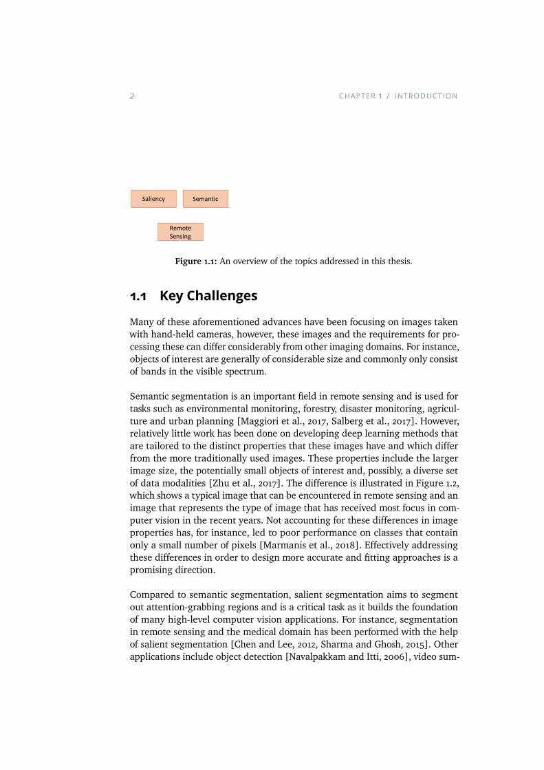
in Figure 1.1 to guide the reader.
1
2 C H A P TE R 1 I N T R O D U C T I O N
Saliency Semantic
Remote
SensingMedical
Domain
Adaptation
Representation
LearningClustering
Zero-shot
Learning
Segmentation Unsupervised
Deep Learning
Figure 1.1: An overview of the topics addressed in this thesis.
1.1 Key Challenges
Many of these aforementioned advances have been focusing on images taken
with hand-held cameras, however, these images and the requirements for pro-
cessing these can differ considerably from other imaging domains. For instance,
objects of interest are generally of considerable size and commonly only consist
of bands in the visible spectrum.
Semantic segmentation is an important field in remote sensing and is used for
tasks such as environmental monitoring, forestry, disaster monitoring, agricul-
ture and urban planning [Maggiori et al., 2017, Salberg et al., 2017]. However,
relatively little work has been done on developing deep learning methods that
are tailored to the distinct properties that these images have and which differ
from the more traditionally used images. These properties include the larger
image size, the potentially small objects of interest and, possibly, a diverse set
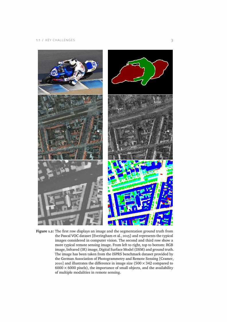
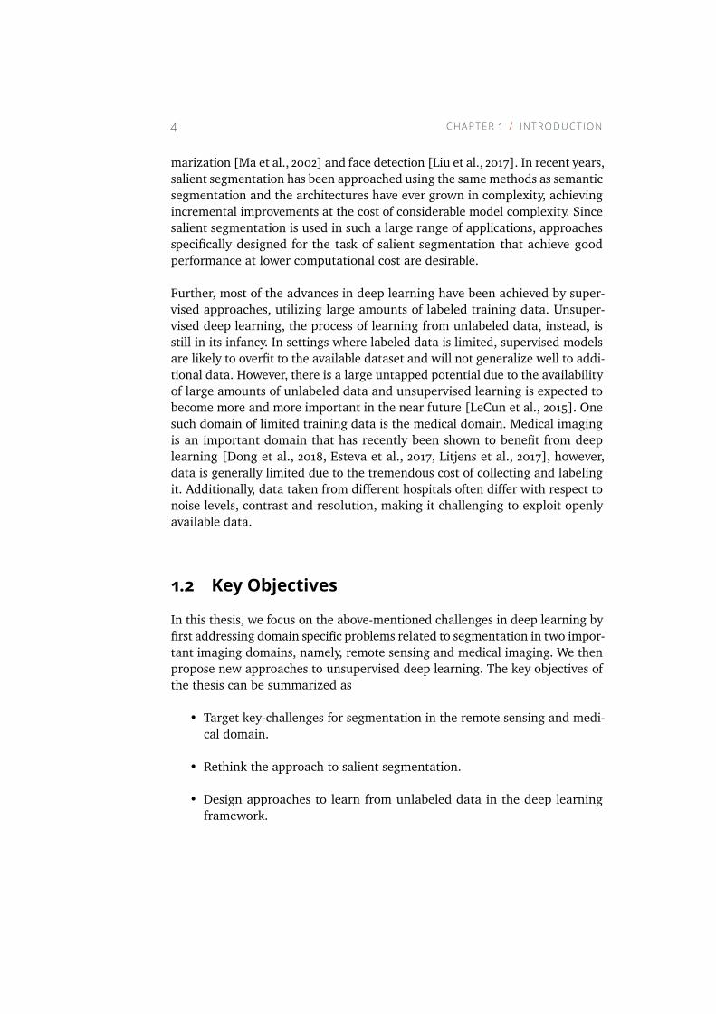
of data modalities [Zhu et al., 2017]. The difference is illustrated in Figure 1.2,
which shows a typical image that can be encountered in remote sensing and an
image that represents the type of image that has received most focus in com-
puter vision in the recent years. Not accounting for these differences in image
properties has, for instance, led to poor performance on classes that contain
only a small number of pixels [Marmanis et al., 2018]. Effectively addressing
these differences in order to design more accurate and fitting approaches is a
promising direction.
Compared to semantic segmentation, salient segmentation aims to segment
out attention-grabbing regions and is a critical task as it builds the foundation
of many high-level computer vision applications. For instance, segmentation
in remote sensing and the medical domain has been performed with the help
of salient segmentation [Chen and Lee, 2012, Sharma and Ghosh, 2015]. Other
applications include object detection [Navalpakkam and Itti, 2006], video sum-
1.1 K E Y C H A L L E N GE S 3
Figure 1.2: The first row displays an image and the segmentation ground truth from
the Pascal VOC dataset [Everingham et al., 2015] and represents the typical
images considered in computer vision. The second and third row show a
more typical remote sensing image. From left to right, top to bottom: RGB
image, Infrared (IR) image, Digital Surface Model (DSM) and ground truth.
The image has been taken from the ISPRS benchmark dataset provided by
the German Association of Photogrammetry and Remote Sensing [Cramer,
2010] and illustrates the difference in image size (500 × 342 compared to
6000 × 6000 pixels), the importance of small objects, and the availability
of multiple modalities in remote sensing.
4 C H A P TE R 1 I N T R O D U C T I O N
marization [Ma et al., 2002] and face detection [Liu et al., 2017]. In recent years,
salient segmentation has been approached using the same methods as semantic
segmentation and the architectures have ever grown in complexity, achieving
incremental improvements at the cost of considerable model complexity. Since
salient segmentation is used in such a large range of applications, approaches
specifically designed for the task of salient segmentation that achieve good
performance at lower computational cost are desirable.
Further, most of the advances in deep learning have been achieved by super-
vised approaches, utilizing large amounts of labeled training data. Unsuper-
vised deep learning, the process of learning from unlabeled data, instead, is
still in its infancy. In settings where labeled data is limited, supervised models
are likely to overfit to the available dataset and will not generalize well to addi-
tional data. However, there is a large untapped potential due to the availability
of large amounts of unlabeled data and unsupervised learning is expected to
become more and more important in the near future [LeCun et al., 2015]. One
such domain of limited training data is the medical domain. Medical imaging
is an important domain that has recently been shown to benefit from deep
learning [Dong et al., 2018, Esteva et al., 2017, Litjens et al., 2017], however,
data is generally limited due to the tremendous cost of collecting and labeling
it. Additionally, data taken from different hospitals often differ with respect to
noise levels, contrast and resolution, making it challenging to exploit openly
available data.
1.2 Key Objectives
In this thesis, we focus on the above-mentioned challenges in deep learning by
first addressing domain specific problems related to segmentation in two impor-
tant imaging domains, namely, remote sensing and medical imaging. We then
propose new approaches to unsupervised deep learning. The key objectives of
the thesis can be summarized as
• Target key-challenges for segmentation in the remote sensing and medi-
cal domain.
• Rethink the approach to salient segmentation.
• Design approaches to learn from unlabeled data in the deep learning
framework.
1.3 K E Y S O LU T I O N S 5
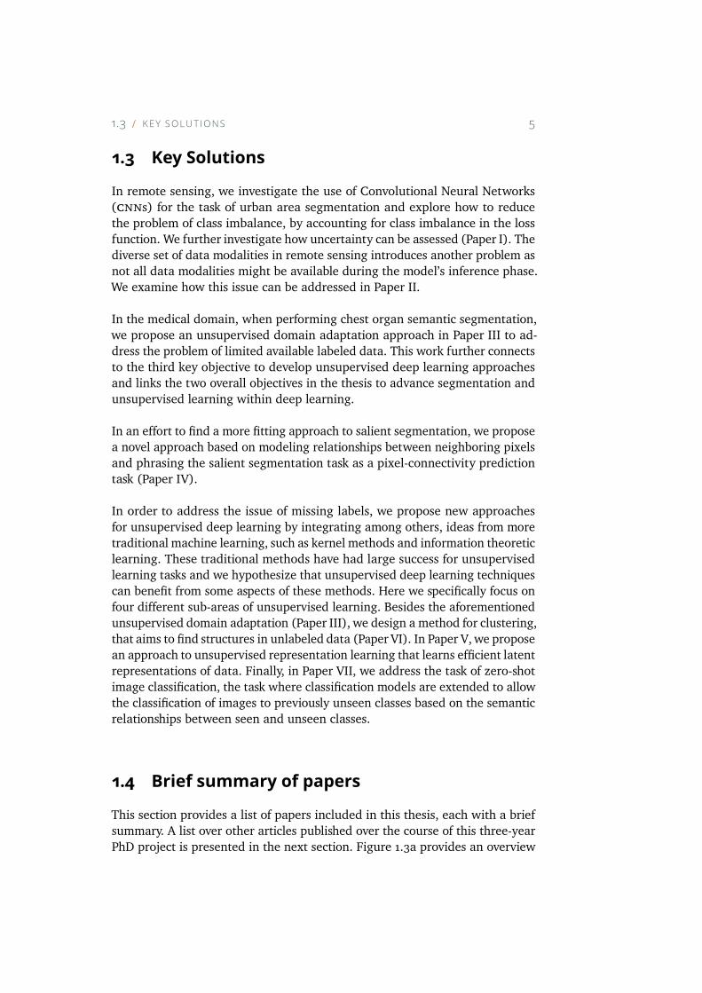
1.3 Key Solutions
In remote sensing, we investigate the use of Convolutional Neural Networks
(cnns) for the task of urban area segmentation and explore how to reduce
the problem of class imbalance, by accounting for class imbalance in the loss
function. We further investigate how uncertainty can be assessed (Paper I). The
diverse set of data modalities in remote sensing introduces another problem as
not all data modalities might be available during the model’s inference phase.
We examine how this issue can be addressed in Paper II.
In the medical domain, when performing chest organ semantic segmentation,
we propose an unsupervised domain adaptation approach in Paper III to ad-
dress the problem of limited available labeled data. This work further connects
to the third key objective to develop unsupervised deep learning approaches
and links the two overall objectives in the thesis to advance segmentation and
unsupervised learning within deep learning.
In an effort to find a more fitting approach to salient segmentation, we propose
a novel approach based on modeling relationships between neighboring pixels
and phrasing the salient segmentation task as a pixel-connectivity prediction
task (Paper IV).
In order to address the issue of missing labels, we propose new approaches
for unsupervised deep learning by integrating among others, ideas from more
traditional machine learning, such as kernel methods and information theoretic
learning. These traditional methods have had large success for unsupervised
learning tasks and we hypothesize that unsupervised deep learning techniques
can benefit from some aspects of these methods. Here we specifically focus on
four different sub-areas of unsupervised learning. Besides the aforementioned
unsupervised domain adaptation (Paper III), we design a method for clustering,
that aims to find structures in unlabeled data (Paper VI). In Paper V,we propose
an approach to unsupervised representation learning that learns efficient latent
representations of data. Finally, in Paper VII, we address the task of zero-shot
image classification, the task where classification models are extended to allow
the classification of images to previously unseen classes based on the semantic
relationships between seen and unseen classes.
1.4 Brief summary of papers
This section provides a list of papers included in this thesis, each with a brief
summary. A list over other articles published over the course of this three-year
PhD project is presented in the next section. Figure 1.3a provides an overview
6 C H A P TE R 1 I N T R O D U C T I O N
Deep Learning
Segm
entation
(1)
(2)
(4)
(3)
(5)
(6)
(7)
(15)
(9)
(17)
(11)
(12)
(13)(14)
(10)
(16)
(8)
(18) (22)
(21)
(19)
(23)Unsuperv
ised
(20)
(a) Overview of papers
Segmentation
Unsupervised
Clustering
Zero Shot
Learning
Semantic
Saliency
Remote
Sensing
Medical
(3)
(5)
(6)
(7)
(4)
(2)
(1)
Representation
Learning
Domain
Adaptation
(b) Included paper hierarchy
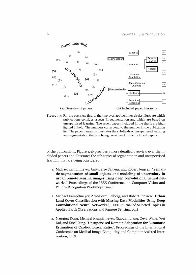
Figure 1.3: For the overview figure, the two overlapping inner circles illustrate which
publications consider aspects in segmentation and which are based on
unsupervised learning. The seven papers included in the thesis are high-
lighted in bold. The numbers correspond to the number in the publication
list. The paper hierarchy illustrates the sub-fields of unsupervised learning
and segmentation that are being considered in the included papers.
of the publications. Figure 1.3b provides a more detailed overview over the in-
cluded papers and illustrates the sub-topics of segmentation and unsupervised
learning that are being considered.
1. Michael Kampffmeyer, Arnt-Børre Salberg, and Robert Jenssen. "Seman-
tic segmentation of small objects and modeling of uncertainty in
urban remote sensing images using deep convolutional neural net-
works." Proceedings of the IEEE Conference on Computer Vision and
Pattern Recognition Workshops, 2016.
2. Michael Kampffmeyer, Arnt-Børre Salberg, and Robert Jenssen. "Urban
Land Cover Classification with Missing Data Modalities Using Deep
Convolutional Neural Networks.", IEEE Journal of Selected Topics in
Applied Earth Observations and Remote Sensing, 2018.
3. Nanqing Dong, Michael Kampffmeyer, Xiaodan Liang, Zeya Wang, Wei
Dai, and Eric P. Xing. "Unsupervised Domain Adaptation for Automatic
Estimation of Cardiothoracic Ratio.", Proceedings of the International
Conference on Medical Image Computing and Computer Assisted Inter-
vention, 2018.
1.4 B R I E F S U M M A R Y O F PA P E R S 7
4. Michael Kampffmeyer, Nanqing Dong, Xiaodan Liang, Yujia Zhang,
and Eric P. Xing. "ConnNet: A Long-Range Relation-Aware Pixel-
Connectivity Network for Salient Segmentation." arXiv preprint
arXiv:1804.07836, 2018 (submitted to IEEE Transactions on Image
Processing).
5. Michael Kampffmeyer, Sigurd Løkse, Filippo M Bianchi, Robert Jenssen,
and Lorenzo Livi. "The Deep Kernelized Autoencoder.", Applied Soft
Computing, 2018.
6. Michael Kampffmeyer, Sigurd Løkse, Filippo M Bianchi, Lorenzo Livi,
Arnt-Børre Salberg, and Robert Jenssen. "Deep Divergence-Based Ap-
proach to Clustering.", submitted to Neural Networks.
7. Michael Kampffmeyer, Yinbo Chen, Xiaodan Liang, Hao Wang, Yujia
Zhang, and Eric P. Xing. "Rethinking Knowledge Graph Propaga-
tion for Zero-Shot Learning." arXiv preprint arXiv:1805.11724, 2018
(submitted to Neural Information Processing Systems 2018).
Paper I and II: Consider semantic segmentation in remote sensing. Paper I com-
pares so-called patch-based approaches with fully convolutional approaches,
proposes the use of a class balanced cost function to address the class imbal-
ance problem, and investigates the use of uncertainty modeling for urban land
cover classification in remote sensing. Paper II instead addresses the problem
of missing data modalities. As many approaches make use of data-fusion to
improve overall accuracy, this raises the question of what can be done when
certain data modalities are missing during testing. We illustrate a possible solu-
tion for situations where multiple or a single modality are completely missing
or only missing for a few images during testing.
Paper III: Proposes a method to perform unsupervised domain adaptation for
estimation of the cardiothoracic ratio, a key indicator for cardiomegaly (heart
enlargement), which is associated with a high risk of sudden cardiac death. We
address the fact that labeled training data is difficult and expensive to obtain,
and the fact that data from different hospitals exhibit differences in noise lev-
els, contrast, and resolution. Based on adversarial learning, an unsupervised
approach is proposed that can be trained with data from one hospital and still
provides good performance on data from another hospital. We further illustrate
that the method can also be used for semi-supervised learning.
Paper IV: Presents a new approach to salient segmentation, segmentation
of the attention-grabbing objects in an image. Unlike recent state-of-the-art
approaches, who approach this task as a binary segmentation task (foreground
vs. background segmentation) and make network architectures more and more
8 C H A P TE R 1 I N T R O D U C T I O N
complicated, the problem is rephrased as a connectivity prediction problem.
This allows for better performance with a simpler model.
Paper V: Develops a deep kernelized auto-encoder architecture that incorpo-
rates a kernel-alignment based regularization term. Efficient data representa-
tions can be learned by exploiting the similarity between data in the input
space and we illustrate that the deep kernelized autoencoder achieves promis-
ing results. It further, introduces a link between kernel methods and deep
learning.
Paper VI: Incorporates more traditional machine learning techniques such
as kernel methods and information theoretic learning into deep learning. It
proposes an unsupervised deep architecture that achieved state-of-the-art clus-
tering results on challenging problems. The commonly used supervised loss
function is replaced by an information theoretic divergence unsupervised loss
function that finds the underlying structures (clusters) in data by enforcing
separation between clusters and compactness within clusters.
Paper VII: This paper focuses on zero-shot learning. Based on recent develop-
ments in the field of Graph Convolutional Neural Networks (gcns), we propose
an Attentive Dense Graph PropagationModule that allows us to achieve state-of-
the-art performance on large-scale zero-shot datasets by exploiting knowledge
graph information.
1.5 Other papers
8. Jonas N Myhre, Michael Kampffmeyer, and Robert Jenssen. "Ambient
space manifold learning using density ridges.", Geometry in Machine
Learning Workshop, International Conference on Machine Learning,
2016.
9. Filippo Maria Bianchi, Michael Kampffmeyer, Enrico Maiorino, and
Robert Jenssen. "Temporal Overdrive Recurrent Neural Network.",
2017 International Joint Conference on Neural Networks, 2017.
10. Jonas N. Myhre, Michael Kampffmeyer, and Robert Jenssen. "Density
ridge manifold traversal.", 2017 IEEE International Conference on
Acoustics, Speech and Signal Processing, 2017.
11. Michael Kampffmeyer, Sigurd Løkse, Filippo M Bianchi, Robert Jenssen,
and Lorenzo Livi. "Deep Kernelized Autoencoders." Scandinavian Con-
ference on Image Analysis. Springer, 2017.
1.5 OT H E R PA P E R S 9
12. Arnt-Børre Salberg, Øivind Due Trier, and Michael Kampffmeyer. "Large-
Scale Mapping of Small Roads in Lidar Images Using Deep Convolu-
tional Neural Networks." Scandinavian Conference on Image Analysis.
Springer, 2017.
13. Michael Kampffmeyer, Arnt-Børre Salberg, and Robert Jenssen. "Urban
Land Cover Classification with Missing Data Using Deep Convolu-
tional Neural Networks.", IEEE International Geoscience and Remote
Sensing Symposium, 2017.
14. Michael Kampffmeyer, Sigurd Løkse, Filippo M Bianchi, Lorenzo Livi,
Arnt-Børre Salberg, and Robert Jenssen. "Deep Divergence-based Clus-
tering.", IEEE International Workshop on Machine Learning for Signal
Processing, 2017.
15. Filippo Maria Bianchi, Enrico Maiorino, Michael Kampffmeyer, Antonello
Rizzi, and Robert Jenssen. "Recurrent Neural Networks for Short-Term
Load Forecasting An Overview and Comparative Analysis.", Springer-
Briefs in Computer Science, 2017.
16. Andreas S Strauman, Filippo M Bianchi, Karl Øyvind Mikalsen, Michael
Kampffmeyer,Cristina Soguero-Ruiz, andRobert Jenssen. "Classification
of postoperative surgical site infections from blood measurements
with missing data using recurrent neural networks.", IEEE Interna-
tional Conference on Biomedical and Health Informatics, 2018.
17. Mads A Hansen, Karl Øyvind Mikalsen, Michael Kampffmeyer, Cristina
Soguero-Ruiz, and Robert Jenssen. "Towards Deep Anchor Learning.",
IEEE International Conference on Biomedical and Health Informatics,
2018.
18. Yujia Zhang, Michael Kampffmeyer, Xiaodan Liang, Min Tan, and Eric
P. Xing. "Query-Conditioned Three-Player Adversarial Network for
Video Summarization.", British Machine Vision Conference, 2018.
19. Kristoffer Knutsen Wickstrøm,Michael Kampffmeyer, and Robert Jenssen.
"Uncertainty Modeling And Interpretability In Convolutional Neural
Networks For Polyp Segmentation.", IEEE International Workshop on
Machine Learning for Signal Processing, 2018.
20. Nanqing Dong, Michael Kampffmeyer, Xiaodan Liang, Zeya Wang, Wei
Dai, and Eric P. Xing. "Reinforced Auto-Zoom Net: Towards Accurate
and Fast Breast Cancer Segmentation in Whole-slide Images.", Pro-
ceedings of the 4th Workshop on Deep Learning in Medical Image Anal-
10 C H A P TE R 1 I N T R O D U C T I O N
ysis, 2018.
21. Filippo Maria Bianchi, Lorenzo Livi, Karl Øyvind Mikalsen, Michael
Kampffmeyer, and Robert Jenssen. "Learning representations for mul-
tivariate time series with missing data using Temporal Kernelized
Autoencoders.", arXiv preprint arXiv:1805.03473, 2018 (submitted to
Neural Networks).
22. Yujia Zhang, Michael Kampffmeyer, Xiaodan Liang, Dingwen Zhang,
Min Tan, and Eric P. Xing. "DTR-GAN: Dilated Temporal Relational
Adversarial Network for Video Summarization.", arXiv preprint
arXiv:1804.11228, 2018 (submitted to IEEE Transactions on Image
Processing).
23. Rogelio Andrade Mancisidor, Michael Kampffmeyer, Kjersti Aas, and
Robert Jenssen. "Segment-Based Credit Scoring Using Latent Clus-
ters in the Variational Autoencoder.", arXiv preprint arXiv:1806.02538,
2018 (submitted to Information Sciences).
1.6 Reading guide
The thesis is organized into three parts,methodology, summary of research, and
included papers.
The methodology part provides the theoretical background for the research pre-
sented in this thesis. Chapter 2 provides a short overview of deep learning and
introduces Convolutional Neural Networks, Graph Convolutional Networks, Au-
toencoders, and Generative Adversarial Networks and is relevant background
material for all papers. Chapter 3 introduces the tasks of semantic segmentation
and salient segmentation and presents how these tasks are addressed using
deep learning. This is relevant for Papers I-IV. Chapter 4 introduces unsuper-
vised learning, briefly summarizing the tasks of clustering, domain adaptation,
representation learning, and zero-shot learning and is relevant for Paper III and
Papers V-VII. Finally, Chapter 5 provides background on kernel methods and
information theoretic learning, which is relevant for Papers V and VI.
The summary of research part provides a short overview of the scientific contri-
bution of each paper in this thesis as well as concluding remarks and a discus-
sion of future directions. Research papers are included in the included papers
part.
Part I
Methodology and context
11
2Deep Learning
Deep learning techniques can today be encountered in many everyday appli-
cations ranging from speech and handwritten character recognition to various
image and object detection tasks. They are representation-learning techniques,
accepting raw data as input and being trained to discover useful features, in-
stead of relying on hand-tuned feature extractors. Deep learning architectures
consist of multiple layers, each consisting of simple modules that are subject to
learning, and learn representations, each layer yielding a slightly more abstract
and "useful" representation.
The idea of learning representations has been around since the late 1950’s,when
the perceptron algorithm was proposed by Frank Rosenblatt and led to the rise
of many perceptron based methods, however, it initially only delivered minor
successes [Rosenblatt, 1958]. In 1969 Minsky and Papert demonstrated that a
perceptron is not able to solve simple non-linear problems such as the XOR
problem, and argued the fact that computational resources, as well as effective
training procedures for large multi-layer networks, did not exist [Minsky and
Seymour, 1969]. This led to a drought in the field of neural networks until an
effective algorithm, the backpropagation algorithm, for training these networks
using stochastic gradient descent was independently discovered by multiple
research groups between 1974 and 1986 [LeCun et al., 2015]. Backpropagation
computes the gradient of the objective function with respect to all weights
and uses this gradient to update the weights in all layers using one of several
proposed gradient descent approaches.
13
14 C H A P TE R 2 D E E P L E A R N I N G
After minor successes of shallow neural networks with backpropagation on,
among others, handwritten digit recognition tasks using a technique called
Convolutional Neural Networks (cnns), most researchers forsake neural
networks for more successful methods, such as the Support Vector Machines
(svms) [Boser et al., 1992] and Random Forests [Ho, 1995]. Neural networks
appeared to commonly get trapped in local minima, thus yielding weight
configurations that on a local scale of the loss surface achieve a minimum,
but on the global scale are far from optimal. Recent results by Dauphin et al.
[2014] and Choromanska et al. [2014] suggest that this might have been a
misconception and that the loss surface in deep neural networks generally
consists mainly of bad saddle-points, as most local minima in large networks
lie close to the global minima. Another problem of neural networks was
the vanishing and exploding gradient problem, where the gradient either
diminishes or explodes as it propagates through the network as part of
backpropagation.
First in 2006, the interest in deep neural network architectures was restored
by the development of unsupervised learning techniques that could be used
to effectively pretrain deep networks. These techniques can be divided into
two main classes, probabilistic models, the most prominent of these methods
being the Restricted Boltzmann Machines (rbms) [Hinton, 2002, Smolensky,
1986] and the Variational Autoencoders (vaes) [Kingma and Welling, 2014],
and methods that directly learn a parametric mapping from the input to the
representation, such as autoencoders [Ballard, 1987, Vincent et al., 2010]. To-
gether with the pretraining idea, advances of fast and programmable Graphics
Processing Units (gpus), larger available datasets, as well as some general
techniques to the neural network concept that addressed gradient propaga-
tion issues, they led to deep neural networks beating state-of-the-art results on
speech recognition tasks [Dahl et al., 2012, Mohamed et al., 2012]. Already in
2012 speech recognition systems based on neural networks were deployed to
consumers (e.g. android mobile phones) [LeCun et al., 2015].
In 2012 another breakthrough happened when a cnnwith≈ 60 million weights
won the ImageNet competition, in which a training set of ≈1.2 million images
containing 1000 classes had to be used to train an image classifier [Krizhevsky
et al., 2012]. Since then cnns have been widely adopted and are now the
dominant approach for most image and object recognition tasks.
In this chapter, we briefly review the deep learning approaches that provide
the backbone of this thesis.
2.1 F U L LY CO N N E C T E D N E U R A L N E T WO R K S 15
2.1 Fully Connected Neural Networks
Fully Connected Neural Networks or Multilayer Perceptrons (mlps), represent
the general foundation of the deep learning architectures and methods pre-
sented in this thesis. They consist of a composition of many simple mappings
and transformations, which are hierarchically organized in several layers. This
allows the modeling of arbitrary complex deterministic functions.
In this section, we will limit our discussion of mlps to the task of supervised
classification. In supervised learning the learning problem can be defined as
follows: given an input space X , an output space Y and a data distribution DoverX ×Y that contains the data that is being observed, the learning procedure
attempts to find a function f : X → Y that minimizes a loss function L(f (x),y).In classification, the loss function quantifies how well the network is able to
map x to class y. In machine learning the optimization problem generally
involves a finite dataset of D = {(x i ,yi ) i = 1, ...,N } that is used to train the
model. Here, (x i ,yi ) corresponds to the ith training sample of data distribution
D. The objective is to learn a function that minimizes the loss, but at the same
time and more importantly generalizes well to a new set of previously unseen
data points drawn from D.
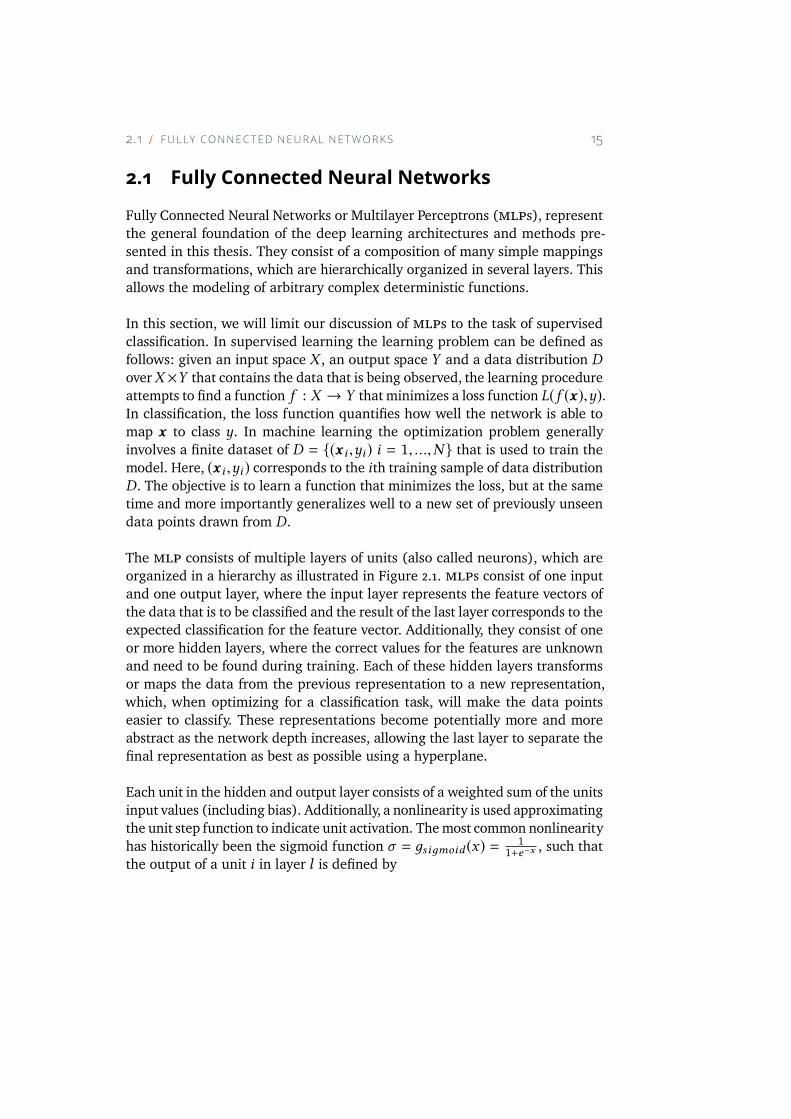
The mlp consists of multiple layers of units (also called neurons), which are
organized in a hierarchy as illustrated in Figure 2.1. mlps consist of one input
and one output layer, where the input layer represents the feature vectors of
the data that is to be classified and the result of the last layer corresponds to the
expected classification for the feature vector. Additionally, they consist of one
or more hidden layers, where the correct values for the features are unknown
and need to be found during training. Each of these hidden layers transforms
or maps the data from the previous representation to a new representation,
which, when optimizing for a classification task, will make the data points
easier to classify. These representations become potentially more and more
abstract as the network depth increases, allowing the last layer to separate the
final representation as best as possible using a hyperplane.
Each unit in the hidden and output layer consists of a weighted sum of the units
input values (including bias). Additionally, a nonlinearity is used approximating
the unit step function to indicate unit activation. Themost common nonlinearity
has historically been the sigmoid function σ = дsiдmoid (x) =1
1+e−x, such that
the output of a unit i in layer l is defined by
16 C H A P TE R 2 D E E P L E A R N I N G
Input
Hidden
Output
. . .
Figure 2.1: The figure displays an example architecture of a mlp with three input
units and four output neurons.
yli = σ (bli +
N∑
j=1
w li jy
l−1j ) , (2.1)
where bi is the bias term, wi j is the weight between layer input yl−1j and
layer output yli . However, in recent years the nonlinearity has been to a large
extent replaced by Rectified Linear Units (relus) [Glorot et al., 2011], which
have more preferable properties when training mlps with a larger number
of hidden layers. The relu is defined as дReLU (x) = max(0,x) leading to
sparse activation patterns and better gradient flow [Glorot et al., 2011]. In the
classification setting, the final layer, commonly makes use of a softmax layer.
The softmax function, дSof tmax (x)j =exj
∑Kk=1
exk, squashes the values of the
output neurons into the range (0,1) and ensures that they sum up to 1.
A common loss function L that is often used in classification settings is the
cross-entropy loss function
L = −1
N
N∑
i=1
K∑
k=1
yki log yki (2.2)
where N corresponds to the number of data points, K to the number of output
neurons, yki to the estimate of the model andyki to the label of the ith datapoint
for the kth output neuron.
Training is performed by minimizing the loss function using a form of gra-
dient descent. For brevity, we limit ourselves to discuss Stochastic Gradient
Descent (sgd), however, in recent years a multitude of alternative gradient-
based optimization techniques such as ADAM [Kingma and Ba, 2015] and ADA-
GRAD [Duchi et al., 2011] have been proposed. sgd evaluates the derivatives
2.1 F U L LY CO N N E C T E D N E U R A L N E T WO R K S 17
Dropout. . .
Input
Hidden
Output
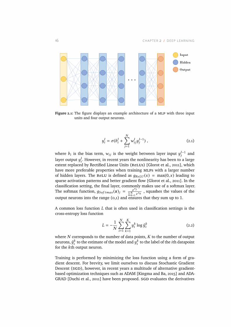
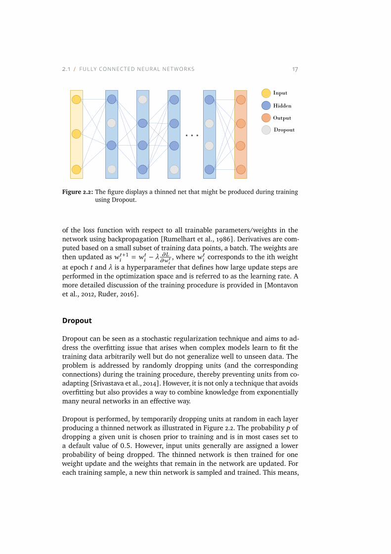
Figure 2.2: The figure displays a thinned net that might be produced during training
using Dropout.
of the loss function with respect to all trainable parameters/weights in the
network using backpropagation [Rumelhart et al., 1986]. Derivatives are com-
puted based on a small subset of training data points, a batch. The weights are
then updated as wt+1i = wt
i − λ∂L∂w t
i
, where wti corresponds to the ith weight
at epoch t and λ is a hyperparameter that defines how large update steps are
performed in the optimization space and is referred to as the learning rate. A
more detailed discussion of the training procedure is provided in [Montavon
et al., 2012, Ruder, 2016].
Dropout
Dropout can be seen as a stochastic regularization technique and aims to ad-
dress the overfitting issue that arises when complex models learn to fit the
training data arbitrarily well but do not generalize well to unseen data. The
problem is addressed by randomly dropping units (and the corresponding
connections) during the training procedure, thereby preventing units from co-
adapting [Srivastava et al., 2014]. However, it is not only a technique that avoids
overfitting but also provides a way to combine knowledge from exponentially
many neural networks in an effective way.
Dropout is performed, by temporarily dropping units at random in each layer
producing a thinned network as illustrated in Figure 2.2. The probability p of
dropping a given unit is chosen prior to training and is in most cases set to
a default value of 0.5. However, input units generally are assigned a lower
probability of being dropped. The thinned network is then trained for one
weight update and the weights that remain in the network are updated. For
each training sample, a new thin network is sampled and trained. This means,
18 C H A P TE R 2 D E E P L E A R N I N G
that each unique network (for n units in the network there are 2n possible
networks) is rarely trained, however, training progresses since all the networks
share the same set of weights.
Computing predictions from all the thin networks is infeasible at test phase,
which instead averages all the prediction of the thinned networks in a single
un-thinned network. This is done by scaling the learned training weights such
thatW(l )test = pW
(l )train
by multiplying them with the drop-probability p.
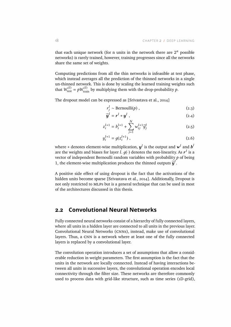
The dropout model can be expressed as [Srivastava et al., 2014]
r lj ∼ Bernoulli(p) , (2.3)
yl= r l ∗yl , (2.4)
zl+1i = bl+1i +
N∑
j=1
w l+1i j ylj (2.5)
yl+1i = д(zl+1i ) , (2.6)
where ∗ denotes element-wise multiplication, yl is the output and w l and bl
are the weights and biases for layer l . д(·) denotes the non-linearity. As r l is avector of independent Bernoulli random variables with probability p of being
1, the element-wise multiplication produces the thinned outputs yl.
A positive side effect of using dropout is the fact that the activations of the
hidden units become sparse [Srivastava et al., 2014]. Additionally, Dropout is
not only restricted to mlps but is a general technique that can be used in most
of the architectures discussed in this thesis.
2.2 Convolutional Neural Networks
Fully connected neural networks consist of a hierarchy of fully connected layers,
where all units in a hidden layer are connected to all units in the previous layer.
Convolutional Neural Networks (cnns), instead, make use of convolutional
layers. Thus, a cnn is a network where at least one of the fully connected
layers is replaced by a convolutional layer.
The convolution operation introduces a set of assumptions that allow a consid-
erable reduction in weight parameters. The first assumption is the fact that the
units in the network are locally connected. Instead of having interactions be-
tween all units in successive layers, the convolutional operation encodes local
connectivity through the filter size. These networks are therefore commonly
used to process data with grid-like structure, such as time series (1D-grid),
2.2 CO N VO LU T I O N A L N E U R A L N E TWO R K S 19
1 2 1
0 0 0
-1 -2 -1
Convolution
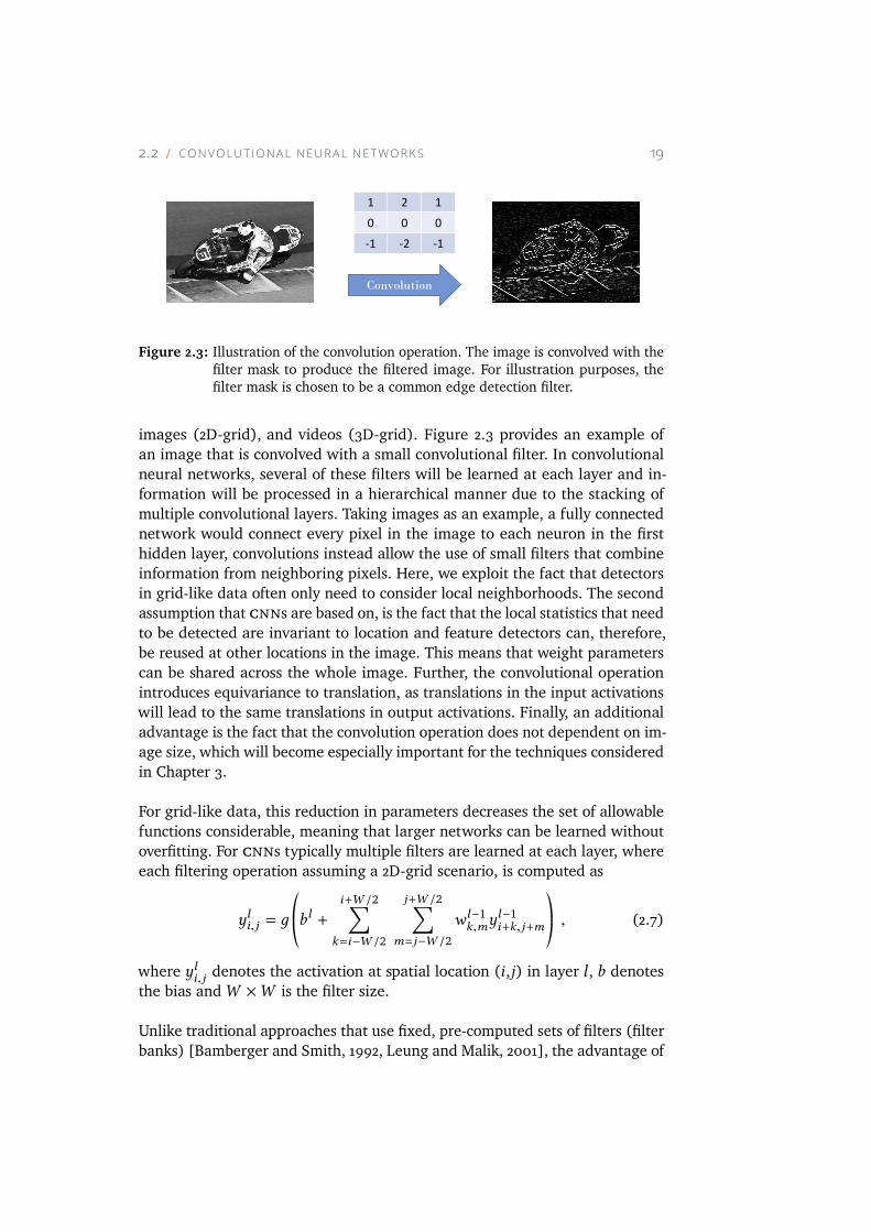
Figure 2.3: Illustration of the convolution operation. The image is convolved with the
filter mask to produce the filtered image. For illustration purposes, the
filter mask is chosen to be a common edge detection filter.
images (2D-grid), and videos (3D-grid). Figure 2.3 provides an example of
an image that is convolved with a small convolutional filter. In convolutional
neural networks, several of these filters will be learned at each layer and in-
formation will be processed in a hierarchical manner due to the stacking of
multiple convolutional layers. Taking images as an example, a fully connected
network would connect every pixel in the image to each neuron in the first
hidden layer, convolutions instead allow the use of small filters that combine
information from neighboring pixels. Here, we exploit the fact that detectors
in grid-like data often only need to consider local neighborhoods. The second
assumption that cnns are based on, is the fact that the local statistics that need
to be detected are invariant to location and feature detectors can, therefore,
be reused at other locations in the image. This means that weight parameters
can be shared across the whole image. Further, the convolutional operation
introduces equivariance to translation, as translations in the input activations
will lead to the same translations in output activations. Finally, an additional
advantage is the fact that the convolution operation does not dependent on im-
age size, which will become especially important for the techniques considered
in Chapter 3.
For grid-like data, this reduction in parameters decreases the set of allowable
functions considerable, meaning that larger networks can be learned without
overfitting. For cnns typically multiple filters are learned at each layer, where
each filtering operation assuming a 2D-grid scenario, is computed as
yli,j = д*.,bl +
i+W /2∑
k=i−W /2
j+W /2∑
m=j−W /2
w l−1k,my
l−1i+k,j+m
+/-, (2.7)
where yli,j denotes the activation at spatial location (i,j) in layer l , b denotes
the bias andW ×W is the filter size.
Unlike traditional approaches that use fixed, pre-computed sets of filters (filter
banks) [Bamberger and Smith, 1992, Leung and Malik, 2001], the advantage of
20 C H A P TE R 2 D E E P L E A R N I N G
Max Pooling
1 4
3 0
2 6
85
1522
2419
9
4 8
5
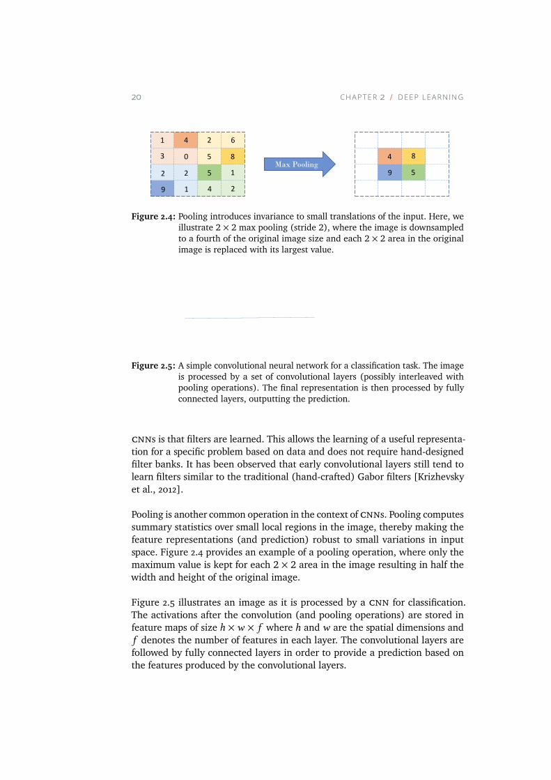
Figure 2.4: Pooling introduces invariance to small translations of the input. Here, we
illustrate 2 × 2 max pooling (stride 2), where the image is downsampled
to a fourth of the original image size and each 2 × 2 area in the original
image is replaced with its largest value.
Prediction:Plane
Feature maps afterconvolutional layers
Feature vectors afterfully connected layers
Figure 2.5: A simple convolutional neural network for a classification task. The image
is processed by a set of convolutional layers (possibly interleaved with
pooling operations). The final representation is then processed by fully
connected layers, outputting the prediction.
cnns is that filters are learned. This allows the learning of a useful representa-
tion for a specific problem based on data and does not require hand-designed
filter banks. It has been observed that early convolutional layers still tend to
learn filters similar to the traditional (hand-crafted) Gabor filters [Krizhevsky
et al., 2012].
Pooling is another common operation in the context of cnns. Pooling computes
summary statistics over small local regions in the image, thereby making the
feature representations (and prediction) robust to small variations in input
space. Figure 2.4 provides an example of a pooling operation, where only the
maximum value is kept for each 2 × 2 area in the image resulting in half the
width and height of the original image.
Figure 2.5 illustrates an image as it is processed by a cnn for classification.
The activations after the convolution (and pooling operations) are stored in
feature maps of size h ×w × f where h andw are the spatial dimensions and
f denotes the number of features in each layer. The convolutional layers are
followed by fully connected layers in order to provide a prediction based on
the features produced by the convolutional layers.
2.3 G R A P H CO N VO LU T I O N A L N E U R A L N E TWO R K S 21
2.3 Graph Convolutional Neural Networks
In recent years, Graph Convolutional Neural Networks (gcns) have been devel-
oped to process datasets that consist of graph structures. In many applications,
it is not convenient to consider data as vectorial or grid-structured data, but
instead, it is more natural to view them as graphs. Initial applications of gcns
have been among others processing of knowledge graphs, social networks, and
molecules [Duvenaud et al., 2015, Kipf and Welling, 2017]. Here, we will limit
the discussion to spectral gcns that were first proposed by Bruna et al. [2014].
More recently, Defferrard et al. [2016] improved scalability, by introducing fast
localized convolutions by expressing filters using Chebyshev polynomials, based
on work done by Hammond et al. [2011]. Simplifications were later introduced
by Kipf and Welling [2017] to further improve scalability. In this section, we
will follow the notation of Kipf and Welling [2017] to briefly summarize the
idea behind gcns.
Convolutions of a signal x ∈ RN with a spectral filter дθ = diag(θ ) can be
expressed as a multiplication in the Fourier domain
дθ ⋆x = UдθUTx . (2.8)
Here, the orthogonal matrix U corresponds to the eigenvector matrix of the
normalized graph Laplacian L = IN − D−12AD−
12 = UΛUT and UTx is the
graph Fourier transform of the signal x . IN is the identity matrix,A ∈ RN×N is
the adjacency matrix, D ∈ RN×N is the degree matrix, and Λ is the diagonal
matrix formed from the eigenvalues of the normalized graph Laplacian. дθis a function of Λ. In order to avoid the eigenvalue decomposition and the
costly matrix multiplications Hammond et al. [2011] showed that a truncated
Chebyshev polynomial expansion of the filter дθ (Λ) is a good approximation.
This means that
д′θ (Λ) ≈
K∑
k=0
θ ′kTk (Λ) , (2.9)
where Tk (Λ) denotes the Chebyshev polynomial of kth order of the scaled
eigenvalues Λ = 2Λλmax− IN and λmax is the largest eigenvalue of the normal-
ized graph Laplacian L. The Chebyshev polynomials are computed as Tk (y) =2yTk−1(y) − Tk−2(y), with T0 = 1 and T1 = y. θ ′ ∈ RN are the Chebyshev
coefficients.
Combining this with Equation 2.8, the spectral convolution on the graph can
be defined as
д′θ ⋆x ≈ U
K∑
k=0
θ ′kTk (Λ)UTx . (2.10)
22 C H A P TE R 2 D E E P L E A R N I N G
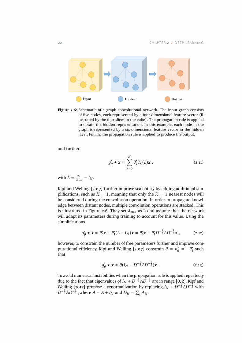
Input Hidden Output
Figure 2.6: Schematic of a graph convolutional network. The input graph consists
of five nodes, each represented by a four-dimensional feature vector (il-
lustrated by the four slices in the cube). The propagation rule is applied
to obtain the hidden representation. In this example, each node in the
graph is represented by a six-dimensional feature vector in the hidden
layer. Finally, the propagation rule is applied to produce the output.
and further
д′θ ⋆x ≈
K∑
k=0
θ ′kTk (L)x , (2.11)
with L = 2Lλmax− IN .
Kipf and Welling [2017] further improve scalability by adding additional sim-
plifications, such as K = 1, meaning that only the K = 1 nearest nodes will
be considered during the convolution operation. In order to propagate knowl-
edge between distant nodes, multiple convolution operations are stacked. This
is illustrated in Figure 2.6. They set λmax as 2 and assume that the network
will adapt its parameters during training to account for this value. Using the
simplifications
д′θ ⋆x ≈ θ′0x + θ
′1(L − IN )x = θ
′0x + θ
′1D− 1
2AD−12x , (2.12)
however, to constrain the number of free parameters further and improve com-
putational efficiency, Kipf and Welling [2017] constrain θ = θ ′0 = −θ′1 such
that
д′θ ⋆x ≈ θ (IN + D− 1
2AD−12 )x . (2.13)
To avoid numerical instabilities when the propagation rule is applied repeatedly
due to the fact that eigenvalues of IN +D− 1
2AD−12 are in range [0,2], Kipf and
Welling [2017] propose a renormalization by replacing IN + D−12AD−
12 with
D−12 AD−
12 ,where A = A + IN and Dii =
∑
j Ai j .
2.4 A U TO E N CO D E R S 23
Hidden�� Output
�
Input��
Encoder Decoder
��
�
��
��
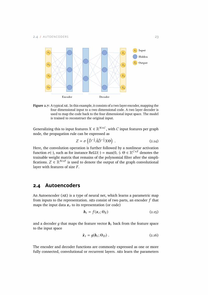
Figure 2.7: A typicalae. In this example, it consists of a two layer encoder,mapping the
four dimensional input to a two dimensional code. A two layer decoder is
used to map the code back to the four dimensional input space. The model
is trained to reconstruct the original input.
Generalizing this to input features X ∈ RN×C , withC input features per graph
node, the propagation rule can be expressed as
Z = σ(
D−12 AD−
12XΘ
)
. (2.14)
Here, the convolution operation is further followed by a nonlinear activation
function σ (·), such as for instance ReLU(·) = max(0, ·). Θ ∈ RC×F denotes the
trainable weight matrix that remains of the polynomial filter after the simpli-
fications. Z ∈ RN×F is used to denote the output of the graph convolutional
layer with features of size F .
2.4 Autoencoders
An Autoencoder (ae) is a type of neural net, which learns a parametric map
from inputs to the representation. aes consist of two parts, an encoder f that
maps the input data x t to its representation (or code)
ht = f (x t ;ΘE ) (2.15)
and a decoder д that maps the feature vector ht back from the feature space
to the input space
x t = д(ht ;ΘD ) . (2.16)
The encoder and decoder functions are commonly expressed as one or more
fully connected, convolutional or recurrent layers. aes learn the parameters
24 C H A P TE R 2 D E E P L E A R N I N G
ΘE and ΘD by optimizing the complete network for the task of reconstruction.
This means that the loss function is represented by a reconstruction error, a
qualitative measure of the difference between the input x t and its reconstruc-
tion x t for training example t . One natural choice of the reconstruction loss
function is the Mean Square Error (mse)
Lr =1
N
N∑
t=1
(x t − x t )2 , (2.17)
where N denotes the total number of training examples. Training the autoen-
coder to minimize the reconstruction loss can, from an information theoretic
standpoint, be interpreted as maximizing the lower bound on the mutual in-
formation between the input and the codes [Vincent et al., 2010]. This is a
meaningful criterion, as it ensures that as much as possible of the information
in the input space is retained in the code representation.
As the aim is to learn a good representation aes can not have a configuration
where the number of hidden units is larger than the number of input (and
output) units unless regularization techniques are employed. This is due to the
fact that the network would be able to learn the identity function, achieving
perfect reconstruction, but would not produce good representations. For non-
regularized aes, a bottleneck has historically been introduced (as seen in Figure
2.7), which forces the encoder to perform a dimensionality reduction.
aes are closely related to more traditional dimensionality reduction techniques
such as Principal Component Analysis (pca). It has been shown that for an
ae trained with a squared error objective and without non-linearities in the
encoder and decoder, the ae will map data to the same subspace as obtained
by pca [Baldi and Hornik, 1989]. ae with non-linearities such as the sigmoid
function can still learn the same subspace when keeping to the linear part of
the non-linear function, however, they are able to learn non-linear mappings
different from pca [Japkowicz et al., 2000].
In more recent years also other approaches have emerged that introduce regu-
larization to constrain the representation without necessarily requiring a bottle-
neck in the architecture. Some of the most prominentmethods will be discussed
in the following sections.
Denoising Auto-Encoders
One of these techniques is the Denoising Autoencoder (dae) [Vincent et al.,
2010], which changes the learning objective of the ae from reconstruction to
denoising of the input. This means that given an input that is corrupted by
2.4 A U TO E N CO D E R S 25
Input������
��
Hidden
Noise
Noisy Input
�� Output
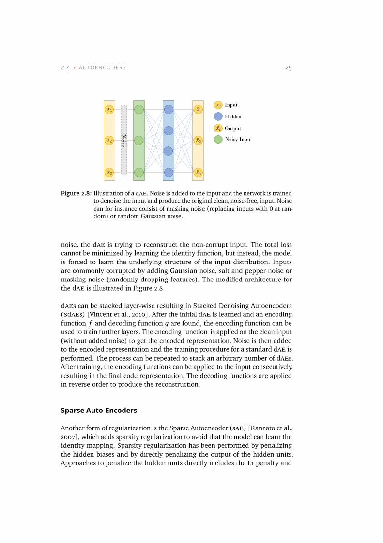
Figure 2.8: Illustration of a dae. Noise is added to the input and the network is trained
to denoise the input and produce the original clean, noise-free, input. Noise
can for instance consist of masking noise (replacing inputs with 0 at ran-
dom) or random Gaussian noise.
noise, the dae is trying to reconstruct the non-corrupt input. The total loss
cannot be minimized by learning the identity function, but instead, the model
is forced to learn the underlying structure of the input distribution. Inputs
are commonly corrupted by adding Gaussian noise, salt and pepper noise or
masking noise (randomly dropping features). The modified architecture for
the dae is illustrated in Figure 2.8.
daes can be stacked layer-wise resulting in Stacked Denoising Autoencoders
(sdaes) [Vincent et al., 2010]. After the initial dae is learned and an encoding
function f and decoding function д are found, the encoding function can be
used to train further layers. The encoding function is applied on the clean input
(without added noise) to get the encoded representation. Noise is then added
to the encoded representation and the training procedure for a standard dae is
performed. The process can be repeated to stack an arbitrary number of daes.
After training, the encoding functions can be applied to the input consecutively,
resulting in the final code representation. The decoding functions are applied
in reverse order to produce the reconstruction.
Sparse Auto-Encoders
Another form of regularization is the Sparse Autoencoder (sae) [Ranzato et al.,
2007], which adds sparsity regularization to avoid that the model can learn the
identity mapping. Sparsity regularization has been performed by penalizing
the hidden biases and by directly penalizing the output of the hidden units.
Approaches to penalize the hidden units directly includes the L1 penalty and

26 C H A P TE R 2 D E E P L E A R N I N G
the Student-t penalty [Bengio et al., 2013].
Contractive Auto-Encoders
Contractive Autoencoders (caes) [Rifai et al., 2011b] are another class of aes
for learning more robust representations. The cae adds a regularizer based on
the Frobenius norm of the encoder’s Jacobian J (x) computed with respect to
the input such that the overall loss is
L =1
N
N∑
t=1
(x t − x t )2+ λ | |J (x t )| |
2F . (2.18)
This penalizes the sensitivity of the features instead of solely penalizing the
reconstruction error and thereby indirectly forces the reconstruction to be more
robust. Additionally, this formulation has the advantage that the penalization
is deterministic and not stochastic. λ controls the trade-off between reconstruc-
tion and robustness. Improved versions of the cae exist, such as the higher
order cae [Rifai et al., 2011a].
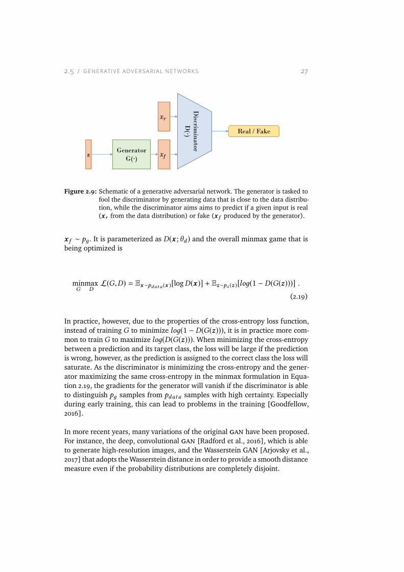
2.5 Generative Adversarial Networks
Generative adversarial networks (gans) [Goodfellow et al., 2014] are genera-
tive models that are trained in an adversarial manner. Unlike the discriminative
models described earlier, generative models aim to estimate and represent the
training data distribution. They are implicit density models, models that do
not define an explicit density function but allow to sample from it. For gans,
two models are trained simultaneously, the so-called generator G that aims to
generate data from a data distribution and a discriminator D, which is tasked
to distinguish generated samples from the actual training data. Figure 2.9
provides a schematic illustration of this process. Training is considered a two-
player minmax game, whereD predicts the probability that a presented sample
belongs to the training data and the generatorG is trained in order to increase
the probability that D makes a mistake. The generator and discriminator are
commonly implemented using deep neural networks and training is performed
in an end-to-end manner using backpropagation.
The generator G maps a noise variable z to the data space G(z;θд), where
the noise distibution is represented by pz(z). The discriminator D produces a
scalar for a given inputx . The scalar represents the probability ofx being drawn
from the data distribution xr ∼ pdata and not from the generator distribution
2.5 G E N E R AT I V E A DV E R S A R I A L N E TWO R K S 27
Discrim
inator
D(∙)
GeneratorG(∙)
z
Real / Fake
����
Figure 2.9: Schematic of a generative adversarial network. The generator is tasked to
fool the discriminator by generating data that is close to the data distribu-
tion, while the discriminator aims aims to predict if a given input is real
(xr from the data distribution) or fake (x f produced by the generator).
x f ∼ pд . It is parameterized as D(x ;θd ) and the overall minmax game that is
being optimized is
minG
maxDL(G,D) = Ex∼pdata (x )[logD(x)] + Ez∼pz (z )[loд(1 − D(G(z)))] .
(2.19)
In practice, however, due to the properties of the cross-entropy loss function,
instead of training G to minimize loд(1 − D(G(z))), it is in practice more com-
mon to trainG to maximize loд(D(G(z))). When minimizing the cross-entropy
between a prediction and its target class, the loss will be large if the prediction
is wrong, however, as the prediction is assigned to the correct class the loss will
saturate. As the discriminator is minimizing the cross-entropy and the gener-
ator maximizing the same cross-entropy in the minmax formulation in Equa-
tion 2.19, the gradients for the generator will vanish if the discriminator is able
to distinguish pд samples from pdata samples with high certainty. Especially
during early training, this can lead to problems in the training [Goodfellow,
2016].
In more recent years, many variations of the original gan have been proposed.
For instance, the deep, convolutional gan [Radford et al., 2016], which is able
to generate high-resolution images, and the Wasserstein GAN [Arjovsky et al.,
2017] that adopts theWasserstein distance in order to provide a smooth distance
measure even if the probability distributions are completely disjoint.
3Segmentation
In this chapter, we will briefly review the tasks of semantic and salient segmen-
tation and briefly introduce some common approaches. The material discussed
in this chapter builds the foundation of Papers I-IV.
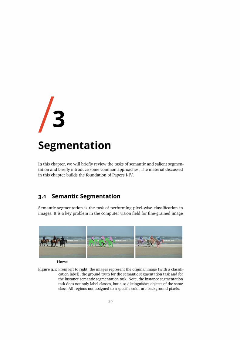
3.1 Semantic Segmentation
Semantic segmentation is the task of performing pixel-wise classification in
images. It is a key problem in the computer vision field for fine-grained image
Horse
Figure 3.1: From left to right, the images represent the original image (with a classifi-
cation label), the ground truth for the semantic segmentation task and for
the instance semantic segmentation task. Note, the instance segmentation
task does not only label classes, but also distinguishes objects of the same
class. All regions not assigned to a specific color are background pixels.
29
30 C H A P T E R 3 S E G M E N TAT I O N
understanding and provides the foundation to enable tasks such as for instance
self-driving cars. Figure 3.1 illustrates the difference between the classification
task and the task of image segmentation. In classification one label is provided
for the whole image, such as for instance Horse or Person in Figure 3.1. For the
segmentation task instead, each pixel is being classified as either belonging to
a specific class or as belonging to the background.
Traditionally, before the recent success of deep learning techniques, approaches
have been heavily relying on the design of hand-crafted features combined
with off-the-shelf classifiers such as svms [Fulkerson et al., 2009] and Random
Forest [Shotton et al., 2008] combined with the inclusion of contextual im-
age information [Carreira et al., 2012] and structured prediction [Carreira and
Sminchisescu, 2011]. However, similarly to image classification, the main factor
limiting these systems were the underlying hand-crafted features. Motivated
by this, deep neural networks quickly found application in segmentation after
their success on classification tasks.
Initial approaches made use of patch-based techniques, where a patch is ex-
tracted around each pixel and the pixel is classified using a CNN based on
the patch [Ciresan et al., 2012, Farabet et al., 2013]. Using a sliding window
approach, this allows for direct application of CNNs that have been designed
for classification on the segmentation task. However, one of the drawbacks of
this approach is the fact that it is computationally expensive, as patches have
considerable overlap. An alternative approach is to perform superpixel segmen-
tation and classify each superpixel using a deep neural network [Mostajabi
et al., 2015]. These approaches have less of a computational overhead due to
the reduced overlap, but struggle if the underlying superpixel segmentation has
errors and require the conversion of the superpixels to a reasonable representa-
tion. However, using the inherent structure of CNNs, the patch-based approach
can be performed more efficiently by avoiding re-computation of the features
in the overlapping regions [Sermanet et al., 2014]. In order to do this, the first
fully connected layer in the network is replaced by a convolutional layer, where
the filter size is equal to the size of the feature map of the previous layer and
the number of filters is equal to the number of neurons in the fully connected
layer. All subsequent fully connected layers are replaced by 1× 1 convolutions.
For the fixed patch-size, these convolutional layers are equivalent to the fully
connected layers. However, it allows the application of the network to larger
images during the inference phase by making use of the fact that convolutions
are not dependent on image size.
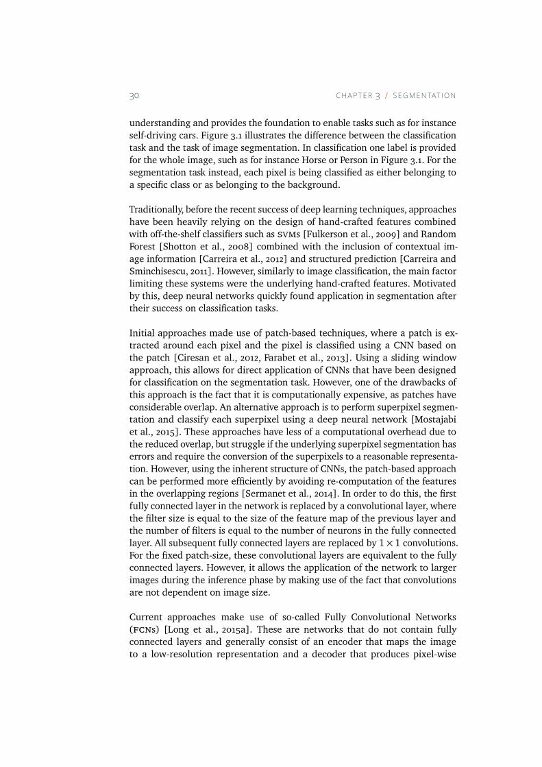
Current approaches make use of so-called Fully Convolutional Networks
(fcns) [Long et al., 2015a]. These are networks that do not contain fully
connected layers and generally consist of an encoder that maps the image
to a low-resolution representation and a decoder that produces pixel-wise
3.1 S E M A N T I C S E GM E N TAT I O N 31
Encoder feature maps Decoder feature maps Skip connection
Figure 3.2: Segmentation using cnns. These architectures consist of an encoder-
decoder architecture and often include skip connections in order to use
the high-resolution encoder activations to improve the upsampling and
segmentation quality.
predictions. Their advantage is the fact that they are more computationally
efficient, do not require a preprocessing segmentation and directly apply
to whole images. Various approaches have been proposed to upsample
the representation in order to produce the pixel-wise predictions from the
low-resolution representation. Figure 3.2 shows such a typical segmentation
architecture. For instance, Long et al. [2015a] make use of fractional strided
convolutions (also referred to as deconvolutions) or bilinear interpolation in
order to learn a gradual upsampling. They further introduce skip connections,
where high-resolution information from the early layers in the encoder is
used to improve segmentation details. Segnet [Badrinarayanan et al., 2015]
instead makes use of a symmetric architecture, where pooling indices from the
encoder are stored and activations in the decoder are upsampled by placing
them in the locations corresponding to the indices. The sparse activations after
’unpooling’ are then processed and made dense by additional convolution
operations. Other more recent advances include for instance DeepLab [Chen
et al., 2018, 2017], which makes use of among others, atrous convolutions.
Atrous convolutions can be used to provide filters with a larger field of view
to enable them to integrate more context. Their advantage is that they do
not add additional parameters compared to a common convolution filter of
equivalent size.
Recently, the task of semantic segmentation has been refined to not only seg-
ment out different classes but further distinguish different objects from the
same class. Figure 3.1 illustrates the difference between traditional seman-
tic segmentation and instance-level semantic segmentation. Initial attempts
approached the problem of instance segmentation by first proposing segmen-
tation proposals and then classify them using object detection networks [Dai
et al., 2016a, Pinheiro et al., 2015]. Alternatively, object detection is performed
32 C H A P T E R 3 S E G M E N TAT I O N
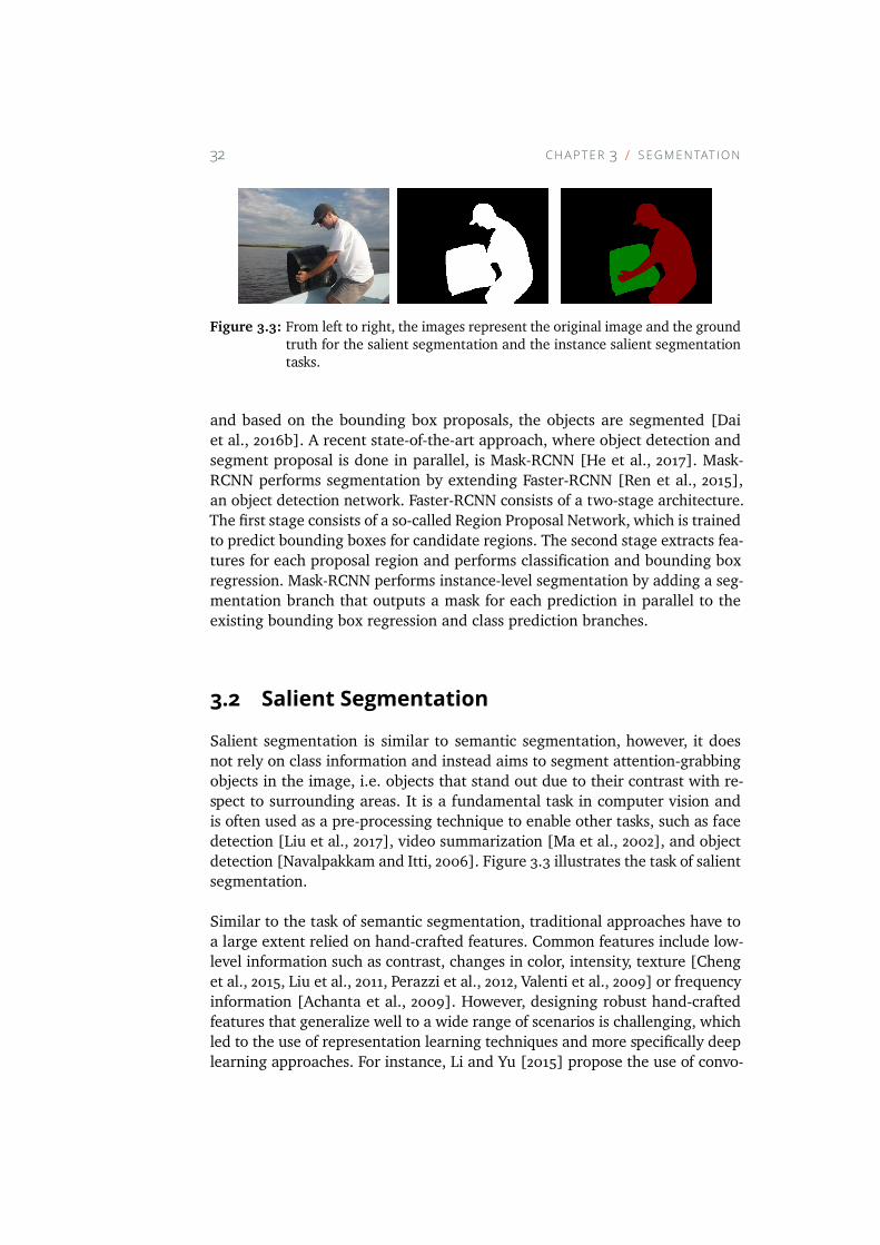
Figure 3.3: From left to right, the images represent the original image and the ground
truth for the salient segmentation and the instance salient segmentation
tasks.
and based on the bounding box proposals, the objects are segmented [Dai
et al., 2016b]. A recent state-of-the-art approach, where object detection and
segment proposal is done in parallel, is Mask-RCNN [He et al., 2017]. Mask-
RCNN performs segmentation by extending Faster-RCNN [Ren et al., 2015],
an object detection network. Faster-RCNN consists of a two-stage architecture.
The first stage consists of a so-called Region Proposal Network, which is trained
to predict bounding boxes for candidate regions. The second stage extracts fea-
tures for each proposal region and performs classification and bounding box
regression. Mask-RCNN performs instance-level segmentation by adding a seg-
mentation branch that outputs a mask for each prediction in parallel to the
existing bounding box regression and class prediction branches.
3.2 Salient Segmentation
Salient segmentation is similar to semantic segmentation, however, it does
not rely on class information and instead aims to segment attention-grabbing
objects in the image, i.e. objects that stand out due to their contrast with re-
spect to surrounding areas. It is a fundamental task in computer vision and
is often used as a pre-processing technique to enable other tasks, such as face
detection [Liu et al., 2017], video summarization [Ma et al., 2002], and object
detection [Navalpakkam and Itti, 2006]. Figure 3.3 illustrates the task of salient
segmentation.
Similar to the task of semantic segmentation, traditional approaches have to
a large extent relied on hand-crafted features. Common features include low-
level information such as contrast, changes in color, intensity, texture [Cheng
et al., 2015, Liu et al., 2011, Perazzi et al., 2012, Valenti et al., 2009] or frequency
information [Achanta et al., 2009]. However, designing robust hand-crafted
features that generalize well to a wide range of scenarios is challenging, which
led to the use of representation learning techniques and more specifically deep
learning approaches. For instance, Li and Yu [2015] propose the use of convo-
3.2 S A L I E N T S E G M E N TAT I O N 33
lutional neural networks to extract feature representations at multiple scales
for a given region in the image and fuse them to produce the salient prediction
for the image region. Wang et al. [2015] approach the task from a patch-based
approach and use cnns to extract features for a center pixel based on the local
surrounding area. Object proposals are then used to refine the salient predic-
tion. In recent years, fcns have also been used for salient segmentation. Li
and Yu [2016] make use of a two-stream approach where one stream consists
of a multi-scale fcn providing pixel-level segmentation results and combine it
with a second stream that provides segmentation results on a superpixel level.
Predictions are fused using an additional convolution operation in order to
obtain the final salient segmentation. Li et al. [2017] makes use of a multi-scale
fcn and utilizes attention weights to fuse the multiple scales.
Inspired by the research on the instance segmentation task, the task of instance
salient segmentation was proposed by Li et al. [2017]. It aims to not only seg-
ment salient regions but further aims to distinguish individual salient objects.
Using their multi-scale fcn with attention weights, they produce both a salient
segmentation and object contours. The object contours are used to produce
salient instance proposal by first generating proposals using multiscale combi-
natorial grouping [Arbeláez et al., 2014] and then making use of a MAP-based
subset optimization framework [Zhang et al., 2016] in order to filter the number
of proposals and produce a compact set. Finally, a fully connected conditional
random field is applied to refine the segmentation results. Note, that this task
is closely related to and can be considered a sub-task of instance segmentation
in the sense that different instances need to be separated. However, no class
information needs to be predicted for instance salient segmentation.
4Unsupervised Learning
Unsupervised learning aims to describe unlabeled data by exploiting the statis-
tical structure of the data. This chapter provides background on the unsuper-
vised tasks considered in this thesis. Namely, we consider unsupervised domain
adaptation in order to support Paper III, representation learning for Paper V,
clustering for Paper VI, and finally zero-shot learning for Paper VII.
4.1 Domain Adaptation
Domain adaptation addresses the problem of domain shift [Gretton et al.,
2009] in machine learning. Domain shift is a phenomena that is often en-
countered in machine learning and arises from the fact that training data
Dtr = {(x tri ,ytri ) i = 1, ...,N }, where x tri ,y
tri are feature vector and label
pairs, might come from a probability distribution Ptr (x ,y), while test data
Dte = {(x tei ,ytei ) i = 1, ...,N } come from a different distribution Pte (x ,y).
The training domain is commonly referred to as the source domain, while the
testing domain is referred to as the target. This can, for instance, be encoun-
tered when satellite images are taken in different countries, where buildings
exhibit considerable differences, or with images that have been acquired us-
ing separate imaging protocols or sensors. Further, there has been increasing
interest in utilizing synthetic data for among others, the task of self-driving
cars [Johnson-Roberson et al., 2017]. Domain adaptation can be used to enable
the use of models that have been trained on synthetic data on real data.
35
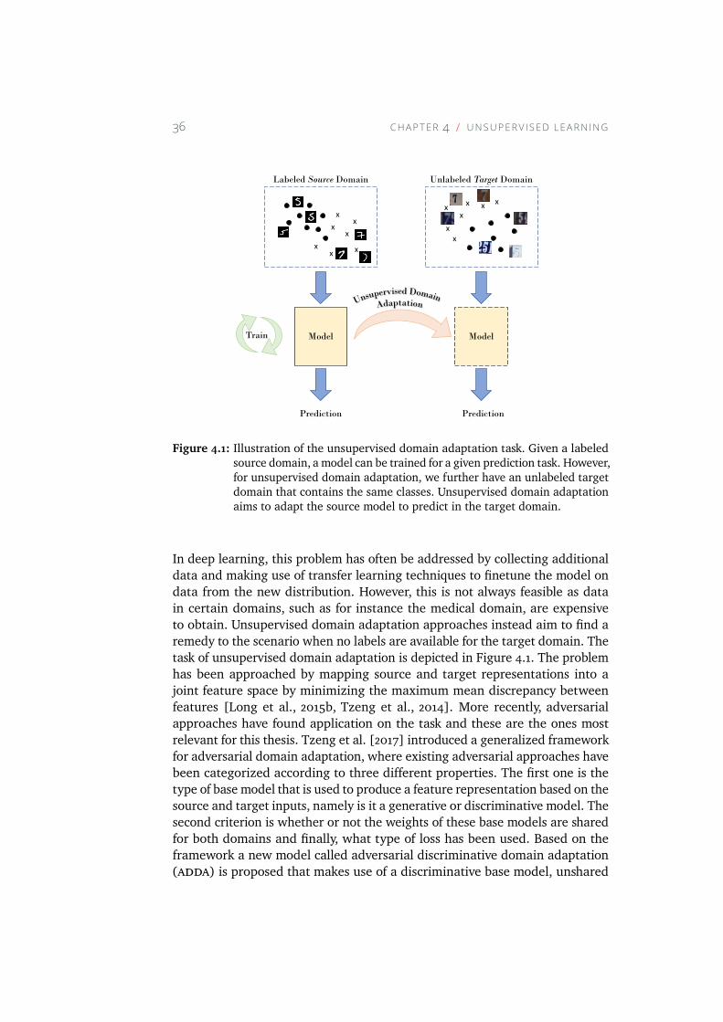
36 C H A P T E R 4 U N S U P E R V I S E D LE A R N I N G
Labeled Source Domain Unlabeled Target Domain
Model Model
Prediction Prediction
Train
x
x
x
x
xx
x
x
x
x
x
x
xx
Figure 4.1: Illustration of the unsupervised domain adaptation task. Given a labeled
source domain, a model can be trained for a given prediction task. However,
for unsupervised domain adaptation, we further have an unlabeled target
domain that contains the same classes. Unsupervised domain adaptation
aims to adapt the source model to predict in the target domain.
In deep learning, this problem has often be addressed by collecting additional
data and making use of transfer learning techniques to finetune the model on
data from the new distribution. However, this is not always feasible as data
in certain domains, such as for instance the medical domain, are expensive
to obtain. Unsupervised domain adaptation approaches instead aim to find a
remedy to the scenario when no labels are available for the target domain. The
task of unsupervised domain adaptation is depicted in Figure 4.1. The problem
has been approached by mapping source and target representations into a
joint feature space by minimizing the maximum mean discrepancy between
features [Long et al., 2015b, Tzeng et al., 2014]. More recently, adversarial
approaches have found application on the task and these are the ones most
relevant for this thesis. Tzeng et al. [2017] introduced a generalized framework
for adversarial domain adaptation, where existing adversarial approaches have
been categorized according to three different properties. The first one is the
type of base model that is used to produce a feature representation based on the
source and target inputs, namely is it a generative or discriminative model. The
second criterion is whether or not the weights of these base models are shared
for both domains and finally, what type of loss has been used. Based on the
framework a new model called adversarial discriminative domain adaptation
(adda) is proposed that makes use of a discriminative base model, unshared
4.2 R E P R E S E N TAT I O N L E A R N I N G 37
weights, and a generative adversarial loss function [Tzeng et al., 2017].
In adda, a CNN is first trained to classify source domain images. Once the
network has been trained, the feature extraction part of the network is sepa-
rated from the classifier, the weights are frozen, and a discriminative loss is
optimized between features for the source domain and features of a feature
extraction network on the target domain. The discriminator is trained to dis-
tinguish features from the source and target domain, forcing the target feature
extraction network to produce features for the target domain that are similar
to the features for the source domain, effectively aligning the features. During
testing, the feature extraction network that has been trained for the target
domain is combined with the classifier that was trained on top of the source
feature extraction network.
In Paper III, we propose a new adversarial approach that aims to learn the
feature extraction and the classifier jointly, apply it for the task of medical
image semantic segmentation, and compare its performance to adda.
4.2 Representation Learning
Representation learning is the process of learning meaningful representations
from data [Bengio et al., 2013] and aims to replace the necessity of hand-crafted
feature design. Hand-crafting of features is a labor-intensive and cumbersome
process that is often very application specific making it difficult to design good
robust features. However, good representations can have a huge impact on
further processing, such as for example for the training of classifiers and clus-
tering. By instead learning feature representations from data machine learning
approaches can be made less reliant on feature design and learning approaches
can be made more robust.
Representation learning has found application in a wide range of domains,
such as image classification [Hinton et al., 2006], object detection [Ren et al.,
2017], speech recognition [Dahl et al., 2010] and methods to produce word em-
beddings [Mikolov et al., 2013]. In this section, we will restrict the discussion
mainly to unsupervised deep learning approaches. In the literature, many as-
sumptions have been proposed on what ameaningful representation consists of.
For instance, sparsity priors have been used in order to ensure that sparse repre-
sentations are encouraged where observations are only represented by a small
set of features. Sparse autoencoders as discussed in Chapter 2.4 are an example
of such a method and other approaches include sparse coding [Olshausen and
Field, 1996]. Other common priors that have been used are that representations
should be robust to noise (i.e. denoising autoencoders [Vincent et al., 2010])
38 C H A P T E R 4 U N S U P E R V I S E D LE A R N I N G
and robust to small input variations (i.e. contractive autoencoders [Rifai et al.,
2011b]).
Beside non-probabilistic approaches such as autoencoders (discussed in Chap-
ter 2.4), probabilistic approaches also exist. One of the most prominent ap-
proaches has been the Restricted Boltzmann Machine (rbm) [Hinton, 2010,
Smolensky, 1986]. rbms are a restricted type of Boltzmann Machine (bm),
which is a class of energy based models and can be viewed as two-layer stochas-
tic, energy-based neural networks that attempt to fit a probability distribution
to the training data. They consist of a layer of visible (input) units that repre-
sent the components of an observation, and a layer of hidden units that models
dependencies between the various observations. The units in the hidden layer
correspond to stochastic binary feature detectors, whereas the visible units
represent the observed binary states. Unlike in a standard neural network,
connections between units are undirected and all units are connected to each
other. Inference is, however, due to the inter-layer connections, intractable for
most scenarios, as computing the conditional probability of visible and hid-
den units requires marginalizing over the rest of the hidden or visible units,
respectively. Adding restrictions to the bm interaction pattern leads to a new
model, the rbm, where all of the units in the hidden and visible layer are
connected with no intra-layer connections to form a complete bipartite graph.
Applications include collaborative filtering [Salakhutdinov et al., 2007], image
generation [Hinton et al., 2006], and speech recognition [Dahl et al., 2010]. For
a more detailed discussion of rbms, the interested reader is referred to Bengio
et al. [2013].
Recently, vaes [Kingma and Welling, 2014], another probabilistic approach has
been proposed. Similar to deterministic autoencoders, these models consist
of an encoder and a decoder. However, unlike in the case of deterministic au-
toencoders, which produces a deterministic latent representation, the encoder
in a vae produces parameters for the distribution that generates the latent
representation (typically a Multivariate Gaussian distribution). For simplicity
it is common to assume a diagonal covariance structure. Given the mean and
the variance of the distribution, a latent representation is sampled from the
distribution and passed to the decoder, which generates a data point, which, in
a trained model, is close to the original input of the autoencoder. The model is
optimized by maximizing the Evidence Lower Bound using stochastic gradient
descent. A detailed discussion of this is out of scope for this thesis and the
interested reader is referred to Kingma and Welling [2014].
4.3 C LU S TE R I N G 39
4.3 Clustering
The process of discovering the underlying structure of data in order to group
data into compact groups, separated from each other, is referred to as cluster-
ing. Due to large amounts of available unlabeled data, the field of clustering
has found application for various tasks. For instance, applications include out-
lier detection [Hodge and Austin, 2004], collaborative filtering [Ungar and
Foster, 1998], pose estimation [Shotton et al., 2011], topic discovery [Sahami
and Koller, 1998] and sequence analysis in computational biology [Eisen et al.,
1998].
Concretely, clustering is the task of finding the underlying K groups, provided
feature representations Xtr = {X i i = 1, ...,N } of N data points, based on
a measure of similarity [Jain, 2010]. The objective is to achieve groupings,
where the underlying groups have high intra-group similarity and low inter-
group similarity. The focus in the clustering field is on how to find meaningful
similarities that allow the discovery of sensible clusters in an unsupervised
manner.
Clustering and the development of clustering methodology has been an active
field of research for decades [Sokal, 1963]. The various approaches to clustering
can be divided into two main categories, hierarchical and partitional clustering
algorithms. The two different approaches are illustrated in Figure 4.2. Hier-
archical approaches are designed to find clusters in a recursive manner and
either i) start by considering each data point as a separate cluster and recur-
sively joining the most similar clusters together (agglomerative hierarchical
clustering) or ii) by initially considering all data points as a single cluster and
recursively divide clusters (divisive hierarchical clustering) [Jain, 2010]. This
results in a hierarchical structure of clusters. Partitional clustering instead, the
clustering performed in this thesis in Paper VI, assigns data points to clusters
without the assumption of hierarchical structure.
A vast number of partitional clustering approaches exist, with some of the
most common approaches being k-means [MacQueen, 1967], mean-shift [Co-
maniciu and Meer, 2002] and expectation maximization based clustering ap-
proaches [Dempster et al., 1977]. However, in order for these algorithms to
succeed it is important to represent data in a way that allows the definition
of meaningful similarity metrics. For complex images, for instance, it will not
be meaningful to only consider the RGB-values of the pixels directly as data
representations for clustering methods such as k-means, as images that contain
identical objects but at different locations will exhibit large differences. Instead,
it is important to define a meaningful feature space as well as a meaningful
distance in this space. Previous work has mainly focused on the distance metric
and to a large extent considered the feature design application-specific.
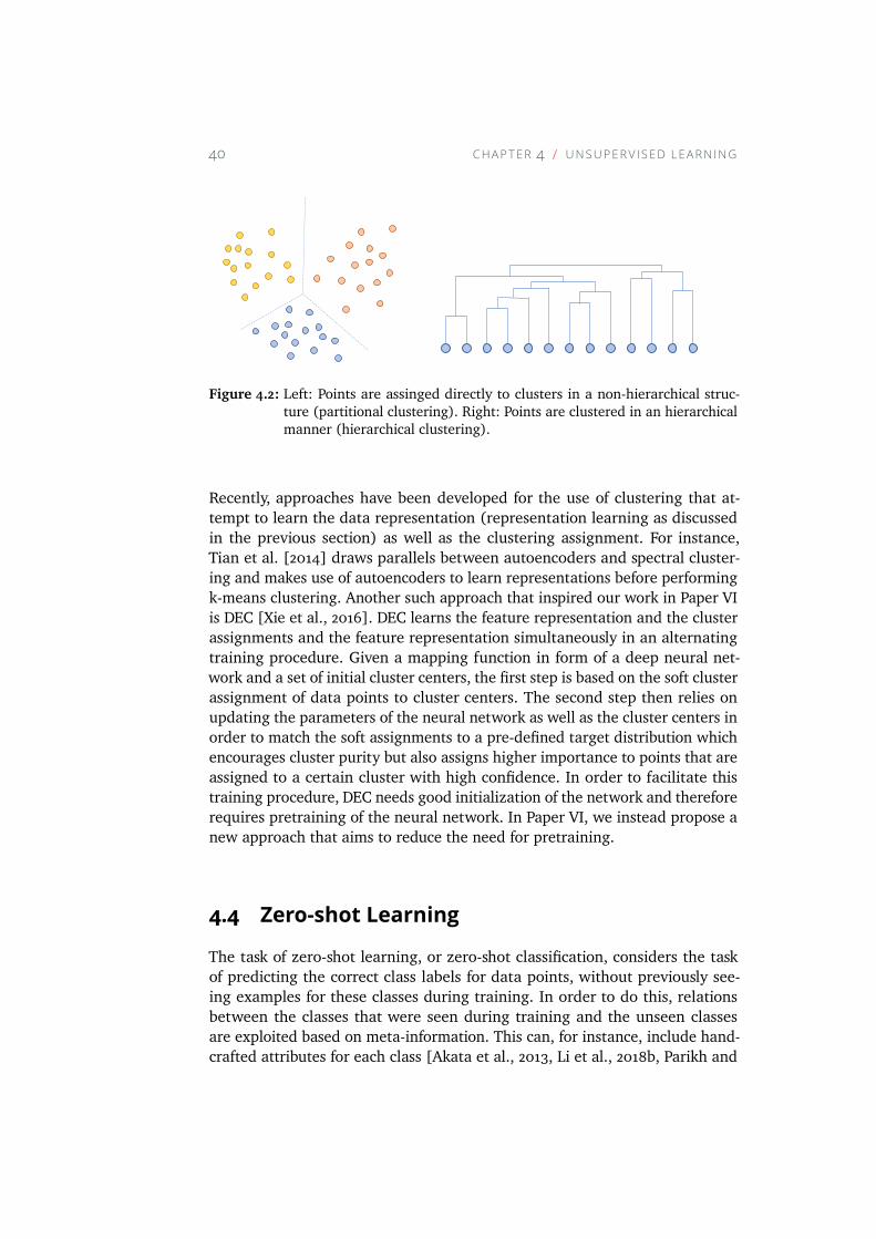
40 C H A P T E R 4 U N S U P E R V I S E D LE A R N I N G
Figure 4.2: Left: Points are assinged directly to clusters in a non-hierarchical struc-
ture (partitional clustering). Right: Points are clustered in an hierarchical
manner (hierarchical clustering).
Recently, approaches have been developed for the use of clustering that at-
tempt to learn the data representation (representation learning as discussed
in the previous section) as well as the clustering assignment. For instance,
Tian et al. [2014] draws parallels between autoencoders and spectral cluster-
ing and makes use of autoencoders to learn representations before performing
k-means clustering. Another such approach that inspired our work in Paper VI
is DEC [Xie et al., 2016]. DEC learns the feature representation and the cluster
assignments and the feature representation simultaneously in an alternating
training procedure. Given a mapping function in form of a deep neural net-
work and a set of initial cluster centers, the first step is based on the soft cluster
assignment of data points to cluster centers. The second step then relies on
updating the parameters of the neural network as well as the cluster centers in
order to match the soft assignments to a pre-defined target distribution which
encourages cluster purity but also assigns higher importance to points that are
assigned to a certain cluster with high confidence. In order to facilitate this
training procedure, DEC needs good initialization of the network and therefore
requires pretraining of the neural network. In Paper VI, we instead propose a
new approach that aims to reduce the need for pretraining.
4.4 Zero-shot Learning
The task of zero-shot learning, or zero-shot classification, considers the task
of predicting the correct class labels for data points, without previously see-
ing examples for these classes during training. In order to do this, relations
between the classes that were seen during training and the unseen classes
are exploited based on meta-information. This can, for instance, include hand-
crafted attributes for each class [Akata et al., 2013, Li et al., 2018b, Parikh and
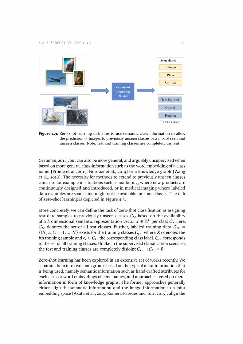
4.4 Z E R O-S H OT LE A R N I N G 41
Zero-shotLearning
ModelTree Squirrel
Opener
Penguin
Baboon
Plane
Sea Lion
Seen classes
Unseen classes
Figure 4.3: Zero-shot learning task aims to use semantic class information to allow
the prediction of images to previously unseen classes or a mix of seen and
unseen classes. Note, test and training classes are completely disjoint.
Grauman, 2011], but can also be more general, and arguably unsupervised when
based on more general class-information such as the word embedding of a class
name [Frome et al., 2013, Norouzi et al., 2014] or a knowledge graph [Wang
et al., 2018]. The necessity for methods to extend to previously unseen classes
can arise for example in situations such as marketing, where new products are
continuously designed and introduced, or in medical imaging where labeled
data examples are sparse and might not be available for some classes. The task
of zero-shot learning is depicted in Figure 4.3.
More concretely, we can define the task of zero-shot classification as assigning
test data samples to previously unseen classes Cte based on the availability
of a L dimensional semantic representation vector z ∈ RL per class C. Here,
Cte denotes the set of all test classes. Further, labeled training data Dtr =
{(X i ,ci ) i = 1, ...,N } exists for the training classes Ctr , where X i denotes the
ith training sample and ci ∈ Ctr the corresponding class label. Ctr corresponds
to the set of all training classes. Unlike in the supervised classification scenario,
the test and training classes are completely disjoint Cte ∩ Ctr = ∅.
Zero-shot learning has been explored in an extensive set of works recently. We
separate them into twomain groups based on the type ofmeta-information that
is being used, namely semantic information such as hand-crafted attributes for
each class or word embeddings of class names, and approaches based on meta-
information in form of knowledge graphs. The former approaches generally
either align the semantic information and the image information in a joint
embedding space [Akata et al., 2015, Romera-Paredes and Torr, 2015], align the
42 C H A P T E R 4 U N S U P E R V I S E D LE A R N I N G
image information with the semantic information in the semantic space [Frome
et al., 2013, Socher et al., 2013] or align the semantic information with the
image information in the image space [Zhang et al., 2017]. In the inference
phase distance metrics are applied in these spaces to find the closest class
representation to a given image.
Approaches that use knowledge graphs are less explored and are based on the
assumption that the unseen classes can exploit the similarity to the seen classes
in the graph. One such recent approach, which can also be considered a hybrid
approach as itmakes use of both semantic information and the knowledge graph
was proposed by Wang et al. [2018]. In this work, a gcn is trained to predict
a set of logistic regression classifiers on top of pretrained CNN features.
In Paper VII, we revisit the use of gcns for the task of zero-shot learning and
propose an efficient knowledge graph propagation procedure that allows us to
improve on previous approaches.
5Kernel Methods and
Information Theoretic
Learning
The material presented in this section will mainly provide the foundations for
the work presented in Paper V and Paper VI. We will first review the underly-
ing ideas of kernel methods and then briefly outline some of the concepts in
Information Theoretic Learning.
5.1 Kernel Methods
Kernel methods aim to model non-linear structure in data, while at the same
time building on the well-understood theory of linear methods. This is achieved
by making use of Mercer kernels to implicitly map data points into a high-
dimensional and possible infinite reproducing kernel Hilbert space (RKHS). In
the high dimensional space, data points are likely to be linear separable [Cover
and Thomas, 1991] and linear methods can be applied. In order to do this, the
so-called kernel trick is applied by expressing the operations in the kernel space
through inner products. In this way, the explicit mappingϕ(·) to the kernel spacedoes not need to be computed, but instead, a kernel is used to directly compute
these inner products. A kernelK(·, ·) is a function that computes inner products
43
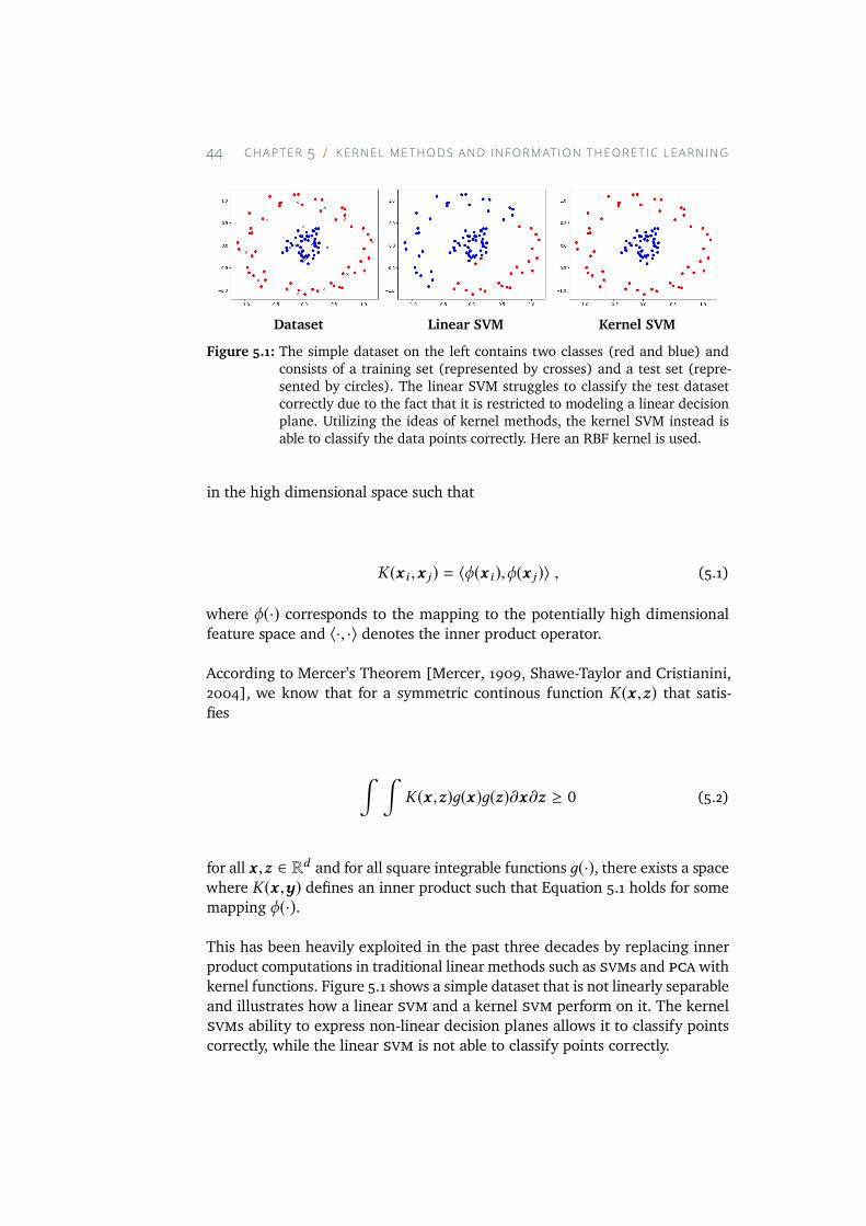
44 C H A P TE R 5 K E R N E L M E TH O D S A N D I N F O R M AT I O N T H E O R E T I C L E A R N I N G
Dataset Linear SVM Kernel SVM
Figure 5.1: The simple dataset on the left contains two classes (red and blue) and
consists of a training set (represented by crosses) and a test set (repre-
sented by circles). The linear SVM struggles to classify the test dataset
correctly due to the fact that it is restricted to modeling a linear decision
plane. Utilizing the ideas of kernel methods, the kernel SVM instead is
able to classify the data points correctly. Here an RBF kernel is used.
in the high dimensional space such that
K(x i ,x j ) = 〈ϕ(x i ),ϕ(x j )〉 , (5.1)
where ϕ(·) corresponds to the mapping to the potentially high dimensional
feature space and 〈·, ·〉 denotes the inner product operator.
According to Mercer’s Theorem [Mercer, 1909, Shawe-Taylor and Cristianini,
2004], we know that for a symmetric continous function K(x ,z) that satis-
fies
∫ ∫
K(x ,z)д(x)д(z)∂x∂z ≥ 0 (5.2)
for all x ,z ∈ Rd and for all square integrable functions д(·), there exists a spacewhere K(x ,y) defines an inner product such that Equation 5.1 holds for some
mapping ϕ(·).
This has been heavily exploited in the past three decades by replacing inner
product computations in traditional linear methods such as svms and pcawith
kernel functions. Figure 5.1 shows a simple dataset that is not linearly separable
and illustrates how a linear svm and a kernel svm perform on it. The kernel
svms ability to express non-linear decision planes allows it to classify points
correctly, while the linear svm is not able to classify points correctly.
5.2 I N F O R M AT I O N T H E O R E T I C L E A R N I N G 45
5.2 Information Theoretic Learning
Traditionally, most approaches to learning adaptive systems have been ad-
dressed using second-order statistics, such as for instance the mse criteria.
These criteria perform well for the learning of linear models and many non-
linear models, however, it can be beneficial to consider higher-order statistical
properties of the underlying processes, especially for tasks such as manifold
learning, classification, and clustering [Jenssen et al., 2006]. Information theo-
retic learning aims to do this by making use of information theoretic objective
functions. One important aspect of information theoretic learning is to define
andmeasure similarity and dissimilarity between PDFs. One of the most known
and used divergence measures is the Kullback-Leibler (kl) divergence, which
for continuous random variables is
DKL(p||q) =
∫
X
p(x) logp(x)
q(x)∂x (5.3)
and for discrete probability distributions is
DKL(p||q) =∑
x
p(x) logp(x)
q(x). (5.4)
The kl-divergence is also sometimes referred to as information gain and repre-
sents the information that is gained if the original distribution p is used instead
of the approximating distribution q. It measures the dissimilarity between the
probability distributions p and q. Note, the minimum of DKL is 0 and obtained
if and only if q = p, however, it is not a metric as it is not symmetric and does
not adhere to the triangle inequality. Symmetric versions of the kl-divergence
exist. For instance, the symmetric Jeffrey (J) divergence [Principe, 2010]
D J (p||q) =
√
1
2(DKL(p||q))2 +
1
2(DKL(q||p))2. (5.5)
5.2.1 Cauchy-Schwartz Divergence
Another divergence and the underlying divergence used in Paper VI is the
Cauchy-Schwartz (cs) divergence. We first present the cs-divergence, before
46 C H A P TE R 5 K E R N E L M E TH O D S A N D I N F O R M AT I O N T H E O R E T I C L E A R N I N G
briefly discussing Parzen kernel density estimation, a non-parametric density
estimation technique, which is used in Paper VI to derive an estimator for the
cs-divergence. Finally, we conclude the section by outlining how the estimator
can be obtained as presented in Jenssen et al. [2006].
The cs-divergence’s name originates from the cs-inequality, which states
that
||x ||2||y||2 ≥ (xTy)2 (5.6)
such that
− log(xTy)√
||x ||2||y||2≥ 0 . (5.7)
Based on this inequality, Principe and Xu [2000] defined the cs-divergence
measure as
DCS (p||q) = −
∫
p(x)q(x)∂x√
∫
p2(x)∂x∫
q2(x)∂x
. (5.8)
From the cs-inequality, we know that this formulation ensures non-negativity
and it will only be 0 if and only ifp(x) = q(x). Similar to the kl-divergence, the
cs-divergence does not adhere to the triangle inequality, however, it is symmet-
ric. In Paper VI, this cost function is utilized to perform clustering by ensuring
that clusters are compact and separated, a natural objective of clustering. Given
two clusters, we can represent each cluster by a PDF. By maximizing the above
formulation, we can see that compactness and separation are inherently repre-
sented. In order to maximize the expressions, the denominator has to be large,
and samples within each of the given clusters must, therefore, be highly similar.
Similarly, the nominator should be small, which is achieved when the similarity
between samples across clusters is small.
Parzen kernel density estimation
Parzen kernel density estimation is a non-parametric density estimation tech-
nique. Unlike in the case of parametric density estimation, non-parametric
techniques do not require a priori assumptions on the parametric model for
the PDF and are therefore ideal in a situation where the underlying model
is unknown. Given a set of N data points x1, ...,xN the density p(x) can be
estimated using the Parzen kernel density estimator
p(x) =1
N
N∑
i=1
Wσ 2(x ,x i ) , (5.9)
5.2 I N F O R M AT I O N T H E O R E T I C L E A R N I N G 47
whereWσ 2 is used to denote the Parzen kernel, which itself has to integrate to
one. Note that this also links to the kernel methods discussed in Chapter 5, as
the density in a point can be viewed as the mean of the inner products between
that point and the other datapoints in kernel space. The most common choice
of kernel is the Gaussian kernel
Wσ 2(x ,x i ) =1
(2πσ 2)d/2e−
||x−xi ||2
2σ 2 . (5.10)
σ is a hyperparameter representing the width of the the kernel and has a large
effect on the estimate. Small σ values generally result in very local spikes that
do not represent the underlying distribution well, while large values lead to
overly smooth estimated distributions.
Estimation of Cauchy-Schwartz Divergence
The estimator discussed in this section was initially proposed in Jenssen et al.
[2006]. In order to estimate the cs-divergence, a parzen kernel density esti-
mate is used for the two densities p and q in Equation 5.8. From Equation 5.9,
we have
p(x) =1
N1
N1∑
i=1
Wσ 2(x ,x i ) , q(x) =1
N2
N2∑
j=1
Wσ 2(x ,x j ) . (5.11)
Further, we can make use of the fact that the convolution of two Gaussian func-
tions is a Gaussian with a variance corresponding to the sum of the variances
of the individual Gaussians. Thus, we have
∫
Wσ 2(x ,x i )Wσ 2(x ,x j )∂x =W2σ 2(x i ,x j ) . (5.12)
Making use of this relation and the parzen estimators forp andq we can express
the nominator in Equation 5.8 as
∫
p(x)q(x)∂x ≈
∫
p(x)q(x)∂x (5.13)
=
1
N1N2
N1,N2∑
i,j=1
W2σ 2(x i ,x j ) (5.14)
=
1
N1N2
N1,N2∑
i,j=1
ki j . (5.15)
48 C H A P TE R 5 K E R N E L M E TH O D S A N D I N F O R M AT I O N T H E O R E T I C L E A R N I N G
Here, we use ki j to denoteW2σ 2(x i ,x j ). Similar we can express the denomina-
tor, such that the estimator for the cs-divergence is given as
DCS (p||q) = − log
∑N1,N2
i,j=1 ki j√
∑N1,N1
i,i′=1kii′∑N2,N2
j,j′=1kj j′. (5.16)

Part II
Summary of research
49

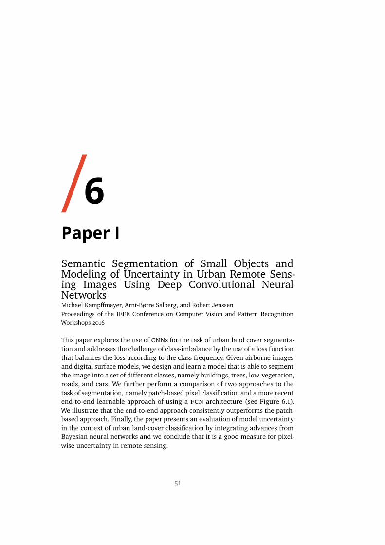
6Paper I
Semantic Segmentation of Small Objects andModeling of Uncertainty in Urban Remote Sens-ing Images Using Deep Convolutional NeuralNetworksMichael Kampffmeyer, Arnt-Børre Salberg, and Robert Jenssen
Proceedings of the IEEE Conference on Computer Vision and Pattern Recognition
Workshops 2016
This paper explores the use of cnns for the task of urban land cover segmenta-
tion and addresses the challenge of class-imbalance by the use of a loss function
that balances the loss according to the class frequency. Given airborne images
and digital surface models, we design and learn a model that is able to segment
the image into a set of different classes, namely buildings, trees, low-vegetation,
roads, and cars. We further perform a comparison of two approaches to the
task of segmentation, namely patch-based pixel classification and a more recent
end-to-end learnable approach of using a fcn architecture (see Figure 6.1).
We illustrate that the end-to-end approach consistently outperforms the patch-
based approach. Finally, the paper presents an evaluation of model uncertainty
in the context of urban land-cover classification by integrating advances from
Bayesian neural networks and we conclude that it is a good measure for pixel-
wise uncertainty in remote sensing.
51
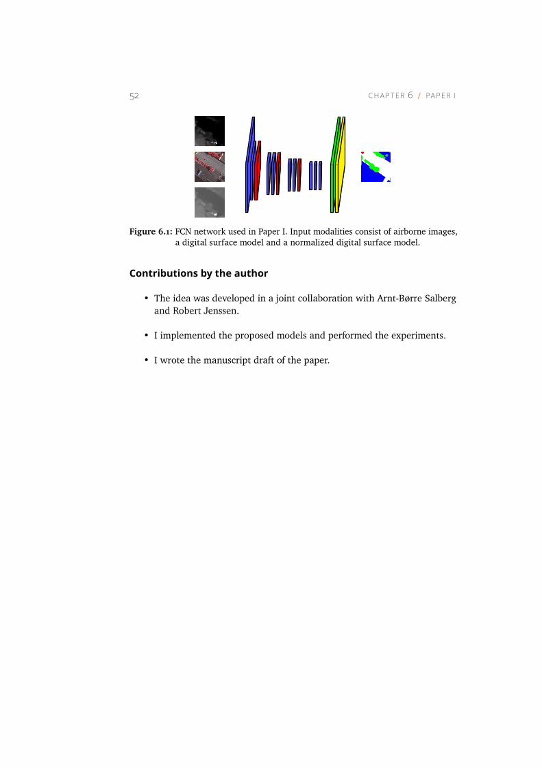
52 C H A P TE R 6 PA P E R I
Figure 6.1: FCN network used in Paper I. Input modalities consist of airborne images,
a digital surface model and a normalized digital surface model.
Contributions by the author
• The idea was developed in a joint collaboration with Arnt-Børre Salberg
and Robert Jenssen.
• I implemented the proposed models and performed the experiments.
• I wrote the manuscript draft of the paper.
7Paper II
Urban Land Cover Classification with MissingData Modalities Using Deep Convolutional Neu-ral NetworksMichael Kampffmeyer, Arnt-Børre Salberg, and Robert Jenssen
Journal of Selected Topics in Applied Earth Observations and Remote Sensing,
2018
This paper is a direct successor of Paper I. In this work, we continue the explo-
ration of cnns for urban land cover classification. Especially we focus in this
paper on the problem of missing data modalities. Fusing different data modal-
ities is a common approach in remote sensing to improve model performance.
For instance, in Paper I we made use of digital surface models in addition to
airborne images. However, this raises the question of what happens if some
data modalities are missing during the inference stage. The naïve approach
to this problem would be to train separate models for the individual modality
pairs, however, in this case, a large amount of information is being ignored
during the inference phase. Instead, based on recent works by Hoffman et al.
[2016] we introduce Hallucination Networks to the task of urban land cover
segmentation. These models allow the use of all available training modalities
by learning mappings from one data modality to the feature representation
of a potentially missing data modality. We further investigate the scenarios of
partly missing data modalities and the scenario where multiple data modal-
ities are missing. Figure 7.1 illustrates the issue addressed in this work. Our
53
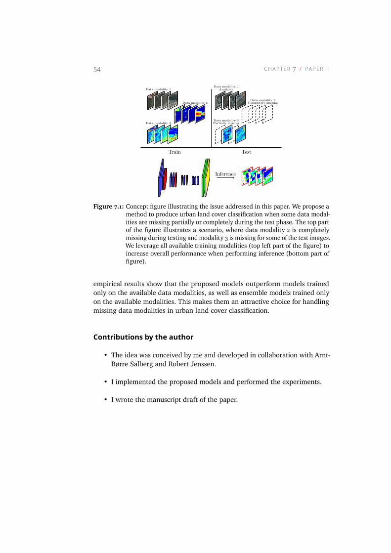
54 C H A P T E R 7 PA P E R I I
Data modality 1
Data modality 2
Data modality 3
Data modality 1Available
Data modality 2Completely missing
Data modality 3Partially missing
Train Test
Inference
Figure 7.1: Concept figure illustrating the issue addressed in this paper. We propose a
method to produce urban land cover classification when some data modal-
ities are missing partially or completely during the test phase. The top part
of the figure illustrates a scenario, where data modality 2 is completely
missing during testing andmodality 3 is missing for some of the test images.
We leverage all available training modalities (top left part of the figure) to
increase overall performance when performing inference (bottom part of
figure).
empirical results show that the proposed models outperform models trained
only on the available data modalities, as well as ensemble models trained only
on the available modalities. This makes them an attractive choice for handling
missing data modalities in urban land cover classification.
Contributions by the author
• The idea was conceived by me and developed in collaboration with Arnt-
Børre Salberg and Robert Jenssen.
• I implemented the proposed models and performed the experiments.
• I wrote the manuscript draft of the paper.
8Paper III
Unsupervised Domain Adaptation for AutomaticEstimation of Cardiothoracic RatioNanqing Dong, Michael Kampffmeyer, Xiaodan Liang, Zeya Wang, Wei Dai, Eric P. Xing
Proceedings of the International Conference on Medical Image Computing and Com-
puter Assisted Intervention 2018
The medical domain is notorious for the limited availability of data due to
privacy concerns and the cost of getting medical experts to provide labels.
A common approach to learn in the presence of limited data is the use of
finetuning, i.e. training models on large available (possibly unrelated) datasets
and finetune the model on the task of interest. However, this requires a set of
labels for the new dataset, which may not be available. A naïve approach would
be to train the model on available datasets that have been obtained by different
hospitals, however, as these images are generally producedwith different image
protocols, they contain different noise levels and varying contrast.
The paper approaches this problem from an unsupervised domain adaptation
perspective. We propose a framework that builds on our intuition that the
segmentation prediction masks should be domain independent and train the
framework in an adversarial manner, utilizing a discriminator that aims to dis-
tinguish the segmentation prediction mask from the ground truth mask. The
framework is illustrated in Figure 8.1. This allows us to perform segmenta-
tion on an unlabeled dataset based on an openly available dataset in order to
55
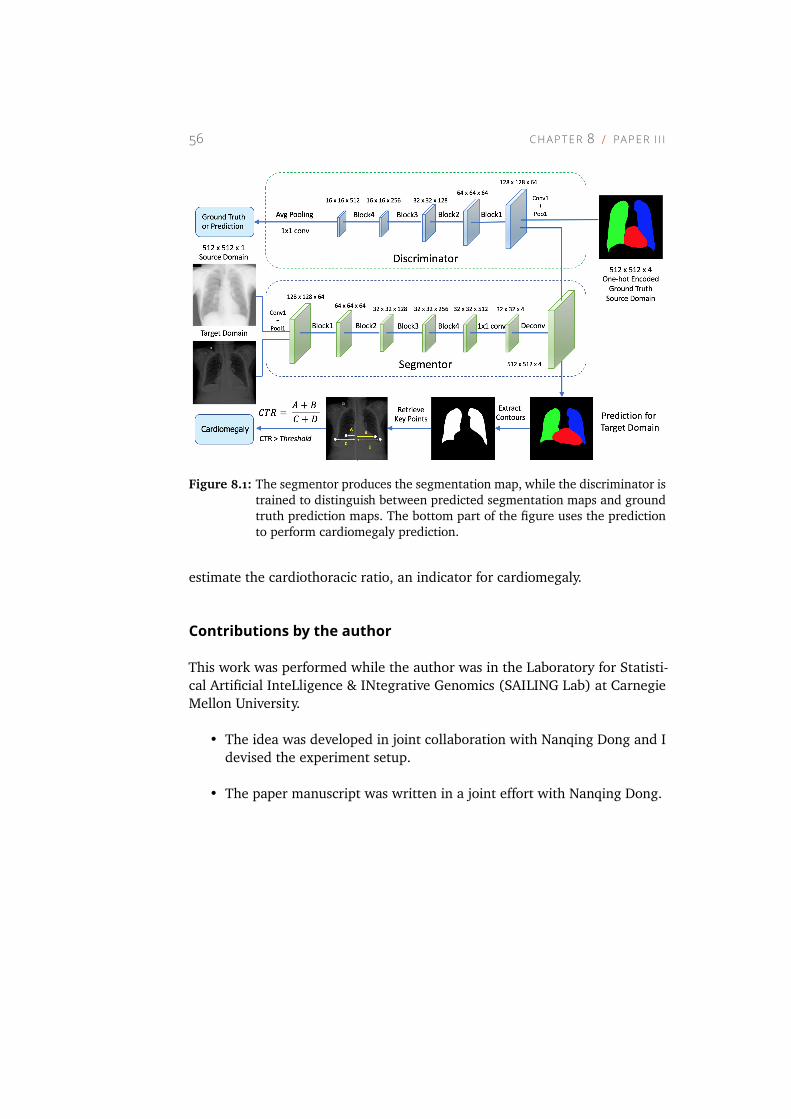
56 C H A P T E R 8 PA P E R I I I
Figure 8.1: The segmentor produces the segmentation map, while the discriminator is
trained to distinguish between predicted segmentation maps and ground
truth prediction maps. The bottom part of the figure uses the prediction
to perform cardiomegaly prediction.
estimate the cardiothoracic ratio, an indicator for cardiomegaly.
Contributions by the author
This work was performed while the author was in the Laboratory for Statisti-
cal Artificial InteLligence & INtegrative Genomics (SAILING Lab) at Carnegie
Mellon University.
• The idea was developed in joint collaboration with Nanqing Dong and I
devised the experiment setup.
• The paper manuscript was written in a joint effort with Nanqing Dong.
9Paper IV
ConnNet: A Long-Range Relation-Aware Pixel-Connectivity Network for Salient SegmentationMichael Kampffmeyer, Nanqing Dong, Xiaodan Liang, Yujia Zhang, and Eric P. Xing
Submitted to IEEE Transactions on Image Processing
Salient segmentation is a fundamental problem in image processing and pro-
vides the foundation of many tasks, such as object detection [Navalpakkam and
Itti, 2006], video summarization [Ma et al., 2002] and face detection [Liu et al.,
2017]. It is, therefore, crucial to achieve good performance on this task. Previous
works in the past have mainly approached this task as a binary class segmenta-
tion task and relied on the use of fcns. In this work, we instead investigate the
use of connectivity modeling in order to improve salient segmentation perfor-
mance and illustrate that our approach outperforms traditional segmentation
based approaches. Figure 9.1 displays the motivation behind our approach. We
predict if a given pixel is connected to its neighbors based on local and global
relations between pixels
Connectivity prediction, by predicting for a given pixel the immediate neigh-
bors, splits the segmentation task into subtasks. Each connectivity sub-task only
aims to group pixels along a certain direction. Further, it is possible to view the
technique from an ensemble viewpoint, as connectivity is a symmetric relation
and neighboring pixels need to agree on whether or not they are connected to
each other. This tends to provide more robust predictions.
57
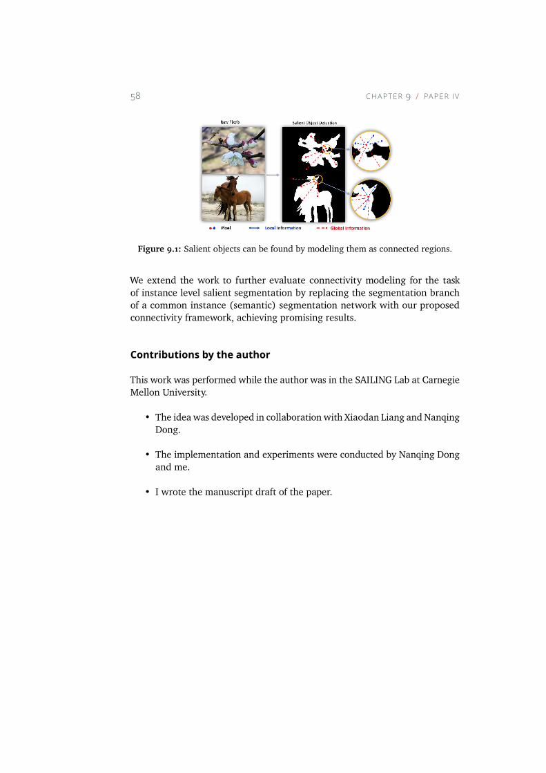
58 C H A P TE R 9 PA P E R I V
Figure 9.1: Salient objects can be found by modeling them as connected regions.
We extend the work to further evaluate connectivity modeling for the task
of instance level salient segmentation by replacing the segmentation branch
of a common instance (semantic) segmentation network with our proposed
connectivity framework, achieving promising results.
Contributions by the author
This work was performed while the author was in the SAILING Lab at Carnegie
Mellon University.
• The idea was developed in collaboration with Xiaodan Liang andNanqing
Dong.
• The implementation and experiments were conducted by Nanqing Dong
and me.
• I wrote the manuscript draft of the paper.
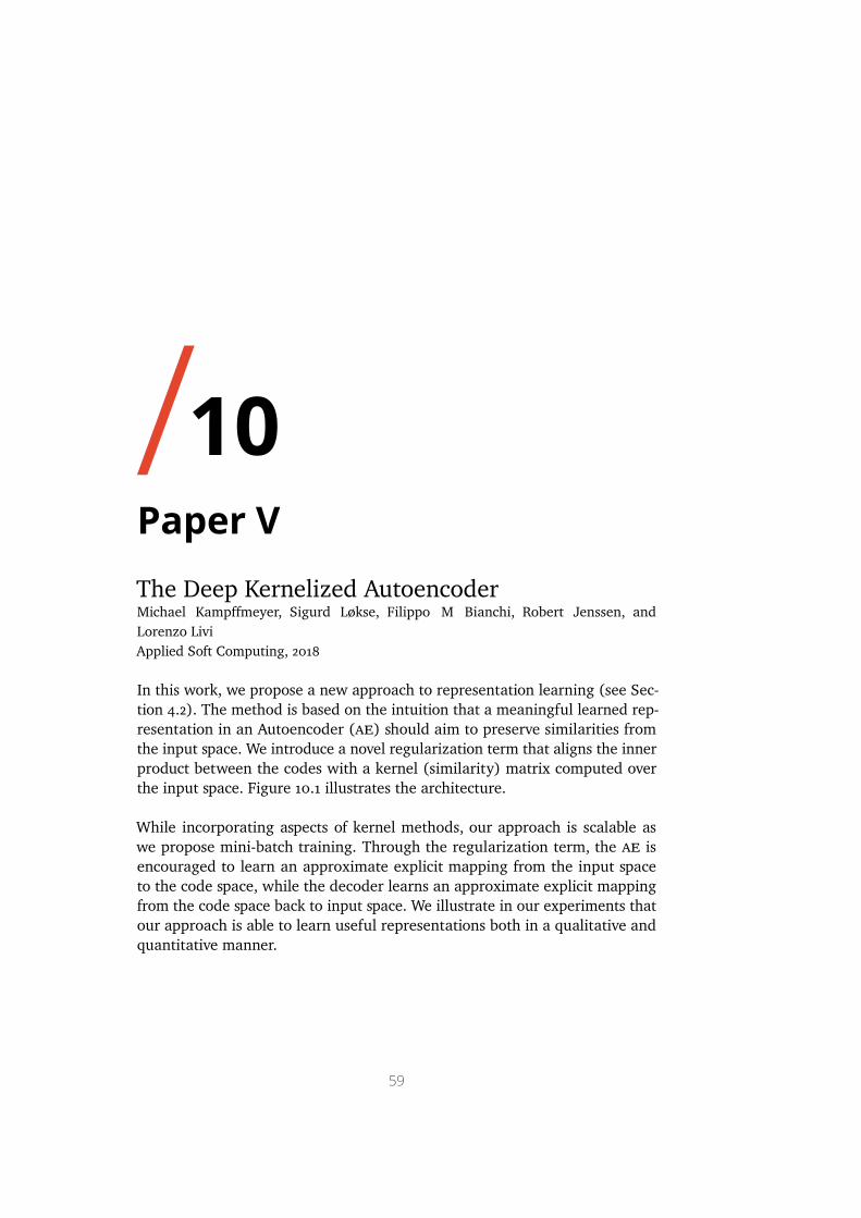
10Paper V
The Deep Kernelized AutoencoderMichael Kampffmeyer, Sigurd Løkse, Filippo M Bianchi, Robert Jenssen, and
Lorenzo Livi
Applied Soft Computing, 2018
In this work, we propose a new approach to representation learning (see Sec-
tion 4.2). The method is based on the intuition that a meaningful learned rep-
resentation in an Autoencoder (ae) should aim to preserve similarities from
the input space. We introduce a novel regularization term that aligns the inner
product between the codes with a kernel (similarity) matrix computed over
the input space. Figure 10.1 illustrates the architecture.
While incorporating aspects of kernel methods, our approach is scalable as
we propose mini-batch training. Through the regularization term, the ae is
encouraged to learn an approximate explicit mapping from the input space
to the code space, while the decoder learns an approximate explicit mapping
from the code space back to input space. We illustrate in our experiments that
our approach is able to learn useful representations both in a qualitative and
quantitative manner.
59
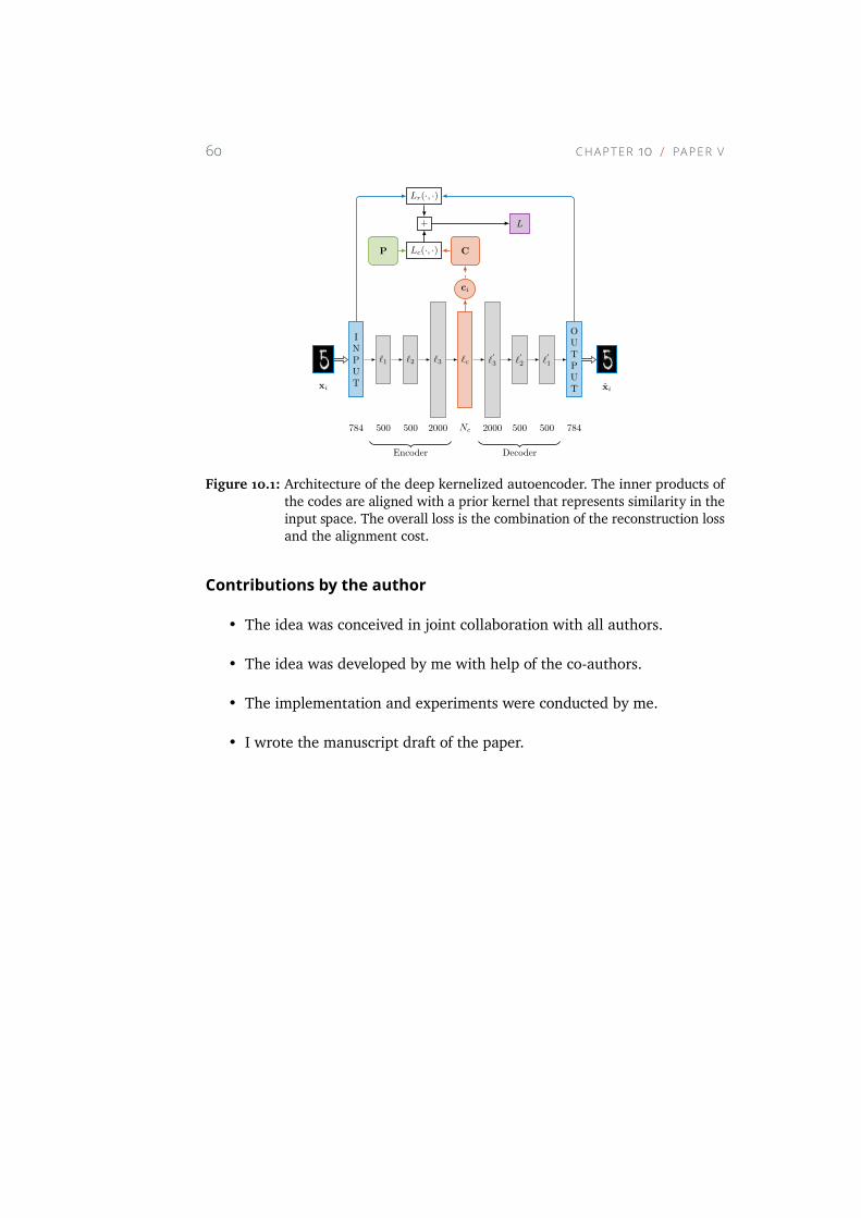
60 C H A P T E R 10 PA P E R V
INPUT
784
OUTPUT
784
xi xi
ℓ1
500
ℓ2
500
ℓ3
2000
Encoder
ℓc
Nc
ℓ′
3
2000
ℓ′
2
500
ℓ′
1
500
Decoder
ci
CP Lc(·, ·)
Lr(·, ·)
+ L
Figure 10.1: Architecture of the deep kernelized autoencoder. The inner products of
the codes are aligned with a prior kernel that represents similarity in the
input space. The overall loss is the combination of the reconstruction loss
and the alignment cost.
Contributions by the author
• The idea was conceived in joint collaboration with all authors.
• The idea was developed by me with help of the co-authors.
• The implementation and experiments were conducted by me.
• I wrote the manuscript draft of the paper.
11Paper VI
Deep Divergence-Based Approach to ClusteringMichael Kampffmeyer, Sigurd Løkse, Filippo M Bianchi, Lorenzo Livi, Arnt-Børre Sal-
berg, and Robert Jenssen
Submitted to Neural Networks
This paper focuses on another unsupervised learning domain, namely cluster-
ing (see Section 4.3). In the presence of unlabeled data, we propose a neural
network based method that finds the underlying structure in the data. We in-
tegrate ideas from both kernel methods and information theoretic learning by
making use of the Cauchy-Schwartz divergence measure in order to encourage
the underlying clusters to be compact and different clusters to be separate from
each other. We illustrate this in Figure 11.1.
Using our proposed loss function, we are able to learn the representations
of the neural network as well as discover an underlying clustering structure.
Experimental results on a set of real and synthetic datasets show promising
results and making use of mini-batch training, the proposed method scales well
to large datasets.
Contributions by the author
• The idea was conceived in joint collaboration with all authors.
61
62 C H A P TE R 11 PA P E R V I
...
DEEP
NEURAL
NETWORK
+
orthogonality
separationcompactnesscluster
assignments
Figure 11.1: Concept figure of Paper VI. Our loss function is trained in order to produce
compact clusters and at the same time force clusters to be separate from
each other.
• The idea was developed by me with help of the co-authors.
• The implementation and experiments were conducted by me.
• I wrote the manuscript draft of the paper.
12Paper VII
Rethinking Knowledge Graph Propagation forZero-Shot LearningMichael Kampffmeyer, Yinbo Chen, Xiaodan Liang, HaoWang, Yujia Zhang, Eric P. Xing
Submitted to Neural Information Processing Systems 2018
In this work, we rethink the use of Graph Convolutional Neural Networks
(gcns) for zero-shot learning. gcns have previously been used to address
the zero-shot learning task as a semi-supervised learning task. The network is
being trained to regress a set of classifier weights based on the classifiers from
seen classes and the word embeddings from all the classes. A knowledge graph
is used to represent relations between classes [Wang et al., 2018]. However, the
propagation rule of the applied gcn can be viewed as performing a Laplacian
smoothing operation at each graph layer Li et al. [2018a]. Smoothing, to some
extent, is beneficial for semi-supervised classification, however, for the task of
regression, this leads to information being diluted.
In order to address this problem, we propose a new way of utilizing gcns for
the task of zero-shot learning. We show that a single layer gcn outperforms
deeper architectures as it limits information dilution. However, a single layer
gcn only propagates information to immediate neighbors. To remedy this,
we propose an Attentive Dense Graph Propagation Module, which exploits the
knowledge graph by adding direct edges between a given node and its ancestors
and descendants allowing information to propagate freely. We utilize a two-
63
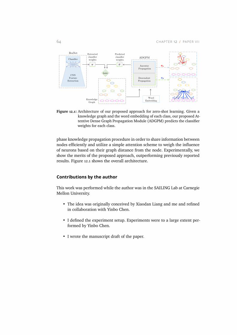
64 C H A P TE R 12 PA P E R V I I
CNNFeatureExtraction
DescendentPropagation
Classifier
WordEmbedding
AncestorPropagation
!"##
$%
ADGPM
ResNet
%
KnowledgeGraph
Predictedclassifierweights
Extractedclassifierweights
&'
&(
)*+
)*+
),+
),+
),+
),+),
+
)*- ),
-
).-
Figure 12.1: Architecture of our proposed approach for zero-shot learning. Given a
knowledge graph and the word embedding of each class, our proposed At-
tentive Dense Graph Propagation Module (ADGPM) predicts the classifier
weights for each class.
phase knowledge propagation procedure in order to share information between
nodes efficiently and utilize a simple attention scheme to weigh the influence
of neurons based on their graph distance from the node. Experimentally, we
show the merits of the proposed approach, outperforming previously reported
results. Figure 12.1 shows the overall architecture.
Contributions by the author
This work was performed while the author was in the SAILING Lab at Carnegie
Mellon University.
• The idea was originally conceived by Xiaodan Liang and me and refined
in collaboration with Yinbo Chen.
• I defined the experiment setup. Experiments were to a large extent per-
formed by Yinbo Chen.
• I wrote the manuscript draft of the paper.
13Conclusion
In this thesis, we advanced deep learning for semantic segmentation, mainly
in the specific application domains of remote sensing and medical image anal-
ysis. The use of cnns for urban land cover classification was investigated and
the merits of using a weighted cross-entropy loss function to address class
imbalance were explored. Since remote sensing often involves the fusion of
multiple data sources, complications arise where certain modalities are missing.
We illustrated approaches to handling missing modalities, especially targeted
towards remote sensing. We quantified uncertainty in our segmentation pre-
diction, in order to allow visualizations of the low-uncertainty predictions, and
proposed an approach to unsupervised domain adaptation in order to perform
segmentation for unlabeled images in the medical domain.
In the context of salient segmentation, we proposed a novel approach based on
the idea that salient prediction can be modeled as a pixel-connectivity task and
illustrated that we are able to outperform existing approaches while keeping
the model relatively simple.
The other topic investigated in this thesis is the potential of deep learning for
unsupervised settings. Besides the approach to unsupervised domain adapta-
tion in the medical domain, we further proposed an approach to representation
learning that incorporates ideas from kernel methods and is able to learn effi-
cient representations by regularizing an autoencoder based on the similarity
between data points. Furthermore, with help of ideas from kernel methods and
information theoretic learning, we illustrated that deep neural networks can be
65
66 C H A P T E R 13 CO N C LU S I O N
trained in an unsupervised manner to perform clustering, achieving promising
results. Finally, we considered the task of zero-shot learning and illustrated that
reconsidering the use of gcns for the task, allows us to achieve state-of-the-art
performance.
13.1 Future Directions
In this part, I would like to add my thoughts on the next steps for segmentation
and unsupervised learning within deep learning.
Segmentation using deep learning approaches has been addressed by a large
number of works in the past few years. However, there are still application-
specific issues that need to be addressed. In the remote sensing domain, for
instance, the use of deep learning techniques for hyperspectral images is un-
derexplored. Most of these works, to my knowledge, are currently based on
small (traditional) datasets and it would be useful to design models for large-
scale hyperspectral image segmentation. One important direction related to
this is the development of novel transfer learning and pretraining approaches
for hyperspectral images. Further, labeling of datasets is a challenge and time-
consuming. Accurate weakly-supervised and unsupervised approaches would
be desirable to train networks for image segmentation.
Unsupervised deep learning is still in its infancy and I believe that, especially
due to its potential, we will see large advances in this part of the field. Current
method are often unstable or demand a delicate tuning of hyperparameters.
Therefore an effort towards more stable methods should be made. This can be
done by devising new cost-functions and regularization approaches as we have
started doing in Paper VI, or by alternative approaches such as for instance
meta-learning. I believe that incorporating more traditional machine learning
concepts into deep learning architectures is a promising avenue, as they are
well-understood and provide a more thorough theoretical foundation.

Part III
Included papers
67
14Paper I
Semantic Segmentation of Small Objects andModeling of Uncertainty in Urban Remote Sens-ing Images Using Deep Convolutional NeuralNetworksMichael Kampffmeyer, Arnt-Børre Salberg, and Robert Jenssen
Proceedings of the IEEE Conference on Computer Vision and Pattern Recognition
Workshops 2016
69
15Paper II
Urban Land Cover Classification with MissingData Modalities Using Deep Convolutional Neu-ral NetworksMichael Kampffmeyer, Arnt-Børre Salberg, and Robert Jenssen
Journal of Selected Topics in Applied Earth Observations and Remote Sensing,
2018
79
16Paper III
Unsupervised Domain Adaptation for AutomaticEstimation of Cardiothoracic RatioNanqing Dong, Michael Kampffmeyer, Xiaodan Liang, Zeya Wang, Wei Dai, Eric P. Xing
Proceedings of the International Conference on Medical Image Computing and Com-
puter Assisted Intervention 2018
91
17Paper IV
ConnNet: A Long-Range Relation-Aware Pixel-Connectivity Network for Salient SegmentationMichael Kampffmeyer, Nanqing Dong, Xiaodan Liang, Yujia Zhang, and Eric P. Xing
Submitted to IEEE Transactions on Image Processing
101
18Paper V
The Deep Kernelized AutoencoderMichael Kampffmeyer, Sigurd Løkse, Filippo M Bianchi, Robert Jenssen, and
Lorenzo Livi
Applied Soft Computing, 2018.
113
19Paper VI
Deep Divergence-Based Approach to ClusteringMichael Kampffmeyer, Sigurd Løkse, Filippo M Bianchi, Lorenze Livi, Arnt-Børre Sal-
berg, and Robert Jenssen
Submitted to Neural Networks
129
20Paper VII
Rethinking Knowledge Graph Propagation forZero-Shot LearningMichael Kampffmeyer, Yinbo Chen, Xiaodan Liang, HaoWang, Yujia Zhang, Eric P. Xing
Submitted to Neural Information Processing Systems 2018
147
Bibliography
Achanta, R., Hemami, S., Estrada, F., and Susstrunk, S. (2009). Frequency-
tuned salient region detection. In Computer vision and pattern recognition,
2009. cvpr 2009. ieee conference on, pages 1597–1604. IEEE.
Akata, Z., Perronnin, F., Harchaoui, Z., and Schmid, C. (2013). Label-embedding
for attribute-based classification. In Computer Vision and Pattern Recognition
(CVPR), 2013 IEEE Conference on, pages 819–826. IEEE.
Akata, Z., Reed, S., Walter, D., Lee, H., and Schiele, B. (2015). Evaluation of
output embeddings for fine-grained image classification. In Proceedings of
the IEEE Conference on Computer Vision and Pattern Recognition, pages 2927–
2936.
Arbeláez, P., Pont-Tuset, J., Barron, J. T., Marques, F., and Malik, J. (2014). Mul-
tiscale combinatorial grouping. In Proceedings of the IEEE conference on
computer vision and pattern recognition, pages 328–335.
Arjovsky, M., Chintala, S., and Bottou, L. (2017). Wasserstein generative ad-
versarial networks. In International Conference on Machine Learning, pages
214–223.
Badrinarayanan, V., Kendall, A., and Cipolla, R. (2015). Segnet: A deep convolu-
tional encoder-decoder architecture for image segmentation. arXiv preprint
arXiv:1511.00561.
Bahdanau, D., Chorowski, J., Serdyuk, D., Brakel, P., and Bengio, Y. (2016). End-
to-end attention-based large vocabulary speech recognition. In Acoustics,
Speech and Signal Processing (ICASSP), 2016 IEEE International Conference
on, pages 4945–4949. IEEE.
Baldi, P. and Hornik, K. (1989). Neural networks and principal component
analysis: Learning from examples without local minima. Neural networks,
2(1):53–58.
161
162 B I B L I O G R A P H Y
Ballard, D. H. (1987). Modular learning in neural networks. In AAAI, pages
279–284.
Bamberger, R. H. and Smith, M. J. (1992). A filter bank for the directional
decomposition of images: Theory and design. IEEE transactions on signal
processing, 40(4):882–893.
Bengio, Y., Courville, A., and Vincent, P. (2013). Representation learning: A
review and new perspectives. Pattern Analysis and Machine Intelligence, IEEE
Transactions on, 35(8):1798–1828.
Bianchi, F. M., Maiorino, E., Kampffmeyer, M. C., Rizzi, A., and Jenssen, R.
(2017). Recurrent Neural Networks for Short-Term Load Forecasting: An
Overview and Comparative Analysis. Springer.
Boser, B. E., Guyon, I. M., and Vapnik, V. N. (1992). A training algorithm for
optimal margin classifiers. In Proceedings of the fifth annual workshop on
Computational learning theory, pages 144–152. ACM.
Bruna, J., Zaremba, W., Szlam, A., and LeCun, Y. (2014). Spectral networks and
locally connected networks on graphs. International Conference on Learning
Representations.
Carreira, J., Caseiro, R., Batista, J., and Sminchisescu, C. (2012). Semantic seg-
mentation with second-order pooling. In European Conference on Computer
Vision, pages 430–443. Springer.
Carreira, J. and Sminchisescu, C. (2011). Cpmc: Automatic object segmentation
using constrained parametric min-cuts. IEEE Transactions on Pattern Analysis
& Machine Intelligence, (7):1312–1328.
Chang, S., Zhang, Y., Han, W., Yu, M., Guo, X., Tan, W., Cui, X., Witbrock, M.,
Hasegawa-Johnson, M. A., and Huang, T. S. (2017). Dilated recurrent neural
networks. In Advances in Neural Information Processing Systems, pages 77–87.
Chen, L.-C., Papandreou, G., Kokkinos, I., Murphy, K., and Yuille, A. L. (2018).
Deeplab: Semantic image segmentation with deep convolutional nets, atrous
convolution, and fully connected crfs. IEEE transactions on pattern analysis
and machine intelligence, 40(4):834–848.
Chen, L.-C., Papandreou, G., Schroff, F., and Adam, H. (2017). Rethink-
ing atrous convolution for semantic image segmentation. arXiv preprint
arXiv:1706.05587.
B I B L I O G R A P H Y 163
Chen, Y. and Lee, J. (2012). Ulcer detection in wireless capsule endoscopy video.
In Proceedings of the 20th ACM international conference on Multimedia, pages
1181–1184. ACM.
Cheng, M.-M., Mitra, N. J., Huang, X., Torr, P. H., and Hu, S.-M. (2015). Global
contrast based salient region detection. Transactions on Pattern Analysis and
Machine Intelligence, 37(3):569–582.
Choromanska, A., Henaff, M., Mathieu, M., Arous, G. B., and LeCun, Y. (2014).
The loss surface of multilayer networks. arXiv preprint arXiv:1412.0233.
Ciresan, D., Giusti, A., Gambardella, L. M., and Schmidhuber, J. (2012). Deep
neural networks segment neuronal membranes in electron microscopy im-
ages. In Advances in neural information processing systems, pages 2843–2851.
Comaniciu, D. and Meer, P. (2002). Mean shift: A robust approach toward
feature space analysis. IEEE Transactions on pattern analysis and machine
intelligence, 24(5):603–619.
Cover, T. M. and Thomas, J. A. (1991). Elements of Information Theory. Wiley,
New York.
Cramer, M. (2010). The dgpf-test on digital airborne camera evaluation–
overview and test design. Photogrammetrie-Fernerkundung-Geoinformation,
2010(2):73–82.
Dahl, G. E., Ranzato,M.,Mohamed, A.-r., and Hinton, G. (2010). Phone recogni-
tion with the mean-covariance restricted boltzmann machine. In Proceedings
of the 23rd International Conference on Neural Information Processing Systems-
Volume 1, pages 469–477.
Dahl, G. E., Yu, D., Deng, L., and Acero, A. (2012). Context-dependent pre-
trained deep neural networks for large-vocabulary speech recognition. IEEE
Transactions on audio, speech, and language processing, 20(1):30–42.
Dai, J., He, K., Li, Y., Ren, S., and Sun, J. (2016a). Instance-sensitive fully con-
volutional networks. In Proceedings of the European Conference on Computer
Vision, pages 534–549. Springer.
Dai, J., He, K., and Sun, J. (2016b). Instance-aware semantic segmentation
via multi-task network cascades. In Proceedings of the IEEE Conference on
Computer Vision and Pattern Recognition, pages 3150–3158.
Dauphin, Y. N., Pascanu, R., Gulcehre, C., Cho, K., Ganguli, S., and Bengio,
164 B I B L I O G R A P H Y
Y. (2014). Identifying and attacking the saddle point problem in high-
dimensional non-convex optimization. In Advances in Neural Information
Processing Systems, pages 2933–2941.
Defferrard, M., Bresson, X., and Vandergheynst, P. (2016). Convolutional neural
networks on graphs with fast localized spectral filtering. In Advances in
Neural Information Processing Systems, pages 3844–3852.
Dempster, A. P., Laird, N. M., and Rubin, D. B. (1977). Maximum likelihood
from incomplete data via the em algorithm. Journal of the royal statistical
society. Series B (methodological), pages 1–38.
Dong, N., Kampffmeyer, M., Liang, X., Wang, Z., Dai, W., and Xing, E. P. (2018).
Reinforced auto-zoom net: Towards accurate and fast breast cancer segmen-
tation in whole-slide images. arXiv preprint arXiv:1807.11113.
Duchi, J., Hazan, E., and Singer, Y. (2011). Adaptive subgradient methods for
online learning and stochastic optimization. Journal of Machine Learning
Research, 12(Jul):2121–2159.
Duvenaud, D. K., Maclaurin, D., Iparraguirre, J., Bombarell, R., Hirzel, T.,
Aspuru-Guzik, A., and Adams, R. P. (2015). Convolutional networks on graphs
for learning molecular fingerprints. In Advances in neural information pro-
cessing systems, pages 2224–2232.
Eisen, M. B., Spellman, P. T., Brown, P. O., and Botstein, D. (1998). Cluster
analysis and display of genome-wide expression patterns. Proceedings of the
National Academy of Sciences, 95(25):14863–14868.
Esteva, A., Kuprel, B., Novoa, R. A., Ko, J., Swetter, S. M., Blau, H. M., and
Thrun, S. (2017). Dermatologist-level classification of skin cancer with deep
neural networks. Nature, 542(7639):115.
Everingham, M., Eslami, S. M. A., Van Gool, L., Williams, C. K. I., Winn, J.,
and Zisserman, A. (2015). The pascal visual object classes challenge: A
retrospective. International Journal of Computer Vision, 111(1):98–136.
Farabet, C., Couprie, C., Najman, L., and LeCun, Y. (2013). Learning hierarchical
features for scene labeling. Pattern Analysis and Machine Intelligence, IEEE
Transactions on, 35(8):1915–1929.
Frome, A., Corrado, G. S., Shlens, J., Bengio, S., Dean, J., Mikolov, T., et al.
(2013). Devise: A deep visual-semantic embedding model. In Advances in
Neural Information Processing Systems, pages 2121–2129.
B I B L I O G R A P H Y 165
Fulkerson, B., Vedaldi, A., and Soatto, S. (2009). Class segmentation and object
localization with superpixel neighborhoods. In Computer Vision, 2009 IEEE
12th International Conference on, pages 670–677. IEEE.
Girshick, R. (2015). Fast r-cnn. In Proceedings of the IEEE International Confer-
ence on Computer Vision, pages 1440–1448.
Glorot, X., Bordes, A., and Bengio, Y. (2011). Deep sparse rectifier neural net-
works. In International Conference on Artificial Intelligence and Statistics,
pages 315–323.
Goodfellow, I. (2016). Nips 2016 tutorial: Generative adversarial networks.
arXiv preprint arXiv:1701.00160.
Goodfellow, I., Pouget-Abadie, J., Mirza, M., Xu, B., Warde-Farley, D., Ozair, S.,
Courville, A., and Bengio, Y. (2014). Generative adversarial nets. In NIPS,
pages 2672–2680.
Gretton, A., Smola, A., Huang, J., Schmittfull, M., Borgwardt, K., and Schölkopf,
B. (2009). Covariate shift and local learning by distribution matching, pages
131–160. MIT Press, Cambridge, MA, USA.
Hammond, D. K., Vandergheynst, P., and Gribonval, R. (2011). Wavelets on
graphs via spectral graph theory. Applied and Computational Harmonic Anal-
ysis, 30(2):129–150.
He,K.,Gkioxari,G.,Dollár, P., andGirshick,R. (2017). Mask r-cnn. In Proceedings
of the IEEE international conference on computer vision, pages 2980–2988.
IEEE.
He, K., Zhang, X., Ren, S., and Sun, J. (2016). Deep residual learning for image
recognition. In Proceedings of the IEEE Conference on Computer Vision and
Pattern Recognition, pages 770–778. IEEE.
Hinton, G. (2002). Training products of experts by minimizing contrastive
divergence. Neural computation, 14(8):1771–1800.
Hinton, G. (2010). A practical guide to training restricted Boltzmann machines.
Momentum, 9(1):926.
Hinton, G., Deng, L., Yu, D., Dahl, G. E., Mohamed, A.-r., Jaitly, N., Senior, A.,
Vanhoucke, V., Nguyen, P., Sainath, T. N., et al. (2012). Deep neural networks
for acoustic modeling in speech recognition: The shared views of four re-
search groups. IEEE Signal processing magazine, 29(6):82–97.
166 B I B L I O G R A P H Y
Hinton, G. E., Osindero, S., and Teh, Y.-W. (2006). A fast learning algorithm
for deep belief nets. Neural computation, 18(7):1527–1554.
Ho, T. K. (1995). Random decision forests. In Document analysis and recognition,
1995., proceedings of the third international conference on, volume 1, pages
278–282. IEEE.
Hodge, V. and Austin, J. (2004). A survey of outlier detection methodologies.
Artificial intelligence review, 22(2):85–126.
Hoffman, J., Gupta, S., and Darrell, T. (2016). Learning with side information
through modality hallucination. In Proceedings of the IEEE Conference on
Computer Vision and Pattern Recognition, pages 826–834.
Jain, A. K. (2010). Data clustering: 50 years beyond k-means. Pattern recogni-
tion letters, 31(8):651–666.
Japkowicz, N., Hanson, S. J., and Gluck, M. A. (2000). Nonlinear autoassocia-
tion is not equivalent to pca. Neural computation, 12(3):531–545.
Jenssen, R., Principe, J. C., Erdogmus, D., and Eltoft, T. (2006). The cauchy–
schwarz divergence and parzen windowing: Connections to graph theory
and mercer kernels. Journal of the Franklin Institute, 343(6):614–629.
Johnson-Roberson, M., Barto, C., Mehta, R., Sridhar, S. N., Rosaen, K., and
Vasudevan, R. (2017). Driving in the matrix: Can virtual worlds replace
human-generated annotations for real world tasks? In Robotics and Automa-
tion (ICRA), 2017 IEEE International Conference on, pages 746–753. IEEE.
Karpathy, A., Toderici, G., Shetty, S., Leung, T., Sukthankar, R., and Fei-Fei, L.
(2014). Large-scale video classification with convolutional neural networks.
In Proceedings of the IEEE conference on Computer Vision and Pattern Recog-
nition, pages 1725–1732.
Kingma, D. and Ba, J. (2015). Adam: A method for stochastic optimization. In
International Conference on Learning Representations.
Kingma, D. P. and Welling, M. (2014). Auto-encoding variational bayes. Inter-
national Conference on Learning Representations.
Kipf, T. N. and Welling, M. (2017). Semi-supervised classification with graph
convolutional networks. In International Conference for Learning Representa-
tion.
B I B L I O G R A P H Y 167
Krizhevsky, A., Sutskever, I., and Hinton, G. E. (2012). Imagenet classification
with deep convolutional neural networks. In Advances in neural information
processing systems, pages 1097–1105.
LeCun, Y., Bengio, Y., and Hinton, G. (2015). Deep learning. Nature,
521(7553):436–444.
Leung, T. and Malik, J. (2001). Representing and recognizing the visual ap-
pearance of materials using three-dimensional textons. International journal
of computer vision, 43(1):29–44.
Li, G., Xie, Y., Lin, L., and Yu, Y. (2017). Instance-level salient object segmenta-
tions. In Proceedings of the IEEE Conference on Computer Vision and Pattern
Recognition. IEEE.
Li, G. and Yu, Y. (2015). Visual saliency based on multiscale deep features. In
Proceedings of the IEEE Conference on Computer Vision and Pattern Recognition,
pages 5455–5463. IEEE.
Li, G. and Yu, Y. (2016). Deep contrast learning for salient object detection. In
Proceedings of the IEEE Conference on Computer Vision and Pattern Recognition,
pages 478–487. IEEE.
Li, Q., Han, Z., andWu, X.-M. (2018a). Deeper insights into graph convolutional
networks for semi-supervised learning. In Proceedings of the 33rd national
conference on Artificial intelligence. AAAI Press.
Li, Y., Zhang, J., Zhang, J., and Huang, K. (2018b). Discriminative learning of
latent features for zero-shot recognition. In Proceedings of the IEEE Conference
on Computer Vision and Pattern Recognition, pages 7463–7471.
Litjens, G., Kooi, T., Bejnordi, B. E., Setio, A. A. A., Ciompi, F., Ghafoorian, M.,
van der Laak, J. A., Van Ginneken, B., and Sánchez, C. I. (2017). A survey on
deep learning in medical image analysis. Medical image analysis, 42:60–88.
Liu, T., Yuan, Z., Sun, J., Wang, J., Zheng, N., Tang, X., and Shum, H.-Y. (2011).
Learning to detect a salient object. Transactions on Pattern Analysis and
Machine Intelligence, 33(2):353–367.
Liu, Y., Zhang, S., Xu, M., and He, X. (2017). Predicting salient face in multiple-
face videos. In Proceedings of the IEEE Conference on Computer Vision and
Pattern Recognition, pages 4420–4428. IEEE.
Long, J., Shelhamer, E., and Darrell, T. (2015a). Fully convolutional networks
168 B I B L I O G R A P H Y
for semantic segmentation. In Proceedings of the IEEE Conference on Computer
Vision and Pattern Recognition, pages 3431–3440.
Long, M., Cao, Y., Wang, J., and Jordan, M. I. (2015b). Learning transferable
features with deep adaptation networks. In Proceedings of the 32nd Inter-
national Conference on International Conference on Machine Learning-Volume
37, pages 97–105. JMLR. org.
Ma, Y.-F., Lu, L., Zhang,H.-J., and Li,M. (2002). A user attention model for video
summarization. In Proceedings of the tenth ACM international conference on
Multimedia, pages 533–542. ACM.
MacQueen, J. (1967). Some methods for classification and analysis of mul-
tivariate observations. In Proceedings of the fifth Berkeley symposium on
mathematical statistics and probability, volume 1, pages 281–297. Oakland,
CA, USA.
Maggiori, E., Tarabalka, Y., Charpiat, G., and Alliez, P. (2017). Convolutional
neural networks for large-scale remote-sensing image classification. IEEE
Transactions on Geoscience and Remote Sensing, 55(2):645–657.
Marmanis, D., Schindler, K., Wegner, J. D., Galliani, S., Datcu, M., and Stilla, U.
(2018). Classification with an edge: Improving semantic image segmentation
with boundary detection. ISPRS Journal of Photogrammetry and Remote
Sensing, 135:158–172.
Mercer, J. (1909). Functions of positive and negative type, and their connection
with the theory of integral equations. Proceedings of the Royal Society of
London Series A, 83:69–70.
Mikolov, T., Chen, K., Corrado, G., and Dean, J. (2013). Efficient estimation of
word representations in vector space. arXiv preprint arXiv:1301.3781.
Minsky, M. and Seymour, P. (1969). Perceptrons. MIT press.
Mohamed, A.-r., Dahl, G. E., and Hinton, G. (2012). Acoustic modeling using
deep belief networks. IEEE Trans. Audio, Speech & Language Processing,
20(1):14–22.
Montavon, G., Orr, G., and Müller, K.-R. (2012). Neural Networks: Tricks of the
Trade, volume 7700. Springer.
Mostajabi, M., Yadollahpour, P., and Shakhnarovich, G. (2015). Feedforward
semantic segmentation with zoom-out features. In Proceedings of the IEEE
B I B L I O G R A P H Y 169
conference on computer vision and pattern recognition, pages 3376–3385.
Navalpakkam, V. and Itti, L. (2006). An integrated model of top-down and
bottom-up attention for optimizing detection speed. In Proceedings of the
IEEE Conference on Computer Vision and Pattern Recognition, volume 2, pages
2049–2056. IEEE.
Norouzi, M., Mikolov, T., Bengio, S., Singer, Y., Shlens, J., Frome, A., Corrado,
G. S., and Dean, J. (2014). Zero-shot learning by convex combination of
semantic embeddings. International Conference for Learning Representation.
Olshausen, B. A. and Field, D. J. (1996). Emergence of simple-cell recep-
tive field properties by learning a sparse code for natural images. Nature,
381(6583):607.
Parikh, D. and Grauman, K. (2011). Relative attributes. In Computer Vision
(ICCV), 2011 IEEE International Conference on, pages 503–510. IEEE.
Perazzi, F., Krähenbühl, P., Pritch, Y., and Hornung, A. (2012). Saliency filters:
Contrast based filtering for salient region detection. In Proceedings of the
IEEE Conference on Computer Vision and Pattern Recognition, pages 733–740.
IEEE.
Pinheiro, P. O., Collobert, R., and Dollár, P. (2015). Learning to segment object
candidates. In Advances in Neural Information Processing Systems, pages
1990–1998.
Principe, J. C. (2010). Information theoretic learning: Renyi’s entropy and kernel
perspectives. Springer Science & Business Media.
Principe, J. C. and Xu, D. (2000). Information theoretic learning. Unsupervised
adaptive filtering.
Radford, A., Metz, L., and Chintala, S. (2016). Unsupervised representation
learning with deep convolutional generative adversarial networks. Interna-
tional Conference for Learning Representation Workshop.
Ranzato, M., Poultney, C., Chopra, S., and Cun, Y. L. (2007). Efficient learning
of sparse representations with an energy-based model. In Advances in neural
information processing systems, pages 1137–1144.
Ren, S., He, K., Girshick, R., and Sun, J. (2015). Faster r-cnn: Towards real-
time object detection with region proposal networks. In Advances in Neural
Information Processing Systems, pages 91–99.
170 B I B L I O G R A P H Y
Ren, S., He, K., Girshick, R., and Sun, J. (2017). Faster r-cnn: towards real-time
object detection with region proposal networks. Transactions on Pattern
Analysis and Machine Intelligence, 39(6):1137–1149.
Rifai, S., Mesnil, G., Vincent, P., Muller, X., Bengio, Y., Dauphin, Y., and Glorot,
X. (2011a). Higher order contractive auto-encoder. In Machine Learning and
Knowledge Discovery in Databases, pages 645–660. Springer.
Rifai, S., Vincent, P., Muller, X., Glorot, X., and Bengio, Y. (2011b). Contractive
auto-encoders: Explicit invariance during feature extraction. In Proceedings
of the 28th International Conference on International Conference on Machine
Learning, pages 833–840. Omnipress.
Romera-Paredes, B. and Torr, P. (2015). An embarrassingly simple approach to
zero-shot learning. In International Conference on Machine Learning, pages
2152–2161.
Rosenblatt, F. (1958). The perceptron: a probabilistic model for information
storage and organization in the brain. Psychological review, 65(6):386.
Ruder, S. (2016). An overview of gradient descent optimization algorithms.
arXiv preprint arXiv:1609.04747.
Rumelhart, D. E., Hinton, G. E., and Williams, R. J. (1986). Learning represen-
tations by back-propagating errors. nature, 323(6088):533.
Sahami,M. and Koller, D. (1998). Using machine learning to improve information
access. PhD thesis, Stanford University, Department of Computer Science.
Salakhutdinov, R., Mnih, A., and Hinton, G. (2007). Restricted Boltzmann
machines for collaborative filtering. In Proceedings of the 24th international
conference on Machine learning, pages 791–798. ACM.
Salberg, A.-B., Trier, Ø. D., and Kampffmeyer, M. (2017). Large-scale mapping
of small roads in lidar images using deep convolutional neural networks. In
Scandinavian Conference on Image Analysis, pages 193–204. Springer.
Sermanet, P., Eigen, D., Zhang, X., Mathieu, M., Fergus, R., and LeCun, Y. (2014).
Overfeat: Integrated recognition, localization and detection using convolu-
tional networks. International Conference on Learning Representations.
Sharma, A. and Ghosh, J. (2015). Saliency based segmentation of satellite im-
ages. ISPRS Annals of Photogrammetry, Remote Sensing & Spatial Information
Sciences, 2.
B I B L I O G R A P H Y 171
Shawe-Taylor, J. and Cristianini, N. (2004). Kernel methods for pattern analysis.
Cambridge university press.
Shotton, J., Fitzgibbon,A., Cook,M., Sharp,T., Finocchio,M.,Moore,R., Kipman,
A., and Blake, A. (2011). Real-time human pose recognition in parts from
single depth images. In Computer Vision and Pattern Recognition (CVPR),
2011 IEEE Conference on, pages 1297–1304. Ieee.
Shotton, J., Johnson, M., and Cipolla, R. (2008). Semantic texton forests for
image categorization and segmentation. In Computer vision and pattern
recognition, 2008. CVPR 2008. IEEE Conference on, pages 1–8. IEEE.
Smolensky, P. (1986). Information processing in dynamical systems: Founda-
tions of harmony theory. Technical report, COLORADO UNIV AT BOULDER
DEPT OF COMPUTER SCIENCE.
Socher, R., Ganjoo, M., Manning, C. D., and Ng, A. (2013). Zero-shot learning
through cross-modal transfer. In Advances in Neural Information Processing
Systems, pages 935–943.
Sokal, R. R. (1963). The principles and practice of numerical taxonomy. Taxon,
pages 190–199.
Srivastava, N., Hinton, G., Krizhevsky, A., Sutskever, I., and Salakhutdinov, R.
(2014). Dropout: A simple way to prevent neural networks from overfitting.
The Journal of Machine Learning Research, 15(1):1929–1958.
Tian, F., Gao, B., Cui, Q., Chen, E., and Liu, T.-Y. (2014). Learning deep repre-
sentations for graph clustering. In AAAI, pages 1293–1299.
Tzeng, E., Hoffman, J., Saenko, K., and Darrell, T. (2017). Adversarial discrimi-
native domain adaptation. In CVPR, pages 2962–2971. IEEE.
Tzeng, E., Hoffman, J., Zhang, N., Saenko, K., and Darrell, T. (2014). Deep
domain confusion: Maximizing for domain invariance. arXiv preprint
arXiv:1412.3474.
Ungar, L. H. and Foster, D. P. (1998). Clustering methods for collaborative
filtering. In AAAI workshop on recommendation systems, volume 1, pages
114–129.
Valenti, R., Sebe, N., and Gevers, T. (2009). Image saliency by isocentric curved-
ness and color. In Proceedings of the IEEE international conference on computer
vision, pages 2185–2192. IEEE.
172 B I B L I O G R A P H Y
Vincent, P., Larochelle, H., Lajoie, I., Bengio, Y., and Manzagol, P.-A. (2010).
Stacked denoising autoencoders: Learning useful representations in a deep
networkwith a local denoising criterion. Journal of machine learning research,
11(Dec):3371–3408.
Wang, L., Lu, H., Ruan, X., and Yang, M.-H. (2015). Deep networks for saliency
detection via local estimation and global search. In Proceedings of the IEEE
Conference on Computer Vision and Pattern Recognition, pages 3183–3192.
IEEE.
Wang, X., Ye, Y., and Gupta, A. (2018). Zero-shot recognition via semantic
embeddings and knowledge graphs. In arXiv preprint arXiv:1803.08035.
Xie, J., Girshick, R., and Farhadi, A. (2016). Unsupervised deep embedding for
clustering analysis. In International conference on machine learning, pages
478–487.
Zhang, J., Sclaroff, S., Lin, Z., Shen, X., Price, B., and Mech, R. (2016). Un-
constrained salient object detection via proposal subset optimization. In
Proceedings of the IEEE conference on computer vision and pattern recognition,
pages 5733–5742.
Zhang, L., Xiang, T., and Gong, S. (2017). Learning a deep embedding model
for zero-shot learning. In Computer Vision and Pattern Recognition (CVPR),
2017 IEEE Conference on, pages 3010–3019. IEEE.
Zhang, Y., Kampffmeyer, M., Liang, X., Tan, M., and Xing, E. P. (2018a). Query-
conditioned three-player adversarial network for video summarization. arXiv
preprint arXiv:1807.06677.
Zhang, Y., Kampffmeyer,M., Liang,X., Zhang,D., Tan,M., and Xing, E. P. (2018b).
Dtr-gan: Dilated temporal relational adversarial network for video summa-
rization. arXiv preprint arXiv:1804.11228.
Zhu, X. X., Tuia, D., Mou, L., Xia, G.-S., Zhang, L., Xu, F., and Fraundorfer, F.
(2017). Deep learning in remote sensing: a comprehensive review and list of
resources. IEEE Geoscience and Remote Sensing Magazine, 5(4):8–36.