Embed Size (px)
Citation preview
Academic excellence for business and the professions
Advances in seismic response spectrum compatible stochastic representations and in non-linearstochastic representations and in non linear stochastic structural dynamics techniques for earthquake engineering applications
Dr Agathoklis GiaralisSenior Lecturer in Structural EngineeringSenior Lecturer in Structural EngineeringStructural Dynamics Research GroupDepartment of Civil Engineering, City University London
Aristotle University of Thessaloniki, 22 April 2013
Overview of challenges in Earthquake Engineering: A structural dynamics perspectiveA structural dynamics perspective
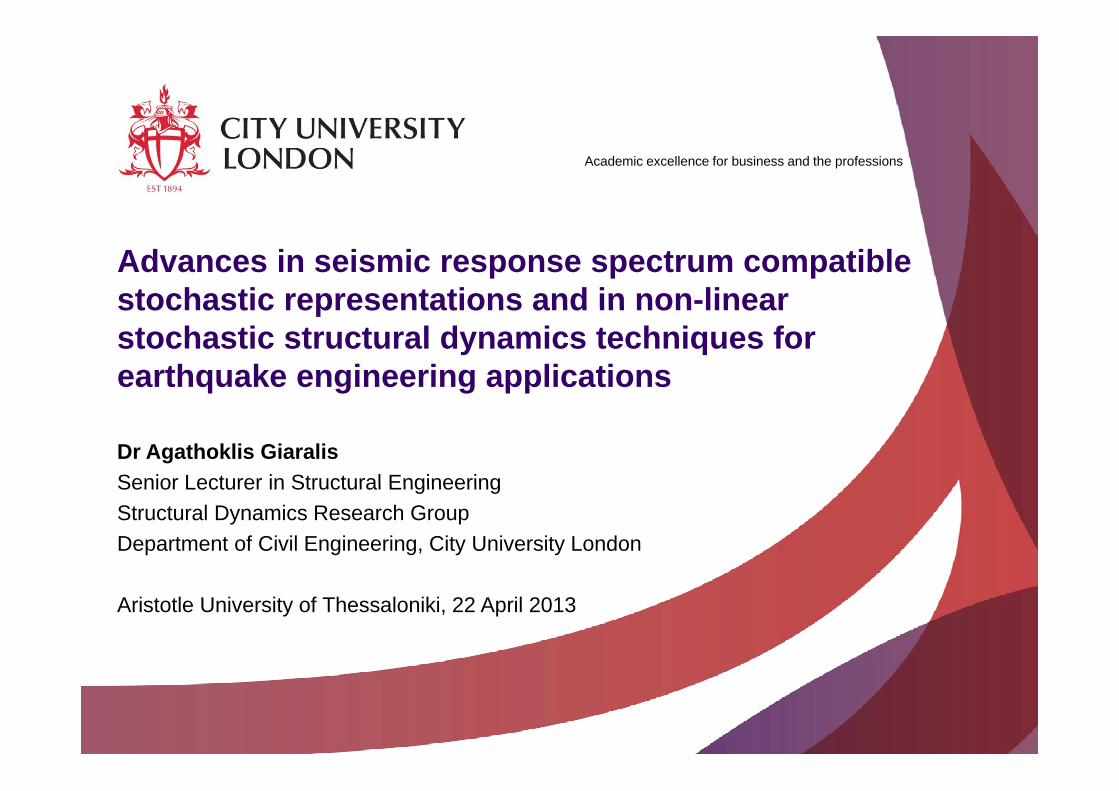
INPUT:INPUT:TimeTime‐‐varying varying
excitation loadsexcitation loads
SYSTEM:SYSTEM:Civil Civil
InfrastructureInfrastructure
OUTPUT:OUTPUT:Structural Structural responseresponseexcitation loadsexcitation loads
‐‐NonNon‐‐linearlinear
+0 00 m
αντισεισμικός αρμός
Ι ό (Pil ti )+0,00 m Ισόγειο (Pilotis)
Υπόγειο
ελαστομεταλλικό εφέδρανο
2000
800
Σκυρόδεμα καθαρότητος
-3.85 m
150
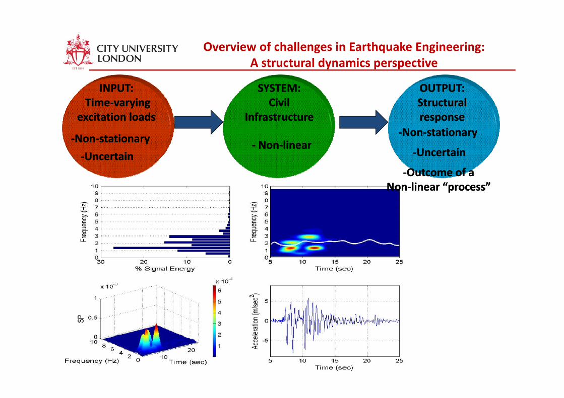
Overview of challenges in Earthquake Engineering: A structural dynamics perspective
INPUT:INPUT:TimeTime‐‐varying varying
SYSTEM:SYSTEM:Civil Civil
OUTPUT:OUTPUT:Structural Structural
A structural dynamics perspective
excitation loadsexcitation loads InfrastructureInfrastructure responseresponse
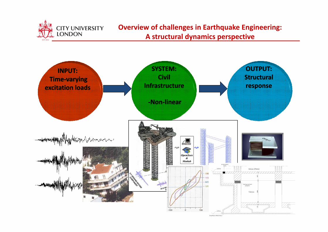
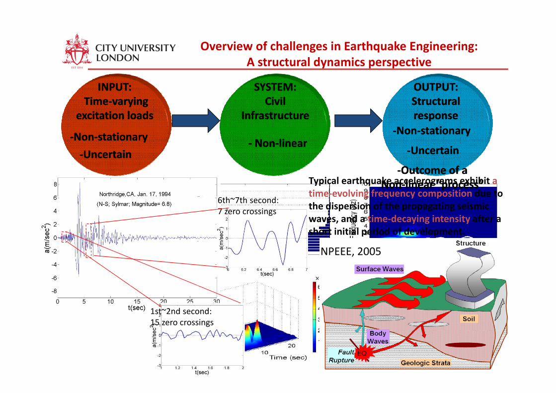
‐‐NonNon‐‐stationarystationary
U t iU t i
‐‐NonNon‐‐stationarystationary‐‐ NonNon‐‐linearlinear
‐‐UncertainUncertain‐‐UncertainUncertain
Typical earthquake accelerograms exhibit a time‐evolving frequency composition due to
‐‐Outcome of Outcome of aaNonNon‐‐linear “process”linear “process”
UncertainUncertain
time evolving frequency composition due to the dispersion of the propagating seismic waves, and a time‐decaying intensity after a short initial period of development.
6th~7th second: 7 zero crossings
NPEEE, 2005
1st~2nd second: 15 zero crossings
Overview of challenges in Earthquake Engineering: A structural dynamics perspective
INPUT:INPUT:TimeTime‐‐varying varying
SYSTEM:SYSTEM:Civil Civil
OUTPUT:OUTPUT:Structural Structural
A structural dynamics perspective
excitation loadsexcitation loads InfrastructureInfrastructure responseresponse
‐‐NonNon‐‐stationarystationary
U t iU t i
‐‐NonNon‐‐stationarystationary‐‐ NonNon‐‐linearlinear
‐‐UncertainUncertain‐‐UncertainUncertain‐‐Outcome of Outcome of aa
NonNon‐‐linear “process”linear “process”
UncertainUncertain
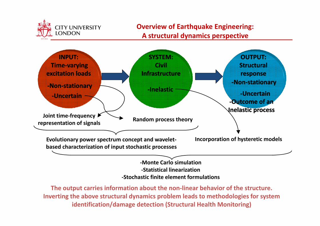
Overview of Earthquake Engineering: A structural dynamics perspective
INPUT:INPUT: SYSTEM:SYSTEM: OUTPUT:OUTPUT:
A structural dynamics perspective
TimeTime‐‐varying varying excitation loadsexcitation loads
Civil Civil InfrastructureInfrastructure
Structural Structural responseresponse
‐‐NonNon‐‐stationarystationary ‐‐NonNon‐‐stationarystationaryI l iI l iNonNon stationarystationary
‐‐UncertainUncertain‐‐Outcome of anOutcome of anInelastic processInelastic process
‐‐InelasticInelastic‐‐UncertainUncertain
ppJoint time‐frequency
representation of signalsRandom process theory
Evolutionary power spectrum concept and wavelet Incorporation of hysteretic modelsEvolutionary power spectrum concept and wavelet‐based characterization of input stochastic processes
Incorporation of hysteretic models
‐Monte Carlo simulationMonte Carlo simulation‐Statistical linearization
‐Stochastic finite element formulations
The output carries information about the non‐linear behavior of the structure.The output carries information about the non linear behavior of the structure. Inverting the above structural dynamics problem leads to methodologies for system
identification/damage detection (Structural Health Monitoring)
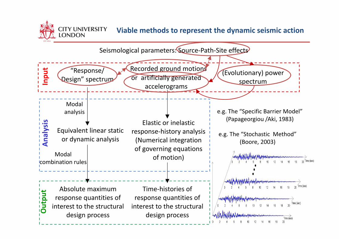
Viable methods to represent the dynamic seismic action
Seismological parameters: Source‐Path‐Site effects
“Response/ Design” spectrum
Recorded ground motions
Inpu
t
(Evolutionary) power spectrumor artificially generated
accelerograms
Modal analysis e.g. The “Specific Barrier Model”
(Papageorgiou /Aki 1983)
Equivalent linear static or dynamic analysis
Elastic or inelastic response‐history analysis (Numerical integration f i i
Ana
lysis (Papageorgiou /Aki, 1983)
e.g. The “Stochastic Method” (Boore, 2003)
of governing equations of motion)Modal
combination rules
Absolute maximum response quantities of
Time‐histories of response quantities of pu
t
p qinterest to the structural
design process
p qinterest to the structural
design processOut
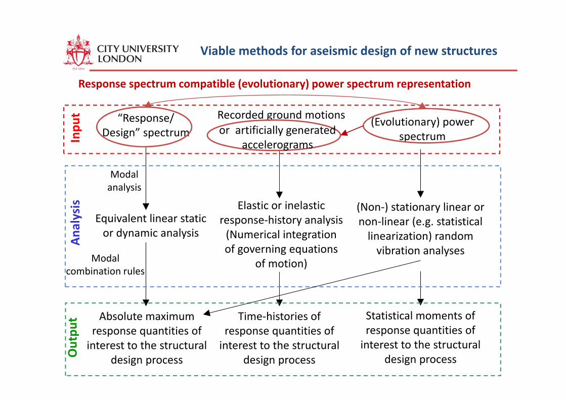
Viable methods for aseismic design of new structures
Response spectrum compatible (evolutionary) power spectrum representation
“Response/ Design” spectrum
Recorded ground motions
Inpu
t
(Evolutionary) power spectrumor artificially generated
accelerograms
Modal analysis
Equivalent linear static or dynamic analysis
Elastic or inelastic response‐history analysis (Numerical integration f i i
Ana
lysis (Non‐) stationary linear or
non‐linear (e.g. statistical linearization) random
of governing equations of motion)Modal
combination rules
vibration analyses
Absolute maximum response quantities of
Time‐histories of response quantities of pu
t Statistical moments of response quantities of p q
interest to the structural design process
p qinterest to the structural
design processOut interest to the structural
design process
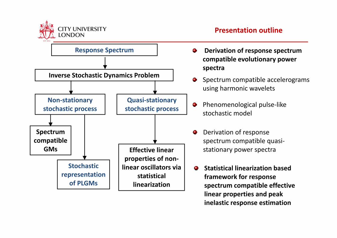
Presentation outline
Response Spectrum Derivation of response spectrum compatible evolutionary power
Inverse Stochastic Dynamics Problemspectra
Spectrum compatible accelerogramsusing harmonic wavelets
Non‐stationary stochastic process
Quasi‐stationary stochastic process Phenomenological pulse‐like
stochastic model
Spectrum compatible
Derivation of response spectrum compatible quasi‐
Stochastic t ti
GMs Effective linear properties of non‐linear oscillators via
stationary power spectra
Statistical linearization based representation
of PLGMsstatistical
linearizationframework for response spectrum compatible effective linear properties and peak
linelastic response estimation
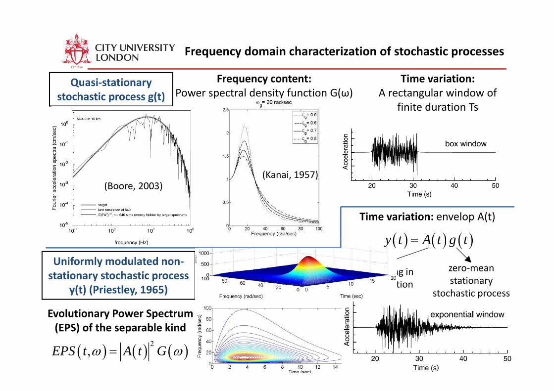
Frequency domain characterization of stochastic processes
Quasi‐stationary stochastic process g(t)
Frequency content:Power spectral density function G(ω)
Time variation:A rectangular window of
finite duration Tsfinite duration Ts
(Boore, 2003)(Kanai, 1957)
Time variation: envelop A(t)
( ) ( ) ( )y t A t g t=
Uniformly modulated non‐stationary stochastic process
( ) ( ) ( )y t A t g t=
zero‐mean stationary
Slowly‐varying in time modulationy(t) (Priestley, 1965)
Evolutionary Power Spectrum (EPS) of the separable kind
ystochastic process
time modulation function
(EPS) of the separable kind
( ) ( ) ( )2,EPS t A t Gω ω=
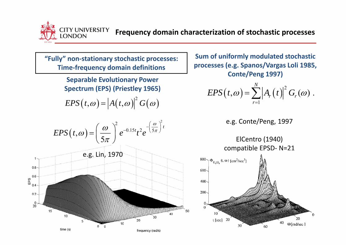
Frequency domain characterization of stochastic processes
“Fully” non‐stationary stochastic processes: Time frequency domain definitions
Sum of uniformly modulated stochastic processes (e.g. Spanos/Vargas Loli 1985,
Separable Evolutionary Power Spectrum (EPS) (Priestley 1965)
Time‐frequency domain definitions processes (e.g. Spanos/Vargas Loli 1985, Conte/Peng 1997)
( ) ( ) 2, ( ) .
N
GEPS t A tω ω=∑( ) ( ) ( )2
, ,EPS t A t Gω ω ω=
22 ⎛ ⎞
( ) ( )1
, ( ) .rr
rGEPS t A tω ω=∑
e g Conte/Peng 1997
( )2
0.15 2 5,5
ttEPS t e t e
ωπωω
π
⎛ ⎞−⎜ ⎟− ⎝ ⎠⎛ ⎞= ⎜ ⎟⎝ ⎠
e.g. Conte/Peng, 1997
ElCentro (1940) compatible EPSD‐ N=21
e.g. Lin, 1970compatible PS N
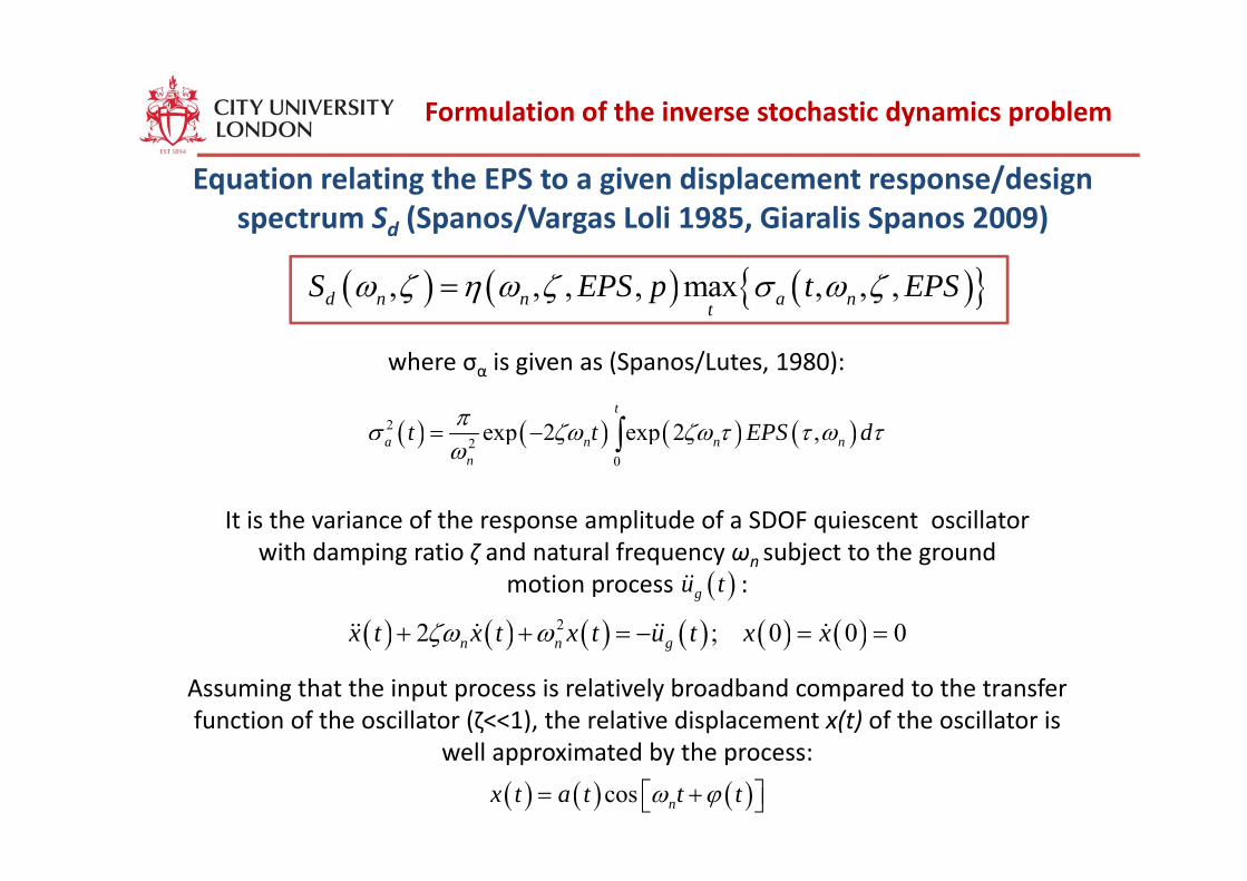
Formulation of the inverse stochastic dynamics problem
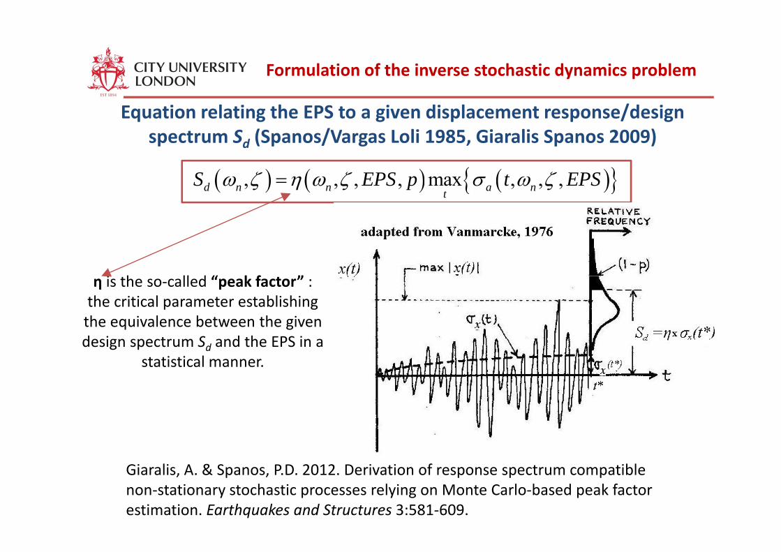
Equation relating the EPS to a given displacement response/design spectrum Sd (Spanos/Vargas Loli 1985, Giaralis Spanos 2009)
( ) ( ) ( ){ }, , , , max , , ,d n n a ntS EPS p t EPSω ζ η ω ζ σ ω ζ=
( ) ( ) ( ) ( )22 exp 2 exp 2 ,
t
a n n nt t EPS dπσ ζω ζω τ τ ω τ= − ∫
where σα is given as (Spanos/Lutes, 1980):
( ) ( ) ( ) ( )20
p p ,a n n nn
ζ ζω ∫
It is the variance of the response amplitude of a SDOF quiescent oscillator
( ) ( ) ( ) ( ) ( ) ( )22 ; 0 0 0x t x t x t u t x xζω ω+ + = − = =
with damping ratio ζ and natural frequency ωn subject to the ground motion process :( )gu t
( ) ( ) ( ) ( ) ( ) ( )2 ; 0 0 0n n gx t x t x t u t x xζω ω+ +
Assuming that the input process is relatively broadband compared to the transfer function of the oscillator (ζ<<1), the relative displacement x(t) of the oscillator is
( ) ( ) ( )cos nx t a t t tω ϕ= +⎡ ⎤⎣ ⎦
well approximated by the process:
Formulation of the inverse stochastic dynamics problem
Equation relating the EPS to a given displacement response/design spectrum Sd (Spanos/Vargas Loli 1985, Giaralis Spanos 2009)
( ) ( ) ( ){ }, , , , max , , ,d n n a ntS EPS p t EPSω ζ η ω ζ σ ω ζ=
i h ll d “ k f ”η is the so‐called “peak factor” : the critical parameter establishing the equivalence between the given d i t S d th EPS idesign spectrum Sd and the EPS in a
statistical manner.
l & f blGiaralis, A. & Spanos, P.D. 2012. Derivation of response spectrum compatible non‐stationary stochastic processes relying on Monte Carlo‐based peak factor estimation. Earthquakes and Structures 3:581‐609.
Formulation of the inverse stochastic dynamics problem
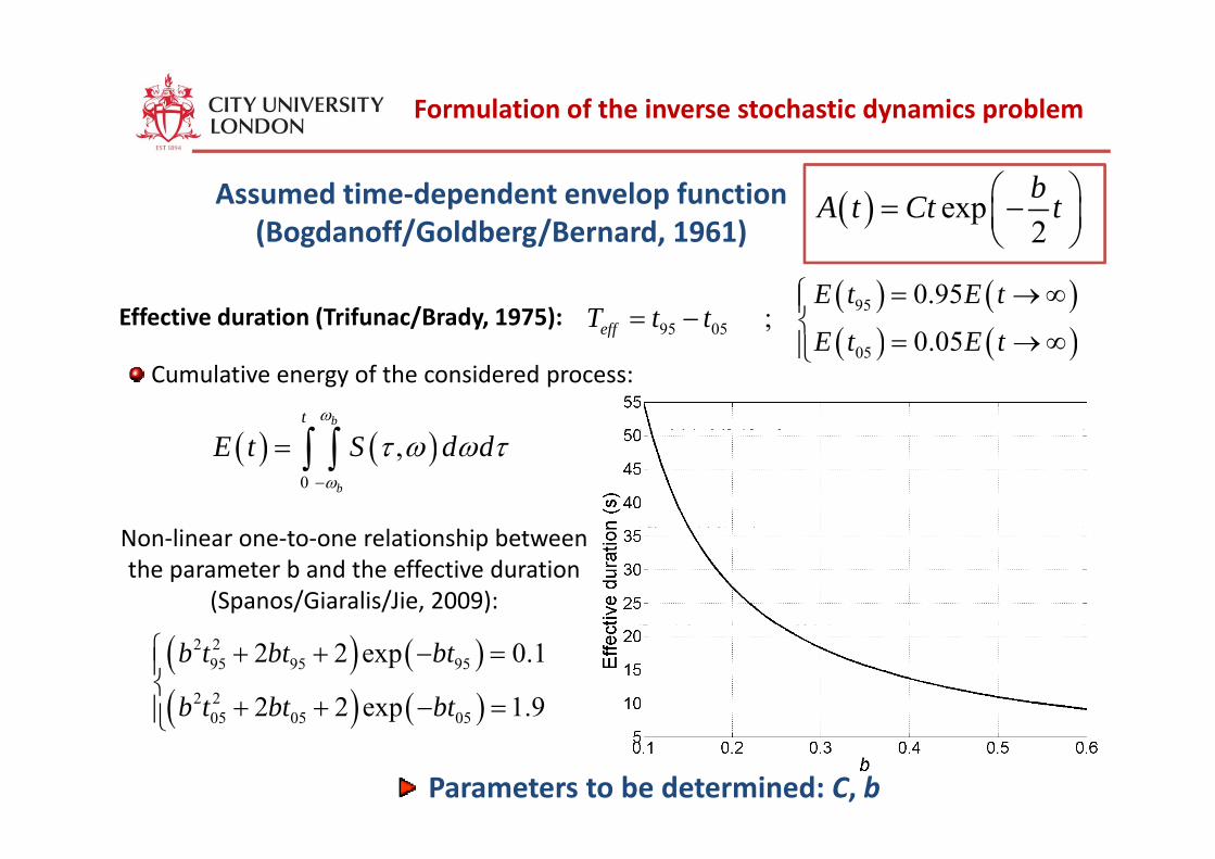
Assumed time‐dependent envelop function (Bogdanoff/Goldberg/Bernard 1961)
( ) exp2bA t Ct t⎛ ⎞= −⎜ ⎟
⎝ ⎠(Bogdanoff/Goldberg/Bernard, 1961) 2⎝ ⎠
( ) ( )( ) ( )
9595 05
0.95;
0 05eff
E t E tT t t
E E
= →∞⎧⎪= − ⎨⎪
Effective duration (Trifunac/Brady, 1975):
bt ω
∫ ∫
( ) ( )95 0505 0.05eff E t E t
⎨= →∞⎪⎩
Cumulative energy of the considered process:
( ) ( )0
,b
E t S d dω
τ ω ω τ−
= ∫ ∫
Non‐linear one‐to‐one relationship between the parameter b and the effective duration
(Spanos/Giaralis/Jie, 2009):
( ) ( )( ) ( )
2 295 95 95
2 205 05 05
2 2 exp 0.1
2 2 exp 1.9
b t bt bt
b t bt bt
⎧ + + − =⎪⎨
+ + − =⎪⎩
Parameters to be determined: C, b
( ) ( )05 05 05⎪⎩
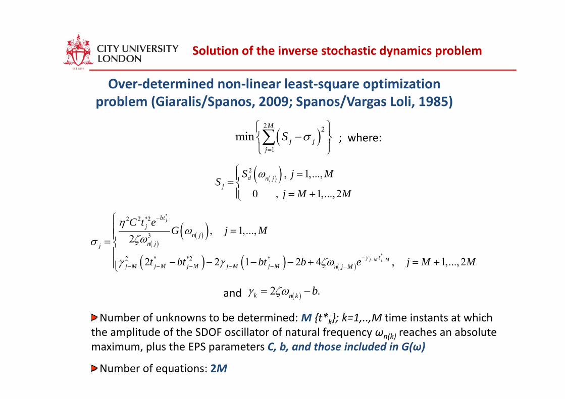
Solution of the inverse stochastic dynamics problem
Over‐determined non‐linear least‐square optimization problem (Giaralis/Spanos, 2009; Spanos/Vargas Loli, 1985)
( )2 2
1min
M
j jj
S σ=
⎧ ⎫−⎨ ⎬
⎩ ⎭∑ ; where:⎩ ⎭
( )( )2 , 1,...,
0 , 1,..., 2d n j
j
S j MS
j M M
ω⎧ =⎪= ⎨= +⎪⎩⎩
( )( )( )
*2 2 *2
3 , 1,...,2
jbtj
n jn jj
C t eG j M
ηω
ζωσ
−⎧⎪ =⎪= ⎨ ( )
( ) ( ) ( )*2 * *2 *2 2 1 2 4 , 1,..., 2j M j M
n jj
tj M j M j M j M j M n j Mt bt bt b e j M Mγ
σ
γ γ ζω − −−− − − − − −
⎨⎪
− − − − + = +⎪⎩
2 bγ ζωd ( )2 .k n k bγ ζω= −
Number of unknowns to be determined: M {t*k}; k=1,..,M time instants at which the amplitude of the SDOF oscillator of natural frequency ωn(k) reaches an absolute
and
the amplitude of the SDOF oscillator of natural frequency ωn(k) reaches an absolute maximum, plus the EPS parameters C, b, and those included in G(ω)
Number of equations: 2M
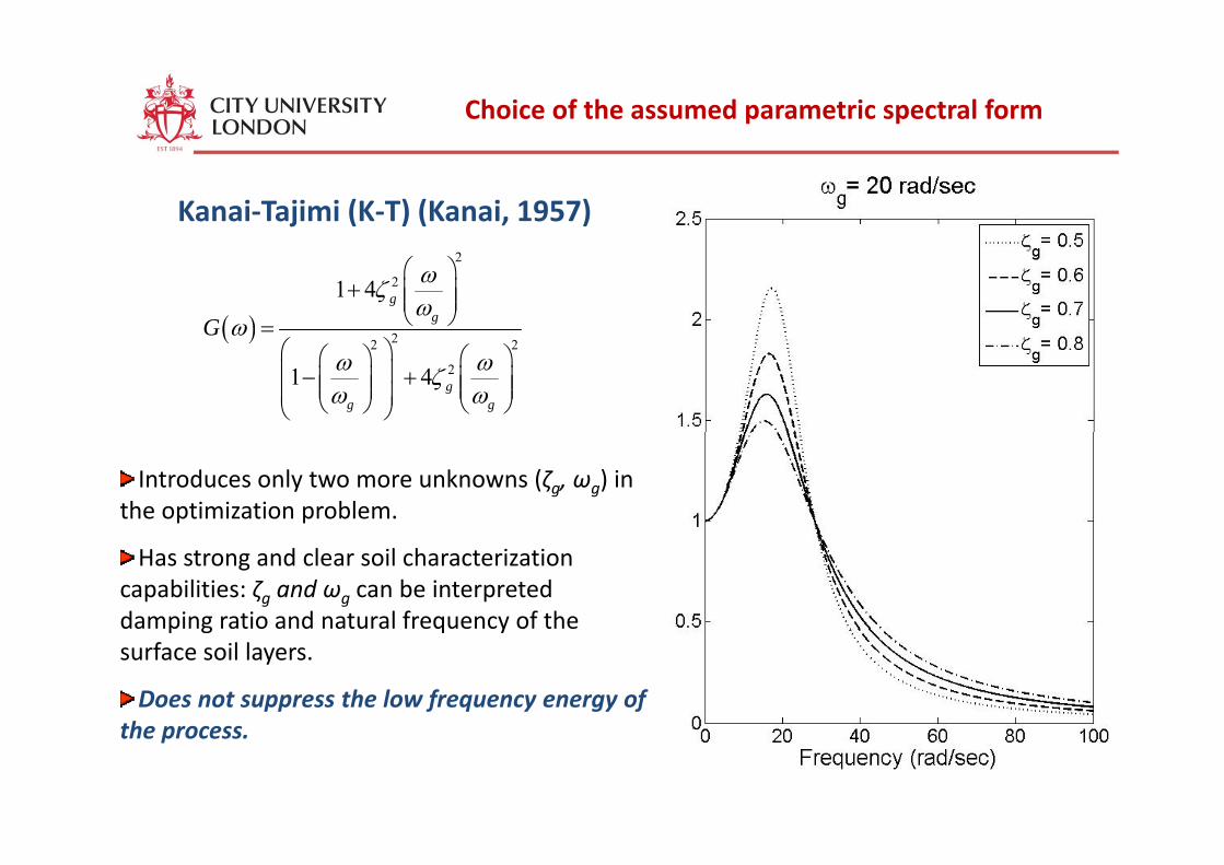
Choice of the assumed parametric spectral form
Kanai‐Tajimi (K‐T) (Kanai, 1957)
( )
2
2
2
1 4 ggG
ωζω
ω
⎛ ⎞+ ⎜ ⎟⎜ ⎟
⎝ ⎠=( ) 22 2
21 4 gg g
G ωω ωζω ω
⎛ ⎞⎛ ⎞ ⎛ ⎞⎜ ⎟− +⎜ ⎟ ⎜ ⎟⎜ ⎟ ⎜ ⎟⎜ ⎟⎝ ⎠ ⎝ ⎠⎝ ⎠
Introduces only two more unknowns (ζg, ωg) in the optimization problem.
Has strong and clear soil characterization capabilities: ζg and ωg can be interpreted damping ratio and natural frequency of the p g q ysurface soil layers.
Does not suppress the low frequency energy of the processthe process.
Choice of the assumed parametric spectral form
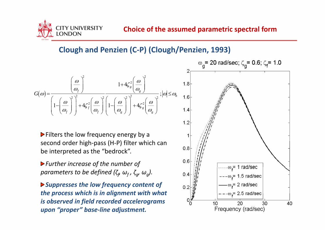
Clough and Penzien (C‐P) (Clough/Penzien, 1993)
2 2
21 4 gω ωζω ω⎛ ⎞ ⎛ ⎞
+⎜ ⎟ ⎜ ⎟⎜ ⎟ ⎜ ⎟⎝ ⎠ ⎝ ⎠( ) 2 22 2 2 2
2 2
;
1 4 1 4
f gb
f gf f g g
Gω ω
ω ω ωω ω ω ωζ ζω ω ω ω
⎜ ⎟ ⎜ ⎟⎝ ⎠ ⎝ ⎠= ≤
⎛ ⎞ ⎛ ⎞⎛ ⎞ ⎛ ⎞ ⎛ ⎞ ⎛ ⎞⎜ ⎟ ⎜ ⎟− + − +⎜ ⎟ ⎜ ⎟ ⎜ ⎟ ⎜ ⎟⎜ ⎟ ⎜ ⎟ ⎜ ⎟ ⎜ ⎟⎜ ⎟ ⎜ ⎟⎝ ⎠ ⎝ ⎠ ⎝ ⎠ ⎝ ⎠⎝ ⎠ ⎝ ⎠
Filters the low frequency energy by a d d hi h (H P) filt hi h
⎝ ⎠ ⎝ ⎠
second order high‐pass (H‐P) filter which can be interpreted as the “bedrock”.
Further increase of the number of parameters to be defined (ζf, ωf , ζg, ωg).
Suppresses the low frequency content of the process which is in alignment with whatthe process which is in alignment with what is observed in field recorded accelerograms upon “proper” base‐line adjustment.
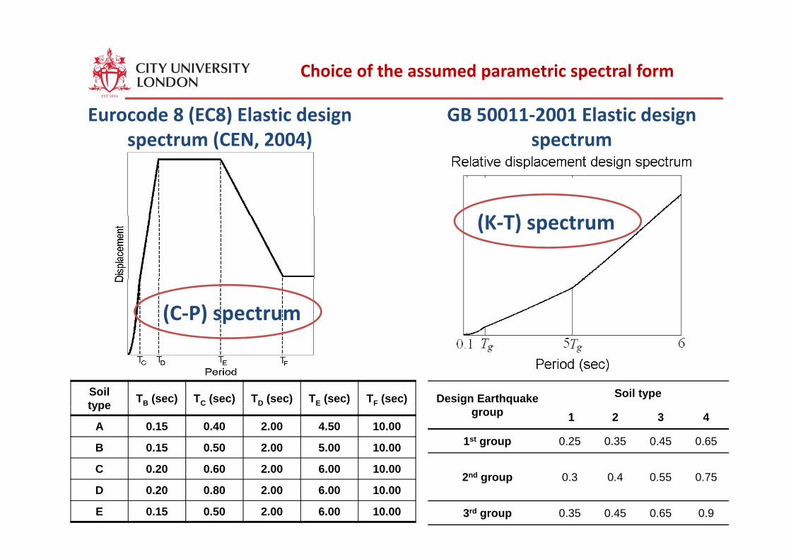
Choice of the assumed parametric spectral form
Eurocode 8 (EC8) Elastic design spectrum (CEN, 2004)
GB 50011‐2001 Elastic design spectrum
(K T)(K‐T) spectrum
(C‐P) spectrum
Soil type TB (sec) TC (sec) TD (sec) TE (sec) TF (sec) Design Earthquake Soil typetype
A 0.15 0.40 2.00 4.50 10.00
B 0.15 0.50 2.00 5.00 10.00
C 0 20 0 60 2 00 6 00 10 00
group 1 2 3 4
1st group 0.25 0.35 0.45 0.65
C 0.20 0.60 2.00 6.00 10.00
D 0.20 0.80 2.00 6.00 10.00
E 0.15 0.50 2.00 6.00 10.00
2nd group 0.3 0.4 0.55 0.75
3rd group 0.35 0.45 0.65 0.9
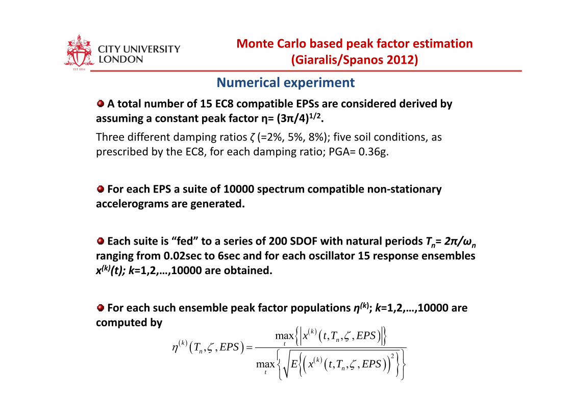
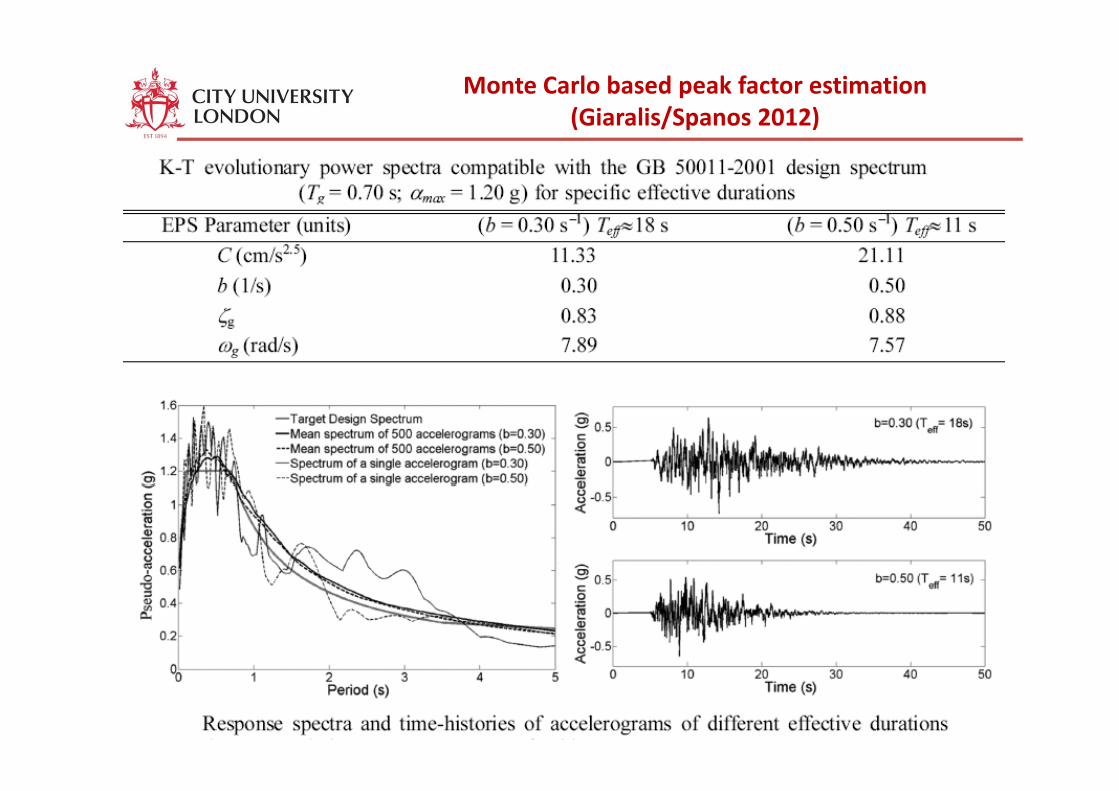
Monte Carlo based peak factor estimation (Giaralis/Spanos 2012) ( / p )
Numerical experimentA total number of 15 EC8 compatible EPSs are considered derived by
assuming a constant peak factor η= (3π/4)1/2.
Three different damping ratios ζ (=2%, 5%, 8%); five soil conditions, as prescribed by the EC8, for each damping ratio; PGA= 0.36g.p y , p g ; g
For each EPS a suite of 10000 spectrum compatible non‐stationary accelerograms are generatedaccelerograms are generated.
Each suite is “fed” to a series of 200 SDOF with natural periods Tn= 2π/ωnn nranging from 0.02sec to 6sec and for each oscillator 15 response ensembles x(k)(t); k=1,2,…,10000 are obtained.
For each such ensemble peak factor populations η(k); k=1,2,…,10000 are computed by
( ) ( ){ }max , , ,kx t T EPSζ( ) ( )
( ){ }( ) ( )( ){ }2
max , , ,, ,
max , , ,
nk tn
knt
x t T EPST EPS
E x t T EPS
ζη ζ
ζ=
⎧ ⎫⎨ ⎬⎩ ⎭
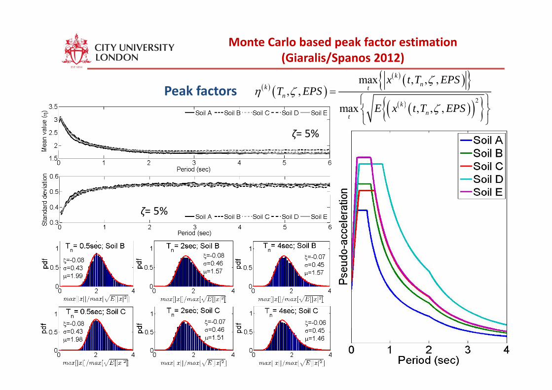
Monte Carlo based peak factor estimation (Giaralis/Spanos 2012)
Peak factors ( ) ( )( ) ( ){ }( ) ( )( ){ }2
max , , ,, ,
knk t
nk
x t T EPST EPS
E t T EPS
ζη ζ
ζ=
⎧ ⎫⎨ ⎬
( / p )
( ) ( )( ){ }max , , ,ntE x t T EPSζ⎨ ⎬
⎩ ⎭ζ= 5%
Type III generalized extreme value distribution (Weibull) provided the best fit in the standard
i lik lih d t t
ζ= 5%
maximum likelihood context (Kotz/Nadarajah 2000)
( )1/1/ 1 zfξμξ ξ
−⎛ ⎞−⎛ ⎞⎜ ⎟⎜ ⎟( )
1 1/
/ , , exp 1
1
f z
z ξ
μξ σ μ ξσ σ
μξσ
− −
⎛ ⎞= − + ×⎜ ⎟⎜ ⎟⎜ ⎟⎝ ⎠⎝ ⎠
−⎛ ⎞+⎜ ⎟⎝ ⎠σ⎝ ⎠
1 0z μξσ−
+ >where
Monte Carlo based peak factor estimation (Giaralis/Spanos 2012)
( ) ( ) ( ){ }, , , , max , , ,d n n a nS EPS p t EPSω ζ η ω ζ σ ω ζ=
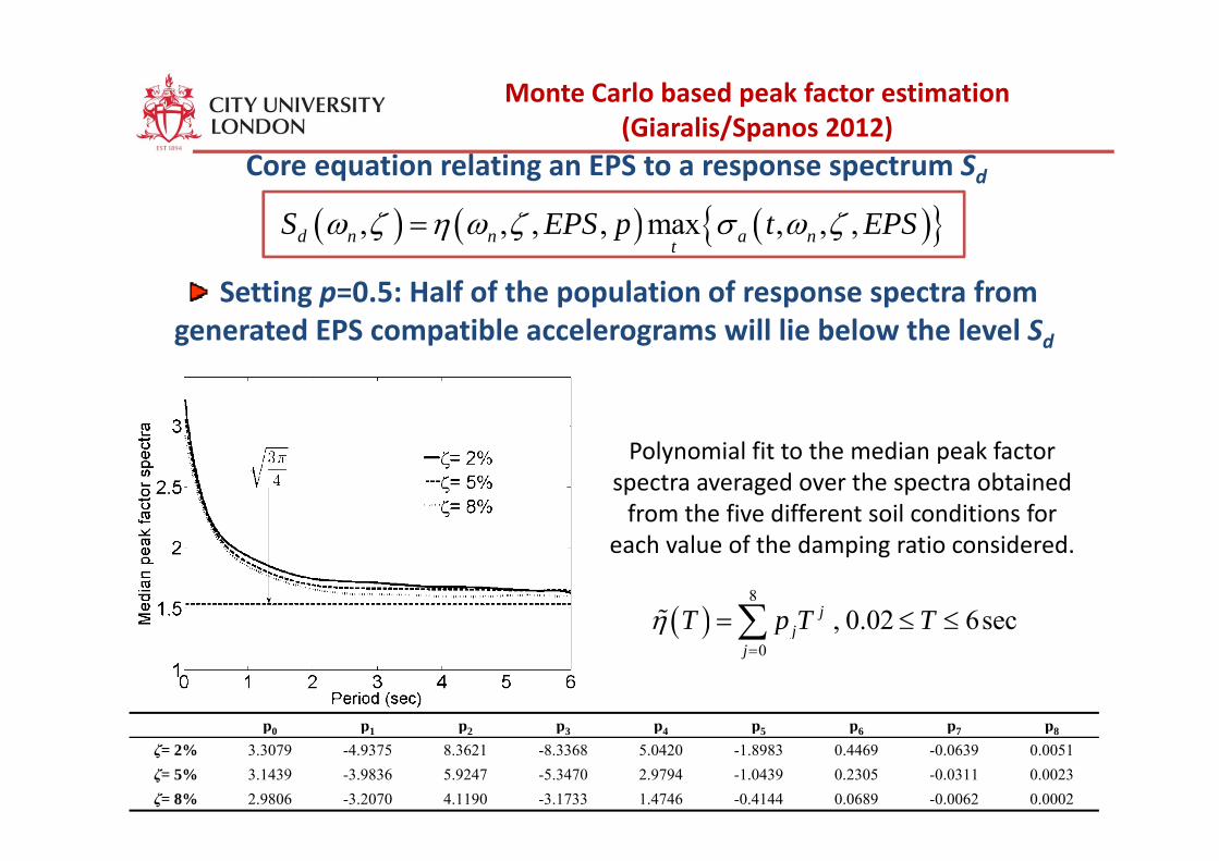
Core equation relating an EPS to a response spectrum Sd
( / p )
( ) ( ) ( ){ }, , , , , , ,d n n a ntpζ η ζ ζ
Setting p=0.5: Half of the population of response spectra from generated EPS compatible accelerograms will lie below the level Sgenerated EPS compatible accelerograms will lie below the level Sd
Polynomial fit to the median peak factor spectra averaged over the spectra obtained from the five different soil conditions for
each value of the damping ratio considered.
( )8
0 02 6secjjT p T Tη = ≤ ≤∑
p p p p p p p p p
( )0
, 0.02 6secjj
T p T Tη=
≤ ≤∑
p0 p1 p2 p3 p4 p5 p6 p7 p8
ζ= 2% 3.3079 -4.9375 8.3621 -8.3368 5.0420 -1.8983 0.4469 -0.0639 0.0051ζ= 5% 3.1439 -3.9836 5.9247 -5.3470 2.9794 -1.0439 0.2305 -0.0311 0.0023ζ= 8% 2.9806 -3.2070 4.1190 -3.1733 1.4746 -0.4144 0.0689 -0.0062 0.0002
Monte Carlo based peak factor estimation (Giaralis/Spanos 2012)
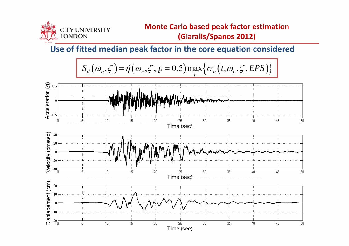
( ) ( ) ( ){ }0 5 maxS p t EPSω ζ η ω ζ σ ω ζ
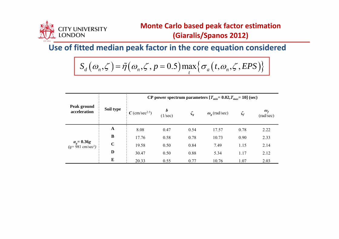
Use of fitted median peak factor in the core equation considered( / p )
( ) ( ) ( ){ }, , , 0.5 max , , ,d n n a ntS p t EPSω ζ η ω ζ σ ω ζ= =
Peak ground acceleration Soil type
CP power spectrum parameters [Tmin= 0.02,Tmax= 10] (sec)
C (cm/sec2.5) b(1/sec) ζg ωg (rad/sec) ζf
ωf(rad/sec)
αg= 0.36g(g= 981 cm/sec2)
A 8.08 0.47 0.54 17.57 0.78 2.22B 17.76 0.58 0.78 10.73 0.90 2.33C 19.58 0.50 0.84 7.49 1.15 2.14(g= 981 cm/sec2) 19.58 0.50 0.84 7.49 1.15 2.14D 30.47 0.50 0.88 5.34 1.17 2.12E 20.33 0.55 0.77 10.76 1.07 2.03
Monte Carlo based peak factor estimation (Giaralis/Spanos 2012)
( ) ( ) ( ){ }0 5 maxS p t EPSω ζ η ω ζ σ ω ζ
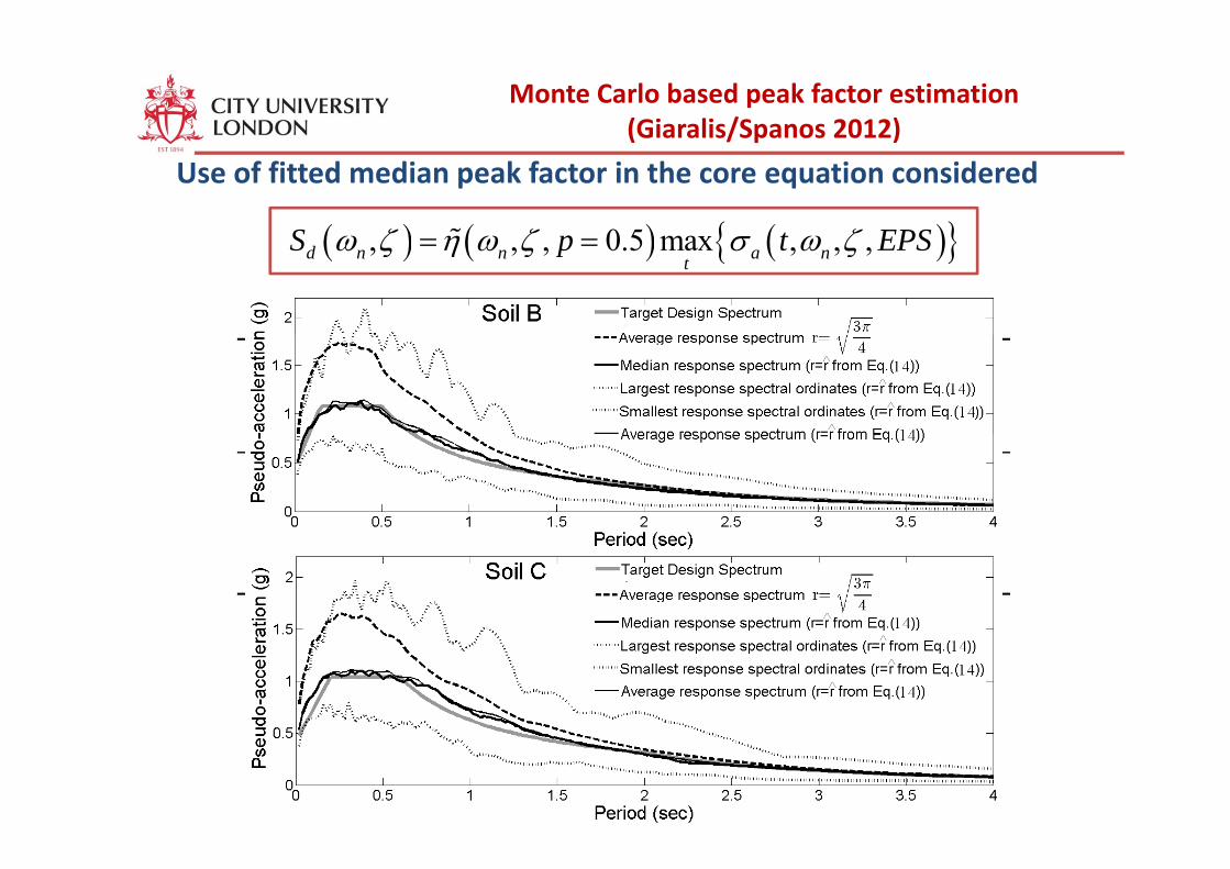
Use of fitted median peak factor in the core equation considered( / p )
( ) ( ) ( ){ }, , , 0.5 max , , ,d n n a ntS p t EPSω ζ η ω ζ σ ω ζ= =
Peak ground acceleration Soil type
CP power spectrum parameters [Tmin= 0.02,Tmax= 10] (sec)
C (cm/sec2.5) b(1/sec) ζg ωg (rad/sec) ζf
ωf(rad/sec)
αg= 0.36g(g= 981 cm/sec2)
A 8.08 0.47 0.54 17.57 0.78 2.22B 17.76 0.58 0.78 10.73 0.90 2.33C 19.58 0.50 0.84 7.49 1.15 2.14(g= 981 cm/sec2) 19.58 0.50 0.84 7.49 1.15 2.14D 30.47 0.50 0.88 5.34 1.17 2.12E 20.33 0.55 0.77 10.76 1.07 2.03
Monte Carlo based peak factor estimation (Giaralis/Spanos 2012)
( ) ( ) ( ){ }0 5 maxS p t EPSω ζ η ω ζ σ ω ζ
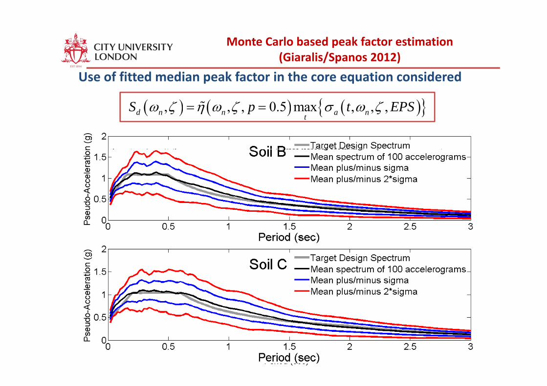
Use of fitted median peak factor in the core equation considered( / p )
( ) ( ) ( ){ }, , , 0.5 max , , ,d n n a ntS p t EPSω ζ η ω ζ σ ω ζ= =
Peak ground acceleration Soil type
CP power spectrum parameters [Tmin= 0.02,Tmax= 10] (sec)
C (cm/sec2.5) b(1/sec) ζg ωg (rad/sec) ζf
ωf(rad/sec)
αg= 0.36g(g= 981 cm/sec2)
A 8.08 0.47 0.54 17.57 0.78 2.22B 17.76 0.58 0.78 10.73 0.90 2.33C 19.58 0.50 0.84 7.49 1.15 2.14(g= 981 cm/sec2) 19.58 0.50 0.84 7.49 1.15 2.14D 30.47 0.50 0.88 5.34 1.17 2.12E 20.33 0.55 0.77 10.76 1.07 2.03
Monte Carlo based peak factor estimation (Giaralis/Spanos 2012)
( ) ( ) ( ){ }0 5 maxS p t EPSω ζ η ω ζ σ ω ζ
Use of fitted median peak factor in the core equation considered( / p )
( ) ( ) ( ){ }, , , 0.5 max , , ,d n n a ntS p t EPSω ζ η ω ζ σ ω ζ= =
Peak ground acceleration Soil type
CP power spectrum parameters [Tmin= 0.02,Tmax= 10] (sec)
C (cm/sec2.5) b(1/sec) ζg ωg (rad/sec) ζf
ωf(rad/sec)
αg= 0.36g(g= 981 cm/sec2)
A 8.08 0.47 0.54 17.57 0.78 2.22B 17.76 0.58 0.78 10.73 0.90 2.33C 19.58 0.50 0.84 7.49 1.15 2.14(g= 981 cm/sec2) 19.58 0.50 0.84 7.49 1.15 2.14D 30.47 0.50 0.88 5.34 1.17 2.12E 20.33 0.55 0.77 10.76 1.07 2.03
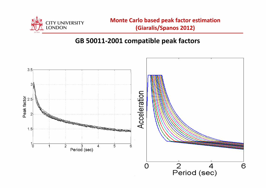
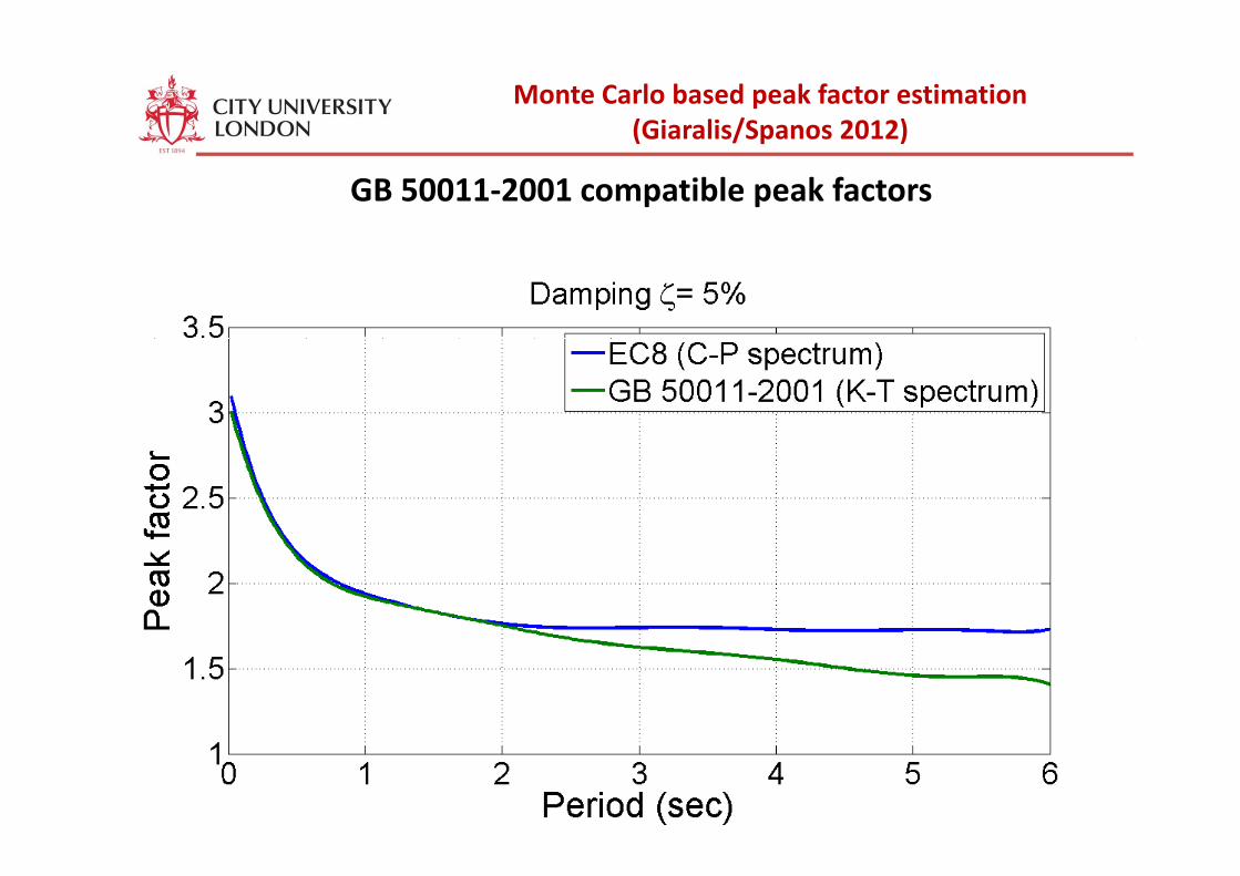
Monte Carlo based peak factor estimation (Giaralis/Spanos 2012)
GB 50011‐2001 compatible peak factors
( / p )
Polynomial fit to the median peak factor spectra averaged over the spectra obtained f th 14 diff t il diti ζ 5%from the 14 different soil conditions ζ=5%.
( )7
0 02 6secjT p T Tη = ≤ ≤∑( )0
, 0.02 6secjj
T p T Tη=
≤ ≤∑
p0: 3.0672 p1: -3.1765 p2: 3.7134 p3: -2.3920
p4: 0.8660 p5: -0.1760 p6: 0.0187 p7: -0.0008
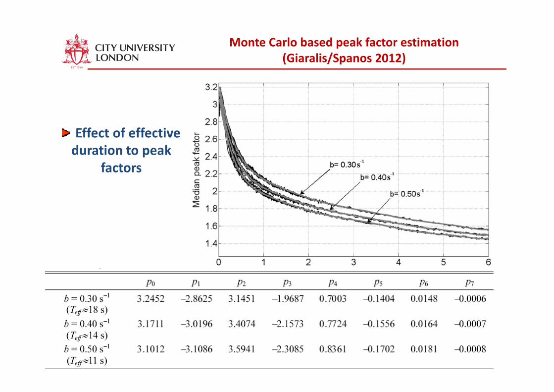
Monte Carlo based peak factor estimation (Giaralis/Spanos 2012) ( / p )
Effect of effective duration to peakduration to peak
factors
Monte Carlo based peak factor estimation (Giaralis/Spanos 2012) ( / p )
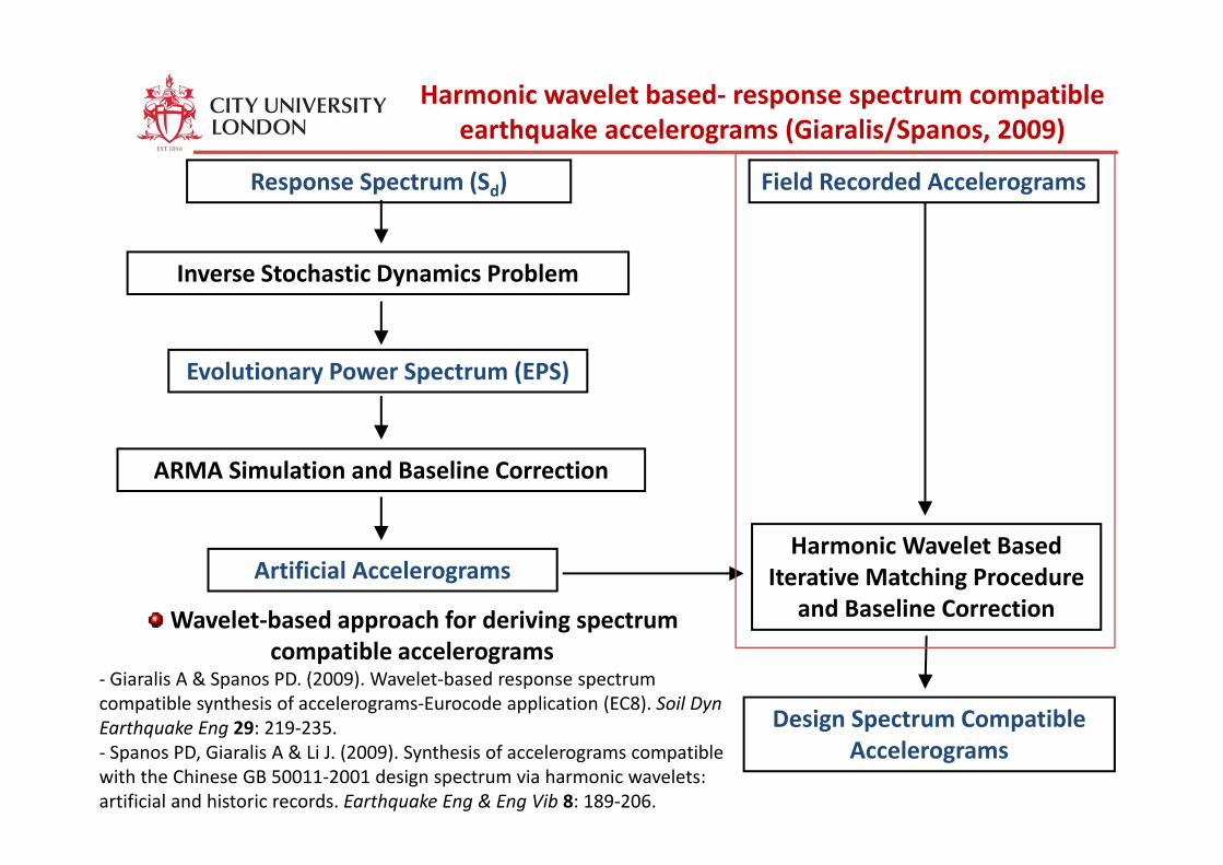
Harmonic wavelet based‐ response spectrum compatible earthquake accelerograms (Giaralis/Spanos, 2009)
Field Recorded AccelerogramsResponse Spectrum (Sd)
earthquake accelerograms (Giaralis/Spanos, 2009)
Inverse Stochastic Dynamics Problem
Evolutionary Power Spectrum (EPS)
ARMA Simulation and Baseline Correction
Artificial AccelerogramsHarmonic Wavelet Based
Iterative Matching Procedure and Baseline CorrectionWavelet‐based approach for deriving spectrum
Design Spectrum Compatible
pp g pcompatible accelerograms
‐ Giaralis A & Spanos PD. (2009). Wavelet‐based response spectrum compatible synthesis of accelerograms‐Eurocode application (EC8). Soil DynEarthquake Eng 29: 219 235 es g Spect u Co pat b e
AccelerogramsEarthquake Eng 29: 219‐235.‐ Spanos PD, Giaralis A & Li J. (2009). Synthesis of accelerograms compatible with the Chinese GB 50011‐2001 design spectrum via harmonic wavelets: artificial and historic records. Earthquake Eng & Eng Vib 8: 189‐206.
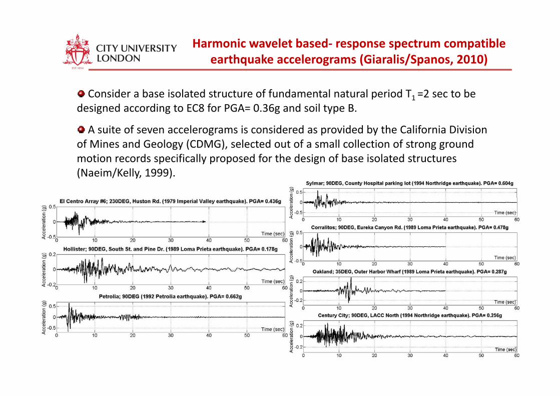
Harmonic wavelet based‐ response spectrum compatible earthquake accelerograms (Giaralis/Spanos, 2010)
Consider a base isolated structure of fundamental natural period T1 =2 sec to be designed according to EC8 for PGA= 0 36g and soil type B
earthquake accelerograms (Giaralis/Spanos, 2010)
designed according to EC8 for PGA= 0.36g and soil type B.
A suite of seven accelerograms is considered as provided by the California Division of Mines and Geology (CDMG), selected out of a small collection of strong ground motion records specifically proposed for the design of base isolated structures (Naeim/Kelly, 1999).
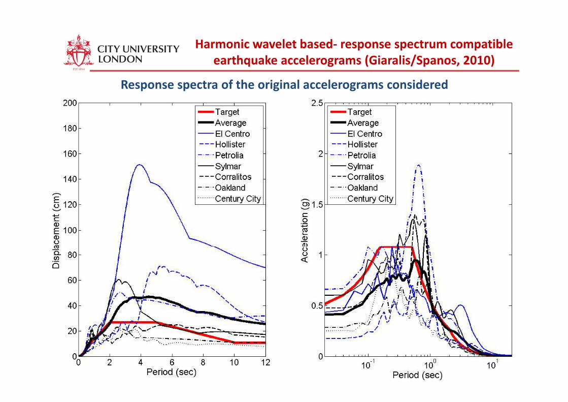
Harmonic wavelet based‐ response spectrum compatible earthquake accelerograms (Giaralis/Spanos, 2010)
Response spectra of the original accelerograms considered
earthquake accelerograms (Giaralis/Spanos, 2010)
Harmonic wavelet based‐ response spectrum compatible earthquake accelerograms (Giaralis/Spanos, 2010)
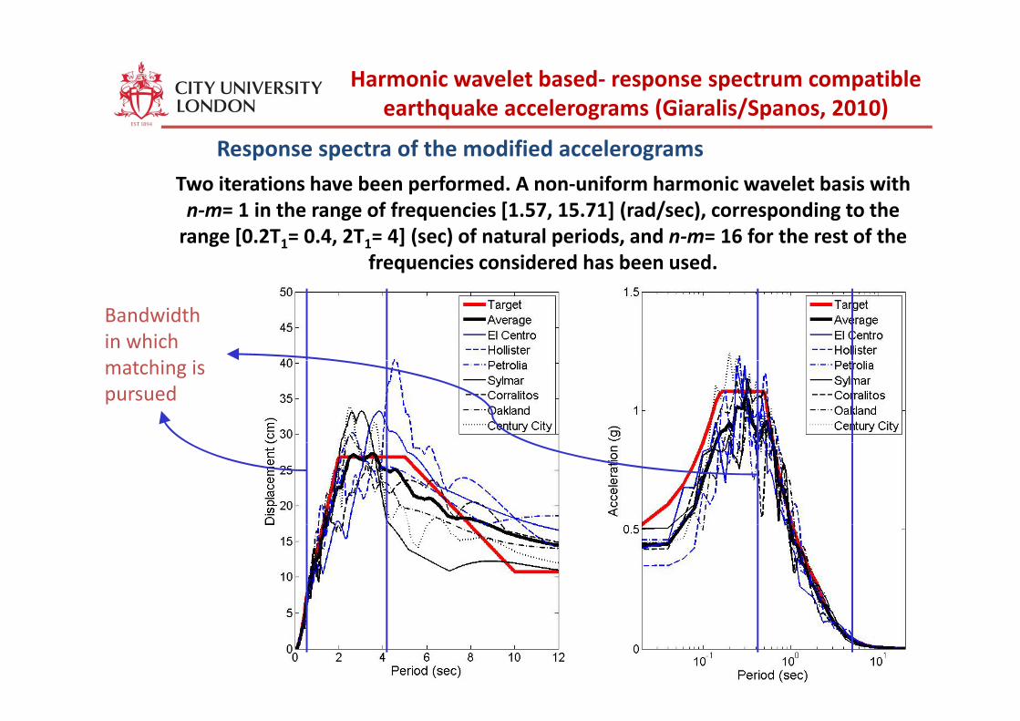
Two iterations have been performed. A non‐uniform harmonic wavelet basis with
Response spectra of the modified accelerograms
earthquake accelerograms (Giaralis/Spanos, 2010)
n‐m= 1 in the range of frequencies [1.57, 15.71] (rad/sec), corresponding to the range [0.2T1= 0.4, 2T1= 4] (sec) of natural periods, and n‐m= 16 for the rest of the
frequencies considered has been used.
Bandwidth in which
hi imatching is pursued
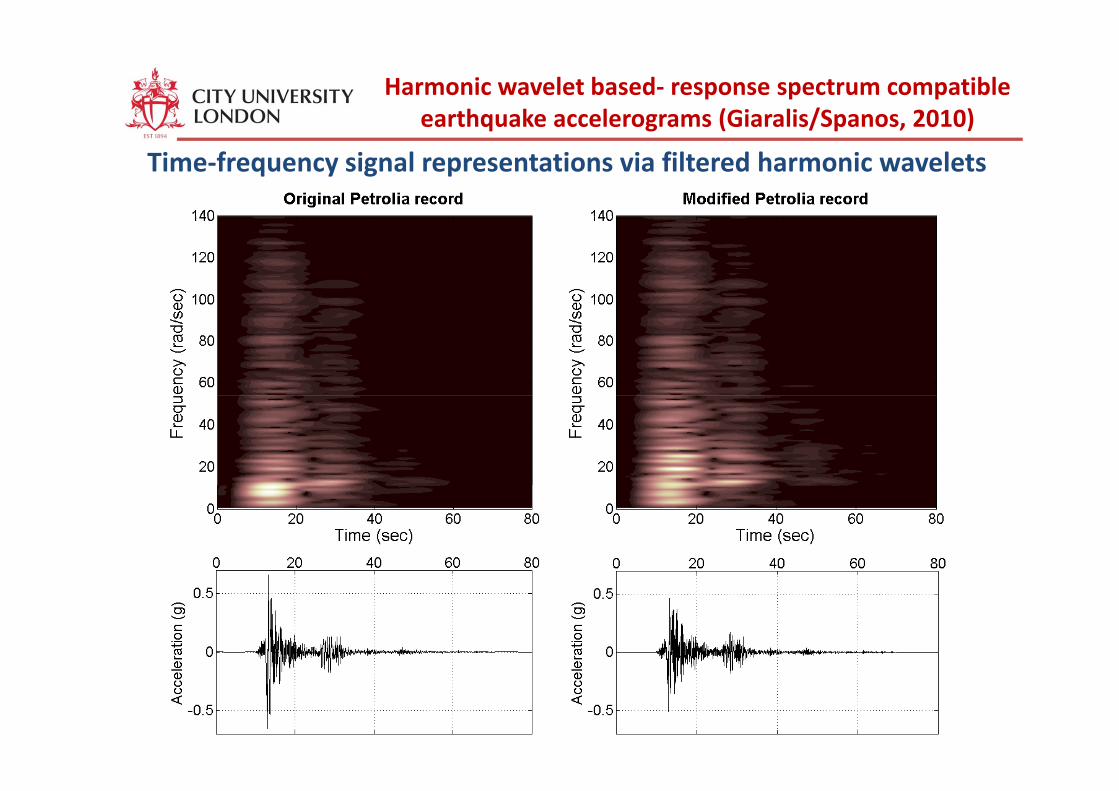
Harmonic wavelet based‐ response spectrum compatible earthquake accelerograms (Giaralis/Spanos, 2010)
Time‐frequency signal representations via filtered harmonic wavelets
earthquake accelerograms (Giaralis/Spanos, 2010)
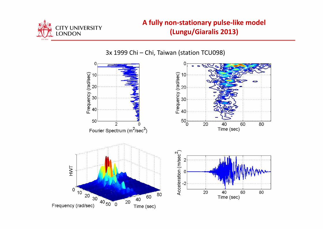
A fully non‐stationary pulse‐like model(Lungu/Giaralis 2013)
3x 1999 Chi – Chi, Taiwan (station TCU098)

A fully non‐stationary pulse‐like model(Lungu/Giaralis 2013)
2 2
Sum of uniformly modulated stochastic processes
2( ) ( )ωHF HFA t G
( ) ( )2 2 2
1
( ) ( ) ( ), ( )( ) .HF HF L rF rr
LFA t G A t G A t GS t ω ωω ω=
+ == ∑
2
1( ) ( )ω
=∑
R
rr
A t G
( ) ( )ωHF HFA t G
2( ) ( )ωLF LFA t G
For energy conserving representations, theevolutionary power spectrum density of a { }2( ) ( )EPSD E TFR
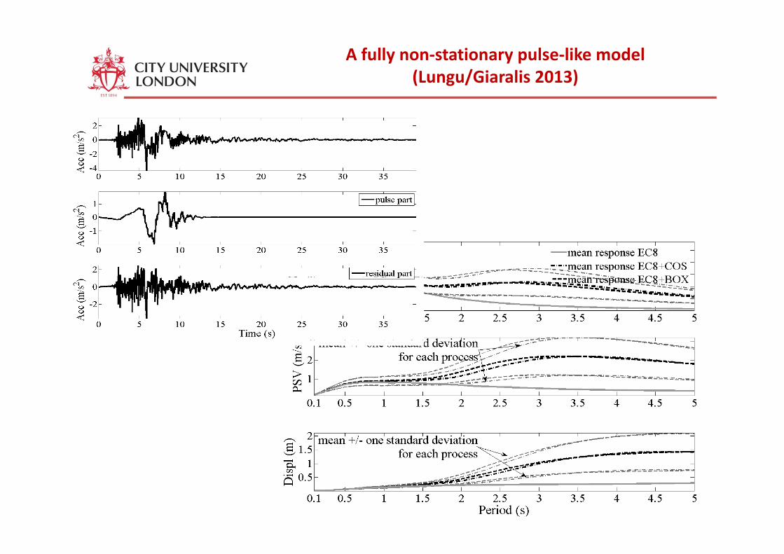
Pulse-like record = LF content (pulse) + HF content
evolutionary power spectrum density of aprocess can be estimated via the coefficientsof the transform (Politis/Giaralis/Spanos,2006; Giaralis/Lungu, 2012)
{ }( , ) ( , )ω ω∝EPSD t E TFR t
A fully non‐stationary pulse‐like model(Lungu/Giaralis 2013)
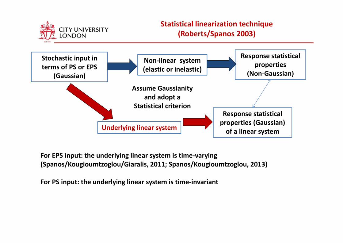
Statistical linearization technique(Roberts/Spanos 2003)
Stochastic input in terms of PS or EPS
Non‐linear systemResponse statistical
propertiesterms of PS or EPS(Gaussian)
(elastic or inelastic)properties
(Non‐Gaussian)
Assume Gaussianity
Response statistical properties (Gaussian)
and adopt aStatistical criterion
Underlying linear systemproperties (Gaussian) of a linear system
For EPS input: the underlying linear system is time‐varying (Spanos/Kougioumtzoglou/Giaralis, 2011; Spanos/Kougioumtzoglou, 2013)
For PS input: the underlying linear system is time‐invariant
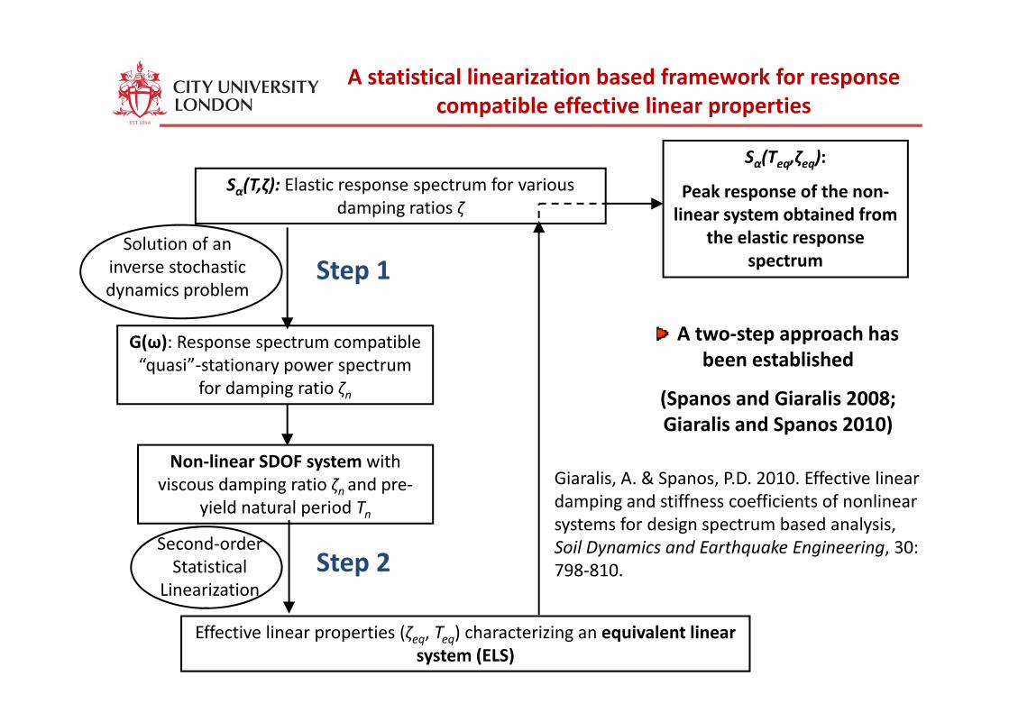
A statistical linearization based framework for response compatible effective linear properties
Sα(Τ,ζ): Elastic response spectrum for various
Sα(Τeq,ζeq):
Peak response of the non‐
p p p
αdamping ratios ζ
Solution of an inverse stochastic
Peak response of the nonlinear system obtained from
the elastic response spectrumStep 1
G(ω): Response spectrum compatible
dynamics problemStep 1
A two‐step approach has been established“quasi”‐stationary power spectrum
for damping ratio ζn
been established
(Spanos and Giaralis 2008; Giaralis and Spanos 2010)
Non‐linear SDOF system with viscous damping ratio ζn and pre‐
yield natural period Tn
Giaralis, A. & Spanos, P.D. 2010. Effective linear damping and stiffness coefficients of nonlinear
f d i b d l iSecond‐order Statistical
LinearizationStep 2
systems for design spectrum based analysis, Soil Dynamics and Earthquake Engineering, 30: 798‐810.
Effective linear properties (ζeq, Teq) characterizing an equivalent linear system (ELS)
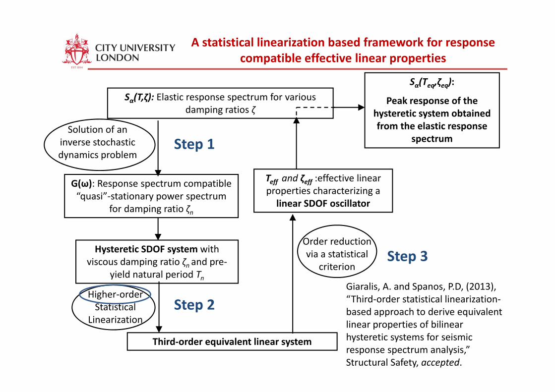
A statistical linearization based framework for response compatible effective linear properties
Sα(Τ,ζ): Elastic response spectrum for various d i ti ζ
Sα(Τeq,ζeq):
Peak response of the
p p p
damping ratios ζ
Solution of an inverse stochastic d i bl
hysteretic system obtained from the elastic response
spectrumStep 1
G(ω): Response spectrum compatible “quasi” stationary power spectrum
Teff and ζeff :effective linear properties characterizing a
dynamics problemp
quasi ‐stationary power spectrum for damping ratio ζn
linear SDOF oscillator
Order reductionHysteretic SDOF system with
viscous damping ratio ζn and pre‐yield natural period Tn
Order reduction via a statistical
criterion Step 3
Giaralis A and Spanos PD (2013)Higher‐order Statistical
LinearizationStep 2
Giaralis, A. and Spanos, P.D, (2013), “Third‐order statistical linearization‐based approach to derive equivalentlinear properties of bilinear
Third‐order equivalent linear system
p physteretic systems for seismicresponse spectrum analysis,” Structural Safety, accepted.
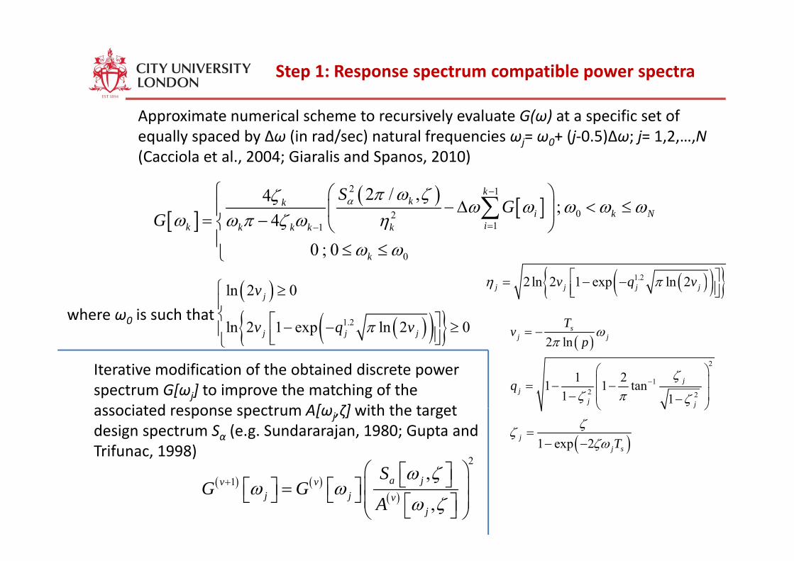
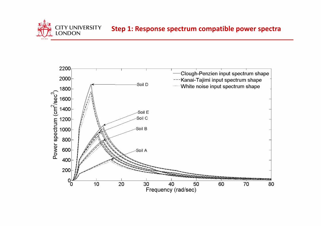
Step 1: Response spectrum compatible power spectra
Approximate numerical scheme to recursively evaluate G(ω) at a specific set of equally spaced by Δω (in rad/sec) natural frequencies ωj= ω0+ (j‐0.5)Δω; j= 1,2,…,N(C i l t l 2004 Gi li d S 2010)(Cacciola et al., 2004; Giaralis and Spanos, 2010)
[ ]( ) [ ]
2 1
02
2 / ,4 ;4
kkk
i k N
SG
Gα π ω ζζ ω ω ω ω ω
ζ
−⎧ ⎛ ⎞− Δ < ≤⎪ ⎜ ⎟
⎨ ⎝ ⎠∑
( )⎧
[ ] [ ] 0211
0
4
0 ; 0
i k Nik k k k k
k
G ω ω π ζ ω η
ω ω=−= −⎨ ⎝ ⎠
⎪ ≤ ≤⎩
∑
( )( ){ }1.22 ln 2 1 exp ln 2v q vη π⎡ ⎤
where ω0 is such that ( )
( )( ){ }1.2
ln 2 0
ln 2 1 exp ln 2 0
j
j j j
v
v q vπ
⎧ ≥⎪⎨ ⎡ ⎤− − ≥⎪ ⎢ ⎥⎣ ⎦⎩
( )( ){ }2ln 2 1 exp ln 2j j j jv q vη π⎡ ⎤= − −⎢ ⎥⎣ ⎦
( )2 lns
j jT
vpω
π= −{ }⎣ ⎦⎩
Iterative modification of the obtained discrete power spectrum G[ωj] to improve the matching of the associated response spectrum A[ω ζ] with the target
( )2
12 2
2 ln
1 21 1 tan1 1
jj
j j
p
q
π
ζπζ ζ
−⎛ ⎞⎜ ⎟= − −⎜ ⎟− −⎝ ⎠associated response spectrum A[ωj,ζ] with the target
design spectrum Sα (e.g. Sundararajan, 1980; Gupta and Trifunac, 1998)
2S ω ζ⎛ ⎞⎡ ⎤⎣ ⎦
( )1 exp 2
j
jj sT
ζζζω
⎝ ⎠
=− −
( ) ( )( )
1 ,
,a jv v
j j vj
SG G
A
ω ζω ω
ω ζ+
⎛ ⎞⎡ ⎤⎣ ⎦⎜ ⎟⎡ ⎤ ⎡ ⎤=⎣ ⎦ ⎣ ⎦ ⎜ ⎟⎡ ⎤⎣ ⎦⎝ ⎠
Step 1: Response spectrum compatible power spectra
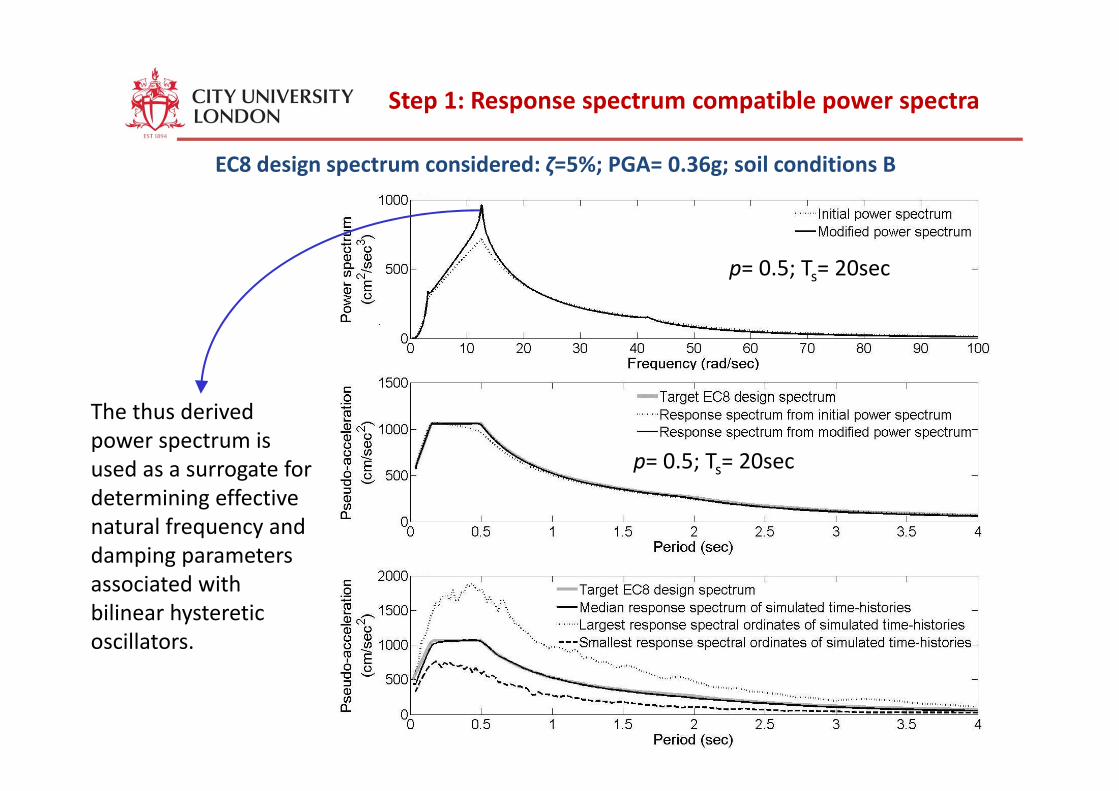
Step 1: Response spectrum compatible power spectra
EC8 design spectrum considered: ζ=5%; PGA= 0.36g; soil conditions B
p= 0.5; Ts= 20sec
The thus derived power spectrum is used as a surrogate for p= 0.5; Ts= 20sec
determining effective natural frequency and damping parameters
d hassociated with bilinear hysteretic oscillators.
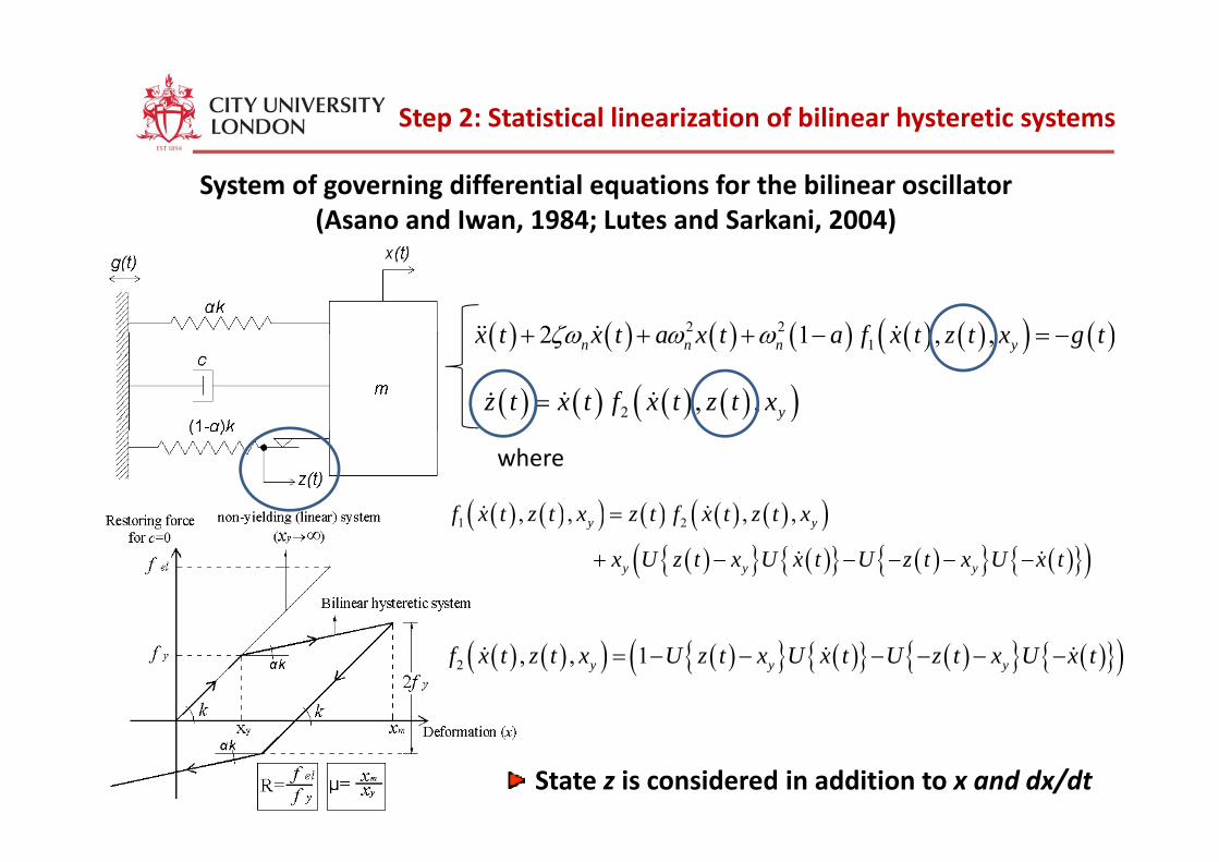
Step 2: Statistical linearization of bilinear hysteretic systems
System of governing differential equations for the bilinear oscillator (Asano and Iwan, 1984; Lutes and Sarkani, 2004)
( ) ( ) ( ) ( ) ( ) ( )( ) ( )2 22 1x t x t a x t a f x t z t x g tζω ω ω+ + +( ) ( ) ( ) ( ) ( ) ( )( ) ( )12 1 , ,n n n yx t x t a x t a f x t z t x g tζω ω ω+ + + − = −
( ) ( ) ( ) ( )( )2 , , yz t x t f x t z t x=
( ) ( )( ) ( ) ( ) ( )( )1 2, , , ,y yf x t z t x z t f x t z t x=
where
( ) ( )( ) ( ) ( ) ( )( )( ){ } ( ){ } ( ){ } ( ){ }( )
y y
y y yx U z t x U x t U z t x U x t+ − − − − −
( ) ( )( ) ( ){ } ( ){ } ( ){ } ( ){ }( )2 , , 1y y yf x t z t x U z t x U x t U z t x U x t= − − − − − −
State z is considered in addition to x and dx/dt
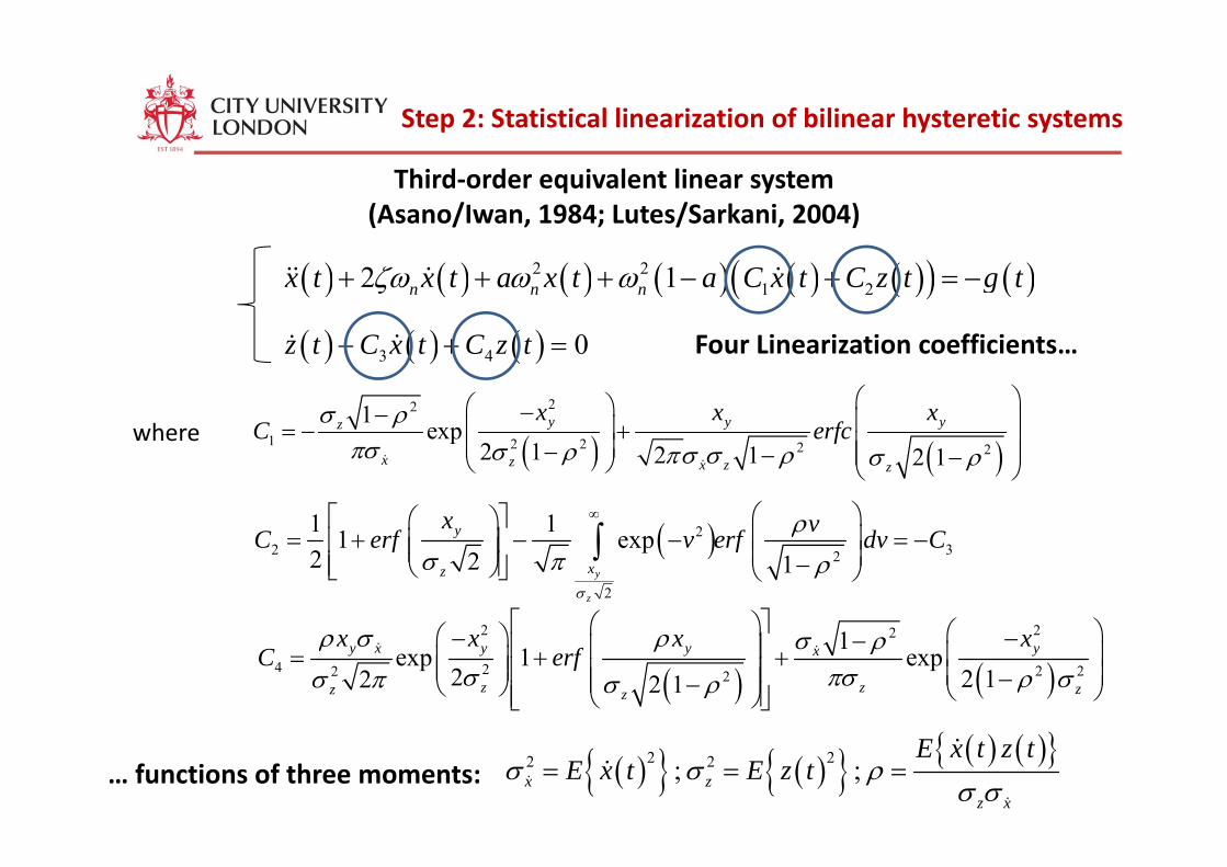
Step 2: Statistical linearization of bilinear hysteretic systems
Third‐order equivalent linear system(Asano/Iwan, 1984; Lutes/Sarkani, 2004)
( ) ( ) ( ) ( ) ( ) ( )( ) ( )2 21 22 1n n nx t x t a x t a C x t C z t g tζω ω ω+ + + − + = −
( ) ( ) ( ) 0C C F Li i i ffi i
where221 exp y y yz x x x
C erfcσ ρ ⎛ ⎞⎛ ⎞−− ⎜ ⎟⎜ ⎟= − + ⎜ ⎟⎜ ⎟
( ) ( ) ( )3 4 0z t C x t C z t+ + = Four Linearization coefficients…
where ( ) ( )1 2 2 2 2exp
2 1 2 1 2 1x z x z z
C erfcπσ σ ρ πσ σ ρ σ ρ
⎜ ⎟= + ⎜ ⎟⎜ ⎟− − ⎜ ⎟−⎝ ⎠ ⎝ ⎠
( )21 11 yx vC f f d Cρ∞ ⎛ ⎞⎡ ⎤⎛ ⎞⎜ ⎟⎢ ⎥⎜ ⎟ ∫ ( )2
2 32
2
1 exp2 2 1y
z
y
xz
C erf v erf dv C
σ
ρσ π ρ
⎜ ⎟= + − − = −⎢ ⎥⎜ ⎟⎜ ⎟ ⎜ ⎟−⎢ ⎥⎝ ⎠⎣ ⎦ ⎝ ⎠∫
2 22⎡ ⎤⎛ ⎞ ⎛ ⎞⎛ ⎞
( ) ( )2 22
4 2 2 22 2
1exp 1 exp2 2 12 2 1
y x y y yx
z z zz z
x x x xC erf
ρ σ ρ σ ρσ πσ ρ σσ π σ ρ
⎡ ⎤⎛ ⎞ ⎛ ⎞⎛ ⎞− −−⎢ ⎥⎜ ⎟ ⎜ ⎟= + +⎜ ⎟⎜ ⎟ ⎢ ⎥⎜ ⎟ ⎜ ⎟−⎜ ⎟−⎝ ⎠ ⎝ ⎠⎢ ⎥⎝ ⎠⎣ ⎦
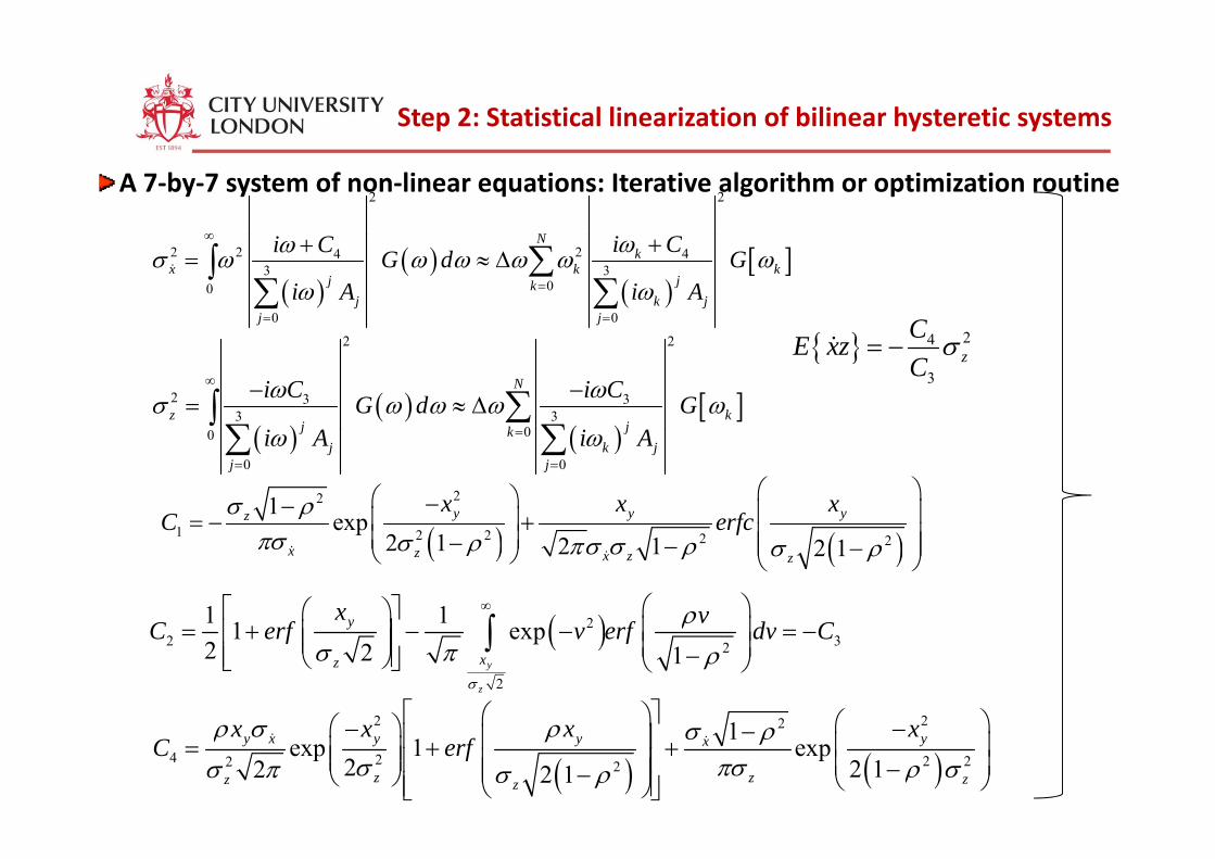
( ){ } ( ){ } ( ) ( ){ }2 22 2; ;x zz x
E x t z tE x t E z tσ σ ρ
σ σ= = =… functions of three moments:
Step 2: Statistical linearization of bilinear hysteretic systems
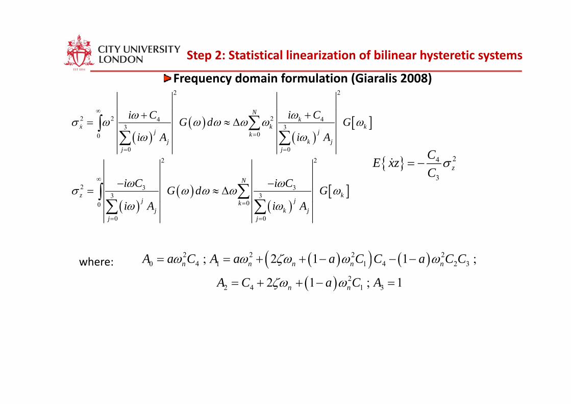
Frequency domain formulation (Giaralis 2008)2 2
N∞
( )( )
( )[ ]2 2 2 44
3 300
0 0
Nk
x k kj jk
j k jj j
i Ci C G d Gi A i A
ωωσ ω ω ω ω ω ωω ω
∞
=
= =
++= ≈ Δ ∑∫
∑ ∑{ } 2C{ } 24
3z
CE xzC
σ= −
( )( )
( )[ ]
2 2
2 3 33 3
0
N
z kj jk
i C i CG d GA A
ω ωσ ω ω ω ω∞ − −
= ≈ Δ ∑∫∑ ∑( ) ( )00
0 0
j jkj k j
j ji A i Aω ω=
= =∑ ∑
( )( ) ( )( )
2 2 2 20 4 1 1 4 2 3
22 4 1 3
; 2 1 1 ;
2 1 ; 1n n n n n
n n
A a C A a a C C a C C
A C a C A
ω ω ζω ω ω
ζω ω
= = + + − − −
= + + − =
where:
Step 2: Statistical linearization of bilinear hysteretic systems
2 2
N∞
A 7‐by‐7 system of non‐linear equations: Iterative algorithm or optimization routine
( )( )
( )[ ]2 2 2 44
3 300
0 0
Nk
x k kj jk
j k jj j
i Ci C G d Gi A i A
ωωσ ω ω ω ω ω ωω ω
∞
=
= =
++= ≈ Δ ∑∫
∑ ∑{ } 2C{ } 24
3z
CE xzC
σ= −
( )( )
( )[ ]
2 2
2 3 33 3
0
N
z kj jk
i C i CG d GA A
ω ωσ ω ω ω ω∞ − −
= ≈ Δ ∑∫∑ ∑( ) ( )00
0 0
j jkj k j
j ji A i Aω ω=
= =∑ ∑
( )22
11 exp y y yz x x x
C erfcσ ρ ⎛ ⎞⎛ ⎞−− ⎜ ⎟⎜ ⎟= − + ⎜ ⎟⎜ ⎟( ) ( )1 2 2 2 2exp
2 1 2 1 2 1x z x z z
C erfcπσ σ ρ πσ σ ρ σ ρ
⎜ ⎟ + ⎜ ⎟⎜ ⎟− − ⎜ ⎟−⎝ ⎠ ⎝ ⎠
( )21 11 yx vC f f d Cρ∞ ⎛ ⎞⎡ ⎤⎛ ⎞⎜ ⎟⎢ ⎥⎜ ⎟ ∫ ( )2
2 32
2
1 exp2 2 1y
z
y
xz
C erf v erf dv C
σ
ρσ π ρ
⎜ ⎟= + − − = −⎢ ⎥⎜ ⎟⎜ ⎟ ⎜ ⎟−⎢ ⎥⎝ ⎠⎣ ⎦ ⎝ ⎠∫
2 22⎡ ⎤⎛ ⎞ ⎛ ⎞⎛ ⎞
( ) ( )2 22
4 2 2 22 2
1exp 1 exp2 2 12 2 1
y x y y yx
z z zz z
x x x xC erf
ρ σ ρ σ ρσ πσ ρ σσ π σ ρ
⎡ ⎤⎛ ⎞ ⎛ ⎞⎛ ⎞− −−⎢ ⎥⎜ ⎟ ⎜ ⎟= + +⎜ ⎟⎜ ⎟ ⎢ ⎥⎜ ⎟ ⎜ ⎟−⎜ ⎟−⎝ ⎠ ⎝ ⎠⎢ ⎥⎝ ⎠⎣ ⎦
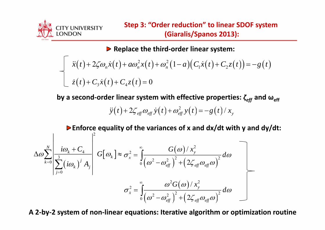
Step 3: “Order reduction” to linear SDOF system(Giaralis/Spanos 2013): ( / p )
( ) ( ) ( ) ( ) ( ) ( )( ) ( )2 22 1t t t C t C t tζ+ + + +
Replace the third‐order linear system:
( ) ( ) ( ) ( ) ( ) ( )( ) ( )2 21 22 1n n nx t x t a x t a C x t C z t g tζω ω ω+ + + − + = −
( ) ( ) ( )3 4 0z t C x t C z t+ + =
( ) ( ) ( ) ( )22 /eff eff eff yy t y t y t g t xζ ω ω+ + = −
by a second‐order linear system with effective properties: ζeff and ωeff
( ) ( ) ( ) ( )ff ff ff y
Enforce equality of the variances of x and dx/dt with y and dy/dt: 2
( )( ) ( )
22
2 22 20
/
2y
x
eff eff eff
G xd
ωσ ω
ω ω ζ ω ω
∞
=− +
∫( )
[ ]43
0
Nk
kjk
k j
i C Gi A
ωω ωω=
+Δ ≈∑
∑ ( ) ( )ff ff ff
( )( ) ( )
2 22
2 2
/ yx
G xd
ω ωσ ω
∞
= ∫
( )0
k jj=∑
( ) ( )2 22 20 2
x
eff eff effω ω ζ ω ω− +∫
A 2‐by‐2 system of non‐linear equations: Iterative algorithm or optimization routine
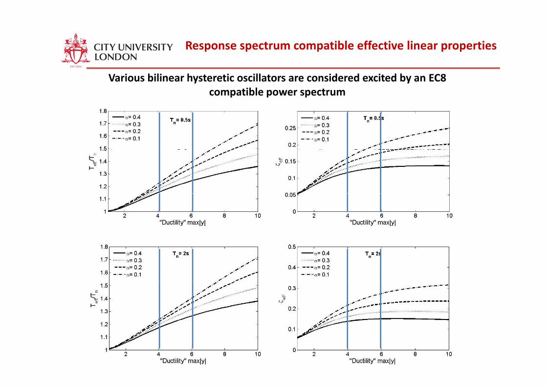
Response spectrum compatible effective linear properties
Various bilinear hysteretic oscillators are considered excited by an EC8 compatible power spectrum
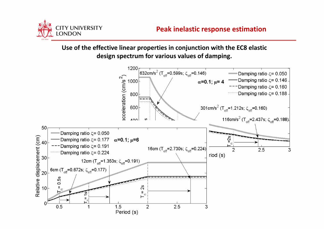
Peak inelastic response estimation
Use of the effective linear properties in conjunction with the EC8 elastic design spectrum for various values of damping.
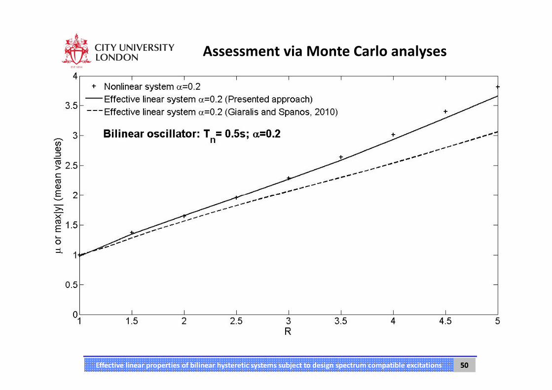
Assessment via Monte Carlo analyses
Effective linear properties of bilinear hysteretic systems subject to design spectrum compatible excitations 5050
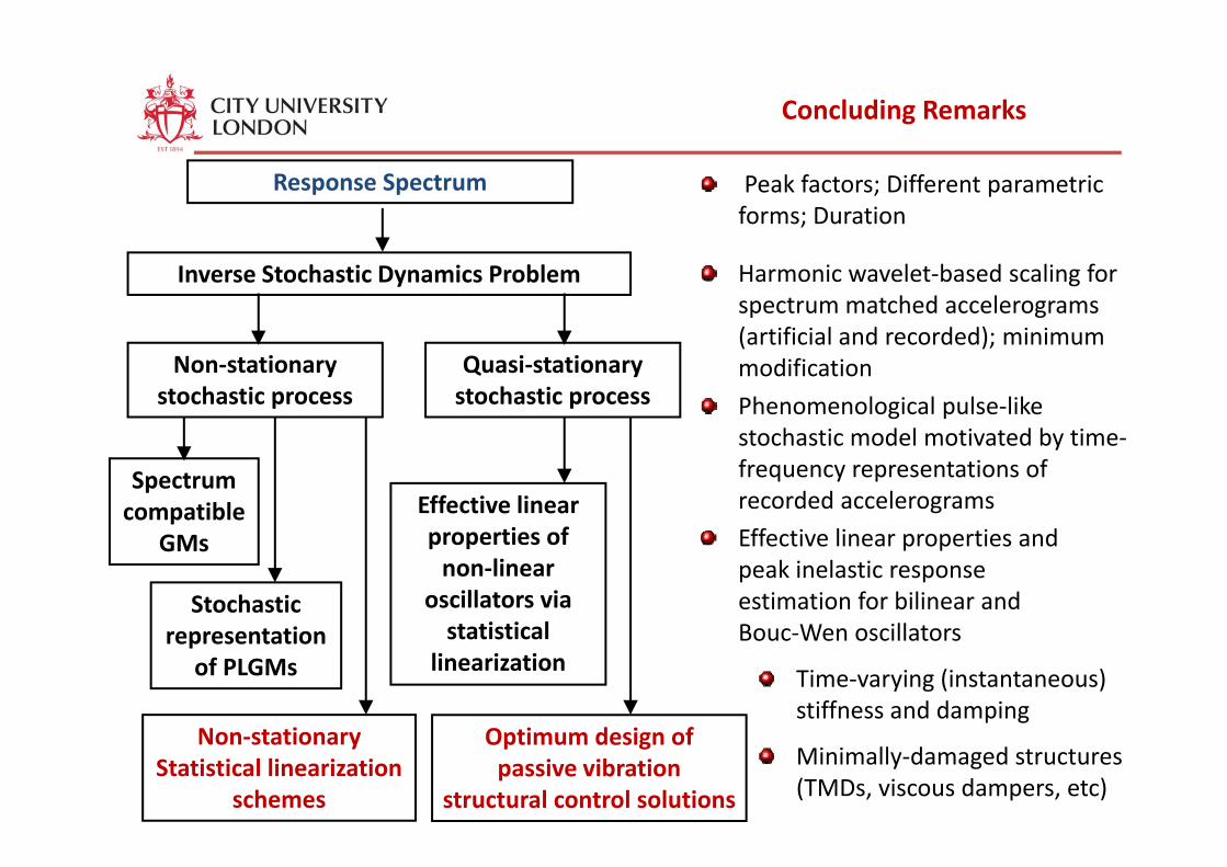
Concluding Remarks
Response Spectrum Peak factors; Different parametric forms; Duration
Inverse Stochastic Dynamics Problem Harmonic wavelet‐based scaling for spectrum matched accelerograms(artificial and recorded); minimum
Non‐stationary stochastic process
Quasi‐stationary stochastic process
(artificial and recorded); minimum modification
Phenomenological pulse‐like stochastic model motivated by time
Spectrum compatible Effective linear
properties of
stochastic model motivated by time‐frequency representations of recorded accelerograms
Eff ti li ti d
Stochastic t ti
GMs properties of non‐linear
oscillators via statistical
Effective linear properties and peak inelastic response estimation for bilinear and Bouc Wen oscillatorsrepresentation
of PLGMsstatistical
linearizationBouc‐Wen oscillators
N i O i d i f
Time‐varying (instantaneous) stiffness and damping
Non‐stationary Statistical linearization
schemes
Optimum design of passive vibration
structural control solutions
Minimally‐damaged structures(TMDs, viscous dampers, etc)

Acknowledgements
Structural Dynamics Research Group
Anca Lungu Paschalis Skrekas Laurentiu Marian Alessandro MargnelliAnca Lungu Paschalis Skrekas Laurentiu Marian Alessandro Margnelli
Senior associateAKT II, London
External Collaborators:External Collaborators:Dr Anastasios Sextos‐ Aristotle University of Thessaloniki, GreeceProf. Pol Spanos‐ Rice University, USADr Ioannis Kougioumtzoglou‐ University of Liverpool, UK
Ευχαριστώ πολύ για City University Pump Priming Grant
g g y p ,Prof. Ji Lie, Tongji‐ University, ChinaProf. Richard Baraniuk‐ Rice University, USA
χ ρ γτην προσοχή σας !
City University‐ Pump Priming GrantEPSRC‐ First Grant SchemeERASMUS LLP‐ Teaching Grant