Embed Size (px)
Citation preview


Statistics for Social and Behavioral Sciences
Advisors:
S.E. Fienberg
W.J. van der Linden
For further volumes:http://www.springer.com/series/3463


Terri D. Pigott
Advances in Meta-Analysis

Terri D. PigottSchool of EducationLoyola University ChicagoChicago, IL, USA
ISBN 978-1-4614-2277-8 e-ISBN 978-1-4614-2278-5DOI 10.1007/978-1-4614-2278-5Springer New York Dordrecht Heidelberg London
Library of Congress Control Number: 2011945854
# Springer Science+Business Media, LLC 2012All rights reserved. This work may not be translated or copied in whole or in part without the writtenpermission of the publisher (Springer Science+Business Media, LLC, 233 Spring Street, New York,NY 10013, USA), except for brief excerpts in connection with reviews or scholarly analysis. Use inconnection with any form of information storage and retrieval, electronic adaptation, computer software,or by similar or dissimilar methodology now known or hereafter developed is forbidden.The use in this publication of trade names, trademarks, service marks, and similar terms, even ifthey are not identified as such, is not to be taken as an expression of opinion as to whether or not theyare subject to proprietary rights.
Printed on acid-free paper
Springer is part of Springer Science+Business Media (www.springer.com)

To Jenny and Alison,who make it all worthwhile.


Acknowledgements
I am grateful to my mentors, Ingram Olkin and Betsy Jane Becker, who were the
reason I have the opportunity to write this book. Larry V. Hedges has always been
in the background of everything I have accomplished in my career, and I thank him
and Judy for all their support.
My graduate students, Joshua Polanin and Ryan Williams, read every chapter,
and, more importantly, listened to me as I worked through the details of the book.
I am a better teacher and researcher because of their enthusiasm for our work
together, and their endless intellectual curiosity.
My colleagues at the Campbell Collaboration and the review authors who
contribute to the Collaboration’s library have been the inspiration for this book.
Together we all continue to strive for high quality reviews of the evidence for social
programs.
My parents, Nestor and Marie Deocampo, have provided a constant supply of
support and encouragement.
As any working, single mother knows, I would not be able to accomplish
anything without a network of friends who can function as substitute drivers,
mothers, and general ombudspersons. I am eternally grateful to the Perri family –
John, Amy and Leah – for serving as our second family. More thanks are due to the
Entennman-McNulty-Oswald clan, especially Judge Sheila, Craig, Erica, Carey,
and Faith, for helping us do whatever is necessary to keep the household function-
ing. I am indebted to Magda and Kamilla for taking care of us when we needed
it most. Alex Lehr served as a substitute chauffeur when I had to teach.
Finally, I thank Rick for always being the river, and Lisette Davison for helping
me transform my life.
Chicago, IL, USA Terri D. Pigott
vii


Contents
1 Introduction. . . . . . . . . . . . . . . . . . . . . . . . . . . . . . . . . . . . . . . . . . . . . . . . . . . . . . . . . . . . . . . . 1
1.1 Background . . . . . . . . . . . . . . . . . . . . . . . . . . . . . . . . . . . . . . . . . . . . . . . . . . . . . . . . . . . 1
1.2 Planning a Systematic Review. . . . . . . . . . . . . . . . . . . . . . . . . . . . . . . . . . . . . . . . 2
1.3 Analyzing Complex Data from a Meta-analysis . . . . . . . . . . . . . . . . . . . . . 4
1.4 Interpreting Results from a Meta-analysis. . . . . . . . . . . . . . . . . . . . . . . . . . . . 4
1.5 What Do Readers Need to Know to Use This Book? . . . . . . . . . . . . . . . . 5
References. . . . . . . . . . . . . . . . . . . . . . . . . . . . . . . . . . . . . . . . . . . . . . . . . . . . . . . . . . . . . . . . . . . 6
2 Review of Effect Sizes . . . . . . . . . . . . . . . . . . . . . . . . . . . . . . . . . . . . . . . . . . . . . . . . . . . . . 7
2.1 Background . . . . . . . . . . . . . . . . . . . . . . . . . . . . . . . . . . . . . . . . . . . . . . . . . . . . . . . . . . . 7
2.2 Introduction to Notation and Basic Meta-analysis . . . . . . . . . . . . . . . . . . . 7
2.3 The Random Effects Mean and Variance . . . . . . . . . . . . . . . . . . . . . . . . . . . . 8
2.4 Common Effect Sizes Used in Examples. . . . . . . . . . . . . . . . . . . . . . . . . . . 10
2.4.1 Standardized Mean Difference. . . . . . . . . . . . . . . . . . . . . . . . . . . . . . 10
2.4.2 Correlation Coefficient. . . . . . . . . . . . . . . . . . . . . . . . . . . . . . . . . . . . . . 10
2.4.3 Log Odds Ratio . . . . . . . . . . . . . . . . . . . . . . . . . . . . . . . . . . . . . . . . . . . . . 11
References. . . . . . . . . . . . . . . . . . . . . . . . . . . . . . . . . . . . . . . . . . . . . . . . . . . . . . . . . . . . . . . . . 12
3 Planning a Meta-analysis in a Systematic Review . . . . . . . . . . . . . . . . . . . . . 13
3.1 Background . . . . . . . . . . . . . . . . . . . . . . . . . . . . . . . . . . . . . . . . . . . . . . . . . . . . . . . . . 13
3.2 Deciding on Important Moderators of Effect Size . . . . . . . . . . . . . . . . . 14
3.3 Choosing Among Fixed, Random
and Mixed Effects Models . . . . . . . . . . . . . . . . . . . . . . . . . . . . . . . . . . . . . . . . . . 16
3.4 Computing the Variance Component in Random
and Mixed Models . . . . . . . . . . . . . . . . . . . . . . . . . . . . . . . . . . . . . . . . . . . . . . . . . . 18
3.4.1 Example . . . . . . . . . . . . . . . . . . . . . . . . . . . . . . . . . . . . . . . . . . . . . . . . . . . . . 20
3.5 Confounding of Moderators in Effect Size Models . . . . . . . . . . . . . . . . 21
3.5.1 Example . . . . . . . . . . . . . . . . . . . . . . . . . . . . . . . . . . . . . . . . . . . . . . . . . . . . . 23
3.6 Conducting a Meta-Regression . . . . . . . . . . . . . . . . . . . . . . . . . . . . . . . . . . . . . 25
3.6.1 Example . . . . . . . . . . . . . . . . . . . . . . . . . . . . . . . . . . . . . . . . . . . . . . . . . . . . . 25
3.7 Interpretation of Moderator Analyses . . . . . . . . . . . . . . . . . . . . . . . . . . . . . . 28
References. . . . . . . . . . . . . . . . . . . . . . . . . . . . . . . . . . . . . . . . . . . . . . . . . . . . . . . . . . . . . . . . . 32
ix

4 Power Analysis for the Mean Effect Size . . . . . . . . . . . . . . . . . . . . . . . . . . . . . . . 35
4.1 Background . . . . . . . . . . . . . . . . . . . . . . . . . . . . . . . . . . . . . . . . . . . . . . . . . . . . . . . . . 35
4.2 Fundamentals of Power Analysis . . . . . . . . . . . . . . . . . . . . . . . . . . . . . . . . . . . 37
4.3 Test of the Mean Effect Size in the Fixed Effects Model. . . . . . . . . . 39
4.3.1 Z-Test for the Mean Effect Size
in the Fixed Effects Model. . . . . . . . . . . . . . . . . . . . . . . . . . . . . . . . . . 39
4.3.2 The Power of the Test of the Mean Effect Size
in Fixed Effects Models. . . . . . . . . . . . . . . . . . . . . . . . . . . . . . . . . . . . . 41
4.3.3 Deciding on Values for Parameters
to Compute Power . . . . . . . . . . . . . . . . . . . . . . . . . . . . . . . . . . . . . . . . . . 42
4.3.4 Example: Computing the Power of the Test
of the Mean . . . . . . . . . . . . . . . . . . . . . . . . . . . . . . . . . . . . . . . . . . . . . . . . . 43
4.3.5 Example: Computing the Number of Studies Needed
to Detect an Important Fixed Effects Mean . . . . . . . . . . . . . . . . 45
4.3.6 Example: Computing the Detectable Fixed Effects
Mean in a Meta-analysis . . . . . . . . . . . . . . . . . . . . . . . . . . . . . . . . . . . . 46
4.4 Test of the Mean Effect Size in the Random Effects Model. . . . . . . 47
4.4.1 The Power of the Test of the Mean Effect Size
in Random Effects Models. . . . . . . . . . . . . . . . . . . . . . . . . . . . . . . . . . 48
4.4.2 Positing a Value for t2 for Power Computations
in the Random Effects Model. . . . . . . . . . . . . . . . . . . . . . . . . . . . . . . 49
4.4.3 Example: Estimating the Power of the Random
Effects Mean . . . . . . . . . . . . . . . . . . . . . . . . . . . . . . . . . . . . . . . . . . . . . . . . 50
4.4.4 Example: Computing the Number of Studies
Needed to Detect an Important Random Effect Mean . . . . . 51
4.4.5 Example: Computing the Detectable Random
Effects Mean in a Meta-analysis. . . . . . . . . . . . . . . . . . . . . . . . . . . . 52
References. . . . . . . . . . . . . . . . . . . . . . . . . . . . . . . . . . . . . . . . . . . . . . . . . . . . . . . . . . . . . . . . . 53
5 Power for the Test of Homogeneity in Fixed
and Random Effects Models . . . . . . . . . . . . . . . . . . . . . . . . . . . . . . . . . . . . . . . . . . . . . 55
5.1 Background . . . . . . . . . . . . . . . . . . . . . . . . . . . . . . . . . . . . . . . . . . . . . . . . . . . . . . . . . 55
5.2 The Test of Homogeneity of Effect Sizes
in a Fixed Effects Model. . . . . . . . . . . . . . . . . . . . . . . . . . . . . . . . . . . . . . . . . . . . 56
5.2.1 The Power of the Test of Homogeneity
in a Fixed Effects Model. . . . . . . . . . . . . . . . . . . . . . . . . . . . . . . . . . . . 56
5.2.2 Choosing Values for the Parameters Needed
to Compute Power of the Homogeneity Test
in Fixed Effects Models. . . . . . . . . . . . . . . . . . . . . . . . . . . . . . . . . . . . . 57
5.2.3 Example: Estimating the Power of the
Test of Homogeneity in Fixed Effects Models . . . . . . . . . . . . . 58
x Contents

5.3 The Test of the Significance of the Variance Component
in Random Effects Models. . . . . . . . . . . . . . . . . . . . . . . . . . . . . . . . . . . . . . . . . . 59
5.3.1 Power of the Test of the Significance of the Variance
Component in Random Effects Models . . . . . . . . . . . . . . . . . . . . 60
5.3.2 Choosing Values for the Parameters Needed to Compute
the Variance Component in Random Effects Models . . . . . . 61
5.3.3 Example: Computing Power for Values of t2,the Variance Component. . . . . . . . . . . . . . . . . . . . . . . . . . . . . . . . . . . . 62
References. . . . . . . . . . . . . . . . . . . . . . . . . . . . . . . . . . . . . . . . . . . . . . . . . . . . . . . . . . . . . . . . . 66
6 Power Analysis for Categorical Moderator
Models of Effect Size . . . . . . . . . . . . . . . . . . . . . . . . . . . . . . . . . . . . . . . . . . . . . . . . . . . . . 67
6.1 Background . . . . . . . . . . . . . . . . . . . . . . . . . . . . . . . . . . . . . . . . . . . . . . . . . . . . . . . . . 67
6.2 Categorical Models of Effect Size: Fixed Effects
One-Way ANOVA Models . . . . . . . . . . . . . . . . . . . . . . . . . . . . . . . . . . . . . . . . . 68
6.2.1 Tests in a Fixed Effects One-Way ANOVA Model . . . . . . . . 68
6.2.2 Power of the Test of Between-Group
Homogeneity, QB, in Fixed Effects Models . . . . . . . . . . . . . . . . 68
6.2.3 Choosing Parameters for the Power of QB in Fixed
Effects Models . . . . . . . . . . . . . . . . . . . . . . . . . . . . . . . . . . . . . . . . . . . . . . 70
6.2.4 Example: Power of the Test of Between-Group
Homogeneity in Fixed Effects Models . . . . . . . . . . . . . . . . . . . . . 70
6.2.5 Power of the Test of Within-Group Homogeneity,
QW, in Fixed Effects Models. . . . . . . . . . . . . . . . . . . . . . . . . . . . . . . . 71
6.2.6 Choosing Parameters for the Test of QW in Fixed
Effects Models . . . . . . . . . . . . . . . . . . . . . . . . . . . . . . . . . . . . . . . . . . . . . . 72
6.2.7 Example: Power of the Test of Within-Group
Homogeneity in Fixed Effects Models . . . . . . . . . . . . . . . . . . . . . 73
6.3 Categorical Models of Effect Size: Random Effects
One-Way ANOVA Models . . . . . . . . . . . . . . . . . . . . . . . . . . . . . . . . . . . . . . . . . 74
6.3.1 Power of Test of Between-Group Homogeneity
in the Random Effects Model. . . . . . . . . . . . . . . . . . . . . . . . . . . . . . . 74
6.3.2 Choosing Parameters for the Test of Between-Group
Homogeneity in Random Effects Models . . . . . . . . . . . . . . . . . . 76
6.3.3 Example: Power of the Test of Between-Group
Homogeneity in Random Effects Models . . . . . . . . . . . . . . . . . . 76
6.4 Linear Models of Effect Size (Meta-regression) . . . . . . . . . . . . . . . . . . . 78
References. . . . . . . . . . . . . . . . . . . . . . . . . . . . . . . . . . . . . . . . . . . . . . . . . . . . . . . . . . . . . . . . . 78
7 Missing Data in Meta-analysis: Strategies and Approaches . . . . . . . . . . 79
7.1 Background . . . . . . . . . . . . . . . . . . . . . . . . . . . . . . . . . . . . . . . . . . . . . . . . . . . . . . . . . 79
7.2 Missing Studies in a Meta-analysis . . . . . . . . . . . . . . . . . . . . . . . . . . . . . . . . . 80
7.2.1 Identification of Publication Bias . . . . . . . . . . . . . . . . . . . . . . . . . . . 80
7.2.2 Assessing the Sensitivity of Results
to Publication Bias . . . . . . . . . . . . . . . . . . . . . . . . . . . . . . . . . . . . . . . . . . 82
Contents xi

7.3 Missing Effect Sizes in a Meta-analysis. . . . . . . . . . . . . . . . . . . . . . . . . . . . 85
7.4 Missing Moderators in Effect Size Models. . . . . . . . . . . . . . . . . . . . . . . . . 86
7.5 Theoretical Basis for Missing Data Methods. . . . . . . . . . . . . . . . . . . . . . . 87
7.5.1 Multivariate Normality in Meta-analysis . . . . . . . . . . . . . . . . . . . 88
7.5.2 Missing Data Mechanisms or Reasons
for Missing Data . . . . . . . . . . . . . . . . . . . . . . . . . . . . . . . . . . . . . . . . . . . . 89
7.6 Commonly Used Methods for Missing Data
in Meta-analysis. . . . . . . . . . . . . . . . . . . . . . . . . . . . . . . . . . . . . . . . . . . . . . . . . . . . . 90
7.6.1 Complete-Case Analysis . . . . . . . . . . . . . . . . . . . . . . . . . . . . . . . . . . . . 90
7.6.2 Available Case Analysis or Pairwise Deletion . . . . . . . . . . . . . 92
7.6.3 Single Value Imputation with the
Complete Case Mean . . . . . . . . . . . . . . . . . . . . . . . . . . . . . . . . . . . . . . . 93
7.6.4 Single Value Imputation Using
Regression Techniques. . . . . . . . . . . . . . . . . . . . . . . . . . . . . . . . . . . . . . 95
7.7 Model-Based Methods for Missing Data in Meta-analysis . . . . . . . . 97
7.7.1 Maximum-Likelihood Methods for Missing
Data Using the EM Algorithm. . . . . . . . . . . . . . . . . . . . . . . . . . . . . . 97
7.7.2 Multiple Imputation for Multivariate Normal Data . . . . . . . . 99
References. . . . . . . . . . . . . . . . . . . . . . . . . . . . . . . . . . . . . . . . . . . . . . . . . . . . . . . . . . . . . . . . 106
8 Including Individual Participant Data in Meta-analysis . . . . . . . . . . . . 109
8.1 Background . . . . . . . . . . . . . . . . . . . . . . . . . . . . . . . . . . . . . . . . . . . . . . . . . . . . . . . . 109
8.2 The Potential for IPD Meta-analysis . . . . . . . . . . . . . . . . . . . . . . . . . . . . . . 110
8.3 The Two-Stage Method for a Mix of IPD and AD. . . . . . . . . . . . . . . . 112
8.3.1 Simple Random Effects Models
with Aggregated Data. . . . . . . . . . . . . . . . . . . . . . . . . . . . . . . . . . . . . . 112
8.3.2 Two-Stage Estimation with Both Individual Level
and Aggregated Data. . . . . . . . . . . . . . . . . . . . . . . . . . . . . . . . . . . . . . . 114
8.4 The One-Stage Method for a Mix of IPD and AD . . . . . . . . . . . . . . . . 115
8.4.1 IPD Model for the Standardized Mean Difference . . . . . . . . 115
8.4.2 IPD Model for the Correlation. . . . . . . . . . . . . . . . . . . . . . . . . . . . . 116
8.4.3 Model for the One-Stage Method
with Both IPD and AD. . . . . . . . . . . . . . . . . . . . . . . . . . . . . . . . . . . . . 116
8.5 Effect Size Models with Moderators Using a Mix
of IPD and AD . . . . . . . . . . . . . . . . . . . . . . . . . . . . . . . . . . . . . . . . . . . . . . . . . . . . . 118
8.5.1 Two-Stage Methods for Meta-regression
with a Mix of IPD and AD . . . . . . . . . . . . . . . . . . . . . . . . . . . . . . . . 119
8.5.2 One-Stage Method for Meta-regression
with a Mix of IPD and AD . . . . . . . . . . . . . . . . . . . . . . . . . . . . . . . . 120
8.5.3 Meta-regression for IPD Data Only . . . . . . . . . . . . . . . . . . . . . . . 121
8.5.4 One-Stage Meta-regression with a Mix
of IPD and AD . . . . . . . . . . . . . . . . . . . . . . . . . . . . . . . . . . . . . . . . . . . . . 121
References. . . . . . . . . . . . . . . . . . . . . . . . . . . . . . . . . . . . . . . . . . . . . . . . . . . . . . . . . . . . . . . . 130
xii Contents

9 Generalizations from Meta-analysis . . . . . . . . . . . . . . . . . . . . . . . . . . . . . . . . . . 133
9.1 Background . . . . . . . . . . . . . . . . . . . . . . . . . . . . . . . . . . . . . . . . . . . . . . . . . . . . . . . 133
9.1.1 The Preventive Health Services (2009) Report
on Breast Cancer Screening . . . . . . . . . . . . . . . . . . . . . . . . . . . . . . 134
9.1.2 The National Reading Panel’s Meta-analysis
on Learning to Read . . . . . . . . . . . . . . . . . . . . . . . . . . . . . . . . . . . . . . 135
9.2 Principles of Generalized Causal Inference . . . . . . . . . . . . . . . . . . . . . . 135
9.2.1 Surface Similarity . . . . . . . . . . . . . . . . . . . . . . . . . . . . . . . . . . . . . . . . . 135
9.2.2 Ruling Out Irrelevancies . . . . . . . . . . . . . . . . . . . . . . . . . . . . . . . . . . 136
9.2.3 Making Discriminations . . . . . . . . . . . . . . . . . . . . . . . . . . . . . . . . . . 137
9.2.4 Interpolation and Extrapolation. . . . . . . . . . . . . . . . . . . . . . . . . . . 138
9.2.5 Causal Explanation. . . . . . . . . . . . . . . . . . . . . . . . . . . . . . . . . . . . . . . . 138
9.3 Suggestions for Generalizing from a Meta-analysis . . . . . . . . . . . . . 139
References. . . . . . . . . . . . . . . . . . . . . . . . . . . . . . . . . . . . . . . . . . . . . . . . . . . . . . . . . . . . . . . . 140
10 Recommendations for Producing a High Quality
Meta-analysis . . . . . . . . . . . . . . . . . . . . . . . . . . . . . . . . . . . . . . . . . . . . . . . . . . . . . . . . . . . 143
10.1 Background . . . . . . . . . . . . . . . . . . . . . . . . . . . . . . . . . . . . . . . . . . . . . . . . . . . . . . . 143
10.2 Understanding the Research Problem . . . . . . . . . . . . . . . . . . . . . . . . . . . . 143
10.3 Having an a Priori Plan for the Meta-analysis . . . . . . . . . . . . . . . . . . . 144
10.4 Carefully and Thoroughly Interpret the Results
of Meta-analysis . . . . . . . . . . . . . . . . . . . . . . . . . . . . . . . . . . . . . . . . . . . . . . . . . . 145
References. . . . . . . . . . . . . . . . . . . . . . . . . . . . . . . . . . . . . . . . . . . . . . . . . . . . . . . . . . . . . . . . 146
11 Data Appendix . . . . . . . . . . . . . . . . . . . . . . . . . . . . . . . . . . . . . . . . . . . . . . . . . . . . . . . . . . 147
11.1 Sirin (2005) Meta-analysis on the Association
Between Measures of Socioeconomic Status
and Academic Achievement. . . . . . . . . . . . . . . . . . . . . . . . . . . . . . . . . . . . . . 147
11.2 Hackshaw et al. (1997) Meta-analysis on Exposure
to Passive Smoking and Lung Cancer. . . . . . . . . . . . . . . . . . . . . . . . . . . . 149
11.3 Eagly et al. (2003) Meta-analysis on Gender Differences
in Transformational Leadership . . . . . . . . . . . . . . . . . . . . . . . . . . . . . . . . . . 151
References. . . . . . . . . . . . . . . . . . . . . . . . . . . . . . . . . . . . . . . . . . . . . . . . . . . . . . . . . . . . . . . . 152
Index . . . . . . . . . . . . . . . . . . . . . . . . . . . . . . . . . . . . . . . . . . . . . . . . . . . . . . . . . . . . . . . . . . . . . . . . . . 153
Contents xiii


Chapter 1
Introduction
Abstract This chapter introduces the topics that are covered in this book. The goal
of the book is to provide reviewers with advanced strategies for strengthening
the planning, conduct and interpretations of meta-analyses. The topics covered
include planning a meta-analysis, computing power for tests in meta-analysis,
handling missing data in meta-analysis, including individual level data in a tradi-
tional meta-analysis, and generalizations from a meta-analysis. Readers of this text
will need to understand the basics of meta-analysis, and have access to computer
programs such as Excel and SPSS. Later chapters will require more advanced
computer programs such as SAS and R, and some advanced statistical theory.
1.1 Background
The past few years have seen a large increase in the use of systematic reviews in
both medicine and the social sciences. The focus on evidence-based practice in
many professions has spurred interest in understanding what is both known and
unknown about important interventions and clinical practices. Systematic reviews
have promised a transparent and replicable method for summarizing the literature to
improve both policy decisions, and the design of new studies. While I believe in the
potential of systematic reviews, I have also seen this potential compromised by
inadequate methods and misinterpretations of results.
This book is my attempt at providing strategies for strengthening the planning,
conduct and interpretation of systematic reviews that include meta-analysis. Given
the amount of research that exists in medicine and the social sciences, policy-
makers, researchers and consumers need ways to organize information to avoid
drawing conclusions from a single study or anecdote. One way to improve the
decisions made from a body of evidence is to improve the ways we synthesize
research studies.
T.D. Pigott, Advances in Meta-Analysis, Statistics for Social and Behavioral Sciences,
DOI 10.1007/978-1-4614-2278-5_1, # Springer Science+Business Media, LLC 2012
1

Much of the impetus for this work derives frommy experience with the Campbell
Collaboration, where I have served as the co-chair of the Campbell Methods group,
Methods editor, and teacher of systematic research synthesis. Two different issues
have inspired this book. As Rothstein (2011) has noted, there are a number of
questions always asked by research reviewers. These questions include: how many
studies do I need to do a meta-analysis? Should I use random effects or fixed effects
models (and by the way, what are these anyway)? How much is too much heteroge-
neity, andwhat do I do about it? I would add to this list questions about how to handle
missing data, what to do with more complex studies such as those that report
regression coefficients, and how to draw inferences from a research synthesis.
These common questions are not yet addressed clearly in the literature, and I hope
that this book can provide some preliminary strategies for handling these issues.
My second motivation for writing this book is to increase the quality of the
inferences we can make from a research synthesis. One way to achieve this goal is to
improve both the methods used in the review, and the interpretation of those results.
Anyone who has conducted a systematic review knows the effort involved. Aside
from all of the decisions that a reviewer makes throughout the process, there is the
inevitable question posed by the consumers of the review: what does this all mean?
What decisions are warranted by the results of this review? I hope the methods
discussed in this book will help research reviewers to conduct more thorough and
thoughtful analyses of the data collected in a systematic review leading to a better
understanding of a given literature.
The book is organized into three sections, roughly corresponding to the stages of
systematic reviews as outlined by Cooper (2009). These sections are planning a
meta-analysis, analyzing complex data from a meta-analysis, and interpreting meta-
analysis results. Each of these sections are outlined below.
1.2 Planning a Systematic Review
One of the most important aspects of planning a systematic review involves
formulating a research question. As I teach in my courses on research synthesis,
the research question guides every aspect of a synthesis from data collection
through reporting of results. There are three general forms of research questions
that can guide a synthesis. The most common are questions about the effectiveness
of a given intervention or treatment. Many of the reviews in the Cochrane and
Campbell libraries are of this form: How effective is a given treatment in addressing
a given condition or problem? A second type of question examines the associations
between two different constructs or conditions. For example, Sirin’s (2005) work
examines the strength of the correlation between different measures of socio-
economic status (such as mother’s education level, income, or eligibility for
free school lunches) and various measures of academic achievement. Another
emerging area of synthesis involves synthesizing information on the specificity
and sensitivity of diagnostic tests.
2 1 Introduction

After refining a research question, reviewers must search and evaluate the studies
considered relevant for the review. Part of the process for evaluating studies includes
the development of a coding protocol, outlining the information that will be impor-
tant to extract from each study. The information coded from each study will not only
be used to describe the nature of the literature collected for the review, but also may
help to explain variations that we find in the results of included studies. As a frequent
consultant on research syntheses, I know the importance of deep knowledge of the
substantive issues in a given field for both decisions on what needs to be extracted
from studies in the review, and what types of analyses will be conducted.
In Chap. 3, I focus on two common issues faced by reviewers: the choice of fixed
or random effects analysis, and the planning of moderator analyses for a meta-
analysis. In this chapter, I argue for the use of logic models (Anderson et al. 2011)
to highlight the important mechanisms that make an intervention effective, or the
relationships that may exist between conditions or constructs. Logic models not
only clarify the assumptions a reviewer is making about a given research area, but
also help guide the data extracted from each study, and the moderator models that
should be examined. Understanding the research area and planning a priori the
moderators that will be tested helps avoid problems with “fishing for significance”
in a meta-analysis. Researchers have paid too little attention to the number of
significance tests often conducted in a typical meta-analysis, sometimes reporting
on a series of single variable moderators, analogous to conducting a series of one-
way ANOVAs or t-tests. These analyses not only capitalize on chance, increasing
Type I error, but they also leave the reader with an incomplete picture of how
moderators are confounded with each other. In Chap. 3, I advocate for the use of
logic models to guide the planning of a research synthesis and meta-analysis, for
carefully examining the relationships between important moderators, and for the
use of meta-regression, if possible, to examine simultaneously the association of
several moderators with variation in effect size.
Another common question is: How many studies do I need to conduct a
meta-analysis? Though my colleagues and I have often answered “two” (Valentine
et al. 2010), the more complete answer lies in understanding the power of the
statistical tests in meta-analysis. I take the approach in this book that power of tests
in meta-analysis like power of any statistical test needs to be computed a priori,
using assumptions about the size of an important effect in a given context, and the
typical sample sizes used in a given field. Again, deep substantive knowledge of a
research literature is critical for a reviewer in order to make reasonable assumptions
about parameters needed for power. Chapters 4, 5, 6 discuss how to compute a
priori power for a meta-analysis for tests of the mean effect size, homogeneity, and
moderator analyses under both fixed and random effects models. We are often
concerned about power of tests in meta-analysis in order to understand the strength
of the evidence we have in a given field. If we expect few studies to exist on a given
intervention, we might check a priori to see how many studies are needed to find
a substantive effect. If we ultimately find fewer studies than needed to detect a
substantive effect, we have a more powerful argument for conducting more primary
studies. For these chapters, readers need to understand basic meta-analysis, and
have access to Excel or a computer program such as SPSS or R.
1.2 Planning a Systematic Review 3

1.3 Analyzing Complex Data from a Meta-analysis
One problem encountered by researchers is missing data. Missing data occurs
frequently in all types of data analysis, and not just a meta-analysis. Chapter 7
provides strategies for examining the sensitivity of the results of a meta-analysis to
missing data. As described in this chapter, studies can be missing, or missing data
can occur at the level of the effect size, or for moderators of effect size variance.
Chapter 7 provides an overview of strategies used for understanding how missing
data may influence the results drawn from a review.
The final chapter in this section (Chap. 8) provides background on individual
participant meta-analysis, or IPD. IPD meta-analysis is a strategy for synthesizing
the individual level or raw data from a set of primary studies. While it has been used
widely in medicine, social scientists have not had the opportunity to use it given the
difficulties in locating the individual participant level data. I provide an overview of
this technique here since agencies such as the National Science Foundation and the
National Institutes of Health are requiring their grantees to provide plans for data
sharing. IPD meta-analysis provides the opportunity to examine how moderators
are associated with effect size variance both within and between studies. Moderator
analyses in meta-analysis inherently suffer from aggregation bias – the relation-
ships we find between moderators and effect size between studies may not hold
within studies. Chapter 9 provides a discussion and guidelines on the conduct of
IPD meta-analysis, with an emphasis on how to combine aggregated or study-level
data with individual level data.
1.4 Interpreting Results from a Meta-analysis
Chapter 9 centers on generalizations from meta-analysis. Though Chap. 9 does not
provide statistical advice, it does address a concern I have about the interpretation
of the results of systematic reviews. For example, the release of the synthesis
on breast cancer screening in women by the US Preventive Services Task Force
(US Preventive Services Task Force 2002) was widely reported and criticized since
the results seemed to contradict current practice. In education, the syntheses
conducted by the National Panel on Reading also fueled controversy in the field
(Ehri et al. 2001), including a number of questions about what the results actually
mean for practice. Chapter 9 reviews both of these meta-analyses as a way to begin
a conversation about what types of actions or decisions can be justified given the
nature of meta-analytic data. All researchers involved in the conduct and use
of research synthesis share a commitment to providing the best evidence available
to make important decisions about social policy. Providing the clearest and
most accurate interpretation of research synthesis results will help us all to reach
this goal.
4 1 Introduction

The final chapter, Chap. 10, provides a summary of elements I consider important
in a meta-analysis. The increased use of systematic reviews and meta-analysis for
policy decisions needs to be accompanied by a corresponding focus on the quality
of these syntheses. The final chapter provides my view of elements that will lead to
both higher quality syntheses, and then to more reasoned policy decisions.
1.5 What Do Readers Need to Know to Use This Book?
Most of the topics covered in this book assume basic knowledge of meta-analysis
such as is covered in the introductory texts by Borenstein et al. (2009), Cooper
(2009), Higgins and Green (2011), and Lipsey and Wilson (2000). I assume, for
example, that readers are familiar with the stages of a meta-analysis: problem
formulation, data collection, data evaluation, data analysis, and reporting of results
as outlined by Cooper (2009). I also assume an understanding of the rationale for
using effect sizes. A review of the most common effect sizes and the notation used
throughout the text are given in Chap. 2. In terms of data analysis, readers should
know about the reasons for using weighted means for computing the mean effect,
the importance of examining the heterogeneity of effect sizes, and the types of
analyses (categorical and meta-regression) used to investigate models of effect size
heterogeneity. I also assume that researchers conducing systematic reviews have
deep knowledge of their area of interest. This knowledge of the substantive issues is
critical for making choices about the kinds of analyses that should be conducted in a
given area as will be demonstrated later in the text.
Later chapters of the book cover advanced topics such as missing data, and
individual participant data meta-analysis. These chapters require some familiarity
with matrix algebra and multi-level modeling to understand the background for the
methods. However, I hope that readers without this advanced knowledge will be
able to see when these methods might be useful in a meta-analysis, and will be able
to contact a statistical consultant to assist in these techniques.
In terms of computer programs used to conduct meta-analysis, I assume that the
reader has access to Excel, and a standard statistical computing package such as
SPSS. Both of these programs can be used for most of the computations in the
chapters on power analysis. Unfortunately, the more advanced techniques presented
for missing data and individual participant data meta-analysis will require the use of
R, a freeware statistical package, and SAS. Each technical chapter in the book
includes an appendix that provides a number of computing options for calculating
the models discussed. The more complex analyses may require the use of SAS, and
may also be possible using the program R. Sample programs for conducting the
analyses are given in the appendices to the relevant chapters.
In addition, all of the data used in the examples are given in the Data Appendix.
Readers will find a brief introduction to each data set as it appears in the text,
with more detail provided in the Data Appendix. The next chapter provides an
overview of the notation used in the book as well as a review of the forms of effect
sizes used throughout.
1.5 What Do Readers Need to Know to Use This Book? 5

References
Anderson, L.M., M. Petticrew, E. Rehfuess, R. Armstrong, E. Ueffing, P. Baker, D. Francis, and
P. Tugwell. 2011. Using logic models to capture complexity in systematic reviews. ResearchSynthesis Methods 2: 33–42.
Borenstein, M., L.V. Hedges, J.P.T. Higgins, and H.R. Rothstein. 2009. Introduction to meta-analysis. Chicester: Wiley.
Cooper, H. 2009. Research synthesis and meta-analysis, 4th ed. Thousand Oaks: Sage.
Ehri, L.C., S. Nunes, S. Stahl, and D. Willows. 2001. Systematic phonics instruction helps students
learn to read: Evidence from the National Reading Panel’s meta-analysis. Review of Educa-tional Research 71: 393–448.
Higgins, J.P.T., and S. Green. 2011. Cochrane handbook for systematic reviews of interventions.Oxford, UK: The Cochrane Collaboration.
Lipsey,M.W., andD.B.Wilson. 2000.Practical meta-analysis. ThousandOaks: Sage Publications.Rothstein, H.R. 2011. What students want to know about meta-analysis. Paper presented at the 6th
AnnualMeeting of the Society for Research SynthesisMethodology, Ottawa, CA, 11 July 2011.
Sirin, S.R. 2005. Socioeconomic status and academic achievement: A meta-analytic review of
research. Review of Educational Research 75(3): 417–453. doi:10.3102/00346543075003417.
US Preventive Services Task Force. 2002. Screening for breast cancer: Recommendations and
rationale. Annals of Internal Medicine 137(5 Part 1): 344–346.
Valentine, J.C., T.D. Pigott, and H.R. Rothstein. 2010. How many studies do you need? A primer
on statistical power in meta-analysis. Journal of Educational and Behavioral Statistics35: 215–247.
6 1 Introduction

Chapter 2
Review of Effect Sizes
Abstract This chapter provides an overview of the three major effect sizes that
will be used in the book: the standardized mean difference, the correlation coeffi-
cient, and the log odds ratio. The notation that will be used throughout the book is
also introduced.
2.1 Background
This chapter reviews the threemajor types of effect sizes that will be used in this text.
These three general types are those used to compare the means of two continuous
variables (such as the standardized mean difference), those used for the association
between twomeasures (such as the correlation), and those used to compare the event
or incidence rate in two samples (such as the odds ratio). Below I outline the general
notation that will be used when talking about a generic effect size, followed by a
discussion of each family of effect sizes that will be encountered in the text. For a
more thorough and complete discussion of the range of effect sizes used in meta-
analysis, the reader should consult any number of introductory texts (Borenstein
et al. 2009; Cooper et al. 2009; Higgins and Green 2011; Lipsey and Wilson 2000).
2.2 Introduction to Notation and Basic Meta-analysis
In this section, I introduce the notation that will be used for referring to a generic
effect size, and review the basic techniques for meta-analysis. I will use Ti asthe effect size in the ith study where i ¼ 1,. . .k, and k is the total number of
studies in the sample. Note that Ti can refer to any of the three major types of
effect size that are reviewed below. Also assume that each study contributes
only one effect size to the data. The generic fixed-effects within-study variance of
T.D. Pigott, Advances in Meta-Analysis, Statistics for Social and Behavioral Sciences,
DOI 10.1007/978-1-4614-2278-5_2, # Springer Science+Business Media, LLC 2012
7

Ti will be given by vi; below I give the formulas for the fixed effects within-study
variance of each of the three major effect sizes.
The fixed-effects weighted mean effect size, T�, is written as
�T� ¼Pki¼1
Tivi
Pki¼1
1vi
¼Pki¼1
wiTi
Pki¼1
wi
(2.1)
where wi is the fixed-effects inverse variance weight or 1/vi. The fixed-effects
variance, v�, of the weighted mean, T�, is
v� ¼ 1
Pki¼1
wi
: (2.2)
The 95% confidence interval for the fixed effects weighted mean effect size is
given as T� � 1:96ðpv�Þ.Once we have the fixed-effects weighted mean and variance, we need to examine
whether the effect sizes are homogeneous, i.e., whether they are likely to come from
a single distribution of effect sizes. The homogeneity statistic, Q, is given by
Q ¼Xk
i¼1
ðTi � T�Þ2vi
¼Xki¼1
wiðTi � T�Þ2 ¼Xki¼1
wiT2i �
Pki¼1
ðwiTiÞ2
Pki¼1
wi
: (2.3)
If the effect sizes are homogeneous, Q is distributed as a chi-square distribution
with k–1 degrees of freedom.
2.3 The Random Effects Mean and Variance
As will be discussed in the next chapter, the random effects model assumes that the
effect sizes in a synthesis are sampled from an unknown distribution of effect sizes
that is normally distributed with mean, y, and variance, t2. Our goal in a random
effects analysis is to estimate the overall weighted mean and the overall variance.
The weighted mean will be estimated as in (2.1), only with a weight for each study
that incorporates the variance, t2, among effect sizes. One estimate of t2 is the
method of moments estimator given as
t2 ¼Q�ðk�1Þ
c if Q � k � 1
0 if Q< k � 1
" #(2.4)
8 2 Review of Effect Sizes

where Q is the value of the homogeneity test for the fixed-effects model, k is the
number of studies in the sample, and c is based on the fixed-effects weights,
c ¼Xki¼1
wi �Pki¼1
w2i
Pki¼1
wi
: (2.5)
The random effects variance for the ith effect size is v�i and is given by
v�i ¼ vi þ t2 (2.6)
where vi is the fixed effects, within-study variance of the effect size, Ti. Chapter 9,on individual participant meta-analysis, will describe other methods for obtaining
an estimate of the between-subjects variance, or t2. The random-effects weighted
mean is written as T�� , and is given by
T�� ¼Pki¼1
Tiv�i
Pki¼1
1v�i
¼Pki¼1
w�i Ti
Pki¼1
w�i
(2.7)
with the variance of the random-effects weighted mean given by v�� below.
v�� ¼Xki¼1
1
vi þ t2¼
Xki¼1
w�i (2.8)
The 95% confidence interval for the random effects weighted mean is given by
T�� � 1:96ðpv��Þ.Once we have computed the random effects weighted mean and variance,
we need to test the homogeneity of the effect sizes. In a random effects model,
homogeneity indicates that the variance component, t2, is equal to 0, that is, that
there is no variation between studies. The test that the variance component zero is
given by
Q ¼Xk
i¼1
wi ðTi � �TiÞ2 (2.9)
If the test of homogeneity is statistically significant, then the estimate of t2 issignificantly different from zero.
2.3 The Random Effects Mean and Variance 9

2.4 Common Effect Sizes Used in Examples
In this section, I introduce the effect sizes used in the examples. The three effect
sizes used in the book are the standardized mean difference, denoted as d, thecorrelation coefficient, denoted as r, and the odds-ratio, denoted as OR. I describeeach of these effect sizes and their related family of effect sizes below.
2.4.1 Standardized Mean Difference
When our studies examine differences between two groups such as men and women
or a treatment and control, we use the standardized mean difference. If �Xi and �Yi arethe means of the two groups, and sX and sY the standard deviations for the two
groups, the standardized mean difference is given by
d ¼ cðdÞ�Xi � �Yi
s2p(2.10)
where s2p is the pooled standard deviation given by
s2p ¼ðnX � 1Þs2X þ ðnY � 1Þs2YðnX � 1Þ þ ðnY � 1Þ ; (2.11)
where the sample sizes for each group are nX and nY, and the small sample bias
correction for d, c(d), is given by
cðdÞ ¼ 1� 3
4ðnX þ nYÞ � 9: (2.12)
The variance of the standardized mean difference is given by
vd ¼ nX þ nYnXnY
þ d2
2ðnX þ nYÞ : (2.13)
The standardized mean difference, d, is the most common form of the effect size
when the studies focus on estimating differences among two independent groups
such as a treatment and a control group, or between boys and girls. Note that in the
case of the standardized mean difference, d, we assume that the unit of analysis is
the individual, not a cluster or a group.
2.4.2 Correlation Coefficient
When we are interested in the association between two measures, we use the
correlation coefficient as the effect size, denoted by r. However, the correlation
10 2 Review of Effect Sizes

coefficient, r, is not normally distributed, and thus we use Fisher’s z-transformation
for our analyses. Fisher’s z-transformation is given by
z ¼ :5 ln1þ r
1� r
� �: (2.14)
The variance for Fisher’s z is
vz ¼ 1
n� 3(2.15)
where n is the sample size in the study. After computing the mean correlation and
its confidence interval in the Fisher’s z metric, the results can be transformed back
into a correlation using
r ¼ e2z � 1
e2z þ 1(2.16)
The correlation coefficient, r, and Fisher’s z are typically used when synthe-
sizing observational studies, when the research question is concerned with
estimating the strength of the relationship between two measures. In Chap. 9, I
also provide an analysis using the raw correlation, r, rather than Fisher’s z.
2.4.3 Log Odds Ratio
When we are interested in differences in incidence rates between two groups, such
as comparing the number of cases of a disease in men and women, we can use a
number of effect sizes such as relative risk or the odds ratio. In this book, we will
use the odds ratio,OR, and its log transformation, LOR. While there are a number of
effect sizes used to synthesize incidence rates or counts, here we will focus on the
log odds ratio since it has desirable statistical properties (Lipsey and Wilson 2000).
To illustrate the odds ratio, imagine we have data in a 2 � 2 table as displayed in
Table 2.1.
The odds ratio for the data above is given by
OR ¼ ad
bc(2.17)
Table 2.1 Example of data for a log odds ratio
Group A Group B
Condition present a b
Condition not present c d
2.4 Common Effect Sizes Used in Examples 11

with the log-odds ratio given by
LOR ¼ lnðORÞ :
The variance of the log-odds ratio, LOR, is given by
vLOR ¼ 1
aþ 1
bþ 1
cþ 1
d: (2.18)
We use the log odds ratio, LOR, since the odds ratio, OR, has the undesirable
property of being centered at 1, and with a range from 0 to 1. The log odds ratio,
LOR, is centered at 0, and ranges from �1 to 1. The reader interested in other
types of effect sizes and in more details about the distributions of these effect sizes
should examine any number of texts of meta-analysis (Borenstein et al. 2009; Cooper
2009; Cooper et al. 2009; Higgins and Green 2011; Lipsey and Wilson 2000).
References
Borenstein, M., L.V. Hedges, J.P.T. Higgins, and H.R. Rothstein. 2009. Introduction to meta-analysis. Chicester/West Sussex/United Kingdom: Wiley.
Cooper, H. 2009. Research synthesis and meta-analysis, 4th ed. Thousand Oaks: Sage.
Cooper, H., L.V. Hedges, and J.C. Valentine (eds.). 2009. The handbook of research synthesis andmeta-analysis. New York: Russell Sage Foundation.
Higgins, J.P.T., and S. Green. 2011. Cochrane handbook for systematic reviews of interventions.Oxford, UK: The Cochrane Collaboration.
Lipsey,M.W., andD.B.Wilson. 2000.Practical meta-analysis. ThousandOaks: Sage Publications.
12 2 Review of Effect Sizes

Chapter 3
Planning a Meta-analysis
in a Systematic Review
Abstract This chapter provides guidance on planning a meta-analysis. The topics
covered include choosing moderators for effect size models, considerations for
choosing between fixed and random effects models, issues in conducting moderator
models in meta-analysis such as confounding of predictors, and computing
meta-regression. Examples are provided using data from a meta-analysis by Sirin
(2005). The chapter’s appendix also provides SPSS and SAS program code for the
analyses in the examples.
3.1 Background
Many reviewers have difficulties in planning and estimating meta-analyses as part
of a systematic review. There are a number of stages in planning and executing a
meta-analysis including: (1) deciding on what information should be extracted from
a study that may be used for the meta-analysis, (2) choosing among fixed, random
or mixed models for the analysis, (3) exploring possible confounding of moderators
in the analyses, (4) conducting the analyses, (5) interpreting the results. Each of
these steps is interrelated, and all depend on the scope and nature of the research
question for the review. Like any data analysis project, a meta-analysis, even if it is
considered a small one, provides complex data that the researcher needs to inter-
pret. Thus, while the literature retrieval and coding phases may take a large
proportion of the time needed to complete a systematic review, the data analysis
stage requires some careful thought about how to examine the data and understand
the patterns that may exist. This chapter reviews the steps for conducting a
moderator analysis, and provides some recommendations for practice. The justifi-
cation for many of the recommendations here is best practice statistical methods;
there have been many instances in the meta-analytic literature where the analytic
procedures have not followed standard statistical analysis practices. If we want our
research syntheses to have influence on practice, we need to make sure our results
are conducted to the highest standard.
T.D. Pigott, Advances in Meta-Analysis, Statistics for Social and Behavioral Sciences,
DOI 10.1007/978-1-4614-2278-5_3, # Springer Science+Business Media, LLC 2012
13

3.2 Deciding on Important Moderators of Effect Size
As many other texts on meta-analysis have noted (Cooper et al. 2009; Lipsey and
Wilson 2000), one critical stage of a research synthesis is coding of the studies. It is
in this stage that the research synthesist should have identified important aspects
of studies that need to be considered when interpreting the effects of an intervention
or the magnitude of a relationship across studies. One strategy for identifying
important aspects of studies is to develop a logic model (Anderson et al. 2011).
A logic model outlines how an intervention should work, and how different
constructs are related to one another. Logic models can be used as a blueprint to
guide the research synthesis; if the effect sizes in a review are heterogeneous, the
logic model suggests what moderator analyses should be conducted, a priori, to
avoid fishing for statistical significance in the data. Part of the logic model may be
suggested by prior claims made in the literature, i.e., that an intervention is most
effective for a particular subset of students. These claims also guide the choice of
moderator analyses. Figure 3.1 is taken from the Barel et al. (2010) meta-analysis of
the long-term sequelae of surviving genocide. As seen in the Figure, prior research
suggests that survivors’ adjustment relates to the age, gender, country of residence,
and type of sample (clinical versus non-clinical). In addition, research design
quality is assumed related to the results of studies examining survivors’ adjustment.
Fig. 3.1 Logic model from Barel et al. (2010)
14 3 Planning a Meta-analysis in a Systematic Review

The model shown in Fig. 3.1 also indicates the range of outcome measures
included in the literature. This conceptual model guides not only the types of codes
to use in the data collection phase of the synthesis, but also the analyses that will
add to our understanding of these processes. Identifying a set of moderator analyses
a priori that are tied to a conceptual framework avoids looking for relationships
after obtaining the data, thus, capitalizing on chance to discover spurious findings.
In medical research, a number of researchers have also discussed the importance of
the use of logic models and causal diagrams in examining research findings
(Greenland et al. 1999; Joffe and Mindell 2006).
Raudenbush (1983) illustrates another method for generating a priori ideas about
possible moderator analyses. In his chapter for the Evaluation Studies Review
Annual, Raudenbush outlines the controversies surrounding studies of teacher
expectancy’s effects on pupil IQ that were debated in the 1970s and 1980s.
Researchers used the same literature base to argue both for and against the existence
of a strong effect of teacher expectancy on students’ measured IQ. These studies
typically induced a teacher’s expectancy about a student’s potential by informing
these teachers about how a random sample of students was expected to make large
gains in their ability during the current school year. Raudenbush describes how a
careful reading of the original Pygmalion study (Rosenthal and Jacobson 1968)
generated a number of ideas about moderator analyses. For example, the critics of
both the original and replication studies generated a number of interesting
hypotheses. One of these hypotheses grew out of the failure of subsequent studies
to replicate the original findings – that the timing of the expectancy induction may
be important. If teachers are provided the expectancy induction after they have
gotten to know the children in their class, any information that does not conform to
their own assessment of the child’s abilities may be discounted, leading to a smaller
effect of the expectancy induction. Raudenbush illustrates how the timing of the
induction does relate to the size of the effect found in these studies. An understand-
ing of a particular literature, and as Raudenbush emphasizes, controversies in that
literature can guide the research reviewer in planning a priori moderator analyses in
a research synthesis.
Other important moderator analyses might be suggested by prior work in
research synthesis as detailed by Lipsey (2009). In intervention research, the nature
of the randomization used often relates to the size of the effect; randomized
controlled trials often result in effect size estimates that are different from studies
using quasi-experimental techniques. Much research has been conducted on the
difference between published and unpublished studies, given the tendency in the
published literature to favor statistically significant results. Littell et al. (2005) have
also found that studies where the program’s developer acts as the researcher/
evaluator result in larger effects for the program than studies using independent
evaluators. No matter how moderators may be chosen, like in any statistical
analysis, a reviewer should have a priori theories about the relationships of interest
that will guide any moderator analysis.
3.2 Deciding on Important Moderators of Effect Size 15

3.3 Choosing Among Fixed, Random and Mixed
Effects Models
Many introductory texts on meta-analysis have discussed this issue in depth such as
Borenstein et al. (2009), as well as the Cochrane Handbook (Higgins and Green
2011). My aim here is not to repeat these thorough summaries, but to clarify what
each of these choices means for the statistical analysis in a research review. These
terms have been used in various ways in both the medical and social science meta-
analysis literature.
The terms fixed, random and mixed effects all refer to choices that a meta-analyst
has in deciding on amodel for ameta-analysis. In order to clarify how these terms are
used, we need to describe the type of model we are looking at in meta-analysis as
well as the assumptions we are making about the error variance in the model. The
first stage in a meta-analysis is usually to estimate the mean effect size and its
variance, and also to examine the amount of heterogeneity that exists across studies.
It is in this stage of estimating a mean effect size that the analyst needs to make
a decision about the nature of the variance that exists among studies in their effect
size estimates.
If we estimate the mean effect size using the fixed effects assumption, we are
assuming that the variation among effect sizes can be explained by sampling error
alone – that the fact that different samples are used in each study accounts for the
differences in effect size magnitude. The heterogeneity among effect sizes is
entirely due to the fact that the studies use different samples of subjects. Hedges
and Vevea (1998) emphasize that in assuming fixed effects, the analyst wishes to
make inferences only about the studies that are gathered for the synthesis. The
studies in a fixed effects model are not representative of a population of studies, and
are not assumed to be a random sample of studies.
If we estimate the mean effect size using the random effects assumption, we are
making a two stage sampling assumption as discussed by Raudenbush (2009). We
first assume that each study’s effect size is a random draw from some underlying
population of effect sizes. This population of effect sizes has a mean y, and variance,t2. Thus, one component of variation among effect size estimates is t2, the variationamong studies. Within each study, we use a different sample of individuals so our
estimate of each study’s effect size will vary from its study mean by the sampling
variance, vi . The variance among effect size estimates in a random effects model
consists of within-study sampling variance, vi, and between-study variance, t2.Hedges and Vevea (1998) note that when using a random effects model, we are
assuming that our studies are sampled from an underlying population of studies, and
that our results will generalize to this population. We are assuming in a random
effects model that we have carefully sampled our studies from the literature,
including as many as fit our a priori inclusion criterion, and including studies from
published and unpublished sources to represent the range of possible results.
When our effect sizes are heterogeneous, and we want to explore reasons for this
variation among effect size estimates, we make assumptions about whether this
16 3 Planning a Meta-analysis in a Systematic Review

variation is fixed, random, or a mix of fixed and random. These choices apply to both
categorical models of effect size (one-way ANOVAs, for example), or to regression
models.With fixed effects models of effect size with moderators, we assume that the
differences among studies can be explained by sampling error, i.e., the differences
among studies in their samples and their procedures. In the early history of
meta-analysis, the fixed effects assumption was the most common. More recently,
reviewers have tended to use random effects models since there are multiple
sources of variation among studies that reviewers do not want to attribute only to
sampling variation. Random effects models also provide estimates with larger
confidence levels (larger variances) since we assume a component of between
study, random variance.
The confusion over mixed and fully random effects models occurs when we are
talking about effect size models with random components. The most common use
of the term "mixed" model refers to the hierarchical linear model formulation of
meta-analysis. At one stage, each study’s effect size estimate is assumed sampled
from a normal distribution with mean y, and variance, t2. At the level of the study,we sample individuals into the study. The two components of variation between
study effect sizes are then t2 and vi, the sampling variance of the study effect size.
This is our typical random effects model specification. We assume that some
proportion of the variation among studies can be accounted for by differences in
study characteristics (i.e., sampling variance), and some is due to the underlying
distribution of effect sizes.
Raudenbush (2009) also calls this mixed model variation the conditional random
effect variance, conditional on the fixed moderators that represent differences in
study characteristics. What is left over after accounting for fixed differences among
studies in their procedures, methods, sample, etc. is the random effects variation. t2.Thus, some of the differences among studies may be due to fixed moderator effects,
and some due to unknown random variation. For example, when we have groups
such as girls versus boys, we might assume that the grouping variable or factor is
fixed – that the groups in our model are not sampled from some universe of groups.
Gender is usually considered a fixed factor since it has a finite number of levels.
When we assume random variation within each group, but consider the levels of the
factor as fixed, we have a mixed categorical model.
If, however, we consider the levels of the factor as random, such as we might do
if we have sampled schools from the population of districts in a state, then we have
a fully random effects model. We consider the effect sizes within groups as sampled
from a population of effect sizes, and the levels of factor (the groups) as also
randomly sampled from a population of levels for that factor.
Borenstein et al. (2009) provide a useful and clear description of random
and mixed effects models in the context of categorical models of effect size.
As they point out, if we are estimating a random effects categorical model of
effect size, we also have to make some assumptions about the nature of the random
variance. We can make three different choices about the nature of the ran-
dom variance among the groups in our categorical model. The simplest assumption
is that the random variance component is the same within each of our groups,
3.3 Choosing Among Fixed, Random and Mixed Effects Models 17

and thus we estimate the random variance assuming that the groups differ in their
true mean effect size, but have the same variance component. A second assumption
is that the variance components within each group differ; one group might
be assumed to have more underlying variability than another. In this scenario, we
estimate the variance component within each group as a function of the differences
among the effect size estimates and their corresponding group mean. For example,
we might have reason to suspect that an intervention group has a larger variance
after the treatment than the control group. We might also assume that each group
has a separate variance component, and the differences among the means are also
random. This assumption, rare in meta-analysis, is a fully random model.
All of the examples in this book will assume a common variance component
among studies. Borenstein et al. (2009) discuss the difficulties in estimating the
variance component with small sample sizes. Chapter 2 provided one estimate for
the variance component, the method of moments, also called the DerSimonian nd
Laird estimator (Dersimonian and Laird 1986). Below I illustrate another estimate
of the variance component that requires iterative methods of estimation that are
available in SAS or R.
3.4 Computing the Variance Component in Random
and Mixed Models
The most difficult part of computing random and mixed effects models is the
estimation of the variance component. As outlined by Raudenbush, to compute the
random effects mean and variance in a simple random effects model requires two
steps. The first step is to compute the random effects variance, and the second uses
that variance estimate to compute the random effects mean. There are at least three
methods for computing the random effect variance: (1) the method of moments
(Dersimonian and Laird 1986), (2) full maximum likelihood, and (3) restricted
maximum likelihood. Only the method of moments provides a closed solution for
the random effects variance. This estimate, though easy to compute, is not efficient
given that it is not based on assumptions about the likelihood. Both the full
maximum likelihood and the restricted maximum likelihood solutions require itera-
tive solutions. Fortunately, several common computing packages will provide
estimates of the variance component using maximum likelihood methods. Below
is an outline of how to obtain the variance component using two of these methods,
the method of moments, and restricted maximum likelihood, in a simple random
effects model with no moderator variables. Raudenbush (2009) compares the per-
formance of both full maximum likelihood and restricted maximum likelihood
methods, concluding that the restricted maximum likelihood method (REML)
provides better estimates. The Appendix provides examples of programs used to
compute the variance components using these methods.
18 3 Planning a Meta-analysis in a Systematic Review
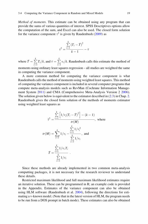
Method of moments. This estimate can be obtained using any program that can
provide the sums of various quantities of interest. SPSS Descriptives options allow
the computation of the sum, and Excel can also be used. The closed form solution
for the variance component t2 is given by Raudenbush (2009) as
t2 ¼Pki¼1
Ti � �Tð Þ2
k � 1� �v
where �T ¼ Pki¼1
Ti=k; and �v ¼ Pki¼1
vi=k. Raudenbush calls this estimate the method of
moments using ordinary least squares regression – all studies are weighted the same
in computing the variance component.
A more common method for computing the variance component is what
Raudenbush calls the method of moments using weighted least squares. This method
of computing the variance component is included in several computer programs that
compute meta-analysis models such as RevMan (Cochrane Information Manage-
ment System 2011) and CMA (Comprehensive Meta-Analysis Version 2 2006).
The solution given below is equivalent to the estimator described in (2.3) in Chap. 2.
Raudenbush gives the closed form solution of the methods of moments estimator
using weighted least squares as
t2 ¼Pki¼1
1=vi Ti � �Tð Þ2h i
� ðk � 1ÞtrðMÞ ; where
trðMÞ ¼Xk
i¼1
1=vi �Pki¼1
1=v 2i
Pki¼1
1=vi
; and
�T ¼Pki¼1
1=vi Ti
Pki¼1
1=vi
:
Since these methods are already implemented in two common meta-analysis
computting packages, it is not necessary for the research reviewer to understand
these details.
Restricted maximum likelihood and full maximum likelihood estimates require
an iterative solution. These can be programmed in R; an example code is provided
in the Appendix. Estimates of the variance component can also be obtained
using HLM software (Raudenbush et al. 2004), following the directions for esti-
mating a v-knownmodel. (Note that in the latest version of HLM, the program needs
to be run from a DOS prompt in batch mode). These estimates can also be obtained
3.4 Computing the Variance Component in Random and Mixed Models 19

using SAS ProcMixed; a sample program is included in the Appendix. The program
R can also be used conducting a simple iterative analysis to compute the restricted
maximum likelihood estimate of the variance component. The Appendix contains a
program that computes the overall variance component as given in Table 3.1. Note
that the most common method for computing the variance component remains the
method of moments. Most research reviewers do not have the computing packages
needed to obtain the REML estimate.
Once the reviewer has made the decision about fixed or random effects models,
and then computed the variance component, if necessary, the analysis proceeds by
first computing the weighted mean effect size (fixed or random), and then testing for
homogeneity of effect sizes. In the fixed effects case, this requires the computation
of the Q statistic as outlined in Chap. 2. In the random effects case, this requires the
test that the estimated variance component, t2, is different from zero as seen in
Chap. 2. More detail about these analyses can be found in introductory texts
(Borenstein et al. 2009; Higgins and Green 2011; Lipsey and Wilson 2000).
3.4.1 Example
Sirin (2005) reports on a meta-analysis of studies estimating the relationship
between measures of socio-economic status and achievement. The socio-economic
status measures used in the studies in the meta-analysis include parental income,
parental education level, and eligibility for free or reduced lunch. The achievement
measures include grade point average, achievement tests developed within each
study, state developed tests, and also standardized tests such as the California
Achievement Test. Below is an illustration of the different options for conducting
a random effects and mixed effects analysis with categorical data. There are eleven
studies in the subset of the Sirin data that use free lunch eligibility as the measure of
SES. Five of these studies use a state-developed test as a measure of achievement,
and six use one of the widely used standardized achievement tests such as the
Stanford or the WAIS. Table 3.1 gives the variance components as computed by
the DerSimonian and Laird (1986) method (also called the method of moments),
and SAS (the programs are given in the Appendix to this chapter). The SAS
estimates use restricted maximum likelihood. Note that I provide both the common
estimate of the variance component, and separate estimates within the two groups.
Table 3.1 Comparison of two methods to compute random effects variance
Test type n Q
Method of moments
estimate
SAS estimate
using REML
State test 5 60.99a 0.0872 0.086
Standardized
achievement test
6 75.14a 0.0247 0.0417
Total 11 514.86a 0.111 0.0957ap < 0.05, indicating significant heterogeneity
20 3 Planning a Meta-analysis in a Systematic Review

In this example, both groups have significant variability among the effect sizes,
indicating that the variance components are all significantly different from zero. We
also see that the method of moments estimate and the estimate using REML differ
in the case of the standardized achievement tests, complicating both the choice of
estimation method and of whether to use separate variance component estimates
within each group or a common estimate.
As Borenstein et al. (2009) point out, the estimates for the variance component
are biased when samples are small. Given the potential bias in the estimates and the
differences in the two estimates for the studies using standardized achievement
tests, the analysis in Table 3.2 uses the SAS estimate of the common variance
component, t2 ¼ 0.0957 to compute the random effects ANOVA. While the
state tests have a mean Fisher’s z-score that is larger than that for the standardized
tests, their confidence intervals do overlap indicating that these two means are not
significantly different.
3.5 Confounding of Moderators in Effect Size Models
As mentioned earlier, there are several examples of meta-analyses that do not follow
standard statistical practice. One example concerns the use of multiple statistical tests
without adjusting the Type I error rate. Many of the meta-analyses in the published
literature report on a series of one-wayANOVAmodelswhen examining the effects of
moderators (Ehri et al. 2001; Sirin 2005). Often the results of examining one modera-
tor at a time are provided, with confidence intervals for each of the mean effect sizes
within groups, and the results of an omnibus test of significance among the mean
values. Examining a series of one-way ANOVA models in meta-analysis has all the
same difficulties as conducting these in any other statistical analysis context. Primary
studies rarely report one-wayANOVAs, relyingmore onmultivariate analyses such as
multi-factor ANOVAor regression.Why themeta-analytic literature has not followed
these recommendations is not clear.
There are a number of reasons why meta-analysts need to be careful about
reporting a series of single-variable analyses. The first is the issue of confounding
moderators. It could easily be the case that the mean effect sizes using different
measures of a construct are significantly different from one another, and that there
are also significant differences among the means for groups of studies whose
participants are of different age ranges. If we only conduct these one-way analyses
Table 3.2 Analysis with a single variance component estimate
Type of achievement
test n Weighted mean
SD of mean
effect size
Lower
95% CI
Upper
95% CI
State 5 0.614 0.146 0.327 0.900
Standardized 6 0.265 0.129 0.012 0.517
Total 11 0.417 0.096 0.228 0.606
3.5 Confounding of Moderators in Effect Size Models 21

without examining the relationship between age of participants and type of measure,
wewill not know if these two variables are confounded. Related to this problem is one
of interpretation. How do we translate a series of one-way ANOVAs results into
recommendations for practice? In our example, which of the twomoderators are more
important? Should we recommend that only one type of measure be used? Or, should
we focus on the effectiveness of the intervention for particular age groups?
A final issue relates to the problem of multiple comparisons. As we learned in
our first statistics course, conducting a series of statistical tests all at the p ¼ 0.05
level will increase our chances of finding a spurious result. The more statistical tests
we conduct, the more likely we will find a statistically significant result by chance.
But, we do not seem to heed this advice in the practice of meta-analysis. We often
see a series of analyses reported, each testing the significance of the mean effect
size or the between-group homogeneity test. Fortunately, more recent research
syntheses have also reported on the confidence intervals for these means, obviating
the problems that may occur with singular reliance on statistical tests. Hedges and
Olkin (1985) discuss the adjustment of the significance level for multiple
comparisons using Bonferroni methods, but few meta-analyses use these methods
across the meta-analysis itself.
What should meta-analysts do when trying to examine the relationship of a
number of moderators to effect size magnitude? The first is to recognize that
moderators are bound to suffer from confounding given the nature of meta-analysis.
Especially in the social sciences, the studies in the synthesis are rarely replications
of one another, and use various samples, measures and procedures. Research
reviewers should examine the relationships among moderators. These relationships
can be examined using correlations, two-way tables of frequencies, or other
methods. Understanding the patterns of moderators across studies will not only
help researchers and readers understand how to interpret the moderator analyses, it
will also highlight the nature of the literature itself. It could be that no study uses the
highest quality measure of a construct with a particular sample of participants, and
thus, we do not know how effective an intervention is with that sample.
Research synthesists should also focus more on the confidence interval for the
mean effect sizes within a given grouping of studies, rather than on the significance
tests. The overlap among the confidence intervals for the mean effect sizes will
provide the same information as the statistical significance test, but is not subject to
the problems with multiple comparisons (Valentine et al. 2010).
More researchers should also use meta-regression to examine the relationship of
multiple predictors on effect magnitude. Once a researcher has explored the possible
confounding among moderators in the literature, a set of moderators could be used
with meta-regression to see how they relate to effect size net of the other variables in
the effect size model. Lipsey (2009) advocates the use of hierarchical regression; the
first set of predictors in the model may be control variables such as type of measure
used, and then themoderators of substantive interest are entered to examine howmuch
of the residual variation is accounted for by these predictors. If one of the goals for
research synthesis is to provide evidence for practice and policy, we need to under-
stand what contextual and study level moderators may explain the differences among
studies in their results.
22 3 Planning a Meta-analysis in a Systematic Review

3.5.1 Example
In the Sirin (2005) study, the results of a number of one-way ANOVA models are
reported. For example, in Table 3.3, I present a subset of the Sirin studies, examin-
ing the mean effect size for groups defined by type of achievement measure and by
type of SES measure. These studies are only a subset of those from the paper, and
do not necessarily reflect the results of the original analysis; they are here for
illustration purposes only. Since the between-group QB test is significant for both
achievement and SES measures, we can state that there is at least one effect size
within each grouping that is not equal to the other means.
What is not clear from this table is whether these two variables, type of achieve-
ment measure and type of SES measure are associated with one another. Table 3.4
below shows the crosstabulation for the number of effect sizes within the cells defined
by these two variables. The Pearson’s chi-square test of independence is significant,
w2ð6Þ ¼ 16:67, p ¼ 0.011. The chi-square test indicates a relationship between type
of SES measure and type of achievement measure. Examining the table, we see that
Table 3.3 One-way fixed effects ANOVA models based on Sirin (2005)
Moderator n z (sd) Lower CI Upper CI QB p
Achievement
GPA 10 0.26(0.011) 0.24 0.29 QB ¼ 23.73 <0.001
Achievement 5 0.27(0.019) 0.24 0.31
State 6 0.21(0.005) 0.20 0.22
Standardized 12 0.22(0.012) 0.20 0.24
SES
Free lunch 11 0.24(0.014) 0.21 0.26 QB ¼ 27.24 <0.001
Income 4 0.21(0.005) 0.20 0.22
Education 18 0.26(0.009) 0.25 0.28
Total 33 0.22(0.004) 0.22 0.23
Table 3.4 Crosstabulation of SES and Achievement
SES measures
Achievement measures Free lunch Income Education
GPA 1 0 9
9.1% 0% 50%
Achievement 0 1 4
0% 25% 22.2%
State 4 2 0
36.4% 50% 0%
Standardized 6 1 5
54.5% 25% 27.8%
Total 11 4 18
100% 100% 100%
3.5 Confounding of Moderators in Effect Size Models 23

most of the studies using GPA for achievement also use education as the proxy for
SES. Studies employing state tests tended to use free lunch status as the proxy for SES,
with the remainder of those studies using income.
The results in Table 3.5 show the random effect size means for the groups defined
by both these variables simultaneously. What we do see is that the four studies using
both state tests and free lunch as the SES proxy have a weighted mean effect size that
is almost twice as large as the other cells that have at least two effects. Figure 3.2
provides an error bar chart for the means and their 95% confidence interval for the
studies using either free lunch or education as the measure of SES. Though all the
confidence intervals overlap, there is some evidence that the studies using free lunch
for SES and the state test for achievement have a larger estimate of the correlation
Table 3.5 Random effects mean effect sizes, and 95% confidence intervals for studies classified
by Achievement and SES measures
SES measures
Achievement measures Free lunch Income Education
GPA 0.41 – 0.16
[0.02, 0.81] [0.03, 0.30]
k ¼ 1 k ¼ 9
Achievement – 0.46 0.28
[0.01, 0.91] [0.07, 0.49]
k ¼ 1 k ¼ 4
State 0.54 0.20 –
[0.32, 0.76] [�0.07, 0.47]
k ¼ 4 k ¼ 2
Standardized 0.26 0.15 0.30
[0.10, 0.43] [�0.24, 0.54] [0.13, 0.48]
k ¼ 6 k ¼ 1 k ¼ 5
0
0.1
0.2
0.3
0.4
0.5
0.6
0.7
0.8
0.9
free lunchstate
free lunchstandardized
educ gpa eduachievement
educstandardized
Fig. 3.2 Error bar plot for random effects means in Sirin (2005)
24 3 Planning a Meta-analysis in a Systematic Review

between SES and achievement. For this subset of studies, there is an interaction
between two moderator variables that can influence the interpretation of results.
This small example illustrates the need for reviewers to examine carefully
the relationships among moderators. As indicated above, meta-regression is a
recommended strategy when there are sufficient numbers of effect sizes since we can
examine the influence of multiple moderators on effect size at the same time. If meta-
regression is not possible, then the reviewer needs to provide evidence that
confounding among the target moderators will not impact the interpretation of the
findings.
3.6 Conducting a Meta-Regression
When a reviewer has a larger sample of studies, conducting a meta-regression can
help a reviewer avoid conducting multiple significance tests, and instead examine
the conditional relationship among the predictors and effect size magnitude. Intro-
ductory text books (Borenstein et al. 2009; Lipsey and Wilson 2000) provide
more detail about the background for conducting a meta-regression; here I will
provide an example of meta-regression using another subset of the Sirin (2005)
data. The Appendix provides both SPSS and SAS sample programs for computing
the model discussed below.
We conduct a meta-regression when we want to examine how a set of p predictorvariables relate to the variation among effect sizes. Our hypothetical linear model
can be written as
yi ¼ b0 þ b1xi1 þ :::þ bpxip;
where yi is the effect size in study i, the xi1,. . .,xip are the values of the predictor
variable for study i, and the b0,. . .,bp are the unknown regression coefficients.
In the fixed effects case, we will use our values of Ti as our estimates of the yiwith vi as the variance of these effect size estimates. We use weighted least squares
regression to estimate the model where our weights are equal to wi ¼ 1/vi. For arandom effects meta-regression, the weights are w�
i ¼ 1=ðvi þ t2Þwhere t2 is
estimated from one of the methods from Sect. 3.4 (For the interested reader,
Chap. 8 illustrates how to estimate the random effects meta-regression using
restricted maximum likelihood methods).
3.6.1 Example
Below I provide sample output from SPSS to illustrate how fixed effects meta-
regression analysis is conducted (The Appendix contains the steps needed
to conduct the meta-regression in SPSS, as well as a sample program for SAS).
3.6 Conducting a Meta-Regression 25

The data used in this example are given in the Data Appendix at the end of the book.
Let us say that we are interested in examining how the values of Fisher’s z-
transformation in the Sirin data are related to the grade level of the students in
the study, the percent of minority students represented in the study’s sample
(percmin), and the way that income was measured in the study. For this example,
I have included two dummy codes, free lunch, which indicates that the study used
eligibility for free lunch to identify low-income students, and education, which
indicates that the study used the level of education of the parent as a indicator of
income. The default SPSS output is given in Fig. 3.3.
The first table in Fig. 3.3 provides the Model Summary. This table should be
ignored. The adjusted R-square value cannot be interpreted as in usual practice
since, as Konstantopolous and Hedges (2009) point out, the maximum value for the
population multiple correlation in this case is often much less than one. The second
table provides the summary of the F-tests for the meta-regression. In this table,
Fig. 3.3 SPSS output for Sirin (2005) meta-regression example
26 3 Planning a Meta-analysis in a Systematic Review

the Sum of Squares for the Residual is the statistic called QE, which provides a test
of the goodness of fit of the linear model. This statistic is the weighted residual sum
of squares about the regression line. When the statistic is significant, the variation
around the regression line is greater than expected given that the model is a good fit
to the data. The statistic QE is compared to a chi-square distribution with (k – p – 1)degrees of freedom. In this case, we have QE ¼ 1,053.85, compared to the 95%
critical value of a chi-square with 34 degrees of freedom which is equal to 48.60.
Thus, we have greater than expected residual variance around our regression line,
indicating that our model is not a good fit to the data.
The third table presents the estimated regression coefficients. As many textbooks
point out (Borenstein et al. 2009; Konstantopolous and Hedges 2009; Lipsey and
Wilson 2000), the standard errors and tests of significance for the coefficients
printed in many weighted regression routines in common statistical packages are
incorrect since they are based on a model slightly different than the one used for
fixed-effects meta-regression. The corrected standard errors and tests of signifi-
cance must be computed by hand. The corrected standard errors are given as
Sj ¼ SEjffiffiffiffiffiffiffiffiffiffiMSE
p (3.1)
where the SEj are the printed standard errors, and MSE is the mean square error
given in ANOVA table for the regression. The correct tests of significance use the Zdistribution. If we wish to test that a given regression coefficient is equal to 0, we
use a two-sided test where we compute the statistics Zj given by
Zj ¼bj�� ��Sj
where bj is the estimated regression coefficient, and Sj is the corrected standard
error given in (3.1). Table 3.6 provides the corrected standard errors and tests of
significance for the Sirin data.
In this example, where k ¼ 39, all of the coefficients are significantly different
from zero. We see that the larger the percent minority included in the sample, the
smaller the Fisher z-transformation (and by extension, correlation) between socio-
economic status and achievement. Higher grade levels have larger Fisher z’s as do
Table 3.6 Corrected table for meta-regression results using Sirin (2005)
Coefficient Estimate SEj Sj Zj p-value
Intercept 0.041 0.081 0.0150 2.73 0.003
% minority �0.001 0.001 0.0002 �5.00 0.000
Grade 0.073 0.024 0.0043 16.98 0.000
Free lunch 0.354 0.068 0.0120 29.50 0.000
Education level 0.104 0.059 0.0110 9.45 0.000
3.6 Conducting a Meta-Regression 27

studies where free lunch or education level are used as the indicators of income.
The comparison category to the indicator of income are rating scales of the
occupational status and actual reported income. Though the value of the QE statistic
indicates that significant residual variation remains, this model does provide insight
into the variation among the effect sizes in this data.
3.7 Interpretation of Moderator Analyses
As seen in the example above, reviewers need to exercise caution in their interpre-
tation of the results of moderator analyses when potential confounding occurs.
Discovering what variables may be confounded is difficult in meta-analysis since
many reviews include only a small number of studies. However, the example
provided above adds to our understanding of the complex relationships among
measures of SES and source of the achievement measures.
Adding to the complexity of the interpretation of moderator analyses is the
nature of these analyses themselves. Research reviewers do not have control over
the population of studies and how these studies were conducted. Thus, unlike a
primary study, we cannot randomly assign particular studies to using just males or
just females, or to assessing achievement only using a single measure. The analyses
in a research synthesis are exploratory and observational. We usually have little
evidence from a meta-analysis about why study characteristics relate to effect
magnitude. We can only describe what the relationships are among achievement
and SES measures, for example. These analyses are observational only, and do not
provide information about why or how these relationships operate. Chapter 9
discusses the nature of the inferences that are possible from a meta-analysis.
Preliminary stages of meta-analysis should conform to standard statistical
analysis practice, such as providing a plot of the data, choosing a priori the
moderators that are of most interest, and exploring homogeneity of the effect
sizes. Choosing these analyses ahead of time ensures that the research reviewer
does not capitalize on chance by conducting a series of analyses without adjusting
the overall Type I error rate. In addition, it is difficult to interpret a series of single
variable analyses since we do not know which moderator should be considered
important. As in the example above, we find that studies using state tests tend to use
eligibility for free lunch as the measure of SES, a measure that is not as sensitive as
income. The ultimate goal of a meta-analysis is to help clarify what is known about
a given intervention or phenomenon, and the analyses we present should aim at
illuminating what is and is not yet known in a given research area. Carefully
interpreting the analyses is ultimately the responsibility of the reviewer.
28 3 Planning a Meta-analysis in a Systematic Review

Appendix
Computing the Variance Component Using SAS
The example in Sect. 3.4.1 involves the computation of the variance component
using restricted maximum likelihood. Below is a SAS program that computes the
estimates for the analyses in Tables 3.1–3.3. The first program enters the data used
in this example. The variables are the study name, the correlation, Fisher’s z
corresponding to the correlation, the variance of Fisher’s z, a code that takes the
value 1 for studies using state tests for achievement, and 2 for standardized tests,
and the study weight. The second program provides the code to compute the
variance component using restricted maximum likelihood. The first line calls
Proc Mixed, with cl proving the confidence limits, and method indicating the
used of restricted maximum likelihood. Themodel statement indicates that Fisher’s
z is the outcome, and the model is a simple random effects model with no
predictors. The options S and CL provide the fixed-effects parameter estimates,
and the confidence interval, respectively. The class statement indicates that study is
a class variable, which will be designated as the random effect later in the code. The
random statement designates the random effect, and the option solution prints
the estimate of the random effect, or in this case, the random effects variance.
The repeated statement specifies the covariance structure of the error term. For
meta-analysis, we use the option group to allow between-group (in this case, study)
heterogeneity. The parms statement provides the starting values for the covariance
parameters. The first value is the starting value for the overall variance component
for this model. The next 11 elements are the within-study estimates of the variance
of the effect size. The option eqcons fixes the variances for the 11 studies in the
analysis since these are considered known in a meta-analysis model.
data sirinch6ex;
input study $ corr zval varz achmeas wt;
cards;
alspurb .7190 .9055717 .0278 1 36.00
alsprur .0720 .0721248 .0097 1 103.00
calban1 .6800 .8291140 .0008 1 1298.00
dixflo .4670 .5062267 .0122 1 82.00
grelan .6500 .7752987 .0086 1 116.00
gulbur .1240 .1246415 .0006 2 1570.00
johnlin .1750 .1768200 .0006 2 1683.00
kling .5400 .6041556 .0030 2 329.00
recste .0600 .0600722 .0077 2 130.00
schu .4300 .4598967 .0077 2 130.00
shawal .1660 .1675505 .0030 2 332.00
;
run;
Appendix 29

proc mixed cl method¼reml data¼sirinch6ex;
class study;
model zval ¼/S CL;
random int/SUBJECT¼study S;
repeated/GROUP¼study;
Parms (0.01 to 2.00 by 0.01)
(.0278) (.0097) (.0008) (.0122)
(.0086) (.0006) (.0006) (.0030)
(.0077) (.0077) (.0030)
/EQCONS¼2 to 12;
run;
Computing the Variance Component Using R
Below is a simple iterative program to obtain the restricted maximum likelihood
estimates from R. The estimates are described by Raudenbush (2009). The first two
lines set up the starting values for the random effects mean and variance, namely a
vector of 100 elements, all having the value of zero. The 100 iterations take place
within the brackets, “{}”. First, the value for the new variance for the vector of
effect sizes is computed as adding our current value of the random effects variance,
sigrmle[i] to the within-study variation, sirin$ztrans. Given this value of the vector
of the within-study variances, vstar, we recomputed a new value of the random
effects mean, beta0. Given this value of the random effects mean, beta0, we
recalculate the value of the variance component sigrmle. We cycle back and forth
for 100 iterations in this program. Below the program are the results from R using
this example.
beta0<�rep(0, c(100))
sigrmle<�rep(0,c(100))
for (i in 1:100) {
vstar<�sirin$var+sigrmle[i]
beta0[i]<�sum(sirin$ztrans/vstar)/sum(1/vstar)
sigrmle[i+1]<�(sum((((sirin$ztrans-beta0[i])**2)-sirin$var)/(vstar**2))/sum(1/
(vstar**2)))+(1/sum(1/vstar))
}
> beta0
[1] 0.3551265 0.4162903 0.4169039 0.4169685 0.4169757 0.4169765 0.4169766
[8] 0.4169766 0.4169766 0.4169766 0.4169766 0.4169766 0.4169766 0.4169766
. . .. . .. . ...> sigrmle
[1] 0.00000000 0.08408039 0.09172159 0.09258992 0.09268741 0.09269834
[7] 0.09269957 0.09269971 0.09269972 0.09269972 0.09269972
0.09269972. . .. . ..
30 3 Planning a Meta-analysis in a Systematic Review

We can see that by the 8th iteration, both the variance component and the
random effects mean do not change. The estimates from R correspond to those
obtained using SAS.
Computing the Fixed Effects Meta-regression Using SPSS
The analysis in Table 3.6 can be computed from the Analyze menu in SPSS, under
Regression, and then under Linear Regression. The Dependent variable will be the
Fisher z-transformations of the correlation coefficients. In this example, the Inde-
pendent variables are the percent minority in the sample, the dummy code
indicating whether free lunch was used as the measure of socio-economic status,
the dummy code indicating whether parent education level was used as the measure
of socio-economic status, and grade level. The WLS Weight for the analysis is the
inverse of the Fisher’s z-transformation variance, or 1/(n – 3).
Computing the Fixed Effects Meta-regression Using SAS
To compute the fixed effects meta-regression in SAS, we use Proc Reg as illustrated
in the code given below. The model statement begins with the outcome, the Fisher
z-transformation, an equals sign, and the list of predictors. An option to the model
statement is given by the slash /and followed by I which indicates that we want the
inverse of the crossproducts matrix. The inverse of the crossproducts matrix will
provide the correct variances for the regression coefficients. The weight statement
indicates that the variable wt should be used in the weighted least squares
regression.
proc reg data¼Chap. 3;
model ztrans¼grade percmin freelunch educ/I;
weight wt;
print;
run;
The output provided by SAS is first the inverse of the crossproducts matrix:
X0X Inverse, Parameter Estimates, and SSE
Intercept Grade % minority Free lunch Parent’s education
Intercept 0.000218 0.0000594 �4.746E-7 �0.0000666 �0.0000709
Grade �0.0000594 0.0000198 3.834E-8 0.0000126 0.0000143
% minority �4.745E-7 3.834E-8 9.403E-9 7.456E-8 5.824E-8
Free lunch �0.0000666 0.0000126 7.456E-8 0.000154 0.0000362
Parent’s education �0.0000709 0.0000143 5.824E-8 0.0000362 0.000117
Appendix 31

The diagonal elements of this matrix are the correct variances for the weighted
regression coefficients. For example, the correct standard error for Parent’s educa-
tion level is √0.000117 ¼ 0.0108, which corresponds to that computed using the
adjusted SPSS values in Table 3.6. Next, SAS provides the ANOVA table for the
regression and the R-squared values.
Analysis of Variance
Source DF Sum of squares Mean square F value Pr > F
Model 4 1081.426 270.356 8.98 <.0001
Error 35 1053.852 30.110
Corrected total 39 2135.278
Root MSE 5.487 R-Square 0.5065
Dependent mean 0.272 Adj R-Sq 0.4501
Coeff var 2014.675
As in the example with SPSS, we will use the square root of the mean square
error given in the output above to correct the standard errors and the significance
tests of the regression coefficients given below.
Variable DF Parameter estimate Standard error t-value Pr >
Intercept 1 0.0408 0.0811 0.50 0.6176
Grade 1 0.0729 0.0244 2.98 0.0052
% minority 1 �0.000999 0.00053 �1.88 0.0686
Free lunch 1 0.353 0.0681 5.19 <.0001
Parent’s education 1 0.104 0.0594 1.75 0.0885
References
Anderson, L.M., M. Petticrew, E. Rehfuess, R. Armstrong, E. Ueffing, P. Baker, D. Francis, and
P. Tugwell. 2011. Using logic models to capture complexity in systematic reviews. ResearchSynthesis Methods 2: 33–42.
Barel, E., M.H. Van IJzendoorn, A. Sagi-Schwartz, and M.J. Bakermans-Kranenburg. 2010.
Surviving the Holocaust: A meta-analysis of the long-term sequelae of a genocide. Psycholog-ical Bulletin 136(5): 677–698.
Borenstein, M., L.V. Hedges, J.P.T. Higgins, and H.R. Rothstein. 2009. Introduction to meta-analysis. Chicester: Wiley.
Cochrane Information Management System. 2011. RevMan 5.1. Oxford, UK: Cochrane
Collaboration.
Comprehensive Meta-Analysis Version 2. 2006. Englewood, NJ: Biostat.
Cooper, H., L.V. Hedges, and J.C. Valentine (eds.). 2009. The handbook of research synthesis andmeta-analysis. New York: Russell Sage.
Dersimonian, R., and N. Laird. 1986. Meta-analysis in clinical trials. Controlled Clinical Trials7: 177–188.
Ehri, L.C., S. Nunes, S. Stahl, and D. Willows. 2001. Systematic phonics instruction helps students
learn to read: Evidence from the National Reading Panel’s meta-analysis. Review of Educa-tional Research 71: 393–448.
32 3 Planning a Meta-analysis in a Systematic Review

Greenland, S., J. Pearl, and J.M. Robins. 1999. Causal diagrams for epidemiologic research.
Epidemiology 10(1): 37–48.Hedges, L.V., and I. Olkin. 1985. Statistical methods for meta-analysis. New York: Academic.
Hedges, L.V., and J.L. Vevea. 1998. Fixed- and random-effects models in meta-analysis. Psycho-logical Methods 3(4): 486–504.
Higgins, J.P.T., and S. Green. 2011. Cochrane handbook for systematic reviews of interventions.Oxford, UK: The Cochrane Collaboration.
Joffe, M., and J. Mindell. 2006. Complex causal process diagrams for analyzing the health impacts
of policy intervention. American Journal of Public Health 96(3): 473–479.
Konstantopolous, S., and L.V. Hedges. 2009. Analyzing effect sizes: Fixed-effects models. In Thehandbook of research synthesis and meta-analysis, 2nd ed, ed. H. Cooper, L.V. Hedges, and
J.C. Valentine. New York: Russell Sage.
Lipsey, M.W. 2009. Identifying interesting variables and analysis opportunities. In Thehandbook of research synthesis and meta-analysis, 2nd ed, ed. H. Cooper, L.V. Hedges, and
J.C. Valentine. New York: Russell Sage.
Lipsey, M.W., and D.B. Wilson. 2000. Practical meta-analysis. Thousand Oaks: Sage
Publications.
Littell, J.H., M. Campbell, S. Green, and B. Toews. 2005. Multisystemic therapy for social,
emotional and behavioral problems in youth aged 10–17. Cochrane Database of SystematcReviews (4). doi:10.1002/14651858.CD004797.pub4.
Raudenbush, S.W. 1983. Utilizing controversy as a source of hypotheses for meta-analysis:
The case of teacher expectancy’s effects on pupil IQ. In Evaluation studies review annual,8th ed, ed. R.J. Light. Beverly Hills: Sage Publications.
Raudenbush, S.W. 2009. Analyzing effect sizes: Random-effects models. In The handbook ofresearch synthesis and meta-analysis, 2nd ed, ed. H. Cooper, L.V. Hedges, and J.C. Valentine.New York: Russell Sage.
Raudenbush, S.W., A.S. Bryk, Y.F. Cheong, and R. Congdon. 2004. HLM 6 for Windows.Lincolnwood: Scientific Software International.
Rosenthal, R., and L. Jacobson. 1968. Pygmalion in the classroom. New York: Holt, Rinehart &
Winston.
Sirin, S.R. 2005. Socioeconomic status and academic achievement: A meta-analytic review of
research. Review of Educational Research 75(3): 417–453. doi:10.3102/00346543075003417.
Valentine, J.C., T.D. Pigott, and H.R. Rothstein. 2010. How many studies do you need? A primer
on statistical power in meta-analysis. Journal of Educational and Behavioral Statistics35: 215–47.
References 33


Chapter 4
Power Analysis for the Mean Effect Size
Abstract This chapter provides methods for computing the a priori power of the
test of the mean effect size. Both fixed and random effects models tests are
discussed. In addition, examples are provided for computing the number of studies
needed to detect a substantively important effect size, and the detectable effect size
with a given number of studies.
4.1 Background
Researchers planning new primary studies use power analysis to increase their odds
of finding results that they believe are present. Power analysis allows the researcher
to determine a priori the number of participants needed in a study to find statistical
significance. For example, if we want to know that an intervention has a substantive
effect, we need to plan a study with sufficient numbers of participants, and ade-
quately sensitive measures and analysis strategies to detect that effect. Few primary
researchers would risk conducting an intervention study without a power analysis.
In research synthesis and meta-analysis, reviewers plan systematic reviews in
areas that have matured enough to have a sufficient body of evidence, and where a
careful review may enhance the overall understanding of a field. Unlike primary
researchers, reviewers cannot plan in advance the sample size (in this case, the
number of primary studies) needed to find important substantive effects. Thus, on
the surface, power analysis in meta-analysis, especially a priori power analyses,
might appear a futile exercise.
I take an alternative view of the value of a power analysis in research synthesis.
As emphasized in Chap. 3, knowledge of an area is critical to the planning of a
synthesis, especially with regard to planning the moderator analyses carefully so as
to avoid Type I errors. The same could be argued for the importance of a power
analysis as preliminary to a systematic review. Though a reviewer might not know
the exact number of studies that will ultimately be relevant to the review, the
reviewer should have a clear understanding of the size of the effect that would be
T.D. Pigott, Advances in Meta-Analysis, Statistics for Social and Behavioral Sciences,
DOI 10.1007/978-1-4614-2278-5_4, # Springer Science+Business Media, LLC 2012
35

considered substantively important and of the statistical methods (such as moderator
analyses) that will be used. Examining the potential power of a meta-analysis prior
to collecting and evaluating the studies will add strength to the reviewer’s later
decisions about conducting particular analyses. Say, for example, we are interested
in understanding the potential magnitude of an adverse effect of a given medical
treatment, but believe the incidence of this effect is rare. The reviewer would know a
priori that an estimate of this adverse effect cannot be examined if there are not a
sufficient number of studies. In an educational setting, if we are interested in
understanding the magnitude of the effect of a dropout prevention program, we
might find that we do not have enough studies to detect, for example, a standardized
mean difference of 0.5 between the treatment and control groups. This information
can then provide a rationale for the statistical analyses conducted (or not) with the
effect size data.
In order to conduct a power analysis a priori, the reviewer must be transparent
about the assumptions he or she is making at the outset of the synthesis. This
transparency can serve as a check for the analysis of the effect size data so that
reviewers do not conduct too many statistical analyses that may capitalize on
chance. Reviewers can also inform policymakers prior to a synthesis of the numbers
of studies that are needed to find a significant effect of an intervention. There are
circumstances where we do not have enough primary research to make an informed,
research-based decision, and an a priori power analysis of a systematic review
would provide empirical evidence for that claim.
As mentioned above, the reviewer conducting a power analysis in meta-analysis
needs to have informed judgments about important characteristics of studies, such
as the typical within-study sample size, and the magnitude of a substantively
important effect size. Since reviewers need to make assumptions about these
quantities, there is a temptation to compute power after analyzing the data. The
use of retrospective power analyses is not new; much has been written in the
medical, natural and behavioral sciences about the limitations and advantages of
power analysis after the study is complete (Goodman and Berlin 1994; Hayes and
Steidl 1997; Reed and Blaustein 1995; Thomas 1997; Zumbo and Hubley 1998).
In many fields, retrospective power analysis has been suggested as a way to
interpret null results. For example, one often-cited study of amphibian populations
by Reed and Blaustein (1995) concludes that prior studies finding a lack of decline
in populations “cannot be supported statistically” (p. 1299) since the statistical
power in these studies ranges from less than 0.06 to 0.45. In medicine, Freiman
et al. (1978) computed the retrospective power of 71 “negative” trials, finding that a
majority of studies had power levels less than 0.80 for detecting a 25% or a 50%
reduction in mortality.
Critics of retrospective power analysis (Goodman and Berlin 1994; Hayes and
Steidl 1997; Zumbo and Hubley 1998) point out the logical flaws in using the
observed results to compute retrospective power. The major issue is that power is
related to statistical significance; once a researcher obtains a finding of no
significant difference, then the researcher knows that power was inadequate.
The observed power, power calculated after the analysis is completed, does not
36 4 Power Analysis for the Mean Effect Size

provide any more evidence than the p-value for a given test. Power makes sense
only in relation to a specific effect size; in other words, power is computed as the
power to detect a specific difference between groups, or size of association
between constructs. It is redundant to compute power for a non-significant test
since we already know that our test is underpowered for our obtained result. For
researchers using research synthesis, power computations need to occur in the
early stages of the review to determine if adequate evidence exists to test a given
hypothesis. As I will discuss later, reviewers should start with substantively
significant values for an average effect size and compute power given a range
of values for the effect size variances, sample sizes within studies, and number
of studies.
The following chapters provide an overview of power analysis in meta-analysis,
and illustrate its use with examples. This chapter begins with a review of power
analysis in general and then in meta-analysis, focusing on tests of the mean effect
size, under both the fixed and random effects model.
4.2 Fundamentals of Power Analysis
All power analyses are conducted with a specific statistical test in mind, and are
described in relation to a null hypothesis and a particular alternative hypothesis.
Though organizations such as the American Psychological Association (Ameri-
can Psychological Association 2009) are emphasizing the interpretation of effect
sizes rather than statistical significance, power computations remain in the realm
of the null and alternative hypothesis. In order to compute power, researchers use
a value for the alternative hypothesis that represents some substantively important
quantity, such as the smallest effect size that would be considered substantively
critical, and then discuss the power of a statistical test under the specific alterna-
tive hypothesis posed.
The computation of power analysis for most statistical tests depends on four
general quantities: the sample size of the study, the substantively important effect
size that will be tested against the null hypothesis, the desired significance level of
the statistical test, and the desired level of power (Cohen 1988; Murphy and Myors
2004). Any three of these four quantities can be used to solve for the fourth one. For
example, researchers often ask about the number of participants needed to find a
given difference between the treatment and control groups. With the particular
value for the difference between the groups, the desired significance level and
power level, the researcher can find the optimal sample size. Alternatively, the
researcher may know how many participants are available, and can compute the
power level for the test given a particular value for the group difference.
When we compute power, we are actually comparing two distributions: that of
our test statistic given that the null hypothesis is true, and that of our test statistic
when the alternative hypothesis is correct. The power of our test is the probability
that our obtained test statistic will be considered significant under the null
4.2 Fundamentals of Power Analysis 37

hypothesis when the alternative hypothesis is really true. Thus, power depends on
both the null and the alternative hypothesis in a given context, and is typically
decided upon prior to computing the test.
Computation of power in a meta-analysis is similar to that for other statistical
tests. For example, we need the number of studies in the review (the “sample
size”), the anticipated overall mean effect size, and the criterion for statistical
significance. Since our unit of analysis is a primary study, power in meta-analysis
also depends on the sample size within studies. Table 4.1 outlines the steps to
compute the power of a meta-analysis. The first three steps are analogous to those
for power computations in primary studies; the fourth step requires knowledge
about the size of the sample and the effect sizes of the individual studies. These
quantities are usually variable across studies, and requires the reviewer to have
deep knowledge about the types of studies typically conducted in a given research
area in order to make accurate assumptions for computing power. Table 4.2
provides more details about the information needed for computing power at two
levels of a systematic review: at the level of the review itself, and at the level of
the individual studies.
The rest of this chapter covers power for the statistical test of the mean effect
size, in both fixed and random effects models. The power for the mean effect size
will be important for planning reviews when the interest is in the overall effect of an
intervention, an estimate of the mean association between two constructs, or the
overall incidence rate of a condition. For example, a policymaker may be interested
in knowing if the average effect of an expensive intervention will be worth the cost.
A reviewer might then want to know the minimum number of studies needed to
detect a substantively important effect size that would justify the cost of the
Table 4.1 Steps for determining power in meta-analysis
1. Establish a critical value for statistical significance, ca2. Posit an overall effect size, y3. Estimate the number of studies included in the meta-analysis, k
4. Decide on fixed or random effects models
a. Posit “typical” within-study samples sizes and effect size variances for fixed effects
b. For random effects also posit typical variance component, t2
5. Compute power for specific tests in a meta-analysis
Table 4.2 Information needed to compute power in meta-analysis
Information needed at the level of the research synthesis
• Critical value/criterion for statistical significance, ca• Effect size of practical significance, y• Number of studies for the meta-analysis, k
• For random effects: variance component (between-studies variance), t2
Information needed at the level of the studies included in the research synthesis
• Within-study sample sizes, N
• Study effect size variances (related to sample size), v
38 4 Power Analysis for the Mean Effect Size

intervention. Alternatively, I may want to know the size of the effect I could detect
with a given number of studies – and whether this detectable effect will be of
substantive interest.
4.3 Test of the Mean Effect Size in the Fixed Effects Model
The first step in any meta-analysis is to examine the mean effect size. In planning a
research synthesis, reviewers may be interested in understanding the average effect
for an intervention, or the average incidence rate across studies. In any given area of
research, a reviewer should have a good understanding of the size of an effect that
would be considered substantively important. The reviewer can then compute the
minimum number of studies needed to detect that effect size with a particular
power. Alternatively, the reviewer might have a rough idea of the number of studies
that exist, perhaps because of the results of a prior review. This information could
help a reviewer to compute the size of an effect that will be able to be detected with
a particular power.
As discussed above, reviewers must make an educated guess about the quantities
given in Table 4.2. Given knowledge of the within-study information (typical
sample sizes and effect size variances), the reviewer can use guesses about two of
the three quantities at the level of the synthesis for a fixed effects model to solve for
the third one. Before illustrating this process, I review the overall test for the mean
effect size under the fixed effects model below.
4.3.1 Z-Test for the Mean Effect Size in the FixedEffects Model
One of the first steps in a meta-analysis is to compute the mean effect size across all
studies. In this section, I outline the steps of the Z-test for the mean effect size under
the fixed effects model, followed by a discussion of how to conduct the power for
this test. If we are interested in the effectiveness of a treatment, we may be
interested in understanding if our mean effect size is different from zero, namely,
if the treatment group differs significantly from the control group. In this case, our
null hypothesis would be H0 : y ¼ 0; that our mean effect size indicates no
difference between the treatment and control groups. We would use the same null
hypothesis to determine if the mean correlation or log-odds ratio was different from
zero. We use y to designate the population mean, estimated by �T� given in (2.1).
We truly expect, however, that our treatment is effective, so that we have an
alternative hypothesis that our mean effect size will be greater than 0. In this
case, our alternative hypothesis is Ha : y � 0. This is the case of a directional
alternative hypothesis which would result in a one-tailed statistical test. If we have
4.3 Test of the Mean Effect Size in the Fixed Effects Model 39

little information about the intervention, we might have a less specific alternative
hypothesis, allowing either the treatment or the control group to have the larger
mean. This non-directional alternative hypothesis is given by Ha : y 6¼ 0, which
results in a two-tailed test.
The test of the mean effect size compares the estimated mean effect size to 0, by
comparing our obtained test statistic to a standard normal distribution. Recall from
Chap. 2 that we designate the estimated effect sizes for each study as Ti, i ¼ 1, 2,
. . ., k where k is the total number of studies. In the fixed effects model, we have a
mean effect size across all the k studies, �T� given in (2.1), and this value estimates
the underlying population mean effect, y. To examine whether our obtained mean
effect size, �T�, is statistically different from 0, we compute the following statistic
Z ¼�T� � 0ffiffiffiffiffi
v�p (4.1)
where v� is the sampling variance of �T� given in (2.2). Once we have our value of Z,we compare it to the standard normal distribution. If our alternative hypothesis is
Ha : y� ya, we reject the null hypothesis if Z is larger than the critical value, ca,where a is our designated significance level, the 100(1 � a) percentile of the
standard normal distribution. For example, if we want to know that our mean effect
size is greater than ya ¼ 0, our ca for a one-tailed test with a ¼ 0.05 is 1.645.
Figure 4.1 displays a standard normal curve. When H0 : y ¼ 0, the curve in
Fig. 4.1 represents the distribution of our Z test statistics. The shaded part of the
curve to the right is the proportion of Z statistics that exceed ca when the null
hypothesis is true.
We might also have a situation where we are not sure of the direction of the
effect size, namely, that the treatment group may score higher or lower than the
control group. In this situation, we have a non-directional alternative hypothesis, or,
Fig. 4.1 Standard normal distribution with shaded area greater than ca ¼ 1.64
40 4 Power Analysis for the Mean Effect Size

Ha : y 6¼ 0. For a two-tailed test, we reject the null hypothesis H0 : y ¼ 0 when
our obtained value of Z is either greater than or less than ca=2, or more formally
when the absolute value of Z exceeds ca=2, or Z � ca=2�� ��.
4.3.2 The Power of the Test of the Mean EffectSize in Fixed Effects Models
The power of a statistical test is the probability that we will reject the null
hypothesis in favor of some specific alternative hypothesis. As we see in (4.1),
we need to have a value for y, the mean effect size we are testing, and the variance
of the mean effect size in a given meta-analysis in order to compute Z, and thus, in
order to compute power. Below, I will discuss how we might compute these
quantities prior to collecting the studies for our synthesis. For now, imagine that
we do have an educated guess about these values, we have computed the statistic Zgiven our guesses about y and v�, and we are testing that our mean effect size is
greater than zero. When the null hypothesis is true, as in H0 : y ¼ 0, the statistic Zhas the standard normal distribution with a mean of 0, and a standard deviation of 1.
When the null hypothesis is false, Z has a normal distribution with a variance of
1 and a mean that is not 0 but is given by
l ¼ y� 0ffiffiffiffiffiv�
p : (4.2)
where the value y is our mean effect size, and v� is the sampling variance of this
mean effect size. Thus, we have two different normal distributions we are going to
compare: the standard normal distribution that corresponds to the null hypothesis,
and the normal distribution that represents our alternative hypothesis. To compute
power, we need to know the proportion of test statistics that exceed ca in the normal
distribution for the alternative hypothesis with mean l from (4.2), and variance 1.
We get this proportion, the power of our test, by computing p
p ¼ 1� Fðca � lÞ (4.3)
where FðxÞ is the cumulative distribution function of the standard normal distribu-
tion, i.e., the area under the standard normal curve from �1 to x. For example,
Fig. 4.2 shows both the standard normal distribution and the normal distribution of
Z test statistics when y 6¼ 0, in this illustration when y ¼ 2:5. The proportion of
tests in the cross-hatched area is equal to the area under the standard normal curve
that exceeds the value of ca � l when Ca ¼ 1:64 and l ¼ 2.50. The exact value of
this area is 1� FðCa � lÞ ¼ 1� Fð�0:86Þ ¼ 1� 0:19 ¼ 0:81. Thus, the power ofthe test under this alternative hypothesis, Ha : y� 0, is 0.81.
4.3 Test of the Mean Effect Size in the Fixed Effects Model 41

A two-tailed test follows similar logic, except that we are interested in the
proportion of test statistics that are either greater than or less than ca=2, or
Z � ca=2�� ��. The test statistics are in the two tails of the distribution so that the
power for our two-tailed test is given by
p ¼ 1� Fðca=2 � lÞ � Fð�ca=2 � lÞ� �¼ 1� Fðca=2 � lÞ þ Fð�ca=2 � lÞ (4.4)
4.3.3 Deciding on Values for Parameters to Compute Power
In order to compute power of the mean effect size, we need to designate a number of
quantities. Our first task is to arrive at a value for y, the mean effect size of interest,
or, in other words, the value of a substantively important effect. This value should
be evident from the context of the review and the typical measures used. For
example, we may know that increasing a child’s reading scores from the 25th to
the 50th percentile is associated with higher achievement in later elementary
grades. We would then be interested in the power of a test to detect an effect size
corresponding to an increase of 25 percentile points. As seen in (4.2), we also need
an estimate of the variance for the mean effect size of interest. This quantity is more
difficult to determine. Looking at (2.2), we see that the variance for the mean effect
size, v�, depends on the variances for the effect sizes within each study, which in
turn depend on the individual study effect sizes and the within-study sample sizes.
One way to think about an estimate for v� is to assume that all studies have the same
within-study sample size, and the same effect size equal to y, our effect size of
interest. With the same within-study sample size and effect size, our studies would
then all have the same within-study effect size variance, v. Note that we compute
v� in this case as
−4 −2 0 2 4 6
0.0
0.1
0.2
0.3
0.4
Fig. 4.2 Power when normal distribution has a mean of 2.5 and ca ¼ 1.64
42 4 Power Analysis for the Mean Effect Size

v� ¼ 1
Pki¼1
w
¼ 1
Pki¼1
1=v
¼ 1
k=v¼ v
k: (4.5)
Finally, we need a value of k, the number of studies we are likely to find as relevant
in the review. In sum, to compute the power for the mean effect size in a fixed
effects model, we need a value for the effect size of interest, y, the within-study
sample size (to compute v), and the total number of studies, k. Below I provide a
number of examples.
4.3.4 Example: Computing the Power of the Test of the Mean
One of the examples we will be examining throughout the text is a meta-analysis of
studies on the effectiveness of coaching programs to increase the SAT-Math and
SAT-Verbal scores of high school students. (The SAT is a common standardized
test used by US colleges and universities in their enrollment decisions). If I am a
parent of a high school student, I would be interested in investing in a coaching
program if my child had the potential to increase their score by 50 points. Since the
SAT test has standard deviation of 100 points, I am interested in an effect size of
y ¼ 50=100 ¼ 0:5. To compute power for this effect size, I also need to have a
guess about the number of studies that I will include in the synthesis and the typical
sample size within those studies in order to estimate the variance of the mean effect
size. Let us say that the typical study has a total of 40 participants, 20 in the
coaching group and 20 in the control. Let us also guess that we will find 10 studies
that are relevant to our review.
Given these numbers, we can compute the common within-study variance, v,using (2.13), as
v ¼ 20þ 20
20 � 20 þ 0:52
2ð20þ 20Þ ¼ 0:10:
With k ¼ 10 studies, we have a value of v� ¼ 0:10=10ð Þ ¼ 0:01 using (4.5). We
can now compute the power for our test given an effect size of interest equal to 0.5,
by first computing l, the mean for our alternative hypothesis,
l ¼ 0:5� 0ffiffiffiffiffiffiffiffiffi0:01
p ¼ 5:
In this case, we are interested in whether the coaching group outperforms the
control group as represented by a mean effect size of 5.0, so we will compute the
power for a one-tailed test as given in (4.3). For a ¼ 0.05, we have power of
p ¼ 1 � F(1.645 � 5.0) ¼ 1 � F(�3.36) ¼ 1. Thus, we have sufficient power
to find an effect size of 0.5 with only 10 studies that have a sample size of 40.
4.3 Test of the Mean Effect Size in the Fixed Effects Model 43

Let us keep the same number of studies, but decrease both the within-study
sample sizes and the effect size of interest to examine how the power changes. Let
us say that we expect to find 10 studies, but the within-study sample size is now
N ¼ 20, with 10 participants in each group. In addition, we want to know the power
for an effect size of 0.20, which corresponds to a 20 point difference between the
coaching and control groups since the standard deviation of the SAT is 100 points. In
this case, let us also use a non-directional test – either the control group or
the treatment group may obtain the higher SAT score. With a total N ¼ 20, with
10 in each group, we would compute a value of v ¼ 0.201. If we have k ¼ 10
studies, then
v� ¼ 1=ðX
1=viÞ ¼ 1=ð10=0:201Þ ¼ 0:02
The value of l in the SAT coaching study is given by
l ¼ 0:20� 0:00ffiffiffiffiffiffiffiffiffi0:02
p ¼ 0:20
0:14¼ 1:41
The next step is to determine the proportion of Z test statistics that are either
greater or less than a given critical value in a normal distribution with mean 1.41
and variance 1. If we are interested in a two-tailed test with a ¼ 0.05, then the
critical value ca=2 is equal to the 97.5 percentile of the standard normal distribution,
or 1.96. In the other tail, we are interested in the critical value equal to the 2.25
percentile or �1.96. We obtain the proportion of Z-test statistics above 1.96 and
below�1.96 by using the cumulative normal distribution function. To compute this
value, we use (4.4) and obtain test statistics that are greater than a value of
1.96 � (1.41) ¼ 0.55 and that are less than �1.96 � (1.41) ¼ �3.37 in the stan-
dard normal distribution.
The power of the two-sided test for the standardized mean difference is then
computed as
p ¼ 1� Fð1:96� 1:41Þ � Fð�1:96� 1:41Þ½ �¼ 1� Fð0:55Þ þ Fð�3:37Þ¼ 1� 0:71þ 0
¼ 0:29
We have low power to find that an effect size of 0.20 is significantly different
from zero, or correspondingly, to detect a test-score difference of 20 points when
we assume that our studies have total samples sizes of N ¼ 20. Figure 4.3 shows the
power for the two-sided test in this example; note that only the value to the right of
the standard normal curve is nonzero. The Appendix to this chapter provides
44 4 Power Analysis for the Mean Effect Size

information about how to compute the values of the cumulative normal distribution
in Excel, SPSS, and R.
4.3.5 Example: Computing the Number of Studies Neededto Detect an Important Fixed Effects Mean
The National Research Council (1986) examined a number of studies of the
effects of exposure to secondhand smoke, and found that non-smoking spouses
exposed to tobacco smoke had a higher risk of developing lung cancer than
non-exposed spouses. This report estimated an odds ratio of 1.30 for developing
lung cancer in exposed spouses versus non-exposed spouses from a set of US
studies completed at the time of the report. If we were planning to update this
review, we might want to know how many studies we need to find an odds ratio
of 1.30 as statistically significant, with power of .80. Estimating the number of
studies needed before collecting the data will help both to guide and to interpret
our findings.
The number of studies needed, k, relates to power through the estimate of our the
common variance of our effect size, v�, as given in (4.5). We will work backwards,
given our value for power of 0.8 and a significance level, a, of 0.05, first obtaining avalue for l, and then solving for v� given an odds ratio of 1.30. To arrive at power
0.8 in a one-tailed test with a ¼ 0.05, we solve the following
1� Fð1:645� lÞ ¼ 0:8
Fð1:645� lÞ ¼ 0:2
1:645� l ¼ �0:842
l ¼ 2:487
−4 −2 0 2 4
0.0
0.1
0.2
0.3
0.4Fig. 4.3 Power when normal
distribution has a mean of
1.41 and ca ¼ 1.96
4.3 Test of the Mean Effect Size in the Fixed Effects Model 45

We have an odds ratio of 1.3, which we convert to a log-odds ratio for our
computations, LOR ¼ ln(1.3) ¼ 0.252. Solving for v� given our value of l and ourlog-odds ratio gives us
0:252� 0ffiffiffiffiffiv�
p ¼ 2:487
ffiffiffiffiffiv�
p ¼ 0:101
v� ¼ 0:010
To compute k, we need to get an estimate of the common within-study variance.
Equation 2.18 provides the formula for the variance of a log-odds ratio, which
requires knowing the actual values in the 2 � 2 table of results. We can reproduce
that table by assuming sample sizes for the number of exposed and non-exposed
spouses. The studies that estimate of the risk of lung cancer with secondhand
smoking exposure are usually large epidemiological studies. Let us assume that
there are a total of 2,000 cases, with 1,000 cases within each group. In the general
population, the current probability of contracting lung cancer between the ages
of 50 and 70 is 2.89% for men and 2.27% for women (National Cancer Institute
2011). If we take a conservative control base rate of 2%, with 1,000 cases for
both exposed and non-exposed spouses, we could create a 2 � 2 table as seen in
Table 4.3.
The table above results in an odds ratio of 1.31, and a variance of the log-odds
ration of
v ¼ 1
26þ 1
974þ 1
20þ 1
980
v ¼ 0:09
Given this value of v, we can now solve for k using (4.5), where v� ¼ v=k, orin our case, 0.01 ¼ 0.09/k so that k ¼ 9. Thus, if our search finds at least 9 studies
that have 2,000 participants within each study, we will have sufficient power to
detect an odds ratio of 1.3.
4.3.6 Example: Computing the Detectable Fixed EffectsMean in a Meta-analysis
We might also be interested in knowing the size of the effect that would be
considered statistically significant (as opposed to substantively significant) given
Table 4.3 Hypothetical lung
cancer incidence rate for
exposure to secondhand
smoke
Group Lung cancer No lung cancer
Exposed spouses 26 974
Not exposed spouses 20 980
46 4 Power Analysis for the Mean Effect Size

k, the number of studies relevant to the review, a particular value of power, and
typical within-study sample sizes. Note that this computation will be possible with
the odds-ratio and correlation as effect sizes since the within-study variance of
the effect size for these two indices depends only on the sample size. For the
standardized mean difference, it will be more difficult to solve for the detectable
effect size given that the within-study variance depends on the effect size itself.
For this example, suppose we have a set of studies that examines the relationship
between student evaluations of instructors and student course grades. Let us assume
that we will find k ¼ 15 studies, each with a within-study sample size of 20. For
power of 0.80, we can solve for the effect size that we will be able to find
statistically different from zero. Using (4.3), we could solve for the value of lthat will produce a power of 0.8 as we did in Example 4.3.4, obtaining a value of
l ¼ 2.487. We need the variance of the effect size given in (2.15), noting that we
typically use Fisher’s z-transformation instead of the correlation. For Fisher’s
z-transformation, we would compute the within-study variance is given as v ¼ 1/
(n � 3) ¼ 1/(20 � 3) ¼ 1/17 ¼ 0.059 when N ¼ 20. Our estimated value for the
variance of the mean effect is found in (4.5), resulting in v� ¼ 0:059=15 ¼ 0:004.We can now solve for y, as
y� 0ffiffiffiffiffiffiffiffiffiffiffi0:004
p ¼ 2:487
y0:063
¼ 2:487
y ¼ 0:16
Our estimate of the effect size is given as Fisher’s z-transformation.
Transforming back to the correlation metric using (2.16) gives us an estimated
r ¼ 0.16. Thus, with k ¼ 15 studies, each with a sample size of 20, we can find a
correlation equal to 0.16 as significantly different from zero with power 0.80.
4.4 Test of the Mean Effect Size in the Random Effects Model
Recall that in the random effects model, we are assuming that the variation among
studies’ effect sizes has two components, one due to sampling variance designated
by vi, and one due to the variance in the underlying distribution of effect sizes, or t2.As we see in Table 4.2, the power of the test of the mean effect size in a random
effects model depends on one additional parameter from the fixed effects model,
the random effects variance, t2. In order to compute power for the random effects
mean, we will need to have an educated guess about the value of t2. Below I
provide the details for the power of the random effects mean effect size, and then
discuss how we might arrive at a value for t2.
4.4 Test of the Mean Effect Size in the Random Effects Model 47

4.4.1 The Power of the Test of the Mean Effect Sizein Random Effects Models
The test of the mean effect size in the random effects model takes a form similar to
the test for the fixed effects mean. We will again compare our estimated mean effect
size to 0, by comparing our obtained test statistic to a standard normal distribution.
To examine whether our obtained mean effect size, �T�� (as given in (2.7)) is
statistically different from 0, we compute the following statistic
Z� ¼�T�� � 0ffiffiffiffiffiv��
p (4.6)
where v�� is the variance of �T�� given in (2.8). Once we have our value of Z*, we
compare it to the standard normal distribution.
As I discuss above, the power of a statistical test is the probability that we will
reject the null hypothesis in favor of some specific alternative hypothesis. To
compute power, we need to have a value for y*, the random mean effect size we
are testing, and the random effects variance of the mean effect size in a given meta-
analysis in order to compute Z*. Below, I will discuss how we might compute a
value for the random effects variance of the mean effect size prior to collecting
the studies for our synthesis. For now, imagine that we have computed the statistic
Z* given our guesses about y* and v��, and we are testing that our mean effect size is
greater than zero. When the null hypothesis is true, as inH0 : y� ¼ 0, the statistic Z*
has the standard normal distribution with a mean of 0, and a standard deviation of 1.
When the null hypothesis is false, Z* has a normal distribution with a variance
of 1 and a mean that is not 0 but is given by
l� ¼ y� � 0ffiffiffiffiffiv��
p : (4.7)
where y* is our random effects mean effect size, and v�� is the variance of our
random effects mean. To compute power, we need to know the proportion of test
statistics that exceed ca in the normal distribution for the alternative hypothesis with
mean l* from (4.7), and variance 1. We get this proportion, the power of our test, by
computing p
p ¼ 1� Fðca � l�Þ (4.8)
where FðxÞ is the cumulative distribution function of the standard normal distribu-
tion, i.e., the area under the standard normal curve from �1 to x.A two-tailed test follows similar logic, except that we are interested in the pro-
portion of test statistics that are either greater than or less than ca=2, or Z� � ca=2
�� ��.
48 4 Power Analysis for the Mean Effect Size

The test statistics are in the two tails of the distribution so that the power for our
two-tailed test is given by
p ¼ 1� Fðca=2 � l�Þ � Fð�ca=2 � l�Þ� �¼ 1� Fðca=2 � l�Þ þ Fð�ca=2 � l�Þ (4.9)
4.4.2 Positing a Value for t2 for Power Computationsin the Random Effects Model
The power of the random effects mean requires us to posit a value of the mean
effect size, y*, the number of studies, k, and a value for l*, which depends on the
variance of the random effects mean, v��. In the section on the power of test of the
fixed effects mean, I illustrate ways we could think about important values for y, k,and v, the common effect size variance. An added complication in the test of the
random effects mean is the need to have a guess about the value of the variance
component t2 in order to compute the variance of the random effects mean.
In Sect. 4.3.3, I suggest that we assume that all effect sizes have the same within-
study variance, or v, in the fixed effects model. This simplification allows us to
estimate the variance of the fixed effects mean equal to v/k. Since the random
effects variance of an individual effect size is equal to v�i ¼ vþ t2, we can use our
convention for assuming a common effect size variance v for part of our estimate of
the random effects variance.
For estimating a value of t2, we can adopt conventions suggested by Higgins andThompson (2002). Higgins and Thompson’s paper introduces another index of
heterogeneity, I2, that is interpreted as the percent of variation that is due to
heterogeneity among effect sizes rather than sampling variance. Higgins and
Thompson consider values of I2 equal to 25%, 50%, and 75% as small, moderate
and large degrees of heterogeneity. We can write I2 in terms of a target value of the
variance component, t2, and a “typical” value for the within-study effect size
variance that we have been denoting as v, or,
I2 ¼ t2
t2 þ v(4.10)
We can then posit values of I2 that could be plausible for a given set of studies.
If I2 is equal to .75, a large degree of heterogeneity, then we could solve (4.10) as
t2
t2 þ v¼ :75
t2 ¼ :75ðt2 þ vÞ:25t2 ¼ :75v
t2 ¼ 3v
4.4 Test of the Mean Effect Size in the Random Effects Model 49

For a moderate degree of heterogeneity, t2 ¼ v. A low degree of heterogeneity
would correspond to t2 ¼ (1/3)v. Given a value of v, we can obtain an estimate for
t2, and thus can compute our value for v�� as
v�� ¼1
Pki¼1
w��
¼ 1
Pki¼1
1=ðvþ t2Þ¼ 1
k=ðvþ t2Þ ¼vþ t2
k(4.11)
4.4.3 Example: Estimating the Power of the RandomEffects Mean
In Example 4.3.4, we estimated the power of the fixed effects mean for a hypo-
thetical set of studies on the effects of coaching on SAT scores. Recall that we
wanted to be able to detect an effect size of y ¼ 50=100 ¼ 0:5. We also assumed
that the typical study has a total of 40 participants, 20 in the coaching group
and 20 in the control, and that we will find 10 studies that are relevant to our
review. We also assumed that the coaching group would score higher than the
control group, leading us to use a one-tailed test with a ¼ 0.5. Given these
assumptions, we find a common within-study effect size variance of v ¼ 0.10.
For the random effects mean, we also need an estimate of the random effects
variance, or, t2. Let us compute power for two different values of t2, one assuming
a large degree of heterogeneity, and one assuming a small degree of hetero-
geneity. With our value of v, we can compute for a large degree of heterogeneity,
t2 ¼ 3v ¼ 0:30, and for a small degree of heterogeneity, t2 ¼1=3ð Þv ¼ 1=3ð Þ0:10 ¼ 0:033. With k ¼ 10 studies and a large degree of hetero-
geneity, we have v�� ¼ ð0:10þ 0:30Þ=10 ¼ 0:04 as given by (4.11). For a small
degree of heterogeneity, we have v�� ¼ ð0:10þ 0:033Þ=10 ¼ 0:133=10 ¼ 0:0133.A large degree of heterogeneity gives us l ¼ (0.5 � 0)/√0.04 ¼ 2.5, and power
of 1 � F(1.645 � 2.5) ¼ 1 � F(�0.855) ¼ 1 � 0.20 ¼ 0.80. A small degree
of heterogeneity gives us l ¼ (0.5 � 0)/√0.0133 ¼ 4.34 and power of 1 �F(1.645 � 4.34) ¼ 1 � F(�2.69) ¼ 1 � 0.003 ¼ 0.997. When we have a large
degree of heterogeneity, we have less power to detect an effect size of 0.5 since
we have more variability among our effect size estimates than when we have a
small degree of heterogeneity.
Now let us compute power for two values of t2 when we assume a smaller effect
size, y ¼ 0.2, within-study sample sizeN ¼ 20, or 10 for each group, and a two-tailed
test with a ¼ 0.05. As in the second half of Example 4.3.4, with the values above, we
obtain an estimate of the common within-study variance, v, equal to 0.20. For a largedegree of heterogeneity, our t2 ¼ 3v ¼ 3 � 0:20 ¼ 0:6. A small degree of heteroge-
neity results in t2 ¼ v=3 ¼ 0:20=3 ¼ 0:07. With k ¼ 10 studies and a large degree
50 4 Power Analysis for the Mean Effect Size

of heterogeneity, we have v�� ¼ ð0:20þ 0:6Þ=10 ¼ 0:08 as given by (4.11).
For a small degree of heterogeneity, we have v�� ¼ ð0:20þ 0:07Þ=10 ¼0:27=10 ¼ 0:027. A large degree of heterogeneity gives us l ¼ (0.2 � 0)/
√0.08 ¼ 0.71. If we are interested in a non-directional test, the power for a large
degree of heterogeneity is 1 � F(1.96 � 0.71) + F(�1.96 � 0.71) ¼ 1 �F(1.25) + F(�2.67) ¼ 1�0.89 + 0 ¼ 0.11. A small degree of heterogeneity gives
us l ¼ (0.2 � 0)/√0.027 ¼ 1.22 and power of 1 � F(1.96 � 1.22) + F(�1.96 �1.22) ¼ 1 � F(0.74) + F(�3.18) ¼ 1 � 0.77 + 0 ¼ 0.23. In general, the power
is lower for the test of the random effects mean as we see in the example above
compared to Example 4.3.4. In addition, larger degrees of heterogeneity result in less
powerful tests of the mean effect size.
4.4.4 Example: Computing the Number of Studies Neededto Detect an Important Random Effect Mean
In Example 4.3.5, we computed the number of studies needed to detect an odds ratio
of 1.3 for the non-smoking spouse of a smoker compared to the non-smoking
spouse of a non-smoker of contracting lung cancer. We can use the results we
obtained in this example to find the number of studies needed to detect this odds
ratio given a large and a small degree of heterogeneity. In Example 4.3.5, we found
a value of l ¼ 2.487. Using the same reasoning, we then would obtain a value for
our v�i ¼ 0:010. If we use the hypothetical data given in Table 4.3 for an odds ratio
of 1.31, we obtain a common value of v ¼ 0.09. Given v�i , v and a value for t2, wecan solve for k.A large degree of heterogeneity would give us t2 ¼ 3 0:09ð Þ ¼ 0:27.We then must solve
0:01 ¼ 0:09þ 0:27ð Þk
k ¼ 0:36
0:01
k ¼ 36
For a small degree of heterogeneity, we obtain t2 ¼ 1=3ð Þ0:09 ¼ 0:03, andsolving for k given the values above yields k ¼ 12. Note that we need more studies
to detect an odds ratio of 1.3 when we assume a random effects model, and more
studies still when we have more heterogeneity among effect sizes.
4.4 Test of the Mean Effect Size in the Random Effects Model 51

4.4.5 Example: Computing the Detectable RandomEffects Mean in a Meta-analysis
Extending example 4.3.6, we can compute the size of the random effects mean
correlation that we would find statistically significant given k, a value of power, thetypical within-study variance and a value for t2. In example 4.3.6, we assumed
k ¼ 15, and the common within-study variance, v, for Fisher’s z-transformation as
0.059 (for N ¼ 20) for the association between instructor ratings and student
grades. For a large degree of heterogeneity, we have t2 ¼ 3 0:059ð Þ ¼ 0:18, andfor a small degree of heterogeneity, we have t2 ¼ 1=3ð Þ0:059 ¼ 0:02. For a one-
tailed test with power of 0.8, we have l ¼ 2.487. Our corresponding values for
v�i ¼ ð0:059þ 0:18Þ=15 ¼ 0:016 for a large degree of heterogeneity, and
v�i ¼ ð0:059þ 0:02Þ=15 ¼ 0:005 for a small degree. We solve for y* with a large
degree of heterogeneity as
y� � 0ffiffiffiffiffiffiffiffiffiffiffi0:016
p ¼ 2:487
y�
0:13¼ 2:487
y� ¼ 0:32
With a small degree of heterogeneity, we obtain y* ¼ 0.19. Both values are
larger than the effect we can detect as statistically significant when we assume a
fixed effects model.
Appendix
Computing Power for Examples in Section 4.3
The examples require the computation of the area under the standard normal
distribution that is either less than or greater than a given critical value, ca. Below
I give the functions and commands necessary to obtain the power for the example
in Sect. 4.3.4.
Excel
In Excel, the function NORMSDIST(x) is the cumulative normal distribution. For
Example 4.3.4,
NORMSDIST(0:55Þ ¼ 0:709
The value given in Excel is the cumulative area less than or equal to x.
52 4 Power Analysis for the Mean Effect Size

SPSS
Using the Compute menu in SPSS, the function CDF.NORMAL(quant, mean, sd)
provides the values for the cumulative normal distribution. To compute the power
for Example 4.3.4,
value = CDF.NORMAL(0:55; 0; 1Þ
returns the value 0.71, or in other words, the cumulative area that is less than
or equal to 0.71.
SAS
In SAS, the function CDF(‘NORMAL’, x, mean, sd) provides the value of the cumula-
tive normal distribution function that is less than x for a normal distribution with the
specified mean and standard deviation. To compute the power for Example 4.3.1,
value ¼ CDFð‘NORMAL’; 0:55; 0; 1Þ:
The above function results in a value of 0.709.
R
In R, the function PNORM(x) gives the area for the cumulative standard normal
distribution to the right of a positive value of x and to the left of a negative value of
x. For Example 4.3.4, the following command produces the area that is greater than
x (since x is positive), or, P(X > x). The command pnorm(0.55) in R would
produce the same result as we see below.
> pnormð0:55Þ> 0:709
References
American Psychological Association. 2009. Publication manual of the American PsychologicalAssociation, 6th ed. Washington, DC: American Psychological Association.
Cohen, J. 1988. Statistical power analysis for the behavioral sciences, 2nd ed. Mahwah: Lawrence
Erlbaum.
Freiman, J.A., T.C. Chalmers, H. Smith, and R.R. Kuebler. 1978. The importance of beta, the type
II error and sample size in the design and interpretations of the randomized control trial.
The New England Journal of Medicine 229: 690–694.
References 53

Goodman, S.N., and J. Berlin. 1994. The use of predicted confidence intervals when planning
experiments and the misuse of power when interpreting results. Annals of Internal Medicine121: 201–206.
Hayes, J.P., and R.J. Steidl. 1997. Statistical power analysis and amphibian population trends.
Conservation Biology 11: 273–275.Higgins, J.P.T., and S.G. Thompson. 2002. Quantifying heterogeneity in a meta-analysis. Statistics
in Medicine 21: 1539–1558.Murphy, K.R., and B. Myors. 2004. Statistical power analysis, 2nd ed. Mahwah: Lawrence
Erlbaum.
National Cancer Institute. 2011. Cancer fact sheet: Cancer of the lung and bronchus. National
Institutes of Health. http://seer.cancer.gov/statfacts/html/lungb.html. Accessed 25 July 2011.
National Research Council. 1986. Environmental tobacco smoke: Measuring exposures andassessing health effects. Washington, DC: National Academy Press.
Reed, J.M., and A.R. Blaustein. 1995. Assessment of “nondeclining” amphibian populations using
power analysis. Conservation Biology 9: 1299–1300.Thomas, L. 1997. Retrospective power analysis. Conservation Biology 11: 276–280.Zumbo, B.D., and A.M. Hubley. 1998. A note on misconceptions concerning prospective and
retrospective power. The Statistician 47: 385–388.
54 4 Power Analysis for the Mean Effect Size

Chapter 5
Power for the Test of Homogeneity in Fixed
and Random Effects Models
Abstract This chapterwill illustratemethods for the power of the test of homogeneity
in fixed and random effects models. In fixed effects models, the test of homogeneity
provides evidence about whether the effect sizes in a meta-analysis are measuring a
common effect size. The test of homogeneity in random effects models is a test of
the statistical significance of the variance component, the between-studies variance.
The chapter gives examples of how to compute the power for the test of homogeneity
in both fixed and random effects models.
5.1 Background
The prior chapter provided background on power analysis in general, and outlined
the specific tests for the power of the mean effect size in both fixed and random
effects models. This chapter will discuss the power for tests of homogeneity
of effect sizes in both fixed and random effects models. For fixed effects, the test
of homogeneity examines whether the amount of variation among effect sizes is
greater than we would expect due to sampling error alone. For random effects
models, the test of homogeneity is the test of whether the variance component, t2,is different from zero. Though each of these tests uses the same computational
form, their underlying distribution is different for the computation of power.
As seen in the prior chapter, one challenge in examining power is deciding on the
values to use for computing power. The test of homogeneity requires an a priori
guess about the amount of variation that we expect among effect sizes in a meta-
analysis. While we often have a priori ideas about values for the mean effect size,
it is more difficult to quantify an amount of heterogeneity. I present two options in
this chapter, one by thinking about the average amount of difference between the
effect sizes and the mean effect in standard deviation units, and one by using
percentages of I2. Below I provide the power for the tests of homogeneity in fixed
and random effects models, and suggest ways to choose values for the parameters
needed to compute power.
T.D. Pigott, Advances in Meta-Analysis, Statistics for Social and Behavioral Sciences,
DOI 10.1007/978-1-4614-2278-5_5, # Springer Science+Business Media, LLC 2012
55

5.2 The Test of Homogeneity of Effect Sizes
in a Fixed Effects Model
In Chap. 3, I discussed the assumptions we make in fixed and random effects
models. The major distinction between these models lies in the source of the
variation among effect size estimates. For a fixed effects model, we assume that
the effect size estimates from studies differ due only to sampling error. Each study
is estimating a common mean effect size, and the estimates differ from each other
since each study uses a different sample of participants. We test this assumption
using the homogeneity statistic, Q. In a meta-analysis, after we estimate our overall
fixed effects mean effect size, we are interested in testing the null hypothesis that
all studies estimate a common effect size, or H0 : y1 ¼ y2 ¼ . . . ¼ yk ¼ y.This test was given in (2.3), and can be written as
Q ¼Xki¼1
ðTi � �T�Þ2vi
¼Xki¼1
wi ðTi � �T�Þ2
where wi ¼ 1/vi, the inverse of the sampling variance of the effect size estimates,
Ti, and the mean of the effect size estimates, �T�, is given by (2.1). We use y to
designate the common population mean estimated by �T�.We compare the obtained value of Q to a chi-square distribution with k � 1
degrees of freedom. We reject the null hypothesis if the value of Q is larger than
the critical value, ca, where a is our designated significance level, the 100(1 � a)percentile of the chi-square distribution with k � 1 degrees of freedom. The test of
homogeneity is a one-tailed test where we reject H0 when Q � ca. Note that a non-significant value of the chi-square distribution indicates that our effect sizes are
homogeneous, that they are estimating a single common mean effect size.
5.2.1 The Power of the Test of Homogeneityin a Fixed Effects Model
In order to compute the power of the test of homogeneity in fixed effects models,
we will need to have an estimate ofQ.Below I discuss howwemight posit values for
the homogeneity statistic. For now, imagine that we are able to arrive at a value
for Q. As indicated above, when the null hypothesis is true, i.e., when all effect
sizes estimate a commonmean,Q has the chi-square distribution with k � 1 degrees
of freedom. When at least one of the effect sizes differs, i.e., when the alter-
native hypothesis, Ha: yi 6¼ y for some value of i, then Q has a non-central
56 5 Power for the Test of Homogeneity in Fixed and Random Effects Models

chi-square distribution with k � 1 degrees of freedom and non-centrality parameter
equal to
l ¼Xki¼1
wiðyi � �y�Þ2: (5.1)
where �y� is the weighted mean of y1, y2, . . ., yk, and can be written as
�y� ¼Pki¼1
wi yi
Pki¼1
wi
: (5.2)
As in the power of the test of the mean effect size, we want to know the proportion
of Q statistics that are greater than ca when we have a non-central chi-square
distribution with a non-centrality parameter l and k � 1 degrees of freedom.
Note that the value of ca is the critical value from a central chi-square distribution
with k � 1 degrees of freedom. Note that (5.1) has the same form as the homogeneity
test,Q.Wewill propose a value ofQ to estimate the non-centrality parameter, l, whenwe compute power. The power of the test of homogeneity in the fixed effects case is
given by
p ¼ 1� Fðca j k � 1; lÞ (5.3)
where Fðca j k � 1; lÞ is the area that is larger than ca of the non-central chi-squarewith k � 1 degrees of freedom and non-centrality parameter l.
5.2.2 Choosing Values for the Parameters Neededto Compute Power of the HomogeneityTest in Fixed Effects Models
The non-centrality parameter is key in computing power for the homogeneity of
effect sizes in a fixed effects context. Looking at (5.1), we see that one component of
the non-centrality parameter is the difference between each effect size, yi, and the
mean effect size y. We could think about this difference in terms of the units of
the standard deviation of the mean effect size, √v•. We might want to see if we could
detect heterogeneity if the average difference between the effect sizes and the mean
effect was .5√v•, one-half of a standard deviation of the mean effect size. If we also
have assumptions about the typical sample size within studies, N, and the number of
studieswe expect to find, k,we can compute a value for the common variance for each
5.2 The Test of Homogeneity of Effect Sizes in a Fixed Effects Model 57

effect size, and the estimated variance for the mean of those effect sizes as we did
in Chap. 4. We can then compute a non-centrality parameter l, in this example, as
l ¼Xki¼1
w ð0:5 ffiffiffiffiffiv�
p Þ2
¼ k w v�ð0:5 Þ2
¼ k v�ð0:5 Þ2v
¼ k
v
v
kð0:5Þ2
¼ ð0:5Þ2 (5.4)
In (5.4), the estimate of v• is given in (2.2), and w ¼ 1/v is the inverse of the
common variance for each effect size. Given that we estimate v• ¼ v/k, one estimate
of l is equal to the square of the number of standard deviations we propose as the
average difference between effect sizes and their mean. We could consider other
values for the average difference between each study’s effect size and the mean
effect size such as 1v• or 2v•, resulting in a value of l as 1, or 4, respectively. BelowI provide an example of these computations.
5.2.3 Example: Estimating the Power of the Testof Homogeneity in Fixed Effects Models
In Chap. 4, we used an example of studies on the effectiveness of coaching
programs to increase the SAT-Math and SAT-Verbal scores of high school
students. In that example, we were interested in a standardized mean difference
of 0.5, and assumed that a typical study had a total sample size of 40, with
20 participants each in the experimental and control groups. In this example, we
obtained a value of the common effect size of v ¼ 0.10. With k ¼ 10 studies,
we have v• ¼ (0.10/10) ¼ 0.01. If we assume that the average difference among the
effect sizes and the mean effect size is 0.5 √v•, then we would compute a value of
the non-centrality parameter equal to
l ¼ ð0:5Þ2 ¼ 0:25
The critical value of the central chi-square is 16.92 for a central chi-square with
k � 1 ¼ 9 degrees of freedom and a ¼ 0.05 meaning that 95% of the central chi-
square distribution with 9 degrees of freedom lies below the value of 16.92. The
power of the homogeneity test in this case is p ¼ 1� Fðca j k � 1; lÞ ¼ 1� F�16:92j9; 0:25ð Þ ¼ 0:058. We do not have much power to detect heterogeneity when
the average difference between effect sizes and the mean is only 0.5√v•. If we
58 5 Power for the Test of Homogeneity in Fixed and Random Effects Models

assume that the average difference between effect sizes and the mean is larger,
say 2v•, we would obtain a value of the non-centrality parameter equal to l ¼ 4.
The power of the homogeneity test is p ¼ 1� Fðca j k � 1; lÞ ¼1� F 16:92j9; 4ð Þ ¼ 0:22. When we have more heterogeneity, say when the aver-
age difference between the effect sizes and the mean is 3√v•, the power is p ¼1� Fðca j k � 1; lÞ ¼ 1� F 16:92j9; 9ð Þ ¼ 0:51. Figure 5.1 provides a graph of thepower for this example using different values for the average difference between
the effect sizes and the mean in standard deviations from 0 to 6. Note that our power
to detect heterogeneity reaches 0.8 only when our effect sizes are on average
4 standard deviations away from the mean effect size.
5.3 The Test of the Significance of the Variance
Component in Random Effects Models
As discussed in Chap. 3, we assume that the variation between effect sizes in a
random effects model consists of two components: one due to sampling error, and
one to the variation in the underlying distribution of effect sizes. When we are
testing homogeneity in the random effects model, we are interested in whether the
underlying variation in the distribution of effect sizes is zero, i.e., whether the only
source of variation is credibly sampling error. Thus, the test of homogeneity in the
random effects model is a test of whether the variance component, t2, is equal to 0.Thus, the null hypothesis for the test of the variance component in random effects
models is H0: t2 ¼ 0, with the alternative hypothesis of Ha: t
2 6¼ 0.
The test that the variance component is equal to zero, t2 ¼ 0, in the random-
effects model has a form that is similar to the homogeneity test,Q, in the fixed effectscase. As in (2.9), the test is given as,
Q ¼Xki¼1
wiðTi � �T�Þ2
0 1 2
Sd of difference
3 4 5 6
0.2
Pow
er0.
40.
60.
81.
0
Fig. 5.1 Power for differences between the effect size estimates and the mean in SD units
5.3 The Test of the Significance of the Variance Component in Random Effects Models 59

We compare the value of Q to a chi-square distribution with k � 1 degrees of
freedom. When the value of Q exceeds the 100(1�a) percentile of the central
chi-square distribution with k � 1 degrees of freedom, we reject the null hypothesis,
and report that our variance component is different from zero.
5.3.1 Power of the Test of the Significance of the VarianceComponent in Random Effects Models
As I discuss above, when the null hypothesis is true, i.e., when H0 : t2 ¼ 0,
the statistic Q has the chi-square distribution with k � 1 degrees of freedom.
However, when the null hypothesis is false, then Q has a complex distribution
under the random effects model. This distribution is a weighted combination of
chi-square distributions and must be approximated. As given in Hedges and Vevea
(1998) and in Hedges and Pigott (2001), one approximation, derived by
Satterthwaite (1946), uses a gamma distribution with mean and variance equal to
functions of the mean and variance of the distribution of Q, this weighted combi-
nation of chi-square distributions. The mean of theQ distribution is given by mQ and
can be written as
mQ ¼ c t2 þ ðk � 1Þ (5.5)
where c is given in (2.5), and t2 is the value of the variance component that we are
testing as significantly different from 0. The variance of Q, s2Q, is computed using
the fixed effects weights and is given by
s2Q ¼2ðk � 1Þ þ 4X
wi �P
w2iP
wi
� �t2
þ 2X
w2i � 2
Pw3iP
wiþP
w2i
� �2P
wið Þ2 !
t4 (5.6)
We can then use a central chi-square distribution with non-integer degrees of
freedom to approximate the gamma distribution with mean given in (5.5), and
variance in (5.6). To compute the correct approximation, we need to compute
two more quantities based on the mean and variance of given in (5.5 and 5.6).
These quantities are r, given by
r ¼ s2Q2mQ
(5.7)
and s, given by
60 5 Power for the Test of Homogeneity in Fixed and Random Effects Models

s ¼ 2ðmQÞ2s2Q
: (5.8)
Then the power of the test when t2 ¼ 0 is given by
Fðca=rj s; 0Þ (5.9)
where F (ca=rj s; 0) is the cumulative distribution function of the central chi-square
with s degrees of freedom (a non-integer value), and ca is the 100(1 � a) percentilepoint of the chi-square distribution with (k � 1) degrees of freedom. Tabled values
of the chi-square and functions that compute the chi-square cumulative distribution
traditionally give the area under the curve that is larger than ca, the critical value.This area larger than the critical value is the power of the test. The Appendix gives
options for computing the distribution of a central chi-square distribution with
non-integer degrees of freedom.
5.3.2 Choosing Values for the Parameters Needed to Computethe Variance Component in Random Effects Models
As seen in Sect. 5.2.1, the test of the variance component requires the researcher to
pose a value for the variance component that the reviewer wishes to test as signifi-
cantly different from 0. Section 4.4.2 presents a method for suggesting values of the
variance component, t2, using conventions suggested by Higgins and Thompson
(2002). Recall that we can use conventions based on values of I2 corresponding to
25% for low heterogeneity, 50% for moderate heterogeneity, and 100% for a large
degree of heterogeneity. Given the relationship in (4.10), where
I2 ¼ t2
t2 þ v
and v is our common value for the within-study sampling variance of the effect size,
we can pose values for t2 equal to (1/3)v, v, and 3v, as our values for low, moderate,
and large degrees of heterogeneity, respectively. As seen in (5.6), we will also need
a value for the common fixed effects weights, w ¼ 1/v. We computed the common
value of v by assuming that each study in the meta-analysis has the same sample
size, and in the case of the standardized mean difference, that each study has the
same effect size. This simplifying assumption allows us to compute a common
value for the sampling variance, v, of the effect size of choice. Example 4.3.4
illustrates how we pose a value for v.
5.3 The Test of the Significance of the Variance Component in Random Effects Models 61

5.3.3 Example: Computing Power for Values of t2,the Variance Component
In Chap. 4, we used an example of studies on the effectiveness of coaching
programs to increase the SAT-Math and SAT-Verbal scores of high school
students. Let us say that we are interested in a standardized mean difference of
0.2, and assume that a typical study has a total sample size of 40, with 20
participants each in the experimental and control groups. We obtain a value of
the common effect size of v below as
v ¼ 20þ 20
20 � 20 þ ð0:2Þ22ð20þ 20Þ ¼ 0:10
Given a value of v,we can compute the power for values of t2. For example, with
a small degree of heterogeneity, we would compute t2 ¼ (1/3)v ¼ 0.033, and with
a large degree of heterogeneity, we would have t2 ¼ 3(0.10) ¼ 0.30. With the
number of studies equal to k ¼ 10, we can compute c, given in (2.5), and equal to
c ¼X10i¼1
w�P10i¼1
w2
P10i¼1
w
¼ 10w� 10w2
10w¼ 10
0:10� ð1=0:10Þ2
ð1=0:10Þ
¼ 100� 10 ¼ 90:
Let us beginwith the computations assuming a small degree of heterogeneity.With
k ¼ 10 studies, and c ¼ 90, we compute a value of mQ ¼ 90(0.033) + (10�1) ¼2.97 + 9 ¼ 11.97. Computing s2Q is more computationally intense as seen in (5.6),
and is given by
s2Q ¼ 2ð10� 1Þ þ 4X
1=0:10�P ð1=0:10Þ2P
1=0:10
!ð0:033Þ2
þ 2X
ð1=0:10Þ2 � 2
P ð1=0:10Þ3P1=0:10
þP ð1=0:10Þ2� �2P
1=0:10ð Þ2
0B@
1CA ð0:033Þ4
¼ 18þ 0:39þ 2½1000� 200þ 100�ð0:001Þ2¼ 18:39þ 0:002 ¼ 18:392 (5.10)
Using (5.7), r ¼ 18.392/(2*11.97) ¼ 0.77, and s ¼ 2(11.97)2/18.392 ¼ 15.58.
With values of r, and s, we can compute the power of the test of the variance
component when t2 ¼ 0.033, a small degree of heterogeneity in this case.
Our critical value for the central chi-square distribution with degrees of freedom,
62 5 Power for the Test of Homogeneity in Fixed and Random Effects Models

k � 1 ¼ 9, and a ¼ 0.05 is ca ¼ 16.92. The power of the test of the variance
component using (5.9), and a ¼ 0.05 is Fðca=rj s; 0Þ ¼ F 16:92=0:77j15:58; 0ð Þ ¼0:13. We have little power to find t2 ¼ 0.033 significantly different from zero in
this example.
If we assume a large degree of heterogeneity, in this case, that t2 ¼ 0.3, we have
mQ ¼ 90(0.3) + (10 � 1) ¼ 27 + 9 ¼ 36. For s2Q, we obtain
s2Q ¼ 2ð10� 1Þ þ 4X
1=0:10�P ð1=0:10Þ2P
1=0:10
!ð0:3Þ2
þ 2X
ð1=0:10Þ2 � 2
P ð1=0:10Þ3P1=0:10
þP ð1=0:10Þ2� �2P
1=0:10ð Þ2
0B@
1CA ð0:3Þ4
¼ 18þ 32:4þ 2½1000� 200þ 100�ð0:09Þ2¼ 50:4þ 14:58 ¼ 64:98 (5.11)
Using (5.7), r ¼ 64.98/(2*36) ¼ 0.90, and s ¼ 2(36)2/64.98 ¼ 20.81. With
values of r, and s, we can compute the power of the test of the variance component
when t2 ¼ 0.3, a large degree of heterogeneity in this case. As above, our critical
value is ca ¼ 16.92. The power of the test of the variance component using (5.9),
is Fðca=rj s; 0Þ¼ F(16.92/0.90| 20.81; 0) ¼ 0.59. We have more power to find
t2 ¼ 0.3 significantly different from zero than in the prior example, though we
still do not reach the level of power ¼ 0.8. Figure 5.2 shows a chi-square distribu-
tion with 18.8 degrees of freedom. The area to the right of x ¼ 20.81 is the power in
this example. See the Appendix for computing options to obtain the values of a
chi-square with non-integer degrees of freedom.
0 10 20 30 40 50
0.00
0.01
0.02
0.03
0.04
0.05
0.06
0.07
Fig. 5.2 Chi-square distribution with 18.8 degrees of freedom
5.3 The Test of the Significance of the Variance Component in Random Effects Models 63

Appendix
Computing Power for the Tests of Homogeneityand the Variance Component
The examples in this chapter require the computation of the area under the non-central
chi-square that is either less than or greater than a given critical value, ca. Below I give
the functions and or commands necessary to obtain the power for the test of homoge-
neity in fixed effects, and the test of the variance component in random effects.
The program Exel only provides the values of the cumulative central chi-square
distribution, and thus cannot be used for the examples in this chapter.
SPSS
Using the Compute menu in SPSS, the function IDF.CHISQ(p, df) provides the
critical value ca for a central chi-square distribution where p equals the area in
the left tail, and df equals the degrees of freedom. The following command returns
the critical value for the example in Sect. 5.2.3.
critval ¼ IDF:CHISQð0:95; 9Þ
SPSS gives the critical value for the command above as 16.919. The function
given by NCDF.CHISQ(quant, df, nc) gives the area less than or equal to quant ¼ cafor a non-central chi-square distribution with df degrees of freedom and non-
centrality parameter equal to nc. To compute the power for Example 5.2.3,
power ¼ 1� NCDF:CHISQð16:92; 9; 4Þ
returns the value 0.225.
The example in Sect. 5.3.3 uses the central chi-square distribution with non-
integer degrees of freedom. The command in SPSS
power ¼ 1� CDF:CHISQð21:974; 15:58Þ
returns the value 0.128.
SAS
In SAS, the function CINV(p, df) provides the critical value, ca, of the cumulative
central chi-square distribution function with df degrees of freedom that is less than
ca. The function CDF(‘CHISQUARE’, x, df, ncp) provides the area in the left tail
64 5 Power for the Test of Homogeneity in Fixed and Random Effects Models

that is less than or equal to x in a non-central chi-square distribution with df degreesof freedom and non-centrality parameter equal to ncp. To compute the power for
the example in Sect. 5.2.3, we first obtain the critical value for the central chi-square
distribution with 9� of freedom at the a ¼ 0.05 level as below
critval ¼ cinvð0:95; 9Þ:
The command above returns a value of 16.9190. The power of the first test in
Sect. 5.2.3 is computed in SAS as
power ¼ 1� cdf ð‘chisquare’; 16:92; 9; 4Þ
The above function results in a value of 0.22536. The example in Sect. 5.3.3
requires the central chi-square distribution with non-integer degrees of freedom.
Power for the first example in Sect. 5.2.3 is computed as
power ¼ 1� cdf ð‘chisquare’; 21:974; 15:58; 0Þ
This command results in a value of 0.12834.
R
In R, the function qchisq(p, df, ncp, lower.tail ¼ TRUE, log.p ¼ FALSE) gives the
critical value for the cumulative chi-square distribution with df degrees of freedomfor the area equal to p. The option lower.tail ¼ TRUE indicates that we want p to
equal the area in the lower tail. The option log.p ¼ FALSE indicates that we do not
want the value of p in log units. The command below computes the critical value for
the 95% point of the chi-square distribution with 9 degrees of freedom and non-
centrality parameter ¼ 0. When the non-centrality parameter is equal to 0, the
distribution is a central chi-square distribution.
> qchisq 0:95; 9; ncp ¼ 0; lower:tail ¼ TRUE; log:p ¼ FALSEð Þ1½ �16:91898
To obtain the power for the second computation in Example 5.2.3, we use the
command
> pchisq 16:919; 9; ncp ¼ 9; lower:tail ¼ FALSE; log:p ¼ FALSEð Þ1½ �0:5104429
Note that in this example, we are asking for the area in the upper tail as indicated
by the option lower.tail ¼ FALSE. The first example in Sect. 5.3.3 is computed as
Appendix 65

> pchisq(21.97, 15.58, ncp = 0, lower.tail = FALSE, log.p = FALSE)
1½ � 0:1284637
As in the prior example, we want the upper tail, so lower.tail ¼ FALSE.
References
Hedges, L.V., and T.D. Pigott. 2001. Power analysis in meta-analysis. Psychological Methods6: 203–217.
Hedges, L.V., and J.L. Vevea. 1998. Fixed- and random-effects models in meta-analysis. Psycho-logical Methods 3(4): 486–504.
Higgins, J.P.T., and S.G. Thompson. 2002. Quantifying heterogeneity in a meta-analysis. Statisticsin Medicine 21: 1539–1558.
Satterthwaite, F.E. 1946. An approximate distribution of estimates of variance components.
Biometrics Bulletin 2: 110–114.
66 5 Power for the Test of Homogeneity in Fixed and Random Effects Models

Chapter 6
Power Analysis for Categorical Moderator
Models of Effect Size
Abstract This chapter provides methods for computing power with moderator
models of effect size. The models discussed are analogues to one-way ANOVA
models for effect sizes. Examples are provided for both fixed and random effects
categorical moderator models. The power for meta-regression models requires
knowledge of the values of the predictors for each study in the model, and is not
provided here.
6.1 Background
The prior two chapters outlined the procedures for computing power to test the mean
effect size and homogeneity in both fixed and random effects models. As discussed
in Chap. 3, reviewers plan many syntheses to test theories about why effect sizes
differ among studies. These theories are formally examined in the form of moderator
analyses in meta-analysis. Given the variability we expect among studies especially
in the social sciences, moderator analyses provide important information about, for
example, how the effects of an intervention vary in different contexts and with
different participants. Computing the power of moderator analyses is critical when
planning a meta-analysis, since examining potential reasons for variance among
effect sizes is an important focus of a systematic review. This chapter will provide
the computations for power for categorical models of effect sizes that are analogous
to one-way ANOVA. These models can be computed under both the fixed or random
effects assumptions, and I discuss the power calculations under both assumptions.
As we have seen in the prior chapters, we face challenges in posing important
values for the parameters needed in the power computations. For categorical
models, we will need to arrive at values for the differences among the means of
groups of effect sizes, and for the degree of heterogeneity within groups. When
using random effects models, we also need to provide plausible values for the
variance component, t2. Both fixed effects and random effects models will be
discussed as well as strategies for providing values for the power parameters.
T.D. Pigott, Advances in Meta-Analysis, Statistics for Social and Behavioral Sciences,
DOI 10.1007/978-1-4614-2278-5_6, # Springer Science+Business Media, LLC 2012
67

6.2 Categorical Models of Effect Size: Fixed Effects
One-Way ANOVA Models
The simplest moderator models for effect size are analogues to one-way ANOVA
models where the researcher is interested in comparing the mean effect sizes across
groups of studies. The groups of studies are formed from a small number of levels of
a categorical factor. For example, one moderator included in many syntheses is
whether the study used random assignment to place individuals into experimental
groups. Computation of categorical models with a single factor in meta-analysis
proceeds in the same manner as one-way ANOVA. In meta-analysis, instead of
computing the sums of squares, we compute between-group and within-group
homogeneity tests. Below I outline the procedures for computing the statistics for
the one-way fixed effects ANOVAmodel in meta-analysis, followed by a discussion
of how to compute power.
6.2.1 Tests in a Fixed Effects One-Way ANOVA Model
As discussed in Chap. 2, we refer to our set of effect sizes using Ti; i ¼ 1; 2; ::: ; k,where k is the total number of studies. Now let us assume that our k studies fall intop groups as defined by a moderator variable. For example, the moderator variable
might be the grade level where the intervention takes place, say elementary or high
school. We assume that p is a small number of categories. We can then designate mi
as the number of studies in the ith group, so that k is the total number of studies,
k ¼ m1 þ m2 þ :::þ mp.
Our interest in a one-way ANOVA effect size model is to examine whether the
means for the groups are equal. We will also want to know if the effect sizes within
each group are homogeneous. We will compute two values of the Q statistic, QB, the
test of between-group homogeneity, and QW, the test of within-group homogeneity.
The QB is analogous to the F-test between groups, and is an omnibus test of whether
all groupmeans are equal. TheQW is an overall test ofwithin-group homogeneity, and
is equal to the sum of the homogeneity tests within each group. Thus, QW ¼ QW1þ
QW2þ :::þ QWp where QWi
, i ¼ 1, 2, . . ., p are the tests of homogeneity within each
group. In addition, the two tests of homogeneity, like the F-tests in ANOVA, sum to
the overall homogeneity test across all effect sizes, or, QT ¼ QB + QW. The power
computations for these two tests of homogeneity are given below.
6.2.2 Power of the Test of Between-Group Homogeneity,QB, in Fixed Effects Models
The first concern in the ANOVA model is whether the group mean effect sizes are
equal. When there are p group means, the omnibus test of the null hypothesis that
the group mean effect sizes are equal is given by
68 6 Power Analysis for Categorical Moderator Models of Effect Size

H0 : �y1� ¼ �y2� ¼ ::: ¼ �yp� (6.1)
To test this hypothesis, we compute the between-groups homogeneity test
given by
QB ¼Xpi¼1
wi� ð �Ti� � �T�� Þ2 (6.2)
where wi• is the sum of the weights in the ith group, �Ti� is the mean effect size in the
ith group, and �T�� is the overall mean effect size. These quantities are more
formally given as
wi� ¼Xmi
j¼1
wij ; where i ¼ 1; :::; p; and j ¼ 1; :::;mi
�Ti� ¼
Pmi
j¼1
wijTij
Pmi
j¼1
wij
�T�� ¼
Ppi¼1
Pmi
j¼1
wijTij
Ppi¼1
Pmi
j¼1
wij
(6.3)
When the null hypothesis in (6.1) is true, that is when all the group means are
equal, QB has the chi-square distribution with (p � 1) degrees of freedom. When
QB > ca where ca is the 100(1 � a) percentile point of the chi-square distributionwith (p � 1) degrees of freedom, we reject the null hypothesis. When the null
hypothesis is false, that is when at least one of the means differs from the other
group means, QB has a non-central chi-square distribution with (k � 1) degrees offreedom and non-centrality parameter lB given by
lB ¼Xpi¼1
wi� ð�yi� � �y�� Þ2: (6.4)
The power of the test of QB is
1� Fðca j p� 1; lB Þ (6.5)
where F(ca |p-1;lB) is the cumulative distribution of the non-central chi-square with
(p � 1) degrees of freedom and non-centrality parameter, lB.
6.2 Categorical Models of Effect Size: Fixed Effects One-Way ANOVA Models 69

6.2.3 Choosing Parameters for the Powerof QB in Fixed Effects Models
As in prior chapters, our challenge is to pose important values for the parameters
in the power computations. Our main interest in the test of between-group homo-
geneity is the difference among the group effect sizes. Thus, we can pose a
substantively important difference that we would like to test among the group
means. If we, for example, want to know if the mean effect size for studies that
use random assignment is at least 0.5 standard deviations smaller than the mean
effect size for quasi-experiments, we could assume that the group mean effect size
for the randomized studies is 0.0, and that for the quasi-experimental studies is 0.5.
Thus, to test the between-group homogeneity, we can pose values for the mean
effect sizes in each group, or at least the difference we would like to test between
groups. We then need to suggest the number of effect sizes we will have in each
group, and compute values for wij, the weights for the individual effect sizes.
In prior chapters, we have made the simplifying assumption that all studies have
the same sample sizes to obtain a common value of the wij, by assuming a “typical”
within-study sample size. Table 6.1 summarizes the values needed to compute
power for a fixed effects categorical moderator model.
6.2.4 Example: Power of the Test of Between-GroupHomogeneity in Fixed Effects Models
One of the data sets used in the book is based on Sirin (2005), a meta-analysis of the
correlations between measures of socio-economic status and academic achieve-
ment. The studies included in this meta-analysis used samples of students at several
grade levels. Let us say that we want to make sure our meta-analysis will have
enough power to detect differences in the mean effect size for studies that use
students at three different grade levels: elementary (K-3), middle (4–8), and high
school (9–12). We may be interested in whether the difference in the mean
Table 6.1 Steps for computing power in fixed effects one-way ANOVA model
1. Establish a critical value for statistical significance, ca2. Decide on the magnitude of the difference between the group means in the effect size metric
used. For example, with standardized mean differences, decide on the number of standard
deviations that are substantively important. For correlations, decide on the difference in
correlations that is important
3. Assign values to the group means, y1,. . .,yp corresponding to the differences between group
means in (2)
4. Estimate the number of studies within each group, m1,. . .,mp
5. Compute wij, the common value of the weights for each effect size, given “typical” values for
the within-study sample sizes
70 6 Power Analysis for Categorical Moderator Models of Effect Size

correlation between elementary and middle school is 0.1, and between elementary
and high school is 0.5 (implying a difference of 0.4 for middle versus high school).
We have three groups, p ¼ 3, and we can assume that our mean effect sizes are�y1 ¼ 0:0, �y2 ¼ 0:1, and �y3 ¼ 0:5. In terms of Fisher’s z-transformations, these
means would be equal to �yz1 ¼ 0:0, �yz2 ¼ 0:10, and �yz3 ¼ 0:55, respectively.
Let us also assume that we have 5 studies per group, and our common within-
group sample size is n ¼ 15. To compute the non-centrality parameter, lB, we firstneed our common value of wij. For Fisher’s z, wij ¼ 1/vij ¼ nij -3 (vij for
correlations is given in 2.15). Thus, we can compute
wi� ¼X5j¼1
wij ¼X5j¼1
ð15� 3Þ ¼X5j¼1
12 ¼ 60
as given in (6.3). The overall mean effect size is �yi� ¼ ð0:0þ 0:10þ 0:55Þ=3 ¼ 0:22,since all effect sizes have the same weight, and we have equal numbers of studies
within each group. (With different weights for each effect size and different numbers
of effect sizes within groups, we would need to use a weighted mean as given in
(6.3). We can compute the non-centrality parameter as
lB ¼X3i¼1
wi� ð�yi� � �y��Þ2
¼ 60ð0:0� 0:22Þ2 þ 60ð0:10� 0:22Þ2 þ 60ð0:55� 0:22Þ2
¼ 60ð�0:22Þ2 þ 60ð�0:12Þ2 þ 60ð0:33Þ2¼ 10:302
The central chi-square distribution with p � 1 ¼ 3�1 ¼ 2 degrees of freedom
has a critical value equal to 5.99 with a ¼ 0.05. The power of the omnibus test that
H0 : �yz1 ¼ �yz2 ¼ �yz3 is given by 1 � F(5.99 | 2;10.302) ¼ 1 � 0.17 ¼ 0.83.
The Appendix in Chap. 5 provides options for computing values of the non-central
chi-square distribution.
6.2.5 Power of the Test of Within-Group Homogeneity,QW, in Fixed Effects Models
If a reviewer finds that the effect size means do differ between groups, then a second
question centers on whether the effect sizes within those groups are homogeneous.
The rationale for this question is similar to that for the overall test of homogeneity.
While the mean effect sizes may differ among groups, we also need to know if the
effect sizes within the group are estimating a common mean effect size. Hedges and
Pigott (2004) refer to the test of within-group homogeneity as a test of the goodness
of fit of the fixed effects model. In other words, the ANOVAmodel proposed fits the
6.2 Categorical Models of Effect Size: Fixed Effects One-Way ANOVA Models 71

data well if the effect sizes within groups are homogeneous, i.e., that the effect sizes
within each group estimate a common mean value. The overall test of within-group
homogeneity is the omnibus test that the effect sizes within each group estimate a
common mean. We can write the null hypothesis as
H0 : yij ¼ �yi� ; i ¼ 1; :::; p; j ¼ 1; :::;mi (6.6)
where the alternative hypothesis is that at least one of the effect sizes in group idiffers from the group mean, and there are mi effect sizes within the ith group. The
test for overall within-group homogeneity is
QW ¼Xpi¼1
Xmi
j¼1
wij ðTij � �Ti� Þ2 ¼Xpi¼1
QWi: (6.7)
Note that this sum can also be written as the sum of the within-group homoge-
neity statistics. QWi. When every group in the model is homogeneous, QW has
the central chi-square distribution with (k � p) degrees of freedom, where k is thenumber of effect sizes and p is the number of groups. We reject the null hypothesis
when, QW > ca where ca is the 100(1 � a) percentile point of the chi-square
distribution with (k� p) degrees of freedom. Rejecting the null hypothesis indicates
that at least one group is heterogeneous, i.e., that at least one effect size differs
significantly from its group mean.
When the null hypothesis is false, the statistic QW has a non-central chi-square
distributionwith (k� p) degrees of freedom, and non-centrality parameter lW given by
lW ¼Xpi¼1
Xmi
j¼1
wij ðyij � �yi� Þ2: (6.8)
The power of the test of QW is given by
1� Fðca j k � p; lW Þ; (6.9)
where F(ca | k � p;lW) is the cumulative distribution of the non-central chi-square
with (k � p) degrees of freedom and noncentrality parameter lW, evaluated at ca,the desired critical value of the central w2.
6.2.6 Choosing Parameters for the Testof QW in Fixed Effects Models
The difficulty in computing the power of within-group heterogeneity is in posing a
substantively important value of heterogeneity. As we did in Chap. 5, we could
decide on the amount of heterogeneity we would want to detect within groups based
72 6 Power Analysis for Categorical Moderator Models of Effect Size

on the standard error of the group mean effect size. For example, we might want to
determine the power to detect heterogeneity if one of the groups had effect sizes
that differed from the mean by 3 standard errors of the mean. Below I illustrate an
example of this strategy.
6.2.7 Example: Power of the Test of Within-GroupHomogeneity in Fixed Effects Models
Let us continue with the example in Sect. 6.2.4. In that example, we have three
groups, p ¼ 3, corresponding to studies with elementary, middle and high school
students, respectively. The mean Fisher z-transformations for each group are given
by �yz1 ¼ 0:0, �yz2 ¼ 0:10, and �yz3 ¼ 0:55, respectively. Let us also assume that we
have 5 studies per group (for a total k ¼ 15), and our common within-group sample
size is n ¼ 15. Thus, we have a common effect size variance of v ¼ 1/(n� 3) ¼ 1/
(15 � 3) ¼ 1/12, with a common weight equal to w ¼ 1/(1/12) ¼ 12. As we did in
Chap. 5, we can decide on how much variation we expect within the groups for our
power computations. Given our within-group sample sizes, we can compute the
variance (and standard error) of our mean effect sizes as
vi� ¼ 1
P5j¼1
w
¼ 1
P5j¼1
12
¼ 1
60¼ 0:017
ffiffiffiffiffiffivi�
p ¼ffiffiffiffiffiffiffiffiffiffiffi0:017
p¼ 0:13
Let us say that the effect sizes using elementary school samples and those from
middle school samples differ by one standard deviation on average from their group
mean, while the effect sizes using high school samples differ by four standard
deviations on average from its group mean. We can compute the non-centrality
parameter, lW, from (6.8) as
lW ¼Xpi¼1
Xmi
j¼1
wij ðyij � �yi� Þ2
¼X5j¼1
12ð0:13Þ2 þX5j¼1
12ð0:13Þ2 þX5j¼1
12ð4 � 0:13Þ2
¼ 5 � 12ð0:017Þ þ 5 � 12ð0:017Þ þ 5 � 12ð0:52Þ2¼ 60ð0:017Þ þ 60ð0:017Þ þ 60ð0:27Þ¼ 1:02þ 1:02þ 16:20
¼ 18:24
6.2 Categorical Models of Effect Size: Fixed Effects One-Way ANOVA Models 73

In the computation above, we replace the difference between the individual
effect sizes and their group mean, ðyij � �yi� Þ2, by the proposed number of standard
deviations, √vi• among the means. To compute power, we need the c0.05 critical
value of a central chi-square with k � p ¼ 15 � 3 ¼ 12 degrees of freedom, which
is equal to 21.03. Equation 6.9 gives the power as 1 � Fðca j k � p; lW Þ ¼1� F 21:03j12; 18:24ð Þ ¼ 1� 0:18 ¼ 0:82. In this example, we have adequate
power to find that at least one of our groups of effect sizes is not homogeneous.
The Appendix in Chap. 5 provides the program code needed to compute values for
the non-central chi-square distribution.
6.3 Categorical Models of Effect Size: Random Effects
One-Way ANOVA Models
As discussed in Chap. 3, a random effects model for effect sizes assumes that each
study’s effect size is a random draw from a population of effect sizes. Thus, each
effect size differs from the overall mean effect size due to the underlying variance
of the population, designated as t2, and due to within-study sampling variance, vi.Our goal in the random effects analysis is to first compute the variance component,
t2, and then to use the variance component to compute the random effects weighted
mean effect size.
When we are interested in estimating a random effects categorical model for
moderators, we will conduct a similar analysis for each group defined by our
categorical factor. As indicated in Chap. 3, we will make the assumption that
there is a common variance component, t2, across studies, regardless of the study’svalue for the categorical factor. Given that we will assume the same variance
component across studies, we will only focus on the test of between-group hetero-
geneity. The test of the significance of the variance component given in Chap. 5 for
the random effects model would apply to the case where we are assuming a
common variance component across studies.
As in Sect. 6.2.1, our k studies fall into p groups as defined by a moderator
variable where, k ¼ m1 þ m2 þ :::þ mp. The effect size in the jth study in the ithgroup is then designated by T�
ij with variance of v�ij. The variance of each effect size
contains two components, one due to sampling error in an individual study, denoted
by vij and one due to the variance component, t2. The random effects variance for
the effect size T�ij can be written as v�ij ¼ vij þ t2.
6.3.1 Power of Test of Between-Group Homogeneityin the Random Effects Model
Similar to the fixed effects case, our test for between-group mean differences is an
omnibus test. The null hypothesis for the test that the random effects group means
differ can be written as
74 6 Power Analysis for Categorical Moderator Models of Effect Size

H0 : y�1� ¼ y�2� ¼ ::: ¼ y�p� (6.10)
where the y�i� the random effects means for the i ¼ 1,. . ., p groups. We test this
hypothesis by computing the between-groups random effects homogeneity test
given by
Q�B ¼
Xpi¼1
w�i� ð �T�
i� � �T���Þ2 : (6.11)
where w�i� is the sum of the weights in the ith group, �T�
i� is the mean effect size in the
ith group, and �T��� is the overall mean effect size, all in the random effects model.
These quantities are more formally given as
w�i� ¼
Xm1
j¼1
w�ij; where i ¼ 1; :::; p; and j ¼ 1; :::;mi
�T�i� ¼
Pmi
j¼1
w�ijT�
ij
Pmi
j¼1
w�ij
�T��� ¼
Ppi¼1
Pmi
j¼1
w�ijT�
ij
Ppi¼1
Pmi
j¼1
w�ij
When the null hypothesis is true, i.e., when all the means are equal, Q�B is
distributed as a central chi-square distribution with (p � 1) degrees of freedom.
When the value of Q�B exceeds the critical value ca which is the 100(1 � a)
percentile point of the central chi-square distribution with (p � 1) degrees of
freedom, we assume that at least one of the random effects group means is
significantly different from the rest of the means. In the case where we reject the
null hypothesis,Q�B has a non-central chi-square distribution with (p� 1) degrees of
freedom, and non-centrality parameter l�B given by
l�B ¼Xpi¼1
w�i� ðy�i� � y��� Þ2: (6.12)
The power of the test for the between-group mean difference in a random effects
model is given as
1� Fðca j p� 1; l�BÞ (6.13)
where Fðca j p� 1; l�BÞ is the cumulative distribution function at ca of the non-
central chi-square with (p� 1) degrees of freedom and non-centrality parameter l�B.
6.3 Categorical Models of Effect Size: Random Effects One-Way ANOVA Models 75

6.3.2 Choosing Parameters for the Test of Between-GroupHomogeneity in Random Effects Models
To compute the power of the test of between-group mean differences, we will need
to decide on the size of the difference between the group means that is of substan-
tive importance. In random effects models, we will also need to decide how much
variation we have between studies, i.e., we need a value for t2. We can use the
convention based on Higgins and Thompson (2002). Recall in Chap. 4 that we
chose a value of t2 based on the value of v, the “typical” within-study sampling
variance of effect sizes. A large degree of heterogeneity, and thus a large value
of t2, was assumed to be t2 ¼ 3v, which corresponds to an I2 value of .75.
A moderate degree of heterogeneity is t2 ¼ v, corresponding to an I2 value of .5,
and a small degree of heterogeneity is t2 ¼ (1/3)v, corresponding to an I2 value
of .25. We can amend the steps in Table 6.1 for the power for differences of random
effects means as seen in Table 6.2.
Thus, to compute the power of the test of the between-group random effects
means, we need to pose values for the number of studies within each group, the
within-study sample size, the degree of heterogeneity we expect, and the magnitude
of the differences between the means that is substantively important.
6.3.3 Example: Power of the Test of Between-GroupHomogeneity in Random Effects Models
Let us return to the example in Sect. 6.2.4. Recall that we have three groups, p ¼ 3,
and we can assume that our mean effect sizes are �y1 ¼ 0:0, �y2 ¼ 0:1, and �y3 ¼ 0:5.In terms of Fisher’s z-transformations, these means would be equal to �yz1 ¼ 0:0,�yz2 ¼ 0:10, and �yz3 ¼ 0:55, respectively. Let us also assume that we have 5 studies
Table 6.2 Steps for computing power in random effect categorical moderator model
1. Establish a critical value for statistical significance, ca2. Decide on the magnitude of the difference between the group means in the effect size metric
used. For example, with standardized mean differences, decide on the number of standard
deviations that are substantively important. For correlations, decide on the difference in
correlations that is important
3. Assign values to the group means, y1,. . .,yp corresponding to the differences between group
means in (2)
4. Estimate the number of studies within each group, m1,. . .,mp
5. Compute v, the common value of the sampling variance for each effect size, given “typical”
values for the within-study sample sizes
6. Compute t2 for levels of heterogeneity based on v. Large degree of heterogeneity is t2 ¼ 3v,moderate level is t2 ¼ v, and a small degree is t2 ¼ (1/3)v
7. Compute the values for the common weight, w ¼ 1/(v + t2)
76 6 Power Analysis for Categorical Moderator Models of Effect Size

per group (with k ¼ 15), and our common within-group sample size is n ¼ 15.
To compute the non-centrality parameter l�B, we first need to posit a value of the
common value of the variance component, t2, across studies, based on our common
value of v. For Fisher’s z-transformation, the common value of the within-group
sampling variance in this example is v ¼ 1/(n � 3) ¼ 1/12 ¼ 0.083. For a large
degree of heterogeneity, the variance component would equal t2 ¼ 3
(0.083) ¼ 0.25, a moderate degree of heterogeneity, t2 ¼ 0.083, and a small
degree of heterogeneity, t2 ¼ (1/3)0.083 ¼ 0.028. Thus, our value for the random
effects variance, v*, is given as v* ¼ 0.083 + t2. Assuming a small degree of
heterogeneity, the value of the weight for the random effects means, w�i�, is given as
w�i� ¼
1
P5i¼1
1
vþ t2
¼ 1
P5i¼1
1
0:083þ 0:028
¼ 1
5 � 9:01 ¼ 0:022
Given our value of w�i�, we can compute the non-centrality parameter l�B as
l�B ¼X3i¼1
w�i� ðy�i � y�� Þ2
¼ 0:022ð0� 0:22Þ2 þ 0:022ð0:1� 0:22Þ2 þ 0:022ð0:55� 0:22Þ2¼ 0:022ð0:048Þ þ 0:022ð0:014Þ þ 0:022ð0:11Þ¼ 0:004
The power of the test of the between-group differences is given as 1� F�ðca j p� 1; l�BÞ in (6.13). With p � 1 ¼ 2 degrees of freedom, the c0.05 critical
value of a central chi-square distribution is 5.99. Thus, the power in this example
with a small degree of heterogeneity is 1� Fð5:99 j 2; 0:004Þ¼ 1 � 0.95 ¼ 0.05.
We can also compute the power with a large degree of heterogeneity as a
comparison. With a large degree of heterogeneity, we have a value for the random
effects variance, v*, as v* ¼ 0.083 + 0.25 ¼ 0.33. Assuming a large degree of
heterogeneity, the value of the weight for the random effects means, w�i�, is given as
w�i� ¼
1
P5i¼1
1
vþ t2
¼ 1
P5i¼1
1
0:33
¼ 1
5 � 3:033 ¼ 1
15:01¼ 0:067
Given our value of w�i�, we can compute the non-centrality parameter l�B as
l�B ¼X3i¼1
w�i� ðy�i � y�� Þ2
¼ 0:067ð0� 0:22Þ2 þ 0:067ð0:1� 0:22Þ2 þ 0:067ð0:55� 0:22Þ2¼ 0:067ð0:048Þ þ 0:067ð0:014Þ þ 0:067ð0:11Þ¼ 0:012
6.3 Categorical Models of Effect Size: Random Effects One-Way ANOVA Models 77

With p � 1 ¼ 2 degrees of freedom, the c0.05 critical value of a central
chi-square distribution is 5.99. Thus, the power in this example with a large degree
of heterogeneity is 1� Fð5:99 j 2; 0:012Þ ¼ 1� 0:95 ¼ 0:05. In the random effects
model, we have little power to detect a difference among the mean effect sizes.
6.4 Linear Models of Effect Size (Meta-regression)
When a reviewer wishes to test a model with a number of moderators, including
continuous predictors, the relatively simple ANOVA models discussed above have
limited utility. Large-scale reviews often include multiple moderators that
reviewers would like to test simultaneously in a linear model, commonly called a
meta-regression. The use of meta-regression models instead of a series of one-way
ANOVA models helps reviewers avoid conducting too many statistical tests.
However, computing the power of meta-regression models a priori is problematic.
As seen in Hedges and Pigott (2004), we need to know the exact values of the
moderators for each study in order to compute power for tests in meta-regression.
These values cannot be guessed a priori, and thus, I will not present the details of
these tests here.
References
Hedges, L.V., and T.D. Pigott. 2004. The power of statistical tests for moderators in meta-analysis.
Psychological Methods 9(4): 426–445.Higgins, J.P.T., and S.G. Thompson. 2002. Quantifying heterogeneity in a meta-analysis. Statistics
in Medicine 21: 1539–1558.Sirin, S.R. 2005. Socioeconomic status and academic achievement: A meta-analytic review of
research. Review of Educational Research 75(3): 417–453. doi:10.3102/00346543075003417.
78 6 Power Analysis for Categorical Moderator Models of Effect Size

Chapter 7
Missing Data in Meta-analysis: Strategies
and Approaches
Abstract This chapter provides an overview of missing data issues that can occur
in a meta-analysis. Common approaches to missing data in meta-analysis are
discussed. The chapter focuses on the problem of missing data in moderators of
effect size. The examples demonstrate the use of maximum likelihood methods and
multiple imputation, the only two methods that produce unbiased estimates under
the assumption that data are missing at random. The methods discussed in this
chapter are most useful in testing the sensitivity of results to missing data.
7.1 Background
All data analysts face the problem of missing data. Survey researchers often find
respondents may refuse to answer a question, or may skip an item on a question-
naire. Experimental studies are also subject to drop-outs in both the treatment and
control group. In meta-analysis, there are three major sources of missing data:
missing studies from the review, missing effect sizes or outcomes for the analysis,
and missing predictors for models of effect size variation. This chapter will provide
strategies for testing the sensitivity of results to problems with missing data. As
discussed throughout this chapter, current methods for missing data require strong
assumptions about the reasons why data are missing, and about the distribution of
the hypothetically complete data that cannot be verified empirically. Instead, re-
analyzing the data under a number of differing assumptions provides the reviewer
with evidence of the robustness of the results.
Over the past 20 years, statisticians have conducted an extensive amount of
research into methods for dealing with missing data. Schafer and Graham (2002)
point out that the main goal of statistical methods for missing data is not to recover
or estimate the missing values but to make valid inferences about a population of
interest. Thus, Schafer and Graham note that appropriate missing data techniques
are embedded in the particular model or testing procedure used in the analysis. This
chapter will take Schafer and Graham’s perspective and provide missing data
T.D. Pigott, Advances in Meta-Analysis, Statistics for Social and Behavioral Sciences,
DOI 10.1007/978-1-4614-2278-5_7, # Springer Science+Business Media, LLC 2012
79

methods adapted from the statistical literature (Little and Rubin 1987; Schafer
1997) for use in meta-analysis. This chapter will focus on the sensitivity of results
to missing data rather than on providing an alternative set of estimates that
compensate for the missing data. For many missing data methods, the strategy
involves recognizing the greater amount of uncertainty in the data caused by the
missing information. Thus, many missing data methods result in a larger variance
around the model estimates. This chapter will focus on methods that formally
incorporate a larger amount of variance when missing data occurs.
The twomost commonstrategies suggested formissingeffect sizes inmeta-analysis
do not take into account the true level of uncertainty caused by missing data. These
two strategies involve filling in either the observedmean using studies that report that
missing variable, and filling in a zero for studies missing an effect size. Filling in the
same value for missing observations in any data set will reduce the variance in the
resulting estimate, making the estimates seem to contain more information than is
truly available. Later in the chapter, we will discuss imputation strategies that
incorporate a larger degree of uncertainty in the estimates reflecting the missing
information in the data, and we will use these estimates to judge the sensitivity of
results to assumptions about missing data.
7.2 Missing Studies in a Meta-analysis
One common form of missing data in a meta-analysis is missing studies. The most
common cause of missing studies is publication bias. As many researchers have
shown (Begg and Berlin 1988; Hemminki 1980; Rosenthal 1979; Smith 1980),
there is a bias in the published literature toward statistically significant results. If a
search strategy for a meta-analysis focuses only on published studies, then there is a
tendency across many disciplines for the overall effect size to be biased toward
statistically significant effects, thus over-estimating the true difference between the
treatment and control group or the strength of the association between two
measures. One strategy for addressing publication bias is the use of thorough search
strategies that focus on published, unpublished and fugitive literatures. This section
will provide an overview of strategies detecting and examining the potential for
publication bias; more detailed information can be found in Rothstein et al. (2005).
7.2.1 Identification of Publication Bias
Even when a search strategy aims for a wide range of published and unpublished
studies, the resulting sample of studies may still suffer from publication bias. One
set of strategies associated with missing studies focuses on the identification of
publication bias. The simplest and most widely known of these strategies is the
funnel plot (Sterne et al. 2005). Funnel plots are scatterplots of the effect size on the
80 7 Missing Data in Meta-analysis: Strategies and Approaches

x-axis and the sample size, variance, or study level weight of the effect size on the
y-axis. (Recall that the study level weight is the inverse of the variance of the effect
size). With no publication bias, the plot should resemble a funnel with the wider end
of the funnel associated with studies of small sample sizes and large variances. The
smaller end of the funnel should have effect sizes that have larger sample sizes
and smaller variances, centered around the mean of the effect size distribution.
If publication bias exists, then the plot will appear asymmetric. If small studies with
small sample sizes are missing, then the funnel plot will appear to have a piece
missing at its widest point. The quadrant with small effect sizes and small sample
sizes would be those most likely to be censored in the published literature. If small
effect sizes are, in general, more unlikely to appear in the literature, then the funnel
will have fewer studies in the area of the graph corresponding to effect sizes close
to zero, despite the sample size.
7.2.1.1 Example of Funnel Plot
Figure 7.1 is a funnel plot of data taken from Hackshaw et al. (1997) study of the
relationship between passive smoking and lung cancer in women. The 33 studies
in the meta-analysis compare the number of cases of lung cancer diagnosed in
individuals whose spouses smoke with the number of cases of lung cancer in
individuals whose spouses are non-smokers. The data used to construct this plot
are given in the Data Appendix. The x-axis is the log-odds ratio, and the y-axis is the
standard error of the log-odds ratio. There is a gap in the lower left-hand corner of
the funnel plot, indicating that some studies with large standard errors and negative
log-odds ratios could be missing. Thus, we see some evidence of publication bias
here (Fig. 7.1).
-2.0 -1.5 -1.0 -0.5 0.0 0.5 1.0 1.5 2.0
0.0
0.2
0.4
0.6
0.8
Sta
ndar
d E
rror
Log odds ratio
Funnel Plot of Standard Error by Log odds ratio
Fig. 7.1 Funnel plot for passive smoking data
7.2 Missing Studies in a Meta-analysis 81

While funnel plots are easily constructed, they can be difficult to interpret. Many
conditions can lead to asymmetric plots even when the sample of studies is not
affected by publication bias. A more formal test of publication bias was proposed
by Egger et al. (1997) using regression techniques. Egger et al.’s method provides a
test of whether a funnel plot shows evidence of asymmetry. The method involves
standardizing the effect size into a standard normal deviate and regressing this
transformed effect size on the precision of the effect size, defined as the inverse of
the standard error of the effect size. The regression equation can be expressed as
Tiffiffiffiffivi
p ¼ b0 þ b11ffiffiffiffivi
p (7.1)
where Ti is the effect size for study i, and vi is the standard error for the effect sizein study i. When the funnel plot is symmetric, that is, when there is no evidence of
publication bias, then b0 is close to zero. Symmetric funnel plots will produce an
estimated regression equation that goes through the origin. Standardizing small
effect sizes using the standard error should create a small standard normal deviate.
In contrast, larger studies will produce larger standard normal deviates since their
standard errors will be small. When publication bias is present, we may have large
studies with normal deviates that are smaller than studies with small sample
sizes – indicating that the small studies differ from large studies in their estimates
of effect size.
Figure 7.2 provides the scatterplot of the standardized effect size by the inverse
of the standard error of the effect size in the passive smoking data. The dotted line in
the graph is the regression line given in (7.1). Table 7.1 provides the regression
coefficients for (7.1) fit to the passive smoking data. The value for the intercept,
b0, is statistically different from zero, thus indicating that there is evidence of
publication bias in the passive smoking data.
7.2.2 Assessing the Sensitivity of Results to Publication Bias
If a reviewer suspects publication bias in the meta-analytic data, there are two
general classes of methods for exploring the sensitivity of results to publication
bias. The first method, trim-and-fill (Duval and Tweedie 2000) is fairly easy to
implement, but relies on strong assumptions about the nature of the missing studies.
As Vevea and Woods (2005) point out, the trim-and-fill method assumes that the
missing studies are one-to-one reflections of the largest effect sizes in the data set,
in essence, that the missing studies have effect sizes values that are the negative of
the largest effect sizes observed in the data set. In addition, the trim-and-fill method
may lead to biased results if the effect sizes are in fact heterogeneous. Vevea and
Woods present a second method that produces estimates for models of effect size
under a series of possible censoring mechanisms, addressing the shortcomings they
82 7 Missing Data in Meta-analysis: Strategies and Approaches

find with the trim-and-fill method This second method provides more flexibility
than trim-and-fill since it allows the examination of sensitivity for a range of models
of effect size.
The trim-and-fill method (Duval and Tweedie 2000) is based on asymmetry in
the funnel plot. This method builds on the funnel plot by “filling in” effect sizes that
are missing from the funnel and then estimating the overall mean effect size
including these hypothetical values. The assumption in this method is that there
are a set of missing effect sizes that are “mirror images” of the largest effect sizes
in the data set. In other words, the method inserts missing effect sizes that are of the
opposite sign, and are mirror reflections of the largest observed effect sizes
with similar sample sizes. The theoretical basis for the method is beyond the
scope of this text, but the analysis itself is fairly simple. The idea is to first estimate
how many effect sizes are “missing” in order to create a symmetric funnel plot.
This computation may require a few iterations to obtain the estimate. Once the
researcher computes the number of missing effect sizes, hypothetical values
for these missing observations are used to re-estimate the mean effect size.
This new mean effect size incorporates the possible effects of publication bias.
Table 7.1 Egger’s test for the passive smoking data set
Coefficient Estimate SE t-Value p
b0 0.933 0.417 2.236 0.033
b1 �0.0155 0.098 �0.158 0.875
2 4 6 8 10
−2
−1
01
2
Inv Var
Std
LO
R
Fig. 7.2 Egger’s test for publication bias for passive smoking data
7.2 Missing Studies in a Meta-analysis 83

In practice, knowing how much bias is possible allows a test of the sensitivity of
results. The reviewer should decide if the difference in these two values is of
substantive importance, and should report these values to readers. While space
does not permit a full example illustrating trim-and-fill, Duval (2005) provides
a step-by-step outline for completing the method. Figure 7.3 is a funnel plot of
the smoking data with the “missing” effect sizes represented by solid circles.
The bottom of the plot shows the mean effect size computed with only the observed
studies, and the mean effect size when the “missing” studies are included. As seen
in Fig. 7.3, the mean effect size does not change significantly if we assume some
publication bias.
A second strategy involves modeling publication bias using a censoring mecha-
nism as described by Vevea andWoods (2005). The model illustrated by Vevea and
Woods proposes a number of censoring mechanisms that could be operating in the
literature. These censoring mechanisms are based on the type of censoring and the
severity of the problem. In general, Vevea and Woods examine the impact of
censoring where the smallest studies with the smallest effect sizes are missing
(one-tailed censoring) and where the studies with non-significant effect sizes (two-
tailed censoring) are missing. Vevea and Woods point out that the trim-and-fill
method assumes that the missing studies are one-to-one reflections of statistically
significant effect sizes, and that the method can only examine the sensitivity of
estimates of the mean effect size. Vevea and Woods’ method can examine the
sensitivity of fixed, random and mixed effects models of effect size to publication
bias. These methods do require the use of more flexible computing environments,
and reviewers may find them more difficult. Readers interested in methods for
publication bias will find more details in Rothstein et al. (2005).
-2.0 -1.5 -1.0 -0.5 0.0 0.5 1.0 1.5 2.0
0.0
0.2
0.4
0.6
0.8
Sta
ndar
d E
rror
Log odds ratio
Funnel Plot of Standard Error by Log odds ratio
Fig. 7.3 Funnel plot for passive smoking data with Trim and Fill results
84 7 Missing Data in Meta-analysis: Strategies and Approaches

7.3 Missing Effect Sizes in a Meta-analysis
When effect sizes are missing from a study, there are few missing data strategies to
analyze the data. The most common method used by reviewers is to drop these
studies from the analysis. The problem is similar to missing data in primary studies.
If an individual patient does not have a measure for the target outcome, then that
patient cannot provide any information about the efficacy of the treatment.
One reason for missing effect sizes is that reviewers either cannot compute an
effect size from the information given in a study or do not know how to compute an
effect size from the results of the study. For example, studies may fail to report
summary statistics needed to compute an effect size such as means and standard
deviations for standardized mean differences, or frequencies for the odds ratio.
Other studies may report only the summary test statistic such as a t-test or an F-test,or only the p-value for the test. These difficulties often occur with older studies
since professional organizations such as the American Psychological Association
and the American Medical Association now have standards for reporting that assist
reviewers in extracting information from a meta-analysis.
Another reason for missing effect sizes in more recently published studies arises
when a reviewer does not know how to translate complex statistical results derived
from techniques such as factorial ANOVA, regression models, or hierarchical
linear models into an effect size for the review. A related problem occurs when
the studies in the review report a wide variety of statistics. For example, one study
in the review may report a t-test from a quasi-experimental study, while another
study may report a correlation coefficient from an observational study. The question
is whether these differing measures of effect size can and should be combined in the
meta-analysis, or whether the reviewer should consider certain types of effect sizes
as missing. Lipsey andWilson (2001) and Shadish et al. (1999) provide a number of
tools for computing effect sizes from commonly provided information in a study.
Wilson (2010) provides a free, web-based, effect size calculator that obtains effect
sizes from a large array of reported statistics. In practice, the reviewer should try
multiple methods for computing an effect size from the data given in the study, and
to contact primary authors for available information. If effect sizes are still not
available, then the reviewer should explore the sensitivity of results to publication
bias. One suggestion often used by reviewers is to impute a value of 0 for all
missing effect sizes. While this method seemingly provides a conservative estimate
of the mean effect size, the standard errors for the mean effect size will be
underestimated. As will be discussed in the next sections, imputing a single value
for any missing observation will not reflect accurately the uncertainty in the data.
A second reason for missing outcomes in a study is selective reporting. A number
of researchers in medicine have documented primary studies where researchers have
not reported on an outcome that was gathered. In many cases, these outcomes are
also ones that are not statistically significant, or may be outcomes reporting on an
adverse outcome. In the Cochrane Collaboration, reviewers are required to report
on whether selective reporting of outcomes has occurred in a study in the Risk of
7.3 Missing Effect Sizes in a Meta-analysis 85

Bias table. Reviewers who suspect outcome reporting bias have few strategies for
dealing with this problem aside from contacting the primary authors for the missing
information. Researchers (Chan et al. 2004; Williamson et al. 2005) have also
developed methods for assessing the potential bias in results when some outcomes
are selectively missing. In the long term, reporting standards and registries of
primary studies may be the most effective strategies for ensuring complete reporting
of all outcomes gathered in a study.
7.4 Missing Moderators in Effect Size Models
Another form of missing data in a meta-analysis is missing moderators or predictors
in effect size models. This form of missing data occurs when the reviewer wants to
code particular aspects of the primary study, but this information is not provided in
the study report. A reviewer examining a body of research on a topic has, in one
sense, fewer constraints than a primary researcher. When a primary researcher
plans a study, they must make decisions about the number and type of measures
used, the optimal design and methods, and in the final report, about what informa-
tion is most relevant. In contrast, a reviewer can examine questions about how the
different decisions made by the primary researcher about study design, measures,
and reporting relates to variation in study results.
Disciplinary practices in a given area of research may constrain how primary
authors collect, measure and report information in a study. Orwin and Cordray
(1985) use the term macrolevel reporting to refer to practices in a given research
area that influence how constructs are defined and reported. In a recent meta-
analysis, Sirin (2005) found multiple measures of socioeconomic status in studies
examining the relationship between income and academic achievement. These
measures included ratings of parents’ occupational status, parental income, parental
education, free lunch eligibility, as well as composites of these measures.
Researchers in some fields may be more inclined to use ratings of parents’ occupa-
tion status whereas other educational researchers may only have a measure of free
lunch eligibility available. Thus, parents’ occupation status may be missing in some
studies since the researchers in one field may rely on free lunch eligibility, for
example, as the primary measure of socioeconomic status. Differences in reporting
among primary studies could be related to disciplinary practices in the primary
author’s field. Primary authors may also be constrained by a particular journal’s
publication practices, and thus do not report on information a reviewer may
consider important.
Researchers also differ in their writing styles and thoroughness of reporting.
Orwin and Cordary (1985) use the term microlevel reporting quality to refer to
individual differences among researchers in their reporting practices. In some cases,
a moderator that is not reported among all studies in a review could be missing in a
random way due to the individual differences among researchers.
86 7 Missing Data in Meta-analysis: Strategies and Approaches

Another reason study descriptors may be missing from primary study reports
relates to bias for reporting only statistically significant results. For example, a
primary researcher may be interested in the relationship between the percentage of
low-income children in a classroom and classroom achievement. If the primary
researcher finds that the percentage of low-income children in a classroom is not
related to classroom achievement, then they may report only that the statistic did
not reach statistical significance. Williamson et al. (2005) provide a discussion of
this problem raising the possibility that the likelihood of a study reporting a given
descriptor variable is related to the statistical significance of the relationship
between the variable and the outcome. In this case, we have selective predictor
reporting that operates in a similar manner to selective outcome reporting as
described above.
Researchers may also avoid reporting study descriptors when those values are
not generally acceptable. For example, if a researcher obtains a racially homoge-
neous sample, the researcher may hesitate to report fully the actual distribution of
ethnicity in the sample. This type of selective reporting may also occur when
reporting in a study is influenced by a desire to “clean up” the results. For example,
attrition information may not be reported in a published study in order to present a
more positive picture. In both of these cases, the values of the study descriptor
influence whether the researcher reports those values.
Missing data in a meta-analysis occur in the form of missing studies from the
review, missing effect sizes and missing predictors. The cases of missing studies
and missing effect sizes correspond to missing an outcome in a primary study. The
only approach to missing outcomes is checking the sensitivity of results to publica-
tion bias or censoring. The major class of missing data methods in the statistical
literature applies most directly to missing data on predictors in models of effect
size. The remainder of this chapter discusses the assumptions, techniques and
interpretations of missing data methods applied to meta-analysis with an emphasis
on handling missing predictors in effect size models.
7.5 Theoretical Basis for Missing Data Methods
The general approach used in current missing data methods involves using the data
at hand to draw valid conclusions, and not to recover all the missing information to
create a complete data set. This approach is especially applicable to meta-analysis
since missing data frequently occur because a variable was not measured, and is
not recoverable. Thus, the approaches taken in this chapter do not attempt to
replace individual missing observations, but instead either estimate the value for
summary statistics in the presence of missing data or sample several possible
values for the missing observations from a hypothetical distribution based on the
data we do observe.
The methods used in this chapter make strong assumptions about the distribution
of the data, and about the mechanism that causes the missing observations.
7.5 Theoretical Basis for Missing Data Methods 87

Generally, the methods here require the assumption that the joint distribution of the
effect size and moderator variables is multivariate normal. A second assumption is
that the reasons for the missing data do not depend on the values of the missing
observations. For example, if our data are missing measures of income for studies
with a large proportion of affluent participants, then the methods we discuss here
could lead to biased estimates. One major difficulty in applying missing data
methods is that assumptions about the nature of the missing data mechanism cannot
be tested empirically. These assumptions can only be subjected to the “is it
possible” test, i.e., is it possible that the reasons for missing observations on a
particular variable do not depend directly on the values of that variable? Missing
observations on income usually fail the test, since it is a well-known result in survey
sampling that respondents with higher incomes tend not to report their earnings.
The following section examines these assumptions in the context of meta-analysis.
7.5.1 Multivariate Normality in Meta-analysis
The missing data methods used in this chapter rely on the assumption that the joint
distribution of the data is multivariate normal. Thus, meta-analysts must assume
that the joint distribution of the effect sizes and the variables coded from the studies
in the review follow a normal distribution. One problematic issue in meta-analysis
concerns the common incidence of categorical moderators in effect size models.
Codes for characteristics of studies often take on values that indicate whether a
primary author used a particular method (e.g., random assignment or not) or a
certain assessment for the outcome (e.g., standardized protocol or test, researcher
developed rating scale, etc.). Schafer (1997) indicates that in the case of categorical
predictors, the normal model will still prove useful if the categorical variables are
completely observed, and the variables with missing observations can be assumed
multivariate normal conditional on the variables with complete data. The example
later in the chapter examines a meta-analysis on gender differences in transforma-
tional leadership. Say we have missing data from some studies on the percent of
men in the sample of participants who are surveyed in each study. We can still
fulfill the multivariate normality condition if we can assume that the variable with
missing observations, the percent of males in the sample, is normally distributed
conditional on a fully observed categorical variable such as whether or not the first
author is a woman. If the histogram of the percent of male subjects in the sample is
normally distributed for the set of studies with male first authors and for the set of
studies with female first authors, then we have not violated the normality assump-
tion. Some ordered categorical predictors can also be transformed to allow the
normal assumption to apply. If key moderators of interest are non-ordered categor-
ical variables, and these variables are missing observations, then missing data
methods based on the multinomial model may apply. There is currently no research
on how to handle missing categorical predictors in meta-analysis.
88 7 Missing Data in Meta-analysis: Strategies and Approaches

7.5.2 Missing Data Mechanisms or Reasons for Missing Data
In addition to assuming that the joint and/or conditional distribution of the data is
multivariate normal, the methods discussed in this chapter also require the
assumption that the missing data mechanism is ignorable. There are two
conditions that meet the conditions of ignorability, missing completely at random
(MCAR) data, and missing at random (MAR) data (Rubin 1976). Missing data are
missing completely at random when the cases with completely observed data are a
random sample of the original data. When there are small amounts of missing data
on an important variable, often analysts assume that the completely observed
cases are as representative of the target population as the original sample. Thus,
when data are missing completely at random, the data analyst does not need to
know the exact reasons or mechanisms that caused the missing data; analyzing
only the cases with complete observations will yield results that provide unbiased
estimates of population parameters.
As applied to meta-analysis, individual differences among primary authors in
their reporting practices may result in missing predictors that could be considered
missing completely at random. The difficulty lies in gathering evidence that the
missing predictors are missing completely at random. One strategy suggested is
using logistic regression models to examine the relationships between whether a
given predictor is observed or not and values of other variables in the data set. The
difficulty arises when these models do not adequately explain the probability of
missing a predictor. The relationships between observed variables and missing
variables could be more complex than represented in the logistic regression
model, or the probability of observing a value could be dependent on other
unknown information. Schafer (1997) suggests that a more practical solution is to
use as much information in the data set to estimate models in the presence of
missing data, a point that will be elaborated later in the chapter.
A second condition that meets the conditions of ignorability is data missing at
random. Unlike MCAR data, the cases with completely observed data are not a
random sample of the original data. When data are MAR, the probability of missing
an observation depends on the values of completely observed variables. Data are
MAR if the conditional distribution of the missing values depends only on
completely observed variables and not on variables with missing observations.
This assumption is less stringent than MCAR, and is plausible in many missing
data situations in meta-analysis. For example, some studies may report the income
level of subjects as a function of the percent of students who qualify for free lunch,
while others report income level as the average income reported by parents. The
differences between these studies could be due to the discipline of the primary
author – studies in education tend to use the percent of students with low income in
a school while larger-scale studies may have the resources to conduct a survey of
parents to obtain a more direct measure of income. A missing value for a particular
measure of income in a particular study is not necessarily related to the value of
income itself but to the choices of the primary author and constraints on the
7.5 Theoretical Basis for Missing Data Methods 89

published version of the study. Thus, if we can posit a plausible mechanism for the
missing observations, say the disciplinary background of the primary author, and
this variable is completely observed in the data, then we can consider income in this
instance MAR.
One set of methods that cannot be addressed fully in this chapter are methods for
nonignorable missing data. Nonignorable missing data occur when the reason for a
missing observation is the value of that observation. For example, self-reports of
income are more frequently missing for those respondents with high income, a
classic example of nonignorable missing data. In the case of nonignorable missing
data, the analysis must incorporate a model for the missing data mechanism instead
of ignoring it as in the case of MCAR and MAR data. A special case of
nonignorable missing data is publication bias. As discussed earlier in the chapter,
these methods usually require specialized computing environments, and provide
information about the sensitivity of results to assumptions about the missing data.
7.6 Commonly Used Methods for Missing Data
in Meta-analysis
Prior to Little and Rubin’s (1987) work, most researchers employed one of three
strategies to handle missing data: using only cases with all variables completely
observed (listwise deletion), using available cases that have particular pairs of
variables observed (pairwise deletion), or replacing missing values on a given
variable with a single value such as the mean for the complete cases (single value
imputation). The performance of these methods depends on the validity of the
assumptions about why the data are missing. In general, these methods will produce
unbiased estimates only when data are missing completely at random. The main
problem with the use of these methods is that the standard errors do not accurately
reflect the fact that variables have missing observations.
7.6.1 Complete-Case Analysis
In complete-case analysis, the researcher uses only those cases with all variables
fully observed. This procedure, listwise deletion, is usually the default procedure
for many statistical computer packages. When the missing data are missing
completely at random, then complete-case analysis will produce unbiased results
since the complete cases can be considered a random sample from the originally
identified set of cases. Thus, if a synthesist can make the assumption that values
are missing completely at random, using only complete cases will produce
unbiased results.
90 7 Missing Data in Meta-analysis: Strategies and Approaches

In meta-analysis as in other analyses, using only complete cases can seriously
limit the number of observations available for the analysis. Losing cases decreases
the power of the analysis, and also ignores the information contained in the
incomplete cases (Kim and Curry 1977; Little and Rubin 1987).
When data are missing because of a nonignorable response mechanism or are
MAR, complete case analysis yields biased estimates since the complete cases
cannot be considered representative of the original sample. With nonignorable
missing data, the complete cases observe only part of the distribution of a particular
variable. With MAR data, the complete cases are also not a random sample of the
original sample. But with MAR data, the incomplete cases still provide information
since the variables that are completely observed across the data set are related to the
probability of missing a particular variable.
7.6.1.1 Example: Complete-Case Analysis
The data for the examples that follow are adapted from a meta-analysis by Eagly
et al. (2003) that examines gender differences in transformational, transactional,
and laissez-faire leadership styles. Six moderators are used in this example: Year
the study was published (Year), if the first author is female, the average age of the
participants, the size of the organization where the study was conducted, whether
random methods were used to select the participants from the organization, and the
percent of males in the leadership roles in the organization. Table 7.2 provides the
complete case results for a meta-regression of the transformational leadership data.
Only 22 or 50% of the cases include all five predictor variables. Positive effect sizes
indicate that males were found to score higher on transformational leadership
scales, while negative effect sizes favor females. For this sample of studies, gender
differences in favor of females are associated with more recently published studies,
with studies that have older samples of participants, when the study’s first author is
female, and in studies conducted in larger organizations. Gender differences in
favor of males are found in studies with a higher percentage of men in leadership
roles in the sample, and when random methods were used to select the sample from
the target population. The complete case results can be obtained from any weighted
regression program usually by default. Most statistical computing packages auto-
matically delete any cases missing at least one variable in the model.
Table 7.2 Complete case analysis using the gender and leadership data
Variable Coefficient SE Z p
Intercept 58.033 22.650 2.562 0.005
Publication year �0.028 0.011 �2.446 0.007
Average age of sample �0.040 0.005 �7.946 0.000
Percent of male leaders 0.001 0.002 4.472 0.000
First author female �0.372 0.087 �4.296 0.000
Size of organization �0.308 0.103 �2.989 0.001
Random selection used 0.110 0.035 3.129 0.000
7.6 Commonly Used Methods for Missing Data in Meta-analysis 91

7.6.2 Available Case Analysis or Pairwise Deletion
An available-case analysis or pairwise deletion estimates parameters using as much
data as possible. In other words, if three variables in a data set are missing 0%, 10%
and 40% of their values, respectively, then the correlation between the first and
third variable would be estimated using the 60% of cases that observe both
variables, and the correlation between the first and second variable would use the
90% of cases that observe these two variables. A different set of cases would
provide the estimate of the correlation of the second and third variables since
there is the potential of having between 40% and 50% of these cases missing
both variables. For example, Table 7.3 shows the pairs of cases that would be
used to estimate parameters using available case analysis in the leadership data. The
letter O indicates that the variable was observed in that missing data pattern.
Assuming the effect sizes are completely observed, the estimate of the correlation
between the effect size and the percentage of men in leadership roles would be
based on 37 studies or 84% of the studies. The correlation between effect size and
average age of the sample would use 25 studies or 57% of the sample. The
estimated correlation of percentage of men in leadership roles and average age of
the sample would use only 22 studies or 50% of the sample.
This simple example illustrates the drawback of using available case analysis –
each correlation in the variance-covariance matrix estimated using available cases
could be based on different subsets of the original data set. If data are MCAR, then
each of these subsets are representative of the original data, and available case
analysis provides estimates that are unbiased. If data are MAR, however, then
each of these subsets is not representative of the original data and will produce
biased estimates.
Much of the early research on methods for missing data focuses on the perfor-
mance of available case analysis versus complete case analysis (Glasser 1964;
Haitovsky 1968; Kim and Curry 1977). Fahrbach (2001) examines the research
on available case analysis and concludes that available case methods provide more
efficient estimators than complete case analysis when correlations between two
independent variables are moderate (around 0.6). This view, however, is not shared
by all who have examined this literature (Allison 2002).
One statistical problem that could arise from the use of available cases under any
form of missing data is a non-positive definite variance-covariance matrix, i.e., a
Table 7.3 Missing data patterns in leadership data
Pattern Effect size % male leaders Average age N
0 O O O 22 (50%)
1 O O – 15 (34%)
2 O – O 3 (7%)
3 O – – 4 (9%)
N 44 (100%) 37 (84%) 25 (57%) 44 (100%)
O indicates observed in data
92 7 Missing Data in Meta-analysis: Strategies and Approaches

variance-covariance matrix that cannot be inverted to obtain the estimates of slopes
for a regressionmodel. One reason for this problem is that different subsets of studies
are used to compute the elements of the variance-covariancematrix. Further, Allison
(2002) points out that a more difficult problem in the application of available case
analysis concerns the computation of standard errors of available case estimates.
At issue is the correct sample size when computing standard errors since each
parameter could be estimated with a different subset of data. Some of the standard
errors could be based on the whole data set, while others may be based on the subset
of studies that observe a particular variable or pair of variables. Though many
statistical computing packages implement available case analysis, how standard
errors are computed differs widely.
7.6.2.1 Example: Available Case Analysis
Table 7.4 provides the results from SPSS estimating a meta-regression for the
leadership studies using pairwise deletion. In this analysis, gender differences
favoring females are associated with an older sample and with studies whose first
author is female. Gender differences favoring males are associated with a higher
percentage of men in leadership roles, larger organizations in the sample, and with
more recent studies. The last two findings, related to larger organizations and more
recent findings, contradicts the findings from the complete case analysis.
While available case analysis is easy to understand and implement, there is little
consensus in the literature about the conditions where available case analysis
outperforms complete case analysis when data are MCAR. As described above,
the performance of available case analysis may relate to the size of the correlations
between variables in the data, but there is no consensus about the optimal size of
these correlations needed to produce unbiased estimates.
7.6.3 Single Value Imputation with the Complete Case Mean
When values are missing in a meta-analysis (or in any statistical analysis), many
researchers have replaced the missing value with a “reasonable” value such as the
Table 7.4 Available case analysis
Variable Coefficient SE Z p
Intercept �46.283 19.71 �2.348 0.009
Publication year 0.024 0.010 2.383 0.009
Average age of sample �0.047 0.006 �7.625 0.000
Percent of male leaders 0.013 0.002 6.166 0.000
First author female �0.260 0.058 �4.455 0.000
Size of organization 0.185 0.062 3.008 0.001
Random selection used 0.037 0.041 0.902 0.184
7.6 Commonly Used Methods for Missing Data in Meta-analysis 93

mean for the cases that observed the variable. Little and Rubin (1987) refer to this
strategy as single-value imputation. Researchers commonly use two different
strategies to fill in missing values. One method fills in the complete case mean,
and the other uses regression with the complete cases to estimate predicted values
for missing observations given the observed values in a particular case.
Replacing the missing values in a variable with the complete case mean of the
variable is also referred to as unconditional mean imputation. When we substitute a
single value for all the missing values, the estimate of the variance of that variable is
decreased. The estimated variance thus does not reflect the true uncertainty in the
variable – instead the smaller variance wrongly indicates more certainty about the
value. These biases get compounded when using the biased variances to estimate
models of effect size. Imputation of the complete case mean never leads to unbiased
variances of variables with missing data.
7.6.3.1 Example: Mean Imputation
In Table 7.5, the missing values of average age and percent of men in leadership
roles were imputed with the complete case mean. These values are given under the
complete case means and standard deviations. While the means for the variables
remains the same, the standard deviations are smaller for the variables when
missing values are replaced by the complete case mean. The problem is
compounded in the regression analysis in Table 7.6. These results would lead us
to different conclusions from those based on either the complete-case or pairwise
deletion analyses.
Using mean imputation in this example would lead us to conclude that men score
higher on transformational leadership scales only in studies that have a larger
Table 7.5 Comparison of complete-case and mean imputation values
Variable N Mean SD
Average age of sample 22 44.88 6.629
Average age, mean imputed 44 44.88 4.952
Percent of male leaders 22 64.97 17.557
Percent of male leaders, mean imputed 44 64.97 16.060
Table 7.6 Linear model of effect size for leadership data using mean imputation
Variable Coefficient SE Z p
Intercept 21.165 11.468 1.846 0.032
Publication year �0.01 0.006 �1.783 0.037
Average age of sample �0.024 0.004 �6.537 0.000
Percent of male leaders 0.006 0.001 4.753 0.000
First author female �0.076 0.035 �2.204 0.014
Size of organization �0.064 0.034 �1.884 0.030
Random selection used �0.013 0.028 �0.469 0.319
94 7 Missing Data in Meta-analysis: Strategies and Approaches

percentage of male leaders in the sample. The use of random selection is not related
to variability in the effect size across studies. All the other predictors favor
women’s scores on transformational leadership.
7.6.4 Single Value Imputation Using Regression Techniques
A single-value imputation method that provides less biased results with missing
data was first suggested by Buck (1960). Instead of replacing each missing value
with the complete case mean, each missing value is replaced with the predicted
value from a regression model using the variables observed in that particular case as
predictors and the missing variable as the outcome. This method is also referred to
as conditional mean imputation or as regression imputation. For each pattern of
missing data, the cases with complete data on the variables in that pattern are used
to estimate regressions using the observed variables to predict the missing values.
The end result is that each missing value is replaced by a predicted value from a
regression using the values of the observed variables in that case. When data are
MCAR, then each of the subsets used to estimate prediction equations are repre-
sentative of the original sample of studies. This method results in more variation
than in unconditional mean imputation since the missing values are replaced with
values that depend on the regression equation. However, the standard errors using
Buck’s method are still too small. This underestimation occurs since Buck’s
method replaces the missing values with predicted values that lie directly on the
regression line used to impute the values. In other words, Buck’s method results in
imputing values that are predicted exactly by the regression equation without error.
Little and Rubin (1987) present the form of the bias for Buck’s method and
suggest corrections to the estimated variances to account for the bias. If we have
two variables, Y1 and Y2, and Y2 has missing observations, then the form of the bias
using Buck’s method to fill in values for Y2 is given by
ðn� nð2ÞÞðn� 1Þ�1s22:1;
where n is the sample size, n(2) is the number of cases that observe Y2, and s22:1 isthe residual variance from the regression of Y2 on Y1. Little and Rubin also providethe more general form of the bias with more than two variables. Table 7.7 compares
the complete case means and standard deviations of average age of the sample and
percent of male leaders with those obtained using regression imputation (Buck’s
method) and Little and Rubin (1987) correction.
The standard deviations for the corrected regression imputation results are larger
than for both complete cases and for the uncorrected regression imputation.
The correction reflects the increased uncertainty in the estimates due tomissing data.
Note that correcting the bias in Buck’s method involves adjusting the variance of
the variable with missing observations. Using Little and Rubin (1987) correction
7.6 Commonly Used Methods for Missing Data in Meta-analysis 95

results in a corrected covariance matrix, and not individual estimates for each
missing observation. Thus, estimating the linear model of effect size in our example
will require estimating the coefficients using only the variance-covariance matrix.
To date, there has not been extensive research on the performance of Buck’s
method to other more complex methods for missing data in meta-analysis. As seen
above, one advantage of using Buck’s method with the corrections suggested by
Little and Rubin is that the standard errors of estimates reflect the uncertainty in the
data and lead to more conservative and less biased estimates than complete case and
available case methods. While using Buck’s method is fairly simple, the
adjustments of the variances and covariances of variables with missing
observations adds another step to the analysis. In addition, it is not clear how to
utilize the corrected variances and covariances when estimating weighted regres-
sion models of effect sizes in meta-analysis. While it is possible to estimate a linear
model using a covariance matrix in the major statistical packages, it is not clear how
to incorporate the weights into the corrected covariance matrix.
When missing predictors are MCAR, then complete case analysis, available case
analysis and conditional mean imputation have the potential for producing unbiased
results. The cost of using these methods lies in the estimation of standard errors. For
complete case analysis, the standard errors will be larger than those from the
hypothetically complete data. In available case and conditional mean imputation,
the standard errors will be too small, though those from conditional mean imputa-
tion can be adjusted. When data are MAR or are missing due to a nonignorable
response mechanism, none of the simpler methods produce unbiased results.
7.6.4.1 Example: Regression Imputation
Table 7.8 provides the estimates of the linear model of effect size when using
regression imputation. The results in the table were produced using SPSS Missing
Values Analysis, saving a data set where missing values are imputed using
regression.
These results differ from the mean imputation results in that both when the first
author is female and whether random selection was used are not related to effect
size magnitude. As in the mean imputation results, only percent of male leaders is
related to high scores on transformational leadership for men. These results are
again not consistent with the available case or complete case results.
Table 7.7 Comparison of methods for imputing missing data
Complete cases
N ¼ 22
Regression imputation
(uncorrected) N ¼ 44
Regression imputation
(corrected) N ¼ 44
Variable Mean SD Mean SD Mean SD
Average age of sample 45.23 6.70 44.52 5.52 44.52 6.91
Percent of male leaders 64.23 17.44 65.44 16.22 65.44 17.52
96 7 Missing Data in Meta-analysis: Strategies and Approaches

7.7 Model-Based Methods for Missing Data in Meta-analysis
The simple methods for missing data discussed above do not provide unbiased
estimates under all circumstances. The general problem with these ad hoc methods
is that they do not take into account the distribution of the hypothetically complete
data. For example, filling in a zero for a missing effect size may be a reasonable
assumption, but it is not based on a plausible distribution for the effect sizes in a
review. The missing data methods outlined in this section begin with a model for
the observed data. Maximum-likelihood methods using the EM algorithm are based
on the observed data likelihood while multiple imputation techniques are based on
the observed data posterior distribution. Given the assumptions of ignorable miss-
ing data and multivariate normal data, the observed data likelihood and the
observed data posterior distribution will provide the information needed to estimate
important data parameters. The next sections outline both methods, providing an
example of its application.
7.7.1 Maximum-Likelihood Methods for Missing DataUsing the EM Algorithm
In statistical inference, we are interested in obtaining an estimate of a parameter
from our data that has optimal properties such as minimum variance and bias. The
method most often used to obtain parameter estimates is maximum likelihood.
Maximum likelihood methods are based on a joint density distribution of the data.
For example, if we assume that our data consist of a sample of n observations fromthe normal distribution, then we can write down our joint density as a product of a
series of n normal densities. The maximum value for this density function is a
parameter estimate that has optimal properties. For example, the arithmetic average
of a set of observations from a normal distribution is the maximum likelihood
estimate of the mean of the population.
Table 7.8 Linear model of effect size for leadership data using
regression imputation
Variable Coefficient SE Z p
Intercept 38.436 11.181 3.438 0.001
Publication year �0.019 0.005 �3.515 <0.001
Average age of sample �0.024 0.003 �7.105 <0.001
Percent of male leaders 0.008 0.001 5.921 <0.001
First author female �0.044 0.035 �1.252 0.105
Size of organization �0.079 0.034 �2.339 0.010
Random selection used �0.018 0.028 �0.65 0.258
7.7 Model-Based Methods for Missing Data in Meta-analysis 97

When the data include missing observations, our data likelihood becomes
complicated. Since our goal is to make inferences about the population, the
relevant likelihood for our problem is the hypothetically complete data likelihood.
This complete data likelihood includes the density of the observed data given the
unknown parameters of the population distribution and the density of the missing
data given the observed data and the unknown population parameters. Since we do
not know the density of the missing data, it would seem impossible to compute the
maximum likelihood estimates of the complete data. However, Dempster et al.
(1977) developed an algorithm called the Expectation-Maximization algorithm,
or EM algorithm. As its name denotes, obtaining maximum likelihood estimates
requires an iterative process. In the first step, the Expectation or E-step, the
algorithm uses an estimate of the data parameters (such as the mean and covari-
ance matrix) to estimate plausible values for the missing observations. These
missing observations are then “filled in” for the Maximization or M-step where
the algorithm re-estimates the population parameters. Thus, in the E-step, we
assume that we have estimates of the population parameters, and we use these to
obtain values for the missing observations. In the M-step, we assume that the
missing observations are “real” and use them to re-compute the population
parameters. The iterations continue until the estimates of the population
parameters do not change, i.e., when the algorithm converges.
When we can assume the data is multivariate normal, the distribution for the
missing values given the observed values is also multivariate normal. It is important
to note that the algorithm provides the maximum likelihood estimates of the
sufficient statistics, the means and covariance matrix, and not the maximum
likelihood of any particular missing observation. Thus, we have maximum likeli-
hood estimates of the means, variances and covariances of our data that we can use
to obtain estimates of other parameters such as regression coefficients for a linear
model. We must also assume that the response mechanism is ignorable, i.e., that our
data are either MCAR or MAR so that the distribution of our data does not need to
include a specification of the response mechanism.
7.7.1.1 Example Using the EM Algorithm
There are a number of options available in commercially-available statistical
packages and in freeware for use in computing the EM estimates. Using Schafer’s
NORM (1999) program, we obtain the maximum likelihood estimates of the means
and standard deviations for our two variables with missing data, average of the
sample and percent of male leaders as seen in Table 7.9. These estimates are
compared with the estimates from the complete case and corrected regression
imputation analyses. The standard deviation from the EM algorithm falls between
the complete case and regression imputation estimates. The standard deviations are
of the same magnitude as the complete case estimates, generally reflecting the same
amount of “information” as in complete cases.
98 7 Missing Data in Meta-analysis: Strategies and Approaches

The difficulty with using the EM algorithm in the context of meta-analysis is
similar to that of the corrected regression imputation analysis – it is not clear how to
estimate the weighted regression coefficients using the sufficient statistics matrix
(the matrix of means, variances and covariances). Thus, the EM algorithm has
limited applicability to meta-analysis since we do not yet have a method for
computing the weighted regression coefficients from the means, variances and
covariances of the variables in the data.
7.7.2 Multiple Imputation for Multivariate Normal Data
Multiple imputation has become the method of choice in many contexts of missing
data. The main advantage of multiple imputation is that the analyst uses the same
statistical procedures in the analysis phase that were planned for completely
observed data. In other words, in the analysis phase of multiple imputation, the
researcher does not need to adjust standard errors as in Buck’s method, and does not
need to estimate a regression from the covariance matrix as in maximum likelihood
with the EM algorithm. Multiple imputation, as its name implies, is a technique that
generates multiple possible values for each missing observation in the data. Each of
these values is used in turn to create a complete data set. The analyst uses standard
statistical procedures to analyze each of these multiply imputed data sets, and then
combines the results of these analyses for statistical inference.
Thus, multiple imputation consists of three phases. The first phase consists of
generating the possible values for each missing observation. The second phase then
analyzes each completed data set using standard statistical procedures. The third
phase involves combining the estimates from the analyses of the second phase to
obtain results to use for statistical inference. Each of these phases is discussed
conceptually below. Readers interested in more details should consult the following
works (Enders 2010; Schafer 1997).
7.7.2.1 Generating Multiple Imputations
Multiple imputation, like maximum likelihood methods for missing data, relies on a
model for the distribution of missing data given the observed data under the
Table 7.9 Comparison of estimates from the EM algorithm, complete-case analysis and regres-
sion imputation
Complete cases
N ¼ 22
Regression imputation
(corrected) N ¼ 44
EM algorithm
N ¼ 44
Variable Mean SD Mean SD Mean SD
Average age of sample 45.23 6.70 44.52 6.91 44.44 6.67
Percent of male leaders 64.23 17.44 65.44 17.52 65.65 17.21
7.7 Model-Based Methods for Missing Data in Meta-analysis 99

condition of MAR data. As in maximum likelihood, this distribution is complex.
The previous section discussed the use of the EM algorithm to estimate sufficient
statistics from this distribution assuming that the hypothetically complete data is
multivariate normal. Multiple imputation uses Bayesian methods to obtain random
draws from the posterior predictive distribution of the missing observations given
the observed observations. These random draws are completed in an iterative
process much like the EM algorithm. Given the means and covariance matrix of
our hypothetically complete multivariate normal data, we can then obtain the form
of the distribution of the missing observations given the observed data, and draw a
random observation from that distribution. That observation would be one plausible
value for a missing value for a given case. Once we have drawn plausible values for
all our missing observations, we obtain a new estimate of our means and covariance
matrix, and repeat the process. Note that again we are assuming that our response
mechanism is ignorable so that the posterior distribution also does not include a
specification of the response mechanism.
In order to generate these random draws, however, we need to use simulation
techniques such as Markov Chain Monte Carlo. These methods allow the use of
simulation to obtain random draws from a complex distribution. While this phase is
the most complex statistically, there are many commercial software packages and
freeware available to generate these imputations, especially in the case where we
can assume the complete data is multivariate normal. The Appendix provides
details about these computer packages.
7.7.2.2 Analyzing the Completed Data Sets
Multiple imputation was first developed in large-scale survey research to assist
researchers who wanted to use public data sets. The idea was to provide researchers
with a way to handle missing data that did not require specialized computer
programming skills or statistical expertise when using these publicly-available
data sets. In this second step, the researcher will obtain a series of completed data
sets, with each missing observation filled in using the methods in the prior section.
Once the imputations are generated, the analyst uses whatever methods were
originally planned for the data. These analyses are repeated for each completed
data set. As Schafer (1997) argues, for most applications of multiple imputation,
five imputations is sufficient to obtain estimates for statistical inference. In this
phase, the analyst takes each completed data set and obtains estimates for the
originally planned model. Table 7.10 provides the estimates for the linear model
of effect size for each of five imputations generated as discussed in the Appendix.
7.7.2.3 Combining the Estimates
Rubin (1987) provides the formulas for combining the multiply-imputed estimates
to obtain overall estimates and their standard errors. Let us denote the mean of our
target estimate for the ith parameter across all j imputations as
100 7 Missing Data in Meta-analysis: Strategies and Approaches

�qi ¼ 1
m
Xmj¼1
qij
where qij is the estimate of the ith parameter from the jth completed-data sets. To
obtain the standard errors of the qij, we need two estimates of variance. Denote the
variance of the estimate, qij, from the jth completed sets as se2(qi). The variance
across the j data sets of the estimate qi is given by
s2qi ¼1
m� 1
Xmj¼1
ðqij � �qiÞ2:
The standard error of the points estimates of the qij is then given by
SEðqiÞ ¼ffiffiffiffiffiffiffiffiffiffiffiffiffiffiffiffiffiffiffiffiffiffiffiffiffiffiffiffiffiffiffiffiffiffiffiffiffiffiffiffiffiffiffiffiffiffiffiffiffiffiffiffiffiffi1
m
Xmj¼1
se2ðqiÞ þ s2qi 1þ 1
m
� �vuut :
Table 7.11 presents the multiply-imputed results for the leadership data. In this
analysis, none of the coefficients are significantly different from zero with
p ¼ 0.05.
Table 7.11 Multiply-imputed regression coefficients
Variable Coefficient SE Z p
Intercept 21.393 27.726 0.77 0.29
Publication year �0.010 0.014 �0.75 0.30
Average age of sample �0.021 0.009 �2.34 0.13
Percent of male leaders 0.006 0.003 2.06 0.14
First author female �0.138 0.094 �1.47 0.19
Size of organization �0.001 0.059 �0.02 0.49
Random selection used 0.033 0.076 0.43 0.37
Table 7.10 Imputations for the leadership data
Variable Imputation 1 Imputation 2 Imputation 3 Imputation 4 Imputation 5
Intercept 17.219 3.276 31.380 0.429 54.661
Publication year �0.008 �0.001 �0.016 0.000 �0.027
Average age of sample �0.018 �0.026 �0.010 �0.021 �0.031
Percent of male leaders 0.005 0.004 0.003 0.007 0.009
First author female �0.174 �0.186 �0.004 �0.147 �0.181
Size of organization �0.016 0.015 �0.046 �0.021 0.063
Random selection used 0.047 0.068 �0.043 �0.018 0.112
7.7 Model-Based Methods for Missing Data in Meta-analysis 101

Multiple imputation is now more widely implemented in statistical computing
packages. SAS (Yuan 2000) implements multiple imputation procedures with
multivariate normal data. The examples in this chapter were computed with
Schafer (1999) NORM program, a freeware program for conducting multiple
imputation with multivariate normal data. The Appendix provides information
about options for obtaining multiple imputation estimates and for combining
those estimates.
In general, multiple imputation is the recommended method for handling
missing data in any statistical analysis, including meta-analysis. The methods
illustrated in this chapter produce divergent results, indicating that the results of
this analysis are sensitive to missing data. A potential difficulty in this data could
be power since there are just slightly over 40 studies available for analysis. More
research is needed to understand the conditions where meta-analysts should use
multiple imputation.
Appendix
Computing Packages for Computation of the MultipleImputation Results
There are a number of options for obtaining multiple imputation results in a meta-
analysis model. Two freeware programs are available. The first is the program
Norm by Schafer and available at http://www.stat.psu.edu/~jls/misoftwa.html. The
Norm program runs as a stand alone program onWindows 95/98/NT. The second is
a program available in R by Honaker et al. called Amelia II and available at http://
gking.harvard.edu/amelia/. Schafer’s norm program was used for the example
given earlier.
The program SAS includes two procedures, one for generating the multiple
imputations, PROC MI, and a second for analyzing the completed data sets,
PROC MIANALYZE. For obtaining the weighted regression results for meta-
analysis, the SAS procedure PROC MIANALYZE will have limited utility since
the standard errors of the weighted regression coefficients will need to be adjusted
as detailed by Lipsey and Wilson (2001). Below is an illustration of the use of
PROC MI for the leadership data.
R Programs
One program available in R for generating multiple imputations is Amelia II
(Honaker et al. 2011). Directions for using the program are available at http://
gking.harvard.edu/amelia/. Once the program is loaded into R, the following
command was used to generate m ¼ 5 imputed data sets.
> a.out < �amelia(leadimp, m ¼ 5, idvars ¼ "ID")
102 7 Missing Data in Meta-analysis: Strategies and Approaches

The imputed data sets can be saved for export into another program to complete
the analyses using the command,
>write.amelia(obj ¼ a.out, file.stem ¼ "outdata").
where “obj” refers to the name given to the object with the imputed data sets (the
result of using the command Amelia), and “file.stem” provides the name of the data
sets that will be written from the program.
Table 7.12 are the weighted regression estimates for the effect size model from
each imputation obtained in Amelia. The two variables missing observations are
average age of subjects and percent of male leaders. There is variation among the
five data sets in their estimates of the regression coefficients. This variation signals
that there is some uncertainty in the data set due to missing observations.
Table 7.13 provides the multiply-imputed estimates for the linear model of effect
size. These estimates were combined in Excel, and are fairly consistent with the
Table 7.12 Regression estimates from each imputation generated using Amelia
Variable Data set 1 Data set 2 Data set 3 Data set 4 Data set 5
Intercept 51.05a
(11.28)b*
68.56
(12.03)*
45.79
(11.061)*
41.854
(10.984)*
�5.974
(13.665)
Year �0.025
(0.006)*
�0.034
(0.006)*
�0.023
(0.006)*
�0.020
(0.005)*
0.003
(0.007)
Average age �0.033
(0.004)*
�0.019
(0.003)*
�0.022
(0.003)*
�0.037
(0.004)*
�0.019
(0.003)*
Percent of male
leaders
0.009
(0.001)*
0.006
(0.001)*
0.006
(0.001)*
0.007
(0.001)*
0.002
(0.001)*
First author
female
�0.284
(0.045)*
�0.127
(0.040)*
�0.060
(0.033)*
�0.338
(0.048)*
�0.154
(0.041)*
Size of
organization
�0.113
(0.039)*
�0.056
(0.037)
�0.140
(0.042)*
�0.237
(0.047)*
�0.001
(0.034)*
Random
selection used
0.049
(0.019)*
0.101
(0.023)*
0.059
(0.019)*
0.075
(0.020)*
0.068
(0.021)*aCoefficient estimatebStandard error of coefficient in parentheses*Coefficient is significantly different from zero
Table 7.13 Multiply-imputed estimates from Amelia
Variable Coefficient SE Z p
Intercept 40.255 32.660 1.232 0.217
Year �0.0198 0.016 �1.207 0.210
Average age �0.026 0.010 �2.617 0.116
Percent of men 0.006 0.003 1.989 0.148
First author female �0.193 0.133 �1.451 0.192
Size of organization �0.110 0.106 �1.039 0.127
Random selection used 0.070 0.030 2.377 0.244
Appendix 103

earlier multiple imputation analysis using Schafer’s Norm program. None of the
coefficients are significantly different from zero.
SAS Proc MI
The SAS procedure PROC MI provides a number of options for analyzing data
with missing data. For the example illustrated in this chapter, we use the Monte
Carlo Markov Chain with a single chain for the multiple imputations. We also
use the EM estimates as the initial starting values for the MCMC analysis.
The commands below were used with the leadership data to produce the five
imputed data sets:
proc mi data ¼ work.leader out ¼ work.leaderimp seed ¼ 101897;
var year ageave perlead gen2 sizeorg2 rndm2 effsize;
mcmc;
The first line of the command gives the name of the data set to use, the name of
the created SAS data set with the imputations, and the seed number for the pseudo-
random number generator. The second command line provides the variables to use
in the imputations. Note that the effect size is included in this analysis. The third
line specifies the use of Markov Chain Monte Carlo to obtain the estimates of the
joint posterior distribution as described by Rubin (1987). Note that the number of
imputations are not specified; the default number of imputed data sets generated is
five, the number recommended by Schafer (1997).
SAS Proc MI provides a number of useful tables, including one outlining the
missing data patterns and the groupmeans for each variable within eachmissing data
pattern. Once the imputations are generated, the procedure gives the estimates for
the mean and standard error of the variables with missing data as illustrated below.
Multiple Imputation Parameter Estimates
Variable Mean SE 95% confidence limits DF
Average age
of sample
44.109 1.619 40.341 47.877 7.596
Percent of male
leaders
65.691 2.898 59.743 71.640 26.869
Variable Minimum Maximum Mu0t for Mean
¼ Mu0 Pr > |t|
Average age
of sample
42.659 45.481 0 27.25 <.0001
Percent of male
leaders
64.586 67.390 0 22.67 <.0001
To obtain the weighted regression results for each imputation, we use Proc Reg
with weights. The command lines are shown below.
104 7 Missing Data in Meta-analysis: Strategies and Approaches

proc reg data ¼ work.leaderimp outest ¼ work.regout covout;
model effsize ¼ year ageave perlead gen2 sizeorg2 rndm2;
weight wt;
by _Imputation_;
run;
The lines given above use the SAS data set generated by Proc MI, and estimate
the coefficients for the effect size model using weighted regression. The results are
computed for each imputation as indicated in the by statement. Table 7.14 provides
the weighted regression results for each imputation.
Table 7.15 gives the multiply-imputed estimates for the weighted regression
results. As in the prior analyses, none of the regression coefficients were signifi-
cantly different from zero.
Table 7.14 Multiple imputations generated using SAS Proc MI
Variable Data set 1 Data set 2 Data set 3 Data set 4 Data set 5
Intercept 29.36a
(14.38)b*
23.70
(11.49)*
�7.962
(14.16)
71.548
(12.560)*
14.935
(11.71)
Year �0.012
(0.006)*
�0.012
(0.006)*
0.004
(0.007)
�0.036
(0.006)*
�0.007
(0.006)
Average age �0.026
(0.004)*
�0.026
(0.004)*
�0.019
(0.004)*
�0.013
(0.003)*
�0.024
(0.003)*
Percent of male
leaders
0.009
(0.001)*
0.009
(0.001)*
0.004
(0.001)*
0.005
(0.001)*
0.004
(0.001)*
First author female �0.198
(0.042)*
�0.198
(0.042)*
�0.171
(0.042)*
�0.053
(0.037)
�0.202
(0.040)*
Size of organization �0.038
(0.034)
�0.038
(0.034)
�0.072
(0.034)*
�0.084
(0.034)*
0.072
(0.041)*
Random selection
used
0.006
(0.031)*
0.062
(0.031)*
0.066
(0.033)*
�0.021
(0.028)*
0.034
(0.029)aCoefficient estimatebStandard error of coefficient in parentheses*Coefficient is significantly different from zero
Table 7.15 Multiply-imputed estimates generated by SAS
Variable Coefficient SE t p
Intercept 26.315 34.305 0.767 0.292
Year �0.013 0.017 �0.749 0.295
Average age �0.020 0.007 �2.744 0.111
Percent of men 0.005 0.003 1.706 0.169
First author female �0.143 0.084 �1.705 0.169
Size of organization �0.026 0.078 �0.336 0.397
Random selection used 0.030 0.050 0.591 0.330
Appendix 105

References
Allison, P.D. 2002. Missing data. Thousand Oaks: Sage.
Begg, C.B., and J.A. Berlin. 1988. Publication bias: A problem in interpreting medical data (with
discussion). Journal of the Royal Statistical Society Series A 151(2): 419–463.
Buck, S.F. 1960. A method of estimation of missing values in multivariate data suitable for use
with an electronic computer. Journal of the Royal Statistical Society Series B 22(2): 302–303.
Chan, A.-W., A. Hrobjartsson, M.T. Haahr, P.C. Gotzsche, and D.G. Altman. 2004. Empirical
evidence for selective reporting of outcomes in randomized trials. Journal of the AmericanMedical Association 291(20): 2457–2465.
Dempster, A.P., N.M. Laird, and D.B. Rubin. 1977. Maximum likelihood from incomplete data via
the EM algorithm. Journal of the Royal Statistical Society Series B 39(1): 1–38.
Duval, S. 2005. The Trim and Fill method. In Publication bias in meta-analysis: Prevention,assessment and adjustments, ed. H.R. Rothstein, A.J. Sutton, and M. Borenstein. West Sussex:
Wiley.
Duval, S., and R. Tweedie. 2000. Trim and fill: A simple funnel plot based method of testing and
adjusting for publication bias in meta-analysis. Biometrics 56(2): 455–463.Eagly, A.H., M.C. Johannesen-Schmidt, and M.L. van Engen. 2003. Transformational, transac-
tional, and laissez-faire leadership styles: A meta-analysis comparing women and men.
Psychological Bulletin 129(4): 569–592.
Egger, M., G.D. Smith, M. Schneider, and C. Minder. 1997. Bias in meta-analysis detected by a
simple, graphical test. British Medical Journal 315(7109): 629–634.Enders, C.K. 2010. Applied missing data analysis. Methodology in the Social Sciences. New York:
Guilford.
Fahrbach, K.R. 2001. An investigation of methods for mixed-model meta-analysis in the presenceof missing data. Lansing: Michigan State University.
Glasser, M. 1964. Linear regression analysis with missing observations among the independent
variables. Journal of the American Statistical Association 59(307): 834–844.
Hackshaw, A.K., M.R. Law, and N.J. Wald. 1997. The accumulated evidence on lung cancer and
environmentaly tobacco smoke. British Medical Journal 315(7114): 980–988.Haitovsky, Y. 1968. Missing data in regression analysis. Journal of the royal Statistical Society
Series B 30(1): 67–82.
Hemminki, E. 1980. Study of information submitted by drug companies to licensing authorities.
British Medical Journal 280(6217): 833–836.Honaker, J., G. King, and M. Blackwell (2011) Amelia II: A program for missing data. http://r.iq.
harvard.edu/src/contrib/
Kim, J.-O., and J. Curry. 1977. The treatment of missing data in multivariate analysis. SociologicalMethods and Research 6(2): 215–240.
Lipsey, M.W., and D.B. Wilson. 2001. Practical meta-analysis. Thousand Oaks: Sage
Publications.
Little, R.J.A., and D.B. Rubin. 1987. Statistical analysis with missing data. New York: Wiley.
Orwin, R.G., and D.S. Cordray. 1985. Effects of deficient reporting on meta-analysis: A concep-
tual framework and reanalysis. Psychological Bulletin 97(1): 134–147.
Rosenthal, R. 1979. The file drawer problem and tolerance for null results. Psychological Bulletin86(3): 638–641.
Rothstein, H.R., A.J. Sutton, and M. Borenstein. 2005. Publication bias in meta-analysis: Preven-tion, Assessment and Adjustments. West Sussex: Wiley.
Rubin, D.B. 1976. Inference and missing data. Biometrika 63(3): 581–592.
Rubin, D.B. 1987. Multiple imputation for nonresponse in surveys. Wiley, New York, NY
Schafer, J.L. 1997. Analysis of incomplete multivariate data. London: Chapman Hall.
Schafer, J.L. 1999. NORM: Multiple imputation of incomplete multivariate data under a normalmodel. Software for Windows. University Park: Department of Statistics, Penn State
University.
106 7 Missing Data in Meta-analysis: Strategies and Approaches

Schafer, J.L., and J.W. Graham. 2002. Missing data: Our view of the state of the art. PsychologicalMethods 7(2): 147–177.
Shadish, W.R., L. Robinson, and C. Lu. 1999. ES: A computer program and manual for effect sizecalculation. St. Paul: Assessment Systems Corporation.
Sirin, S.R. 2005. Socioeconomic status and academic achievement: A meta-analytic review of
research. Review of Educational Research 75(3): 417–453. doi:10.3102/00346543075003417.
Smith, M.L. 1980. Publication bias and meta-analysis. Evaluation in Education 4: 22–24.
Sterne, J.A.C., B.J. Becker, and M. Egger. 2005. The funnel plot. In Publication bias in meta-analysis: Prevention, assessment and adjustment, ed. H.R. Rothstein, A.J. Sutton, and M.
Borenstein. West Sussex: Wiley.
Vevea, J.L., and C.M. Woods. 2005. Publication bias in research synthesis: Sensitivity analysis
using a priori weight functions. Psychological Methods 10(4): 428–443.Williamson, P.R., C. Gamble, D.G. Altman, and J.L. Hutton. 2005. Outcome selection biase in
meta-analysis. Statistical Methods in Medical Research 14(5): 515–524.
Wilson, D.B. 2010. Practical meta-analysis effect size calculator. Campbell Collaboration. http://
www.campbellcollaboration.org/resources/effect_size_input.php. Accessed 16 July 2011.
Yuan, Y.C. 2000. Multiple imputation for missing data: Concepts and new developments. http://
support.sas.com/rnd/app/papers/multipleimputation.pdf. Accessed 2 April 2011.
References 107


Chapter 8
Including Individual Participant
Data in Meta-analysis
Abstract This chapter introduces methods for including individual participant
data in a traditional meta-analysis. Since meta-analyses use data aggregated to
the study, there is potential for aggregation bias, finding relationships between the
effect size and study characteristics that may hold only at the level of the study.
The potential of aggregation bias may limit the application of meta-analysis results
to practice and policy. This chapter provides an example of including publicly
available data in a traditional meta-analysis.
8.1 Background
Since Glass (1976) coined the term “meta-analysis,” researchers have continued to
develop statistical techniques for synthesizing results across studies (Cooper et al.
2009; Hedges and Olkin 1985; Hunter and Schmidt 2004; Rosenthal 1991).
In education and psychology, these developments have centered on aggregated
data meta-analysis, using summary statistics from primary studies to compute an
effect size that is combined across studies. In all meta-analyses, the results depend
on the quality and depth of the information provided in a primary study. Cooper and
Patall (2009) note that research reviewers are constrained by the information
provided by the primary authors, and often face difficulties since authors’ reporting
practices differ. Researchers conducting syntheses also find that studies fail to
report enough statistical data to compute an effect size, or incompletely report
information about the study itself for use in moderator analyses. In medicine, meta-
analysis researchers have advocated the use of individual patient data as one
possible solution to the problem of missing data across studies. Meta-analyses
using individual participant data (IPD) have been conducted in a number of
reviews, including in colorectal cancer treatments, the effects of anti-depressant
drugs in moderately depressed patients (Fournier et al. 2009), and in the study of the
relationship between maternal age and type I diabetes (Cardwell et al. 2010).
T.D. Pigott, Advances in Meta-Analysis, Statistics for Social and Behavioral Sciences,
DOI 10.1007/978-1-4614-2278-5_8, # Springer Science+Business Media, LLC 2012
109

In medicine, IPD meta-analysis has been referred to as the gold standard of
meta-analysis (Simmonds and Higgins 2007). Analyses that use individual level
data may lead to conclusions that differ from meta-analyses that use only the
aggregated data presented in a study (Schmid et al. 2004) due to problems
associated with aggregation and ecological bias. Relationships found between
effect size and study methods across studies may not reflect the relationship that
exists within studies. One advantage of IPD meta-analysis over traditional or
aggregated data meta-analysis (AD) is the increased opportunities to fit nested
models of the effects of interventions, recognizing that variation in treatment
effects could be due to factors both within and between studies.
This chapter will illustrate methods for including individual participant data in a
traditional meta-analysis. The methods discussed in this chapter focus on meta-
analyses that include a mix of individual participant data and aggregated study level
data, a situation likely to be the most common application of IPD meta-analysis in
the social sciences. The example used is the meta-analysis by Sirin (2005) that
includes several publicly available data sets that can illustrate how to combine
individual participant data with aggregated data from a study into a single meta-
analysis.
8.2 The Potential for IPD Meta-analysis
While IPD meta-analysis has been used in medicine, there exists only one example
of its use in the social sciences; Goldstein et al. (2000) combined data from studies
of the effects of class size with primary data from the Tennessee STAR experiment.
IPD appears more in medicine since there is a longer tradition in the medical
sciences to register clinical trials and to archive data. The opportunities to analyze
pooled data sets in the social sciences are expanding given the increased attention
given to data warehousing by both the National Institute of Health (2003) and the
National Science Foundation (n.d.). The National Institute of Health (2003) state-
ment on sharing research data indicates that all applications with direct costs above
$500,000 must address data sharing. The Social and Economic Science division of
the National Science Foundation (n.d.) requires investigators to have a written plan
for the archiving of quantitative social and economic data sets collected with NSF
support. Journals are also making use of websites for posting computer code or
technical appendices that cannot be included in the published article, and may also
be a forum for archiving primary study data.
There exist a number of advantages for individual participant data meta-analysis.
As mentioned above, individual-level data may alleviate problems with missing
data, either for missing effect sizes, or for potential moderators. With the original
data, effect sizes can be computed with full information, and analyses of effect size
variation can use more detailed background characteristics of the study and
participants.
110 8 Including Individual Participant Data in Meta-analysis

Another potential benefit of IPD meta-analysis is in statistical power. Lambert
et al. (2002) compare the power for detecting interactions among study level
characteristics and effect sizes in an ADmeta-analysis versus an IPDmeta-analysis.
Under many conditions, an IPD meta-analysis has greater power than an AD meta-
analysis. These conditions depend on the within- and between-study variation in the
moderators of study effect sizes. When studies have moderators whose values differ
widely across studies, then AD meta-analysis using meta-regression will have at
least as much power as an IPD meta-analysis, and is much less costly (Cooper and
Patall 2009). Alternatively, when moderators vary within studies and are related to
the within-study outcome, only an IPD meta-analysis will be able to estimate these
within-study interactions. Increased statistical power has also been cited as a reason
for encouraging the use of pooled data analysis and data warehousing (Schneider
2010). Many studies of educational interventions use small samples, and pooling
these studies could provide more power for investigating the differential effects of
these interventions.
As researchers using multi-level modeling have long stressed, aggregation bias
operates within nested educational data (Raudenbush and Bryk 2002) and should be
carefully monitored in conclusions of AD meta-analysis (Cooper and Patall 2009;
Schmid et al. 2004). Having the individual participant data allows the examination
of differences in treatment effectiveness at the level of the individual rather than at
the level of the study. Being able to make inferences at the individual participant
level not only avoids aggregation bias, it may lead to inferences for a meta-analysis
that are more readily applied to practice. If we can model how treatment effective-
ness varies across studies and also across students within those studies, we have
much more information about what works.
A negative example of how AD meta-analysis results can be misinterpreted is
the controversy over the use of mammography as a screening tool for breast cancer.
While an AD meta-analysis may find that across studies, there is little benefit for
screening in women aged 39–49, the meta-analysis cannot tell us about how
screening may work for an individual woman with particular characteristics, an
analysis that can only be carried out with individual level information about
participants. The AD meta-analysis cannot necessarily provide evidence for indi-
vidual women to make a decision about mammography, only how the benefits of
screening vary across studies. More refined analyses using individual student
characteristics could lead to inferences that are more directly related to practice
than those from data aggregated to the level of the study. One goal of research
synthesis is the ability to contribute to decisions about effective treatments. In an
IPD meta-analysis, information at the level of student allows stronger inferences
without the threat of aggregation bias.
While there are many potential benefits for IPD meta-analysis in educational
research, the fact remains that the costs of IPD are much higher than for AD meta-
analysis (Shrout 2009; Cooper and Patall 2009). A study estimating the relationship
between oral contraceptive use and ovarian cancer (Steinberg et al. 1997) found that
the individual participant data meta-analysis on this topic cost approximately five
times that of the aggregated meta-analysis. The most costly activities concern the
8.2 The Potential for IPD Meta-analysis 111

gathering of the data from multiple researchers, and organizing the data into a form
that is comparable across studies. Social scientists use of IPD will likely be limited
to supplementing aggregated study data with individual level data from data
sources that are publicly available. Below I introduce the basic methods of IPD
meta-analysis, and illustrate how to use these methods when there is a mix of both
aggregated data as in a traditional meta-analysis, and individual-level data.
8.3 The Two-Stage Method for a Mix of IPD and AD
There are two methods for analyzing a mix of individual participant data and
aggregated data: the one-stage method, and the two-stage method. The one-stage
method is based on multi-level modeling techniques, while the two-stage method
aggregates the individual participant data to the study level, obtaining essentially
the same information as a reviewer would extract from a primary research study,
and then uses standard meta-analysis methods. In order to present the models that
will be used, I begin with a brief outline of random effects models for aggregated
data meta-analysis, and then discuss the two-stage model for combining both
aggregated data and individual-level data.
8.3.1 Simple Random Effects Models with Aggregated Data
In order to present the models in this chapter, I will need to introduce notation for
the simple random effects model. Recall from Chap. 2 we refer to our generic effect
size as Ti where i¼1,. . ., k with a within-study variance for the effect size denoted
by vi. When we use a random effects model, we assume that the variance of our
effect sizes has two components, one due to sampling variance, vi, and one due to
the variance in the underlying population of effect sizes, t2. The random effects
variance for our effect size is denoted by v�i ¼ vi þ t2. We can write the random
effects model using two levels. With y�i as our underlying population effect size forstudy i, we can write our estimated effect size, Ti, as in Raudenbush (2009) as
Ti ¼ y�i þ ei ; where ei � �ð0; viÞ: (8.1)
The residual for study i, ei, is normally distributed with a mean of 0 and a
variance of vi, which is known in ADmeta-analysis. Level-2 is the model of the true
effect sizes, y�i , given as
y�i ¼ y� þ ui ; where ui � �ð0; t2Þ (8.2)
112 8 Including Individual Participant Data in Meta-analysis

and where y� is the overall mean effect size in the population, and the residual ui isassumed normally distributed with mean 0 and variance, t2. Thus the total variancein the observed effect sizes, Ti, is v
�i ¼ vi þ t2. The random effects variance, t2, can
be estimated either directly using the method of moments, or with restricted
maximum likelihood as detailed by Raudenbush (2009) and illustrated later in the
chapter when discussing one-stage methods. We then estimate the mean effect
size y�as the random effects weighted mean of the Ti, or
y� ¼ �T�� ¼
Pk
i¼1
Ti=v�i
Pk
i¼1
1=v�i
: (8.3)
with variance given by
varðy�Þ ¼ 1
Pk
i¼1
1=v�i
: (8.4)
The model above can be used with the standardized mean difference. With
correlation coefficients, the AD model is different from the one we normally use
in standard meta-analysis practice. Common practice in the synthesis of
correlations is to use Fisher’s z-transformation to normalize the distribution of the
correlations as detailed in many texts on meta-analysis (Borenstein et al. 2009;
Lipsey and Wilson 2000). In this paper, we will use the correlation as the effect size
without transforming it in order to be consistent with the one-stage models
presented later. Thus, we can write our simple random effects model for the
correlations, ri, from each study i ¼1,. . .,k, as
ri ¼ y�i þ ei
y�i ¼ y� þ ui
ei � �ð0; viÞui � �ð0; t2Þ
(8.5)
where within studies, the correlation, ri, estimates the underlying population value,
y�i , and ei is distributed normally with mean 0 and variance vi which is considered
known in the meta-analysis context, and is given below. Each studies’ underlying
population mean effect size is also considered sampled from a distribution of effects
sizes with overall mean equal to y* and ui distributed normally with mean 0 and
variance equal to t2. Within studies, the variance of the correlation is considered
known and is given by
vi ¼ ð1� r2i Þ2n
(8.6)
8.3 The Two-Stage Method for a Mix of IPD and AD 113

Hedges and Olkin (1985) note that this approximation to the variance for the
correlation is unbiased when the sample size of the study is at least 15, a situation
that holds in our example
8.3.2 Two-Stage Estimation with Both Individual Leveland Aggregated Data
As Riley et al. (2008) state, the easiest method to employ with a mix of IPD and AD
is a two-stage model. The researcher first computes the study level effect sizes from
each IPD study, and then continues with estimating the random effects model
given in (8.1) for the standardized mean difference, and in (8.5) for the correlation
coefficient. For example, if we are using the standardized mean difference between
the treatment and control group as our effect size, we would use the individual level
data from study i to compute the treatment and control group means, �Ytrt, and �Ycntl,and the pooled standard deviation of the outcome, sp. We would then obtain the
effect size, Ti, for study i, and estimate the model given in (8.1). Chapter 3 provides
computing options for estimating the variance component, t2.
8.3.2.1 Example: Two-Stage Method Using Correlation as the Effect Size
Sirin (2005) reports on a meta-analysis of studies that estimate the association
between socioeconomic status and academic achievement. Included in the Sirin
(2005) meta-analysis is a number of publicly-available data sets, including the
National Educational Longitudinal Survey (NELS), the National Longitudinal
Study of Youth (NLSY), the Longitudinal Study of American Youth, and the
National Transition Demonstration Project. These data sets can be used at the
individual-participant level to obtain an estimate of the correlation between
measures of socioeconomic status and achievement. The table in the Data Appendix
provides the correlations between SES and achievement for the NELS and the
NLSY data set that will be used for the two-stage analysis.
For the two-stage method, we take the correlations estimated from NELS and
NLSY along with those from the aggregated data in the Data Appendix and compute
a simple random effects model. Note that we are using the correlation in this
model rather than Fisher’s z-transformation. Using SAS Proc Mixed (the code is
given in the Appendix) yields an estimate of the random effects mean correlation of
y� ¼ 0:283with an estimate of the variance component, t2¼ 0.0336. The histograms
of the correlations and their Fisher-z transformations both appear fairly normal, and
thus the analysis is assumed robust to the distribution of the correlations in this data.
The variance component and mean correlation in this example are computed using
restricted maximum likelihood (REML). The output from SAS Proc Mixed gives
both the random effects mean and the variance component in one step, unlike the
114 8 Including Individual Participant Data in Meta-analysis

method of moments discussed in Chap. 3. Recall that in the method of moments, we
first compute t2, add this value to our fixed effects study weights, and then compute
the mean effect size with the newly constructed weights. Using REML in SAS, we
can do the estimation of t2 and y* in one step.Though the two-stage method is easily computed, it suffers from the same issues
as all aggregated data analysis – only relationships at the level of the study are
estimated leaving open the possibility of aggregation bias. Reviewers must exercise
caution in applying results from a meta-analysis using only aggregated study-level
data to within-study relationships. For example, while we may find that an inter-
vention effect is not homogeneous across studies, this result does not imply that the
intervention effect is not homogeneous among participants within a study.
8.4 The One-Stage Method for a Mix of IPD and AD
In order to illustrate the one-stage method, we begin with a model for the data from
a study that provides only individual participant data. The model with only indivi-
dual participant data will use the individual level measures, with a parameter in the
model that represents the target effect size. I will illustrate the model for IPD with
both the standardized mean difference and the correlation.
8.4.1 IPD Model for the Standardized Mean Difference
The standardized mean difference is used when we have a study that utilizes two
experimental groups, say a treatment group and a control group. The outcome for
the IPD model is the individual participant’s response on the target measurement,
denoted for participant j, in study i, denoted as yij. In order to make the outcomes
parallel in an IPD analysis with an AD analysis using the standardized mean
difference, we will use the standardized outcome, denoted here by ZYij for studentj, j ¼ 1,. . ., nj, in study i, i¼1,. . .,k. Thus, each students’ outcome will be
standardized using the overall mean and standard deviation of the outcome
observed in that study. We can write a hierarchical linear or mixed model for our
IPD data following Riley et al. (2008). For a study that uses the standardized mean
difference as the effect size, the model can be given as
ZYij ¼ fi þ y�i xij þ eij
y�i ¼ y� þ ui
eij � �ð0; 1Þui � �ð0; t2Þ
(8.7)
8.4 The One-Stage Method for a Mix of IPD and AD 115

where xij is a 0/1 code designating control or treatment group membership, the fixed
study effect is fi, with the random treatment effect in study i given by y�i . Given theparameters in (8.7), the value for y�iwill be the difference between the treatment
and control group, standardized by the pooled sample standard deviation which
is equivalent to the standardized mean difference in an AD meta-analysis, Ti.The variance within each study for the outcome is 1, since we have standardized
our outcomes, and the variance for the y�i is t2. Our goal in an IPD meta-analysis
would be to estimate the mean treatment effect, y�, and its variance, t2, usingstandard methods of hierarchical linear models (Raudenbush and Bryk 2002).
The individual level models rely on parameterizing the variables in IPD so that
one of the regression coefficients will be equal to the estimate of the effect size in a
meta-analysis that uses aggregated data.
8.4.2 IPD Model for the Correlation
As in the model for IPD with the standardized mean difference, we can write a
model for our correlation effect sizes that includes the target correlation as a
coefficient in the model. If we are interested in the correlation between Y and X,using the standardized version of X to predict the standardized version of Y results
in the regression coefficient equal to the correlation between the two variables.
Between studies, we remain interested in the estimate of the random effect mean
correlation and its random effects variance. Using the standardized versions of our
variables Yij and Xij as given by ZYij and ZXij, our model can be written as
ZYij ¼ fi þ y�i ZXij þ eij
y�i ¼ y� þ ui
eij � �ð0; 1Þui � �ð0; t2Þ
(8.8)
where fi is the fixed effect for study i, y�i is the target correlation for the meta-
analysis, and eij is distributed normally with mean 0 and variance 1 since we
standardized the variables. Note that i¼1,. . .,k where k is the number of studies,
and j¼1,. . ., ni where ni is the number of cases in study i. The second line of (8.8)
is the same as in (8.5), where the correlation from each study is assumed to
estimate a grand mean, y�, with ui distributed normally with mean 0 and variance
equal to t2.
8.4.3 Model for the One-Stage Method with Both IPD and AD
One-stagemethods for amix of IPD andADwould be analogous to fitting hierarchical
linear models when some of the level-2 units do not provide individual level data.
116 8 Including Individual Participant Data in Meta-analysis

When we combine both types of data using the one-stage method, the AD studies
will contribute only the effect size and its variance, while the studies with IPD will
contribute individual level data. For the standardizedmean difference this will be the
standardized outcome, and for correlations, the standardized versions of the two
variables whose correlation is the review’s focus.
We will use the models given in (8.7) and (8.8) for both AD and IPD, but
the values that the IPD studies and the AD studies contribute to the model will be
different. For example, the AD studies will have a single value for ZYij when we areinterested in the standardized mean difference. For correlations, the value for ZXijwill be equal to 1 and ZYij will equal the study correlation, ri, so that (8.8) simplifies
to the level 1 model given in (8.5) for the AD studies.
To combine AD and IPD in the one-stage method, we will add a dummy
variable, Di, that takes the value 1 when the study contributes individual level
data, and 0 when the study contributes aggregated data. For the standardized mean
difference, the model given by Riley et al. (2008) is
Z0Yij ¼ Di fi þ y�i xij þ e0ijy�i ¼ y� þ ui
e0ij � �ð0; v0iÞui � �ð0; t2Þ
(8.9)
For each IPD study, the outcome is ZYij, the standardized value of the outcome,
and the v0i ¼ 1since we have standardized our outcomes within studies. The dummy
code Di ¼ 1, and øi is the fixed study effect. In the AD studies, we assume only one
observation (j¼ 1), and we set xij¼1, and Di ¼ 0. The response in the AD studies is
the estimate of the effect size in that study, Z0Yij ¼ Ti, and v0ij ¼ vi, the within-study
sampling variance of Ti.When the outcome is the correlation coefficient, the model is given by
Z0Yij ¼ Di fi þ y�i Z
0Xij þ e0ij
y�i ¼ y� þ ui
e0ij � �ð0; v0iÞui � �ð0; t2Þ
(8.10)
For the IPD studies, the outcome is Z0Yij ¼ ZYij and Z0
Xij ¼ ZXij, the standardizedversions of the variables in the target correlation. As in the standardized
mean difference case, the v0i ¼ 1 since the variables are standardized. The dummy
code Di ¼ 1, and øi is the fixed study effect. In the AD studies, we also assume
only one observation per study, and we set our outcome equal to Z0Yij ¼ ri. We also
set Di ¼ 0, and Z0Xij ¼ 1so that for the AD studies, (8.10) reduces to (8.5), with vi
defined in (8.6).
8.4 The One-Stage Method for a Mix of IPD and AD 117

8.4.3.1 Example: One-Stage Method with Correlations
In the Sirin data, we are interested in estimating the correlation between measures
of student achievement and measures of socio-economic status. The estimated
parameter y�is then the correlation of interest in the meta-analysis. The one-stage
model for correlations can be written as
Z0achij ¼ Di fi þ y�i Z0sesij þ e0ij
y�i ¼ y� þ ui
e0ij � �ð0; v0iÞui � �ð0; t2Þ
(8.11)
Following the model given by Riley et al., the dummy code Di takes the value 1
when the study provides individual participant data, and 0 when the study provides
only aggregated data. For each IPD study, the outcome, Z0achij, is the standardizedvalue for the achievement test in study i, Z0sesij is the standardized value for the
measure of SES in study i, and thus, v0i ¼ 1 since we have standardized the
variables. When both variables are standardized, then the y�i estimated in the first
equation above is equal to the correlation between the two variables. In the AD
studies, we assume only one observation so that j ¼ 1, Z0achij ¼ ri, Z0sesij ¼ 1, and
the variance is approximated by v0i ¼ vi given in (8.6). This formulation for the AD
studies then simplifies to the equation for the one-way random effects model.
Using SAS Proc Mixed (the code is given in the Appendix), the one-step method
provides an estimate of the random effects mean correlation, y� ¼ 0:312, with an
estimate of the variance component, t2 ¼ 0:03404. Both estimates are slightly
larger than that for the two-step method.
8.5 Effect Size Models with Moderators
Using a Mix of IPD and AD
One advantage of IPD emphasized in the literature (Cooper and Patall 2009;
Higgins et al. 2001; Riley et al. 2008) is the ability to fit effect size moderator
models that have more power than meta-regression models with only aggregated
data. Simmonds and Higgins (2007) demonstate that the power of meta-regression
in aggregated data meta-analysis as compared to individual level data depends on
the variation in the target moderator. If the effects of treatment vary within studies
as a function of the moderator, then an IPD analysis will have more power.
However, if the moderator values vary across studies, then the AD meta-analysis
will have more power to detect these study-level relationships. With a mix of IPD
and AD, the models discussed in this section can examine the relationships between
118 8 Including Individual Participant Data in Meta-analysis

potential moderators and effect size both within and between studies. For example,
we may see that within a study, age may not be related to the effectiveness of a
treatment, but across studies, due to the variation in samples, age does appear
related to effect size magnitude. Below I present the two-stage method for meta-
regression models with a mix of IPD and AD, and then the one-stage method.
8.5.1 Two-Stage Methods for Meta-regressionwith a Mix of IPD and AD
As in the two-stage method for computing the mean effect size, the two-stage
method for a meta-regression involves aggregating the individual level data to the
level of the study, and then proceeding with standard meta-regression techniques.
For a two-stage analysis using both IPD and AD, and with the standardized mean
difference as our effect size, we would fit a random effects meta-regression given by
Ti ¼ y�i þ b �mi� þ ei
y�i ¼ y� þ ui
ei � �ð0; viÞui � �ð0; t2Þ
(8.12)
The mean value of the moderator variable (for example, mean grade level) is
denoted by �mi� for study i. This random effects meta-regression model is a simple
bivariate model examining the relationship between a single moderator and the
effect size. In a standard meta-regression application, b is the weighted least-
squares regression coefficient for the predictor m. For studies with IPD, we would
estimate the effect size Ti and the mean of the moderator �mi� using the individual
level data, and then add those values to the aggregated data set to estimate the meta-
regression model.
When the effect sizes in our studies are correlations, we have a model similar to
that in (8.12). We have an estimate of the correlation, ri, and the variance of that
correlation, vi, given in (8.6). We also have a moderator variable, �mi�, or the studylevel mean of a moderator, m, such as the average age of the study participants, or
the percentage of minority students included in the sample. We can write the
random effects meta-regression as
ri ¼ y�i þ b �mi� þ ei
y�i ¼ y� þ ui
ei � �ð0; viÞui � �ð0; t2Þ
(8.13)
8.5 Effect Size Models with Moderators Using a Mix of IPD and AD 119

As in the model for the standardized mean differences, with IPD, we would
compute the target correlation, and the study level mean for the moderator, and add
these values to the aggregated data.
8.5.1.1 Example: Two-Stage Model with a Mix of IPD and AD
One of the potential moderators in the Sirin (2005) meta-analysis of the correlation
between socio-economic status and academic achievement is the percent of minor-
ity students in the study sample. In the NELS and NLSY studies, we have the racial
background for each individual, and thus can aggregate to the study level the
percentage of minority (non-white) students in each of these two data sets.
The data table in the Data Appendix gives the aggregated percent of minority
students for the sample of NELS and NLSY participants in this meta-analysis,
and the percent of minority students in the AD studies. Using SAS Proc Mixed
(code given in the Appendix), we find in Table 8.1 that the percentage of minority
students included in the study was inversely related to the study’s correlation,
however this effect was not statistically significant, (b ¼ -0.146, S.E. ¼ 0.082,
C.I.: -0.306, 0.014). The estimate of the random effects mean correlation, y�, was0.356 (with S.E.¼ 0.050, 95% C.I.: 0.258, 0.454), slightly larger than in the simple
random effects analysis. The estimate of the random effects variance was slightly
smaller than in the simple mixed effects model (t2¼ 0.0321). The small decrease in
the variance estimate is due to the inclusion of the across-study moderator, percent
minority students in the sample.
As in the example in Sect. 8.3.2.1, we are using REML as our estimation
procedure for the variance component. SAS Proc Mixed allows the estimation of
y�; b and t2 in one step.
8.5.2 One-Stage Method for Meta-regressionwith a Mix of IPD and AD
As in the discussion of the simple random effects model for IPD and AD, I will
first present a model that assumes only individual level data. Then we will combine
that model with the one given in 8.12 and (8.13). If we only had individual
level data, we would be adding a moderator to the model given in (8.7) and (8.8).
For the standardized mean difference, the model in (8.7) uses the standardized
outcome, ZYij, and a dummy code, xij, to indicate membership in the treatment
or control group. For correlations, the model in (8.8) has the standardized version
of one of our variables, ZYij, as the outcome and one predictor, the standardized
version of the other variable, ZXij.
Table 8.1 Estimates from
meta-regression using
two-step method
Effect Estimate SE Lower CI Upper CI
y* 0.356 0.050 0.258 0.454
% minority �0.146 0.082 �0.306 0.014
120 8 Including Individual Participant Data in Meta-analysis

8.5.3 Meta-regression for IPD Data Only
I first present the model for the standardized mean difference when we only have
IPD. Let mij be the value for the moderator variable centered at the mean for the
study i, person j. This value could be for example, the actual age of the participant,
or a dummy code for whether the individual is a minority or not, centered at the
study mean value for the predictor. The IPD model, with interactions between the
predictors, is given by
ZYij ¼ fi þ y�i xij þ g1 mij þ g2 xij mij þ b xij �mi� þ eij
y�i ¼ y� þ ui
eij � �ð0; viÞui � �ð0; t2Þ
(8.14)
In this model, we have interaction effects with the moderator at both the within-
study and between-study levels. The two coefficients, g1 and g2, capture the
within-study effect of the moderator mij and its interaction with xij, respectively.At the between-study level, we have the interaction effect between xij and the
study-level mean of the moderator, �mi�, for study i.The model for studies with only IPD and correlations as the effect size is similar
to (8.14), and is given by
ZYij ¼ fi þ y�i ZXij þ g1 mij þ g2 ZXij mij þ bZXij �mi� þ eij
y�i ¼ y� þ ui
eij � �ð0; viÞui � �ð0; t2Þ
(8.15)
As in the model in (8.14), we estimate two coefficients within the study, one for
the effect for the moderator, mij, and the second for the interaction between ZXij andthe moderator, mij. At the between-study level, we have the interaction effect
between ZXij and the study-level mean of the moderator, �mi�, for study i.
8.5.4 One-Stage Meta-regression with a Mix of IPD and AD
To add studies with aggregated data to the model in (8.14) and (8.15), we need to
use the dummy code, Di, which takes the value 1 when the study contributes
individual level data and 0 when the study contributes aggregated data. For the
standardized mean difference, the model is
Z0Yij ¼ Difi þ y�i xij þ Di g1mij þ Di g2 xij mij þ b xij �mi� þ e0ijy�i ¼ y� þ ui
e0ij � �ð0; v0iÞui � �ð0; t2Þ
(8.16)
8.5 Effect Size Models with Moderators Using a Mix of IPD and AD 121

As in (8.9), the outcome for IPD studies is the standardized value of yij, orZ0Yij ¼ ZYij, and v0i ¼ 1. For AD studies, we assume only one observation for that
study, and set the outcome as Z0Yij ¼ Ti, the standardized mean difference for that
study. The other values are set as xij ¼ 1, the Di ¼ 0, and v0i ¼ vi, the within study
sampling variance for the effect size, Ti .For the correlation coefficient, the model is
Z0Yij ¼ Di fi þ y�i Z
0Xij þ Di g1 mij þ Di g2 Z
0Xij mij þ b Z0
Xij �mi� þ e0ijy�i ¼ y� þ ui
e0ij � �ð0; v0iÞui � �ð0; t2Þ
(8.17)
The values for IPD studies are the same as in (8.10), where Z0Yij ¼ ZYij and Z0Xij ¼
ZXij are the standardized versions of the variables in the target correlation. The valueof the variance is v0i ¼ 1 since the variables are all standardized. In the AD studies,
we only have one observation where Z0Yij ¼ ri and Z0
Xij ¼ 1. The variance v0i ¼ vi,the within-study sampling variance of the ri. Since Di ¼ 0, (8.17) simplifies to
(8.13) when the study contributes only aggregated data.
8.5.4.1 Example: One-Stage Method for Meta-regression
with Correlations
As in Example 8.5.1.1, an important study-level moderator in the Sirin (2005) data
is the percent of minority students in the sample. The magnitude of the correlation
between achievement and socioeconomic status may vary with race. Within the IPD
studies, we can code each observation using a dummy code mij which takes the
value 0 if the student is identified as White, and 1 if the student is either Asian,
Black, Hispanic or Native American. We will use the centered version of the
dummy code in the analysis to be consistent with the AD model at the study
level. At the study level, the mean of these dummy codes, �mi�, corresponds to the
percent of minority students in the sample. For the one-step method, the combined
model for the Sirin data can be given as
Z0achij ¼ Di fi þ y�i Z0sesij þ Di g1 mij þ Di g2 Z
0sesij mij
þ b Z0sesij �mi� þ e0ijy�i ¼ y� þ ui
e0ij � �ð0; v0iÞui � �ð0; t2Þ
(8.18)
122 8 Including Individual Participant Data in Meta-analysis

Using SAS Proc Mixed (the code is given in the Appendix) to fit the model in
(8.18) across both AD and IPD studies, we obtain the following:
The variance component for this analysis is t2 ¼ 0.0328. Note that in this
analysis, the between-studies moderator, percent minority students in the sample,
is significantly related to the correlation, as indicated by the estimate for b. We have
more power in this analysis given the individual participant data to estimate this
relationship than in the two-step method. Across studies, the correlation between
achievement and SES is smaller for studies with a larger percentage of minority
students. Within the NELS and NLSY studies, minority students, in general, have a
lower correlation between SES and achievement, as indicated by the estimate for g1.There is also a significant interaction between minority and SES. As seen in
the value for g2, minority students with higher SES have an even lower correlation
between SES and achievement than White students with a similar SES.
This interaction is not apparent unless we have individual level data.
The procedures used here can be applied beyond the context of traditional meta-
analysis. The current federal education policies are moving toward state-based
accountability systems. In order to compare differences across states, we will
need methodology that can combine data across states that use different types
of assessments, where some of the individual-level data will be available, while
other data will be aggregated to the state or district. The methods of IPD meta-
analysis could provide more sensitive analyses that take into account the nested
nature of the data. As in the Sirin (2005) example above, there could be
relationships between variables within studies that cannot be examined with a
typical AD meta-analysis.
Appendix: SAS Code for Meta-analyses
Using a Mix of IPD and AD
SAS Code for Simple Random Effects ModelUsing the Two-Step Method
Below is the code needed to run a random effects meta-analysis with the raw
correlation. The model for this analysis is given in (8.5). The data for this analysis
should include a variable “outcome” that holds the effect size for each study (in this
case, the correlation coefficient), a variable that provides a unique identifier for each
Effect Estimate SE Lower CI Upper CI
y* 0.362 0.022 0.319 0.406
g1 (minority) �0.200 0.018 �0.235 �0.166
g2 (interaction of minority and SES) �0.089 0.016 �0.122 �0.056
b (% minority in study) �0.167 0.058 �0.280 �0.054
Appendix: SAS Code for Meta-analyses Using a Mix of IPD and AD 123

study, labeled “study” in this example. We also need the variances for each effect
size estimate, in this example, the estimated variance of the correlation coefficient as
given in (8.6). The first line of code calls the SAS procedure ProcMixed. The options
in this line, noclprint and covtest are options for output. The noclprint suppresses
the printing of class level information, or the list of all studies in this example. The
covtest prints out the standard errors and test statistics for the variance and covari-
ance parameters. The class statement indicates that “study” is a class variable, which
will be designated as the random effect later in the code. Themodel statement asks
for a simple random effects model with “outcome” as the dependent variable. The
option solution prints out the fixed-effects parameter estimates, which in this
example is the estimate of the mean effect size (“outcome”). The random statement
designates the random effect, and the option solution prints the estimate of the
random effect, or in this case, the random effects variance. The repeated statement
specifies the covariance matrix for the error terms, and in this case, allows between
group heterogeneity. The parms statement provides the starting values for the
covariance parameters. The first value is the starting value for the overall variance
component for this model. The next 42 elements are the within-study estimates of
the variance of the effect size, here the correlation. The option eqcons fixes the
variances for the 42 studies in the analysis since these are considered known in a
meta-analysis model.
proc mixed noclprint covtest;
class study;
model outcome ¼/solution;
random study/solution;
repeated/group ¼ study;
parms
(0.05)
(.000071) (.000311) (.001584) (.008978) (.000222) (.000041) (.000072)
(.004656) (.002213) (.007193) (.002426) (.008054) (.002803) (.003252)
(.000616) (.005791) (.000557) (.001512) (.000676) (.001345) (.002302)
(.002746) (.003254) (.007465) (.010415) (.004995) (.008849) (.002823)
(.002765) (.000083) (.000221) (.002669) (.000665) (.002237) (.000598)
(.000924) (.000813) (.001663) (.003136) (.001659) (.027218) (.005051)
/eqcons¼2 to 43;
run;
Output from Two-Stage Simple Random Effects Model
Table 8.2 gives the estimate of the variance component in the first line along with its
standard error and test of significance. Table 8.3 provides the random effects mean
for the overall effect size.
124 8 Including Individual Participant Data in Meta-analysis

SAS Code for Meta-regression Using the Two-Stage Method
The code here is the same as for the aggregated data simple random effects model
except for the addition of a moderator in the model statement. The model for this
analysis is given in (8.8). The moderator in this example is permin, the percent of
minority students in the study sample. As in the example above, restricted maxi-
mum likelihood is the default estimation method.
proc mixed noclprint covtest;
class study;
model outcome ¼ permin/solution;
random study/solution;
repeated/group ¼ study;
parms
(0.05)
(.000071) (.000311) (.001584) (.008978) (.000222) (.000041) (.000072)
(.004656) (.002213) (.007193) (.002426) (.008054) (.002803) (.003252)
(.000616) (.005791) (.000557) (.001512) (.000676) (.001345) (.002302)
(.002746) (.003254) (.007465) (.010415) (.004995) (.008849) (.002823)
(.002765) (.000083) (.000221) (.002669) (.000665) (.002237) (.000598)
(.000924) (.000813) (.001663) (.003136) (.001659) (.027218) (.005051)
/eqcons¼2 to 43;
run;
Table 8.2 Estimate of variance component from SAS Proc Mixed
Covariance parameter estimates
Cov parm Group Estimate Standard error Z value Pr > Z
Study 0.03362 0.007880 4.27 < .0001
Residual Study 1Nels 0.000071 0 . .
Residual Study 2Nlsy 0.000311 0 . .
Residual Study alexent 0.001584 0 . .
. . .. . .. . . .. . .. . . .. . ...
Residual Study watk 0.005051 0 . .
Table 8.3 Estimate of random effects mean from SAS Proc Mixed
Solution for fixed effects
Effect Estimate Standard error DF t value Pr > |t|
Study 0.2830 0.02954 41 9.58 < .0001
Appendix: SAS Code for Meta-analyses Using a Mix of IPD and AD 125

Output from Meta-regression Using the Two-Stage Method
Table 8.4 gives the estimate of the variance component in the first line along with
its standard error and test of significance conditional on the moderator permin.
Table 8.5 provides the random effects mean for the overall effect size given the
percent of minority students in the sample. Note that the slope for permin is not
statistically significant, and thus in this analysis, the percent of theminority students in
the sample is not associated with the correlation between SES and achievement in
these studies.
SAS Code for Simple Random Effects ModelUsing the One-Stage Model
The code below estimates a simple random effects model with both IPD and AD
data. The data is set up as in Table 8.6. Two of the AD studies are given in the first
two lines of the table. The AD studies contribute one observation (Person¼1), does
not provide individual level data (IPD ¼ 0), has a value of the standardized SES of
Table 8.4 Estimate of variance component from SAS Proc Mixed for meta-regression
Covariance parameter estimates
Cov parm Group Estimate Standard error Z value Pr > Z
Study 0.03207 0.007574 4.23 < .0001
Residual Study 1Nels 0.000071 0 . .
Residual Study 2Nlsy 0.000311 0 . .
Residual Study alexent 0.001584 0 . .
. . .. . .. . . .. . .. . . .. . ...
Residual Study watk 0.005051 0 . .
Table 8.5 Estimates for meta-regression using SAS Proc Mixed
Solution for fixed effects
Effect Estimate Standard error DF t value Pr > |t|
Intercept 0.3560 0.05016 40 7.10 < .0001
Permin �0.1456 0.08170 0 �1.78 .
Table 8.6 Example of data for a mixed IPD and AD analysis
Study Person ipd Zses Outcome
Watk 1 0 1 0.3600
Whitr 1 0 1 0.1540
NELS 0001 1 1.38817 1.90799
NLSY 0803 1 1.38817 0.87512
126 8 Including Individual Participant Data in Meta-analysis

1, and has an outcome equal to the correlation estimated in that study. The last lines
provide examples of data from individuals in the NELS and NLSY data set. Each
individual has a person identification number, has a value of IPD¼1 since individ-
ual level data is provided, and also provides a standardized value for SES and for
the outcome which is achievement in our example.
Given the values for the variables in Table 8.6, the SAS code follows the general
structure of the examples for the AD random effects models. The first line calls
the SAS Proc Mixed, with option cl and noclprint defined as in earlier sections.
The optionmethod ¼ reml specifies the estimation method as restricted maximum
likelihood (the default). Since we have two levels in our model – the within-study
level for the studies that provide IPD, and the between-study level, we have two class
variables, person and study. The model statement reflects the model discussed in
(8.13). The outcome for the IPD studies, achievement in its standardized form, will
be modeled with study as a factor, and zses as a predictor. Since ipd ¼0 for the AD
studies and zses ¼ 1, the model for the AD studies will be equivalent to the model
given for simple random effects as given above. The options for the model command
are noint which fits a no-intercept model, s which is short for solution and provides
the solution for the fixed effects parameters. The option cl produces the confidence
limits for the covariance parameter estimates, and covb gives the estimated vari-
ance-covariance matrix of the fixed-effects parameters. The random command line
indicates that study is a random effect. The command line for repeated specifies
the variance-covariance matrix for the mixed model. The option type¼ un specifies
that the variance-covariance matrix is unstructured. The option subject ¼ study
(person) indicates that the variable persons is nested within study. The option
group¼study indicates that observations having the same value of study are at
the same level and should have the same covariance parameters. The parms
command provides a number of values for the variance parameters. The first three
values after parms are the starting values for the random effects variances, the first
for the overall random effects variance between studies, the second two for the
NELS and the NLSY studies. The next set of parameters is the within-study
variances for the outcome or effect size.
proc mixed noclprint cl method¼reml;
class person study;
model outcome ¼ study*ipd zses/noint s cl covb;
random study;
repeated/type ¼ un subject ¼ study(person) group ¼ study;
parms
(0.05) (0.05) (0.05)
(0.001584129) (0.008978216) (0.000222147) (4.14666E-05)
(7.23005E-05) (0.004655734) (0.002213119) (0.007192762)
(0.000221388) (0.002668852) (0.000664976) (0.002236663)
(0.002425768) (0.008054047) (0.002802574) (0.00325176)
(0.000616328) (0.005790909) (0.000557348) (0.000597936)
(0.000923595) (0.001511538) (0.000676163) (0.001345186)
Appendix: SAS Code for Meta-analyses Using a Mix of IPD and AD 127

(0.002302425) (0.002746439) (0.003253767) (0.000812903)
(0.007464759) (0.010414583) (0.004995399) (0.008849115)
(0.002822828) (0.002765381) (8.29676E-05) (0.001659)
(0.001662966) (0.003136358) (0.02721837) (0.005050641)
/eqcons¼ 4 to 43;
run;
Output from One-Stage Simple Random Effects Model
The important parts of this output are under Covariance Parameter Estimates, which
gives the estimate of the variance component for the simple random effects model
with both individual-level and study-level data. The table below looks different
from the one in the simple random effects model with only study-level data since
one option used here was cl, the confidence limits for the covariance parameters.
The second table gives the estimate of the random effects mean effect size, as the
solution for the fixed effects for the variable Zses (Tables 8.7 and 8.8).
Table 8.7 Estimate of variance component from SAS Proc Mixed for simple random effects
model using the one-step method
Covariance parameter estimates
Cov parm Subject Group Estimate Alpha Lower Upper
Study 0.03404 0.05 0.0223 0.0583
UN(1,1) Study(person) Study 1Nels 0.8937 0.05 0.8709 0.9176
UN(1,1) Study(person) Study 2Nlsy 0.9324 0.05 0.8853 0.9835
UN(1,1) Study(person) Study alexent 0.001584 . . .
. . .. . .. . . .. . .. . . .. . ...
UN(1,1) Study(person) Study watk 0.005051 . . .
Table 8.8 Estimates for simple random effects model using SAS Proc Mixed
Solution for fixed effects
Effect Study Estimate Standard error DF t value Pr > |t|
ipd*study Nels 0.000 0.1847 1403 0.00 1.000
ipd*study Nlsy �0.00052 0.1854 1403 0.00 0.9978
ipd*study Alexent 0 . . . .
. . . . . . .. .. .. .. ..
ipd*study Watk 0 .. .. .. ..
Zses 0.3125 0.007769 1403 40.22 <.0001
128 8 Including Individual Participant Data in Meta-analysis

SAS Code for a Meta-regression Model Using the One-Step Method
The SAS code for ameta-regressionmoderatormodel in the one-stepmethod includes
the same code as for the simple random effects models as given above. The main
difference occurs in the “model” statement, where we add a number of variables and
interactions to the model. The “ipd*min” variable is the within-study effect of being a
minority student on the association between achievement and SES within the IPD
studies. The dummy code for minority student has also been centered at the study
mean. The factor “idp*zses*min” is the interaction effect between SES and being a
minority student on student achievement. The “zses*permin” effect is the between-
study association of the percent of minority students with the study-level correlation
between achievement and SES. The rest of the command lines are the same as in the
one-step method for the simple random effects model.
proc mixed cl noclprint method¼reml;
class person study;
model outcome ¼ newid*ipd zses ipd*min ipd*zses*min zses*permin/noint s cl
covb;
random study;
repeated/type ¼ un subject ¼ study(person) group ¼ study;
parms
(0.05) (0.05) (0.05)
(0.001584129) (0.008978216) (0.000222147) (4.14666E-05)
(7.23005E-05) (0.004655734) (0.002213119) (0.007192762)
(0.000221388) (0.002668852) (0.000664976) (0.002236663)
(0.002425768) (0.008054047) (0.002802574) (0.00325176)
(0.000616328) (0.005790909) (0.000557348) (0.000597936)
(0.000923595) (0.001511538) (0.000676163) (0.001345186)
(0.002302425) (0.002746439) (0.003253767) (0.000812903)
(0.007464759) (0.010414583) (0.004995399) (0.008849115)
(0.002822828) (0.002765381) (8.29676E-05) (0.001659)
(0.001662966) (0.003136358) (0.02721837) (0.005050641)
/eqcons¼ 4 to 43;
run;
Output for Meta-regression Using the One-Step Method
Table 8.9 below gives the conditional random variance component for the model,
0.0319, which is similar to the meta-regression estimate using the two-step method.
In Table 8.10, we see the estimates for the multilevel model for the one-step method.
The overall estimate of the random effects conditional mean is 0.362, similar to the
two-step result, with the overall estimate of the between-study effect of percent of
Appendix: SAS Code for Meta-analyses Using a Mix of IPD and AD 129

minority students as �0.167, which in this analysis is statistically significant.
The two within-study factors, being a minority study, and the interaction between
minority status and SES, are also both significant as seen in the lines just before the
bottom of the second table.
References
Borenstein, M., L.V. Hedges, J.P.T. Higgins, and H.R. Rothstein. 2009. Introduction to meta-analysis. Chicester: Wiley.
Cardwell, C.R., L.C. Stene, G. Joner, M.K. Bulsara, O. Cinek, J. Rosenbauer, and J. Ludvigsson.
2010. Maternal age at birth and childhood Type 1 diabetes: A pooled analysis of observational
studies. Diabetes 59: 486–494.Cooper, H., L.V. Hedges, and J.C. Valentine (eds.). 2009. The handbook of research synthesis and
meta-analysis. New York: Russell Sage.
Cooper, H., and E.A. Patall. 2009. The relative benefits of meta-analysis conducted with individual
participant data versus aggregated data. Psychological Methods 14: 165–176.
Table 8.10 Estimates for meta-regression in one-step method
Solution for fixed effects
Effect Study Estimate Standard error DF t value Pr > |t|
ipd*study Nels �0.0089 0.1814 1403 �0.05 0.9607
ipd*study Nlsy 0.0001 0.1821 1403 0.00 0.999
ipd*study Alexent 0 . . . .
. . . . . . .. .. .. .. ..
ipd*study Watk 0 .. .. .. ..
Zses 0.3622 0.02205 1403 16.43 <.0001
idp*min �0.2007 0.01754 1403 �11.44 <.0001
idp*zses*min �0.08902 0.01678 1403 �5.30 <.0001
Zses*permin �0.1674 0.05755 1403 �2.91 0.0036
Table 8.9 Estimate of the variance component from SAS Proc Mixed for meta-regression model
using one-step method
Covariance parameter estimates
Cov parm Subject Group Estimate Alpha Lower Upper
Study 0.03284 0.05 0.0217 0.0556
UN(1,1) Study(person) Study 1Nels 0.9015 0.05 0.8781 0.9258
UN(1,1) Study(person) Study 2Nlsy 0.8558 0.05 0.8111 0.9044
UN(1,1) Study(person) Study alexent 0.001584 . . .
. . .. . .. . . .. . .. . . .. . ...
UN(1,1) Study(person) Study watk 0.005051 . . .
130 8 Including Individual Participant Data in Meta-analysis

Fournier, J.C., R.J. DeRubeis, S.D. Hollon, S. Dimidjian, J.D. Amsterdam, R.D. Shelton, and
J. Fawcett. 2009. Antidepressant drug effects and depresssion severity: A patient-level meta-
analysis. Journal of the American Medical Association 303(1): 47–53.
Glass, G.V. 1976. Primary, secondary, and meta-analysis. Educational Researcher 5(10): 3–8.Goldstein, H., M. Yang, R. Omar, R. Turner, and S. Thompson. 2000. Meta-analysis using
multilevel models with an application to the study of class size effects. Applied Statistics49: 399–412.
Hedges, L.V., and I. Olkin. 1985. Statistical methods for meta-analysis. New York: Academic.
Higgins, J.P.T., A. Whitehead, R.M. Turner, R.Z. Omar, and S.G. Thompson. 2001. Meta-analysis
of continuous outcome data from individual patients. Statistics in Medicine 20: 2219–2241.Hunter, J.E., and F.L. Schmidt. 2004. Methods of meta-analysis: Correcting error and bias in
research findings, 2nd ed. Thousand Oaks: Sage.
Lambert, P.C., A.J. Sutton, K.R. Abrams, and D.R. Jones. 2002. A comparison of summary
patient-level covariates in meta-regression with individual patient data meta-analysis. Journalof Clinical Epidemiology 55: 86–94.
Lipsey, M.W., and D.B. Wilson. 2000. Practical meta-analysis. Thousand Oaks: Sage.
National Institutes of Health. 2003. Final NIH statement on sharing research data. NIH.
National Science Foundation Directorate for Social BES. n.d. Data archiving policy. National
Science Foundation. http://www.nsf.gov/sbe/ses/common/archive.jsp. Accessed 29 May 2010.
Raudenbush, S.R. 2009. Analyzing effect sizes: Random-effects models. In The handbook ofresearch synthesis and meta-analysis, 2nd ed, ed. H. Cooper, L.V. Hedges, and J.C. Valentine.New York: Russell Sage.
Raudenbush, S.R., and A.S. Bryk. 2002. Hierarchical linear models: Applications and dataanalysis methods, 2nd ed. Thousand Oaks: Sage.
Riley, R.D., P.C. Lambert, J.A. Staessen, J. Wang, F. Gueyffier, L. Thijs, and F. Bourtitie. 2008.
Meta-analysis of continuous outcomes combining individual patient data and aggregate data.
Statistics in Medicine 27: 1870–1893.Rosenthal, R. 1991. Meta-analytic procedures for social research, 2nd ed. Newbury Park: Sage.
Schmid, C.H., P.C. Stark, J.A. Berlin, P. Landais, and J. Lau. 2004. Meta-regression detected
associations between heterogeneous treatment effects and study-level, but not patient-level,
factors. Journal of Clinical Epidemiology 57: 683–697.Schneider, B. 2010. Personal communication, March 2010.
Shrout, P.E. 2009. Short and long views of integrative data analysis: Comments on contributions to
the special issue. Psychological Methods 14(2): 177–181.Simmonds, M.C., and J.P.T. Higgins. 2007. Covariate heterogeneity in meta-analysis: Criteria for
deciding between meta-regression and individual patient data. Statistics in Medicine26: 2982–2999.
Sirin, S.R. 2005. Socioeconomic status and academic achievement: A meta-analytic review of
research. Review of Educational Research 75(3): 417–453. doi:10.3102/00346543075003417.
Steinberg, K.K., S.J. Smith, D.F. Stoup, I. Olkin, N.C. Lee, G.D. Williamson, and S.B. Thacker.
1997. Comparison of effect estimates from a meta-analysis of summary data from published
studies and from a meta-analysis using individual patient data for ovarian cancer studies.
American Journal of Epidemiology 145: 917–925.
References 131


Chapter 9
Generalizations from Meta-analysis
Abstract This chapter discusses the kinds of inferences and generalizations we
can make from a meta-analysis. The chapter reviews the framework outlined by
Shadish et al. (2002) for meta-analysis, and provides examples from two recent
syntheses that had an influence on policy.
9.1 Background
What kinds of decisions can we make from a meta-analysis? Are we justified in
making policy decisions from the results of a meta-analysis about implementation of
an intervention, such as the use of systematic phonics instruction? What about
decisions of a more personal nature – such as should I have a mammography
annually in my forties? These are questions asked about meta-analyses from policy
makers, practitioners, and consumers of this information. This chapter reviews the
basis whereby we can make inferences from a meta-analysis, and the kinds of
inferences that can be supported. It also argues for the transparency that reviewers
of evidence should provide so that the results of systematic reviews can be used
appropriately.
As many researchers have pointed out, the results of meta-analyses are observa-
tional. Reviewers cannot manipulate the kinds of methods used, or the participants in
the sample, and thus cannot fulfill the requirements of an experimental study that
aims to identify causes. In a meta-analysis, we do not have the ability to assign the
conditions of the study. The studies already exist, and use a variety of procedures,
methods, participants, in a variety of settings. Despite this fact, we still want to make
decisions about the types of interventions that are most effective, or about what
personal choice I should make about my own health. Given the nature of meta-
analysis, we cannot use statistical reasoning as we do in a randomized controlled trial
to reach a causal inference. Instead, we need a different basis for arguing about cause.
T.D. Pigott, Advances in Meta-Analysis, Statistics for Social and Behavioral Sciences,
DOI 10.1007/978-1-4614-2278-5_9, # Springer Science+Business Media, LLC 2012
133

AsMatt andCook (2009) and Shadish et al. (2002) point out, causal inferences can be
supported in a meta-analysis using a logic or basis different from classic arguments
about cause. These researchers argue that the warrant formaking causal claims from a
meta-analysis depends on ruling out threats to the validity of that inference. In other
words, we argue a causal claim from ameta-analysis by systematically addressing all
other plausible explanations for the causal relationship we propose.
Shadish et al. outline how we can proceed by arguing from the five principles of
generalized causal inference: (1) surface similarity, (2) ruling out irrelevancies,
(3) making discriminations, (4) interpolation and extrapolation, and (5) causal
explanation. Causal inferences from a meta-analysis require examining the
conditions and methods used across studies. As Shadish et al. argue, the number
of methods and conditions represented across studies in a meta-analysis allows us to
have more evidence about how an intervention or a relationship varies than in a
single study that cannot include all of these conditions.
This chapter will use the Preventive Health Services (Nelson et al. 2009) report on
breast cancer screening and Ehri et al. (2001) meta-analysis on the effects of
systematic phonics instruction to illustrate the five principles of generalized causal
inference described by Shadish et al. In the discussion that follows, I use
Cronbach (1982) acronym, UTOS, as a shorthand for the generalizations we
want to make from the meta-analysis. UTOS stands for the Units (persons) who
receive the treatment and to whomwewish to generalize, the Treatments in the study
and those treatments we want to generalize about, the Observations (measures) used
in the study and those we wish to generalize to, and the Settings where the study
takes place, and settings where we want to generalize these findings. Below is an
introduction to the report on breast cancer screening as well as to the work of the
National Reading Panel (2000) followed by a discussion of each of the five principles
of generalized causal inference in the context of these reviews.
9.1.1 The Preventive Health Services (2009) Reporton Breast Cancer Screening
In 2009, the United States Preventive Health Services (USPHS) released an update
of their previous synthesis on studies focusing on the outcomes of breast cancer
screening. The update included two new trials, the Age trial from the United
Kingdom (Moss et al. 2006), and an update of the data from the Gothenburg trial
conducted in Sweden (Bjurstam et al. 2003). The Age trial specifically targeted
outcomes in women aged 40–49, and resulted in the USPHS revising their original
(US Preventive Services Task Force 2002) recommendations for this specific group
of women. Essentially, the recommendations were that the evidence no longer
supported routine, annual mammography for women aged 40–49, given the risk
of false positive results and over diagnosis. The release of the results coincided with
the healthcare reform debates that were occupying the US Congress and the media.
134 9 Generalizations from Meta-analysis

In some instances, the report’s recommendations were linked to the healthcare
reform debate (Woolf 2010), one clear example of how the results of this review
were misinterpreted. There have been many commentaries in the media and in the
medical literature discussing what conclusions can be drawn, and how women
should respond to the report.
9.1.2 The National Reading Panel’s Meta-analysison Learning to Read
The U. S. Congress in 1997 asked that a panel be convened to review research on
strategies to teach children to read. The panel, appointed by the National Institute of
Child Health and Human Development (NICHD) and the Department of Education
conducted a series of systematic reviews of the evidence. One of these subgroup
analyses is a meta-analysis conducted by Ehri et al. (2001) on the effects of system-
atic phonics instruction on students’ ability to read words. The National Panel’s
report had wide-spread influence, contributing to the language in the No Child Left
Behind Act (Allington 2006) that calls for the use of research-based teaching
strategies. The National Panel’s report was widely criticized on various grounds
(Camilli et al. 2006; Hammill and Swanson 2006; Pressley et al. 2004), with many
researchers questioning how well the results could generalize to real classrooms.
Below I outline the five principles of generalized causal inference, using both the
Ehri et al. meta-analysis and the breast cancer screening study as examples.
9.2 Principles of Generalized Causal Inference
9.2.1 Surface Similarity
Surface similarity was first discussed by Campbell (1957) in terms of construct
validity. We can more safely apply a generalization from one measure to another
measure that is based on a similar construct. In the context of meta-analysis, we can
apply a finding from a meta-analysis to those UTOS that are represented in the
studies included in the synthesis. Conversely, we may caution about generalizing
from a meta-analysis to a context that is not represented in the meta-analysis.
One criticism of the breast cancer screening meta-analysis was that the studies in
the meta-analysis did not include a sufficient number of African-American women,
and thus the results should not be generalized to this group of women. For example,
Murphy (2010) cautions that clinicians applying the findings of the report need to
keep in mind that African-American women have a higher risk of mortality from
breast cancer, and women of Ashkenazi Jewish descent are at higher risk of
genetically mediated breast cancer. The synthesis did not include studies with a
9.2 Principles of Generalized Causal Inference 135

large sample of these groups of women, and thus the synthesis provides no evidence
about how breast cancer screening is related to the mortality from breast cancer for
these two groups. In terms of other groups of women who might be at higher risk,
such as women exposed to high levels of radiation, there is not enough specific
information included about the characteristics of women in the trial to make
generalizations about particular sub-groups. Our ability to examine surface similarity
from the report itself is limited. The report does update findings about one particular
group of women, those aged 40–49, since new evidence from the Age Trial (Moss
et al. 2006) provides more direct evidence about this group. There were, however,
no new trials that could provide insight for the screening ofwomen over the age of 70,
and thus the report does not revise the guidelines for women in this age group.
In the debate over the National Reading Panel’s meta-analysis on systematic
phonics, Garan (2001) questioned the use of measures of different reading outcomes
as equivalent in the meta-analysis. The Ehri et al. meta-analysis used the construct of
general literacy to include decoding regular words, decoding pseudowords, spelling
words and reading text orally to name a few. To Garan, these measures are not
sufficiently similar to each other to constitute a single construct. In the Ehri et al.
review, the effect sizes for the different measures are reported separately though they
are treated as measuring the effectiveness of programs on systematic phonics.
9.2.2 Ruling Out Irrelevancies
Related to surface similarity is the principle of ruling out irrelevancies. In order to
generalize a finding to a set of UTOS that were not represented in the meta-analysis,
we need to understand whether a given situation is similar to the ones represented in
the meta-analysis, and what differences between our given situation and those in the
meta-analysis are irrelevant to the findings. In the breast cancer screening review,
one issue deemed irrelevant to mortality of breast screening is whether the mam-
mography used film or digital technology. The research question guiding the review
includes both of these mammography procedures, but does not provide a compari-
son of their effectiveness on mortality outcomes in the review. Thus, the reviewers
conducted the review on the assumption that film and digital mammography lead to
the same mortality rates. However, some researchers do raise issues about whether
the method of screening is really irrelevant. For example, Berg (2010) presents
evidence that magnetic resonance imaging (MRI) for women at high risk improves
detection by 40% over mammography and ultrasound combined. The report
does not compare outcomes using MRI versus film or digital technology. Murphy
(2010) also suggests that to avoid higher rates of false positives, younger women
should consider having their screening at facilities with radiologists that focus
on breast imaging and that use digital technology. Here Murphy questions whether
film versus digital technology is actually an irrelevant factor. It may not be possible
136 9 Generalizations from Meta-analysis

to test empirically whether outcomes are different between film and digital
mammography with the current evidence, so this may be an area that needs more
research.
Camilli et al. (2006), in their review of the findings of the National Reading
Panel on systematic phonics, note that the meta-analysis compares treatments that
received various levels of systematic phonics with a no-treatment control. Camilli
et al. argues that while the report’s findings (as indicated in the title the Ehri et al.
2001) states that systematic phonics increases student reading achievement, the
meta-analysis itself did not and could not examine the differences among the
different types of systematic phonics programs represented in the sample of studies.
Thus, we are not able to determine from this meta-analysis whether the difference
among systematic phonics programs in the amount of phonics instruction is an
irrelevant factor.
9.2.3 Making Discriminations
As Shadish et al. (2002) describe, we make discriminations in a meta-analysis about
the conditions where the cause and effect relationship does not hold, or, in other
words, for those persons, treatments, measures and settings where the findings are
found not to apply. This principle is different from surface similarities in that it
refers to the examination of moderators of a given cause and effect relationship.
For example, Littell et al. (2005) has found that the reported effectiveness of
multisystemic therapy for at-risk children varies as a function of the involvement
of the researcher in the development of the intervention. Studies that were
conducted by researchers other than the original developers have smaller effect
sizes. We can think of this finding as discriminating about the conditions where the
treatment is most effective. The breast cancer screening study is limited in its ability
to make discriminations partly due to the lack of information about the backgrounds
of the women involved in the studies, and partly due to the small number of trials
(seven). Moderator analyses examining how the results might vary systematically
among persons, treatments, measures and settings are not possible since there are
only seven trials that meet the inclusion criterion. We do not have enough statistical
power to make discriminations about the relative effectiveness of screening across
different UTOS.
One finding from the Ehri et al. (2001) meta-analysis that was not subject to
debate was that systematic phonics instruction did not appear as effective for older
elementary school children as for those in kindergarten and first grade. This finding
was based on a number of studies that included older children. In fact, Ehri et al.
used simple moderator analyses to examine both grade and reading ability, finding
that kindergartners and first graders at risk had the largest benefit from systematic
phonics instruction. Children in 2nd through 6th grade had little benefit.
9.2 Principles of Generalized Causal Inference 137

9.2.4 Interpolation and Extrapolation
Another interrelated principle is interpolation and extrapolation. In examining a
causal claim from a meta-analysis, we need to specify the range of characteristics of
UTOSwhere the cause and effect relationship applies. In a single, primary study, we
are careful not to extrapolate to contexts outside of the ones represented in the study
itself – a single study cannot provide much evidence about whether the findings hold
outside of the UTOS used in the study. In somemeta-analyses, we could have a wide
range of persons, treatments, measures and settings represented across studies, and
we can systematically examine whether the cause and effect relationship applies
across the studies. One method for interpolating and extrapolating studies is to use
modeling strategies with effect sizes, using meta-regression, for example, to see
what combinations of characteristics of studies may find larger or smaller effect
sizes. As described above, the breast cancer screening review does not include
enough studies to model the range of possible study characteristics where the results
do or do not apply. The breast cancer screening review does not make
recommendations on the effects of screening on women older than 70 – the sample
of studies simply does not provide evidence about this group, and the authors of the
review do not extrapolate the results. One classic example of the use of modeling
in this way is illustrated in Raudenbush and Bryk (1985). Using a random effects
meta-regression model, Raudenbush shows that the effect size in the teacher expec-
tancy studies drops off considerably when the induction of expectancy is performed
after the teachers have known their students for 3 weeks or more.
One issue of extrapolation and interpolation raised in the systematic phonics
meta-analysis relates to the nature of the phonics programs. As Camilli et al. (2006)
explains, the reading treatment described in the literature can rarely be classified as
including systematic phonics instruction versus less systematic phonics instruction
as might occur in a classroom where phonics is only taught when needed. Under-
lying this criticism of the phonics meta-analysis is the question of whether the
phonics treatment as described in these studies is implemented in a similar way in
classrooms. Pearson (2004) raises this question in a history of the whole language
movement prior to the National Reading Panel report; teachers were less involved
and invested in the critiques around the National Reading Panel and No Child Left
Behind than academics. The realities of systematic instruction of phonics in a
classroom may not resemble the studies in the meta-analysis, and may also be
difficult to classify.
9.2.5 Causal Explanation
The fifth principle is causal explanation. Though a meta-analysis may not include
information about how an intervention works, Shadish et al. (2002) argue that with
good theory, meta-analyses can contribute to our understanding about causes.
138 9 Generalizations from Meta-analysis

Causal explanation can be facilitated in a meta-analysis by breaking down the
intervention reviewed into its component parts, and positing a theory about both
the critical ingredients of an intervention and how those ingredients relate to one
another. A meta-analysis can then focus on the parts of this theory of action, using
effect size modeling to examine what components of the intervention are most
strongly associated with the magnitude of the effect size. In addition, a logic model
or theory of action can provide a map of what evidence exists in the literature about
particular aspects of a mediating process, and where more studies are needed to
provide insight into aspects of the model. In the breast cancer screening study, there
are not enough studies to map out an elaborated logic model. However, there are
areas in the social sciences that may have the potential of supporting this type of
analysis.
Pressley et al. (2004) raise the issue of theory of action or model of reading that
is implied by the National Reading Panel work. For Pressley et al., the Reading
Panel focused on a set of skills that are related to reading but may be much more
narrow than intended. Pressley et al. argue that the theory of reading underlying the
National Panel work suggests that “beginning reading only requires instruction in
phonemic awareness, phonics, fluency, vocabulary, and comprehension strategies”
(p. 41). The criticism of the report may have been tied to this difference in theory of
how reading develops in children. The report may not have emphasized enough that
the meta-analyses examined component parts of an effective reading program, and
were not intended to define a comprehensive reading curriculum.
9.3 Suggestions for Generalizing from a Meta-analysis
Both the breast cancer screening study and the meta-analysis on systematic phonics
instruction captured much attention due to the characterization of their findings by
various groups. In the breast cancer screening case, the findings appeared to
contradict current practice (yearly mammography) particularly in women aged
39–50. The meta-analysis on systematic phonics stirred controversy since its
findings were influential on subsequent education policy. The question is what
can reviewers do to decrease potential for misinterpreting meta-analysis findings
and misapplying them to policy and practice? One suggestion is based on the
Cochrane Handbook’s (Higgins and Green 2011) risk of bias tables. With the
assistance of experts in the field of study, reviewers might attempt a summary of
what aspects of UTOS in a given field appear to have enough evidence to make a
recommendation, and where we have equivocal or no evidence. Table 9.1 below is
an attempt at a table for the Ehri et al. (2001) work.
Table 9.1 is not complete, but may serve as a way to summarize where we do
have evidence to take an action. For each element of UTOS, I indicate the level of
evidence for particular generalizations from Ehri et al. Both Pearson (2004) and
Pressley et al. (2004) mention the role of policymakers in using the results of the
National Panel report in ways that went beyond the data gathered. We do need ways
9.3 Suggestions for Generalizing from a Meta-analysis 139

to communicate complex findings to those who may use our reviews. Those who
are interested in this book are by nature interested in meta-analysis and
summarizing the evidence in an area, and thus we also must be as careful in how
we describe what actually can be done with our results.
References
Allington, R.L. 2006. Reading lessons and federal policymaking: An overview and introduction to
the special issue. The Elementary School Journal 107: 3–15.Berg, W.A. 2010. Benefits of screening mammography. Journal of the American Medical Associ-
ation 303(2): 168–169.
Bjurstam, N., L. Bjorneld, J. Warwick, et al. 2003. The Gothenburg breast screening trial. Cancer97(10): 2387–2396.
Camilli, G., P.M. Wolfe, and M.L. Smith. 2006. Meta-analysis and reading policy: Perspectives on
teaching children to read. The Elementary School Journal 107: 27–36.Campbell, D.T. 1957. Factors relevant to the validity of experiments in social settings. Psycholo-
gical Bulletin 54(4): 297–312.
Cronbach, L.J. 1982. Designing evaluations of educational and social programs. San Francisco:
Jossey-Bass.
Ehri, L.C., S. Nunes, S. Stahl, and D. Willows. 2001. Systematic phonics instruction helps students
learn to read: Evidence from the National Reading Panel’s meta-analysis. Review of Educa-tional Research 71: 393–448.
Garan, E.M. 2001. Beyond the smoke and mirrors: A critique of the National Reading Panel report
on phonics. Phi Delta Kappan 87(7): 500–506.
Hammill, D.D., and H.L. Swanson. 2006. The National Reading Panel’s meta-analysis of phonics
instruction: Another point of view. The Elementary School Journal 107: 17–26.Higgins, J.P.T., and S. Green. 2011. Cochrane handbook for systematic reviews of interventions.
Oxford, UK: The Cochrane Collaboration.
Littell J.H., M. Campbell, S. Green, and B. Toews. 2005. Multisystemic therapy for social,
emotional and behavioral problems in youth aged 10–17. Cochrane Database of SystematicReviews (4). doi:10.1002/14651858.CD004797.pub4.
Table 9.1 Outline of generalizations supported in Ehri et al. (2001)
Area Evidence Equivocal evidence No evidence
Units Adequate for K-1
graders at risk
Second
language
learners
Treatments Differences in effectiveness among types
of programs, and how much systematic
phonics instruction is necessary
Observations/
measures
Word reading and
pseudo –word
reading
General reading ability not well defined so
that not clear that tests of comprehension
are equivalent to tests of work reading
Settings No differences found among instructional
delivery units of tutoring, small group
or whole class
140 9 Generalizations from Meta-analysis

Matt, G.E., and T.D. Cook. 2009. Threats to the validity of generalized inferences. In Thehandbook of research synthesis and meta-analysis, ed. H. Cooper, L.V. Hedges, and
J.C. Valentine, 537–560. New York: Russell Sage.
Moss, S.M., H. Cuckle, A. Evans, et al. 2006. Effect of mammographic screening from age
40 years on breast cancer mortality at 10 years’ follow-up: A randomised controlled trial.
Lancet 386(9552): 2053–2060.Murphy, A.M. 2010. Mammography screening for breast cancer: A view from 2 worlds. Journal of
the American Medical Association 303(2): 166–167.
National Reading Panel. 2000. Report of the National Reading Panel: Teaching chidren to read:An evidence-based assessment of the scientific research literature on reading and itsimplications for reading instruction: Reports of the subgroups. Rockvill: NICHD
Clearinghouse.
Nelson, H.D., K. Tyne, A. Naik, C. Bougatsos, B. Chan, P. Nygren, and L. Humphrey. 2009.
Screening for breast cancer: Systematic evidence review update for the U. S. Preventive
Services Task Force (trans: Agency for Healthcare Research and Quality). Rockville, MD:
U. S. Department of Health and Human Services.
Pearson, P.D. 2004. The reading wars. Educational Policy 18: 216–252.Pressley, M., N.K. Duke, and E.C. Boling. 2004. The educational science and scientifically based
instruction we need: Lessons from reading research and policymaking. Harvard EducationalReview 74: 30–61.
Raudenbush, S.W., and A.S. Bryk. 1985. Empirical Bayes meta-analysis. Journal of EducationalStatistics 10: 75–98.
Shadish, W.R., T.D. Cook, and D.T. Campbell. 2002. Experimental and quasi-experimentaldesigns for generalized causal inference. Boston: Houghton Mifflin Company.
US Preventive Services Task Force. 2002. Screening for breast cancer: Recommendations and
rationale. Annals of Internal Medicine 137(5 Part 1): 344–346.
Woolf, S.H. 2010. The 2009 breast cancer screening recommendations of the US Preventive
Services Task Force. Journal of the American Medical Association 303(2): 162–163.
References 141


Chapter 10
Recommendations for Producing
a High Quality Meta-analysis
Abstract This chapter provides a set of recommendations based on prior chapters
in the book for improving the quality of meta-analyses.
10.1 Background
The prior chapters of the book illustrate methods for advanced meta-analysis, with
the goal of increasing the quality of both the meta-analytic techniques used and the
inferences drawn from these reviews. As a summary, this chapter provides
recommendations for increasing the quality of the meta-analyses that are produced
to inform evidence-based decisions. Systematic reviews that include ameta-analysis
represent one consideration used by policymakers to make decisions; as
Gibbs (2003) states, preferences of the clients, values of the organization, and the
resources available all enter into policy debates for good reason. What I hope is that
when a systematic review andmeta-analysis can bring evidence to bear on a problem
that the review itself fairly represents the literature available, and the data itself.
Below I provide recommendations for raising the quality of the meta-analysis part of
a systematic review.
10.2 Understanding the Research Problem
A systematic review and meta-analysis requires a deep substantive understanding
of the focus area of the review. Completing a research synthesis and meta-analysis
requires patience, and many small decisions about how to handle particular studies
and data within those studies. Though not every problem can be anticipated prior to
conducting a systematic review and meta-analysis, a substantive understanding of
the area of research can serve as a guide for making important decisions about the
meta-analysis. For example, Chaps. 4, 5, and 6 provide examples of how to
T.D. Pigott, Advances in Meta-Analysis, Statistics for Social and Behavioral Sciences,
DOI 10.1007/978-1-4614-2278-5_10, # Springer Science+Business Media, LLC 2012
143

compute the power of the statistical tests in a meta-analysis. A researcher cannot
compute power without knowledge of what constitutes a substantively important
effect, the typical sample sizes of studies in the area, and the likely number of
studies that may exist for synthesis. Another reason for having substantive knowl-
edge of an area appears in Chap. 3. Reviewers need to make decisions about the use
of random versus fixed effects models based on the nature of the focus intervention,
and/or the characteristics of the studies. Interventions that include multiple
components, are difficult to implement with fidelity, or that are widely used may
include variability that is likely due to unknown between-study differences and thus
is more realistically modeled with random effects.
Another advantage of substantive expertise is the opportunity to include indi-
vidual participant data. As discussed in Chap. 8, IPD meta-analysis allows analyses
of associations within studies, and can add more specific understanding of how
interventions, for example, are related to participant characteristics rather than
average features of a study sample. A substantive expert may know which publicly
available data sets have been used in the area, and may also have informal contacts
for obtaining individual-level data from a primary author.
Having deep knowledge of the research problem will also increase the likelihood
that the results of the meta-analysis are discussed in ways that contribute to policy
and practice. If the reviewer knows the major controversies in the literature either
about differential effectiveness of an intervention or about how constructs relate to
each other, then the reviewer can direct attention in the research synthesis and meta-
analysis toward those issues. If the literature base does not support analyses directed
at these issues, then the reviewer is contributing just by pointing out a major gap in
the knowledge base. One problem that might not be alleviated by substantive
expertise is over-generalizing from meta-analytic results. As Chap. 9 discusses,
researchers cannot make causal inferences from meta-analyses in the same way as
they can from well-controlled randomized experiments. The process for making
inferences from a meta-analysis about possible causal relationships has to be based
on ruling out possible reasons for the association found between study character-
istics and study results. However, substantive experts may have more background
for examining alternative explanations for associations found in a meta-analysis
than those new to a field.
10.3 Having an a Priori Plan for the Meta-analysis
With substantive expertise, the reviewers can also develop an a priori plan for the
meta-analysis. Creating a logic model or a map of how constructs relate to one
another identifies the potential moderators for the analysis. Having a plan can also
help avoid the problem of Type I errors when reviewers conduct a series of statistical
tests. Reviewers should have an a priori idea of what analyses will be critical, and
how to minimize the number of statistical tests included. With an a priori plan, a
reviewer can also conduct power analyses of the most substantively important tests
144 10 Recommendations for Producing a High Quality Meta-analysis

to see howmany studies would be needed to detect a given effect. Once the literature
search and coding are complete, then the reviewer will have a clearer idea of what
tests are possible, and what tests will also provide adequate power.
An a priori plan identifying potential moderators will also help reviewers handle
missing data when it occurs. If particular moderators are likely to be missing, then
reviewers can make sure that other data is coded from a study that could serve as
proxies for those moderators, or could be used in a multiple imputation to help
model the complete data distribution as illustrated in Chap. 7.
10.4 Carefully and Thoroughly Interpret the Results
of Meta-analysis
An understanding of the research problem and an a priori analysis plan should lead
a reviewer to a more thorough interpretation of meta-analytic results. Substantive
expertise can highlight the important controversies in the literature that can then
serve as a basis for an analysis plan. The plan can also alert reviewers to areas where
power to test a given question might be inadequate. Identifying the critical issues,
and carrying out analyses to address those issues then allows the reviewer to
examine carefully the nature of the evidence that can apply to a given problem.
In the interpretation of results, reviewers with substantive knowledge should
also focus on ways to transform effect sizes to metrics that readers can understand.
Often standardized mean differences can be translated to a metric familiar to
readers such as points on a common standardized test like the SAT. Odds ratios
can also be discussed in ways that emphasize the different risks between two
groups. Not knowing how to interpret effect sizes in substantively useful ways
limits readers’ understanding and subsequent application of the review’s results.
The identified research issues and a priori plan may help researchers being
overwhelmed by the amount of data collected in the meta-analysis, and also
allow reviewers to be guided by theory rather than the data. An example of this
problem is meta-analyses that include a series of one-way ANOVA models.
The fact that study results vary on the basis of a single variable at a time does not
lead to a coherent conclusion. I find myself wanting to know about combinations of
these potential moderators, i.e., whether instruction programs are more effective
with all low-income children regardless of age, or whether their effectiveness
depends on both income level and grade level. These analyses are possible with
meta-regression, and even if meta-regression is not feasible due to limited numbers
of studies, exploring how these moderators are related to one another would add to
our understanding of what programs work for what types of students.
If the reviewer makes an informed and careful interpretation of the results, then
we may also decrease the potential of misinterpretation of the meta-analysis.
Presenting tables of one-way ANOVA results increases the likelihood that a reader
will make a causal inference based on a single one-way ANOVA, and apply that
inference to a policy decision.
10.4 Carefully and Thoroughly Interpret the Results of Meta-analysis 145

Thinking carefully about Shadish et al. (2002) principles of generalized causal
inference will also provide a check on the types of inferences made from a meta-
analysis. Even if the systematic review yields equivocal results, a well-conducted
systematic review should help to illuminate the issues. Using tables such as the one
at the end of Chap. 9 to summarize the limits of the inferences possible could lead to
better studies in the future, or at least acknowledgement that an evidence-based
decision may not be possible given the state of the literature.
More careful and more nuanced interpretation, while not necessarily palatable to
policy-makers, may, in fact, increase the usefulness of meta-analyses by providing
an accurate picture of how the effectiveness of interventions can vary. In this way,
reviewers may help policy-makers to avoid non-evidence-based decision-making,
a goal all systematic reviews share.
References
Gibbs, L.E. 2003. Evidence-based practice for the helping professions: A practical guide withintegrated multimedia. Pacific Grove: Brooks/Cole-Thomson.
Shadish, W.R., T.D. Cook, and D.T. Campbell. 2002. Experimental and quasi-experimentaldesigns for generalized causal inference. Boston: Houghton Mifflin Company.
146 10 Recommendations for Producing a High Quality Meta-analysis

Chapter 11
Data Appendix
11.1 Sirin (2005) Meta-analysis on the Association
Between Measures of Socioeconomic Status
and Academic Achievement
Sirin (2005) conducted a systematic review of studies reporting a correlation
between socioeconomic status (SES) and academic achievement. A number of
different measures have been used in the literature for both SES and achievement;
the goal of the meta-analysis was to examine whether variation in the strength of the
association between SES and achievement varies depending on the types of
measures used, and characteristics of the studies and their samples. The data used
to construct Table 3.1 through 3.6 are given in Table 11.1 below.
The data below are the cases from Sirin (2005) used in the meta-regression in
Chap. 3 (Table 11.2).
T.D. Pigott, Advances in Meta-Analysis, Statistics for Social and Behavioral Sciences,
DOI 10.1007/978-1-4614-2278-5_11, # Springer Science+Business Media, LLC 2012
147

Table 11.1 Selected cases from Sirin (2005)
Case N r Achievement measure SES measure
1 453 0.391 GPA Free lunch
2 39 0.719 State Test Free lunch
3 106 0.072 State Test Free lunch
4 85 0.467 State Test Free lunch
5 119 0.65 State Test Free lunch
6 1,573 0.124 Standardized Test Free lunch
7 1,686 0.175 Standardized Test Free lunch
8 332 0.54 Standardized Test Free lunch
9 133 0.06 Standardized Test Free lunch
10 133 0.43 Standardized Test Free lunch
11 335 0.166 Standardized Test Free lunch
12 74 0.43 Achievement Test Income
13 21,263 0.247 State Test Income
14 13,279 0.142 State Test Income
15 415 0.15 Standardized Test Income
16 120 0.13 GPA Education
17 302 0.095 GPA Education
18 696 0.18 GPA Education
19 113 0.005 GPA Education
20 3,533 0.34 GPA Education
21 372 0.06 GPA Education
22 1,368 0.215 GPA Education
23 446 0.035 GPA Education
24 150 0.36 GPA Education
25 213 0.307 Achievement Test Education
26 1,328 0.33 Achievement Test Education
27 1,028 0.16 Achievement Test Education
28 29 0.334 Achievement Test Education
29 317 0.403 Standardized Test Education
30 335 0.202 Standardized Test Education
31 563 0.18 Standardized Test Education
32 286 0.23 Standardized Test Education
33 392 0.44 Standardized Test Education
Table 11.2 Data for the meta-regression in Table 3.7
Case Grade
Percent
minority
Free
lunch
Education
level r N
1 Primary 0 0 1 1,328 0.33
2 Primary 21 1 0 1,573 0.124
3 Primary 48 0 1 29 0.334
4 Primary 60 1 0 453 0.391
5 Primary 83 0 1 317 0.403
6 Primary 100 0 1 1,028 0.16
7 Elementary 17 0 0 168 0.34
(continued)
148 11 Data Appendix

11.2 Hackshaw et al. (1997) Meta-analysis on Exposure
to Passive Smoking and Lung Cancer
We use data from Hackshaw et al. (1997) study of the relationship between passive
smoking and lung cancer in women to illustrate computations using odds-ratios.
The 37 studies included in the meta-analysis compare the number of cases of lung
cancer diagnosed in a group of individuals whose spouses smoke with the number
of cases of lung cancer diagnosed in individuals whose spouses were non-smokers.
Table 11.3 presents the data used in the odds-ratio examples.
Table 11.2 (continued)
Case Grade
Percent
minority
Free
lunch
Education
level r N
8 Elementary 19 1 0 332 0.54
9 Elementary 23 0 1 150 0.36
10 Elementary 36 0 0 143 0.3
11 Elementary 38 0 0 868 0.4
12 Elementary 38 1 0 119 0.65
13 Elementary 55 0 1 392 0.44
14 Elementary 96 0 1 113 0.005
15 Elementary 100 0 1 563 0.18
16 Elementary 100 1 0 133 0.06
17 Elementary 100 1 0 133 0.43
18 Middle 0 0 0 74 0.43
19 Middle 2 0 1 302 0.095
20 Middle 6 1 0 335 0.166
21 Middle 19 0 0 357 0.08
22 Middle 33 1 0 1,686 0.175
23 Middle 49 0 0 398 0.132
24 Middle 75 1 0 85 0.467
25 Middle 100 0 1 120 0.13
26 Middle 100 0 1 286 0.23
27 High school 0 0 0 21,263 0.247
28 High school 0 0 1 3,533 0.34
29 High school 0 0 1 1,368 0.215
30 High school 28 0 1 335 0.202
31 High school 60 0 0 415 0.15
32 High school 76 0 1 696 0.18
33 High school 85 0 0 96 0.01
34 High school 100 0 0 13,279 0.142
35 High school 100 0 1 372 0.06
36 High school 100 0 1 446 0.035
37 Post-secondary 27 1 0 2,307 0.75
38 Post-secondary 31 0 1 1,200 0.315
39 Post-secondary 44 1 0 1,301 0.68
40 Post-secondary 50 0 0 116 0.621
11.2 Hackshaw et al. (1997) Meta-analysis on Exposure to Passive Smoking. . . 149

The table provides the total sample sizes for the group of non-smoking women
whose spouses smoked, the group of non-smoking women whose spouses did
not smoke, the odds-ratio, and the 95% confidence interval for the odds-ratio.
The odds-ratio is the ratio of the odds of being diagnosed with lung cancer given
exposure to secondhand smoking to the odds of being diagnosed with lung cancer
given no exposure to secondhand smoke. In all but six of the studies, the odds of
non-smoking women being diagnosed with lung cancer were higher when they had
a spouse who smoked versus non-smoking women whose spouse did not smoke
(Table 11.3).
Table 11.3 Passive smoking and lung cancer studies
Study Exposed Not exposed Log odds-ratio Variance
Liu et al. 84 139 �0.301 0.18
Chan et al. 22 133 �0.288 0.08
Kabat et al. 62 190 �0.236 0.339
Wu-Williams et al. 41 196 �0.236 0.016
Buffler et al. 24 25 �0.223 0.193
Brownson et al. 60 144 �0.03 0.013
Lee et al. 134 402 0.03 0.217
Pershagen et al. 29 62 0.03 0.072
Sobue 94 270 0.058 0.034
Shimizu et al. 32 66 0.077 0.071
Kabat et al. 86 136 0.095 0.086
Wang et al. 70 294 0.104 0.066
Sun et al. 20 162 0.148 0.036
Du et al. 199 335 0.174 0.089
Gao et al. 246 375 0.174 0.036
Wu et al. 19 47 0.182 0.231
Garfinkel et al. 54 93 0.207 0.046
Fontham et al. 90 163 0.231 0.01
Akiba et al. 22 47 0.419 0.08
Brownson et al. 90 116 0.419 0.484
Koo et al. 144 731 0.438 0.077
Stockwell et al. 417 602 0.47 0.114
Kalandidi et al. 54 202 0.482 0.09
Lam et al. 23 45 0.501 0.032
Liu et al. 431 1,166 0.507 0.176
Zaridze et al. 210 301 0.507 0.04
Lam 75 128 0.698 0.098
Correa et al. 38 69 0.728 0.227
Trichopolous et al. 651 1,253 0.756 0.089
Geng et al. 67 173 0.77 0.124
Jockel 162 285 0.82 0.317
Humble et al. 230 230 0.85 0.293
Inoue et al. 135 135 0.936 0.398
150 11 Data Appendix

11.3 Eagly et al. (2003) Meta-analysis on Gender Differences
in Transformational Leadership
The data in Table 11.4 is adapted from a meta-analysis by Eagly et al. (2003)
focusing on gender differences in transformational, transactional and laissez-faire
leadership styles. Eagly et al. found that female leaders were more transformational
than male leaders, while men tended to use more transactional and laissez-faire
types than women. In the examples in the rest of the text using this data, we focus on
gender differences in transformational leadership, using characteristics of studies as
potential moderators of this gender difference: (a) publication year, (b) average age
of the participants, (c) percentage of males in leadership roles in the organization
studied, (d) whether the first author is female (1¼ female, 0¼male), (e) size of the
organization (0 ¼ small, 1 ¼ mixed, 2 ¼ large), (f) whether random selection was
used (0 ¼ random, 1 ¼ unsuccessful random, 2 ¼ nonrandom).
Table 11.4 Selected cases from Eagly et al. (2003)
Case
Male
N
Female
N
Effect
size Variance
Pub
year Age
% male
leaders
Female
1st author
Size
of org
Random
selection
AMA1 963 149 �0.16 0.007761 2001 85 1.00 1.00 1.00
AMA2 613 421 �0.14 0.004016 2001 58 1.00 1.00 2.00
Ay 58 51 �0.19 0.037015 2000 1.00 1.00 1.00
B1 15 8 �0.37 0.194643 1985 65 0.00 2.00 2.00
B2 29 16 �0.24 0.097623 1985 64 0.00 1.00 2.00
B21 574 303 �0.26 0.005081 1996 66 0.00 2.00 2.00
B22 164 107 �0.23 0.015541 1996 60 0.00 1.00 0.00
B23 420 493 �0.09 0.004414 1996 43 46 0.00 1.00 2.00
BJ 112 77 �0.10 0.021942 2000 39 1.00 1.00 1.00
BO 30 31 �0.62 0.068742 1994 50 49 1.00 2.00 1.00
CA 368 240 �0.17 0.006908 1998 38 61 1.00 2.00 1.00
CH 209 111 �0.22 0.013869 1996 45 65 0.00 1.00 1.00
CLS 6,098 2,856 �0.11 0.000515 2000 0.00 1.00 2.00
CU 65 53 �0.17 0.034375 2002 38 1.00 1.00 2.00
CW 456 50 0.61 0.022561 1998 49 90 0.00 2.00 2.00
CW 1,236 132 0.20 0.008399 1999 44 90 0.00 2.00 0.00
DA 27 24 �0.15 0.078924 1996 50 1.00 2.00 2.00
DF 130 72 �0.25 0.021736 1997 49 64 1.00 2.00 2.00
ER 821 699 �0.06 0.002650 1998 1.00 1.00 1.00
EV 16 109 �0.43 0.072414 1997 28 0.00 2.00 0.00
FL 116 77 �0.47 0.022180 1997 90 1.00 1.00 1.00
GM 92 19 �0.10 0.063546 2000 46 83 1.00 2.00 2.00
GO 128 26 �0.25 0.046477 1999 83 1.00 2.00 1.00
HI 29 11 �0.36 0.127012 2000 49 73 1.00 2.00 1.00
JB 134 160 �0.13 0.013741 2000 39 46 0.00 1.00 1.00
JL 288 135 �0.29 0.010979 1996 49 68 1.00 2.00 1.00
JO 6 5 �0.04 0.366739 1992 55 1.00 0.00 0.00
(continued)
11.3 Eagly et al. (2003) Meta-analysis on Gender Differences. . . 151

References
Eagly, A.H., M.C. Johannesen-Schmidt, and M.L. van Engen. 2003. Transformational, transac-
tional, and laissez-faire leadership styles: A meta-analysis comparing women and men.
Psychological Bulletin 129(4): 569–592.
Hackshaw, A.K., M.R. Law, and N.J. Wald. 1997. The accumulated evidence on lung cancer and
environmentaly tobacco smoke. British Medical Journal 315(7114): 980–988.Sirin, S.R. 2005. Socioeconomic status and academic achievement: A meta-analytic review of
research. Review of Educational Research 75(3): 417–453. doi:10.3102/00346543075003417.
Table 11.4 (continued)
Case
Male
N
Female
N
Effect
size Variance
Pub
year Age
% male
leaders
Female
1st author
Size
of org
Random
selection
KO 296 383 0.31 0.006060 1991 28 42 1.00 2.00 0.00
KP 4,571 1,267 0.04 0.001008 1995 78 0.00 1.00 2.00
KUG 34 7 �0.31 0.173441 1999 35 77 0.00 2.00 1.00
KUU 73 31 0.09 0.045996 1999 55 70 0.00 2.00 1.00
LAN 7 9 �0.26 0.256081 1996 1.00 1.00 2.00
LAV 39 22 �0.33 0.071988 1998 64 1.00 2.00 1.00
LJ 965 288 �0.35 0.004557 1997 59 77 0.00 2.00 1.00
MA 44 59 �0.08 0.039707 2000 43 43 1.00 0.00 1.00
MCG 42 32 �0.72 0.058562 1997 48 57 0.00 2.00 1.00
PO 192 26 �0.27 0.043837 1998 88 1.00 1.00 1.00
RH 229 316 �0.36 0.007650 1996 41 42 1.00 2.00 1.00
RO 29 67 �0.44 0.050416 1993 48 88 1.00 2.00 2.00
SM 112 14 0.00 0.080357 1999 46 85 0.00 2.00 1.00
SP 326 204 �0.21 0.008011 2000 41 62 1.00 2.00 1.00
ST 247 81 0.01 0.016394 2000 74 1.00 0.00 1.00
WH 14 29 0.12 0.106079 2000 33 1.00 2.00 1.00
WI 29 55 �0.87 0.057170 1999 50 35 0.00 2.00 0.00
152 11 Data Appendix

Index
A
Adjusted R-squared, 26
Aggregated data (AD) meta-analysis,
110–112, 116, 118, 123
Aggregation bias, 4, 111, 115
Analogues to one-way ANOVA, 68
A priori power, 35, 36
B
Between-group homogeneity, 22, 68–70,
74–76
Bonferroni tests of significance, 22
C
Categorical models, 17, 67–78
Categorical moderator models, 67–78, 88
Causal diagrams, 15
Causal explanation, 134, 138–139
Complete case analysis, 90–93, 96, 99
Conditional mean imputation, 94–96
Confounding of moderators, 13, 21–25
Correlation, 2, 7, 10–11, 22, 24, 26, 27, 29,
31, 39, 47, 52, 70, 71, 76, 85, 92,
93, 113–124, 126, 127, 129, 147
D
DerSimonian and Laird estimator, 18
Directional alternative hypothesis, 40
E
Effect size, 3–5, 7–12, 14–18, 20–25, 28–30,
35–52, 55–59, 61, 62, 67–88, 91, 92,
94–97, 100, 103–105, 109–124,
126–128, 136, 138, 139, 145, 151
Egger’s regression test for publication bias,
82, 83
Expectation-maximization (EM) algorithm,
97–100
F
Fisher’s z-transformation, 11, 31, 47, 52, 71,
76, 77, 113, 114
Fixed effects, 2, 7–9, 16, 17, 20, 23, 25, 27, 29,
31–32, 39–50, 52, 55–64, 67–74, 115,
116, 124–128, 130, 144
Full maximum likelihood, 18, 19
Funnel plot, 80–84
G
Gamma distribution, 60
Generalized causal inference, 134–139
H
Heterogeneity, 5, 16, 20, 29, 49–52, 55, 57–59,
61–63, 67, 72, 73, 76–78, 124
Hierarchical regression methods, 22
Homogeneity, 3, 8, 9, 20, 22, 28, 55–78
I
I 2, 49, 55, 61, 76
Ignorable response mechanism, 98, 100
Individual participant data (IPD)
meta-analysis, 4, 5, 109–130, 144
Interpolation and extrapolation, 134, 138
T.D. Pigott, Advances in Meta-Analysis, Statistics for Social and Behavioral Sciences,
DOI 10.1007/978-1-4614-2278-5, # Springer Science+Business Media, LLC 2012
153

IPD meta-analysis See Individual participantdata (IPD) meta-analysis
L
Listwise deletion, 90
Logic models, 3, 14, 15, 139, 144
Log odds ratio, 11–12, 39, 46, 81, 84, 150
M
Making discriminations, 134, 137
MAR. See Missing at random (MAR)
Maximum likelihood methods for missing
data, 97–99
MCAR. See Missing completely at random
(MCAR)
Mean imputation, 94–96
Mean square error (MSE) for regression, 27, 32
Meta-regression, 3, 5, 22, 25–28, 31–32, 78,
91, 93, 111, 118–123, 125–126,
128–130, 138, 145, 147, 148
Method of moments
estimator, 8, 20, 21
with ordinary least squares, 19
with weighted least squares, 19
Missing at random (MAR), 89–92, 96, 98, 100
Missing completely at random (MCAR), 89,
90, 92, 93, 95, 96, 98
Missing data, 2, 4, 5, 79–102, 104, 109, 145
Mixed effects models, 16–18, 84, 120
Model-based missing data methods, 97–102
Moderator analyses, 3, 13–15, 22, 28, 35, 67,
109, 137
MSE for regression. See Mean square error
(MSE) for regression
Multiple imputation, 97, 99–102, 104, 105, 145
Multivariate normal distribution, 88, 89, 97–102
N
Non-central distribution, 56, 57, 64, 65, 69, 71,
72, 74, 75
Non-centrality parameter, 57–59, 65, 69, 71,
72, 75, 77
Non-directional alternative hypothesis, 40
Nonignorable missing data, 90
O
Observed power, 36
Odds ratio, 7, 10–12, 39, 45–47, 51, 81, 84, 85,
145, 149, 148, 150
One-stage meta-regression with IPD and AD,
121–123
One-stage method for IPD and AD,
115–118
One-tailed test of significance, 39, 40,
43, 45, 50, 56
One-way ANOVA models, 21, 23,
68–78, 145
Outcome reporting bias, 86
P
Pairwise deletion, 90, 92–93
Power, 3, 5, 35–53, 55–78, 91, 102, 111,
118, 123, 137, 144, 145
Publication bias, 80–84, 90
Q
Q, 8, 9, 20, 56, 57, 59, 68Q*, 9, 59, 60, 75QB, 23, 68–70
QE, 27, 28
QW, 68, 71–73
R
Random effects, 2, 3, 8–9, 16–18, 20, 21,
24, 25, 29–31, 37, 38, 47–52,
55–64, 67, 74–78, 112–114, 116,
118–120, 123–129, 138, 144
Regression imputation, 95–99
Restricted maximum likelihood, 18–20, 25,
29, 30, 114
Retrospective power analysis, 36
Ruling out irrelevancies, 134, 136–137
S
Single value imputation, 93–97
Standardized mean difference, 7, 10, 44, 47,
58, 61, 62, 70, 76, 85, 113–117,
120–122, 145
Sum of squares for residual in
meta-regression, 32
Surface similarity, 134–137
T
Trim and fill, 82–84
Two-stage meta-regression with IPD and AD,
119–120
Two-stage method for IPD and AD, 112–115
154 Index

Two-tailed test of significance, 40–42, 44, 48, 50
Type I error rate, 21, 28
V
Variance component, 9, 17–21, 29–31, 38, 49,
55, 59–67, 74, 77, 114, 118, 120,
123–126, 128–130
W
Weighted least squares, 19, 25, 31
Within-group homogeneity, 68, 71–72
Z
Z-test for mean effect size, 39–41
Index 155


![META [DADOS] / META [DATA]](https://img.pdfslide.us/doc/110x75/5790780b1a28ab6874c09b8f/meta-dados-meta-data.jpg)

