Advances in Global Positioning System Technology for Geodynamics Investigations: 1978-1992

GEOFFREY BLEWITI'

Jet Propkion Laboratory, California Institute of Technology, Pasadena

Over the last decade, users of the Global Positioning System (GPS) have developed the technology capable of meeting the stringent requirements to study geodynamics signals. Positioning precision is currently at the millimeter level on local scales (-10 h). and at the centimeter level on global scales (-10,000 km). Now that the GPS constellation is nearing completion and techniques are maturing, the doors are open to deeper investigations of geophysical phenomena covering a broad temporal and spatial spectrum. After a decade of great strides in improving geodetic precision, the focus is moving to operational systems and quality control. Several GPS analysis groups are now routinely estimating Earth polar motion parameten and geocentric coordinates of 20-30 stations on a daily basis with centimeter accuracy, besides providing precise estimates of GPS satellite positions to support regional geodynamics investigations. Within the next few years, this analysis will grow to include the computation of geocentric coordinates for -200 stations, every day. Hence, GPS will allow us to view the Earth as a 200-vertex, deforming, rotating polyhedron.

INTRODUC~ON Over the last few years, various investigators have

demonstrated centimeter-level precision using GPS not only over local scales (tens of km), but also over regional scales (hundreds of km) and, more recently, global scales (thousands of km). Each of these scales has its own regime of scientific applications and, correspondingly, its own se t of technical developments that deliver the required accuracy.

Table 1 summarizes s o m e of these applications, requirements, and a list of techniques appropriate to each scale. This is not an exhaustive list, but it simply helps to put things in perspective. Clearly, GPS has major contributions to offer science where other techniques may be more costly and inconvenient. However, achieving the highest precision for regional and global scales does come at a cost. As we shall see, we must take a degree of care, which is not normally required for local networks, in the design of regional networks, treatment of GPS orbits, parameter estimation strategy, and ambiguity resolution. Kinematic, pseudokinematic, and rapid static surveying represent more efficient means to conduct local surveys; these methods have required their own class of technical development.

The last decade has witnessed the rise of the Global Positioning System (GPS) a s the primary tool of geodetic investigators. This has occurred for 4 major reasons: (I) easy

and economical access to GPS hardware and software; (2) portability of field equipment; (3) international collaboration, which is beneficial from both an economical and a global- geodetic point of view; and (4) dramatic improvements in techniques for high-precision GPS geodesy.

This paper summarizes some of the major technological advances that have brought GPS to the forefront of geodetic investigations. The precision of GPS geodetic baselines has improved by 3 orders of magnitude over the last decade. Figure 1 shows an exponential fit to GPS baseline precision taken from a sample of the literature over the last decade. The reason for this improvement can be explained by a combination of continuous refinement and breakthrough in analys is techniques, hardware, global network coverage. and the GPS satellite constellation (which is now almost complete). This paper documents these improvements, and as such, takes on a rather historical perspective.

It is doubtful that the curve in Figure 1 can be extrapolated like this, but it is clear that investigators that strive for the ultimate in precision are not short of ideas on ways to improve current precision. To give the reader some perspective on the current level of precision, and why this level of precision is important for geophysical studies, Figure 2 shows a CO-

seismic displacement signal of a few millimeters over a distance of 1700 km [Blewitt et al., 1993; Bock et al., 19931.

Contributiom of Space Geodesy to Geodynamios: Technology Scope of this Paper

Qeodynamics 25 In order to limit the length of this paper, it has been

This paper ie mt subject to U.S. copyright. Published necessary to assume that the reader has already been introduced in 1993 by the American Geophysical Union to GPS and its application to geodynamics [Bilham, 1991;

TABLE 1. GPS Applications, Precision, and Techniques as a Function of Network Scale

Scale Geophysical Applications Precision Important Techniques

Ve Local: 3-dimensional geodetic ties for: 7 1 0 - 10'km technique intercomparison technique combination reference frame unification.

Local: Deformation in fault zones: 100 - lo2 km secular strain accumulation

seismic and aseismic slip post-seismic relaxation precursory signals 7

Surface topographic change volcanic uplift glaciology and ice sheets mountain/valley formation

With airborne gravimetry, spatial and temporal variations of local gravity field

0.1 - 1 mm Broadcast orbits (assuming no S/A) (in ld see) Multipath calibration

Kinematic surveying

1 - 4 mm Improved orbits (in ld see) Ionosphere-free phase

LocPl troposphere models Regional network to resolve absolute troposphere delay Rapid static survey (4th fast ambiguity resolution) Tracking of platforms (airborne & surface):

gravimetry altimetry interferometric SAR photogrammetry

Re ional: Plate boundary structure 4 - 10 mm Precise orbits (either supplied or estimated) 12- 1d km Microplates (Mock rotation) (in 104 sec) Fiducial oetwork to provide reference frame (and orbit Subduction and spreading zones estimation) Continental collision Mix of baseline lengths (ambiguity resolution) Intra-plate deformation Site-specific, stochastic, tropospheric delay Far-field seismic displacement Tracking of buoys for marine geodesy Surface topographic change:

ice sheet volume change mountain range formation

Global: Plate tectonics -1 cm Accurate satellite force modeling and orbit determination ld -lob km Excitation of Earth wobble and spin rate (in ld sec) with global network (> 20 stations)

(atmosphere, oceans, etc.) Free-network solution Absolute geocentric height Accurate Earth models Sea-level change Precise pseudorange for ambiguity resolution Post-glacial rebound Daily estimation of polar motion and length-ofday 'lidal effects Tracking of Earth orbiters (altimetry, gravimetry) Oceanic & atmospheric loading Sea-surface topography High resolution gravity field

Dixon, 1991; Larson and Agnew, 1991, Larson et al., 1991; Davis et al., 1991; King and Blewitt, 1990; Blewitt et al., 1988; Blewitt, 1 9 9 k , Hager et al., 1991; Tsuji and Murata, 1992; Shimada and Bock, 19921. This paper emphasizes ground-based geodesy; certain specialized topics, such a s using GPS for tracking instrument platforms (e.g., airborne gravimetry), a r e beyond the scope of this review. Unfortunately, there is not sufficient space here to discuss the various geophysical experiments and scientific results. The reader may find these topics discussed in other papers within this monograph.

First Generation Receivers In the late 1970's, several people realized that we could use

the GPS satellites for precise relative positioning, similar to how w e use quasars for very long baseline interferometry (VLBI). MacDoran [I9791 proposed and developed a system

known as SERIES, which measured the group delay of GPS signals with the aid of a small antenna dish [Buennagel et al., 19841. This approach proved to be cumbersome and inadequate for high-precision applications. Counselman and Shapiro [I9791 proposed tracking several satellites simultaneously, emphasizing the importance of measuring the phase delay of the carrier signals. They proposed a geodetic system that contains the essential principles in use today [Bossler et al., 19801. An omnidirectional antenna could be used instead of an antenna dish, because carrier phase measurements are less susceptible to multipath (caused by signal reflections from local objects). Differencing the data between simultaneously observed satellites effectively eliminated clock bias, thereby dramatically reducing the requirements on the stability of the local oscillator.

Counselman e t al. [I9791 developed the omni-directional, dual-frequency MITES system, with which they demonstrated short baseline estimation [Counselman et al., 19811. They demonstrated that carrier phase multipathing was not a serious

Date

Fig. 1. Fit to GPS baseline precision as reported in the literature.

problem. The Macrometer system [Counselman, 19821 demonstrated baseline precision at the few-mm level over a few kilometers [Counselman et al. 1983; Goad and Remondi, 1984; Bock et al., 19841. Also in the early 19809s, the U.S. Air Force (AFGL) developed dual-frequency, omni-directional, codeless receivers (based on the Macrometer), with additional support by the United States Geological Survey (USGS) and the National Aeronautical and Space Administration (NASA). King et al. [I9841 used AFGL receivers in 1983 for a long baseline study (Richmond, FL to Haystack, MA). The Jet Propulsion Laboratory (JPL) began the SERIES-X project to develop an omni-directional receiver that provided dual-frequency phase and group delay measurements [Crow et al., 19841. JPL used

- 6 0 L ' ~ ~ " ' ' ~ ~ ' ~ ~ ~ ' " r ' ~ ~ ' ~ ~ ' " ' ' ~ ~ ' ~ ~ ~ - ' ~ ' ~ ~ ' " J - 3 0 - 2 5 -20 - 1 5 - 1 0 - 5 0 5 10 15 2 0 25 30

Days from 28 June 1992

Fig. 2. Co-seismic displacement due to the Landers earthquake detected at the few-mm level over a distance of 1700 km between JPLM (California) and DRAO (British Columbia), [Blewitt et a]., 1993; Bock et al., 19931.

a C

O 0: E 0 0 -20

the SERIES-X receiver several times during the mid-1980's to measure a 245-km baseline in California.

Despite their greater cost, dual-frequency systems became increasingly desirable for precise work, because they allowed for the removal of ionospheric delay bias from geodetic solutions (which is of the order of baseline length) [Spilker, 19801. Under contract with the Defense Mapping Agency, the National Oceanic and Atmospheric Administration, and USGS, Texas Instruments developed the first commercial receiver to produce dual-frequency pseudorange and carrier phase observables that were derived using knowledge of the P-code [Ward, 1980 and 1982; Henson et al., 19851. A survey of the literature shows that the TI-4100 receiver was an important workhorse for precise GPS geodesy in the late-1980's [Beutler et al., 1987; Tralli et al., 1988; Prescott et al., 1989; Davis et a]., 1989; Dong and Bock, 1989; Blewitt, 1989; Schutz et al., 1990; Freymueller and Kellogg, 1990; Murray et al., 1990; Larson and Agnew, 1991; Kornreich Wolf et al., 1990; Dixon et al., 19911.

On the practical side, receivers like the TI-4100 gave geodetic investigators easy access to the broadcast ephemerides, and receiver synchronization was possible in post-processing software using the pseudorange data. One of the principal reasons for developing the TI-4100 was that geodesists desired full-wavelength ambiguity on the L2 channel, which improves ambiguity resolution for long baselines [Bender and Larden, 19851. The TI-4100 provided important data sets that researchers used to test new algorithms for data editing and long-baseline ambiguity resolution. For example, Figure 3 shows the TurboEdit algorithm [Blewitt, 1990a1, which uses the pseudorange to automatically detect and correct cycle-slips in the widelane phase ($1-02) . However, the TI-4100 could track no more than 4 satellites simultaneously; with the launch of more GPS satellites, it became sub optimal for precise positioning applications.

Z - = = T ........................ : I I" &?+- 9------- : I f ' - i I .

Second Generation Receivers The late 1980's saw the development of receivers that could

simultaneously track 8 satellites or more. Codeless receivers by Trimble Navigation, Ashtech, and Aero Service (the Mini Mac) were coming into use. These receivers were highly

L

/ cycle-slip, or

Widelane carrier phase \ ( 4 1 6 2 )

integer Difference

-- l l M E

Fig. 3. A simplified illustration of the TurboEdit algorithm for detecting and correcting cycle-slips. An appropriate linear combination of PI and P2 pseudorange is formed which theoretically matches the geometrical, ionospheric, and clock variations in phase delay [Blewitt, 1990al.

ADVANCBP M GPS T~~HNOLOOY: 1978-1972 197

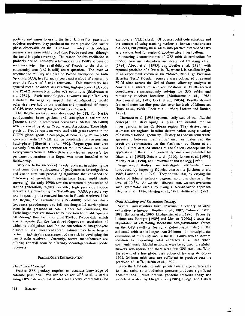
portable and easier to use in the field. Unlike first generation codeless receivers, they produced the more precise CIA carrier phase observable on the L1 channel. Today, such codeless receivers are more widely used than P-code receivers, although the trend is again reversing. The reason for this vacillation is probably due to industry's reluctance in the 1980's to develop receivers when the availability of P-code to the civilian community was (and is still) under question. The issue of whether the military will turn on P-code encryption, or Anti- Spoofing (A/S), has for many years cast a cloud of uncertainty over the future of P-code receivers. This uncertainty has spurred recent advances in extracting high-precision CIA code and PI-P2 observables under A/S conditions [Srinivasan et al., 19891. Such technological advances may effectively eliminate the negative impact that Anti-Spoofing would otherwise have had on the precision and operational efficiency of GPS-based geodesy for geodynamics research.

The Rogue receiver was developed by JPL for NASA geodynamics investigations and ionospheric calibrations [Thomas, 19881. Commercial derivatives (SNR-8, SNR-800) were produced by Allen Osborne and Associates. These high- precision P-code receivers were used with great success in the GIG'91 global geodetic campaign, demonstrating 12 mm RMS agreement with 33 VLBI station coordinates in the northern hemisphere [Blewitt et al.. 19921. Rogue-type receivers currently form the core network for the International GPS and Geodynamics Service. Although very precise and successful for permanent operations, the Rogue was never intended to be fieldworthy.

Partly due to the success of P-code receivers in achieving the most demanding requirements of geodynamics investigations, and due to new data processing algorithms that enhanced the efficiency of geodetic investigations (e.g., rapid static surveying), the early 1990's saw the commercial production of second-generation, highly portable, high precision P-code receivers. By developing the TurboRogue, NASA played a key role in spurring this renewed interest in P-code receivers. Like the Rogue, the TurboRogue (SNR-8000) produces dual- frequency pseudorange and full-wavelength L2 carrier phase even in the presence of A/S. Under A/S conditions, the TurboRogue receiver shows better precision for dual-frequency pseudorange than for the original TI-4100 P-code data, which was adequate for the baseline-independent resolution of widelane ambiguities and for the correction of integer-cycle discontinuities. These enhanced features may have been a factor in industry's reassessment of the risk in developing the new P-code receivers. Currently, several manufacturers are offering (or will soon be offering) second-generation P-code receivers.

PRECISE ORBIT D ~ I N A T T O N

The Fiducial Concept Precise GPS geodesy requires an accurate knowledge of

satellite positions. We can solve for GPS satellite orbits using GPS data recorded at sites with known coordinates (for

example, at VLBI sites). Of course, orbit determination and the concept of using tracking stations at known locations are old ideas, but putting these ideas into practice established GPS as a serious tool for regional geodynamics investigations.

Pioneering demonstrations of GPS orbit determination for precise baseline estimation are described by King et al. [1984], Abbot et al. [1985], and Beutler et al. [1985], with reported precision of a few x 10-'L, where L is baseline length. In an experiment known as the 'March 1985 High Precision Baseline Test," fiducial receivers were collocated at several VLBI sites across the United States, allowing analysts to constrain a subset of receiver locations at ~ ~ ~ 1 - i n f e r r e d coordinates, simultaneously solving for GPS orbits and remaining receiver locations [Melbourne et al., 1985; Davidson et al., 1985; Bock et al., 1985bl. Results showed few-centimeter baseline precision over hundreds of kilometers [Bock et al., 1986a; Bock et al., 1986b; Lichten and Border, 19871.

Thornton et al. [I9861 systematically studied the -fiducial concept" in developing a plan for crustal motion investigations in the Caribbean region. They derived error estimates for regional baseline determination using a variety of assumed fiducial geometry. History has shown remarkable agreement between their initial error estimates and the precision demonstrated in the Caribbean by Dixon et al. [1991]. Other detailed studies of the fiducial concept and its application to the study of crustal dynamics are presented by Dixon et al. [1985], Schutz et al. [1990], Larson et al. [1991], Murray et al. [1990], and Freymueller and Kellogg [1990].

Some recent studies have investigated systematic errors introduced by imposing fiducial constraints [Lichten et al., 1989, Larson et al., 19911. They showed that, by varying the choice of fiducial network, regional solutions change at the level of ~ O - ~ L . As we shall discuss later, we can overcome such systematic errors by using a free-network approach [Beutler et al., 1986; Herring et al., 1991; Heflin et al., 19921.

Orbit Modeling and Estimation Strategy Several investigators have described a variety of orbit

estimation techniques [Beutler et al., 1987; Colombo. 1986, 1989; Schutz et al.. 1990; Lindqwister et al., 19901. Papers by Lichten and Bertiger [I9891 and Lichten [1990a] discuss the importance of estimating stochastic non-gravitational forces on the GPS satellites (using a Kalman-type filter) if the estimated orbit arc is longer than 24 hours. In hindsight, the estimation of multi-day arcs in the late 1980's was an interim solution to improving orbit accuracy at a time when continental-scale-fiducial networks were being used, the global network was sparse, and there were few GPS satellites. With the advent of a true global distribution of tracking stations in 1992, 24-hour orbit ires are sufficient to produce baseline precision of ~ o - ~ L [Heflin et al., 19921.

Since the GPS satellite solar panels have a large surface area to mass ratio, solar radiation pressure produces significant accelerations. Most precise geodetic software today use models described by Fliegel et al. [1985], Fliegel and Gallini

[I9891 and Fliegel et al. [1991]. It remains an outstanding problem in GPS orbit determination to model eclipsing satellite trajectories adequately [Lichten, 1990a; Schutz et al., 19901. Vigue and Schutz [I9901 and Feltens and Groten [I9901 have conducted preliminary studies into thermal effects, which may be the key to this problem.

Routint; High-Precision Orbit Production Starting June 1992, several analysis groups participating in

the International GPS and Geodynamics Service (IGS) have been (electronically) publishing precise GPS orbit positions every week, which regional geodynamics investigators can then use to achieve baseline accuracy of ~ O - ~ L . The transfer of this burden to a few dedicated groups has numerous advantages: (1) on any given day, there are solutions by several independent groups which can be intercompared to assess accuracy; (2) satellite and station problems are more readily identified, and the user will be warned of anomalies; (3) the satellite positions are all given in the International Terrestrial Reference Frame (ITRF), ensuring a level of compatibility between the different regional analyses; and (4) the alternative would require that every regional investigator go through the time-consuming process of estimating and assessing the accuracy of GPS orbits lor each experiment.

TROPOSPHERIC MODELING AND ES'IIMA~ON Tropospheric delay has a wet and dry component [Davis et

al., 19851. The dry component is -2 m at zenith, and varies slowly and smoothly (since it is largely determined by air pressure). Atmospheric water vapor causes the wet component, which is only -10 cm at zenith, but it has random variations over a broad spatial and temporal scale (since the variations are related to turbulence). It is important to model these delays accurately, especially for the estimation of vertical station coordinates. We can theoretically map wet and dry delays to an equivalent zenith delay using a mapping function (one for wet, one for dry) [Lanyi, 1984, Davis et al., 19851. We can then

estimate a residual zenith delay bias using the GPS data themselves. Alternatively, we can constrain the zenith delay to values determined by surface meteorological instruments or water vapor radiometers (WVR's) [Ware et al., 1986; Rocken et al., 1991; Johansson, 19921.

Stochastic Estimation Analyses of various experiments have demonstrated that

stochastic estimation of a zenith tropospheric bias (using a Kalman-type filter) produces comparable results to using a WVR in a variety of regions (including California, Mexico, Caribbean, Central and South America). In some circumstances (e.g., rainy conditions), WVR's are ineffective; thus, stochastic estimation tends to be a more robust approach from this point of view. Moreover, WVR's are currently bulky, heavy, and are very expensive (>$loOK) if we require a retrieved delay accuracy of 5 mm.

An approach that appears to work well both in VLBI and GPS is to estimate a zenith bias as a random walk process, which Figure 4 illustrates. In this figure, the dots represent estimates of the zenith tropospheric bias, and are derived using a batch sequential filter as follows. Let us take the black dot on the left as the current estimate. We can map this estimate forward in time to provide a future estimate, represented by the white dot. We then add (in quadrature) the error bar to random-walk process noise, which grows as the square root of time. The lined dots represent a future, independent data estimate. A weighted average of this data estimate and the mapped estimate provides a new current estimate represented by the second black dot, and so on. Figure 4 considerably exaggerates the process noise, since it is usually much smaller than the error bars. Tralli and Lichten [I9901 and Lichten [1990b] describe this procedure more rigorous1 y.

Over the period of 1 hour, optimal values for the random walk parameter allow for 0.5 to 2 cm variations in the zenith bias. Dixon and Kornreich Wolf [I9901 investigated empirically the optimal value of this parameter, using' daily

* TIME

Fig. 4. An illustration of the application of random walk process noise.

ADVAN- IN GPS -0-Y: 1978-1972 199

baseline repeatability as an indicator; they found a value of 1.2 cm per square-root hour to give the best repeatability for the January 1988 GPS experiment in Central and South America (CASA Uno). Lichten and Border [1987], and Blewitt (19891 had used the same value with success in California. Introducing a novel way to assess estimation strategies, Dixon et al. [I9911 optimized ambiguity resolution in the Caribbean region when using a random walk value of 1.0 cm per square- root hour. They also report that this value was consistent with observed variations (1.1 cm per square-root hour) in retrieved path delays from a WVR operating during the experiment.

Lichten and Border [I9871 showed that estimating a stochastic, rather than a constant zenith tropospheric bias resulted in a factor of 2 improvement in baseline repeatability in California. They also reported a similar improvement in orbit repeatability (i.e., the RMS difference between independently determined orbit arcs, mapped to a common time interval). Tralli et a]. [1988], analyzing data from the Gulf of California, Mexico, found that stochastic estimation of a zenith bias gave similar baseline repeatability as using WVR's. For the CASA Uno experiment, Dixon and Kornreich Wolf [I9901 showed a factor of 2 improvement in baseline repeatability when the zenith tropospheric bias was estimated stochastically, giving almost identical results as using WVR's. Dixon et al. [I9911 showed an insignificant difference in baseline repeatability in the Caribbean region when comparing the random-walk estimation method with the use of WVR's.

Local tropospheric modeling For local networks (tens of km), tropospheric modeling and

estimation techniques are essential to achieve few millimeter- level vertical precision. Gurtner et al. [I9891 and Rothacher et al. [1990a] emphasized this point, especially for networks in mountainous regions. They suggested that statements concerning 'millimeter-level precision- currently do not apply to the vertical components of baselines except to those shorter than 1 km where there is negligible height difference between the two receivers.

Local tropospheric models are important for rapid static surveying (to be discussed later), because there is not enough information in 5 minutes of data to adequately reduce the correlation between the zenith tropospheric delay and the vertical station coordinate. Employing a very simple local tropospheric model, Hurst et al. [I9901 demonstrated 1.4 cm standard deviation in the vertical baseline component (for rapid static surveys separated by 3 months).

Stations separated by as much as 100 km have tropospheric delays that correlate to some extent. Davis et al. [I9871 outlined a scheme that applies an a priori model of zenith tropospheric correlation as a function of baseline length, and demonstrated improved vertical repeatability. This method ought to be most useful when the information content of the data is deficient for some reason (e.g., when tracking only 4 satellites). Presumably, this method is not commonly used since most of today's geodetic receivers can track 8 satellites simultaneously.

Introduction Ambiguity resolution refers to the determination of an

integer-cycle bias for each set of double-difference carrier phase measurements. Ambiguity resolution is essential for the best achievable precision and accuracy, with improvement factors of 2 to 3 reported by Dong and Bock [I9891 and Blewitt [1989], for regional-scale networks with baselines up to 2000 km.

In the early days of GPS, Counselman and Shapiro 119791 emphasized the importance of ambiguity resolution. Bossler et al. [I9801 described the method whereby carrier phase biases are first estimated as real-valued parameters, then held fixed to integer values; hence the term 'bias-fixing.- Bias-fixing was routinely used in the early 1980's for short (few km) baselines. Bock et al. [1985a] demonstrated a full-network solution using bias-fixing. The network was tens of kilometers in aperture, and baseline precision was ~ o - ~ L . Such a network approach is now standard.

Long-Baseline Ambiguity Resolution The problem of extending ambiguity resolution to longer

baselines was not trivial, as evidenced by the 10 years that were to pass between papers by Counselman and Shapiro [I9791 and the papers by Dong and Bock [I9891 and Blewitt

[1989], which describe the techniques in routine use today. The basic problems were (1) the paradox that, to be successful, the process of long baseline ambiguity resolution cannot proceed without first obtaining a precise geodetic solution, and (2) that, without additional information, the ambiguity parameters of the L1 and L2 phases are perfectly correlated.

The first problem requires (1) a sufficiently long arc of data (hours for regional scales), and (2) accurate modeling of the phase observables. For example, precise orbit determination is required for regional-scale ambiguity resolution. As we saw previously, Dixon et a]. [I9911 showed that ambiguity resolution improved by stochastically estimating the tropospheric delay. As baselines get longer, more models become important, such as tidal effects, and circular- polarization effects due to relative antenna rotation between the station and satellite [Wu, J.T. et al., 19931. Accurate modeling of the phase observables does not require fiducial constraints, as Blewitt and Lichten [I9921 pointed out with their demonstration of global-scale ambiguity resolution. The reason for this is that integer-cycle ambiguities are scalar quantities, which are not affected by choice of reference frame. In fact, ambiguity resolution may be impossible, or could have negative side effects, if the fiducial constraints nave significant error.

The second problem, as Bender and Larden [I9851 succinctly explained, can be solved by using pseudorange observations or ionospheric constraints (or both). One of their suggestions was using pseudorange data to estimate ionospheric delay, which could in turn be used to constrain the selection of possible integer values for the L1 and L2 channels. Melbourne

I Widetane carrier phase (+I-@)

............................................................. N+l N Difference N-1

Fig. 5. Use of pseudorange for resolving the integer-cycle ambiguity in the widelane carrier phase data ($1-412). The wavelength for widelane phase is 86.3 cm. This method is independent of baseline length [Melbourne, 19851.

[I9851 and Wubbena 119851 independently proposed a more direct approach that uses pseudorange data to resolve the widelane ambiguity (referring to the phase difference between L1 and L2 channels). This method of widelaning, shown in Figure 5, has the useful property that it is model-independent, and therefore should not degrade with baseline length. Blewi tt et al. [I9881 and Dong and Bock [I9891 applied this technique to resolve the widelane ambiguity (referring to the phase difference between L1 and L2 channels), on several baselines of -1000 km. Without the availability of pseudorange data. the use of ionospheric constraints was implemented in various forms by Bock et al. [1986a], Shaffrin and Bock [1988], Dong and Bock [1989], and Blewitt [1989]. Abbot et al. [I9891 demonstrated an alternative approach that explicitly estimates parameters of an ionospheric model.

Network Design and Bootstrapping Around 1986, investigators agreed that a mix of baseline

lengths enhances the ability to resolve integer-cycle ambiguities for regional geodesy. This was independently demonstrated by Blewitt et al. [1988], Dong and Bock [1989], and Counselman and Abbot [1989]. All these investigations used a -4000 km-aperture fiducial network spanning North America with a broad mix of baseline lengths. There are several reasons why multiple baseline lengths assist ambiguity resolution: (1) longer baselines provide a wide- aperture view of the GPS orbits, reducing errors for the shorter baselines to much smaller than a wavelength; (2) if biases associated with the shortest baselines can be resolved, estimates of biases associated with longer baselines can be subsequently improved using the computed correlation between bias parameters; (3) biases associated with longer baselines can be expressed as a linear combination of several biases associated with intermediate baselines; thus, only biases associated with the intermediate baselines need be resolved.

Taking advantage of a wide distribution of baseline lengths in their networks, Dong and Bock [1989], Blewitt [1989], and Counselman and Abbot [I9891 explained and demonstrated bootstrapping algorithms that were different in detail, but

similar in concept. As an example of such an approach: (1) select the best determined carrier phase bias first (where 'best determined" is objectively defined as a function of the distance to the nearest integer, and the formal computed error); (2) if there is sufficient confidence, fix it to the nearest integer value, and compute how this perturbs all other carrier phase biases (which implicitly improves orbit parameters, station locations, etc.); (3) get the next best determined bias until a pre-specified confidence limit is exceeded; (4) back-substitute the fixed integer-bias solutions to recompute the geodetic and orbit estimates (retaining the unresolved biases as real-valued parameters). This algorithm uses off-diagonal information in the covariance matrix, but avoids the computationally prohibitive task of using all the information, which would require a search in a very high-dimensional lattice (and computation time longer than the age of the universe!). Key to such an approach is having short baselines (100 km) in the network to resolve ambiguities for the long baselines (-1000 km). Dong and Bock [I9891 extended this approach by searching the lattice a few dimensions at a time.

Blewitt and Lichten [I9921 showed that the above restrictions may be relaxed for a sufficiently dense global network. For a 21 station, global GPS network, they demonstrated ambiguity resolution without any bootstrapping for baselines up to 1500 km. Using bootstrapping then allowed the resolution of ambiguities for even the longest baselines (-10000 km).

The well-known double-difference method of eliminating clock bias, which has its origins before GPS [Counselman et a]., 19721, allows for efficient computation of the least- squares geodetic solution. However, the clock elimination problem can be generalized to a clock estimation problem. Wu. J.T. [I9841 describes a method of processing undifferenced data, which later evolved into the current method in the GIPSYIOASIS software [Wu. S.C. and Thornton, 19851 whereby clock biases are estimated as a stochastic process. 'Stochastic estimation" here includes the logical extremes, ranging from the completely unpredictable behavior of white noise to models which allow time-correlated colored noise, polynomial behavior, or some combination of the above.

There are now several software packages [Swift, 1987; Lichten and Border. 1987; Landau, 1988; Andersen et al.. 1992; Ch. Reigber. IGS electronic mail #40. 19921 which use the clock estimation method rather than the double-difference method, so it deserves some explanation as to the differences between these approaches.

First, let us discuss why differences between geodetic solutions may arise from softwares that implement different approaches to dealing with clock bias. What are the most significant causes of these differences?

Differences Between Stochastic Solutions For a given stochastic model (e.g., white noise clocks), tests

have shown that UD filtering versus SRIF filtering give

ADVAN- IN GPS ~ O L O Q Y : 1978-1972 201

essentially identical results (limited by the numerical precision of the computer). This is perhaps not surprising; theoretically, UD and SRIF filters ought to give the same results despite the very different calculations which are carried out [Bierman. 19771. Theoretically, Kalman filtering ought to give the same results too, however the numerical precision will be slightly degraded (because Kalman filtering deals with the covariance matrix instead of the square-root covariance matrix). This degradation is probably insignificant for double- precision machines, assuming an appropriate choice of units and nominal values.

Of course, changing the stochastic model will generally result in different solutions [Lichten and Border, 19871. As the choice of stochastic model more truely represents the random behavior of the clock, so the solution will be more accurate. On the other hand, the quest for accuracy must consider the need for robustness. If the clock has an unpredictable glitch which is not represented by the stochastic model, then the constraints implicit in that model will unfavorably bias the solution. The white noise model, which assumes no correlation between past and future behavior, is the most robust model (it can readily tolerate step-functions in clock bias or rate, which are not uncommon). It is often said that white noise clock estimation is equivalent to double- differencing. As we shall see, this is not as simple as often stated, and in some cases the statement is false.

Finally, note that only relative clock behavior is estimable. Geodetic estimates can differ substantially due to an inappropriate selection of a reference clock. Unless the analyst corrects for the reference clocks errors using point positioning solutions, it is important to select a reference clock that is accurate to the few-microsecond level. (This corresponds to the time it takes for a GPS satellite to move approximately 1 cm.) Since many GPS receivers in the global network use H-maser external frequencies, this is not usually a problem.

Differences Between Double-Dqference Solutions For the double-difference method, answers can vary

depending on the amount of rigor which is incorporated into the algorithm. The best software packages are quite rigorous, accounting for correlation in the double-difference observations, and implementing algorithms to select the double-difference observations which maximize information content. However, almost without exception, the actual practice of double-differencing begins with the formation of single-difference data files (between 2 stations), and it is at this stage that significant information can be lost if decisions are made by the user rather than by an automated, generalized algorithm.

Stochastic versus Double-Dqference Methods Phase and Pseudorange. One feature of stochastic estimation

which will produce different solutions than double-differencing is the case where both carrier phase and pseudorange data are filtered simultaneously [Lichten and Border, 19871. In this case, one common clock parameter can be estimated for both

carrier phase and pseudorange data, whereas double- differencing the pseudorange is equivalent to estimating an independent clock for that data type. In practice, this problem is addressed in double-differencing software by prior initialization of the clock parameters using pseudorange data in point positioning solutions. The results may be very effective, but in principle, a different least-squares problem is being solved.

Information Content. Ignoring the issue of simultaneous processing of carrier phase and pseudorange, let us return to the question, 'Are double-differencing and white-noise clock estimation equivalent?" The answer is, 'Sometimes.' We must look at the underlying assumptions. For practical purposes, regional scale networks (or smaller) should give insignificantly different solutions, provided that the double- difference software rigorously deals with issues of correlation and data selection. However, it is a myth that they are theoretically equivalent for all data sets. They may, in fact, be different for global-scale data sets. Figure 6 illustrates a counter-example where no double-difference measurement can be constructed; however, the method of white noise clock estimation is able to extract geodetic information. In this example, 3 single-differences (from common satellites) could themselves be differenced to form a measurement which would eliminate clock bias. This is analogous to the double- difference measurement, where 2 single-differences are differenced. Double-differencing software cannot handle this case. However, it could be handled by what we might call 'generalized differencing" software, an example being the Householder method proposed by Wu, J.T. [1984, 19861. It would therefore be more correct to say that white noise clock estimation is equivalent to Householder clock-elimination rather than double-differencing. Of course, i f the global network were sufficiently dense everywhere, the loss of information would be negligible. For most applications, this issue may not be worth serious consideration.

Practical Considerations. More relevant to most users are the practical consequences of choosing stochastic clock estimation versus double-differencing. Since double- differencing eliminates nuisance parameters up front, it is

Sat

2

Sat 3

Fig. 6. In this example where each satellite is observed by 2 stations, no double-difference data can be formed; however the linear combination A = (pll - p13)- (pZ1 - p l ) -(p32 - p33) eliminates clock bias, and contains valuable geodetic information.

computationally more efficient. It is much easier to detcct cycle slips in double-difference data at the preprocessing stage. This is a strong argument for using double-differencing software for codeless receivers without precise pseudorange capability. On the other hand, it is easy to find cycle-slips or data problems by inspecting post-fit residuals after filtering undifferenced data. In fact, this process can be automated, and the cycle-slips can be repaired by the same module that performs ambiguity resolution; but this is another reason why clock estimation can be more computationally expensive. However, these extra computations do provide the user with (1) residuals on a site-by-site basis, and (2) explicit, precise clock solutions for each receiver and satellite (relative to the selected reference clock) [Swift and Gouldman, 19891. The RMS of post-fit residuals has been particularly useful as a measure of multipath at each of the global network sites.

Ambigu i ty resolut ion t echn iques for k inemat i c , pseudokinematic, and rapid static surveying are quite different to methods used for long-baseline static positioning. First, let us define these surveying techniques. (As a note of caution, the following definitions may not be universally accepted.)

Kinematic surveying Remondi [I9851 developed kinematic surveying, which

several investigators have used for precise positioning [Mader and Strange, 1987; Goad, 19891. The kinematic technique uses a stationary reference GPS receiver, and another receiver that moves from point to point, roving within a radius of several kilometers. The analyst can resolve cycle ambiguities, using an initialization technique (e.g., antenna swapping). Analysis software can recover from loss of phase lock, if there are enough satellites in view, or if the field operator, having realized that the receiver had lost lock, returned to the last stopping point. The Field operator must therefore be quite careful, otherwise a large fraction of data could be rendered unuseable. Relative positioning accuracy at the 1-cm level is possible for site occupations of seconds [Ashkenazi e t al., 19901, given at least 5 satellites should be in view, and provided that the environment does not cause significant multipath.

Pseudokinemotic Surveying Remondi [1988, 19901 also introduced pseudokinematic

surveying. This method does not require that data be collected while moving an antenna from one point to another; however, it does require that each point be revisited a second time after a significant time-lapse (e.g., 1 hour). The idea is to connect piiase between the two occupations, resulting in information content that is almost equivalent to staying on every point for the entire time-span.

The key to making this work is successful ambiguity resolution. The ambiguity function method, developed for VLBI phase analysis by Rogers et al. [1978], was first tested for GPS by Counselman and Gourevitch [1981]. This method

lay dormant until 1990 when Remondi [I9901 and Mader [I9901 revived it, successfully applying it to short baseline pseudokinematic surveying. Frei and Beutler [I9901 have proposed and demonstrated the 'Fast ambiguity resolution method" (FARA), which searches the ambiguity lattice space for the most likely solution. In cases where return to the same site is unnecessary, the FARA method is applicable to rapid static surveying (see below) for codeless receivers.

Kinematic Positioning Investigators have used kinematic positioning to track

antennas on a moving platform (e.g.. aircraft). In principle, the method is no different than kinematic surveying; the only difference is the application. The technique is described by Hatch [1986, 1989, 19901, Mader [1986, 19901, Evans [1986]. and Hein et al. [1988]. This method has many applications; for example, monitoring sea-level by locating floating buoys relative to fixed points on land [Rocken et al., 19901. Sea-floor geodesy a s proposed by Spiess [I9851 uses (1) acoustic ranging to locate a floating buoy relative to transponders fixed to the sea-floor, and (2) GPS to tie the buoy to points on land. Young et al. [I9901 described a preliminary experiment showing the potential for marine geodesy to measure oceanic crustal motion. Minster and Genrich [I9881 presented an approach to the simultaneous reduction of shipboard GPS data and gravity measurements.

Rapid Static Survtying Rapid static surveying was a phrase introduced by Blewitt et

al. [1989a] to describe a local surveying technique, which neither required that the receiver track while moving from one point to the next, nor required a second occupation of each site. Euler et al. [I9901 described a similar technique, and Frei and Beutler [I9901 proposed another successful approach. Typically a roving receiver stops at each site for about 5 to 1 0 minutes, and its location is referenced to a continuously operating receiver at a distance of up to 20 km or so. The time spent at each site could in principle be only a few seconds, but in practice, 5- to 10-minute occupations give the analyst enough data to assess the level multipath-induced errors at each site (an important error source for short data spans), and the. occupation time is still less than the time it takes to travel between points, set up the equipment, and break it down.

Again, the trick is to be able to resolve the carrier phase ambiguities. The method of Blewitt et al. [1989b] is to use P- code pseudorange to resolve the widelane ambiguity, and then resolve the remaining ambiguity by relying on the likelihood that the differential L1-L2 delay between the Fixed and roving receivers is much less than a wavelength (actually, it needs to be at the 1 cm-level to be sufficiently confident). During the 1989 peak of the 11-year solar cycle, it was possible to resolve ambiguities up to 3 0 km at night, but only over a few km during daylight hours. In 1992, ionospheric activity had reduced such that it became possible to resolve ambiguities over 20 km during daylight hours. The years of 1993-1996 should prove to be very favorable to the rapid static technique

ADVANCE4 IN GPS -0UXtY: 1978-1972 203

during daylight hours. (Ionospheric modeling may be useful to extend the application of rapid static surveying, but i t is difficult to account for fine structure at short temporal and spatial scales [Abidin and Wells, 19901.)

Having surveyed the network for the first time, subsequent surveys could use codeless receivers, since ambiguity resolution can now proceed by applying geodetic constraints from the first solution (provided that station motion in the intervening time is only a few centimeters). Once the ambiguities are resolved, the solution can be recomputed such that it is not biased by the first solution. Blewitt et al. [1989b] used rapid static surveying to monitor post-seismic motion following the Loma Prieta earthquake of October 1989. Hurst et al. [I9901 showed that inter-experiment repeatability was sub centimeter in horizontal components, and 1.4 cm in the vertical over -20 km (see above section on tropospheric modeling).

For a detailed assessment of GPS precision and accuracy over regional scales, see the in-depth study by Larson and Agnew [I9911 who used -2.5 years of data from California. Larson et a]. [I9911 went further into the question of systematic errors introduced by constraining the coordinates of fiducial sites.

Three methods have been widely used for assessing GPS geodetic accuracy and precision: (1) repeatability (i.e.. weighted RMS scatter) of coordinate estimates, (2) intercomparison with other techniques, and (3) formal computation of the expected standard deviations using the measurement matrix and an assumed data variance. All three of these methods have yielded reasonably comparable results, provided there are no data problems and the estimation strategy is appropriate. In producing error bars for coordinate estimates, investigators have frequently used either methods (1) or (3), or some combination of the two (for example, scaling the formal covariance such that computed baseline length errors agree on average with the repeatability).

Daily Repeatability Baseline repeatability is a function of the time spanned by

each solution. Typical regional experiments last several days, in which case daily repeatability is a valuable indicator of precision [Bock et al., 1985al. The improvement in daily repeatability is perhaps the best indicator of successful ambiguity resolution; an improvement by a factor of 2 to 3 is typical for static surveying [Bock et al., 1985a; Dong and Bock, 1989; Blewitt, 19891. Repeatability has a well-defined relationship with baseline length only if fiducial constraints are not used. When reporting repeatability as a function of length, it is important not to draw baselines between stations khat are near fiducial stations. In this case, length is not a relevant characteristic of the baseline; more relevant is the distance to the nearest fiducial station.

A comprehensive study of California GPS solutions by Larson and Agnew [I9911 shows daily baseline re geatabiiity of 2 mm + 6 x ~ o - ~ L for the north, 2 mm + 13 x 10- L for the

east, and 17 mm for the vertical component, with no obvious length dependence. The limiting repeatability of 2 to 4 mm observed by many investigators for short (but not very short) baselines is probably due to tropospheric variations (since multipath errors approximately repeat from day to day).

Results from -10-m baselines show daily repeatability better than 0.1 mm (George Purcell, private comm.). Genrich and Bock I19921 used GPS as a strain meter across the San Andreas Fault, showing sub-millimeter daily repeatability for -100 meter baselines with short occupation times. They employed a method to filter out the daily repeating multipath signals. Such a technique has applications to kinematic, pseudokinematic, and rapid static surveys.

Long-Term Repeatability Many systematic errors (e.g., tropospheric mapping

function errors, mismodeling of solar radiation pressure, or multipathing) tend to repeat from day to day; thus, long-term repeatability is a much better indication of precision. Of course, if results are to be compared over several years, the results should be detrended to remove secular crustal motions. This approach has been taken by Murray et al. [1988], Davis et al. [1989], Prescott et al. [1989], Larson and Agnew [1991], and Murray [1991]. These studies typically indicate long-term regional baseline repeatability (up to -400 km) at the several- millimeter level in the north and east baseline components, and 20-40 millimeters in the vertical component. Of course, these early studies have necessarily included data from 4- channel receivers, so we should expect recent solutions using %channel receivers to prove to be more precise than this.

The vertical baseline component generally has a greater standard deviation than horizontal components. This is simply because we can only look up at the satellites, and not down; hence the data do not constrain the vertical as well, and the vertical is more sensitive to errors in tropospheric delay. Repeatability in the vertical of -30 mm was quite common using 4-channel receivers. Using 8-channel receivers in the California Permanent GPS Geodetic Array (PGGA), Lindqwister et al. [I9911 showed sub centimeter repeatability in the vertical component for regional-scale baselines. This improvement in precision partly results from the dramatic reduction in the magnitude of the correlation coefficient between the vertical parameter and the zenith troposphere parameter when increasing the number of simultaneously observed satellites from 4 to 5 (and to a lesser extent from 5 to 6, etc.).

As we saw in Figure 2, Bock et al. [I9931 and Blewitt et al. [I9931 detected a co-seismic displacement of a few millimeters on a 1700 km baseline (from JPLM, California to DRAO, British Columbia), caused by the Landers earthquake sequence of June 28, 1992. Each group independently (and with different software) estimated absolute co-seismic displacement estimates for a few stations in California. These estimates agreed to within their 95% confidence ellipses. For PGGA baselines (-200 km), the daily baseline repeatability (over a

period of 2 months) was 4 mm (horizontal) and 10-15 mm (vertical).

Intercomparisons Although repeatability is an important tool to assess

solution precision, it is clearly important to assess accuracy by comparing GPS results with the VLBI and satellite laser ranging (SLR) techniques. This is not trivial, since one must correctly account for the vector between the phase center of the GPS antenna and the intersection of axes of the VLBI antenna (and similarly for SLR). This vector comprises of (1) a test- range measurement of the vector between the GPS phase center and a reference mark on the antenna, (2) the eccentricity vector of the antenna relative to the underlying monument, (3) the vector between the GPS monument and the monument under the VLBI antenna, and (4) the vector between this monument and intersection of the VLBI antenna's rotation axes (information that the original engineering diagrams may contain). Moreover, one must also account for the crustal motion between, the experiment epoch, and the quoted reference epoch of the VLBI solution.

Despite these difficulties, there have been several successful intercomparisons between coordinates estimated by SLR, VLBI, and GPS [Ray et al., 1991; Blewitt et al., 19921, and this method remains perhaps the most believable indicator (albeit a conservative one) of the accuracy of all three techniques. Intercomparisons by Beutler et al. [I9871 showed few-centimeter agreement in Alaska. Strange [I9881 showed centimeter-level agreement on several baselines in California. Davis et al. 119891 report repeated measurements of the Pales Verdes-Mojave-Vandenberg triangle, indicating centimeter- level agreement. Lichten and Bertiger [I9891 demonstrated 1 x ~ O - ~ L accuracy for L > 1000 km. Larson [I9901 used the technique of comparing GPS baseline rate with VLBI, which has the advantage that it is independent of ground survey errors. A linear fit to 18 GPS occupations of the Mojave- Vandenberg baseline (over a span of 2.3 years) gave agreement at the level of 2 mmlyr.

GLOBAL GEODEnC PRECISION

By 1989, regional baseline precision had clearly become limited by orbit accuracy, which in turn was limited by the size of the satellite tracking networks. During the late 1980's a global network of GPS receivers gradually came into existence. Called 'CIGNET (Cooperative International GPS NETwork), this saved the investigators the burden of installing tracking receivers at fiducial points every time they conducted an experiment. CIGNET has been used to advantage for regional GPS investigations all over the globe (for example, by university researchers collaborating in the UNAVCO consortium). The National Geodetic Survey (NGS) continues to play a central role in CIGNET in the retrieval and dissemination of global GPS tracking data to the geodetic community.

A temporary, semi-global tracking network supported the January 1988, "CASA UNO" experiment in Central and South

America. Results by several investigators showed the tangible improvement in regional baseline precision due to near-global tracking [Kornreich Wolf et at., 1990; Freymueller and Kellogg, 1990; Lichten 1990al. Focusing on the global tracking network itself, Schutz et al. [I9901 showed 1 x 10-'L baseline precision over thousands of kilometers.

Following the CASA UNO experiment, Melbourne et al. [I9881 and Mueller [I9901 proposed that an international organization install and maintain a global high-quality GPS network to provide a service to geodynamics investigators, allowing for routine baseline precision of a few x ~ o - ~ L . As a test campaign under the auspices of the International Earth Rotation Service (IERS), the GIG'91 experiment successfully demonstrated precise global tracking during 3 weeks in early 1991 [Blewitt, 19911. GIG'91 served as a prototype to the global network under development today. Using the GIPSY/OASIS software to resolve ambiguities on a global scale, Blewitt and Lichten [I9921 showed baseline repeatability of 2 mm + 2 x ~ o - ~ L from 21 globally distributed P-code receivers, without the use of fiducial constraints.

.# Blewitt et al. [I9921 transformed a global network solution into the International Terrestrial Reference Frame (ITRF) [Boucher and Altamimi. 19911, showing 12 mm RMS agreement for 3 3 station coordinates in the northern hemisphere. Using the GEOSAT software to analyze the GIG'91 data, Andersen et al. [I9921 demonstrated baseline repeatability of 1 mm + 2 x ~ o - ~ L for baselines shorter than 4000 km. and, after transforming the solution to ITRF. showed 15 mm RMS agreement with ITRF coordinates.

The results from the GIG'91 experiment represented a major advance in demonstrating the potential of GPS, giving precision at least an order of magnitude better for UT1 variations, polar motion, and geocenter determination than earlier pioneering work by Swift [1985, 19891, Bangert [1986], Abbot et al. [1988], Malys [1988], and Malla and Wu [1989]. The estimated location of the Earth center of mass was within 15 cm of the ITRF geocenter [Vigue et al., 19921. Herring et al. [I9911 and Lindqwister et al. [I9921 showed 0.5 marcsec (c 2 cm) agreement between Earth pole orientation variations estimated by GPS, VLBI, and SLR. Lichten et al. [I9921 showed 50 wsec (2 cm) agreement in UTl variations when comparing GPS to VLBI.

Both (1) the impressive results from the 3-week GIG'91 experiment, and (2) the convenience that CIGNET provided, were important actors in convincing the international community that the time had come for an operational 'International GPS and Geodynamics Service" (IGS) [Mueller, 19901. Several independent groups analyzed data from 20 to 30 stations every day during the first 3 months of full-time IGS operations (which began June 1992), their results indicating sub-meter level GPS orbit accuracy, marcsec-level daily estimates of the Earth pole direction, and centimeter-level determination of global station coordinates.

It is important to realize that the global network is now sufficiently dense that geocentric station coordinates (latitude, longitude, and geodetic height) can be estimated with sub

ADVANCES m GPS TECHNOLOGY: 1978-1972 205

0 Longitude Latitude

1992.5 1992.6

Date (yr)

Fig. 7. Time-series of weekly geocentric coordinate estimates for the GPS global network station at Wettzell, Germany, from 1 June, 1992 to 30 August, 1992.

centimeter precision. As an example of this, Figure 7 shows a time series of weekly geocentric coordinate solutions (minus nominal values) for Wettzell, Germany, from 1 June to 30 August, 1992 (during the IGS test campaign). The global network solution, from which Figure 7 was derived, is a pure GPS solution (using GPS estimates of polar motion and length of day, and using no fiducials). The level of height precision demonstrated appears to be sufficient to meet the requirements (few mm per year) for measuring post-glacial rebound over a period of several years. It also demonstrates the role that GPS could play in measuring global sea-level change. It is worth noting that the solutions presented in Figure 7 make no use of surface meterological data or WVR data.

General Software Features Concurrent with the above demonstration of techniques was

the development of GPS geodetic data analysis software that embodied algorithms as they became established. Beutler et al. [I9881 point out that software designers must consider (1) the end user, (2) the technical problems to be addressed, and (3) the definition of guidelines on structuring the system. Following this outline, let us first recognize that the kind of processing software we are discussing here is for scientific use and professional use in agencies concerned with high-precision surveys. Second, software packages need to include (1) accurate orbit integration with appropriate force models; (2) data editing capability; (3) accurate modeling of Earth orientation, tides, and media propagation; (4) capability to estimate station coordinates, satellite states, tropospheric bias,

receiver time-tag errors, carrier phase biases, UT1 variations, and polar motion; (5) an algorithm implementing the bootstrapping mechanism for ambiguity resolution.

The adoption of the RINEX standard format [Gurtner and Mader, 19901 largely solved the problem of handling different receiver data Formats; however, for some mixed-receiver networks, normal pointing algorithms must align receiver time-tags to the same epochs to eliminate clock bias [Blewitt, 1990~1. In doing so, the algorithm must be careful to reduce systematic error from frequency variations caused by selective availability [Wu, S.C., et al., 1990; Davis, E.S., 1990; Feigl et al., 1990; Rocken and Meertens, 19911.

All software packages must be capable of handling outliers and cycle-slips in the carrier phase data. As mentioned previously, software packages that form double-differences are probably better at handling codeless data. This is an important consideration for users which process data from a wide variety of receiver types. For the reduction of global-scale data sets, the user should consider processing undifferenced data from receivers with high-precision pseudorange (as discussed previously). Useful products of undifferenced data processing include (1) post-fit residuals for individual station-satellite pairs, and (2) explicit clock estimates. The choice of double- differencing versus stochastic estimation is not simply a question of which is better, but which better suits the needs of the user.

Another user consideration is 'Sequential filter or standard inversion of the normal equations?". A sequential filter (e.g., Kalman, UD, or square-root information) is useful to fit variations in tropospheric delay and unmodeled satellite fgrces [S.C. Wu and Thornton, 1985; Lichten, 1990bl. However,

experience from VLBI seems to imply that piecewise linear models for the troposphere may be as effective as random walk stochastic estimation in improving long-term baseline repeatability.

'Should the software be more interactively oriented, or batch oriented?" For routine analysis of permanent GPS arrays, batch processing is obviously preferable, with the entire processing as automated as possible. Interactively oriented software is much better for users who conduct field experiments, where new sites are the rule rather than the exception. A third consideration is the flexibility of the software, which allows the user to perform R&D style analyses, testing out new Earth models, orbit dynamics, and estimation strategies. (Rarely is this type of software available commercially.)

It is quite a common practice for the users of today's high precision software to contribute to its improvement. Modularity is essential in this regard. It should be possible for a software developer to simply insert a new data editing module into the overall data flow. What is not a universal feature of today's software is the ability for the non-specialist to produce a high-precision geodetic solution reliably on an arbitrary data set without a significant amount of training (or luck). However, as stated previously, we are discussing software that is designed for professional use in agencies concerned with high-accuracy surveys, and training is usually facilitated by such agencies. As systems are becoming more precise, robust, and automated, and as distributed ephemerides are becoming more accurate and reliable, geophysicists should soon be able to produce good solutions without much training other than reading a short user's guide.

Major Sojwore Packages The following is an alphabetically ordered list of major

software packages, which are in routine use today for geodynamics research, are capable of orbit improvement, and are capable of producing ~ O ' ~ L baseline accuracy.

BERNESE by the University of Berne, Switzerland [Gurtner et al., 1985; Beutler et al., 1987, 1988; Rothacher et al., 1990b; Davis et al., 19891 is available commercially. This is probably the most widely used package by the geodynamics community. It is used for daily IGS analysis. It forms double- difference data.

DIPOP-E by the University of New Brunswick, Canada [Chen and Langley, 19901 forms double-difference data.

GAMIT by the Massachusetts Institute of Technology [Bock et al.. 1986a; Schaffrin and Bock, 1988; Dong and Bock, 19891. The recent combination with the Kalman filter in the GLOBK software allows for stochastic estimation of orbit parameters [Herring et al., 19911. It is used for daily IGS analysis. It forms double-difference data.

GEODYN [Martin, 19851 and its commercial derivative Microcosm [Van Martin Systems Inc., 1990; Colombo, 1989; and Ferland and Lahaye, 19901 developed by NASA Goddard Space Flight Center. It forms double-di fference data.

GEOSAT by the Norwegian Defense Research Establishment

[Andersen, 1986; Andersen et al., 19921. The most recent version uses a UD factorized filter instead of double- differencing.

GEPHARD4.0 by the GeoForschungsZentrum, Potsdam, Germany [Ch. Reigber, IGS electronic mail #40, 19921. It is used for daily IGS analysis. It uses a filter instead of double- differencing.

GIPSY/OASIS by the Jet Propulsion Laboratory [Sovers and Border, 1987; Lichten and Border, 1987; Blewitt, 1989, 1990a; Lichten, 1990bl. The new GIPSY/OASIS I1 is currently used for daily IGS analysis, uses a SRIF filter, and can estimate stochastic satellite forces.

GPSOBS/BAHNS by the European Space Agency, Darmstadt, Germany [J. Dow, IGS electronic mail #51, 19921. It is used for daily IGS analysis. It forms double-difference data.

M S O D P l m X G A P by the University of Texas at Austin [Abusali et al., 1986; Schutz et al., 1989, 19901. It is currently used for daily IGS analysis. It uses double- differencing.

TOPAS by the Institute of Astronomical and Physical Geodesy, University of FAF, Munich, Germany [Landau, 1988; Bastos et al., 19901 is available commercially. It uses a UD factorized filter.

LWITS ON GPS-GEODETIC PRECISION

Long Baseline Precision GPS-baseline repeatability is a function of baseline length.

Using a sample of 136 baselines over 21 days, Heflin et al. [I9921 demonstrated that this function is almost perfectly linear for global-scale free-network solutions. Presumably. this trend is due to error sources that decorrelate with increasing baseline length. Since VLBI analyses show a similar trend [Caprette et al., 1990, p. 241, we cannot assume that GPS-orbit errors dominate (as is often assumed). Perhaps the most important source of error is tropospheric delay. which, through the curvature of the Earth, increasingly maps into baseline length errors for longer baselines.

Goal for Estimating Tropospheric Delay Each station's zenith tropospheric delay is almost

completely decorrelated from neighboring stations over 1000 km away, causing random errors for each station's position in the vertical direction. The following simple derivation (which assumes a spherical Earth) demonstrates that this produces a scaling law. From Figure 8, we see that an error in the vertical AV at one end of a baseline causes an error in length AL - AVLRR, where L is the baseline length, and R is the earth radius.

If we assume that tropospheric errors are uncorrelated for global networks (with baselines > 1000 km), we get the following scaling law:

where ov is the standard deviation in the vertical station

Fig. 8. Scaling of baseline length error caused by vertical eriors.

coordinate, and is the standard deviation in baseline length, which is a linear function of baseline length provided rn is independent of baseline length. Equation (1) shows that w must be less than 9 mm to achieve baseline precision better than ~ o - ~ L . Since errors in w correspond roughly to 3-4 times the error in wet zenith tropospheric delay, this requires 3-mm accuracy in the zenith tropospheric delay. Water vapor radiometers have not yet consistently demonstrated performance at this level. This goal may be achievable using the GPS data themselves to estimate tropospheric delay, using mapping functions perhaps tailored to specific sites, to the time of year, and to meteorological conditions. Current accuracy is probably at the 10 mm level.

Local and Regional Scales. We can use the above information to construct a limiting

error model for the vertical component of local and regional scale baselines. Tropospheric delay is very correlated on a local scale, and is to some extent correlated on a regional scale, so we expect the scaling law to break down somewhere below 1000 km. If we assume that Kolmogorov turbulence provides a reasonable model for tropospheric variations, we would expect the variance in differential tropospheric delay to be proportional to L ~ / ~ [Truehaft and Lanyi, 19871. Turbulence can be described as an ever increasing size of cells, thus implying some level of correlation in tropospheric delay even for the longest baselines; however, in reality other factors (such as the presence of mountain ranges and coastlines) may limit the validity of this law to regional scales (or even shorter). For purposes of discussion, let us assume (1) this scaling law is correct, (2) we attempt to use this information in some optimal estimation strategy, and (3) final errors in the vertical baseline coordinates are proportional to the RMS variations in differential tropospheric delay:

where the factor of 3 roughly accounts for the mapping of zenith tropospheric errors into vertical errors, E is the fraction of the wet delay that is incorrectly modeled, and the theoretical work of Truehaft and Lanyi [I9871 suggests a typical value a = 5 x loe6 km2/3. Let us further assume that we can achieve the

above goal and estimate the absolute zenith troposphere with an accuracy of 3 mm. By substituting L = 1000 km in equation (2), this corresponds roughly to a value E = 0.05; that is. the wet troposphere is modeled with 5% accuracy. Thus, in the absence of other error sources (such as multipathing), the limiting vertical error on regional scales is

w (mm) = 0.75L 'l3(km) (3)

This gives values of 0.35 mm over 0.1 km, 0.75 mm over 1 km, 1.6 mm over 1 0 km, 3.5 mm over 100 km, 7.5 mm over 1000 km. Again, it must be emphasized that results of this quality would require estimation of the wet troposphere to better than 5%, that multipath is adequately controlled or calibrated, and that orbit mismodeling is negligible.

This model agrees quite well with daily vertical repeatability by Genrich and Bock [I9921 over 0.1-1 km where the data were calibrated for multipath. Daily vertical repeatability at the 4-8 mm level was observed by Lindqwister et al. [I9911 over distances of 100-200 km, where zenith tropospheric delay was stochastically estimated using a random walk constraint of 12 mm per square-root hour. For their study, multipath probably caused a vertical bias which repeated almost exactly from day to day. Of course, this comparison in itself does not validate the model; the main purpose of this exercise was to determine a rough criterion as to how well we must estimate wet tropospheric delay in order to satisfy geodetic goals, and the answer appears to be < 5%.

Baseline length error on local and regional scales are probably limited by multipathing errors and azimuthal asymmetry in tropospheric delay. Limiting orbital errors would be almost insignificant (< I mm baseline length error) for baselines shorter than 1000 km. There is therefore reason for optimism for achieving millimeter-level precision in the horizontal components of regional baselines.

Future Developments Future technological developments will be aimed at (1)

automating data analysis, allowing for routine global network estimates, and (2) reducing error sources, such as tropospheric delay as discussed above. Promising work in filtering out multipath error from day to day has been demonstrated by Genrich and Bock [1992]. Higher order ionospheric effects may become significant for baselines longer than 1000 km (approximately the correlation distance of the ionosphere). Work on reducing higher order ionospheric effects is presented by Brunner and Gu [1991.]. Other areas that require more work include orbit modeling (especially for eclipsing satellites); global ambiguity resolution [Blewitt and Lichten, 19921; antennas [Schupler and Clark, 1991.1; mixing receiver types [Rocken and Meertens, unpublished UNAVCO report, 19921, allowing for anisotropic variations and perhaps including auxiliary meteorological information to tune mapping functions and filtering strategies; filtering strategies for estimating UT1 and polar motion; and improved models for Earth tides, and oceanic and atmospheric loading.

CONCLUSIONS The last decade has witnessed roughly 3 orders of magnitude

improvement in GPS-baseline precision over all distance scales. Recent reports indicate the best RMS precision ranges from 0.1 mm on a very local scale (-10 m), to 1 cm on a global scale (-10,000 km). Daily changes in the orientation of the Earth's pole and the rotation of the Earth's crust about the pole can be measured with a precision of -15 mm at the Earth's surface. Advances in receiver hardware, data analysis software, and analysis techniques have made these results possible. Further improvements to present systems a re possible, the most pressing being the ability to produce high-quality results routinely and with less effort. At the time of writing, this issue was a major concern for the success of the IGS. However, since June 1992, several international groups have succeeded in producing highly precise GPS global solutions every day. The emphasis will n o w probably rever t to fur ther improvements in media delay, multipathing, antenna phase center variation, the modeling of satellite forces, Earth tidal and loading effects, Earth orientation estimation strategy. higher order ionospheric delay, and routine ambiguity resolution on a global scale.

It i s l ikely that, wi th in the next f ew years, -200 permanently located, high-precision GPS receivers will be operating continuously for geodynamics research. In some respects, the challenge of handling this much data is not a s great as the initial hurdle of routinely reducing the data from the current -30 station global ne twork. Obviously, partitioning will play a large role in reducing the least-squares problem to a practical level. What will be a challenge is to combine the various regional solutions in to a single, consistent time-series, which shows daily variations in the shape, orientation, scale, and origin of the global polyhedron. The Earth will be approximated by a 200-vertex, rotating, deforming, polyhedron, with important details filled in by regional and local experiments.

Ending o n a personal note, I believe this development represents an inevitable new paradigm for geodesy, which will influence the way we think about the Earth and the meaning of geodesy. The development of GPS technology has not been the only responsible factor; true international cooperation and the vision of the geodetic community have been just as important.

Acknowledgments. I am grateful to the .many who responded to my request to send me information on important work conducted over the last decade, and to R.W. King and Y. Bock for candidly reviewing this paper, for pointing out deficiencies and errors, and for providing me with additional information that I incorporated into the text. (Any remaining ermrs are my responsibility.) The work described in this paper was carried out by the Jet Propulsion Laboratory, California Institute of Technology, under contract with the National Aeronautics and Space Administration.

Abidin, H., and D.E. Wells, Extra-widelaning for on the fly ambiguity resolution: Simulation of ionospheric effects, in Proc. of the 2nd I d .

Symp. on Precise Positioning with the Global Positioning System, GPS19O, pp. 1217-1232, The Canadian Institute of Surveying and Mapping. Ottawa. Canada. 1990.

Abbot, R.I., Y. Bock, C.C. Counselman, R.W. King, S.A. Gourevitch, and B.J. Rosen, Interferometric determination of GPS satellite orbits, Proc. 1st Int. Symp. on Prec. Positioning with the Global Positioning System, Vol. I., pp. 63-72, U.S. Dept. of Commerce, Rockville, MD, 1985.

Abbot, R.I., R.W. King, Y. Bock, C.C. Counselman, Earth rotation from radio interferometric tracking of GPS satellites, in The Earth's Rotation and Reference Frames for Geodesy and Geodynamics, edited by A. Babcock and G. Wilkins, D. Reidel Publ. Co., Dordrecht, 1988.

Abbot, R.I., C.C. Counselman, and S.A. Gourevitch, Ionospheric modeling enhances ambiguity resolution in GPS orbit and baseline determination, Eos, Trans. Am. Geophys. U., Vol. 70, No. 43, p. 1049, 1989.

Abusali, P.A.M., B.E. Schutz, B.D. Tapley, and C.S. Ho, Determination of GPS orbits and analysis of results, in Proc. of the 4th Inf. Geodetic Symp. on Satellite Positioning, Austin, TX, pp. 355-364, 1986.

Andersen, P.H., GEOSAT - A computer program for precise reduction and simulation of satellite tracking data, in Proc. of the 4th In!. Geodetic Symp. on Satellite Positioning, Vol. I, Austin, TX, 1986.

Andersen, P.H., S. Hauge, and 0. Kristiansen, GPS relative positioning at a precise level of one part per billion, Man. Geod., in press, 1992.

Ashkenazi, V., C.J. Hill. P.J. Summerfield, and J.M. Westrop, High speed, high precision surveying by GPS, in Proc. of the2nd In!. Symp. on Precise Pmitioning with Ihe Global Positioning System, GPSPO, pp. 524-536, The Canadian Institute of Surveying and Mapping, Ottawa, Canada, 1990.

Bangert, J.A., The DMAJGPS Earth orientation prediction service, in Proc. of the 4th Int. Geodetic Symp. on Satellite Positiottitlg, Austin. TX, pp. 151-164, 1986.

Bastos, L., J. Osorio, H. Landau, and G. Hein, Results of the TANGO campaign, in Proc. of the 2nd IN!. Symp. on Precise Positiorlirrg rrsirrg the Global Positioning System, GPS190, pp. 343-355. The Canadian Institute of Surveying and Mapping, Ottawa, Canada, 1990.

Bender, P.L., and D.R. Larden, GPS carrier phase ambiguity resolution over long baselines, in Proc. of 1st In!. Symp. on Precise Positio~lirrg with the Global Positioning System, pp. 357-362, U.S. Dept. of Commerce, Rockville, MD, 1985.

Beutler, G., W. Gurtner, I. Bauersima, and R. Langley, Modeling and estimating the orbits of GPS satellites, in Proc. of the 1st In!. Symp. 0 1 1

Precise Positioning wifh the Giobal Positioning System, U.S. Dept. of Commerce, Rockville, MD, 1985.

Beutler, G., W. Gurtner M. Rothacher, T. Schildknecht, and I. Bauersima, Evaluation of the March 1985 high precision baseline (HPBL) test: Fiducial point concept versus free network solutions, Eos, Trans. Am. Geophys. (I., Vol. 67, No. 44, p. 91 1, 1986.

Beutler, G., I. Bauersima, W. Gurtner, M. Rothacher, and T. Schildknecht. Evaluation of the 1984 Alaska Global Positioning System campaign with the Bernese GPS software, Journ. Geophys. R&., 92, B2 pp. 1295-1303. 1987. . .

Beutler, G., I. Bauersima, W. Gurtner, M. Rothacher, and T. Schildknecht, Static positioning with the Global Positioning (GPS): State of the art, GPS geodesy with centimeter accuracy, in Lecture Notes in Earth Sciences, edited by E. Groten and R. Strauss. Springer- Verlag, New York, pp. 363-380, 1988.

Bierman, G., Factorization methods for discrete sequential estimation, Academic Press, New York, NY, 1977.

Bilham, R., Earthquakes and sea level: Space and terrestrial metrology on changing planet, Rev. Geophys., 29, No. 1 , pp. 1-29, 1991.

Blewitt, G., W. G. Melbourne, W.I. Bertiger, T.H. Dixon, P.M. Kroger, S.M. Lichten, T.K. Meehan, R.E. Neilan, L.L. Skrumeda, C.L. Thornton, S.C. Wu, and L.E. Young, GPS geodesy with centimeter accuracy, in Lecture Notes in Earth Sciences, edited by E. Gmten and R. Strauss, Springer-Verlag, New York. pp. 30-40, 1988.

Blewin, G., L.E. Young, and T.H. Meehan, Sub-centimeter baselines within seconds using Rogue receivers: Introducing the rapid static

AD VAN^ IN GPS TBCHNO~Y: 1978-1972 7-09

survey method (RSS), in International Association of Geodesy Conference, Edinburgh, August. 1989a.

Blewitt. G., U.J. Lindqwister, and K.W. Hudnut, Densification of continuously operating GPS arrays using a rapid static surveying technique, Eos, Trans. Am. Geophys. U., Vol. 70, No. 43, p. 1054, 1989b.

Blewitt, G., Carrier phase ambiguity resolution for the Global Positioning System applied to geodetic baselines up to 2000 km, Journ. Geophys. Rcs., 94, (B8), pp. 10,187-10.283. 1989.

Blewitt, G., An automatic editing algorithm for GPS data. Geophys. Res. Lett., 17, No. 3, pp. 199-202, 1990a.

Blewitt G., GPS techniques for monitoring geodynamics at regional scales, in Proc. of the 2nd Int. Symp. on Precise Positioning with the Global Positioning System, GPSf90, pp. 494-507, The Canadian Institute of Surveying and Mapping. Ottawa, Canada, 1990~.

Blewitt G., Measuring the Earth to within an inch using GPS satellites, Geophysics News 1991, pp. 19-20, 1991.

Blewitt, G., and S.M. Lichten, Carrier phase ambiguity resolution up to 12000 km: Results from the GIG'91 experiment, in Proc. of the Sirrlr In!. Symp. on Satellite Positioning, Columbus, Ohio State University, 1992.

Blewitt, G., M.B. Heflin, F.H. Webb, U. J. Lindqwister, and R.P. Malla. Global coordinates with centimeter accuracy in the International Terrestrial Reference Frame using the Global Positioning System, Geophys. Res. Lett., 19, pp. 853-856, 1992.

Blewitt, G., M.B. Heflin, K J . Hurst, D.C. Jefferson, F.H. Webb, and J.F. Zumberge, Absolute far-field displacements from the 28 June 1992 Landers earthquake sequence, Nature, 361, pp. 340-342, 1993.

Bock, Y., C.C. Counselman. S.A. Gourevitch, R.W. King, and A.R. Paradis, Geodetic accuracy of the Macrometer model V-1000, Brrll. Geod., Vol. 58, pp. 211-221, 1984.

Bock, Y., R.I. Abbot, C.C. Counselman. S.A. Gourevitch, and R.W. King, Establishment of three-dimensional geodetic control by interferometry with the Global Positioning System, Journ. Geophys. Res., Vol. 90, (B9). 1985a.

Bock, Y., R.I. Abbot, C.C. Counselman, and R.W. King, Results of the March 1985 GPS high-precision baseline test: Orbit determination, Eos, Trans. Am. Geophys. U., Vol. 66, No. 46, p. 843, 1985b.

Bock, Y., S.A. Gourevitch. C.C. Counselman, R.9. King, and R.I. Abbot, Interferometric analysis of GPS phase observations, Man. Geod., 11, pp. 282-288, 1986a.

Bock, Y.. R.I. Abbo C.C. Counselman, and R.W. King, A demonstration 4 of 1-2 parts in 10 accuracy using GPS, Bull. Geod., 60, pp. 241-254, 1986b.

Bock, Y., D.C. Agnew, P. Fang, J.F. Genrich, B.H. Hager, T.A. Herring, R.W. King, S. Larsen, J.B. Minster, K. Stark, S. Wdowinski, and F.K. Wyatt, Detection of crustal deformation from the Landers earthquake sequence using continuous geodetic measurements, Nature, 361, pp. 338-340, 1993.

Bossler, J., C. Goad, and P.L. Bender, Using the Global Positioning system (GPS) for geodetic positioning, Bull. Geod., Vol. 54, pp. 553- 563,1980.

Boucher, C., and 2. Altamimi, ITRF 89 and other realizations of the IERS terrestrial reference system for 1989, IERS Technical Note 6, Observatoire de Paris, 1991.

Brunner, F.K., and M. Gu, An improved model for the dual frequency ionospheric correction of GPS observations, Man. Geod., 16, 205-214, 1991.

Buennagel, L.A., P.F. MacDoran. R.E. Neilan, D.J. Spitzmesser, and LE . Young, Satellite emission range inferred Earth survey (SERIES) project: Final report on research and development phase, 1979 to 1983, JPL Publication 84-16, Jet Propulsion Laboratory, Pasadena, Calif., 1984.

Caprette, D.S., C. Ma, and J.W. Ryan, Crustal Dynamics Project Data Analysis-1990: VLBI geodetic results 1979-1989, NASA Technical Memorandum 100765, Goddard Space Flight Center, Greenbelt, MD, 1990.

Chen D., and R.B. Langley, DIPOP-E: An enhanced version of UNB GPS Differential Positioning Program package, in Proc. of the 2nd Int.

Symp. on Precise Positioning with the Global Positioning System, GPSf90, pp. 269-284, The Canadian Institute of Surveying and Mapping, Ottawa. Canada, 1990.

Colombo, 0.L. Ephemeris errors of GPS satellites, BUN. Geod. 60, pp. 64-84, 1986.

Colombo O.L., The dynamics of GPS orbits and the determination of precise ephemerides, Journ. Geophys. Res., 94, B7, pp. 9167-9182, 1989.

Counselman, C.C., H.F. Hinteregger, and 1.1. Shapiro. Astronomical applications of differential interferometry, Science, 178, pp. 607-608, 1972.

Counselman, C.C., and 1.1. Shapiro, Miniature interferometer terminals for Earth surveying, Bull. Geod., Vol. 53, No. 2, pp. 139-163, 1979.

Counselman, C.C., 1.1. Shapiro, and R.L Greenspan, Backpack VLBI terminal with sub centimeter capability, in Radio Interferometry Techniques for Geodesy, NASA Conference Publication 2115, NASA Scientific and Technical Information Office, Washington, DC, pp. 409-414, 1979.

Counselman, C.C., S.A. Gourevitch, R.W. King, T.A. Herring, 1.1. Shapiro, R.L. Greenspan, A.E.E. Rogers, A.R. Whitney, and R.J. Cappallo, Accuracy of baseline determinations by MITES assessed by comparisons with tape, theodelite, and geodimeter measurements, Eos Trans.Am. Geophys. U., Vol. 62, No. 17, p. 260, 1981.

Counselman, C.C., and S.A. Gourevitch, Miniature interferometer terminals for Earth surveying: ambiguity resolution and multipath with the Global Positioning System, IEEE Trans. on Geoscience and Rem. Sensing, Vol. GE-19, No. 4 , 1981.

Counselman, C.C.. The Macrometer interferometric surveyor, in Symposium on Land Information at theLocal Level, pp. 233-241, Univ. of Maine, Orono, 1982.

Counselman, C.C., R.I. Abbot, S. A. Gourevitch, R.W. King, and A.R. Paradis, Centimeter-level relative positioning with GPS, Journ. Sum. Eng., 109, pp. 81-89, 1983.

Counselman, C.C., and R.I. Abbot, Method of resolving radio phase ambiguity in satellite orbit determination, Journ. of Geophys. Res., Vol. 94, pp. 7058-7064, 1989.

Crow, R.B., F.R. Blemcker. R.J. Najarian, G.H. Purcell, J.I. Statman, and J.B. Thomas, SERIES-X final engineering report, JPL Documetrt 0-1476, Jet Propulsion Laboratory, Pasadena, Calif., 1984.

Davidson. J.M., C.L Thornton, C.J. Vegos. LE. Young, and T.P. Yunck. The March 1985 demonstration of the fiducial network for GPS geodesy: A preliminary report. in Proc. of the First Int. Symp. on Precise Positioning with GPS, edited by Clyde Goad, pp. 603-612, NOAA, Rockville, MD, 1985.

Davis, E.S., GPS applications to spaced-based remote sensing missions: Coping with denial of accuracy, in Proc. 2nd Int. Symp. on Precise Positioning with the Global Positioning System, GPS'QO, pp. 25-33, The Canadian Institute of Surveying and Mapping, Ottawa. Canada, 1990.

Davis, J.L, T.A. Herring, 1.1. Shapiro, A.E.E. Rogers, and G. Elgered, Geodesy by radio interferometry: Effects of atmospheric modeling errors on estimates of baseline length, Radio Sci., 20, pp. 1593-1607, 1985.

Davis, J.L., M.H. Murray, R.W. King, and Y. Bock, Assessing the effects of atmospheric errors on estimates of relative position obtained from GPS data, Eos, Trans. Am. Geophys. U., Vol. 68, No. 16, p. 286, 1987.

Davis, J.L., W.H. Rescon, J.L. Svarc, and KJ . Wendt, ~sse&ment of Global Positioning System measurements for studies of crustal deformation, Journ. Gwphys. Res., Vol. 94, (BlO), pp. 13,635-13.650, 1989.

Dixon, T.H., M.P. Golombek, and C.L Thornton, Constraints on Pacific plate kinematics and dynamics with Global Positioning System measurements, IEEE Tram. on Geoscience and Rem. Sensing, V O ~ . GE-2.1, No. 4, pp. 491-501, 1985.

Dixon, T.H., and S. Kornreich Wolf, Some tests of wet tropospheric calibration for the CASA UNO Global Positioning System experiment, Geophys. Rcs. Lett., 17, No. 3, pp. 203-206, 1990.

Dixon, T.H., G. Gonzalez, S.M. Lichten, and E. Katsigris, First epoch gecdetic measurements with the Global Positioning System across the

Northern Caribbean plate boundary zone, Journ. Geophys. Res., Vol. % (B2), pp. 2397-2415, 1991.

Dixon, T.H., An introduction to the Global Positioning System and some geological applications, Rev. Geophys., 29, No. 2, pp. 249-276, 1991.

Dong, D., and Y. Bock, GPS network analysis with phase ambiguity resolution applied to cmstal deformation studies in California, Journ. Geophys. Res., 94 (B4), pp. 3949-3966. 1989.

Euler, H.J., K. Sauermann, and M. Becker, Rapid ambiguity fixing in small scale networks, in Proc. of the 2nd Int. Symp. on Precise Positioning with the Global Positioning System, GPSPO, pp. 508-523, The Canadian Institute of Surveying and Mapping, Ottawa, Canada, 1990.

Evans, A.G., Use of GPS phase measurements for dynamic relative positioning and velocity estimation: Laboratory test results, in Proc. of the 4th Int. Geodetic Symp. on Satellite Positioning, Austin, TX, 1986.

Feigl, K L , R.W. King, T.A. Herring, and M. Rothacher, A scheme for reducing the effect of selective availability on precise GPS carrier phase measurements, Geophys. Res. Lett., 18, pp. 1289-1292, 1990.

Feltens, J., and E. Groten, Modeling of Non-gravitational forces acting on complex shaped satellites at high altitude, in Proc. of the INTERCOSMOS meeting, Latvian Univ., Riga, Latvia, 1990.

Ferland, R., and R. Lahaye, GIPSY and Microcosm comparison using the GPS standard data set, in Proc. of the 2nd Int. Symp. on Precise Positioning using the Global Pmitioning System, GPSW, pp. 739-756, The Canadian Institute of Surveying and Mapping, Ottawa. Canada, 1990.

Fliegel, H.F., W.A. Feess, W.C. Layton, and N.W. Rhodus, The GPS radiation force model, in Proc. of the First Int. Sym. on Precise Positioning with the Global Positioning System, Vol. I., pp. 113-119, National Geodetic Survey, N O a Rockville, MD, 1985.

Fliegel, H.F., and T.E. Gallini, Radiation pressure models for Block I1 GPS satellites in Proc. of the Fiph Int. Geodetic Symp. on Satellite Positioning, pp. 789-798, Na~ional Geodetic Survey, NOAA, Rockville. MD, 1989.

Fliegel, H.F.. T.E. Gallini, and E.R. Swift, Global Positioning System radiation form model for geodetic applications, Journ. Geophys. Res., Vol. 97, No. B1, pp. 559-568, 1991.

Frei, E., and G. Beutler, Rapid static positioning based on the fast ambiguity resolution approach FARA: Theory and first results, Man. Geod., 15, pp. 325-356, 1990.

Freymueller, J.T., and J.N. Kellogg, ?he extended tracking network and indications of baseline precision and accuracy in the North Andes, Geophys. Res. Lett., 17, pp. 207-210, 1990.

Genrich J.F., and Y. Bock, Rapid resolution of crustal motion with short- range GPS, Journ. Geophys. Res., in press, 1992.

Goad, C.C., and B.W. Remondi, Initial relative positioning results using the Global Positioning System, Bull. Geod., 58, pp. 193-210, 1984.

Goad, C.C., Kinematic survey of Clinton Lake Dam, Journ. of Surv. Eng., Vol. 115, No. 1, pp. 67-77, 1989.

Gurtner, W., G. Beutler, I. Bauersima, and T. Schildknecht, Evaluation of the GPS carrier difference observations: The BERNESE second generation software package, in First Int. Symp. on Precise Positioning with the Global Positioning System, edited by Clyde Goad, U.S. Dept. of Commerce, Rockville, MD, 1985.

Gurtner, W., G. Beutler. S. Botton, M. Rothacher, A. Geiger, H.-G. Kahle, D. Schneider, and A. Wiget. The use of the Global Positioning System in mountainous areas, Man. Geod., 14, pp. 53-60, 1989.

Gurtner, W., and G.L. Mader, The RINEX format: Current status, future developments, Proc. of the 2nd Int. Symp. on Precise Positioning with l e Global Positioning System, GPS90, pp. 977-992, The Canadian Institute of Surveying and Mapping. Ottawa, Canada. 1990.

Hager, B.H., R.W. King, and M.H. Murray, Measurement of crustal deformation using the Global Positioning System, Annu. Rev. Planet. Sci., 19, pp. 351-382. 1991.

Hatch, R.R., Dynamic differential GPS at the centimeter level, in Proc. 4th I d . Geod. Symp. on Satellite Positioning, Austin, TX, pp. 1287- 1298,1986.

Hatch, R.R., Ambiguity resolution in the fast lane, in Proc. Inst. of Navigation, GPS-89, Colorado Springs, CO, pp. 45-50. 1989.

Hatch, R.R. Ambiguity resolution via satellite redundancy, Eos, Trarrs. Am. Gwphys. U., Vol. 71, No. 17, p. 484, 1990.

Heflin, M.B., W.I. Bertiger, G. Blewitt, AP. Freedman, K.J. Hurst, S.M. Lichten, UJ. Lindqwister, Y. Vigue. F.H. Webb, T.P. Yunck, and J.F. Zumberge, Global geodesy using GPS without fiducial sites, Geophys. Res. Lett., 19, pp. 131-134, 1992.

Hein, G.W., H. Landau, and G. Baustert, Terrestrial and aircraft differential kinematic GPS positioning, in Lecture Notes irr Earth Sciences, edited by E. Groten and R. Strauss, Springer-Verlag, New York pp. 307-349, 1988.

Henson, DJ., E.A. Collier, and KR. Schneider, Geodetic applications of the Texas Instruments TI-4100 GPS navigator, in Proc. of 1st 111t. Symp. on Precise Positioning with the Global Positioning System, edited by C. Goad, pp. 191-200, U.S. Dept. of Commerce, Rockville, MD, 1985.

Herring, T.A., D. Dong, and R.W. King, Sub-rnilliarcsecond determination of pole position using Global Positioning System data, Geophys. Res. Lett., 18, pp. 1893-1896, 1991.

Hurst, K., G. Blewitt, and K. Hudnut, Monitoring post-seismic deformation from the Loma Prieta Earthquake using three epochs of Rapid Static GPS surveying, Eos, Tram. Am Geophys. U., Vol. 71, No. 43, p. 1273, 1990.

Johansson, J., A study of precise position measurements using space geodetic systems, Ph.D. Thesis, Technical Report No. 229, Cl~aln~ers Univ. of Technology, Gothenberg, Sweden, 1992.

King, R.W., R.I. Abbot, C.C. Counselman, S.A. Gourevitch, B.J. Rosen, and Y. Bock, Interferometric determination of GPS satellite orbits, Eos. Trans. Am. Geophys. U., Vol. 65, p. 853, 1984.

King, R.W., and G. Blewitt, Present capabilities of GPS for high precision regional surveys, in General Meeting of the Internatiorral Association for Geodesy, Symposium 102: GPS and Other Radio Tracking Systems, edited by Y. Bock and N. Leppard, Springer- Verlag, New York, 1990.

Kornreich Wolf, S., T.H. Dixon, and J. Freymueller, The effects of tracking network configuration of GPS baseline estimates for the CASA UNO experiment, Geophys. Res. Lett., 17, No. 5, pp. 647-650, 1990.

Landau, H., TOPAS, A new GPS adjustment system for multi-station positioning and orbit determination, in Lecture Notes in Earth Sciences, edited by E. Groten and R. Strauss, Springer-Verlag, New York, pp. 503, 1988.

Lanyi, G., Tropospheric calibration in radio interferometry, in Proc. of the int. Symp. on Space Techniques for Geodynamics, edited by J . Somogyi and Ch. Reigber, p. 184, IAGICOSPAR, Sopron. Hungary. 1984.

Larson, K.M., Precision, accuracy, and tectonics from the Global Positioning System, PhD. Theris, Univ. of Calif., San Diego, CA, 1990.

Larson, KM., and D. Agnew, Application of the Global Positioning System to crustal deformation measurement: 1. Precision and accuracy, Jatrn. Geophys. Res., Vol. %, No. BIO, pp. 16, 547-16.565, 1991.

Larson, KM., F.H. Webb, and D. Agnew, Application of the Global Positioning System to crustal deformation measurement: 2. The influence of errors in orbit determination networks. Journ. Geophys. Res., Vol. 96, No. BIO, pp. 16567-16584,1991. -.

Lichten, S.M., and J.S. Border, Strategies for high-precision Global Positioning System orbit determination, Journ. Geophys. Rm., 92, pp. 1275 1-12.762, 1987.

Lichten. S.M., and W.I. Bertiger, Demo stration of sub-meter GPS orbit determination and 1.5 parts in I& three-dimensional baseline accuracy, Bull. Geod., 6.3, pp. 167-189, 1989.

Lichten, S.M., W.I. Bertiger, and U.J. Lindqwister, The effect of fiducial network strategy on high-accuracy GPS orbit determination and baseline determination, in Proc. 5th Int. Geodetic Symp. on Satellite Positioning, Las Cruces, NM, 1989.

ADVANCE3 IN GPS 'Il?CHNOLGGY: 1978-1972 21 1

Lichten, S.M., Toward GPS orbit accuracy of tens of centimeters, Geophys. Res. Lett., 17, No. 3, 215-218, 1990a.

Lichten, S.M., Estimation and filtering for high-precision GPS positioning algorithms, Man Gwd., 14, 159-176, 1990b.

Lichten, S.M., S.L. Marcus, and J.O. Dickey, Sub-daily resolution of Earth rotation variations with Global Positioning System measurements, Geophys. Res. Lett., 19, pp. 537-540, 1992.

Lindqwister, UJ., S.M. Lichten, and G. Blewitt, Precise regional baseline estimation using a priori orbital information, Geophys. R u . Lett., 17, NO. 3, pp. 219-222, 1990.

Lindqwister, U.J., J.F. Zumberge, F.H. Webb, and G. Blewitt. Few millimeter precision for baselines in the California Permanent GPS geodetic Array, Geophys. Res. Lett., 18, pp. 1135-1138, 1991.

Lindqwister, UJ., A.P. Freedman, and G. Blewitt, Daily estimates of the Earth's pole position with the Global Positioning System, Geophys. Res. Lett., 19, pp. 845-848, 1992.

MacDoran, P.F., Satellite Emission Radio lnterferometric Earth Surveying SERIES-GPS geodetic system. Bull. Gwd. , Vol. 53, pp. 117- 138,1979.

Mader, G.L., Dynamic positioning using GPS carrier phase measurements, Man Geod., 2, pp. 272-277.1986.

Mader, G.L., and W.E. Strange, Local crustal deformation monitoring using kinematic GPS technique, Eos, Trans. Am. Gwphys. U., Vol. 68, No. 44. p. 1236, 1987.

Mader, G.L., Ambiguity function techniques for GPS phase initialization and kinematic resolutions, Eos, Trans. Am. Geophys. [I., Vol. 71, No. 17, p. 484, 1990.

Malla, R.P., and S.C. Wu, GPS inferred geocentric reference frame for satellite positioning and navigation, Bull. Geod., Vol. 6.3, pp. 263-279, 1989.

Malys, S., Similarity transformation between NAVSAT and GPS reference frames, paper presented at AGU Chapman Conference on GPS Measurements for Geodynamics, Ft. Lauderdaie, FL, 1988.

Martin, T.V., W.F. Eddy. B. Rosen, A. Brenner, and J. McCarthy, GEODYN system description, contract NAS 5-22849, EG&G WASC, Inc., prepared for Goddard Space Flight Center, NASA, Greenbell. MD, 1985.

Melbourne, W.G., The case for ranging in GPS based geodetic systems, in Proc. of 1st Int. Symp. on Precise Positioning with the Global Positioning System, U.S. Dept. of Commerce, Rockville, MD, 1985.

Melbourne, W.G., J.R. Clynch, B.H. Hager, R.L Merrell, S. Moseley, B.E. Schutz, and R.H. Ware, The March 1985 demonstration of GPS- based geodesy: An overview, Eos, Trans. Am. Geophys. U., Vol. 46, No. 18, p. 843, 1985.

Melbourne, W.G., G. Blewitt, S.M. Lichten, R.E. Neilan, S.C. Wu, and B.E. Schuh, Establishing a global GPS tracking system for fiducial control and ephemeris production, Eos, Trans. Am. G w . U., Vol. 69, p. 323,1988.

Minster, J.B., and J.F. Genrich, Simultaneous Kalman processing of navigation and shipboard gravity measurements, Eos, Vol. 69, No. 44, p. 1150,1988.

Mueller, I.I.,, Satellite positioning and the IAG, Proc. 2nd Int. Symp. on Prec. Pos. with GPS, pp. xlviii-lxvi, Canadian Inst. of Surveying and Mapping, Ottawa, Canada, 1990.

Murray, M.H., Y. Bock, D.N. Dong, KL. Feigl, T.H. Jordan, and R.W. King, Assessing the long-term repeatability and accuracy of GPS: Analysis of four campaigns in California, Eos, Trans. Am. Geo. U., Vol. 69,No.44,p. 1151, 1988.

Murray, M.H., R.W. King, D.N. Dong, KL. Feigl, T.H. Jordan, and Y. Bock, Global Positioning System measurement of crustal deformation in central California: 1987-1990, Eos, Trans. Am. Gco. U., Vol. 71, No. 43, p. 1273. 1990.

Murray, M.H., Global Positioning System measurement of crustal deformation in central California, Ph.D. Thesis, Massachusetts Institute of Technology, Cambridge, MA, 1991.

Prescon, W.H., J.L. Davis, and J.L Svarc, Global Positioning System measurements for crustal deformation: Precision and accuracy, Science, Vol. 244, pp. 1337-1340, 1989.

Ray, J.R., C. Ma, J.W. Ryan, T.A. Clark, R.J. Eanes, M.M. Watkios, B.E. Schutz, and B.D. Tapley, Comparison of VLBI and SLR geocentric site coordinates, Geophys. R u . Lett., 18, pp. 231-234, 1991.

Remondi, B., Performing centimeter accuracy relative surveys in seconds using GPS carrier phase, in Proc. First Int. Symp. on Precise Positioning with GPS, Rockville, MD, pp. 789-797, 1985.

Remondi, B., Kinematic and pseudo-kinematic GPS. Proc. Inst. of Navigation, GPS-88, Colorado Springs, CO, pp. 115-121, 1988.

Remondi, B., Pseudo-Kinematic GPS results using the ambiguity function method NOAA Technical Memorandum NOS-NGS-52, U.S. Dept. of Commerce, Rockville, MD, 1990.

Rocken, C., T.M. Kelecy, G.H. Born, L.E. Young, G.H. Purcell, and S. Kornreich Wolf, Measuring precise sea level from a buoy using the Global Positioning System, Geophys. Res. Lett., Vol. 17, No. 12, pp. 2145-2148,1990.

Rocken, C., and C.M. Meertens, Monitoring selective availability dither frequencies and their effect on GPS data, Bull. Geod., 65, pp. 162- 169,1991.

Rocken, C., J.M. Johnson, R.E. Neilan, M. Cerew, J.R. Jordan, MJ. Falls, LD. Nelson, R.H. Ware, and M. Hayes, The measurement of atmospheric water vapor, radiometer comparison and spatial variations, IEEE Transactions on Geoscience and Remote Sensing, 29, pp. 3-8, 1991.

Rogers, A.E.E., C.A. Knight, H.F. Hinteregger, A.R. Whitney, C.C. Counselman, 1.1. Shapiro, S.A. Gourevitch, and T.A. Clark, Geodesy by radio interferometry: Determination of a 1.24-km base line vector with -5-mm repeatability, Journ. Geophys. Res., 83, pp. 325-334, 1978.

Rothacher, M., G. Beutler, W. Gurtner, D. Schneider, A. Wiget, A. Geiger, H.-G. Kahle, The role of the atmosphere in small GPS networks, in Proc. of the 2nd Itrt. Symp. on Precise Positioning with the Global Positioning System, GPS'90, pp. 581-598, The Canadian Institute of Surveying and Mapping, Ottawa, Canada, 1990a.

Rothacher, M., G. Beutler, W. Gurtner, T. Schildknecht, and U. Wild, BERNESE GPS software version 3.2, Printing Office, Univ. of Berne, Switzerland, l990b.

Schaffrin, B., and Y. Bock, A unified computational scheme for processing GPS dual-band phase observations, Bull. Geod., 62, pp. 142-160, 1988.

Schupler, B.R., and T.A. Clark, How different antennas affect the GPS observable, GPS World, 2, No. 10, pp. 32-36, 1991

Schuh, B.E., B.D. Tapley, C.S. Ho, H.J. Rim, and P.A.M. Abusali, GPS orbit determination: Experiments and results, in Proc. of the Fifth Int. Geodetic Symp. on Satellite Positioning, pp. 201-209, National Geodetic Survey, NOAA, Rockville, MD, 1989.

Schutz, B.E., C.S. Ho, P.A.M. Abusali, and B.D. Tapley, CASA UNO GPS orbit and baseline experiments, Geophys. Res. Lett., 17, No. 5, pp. 643-646, 1990.

Shimada, S., and Y. Bock, Crustal deformation measurements in central Japan determined by a Global Positioning System fixed-point network, Jarrn. Geophys. Res., 97, No. B9, pp. 12.437-12,456, 1992.

Sovers, O.J., and J.S. Border, Observation model and parameter partials for the JPL geodetic software, "GPSOMC", JPL Pub. 87-21, Jet Propulsion Laboratory, Pasadena. CA, 1987.

Spiess, F.N., Sub oceanic geodetic measurements, IEEE Trans. on Geoscience and R m . Sensing, Vol. GE-23, No. 4 , pp. 5M-510, 1985.

Spilker, J.J., GPS signal structure and performance characteristics, in Global Positioning System, Papers Published in Navigation, Vol. 1, p. 29, edited by P.M. Janiczek, The Institute of Navigation, Washington, D.C., 1980.

Srinivasan, J.M., T.K. Meehan. and L.E. Young, Code and codeless ionospheric measurements with NASA's Rogue GPS receiver, in Proc. Inst. ofNav. GPS-89 Conf, 451-454, Inst. of Navigation, 1989.

Strange, W.E., Comparisons of GPS and mobile VLBl measurements in Southern California, Eos, Trans. Am. Geophys. U., Vol. 69, No. 16, p. 1237,1988.

Swift, E.R., NSWC's GPS orbit/clock determination system, in Proc. of the 1st Symp. on Prec. Positioning with the Global Positioning System, U.S. Dept. of Commerce, Rockville, MD, 1985.

Swift, E.R., Mathematical description of the GPS multi-satellite FILTERBMOOTHER, NSWC TR 87-187, Naval Surface Warfare Center, Dahlgren, Virginia, 1987.

Swift, E.R., Comparison of GPS-derived Earth orientation parameters with final BIWlERS and USNO values, in Proc. 5th Int. Geod. Symp. on Satellite Pmitioning, Las Cruces, NM, 1989.

Swift, E.R. and M. W. Gouldman. Preliminary evaluation of GPS orbitlclock determination accuracy, Man. Geod., 14, pp. 125-132, 1989.

Thomas. J.B., Functional description of signal processing in the Rogue GPS receiver, JPL Publication, 88-15, Jet Propulsion Laboratory, Pasadena, CA, 1988.

Thornton, C.L., J.L. Fanselow, and N.A. Renzetti, GPS-based geodetic measurement systems, in Space Geodesy and Geodynamics, edited by A.A. Anderson and A. Cazenave, pp. 197-217, Academic Press, New York, 1986.

Tralli, D.M., T.H. Dixon, and S.A. Stephens. The effect of wet tropospheric path delays on estimation of geodetic baselines in the Gulf of California using the Global Positioning System, Journ. of Geophys. Res., 93, (B6). pp. 6545-6557, 1988.

Tralli, D.M., and S.M. Lichten, Stochastic estimation of tropospheric path delays in Global Positioning System geodetic measurements, Bttll. Geod., 64, pp. 127-159, 1990.

Truehaft, R.N., and G.E. Lanyi, The effects of the dynamic wet troposphere on radio interferometric measurements. Radio Sci., 22, pp. 251-265, 1987.

Tsuji, H., and M. Murata, Evolution of GPS orbit accuracy from 10 m to 50 cm in 7 yean, Journ. of the Geod. Soc. of Japan, 38, No. 4, pp. 349-366, 1992.

Van Martin Systems, Inc., Microcosm systems descriptiotr version 0005.W, Vol. I, Rockville, MD, 1990.

Vigue, Y., and B.E. Schutz, GPS thermal imbalance force simulation and analysis using the finite element method, Em, Trans. Am. Geophys. U., Vol. 71, No. 43, p. 1279, 1990.

Vigue, Y., S.M. Lichten, G. Blewitt. M.B. Heflin, and R.P. Malla. Precise determination of the Earth's center of mass using measurements iron) the Global Positioning system, Geophys. Res. Lett., 19, pp. 1487-1490, 1992.

Ward, P., An advanced NAVSTAR GPS multiplex receiver, in Proc. IEEE 1980 Pmition and Navigation Symp., 19N.

Ward, P., An advanced NAVSTAR GPS geodetic receiver, in Proc. of the 3rd International Geod. Symp. on Sat. Doppler Positioning, pp. 1123-1142, 1982.

Ware, R.H., C. Rocken, and K.J. Hunt, A Global Positioning System baseline determination including bias fixing and water vapor radiometer corrections, Journ. Geophys. Res., 91, pp. 9183-9192, 1986.

Wu, J.T., Estimation of clock errors in a GPS based tracking system, in Proc. of theAIAA1M Astrodynamics Conference, Seattle. W A 1984.

Wu, J.T., OASIS mathematical description, Chapter 5, JPL publication 0-3139, Jet Propulsion Laboratory, Pasadena, CA, 1986.

Wu, J.T., G.A. Hajj. S.C. Wu, W.I. Bertiger, and S.M. Lichten, Effects of antenna orientation on GPS carrier phase, Man. Geod., in press, 1993.

Wu. S.C. and C.L. Thornton, OASIS- A new GPS covariance and simulation analysis software system, in Proc of 1st Int. Symp. on Precise Positioning with the Global Positioning System, Vol. I, pp. 337- 345, U.S. Dept. of Commerce. Rockville, MD, 1985.

Wu, S.C., W.I. Bertiger, and J.T. Wu, 1990, Minimizing selective availability error on Topex GPS measurements, in Proc. of the AIAA 26th Aerospace Sciences Meeting, Reno, AlAA paper #88-0573, 1990.

Wubbena, G., Software developments for geodetic positioning with GPS using TI-4100 code and carrier measurements, in Proc. of 1st Int. Symp. on Precise Positioning with the Global Positioning System, U.S. Dept. of Commerce. Rockville. MD. 1985.

Young, L., G.H. Purcell, S. Kornreich Wolf, F.N. Spiess, D.E. Boegeman, and C.D. Lowenstein, The first sea floor geodesy test incorporating both GPS and acoustic techniques. Eos, Trans. Am. Geophys. U., Vol. 71, No. 43, p. 1278, 1990.

G. Blewitt, Jet Propulsion Laboratory, Mail Stop 238-600, 4800 Oak Grove Drive, Pasadena, CA 91109.

ADVANCE^ IN GPS TBCHNOLOOY: 1978-1972 213