Embed Size (px)
Citation preview

9HSTFMG*agbeib+
ISBN 978-952-60-6148-1 (printed) ISBN 978-952-60-6149-8 (pdf) ISSN-L 1799-4934 ISSN 1799-4934 (printed) ISSN 1799-4942 (pdf) Aalto University School of Science Department of Information and Computer Science www.aalto.fi
BUSINESS + ECONOMY ART + DESIGN + ARCHITECTURE SCIENCE + TECHNOLOGY CROSSOVER DOCTORAL DISSERTATIONS
Aalto-D
D 4
3/2
015
Nowadays, due to advances in technology, the size and dimensionality of data sets used in machine learning have grown very large and continue to grow by the day. For this reason, it is important to have efficient computational methods and algorithms that can be applied to large data sets, such that it is still possible to complete the machine learning task in reasonable time. This dissertation introduces several machine learning methods based on Extreme Learning Machines (ELMs), meant to deal with these challenges. It focuses on developing efficient, yet accurate and flexible methods. These contributions take three main directions. Firstly, ensemble approaches based on ELM, that adapt to context and can scale to large data. Secondly, ELM-based variable selection approaches, that result in more accurate and efficient models. Finally, training algorithms for ELM that allow for a flexible trade-off between accuracy and computational time.
Mark van H
eeswijk
Advances in E
xtreme L
earning Machines
Aalto
Unive
rsity
Department of Information and Computer Science
Advances in Extreme Learning Machines
Mark van Heeswijk
DOCTORAL DISSERTATIONS
Aalto University publication series DOCTORAL DISSERTATIONS 43/2015
Advances in Extreme Learning Machines
Mark van Heeswijk
A doctoral dissertation completed for the degree of Doctor of Science (Technology) to be defended, with the permission of the Aalto University School of Science, at a public examination held at the lecture hall T2 at the Aalto University School of Science (Espoo, Finland) on the 17th of April 2015 at 12 noon.
Aalto University School of Science Department of Information and Computer Science Environmental and Industrial Machine Learning Group
Supervising professor Aalto Distinguished Prof. Erkki Oja Thesis advisor Dr. Yoan Miche Preliminary examiners Prof. Guang-Bin Huang, Nanyang Technological University, Singapore Prof. Jonathan Tapson, University of Western Sydney, Australia Opponent Prof. Donald C. Wunsch, Missouri University of Science & Technology, United States
Aalto University publication series DOCTORAL DISSERTATIONS 43/2015 © Mark van Heeswijk ISBN 978-952-60-6148-1 (printed) ISBN 978-952-60-6149-8 (pdf) ISSN-L 1799-4934 ISSN 1799-4934 (printed) ISSN 1799-4942 (pdf) http://urn.fi/URN:ISBN:978-952-60-6149-8 Unigrafia Oy Helsinki 2015 Finland
Abstract Aalto University, P.O. Box 11000, FI-00076 Aalto www.aalto.fi
Author Mark van Heeswijk Name of the doctoral dissertation Advances in Extreme Learning Machines Publisher School of Science Unit Department of Information and Computer Science
Series Aalto University publication series DOCTORAL DISSERTATIONS 43/2015
Field of research Information and Computer Science
Manuscript submitted 19 January 2015 Date of the defence 17 April 2015
Permission to publish granted (date) 9 March 2015 Language English
Monograph Article dissertation (summary + original articles)
Abstract Nowadays, due to advances in technology, data is generated at an incredible pace, resulting
in large data sets of ever-increasing size and dimensionality. Therefore, it is important to have efficient computational methods and machine learning algorithms that can handle such large data sets, such that they may be analyzed in reasonable time. One particular approach that has gained popularity in recent years is the Extreme Learning Machine (ELM), which is the name given to neural networks that employ randomization in their hidden layer, and that can be trained efficiently. This dissertation introduces several machine learning methods based on Extreme Learning Machines (ELMs) aimed at dealing with the challenges that modern data sets pose. The contributions follow three main directions.
Firstly, ensemble approaches based on ELM are developed, which adapt to context and can scale to large data. Due to their stochastic nature, different ELMs tend to make different mistakes when modeling data. This independence of their errors makes them good candidates for combining them in an ensemble model, which averages out these errors and results in a more accurate model. Adaptivity to a changing environment is introduced by adapting the linear combination of the models based on accuracy of the individual models over time. Scalability is achieved by exploiting the modularity of the ensemble model, and evaluating the models in parallel on multiple processor cores and graphics processor units. Secondly, the dissertation develops variable selection approaches based on ELM and Delta Test, that result in more accurate and efficient models. Scalability of variable selection using Delta Test is again achieved by accelerating it on GPU. Furthermore, a new variable selection method based on ELM is introduced, and shown to be a competitive alternative to other variable selection methods. Besides explicit variable selection methods, also a new weight scheme based on binary/ternary weights is developed for ELM. This weight scheme is shown to perform implicit variable selection, and results in increased robustness and accuracy at no increase in computational cost. Finally, the dissertation develops training algorithms for ELM that allow for a flexible trade-off between accuracy and computational time. The Compressive ELM is introduced, which allows for training the ELM in a reduced feature space. By selecting the dimension of the feature space, the practitioner can trade off accuracy for speed as required.
Overall, the resulting collection of proposed methods provides an efficient, accurate and flexible framework for solving large-scale supervised learning problems. The proposed methods are not limited to the particular types of ELMs and contexts in which they have been tested, and can easily be incorporated in new contexts and models.
Keywords Extreme Learning Machine (ELM), high-performance computing, ensemble models, variable selection, random projection, machine learning
ISBN (printed) 978-952-60-6148-1 ISBN (pdf) 978-952-60-6149-8
ISSN-L 1799-4934 ISSN (printed) 1799-4934 ISSN (pdf) 1799-4942
Location of publisher Helsinki Location of printing Helsinki Year 2015
Pages 192 urn http://urn.fi/URN:ISBN:978-952-60-6149-8

Preface
This work has been carried out at the Department of Information and
Computer Science at the Aalto University School of Science and was made
possible thanks to the funding and support of the Adaptive Informatics
Research Centre (AIRC), the Department of Information and Computer
Science, the Helsinki Graduate School in Science and Engineering (Hecse)
and the Finnish Cultural Foundation (SKR). In addition, I would like to
thank the Nokia Foundation for its financial support.
I am very grateful to my supervisor Erkki Oja for his support and ex-
cellent supervision. Thank you for always having an open door and some
words of advice and encouragement, whenever it was needed. Further-
more, I would like to thank my instructor Yoan Miche and former in-
structor Amaury Lendasse for their expertise and guidance in the daily
research and helping me develop and find my way as a researcher.
I am thankful to Guang-Bin Huang and Jonathan Tapson for their care-
ful pre-examination of the thesis. Thank you for your valuable comments
and suggestions for improvements. Furthermore, I would like to thank
Donald C. Wunsch for the honor of having him as my opponent.
In addition to my instructors, I would like to thank Juha Karhunen, who
is currently leading the Environmental and Industrial Machine Learning
Group, as well as current and former members of our group: Francesco
Corona, Federico Montesino Pouzols, Antti Sorjamaa, Qi Yu, Elia Liitiäi-
nen, Dušan Sovilj, Emil Eirola, Alexander Grigorievskiy, Luiza Sayful-
lina, Ajay Ramaseshan, Anton Akusok and Li Yao and Zhangxing Zhu
(in no particular order). It is impossible to thank all my colleagues from
the department by name, but let me at least thank here: Mats Sjöberg,
Kyunghyun Cho, Xi Chen, Nicolau Gonçalves, Ricardo Vigário, Oskar
Kohonen, Mari-Sanna Paukkeri, Tiina Lindh-Knuutila, Nima Reyhani,
Onur Dikmen, Zaur Izzatdust and Paul Wagner (also, in no particular
i

Preface
order). Thank you for the many interesting discussions, pre-Christmas
parties and trips throughout the years. Special thanks as well to Minna
Kauppila, Leila Koivisto and Tarja Pihamaa, who on many an occasion
helped organize practical matters for conference travels.
I would like to thank my friends and family for their support. I am ex-
tremely grateful to my parents as well as my brother Rob for their support
and always believing in me, no matter what path I chose to pursue. Thank
you! Finally, my love and deepest gratitude go to Gosia for her support,
love and patience during these past years. You make everything better.
Espoo, March 2015,
Mark van Heeswijk
ii
Contents
Preface i
Contents iii
List of Publications vii
Author’s Contribution ix
List of Abbreviations xiii
List of Notations xv
1. Introduction 1
1.1 Motivation and scope . . . . . . . . . . . . . . . . . . . . . . . 1
1.2 Contributions of the thesis . . . . . . . . . . . . . . . . . . . . 2
1.3 Structure of the thesis . . . . . . . . . . . . . . . . . . . . . . 3
2. Machine learning 5
2.1 Unsupervised learning . . . . . . . . . . . . . . . . . . . . . . 5
2.2 Supervised learning . . . . . . . . . . . . . . . . . . . . . . . . 6
2.2.1 Functional approximation . . . . . . . . . . . . . . . . 6
2.2.2 Model structure selection . . . . . . . . . . . . . . . . 8
2.2.3 Model selection methods . . . . . . . . . . . . . . . . . 10
3. Extreme Learning Machines 13
3.1 Historical context . . . . . . . . . . . . . . . . . . . . . . . . . 14
3.2 Standard ELM algorithm . . . . . . . . . . . . . . . . . . . . 15
3.3 Theoretical foundations . . . . . . . . . . . . . . . . . . . . . 16
3.4 Building a sound and robust architecture . . . . . . . . . . . 17
3.4.1 Incremental approaches . . . . . . . . . . . . . . . . . 18
3.4.2 Pruning approaches . . . . . . . . . . . . . . . . . . . . 19
iii
Contents
3.4.3 Regularization approaches . . . . . . . . . . . . . . . . 20
3.4.4 ELM pre-training . . . . . . . . . . . . . . . . . . . . . 20
3.5 Other ELM approaches . . . . . . . . . . . . . . . . . . . . . . 23
3.6 ELM in practice . . . . . . . . . . . . . . . . . . . . . . . . . . 23
4. Ensemble learning 25
4.1 Ensemble Models . . . . . . . . . . . . . . . . . . . . . . . . . 25
4.1.1 Error reduction by taking simple average of models . 26
4.1.2 Ensemble weight initialization . . . . . . . . . . . . . 27
4.1.3 Ensembling strategies . . . . . . . . . . . . . . . . . . 28
4.2 Adaptive ensemble models . . . . . . . . . . . . . . . . . . . . 28
4.2.1 Adaptive ensemble model of ELMs . . . . . . . . . . . 29
4.2.2 Experiments . . . . . . . . . . . . . . . . . . . . . . . . 32
4.3 GPU-accelerated and parallelized ELM ensembles . . . . . . 35
4.3.1 Parallelization across multiple cores . . . . . . . . . . 35
4.3.2 GPU-acceleration of required linear algebra operations 36
4.3.3 Efficient leave-one-out computation . . . . . . . . . . 38
4.3.4 Experiments . . . . . . . . . . . . . . . . . . . . . . . . 40
5. Variable Selection 45
5.1 Variable selection . . . . . . . . . . . . . . . . . . . . . . . . . 45
5.1.1 Motivation . . . . . . . . . . . . . . . . . . . . . . . . . 45
5.1.2 Dimensionality reduction . . . . . . . . . . . . . . . . 46
5.1.3 Variable selection methods . . . . . . . . . . . . . . . . 47
5.2 ELM-FS: ELM-based feature selection . . . . . . . . . . . . . 49
5.2.1 Feature selection using the ELM . . . . . . . . . . . . 49
5.2.2 Feature selection path . . . . . . . . . . . . . . . . . . 51
5.2.3 Sparsity-error trade-off curve . . . . . . . . . . . . . . 51
5.2.4 Experiments . . . . . . . . . . . . . . . . . . . . . . . . 52
5.3 Fast feature selection using a GPU-accelerated Delta Test . 53
5.3.1 Parallelization of the Delta Test . . . . . . . . . . . . . 53
5.4 Binary/Ternary ELM . . . . . . . . . . . . . . . . . . . . . . . 55
5.4.1 Improved hidden layer weights . . . . . . . . . . . . . 55
5.4.2 Motivation for BIP pre-training . . . . . . . . . . . . . 56
5.4.3 Fast L2 regularization through SVD . . . . . . . . . . 58
5.4.4 Experiments . . . . . . . . . . . . . . . . . . . . . . . . 59
6. Trade-offs in Extreme Learning Machines 65
6.1 Trade-offs between computational time and accuracy . . . . 66
iv
Contents
6.1.1 Time-accuracy curves . . . . . . . . . . . . . . . . . . . 66
6.1.2 Examples from Extreme Learning Machines . . . . . 66
6.2 Compressive ELM . . . . . . . . . . . . . . . . . . . . . . . . 69
6.2.1 Low-distortion embeddings . . . . . . . . . . . . . . . 69
6.2.2 Randomized numerical linear algebra . . . . . . . . . 69
6.2.3 Faster Sketching . . . . . . . . . . . . . . . . . . . . . 70
6.2.4 Experiments . . . . . . . . . . . . . . . . . . . . . . . . 71
7. Conclusions and Discussion 75
7.1 Contributions . . . . . . . . . . . . . . . . . . . . . . . . . . . 75
7.2 Future directions . . . . . . . . . . . . . . . . . . . . . . . . . 76
Bibliography 79
Publications 89
v

Contents
vi
List of Publications
This thesis consists of an overview and of the following publications which
are referred to in the text by their Roman numerals.
I Mark van Heeswijk, Yoan Miche, Tiina Lindh-Knuutila, Peter A.J. Hilbers,
Timo Honkela, Erkki Oja, and Amaury Lendasse. Adaptive Ensemble
Models of Extreme Learning Machines for Time Series Prediction. In
LNCS 5769 - Artificial Neural Networks, ICANN’09: International Con-
ference on Artificial Neural Networks, pp. 305-314, September 2009.
II Mark van Heeswijk, Yoan Miche, Erkki Oja, and Amaury Lendasse.
GPU-accelerated and parallelized ELM ensembles for large-scale re-
gression. Neurocomputing, 74 (16): pp. 2430-2437, September 2011.
III Benoît Frenay, Mark van Heeswijk, Yoan Miche, Michel Verleysen,
and Amaury Lendasse. Feature selection for nonlinear models with ex-
treme learning machines. Neurocomputing, 102, pp. 111-124, February
2013.
IV Alberto Guillén, Maribel García Arenas, Mark van Heeswijk, Dušan
Sovilj, Amaury Lendasse, Luis Herrera, Hector Pomares and Ignacio
Rojas. Fast Feature Selection in a GPU Cluster Using the Delta Test.
Entropy, 16 (2): pp. 854-869, 2014.
V Mark van Heeswijk, and Yoan Miche. Binary/Ternary Extreme Learn-
ing Machines. Neurocomputing, 149, pp. 187-197, February 2015.
vii

List of Publications
VI Mark van Heeswijk, Amaury Lendasse, and Yoan Miche. Compressive
ELM: Improved Models Through Exploiting Time-Accuracy Trade-offs.
In CCIS 459 - Engineering Applications of Neural Networks, pp. 165-
174, 2014.
viii
Author’s Contribution
Publication I: “Adaptive Ensemble Models of Extreme LearningMachines for Time Series Prediction”
This publication introduces an ensemble of ELMs for one-step-ahead time
series prediction, with ensemble weights adapting after each prediction
step, depending on the error of the individual models. This allows the
ensemble to adapt to nonstationarities in the time series. Furthermore,
various retraining strategies are explored for retraining the models on a
sliding or growing window. The proposed method is tested on stationary
and nonstationary time series. Experiments show that the adaptive en-
semble model has low computational cost, and achieves a test error com-
parable to the best methods, while keeping adaptivity. The present author
defined the problem together with the other authors, and was responsible
for most of the coding, experiments, and writing of the article.
Publication II: “GPU-accelerated and parallelized ELM ensemblesfor large-scale regression”
This publication presents an ensemble of GPU-accelerated ELMs, which
are trained in parallel on multiple GPUs, such that regression on large
data sets can be performed in reasonable time. Furthermore, an efficient
method based on PRESS statistics is exploited for model selection. The
experiments show that competitive performance is obtained on the re-
gression tasks, and that the GPU-accelerated and parallelized ELM en-
semble achieves attractive speedups over using a single CPU. Finally, the
proposed approach is not limited to a specific type of ELM and can be em-
ployed for a large variety of ELMs. The present author was responsible
ix
Author’s Contribution
for the proposal of the topic, coding, experiments, and most of the writing
of the paper.
Publication III: “Feature selection for nonlinear models with extremelearning machines”
This publication explores a feature selection method based on Extreme
Learning Machines, which returns a complete feature selection path rep-
resenting the trade-off between the best feature subset for each subset
size and the corresponding generalisation error. The present author con-
tributed extensively to the definition of the problem and was responsible
for the coding and write-up of the baseline experiments, consisting of var-
ious feature selection methods using the mutual information criterion.
Publication IV: “Fast Feature Selection in a GPU Cluster Using theDelta Test”
This publication proposes a ’genetic algorithm’-based feature selection
method. The proposed algorithm is designed to be applied with very large
datasets which could otherwise not be evaluated due to memory or time
limitations. The workload is distributed over multiple nodes using the
classical island approach. Furthermore, the main computational bottle-
neck (evaluation of the fitness function/Delta Test) is parallelized and
evaluated across multiple GPUs. The present author was responsible for
the initial implementation of the (multi-)GPU-accelerated Delta Test and
writing the related parts of the paper.
Publication V: “Binary/Ternary Extreme Learning Machines”
This publication proposes two new ELM variants: Binary ELM, with a
weight initialization scheme based on (0,1)-weights; and Ternary ELM,
with a weight initialization scheme based on (-1,0,1)-weights. The moti-
vation behind this approach is that these features will be from very differ-
ent subspaces and therefore each neuron extracts more diverse informa-
tion from the inputs than neurons with completely random features tradi-
tionally used in ELM. Experiments show that indeed ELMs with ternary
weights generally achieve lower test error, and additionally are more ro-
x
Author’s Contribution
bust to irrelevant and noisy variables. Since only the weight generation
scheme is adapted, the computational time of the ELM is unaffected, and
the improved accuracy, added robustness and the implicit variable selec-
tion of Binary ELM and Ternary ELM come for free. The present author
was responsible for the proposal of the topic, coding, experiments, and
most of the writing of the paper.
Publication VI: “Compressive ELM: Improved Models ThroughExploiting Time-Accuracy Trade-offs”
This publication investigates the trade-off between the time spent opti-
mizing and training several variants of the Extreme Learning Machine,
and their final performance. Ideally, an optimization algorithm finds the
model that has best test accuracy from the hypothesis space as fast as
possible, and this model is efficient to evaluate at test time as well. How-
ever, in practice, there exists a trade-off between training time, testing
time and testing accuracy, and the optimal trade-off depends on the user’s
requirements. The proposed model in this publication, the Compressive
Extreme Learning Machine, allows for a time-accuracy trade-off by train-
ing the model in a reduced space. Experiments indicate that this trade-off
is efficient in the sense that on average more time can be saved than ac-
curacy lost and therefore might provide a mechanism for obtaining better
models in less time. The present author was responsible for the proposal
of the topic, coding, experiments, and most of the writing of the paper.
xi

Author’s Contribution
xii

List of Abbreviations
AIC Akaike Information Criterion
BIC Bayesian Information Criterion
BIP Batch Intrinsic Plasticity
BW Backward
CV Cross-Validation
DT Delta Test
ELM Extreme Learning Machine
FSP Feature Selection Path
FW Forward
FWBW Forward-Backward
GPU Graphics Processing Unit
LARS Least Angle Regression
LOO Leave One Out
MI Mutual Information
MSE Mean Square Error
MRSR Multiresponse Sparse Regression
PRESS Predictive Sum of Squares
RMSE Root Mean Square Error
SLFN Single-Layer Feedforward Network
SET Sparsity Error Trade-off
SVD Singular Value Decomposition
TR Tikhonov-Regularized
xiii

List of Abbreviations
xiv

List of Notations
x, y vectors
X, Y matrices
y estimation of y
xi ithsample
xij ithsample, jthentry
N number of samples
d dimension of input samples
M number of hidden neurons
wi hidden layer weights of neuron i
bi hidden layer bias of neuron i
f(·) (transfer) function
H hidden layer output matrix
H† Moore-Penrose pseudo-inverse of H
β hidden layer output weights
|·| absolute value
‖·‖ L2 norm
δ Delta Test
xv

List of Notations
xvi
1. Introduction
1.1 Motivation and scope
Due to technological advances, nowadays data gets generated at an ever-
increasing pace and the size and dimensionality of data sets continue to
grow by the day. Therefore, it is important to develop efficient and effec-
tive machine learning methods, that can be used to analyze this data and
extract useful knowledge and insights from this wealth of information.
In recent years, Extreme Learning Machines (ELMs) have emerged as a
popular framework in machine learning. ELMs are a type of feed-forward
neural networks characterized by a random initialization of their hidden
layer weights, combined with a fast training algorithm. The effectiveness
of this random initialization and their fast training makes them very ap-
pealing for large data analysis.
Although in theory ELMs have been proven to be universal approxima-
tors and the random initialization of the hidden neurons should be suffi-
cient to solve any approximation problem, in practice it matters greatly
how many samples are available for training; whether there are any out-
liers in the data; and which variables are used as inputs. Therefore,
proper care needs to be taken to obtain a robust and accurate model, and
prevent overfitting. Furthermore, even though ELMs have efficient train-
ing algorithms, due to the size of modern data sets, ELMs can benefit from
strategies for accelerating their training.
The focus of this thesis therefore is on developing efficient, and effec-
tive ELM-based methods that are specifically suited for handling the chal-
lenges posed by modern data sets. The contributions of the dissertation
are along three directions, described in the following section.
1
Introduction
1.2 Contributions of the thesis
Firstly, ELM-based ensemble methods are developed, which adapt to
context and can scale to large data. The stochastic nature of ELMs makes
them particularly suited for ensembling, since each ELM tends to make
different errors when modeling data. By combining them in an ensemble
model, these errors are averaged out, resulting in a more accurate model.
In particular, Publication I introduces an adaptive ensemble of ELMs,
which allows for adapting to nonstationarities in the data by adjusting the
linear combination of the models based on their accuracy over time. Pub-
lication II on the other hand, is aimed at reducing the computational time
of the ensemble model, such that it may scale to larger data. Scalability is
achieved by exploiting the modularity of the ensemble model, and evalu-
ating its constituent models in parallel on multiple processor cores and by
accelerating their training by performing it on graphical processing units
(GPUs). Furthermore, an efficient method (based on PRESS-statistics) is
exploited for fast model selection.
Secondly, variable selection approaches based on ELM and Delta
Test are developed for reducing the dimensionality of the data by select-
ing only the relevant variables. This, in turn, results in more accurate and
efficient models. In particular, Publication III introduces a new variable
selection method based on ELM, which is shown to be a competitive al-
ternative to traditional variable selection methods. Publication IV focuses
on variable selection with a genetic algorithm using the Delta Test crite-
rion for estimating the accuracy a nonlinear model can achieve for a given
variable subset. The scalability of variable selection using Delta Test is
achieved by accelerating it on GPU, and by parallelizing the workload
over multiple cluster nodes. Finally, besides these explicit variable selec-
tion methods, Publication V develops a new weight initialization scheme
for ELM consisting of binary and ternary sparse weights. As a result, the
hidden neurons extract more diverse information from the data, which re-
sults in more accurate and effective models. This weight scheme is shown
to perform implicit variable selection. Since only the weight scheme is
adapted, the resulting increased robustness and accuracy come for free
and at no increase in computational cost.
Finally, training algorithms for ELM are developed that allow for a flex-
ible trade-off between accuracy and computational time. In partic-
ular, Publication VI introduces the Compressive ELM, which provides a
2
Introduction
way to reduce the computational time by performing the training of ELM
in a reduced feature space. This allows for a flexible time-accuracy trade-
off (and might provide a way to obtain more accurate models in less time).
Overall, the resulting collection of proposed methods provides an effi-
cient, accurate and flexible framework for solving large-scale supervised
learning problems. The developed methods are not limited to the particu-
lar types of ELMs and contexts in which they have been tested, and may
readily be adapted to new contexts and models.
1.3 Structure of the thesis
The remainder of this thesis gives an introduction to topics and theory rel-
evant to the thesis, and highlights results from the included publications.
In particular, chapter 2 discusses the general machine learning back-
ground relevant to the thesis. Chapter 3 introduces Extreme Learning
Machines and some of its variants. Chapter 4 discusses ensemble models
and contributions to ensembles of ELMs. Chapter 5 gives an overview
of feature selection and related contributions. Chapter 6 discusses the
compressive ELM and finally, Chapter 7 provides conclusions and future
work.
3

Introduction
4
2. Machine learning
“All models are wrong, but some are useful.”
– George Box
Machine learning is a challenging field, which is concerned with the
problem of building models that can extract useful information or insights
from given data. As mentioned in the introduction already, the size and
dimensionality of the data sets become larger by the day, and it is there-
fore important to develop efficient computational methods and algorithms
that are able to handle these large data sets, such that the machine learn-
ing tasks can still be performed in reasonable time.
This chapter gives an overview of the basic concepts of machine learning
relevant to this thesis, and on supervised learning in particular.
2.1 Unsupervised learning
In machine learning, at least two different types of learning can be distin-
guished: supervised learning and unsupervised learning (Bishop, 2006;
Murphy, 2012; Alpaydin, 2010). In unsupervised learning, no target vari-
ables are given, and the task is to extract useful patterns or information
from just (xi)Ni=1, where xi refers to the ith sample in a data set of N sam-
ples (e.g. corresponding to images). Examples of unsupervised learning
include clustering and principal component analysis (PCA), where the al-
gorithm tries to discover latent structure in the data. Other uses of unsu-
pervised learning are visualization or exploration of the data.
5
Machine learning
2.2 Supervised learning
In supervised learning on the other hand, the goal is to model the rela-
tionship between a set of explanatory variables xi and the corresponding
target variable (or target variables) yi, where subscript i indicates the
sample. That is, given a set of data (xi, yi)Ni=1, model the relationship be-
tween inputs xi and outputs yi as a function f , such that f(xi) matches yi
as closely as possible. This is often referred to as functional approxima-
tion.
In case the target variable yi ∈ R, this is known as regression. In case
yi corresponds to a category or class, this is known as classification.
2.2.1 Functional approximation
An example of a functional approximation problem is time series predic-
tion, where the task is to predict future values of a particular time series
based on its past values. One possibility for using past data to predict
the future would be to model the next value of the time series (at time
t + 1) as a function of the values in the previous d time steps. Having
recast the task of time series prediction as a functional approximation (or
regression) problem, the problem of one-step ahead time series prediction
can be described as follows
yi = f(xi,β) (2.1)
where xi is a 1× d vector [x(t− d+ 1), . . . , x(t)] with d the number of past
values that are used as input, and yi the approximation of x(t + 1). Note
the difference between xi and x(t).
Depending on what kind of relation is expected to exist between the in-
put variables and output variables of a given problem, the regression is
performed on either the input variables themselves or nonlinear trans-
formations of them, e.g. like in neural networks which perform linear
regression on nonlinear transformations of the input variables (i.e. the
outputs of the hidden layer) and the target variables.
2.2.1.1 Linear regression
In linear regression, as the name suggests, the function f becomes a linear
combination of the input variables, i.e.
f(xi,β) = β0 + β1xi1 + · · ·+ βdxid. (2.2)
6
Machine learning
Given a number of training samples (xi, yi)Ni=1, the inputs xi and targets
yi can be gathered in matrices, such that the linear system can be written
as
Xβ = Y (2.3)
where
X =
⎡⎢⎢⎢⎢⎢⎢⎣
1 x11 x12 · · · x1d
1 x21 x22 · · · x2d...
...... . . . ...
1 xN1 xN2 · · · xNd
⎤⎥⎥⎥⎥⎥⎥⎦, Y =
⎡⎢⎢⎢⎢⎢⎢⎣
y1
y2...
yN
⎤⎥⎥⎥⎥⎥⎥⎦, (2.4)
d is the number of inputs and N the number of training samples. The
matrix X is also know as the regressor matrix and each row contains an
input and a column of ones corresponding to β0, while the corresponding
row in Y contains the target to approximate.
The weight vector β which results in the least mean square error (MSE)
approximation of the training targets Y given input X can now be com-
puted as follows (Bishop, 2006):
Xβ = Y
XTXβ = XTY
(XTX)−1(XTX)β = (XTX)−1XTY
β = (XTX)−1XT = X†Y
where X† is known as the pseudo-inverse or Moore-Penrose inverse (Rao
and Mitra, 1971).1
Furthermore, since the approximation of the output for given X and β
is defined as Y = Xβ
Y = Xβ
= X(XTX)−1XTY
= HAT ·Y
where the HAT-matrix is the matrix that transforms the output Y into
the approximated output Y. It is defined as X(XTX)−1XT and plays an
important role in this thesis, as it provides an efficient way to estimate the
1The matrix XTX is invertible (non-singular) exactly when its rank equals di-mension d, which is usually the case if N ≥ d. In case N < d, X† =XT (XXT )−1
7
Machine learning
expected performance of a linear model, and therefore an efficient way to
perform model selection.
2.2.1.2 Linear basis function models
Instead of doing regression on the input variables, one can also perform
regression on non-linear transformations of the input variables. These
nonlinear transformations are often referred to as basis functions, and
the approach as a whole as basis function expansion. This approach is
more powerful than linear regression and can, given enough basis func-
tions, approximate any given function under the condition that these basis
functions are infinitely differentiable. In other words, they are universal
approximators (Hornik et al., 1989; Cybenko, 1989; Funahashi, 1989).
2.2.2 Model structure selection
In supervised learning, a model tries to learn the relationship between a
set of inputs and a set of outputs. This could for example be a set of images
that needs to be classified into a number of categories, or a time series
prediction problem, in which future values of that time series need to be
predicted given its past values and possibly other external information.
The model that is used to represent and learn this relationship has a cer-
tain structure determined by its parameters and a corresponding learn-
ing algorithm with its hyper-parameters. The class of possible models is
sometimes known as the hypothesis space (Alpaydin, 2010), and it is up to
the learning algorithm to find the best model from the hypothesis space
(in terms of some criterion like e.g. accuracy) that models the relation-
ship between input and output data best, and can consequently be used
to accurately predict the output for future unseen inputs.
In optimizing the structure of a model, many models with different
structure and parameters are evaluated according to some criteria. For
example, in case of neural networks the models could differ in terms of
the number or type of neurons in the hidden layer; how many and which
variables are taken as input; and the algorithm and parameters used to
train the neural network.
A commonly used criterion is the accuracy of the model. However, since
the future samples are not necessarily the same as the currently available
samples (e.g. due to noise or other changes in the environment), it is
important that the model generalizes to this new unseen data: i.e. it is
not enough to perfectly model the training data.
8
Machine learning
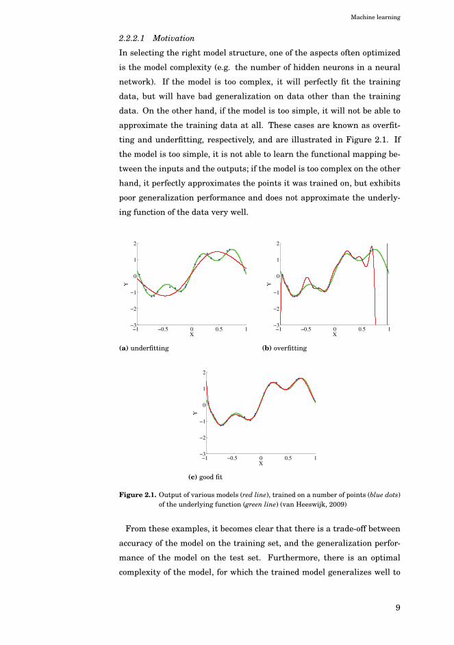
2.2.2.1 Motivation
In selecting the right model structure, one of the aspects often optimized
is the model complexity (e.g. the number of hidden neurons in a neural
network). If the model is too complex, it will perfectly fit the training
data, but will have bad generalization on data other than the training
data. On the other hand, if the model is too simple, it will not be able to
approximate the training data at all. These cases are known as overfit-
ting and underfitting, respectively, and are illustrated in Figure 2.1. If
the model is too simple, it is not able to learn the functional mapping be-
tween the inputs and the outputs; if the model is too complex on the other
hand, it perfectly approximates the points it was trained on, but exhibits
poor generalization performance and does not approximate the underly-
ing function of the data very well.
−1 −0.5 0 0.5 1−3
−2
−1
0
1
2
X
Y
(a) underfitting
−1 −0.5 0 0.5 1−3
−2
−1
0
1
2
X
Y
(b) overfitting
−1 −0.5 0 0.5 1−3
−2
−1
0
1
2
X
Y
(c) good fit
Figure 2.1. Output of various models (red line), trained on a number of points (blue dots)of the underlying function (green line) (van Heeswijk, 2009)
From these examples, it becomes clear that there is a trade-off between
accuracy of the model on the training set, and the generalization perfor-
mance of the model on the test set. Furthermore, there is an optimal
complexity of the model, for which the trained model generalizes well to
9
Machine learning
the unseen test set.
In order to determine the optimal complexity, the expected generaliza-
tion error needs to be estimated, and it needs to be determined without
using the test set. Here, three approaches are discussed: validation, k-fold
cross-validation and leave-one-out cross-validation. See (Bishop, 2006)
and (Efron and Tibshirani, 1993) for more detailed information on model
(structure) selection methods.
2.2.3 Model selection methods
A good model performs well on the training set, and the input-output map-
ping that the model learned from the training set transfers well to the
test set. In other words, the model approximates the underlying function
of the data well and has good generalization.
How well a model generalizes can be measured in the form of the gener-
alization error. In case of a functional approximation problem, and using
an �2 loss function, the generalization error can be defined as
Egen(θ) = limN→∞
1
N
N∑i=1
(yi − f(xi,θ))2 (2.5)
where N is the number of samples, xi is the d-dimensional input, θ con-
tains the model parameters, and yi is the output corresponding to input
vector xi.
Of course, in reality there is no infinite number of samples, but only
a limited amount of samples in the form of a training set and a test set,
consisting of samples that the model will be trained on and samples that
the model will be tested on, respectively. Therefore, the training set is to
be used to estimate the generalization performance, and thus the quality,
of a given model.
Below, three different methods are discussed that are often used in
model selection and the estimation of the generalization error of a model.
Validation In validation, part of the training set is set aside in order to
evaluate the generalization performance of the trained model. If the in-
dices of the samples in the validation set are denoted by val and the in-
dices of the samples in the full training set by train, then the estimation
of the generalization error is defined as
EVALgen (θ∗) =
1
|val|∑i∈val
(yi − f(xi,θ∗train�val))
2 (2.6)
10
Machine learning
where θ∗train�val denotes the model parameters trained on all samples that
are in the training set, but not in the validation set. Note that once
the validation procedure and model selection is completed, the model is
trained on the full training set.
The problem with this validation procedure is that it is not very reliable,
since a small part of the data is held out for validation, and it is unknown
how representative this sample is for the test set.
k-Fold cross-validation k-fold cross-validation is similar to validation,
except that the training set is divided into k parts (typically k = 10), each
of which is used as validation set once, while the rest of the samples are
used for training. The final estimation of the generalization error is the
mean of the generalization errors obtained in each of the k folds
EkCVgen (θ∗) =
1
k
k∑s=1
⎡⎣ 1
|vals|∑
i∈vals(yi − f(xi,θ
∗train�vals))
2
⎤⎦ (2.7)
where θ∗train�vals denotes the model parameters trained on all samples
that are in the training set, but not in validation set vals.
Although k-fold cross-validation gives a better estimation of the gener-
alization error, it is computationally more intensive than validation, since
the validation is performed k times.
Leave-one-out cross-validation Finally, Leave-one-out (LOO)
cross-validation is a special case of k-fold cross-validation, namely the
case where k = N . The models are trained on N training sets, each of
which omits exactly one of the samples. The left-out sample is used for
validation, and the final estimation of the generalization error is the mean
of the N obtained errors
ELOOgen (θ∗) =
1
N
N∑i=1
(f(xi,θ∗−i)− yi)
2 (2.8)
where θ∗−i denotes the model parameters trained on all samples that are
in the training set except on sample i.
Due to the fact that better use is made of the training set, the LOO
cross-validation gives the more reliable estimate of the generalization er-
ror. Although the amount of computation for LOO cross-validation might
seem excessive, for linear models, a closed-form formula exists that can
compute all leave-one-out errors efficiently.
Leave-one-out computation using PRESS statistics Although it might seem
like a lot of work to compute the leave-one-out errors (i.e. N models would
11
Machine learning
need to be trained), the leave-one-out errors of a linear model can be com-
puted efficiently from its residuals (i.e. the errors of the trained model
on the training set) through PRESS (Prediction Sum of Squares) statis-
tics (Allen, 1974; Myers, 1990)
PRESS =
N∑i=1
(yi − xiβ−i)2 =
N∑i=1
(yi − yi,−i)2 =
N∑i=1
(εi,−i)2.
where εi,−i denotes the leave-one-out error when sample i is left out (also
known as the PRESS residual); yi denotes the target output specified by
sample i from the training set, and β−i denotes the weight vector obtained
when training the linear model on the training set with sample i left out.
The PRESS residuals εi,−i can be computed efficiently as follows
εi,−i =εi
1− xi·(XTX)−1xTi·
=yi − yi
1− xi·(XTX)−1xTi·
=yi − xiβ
1− xi·(XTX)−1xTi·
=yi − xiβ
1− hii(2.9)
where xi· is the ith row of matrix X, hii is the ith element on the diago-
nal of the HAT matrix X(XTX)−1XT , which was already encountered in
Section 2.2.1.1. Therefore, the model only needs to be trained once on
the entire training set in order to obtain β, as well as the HAT matrix.
Once the model is trained, all the PRESS residuals can easily be derived
using Equation 2.9. Obviously, this involves a lot less computation than
training the model for all N possible training sets.
Although PRESS statistics define an efficient way to compute the leave-
one-out errors for linear models, this approach is not limited to models
that are linear in the input variables: e.g. it can also be used in models
that are linear in nonlinear transformations of the input variables, an
important class of which is Extreme Learning Machines.
12
3. Extreme Learning Machines
“Not all those who wander are lost.”
– J.R.R. Tolkien, Lord of the Rings
Extreme Learning Machines (ELMs) (Huang et al., 2004, 2006b) is the
name for a collection of neural network models, which employ randomiza-
tion of the hidden layer weights and a fast training algorithm. Typically,
instead of optimizing the hidden layer and output weights through an it-
erative algorithm like backpropagation (Rumelhart et al., 1986), ELMs
initialize the hidden layer randomly and training consists of solving the
linear system defined by the hidden layer outputs and the targets. Despite
the hidden layer weights being random, it has been proven that the ELM
is still capable of universal approximation of any non-constant piecewise
continuous function (Huang et al., 2006a; Huang and Chen, 2007, 2008).
Due to its speed and broad applicability, the ELM framework has become
very popular in the past decade.
The goal of this chapter is not to give an exhaustive overview of the en-
tire ELM literature, nor is the goal to include every single proposed ELM
variant. Rather, the goal is to give a birds-eye view of Extreme Learning
Machines; to put them in historical context; and to identify some of the
learning principles used. For example, an ELM variant might include L1
regularization, L2 regularization, or might be pre-trained in some way.
The amount of possible combinations of these learning principles (and
thus the number of ELM variants) increases rapidly, yet the number of
possible ways to optimize an ELM is relatively limited. The focus in this
chapter will be mainly on variants related to the models developed in this
thesis. For a more complete overview of ELM variants and applications,
the reader is referred to Huang et al. (2011, 2015).
13
Extreme Learning Machines
3.1 Historical context
The idea of randomization of the hidden layer of neural networks has
become very popular under the name Extreme Learning Machines and
the name has become associated with a vast assortment of different mod-
els and variants of neural networks with randomized weights, including
Single-Layer Feedforward Networks (SLFNs) (Huang et al., 2006b), ker-
nelized SLFNs (Frénay and Verleysen, 2010, 2011; Huang et al., 2010),
and deep architectures (Kasun et al., 2013).
The idea of randomization of the hidden layer in neural networks has
been proposed several times. For example, the Random Vector Functional
Link (RVFL) network (Pao and Takefuji, 1992; Pao et al., 1994; Igelnik
and Pao, 1995) incorporates random hidden layer weights and biases, and
direct connections between the input layer and output layer. Further-
more, several authors (Schmidt et al., 1992; te Braake and van Straten,
1995; te Braake et al., 1996; Chen, 1996; te Braake et al., 1997) intro-
duced neural networks with a randomly initialized hidden layer, trained
using the pseudo-inverse. This approach has also been used in the past
for initializing the weights of a neural network (Yam and Chow, 1995;
Yam et al., 1997; Yam and Chow, 2000) before training it with e.g. back-
propagation. Finally, more recently, (Widrow et al., 2013) proposed the
No-Prop algorithm, which has a random hidden layer and uses the LMS
algorithm for training the output weights, rather than the pseudo-inverse.
For an overview of how ELM compares to other methods incorporating
randomization, see (Wang and Wan, 2008; Huang, 2008, 2014).
Although the idea of randomization in neural networks appears else-
where, it cannot be denied that with the development of the Extreme
Learning Machine over the past decade, the idea and theory of using ran-
domization in neural networks has really come to fruition, and has been
developed into a framework (rather than a single method) covering many
machine learning methods, the uniting factor being the fact that some
sort of random basis expansion / randomized hidden layer is used. Along
with these methods, many theoretical and empirical results have been de-
veloped regarding the effectiveness of randomized features (Huang et al.,
2015).
14
Extreme Learning Machines
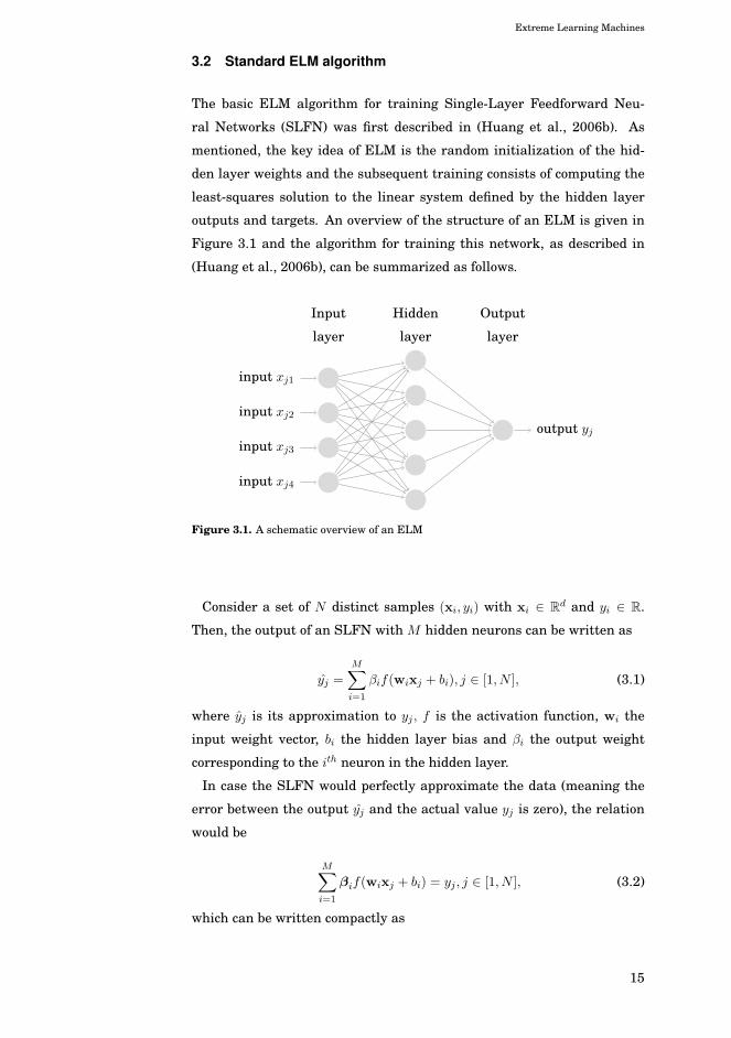
3.2 Standard ELM algorithm
The basic ELM algorithm for training Single-Layer Feedforward Neu-
ral Networks (SLFN) was first described in (Huang et al., 2006b). As
mentioned, the key idea of ELM is the random initialization of the hid-
den layer weights and the subsequent training consists of computing the
least-squares solution to the linear system defined by the hidden layer
outputs and targets. An overview of the structure of an ELM is given in
Figure 3.1 and the algorithm for training this network, as described in
(Huang et al., 2006b), can be summarized as follows.
input xj1
input xj2
input xj3
input xj4
output yj
Hidden
layer
Input
layer
Output
layer
Figure 3.1. A schematic overview of an ELM
Consider a set of N distinct samples (xi, yi) with xi ∈ Rd and yi ∈ R.
Then, the output of an SLFN with M hidden neurons can be written as
yj =
M∑i=1
βif(wixj + bi), j ∈ [1, N ], (3.1)
where yj is its approximation to yj , f is the activation function, wi the
input weight vector, bi the hidden layer bias and βi the output weight
corresponding to the ith neuron in the hidden layer.
In case the SLFN would perfectly approximate the data (meaning the
error between the output yj and the actual value yj is zero), the relation
would be
M∑i=1
βif(wixj + bi) = yj , j ∈ [1, N ], (3.2)
which can be written compactly as
15
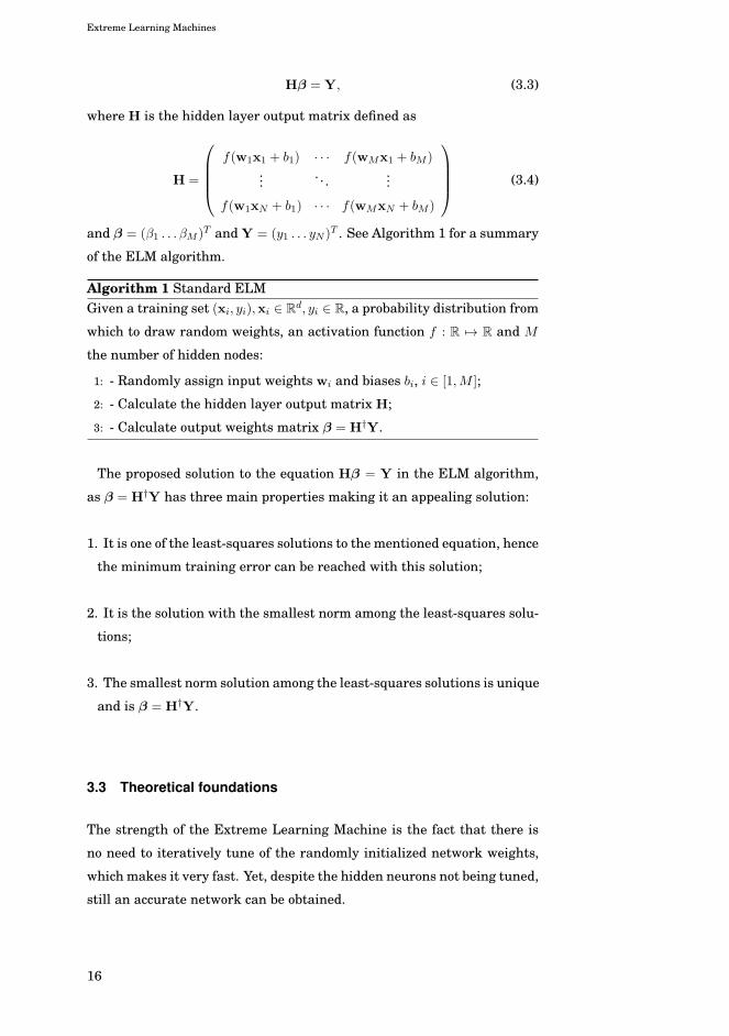
Extreme Learning Machines
Hβ = Y, (3.3)
where H is the hidden layer output matrix defined as
H =
⎛⎜⎜⎜⎝
f(w1x1 + b1) · · · f(wMx1 + bM )... . . . ...
f(w1xN + b1) · · · f(wMxN + bM )
⎞⎟⎟⎟⎠ (3.4)
and β = (β1 . . . βM )T and Y = (y1 . . . yN )T . See Algorithm 1 for a summary
of the ELM algorithm.
Algorithm 1 Standard ELMGiven a training set (xi, yi),xi ∈ R
d, yi ∈ R, a probability distribution from
which to draw random weights, an activation function f : R �→ R and M
the number of hidden nodes:
1: - Randomly assign input weights wi and biases bi, i ∈ [1,M ];
2: - Calculate the hidden layer output matrix H;
3: - Calculate output weights matrix β = H†Y.
The proposed solution to the equation Hβ = Y in the ELM algorithm,
as β = H†Y has three main properties making it an appealing solution:
1. It is one of the least-squares solutions to the mentioned equation, hence
the minimum training error can be reached with this solution;
2. It is the solution with the smallest norm among the least-squares solu-
tions;
3. The smallest norm solution among the least-squares solutions is unique
and is β = H†Y.
3.3 Theoretical foundations
The strength of the Extreme Learning Machine is the fact that there is
no need to iteratively tune of the randomly initialized network weights,
which makes it very fast. Yet, despite the hidden neurons not being tuned,
still an accurate network can be obtained.
16
Extreme Learning Machines
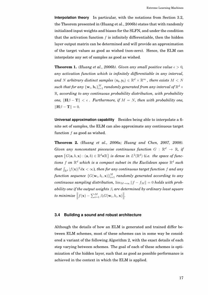
Interpolation theory In particular, with the notations from Section 3.2,
the Theorem presented in (Huang et al., 2006b) states that with randomly
initialized input weights and biases for the SLFN, and under the condition
that the activation function f is infinitely differentiable, then the hidden
layer output matrix can be determined and will provide an approximation
of the target values as good as wished (non-zero). Hence, the ELM can
interpolate any set of samples as good as wished.
Theorem 1. (Huang et al., 2006b). Given any small positive value ε > 0,
any activation function which is infinitely differentiable in any interval,
and N arbitrary distinct samples (xi,yi) ∈ Rd × R
m , there exists M < N
such that for any {wi,bi}Mi=1 randomly generated from any interval of Rd×R, according to any continuous probability distribution, with probability
one, ‖Hβ −T‖ < ε . Furthermore, if M = N , then with probability one,
‖Hβ −T‖ = 0.
Universal approximation capability Besides being able to interpolate a fi-
nite set of samples, the ELM can also approximate any continuous target
function f as good as wished.
Theorem 2. (Huang et al., 2006a; Huang and Chen, 2007, 2008).
Given any nonconstant piecewise continuous function G : Rd → R, if
span{G(a, b,x) : (a, b) ∈ R
d×R}
is dense in L2(Rd) (i.e. the space of func-
tions f on Rd which is a compact subset in the Euclidean space R
d such
that´Rd |f(x)|2dx < ∞), then for any continuous target function f and any
function sequence {G(wi, bi,x)}Mi=1 randomly generated according to any
continuous sampling distribution, limM→∞ ‖f − fM‖ = 0 holds with prob-
ability one if the output weights βi are determined by ordinary least square
to minimize∥∥∥f(x)−∑M
i=1 βiG(wi, bi,x)∥∥∥.
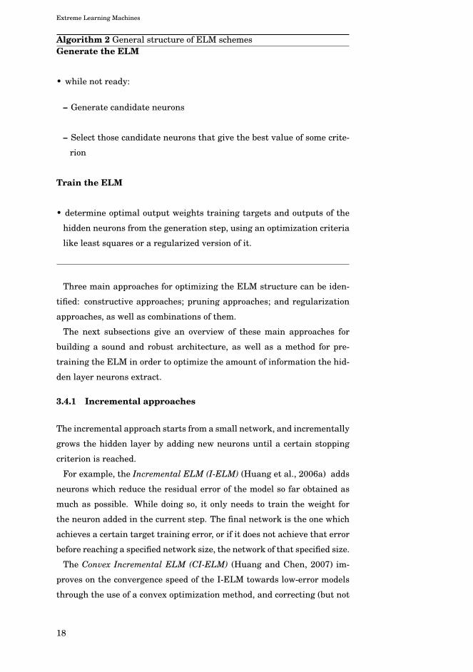
3.4 Building a sound and robust architecture
Although the details of how an ELM is generated and trained differ be-
tween ELM schemes, most of these schemes can in some way be consid-
ered a variant of the following Algorithm 2, with the exact details of each
step varying between schemes. The goal of each of these schemes is opti-
mization of the hidden layer, such that as good as possible performance is
achieved in the context in which the ELM is applied.
17
Extreme Learning Machines
Algorithm 2 General structure of ELM schemesGenerate the ELM
• while not ready:
– Generate candidate neurons
– Select those candidate neurons that give the best value of some crite-
rion
Train the ELM
• determine optimal output weights training targets and outputs of the
hidden neurons from the generation step, using an optimization criteria
like least squares or a regularized version of it.
Three main approaches for optimizing the ELM structure can be iden-
tified: constructive approaches; pruning approaches; and regularization
approaches, as well as combinations of them.
The next subsections give an overview of these main approaches for
building a sound and robust architecture, as well as a method for pre-
training the ELM in order to optimize the amount of information the hid-
den layer neurons extract.
3.4.1 Incremental approaches
The incremental approach starts from a small network, and incrementally
grows the hidden layer by adding new neurons until a certain stopping
criterion is reached.
For example, the Incremental ELM (I-ELM) (Huang et al., 2006a) adds
neurons which reduce the residual error of the model so far obtained as
much as possible. While doing so, it only needs to train the weight for
the neuron added in the current step. The final network is the one which
achieves a certain target training error, or if it does not achieve that error
before reaching a specified network size, the network of that specified size.
The Convex Incremental ELM (CI-ELM) (Huang and Chen, 2007) im-
proves on the convergence speed of the I-ELM towards low-error models
through the use of a convex optimization method, and correcting (but not
18
Extreme Learning Machines
recomputing) the output weights with each incremental step.
As a final example, in the Error-Minimized ELM (EM-ELM) (Feng et al.,
2009), more than one neuron can be added at the same time to grow the
hidden layer. Additionally, the method has closed-form update rules for
the weights when adding the new neurons, making the growing step fast.
3.4.2 Pruning approaches
Contrary to incremental approaches, pruning approaches first generate a
larger than needed set of neurons. Given this set of candidate neurons,
what remains is picking the best subset of M neurons for use in the SLFN.
In the Pruned ELM (Rong et al., 2008), a large set of candidate neu-
rons is generated and ranked according to statistical relevance, using the
χ2 criterion or the information-gain criterion. An optimal threshold for
this criterion is then determined using a separate validation set and the
Akaike Information Criterion (AIC) (Akaike, 1974), after which the net-
work is retrained on the entire training set.
The Optimally Pruned ELM (OP-ELM) (Miche et al., 2010) on the other
hand, exploits the fact that the ELM is linear in the output of the hidden
layer. This permits a fast and optimal ranking (in terms of training error)
of the candidate neurons, using Least Angle Regression (LARS) (Efron
et al., 2003), or Multiresponse Sparse Regression (MRSR) (Similä and
Tikka, 2005). Once ranked, the optimal prefix of the sorted list of neu-
rons is determined using the leave-one-out error, which can be efficiently
computed using PRESS statistics (Allen, 1974; Myers, 1990).
Although the term ’pruned’ suggest that the network architecture is be-
ing built starting from the largest network, and neurons are removed one-
by-one, in fact the above approaches are quite similar to the incremental
approach. The difference is that instead of randomly generating new neu-
rons at each step, the entire candidate list of neurons is generated and
ranked as a first step in the algorithm, and the neurons to be added are
taken from that ranked candidate list of neurons. Therefore, the differ-
ence between the incremental and pruning approach is not that clear-cut.
For example, a recently proposed variant of the OP-ELM (which adds a
number of regressors in each step of an MRSR-like algorithm, rather than
a single one) was called the Constructive Multi-output ELM (Wang et al.,
2014).
19
Extreme Learning Machines
3.4.3 Regularization approaches
As an alternative to selecting the subset of hidden neurons, it is also pos-
sible to generate a large enough set of hidden neurons, and prevent over-
fitting by properly regularizing the network.
The Regularized ELM (R-ELM) (Deng et al., 2009) for example, is an
approach in which the set of candidate neurons is fixed and taken large
enough, while L2 regularization is used to prevent overfitting.
Finally, the Tikhonov Regularized OP-ELM (TROP-ELM) (Miche et al.,
2011) is a variant of the OP-ELM, which efficiently incorporates the opti-
mization of an L2 regularization parameter in the OP-ELM by integrat-
ing it in the SVD approach to computing pseudo-inverse H†. This way,
besides the advantage of sparsity, the output weights remain small and
overfitting is prevented.
3.4.4 ELM pre-training
As it is extensively used in Publication V and Publication VI, in this sec-
tion reviews intrinsic plasticity, as well as its adaptation to ELM (BIP-
ELM) by (Neumann and Steil, 2011, 2013).
3.4.4.1 Motivation
Although ELMs are universal approximators, since often there are only
limited training samples available. Therefore, it is important that the
hidden layer neurons extract as much information as possible from the
inputs.
A recently proposed pre-training method that achieves this is Batch In-
trinsic Plasticity (BIP) (Neumann and Steil, 2011, 2013), which makes
the ELM more robust by adapting the randomly generated hidden layer
weights and biases such that each neuron achieves an exponential output
distribution with a specified mean, and the amount of information that
the hidden layer extracts from the limited amount of training samples is
optimized.
Furthermore, the mechanism of intrinsic plasticity is one that is orthog-
onal to all the above-mentioned approaches. Namely, it generally takes
place right after generating the random weights of the neurons, and its re-
sult is subsequently used in the further optimization, pruning and train-
ing of the ELM. As such, it can be used in combination with most other
ELM approaches.
20
Extreme Learning Machines
3.4.4.2 Intrinsic Plasticity
The concept of intrinsic plasticity has a biological background and refers
to the fact that neurons adapt in such a way that they maximize their
entropy (and thus the amount of information transmitted), while keeping
the mean firing rate low. Intrinsic plasticity has been first used in papers
regarding reservoir computing, recurrent neural networks, liquid state
machines and echo state networks as a learning rule which maximizes
information transmitted by the neurons (Triesch, 2005a,b; Verstraeten
et al., 2007).
The information transmission of neurons is maximized by having the
neuron outputs approximate an exponential distribution, which is the
maximum entropy distribution among all positive distributions with fixed
mean (Steil, 2007).
Furthermore, as (Verstraeten et al., 2007) notes in the context of reser-
voir computing, reservoirs are constructed in a stochastic manner, and
the search for a method to construct a priori suitable reservoirs that are
guaranteed or likely to offer a certain performance is an important line of
research. Intrinsic plasticity is such a method which aims at construct-
ing a network which is likely to give good performance. The recent study
(Neumann et al., 2012) provides an in-depth analysis of intrinsic plastic-
ity pre-training, and shows that it indeed results in well-performing net-
works with an impressive robustness against other network parameters
like network size and strength of the regularization.
3.4.4.3 (Batch) Intrinsic Plasticity: BIP-ELM
In (Neumann and Steil, 2011, 2013; Neumann, 2013) the principle of in-
trinsic plasticity is transferred to ELMs and introduced as an efficient
pre-training method, aimed at adapting the hidden layer weights and bi-
ases, such that the output distribution of the hidden layer is shaped like
an exponential distribution. The motivation for this is that the exponen-
tial distribution is the maximum-entropy distribution over all distribu-
tions with fixed mean, maximizing the information transmission through
the hidden layer. The only parameter of batch intrinsic plasticity is the
mean of exponential distribution. This parameter determines the exact
shape of the exponential distribution from which targets will be drawn,
and can be set in various ways, as explained below.
Following (Neumann and Steil, 2011), the algorithm can be summarized
as described as below.
21
Extreme Learning Machines
Given the inputs (x1, . . . ,xN ) ∈ RN×d and input matrix Win ∈ R
d×M
(with N the number of samples in the training set, d the dimensionality
of the data, and M the number of neurons), the synaptic input to neu-
ron i is given by si(k) = xkWin·i . Now, it is possible to adapt slope ai and
bias bi, such that the desired output distribution is achieved for neuron
output hi = f(aisi(k) + bi). To this end, for each neuron random targets
t = (t1, t2, . . . , tN ) are drawn from the exponential distribution with a par-
ticular mean, and sorted such that t1 < · · · < tN . The synaptic inputs to
the neuron are sorted as well into vector si = (si(1), si(2), . . . , si(N)), such
that si(1) < si(2) < · · · < si(N).
Given an invertible transfer function, the targets can now be propagated
back through the hidden layer, and a linear model can be defined that
maps the sorted si(k) as closely as possible to the sorted tk. To this end,
a model Φ(si) = (sTi , (1 . . . 1)T ) and parameter vector vi = (ai, bi)
T are
defined. Then, given the invertible transfer function f the optimal slope
ai and bias bi for which each si(k) is approximately mapped to tk can be
found by minimizing
||Φ(si) · vi − f−1(t)||
The optimal slope ai and bias bi can therefore, like in ELM, be determined
using the Moore-Penrose pseudo-inverse:
vi = (ai, bi)T = Φ†(si) · f−1(t)
This procedure is performed for every neuron with an invertible transfer
function, and even though the target distribution can often not exactly be
matched (due to the limited degrees of freedom in the optimization prob-
lem) it has been shown in (Neumann and Steil, 2011, 2013; Neumann,
2013) that batch intrinsic plasticity is an effective and efficient scheme
for input-specific tuning of input weights and biases used in the non-linear
transfer functions.
The stability of BIP-ELM combined with ridge regression like in the R-
ELM (Deng et al., 2009) essentially removes the need to tune the amount
of hidden neurons, and the only parameter of batch intrinsic plasticity is
the mean of the exponential target distribution from which targets t are
drawn, which is either set to a fixed value c, or randomly in the interval
[0, 1] on a per-neuron basis (Neumann and Steil, 2011, 2013; Neumann,
2013). These variants will be referred to as BIP(c)-ELM and BIP(rand)-
ELM in this thesis.
22
Extreme Learning Machines
3.5 Other ELM approaches
Besides the above-mentioned approaches, several other approaches have
been developed over the past years, extending the ELM framework to dif-
ferent types of models, namely kernelized ELM (Frénay and Verleysen,
2010, 2011; Huang et al., 2010; Parviainen et al., 2010), multiple kernel
ELM (Liu et al., 2015), representation learning using ELM (Kasun et al.,
2013), ELMs with shaped input weights (Tapson et al., 2014; McDonnell
et al., 2014), and semi-supervised and unsupervised ELM (Huang et al.,
2014). More details on these methods can be found in the cited references,
or in (Huang et al., 2015).
Furthermore, randomization ideas akin to ELM are increasingly being
used in modern kernel methods, in order to let them scale to larger data,
namely Random Kitchen Sinks (Rahimi and Recht, 2007, 2008), and Fast-
food (Le et al., 2013).
3.6 ELM in practice
In theory, random initialization of the hidden layer and use of any non-
constant piecewise continuous transfer function is sufficient for approxi-
mating any function, given enough neurons. In practice, however, there
are a number of practical strategies that can be used for obtaining more
accurate and effective ELMs. This section lists some of those practical
tips for building a more effective ELM.
Normalization and pre-training As is well-known, data should be normal-
ized such that each variable is zero-mean and unit-variance (or scaled to
e.g. interval [−1, 1] . In practice, the former approach is more robust, since
it is not as sensitive to outliers.
The range and number of input variables, together with the random
weights of an ELM, will result in an expected activation at the input of
each neuron, and one should make sure that e.g. the sigmoid neuron is
not always operating in the saturated or linear region. For example, by
letting the parameters of the probability distribution from which the ran-
dom layer weights and biases are drawn depend on the number of inputs
and transfer function, or by cross-validating them to optimize accuracy.
Another fast option is to use the Batch-Intrinsic Plasticity pre-training
from Section 3.4.4, which automatically adapts the randomly drawn hid-
den layer weights and biases, such that each neuron operates in a useful
23
Extreme Learning Machines
regime.
Approximating the constant component In the non-kernel version of ELM,
it might be helpful to include a bias in the output layer (i.e. achieved by
concatenating the H matrix with a column of ones). Although this output
bias is often not included in the description of the ELM since theoretically
it is not needed, it allows the ELM to adapt to any non-zero mean in the
targets at the expense of only a single extra parameter, namely the extra
output weight.
Approximating the linear component Furthermore, in most problems, it
is helpful to include a linear neuron for each input variable. This way,
the rest of the nonlinear neurons can focus on fitting the nonlinear part
of the problem, while the linear neurons take care of the linear part of
the problem. Equivalently, an ELM could be trained on the residual of
a linear model. This approach of decomposing the problem into a linear
part and a nonlinear part has proven to be very effective in the context of
deep learning (Raiko and Valpola, 2012).
24
4. Ensemble learning
“The only way of discovering the limits of the possible is to venture
a little way past them into the impossible.”
– Arthur C. Clarke
When discussing ensemble models it is helpful to look at a real-world
example first. At fairs and exhibitions, sometimes there are these contests
where the goal is to guess the number of marbles in a vase, and the person
who makes the best guess wins the price. It turns out that while each
individual guess is likely to be pretty far off, the average of all guesses is
often a relatively good estimate of the real number of marbles in the vase.
This phenomenon is often referred to as ’wisdom of the crowds’.
A similar strategy is employed in ensemble models: a number of individ-
ual models is built to solve a particular task, and these models are then
combined into an ensemble model. Although the individual models might
vary a lot in terms of accuracy, the combination gives a more accurate
result.
This chapter introduces ensemble models, and the ELM-based ensemble
models developed in this thesis, which make the ensemble adaptive to
changes in the environment (Publication I) and allow them to scale to
larger data (Publication II).
4.1 Ensemble Models
An ensemble model or committee (Bishop, 2006), combines multiple indi-
vidual models, with the goal of reducing the expected error of the model.
Commonly, this is done by taking the average or a weighted average of
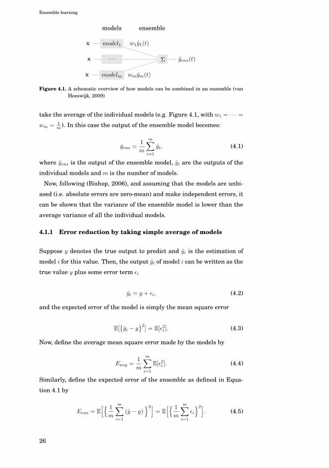
the individual models (see Figure 4.1).
Ensemble methods rely on having multiple good models with sufficiently
uncorrelated errors. The simplest way to build an ensemble model is to
25
Ensemble learning
model1x
· · ·x
modelmx
Σ yens(t)
models ensemble
w1y1(t)
wmym(t)
Figure 4.1. A schematic overview of how models can be combined in an ensemble (vanHeeswijk, 2009)
take the average of the individual models (e.g. Figure 4.1, with w1 = · · · =wm = 1
m ). In this case the output of the ensemble model becomes:
yens =1
m
m∑i=1
yi, (4.1)
where yens is the output of the ensemble model, yi are the outputs of the
individual models and m is the number of models.
Now, following (Bishop, 2006), and assuming that the models are unbi-
ased (i.e. absolute errors are zero-mean) and make independent errors, it
can be shown that the variance of the ensemble model is lower than the
average variance of all the individual models.
4.1.1 Error reduction by taking simple average of models
Suppose y denotes the true output to predict and yi is the estimation of
model i for this value. Then, the output yi of model i can be written as the
true value y plus some error term εi
yi = y + εi, (4.2)
and the expected error of the model is simply the mean square error
E[{yi − y
}2] = E[ε2i ]. (4.3)
Now, define the average mean square error made by the models by
Eavg =1
m
m∑i=1
E[ε2i ]. (4.4)
Similarly, define the expected error of the ensemble as defined in Equa-
tion 4.1 by
Eens = E
[{ 1
m
m∑i=1
(y − y)}2]
= E
[{ 1
m
m∑i=1
εi
}2]. (4.5)
26
Ensemble learning
Then, assuming the errors εi are uncorrelated (i.e. E[εiεj ] = 0) and are
zero-mean (i.e. E[εi] = 0), the expected ensemble error can be written as
Eens =1
mEavg =
1
m2
m∑i=1
E[ε2i ], (4.6)
which suggests a great reduction of the error through ensembling. These
equations assume completely uncorrelated errors between the models,
while in practice errors tend to be highly correlated. Therefore, errors
are often not reduced as much as suggested by these equations. It can be
shown though that Eens < Eavg always holds (Bishop, 2006), so through
ensembling, the test error of the ensemble is expected to be smaller than
the average test error of the models.
Note however, that it is not a guarantee that the ensemble is more ac-
curate than the best model in the ensemble, but only as accurate as the
models, on average. Therefore, besides being as independent as possible,
it is important that the models used to build the ensemble are sufficiently
accurate.
4.1.2 Ensemble weight initialization
Besides taking a simple average of the models, it is also possible to take
a weighted linear combination based on some criterion that measures the
quality of the models.
Two different ensemble weight initializations are investigated in the
publications in this thesis: uniform weight initialization (Publication I)
and leave-one-out weight initialization (Publication II).
Uniform weight initialization For initialization of the ensemble model, each
of the individual models is trained on a given training set, and initially
each model contributes with the same weight to the output of the ensem-
ble. This will be referred to as uniform weight initialization.
Leave-one-out weight initialization As an alternative to uniform weight
initialization, the initial weights can be based on the leave-one-out output
of the models on the training set, like in Breiman (1996b). This will be
referred to as leave-one-out weight initialization.
Using Equation 2.9, for a any model that is linear in the parameters
(like ELM), the leave-one-out errors can be efficiently computed. There-
fore, the leave-one-out outputs (i.e. the estimations of the sample that is
left out in each of the N folds) can be obtained efficiently as well, given
the leave-one-out errors and the true targets.
27
Ensemble learning
Finally, the initial ensemble weights are obtained by fitting a non-negative
linear combination of the leave-one-out outputs for all m models to the tar-
get outputs. Using this procedure, models that have bad generalization
performance get relatively low weight, while models with good general-
ization performance get higher weights.
4.1.3 Ensembling strategies
It was shown in (Hansen and Salamon, 1990), that through combining
multiple neural networks, accuracy can be improved as compared to the
individual neural networks. Since, several strategies have been proposed
for building ensembles. In mixture of experts (Jacobs et al., 1991), sev-
eral models are built, each of which specializes on part of the problem
domain. The weights of the ensemble model depend on the part of the
domain in which a prediction is required. In stacking (Wolpert, 1992) and
boosting (Freund and Schapire, 1996; Schapire et al., 1998), the models
are built in sequence, taking into account the performance of the earlier
built models, in order to improve on them. In bootstrap aggregating, or
bagging (Breiman, 1996a), on the other hand, diversity between the mod-
els is obtained by training them on re-sampled versions of the training
set, while in stacked regressions (Breiman, 1996b), leave-one-out cross-
validation is used to obtain the ensemble weights. Finally, in (Liu and Yao,
1999) accuracy of a neural network ensemble is enhanced through nega-
tive correlation learning, which promotes diversity between the neural
networks. For an overview of ensemble methods in general, see (Bishop,
2006; Murphy, 2012).
In the next section, adaptive ensemble models, and the contributions
made in this thesis are discussed.
4.2 Adaptive ensemble models
When solving a particular regression or classification problem, it is of-
ten unknown in advance what the optimal model class and structure is.
One alternative for selecting the optimal model class or structure would
be through validation, cross-validation or leave-one-out validation, as dis-
cussed in Section 2.2.2. However, it is not guaranteed that the model se-
lected based on a set of training samples will be the best model for newly
28
Ensemble learning
obtained samples. For example, in a nonstationary context where the
i.i.d. assumption does not hold and the information gathered from past
samples can become inaccurate.
One strategy for handling nonstationarities would be to keep learning
as new samples become available. For example, by retraining the model
repeatedly on a finite window into the past such that it ’tracks’ the non-
stationarity.
Another strategy for adapting to nonstationarities is to use a strategy
similar to (Jacobs et al., 1991), but instead of letting the linear combi-
nation of models depend on the part of the input space, let the linear
combination directly depend on the accuracy of the models.
4.2.1 Adaptive ensemble model of ELMs
In Publication I, both strategies are investigated in one-step ahead predic-
tion on both stationary and nonstationary time series, in which the next
value of the time series is predicted, given all its past values.
Besides the already mentioned advantages of ensemble models over sin-
gle models, this allows for adaptivity of the ensemble model to environ-
mental changes.
Related Work The retraining of the ELMs in this ensemble is similar to
the Online Sequential ELM (OS-ELM) (Liang et al., 2006), the important
difference being that contrary to OS-ELMs, Publication I also provides
a way to incrementally remove samples from the trained model. Fur-
thermore, compared to the ensemble of OS-ELM (EOS-ELM) (Lan et al.,
2009), which was introduced around the same time as Publication I, the
adaptive ensemble adjusts the linear combination to optimize ensemble
accuracy.
Both the ability to train on sliding windows, and the adaptive ensemble
weights turn out to be an important contribution in the nonstationary
environments, in which online sequential learning is typically applied.
Initializing the adaptive ensemble model The adaptive ensemble model
consists of a number of randomly generated ELMs, which each have their
own parameters. Because of the stochastic nature of the ELM, they are
diverse in nature and will have different biases and input layer weights.
To further increase diversity between the models, each ELM is built us-
ing different regressor variables; different regressor size; and different
number of hidden neurons. Uniform weight initialization is used for the
29
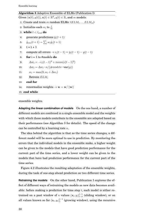
Ensemble learning
Algorithm 3 Adaptive Ensemble of ELMs (Publication I)Given (x(t), y(t)), x(t) ∈ R
d, y(t) ∈ R, and m models:
1: Create and train m random ELMs: (ELM1 . . .ELMm)
2: Initialize each wi to 1m
3: while t < tend do
4: generate predictions yi(t+ 1)
5: yens(t+ 1) =∑
iwiyi(t+ 1)
6: t = t + 1
7: compute all errors → εi(t− 1) = yi(t− 1)− y(t− 1)
8: for i = 1 to #models do
9: Δwi = −εi(t− 1)2 +mean(ε(t− 1)2)
10: Δwi = Δwi · α/(#models · var(y))11: wi = max(0, wi +Δwi)
12: Retrain ELMi
13: end for
14: renormalize weights → w = w/ ||w||15: end while
ensemble weights.
Adapting the linear combination of models On the one hand, a number of
different models are combined in a single ensemble model and the weights
with which these models contribute to the ensemble are adapted based on
their performance (see Algorithm 3 for details). The speed of the change
can be controlled by a learning rate α.
The idea behind the algorithm is that as the time series changes, a dif-
ferent model will be more optimal to use in prediction. By monitoring the
errors that the individual models in the ensemble make, a higher weight
can be given to the models that have good prediction performance for the
current part of the time series, and a lower weight can be given to the
models that have bad prediction performance for the current part of the
time series.
Figure 4.2 illustrates the resulting adaptation of the ensemble weights,
during the task of one-step ahead prediction on two different time series.
Retraining the models On the other hand, Publication I explores the ef-
fect of different ways of retraining the models as new data becomes avail-
able: before making a prediction for time step t, each model is either re-
trained on a past window of n values (xi, yi)t−1t−n (sliding window), or on
all values known so far (xi, yi)t−11 (growing window), using the recursive
30
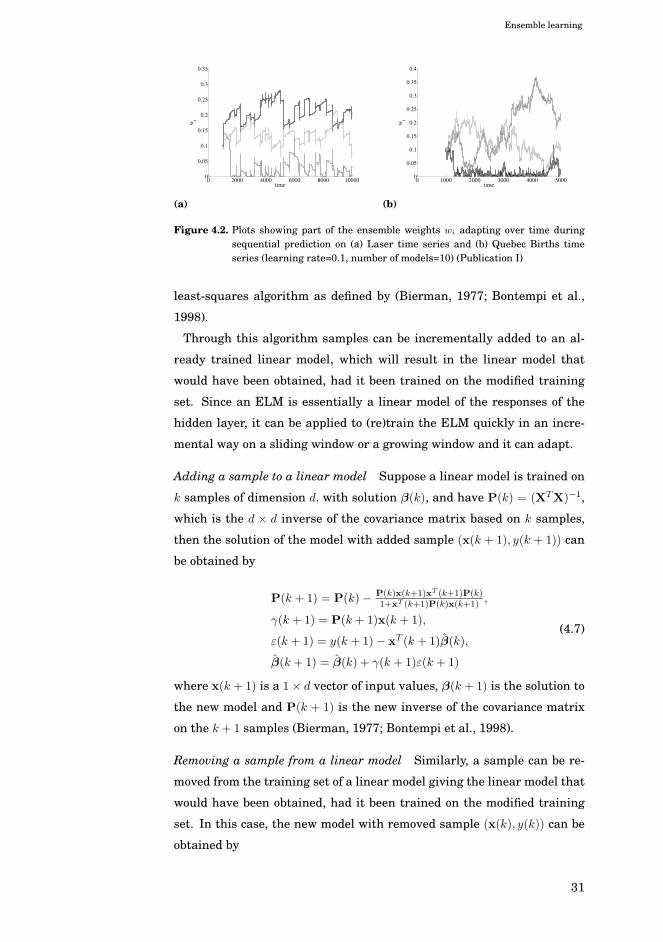
Ensemble learning
0 2000 4000 6000 8000 100000
0.05
0.1
0.15
0.2
0.25
0.3
0.35
timew
i
(a)
0 1000 2000 3000 4000 50000
0.05
0.1
0.15
0.2
0.25
0.3
0.35
0.4
time
wi
(b)
Figure 4.2. Plots showing part of the ensemble weights wi adapting over time duringsequential prediction on (a) Laser time series and (b) Quebec Births timeseries (learning rate=0.1, number of models=10) (Publication I)
least-squares algorithm as defined by (Bierman, 1977; Bontempi et al.,
1998).
Through this algorithm samples can be incrementally added to an al-
ready trained linear model, which will result in the linear model that
would have been obtained, had it been trained on the modified training
set. Since an ELM is essentially a linear model of the responses of the
hidden layer, it can be applied to (re)train the ELM quickly in an incre-
mental way on a sliding window or a growing window and it can adapt.
Adding a sample to a linear model Suppose a linear model is trained on
k samples of dimension d, with solution β(k), and have P(k) = (XTX)−1,
which is the d × d inverse of the covariance matrix based on k samples,
then the solution of the model with added sample (x(k + 1), y(k + 1)) can
be obtained by
P(k + 1) = P(k)− P(k)x(k+1)xT (k+1)P(k)1+xT (k+1)P(k)x(k+1)
,
γ(k + 1) = P(k + 1)x(k + 1),
ε(k + 1) = y(k + 1)− xT (k + 1)β(k),
β(k + 1) = β(k) + γ(k + 1)ε(k + 1)
(4.7)
where x(k + 1) is a 1× d vector of input values, β(k + 1) is the solution to
the new model and P(k + 1) is the new inverse of the covariance matrix
on the k + 1 samples (Bierman, 1977; Bontempi et al., 1998).
Removing a sample from a linear model Similarly, a sample can be re-
moved from the training set of a linear model giving the linear model that
would have been obtained, had it been trained on the modified training
set. In this case, the new model with removed sample (x(k), y(k)) can be
obtained by
31
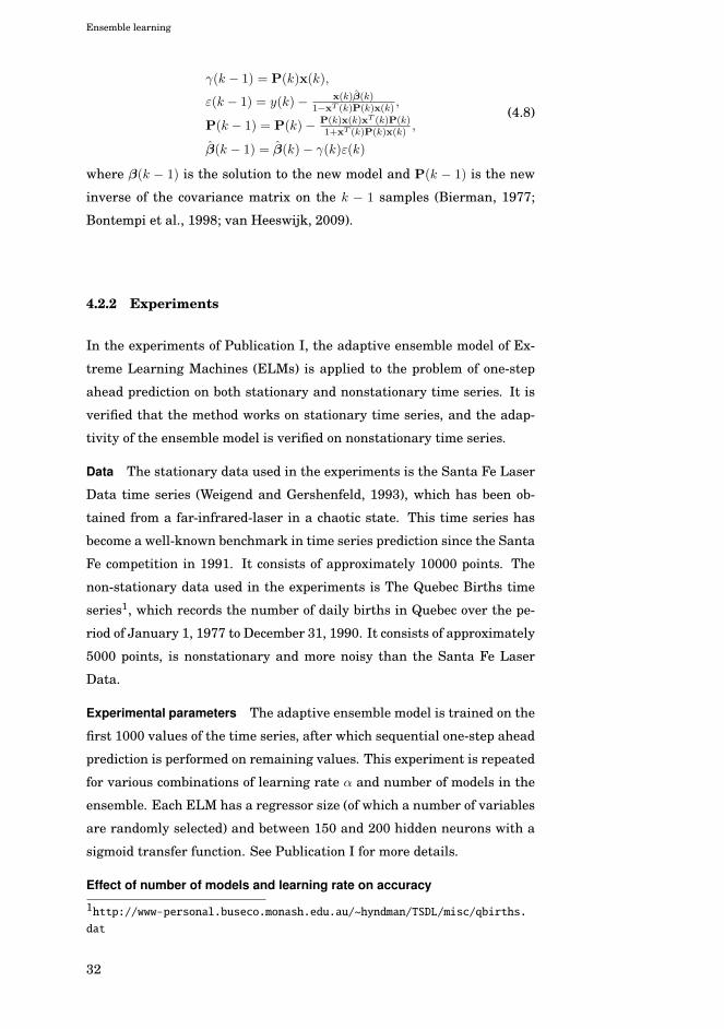
Ensemble learning
γ(k − 1) = P(k)x(k),
ε(k − 1) = y(k)− x(k)β(k)1−xT (k)P(k)x(k)
,
P(k − 1) = P(k)− P(k)x(k)xT (k)P(k)1+xT (k)P(k)x(k)
,
β(k − 1) = β(k)− γ(k)ε(k)
(4.8)
where β(k − 1) is the solution to the new model and P(k − 1) is the new
inverse of the covariance matrix on the k − 1 samples (Bierman, 1977;
Bontempi et al., 1998; van Heeswijk, 2009).
4.2.2 Experiments
In the experiments of Publication I, the adaptive ensemble model of Ex-
treme Learning Machines (ELMs) is applied to the problem of one-step
ahead prediction on both stationary and nonstationary time series. It is
verified that the method works on stationary time series, and the adap-
tivity of the ensemble model is verified on nonstationary time series.
Data The stationary data used in the experiments is the Santa Fe Laser
Data time series (Weigend and Gershenfeld, 1993), which has been ob-
tained from a far-infrared-laser in a chaotic state. This time series has
become a well-known benchmark in time series prediction since the Santa
Fe competition in 1991. It consists of approximately 10000 points. The
non-stationary data used in the experiments is The Quebec Births time
series1, which records the number of daily births in Quebec over the pe-
riod of January 1, 1977 to December 31, 1990. It consists of approximately
5000 points, is nonstationary and more noisy than the Santa Fe Laser
Data.
Experimental parameters The adaptive ensemble model is trained on the
first 1000 values of the time series, after which sequential one-step ahead
prediction is performed on remaining values. This experiment is repeated
for various combinations of learning rate α and number of models in the
ensemble. Each ELM has a regressor size (of which a number of variables
are randomly selected) and between 150 and 200 hidden neurons with a
sigmoid transfer function. See Publication I for more details.
Effect of number of models and learning rate on accuracy
1http://www-personal.buseco.monash.edu.au/~hyndman/TSDL/misc/qbirths.dat
32
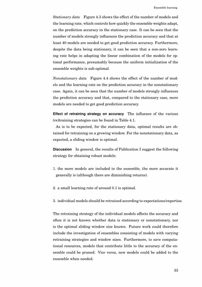
Ensemble learning
Stationary data Figure 4.3 shows the effect of the number of models and
the learning rate, which controls how quickly the ensemble weights adapt,
on the prediction accuracy in the stationary case. It can be seen that the
number of models strongly influences the prediction accuracy and that at
least 40 models are needed to get good prediction accuracy. Furthermore,
despite the data being stationary, it can be seen that a non-zero learn-
ing rate helps in adapting the linear combination of the models for op-
timal performance, presumably because the uniform initialization of the
ensemble weights is sub-optimal.
Nonstationary data Figure 4.4 shows the effect of the number of mod-
els and the learning rate on the prediction accuracy in the nonstationary
case. Again, it can be seen that the number of models strongly influences
the prediction accuracy and that, compared to the stationary case, more
models are needed to get good prediction accuracy.
Effect of retraining strategy on accuracy The influence of the various
(re)training strategies can be found in Table 4.1.
As is to be expected, for the stationary data, optimal results are ob-
tained for retraining on a growing window. For the nonstationary data, as
expected, a sliding window is optimal.
Discussion In general, the results of Publication I suggest the following
strategy for obtaining robust models:
1. the more models are included in the ensemble, the more accurate it
generally is (although there are diminishing returns).
2. a small learning rate of around 0.1 is optimal.
3. individual models should be retrained according to expectations/expertise.
The retraining strategy of the individual models affects the accuracy and
often it is not known whether data is stationary or nonstationary, nor
is the optimal sliding window size known. Future work could therefore
include the investigation of ensembles consisting of models with varying
retraining strategies and window sizes. Furthermore, to save computa-
tional resources, models that contribute little to the accuracy of the en-
semble could be pruned. Vice versa, new models could be added to the
ensemble when needed.
33
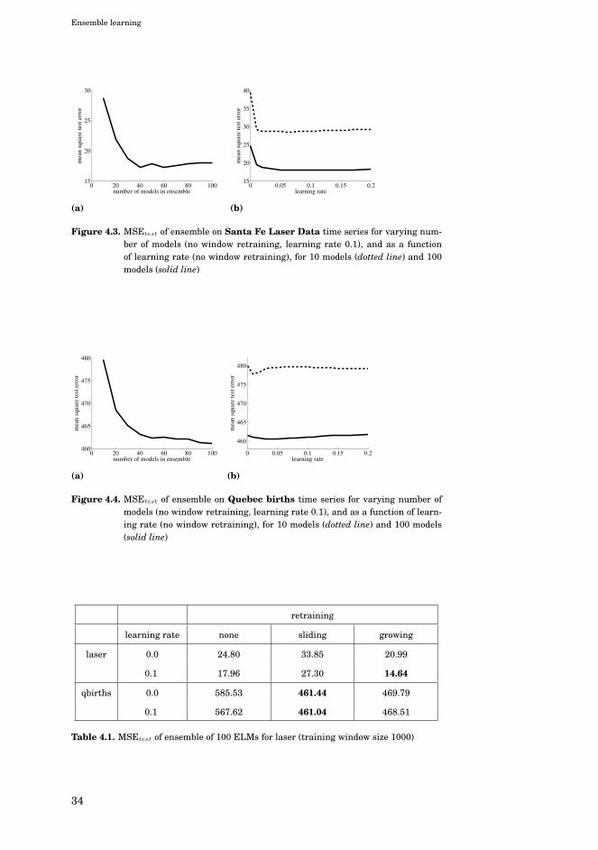
Ensemble learning
0 20 40 60 80 10015
20
25
30
number of models in ensemble
mea
n sq
uare
test
err
or
(a)
0 0.05 0.1 0.15 0.215
20
25
30
35
40
learning rate
mea
n sq
uare
test
err
or
(b)
Figure 4.3. MSEtest of ensemble on Santa Fe Laser Data time series for varying num-ber of models (no window retraining, learning rate 0.1), and as a functionof learning rate (no window retraining), for 10 models (dotted line) and 100models (solid line)
0 20 40 60 80 100460
465
470
475
480
number of models in ensemble
mea
n sq
uare
test
err
or
(a)
0 0.05 0.1 0.15 0.2
460
465
470
475
480
learning rate
mea
n sq
uare
test
err
or
(b)
Figure 4.4. MSEtest of ensemble on Quebec births time series for varying number ofmodels (no window retraining, learning rate 0.1), and as a function of learn-ing rate (no window retraining), for 10 models (dotted line) and 100 models(solid line)
retraining
learning rate none sliding growing
laser 0.0 24.80 33.85 20.99
0.1 17.96 27.30 14.64
qbirths 0.0 585.53 461.44 469.79
0.1 567.62 461.04 468.51
Table 4.1. MSEtest of ensemble of 100 ELMs for laser (training window size 1000)
34
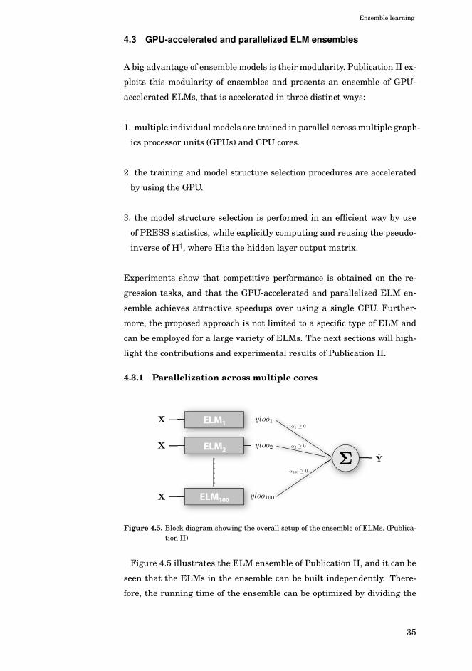
Ensemble learning
4.3 GPU-accelerated and parallelized ELM ensembles
A big advantage of ensemble models is their modularity. Publication II ex-
ploits this modularity of ensembles and presents an ensemble of GPU-
accelerated ELMs, that is accelerated in three distinct ways:
1. multiple individual models are trained in parallel across multiple graph-
ics processor units (GPUs) and CPU cores.
2. the training and model structure selection procedures are accelerated
by using the GPU.
3. the model structure selection is performed in an efficient way by use
of PRESS statistics, while explicitly computing and reusing the pseudo-
inverse of H†, where His the hidden layer output matrix.
Experiments show that competitive performance is obtained on the re-
gression tasks, and that the GPU-accelerated and parallelized ELM en-
semble achieves attractive speedups over using a single CPU. Further-
more, the proposed approach is not limited to a specific type of ELM and
can be employed for a large variety of ELMs. The next sections will high-
light the contributions and experimental results of Publication II.
4.3.1 Parallelization across multiple cores
Σ
EELM1
ELM2
ELM100
X
X
X
α1 ≥ 0
α2 ≥ 0
α100 ≥ 0
yloo2
yloo100
Y
yloo1
Figure 4.5. Block diagram showing the overall setup of the ensemble of ELMs. (Publica-tion II)
Figure 4.5 illustrates the ELM ensemble of Publication II, and it can be
seen that the ELMs in the ensemble can be built independently. There-
fore, the running time of the ensemble can be optimized by dividing the
35
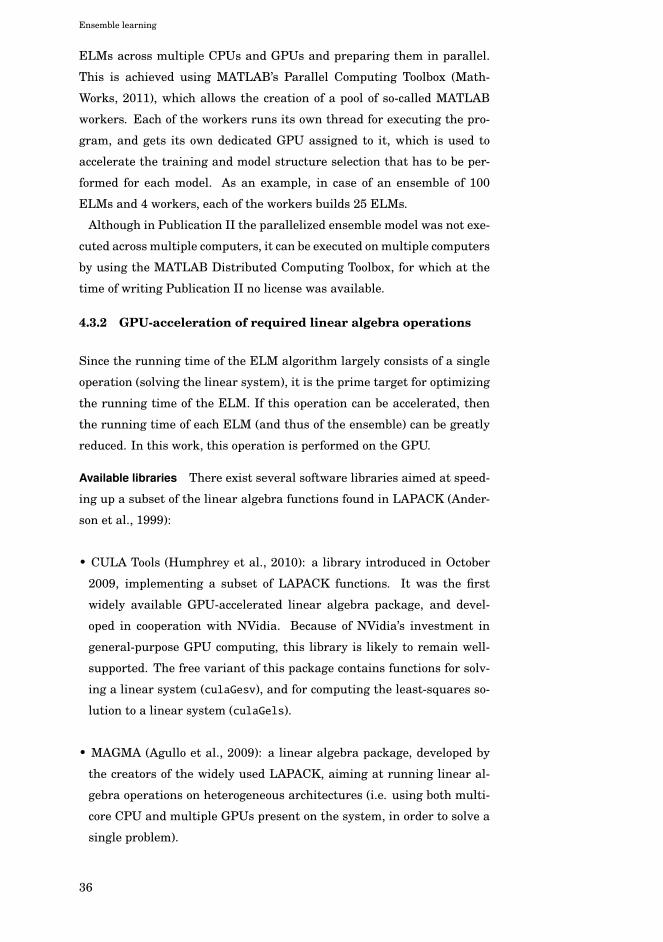
Ensemble learning
ELMs across multiple CPUs and GPUs and preparing them in parallel.
This is achieved using MATLAB’s Parallel Computing Toolbox (Math-
Works, 2011), which allows the creation of a pool of so-called MATLAB
workers. Each of the workers runs its own thread for executing the pro-
gram, and gets its own dedicated GPU assigned to it, which is used to
accelerate the training and model structure selection that has to be per-
formed for each model. As an example, in case of an ensemble of 100
ELMs and 4 workers, each of the workers builds 25 ELMs.
Although in Publication II the parallelized ensemble model was not exe-
cuted across multiple computers, it can be executed on multiple computers
by using the MATLAB Distributed Computing Toolbox, for which at the
time of writing Publication II no license was available.
4.3.2 GPU-acceleration of required linear algebra operations
Since the running time of the ELM algorithm largely consists of a single
operation (solving the linear system), it is the prime target for optimizing
the running time of the ELM. If this operation can be accelerated, then
the running time of each ELM (and thus of the ensemble) can be greatly
reduced. In this work, this operation is performed on the GPU.
Available libraries There exist several software libraries aimed at speed-
ing up a subset of the linear algebra functions found in LAPACK (Ander-
son et al., 1999):
• CULA Tools (Humphrey et al., 2010): a library introduced in October
2009, implementing a subset of LAPACK functions. It was the first
widely available GPU-accelerated linear algebra package, and devel-
oped in cooperation with NVidia. Because of NVidia’s investment in
general-purpose GPU computing, this library is likely to remain well-
supported. The free variant of this package contains functions for solv-
ing a linear system (culaGesv), and for computing the least-squares so-
lution to a linear system (culaGels).
• MAGMA (Agullo et al., 2009): a linear algebra package, developed by
the creators of the widely used LAPACK, aiming at running linear al-
gebra operations on heterogeneous architectures (i.e. using both multi-
core CPU and multiple GPUs present on the system, in order to solve a
single problem).
36
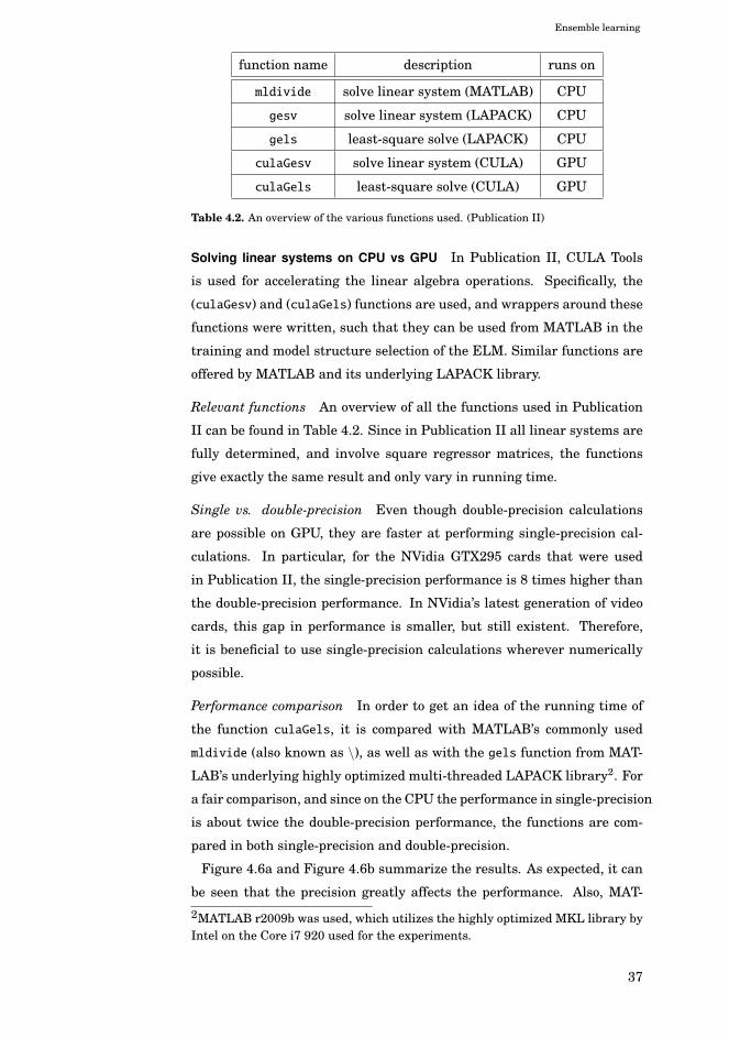
Ensemble learning
function name description runs on
mldivide solve linear system (MATLAB) CPU
gesv solve linear system (LAPACK) CPU
gels least-square solve (LAPACK) CPU
culaGesv solve linear system (CULA) GPU
culaGels least-square solve (CULA) GPU
Table 4.2. An overview of the various functions used. (Publication II)
Solving linear systems on CPU vs GPU In Publication II, CULA Tools
is used for accelerating the linear algebra operations. Specifically, the
(culaGesv) and (culaGels) functions are used, and wrappers around these
functions were written, such that they can be used from MATLAB in the
training and model structure selection of the ELM. Similar functions are
offered by MATLAB and its underlying LAPACK library.
Relevant functions An overview of all the functions used in Publication
II can be found in Table 4.2. Since in Publication II all linear systems are
fully determined, and involve square regressor matrices, the functions
give exactly the same result and only vary in running time.
Single vs. double-precision Even though double-precision calculations
are possible on GPU, they are faster at performing single-precision cal-
culations. In particular, for the NVidia GTX295 cards that were used
in Publication II, the single-precision performance is 8 times higher than
the double-precision performance. In NVidia’s latest generation of video
cards, this gap in performance is smaller, but still existent. Therefore,
it is beneficial to use single-precision calculations wherever numerically
possible.
Performance comparison In order to get an idea of the running time of
the function culaGels, it is compared with MATLAB’s commonly used
mldivide (also known as \), as well as with the gels function from MAT-
LAB’s underlying highly optimized multi-threaded LAPACK library2. For
a fair comparison, and since on the CPU the performance in single-precision
is about twice the double-precision performance, the functions are com-
pared in both single-precision and double-precision.
Figure 4.6a and Figure 4.6b summarize the results. As expected, it can
be seen that the precision greatly affects the performance. Also, MAT-
2MATLAB r2009b was used, which utilizes the highly optimized MKL library byIntel on the Core i7 920 used for the experiments.
37
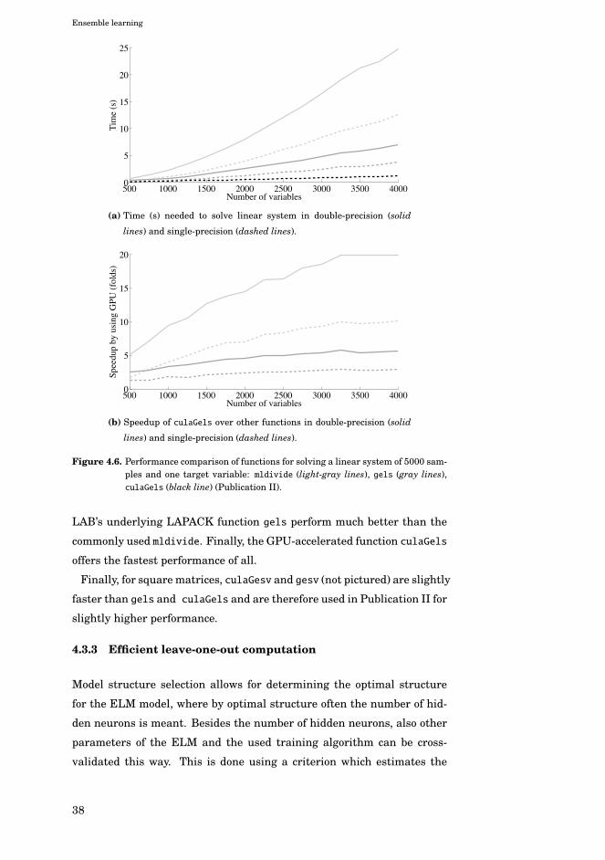
Ensemble learning
500 1000 1500 2000 2500 3000 3500 40000
5
10
15
20
25
Number of variables
Tim
e (s
)
(a) Time (s) needed to solve linear system in double-precision (solid
lines) and single-precision (dashed lines).
500 1000 1500 2000 2500 3000 3500 40000
5
10
15
20
Number of variables
Spee
dup
by u
sing
GPU
(fo
lds)
(b) Speedup of culaGels over other functions in double-precision (solid
lines) and single-precision (dashed lines).
Figure 4.6. Performance comparison of functions for solving a linear system of 5000 sam-ples and one target variable: mldivide (light-gray lines), gels (gray lines),culaGels (black line) (Publication II).
LAB’s underlying LAPACK function gels perform much better than the
commonly used mldivide. Finally, the GPU-accelerated function culaGels
offers the fastest performance of all.
Finally, for square matrices, culaGesv and gesv (not pictured) are slightly
faster than gels and culaGels and are therefore used in Publication II for
slightly higher performance.
4.3.3 Efficient leave-one-out computation
Model structure selection allows for determining the optimal structure
for the ELM model, where by optimal structure often the number of hid-
den neurons is meant. Besides the number of hidden neurons, also other
parameters of the ELM and the used training algorithm can be cross-
validated this way. This is done using a criterion which estimates the
38
Ensemble learning
model generalization capabilities for the varying numbers of neurons in
the hidden layer and the different other possible values for model param-
eters considered.
Minimal overhead in LOO computation by re-using pseudo-inverse Recall
from Equation 2.9, that the HAT matrix needed in the computation of the
leave-one-out error largely consists of the Moore-Penrose generalized in-
verse of the regressor matrix. Using the notations of ELM, HAT = HH†.
Therefore, instead of just computing the solution to the linear system
while training the ELM, combined training and leave-one-out computa-
tion can be optimized by using a method that explicitly computes H†. The
H† computed during training can then be reused in the computation of
the leave-one-out error.
Furthermore, since only the diagonal of the HAT-matrix is needed, it is
sufficient to compute only the diagonal by taking the row-wise dot-product
between H and H†T , and it is not needed to compute HH† in full. There-
fore, the computation of the leave-one-out error then comes at a very low
overhead once the pseudo-inverse is already computed.
Figure 4.7 illustrates this by comparing the running times for train-
ing and combined training and leave-one-out computation. It can be seen
that although by explicitly computing H†, the training procedure becomes
somewhat slower, due to the re-use of H† in the leave-one-out-computation,
combined training and leave-one-out computation can be done about as
fast as just training the model.
Incidentally, because leave-one-out cross-validation virtually comes for
free after training, it is a great alternative to using information criteria
like AIC (Akaike, 1974) and BIC (Schwarz, 1978), which are often used in
situations where cross-validation would be prohibitively slow.
The algorithm for fast training and leave-one-out-based model structure
selection of ELM can then be summarized as in Algorithm 4. Although
this particular example is for cross-validating the number of hidden neu-
rons, the same approach can be used when cross-validating for other com-
binations of model parameters. Also, in case the neurons would be sorted
by relevance first, the algorithm corresponds to OP-ELM (Miche et al.,
2010). In case also an L2-regularization parameter is optimized at each
number of neurons considered, this corresponds to TROP-ELM (Miche
et al., 2011).
39
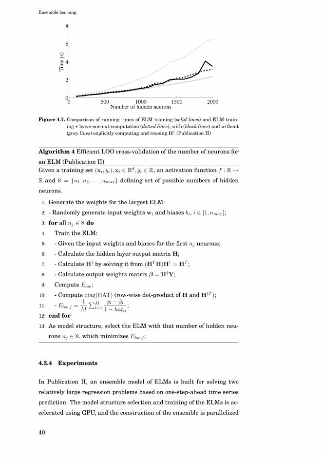
Ensemble learning
0 500 1000 1500 20000
2
4
6
8
Number of hidden neurons
Tim
e (s
)
Figure 4.7. Comparison of running times of ELM training (solid lines) and ELM train-ing + leave-one-out-computation (dotted lines), with (black lines) and without(gray lines) explicitly computing and reusing H† (Publication II)
Algorithm 4 Efficient LOO cross-validation of the number of neurons for
an ELM (Publication II)Given a training set (xi, yi),xi ∈ R
d, yi ∈ R, an activation function f : R �→R and ℵ = {n1, n2, . . . , nmax} defining set of possible numbers of hidden
neurons.
1: Generate the weights for the largest ELM:
2: - Randomly generate input weights wi and biases bi, i ∈ [1, nmax];
3: for all nj ∈ ℵ do
4: Train the ELM:
5: - Given the input weights and biases for the first nj neurons;
6: - Calculate the hidden layer output matrix H;
7: - Calculate H† by solving it from (HTH)H† = HT ;
8: - Calculate output weights matrix β = H†Y;
9: Compute Eloo:
10: - Compute diag(HAT) (row-wise dot-product of H and H†T );
11: - Eloo,j =1
M
∑Mi=1
yi − yi1− hatii
;
12: end for
13: As model structure, select the ELM with that number of hidden neu-
rons nj ∈ ℵ, which minimizes Eloo,j ;
4.3.4 Experiments
In Publication II, an ensemble model of ELMs is built for solving two
relatively large regression problems based on one-step-ahead time series
prediction. The model structure selection and training of the ELMs is ac-
celerated using GPU, and the construction of the ensemble is parallelized
40
Ensemble learning
by distributing the work over multiple CPUs and GPUs. The influence of
the GPU-acceleration and parallelization is measured, and scalability of
the approach is verified on two data sets.
Data The first data set is again the Santa Fe Laser Data time series
(Weigend and Gershenfeld, 1993), which consists of approximately 10000
samples.
The second data set is the ESTSP’08 Competition data set number 33,
which consists of approximately 30000 samples, and is computationally
also more challenging due to the size of the regressor needed (Olteanu,
2008; Kourentzes and Crone, 2008).
Experimental parameters The samples from the time series are obtained
using respectively 12, and 168 time steps for the Santa Fe Laser data and
ESTSP’08 Competition data, after which the data is randomly divided
into 85% for training and 15% for testing.
The ELMs have their number of neurons optimized using efficient leave-
one-out cross-validation and for diversity, each ELM uses random vari-
ables from the regressor. The ensemble weights are determined through
leave-one-out initialization and remain fixed.
The effect of GPU-acceleration and parallelization on the performance
is consequently measured by varying the function used in model structure
selection and training, as well as varying the number of MATLAB workers
(i.e. threads). See Publication II for more details.
Effect of GPU-acceleration and used function Table 4.3 summarizes the
results of the experiments performed in Publication II, and clearly shows
the effect of the GPU-acceleration and the used function.
It can be seen that generally mldiv and gesv achieve similar perfor-
mances, while both the use of single-precision and the use of GPU sig-
nificantly speed up the ensemble.
Effect of number of workers on computational time Table 4.3 and Fig-
ure 4.8 summarize the influence of the number of MATLAB workers on
the ensemble performance.
When not using any explicit parallelization through MATLAB workers
(i.e. the line N = 0 in Table 4.3), the differences between using CPU
and GPU are relatively modest. This is due to the fact that for mldiv
and gesv, MATLAB automatically parallelizes the computation over the
3available from http://research.ics.aalto.fi/eiml/datasets.shtml
41
Ensemble learning
multiple CPU cores of the Intel Core i7 920, and can therefore keep up
quite well with the single GPU being used for culaGesv.
However, when explicitly parallelizing the computation over N cores
and GPUs, the difference between CPU and GPU significantly increases.
Overall, the experiments show a 3.3 times speedup over the typical
double-precision implementation of an ensemble of ELMs, by using the
GPU to speed up the slowest part of the algorithm, and parallelizing
across multiple CPU cores and GPUs (i.e. t(mldivdp) / t(culaGesvsp)).
Effect of number of models on accuracy Finally, Figure 4.9 shows the
influence of the number of models in the ensemble on the accuracy of
the ensemble. Similarly to Publication I, the results show that the more
models are added to the ensemble, the more accurate it gets.
Discussion This fact alone (that more models is generally better in en-
semble models), is additional justification for the approach proposed in Pub-
lication II. By parallelization and GPU-acceleration of the ensemble, it is
possible to train more models and to train them faster, which results in a
more accurate model that can be obtained in less time.
Some interesting questions to explore therefore would be: how fast can
an ensemble model of a particular accuracy be obtained? Of course the
easiest way to speed up the ensemble would be to evaluate each model
on its own dedicated node, but even then, would it be possible to further
speed up the ensemble model while retaining or improving accuracy?
One possibility would be to parallelize other parts of the ELM, like the
multiplication of the hidden layer weights and the inputs, as has been
done in (He et al., 2011) and (He et al., 2013).
Another interesting direction to explore would be to make the ELMs
more effective and accurate by an altered weight scheme (which is ex-
plored in Publication V), or by trading off speed for accuracy in the indi-
vidual ELMs (which is explored in Publication VI) and ensembling more
of them.
Before giving an overview of those publications though, the next chapter
will highlight some contributions of the thesis to variable selection.
42
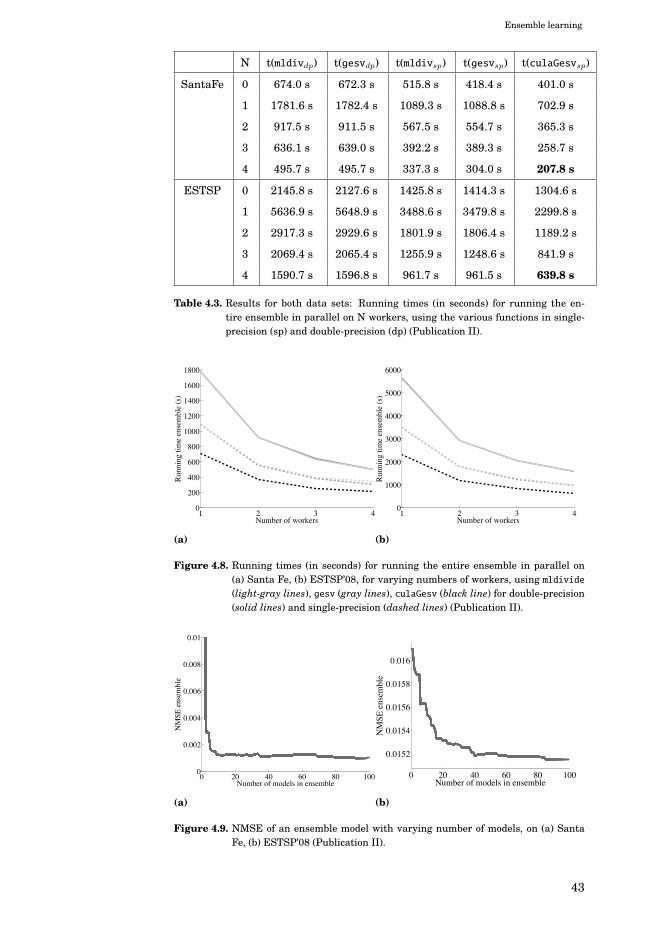
Ensemble learning
N t(mldivdp) t(gesvdp) t(mldivsp) t(gesvsp) t(culaGesvsp)
SantaFe 0 674.0 s 672.3 s 515.8 s 418.4 s 401.0 s
1 1781.6 s 1782.4 s 1089.3 s 1088.8 s 702.9 s
2 917.5 s 911.5 s 567.5 s 554.7 s 365.3 s
3 636.1 s 639.0 s 392.2 s 389.3 s 258.7 s
4 495.7 s 495.7 s 337.3 s 304.0 s 207.8 s
ESTSP 0 2145.8 s 2127.6 s 1425.8 s 1414.3 s 1304.6 s
1 5636.9 s 5648.9 s 3488.6 s 3479.8 s 2299.8 s
2 2917.3 s 2929.6 s 1801.9 s 1806.4 s 1189.2 s
3 2069.4 s 2065.4 s 1255.9 s 1248.6 s 841.9 s
4 1590.7 s 1596.8 s 961.7 s 961.5 s 639.8 s
Table 4.3. Results for both data sets: Running times (in seconds) for running the en-tire ensemble in parallel on N workers, using the various functions in single-precision (sp) and double-precision (dp) (Publication II).
1 2 3 40
200
400
600
800
1000
1200
1400
1600
1800
Number of workers
Run
ning
tim
e en
sem
ble
(s)
(a)
1 2 3 40
1000
2000
3000
4000
5000
6000
Number of workers
Run
ning
tim
e en
sem
ble
(s)
(b)
Figure 4.8. Running times (in seconds) for running the entire ensemble in parallel on(a) Santa Fe, (b) ESTSP’08, for varying numbers of workers, using mldivide(light-gray lines), gesv (gray lines), culaGesv (black line) for double-precision(solid lines) and single-precision (dashed lines) (Publication II).
0 20 40 60 80 1000
0.002
0.004
0.006
0.008
0.01
Number of models in ensemble
NM
SE e
nsem
ble
(a)
0 20 40 60 80 100
0.0152
0.0154
0.0156
0.0158
0.016
Number of models in ensemble
NM
SE e
nsem
ble
(b)
Figure 4.9. NMSE of an ensemble model with varying number of models, on (a) SantaFe, (b) ESTSP’08 (Publication II).
43

Ensemble learning
44
5. Variable Selection
“And what is good, Phaedrus,
And what is not good–
Need we ask anyone to tell us these things?”
– Robert M. Pirsig,
Zen and the Art of Motorcycle Maintenance
Variable selection is a central issue in machine learning. The higher
the dimensionality of the data, the more samples are needed to reliably
train a model. This is sometimes referred to as the curse of dimension-
ality. Therefore, given the often limited number of training samples, it is
important that the dimensionality is sufficiently reduced (without losing
too much information) such that a reliable model can be trained.
This chapter introduces the basic concepts of variable selection, and
highlights the related contributions of this thesis: an ELM-based method
for variable selection (Publication III); a (multi-)GPU-accelerated Delta
Test criterion used as criterion in a parallelized genetic algorithm for vari-
able selection (Publication IV); and finally, a new weight scheme for ELM
that results in more effective and efficient neural networks, and makes
the ELM more robust to irrelevant and noisy variables (Publication V).
5.1 Variable selection
5.1.1 Motivation
Due to the technological developments of the past decades, it is easier
than ever to gather large amounts of data. The grand challenge, then,
is to extract relevant information from this data in order to gain useful
knowledge.
45
Variable Selection
Part of that challenge is being able to scale the methods to the size of
modern data sets (which was partly the focus of Chapter 4). However,
besides challenges in scaling due to the large amount of samples in mod-
ern data sets, another challenge is posed by their high dimensionality.
Namely, the high dimensionality of modern data sets poses a problem
when trying to train reliable and accurate models due to the curse of di-
mensionality (Bellman, 1961; Verleysen et al., 2003): the number of sam-
ples required to be able to train an accurate model scales exponentially
with the dimensionality of the input space (i.e. the dimensionality of the
data). Therefore, it is important to reduce the dimensionality as much as
possible, so that more accurate models may be trained.
5.1.2 Dimensionality reduction
Feature extraction Although the data is high-dimensional, it is often not
evenly spread throughout the input space. Instead, the samples will lie
on some lower-dimensional manifold embedded in that high-dimensional
space. Therefore, one strategy for handling high-dimensional data is by
dimensionality reduction through feature extraction. Here, the goal is to
find an alternate representation of the data by extracting its latent fea-
tures, and representing the data in terms of these features. For example,
if the data lies linear in some linear subspace, then Principal Component
Analysis (PCA) can be used to obtain a more compact representation (Jol-
liffe, 2002). Note however, that this by itself does not take into account
the relevance of a latent feature for predicting the output, as it is unsu-
pervised.
Variable selection Contrary to unsupervised feature extraction, variable
selection (Guyon and Elisseeff, 2003) is supervised and does take into ac-
count the relevance of a variable for predicting the output1. Through a
search algorithm, the variable subset is optimized according to a statisti-
cal criterion measuring the quality of the variable subset.
Besides improving model accuracy, another motivation for performing
variable selection may be interpretability of the models and gaining a
better understanding about the problem at hand. For example, in gene
1Of course, feature extraction and variable selection can be combined, and ex-tracted features can become input variables to some model. In this work, it isassumed that feature extraction has already taken place, and the focus is on se-lecting the best variable subset, given a set of input variables. The terms variableselection and feature selection will be used interchangeably.
46
Variable Selection
expression analysis, variable selection can help identifying those genes
that are relevant for predicting whether a patient is sick, and are there-
fore likely to play a role in the disease itself (Guyon and Elisseeff, 2003).
Finally, sometimes it is very expensive to obtain new samples and mea-
sure particular variables. Therefore, through variable selection, money
and effort can be saved by only measuring and collecting the most rele-
vant variables.
5.1.3 Variable selection methods
Approaches Several main approaches for variable selection are distin-
guished in (Guyon and Elisseeff, 2003): wrapper methods, filter methods,
and embedded methods, which will be described shortly below.
Filter approach In filter approaches, as the name suggests, the variable
subset is filtered before being passed on to a model for learning, and some
criterion is used to evaluate the quality of a particular subset of variables.
For example, as a criterion, mutual information (MacKay, 2003; Kraskov
et al., 2004) can be used to estimate how much information a particular
variable subset contains about the targets (Rossi et al., 2006; François
et al., 2007; Verleysen et al., 2009). The mutual information criterion was
used in the baseline variable selection experiments of Publication III.
Another criterion that can be used for variable selection is the Delta Test
(Eirola et al., 2008; Eirola, 2014; Sovilj, 2014). The Delta Test is a noise
variance estimator, which indicates the performance a non-linear model
can possibly attain, given particular data. The Delta Test criterion was
used in Publication IV.
As a final example, a filter method based on Least Angle Regression
(LARS) (Efron et al., 2003) could rank the variables according to rele-
vance, and return a subset of the most relevant variables. This approach
is included in the baseline experiments of Publication III.
Wrapper approach Whereas filter strategies use some statistical crite-
rion for variable selection, in the wrapper strategy, the model is used di-
rectly for evaluating the quality of a variable subset. For example, an
Extreme Learning Machine could be built with many different variable
subsets, and have its generalization performance estimated using fast
leave-one-out cross-validation. The variable subset that achieves mini-
mum leave-one-out error will then be used for building the final ELM.
Therefore, it can be seen as some sort of model structure selection. The
47
Variable Selection
advantage of wrapper strategies is that, since the actual model is used,
the feature subset is likely to be better-optimized for that model. How-
ever, since the actual model needs to be trained, depending on the model,
and the fact that there might not be a way to efficiently estimate the gen-
eralization performance, wrapper strategies can be computationally very
expensive. Furthermore, care should be taken not to overfit during the
feature selection process (Reunanen, 2003).
Embedded approach In the embedded approach, the learning machine
itself incorporates variable selection as part of its training, and selection
is not performed explicitly using a wrapper or filter approach. Although it
could be argued that explicit variable selection in the training algorithm is
actually model structure selection using a wrapper approach (rather than
training and an embedded approach), it is useful to distinguish the em-
bedded variable selection approach from filter and wrapper approaches,
as the learning method might implicitly perform variable selection as a
result of its structure (for example, like in the Binary ELM and Ternary
ELM proposed in Publication V).
Search methods Besides a statistical criterion like mutual information,
or an estimated performance of a model, a method is needed to explore
the solution space of all possible variable selections in a systematic way,
especially considering that the number of possible variable subsets is ex-
ponential in the number of variables.
One possibility is to use a local search method and, starting from a par-
ticular solution in the solution space, optimize the solution by repeatedly
evaluating and jumping to neighboring candidate solutions, until an opti-
mum is found. For example, Forward selection (Hastie et al., 2001) starts
from an empty variable subset, and repeatedly adds the variable that
improves the criterion the most. Similarly, Backward selection (Hastie
et al., 2001) starts from the full variable subset, and repeatedly removes
the variable that deteriorates the criterion the least. Finally, Forward-
Backward selection allows both adding and removing variables at each
step (Hastie et al., 2001). These local search methods are used in the
baseline experiments of Publication III, in combination with the mutual
information criterion.
Another possibility, which is explored in Publication IV, is to use a ge-
netic algorithm to explore the space of possible solutions. Here, the candi-
date solutions are encoded in a population of individuals and consequently
optimized through an evolution-like algorithm.
48
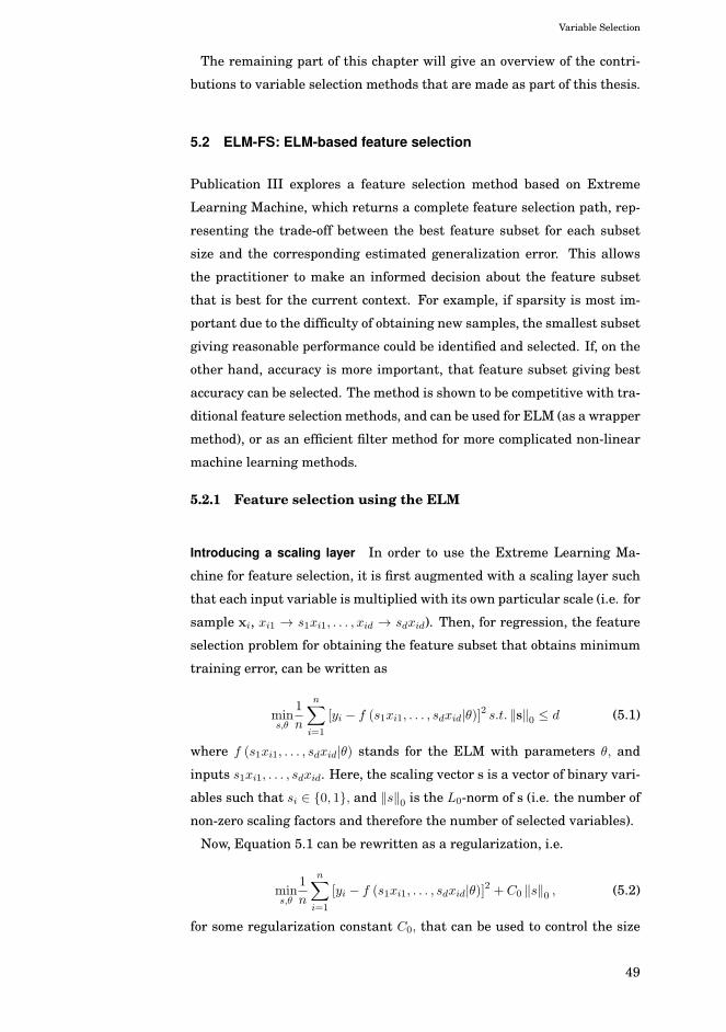
Variable Selection
The remaining part of this chapter will give an overview of the contri-
butions to variable selection methods that are made as part of this thesis.
5.2 ELM-FS: ELM-based feature selection
Publication III explores a feature selection method based on Extreme
Learning Machine, which returns a complete feature selection path, rep-
resenting the trade-off between the best feature subset for each subset
size and the corresponding estimated generalization error. This allows
the practitioner to make an informed decision about the feature subset
that is best for the current context. For example, if sparsity is most im-
portant due to the difficulty of obtaining new samples, the smallest subset
giving reasonable performance could be identified and selected. If, on the
other hand, accuracy is more important, that feature subset giving best
accuracy can be selected. The method is shown to be competitive with tra-
ditional feature selection methods, and can be used for ELM (as a wrapper
method), or as an efficient filter method for more complicated non-linear
machine learning methods.
5.2.1 Feature selection using the ELM
Introducing a scaling layer In order to use the Extreme Learning Ma-
chine for feature selection, it is first augmented with a scaling layer such
that each input variable is multiplied with its own particular scale (i.e. for
sample xi, xi1 → s1xi1, . . . , xid → sdxid). Then, for regression, the feature
selection problem for obtaining the feature subset that obtains minimum
training error, can be written as
mins,θ
1
n
n∑i=1
[yi − f (s1xi1, . . . , sdxid|θ)]2 s.t. ‖s‖0 ≤ d (5.1)
where f (s1xi1, . . . , sdxid|θ) stands for the ELM with parameters θ, and
inputs s1xi1, . . . , sdxid. Here, the scaling vector s is a vector of binary vari-
ables such that si ∈ {0, 1}, and ‖s‖0 is the L0-norm of s (i.e. the number of
non-zero scaling factors and therefore the number of selected variables).
Now, Equation 5.1 can be rewritten as a regularization, i.e.
mins,θ
1
n
n∑i=1
[yi − f (s1xi1, . . . , sdxid|θ)]2 + C0 ‖s‖0 , (5.2)
for some regularization constant C0, that can be used to control the size
49
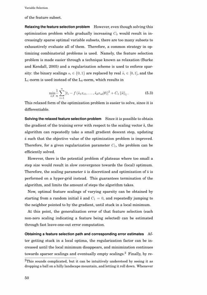
Variable Selection
of the feature subset.
Relaxing the feature selection problem However, even though solving this
optimization problem while gradually increasing C0 would result in in-
creasingly sparse optimal variable subsets, there are too many subsets to
exhaustively evaluate all of them. Therefore, a common strategy in op-
timizing combinatorial problems is used. Namely, the feature selection
problem is made easier through a technique known as relaxation (Burke
and Kendall, 2005) and a regularization scheme is used to enforce spar-
sity: the binary scalings si ∈ {0, 1} are replaced by real si ∈ [0, 1], and the
L1-norm is used instead of the L0-norm, which results in
mins,θ
1
n
n∑i=1
[ti − f (s1xi1, . . . , sdxid|θ)]2 + C1 ‖s‖1 . (5.3)
This relaxed form of the optimization problem is easier to solve, since it is
differentiable.
Solving the relaxed feature selection problem Since it is possible to obtain
the gradient of the training error with respect to the scaling vector s, the
algorithm can repeatedly take a small gradient descent step, updating
s such that the objective value of the optimization problem is improved.
Therefore, for a given regularization parameter C1, the problem can be
efficiently solved.
However, there is the potential problem of plateaus where too small a
step size would result in slow convergence towards the (local) optimum.
Therefore, the scaling parameter s is discretized and optimization of s is
performed on a hyper-grid instead. This guarantees termination of the
algorithm, and limits the amount of steps the algorithm takes.
Now, optimal feature scalings of varying sparsity can be obtained by
starting from a random initial s and C1 = 0, and repeatedly jumping to
the neighbor pointed to by the gradient, until stuck in a local minimum.
At this point, the generalization error of that feature selection (each
non-zero scaling indicating a feature being selected) can be estimated
through fast leave-one-out error computation.
Obtaining a feature selection path and corresponding error estimates Af-
ter getting stuck in a local optima, the regularization factor can be in-
creased until the local minimum disappears, and minimization continues
towards sparser scalings and eventually empty scalings.2 Finally, by re-2This sounds complicated, but it can be intuitively understood by seeing it asdropping a ball on a hilly landscape mountain, and letting it roll down. Whenever
50
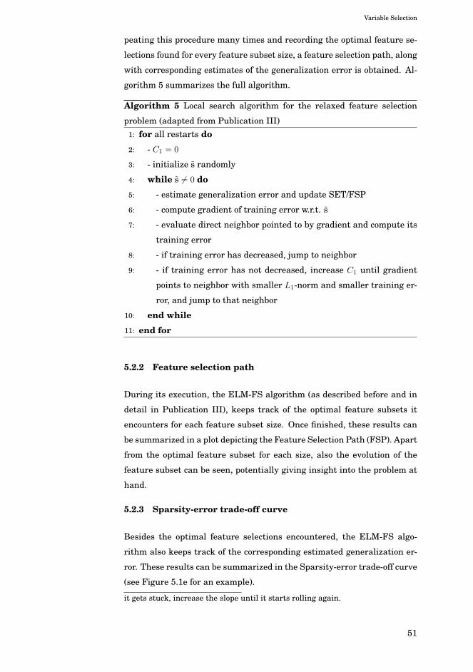
Variable Selection
peating this procedure many times and recording the optimal feature se-
lections found for every feature subset size, a feature selection path, along
with corresponding estimates of the generalization error is obtained. Al-
gorithm 5 summarizes the full algorithm.
Algorithm 5 Local search algorithm for the relaxed feature selection
problem (adapted from Publication III)1: for all restarts do
2: - C1 = 0
3: - initialize s randomly
4: while s = 0 do
5: - estimate generalization error and update SET/FSP
6: - compute gradient of training error w.r.t. s
7: - evaluate direct neighbor pointed to by gradient and compute its
training error
8: - if training error has decreased, jump to neighbor
9: - if training error has not decreased, increase C1 until gradient
points to neighbor with smaller L1-norm and smaller training er-
ror, and jump to that neighbor
10: end while
11: end for
5.2.2 Feature selection path
During its execution, the ELM-FS algorithm (as described before and in
detail in Publication III), keeps track of the optimal feature subsets it
encounters for each feature subset size. Once finished, these results can
be summarized in a plot depicting the Feature Selection Path (FSP). Apart
from the optimal feature subset for each size, also the evolution of the
feature subset can be seen, potentially giving insight into the problem at
hand.
5.2.3 Sparsity-error trade-off curve
Besides the optimal feature selections encountered, the ELM-FS algo-
rithm also keeps track of the corresponding estimated generalization er-
ror. These results can be summarized in the Sparsity-error trade-off curve
(see Figure 5.1e for an example).
it gets stuck, increase the slope until it starts rolling again.
51
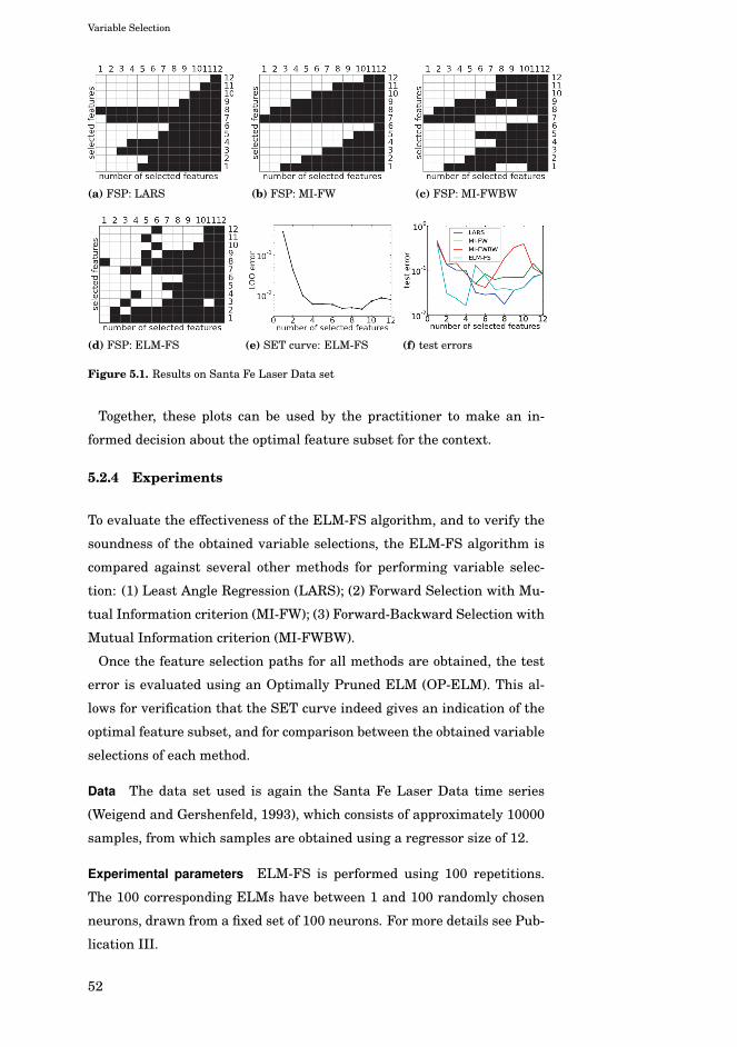
Variable Selection
(a) FSP: LARS (b) FSP: MI-FW (c) FSP: MI-FWBW
(d) FSP: ELM-FS (e) SET curve: ELM-FS (f) test errors
Figure 5.1. Results on Santa Fe Laser Data set
Together, these plots can be used by the practitioner to make an in-
formed decision about the optimal feature subset for the context.
5.2.4 Experiments
To evaluate the effectiveness of the ELM-FS algorithm, and to verify the
soundness of the obtained variable selections, the ELM-FS algorithm is
compared against several other methods for performing variable selec-
tion: (1) Least Angle Regression (LARS); (2) Forward Selection with Mu-
tual Information criterion (MI-FW); (3) Forward-Backward Selection with
Mutual Information criterion (MI-FWBW).
Once the feature selection paths for all methods are obtained, the test
error is evaluated using an Optimally Pruned ELM (OP-ELM). This al-
lows for verification that the SET curve indeed gives an indication of the
optimal feature subset, and for comparison between the obtained variable
selections of each method.
Data The data set used is again the Santa Fe Laser Data time series
(Weigend and Gershenfeld, 1993), which consists of approximately 10000
samples, from which samples are obtained using a regressor size of 12.
Experimental parameters ELM-FS is performed using 100 repetitions.
The 100 corresponding ELMs have between 1 and 100 randomly chosen
neurons, drawn from a fixed set of 100 neurons. For more details see Pub-
lication III.
52
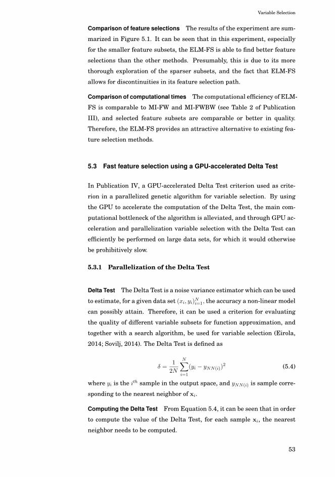
Variable Selection
Comparison of feature selections The results of the experiment are sum-
marized in Figure 5.1. It can be seen that in this experiment, especially
for the smaller feature subsets, the ELM-FS is able to find better feature
selections than the other methods. Presumably, this is due to its more
thorough exploration of the sparser subsets, and the fact that ELM-FS
allows for discontinuities in its feature selection path.
Comparison of computational times The computational efficiency of ELM-
FS is comparable to MI-FW and MI-FWBW (see Table 2 of Publication
III), and selected feature subsets are comparable or better in quality.
Therefore, the ELM-FS provides an attractive alternative to existing fea-
ture selection methods.
5.3 Fast feature selection using a GPU-accelerated Delta Test
In Publication IV, a GPU-accelerated Delta Test criterion used as crite-
rion in a parallelized genetic algorithm for variable selection. By using
the GPU to accelerate the computation of the Delta Test, the main com-
putational bottleneck of the algorithm is alleviated, and through GPU ac-
celeration and parallelization variable selection with the Delta Test can
efficiently be performed on large data sets, for which it would otherwise
be prohibitively slow.
5.3.1 Parallelization of the Delta Test
Delta Test The Delta Test is a noise variance estimator which can be used
to estimate, for a given data set (xi, yi)Ni=1, the accuracy a non-linear model
can possibly attain. Therefore, it can be used a criterion for evaluating
the quality of different variable subsets for function approximation, and
together with a search algorithm, be used for variable selection (Eirola,
2014; Sovilj, 2014). The Delta Test is defined as
δ =1
2N
N∑i=1
(yi − yNN(i))2 (5.4)
where yi is the ith sample in the output space, and yNN(i) is sample corre-
sponding to the nearest neighbor of xi.
Computing the Delta Test From Equation 5.4, it can be seen that in order
to compute the value of the Delta Test, for each sample xi, the nearest
neighbor needs to be computed.
53
Variable Selection
Figure 5.2. Division of nearest-neighbor computations in Multi-GPU-accelerated DeltaTest
The approach used in Publication IV is the brute-force method for com-
puting the nearest neighbors, which involves computing an N×N distance
matrix. Once computed, for each xi, the index of the nearest neighbor can
be determined from the distance matrix, and the Delta Test criterion can
be computed. Since the approach involves computing an N × N distance
matrix, for modern data sets this can be quite challenging, and strategies
are desired for making the computation feasible.
Delta Test at scale The Delta Test is implemented on GPU using the ex-
cellent GPU-accelerated nearest-neighbor library by (Garcia et al., 2008,
2010), and for e.g. 17000 samples and with a 1000 variables, a 40-50×speedup can be obtained over using the CPU.
Although not exploited in Publication IV, the nearest-neighbor problem
is embarrassingly parallel (i.e. the nearest neighbor for each point can be
determined independently). Therefore, the Delta Test computation can be
further accelerated by dividing the nearest-neighbor computations over
multiple GPUs, and let each GPU determine the nearest neighbor for
part of the data set (see Figure 5.2). Experiments show that for a vari-
able selection problem with 100k samples and 274 dimensions, on a sin-
gle machine with 5 GPUs, an additional speedup of roughly ~4× can be
achieved.
Discussion The (multi-)GPU-acceleration of the Delta Test makes it a
very attractive criterion to use as a filter approach for ELM, either in
combination with a local search method like Forward-Backward search as
encountered in Publication III, or in combination with genetic algorithm
like in Publication IV.
54
Variable Selection
5.4 Binary/Ternary ELM
Although in theory, ELM is a universal approximator, in practice, there
are a limited number of samples available, and there is a risk of overfit-
ting. Therefore, the functional approximation should use as limited num-
ber of neurons as possible, and the hidden layer should extract and retain
as much information as possible from the input samples. The question
then becomes, which neurons work well together to extract as much use-
ful information as possible?
Publication V proposes two new ELM variants: Binary ELM, with a
weight initialization scheme based on {0,1}-weights; and Ternary ELM,
with a weight initialization scheme based on {-1,0,1}-weights. This weight
initialization scheme results in features from very different subspaces
and therefore, each neuron extracts more diverse information from the
inputs than neurons with completely random features traditionally used
in ELM. Experiments show that indeed ELMs with ternary weights gen-
erally achieve lower test error, and additionally are more robust to irrel-
evant and noisy variables. Since only the weight generation scheme is
adapted, the computational time of the ELM is unaffected, and the im-
proved accuracy, added robustness and the implicit variable selection of
Binary ELM and Ternary ELM come for free.
5.4.1 Improved hidden layer weights
Traditionally, the hidden layer weights of the ELM are initialized ran-
domly, with weights and biases drawn from a continuous probability dis-
tribution. For example, a uniform distribution on interval [-3, 3], or a
Gaussian distribution with certain variance σ. These hidden layer weights,
together with the transfer function and the data, result in particular ac-
tivations of the hidden layer.
A typical transfer function (like sigmoid) takes the inner product of the
weight and a sample, adds a bias, and transforms the result in a nonlinear
way, i.e. it looks like f (〈wi,x〉+ bi) ,where 〈wi,x〉 is the inner product of
weight wi and x is the input vector. Since〈wi,x〉 = |wi||x| cos θ, it can be
seen that the typical activation of f depends on:
1. the expected length of wi
2. the expected length of x
3. the angles θ between the weights and the samples
55
Variable Selection
5.4.1.1 Orthogonal weights?
An important factor affecting the diversity of the hidden neuron activa-
tions consists of the angles between the hidden layer weights and the sam-
ples. Therefore, the primary strategy that comes to mind for improving
the diversity of the hidden neuron activations is to improve the diversity
by taking weights that are mutually orthogonal (e.g. M d-dimensional ba-
sis vectors, randomly rotated in the d-dimensional space, where d is the
dimension of the input space).
However, experiments suggested that this strategy does not significantly
improve accuracy. Presumably, for the tested cases, the random weight
scheme of ELM already covers the possible weight space pretty well (fur-
thermore, randomly drawn zero-mean vectors are close to orthogonal in
the first place).
5.4.1.2 Binary weight scheme
Another way to improve the diversity of the weights is by having each
of them work in a different subspace (e.g. each weight vector has differ-
ent subset of variables as input). This strategy turns out to significantly
improve accuracy, at no extra computational cost.
In the binary weight scheme (see Algorithm 6, Figure 5.3 and Figure
5.4), binary weights are generated and added, starting from the spars-
est subspace, until the desired amount of weights is reached. Weights
within a subspace are added in random order to avoid bias towards par-
ticular variables. Once generated, the weights are normalized or adapted
through Batch-Intrinsic Plasticity (BIP) pre-training (see Section 3.4.4
and Section 5.4.2) to ensure the neurons are activated in the right region
(neither completely in the linear part, nor in the saturated part).
5.4.1.3 Ternary weight scheme
The ternary weight scheme (see Figure 5.3 and 5.4) is identical to the
binary weight scheme, except that due to the sign of the weights there
are more possible weights for each possible subspace, rather than a single
one, allowing for richer weights.
5.4.2 Motivation for BIP pre-training
Since for given weight w and input x, the expected value of |w||x| deter-
mines which part of the transfer function is activated most, the norm of
the weights is important and affects the performance of ELM. Of course,
56

Variable Selection
Algorithm 6 Binary weight scheme, with M the desired number of hid-
den neurons, n the dimension of the subspaces in which to generate
weights, and d the number of inputs1: Generate ELM:
2: n = 1;
3: while number of neurons ≤ M and n ≤ d do
4: - Generate the(dn
)possible assignments of n ones to d positions
5: - Shuffle the order of the generated weights to avoid bias to certain
inputs due to the scheme used to generate the(dn
)assignments
6: - Add the generated weights (up to a maximum of M neurons)
7: - n = n+ 1;
8: end while
9: - Normalize the norm of the weights, such that they are unit length.
1 var
2 vars
3 vars
⎡⎢⎢⎢⎢⎢⎢⎢⎢⎢⎢⎢⎢⎢⎢⎢⎢⎢⎢⎢⎢⎢⎢⎢⎢⎢⎢⎢⎢⎢⎣
1 0 0 0 0
0 1 0 0 0
0 0 1 0 0
0 0 0 1 0
0 0 0 0 1
1 1 0 0 0
1 0 1 0 0
1 0 0 1 0
1 0 0 0 1...
......
......
0 0 0 1 1
etc.
⎤⎥⎥⎥⎥⎥⎥⎥⎥⎥⎥⎥⎥⎥⎥⎥⎥⎥⎥⎥⎥⎥⎥⎥⎥⎥⎥⎥⎥⎥⎦
(a) binary weight scheme
1 var
2 vars
3 vars
⎡⎢⎢⎢⎢⎢⎢⎢⎢⎢⎢⎢⎢⎢⎢⎢⎢⎢⎢⎢⎢⎢⎢⎢⎢⎢⎢⎢⎢⎢⎣
+1 0 0 0
−1 0 0 0
0 +1 0 0
0 −1 0 0...
......
...
+1 +1 0 0
+1 −1 0 0
−1 +1 0 0
−1 −1 0 0...
......
...
0 0 −1 −1
⎤⎥⎥⎥⎥⎥⎥⎥⎥⎥⎥⎥⎥⎥⎥⎥⎥⎥⎥⎥⎥⎥⎥⎥⎥⎥⎥⎥⎥⎥⎦
(b) ternary weight scheme
Figure 5.3. Illustration of the binary and ternary weight schemes. Note that weights areadded starting from the sparsest subspace, and from each subspace they areadded in random order to avoid bias towards particular variables.
57
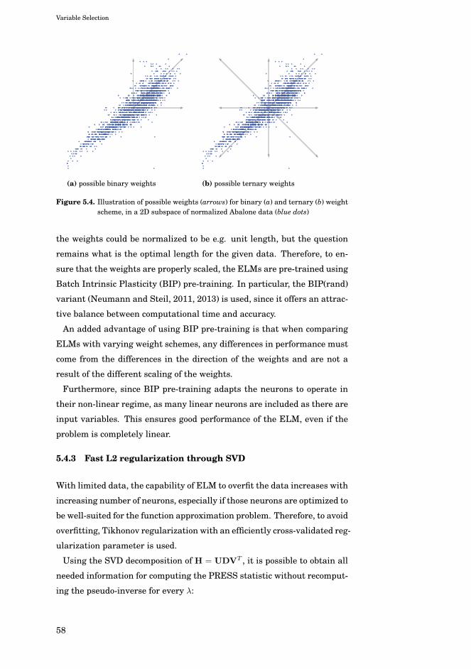
Variable Selection
(a) possible binary weights (b) possible ternary weights
Figure 5.4. Illustration of possible weights (arrows) for binary (a) and ternary (b) weightscheme, in a 2D subspace of normalized Abalone data (blue dots)
the weights could be normalized to be e.g. unit length, but the question
remains what is the optimal length for the given data. Therefore, to en-
sure that the weights are properly scaled, the ELMs are pre-trained using
Batch Intrinsic Plasticity (BIP) pre-training. In particular, the BIP(rand)
variant (Neumann and Steil, 2011, 2013) is used, since it offers an attrac-
tive balance between computational time and accuracy.
An added advantage of using BIP pre-training is that when comparing
ELMs with varying weight schemes, any differences in performance must
come from the differences in the direction of the weights and are not a
result of the different scaling of the weights.
Furthermore, since BIP pre-training adapts the neurons to operate in
their non-linear regime, as many linear neurons are included as there are
input variables. This ensures good performance of the ELM, even if the
problem is completely linear.
5.4.3 Fast L2 regularization through SVD
With limited data, the capability of ELM to overfit the data increases with
increasing number of neurons, especially if those neurons are optimized to
be well-suited for the function approximation problem. Therefore, to avoid
overfitting, Tikhonov regularization with an efficiently cross-validated reg-
ularization parameter is used.
Using the SVD decomposition of H = UDVT , it is possible to obtain all
needed information for computing the PRESS statistic without recomput-
ing the pseudo-inverse for every λ:
58

Variable Selection
Y = Hβ
= H(HTH+ λI)−1HTY
= HV(D2 + λI)−1DUTY
= UDVTV(D2 + λI)−1DUTY
= UD(D2 + λI)−1DUTY
= HAT ·Y
where D(D2 + λI)−1D is a diagonal matrix with d2iid2ii+λ
as the ith diagonal
entry. Now
MSETR-PRESS =1
N
N∑i=1
(yi − yi1− hatii
)2
=1
N
N∑i=1
(yi − yi
1− hi·(HTH+ λI)−1hTi·
)2
=1
N
N∑i=1
⎛⎝ yi − yi
1− ui·(
d2iid2ii+λ
)uTi·
⎞⎠
2
where hi· and ui· are the ith row vectors of H and U, respectively. Now, the
Tikhonov-regularized PRESS and corresponding λ can be computed using
Algorithm 7, where A◦B refers to the element-wise product of matrices A
and B (Schur product). Due to the convex nature of criterion MSETR-PRESS
with respect to regularization parameter λ, the Nelder-Mead procedure
used for optimizing λ converges quickly in practice (Nelder and Mead,
1965; Lagarias et al., 1998). This efficient optimization of the regulariza-
tion parameter for ELM, by incorporating it in the SVD decomposition
first appeared (in slightly different form) in (Miche et al., 2011).
5.4.4 Experiments
In Publication V, for evaluating the performance of the gaussian, binary
and ternary weight schemes, their resulting performance in terms of accu-
racy is compared on various regression tasks. Since the weight range de-
termines the typical activation of the transfer function (remember 〈wi,x〉 =|wi||x| cos θ), the ELMs are pre-trained using Batch Intrinsic Plasticity
pre-training. Any performance difference between weight schemes will be
a result of the different directions of the weights. Furthermore, since BIP
pre-training adapts the neurons to operate in their non-linear regime, as
many linear neurons are included as there are input variables. This en-
sures good performance of the ELM, even if the problem is completely
59
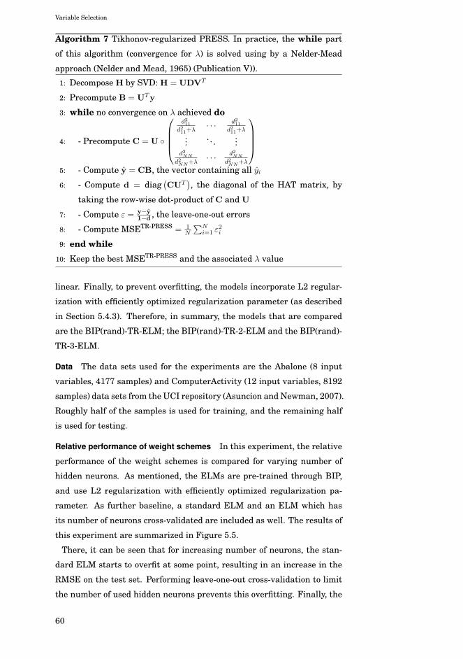
Variable Selection
Algorithm 7 Tikhonov-regularized PRESS. In practice, the while part
of this algorithm (convergence for λ) is solved using by a Nelder-Mead
approach (Nelder and Mead, 1965) (Publication V)).
1: Decompose H by SVD: H = UDVT
2: Precompute B = UTy
3: while no convergence on λ achieved do
4: - Precompute C = U ◦
⎛⎜⎜⎜⎝
d211d211+λ
· · · d211d211+λ
... . . . ...d2NN
d2NN+λ· · · d2NN
d2NN+λ
⎞⎟⎟⎟⎠
5: - Compute y = CB, the vector containing all yi6: - Compute d = diag
(CUT
), the diagonal of the HAT matrix, by
taking the row-wise dot-product of C and U
7: - Compute ε = y−y1−d , the leave-one-out errors
8: - Compute MSETR-PRESS = 1N
∑Ni=1 ε
2i
9: end while
10: Keep the best MSETR-PRESS and the associated λ value
linear. Finally, to prevent overfitting, the models incorporate L2 regular-
ization with efficiently optimized regularization parameter (as described
in Section 5.4.3). Therefore, in summary, the models that are compared
are the BIP(rand)-TR-ELM; the BIP(rand)-TR-2-ELM and the BIP(rand)-
TR-3-ELM.
Data The data sets used for the experiments are the Abalone (8 input
variables, 4177 samples) and ComputerActivity (12 input variables, 8192
samples) data sets from the UCI repository (Asuncion and Newman, 2007).
Roughly half of the samples is used for training, and the remaining half
is used for testing.
Relative performance of weight schemes In this experiment, the relative
performance of the weight schemes is compared for varying number of
hidden neurons. As mentioned, the ELMs are pre-trained through BIP,
and use L2 regularization with efficiently optimized regularization pa-
rameter. As further baseline, a standard ELM and an ELM which has
its number of neurons cross-validated are included as well. The results of
this experiment are summarized in Figure 5.5.
There, it can be seen that for increasing number of neurons, the stan-
dard ELM starts to overfit at some point, resulting in an increase in the
RMSE on the test set. Performing leave-one-out cross-validation to limit
the number of used hidden neurons prevents this overfitting. Finally, the
60

Variable Selection
proposed methods generally achieve much better RMSE than the basic
ELM variants and generally, ternary weights outperform weights drawn
from a Gaussian distribution, while binary weights perform worse than
ternary and Gaussian weights for large number of neurons.
0 100 200 300 400 500 600 700 800 900 1,0000.62
0.63
0.64
0.65
0.66
0.67
0.68
0.69
0.7
#hidden neurons
RM
SE
ELMLOO(CV)-ELMBIP(rand)-TR-ELMBIP(rand)-TR-2-ELMBIP(rand)-TR-3-ELM
(a) Abalone
0 100 200 300 400 500 600 700 800 900 1,000
0.14
0.16
0.18
0.2
0.22
0.24
0.26
0.28
0.3
0.32
#hidden neurons
RM
SE
ELMLOO(CV)-ELMBIP(rand)-TR-ELMBIP(rand)-TR-2-ELMBIP(rand)-TR-3-ELM
(b) ComputerActivity
Figure 5.5. number of neurons vs. average achieved test RMSE for ELM (black, dashed),LOO(CV)-ELM (purple), BIP(rand)-TR-ELM with Gaussian (black), binary(blue), ternary (green) weight scheme (Publication V).
Robustness against irrelevant variables In this experiment, the robust-
ness of the different weight schemes against irrelevant variables is inves-
tigated by measuring the effect of up to 30 added noise variables on the
RMSE. The results are summarized in Figure 5.5 and Table 5.1, where
it can be seen that the proposed weight schemes are more robust against
irrelevant variables. The difference is especially large for the Computer-
Activity Data set.
0 2 4 6 8 10 12 14 16 18 20 22 24 26 28 300.64
0.65
0.66
0.67
0.68
0.69
0.7
0.71
number of added noise variables
RM
SE
BIP(rand)-TR-ELMBIP(rand)-TR-2-ELMBIP(rand)-TR-3-ELM
(a) Abalone
0 2 4 6 8 10 12 14 16 18 20 22 24 26 28 300.15
0.2
0.25
0.3
0.35
0.4
number of added noise variables
RM
SE
BIP(rand)-TR-ELMBIP(rand)-TR-2-ELMBIP(rand)-TR-3-ELM
(b) ComputerActivity
Figure 5.6. Effect of adding irrelevant extra variables on RMSE for BIP(rand)-TR-ELMwith 1000 hidden neurons and with Gaussian (black), binary (blue), ternary(green) weight scheme (Publication V).
61
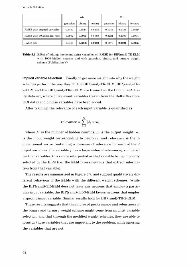
Variable Selection
Ab Co
gaussian binary ternary gaussian binary ternary
RMSE with original variables 0.6497 0.6544 0.6438 0.1746 0.1785 0.1639
RMSE with 30 added irr. vars 0.6982 0.6932 0.6788 0.3221 0.2106 0.1904
RMSE loss 0.0486 0.0388 0.0339 0.1475 0.0321 0.0265
Table 5.1. Effect of adding irrelevant extra variables on RMSE for BIP(rand)-TR-ELMwith 1000 hidden neurons and with gaussian, binary, and ternary weightscheme (Publication V).
Implicit variable selection Finally, to get more insight into why the weight
schemes perform the way they do, the BIP(rand)-TR-ELM, BIP(rand)-TR-
2-ELM and the BIP(rand)-TR-3-ELM are trained on the ComputerActiv-
ity data set, where 5 irrelevant variables (taken from the DeltaElevators
UCI data) and 5 noise variables have been added.
After training, the relevance of each input variable is quantified as
relevance =
M∑i=1
|βi ×wi|,
where M is the number of hidden neurons; βi is the output weight; wi
is the input weight corresponding to neuron i, and relevance is the d-
dimensional vector containing a measure of relevance for each of the d
input variables. If a variable j has a large value of relevancej , compared
to other variables, this can be interpreted as that variable being implicitly
selected by the ELM (i.e. the ELM favors neurons that extract informa-
tion from that variable).
The results are summarized in Figure 5.7, and suggest qualitatively dif-
ferent behaviour of the ELMs with the different weight schemes. While
the BIP(rand)-TR-ELM does not favor any neurons that employ a partic-
ular input variable, the BIP(rand)-TR-3-ELM favors neurons that employ
a specific input variable. Similar results hold for BIP(rand)-TR-2-ELM.
These results suggests that the improved performance and robustness of
the binary and ternary weight scheme might come from implicit variable
selection, and that through the modified weight schemes, they are able to
focus on those variables that are important to the problem, while ignoring
the variables that are not.
62
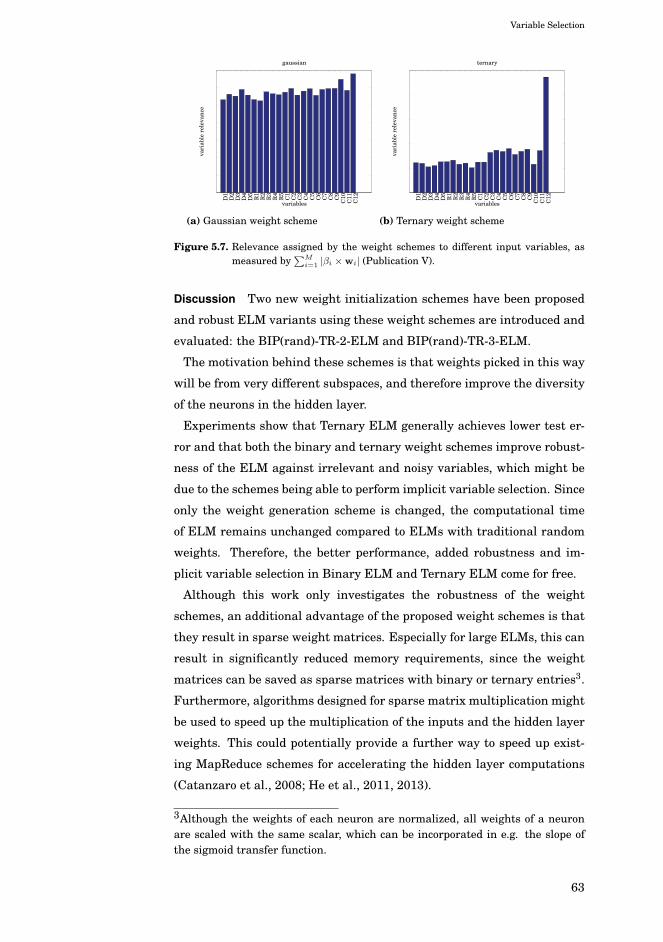
Variable Selection
D1
D2
D3
D4
D5
R1
R2
R3
R4
R5
C1
C2
C3
C4
C5
C6
C7
C8
C9
C10
C11
C12
variablesva
riab
lere
leva
nce
gaussian
(a) Gaussian weight scheme
D1
D2
D3
D4
D5
R1
R2
R3
R4
R5
C1
C2
C3
C4
C5
C6
C7
C8
C9
C10
C11
C12
variables
vari
able
rele
vanc
e
ternary
(b) Ternary weight scheme
Figure 5.7. Relevance assigned by the weight schemes to different input variables, asmeasured by
∑Mi=1 |βi ×wi| (Publication V).
Discussion Two new weight initialization schemes have been proposed
and robust ELM variants using these weight schemes are introduced and
evaluated: the BIP(rand)-TR-2-ELM and BIP(rand)-TR-3-ELM.
The motivation behind these schemes is that weights picked in this way
will be from very different subspaces, and therefore improve the diversity
of the neurons in the hidden layer.
Experiments show that Ternary ELM generally achieves lower test er-
ror and that both the binary and ternary weight schemes improve robust-
ness of the ELM against irrelevant and noisy variables, which might be
due to the schemes being able to perform implicit variable selection. Since
only the weight generation scheme is changed, the computational time
of ELM remains unchanged compared to ELMs with traditional random
weights. Therefore, the better performance, added robustness and im-
plicit variable selection in Binary ELM and Ternary ELM come for free.
Although this work only investigates the robustness of the weight
schemes, an additional advantage of the proposed weight schemes is that
they result in sparse weight matrices. Especially for large ELMs, this can
result in significantly reduced memory requirements, since the weight
matrices can be saved as sparse matrices with binary or ternary entries3.
Furthermore, algorithms designed for sparse matrix multiplication might
be used to speed up the multiplication of the inputs and the hidden layer
weights. This could potentially provide a further way to speed up exist-
ing MapReduce schemes for accelerating the hidden layer computations
(Catanzaro et al., 2008; He et al., 2011, 2013).
3Although the weights of each neuron are normalized, all weights of a neuronare scaled with the same scalar, which can be incorporated in e.g. the slope ofthe sigmoid transfer function.
63

Variable Selection
64
6. Trade-offs in Extreme LearningMachines
“There are all kinds of interesting questions that come from a
knowledge of science, which only adds to the excitement and mys-
tery and awe of a flower. It only adds. I don’t understand how it
subtracts.”
– Richard P. Feynman
In the training of neural networks, there often exists a trade-off between
the time spent optimizing the model under investigation, and its final
performance. Ideally, an optimization algorithm finds the model that has
best test accuracy from the hypothesis space as fast as possible, and this
model is efficient to evaluate at test time as well. However, in practice,
there exists a trade-off between training time, testing time and testing
accuracy, and the optimal trade-off depends on the user’s requirements.
This chapter gives an overview of some of those trade-offs within the
context of ELMs and highlights the results from Publication VI, which
introduces the Compressive ELM and forms an initial investigation into
these trade-offs within Extreme Learning Machines.
Whereas the other contributions are mostly aimed at directly improving
the accuracy of the ELM-based methods, either by ensembling them (Pub-
lication I, Publication II), by obtaining better variable selections (Publi-
cation III, Publication IV), or by improved weight initialization schemes
(Publication V), the Compressive ELM takes a contrary approach.
Instead of directly improving the accuracy, the Compressive ELM fo-
cuses on improving the computational time by providing a time-accuracy
trade-off and training the model in a reduced space, while trying to retain
accuracy as much as possible. Experiments indicate that potentially more
time can be saved than accuracy lost and therefore the compressive train-
ing mechanism may provide an avenue towards obtaining more accurate
models in less time.
65
Trade-offs in Extreme Learning Machines
6.1 Trade-offs between computational time and accuracy
When choosing a model for solving a machine learning problem, which
model is most suitable depends a lot on the context and the requirements
of the application. For example, it might be the case that the model is
trained on a continuous stream of data, and therefore has some restric-
tions on the training time. On the other hand, the computational time in
the testing phase might be restricted, like in a setting where the model is
used as the controller for an aircraft or a similar setting that requires fast
predictions. Alternatively, the context in which the model is applied might
not have any strong constraints on the computational time and, above all,
accuracy or interpretability could be considered most important regard-
less of the computational time.
6.1.1 Time-accuracy curves
This chapter focuses on time-accuracy trade-offs in Extreme Learning Ma-
chines, and on trade-offs between training time and accuracy in particu-
lar, which can be affected in two ways:
• by improving the accuracy through spending more time optimizing
the model,
• or vice-versa, by reducing the computational time of the model,
without sacrificing accuracy too much.
Each type of model has its own ways of balancing computational time
and accuracy, and has an associated training time-accuracy curve that
expresses the efficiency of the model in achieving a certain accuracy (the
closer the curve is to the bottom left, the better). Thus, given a collection
of models, the question becomes: which model produces the best accuracy
the fastest?
6.1.2 Examples from Extreme Learning Machines
In order to illustrate what time-accuracy trade-offs exist within Extreme
Learning Machines, this section presents time-accuracy trade-offs of sev-
eral Extreme Learning Machine variants.
66
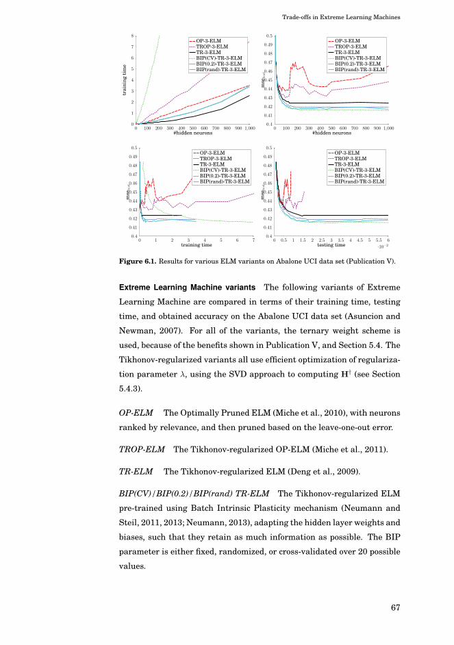
Trade-offs in Extreme Learning Machines
0 100 200 300 400 500 600 700 800 900 1,0000
1
2
3
4
5
6
7
8
#hidden neurons
trai
ning
tim
e
OP-3-ELMTROP-3-ELMTR-3-ELMBIP(CV)-TR-3-ELMBIP(0.2)-TR-3-ELMBIP(rand)-TR-3-ELM
0 100 200 300 400 500 600 700 800 900 1,0000.4
0.41
0.42
0.43
0.44
0.45
0.46
0.47
0.48
0.49
0.5
#hidden neurons
mse
test
OP-3-ELMTROP-3-ELMTR-3-ELMBIP(CV)-TR-3-ELMBIP(0.2)-TR-3-ELMBIP(rand)-TR-3-ELM
0 1 2 3 4 5 6 70.4
0.41
0.42
0.43
0.44
0.45
0.46
0.47
0.48
0.49
0.5
training time
mse
test
OP-3-ELMTROP-3-ELMTR-3-ELMBIP(CV)-TR-3-ELMBIP(0.2)-TR-3-ELMBIP(rand)-TR-3-ELM
0 0.5 1 1.5 2 2.5 3 3.5 4 4.5 5 5.5 6
·10−2
0.4
0.41
0.42
0.43
0.44
0.45
0.46
0.47
0.48
0.49
0.5
testing time
mse
test
OP-3-ELMTROP-3-ELMTR-3-ELMBIP(CV)-TR-3-ELMBIP(0.2)-TR-3-ELMBIP(rand)-TR-3-ELM
Figure 6.1. Results for various ELM variants on Abalone UCI data set (Publication V).
Extreme Learning Machine variants The following variants of Extreme
Learning Machine are compared in terms of their training time, testing
time, and obtained accuracy on the Abalone UCI data set (Asuncion and
Newman, 2007). For all of the variants, the ternary weight scheme is
used, because of the benefits shown in Publication V, and Section 5.4. The
Tikhonov-regularized variants all use efficient optimization of regulariza-
tion parameter λ, using the SVD approach to computing H† (see Section
5.4.3).
OP-ELM The Optimally Pruned ELM (Miche et al., 2010), with neurons
ranked by relevance, and then pruned based on the leave-one-out error.
TROP-ELM The Tikhonov-regularized OP-ELM (Miche et al., 2011).
TR-ELM The Tikhonov-regularized ELM (Deng et al., 2009).
BIP(CV)/BIP(0.2)/BIP(rand) TR-ELM The Tikhonov-regularized ELM
pre-trained using Batch Intrinsic Plasticity mechanism (Neumann and
Steil, 2011, 2013; Neumann, 2013), adapting the hidden layer weights and
biases, such that they retain as much information as possible. The BIP
parameter is either fixed, randomized, or cross-validated over 20 possible
values.
67
Trade-offs in Extreme Learning Machines
Most desirable model depends on requirements The results are summa-
rized in Figure 6.1, and show that it depends on the user’s criteria which
model is most suitable for that context.
Training time most important If it is most important that the model can
be trained fast, then it can be argued that the BIP(rand)-TR-3-ELM offers
the best trade-off. It does take slightly longer to train than the TR-3-
ELM, however, for that modest overhead the test accuracy is generally
improved.
Test error most important If accuracy is all that matters, then the re-
sults suggest it might be worth it to cross-validate the BIP parameter,
instead of setting it randomly per-neuron. Although the training time for
BIP(CV)-TR-3-ELM is many times higher due to the cross-validation of
the BIP parameter, it generally results in the most accurate model.
Testing time most important If the speed of the model at test time is most
important, then, surprisingly, the results suggest that the BIP(rand)-TR-
3-ELM is the most suitable model. This result is unexpected, since a
model that has its irrelevant neurons pruned (like OP-ELM and TROP-
ELM) is generally faster at test time. However, for this context, the re-
sults reveal that, even though the OP-ELM and TROP-ELM are faster,
they tend to slightly overfit while pruning the neurons, resulting in slightly
worse test accuracy.
From Figure 6.1, it can be seen that because of this, the TR-3-ELM vari-
ants are more attractive when it comes to testing time (i.e. for a given
testing time, they are always able to provide the better accuracy).
This surprising result shows the importance of analyzing ELM algo-
rithms in terms of their time-accuracy trade-off. Furthermore, this time-
accuracy trade-off analysis suggests further research directions into the
prevention of overfitting in model structure selection (Reunanen, 2003).
An initial work along these lines is (Wang et al., 2014), which provides
a variant of OP-ELM that computes an approximate ranking of the neu-
rons, rather than an exact ranking, and is shown to achieve better accu-
racy. Presumably, this is because the approximate ranking prevents the
model structure selection from overfitting.
Since TR-3-ELM offers attractive trade-offs between speed and accu-
racy, this model is used for the Compressive Extreme Learning Machine,
which will be discussed next.
68
Trade-offs in Extreme Learning Machines
6.2 Compressive ELM
In the previous section on time-accuracy trade-offs, two possible strate-
gies have been discussed that can affect this trade-off: (1) improving the
accuracy of the models, and (2) reducing the computational time of the
model. In terms of training time-accuracy plots, this would be “pushing
the curve down” and “pushing the curve to the left”, respectively.
Whereas the other contributions discussed in this thesis mainly focus
on improving the accuracy of the models by ensembling them (Publica-
tion I, Publication II), by obtaining better variable selections (Publication
III, Publication IV), or by improved weight initialization schemes (Publi-
cation V), the Compressive ELM focuses on reducing computational time
by performing the training in a reduced space, while retaining accuracy
as much as possible.
6.2.1 Low-distortion embeddings
To achieve this, the dimensionality of the hidden layer output matrix is re-
duced by creating a low-distortion embedding of it in a lower-dimensional
space through Johnson-Lindenstrauss-like embeddings (Johnson and Lin-
denstrauss, 1984; Achlioptas, 2003; Matoušek, 2008), which approximately
preserve the distances between the points and retain the relevant struc-
ture as much as possible. These embeddings occur in approximate distance-
based machine learning algorithms like approximate nearest-neighbors
(Indyk and Motwani, 1998), and are extensively used in the field of Ran-
domized numerical linear algebra (Martinsson, 2009).
6.2.2 Randomized numerical linear algebra
Part of many algorithms in randomized numerical linear algebra is the
embedding (or sketching) of the data into a lower dimension. In compari-
son to distance-based methods though, in linear algebra, the requirement
for preserving the distances is not as strict, and as long as the distances
are roughly preserved (within some factor) it is useful (Martinsson, 2009).
One aspect of linear algebra in which low-distortion embeddings can be
used is in approximate matrix decomposition. Given a matrix, an approx-
imate matrix decomposition can be achieved by first embedding the rows
of the matrix into a lower-dimensional space (through one of many avail-
able low-distortion Johnson-Lindenstrauss-like embeddings), solving the
69
Trade-offs in Extreme Learning Machines
decomposition, and then projecting back to the full space. If such an em-
bedding (or sketch) is accurate, then this allows for solving the problem
with high accuracy in reduced time. An example of such an algorithm is
the approximate SVD.
Approximate SVD The algorithm for approximate SVD is summarized in
Algorithm 8. More background on the algorithm can be found in (Halko
et al., 2011).
Algorithm 8 Approximate SVD (Halko et al., 2011) (Publication V).Given an m × n matrix A, compute k-term approximate SVD A ≈UDVTas follows:
1: - Form the n×(k+p) random matrix Ω. (where p is small oversampling
parameter)
2: - Form the m × (k + p) sampling matrix Y = AΩ. ("sketch" it by
applying Ω)
3: - Form the m × (k + p) orthonormal matrix Q, such that range(Q) =
range(Y).
4: - Compute B = Q∗A.
5: - Form the SVD of B so that B = UDVT
6: - Compute the matrix U = QU
Application to ELM Through the approximate SVD, the time it takes to
train the ELM can be reduced. Furthermore, the efficient L2 regulariza-
tion from Section 5.4.3 can be easily integrated in it as well. The main
question now is, whether it is actually possible to obtain more accurate
models in less time.
Before giving an overview of the experiments investigating this, the next
section gives a short overview of fast sketching algorithms that can be
used as part of the approximate SVD algorithm.
6.2.3 Faster Sketching
Typically, the bottleneck in Algorithm 8 is the time it takes to sketch the
matrix. Rather than using a class of random matrices of Gaussian vari-
ables for sketching A, one can also use random matrices that are sparse or
structured in some way (Achlioptas, 2003; Matoušek, 2008), and for which
the matrix-vector product can be computed more efficiently. Furthermore,
(Ailon and Chazelle, 2006) introduced the Fast Johnson-Lindenstrauss
Transform (FJLT), which uses a class of random matrices that permit ap-
70
Trade-offs in Extreme Learning Machines
plication to vectors from an n× n matrix to a vector in O(n log(n)), rather
than the usual O(n2). Besides this obvious speedup, this class of matri-
ces is also more successful in creating a low-distortion embedding when
applied to a sparse matrix. These transforms consist of the application of
three easy-to-compute matrices
(P
)k×n
(W
)n×n
(D
)n×n
where P, W, and D vary depending on the exact scheme. Generally, D
is a diagonal matrix with random Rademacher variables {−1,+1} on the
diagonal. In this work, the following transforms are considered for faster
sketching:
• Fast Johnson Lindenstrauss Transform (FJLT), introduced in
(Ailon and Chazelle, 2006) for which P is a sparse matrix of random
Gaussian variables, and W encodes the Discrete Walsh-Hadamard Trans-
form.
• Subsampled Randomized Hadamard Transform (SRHT), for which
P is a matrix selecting k random columns from W, and W encodes the
Discrete Walsh-Hadamard Transform.
Both sketching methods were implemented for the Compressive ELM by
adapting the excellent Blendenpik library (Avron et al., 2010).
6.2.4 Experiments
The experiments of Publication V investigate the trade-off between com-
putational time (both training and test), and the accuracy of the Com-
pressive ELM in relation to the dimensionality of the space into which
the problem is reduced, using the sketch. For sketching, Compressive
TR-3-ELMs with a Gaussian, FJLT, and SRHT sketching scheme are con-
sidered, and compared with the standard TR-3-ELM.
Data The experiments are performed using the CaliforniaHousing data
set (Asuncion and Newman, 2007), and the data is divided randomly into
8000 random samples for training and the remaining 12640 samples for
testing.
Experimental parameters The number of hidden neurons in each model
is varied between 2 and 1000, and parameter k = [50, 100, 200, 400, 600].
71

Trade-offs in Extreme Learning Machines
0 100 200 300 400 500 600 700 800 900 1,0000
2
4
6
8
10
12
#hidden neurons
trai
ning
tim
e
TR-3-ELMCS-TR-3-ELM(k=50)CS-TR-3-ELM(k=100)CS-TR-3-ELM(k=200)CS-TR-3-ELM(k=400)CS-TR-3-ELM(k=600)
0 100 200 300 400 500 600 700 800 900 1,0000.2
0.22
0.24
0.26
0.28
0.3
0.32
0.34
0.36
0.38
0.4
#hidden neurons
mse
test
TR-3-ELMCS-TR-3-ELM(k=50)CS-TR-3-ELM(k=100)CS-TR-3-ELM(k=200)CS-TR-3-ELM(k=400)CS-TR-3-ELM(k=600)
0 0.2 0.4 0.6 0.8 1 1.2 1.4 1.6 1.8 20.2
0.22
0.24
0.26
0.28
0.3
0.32
0.34
0.36
0.38
0.4
training time
mse
test
TR-3-ELMCS-TR-3-ELM(k=50)CS-TR-3-ELM(k=100)CS-TR-3-ELM(k=200)CS-TR-3-ELM(k=400)CS-TR-3-ELM(k=600)
0.1 0.2 0.3 0.4 0.5 0.6 0.70.2
0.22
0.24
0.26
0.28
0.3
0.32
0.34
0.36
0.38
0.4
testing time
mse
test
TR-3-ELMCS-TR-3-ELM(k=50)CS-TR-3-ELM(k=100)CS-TR-3-ELM(k=200)CS-TR-3-ELM(k=400)CS-TR-3-ELM(k=600)
Figure 6.2. Results for Compressive ELMs using FJLT sketching with varying k on Cal-iforniaHousing UCI data set (Publication V).
Experiments are repeated with 200 random realizations of the training
and test set, and average results over those 200 runs are reported.
Effect of embedding dimension Figure 6.2 shows the time-accuracy trade-
offs achieved by the various methods, and shows the effect of the embed-
ding dimension. Although only the results of FJLT sketching are pre-
sented here, similar results hold for the other sketching methods. It can
be seen that
• setting k lower than the number of neurons results in faster training
times (which makes sense since the problem solved is smaller).
• as long as parameter k is chosen large enough, the method is not losing
efficiency (i.e. there is no model that achieves better error in the same
computational time), and it is potentially gaining efficiency (as shown
by the bottom-left plot of Figure 6.2.
Effect of embedding scheme Finally, the experiments showed that
sketches with Gaussian matrices are generally the fastest, and for the
tested problem sizes, the SRHT is slightly faster than the FJLT.
72
Trade-offs in Extreme Learning Machines
Discussion Surprisingly, the experiments did not show substantial dif-
ferences in terms of computational time for the different embedding
schemes. Therefore, for the datasets tested, it seems that although FJLT
permits faster matrix multiplications, no advantage could be taken of it
in the tested problems. More research is required to gain more insight
into this behaviour, and to understand in what contexts the FJLT can
effectively be exploited.
Furthermore, the results indicate that although the Compressive ELM
provides an effective trade-off between time and accuracy, in this case,
little compression could be obtained for the information in the hidden
layer: as soon as k is set lower than the number of neurons, the accu-
racy decreases accordingly. This challenge to significantly compress the
information in the hidden layer might be due to the quality of the fea-
tures used in the Tikhonov-regularized Ternary Compressive ELM: they
might result in a full-rank matrix that has no redundancies. However,
more research is needed to better understand in what architectures and
applications the Compressive ELM can effectively compress the randomly
extracted features.
In summary, the Compressive ELM provides a way for trading off com-
putational time and accuracy, by performing the training in a reduced
space, using low-distortion embeddings and approximate matrix decom-
positions based on them. Experiments indicate that through this mecha-
nism, potentially more time can be saved than accuracy lost and therefore
the compressive training mechanism may provide a way to obtain more
accurate models in less time.
Finally, developing low-distortion embeddings and related theoretical
results is currently a very active field of research, and new developments
in this area can be readily integrated to improve the performance of Com-
pressive ELM.
73

Trade-offs in Extreme Learning Machines
74
7. Conclusions and Discussion
7.1 Contributions
The thesis develops several ensembling strategies based on ELM that
can be applied in nonstationary environments and to large-scale learn-
ing problems. Due to the fine-grained structure of the ensemble models,
they are very flexible, and can be evaluated in a parallel fashion. The
individual models can be built and evaluated efficiently by performing
the training and model structure selection on GPUs. Finally, the (adap-
tive) combination of diverse individual models results in a more accurate
model. The models themselves can be relatively simple, while due to en-
sembling the overall model is still accurate. The results suggest this to
be an accurate, yet flexible approach that can be used for analyzing large-
scale potentially nonstationary streams of data.
Furthermore, several very different variable selection strategies have
been explored. Firstly, in the ELM-FS, the use of the ELM architecture
for variable selection, through relaxation of the variable selection prob-
lem is investigated. Besides providing a good subset of variables, the pre-
sented approach determines for each subset size, which variable subset
would be best, and how the generalization error is expected to change de-
pending on the number of variables selected. This provides insight into
the problem, and allows for an informed decision on the variable subset
that is best for the current context. Secondly, a filter method is presented
for variable selection, which allows for variable selection in large-scale
problems through the use of (multi-)GPU-acceleration of the Delta Test
criterion, used in a parallelized genetic algorithm. Finally, new binary
and ternary random weight schemes for ELM are developed, which re-
sult in more accurate and compact models. Experiments suggest that the
75
Conclusions and Discussion
changed weight schemes make the ELM more robust to noisy and irrele-
vant variables, and are therefore a promising target for future research.
Finally, an approach was presented for reducing the computational time
needed for training the ELM by embedding the random feature expan-
sions in a lower-dimensional space. This allows for a flexible trade-off
between accuracy and speed of the ELM, and could potentially reduce
redundancy in the hidden neurons, resulting in more effective models.
Experiments suggest that this approach may provide a path towards ob-
taining more accurate models in less time.
Overall, the collection of proposed methods provides an efficient, accu-
rate and flexible framework for solving large-scale supervised learning
problems. Several distinct strategies are explored for obtaining faster and
more accurate models that are particularly suited for handling modern
large-scale data sets. The developed methods are not limited to the par-
ticular types of ELMs and contexts in which they have been tested, and
they may be readily combined, adapted and integrated for application in
different contexts and models.
7.2 Future directions
Of course research is a continuing process, and every new development
and result brings new questions. To conclude, this section gives a short
overview of some of those possible future research directions.
Better training and regularization strategies Several results from the the-
sis suggest the importance of proper regularization for obtaining an ac-
curate model and preventing overfitting. Furthermore, recent results in
deep learning (Ba and Caruana, 2014), suggest that the success of deep
neural networks may be due to the way they are trained, rather than just
their architecture: i.e. it is possible to train a shallow mimic network
based on an already trained deep network, which attains better accuracy
than when a shallow network is trained directly. Perhaps what is missing
for shallow networks, in order to obtain as good or similar performance as
deep networks, is the right algorithm?
Therefore, an important line of research is exploring alternative train-
ing and regularization strategies in ELM-based architectures. What is the
best strategy in training and performing model structure selection, such
that the model obtains high accuracy and does not suffer from overfitting?
76

Conclusions and Discussion
Improved data-agnostic random features The results from the Binary and
Ternary ELM suggest that improved data-agnostic random features can
be obtained by using weight initialization schemes other than the ones
typically used in hidden layer initialization. Why exactly does one weight
scheme work better than another, and can insights into this inform on
even better weight schemes?
Overall then, aside from the question “what is the best accuracy a model
can achieve?”, in my opinion the more interesting question is “what is the
most effective way to achieve this accuracy?”. What routes exist towards
obtaining optimal performance, and what effective shortcuts exist along
the way for getting there faster?
77

Conclusions and Discussion
78
Bibliography
D. Achlioptas. Database-friendly random projections: Johnson-Lindenstrausswith binary coins. Journal of Computer and System Sciences, 66(4):671–687,June 2003. ISSN 00220000. doi: 10.1016/S0022-0000(03)00025-4.
E. Agullo, J. Demmel, J. Dongarra, B. Hadri, J. Kurzak, J. Langou, H. Ltaief,P. Luszczek, and S. Tomov. Numerical linear algebra on emerging architec-tures: The PLASMA and MAGMA projects. Journal of Physics: ConferenceSeries, 180:012037, 2009. ISSN 1742-6596. doi: 10.1088/1742-6596/180/1/012037.
N. Ailon and B. Chazelle. Approximate nearest neighbors and the fast Johnson-Lindenstrauss transform. In Proceedings of the thirty-eighth annual ACMsymposium on Theory of computing - STOC ’06, New York, New York, USA,2006. ACM Press. ISBN 1-59593-134-1. doi: 10.1145/1132516.1132597.
H. Akaike. A new look at the statistical model identification. IEEE Transactionson Automatic Control, 19(6):716–723, 1974. ISSN 00189286. doi: 10.1109/TAC.1974.1100705.
D. M. Allen. The relationship between variable selection and data agumentationand a method for prediction. Technometrics, pages 125–127, Dec. 1974.
E. Alpaydin. Introduction to Machine Learning. MIT Press, 2nd edition, 2010.
E. Anderson, Z. Bai, C. Bischof, S. Blackford, J. W. Demmel, J. Dongarra, J. D.Croz, A. Greenbaum, S. Hammarling, A. McKenney, and D. Sorensen. LA-PACK Users’ guide. Society for Industrial Mathematics, Philadelphia, PA,third edition, Apr. 1999. ISBN 0-89871-447-8 (paperback).
A. Asuncion and D. J. Newman. UCI Machine Learning Repository, 2007.
H. Avron, P. Maymounkov, and S. Toledo. Blendenpik: Supercharging LAPACK’sleast-squares solver. SIAM Journal on Scientific Computing, 32(3):1217–1236,2010.
J. Ba and R. Caruana. Do Deep Nets Really Need to be Deep? In Z. Ghahramani,M. Welling, C. Cortes, N. D. Lawrence, and K. Q. Weinberger, editors, Advancesin Neural Information Processing Systems 27, pages 2654–2662. Curran Asso-ciates, Inc., 2014.
R. E. Bellman. Adaptive Control Processes: A Guided Tour. Princeton UniversityPress, 1961.
79
Bibliography
G. J. Bierman. Factorization Methods for Discrete Sequential Estimation. Aca-demic Press, New York, NY, 1977.
C. M. Bishop. Pattern recognition and machine learning. Springer, Secaucus,2006. ISBN 0-387-31073-8.
G. Bontempi, M. Birattari, and H. Bersini. Recursive Lazy Learning for Modelingand Control. In European Conference on Machine Learning, pages 292–303,1998.
L. Breiman. Bagging predictors. Machine Learning, 24(2):123–140, Aug. 1996a.ISSN 0885-6125. doi: 10.1007/BF00058655.
L. Breiman. Stacked regressions. Machine Learning, 24:49–64, 1996b. ISSN0885-6125. doi: 10.1007/BF00117832.
E. K. Burke and G. Kendall. Search methodologies: Introductory tutorials inoptimization and decision support techniques. pages 1–620, 2005. ISSN 1873-2518. doi: 10.1007/0-387-28356-0.
B. C. Catanzaro, N. Sundaram, and K. Keutzer. Fast Support Vector MachineTraining and Classification on Graphics Processors. In Proceedings of the 25thInternational Conference on Machine Learning (ICML 2008), pages 104–111,Helsinki, Finland, 2008. ACM.
C. P. Chen. A rapid supervised learning neural network for function interpolationand approximation. IEEE Transactions on Neural Networks, 7(5):1220–30,Jan. 1996. ISSN 1045-9227. doi: 10.1109/72.536316.
G. Cybenko. Approximation by superpositions of a sigmoidal function. Mathe-matics of Control, Signals, and Systems (MCSS), pages 303–314, 1989.
W. D. W. Deng, Q.-H. Zheng, and L. C. L. Chen. Regularized Extreme LearningMachine. In 2009 IEEE Symposium on Computational Intelligence and DataMining, number 60825202 in 2009 IEEE Symposium on Computational In-telligence and Data Mining, CIDM 2009, pages 389–395, MOE KLINNS Laband SKLMS Lab, Xi’an Jiaotong University, Xi’an, China, 2009. IEEE. ISBN978-1-4244-2765-9. doi: 10.1109/CIDM.2009.4938676.
B. Efron and R. J. Tibshirani. An Introduction to the Bootstrap, volume 57. Chap-man & Hall/CRC, May 1993. ISBN 0-412-04231-2.
B. Efron, T. Hastie, I. Johnstone, and R. Tibshirani. Least Angle Regression. TheAnnals of Statistics, 32(2):1–44, 2003.
E. Eirola. Machine learning methods for incomplete data and variable selection.Ph.D. Thesis, Aalto University, 2014.
E. Eirola, E. Liitiäinen, A. Lendasse, F. Corona, and M. Verleysen. Using theDelta test for variable selection. In Proc. of ESANN 2008 European Sympo-sium on Artificial Neural Networks, pages 25–30, 2008. ISBN 2930307080.
G. Feng, G.-B. Huang, Q. Lin, and R. Gay. Error Minimized Extreme Learn-ing Machine With Growth of Hidden Nodes and Incremental Learning. IEEETransactions on Neural Networks, 20(8):1352–1357, 2009. ISSN 10459227.doi: 10.1109/TNN.2009.2024147.
80
Bibliography
D. François, F. Rossi, V. Wertz, and M. Verleysen. Resampling methods forparameter-free and robust feature selection with mutual information. Neu-rocomputing, 70:1276–1288, 2007. ISSN 09252312. doi: 10.1016/j.neucom.2006.11.019.
B. Frénay and M. Verleysen. Using SVMs with randomised feature spaces: anextreme learning approach. ESANN 2010: 18th European Symposium on Ar-tificial Neural Networks, Computational Intelligence and Machine Learning,(April):315–320, 2010.
B. Frénay and M. Verleysen. Parameter-insensitive kernel in extreme learningfor non-linear support vector regression. Neurocomputing, 74(16):2526–2531,Sept. 2011. ISSN 09252312. doi: 10.1016/j.neucom.2010.11.037.
Y. Freund and R. E. Schapire. Experiments with a New Boosting Algorithm. InInternational Conference on Machine Learning, pages 148–156, 1996. ISBN1558604197. doi: 10.1.1.133.1040.
K.-I. Funahashi. On the approximate realization of continuous mappings byneural networks. Neural Networks, 2(3):183–192, 1989. ISSN 0893-6080.
V. Garcia, E. Debreuve, and M. Barlaud. Fast k nearest neighbor search us-ing GPU. 2008 IEEE Computer Society Conference on Computer Vision andPattern Recognition Workshops, pages 1–6, 2008. ISSN 2160-7508. doi:10.1109/CVPRW.2008.4563100.
V. Garcia, E. Debreuve, F. Nielsen, and M. Barlaud. K-nearest neighbor search:Fast GPU-based implementations and application to high-dimensional fea-ture matching. In Proceedings - International Conference on Image Processing,ICIP, pages 3757–3760, 2010. ISBN 9781424479948. doi: 10.1109/ICIP.2010.5654017.
I. Guyon and A. Elisseeff. An introduction to variable and feature selection.Journal of Machine Learning Research, 3:1157–1182, 2003. ISSN 15324435.doi: 10.1162/153244303322753616.
N. Halko, P.-G. Martinsson, and J. A. Tropp. Finding structure with randomness:Probabilistic algorithms for constructing approximate matrix decompositions.SIAM review, pages 1–74, Sept. 2011.
L. K. Hansen and P. Salamon. Neural network ensembles. Pattern Analysisand Machine Intelligence, IEEE Transactions on, 12(10):993–1001, Oct. 1990.ISSN 0162-8828.
T. Hastie, R. Tibshirani, and J. H. Friedman. The Elements of Statistical Learn-ing: Data Mining, Inference, and Prediction. 2001.
Q. He, C. Du, Q. Wang, F. Zhuang, and Z. Shi. A parallel incremental extremeSVM classifier. Neurocomputing, 74(16):2532–2540, 2011. ISSN 09252312(ISSN).
Q. He, T. Shang, F. Zhuang, and Z. Shi. Parallel extreme learning machine forregression based on MapReduce. Neurocomputing, 102(0):52–58, Feb. 2013.ISSN 0925-2312. doi: http://dx.doi.org/10.1016/j.neucom.2012.01.040.
K. Hornik, M. B. Stinchcombe, and H. White. Multilayer feedforward networksare universal approximators. Neural Networks, 2(5):359–366, 1989.
81
Bibliography
G. Huang, S. Song, J. N. D. Gupta, and C. Wu. Semi-Supervised and Unsuper-vised Extreme Learning Machines. IEEE Transactions on Cybernetics, 44(12):2405–17, Dec. 2014. ISSN 21682267. doi: 10.1109/TCYB.2014.2307349.
G. Huang, G.-B. Huang, S. Song, and K. You. Trends in extreme learning ma-chines: A review. Neural Networks, 61:32–48, Jan. 2015. ISSN 08936080. doi:10.1016/j.neunet.2014.10.001.
G.-B. Huang. Reply to "Comments on "The extreme learning machine"". IEEETransactions on Neural Networks, 19(8):1495–1496, 2008. ISSN 10459227(ISSN).
G.-B. Huang. An Insight into Extreme Learning Machines: Random Neurons,Random Features and Kernels. Cognitive Computation, 6(3):376–390, Apr.2014. ISSN 1866-9956. doi: 10.1007/s12559-014-9255-2.
G.-B. Huang and L. Chen. Convex incremental extreme learning machine.Neurocomputing, 70(16-18):3056–3062, Oct. 2007. ISSN 09252312. doi:10.1016/j.neucom.2007.10.008.
G.-B. Huang and L. Chen. Enhanced random search based incremental extremelearning machine. Neurocomputing, 71(16-18):3460–3468, Oct. 2008. ISSN09252312. doi: 10.1016/j.neucom.2007.10.008.
G.-B. Huang, Q.-Y. Zhu, and C.-K. Siew. Extreme Learning Machine: A NewLearning Scheme of Feedforward Neural Networks. In Proceedings of the Inter-national Joint Conference on Neural Networks, volume 2 of 2004 IEEE Interna-tional Joint Conference on Neural Networks - Proceedings, pages 985–990, Sch.of Elec. and Electron. Eng., Nanyang Technological University, Nanyang Av-enue, Singapore 639798, Singapore, 2004. doi: 10.1109/IJCNN.2004.1380068.
G.-B. Huang, L. Chen, and C.-K. Siew. Universal approximation using incre-mental constructive feedforward networks with random hidden nodes. IEEETransactions on Neural Networks, 17(4):879–892, 2006a. ISSN 10459227(ISSN). doi: 10.1109/TNN.2006.875977.
G.-B. Huang, Q.-Y. Zhu, and C.-K. Siew. Extreme learning machine: Theory andapplications. Neurocomputing, 70(1-3):489–501, Dec. 2006b. ISSN 09252312.doi: 10.1016/j.neucom.2005.12.126.
G.-B. Huang, X. Ding, and H. Zhou. Optimization method based extreme learningmachine for classification. Neurocomputing, 74(1-3):155–163, Dec. 2010. ISSN09252312. doi: 10.1016/j.neucom.2010.02.019.
G.-B. Huang, D. H. Wang, and Y. Lan. Extreme learning machines: a survey. In-ternational Journal of Machine Learning and Cybernetics, 2(2):107–122, May2011. ISSN 1868-8071. doi: 10.1007/s13042-011-0019-y.
J. R. Humphrey, D. K. Price, K. E. Spagnoli, A. L. Paolini, and E. J. Kelmelis.CULA: hybrid GPU accelerated linear algebra routines. In Defense, volume7705, pages 770502–770502–7, 2010. ISBN 9780819481696. doi: 10.1117/12.850538.
B. Igelnik and Y.-H. Pao. Stochastic choice of basis functions in adaptive func-tion approximation and the functional-link net. IEEE Transactions on NeuralNetworks, 6(6):1320–9, Jan. 1995. ISSN 1045-9227. doi: 10.1109/72.471375.
82
Bibliography
P. Indyk and R. Motwani. Approximate nearest neighbors: towards removing thecurse of dimensionality. Proceedings of the thirtieth annual ACM symposiumon Theory of computing, 126:604–613, 1998. ISSN 00123692. doi: 10.4086/toc.2012.v008a014.
R. A. Jacobs, M. I. Jordan, S. J. Nowlan, and G. E. Hinton. Adaptive Mixtures ofLocal Experts. Neural Computation, 3(1):79–87, Feb. 1991. ISSN 0899-7667.doi: 10.1162/neco.1991.3.1.79.
W. Johnson and J. Lindenstrauss. Extension of Lipschitz maps into a Hilbertspace. Contemp. Math., 26:189–206, 1984.
I. T. Jolliffe. Principal Component Analysis, Second Edition. Encyclopedia ofStatistics in Behavioral Science, 30:487, 2002. ISSN 00401706. doi: 10.2307/1270093.
L. L. C. Kasun, H. Zhou, G.-B. Huang, and C. M. Vong. Representational Learn-ing with Extreme Learning Machine for Big Data. IEEE Intelligent Systems,28(6):31–34, 2013.
N. Kourentzes and S. F. Crone. Automatic modeling of neural networks for timeseries prediction - in search of a uniform methodology across varying timefrequencies. In Proceedings of the 2nd European Symposium on Time SeriesPrediction, ESTSP’08, pages 117–127, Porvoo, Finland, Sept. 2008.
A. Kraskov, H. Stögbauer, and P. Grassberger. Estimating mutual information.Physical Review E, 69(6), June 2004. ISSN 1539-3755. doi: 10.1103/PhysRevE.69.066138.
J. C. Lagarias, J. A. Reeds, M. H. Wright, and P. E. Wright. ConvergenceProperties of the Nelder–Mead Simplex Method in Low Dimensions. SIAMJournal on Optimization, 9:112–147, 1998. ISSN 1052-6234. doi: 10.1137/S1052623496303470.
Y. Lan, Y. C. Soh, and G.-B. Huang. Ensemble of online sequential extremelearning machine. Neurocomputing, 72(13-15):3391–3395, Aug. 2009. ISSN09252312. doi: 10.1016/j.neucom.2009.02.013.
Q. Le, T. Sarlós, and A. J. Smola. Fastfood - Approximating Kernel Expansionsin Loglinear Time. International Conference on Machine Learning, 28, 2013.
N.-Y. Liang, G.-B. Huang, P. Saratchandran, and N. Sundararajan. A Fast andAccurate Online Sequential Learning Algorithm for Feedforward Networks.IEEE Transactions on Neural Networks, 17(6):1411–1423, Nov. 2006. ISSN1045-9227. doi: 10.1109/TNN.2006.880583.
X. Liu, L. Wang, G.-B. Huang, J. Zhang, and J. Yin. Multiple kernel extremelearning machine. Neurocomputing, 149:253–264, Feb. 2015. ISSN 09252312.doi: 10.1016/j.neucom.2013.09.072.
Y. Liu and X. Yao. Ensemble learning via negative correlation. Neural Networks,12:1399–1404, 1999. ISSN 0893-6080. doi: 10.1016/S0893-6080(99)00073-8.
D. J. C. MacKay. Information Theory, Inference and Learning Algorithms. Cam-bridge University Press, 2003. ISBN 0521642981.
83
Bibliography
P.-G. Martinsson. Randomization: Making Very Large-Scale Linear AlgebraicComputations Possible. Technical report, 2009.
MathWorks. MATLAB Parallel Computing Toolbox, 2011. URL http://www.mathworks.com/products/parallel-computing.
J. Matoušek. On variants of the Johnson-Lindenstrauss lemma. Random Struc-tures & Algorithms, pages 142–156, 2008. doi: 10.1002/rsa.
M. D. McDonnell, M. D. Tissera, A. van Schaik, and J. Tapson. Fast, simpleand accurate handwritten digit classification using extreme learning machineswith shaped input-weights. arXiv preprint arXiv:1412.8307, Dec. 2014.
Y. Miche, A. Sorjamaa, P. Bas, O. Simula, C. Jutten, and A. Lendasse. OP-ELM:optimally pruned extreme learning machine. IEEE Transactions on NeuralNetworks, 21(1):158–162, Oct. 2010. ISSN 10459227 (ISSN). doi: 10.1109/TNN.2009.2036259.
Y. Miche, M. van Heeswijk, P. Bas, O. Simula, and A. Lendasse. TROP-ELM: Adouble-regularized ELM using LARS and Tikhonov regularization. Neurocom-puting, 74(16):2413–2421, Sept. 2011. ISSN 09252312. doi: 10.1016/j.neucom.2010.12.042.
K. P. Murphy. Machine Learning: A Probabilistic Perspective. The MIT Press,2012.
R. H. Myers. Classical and Modern Regression with Applications, 2nd edition.Duxbury, Pacific Grove, CA, USA, 1990.
J. A. Nelder and R. Mead. A simplex method for function minimization. TheComputer Journal, 7(4):308–313, 1965.
K. Neumann. Reliability of Extreme Learning Machines. Ph.D. Thesis, BielefeldUniversity, 2013.
K. Neumann and J. J. Steil. Batch intrinsic plasticity for extreme learning ma-chines. In Artificial Neural Networks and Machine Learning - ICANN 2011,volume 6791 LNCS of 21st International Conference on Artificial Neural Net-works, ICANN 2011, pages 339–346, Research Institute for Cognition andRobotics (CoR-Lab.), Bielefeld University, Universit{ä}tsstr. 25, 33615 Biele-feld, Germany, 2011. Springer. ISBN 978-3-642-21734-0.
K. Neumann and J. J. Steil. Optimizing Extreme Learning Machines via RidgeRegression and Batch Intrinsic Plasticity. Neurocomputing, 102(0):555–560,Feb. 2013. ISSN 0925-2312. doi: http://dx.doi.org/10.1016/j.neucom.2012.01.041.
K. Neumann, C. Emmerich, and J. J. Steil. Regularization by Intrinsic Plasticityand its Synergies with Recurrence for Random Projection Methods. Journalof Intelligent Learning Systems and Applications, 4(3):230–246, 2012. ISSN2150-8402.
M. Olteanu. Revisiting linear and non-linear methodologies for time seriesprediction-application to {ESTSP}’08 competition data. In Proceedings of the2nd European Symposium on Time Series Prediction, ESTSP’08, pages 139–148, Porvoo, Finland, Sept. 2008.
84
Bibliography
Y.-H. Pao and Y. Takefuji. Functional-link net computing: theory, system archi-tecture, and functionalities. Computer, 25(5):76–79, May 1992. ISSN 0018-9162. doi: 10.1109/2.144401.
Y.-H. Pao, G.-H. Park, and D. J. Sobajic. Learning and generalization character-istics of the random vector functional-link net. Neurocomputing, 6(2):163–180,Apr. 1994. ISSN 09252312. doi: 10.1016/0925-2312(94)90053-1.
E. Parviainen, J. Riihimäki, Y. Miche, and A. Lendasse. Interpreting extremelearning machine as an approximation to an infinite neural network. In KDIR2010 - Proceedings of the International Conference on Knowledge Discoveryand Information Retrieval, International Conference on Knowledge Discoveryand Information Retrieval, KDIR 2010, pages 65–73, Dept. of Biomedical En-gineering and Computational Science (BECS), Aalto University School of Sci-ence and Technology, Aalto, Finland, 2010. ISBN 978-989-8425-28-7 (ISBN).
A. Rahimi and B. Recht. Random Features for Large-Scale Kernel Machines.Advances in Neural Information Processing Systems, 2007.
A. Rahimi and B. Recht. Weighted sums of random kitchen sinks: Replacingminimization with randomization in learning. Advances in Neural Informa-tion Processing Systems, 2008.
T. Raiko and H. Valpola. Deep Learning Made Easier by Linear Transforma-tions in Perceptrons. In Proceedings of the 15th International Conference onArtificial Intelligence and Statistics, pages 924–932, 2012.
C. R. Rao and S. K. Mitra. Generalized Inverse of the Matrix and Its Applications.John Wiley & Sons Inc, Jan. 1971.
J. Reunanen. Overfitting in Making Comparisons Between Variable SelectionMethods. Journal of Machine Learning Research, 3:1371–1382, 2003. ISSN15324435. doi: 10.1162/153244303322753715.
H.-J. Rong, Y.-S. Ong, A.-H. Tan, and Z. Zhu. A fast pruned-extreme learningmachine for classification problem. Neurocomputing, 72(1-3):359–366, Dec.2008. ISSN 09252312. doi: 10.1016/j.neucom.2008.01.005.
F. Rossi, A. Lendasse, D. François, V. Wertz, and M. Verleysen. Mutual infor-mation for the selection of relevant variables in spectrometric nonlinear mod-elling. Chemometrics and Intelligent Laboratory Systems, 80(2):215–226, Feb.2006. doi: doi:10.1016/j.chemolab.2005.06.010.
D. E. Rumelhart, G. E. Hinton, and R. J. Williams. Learning representations byback-propagating errors. Nature, 323:533–536, 1986. ISSN 0028-0836. doi:10.1038/323533a0.
R. E. Schapire, Y. Freund, P. L. Bartlett, and W. S. Lee. Boosting the margin: anew explanation for the effectiveness of voting methods. The Annals of Statis-tics, 26:322–330, 1998.
W. Schmidt, M. Kraaijveld, and R. Duin. Feedforward neural networks with ran-dom weights. In Proceedings., 11th IAPR International Conference on PatternRecognition. Vol.II. Conference B: Pattern Recognition Methodology and Sys-tems, pages 1–4. IEEE Comput. Soc. Press, 1992. ISBN 0-8186-2915-0. doi:10.1109/ICPR.1992.201708.
85
Bibliography
G. Schwarz. Estimating the dimension of a model. The Annals of Statistics, 6(2):461–464, 1978.
T. Similä and J. Tikka. Multiresponse sparse regression with application to mul-tidimensional scaling. In Artificial Neural Networks: Formal Models and TheirApplications - ICANN 2005, volume 3697, pages 97–102, 2005.
D. Sovilj. Learning Methods for Variable Selection and Time Series Prediction.Ph.D. Thesis, Aalto University, 2014.
J. J. Steil. Online reservoir adaptation by intrinsic plasticity forbackpropagation-decorrelation and echo state learning. Neural Networks, 20(3):353–364, Apr. 2007. ISSN 0893-6080.
J. Tapson, P. de Chazal, and A. van Schaik. Explicit Computation of InputWeights in Extreme Learning Machines. Proceedings of ELM-2014 Volume1: Algorithms and Theories, pages 41–49, 2014.
H. A. B. te Braake and G. van Straten. Random activation weight neural net(RAWN) for fast non-iterative training. Engineering Applications of ArtificialIntelligence, 8(1):71–80, Feb. 1995. ISSN 0952-1976.
H. A. B. te Braake, H. J. L. van Can, G. van Straten, and H. B. Verbruggen.Regulated activation weights neural network (RAWN). ESANN 1996, Euro-pean Symposium on Artificial Neural Networks, Bruges, Belgium, (April):19–24, 1996.
H. A. B. te Braake, H. J. L. van Can, G. van Straten, and H. B. Verbruggen. Two-step approach in the training of regulated activation weight neural networks(RAWN). Engineering Applications of Artificial Intelligence, 10(2):157–170,Apr. 1997. ISSN 0952-1976.
J. Triesch. A Gradient Rule for the Plasticity of a Neuron’s Intrinsic Excitability.In W. Duch, J. Kacprzyk, E. Oja, and S. Zadrozny, editors, Artificial NeuralNetworks: Biological Inspirations - ICANN 2005, volume 3696 of Lecture Notesin Computer Science, pages 65–70. Springer Berlin / Heidelberg, 2005a. ISBN978-3-540-28752-0. doi: 10.1007/11550822_11.
J. Triesch. Synergies between intrinsic and synaptic plasticity in individualmodel neurons. In NIPS, 2005b.
M. van Heeswijk. Adaptive Ensembles of Extreme Learning Machines for TimeSeries Prediction. M.Sc Thesis, Eindhoven University of Technology, 2009.
M. Verleysen, D. François, G. Simon, and V. Wertz. On the effects of dimension-ality on data analysis with neural networks. In Artificial Neural Nets ProblemSolving Methods, volume 2687, pages 105–112. 2003. ISBN 978-3-540-40211-4. doi: 10.1007/3-540-44869-1_14.
M. Verleysen, F. Rossi, and D. François. Advances in feature selection withmutual information. In Lecture Notes in Computer Science (including sub-series Lecture Notes in Artificial Intelligence and Lecture Notes in Bioin-formatics), volume 5400, pages 52–69, 2009. ISBN 9783642018046. doi:10.1007/978-3-642-01805-3_4.
86
Bibliography
D. Verstraeten, B. Schrauwen, M. D’Haene, and D. Stroobandt. An experimentalunification of reservoir computing methods. Neural Networks, 20(3):391–403,Apr. 2007. ISSN 0893-6080.
L. P. Wang and C. R. Wan. Comments on "The extreme learning machine".IEEE Transactions on Neural Networks, 19(8):1494–1495, Aug. 2008. ISSN10459227 (ISSN). doi: 10.1109/TNN.2008.2002273.
N. Wang, M. Han, N. Dong, and M. J. Er. Constructive multi-output extremelearning machine with application to large tanker motion dynamics iden-tification. Neurocomputing, 128:59–72, Mar. 2014. ISSN 09252312. doi:10.1016/j.neucom.2013.01.062.
A. S. Weigend and N. A. Gershenfeld. Time Series Prediction: Forecasting theFuture and Understanding the Past. Addison-Wesley, Reading, 1993.
B. Widrow, A. Greenblatt, Y. Kim, and D. Park. The No-Prop algorithm: A newlearning algorithm for multilayer neural networks. Neural Networks, 37:182–188, 2013. ISSN 08936080. doi: 10.1016/j.neunet.2012.09.020.
D. H. Wolpert. Stacked generalization. Neural Networks, 5:241–259, 1992. ISSN08936080. doi: 10.1016/S0893-6080(05)80023-1.
J. Y. Yam and T. W. Chow. A weight initialization method for improving trainingspeed in feedforward neural network. Neurocomputing, 30(1-4):219–232, Jan.2000. ISSN 09252312. doi: 10.1016/S0925-2312(99)00127-7.
Y. F. Yam and T. W. S. Chow. Determining initial weights of feedforward neuralnetworks based on least squares method. Neural Processing Letters, 2(2):13–17, Mar. 1995. ISSN 1370-4621. doi: 10.1007/BF02312350.
Y. F. Yam, T. W. S. Chow, and C. T. Leung. A new method in determining initialweights of feedforward neural networks for training enhancement. Neurocom-puting, 16:23–32, 1997. ISSN 09252312. doi: 10.1016/S0925-2312(96)00058-6.
87

Bibliography
88
DISSERTATIONS IN INFORMATION AND COMPUTER SCIENCE
Aalto-DD156/2014 Sjöberg, Mats
From pixels to semantics: visual concept detection and its
applications. 2014.
Aalto-DD157/2014 Adhikari, Prem Raj
Probabilistic Modelling of Multiresolution Biological Data. 2014.
Aalto-DD171/2014 Suvitaival, Tommi
Bayesian Multi-Way Models for Data Translation in Computational
Biology. 2014.
Aalto-DD177/2014 Laitinen, Tero
Extending SAT Solver with Parity Reasoning. 2014.
Aalto-DD178/2014 Gonçalves, Nicolau
Advances in Analysis and Exploration in Medical Imaging. 2014.
Aalto-DD191/2014 Kindermann, Roland SMT-based Verification of Timed Systems and Software. 2014.
Aalto-DD207/2014 Chen, Xi
Real-time Action Recognition for RGB-D and Motion Capture Data.
2014.
Aalto-DD211/2014 Soleimany, Hadi
Studies in Lightweight Cryptography. 2014.
Aalto-DD28/2015 Su, Hongyu
Multilabel Classification through Structured Output Learning –
Methods and Applications. 2015.
Aalto-DD31/2015 Talonen, Jaakko
Advances in Methods of Anomaly Detection and Visualization of
Multivariate Data. 2015.
9HSTFMG*agbeib+
ISBN 978-952-60-6148-1 (printed) ISBN 978-952-60-6149-8 (pdf) ISSN-L 1799-4934 ISSN 1799-4934 (printed) ISSN 1799-4942 (pdf) Aalto University School of Science Department of Information and Computer Science www.aalto.fi
BUSINESS + ECONOMY ART + DESIGN + ARCHITECTURE SCIENCE + TECHNOLOGY CROSSOVER DOCTORAL DISSERTATIONS
Aalto-D
D 4
3/2
015
Nowadays, due to advances in technology, the size and dimensionality of data sets used in machine learning have grown very large and continue to grow by the day. For this reason, it is important to have efficient computational methods and algorithms that can be applied to large data sets, such that it is still possible to complete the machine learning task in reasonable time. This dissertation introduces several machine learning methods based on Extreme Learning Machines (ELMs), meant to deal with these challenges. It focuses on developing efficient, yet accurate and flexible methods. These contributions take three main directions. Firstly, ensemble approaches based on ELM, that adapt to context and can scale to large data. Secondly, ELM-based variable selection approaches, that result in more accurate and efficient models. Finally, training algorithms for ELM that allow for a flexible trade-off between accuracy and computational time.
Mark van H
eeswijk
Advances in E
xtreme L
earning Machines
Aalto
Unive
rsity
Department of Information and Computer Science
Advances in Extreme Learning Machines
Mark van Heeswijk
DOCTORAL DISSERTATIONS


![DOCTORAL THESIS [TESIS DOCTORAL] - UAM](https://img.pdfslide.us/doc/110x75/62162d5b17f9b23eb24b8a87/doctoral-thesis-tesis-doctoral-uam.jpg)