Advances in Engineering Software 41 (2010) 987–999

Contents lists available at ScienceDirect

Advances in Engineering Software

journal homepage: www.elsevier .com/locate /advengsoft

A computer code for finite element analysis and design of post-tensionedvoided slab bridge decks with orthotropic behaviour

J. Díaz *, S. Hernández, A. Fontán, L. RomeraStructural Mechanics Group, School of Civil Engineering, University of La Coruña, Campus de Elviña, 15071 La Coruña, Spain

a r t i c l e i n f o a b s t r a c t

Article history:Received 22 December 2008Received in revised form 15 October 2009Accepted 30 April 2010Available online 8 June 2010

Keywords:Bridge designVoided slabConcrete deckFinite element analysisOrthotropic plate

0965-9978/$ - see front matter � 2010 Elsevier Ltd. Adoi:10.1016/j.advengsoft.2010.04.005

* Corresponding author.E-mail address: jdiaz@udc.es (J. Díaz).URL: http://gme.udc.es (J. Díaz).

This paper presents a computer software which allows the generation of a complete structural model of aconcrete bridge with a voided slab deck, a common design for medium span bridges. The code imple-ments the orthotropic plate paradigm and provides a graphical user interface, which allows both prepro-cessing and post-processing, linked to a commercial finite element package. A description of the code ispresented, along with the formulation of the orthotropic plate. Verification and comparison examplesdemonstrate the performance and features of the software and also the applicability of the formulation.

� 2010 Elsevier Ltd. All rights reserved.

1. Introduction

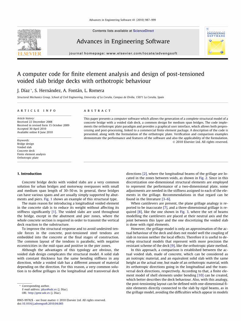
Concrete bridge decks with voided slabs are a very commonsolution for urban bridges and motorway overpasses with smalland medium span length of 30–50 m. In general, these bridgescan have various spans and are usually simply supported by abut-ments and piers. Fig. 1 shows an example of this structural type.

The main reason for introducing a longitudinal voided elementin the concrete slab is to reduce its weight without affecting itsstiffness significantly [1]. The voided slabs are used throughoutthe bridge, except in the abutment and pier zones, where thewhole concrete section is required in order to transmit the verticaldeck reaction to the substructure.

To improve the structural response and to avoid undesired ten-sile forces in the concrete, post-tensioned steel tendons areembedded into the concrete at the final stages of construction.The common layout of the tendons is parabolic, with negativeeccentricities in the mid-span and positive in the pier zones.

Although the advantages of this typology are obvious, thevoided slab design complicates the structural model. A solid slabwith constant thickness has the same bending stiffness in anydirection, while a voided slab has a different amount of materialdepending on the direction. For this reason, a very common solu-tion is to define grillages in the longitudinal and transversal deck

ll rights reserved.

directions [2], where the longitudinal beams of the grillage are lo-cated in the zones between voids, as shown in Fig. 2. Since in thisdiscretization one-dimensional structural elements are employedto represent the performance of a two-dimensional plate, someadjustments are needed in the stiffness assigned to each of the ele-ments in the grillage. Recommendations in that regard can befound in the literature [3–6].

When cantilevers are present, the plane grillage analogy is re-ported to be inaccurate [7], and a three-dimensional grillage is re-quired [8], like the one shown in Fig. 3, where the set of beamsmodelling the cantilevers are placed at their neutral axis and thejoint between this layer and the one discretizing the voided slabis done with rigid elements.

However, the grillage model is only an approximation of the ac-tual behaviour of the deck and does not model well the coupling ofslab in torsion neither the local effects. Therefore it is useful to de-velop structural models that represent with more precision theresistant scheme of the deck [9], like the orthotropic plate method.

In this approach, a comparison is established between the ac-tual voided slab, made of concrete, which can be considered asan isotropic material, and an equivalent solid slab with the sameheight as the actual one, but made of an orthotropic material, withits orthotropic directions going in the longitudinal and the trans-versal deck directions, respectively. According to that, a finite ele-ment model of shell elements under bending [10] can be created,which better describes the deck behaviour. Also, with this analogy,the post-tensioning layout can be defined with one-dimensional fi-nite elements directly connected to the slab by rigid beams, as inthe grillage model, avoiding the difficulties which appear in models

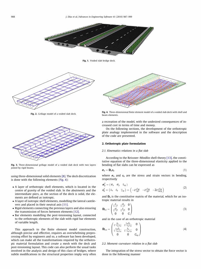
Fig. 2. Grillage model of a voided slab deck.

Fig. 3. Three-dimensional grillage model of a voided slab deck with two layersjoined by rigid beams.

Fig. 4. Three-dimensional finite element model of a voided slab deck with shell andbeam elements.

Fig. 1. Voided slab bridge deck.

988 J. Díaz et al. / Advances in Engineering Software 41 (2010) 987–999

using three-dimensional solid elements [8]. The deck discretizationis done with the following elements (Fig. 4):

� A layer of orthotropic shell elements, which is located in thecentre of gravity of the voided slab. In the abutments and theintermediate piers, as the section of the deck is solid, the ele-ments are defined as isotropic.� A layer of isotropic shell elements, modelling the lateral cantile-

vers and placed in their neutral axis [11].� Rigid elements connecting the previous layers and also ensuring

the transmission of forces between elements [12].� Bar elements modelling the post-tensioning layout, connected

to the orthotropic elements of the slab with rigid bar elementsof variable length.

This approach to the finite element model construction,although precise and effective, requires an overwhelming prepro-cessing effort by engineers and so, a software has been developed,which can make all the transformations required by the orthotro-pic material formulation and create a mesh with the deck andpost-tensioning layout. This code can also perform the usual tasksinvolved in the analysis and design of this class of bridges, wheresubtle modifications in the structural properties imply very often

a recreation of the model, with the undesired consequences of in-creased cost in terms of time and money.

On the following sections, the development of the orthotropicplate analogy implemented in the software and the descriptionof the code are presented.

2. Orthotropic plate formulation

2.1. Kinematics relations in a flat slab

According to the Reissner–Mindlin shell theory [13], the consti-tutive equation of the three-dimensional elasticity applied to thebending of flat slabs can be expressed as

rb ¼ Dbeb ð1Þ

where rb and eb are the stress and strain vectors in bending,respectively

rTb ¼ rx ry sxyð Þ

eTb ¼ ex ey cxy

� �¼ �z @2w

@x2 �z @2w@y2 �2z @2w

@x@y

� � ð2Þ

and Db is the constitutive matrix of the material, which for an iso-tropic material results in

Db;i ¼

E1�m2

mE1�m2 0

mE1�m2

E1�m2 0

0 0 G

0B@

1CA ð3Þ

and in the case of an orthotropic material

Db;o ¼

Ex1�mxymyx

myxEy

1�mxymyx0

mxyEy

1�mxymyx

Ey

1�mxymyx0

0 0 Gxy

0BB@

1CCA ð4Þ

2.2. Moment–curvature relation in a flat slab

The integration of the stress vector to obtain the force vector isdone in the following manner

J. Díaz et al. / Advances in Engineering Software 41 (2010) 987–999 989

rb ¼Z h=2

�h=2zrbdz ¼

Z h=2

�h=2zDbebdz ¼ bDbeb ð5Þ

where h is the thickness of the slab and rb and eb are the general-ized force and strain vectors in bending, respectively

rTb ¼ Mx My Mxyð Þ ð6Þ

eTb ¼ � @2w

@x2 � @2w@y2 �2 @2w

@x@y

� �ð7Þ

and bDb is the generalized constitutive matrix of the material inbending

bDb ¼Z h=2

�h=2z2Dbdz ð8Þ

which for a voided flat slab of an isotropic material, correspondingwith the actual voided deck, is

bDb;i ¼

EIy

1�m2mEIy

1�m2 0mEIx

1�m2EIx

1�m2 00 0 GIx

0B@

1CA ð9Þ

where Ix and Iy are the moments of inertia per unit length in the cor-responding axes x and y. In the case of a solid flat slab made of anorthotropic material, the Eq. (8) turns out to be

bDb;o ¼

ExI1�mxymyx

myxEyI1�mxymyx

0mxyEyI

1�mxymyx

EyI1�mxymyx

0

0 0 GxyI

0BB@

1CCA ð10Þ

where I is the moment of inertia per unit length

I ¼ h3

12ð11Þ

2.3. Identification of the mechanical parameters of the orthotropic slab

From the developments of the previous sections and establish-ing the equality between the elements of the generalized constitu-tive matrices of the orthotropic material (10) and the isotropicones (9), the expressions of orthotropic mechanical parameters of

Fig. 5. Membrane stress in x d

Fig. 6. Membrane stress in x direction

the equivalent slab are obtained. Thus, considering 1 � m2 ’ 1and 1 � mxymyx ’ 1, it can be concluded that

Ex ¼Iy

IE ð12Þ

Ey ¼Ix

IE ð13Þ

Exy ¼Ix

IG ð14Þ

While Ex, Ey and Exy are determined uniquely, there are twodifferent expressions for mxy, so the average value is chosen ascommon practice

mxy ¼Ix þ Iy

2Iym ð15Þ

Since the height of the equivalent orthotropic slab is the sameas the voided slab, a fictitious orthotropic material density mustbe defined to ensure that the weight of both slabs is the same. Ifqr is defined as the actual concrete density and qf as the fictitiousorthotropic material density, the relation of weight equality in thecross section leads to

qf ¼ qrAr;x

Af ;xð16Þ

where Ar,x is the actual area of the voided slab cross section and Af,x

is the area of the equivalent fictitious solid slab.

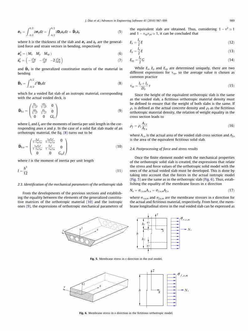
2.4. Postprocessing of force and stress results

Once the finite element model with the mechanical propertiesof the orthotropic solid slab is created, the expressions that relatethe stress and force values of the orthotropic solid model with theones of the actual voided slab must be developed. This is done bytaking into account that the forces in the actual isotropic model(Fig. 5) are the same as in the orthotropic slab (Fig. 6). Thus, estab-lishing the equality of the membrane forces in x direction

Nx ¼ rr;x;mAr;x ¼ rf ;x;mAf ;x ð17Þ

where rr,x,m and rf,x,m are the membrane stresses in x direction forthe actual and fictitious material, respectively. From here, the mem-brane longitudinal stress in the real voided slab can be expressed as

irection in the real model.

in the fictitious orthotropic model.

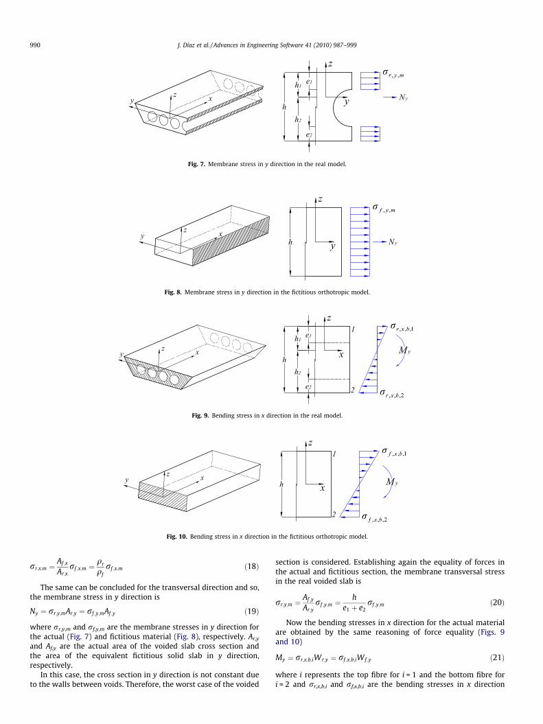
Fig. 7. Membrane stress in y direction in the real model.

Fig. 8. Membrane stress in y direction in the fictitious orthotropic model.

Fig. 9. Bending stress in x direction in the real model.

Fig. 10. Bending stress in x direction in the fictitious orthotropic model.

990 J. Díaz et al. / Advances in Engineering Software 41 (2010) 987–999

rr;x;m ¼Af ;x

Ar;xrf ;x;m ¼

qr

qfrf ;x;m ð18Þ

The same can be concluded for the transversal direction and so,the membrane stress in y direction is

Ny ¼ rr;y;mAr;y ¼ rf ;y;mAf ;y ð19Þ

where rr,y,m and rf,y,m are the membrane stresses in y direction forthe actual (Fig. 7) and fictitious material (Fig. 8), respectively. Ar,y

and Af,y are the actual area of the voided slab cross section andthe area of the equivalent fictitious solid slab in y direction,respectively.

In this case, the cross section in y direction is not constant dueto the walls between voids. Therefore, the worst case of the voided

section is considered. Establishing again the equality of forces inthe actual and fictitious section, the membrane transversal stressin the real voided slab is

rr;y;m ¼Af ;y

Ar;yrf ;y;m ¼

he1 þ e2

rf ;y;m ð20Þ

Now the bending stresses in x direction for the actual materialare obtained by the same reasoning of force equality (Figs. 9and 10)

My ¼ rr;x;b;iWr;y ¼ rf ;x;b;iWf ;y ð21Þ

where i represents the top fibre for i = 1 and the bottom fibre fori = 2 and rr,x,b,i and rf,x,b,i are the bending stresses in x direction

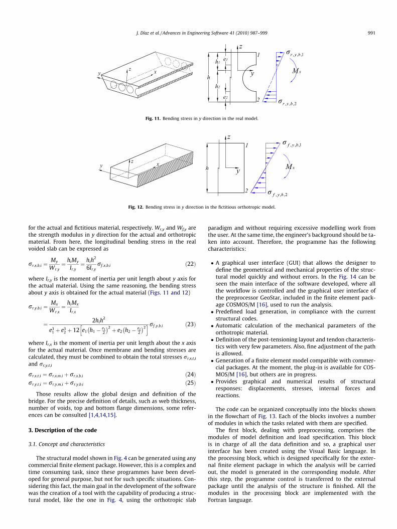
Fig. 11. Bending stress in y direction in the real model.

Fig. 12. Bending stress in y direction in the fictitious orthotropic model.

J. Díaz et al. / Advances in Engineering Software 41 (2010) 987–999 991

for the actual and fictitious material, respectively. Wr,y and Wf,y arethe strength modulus in y direction for the actual and orthotropicmaterial. From here, the longitudinal bending stress in the realvoided slab can be expressed as

rr;x;b;i ¼My

Wr;y¼ hiMy

Ir;y¼ hih

2

6Ir;yrf ;x;b;i ð22Þ

where Ir,y is the moment of inertia per unit length about y axis forthe actual material. Using the same reasoning, the bending stressabout y axis is obtained for the actual material (Figs. 11 and 12)

rr;y;b;i ¼Mx

Wr;x¼ hiMx

Ir;x

¼ 2hih2

e31 þ e3

2 þ 12 e1 h1 � e12

� �2 þ e2 h2 � e22

� �2h irf ;y;b;i ð23Þ

where Ir,x is the moment of inertia per unit length about the x axisfor the actual material. Once membrane and bending stresses arecalculated, they must be combined to obtain the total stresses rr,x,t,i

and rr,y,t,i

rr;x;t;i ¼ rr;x;m;i þ rr;x;b;i ð24Þrr;y;t;i ¼ rr;y;m;i þ rr;y;b;i ð25Þ

Those results allow the global design and definition of thebridge. For the precise definition of details, such as web thickness,number of voids, top and bottom flange dimensions, some refer-ences can be consulted [1,4,14,15].

3. Description of the code

3.1. Concept and characteristics

The structural model shown in Fig. 4 can be generated using anycommercial finite element package. However, this is a complex andtime consuming task, since these programmes have been devel-oped for general purpose, but not for such specific situations. Con-sidering this fact, the main goal in the development of the softwarewas the creation of a tool with the capability of producing a struc-tural model, like the one in Fig. 4, using the orthotropic slab

paradigm and without requiring excessive modelling work fromthe user. At the same time, the engineer’s background should be ta-ken into account. Therefore, the programme has the followingcharacteristics:

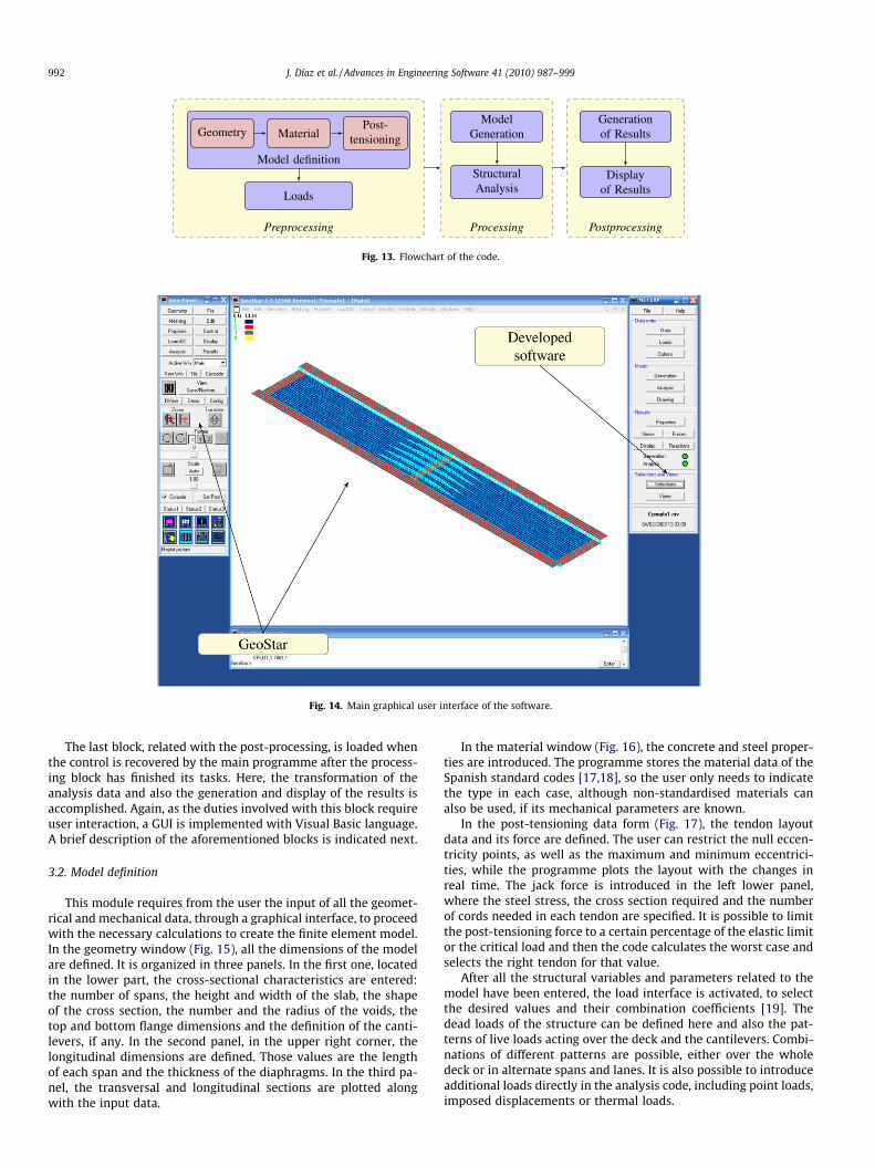
� A graphical user interface (GUI) that allows the designer todefine the geometrical and mechanical properties of the struc-tural model quickly and without errors. In the Fig. 14 can beseen the main interface of the software developed, where allthe workflow is controlled and the graphical user interface ofthe preprocessor GeoStar, included in the finite element pack-age COSMOS/M [16], used to run the analysis.� Predefined load generation, in compliance with the current

structural codes.� Automatic calculation of the mechanical parameters of the

orthotropic material.� Definition of the post-tensioning layout and tendon characteris-

tics with very few parameters. Also, fine adjustment of the pathis allowed.� Generation of a finite element model compatible with commer-

cial packages. At the moment, the plug-in is available for COS-MOS/M [16], but others are in progress.� Provides graphical and numerical results of structural

responses: displacements, stresses, internal forces andreactions.

The code can be organized conceptually into the blocks shownin the flowchart of Fig. 13. Each of the blocks involves a numberof modules in which the tasks related with them are specified.

The first block, dealing with preprocessing, comprises themodules of model definition and load specification. This blockis in charge of all the data definition and so, a graphical userinterface has been created using the Visual Basic language. Inthe processing block, which is designed specifically for the exter-nal finite element package in which the analysis will be carriedout, the model is generated in the corresponding module. Afterthis step, the programme control is transferred to the externalpackage until the analysis of the structure is finished. All themodules in the processing block are implemented with theFortran language.

Preprocessing Processing Postprocessing

Model definition

MaterialGeometryPost-

tensioning

Loads

ModelGeneration

StructuralAnalysis

Generationof Results

Displayof Results

Fig. 13. Flowchart of the code.

Fig. 14. Main graphical user interface of the software.

992 J. Díaz et al. / Advances in Engineering Software 41 (2010) 987–999

The last block, related with the post-processing, is loaded whenthe control is recovered by the main programme after the process-ing block has finished its tasks. Here, the transformation of theanalysis data and also the generation and display of the results isaccomplished. Again, as the duties involved with this block requireuser interaction, a GUI is implemented with Visual Basic language.A brief description of the aforementioned blocks is indicated next.

3.2. Model definition

This module requires from the user the input of all the geomet-rical and mechanical data, through a graphical interface, to proceedwith the necessary calculations to create the finite element model.In the geometry window (Fig. 15), all the dimensions of the modelare defined. It is organized in three panels. In the first one, locatedin the lower part, the cross-sectional characteristics are entered:the number of spans, the height and width of the slab, the shapeof the cross section, the number and the radius of the voids, thetop and bottom flange dimensions and the definition of the canti-levers, if any. In the second panel, in the upper right corner, thelongitudinal dimensions are defined. Those values are the lengthof each span and the thickness of the diaphragms. In the third pa-nel, the transversal and longitudinal sections are plotted alongwith the input data.

In the material window (Fig. 16), the concrete and steel proper-ties are introduced. The programme stores the material data of theSpanish standard codes [17,18], so the user only needs to indicatethe type in each case, although non-standardised materials canalso be used, if its mechanical parameters are known.

In the post-tensioning data form (Fig. 17), the tendon layoutdata and its force are defined. The user can restrict the null eccen-tricity points, as well as the maximum and minimum eccentrici-ties, while the programme plots the layout with the changes inreal time. The jack force is introduced in the left lower panel,where the steel stress, the cross section required and the numberof cords needed in each tendon are specified. It is possible to limitthe post-tensioning force to a certain percentage of the elastic limitor the critical load and then the code calculates the worst case andselects the right tendon for that value.

After all the structural variables and parameters related to themodel have been entered, the load interface is activated, to selectthe desired values and their combination coefficients [19]. Thedead loads of the structure can be defined here and also the pat-terns of live loads acting over the deck and the cantilevers. Combi-nations of different patterns are possible, either over the wholedeck or in alternate spans and lanes. It is also possible to introduceadditional loads directly in the analysis code, including point loads,imposed displacements or thermal loads.

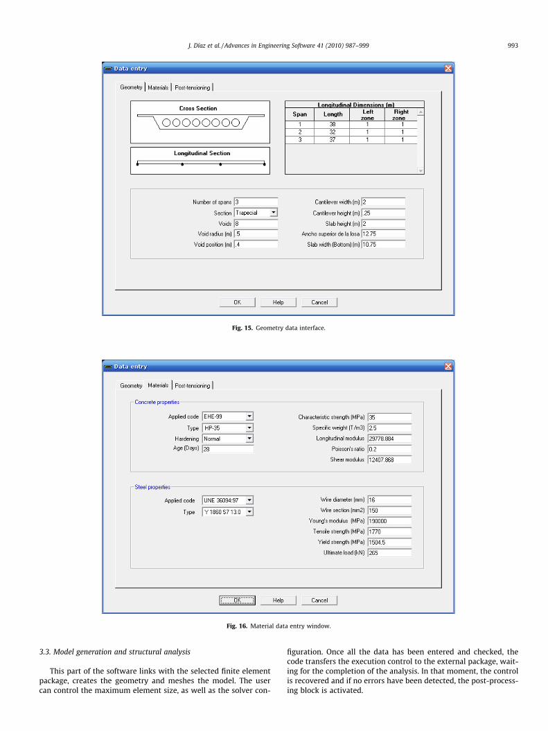
Fig. 15. Geometry data interface.

Fig. 16. Material data entry window.

J. Díaz et al. / Advances in Engineering Software 41 (2010) 987–999 993

3.3. Model generation and structural analysis

This part of the software links with the selected finite elementpackage, creates the geometry and meshes the model. The usercan control the maximum element size, as well as the solver con-

figuration. Once all the data has been entered and checked, thecode transfers the execution control to the external package, wait-ing for the completion of the analysis. In that moment, the controlis recovered and if no errors have been detected, the post-process-ing block is activated.

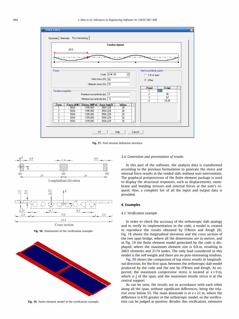
Fig. 18. Dimensions of the verification example.

Fig. 19. Finite element model of the verification example.

Fig. 17. Post-tension definition interface.

994 J. Díaz et al. / Advances in Engineering Software 41 (2010) 987–999

3.4. Generation and presentation of results

In this part of the software, the analysis data is transformedaccording to the previous formulation to generate the stress andinternal force results in the voided slab, without user intervention.The graphical postprocessor of the finite element package is usedto display the structural responses, such as displacements, mem-brane and bending stresses and internal forces at the user’s re-quest. Also, a complete list of all the input and output data isprovided.

4. Examples

4.1. Verification example

In order to check the accuracy of the orthotropic slab analogyand to verify its implementation in the code, a model is createdto reproduce the results obtained by O’Brien and Keogh [8].Fig. 18 shows the longitudinal elevation and the cross section ofthe two span bridge, where all the dimensions are in metres, andin Fig. 19 the finite element model generated by the code is dis-played, where the maximum element size is 0.8 m, resulting in2663 elements and 2174 nodes. The only load considered in thismodel is the self weight and there are no post-tensioning tendons.

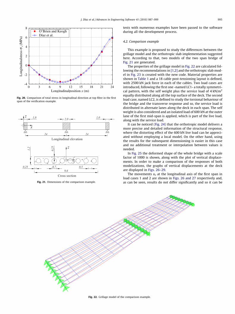
Fig. 20 shows the comparison of top stress results in longitudi-nal direction, for the first span, between the orthotropic slab modelproduced by the code and the one by O’Brien and Keogh. As ex-pected, the maximum compressive stress is located at x = 9 m,which is 3

8 of the span, and the maximum tensile stress is at thecentral support.

As can be seen, the results are in accordance with each otheralong all the span, without significant differences, being the rela-tive error below 5%. The main downside is at x = 21 m, where thedifference is 4.9% greater in the orthotropic model, so the verifica-tion can be judged as positive. Besides this verification, extensive

-4

-2

0

2

4

6

8

0 3 6 9 12 15 18 21 24

Lon

gitu

dina

lstr

ess

σx (M

Pa)

Longitudinalposition x (m)

O’Brien and KeoghDíaz et al.

Fig. 20. Comparison of total stress in longitudinal direction at top fibre in the firstspan of the verification example.

Fig. 21. Dimensions of the comparison example.

Fig. 22. Grillage model of th

J. Díaz et al. / Advances in Engineering Software 41 (2010) 987–999 995

tests with numerous examples have been passed to the softwareduring all the development process.

4.2. Comparison example

This example is proposed to study the differences between thegrillage model and the orthotropic slab implementation suggestedhere. According to that, two models of the two span bridge ofFig. 21 are generated.

The properties of the grillage model in Fig. 22 are calculated fol-lowing the recommendations in [1,2] and the orthotropic slab mod-el in Fig. 23 is created with the new code. Material properties areshown in Table 1 and a 18 cable post-tensioning layout is defined,with 2500 kN jack force in each of the cables. Two load cases areintroduced, following the first one -named LC1- a totally symmetri-cal pattern, with the self weight plus the service load of 4 kN/m2

equally distributed along all the top surface of the deck. The secondload case, named LC2, is defined to study the torsional behaviour ofthe bridge and the transverse response and so, the service load isdistributed in alternate lanes along the deck in each span. The selfweight is also considered and an isolated load of 600 kN at the outerlane of the first mid-span is applied, which is part of the live load,along with the service load.

It can be noticed (Fig. 24) that the orthotropic model delivers amore precise and detailed information of the structural response,where the distorting effect of the 600 kN live load can be appreci-ated without employing a local model. On the other hand, usingthe results for the subsequent dimensioning is easier in this caseand no additional treatment or interpolation between values isneeded.

In Fig. 25 the deformed shape of the whole bridge with a scalefactor of 1000 is shown, along with the plot of vertical displace-ments. In order to make a comparison of the responses of bothmodelizations, the graphs of vertical displacements at the deckare displayed in Figs. 26–29.

The movements uz at the longitudinal axis of the first span inload cases 1 and 2 are shown in Figs. 26 and 27 respectively and,as can be seen, results do not differ significantly and so it can be

e comparison example.

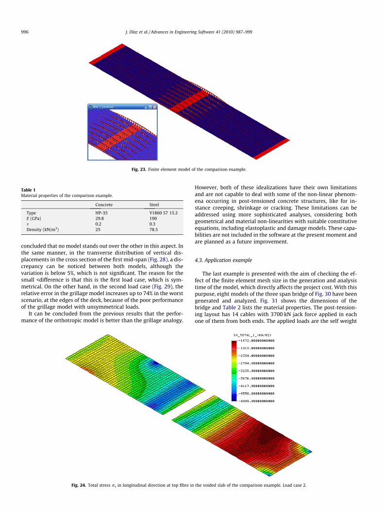
Fig. 23. Finite element model of the comparison example.

Table 1Material properties of the comparison example.

Concrete Steel

Type HP-35 Y1860 S7 15.2E (GPa) 29.8 190m 0.2 0.3Density (kN/m3) 25 78.5

996 J. Díaz et al. / Advances in Engineering Software 41 (2010) 987–999

concluded that no model stands out over the other in this aspect. Inthe same manner, in the transverse distribution of vertical dis-placements in the cross section of the first mid-span (Fig. 28), a dis-crepancy can be noticed between both models, although thevariation is below 5%, which is not significant. The reason for thesmall <difference is that this is the first load case, which is sym-metrical. On the other hand, in the second load case (Fig. 29), therelative error in the grillage model increases up to 74% in the worstscenario, at the edges of the deck, because of the poor performanceof the grillage model with unsymmetrical loads.

It can be concluded from the previous results that the perfor-mance of the orthotropic model is better than the grillage analogy.

Fig. 24. Total stress rx in longitudinal direction at top fibre in

However, both of these idealizations have their own limitationsand are not capable to deal with some of the non-linear phenom-ena occurring in post-tensioned concrete structures, like for in-stance creeping, shrinkage or cracking. These limitations can beaddressed using more sophisticated analyses, considering bothgeometrical and material non-linearities with suitable constitutiveequations, including elastoplastic and damage models. These capa-bilities are not included in the software at the present moment andare planned as a future improvement.

4.3. Application example

The last example is presented with the aim of checking the ef-fect of the finite element mesh size in the generation and analysistime of the model, which directly affects the project cost. With thispurpose, eight models of the three span bridge of Fig. 30 have beengenerated and analyzed. Fig. 31 shows the dimensions of thebridge and Table 2 lists the material properties. The post-tension-ing layout has 14 cables with 3700 kN jack force applied in eachone of them from both ends. The applied loads are the self weight

the voided slab of the comparison example. Load case 2.

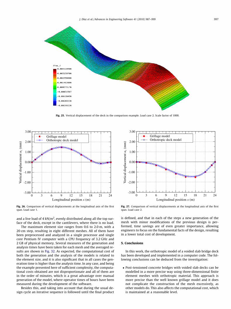
Fig. 25. Vertical displacement of the deck in the comparison example. Load case 2. Scale factor of 1000.

-3.00

-2.00

-1.00

0.00

1.00

2.00

3.00

0 3 6 9 12 15 18 21 24

Ver

tical

disp

lace

men

tuz

(mm

)

Longitudinal position x (m)

Grillage modelOrthotropic deck model

Fig. 26. Comparison of vertical displacements at the longitudinal axis of the firstspan. Load case 1.

-3.00

-2.00

-1.00

0.00

1.00

2.00

3.00

0 3 6 9 12 15 18 21 24

Ver

tical

disp

lace

men

tuz

(mm

)

Longitudinal position x (m)

Grillage modelOrthotropic deck model

Fig. 27. Comparison of vertical displacements at the longitudinal axis of the firstspan. Load case 2.

J. Díaz et al. / Advances in Engineering Software 41 (2010) 987–999 997

and a live load of 4 kN/m2, evenly distributed along all the top sur-face of the deck, except in the cantilevers, where there is no load.

The maximum element size ranges from 0.6 to 2.0 m, with a20 cm step, resulting in eight different meshes. All of them havebeen preprocessed and analyzed in a single processor and singlecore Pentium IV computer with a CPU frequency of 3.2 GHz and2 GB of physical memory. Several measures of the generation andanalysis times have been taken for each mesh and the averaged re-sults are shown in Fig. 32. As expected, the computational cost ofboth the generation and the analysis of the models is related tothe element size, and it is also significant that in all cases the gen-eration time is higher than the analysis time. In any case, and beingthe example presented here of sufficient complexity, the computa-tional costs obtained are not disproportionate and all of them arein the order of minutes, which is a great advantage over manualgeneration of the model, where operator times of hours have beenmeasured during the development of the software.

Besides this, and taking into account that during the usual de-sign cycle an iterative sequence is followed until the final product

is defined, and that in each of the steps a new generation of themesh with minor modifications of the previous design is per-formed, time savings are of even greater importance, allowingengineers to focus on the fundamental facts of the design, resultingin a lower total cost of development.

5. Conclusions

In this work, the orthotropic model of a voided slab bridge deckhas been developed and implemented in a computer code. The fol-lowing conclusions can be deduced from the investigation:

� Post-tensioned concrete bridges with voided slab decks can bemodelled in a more precise way using three-dimensional finiteelement meshes with orthotropic material. This approach ismore precise than the well known grillage model and it doesnot complicate the construction of the mesh excessively, asother models do. This also affects the computational cost, whichis maintained at a reasonable level.

0.00

0.25

0.50

0.75

1.00

1.25

1.50

-5 -3.75 -2.5 -1.25 0 1.25 2.5 3.75 5

Ver

tical

disp

lace

men

tuz

(mm

)

Transverse position y (m)

Grillage modelOrthotropic deck model

Fig. 28. Comparison of vertical displacements at the transverse section of the firstmid-span. Load case 1.

-3.75

-3.00

-2.25

-1.50

-0.75

0.00

0.75

-5 -3.75 -2.5 -1.25 0 1.25 2.5 3.75 5

Ver

tical

disp

lace

men

tuz

(mm

)

Transverseposition y (m)

Grillage modelOrthotropic deck model

Fig. 29. Comparison of vertical displacements at the transverse section of the firstmid-span. Load case 2.

Fig. 30. Finite element model of the application example.

Fig. 31. Dimensions of the application example.

0

50

100

150

200

250

300

0.60.811.21.41.61.820

1000

2000

3000

4000

5000

6000T

ime

(s)

Num

ber

of n

odes

Maximum size of finite elements (m)

Generation timeAnalysis timeNumber of nodes

Fig. 32. Computational cost of the application example.

998 J. Díaz et al. / Advances in Engineering Software 41 (2010) 987–999

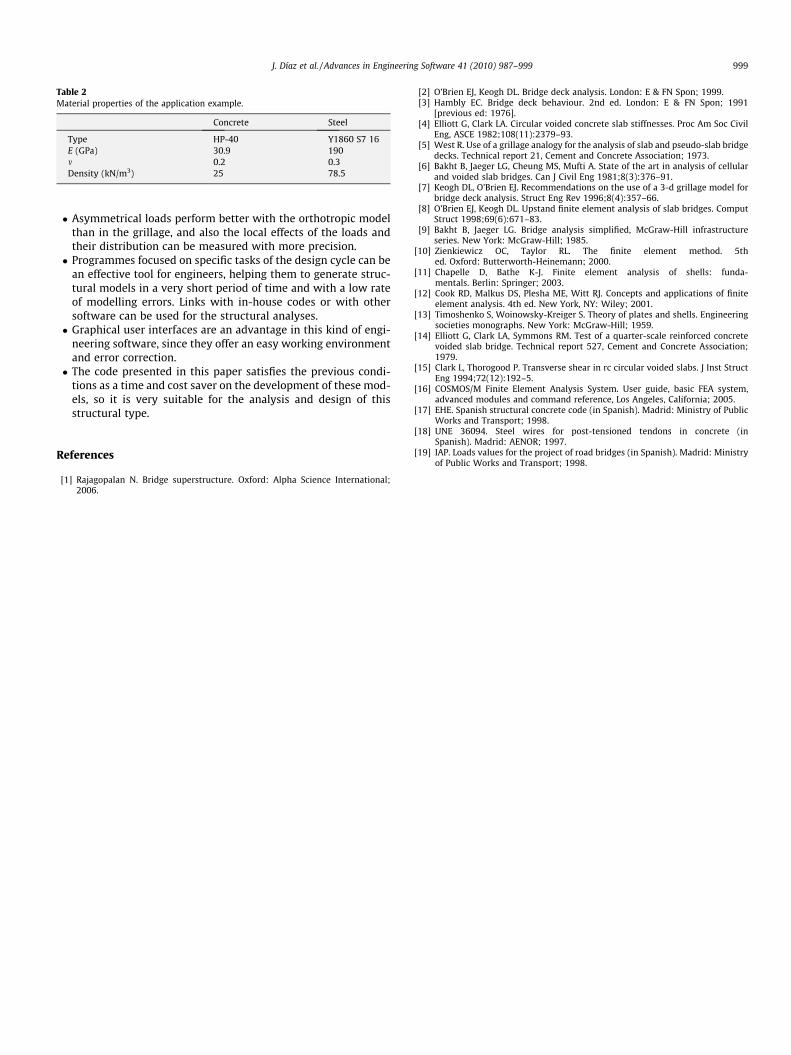
Table 2Material properties of the application example.

Concrete Steel

Type HP-40 Y1860 S7 16E (GPa) 30.9 190m 0.2 0.3Density (kN/m3) 25 78.5

J. Díaz et al. / Advances in Engineering Software 41 (2010) 987–999 999

� Asymmetrical loads perform better with the orthotropic modelthan in the grillage, and also the local effects of the loads andtheir distribution can be measured with more precision.� Programmes focused on specific tasks of the design cycle can be

an effective tool for engineers, helping them to generate struc-tural models in a very short period of time and with a low rateof modelling errors. Links with in-house codes or with othersoftware can be used for the structural analyses.� Graphical user interfaces are an advantage in this kind of engi-

neering software, since they offer an easy working environmentand error correction.� The code presented in this paper satisfies the previous condi-

tions as a time and cost saver on the development of these mod-els, so it is very suitable for the analysis and design of thisstructural type.

References

[1] Rajagopalan N. Bridge superstructure. Oxford: Alpha Science International;2006.

[2] O’Brien EJ, Keogh DL. Bridge deck analysis. London: E & FN Spon; 1999.[3] Hambly EC. Bridge deck behaviour. 2nd ed. London: E & FN Spon; 1991

[previous ed: 1976].[4] Elliott G, Clark LA. Circular voided concrete slab stiffnesses. Proc Am Soc Civil

Eng, ASCE 1982;108(11):2379–93.[5] West R. Use of a grillage analogy for the analysis of slab and pseudo-slab bridge

decks. Technical report 21, Cement and Concrete Association; 1973.[6] Bakht B, Jaeger LG, Cheung MS, Mufti A. State of the art in analysis of cellular

and voided slab bridges. Can J Civil Eng 1981;8(3):376–91.[7] Keogh DL, O’Brien EJ. Recommendations on the use of a 3-d grillage model for

bridge deck analysis. Struct Eng Rev 1996;8(4):357–66.[8] O’Brien EJ, Keogh DL. Upstand finite element analysis of slab bridges. Comput

Struct 1998;69(6):671–83.[9] Bakht B, Jaeger LG. Bridge analysis simplified, McGraw-Hill infrastructure

series. New York: McGraw-Hill; 1985.[10] Zienkiewicz OC, Taylor RL. The finite element method. 5th

ed. Oxford: Butterworth-Heinemann; 2000.[11] Chapelle D, Bathe K-J. Finite element analysis of shells: funda-

mentals. Berlin: Springer; 2003.[12] Cook RD, Malkus DS, Plesha ME, Witt RJ. Concepts and applications of finite

element analysis. 4th ed. New York, NY: Wiley; 2001.[13] Timoshenko S, Woinowsky-Kreiger S. Theory of plates and shells. Engineering

societies monographs. New York: McGraw-Hill; 1959.[14] Elliott G, Clark LA, Symmons RM. Test of a quarter-scale reinforced concrete

voided slab bridge. Technical report 527, Cement and Concrete Association;1979.

[15] Clark L, Thorogood P. Transverse shear in rc circular voided slabs. J Inst StructEng 1994;72(12):192–5.

[16] COSMOS/M Finite Element Analysis System. User guide, basic FEA system,advanced modules and command reference, Los Angeles, California; 2005.

[17] EHE. Spanish structural concrete code (in Spanish). Madrid: Ministry of PublicWorks and Transport; 1998.

[18] UNE 36094. Steel wires for post-tensioned tendons in concrete (inSpanish). Madrid: AENOR; 1997.

[19] IAP. Loads values for the project of road bridges (in Spanish). Madrid: Ministryof Public Works and Transport; 1998.