Advances in Concurrent Motion and Field-Inhomogeneity Correction in Functional MRI

by

Teck Beng Desmond Yeo

A dissertation submitted in partial fulfillment of the requirements for the degree of

Doctor of Philosophy (Electrical Engineering: Systems)

in The University of Michigan 2008

Doctoral Committee: Professor Jeffrey A. Fessler, Co-chair Assistant Research Professor Boklye Kim, Co-chair Professor Charles R. Meyer

Professor Thomas L. Chenevert Assistant Professor Clayton D. Scott

ii

© Teck Beng Desmond Yeo 2008

All Rights Reserved

iii

DEDICATION

To my parents, Robert Kim Chye Yeo and Julia Khin Neo Lee, my wife, Patricia Yoke

Hiang Loh, and our little girl, Skylar.

iv

ACKNOWLEDGEMENTS

I am glad I am finally able to officially thank the wonderful people who have been

indispensable in the completion of my doctorate. I wish to thank my advisors, Professors

Jeffrey Fessler and Boklye Kim, for their mentorship, encouragement, and kindness. As

my EECS research advisor, Prof. Fessler has been nothing short of inspirational, not only

because of his brilliant technical guidance, but also because of his commitment to his

students. I recall him driving to my apartment once to help review my qualifying

examination slides on a day when the buses stopped running unexpectedly. It is difficult

to forget something like that. Prof. Kim has been a stellar example of maintaining balance

between technical research and clinical relevance. She has provided excellent alternative

perspectives of different technical challenges, and has managed to steer me away from

developing technical tunnel vision. I am also very grateful to Prof. Chuck Meyer for

having agreed to interview me five and a half years ago. I would never have had the

opportunity to study in Ann Arbor if he and Prof. Kim had not taken a chance on a

bright-eyed student looking to transit into a different research field. I would also like to

thank Prof. Thomas Chenevert for his advice, clinical insights, and for being a great

source of support for all our MRI scans, especially those in the wee hours of the day. I

would also like to express my sincere gratitude to Prof. Clayton Scott for his invaluable

time and advice in reviewing my dissertation, and to Prof. Douglas Noll for his very

helpful and timely counsel.

ii

I am thankful to colleagues and friends including Roshni Bhagalia, Hyunjin Park,

Bing Ma, Ted Way, Somesh Srivastava, Saradwata Sarkar, Peyton Bland, Gary Laderach,

Ramakrishnan Narayanan, Kalyanakrishnan Vadakkeveedu, and Mukundakumar

Rajukumar for the good-spirited camaraderie and interesting hallway discussions.

I am very grateful to my parents who selflessly endured our years of absence from

Singapore, while encouraging us to pursue our dreams. I would also like to thank my

wife, Patricia Loh, for standing steadfastly with me through our good and bad times. You

are truly my better half. Last, but most importantly, I would like to thank God for giving

a kampong (village) boy opportunities that he could only dream of, and the strength and

ability to harness them.

This work was supported in part by the National Institute of Health grants 1P01

CA87634 and 8R01 EB00309.

iii

TABLE OF CONTENTS

DEDICATION.......................................................................................................... iii ACKNOWLEDGEMENTS..................................................................................... iv LIST OF FIGURES.................................................................................................. vi LIST OF TABLES................................................................................................... xii ABSTRACT ........................................................................................................... xvii CHAPTERS 1. Introduction ........................................................................................................... 1

1.1 Thesis Outline ........................................................................................................ 2 1.2 Contributions.......................................................................................................... 3

2. Background ............................................................................................................ 5

2.1 MRI Physics and Data Acquisition ........................................................................ 5 2.2 Cartesian Blipped EPI in Functional MRI.............................................................. 9 2.3 B0 Field-Inhomogeneity Map Estimation............................................................... 9 2.4 B0 Field-Inhomogeneity in Cartesian Blipped EPI............................................... 10

2.4.1 Overview of Field-Inhomogeneity Artifacts ........................................ 10 2.4.2 Two-Dimensional Geometric Distortion.............................................. 11 2.4.3 Two-Dimensional Geometric Distortion Correction............................ 13 2.4.4 Field-Inhomogeneity Induced In-Plane Signal Loss Correction .......... 17

2.5 Retrospective Motion Correction Methods .......................................................... 18 2.5.1 Rigid Body Registration....................................................................... 18 2.5.2 Mutual Information .............................................................................. 19 2.5.3 Map Slice-to-Volume Motion Correction ............................................ 20

2.6 Joint Two-Dimensional Motion and Geometric Distortion Problem ................... 21 3. Motion-Robust Field-Inhomogeneity Estimation Using Dual-Echo Fast GRE

............................................................................................................................... 23

3.1 Introduction .......................................................................................................... 23 3. 2 Dual-Echo Fast Gradient Echo Pulse Sequence.................................................. 25

iv

3. 3 Residual Phase Error Correction ......................................................................... 28 3. 4 Empirical Approximation of β ............................................................................ 31 3. 5 Phantom and Human Subject Data...................................................................... 32 3. 6 Results ................................................................................................................. 33 3. 7 Discussion ........................................................................................................... 37 3. 8 Conclusions ......................................................................................................... 39

4. Concurrent Field Map and Map-Slice-to-Volume (CFMMSV) Motion

Correction for EPI .............................................................................................. 41

4.1 Introduction .......................................................................................................... 42 4.2 Background .......................................................................................................... 44

4.2.1 EPI Geometric Distortion..................................................................... 44 4.2.2 Iterative Field-Corrected Reconstruction ............................................. 44 4.2.3 Map Slice-To-Volume (MSV) Registration in fMRI........................... 46

4.3 Concurrent Field-inhomogeneity Correction with MSV...................................... 47 4.4 Motion, Functional Activation and Geometric Distortion Simulation in EPI

Time Series .......................................................................................................... 49 4.5 Activation Detection with Random Permutation Test.......................................... 51 4.6 Results .................................................................................................................. 52 4.7 Discussion ............................................................................................................ 58 4.8 Conclusions .......................................................................................................... 61

5. Motion-Induced Magnetic Susceptibility and Field Inhomogeneity Estimation

using Regularized Image Restoration Techniques for fMRI .......................... 62

5.1 Introduction .......................................................................................................... 62 5.2 Theory .................................................................................................................. 63

5.2.1 Susceptibility Voxel Convolution for Field Map Computation ........... 63 5.2.2 Dynamic Field Map Estimation with Penalized Weighted Least

Squares Estimation of Magnetic Susceptibility Map – A 3D Image Restoration Approach ............................................................. 64

5.3 Methods................................................................................................................ 66 5.3.1 Data Simulation.................................................................................... 66 5.3.2 Experiments.......................................................................................... 66

5.4 Results .................................................................................................................. 67 5.5 Discussion and Conclusions................................................................................. 72

6. Formulation of Current Density Weighted Indices for Correspondence

between fMRI and Electrocortical Stimulation Maps..................................... 74

6.1 Introduction......................................................................................................... 74 6.2 Methods .............................................................................................................. 78

6.2.1 Activation Localization in fMRI....................................................... 78 6.2.2 Euclidean Distance and Voxel-Based Fixed Radii ECS-fMRI

Correspondence Indices.................................................................. 79 6.2.3 Current Density Weighted ECS-fMRI Correspondence Indices....... 79 6.2.4 Dynamic Ranges of Current Density Weighted Correspondence

Indices............................................................................................. 82 6.2.5 Numerical Approximation of Current Density.................................. 85

v

6.2.6 Data Simulation................................................................................. 86 6.2.7 Clinical Data ..................................................................................... 89

6.3 Results ................................................................................................................ 91 6.3.1 Simulation Data Results.................................................................... 91 6.3.2 Clinical Human Data....................................................................... 104

6.4 Discussion......................................................................................................... 109 6.5 Conclusions....................................................................................................... 110

7. Summary and Future Work ............................................................................. 112

7.1 Summary........................................................................................................... 112 7.2 Future Work...................................................................................................... 113

BIBLIOGRAPHY ................................................................................................. 115

vi

LIST OF FIGURES

Figure

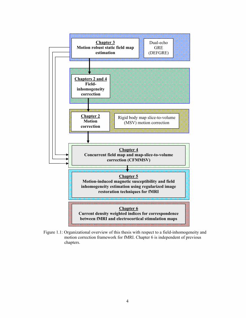
1.1 Organizational overview of this thesis with respect to a field-inhomogeneity and motion correction framework for fMRI. Chapter 6 is independent of previous chapters.......................................................................................................... 4

2.1 Single proton precessing in a B0 magnetic field and spinning about its own

axis. .............................................................................................................................. 5 2.2 Distribution of proton energy states when a group of protons are placed in a

magnetic field B0 .......................................................................................................... 6 2.3 Net magnetization,is tipped 90º downwards and precesses after applying a 90º

RF excitation pulse. (a) Spins begin to precess in phase when B1 is just applied. starts to tip downwards and precesses. (b) tips 90º downwards and precesses after 90º RF pulse is removed. Receiver coil measures induced voltage (MR signal). .......................................................................................................................... 6

2.4 (a) Slice selection gradient Gz, (b) phase encode gradient strength Gy(t) varies

for different readout cycles, (c) readout gradient Gx constant for readout cycles. ....... 7 2.5 Basic gradient echo pulse sequence. ............................................................................ 7 2.6 Single slice k-space trajectories for (a) basic gradient echo and (b) single-shot

blipped GRE echo-planar imaging protocols. .............................................................. 9 2.7 2D signal equation reduced to a set of 1D problems.................................................. 12 2.8 Rigid body rotate translate transformation parameters............................................... 18 2.9 Overview of MSV registration scheme. ..................................................................... 21 3.1 Off-resonance maps of phantom estimated by (a) standard off-resonance

method, (b) uncorrected dual-echo method showing linear phase wrapping in readout direction (x direction downwards)................................................................. 26

3.2 Simplified dual-echo pulse sequence with back-to-back Greadout pulses with

opposite polarity. Readout data from TE1 may be off-center relative to data from TE2. The first order phase shift correction term α is proportional to the time delay τ................................................................................................................. 27

vii

3.3 Frequency shifted k-space data is transformed via inverse Fourier transform to an image with an affine phase error term in the readout direction x. ......................... 27

3.4 A column of the spherical phantom off-resonance map samples in the readout

direction for (a) standard off-resonance method, (b) dual-echo off-resonance method, (c) corrected dual-echo off-resonance method. ............................................ 34

3.5 Two slices of off-resonance maps in Hz from (top) DEFGRE without

correction, (middle) DEFGRE after correction with affine phase term and (bottom) two separate single-echo acquisitions for (a) susceptibility phantom in scan 1, (b) susceptibility phantom in scan 2 (acquired 4 months after scan 1), (c) sphere phantom in scan 2. Quantitative results for entire volumes are shown in Table 3.2................................................................................................................. 35

3.6 Subject 1 (first column), subject 2 (second column) and subject 3 (third

column) off-resonance slices from (a) uncorrected DEFGRE data (direct application of Eq. (7)), (b) DEFGRE field map corrected with affine phase term (empirically determined β), (c) standard 2 single-echo 3D SPGR data. Note that the linearly varying phase error in (a) has been removed in (b). Part (a) is displayed on a scale from -1500 Hz to 1500 Hz while (b) and (c) are both displayed on a scale from -100 Hz to 200 Hz. ........................................................... 37

4.1 Recovered raw MSV motion estimates, median filtered MSV motion estimates

and ground truth of a subset of simulated dataset A with applied translation in the z direction. The RMSE values of raw MSV and median filtered MSV results are 1.10mm and 0.19mm respectively. The standard deviation values of the estimation error for raw MSV and median filtered MSV are 1.06mm and 0.13mm respectively. ................................................................................................. 47

4.2 Simulated field-map slices from a single volume with significant field-

inhomogeneity near frontal lobe and inferior temporal lobe regions. Field-map values range from -64 Hz to +320 Hz to simulate a maximum field-inhomogeneity of 5 ppm at 1.5 T. .............................................................................. 50

4.3 (a) T2 ICBM slice before simulated geometric distortion. (b) T2 ICBM slice

after simulated geometric distortion with a peak field-inhomogeneity of 5 ppm at 1.5 T........................................................................................................................ 51

4.4 Median filtered MSV motion parameter ty recovered at various correction

cycles for dataset A. Field-inhomogeneity induced geometric distortion in the PE direction y cause significant MSV errors for the distorted EPI data as well as the corrected data in cycle 0 (κ=0). Correction cycles 1 to 3 yield estimates of ty that are close to the ground truth as shown in Tables 4.1 and 4.2. ..................... 53

4.5 Normalized RMSE (NRMSE) values for each EPI slice in the same position in

the head averaged over 120 volumes for various correction cycles for (a) dataset A with applied tx, ty, tz and θz motion, and (b) dataset B with applied θx, θy, θzBB motion. ........................................................................................................... 54

4.6 (a-e, k-o) Intensity and (f-j, p-t) absolute difference images with respect to

ground truth images for two sample slices from dataset A at various stages in

viii

the CFMMSV correction process. (Top row) Geometrically distorted dataset, (second row) cycle 0, (third row) cycle 1, (fourth row) cycle 2, (fifth row) cycle 3. All images are displayed on the same normalized intensity scale ranging from 0 to 1. ................................................................................................................. 55

4.7 ROC curves showing activation detection performance for (a) dataset A and (b)

dataset B at several stages in the CFMMSV correction process. ............................... 57 4.8 Activation detection maps (P=0.001) overlaid on anatomical data of two

sample slices from (a-d,f-i) dataset A and (k-r) dataset B at several stages in the CFMMSV correction process. Each row of activation maps corresponds to a specific correction stage consisting of (top row) geometrically distorted, (second row) cycle 0, (third row) cycle 3 and (fourth row) ground truth time series images. The simulated activation maps applied to the two slices are shown in (e) and (j). ................................................................................................... 58

5.1 (Top row) Non-tilted χ map slice (y-z plane) from (a) true χ map, (b)

thresholded inverse filter estimate, (c) Wiener filter estimate (using constant object power spectra), (d) QPWLS estimate with β=0.7. (Second row) χ map slice rotated 45° using non-tilted (e) true χ map, (f) thresholded inverse filter estimate, (g) Wiener filter estimate (using constant object power spectra), (h) QPWLS estimate with β=0.7. All images are displayed on the same intensity scale. ........................................................................................................................... 68

5.2 (Top row) Non-tilted field map slice (y-z plane) from (a) originally observed

field map, (b) thresholded inverse filter estimate, (c) Wiener filter estimate (using constant object power spectra), (d) QPWLS estimate with β=0.7. (Second row) 45° rotated field map slice from (e) rotation of original observed field map, (f) application of SVC on rotated estimate of χ from thresholded inverse filter, (g) application of SVC on rotated estimate of χ from Wiener filter (using constant object power spectra), (h) application of SVC on rotated estimate of χ from QPWLS. (Bottom row) Ground truth field maps for (i) non-tilted, and (j) 45° tilted positions. All images are displayed on the same intensity scale. ............................................................................................................ 69

5.3 Dynamic field map RMSE values versus rotation angles for different

estimation methods when object was rotated about the x-axis from 0° to 180°. A constant object power spectra was used in the Wiener filter.................................. 70

5.4 (Top row) Non-tilted χ map slice (y-z plane) from (a) true χ map, (b)

thresholded inverse filter estimate, (c) Wiener filter estimate (using true object power spectra), (d) QPWLS estimate with β=0.7. (Second row) χ map slice rotated 45° using non-tilted (e) true χ map, (f) thresholded inverse filter estimate, (g) Wiener filter estimate (using true object power spectra), (h) QPWLS estimate with β=0.7. All images are displayed on the same intensity scale. ........................................................................................................................... 70

5.5 (Top row) Non-tilted field map slice (y-z plane) from (a) originally observed

field map, (b) thresholded inverse filter estimate, (c) Wiener filter estimate (using true object power spectra), (d) QPWLS estimate with β=0.7. (Second row) 45° rotated field map slice from (e) rotation of original observed field

ix

map, (f) application of SVC on rotated estimate of χ from thresholded inverse filter, (g) application of SVC on rotated estimate of χ from Wiener filter (using true object power spectra), (h) application of SVC on rotated estimate of χ from QPWLS. (Bottom row) Ground truth field maps for (i) non-tilted, and (j) 45° tilted positions. All images are displayed on the same intensity scale. ...................... 71

5.6 Dynamic field map RMSE values versus rotation angles for different

estimation methods when object was rotated about the x-axis from 0° to 180°. The true object power spectra was used in the Wiener filter...................................... 72

6.1 In the voxel-based fixed radii method (left), fMRI activation voxels

(represented by vertical bars with values of 1) within a user-specified radius around ON (solid shaded discs/ circles) and OFF (diagonal shaded discs/ circles) electrodes are true positives and false positives respectively. In the Euclidean distance method (right), the mean Euclidean distances from ON electrodes to the edges and centroids of all fMRI activation clusters are computed. ................................................................................................................... 76

6.2 In the current density weighted method, fMRI activation voxels (vertical bars)

weighted by the ON (solid shaded discs) and OFF electrodes’ (diagonally shaded discs) current density values (dotted line) at the voxels’ locations contribute to the true positive (TP) and false positive (FP) quantities respectively. The fMRI non-activated voxels weighted by the ON and OFF current density values contribute to the false negative (FN) and true negative (TN) quantities respectively. ...................................................................................... 80

6.3 (a) Sum of two ON electrode pairs’ current density maps (stimulated at 0.6 V)

on a simulated 5-by-7 electrode grid. OFF electrode pairs’ current density maps are not shown. (b) 1D profile plot of dashed line in (a) showing artificially activated voxels (solid shaded blocks) obtained by thresholding profile plot at two different threshold levels (α and β). Image columns spanned by red (taller block) and purple regions are designated as activated voxels for threshold levels β and α, respectively. (c) Samples from series of images showing artificially activated voxels which yield decreasing current density weighted sensitivity values (white denotes activated locations). Each map is generated by designating voxels in (a) that are above a threshold as activated. (d) Plot of proposed current density weighted sensitivity, specificity and gmean values for series of artificial fMRI maps generated with increasing threshold values. The sensitivity decreases from 1.0 while specificity increases from 0. The maximum possible gmean value, max_gmean, serves as a reference “best score” value for computed gmean values. .................................................................. 84

6.4 Current density magnitude for different simulated electrical stimulus levels

(leftmost pair: 0.6 V, rightmost pair: 2 V). (a) Top view contour plot (6 mm below simulated electrodes positions), and (b) cross-sectional view contour plot (sliced along dashed line in (a)), and (c) 1D profile plot of (a) along dashed line in (a). The display range for both electrode pairs in each contour plot is the same to facilitate the comparison of current density distribution spreads at different electrical stimulus levels.............................................................................. 86

x

6.5 Electrode grid overlaid on current density maps (6 mm below electrodes) for simulated ECS maps labeled E1 to E6. In E1 to E6, high current density regions (orange-red regions) indicate locations of ON electrode pairs. All other horizontally adjacent electrode pairs are either OFF electrode pairs (diamonds) or untested (dots on grid), e.g., ECS map E6. F1 to F3 denote simulated fMRI activation test cases where activated voxels are grouped into solid red ellipses (F1, F2) or circles (F3). S1 uses an input peak voltage of 0.6 V for all ON and OFF electrodes. Test case S2 uses an input peak voltage of 0.2 V for the leftmost and 0.6 V for the rightmost ON electrode pairs. All OFF electrodes for all test cases have stimulus voltages of 0.6 V. ........................................................... 88

6.6 Overview of fMRI and ECS mapping procedure for patients undergoing

surgery for lesion removal.......................................................................................... 90 6.7 Simulated dataset E1-F1-S1. (a) Current density map overlaying electrode grid

with an fMRI cluster moving from left to right side of image. (b) Current density weighted TP, FP and FN as centroid of left fMRI cluster moves along dashed line in (a). (c) Current density weighted ECS-fMRI correspondence indices. (d) Fixed radii method correspondence indices. (e) Euclidean distance method........................................................................................................................ 95

6.8 Simulated dataset E1-F3-S1. This test case has larger fMRI clusters compared

to Fig. 6.7 and illustrates that higher peak values of sensitivity and gmean are obtained (compared to Fig. 6.7) when more fMRI voxels occur in regions with high current density energy levels, i.e., near ON electrodes. Parts (a) to (e) denote images and plots as described in Fig. 6.7. ...................................................... 96

6.9 Simulated dataset E1-F2-S1. In this test case, a second (rightmost) fMRI

cluster, i.e., additional false positives, was added to the cluster (leftmost) in Fig. 6.7. Parts (a) to (e) denote images and plots as described in Fig. 6.7. ................ 97

6.10 Simulated dataset E2-F1-S1. This test case is similar to Fig. 6.7 except for an

additional ON electrode pair (rightmost). It illustrates the effects of additional false negative voxels and highlights a limitation of Euclidean distance-based indices. Parts (a) to (e) denote images and plots as described in Fig. 6.7. ................. 98

6.11 Simulated dataset E2-F1-S2. This test case is similar to Fig. 6.10 except that

the leftmost ON electrode pair was stimulated at 0.2 V while the rightmost ON pair was stimulated at 0.6 V. In Fig. 6.10, both ON electrode pairs were stimulated at 0.6 V. Parts (a) to (e) denote images and plots as described in Fig. 6.7............................................................................................................................... 99

6.12 Simulated dataset E3-F1-S1. This test case is identical to Fig. 6.7 except for the

addition of an adjacent ON electrode pair (rightmost). Parts (a) to (e) denote images and plots as described in Fig. 6.7. ................................................................ 100

6.13 Simulated dataset E4-F1-S1. This test case is similar to Fig. 6.7 except that the

ON electrode pair is now surrounded by OFF electrode pairs. Parts (a) to (e) denote images and plots as described in Fig. 6.7. .................................................... 101

xi

6.14 Simulated dataset E5-F1-S1. This test case is similar to Fig. 6.12 except that the ON electrode pairs are now surrounded by OFF electrode pairs. Parts (a) to (e) denote images and plots as described in Fig. 6.7. ............................................... 102

6.15 Simulated dataset E6-F1-S1. This test case is similar to Fig. 6.7 except that

several electrode pairs around the ON electrode are not tested (dotted locations). Parts (a) to (e) denote images and plots as described in Fig. 6.7............ 103

6.16 Coronal view of human CT datasets with overlaid current density maps

displayed on a color scale (red indicates higher values) for (a) patient 1, (b) patient 2, and (c) patient 3. Each image shows the cross-sectional view of the current density distribution around one stimulated electrode (of a pair of them). The second electrodes of the stimulated pairs lie in different coronal slice planes and thus are not visible in these images. To calculate the current density weighted ECS-fMRI indices, the 3D current density distributions for each pair of stimulated ON and OFF electrodes were computed. ........................................... 107

6.17 Composite 3D MR anatomical, CT electrode grid and fMRI activation datasets

(red for positive fMRI activation) for (a) patient 1 picture naming task, (b) patient 1 responsive naming task, (c) patient 2 picture naming task, (d) patient 2 responsive naming task, (e) patient 3 picture naming task, and (f) patient 3 responsive naming task. Solid shaded dark blue circular tags on electrode grid denote ON electrodes. .............................................................................................. 108

xii

LIST OF TABLES

Table 2.1 Magnetic susceptibility values with respect to air [19]. ............................................. 11 3.1 Estimated phase correction parameters for phantom data acquired on same

scanner using i) DEFGRE and 2D SPGR data with Eq. (3.8) (first two rows), and ii) DEFGRE data and mean 2D SPGR off-resonance value with empirical method........................................................................................................................ 32

3.2 Off-resonance RMSE values in Hz and ppm (B0=1.5 T) between each

phantom’s corrected dual-echo field map (using parameters computed in Table 3.1) and corresponding field maps computed with the standard field map method (using 2D SPGR data). Only pixels with MR image intensity values above 10% of the maximum image intensity of the respective datasets are used in the computation of the RMSE values..................................................................... 35

3.3 Off-resonance RMSE values in Hz and ppm (B0=1.5 T) between each human

subject’s corrected dual-echo field map (using α=-0.10 with β computed empirically for each scan) and corresponding field maps computed with the standard field map method (using 3D SPGR data). Only pixels with intensity values above 10% of the maximum image intensity of the respective datasets are used in the computation of the RMSE values....................................................... 36

4.1 RMS error of median filtered MSV estimates for simulated EPI datasets A and

B. ................................................................................................................................ 59 4.2 Standard deviation of the error of median filtered MSV estimates for simulated

EPI datasets A and B. ................................................................................................. 59 4.3 Area under ROC curve (AUC) values for activation detection of datasets A and

B at various stages in CFMMSV correction............................................................... 60 6.1 Current density weighted ECS-fMRI correspondence indices for picture

naming, responsive naming and combined (OR operation) picture-responsive naming fMRI maps for patient 1. Approximate value of maximum possible gmean is 0.78............................................................................................................ 105

xvi

6.2 Current density weighted ECS-fMRI correspondence indices for picture naming, responsive naming and combined (OR operation) picture-responsive naming fMRI maps for patient 2. Approximate value of maximum possible gmean is 0.80............................................................................................................ 105

6.3 Current density weighted ECS-fMRI correspondence indices for picture

naming, responsive naming and combined (OR operation) picture-responsive naming fMRI maps for patient 3. Approximate value of maximum possible gmean value is 0.80. ................................................................................................. 105

xvii

ABSTRACT

ADVANCES IN CONCURRENT MOTION AND FIELD-INHOMOGENEITY CORRECTION IN FUNCTIONAL MRI

by

Teck Beng Desmond Yeo

Co-Chairs: Jeffrey A. Fessler and Boklye Kim

Head motion and static magnetic field (B0) inhomogeneity are two important sources of image

intensity variability in functional MRI (fMRI). Ideally, in MRI, any deviation in B0 homogeneity

in an object occurs only by design. However, due to imperfections in the main magnet and

gradient coils, and, magnetic susceptibility differences in the object, undesired B0 deviations may

occur. This causes geometric distortion in Cartesian EPI images. In addition to spatial shifts and

rotations of images, head motion during an fMRI experiment may induce time-varying field-

inhomogeneity changes in the brain. As a result, correcting for motion and field-inhomogeneity

effects independently of each other with a static field map may be insufficient, especially in the

presence of large out-of-plane rotations. Our primary concern is the correction of the combined

effects of motion and field-inhomogeneity induced geometric distortion in Cartesian EPI fMRI

images. We formulate a concurrent field-inhomogeneity with map-slice-to-volume motion

correction, and develop a motion-robust dual-echo bipolar gradient echo static field map

estimation method. We also propose and evaluate a penalized weighted least squares approach to

xviii

dynamic field map estimation using the susceptibility voxel convolution method. This technique

accounts for field changes due to out-of-plane rotations, and estimates dynamic field maps from a

high resolution static field map without requiring accurate image segmentation, or the use of

literature susceptibility values. Experiments with simulated data suggest that the technique is

promising, and the method will be applied to real data in future work.

In a separate clinical fMRI project, which is independent of the above work, we also

formulate a current density weighted index to quantify correspondence between electrocortical

stimulation and fMRI maps for brain presurgical planning. The proposed index is formulated with

the broader goal of defining safe limits for lesion resection, and is characterized extensively with

simulated data. The index is also computed for real human datasets.

1

CHAPTER 1

Introduction

Functional magnetic resonance imaging (fMRI) is a dynamic imaging method that is widely used

to map the function of the human brain non-invasively. In a typical fMRI experiment, the subject

is scanned with a fast MR imaging protocol while subjected to a time-controlled set of stimuli.

Image intensity differences over time, induced by local magnetic susceptibility changes due to

cerebral blood flow (CBF) changes, are analyzed statistically to determine if a region of the brain

is activated in response to the given stimuli. Since fMRI is essentially a dynamic study of this

Blood Oxygenation Level Dependent (BOLD) contrast, fast MR imaging protocols must be used

to achieve adequate temporal resolution.

Echo-planar imaging (EPI) [1] is a group of fast imaging protocols that is commonly used

in fMRI studies. A popular protocol in this family is the single-shot Cartesian blipped EPI

protocol that acquires almost uniformly spaced k-space samples in a Cartesian grid, which allows

for efficient image reconstruction using the inverse fast Fourier transform (FFT). Unfortunately,

in the presence of inhomogeneity in the main magnetic field B0, artifacts such as geometric

distortion [2] and blurring are observed in blipped EPI and spiral EPI images respectively when

an inverse FFT is applied directly to the re-gridded k-space samples for image reconstruction.

This is due to the inadvertent field-inhomogeneity induced phase accrual in the MR signal during

the long readout time following every radio frequency (RF) pulse. The main sources of field-

inhomogeneity include eddy currents induced by the switching gradient fields, imperfect gradient

fields, main magnet imperfections and the interaction of B0 at the boundaries of tissues of

different magnetic susceptibility values. The latter is particular significant because it is object-

specific and may change non-linearly with object motion. In addition to geometric distortion and

blurring, field-inhomogeneity also causes signal loss due to in-plane and through-plane intra-

voxel dephasing. Another artifact that is often ignored is the susceptibility induced slice profile

warp which, if severe enough, can map activated voxels onto incorrect slice locations in an

anatomically correct structural scan and thus yield misleading results.

2

1.1 Thesis Outline

Parts of this thesis focus on susceptibility-induced geometric distortion correction for a single

shot blipped EPI protocol. To perform geometric distortion correction, some form of field-

inhomogeneity map is often assumed to be available [2-8]. A field map is said to be static if it is

acquired at only one time point in the fMRI experiment and thus does not track the field-

inhomogeneity changes when the head moves. A dynamic field map is a set of temporal field

maps that tracks the field-inhomogeneity changes with head motion and is usually acquired

together with the EPI data [9,10]. A static field map may suffer from errors induced by motion

between the acquisitions of the two gradient echo datasets required to estimate the field map. The

dual-echo fast gradient recalled echo (DEFGRE) field map acquisition method [11] in Chapter 3

attempts to reduce field map estimation errors due to such motion between the two echo signals.

Head motion is another source of image intensity variation that can severely curtail

activation detection accuracy. Motion correction techniques generally use an affine

transformation model, of which the rigid body model is a special case, or a non-linear

transformation model, which is computationally more expensive. If geometric distortion

correction for blipped EPI is not performed, rigid body registration techniques generally do not

have sufficient degrees of freedom to accurately reposition all the EPI slices into a structural scan,

and thus, non-linear registration techniques are required. In addition, head motion may change the

angles between B0 and tissue interfaces which in turn can cause the field-inhomogeneity to vary

non-linearly with head motion. Thus, correcting for head motion and field-inhomogeneity

separately with only a static field map may yield significant errors. The concurrent field map and

map-slice-to-volume motion correction (CFMMSV) method [13] in Chapter 4 attempts to

estimate a pseudo-dynamic field map to perform geometric distortion correction and uses map-

slice-to-volume (MSV) motion correction parameters to compute an updated field map from a

static field map. This correction method may have limitations for large out-of-plane rotations and

thus, in Chapter 5, we propose a novel penalized weighted least squares approach to field map

estimation to account for such motion. We present preliminary results of the proposed approach

to estimating dynamic field maps from a measured high resolution 3D static field map using a

statistical version of the deterministic susceptibility voxel convolution method. The proposed

method does not require head image segmentation, or the associated assignment of literature

magnetic susceptibility values to voxels of the brain.

In Chapter 6, we propose a current density weighted index to quantify the correspondence

between fMRI and electrocortical stimulation (ECS) maps for brain lesion presurgical planning.

3

ECS is the current gold standard for brain functional mapping in presurgical planning, but it is

highly invasive. The definition of a systematic and physiologically relevant correspondence index

is a first step to evaluating fMRI as a non-invasive alternative to ECS for presurgical planning. In

this work, various techniques, including non-linear registration, rigid body slice-to-volume

registration, fMRI time series analysis, and subdural electrode current density computation, are

employed to facilitate the definition of the proposed correspondence index.

In summary, Chapters 1 and 2 of this report provide the necessary background

information for the remaining chapters. Chapters 3 and 4 describes work already done [11,13],

while Chapters 5 and 6 present preliminary results with suggestions for future work. Fig. 1.1

provides an organizational overview of this thesis.

1.2 Contributions

The main contributions of this work are:

• The problem formulation and development of an affine phase error correction technique that

facilitates motion robust static field map estimation using a dual-echo bipolar gradient

recalled echo protocol [11]. Validation of the technique is performed using phantom and

human data.

• The development of a concurrent motion and field inhomogeneity correction framework for

EPI time series images [13]. The concurrent field-map MSV (CFMMSV) method employs

iterative field-corrected quadratic penalized least squares (QPLS) image reconstruction [5]

followed by a field map approximation procedure to enhance the MSV rigid body motion-

correction scheme, therefore accounting for field inhomogeneity changes with inter-slice

head motion.

• The formulation of a novel regularized 3D image restoration approach to dynamic

susceptibility map estimation by solving the inverse susceptibility voxel convolution

problem. Using realistically simulated noisy 3D field maps of a spherical air compartment in

water, preliminary results suggest that the proposed method may yield more accurate

dynamic field map estimates compared to simpler methods, while requiring less prior

information. In fMRI, this may potentially improve dynamic field map estimates and hence,

geometric distortion correction accuracy.

• The definition and evaluation of a new set of current density weighted indices to quantify the

correspondence between subdural electrocortical stimulation and fMRI maps [58]. Simulated

datasets are used to characterize the indices in detail, after which, they were computed for

several patient datasets.

4

Figure 1.1: Organizational overview of this thesis with respect to a field-inhomogeneity and

motion correction framework for fMRI. Chapter 6 is independent of previous chapters.

Chapter 3 Motion robust static field map

estimation

Chapters 2 and 4 Field-

inhomogeneity correction

Chapter 2 Motion

correction

Dual-echo GRE

(DEFGRE)

Rigid body map slice-to-volume (MSV) motion correction

Chapter 4 Concurrent field map and map-slice-to-volume

correction (CFMMSV)

Chapter 5 Motion-induced magnetic susceptibility and field

inhomogeneity estimation using regularized image restoration techniques for fMRI

Chapter 6 Current density weighted indices for correspondence between fMRI and electrocortical stimulation maps

5

CHAPTER 2

Background

2.1 MRI Physics and Data Acquisition

An MR image is a map of an object’s spatially varying net transverse (x-y plane component)

magnetization generated by atomic nuclei that exhibit the nuclear magnetic resonance (NMR)

phenomenon. The hydrogen nucleus, which is abundant in human soft tissue, is the predominant

NMR-active nucleus imaged in brain MR images. The NMR phenomenon occurs when the

NMR-active nucleus is placed in an external magnetic field, B0, and excited by an applied RF

pulse B1 that is orthogonal to B0. An NMR-active nucleus spins and behaves like a bar magnet

with a small magnetic field referred to as the magnetic moment, µv . A nucleus-specific

gyromagnetic ratio γ constant quantifies the ratio of the nucleus’ angular momentum to its

magnetic moment.

A hydrogen nucleus (single proton) placed in a homogenous magnetic field, B0 is

magnetized and will align itself either parallel (low energy state) or anti-parallel (high energy

state) to B0. Besides spinning on its own axis, each proton will also precess or rotate about the B0

axis like a spinning top at the Lamor frequency, ω, as shown in Fig. 2.1 and described by Eq.

(2.1).

ω = γB0 (2.1)

Figure 2.1: Single proton precessing in a B0 magnetic field and spinning about its own axis.

µvB0 precession

Spinning proton

6

The aggregate sum of the magnetic moments of the nuclei in a closed volume shown in

Fig. 2.2 form the net magnetization, Mv

. At thermal equilibrium without the RF pulse, the spins

do not precess in phase and thus cancel out each others transverse components. Thus Mv

does not

precess and is aligned with B0 as shown in Fig. 2.2.

Figure 2.2: Distribution of proton energy states when a group of protons are placed in a

magnetic field B0

Figure 2.3: Net magnetization, M

vis tipped 90º downwards and precesses after applying a 90º RF

excitation pulse. (a) Spins begin to precess in phase when B1 is just applied. Mv

starts to tip downwards and precesses. (b) M

vtips 90º downwards and precesses after 90º

RF pulse is removed. Receiver coil measures induced voltage (MR signal).

When an RF pulse oscillating at the proton Lamor frequency is applied perpendicular to

B0, all proton spins begin to precess in phase with each other. Some spins in the low energy state

make a transition into the higher energy state by absorbing energy from the RF pulse and this

causes the net magnetization to tip towards the transverse plane. This is the NMR phenomenon.

An αº RF pulse is one that has sufficient energy to tip Mv

by αº. Fig. 2.3 shows the net

magnetization, Mv

, after applying a 90º RF pulse to a group of protons. The precessing net

(a) (b)

B1 RF pulse applied

B0

Mv

Low energy state (has more spins)

High energy state (has fewer spins)

Receiver coil

yB0

Low energy state (lost spins to high energy state)

High energy state (gained spins from low energy state)

Mv

x

z

High energy state

B0Mv

Low energy state

7

transverse magnetization xyMv

is used to induce a voltage across a receiver coil according to

Faraday’s Law of Induction as shown in Fig. 2.3(b). The induced voltage constitutes the

measured MRI signal s(t).

After the RF pulse is removed, three main processes cause the received signal s(t) to

decay with time: spin-lattice energy loss caused by thermal perturbations (characterized by T1),

dephasing due to spin-spin interactions (characterized by T2) and field-inhomogeneity induced

dephasing (characterized by T2*). Assuming the field-inhomogeneity has a Lorentzian

distribution, the signal decays with a time-constant T2* where T2

* = 1/ T2 + 1/ T∆B and T∆B ≈

(γ∆B)-1. T∆B is the time-constant for the decay that occurs due to magnetic field-inhomogeneity

∆B. Field-inhomogeneity is often expressed in parts per million of the main magnetic field, i.e.

∆Bppm=(∆B/B0)*106), and usually varies spatially.

Spatial localization in MRI is typically achieved by applying magnetic field gradients in

three orthogonal directions to encode spatial information about the object as shown in Fig. 2.4.

Figure 2.4: (a) Slice selection gradient Gz, (b) phase encode gradient strength Gy(t) varies for different readout cycles, (c) readout gradient Gx constant for readout cycles.

Figure 2.5: Basic gradient echo pulse sequence.

RF pulse

(c) Frequency encoding (a) Slice selection

Bz=Gzz By=Gy(t)y Bx=Gxx

(b) Phase encoding z

x

y

RF

TE

ADC s(t)

Gx(t)

Gz(t)

Gy(t)

TR

Tpe

Treadout

8

As an example, a basic multi-slice gradient echo pulse sequence is shown in Fig. 2.5. A

slice-selection gradient Gz(t) is first applied to set up a linear Lamor frequency variation in the z

direction as shown in Fig. 2.5. A B1 pulse with a bandwidth that covers the Lamor frequency

range of the slice of interest is then applied. All subsequent data measurements pertain only to

this slice. After a slice has been selected, a phase encode field gradient Gy(t) is applied in the y

direction for Tpe seconds. This causes a linearly varying spin phase accrual ydGpeT

y ⎥⎥

⎦

⎤

⎢⎢

⎣

⎡∫0

)( ττγ in

the y direction. The term ∫peT

y dG0

)( ττγ is also known as the y-direction spatial frequency, ky(t).

The gradient strength of Gy(t) changes for each cycle of the pulse sequence so that data at

different values of ky(t) can be measured. No signal is read during the application of the phase

encode pulse Gy(t). For each readout cycle with a constant Gy(t)=Gy, ky is just γGyTpe cycles/ mm.

Following the phase encode pulse, a readout pulse Gx(t) is applied during which the

signal s(t) is read off the receiver coil. A constant Gx(t) pulse causes the Lamor frequency to vary

linearly with x. As time passes, the phase accrual per unit length in the x direction

∫=t

xx dGtk0

)()( ττγ gets larger. Physically, the net magnetization gets rotated by xtjkxe )(− for

each value of x at time t The MR signal s(t), which is the sum of all the rotated spins’

magnetization at time t, is sampled for various values of kx(t) as t increases. After the signal is

acquired, the spins are allowed to relax for TR seconds before the next RF pulse is applied. Recall

that the Fourier transform F(ω) of a one dimensional function f(x) can be viewed as a weighted

integral of f(x) where the weights are spatially linear phase terms xje ω− . In other words, the

Fourier transform at a specific frequency ωi is the integral over x of f(x) rotated by a spatially

linear phase term xj ie ω− . Since this is what happens physically to the magnetization when linear

localization gradients are applied, the MR signal s(t) or s(kx(t),ky(t)) of an infinitely thin slice in

the z direction can be expressed as the Fourier transform of the imaged object f(x,y) with spatial

frequencies kx(t) and ky(t),

∫ ∫∞

∞

∞

∞

+−== dxdyeyxftktksts ytkxtkjyx

yx ),( ))(),(( )( ))()((2π . (2.2)

The map of kx and ky (and kz for 3D imaging) is known as k-space in MRI literature. The

relationship between t, kx(t) and ky(t) is expressed in the k-space trajectory, which shows the

9

chronological order in which samples of k-space s(kx(t), ky(t)) are acquired. The k-space trajectory

is determined by how the spatial localization gradients are applied.

2.2 Cartesian Blipped EPI in Functional MRI

Fig. 2.6 shows the k-space trajectory of the basic gradient echo pulse sequence of Fig. 2.5 and the

blipped gradient echo EPI pulse sequence. Gradient echo EPI yields images that are sensitive to

local susceptibility changes due to blood oxygenation level variations in fMRI experiments.

However, in the presence of macroscopic field-inhomogeneity, especially that induced by

magnetic susceptibility differences at tissue boundaries, the longer readout time Treadout in EPI

(typically about 30-100 ms) induces significant levels of undesirable phase accrual. If

uncorrected, the extra phase accrued leads to geometric distortion in the reconstructed EPI images

which will yield incorrect fMRI activation detection results.

Figure 2.6: Single slice k-space trajectories for (a) basic gradient echo and (b) single-shot blipped

GRE echo-planar imaging protocols.

2.3 B0 Field-Inhomogeneity Map Estimation

The field-inhomogeneity map or off-resonance map, represented by the symbols ∆B( rv ) and

∆ω( rv )=2πγ∆B( rv ) respectively, quantifies the deviation of the magnetic field in the MR scanner

from the applied magnetic field. Some authors refer to the two maps simply as the field map.

Field-inhomogeneity in MRI may be induced by object-specific causes such as tissue

Gy(t) Gx(t) A/D

Gz(t)

ky

RF

Each row acquired following one RF pulse

(a) Gradient echo

TR in order of seconds

Treadout

ky

kx

Gy(t) Gx(t)

A/D

Gz(t)

RF

Entire k-space acquired following one RF pulse

(b) Blipped GRE echo-planar imaging

exp(-t/T2*)

TR in order of seconds

Treadout ≈ 40-70ms

kx

10

susceptibility differences or by scanner-specific causes such as main B0 or gradient field

variations. The use of shimming techniques can reduce the field-inhomogeneity over a human

head to smaller than 1 ppm everywhere except the anterior frontal lobe and the inferior temporal

lobes. These regions have significant susceptibility-induced field-inhomogeneities due to the

presence of air-tissue and bone-tissue interfaces. Ideally, the magnetic field in an object in a

homogenous B0 field should be B0. However, due to magnetic susceptibility χ, the actual field is

B=(1+χ)B0 instead. At a boundary of two tissues with significant susceptibility difference, there is

a local change in the magnetic field and thus the spins’ Lamor frequencies are no longer

homogeneous.

Many proposed field map estimation methods revolve around taking the phase difference

between two gradient recall echo (GRE) scans of the same object, each acquired at a different

echo time [14-17]. These methods assume that all the phase accrual occurs at the respective echo

times. The echo time difference is typically chosen to be small to prevent phase wrapping. In the

context of fMRI time-series imaging, a field map acquired at a single time point in the course of

the experiment is known as a static field map. Section 3.1.2 describes a conventional static field

map estimation method in greater detail. Field maps acquired at multiple time points during the

fMRI experiment form a set of dynamic field maps that tracks some of the the field-

inhomogeneity changes for the duration of the experiment [9,18]. A static field map is generally

higher in spatial resolution but prone to motion-induced errors. These errors may arise due to

motion in-between the two echoes acquired for field map estimation and to motion in–between

field map acquisition and time-series data acquisition. Dynamic field maps are more impervious

to motion-induced field map errors but generally suffer from lower field map resolution [9],

increased complexity in the estimation process [10,12] or the need for pulse sequence

modification [9].

2.4 B0 Field-Inhomogeneity in Cartesian Blipped EPI

2.4.1 Overview of Field-Inhomogeneity Artifacts

This magnetic field variation can cause four artifacts [19] of which the first is the main topic of

interest in this report:

i) in-plane 2D geometric distortion,

ii) signal loss due to in-plane (i.e. echo-shifting effect) intra-voxel dephasing,

iii) signal loss due to through-plane intra-voxel dephasing,

iv) slice selection profile warp.

11

2.4.2 Two-Dimensional Geometric Distortion

Geometric distortion is readily observed at locations where the magnetic susceptibility varies

significantly across material boundaries. Table 2.1 shows the three main types of materials

present in a human head – water or soft tissue, bone and air. The largest susceptibility difference

occurs at the boundary of soft tissue and air (-9.05 ppm/cm3) followed by the boundary of bone

and air (-8.86 ppm/cm3). As such, in brain imaging, susceptibility-induced field-inhomogeneities

often occur around the petrous bone where the ear structures are located, and the region

surrounding the sinuses (air/ tissue interface) which lead to distortion in the temporal lobes and

anterior frontal regions respectively [2]. Changing the orientation of the susceptibility interface

with B0 (out-of-plane rotations) will change the field map. Translations and in-plane rotation are

less likely to change the susceptibility-induced component of the field map since the tissue

interface-B0 orientation remains the same.

Table 2.1: Magnetic susceptibility values with respect to air [19]. B0=1.5T, FOV=240mm, 32 kHz, Gz = 3.13 mT/m, 256 pixels

Material χ (ppm / cm3)

H2O (soft tissue) -9.05

Bone -8.86

Air 0.0

It is useful to quantify how geometric distortion arises in EPI images in the presence of

field-inhomogeneity. To do that, the point spread function (PSF) of the EPI imaging process in

the presence of field-inhomogeneity can be derived [3]. Ignoring relaxation effects, the signal

equation for a 2D MRI slice with field-inhomogeneity is

∫ ∫∞

∞−

∞

∞−

+−∆−== dxdyeeyxftktksts ytkxtkjkktyxBjyx

yxyx ),( ))(),(( )( ))()((2)],(),([2 ππγ , (2.3)

where ∆B(x,y) is the field-inhomogeneity at location (x,y), t(kx,ky) is the acquisition time-point for

k-space sample at (kx,ky) and f(x,y) is the imaged object. Note that in the presence of the field-

inhomogeneity term, s(t) is no longer the Fourier transform of f(x,y). This is because the field-

inhomogeneity term varies with time. The data acquisition time in EPI is negligible in the kx

direction and thus an approximation t(kx, ky) ≈ t(ky) can be made as suggested in [3]. The first

exponential term in Eq. (2.3) is now independent of kx and thus the 1D inverse Fourier transform

of s(t) can be evaluated with respect to kx as in

12

∫∞

∞−

−∆−= dyeeyxftkxs ytkjktyxBjiyi

yyi ),( ))(,(ˆ ))((2)](),([2 ππγ , (2.4)

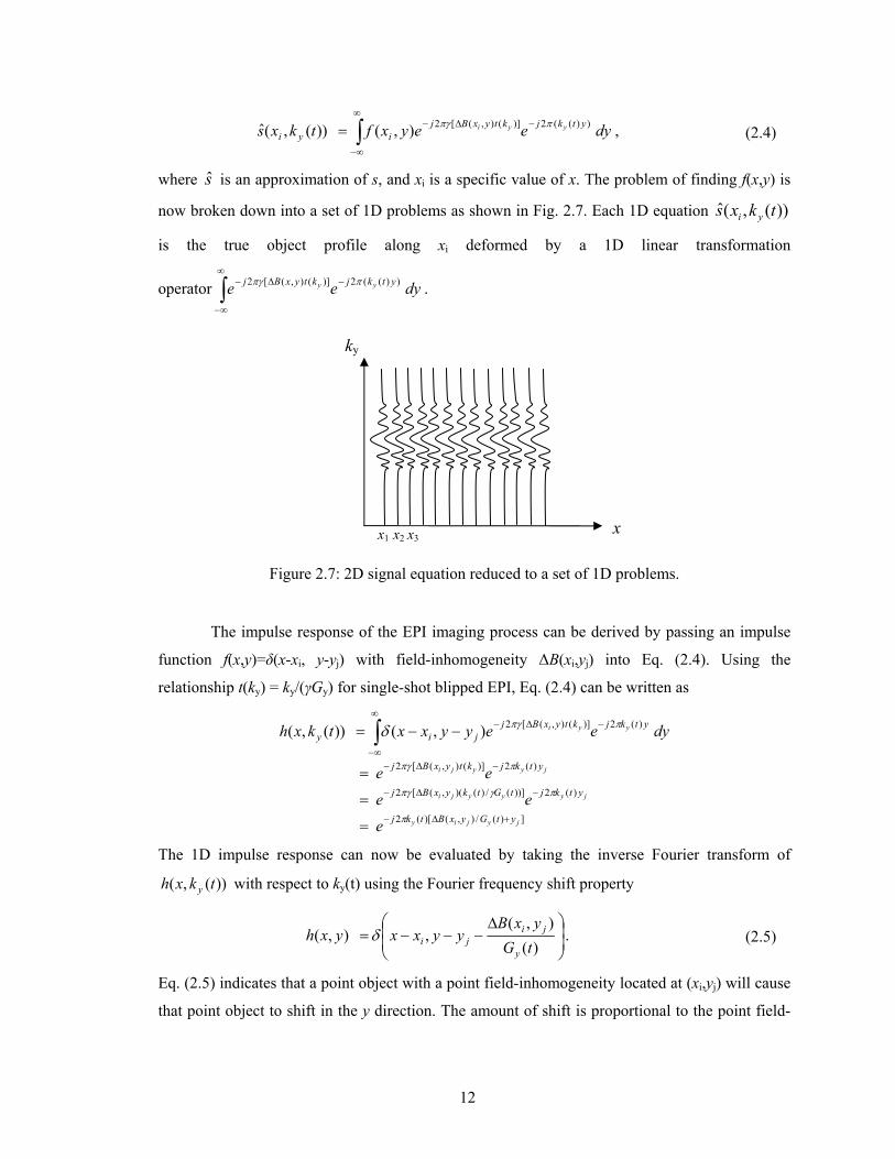
where s is an approximation of s, and xi is a specific value of x. The problem of finding f(x,y) is

now broken down into a set of 1D problems as shown in Fig. 2.7. Each 1D equation ))(,(ˆ tkxs yi

is the true object profile along xi deformed by a 1D linear transformation

operator ∫∞

∞−

−∆− dyee ytkjktyxBj yy ))((2)](),([2 ππγ .

Figure 2.7: 2D signal equation reduced to a set of 1D problems.

The impulse response of the EPI imaging process can be derived by passing an impulse

function f(x,y)=δ(x-xi, y-yj) with field-inhomogeneity ∆B(xi,yj) into Eq. (2.4). Using the

relationship t(ky) = ky/(γGy) for single-shot blipped EPI, Eq. (2.4) can be written as

])(/),()[(2

)(2))](/)()(,([2

)(2)](),([2

)(2)](),([2

),( ))(,(

jyjiy

jyyyji

jyyji

yyi

ytGyxBtkj

ytkjtGtkyxBj

ytkjktyxBj

ytkjktyxBjjiy

e

ee

ee

dyeeyyxxtkxh

+∆−

−∆−

−∆−

∞

∞−

−∆−

=

=

=

−−= ∫

π

πγπγ

ππγ

ππγδ

The 1D impulse response can now be evaluated by taking the inverse Fourier transform of

))(,( tkxh y with respect to ky(t) using the Fourier frequency shift property

⎟⎟⎠

⎞⎜⎜⎝

⎛ ∆−−−=

)(),(

, ),(tGyxB

yyxxyxhy

jijiδ . (2.5)

Eq. (2.5) indicates that a point object with a point field-inhomogeneity located at (xi,yj) will cause

that point object to shift in the y direction. The amount of shift is proportional to the point field-

x

ky

x1 x2 x3

13

inhomogeneity and inversely proportional to the phase encode gradient strength. It is more useful

to see Eq. (2.5) in terms of pixel shifts.

From Nyquist sampling theorem, the sampling interval ∆y of a 1D bandlimited signal

must be at least 1/2ky(max) to prevent aliasing. If the time duration in which s(t) is acquired is

Treadout and if rectangular phase encode gradient pulses are used in the blipped EPI sequence, then

the y-direction spatial resolution ∆y can be expressed as

yTTd

ky

readoutreadouty ∆=⇒===∆

∫γγ

ττγ

1G G

1

)(G

1 2

1 yy

T

0y

(max)readout

. (2.6)

Substituting Eq. (2.6) into Eq. (2.5), we obtain

)),(,(),( yTyxByyxxyxh readoutjiji ∆∆−−−≈ γδ . (2.7)

Since ∆y is the y-direction pixel size, Eq. (2.7) shows that the point object at (xi,yj) with point

field-inhomogeneity shifts in the y-direction by γ∆B(xi,yj)Treadout pixels. The term 1/Treadout is also

known as the pixel bandwidth in the phase encoded direction. The bandlimited k-space is actually

a truncated Fourier space and thus s(kx(t), ky(t)) is actually multiplied by a window function

rect(kx(t)/2kx(max), ky(t)/2ky(max)). Thus, the final impulse response is Eq. (2.7) convolved with a

sinc(2kx(max)x, 2ky(max)y) function. In other words, the final impulse response is a space variant

shift-and-blur operation. The space-variant pixel shift in the phase encode direction causes

geometric distortion, intensity accumulation and/ or intensity spread, which adversely affect

fMRI activation detection.

2.4.3 Two-Dimensional Geometric Distortion Correction

Most field-correction methods that undo the geometric distortion due to field-inhomogeneity use

field maps [2-8]. The field maps have been used to directly shift pixels in the distorted images

back to its estimated original positions based on Eq. (2.7) [2], and also to perform field-

compensated reconstructions from the MRI measured data to obtain the geometrically correct

images [3,5,7,8]. Pixel shift methods are simple to implement and useful for quick evaluations but

sub-optimal in distortion-correction performance because it cannot separate the individual

contribution of several pixels that map into the same pixel during the distortion process. A

popular field-corrected reconstruction method, the conjugate phase technique, tries to compensate

for the off-resonance phase accrual at each time point. It should perform better than the pixel-shift

method but its performance degrades when the field map is spatially not smooth. This is

unfortunate since susceptibility-induced field-inhomogeneities are typically not smoothly

14

varying. An iterative model-based field-corrected reconstruction method [5] that does not require

a smooth field map will be discussed in this section.

The process of estimating the true unknown object )(rf v from the sampled k-space data

s(ti) constitutes the MRI image reconstruction problem. The first step in formulating the problem

is to parameterize the image into pixels and treat each pixel value as an unknown. Then a system

of linear equations can be set up according to the parameterized MR signal equation with additive

Gaussian noise. Finally, the system of equations is solved by non-iterative or iterative algorithms.

The system of linear equations can be represented in the matrix form. In the notation used here,

matrices are printed as upper-case bold characters (e.g. A) and column vectors are labeled with an

arrow above the variables (e.g. rk vv, ).

Ignoring spin relaxation and assuming spatially invariant receiver coil sensitivity, the

non-parameterized MR signal equation for a selected slice in the presence of field-

inhomogeneities is

∫∞

∞

⋅−∆−= rdeerfts rtkjtrji

iivv vvv

)( )( ))((2)( πω , (2.8)

where s(ti) is the baseband signal sample at time ti during the readout, ∆ω( rv ) is the spatially

variant field-inhomogeneity and f( rv ) is a continuous-space function of the net transverse

magnetization of the object. Eq. (2.8) can be represented as the result of a linear operator A

applied to the true object f. This is a continuous-to-discrete mapping which is inherently ill-posed

and under-constrained. There are many potential solutions to f( rv ) for any single set of s(ti) values

due to the smoothing effect of the integral operator.

The dominant noise in MRI is from the thermal vibrations of ions and electrons and is

conventionally modeled as a white Gaussian noise [20]. Thus, the sampled signal yi includes s(ti)

and an additive complex independent and identically distributed (i.i.d.) white Gaussian noise ε

that can be expressed [5] as

εfynitsy iii

+==+=

A or 1..... )( dε

. (2.9)

To limit the number of parameters to be estimated, the continuous object f and field map is

parameterized into a sum of np weighted rect basis functions )( nrrb vv − as follows.

∑∑

∑∑−

=

−

=

−

=

−

=

−=−

≈

−=−

≈

1

0

1

0

1

0

1

0

)()()(

)()()(

pp

pp

n

nnn

n

n

nn

n

nnn

n

n

nn

rrbrrrrectr

rrbfrrrrectfrf

vvv

vvv

vvv

vvv

ωωω ∆∆

∆∆

∆. (2.10)

15

Eq. (2.8) can now be written as a summation over space

∑−

=

⋅−∆−≈1

0

))((2))(( )(p

niin

n

n

rtkjtjnii eeftkBts

vvv πω . (2.11)

where ))(( itkBv

is the Fourier transform of )(rb v (a sinc) and fn is the object intensity at location

nrv . The continuous-discrete model of Eq. (2.9) can now be written as a discrete-discrete model

εfy += A . (2.12)

where f is the column-wise stacked vector of the parameterized object, y is the k-space data vector

and A is the possibly ill-conditioned nd-by-np system-object matrix with elements ))((2

, ))(( nmmn rtkjtjmnm eetkBa

vvv ⋅−∆−= πω . The image reconstruction problem is now to estimate f

given y and the system-object matrix A (which requires knowledge of ∆ω).

There are three main considerations in choosing the cost function and an algorithm to

solve Eq. (2.12). First, A may be ill-conditioned and thus some form of regularization must be

integrated into the cost function. Secondly, A is a huge matrix even for small image sizes. Thus

computing the pseudo-inverse of A to find a solution for f will require extensive storage resources

and computation time. Thus, an iterative approach is taken to solve for f. Thirdly, the solution

must take into account MR Gaussian noise in y.

Most field-corrected reconstruction methods involve two steps: measuring a field map

and using it to reconstruct a field-corrected image. Many non-iterative methods like the conjugate

phase reconstruction technique [8] work better with a spatially smooth field map. This

requirement may hold for field-inhomogeneities due to hardware imperfections but not for

susceptibility-induced field-inhomogeneities which have higher order spatial variations. Model-

based iterative reconstruction methods do not require a smooth field map and models the problem

with noise more accurately. It has been reported [7] that iterative conjugate gradient methods

outperform the conjugate phase method for EPI images. The conjugate phase estimator attempts

to reconstruct the image by compensating for the phase accrual at each time point in Eq. (2.11). A

weighting matrix is often included for non-uniformly sampled k-space data. Since the EPI k-space

data is assumed to be uniformly sampled for simplicity, this weighting matrix is the identity

matrix and the conjugate phase estimator becomes

)( )(ˆ **1

0

))((2)( εAfAyA +=== ∑−

=

⋅∆d iin

i

rtkjtrjiCP eeyrf

vvvv πω . (2.13)

In [5], f is estimated directly from the k-space data y by minimizing a quadratic penalized least

squares cost function using the conjugate gradient optimization algorithm. The reconstruction

obtained from the density compensated non-iterative conjugate phase algorithm is used as the

16

initial guess of f in the conjugate gradient algorithm. In EPI, since the measured samples are

assumed to be uniformly spaced, we can assign an identity matrix to the weighting matrix in [5].

The cost function and estimator can thus be written as

fffyf CCA TTβψ21

21)( 2

1 +−= . (2.14)

[ ]εAfARAAff ++== ∗−∗ 1][ )( min arg ˆ1

βψf

QPLS . (2.15)

where C is a np-1×np differencing matrix and R=

⎥⎥⎥⎥⎥⎥⎥⎥

⎦

⎤

⎢⎢⎢⎢⎢⎢⎢⎢

⎣

⎡

−−−

−−−−

−

=

1100012100

012100012100011

K

K

MMMMMM

L

L

L

CCT .

Since the dominant noise in MRI measurements is i.i.d. Gaussian, the least squares-based

estimator is appropriate. Without regularization, the least squares estimator LSf given i.i.d.

Gaussian measurements is also the maximum likelihood estimator. To lower the condition

number of the matrix A, some form of regularization must be added. This adds bias to the

estimator. The first term in Eq. (2.14) is the least squares data-consistency criteria in that it

encourages a solution QPLSf that, when forward projected by A, is closest in the least squares

sense to the measured data y. The second term ff CCTT is a regularization function R(f) which

penalizes the roughness of the estimate and reduces the condition number of the potentially ill-

conditioned matrix A. This regularization function has the effect of constraining the candidate

solutions to those that are spatially smooth and acts like a low-pass filter. The regularization

parameter β controls how smooth these candidate solutions are. A larger value of β will reduce

the spatial resolution of the reconstructed image and introduce a greater bias to the estimate QPLSf .

β is chosen small enough such that the resultant point spread function of the reconstructed image

is not too much greater than the natural resolution associated with the EPI k-space trajectory.

The iterative conjugate gradient (CG) method is an efficient way to minimize Eq. (2.14)

especially when A is large and sparse. The conjugate gradient algorithm operates exactly like the

iterative steepest descent algorithm except that instead of searching in the direction of the steepest

gradient, the nth search direction is A-orthogonal to all previous search directions. Theoretically,

the CG algorithm converges in at most m iterations where m is the number of eigenvalues of A. In

the implementation, the CG algorithm uses the conjugate phase reconstructed image as the initial

guess of f.

17

As stated previously, the signal equation with field-inhomogeneity is no longer the

Fourier transform of the object because the off-resonance term tj ne ω∆− depends on t. Otherwise,

the term can be treated as a constant and be absorbed into the object )(rf v and Eq. (2.3) becomes

a Fourier transform expression again. This problem is handled in [5] by dividing the acquisition

window into L+1 time segments of width τ such that ∑=

∆−∆− ≈L

l

ljl

trj netae0

)( )( τωω v

. Substituting this

expression of trje )( vω∆− into Eq. (2.11), the time-segmented approximation to the signal equation

is

[ ]∑ ∑=

−

=

⋅−∆−≈L

l

n

n

rtkjljnl

p

nn eeftatkBts0

1

0

))((2)())(( )(ˆvvv πτω . (2.16)

where )(tal is the interpolation coefficient for the lth time-segmented point and is chosen such that

the error in approximating )( its with )(ˆ its is minimized. This is done using the min-max

criterion described in [5]. Eq. (2.16) shows a weighted sum of DFTs for EPI data where the

frequency samples are assumed to be uniformly spaced.

One of the greatest limitations of EPI occurs when a local field gradient causes a phase

change of about 2π or more across a voxel. In this case the signal from that voxel is not displaced

but lost all together due to signal dephasing. It was reported previously that it is not possible to

correct for susceptibility induced signal loss using field mapping techniques [21].

2.4.4 Field-Inhomogeneity Induced In-Plane Signal Loss Correction

Field-inhomogeneity gradients in the phase encoded and frequency encoded directions give rise

to echo shifts in k-space. The displacement of the echoes diminishes the image contrast

information found in the lower frequency regions. If the field-inhomogeneity gradients are strong

enough, the echoes may be shifted outside the MR signal acquisition window and thus lead to

complete signal loss. Local field-inhomogeneity gradients will lead to decreased image intensity

in the locality of the field-inhomogeneity gradients. To correct for such signal loss in the iterative

reconstruction framework [5], the field map should be modeled with piece-wise linear or

triangular basis functions to account for field gradients [48].

18

2.5 Retrospective Motion Correction Methods

2.5.1 Rigid Body Registration

Image registration involves determining a transformation T that relates the position of features in

one image or coordinate space to another. Image registration can be done from 2D to 2D space,

3D to 3D space or 3D to 2D space. If the images to be registered generally differ only in their

relative global positions, then we can describe the required transformation in terms of just

rotations and translations. This is known as a rigid body transformation. This assumption works

very well for brain images since the skull restricts the brain movement to less than 1 mm [22].

For this project, only 3D to 3D slice-to-volume rigid body registration is used.

For 3D to 3D rotate-translate rigid body registration, there are six degrees of freedom or

six unknown transformation parameters shown in Fig. 2.8. They include the translation

parameters tx, ty, tz in the x, y and z directions and the rotation angles θx ,θy ,θz about the x, y, z

axes respectively. This transformation can be represented in matrix form as a series of rotation

operations R followed by translations t.

⎟⎟⎟⎟⎟

⎠

⎞

⎜⎜⎜⎜⎜

⎝

⎛

⎟⎟⎟⎟⎟

⎠

⎞

⎜⎜⎜⎜⎜

⎝

⎛+−−+

=

⎟⎟⎟

⎠

⎞

⎜⎜⎜

⎝

⎛+

⎟⎟⎟

⎠

⎞

⎜⎜⎜

⎝

⎛

⎟⎟⎟⎟

⎠

⎞

⎜⎜⎜⎜

⎝

⎛

+−−+

=

+=

11000coscoscossin-sin

sinsincoscossinsinsinsincoscossincos-cossincossinsincossinsinsincoscoscos

coscoscossin-sinsinsincoscossinsinsinsincoscossincos-cossincossinsincossinsinsincoscoscos

)r(

zyx

ttt

ttt

zyx

r

zyxyxy

yzyxzxzyxzxzy

xzyxzxzyxzxzy

z

y

x

yxyxy

zyxzxzyxzxzy

zyxzxzyxzxzy

rigid

θθθθθθθθθθθθθθθθθθθθθθθθθθθθθ

θθθθθθθθθθθθθθθθθθθθθθθθθθθθθ

tRT vv

.

(2.17)

Figure 2.8: Rigid body rotate translate transformation parameters.

y

z

θyθx

θz

tx

ty

tz

x

19

For registration algorithms that use voxel intensities directly, the transformation T can be

found by iteratively optimizing a similarity measure derived from the comparison of the

intensities in the overlapping regions of the two images.

2.5.2 Mutual Information

Mutual information (MI) is a concept from information theory that measures the

statistical dependence between two random variables. In other words, it measures the information

that one random variable contains about the other. In the image registration problem, the random

variables are the image intensities A and B of the two images to be registered with marginal

probability density functions pA(a) and pB(b) and joint probability density function pAB(a,b) . A

and B are statistically independent if pAB(a,b) = pA(a)pB(b). They are maximally dependent if they

are related by a one-to-one mapping T: pA(a) = pB(T(a)) = pAB(a,T(a)). In image registration, MI

is maximal when the images are registered. MI measures the statistical dependence between A

and B by measuring the Kullback-Leibler distance [23] between the actual joint distribution

pAB(a,b) and the joint distribution for which A and B are independent, i.e. pA(a)pB(b). MI can be

expressed as

∑=ba BA

ABAB bpap

bapbapBAI, )()(

),(log),(),( . (2.18)

If the intensities of the two datasets to be registered are linearly correlated, similarity

measures such as absolute difference, cross-correlation or sum-of-squared differences of

intensities within overlapping regions can be used. This is usually true for intra-modality

registration or registration between images acquired by the same imaging technique. However,

this is generally not true for inter-modality registration. For MI, the nature of the dependence

(linear, non-linear) of A and B is not assumed which makes it highly data independent. In fMRI,

motion correction is typically performed between T2*-weighted EPI slices or between T2

*-

weighted EPI slices and a T1-weighted 3D anatomical volume. Since T2*-weighted and T1-

weighted images are not linearly correlated with each other, MI is a good choice for the motion

correction similarity measure.

MI is closely related to the entropies of the random variables A and B. The entropy H(A)

and H(B) is known as the amount of uncertainty associated with the respective random variables.

H(A,B) is the joint entropy of A and B. H(A|B) be the conditional entropy of A given B or the

uncertainty left in A upon knowing B. MI is related to entropy by the following equations

20

)|()()|()(),()()(),( ABHBHBAHAHBAHBHAHBAI −=−=−+= . (2.19)

The Shannon entropy equations of interest are defined as follows.

∑−=a

AA apapAH )(log)()( . (2.20)

∑−=ba

ABAB bapbapBAH,

),(log),(),( . (2.21)

∑−=ba

BAAB bapbapBAH,

| )|(log),()|( . (2.22)

An optimization method is required to search for the transformation that gives the highest MI

value. Unlike quadratic cost functions, the MI metric does not have a tractable analytical form to

its gradient with respect to the motion parameters. The MI metric as a function of motion

parameters also consists of many local minima, unlike the concave quadratic cost function. Thus

common gradient-based optimization techniques like steepest descent or conjugate gradient

cannot be used directly. A direct search method known as the Nelder Mead simplex optimization

method implemented in the MIAMI Fuse software [24] by the University of Michigan Radiology

Department’s Digital Image Processing Laboratory is used for this project. The Nelder-Mead

simplex algorithm used is robust and computationally simple but may be sub-optimal in that the

number of iterations required to reach a solution is not the minimum possible.

2.5.3 Map Slice-to-Volume Motion Correction

Conventionally, in fMRI, motion correction is done by performing rigid body slice-to-slice

registration of the EPI slices to a designated ‘typical’ EPI slice in the time-series. This form of

registration ignores out-of-plane motion which is not realistic since the head can move in any of

the six degrees of freedom. Volume-to-volume rigid body registration between each time-series

volume to a reference or an anatomically accurate 3D volume is also sometimes done for motion

correction. This model is inaccurate for multi-slice EPI since it does not account for inter-slice

head motion. A more accurate motion correction model allows each slice to have its own six DOF

motion parameters. Motion correction is then done by registering each EPI slice to a 3D

anatomical volume as shown in Fig. 2.9.

Automated 3D registration of a slice into an anatomical volume is accomplished in [25]

by optimizing the mutual information metric calculated from the gray values of the overlapping

region of the image pair. For rigid body registration, three control points are placed in the

reference anatomical volume as well as the EPI slice in a 3D space. The Nelder-Mead simplex

algorithm generates an ordered set of search positions for the control points within a user-

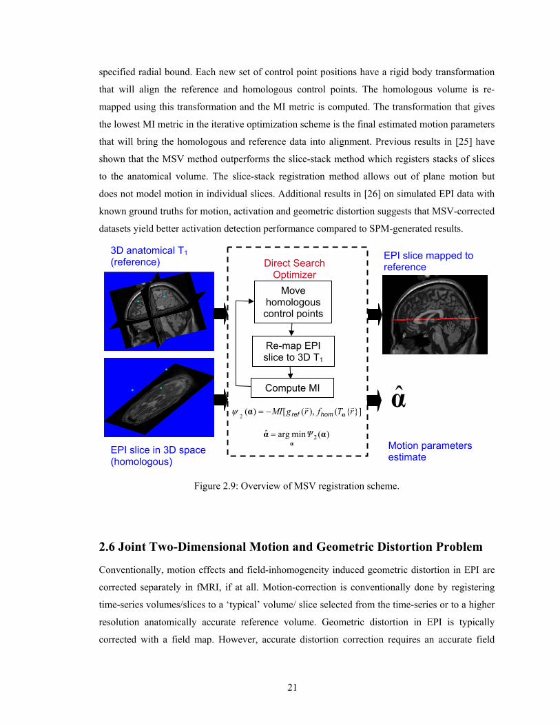
21

specified radial bound. Each new set of control point positions have a rigid body transformation

that will align the reference and homologous control points. The homologous volume is re-

mapped using this transformation and the MI metric is computed. The transformation that gives

the lowest MI metric in the iterative optimization scheme is the final estimated motion parameters

that will bring the homologous and reference data into alignment. Previous results in [25] have

shown that the MSV method outperforms the slice-stack method which registers stacks of slices

to the anatomical volume. The slice-stack registration method allows out of plane motion but

does not model motion in individual slices. Additional results in [26] on simulated EPI data with

known ground truths for motion, activation and geometric distortion suggests that MSV-corrected

datasets yield better activation detection performance compared to SPM-generated results.

Figure 2.9: Overview of MSV registration scheme.

2.6 Joint Two-Dimensional Motion and Geometric Distortion Problem

Conventionally, motion effects and field-inhomogeneity induced geometric distortion in EPI are

corrected separately in fMRI, if at all. Motion-correction is conventionally done by registering

time-series volumes/slices to a ‘typical’ volume/ slice selected from the time-series or to a higher

resolution anatomically accurate reference volume. Geometric distortion in EPI is typically

corrected with a field map. However, accurate distortion correction requires an accurate field

3D anatomical T1 (reference)

EPI slice in 3D space (homologous)

Motion parameters estimate

EPI slice mapped to reference

Move homologous control points

Re-map EPI slice to 3D T1

Compute MI

](),([)(2

rTfrgMI vvαα homref−=ψ

Direct Search Optimizer

)(min argˆ 2 ααα

Ψ=

α

22

map. Unfortunately, the two problems are inter-related in that the field map changes as the head

moves. Ideally, in order to do accurate geometric distortion correction, multiple field maps should

be acquired during the fMRI scan to track the temporal changes in the field-inhomogeneity.

However, for a variety of reasons, only one field map is usually acquired prior to, or, after the

fMRI experiment. Some of these reasons include the additional effort required to modify pulse

sequences for dynamic field map acquisition [9], increased computational complexity [10] and

the need to balance the tradeoffs between obtaining acceptable field map spatial resolution and

good image time series temporal resolution [9].

23

CHAPTER 3

Motion-Robust Field-Inhomogeneity Estimation Using Dual-

Echo Fast GRE

In this section, a dual-echo fast gradient echo (DEFGRE) pulse sequence using two back-to-back

readout gradients, each at a different echo time and of opposing polarity to the other, is

investigated for static field map estimation [11]. This pulse sequence can yield field maps with

reduced motion-induced errors compared to the conventional static field map acquisition method

using two different echo times. This is due to the greatly reduced time elapsed between data

acquisition of the two different echoes. However, there is an inherent phase error in the dual-echo

method due to the opposite polarity of the two readout pulses. Results from three phantoms and

three patients scanned over a period of two years by the same GE Signa 1.5T scanner show that

the first order phase error inherent in the dual-echo field map is relatively constant at 0.1 rad/

pixel and hence may be applied to different data acquired over time. The zero order phase error

changes with time but can be approximated empirically.

3.1 Introduction

The static magnetic field passing through an object in an MRI scanner is perturbed by disjoint

object regions with different magnetic susceptibilities that augment the magnetic field-

inhomogeneity caused by imperfections in the gradients and main magnet. Field-inhomogeneity

causes image artifacts that increase in severity as the static magnetic field strength, B0, increases.

Such artifacts are especially apparent in high-speed MRI techniques like echo-planar imaging and

spiral imaging where geometric distortion and blurring are observed, respectively, because of the

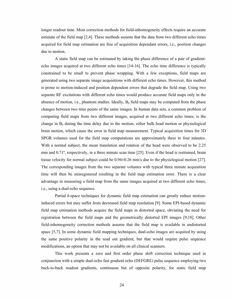
24

longer readout time. Most correction methods for field-inhomogeneity effects require an accurate

estimate of the field map [2,4]. These methods assume that the data from two different echo times

acquired for field map estimation are free of acquisition dependant errors, i.e., position changes

due to motion.

A static field map can be estimated by taking the phase difference of a pair of gradient-

echo images acquired at two different echo times [14-16]. The echo time difference is typically

constrained to be small to prevent phase wrapping. With a few exceptions, field maps are

generated using two separate image acquisitions with different echo times. However, this method

is prone to motion-induced and position dependent errors that degrade the field map. Using two

separate RF excitations with different echo times would produce accurate field maps only in the

absence of motion, i.e., phantom studies. Ideally, B0 field maps may be computed from the phase

changes between two time points of the same images. In human data sets, a common problem of

computing field maps from two different images, acquired at two different echo times, is the

change in B0 during the time delay due to the motion, either bulk head motion or physiological

brain motion, which cause the error in field map measurement. Typical acquisition times for 3D

SPGR volumes used for the field map computations are approximately three to four minutes.

With a normal subject, the mean translation and rotation of the head were observed to be 2.25

mm and 0.71º, respectively, in a three minute scan time [25]. Even if the head is restrained, brain

tissue velocity for normal subject could be 0.94±0.26 mm/s due to the physiological motion [27].

The corresponding images from the two separate volumes with typical three minute acquisition

time will then be misregistered resulting in the field map estimation error. There is a clear

advantage in measuring a field map from the same images acquired at two different echo times,

i.e., using a dual-echo sequence.

Partial k-space techniques for dynamic field map estimation can greatly reduce motion-

induced errors but may suffer from decreased field map resolution [9]. Some EPI-based dynamic

field map estimation methods acquire the field maps in distorted space, obviating the need for

registration between the field maps and the geometrically distorted EPI images [9,18]. Other

field-inhomogeneity correction methods assume that the field map is available in undistorted

space [5,7]. In some dynamic field mapping techniques, dual-echo images are acquired by using

the same positive polarity in the read out gradient, but that would require pulse sequence

modifications, an option that may not be available on all clinical scanners.

This work presents a zero and first order phase shift correction technique used in

conjunction with a simple dual-echo fast gradient echo (DEFGRE) pulse sequence employing two

back-to-back readout gradients, continuous but of opposite polarity, for static field map

25

estimation. This work describes a relatively straightforward technique that allows computation of

field maps without the need to modify a commonly available sequence in a clinical set up where

the sequence modification is not accessible. The pulse sequence, DEFGRE, acquires two echoes

efficiently with one RF pulse and the image data can be used to compute field maps without inter-

echo motion-induced position errors. It is to be noted that inter-phase encode motion is not

addressed with this technique. A caveat in using this sequence is that, due to the asymmetry of the

readout gradients, artifactual phase shifts causing phase wraps are evident in the phase difference

map. This study focuses on correcting this residual phase error to remove the phase wraps without

using elaborate phase unwrapping algorithms [28,29]. We formulate a hypothesis of how the

asymmetric readout pulses cause the artifactual phase shift and then model the phase error as an

affine term in the readout direction. The unknown affine model parameters are then estimated

using motionless phantom data. Results from several sets of phantom and patient data acquired on

the same scanner with the same scan parameters over a period of two years suggest that the first

order phase correction term does not change for a given scanner over time and hence can be

applied to the field map estimation of different data sets. The zero order phase correction term

may change with time but can be estimated empirically from the dual-echo data for each new

scan.

3. 2 Dual-Echo Fast Gradient Echo Pulse Sequence

In the generally used static field map estimation method, two complex images, ITE1,sep and ITE2,sep,

are acquired separately at two different echo-times, TE1 and TE2 where TE2>TE1. Assuming all

scan parameters, excluding the echo-time, are identical for the two sets of images, ITE2,sep will

approximately be equal to the complex magnetization Msep of ITE1,sep multiplied by a complex

phase term dependent on the field-inhomogeneity. The two sets of images can be written as

)()()( 1sepTE1,sep rrr ε+= MI , (3.1)

)()()( 2)TE)((

sepTE2,sepsepsep rrr εω += ∆∆ rjeMI (3.2)

where the spatial variable is r = [x y z]T, the true off-resonance map is denoted by ∆ωsep,

∆TE=TE2-TE1, and the images have complex noise denoted by ε1 and ε2. The off-resonance map

can be estimated as

26

[ ])(

TE)()(

)(ˆ sepsep

TE1,sepTE2,sepsep r

rrr ωω ∆≈

∆

∠=∆

∗II , (3.3)

Where I*TE1,sep denotes the complex conjugate of ITE1,sep. Fig. 3.1(a) shows an example of an off-

resonance map estimated with Eq. (3.3).

Figure 3.1: Off-resonance maps of phantom estimated by (a) standard off-resonance method, (b)

uncorrected dual-echo method showing linear phase wrapping in readout direction (x direction downwards).

In the proposed dual-echo field map method, two complex images ITE1,dual and ITE2,dual are

acquired with back-to-back readout gradients. There is no delay between the pulses, which have

opposite polarity, as shown in Fig. 3.2.

a b

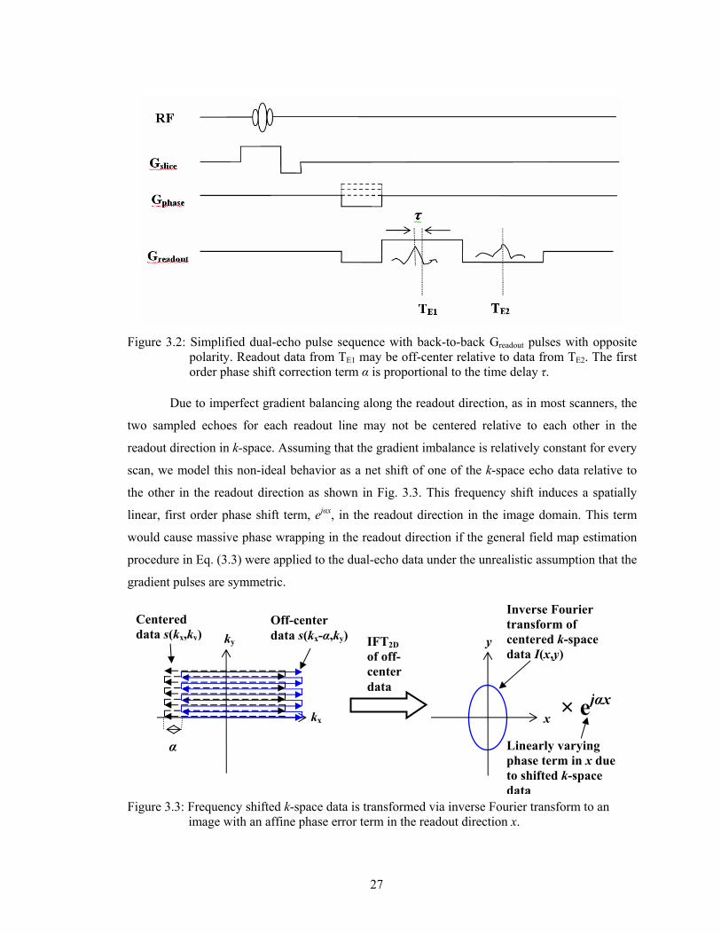
27

Figure 3.2: Simplified dual-echo pulse sequence with back-to-back Greadout pulses with opposite

polarity. Readout data from TE1 may be off-center relative to data from TE2. The first order phase shift correction term α is proportional to the time delay τ.

Due to imperfect gradient balancing along the readout direction, as in most scanners, the

two sampled echoes for each readout line may not be centered relative to each other in the

readout direction in k-space. Assuming that the gradient imbalance is relatively constant for every

scan, we model this non-ideal behavior as a net shift of one of the k-space echo data relative to

the other in the readout direction as shown in Fig. 3.3. This frequency shift induces a spatially

linear, first order phase shift term, ejαx, in the readout direction in the image domain. This term

would cause massive phase wrapping in the readout direction if the general field map estimation

procedure in Eq. (3.3) were applied to the dual-echo data under the unrealistic assumption that the

gradient pulses are symmetric.

Figure 3.3: Frequency shifted k-space data is transformed via inverse Fourier transform to an

image with an affine phase error term in the readout direction x.

Inverse Fourier transform of centered k-space data I(x,y)

kx

ky

Centered data s(kx,ky)

Off-center data s(kx-α,ky)

α

x

y

× ejαx

Linearly varying phase term in x due to shifted k-space data

IFT2D of off-center data

28

Ignoring T2 relaxation effects, we model ITE2,dual as the complex magnetization of ITE1,dual,

denoted by Mdual, multiplied by several complex terms as follows:

)()()( 3dualdualTE1, rrr ε+= MI (3.4)

)()()( 4)()TE)((

dualdualTE2,dualsep rrr r εβαω += +∆∆ xjj eeMI (3.5)

where the field-inhomogeneity induced complex term is denoted by )TE)(( dualsep ∆∆ rωje and the

first order phase shift is modeled by ejαx where x is the readout direction. The complex term ejβ

attempts to model any residual zero order phase shift left over after the first order phase

component has been removed. Multiplying Eq. (3.4) by the complex conjugate of Eq. (3.5) and

dividing by its magnitude, we obtain

)()(

)(/)()()(

5)())((

,1,1,2

rr

rrrrr εβαω +=

=+∆∆

∗∗

xjTEjdual

dualTEdualTEdualTEdual

eeM

IIIIdualsep

(3.6)

where the phase of the complex magnetization Mdual cancels out. The off-resonance map can be

estimated by taking the ratio of the phase of Idual and ∆TEdual,

[ ] )()()()(ˆ 1 rrrr ηβαωω +∆

++∆=

∆∠

=∆dual

sepdual

dualdual TE

xTEI . (3.7)

However, for the DEFGRE acquisitions, this estimate of the field map is highly inaccurate unless

the massive phase wrapping caused by the first order phase term ejαx, as shown in Fig. 3.1(b), is

removed.

3. 3 Residual Phase Error Correction

To obtain field maps with DEFGRE, we assume that the affine phase parameters α and β are

independent of the object being scanned, in which case they need to be calibrated only once for

all the data acquired in the same scanner with a given set of imaging parameters, i.e., imaging

sequence and field-of-view. A phantom filled with doped water, which has a well-defined

homogeneous region, was scanned for the purpose of computing the calibration term, first, using

2D fast SPGR sequence, twice, at different echo times followed by a dual-echo aquisition using

29

DEFGRE sequence. The off-resonance map estimates sepω∆ and dualω∆ were then computed

using Eqs. (3.3) and (3.7) respectively. Since the spherical phantom is motionless, it is reasonable

to consider sepω∆ to be the ground truth of the phantom field map. We estimate the correction

parameters α and β by minimizing the following cost function with phantom data:

∑−

=∆∠−

⎪⎭

⎪⎬⎫

⎪⎩

⎪⎨⎧

⎥⎥⎦

⎤

⎢⎢⎣

⎡

∆∆−+

∠=1

0

2

0sepdual

0dual

,)),(ˆexp(

TE),(ˆ

expmin argˆ,ˆN

xyxj

yxxj ω

φβαβα

βα, (3.8)

where y0 is a column of N pixels for which |Mdual| is significantly large, i.e. |Mdual| exceeds 10% of

the maximum image intensity of dual-echo data, dualφ∆ is the estimate of the dual-echo phase

difference map or [ ]dualI∠ , ∆TEdual is the time difference between the two echoes in the DEFGRE

sequence, y is the phase encoding direction, x is the readout direction and sepω∆ is the estimate of

the off-resonance map obtained with Eq. (3.3). The first order phase error α is solely dependent

on the gradient imbalance, and should not change considerably with different ∆TEdual. The

estimation of α will serve to unwrap the linear component of the phase error. Data from a single

column y0 is used in Eq. (3.8) since the first order phase shift is modeled in the readout or x

direction. The values of α and β estimated via the Nelder-Mead simplex method are used to

correct the dual-echo field map acquired for subsequent studies. All phase correction

computational work was performed on an Intel Pentium 4 3.6 GHz CPU using MATLAB (The

Mathworks Inc., Natick, MA).

The cost function in Eq. (3.8) is periodic with respect to β and has many local minimum

points with respect to α in the vicinity of the global minimum. This may cause the Nelder-Mead

algorithm to yield a local minimum point as the optimum solution. An alternative optimization

method is to perform a line search with respect to α, and then use the solution of α in a derived

maximum likelihood analytical solution for β assuming a white Gaussian observation model. A

maximum likelihood estimator can be derived for β while α can be estimated via a line search.

Let the observation model be

NmeZ j += θ , (3.9)

30

where m is an unknown magnitude, θ is the unknown phase of interest and N is complex, zero-

mean Gaussian noise with variance σ2, i.e., ( )NNNNNimagNreal

Σ=⎟⎟⎠

⎞⎜⎜⎝

⎛

⎥⎥⎦

⎤

⎢⎢⎣

⎡⎥⎦

⎤⎢⎣

⎡⎥⎦

⎤⎢⎣

⎡,

00,

00

~)()(

2

2µ

σσ . Thus, the

likelihood function can be written as follows:

2/)()( 1

)2(

1);( NNH

N zz

NnZ ezf µµ

πθ −Σ−− −

Σ= , (3.10)

where ][ZEN =µ . Taking the logarithm of Eq. (3.10) and removing the terms that are

independent of θ, the log-likelihood can be written as

( )( )

)cos(

Re21

21

2121

);(log

*

*

*

2

zzmmezm

mezzme

mezmez

mez

zf

j

jj

jj

j

Z

∠−==

+≡

−−−=

−−≡

−

−

θ

θ

θ

θθ

θθ

θ

(3.11)

where ‘≡’ denotes equality after removing terms that are independent of θ. For the dual-echo field

map estimation problem, let

)()(

)(/)()(sepsepdual TE)(ˆ)(

dual

sep*sepdual

rr

rrrrr εω +=

=∆∆−∠IjeM

IIIz (3.12)

Since the true magnitude of Idual is approximately equal to the observed noisy magnitude of z, we

assume m≈|z|. The magnitude and angle of z can be stated as )(dual rMz ≈ and

sepsepdual TE)(ˆ)( ∆∆−∠≈∠ rr ωIz . In reality, )(dual rM is also unknown and is approximated by

)(dual rI . By having βαθ += x where x is the frequency encoded readout direction, Eq. (3.11)

can be written as follows:

31

))(cos()(

)TE)(ˆ)(cos()(

)cos(

);(log

2dual

sepsepdual2

dual

2

βϕ

βαω

θ

θ

−=

−−∆∆−∠=

−∠∝

xxM

xxxIxM

zz

zf Z

(3.13)

where xTExxIx sepsepdual αωϕ −∆∆−∠= )(ˆ)()( .

Using the identity ),(sinsin)(coscos))(cos( xxx ϕβϕββϕ +=− Eq. (3.13) can be

expressed as

⎥⎦⎤

⎢⎣⎡+⎥⎦

⎤⎢⎣⎡=

−=

∑=

∑=

∑=

βϕβϕ

βϕ

βαψ

sin)(sin)()cos()(cos)(

))(cos()(

),,(

1

2dual

1

2dual

1

2dual

N

x

N

x

N

x

xxMxxM

xxM

x

(3.14)

where N is the number of pixels used in a readout line. Assuming α can be found via a line

search, the maximum likelihood estimator of β can be obtained by taking the derivative of Eq.

(3.14) with respect to β as follows:

⎥⎥⎥

⎦

⎤

⎢⎢⎢

⎣

⎡

=⇒

=⎥⎦⎤

⎢⎣⎡+⎥⎦

⎤⎢⎣⎡−=

∂∂

∑=

∑=

∑=

∑=

N

x

N

x

N

x

N

x

xxM

xxM

xxMxxM

x

1

2dual

1

2dual

1

2dual

1

2dual

)(cos)(

)(sin)(arctan

0cos)(sin)()sin()(cos)(

),(

ϕ

ϕβ

βϕβϕ

ββψ

(3.15)

In summary, the ML estimator for β in Eq. (3.15) can be substituted into Eq. (3.13) and a

line search performed with respect to α to maximize Eq.(3.13). The resultant solution for α is then

substituted into Eq. (3.15) to yield a solution for β.

3. 4 Empirical Approximation of β

Table 3.1 reports that while α remained constant over different scans of phantoms on the same

scanner, β varied with different scan sessions. This indicates that α has to be estimated only once

for a given scanner. As the goal of this study is to be able to compute a field map from the

32

DEFGRE data directly without the need to acquire additional data for human studies, an

empirical method to estimate β was implemented. As the study progressed, β was determined for

a new human subject scan by computing the difference between the mean of two-single-echo

SPGR off-resonance values, over several homogeneous regions in several previously scanned

images from different human subjects, and the corresponding mean DEFGRE off-resonance value

of the new subject after linear phase correction with α. This difference is computed in Hz, and β

is then estimated by multiplying the off-resonance difference by 2π∆TEdual. The two single-echo

SPGR off-resonance values of the homogeneous regions across the scanned subjects used to

calculate the mean value show little variation (standard deviation of 2.22 Hz).

Table 3.1: Estimated phase correction parameters for phantom data acquired on same scanner using i) DEFGRE and 2D SPGR data with Eq. (3.8) (first two rows), and ii) DEFGRE data and mean 2D SPGR off-resonance value with empirical method.

Estimated parameters for phantom data

Scan 1

(susceptibility)

Scan 2 (4 months later)

(susceptibility)

Scan 2 (4 months later)

(sphere)

α (rad/ unit distance) -0.10 -0.10 -0.10

β (rad) using Eq.(3.8) 2.26 0.27 0.11

β (rad) empirical 2.15 0.31 0.12

3. 5 Phantom and Human Subject Data

Along with the homogeneous sphere phantom (17 cm in diameter) filled with Gadolinium-doped

water, an air-water phantom (i.e., susceptibility phantom) representing susceptibility changes in a

typical human head was imaged. The susceptibility phantom was constructed with a cylinder (13

cm in diameter and 20 cm in height) filled with doped water and a lateral air-column suspended

in the middle, which induces inhomogeneity in the static magnetic field. Each phantom was

scanned with two pulse sequence protocols: (i) 2D dual-echo fast gradient echo (with readout

gradients in opposite polarities) (TR=200 ms, TE1=2.6 ms, TE2=5.3 ms, ∆TE=2.7 ms, image

matrix=256x256x68); (ii) twice with single-echo 2D SPGR (TR=200 ms, image

matrix=256x256x68) at TE1=2.7 ms and TE2=4.2 ms, where ∆TE=1.5 ms. The slice locations

were kept consistent with the dual-echo data. All the above scans were performed twice on each

phantom in an interval of four months on the same 1.5 T GE SIGNA MR scanner (GE Medical

Systems, Milwaukee, WI).

In addition, data from three different human subjects were acquired over a period of two

years after the first phantom scan. The studies were conducted in accordance with the guidelines

33

set by the University of Michigan Medical School Internal Review Board. Informed consent was

obtained from all three subjects. The data were acquired with two pulse sequence protocols: (i)

2D dual-echo fast gradient echo (TE1=2.7 ms, TE2=5.3 ms, ∆TE=2.6 ms, image

matrix=256x256x54); (ii) Two single-echo 3D SPGR (TE1=2.4 ms, TE2=4.2 ms, ∆TE=1.8 ms,

image matrix=256x256x128). All phantom and human scans were performed on the same

scanner.

The first order phase correction terms are useful if they are constant over time for a given

scanner and can be applied to yield corrected field maps from dual-echo acquisitions. For

phantom data, the corrected field map can be validated with the truth map, i.e., a field map

calculated from two separate single echo acquisitions. The constant first order phase correction

terms can then be routinely applied to calculate the initial field map from a dual-echo acquisition

for the correction of the B0 inhomogeneity that induces image distortions in clinical human data.

The values from the homogeneous phantom regions were used to compute the first order phase

correction terms without the effect of the field-inhomogeneity of the sample.

3. 6 Results

Table 3.1 shows that α was consistently estimated to be -0.10 radians/ pixel for all the phantom

data from the same scanner. The value of β estimated with Eq. (3.8) however changes for

different scans. A surface plot of the cost function in the range -1.0 ≤ α ≤ 1.0 and -4.0 ≤ β ≤ 4.0

was computed to verify that the estimated values correspond to global minimum points. Fig. 3.4

shows the true, dual-echo and corrected dual-echo field map profiles of a single column of the

sphere phantom in the readout direction. The first order phase error in Fig. 3.4(b) is corrected as

observed in Fig. 3.4(c). The third row of Table 3.1 shows the respective values of β computed

using the empirical method. It is noted that they closely approximate the β values computed with

Eq. 3.8 shown in the second row of Table 3.1. The values of α and β (non-empirical) in Table 3.1

were then used to correct the respective dual-echo field maps of phantoms in each scan session.

34

Figure 3.4: A column of the spherical phantom off-resonance map samples in the readout

direction for (a) standard off-resonance method, (b) dual-echo off-resonance method, (c) corrected dual-echo off-resonance method.

Figs. 3.5(a-c) show sample slices from the susceptibility phantom from (a) scan time 1

and (b) scan time 2 and (c) sphere phantom from scan time 2. In each sub-figure, the off-

resonance maps are shown in rows of sample slices selected from (top) the dual-echo data

without correction, (middle) after applying the affine phase correction terms and (bottom) two

separate single-echo acquisitions. It is evident that massive phase wrapping in the corrected

DEFGRE off-resonance maps in the middle row due to the first order phase shift has been

removed.

(a)

(b)

(c)

35

Figure 3.5: Two slices of off-resonance maps in Hz from (top) DEFGRE without correction,

(middle) DEFGRE after correction with affine phase term and (bottom) two separate single-echo acquisitions for (a) susceptibility phantom in scan 1, (b) susceptibility phantom in scan 2 (acquired 4 months after scan 1), (c) sphere phantom in scan 2. Quantitative results for entire volumes are shown in Table 3.2.

The root-mean-square error (RMSE) values between the dual-echo and corrected dual-

echo field maps, and the ground truth field maps over all 68 slices in each phantom scan are

shown in Table 3.2. The relatively low RMSE values (ranging from 0.17 ppm to 0.43 ppm) for

the corrected dual-echo off-resonance maps strongly suggest that the affine phase error model is

suitable for field map estimation with the dual-echo pulse sequence in Fig. 3.2.

Table 3.2: Off-resonance RMSE values in Hz and ppm (B0=1.5 T) between each phantom’s corrected dual-echo field map (using parameters computed in Table 3.1) and corresponding field maps computed with the standard field map method (using 2D SPGR data). Only pixels with MR image intensity values above 10% of the maximum image intensity of the respective datasets are used in the computation of the RMSE values.

RMSE (Hz, ppm)

Scan 1

(susceptibility)

Scan 2 (4 months later)

(susceptibility)

Scan 2 (4 months later)

(sphere )

27.26 Hz, 0.43 ppm 23.43 Hz, 0.37 ppm 11.16 Hz, 0.17 ppm

Results from the three human subject scans confirm that the same value of α obtained in

Table 3.1 gives good correction results for the same scanner over a period of two years. Prior to

obtaining empirical approximations of β, the mean off-resonance value of homogeneous regions

(a) (b) (c)

36

of three human subject brains over 10 slices each, fsep,mean, was computed to be 18.89 Hz. The

DEFGRE off-resonance map for each subject was corrected with the first order phase term α, and

the mean off-resonance values, fdual,mean,1, fdual,mean,2 and fdual,mean,3, of corresponding homogeneous

regions over 10 slices of the resultant data were computed to be 165.54 Hz, -130.30 Hz and

188.84 Hz, respectively. The corresponding value of β (radians) for the ith subject is obtained by

βi=2π(fsep,mean- fdual,mean,i)∆TEdual, which yield β1=-2.40 rad, β2=2.44 rad and β3=-2.78 rad for the

three subjects, respectively. Table 3.3 shows that the RMSE values for the corrected DEFGRE

using the empirically determined values of β, compared to the reference 3D SPGR off-resonance

maps, are relatively low (ranging from 0.44 ppm to 0.53 ppm ), indicating that the corrected off-

resonance maps are close to the 3D SPGR off-resonance maps. This RMSE comparison is

performed to determine if the empirically computed values of β have corrected most of the zero

order phase shift. Only pixels having significant MR signal (i.e., image intensity values above

10% of the maximum image intensity value)) were used in computing the RMSE.

Table 3.3: Off-resonance RMSE values in Hz and ppm (B0=1.5 T) between each human subject’s

corrected dual-echo field map (using α=-0.10 with β computed empirically for each scan) and corresponding field maps computed with the standard field map method (using 3D SPGR data). Only pixels with intensity values above 10% of the maximum image intensity of the respective datasets are used in the computation of the RMSE values.

RMSE (Hz, ppm)

Subject 1 Subject 2 Subject 3

33.88 Hz, 0.53 ppm 27.98 Hz, 0.44 ppm 32.03 Hz, 0.50 ppm

Fig. 3.6 shows DEFGRE off-resonance map slices for three of the subjects before and

after the affine phase correction with empirically determined values of β. It is observed that the

zero and first order phase errors have been largely removed after the phase correction procedure.

37

Figure 3.6: Subject 1 (first column), subject 2 (second column) and subject 3 (third column) off-

resonance slices from (a) uncorrected DEFGRE data (direct application of Eq. (3.7)), (b) DEFGRE field map corrected with affine phase term (empirically determined β), (c) standard 2 single-echo 3D SPGR data. Note that the linearly varying phase error in (a) has been removed in (b). Part (a) is displayed on a scale from -1500 Hz to 1500 Hz while (b) and (c) are both displayed on a scale from -100 Hz to 200 Hz.

3. 7 Discussion

The first order phase correction term α was computed with field maps generated from phantom

data acquired with a single echo SPGR at two different echo times and a dual-echo sequence, and

was used to remove the linearly varying phase error in field maps acquired using the same dual-

echo protocol on the same scanner. The correction was tested on multiple sets of human brain

data as well as phantom data that exhibit susceptibility artifacts. The results show that α was

observed to be constant on the same scanner over a period of two years. The computation process

is straightforward and no elaborate phase unwrapping is required to correct for the first order

component of the phase error. The estimation of α on each scanner needs to be done only once

(a)

(b)

(c)

38

and can be used to perform field map estimation with dual-echo data thereafter. In the event that

the scanning environment changes, the recalibration can be done by following the simple protocol

set up to acquire data with the two single-echo GRE and DEFGRE sequences using a

homogeneous spherical phantom.

Although the zero order phase term β varies with different scan sessions, we have

proposed an empirical method to approximate it using only DEFGRE data and an average off-

resonance value computed from suitable homogeneous regions of objects previously scanned

with the two single-echo SPGR protocol on the same scanner. This empirical method yielded

corrected DEFGRE off-resonance maps that had relatively low off-resonance RMSE values

(≤0.53 ppm for human subjects at B0=1.5 T). As stated previously, the off-resonance maps

computed with the two single-echo acquisitions are prone to motion artifacts since the data are

acquired from two separate echoes. Thus, the RMSE values for the human subject data are meant

to be approximations of how close the corrected DEFGRE off-resonance maps are to the standard

off-resonance maps, but not measures of accuracy in the corrected DEFGRE field maps. This is

useful information only because, in the absence of a ground truth field map without motion, it

shows that the corrected DEFGRE estimates do not deviate significantly from the standard field

map. For the phantom data, the field maps computed using the standard method is a closer

approximation to the ground truth field map since the phantoms do not move during the scans.

Thus, using the standard field maps as ground truth field maps, the RMSE values of phantom

dual-echo data after phase shift correction are better measures of the accuracy of the corrected

DEFGRE method.

Other factors like the different field map SNR values obtained with different ∆TE values

used in the 3D SPGR and DEFGRE protocols may influence the accuracy of the RMSE values. It

is observed that the field maps computed using the two separate single echo acquisition method

are noisier than the corrected DEFGRE field maps. This is true for both phantom and human data.

For the phantom experiments, the standard deviation values of homogeneous field map regions,

which approximate the field map noise levels, were 4.9, 6.0, 6.9 Hz for single echo while the

values for the corresponding regions in the respective dual-echo datasets were 3.15, 0.4, 4.3 Hz.

Similarly, the human field map measurements were 20.6, 24.2, 19.7 Hz for single echo and 15.6,

12.5, 11.6 Hz for dual-echo experiments. Among other reasons, this phenomenon may be due to

∆TEdual>∆TEsep combined with motion-induced noise. The human subjects’ noise standard

deviation values are larger than phantom noise standard deviation values which may be attributed

to additional noise sources in humans, i.e., motion, body thermal noise, etc. Performing a future

field map SNR study of phantom (with and without motion) and human data with ∆TEdual=∆TEsep

39

may aid in quantifying any motion-related SNR gain in using the DEFGRE field map estimation

method compared to the standard field map method.

It is ideal to keep the ∆TE values equal in order to be able to compare SNRs in field maps

fairly. For field map measurements, ∆TE was kept as close as possible for the standard and dual-

echo sequences while avoiding spontaneous changes in other acquisition parameters due the

scanner’s built-in timing restrictions in choosing values for TE. Our key motive was to use the

DEFGRE sequence for field map estimation as it was with the limitations in sequence timing

included, and results strongly suggest that the affine phase error model holds over time (two

years).

3. 8 Conclusions

The dual-echo bipolar readout gradient technique offers an efficient way of collecting data and

computing static field maps with reduced motion-induced errors compared to the widely used,

two separate single echo acquisition method. The affine parameters modeling the phase error

inherent in the dual-echo bipolar readout gradient technique is estimated with data from a

phantom of homogeneous medium where the field-inhomogeneity is mainly system-induced. The

estimated phase correction parameters are then applied to DEFGRE data of an air-tissue

susceptibility phantom. Results have shown that the first order phase error term stays constant

with time as expected with the same scanner using the same DEFGRE protocol parameters,

allowing the technique to be used for human subject field map estimation once the first order

phase error term has been characterized. The first order term is due to the readout imbalance

which is scanner dependent and yields similar k-space shifts in each readout line acquired with

the dual-echo acquisition. The zeroth order term has off-resonance contributions from other

sources such as heating effects of coils depending on the object being scanned. The phase error

from the zeroth order term changes with different scan sessions but can be estimated empirically

using the previously scanned two-single echo field maps. The proposed method has been tested

on three human subjects and the results strongly suggest that the DEFGRE pulse sequence can

yield good field map estimates. The relatively low RMSE values (ranging from 0.17 ppm to 0.43

ppm) for the corrected dual-echo off-resonance maps at 1.5 T suggest that the affine phase error

model is suitable for field map estimation with the dual-echo pulse sequence. Since the first order

correction term depends largely on how the readout gradient switches and not on how strong the

B0 field is, an affine phase error model is expected to hold for images from different field

strengths. The value of the linear phase term may be different for different scanners but should be

constant for any one scanner. Future work includes an evaluation of the proposed field map

40

estimation method at 3 T and the investigation of methods to improve the reliability of the zero

order phase error estimate.

41

CHAPTER 4

Concurrent Field Map and Map-Slice-to-Volume (CFMMSV) Motion Correction for EPI

A popular method of estimating field-inhomogeneity involves scanning the sample at two

different echo times with a T2*-weighted pulse sequence (e.g. GRE) and computing the phase

difference divided by the echo time difference. This is typically done once in the beginning or the

end of an fMRI experiment. This method may be insufficient for two reasons. First, the acquired

field map is spatially inaccurate in the presence of motion between the two echoes. Secondly, the

acquired static field map does not account for head motion during the acquisition of the fMRI

time-series. Dynamic field map estimation methods such as partial k-space methods are robust to

subject motion but may either reduce the temporal resolution of fMRI images or the spatial

resolution of the field maps [9].

The objective of this section is to propose a concurrent motion and field-inhomogeneity

correction framework in which the effects of head motion on the field map (and hence geometric

distortion) are accounted for. The slice-profile warp is ignored in this section. The concurrent

field map and MSV (CFMMSV) correction framework uses iterative reconstruction and MSV

registration. The key difference in the following methods within this framework revolves around

the dynamic field map update method.

Our previously reported CFMMSV method [13] attempted to estimate dynamic field

maps from an initially collected field map using the MSV rigid body motion parameters obtained

by registering the EPI time-series to a 3D anatomical dataset. This method does concurrent field-

inhomogeneity and slice motion correction using only one field map but is unable handle larger

out-of-plane rotations. This is because rigid body transformation of a field map does not

accurately describe the true field map changes with out-of-plane motion. Preliminary results on

simulated data show that the final reconstructed image quality and estimated motion parameters

improve in accuracy compared to a conventional non-concurrent correction scheme.

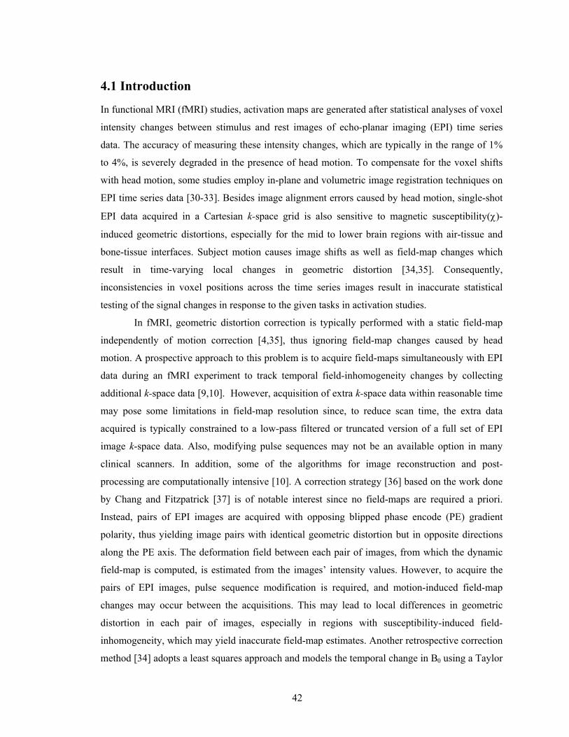
42

4.1 Introduction

In functional MRI (fMRI) studies, activation maps are generated after statistical analyses of voxel

intensity changes between stimulus and rest images of echo-planar imaging (EPI) time series

data. The accuracy of measuring these intensity changes, which are typically in the range of 1%

to 4%, is severely degraded in the presence of head motion. To compensate for the voxel shifts

with head motion, some studies employ in-plane and volumetric image registration techniques on

EPI time series data [30-33]. Besides image alignment errors caused by head motion, single-shot

EPI data acquired in a Cartesian k-space grid is also sensitive to magnetic susceptibility(χ)-

induced geometric distortions, especially for the mid to lower brain regions with air-tissue and

bone-tissue interfaces. Subject motion causes image shifts as well as field-map changes which

result in time-varying local changes in geometric distortion [34,35]. Consequently,

inconsistencies in voxel positions across the time series images result in inaccurate statistical

testing of the signal changes in response to the given tasks in activation studies.

In fMRI, geometric distortion correction is typically performed with a static field-map

independently of motion correction [4,35], thus ignoring field-map changes caused by head

motion. A prospective approach to this problem is to acquire field-maps simultaneously with EPI

data during an fMRI experiment to track temporal field-inhomogeneity changes by collecting

additional k-space data [9,10]. However, acquisition of extra k-space data within reasonable time

may pose some limitations in field-map resolution since, to reduce scan time, the extra data

acquired is typically constrained to a low-pass filtered or truncated version of a full set of EPI

image k-space data. Also, modifying pulse sequences may not be an available option in many

clinical scanners. In addition, some of the algorithms for image reconstruction and post-

processing are computationally intensive [10]. A correction strategy [36] based on the work done

by Chang and Fitzpatrick [37] is of notable interest since no field-maps are required a priori.

Instead, pairs of EPI images are acquired with opposing blipped phase encode (PE) gradient

polarity, thus yielding image pairs with identical geometric distortion but in opposite directions

along the PE axis. The deformation field between each pair of images, from which the dynamic

field-map is computed, is estimated from the images’ intensity values. However, to acquire the

pairs of EPI images, pulse sequence modification is required, and motion-induced field-map

changes may occur between the acquisitions. This may lead to local differences in geometric

distortion in each pair of images, especially in regions with susceptibility-induced field-

inhomogeneity, which may yield inaccurate field-map estimates. Another retrospective correction

method [34] adopts a least squares approach and models the temporal change in B0 using a Taylor

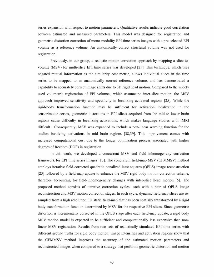
43

series expansion with respect to motion parameters. Qualitative results indicate good correlation

between estimated and measured parameters. This model was designed for registration and

geometric distortion correction of mono-modality EPI time series images with a pre-selected EPI

volume as a reference volume. An anatomically correct structural volume was not used for

registration.

Previously, in our group, a realistic motion-correction approach by mapping a slice-to-

volume (MSV) for multi-slice EPI time series was developed [25]. This technique, which uses

negated mutual information as the similarity cost metric, allows individual slices in the time

series to be mapped to an anatomically correct reference volume, and has demonstrated a

capability to accurately correct image shifts due to 3D rigid head motion. Compared to the widely

used volumetric registration of EPI volumes, which assume no inter-slice motion, the MSV

approach improved sensitivity and specificity in localizing activated regions [25]. While the

rigid-body transformation function may be sufficient for activation localization in the

sensorimotor cortex, geometric distortions in EPI slices acquired from the mid to lower brain

regions cause difficulty in localizing activations, which makes language studies with fMRI

difficult. Consequently, MSV was expanded to include a non-linear warping function for the

studies involving activations in mid brain regions [38,39]. This improvement comes with

increased computational cost due to the longer optimization process associated with higher

degrees of freedom (DOF) in registration.

In this work, we developed a concurrent MSV and field inhomogeneity correction

framework for EPI time series images [13]. The concurrent field-map MSV (CFMMSV) method

employs iterative field-corrected quadratic penalized least squares (QPLS) image reconstruction

[25] followed by a field-map update to enhance the MSV rigid body motion-correction scheme,

therefore accounting for field-inhomogeneity changes with inter-slice head motion [5]. The

proposed method consists of iterative correction cycles, each with a pair of QPLS image

reconstruction and MSV motion correction stages. In each cycle, dynamic field-map slices are re-

sampled from a high resolution 3D static field-map that has been spatially transformed by a rigid

body transformation function determined by MSV for the respective EPI slices. Since geometric

distortion is incrementally corrected in the QPLS stage after each field-map update, a rigid body

MSV motion model is expected to be sufficient and computationally less expensive than non-

linear MSV registration. Results from two sets of realistically simulated EPI time series with

different ground truths for rigid body motion, image intensities and activation regions show that

the CFMMSV method improves the accuracy of the estimated motion parameters and

reconstructed images when compared to a strategy that performs geometric distortion and motion

44

correction independently using just a static field-map. Non-parametric random permutation tests

were also performed on all datasets at various stages in the CFMMSV correction process to

compute activation detection receiver operating characteristic (ROC) curves. The areas under

these ROC curves show that the CFMMSV method improves the activation detection accuracy.

4.2 Background

4.2.1 EPI Geometric Distortion

In brain EPI data that is reconstructed without field-inhomogeneity correction, geometric

distortion is observed in regions where the local magnetic field is inhomogeneous, especially at

the boundaries of tissues with significant magnetic susceptibility differences. Head motion that

changes the orientation of the inter-tissue boundary with B0 (out-of-plane rotations) may induce

significant field-inhomogeneity changes in the region around the boundary. Translations and in-

plane rotation are less likely to cause such changes in the susceptibility-induced component of the

field-map. Such motion mainly induces shifts and in-plane rotation of the entire field-map. In

blipped EPI, due to the long readout time, field-inhomogeneity causes pixel shifts mainly in the

phase encode direction [2] as shown in Eq. (2.7). These space-variant pixel shifts depend on the

EPI slice readout time Treadout and the field-inhomogeneity map. The resultant geometric distortion

and image intensity errors can adversely affect fMRI activation detection performance.

4.2.2 Iterative Field-Corrected Reconstruction

To perform geometric distortion correction, we use the iterative field-corrected reconstruction

method [5] described in Chapter 2. The continuous object f and field-map ∆ω are parameterized

into a sum of weighted rect functions )( nrr −φ where r is the vector of spatial coordinates. Some

of the equations from Chapter 2 are reproduced here to specifically denote the correction of EPI

time series image slices. Ignoring spin relaxation and assuming uniform receiver coil sensitivity,

the parameterized MR signal equation of slice frame l in an EPI time series is

1...0 ,))((

)()()(1

0

))((2 −=≈

+=

∑−

=

⋅−∆− Lleeft Φ

ttstuN

n

tjtjlnm

ml

ml

ml

nmmln rkk πω

ε (4.2)

where sl(tm) is the baseband MR signal sample at time tm during readout, εl(tm) denotes white

Gaussian noise [20], Φ(k(tm)) denotes the Fourier transform of )(rφ , N is the number of pixels in

a slice, L is the total number of slice frames in the EPI time series and lnf and l

nω∆ are the object

45

intensity and field-inhomogeneity values, respectively, at rn. The matrix-vector form of Eq. (4.2)

can be written as follows:

llll εfAu += (4.3)

where ),..,( 10l

Nll ff −=f and elements of the M × N system-object matrix Al are

))(( ))((2,

nmmln tjtj

ml

nm eetΦa rkk ⋅−∆−= πω (4.4)

To estimate the unknown object slice f l from the observed k-space data, the iterative conjugate

gradient algorithm is used to minimize the QPLS cost function

22

1 )( lllll CffAuf β+−=Ψ (4.5)

where C is a first-order difference matrix, and β is a parameter that controls the tradeoff between

obtaining a data-consistent estimate and a smoothed, regularized estimate. The QPLS estimate of

f l is

llll

f

lQPLS uACCAAff *1**

1 ][)(minargˆ −−=Ψ= β , (4.6)

however, we minimize Eq. (4.5) using the conjugate gradient algorithm instead of evaluating Eq.

(4.6) directly.

To accurately perform field-corrected reconstruction in the presence of head motion,

every slice of observed data ul should be paired with a dynamic field-map slice ∆ωl that describes

the field-inhomogeneity at frame l of the fMRI experiment. Typically, however, only a static

field-map ∆ωstatic is available. This field-map is usually acquired before or after the experiment

and does not track field-inhomogeneity changes during the acquisition of the fMRI time series

images. Each volume in the EPI time series typically has a lower spatial resolution and larger

slice thickness than ∆ωstatic. A simple approach to obtain field-corrected fMRI images is to

register each time series volume to the image intensity volume acquired in the same coordinate

space as the static field-map volume, and then use re-sampled slices of ∆ωstatic in place of ∆ωl in

46

minimizing Eq. (4.5). This correction method ignores inter-slice motion and field-inhomogeneity

changes due to head motion and thus yields potentially significant image reconstruction errors.

4.2.3 Map Slice-To-Volume (MSV) Registration in fMRI

The MSV motion correction technique [25] models the 3D motion of multislice EPI data by

allowing each slice to have its own six DOF motion. To perform MSV motion correction for

fMRI time series images, each reconstructed EPI slice f l is registered with a 3D reference volume

gref using the six DOF rigid body transform denoted by lTα . The vector αl consists of the six MSV

motion parameters tx, ty, tz, θx, θy, θz for slice l. This is performed by minimizing a function Ψ2(αl)

that measures the dissimilarity between f l and gref. In the implementation of MSV, the negated

mutual information (MI) is used, which performs well for multi-modality datasets, i.e. T2*-

weighted EPI slices registered with a T1-weighted reference volume. The motion parameters αl

are estimated by minimizing the following cost function over αl using the Nelder-Mead downhill

simplex optimization algorithm

)))((,(MI)(2 rfgα αlTlref

l −=Ψ (4.7)

Each set of optimized motion parameters is then used to transform and interpolate

(trilinear) its respective slice f l into a volume with the same spatial coordinates as the reference

volume. In the original MSV method, the motion of each slice is computed independent of other

slices and allows six DOF between each slice acquisition. For single shot acquisition, intra-slice

motion is negligible. Given that head motion is typically correlated in time and that MSV may

generate outlier estimates, especially for top slices where the information content is reduced, we

apply temporal median filtering on the recovered MSV motion parameters before use. A median

filter was chosen because the MSV motion estimates obtained from data with simulated smooth

motion were observed to track the ground truth except for intermittent outlier estimates. Fig. 4.1

shows a motion parameter recovered from a 120-volume simulated EPI time series using MSV

alone and MSV with a nine point median filter. The ground truth is also plotted. The RMSE

values of the raw and median filtered MSV results in Fig. 4.1 are 1.10mm and 0.19mm,

respectively.

47

Figure 4.1: Recovered raw MSV motion estimates, median filtered MSV motion estimates and

ground truth of a subset of simulated dataset A with applied translation in the z direction. The RMSE values of raw MSV and median filtered MSV results are 1.10mm and 0.19mm respectively. The standard deviation values of the estimation error for raw MSV and median filtered MSV are 1.06mm and 0.13mm respectively.

4.3 Concurrent Field-inhomogeneity Correction with MSV

To design a concurrent correction technique that involves Eqs. (4.5) and (4.7) with a rigid body

transformation function, the main challenge is the approximation of the dynamic field-map from

the initial static field-map. To partially account for field-map changes due to 3D head motion

during the fMRI experiment, we propose and evaluate the following “concurrent” correction

approach. The concurrent field-map and MSV motion correction framework (CFMMSV) loops

through several correction cycles, each of which consists of a field-corrected reconstruction stage

followed by MSV registration. The changing field-map is approximated using the recovered

MSV motion estimates and the static field-map. As the number of correction cycles increases, the

geometric distortion is incrementally corrected in the image reconstruction stage. Thus, a rigid

body transformation function in MSV is expected to be sufficient to correct for head motion. This

leads to a faster image registration process compared to the use of 3D non-linear warping

functions.

Since the true dynamic field-map ∆ωl in Eq. (4.4) is unavailable, the EPI time series

image reconstruction in the initial cycle (κ = 0) of the concurrent correction algorithm is

performed with the static field-map volume ∆ωstatic. The elements of the system matrix Al,κ=0 can

be written as

48

))(( ))((20,,

, nmml

staticn tjtjm

lnm eetΦa rkk ⋅−∆−= = πωκ (4.8)

where κ denotes the correction cycle number. The first field-corrected estimate of slice frame l, 0,ˆ =κlf , is then obtained by minimizing Eq. (4.5) with Al

P= Al,κ=0. The reconstructed slices are then

registered via MSV to the reference volume gref by minimizing Eq. (4.7). Each set of median

filtered motion parameters κ,ˆ lfiltα , l = 0,..,L-1, is applied to the original static field-map volume and

the respective slice within the transformed field-map volume is re-sampled and stacked into a

new field-map volume

))((ˆ ,ˆ1, rα κωω κ

lTH staticll =∆ + , l = 0,..,L-1, (4.9)

where HlU denotes an operator which re-samples slice l from a volume U. This updated field-

map is then used in the next cycle to reconstruct field-corrected images again from the original k-

space data.

Since geometric distortion in EPI is predominantly in the PE direction, the recovered

MSV motion parameters in the phase encoding direction are not used to transform the static field-

map in the initial field-map update when κ = 0. This is because the EPI image shifts in the PE

direction may be largely influenced by field-inhomogeneity induced geometric distortion rather

than object motion. In addition, the field-map may change significantly with out-of-plane

rotations which would render these motion parameters unreliable for the initial field-map update.

Thus, for κ = 0, the motion parameters ty (translation in PE direction), θx and θy (out-of-plane

rotations) are omitted when applying the transformation 0,ˆ =κlTα to the static field-map. For the

following cycles, κ ≥ 1, all six DOF are used when applying κ,ˆ lTα to update the field-map. The

original raw data u and static field-map ∆ωstatic are used in each cycle to approximate the dynamic

field-map and field-corrected EPI images to avoid error propagation due to intermediate

processing steps as the number of cycles increases. The CFMMSV method is summarized as

follows:

Algorithm. Concurrent QPLS-MSV for EPI Motion and Field-Inhomogeneity Correction Initial data: 0,ˆ =∆ κω l (slice l of static field-map staticω∆ ), u P

lP (k-space data), l=0...L-1

for κ=0…K (correction cycles) Step 1: 22,, )ˆ(∆minargˆ CffAuf

fβω κκ +−= lll do for l=0…L-1 (QPLS)

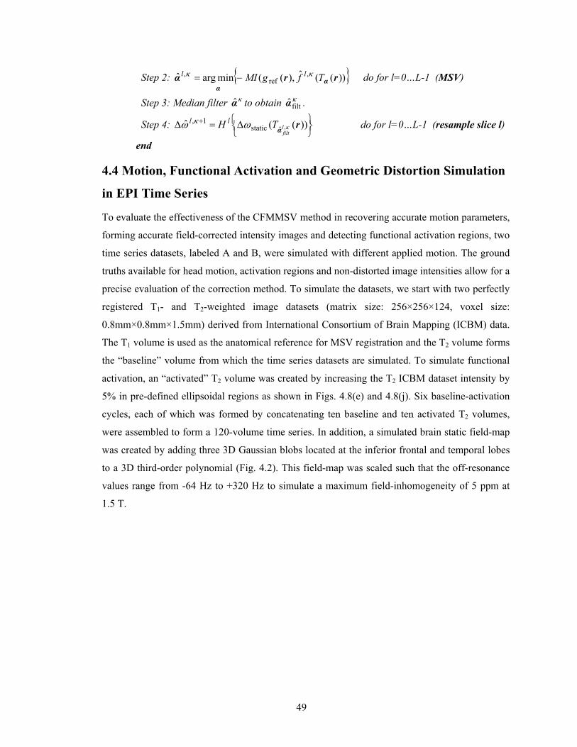
49

Step 2: ))((ˆ),((minargˆ ,ref

, rrα αα

TfgMI ll κκ −= do for l=0…L-1 (MSV)

Step 3: Median filter κα to obtain κfiltα .

Step 4: ⎭⎬⎫

⎩⎨⎧∆=∆ + ))((ˆ ,ˆstatic

1, rα κωω κlfilt

TH ll do for l=0…L-1 (resample slice l)

end

4.4 Motion, Functional Activation and Geometric Distortion Simulation

in EPI Time Series

To evaluate the effectiveness of the CFMMSV method in recovering accurate motion parameters,

forming accurate field-corrected intensity images and detecting functional activation regions, two

time series datasets, labeled A and B, were simulated with different applied motion. The ground

truths available for head motion, activation regions and non-distorted image intensities allow for a

precise evaluation of the correction method. To simulate the datasets, we start with two perfectly

registered T1- and T2-weighted image datasets (matrix size: 256×256×124, voxel size:

0.8mm×0.8mm×1.5mm) derived from International Consortium of Brain Mapping (ICBM) data.

The T1 volume is used as the anatomical reference for MSV registration and the T2 volume forms

the “baseline” volume from which the time series datasets are simulated. To simulate functional

activation, an “activated” T2 volume was created by increasing the T2 ICBM dataset intensity by

5% in pre-defined ellipsoidal regions as shown in Figs. 4.8(e) and 4.8(j). Six baseline-activation

cycles, each of which was formed by concatenating ten baseline and ten activated T2 volumes,

were assembled to form a 120-volume time series. In addition, a simulated brain static field-map

was created by adding three 3D Gaussian blobs located at the inferior frontal and temporal lobes

to a 3D third-order polynomial (Fig. 4.2). This field-map was scaled such that the off-resonance

values range from -64 Hz to +320 Hz to simulate a maximum field-inhomogeneity of 5 ppm at

1.5 T.

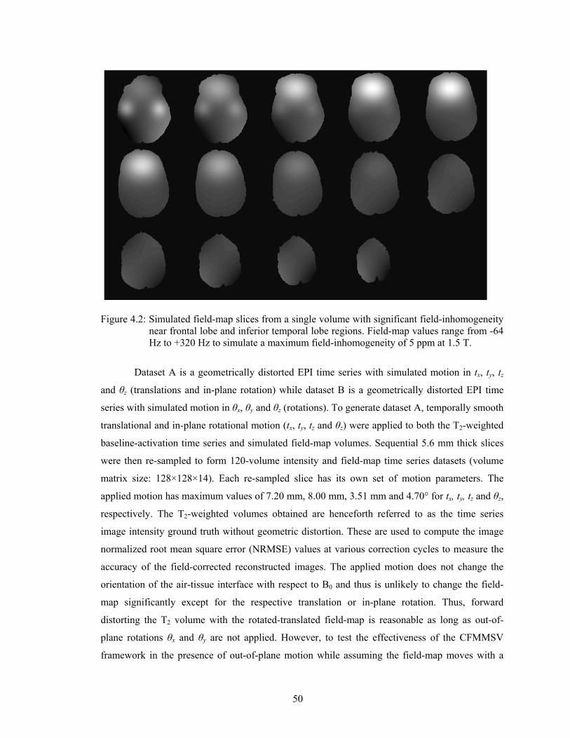
50

Figure 4.2: Simulated field-map slices from a single volume with significant field-inhomogeneity

near frontal lobe and inferior temporal lobe regions. Field-map values range from -64 Hz to +320 Hz to simulate a maximum field-inhomogeneity of 5 ppm at 1.5 T.

Dataset A is a geometrically distorted EPI time series with simulated motion in tx, ty, tz

and θz (translations and in-plane rotation) while dataset B is a geometrically distorted EPI time

series with simulated motion in θx, θy and θz (rotations). To generate dataset A, temporally smooth

translational and in-plane rotational motion (tx, ty, tz and θz) were applied to both the T2-weighted

baseline-activation time series and simulated field-map volumes. Sequential 5.6 mm thick slices

were then re-sampled to form 120-volume intensity and field-map time series datasets (volume

matrix size: 128×128×14). Each re-sampled slice has its own set of motion parameters. The

applied motion has maximum values of 7.20 mm, 8.00 mm, 3.51 mm and 4.70° for tx, ty, tz and θz,

respectively. The T2-weighted volumes obtained are henceforth referred to as the time series

image intensity ground truth without geometric distortion. These are used to compute the image

normalized root mean square error (NRMSE) values at various correction cycles to measure the

accuracy of the field-corrected reconstructed images. The applied motion does not change the

orientation of the air-tissue interface with respect to B0 and thus is unlikely to change the field-

map significantly except for the respective translation or in-plane rotation. Thus, forward

distorting the T2 volume with the rotated-translated field-map is reasonable as long as out-of-

plane rotations θx and θy are not applied. However, to test the effectiveness of the CFMMSV

framework in the presence of out-of-plane motion while assuming the field-map moves with a

51

rigid body transformation function together with the head, a second pair of 120-volume time

series intensity and field-map datasets (dataset B) were simulated with temporally smooth motion

in three rotation parameters θx, θy and θz. This assumption, while simplistic in the presence of

large out-of-plane motion, provides a way to generate an otherwise realistic time series dataset

with out-of-plane motion and subsequent field-inhomogeneity induced geometric distortion. The

simulated rotational motion has maximum values of 5.0°, 8.6° and 8.1° for θx, θy and θz

respectively. Slice acquisition interleaving was incorporated when generating both time series

datasets.

To forward distort the T2 time series images from both datasets, simulated blipped EPI

Cartesian k-space data of the distorted images were generated in conjunction with the respective

field-map time series with motion using Eq. (4.2). The distorted images (Fig. 4.3(b)) were then

reconstructed from this k-space data using a system-object matrix with a field-map set to zero

[13]. The simulated readout time was 43.8 ms and the pixel bandwidth in the PE direction was

22.8 Hz. In subsequent sections, datasets A and B will refer to the final geometrically distorted

time series with the respective applied motion.

Figure 4.3: (a) T2 ICBM slice before simulated geometric distortion. (b) T2 ICBM slice after

simulated geometric distortion with a peak field-inhomogeneity of 5 ppm at 1.5 T.

4.5 Activation Detection with Random Permutation Test

After re-positioning all the EPI time series slices into volumes, MSV yields time series volumes

that may have empty voxels. This results in variable sample sizes for different voxels for

statistical analysis. The non-parametric statistical method of voxel-wise random permutation,

using the averaged difference between activation and rest images as the test statistic, was used for

52

significance testing of differences in voxel intensities in the simulated datasets [25,40]. This

statistical technique is simple, robust and independent of sample size variability [41]. Random

draws of 2000 permutations of activated and rest periods were used to form a permutation

distribution for each voxel from which activated regions are identified by testing the null

hypothesis of no activation at a fixed threshold of α = 0.001. To obtain ROC curves, we vary the

threshold P values from 10-4 to 1.0 to obtain a set of activation maps and, together with the

ground truth activation map, compute the true positive and false alarm rates. The area under each

ROC curve (AUC) is used to measure how accurately the activation regions have been detected.

4.6 Results

In our experiments, the concurrent correction scheme was evaluated on simulated EPI time series

datasets A (with simulated motion in tx, ty, tz and θz) and B (with simulated motion in θx, θy and

θz). Both datasets have known ground truths for the applied slice-wise motion parameters which

allow for precise evaluation of MSV registration performance. In addition, the non-distorted time

series intensity images with applied motion is available to serve as image intensity ground truths

to evaluate the performance of the field-corrected image reconstruction process. Tables 4.1 and

4.2 list the RMSE and MSV error standard deviation values of the estimated MSV motion

parameters. With median filtering of the estimated MSV parameters, the errors decrease as κ

increases and empirically converge to relatively small values. This implies that registration

accuracy has improved with the concurrent correction method compared to a single-cycle

correction method where a static field-map is used for geometric distortion correction prior to

MSV (cycle 0). The observed empirical convergence strongly suggests that the algorithm is

relatively stable as κ increases.

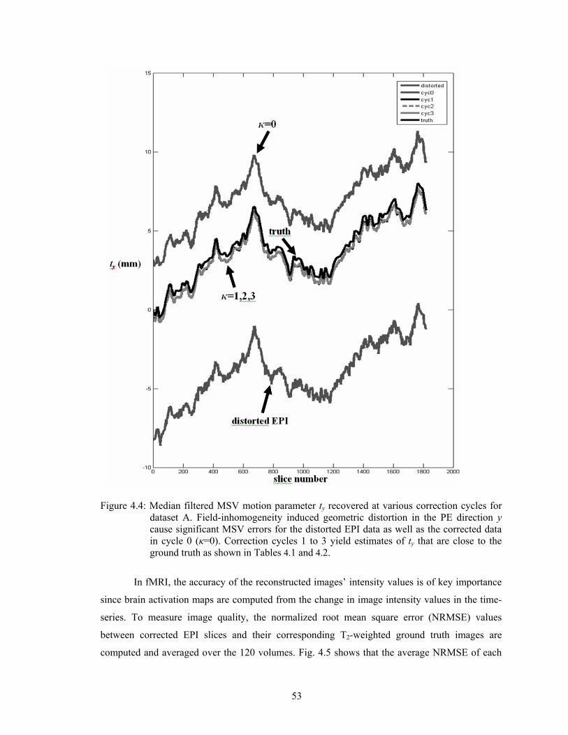
53

Figure 4.4: Median filtered MSV motion parameter ty recovered at various correction cycles for

dataset A. Field-inhomogeneity induced geometric distortion in the PE direction y cause significant MSV errors for the distorted EPI data as well as the corrected data in cycle 0 (κ=0). Correction cycles 1 to 3 yield estimates of ty that are close to the ground truth as shown in Tables 4.1 and 4.2.

In fMRI, the accuracy of the reconstructed images’ intensity values is of key importance

since brain activation maps are computed from the change in image intensity values in the time-

series. To measure image quality, the normalized root mean square error (NRMSE) values

between corrected EPI slices and their corresponding T2-weighted ground truth images are

computed and averaged over the 120 volumes. Fig. 4.5 shows that the average NRMSE of each

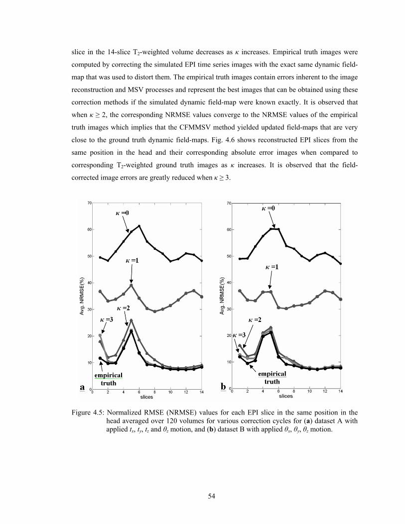
54

slice in the 14-slice T2-weighted volume decreases as κ increases. Empirical truth images were

computed by correcting the simulated EPI time series images with the exact same dynamic field-

map that was used to distort them. The empirical truth images contain errors inherent to the image

reconstruction and MSV processes and represent the best images that can be obtained using these

correction methods if the simulated dynamic field-map were known exactly. It is observed that

when κ ≥ 2, the corresponding NRMSE values converge to the NRMSE values of the empirical

truth images which implies that the CFMMSV method yielded updated field-maps that are very

close to the ground truth dynamic field-maps. Fig. 4.6 shows reconstructed EPI slices from the

same position in the head and their corresponding absolute error images when compared to

corresponding T2-weighted ground truth images as κ increases. It is observed that the field-

corrected image errors are greatly reduced when κ ≥ 3.

Figure 4.5: Normalized RMSE (NRMSE) values for each EPI slice in the same position in the

head averaged over 120 volumes for various correction cycles for (a) dataset A with applied tx, ty, tz and θz motion, and (b) dataset B with applied θx, θy, θzBB motion.

55

Figure 4.6: (a-e, k-o) Intensity and (f-j, p-t) absolute difference images with respect to ground

truth images for two sample slices from dataset A at various stages in the CFMMSV correction process. (Top row) Geometrically distorted dataset, (second row) cycle 0, (third row) cycle 1, (fourth row) cycle 2, (fifth row) cycle 3. All images are displayed on the same normalized intensity scale ranging from 0 to 1.

As κ increases from zero, the field-corrected EPI images become more similar to the

ground truth T2 images. It is possible to obtain improved image NRMSE values without a

corresponding improvement in activation detection performance since the simulated intensity

increase is only 5% and applied to a relatively small subset of activated voxels. Thus, we applied

the statistical random permutation test on datasets A and B at all stages of the CFMMSV

correction process and computed ROC curves and respective AUC values to verify that activation

detection performance improves as κ increases. Figs. 4.7(a-b) show the ROC curves for both

datasets at several stages of the CFMMSV correction process and Table 4.3 shows the

56

corresponding AUC values. It is observed for both datasets that the AUC values increase

significantly between cycle 0, which are the results one would obtain if the same static field-map

was used to correct all the time series data, and cycle 3, which are the final results after applying

the CFMMSV method. The improvement in activation detection is even more significant upon

considering that fMRI studies are often performed directly on EPI datasets without any form of

geometric distortion correction i.e. compare the AUC values between the distorted dataset and

cycle 3. Fig. 4.8 shows the activation maps obtained (α = 0.001) for two slices from datasets A

and B at several stages in the CFMMSV correction process. Comparing the activation maps for

cycle 0 (second row) and cycle 3 datasets (third row), it is readily observed that the latter has

more true positives and fewer false positives. The ground truth activation regions for the two

slices are shown in Figs. 4.8(e) and 4.8(j). Activation maps obtained by applying the random

permutation test on the ground truth time series images for both datasets are also shown (fourth

row) to illustrate the best performance obtainable with the statistical analysis method used.

All experiments were performed on Intel Pentium 4 Xeon 3.0GHz CPUs using MATLAB

(The Mathworks Inc., Natick, MA, USA) and Advanced Visual Systems (Advanced Visual

Systems Inc., Waltham, MA, USA).

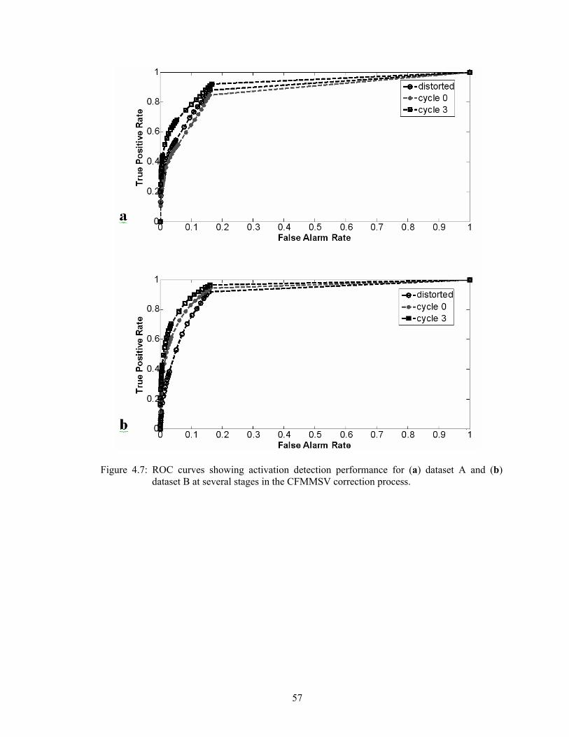
57

Figure 4.7: ROC curves showing activation detection performance for (a) dataset A and (b)

dataset B at several stages in the CFMMSV correction process.

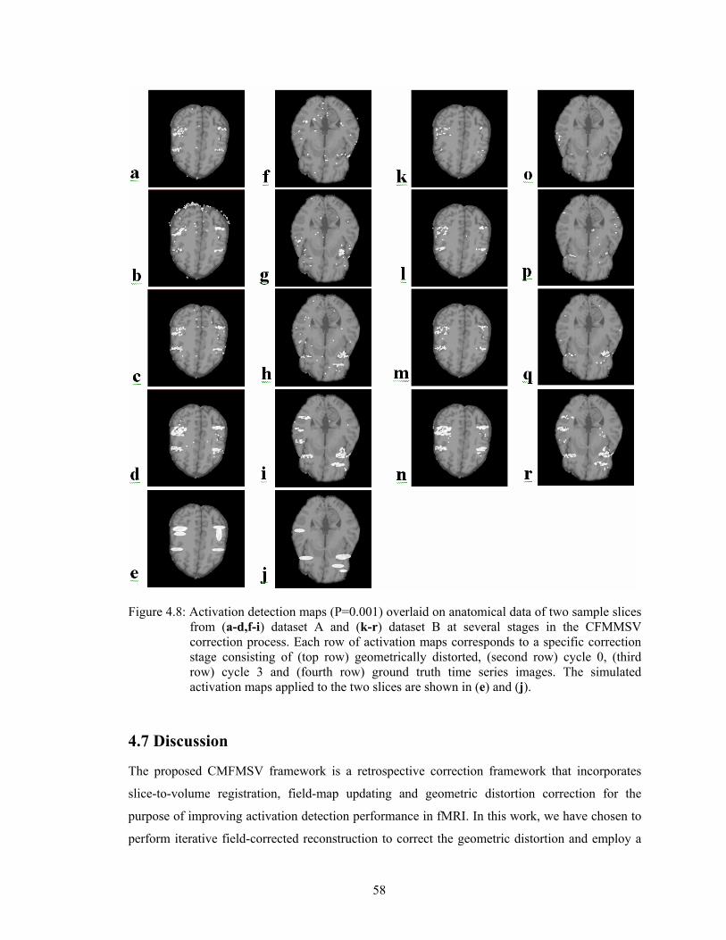
58

Figure 4.8: Activation detection maps (P=0.001) overlaid on anatomical data of two sample slices

from (a-d,f-i) dataset A and (k-r) dataset B at several stages in the CFMMSV correction process. Each row of activation maps corresponds to a specific correction stage consisting of (top row) geometrically distorted, (second row) cycle 0, (third row) cycle 3 and (fourth row) ground truth time series images. The simulated activation maps applied to the two slices are shown in (e) and (j).

4.7 Discussion

The proposed CMFMSV framework is a retrospective correction framework that incorporates

slice-to-volume registration, field-map updating and geometric distortion correction for the

purpose of improving activation detection performance in fMRI. In this work, we have chosen to

perform iterative field-corrected reconstruction to correct the geometric distortion and employ a

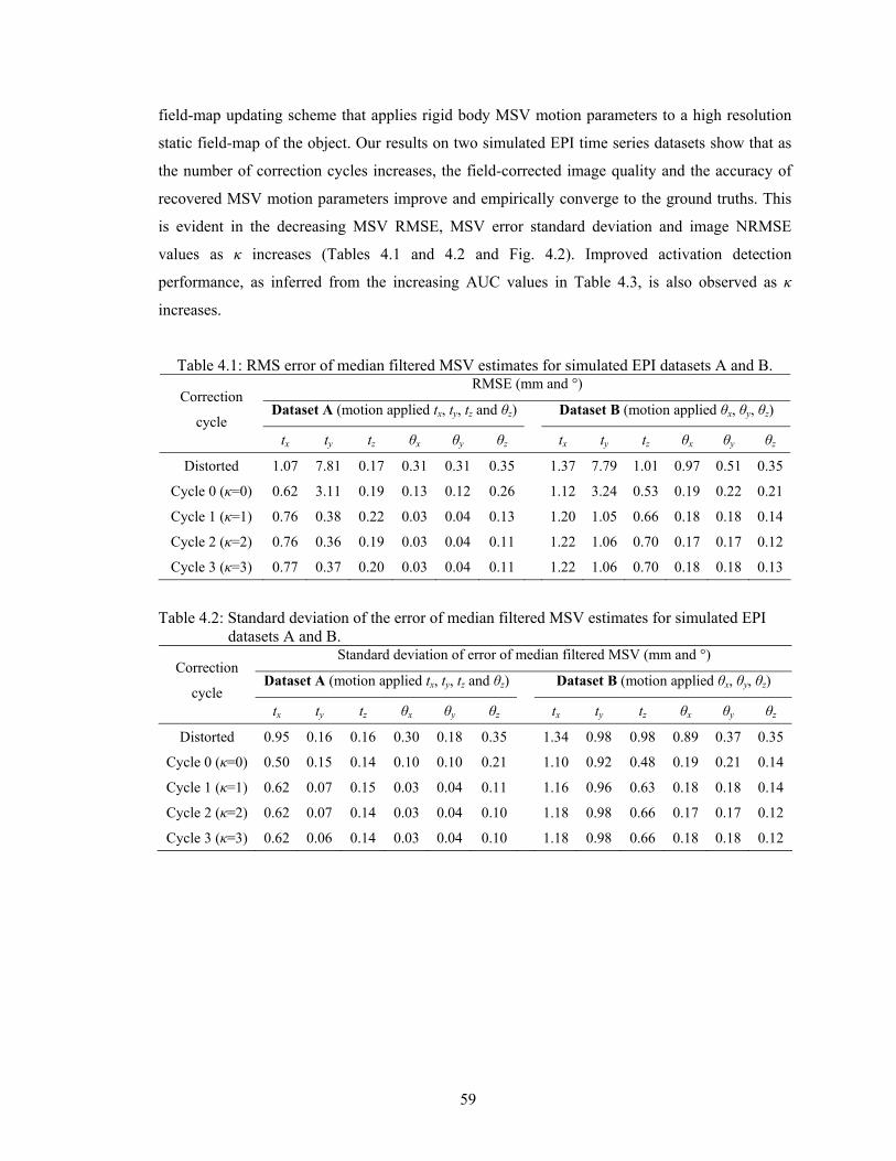
59

field-map updating scheme that applies rigid body MSV motion parameters to a high resolution

static field-map of the object. Our results on two simulated EPI time series datasets show that as

the number of correction cycles increases, the field-corrected image quality and the accuracy of

recovered MSV motion parameters improve and empirically converge to the ground truths. This

is evident in the decreasing MSV RMSE, MSV error standard deviation and image NRMSE

values as κ increases (Tables 4.1 and 4.2 and Fig. 4.2). Improved activation detection

performance, as inferred from the increasing AUC values in Table 4.3, is also observed as κ

increases.

Table 4.1: RMS error of median filtered MSV estimates for simulated EPI datasets A and B. RMSE (mm and °)

Dataset A (motion applied tx, ty, tz and θz) Dataset B (motion applied θx, θy, θz) Correction

cycle tx ty tz θx θy θz

tx ty tz θx θy θz

Distorted 1.07 7.81 0.17 0.31 0.31 0.35 1.37 7.79 1.01 0.97 0.51 0.35

Cycle 0 (κ=0) 0.62 3.11 0.19 0.13 0.12 0.26 1.12 3.24 0.53 0.19 0.22 0.21

Cycle 1 (κ=1) 0.76 0.38 0.22 0.03 0.04 0.13 1.20 1.05 0.66 0.18 0.18 0.14

Cycle 2 (κ=2) 0.76 0.36 0.19 0.03 0.04 0.11 1.22 1.06 0.70 0.17 0.17 0.12

Cycle 3 (κ=3) 0.77 0.37 0.20 0.03 0.04 0.11 1.22 1.06 0.70 0.18 0.18 0.13

Table 4.2: Standard deviation of the error of median filtered MSV estimates for simulated EPI datasets A and B.

Standard deviation of error of median filtered MSV (mm and °)

Dataset A (motion applied tx, ty, tz and θz) Dataset B (motion applied θx, θy, θz) Correction

cycle tx ty tz θx θy θz

tx ty tz θx θy θz

Distorted 0.95 0.16 0.16 0.30 0.18 0.35 1.34 0.98 0.98 0.89 0.37 0.35

Cycle 0 (κ=0) 0.50 0.15 0.14 0.10 0.10 0.21 1.10 0.92 0.48 0.19 0.21 0.14

Cycle 1 (κ=1) 0.62 0.07 0.15 0.03 0.04 0.11 1.16 0.96 0.63 0.18 0.18 0.14

Cycle 2 (κ=2) 0.62 0.07 0.14 0.03 0.04 0.10 1.18 0.98 0.66 0.17 0.17 0.12

Cycle 3 (κ=3) 0.62 0.06 0.14 0.03 0.04 0.10 1.18 0.98 0.66 0.18 0.18 0.12

60

Table 4.3: Area under ROC curve (AUC) values for activation detection of datasets A and B at various stages in CFMMSV correction.

Area under ROC Curve (AUC) Correction

cycle Dataset A Dataset B

Distorted 0.8880 0.9043

Cycle 0 (κ=0) 0.8664 0.9295

Cycle 1 (κ=1) 0.8990 0.9382

Cycle 2 (κ=2) 0.9053 0.9519

Cycle 3 (κ=3) 0.9208 0.9521

Ground truth T2 0.9209 0.9659

These results demonstrate that, under the simulated conditions, the CFMMSV method

can provide effective correction of motion artifacts that are complicated by the field effects

induced by rigid head motion. It is interesting to note that for dataset A, the AUC value for cycle

0 actually decreased when compared to the AUC value for the distorted dataset. The AUC values

increased subsequently in cycles 1 through 3. This illustrates that in the presence of significant

motion, using a static field-map to correct an entire time series can lead to degraded activation

detection performance, even after applying motion correction to the time series data. This is

because the field-map changes due to motion were not accounted for.

Dataset A was simulated with relatively realistic assumptions of how the susceptibility-

induced field-map changes with translations and in-plane rotation. Thus, the results obtained from

that dataset are a reasonable indication of the performance of the concurrent correction method on

well-shimmed real MR data with such motion. For real MR data, the field-map may include other

contributions like post-shim system-induced field-inhomogeneity that remain stationary with

respect to the head. Since the focus of the simulation study is on susceptibility-induced artifacts,

we have assumed that these additional field-map contributions are less dominant and can be

characterized separately, if necessary. This is a reasonable assumption for data collected from a

well-shimmed magnet. Dataset B was simulated with similar assumptions as dataset A except that

local field-map changes that may arise due to out-of-plane rotations are not modeled exactly.

Thus, the results from dataset B are less indicative of the CFMMSV method’s performance on

real MR data in the presence of larger out-of-plane rotation. However, for small out-of-plane

motion, the local field-map changes may be small enough [35] to justify the assumption that the

dynamic field-map can be approximated with a rigid-body transformation of the static field-map.

For time series datasets that do not have ground truths, an appropriate stopping criterion

is necessary to terminate the CFMMSV correction process automatically. In Table 4.1 and Fig.

61

4.2, respectively, the MSV RMSE and image NRMSE values remain relatively constant for κ ≥ 2

for both datasets A and B which suggests that the procedure could be terminated earlier, thus

reducing computation time. However, the increasing AUC values in Table 4.3 indicate that

activation detection performance continues to improve for κ ≥ 2. Thus, there is a computation

time versus activation detection performance tradeoff that may influence the choice for the

stopping criterion. To obtain minimal computation time at the expense of activation detection

performance, the CFMMSV process can be tasked to automatically terminate when the time

series’ average NRMSE difference for the previous two cycles are below a threshold value. For

maximal activation detection performance, the number of non-overlapping activated voxels for

the previous two cycles can be used as a dissimilarity measure to automatically stop the

CFMMSV process.

The CFMMSV framework was formulated to jointly correct for motion and geometric

distortions arising from susceptibility-induced field-inhomogeneity without the explicit

acquisition of dynamic field-maps. The framework can be further improved by using field-map

update techniques that account for susceptibility-induced field-map changes with out-of-plane

rotation. For example, a conceivable modification would be to apply MSV motion parameters to a

high resolution 3D volume of a brain that has been pre-segmented into air, bone and soft tissue

regions. The susceptibility-induced component of the dynamic field-map can then be re-estimated

from the transformed 3D structural volume using numerical techniques to approximate solutions

to the magnetostatic scalar potential based on Maxwell’s equations [42,43]. This will increase the

computational cost but may yield improved performance.

4.8 Conclusions

A proposed technique to perform concurrent susceptibility-induced geometric distortion

correction with slice-to-volume motion correction for EPI fMRI data has been evaluated on two

120-volume simulated time series with different applied motion. Under the simulated conditions,

the CFMMSV method improved the accuracy in recovering both the MSV motion parameters and

the field-corrected reconstructed images compared to the simpler method of performing motion

and geometric distortion correction independently. Activation detection performance, quantified

using the AUC values at various stages in the CFMMSV correction process, also improved with

the CFMMSV method. Although the CFMMSV method may currently be limited to small out-of-

plane rotations, it presents a correction framework that addresses geometric distortion and slice-

wise head motion as a joint problem and has the potential to perform better than methods that do

not account for the relationship between these two problems.

62

CHAPTER 5

Motion-Induced Magnetic Susceptibility and Field Inhomogeneity Estimation using Regularized Image

Restoration Techniques for fMRI

5.1 Introduction

In functional MRI (fMRI), times series images are acquired with high speed pulse sequences that

are typically adversely affected by magnetic field-inhomogeneities. As a result, these images may

be geometrically distorted or blurred depending on the pulse sequence used. A static field-

inhomogeneity map may be measured before or after a fMRI session to correct for such

distortions [4,35], but it does not account for magnetic field changes due to head motion during

the times series acquisition. To address this, several prospective dynamic field mapping

techniques have been proposed [9,10]. However, they require pulse sequence modifications or

high computational cost. This work focuses on regularized image restoration methods to

approximate dynamic field maps retrospectively without pulse sequence modifications.

In Chapter 4, the concurrent field map and MSV (CFMMSV) correction method [13]

applies rigid body transformations directly to a static field map, which may be inaccurate in the

presence of significant out-of-plane rotations. In the presence of such rotations, that method may

not be suitable since field-inhomogeneities may change nonlinearly [43]. Our approach is to

retrospectively estimate the object’s magnetic susceptibility (χ) map from an observed

susceptibility induced static field map using regularized image restoration principles. To compute

the dynamic field maps, we apply rigid body motion to the χ-map estimate, and apply 3D

susceptibility voxel convolution (SVC) [44] to the resultant spatially translated/ rotated χ-map.

SVC is a deterministic, physics-based discrete convolution model for computing susceptibility

induced field-inhomogeneity given a 3D χ-map. A simpler way to approximate the object’s χ-map

would be to segment a T1-weighted anatomical reference volume into air, bone and soft tissue,

and apply literature susceptibility values to different voxels. However, this may introduce

63

segmentation errors and the use of incorrect susceptibility values, which may lead to inaccurate

field map estimates. Our approach obviates the burden of ensuring good accuracy in both the

segmentation process, and the susceptibility values used. We estimate the χ-map from a measured

high resolution 3D static field map using 3D regularized image restoration techniques, i.e.,

solving the inverse problem of the noisy forward SVC model. The approach is demonstrated with

realistically simulated noisy 3D field maps of a spherical air compartment in water.

5.2 Theory

5.2.1 Susceptibility Voxel Convolution for Field Map Computation

Previous work [42] has shown that given an object with K independent closed compartments of

constant χ values, a Lorentz-corrected boundary element approach to computing the z-component

of the χ-induced magnetic field map, Bp(r), yields

∑ ∫=

−+ ⋅−

−−+≈

K

k Skk

k

'zz1

030p d'

')(4ˆ

3)(

)( SBrr

zBr

rB χχπ

χ (Tesla), (5.1)

where z is a unit vector parallel to the scanner’s main magnetic field B0, +kχ and −

kχ denote the

susceptibilities outside and inside the kth compartment, respectively, Sk is the kth surface, r′ is a

surface point, dS′ is perpendicular to the surface at r′. In the presence of out-of-plane rotations,

the orientation of the surfaces with B0, i.e., B0·dS′, changes, thus resulting in nonlinear field map

changes.

Susceptibility voxel convolution (SVC) [44] applies Eq. (5.1) directly to voxels of an

object. Each voxel is defined as a closed six-sided compartment of uniform susceptibility. The dot

product, B0·dS′, is non-zero only for the top and bottom surfaces of a voxel. Only the upper

surface is used since the superposition principle allows each surface to be used only once in

computing Bp(x). The values of χk- and χk

+ are obtained from the kth voxel, and the voxel above it

in the z direction, respectively. The χ-induced field equation now becomes

⎥⎥

⎦

⎤

⎢⎢

⎣

⎡

−

−+−+≈ ∑ ∫ ∫

=

+

−

+

−

−+K

k

ly

ly

lx

lx

zkkk

yk

yk

xk

xk

dydxzlz

1

2/

2/

2/

2/ 30p '''

)2/()(

41

3)()(

rr

rBrB χχπ

χ , (5.2)

where (xk, yk, zk) is the center of voxel k, and lx, ly, lz are the x, y, and z lengths of a voxel. After

discretisation in r, Eq. (5.2) becomes a 3D discrete convolution in space domain. The convolution

kernel can be written as

64

[ ] , '')2/()'()'()2/(

),,(2/

2/

2/

2/

2/3222∫ ∫

+

−

+

−

−−++−+−−+

=−−−yk

yk

xk

xk

ly

ly

lx

lxzkzk

kkk

dydxzlzyyxxzlz

zzyyxxK

(5.3)

and the SVC impulse response is

[ ]π

δδδ4

),,()1,,(3

)'()'()'(),,(

jihKjihKnnmmlljihd

−−+

−−−= , (5.4)

where (l,m,n) denotes the voxel where Bp is to be calculated, and (l′,m′,n′) denotes voxels in the

field of view. The discrete convolution of Eq. (5.2) becomes

)',','()',','(),,(FOV',','

0p nnmmlldnmlnmlnml

−−−= ∑∈χBB , (5.5)

which can be computed with

( ))()( 331

300p dd DDD ℑℑℑ=∗∗∗= − χχ BBB , (5.6)

where *** denotes 3D convolution and D3ℑ denotes 3D Fourier transform. The discrete

convolution can also be written in matrix-vector notation as

DχB =p , (5.7)

where D denotes the SVC “system” matrix and χ is the column-stacked χ-map vector. The χ-

induced field map in Hz is ∆ωp=γBp, where γ is the gyromagnetic ratio of hydrogen.

The SVC impulse response is linear shift invariant and depends only on the voxel size

and orientation with respect to B0. The impulse response remains unchanged when a 3D

susceptibility map undergoes rigid body transformation.

5.2.2 Dynamic Field Map Estimation with Penalized Weighted Least Squares

Estimation of Magnetic Susceptibility Map – A 3D Image Restoration

Approach

A static field map, ∆ωstatic, is typically approximated by taking the phase difference of a pair of

gradient-echo images acquired at two different echo times [14], and may be composed of

susceptibility and non-susceptibility induced field inhomogeneity sources. The two complex-

valued images may be denoted by

TE1TE1jjj fI ε+= , (5.8)

TE2TTE2 ,staticj

Eijj

jefI εω += ∆∆− , (5.9)

where f is the complex transverse magnetization of the object, j is the voxel number, ∆TE is the

echo time difference, and ε is independent identically distributed MR Gaussian noise. The echo

65

time difference is typically small to prevent phase wrapping. In previous work [17], the maximum

likelihood estimator for ∆ωstatic was shown to be

[ ])TEcos(1min argˆ ,staticTE1TE2TE12TE

staticstatic

∆∆−∠−∠−=∆ ∑∆

jjjj

jj IIII ωω

ω . (5.10)

Ignoring phase wrapping, and decomposing ∆ωstatic,j into susceptibility and system induced parts,

i.e., ∆ωstatic,j = γ[Dχ]j + ∆ωsys,j, and since a minimum exists when the cosine term equals one, the

maximum likelihood estimator for χ is

jj E ⎥

⎥⎦

⎤

⎢⎢⎣

⎡

⎥⎥⎦

⎤

⎢⎢⎣

⎡∆−

∆∠−∠

= −sys

TE1TE21

T1ˆ ωIIDγ

χ . (5.11)

For simplicity, we assume that ∆ωsys is negligible, or can be measured empirically. Since the

SVC frequency response has very small values at some frequencies, the inverse SVC problem is

ill-posed, and thus 3D smoothness regularization is desirable when solving for χ. We propose to

use a quadratic penalized weighted least squares (QPWLS) image restoration approach to

estimate χ by minimizing the cost function

22

21)( CχDχgχ W βγ +−=Ψ , (5.12)

where g is the observed static field map (∠ ITE2- ∠ ITE1)/∆TE, W is a weighting matrix that

assigns higher weights to voxels where MR image intensity, i.e., |IjTE2Ij

TE1|, is higher, β is a

regularization parameter that determines the amount of smoothing, and C is a first order finite-

differencing matrix. We minimize the cost function using the conjugate gradient algorithm. Any

available motion estimates for each slice/ volume in the fMRI time series can then be used to

rotate/ translate the χ-map estimate. Since the SVC impulse response is linear shift invariant and

depends only on the voxel size and orientation with respect to B0, it remains unchanged when a χ-

map undergoes rigid body transformation. Thus, the same SVC matrix used in estimating the χ-

map can be used to compute the dynamic field map after the desired motion has been applied.

The proposed QPWLS method was compared to three other methods of approximating

the dynamic field map from an observed field map: thresholded inverse filtering, Wiener filtering

[45], and direct rotation of the observed field map to the tilted positions [13]. The thresholded

inverse filter ignores noise statistics and amplifies noise in frequency bands where the SVC

frequency response has small values. To mitigate the latter, while preserving as much spatial

information as possible, the threshold parameter needs to be chosen carefully, usually in an

empirical manner. The Wiener filter assumes that χ and the additive field map noise are stationary

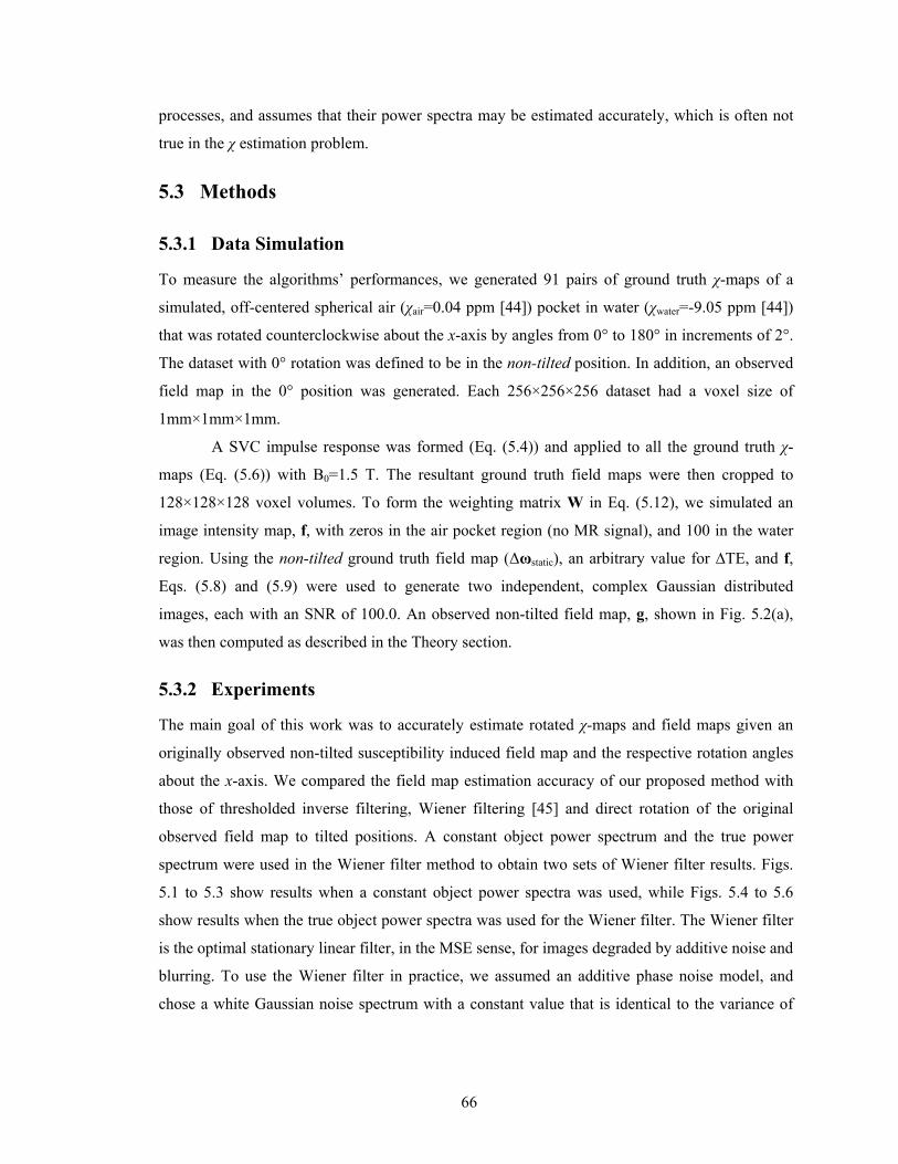
66

processes, and assumes that their power spectra may be estimated accurately, which is often not

true in the χ estimation problem.

5.3 Methods

5.3.1 Data Simulation

To measure the algorithms’ performances, we generated 91 pairs of ground truth χ-maps of a

simulated, off-centered spherical air (χair=0.04 ppm [44]) pocket in water (χwater=-9.05 ppm [44])

that was rotated counterclockwise about the x-axis by angles from 0° to 180° in increments of 2°.

The dataset with 0° rotation was defined to be in the non-tilted position. In addition, an observed

field map in the 0° position was generated. Each 256×256×256 dataset had a voxel size of

1mm×1mm×1mm.

A SVC impulse response was formed (Eq. (5.4)) and applied to all the ground truth χ-

maps (Eq. (5.6)) with B0=1.5 T. The resultant ground truth field maps were then cropped to

128×128×128 voxel volumes. To form the weighting matrix W in Eq. (5.12), we simulated an

image intensity map, f, with zeros in the air pocket region (no MR signal), and 100 in the water

region. Using the non-tilted ground truth field map (∆ωstatic), an arbitrary value for ∆TE, and f,

Eqs. (5.8) and (5.9) were used to generate two independent, complex Gaussian distributed

images, each with an SNR of 100.0. An observed non-tilted field map, g, shown in Fig. 5.2(a),

was then computed as described in the Theory section.

5.3.2 Experiments

The main goal of this work was to accurately estimate rotated χ-maps and field maps given an

originally observed non-tilted susceptibility induced field map and the respective rotation angles

about the x-axis. We compared the field map estimation accuracy of our proposed method with

those of thresholded inverse filtering, Wiener filtering [45] and direct rotation of the original

observed field map to tilted positions. A constant object power spectrum and the true power

spectrum were used in the Wiener filter method to obtain two sets of Wiener filter results. Figs.

5.1 to 5.3 show results when a constant object power spectra was used, while Figs. 5.4 to 5.6

show results when the true object power spectra was used for the Wiener filter. The Wiener filter

is the optimal stationary linear filter, in the MSE sense, for images degraded by additive noise and

blurring. To use the Wiener filter in practice, we assumed an additive phase noise model, and

chose a white Gaussian noise spectrum with a constant value that is identical to the variance of

67

the simulated noise. In reality, noise in a complex MRI image is additive Gaussian while phase

noise is not.

The first part of the experiment involved the estimation of the original, non-tilted χ-map

using the various methods. All estimates of χ were shown in Figs. 5.1 and 5.4. We applied the

SVC matrix to these χ-map estimates to compute field map estimates from which a slice is shown

in the top rows of Figs. 5.2 and 5.5. Root mean-square-error (RMSE) values were then computed

with reference to the 3D ground truth non-tilted field map, ∆ωstatic. In the second part of the

experiment, the χ-map estimates from the first part were all rotated about the x-axis by the same

range of values used to create the 91 pairs of ground truth maps, i.e., 0° to 180° in increments of

2°. The SVC matrix was again applied to these rotated χ-map estimates to compute the dynamic

field map estimates. Root mean-square-error (RMSE) values were then computed with reference

to the 3D ground truth tilted field maps. The second rows in Figs. 5.2 and 5.5 show a field map

slice of the object rotated by 45° about the x axis. The field map RMSE values for all positions

and methods were plotted in Figs. 5.3 and 5.6.

The QPWLS implementation was built upon previous work [46], and 50 iterations of the

algorithm were performed for each dataset with β=0.7. The initial guess for the conjugate gradient

algorithm was a volume filled with zeros. For the thresholded inverse filter, a threshold value of

10 (0.2 % of the maximum absolute value of the inverse of the SVC frequency response) was

used. All algorithms in this work were implemented in MATLAB (The Mathworks Inc., Natick,

MA, USA) and C++, and were executed on Intel Pentium 4 Xeon 3.0GHz CPUs.

5.4 Results

The RMSE values over entire 3D field map estimates for all rotated positions using the various

field map estimation methods are shown in Figs. 5.2 and 5.5. In Fig. 5.2, when the object power

spectra for the Wiener filter was constant, it was observed that the QPWLS method had the

lowest (best performing) RMSE values, and RMSE variability, across all rotated positions. In Fig.

5.5, when the true object power spectra was used for the Wiener filter, the RMSE values for the

QPWLS method were comparable to the Wiener filter method. Compared to the QPWLS method,

the Wiener filter’s dependence on prior knowledge of the object’s power spectra is a key

disadvantage.

Fig. 5.1 shows slices in the y-z plane at the same spatial location of χ-map estimates of

the object in the 45° rotated position, i.e., slices from a snapshot of Fig. 5.3. The x-axis points into

the plane of the page. It was observed that the associated field map estimates in the spherical air

region were invariably noisy for the inverse filter and Wiener filter (using a constant object power

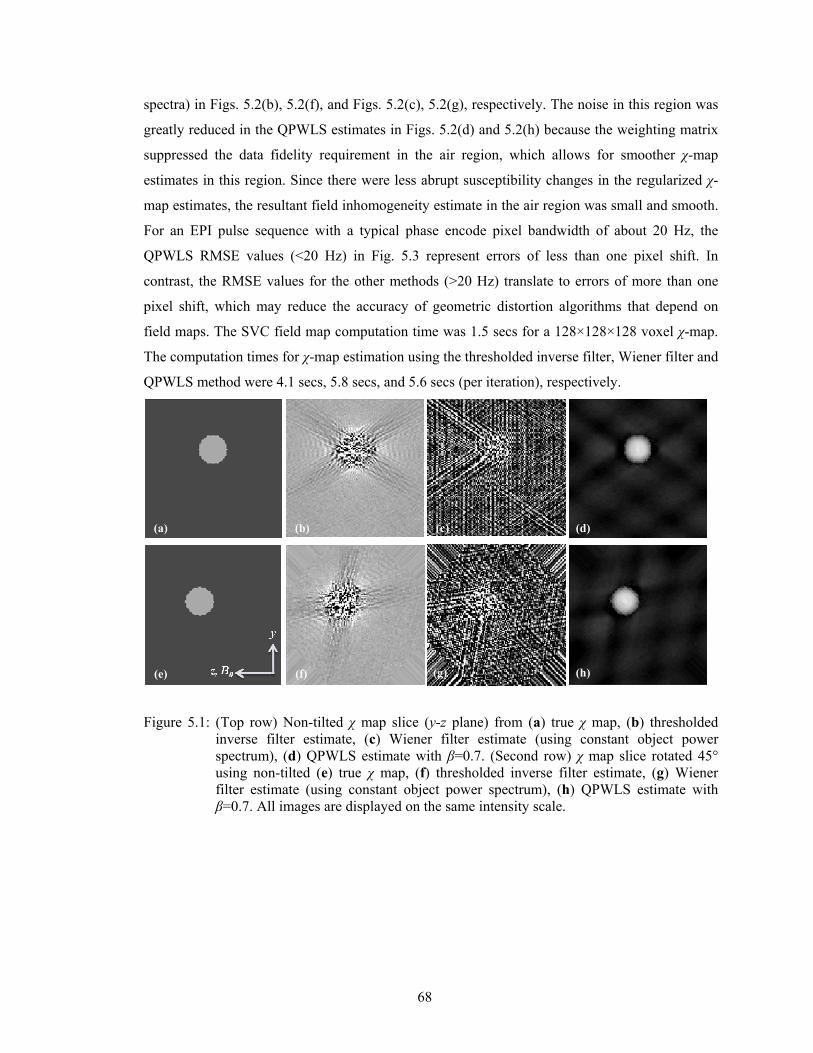
68

spectra) in Figs. 5.2(b), 5.2(f), and Figs. 5.2(c), 5.2(g), respectively. The noise in this region was

greatly reduced in the QPWLS estimates in Figs. 5.2(d) and 5.2(h) because the weighting matrix

suppressed the data fidelity requirement in the air region, which allows for smoother χ-map

estimates in this region. Since there were less abrupt susceptibility changes in the regularized χ-

map estimates, the resultant field inhomogeneity estimate in the air region was small and smooth.

For an EPI pulse sequence with a typical phase encode pixel bandwidth of about 20 Hz, the

QPWLS RMSE values (<20 Hz) in Fig. 5.3 represent errors of less than one pixel shift. In

contrast, the RMSE values for the other methods (>20 Hz) translate to errors of more than one

pixel shift, which may reduce the accuracy of geometric distortion algorithms that depend on

field maps. The SVC field map computation time was 1.5 secs for a 128×128×128 voxel χ-map.

The computation times for χ-map estimation using the thresholded inverse filter, Wiener filter and

QPWLS method were 4.1 secs, 5.8 secs, and 5.6 secs (per iteration), respectively.

Figure 5.1: (Top row) Non-tilted χ map slice (y-z plane) from (a) true χ map, (b) thresholded inverse filter estimate, (c) Wiener filter estimate (using constant object power spectrum), (d) QPWLS estimate with β=0.7. (Second row) χ map slice rotated 45° using non-tilted (e) true χ map, (f) thresholded inverse filter estimate, (g) Wiener filter estimate (using constant object power spectrum), (h) QPWLS estimate with β=0.7. All images are displayed on the same intensity scale.

(a) (b) (c)

(e) (f) (g)

(d)

(h)

69

Figure 5.2: (Top row) Non-tilted field map slice (y-z plane) from (a) originally observed field map, (b) thresholded inverse filter estimate, (c) Wiener filter estimate (using constant object power spectrum), (d) QPWLS estimate with β=0.7. (Second row) 45° rotated field map slice from (e) rotation of original observed field map, (f) application of SVC on rotated estimate of χ from thresholded inverse filter, (g) application of SVC on rotated estimate of χ from Wiener filter (using constant object power spectrum), (h) application of SVC on rotated estimate of χ from QPWLS. (Bottom row) Ground truth field maps for (i) non-tilted, and (j) 45° tilted positions. All images are displayed on the same intensity scale.

RMSE: 32.1 Hz (a) RMSE: 43.0 Hz (b) RMSE: 32.2 Hz (c)

RMSE: 28.2 Hz (e) RMSE: 39.9 Hz (f) RMSE: 188.6 Hz (g)

(i) (j) z, B0

y

RMSE:18.1 Hz (d)

RMSE: 13.4 Hz (h)

70

Figure 5.3: Dynamic field map RMSE values versus rotation angles for different estimation methods when object was rotated about the x-axis from 0° to 180°. An arbitrary constant object power spectrum was used in the Wiener filter.

Figure 5.4: (Top row) Non-tilted χ map slice (y-z plane) from (a) true χ map, (b) thresholded

inverse filter estimate, (c) Wiener filter estimate (using true object power spectrum), (d) QPWLS estimate with β=0.7. (Second row) χ map slice rotated 45° using non-tilted (e) true χ map, (f) thresholded inverse filter estimate, (g) Wiener filter estimate (using true object power spectrum), (h) QPWLS estimate with β=0.7. All images are displayed on the same intensity scale.

(a) (b) (c)

(e) (f) (g)

(d)

(h)

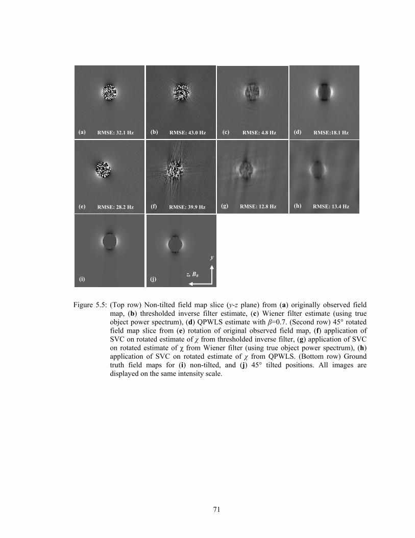
71

Figure 5.5: (Top row) Non-tilted field map slice (y-z plane) from (a) originally observed field map, (b) thresholded inverse filter estimate, (c) Wiener filter estimate (using true object power spectrum), (d) QPWLS estimate with β=0.7. (Second row) 45° rotated field map slice from (e) rotation of original observed field map, (f) application of SVC on rotated estimate of χ from thresholded inverse filter, (g) application of SVC on rotated estimate of χ from Wiener filter (using true object power spectrum), (h) application of SVC on rotated estimate of χ from QPWLS. (Bottom row) Ground truth field maps for (i) non-tilted, and (j) 45° tilted positions. All images are displayed on the same intensity scale.

RMSE: 32.1 Hz (a) RMSE: 43.0 Hz (b) RMSE: 4.8 Hz (c)

RMSE: 28.2 Hz (e) RMSE: 39.9 Hz (f) RMSE: 12.8 Hz (g)

(i) (j) z, B0

y

RMSE:18.1 Hz (d)

RMSE: 13.4 Hz (h)

72

Figure 5.6: Dynamic field map RMSE values versus rotation angles for different estimation

methods when object was rotated about the x-axis from 0° to 180°. The true object power spectrum was used in the Wiener filter.

5.5 Discussion and Conclusions

The proposed method estimates dynamic susceptibility induced field maps from an observed

static susceptibility induced field map, while accounting for the proper MR noise model. It does

not require segmentation or pulse sequence modifications, and may yield higher resolution

dynamic field maps that address nonlinear changes due to out-of-plane rotations. Fig. 5.3 shows

quantitatively that the QPWLS RMSE values were the lowest (best performing) among all the

other methods. Figs. 5.2(d) and 5.2(h) show qualitatively that the field map estimates were close

to the ground truths. For our spherical air pocket in water, nonlinear field map changes would

typically be worst at the 90° position, hence a peak is observed at that position in Fig. 5.3 for the

method that simply rotates the observed field map. In contrast, the low QPWLS RMSE variability

across rotation angles in Fig. 5.3 suggests that the method performs reasonably well regardless of

rotation angles. Further improvements in the proposed method may be possible upon optimizing

the choice for the regularization parameter, coupled with the implementation of regularization

functions that utilizes prior spatial information that is specific to a brain’s χ-map. Since the χ-map

of the brain is smooth, with the exception of air-tissue, bone-air and bone-tissue interfaces, an

73

edge preserving regularization function, e.g., Huber function, may be used instead. Coarse

segmentation of a T1 weighted map of the brain into air, tissue and bone regions may still be

helpful to identify voxels around susceptibility interfaces where edge preserving regularization

can be selectively applied, while quadratic regularization is used for non-interface regions where

the susceptibility map is expected to be smooth. This regularization scheme favors smoothly

varying susceptibility map estimates within soft tissue, air and bone regions while allowing for

abrupt susceptibility changes at the susceptibility interfaces. It is noted that segmentation is used

here as an aid to choose the type of regularization for different brain regions and not for direct

computation of the field map. A wrongly chosen regularization function will only lead to more, or

less, blurring of the susceptibility map but should not change the locations of the susceptibility

interfaces significantly.

The initial guess for the conjugate gradient algorithm was a volume filled with zeros. The

use of the static field map as an initial guess for the algorithm may improve the rate of

convergence since the static field map resembles the true field map more than a zero volume.

A potential limitation of the proposed method may arise because ∆ωsys was ignored in

Eq. (5.11) for simplicity. In our future work, we will investigate methods to reliably measure non-

χ induced field inhomogeneities, and characterize their effects on the various approaches in this

work.

A novel regularized image restoration approach to estimate field maps of a moving object

was proposed and shown, with simulated data, to be more effective than non-regularized methods

or simple transformations of an observed field map. In fMRI, this may potentially improve

dynamic field map estimates and hence, geometric distortion correction accuracy.

74

CHAPTER 6

Formulation of Current Density Weighted Indices for Correspondence between fMRI and Electrocortical Stimulation

Maps

6.1 Introduction

Epilepsy surgery to remove identifiable epileptogenic regions of the brain is often achieved in

conjunction with an electrocortical stimulation (ECS) [47] map obtained either before or during

the resection surgery. The goal of this mapping is to identify brain regions that are essential for

language and sensorimotor functions prior to frontal or temporal lobe resection. Defining

hemispheric language and sensorimotor localization in patients with intractable epilepsy is

important for avoiding complications of epilepsy surgery involving eloquent cortex. Currently,

intraoperative or extraoperative electrocortical stimulation mapping of sensory, motor, and

language are used to define the safe limits of resection. The intraoperative ECS procedure

performed during an awake craniotomy, followed by resection, subjects the patient to additional

strain during surgery. In extraoperative ECS, the placement of subdural electrode arrays for

functional mapping places the patient at risk for complications.

Functional magnetic resonance imaging (fMRI) techniques show strong potential for

presurgical evaluation of patients with brain tumors or epileptic lesions and may provide a non-

invasive alternative to the ECS method to define eloquent cortex at risk during epilepsy surgery.

In constant current bipolar ECS, each pair of adjacent electrodes on an electrode grid is

stimulated with alternating polarity square wave current pulses. The stimulus current intensity is

increased gradually until either the patient’s response changes, or an afterdischarge, is observed.

In fMRI, an increase in cerebral blood flow induced by local neuronal activity modulates the

proportion of oxyhemoglobin to deoxyhemoglobin in nearby vasculature. This results in a

magnetic susceptibility difference between the blood vessel and surrounding tissue which can be

imaged with a T2*-weighted MRI protocol. Because fMRI’s stimulation mechanism differs from

ECS as the standard technique for presurgical functional mapping, the accuracy of fMRI

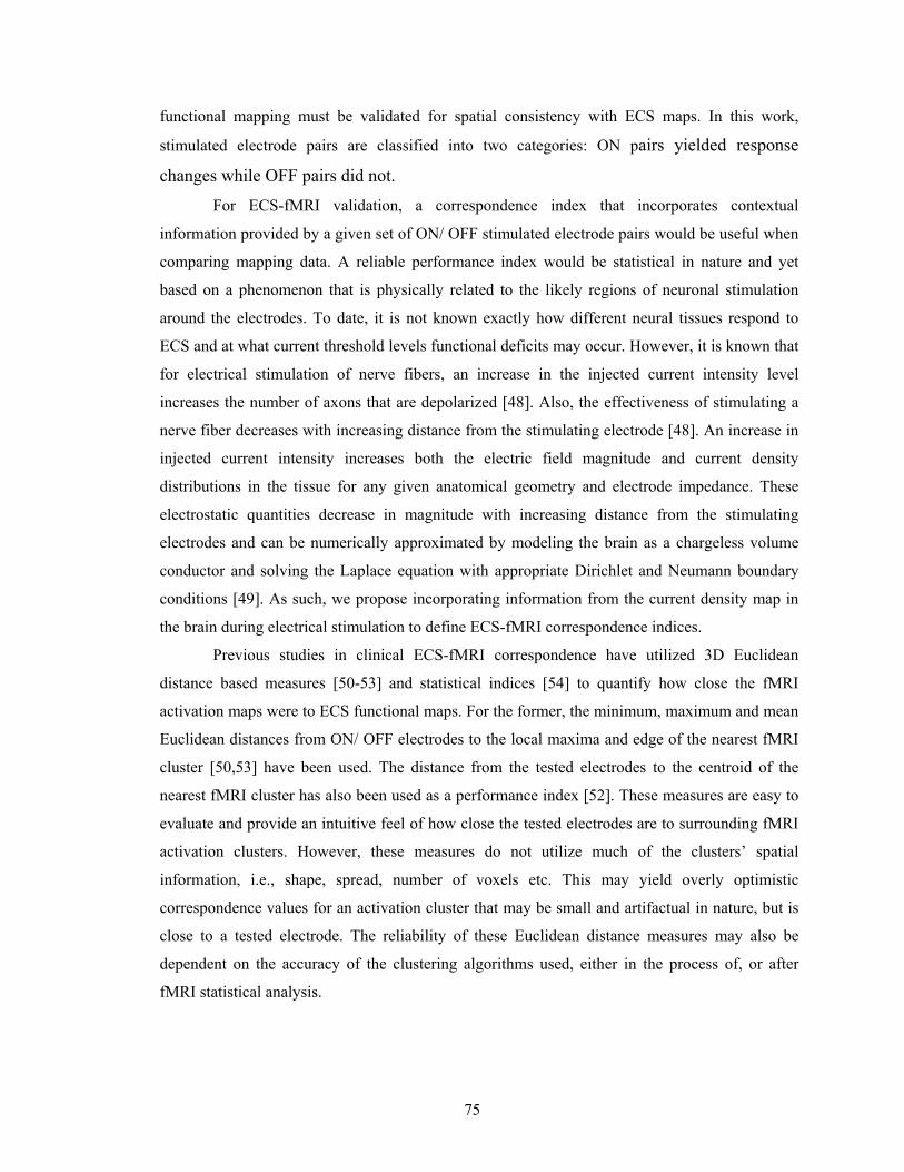
75

functional mapping must be validated for spatial consistency with ECS maps. In this work,

stimulated electrode pairs are classified into two categories: ON pairs yielded response

changes while OFF pairs did not.

For ECS-fMRI validation, a correspondence index that incorporates contextual

information provided by a given set of ON/ OFF stimulated electrode pairs would be useful when

comparing mapping data. A reliable performance index would be statistical in nature and yet

based on a phenomenon that is physically related to the likely regions of neuronal stimulation

around the electrodes. To date, it is not known exactly how different neural tissues respond to

ECS and at what current threshold levels functional deficits may occur. However, it is known that

for electrical stimulation of nerve fibers, an increase in the injected current intensity level

increases the number of axons that are depolarized [48]. Also, the effectiveness of stimulating a

nerve fiber decreases with increasing distance from the stimulating electrode [48]. An increase in

injected current intensity increases both the electric field magnitude and current density

distributions in the tissue for any given anatomical geometry and electrode impedance. These

electrostatic quantities decrease in magnitude with increasing distance from the stimulating

electrodes and can be numerically approximated by modeling the brain as a chargeless volume

conductor and solving the Laplace equation with appropriate Dirichlet and Neumann boundary

conditions [49]. As such, we propose incorporating information from the current density map in

the brain during electrical stimulation to define ECS-fMRI correspondence indices.

Previous studies in clinical ECS-fMRI correspondence have utilized 3D Euclidean

distance based measures [50-53] and statistical indices [54] to quantify how close the fMRI

activation maps were to ECS functional maps. For the former, the minimum, maximum and mean

Euclidean distances from ON/ OFF electrodes to the local maxima and edge of the nearest fMRI

cluster [50,53] have been used. The distance from the tested electrodes to the centroid of the

nearest fMRI cluster has also been used as a performance index [52]. These measures are easy to

evaluate and provide an intuitive feel of how close the tested electrodes are to surrounding fMRI

activation clusters. However, these measures do not utilize much of the clusters’ spatial

information, i.e., shape, spread, number of voxels etc. This may yield overly optimistic

correspondence values for an activation cluster that may be small and artifactual in nature, but is

close to a tested electrode. The reliability of these Euclidean distance measures may also be

dependent on the accuracy of the clustering algorithms used, either in the process of, or after

fMRI statistical analysis.

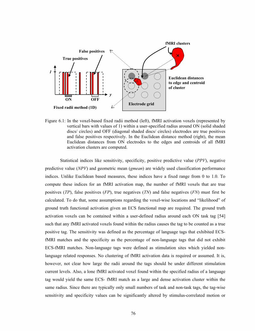
76

Figure 6.1: In the voxel-based fixed radii method (left), fMRI activation voxels (represented by

vertical bars with values of 1) within a user-specified radius around ON (solid shaded discs/ circles) and OFF (diagonal shaded discs/ circles) electrodes are true positives and false positives respectively. In the Euclidean distance method (right), the mean Euclidean distances from ON electrodes to the edges and centroids of all fMRI activation clusters are computed.

Statistical indices like sensitivity, specificity, positive predictive value (PPV), negative

predictive value (NPV) and geometric mean (gmean) are widely used classification performance

indices. Unlike Euclidean based measures, these indices have a fixed range from 0 to 1.0. To

compute these indices for an fMRI activation map, the number of fMRI voxels that are true

positives (TP), false positives (FP), true negatives (TN) and false negatives (FN) must first be

calculated. To do that, some assumptions regarding the voxel-wise locations and “likelihood” of

ground truth functional activation given an ECS functional map are required. The ground truth

activation voxels can be contained within a user-defined radius around each ON task tag [54]

such that any fMRI activated voxels found within the radius causes the tag to be counted as a true

positive tag. The sensitivity was defined as the percentage of language tags that exhibited ECS-

fMRI matches and the specificity as the percentage of non-language tags that did not exhibit

ECS-fMRI matches. Non-language tags were defined as stimulation sites which yielded non-

language related responses. No clustering of fMRI activation data is required or assumed. It is,

however, not clear how large the radii around the tags should be under different stimulation

current levels. Also, a lone fMRI activated voxel found within the specified radius of a language

tag would yield the same ECS- fMRI match as a large and dense activation cluster within the

same radius. Since there are typically only small numbers of task and non-task tags, the tag-wise

sensitivity and specificity values can be significantly altered by stimulus-correlated motion or

Electrode grid

fMRI clusters

Euclidean distances to edge and centroid of cluster

Fixed radii method (1D)

ON OFF y

1

True positives

False positives

77

noise-induced fMRI activation voxels that happen to fall within the specified radii of the task or

non-task tags. Thus, it may be more desirable to consider the actual number of voxels that fall

within the radii of the tags as well.

In the above fixed radii method, all activated voxels within the radii are given the same

level of influence in determining the indices, irrespective of their relative distances from the

electrodes. Activated voxels located outside these radii are not counted. These fixed windows of

ground truth voxels make it difficult to measure incremental improvements in ECS-fMRI

correspondence when fMRI activated voxels consistently fall outside the windows but are

nevertheless inching towards the ON electrodes, e.g., as a result of improved data processing

techniques. The true positive count will still be zero. A Euclidean distance measure would be

useful in these cases but the previously mentioned limitations would then arise.

There are indications that the level of elicited neuronal activation is influenced by applied

stimulus levels [48]. Since a higher stimulus current intensity would likely exceed a wider range

of neuronal activation threshold levels, an ECS-fMRI correspondence index may be physically

more meaningful and reliable if information from the electric field or current density map was

incorporated into its definition. We propose a current density weighted method that combines the

advantages of distance-based measures with voxel-wise statistical indices to quantify ECS-fMRI

correspondence. We do not calculate Euclidean distances between reference points explicitly and

do not assume that the fMRI maps consist of clusters. Information of the Euclidean distance

between each activated voxel with respect to ON or OFF electrodes is embedded in numerically

computed current density maps by solving the Laplace equation for a quasistatic volume

conductor using the finite difference method. Each current density map is unique to each patient-

task combination and depends solely on the ECS functional map and current or voltage

stimulation parameters.

The goals of this study are to (i) examine and evaluate the ECS-fMRI correspondence

indices in various simulated test cases, and, (ii) to demonstrate the use of these indices in human

data. We formulate a current density weighted scheme to assess the relative numbers of fMRI true

positives, true negatives, false positives and false negatives [58], i.e., populate a contingency

table or confusion matrix. These values are then used to compute five existing statistical measures

for classification performance, i.e., sensitivity, specificity, positive predictive value (PPV),

negative predictive value (NPV) and geometric mean (gmean) [55]. A 3D volume with a

simulated electrode grid and simulated fMRI activation maps are used to investigate and compare

the behaviors of the proposed current density weighted measures and modified versions of two

previously reported correspondence indices [50,54]. The current density weighted indices are also

78

computed for three different patients who participated in fMRI studies for verbalized language

tasks followed by language mapping with extraoperative ECS procedures prior to surgical

treatment. The patient studies demonstrate the feasibility of current density weighted statistical

measures for evaluating fMRI activation localization with extraoperative ECS mapping.

6.2 Methods

All computational work was performed on Intel Pentium 4 Xeon 3.0 GHz CPUs using MATLAB

(The Mathworks Inc., Natick, MA, USA) and Advanced Visual Systems (Advanced Visual

Systems Inc., Waltham, MA, USA). The patient studies were conducted in accordance with the

guidelines set by the University of Michigan Medical School Institutional Review Board.

Informed consent was obtained from all three subjects.

The post-grid CT datasets were acquired on GE MDCT LightSpeed machines, LS16,

LS16pro, LSultra(8) and LS4slice scanners. The acquisition protocol was axial slices through

electrodes, posterior fossa through vertex and slice thickness of 1.25 mm in a tilted mode so as

not to include the lenses with a field of view of 23 cm. All MRI data were acquired on a 1.5 T GE

SIGNA MR scanner (GE Medical Systems, Milwaukee, WI). All anatomical MR datasets were

acquired with a 3D Spoiled GRASS (SPGR) protocol with the following parameters: TR=10 ms,

TE=3.7 ms, flip angle=8 degrees, FOV=25 cm, voxel size=1.0 mm×1.0 mm×1.5 mm, image

matrix = 256×256×120. Functional MRI datasets were acquired prior to the grid electrode

implant. An echo-planar imaging (EPI) sequence with slice interleaving was used with the

following parameters: TR=3000 ms, TE=30 ms, flip angle=90 degrees, FOV=24 cm, voxel

size=1.95 mm×1.95 mm×6.0 mm, image matrix = 128×128×16.

6.2.1 Activation Localization in fMRI

Each set of fMRI time series for a test paradigm consists of six cycles of 30 s of stimuli

presentation followed by 30 s of rest. Language paradigms in fMRI sessions were designed to

follow the equivalent tests in ECS language mapping, which include confrontation naming,

responsive naming, and tongue rapid alternating lateral movement (tongue RAMs). For the visual

confrontation naming (picture naming of line drawings of objects) task during fMRI, each patient

was instructed to name aloud the objects projected on a screen. For responsive naming, the

patient would respond verbally to a series of questions asked through intercom during the

activation periods. The tongue RAMs task was a self-paced tongue movement from one corner of

the lips to the other for 30 s followed by 30 s rest for six cycles.

79

6.2.2 Euclidean Distance and Voxel-Based Fixed Radii ECS-fMRI

Correspondence Indices

To facilitate a fairer comparison of the afore-mentioned tag-wise fixed radii method with our

voxel-based current density weighted correspondence indices, and to improve the former’s

robustness to errors in the presence of lone fMRI activated voxels, we reconfigured the tag-wise

fixed radii method by defining voxels within the radii of ON electrodes (task tags) as ground truth

positives and OFF electrodes (non-task tags) as ground truth negatives. The values of TP and FP

are computed by counting the total number of fMRI activation voxels within the fixed radii

around the ON electrodes and OFF electrodes, respectively. The values of FN and TN are the total

number of fMRI non-activation voxels within the fixed radii around the ON electrodes and OFF

electrodes, respectively. The sensitivity, specificity, PPV, NPV and gmean indices are then

computed using the voxel-based quantities TP, FP, FN and TN. The sensitivity is now the

percentage of voxels (of all voxels within the radii of task tags) that have corresponding fMRI

activation, i.e., true positive accuracy. The specificity is now the percentage of voxels (of all

voxels within the radii of non-task tags) that do not have corresponding fMRI activation, i.e., true

negative accuracy. The choice of the radius around the tags is still arbitrary. This voxel-based

method of computing statistical performance indices will be referred to as the “voxel-based fixed

radii” method (Fig. 6.1).

6.2.3 Current Density Weighted ECS-fMRI Correspondence Indices

For a current density weighted method for computing the ECS-fMRI correspondence indices, let

an fMRI activation map, which is a 3D binary map of activated (‘1’) and non-activated (‘0’)

voxels, be denoted by m(r) where r is the vector of 3D spatial variables (x, y, z). It is assumed that

m(r) is spatially registered to a 3D T1-weighted anatomical reference volume gref(r). Let JON,k(r)

denote the magnitude of the 3D current density vector field when the kth pair (out of K pairs) of

ON electrodes is stimulated. To obtain good ECS-fMRI correspondence, it is expected that fMRI

activation would occur near ON electrode pairs and not in the proximity of OFF electrode pairs.

The weighted number of true positives is computed by multiplying each fMRI activated voxel,

which has a value of 1, with the current density magnitude at that voxel for each ON electrode

pair, and then summing all these weighted voxels as follows:

∑ ∑= ∈

=K

k FOVikONi

i

JmTP1

, )()(r

rr , (6.1)

80

where ri is the spatial vector variable (xi, yi, zi) for the ith voxel and FOV denotes the imaging field

of view. In other words, TP is the sum of all fMRI activated voxels weighted by corresponding

current density map voxels for all ON electrode pairs. An activated voxel that is far away from

any ON electrode pair is effectively ignored since the corresponding current density value will be

negligible. In a similar manner, FP is computed by using JOFF,l(r), the current density map when

the lth pair (out of L pairs) of OFF electrodes was stimulated

∑ ∑= ∈

=L

l FOVilOFFi

i

JmFP1

, )()(r

rr . (6.2)

The number of true negative and false negatives are computed as

∑ ∑= ∈

−=L

l FOVilOFFi

i

JmTN1

, )())(1(r

rr and (6.3)

∑ ∑= ∈

−=K

k FOVikONi

i

JmFN1

, )())(1(r

rr (6.4)

where 1-m(ri) is equal to 1 for non-activated voxels and 0 for activated voxels. Fig. 6.2 illustrates

the above equations in one dimension.

Figure 6.2: In the current density weighted method, fMRI activation voxels (vertical bars)

weighted by the ON (solid shaded discs) and OFF electrodes’ (diagonally shaded discs) current density values (dotted line) at the voxels’ locations contribute to the true positive (TP) and false positive (FP) quantities respectively. The fMRI non-activated voxels weighted by the ON and OFF current density values contribute to the false negative (FN) and true negative (TN) quantities respectively.

With the above quantities, the following ECS-fMRI correspondence indices, all of which

are in the range of 0 to 1.0, can be evaluated:

FNFPTNTPTNTPaccuracy

++++

= , (6.5)

FNTPTPysensitivit+

= , (6.6)

ON ON

True positives False positives

OFF OFFy

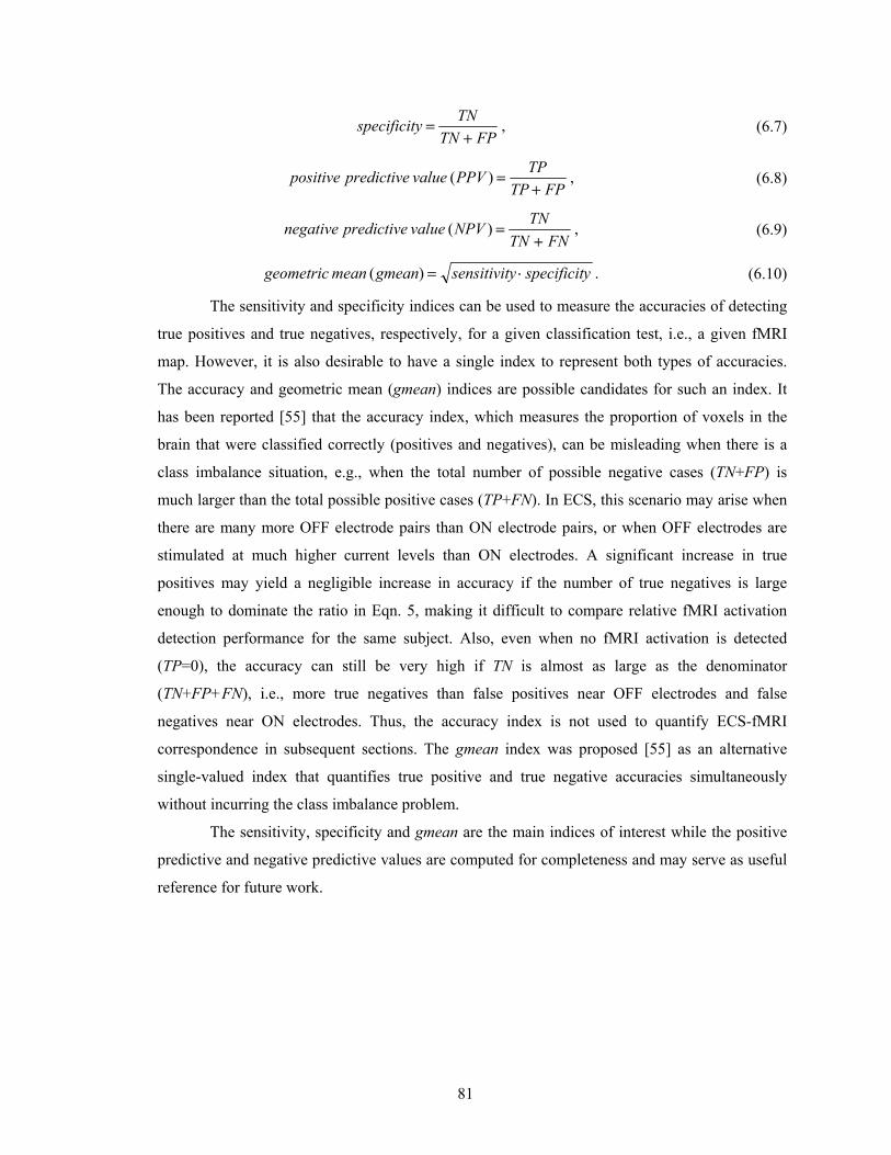
81

FPTNTNyspecificit+

= , (6.7)

FPTPTPPPVvalue predictive positive+

=)( , (6.8)

FNTNTNNPVvalue predictive negative+

=)( , (6.9)

yspecificitysensitivitgmeanmean geometric ⋅=)( . (6.10)

The sensitivity and specificity indices can be used to measure the accuracies of detecting

true positives and true negatives, respectively, for a given classification test, i.e., a given fMRI

map. However, it is also desirable to have a single index to represent both types of accuracies.

The accuracy and geometric mean (gmean) indices are possible candidates for such an index. It

has been reported [55] that the accuracy index, which measures the proportion of voxels in the

brain that were classified correctly (positives and negatives), can be misleading when there is a

class imbalance situation, e.g., when the total number of possible negative cases (TN+FP) is

much larger than the total possible positive cases (TP+FN). In ECS, this scenario may arise when

there are many more OFF electrode pairs than ON electrode pairs, or when OFF electrodes are

stimulated at much higher current levels than ON electrodes. A significant increase in true

positives may yield a negligible increase in accuracy if the number of true negatives is large

enough to dominate the ratio in Eqn. 5, making it difficult to compare relative fMRI activation

detection performance for the same subject. Also, even when no fMRI activation is detected

(TP=0), the accuracy can still be very high if TN is almost as large as the denominator

(TN+FP+FN), i.e., more true negatives than false positives near OFF electrodes and false

negatives near ON electrodes. Thus, the accuracy index is not used to quantify ECS-fMRI

correspondence in subsequent sections. The gmean index was proposed [55] as an alternative

single-valued index that quantifies true positive and true negative accuracies simultaneously

without incurring the class imbalance problem.

The sensitivity, specificity and gmean are the main indices of interest while the positive

predictive and negative predictive values are computed for completeness and may serve as useful

reference for future work.

82

6.2.4 Dynamic Ranges of Current Density Weighted Correspondence Indices

A physical interpretation of the upper and lower limits of the current density weighted sensitivity,

specificity and gmean indices is useful to understand the scenarios that yield the worst and best

case values. Assuming there is at least one pair of ON and one pair of OFF electrodes, the

sensitivity will be 1.0 if every fMRI voxel in the field-of-view is activated (hence, specificity will

be 0), and 0 if no fMRI activation is observed (hence, specificity will be 1.0). These extreme

cases are easily detected. For practical fMRI maps with at least some fMRI activation voxels near

the electrodes, a sensitivity value close to 1.0 indicates that fMRI activation occurred in regions

where the combined current density distribution function of ON electrodes has the most energy

(close to ON electrodes). A sensitivity value close to 0 indicates that either only a few fMRI

activation voxels are present, or that fMRI activation occurred predominantly in low energy

regions of the ON electrodes’ current density function (far from ON electrodes). Likewise, a

specificity value close to 1.0 indicates that fMRI non-activation voxels occurred in regions where

the combined current density distribution function of OFF electrodes has the most energy (close

to OFF electrodes) while a specificity value close to 0 indicates either the presence of only a few

fMRI non-activation voxels, or that fMRI non-activation voxels occurred predominantly in low

energy regions (far away from OFF electrodes) of the OFF electrodes’ current density function.

Since gmean depends on the product of sensitivity and specificity, a gmean value close to 1.0

indicates that the sensitivity and specificity values are both close to 1.0. A gmean value close to 0

indicates that either the sensitivity or specificity, or both indices, are close to zero.

Due to the possible overlapping of ON and OFF electrode current density distributions,

the sensitivity and specificity values, and hence the associated gmean value, rarely attain their

maximum values of 1.0 simultaneously. The maximum possible gmean depends on the how much

the ON and OFF electrode current density distributions overlap and may vary from patient to

patient. As such, it may be useful to approximate the maximum possible gmean value for each

patient before computing the empirical gmean values. ECS-fMRI correspondence can then be

evaluated using

)_/(*100 gmeanmaxgmean(%) gmean = . (6.11)

Eq. (6.11) is especially relevant for clinical data because it provides a reference point to evaluate

computed gmean values with respect to the best “score” that can be achieved for a specific ECS

map. This may also be helpful for inter-patient comparisons. In our work, values of gmean(%)

were computed only for clinical cases.

To approximate max_gmean, one would need to find an artificial fMRI map that yields

the best gmean score. A simple strategy to find such an activation map is to create a series of

83

artificial fMRI maps that yield decreasing sensitivity values from a maximum of 1.0 (with

associated increasing specificity values from a minimum of 0). Fig. 6.3 shows an example of

finding max_gmean for a simulated test case with two ON electrode pairs and 28 OFF electrode

pairs. To create each artificial fMRI map, each voxel location is designated as activated if the

combined ON electrodes current density distribution at that location exceeds a threshold (Fig.

6.3(b)). Each artificial fMRI map has a different threshold value, which starts from 0 where all

voxels are designated as activated voxels (Fig. 6.3(c) – map 1), i.e., sensitivity of 1.0, specificity

and gmean values of 0. As the threshold increases, the sensitivity decreases from 1.0 while the

specificity, and hence gmean, increases from 0 as shown in Fig. 6.3(d). The increasing gmean

will reach a maximum value and then start to decrease as the sensitivity tends to 0. The ordinate

value in Fig. 6.3(d) at which the sensitivity, specificity and gmean plots intersect is the maximum

gmean value.

84

Figure 6.3: (a) Sum of two ON electrode pairs’ current density maps (stimulated at 0.6 V) on a

simulated 5-by-7 electrode grid. OFF electrode pairs’ current density maps are not shown. (b) 1D profile plot of dashed line in (a) showing artificially activated voxels (solid shaded blocks) obtained by thresholding profile plot at two different threshold levels (α and β). Image columns spanned by red (taller block) and purple regions are designated as activated voxels for threshold levels β and α, respectively. (c) Samples from series of images showing artificially activated voxels which yield decreasing current density weighted sensitivity values (white denotes activated locations). Each map is generated by designating voxels in (a) that are above a threshold as activated. (d) Plot of proposed current density weighted sensitivity, specificity and gmean values for series of artificial fMRI maps generated with increasing threshold values. The sensitivity decreases from 1.0 while specificity increases from 0. The maximum possible gmean value, denoted by max_gmean, serves as a reference “best score” value for computed gmean values.

(a)

(c)

ON (b)

increasing threshold

α

β

Map 1 Map 39 Map 5

(d)

Map 1 Map 39

Map 5 Maximum

gmean

85

6.2.5 Numerical Approximation of Current Density

In ECS, the brain can be modeled as a volume conductor with no electrical charges within the

conductor. A quasistatic condition is assumed where the temporal variations in the electrostatic

quantities are ignored, i.e., only the steady-state scalar potential is of interest [49]. This condition

corresponds to a snapshot in time when the maximum voltage magnitude is applied across the

electrode pair and the electrostatic quantities are allowed to settle to an equilibrium state. For

each stimulated electrode pair, the scalar potential field, Ф(r), is computed by solving the Laplace

equation,

02

2

2

2

2

22 =⎟⎟

⎠

⎞⎜⎜⎝

⎛∂Φ∂

+∂Φ∂

+∂Φ∂

⋅=Φ∇zyx

σσ , (6.12)

where σ is the electrical conductivity. For simplicity, we assume that the volume conductor has

isotropic conductivity, i.e., equal conductivity in all directions and σ is a scalar. The boundary

conditions required for a unique solution include the applied voltage levels at the electrode-brain

interface (Dirichlet boundary condition) and knowledge that the first derivative of the scalar

potential perpendicular to the brain surface is zero (Neumann boundary condition)

0=⋅∇− nΦσ , (6.13)where n is a vector normal to the brain surface. The scalar potential maps are numerically

computed using the finite difference method with 3D 7-element centered approximation. The

Gauss Seidel algorithm was used to solve the resultant finite difference equations. The current

density maps are then evaluated from the scalar potential field with Ohm’s law

Φ∇−= σJ . (6.14)Fig. 6.4 shows top (a slice that is 6 mm below electrodes) and cross-sectional views of current

density magnitude contour plots computed for a simulated 3D volume with two pairs of simulated

electrodes stimulated at two different stimulus levels. The leftmost electrode pair has an input

voltage magnitude of 0.6 V while the rightmost pair has an input voltage magnitude of 2.0 V.

Assuming the electrode impedance is 60 Ω and ignoring all other impedances, this would be

equivalent to injected current intensities of 10 mA and 33 mA, respectively. Fig. 6.4 illustrates

that a higher electrical stimulus level induces a wider current density distribution spread.

86

Figure 6.4: Current density magnitude for different simulated electrical stimulus levels (leftmost

pair: 0.6 V, rightmost pair: 2 V). (a) Top view contour plot (6 mm below simulated electrodes positions), and (b) cross-sectional view contour plot (sliced along dashed line in (a)), and (c) 1D profile plot of (a) along dashed line in (a). The display range for both electrode pairs in each contour plot is the same to facilitate the comparison of current density distribution spreads at different electrical stimulus levels.

6.2.6 Data Simulation

In this section, simulated datasets are used to compare the current density weighted statistical

indices to the voxel-based fixed radii method indices and the Euclidean distances from ON

electrodes to nearest fMRI clusters’ edges and centroids. A 115×115×100 voxel

(115mm×115mm×100mm) 3D rectangular volume (MRI) with an overlaid electrode grid (CT)

with known stimulation voltages was simulated. For simplicity, each voxel is assigned the

electrical conductivity value of brain grey matter (0.004 Ω-1 cm-1). Each circular electrode has a

radius of 2 mm and adjacent electrodes are spaced 10 mm in both vertical and horizontal

directions. Each voxel is 1 mm×1 mm×1 mm in size. It is assumed that all simulated fMRI

(a)

(b)

(c)

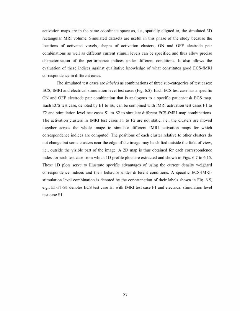
87

activation maps are in the same coordinate space as, i.e., spatially aligned to, the simulated 3D

rectangular MRI volume. Simulated datasets are useful in this phase of the study because the

locations of activated voxels, shapes of activation clusters, ON and OFF electrode pair

combinations as well as different current stimuli levels can be specified and thus allow precise

characterization of the performance indices under different conditions. It also allows the

evaluation of these indices against qualitative knowledge of what constitutes good ECS-fMRI

correspondence in different cases.

The simulated test cases are labeled as combinations of three sub-categories of test cases:

ECS, fMRI and electrical stimulation level test cases (Fig. 6.5). Each ECS test case has a specific

ON and OFF electrode pair combination that is analogous to a specific patient-task ECS map.

Each ECS test case, denoted by E1 to E6, can be combined with fMRI activation test cases F1 to

F2 and stimulation level test cases S1 to S2 to simulate different ECS-fMRI map combinations.

The activation clusters in fMRI test cases F1 to F2 are not static, i.e., the clusters are moved

together across the whole image to simulate different fMRI activation maps for which

correspondence indices are computed. The positions of each cluster relative to other clusters do

not change but some clusters near the edge of the image may be shifted outside the field of view,

i.e., outside the visible part of the image. A 2D map is thus obtained for each correspondence

index for each test case from which 1D profile plots are extracted and shown in Figs. 6.7 to 6.15.

These 1D plots serve to illustrate specific advantages of using the current density weighted

correspondence indices and their behavior under different conditions. A specific ECS-fMRI-

stimulation level combination is denoted by the concatenation of their labels shown in Fig. 6.5,

e.g., E1-F1-S1 denotes ECS test case E1 with fMRI test case F1 and electrical stimulation level

test case S1.

88

Figure 6.5: Electrode grid overlaid on current density maps (6 mm below electrodes) for

simulated ECS maps labeled E1 to E6. In E1 to E6, high current density regions (orange-red regions) indicate locations of ON electrode pairs. All other horizontally adjacent electrode pairs are either OFF electrode pairs (diamonds) or untested (dots on grid), e.g., ECS map E6. F1 to F3 denote simulated fMRI activation test cases where activated voxels are grouped into solid red ellipses (F1, F2) or circles (F3). S1 uses an input peak voltage of 0.6 V for all ON and OFF electrodes. Test case S2 uses an input peak voltage of 0.2 V for the leftmost and 0.6 V for the rightmost ON electrode pairs. All OFF electrodes for all test cases have stimulus voltages of 0.6 V.

E1 E2 E3

E4 E5 E6

F1 F2 F3

S1 S2

89

6.2.7 Clinical Data

6.2.7.1 MR Imaging and Extraoperative ECS Functional Mapping Overview

Fig. 6.6 shows an overview of the fMRI and ECS mapping procedure prior to surgery for lesion

resection. An MRI T1-weighted pre-grid anatomical reference volume was acquired in the same

scan session as T2*-weighted fMRI time series images corresponding to various specified test

paradigms. A fully automated 3D nonlinear registration process using our Mutual Information

Automated Multimodality Image Fusion (MIAMI Fuse) software [24] was then used to register

the T2*-weighted fMRI time series to the T1-weighted anatomical reference volume. In addition,

2D to 3D rigid body mapping of slice-to-volume (MSV) was performed to improve motion

correction accuracy [25]. Statistical analysis was then performed on the resultant motion

corrected datasets to compute fMRI activation maps that indicate the regions of the brain that

have increased Blood Oxygenation Level Dependent (BOLD) response to the specified stimuli.

With the MSV motion correction technique, slices are repositioned to account for inter-slice

motion. In most data sets, out-of-slice motions are detected and unequal number of temporal

samples per voxel may be observed. A robust approach in statistical testing using random

permutation was chosen to compute the fMRI activation maps [40]. This statistical technique is

simple, non-parametric and independent of sample size variability [41].

Following the pre-grid MR scans, the patient undergoes the first craniotomy to implant a

subdural electrode grid. Post-grid computed tomography (CT) and MRI scans are subsequently

performed. The CT volume is then registered to the post-grid MR volume using the MIAMI Fuse

software. To bring the post-grid registered CT volume in alignment with the pre-grid MR

anatomical volume, the post-grid MR volume is non-linearly registered to the pre-grid MR

volume and the resultant deformation field is applied to the pre-grid CT volume as shown in Fig.

6.6. Consequently, both the fMRI activation and CT datasets are non-linearly registered to the

pre-grid MR reference volume. The electrode positions are extracted semi-automatically via k-

means clustering [56] of the intensity-thresholded CT volume.

Just before the second craniotomy, three sets of information are available for each

patient: a T1 pre-grid anatomical reference volume, several sets of fMRI activation maps for

different paradigms (e.g., responsive naming and picture naming), and a post-grid CT volume

which shows ON and OFF electrode pair locations along with maximum stimulation current

levels applied. These datasets are all registered to the T1 pre-grid anatomical reference. The

primary interest in our work is to quantify the “closeness” of the fMRI activation maps to their

corresponding ECS functional maps.

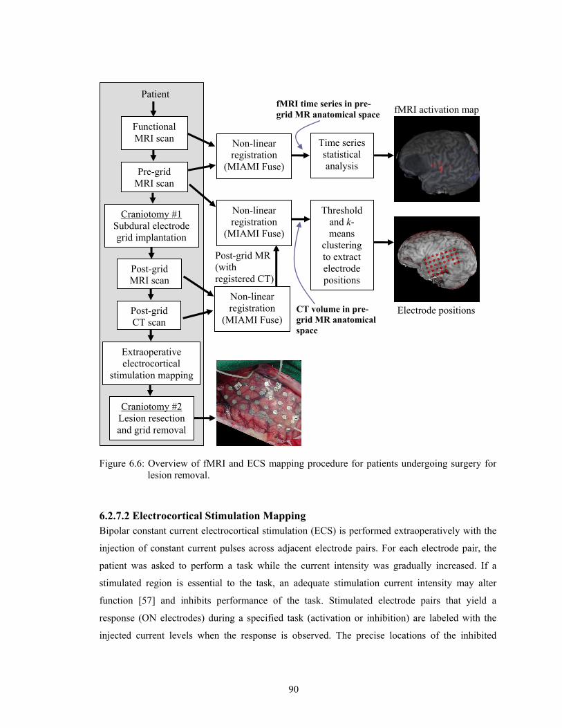
90

Figure 6.6: Overview of fMRI and ECS mapping procedure for patients undergoing surgery for

lesion removal.

6.2.7.2 Electrocortical Stimulation Mapping Bipolar constant current electrocortical stimulation (ECS) is performed extraoperatively with the

injection of constant current pulses across adjacent electrode pairs. For each electrode pair, the

patient was asked to perform a task while the current intensity was gradually increased. If a

stimulated region is essential to the task, an adequate stimulation current intensity may alter

function [57] and inhibits performance of the task. Stimulated electrode pairs that yield a

response (ON electrodes) during a specified task (activation or inhibition) are labeled with the

injected current levels when the response is observed. The precise locations of the inhibited

Functional MRI scan

Pre-grid MRI scan

Craniotomy #1 Subdural electrode grid implantation

Post-grid MRI scan

Extraoperative electrocortical

stimulation mapping

Craniotomy #2 Lesion resection and grid removal

Non-linear registration

(MIAMI Fuse)

Time series statistical analysis

Threshold and k-means

clustering to extract electrode positions

Patient fMRI time series in pre-grid MR anatomical space

CT volume in pre-grid MR anatomical space

fMRI activation map

Non-linear registration

(MIAMI Fuse) Electrode positionsPost-grid

CT scan

Non-linear registration

(MIAMI Fuse)

Post-grid MR (with registered CT)

91

neurons under the ON electrodes are not available from the ECS procedure. However, the

location of each electrode and a map of ON and OFF electrode pairs are available.

During ECS mapping with the implanted subdural grid electrodes (Ad-Tech Medical

Instrument Corp., Racine, WI, USA), stimulus biphasic current with a pulse duration of 300 µs

and a pulse interval of 20 ms (frequency of 50 Hz) was applied across horizontally adjacent

electrode pairs using a Grass Model S12 isolated biphasic stimulator (Astro-Med Inc., West

Warwick, RI, USA). The pulse train duration used was 2 s. Each electrode has an exposed

diameter of 2.3 mm and an approximate electrical resistance of 50 to 60 Ω. The spacing between

the centers of adjacent electrodes is 10 mm. During ECS mapping, the current intensity is

gradually increased from 1 mA for motor and sensory mapping, and 3mA for language mapping

until either a response is detected or significant afterdischarges are observed. Responses are

confirmed by observing consistent effects with repeated stimulation. The injected current

intensity increases in steps of 1 mA for motor/ sensory and 3 mA for language mapping. The final

applied voltages for each stimulated electrode pairs are approximated by multiplying the peak

injected current intensity by the electrode impedance (Ohms’s law). The Grass S12 stimulator

allows the peak voltages to be read during stimulation, which may yield more accurate

approximations of the actual applied voltage levels for future patient studies.

6.3 Results

6.3.1 Simulation Data Results

Figs. 6.7 to 6.15 show plots of correspondence indices for various combinations of ECS map,

fMRI map and stimulus level test cases described in Fig. 6.5. In this section, the characteristics of

the current density weighted indices are reported for each test case combination, and then

compared to the voxel-based fixed radii and Euclidean distance methods where appropriate. The

test cases presented are inter-related to each other in that subsequent test cases are often more

complicated variations of previous test cases. Figs. 6.7 to 6.15 each consists of five parts. Part A

shows the current density maps with overlaying electrode grids and fMRI cluster(s) moving from

the left to right sides of the images. Part B shows the current density weighted counts of TP, FP

and FN as the centroids of the leftmost fMRI cluster (if there are more than one cluster, i.e., F2

and F3) move along the dashed line displayed in part A. Part C shows the current density

weighted ECS-fMRI correspondence indices while parts D and E show the voxel-based fixed

radii method and Euclidean distance method correspondence indices, respectively.

92

The simplest test case, labeled E1-F1-S1 (Fig. 6.7(a)), has an elliptical fMRI activation

cluster of radii 2 mm and 4 mm along the minor and major axes of the ellipse respectively. As the

fMRI cluster moves across the dashed line in Fig. 6.7(a), the current density weighted true

positives (TP) plot (Fig. 6.7(b)) peaks when the cluster is directly under each of the two ON

electrodes. This leads to corresponding valleys in the FN plot since (TP+FN) is a constant for any

ECS map, i.e., sum of Eqns. 1 and 4 is a constant. The resultant sensitivity plot (Fig. 6.7(c)) is

bimodal or double-peak, which indicates higher ECS-fMRI correspondence for fMRI activated

voxels (m(r)=1) that are nearer any ON electrode. Since there are 29 pairs of OFF electrodes in

Fig. 6.7(a), the number of true negatives (TN) is much larger than FP, thus yielding a specificity

plot (Fig. 6.7(c)) with all values close to 1.0. The gmean plot has a similar shape as the sensitivity

plot (Fig. 6.7(c)) and summarizes classification accuracies for both true positives and true

negatives. Local minima in the sensitivity and gmean plots, which become more pronounced as

the inter-electrode spacing increases, are also observed in between the two ON electrodes. The

sensitivity and gmean plots computed using the voxel-based fixed radii method (Fig. 6.7(d)) are

zero outside the fixed windows and rises/ falls abruptly at the edges of the windows. Plateaus are

also observed in the fixed radii sensitivity and gmean plots when the fMRI cluster is located

within the fixed windows of the ON electrodes. As long as the fMRI cluster is completely within

the fixed windows, the voxel-based fixed radii method reports constant sensitivity and gmean

values, making it difficult to assess incremental improvements/ deterioration in fMRI

performance. For example, an fMRI cluster located within the radii and moving closer to an ON

electrode will still yield similar indices’ values. This limitation is exacerbated by the lack of a

principled method to decide how large the stimulation radius should be, e.g., a larger radius will

yield wider plateaus in the sensitivity and gmean plots making it even less effective in tracking

incremental improvements in fMRI maps. The mean of the minimum electrode-edge and

electrode-centroid Euclidean distances have global minima, indicating best ECS-fMRI

correspondence, in between the ON electrodes (Fig. 6.7(e)). This implication that an fMRI cluster

located in between ON electrodes would yield the best correspondence is not based on any

electrostatic or physiological evidence, especially in light of computed current density maps that

show maximum electrical stimulus levels directly under ON electrodes, rather than in–between

them.

Test case combination E1-F3-S1 (Fig. 6.8(a)) illustrates the improvement in ECS-fMRI

correspondence when two larger fMRI activation clusters, each of radius 4 mm and spaced 10

mm apart, are found in high energy regions of the ON electrode pair’s current density map. As

the number of fMRI activated voxels around ON electrodes increases at locations where current

93

density magnitude values are highest, the current density weighted sensitivity values will increase

and tend to a maximum value of 1.0. The maximum current density weighted sensitivity value in

Fig. 6.8(c) is much higher (0.69) than that of Fig. 6.7(c) (0.45) due to the larger number of true

positives (TP) in the former. The maximum sensitivity and gmean values occur when the two

fMRI clusters are simultaneously located under the two ON electrodes.

In test case E1-F2-S1 (Fig. 6.9(a)), a second elliptical fMRI activation cluster, spaced

five electrodes away from the leftmost cluster in Fig. 6.7, was added. The number of true

positives (Fig. 6.9(b)), due largely to the leftmost cluster, is approximately the same as test case

E1-F1-S1 in Fig. 6.7(b) but the number of false positives has increased because of the rightmost

cluster. As such, the current density weighted sensitivity values in Fig. 6.9(c) does not change

appreciably while a slight decrease in specificity values is observed. The decrease in specificity is

not large because there are many OFF electrodes, i.e., TN is large.

Test case E2-F1-S1 (Fig. 6.10(a)) uses the same elliptical fMRI activation cluster as in

Fig. 6.7(a) but with two ON electrode pairs. The current density weighted sensitivity and gmean

plots (Fig. 6.10(c)) have similar shapes to those in Fig. 6.7(c) (test case E1-F1-S1). The maximum

sensitivity and gmean values in Fig. 6.10(c), however, are smaller (0.10, 0.31 respectively)

because for every location that the fMRI cluster visits, FN has increased due to the presence of

the additional ON electrode pair. This is desirable since the indices report poorer correspondence

when there is an additional ON electrode pair, without any fMRI activation under it. This is

unlike the current density weighted PPV which has same maximum values in both Figs. 6.7(c)

and 6.10(c), which is an undesirable feature. The means of the Euclidean distances in Fig. 6.10(e)

have minima in-between the two pairs of ON electrodes. This indicates that an fMRI cluster

found directly under an ON electrode can have worst or equal ECS-fMRI correspondence than an

identical cluster that is equidistant from all ON electrodes, but yet is not near any ON electrode.

This assignment of highest ECS-fMRI correspondence to potentially improbable occurrences of

stimulation-induced neuronal activation runs contrary to evidence that bipolar ECS stimulation is

localized around ON electrode pairs [49].

Test case E2-F1-S2 (Fig. 6.11(a)) is identical to Fig. 6.10(a) except that the leftmost ON

electrode pair is stimulated at 0.2 V instead of 0.6 V as used in the rightmost ON electrode pair.

The local maxima of the current density weighted sensitivity and gmean plots are higher under

the leftmost ON electrode pair (0.05, 0.22 respectively) than the rightmost ON electrode pair

(0.15, 0.38). This may be desirable because higher electrical stimulus levels increases both the

magnitude and spread of the current density distribution (Fig. 6.4), thus increasing the spatial

extent of the stimulated region, as well as the range of neuronal stimulation thresholds that the

94

stimuli may overcome. The voxel-based fixed radii method does not incorporate information on

stimulus levels as illustrated in the plateaus of similar maximum values under both pairs of ON

electrodes in the sensitivity and gmean plots of Fig. 6.11(d).

In test case E3-F1-S1 (Fig. 6.12(a)), two overlapping pairs of horizontally adjacent

electrodes are stimulated. The second ON electrode, where the summed current density map

values are highest, is more likely to be near task-related neuronal regions than neighboring ON

electrodes since it was stimulated twice and both its horizontally adjacent neighbors are also ON

electrodes. Indeed, maximum current density weighted sensitivity and gmean values are observed

when the fMRI cluster is located directly under the second ON electrode. The fixed radii

sensitivity and gmean plots (Fig. 6.12(d)) have plateaus across the three ON electrodes and is not

able to extract such contextual information.

Test cases E4-F1-S1 (Fig. 6.13(a)) and E5-F1-S1 (Fig. 6.14(a)) are similar to Figs. 6.7(a)

and 6.12(a), respectively, except that the ON electrode pairs in the former are now surrounded by

OFF electrodes. There are no noticeable changes in the shape or maxima values (sensitivity: 0.19,

specificity: 1.00, gmean: 0.44) in the current density weighted sensitivity, specificity and gmean

plots. This implies that the presence or absence of OFF electrodes around ON electrodes does not

significantly affect the ECS-fMRI correspondence when an fMRI cluster is found under an ON

electrode. This is desirable if OFF electrodes are defined as stimulated electrodes that did not

yield a task-related inhibitory response. In this case, it cannot be conclusively stated that regions

under these electrodes do not have task-essential neuronal tissue, even though the likelihood of

that should be higher compared to an untested electrode pair. It might be that the electrical

stimulus level was just not high enough. Thus, it would be premature to penalize ECS-fMRI

correspondence values when an fMRI cluster is located near ON electrodes surrounded by OFF

electrodes.

Test case E6-F1-S1 (Fig. 6.15(a)) is identical to E1-F1-S1 (Fig. 6.7(a)) except that

several electrodes surrounding the ON electrode pair are not tested (neither ON nor OFF). The

current density weighted sensitivity, specificity and gmean plots are similar in both Figs. 6.15(a)

and 6.7(a) with similar maximum values as Figs. 6.13(c) and 6.14(c). This illustrates an example

of how neighboring OFF and untested electrodes are similar in their effect on current density

weighted indices.

95

Figure 6.7: Simulated dataset E1-F1-S1. (a) Current density map overlaying electrode grid with

an fMRI cluster moving from left to right side of image. (b) Current density weighted TP, FP and FN as centroid of left fMRI cluster moves along dashed line in (a). (c) Current density weighted ECS-fMRI correspondence indices. (d) Fixed radii method correspondence indices. (e) Euclidean distance method.

(a)

(d)

(e)

(c)

(b)

96

Figure 6.8: Simulated dataset E1-F3-S1. This test case has larger fMRI clusters compared to Fig.

6.7 and illustrates that higher peak values of sensitivity and gmean are obtained (compared to Fig. 6.7) when more fMRI voxels occur in regions with high current density energy levels, i.e., near ON electrodes. Parts (a) to (e) denote images and plots as described in Fig. 6.7.

(a)

(d)

(e)

(c)

(b)

97

Figure 6.9: Simulated dataset E1-F2-S1. In this test case, a second (rightmost) fMRI cluster, i.e.,

additional false positives, was added to the cluster (leftmost) in Fig. 6.7. Parts (a) to (e) denote images and plots as described in Fig. 6.7.

(a)

(d)

(e)

(c)

(b)

98

Figure 6.10: Simulated dataset E2-F1-S1. This test case is similar to Fig. 6.7 except for an

additional ON electrode pair (rightmost). It illustrates the effects of additional false negative voxels and highlights a limitation of Euclidean distance-based indices. Parts (a) to (e) denote images and plots as described in Fig. 6.7.

(a)

(d)

(e)

(c)

(b)

99

Figure 6.11: Simulated dataset E2-F1-S2. This test case is similar to Fig. 6.10 except that the

leftmost ON electrode pair was stimulated at 0.2 V while the rightmost ON pair was stimulated at 0.6 V. In Fig. 6.10, both ON electrode pairs were stimulated at 0.6 V. Parts (a) to (e) denote images and plots as described in Fig. 6.7.

(a)

(d)

(e)

(c)

(b)

100

Figure 6.12: Simulated dataset E3-F1-S1. This test case is identical to Fig. 6.7 except for the

addition of an adjacent ON electrode pair (rightmost). Parts (a) to (e) denote images and plots as described in Fig. 6.7.

(a)

(d)

(e)

(c)

(b)

101

Figure 6.13: Simulated dataset E4-F1-S1. This test case is similar to Fig. 6.7 except that the ON

electrode pair is now surrounded by OFF electrode pairs. Parts (a) to (e) denote images and plots as described in Fig. 6.7.

(a)

(d)

(e)

(c)

(b)

102

Figure 6.14: Simulated dataset E5-F1-S1. This test case is similar to Fig. 6.12 except that the ON

electrode pairs are now surrounded by OFF electrode pairs. Parts (a) to (e) denote images and plots as described in Fig. 6.7.

(a)

(d)

(e)

(c)

(b)

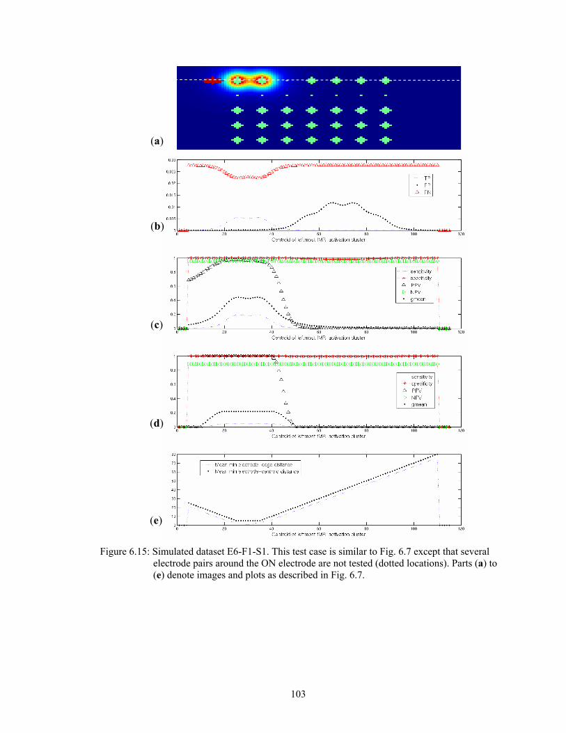
103

Figure 6.15: Simulated dataset E6-F1-S1. This test case is similar to Fig. 6.7 except that several

electrode pairs around the ON electrode are not tested (dotted locations). Parts (a) to (e) denote images and plots as described in Fig. 6.7.

(a)

(d)

(e)

(c)

(b)

104

6.3.2 Clinical Human Data

Fig. 6.16 shows a cross-sectional view of the ECS current density distributions for three patients

overlaid on non-linearly registered post-grid CT images. The current density weighted

correspondence indices for all three patients are shown in Tables 6.1 to 6.3. The maximum

possible gmean values, with which gmean(%) values in Tables 6.1 to 6.3 were computed, are

approximately the same for all three patients (0.78, 0.80 and 0.80, respectively) so it is reasonable

to use either gmean or gmean(%) when comparing ECS-fMRI correspondence across these

patients. Fig. 6.17 shows the picture and responsive naming fMRI activation maps, and electrode

grids, overlaid on the anatomical MR datasets for all three patients. In Table 6.1, the gmean and

sensitivity values (0.26 and 0.07, respectively) for the picture naming paradigm for patient 1 are

the largest among all other datasets. Fig. 6.17(a) (patient 1 - picture naming) shows that a dense

cluster of fMRI activation occurs in the proximity of at least two ON electrodes while Fig.

6.17(b) (patient 1 - responsive naming) has a smaller fMRI cluster in close proximity to one ON

electrode. Thus, recalling the results of the simulation test cases in Fig. 6.7 and Fig. 6.8 where the

activation cluster in the latter was increased in size and covered more of the high energy regions

of the current density distribution, it is expected that the sensitivity and gmean values for Fig.

6.17(a) would be higher than those for Fig. 6.17(b). In Fig. 6.17(c) (patient 2 - picture naming)

and Fig. 6.17(d) (patient 2 - responsive naming), hardly any fMRI activation was detected in the

vicinity of ON electrodes. Also, Figs. 6.17(c) and 6.17(d) have five more ON electrode pairs than

Figs. 6.17(a) and 6.17(b), i.e., the former would require more activated voxels than the latter to

achieve the same sensitivity score. It is thus expected that the sensitivity and gmean values for

patient 2 (Table 6.2) would be very much smaller than those for patient 1 (Table 6.1). For patient

3, Fig. 6.17(e) (picture naming) shows hardly any activation near ON electrodes and thus the

associated gmean value in Table 6.3 is small. Fig. 6.17(f) (patient 3-responsive naming) shows a

fMRI cluster just under the top rightmost ON electrode, which, as expected, yielded a higher

gmean value in Table 6.3 than for the fMRI map in Fig. 6.17(e).

105

Table 6.1: Current density weighted ECS-fMRI correspondence indices for picture naming, responsive naming and combined (OR operation) picture-responsive naming fMRI maps for patient 1. Approximate value of maximum possible gmean is 0.78.

fMRI

Task TP TN FP FN accuracy sensitivity specificity gmean

gmean

(%)

picture

naming 0.41 14.95 0.27 5.56 0.73 0.07 0.98 0.26 33.33

responsive

naming 0.07 15.18 0.04 5.89 0.72 0.01 1.00 0.11 14.10

combined 0.47 14.91 0.31 5.49 0.73 0.08 0.98 0.28 35.90

Table 6.2: Current density weighted ECS-fMRI correspondence indices for picture naming, responsive naming and combined (OR operation) picture-responsive naming fMRI maps for patient 2. Approximate value of maximum possible gmean is 0.80.

fMRI

Task TP TN FP FN accuracy sensitivity specificity gmean

gmean

(%)

picture

naming 0 14.28 0 7.64 0.65 0 1.00 0.01 1.25

responsive

naming 0.01 14.28 0.01 7.64 0.65 0 1.00 0.03 3.75

combined 0.01 14.28 0.01 7.64 0.65 0 1.00 0.03 3.75

Table 6.3: Current density weighted ECS-fMRI correspondence indices for picture naming, responsive naming and combined (OR operation) picture-responsive naming fMRI maps for patient 3. Approximate value of maximum possible gmean value is 0.80.

fMRI

Task TP TN FP FN accuracy sensitivity specificity gmean

gmean

(%)

picture

naming 0.01 29.52 0.51 3.02 0.89 0 0.98 0.05 6.25

responsive

naming 0.10 29.96 0.07 2.93 0.91 0.03 1.00 0.18 22.50

combined 0.10 29.46 0.58 2.92 0.89 0.03 0.98 0.18 22.50

The preceding comparisons of correspondence indices for fMRI maps from separate

picture and responsive naming paradigms showed that the indices behaved in a manner consistent

with notions of what constitutes good and bad ECS-fMRI correspondence. As shown in the use of

106

identical ECS ON electrode configurations for different fMRI paradigms in each patient in Fig.

6.17, the clinical ECS language maps show a combination of tasks, i.e., mapping of language tags

using both picture and naming tasks. In these cases, it would be more accurate to first combine

the picture naming and responsive naming fMRI maps using a logical OR operation, and then

compute correspondence indices of the resultant combined fMRI map. This is computed for all

three patients in the third rows of Tables 6.1 to 6.3. However, since our purpose was to

demonstrate the application of the current density weighted indices on real data, and to compare

different fMRI maps for the same patient and between different patients, it was more informative

to analyze the correspondence indices for the separate fMRI maps (first and second rows of

Tables 6.1 to 6.3) with the pictures in Fig. 6.17.

The class imbalance problem, discussed in the Methods section, is reflected in the

relatively constant accuracy index values for each patient in Tables 6.1 to 6.3. For example, even

though Fig. 6.17(a) exhibits better ECS-fMRI correspondence (qualitatively) than Fig. 6.17(b),

the accuracy values are approximately the same in Table 6.3. This is because each patient’s ECS

map had many OFF electrode pairs that gave rise to larger numbers of true negatives compared to

true positives, especially when only a few fMRI activation voxels are detected. Thus, the

numerator of the accuracy measure in Eqn. 5 is dominated by TN, as observed in the large TN

values in Tables 6.1 to 6.3, which makes the accuracy index relatively insensitive to small

changes in TP. This makes the accuracy index less reliable for intra-patient ECS-fMRI

correspondence comparisons with different fMRI activation maps.

The purpose of computing the proposed correspondence indices for three human datasets

is to illustrate that the method can be applied to real data. It is not our intention, at this time, to

make any statistical conclusions about ECS-fMRI validation based on the limited patient data

available in this report. A more comprehensive statistical analysis of the current density weighted

indices with multiple patients and different fMRI data correction/ processing methods is planned

for future work.

107

Figure 6.16: Coronal view of human CT datasets with overlaid current density maps (red

indicates higher values) for (a) patient 1, (b) patient 2, and (c) patient 3. Each image shows the cross-sectional view of the current density distribution around one stimulated electrode (of a pair of them). The second electrodes of the stimulated pairs lie in different coronal slice planes and thus are not visible in these images. To calculate the current density weighted ECS-fMRI indices, the 3D current density distributions for each pair of stimulated ON and OFF electrodes were computed.

(b)

(c)

(a)

108

Figure 6.17: Composite 3D MR anatomical, CT electrode grid and fMRI activation datasets (red

for positive fMRI activation) for (a) patient 1 picture naming task, (b) patient 1 responsive naming task, (c) patient 2 picture naming task, (d) patient 2 responsive naming task, (e) patient 3 picture naming task, and (f) patient 3 responsive naming task. Solid shaded dark blue circular tags on electrode grid denote ON electrodes.

(b)

(c)

(a)

(d)

(e) (f)

109

6.4 Discussion

ECS, in itself, is a surface map of a limited area of the brain (under the electrode grid) and maps

essential language regions while fMRI is a 3D functional map of the entire brain. Thus, it may not

be accurate to compare an ECS surface map to 3D fMRI directly. The current density weighted

method effectively extends the ECS surface map into a 3D map using electrostatic principles in

electrical stimulation. It was shown with simulated data that the current density weighted

sensitivity and gmean indices had higher values when fMRI activation voxels occur near ON

electrodes, which is expected for good ECS-fMRI correspondence. Unlike the voxel-based fixed

radii and Euclidean distance indices, the current density weighted indices were able to measure

correspondence levels while taking into account contextual information such as the number of

surrounding ON electrodes (Fig. 6.12(c)) as well as different electrode stimulus levels (Fig.

6.11(c)). Also, unlike the voxel-based fixed radii method, the current density weighted indices

can track incremental improvements in ECS-fMRI correspondence when fMRI activated voxels,

which are already near ON electrodes, move even closer to these ON electrodes. All these

advantages were achieved without direct computation of Euclidean distances while taking into

account variations in electrode grid and brain tissue geometry in the computation of the current

density maps.

Simulated data were used to characterize the correspondence indices because they consist

of fixed ECS and fMRI maps. If a real patient-task ECS map was chosen and fMRI activation

locations were artificially shifted, the behavior of the indices with respect to activation location

may be unnecessarily difficult to interpret because of the additional complexity in the 3D

electrode grid and brain geometries. The simulation results of the current density weighted

indices depended primarily on the current density magnitudes at different voxel locations. Thus,

if a patient’s current density map is computed accurately, the indices would exhibit similar

characteristics as observed in the simulated data.

The proposed current density map indices can be used for intra-patient studies, and

possibly for inter-patient comparisons as well, i.e., with gmean(%). In future work, the current

density weighted correspondence indices will be used to evaluate fMRI correspondence in a study

involving a larger number of patients. In addition to ECS-fMRI validation in general, an ECS-

fMRI correspondence index that incorporates contextual information provided by a given set of

active/ inactive stimulated electrode pairs can be very useful when comparing data processing

algorithms in fMRI, e.g., motion correction, activation detection. Functional MRI maps from

different but relevant stimuli paradigms, or single paradigm fMRI datasets that are processed

110

differently, may be evaluated and compared for best ECS-fMRI correspondence. This can aid in

the validation of fMRI data processing algorithms.

It is important to note that although fMRI and ECS are similar in function, they are not

necessarily identical. This may explain why it is not likely that one would observe perfect ECS-

fMRI correspondence for human data. In our patient data, the highest (relative to three patient

datasets) current density weighted gmean and gmean(%) values (Table 6.1) are 0.26 and 35.9%,

respectively. These values are large compared to the other two patients (Tables 6.2 and 6.3), but

small relative to the maximum values attainable, i.e., 1.00 and 100.0% for gmean and gmean(%),

respectively. These relatively small values may have arisen from a combination of data

processing errors, inconsistent patient response in fMRI tasks, and the inherent physiological

differences in ECS and fMRI paradigms. The current density weighted indices may be used to

investigate these individual issues in future work with more human data.

It should be noted that for true negative counts, the criteria with which OFF electrodes

are defined may have an impact on computing the correspondence indices. In our simulations, the

OFF electrodes were defined as stimulated electrodes that did not yield responses. Alternatively,

OFF electrodes could be defined as stimulated electrodes that yielded non-function related

responses [54]. For our validation purposes, the ECS stimulated electrode pairs that elicited motor

or sensory responses have been classified as ON electrodes. Thus, verbalized language tasks,

without further consideration of stimulus paradigm designs that activate only the language region,

would show activations in motor, language or sensory areas. However, the definition of OFF

electrodes does not affect the overall formulation of the current density weighted correspondence

indices, which are of primary interest of this study.

The accuracy of numerically computed current density maps depends on the accuracy of

electrodes and brain tissue geometries and the modeling of electrical conductivity within the

brain. A more accurate way of modeling the complex brain geometry would be to use the finite

element method (FEM) to compute the current density map, but at a much higher computational

cost in terms of time and memory. Another approach to improving accuracy is to model the

tensorial electrical conductivity of brain tissue using MR diffusion tensor imaging (DTI) data.

6.5 Conclusions

With simulated data, the current density weighted sensitivity, specificity and gmean indices were

found to measure ECS-fMRI correspondence in a consistently predictable manner with expected

notions of good and poor ECS-fMRI correspondence. These indices are more sensitive to

incremental improvements in ECS-fMRI correspondence that were not detected by the voxel-

111

based fixed radii method. In addition, the current density weighted indices were able to reflect

certain contextual information provided by surrounding electrodes. While the correspondence

results computed for three human datasets were not sufficient to make conclusions about ECS-

fMRI validation in general, they demonstrate the applicability of the current density

correspondence method to analysis of human data. This work provides a systematic way to

quantify 3D ECS-fMRI correspondence.

112

CHAPTER 7

Summary and Future Work

7.1 Summary

We developed an affine phase correction technique that facilitated the use of a dual-echo bipolar

readout gradient protocol for motion robust static field map estimation. The zeroth order phase

error term was found to be constant for a given MR scanner. The first order phase term varies

across scanners, but can be approximated empirically. We also developed a concurrent motion

and B0 field inhomogeneity correction framework and evaluated it with simulated EPI time series

data with known motion, geometric distortion and activation. Dynamic field maps were

approximated by resampling a spatially transformed static field map. Empirical convergence of

the algorithm was observed under the simulated conditions. However, the correction framework

did not address field map changes due to large out-of-plane rotations. To address this challenge,

we proposed a novel retrospective dynamic field map estimation technique by applying a

quadratic penalized weighted least squares (QPWLS) approach to solve the inverse susceptibility

voxel convolution problem. This is similar to regularized image restoration in image processing.

In this work, our goal was to estimate a susceptibility map from a high resolution, noisy,

susceptibility-induced field map. Rigid body motion was applied to the estimate and a new

dynamic field map was computed using the forward susceptibility voxel convolution method.

Compared with simpler image restoration algorithms such as thresholded inverse filtering and

Wiener filtering, preliminary results with realistically simulated data suggest that the QPWLS

method would yield the most accurate field map estimates, while requiring the least amount of

object-specific prior information, e.g., object power spectra. In another separate project, we

formulated a current density weighted approach to quantify the correspondence between subdural

electrocortical stimulation (ECS) and fMRI maps for brain lesion presurgical planning. Detailed

experiments were performed on simulated electrode grids and fMRI activation to characterize the

113

behavior of the index before the technique was applied to three patient datasets. The proposed

index may provide a more systematic and physiologically correct way to

quantify ECS-fMRI correspondence, as opposed to the commonly used Euclidean distance based

methods.

7.2 Future Work

The following are several suggestions for future work:

• The SVC impulse response is similar to a finite difference operator in the z direction, i.e., it

has a larger response to abrupt transitions of χ in the z direction than a constant χ. Thus, an

edge preserving regularization function, e.g., Huber function, may be used in Chapter 5. This

scheme favors smoothly varying susceptibility map estimates within soft tissue, air and bone

regions while allowing for abrupt changes in χ at tissue interfaces.

• A potential limitation of the proposed method in Chapter 5 may arise because ∆ωsys was

ignored in Eq. (5.11). Methods to reliably measure this non-χ induced field inhomogeneity

may be developed to facilitate the use of the proposed technique.

• The segmentation-SVC approach for dynamic field map estimation, as described in Chapter

5, should be implemented and its performance compared with the proposed QPWLS method.

• Upon validation, the proposed technique in Chapter 5 may replace the field map update stage

in the CFMMSV framework of Chapter 4. The performance of the improved CFMMSV

algorithm can then be evaluated with data of an MR phantom in motion.

• Having characterized the ECS-fMRI correspondence indices in Chapter 6 with simulated

datasets, and having demonstrated clinical feasibility by applying them to three patient

datasets, the indices should now be computed for a larger number of patients to assess clinical

ECS-fMRI correspondence.

114

BIBLIOGRAPHY

115

BIBLIOGRAPHY

[1] Mansfield P. Multi-planar image formation using NMR spin-echoes. J. Phys. C: Solid State

Phys. 1977;10:L55-L58.

[2] Jezzard P, Balaban RS. Correction for geometric distortion in echo planar images from B0

field variations. Magn Reson Med 1995;34:65-73.

[3] Kadah YM, Hu X. Algebraic reconstruction for magnetic resonance imaging under B0

inhomogeneity. IEEE Trans on Med Imaging 1998;17:362-370.

[4] Cusack R, Brett M, Osswald K. An evaluation of the use of magnetic field-maps to undistort

echo-planar images. Neuroimage 2003;18:127-142.

[5] Sutton BP, Noll DC, Fessler JA. Fast, iterative image reconstruction for MRI in the presence

of field inhomogeneities. IEEE Trans on Med Imaging 2003;22:178-188.

[6] Zeng H, Constable RT. Image distortion correction in EPI: Comparison of field mapping

with point spread function mapping. Magn Reson Med 2002;48:137-146.

[7] Munger P, Crelier GR, Peters TM, Pike GB. An inverse problem approach to the correction

of distortion in EPI images. IEEE Trans on Med Imaging 2000;19:681-689.

[8] Schomberg H. Off-resonance correction of MR images. IEEE Trans on Med Imaging

1999;18:481-495.

[9] Roopchansingh V, Cox RW, Jesmanowicz A, Ward BD, Hyde JS. Single-shot magnetic

field mapping embedded in echo-planar time-course imaging. Magn Reson Med

2003;50:839-843.

[10] Sutton BP, Noll DC, Fessler JA. Dynamic field map estimation using a spiral-in/spiral-out

acquisition. Magn Reson Med 2004;51:1194-1204.

[11] Yeo DTB, Chenevert TL, Fessler JA, Kim B. Zero and First Order Phase Shift Correction

for Field Map Estimation with Dual-Echo GRE Using Bipolar Gradients. Magn Reson Imag

2007;25:1263-1271.

[12] Chen N, Oshio K, Panych LP. Application of k-space energy spectrum analysis to

susceptibility field mapping and distortion correction in gradient-echo EPI. Neuroimage

2006;31:609-622.

116

[13] Yeo DTB, Fessler JA, Kim B. Concurrent Correction of Geometric Distortion and Motion

Using the Map-Slice-to-Volume Method in Echo-Planar Imaging. Magn Reson Imag 2008

(In Press).

[14] Schneider E, Glover G. Rapid in vivo proton shimming. Magn Reson Med 1991;18:335-47.

[15] Park H, Kim Y, Cho Z. Fast gradient-echo chemical-shift imaging. Magn Reson Med

1988;7:340-45.

[16] Webb P, Macovski A. Rapid, fully automatic, arbitrary-volume in vivo shimming. Magn

Reson Med 1991;20:113-22.

[17] Fessler JA, Yeo DTB, Noll DC. Regularized Fieldmap Estimation in MRI. In: Proceedings

of IEEE International Symposium of Biomedical Imaging (ISBI). p. 706-709, 2006.

[18] Reber PJ, Wong EC, Buxton RB, Frank LR. Correction of off-resonance-related distortion in

echo-planar imaging using EPI-based field maps. Magn Reson Med 1998;39:328-30.

[19] Thilaka S, Sumanaweera TS, Glover GH, Binford TO, Adler JR. MR susceptibility

misregistration correction. IEEE Trans on Med Imaging 1993;12:251-259.

[20] Haacke EM, Brown RW, Thomson MR, Venkatesan R, Magnetic resonance imaging:

physical principles and sequence design. New York: Wiley-Liss; 1999.

[21] Hutton C, Bork A, Josephs O, Deichmann R, Ashburner J, Turner R. Image distortion

correction in fMRI: a quantitative evaluation. Neuroimage 2002;16;217-240.

[22] Poncelet BP, Wedeen VJ, Weisskoff RM, Cohen MS. Brain parenchyma motion:

measurement with cine echoplanar MR imaging. Radiology 1992;185:645-651.

[23] Vajda I. Theory of Statistical Inference and Information, Dordrecht, Netherlands: Kluwer;

1989.

[24] Meyer CR, Boes JL, Kim B, Bland PH, et al. Demonstration of accuracy and clinical

versatility of mutual information for automatic multimodality image fusion using affine and

thin plate spline warped geometric deformations. Medical Image Analysis 1997;1:195-206.

[25] Kim B, Boes JL, Bland PH, Chenevert TL, Meyer CR. Motion correction in fMRI via

registration of individual slices into an anatomical volume. Magn Reson Med 1999;41:964-

972.

[26] Yeo DTB, Bhagalia RR, Kim B. Improved Map-Slice-to-Volume Motion Correction with

B0 Inhomogeneity Correction: Validation of Activation Detection Algorithms Using ROC

Curve Analyses. In: Larsen R, Nielsen M, Sporring J, eds. Medical Image Computing and

Computer-Assisted Intervention. Lecture Notes in Computer Science 4191:276-283.

Springer Verlag;2006.

117

[27] Wirestam R, Salford LG, Thomsen C, Brockstedt S, Persson BRR, Stahlberg F.

Quantification of low-velocity motion using a navigator-echo supported MR velocity-

mapping technique: Application to intracranial dynamics in volunteers and patients with

brain tumours. Magn Reson Imag 1997;15(1):1-11.

[28] Ghiglia DC, Pritt MD. Two-dimensional phase unwrapping: Theory, algorithms, and

software. Wiley: New York; 1998.

[29] Cusack R, Papadakis N. New robust 3-D phase unwrapping algorithms: Application to

magnetic field mapping and undistorting echoplanar images. Neuroimage 2002;16:754-64.

[30] Friston KJ, Ashburner J, Frith CD, Poline JB, Heather JD, Frackowiak RSJ. Spatial

registration and normalization of Images. Hum Brain Map 1995;2:165–189.

[31] Bullmore E, Brammer M, Williams SCR, Rabe-Hesketh S, Janot N, David A, Meller J,

Howard R, Sham P. Statistical methods and estimation and inference for functional MR

image analysis. Magn Reson Med 1996;35:261–277.

[32] Hu X, Le TH, Parrish T, Erhard P. Retrospective estimation and correction of physiological

fluctuation in functional MRI. Magn Reson Med 1995;34:201–212.

[33] Hajnal JV, Myers R, Oatridge A, Schwieso JE, Young IR, Bydder GM. Artifacts due to

stimulus correlated motion in functional imaging of the brain. Magn Reson Med

1994;31:283–291.

[34] Andersson JLR, Hutton C, Ashburner J, Turner R, Friston K. Modeling geometric

deformations in EPI time series. Neuroimage 2001;13:903-919.

[35] Jezzard P, Clare S. Sources of distortion in functional MRI data. Human Brain Mapping

1999;8:80-85.

[36] Andersson JLR, Skare S, Ashburner J. How to correct susceptibility distortions in spin-echo

echo-planar images: application to diffusion tensor imaging. Neuroimage 2003;20:870-888.

[37] Chang H, Fitzpatrick JM. A technique for accurate magnetic resonance imaging in the

presence of field inhomogeneities. IEEE Trans on Med Imaging 1992;11:319-329.

[38] Kim B, Bland PH, Meyer CR. Correction of local deformations in fMRI by 3D non-linear

warping in map-slice-to-volume approach. In: Proceedings of the 7th Annual Meeting of

ISMRM, Philadelphia, USA, 2000. p 1765.

[39] Kim B, Chenevert TL, Meyer CR. Motion correction with a non-linear warping solution for

activations in temporal region. In: Proceedings of the 10th Annual Meeting of ISMRM,

Honolulu, USA, 2002. p 2304.

[40] Nichols TE, Holmes AP. Nonparametric permutation tests for functional neuroimaging: A

primer with examples. Hum Brain Map 2002;15:1-25.

118

[41] Good P. Permutation tests. New York: Springer-Verlag; 1994.

[42] de Munck JC, Bhagwandien R, Muller SH, Verster FC, Van Herk MB. The computation of

MR image distortions caused by tissue susceptibility using the boundary element method.

IEEE Trans on Med Imaging 1996;15:620-627.

[43] Truong TK, Clymer BD, Chakeres DW, Schmalbrock P. Three-dimensional numerical

simulations of susceptibility-induced magnetic field inhomogeneities in the human head.

Magn Reson Imag 2002;20:759-770.

[44] Yoder DA, Zhao Y, Paschal CB, Fitzpatrick JM. MRI simulator with object-specific field

map calculations. Magn Reson Imag 2004;22:315-328.

[45] Lim JS. Two-dimensional signal and image processing. New Jersey: Prentice Hall; 1990.

[46] J A Fessler, Image Reconstruction Toolbox, 2007. Available from

http://www.eecs.umich.edu/~fessler.

[47] Ojemann G, Sutherling W, Lesser R, Dinner D, Jayakar P, Saint-Hilaire J. Cortical

stimulation. In Engel J Jr. (Ed) Surgical Treatment of the Epilepsies. New York: Raven

Press; 1993.

[48] Møller AR. Intraoperative Neurophysiological Monitoring. New Jersey: Humana Press;

2006.

[49] Nathan SS, Sinha SR, Gordon B, Lesser RP, Thakor NV. Determination of current density

distributions generated by electrical stimulation of the human cerebral cortex.

Electroencephalography and Clinical Neurophysiology 1993;86:183-192.

[50] Hill DLG, Smith ADC, Simmons A, Maurer CR Jr., Cox TCS, Elwes R, Brammer M,

Hawkes DJ, Polkey CE. Sources of error in comparing functional magnetic resonance

imaging and invasive electrophysiological recordings. J Neurosurg 2000;93:214-223.

[51] Krings T, Schreckenberger M, Rohde V, Spetzger U, Sabri O, Reinges MHT, Hans FJ,

Meyer PT, Möller-Hartmann W, Gilsbach JM, Buell U, Thron A. Functional MRI and 18F

FDG-positron emission tomography for presurgical planning: Comparison with electrical

cortical stimulation. Acta Neurochir 2002;144:889-899.

[52] Pirotte B, Neugroschl C, Metens T, Wikler D, Denolin V, Voordecker P, Joffroy A,

Massager N, Brotchi J, Levivier M, Baleriaux D. Comparison of functional MR imaging

guidance to electrical cortical mapping for targeting selective motor cortex areas in

neuropathic pain: A study based on intraoperative stereotactic navigation. Am J Neuroradiol

2005;26:2256-2266.

119

[53] O’Shea JP, Whalen S, Branco DM, Petrovich NM, Knierim KE, Golby AJ. Integrated

image- and function-guided surgery in eloquent cortex: a technique report. The Intl Journal

of Medical Robotics and Computer Assisted Surgery 2006;2:75-83.

[54] FitzGerald DB, Cosgrove GR, Ronner S, Jiang H, Buchbinder BR, Belliveau JW, Rosen BR,

Benson RR. Location of language in the cortex: A comparison between functional MR

imaging and electrocortical stimulation. Am J Neuroradiol 1997;18:1529-1539.

[55] Kubat M, Holte RC, Matwin S. Machine learning for the detection of oil spills in satellite

radar images. Machine Learning 1998;30:195–215.

[56] Hastie T, Tibshirani R, Friedman J. The Elements of Statistical Learning: Data Mining,

Inference, and Prediction. New York : Springer-Verlag; 2001.

[57] Ojemann GA, Creutzfeldt OD, Lettich E. Neuronal activity in human temporal cortex related

to naming and short-term verbal memory. In Engle J Jr, (Ed) Fundamental Mechanisms of

Human Brain Function. New York: Raven Press pp. 61-68; 1987.

[58] Yeo DTB, Meyer CR, Parent JM, Minecan DN, Sagher O, Kluin KJ, Kim B. Formulation of

current density weighted indices for correspondence between fMRI and electrocortical

stimulation maps. In: Proceedings of the 16th Scientific Meeting of International Society for

Magnetic Resonance in Medicine (ISMRM), Toronto, Canada, 2008.