Advances in Computational Fluid Dynamics (CFD) of 3 ... · PDF fileAdvances in Computational Fluid Dynamics (CFD) ... multiphase flow modeling for gas-liquid two-phase flows will be

1 NAFEMS Seminar: „Simulation of Complex Flows (CFD)“

April 25 - 26, 2005 Niedernhausen/Wiesbaden, Germany

Advances in Computational Fluid Dynamics (CFD) of 3-dimensional Gas-Liquid Multiphase Flows

Thomas Frank

ANSYS Germany GmbH, Otterfing, Germany

[email protected]

Summary: The paper describes the need for multiphase flow modeling in industrial flow simulations in dependence on the encountered flow regimes and conditions. The principal concepts behindmultiphase flow modeling for gas-liquid two-phase flows will be described and some current model formulations will be outlined in greater detail. Applications and validation studies for the presented model formulations will be shown for monodisperse bubbly flows under varying flow conditions, for polydisperse bubbly flows showing a broader bubble size distribution, bubble breakup & coalescence processes by using a new population balance model (the inhomogeneous NxM MUSIG model) and for gas-liquid stratified flows (slug flow) using an inhomogeneous VOF (free surface) model. Keywords: CFD, multiphase flow, industrial flows, gas-liquid two-phase flow, bubbly flow, bubble size distribution, population balance, MUSIG model, inhomogeneous VOF model, free surface flow, slug flow



1 Introduction

Multiphase flows are defined as flow of a heterogeneous mixture of multiple fluids or phases, where the fluid or solid particles can be identified as macroscopic structures. So the fluids in a multiphase flow are not homogeneously mixed at a molecular level, but macroscopic regions of the one or the other fluid or phase can be observed, e.g. solid particles, droplets, bubbles, slugs, liquid films or ligaments, etc. Typical examples of such kind of multiphase flows are bubbly flows, sprays, gas- or liquid-solid flows (e.g. in sand blasting, abrasive-jet or water-jet cutting applications), but also stratified flows where fluids are separated by a free surface like in annular and slug flow regime of gas-liquid two-phase flows in pipes and channels. Due to the presence of multiphase flows in many industrial applications there numerical prediction by means of state-of-the-art CFD is of common interest for a multitude of industrial branches. So multiphase flows play an important role e.g. in power generation (from fossil fuels, in water and nuclear power plants), in nuclear and chemical reactor safety technology, in food processing industry, in chemical and mechanical process technology as well as in processes in the automobile, aeronautic and space industry.

The main difficulty in the physico-mathematical description of multiphase flows arises from the fact, that for most multiphase flows the flow morphology and thereby the shape and interfacial area of the phase interface separating the two or more phases of the multiphase mixture is priory unknown. The numerical prediction of a multiphase flow can become further complicated, if phase change processes or chemical reactions are part of the application, leading to mass, momentum and heat transfer between phases or fluids. Physical modeling is required, since not all length scales of the flow morphology and not all microscopic processes at the phase interface can be described or resolved in full detail with there spatial and temporal distribution.

Gas volume fraction Horizontal pipe flow Vertical pipe flow

finely dispersed bubbly flow finely dispersed bubbly flow

disperse bubbly flow with near wall void fraction maximum

slug flow / plug flow disperse bubbly flow with

breakup & coalescence; gas volume fraction core peak

Taylor bubble or slug flow stratified flow with free surface (smooth, wavy, etc.) churn turbulent flow

annular / wall film flow annular / wall film flow

small gas volume fraction (rα∼0)

high gas volume fraction (rα∼1) droplet flow droplet flow

Table 1: Flow regimes / flow patterns for gas-liquid two-phase flows in horizontal and vertical pipes in dependence on the gas volume fraction.

In order to reduce the complexity of the problem, the present paper concentrates on the development and application of contemporary CFD models for gas-liquid two-phase flows, also the main concepts and ideas are applicable to gas-solid and liquid-liquid multiphase flow systems with two or more phases as well. Table 1 gives an introductory overview on flow regimes and flow patterns of gas-liquid two-phase flows in horizontal and vertical pipelines, when the volume fraction of the gaseous phase is

changed from very small values (rα∼0) to flow regime, where the gaseous phase becomes the

continuous phase (rα∼1). The multiphase models and applications described in the following sections will focus on mono- and polydisperse bubbly flows in vertical pipes and on the prediction of slug flow regime in horizontal pipes.

2 Disperse Bubbly Flows in Vertical Pipes

Disperse bubbly flows with small to moderate gas volume fraction are characterized for a wider range of flow parameters by a characteristic bubble diameter (monodispersed bubbly flow), also the bubbles can vary in shape from spherical, ellipsoidal to spherical cap bubbles in dependence on Eötvos and Morton numbers. Therefore the flow morphology of disperse bubbly flows can be mathematically described and the mass, momentum and heat transfer processes at the phase interface can be modeled.

2.1 Governing Equations

The mathematical description of dispersed bubbly flows is based on the two-fluid (or multifluid) Euler-Euler approach. The Eulerian modeling framework is based on the assumption of interpenetrating continua or fluids, where each fluid is represented by a local volume fraction and where the sum of



volume fractions over the number of fluids is summing up to unity at each location in the physical space and for each moment in time. Then the Eulerian modeling framework leads to ensemble-averaged mass and momentum transport equations for all phases, so for the two-phase flow under investigation to a set of two continuity and two Navier-Stokes equations. Regarding the liquid phase as

continuum (α=L) and the gaseous phase (bubbles) as disperse phase (α=G) with a constant bubble diameter dP these equations without mass transfer between phases read:

( ) ( ) 0. =∇+∂

∂ααααα ρρ Urr

t

r (1)

( ) ( ) ( ). . ( ( ) )T

Dr U r U U r U U r p r g F Mt

α α α α α α α α α α α α α α αρ ρ µ ρ∂

+ ∇ ⊗ = ∇ ∇ + ∇ − ∇ + + +∂

r r r r r r rr (2)

where Mα represents the sum of interfacial forces besides the drag force FD, like lift force FL, wall lubrication force FWL and turbulent dispersion force FTD. For the investigations within the scope of this paper it had been proven that the virtual mass force FVM is small in comparison with the other non-drag forces and therefore it can be safely neglected. Turbulence of the liquid phase is modeled using

either a standard k-ε model or Menter’s k-ω Shear Stress Transport (SST) model [1]. The turbulence of the disperse bubbly phase is modeled using a zero equation turbulence model and bubble induced turbulence is taken into account according to Sato [2]. Then the flow fields of gaseous and liquid phases are coupled by the momentum exchange at the phase interface, which is characterized by the acting interfacial forces. The main interfacial force is the drag force, which has been studied for bubbly flows for many years by various authors. Various correlations for bubble drag over Particle-Reynolds, Eötvos and Morton number exists in literature, e.g. from Ishii-Zuber [3], Grace [4] and Tomiyama [5] (see also [22]), taking into account bubble deformation and the resulting change in bubble drag under varying flow conditions.

2.2 Modeling of Non-Drag Forces

2.2.1 The lift force

The void fraction distribution in gas-liquid two-phase flows is not only determined by the drag force but is mainly influenced by the so-called ‘non-drag forces’. In vertical pipe flows the main contribution of the non-drag forces is directed perpendicular to the flow direction or pipe axis. So the transversal lift force acting on a spherical particle due to fluid velocity shear can be expressed as:

LGLLGLL UUUrCFrrrr

×∇×−= )(ρ (3)

For solid spherical particles the lift force coefficient CL is usually positive and can be determined in dependency on the particle Reynolds number and a dimensionless shear rate parameter. Corresponding correlations had been published by Saffman (1965/68), McLaughlin (1991/93), Dandy & Dwyer (1990), Mei, Adrian & Klausner (1991/92/94), Legendre & Magnaudet (1998) and Tomiyama (1998) (see [6, 7]). In the papers of Tomiyama (1998) and Moraga et al. (1999) negative values for the lift force coefficient for bubbles and spherical solid particles were reported. The correlation given by Moraga et al. was based on experimental data of Alajbegovic et al. (1994) and was explained by superposition of inviscid aerodynamic and vortex-shedding induced lift forces resulting in a sign change of the lift force with increasing particle Reynolds number and shear rate. Similarly for bubbles with a larger bubble diameter, bubble deformation and asymmetric wake effects become of importance, so that the lift force coefficient CL becomes negative. A correlation for CL as a function of the bubble Eötvös number was published by Tomiyama [8]. This correlation has been used here in a slightly modified form, where the value of CL for Eod>10 has been changed to CL=-0.27 to ensure a steady dependency of CL= CL(Eod):

[ ]

>−

≤≤

<

=

10,27.0

104),(

4,)(),Re121.0tanh(288.0min

d

dd

ddP

L

Eo

EoEof

EoEof

C (4)

with:

474.00204.00159.000105.0)(23 +−−= dddd EoEoEoEof (5)

where Eod is the Eötvös number based on the long axis dH of a deformable bubble, i.e.:



( ) ( )

σ

ρρ

σ

ρρ 2

3/1

2

,)163.01(, PGL

PH

HGL

d

dgEoEodd

dgEo

−=+=

−= (6)

2.2.2 The wall lubrication force

Antal [9] proposed an additional wall lubrication force to model the repulsive force of a wall on a bubble, which is caused by the asymmetric fluid flow around bubbles in the vicinity of the wall due to the fluid boundary layer:

WWWrelrelLGWLWL nnnUUrCFrrrrrr 2

)( ⋅−−= ρ (7)

with:

+=W

W

P

WWL

y

C

d

CC 21,0max (8)

The authors recommended coefficient values of CW1=-0.01 and CW2=0.05. Tomiyama [8] has modified the wall lubrication force formulation of Antal based on experiments with air bubbles in glycerin:

−−=

223)(

11

2 WW

PWWL

yDy

dCC (9)

where the coefficient CW3 is dependent on the Eötvös number for deformable bubbles and therefore introduces a dependency of the force amplitude on the bubble surface tension. Again due to the assumption of a steady dependency of C W3= CW3(Eo) we use a slightly changed expression for this wall lubrication coefficient:

<

≤<

≤≤

−=

+−

Eo

Eo

Eo

Eo

e

C

Eo

W

33

335

51

179.0

0187.000599.0

179.0933.0

3 (10)

Both formulations of Antal and Tomiyama have there disadvantages. While the Antal formulation is geometry independent, it can be shown from numerical simulations that the formulation fails under certain flow conditions because the wall lubrication force predicted by eq. (7) and (8) is too small by amplitude in order to balance strong lift forces arising from eq. (3) and (4) (see Fig. 2, e.g. FZR-030 and FZR-042). This results in overpredicted near wall gas volume fraction maxima with highest gas void fraction reached in the grid element closest to the wall. The Tomiyama formulation for the wall lubrication force from eq. (9) and (10) leads to improved prediction of gaseous phase volume fraction profiles for a wider range of flow conditions (see section 2.3). This is mainly due to the fact of the higher amplitude of the Tomiyama wall lubrication force in the vicinity of the wall proportional to 1/yW

2

balancing the Tomiyama lift force and therefore predicting the amplitude and radial location of gas volume fraction maxima in better agreement with experimental data. But the formulation is limited to pipe flow investigations since it contains the pipe diameter as a geometry length scale. In order to derive a geometry independent formulation for the wall lubrication force while preserving the general behavior of Tomiyama’s formulation, the author [11] supposes a generalized formulation for the wall lubrication force as follows:

⋅

−

⋅⋅=−13

11

,0max)Eo(p

PWC

W

W

PWC

W

WD

WWL

dC

yy

dC

y

CCC (11)

with the cut-off coefficient CWC, the damping coefficient CWD and a variable potential law for FWL~1/yW

p-1. The Eötvos number dependent coefficient CW3 (Eo) is determined from eq. (10)

preserving the dependency on bubble surface tension. From numerical simulations it was found, that a good agreement with experimental data can be obtained for CWC=10.0, CWD=6.8 and p=1.7 (see Fig. 2). The near wall behavior of the Tomiyama wall lubrication force is almost identically recovered by the given formulation of eq. (11) and the given parameter values thereby avoiding the introduction of an additional geometrical length scale, which can be hardly correctly defined in arbitrary geometries.



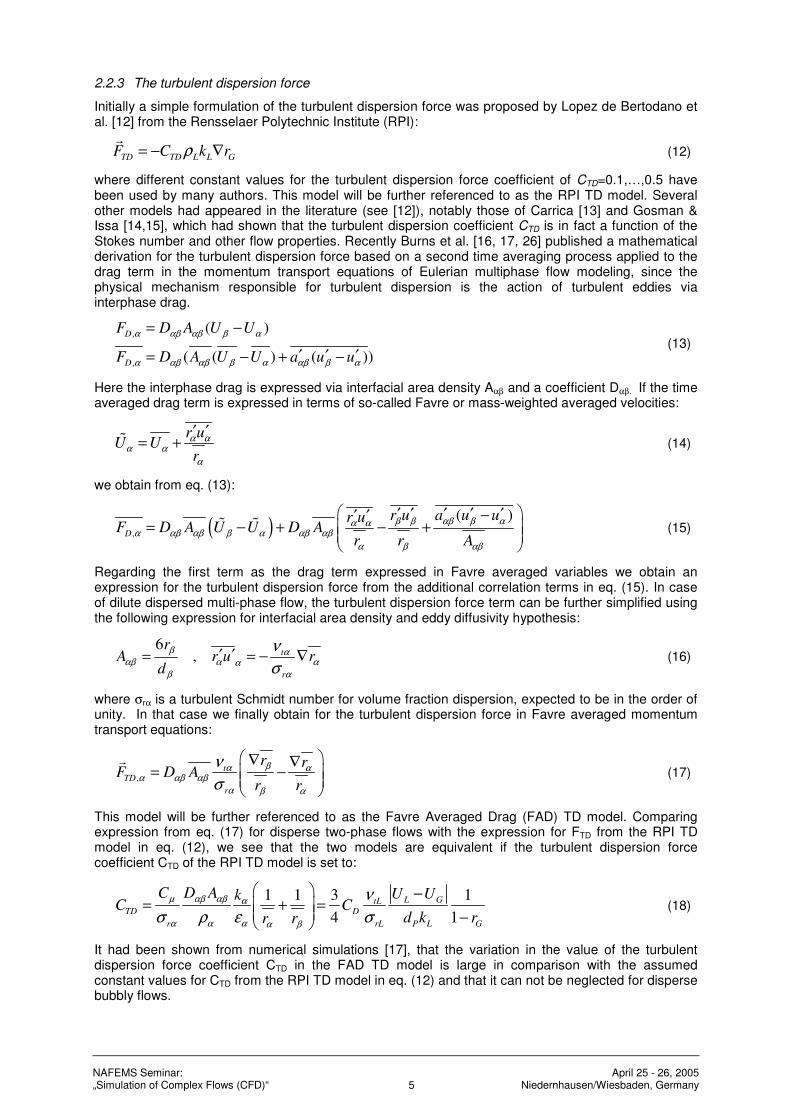
2.2.3 The turbulent dispersion force

Initially a simple formulation of the turbulent dispersion force was proposed by Lopez de Bertodano et al. [12] from the Rensselaer Polytechnic Institute (RPI):

TD TD L L GF C k rρ= − ∇r

(12)

where different constant values for the turbulent dispersion force coefficient of CTD=0.1,…,0.5 have been used by many authors. This model will be further referenced to as the RPI TD model. Several other models had appeared in the literature (see [12]), notably those of Carrica [13] and Gosman & Issa [14,15], which had shown that the turbulent dispersion coefficient CTD is in fact a function of the Stokes number and other flow properties. Recently Burns et al. [16, 17, 26] published a mathematical derivation for the turbulent dispersion force based on a second time averaging process applied to the drag term in the momentum transport equations of Eulerian multiphase flow modeling, since the physical mechanism responsible for turbulent dispersion is the action of turbulent eddies via interphase drag.

,

,

( )

( ( ) ( ))

D

D

F D A U U

F D A U U a u u

α αβ αβ β α

α αβ αβ β α αβ β α

= −

′ ′ ′= − + − (13)

Here the interphase drag is expressed via interfacial area density Aαβ and a coefficient Dαβ. If the time averaged drag term is expressed in terms of so-called Favre or mass-weighted averaged velocities:

r u

U Ur

α αα α

α

′ ′= +% (14)

we obtain from eq. (13):

( ),

( )D

r u a u ur uF D A U U D A

r r A

β β αβ β αα αα αβ αβ β α αβ αβ

α β αβ

′ ′ ′ ′ ′−′ ′= − + − +

% % (15)

Regarding the first term as the drag term expressed in Favre averaged variables we obtain an expression for the turbulent dispersion force from the additional correlation terms in eq. (15). In case of dilute dispersed multi-phase flow, the turbulent dispersion force term can be further simplified using the following expression for interfacial area density and eddy diffusivity hypothesis:

6

, t

r

rA r u r

d

β ααβ α αα

β α

ν

σ′ ′= = − ∇ (16)

where σrα is a turbulent Schmidt number for volume fraction dispersion, expected to be in the order of unity. In that case we finally obtain for the turbulent dispersion force in Favre averaged momentum transport equations:

,t

TD

r

r rF D A

r r

βα αα αβ αβ

α β α

ν

σ

∇ ∇= −

r (17)

This model will be further referenced to as the Favre Averaged Drag (FAD) TD model. Comparing expression from eq. (17) for disperse two-phase flows with the expression for FTD from the RPI TD model in eq. (12), we see that the two models are equivalent if the turbulent dispersion force coefficient CTD of the RPI TD model is set to:

1 1 3 1

4 1

L GtL

TD D

r rL P L G

C D A U UkC C

d k rr r

µ αβ αβ α

α α α α β

ν

σ ρ ε σ

−= + =

− (18)

It had been shown from numerical simulations [17], that the variation in the value of the turbulent dispersion force coefficient CTD in the FAD TD model is large in comparison with the assumed constant values for CTD from the RPI TD model in eq. (12) and that it can not be neglected for disperse bubbly flows.



MT-Loop

TOPFLOW

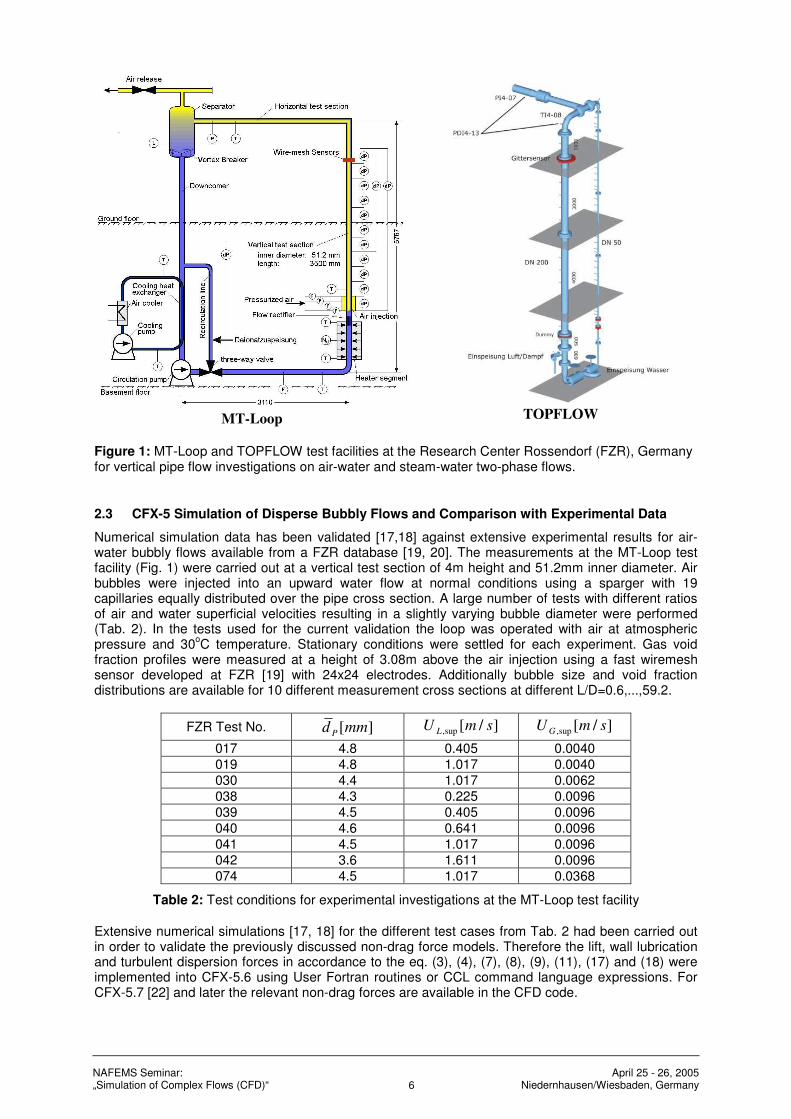
Figure 1: MT-Loop and TOPFLOW test facilities at the Research Center Rossendorf (FZR), Germany for vertical pipe flow investigations on air-water and steam-water two-phase flows.

2.3 CFX-5 Simulation of Disperse Bubbly Flows and Comparison with Experimental Data

Numerical simulation data has been validated [17,18] against extensive experimental results for air-water bubbly flows available from a FZR database [19, 20]. The measurements at the MT-Loop test facility (Fig. 1) were carried out at a vertical test section of 4m height and 51.2mm inner diameter. Air bubbles were injected into an upward water flow at normal conditions using a sparger with 19 capillaries equally distributed over the pipe cross section. A large number of tests with different ratios of air and water superficial velocities resulting in a slightly varying bubble diameter were performed (Tab. 2). In the tests used for the current validation the loop was operated with air at atmospheric pressure and 30

oC temperature. Stationary conditions were settled for each experiment. Gas void

fraction profiles were measured at a height of 3.08m above the air injection using a fast wiremesh sensor developed at FZR [19] with 24x24 electrodes. Additionally bubble size and void fraction distributions are available for 10 different measurement cross sections at different L/D=0.6,...,59.2.

FZR Test No. ][mmd P ]/[sup, smU L ]/[sup, smU G

017 4.8 0.405 0.0040

019 4.8 1.017 0.0040

030 4.4 1.017 0.0062

038 4.3 0.225 0.0096

039 4.5 0.405 0.0096

040 4.6 0.641 0.0096

041 4.5 1.017 0.0096

042 3.6 1.611 0.0096

074 4.5 1.017 0.0368

Table 2: Test conditions for experimental investigations at the MT-Loop test facility

Extensive numerical simulations [17, 18] for the different test cases from Tab. 2 had been carried out in order to validate the previously discussed non-drag force models. Therefore the lift, wall lubrication and turbulent dispersion forces in accordance to the eq. (3), (4), (7), (8), (9), (11), (17) and (18) were implemented into CFX-5.6 using User Fortran routines or CCL command language expressions. For CFX-5.7 [22] and later the relevant non-drag forces are available in the CFD code.



0.0

0.5

1.0

1.5

2.0

2.5

3.0

3.5

0.00 5.00 10.00 15.00 20.00 25.00

Radius [mm]

no

rma

lized

vo

lum

e f

racti

on

[-]

Experiment FZR-019

Antal W.L.F., Grid 2

Tomiyama W.L.F., Grid 2

Frank W.L.F., Grid 2

FZR-019

0.0

1.0

2.0

3.0

4.0

5.0

0.00 5.00 10.00 15.00 20.00 25.00

Radius [mm]

no

rmalized

vo

lum

e f

racti

on

[-]

Experiment FZR-030




FZR-030

0.0

0.5

1.0

1.5

2.0

2.5

3.0

3.5

0.00 5.00 10.00 15.00 20.00 25.00

Radius [mm]

no

rmalized

vo

lum

e f

racti

on

[-]

Experiment FZR-038




FZR-038

0.0

0.5

1.0

1.5

2.0

2.5

3.0

3.5

0.00 5.00 10.00 15.00 20.00 25.00

Radius [mm]

no

rmalized

vo

lum

e f

racti

on

[-]

Experiment FZR-040




FZR-040

0.0

1.0

2.0

3.0

4.0

5.0

0.00 5.00 10.00 15.00 20.00 25.00

Radius [mm]

no

rmalized

vo

lum

e f

racti

on

[-]

Experiment FZR-042




FZR-042

0.0

0.5

1.0

1.5

2.0

0.00 5.00 10.00 15.00 20.00 25.00

Radius [mm]

no

rmaliz

ed

vo

lum

e f

racti

on

[-]

Experiment FZR-074




FZR-074

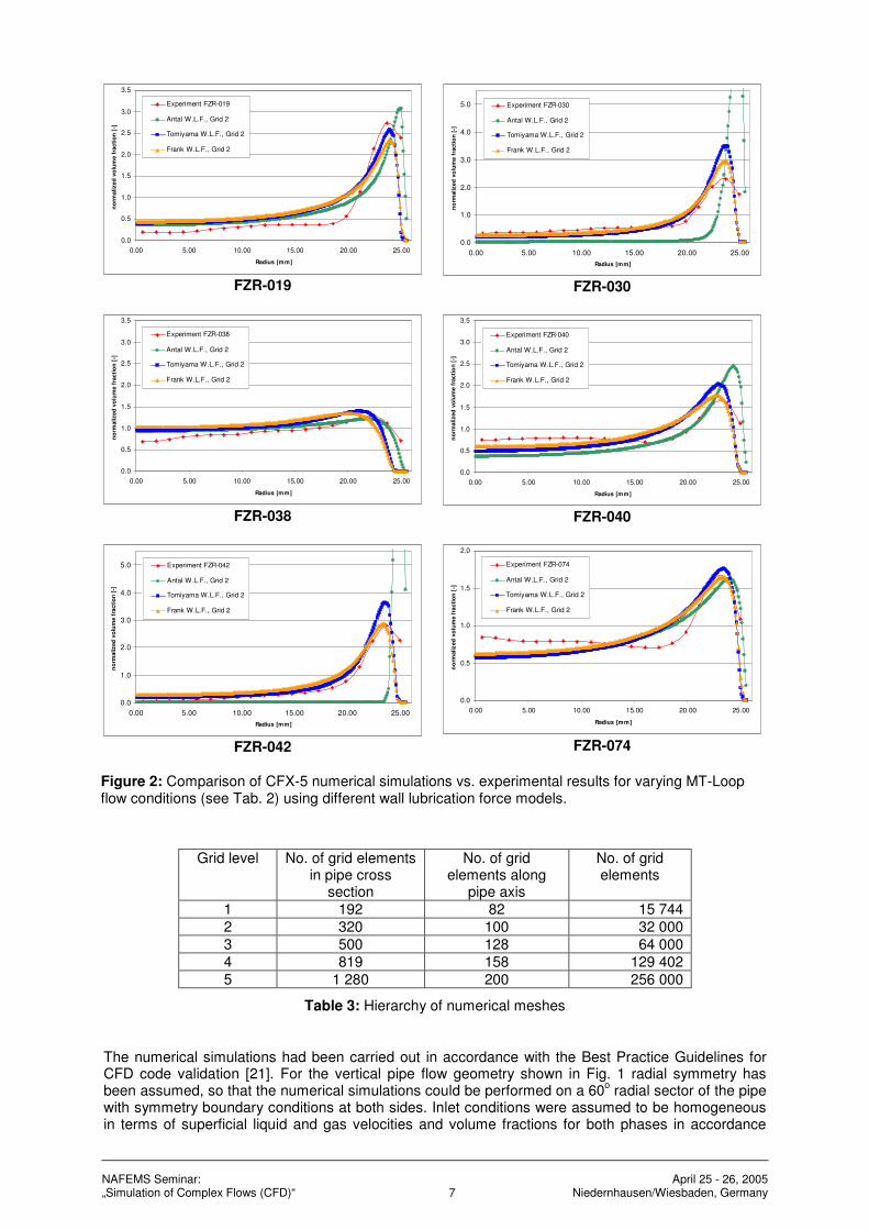
Figure 2: Comparison of CFX-5 numerical simulations vs. experimental results for varying MT-Loop flow conditions (see Tab. 2) using different wall lubrication force models.

Grid level No. of grid elements in pipe cross

section

No. of grid elements along

pipe axis

No. of grid elements

1 192 82 15 744

2 320 100 32 000

3 500 128 64 000

4 819 158 129 402

5 1 280 200 256 000

Table 3: Hierarchy of numerical meshes

The numerical simulations had been carried out in accordance with the Best Practice Guidelines for CFD code validation [21]. For the vertical pipe flow geometry shown in Fig. 1 radial symmetry has been assumed, so that the numerical simulations could be performed on a 60

o radial sector of the pipe

with symmetry boundary conditions at both sides. Inlet conditions were assumed to be homogeneous in terms of superficial liquid and gas velocities and volume fractions for both phases in accordance



with the experimental setup conditions from Tab. 2. For the disperse bubbly phase a mean bubble diameter was specified, which was determined from the test case wiremesh sensor data. At the outlet cross section of the 3.8m long pipe section an averaged static pressure outlet boundary condition was used. A hierarchy of 5 numerical grids was constructed, where the number of grid elements has been increased by a factor of 2 from a coarser to a finer mesh (scaling factor of 2

1/3 in each coordinate

direction, see Tab. 3). The numerical meshes used local refinement towards the outer pipe wall, while min/max cell size and cell aspect ratios were kept almost constant for all different numerical grids. Dimensionless y

+ values varied between y

+=29.2 on the coarsest mesh and y

+=12.5 on the finest

mesh. For investigation of flow solver convergence the gas holdup and the global mass balances for both phases in the vertical pipe were defined as monitored target variables. Reliable converged solutions could be obtained on all grid levels for a satisfied convergence criterion based on the maximum

residuals of 1.0⋅10-5

and for a physical time scale of the fully implicit solution method of ∆t=0.005s.

Fig. 2 shows the comparison of CFX-5 numerical simulations using the above described physical models for monodispersed bubbly flows with experimental data from the MT-Loop experiments at FZR for different flow conditions. For the comparison of the numerically predicted and measured gas volume fraction profiles at the uppermost measurement cross section of MT-Loop at z=3.03m (L/D=59.2) all data have been normalized:

*

/ 2

2 0

( )( )

8( )

GG D

G

r xr x

r x x dxD

=

∫ (19)

where x is the coordinate in radial direction. For the presented numerical simulations Grace drag law, Tomiyama lift force coefficient correlation and the FAD turbulent dispersion force model had been used, while the numerical results predicted with Antal, Tomiyama and Frank wall lubrication force models can be compared from the diagrams of Fig. 2. For almost all investigated testcases the numerical results predicted with the generalized wall lubrication force formulation of eq. (11) are in best and very good agreement with the experimental data. These results using the Frank wall lubrication force model are close to the numerical solution given by the Tomiyama wall lubrication force as well, but simultaneously avoid the fixed geometrical length scale D of eq. (9). It can further observed that the Antal wall lubrication force formulation results in a gas volume fraction maximum of too high amplitude, which is located too close to the pipe wall for most testcases. Especially for testcase conditions of FZR-030 and FZR-042 the Antal wall lubrication force is not able to balance the arising near wall lift force acting on the bubbles, which leads to a strong overprediction in gas volume fraction maxima. Further investigation results are available from [17], [18] and [19].

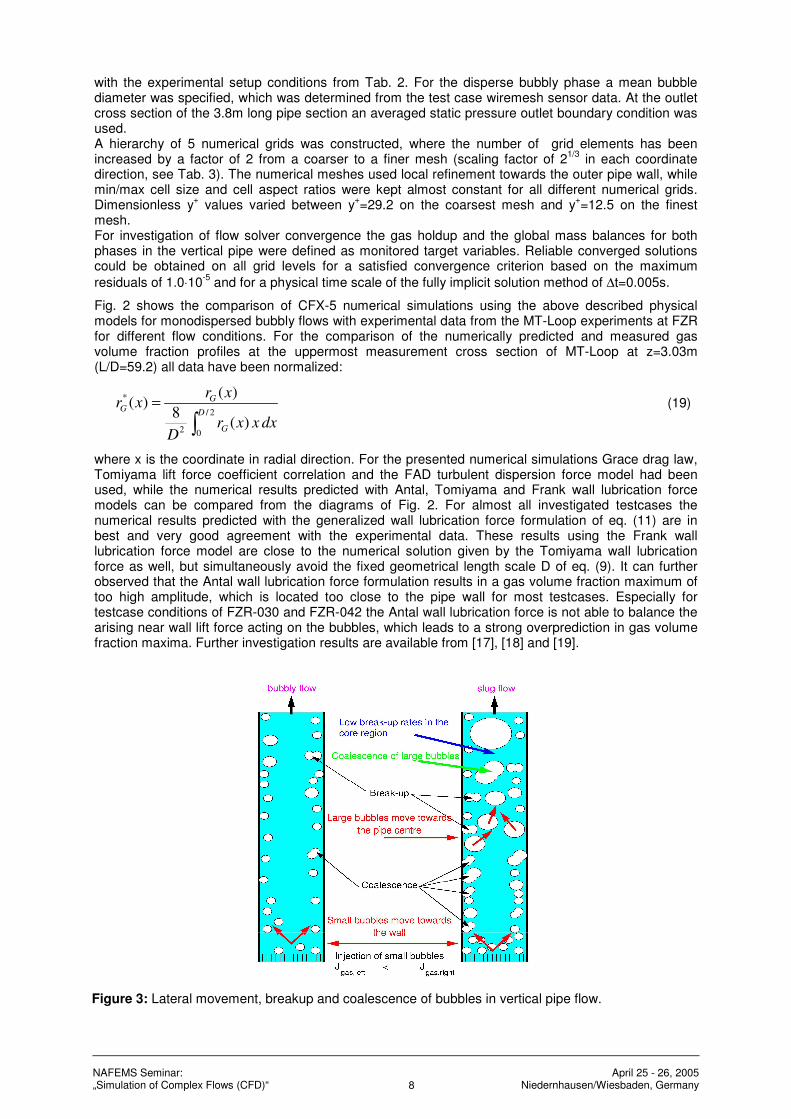
Figure 3: Lateral movement, breakup and coalescence of bubbles in vertical pipe flow.



3 Bubbly Flows with Bubble Breakup and Coalescence in Vertical Pipes

Bubbly flows investigated in section 2 show a flow pattern, where the governing flow conditions lead to a very narrow bubble size distribution and therefore satisfy the assumption of a monodisperse bubbly flow with a single characteristic bubble diameter. If for a given fluid flow rate the gas volume fraction is further increased by e.g. increasing the gas superficial velocity, then processes of bubble breakup and coalescence become of crucial importance for the numerical prediction of the resulting gas-liquid two-phase flow and the gas volume fraction distribution. These processes become of importance even for flow conditions, where the pipe averaged gas volume fraction is still at a low level as e.g. rG~3-5% if the pipe cross section is larger then that of the MT-Loop facility. Experiments at the FZR TOPFLOW test facility (see Fig. 1) with D=200mm show, that bubble size distribution and flow pattern for the testcase FZR-074 is substantially changed in comparison with the MT-Loop experiment for D=51.2mm and under the same flow conditions, i.e. fluid and gas superficial velocities. Fig. 3 reveals the main mechanisms leading to the changed bubble size distribution due to bubble breakup and coalescence processes, which occur in the near wall region where substantially higher gas volume fractions of about rG~15-25% are developing with increasing pipe length or are arising directly from near wall gas injection through wall nozzles. The lift force acting on small bubbles (small in comparison with the characteristic bubble diameter, where the Tomiyama lift force shows a lift force sign change at approx. dP= 5.9mm) leads to a lateral movement of small bubbles towards the wall and corresponding high near wall gas concentrations. Within this near wall range of higher gas concentration bubble

coalescence occurs and arising bubbles with large bubble diameters (dP≥5.9mm) are subject to lift forces acting towards the pipe center. Besides bubble coalescence, turbulence induced bubble breakup occurs within this near wall region as well due to higher turbulence level in the boundary layer resulting in an equilibrium bubble size distribution. For a larger number of testcases the lateral movement of large bubbles towards the pipe center leads to a volume fraction profile with a pronounced core maximum in the quasi-steady state of the gas-liquid flow measured at the upper pipe level. The measured bubble size distributions show a wider range of observed bubble sizes from very small bubbles (dP~1mm) up to large bubbles, Taylor bubbles or even slugs with bubble diameters of about dP~12-65mm depending on testcase flow conditions. Since the assumption of a monodisperse bubbly flow made for the investigations in section 2 is violated for these bubble flow regimes, the derived bubbly flow models have to be extended in order to take bubble size distribution as well as bubble breakup and coalescence processes into account. Three different approaches are available with CFX-5 and had been applied and validated for the given class of gas-liquid two-phase flows.

homogeneous MUSIG model (1xM)

partially inhomogeneous NxM MUSIG model

Figure 4: Scheme of gaseous phase velocity groups and bubble size classes for the homogeneous (1xM) and partially inhomogeneous NxM MUSIG models.

3.1 The Homogeneous MUSIG Model

In the homogeneous MUSIG (Multiple Size Group) model (see Fig. 4) developed by Lo [23, 24] the bubble/particle size distribution is divided in a number of M discrete size classes, while it is assumed that bubbles/particles of all sizes share a common velocity field. This assumption is satisfied, if the size distribution covers a smaller particle/bubble size range (e.g. in crystallization processes), the particles/bubbles are of small inertia and/or the flow under investigation is dominated by strong convection as e.g. in stirred vessel reactors. Unfortunately the homogeneous MUSIG model can not be applied to the gas-liquid flows in vertical pipes or similar flows dominated by non-drag forces, since the lateral bubble motion leading to a demixing of bubbles of different sizes can not be predicted with a single shared bubble velocity field.

dP1 dPa

V1 V2

dPa+1 dPb dPx+ dPM

VN

dP1 dP2 dP3 dPM

V1



Averaged flow parameters phase Air 1 phase Air 2 Phase Air 3

FZR Test No.

]/[

sup,

sm

U L

]/[

sup,

sm

U G

][−

Gr

][

1

mm

d P

][

1

−

Gr

][

2

mm

d P

][

2

−

Gr

][

3

mm

d P

][

3

−

Gr

070 0.161 0.0368 22.86 4.8 12.20 7.0 10.66 - -

083 0.405 0.0574 12.76 3.7 1.00 5.0 8.86 6.7 2.90

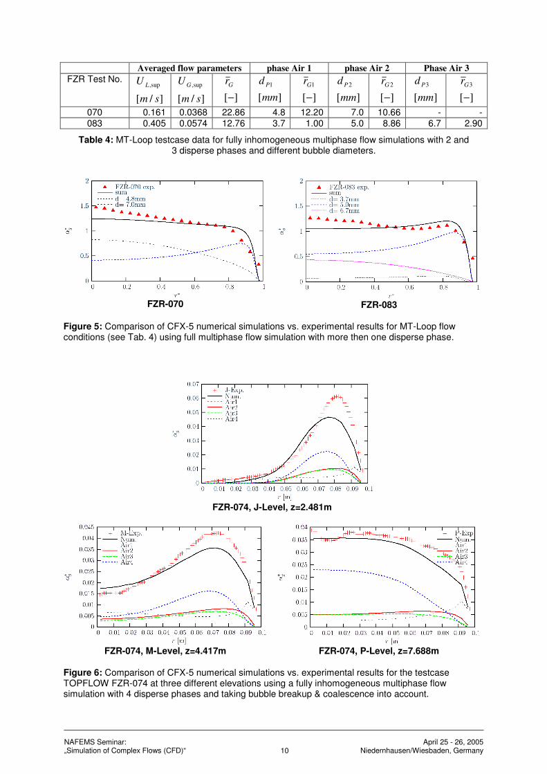
Table 4: MT-Loop testcase data for fully inhomogeneous multiphase flow simulations with 2 and 3 disperse phases and different bubble diameters.

FZR-070

FZR-083

Figure 5: Comparison of CFX-5 numerical simulations vs. experimental results for MT-Loop flow conditions (see Tab. 4) using full multiphase flow simulation with more then one disperse phase.

FZR-074, J-Level, z=2.481m

FZR-074, M-Level, z=4.417m

FZR-074, P-Level, z=7.688m

Figure 6: Comparison of CFX-5 numerical simulations vs. experimental results for the testcase TOPFLOW FZR-074 at three different elevations using a fully inhomogeneous multiphase flow simulation with 4 disperse phases and taking bubble breakup & coalescence into account.



3.2 The Fully Inhomogeneous Multiphase Flow Simulation

Significant progress in the simulation of polydisperse gas-liquid two-phase flow could be established by applying a fully inhomogeneous multiphase flow simulation to the gas-liquid bubbly flows of higher gas concentration, where a coupled equation system of the type of eq. (1) and (2) is solved for the continuous liquid phase and a number N of disperse bubbly phases [25-27]. Here each disperse phase with its own velocity field represents a bubble size class of the bubble size distribution. Numerical simulations without bubble breakup and coalescence processes have been carried out by Shi, Frank et al. [26] for up to 4 disperse phases. Using the quasi-steady state equilibrium bubble size distribution measured in the upper-most pipe cross section for the numerical simulation good agreement between numerical simulation results and measured gas volume fraction distributions could be obtained for a number of testcases from the MT-Loop testcase matrix showing a broader bubble size distribution. Examples of such simulation results for MT-Loop testcases FZR-070 and FZR-083 (see Table 4) using 2 or 3 disperse phases with different bubble diameters and without taking bubble breakup and coalescence into account are shown in Fig. 5. This numerical approach has further enhanced by taking additionally bubble breakup and coalescence into account [27]. Therefore mass source and sink terms for each phase have been introduced in the continuity equations of the gaseous phases, which are in correspondence with the amount of gaseous mass transferred from one bubble size class (i.e. disperse phase) to the other due to breakup and coalescence processes. For the prediction of the mass source and sink terms the same breakup and coalescence models of Luo & Svendsen [28] and Prince & Blanch [29] as for the homogeneous MUSIG model were used. The mass source and sink terms were implemented in CFX-5.7 using User Fortran routines, CCL and Perl Power Syntax. The resulting numerical approach, also referenced to as the Nx1 fully inhomogeneous MUSIG model with N velocity groups each with a single bubble size class, subsequently was applied to the TOPFLOW (see Fig. 1) testcase FZR-074 using N=4 and N=8 disperse phases. The testcase data for the superficial air and water velocities are the same as for the corresponding MT-Loop testcase from Table 2. Due to the larger inner diameter of D=200mm TOPFLOW differs from MT-Loop in the method of gas injection. While MT-Loop uses an array of 19 individual nozzles distributed over the pipe cross section and resulting in an almost homogeneous inlet distribution of gas volume fraction, the TOPFLOW gas injection is realized through 72 circumferentially arranged wall nozzles at z=0.0m with 1mm diameter leading to an initially high gas concentration at the wall near and above the gas injection location. The TOPFLOW test facility has an overall pipe length of about L=8m above the lowest gas injection location (max. L/D=40). Fig. 6 shows the comparison of a 5-phase simulation (1 continuous and 4 disperse phases) using the above outlined numerical approach taking the bubble breakup & coalescence into account – so using a 4x1 fully inhomogeneous MUSIG model. Characteristic mean bubble diameters of dP1=4.16mm, dP2=5.38mm, dP3=6.51mm and dP4=8.56mm were used for the four disperse phases. The relative volume fraction of the four disperse phases with respect to the total gas volume flow rate was

assigned to 1 1.2%G

r = , 2 5.3%G

r = , 3 32.1%G

r = and 4 61.4%G

r = respectively. Measurement data

and simulation results for the non-normalized gas volume fraction profiles are compared at 3 different elevations above the gas injection point at z=2.481m (J-level), z=4.417m (M-level) and at one of the uppermost measurement locations at z=7.688 (P-level). The diagrams in Fig. 6 show the bubble size class resolved gas volume fraction profiles as well as the cumulative air volume fraction distribution, which is in good agreement with the experimental data and show the axial development of the gas volume fraction core peak at P-level from a wall peak at J- and M-level by gas mass transfer from smaller bubble size classes (phases) to larger bubble size classes due to strong coalescence in the high gas concentration near wall region. Further results are available for N=8 and at other pipe elevations in [27].

3.3 The Partially Inhomogeneous NxM MUSIG Model – a New Population Balance Model

Of course, the above described fully inhomogeneous multiphase flow simulations are computationally very expensive and are therefore limited to a small number of disperse phases or bubble size classes. But for gas-liquid flows with a broad bubble size distribution its representation with a larger number of discrete bubble size classes might be required. Therefore, based on a first outline of this approach in [30], a partially inhomogeneous NxM MUSIG (or population balance) model has been developed and

implemented as a β-feature in CFX-5.8, which uses N velocity groups/fields for the gaseous phase and inside of each velocity group M bubble size classes sharing the same velocity field (see Fig. 4). Therefore a total of NxM bubble size classes are available for the bubble breakup & coalescence models [28, 29], while the numerical effort can be limited to comparable values of a 3- or 4-phase simulation. First simulations with the newly developed NxM MUSIG model have been carried out for the TOPFLOW FZR-074 testcase as already used for validation in section 3.2. Fig. 7 shows the

experiment vs. numerical prediction comparison for CFX-5.8α simulations using a 3x7 inhomogeneous



0.0

5.0

10.0

15.0

20.0

0.0 25.0 50.0 75.0 100.0

x [mm]

Air

vo

lum

e f

rac

tio

n [

-]Exp. FZR-074, level A

CFX, Inlet level: Air VF

CFX, Inlet level: Air1 VF



FZR-074, Inlet-Level, z=0.0m

0.0

2.0

4.0

6.0

0.0 25.0 50.0 75.0 100.0

x [mm]

Air

vo

lum

e f

rac

tio

n [

-]

Exp. FZR-074, level L

CFX, level L: Air VF

CFX, level L: Air1 VF



FZR-074, L-Level, z=2.595m

0.0

1.0

2.0

3.0

4.0

5.0

0.0 25.0 50.0 75.0 100.0

x [mm]

Air

vo

lum

e f

rac

tio

n [

-]

Exp. FZR-074, level O

CFX, level O: Air VF

CFX, level O: Air1 VF



FZR-074, O-Level, z=4.531m

0.0

1.0

2.0

3.0

4.0

5.0

0.0 25.0 50.0 75.0 100.0

x [mm]

Air

vo

lum

e f

rac

tio

n [

-]

Exp. FZR-074, level R

CFX, level R: Air VF

CFX, level R: Air1 VF



FZR-074, R-Level, z=7.802m

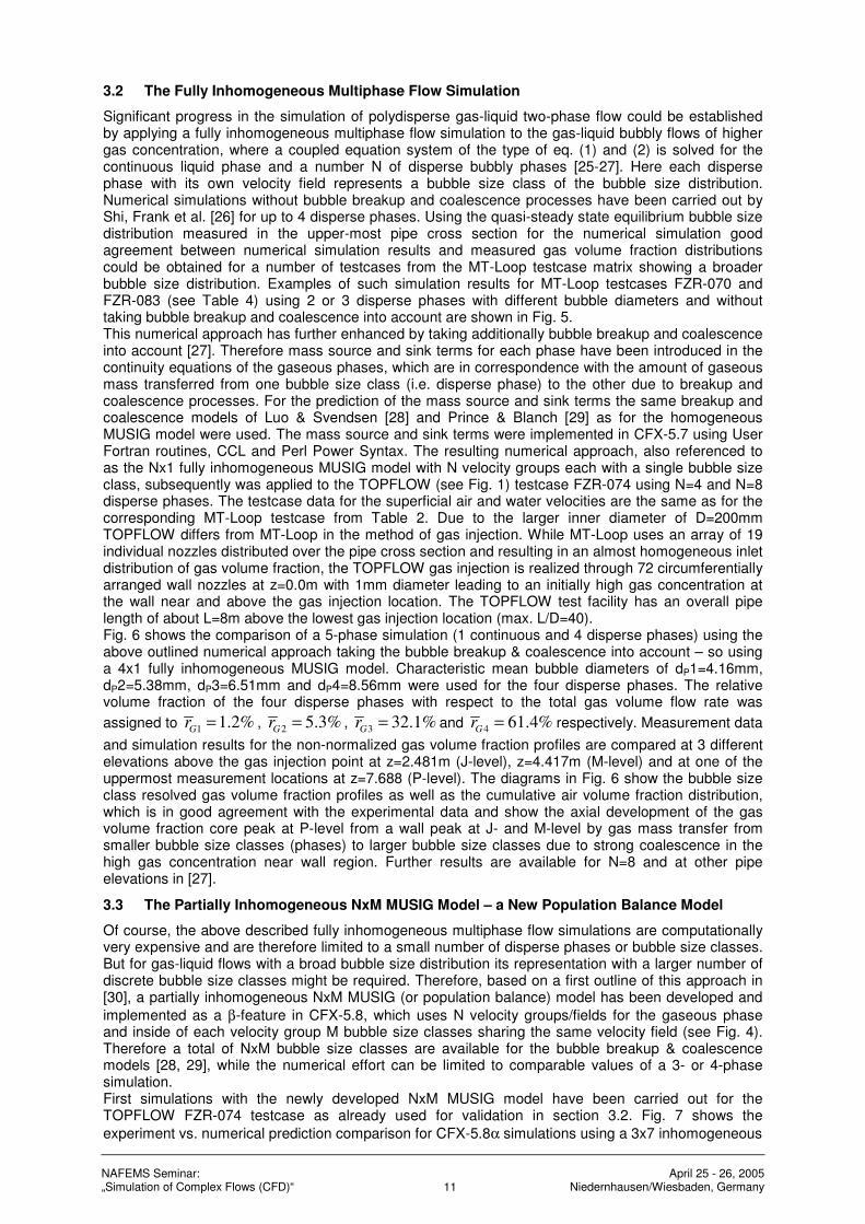
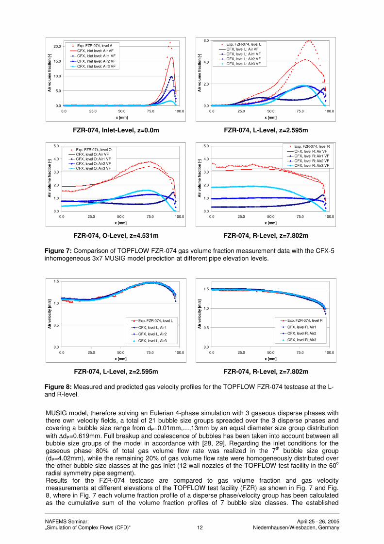
Figure 7: Comparison of TOPFLOW FZR-074 gas volume fraction measurement data with the CFX-5 inhomogeneous 3x7 MUSIG model prediction at different pipe elevation levels.

0.0

0.5

1.0

1.5

0.0 25.0 50.0 75.0 100.0

x [mm]

Air

ve

loc

ity

[m

/s]

Exp. FZR-074, level L

CFX, level L, Air1

CFX, level L, Air2

CFX, level L, Air3

FZR-074, L-Level, z=2.595m

0.0

0.5

1.0

1.5

0.0 25.0 50.0 75.0 100.0

x [mm]

Air

ve

loc

ity

[m

/s]

Exp. FZR-074, level R

CFX, level R, Air1

CFX, level R, Air2

CFX, level R, Air3

FZR-074, R-Level, z=7.802m

Figure 8: Measured and predicted gas velocity profiles for the TOPFLOW FZR-074 testcase at the L- and R-level.

MUSIG model, therefore solving an Eulerian 4-phase simulation with 3 gaseous disperse phases with there own velocity fields, a total of 21 bubble size groups spreaded over the 3 disperse phases and covering a bubble size range from dP=0.01mm,…,13mm by an equal diameter size group distribution

with ∆dP=0.619mm. Full breakup and coalescence of bubbles has been taken into account between all bubble size groups of the model in accordance with [28, 29]. Regarding the inlet conditions for the gaseous phase 80% of total gas volume flow rate was realized in the 7

th bubble size group

(dP=4.02mm), while the remaining 20% of gas volume flow rate were homogeneously distributed over the other bubble size classes at the gas inlet (12 wall nozzles of the TOPFLOW test facility in the 60

o

radial symmetry pipe segment). Results for the FZR-074 testcase are compared to gas volume fraction and gas velocity measurements at different elevations of the TOPFLOW test facility (FZR) as shown in Fig. 7 and Fig. 8, where in Fig. 7 each volume fraction profile of a disperse phase/velocity group has been calculated as the cumulative sum of the volume fraction profiles of 7 bubble size classes. The established



accuracy and agreement with the experimental data for both the gas volume fraction and velocity profiles is very good. From Fig. 7 it can be seen, that the gas bubble plume injected through the wall nozzles at the inlet level (z=0.0m) is spreading a little bit to fast inward in radial direction. At the same time, while the gas bubble plume rising from the wall nozzles is dispersed by turbulent dispersion, coalescence of bubbles takes place leading to an increasing gas volume fraction in the bubble size classes with larger bubble diameters (in the disperse phase Air3). Simultaneously large bubbles are decaying into smaller ones due to bubble breakup in shear layers close to the wall. At the uppermost measurement cross section at the R-level small bubbles (Air1) show a slightly pronounced wall peak, medium sized bubbles (Air2) are almost homogeneously distributed over the pipe cross section, while for the large bubbles (Air3) a remarkable core peak in the gas volume fraction profiles can be observed. The cumulative gas volume fraction profile finally shows a core peak, which is again in very good agreement with the measurements. Further the gas velocity profiles at different elevations are in good quantitative agreement with measured gas velocities too, as can be seen from Fig. 8.

4 Simulation of Slug Flow in Horizontal Pipes

Finally gas-liquid two-phase flows in horizontal pipelines have been investigated [31, 32] based on experimental investigation of Lex [33] at the TU Munich (TD/TUM) and using the CFX-5 multiphase flow models. Special interest have been directed to the regime of slug flow, which is a quit common multiphase flow regime in horizontal pipelines and channels, which can be potentially hazardous to the structure of the pipe system or to apparatus and processes following the slug flow pipe section due to the strong oscillating pressure levels formed behind liquid slugs. Areas of application are in the chemical and process industry as well as in safety research and thermo-hydraulic engineering for nuclear power plants. Fluid mechanics of air-water slug flows in horizontal circular pipes is investigated using detailed, transient, 3-dimensional Computational Fluid Dynamics (CFD) simulations. The inhomogeneous two-phase or mixture model combined with the interface sharpening (free surface) algorithm implemented in CFX-5.7 has been used to predict the transition of a segregated air-water flow into slug flow regime for a L=8m long pipe with circular cross section and an inner diameter D=0.054m. The pipe was initially filled with 50% volume fraction of the gaseous phase and 50% of the liquid phase, while the separating free surface was periodically agitated with amplitude of 0.25D and a wave length of 0.25L based on experimental observations at the TD/TUM test rig.

4.1 The Multiphase Mixture or Inhomogeneous VOF Model

If we assume, that gaseous and liquid phases in the slug flow regime are fully segregated, than it seems to be the most appropriate and economical approach to use the homogeneous VOF method with shared velocity field assumption for this type of application. In this case only one set of Navier-Stokes equations for the gas-liquid mixture together with two volume fraction equations and turbulence model equations are solved. However, experimental observations show that on the leading front of a liquid slug the flow tends to the formation of breaking waves, droplets and liquid ligaments. These partial phenomena can lead to gas entrainment into the liquid phase. Since in the homogeneous model both phases share the same velocity field, phases are demixing only through 3-dimensional motion and not by interpenetration of phases. This usually leads to delayed demixing times and a generally different behavior of the multiphase mixture in areas of higher gas entrainment. Therefore the numerical simulations were based on the CFX-5.7 two-fluid (or multifluid) Euler-Euler approach. The Eulerian modeling framework is based on ensemble-averaged mass and momentum transport equations for all phases, gas and liquid. Regarding both phases as continua, which are segregated or mixed at a macroscopic level (mixture model), these equations without mass transfer between phases read:

( ) ( ) 0. =∇+∂

∂ααααα ρρ Urr

t

r (19)

( ) ( ) ( ). . ( ( ) )

T

Dr U r U U r U U r p r g F

tα α α α α α α α α α α α α αρ ρ µ ρ

∂+ ∇ ⊗ = ∇ ∇ + ∇ − ∇ + +

∂

r r r r r rr

(20)

where U α

urrepresents the velocity field of phase α (with α=L for the liquid and α=G for the gaseous

phase), rα - volume fraction, ρα - density, p - pressure, µα - viscosity, g - gravitation and FD represents the drag force due to momentum transfer at the interface between phases. In contrary to the model outlined in section 2.1 this drag force can not be modeled in accordance to the particle model, but has to take into account the effective interfacial area density at the free surface separating both phases. Therefore the liquid and gaseous phases are coupled through an interfacial drag FD, which can be

expressed through a drag coefficient CD and the interfacial area density Aαβ:

, ( )D DF C A U Uα αβ αβ β αρ= − (21)



with:

60.44 , , ,D

r rC r r A d r d r d

d

α β

αβ α β β α αβ αβ α β β α

αβ

ρ ρ ρ= = + = = + (22)

The user supplied phase specific length scales have been set to dα=dβ=0.001m in the assumption, that entrained droplets or gas bubbles are approximately of this size for the given type of flow. Similar results have been obtained in the numerical predictions using a drag law derived by Ishii [34, p. 37] for gas-liquid slug flows instead of Newton’s drag law:

( )

3

9.8 1D

C rβ= −

(23)

where rβ is the volume fraction of the gaseous phase. Also it is quite uncertain whether this macroscale drag law can be applied to the microscale interfacial processes between the two phases. For the present simulation the two-phase mixture model has been combined with the CFX free surface model. It makes use of a compressive advection scheme in order to avoid smearing of the interface between the two phases due to numerical diffusion of the solution algorithm. The surface tension at the interface has been neglected for the present simulation. Details of the CFX-5 free surface model can be found in [22, 35].

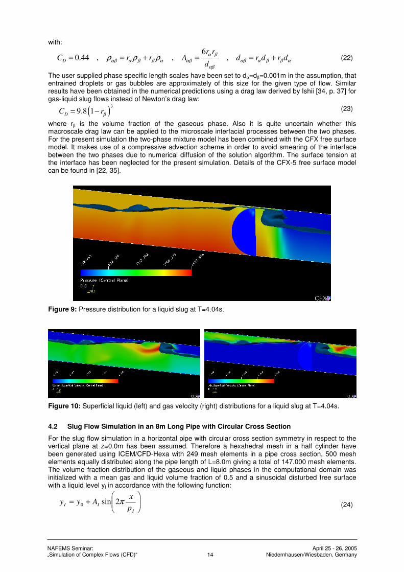
Figure 9: Pressure distribution for a liquid slug at T=4.04s.

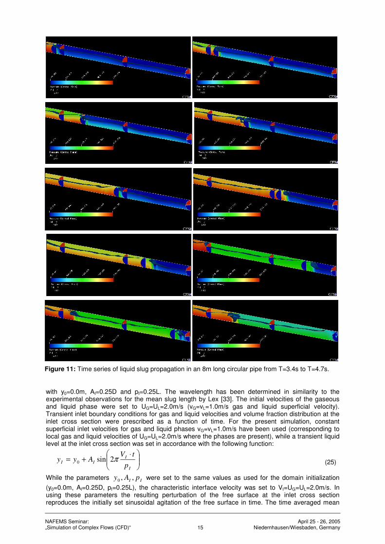
Figure 10: Superficial liquid (left) and gas velocity (right) distributions for a liquid slug at T=4.04s.

4.2 Slug Flow Simulation in an 8m Long Pipe with Circular Cross Section

For the slug flow simulation in a horizontal pipe with circular cross section symmetry in respect to the vertical plane at z=0.0m has been assumed. Therefore a hexahedral mesh in a half cylinder have been generated using ICEM/CFD-Hexa with 249 mesh elements in a pipe cross section, 500 mesh elements equally distributed along the pipe length of L=8.0m giving a total of 147.000 mesh elements. The volume fraction distribution of the gaseous and liquid phases in the computational domain was initialized with a mean gas and liquid volume fraction of 0.5 and a sinusoidal disturbed free surface with a liquid level yI in accordance with the following function:

+=

I

IIp

xAyy π2sin0

(24)



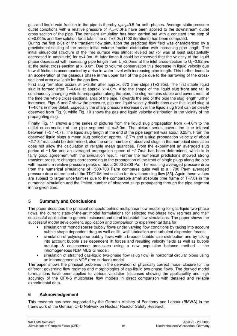
Figure 11: Time series of liquid slug propagation in an 8m long circular pipe from T=3.4s to T=4.7s.

with y0=0.0m, AI=0.25D and pI=0.25L. The wavelength has been determined in similarity to the experimental observations for the mean slug length by Lex [33]. The initial velocities of the gaseous and liquid phase were set to UG=UL=2.0m/s (vG=vL=1.0m/s gas and liquid superficial velocity). Transient inlet boundary conditions for gas and liquid velocities and volume fraction distribution at the inlet cross section were prescribed as a function of time. For the present simulation, constant superficial inlet velocities for gas and liquid phases vG=vL=1.0m/s have been used (corresponding to local gas and liquid velocities of UG=UL=2.0m/s where the phases are present), while a transient liquid level at the inlet cross section was set in accordance with the following function:

⋅+=

I

I

IIp

tVAyy π2sin0

(25)

While the parameters II pAy ,,0 were set to the same values as used for the domain initialization

(y0=0.0m, AI=0.25D, pI=0.25L), the characteristic interface velocity was set to VI=UG=UL=2.0m/s. In using these parameters the resulting perturbation of the free surface at the inlet cross section reproduces the initially set sinusoidal agitation of the free surface in time. The time averaged mean



gas and liquid void fraction in the pipe is thereby rG=rL=0.5 for both phases. Average static pressure outlet conditions with a relative pressure of Prel=0.0Pa have been applied to the downstream outlet cross section of the pipe. The transient simulation has been carried out with a constant time step of dt=0.005s and flow solution for a total time of T=7.0s (1400 iterations) has been computed. During the first 2-3s of the transient flow simulation the predicted flow field was characterized by a gravitational settling of the preset initial volume fraction distribution with increasing pipe length. The initial sinusoidal structure of the free surface was almost leveled out (or was at least substantially decreased in amplitude) for x>4.0m. At later times it could be observed that the velocity of the liquid phase decreased with increasing pipe length from UL=2.0m/s at the inlet cross-section to UL~0.82m/s at the outlet cross-section at x=8.0m. Due to volume conservation this decrease in liquid velocity due to wall friction is accompanied by a rise in water level with increasing pipe length. This further leads to an acceleration of the gaseous phase in the upper half of the pipe due to the narrowing of the cross-sectional area available for the gas flow. First slug formation occurs at x~3.8m after approx. 670 time steps (T=3.35s). The first stable liquid slug is formed after T=4.04s at approx. x~4.0m. Also the shape of the liquid slug front and tail is continuously changing with its propagation along the pipe, the slug remains stable and covers most of the time the whole cross-sectional area of the pipe. Towards the end of the pipe the slug length further increases. Figs. 6 and 7 show the pressure, gas and liquid velocity distributions over this liquid slug at T=4.04s in more detail. Especially the sharp pressure increase over the liquid slug front can be clearly observed from Fig. 9, while Fig. 10 shows the gas and liquid velocity distribution in the vicinity of the propagating slug.

Finally Fig. 11 shows a time series of pictures from the liquid slug propagation from x=4.0m to the outlet cross-section of the pipe segment at x=8.0m. The picture series covers the time interval between T=3.4-4.7s. The liquid slug length at the end of the pipe segment was about 0.25m. From the observed liquid slugs a mean slug period of approx. ~2.7m and a slug propagation velocity of about ~2.7-3.1m/s could be determined, also the small number of observed slugs in the numerical simulation does not allow the calculation of reliable mean quantities. From the experiment an averaged slug period of ~1.8m and an averaged propagation speed of ~2.7m/s has been determined, which is in fairly good agreement with the simulation result. Further the numerical predictions showed strong transient pressure changes corresponding to the propagation of the front of single plugs along the pipe with maximum relative pressure peaks of about 2000-2800 Pa. The resulting averaged pressure drop from the numerical simulations of ~500-700 Pa/m compares quite well to a ~700 Pa/m averaged pressure drop determined at the TD/TUM test section for developed slug flow [33]. Again these values are subject to larger uncertainties due to the comparable small absolute time frame of T=7.0s in the numerical simulation and the limited number of observed slugs propagating through the pipe segment in the given time.

5 Summary and Conclusions

The paper describes the principal concepts behind multiphase flow modeling for gas-liquid two-phase flows, the current state-of-the-art model formulations for selected two-phase flow regimes and their successful application to generic testcases and semi-industrial flow simulations. The paper shows the successful model development, application and comparison to experimental data for:

• simulation of monodisperse bubbly flows under varying flow conditions by taking into account bubble shape dependent drag as well as lift, wall lubrication and turbulent dispersion forces;

• simulation of polydisperse bubbly flows with a broader bubble size distribution and by taking into account bubble size dependent lift forces and resulting velocity fields as well as bubble breakup & coalescence processes using a new population balance method – the inhomogeneous NxM MUSIG model;

• simulation of stratified gas-liquid two-phase flow (slug flow) in horizontal circular pipes using an inhomogeneous VOF (free surface) model.

The paper shows the principal problems in the derivation of physically correct model closure for the different governing flow regimes and morphologies of gas-liquid two-phase flows. The derived model formulations have been applied to various validation testcases showing the applicability and high accuracy of the CFX-5 multiphase flow models in direct comparison with detailed and reliable experimental data.

6 Acknowledgement

This research has been supported by the German Ministry of Economy and Labour (BMWA) in the framework of the German CFD Network on Nuclear Reactor Safety Research.



7 References

[1] Menter F.R.: “Two-equation eddy-viscosity turbulence models for engineering applications”, AIAA-Journal, Vol. 32, No. 8, 1994.

[2] Sato Y., Sekoguchi K.: “Liquid velocity distribution in two phase bubble flow”, Int. J. Multiphase Flow, Vol. 2, pp. 79, 1975.

[3] Ishii N., Zuber M.: “Drag coefficient and relative velocity in bubbly, droplet or particulate flows”, AIChE J., Vol. 25, pp. 843-855, 1979.

[4] Clift R., Grace J.R., Weber M.E.: “Bubbles, Drops and Particles”, Academic Press, New York, USA, 1978.

[5] Tomiyama A.: "Single bubbles in stagnant liquids and in linear shear flows", Workshop on Measurement Technology (MTWS5), FZ Rossendorf, Dresden, Germany, 2002, pp. 3-19.

[6] Frank Th.: “A review on advanced Eulerian multiphase flow modeling for gas-liquid flows”, ANSYS CFX Germany, Technical Report No. TR-03-08, pp. 23, March 2003.

[7] Frank Th.: „Parallele Algorithmen für die numerische Simulation dreidimensionaler, disperser Mehrphasenströmungen und deren Anwendung in der Verfahrenstechnik“, Berichte aus der Strömungstechnik, Shaker Verlag, Aachen, pp. 328, 2002.

[8] Tomiyama A.: “Struggle with computational bubble dynamics”, ICMF’98, 3rd Int. Conf. Multiphase Flow, Lyon, France, pp. 1-18, June 8.-12. 1998.

[9] Antal S.P., Lahey R.T., Flaherty J.E.: “Analysis of phase distribution in fully developed laminar bubbly two-phase flow”, Int. J. Multiphase Flow, Vol. 7, pp. 635-652, 1991.

[10] Krepper E., Prasser H.M.: “Measurements and CFX-Simulations of a bubbly flow in a vertical pipe”, AMIF-ESF Workshop "Computing Methods for Two-Phase Flow", Aussois, France, pp. 8, 12-14 January 2000.

[11] Frank Th. , Shi J., Krepper E.: "Non-drag Forces in Gas-Liquid Bubbly Flows and Validation of Existing Formulations", 2

nd Joint Workshop "Multiphase Flow: Simulation, Experiment and

Application", FZ Rossendorf & Ansys Germany GmbH, 28.-30. Juni 2004, Dresden, Germany. [12] Moraga F.J., Larreteguy A.E., Drew D.A., Lahey R.T.: “Assessment of turbulent dispersion

models for bubbly flows in the low Stokes number limit”, Int. J. Multiphase Flow, Vol. 29, pp. 655-673, 2003.

[13] Carrica P.M., Drew D.A., Lahey R.T.: “A polydisperse model for bubbly two-phase flow around a surface ship”, Int. J. Multiphase Flow, Vol. 25, pp. 257-305, 1999.

[14] Behzadi A., Issa R.I., Rusche H.: “Effects of turbulence on inter-phase forces in dispersed flow”, ICMF’2001, 4th Int. Conf. Multiphase Flow, New Orleans, LA, USA, pp. 1-12, June 2001.

[15] Gosman A.D., Lekakou C., Politis S., Issa R.I., Looney M.K.: “Multidimensional modeling of turbulent two-phase flows in stirred vessels”, AIChE Journal, Vol. 38, No. 12, pp. 1946-1956, December 1992.

[16] Burns A.D., Frank Th., Hamill I., Shi J.: “The Favre Averaged Drag Model for Turbulence Dispersion in Eulerian Multi-Phase Flows”, ICMF’2004, 5th Int. Conf. Multiphase Flow, Yokohama, Japan, 2004.

[17] Frank Th., Shi J., Burns A.D.: “Validation of Eulerian multiphase flow models for nuclear reactor safety applications”, 3rd International Symposium on Two-phase Flow Modelling and Instrumentation, Pisa, 22.-24. Sept. 2004.

[18] Frank Th.: “Bubble flow in vertical pipes – Investigation of the testcase VDL-01/1 (FZR-074) for the validation of CFD”, ANSYS CFX Germany, Technical Report No. TR-03-09, pp. 34, October 2003.

[19] Prasser H.M., Lucas D., Krepper E., Baldauf D., Böttger A., Rohde U. et al.: „Strömungskarten und Modelle für transiente Zweiphasenströmungen“, Forschungszentrum Rossendorf, Germany, Report No. FZR-379, pp. 183, June 2003.

[20] Lucas D., Krepper E., Prasser H.M.: “Development of bubble size distributions in vertical pipe flow by consideration of radial gas fraction profiles”, ICMF’2001, 4th Int. Conf. Multiphase Flow, New Orleans, LA, USA, pp. 1-12, June 2001.

[21] Menter F.R.: “CFD Best Practice Guidelines (BPG) for CFD code validation for reactor safety applications”, EC Project ECORA, Report EVOL-ECORA-D01, pp. 1-47, 2002.

[22] CFX-5.7 Users Manual, ANSYS, 2004. [23] Lo S.: “Application of the MUSIG model to bubbly flows”, Technical Report AEAT-1096, AEA

Technology, June 1996. [24] Lo S.: “Some recent developments and applications of CFD to multiphase flows in stirred

reactors”, AMIF-ESF Workshop “Computing Methods for Two-phase Flows”, Aussois, France, 12-14 January 2000, pp.1-15.

[25] Frank Th.: “Simplified User FORTRAN implementation of the inhomogeneous MUSIG (Multiple Size Group) model”, ANSYS CFX Germany, Technical Report No. TR-04-07, pp. 9, June 2004.



[26] Shi J., Frank Th., Burns A.D.: “Turbulent dispersion force – Physics, model derivation and evaluation”, ", 2

nd Joint Workshop "Multiphase Flow: Simulation, Experiment and Application",

FZ Rossendorf & Ansys Germany GmbH, 28.-30. Juni 2004, Dresden, Germany. [27] Shi J., Frank Th., Prasser H.M., Rohde U.: “Nx1 MUSIG model – Implementation and

application to gas-liquid flows in vertical pipe”, 22. CADFEM & ANSYS CFX Users Meeting, Dresden, Germany, 9.-12. November 2004.

[28] Luo H., Svendsen H.F.: “Theoretical model for drop and bubble breakup in turbulent dispersion”, AIChE J., Vol. 42, No. 5, pp. 1225-1233, 1996.

[29] Prince M.J., Blanch H.W.: “Bubble coalescence and break-up in air-sparged bubble columns”, AIChE J., Vol. 36, No. 10, pp. 1485-1499, 1990.

[30] Shi J., Krepper E., Lucas D., Rohde U.: “Some concepts for improving the MUSIG model”, FZR Internal Report, FZ Rossendorf, Germany, pp. 1-9, March 2003.

[31] Frank Th.: „Numerical simulation of slug flow in horizontal pipes using CFX-5 (Validation testcase HDH-01/1)“, Technical Report TR-04-06, CFD-Network “Nuclear Reactor Safety”, ANSYS Germany, pp. 1-52, 2004.

[32] Frank Th.: „Numerical simulation of slug flow regime for an air-water two-phase flow in horizon-tal pipes“, 11

th International Topical Meeting on Nuclear Reactor Thermal-Hydraulics (NURETH-11),

Popes’ Palace Conference Center, Avignon, France, October 2-6, pp. 1-13, 2005. [33] Lex Th.: 2003. „Beschreibung eines Testfalls zur horizontalen Gas-Flüssigkeitsströmung“,

Internal Report, Technische Universität München, Lehrstuhl für Thermodynamik, pp. 1-3, 2003. [34] Ishii M. : „Two-fluid model for two-phase flow“, Multiphase Science and Technology, Vol. 5,

Edited by G.F. Hewitt, J.M. Delhaye, N. Zuber, Hemisphere Publishing Corporation, pp. 1-64, 1990.

[35] Zwart P.J., Scheuerer M., Bogner M.: „Free surface flow modelling of an impinging jet“, ASTAR Int. Workshop on Advanced Numerical Methods for Multidimensional Simulation of Two-phase Flows, GRS, Garching, Germany, September 15-16, 2003, pp. 1-12.

Documents

Advances in Computational Fluid Dynamics (CFD) of 3 ... · PDF fileAdvances in Computational Fluid Dynamics (CFD) ... multiphase flow modeling for gas-liquid two-phase flows will be