Embed Size (px)
Citation preview
Combinatorial Optimization for Graphical Models
Rina DechterDonald Bren School of Computer Science
University of California, Irvine, USA
Radu MarinescuCork Constraint Computation Centre
University College Cork, Ireland
Simon de Givry & Thomas SchiexDept. de Mathématique et Informatique Appliquées
INRA, Toulouse, France
with contributed slides by Javier Larrosa (UPC, Spain)
http://4c.ucc.ie/~rmarines/talks/tutorial-IJCAI-09-syllabus.pdf
2
Outline
Introduction Graphical models Optimization tasks for graphical models
Inference Variable Elimination, Bucket Elimination
Search (OR)
Branch-and-Bound and Best-First Search
Lower-bounds and relaxations Bounded variable elimination and local consistency
Exploiting problem structure in search AND/OR search spaces (trees, graphs)
Software
3
Outline
Introduction Graphical models Optimization tasks for graphical models Solving optimization problems by inference and search
Inference Search (OR)
Lower-bounds and relaxations Exploiting problem structure in search Software

Combinatorial Optimization
Find an schedule for thesatellite that maximizes
the number of photographs taken,subject to the on-board recording
capacity
Earn 8 cents per invested dollar such thatthe investment risk is minimized
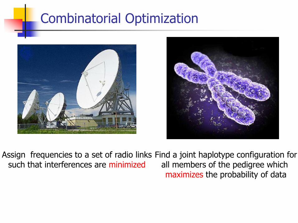
Combinatorial Optimization
Assign frequencies to a set of radio linkssuch that interferences are minimized
Find a joint haplotype configuration forall members of the pedigree which maximizes the probability of data
6
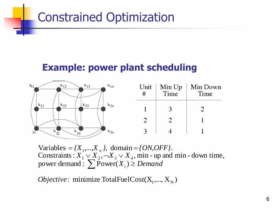
Constrained Optimization
Example: power plant scheduling
)X,...,ost(XTotalFuelC minimize :
)(Power : demandpower time,down-min and up-min ,, :sConstraint
. domain ,Variables
N1
4321
1
Objective
DemandXXXXX
{ON,OFF}},...,X{X
i
n
7
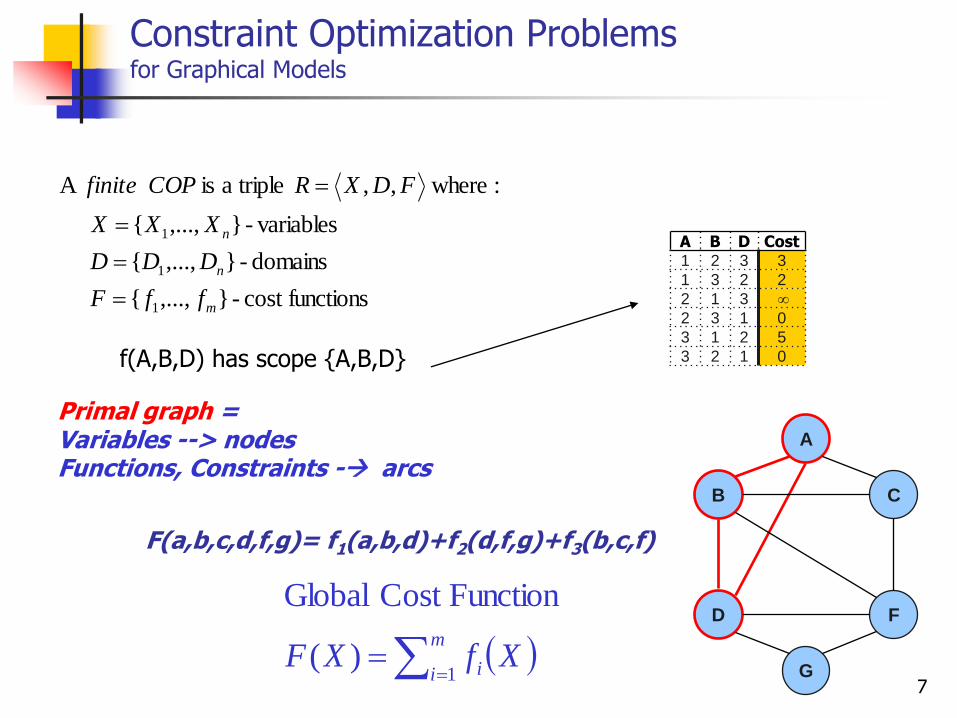
Constraint Optimization Problemsfor Graphical Models
functionscost - },...,{
domains - },...,{
variables- },...,{
:where,, triplea is A
1
1
1
m
n
n
ffF
DDD
XXX
FDXRCOPfinite
A B D Cost1 2 3 3
1 3 2 2
2 1 3
2 3 1 0
3 1 2 5
3 2 1 0
G
A
B C
D F
m
i i XfXF1
)(
FunctionCost Global
Primal graph =Variables --> nodesFunctions, Constraints - arcs
f(A,B,D) has scope {A,B,D}
F(a,b,c,d,f,g)= f1(a,b,d)+f2(d,f,g)+f3(b,c,f)

8
A Bred green
red yellow
green red
green yellow
yellow green
yellow red
Map coloring
Variables: countries (A B C etc.)
Values: colors (red green blue)
Constraints: etc. ,ED D, AB,A
C
A
B
D
E
F
G
Constraint Networks
Constraint graph
A
B
D
C
GF
E

9
A Bred green 0
red yellow 0
green red 0
green yellow 0
yellow green 0
yellow red 0
Others
Map coloring
Variables: countries (A B C etc.)
Values: colors (red green blue)
Constraints: etc. ,ED D, AB,A
C
A
B
D
E
F
G
Constraint Networks
Constraint graph
A
B
D
C
GF
E
10
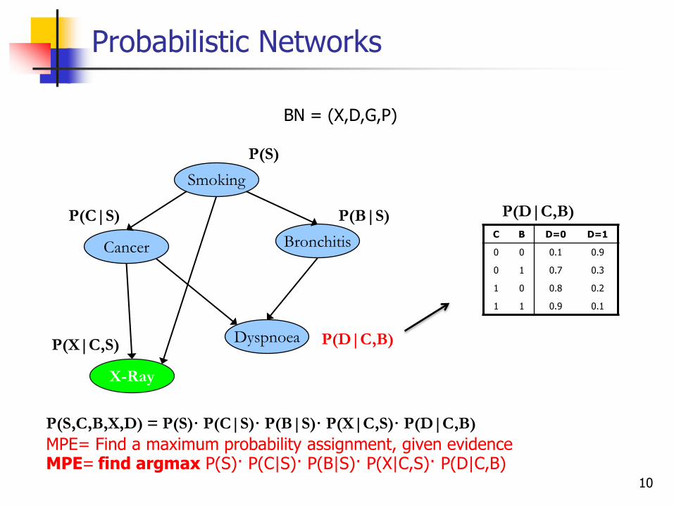
Probabilistic Networks
Smoking
BronchitisCancer
X-Ray
Dyspnoea
P(S)
P(B|S)
P(D|C,B)
P(C|S)
P(X|C,S)
P(S,C,B,X,D) = P(S)· P(C|S)· P(B|S)· P(X|C,S)· P(D|C,B)
MPE= Find a maximum probability assignment, given evidenceMPE= find argmax P(S)· P(C|S)· P(B|S)· P(X|C,S)· P(D|C,B)
C B D=0 D=1
0 0 0.1 0.9
0 1 0.7 0.3
1 0 0.8 0.2
1 1 0.9 0.1
P(D|C,B)
BN = (X,D,G,P)
11
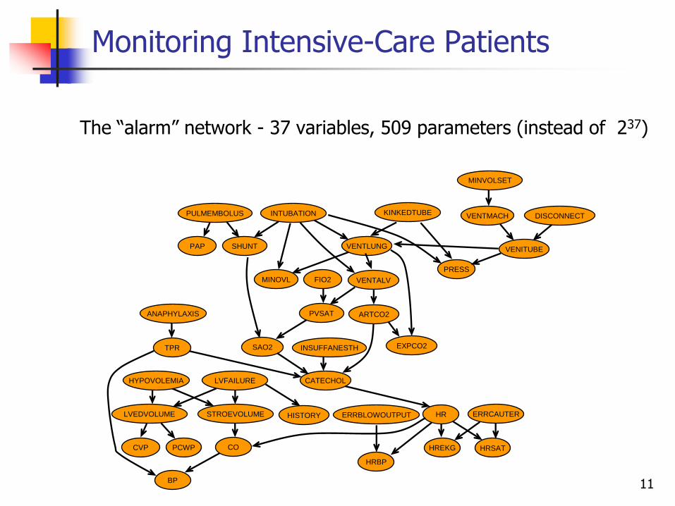
Monitoring Intensive-Care Patients
The ―alarm‖ network - 37 variables, 509 parameters (instead of 237)
PCWP CO
HRBP
HREKG HRSAT
ERRCAUTERHRHISTORY
CATECHOL
SAO2 EXPCO2
ARTCO2
VENTALV
VENTLUNG VENITUBE
DISCONNECT
MINVOLSET
VENTMACHKINKEDTUBEINTUBATIONPULMEMBOLUS
PAP SHUNT
ANAPHYLAXIS
MINOVL
PVSAT
FIO2
PRESS
INSUFFANESTHTPR
LVFAILURE
ERRBLOWOUTPUTSTROEVOLUMELVEDVOLUME
HYPOVOLEMIA
CVP
BP

21? ?? ?
A aB b
A AB b
3 4A | ?B | ?
? ?? ?
5 6A | aB | b •6 individuals
•Haplotype: {2, 3}• Genotype: {6}• Unknown
Linkage Analysis
13
L11m L11f
X11
L12m L12f
X12
L13m L13f
X13
L14m L14f
X14
L15m L15f
X15
L16m L16f
X16
S13m
S15m
S16mS15m
S15m
S15m
L21m L21f
X21
L22m L22f
X22
L23m L23f
X23
L24m L24f
X24
L25m L25f
X25
L26m L26f
X26
S23m
S25m
S26mS25m
S25m
S25m
L31m L31f
X31
L32m L32f
X32
L33m L33f
X33
L34m L34f
X34
L35m L35f
X35
L36m L36f
X36
S33m
S35m
S36mS35m
S35m
S35m
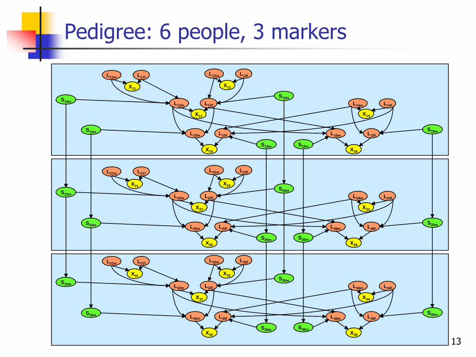
Pedigree: 6 people, 3 markers
14
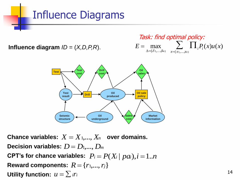
Influence Diagrams
Influence diagram ID = (X,D,P,R).
Chance variables: over domains.
Decision variables:
CPT’s for chance variables:
Reward components:
Utility function: iiru
},...,{ 1 jrrR
nipaXPP iii ..1),|(
mDDD ,...,1
nXXX ,...,1
)()(max)1)1 ,...,(,...,(
xuxPE iixxx nm
Task: find optimal policy:
Test
DrillOil sale
policy
Test
result
Seismic
structure
Oil
underground
Oil
produced
Test
cost
Drill
cost
Sales
cost
Oil
sales
Market
information

15
A graphical model (X,D,F): X = {X1,…Xn} variables
D = {D1, … Dn} domains
F = {f1,…,fm} functions(constraints, CPTS, CNFs …)
Operators: combination
elimination (projection)
Tasks: Belief updating: X-y j Pi
MPE: maxX j Pj
CSP: X j Cj
Max-CSP: minX j fj
Graphical Models
)( : CAFfi
A
D
BC
E
F
All these tasks are NP-hard
exploit problem structure
identify special cases
approximate
A C F P(F|A,C)
0 0 0 0.14
0 0 1 0.96
0 1 0 0.40
0 1 1 0.60
1 0 0 0.35
1 0 1 0.65
1 1 0 0.72
1 1 1 0.68
Primal graph(interaction graph)
A C F
red green blue
blue red red
blue blue green
green red blue
Relation
16
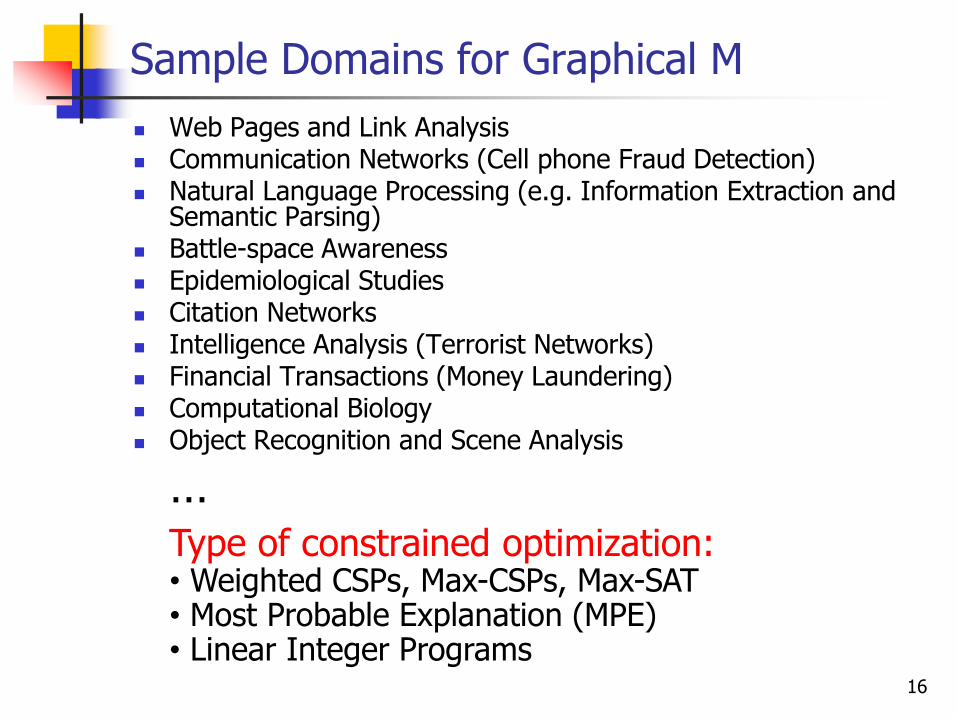
Sample Domains for Graphical M
Web Pages and Link Analysis Communication Networks (Cell phone Fraud Detection) Natural Language Processing (e.g. Information Extraction and
Semantic Parsing) Battle-space Awareness Epidemiological Studies Citation Networks Intelligence Analysis (Terrorist Networks) Financial Transactions (Money Laundering) Computational Biology Object Recognition and Scene Analysis
…Type of constrained optimization:• Weighted CSPs, Max-CSPs, Max-SAT• Most Probable Explanation (MPE) • Linear Integer Programs
17
Outline
Introduction Graphical models Optimization tasks for graphical models Solving optimization problems by inference and search
Inference Search (OR)
Lower-bounds and relaxations Exploiting problem structure in search Software
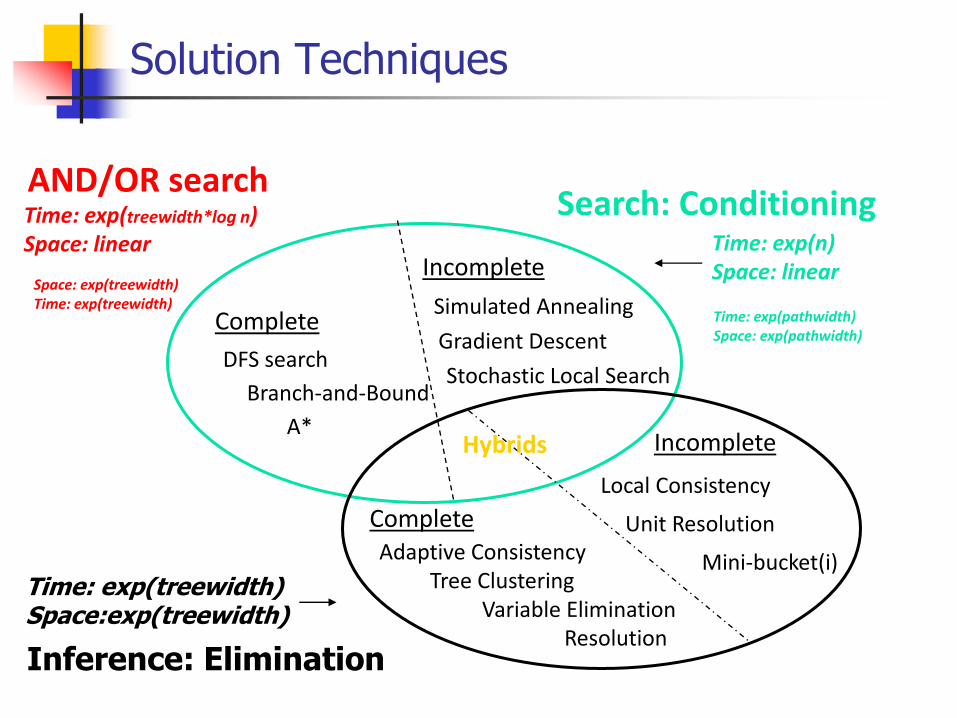
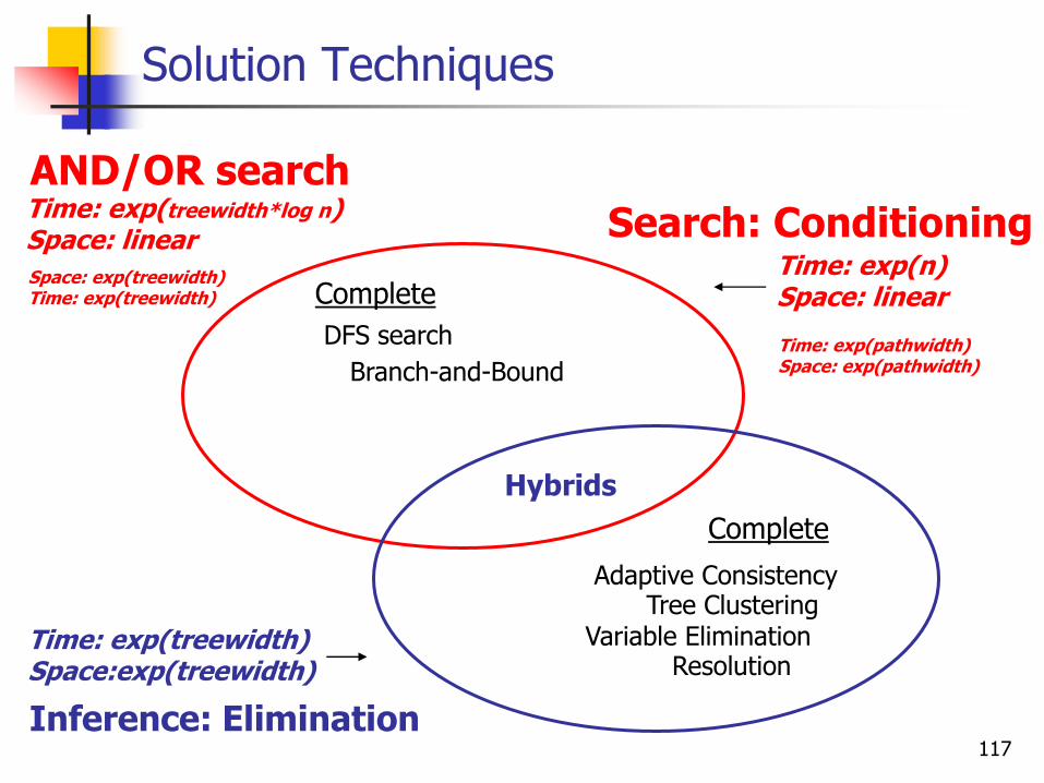
Solution Techniques
Search: Conditioning
Complete
Incomplete
Simulated Annealing
Gradient Descent
Complete
Incomplete
Adaptive ConsistencyTree Clustering
Variable EliminationResolution
Local Consistency
Unit Resolution
Mini-bucket(i)
Stochastic Local SearchDFS search
Branch-and-Bound
A*
Inference: Elimination
Time: exp(treewidth)Space:exp(treewidth)
Time: exp(n)Space: linear
AND/OR searchTime: exp(treewidth*log n)Space: linear
Hybrids
Space: exp(treewidth)Time: exp(treewidth)
Time: exp(pathwidth)Space: exp(pathwidth)
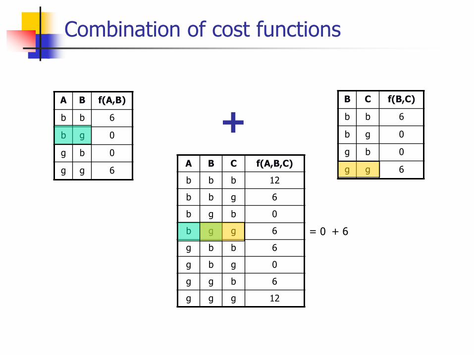
Combination of cost functions
A B f(A,B)
b b 6
b g 0
g b 0
g g 6
B C f(B,C)
b b 6
b g 0
g b 0
g g 6A B C f(A,B,C)
b b b 12
b b g 6
b g b 0
b g g 6
g b b 6
g b g 0
g g b 6
g g g 12
+
= 0 + 6
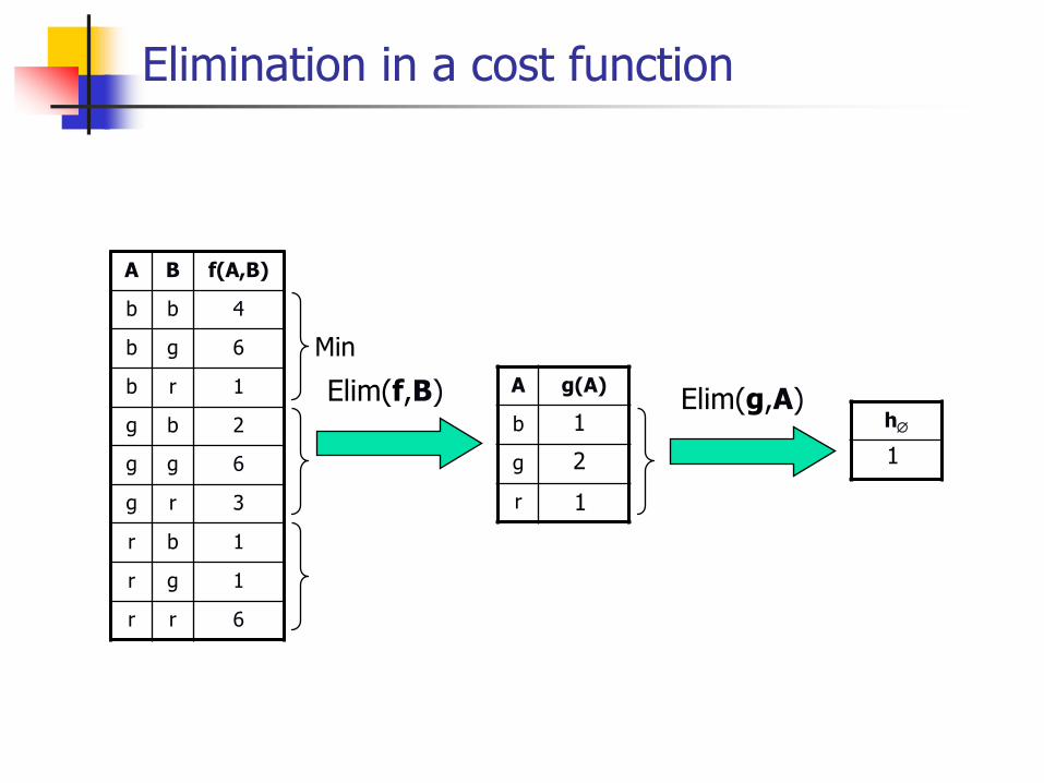
Elimination in a cost function
A B f(A,B)
b b 4
b g 6
b r 1
g b 2
g g 6
g r 3
r b 1
r g 1
r r 6
Elim(f,B) A g(A)
b
g
r
1
1
2
Elim(g,A)h
1
Min
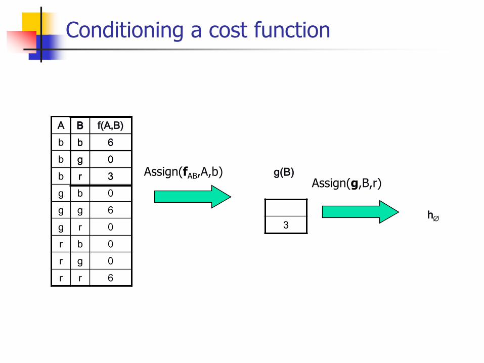
Conditioning a cost function
A B f(A,B)
b b 6
b g 0
b r 3
g b 0
g g 6
g r 0
r b 0
r g 0
r r 6
Assign(fAB,A,b)
B
b 6
g 0
r 3 g(B)Assign(g,B,r)
0
3h

22
Conditioning vs. Elimination
A
G
B
C
E
D
F
Conditioning (search) Elimination (inference)
A=1 A=k…
G
B
C
E
D
F
G
B
C
E
D
F
A
G
B
C
E
D
F
G
B
C
E
D
F
k ―sparser‖ problems 1 ―denser‖ problem
23
Outline
Introduction
Inference Variable Elimination, Bucket Elimination
Search (OR)
Lower-bounds and relaxations Exploiting problem structure in search Software

24
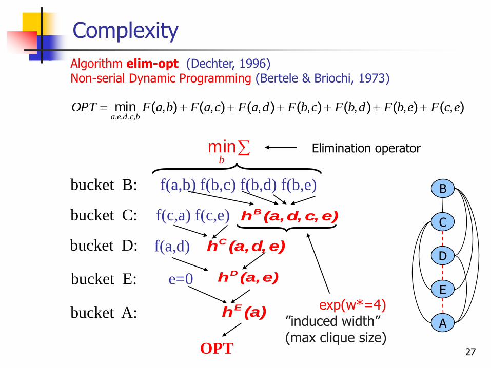
Computing the Optimal Cost Solution
0emin
Constraint graph
A
D E
CBB C
ED
Variable Elimination
bcde ,,,min0
f(a,b)+f(a,c)+f(a,d)+f(b,c)+f(b,d)+f(b,e)+f(c,e)OPT =
f(a,c)+f(c,e) +c
min
),,,( ecdahB
f(a,b)+f(b,c)+f(b,d)+f(b,e)b
mind
min f(a,d) +
Combination
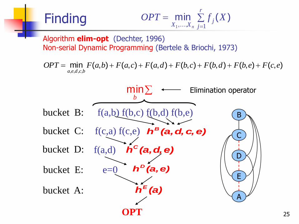
25
Elimination operator
OPT
bucket B:
f(c,a) f(c,e)
f(a,b) f(b,c) f(b,d) f(b,e)
bucket C:
bucket D:
bucket E:
bucket A:
e=0
(a)hE
e)c,d,(a,hB
e)d,(a,hC
Finding
b
min
r
jj
XXXfOPT
n 11
)(min,...,
Algorithm elim-opt (Dechter, 1996)Non-serial Dynamic Programming (Bertele & Briochi, 1973)
B
C
D
E
A
f(a,d)
e)(a,hD
),(),(),(),(),(),(),(min,,,,
ecFebFdbFcbFdaFcaFbaFOPTbcdea
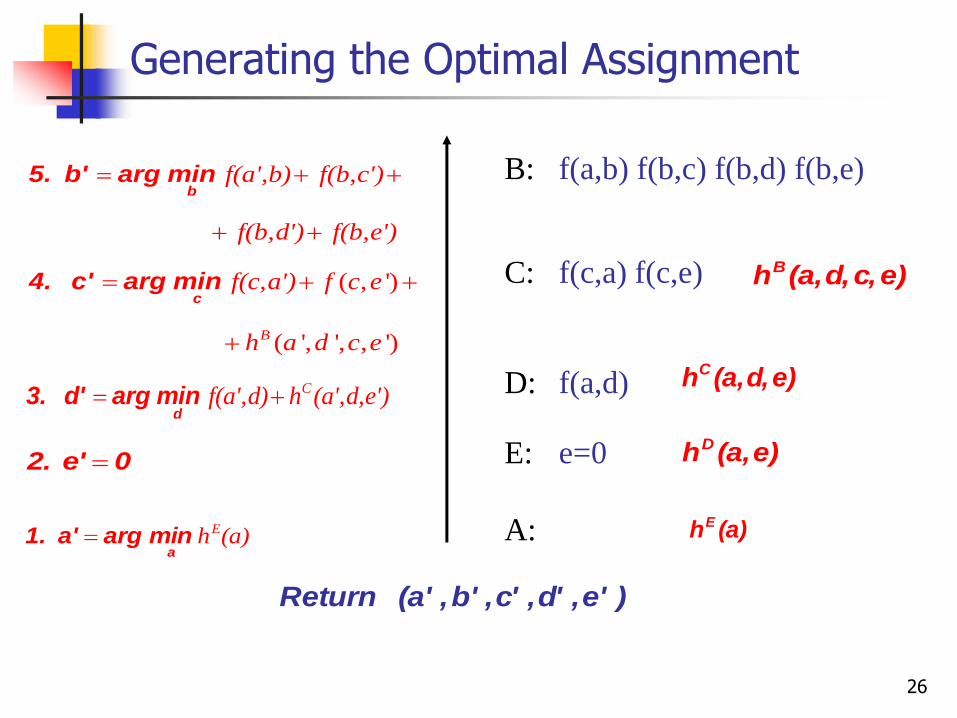
26
Generating the Optimal Assignment
C:
E:
f(a,b) f(b,c) f(b,d) f(b,e)B:
D:
A:
f(c,a) f(c,e)
e=0 e)(a,hD
(a)hE
e)c,d,(a,hB
e)d,(a,hC
(a)hE
amin arga' 1.
0e' 2.
Cf(a',d) h (a',d,e') d
3. d' arg min
( , ')
( ', ', , ')B
f(c,a') f c e
h a d c e
c4. c' arg min
f(a',b) f(b,c')
f(b,d') f(b,e')
b5. b' arg min
)e',d',c',b',(a' Return
f(a,d)
27
exp(w*=4)‖induced width‖ (max clique size)
Complexity
Elimination operator
OPT
bucket B:
f(c,a) f(c,e)
f(a,b) f(b,c) f(b,d) f(b,e)
bucket C:
bucket D:
bucket E:
bucket A:
e=0
(a)hE
e)c,d,(a,hB
e)d,(a,hC
b
min
B
C
D
E
A
f(a,d)
e)(a,hD
Algorithm elim-opt (Dechter, 1996)Non-serial Dynamic Programming (Bertele & Briochi, 1973)
),(),(),(),(),(),(),(min,,,,
ecFebFdbFcbFdaFcaFbaFOPTbcdea
29
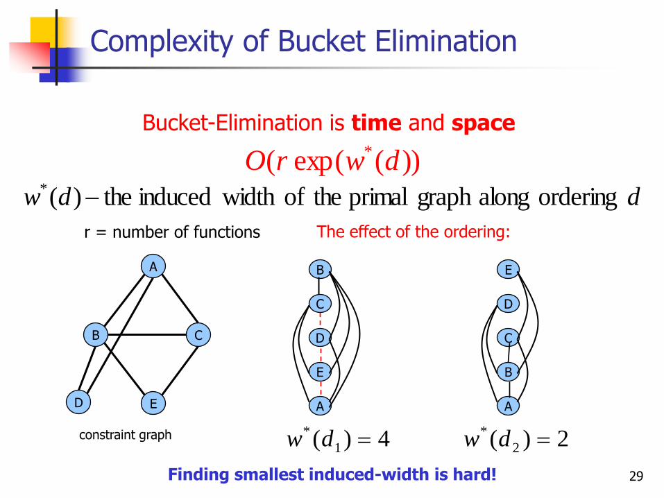
Complexity of Bucket Elimination
))((exp ( * dwrO
ddw ordering alonggraph primal theof width induced the)(*
The effect of the ordering:
4)( 1
* dw 2)( 2
* dwconstraint graph
A
D E
CB
B
C
D
E
A
E
D
C
B
A
Finding smallest induced-width is hard!
r = number of functions
Bucket-Elimination is time and space
30
Outline
Introduction Inference
Search (OR)
Branch-and-Bound and Best-First search
Lower-bounds and relaxations Exploiting problem structure in search Software

31
The Search Space
9
1
mini
iX ff
A
E
C
B
F
D
0 1 0 1 0 1 0 1
0 1 0 1 0 1 0 1 0 1 0 1 0 1 0 1
0 1 0 1 0 1 0 1 0 1 0 1 0 1 0 1 0 1 0 1 0 1 0 1 0 1 0 1 0 1 0 1 0 1 0 1 0 1 0 1 0 1 0 1 0 1 0 1 0 1 0 1 0 1 0 1 0 1 0 1 0 1 0 1
0 1 0 1 0 1 0 1 0 1 0 1 0 1 0 1 0 1 0 1 0 1 0 1 0 1 0 1 0 1 0 1
0 1 0 1
C
D
F
E
B
A 0 1
Objective function:
A B f10 0 20 1 01 0 11 1 4
A C f20 0 30 1 01 0 01 1 1
A E f30 0 00 1 31 0 21 1 0
A F f40 0 20 1 01 0 01 1 2
B C f50 0 00 1 11 0 21 1 4
B D f60 0 40 1 21 0 11 1 0
B E f70 0 30 1 21 0 11 1 0
C D f80 0 10 1 41 0 01 1 0
E F f90 0 10 1 01 0 01 1 2
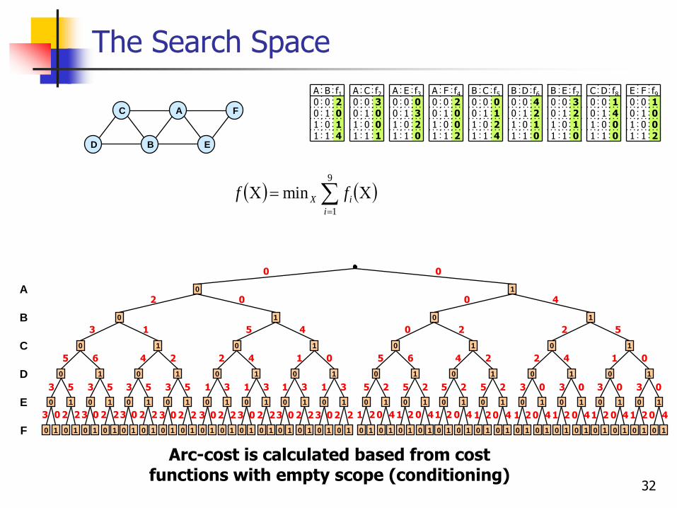
32
The Search Space
Arc-cost is calculated based from cost functions with empty scope (conditioning)
0 1 0 1 0 1 0 1
0 1 0 1 0 1 0 1 0 1 0 1 0 1 0 1
0 1 0 1 0 1 0 1 0 1 0 1 0 1 0 1 0 1 0 1 0 1 0 1 0 1 0 1 0 1 0 1 0 1 0 1 0 1 0 1 0 1 0 1 0 1 0 1 0 1 0 1 0 1 0 1 0 1 0 1 0 1 0 1
0 1 0 1 0 1 0 1 0 1 0 1 0 1 0 1 0 1 0 1 0 1 0 1 0 1 0 1 0 1 0 1
0 1 0 1
C
D
F
E
B
A 0 1
A B f10 0 20 1 01 0 11 1 4
A
E
C
B
F
D
A C f20 0 30 1 01 0 01 1 1
A E f30 0 00 1 31 0 21 1 0
A F f40 0 20 1 01 0 01 1 2
B C f50 0 00 1 11 0 21 1 4
B D f60 0 40 1 21 0 11 1 0
B E f70 0 30 1 21 0 11 1 0
C D f80 0 10 1 41 0 01 1 0
E F f90 0 10 1 01 0 01 1 2
3 0 2 2 3 0 2 23 0 2 2 3 0 2 2 3 0 2 2 3 0 2 23 0 2 2 3 0 2 2
0 0
3 5 3 5 3 5 3 5 1 3 1 3 1 3 1 3
5 6 4 2 2 4 1 0
3 1
2
5 4
0
1 2 0 4 1 2 0 41 2 0 4 1 2 0 4 1 2 0 4 1 2 0 41 2 0 4 1 2 0 4
5 2 5 2 5 2 5 2 3 0 3 0 3 0 3 0
5 6 4 2 2 4 1 0
0 2 2 5
0 4
9
1
mini
iX ff
33
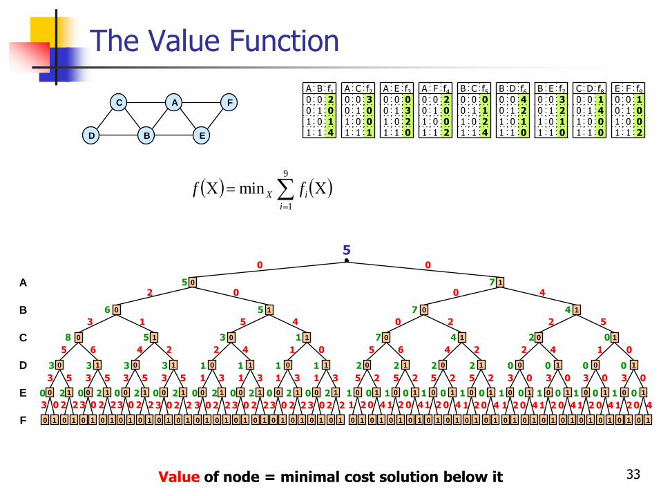
The Value Function
Value of node = minimal cost solution below it
0 1 0 1 0 1 0 1
0 1 0 1 0 1 0 1 0 1 0 1 0 1 0 1
0 1 0 1 0 1 0 1 0 1 0 1 0 1 0 1 0 1 0 1 0 1 0 1 0 1 0 1 0 1 0 1 0 1 0 1 0 1 0 1 0 1 0 1 0 1 0 1 0 1 0 1 0 1 0 1 0 1 0 1 0 1 0 1
0 1 0 1 0 1 0 1 0 1 0 1 0 1 0 1 0 1 0 1 0 1 0 1 0 1 0 1 0 1 0 1
0 1 0 1
C
D
F
E
B
A 0 1
A B f10 0 20 1 01 0 11 1 4
A
E
C
B
F
D
A C f20 0 30 1 01 0 01 1 1
A E f30 0 00 1 31 0 21 1 0
A F f40 0 20 1 01 0 01 1 2
B C f50 0 00 1 11 0 21 1 4
B D f60 0 40 1 21 0 11 1 0
B E f70 0 30 1 21 0 11 1 0
C D f80 0 10 1 41 0 01 1 0
E F f90 0 10 1 01 0 01 1 2
3 0
0
2 2
6
2
3
3 0 2 23 0 2 2 3 0 2 2 3 0 2 2 3 0 2 23 0 2 2 3 0 2 2
0 0 02 2 2 0 2 0 0 02 2 2
3 3 3 1 1 1 1
8 5 3 1
5
5
1 0 1 1 10 0 0 1 0 1 1 10 0 0
2 2 2 2 0 0 0 0
7 4 2 0
7 4
7
50 0
3 5 3 5 3 5 3 5 1 3 1 3 1 3 1 3
5 6 4 2 2 4 1 0
3 1
2
5 4
0
1 2 0 4 1 2 0 41 2 0 4 1 2 0 4 1 2 0 4 1 2 0 41 2 0 4 1 2 0 4
5 2 5 2 5 2 5 2 3 0 3 0 3 0 3 0
5 6 4 2 2 4 1 0
0 2 2 5
0 4
9
1
mini
iX ff
34
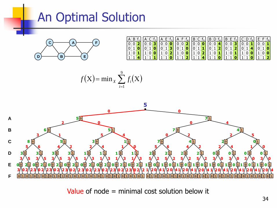
An Optimal Solution
Value of node = minimal cost solution below it
0 1 0 1 0 1 0 1
0 1 0 1 0 1 0 1 0 1 0 1 0 1 0 1
0 1 0 1 0 1 0 1 0 1 0 1 0 1 0 1 0 1 0 1 0 1 0 1 0 1 0 1 0 1 0 1 0 1 0 1 0 1 0 1 0 1 0 1 0 1 0 1 0 1 0 1 0 1 0 1 0 1 0 1 0 1 0 1
0 1 0 1 0 1 0 1 0 1 0 1 0 1 0 1 0 1 0 1 0 1 0 1 0 1 0 1 0 1 0 1
0 1 0 1
C
D
F
E
B
A 0 1
A B f10 0 20 1 01 0 11 1 4
A
E
C
B
F
D
A C f20 0 30 1 01 0 01 1 1
A E f30 0 00 1 31 0 21 1 0
A F f40 0 20 1 01 0 01 1 2
B C f50 0 00 1 11 0 21 1 4
B D f60 0 40 1 21 0 11 1 0
B E f70 0 30 1 21 0 11 1 0
C D f80 0 10 1 41 0 01 1 0
E F f90 0 10 1 01 0 01 1 2
3 0
0
2 2
6
2
3
3 0 2 23 0 2 2 3 0 2 2 3 0 2 2 3 0 2 23 0 2 2 3 0 2 2
0 0 02 2 2 0 2 0 0 02 2 2
3 3 3 1 1 1 1
8 5 3 1
5
5
1 0 1 1 10 0 0 1 0 1 1 10 0 0
2 2 2 2 0 0 0 0
7 4 2 0
7 4
7
50 0
3 5 3 5 3 5 3 5 1 3 1 3 1 3 1 3
5 6 4 2 2 4 1 0
3 1
2
5 4
0
1 2 0 4 1 2 0 41 2 0 4 1 2 0 4 1 2 0 4 1 2 0 41 2 0 4 1 2 0 4
5 2 5 2 5 2 5 2 3 0 3 0 3 0 3 0
5 6 4 2 2 4 1 0
0 2 2 5
0 4
9
1
mini
iX ff
35
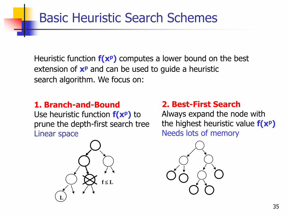
Basic Heuristic Search Schemes
Heuristic function f(xp) computes a lower bound on the best
extension of xp and can be used to guide a heuristic
search algorithm. We focus on:
1. Branch-and-BoundUse heuristic function f(xp) to prune the depth-first search treeLinear space
2. Best-First SearchAlways expand the node with the highest heuristic value f(xp)Needs lots of memory
f L
L

36
Classic Branch-and-Bound
n
g(n)
h(n) - under-estimatesOptimal cost below n
f(n) = g(n) + h(n)f(n) = lower bound
Prune if f(n) ≥ UB
(UB) Upper Bound = best solution so far
Each node is a COP subproblem(defined by current conditioning)
37
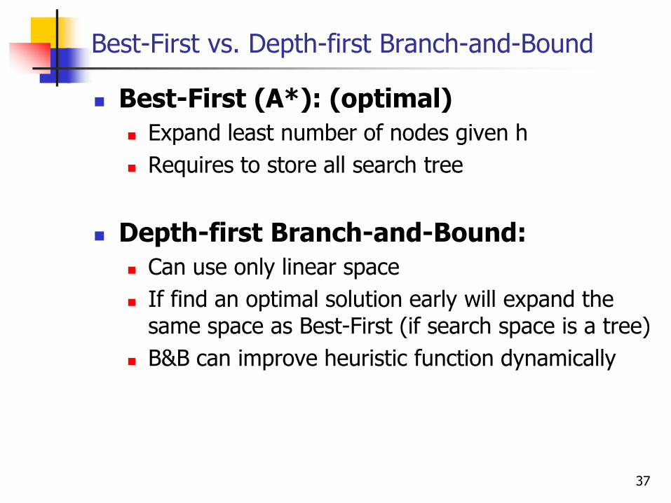
Best-First vs. Depth-first Branch-and-Bound
Best-First (A*): (optimal)
Expand least number of nodes given h
Requires to store all search tree
Depth-first Branch-and-Bound:
Can use only linear space
If find an optimal solution early will expand the same space as Best-First (if search space is a tree)
B&B can improve heuristic function dynamically
38
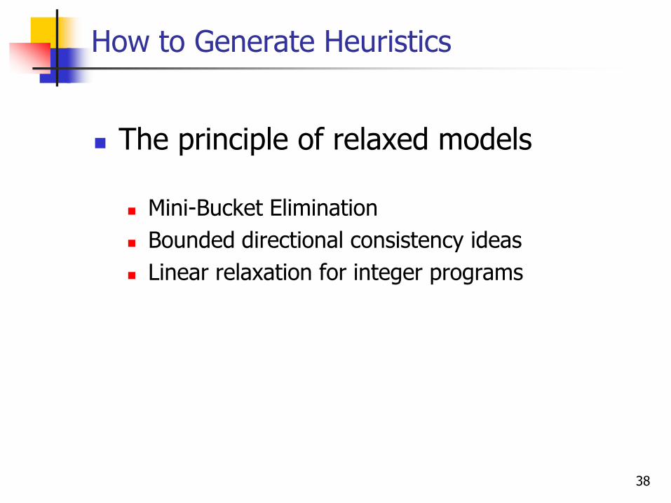
How to Generate Heuristics
The principle of relaxed models
Mini-Bucket Elimination
Bounded directional consistency ideas
Linear relaxation for integer programs

39
Outline
Introduction Inference Search (OR)
Lower-bounds and relaxations Bounded variable elimination
Mini-Bucket Elimination Generating heuristics using mini-bucket elimination
Local consistency
Exploiting problem structure in search Software
40
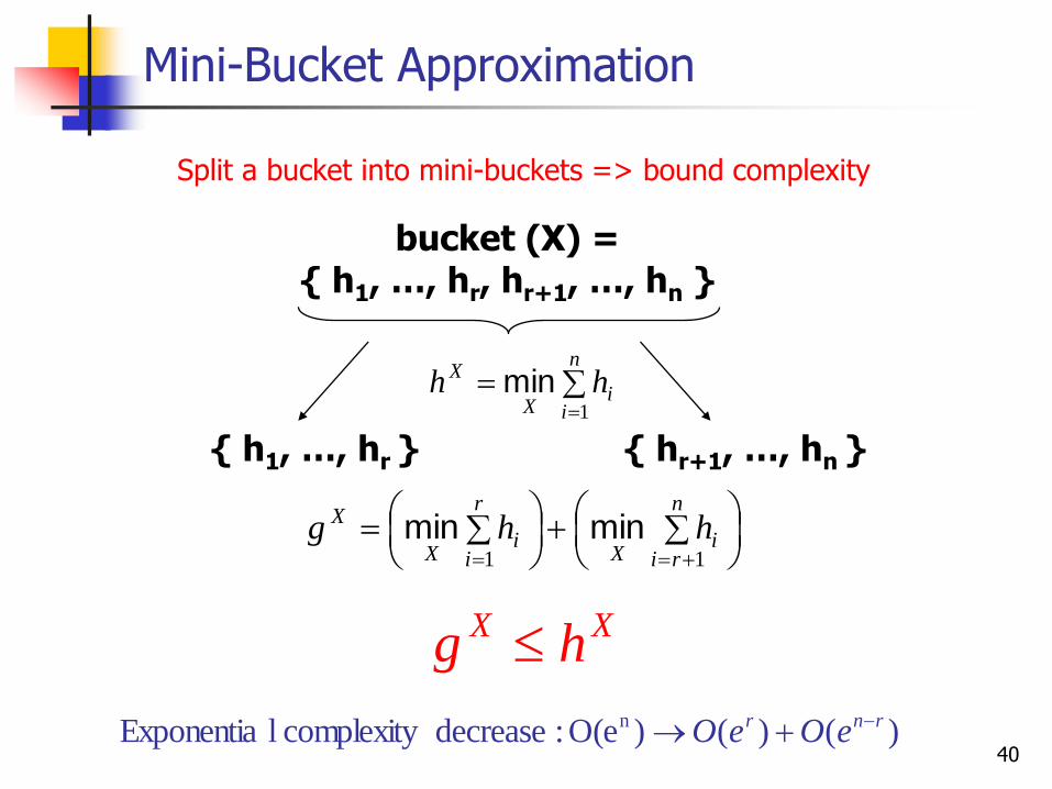
Mini-Bucket Approximation
n
ii
X
X hh1
min
n
rii
X
r
ii
X
X hhg11
minmin
Split a bucket into mini-buckets => bound complexity
)()()O(e :decrease complexity lExponentia n rnr eOeO
bucket (X) ={ h1, …, hr, hr+1, …, hn }
{ h1, …, hr } { hr+1, …, hn }
XX hg

41
Mini-Bucket Elimination
bucket A:
bucket E:
bucket D:
bucket C:
bucket B:
minBΣ
f(b,e)
f(a,d)
hE(a)
hB(e)
hB(a,d)
hD(a)
f(a,b) f(b,d)
f(c,e) f(a,c)
hC(e,a)
Lb = lower bound
Mini-buckets
A
B C
D E
42
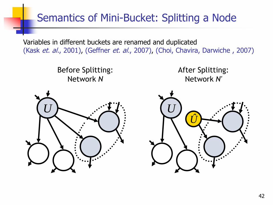
Semantics of Mini-Bucket: Splitting a Node
U UÛ
Before Splitting:
Network N
After Splitting:
Network N'
Variables in different buckets are renamed and duplicated (Kask et. al., 2001), (Geffner et. al., 2007), (Choi, Chavira, Darwiche , 2007)

4343
Mini-Bucket Elimination semantic
minBΣ
Mini-buckets
A
B C
D E
minBΣ
bucket A:
bucket E:
bucket D:
bucket C:
bucket B: F(a,b’)
F(a,d)
hE(a)
hB(a,c)
hB(d,e)
F(b,d) F(b,e)
F(c,e) F(a,c)
hC(e,a)
L = lower bound
F(b’,c)
hD(e,a)
A
B D
C
E
B’
44
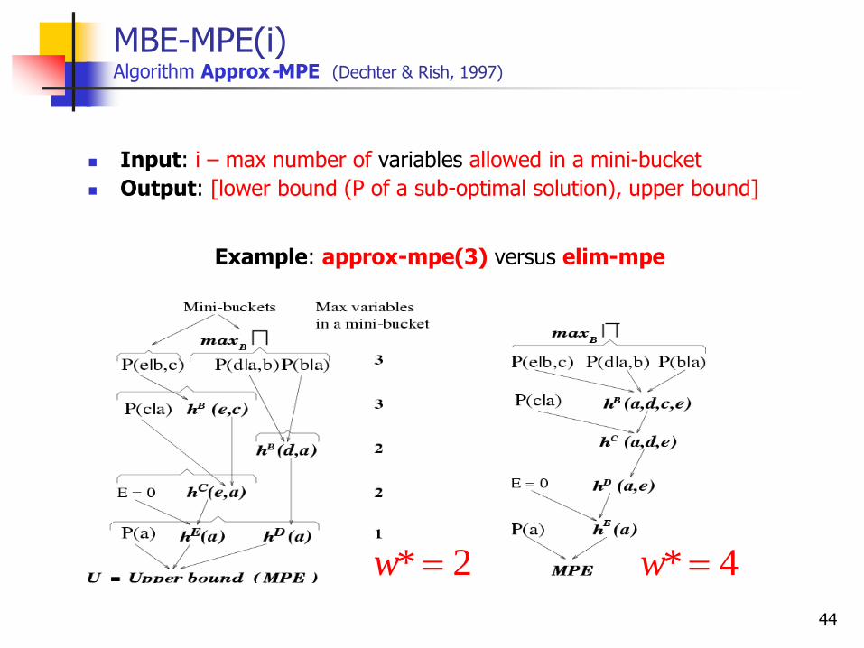
MBE-MPE(i) Algorithm Approx-MPE (Dechter & Rish, 1997)
Input: i – max number of variables allowed in a mini-bucket
Output: [lower bound (P of a sub-optimal solution), upper bound]
Example: approx-mpe(3) versus elim-mpe
2* w 4* w

45
Properties of MBE(i)
Complexity: O(r exp(i)) time and O(exp(i)) space
Yields an upper-bound and a lower-bound
Accuracy: determined by upper/lower (U/L) bound
As i increases, both accuracy and complexity increase
Possible use of mini-bucket approximations:
As anytime algorithms
As heuristics in search
Other tasks: similar mini-bucket approximations for:
Belief updating, MAP and MEU (Dechter & Rish, 1997)
46
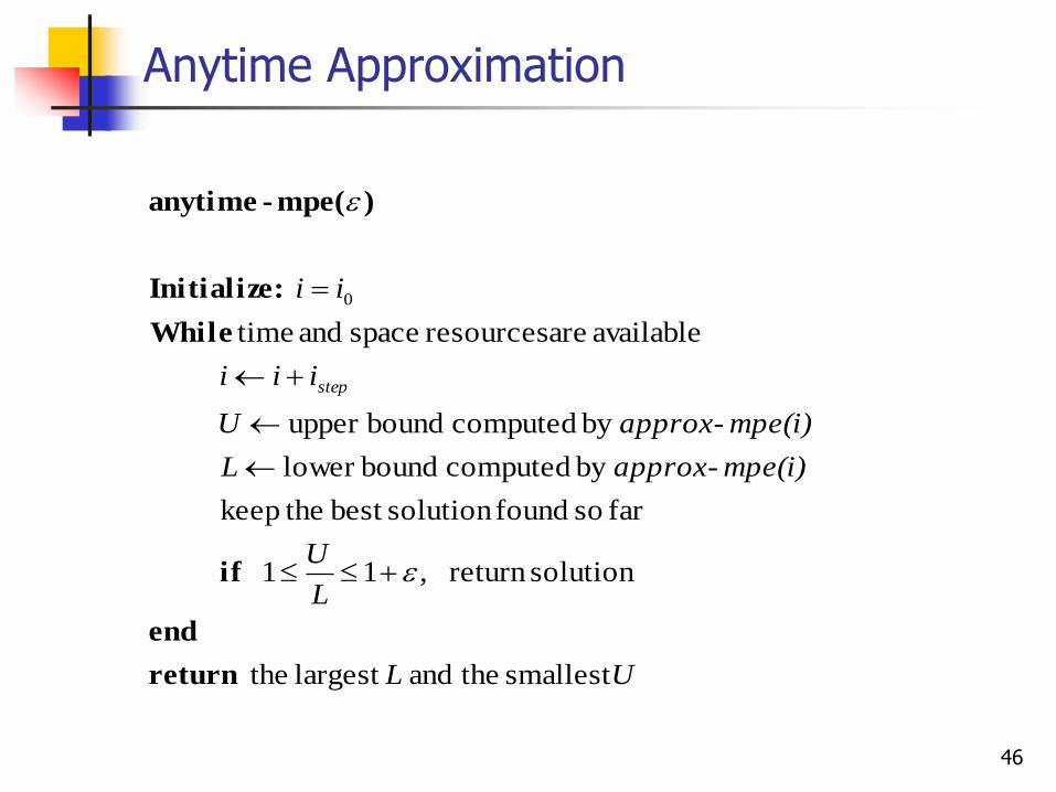
Anytime Approximation
UL
L
U
mpe(i)-approxL
mpe(i)-approxU
iii
ii
step
smallest theand largest the
solutionreturn ,11
far so foundsolution best thekeep
by computed boundlower
by computed boundupper
available are resources space and time
0
return
end
if
While
:Initialize
)mpe(-anytime

47
Empirical Evaluation(Rish & Dechter, 1999)
Benchmarks
Randomly generated networks
CPCS networks
Probabilistic decoding
Task
Comparing approx-mpe and anytime-mpeversus bucket-elimination (elim-mpe)
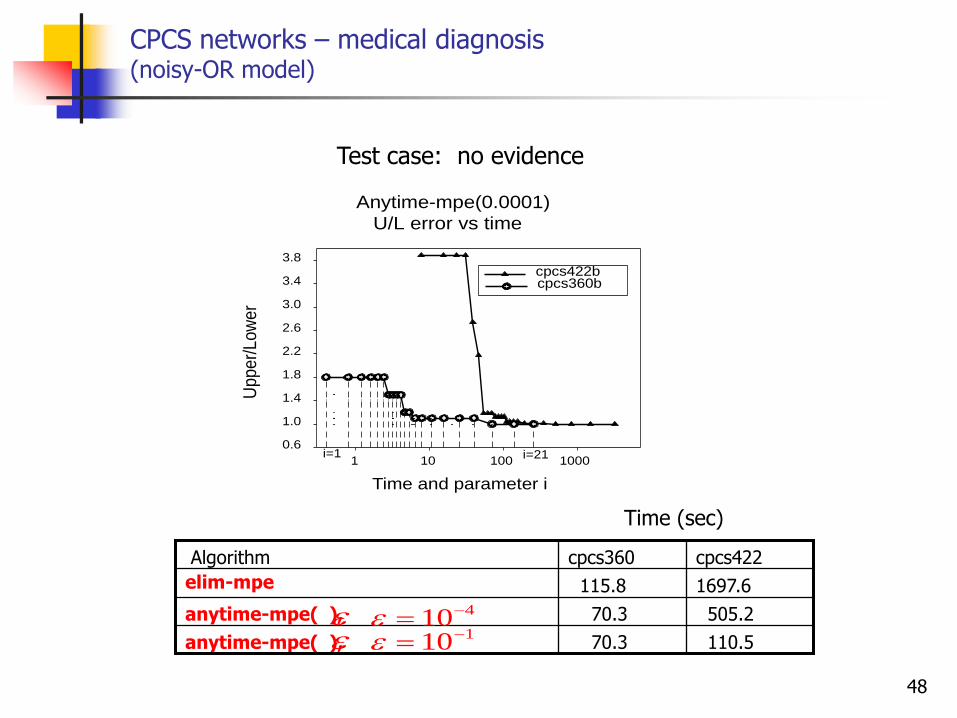
48
Anytime-mpe(0.0001)
U/L error vs time
Time and parameter i
1 10 100 1000
Upper/
Low
er
0.6
1.0
1.4
1.8
2.2
2.6
3.0
3.4
3.8
cpcs422b cpcs360b
i=1 i=21
CPCS networks – medical diagnosis(noisy-OR model)
Test case: no evidence
505.270.3anytime-mpe( ),
110.570.3anytime-mpe( ),
1697.6115.8elim-mpe
cpcs422 cpcs360 Algorithm
Time (sec)
410 110
49
Outline
Introduction Inference Search (OR)
Lower-bounds and relaxations Bounded variable elimination
Mini-Bucket Elimination Generating heuristics using mini-bucket elimination
Local consistency
Exploiting problem structure in search Software
50
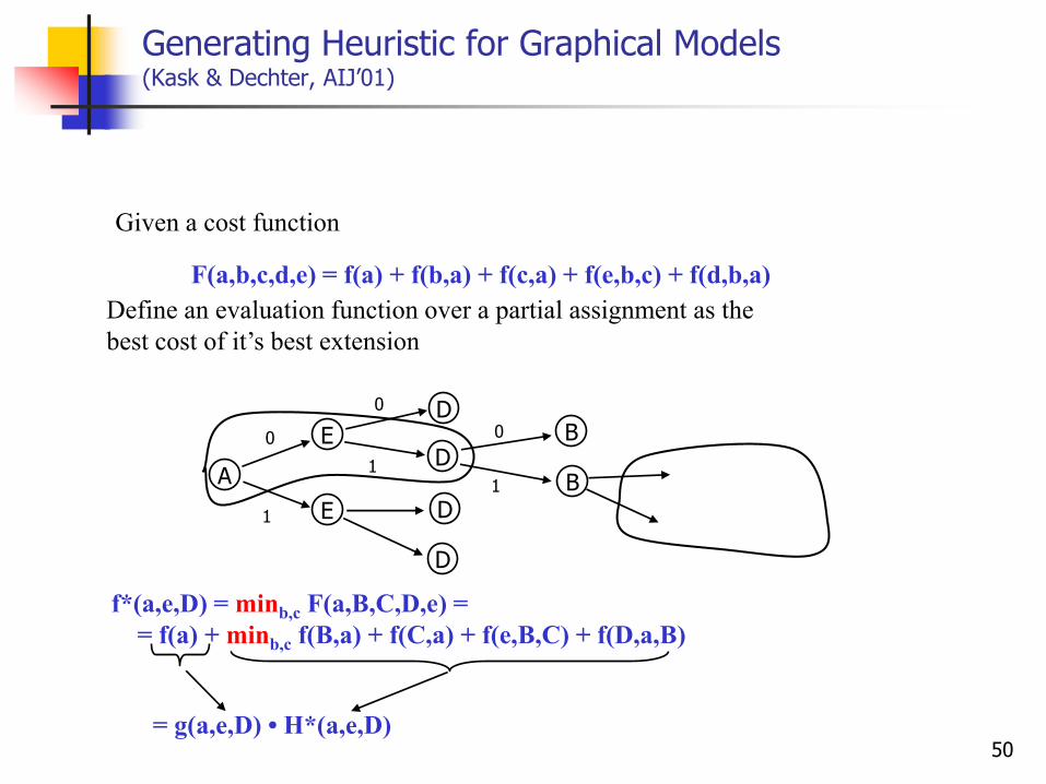
Generating Heuristic for Graphical Models(Kask & Dechter, AIJ’01)
Given a cost function
F(a,b,c,d,e) = f(a) + f(b,a) + f(c,a) + f(e,b,c) + f(d,b,a)
Define an evaluation function over a partial assignment as the
best cost of it’s best extension
f*(a,e,D) = minb,c F(a,B,C,D,e) =
= f(a) + minb,c f(B,a) + f(C,a) + f(e,B,C) + f(D,a,B)
= g(a,e,D) • H*(a,e,D)
D
E
E
DA
D
BD
B
0
1
1
0
1
0
51
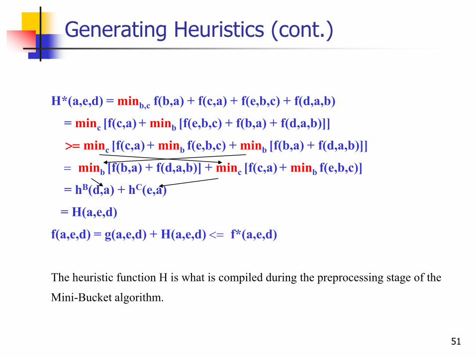
Generating Heuristics (cont.)
H*(a,e,d) = minb,c f(b,a) + f(c,a) + f(e,b,c) + f(d,a,b)
= minc [f(c,a) + minb [f(e,b,c) + f(b,a) + f(d,a,b)]]
> minc [f(c,a) + minb f(e,b,c) + minb [f(b,a) + f(d,a,b)]]
minb [f(b,a) + f(d,a,b)] + minc [f(c,a) + minb f(e,b,c)]
= hB(d,a) + hC(e,a)
= H(a,e,d)
f(a,e,d) = g(a,e,d) + H(a,e,d) < f*(a,e,d)
The heuristic function H is what is compiled during the preprocessing stage of the
Mini-Bucket algorithm.
52
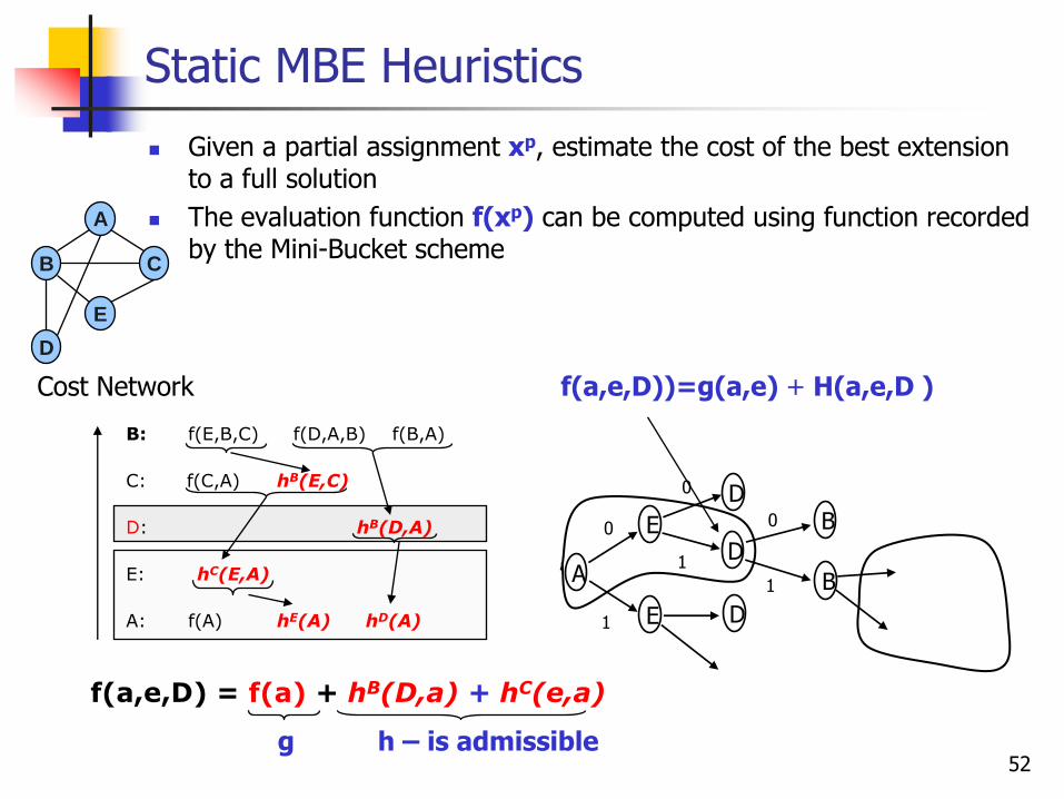
Static MBE Heuristics
Given a partial assignment xp, estimate the cost of the best extension to a full solution
The evaluation function f(xp) can be computed using function recorded by the Mini-Bucket scheme
B: f(E,B,C) f(D,A,B) f(B,A)
A:
E:
D:
C: f(C,A) hB(E,C)
hB(D,A)
hC(E,A)
f(A) hE(A) hD(A)
f(a,e,D) = f(a) + hB(D,a) + hC(e,a)
g h – is admissible
A
B C
D
E
Cost Network
E
E
DA
D
B
D
B
0
1
1
0
1
0
f(a,e,D))=g(a,e) + H(a,e,D )
53
Heuristics Properties
MB Heuristic is monotone, admissible
Computed in linear time
IMPORTANT:
Heuristic strength can vary by MB(i)
Higher i-bound more pre-processing stronger heuristic less search
Allows controlled trade-off between preprocessing and search
54
Experimental Methodology
Algorithms BBMB(i) - Branch-and-Bound with MB(i)
BBFB(i) - Best-First with MB(i)
MBE(i) – Mini-Bucket Elimination
Benchmarks Random Coding (Bayesian)
CPCS (Bayesian)
Random (CSP)
Measures of performance Compare accuracy given a fixed amount of time
i.e., how close is the cost found to the optimal solution
Compare trade-off performance as a function of time

55
Empirical Evaluation of Mini-Bucket heuristics:Random coding networks (Kask & Dechter, UAI’99, Aij 2000)
Time [sec]
0 10 20 30
% S
olv
ed E
xactly
0.0
0.1
0.2
0.3
0.4
0.5
0.6
0.7
0.8
0.9
1.0
BBMB i=2
BFMB i=2
BBMB i=6
BFMB i=6
BBMB i=10
BFMB i=10
BBMB i=14
BFMB i=14
Random Coding, K=100, noise=0.28 Random Coding, K=100, noise 0.32
Time [sec]
0 10 20 30
% S
olv
ed E
xactly
0.0
0.1
0.2
0.3
0.4
0.5
0.6
0.7
0.8
0.9
1.0
BBMB i=6
BFMB i=6
BBMB i=10
BFMB i=10
BBMB i=14
BFMB i=14
Random Coding, K=100, noise=0.32
Each data point represents an average over 100 random instances

56
Dynamic MB and MBTE Heuristics(Kask, Marinescu and Dechter, UAI’03)
Rather than pre-compile compute the heuristics during search
Dynamic MB: use the Mini-Bucket algorithm to produce a bound for any node during search
Dynamic MBTE: We can compute heuristics simultaneously for all un-instantiated variables using mini-bucket-tree elimination
MBTE is an approximation scheme defined over cluster-trees. It outputs multiple bounds for each variable and value extension at once
57
Branch-and-Bound w/ Mini-Buckets
BB with static Mini-Bucket Heuristics (s-BBMB)
Heuristic information is pre-compiled before search
Static variable ordering, prunes current variable
BB with dynamic Mini-Bucket Heuristics (d-BBMB)
Heuristic information is assembled during search
Static variable ordering, prunes current variable
BB with dynamic Mini-Bucket-Tree Heuristics (BBBT)
Heuristic information is assembled during search.
Dynamic variable ordering, prunes all future variables
58
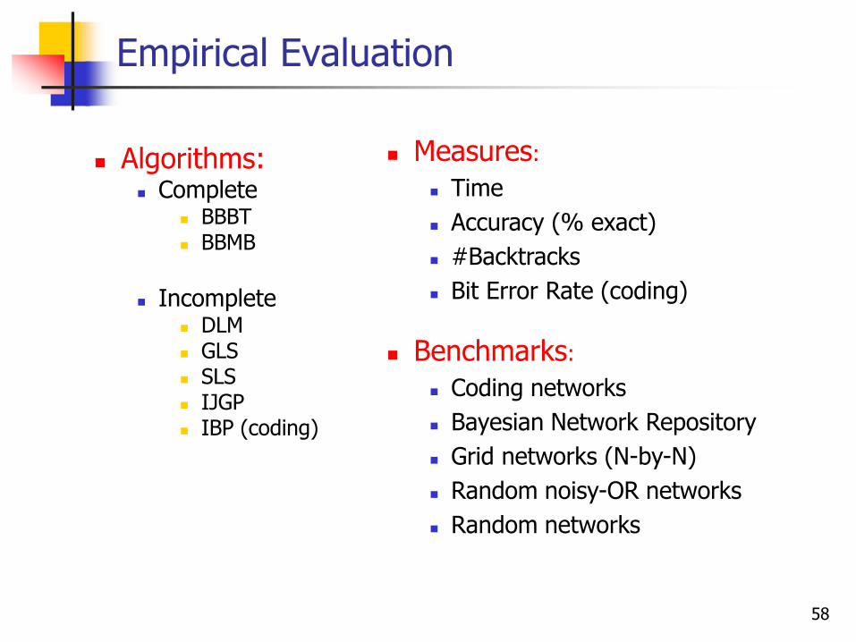
Empirical Evaluation
Algorithms: Complete
BBBT BBMB
Incomplete DLM GLS SLS IJGP IBP (coding)
Measures:
Time
Accuracy (% exact)
#Backtracks
Bit Error Rate (coding)
Benchmarks:
Coding networks
Bayesian Network Repository
Grid networks (N-by-N)
Random noisy-OR networks
Random networks
59
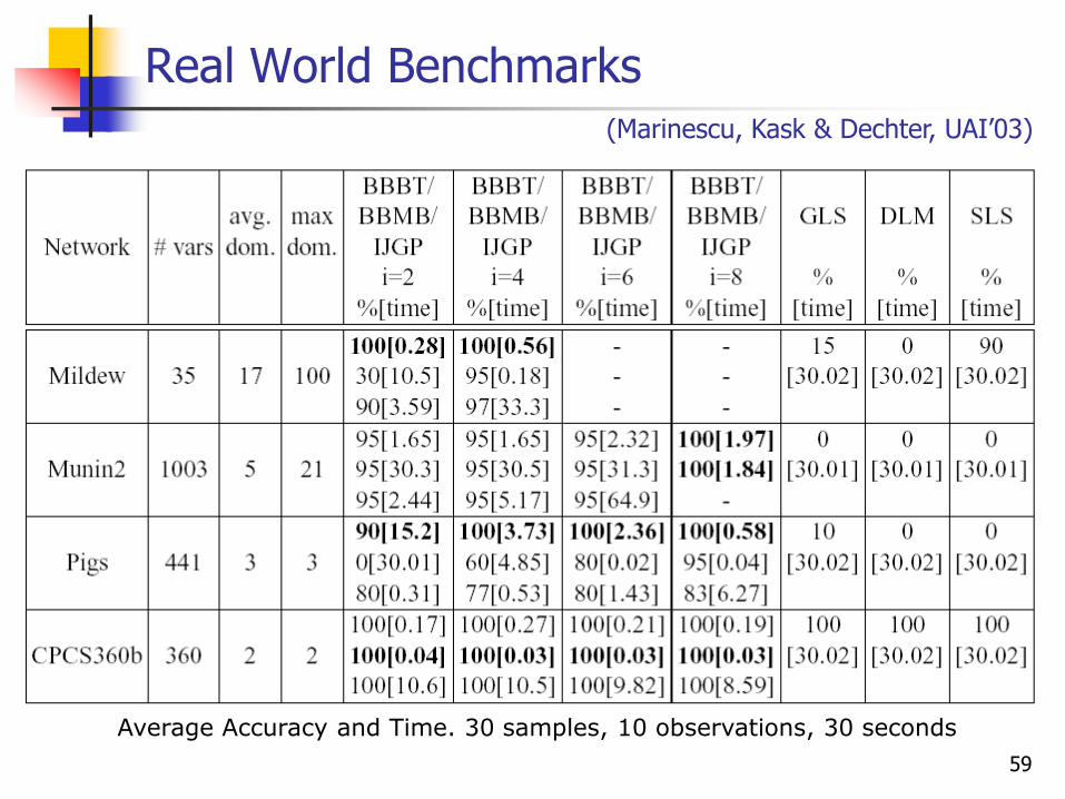
Real World Benchmarks
Average Accuracy and Time. 30 samples, 10 observations, 30 seconds
(Marinescu, Kask & Dechter, UAI’03)

Hybrid of Variable-elimination and Search
Tradeoff space and time
60
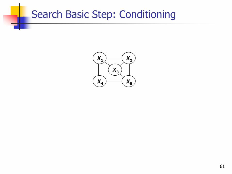
61
X1
X3
X5X4
X2
Search Basic Step: Conditioning

62
X1
X3
X5X4
X2• Select a variable
Search Basic Step: Conditioning
63
X1
X3
X5X4
X2
X3
X5X4
X2
X3
X5X4
X2
X3
X5X4
X2
…...
…...
X1 a
X1 b
X1 c
Search Basic Step: Conditioning
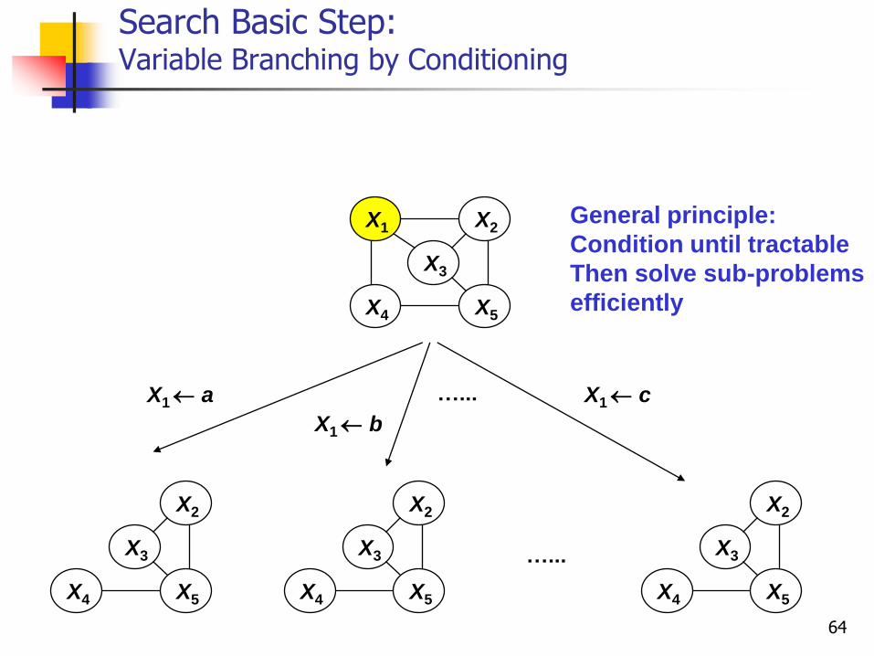
64
X1
X3
X5X4
X2
X3
X5X4
X2
X3
X5X4
X2
X3
X5X4
X2
…...
…...
X1 a
X1 b
X1 c
General principle:
Condition until tractable
Then solve sub-problems
efficiently
Search Basic Step: Variable Branching by Conditioning

65
X1
X3
X5X4
X2
X3
X5X4
X2
X3
X5X4
X2
X3
X5X4
X2
…...
…...
X1 a
X1 b
X1 c
Example: solve subproblem
by inference, BE(i=2)
Search Basic Step: Variable Branching by Conditioning
66
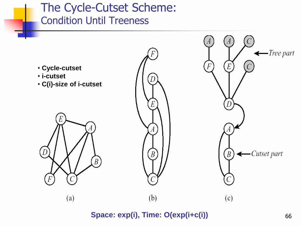
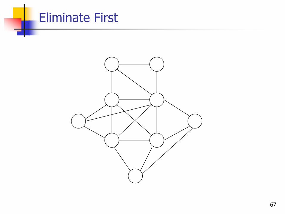
The Cycle-Cutset Scheme:Condition Until Treeness
• Cycle-cutset
• i-cutset
• C(i)-size of i-cutset
Space: exp(i), Time: O(exp(i+c(i))
67
Eliminate First
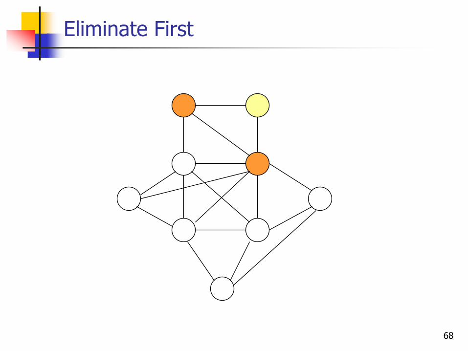
68
Eliminate First
69
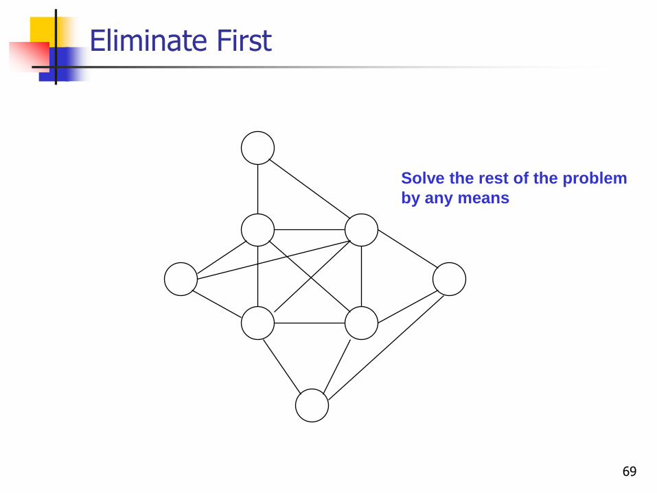
Eliminate First
Solve the rest of the problem
by any means
70
Hybrids Variants
Condition, condition, condition … and then only eliminate (w-cutset, cycle-cutset)
Eliminate, eliminate, eliminate … and then only search
Interleave conditioning and elimination (elim-cond(i), VE+C)

71
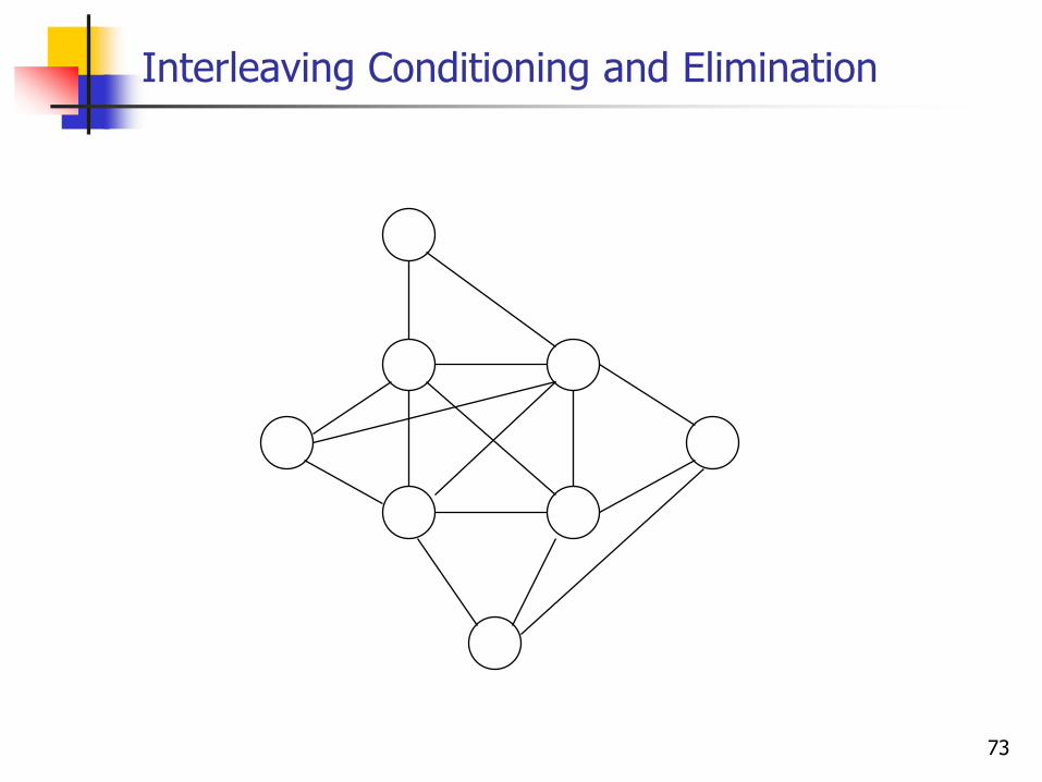
Interleaving Conditioning and Elimination(Larrosa & Dechter, CP’02)
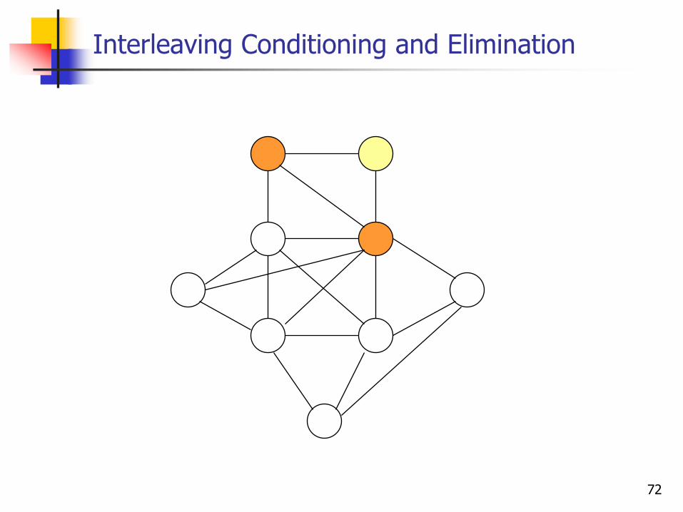
72
Interleaving Conditioning and Elimination
73
Interleaving Conditioning and Elimination

74
Interleaving Conditioning and Elimination

75
Interleaving Conditioning and Elimination

76
Interleaving Conditioning and Elimination
77
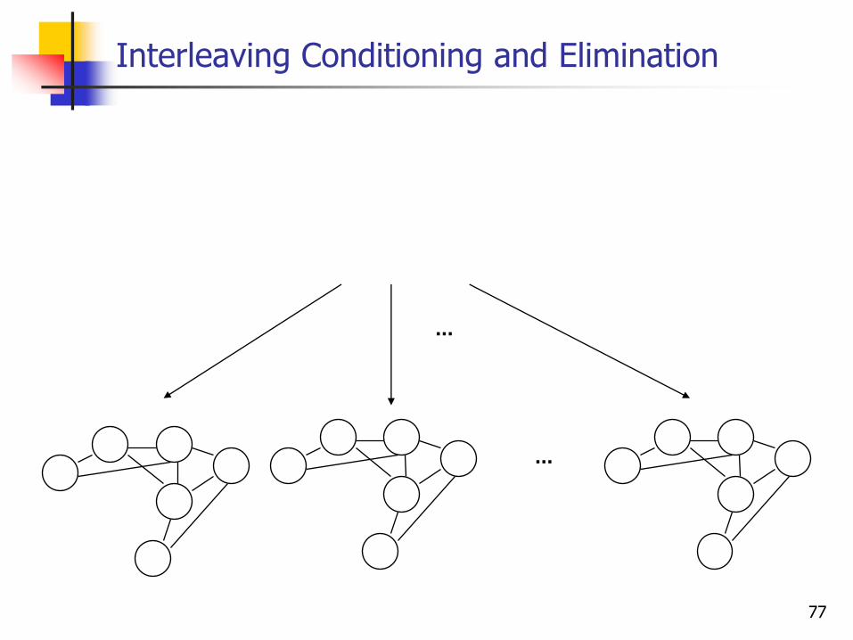
Interleaving Conditioning and Elimination
...
...
78
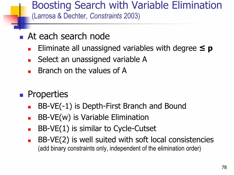
Boosting Search with Variable Elimination (Larrosa & Dechter, Constraints 2003)
At each search node
Eliminate all unassigned variables with degree ≤ p
Select an unassigned variable A
Branch on the values of A
Properties
BB-VE(-1) is Depth-First Branch and Bound
BB-VE(w) is Variable Elimination
BB-VE(1) is similar to Cycle-Cutset
BB-VE(2) is well suited with soft local consistencies(add binary constraints only, independent of the elimination order)

79
Mendelian error detection
Given a pedigree and partial observations (genotypings)
Find the erroneous genotypings, such that their removal restores consistency
Checking consistency is NP-complete (Aceto et al., Comp. Sci. Tech. 2004)
Minimize the number of genotypings to be removed
Maximize the joint probability of the true genotypes (MPE)
Pedigree problem size: n≤20,000 ; d=3—66 ; e(3)≤30,000
(Sanchez et al, Constraints 2008)
80
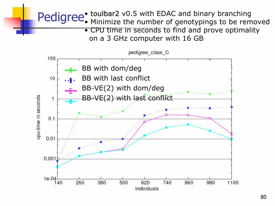
Pedigree
BB with dom/deg
BB with last conflict
BB-VE(2) with dom/deg
BB-VE(2) with last conflict
• toulbar2 v0.5 with EDAC and binary branching• Minimize the number of genotypings to be removed• CPU time in seconds to find and prove optimalityon a 3 GHz computer with 16 GB
81
Outline
Introduction Inference Search (OR)
Lower-bounds and relaxations Bounded variable elimination Local consistency
Equivalence Preserving Transformations Chaotic iteration of EPTs Optimal set of EPTs Improving sequence of EPTs
Exploiting problem structure in search Software

DepthFirst Branch and Bound (DFBB)
(LB) Lower Bound
(UB) Upper Bound
If UB then pruneVariable
s (d
ynam
ic o
rdering)
under estimation of the best solution in the sub-tree
= best solution so far
Each node is a COP subproblem(defined by current conditioning)
LBf
= f
= k
k
Obtained by enforcing local consistency
82
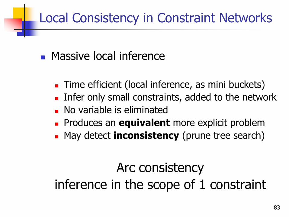
Local Consistency in Constraint Networks
Massive local inference
Time efficient (local inference, as mini buckets)
Infer only small constraints, added to the network
No variable is eliminated
Produces an equivalent more explicit problem
May detect inconsistency (prune tree search)
Arc consistency
inference in the scope of 1 constraint
83
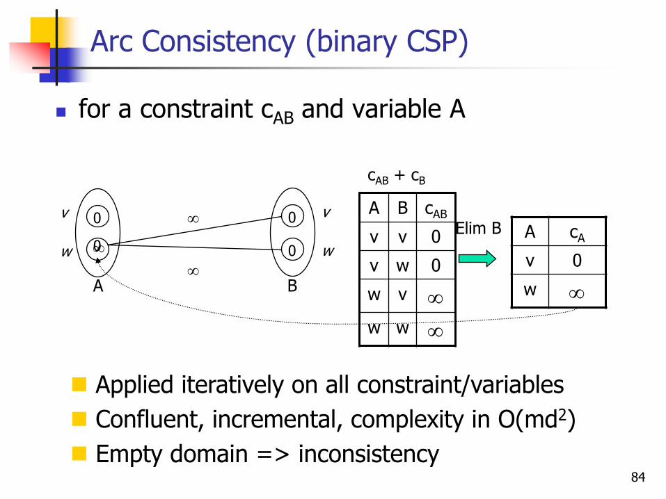
Arc Consistency (binary CSP)
for a constraint cAB and variable A
w
v v
w
0
0
0
0
A B
A B cAB
v v 0
v w 0
w v
w w
A cA
v 0
w
cAB + cB
Elim B
Applied iteratively on all constraint/variables
Confluent, incremental, complexity in O(md2)
Empty domain => inconsistency84
1
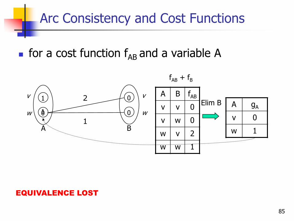
Arc Consistency and Cost Functions
for a cost function fAB and a variable A
w
v v
w
0
0
1
0
A B
2
1
A B fAB
v v 0
v w 0
w v 2
w w 1
A gA
v 0
w 1
fAB + fB
Elim B
EQUIVALENCE LOST
85
1
1
2
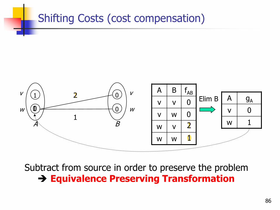
Subtract from source in order to preserve the problem Equivalence Preserving Transformation
Shifting Costs (cost compensation)
w
v v
w
0
0
1
A B1
0
A B fAB
v v 0
v w 0
w v
w w
A gA
v 0
w 11
0
2
1
Elim B
86
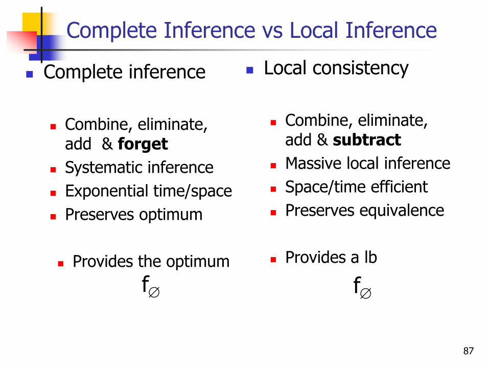
Complete Inference vs Local Inference
Local consistency
Combine, eliminate, add & subtract
Massive local inference
Space/time efficient
Preserves equivalence
Provides a lb
f
Complete inference
Combine, eliminate, add & forget
Systematic inference
Exponential time/space
Preserves optimum
Provides the optimum
f
87
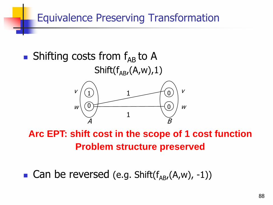
Shifting costs from fAB to A
Shift(fAB,(A,w),1)
Can be reversed (e.g. Shift(fAB,(A,w), -1))
0
1
Equivalence Preserving Transformation
w
v v
w
0
0
1
A B1
Arc EPT: shift cost in the scope of 1 cost function
Problem structure preserved
88

Equivalence Preserving Transformations
1f =
• EPTs may cycle• EPTs may lead to different f0
•Which EPTs should we apply?
Shift(fAB,(A,b),1)
Shift(fA,(),1) Shift(fAB,(B,a),-1)
Shift(fAB,(B,a),1)
A B A B A B
89
Local Consistency
Equivalence Preserving Transformation
Chaotic iteration of EPTs
Optimal set of EPTs
Improving sequence of EPTs
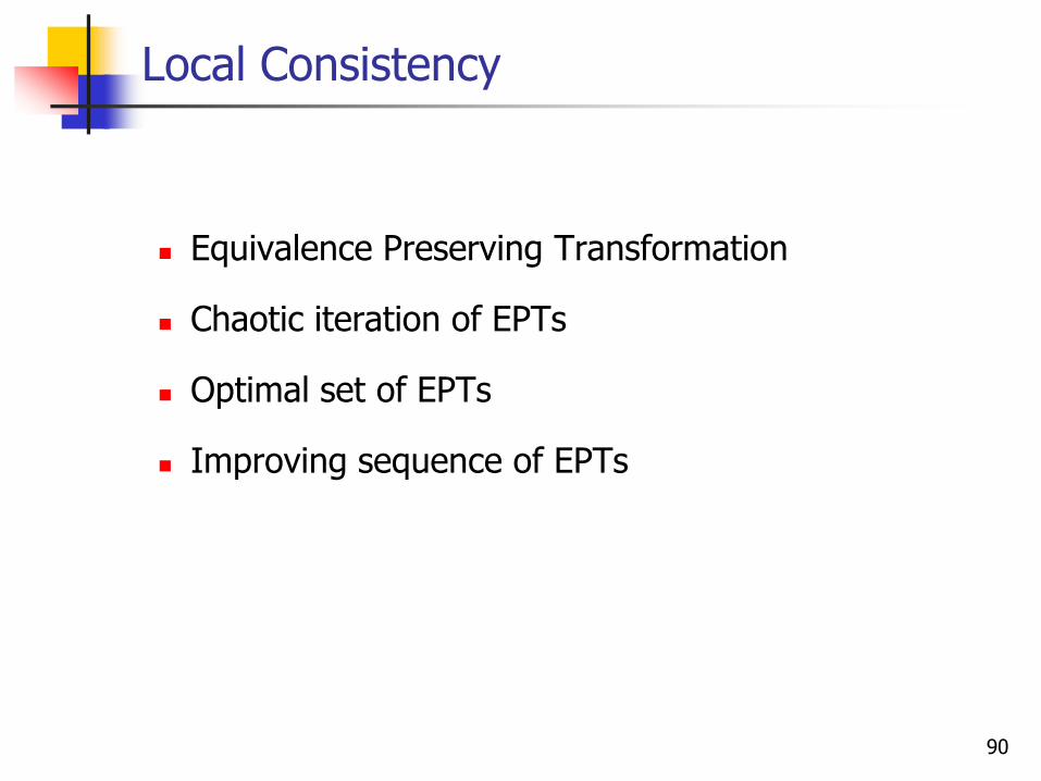
90
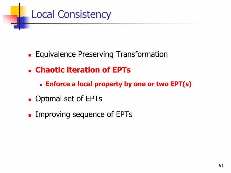
Local Consistency
Equivalence Preserving Transformation
Chaotic iteration of EPTs
Enforce a local property by one or two EPT(s)
Optimal set of EPTs
Improving sequence of EPTs
91

Node Consistency (NC*)
For any variable A a, f + fA(a)<k
a, fA (a)= 0
Complexity:
O(nd) w
v
v
v
w
w
f =k =
32
2
11
1
1
1
0
0
1
A
B
C
0
0
014
Shift(fC, ,1) Shift(fA, ,-1);Shift(fA, ,1)
(Larrosa, AAAI 2002)
92
0
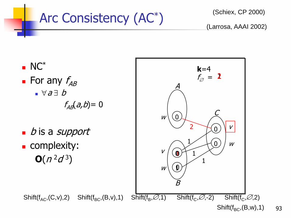
Arc Consistency (AC*)
NC*
For any fAB
a b
fAB(a,b)= 0
b is a support
complexity:
O(n 2d 3)
wv
v
w
w
f =k=4
2
11
1
0
0
0
0
1
A
B
C
1
12
0
Shift(fAC,(C,v),2) Shift(fBC,(B,v),1)
Shift(fBC,(B,w),1)
Shift(fB,,1) Shift(fC,,-2) Shift(fC,,2)
(Larrosa, AAAI 2002)
(Schiex, CP 2000)
93
1
1
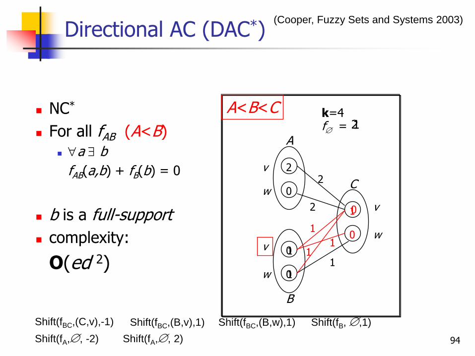
Directional AC (DAC*)
NC*
For all fAB (A<B)
a b
fAB(a,b) + fB(b) = 0
b is a full-support
complexity:
O(ed 2)
w
v
v
v
w
w
f =k=4
22
2
1
1
1
0
0
0
0
A
B
C
A<B<C
0
1
1
12
(Cooper, Fuzzy Sets and Systems 2003)
Shift(fBC,(C,v),-1) Shift(fBC,(B,v),1) Shift(fBC,(B,w),1) Shift(fB, ,1)
Shift(fA,, -2) Shift(fA,, 2) 94

DAC lb = Mini-Bucket(2) lb
bucket A:
bucket E:
bucket D:
bucket C:
bucket B: f(b,e)
f(a,d)
hE(Ø)
hB(e)
hB(d)
hD(a)
f(a,b)f(b,d)
f(c,e) f(a,c)
hC(e)
lb = lower bound
Mini-buckets
A
B C
D E
A < E < D < C < B
hB(a)
DAC provides an equivalent problem: incrementality DAC+NC (value pruning) can improve lb
hC(a)
95

Other « Chaotic » Local Consistencies
FDAC* = DAC+AC+NC
Stronger lower bound
O(end3)
Better compromise
EDAC* = FDAC+ EAC (existential AC)
Even stronger
O(ed 2 max{nd, k})
Currently among the best practical choice
(Larrosa & Schiex, IJCAI 2003)
(Cooper, Fuzzy Sets and Systems 2003)
(Larrosa & Schiex, AI 2004)
(Cooper & Schiex, AI 2004)
(Heras et al., IJCAI 2005)
(Sanchez et al, Constraints 2008)
96

Local Consistency
Equivalence Preserving Transformation
Chaotic iteration of EPTs
Optimal set of simultaneously applied EPTs
Solve a linear problem in rational costs
Improving sequence of EPTs
97

Finding an EPT Sequence Maximizing the LB
Bad news
Finding a sequence of integer arc EPTs that maximizes the lower bound defines an NP-hard problem
(Cooper & Schiex, AI 2004)
98
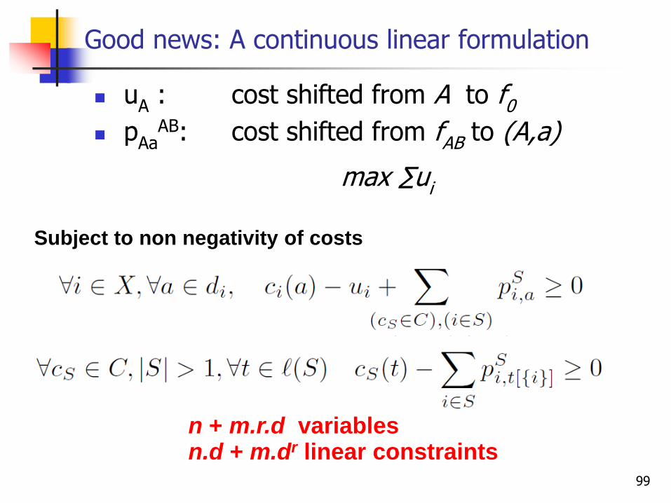
Good news: A continuous linear formulation
uA
: cost shifted from A to f0 p
AaAB: cost shifted from fAB to (A,a)
max ∑ui
n + m.r.d variablesn.d + m.dr linear constraints
Subject to non negativity of costs
99
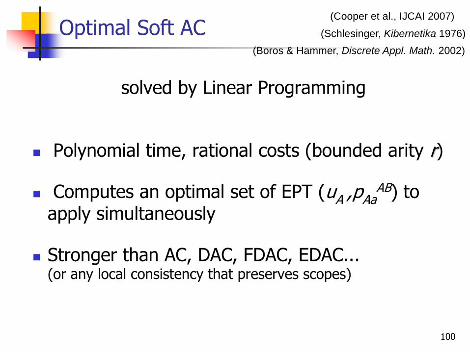
Optimal Soft AC
solved by Linear Programming
Polynomial time, rational costs (bounded arity r)
Computes an optimal set of EPT (uA ,pAaAB) to
apply simultaneously
Stronger than AC, DAC, FDAC, EDAC...(or any local consistency that preserves scopes)
(Cooper et al., IJCAI 2007)
(Boros & Hammer, Discrete Appl. Math. 2002)
(Schlesinger, Kibernetika 1976)
100
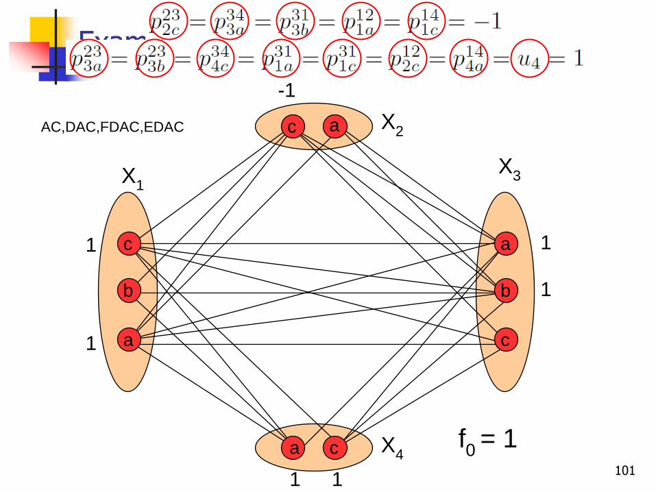
Example
-1
1
1
1
1
1
1
f0 = 1
a
bb
c
a c
c
ca
a
X1
X2
X3
X4
AC,DAC,FDAC,EDAC
101
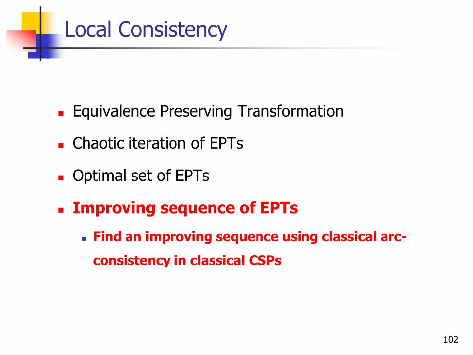
Local Consistency
Equivalence Preserving Transformation
Chaotic iteration of EPTs
Optimal set of EPTs
Improving sequence of EPTs
Find an improving sequence using classical arc-
consistency in classical CSPs
102
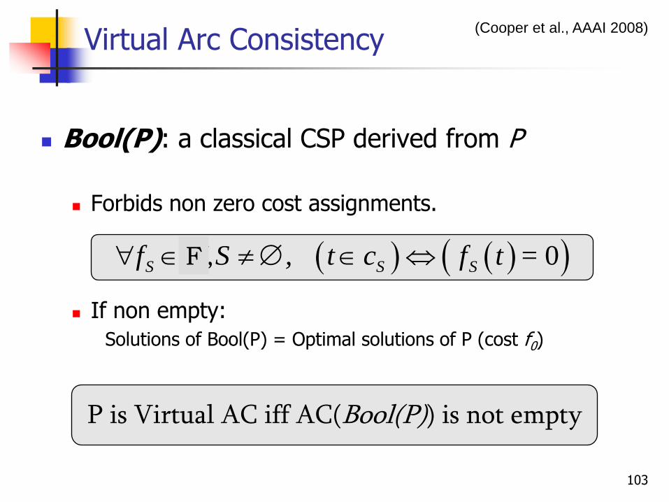
Virtual Arc Consistency
Bool(P): a classical CSP derived from P
Forbids non zero cost assignments.
If non empty:
Solutions of Bool(P) = Optimal solutions of P (cost f0)
0S S Sf W,S , t c f t =
P is Virtual AC iff AC(Bool(P)) is not empty
(Cooper et al., AAAI 2008)
F
103

Properties
Solves the polynomial class of submodular cost functions
In Bool(P) this means
Bool(P) max-closed: AC implies consistency
t,t', f t + f t' f max t,t' + f min t,t'
t't,minct't,maxct'ctc,t't,
104
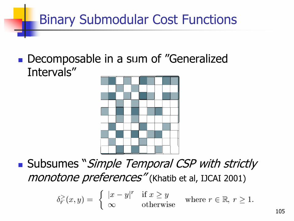
Binary Submodular Cost Functions
Decomposable in a sum of ‖Generalized Intervals‖
Subsumes ―Simple Temporal CSP with strictly monotone preferences‖ (Khatib et al, IJCAI 2001)
x1
x2
105
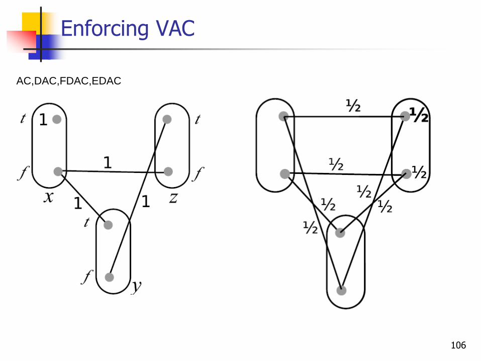
Enforcing VAC
AC,DAC,FDAC,EDAC
106
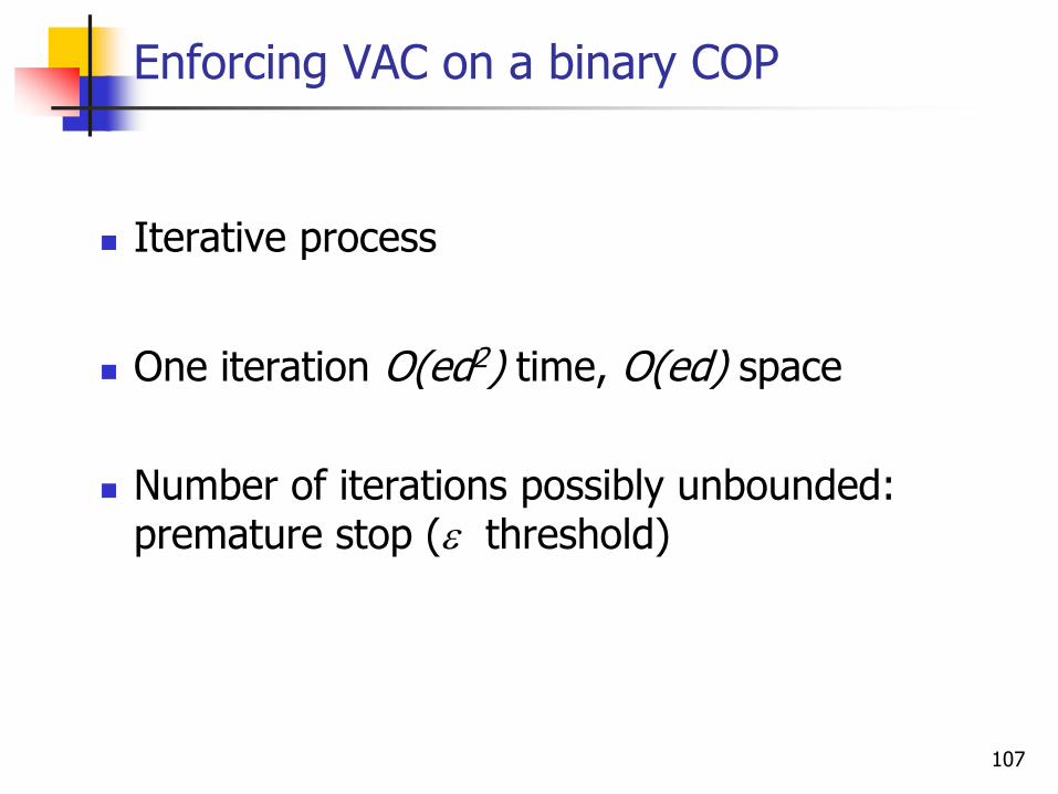
Enforcing VAC on a binary COP
Iterative process
One iteration O(ed2) time, O(ed) space
Number of iterations possibly unbounded: premature stop ( threshold)
107
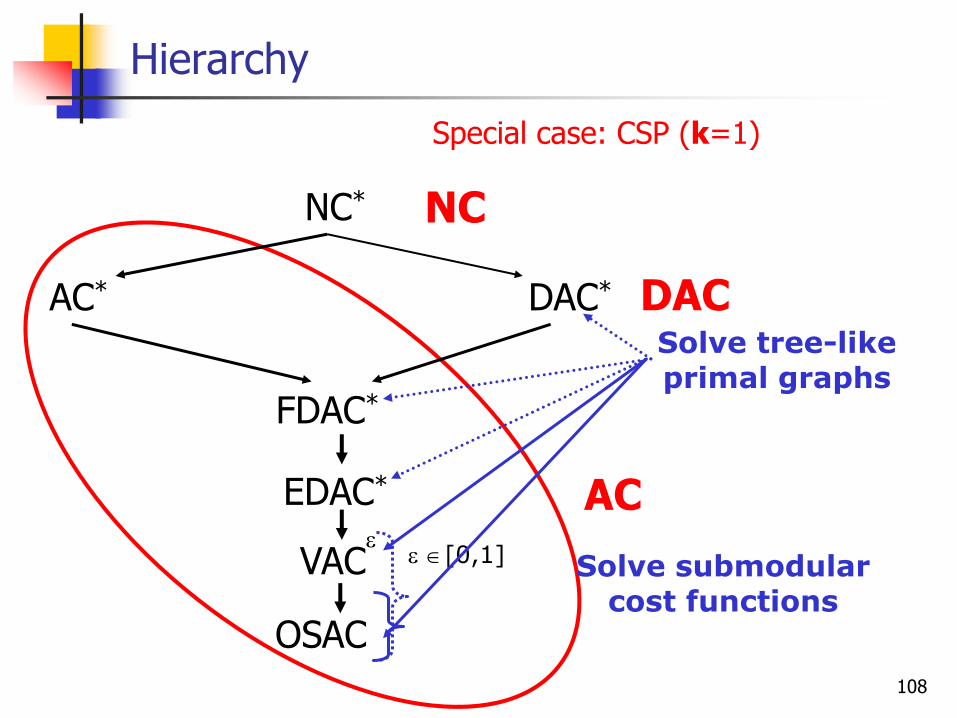
Hierarchy
NC*
AC* DAC*
FDAC*
AC
NC
DAC
Special case: CSP (k=1)
EDAC*
VAC [0,1]
OSAC
Solve tree-likeprimal graphs
Solve submodularcost functions
108
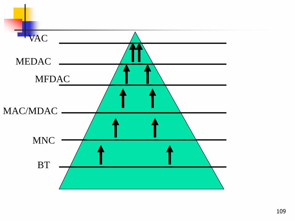
BT
MNC
MAC/MDAC
MFDAC
MEDAC
VAC
109

Radio Link Frequency Assignment Problem (Cabon et al., Constraints 1999) (Koster et al., 4OR 2003)
Given a telecommunication network
…find the best frequency for each communication link, avoiding interferences
Best can be:
Minimize the maximum frequency, no interference (max)
Minimize the global interference (sum)
Generalizes graph coloring problems: |f1 – f2| a
CELAR problem size: n=100—458 ; d=44 ; m=1,000—5,000
110

CELAR
SCEN-06-sub1n = 14, d = 44,
m = 75, k = 2669
Solver: toulbar2BB-VE(2), last conflict,dichotomic branching
Time Nodes
VAC 18 sec 25 103
EDAC 7 sec 38 103
FDAC 10 sec 72 103
AC 23 sec 410 103
DAC 150 sec 2.4 106
NC 897 sec 26 106
toulbar2 v0.6 running on a 3 GHz computer with 16 GB
111
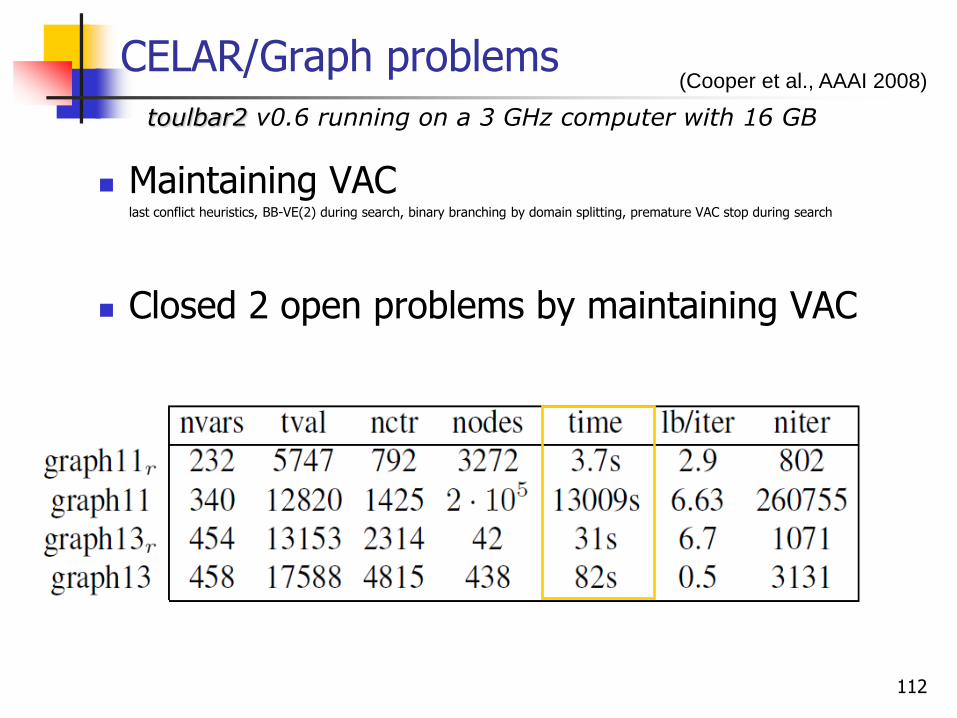
CELAR/Graph problems
Maintaining VAClast conflict heuristics, BB-VE(2) during search, binary branching by domain splitting, premature VAC stop during search
Closed 2 open problems by maintaining VAC
toulbar2 v0.6 running on a 3 GHz computer with 16 GB
(Cooper et al., AAAI 2008)
112
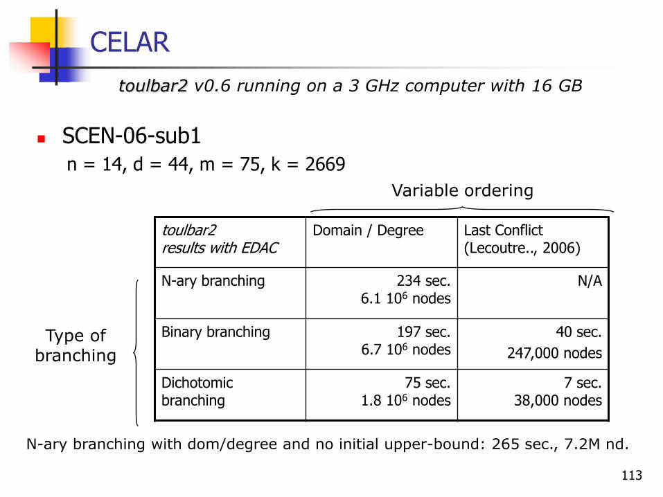
CELAR
SCEN-06-sub1
n = 14, d = 44, m = 75, k = 2669
toulbar2results with EDAC
Domain / Degree Last Conflict (Lecoutre.., 2006)
N-ary branching 234 sec.6.1 106 nodes
N/A
Binary branching 197 sec.6.7 106 nodes
40 sec.
247,000 nodes
Dichotomic branching
75 sec.1.8 106 nodes
7 sec.38,000 nodes
N-ary branching with dom/degree and no initial upper-bound: 265 sec., 7.2M nd.
Type ofbranching
Variable ordering
toulbar2 v0.6 running on a 3 GHz computer with 16 GB
113

CELAR: Local vs. Partial search with LC
Incomplete solvers toulbar2 with Limited Discrepancy Search (Harvey & Ginsberg,
IJCAI 1995) exploiting unary cost functions produced by EDAC
INCOP (Neveu, Trombettoni and Glover, CP 2004)
Intensification/Diversification Walk meta-heuristic
CELAR SCEN-06 Time Solution cost
LDS(8), BB-VE(2) 35 sec 3394
INCOP 36 sec/run 3476 (best)
3750 (mean over 10 runs)
Local consistency enforcement informsvariable and value ordering heuristics
toulbar2 v0.6 running on a 3 GHz computer with 16 GB
114

Perspectives
Improve modeling capabilities Global cost functions (Lee and Leung, IJCAI 2009) &
Virtual GAC,…
Study stronger soft local consistencies Singleton arc consistency,…
Extension to other tasks Probabilistic inference,…
115

Outline
Introduction Inference Search (OR)
Lower-bounds and relaxations
Exploiting problem structure in search AND/OR search trees (linear space) AND/OR Branch-and-Bound search AND/OR search graphs (caching) AND/OR search for 0-1 integer programming
Software
116
Solution Techniques
Search: Conditioning
Complete
Complete
Adaptive ConsistencyTree Clustering
Variable EliminationResolution
DFS search
Branch-and-Bound
Inference: Elimination
Time: exp(treewidth)Space:exp(treewidth)
Time: exp(n)Space: linear
AND/OR searchTime: exp(treewidth*log n)Space: linear
Hybrids
Space: exp(treewidth)Time: exp(treewidth)
Time: exp(pathwidth)Space: exp(pathwidth)
117
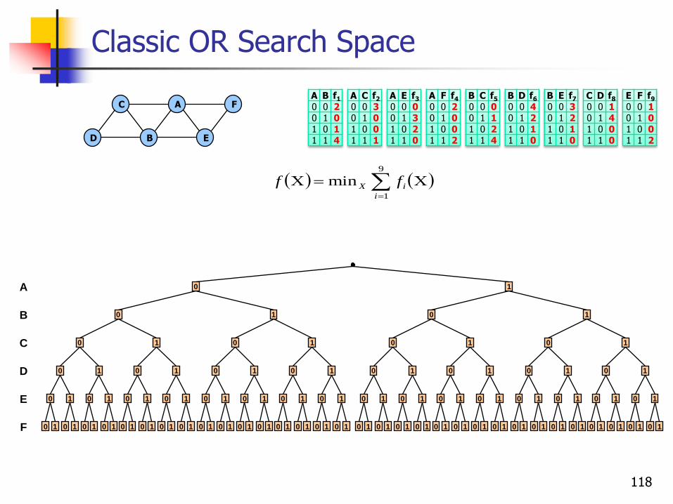
Classic OR Search Space
9
1
mini
iX ff
A
E
C
B
F
D
Objective function:
A B f1
0 0 20 1 01 0 11 1 4
A C f2
0 0 30 1 01 0 01 1 1
A E f3
0 0 00 1 31 0 21 1 0
A F f4
0 0 20 1 01 0 01 1 2
B C f5
0 0 00 1 11 0 21 1 4
B D f6
0 0 40 1 21 0 11 1 0
B E f7
0 0 30 1 21 0 11 1 0
C D f8
0 0 10 1 41 0 01 1 0
E F f9
0 0 10 1 01 0 01 1 2
0 1 0 1 0 1 0 1
0 1 0 1 0 1 0 1 0 1 0 1 0 1 0 1
0 1 0 1 0 1 0 1 0 1 0 1 0 1 0 1 0 1 0 1 0 1 0 1 0 1 0 1 0 1 0 1 0 1 0 1 0 1 0 1 0 1 0 1 0 1 0 1 0 1 0 1 0 1 0 1 0 1 0 1 0 1 0 1
0 1 0 1 0 1 0 1 0 1 0 1 0 1 0 1 0 1 0 1 0 1 0 1 0 1 0 1 0 1 0 1
0 1 0 1
C
D
F
E
B
A 0 1
118

The AND/OR Search Tree
A
E
C
B
F
D
A
D
B
EC
F
Pseudo tree (Freuder & Quinn85)
OR
AND
OR
AND
OR
OR
AND
AND
A
0
B
0
E
F F
0 1 0 1
0 1
C
D D
0 1 0 1
0 1
1
E
F F
0 1 0 1
0 1
C
D D
0 1 0 1
0 1
1
B
0
E
F F
0 1 0 1
0 1
C
D D
0 1 0 1
0 1
1
E
F F
0 1 0 1
0 1
C
D D
0 1 0 1
0 1
119

The AND/OR Search Tree
A
E
C
B
F
D
A
D
B
EC
F
Pseudo tree
OR
AND
OR
AND
OR
OR
AND
AND
A
0
B
0
E
F F
0 1 0 1
0 1
C
D D
0 1 0 1
0 1
1
E
F F
0 1 0 1
0 1
C
D D
0 1 0 1
0 1
1
B
0
E
F F
0 1 0 1
0 1
C
D D
0 1 0 1
0 1
1
E
F F
0 1 0 1
0 1
C
D D
0 1 0 1
0 1
A solution subtree is (A=0, B=1, C=0, D=0, E=1, F=1) 120
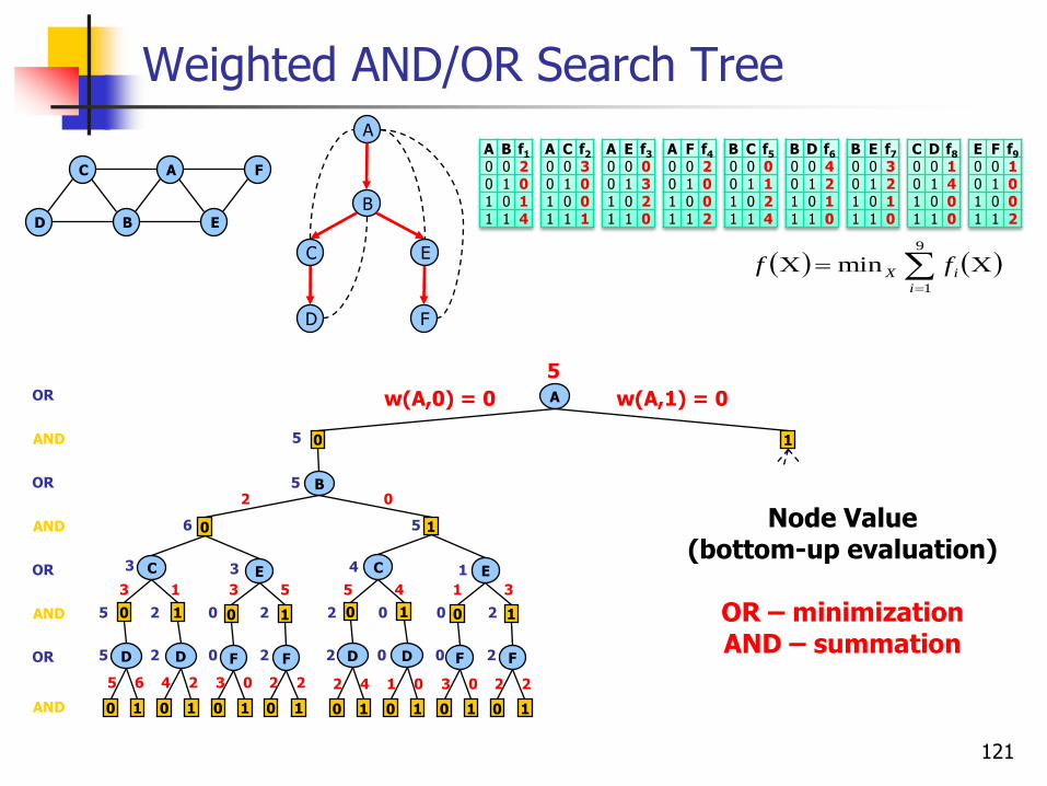
Weighted AND/OR Search Tree
9
1
mini
iX ff
A
E
C
B
F
D
Objective function:
A
D
B
EC
F
A
0
B
0
E
F F
0 1 0 1
OR
AND
OR
AND
OR
OR
AND
AND 0 1
C
D D
0 1 0 1
0 1
1
E
F F
0 1 0 1
0 1
C
D D
0 1 0 1
0 1
5 6 4 2 3 0 2 2
5 2 0 2
5 2 0 2
3 3
6
5
5
5
3 1 3 5
2
2 4 1 0 3 0 2 2
2 0 0 2
2 0 0 2
4 1
5
5 4 1 3
0
1
w(A,0) = 0 w(A,1) = 0
Node Value(bottom-up evaluation)
OR – minimizationAND – summation
A B f1
0 0 20 1 01 0 11 1 4
A C f2
0 0 30 1 01 0 01 1 1
A E f3
0 0 00 1 31 0 21 1 0
A F f4
0 0 20 1 01 0 01 1 2
B C f5
0 0 00 1 11 0 21 1 4
B D f6
0 0 40 1 21 0 11 1 0
B E f7
0 0 30 1 21 0 11 1 0
C D f8
0 0 10 1 41 0 01 1 0
E F f9
0 0 10 1 01 0 01 1 2
121
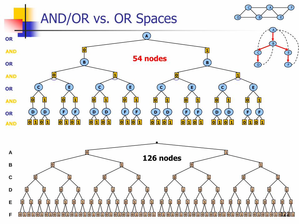
AND/OR vs. OR Spaces
0 1 0 1 0 1 0 1
0 1 0 1 0 1 0 1 0 1 0 1 0 1 0 1
0 1 0 1 0 1 0 1 0 1 0 1 0 1 0 1 0 1 0 1 0 1 0 1 0 1 0 1 0 1 0 1 0 1 0 1 0 1 0 1 0 1 0 1 0 1 0 1 0 1 0 1 0 1 0 1 0 1 0 1 0 1 0 1
0 1 0 1 0 1 0 1 0 1 0 1 0 1 0 1 0 1 0 1 0 1 0 1 0 1 0 1 0 1 0 1
0 1 0 1
C
D
F
E
B
A 0 1
OR
AND
OR
AND
OR
OR
AND
AND
A
0
B
0
E
F F
0 1 0 1
0 1
C
D D
0 1 0 1
0 1
1
E
F F
0 1 0 1
0 1
C
D D
0 1 0 1
0 1
1
B
0
E
F F
0 1 0 1
0 1
C
D D
0 1 0 1
0 1
1
E
F F
0 1 0 1
0 1
C
D D
0 1 0 1
0 1
A
E
C
B
F
D
A
D
B
EC
F
54 nodes
126 nodes
122
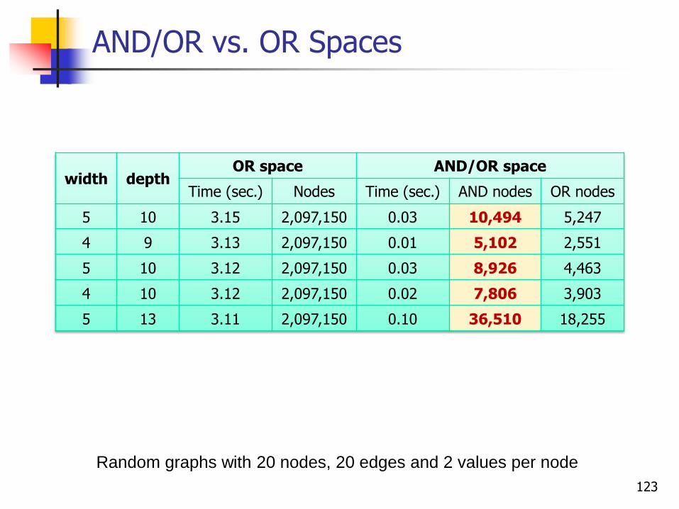
AND/OR vs. OR Spaces
width depthOR space AND/OR space
Time (sec.) Nodes Time (sec.) AND nodes OR nodes
5 10 3.15 2,097,150 0.03 10,494 5,247
4 9 3.13 2,097,150 0.01 5,102 2,551
5 10 3.12 2,097,150 0.03 8,926 4,463
4 10 3.12 2,097,150 0.02 7,806 3,903
5 13 3.11 2,097,150 0.10 36,510 18,255
Random graphs with 20 nodes, 20 edges and 2 values per node
123
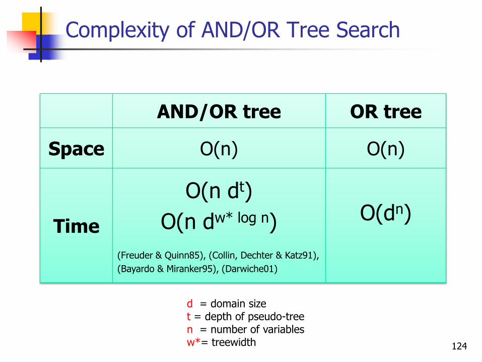
Complexity of AND/OR Tree Search
AND/OR tree OR tree
Space O(n) O(n)
Time
O(n dt)
O(n dw* log n)
(Freuder & Quinn85), (Collin, Dechter & Katz91),
(Bayardo & Miranker95), (Darwiche01)
O(dn)
d = domain sizet = depth of pseudo-treen = number of variablesw*= treewidth 124
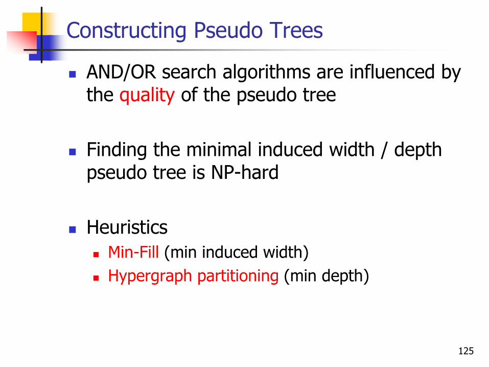
Constructing Pseudo Trees
AND/OR search algorithms are influenced by the quality of the pseudo tree
Finding the minimal induced width / depth pseudo tree is NP-hard
Heuristics
Min-Fill (min induced width)
Hypergraph partitioning (min depth)
125
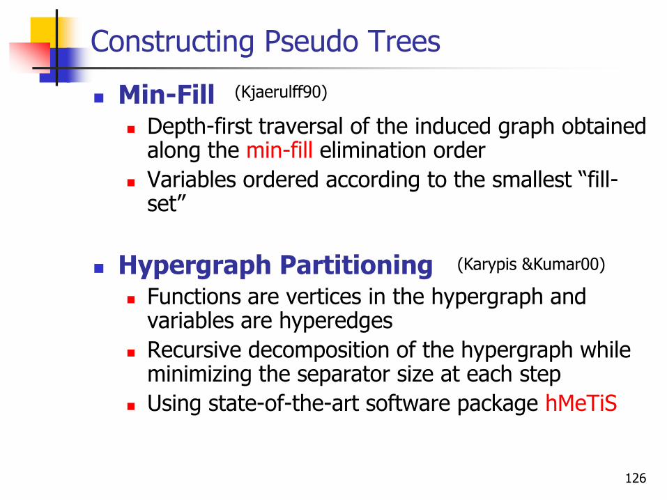
Constructing Pseudo Trees
Min-Fill Depth-first traversal of the induced graph obtained
along the min-fill elimination order
Variables ordered according to the smallest ―fill-set‖
Hypergraph Partitioning Functions are vertices in the hypergraph and
variables are hyperedges
Recursive decomposition of the hypergraph while minimizing the separator size at each step
Using state-of-the-art software package hMeTiS
(Kjaerulff90)
(Karypis &Kumar00)
126
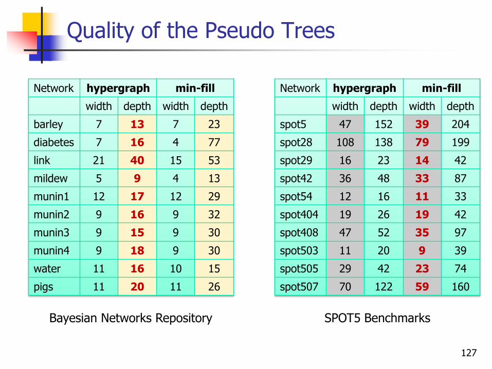
Quality of the Pseudo Trees
Network hypergraph min-fill
width depth width depth
barley 7 13 7 23
diabetes 7 16 4 77
link 21 40 15 53
mildew 5 9 4 13
munin1 12 17 12 29
munin2 9 16 9 32
munin3 9 15 9 30
munin4 9 18 9 30
water 11 16 10 15
pigs 11 20 11 26
Network hypergraph min-fill
width depth width depth
spot5 47 152 39 204
spot28 108 138 79 199
spot29 16 23 14 42
spot42 36 48 33 87
spot54 12 16 11 33
spot404 19 26 19 42
spot408 47 52 35 97
spot503 11 20 9 39
spot505 29 42 23 74
spot507 70 122 59 160
Bayesian Networks Repository SPOT5 Benchmarks
127
Outline
Introduction Inference Search (OR)
Lower-bounds and relaxations
Exploiting problem structure in search AND/OR search trees AND/OR Branch-and-Bound search
Lower bounding heuristics Dynamic variable orderings
AND/OR search graphs (caching) AND/OR search for 0-1 integer programming
Software & Applications
128
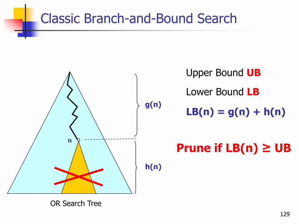
Classic Branch-and-Bound Search
n
g(n)
h(n)
LB(n) = g(n) + h(n)
Lower Bound LB
OR Search Tree
Prune if LB(n) ≥ UB
Upper Bound UB
129

Partial Solution Tree
0
D
0
(A=0, B=0, C=0, D=0)
0
A
B C
0
0
A
B C
00
D
1
(A=0, B=0, C=0, D=1)
0
A
B C
01
D
0
(A=0, B=1, C=0, D=0)
0
A
B C
01
D
1
(A=0, B=1, C=0, D=1)
A
B C
D
Pseudo tree
Extension(T’) – solution trees that extend T’
130
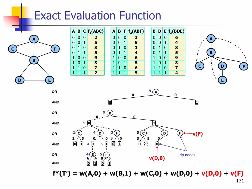
Exact Evaluation Function
OR
AND
OR
AND
OR
OR
AND
AND
A
0
B
0
D
E E
0 1 0 1
0 1
C
1
1
6 4 8 54 5
4 5
2 4
9
9
2 5 0 0
0 0
0
1
0
0
D
0
C
1
v(D,0)
3
3 5 0
0
9
tip nodes
F
1
3
3 5
0
F v(F)
A
B
C
D E
F
A
B
C D
E
F
A B C f1(ABC)
0 0 0 20 0 1 50 1 0 30 1 1 51 0 0 91 0 1 31 1 0 71 1 1 2
A B F f2(ABF)
0 0 0 30 0 1 50 1 0 10 1 1 41 0 0 61 0 1 51 1 0 61 1 1 5
B D E f3(BDE)
0 0 0 60 0 1 40 1 0 80 1 1 51 0 0 91 0 1 31 1 0 71 1 1 4
f*(T’) = w(A,0) + w(B,1) + w(C,0) + w(D,0) + v(D,0) + v(F)131

Heuristic Evaluation Function
OR
AND
OR
AND
OR
OR
AND
AND
A
0
B
0
D
E E
0 1 0 1
0 1
C
1
1
6 4 8 54 5
4 5
2 4
9
9
2 5 0 0
0 0
0
1
0
0
D
0
C
1
h(D,0) = 4
3
3 5 0
0
9
tip nodes
F
1
3
3 5
0
F h(F) = 5
A
B
C
D E
F
A
B
C D
E
F
A B C f1(ABC)
0 0 0 20 0 1 50 1 0 30 1 1 51 0 0 91 0 1 31 1 0 71 1 1 2
A B F f2(ABF)
0 0 0 30 0 1 50 1 0 10 1 1 41 0 0 61 0 1 51 1 0 61 1 1 5
B D E f3(BDE)
0 0 0 60 0 1 40 1 0 80 1 1 51 0 0 91 0 1 31 1 0 71 1 1 4
f(T’) = w(A,0) + w(B,1) + w(C,0) + w(D,0) + h(D,0) + h(F) = 12 ≤ f*(T’)
h(n) ≤ v(n)
132
AND/OR Branch-and-Bound Search
OR
AND
OR
AND
OR
OR
AND
AND
A
0
B
0
D
E E
0 1 0 1
0 1
C
1
1
∞ 3 ∞ 4
3 4
3 4
∞ 4
∞
5
5
5
∞ ∞ 1 ∞
0
5
0
0
111
0
0
D
E E
0 1 0 1
0 1
C
1
∞ 3 ∞ 4
3 4
3 4
2 3
∞ 2 0 2
0
B
0 111
11
0 0
f(T’) ≥ UB
UB
133
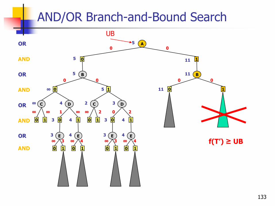
AND/OR Branch-and-Bound Search (AOBB)(Marinescu & Dechter, IJCAI’05)
Associate each node n with a heuristic lower bound h(n) on v(n)
EXPAND (top-down)
Evaluate f(T’) and prune search if f(T’) ≥ UB
Expand the tip node n
PROPAGATE (bottom-up)
Update value of the parent p of n
OR nodes: minimization
AND nodes: summation
134

Heuristics for AND/OR Branch-and-Bound
In the AND/OR search space h(n) can be computed using any heuristic. We used:
Static Mini-Bucket heuristics(Kask & Dechter, AIJ’01), (Marinescu & Dechter, IJCAI’05)
Dynamic Mini-Bucket heuristics(Marinescu & Dechter, IJCAI’05)
Maintaining local consistency
(Larrosa & Schiex, AAAI’03), (de Givry et al., IJCAI’05)
LP relaxations(Nemhauser & Wosley, 1998)
135
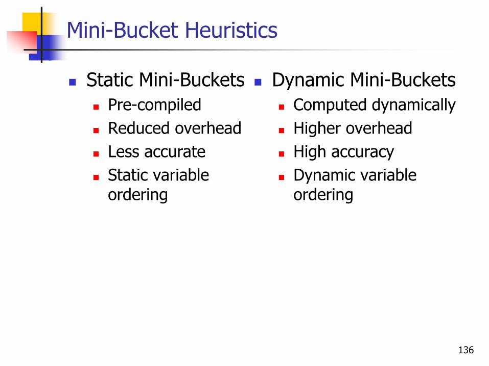
Mini-Bucket Heuristics
Static Mini-Buckets
Pre-compiled
Reduced overhead
Less accurate
Static variable ordering
Dynamic Mini-Buckets
Computed dynamically
Higher overhead
High accuracy
Dynamic variable ordering
136

Bucket Elimination
A
f(A,B)B
f(B,C)C f(B,F)F
f(A,G) f(F,G)
Gf(B,E) f(C,E)
Ef(A,D) f(B,D) f(C,D)
D
hG (A,F)
hF (A,B)
hB (A)
hE (B,C)hD (A,B,C)
hC (A,B)
A B
CD
E
F
G
A
B
C F
GD E
Ordering: (A, B, C, D, E, F, G)
h*(a, b, c) = hD(a, b, c) + hE(b, c)
137
Static Mini-Bucket Heuristics
A
f(A,B)B
f(B,C)C f(B,F)F
f(A,G) f(F,G)
Gf(B,E) f(C,E)
Ef(B,D) f(C,D)
D
hG (A,F)
hF (A,B)
hB (A)
hE (B,C)hD (B,C)
hC (B)
hD (A)
f(A,D)D
mini-buckets
A B
CD
E
F
G
A
B
C F
GD E
Ordering: (A, B, C, D, E, F, G)
h(a, b, c) = hD(a) + hD(b, c) + hE(b, c)≤ h*(a, b, c)
MBE(3)
138
Dynamic Mini-Bucket Heuristics
A
f(a,b)B
f(b,C)C f(b,F)F
f(a,G) f(F,G)
Gf(b,E) f(C,E)
Ef(a,D) f(b,D) f(C,D)
D
hG (F)
hF ()
hB ()
hE (C)hD (C)
hC ()
A B
CD
E
F
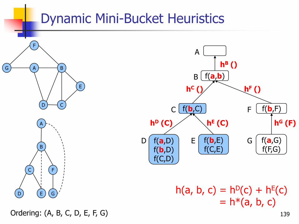
G
A
B
C F
GD E
Ordering: (A, B, C, D, E, F, G)
h(a, b, c) = hD(c) + hE(c)= h*(a, b, c)
MBE(3)
139
Outline
Introduction Inference Search (OR)
Lower-bounds and relaxations
Exploiting problem structure in search AND/OR search trees AND/OR Branch-and-Bound search
Lower bounding heuristics Dynamic variable orderings
AND/OR search graphs (caching) AND/OR search for 0-1 integer programming
Software & Applications
140
Dynamic Variable Orderings(Marinescu & Dechter, ECAI’06)
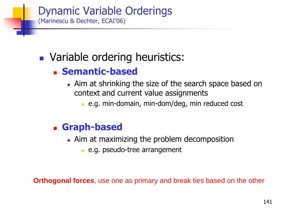
Variable ordering heuristics:
Semantic-based
Aim at shrinking the size of the search space based on context and current value assignments
e.g. min-domain, min-dom/deg, min reduced cost
Graph-based
Aim at maximizing the problem decomposition
e.g. pseudo-tree arrangement
Orthogonal forces, use one as primary and break ties based on the other
141
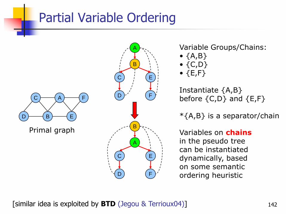
Partial Variable Ordering
A
E
C
B
F
D
A
D
B
EC
F
B
D
A
EC
F
Variables on chainsin the pseudo tree can be instantiated dynamically, basedon some semantic ordering heuristic
Variable Groups/Chains: • {A,B} • {C,D} • {E,F}
Instantiate {A,B} before {C,D} and {E,F}
*{A,B} is a separator/chain
[similar idea is exploited by BTD (Jegou & Terrioux04)]
Primal graph
142

Full Dynamic Variable Ordering
DA={0,1} DB={0,1,2}
DE={0,1,2,3}
DC=DD=DF=DG=DH=DE
domains
A B f(AB)
0 0 30 1 8
0 2 8
1 0 41 1 01 2 6
A E f(AE)
0 0 00 1 50 2 10 3 41 0 8
1 1 8
1 2 01 3 5
cost functions
A
D
B C
E F
H
GA
B
D
C
F
P1 P2
H
E
G
[similar idea exploited in #SAT (Bayardo & Pehoushek00)]
0
0
1
E
1
B
1
D
C
F
P1 P2
H G
143
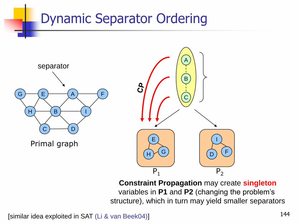
Dynamic Separator Ordering
A
D
B I
E F
H
G
C
separatorA
B
C
P1
H
E
G
P2
D
I
F
Constraint Propagation may create singleton
variables in P1 and P2 (changingtheproblem’s
structure), which in turn may yield smaller separators
[similar idea exploited in SAT (Li & van Beek04)]
Primal graph
144

Experiments
Benchmarks
Belief Networks (BN)
Weighted CSPs (WCSP)
Algorithms
AOBB
SamIam (BN)
Superlink (Genetic linkage analysis)
Toolbar (ie, DFBB+EDAC)
Heuristics
Mini-Bucket heuristics (BN, WCSP)
EDAC heuristics (WCSP)
145

Genetic Linkage Analysis
pedigree(n, d)(w*, h)
Superlinkv. 1.6
time
SamIamv. 2.3.2
time
MBE(i)BB+SMB(i)
AOBB+SMB(i)i=12
MBE(i)BB+SMB(i)
AOBB+SMB(i)i=16
MBE(i)BB+SMB(i)
AOBB+SMB(i)i=20
time nodes time nodes time nodes
ped18(1184, 5)(21, 119)
139.06 157.050.51
--
--
4.59-
270.96-
2,555,078
19.30-
20.27-
7,689
ped25(994, 5)(29, 53)
- out0.34
--
--
3.20--
--
33.42-
1894.17-
11,709,153
ped30(1016, 5)(25, 51)
13095.83 out0.31
-5563.22
-63,068,960
2.66-
1811.34-
20,275,620
24.88-
82.25-
588,558
ped33(581, 5)(26, 48)
- out0.41
-2335.28
-32,444,818
5.28-
62.91-
807,071
51.24-
76.47-
320,279
ped39(1272, 5)(23, 94)
322.14 out0.52
--
--
8.41-
4041.56-
52,804,044
81.27-
141.23-
407,280
(Fishelson&Geiger02)
Min-fill pseudo tree. Time limit 3 hours.146
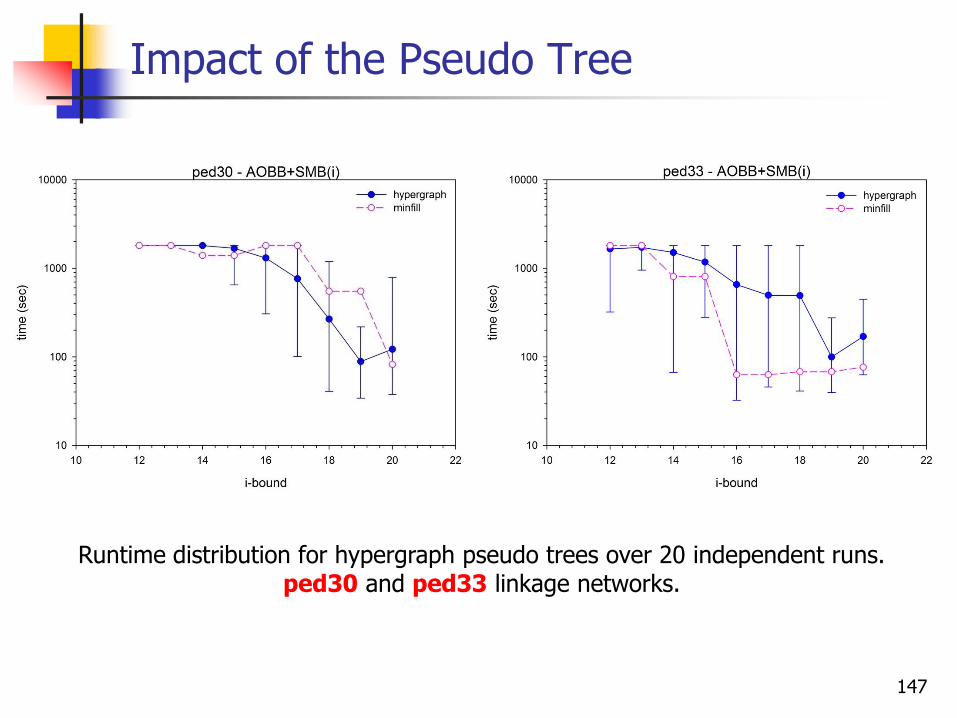
Impact of the Pseudo Tree
Runtime distribution for hypergraph pseudo trees over 20 independent runs.ped30 and ped33 linkage networks.
147
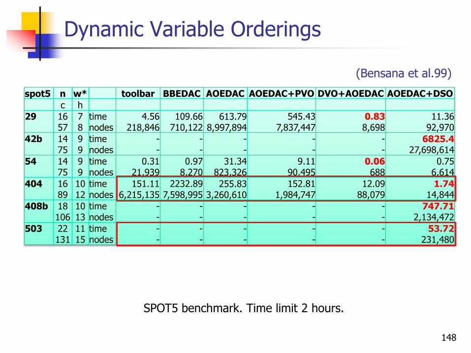
Dynamic Variable Orderings
spot5 n w* toolbar BBEDAC AOEDAC AOEDAC+PVO DVO+AOEDAC AOEDAC+DSO
c h
29 1657
78
timenodes
4.56218,846
109.66710,122
613.798,997,894
545.437,837,447
0.838,698
11.3692,970
42b 1475
99
timenodes
--
--
--
--
--
6825.427,698,614
54 1475
99
timenodes
0.3121,939
0.978,270
31.34823,326
9.1190,495
0.06688
0.756,614
404 1689
1012
timenodes
151.116,215,135
2232.897,598,995
255.833,260,610
152.811,984,747
12.0988,079
1.7414,844
408b 18106
1013
timenodes
--
--
--
--
--
747.712,134,472
503 22131
1115
timenodes
--
--
--
--
--
53.72231,480
SPOT5 benchmark. Time limit 2 hours.
(Bensana et al.99)
148

Summary
New generation of depth-first AND/OR Branch-and-Bound search
Heuristics based on
Mini-Bucket approximation (static, dynamic)
Local consistency (EDAC)
Dynamic variable orderings
Superior to state-of-the-art solvers traversing the classic OR search space
149
Outline
Introduction Inference Search (OR)
Lower-bounds and relaxations
Exploiting problem structure in search AND/OR search trees AND/OR Branch-and-Bound search AND/OR search graphs (caching)
AND/OR Branch-and-Bound with caching Best-First AND/OR search
AND/OR search for 0-1 integer programming
Software
150

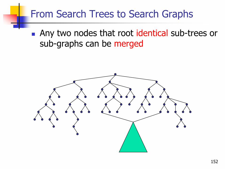
From Search Trees to Search Graphs
Any two nodes that root identical sub-trees or sub-graphs can be merged
151
From Search Trees to Search Graphs
Any two nodes that root identical sub-trees or sub-graphs can be merged
152
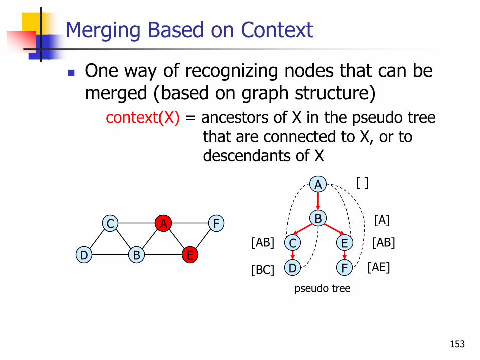
Merging Based on Context
One way of recognizing nodes that can be merged (based on graph structure)
context(X) = ancestors of X in the pseudo tree that are connected to X, or to descendants of X
[ ]
[A]
[AB]
[AE][BC]
[AB]
A
D
B
EC
F
pseudo tree
A
E
C
B
F
D
A
E
C
B
F
D
153
AND/OR Search Graph
9
1
mini
iX ff
A
E
C
B
F
D
Objective function:
A
D
B
EC
F
A B f1
0 0 20 1 01 0 11 1 4
A C f2
0 0 30 1 01 0 01 1 1
A E f3
0 0 00 1 31 0 21 1 0
A F f4
0 0 20 1 01 0 01 1 2
B C f5
0 0 00 1 11 0 21 1 4
B D f6
0 0 40 1 21 0 11 1 0
B E f7
0 0 30 1 21 0 11 1 0
C D f8
0 0 10 1 41 0 01 1 0
E F f9
0 0 10 1 01 0 01 1 2
context minimal graph
AOR
0AND
BOR
0AND
OR E
OR
AND
AND 0 1
C
D D
0 1 0 1
0 1
1
E
F F
0 1 0 1
0 1
C
D D
0 1 0 1
0 1
1
B
0
E
F F
0 1 0 1
0 1
C
0 1
1
E
0 1
C
0 1
B C Value0 00 11 01 1
Cache table for D
[]
[A]
[AB]
[AE]
[AB]
[BC]
154
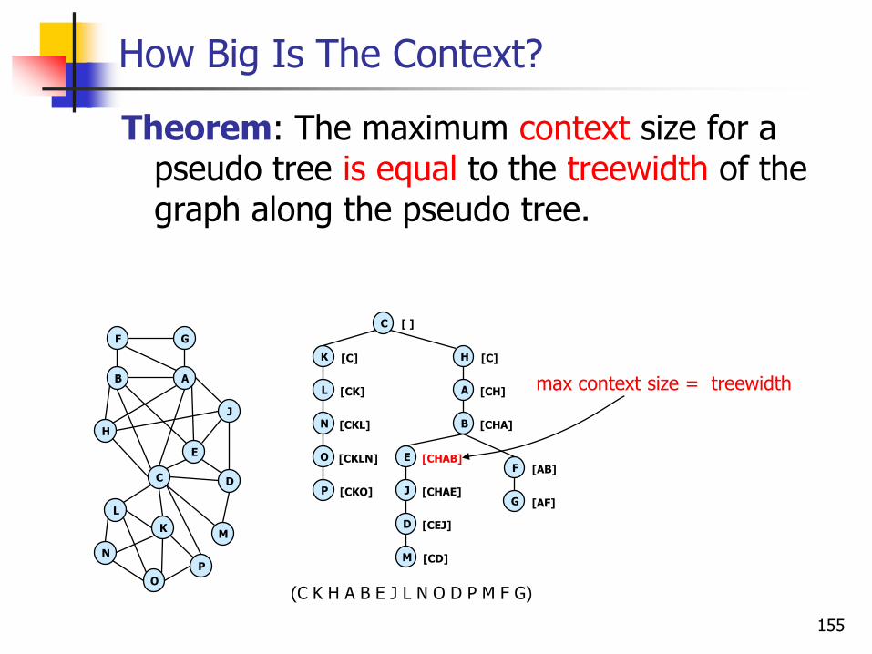
How Big Is The Context?
Theorem: The maximum context size for a pseudo tree is equal to the treewidth of the graph along the pseudo tree.
C
HK
D
M
F
G
A
B
E
J
O
L
N
P
[AB]
[AF][CHAE]
[CEJ]
[CD]
[CHAB]
[CHA]
[CH]
[C]
[ ]
[CKO]
[CKLN]
[CKL]
[CK]
[C]
(C K H A B E J L N O D P M F G)
B A
C
E
F G
H
J
D
KM
L
N
O
P
max context size = treewidth
155
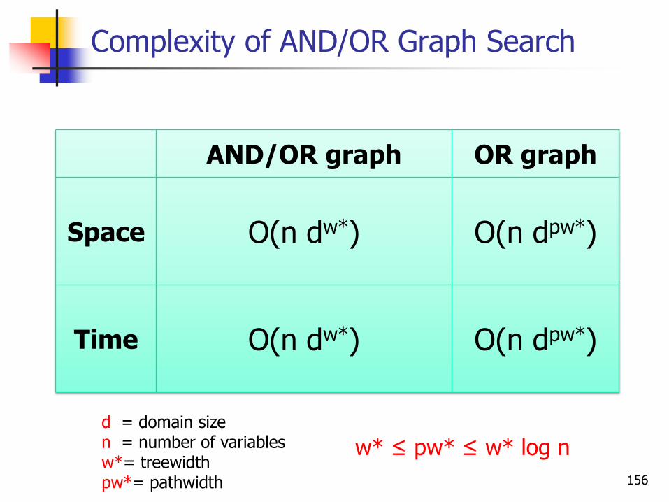
Complexity of AND/OR Graph Search
AND/OR graph OR graph
Space O(n dw*) O(n dpw*)
Time O(n dw*) O(n dpw*)
d = domain sizen = number of variablesw*= treewidthpw*= pathwidth
w* ≤ pw* ≤ w* log n
156
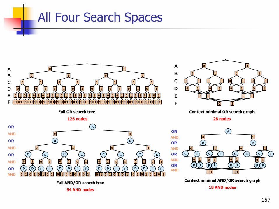
All Four Search Spaces
Full OR search tree
126 nodes
0 1 0 1 0 1 0 1
0 1 0 1 0 1 0 1 0 1 0 1 0 1 0 1
0 1 0 1 0 1 0 10 1 0 1 0 1 0 1 0 1 0 1 0 1 0 10 1 0 1 0 1 0 1 0 1 0 1 0 1 0 10 1 0 1 0 1 0 1 0 1 0 1 0 1 0 1 0 1 0 1 0 1 0 1
0 1 0 1 0 1 0 1 0 1 0 1 0 1 0 1 0 1 0 1 0 1 0 1 0 1 0 1 0 1 0 1
0 1 0 1
C
D
F
E
B
A 0 1
Full AND/OR search tree
54 AND nodes
AOR
0AND
BOR
0AND
OR E
OR F F
AND 0 1 0 1
AND 0 1
C
D D
0 1 0 1
0 1
1
E
F F
0 1 0 1
0 1
C
D D
0 1 0 1
0 1
1
B
0
E
F F
0 1 0 1
0 1
C
D D
0 1 0 1
0 1
1
E
F F
0 1 0 1
0 1
C
D D
0 1 0 1
0 1
Context minimal OR search graph
28 nodes
0 1 0 1 0 1 0 1
0 1 0 1 0 1 0 1
0 1
0 1 0 1
0 1 0 1
C
D
F
E
B
A 0 1
Context minimal AND/OR search graph
18 AND nodes
AOR
0AND
BOR
0AND
OR E
OR F F
AND0 1
AND 0 1
C
D D
0 1
0 1
1
EC
D D
0 1
1
B
0
E
F F
0 1
C
1
EC
157

AND/OR Branch-and-Bound with Caching(Marinescu & Dechter, AAAI’06)
Associate each node n with a heuristic lower bound h(n) on v(n)
EXPAND (top-down) Evaluate f(T’) and prune search if f(T’) ≥ UB
If not in cache, expand the tip node n
PROPAGATE (bottom-up) Update value of the parent p of n
OR nodes: minimization
AND nodes: summation
Cache value of n, based on context
158
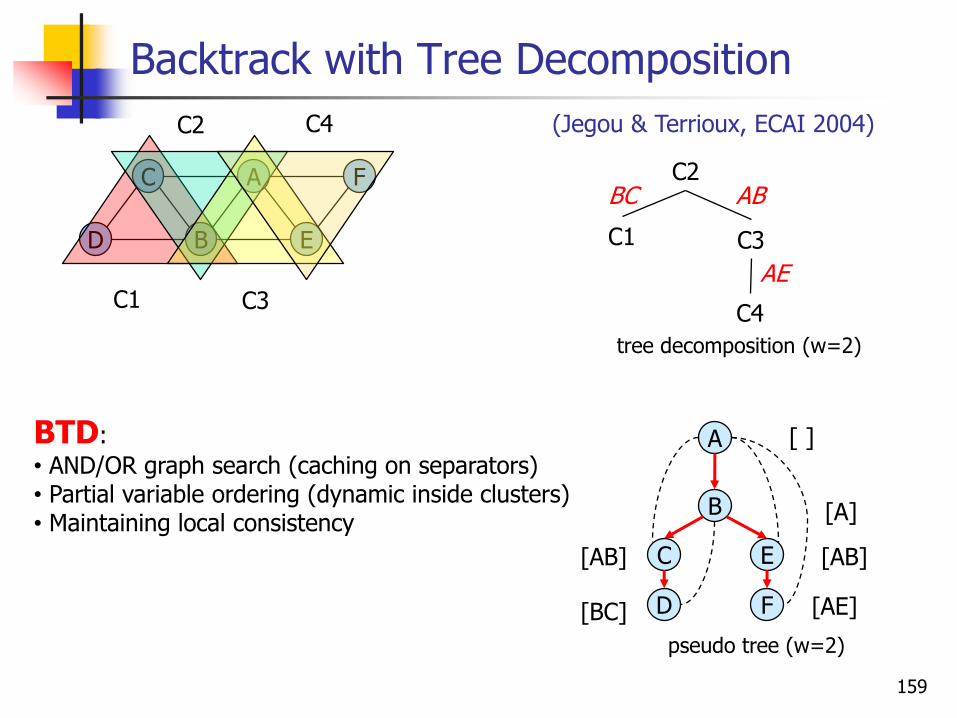
Backtrack with Tree Decomposition
A
E
C
B
F
D
C1
C2
C3
C4
C2
C1 C3
C4
AB
AE
BC
tree decomposition (w=2)
BTD:
• AND/OR graph search (caching on separators)• Partial variable ordering (dynamic inside clusters)• Maintaining local consistency
A
D
B
EC
F
pseudo tree (w=2)
[ ]
[A]
[AB]
[AE][BC]
[AB]
(Jegou & Terrioux, ECAI 2004)
159

Backtrack with Tree Decomposition
Before the search
Merge clusters with a separator size > p
Time O(k exp(w’)), Space O(exp(p))
More freedom for variable ordering heuristics
Properties
BTD(-1) is Depth-First Branch and Bound
BTD(0) solves connected components independently
BTD(1) exploits bi-connected components
BTD(s) is Backtrack with Tree Decomposition
s: largest separator size
160
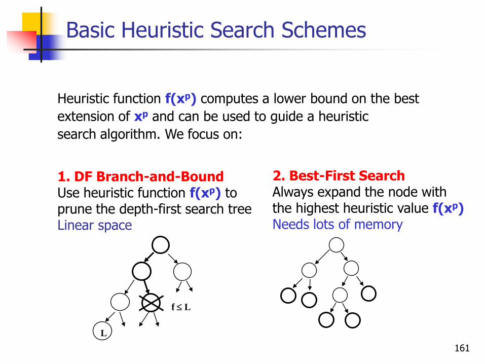
Basic Heuristic Search Schemes
Heuristic function f(xp) computes a lower bound on the best
extension of xp and can be used to guide a heuristic
search algorithm. We focus on:
1. DF Branch-and-BoundUse heuristic function f(xp) to prune the depth-first search treeLinear space
2. Best-First SearchAlways expand the node with the highest heuristic value f(xp)Needs lots of memory
f L
L
161

Best-First Principle
Best-first search expands first the node with the best heuristic evaluation function among all node encountered so far
It never expands nodes whose cost is beyond the optimal one, unlike depth-first search algorithms (Dechter & Pearl, 1985)
Superior among memory intensive algorithms employing the same heuristic function
162
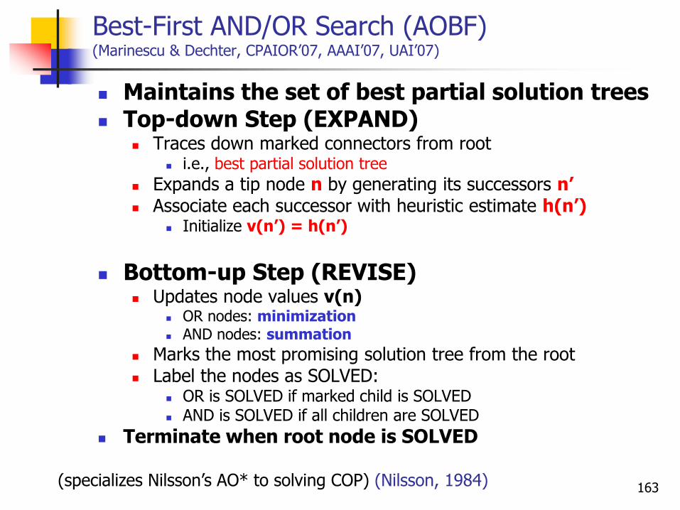
Best-First AND/OR Search (AOBF)(Marinescu & Dechter, CPAIOR’07, AAAI’07, UAI’07)
(specializes Nilsson’s AO* to solving COP) (Nilsson, 1984)
Maintains the set of best partial solution trees Top-down Step (EXPAND)
Traces down marked connectors from root i.e., best partial solution tree
Expands a tip node n by generating its successors n’ Associate each successor with heuristic estimate h(n’)
Initialize v(n’) = h(n’)
Bottom-up Step (REVISE) Updates node values v(n)
OR nodes: minimization AND nodes: summation
Marks the most promising solution tree from the root Label the nodes as SOLVED:
OR is SOLVED if marked child is SOLVED AND is SOLVED if all children are SOLVED
Terminate when root node is SOLVED
163
AOBF versus AOBB
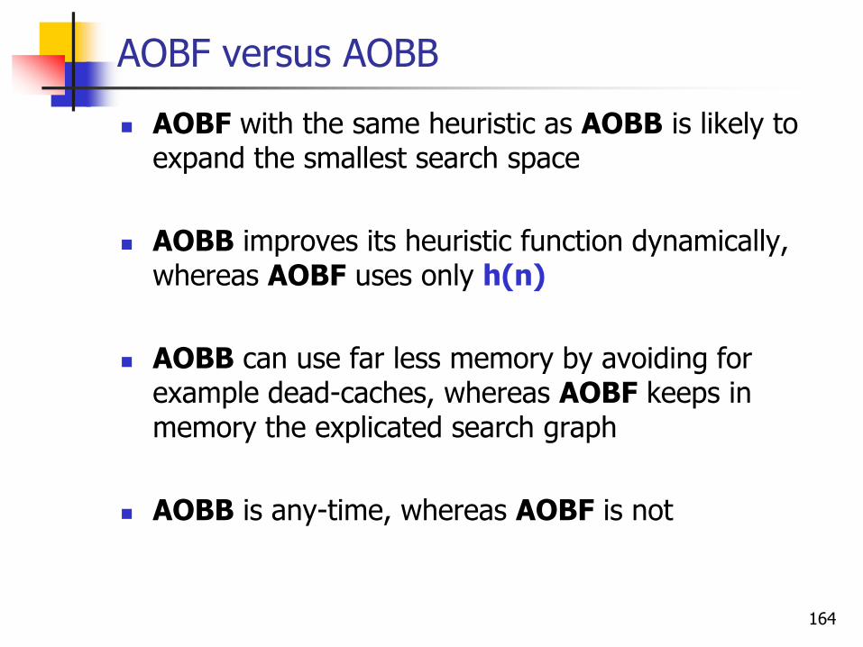
AOBF with the same heuristic as AOBB is likely to expand the smallest search space
AOBB improves its heuristic function dynamically, whereas AOBF uses only h(n)
AOBB can use far less memory by avoiding for example dead-caches, whereas AOBF keeps in memory the explicated search graph
AOBB is any-time, whereas AOBF is not
164

Lower Bounding Heuristics
AOBF can be guided by:
Static Mini-Bucket heuristics(Kask & Dechter, AIJ’01), (Marinescu & Dechter, IJCAI’05)
Dynamic Mini-Bucket heuristics(Marinescu & Dechter, IJCAI’05)
LP Relaxations(Nemhauser & Wosley, 1988)
165
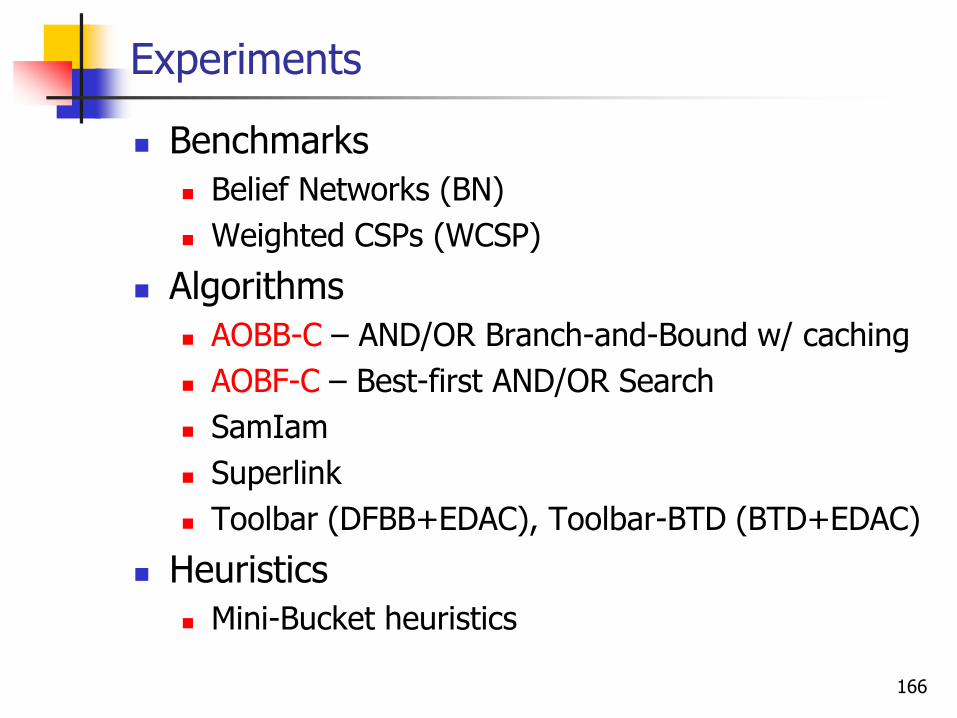
Experiments
Benchmarks
Belief Networks (BN)
Weighted CSPs (WCSP)
Algorithms
AOBB-C – AND/OR Branch-and-Bound w/ caching
AOBF-C – Best-first AND/OR Search
SamIam
Superlink
Toolbar (DFBB+EDAC), Toolbar-BTD (BTD+EDAC)
Heuristics
Mini-Bucket heuristics
166
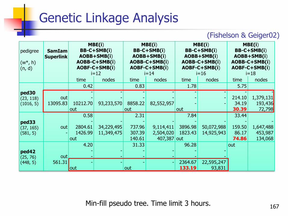
Genetic Linkage Analysis
pedigree
(w*, h)(n, d)
SamIamSuperlink
MBE(i)BB-C+SMB(i)AOBB+SMB(i)
AOBB-C+SMB(i)AOBF-C+SMB(i)
i=12
MBE(i)BB-C+SMB(i)AOBB+SMB(i)
AOBB-C+SMB(i)AOBF-C+SMB(i)
i=14
MBE(i)BB-C+SMB(i)AOBB+SMB(i)
AOBB-C+SMB(i)AOBF-C+SMB(i)
i=16
MBE(i)BB-C+SMB(i)AOBB+SMB(i)
AOBB-C+SMB(i)AOBF-C+SMB(i)
i=18
time nodes time nodes time nodes time nodes
ped30(23, 118)(1016, 5)
out13095.83
0.42--
10212.70out
--
93,233,570
0.83--
8858.22out
--
82,552,957
1.78---
out
---
5.75-
214.1034.19
30.39
-1,379,131
193,43672,798
ped33(37, 165)(581, 5)
out-
0.58-
2804.611426.99
out
-34,229,49511,349,475
2.31-
737.96307.39140.61
-9,114,4112,504,020
407,387
7.84-
3896.981823.43
out
-50,072,98814,925,943
33.44-
159.5086.17
74.86
-1,647,488
453,987134,068
ped42(25, 76)(448, 5)
out561.31
4.20---
out
---
31.33---
out
---
96.28--
2364.67133.19
--
22,595,24793,831
out
Min-fill pseudo tree. Time limit 3 hours.
(Fishelson & Geiger02)
167
Mastermind Games
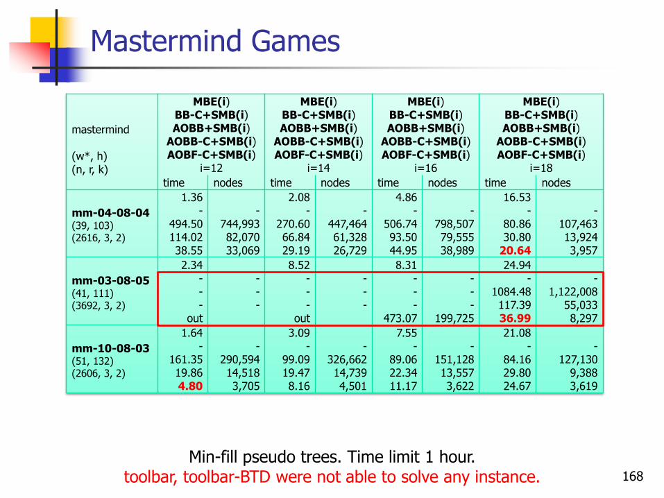
mastermind
(w*, h)(n, r, k)
MBE(i)BB-C+SMB(i)AOBB+SMB(i)
AOBB-C+SMB(i)AOBF-C+SMB(i)
i=12
MBE(i)BB-C+SMB(i)AOBB+SMB(i)
AOBB-C+SMB(i)AOBF-C+SMB(i)
i=14
MBE(i)BB-C+SMB(i)AOBB+SMB(i)
AOBB-C+SMB(i)AOBF-C+SMB(i)
i=16
MBE(i)BB-C+SMB(i)AOBB+SMB(i)
AOBB-C+SMB(i)AOBF-C+SMB(i)
i=18
time nodes time nodes time nodes time nodes
mm-04-08-04(39, 103)(2616, 3, 2)
1.36-
494.50114.0238.55
-744,99382,07033,069
2.08-
270.6066.8429.19
-447,46461,32826,729
4.86-
506.7493.5044.95
-798,50779,55538,989
16.53-
80.8630.80
20.64
-107,46313,9243,957
mm-03-08-05(41, 111)(3692, 3, 2)
2.34---
out
---
8.52---
out
---
8.31---
473.07
---
199,725
24.94-
1084.48117.3936.99
-1,122,008
55,0338,297
mm-10-08-03(51, 132)(2606, 3, 2)
1.64-
161.3519.864.80
-290,59414,5183,705
3.09-
99.0919.478.16
-326,66214,7394,501
7.55-
89.0622.3411.17
-151,12813,5573,622
21.08-
84.1629.8024.67
-127,130
9,3883,619
Min-fill pseudo trees. Time limit 1 hour.toolbar, toolbar-BTD were not able to solve any instance. 168
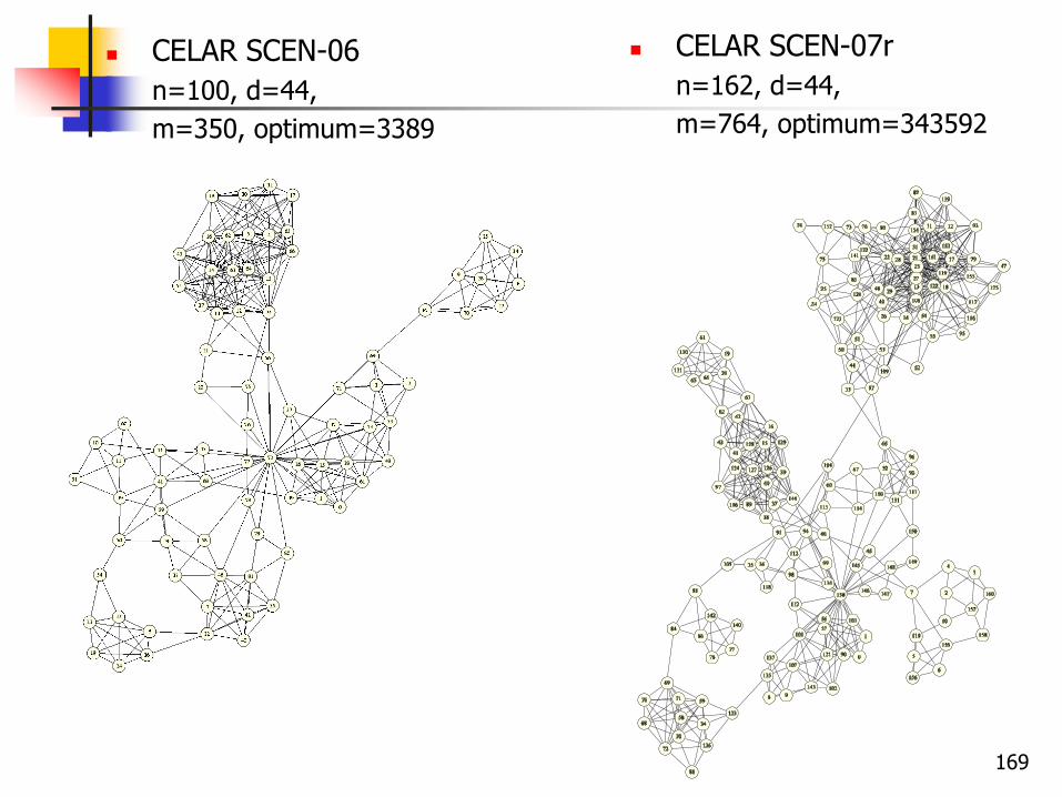
CELAR SCEN-06
n=100, d=44,
m=350, optimum=3389
CELAR SCEN-07r
n=162, d=44,
m=764, optimum=343592
169
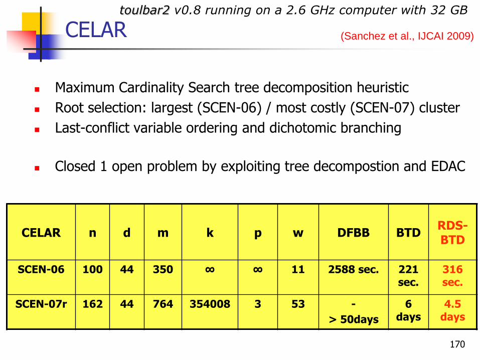
CELAR
Maximum Cardinality Search tree decomposition heuristic
Root selection: largest (SCEN-06) / most costly (SCEN-07) cluster
Last-conflict variable ordering and dichotomic branching
Closed 1 open problem by exploiting tree decompostion and EDAC
CELAR n d m k p w DFBB BTDRDS-BTD
SCEN-06 100 44 350 ∞ ∞ 11 2588 sec. 221 sec.
316 sec.
SCEN-07r 162 44 764 354008 3 53 -
> 50days
6 days
4.5 days
toulbar2 v0.8 running on a 2.6 GHz computer with 32 GB
(Sanchez et al., IJCAI 2009)
170

Summary
New memory intensive AND/OR search algorithms for optimization in graphical models
Depth-first and best-first control strategies
Superior to state-of-the-art OR and AND/OR Branch-and-Bound tree search algorithms
171
Outline
Introduction Inference Search (OR)
Lower-bounds and relaxations
Exploiting problem structure in search AND/OR search spaces (tree, graph) Searching the AND/OR space AND/OR search for 0-1 integer programming
Software
172

0-1 Integer Linear Programming
1021
2211
222
221
21
112
121
11
2211
,,,,
n
mn
mn
mm
nn
nn
nn
xxx
bxaxaxa
bxaxaxa
bxaxaxa
xcxcxcz
:tosubject
:minimize
1,0,,,,,
13
242
2352
3123
:subject to
865237 :minimize
FEDCBA
FEA
EBA
DCB
CBA
FEDCBAz
AC
B E
F
D
primal graph
Applications: VLSI circuit design Scheduling Routing Combinatorial auctions Facility location … 173
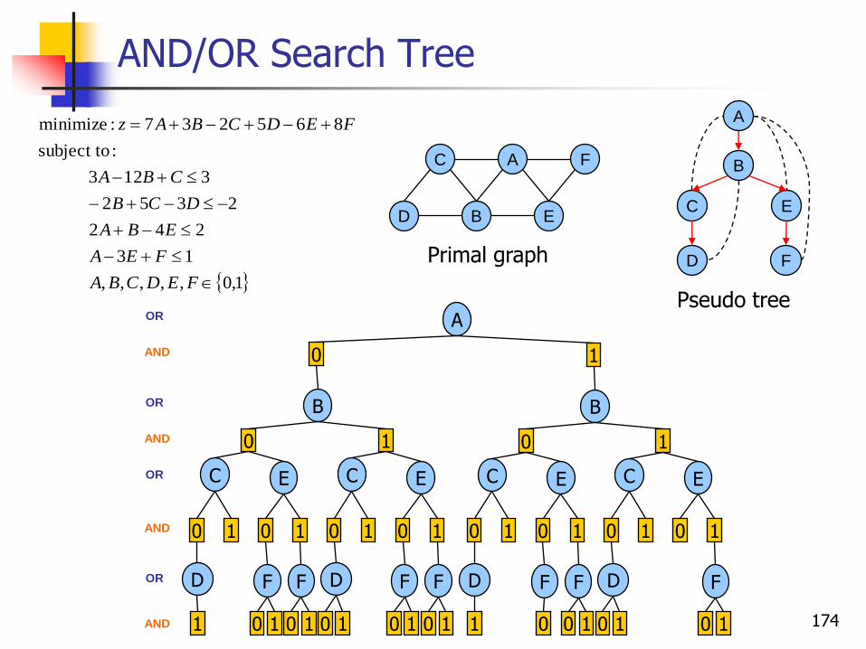
AND/OR Search Tree
1,0,,,,,
13
242
2352
3123
:subject to
865237 :minimize
FEDCBA
FEA
EBA
DCB
CBA
FEDCBAz
A
E
C
B
F
D
OR
AND
OR
AND
OR
OR
AND
AND
A
0
B
0
E
F F
0 1 0 1
0 1
C
D
1
0 1
1
E
F F
0 1 0 1
0 1
C
D
0 1
0 1
1
B
0
E
F F
0 0 1
0 1
C
D
1
0 1
1
E
F
0 1
0 1
C
D
0 1
0 1
Primal graph
Pseudo tree
A
D
B
EC
F
174
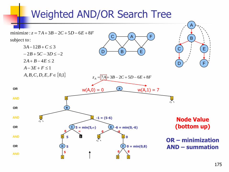
Weighted AND/OR Search Tree
AOR
0AND
BOR
0AND
OR
OR
AND
AND
1
C E
D F
1 0 1
0 10 1
1
FEDCBAzA 865237
5
5
5
0 = min(0,8)
-60
-6 = min(0,-6)
-1 = (5-6)
w(A,0) = 0 w(A,1) = 7
0 8
0
0
5 = min(5,)
Node Value(bottom up)
OR – minimizationAND – summation
A
E
C
B
F
D
A
D
B
EC
F
1,0,,,,,
13
242
2352
3123
:subject to
865237 :minimize
FEDCBA
FEA
EBA
DCB
CBA
FEDCBAz
175
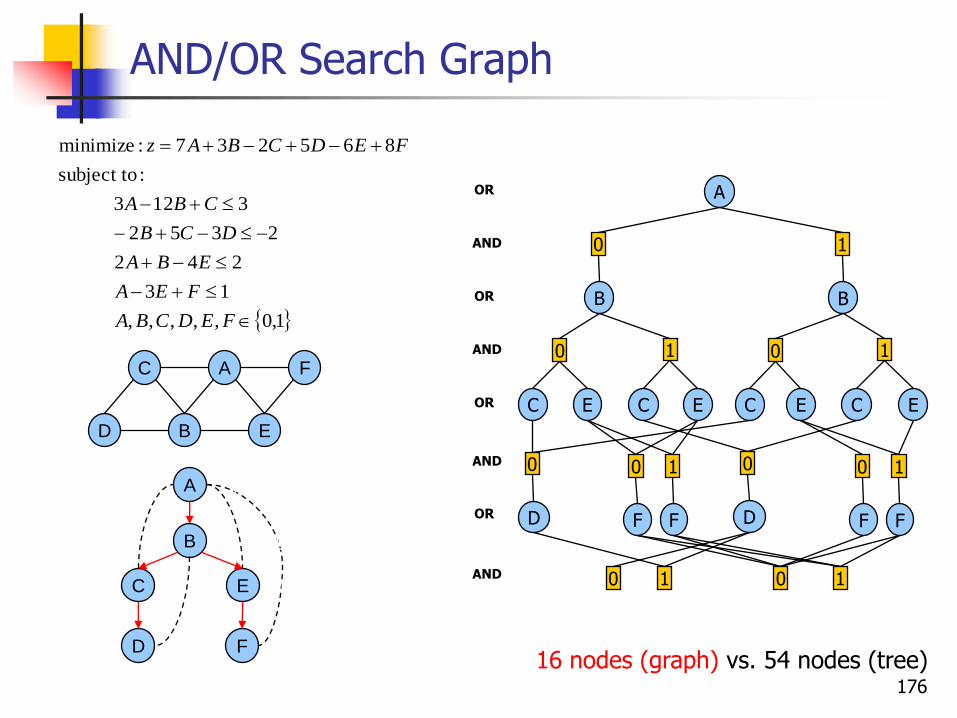
AND/OR Search Graph
AOR
0AND
BOR
0AND
OR E
OR F F
AND 0 1
AND 0 1
C
D
0 1
0
1
EC
D
0
1
B
0
E
F F
0 1
C
1
EC
A
E
C
B
F
D
A
D
B
EC
F
1,0,,,,,
13
242
2352
3123
:subject to
865237 :minimize
FEDCBA
FEA
EBA
DCB
CBA
FEDCBAz
[A]
[BA]
[EA]
[F]
[CB]
[D]16 nodes (graph) vs. 54 nodes (tree)
176
Experiments
Algorithms AOBB, AOBF – tree search
AOBB+PVO, AOBF+PVO – tree search
AOBB-C, AOBF-C – graph search
lp_solve 5.5, CPLEX 11.0, toolbar (DFBB+EDAC)
Benchmarks Combinatorial auctions
MAX-SAT instances
Implementation LP relaxation solved by lp_solve 5.5 library
BB (lp_solve) baseline solver
177
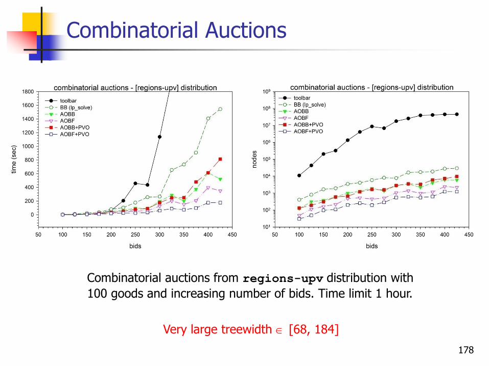
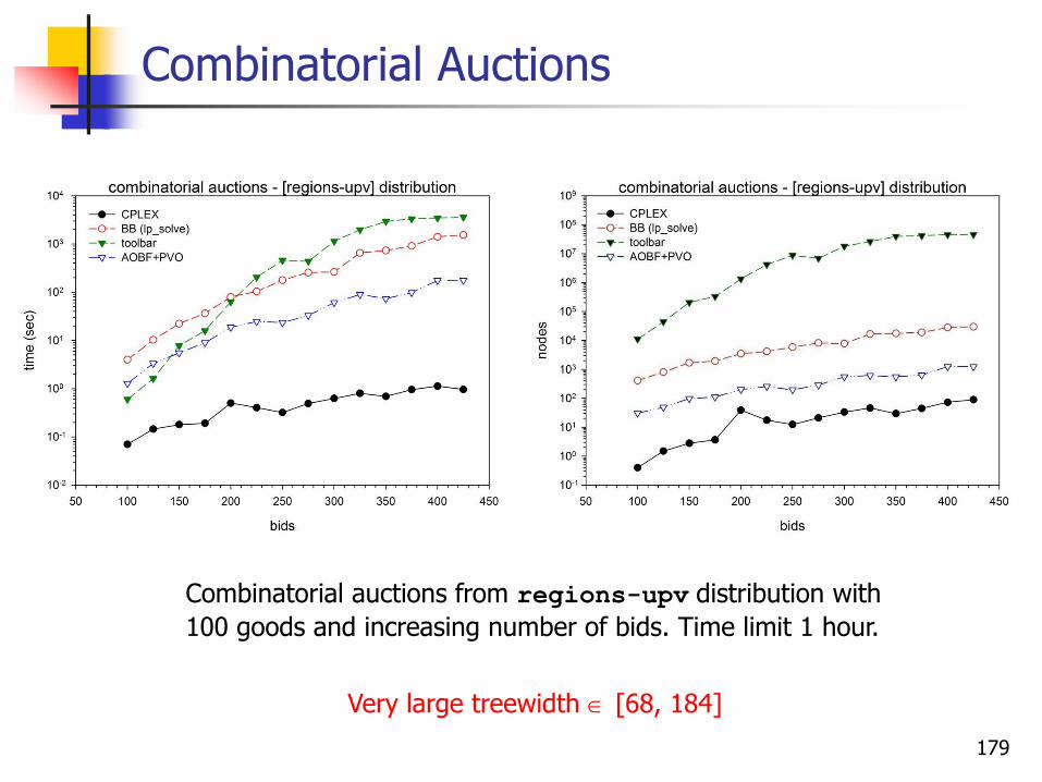
Combinatorial Auctions
Combinatorial auctions from regions-upv distribution with
100 goods and increasing number of bids. Time limit 1 hour.
Very large treewidth [68, 184]
178
Combinatorial Auctions
Combinatorial auctions from regions-upv distribution with
100 goods and increasing number of bids. Time limit 1 hour.
Very large treewidth [68, 184]
179

MAX-SAT Instances (pret)
pret
(w*, h)
BB
CPLEXAOBBAOBF
AOBB+PVOAOBF+PVO
AOBB-CAOBF-C
time nodes time nodes time nodes time nodes
pret60-40(6, 13)
-
676.94
-
3,926,4227.887.56
1,2551,202
8.418.70
1,2161,326
7.383.58
1,216568
pret60-60(6, 13)
-
535.05
-
2,963,4358.568.08
1,2591,184
8.708.31
1,2471,206
7.303.56
1,140538
pret60-75(6, 13)
-
402.53
-
2,005,7386.977.38
1,1241,145
6.808.42
1,0891,149
6.343.08
1,067506
pret150-40(6, 15)
-
out
- 95.11101.78
6,6256,535
108.84101.97
7,1526,246
75.1919.70
5,6251,379
pret150-60(6, 15)
-
out
- 98.88106.36
6,8516,723
112.64102.28
7,3476,375
78.2519.75
5,8131,393
pret150-75(6, 15)
-
out
- 108.1498.95
7,3116,282
115.16103.03
7,4526,394
84.9720.95
6,1141,430
Tree search Tree search Graph search
pret MAX-SAT instances. Time limit 10 hours.
BB solver could not solve any instance.
180

Summary
New AND/OR search algorithms for 0-1 Integer Programming
Dynamic variable orderings
Superior to baseline OR Branch-and-Bound from the lp_solve library
Outperform CPLEX on selected MAX-SAT instances (e.g., pret, dubois)
181

Algorithms for AND/OR Space
Back-jumping for CSPs (Gaschnig 1977), (Dechter 1990), (Prosser, Bayardo & Mirankar, 1995)
Pseudo-search re-arrangement, for any CSP task (Freuder & Quinn 1985)
Pseudo-tree search for soft constraints (Larrosa, Meseguer & Sanchez, 2002)
Recursive Conditioning(Darwiche, 2001), explores the AND/OR tree or graph for any query
BTD: Searching tree-decompositions for optimization(Jeagou & Terrioux, 2004)
Value Elimination(Bacchus, Dalmao & Pittasi, 2003)
182
Outline
Introduction Inference Search (OR)
Lower-bounds and relaxations Exploiting problem structure in search
Software aolib and toulbar2 software packages Results from UAI-06, CP-06 and UAI-08 solver competitions
183

184
Software
Reports on competitions
UAI’06 Inference Evaluation
57 MPE instances
CP’06 Competition
686 2-ary MAX-CSP instances
135 n-ary MAX-CSP instances
CP’08 Competition
534 2-ary MAX-CSP instances
278 n-ary MAX-CSP instances
UAI’08 Competition
480 MPE instances
Toulbar2 and aolib
toulbar2
http://mulcyber.toulouse.inra.fr/gf/project/toulbar2(Open source WCSP, MPE solver in C++)
aolib
http://graphmod.ics.uci.edu/group/Software
(WCSP, MPE, ILP solver in C++, inference and counting)
Large set of benchmarks
http://carlit.toulouse.inra.fr/cgi-bin/awki.cgi/SoftCSP
http://graphmod.ics.uci.edu/group/Repository
185
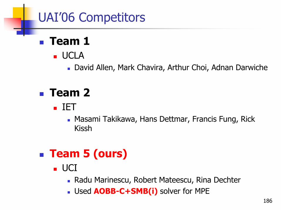
UAI’06 Competitors
Team 1
UCLA
David Allen, Mark Chavira, Arthur Choi, Adnan Darwiche
Team 2
IET
Masami Takikawa, Hans Dettmar, Francis Fung, Rick Kissh
Team 5 (ours)
UCI
Radu Marinescu, Robert Mateescu, Rina Dechter
Used AOBB-C+SMB(i) solver for MPE186
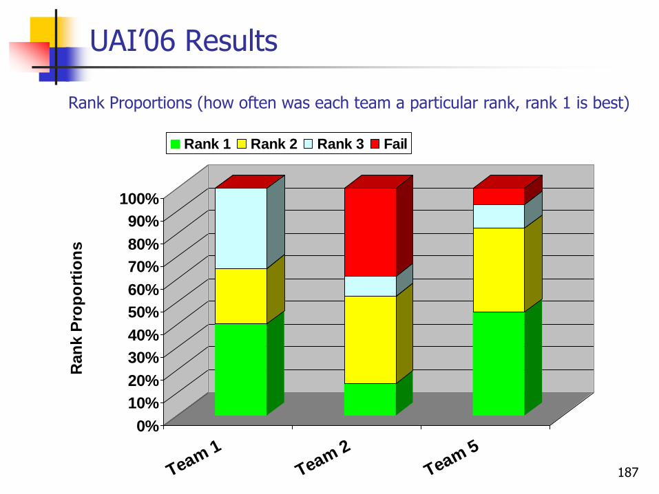
UAI’06 Results
0%
10%
20%
30%
40%
50%
60%
70%
80%
90%
100%
Ran
k P
rop
ort
ion
s
Team 1
Team 2
Team 5
Rank 1 Rank 2 Rank 3 Fail
Rank Proportions (how often was each team a particular rank, rank 1 is best)
187
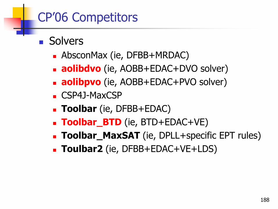
CP’06 Competitors
Solvers
AbsconMax (ie, DFBB+MRDAC)
aolibdvo (ie, AOBB+EDAC+DVO solver)
aolibpvo (ie, AOBB+EDAC+PVO solver)
CSP4J-MaxCSP
Toolbar (ie, DFBB+EDAC)
Toolbar_BTD (ie, BTD+EDAC+VE)
Toolbar_MaxSAT (ie, DPLL+specific EPT rules)
Toulbar2 (ie, DFBB+EDAC+VE+LDS)
188
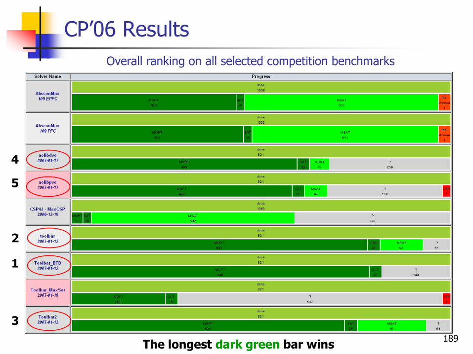
CP’06 Results
Overall ranking on all selected competition benchmarks
1
2
3
4
5
The longest dark green bar wins189
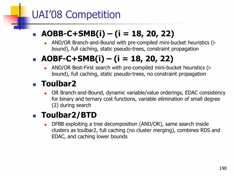
UAI’08 Competition
AOBB-C+SMB(i) – (i = 18, 20, 22) AND/OR Branch-and-Bound with pre-compiled mini-bucket heuristics (i-
bound), full caching, static pseudo-trees, constraint propagation
AOBF-C+SMB(i) – (i = 18, 20, 22) AND/OR Best-First search with pre-compiled mini-bucket heuristics (i-
bound), full caching, static pseudo-trees, no constraint propagation
Toulbar2 OR Branch-and-Bound, dynamic variable/value orderings, EDAC consistency
for binary and ternary cost functions, variable elimination of small degree (2) during search
Toulbar2/BTD DFBB exploiting a tree decomposition (AND/OR), same search inside
clusters as toulbar2, full caching (no cluster merging), combines RDS and EDAC, and caching lower bounds
190
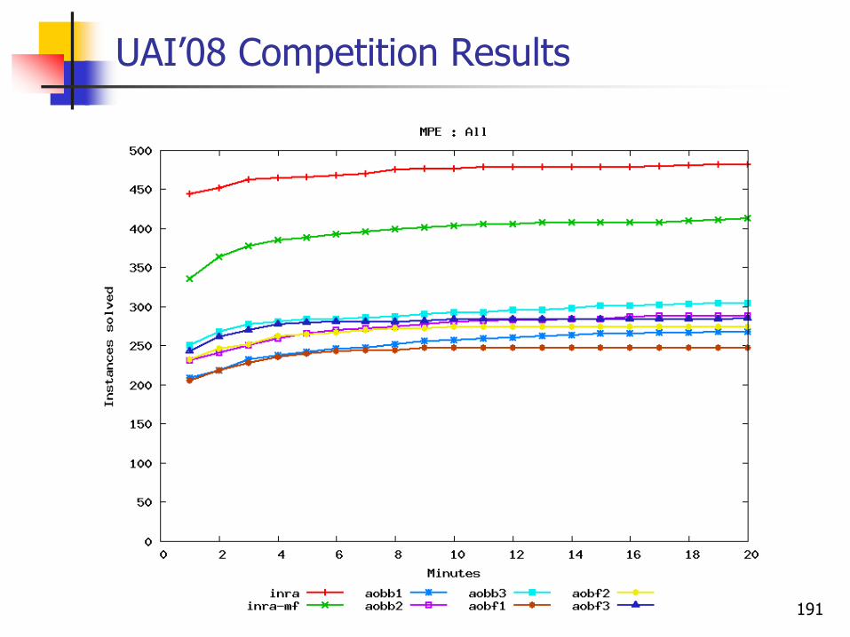
UAI’08 Competition Results
191

UAI’08 Competition Results (II)
192

UAI’08 Competition Results (III)
193

194
CP’08 Competitors
Solvers
AbsconMax (ie, DFBB+MRDAC)
CSP4J-MaxCSP
Sugar (SAT-based solver)
Toulbar2 (ie, BTD+EDAC+VE)
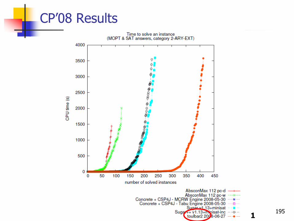
195
CP’08 Results
1
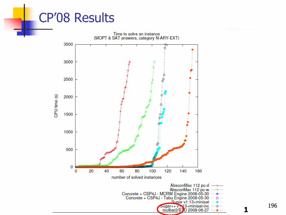
196
CP’08 Results
1

Conclusions
Only a few principles:
1. Inference and search should be combined time-space trade-off
2. AND/OR search should be used
3. Caching in search should be used
197