ADVANCES IN CLINICAL TRIAL B IOSTATISTI CSthe-eye.eu/public/Books/BioMed/Advances in Clinical Trial...Bayesian Reporting of Clinical Trials Simon Weeden, Laurence S. Freedman, and

ADVANCES IN CLINICAL TRIAL B IOSTATISTI CS

edited by

NANCY L. GELLER National Heart, Lung, and Blood Institute

National Institutes of Health Bethesda, Maryland, U.S.A.

M A R C E L

MARCEL DEKKER, INC.

D E K K E R

NEW YORK - BASEL

Copyright n 2004 by Marcel Dekker, Inc. All Rights Reserved.

This book was edited by Nancy L. Geller in her private capacity. The views expressed do not

necessarily represent the views of NIH, DHHS, or the United States.

Although great care has been taken to provide accurate and current information, neither the

author(s) nor the publisher, nor anyone else associatedwith this publication, shall be liable for

any loss, damage, or liability directly or indirectly caused or alleged to be caused by this book.

The material contained herein is not intended to provide specific advice or recommendations

for any specific situation.

Trademark notice: Product or corporate names may be trademarks or registered trademarks

and are used only for identification and explanation without intent to infringe.

Library of Congress Cataloging-in-Publication Data

A catalog record for this book is available from the Library of Congress.

ISBN: 0-8247-9032-4

This book is printed on acid-free paper.

Headquarters

Marcel Dekker, Inc., 270 Madison Avenue, New York, NY 10016, U.S.A.

tel: 212-696-9000; fax: 212-685-4540

Distribution and Customer Service

Marcel Dekker, Inc., Cimarron Road, Monticello, New York 12701, U.S.A.

tel: 800-228-1160; fax: 845-796-1772

Eastern Hemisphere Distribution

Marcel Dekker AG, Hutgasse 4, Postfach 812, CH-4001 Basel, Switzerland

tel: 41-61-260-6300; fax: 41-61-260-6333

World Wide Web

http://www.dekker.com

The publisher offers discounts on this book when ordered in bulk quantities. For more

information, write to Special Sales/Professional Marketing at the headquarters address

above.

Copyright nnnnnnnnn 2004 by Marcel Dekker, Inc. All Rights Reserved.

Neither this book nor any part may be reproduced or transmitted in any form or by any

means, electronic or mechanical, including photocopying, microfilming, and recording, or by

any information storage and retrieval system, without permission in writing from the

publisher.

Current printing (last digit):

10 9 8 7 6 5 4 3 2 1

PRINTED IN THE UNITED STATES OF AMERICA


http://www.dekker.com

Biostatistics: A Series of References and Textbooks

Series Editor

Shein-Chung Chow Vice President, Clinical Biostatistics and Data Management

Millennium Pharmaceuticals, Inc. Cambridge, Massachusetts

Adjunct Professor Temple University

Philadelphia, Pennsylvania

1. Design and Analysis of Animal Studies in Pharmaceutical Devel- opment, edited by Shein-Chung Chow and Jen-pei Liu

2. Basic Statistics and Pharmaceutical Statistical Applications, James E. De Muth

3. Design and Analysis of Bioavailability and Bioequivalence Studies, Second Edition, Revised and Expanded, Shein-Chung Chow and Jen-pei Liu

4. Meta-Analysis in Medicine and Health Policy, edited by Dalene K. Stangl and Donald A. Berry

5. Generalized Linear Models: A Bayesian Perspective, edited by Dipak K. Dey, Sujit K. Ghosh, and Bani K. Mallick

6. Difference Equations with Public Health Applications, Lemuel A. Moye and Asha Seth Kapadia

7. Medical Biostatistics, Abhaya lndrayan and Sanjeev B. Sarrriukaddam 8. Statistical Methods for Clinical Trials, Mark X. Norleans 9. Causal Analysis in Biomedicine and Epidemiology: Based on Minimal

Sufficient Causation, Mike1 Aickin 10. Statistics in Drug Research: Methodologies and Recent Develop-

ments, Shein-Chung Chow and Jun Shao 11. Sample Size Calculations in Clinical Research, Shein-Chung Chow,

Jun Shao, and Hansheng Wang 12. Applied Statistical Designs for the Researcher, Daryl S. Paulson 13. Advances in Clinical Trial Biostatistics, Nancy L. Geller

ADDITIONAL VOLUMES IN PREPARATION


Series Introduction

The primary objectives of the Biostatistics series are to provide useful ref-erence books for researchers and scientists in academia, industry, andgovernment, and also to offer textbooks for undergraduate and/or grad-uate courses in the area of biostatistics. The series provides comprehensiveand unified presentations of statistical designs and analyses of importantapplications in biostatistics, such as those in biopharmaceuticals. A well-balanced summary is given of current and recently developed statisticalmethods and interpretations for both statisticians and researchers/scien-tists with minimal statistical knowledge who are engaged in the field ofapplied biostatistics. The series is committed to presenting easy-to-under-stand, state-of-the-art references and textbooks. In each volume, statisticalconcepts and methodologies are illustrated through real-world exampleswhenever possible.

Clinical research is a lengthy and costly process that involves drugdiscovery, formulation, laboratory development, animal studies, clinicaldevelopment, and regulatory submission. This lengthy process is necessarynot only for understanding the target disease but also for providing sub-stantial evidence regarding efficacy and safety of the pharmaceutical com-pound under investigation prior to regulatory approval. In addition, itprovides assurance that the drug products under investigation will possessgood characteristics such as identity, strength, quality, purity, and stabilityafter regulatory approval. For this purpose, biostatistics plays an impor-


tant role in clinical research not only to provide a valid and fair assess-ment of the drug product under investigation prior to regulatory approvalbut also to ensure that the drug product possesses good characteristics withthe desired accuracy and reliability.

This volume provides a comprehensive summarization of recentdevelopments regarding methodologies in design and analysis of studiesconducted in clinical research. It covers important topics in early-phaseclinical development such as Bayesian methods for phase I cancer clinicaltrials and late-phase clinical development such as design and analysis oftherapeutic equivalence trials, adaptive two-stage clinical trials, and clusterrandomization trials. The book also provides useful approaches to criticalstatistical issues that are commonly encountered in clinical research such asmultiplicity, subgroup analysis, interaction, and analysis of longitudinaldata with missing values. It will be beneficial to biostatisticians, medicalresearchers, and pharmaceutical scientists who are engaged in the areas ofclinical research and development.

Shein-Chung Chow

Series Introductioniv


Preface

As the medical sciences rapidly advance, clinical trials biostatisticians andgraduate students preparing for careers in clinical trials need to maintainknowledge of current methodology. Because the literature is so vast andjournals are published so frequently, it is difficult to keep up with the rel-evant literature. The goal of this book is to summarize recent methodologyfor design and analysis of clinical trials arranged in standalone chapters.

The book surveys a number of aspects of contemporary clinical trials,ranging from early trials to complex modeling problems. Each chaptercontains enough references to allow those interested to delve more deeplyinto an area. A basic knowledge of clinical trials is assumed, along with agood background in classical biostatistics. The chapters are at the level ofjournal articles in Biometrics or Statistics in Medicine and are meant to beread by second- or third-year biostatistics graduate students, as well as bypracticing biostatisticians.

The book is arranged in three parts. The first consists of two chapterson the first trials undertaken in humans in the course of drug development(Phase I and II trials). The second and largest part is on randomized clinicaltrials, covering a variety of design and analysis topics. These include designof equivalence trials, adaptive schemes to change sample size during thecourse of a trial, design of clustered randomized trials, design and analysisof trials with multiple primary endpoints, a newmethod for survival analy-sis, and how to report a Bayesian randomized trial. The third section deals


with more complex problems: including compliance in the assessment oftreatment effects, the analysis of longitudinal data with missingness, andthe particular problems that have arisen in AIDS clinical trials. Several ofthe chapters incorporate Bayesian methods, reflecting the recognition thatthese have become acceptable in what used to be a frequentist discipline.

The 20 authors of this volume represent five countries and 10 insti-tutions.Many of the authors are well known internationally for their meth-odological contributions and have extensive experience in clinical trialspractice as well as being methodologists. Each chapter gives real and rel-evant examples from the authors’ personal experiences, making use of awide range of both treatment and prevention trials. The examples reflectwork in a variety of fields ofmedicine, such as cardiovascular diseases, neu-rological diseases, cancer, and AIDS. While it was often the clinical trialitself that gave rise to a question that required newmethodology to answer,it is likely that the methods will find applications in other medical fields. Inthis sense, the contributions are examples of ‘‘ideal’’ biostatistics, tran-scending the boundary between statistical theory and clinical trials prac-tice.

I wish to express my deep appreciation to all the authors for theirpatience and collegiality and for their fine contributions and outstandingexpositions. I also thank my husband for his constant encouragementand Marcel Dekker, Inc., for their continuing interest in this project.

Nancy L. Geller

Prefacevi


Contents

Series IntroductionPrefaceContributors

Part I METHODS FOR EARLY TRIALS

1. Bayesian Methods for Cancer Phase I Clinical Trials

James S. Babb and Andre Rogatko

2. Design of Early Trials in Stem Cell Transplantation:

A Hybrid Frequentist-Bayesian Approach

Nancy L. Geller, Dean Follmann, Eric S. Leifer, andShelly L. Carter

Part II METHODS FOR RANDOMIZED TRIALS

3. Design and Analysis of Therapeutic Equivalence Trials

Richard M. Simon

4. Adaptive Two-Stage Clinical Trials

Michael A. Proschan

5. Design and Analysis of Cluster Randomization Trials

David M. Zucker


6. Design and Analysis of Clinical Trials with Multiple

Endpoints

Nancy L. Geller

7. Subgroups and Interactions

Dean Follmann

8. A Class of Permutation Tests for Some Two-Sample

Survival Data Problems

Joanna H. Shih and Michael P. Fay

9. Bayesian Reporting of Clinical Trials

Simon Weeden, Laurence S. Freedman, and MaheshParmar

Part III MORE COMPLEX PROBLEMS

10. Methods Incorporating Compliance in Treatment

Evaluation

Juni Palmgren and Els Goetghebeur

11. Analysis of Longitudinal Data with Missingness

Paul S. Albert and Margaret C. Wu

12. Statistical Issues Emerging from Clinical Trials in HIV

Infection

Abdel G. Babiker and Ann Sarah Walker

Index of AbbreviationsIndex of Clinical Trials Used as ExamplesSubject Index

Contentsviii


Contributors

Paul S. Albert, Ph.D. Mathematical Statistician, Biometrics ResearchBranch, Division of Cancer Treatment and Diagnosis, National CancerInstitute, National Institutes of Health, Bethesda, Maryland, U.S.A.

James S. Babb, Ph.D. Department of Biostatistics, Fox Chase CancerCenter, Philadelphia, Pennsylvania, U.S.A.

Abdel G. Babiker, Ph.D. Head, Division of HIV and Infections, andProfessor of Medical Statistics and Epidemiology, Medical ResearchCouncil Clinical Trials Unit, London, England

Shelly L. Carter, Sc.D. Senior Biostatistician, The Emmes Corporation,Rockville, Maryland, U.S.A.

Michael P. Fay, Ph.D. Mathematical Statistician, Statistical Researchand Applications, National Cancer Institute, National Institutes ofHealth, Bethesda, Maryland, U.S.A.

Dean Follmann, Ph.D. Chief, Biostatistics Research Branch, NationalInstitute of Allergy and Infectious Diseases, National Institutes of Health,Bethesda, Maryland, U.S.A.


Laurence S. Freedman, M.A., Dip.Stat., Ph.D. Professor, Departmentsof Mathematics and Statistics, Bar-Ilan University, Ramat Gan, Israel

Nancy L. Geller, Ph.D. Director, Office of Biostatistics Research,National Heart, Lung, and Blood Institute, National Institutes of Health,Bethesda, Maryland, U.S.A.

Els Goetghebeur, Ph.D. Professor, Department of Applied Mathematicsand Computer Science, University of Ghent, Ghent, Belgium

Eric S. Leifer, Ph.D. Mathematical Statistician, Office of BiostatisticsResearch, National Heart, Lung, and Blood Institute, National Institutesof Health, Bethesda, Maryland, U.S.A.

Juni Palmgren, Ph.D. Professor, Department of Mathematical Statisticsand Department of Medical Epidemiology and Biostatistics, StockholmUniversity and Karolinska Institutet, Stockholm, Sweden

Mahesh Parmar, D.Phil., M.Sc., B.Sc. Professor of Medical Statisticsand Epidemiology, Cancer Division, Medical Research Council ClinicalTrials Unit, London, England

Michael A. Proschan, Ph.D. Mathematical Statistician, Office of Bio-statistical Research, National Heart, Lung, and Blood Institute, NationalInstitutes of Health, Bethesda, Maryland, U.S.A.

Andre Rogatko, Ph.D. Department of Biostatistics, Fox Chase CancerCenter, Philadelphia, Pennsylvania, U.S.A.

Joanna H. Shih, Ph.D. Mathematical Statistician, Biometric ResearchBranch, Division of Cancer Treatment and Diagnosis, National CancerInstitute, National Institutes of Health, Bethesda, Maryland, U.S.A.

Richard M. Simon, D.Sc. Chief, Biometric Research Branch, Division ofCancer Treatment and Diagnosis, National Cancer Institute, NationalInstitutes of Health, Bethesda, Maryland, U.S.A.

Ann Sarah Walker, Ph.D., M.Sc. Medical Research Council ClinicalTrials Unit, London, England

Contributorsx


Simon Weeden, M.Sc. Senior Medical Statistician, Cancer Division,Medical Research Council Clinical Trials Unit, London, England

Margaret C. Wu, Ph.D.* Mathematical Statistician, Office of Biostatis-tics Research, National Heart, Lung, and Blood Institute, National Insti-tutes of Health, Bethesda, Maryland, U.S.A.

David M. Zucker, Ph.D. Associate Professor, Department of Statistics,Hebrew University, Jerusalem, Israel

*Retired.

Contributors xi


1Bayesian Methods for CancerPhase I Clinical Trials

James S. Babb and Andre RogatkoFox Chase Cancer Center, Philadelphia, Pennsylvania, U.S.A.

1. INTRODUCTION

1.1. Goal and Definitions

The primary statistical objective of a cancer phase I clinical trial is todetermine the optimal dose of a new treatment for subsequent clinicalevaluation of efficacy. The dose sought is typically referred to as themaximum tolerated dose (MTD), and its definition depends on theseverity and manageability of treatment side effects as well as on clinicalattributes of the target patient population. For most anticancer regimens,evidence of treatment benefit, usually expressed as a reduction in tumorsize or an increase in survival, requires months (if not years) of obser-vation and is therefore unlikely to occur during the relatively short timecourse of a phase I trial (O’Quigley et al., 1990; Whitehead, 1997).Consequently, the phase I target dose is usually defined in terms of theprevalence of treatment side effects without direct regard for treatmentefficacy. For the majority of cytotoxic agents, toxicity is considered aprerequisite for optimal antitumor activity (Wooley and Schein, 1979)and the probability of treatment benefit is assumed to monotonicallyincrease with dose, at least over the range of doses under consideration inthe phase I trial. Consequently, the MTD of a cytotoxic agent typicallycorresponds to the highest dose associated with a tolerable level of


toxicity. More precisely, the MTD is defined as the dose expected toproduce some degree of medically unacceptable, dose limiting toxicity(DLT) in a specified proportion u of patients (Storer, 1989; Gatsonis andGreenhouse, 1992). Hence we have

ProbfDLT j Dose ¼ MTDg ¼ u ð1Þwhere the value chosen for the target probability u would depend on thenature of the dose limiting toxicity; it would be set relatively high when theDLT is a transient, correctable, or nonfatal condition, and low when it islethal or life threatening (O’Quigley et al., 1990). Participants in cancerphase I trials are usually late stage patients for whommost or all alternativetherapies have failed. For such patients, toxicity may be severe before it isconsidered an intolerable burden (Whitehead, 1997). Thus, in cancer phaseI trials, dose limiting toxicity is often severe or potentially life threateningand the target probability of toxic response is correspondingly low,generally less than or equal to 1/3. As an example, in a phase I trialevaluating 5-fluorouracil (5-FU) in combination with leucovorin andtopotecan (see Sec. 1.4.1), dose limiting toxicity was defined as any treat-ment attributable occurrence of: (1) a nonhematologic toxicity (e.g.,neurotoxicity) whose severity according to the Common Toxicity Criteria*

of the National Cancer Institute (1993) is grade 3 or higher; (2) a grade 4hematologic toxicity (e.g., thrombocytopenia or myelosuppression) per-sisting at least 7 days; or (3) a 1week or longer interruption of the treatmentschedule. The MTD was then defined as the dose of 5-FU that is expectedto induce such dose limiting toxicity in one-third of the patients in thetarget population. As illustrated with this example, the definition of DLTshould be broad enough to capture all anticipated forms of toxic responseas well as many that are not necessarily anticipated, but may nonethelessoccur. This will reduce the likelihood that the definition of DLT will needto be altered or clarified upon observation of unanticipated, treatment-attributable adverse events—a process generally requiring a formalamendment to the trial protocol and concomitant interruption of patientaccrual and treatment.

It is important to note that there is currently no consensus regard-ing the definition of the MTD. When the phase I trial is designed

* The Common Toxicity Criteria can be found on the Internet at http://ctep.info.nih.gov/

CTC3/default.htm.

Babb and Rogatko2


according to traditional, non-Bayesian methods (e.g., the up-and-downschemes described in Storer, 1989), an empiric, data-based definition ismost often employed. Thus, the MTD is frequently taken to be the high-est dose utilized in the trial such that the percentage of patientsmanifesting DLT is equal to a specified level such as 33%. For example,patients are often treated in cohorts, usually consisting of three patients,with all patients in a cohort receiving the same dose. The dose is changedbetween successive cohorts according to a predetermined schedule typi-cally based on a so-called modified Fibonacci sequence (Von Hoff et al.,1984). The trial is terminated the first time at least some number ofpatients (generally 2 out of 6) treated at the same dose exhibit DLT. Thisdose level constitutes the MTD. The dose level recommended for phase IIevaluation of efficacy is then taken to be either the MTD or one dose levelbelow the MTD (Kramar et al., 1999). Although this serves as anadequate working definition of the MTD for trials of nonparametricdesign, such an empiric formulation is not appropriate for use with mostBayesian and other parametric phase I trial design methodologies.Consequently, it will be assumed throughout the remainder of this chap-ter that the MTD is defined according to Eq. (1) for some suitable defi-nition of DLT and choice of target probability u.

The fundamental conflict underlying the design of cancer phase Iclinical trials is that the desire to increase the dose slowly to avoidunacceptable toxic events must be tempered by an acknowledgment thatescalation proceeding too slowly may cause many patients to be treatedat suboptimal or nontherapeutic doses (O’Quigley et al., 1990). Thus,from a therapeutic perspective, one should design cancer Phase I trials tominimize both the number of patients treated at low, nontherapeuticdoses as well as the number given severely toxic overdoses.

1.2. Definition of Dose

Bayesian procedures for designing phase I clinical trials require thespecification of a model for the relationship between dose level andtreatment related toxic response. Depending on the agent under inves-tigation and the route and schedule of its administration, the model mayrelate toxicity to the physical amount of agent given each patient, or tosome target drug exposure such as the area under the time vs. plasmaconcentration curve (AUC) or peak plasma concentration. The choice offormulation is dependent on previous experience and medical theory andis beyond the scope of the present chapter. Consequently, it will be

Bayesian Methods for Cancer Phase I Clinical Trials 3


assumed that the appropriate representation of dose level has been de-termined prior to specification of the dose-toxicity model.

1.3. Choice of Starting Dose

In cancer therapy, the phase I trial often represents the first time aparticular treatment regimen is being administered to humans. Due toconsequent safety considerations, the starting dose in a cancer phase Itrial is traditionally a low dose at which no significant toxicity isanticipated. For example, the initial dose is frequently selected on thebasis of preclinical investigation to be one-tenth of the murine equivalentLD10 (the dose that produces 10% mortality in mice) or one-third thetoxic dose low (first toxic dose) in dogs (Geller, 1984; Penta et al., 1992).Conversely, several authors (e.g., O’Quigley et al., 1990) suggest that thestarting dose should correspond to the experimenter’s best prior estimateof the MTD, which may not be a conservative initial level. This may beappropriate since starting the trial at a dose level significantly below theMTD may unduly increase the time and number of patients required tocomplete the trial and since retrospective studies (Penta et al., 1992;Arbuck, 1996) suggest that the traditional choice of starting dose oftenresults in numerous patients being treated at biologically inactive doselevels. In the sequel, it will be assumed that the starting dose is pre-determined; its choice based solely on information available prior to theonset of the trial.

1.4. Examples

Selected aspects of the Bayesian approach to phase I trial design will beillustrated using examples based on two phase I clinical trials conductedat the Fox Chase Cancer Center.

5-FU Trial

In this trial a total of 12 patients with malignant solid tumors weretreated with a combination of 5-fluorouracil (5-FU), leucovorin, andtopotecan. The goal was to determine the MTD of 5-FU, defined as thedose that, when administered in combination with 20 mg/m2 leucovorinand 0.5 mg/m2 topotecan, results in a probability u= 1/3 that a DLT willbe manifest within 2 weeks. The relevant data obtained from this trial aregiven in Table 1.

Babb and Rogatko4


PNU Trial

The incorporation of patient-specific covariate information into a Baye-sian design scheme will be exemplified through a phase I study of PNU-214565 (PNU) involving patients with advanced adenocarcinomas ofgastrointestinal origin (Babb and Rogatko, 2001). Previous clinical andpreclinical studies demonstrated that the action of PNU is moderated bythe neutralizing capacity of anti-SEA antibodies. Based on this, the MTDof PNU was defined as a function of the pretreatment concentration ofcirculating anti-SEA antibodies. Specifically, the MTD was defined as thedose level expected to induce DLT in a proportion u = .1 of the patientswith a given pretreatment anti-SEA concentration.

2. GENERAL BAYESIAN METHODOLOGY

The design and conduct of phase I clinical trials would benefit fromstatistical methods that can incorporate information from preclinicalstudies and sources outside the trial. Furthermore, both the investigator

Table 1 Dose Level of 5-FU (mg/m2) and BinaryAssessment of Treatment-Induced Toxic Response

for the 12 Patients in the 5-FU Phase I Trial

Patienta 5-FU Dose Response

1 140 No DLT2 210 No DLT

3 250 No DLT4 273 No DLT5 291 No DLT6 306 No DLT

7 318 No DLT8 328 No DLT9 337 No DLT

10 345 No DLT11 352 DLT12 338 DLT

a Patients are listed in chronological order according to date

of accrual.



and patient might benefit if updated assessments of the risk of toxicitywere available during the trial. Both of these needs can be addressedwithin a Bayesian framework. In Sections 2.1 through 2.5 we present adescription of selected Bayesian procedures developed for the specificcase where toxicity is assessed on a binary scale (presence or absence ofDLT), only a single agent is under investigation (the levels of any otheragents being fixed) and no relevant pretreatment covariate informationis available to tailor the dosing scheme to individual patient needs.We discuss extensions and modifications of the selected methods inSection 3.

2.1. Formulation of the Problem

Dose level will be represented by the random variable X whose realizationis denoted by x. For notational compactness, the same variable will beused for any formulation of dosage deemed appropriate. Thus, forexample, X may represent some target drug exposure (e.g., AUC), thephysical amount of agent in appropriate units (e.g., mg/m2), or theamount of agent expressed as a multiple of the starting dose, and mightbe expressed on a logarithmic or other suitable scale. It will be assumedthroughout that the MTD is expressed in a manner consistent with X.

The data observed for k patients will be denoted Dk = {(xi, yi); i =1, . . . , k}, where xi is the dose administered patient i, and yi is an indicatorfor dose limiting toxicity assuming the value yi = 1 if the ith patientmanifests DLT and the value yi = 0, otherwise. The MTD is denoted byg and corresponds to the dose level expected to induce dose limitingtoxicity in a proportion u of patients.

In the ensuing sections, a general Bayesian paradigm for the designof cancer phase I trials will be described in terms of three components:

1. A model for the dose-toxicity relationship. The model specifiesthe probability of dose limiting toxicity at each dose level as afunction of one or more unknown parameters.

2. A prior distribution for the vector N containing the unknownparameters of the dose-toxicity model. The prior will berepresented by a probability density function h defined on theparametric space Q specified for N. It is chosen so that HðIÞ ¼mIhðuÞdu is an assessment of the probability that N is containedin I p Q based solely on the information available prior to theonset of the phase I trial.

Babb and Rogatko6


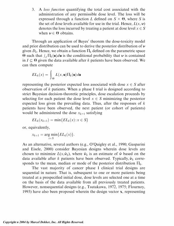
3. A loss function quantifying the total cost associated with theadministration of any permissible dose level. The loss will beexpressed through a function L defined on S � Q, where S isthe set of dose levels available for use in the trial. Hence, L(x, N)denotes the loss incurred by treating a patient at dose level x 2 Swhen N 2 Q obtains.

Through an application of Bayes’ theorem the dose-toxicity modeland prior distribution can be used to derive the posterior distribution of Ngiven Dk. Hence, we obtain a function Ck defined on the parametric spaceQ such that mI CkðuÞdu is the conditional probability that N is containedin I p Q given the data available after k patients have been observed. Wecan then compute

ELkðxÞ ¼Z

HLðx; uÞCkðuÞdu

representing the posterior expected loss associated with dose x 2 S afterobservation of k patients. When a phase I trial is designed according tostrict Bayesian decision-theoretic principles, dose escalation proceeds byselecting for each patient the dose level x 2 S minimizing the posteriorexpected loss given the prevailing data. Thus, after the responses of kpatients have been observed, the next patient (or cohort of patients)would be administered the dose xk+1 satisfying

ELkðxkþ1Þ ¼ minfELkðxÞ :x 2 Sgor, equivalently,

xkþ1 ¼ arg minx �S

fELkðxÞg:

As an alternative, several authors (e.g., O’Quigley et al., 1990; Gaspariniand Eisele, 2000) consider Bayesian designs wherein dose levels arechosen to minimize L(x, Nk), where Nk is an estimate of N based on thedata available after k patients have been observed. Typically, Nk corre-sponds to the mean, median or mode of the posterior distribution Ck.

The vast majority of cancer phase I clinical trial designs aresequential in nature. That is, subsequent to one or more patients beingtreated at a prespecified initial dose, dose levels are selected one at a timeon the basis of the data available from all previously treated patients.However, nonsequential designs (e.g., Tsutakawa, 1972, 1975; Flournoy,1993) have also been proposed wherein the design vector x, representing



the entire collection of dose levels to be used in the trial, is chosen prior tothe onset of the trial. In such circumstances, x is chosen to minimize theexpected loss with respect to the prior distribution h and patients (orcohorts of patients) are then randomly assigned to the dose levels soobtained. In the ensuing formulations only sequential designs will beexplicitly discussed. In other words, we consider designs that select doseson the basis of the information conveyed by the posterior distribution Ck

rather than the prior distribution h.

2.2. Dose-Toxicity Model

A mathematical model is specified for the relationship between dose leveland the probability of dose limiting toxicity. The choice of model is basedon previous experience with the treatment regimen under investigation,preclinical toxicology studies, medical theory, and computational trac-tability. We note that the dose to be administered to the first patient orcohort of patients is typically chosen on the basis of prior informationalone. Thus, its selection does not in general depend on the model for thedose-toxicity relationship. Consequently, it may be advantageous todelay the specification of the model until after a pharmacologic andstatistical evaluation of the data from the cohort of patients treated at thepreselected starting dose.

The models most frequently used in cancer phase I clinical trials areof the form

ProbfDLTjDose ¼ xg ¼Fðh0 þ h1xÞy ð2Þwhere F is a cumulative distribution function (CDF) referred to as thetolerance distribution, y and h1 are both assumed to be positive so thatthe probability of dose limiting toxicity is a strictly increasing function ofdose, and one or more of y, h0 and h1 may be assumed known. Mostapplications based on this formulation use either a logit or probit modelwith typical examples including the two-parameter logistic (Gatsonis andGreenhouse, 1992; Babb et al., 1998)

ProbfDLTjDose ¼ xg ¼ expðh0 þ h1xÞ1þ expðh0 þ h1xÞ ð3Þ

(with y = 1 assumed known) and the one-parameter hyperbolic tangent(O’Quigley et al., 1990).

Babb and Rogatko8


ProbfDLTjDose ¼ xg ¼ tanhðxÞ þ 1

2

� �y: ð4Þ

To facilitate comparisons between these two models, the hyperbolictangent model can be rewritten as

Prob DLT jDose ¼ xf g ¼ expð2xÞ1þ expð2xÞ� �y

which is consistent with the form given in Eq. (2) with h0 = 0 and h1 = 2assumed known. For exposition we consider the two-parameter logisticmodel given in (3). With this model the MTD is

g ¼ lnðuÞ � lnð1� uÞ � h0

h1:

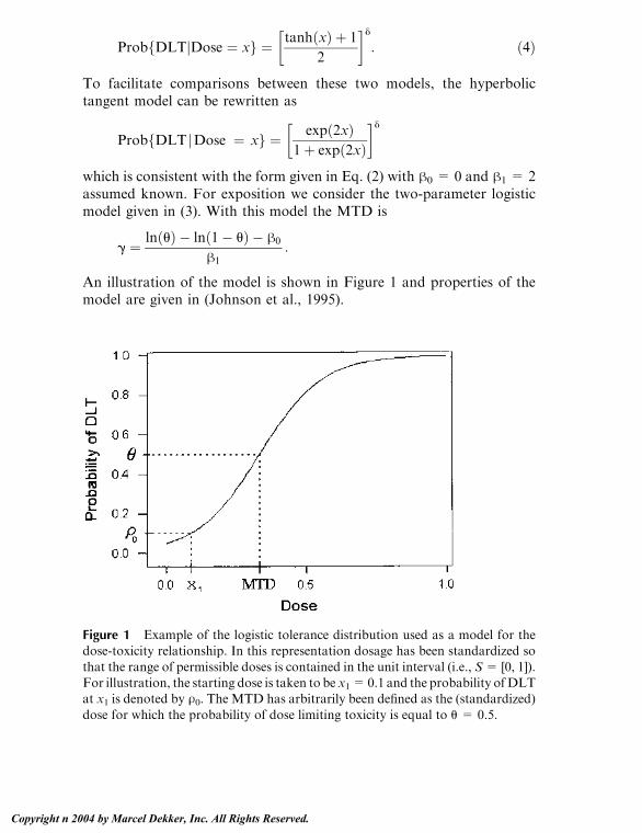
An illustration of the model is shown in Figure 1 and properties of themodel are given in (Johnson et al., 1995).

Figure 1 Example of the logistic tolerance distribution used as a model for thedose-toxicity relationship. In this representation dosage has been standardized so

that the range of permissible doses is contained in the unit interval (i.e., S= [0, 1]).For illustration, the starting dose is taken to be x1=0.1 and the probability ofDLTat x1 is denoted by U0. The MTD has arbitrarily been defined as the (standardized)

dose for which the probability of dose limiting toxicity is equal to u = 0.5.



An alternative formulation describes the dose-toxicity relationship asit applies to the set S={x1, x2, . . . , xk} of prespecified dose levels availablefor use in the trial. For example, Gasparini and Eisele (2000) present acurve-free Bayesian phase I design discussed the possibility of using oneprior distribution (the design prior) to determine dose assignments duringthe phase I trial and a separate prior (the inference prior) to estimate theMTDupon trial completion. Although the use of separate priors for designand inference may appear inconsistent, its usefulness is defended byarguing that analysis occurs later than design (Tsutakawa, 1972). Con-sequently, our beliefs regarding the unknown parameters of the dose-toxicitymodelmay change during the time fromdesign to inference inwaysnot entirely accounted for by a sequential application of Bayes’ theorem.

Since estimation of the MTD is the primary statistical aim of aphase I clinical trial, our subsequent attention will be focused on dose-toxicity models parameterized in terms of N = [g N] for some choice of(possibly null) vector N of nuisance parameters. To facilitate elicitation ofprior information, the nuisance vector N should consist of parametersthat the investigators can readily interpret.

As discussed above, the starting dose of a phase I trial is frequentlyselected on the basis of preclinical investigation. Consequently, priorinformation is often available about the risk of toxicity at the initial dose.To exploit this, Gatsonis and Greenhouse (1992) and Babb et al., (1998)considered the logistic model given by (3) parameterized in terms of theMTD

g ¼ lnðuÞ � lnð1� uÞ � h0

h1

and

U0 ¼ expðh0 þ h1x1Þ1þ expðh0 þ h1x1Þ

the probability of DLT at the starting dose. Due to safety considerations,the dose for the first patient (or patient cohort) is typically chosen so thatit is believed a priori to be safe for use with humans. Consequently, it isgenerally assumed that U0 V u. This information about the initial dosecan be expressed through a marginal prior distribution for U0 whose massis concentrated on [0, u]. Examples include the truncated beta (Gatsonisand Greenhouse, 1992) and uniform distributions (Babb et al., 1998)defined on the interval (0, a) for some known value a V u. Prior in-

Babb and Rogatko10


formation about the MTD is frequently more ambiguous. Such priorignorance can be reflected through the use of vague or non-informativepriors. Thus, for example, the marginal prior distribution of the MTDmight scheme in which the toxicity probabilities are modeled directly asan unknown k-dimensional parameter vector. That is, the dose-toxicitymodel is given by

Prob DLTjDose ¼ xif g ¼ ui i ¼ 1; 2; . . . ; k ð5Þ

with N = [u1 u2 . . . , uk] unknown. The authors maintain that byremoving the assumption that the dose-toxicity relationship follows aspecific parametric curve, such as the logistic model in (3), this modelpermits a more efficient use of prior information. A similar approach isbased on what has variously been referred to as an empiric discrete model(Chevret, 1993), a power function (Kramar et al., 1999; Gasparini andEisele, 2000) or a power model (Heyd and Carlin, 1999). The model isgiven by

Prob DLTjDose ¼ xif g ¼ uyi ð6Þ

where y>0 is unknown and u i (i=1, 2, . . . , k) is an estimate of theprobability of DLT at dose level xi based solely on informationavailable prior to the onset of the phase I trial. With this model thetoxicity probabilities can be increased or decreased through the param-eter N = y as accumulating data suggests that the regimen is more orless toxic than was suggested by prior opinion. As noted by Gaspariniand Eisele (2000), the empiric discrete model of Eq. (6) is equivalent tothe hyperbolic tangent model of Eq. (4) provided one uses as priorestimates

ui ¼ tanhðxiÞ þ 1

2i ¼ 1; 2; . . . ; k :

2.3. Prior Distribution

The Bayesian formulation requires the specification of a prior probabilitydistribution for the vector v containing the unknown parameters of thedose-toxicity model. The prior distribution is subjective; i.e., it conveys



the opinions of the investigators prior to the onset of the trial. It isthrough the prior that information from previous trials, clinical andpreclinical experience, and medical theory are incorporated into theanalysis. The prior distribution should be concentrated in some mean-ingful way around a prior guess N0 (provided by the clinicians), yet itshould also be sufficiently diffuse as to allow for dose escalation in theabsence of dose limiting toxicity (Gasparini and Eisele, 2000). We notethat several authors (e.g., Tsutakawa, 1972, 1975) have be taken to be auniform distribution on a suitably defined interval (Babb et al., 1998) or anormal distribution with appropriately large variance (Gatsonis andGreenhouse, 1992).

Example: 5-FU Trial (continued)

The statistical goal of the trial was to determine the MTD of 5-FUwhen administered in conjunction with 20 mg/m2 leucovorin and 0.5 mg/m2 topotecan. The dose-toxicity model used to design the trial was thatgiven by Eq. (3), reparameterized in terms of r = [g U0]. Preliminarystudies indicated that 140 mg/m2 of 5-FU was well tolerated when givenconcurrently with up to 0.5 mg/m2 topotecan. Consequently, this levelwas selected as the starting dose for the trial and was believed a priorito be less than the MTD. Furthermore, previous trials involving 5-FUalone estimated the MTD of 5-FU as a single agent to be 425 mg/m2.Since 5-FU has been observed to be more toxic when in combinationwith topotecan than when administered alone, the MTD of 5-FU incombination with leucovorin and topotecan was assumed to be lessthan 425 mg/m2. Overall, previous experience with 5-FU led to theassumption that g 2 [140, 425] and U0 < 1/3 with prior probability one.Based on this, the joint prior probability density function of N wastaken to be

hðNÞ ¼ 57�1IQðg;U0Þ Q ¼ ½140; 425� � ½0; 0:2� ð7Þ

where, for example, IS denotes the indicator function for the set S [i.e.,IS (x) = 1 or 0 according as x does or does not belong to S ]. It followsfrom (7) that the MTD and U0 were assumed to be independently andmarginally distributed as uniform random variables. In the exampleabove, there was a suitable choice for an upper bound on the range ofdose levels to be searched for the MTD. That is, prior experience with

Babb and Rogatko12


5-FU suggested that, when given in combination with topotecan, theMTD of 5-FU was a priori believed to be less than 425 mg/m2. Inconsequence, the support of the prior for the MTD was finite. In manycontexts, there will not be sufficient information available prior to theonset of the phase I trial to unambiguously determine a suitable upperbound for the MTD (and hence for the range of dose levels to besearched). In this case, one might introduce a hyperparameter Xmax andspecify a joint prior distribution for the MTD and Xmax as

hðg;XmaxÞ ¼ f1ðg j XmaxÞ f0ðXmaxÞ

with, to continue the 5-FU example, f1(gjXmax) denoting the probabilitydensity function (pdf) of a uniform random variable on [140, 425] andf0 (Xmax) a monotone decreasing pdf defined on [425, l), such as atruncated normal with mean 425 and suitable standard deviation.

Flournoy (1993) considered the two-parameter logistic model in Eq.(3) reparameterized in terms of the MTD and the nuisance parameterN= h2. The parameters g and N were assumed to be independent a prioriwith g having a normal and N having a gamma distribution. Thus, thejoint prior distribution of v = [g h2] was defined on Q = R � (0, l)by

hðnÞ ¼ ½GðaÞbajffiffiffiffiffiffi2k

p��1h2ða�1Þexp

��ðg� AÞ22j2

� h2

b

�:

As rationale for the choice of prior distribution for N, it was noted thatN�1 is proportional to the variance of the logistic tolerance distributionand that the gamma distribution is frequently used to model the inverseof a variance component. In order to determine values for the hyper-parameters a, b, A, and j, physicians were asked to graph curvescorresponding to a prior 95% confidence band for the true dose-toxicityrelationship. Values were then chosen for the hyperparameters so that the95% confidence intervals at selected doses, as determined by the upperand lower hand drawn graphs at each dose, agreed with the correspond-ing confidence intervals implied by the prior.

Various authors (e.g., Chevret, 1993; Faries, 1994; Moller, 1995;Goodman et al., 1995) studying the continual reassessment method(O’Quigley et al., 1990) have considered monoparametric dose-toxicitymodels such as the hyperbolic tangent model of Eq. (4) and the empiric



discrete model given by (6). Prior distributions used for the unknownparameter y include the exponential

gðyÞ ¼ expð�yÞ y 2 ð0;lÞ ð8Þ

and the uniform

gðyÞ ¼ 1=3 y 2 ð0; 3Þ ð9Þ

corresponding to priors observed to work well in computer simulationstudies (O’Quigley et al., 1990; Chevret, 1993). Since the hyperbolictangent model implies that

g ¼ ln u1=y

1� u1=y

the priors induced for the MTD by the choice of (8) and (9) as the priordistribution for y are

hðgÞ ¼jJ jexp�

lnðuÞlnð1þ e2gÞ � 2g

�g 2 ð�l;lÞ

and

hðgÞ ¼ jJ j3

g 2 �l; lnu1=3

1� u1=3

� �

respectively, where the Jacobian is given by

J ¼ �2 lnðuÞð1þ e2gÞ½lnð1þ e2gÞ � 2g�2

and jJj is the absolute value of the determinant of J. Chevret (1993)conducted a simulation study to compare the relative utility of usingexponential, gamma, log-normal, uniform, and Weibull distributions aspriors for the lone unknown parameter in the dose-toxicity models givenby Eqs. (4) and (6) or in the two-parameter logistic model with known

Babb and Rogatko14


intercept parameter. The results suggested that estimation of the MTDwas not significantly affected by the choice of prior distribution and thatno one prior distribution performed consistently better than the othersunder a broad range of circumstances.

An alternative formulation of the prior distribution, suggested byTsutakawa (1975) and discussed by Patterson et al. (1999) and Whitehead(1997), is based on a prior assessment of the probability of DLT atselected dose levels. As a simple example, consider two prespecified doselevels z1 and z2. These dose levels need not be available for use in thephase I trial, but often represent doses used in previous clinical inves-tigations. For i = 1, 2, positive constants t(i) and n(i) are chosen so thatt(i)/n(i) corresponds to a prior estimate of the probability of DLT at thedose zi. The prior for N is then specified as

hðNÞ ¼ n P2

i¼1pðzi j NÞtðiÞ½1� pðzi j NÞ�nðiÞ�tðiÞ

where n is the standardizing constant rendering h a proper probabilitydensity function and p(�jN) is the model for the dose-toxicity relationshipparameterized in terms of N. In this formulation the prior is proportionalto the likelihood function for N given a data set in which, for i = 1, 2, n(i)patients were treated at dose zi with exactly t(i) manifesting DLT.Consequently, this type of prior is typically referred to as a ‘‘pseudo-data’’ prior. As noted by Whitehead (1997), the pseudodata mightinclude observations from previous studies at one or both of z1 and z2.Such data might be downweighted to reflect any disparity betweenprevious and present clinical circumstances by choosing values for then(i) that are smaller than the actual number of previous patientsobserved.

The curve-free method of Gasparini and Eisele (2000) is based onthe dose-toxicity model given by (5). Hence, the dose-toxicity relationshipis modeled directly in terms of N = [u1 u2 . . . uk], the vector oftoxicity probabilities for the k dose levels selected for use in the trial.The prior selected for r is referred to as the product-of-beta prior andcan be described as follows. Let c1 = 1 � p1 and for i = 2, 3, . . . , k, letci = (1 � pi)/(1 � pi�1). The product-of-beta prior is the distributioninduced for N by the assumption that the ci (i = 1, 2, . . . , k) areindependent with ci distributed as a beta with parameters ai and bi. Theauthors provide a method for determining the hyperparameters ai and biso that the marginal prior distribution of ui is concentrated near u i,



corresponding to the clinicians’ prior guess for ui, and yet disperse enoughto permit dose escalation in the absence of toxicity. They also discuss whyalternative priors, such as the ordered Dirichlet distribution, may not beappropriate for use in cancer phase I trials designed according to thecurve-free method.

2.4. Posterior Distribution

Perceptions concerning the unknown model parameters change as thetrial progresses and data accumulate. The appropriate adjustment ofsubjective opinions can be made by transforming the prior distribution hthrough an application of Bayes’ theorem. Thus, we obtain the posteriordistribution Ck which reflects our beliefs about N based on a combinationof prior knowledge and the data available after k patients have beenobserved.

The transformation from prior to posterior distribution is accom-plished through the likelihood function. If we denote the dose-toxicitymodel parameterized in terms of N as

pðxjNÞ ¼ ProbfDLT jDose ¼ xg

then the likelihood function for r= [g N] given the data Dk is

LðNjDkÞ ¼ Pk

i¼1pðxijNÞyif1� pðxijNÞg1�yi :

Bayes’ theorem then implies that the joint posterior distribution of (g, N)given the data Dk is

C kðg;NjDkÞ ¼ Lðg;NjDkÞhðg;NÞmLðujDkÞhðuÞdu

where the integral is over Q. To facilitate exposition, it will hereafter beassumed that the prior distribution h is defined on some set G � Vcontaining the parameter space Q such that g 2 G and N 2 V with priorprobability 1. Whenever necessary, this will entail extending h fromQ to G� V by defining h to be identically equal to zero on the difference (G �V)\Q. This convention will simplify ensuing formulations without a loss of

Babb and Rogatko16


generality. For example, the marginal posterior distribution of the MTDgiven the data from k patients can then be simply expressed as

PkðgÞ ¼Z

XC kðc; u jDkÞdu

irrespective of whether or not g and N were assumed to be independent apriori.


The dose-toxicity relationship was modeled according to the logistictolerance distribution given by (3) reparameterized in terms of N= [g U0],where U0 is the probability of DLT at the starting dose x1 = 140. Asshown by Eq. (7), the prior distribution for r was taken to be the uniformon G � V = [140, 425] � [0, .2]. It follows that the marginal posteriorprobability density function of the MTD given the data Dk is

PkðgÞ ¼Z 0:2

0

C ki¼1

ðexpfyi f ðg; ujxiÞg½1þ expf f ðg; ujxiÞgÞ du g 2 ½140; 425�

where

fðg; ujxiÞ ¼ ðg� xiÞlnfu=ð1� uÞg þ ðxi � 140Þlnfu=ð1� uÞgg� 140

:

The marginal posterior distribution Pk represents a probabilistic summaryof all the information about the MTD that is available after the observa-tion of k patients. Figure 2 shows the marginal posterior distribution ofthe MTD given the data shown in Table 1.

2.5. Loss Function

As each patient is accrued to the trial, a decision must be made regardingthe dose level that the patient is to receive. In a strict Bayesian setting, thedecisions are made by minimizing the posterior expected loss associatedwith each permissible choice of dose level. To accomplish this, the set S ofall permissible dose levels is specified and a loss function is chosen toquantify the cost or loss arising from the administration of eachpermissible dose under each possible value of N. The loss may beexpressed in financial terms, in terms of patient well-being, or in terms



of the gain in scientific knowledge (Whitehead, 1997). Uncertainty aboutN is reflected through the posterior distribution and the expected lossassociated with each permissible dose x is determined by averaging theloss attributed to x over the parameter space G � V according to theposterior distribution Ck. Thus, after k patients have been observed,the posterior expected loss associated with dose x 2 S is

ELkðxÞ ¼Z

HLðx; uÞC kðuÞdu

and the next patient would receive the dose

xkþ1 ¼ arg minx2S

fELkðxÞg:

Figure 2 Marginal posterior probability density function of the MTD of 5-FUgiven the data from all 12 patients treated in the 5-FU phase I trial.

Babb and Rogatko18


For example, the dose for each patient might be chosen to minimize theposterior expected loss with respect to the loss function L(x, N) = d{u,p(x, N)} or L(x, N) =m(x, g) for some choice of metrics d andm defined onthe unit square and S � G, respectively. Thus, patients might be treated atthe mean, median, or mode of the marginal posterior distribution of theMTD, corresponding to the respective choices of loss function L(x, N) =(x � g)2, L(x, N) = jx � gj, and L(x, N) = I(0,q) (jx � gj), for somearbitrarily small positive constant q.

Instead of minimizing the posterior expected loss, dose levels can bechosen so as to minimize the loss function after substituting an estimatefor N. Consequently, given the data from k patients, one might estimate Nas Nk and administer to the next patient the dose

xkþ1 ¼ arg minxeS

fLðx; NkÞg:

In the remainder of this section we describe various loss functions that havebeen discussed in the literature concerning cancer phase I clinical trials.

Since the primary statistical aim of a phase I clinical trial is todetermine the MTD, designs have been presented which seek to maximizethe efficiency with which theMTD is estimated. As an example, Tsutakawa(1972, 1975) considered the following design which, for simplicity, wedescribe in terms of a dose-toxicity model whose only unknown parameteris g. Let x denote the vector of dose levels to be administered to the nextcohort of patients accrued to the trial. Given g= g0, the posterior varianceof g before observing the response at x is approximated by the loss function

Lðx; g0Þ ¼ fBðhÞ þ Iðx; g0Þg�1

where B(h) is a nonnegative constant which may depend on the prior hchosen for g and I(x, g0) is the Fisher information contained in the samplewhen using x and g0 obtains. The constant termB is introduced so thatL(x,g0) is bounded above (when B > 0) and so that L becomes the exactposterior variance of g under suitable conditions. The method is illustratedusing the specific choice B(h) / H �1, where H is the variance of the priordistribution assumed for g. After observing the responses of k patients, thedoses to be used for the next cohort are given by the vector x minimizing

ELkðxÞ ¼Z

GLðx; uÞC kðuÞ du

the expected loss with respect to the posterior distribution Ck of N = g.Methods to accomplish the minimization of G are discussed in Tsutakawa



(1972, 1975) andpresented in (Chaloner andLarntz, 1989).Once xhas beendetermined, random sampling without replacement can be used to deter-mine the dose level contained in x that is to be administered each patient inthe next cohort.

For cancer phase I trials, we typically seek to optimize the treatmentof each individual patient. Attention might therefore focus on identifyinga dose that all available evidence indicates to be the best estimate of theMTD. This is the basis for the continual reassessment method (CRM)proposed by O’Quigley et al. (1990). In the present context their originalformulation can be described as follows. Let p(�jN) denote the modelselected for the dose-toxicity relationship parameterized in terms of N.Given the data from k patients, the probability of DLT at any permissibledose level x 2 S can be estimated as

ukðxÞ ¼Z

HpðxjuÞC kðuÞdu

or

ukðxÞ ¼ pðxjNkÞ ð10Þ

where Nk denotes an estimate of N. The next patient is then treated at thedose for which the estimated probability of DLT is as close as possible, insome predefined sense, to the target probability u. Thus, for example, afterobservation of k patients, the next patient might receive the dose level xk+1

satisfying

jukðxkþ1Þ � ujV jukðxÞ � uj bx 2 S

In an effort to balance the ethical and statistical imperatives inherentto cancer phase I trials, methods have been proposed to construct dosesequences that, in an appropriate sense, converge to the MTD as fast aspossible subject to a constraint on each patient’s predicted risk of beingadministered an overdose (Eichhorn and Zacks, 1973, 1981; Babb et al.,1998) or of manifesting DLT (Robinson, 1978; Shih, 1989). Thus, forexample, the Bayesian feasible methods first considered by Eichhorn andZacks (1973) select dose levels for use in the trial so that the expectedproportion of patients receiving a dose above the MTD does not exceed aspecified value a, called the feasibility bound. This can be accomplished byadministering to each patient the dose level corresponding to the a-fractileof the marginal posterior cumulative distribution function (CDF) of the

Babb and Rogatko20


MTD. Specifically, after k patients have been observed, the dose for thenext patient accrued to the trial is

xkþ1 ¼ F�1k ðaÞ ð11Þ

where

FkðxÞ ¼Z x

0

ZX

Ykðg;NÞ dN dg ð12Þ

is the marginal posterior CDF of the MTD given Dk. Thus, subsequent tothe first cohort of patients, the dose selected for each patient corresponds tothe dose having minimal posterior expected loss with respect to

Lðx;NÞ ¼aðg� xÞ if xV g ði:e:; if x is an underdoseÞ

ð1� aÞðx� gÞ if x > c ði:e:; if x is an overdoseÞ:

8<:The use of this loss function implies that for any y>0 the loss incurred bytreating a patient at y units above the MTD is (1� a)/a times greater thanthe loss associated with treating the patient at y units below theMTD. Thisinterpretation might provide a meaningful basis for the selection of thefeasibility bound (Babb et al., 1998). The value selected for the feasibilitybound will determine the rate of change in dose level between successivepatients. Low values will result in a cautious escalation scheme withrelatively small increments in dose, while high values would result in amore aggressive escalation. In a typical application the value of thefeasibility bound is initially set at a small value (a = 0.25, say) and thenallowed to increase in a predeterminedmanner until a=0.5. The rationalebehind this approach is that uncertainty about the MTD is highest at theonset of the trial and a small value of a affords protection against thepossibility of administering dose levels much greater than the MTD. Asthe trial progresses, uncertainty about theMTDdeclines and the likelihoodof selecting a dose level significantly above the MTD becomes smaller.Consequently, a relatively high probability of exceeding the MTD can betolerated near the conclusion of the trial because the magnitude by whichany dose exceeds the MTD is expected to be small.



As defined by Eichhorn and Zacks (1973), a dose sequence {xj}nj=1

is Bayesian feasible of level 1 � a if Fj (xj+1) V a, bj = 1, . . . , n � 1,where Fj the marginal posterior CDF of the MTD given Dj as defined inEq. (12). Correspondingly, the design of a phase I clinical trial is said tobe Bayesian feasible (of level 1 � a) if the posterior probability that eachpatient receives an overdose is no greater than the feasibility bound a.Zacks et al., (1998) showed that the dose sequence specified by Eq. (11) isconsistent (i.e., under suitable conditions, the dose sequence converges inprobability to the MTD) and is optimal among Bayesian feasible designsin the sense that it minimizes mGmVðg� xkÞIð�l;xkÞðgÞCkðg;NÞ dN dg, theexpected amount by which any given patient is underdosed. Conse-quently, the method defined by equation (11) is referred to as the optimalBayesian feasible design.

Figure 3 Dose levels for patients 2–5 of the 5-FU trial conditional on thetreatment-attributable toxicities observed.

Babb and Rogatko22



The 5-FU trial was designed according to the optimal Bayesian feasibledose escalation method known as EWOC (Babb et al., 1998). For thistrial the feasibility bound was set equal to a = 0.25, this value being acompromise between the therapeutic aim of the trial and the need toavoid treatment attributable toxicity. Consequently, escalation of 5-FUbetween successive patients was to the dose level determined to haveposterior probability equal to 0.25 of being an overdose (i.e., greater thanthe MTD). The first patient accrued to the trial received the preselecteddose 140 mg/m2. Based on the EWOC algorithm, as implementedaccording to Rogatko and Babb (1998), the doses administered the nextfour patients were selected according to the schedule given in Figure 3.

In contrast to the Bayesian feasible methods, the predictionapproaches of Robinson (1978) and Shih (1989) provide sequential searchprocedures which control the probability that a patient will exhibit DLT.Their formulation is non-Bayesian, being based on the coverage distri-bution (Shih, 1989) rather than the posterior distribution of N.

3. MODIFICATIONS AND EXTENSIONS

3.1. Maximum Likelihood

In its original presentation CRM (O’Quigley et al., 1990) utilizedBayesian inference. Subsequently, to overcome certain difficulties asso-ciated with the Bayesian approach (see, for example, Gasparini andEisele, 2000) a maximum likelihood based version of CRM (CRML)was introduced (O’Quigley and Shen, 1996). Essentially, the Bayesianand likelihood based approaches differ with respect to the method used toestimate the probability of DLT at each permissible dose level. Thus, forexample, both CRM and CRML might utilize the estimates given byEq. (10) with N k respectively corresponding to either a Bayesian ormaximum likelihood estimate of N. Simulation studies (Kramar et al.,1999) comparing Bayesian CRM with CRML showed the methods tohave similar operating characteristics. However, one key distinctionbetween the Bayesian and likelihood approaches is that the latter requiresa trial to be designed in stages. More specifically, the maximum like-lihood estimate, uk(x), of the probability of DLT at any dose x will betrivially equal to either zero or one, or perhaps even fail to exist, until atleast one patient manifests DLT and one fails to exhibit DLT. Hence, the



use of CRML must be preceded by an initial stage whose design does notrequire maximum likelihood estimation. This stage might be designedaccording to Bayesian principles (e.g., by original CRM) or by use ofmore traditional up-and-down schemes based on a modified Fibonaccisequence. Once at least one patient manifests and one patient is treatedwithout DLT, the first stage can be terminated and subsequent doseescalations can be determined through the use of CRML. Since CRML isinherently non-Bayesian, it will not be discussed further in this chapter.Instead we refer interested readers to O’Quigley and Shen (1996) andKramar et al. (1999) for details regarding the implementation of CRML.

3.2. Delayed Response

Since cancer patients often exhibit delayed response to treatment, thetime required to definitively evaluate treatment response can be longerthan the average time between successive patient accruals. Consequently,new patients frequently become available to the study before theresponses of all previously treated patients have unambiguously beendetermined (O’Quigley et al., 1990). It is therefore important to note thatBayesian procedures do not require knowledge of the responses of allpatients currently on study before a newly accrued patient can begintreatment. Instead, the dose for the new patient can be selected on thebasis of whatever data are currently available (O’Quigley et al., 1990;Babb et al, 1998). Thus, it can be left to the discretion of the clinician todetermine whether to treat a newly accrued patient at the dose recom-mended on the basis of all currently known responses, or to wait until theresolution of one or more unknown responses and then treat the newpatient at an updated determination of dose.

3.3. Rapid Initial Escalation

Recently, ethical concerns have been raised regarding the large number ofpatients treated in cancer phase I trials at potentially biologically inactivedose levels (Hawkins, 1993; Dent and Eisenhauer, 1996). A summary(Decoster et al., 1990) of the antitumor activity and toxic deaths reportedfor 6639 phase I cancer patients revealed that only 0.3% (n=23) exhibiteda complete response, 4.2% (279) manifested a partial response and toxicdeaths occurred in only 0.5% (31) of the patients. A similar review of 6447patients found that only 4.2%achieved an objective response (3.5%partialresponse, 0.7% complete remission). As a result, the last several years haveseen the production of numerous suggested modifications of the standard

Babb and Rogatko24


trial paradigm (ASCO, 1997). Such design alternatives, often referred to asaccelerated titration designs (Simon et al., 1997), begin with an aggressive,rapid initial escalation of dose and mandate switching to a more con-servative approach when some prespecified target is achieved. The switch-ing rule is usually based on adefined incidence of some level of toxicity (e.g.,the second hematologic toxicity of grade 2 or higher), or a pharmacologicendpoint such as 40% of the AUC at the mouse LD10. In the context ofBayesian phase I designs, Moller (1995) and Goodman et al. (1995)proposed two-stage phase I dose escalation schemes wherein implementa-tion of a Bayesian design was preceded by a rapid ad hoc dose escalationphase. Theremay be considerable advantage in adopting the two-stage trialdesign since the first stage may not only reduce the incidence of non-therapeutic dose assignments, but would also provide meaningful priorinformation on which to base the Bayesian design of the second stage.

3.4. Constrained Escalation

In their inception, Bayesian methods were not widely accepted in thecontext of cancer phase I clinical trials. The major criticism was that theymight unduly increase the chance of administering overly toxic dose levels(Faries, 1994). Consequently, many recently proposed Bayesian designmethods (e.g., Faries, 1994; Moller, 1995; Goodman et al., 1995) incorpo-rate guidelines that limit the magnitude by which the dose level can beincreased between successive patients. As an example, the protocol of thePNU trial prohibited escalation at any stage of the trial to a dose levelgreater than twice the highest dose previously administered without induc-tion of dose limiting toxicity (Babb and Rogatko, 2001). Similarly, designshave been proposed (Faries, 1994) wherein each dose is selected from asmall number of prespecified levels according to CRM, but with escalationbetween successive cohorts limited to one dose level. As an alternative, thetrial might be designed to provide maximal statistical efficiency subject tosome formal constraint reflecting patient safety. For example, the dose foreach patient might be selected so as to minimize the posterior expectedvariance of the MTD (as in Tsutakawa, 1972, 1975; Flournoy, 1993) overthe subset of permissible dose levels that are Bayesian feasible at some level1 � a (as in Eichhorn and Zacks, 1973; Babb et al., 1998).

3.5. Multinomial and Continuous Response Measures

Phase I trials frequently provide more information about toxicity than isexploited by the methods described in Section 2. For example, whereas



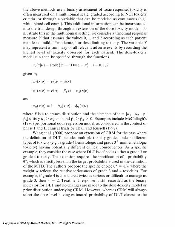
the above methods use a binary assessment of toxic response, toxicity isoften measured on a multinomial scale, graded according to NCI toxicitycriteria, or through a variable that can be modeled as continuous (e.g.,white blood cell count). This additional information can be incorporatedinto the trial design through an extension of the dose-toxicity model. Toillustrate this in the multinomial setting, we consider a trinomial responsemeasure Y that assumes the values 0, 1, and 2 according as each patientmanifests ‘‘mild,’’ ‘‘moderate,’’ or dose limiting toxicity. The variable Ymay represent a summary of all relevant adverse events by recording thehighest level of toxicity observed for each patient. The dose-toxicitymodel can then be specified through the functions

fiðxjNÞ ¼ ProbfY ¼ ijDose ¼ xg i ¼ 0; 1; 2

given by

f2ðxjNÞ ¼ Fða2 þ h2xÞ

f1ðxjNÞ ¼ Fða1 þ b1xÞ � f2ðxjNÞand

f0ðxjNÞ ¼ 1� f2ðxjNÞ � f1ðxjNÞwhere F is a tolerance distribution and the elements of N = [a1 a2 h1

h2] satisfy a1 z a2 > 0 and h1 z h2 > 0. Examples include McCullagh’s(1980) proportional odds regression model, as considered in the context ofphase I and II clinical trials by Thall and Russell (1998).

Wang et al. (2000) propose an extension of CRM for the case wherethe definition of DLT includes multiple toxicity grades and/or differenttypes of toxicity (e.g., a grade 4 hematologic and grade 3+ nonhemetalogictoxicity) having potentially different clinical consequences. As a specificexample, they consider the case where DLT is defined as either a grade 3 orgrade 4 toxicity. The extension requires the specification of a probabilityu*, which is strictly less than the target probability u used in the definitionof the MTD. The authors propose the specific choice u* = u/w where theweight w reflects the relative seriousness of grade 3 and 4 toxicities. Forexample, if grade 4 is considered twice as serious or difficult to manage asgrade 3, then w = 2. Treatment response is still recorded as the binaryindicator for DLT and no changes are made to the dose-toxicity model orprior distribution underlying CRM. However, whereas CRM will alwaysselect the dose level having estimated probability of DLT closest to the

Babb and Rogatko26


target u, the extended version recommends using the dose with estimatedprobability of DLT nearest u* after the observation of a grade 4 toxicity.Hence, whenever a grade 3 or lower toxicity is observed, the extendedCRM selects the dose level with estimated DLT probability nearest u,exactly as prescribed by standard CRM. Only upon observation of a grade4 toxicity will the extended version select a dose different from (moreprecisely, less than or equal to) that recommended by CRM. As a result,use of the extended version of CRM will result in a more cautiousescalation of dose level in the presence of severe toxicity.

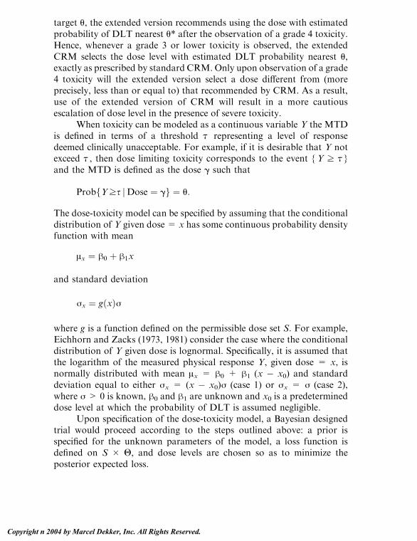
When toxicity can be modeled as a continuous variable Y the MTDis defined in terms of a threshold H representing a level of responsedeemed clinically unacceptable. For example, if it is desirable that Y notexceed H , then dose limiting toxicity corresponds to the event {Y z H }and the MTD is defined as the dose g such that

ProbfYzs jDose ¼ gg ¼ u:

The dose-toxicity model can be specified by assuming that the conditionaldistribution of Y given dose = x has some continuous probability densityfunction with mean

Ax ¼ h0 þ h1x

and standard deviation

jx ¼ gðxÞj

where g is a function defined on the permissible dose set S. For example,Eichhorn and Zacks (1973, 1981) consider the case where the conditionaldistribution of Y given dose is lognormal. Specifically, it is assumed thatthe logarithm of the measured physical response Y, given dose = x, isnormally distributed with mean Ax = h0 + h1 (x � x0) and standarddeviation equal to either jx = (x � x0)j (case 1) or jx = j (case 2),where j > 0 is known, h0 and h1 are unknown and x0 is a predetermineddose level at which the probability of DLT is assumed negligible.

Upon specification of the dose-toxicity model, a Bayesian designedtrial would proceed according to the steps outlined above: a prior isspecified for the unknown parameters of the model, a loss function isdefined on S � Q, and dose levels are chosen so as to minimize theposterior expected loss.



3.6. Designs for Drug Combinations

In the development of a new cancer therapy, the treatment regimen underinvestigation will often consist of two or more agents whose levels are tobe determined by phase I testing. In such contexts, a simple approach isto conduct the trial in stages with the level of only one agent escalated ineach stage. The methods described above can then be implemented todesign each stage. An example of this is given by the 5-FU trial.


The protocol of the 5-FU trial actually included two separate stages of doseescalation. In the first stage, outlined above, 12 patients were eachadministered a dose combination consisting of 20 mg/m2 leucovorin, 0.5mg/m2 topotecan, and a dose of 5-FU determined by the EWOC algo-rithm. In the second stage, the level of 5-FU was held fixed at 310 mg/m2,corresponding to the dose recommended for the next (i.e., thirteenth)patient had the first stage been allowed to continue. An additional 12patients were accrued during the second stage with each patient receiving310 mg/m2 5-FU, 20 mg/m2 leucovorin, and a dose of topotecan deter-mined by EWOC. For these 12 patients the feasibility bound was initiallyset equal to 0.25 (as in the first stage) and then allowed to increase by 0.05with each successive dose assignment until the value a=0.5 was attained.Hence, for example, the first two patients in stage 2 received respectivedoses of topotecan determined to have posterior probability 0.25 and 0.3 ofexceeding the MTD. All stage 2 patients including and subsequent to thesixth patient received a dose of topotecan corresponding to the median ofthe marginal posterior distribution of the MTD given the prevailing data.

A single stage scheme was proposed by Flournoy (1993) as amethod to determine the MTD of a combination of cyclophosphamide(denoted x) and busulfan ( y). To define a unique MTD and implementdesign methods appropriate for single agent regimens, attention wasrestricted to a set S of dose combinations lying along the line segmentdelimited by the points (x, y) = (40, 6) and (x, y) = (180, 20). Since forany (x, y) 2 S the level of one agent is completely determined by the levelof the other, the design methods described above for single agent trialscan be used to select dose combinations in the multiple agent trial. As anexample, Flournoy (1993) considered a design wherein k patients are tobe treated at each of six equally spaced dose combinations to be selectedfrom the set S defined above. The single agent design method ofTsutakawa (1980) was implemented to determine the optimal placement

Babb and Rogatko28


and spacing of the dose combinations and so define the set of dosecombinations to be used in the trial. This approach can easily begeneralized to accommodate either nonlinear search regions or combi-nations of more than two agents. For example, the set S of dose levels tobe searched for an MTD could be chosen so that given any two distinctdose combinations in S, one will have the levels of all agents higher thanthe other. As a result, the combinations in S can be unambiguouslyordered and the dose-toxicity relationship can be meaningfully modeledas an increasing function of the distance of each permissible dosecombination from the ‘‘minimum’’ combination. Since this formulationrepresents each permissible dose combination by a single real number, thedesign methods described above for single agent trials can be used toselect dose combinations in the multiple agent trial.

Since the curve-free method of Gasparini and Eisele (2000) isapplicable whenever dose levels can be meaningfully ordered, it can beused to design a phase I study of treatment combinations. With thisapproach one must preselect k dose combinations d1, d2, . . . , dk orderedso that, with prior probability one, Prob{DLTjDose = di} V Prob{DLTjDose = dj} for all i < j. The dose-toxicity relationship is thenmodeled according to Eq. (5) and a pseudodata prior is assumed for N =[u1 u2 . . . uk], where ui = Prob{DLTjDose = di}. It is important tonote that by not requiring the specification of a parametric curve relatingthe toxicity probabilities of different dose combinations, this approacheliminates the need to model any synergism or interaction between theagents.

Kramar et al. (1999) describe the application of CRML in a phase Itrial to determine the MTD of the combination of docetaxel andirinotecan. The method is based on the discrete empiric model given byEq. (6). Use of this model requires a procedure for obtaining a priorestimate of the probability of DLT at each of the k dose combinationspreselected for use in the trial. Kramar et al. (1999) describe how theestimates can be obtained prior to the onset of the phase I trial by usingdata from trials investigating each agent separately. Once these estimateshave been obtained, the multiple agent trial can proceed according toCRML exactly as it applies to a single agent trial.

3.7. Incorporation of Covariate Information

As defined above, the MTD may well quantify the average response of aspecific patient population to a particular treatment, but no allowance is



made for individual differences in susceptibility to the treatment (Dillmanand Koziol, 1992). Recent developments in our understanding of thegenetics of drug-metabolizing enzymes and the importance of individualpatient differences in pharmacokinetic and relevant clinical parameters isleading to the development of new treatment paradigms (ASCO, 1997).For example, the observation that impaired renal function can result inreduced clearance of carboplatin, led to the development of dosingformulas based on renal function that permit careful control overindividual patient exposure (Newell, 1994). Consequently, methods arebeing presented for incorporating observable patient characteristics intothe design of cancer phase I trials.

In cancer clinical trials, the target patient population can often bepartitioned according to some categorical assessment of susceptibility totreatment. Separate phase I investigations can then be conducted todetermine the appropriate dose for each patient sub-population. As anexample, the NCI currently accounts for the contribution of priortherapy by establishing separate MTDs for heavily pretreated andminimally pretreated patients. In such contexts, independent phase Itrials can be designed for each patient group according to the methodsoutlined above. Alternatively, a single trial might be conducted withrelevant patient information directly incorporated into the trial design.Thus, the dose-toxicity relationship is modeled as a function of patientattributes represented by the vector c of covariate measurements. Forexposition, we consider the case where a single covariate observation c isobtained for each patient. The relationship between dose and responsemight then be characterized as

pðx; cÞ ¼ expðaþ hxþ ycÞ1þ expðaþ hxþ ycÞ ð13Þ

where

pðx; cÞ u Prob½DLTjDose ¼ x;Covariate ¼ c�:

The overall design of the trial will depend in part on whether or not theobservation c can be obtained for each patient prior to the onset oftreatment. For example, when the covariate assessment can be madebefore the initial course of treatment, the dose recommended for phase IItesting can be tailored to individual patient needs. Specifically, the MTD

Babb and Rogatko30


for patients with covariate c is defined as the dose g(c) such that p{g(c), c}= u. Thus, g(c) is the dose that is expected to induce DLT in aproportion u of patients with pretreatment covariate observation c. Whenrelevant covariate information can only be accumulated after or duringthe course of treatment (as would be true for most pharmacokineticassessments), the information can be used to improve the efficiency withwhich the MTD is determined, but cannot form the basis for a tailoreddosing regimen. In this case, a global MTD is defined representing thedose recommended for use by all patients in the target population.

Upon specification of a joint prior distribution for the unknownmodel parameters, the conduct of the trial would proceed along the linesgiven in Sections 2.4 and 2.5 (see, for example, Babb and Rogatko, 2001).Consequently, we conclude this section with an example illustrating thespecification of the prior distribution in the PNU trial. Alternativeformulations are given inMick et al. (1994) and Piantadosi and Liu (1996).

Example: PNU Trial (continued)

Preliminary studies with PNU indicated that dose levels should be adjustedfor baseline pretreatment concentrations of circulating anti-SEA anti-bodies. Consequently, the MTD g(c) was defined to be the dose level ofPNU (ng/kg) that produces DLT in a proportion u = 0.1 of the patientswith baseline anti-SEA equal to c, as assessed 3 days prior to the onset oftreatment. The small value chosen for u reflects the severity of the treat-ment induced toxicities (e.g., myelosuppression) observed in previousstudies.

Prior to the recognition of the importance of anti-SEA, a total of 77patients were treated at dose levels between 0.01 and 37 ng/kg. The resultssuggested that, irrespective of anti-SEA concentration, patients could besafely treated at 0.5 ng/kg and that patients with anti-SEA concentrationequal to c (pmol/ml) could tolerate doses up to M(c) = min{3.5, c/30}ng/kg without significant toxicity. Hence,

x1ðcÞ ¼ Ið0;15�ðcÞ þ ðc=30ÞIð15;105�ðcÞ þ 3:5Ið105;lÞðcÞ

was chosen as both the starting dose and the minimum permissible dosefor the trial. Due to the nature of the agent and as a precaution, it wasdecided not to consider doses above 1000 ng/kg and to never treat apatient at a dose above his/her pretreatment anti-SEA (in pmol/mL).



Consequently, the set of permissible doses levels for patients withpretreatment anti-SEA concentration equal to c is

SðcÞ ¼ fx : x1ðcÞV x V minðc; 1000Þg:

The model for the dose-toxicity relationship was taken to be the logisticmodel given in equation (13) with both dose and anti-SEA expressed onthe natural log scale. To account for the fact that anti-SEA mitigates thetoxic effects of PNU, it was assumed that y < 0. To elicit priorinformation it was necessary to reformulate the dose-toxicity model interms of parameters the clinicians could readily interpret. Since theclinicians could easily understand the probability of DLT associatedwith selected combinations of dose and anti-SEA, the model wasexpressed in terms of g(c2), U1 = U{0.5, c1} and U2 = U{0.5, c2} forvalues c1 = 0.01 and c2 = 1800 selected to span the range of anti-SEAconcentrations expected in the trial. We note that U1 and U2 are theprobabilities of DLT when the minimum allowable dose 0.5 ng/kg isadministered to patients with pretreatment anti-SEA c1 = 0.05 and c2 =1800, respectively. g(c2) is the MTD associated with the maximumanticipated concentration of anti-SEA. Since the probability of DLT ata given dose is a decreasing function of anti-SEA, we have U2 < U1. Thus,the parameter space associated with N = [U1, U2] was taken to be V ={(x, y): 0 V x V u, 0 V y V x}. The prior distribution of N= [g(c2), N] wasspecified by assuming g(c2) and N to be independent a priori with Ndistributed as a uniform on V and with ln{g(c2)} distributed as a uniformon [ln(3.5), ln(1000)]. Thus, the prior distribution was taken to be

hfgðc2Þ;Ng / gðc2Þ�1I½3:5;1000�fcðc2ÞgIVðNÞ:

3.8. Monitoring Safety and Efficacy in Phase I and IITrials

Upon completion of the phase I trial a decision is made to either removethe treatment from further investigation or to progress to a phase IIevaluation of treatment efficacy. In the phase II setting, patients aretreated at an estimate of the MTD and the primary statistical focus is onthe incidence of some threshold level of antitumor activity. Typically it is

Babb and Rogatko32


assumed that the agent is sufficiently safe at the recommended phase IIdose. Consequently, safety considerations are rarely formally accountedfor in the design of phase II trials (Thall et al., 1996). However, since thephase II dose is generally determined on the basis of data from arelatively small number (usually 20 or fewer) of phase 1 patients, thesafety of the new agent at the recommended dose may not be wellestablished (Conaway and Petroni, 1996). Consequently, designs forearly phase clinical trial are being proposed (e.g., Conaway and Petroni,1996; Thall et al., 1996; Thall and Russell, 1998, Thall et al., 1999) whichpermit the monitoring of both patient safety and treatment efficacy. Suchdesigns are considered here since they represent what can be regarded ascombination phase I/II trials (Thall and Russell, 1998).

For the combination phase I/II trial, both safety and efficacy areassessed as binary endpoints (Conaway and Petroni, 1996). For example,safety is represented by the indicator variable for dose limiting toxicitywhile efficacy is indicated by the presence or absence of a given level ofantitumor activity (such as complete remission or a reduction of at least50% in the largest tumor diameter). The method of Thall and Russell(1998) is based on a trinary assessment of overall treatment response.Thus, response is represented by a random variable Y such that: Y = 0 ifneither DLT nor the desired efficacy outcome is manifest; Y = 1 if apatient exhibits positive response without DLT; and Y = 2 if DLT ismanifest (either with or without positive response to treatment). Therelationship between dose and overall response is modeled by assumingthat the conditional distribution of Y given dose follows McCullagh’s(1980) proportional odds regression model. Specifically, letting Bi(x) =Prob{Y z ijDose = x}, i = 0, 1, 2, and writing logit(p) = log[p/(1 � p)],the dose-toxicity model is given by

logit½BiðxÞ� ¼ Ai þ hx i ¼ 1; 2

and

B0ðxÞ ¼ 1� B1ðxÞ

with A1 > A2 and h > 0. As noted by Thall and Russell (1998), animportant consequence of the model is that the probability of the desiredoutcome Y = 1 (i.e., positive response without DLT) is not necessarily amonotone function of dose, which is in accordance with clinical experi-



ence. The prior distribution is specified by assuming that A1, A2, and h areindependently distributed as uniform random variables on their respec-tive domains. The authors present a graphical method for determiningappropriate domains for the model parameters. The design of the trialrequires specification of probabilities u1 and u2 and thresholds H1 and H2such that a given dose x is considered to be insufficiently efficacious ifY

*kfp1ðxÞ < u1g > s1 ð14Þ

and intolerably toxic ifY*kfp2ðxÞ > u2g > s2 ð15Þ

where, for i = 1, 2, pi(x) = Prob{Y = ijDose = x} and Ck*(E ) denotes

the posterior probability of the event E given the data available afterobservation of k patients. A dose level x is said to be acceptable if it isdeemed neither insufficiently efficacious nor intolerably toxic. The prob-abilities u1 and u2 are specified by the clinicians and represent standardsdefining acceptable rates of toxicity and positive response. The thresholdsH 1 and H 2 are chosen on the basis of simulation studies so that the finaldesign has adequate operating characteristics. Once these probabilitiesand thresholds have been chosen, the trial progresses as follows. Apredetermined number N of patients are treated in cohorts of fixed sizewith each patient in a cohort receiving the same dose. The first cohort ofpatients is administered the lowest dose in the permissible dose set S ={x1, x2, . . . , xk}. Subsequently, if the last dose used is:

� Unacceptably toxic according to (15), then terminate the trial ifthe last dose is the lowest permissible dose x1; or deescalate thedose one level.

� Acceptably toxic, but unacceptably active according to (14), thenterminate the trial if the last dose is the highest permissible dosexk; terminate the trial if the next higher dose is unacceptablytoxic; or escalate the dose one level if the next higher dose hasacceptable toxicity.

� Acceptable, then treat the next cohort at the acceptable dose x*2 S minimizing Ck

* { p1(x*) < u1}, subject to the constraint thatthe dose not be escalated by more than one level unless somepatients have been treated at all intermediate dose levels.

Babb and Rogatko34


4. STATISTICAL CONSIDERATIONS

Upon completion of the phase I trial the MTD can be estimated byminimizing the posterior expected loss with respect to some choice of lossfunction L. Thus, the dose that is recommended for use in a subsequentphase II trial is the level

g ¼ arg ming2G

�ZXLðg; uÞ

Ynðg; uÞdu

�where n is the total number of patients accrued to the trial. Candidateestimators would include the mean, median, and mode of the marginalposterior distribution of the MTD. Consideration should be given toasymmetric loss functions since under- and overestimation of the MTDwould have very different consequences. To reflect the often substantialdifference in the characteristics of the phase I and II patient populations,estimation of the MTD can be based on a different prior distribution orloss function than was used to design the phase I trial (Tsutakawa, 1972,1975). A further separation of the design and inferential aspects of thephase I trial has been suggested by authors (e.g., Watson and Pelli, 1983)who recommend the use of Bayesian methods to design the trial and theuse of maximum likelihood to estimate the MTD.

As discussed in Gatsonis and Greenhouse (1992) and indicated byEq. (10), Bayesian methods can also be used to derive an estimate uk (x) ofthe probability of DLT at a specific dose x. Such information might beincorporated into the informed consent process and provide a basis forstatistical stopping rules or for modifying other aspects of the study design.

In addition to being a means to design a phase I trial, Bayesianprocedures provide a useful summary of all the information available atany time in the trial. For example, the precision with which the phase IIdose has been determined can be reflected through the highest posteriordensity (HPD) credible interval for the MTD. The HPD credibleinterval is constructed so that it contains the most likely values forthe target dose and so that the posterior probability that it contains thetrue MTD is equal to a specified credibility level y. Since the length of acredible interval measures our uncertainty about the parameter underinvestigation, the HPD credible interval for the MTD would provide asuitable basis for determining when the phase II dose has been deter-mined with sufficient precision that no further phase I testing isrequired. Similarly, Goodman et al. (1995) suggest a stopping rule basedon the length of the 95% HPD credible interval for the unknown slope



parameter in the two-parameter logistic dose-toxicity model of Eq. (3)with known intercept. Heyd and Carlin (1999) present simulation resultsfor this stopping rule.

5. CONCLUDING REMARKS

One of the challenging aspects associated with cancer phase I clinical trialsis the need to make accurate assessments of the dose levels to be givenpatients at the onset trial when only limited information is available. TheBayesian approach permits full utilization of the information availablefrom preclinical studies generally conducted prior to the onset of the trial.Furthermore, since the Bayesian designs do not in general rely on asymp-totic properties, they are suitable for use in the small sample setting typicalof most cancer phase I trials. As result, many researchers are currentlyfocused on improving the performance and generality of phase I designmethodologies through the Bayesian perspective.

REFERENCES

Arbuck, S. G. (1996). Workshop on phase I study design. Annals of Oncology7:567–573.

ASCO special report. Critical role of phase I clinical trials in cancer treatment.Journal of Clinical Oncology 15:853–859.

Babb, J., Rogatko, A., Zacks, S. (1998). Cancer phase I clinical trials: Efficient dose

escalation with overdose control. Statistics in Medicine 17:1103–1120.Babb, J. S., Rogatko, A. (2001). Patient specific dosing in a cancer phase I clinical

trial. Statistics in Medicine 20:2079–2090.

Chaloner, K., Larntz, K. (1989). Optimal Bayesian design applied to logisticregression experiments. Journal of Planning and Inference 21:191–208.

Chevret, S. (1993). The continual reassessment method in cancer phase I clinicaltrials: A simulation study. Statistics in Medicine 12:1093–1108.

Conaway, M. R., Petroni, G. R. (1996). Designs for phase II trials allowing for atrade-off between response and toxicity. Biometrics 52:1375–1386.

Decoster, G., Stein, G., Holdener, E. E. (1990). Responses and toxic deaths in

phase I clinical trials. Annals of Oncology 1:175–181.Dent, S. F., Eisenhauer, E. A. (1996). Phase I trial design: Are new methodologies

being put into practice? Annals of Oncology 6:561–566.

Dillman, R. O., Koziol, J. A. (1992). Phase I cancer trials: Limitations andimplications. Molecular Biotherapy 4:117–121.

Eichhorn, B.H., Zacks, S. (1973). Sequential search of an optimal dosage I. Journalof American Statistical Association 68:594–598.

Babb and Rogatko36


Eichhorn, B. H., Zacks, S. (1981). Bayes sequential search of an optimal dosage:

Linear regression with both parameters unknown. Communications inStatistics-Theory and Methods 10:931–953.

Faries, D. (1994). Practical modifications of the continual reassessment method for

phase I cancer clinical trials. Journal of Biopharm 4:147–164.Flournoy, N. (1993). A clinical experiment in bone marrow transplantation:

Estimating a precentage point of a quantal response curve. In: Gatsonis, C.,

Hodges, J. S., Kass, R. E., Singpurwalla, D., eds. Lecture Notes in Statistics.New York: Springer-Verlag, pp. 324–336.

Gasparini, M., Eisele, J. (2000). A curve-free method for phase I clinical trials.Biometrics 56:609–615.

Gatsonis, C., Greenhouse, J. B. (1992). Bayesian methods for phase I clinical trials.Statistics in Medicine 11:1377–1389.

Geller, N. L. (1984). Design of phase I and II clinical trials in cancer: a statistician’s

view. Cancer Investigation 2:483–491.Goodman, S. N., Zahurak, M. L., Piantadosi, S. (1995). Some practical

improvements in the continual reassessment method for phase I studies.

Statistics in Medicine 5:1149–1161.Hawkins, M. J. (1993). Early cancer clinical trials: Safety, numbers, and consent.

Journal of the National Cancer Institute 85:1618–1619.

Heyd, J. M., Carlin, B. P. (1999). Adaptive design improvements in the ContinualReassessment Method for phase I studies. Statistics in Medicine 18: 1307–1321.

Johnson, N. L., Kotz, S., Balakrishnam, N. (1995). Continuous Univariate

Distributions. New York: John Wiley.Kramar, A., Lebecq, A., Candalh, E. (1999). Continual reassessment methods in

phase I trials of the combination of two drugs in oncology. Statistics in

Medicine 18:1849–1864.McCullagh, P. (1980). Regression models for ordinal data (with discussion).

Journal of the Royal Statistical Society 42:109–142.

Mick, R., Lane, N., Daugherty, C. (1994). Physician-determined patient risk oftoxic effects: impact on enrollment and decision making in phase I cancertrials. Journal of the National Cancer Institute 86:1685–1693.

Moller, S. (1995). An extension of the continual reassessment methods using a

preliminary up-and-down design in a dose finding study in cancer patients, inorder to investigate a greater range of doses. Statistics in Medicine 14: 911–923.

National Cancer Institute (1993). Investigator’s handbook: A manual for par-ticipants in clinical trials of investigational agents sponsored by the Divisionof Cancer Treatment, National Cancer Institute.

Newell, D. R. (1994). Pharmacologically based phase I trials in cancer chemo-therapy. Hematology Oncology Clinics of North America 8:257–275.

O’Quigley, J., Pepe, M., Fisher, L. (1990). Continual reassessment method: A

practical design for phase I clinical trials in cancer. Biometrics 46:33–48.



O’Quigley, J., Shen, L. (1996). Continual Reassessment Method: A likelihood

approach. Biometrics 52:673–684.Patterson, S., Francis, S., Ireson, M., Webber, D., Whitehead, J. (1999). A novel

Bayesian decision procedure for early-phase dose-finding studies. Journal

Biopharm Statistics 9:583–597.Penta, J. S., Rosner, G. L., Trump, D. L. (1992). Choice of starting dose and

escalation for phase I studies of antitumor agents. Cancer Chemotherapy

and Pharmacology 31:247–250.Piantadosi, S., Liu, G. (1996). Improved designs for dose escalation studies using

pharmacokinetic measurements. Statistics in Medicine 15:1605–1618.Rogatko, A., Babb, J. (1998). Escalation with overdose control. User’s guide.

Version 1. beta. The URL address is http://www.fccc.edu/users/rogatko/ewoc.html.

Robinson, J. A. (1978). Sequential choice of an optimal dose: A prediction intervals

approach. Biometrika 65:75–78.Shih, W. J. (1989). Prediction approaches to sequentially searching for an optimal

dose. Biometrics 45:623–628.

Simon, R., Freidlin, B., Rubinstein, L., Arbuck, S. G., Collins, J., Christian, M. C.(1997). Accelerated titration designs for phase I clinical trials in oncology.Journal of the National Cancer Institute 89:1138–1147.

Storer, B. (1989). Design and analysis of phase I clinical trials. Biometrics 45:925–937.

Thall, P. F., Simon, R. M., Estey, E. H. (1996). New statistical strategy formonitoring safety and efficacy in single-arm clinical trials. Journal of Clinical

Oncology 14:29.Thall, P. F., Russell, K. E. (1998). A strategy for dose-finding and safety

monitoring based on efficacy and adverse outcomes in phase I/II clinical

trials. Biometrics 54:251–264.Thall, P. F., Estey, E. H., Sung, H. G. (1999). A new statistical method for dose-

finding based on efficacy and toxicity in early phase clinical trials.

Investigational New Drugs 17:155–167.Tsutakawa, R. K. (1972). Design of experiment for bioassay. Journal of American

Statistical Association 67:584–590.Tsutakawa, R. K. (1975). Bayesian inference for bioassay. Technical Report 5.

Mathematical Sciences, University of Missouri: Columbia.Tsutakawa, R. K. (1980). Selection of dose levels for estimating a percentage point

of a logistic response curve. Journal of the Royal Statistical Society. Series C:

Applied Statistics 29:25–33.Von Hoff, D. D., Kuhn, J., Clark, G. (1984). Cancer Clinical Trials: Methods and

Practice. Oxford University Press.

Wang, C., Chen, T. T., Tyan, I. (2000). Designs for phase I cancer clinical trials withdifferentiation of graded toxicity. Communications in Statistics—Theoryand Methods 29:975–987.

Babb and Rogatko38


http://www.fccc.edu/users/rogatko/ ewoc.html

Watson, A. B., Pelli, D. G. (1983). QUEST: A Bayesian adaptive psychometric

method. Perception and Psychometrics 33:113–120.Whitehead, J. (1997). Bayesian decision procedures with application to dose-

finding studies. International Journal of Pharmaceutical Medicine 11:201–

208.Wooley, P. V., Schein, P. S. (1979). Methods of Cancer Research. New York:

Academic Press.

Zacks, S., Rogatko, A., Babb, J. (1998). Optimal Bayesian-feasible dose escalationfor cancer phase I clinical trials. Statistics and Probability Letters 38:215–220.



2Design of Early Trials in Stem CellTransplantation: A HybridFrequentist-Bayesian Approach*

Nancy L. Geller and Eric S. LeiferNational Heart, Lung, and Blood Institute, National Institutes of Health,Bethesda, Maryland, U.S.A.

Dean FollmannNational Institute of Allergy and Infectious Diseases, National Institutesof Health, Bethesda, Maryland, U.S.A.

Shelly L. CarterThe Emmes Corporation, Rockville, Maryland, U.S.A.

1. INTRODUCTION

Clinical trials in humans generally progress from dose finding trials(phase I) to first trials of efficacy (phase II) to definitive trials of efficacy(phase III). In the interest of making development of clinical therapymore efficient, we propose combining phase I and II trials so that oncedose finding is completed, patients can continue entry at that dose, andthe first assessment of efficacy can be made. The concept itself is simple,

*NancyL.Geller,DeanFollmann, andEric Leifer wrote this chapter in their private capacity.

The views expressed in the chapter do not necessarily represent the views of NIH, DHHS, or

the United States.


but has not found widespread application. While the phase I/II portionmay use any of the designs in the literature, we have nested the phase Iescalation portion into frequentist phase II designs with early stoppingrules. In addition, in the phase II portion of the trial, we include Bayesianstopping rules for safety.

We have applied these designs in a series of allogeneic peripheralblood stem cell transplantation (PBSC) trials with HLA-identical siblingsas donors. These trials differ from conventional bone marrow trans-plantation trials in that the preparative regimen is immunosuppressive,but not myeloablative. However, the sequella of PBSC transplantationare similar to those of bone marrow transplantation and much is knownabout bone marrow transplantation. We incorporate this prior knowl-edge into our designs.

There are many possibilities for a primary endpoint in transplanta-tion trials. The earliest endpoint is engraftment, because for a patient tosurvive disease-free, the donor cells must first engraft and the engraftmentmust be sustained. The goal in transplantation is for the donor’s immunesystem to replace the patient’s; this is known as full donor chimerism. Thusfull donor chimerism is a second early endpoint. If mixed donor chimerism(less than full donor chimerism) is not achieved by day 100, it is unlikelythat full donor chimerism will ever occur. Thus mixed donor chimerism byday 100 is another early endpoint. Following a transplant, patients are atrisk for acute graft versus host disease (aGVHD), usually defined as occur-ring prior to day 100. Thus, aGVHDof grade II or less by day 100might beused as an endpoint. Failure in any of these endpointsmight result in death.Another cause of early death is infection, which might occur because thepatient is immune-suppressed. Thus transplant-related mortality, that is,death due to the transplant or its sequella by day 100 or 200, is anotherpossible primary endpoint.

Aside from these early endpoints, other usual cancer disease end-points may be considered, such as complete response (absence of disease)by a certain day, or survival to a certain day. When therapy is well devel-oped and definitive trials are undertaken, it is commonplace to use disease-free survival or even overall survival as the trial endpoint.

The choice of the primary endpoint in a transplantation trial dependson the developmental stage of the therapy. Because our trials were amongthe first PBSC transplants, they were designed to select a preparative regi-men that had high probability of achieving donor engraftment. As treat-ment became more successful, the primary endpoint of succeeding trials

Geller et al.42


would focus on endpoints either further along in time or sustained for alonger period.

2. A PHASE I/II DESIGN FOR PBSC TRANSPLANTATIONTRIALS

The initial trial was designed as a phase I/II study. The primary goal wasto find the minimal dose of preparative regimen (of three considered)which would establish that the probability of engraftment by day 42 wasgreater than .80. If such a dose were found, we would assess efficacy byaccruing a sufficient number of patients to estimate the proportion ofresponse (complete or partial response for at least one month’s duration)with a prespecified precision (e.g., to within F.20).

The null hypothesisH0 that the proportion p of patients that engraftby day 42, was at most .80 was tested versus the alternative hypothesisHA

that the proportion of patients who engraft was at least .95:

H0 : p V :80 versus HA : p z :95 :

We chose a design with overall significance level .05 and power .80.We used Simon’s optimal two-stage design (1989). Simon’s design is

optimal in the sense that among all two-stage designs (of the prescribedsize and power) that allow for acceptance (but not rejection) of H0 afterthe first stage, it has the minimum expected sample size under the point-null hypothesis p=.80. The rationale is that it is often attractive toinvestigators to minimize sample size when the treatment is unsuccessful,but that sample size is less of concern when the treatment is successful.

Patients were to be entered in two stages, with the first (minimum)dose level of the preparative regimen stopped after the first stage if therewere not a sufficient number of engraftments. If, among the first 9 patientstreated, 7 or fewer engrafted, H0 would be accepted and the trial wouldstop. Thus we could stop with as few as two failures, even if they were thefirst two patients entered into the trial. In that case, the preparative regi-men would be escalated to the second dose level. However, if at least 8patients engrafted at the first dose level, up to 20 additional patients wouldbe enrolled at that dose. If there were three failures (even before all 20additional patients were enrolled), we would stop using the first prepara-tive regimen, in this case accepting H0, and the dose of the preparative

Design of Early Trials in Stem Cell Transplantation 43


regimen would be escalated. In any case, a 95% confidence interval for theproportion of engraftment would be given which considered the two-stagedesign (Jennison and Turnbull, 1983).

If the initial preparative regimen were found to have a lowproportion of engraftment (i.e., H0 was accepted), we would proceed tothe second preparative regimen dose level. We would then use the samedesign as described above to test the same hypotheses with the secondpreparative regimen. If the second preparative regimen were found tohave a low proportion of engraftment (i.e., we accept H0), the thirdpreparative regimen would be used and the same hypotheses tested.

The first preparative regimen at which H0 was not accepted in favorof HA would be the recommended dose for further study. For such aregimen, a 95% confidence interval for response (conditional on engraft-ment) would be given. If the null hypothesis were accepted for any of thethree preparative regimens, other preparative regimens would need to beconsidered in another trial. In addition, a 95% confidence interval forresponse to this preparative regimen (counting graft failures as treatmentfailures) may be given.

An attractive feature of this design is that it uses the same patientsto undertake phase I and II activities, i.e., dose finding and hypothesistesting, all while using the optimality properties of Simon’s design, whichwas developed for phase II designs. For the specific design described above,we note that for a particular dose under investigation,H0 is accepted wheneither a second patient fails to engraft among the first nine patients testedat that dose, or a third patient fails in any case. In this way, the expectednumber of patients given an inadequate dose of the preparative regimenis minimized.

There are, of course, other ways in which phase I and II activitiescould be combined. Instead of Simon’s design, we have sometimes usedFleming’s (1982) design in the same fashion as described above. Fleming’s(1982) design allows early stopping to either accept or reject the nullhypothesis. Since Fleming’s design is ultimately based on Wald’s (1947)sequential probability ratio test, it approximately minimizes expectedsample sizes under the point-null and point-alternative hypotheses. Thesedesigns are preferable in certain situations to Simon’s designs which, asdiscussed above, only minimizes expected sample size under the point-nullhypothesis.

Alternatively, doses could be escalated according to methods ofO’Quigley, et al. (1990, 2001) or Stylianou and Flournoy (2002) or Ro-gatko and Babb (2003). Such escalation schemes were designed to under-

Geller et al.44


take dose finding efficiently and if they are used in a phase I/II trial, it islikely that additional patients for the phase II portion of the trial will berequired. The phase I/II trial proposed here does not require additionalpatients for phase II.

When there are a sufficient number of engraftments to accept apreparative regimen in the particular design we propose, we can estimatethe response proportion (conditional on engraftment) in addition toperforming hypothesis testing on the proportion of patients that engraft.If there were no responders in 19 engrafters, we could also conclude thatthe response proportion (conditional on engraftment) is .15 or less with95% confidence. If there were no responders in 29 engrafters, we couldconclude with 95% confidence that the response proportion (conditionalon engraftment) is .10 or less.

3. BAYESIAN STOPPING RULE FOR SAFETY

The trial described in Section 2 was monitored by a data and safetymonitoring board, which expressed a concern that engraftment by day42 was not sufficient to assure the longer term safety of the patients whounderwent this procedure. They requested a stopping rule for a longer termendpoint to monitor safety. We chose 100 day transplant-related mortality(TRM) as the safety endpoint. TRM encompasses multiple causes of deathand so serves as a suitable safety endpoint. Thus patients who died becauseof failure to engraft, graft failure after engraftment, toxicity from thepreparative regimen, graft versus host disease or infection would count asfailures in the safety endpoint. Day 100 was chosen to include the earlysequella of the transplant, but not later events, such as chronic graft versushost disease or recurrence. To monitor day 100 TRM, we adopted aBayesian approach which formally incorporated ‘‘prior’’ expectationsabout the proportion of patients experiencing TRM.

Several authors have used Bayesian methods in other settings. Thalland Simon (1994) discuss Bayesian guidelines for phase II trials wherecomparison to a previously established standard will be made and thedata are monitored continuously. Thall et al., (1995) discuss Bayesiansequential monitoring in phase II trials with multiple outcomes. Foll-mann and Albert (1999) discuss Bayesian monitoring with censored data.Thall and Russell (1998) use a Bayesian approach to assess dose andefficacy simultaneously by defining adverse, efficacious and neither asoutcomes and using a cumulative odds model.



The proportion of patients experiencing TRM up through day 100post-transplant, pTRM, was assumed to follow a binomial distribution.For the prior distribution of pTRM, we used the beta distribution. Thiswas done for two reasons. First, it is a ‘‘natural’’ conjugate prior for thebinomial distribution; that is, the likelihood functions for both the betaand the binomial distributions have the same functional form (Berger,1985). Thus, the posterior distribution may be easily recalculated eachtime a patient is evaluated. Second, using a beta prior has the followingattractive property: Suppose a beta prior distribution with parametersa and b is used, and so its mean is a/(a+b) and variance is ab/[(a + b)2

(a+b+1)]. Further, suppose that among n patients enrolled, y have notengrafted (failure), and the remaining n� y have engrafted (success).Then the posterior beta distribution has parameters a+y and b+(n�y)and mean (a+y) / (n+a+b). This mean is the maximum likelihoodestimate of pTRM based on a+y successes and (n�y)+b failures. Thusthe prior may be thought of as contributing a ‘‘imaginary’’ failures andb ‘‘imaginary’’ successes to the posterior distribution and so is ‘‘worth’’a+b ‘‘patients’’ compared to the n ‘‘real’’ patients that have been en-rolled (Santner and Duffy, 1989).

This interpretation provides a simplified approach to specifying theprior distribution. We specify the prior mean at say r and take the worthof the prior to be a modest proportion of the total planned sample size,that is, a+b is a modest proportion of n. This assures that the prior willbe influential in the early stage of the study, but that later, the data willdominate the prior.

A stopping boundary would be reached if the proportion experienc-ing TRM exceeds the anticipated proportion with posterior probabilityat some threshold, say .90 or .95. From prior experience we anticipatedthe mean to be .20 and we take our prior to be ‘‘worth’’ six patients. Thusthe parameters of the prior distribution were 1.2 and 4.8 which also im-plies that the variance of the prior distribution is .0229.

We took the threshold probability for stopping as .90. That is, wewould recommend stopping if the number of patients patients experienc-ing TRM implied the posterior distribution had .90 of its probability massexceeding the mean of the prior, .20. For the purpose of preserving power,we did not allow for stopping after every patient, but, instead, after groupsof patients. The resulting stopping boundaries are given in Table 1.

In implementing this stopping rule, it is important to be even-handed in counting those alive and dead by 100 days. Strictly speaking,we should not tally a patient as having 100 day TRM or not until their

Geller et al.46


100 day enrollment anniversary has passed. However, if meeting theboundary is certain to occur, we can relax this restriction. For example,if the first four patients enroll simultaneously and all die within 10 days,there is no need to wait an additional 90 days to say the boundary hasbeen crossed.

The stopping rule was assessed by simulation. Based on 10,000repetitions, the probability of meeting the stopping boundary was .16under the null hypothesis of pTRM=.80 and .88 under the alternativehypothesis that pTRM=.40. We concluded that the likelihood of stoppingwas satisfactory to protect patient safety for 100 day TRM. It isimportant to undertake simulations to evaluate the repeated samplingbehavior of planned stopping rules in order to feel comfortable abouttheir performance.

S+ programs for Bayesian stopping rules and their assessment areavailable from the authors.

4. A PHASE II TRIAL DESIGN WITH AN INTERMEDIATEENDPOINT AND BAYESIAN STOPPING RULES FOREARLY FAILURE

Several phase I/II PBSC transplantation clinical trials were designed fordifferent diseases using the paradigm above. The new treatment methodwas considered successful, in that there was one preparative regimen thatgave engraftment in a high proportion of cases in several different trials.Because of this progress, the next set of trials used a longer term primaryendpoint, 200 day disease-free survival. A Bayesian stopping rule forearlier failure was also included.

Table 1 Bayesian Stopping Rule for100 Day TRM

No. patients

Stop if number oftransplant-relateddeaths by day 100reaches or exceeds

9 419 728 9



Here is an example of a design to estimate the 200 day disease-freesurvival which was used in a PBSC transplant trial of patients withdebilitating non-malignant hematological diseases. The expected 200 daydisease-free survival for such patients was .30. Forty-five patients were tobe enrolled. After all patients had been followed for 200 days, a 95%confidence interval for the 200 day survival was to be given based on theKaplan–Meier (1958) estimate and Greenwood’s formula (1926) for thevariance. This sample size is the number of patients required (assumingthat no early stopping was permitted) to estimate the true 200 daysurvival proportion to within approximately F.13 with 95% confidenceif the Kaplan–Meier estimate of 200 day survival was in the range of .30–.40 (Simon and Lee, 1982).

In this trial, we also considered Bayesian stopping rules for earlyfailure. We illustrate with a stopping rule for acute GVHD (grade 3 orhigher up to day 100) based on a Bayesian formulation. Prior experiencein transplantation has resulted in the proportion of patients with grade 3or higher acute GVHD. paGVHD, is most likely to be .20. Given that therewould be 45 patients in the trial, we used a beta prior distribution withmean .20 and ‘‘worth’’ 18 patients, i.e., with parameters 4 and 16 (var-iance 0.0076). With this prior distribution, the probability of grade 3 orhigher acute GVHD was unlikely to be less than .08 (prior probability.06) or greater than .40 (prior probability .02), also consistent with ex-perience. Stopping would be recommended whenever the posterior dis-tribution had .95 of its mass exceeding the mean of the prior distribution,.20. The stopping rule is shown in Table 2.

Table 2 Bayesian Stopping Rule for Acute

GVHD

No. patientsNo. cases to

recommend stopping

5–6 57–10 6

11–13 714–17 818–21 9

22–25 1026–29 1130–33 12

Geller et al.48


This stopping rule was assessed by simulation. Based on 10,000 repe-titions, the probability of stopping early for an excess of acute GVHDover the course of the trial was .04 when paGVHD = .20 and .76 whenpaGHVD = .40. This was deemed reasonable for protecting patient safety.

5. A PHASE II DESIGN WITH MULTIPLE PRIORITIZEDENDPOINTS

Other designs are feasible for the phase II portion of a phase I/II trial.Several authors have considered trials with multiple endpoints in the phaseII setting. Conaway and Petroni (1995), Jennison and Turnbull (1993), andThall et al. (1995) design trials which evaluate bivariate responses and suchdesigns might be considered in the phase II portion of a phase I/II trial.

Below we present a method for a phase II portion of a phase I/IItrial, where a priority among multiple endpoints can be specified. As anexample, consider using mixed chimerism by day 100 and absence ofdisease at day 100 as joint endpoints. Suppose we are interested in testingif the proportion of those with mixed chimerism at day 100 is .75, but thisis only of interest if the proportion of those with absence of disease at day100 is at least .50.

1. Test

H01 : p ðdisease at day 100Þ V :50 versus

HA1 : p ðdisease at day 100Þ > :50

2. If H01 is rejected (at, say, a = .05), test

H02 : p ðmixed chimerismÞ V :75 versus

HA2 : p ðmixed chimerismÞ > :75

at the same level a=.05.

Because the two hypotheses are prioritized and H02 is not testedunlessH01 is rejected, the overall type I error of this procedure is .05, that isP(Reject H01 or H02 j H01 and/or H02 is true) = .05. The procedurepreserves a because the second hypothesis is tested only if the first isrejected, but not otherwise. Of course if H02 were tested regardless ofwhetherH01 was rejected, then the overall type I error would be inflated to



P(RejectH01 jH01 is true)+ P(RejectH02 jH02 is true); this quantity couldbe as large as .10.

Suppose we set sample size to have adequate power to test the firsthypothesis. With two-sided a=.05 and power .90, for example, a samplesize of 65 can detect the alternative that the proportion of patients withdisease at day 100 is .70. We might introduce some planned interim analy-ses, which would lower the power slightly. We recommend sample size beset based on the power to detect an alternative of interest on the endpointwith first priority, since the lower priority hypotheses may not be tested.One would also calculate the power to detect a difference of interest on thesecondary hypothesis. If a larger sample size is needed for the secondaryendpoint than the primary endpoint, it might seem natural to increase thedifference of interest on the secondary hypothesis. However, we recom-mend reconsidering if the priority of the endpoints is correct, and, in par-ticular, if this is the approach that is appropriate.

6. DISCUSSION

This chapter presents designs for phase I/II trials. Simon’s designs, whichwere developed for the phase II frequentist setting, were used to establishstopping rules for finding a safe dose level in the phase I portion of ourtrial, as well as for hypothesis testing in the phase II portion, if a safe dosewas found. When a safe dose was found, we also proposed an estimate oftreatment efficacy at the safe dose level. In addition, we incorporateBayesian stopping rules for safety.

What is the logical basis for combining frequentist and Bayesianapproaches in early trials? For those who prefer a frequentist approach, theargument can be made that when there is prior knowledge about safetyendpoints, a Bayesian approach is appropriate. The associated toxicitiesand the course of recovery for those undergoing PBSC transplantationare well known frombonemarrow transplantation. The frequentist can usehis or her preferred design for the primary endpoint, yet incorporate thiswealth of experience into the secondary endpoints. For those who preferBayesian approaches altogether, one could undertake a phase I/II trialwith both phases Bayesian.

For the frequentist, the safety stopping rules do not affect a, butlower the power of the trial. That is, the possibility of stopping for safetyreasons makes it easier to miss a treatment effect of interest. However, if a

Geller et al.50


trial is stopped early for safety reasons, the treatment effect is of limitedinterest. Both the number of stopping rules for safety and the possiblestopping times should also be limited to avoid an excessive decrease inpower and to reduce the chance of stopping unnecessarily.

The choice of primary endpoints in early trials is difficult and mustrely on clinical judgment. The statistician can help the clinician keep inmind that new therapies should be assessed by early endpoints and it is onlywhen treatment is better established that longer term endpoints should beprimary. In designing early trials, recent designs, such as those that prior-itize among multiple endpoints, should be considered. The frequentistapproach to efficacy with a Bayesian approach for safety provides a para-digm for efficient design of these early studies.

REFERENCES

Berger, J. O. (1985). Statistical Decision Theory and Bayesian Analysis. 2d ed.New York: Springer-Verlag.

Conaway, M. R., Petroni, G. R. (1995). Bivariate sequential designs for phase IIclinical trials. Biometrics 51:656–664.

Fleming, T. R. (1982). One-sample multiple testing procedure for phase II clinicaltrials. Biometrics 38:143–151.

Follmann, D. A., Albert, P. (1999). Bayesian monitoring of event rates with cen-

sored data. Biometrics 55:603–607.Greenwood, M. (1926). A report on the natural duration of cancer. Reports on

Public Health. Vol. 33. London: H.M. Stationery Office, pp. 1–26.

Jennison, C., Turnbull, B. (1983). Confidence intervals for a binomial parameterfollowing a multistage test with application to MIL-STD 105D and medicaltrials. Technometrics 25:49–58.

Jennison, C., Turnbull, B. W. (1993). Group sequential tests for bivariate safetyendpoints. Biometrics 49:741–752.

Kaplan, E. L., Meier, P. (1958). Nonparametric estimation from incomplete ob-servations. Journal of the American Statistical Association 53:457–481.

O’Quigley, J., Hughes, M. D., Fenton, T. (2001). Dose-finding designs for HIVstudies. Biometrics 57:1018–1029.

O’Quigley, J., Pepe, M., Fisher, L. (1990). Consistency of continual reassessment

method in dose finding studies. Biometrika 83:395–406.Rogatko, A., Babb, J. (2003). Bayesian methods in phase I clinical trials. In: Geller,

N., ed. Contemporary Biostatistical Methods in Clinical Trials. New York:

Marcel Dekker, pp. 1–40.Santner, T. J., Duffy, D. E. (1989). The Statistical Analysis of Discrete Data. New

York: Springer-Verlag, pp. 24–25.



Simon, R. (1989). Optimal two-stage designs for phase II clinical trials. Controlled

Clinical Trials 10:1–10.Simon, R., Lee, Y. J. (1982). Nonparametric confidence limits for survival proba-

bilities and median survival time. Cancer Treatment Reports 66:37–42.

Stylianou, M., Flournoy, N. (2002). Dose finding using the biased coin up-and-down design and isotonic regression. Biometrics 58:171–177.

Thall, P. F., Russell, K. E. (1998). A strategy for dose-finding and safety moni-

toring based on efficacy and adverse outcomes in Phase I/II clinical trials.Biometrics 54:251–264.

Thall, P., Simon, R. (1994). Practical Bayesian guidelines for Phase IIB clinicaltrials. Biometrics 50:337–349.

Thall, P., Simon, R., Estey, E. (1995). Bayesian sequential monitoring designs forsingle-armed clinical trials with multiple outcomes. Statistics in Medicine357–379.

Geller et al.52


3Design and Analysis of TherapeuticEquivalence Trials

Richard M. SimonNational Cancer Institute, National Institutes of Health, Bethesda,Maryland, U.S.A.

1. INTRODUCTION

Active control clinical trials compare a new treatment to a treatmentknown to be active in the disease in question. Active control trials aresometimes called non-inferiority trials or therapeutic equivalence trialsand we will use the terms interchangeably. There are two common objec-tives to active control trials. The first is to demonstrate that the new treat-ment (E, experimental) is effective relative to no treatment or relative to aplacebo. In the context of a serious or life-threatening disease, if there is aneffective treatment (C, active control), it will not be justifiable to performa randomized clinical trial comparing E to placebo or no treatment (P ).Consequently, demonstration of the effectiveness of E is often attemptedby comparing E to C. The hope is that if one can conclude that E is equiv-alent to C and if C is known to be effective, then E must be effective.

The second objective of an active control trial is to determinewhether E is equivalent to C. For example, C may represent mastectomyfor breast cancer and E lumpectomy with radiation treatment. Or C maybe 12 months of adjuvant chemotherapy after surgery for colon cancerand E may be 6 months of chemotherapy. The goal of demonstratingtherapeutic equivalence frequently occurs when E is a less debilitating or


less toxic version of C. The goal of demonstrating that E is effectiverelative to P frequently occurs when E is a new drug for which one seeksregulatory approval.

Therapeutic equivalence trials should not be confused with bio-equivalence trials. The goal of a bioequivalence trial is to compare theserum concentrations of a specified molecule as functions of time for twotreatments. The treatments often represent two different routes orschedules of administration of a drug. Bioequivalence trials are oftenconducted as small two-period crossover studies. Because the endpointpermits the use of the crossover design to eliminate interpatient varia-bility and because the endpoint can usually be measured precisely, thebioequivalence objective can usually be accomplished adequately withrelatively few patients.

In contrast to bioequivalence trials, therapeutic equivalence oractive control trials are problematic. There are two major problems.One is that we can never establish that E is equivalent to C. In statisticalhypothesis testing we frequently express the null hypothesis that E isequivalent to C. It is a fallacy, however, to believe that failure to reject anull hypothesis represents demonstration of its truth. We will describe inthe next section several statistical formulations of active control trialsthat attempt to deal with the problem that one can never establish theequivalence of two treatments.

The second major problem with the strategy of trying to establisheffectiveness of E through a therapeutic equivalence trial is that C mustbe known to be effective. This means effective with regard to the endpointused in the active control trial and that endpoint must be a measure ofpatient benefit. Many active control trials fail at this point. For example,in several types of advanced cancer, standard treatments are used forwhich there is little evidence of effectiveness. The treatments are known tobe ‘‘active’’ in the sense that they cause partial shrinkage of a percentageof tumors, but that shrinkage is not direct evidence of effective palliationor patient benefit, particularly in light of the toxicities of the treatments.To know that C is effective, one should generally have randomizedclinical trials of C versus P that establishes the effectiveness of C withregard to a medically meaningful endpoint that can be used in the activecontrol trial. Even that is not enough because one must be able toconclude that C is effective for the patients to be studied in the activecontrol trial. Hence there must be evidence that the patients to be includedin the active control trial are very similar to those that were includedin the randomized trials of C versus P that established the effectivenessof C.

Simon54


In the following sections we will describe the statistical approachesthat are commonly used for the design and analysis of active controltrials. We will elaborate on the problems of establishing therapeuticequivalence or treatment effectiveness via active control trials and willcritique the commonly used statistical formulations. We will also presenta new Bayesian approach to the design and analysis of active controltrials and will illustrate its application.

2. COMMONLY USED STATISTICAL FORMULATIONS

2.1. Testing the Null Hypothesis of Equivalence

Most clinical trials are designed to test the null hypothesis that the twotreatments are equivalent with regard to the primary endpoint. For anactive control trial, the null hypothesis can be represented as H0: FE =FC, where FE denotes the distribution function of the endpoint fortreatment E and FC is defined analogously. Let the probability ofrejecting H0 be no greater than a whenever H0 is true. The usualapproach is to define an alternative hypothesis HA that represents thesmallest difference between the treatments that is medically important. Ifthe distribution functions FE and FC are normal with possibly differentmeans but the same variances, then the distance between FE and FC canbe represented by the difference in means D=AC�AE. In order to havepower 1�h for rejecting the null hypothesis when the alternative hypoth-esis D=D* is true, we require

D*

H¼ z1�a þ z1�h ð1Þ

where H ¼ ffiffiffiffiffiffiffiffiffiffiffiffi2j2=n

pis the standard error of the maximum likelihood

estimate (MLE) of D, z1�a and z1�h are percentiles of the standard normaldistribution and n is the sample size per treatment arm. Equation (1) canbe used for planning the sample size of the trial. When the endpoint isbinary, a number of normal approximations are available for sample sizeplanning, one of the most accurate being that of Casagrande et al. (1978).For time to event endpoints, the target number of events can be plannedusing the results of Rubenstein et al. (1981) when the alternativehypothesis is based on proportional hazards.

A major objection to the conventional statistical formulation oftesting the null hypothesis for active control trials is that failure to rejectthe null hypothesis is often considered a basis for accepting the nullhypothesis. In superiority trials, acceptance of the null hypothesis is

Design and Analysis of Therapeutic Equivalence Trials 55


equivalent to rejection of the experimental treatment E. If the clinical trialis inadequately small, it will have poor statistical power and will likelyresult in failure to reject the null hypothesis. Consequently, an inad-equately tested new treatment will not be adopted. The decision structureis reversed, however, for active control trials. Acceptance of the nullhypothesis is acceptance of therapeutic equivalence. This may lead toadoption of the experimental treatment E. Here an inadequately smalltrial will likely lead to failure to reject the null hypothesis and acceptanceof therapeutic equivalence. There are other defects, in addition toinadequate sample size, that can impair the statistical power of an activecontrol trial and lead to erroneous adoption of E. Having many patientslost to follow-up, many protocol violations or selecting patients who areunlikely to benefit from either treatment are but a few examples.

In using this formulation one must bear in mind that for activecontrol trials the type 2 error h is at least as important as the type 1 errora because the decision structure is reversed from the formulation forsuperiority trials. Hence it is not unusual to use h=.05 and a=.10 foractive control trials. It is also noteworthy that the significance test is one-sided for active control trials.

The issue of sample size planning for active control trials is complexand will be dealt with more fully in Section 3.2. Most trials with theobjective of demonstrating equivalence of a less debilitating or moreconvenient therapy for a life-threatening disease, however, must be verylarge. This is because the secondary endpoints of convenience or lessdebilitation are desirable only if one is assured that the decrease inefficacy for the primary endpoint is very small. Hence the trial must havehigh power for rejecting the null hypothesis for a very small value of D*.This results in a large sample size.

2.2. Testing a Nonnull Hypothesis

Inadequately sized active control trials are sometimes taken as convincingdemonstration of equivalence by a large portion of the medical audience.Many do not appreciate that failure to reject the null hypothesis is not avalid basis for concluding that the null hypothesis is true, particularlywhen the statistical power is low. In order to limit the potential formisinterpretation of active control trials, Blackwelder (1982) proposedthat they be designed and analyzed by testing the alternative hypothesisHA: AC�AE=D*. If the power for rejecting D=D* is low, then theconclusion will be that the treatments are not equivalent and hence Ewill not be accepted.

Simon56


For the normal model with common variance, in order to test D=D*

with one-sided significance level h and power 1�a for rejecting D=D*

when D=0, the resulting sample size is given by the same formula (1) asdescribed above for the conventional formulation. For binary or time-to-event endpoints, the sample size formulas for the two formulations differsomewhat because the standard error of the maximum likelihood esti-mate of treatment difference is not the same under the null and alterna-tive hypotheses. But the differences are not large. The main potentialadvantage of the approach of basing the analysis on testing the alterna-tive hypothesis is to protect against erroneous acceptance of the nullhypothesis when the statistical power is poor because of inadequatesample size.

2.3. Confidence Intervals

Many of the misinterpretations of the results of active control trials canbe avoided by reporting confidence intervals for the treatment differencerather than significance tests (Simon, 1993). Unfortunately, confidenceintervals are rarely reported. When they are, it is usually confidenceintervals for each treatment mean rather than for the difference.

We do clinical trials to learn about the relative merits of twotreatments. The relative merits are based on various types of outcomes.Sensible clinical decision making is based on weighing trade-offs amongthe differences between the treatments with regard to multiple endpoints.Clinical decisions are often based on the magnitudes of effects that can beexpected; hence, estimation is crucial. The most common problem withsignificance tests is that they are misinterpreted as measures of themagnitude of effect. A ‘‘statistically significant’’ effect is considered animportant effect and a nonstatistically significant effect is considered noeffect. Although this is a problem with the interpretation and not with thetool itself, it indicates that investigators and clinicians want measures ofeffect in order to make their decisions. Significance tests are poorsurrogates for binary indicators of clinical significance. This is becausethey are determined simultaneously by the magnitude of the effect andthe precision by which it is measured. A major effect in a small study maynot be statistically significant and a small effect in a large study may bestatistically significant. There has been such an overreliance on signifi-cance tests that sometimes even point estimates of the magnitude of effectget buried. Confidence intervals are less easily mistaken for decisionprocedures and help focus attention on one component of the decisionprocess, estimating the size of effects.



Many published clinical trials are noninformative rather thannegative. That is, the confidence interval is consistent with both clinicallysignificant and with null effects. One might argue that a statement of thestatistical power of the study would have served equally well. This is nottrue, although the influential article by Freiman and Chalmers has led ageneration of clinical trialists to believe that it is (Frieman et al., 1978).Statistical power does not utilize the results actually obtained. Hence, astudy with limited power may reliably demonstrate that an experimentaltreatment is not better than control to a clinically significant degree if theobserved difference favors control. This is illustrated in the results for 71‘‘negative’’ clinical trials published by Frieman et al. (1978). There were50 clinical trials with less than 90% power for detecting a 50% reductionin the event rate. Of these 50, a 90% confidence interval excludes effectsas large as a 50% reduction in 16 (32%) cases. Hence confidence intervalsare more informative than power statements in the reporting of results.The paper by Simon describes for clinical investigators how to calculatesuch confidence intervals for treatment effects and why one should(Simon, 1986). That paper provides simple approximate methods forcomputing confidence intervals for treatment effects in common situa-tions such as with binary or time to event endpoints. The confidenceinterval makes explicit the strengths and limitations of the trial fordistinguishing between null and alternative hypotheses.

One can also plan the size of an active control trial based on aconfidence interval analysis (Makuch and Simon, 1978; Durrleman andSimon, 1990). Suppose one plans to report a one-sided 1�a level con-fidence interval for D=AC�AE. This confidence interval can be writtenD+z1�aH , where D is the maximum likelihood estimator of D and H is itsstandard error. We may wish to conclude that E is not substantiallyinferior to C if the upper confidence limit is no greater than a specifiedD*. If D=0, the probability that the upper confidence limit is less than D* isA(D*/H�z1�a) where A is the cumulative distribution function for thestandard normal distribution. Requiring that this probability equals 1�hresults in Eq. (1). A lower 1�a level confidence limit for D is D�z1�aH . Ifthis lower limit exceeds 0, then one may conclude that the treatments arenot equivalent. IfD=D*, the probability that the lower limit exceeds zero isagain A(D*/H�z1�a). Hence, for the case of normal endpoints with equalvariance, expression (1) provides for a probability of 1�h that the 1�a one-sided upper confidence limit is less than D* when D=0 and a probability1�h that the 1�a one-sided lower confidence limit is greater than zero

Simon58


when D=D*. Since both conditions are relevant, it seems appropriate todesign the trial for use of a two-sided 1�2a confidence interval. In manycases, it may be reasonable to use 2a=0.1 and 1�h=0.9. A more stringentcondition for planning is to require that thewidth of the confidence intervalbe D*. This ensures that in all cases either DzD* is excluded or DV0 isexcluded. It requires a substantially greater number of patients however.For sample size planning with time to event data one can use expression (1)with the approximation that j2=total events/4.

2.4. Specification of D*

In an important sense, none of the above approaches represents asatisfactory statistical framework for the design and analysis of activecontrol trials. These approaches depend on specification of the minimaldifference in efficacy D* that one will be able to detect with highprobability. If D* is selected based on practical considerations such aspatients available, the trial may not demonstrate equivalence. In general,the difference D should represent the largest difference that a patient iswilling to give up in efficacy for the secondary benefits of the exper-imental treatment E. The difference Dmust be no greater than the efficacyof C relative to P and will in general be a fraction of that quantity Dc.Estimation of Dc requires review of clinical trials that established theeffectiveness of C relative to P. Dc should not be taken as the maximumlikelihood estimate of treatment effect from such trials because there issubstantial probability that the true treatment effect in those trials wasless than the MLE.

None of the approaches described previously deal with how D* isdetermined. Fleming (1990) and Gould (1991, 1993) have noted that thedesign and interpretation of active control trials must utilize informationabout previous trials of the active control. Fleming proposed that the newtreatment be considered effective if an upper confidence limit for theamount by which the new treatment may be inferior to the active controldoes not exceed a reliable estimate of the improvement of the activecontrol over placebo or no treatment. Gould provided a method forcreating a synthetic placebo control group in the active controlled trialbased on previous trials comparing the active control to placebo. Thenext section presents a general Bayesian approach to the utilization ofinformation from previous trials in the design and analysis of an activecontrolled trial (Simon, 1999).



3. BAYESIAN DESIGN AND ANALYSIS OF ACTIVECONTROL TRIALS

3.1. Analysis

We use the following model for the active control trial:

Y¼aþhXþgZþe

where Y denotes the response of a patient, X=0 for placebo or theexperimental treatment and 1 for the control treatment, Z=0 for placeboor the control treatment and 1 for the experimental treatment, and q isnormally distributed experimental error with mean zero and variance j2.Hence the expected response for C is a+h, the expected response for E isa+g, and the expected response for P is a.

Assuming that j2 is known and that the parameters a, h, g haveindependent normal prior densities N(Aa, ja2), N(Ah, jh2), N(Ag, jg2), theposterior distribution of the parameters (a, h, g) can be shown to bemultivariate normal (Simon, 1999). The covariance matrix is

X¼ K

j2

ð1þrhÞð1þrcÞ �ð1þrgÞ �ð1þrhÞ

�ð1þrgÞ rgþð1þraÞð1þrgÞ 1

�ð1þrhÞ 1 rh þ ð1þraÞð1þrhÞ

0BBBB@1CCCCA ð2Þ

where ra=j2/ja2, rh = j2/jh2, and rg = j2/jg2 and

K¼rað1þrhÞð1þrgÞþrhð1þrgÞþð1þrhÞrg:The mean vector H=(Da, Dh, Dg) of the posterior distribution is

Da¼rað1þrhÞð1þrgÞAaþrhð1þrgÞðyC�AhÞþrgð1þrhÞðyE�AgÞK

ð3ÞDh¼rhfrgþð1þraÞð1þrgÞgAhþrað1þrgÞðyC�AaÞþrgðyC�yEþAgÞK

Dg¼rgfrhþð1þraÞð1þrhÞgAgþrað1þrhÞðyE�AaÞþrhðyE�yCþAhÞ

K

where yC and –yE are the observed mean responses in the active control trialfor the control group and experimental treatment group, respectively.

Expression (3) indicates that the posterior mean of a is a weightedaverage of three estimates of a. The first estimate is the prior mean Aa.The second estimate is the observed yC minus the prior mean for h. Thismakes intuitive sense since the expectation of yC is a+h. The third

Simon60


estimate in the weighted average is the observed –yE minus the prior meanfor g. The expectation of –yE is a+g. The sum of the weights is K. Theother posterior means are similarly interpreted.

The marginal posterior distribution of c is normal with mean Dg andvariance the (3, 3) element of A given in (2). The parameter c representsthe contrast of experimental treatment versus placebo. One can thuseasily compute the posterior probability that g>0 which would be aBayesian analog of a p value of a test of the null hypothesis that theexperimental regimen is no more effective than placebo (if negative valuesof the parameter represent effectiveness).

The posterior distribution of g�kh is univariate normal with meanDg�kDh and variance A33+k2A22�2kA23. Consequently, one can alsoeasily compute the posterior probability that g�khV0. For k=.5, if h<0this represents the probability that the experimental regimen is at leasthalf as effective as the active control. Since there may be positiveprobability that h>0, it is more appropriate to compute the jointprobability that h<0 and g�khV0 to represent the probability that theexperimental regimen is at least a kth as effective as the active control.

Often there will be no previous randomized trials on which to base aprior distribution for the effectiveness of the experimental treatment andit will be appropriate to use a noninformative prior for g. The parametera represents the expected response of untreated or placebo treatedpatients. This may be highly variable among trials. In the special casewhere a noninformative prior distributions are adopted for a and g,setting ja and jg to infinity in (2), the covariance matrix of the posteriordistribution of the parameters takes the form

X¼ j2

h

1þrh �1 �ð1þrhÞ

�1 1 1

�ð1þrhÞ 1 1þ2rh

0BBBB@1CCCCA: ð4Þ

In this case the posterior distribution of h is the same as the prior dis-tribution, the posterior distribution of g is N(Ah+yE � yC, jh2 + 2j2) andthe posterior distribution of a is N(–yC�Ah, jh2+j2). It can be seen that theclinical trial comparing C to E contains information about a if aninformative prior distribution is used for h.

One may permit correlation among the prior distributions. Let Sdenote the covariance matrix for the multinormal prior distribution for(a h g). Then A�1 = M + S�1, where



M¼ 1

j2

2 1 1

1 1 0

1 0 1

0BBBB@1CCCCA ð5Þ

and the posterior mean vector is the solution of A�1H=(1/j2)( y� yC yE)’ +S�1MV, where M = (Aa Ah Ag) and y� = yC + yE.

The above results can be applied to binary outcome data byapproximating the log odds of failure by a normal distribution. Let Ydenote the natural logarithm of the ratio of number of failures in atreatment arm of the trial divided by the number of nonfailures, forexample, for the active control group yC¼ log fC

nC�fC

� . The standard approx-

imation for the variance of the logit is r2¼ nCfCðnC�fCÞ.

The approach can also be extended in an approximate manner tothe proportional hazards model. Let the hazard be written as

EðtÞ¼E0ðtÞ expðhX þ gZÞwhere E0(t) denotes the baseline hazard function and the indicatorvariables X and Z are the same as described at the start of Section 3.The data will be taken as the maximum likelihood estimate of the loghazard ratio for E relative to C for the active control study and will bedenoted by y. For large samples y is approximately normally distributedwith mean g�h and variance j2=1/dC+1/dE, where the d ’s denote thenumber of events observed on C and E, respectively. Using normal priorsfor h and g as above, the same reasoning results in the posteriordistribution of the parameters (h, g) being approximately normal withmean H=(Dh, Dg) and covariance matrix A=(Eij)�1 with

E11¼ 1

j2þ 1

j2h

E22¼ 1

j2þ 1

j2g

E12¼� 1

j2

and mean vector determined by

L�¼Ahj2h� y

j2

y

j2þAgj2g

0BB@1CCA:

Simon62


If a noninformative prior is used for g, then E22=�E12, and we obtain thatthe posterior distribution of h is N(Ah, jh2), the same as the prior dis-tribution. In this case the posterior distribution of g is N(Ah+y, jh2+j2).The posterior covariance of h and g is �jh2. Hence, the posterior proba-bility that the experimental treatment is effective relative to placebo is

A � Ahþyffiffiffiffiffiffiffiffiffiffij2hþj2

p� �

.

3.2. Design

Aminimal objective of the active controlled trial is to determine whether ornot the E is effective relative to P. Hence, we might require that if g=h,then it should be very probable that the trial will result in data y=(yE, yC)such that Pr(g<0jy) > 0.95, where g<0 represents effectiveness of theexperimental treatment. Thus, we want

PrDgffiffiffiffiffiffiffiA33

p V1:645

!zs ð6Þ

where Dg, A33 are the posterior mean and variance of g, the probability iscalculated assuming g=h and that h is distributed according to its priordistribution, and s is some appropriately large value such as .90. In thespecial case where noninformative prior distributions are adopted for aand g, this results in

�1:645ffiffiffiffiffiffiffiffiffiffiffiffiffiffiffiffiffiffiffiffiffi1þ2j2=j2

h

q�Ah=jhffiffiffiffiffiffiffiffiffiffiffiffiffiffiffi

2j2=j2h

q ¼ zs ð7Þ

where zs is the 100sth percentile of the standard normal distribution. Thesample size of the trial may be determined by finding the value of j2 thatsatisfies (7). j2 represents the variance of the means –yE and –yC and hence isinversely proportional to the sample size per treatment arm in the activecontrolled trial.

It is of interest that Ah/jh is the ‘‘z value’’ for the evaluation of theactive control versus placebo. The required sample size for the activecontrol trial is very sensitive to that z value. For example, suppose thatAh/jh=3. This represents substantial evidence that the active control isindeed effective relative to placebo. In this case, for s=0.8 one requires thatthe ratio r=2j2/jh2=0.8 in order for (7) to be satisfied. Since jh2 is knownand since 2j2 represents the variance of the difference in mean responses



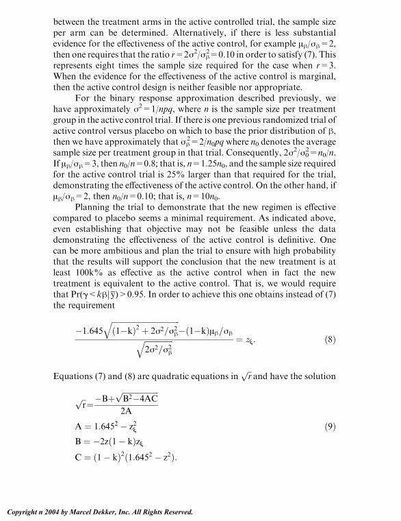
between the treatment arms in the active controlled trial, the sample sizeper arm can be determined. Alternatively, if there is less substantialevidence for the effectiveness of the active control, for example Ah/jh=2,then one requires that the ratio r=2j2/jh2=0.10 in order to satisfy (7). Thisrepresents eight times the sample size required for the case when r=3.When the evidence for the effectiveness of the active control is marginal,then the active control design is neither feasible nor appropriate.

For the binary response approximation described previously, wehave approximately j2=1/npq, where n is the sample size per treatmentgroup in the active control trial. If there is one previous randomized trial ofactive control versus placebo on which to base the prior distribution of h,then we have approximately that jh2=2/n0pq where n0 denotes the averagesample size per treatment group in that trial. Consequently, 2j2/j02=n0/n.If Ah/jh=3, then n0/n=0.8; that is, n=1.25n0, and the sample size requiredfor the active control trial is 25% larger than that required for the trial,demonstrating the effectiveness of the active control. On the other hand, ifAh/jh=2, then n0/n=0.10; that is, n=10n0.

Planning the trial to demonstrate that the new regimen is effectivecompared to placebo seems a minimal requirement. As indicated above,even establishing that objective may not be feasible unless the datademonstrating the effectiveness of the active control is definitive. Onecan be more ambitious and plan the trial to ensure with high probabilitythat the results will support the conclusion that the new treatment is atleast 100k% as effective as the active control when in fact the newtreatment is equivalent to the active control. That is, we would requirethat Pr(g<khjy)>0.95. In order to achieve this one obtains instead of (7)the requirement

�1:645ffiffiffiffiffiffiffiffiffiffiffiffiffiffiffiffiffiffiffiffiffiffiffiffiffiffiffiffiffiffiffiffiffiffiffiffið1�kÞ2 þ 2j2=j2

h

q�ð1�kÞAh=jhffiffiffiffiffiffiffiffiffiffiffiffiffiffiffi

2j2=j2h

q ¼ zs: ð8Þ

Equations (7) and (8) are quadratic equations inffiffir

pand have the solution

ffiffir

p ¼�BþffiffiffiffiffiffiffiffiffiffiffiffiffiffiffiffiffiffiffiB2�4AC

p

2A

A ¼ 1:6452 � z2s ð9ÞB ¼ �2zð1� kÞzsC ¼ ð1� kÞ2ð1:6452 � z2Þ:

Simon64


3.3. Example

The Tamoxifen Prevention Trial evaluated the effectiveness of Tamoxifenfor preventing breast cancer in high-risk women (Fisher et al., 1998).Tamoxifen was found to be effective, but also led to side effects, includingincreasing the risk of endometrial cancer. Consequently, there is interest inthe identification of other antiestrogen drugs that are as effective asTamoxifen for preventing breast cancer but with fewer side effects. TheTamoxifen trial randomized 13,388 women and found 175 invasive breastcancers in those assigned to the placebo group compared to only 89 in theTamoxifen group. This is a total of 264 events. The investigators reported arisk ratio of 0.51 with an associated 95% confidence interval of 0.39–0.66.

Suppose one were planning an active control trial to evaluate a newerantiestrogen, such as Raloxifene, compared to Tamoxifen. One may useexpression (9) to determine the size of the trial needed. Taking thelogarithm of the risk ratio as approximately normally distributed, thepoint estimate and confidence interval reported yield a value of z=Ah/jh ofabout 5. Using this value in (9) with k=0 and zs=1.28 gives a valuer=2.38. Since the precision of estimation of relative risk is approximatelydetermined by the total number of events observed, this result indicatesthat the active control trial need only observe 1/(2.38) or 42% as manyevents as the initial trial in order to establish that the new treatment iseffective compared to placebo. In order to establish that the new treatmentis 80% as effective as Tamoxifen, when it is equivalent to Tamoxifen, oneuses (9) with k=0.8 and obtains r=0.095. Consequently, the active controltrial would have to contain 1/0.095 or 10.5 times as many events as theoriginal trial. In order to establish that the new treatment is more effectivethan placebo and 50% as effective as Tamoxifen (k=0.5) requires r=0.59or 1.695 times as many events as the original trial, or 431 events. The cur-rent trial comparing Raloxifene to Tamoxifen for the prevention of pri-mary breast cancer is planned to observe 327 invasive breast cancers at thetime of the definitive analysis. The Bayesian analysis described here sug-gests that this is sufficient to determine whether Raloxifene is effectiverelative to placebo but not sufficient to determine whether Raloxifene isat least 50% as effective as Tamoxifen.

4. CONCLUSION

In this chapter we have attempted to describe the serious limitations ofactive control trials and to indicate that the standard methods for planningand analysis of such trials are problematical and potentially misleading.



We have also described a new approach to planning and analysis of activecontrol trials. The new approach is based on the premise that an activecontrol trial is not interpretable unless one provides the quantitativeevidence that the control treatment is effective. Active control trials arenot practical unless there is very strong evidence for the effectiveness of thecontrol treatment. Superiority trials are strongly preferable to activecontrol trials whenever they are ethically possible.

REFERENCES

Blackwelder, W. (1982). Proving the null hypothesis in clinical trials. ControlledClinical Trials 3:345–353.

Casagrande, J. T. and Pike, M. C. (1978). An improved formula for calculatingsample sizes for comparing two binomial distributions. Biometrics 34:483–486.

Durrleman, S., Simon, R. (1990). Planning and monitoring of equivalence studies.Biometrics 46:329–336.

Fisher, B., Costantino, J. P., Wickerham, L., et al. (1998). Tamoxifen for Pre-

vention of Breast Cancer: Report of the National Surgical Adjuvant Breastand Bowel Project P-1 Study. Journal of the National Cancer Institute 90:1371–1388.

Fleming, T. (1990). Evaluation of active control trials in AIDS. Journal ofAcquired Immune Deficiency Syndromes 3:S82–S87.

Freiman, J. A., Chalmers, T. C., Smith, H., Kuebler, R. R. The importance of betathe type II error and sample size in the design and interpretation of the

randomized control trial: survey of 71 ‘‘negative’’ trials. New EnglandJournal of Medicine 299:690–694.

Gould, A. (1991). Another view of active-controlled trials. Controlled Clinical

Trials 12:474–485.Gould, L. (1993). Sample sizes for event rate equivalence trials using prior infor-

mation. Statistics in Medicine 12:2001–2023.

Makuch, R., Simon, R. (1978). Sample size requirements for evaluating a conser-vative therapy. Cancer Treatment Reports 62:1037–1040.

Rubenstein, L. V., Gail, M. H., Santner, T. J. (1981). Planning the duration of a

comparative clinical trial with loss to follow-up and a period of continuedobservation. Journal of Chronic Diseases 34:469–479.

Simon, R. (1986). Confidence intervals for reporting results from clinical trials.Annals of Internal Medicine 105:429–435.

Simon, R. (1993). Why confidence intervals are useful tools in clinical therapeutics.Journal of Biopharmaceutical Statistics 3(2):243–248.

Simon, R. (1999). Bayesian design and analysis of active control clinical trials.

Biometrics 55:484–487.

Simon66


4Adaptive Two-Stage Clinical Trials*

Michael A. ProschanNational Heart, Lung, and Blood Institute, National Institutes of Health,Bethesda, Maryland, U.S.A.

1. INTRODUCTION

A very important part of the planning of any clinical trial is the estimationof sample size and power. It is difficult because these depend not only onthe size of the treatment effect one wishes to detect, but also on the values ofcertain nuisance parameters. For example, in a trial comparing two treat-ments with respect to a continuous measure like blood pressure changefrom baseline to end of study using a t test, power depends on both thedifference inmean blood pressures between the treatment and control arms(the treatment effect) and the standard deviation (the nuisance parameter).In a trial with a dichotomous outcome such as 30 day mortality, one mustspecify the difference in event probabilities in the two arms (the treatmenteffect) and the overall event probability across the two treatments (thenuisance parameter).

Although the treatment effect and nuisance parameter are bothcritical components of power calculations, they are quite different in thatthe nuisance parameter must be accurately estimated, whereas the treat-ment effect is usually assumed. One usually specifies theminimum clinically

*This chapter was written by Michael Proschan in his private capacity. The views expressed

in the chapter do not necessarily represent the views of NIH, DHHS, or the United States.


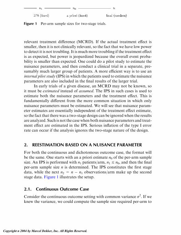
relevant treatment difference (MCRD). If the actual treatment effect issmaller, then it is not clinically relevant, so the fact that we have low powerto detect it is not troubling. It is muchmore troubling if the treatment effectis as expected, but power is jeopardized because the overall event proba-bility is smaller than expected. One could do a pilot study to estimate thenuisance parameters, and then conduct a clinical trial in a separate, pre-sumably much larger group of patients. A more efficient way is to use aninternal pilot study (IPS) in which the patients used to estimate the nuisanceparameters are also included in the final results of the larger trial.

In early trials of a given disease, an MCRD may not be known, soit must be estimated instead of assumed. The IPS in such cases is used toestimate both the nuisance parameters and the treatment effect. This isfundamentally different from the more common situation in which onlynuisance parameters must be estimated. We will see that nuisance param-eter estimates are essentially independent of the treatment effect estimate,so the fact that there was a two-stage design can be ignored when the resultsare analyzed. Such is not the casewhen both nuisance parameters and treat-ment effect are estimated in the IPS. Serious inflation of the type I errorrate can occur if the analysis ignores the two-stage nature of the design.

2. REESTIMATION BASED ON A NUISANCE PARAMETER

For both the continuous and dichotomous outcome case, the format willbe the same. One starts with an a priori estimate n0 of the per-arm samplesize. An IPS is performed with n1 patients/arm, n1 V n0, and then the finalper-arm sample size n is determined. The IPS constitutes the first stagedata, while the next n2 = n � n1 observations/arm make up the secondstage data. Figure 1 illustrates the setup.

2.1. Continuous Outcome Case

Consider the continuous outcome setting with common variance r2. If weknew the variance, we could compute the sample size required per-arm to

Figure 1 Per-arm sample sizes for two-stage trials.

Proschan68


detect theMCRD, d. For 100(1� b)%power for a two-tailed test at level a,the required sample size per-arm is approximately

wðr2Þ ¼ 2r2ðza=2 þ zbÞ2d2

ð1Þ

where za denotes the 100(1 � a)th percentile of a standard normaldistribution. In practice, a prior estimate r0

2 will have to be used, givingan estimated per-arm sample size of n0 = w(r0

2).We take a preliminary sample of n1 observations in each arm and

compute the pooled variance s12. Based on this estimate, we revise the per-

arm sample size from our initial estimate of n0 to n.Wemay take n=w(s12),

or n= w(r*2), where r*

2 is an estimate of the variance combining r02 and s1

2.Note that n is a random variable, as is the second stage per-arm sample size,n2 = n � n1.

The treatment effect estimator using all of the data from the first andsecond stages is d= (n1d1 + n2d2)/n, where di is the difference in treatmentand control sample means for data of stage i, i = 1,2. Now s1

2 isstatistically independent of d1 , so conditioned on s21;Z ¼ ðd� dÞ=ffiffiffiffiffiffiffiffiffiffiffiffi

2r2=np

has a standard normal distribution. Because the conditionaldistribution of Z given s1

2 is the same for all s12, Z and s1

2 are independent inthis adaptive sample size setting, with Z having a standard normaldistribution and s1

2/r2 having the distribution of a chi-squared randomvariable divided by its degrees of freedom, n1� 1. It follows that under thenull hypothesis, T ¼ Z=

ffiffiffiffiffiffiffiffiffiffiffis21=r

2p ¼ d=

ffiffiffiffiffiffiffiffiffiffiffi2s21=n

phas a t distribution with 2(n1

� 1) degrees of freedom. In other words, if we use the pooled variancefrom the IPS only, an exact p value may be obtained by referring T to a tdistribution with 2(n1 � 1) degrees of freedom. This result is due to Stein(1945).

Stein’s procedure is not commonly used in clinical trials for at leasttwo reasons. One is its perceived inefficiency in estimating the varianceusing only 2n1 of 2n observations. Another is that r2may increase over timebecause of changes in the patient population, for example. Using only thefirst 2n1 patients could underestimate the true variability and increase thechance of a type I error. It is therefore more natural to use s2, the pooledvariance estimate based on all 2n observations. Unfortunately, the distri-bution of s2 is not the same as if n had been fixed in advance. In fact, s2

systematically underestimates r2.Wittes et al. (1999) have shown thatE(s2)¼ r2 + (n1 � 1) cov{s1

2, 1/(n� 1)}; the covariance term is negative becauses12 is an increasing function of s1

2 and 1/(n� 1) is a decreasing function of s12.

Still, the bias is so small that the type I error rate of this approximate t test

Adaptive Two-Stage Clinical Trials 69


is very close to a if the size of the internal pilot study is 20 or more (Wittesand Brittain, 1990; Birkett and Day, 1994; Wittes et al., 1999).

Those who worry about even small amounts of a inflation but wantto use a better estimate of variance than Stein’s can do so with a restrictedtest, whereby the final per-arm sample size is restricted to be at least as largeas the originally planned n0. Proschan and Wittes (2000) point out thatinstead of using the pooled variance from the IPS, one could augment eacharm of the IPS with the first n0 � n1 observations from the correspondingarm in the second stage. The resulting test statistic has a null t distributionwith 2(n0 � 1) degrees of freedom instead of 2(n1 � 1) degrees of freedomfor Stein’s procedure. This clear improvement is still unsatisfying becauseuse of the first n0 � n1 observations per arm from the second stage isarbitrary; any set of n0 � n1 second stage observations could be used. Whynot average over all possible augmentations of the IPS with 2(n0 � n1)observations from stage 2? Proschan andWittes (2000) propose somethingvery close to this. Their variance estimate reduces to j2= Es12+ (1� E)j2,where j2= {(n� 1)s2� (n1� 1)s1

2}/(n� n1) and E=(n1� 1)/(n0� 1). Theyprove that referring d=

ffiffiffiffiffiffiffiffiffiffiffiffi2r2=n

pto a t distribution with 2(n0 � 1) degrees of

freedom has a type I error rate no greater than a.

2.2. Example: DASH

We illustrate these methods with the Dietary Approaches to Stop Hyper-tension Study (DASH). Three dietary patterns were compared with respectto change in diastolic blood pressure (DBP) from baseline to the end of 8weeks of intervention in participants with blood pressures ranging fromhigh normal to stage 1 hypertension (80VDBPV 95). The control diet wassimilar to what many Americans eat; one of the active diets was rich infruits and vegetables, while the other was rich in fruits and vegetables andlow-fat dairy products. Adjustments were made for the two comparisonswith control. Thus, to be significant, the approximate z statistic comparingan active diet to the control had to exceed 2.24, the critical value for a 2-tailed test at level .025. The standard deviation of DBP change wasestimated to be about 5 mmHg, while the minimum treatment effectthought to have strong public health importance was d = 2 mmHg. For85% power for a control comparison, approximately n0=2(2.24 +1.04)2(5)2/22 = 135 evaluable participants per arm were needed. Furtherdetails of the design of DASH may be found in Sacks et al. (1995).

At some point in the trial the issue was raised that the standarddeviation may have been overestimated because it did not take intoaccount the fact that a ‘‘funnel’’ was used prior to enrollment to eliminate

Proschan70


participants whose blood pressures were too large or too small. Simulationresults suggested that taking this funnel into account might decrease thestandard deviation from 5 to 4.5. This would allow almost a 20% reductionin sample size to achieve the same power.

As it turned out, the standard deviation at an interim look was quiteclose to 5, so no changes were made in the sample size. For the sake ofillustration, suppose hypothetically that after 68 observations in an activediet and 68 in the control diet, the variance pooled across these two dietswere s1

2= 4.52=20.25, as hoped. The sample size could have been reducedto n = 2(2.24 + 1.04)2(4.5)2/22 = 109 evaluable participants per arm. Atthe end of the study, the ordinary t statistic could be usedwith 2(109� 1)=216 degrees of freedom for the comparisons with control. If one wanted tobe conservative and avoid even the slightest a inflation, one could useStein’s procedure. For example, if after 109 observations per arm thedifference between the control and combination diet means were d = 2.1,the t statistic would be 2:1=

ffiffiffiffiffiffiffiffiffiffiffiffiffiffiffiffiffiffiffiffiffiffi2ð4:5Þ2=109

p¼ 3:45, even if the pooled variance

of all of the observations were s2 = 4.82 = 23.04, for example. TheProschan–Wittes method cannot be used in this example because the goalwas to see if the sample size could be reduced, and hence it was not arestricted design.

2.3. The Dichotomous Outcome Case

Suppose that the primary outcome of a clinical trial is the presence orabsence of a short-term event such as 30-day mortality. Let pC and pT bethe probabilities of experiencing such an event for patients in the controland treatment arms, respectively. Then d = pC � pT is the treatmentdifference, and p = ( pC + pT)/2 is the average event probability over thetwo arms. Sample size per arm to achieve power 100(1� h) for a two-tailedtest at level a is given approximately by

n ¼ ½za=2ffiffiffiffiffiffiffiffiffiffiffiffiffiffiffiffiffiffiffiffi2pð1� pÞp þ zb

ffiffiffiffiffiffiffiffiffiffiffiffiffiffiffiffiffiffiffiffiffiffiffiffiffiffiffiffiffiffiffiffiffiffiffiffiffiffiffiffiffiffiffiffiffiffiffiffiffiffipCð1� pCÞ þ pTð1� pTÞ

p �2ðpC � pTÞ2

: ð2Þ

Here the nuisance parameter is p, estimated by p1, the overall eventproportion among the 2n1 observations in the IPS. Note that p1 isuncorrelated with d1 , the difference in event proportions between thecontrol and treatment arms in the IPS. If 2n1 is moderately large, then p1and d1 are approximately bivariate normally distributed. If they wereexactly bivariate normal, their lack of correlation would imply statisticalindependence. Thus, as in the continuous outcome case, the nuisanceparameter estimate is approximately independent of the treatment effect



estimator. Again it seems reasonable to treat the per-arm sample size n as ifit had been fixed in advance and use an ordinary test of proportions on the2n observations at the end of the study. Several authors have shown thatthe effect on the type I error rate of treating the final sample size as fixed isminimal. See, for example, Gould (1992) or Herson and Wittes (1993).

As with the continuous outcome case, there is a way to obtain anexact a level procedure for those who do not want even a slight inflation ofthe type I error rate. Instead of implementing the usual z test of pro-portions, one can condition on the total numbers of events at the first andsecond stages using, for example, the Mantel-Haenzel test. The p value isalso conditional on these numbers of events, so the fact that the secondstage sample size was driven by the first stage results becomes irrelevant.

2.4. DASH Example Embellished

Consider the DASH clinical trial described previously. Suppose thatinstead of treating the change in DBP as a continuous outcome, the DASHinvestigators had compared the proportions of patients in each arm whoseDBP decreased by 3 mmHg or more. Call these patients ‘‘responders.’’Further assume that the investigators were interested in detecting adoubling of the proportion of responders in an active diet relative tocontrol. Suppose, hypothetically, that from the first 100 participantsevaluated in the control and 100 in an active arm, 60 responded. Thenp ¼ 60=200 ¼ :30. Treat this as a population parameter and set ( pC+ pT)/2¼ .30, pT¼ 2pC. This yields pC = .20, pT = .40. Substituting into (2) andusing 85% power and the adjusted two-tailed alpha level of .025 (za/2=2.24) yields 112 participants per arm. Thus, only 12 more participantswould be needed in each arm.

Suppose that the results were as shown in Table 1. Overall, pC ¼30=112 ¼ :268 and pT ¼ 41=112 ¼ :366. The ordinary test of proportionson the entire data yields a p value of .11. This analysis treats the sample size

Table 1 Hypothetical Results for the First 100 Participants/Arm (1st 2�2Table), the Next 12 Participants/Arm (2nd 2�2 Table), and the Total of112/Arm (Last 2�2 Table) in the Embellishment of the DASH Example

Considering Responders (R) and Nonresponders (NR)

R NR R NR R NR

C 25 75 5 7 30 82T 35 65 6 6 41 71

Proschan72


of 128 per arm as if it had been fixed in advance. As stated above, this ishighly accurate, producing only very slight a inflation.We could avoid anyinflation by conditioning on the total numbers of events at stages 1 and 2.For example, the two-tailed p value using the exact distribution of theMantel-Haenzel statistic is .15.

3. SAMPLE SIZE REESTIMATION BASED ON TREATMENTEFFECT

As mentioned earlier, it is highly desirable to base sample size on theminimal clinically relevant treatment difference, but this is not alwayspossible. For example, in heart disease trials using an angiographicendpoint such as the average change in minimum lumen diameter overmany different segments of a coronary artery, it is not clear what sizetreatment difference would result in clinical benefit. In these cases one maywish to use the IPS to estimate both the nuisance parameter andthe treatment effect. This is different from the nuisance parameter situationin that it is inherently a one-tailed testing situation; one would not beinterested in determining the number of additional observations to provethe treatment harmful. Thus, one-tailed testing is assumed in this section.In practice one might use one-tailed a = .025 instead of .05.

Unlike the earlier scenarios in which only the nuisance parametershad to be estimated, the treatment effect at the end of the study is highlycorrelated with the parameters estimated at the first stage. Thus, therandom per-arm sample size n contains very relevant information aboutthe size of the treatment effect; acting as though it were fixed in advance canlead to serious inflation of the type I error rate. Proschan and Hunsberger(1995) show that depending on how one chooses the second stage samplesize, the actual type I error rate can be as high as a+exp(� za

2/2)/4. Thus,for a .025 (.05) level one-tailed test, the actual type I error rate can be asgreat as .06 (.11).

One can avoid inflation of the type I error rate by using a largercritical value at the end of the study. For example, suppose one takes n2(z1)additional observations per-arm based on the IPS z score z1, but then usescritical value c = c(z1, n2). The actual type I error rate isZ l

�lCP0ðn2; cjz1Þ/ðz1Þdz1 ð3Þ

where / is the standard normal density function andCP0 (n2, c|z1) denotesthe conditional probability, computed under the null hypothesis, that the z



score using all 2(n1+ n2) observations will exceed c, given z1. Now supposethat prior to the study we had selected a rule A(z1) dictating how muchconditional type I error rate to use, given z1, such thatZ

Aðz1Þ/ðz1Þ dz1 ¼ a : ð4Þ

A(z1) is called a conditional error (CE) function. Further suppose that re-gardless of the additional number of observations per arm, n2, we couldfind a critical value c= c(z1, n2) to make CP0(n2, c|z1)=A(z1). Then by (3)and (4), the procedure would have level a.

Proschan and Hunsberger (1995) have shown that it is always pos-sible to find such a c:

c ¼ffiffiffiffiffin1

pz1 þ ffiffiffiffiffi

n2p

zAffiffiffiffiffiffiffiffiffiffiffiffiffiffiffin1 þ n2

p ð5Þ

where zA is short-hand notation forA�1 {1�A(z1)}. Onemay then select n2

such that CPd(n2, c), computed under the alternative hypothesis of treat-ment effect d, reaches a desired level 1 � b:

n2 ¼ 2ðzA þ zbÞ2d2

: ð6Þ

The formula for n2 is easy to interpret when one recognizes that theconditional error function approach is mathematically equivalent to thefollowing procedure: Having observed z1, take n2 additional observationsper arm and perform a z test on only the second stage data, rejecting thenull hypothesis if that z score exceeds the critical value corresponding tosignificance level A(z1). The sample size formula (6) yielding conditionalpower 1� b is the sample size corresponding to unconditional power 1� bin a z test applied only to the second stage data.

Similarly, for any given value n2, the conditional power assumingthat the true treatment effect is d is the same as the unconditional power in atrial at level A(z1) with n2 observations per arm:

CP ¼ 1� U zA �ffiffiffiffiffiffiffiffiffiffin2=2

pd=r

� : ð7Þ

As any conditional error function A(z1) may be used, the proce-dure is very general. In fact, as Proschan (2000) points out, CE func-tions and two-stage tests are really synonymous; associated with any

Proschan74


two-stage test statistic T is a CE function A(z1) = Pr(T is significant j Z1

¼ z1). Thus, it might be easier to consider good two-stage tests andsee what CE functions they induce rather than directly trying to findgood CE functions. Once we determine the induced CE function, we canuse (7) to choose a second-stage sample size yielding the desired condi-tional power.

How do we choose a reasonable two-stage test? If the second stagesample size were fixed in advance, things would be very easy; we would betesting whether the mean of (Z1,Z2) was (0, 0) against a specific alternativeproportional to ð ffiffiffiffiffi

n1p

;ffiffiffiffiffin2

p Þ. The problem is that we do not know n2 a priori,so we do not know the alternative direction.We only know that, because n2z 0, the alternative lies somewhere in the positive quadrantQ+={(z1, z2):z1z 0, z2z 0}. Tests powerful against the positive quadrant alternative aretherefore appealing.

One such test is due to O’Brien (1984). The null hypothesis is rejectedif ðz1 þ z2Þ=

ffiffiffi2

p> za. This is the optimal test statistic for the fixed sample

size setting with n2 = n1, but it can be used even if one changes n2 afterseeing z1.

To find the induced CE function, note that the amount of conditionaltype I error rate one uses after seeing Z1 = z1 is

Aðz1Þ ¼ PrðZ1 þ Z2 >ffiffiffi2

pzajZ1 ¼ z1Þ ¼ 1�Að

ffiffiffi2

pza � z1Þ: ð8Þ

This is a member of what Proschan andHunsberger (1995) called the linearclass of CE functions, even though it is zA ¼ ffiffiffi

2p

za � z1 that is linear in z1.The induced CE function is used, in part, to reexpress the rejection regionvia (5) in terms of ð ffiffiffiffiffi

n1p

z1 þ ffiffiffiffiffin2

pz2Þ=

ffiffiffin

p, the usual z score on all 2(n1 + n2)

observations. Investigators would naturally want to compare the two-stage test to the more familar one-stage test with the same number ofobservations; they would feel legitimately uneasy if a two-stage procedurerejected the null hypothesis while the one-stage procedure did not.

The above procedure is a no-cost extension of the fixed sample sizetest; if one decides to use the originally planned second stage sample size,the test is equivalent to rejecting the null hypothesis when the usual fixed-sample z statistic exceeds za. The advantage is that at the first stage onecould choose to change the second stage sample size.

One would probably not continue to the second stage if z1 < 0.Furthermore, it makes no sense to reject at the end of the second stage if z2< 0; if the evidence was not convincing at stage 1, how could it be moreconvincing having observed a negative trend since stage 1? Thus, it is agood idea to modify the above procedure. One stops at stage 1 without



rejection of H0 if z1 < 0, and with rejection if z1 > k, where k=2.79 for a¼ .025 and k=2.36 for a= .05. If 0V z1 V k, one proceeds to stage 2 andrejects if z1+ z2> k. The ‘‘linear’’CE function is shown as the solid line inFigure 2 for a = .025.

Another test that could be used is the likelihood ratio test for thepositive quadrant alternative. One rejects the null hypothesis if z1z k or z2z k or

ffiffiffiffiffiffiffiffiffiffiffiffiffiffiz21 þ z22

p> kand (z1, z2)aQ+. Eliminating z1< 0 andmodifying k

to maintain an a-level procedure yields the rejection region z1z k or 0V z1V k and z2 >

ffiffiffiffiffiffiffiffiffiffiffiffiffiffik2 � z21

p. What is the induced CE function? For z1< 0 there

is no chance of rejecting the null hypothesis, while for z1 > k there isprobability 1 of rejecting the null hypothesis. For z1 in the continuationregion [0, k], the null probability of rejectingH0 is PrðZ2 >

ffiffiffiffiffiffiffiffiffiffiffiffiffiffik2 � z21

p Þ ¼ 1�Að ffiffiffiffiffiffiffiffiffiffiffiffiffiffi

k2 � z21p Þ. Thus, the induced conditional error function is

Acirðz1Þ ¼0 if z1 V 0

1�A

� ffiffiffiffiffiffiffiffiffiffiffiffiffiffiffik2 � z21

q �if 0 < z1 Vk

1 if z1 > k:

8>><>>: ð9Þ

Figure 2 Linear and circular conditional error functions for a=.025.

Proschan76


For a one-tailed alpha of .025(.05) k = 2.27 (1.95). Proschan and Huns-berger (1995) called Acir(z1) a ‘‘circular’’ CE function because over thecontinuation region [0, k] zA is the equation of a circle centered at the originwith radius k. The dotted curve in Figure 2 shows the circular CE function.Again it is convenient to express the rejection region in terms of the usual zscore for 2(n1 + n2) observations using (5).

The circular CE function procedure stops for futility if z1 < 0, but itcan be modified to stop for futility for other values of z1. It is easier tointerpret if we rephrase this as follows. We stop for futility when the first-stage p value, p1, exceeds some number a0; a0 = .5 corresponds to the z1 <0 case already considered. For smaller values of a0, the value of k requiredfor an a-level procedure decreases. Table 2 gives the value of k for differentvalues of a and a0.

If one proceeds to the second stage, the critical value for z isgiven by (5). The circular CE function has the property that the criticalvalue at the second stage is no greater than k, the critical value at stage1. Furthermore, among all two-stage tests with the same continuationregion as the circular CE function, the circular CE function is the onlyone that can guarantee this for all possible values of n2 (see Proschan,2003).

3.1. Example

Suppose that a clinical trial in patients with coronary heart diseasecompares a cholesterol reducing drug to placebo with respect to angio-graphic changes from baseline to end of study. Specifically, coronaryarteries are first divided into segments; for each segment the difference inminimum lumen diameter from baseline to end of study is computed, andthe average difference over all segments of a patient is the outcomemeasure. It is not known what constitutes a clinically relevant change,

Table 2 Values of k for Different Values of the Overall Significance Level a andthe First Stage Futility Level a0 for the Circular CE Function Approach

a0

a .10 .15 .20 .25 .30 .35 .40 .45 .50

.025 2.13 2.17 2.19 2.21 2.22 2.23 2.25 2.26 2.27

.050 1.77 1.82 1.85 1.88 1.89 1.91 1.93 1.94 1.95



but another similar study showed an effect size of about one third of astandard deviation. The sample size required for 90% power to detect asimilar effect size is about 190 patients per arm, or 380 total. After 95 areevaluated in each arm, we compute the estimated effect size, namely thedifference in sample means divided by the square root of the pooledestimate of variance. Which method we use must be specified in advance.

If we use the circular conditional error function approach, we stopthe trial and declare a significant treatment effect at the first stage if z1 >2.27. We stop for lack of treatment effect if z1 < 0. If 0 V z1 V 2.27, weproceed to the second stage. Suppose that the first-stage z score were 1.5.This corresponds to an estimated effect size of about .218 standarddeviations instead of the originally anticipated one third of a standarddeviation. The value of the conditional error function is Að1:5Þ ¼ 1�Aðffiffiffiffiffiffiffiffiffiffiffiffiffiffiffiffiffiffiffiffiffiffiffiffiffi2:272 � 1:52

pÞ, so zA ¼

ffiffiffiffiffiffiffiffiffiffiffiffiffiffiffiffiffiffiffiffiffiffiffiffiffi2:272 � 1:52

p¼ 1:704. To have 80% conditional

power under the empirically estimated treatment effect, we use Eq. (6): n2¼ 2(1.704 + .84)2/.2182 = 273. Thus, we would need 273 more patientsper-arm, making the total sample size 2(95 + 273) = 736. Given that theoriginally projected sample size was 380, such a large increase may beprohibitive. Instead one might prefer to see the conditional power fordifferent total sample sizes using equation (7). If we stick with the originallyplanned sample size of 190 per arm, so n2 = 190 � 95 = 95, conditionalpower under the empirical estimate will be 1�Af1:704� ffiffiffiffiffiffiffiffiffiffi

95=2p ð:218Þg

¼ :42. Increasing the sample size to 250 per arm (a second stage sample sizeof 155 per arm) increases the conditional power to about .59. Thesecalculations are all under the empirical estimate of treatment effect. Afterthe first stage, wemight want to compute power under an alternative that isnot as optimistic as what was originally hypothesized, but not as pessi-mistic as what has been observed so far. For example, we might prefer touse an effect size of one fourth of a standard deviation. At any rate, supposewe decided to take 200more per arm. If the z score for the second half of thedata were 1.9, then z1

2 + z22 = 1.52 + 1.92 = 5.86 exceeds 2.272 = 5.15, so

the null hypothesis would be rejected. Results would probably be reportedin the following equivalent way. The full-data z score is ð95þ 200Þ�1=2

f ffiffiffiffiffi95

p ð1:5Þþ ffiffiffiffiffiffiffiffi200

p ð1:9Þg ¼ 2:42. The critical value (5) is ð95þ 200Þ�1=2

f ffiffiffiffiffi95

p ð1:5Þþ ffiffiffiffiffiffiffiffi200

p ð1:704Þg¼ 2:25; therefore the null hypothesis is rejected.Bauer and Kohne (1994) considered a much more general setting in

which the first-stage data was used not only to modify sample size, but tomake more drastic alterations such as changing the test statistic. Theirmethod is based on Fisher’s product of independent p values. Recall that pvalues are uniformly distributed under the null hypothesis for any test

Proschan78


statistic with a continuous distribution function. If p1 and p2 are inde-pendent p values, then �2 ln( p1p2) has a chi-squared distribution with 4degrees of freedom under the null hypothesis. The null hypothesis isrejected if T = p1p2 < ca = exp{� m4,a

2 /2}, where m4,a2 is the upper a

point of a chi-squared distribution with 4 degrees of freedom; ca= .004 or.009 for a = .025 or a = .05, respectively.

Fisher’s test can be applied to first- and second-stage p values even ifthe second-stage sample size n2 depends on p1. The reason is that p1 is uni-formly distributed, and for given p1, n2 becomes fixed and p2 is uniformlydistributed. Because p2 has the same (uniform) conditional distribution forany given value of p1, p1 and p2 are independent uniforms, and Fisher’sproduct of p values test is valid. Bauer and Kohne imply that their pro-cedure can be used even if one changes the test statistic after seeing the firststage data, but some care is needed (Liu, Proschan, and Pledger, 2002).

Note that if p1 < ca, there is no point in continuing the study sincep1p2 is assured of being less than ca. Bauer and Kohne also consider avariant in which one stops at the first stage without rejecting the nullhypothesis if p1 > a0. By allowing the possibility of stopping early forfutility, one can decrease the level of evidence required to declare statisticalsignificance at stage 1. Table 3 shows a1, the p value required to declaresignificance at stage 1 as a function of a and a0. For example, for a= .025and a0 = .5, a1 = .010. Thus the continuation region is .010 V p1 V .5,which corresponds to 0 V z1 V 2.32.

Note the similarity between the Bauer-Kohne continuation regionand that of the circular CE function with a0 = .5. Wassmer (1998) showedthat the power functions were also quite close. This is because of thesimilarity of the induced CE functions. An advantage of the Bauer-Kohneprocedure is that it is exact. One need not make the assumption that thesample size is large enough to estimate the variance accurately.

Table 3 Values of a1, the Required p-Value to Declare Significance at Stage 1

for the Bauer-Kohne Procedure That Stops for Futility at Stage 1 if p1 > a0. (If a1V p1 V a0, One Proceeds to Stage 2 and Rejects the Null Hypothesis if p1p2 < ca.)

a0

a ca .10 .15 .20 .25 .30 .35 .40 .45 .50

.025 .004 .019 .017 .015 .014 .013 .012 .012 .011 .010

.050 .009 .043 .038 .035 .032 .030 .028 .026 .025 .023



4. CONCLUSIONS

Clinical trials must be large enough to have reasonable power to detecttreatment differences. Unfortunately, the information needed to determinethe sample size is not always available or accurate; other studies uponwhich estimates are based may not be sufficiently similar to the one beingplanned. It therefore becomes appealing to use part of the current trial datato estimate the parameters needed to determine sample size. Often thisinvolves estimation of only nuisance parameters, because one can usuallyspecify a minimum clinically relevant treatment difference. When onlynuisance parameters are estimated during the IPS, one can essentiallyignore the two-stage nature of the design when it is time to analyze theresults. This is true for both continuous and dichotomous outcomes.

In some cases the IPS is used to estimate treatment effects as well.Muchmore caution is required. The two-stage nature of the designmust betaken into account when results are analyzed. Adaptive sample sizeestimation based on treatment effect is usually one-tailed; one would notwant to increase the sample size to show harm. Under an alternative hy-pothesis, the mean of (Z1, Z2) lies somewhere in the positive quadrant,so tests of the positive quadrant alternative are attractive. Two such testsare O’Brien’s and the likelihood ratio test (LRT). The properties of theseand other tests depend on their induced conditional error functions. TheO’Brien and LRT tests induce the linear and circular CE functions, re-spectively. An advantage of the linear CE function is that if one maintainsthe originally planned sample size, the test reduces to the usual fixed samplesize test. An advantage of the circular CE function is that the critical valueat the end of the study can be no greater than that of the first stage.Conditional power and sample size to achieve a given conditional powermay be obtained using the formulas for fixed sample size trials conductedat level A(z1) instead of a.

REFERENCES

Bauer, P., Kohne, K. (1994). Evaluation of experiments with adaptive interim

analyses. Biometrics 50:1029–1041.Birkett, M. A., Day, S. J. (1994). Internal pilot studies for estimating sample size.

Statistics in Medicine 13:2455–2463.

Gould, A. (1992). Interim analyses for monitoring clinical trials that do notmaterially affect the type I error rate. Statistics in Medicine 11:55–66.

Proschan80


Herson, J., Wittes, J. (1993). The use of interim analysis for sample size adjust-

ment. Drug Information Journal 27:753–760.Liu, Q. Proschan, M. A., Pledger, G. W. (2002). A unified theory of two-stage

adaptive designs. Journal of the American Statistical Association 97:1034–

1041.O’Brien, P. C. (1984). Procedures for comparing samples with multiple endpoints.


Proschan, M. A. (2003). The geometry of two-stage tests. Statistica Sinica 13:163–177.

Proschan, M. A., Wittes, J. (1999). An improved double sampling procedure basedon the variance. Biometrics 56:1183–1187.

Sacks, F. M., Obarzanek, E., Windhauser, M. M., Svetkey, L. P., Vollmer, W. M.,McCullough, M., Karanja, N., Lin, P., Steele, P., Proschan, M. A., Evans,M. A., Appel, L. J., Bray, G. A., Vogt, T. M., Moore, T. J., for the DASH

Investigators. (1995). Rationale and design of the Dietary Approaches toStop Hypertension (DASH) trial. Annals of Epidemiology 5:108–118.

Stein, C. (1945). A two-sample test for a linear hypothesis whose power is

independent of the variance. Annals of Mathematical Statistics 16:243–258.Wassmer, G. (1998). A comparison of two methods for adaptive interim analyses

in clinical trials. Biometrics 54:696–705.

Wittes, J., Brittain, E. (1990). The role of internal pilot studies in increasing theefficiency of clinical trials. Statistics in Medicine 9:65–72.

Wittes, J., Schabenberger, O., Zucker, D., Brittain, E., Proschan, M. (1999).Internal pilot studies I: Type I error rate of the naive t-test. Statistics in

Medicine 18:3481–3491.



5Design and Analysis of ClusterRandomization Trials

David M. ZuckerHebrew University, Jerusalem, Israel

1. INTRODUCTION

In the great majority of clinical trials, randomization is performed at thelevel of the individual subject. In certain trials, however, the appropriateunit of randomization is some aggregate of individuals. This form of ran-domization is known as cluster randomization or group randomization.Cluster randomization is employed by necessity in trials in which theintervention is by nature designed to be applied at the cluster level. Exam-ples of this type of trial include trials of community-based interventions,such as the Community Health Trial for Smoking Cessation (COMMIT)(Gail et al., 1992; COMMIT Research Group, 1995), and trials of school-based interventions, such as the Child and Adolescent Trial for Cardio-vascular Health (CATCH) (Zucker et al., 1995; Luepker et al., 1996).Cluster randomization is also sometimes employed for convenience of trialadministration in trials in which the intervention is applied at the level ofthe individual. An example of this situation is the trial design in whichclinics are assigned to the various experimental arms, with all patients in agiven clinic receiving the treatment towhich the clinic was assigned (Simon,1981).

The cluster randomization design poses special issues in the areas ofdesign, logistics, sample size calculation, and statistical analysis. This point


was raised in the epidemiological literature by Cornfield (1978), and hasreceived increasing attention since then. The purpose of this chapter is toreview these special issues. Comprehensive discussion of cluster random-ization trials is provided in the recent monographs of Murray (1998) andDonner and Klar (2000). In this chapter, emphasis is placed on the fol-lowing aspects: (1) the rationale for taking the cluster as the unit ofanalysis: (2) statistical handling of individuals who drop out of the trial:(3) analytical methods that are both statistically efficient and statisticallyrigorous, in the sense of scrupulously protecting the type 1 error level: (4)sample size calculation for cluster randomized trials, taking into accountintracluster correlation.

2. GENERAL DESIGN CONSIDERATIONS

2.1. Unit of Randomization and Analysis

Randomization of experimental units is designed to provide three keybenefits: (1) avoidance of investigator bias in the allocation process, (2)experimental arms that are appropriately balanced with respect to bothknown and unknown factors that may affect response, and (3) a basis foranalyzing the study results without statistical modeling assumptions. Theanalytical benefit arises because the randomization itself provides thestatistical structure whereby the study results may be judged in principlethrough the use of a randomization test, though in common practicethrough the use of a normal-theory test that approximates the random-ization test (Fisher, 1935; Kempthorne, 1952).

To preserve the analytical benefit, the statistical analysis must fol-low the form of randomization. In a cluster randomization trial, it isparticularly important to ‘‘analyze as you randomize.’’ Under clusterrandomization, the mean response in each experimental arm is subject totwo sources of variation: variation from cluster to cluster and variationacross individuals within a cluster. Donner et al. (1981) have described theincreased variance of the sample mean in each experimental arm thatresults from between-cluster variation in terms of a variance inflationfactor (IF) involving the intraclass correlation coefficient (ICC): if theclusters are all of the same size n, then IF = 1+ (n � 1) ICC. An analysisin which the unit of analysis is the individual rather than the cluster failsto account properly for the between-cluster variation and therefore isliable to produce misleading results. In effect, the treatment effects be-come confounded with the natural cluster-to-cluster variability, and se-

Zucker84


rious inflation in the Type I error level may result (Zucker, 1990; Glassand Stanley, 1970). To avoid this error, the unit of analysis must be thecluster.

To provide statistically rigorous results, a cluster randomization trialmust include an adequate number of clusters. Many cluster randomizationstudies are conducted with a very small number of clusters per arm, such astwo or four. Such studies cannot yield statistically definitive conclusionsabout treatment benefit because it is impossible for a randomization-basedanalysis of such a trial to yield a statistically significant result. Applicationof a normal-theory procedure such as ANOVA to such data rests on baldassumptions with no clear justication: for a trial of this small size, the usualcentral limit theorem argument supporting a normal-theory analysis as anapproximation to a randomization-based analysis does not apply. A trialof such small size often will be a very useful means of assessing thefeasibility of implementing the intervention and obtaining preliminaryindications of the likelihood that the intervention will succeed, but such atrial cannot provide a definitive basis for evaluating the benefit of theintervention. By contrast, studies such as the CATCH trial (Zucker et al.,1995, Luepker et al., 1996), involving 96 schools, the COMMIT trial (Gailet al., 1992; COMMITResearchGroup, 1995), involving 11matched pairsof communities, and the Jerusalem Study of Hygiene Education inKinder-gartens (Rosen, 2003), involving 40 kindergartens, include an adequatenumber of units to permit a meaningful statistical analysis. In COMMIT,in view of the relatively small number of units, the intervention effect wasassessed using a randomization-based permutation test rather than anormal-theory test.

Some authors, for example Hopkins (1982), suggest that one mayperform a statistical test for between-cluster variation, and that if the testresult is not statistically significant one may take the unit of analysis to bethe individual. This procedure is problematic for at least two reasons.Firstly, the test for between-cluster variation tends to have very low powerwhen the number of clusters is small. As a result, even under the classicalnested ANOVA assumptions, the procedure has inflated Type I error(Bozivich et al., 1956; Hines, 1996). Secondly, the procedure relies on theclassical nested ANOVA assumptions that between-cluster and within-cluster effects are all normally distributed and the within-cluster depen-dence can be completely described by an additive cluster effect. In general,especially for trials with a small number of clusters, there is no definite basisfor these assumptions. Thus, it is preferable to keep the cluster as the unit ofanalysis in all cases.

Design and Analysis of Cluster Randomization Trials 85


2.2. Sampling Methodology and Handling of ParticipantMigration

A further statistical issue in the analysis of long-term school-based orcommunity-based trials is of how to identify individuals from the school orcommunity for measurement and statistical analysis. This issue involvesinto two aspects: (1) determining how to sample individuals for measure-ment and (2) defining the primary study population for statistical analysispurposes.

There are twomain approaches to sampling individuals for measure-ment. In the cohort approach, a sample of the individuals initially enteredinto the study (possibly all such individuals) is selected to be measuredthroughout the duration of the study. In the cross-sectional approach,separate samples of individuals are taken at each measurement time point.Hybrid schemes combining these two sampling approaches also may beconsidered.

The main advantage of the cohort approach is that within-individualcorrelation can be exploited to enhance precision. A major advantage ofthe cross-sectional approach is that the measurement load is more evenlydistributed across individuals. This feature of the cross-sectional designcan be an important one from a logistic standpoint when the design callsfor multiple repeated measurements, and is particularly beneficial insituations where there is serious concern that the act of measurement itselfcan influence participants’ subsequent behavior. When every individual ina pre-defined study population is to be measured, the cohort and cross-sectional approaches obviously coincide.

The main issue in defining the primary study population for thepurpose of analysis is how to handle outmigrating and inmigratingindividuals. This issue is closely related to the issue of how to handlepatients in a classical clinical trial with individual-level randomization whoswitch from the assigned intervention to another therapy during the courseof the trial, i.e., dropouts and dropins. In the clinical trials field, there is agenerally well-accepted ‘‘intention to treat’’ principle that states thatpatients should be handled in the analysis according to their originalassignment, regardless of the therapy subsequently received (Friedman etal., 1996; Pocock, 1983). In school-based or community-based interventionresearch, the following represent three possible options for defining theprimary study population:

1. Include individuals who were in the school or community andmeasured at the beginning of the trial regardless of what

Zucker86


happened afterwards, with suitable tracking of outmigratingindividuals.

2. Include individuals who were in the school or community atboth the beginning of the trial and at the measurement point inquestion.

3. Include individuals who happen to be present in the school orcommunity at the specific measurement time in question.

The first approach is analogous to the intention to treat approach inclinical trials. The other two approaches represent two different forms of‘‘on-treatment’’ analysis. The advantages and disadvantages of the intentto treat approach as compared with the on-treatment approaches aresimilar to those in the classical individual-level randomization clinical trial.The main point calling for special mention is that bias can arise not only asthe result of an entire cluster being eliminated from analysis, but also as theresult of certain individuals within the various clusters being eliminatedfrom or added to the analysis. Such a bias threat exists because thebehavior leading to inclusion or exclusion from analysis, e.g., migration,may be influenced by the intervention. The bias threat posed by migrationis analogous to the well-recognized bias threat posed by missing data insample surveys (see Cochran, 1977).

An extended discussion of the migration issue is given in theCATCH statistical design paper (Zucker et al., 1995). The most appro-priate strategy is to perform analyses using a variety of approaches tohandling migrators, with the outlook that the truth probably lies some-where in the middle of the range spanned by the various approaches. Inconcluding whether or not the study provides definite statistical evidenceof efficacy, primary emphasis should be given to the intent to treatapproach.

2.3. Some Further Considerations

In a trial with individual-level randomization, there is generally no need forspecial close cooperation with organizations outside the trial group itself.It suffices to secure the cooperation of each individual participant. Bycontrast, in the typical cluster randomization trial the trial groupmust gainthe cooperation of various administrative offices. For example, in a school-based intervention trial, it is necessary to gain the approval and cooper-ation of school district administrators, school principals, and teachers.Also, in implementing and assessing the intervention, in the typical clinical



trial the participant visits the study clinic, but in many cluster random-ization trials, study staff must go out into the field.

Frequently, the cluster randomization design is used to assessbehavioral intervention programs, because such programs often aredeveloped for implementation at a school or community level. Susser(1995) has observed that an number of major behavior-oriented clusterrandomization trials have failed to exhibit an intervention effect; thisobservation raises concern about this type of trial. Susser discusses possibleexplanations for the negative results seen in these trials. One possibilitysuggested is that the treatment effect may be diluted by a general pop-ulation trend toward adopting the behavior change in question or byexposure of the control group to a extant program of similar nature.Another possibility suggested is that the type of behavioral change soughtmay be unlikely to occur in a substantial proportion of individuals over therelatively short time frame of a clinical trial. In considering a trial of aschool-based or community-based behavioral change program, it is wise totake due account of the possibility of dilution effects and to considercarefully how large an intervention effect realistically can be expected overthe time frame of the trial.

3. STATISTICAL ANALYSIS STRATEGIES

In this section and the next we discuss statistical methods and sample sizeconsiderations for the analysis of a single outcome variablemeasured at theend of the study on a specified cohort of individuals in each cluster (asidefrommissing data), with the possibility of using baseline measurements onthese individuals as covariates. The structure of the resulting data set isformally the same as that arising from repeated measures studies, in thateach involves sampling of a number of units and observation on a numberof subunits within each unit. For a cluster randomization study, the unit isthe cluster and the subunit is the individual; in a repeated measures studythe unit is the individual and the subunit is the measurement time point.Because of this common structure, the analytical methods used for the twotypes of study are similar.

3.1. Unadjusted Analyses

Let Yijk denote the response for individual ijk, with i indexing theexperimental arms, j indexing the clusters within an arm, and k indexing

Zucker88


the individuals within a cluster. We consider first the case in which thenumber of clusters within each group is moderate to large (say about 30clusters per arm). For a continuous response, it is appropriate to analyzethe data using the conventional mixed ANOVA model

Yijk ¼ lþ ai þ bjðiÞ þ ekðijÞ ð1Þwhere l represents the overall response level, ai is a fixed parameterrepresenting the effect of treatment i, bj(i) is a random cluster effect termassumed distributedN(0, rb

2), and ek(ij) is an individual error term assumeddistributed N(0, je2), with all random variables assumed independent.

The variance of an individual response Yijk is r2 = rb2 + re

2. Theintraclass correlation coefficient (ICC) is given by q = rb

2/r2.Let nij denote the number of individuals in cluster ij. When the nij are

all equal, then the model (1) may be analyzed by the classical mixedANOVA procedure described in basic experimental design texts such asthat of Winer (1971). This procedure is equivalent to applying the classicaltwo-sample t test or one-way fixed ANOVA model to the cluster meansY ij. . When the nij are not equal, the theoretically most efficient approachis to applymaximum likelihood or restrictedmaximum likelihood analysis,as described by Laird andWare (1982) and Jennrich and Schluchter (1986).These methods, which require iterative fitting for the parameter estima-tion, are available in major statistical computation packages such as SAS(PROCMIXED) and BMDP (5V). Alternatively, one may use a moment-based method, for which closed-form expressions are available. Wedescribe a typical moment-based method, for simplicity for the case oftwo experimental arms. Denote the overall treatmentmeans by Y i.. . Definea cluster mean squareMSC and a error mean squareMSE by the followingformulas (cf. Henderson, 1953):

MSC ¼ 1

J� 1

Xij

nij ðYij:�Yi::Þ2

MSE ¼ 1

N� J

Xijk

ðYijk �Yij:Þ2;

where J denotes the total number of clusters and N the total number ofobservations in the analysis. These expressions reduce to the classical meansquare expressions when the nij are equal. The intraclass correlation q isestimated by

q ¼ MSC�MSE

MSCþ ðn*� 1ÞMSE



with

n* ¼ n� 1

nJðJ� 1ÞXij

ðnij � nÞ2

where n= N/J. We set q= 0 if MSC< MSE. The variance j2 of a givenresponse is estimated by r2=MSE / (1� q). The expected response li= l+ ai in arm i is estimated by

li ¼Xj

wijYij:

Wi

where wij = nij/[1 + (nij � 1)q] and Wi = Rj wij. The two arms are thencompared using the t statistic

t ¼ l1 � l2ffiffiffiffiffiffiffiffiffiffiffiffiffiffiffiffiffiffiffiffiffiffiffiffiffiffiffiffiffiffiffiffiffir2ðW�1

1 þW�12 Þ

q ð2Þ

which is regarded as t distributed with J � 2 degrees of freedom.The idea behind the estimate li is as follows. The variance of Yij. is

r2[1 + (nij � 1) q]/nij. In the estimate li, the cluster mean Yij. is weightedaccording to the reciprocal of its variance, which represents the amount ofinformation contained in cluster ij.

For a binary (0–1) response representing the occurrence of someevent, the ANOVA model (1) is not applicable, but methods similar inform may be used. Here li = E [Yijk] is the event probability for anindividual in arm i and the intraclass correlation coefficient q =Cov(Yijk, YijkV)/Var(Yijk), k p kV, becomes the Cohen (1960) kappacoefficient, which may be expressed as q=[Pr(Yijk=1, YijkV=1)�li

2]/[li(1�li)]. When the nij are equal, one may again apply the usual two-sample t test or the one-way fixed ANOVA F-test to the cluster meansY ij. . When the nij differ, one may employ a model for binary data withrandom effects as described below in the discussion of adjusted analy-ses. Alternatively, one may employ the moment-based method describedabove for the continuous response case. For the case of binary data, theexpression for MSE simplifies to the following (Fleiss, 1981, sec. 13.2):

MSE ¼ 1

N� J

Xij

nijYij:ð1�Yij:Þ:

The foregoingmethods are easily extended to the case of stratified analysis;Donner and Donald (1987) discuss such extension of the moment-basedmethod for the case of a binary response.

Zucker90


When the number of units per arm is small, a permutation-basedanalysis is preferable. Recently, efficient statistical software for permuta-tion tests has become available (Hirji et al., 1987; Reboussin and DeMets,1996); Cytel’s Stat-Xact is a prominent software package for such tests.When the nij are equal, a permutation test may be applied to the clustermeans Y ij.. When the nij differ, a more powerful test is obtained byfactoring in the weights wij. For the permutation approach to go through,the calculation of the weights wij must be modified by replacing theestimate qˆ by an estimate that does not distinguish between the exper-imental arms: specifically, in the expression forMSC, one must replace thecluster mean Y i.. by the overall mean Y ... . Braun and Feng (2001) discussweighted permutation tests. As these authors show, the optimal procedureis to apply a permutation test to the scoresUij= wij(Yij.� l ), with l =

Pij

wijYij./P

ij wij.

3.2. Adjusted Analyses

We now consider methods that allow covariate adjustment. In clusterrandomization trials one may have both cluster-level covariates (e.g.,location of school, urban or rural) and individual-level covariates (e.g.,ethnicity of the student). A proper analysis scheme must account for bothtypes of covariates and for cluster-to-cluster variability. Below we presentthe two most popular analytical approaches, namely the mixed modelapproach and the GEE approach. In addition, we present a two-stageanalysis strategy that allows for inference that is robust tomis-specificationof the model. We then provide a brief discussion. The presentation here isadapted from Zucker et al. (1995). We let Xijk denote the vector ofcovariates, including both cluster-level and individual-level covariates,for individual ijk.

Mixed Model Approach

For a continuous response, the standardmixed linear model is given by thefollowing simple generalization of the model (1):

Yijk ¼ lþ ai þ bjðiÞ þ bTXijk þ ekðijÞ ð3Þwhere the bj(i) and ek(ij) satisfy the same assumptions as in the model (1).Inference for this model is discussed by Laird and Ware (1982) andJennrich and Schluchter (1986). The computations may be accomplishedin SAS PROC MIXED or BMDP5V.



For a binary response, the corresponding model is

ProbðYijk ¼ 1Þ ¼ Gðlþ ai þ bjðiÞ þ bTXijkÞ ð4Þwhere G is a continuous, strictly increasing distribution function and thebj(i) are i.i.d. with some specified distribution. Themost common version ofthis model takesG to be the logistic distributionG(u)= eu/(eu+1) and thebj(i) to be normal. One then obtains logistic regression with a normalrandom effect (Longford, 1994). This model may be fit using the the recentSAS procedure PROC NLMIXED.

In principle, it is possible to allow cluster-to-cluster variation in theregression coefficients corresponding to the individual-level covariates.This extension is discussed in the references cited. The extension, however,is usually of less interest in cluster randomization studies than in repeatedmeasures studies, where, for example, one commonly postulates a unit-specific intercept and slope. In cluster randomization studies with anumber of repeated measurements over time, however, this extension isof importance (Murray et al., 1998).

GEE Approach

An alternative approach is the generalized estimating equations (GEE)approach advanced by Liang and Zeger (1986) (see also Prentice, 1988).In this approach a model is postulated for the marginal expectationE [Yijk |Xijk], and estimating equations are developed for the model param-eters that take into account the presumed form of the dependence of theobservations within a cluster. Variance estimates for the parameterestimates are obtained that are robust to mis-specification of the depend-ence structure. Software developed by M. Karim, a student of Zeger andLiang, has been available for some time; recently, the method has beenincorporated into SAS PROC GENMOD.

The models for E [Yijk|Xijk] are fairly standard. For continuous datathe typical model is

E½YijkjXijk� ¼ lþ bTXijk; ð5Þfor binary data the typical model is

E½YijkjXijk� ¼ Gðlþ bTXijkÞ ð6Þfor a suitable distribution function G such as the logistic.

Zeger et al. (1988) discuss the relationship between the mixed modelapproach and the GEE approach. The mixed model approach is more

Zucker92


relevant when interest focuses on the effect of intervention at the clusterlevel, whereas the GEE approach is more relevant when interest focuses onthe intervention effect on a general population level averaging acrossclusters. In cluster randomization studies, both levels of analysis couldbe of interest. The two levels of analysis coincide for the linear statisticalmodels typically used for a continuous response, but are distinct for thenonlinear models typically used for a binary response.

Two-Stage Analysis Strategy

Following Gail et al. (1988), either of the foregoing analytical approachesmay be modified to yield an analysis that is robust to violations of theunderlying model assumptions. The procedure operates in two stages. Inthe first stage, a model of the form discussed above is fit, but omitting thetreatment effect term ai. In the second stage, residuals Zijk are defined by

Zijk ¼ Yijk � E½YijkjXijk�where the second term represents the expectation of Yijk evaluated at themodel parameter estimates. These residuals are then subjected to ananalysis of the form described in the subsection on unadjusted analyses.

For the continuous-data case, under either themixedmodel (3) or theGEE model (5), we have simply E [Yijk|Xijk] = l+ bTXijk. For the binary-data case, under the GEE approach the estimated expectation is obtainedsimply by substituting the estimated l and b into (6). Under the mixedmodel approach, the situation is more complex. The expectation E [Yijk|Xijk] is given by

E½YijkjXijk� ¼Z

Gðlþ bþ bTXijkÞfðbÞ db

where f(b) denotes the density function of bj(i). Generally it is not possibleto evaluate the integral in closed form, and resort must be made tonumerical methods related to those used in the fitting algorithm itself.Numerical integration may be employed relatively straightforwardly,because the integral in the present context is one dimensional. Alterna-tively, an approximation may be used. A very simple approximation isgiven by

Eð1Þ ¼ Gðlþ bTXijkÞa more refined approximation is given by

Eð2Þ ¼ Eð1Þ þ r2b½GWðlþ bTXijkÞ�2:



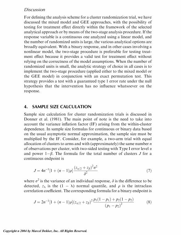
Discussion

For defining the analysis scheme for a cluster randomization trial, we havediscussed the mixed model and GEE approaches, with the possibility oftesting for treatment effect directly within the framework of the selectedanalytical approach or bymeans of the two-stage analysis procedure. If theresponse variable is a continuous one analyzed using a linear model, andthe number of randomized units is large, the various analytical options arebroadly equivalent. With a binary response, and in other cases involving anonlinear model, the two-stage procedure is preferable for testing treat-ment effect because it provides a valid test for treatment effect withoutrelying on the correctness of the model assumptions. When the number ofrandomized units is small, the analytic strategy of choice in all cases is toimplement the two-stage procedure (applied either to the mixed model orthe GEE model) in conjunction with an exact permutation test. Thisstrategy provides a test with a guaranteed type 1 error rate under the nullhypothesis that the intervention has no influence whatsoever on theresponse.

4. SAMPLE SIZE CALCULATION

Sample size calculation for cluster randomization trials is discussed inDonner et al. (1981). The main point of note is the need to take intoaccount the variance inflation factor (IF) arising from the within-clusterdependence. In sample size formulas for continuous or binary data basedon the usual asymptotic normal approximation, the sample size must bemultiplied by the IF. Consider, for example, a two-arm trial with equalallocation of clusters to arms and with (approximately) the same number nof observations per cluster, with two-sided testing with Type I error level aand power 1�b. The formula for the total number of clusters J for acontinuous endpoint is

J ¼ 4n�1½1þ ðn� 1Þq� ðza=2 þ zbÞ2r2d2

ð7Þ

where r2 is the variance of an individual response, d is the difference to bedetected, zE is the (1 � E) normal quantile, and q is the intraclasscorrelation coefficient. The corresponding formula for a binary endpoint is

J ¼ 2n�1½1þ ðn� 1Þq�ðza=2 þ zbÞ2 p1ð1� p1Þ þ p2ð1� p2Þðp1 � p2Þ2

ð8Þ

Zucker94


where pi is the event probability for a given individual in arm i and q is thekappa coefficient as defined in Section 3.1. In either case, the total numberof individuals is Jn. In power calculations based on the noncentral tdistribution, the noncentrality parameter must be divided by the IF.

Typically the ICC is relatively small. But if the ICC is moderate tolarge, substantial effort may be saved with modest loss of efficiency bysubsampling individuals within the clusters. Let m denote the total clustersize. Then, for given q, the relative efficiency (RE) of measuring only nindividuals in each cluster as compared with measuring all individuals ineach cluster is given as

RE ¼qþ ð1� qÞ

m

qþ ð1� qÞn

:

That is, the number of clusters J needed if n individuals in each cluster aremeasured is 1/RE times the number of clusters needed if allm individuals ineach cluster are measured. In cases with large enough q the cost of addingfurther clusters may be offset by the reducedmeasurement cost engenderedby sampling.

To calculate the sample size, one needs to specify not only the usualparameters such as r2 and d or p1 and p2 but also the ICC. In somesituations, a prior data set is available that includes data on the outcome ofinterest under a cluster structure identical or similar to the cluster structurethat will exist in the planned study. In this case, a prior estimate of the ICCis readily obtained. Otherwise, one must make some educated guess aboutthe ICC. It is often useful to examine ICCs obtained in other settings and tomake a guess of the ICC in the planned study based on the range of ICCs inthe other settings and a judgment of which of the other settings is likely tohave a level of within-cluster dependence similar to that in the setting athand. Donner and Klar (1994) have presented ICC’s for a range of publichealth settings.

5. EXAMPLE: THE CATCH TRIAL

As as example of a cluster randomized trial, we describe the Child andAdolescent Trial for Cardiovascular Health (CATCH). Details concerningthe design of this trial are reported in Zucker et al. (1995), and the maintrial results are reported in Luepker et al. (1996). The CATCH studyinvestigated a school-based educational and environmental interventionaimed at promoting heart-healthy habits in elementary school children.



Because the intervention was implemented the school level, a clusterrandomization design was mandatory.

The trial involved randomization of 96 schools, of which 40 wereassigned to the control group C, 28 were assigned to receive the school-based intervention S, and 28 were assigned to receive the school-basedintervention plus a supplementary family-based intervention (S+F ). Themain trial comparison was that between the combination of S and S+Fgroups and the control group.

The intervention was aimed at changing a number of behaviors,principally fat and salt consumption and physical exercise. The primarytrial endpoint was taken to be serum total cholesterol, because it was feltthat dietary and exercise habit measures would be susceptible to reportingbias, whereas cholesterol would be free of such bias but responsive enoughto reflect true diet and exercise changes. Various diet, exercise, and otherendpoints were included as secondary endpoints.

The primary study cohort was defined to be those students whounderwent a baseline cholesterol measurement. Provisions were made totrack outmigrating students and to attempt to measure cholesterol in thesestudents at the end of the study.

The sample size was determined by the following slightly extendedversion of the formula (7):

J ¼ ½CScð1� cÞ��1½1þ ðS� 1Þq1 þ ðC� 1ÞSq2�ðza=2 þ zbÞ2r2

d2ð9Þ

where C denotes the number of classrooms in a school, S denotes thenumber of students per classroom with available data, q1 denotes thewithin-classroom correlation, q2 denotes the within-school correlation forstudents in different classrooms in the same school, and g denotes theproportion of clusters assigned to the intervention arm.

The CATCH calculations assumed 3–4 classrooms per school (3.5 onaverage) and 17 students with available data per class. On the basis of paststudies the standard deviation r was estimated to be 28 mg/dl. The cor-relations q1 and q2 were estimated on the basis of a variance componentsanalysis of a small data set on cholesterol levels among schoolchildren in aprior observational study conducted by one of the study centers inCATCH. The estimates were q1 = 0.023 and q2 = 0.003. The projectedtreatment difference on cholesterol (S and S+ F versus C) was determinedto be 5.1 mg/dl. A conservative adjustment factor was incorporated toaccount for possible missing data bias; see Zucker et al. (1995) for details.The effect of the adjustment was to reduce the difference d to be detected

Zucker96


from 5.1 mg/dl to an effective difference, after the adjustment, of 2.9 mg/dl.The intervention (S+F and S ) to control C allocation ratio was 7:5 (toenhance the power of the S+F versus S comparison), so that c = 0.583.Substituting these parameters into the formula (9) yields a sample sizerequirement of 102 schools total for 90% power at the two-sided 0.05 level.Based on administrative considerations, the final sample size was taken tobe 96 schools total.

The sample size calculation incorporated both school and classroomeffects because at the design stage it was felt important to do so. As regardsthe analysis, with school-level assignment the randomization theory ofstatistical testing requires school to be the primary unit of analysis.However, the theory does not require incorporation of classroom as afactor for the analysis to be valid in terms of type I error. In fact, the finalCATCH analysis did not include classroom as a factor.

The serum cholesterol results were analyzed using a mixed linearmodel of the form (3), with experimental arm, CATCH center, baselinecholesterol level, and a number of relevant covariates as fixed effect termsand school as a random effect. The post-study mean cholesterol levels were168.3 mg/dl for treatment (S and S+F ) and 169.5 mg/dl for control; thetreatment-control difference was not statistically significant. On the otherhand, nominally statistically significant though modest differences werefound on dietary and physical activity measures. As possible explanationsfor the negative finding on cholesterol, the investigators point up thesmaller than projected dietary changes and the effects of puberty.

In regard to cooperation with study procedures, the percentage ofstudents in the study schools who had a baseline cholesterol measurementand were entered into the primary CATCH cohort was 60% as opposed tothe projected 80%. Among the students in the primary cohort, 72%continued in CATCH schools up to the end of the study. Of these, 90%underwent the final cholesterol measurement. Of the students whomigrated out of CATCH schools, 50% underwent the final cholesterolmeasurement. Thus, overall, 79% of the students in the primary CATCHcohort had a final cholesterol measurement, representing a data complete-ness level not too far from the projected 85%.

6. SUMMARY

A cluster randomization design is necessary when assessing a cluster-levelintervention and sometimes convenient in other clinical trial settings.When cluster randomization is employed, the primary unit of analysis



must be the cluster to preserve validity of the type I error. Though it isuncommon for entire clusters to drop out from the trial, dropout at theindividual level is quite common, and a intention-to-treat approach toanalysis is called for to avoid dropout bias. The analysis plan and samplesize determinationmust be appropriately tailored to account for the role ofthe cluster as the primary analysis unit. Suitable approaches are availablefor ensuring a valid analysis while allowing adjustment for both cluster-level and individual-level covariates.

REFERENCES

Braun, T., Feng, Z. (2001). Optimal permutation tests for the analysis of group

randomized trials. Journal of the American Statistical Association 96:1424–1432.

Bozivich, H., Bancroft, T. A., Hartley, H. O. (1956). Power of analysis of variance

test procedures for certain incompletely specified models. Annals ofMathematical Statistics 27:1017–1043.

Cochran, W. G. (1977). Sampling Techniques. 3rd ed. New York: John Wiley.Cohen, J. (1960). A coefficient of agreement for nominal data. Educational and

Psychological Measurement 20:37–46.COMMIT Research Group. Community Intervention Trial for Smoking Ces-

sation (COMMIT): I. Cohort results from a four-year community inter-

vention. American Journal of Public Health 85:183–192.Cornfield, J. (1978). Randomization by cluster: A formal analysis. American

Journal of Epidemiology 108:100–102.

Donner, A., Birkett, N., Buck, C. (1981). Randomization by cluster: Sample sizerequirements and analysis. Americal Journal of Epidemiology 114:906–914.

Donner, A., Donald, A. (1987). Analysis of data arising from a stratified design

with cluster as the unit of randomization. Statistics in Medicine 6:43–52.Donner, A., Klar, N. (1994). Methods for comparing event rates in intervention

studies when the unit of allocation is a cluster. American Journal of Epi-demiology 140:279–289.

Donner, A., Klar, N. S. (2000). Design and Analysis of Cluster RandomizationTrials in Health Research. London: Arnold.

Fisher, R. A. (1935). The Design of Experiments. Edinburgh: Oliver and Boyd.

8th ed. New York: Hafner, 1966.Fleiss, J. L. (1981). Statistical Analysis of Rates and Proportions. 2nd ed. New

York: John Wiley.

Friedman, L. M., Furberg, C. D., DeMets, D. L. (1996). Fundamentals ofClinical Trials. 3rd ed. St. Louis MO: Mosby—Year Book.

Gail, M.H., Byar, D.P., Pechacck, T.F., Corle, D.K. (1992). Aspects of the sta-

Zucker98


tistical design for the Community Health Trial for Smoking Cessation

(COMMIT). Controlled Clinical Trials 13:6–21.Gail, M. H., Tan, W. Y., Piantadosi, S. (1988). Tests for no treatment effect in

randomized clinical trials. Biometrika 75:57–64.

Glass, G. V., Stanley, J. C. (1970). Statistical Methods in Education and Psy-chology. Englewood Cliffs, NJ: Prentice-Hall.

Henderson, C. R. (1953). Estimation of variance and covariance components.

Biometrics 9:226–252.Hines, W. G. S. (1996). Pragmatics of pooling in ANOVA tables. American

Statistician 50:127–139.Hirji, K. F., Mehta, C. R., Patel, N. R. (1987). Computing distributions for exact

logistic regression. Journal of the American Statistical Association 82:1110–1117.

Hopkins, K. D. (1982). The unit of analysis: Group means versus individual

observations. American Educational Research Journal 19:5–19.Jennrich, R. I., Schluchter, M. D. (1986). Unbalanced repeated-measures models

with structured covariance matrices. Biometrics 42:805–820.

Kempthorne, O. (1952). The Design and Analysis of Experiments. New York:John Wiley.

Laird, N. M., Ware, J. H. (1982). Random-effects models for longitudinal data.

Biometrics 38:963–974.Liang, K. Y., Zeger, S. L. (1986). Longitudinal data analysis using generalized

linear models. Biometrika 73:13–22.Longford, N. (1994). Logistic regression with random coefficients. Computational

Statistics and Data Analysis 17:1–15.Luepker, R. V., Perry, C. L., McKinlay, S. M., Nader, P. R., Parcel, G. S., Stone,

E. J., Webber, L. S., Elder, J. P., Feldman, H. A., Johnson, C. C., Kelder,

S. H., Wu, M. (1996). Outcomes of a field trial to improve children’s dietarypatterns and physical activity: The Child and Adolescent Trial forCardiovascular Health (CATCH). Journal of the American Medical Asso-

ciation 275:768–776.Murray, D. M. (1998). Design and Analysis of Group-Randomized Trials.

Oxford: Oxford University Press.Murray, D. M., Hannan, P. J., Wolfinger, R. D., Baker, W. L., Dwyer, J. H.

(1998). Analysis of data for group-randomized trial with repeat measureson the same group. Statistics in Medicine 17:1581–1600.

Pocock, S. J. (1983). Clinical Trials: A Practical Approach. New York: John

Wiley and Sons.Prentice, R. (1988). Correlated binary regression with covariates specific to each

binary observation. Biometrics 44:1033–1048.

Reboussin, D. M., DeMets, D. L. (1996). Exact permutation inference for twosample repeated measures data. Communications in Statistics, Theory andMethods 25:2223–2238.



Rosen, L. J. (2003). The effect of a health promotion program on hygiene be-

havior and illness-related absenteeism. Ph.D. dissertation. School of Pub-lic Health, Hebrew University of Jerusalem. In preparation.

Simon, R. (1981). Composite randomization designs for clinical trials. Biometrics

37:723–731.Susser, M. (1995). Editorial: The tribulations of trials—intervention in commu-

nities. American Journal of Public Health 85:156–158.

Winer, B. J. (1971). Statistical Principles in Experimental Design. 2nd ed. NewYork: McGraw-Hill.

Zeger, S. L., Liang, K. Y., Albert, P. A. (1988). Models for longitudinal data: ageneralized estimating equations approach. Biometrics 44:1049–1060.

Zucker, D. M. (1990). An analysis of variance pitfall: The fixed effects analysis ina nested design. Educational and Psychological Measurement 50:731–738.

Zucker, D. M., Lakatos, E., Webber, L. S., Murray, D. M., McKinlay, S. M.,

Feldman, H. A., Kelder, S. H., Nader, P. R. (1995). Statistical design of theChild and Adolescent Trial for Cardiovascular Health (CATCH).Controlled Clinical Trials 16:96–118.

Zucker100


6Design and Analysis of ClinicalTrials with Multiple Endpoints*

Nancy L. GellerNational Heart, Lung, and Blood Institute, National Institutes of Health,Bethesda, Maryland, U.S.A.

1. INTRODUCTION AND NOTATION

In many clinical trials, there are several endpoints of comparableimportance, rather than one primary endpoint. In cholesterol-loweringtrials, for example, we may be interested in LDL and HDL or LDL andthe ratio of total cholesterol to HDL and tryglycerides. In patients withcoronary heart disease, we may be interested in both resting andexercise ejection fractions. In blood pressure lowering trials, we mightbe interested in diastolic and systolic blood pressure or mean arterialpressure and pulse pressure. In stroke treatment there are a number ofscales used to measure recovery and no one scale is believed to assess alldimensions. We later will consider an example using four of thesescales, the Barthel Index, NIH Stroke scale, Glasgow Outcome score,and the modified Rankin score. In lung diseases, we may be interestedin several lung function tests such as FEV1, FVC, PI. In behavioralstudies, we may be interested in several scales for quality of life. Recentadvances in DNA technology have led investigators to undertake

* This chapter was written by Nancy L. Geller in her private capacity. The views expressed

in the chapter do not necessarily represent the views of NIH, DHHS, or the United States.


exploratory studies, seeking genes which are over- or underexpressed in(say) a diseased population compared to a control. The number of geneswhich are examined is often in the thousands.

The examples illustrate that restricting ourselves to one primaryendpoint when designing or analyzing a clinical study may be inappro-priate. Further, the multiple endpoints one might consider are corre-lated with one another. Here we consider methodology for situationswhere there are multiple primary endpoints in a clinical study. We con-centrate on clinical trials, although the methods are applicable to otherstudies as well.

Let Xij i = 1, 2, j = 1, 2, . . . , ni, be independent vectors of length Krepresenting the jth observation of the ith sample. We assume that Xij hasa multivariate normal distribution with mean Ai and known variance-covariance matrix A0.

We are interested in testing a null hypothesis that twoK-dimensionalmean vectors of k endpoints are equal against an alternative hypothesisthat the difference in mean vectors is a vector of positive constants:

H0f1;2; : : : ;Kg: m2 ¼ m1

HAf1;2; : : : ; Kg: m2 � m1 ¼ dk

where Mi, i = 1, 2, is a K � l column vector of the true means and D is acolumn vector of specified positive treatment differences (of length K) andE is a positive scalar. We may think of the second sample as representing anew treatment, the first sample as representing a control treatment, andthe alternative as specifying that the new treatment is better than controlon all endpoints. We develop one-sided tests, although extensions to two-sided alternatives (that one treatment is superior to the other, withoutspecifying which) are straightforward.

We subscript the null and alternative hypotheses by {1, 2, . . . , K} toindicate hypotheses involving all K endpoints. Later we will considertesting null hypotheses on various subsets of endpoints. We will alsomention extensions to more than two samples.

2. SOME HYPOTHESIS TESTS FOR MULTIPLEENDPOINTS

In this section, we describe a number of the statistics which have beenproposed for testing null hypotheses involvingmultiple primary endpoints.

Geller102


2.1. Bonferroni Methods

Perhaps the simplest methods perform univariate tests on each of theK endpoints and adjust the p value in one of a number of ways. Theoriginal method used the Bonferroni inequality, performing univariate(one-sided) tests on each endpoint at level a/K. This maintains an over-all type I error a, but is conservative, with the degree of conservatismincreasing with K and as the correlation increases (Pocock, Geller, andTsiatis, 1987).

A number of modifications have been proposed (Holm, 1979;Hochberg, 1988; Simes, 1986) to decrease the conservatism of the Bonfer-roni procedure. Holm’s sequentially rejective procedure performs theunivariate tests on each endpoint and orders the univariate p values fromsmallest to largest, denoted by P(1) V P(2) V : : : V P(K). If P(1) > a/K,Holm’s procedure stops and we do not reject any of the null hypotheses. IfP(1) V a/K, Holm’s procedure rejects the corresponding null hypothesis;then if P(2) >a/(K-1), Holm’s procedure stops and rejects only the firstnull hypothesis, but not the others; if P(2) V a/(K-1), Holm’s procedurerejects also the corresponding null hypothesis, etc. Holm’s procedure isclearly less conservative (and hence more powerful) than the originalBonferroni procedure, yet still protects the type I error.

Simes (1986) proposed rejecting H0{1, 2, . . . , K} if P(i)< ia/K for atleast one i. Since the rejection region contains the Bonferroni rejectionregion, Simes’s procedure is always more powerful than Bonferroni’s.However, Simes only proved his procedure maintained a when the teststatistics were independent. Sarkar and Chang (1997) proved that Simes’sprocedure maintained a when the distribution of the vector of teststatistics was positively dependent under the null hypothesis. The as-sumption of positive dependence needed for the Simes’s procedure can-not be verified until the data are seen.

Procedures of the Bonferroni type are appealing because they aresimple and distribution-free. The Bonferroni and Holm proceduresrequire at least one endpoint to be highly significant to reject H0{1, 2,

. . . , K}. In the case of five endpoints, each with p value .02, the Bonferroniand Holm procedures would not reject H0{1, 2, . . . , K}, yet if all of theendpoints go in the same direction, the null hypothesis is not likely to betrue. The Bonferroni and Holm procedures do not use the informationabout the relationship between endpoints and so lose power. Resamplingmethods improve on this.

Design and Analysis of Clinical Trials with Multiple Endpoints 103


2.2. Resampling Methods (Westfall and Young, 1993;Troendle, 1995, 1996)

Consider the univariate comparisons on the K individual endpoints andorder the test statistics Ti. Let t(1)V t(2)V: : : V t(K) be the ordered valuesof the Ti and H0(1), H0(2), . . . , H0(K) be the corresponding ordered nullhypotheses. Determine constants q1, q2 . . . , qK and sequentially accepthypothesesH0(1),H0(2), . . . until the first time t(i)> qi, at which point rejectH0(1), . . . ,H0(K). The constants qi are determined so that the probability ofrejecting any true hypothesis under any parameter configuration is at mosta. In effect this procedure can be viewed as an exact version of Holm’sprocedure. An algorithm (which uses permutational resampling) deter-mines the constants and it is shown (under certain conditions) that thefamilywise error is strongly controlled asymptotically.

An overall adjusted p value for a subset of hypotheses on singleendpoints is available from this procedure. The adjusted p value is thesmallest overall significance level a for which the given subset of hy-potheses would be rejected by the multiple test procedure using the ob-served test statistics.

2.3. Linear Combinations of Endpoints

Several statistics which are linear combinations of the endpoints havebeen suggested. Assume first that the underlying data have a normaldistribution with known covariance matrix A and that there are ni = Npatients assigned to each treatment. We consider three linear combina-tion tests for testing H0{1, 2, . . . , K} versus HA{1, 2, . . . , K}. Each test statistichas a standard normal distribution and H0{1, 2, . . . , K} would be rejectedfor large values of the test statistic.

Let Y be the column vector of differences in means for the Kendpoints (second sample minus first sample), R=(jim) the covariancematrix of Y, and jmm = jm2 , the variance of the mth mean difference. Theordinary least squares (OLS) statistic (O’Brien, 1984) is a function of theaverage of Ym/jm, which is then properly normalized:

ZOLS ¼ ðN=2Þ1=2JTYðJTRJÞ1=2

where J=(j1-1, j2-1, . . . , jK-1)T.

Geller104


The generalized least squares (GLS) statistic (O’Brien, 1984) is aweighted average of the Ym/jm:

ZGLS ¼ ðN=2Þ1=2dTR�1Y

ðdTR�1dÞ1=2

where d=alternative vector (fixed). Here Y is weighted by dT A-1. A thirdlinear combination, the centered linear combination (CLC) statistic, wassuggested by Tang, et al. (1993):

ZCLC ¼ ðN=2Þ1=2JT1D1=2Y

ðJT1D1=2RD1=2J1Þ1=2

where J1=(1, 1, . . . , 1)T and D=diag[(R-1)11, . . . , (R-1)KK], the matrix

with the same diagonal elements as R-1 and off-diagonal elements 0.ZCLC was suggested because among all linear combinations, this choiceof coefficients maximizes the minimum power over the positive orthant.

All of the linear combination statistics are appealing because theyare simple. Tang et al. (1989a) showed that O’Brien’s GLS statistic has apower advantage over the univariate statistics that comprise it in thefollowing sense. Suppose ddd, a, and 1 - h are fixed. Suppose we calculatethe required sample sizes based on each of the K endpoints. If we alsocalculate the required sample size based on the GLS test, the requiredsample size for the GLS test is at most the minimum of the sample sizesrequired if any one endpoint were used to set sample size for the trial. Theother linear combinations are not known to have the same poweradvantage. Of course the disadvantage is that if a trial were designedusing O’Brien’s GLS test, there would be limited power to detect differ-ences in individual endpoints.

A disadvantage of the GLS test is that it does not always have pos-itive coefficients. This implies that the GLS test is inadmissible and thatpeculiar results might emerge from the combination of a large negativetest statistic with a negative coefficient (Pocock, Geller, and Tsiatis 1986;Follmann, 1995; Perlman and Wu, 1999). Both the OLS and the CLC willalways have positive coefficients and therefore are to be preferred.

2.4. Wald-Type Test for Multiple Binary Outcomes

Lefkopoulou and Ryan (1992) considered an experiment involving twotreatment groups where K binary variables were recorded for eachsubject. Let Xijm represent the mth response, m= 1, 2, . . . , K in the ith



group for the jth subject, j=1, 2, . . . , ni. For two groups, i=1 (conven-tional treatment group) and 2 (experimental group). Assume that theobservation vectors for each subject are independent, with mean vectorE(Xijm)= Aim and var(Xijm) = Aim (1 - Aim). The outcomes within a subjectmay be correlated.

For multiple binary outcomes, assume a linear logistic model forthe probabilities of a favorable outcome, that is, Aim satisfies

logit lim ¼ am þ bði� 1Þwhere am allows for a different control level for each of the endpoints andh is the intervention effect coefficient for each of the endpoints. Thus hrepresents a single log odds for the endpoints.

Generalized estimating equations were used to obtain a Wald-typetest to test the null hypotheses that the set of endpoints were equal in thetwo treatment groups against the alternative hypothesis

HA : b> 0:

The test statistic is asymptotically m2 with 1 d.f. The methodology alsoallows the estimation of b which is interpreted as the odds ratio ofimprovement on all of the endpoints with experimental treatment relativeto conventional treatment. 95% (or other) confidence limits for the oddsratio can be obtained.

When the correlations between the pairs of endpoints are equal(am=a for m=1, 2, . . . , K ) the Lefkopoulou/Ryan statistic coincideswith O’Brien’s OLS (and GLS in this case).

The Lefkopoulou/Ryan statistic was developed in the context ofstudies on laboratory offspring and was more general than developedhere, e.g., it applies to more than two treatments and a different numberof endpoints for each subject. Tilley et al. (1996) discussed use of theLefkopoulou/Ryan statistic in the context of the stroke clinical trialdescribed below.

2.5. Likelihood Ratio Tests

Likelihood Ratio and Approximate Likelihood Ratio Test

The distribution of the likelihood ratio test of H0{1, 2, : : : , K} versus

HAf1; 2; : : : ; Kg: m1�m2z 0

with strict inequality holding for at least one endpoint was obtained byKudo (1963) when the covariance matrix was known. Perlman (1969)

Geller106


obtained corresponding results with unknown covariance matrix.Because evaluating these distributions for purposes of application weredifficult, Tang et al. (1989b) proposed the approximate likelihood ratio(ALR) test. When R is a known diagonal matrix, the ALR statistic co-incides with the LR statistic and can be evaluated as

N

2RðYþ

i Þ2

where Yi+ is the maximum of Yi and 0 and the summation is over the K

endpoints. For a general covariance matrix, the mean vector Y must betransformed before the statistic is calculated. Let A be a square matrixsuch that AVA=R-1. Note that A is not unique and Z=(N/2)1/2 AY is avector of independent normal variables with unit variance. The ALR test,g(Z) is

gðZÞ ¼ RðZþi Þ2

where Zi is the ith component of Z, Zi+ is the maximum of Zi and 0, and

the summation extends over the K endpoints. A is chosen so that g(Z)suitably approximates the likelihood ratio statistic of H0{1, 2, . . . , K} versusHA {1, 2, . . . , K}. The method to choose A is given in the appendix of Tanget al., 1993. Tang et al. (1989b) showed that the null hypothesis distri-bution of g(Z) is a weighted sum of m2 random variables. They comparedthe power performance of the ALR test, O’Brien’s GLS test and Hotel-ling’s T2. The performance in terms of power hinges on the closeness ofthe true direction of the alternative to the model direction. They note thatthe ALR test ignores differences going in the wrong direction and so urgecaution when using one-sided multivariate testing.

The X+2 Test

Follmann (1996) proposed rejectingH0{1, 2, . . . , K} in favor ofHA {1, 2, . . . , K}

using Hotelling’s T2 at the 2a level as long as the sum of the differencein mean vectors is positive. This simple test has type I error equal to a,even when the variance-covariance matrix is unknown. The test has rea-sonable power when the mean vector is positive and not in a prespecifieddirection.

2.6. Nonparametric Tests

A number of authors have suggested other global tests, some of which arevery briefly described here.



Rank Tests

An alternative approach which does not require the normality assump-tion is the rank sum statistic proposed by O’Brien (1984). O’Briensuggested ranking the Xijm over all i and j for each m, summing theranks for each subject, then ranking the subject sums and applying aMann-Whitney-Wilcoxon test. While this procedure is very simple, itmust be noted that it does not consider the correlation between either theendpoints or their ranks. Another rank test has recently been investigatedby Huang and Hall (2002), where the covariance of the ranks is included.

One-Sided Bootstrap Tests

Bloch, Lai, and Tubert-Bitter (2001) consider alternatives of the form

HA : A1m > A2m for some m

and

l1m > A2m � em for all m

i.e., treatment 1 is superior to treatment 2 on at least one of the endpointsand all of the other endpoints for treatment 1 are noninferior to those oftreatment 2.

They consider the intersection of the rejection region for the like-lihood ratio test of H0 (Hotelling’s T 2) with the rejection region for thenon-inferiority region (a set of univariate tests). They show that thisresults in a level a test and generate its bootstrap distribution. Becausethey are using the bootstrap, the normality assumption required by manyof the other tests is not needed. Although numerically intense, this for-mulation is shown to have high power and type I error close to alphaunder various distributions, such as a mixture of normals and a normal-exponential mixture.

3. A STEP-DOWN CLOSED PROCEDURE FORDETERMINING WHICH ENDPOINTS DIFFERFOLLOWING A GLOBAL TEST

When dealing with multiple endpoints, aside from establishing an overalltreatment effect, investigators are always interested in which individualendpoints differ. The theory of multiple comparison procedures adaptsnicely to this setting.

Geller108


Let Z{1, 2, . . . , K} denote any global test statistic based on all Kendpoints. Let ZF denote the same test statistic based on the subset F ofthe K endpoints. If the type I error for the global test Z{1, 2, . . . , K} is a andsimultaneously there is control at level a for each test ZF for all subsets F,we say that the type 1 error is strongly controlled (protected) at level a. Ifthere is control at level a only for Z{1, 2, . . . , K} we say that the type I erroris protected weakly (at level a).

3.1. Lehmacher et al.’s Procedure

Lehmacher, Wassmer, and Reitmeir (1991) proposed a step-down closedprocedure to determine which of the k endpoints differ in the twotreatment groups. Suppose Z{1, 2, . . . , K} is conducted at level a at theend of a trial and H0{1, 2, . . . , K} is rejected. A step-down closed pro-cedure very similar to that used for multiple comparisons can beapplied to find if individual endpoints differ. Consider Z(2, 3, . . . , K},Z{1, 3, 4, . . . , K}, . . . , Z{1, 2, . . . , K-1}. Whenever one of these rejects at levela, form the global test statistics on each subset of K� 2 endpoints andtest at level a. Whenever the null hypothesis on K� 2 endpoints is re-jected, step down again. Whenever we do not reject, declare that set ofendpoints not significantly different and do not continue stepping down.Once a set of endpoints does not differ by one path, endpoints in thatset are not considered if they arise via another path.

This step-down closed procedure yields strong control of a andprovides a method to find individual endpoints which differ. The proce-dure may be applied using any of the test statistics described above. Ofcourse, it is possible that a global test statistic rejects H0{1, 2, . . . , K} but noindividual endpoints differ. This may be an issue of power, but also maybe an issue of the correlation between the pairs of endpoints.

3.2. A Procedure with Weak Control of the Overall TypeI Error

When H0{1, 2, . . . , K} is rejected, we may be interested in testing equality ofindividual endpoints irrespective of the outcome of the step-down pro-cedure. Such a procedure yields only weak control of the overall type Ierror; that is, the probability of rejecting the true global null hypothesisthat the mean vectors are equal is a, but the type I error for a true subsetof the global null hypothesis is not maintained at a.



4. GROUP SEQUENTIAL METHODS IN TRIALS WITHMULTIPLE ENDPOINTS

Several of the aforementioned test statistics have been considered in agroup sequential setting. Suppose we undertake analysis of H0{1, 2, . . . , K}

at time t based on a global statistic Z(t).

4.1. Asymptotically Normally Distributed Test Statisticswith Known Covariance Matrix

With known R, Tang et al. (1989a) and Tang et al. (1993) observed thatthe ‘‘ordinary’’ two-sample group sequential theory could be applied tothe linear combination statistics. In 1997 Jennison and Turnbull providedan elegant general theory for application of group sequential proceduresfor (asymptotically) normally distributed test statistics. The linear com-bination statistics fall under the Jennison and Turnbull theory (c.f.Jennison and Turnbull, 2000, chaps. 11, 15) as does the (square root ofthe) Wald-type test of Lefkopoulou and Ryan (1993) as developed here.When the covariance matrix is unknown, it may be estimated from thedata, but the implication is that resulting tests are no longer exact.

4.2. Nonnormally Distributed Test Statistics

For test statistics which are not asymptotically normally distributed, agroup sequential theory may need to be developed. Jennison and Turn-bull (1999) suggest that the sequences of p-values based on normallydistributed test statistics provide an adequate approximation in manycases. The ALR statistic of Tang et al. (1989b) and Tang et al. (1993)is an example of a multiple endpoint test statistic with known nonnor-mal distribution, where, indeed, the sequences of nominal p values forgroup sequential testing are very close to those of normally distributedtest statistics.

4.3. Step-Down Procedures for Group Sequential Trialswith Multiple Primary Endpoints

Tang and Geller (1999) extended the Lehmacher et al. (1991) procedureof Section 3 to group sequential trials. Suppose Z(t)

1, 2, . . . , K denotes amultiple endpoint test statistic at time t and we have a group sequentialboundary c(t)1, 2, . . . , K for Z(t)

1, 2, . . . , K at time t.

Geller110


Proposition 1. The following procedure preserves strong control of thetype I error:

Step 1. Conduct interim analyses to test the null hypothesisH0{1, 2, . . . , K}

based on a group sequential boundary {c(t)1, 2, . . . , K, t = 1, 2, . . . , g}.

Step 2. When H0{1, 2, . . . , K} is rejected, say at time t*, stop the trial andapply the step-down closed testing procedure to test all the other nullhypotheses H0F, using ZF

(t*) and boundaries cF(t*), where F is a subset of

the indices 1, 2, . . . , k.The procedure in Proposition 1 does not allow for continuation of thetrial once a stopping boundary is crossed. However, this is possible usingan alternative closed step down procedure given in Proposition 2.

Proposition 2. The following procedure preserves strong control of thetype I error:

Step 1. Conduct interim analyses to test the null hypothesisH0{1, 2, . . . , K}

based on a group sequential boundary {c(t)1, 2, . . . ,K, t = 1, 2, . . . , g}.

Step 2. WhenH0{1, 2, . . ., K} is rejected, say at time t*, apply the step-downclosed testing procedure to test all the other null hypotheses H0F usingZF(t*) and boundaries cF

(t*), where F is a subset of the indices 1, 2, . . . , K.

Step 3. If any hypothesis is not rejected, continue collecting data in thetrial to the next interim analysis, at which time the closed testing pro-cedure is repeated, with the previously rejected hypotheses automaticallyrejected without retesting.

Step 4. Reiterate step 3 until all hypotheses are rejected or the last stageis reached.

In Table 1, we give an illustration of Proposition 2 for fourendpoints. All testing is conducted at a fixed significance level a. In thisexample, the global null hypothesis was rejected at the first analysis timet1, but no three-endpoint hypotheses were rejected at time t1. Thereforemore data were collected on all endpoints and at time t2, a secondanalysis was conducted on the four three-endpoint hypotheses. It isconvenient to superscript the hypotheses to indicate the time at whichthe hypotheses are tested. Of the three endpoint hypotheses at time t2,



only H (t2)0{1, 3, 4} was rejected, so at time t2 the step-down procedure was

conducted on the three pairs of endpoints {1, 3}, {1, 4} and {3, 4}. SinceH (t2)

0{1, 3} was rejected, we conducted the hypothesis tests of H(t2)0{1} and

H (t2)0{3}. These were not rejected. We continued collecting data on all

endpoints so that at time t3, we could retest the null hypotheses onendpoints {1, 2, 3}, {2, 3, 4}, and {1, 2, 4}. At time t3, we also retestedH (t3)

0{1, 4} and H (t3)0{3, 4}. H

(t3)0{1, 4} and H (3)

0{3, 4} were not rejected and so we didnot step down. Because H (t2)

0{1, 3} was rejected and H (t2)0{1} and H (t2)

0{3} werenot rejected, at time t3 we also tested H (t3)

0{1} and H (t3)0{3}. Of these, the first

was rejected. The conclusion was that there was a difference in endpoint1, but not in the other three endpoints.

The complexity of the example of Table 1 illustrates that in practice,the use of Propositions 1 and 2 require certain care. Further, the stoppingrule, that is, whether Proposition 1 or 2 will be used, should be decidedwhen the study is planned. This is especially important in using Propo-sition 2, where one must consider if ethics allow continuing collectingdata when a global null hypothesis is rejected. Of course, if singleendpoint hypotheses are rejected at an interim analysis, there is no needto continue to collect that endpoint if the trial continues. In contrast to

Table 1 Illustration of a Group Sequential Step-Down Procedure UsingProposition 2

Null hypothesis Test statistic t1 t2 t3

H0, {1,2,3,4} Z1234 x — —H0, {1,2,3} Z123 o o oH0, {2,3,4} Z234 o o o

H0, {1,3,4} Z134 o x —H0, {1,2,4} Z124 o o oH0, {1,2} Z12 — — —H0, {1,3} Z13 — x —

H0, {1,4} Z14 — o oH0, {2,3} Z23 — — —H0, {2,4} Z24 — — —

H0, {3,4} Z34 — o oH0, {1} Z1 — o xH0, {2} Z2 — — —

H0, {3} Z3 — o oH0, {4} Z4 — — —

x = test and reject; o = test and do not reject; — = test not done.

Geller112


Proposition 1, Proposition 2 allows continuation of data collection untila difference in at least one individual endpoint is found (or full samplesize is reached).

5. AN EXAMPLE: THE NINDS STROKE TRIAL

The NINDS tissue Plasminogen Activator (t-PA) trial (sponsored by theNational Institute of Neurologic Disorders and Stroke, or NINDS)randomized patients within 6 hours of onset of (nonhemorrhagic) stroketo intravenous t-PA or placebo. Recombinant t-PA is a thrombolyticagent or ‘‘clot buster, ’’ which was believed to be effective in ischemicstroke, although intracerebral hemorrhage had been reported in earlytrials. Details are found in The New England Journal of Medicine (1995)333, 1581–1587.

Accrual took place between January 1991 and October 1994. Thetrial was designed with 320 patients in order to have 95% power to detecta 20% improvement in the Bartel Index (Bartel) at 90 days (16% versus36%) when hypothesis testing was conducted at the a=.05 level. Threehundred and thirty-three patients were randomized, and, aside from theBartel, three other stroke scales at 90 days were of interest, the modifiedRankin scale (mod RS), the National Institutes of Health Stroke Scale(NIHSS) and the Glasgow scale (Glasgow). We refer to endpoints 1, 2, 3,4 to refer to the Bartel, mod RS, NIHSS and the Glasgow scales,respectively.

While the trial was ongoing, the data and safety monitoring boardmet and decided that for the new treatment to be acceptable, the trialshould show a ‘‘clear and substantial evidence of an overall improve-ment.’’ Therefore the endpoints were dichotomized to define ‘‘improve-ment’’ and the test statistic used for the trial was the Wald test ofLefkopoulou and Ryan based on the four dichotomized endpoints. Two-sided testing was conducted. The results were published in December1995, indicating the superiority of t-PA over placebo with a p value of.008 based on the Lefkopoulou/Ryan statistic. The univariate test resultsreported by the investigators on the individual endpoints are shown inTable 2. The odds ratio for favorable outcome in t-PA group relative toplacebo was 1.7 with 95% C.I. 1.2 to 2.6.

We performed a reanalysis of the NINDS t-PA trial using theoriginal study data (and two-sided testing to be consistent), assuming thatit had been designed as a group sequential trial with analyses planned



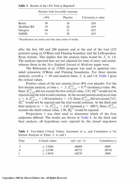
after the first 100 and 200 patients and at the end of the trial (333patients) using an O’Brien and Fleming boundary and the Lefkopoulou/Ryan statistic. This implies that the analysis times would be .3, .6, 1.0.The analyses reported here are not adjusted for time of entry and center,whereas those in the New England Journal of Medicine paper were.

The Reboussin et al. (1998) program was used to generate two-sided symmetric O’Brien and Fleming boundaries. For three interimanalyses, overall a = .05 and analysis times .3, .6, and 1.0, Table 3 givesthe critical values.

Positive values of the test statistic favor tPA over placebo. For thefirst interim analysis, at time t1 = .3, Z

ðt1Þ1;2;3;4 = 0.77 (nominal p value .44).

Since Zðt1Þ1;2;3;4 did not exceed the first critical value, 3.93, H0

(t1) would not berejected and the trial would continue. At the second interim analysis at timet2 = .6,Z

ðt2Þ1;2;3;4= 1.44 (nominal p= .15). SinceZ

ðt2Þ1;2;3;4 did not exceed 2.67,

Hðt2Þ0 would not be rejected and the trial would continue. At the third and

final analysis (t3 = 1), Zðt3Þ1;2;3;4 = 2.62 (nominal p = .0087). Since Z

ðt3Þ1;2;3;4

exceeds the third critical value, 1.98, Hðt3Þ0 would be rejected.

Proposition 1 was then used to determine which of the fourendpoints differed. The results are shown in Table 4. At the third andfinal analysis, all hypotheses were rejected by the closed step-down

Table 2 Results of the t-PA Trial as Reporteda

Percent with favorable outcome

t-PA Placebo Univariate p value

Bartel 50 38 .026Modified RS 39 26 .019Glasgow 44 32 .025

NIHSS 31 20 .033

aStratification on center and time since onset of stroke.

Table 3 Two-Sided Critical Values, Increment in a, and Cumulative a forInterim Analyses at Times .3, .6, and 1

Time Critical values a(i)�a(i�1) Cumulative a

.3 F 3.9286 .00009 .0009

.6 F 2.6700 .00753 .007621 F 1.9810 .04238 .5000

Geller114


procedure. Thus the conclusion was that t-PA was superior to placebowith respect to each of the four stroke scales (with strong control of a).The t-PA investigators reported the global test and the single endpointnominal p values without performing the intermediate tests. This resultedin weak control of a.

6. EXTENSIONS TO MORE THAN TWO SAMPLES

Follmann et al. (1994) and more recently Hellmich (2001) consideredmonitoring single endpoint trials which had two or more treatment arms.The spending function approach was generalized and one is allowed todrop treatments which are inferior. Hellmich proved the strong family-wise error control of the sequentially rejective approach proposed byFollmann et al. for the Pocock and O’Brien and Fleming spending

Table 4 Results of the Step-Down Procedure (Reanalysis of the t-PA Trial)

Comparison Z-value (nominal p value) Decision

1. Compare global test statistic based on four

endpoints to 1.981.

2.62 (.087) Reject

2. Step down to all comparisons of threeendpoints. Compare each Z to 1.981.

NIHSS, Bartel, modified RS 2.63 (.009) RejectNIHSS, Bartel, Glasgow 2.63 (.009) RejectNIHSS, Modified RS, Glasgow 2.59 (.010) Reject

Bartel, Modified RS, Glasgow 2.50 (.012) Reject3. Step down to all comparisons of two

endpoints. Compare each Z to 1.981.

NIHSS, Bartel 2.58 (.010) RejectNIHSS, Modified RS 2.61 (.009) RejectNIHSS, Glasgow 2.52 (.012) RejectBartel, Modified RS 2.50 (.012) Reject

Bartel, Glasgow 2.45 (.014) RejectModified RS, Glasgow 2.46 (.014) Reject

4. Step down to all comparisons of individual

endpoints. Compare Z to 1.981.Bartel 2.28 (.023) RejectModified RS 2.46 (.014) Reject

Glasgow 2.35 (.019) RejectNIHSS 2.29 (.022) Reject



function. We observe here that these results would hold whether the trialhad a single or multiple endpoints.

Suppose we have A treatment arms which will be compared onmultiple endpoints. We test

H0f1; 2; : : : ;Kg: m1 ¼ m2 ¼ : : : ¼ mA

against an alternative hypothesis, e.g.,

HAf1; 2; : : : ;Kg: ms � mt ¼ dð>0Þ for at least one s and all t p s:

One can envision different schemes for monitoring such a trial combiningthe methodology of Hellmich and that here. For this alternative hypoth-esis and multivariate normally distributed data, one could use a groupsequential version of the F test proposed by O’Brien (1984). For otheralternative hypotheses, one might use the chi-squared or F tests proposedby Jennison and Turnbull (1991) or Lauter (1996).

For any alternative, one could monitor arms as suggested byHellmich (2001) until the trial is stopped and follow this by a step-downprocedure to determine which endpoints differ. Alternately, one couldmonitor arms-then-endpoints during the course of the trial. The advan-tages and disadvantages of various schema have not been investigated.When one is allowed to drop either arms or endpoints during the courseof a trial, care needs to be taken that the results are interpretable byclinicians as well as statisticians.

There are other limitations to implementing such methodology atpresent. There are a limited number of test statistics for combiningendpoints of different types (continuous, discrete, censored) and proper-ties of different test statistics in complex settings are not well studied. Theadequacy of using the group sequential boundaries of the ‘‘normaltheory’’ as approximations when parameters are estimated may beunknown. Further research into the multiple arm and multiple endpointsproblem is needed.

7. DISCUSSION

Methodology has been given in this chapter for determining whichendpoints differ in a clinical trial with multiple endpoints when groupsequential monitoring will occur. We combine step-down procedures withgroup sequential methods to determine which individual endpoints differ.The theory has many missing pieces, leaving room for further research.

Geller116


Several points need to be considered in undertaking a clinical trialwith multiple endpoints. One-sided hypothesis testing has inherentlimitations (whether on one or more endpoints). Endpoints with smallunivariate test statistics can dilute the significance of the global teststatistics. Indeed, the number of endpoints and their correlation structurewill determine whether the trial will stop or continue. Examples can begiven to show we can cross a boundary with K endpoints, but not withany subset of them, as well as the reverse. Thus, one needs to considercarefully the selection of the multiple endpoints in a particular situation.In particular in designing a trial using multiple endpoints, the plans foranalysis, including the test statistic, should be chosen in advance.

ACKNOWLEDGMENTS

We are grateful to the t-PA investigators for the use of their data as anexample and to Ms. Mei Lu for undertaking the calculations on that dataset which are reported here and to Drs. Dean Follmann and Dei-In Tangfor comments on this chapter.

REFERENCES

Bloch, D. A., Lai, T. L., Tubert-Bitter, P. (2001). One-sided tests in clinical trialswith multiple endpoints. Biometrics 57:1039–1047.

Follmann, D. (1995). Multivariate tests for multiple endpoints in clinical trials.Statistics in Medicine 14:1163–1176.

Follmann, D. (1996). A simple multivariate test for one-sided alternatives.Journal of the American Statistical Association 91:854–861.

Follmann, D. A., Proschan, M. A., Geller, N. L. (1994). Monitoring pairwise

comparisons in multi-armed clinical trials. Biometrics 50:325–336.Hellmich, M. (2001). Monitoring clinical trials with multiple endpoints.


Hochberg, Y. (1988). A sharper Bonferroni procedure for multiple tests ofsignificance. Biometrika 75:800–802.

Holm, S. (1979). A simple sequentially rejective multiple test procedure.Scandanavian Journal of Statistics 6:65–70.

Huang, P., Hall, W. J. (2002). Multivariate rank tests for comparing severalresponses between two samples. Presented at the Eastern North AmericanRegion of the Biometrics Society meeting, March 2002.

Jennison, C., Turnbull, B. W. (1991). Exact calculations for sequential t, m2 and Ftests. Biometrika 78:133–141.



Jennison, C., Turnbull, B. W. (1997). Group-sequential analysis incorporating

covariate information. Journal of the American Statistical Association92:1330–1341.

Jennison, C., Turnbull, B. W. (1999). Group sequential methods with applications

to clinical trials. Boca Raton, FL: Chapman & Hall/CRC.Kudo, A. (1963). A multivariate analogue of the one-sided test. Biometrika

50:403–418.

Lauter, J. (1996). Exact t and F tests for analyzing studies with multipleendpoints. Biometrics 52:964–970.

Lefkopoulou, M., Ryan, L. (1993). Global tests for multiple binary outcomes.Biometrics 49:975–988.

Lehmacher, W., Wassmer, G., Reitmeir, P. (1991). Procedures for two-samplecomparisons with multiple endpoint controlling the experimentwise errorrate. Biometrics 47:511–521.

O’Brien, P. C. (1984). Procedures for comparing samples with multiple endpoints.Biometrics 40:1079–1087.

Perlman, M. D. (1969). One-sided testing problems in multivariate analysis.

Annals of Mathematical Statistics 40:549–567.Perlman, M. D., Wu, L. (1999). The emperor’s new tests, with Comments.

Statistical Sciences 14:355–381.

Pocock, S. J., Geller, N. L., Tsiatis, A. A. (1987). The analysis of multipleendpoints in clinical trials. Biometrics 43:487–498.

Reboussin, D. M., DeMets, D. L., Kim, K., Lan, K. L. G. (1998). Programs forcomputing group sequential boundaries using the Lan-DeMets method

Version 2. http://www.biostat.wisc.edu/landemets/.Sarkar, S. K., Chang, C. -K. (1997). The Simes method for multiple hypothesis

testing with positively dependent test statistics. Journal of the American

Statistical Association 92:1601–1608.Simes, R. J. (1986). An improved Bonferroni procedure for multiple tests of

significance. Biometrika 73:751–754.

Tang, D. -I., Geller, N. L. (1999). Closed testing procedures for group sequentialclinical trials with multiple endpoints. Biometrics 55:1188–1192.

Tang, D. -I., Geller, N. L., Pocock, S. J. (1993). On the design and analysis ofrandomized clinical trials with multiple endpoints. Biometrics 49:23–30.

Tang, D. -I., Gnecco, C., Geller, N. L. (1989a). Design of group sequentialclinical trials with multiple endpoints. Journal of the American StatisticalAssociation 84:776–779.

Tang, D. -I., Gnecco, C., Geller, N. L. (1989b). An approximate likelihood ratiotest for a normal mean vector with nonnegative components with appli-cation to clinical trials. Biometrika 76:577–583.

The National Institute of Neurological Disorders and Stroke rt-PA Stroke StudyGroup (1995). Tissue plasminogen activator for acute ischemic stroke. NewEngland Journal of Medicine 333:1581–1587.

Geller118


http://www.biostat.wisc.edu/landemets

Tilley, B. C., Marler, J., Geller, N., Lu, M., Legler, J., Ryan, L., Grotta, J. (1996).

Use of a global test for multiple outcomes in stroke trials with applicationto the National Institute of Neurological Disorders and Stroke t-PA stroketrial. Stroke 27:2136–2141.

Troendle, J. F. (1995). A stepwise resampling method of multiple hypothesistesting. Journal of the American Statistical Association 85:370–378.

Troendle, J. F. (1996). A permutational step-up method of testing multiple

outcomes. Biometrics 52:846–859.Westfall, P. H., Young, S. S. (1993). Resampling-Based Multiple Testing:

Examples and Methods for P-Value Adjustment, vol. I. New York: JohnWiley.



7Subgroups and Interactions*

Dean FollmannNational Institute of Allergy and Infectious Diseases,National Institutes of Health, Bethesda, Maryland, U.S.A.

1. INTRODUCTION

Clinical trials are generally not designed to identify if the benefit of treat-ment differs as a function of patient characteristics. The anticipation isthat each randomized group will respond relatively homogeneously and asingle pronouncement regarding benefit will suffice for the entire cohort.While one might well expect that different patients will respond some-what differently, we will not be led astray with a single pronouncementunless some subset of patients is actually harmed by treatment. Thusit seems that for the primary goal of a standard clinical trial, subgroupanalyses should be undertaken to confirm that a single pronouncementis justified.

In practice, however, clinical trials involve a substantial investmentin resources and there is proper interest in examining the data in somedetail. Such exploratory analyses can be useful in suggesting new questionswhich might be answered in future trials. Estimating how the effect oftreatment varies with baseline characteristics may be of interest for avariety of reasons, even if treatment harms no one. For example, some pa-

* This chapter was written by Dean Follmann in his private capacity. The views expressed in

the chapter do not necessarily represent the views of NIH, DHHS, or the United States.


tients may appear to receive marginal benefit. Such an observation mightlead one to consider a trial for this subgroup where an alternative treat-ment is evaluated. Also, while clinical trials are designed to answer aclinical question, they can provide insights to nonclinical questions. Forexample, a treatment may benefit all patients, but there may be a strongdifferential in this benefit as a function of a baseline covariate. Identifyingsuch a differential may provide insight into the biology of the disease or themechanism of action of the treatment.

In this chapter we provide a survey of statistical techniques forsubgroup analyses and interaction. Our view is that one perspective isappropriate for the paper reporting the main results of the clinical mainwhile another perspective is reasonable for secondary papers. Severalexcellent papers on the use and abuse of subgroup analyses have beenwritten (see e.g., Yusuf et al. 1991, Oxman and Guyatt 1992, Bulpitt 1988,Simon 1982). They chiefly provide a strong justification for the ‘‘mainresults’’ view and emphasize the danger in making strong conclusionsbased on exploratory subgroup analyses. Another useful dichotomy ofsubgroup analyses has been proposed by Peto (1995) who distinguishesbetween qualitative interactions, where the treatment is actually harmfulto some subgroup of patients and beneficial to other, and quantitativeinteractions, where the magnitude of treatment benefit varies, but the signdoes not. Peto argues that the former are clinically important and rare,while the latter are clinically unimportant and common.

This chapter is organized as follows. We begin by developing stan-dard approaches to subgroups and interaction in a simple setting. Wethen develop in some detail nonstandard approaches to tests of inter-action. We end by discussing some practical issues that were encounteredin the AVID clinical trial.

2. STANDARD APPROACHES

Throughout we assume a randomized two-armed clinical trial. To keepmatters simple, we will assume that the primary endpoint is continuous,such as diastolic blood pressure (DBP). Our basic arguments apply toother endpoints with obvious modifications. Let Yi be the endpointmeasured on the ith subject where i = 1, . . . , n. We will use Z = 1(0)to identify the treatment (control) group, and use X to denote a vector ofcovariates, e.g. prognostic variables or subgroup identifiers. We assumean equal number of patients in each treatment group.

Follmann122


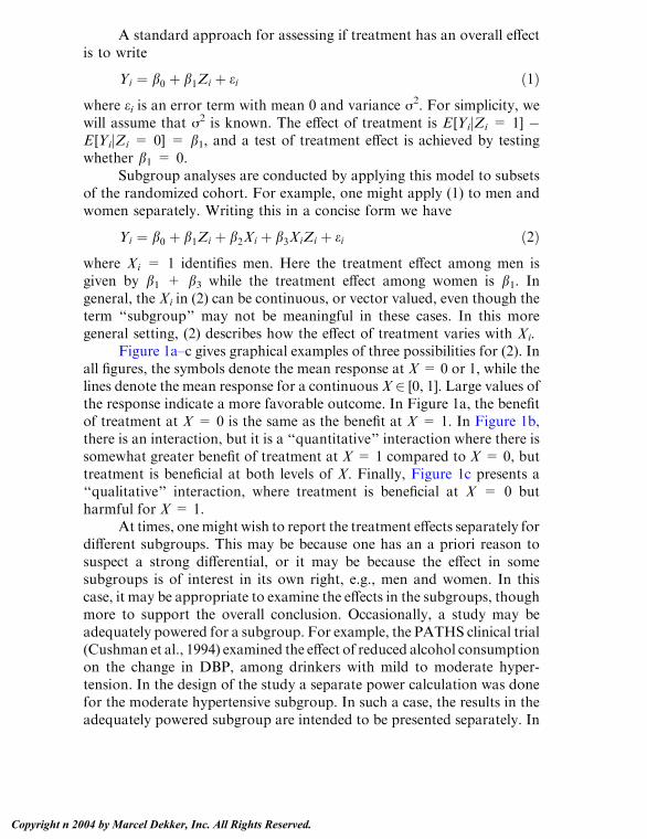
A standard approach for assessing if treatment has an overall effectis to write

Yi ¼ b0 þ b1Zi þ ei ð1Þwhere ei is an error term with mean 0 and variance j2. For simplicity, wewill assume that j2 is known. The effect of treatment is E [YijZi = 1] �E [YijZi = 0] = b1, and a test of treatment effect is achieved by testingwhether b1 = 0.

Subgroup analyses are conducted by applying this model to subsetsof the randomized cohort. For example, one might apply (1) to men andwomen separately. Writing this in a concise form we have

Yi ¼ b0 þ b1Zi þ b2Xi þ b3XiZi þ ei ð2Þwhere Xi = 1 identifies men. Here the treatment effect among men isgiven by b1 + b3 while the treatment effect among women is b1. Ingeneral, the Xi in (2) can be continuous, or vector valued, even though theterm ‘‘subgroup’’ may not be meaningful in these cases. In this moregeneral setting, (2) describes how the effect of treatment varies with Xi.

Figure 1a–c gives graphical examples of three possibilities for (2). Inall figures, the symbols denote the mean response at X= 0 or 1, while thelines denote the mean response for a continuous X 2 [0, 1]. Large values ofthe response indicate a more favorable outcome. In Figure 1a, the benefitof treatment at X = 0 is the same as the benefit at X = 1. In Figure 1b,there is an interaction, but it is a ‘‘quantitative’’ interaction where there issomewhat greater benefit of treatment at X = 1 compared to X = 0, buttreatment is beneficial at both levels of X. Finally, Figure 1c presents a‘‘qualitative’’ interaction, where treatment is beneficial at X = 0 butharmful for X = 1.

At times, onemight wish to report the treatment effects separately fordifferent subgroups. This may be because one has an a priori reason tosuspect a strong differential, or it may be because the effect in somesubgroups is of interest in its own right, e.g., men and women. In thiscase, it may be appropriate to examine the effects in the subgroups, thoughmore to support the overall conclusion. Occasionally, a study may beadequately powered for a subgroup. For example, the PATHS clinical trial(Cushman et al., 1994) examined the effect of reduced alcohol consumptionon the change in DBP, among drinkers with mild to moderate hyper-tension. In the design of the study a separate power calculation was donefor the moderate hypertensive subgroup. In such a case, the results in theadequately powered subgroup are intended to be presented separately. In

Subgroups and Interactions 123


general, subgroups need to be interpreted within the context of the trial,other studies, and the biological phenomena being investigated (Yusuf etal., 1991).

Treating a single trial as if it were two separate trials, one for eachsubgroup, when in fact it was designed as a single study can be verymisleading. This point is forcefully made by reexpressing an observationmade by Peto (1995). Imagine a clinical trial which has a continuousendpoint and uses the standardized mean difference to test treatmentefficacy. Suppose that the mean difference is 2 and the standard error ofthis difference is known to be 1 so that the overall test of significance, is 2.The p value is just less than .05, so treatment appears efficacious.We’re alsovery interested in two equally sized subgroups, e.g., men and women, anddecide to report these separately.We perform the calculations and discoverthat in men, the test statistic (mean difference divided by standard error) is

Figure 1 Three possibilities for the effect of treatment as a function of X. Solidcircles and lines denote the treatment group; open circles and dashed lines denotethe control group. Larger values of the response are more desirable.

Follmann124


3=ffiffiffi2

pand thus men have a p value of about .03. The overall result and the

result in men imply that the test of treatment effect in women is 1=ffiffiffi2

pwith

associated p value of about .48. It may seem that the answer is clear thatmen benefit while women do not. However, the chance of seeing adiscrepancy in the treatment effects between men and women at least aslarge as the observed value (i.e., j3� 1j= ffiffiffi

2p

) is about 1 in 3, provided thetrue effect of treatment is the same inmen andwomen. Evenwith an overallsignificant result, simply looking at subgroup p values is likely to suggestheterogeneity in response which may well be due to chance. As argued byPeto (1995), Yusuf et al. (1991), and others, we would generally expect theoverall result to provide a better estimate of the effect within subgroups.

Another problem results from trying to identify subgroups for whichthe treatment effect is significant, when the overall treatment is nonsig-nificant but with a trend towards significance. It is natural enough to thinkthat surely treatment must have worked somewhere and to feel obliged toidentify where. Such tendencies should be avoided. For such trials, theoverall type I error has already been used up so that it is unclear what thetype I error for subgroups even means here. Nonetheless, such subgroupanalyses are sometimes done. Suppose we have two equal sized subgroups,use the standardized mean difference to test efficacy, have equal treatmenteffects in each subgroup, and, for simplicity, a one-sided hypothesis.Figure 2 graphs the conditional probability of having a p value in one ofthe two subgroups less than .05 given the overall p value. (Since the overallp value is nonsignificant, it is impossible to have both subgroup p valuesless than .05, thus this is the probability of one subgroup p value less than.05 and the other subgroup p value greater than .05.) Thus Figure 2 graphsthe probability of incorrect discordant conclusions about the treatmenteffect in the two subgroups.With an overall p value of just greater than .05,the chance of having one subgroup p value less than .05 and the othergreater than .05 is nearly .5. Even with an overall p value of .25, the chanceof finding one significant and one nonsignificant subgroup is about .10. Ifseveral mutually exclusive subgroupings are analyzed the chance of‘‘identifying’’ a significant subgroup can be quite large. As pointed outby Bulpitt (1988), subgroup analyses showing harm or benefit when a trialdoes not reveal an overall effect may be particularly misleading.

A statistical method to guard against overinterpreting the results ofa trial within subgroups is provided by a test of interaction. In the contextof model (2) this amounts to testing whether b3 = 0. (In words, we seewhether the treatment effect among women equals the treatment effectamong men.) Subgroup analyses provide the estimate of treatment effectwithin a subgroup, albeit with a lot of noise due to the small sample sizes.



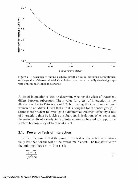
A test of interaction is used to determine whether the effect of treatmentdiffers between subgroups. The p value for a test of interaction in theillustration due to Peto is about 1/3, buttressing the idea than men andwomen do not differ. Given that a trial is designed for the entire group, itseems more prudent to investigate a differential treatment effect by a testof interaction, than by looking at subgroups in isolation. When reportingthe main results of a study, tests of interaction can be used to support therelative homogeneity of treatment effect.

2.1. Power of Tests of Interaction

It is often mentioned that the power for a test of interaction is substan-tially less than for the test of the overall main effect. The test statistic forthe null hypothesis b1 = 0 in (1) is

Y1 �Y0ffiffiffiffiffiffiffiffiffiffiffiffir24=n

p ð3Þ

Figure 2 The chance of finding a subgroupwith a p value less than .05 conditionedon the p value of the overall trial. Calculation based on two equally sized subgroupswith continuous Gaussian response.

Follmann126


whereYj is the sample mean in group j. Assuming equal numbers of menand women, with exactly half of each in the treatment group, the teststatistic for b3 = 0 in (2)

Y11 �Y10 � ðY01 �Y00Þffiffiffiffiffiffiffiffiffiffiffiffiffiffiffir216=n

p ð4Þ

where Yjl is the sample mean for the people in treatment group j withcovariate X = l.

The variance of the numerator of the test statistic for interaction (4)is 4 times greater than that for the test of overall effect (3). If a trial haspower equal to .90 to detect an overall effect of treatment equal to d, thetrial will have power equal to about .37 to detect an interaction of size d.If men and women are not equally numbered, the denominator in (4) islarger and the power is less. Power is .9 to detect interactions of size 2d.Of course, there is no inherent reason why d should be a plausible ormeaningful difference for the interaction: d is chosen to be clinicallymeaningful for the test of overall effect.

In principle one might have marked heterogeneity among patients,and such a differential in treatment effect might be anticipated. However ifsuch marked heterogeneity were recognized during the planning of thetrial, one might well choose not to include those patients with the relativelysmall anticipated treatment effect. The generally poor power of tests ofinteraction should encourage skepticism when interpreting interactionsthat are statistically significant. In the design of a standard clinical trial,one’s prior opinion is that the result of the study should be applicable to theentire randomized cohort and one should need reasonably strong evidenceto be dissuaded from this opinion. For the main results paper, examininginteractions and subgroups should be done, but more for assurance thatnothing unexpected has occurred.

2.2. Multiplicity

In practice, many characteristics of patients are measured at baseline. Ifseveral of these covariates are examined using tests of interaction, as iscommonly done, the chance of seeing at least one significant at p = .05 isincreased, even if the true treatment effect is constant over all baselinecovariates. The exact probability of at least one p value less than .05depends on the number of tests conducted and the correlation between thetest statistics. Suppose K tests are conducted which are all independent ofeach other. The probability of at least one p value less than .05 is 1 - .95K. Ifthe tests are so dependent that they are all identical, the probability of at



least one p value less than .05 is .05. In practice, the test statistics will havea correlation between 0 and 1 and the true probability of at least onesignificant p value will lie between 1 - .95K and .05.

To more accurately gauge the extent of the multiplicity problem, weconducted a small simulation. We imagined a large clinical trial where Ktests of interaction were conducted. Since this imaginary trial was largeand the treatment effect constant over all subgroups and covariates, the Ktests of interaction were approximately univariate normal with mean 0and variance 1. While in practice the correlation between the various testswould be different, for simplicity we assumed that all tests of interactionhad a common correlation q. For various values of K and q, we generated100,000 imaginary clinical trials, and recorded the percentage of timesthat at least one of the test exceeded 1.96 in absolute value. Figure 3 (leftpanel) presents the results. For 32 independent tests, there is about an80% false positive rate. This decreases with decreasing number of testsand also decreases as the correlation increases.

A simple correction for this problem of multiplicity is the Bonferronicorrection. Recall that

PðR1 [ : : : [ RKÞV PðR1Þ þ : : : þ PðRKÞwhere Rk denotes rejection of the null hypothesis using covariate k. To en-sure that the probability of at least one type I error, i.e., P(R1 [ : : : [ RK),is at most a we require P(Rk) V a/K for each k. Thus if K tests are con-ducted, one requires a p value smaller than .05/K to declare significance.Figure 3 (right panel) illustrates the degree of conservatism for this pro-cedure when all tests have equal correlation. We see that the correction isnot very conservative provided the common correlation is less than about.4. The degree of conservatism increases with the number of covariatesand the correlation. Pocock, Geller, and Tsiatis (1987) make a similarconclusion, but based on an exact calculation rather than simulation.

A simple improvement on the Bonferroni method is the sequentiallyrejective Bonferroni procedure of Holm (1979). Here one orders the K pvalues from smallest to largest, say p(1) V p(2) V : : : V p(K). The smallest pvalue, p(1) is compared to .05/K. If p(1) V .05/K, we reject the null hypothe-sis for the associated hypothesis and then compare the second smallestp value p(2) to .05/(K � 1). If p(2) V .05/(K � 1), we then compare the thirdsmallest p value to .05/(K � 2) and continue on in this fashion until wecannot reject. This sequentially rejective procedure provides the sameprotection of the probability of at least 1 type I error, but is more powerfulthan the Bonferroni method, because smaller critical values are used.

Follmann128


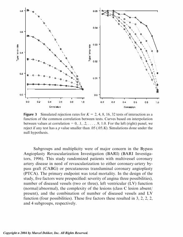
Subgroups and multiplicity were of major concern in the BypassAngioplasty Revascularization Investigation (BARI) (BARI Investiga-tors, 1996). This study randomized patients with multivessel coronaryartery disease in need of revascularization to either coronary-artery by-pass graft (CABG) or percutaneous transluminal coronary angioplasty(PTCA). The primary endpoint was total mortality. In the design of thestudy, five factors were prespecified: severity of angina three possibilities),number of diseased vessels (two or three), left ventricular (LV) function(normal/abnormal), the complexity of the lesions (class C lesion absent/present), and the combination of number of diseased vessels and LVfunction (four possibilities). These five factors these resulted in 3, 2, 2, 2,and 4 subgroups, respectively.

Figure 3 Simulated rejection rates for K= 2, 4, 8, 16, 32 tests of interaction as afunction of the common correlation between tests. Curves based on interpolation

between values at correlation=0, .1, .2, . . . , .9, 1.0. For the left (right) panel, wereject if any test has a p value smaller than .05 (.05/K). Simulations done under thenull hypothesis.



As is common, BARI was monitored by an independent Data SafetyMonitoring Board (DSMB) while the study was ongoing. The DSMBmonitored mortality differences between the two groups, overall and forthe five factors. While tests of interaction could have been used here, it wasdecided to monitor within subgroups. In 1992, the DSMB requested thatthe treatment effect in diabetics and nondiabetics also be monitored asadditional subgroups. Due to the concern about multiplicity, a p value of.005 was decided upon as a threshold for the test of treatment effect in thediabetic subgroup.

Before the study was completed, a striking result was observed inthe diabetic subgroup: the 5 year survival for CABG as 80.6 percentcompared to 65.5 percent for PTCA (nominal p = .0024). This was lessthan the threshold of .005 and these results were disseminated before thecompletion of followup for the main trial by a Clinical Alert. Becausediabetics were chosen as a subgroup a priori and because of the concernabout multiplicity, the primary results paper suggested that the result inthe diabetic subgroup should be confirmed in other populations. Overall,the 5 year survival rates were 89.3 (CABG) and 86.3 (PTCA), p = .19.

After BARI was over, a permutation method was was used to pro-vide an exact p value for the result observed in diabetics, controlling forthe multiple subgroups. Based on the 5 initial variables plus the diabeticvariable, there were a total of 15 overlapping subgroups. Within eachsubgroup, a standardized log-rank test statistic was used so that therewere 15 test statistics, T1, . . . ,T15. A Bonferroni correction applied to these15 tests would require a p value less than .05/15 or .0033 to declaresignificance. Since the nominal p value in diabetics was .0024, a Bonferroniadjusted p value is 15� .0024= .036. However, the Bonferroni correctionis conservative and a simple permutation method was used to provide anexact adjustment for the multiplicity. Under this method, the treatmentand control labels were permuted a large number of times and for a genericpermutation, say the bth, the vector of test statistics T1

(b) , , . . . ,TK(b), was

calculated as well as Mb = max(jT1(b)j , . . . , jTK

(b)j). By simulation, Brookset al. (1997) estimated a permutation p value for the diabetic subgroup of.026, i.e. the maximum associated with the original vector of test statistics,M = max(jT1j , . . . , jTKj), was at the 97.4th percentile of the Mbs. In thisanalysis, the Bonferroni correction is not very conservative. Strictly speak-ing, this permutation procedure tests the strong null that treatment has noeffect whatsoever, i.e. no overall effect, and no effect in any subgroup. See,e.g., Edgington (1995).

Though we have focused on the impact of multiplicity on testing,multiplicity also has an impact on estimation. If several variables are

Follmann130


examined for interactions or subgroups and the single variable with themost extreme value is selected, the estimate of the effect of treatmentassociated with this variable is likely to be biased. Suppose that Ksubgroups are examined, and the subgroup with the most extreme estimateof treatment effect singled out. This will provide a biased (away from 0)estimate of treatment effect in that subgroup. The amount of bias dependson the configuration of the true treatment effects in the K subgroups, e.g.d1 , . . . , dK. If dk = d for all k, the bias is most extreme. Harrell, Lee, andMark (1996) discuss strategies which produce statistical models withaccurate estimates of treatment effect while allowing for differential effectsacross subgroups or covariates.

3. OTHER APPROACHES TO INTERACTION

In terms of statistical methodology, the standard approaches to sub-groups and interaction are quite straightforward as both can be effectedby fitting model (2). In this section, we discuss some other methods thatmay be useful in certain settings.

3.1. Tests of Qualitative Interaction

As argued by Peto and others, quantitative interactions are likely to exist,but are unlikely to be clinically important. Here, treatment causes noharm at any value of X, but may be relatively better for certain values ofX compared to other values of X (see Fig. 1b). Unless there were values ofX for which treatment was basically the same as control, and treatmentwere associated with some nontrivial side effects, the clinical implicationof a quantitative interaction would be that treatment should be given toanyone satisfying the inclusion criteria of the trial.

On the other hand, qualitative interaction where treatment causesharm for certain values of X is quite clinically important (see Fig. 1c). Itseems important therefore to check for qualitative interaction whenreporting the main results of the trial. There are two ways of doing this.First, one could check for harm in various subgroups. However, ifapparent harm is observed in a specific subgroup (e.g., p< .05) it maybe due to chance, for reasons of multiplicity as well as the arguments givenby Peto (1995). Therefore it seems more logical to perform a formal test ofinteraction here.

A standard test of interaction [H0 : b3 = 0 in (2)] does not make adistinction between quantitative and qualitative interaction. Thus if b3 is



rejected we only know there is evidence of an interaction, not necessarilya qualitative interaction. If detecting qualitative interaction is of primeconcern, it makes sense to apply a non-standard test, specifically derivedto detect qualitative interactions. Gail and Simon (1985) proposed such atest which we outline below.

Suppose that there are k = 1, . . . , K mutually exclusive subgroups.Within each subgroup, let Dk be the estimate of treatment effect. The Dk’sare assumed to be normally distributed with mean yk and known variancerk2. Gail and Simon’s procedure is appropriate even if the Dk’s are

approximately normal and accurate estimates of rk2 are used. Let d =

(y1, . . . , yK). The null hypothesis of no qualitative interaction means thatthe elements of d are either all positive (treatment always helpful) or allnegative (treatment always harmful). Let O+ denote the positive orthant{D j yk z 0, k = 1, . . . , K} and O

� = �O+ the negative orthant. A like-

lihood ratio test for

H0: D 2Oþ[[[[[[[[[[[[[[[[[[[[[[[[[O

�

versus the complement of H0 is constructed by taking the ratio ofmaximized likelihoods under HA and H0 and rejecting for large values ofthis ratio. This reduces to rejecting H0 ifX�

D2k

r2k

�IðDk > 0Þ > c and

X�D2

k

r2k

�IðDk < 0Þ > c

where I(A) is the indicator function for the event A and c is chosen so thatthe type I error rate is a. Gail and Simon provide critical values for this testfor various values of K and a.

A generalization of this test is discussed by Russek-Cohen andSimon (1993), whereby the estimates of treatment effect in the K subsetsare allowed to be correlated. Correlated estimates arise in a variety ofpractical settings. For example, suppose X 2 [0, 1] is a continuous co-variate and that model (2) is fit. The hypothesis of no qualitative inter-action means that the sign of the treatment effect (b1 + b3X ) does notchange over X 2 [0, 1], or more simply, that the signs of d1, d2 are thesame, where (d1, d2) = (b1, b1 + b3). Thus the setup of Gail and Simonapplies, but the estimates of d1, d2 are correlated.

The approach of Gail and Simon should work best if the treatment issuperior to the control for some subgroups and vice versa for other sub-groups, but we don’t have an idea about the number of harmful subgroups.If control is harmful for only one of a few subgroups while treatment issuperior for the remaining subgroups, a more powerful procedure can be

Follmann132


developed. Piantadosi and Gail (1993) develop a range test for this settingwhere the null hypothesis of no qualitative interaction is rejected if both

maxDk

rk> c V and min

Dk

rk< �c V:

They evaluate the power of this procedure and conclude that for K= 2 or3, there is little difference between the range test and the LRT. For K> 3,however, the different tests have more of a differential in performance. If,e.g., d/ (�1, 1, 1, 1, 1, 1), then the range test is preferred, while if d/ (�1,�1, �1, 1, 1, 1) the approach of Gail and Simon is preferred.

3.2. Multivariate Approaches to Interaction

In many settings, it is reasonable to postulate that the effect of treatmentmay depend on the severity of the underlying disease (see, e.g., Peto 1995;Smith, Egger, and Phillips 1997; Gueyffier et al. 1997; or Friedman,Furberg, and DeMets 1996). Examining for interaction along diseaseseverity may yield insights regarding the mechanism of action of thetreatment. For example, sicker patients may benefit more than healthierpatients, or sicker patients might benefit less than healthier patients.

A straightforward way to proceed is to identify baseline covariateswhich are related to severity and to separately test each one for an inter-actionwith treatment. Frequently, however, severity of disease is not reallycaptured by a single variable, but is better determined by a combination offactors. Suppose that a severity score Si = BV Xi were available on eachpatient, where Xi is a vector of baseline covariates and B is a vector ofparameters. One could imagine that Bwas estimated with an ancillary dataset using the model

Yi ¼ BVXi þ ei:

If bwere known, it would be a simple matter to replaceXiwith Si in (2) andand perform a test of interaction in the usual way.

In practice there is probably no ancillary data set and, to pursuethis tack, one needs to both estimate B and test for interaction simulta-neously. Follmann and Proschan (1999) proposed such a procedure. Onepostulates

Yi ¼ b0 þ b1Zi þ B2VXi þ hB2VXiZi þ ei ð5Þwhere h0, h1, B2, h are parameters to be estimated. Under this model, theparameter vector for Xi in the treatment group (hB2) is assumed propor-



tional to the parameter vector for Xi in the control group (b2). To test foran interaction along the univariate quantity B2VX, Follmann and Proschanderive the likelihood ratio test for H0: h = 1 versus Ha: h p 1.

A simple way to calculate the test statistic is to fit the model

Yi ¼ b0j þ b2jVXi þ "i ð6Þ

in group j = 0, 1. Let B2j be the estimated parameter vector in group j =0, 1, and let A be the average of the control and treatment estimates of thecovariance of B2j. Decompose � as � = �1/2 [�1/2] V, and define Uj =A�1/2 b2j. Minus twice the log of the ratio of likelihoods is

T ¼ NU1 �U0N2

2� NU1 � m1N

2 � NU0 � m0N2

where

m0 ¼aU1 þU0

a2 þ 1

a ¼ðR� 1=RÞ þ

ffiffiffiffiffiffiffiffiffiffiffiffiffiffiffiffiffiffiffiffiffiffiffiffiffiffiffiffiffiffiffiffiffiffiffiffiffiffiffiffiffiffiffiffiffiffiffiðR� 1=RÞ2 þ 4 cos2ðhÞ

q2 cosðhÞ

M1 ¼ aM0

R ¼ NU1NNU0N

cosðhÞ ¼ U0:U1

NU0NNU1N

and NwN ¼ffiffiffiffiffiffiffiffiffiffiffiffiffiffiffiffiffiffiffiffiffiffiffiffiffiffiffiffiw21 þ : : : þ w2

k

q, where w = (w1, . . . ,wk). Under the null

hypothesis T has an asymptotic chi-square distribution with one degreeof freedom and we reject H0 for large values provided b2 p 0, If b2 is tooclose to 0, or the sample size too small, the chi-square approximationmay not be accurate.

The procedure of Follmann and Proschan (1999) will work best iftreatment interacts with Si, or, put another way, if b20 / b21. If theinteractive effect is concentrated in a few elements of Xi, e.g. the element-wise division of b20/b21= (a, 1, 1, 1, 1), then examining each element ofXi

in turn should be more powerful. Simulations studies confirmed this point.A different multivariate approach to interaction is suggested by

Shuster and van Eys (1983) whereby the vector of covariates Xi is

Follmann134


examined for a region of indifference between treatments and regions ofsuperiority for treatment or control. The case of a single prognosticvariable is instructive. Here we fit

Yi ¼ b0 þ b1Zi þ b2Xi þ b3ZiXi þ ei: ð7ÞAt a specific Xi = x, the treatment effect is

DðxÞ ¼ b1 þ b3x:

The solution for D(x) = 0, say x0 is given by �b1/b3. They propose usingFieller’s theorem to construct confidence intervals for x0, say (X0L, X0U).Within the confidence interval, neither treatment is preferred, while outsideof the interval, either treatment or control is preferred. Of course, either ofthe regions outside (X0L, X0U) may be vacuous since X has a restrictedrange.

Shuster and van Eys discuss generalizing this method to the multi-variate setting. Confidence regions for the solutions to D(x) = 0 aredescribed. However, there is a multiplicity problem to this approach, aspointed out by Gail and Simon (1985), and the procedure can be veryanticonservative.

4. AVID TRIAL

In this section, we apply some of the principles andmethods outlined in thischapter to the Antiarrhythmics versus Implantable Defibrillators (AVID)Trial (AVID Investigators, 1997). The AVID study was a randomizedclinical trial that enrolled patients with either ventricular fibrillation (VF)or serious sustained ventricular tachycardia (VT). Patients were random-ized to treatment by either an implantable cardioverter-defibrillator (ICD)or by an antiarrhythmic drug (AAD). The primary endpoint was all causemortality. The study planned on enrolling 1200 patients, but was stoppedearly due to a substantial reduction in mortality associated with the ICD.At study’s end, 1016 patients had been randomized.

An important aspect of the AVID study was whether the ICD wouldbe homogeneous in terms of benefit. Thus subgroup analyses wereplanned at the outset for the following important categories: age, leftventricular ejection fraction (LVEF), arrhythmia due to coronary arterydisease (CAD = 1 yes, CAD = 0 no), and type or arrhythmia (VF = 1due to VF, VF = 0 due to VT). In the main results paper, hazard ratioswere graphed for subgroups created on the basis of these four variables.



Three subgroups were created for age (<60,z70, and 60–69), while LVEFwas dichotomized (LVEF > .35, LVEF V .35), as were CAD and VF.

Figure 4 displays the hazard ratios along with 95% confidenceintervals for these subgroups. The hazard ratios are calculated from aCox regression model with

EðtÞ ¼ E0ðtÞ expðbZiÞwhere Zi identifies treatment group. The above Cox model is appliedrepeatedly within each subgroup. There are some subgroups for which theconfidence interval overlaps 1. If one incorrectly viewed AVID as beingseparate trials in each of these subgroups, one would conclude that it is notbeneficial for LVEF>.35, for causes of arrhythmia other than CAD, andfor patients with VT. Such an interpretation does not make sense as the

Figure 4 Hazard estimates with confidence bars for four subgroupings of thetrial participants of the AVID study. Overall hazard given by dashed vertical line.

Follmann136


study was not designed as separate trials. Indeed, it is not particularlysurprising that ICD shows no benefit in each age subgroup. If enough smallsubgroups are created, tests of treatment effect in each have low power.

A proper interpretation of Figure 4 evaluates the confidence inter-vals relative to the overall estimated hazard. None of the subgroupconfidence intervals excludes .62 suggesting that the effect of treatment isrelatively homogeneous. To buttress this impression, we conducted stand-ard tests of interaction for each of the four subgroupings: age, LVEF,CAD, VF. Age and LVEF were treated as continuous covariates, whileCAD andVFwere binary covariates. For each test of interaction, we fit theCox regression model:

EðtÞ ¼ E0ðtÞ expðb1Zi þ b2Xi þ b3XiZiÞwhere Xi was one of the four covariates. Based on this model we testedwhether b3 was equal to 0. The p value for each of the four tests ofinteraction was at least .10. On the basis of the standard analysis, the effectappears homogeneous as a function of prespecified baseline covariates.

We next apply the other tests of interaction discussed in this chapter.For each of the four methods of subgrouping in Figure 4, the test of Gailand Simon can be applied. However, since the estimate of the log hazardratio is always negative the conditionX�

D2k

r2k

�IðDk > 0Þ > c and

X�D2

k

r2k

�IðDk < 0Þ > c

is satisfied for no c and the test will not reject for any a. The test ofPiantadosi and Gail (1993) similarly cannot reject. Intuitively this makessense. To conclude that a qualitative interaction exists we need to assureourselves that the point estimates for some subgroups lie well within theregion where treatment is harmful while the point estimates for other sub-groups lie well within the region where treatment is beneficial. If all pointestimates lie in the same region, there is little evidence of a qualitativeinteraction.

While examining these factors each in turn does not suggest aninteraction, it could be that risk varies with the severity of disease. We thusalso calculated the test of Follmann and Proschan (1999). The value of thetest statistic is .209 which has a p-value of .65. All in all, the main result ofAVID seems to be that there is really no evidence of harm of the ICD foranyone and the results of the study can be applied to the overall cohort.

After the main results of AVID were reported, dozens of othermanuscripts were prepared. Some of these analyses focused on the effect



of subgroups or specifically investigated the effect of treatment as afunction of a baseline covariate. A good example of the latter is given bythe paper byDomanski et al. (2000) which evaluated the effect of treatmentas a function of left ventricular dysfunction. They demonstrated that whilethe effect of treatment did not interact with baseline ejection fraction, theeffect did appear to be somewhat diminished for patients with wellpreserved LV function. They suggest that further studies of ICD versusantiarrhythmic drugs may be of interest.

5. DISCUSSION

In this chapter we have tried to provide a perspective on conducting testsof interaction and subgroup analyses in clinical trials. In reporting themain results of a clinical trial, it makes sense to be cautious in suchanalyses. Subgroup analyses should be performed to confirm the lack ofclinically important heterogeneity. In secondary papers, exploratoryanalyses of the effect of treatment for different subgroups may yielduseful scientific insights.

ACKNOWLEDGMENTS

I would like to thank Maria Mori Brooks, Al Hallstrom, and NancyGeller for help in preparing this chapter.

REFERENCES

AVID Investigators (1997). A comparison of antiarrhythmic-drug therapy withimplantable defibrillators in patients resuscitated from near-fatal ventriculararrhythmias. The New England Journal of Medicine 337:1576–1583.

BARI Investigators (1996). Comparison of coronary bypass surgery with

angioplasty in patients with multivessel disease. The New England Journalof Medicine 335:217–225.

Brooks, M. M., Rosen, A. D., Holubkov, R., Kelsey, S. F., Detre, K. (1997).

Treatment comparisons controlling for multiple testing. Controlled ClinicalTrials 18:81S.

Bulpitt, C. J. (1988). Subgroup analysis. The Lancet 31–34.

Cushman, W. C., Cutler, J. A., Bingham, S., Harford, T., Hanna, E., Dubbert, P.,Collins, J., Dufour,M., Follmann,D.A. (1994). Prevention and treatment of

Follmann138


hypertension study (PATHS): Rationale and design. American Journal of

Hypertension 7:814–823.

Domanski, M. J., Sakseena, S., Epstein, A. E., Hallstrom, A. P., Brodsky, M. A.,Kim, S., Lancaster, S., Schron, E. (2000). Relative effectiveness of the im-plantable cardioverter-defibrillator and antiarrhythimc drugs in patients

with varying degrees of left ventricular dysfunction who have survivedmalignant ventricular arrhythmias. Journal of the American College ofCardiology 34: 1090–1095.

Edgington, E. S. (1995). Randomization Tests. New York: Marcel Dekker.

Follmann, D. A., Proschan, M. A. (1999). A multivariate test of interaction for usein clinical trials. Biometrics 55:1151–1155.

Friedman, L., Furberg, C., DeMets, D. (1996). Fundamentals of Clinical Trials.St. Louis: Mosby.

Gail, M., Simon, R. (1985). Testing for qualitative interations between treatmenteffects and patient subsets. Biometrics 41:361–372.

Gueyffier, F., Boutitie, F., Boissel, J.-P., Pocock, S., Coope, J., Cutler, J., Ekbom,T., Fagard, R., Friedman, L., Perry, M., Prineas, R., Schron, E. (1997).

Effects of antihypertensive drug treatment on cardiovascular outcomes inwomen and men. Annals of Internal Medicine 126:761–767.

Harrell, F. E., Lee, K. L., Mark, D. B. (1996). Tutorial in biostatistics: Issues indeveloping models, evaluating assumptions and adequacy, and measuring

and reducing errors. Statistics in Medicine 15:361–387.Holm, S. (1979). A simple sequentially rejective multiple test procedure.

Scandanavian Journal of Statistics 6:65–70.

Oxman, A. D., Guyatt, G.H. (1992). A consumer’s guide to subgroup analyses.Annals of Internal Medicine 116:78–84.

Peto, R. (1995). Statistical aspects of cancer trials. In: Price, P., Sikoa, K., eds.

Treatment of Cancer. 3rd ed. London: Chapman and Hall, pp. 1039–1043.Piantadosi, S., Gail, M. H. (1993). A comparison of the power of two tests of

qualitative interaction. Statistics in Medicine 12:1239–1248.Pocock, S. J., Geller, N. L., Tsiatis, A. A. (1987). The analysis of multiple endpoints

in clinical trials. Biometrics 43:487–498.Russek-Cohen, E., Simon, R. M. (1993). Qualitative interactions in multifactor

studies. Biometrics 49:467–477.

Shuster, J., van Eys, J. (1983). Interaction between prognostic factors andtreatment. Controlled Clinical Trials 4:209–214.

Simon, R. (1982). Patient subsets and variation in therapeutic efficacy. British

Journal of Clinical Pharmacology 14:473–482.

Smith, G. D., Egger, M., Phillips, A. N. (1997). Meta-analysis: Beyond the grandmean? British Medical Journal 315:1610–1614.

Yusuf, S., Wittes, J., Probstfield, J., Tyroler, H. A. (1991). Analysis and inter-pretation of treatment effects in subgroups of patients in randomized clinical

trials. Journal of the American Medical Association 266:93–98.



8A Class of Permutation Testsfor Some Two-Sample SurvivalData Problems

Joanna H. Shih and Michael P. FayNational Cancer Institute, National Institutes of Health,Bethesda, Maryland, U.S.A.

1. INTRODUCTION

In clinical trials with right-censored failure time responses, inference goalsoften focus on comparing the survival distributions of different treatmentgroups, and the ordinary logrank test (Mantel, 1966) is most commonlyused for testing the treatment difference. The appeal of the test comes fromits simplicity and being nonparametric in the sense that it does not requirespecifying the parametric form of the underlying survival distributions.The logrank test is a score test and has full Pitman efficiency under theproportional hazards alternative (Kalbfleisch and Prentice, 1980, p. 106).However, it may lose efficiency under different alternative models. Thegoal of this chapter is to consider modifications to this standard situation,and to address them with a unifying approach based on a framework ofthe distribution permutation tests (DPT) (Fay and Shih, 1998; Shih andFay, 1999). Specifically, we consider cases where the hazards are non-proportional, where the data are interval-censored, and where there isstratification, including the matched-pair case. Although we focus on thetwo-sample case here, it is straightforward to modify the method to handleK-sample tests and linear permutation tests (see Fay and Shih, 1998). The


DPT tests may be applied whenever the censoring mechanism can beassumed to be independent of the failure mechanism and of the treatmentassignment. The advantage of the DPT approach is threefold. First, itpresents a unifying approach for all the above situations. Second, when theDPT tests presented here are used on stratified data, they provide goodpower whether the strata effect is large or small. Thus, there is no need todecide a priori between a traditional stratified test, which gives betterefficiency when there is a large strata effect, or an unstratified test, whichgives better efficiency when there is little or no strata effect. Finally, exactDPT tests may be calculated for small sample sizes, but asymptoticmethods are availible for large sample sizes. There are two disadvantagesof the permutation approach; in some situations the assumptions on thecensoring may not hold, and the approach cannot make adjustments forcovariates as may be needed in some nonrandomized trials.

The DPT framework creates tests by permuting scores based on afunctional of estimated distributions for right-, left-, or interval-censoreddata. The setup is flexible so that by choosing different functionals orestimated distributions new tests can be produced. We will focus on twofunctionals—the difference in means functional and the weighted Mann-Whitney functional. For stratified data, the estimated distribution functionfor each observation is based on a shrinkage estimator similar to thenonparametric empirical estimator of Ghosh, Lahiri, and Tiwari (1989), ofwhich we will give the rationale and details later.

The remainder of the chapter is organized as follows. In Section 2, wereview the DPT framework for censored, stratified data. In Section 3 weconsider the two-sample case without stratification, in Section 4 we con-sider general stratified data, and in Section 5 we consider the special case ofmatch-pair data. In Sections 3 to 5 we show how to apply the DPTs to eachof these situations, and illustrate the methodology with real data. Finally,in Section 6 we reference some work for handling these types of data whenthe censoring assumptions of the permutation test do not hold.

2. DPT FRAMEWORK

Let Xij and xij be the random variable and associated response for the jthresponse of the ith stratum, where i= 1, . . . , n and j= 1, . . . ,mi. In latersections, we consider applications to special cases; in Section 3 we let n=1and in Section 5 we let mi = 2 for all i. If the individual is censored, we donot observe xij but only know that it lies in some interval, say (Lij,Rij].With

Shih and Fay142


a slight abuse of notation, we letRij=l for right-censored data andLij=lim q!0 Rij � q for data that are known, so we can write left-, right-, andinterval-censored data in the form xij e (Lij, Rij]. Thus, we write responsesfor the ith stratum as { yij}u {(Lij,Rij]}. Let zij be the associated treatmentassignment and assume that if zij = a then Xij comes from the distributionCia, a = 1, 2. We assume that the censoring may vary with each stratumbut not the treatment. We test the null hypothesis,H0:Ci1=Ci2=Ci, forall i = 1, . . . , n, against the alternative H1: Ci1 p Ci2, for some i.

The DPT has a simple form. We create permutation tests based on ascore for each subject. We define the score cij by

cij ¼ / Fij jbCi

; bCi

� ð1Þ

where bCi is an estimated distribution for Ci under the null hypothesis,

Fij jbCi

sð Þ ¼ PrXij V s j yij; zij ¼ a;Cia ¼ bCi

�

¼0 if s < LijbCi sð Þ �bCi Lij

� bCi Rij

� �bCi Lij

� if Lij V sVRij

1 if s > Rij

8>><>>:which is the distribution for the jth response of the ith stratum under thenull hypothesis given yij andCi=bCi, and where /(. , .) is a functional usedto compare two distributions. In (1), / is used to compare the individualdistribution of a response with the distribution for its stratum.We considertwo functionals:

Weighted Mann-Whitney (WMW) functional:

/WMW F;Gð Þ ¼Z

w sð ÞG sð ÞdF sð Þ �Z

w sð ÞF sð ÞdG sð Þ

Difference in means (DiM) functional:

/DiM F;Gð Þ ¼Z

xdF xð Þ �Z

ydG yð Þ:

When the weight function w(.) u 1, the WMW functional becomesthe ordinaryMann-Whitney (MW) functional which can also be expressedby

/MW F;Gð Þ ¼ 2 Pr X > Yð Þ þ 1

2Pr X ¼ Yð Þ

� �� 1

A Class of Permutation Tests 143


whereX andY are the random variables associated with the distributions Fand G, respectively.

With a functional chosen, the permutation test is based on thestatistic

L0 ¼Xi

Xj

zij � zi�

cij � ci�

ð2Þ

where zi = Ajzij/mi and ci = Ajcij/mi. Under the null hypothesis, cij’s areexchangeable within each stratum and E(L0) = 0, where the expectation istaken over the permutation distribution induced by the set of all

Qni ¼ 1 mi!

possible permutations within each stratum of covariates to scores. Theassociated variance of L0 is

V ¼Xi

1

mi � 1

Xj

cij � ci� 2" # X

j

zij � zi� 2" #

:

The test statistic is T ¼ L20=V. When n and m Vis is are small, we create an

exact permutation test. Under regularity conditions and the null hypoth-esis, as n ! lor min1ViVn mið Þ ! l, T is asymptotically distributed as v2

with 1 degree of freedom (Sen, 1985).To understand how the DPT works, consider a simple case where

n=1and xij’s are observed (i.e., we have two independent samples withoutcensoring). If we use the empirical distribution for bC1, the distribution ofx1j underH0, then F

1j jbC1has point mass at x1j. With the DiM functional,

c1j = x1j � x1, where xi = Ajxij/mi. The test statistic compares the meandifference in the two samples, and the permutations are done by permut-ing the treatment assignments. The test statistic

ffiffiffiffiT

pis similar to the con-

ventional t-test but with the sample variance calculated about the overallmean.

Rank tests can also be generated using the DPT. For example, ageneralization of the Wilcoxon rank sum test that fits the DPT uses theMann-Whitney functional for /. The Mann-Whitney scores c1j under nocensoring are linearly related to the midranks, which are the standardranks that are averaged at tied values. Thus the test statistic compares therank sum difference in the two samples, and the permutations are done bypermuting the treatment assignments to the midranks.

The DPT framework is flexible. It creates different tests with differ-ent choices of / and bCi’s. In the sequel, we apply the DPTs with / and bCi

chosen to provide good power.

Shih and Fay144


3. TWO INDEPENDENT SAMPLES

As mentioned earlier, for the case of two independent samples, the ordi-nary logrank test is commonly used and has full Pitman efficiency whenthe assumption of proportional hazards holds. However, the logrank testmay lose efficiencywhen the assumption is violated. For example, when thedifference of the two hazards decreases with time, the Wilcoxon statistic(Peto and Peto, 1972) is more efficient than the logrank test. When the twohazards cross, the logrank test may have more efficiency loss than alterna-tive tests. Pepe and Fleming (1989) generalized the Z test to right-censoreddata by introducing the class of tests known as weighted Kaplan-Meier(WKM) statistics. Petroni andWolfe (1994) generalized theWKM tests tointerval-censored data. They call these tests IWD tests since the tests com-pare the integrated weighted difference between the survival estimatorsfrom the two samples. Numerical studies (Pepe and Fleming, 1989; Petroniand Wolfe, 1994) indicate that the IWD tests compare favorably withthe logrank test even under the proportional hazards alternative, andmay perform better than the logrank test under some crossing hazardsalternatives.

The permutation form of the Wilcoxon, logrank, and Z test or t test(the permutation forms of the Z test and t test are equivalent) for censoreddata may be obtained from the DPTs with certain choices of the func-tionals and using a censored data estimator for C1. Unlike the IWD sta-tistics which apply only to data with large samples, these permutation testsallow for exact tests for small sample sizes. In the following, we first con-sider estimation of C1, then consider the three functional choices.

3.1. Estimation of C1

When there is only one stratum, we use the nonparametric maximumlikelihood estimate (NPMLE), C1, for bC1. If there is no censoring, then ~C1

is equal to the empirical distribution function and F1jj ~C1has point mass at

x1j. For right-censored data, 1� ~C1 is the usual Kaplan-Meier survivalestimator.More generally, theNPMLE can be found iteratively by the self-consistent algorithm (Turnbull, 1976) a special case of the EM-algorithm(Dempster, Laird, and Rubin, 1977) or by the iterative convex minorantalgorithm (Groeneboom and Wellner, 1992). We describe a simple self-consistent (or EM) algorithm to find ~C1. First, partition the response spaceinto disjoint intervals, (s0, s1], (s1, s2], . . ., (sm�1, sm], such that Lij e {s0, . . . ,sm�1} andRij e {s1, . . . , sm}. Given the bth estimate ofC1,bC bð Þ

1 , theE step of



the EM algorithm assigns F1j jbC bð Þ

1

skð Þ for all j=1, . . . ,m1, and k=1, . . . ,m. The M step is

bC bþ1ð Þ1 skð Þ ¼ m�1

1

Xj

F1j��bC bð Þ

1

skð Þ for k ¼ 1; . . . ;m:

In practice, we use the self-consistent algorithm with some computa-tional modifications (see Aragon and Eberly, 1992; and Gentleman andGeyer, 1994).

3.2. Tests

Wilcoxon Test

With no censoring, the Wilcoxon test may be derived from a score test ona shift in a logistic distribution based on the marginal likelihood of theranks. The Wilcoxon test may be generalized to right-censored data, usingeither the marginal likelihood of the ranks (Prentice, 1978) or using thegrouped continuous model (Peto and Peto, 1972). Both formulations givesimilar results and it is the latter formulation that produces the scoresassociated with the Mann-Whitney functional here. Fay and Shih (1998)show that the Mann-Whitney scores have the simple form

c1j ¼ /MW F1j j ~C1; ~C1

� ¼ ~C1 R1j

� þ ~C1 L1j

� � 1:

TheWilcoxon test is efficient in detecting the early difference of the hazards(Fleming and Harrington, 1991).

Logrank Test

The logrank test may be derived as a score test from the proportional haz-ards model. As in the Wilcoxon case, when censoring occurs, two differ-ent forms of the test can be created depending on the assumed likelihood.For a detailed discussion on the two forms of the test as applied to bothright-censored and interval-censored data see Fay (1999). In practice,both forms give similar results. Fay and Shih (1998) show that using thegrouped continuous model and with a suitable choice of the weight func-tion for the weighted Mann-Whitney functional, we can obtain a permu-tation form of the logrank test. The score has the expression

c1j ¼ /LR F1jj ~C1; ~C1

� ¼ S1 R1j

� log S1 R1j

� �� S1 L1j

� log S1 L1j

� �S1 R1j

� � S1 L1j

� where we let S1(s) = 1 � ~C1(s) and we define 0 log 0 = 0.

Shih and Fay146


Difference in Means Test

A permutation form of an unweighted IWD test may be obtained whenthe DPT with the DiM functional is applied to censored data. InsertingF1j jW1

and C1 to the DiM functional, we obtain the score

c1j ¼Xmk ¼ 1

ska1jk

~C1 R1j

� � ~C1 L1j

� � 1

( )~C1 skð Þ � ~C1 sk�1ð Þ� �

where

aijk ¼ 1 ifLij < sk VRij

0 otherwise:

�If sm=l and ~C(sm)� ~C(sm�1) > 0, then we let sm= sm�1 [but we do notchange the value of ~C1 smð Þ ]. This modification is common for right-censored data (Efron 1967; James 1987). The IWD test usually gives lowerweights to the smaller values of the survival function estimates because oftheir high variablity due to censoring. Because the DPTs are permutationtests and the instability does not affect the validity, we need not introduceweights to stabilize the test statistic. Fay and Shih (1998) show throughsimulations that the DPT with the DiM functional is more stable than theboth an unweighted and a weighted IWD test.

3.3. Examples

We show two data examples below to emphasize the differences betweenthe choices for the functional. In practice, only one test would beperformed, and this test would be chosen prior to any data analysis and,ideally, prior to any data collection.

Example 1: Gastrointestinal Tumor Study

These data were previously analyzed by Stablein and Koutrouvelis (1985).The study reported on the results of a trial comparing chemotherapy versuscombined chemotherapy and radiation therapy in the treatment of locallyunresectable gastric cancer. There are 45 patients in each treatment group.Figure 1 displays the Kaplan-Meier survival curves. The two survivalcurves cross, suggesting that theDPT using theDiM functional may not beable to detect the difference, because the means, which are the areas underthe survival curves, are similar. The crossing of the survival curves impliesthat the corresponding hazards also cross at some point before the survival



curves cross. Thus, the logrank test may not capture the difference in sur-vival in the two treatment groups either. Figure 1 shows that a large differ-ence in survival occurs during the early follow-up suggesting theWilcoxontest is more suitable in detecting such a difference. TheDPTusing theDiM,MW, and logrank functionals result in asymptotic p values of .97, .05, and.66 respectively. Thus, only the DPT using the MW functional gives asignificant result.

Example 2: Breast Cosmesis Study

For this data set, described in Finkelstein and Wolfe (1985), breast cancerpatients were randomized to either radiation therapy with chemotherapyor radiation therapy alone. The outcome was time until the onset of breastretraction. A total of 94 patients were followed and were seen, on average,every 4–6 months. The frequency of visits decreased with increasing timefrom the completion of treatment. Forty percent of the patients had notexperienced retraction by the time of their final visit and therefore wereright-censored. The data are interval-censoredbecause the time until occur-

Figure 1 Kaplan-Meier estimate of the survival distribution for the gastrointes-tinal tumor study.

Shih and Fay148


ence of breast retraction was not known exactly but only known to haveoccured between two visits. In addition, the time between visits was irreg-ular andmany patients missed visits. Figure 2 is a plot of the self-consistentsurvival estimates for each treatment. Although the two survival curvescross, the crossing occurs very early and thus wouldn’t have much effecton the performance of any of these tests. The DPTs apply to the interval-censored data directly without requiring any modification. The DPT usingthe MW functional, WMW (logrank) functional, and the DiM functionalyield asymptotic p values of .030, .007, and .019 respectively. Thus, thethree tests all produce significant results.

4. STRATIFIED DATA

In clinical studies when survival changes with important prognosticfactors, stratification on different level of those factors is often done eitherat the design stage to ensure treatment balance in each stratum, or at theanalysis stage. The ordinary logrank test, ignoring strata effect, is conser-vative and is biased when there is treatment imbalance in each prognostic

Figure 2 Self-consistent estimate of the survival distribution for the breast cos-mesis study.



subgroup. The stratified logrank test, on the other hand, is unbiased andretains high efficiency as long as the number of strata is small. However,when the number of strata gets large, the stratified test can become veryinefficient unless there is a large strata effect. Shih and Fay (1999) havedeveloped a versatile test based on the DPT framework which combinesthe advantages of both the ordinary and stratified logrank tests. That is,when the number of observations in each stratum is large or when thewithin-strata variance is small relative to the between-strata variance,the test weights each stratum approximately equally and performs like thestratified logrank test. Conversely, when the within-strata variance is largerelative to the between-strata variance, the test weights each stratum pro-portional to the stratum size and performs like the ordinary logrank test.For cases between these two extremes, the versatile test is a compromisebetween the ordinary logrank and stratified logrank tests. The attractivefeature of the proposedmethod is that we do not need to choose in advancewhether to do a stratified analysis or not and hope that the correct decisionwas made; the method automatically does this primarily based on theestimated within- and between-strata variances.

The DPT setup is the same as above, but now we choose an appro-priate estimator for Ci, i = 1, . . . , n, when n > 1. Once chosen, thisestimator is inserted in (1) to calculate the scores cij and then the teststatistic (2).

4.1. Estimation of Ci

We consider the following shrinkage estimator for Ci, i= 1, . . . , n, n>1,

bCi ¼ wi~Ci þ 1� wið Þ

Pj wj

~Cj*P

k wk

( )ð3Þ

where ~Ci is the NPMLE for the ith stratum ~Ci* ¼ m�1

i

Pj Fij

:Cj ,

:C is the

NPMLE for all the data ignoring the strata, wi ¼ mi= mi þ sð Þ; s ¼ r2=D if D > 0; and r2 and D defined below, are the estimates of the within-cluster (i.e., strata) variance, r2, and between-cluster variance, D. WhenD V 0, following Fay and Shih (1998), bCi is defined as bCi ¼ Rjmj

~Cj*Rkmk

¼:C.

The above shrinkage estimator is slightly different from the one in Shihand Fay (1999) where ~Cj is used in place of ~Cj

*. The two shrinkage es-timators are identical for uncensored data, but are slightly different forcensored data. For example, when wi ! 0, (3) approaches

�C , but

the estimator in Shih and Fay (1999) approachesP

jmjCj=P

mj.

Shih and Fay150


In the absence of censoring, the above estimator is the shrinkageestimator proposed by Ghosh, Lahiri, and Tiwari (1989), where ~Ci is theempirical distribution function for the ith stratum,

r2 ¼Pn

i¼1

Pmi

j¼1 xij � xi� 2P

mi � 1ð Þ

D ¼P

mi

�xi � x

2� �� n� 1ð Þr2P

mi �P

m2i =P

mi

where xi is the mean of the ith strata and x is the overall mean. In thepresence of censoring, since xij is not observed, r2 and D are modifiedsuch that

r2 ¼Pn

i¼1

Pmi

j¼1 EFijjC: Xij � :

xi� 2P

mi � 1ð Þand

D ¼P

mi:xi � :

xð Þ2n o

� n� 1ð Þr2Pmi �

Pm2

i =P

mi

where �xij ¼ EFijjC: Xij

� ¼Pk sk½FijjC: skð Þ � FijjC: sk�1ð Þ�; :xi ¼ m�1i

Pj:xij; and

:x ¼ P

mið Þ�1Pi

Pj:xij and

:C is the NPMLE for all the data ignoring the

strata. We use:C instead of ~Ci because when the number in each stratum

is small, ~Ci shows little within stratum differences if the censoring inter-vals overlap.

The above estimates of r2 and D are not rank invariant. Theywould be used with tests using the difference in means functional. Forrank tests, we transform the response to a function of the ranks byreplacing FijjC: with Fij*, where Fij* s*ð Þ ¼ Fijj �C sð Þ; s* ¼ /MW ds; jC

:� ; and

ds xð Þ ¼ 1 if x � s and zero otherwise. When there is no censoring, theeffect of the transformation is equivalent to replacing each xij with itsmidrank from the entire data ignoring strata.

Once the values for bCi are calculated, the calculation of the scores,cij, proceeds analogously to the calculations in Section 3. Thus, thelogrank scores are

cij ¼ /LR FijjbCi

;bCi

� ¼

Si Rij

� log Si Rij

� h i� Si Lij

� log Si Lij

� h iSi Rij

� � Si Lij

� ð4Þ



where Si(s) = 1 � bCi(s), and the Mann-Whitney scores are

cij ¼ /MW FijjbCi

;bCi

� ¼ bCi Rij

� þbCi Lij

� � 1:

4.2. Features

An advantage of using bCi is that it induces the desired features of aversatile test. Consider a permutation form of the logrank test corre-sponding to the DPTwith theWMW functional. If r2 is small relative to Dor mi is large, then wi ! 1, and bCi approaches the NPMLE C1. Thus L0 isequal to the permutation form of a stratified logrank test. Conversely, if r2

is large relative to D, wi is close to zero and bCi approaches:C, the NPMLE

for all the data ignoring strata. Consequently, the induced test is just astratified permutation of an ordinary logrank test. That is, each score iscalculated from all the data ignoring strata and then permutation is donewithin each stratum. We call this latter test the MC test because a similartest was proposed by Mantel and Ciminera (1979). (The only difference isthat they use the other form of the logrank scores, see Section 3.2.)

We conducted a simulation study which compares the versatile testwith three tests: permutation forms of the ordinary logrank test, stratifiedlogrank test, and the MC permutation test. All simulations have 1000replicates and test the equality of two treament effects. Each survival timehas the following form: if zij = a, a = 1, 2, let Pr (Xij > xij) = (exp(�habixij), where h1 = 1, h2 = 2.4. Let bi u G(1/x,x), where G(a, b) is agamma distribution with mean ab and variance ab2. We choose x = 0,.22, .86, 2 corresponding to values of 0, .01, .3, .5 respectively forKendall’s tau, where we define the distribution with x = 0 as a pointmass at 1. The stratum size mi is random were mi � 1 follows a Poissondistribution with parameter c � 1, such that E(mi) = c. In each stratum,half of the individuals receive one treatment. We introduce right-censor-ing which is uniformly distributed over (0, 1), producing 51, 53, 60, and66% censoring for the four values of x, respectively. We use the criticalvalue based on the asymptotic permutation distribution.

Table 1 presents the simulated power. Overall, when there is no oronly a small strata effect, the stratified logrank test has high efficiency lossunless the strata size is large. On the other hand, the ordinary logrank testretains high efficiency when the strata effect is small, but loses efficiencywhen the strata effect is large. The MC test and the versatile test arecomparable for moderate strata effect, and the latter has higher power fora large strata effect. Both tests have the advantages of ordinary and

Shih and Fay152


stratified logrank tests. That is, when the strata effect is small, theyperform like the ordinary logrank test. And when the strata effect getslarge, they perform like the stratified logrank test.

4.3. Example 3: Prostate Cancer Clinical Trial

This example concerns a VACURG (Veterans Administration Cooper-ative Urological Research Group) prostate treatment study. This studywas the first of a series of multicenter randomized clinical trials to studytreatments for newly diagnosed prostate cancer (see Byar and Corle, 1988and references therein). Here, we reanalyze a subset of study I of thosetrials, where 299 patients were randomized to either radical prostatec-tomy and placebo, or radical prostatectomy and 5.0 mg diethylstilbestrol(DES) daily. The primary endpoint was death from any cause. Patientsentered study I from 1960 until 1967, and here we have followup forpatients until February 1995. We compare patients in the initial treat-ment groups, under an intent-to-treat analysis, noting that clinicians werefree to change treatments at their discretion.

In these data, all patients had either stage I or stage II prostatecancer, defined prior to randomization. In these two stages the cancer isconfined to the prostate, and the stages are differentiated by whether the

Table 1 Empirical Power at .05 Level with Uniform (0, 1) Right-Censoring and1000 Replicates

E(mi), n Strata effect x Ordinary LR Stratified LR MC T

5, 20 0 84.4 71.3 82.0 81.90.22 77.7 68.6 75.7 76.10.86 61.9 63.4 67.0 69.3

2.0 38.5 50.9 51.4 55.7

20, 5 0 83.4 78.6 81.7 81.7

0.22 77.1 77.5 79.1 79.10.86 60.2 70.6 67.4 71.82.0 40.6 61.2 53.4 62.2

50, 2 0 85.4 84.1 85.4 85.20.22 75.8 77.1 77.7 77.5

0.86 63.7 73.5 70.1 73.82.0 46.6 59.1 55.6 58.9



tumor is detectable (stage II) or not (stage I) by rectal examination(standard staging for prostate cancer has changed since that time; seeAJCC Cancer Staging Manual, 1997). Although stage I describes lesssevere cancer, the survival of the patients in stage I may be worse due tothe differing methods of selecting patients in the two stages (Byar andCorle, 1988). For our analysis we use six strata, three age groups in eachof the two stages, where we categorize age at randomization into threecategories,<65, 65–70, z70. This stratification and analysis is a reason-able one that could have been planned prior to the start of the study. Thesample sizes in the 6 strata range from 29 to 54, and the values of r2 andD are equal to .3295 and .0061, respectively. The resulting weights for thesix strata range from .35 to .60. Since the protocol allowed modificationof treatment after randomization, we expect the differences betweentreatments to become diluted as more time elapses from the random-ization time. For this reason, we use the permutation form of the Peto-Prentice-Wilcoxon (PPW) test that emphasizes early differences. Theresulting asymptotic p values for the ordinary PPW test, stratified PPWtest, MC test, and the versatile test are .12, .12, .11, and .11, respectively.

5. MATCHED-PAIR DATA

In comparing the treatment effects, the two samples may be correlatedeither by design or by natural pairing. For example, in the DiabeticRetinopathy Study (Huster et al., 1989), patients with diabetic retinop-athy in both eyes and visual acuity of 20/100 or better in both eyes wereeligible for the study. One eye of each patient was randomly selected fortreatment and the other eye was observed without treatment. Since eachpair is considered a stratum, the versatile test described in the previoussection applies. The purpose of this section is to relate the versatile test tomany known tests for matched-pair survival data. In addition, weinvestigate a new test using the DPT with the DiM functional formatched-pair survival data.

5.1. Rank Tests

When the versatile test using the MW functional is applied to thematched-pair data with each stratum corresponding to a pair and wi =1 (i.e., no pooling over strata in estimating Ci), the test is a sign test in theabsence of censoring. When wi = 0, it is similar to a permutation form of

Shih and Fay154


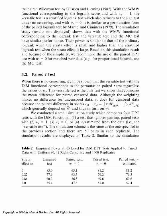
the paired Wilcoxon test by O’Brien and Fleming (1987). With the WMWfunctional corresponding to the logrank score and with wi = 1, theversatile test is a stratified logrank test which also reduces to the sign testunder no censoring, and with wi = 0, it is similar to a permutation formof the paired logrank test by Mantel and Ciminera (1979). The simulationstudy (results not displayed) shows that with the WMW functionalcorresponding to the logrank test, the versatile test and the MC testhave similar performance. Their power is similar to that of the ordinarylogrank when the strata effect is small and higher than the stratifiedlogrank test when the strata effect is large. Based on this simulation resultand because of the simplicity, we recommend the use of the paired DPTtest with wi = 0 for matched-pair data (e.g., for proportional hazards, usethe MC test).

5.2. Paired t Test

When there is no censoring, it can be shown that the versatile test with theDiM functional corresponds to the permutation paired t test regardlessthe values of wi. This versatile test is the only test we know that comparesthe mean difference for paired censored data. Although the weightingmakes no difference for uncensored data, it does for censored databecause the paired difference in scores ci1 � ci2 ¼

Rx dF

i1jbCi� R y dF

i2jbCi

which generally depend on bCi and thus in turn on wi.We conducted a small simulation study which compares four DPT

tests with the DiM functional: (1) a test that ignores pairing, paired testswith (2) wi = 1, (3) wi = 0, or (4) wi estimated from the data (i.e., the‘‘versatile test’’). The simulation scheme is the same as the one specified inthe previous section and there are 50 pairs in each replicate. Thesimulation results are displayed in Table 2. Similar to the simulation

Table 2 Empirical Power at .05 Level for DiM DPT Tests Applied to PairedData with Uniform (0, 1) Right-Censoring and 1000 Replicates

Strata

effect xUnpaired

test

Paired test,

wi = 1

Paired test,

wi = 0

Paired test, wi

estimated

0 83.0 63.1 81.2 81.20.22 77.6 63.3 79.2 79.30.86 60.2 56.8 69.6 69.6

2.0 35.4 47.8 57.0 57.4



results for the rank tests, the versatile test performs similarly to theunpaired test when the strata effect is small and outperforms both theunpaired and paired test with wi = 1 when the strata effect is large. Notethat the versatile test and the paired test with wi = 0 have similarperformance. Thus, as for the rank test, the paired test with fixed weightof zero is recommended for practical use.

5.3. Example 4: Skin Graft Data

We apply the weight-zero paired test with the DiM functional and thelogrank functional to data from a study on HLA matching and skin graftsurvival (Holt and Prentice, 1974; see also Kalbfleisch and Prentice, 1980,p. 190). The days of survival of closely matched and poorly matched skingrafts on the same person were recorded. There were in total of 11patients. Four of the 22 observations are interval-censored, 2 right-censored, and the rest known exactly. Previous analyses have replacedthe interval-censored observations with a point on the interior of theinterval, but the DPT handles interval-censored observations in astraightforward way. The null hypothesis is that the closely matchedand poorly-matched skin grafts have the same distribution. Using theDiM functional and logrank score gives exact p values of .010 and .012,respectively. Thus both tests produce statistically significant result, andshow that closely matched skin grafts have better survival.

6. ALTERNATIVE METHODS

The class of permutation tests (DPT tests) described above provides aunifying approach to many types of survival data. For nonrandomizedtrials with covariates, regression methods may be more appropriate thanthe DPT tests to ensure that the apparent treatment effects are not relatedto the covariates (for right-censored data see, e.g., Kalbfleisch andPrentice, 1980; for proportional hazards models for interval-censoreddata see Satten, 1996 and Goggins et al., 1998). However, for randomizedtrials this adjustment is often not necessary nor desired.

When the assumption on the censoring does not hold, the DPT testsmay not retain alpha level. When censoring is related to treatment andthe data are right-censored, it has been suggested that the rank-basedmethods based on the score test may perform better than the permutation

Shih and Fay156


tests since the assumptions of the permutation tests do not hold (Kalb-fleisch and Prentice, 1980). However, Janssen (1991) has shown that, inthe nonstratified case at least, the permutation rank tests with unequalcensoring between treatment groups are asymptotically equivalent to thelikelihood approach. For the stratified case, Schoenfeld and Tsiatis(1987) developed a stratified logrank test for cases where the censoringdepends on treatment. However, large sample sizes may be required toensure that their test is close to alpha level (see Shih and Fay, 1999). Thepreviously mentioned WKM test (Pepe and Fleming, 1989), a general-ization of the Z test to right-censored data, should perform reasonablywhen censoring is related to treatment and sample sizes are large.

For paired right-censored data, Michalek and Mihalko (1980) offeran example where censoring is related to both treatment and thestratification variable, and they show how this can cause the Mantel-Ciminera test to give misleading results. When this violation of assump-tions occurs, O’Brien and Fleming (1987) offered a modification to theMC-type tests (i.e., tests with wi = 0 for paired right-censored data),which effectively eliminates from the analysis strata where there iscensoring.

For interval-censored data, again the likelihood-based methodsappear safer when there is unequal censoring between treatment groups(for the proportional hazards model see Satten, 1996, and Goggins et al.,1998; for more general rank methods see Self and Grossman, 1986 andFay, 1999; for generalizations of the Z test see Petroni and Wolfe, 1994).

When censoring is not independent of failure time, then neither thepermutation tests nor standard likelihood-based survival tests may beapplied. In clinical trials, this may happen if patients are more likely todrop out of the study (and hence be censored) as they get sicker and arecloser to death.

A type of survival data not discussed in this chapter is clusteredfailure time data where all individuals within a cluster receive the sametreatment. Cai and Shen (2000) describe how permutation tests may beformed for this type of data. They study several test statistics, weightedlogrank statistics (e.g., the logrank and Wilcoxon tests), as well assupremum versions of those statistics. These statistics are the standardones that ignore clustering, and Cai and Shen (2000) estimate thepermutation distribution associated with the test statistics by takingMonte Carlo samples from the

� nn1

possible permutations of clusters

to treatments, where here n is the total number of clusters and n1 is the



number of clusters getting the first treatment. We can write theirWilcoxon-type test statistic in our notation. The test statistic is

L0* ¼

Xi

Xj

zij � z�

cij � c� ¼X

i

Xj

zijcij ¼Xi

zi1mici

where the i index here denote clusters not strata, c ¼ �Pi mi

�1�Pi

Pj

cij ¼ 0; z ¼ �Pi mi

�1�Pi

Pj zij , for the Wilcoxon-type test we use the

the Mann-Whitney functional, and Ci is estimated with�C. [To show the

equivalence of the two notations see Fay (1999) and Fleming andHarrington (1991, pp. 256–257], and note that when Ci is estimated with�C then c = 0 for any of the functionals discussed in this chapter.] Alogrank-type test can be formed similarly but it is a slightly different formthan Cai and Shen’s test (see Section 3.2). We can extend Cai and Shen’swork by using the DiM functional to get a difference in means test.Further, a permutational central limit theorem may be applied topermutations done this way; the variance in this situation is

V* ¼ 1

n� 1

Xi

micið Þ2( ) X

i

zi1 �P

h zh1n

� �2( )

and L0*2=V* is asymptotically distributed as v2 with 1 degree of freedom

(see Sen, 1985 for details).

ACKNOWLEDGMENT

We thank Don Corle for providing the data for Example 3.

REFERENCES

American Joint Committee on Cancer. (1997). AJCC cancer staging manual.Philadelphia, PA: Lippincott-Raven Publishers.

Aragon, J., Eberly, D. (1992). On convergence of convex minorant algorithms for

distribution estimation with interval-censored data. Journal of Computa-tional and Graphical Statistics 1:129–140.

Byar, D. P., Corle, D. K. (1988). Hormone therapy for prostate cancer: results of

the veterans administration cooperative urological research group studies.NCI Monographs 7:165–170.

Cai, J., Shen, Y. (2000). Permutation tests for comparing marginal survivalfunctions with clustered failure time data. Statistics in Medicine 19:2963–

2973.

Shih and Fay158


Dempster, A. P., Laird, N. M., Rubin, D. B. (1977). Maximum likelihood

from incomplete data via the EM algorithm (with discussion). Journal ofthe Royal Statistical Society, Series B 39:1–38.

Efron, B. (1967). The two sample problem with censored data. Proceedings of the

5th Berkeley Symposium 4:831–853.Fay, M. P., Shih, J. H. (1998). Permutation tests using estimated distribution

functions. Journal of the American Statistical Association 93:387–396.

Fay, M. P. (1999). Comparing several score tests for interval censored data.Statistics in Medicine 18:273–285.

Finkelstein, D. M., Wolfe, R. A. (1985). A semiparametric model for regressionanalysis of interval-censored failure time data. Biometrics 41:933–945.

Fleming, T. R., Harrington, D. P. (1991). Counting Processes and SurvivalAnalysis. New York: Wiley.

Gentleman, R., Geyer, C. J. (1994). Maximum likelihood for interval censored

Data: consistency and computation. Biometrika 81:618–623.Ghosh, M., Lahiri, P., Tiwari, R. C. (1989). Nonparametric empirical Bayes

estimation of the distribution function and the mean. Communications in

Statistics—Theory and Methods 18(1):121–146.Goggins, W. B., Finkelstein, D. M., Schoenfeld, D. A., Zaslavsky, A. M. (1998).

A Markov chain Monte Carlo EM algorithm for analyzing interval-

censored data under the cox proportional hazard model. Biometrics54:1498–1507 (Journal of Chronic Diseases 31, 445–454).

Groeneboom, P., Wellner, J. A. (1992). Information Bounds and NonparametricMaximum Likelihood Estimation. Boston: Birkhauser-Verlag.

Holt, J. D., Prentice, R. L. (1974). Survival analysis in twin studies and matchedpair experiments. Biometrika 65:159–166.

Huster, W. J., Brookmeyer, R., Self, S. G. (1989). Modeling paired survival data

with covariates. Biometrics 45:145–156.James, I. R. (1987). Tests for location with k samples and censored data. Bio-

metrika 74:599–607.

Janssen, A. (1991). Conditional rank tests for randomly censored data. Annals ofStatistics 19:1434–1456.

Kalbfleisch, J. D., Prentice, R. (1980). The Statistical Analysis of Failure TimeData. New York: Wiley.

Mantel, N. (1966). Evaluation of survival data and two new rank statistics arisingin its consideration. Cancer Chemo. Rep. 50:163–170.

Mantel, N., Ciminera, J. L. (1979). Mantel-Haenszel analysis of litter-matched

time-to-response data with modification for recovery of interlitter infor-mation. Cancer Research 37:3863–3868.

Michalek, J. E., Mihalko, D. (1983). On the use of logrank scores in the analysis

of litter-matched data on time to tumor appearance. Statistics in Medicine2:315–321.

O’Brien, P. C., Fleming, T. R. (1987). A paired Prentice-Wilcoxon test for

censored paired data. Biometrics 43:169–180.



Pepe, M. S., Fleming, T. R. (1989). Weighted Kaplan-Meier statistics: A class of

distance tests for censored survival data. Biometrics 45:497–507.Peto, R., Peto, J. (1972). Asymptotically efficient rank invariant test procedures

(with discussion). Journal of the Royal Statistical Society, Series A 135,

part 2:185–207.Petroni, G. R., Wolfe, R. A. (1994). A two-sample test for stochastic ordering

with interval-censored data. Biometrics 50:77–87.

Prentice, R. L. (1978). Linear rank tests with right censored data. Biometrika65:167–179.

Satten, G. A. (1996). Rankbased inference in the proportional hazards model forinterval censored data. Biometrika 83:355–370.

Schoenfeld, D. A., Tsiatis, A. A. (1987). A modified log rank test for highlystratified data. Biometrika 74:167–175.

Self, S. G., Grossman, E. A. (1986). Linear rank tests for interval-censored data

with application to PCB. Biometrics 42:521–530.Sen, P. K. (1985). Permutational central limit theorems. In: Kotz, S., Johnson, N.

L. (Eds.), Encyclopedia of Statistical Sciences Vol. 6. New York: Wiley.

Shih, J. H. (1999). A class of permutation tests for stratfied survival data. Bio-metrics 55:1156–1161.

Stablein, D. M., Koutrouvelis, I. A. (1985). A two-sample test sensitive to

crossing hazards in uncensored and singly censored data. Biometrics41:643–652.

Turnbull, B. W (1976). The empirical distribution function with arbitrarilygrouped, censored, and truncated data. Journal of the Royal Statistical

Society (Series B) 38:290–295.

Shih and Fay160


9Bayesian Reporting of ClinicalTrials

Simon Weeden and Mahesh ParmarMedical Research Council Clinical Trials Unit, London, England

Laurence S. FreedmanBar-Ilan University, Ramat Gan, Israel

1. INTRODUCTION

Over the last 10 years many articles have been written about the use ofBayesian statistical methods for designing, monitoring, analyzing, and in-terpreting the results of randomized clinical trials. Spiegelhalter and col-leagues provided a summary and synthesis of such work (Spiegelhalter,Freedman, and Parmar, 1994), but extensions and applications for partic-ular circumstances continue to appear (Parmar, Ungerleider, and Simon,1996; Thall, Simon, and Estey, 1996; Abrams, Ashby, and Errington, 1996;Simon and Freedman, 1997; Stangl and Greenhouse, 1998; Parmar et al.,2001).

Despite these developments, very few reports of clinical trials ana-lyzed exclusively by Bayesian methods appear in the medical literature.Themain reason for this is probably due to the anticipation of authors thatthey will encounter extra resistance from referees to such a ‘‘novel’’ form ofanalysis. Every investigator writes a report in the hope that it will be ac-cepted by his/her journal of choice, and after the arduous and often longprocess of a clinical trial, the investigator wishes tominimize the difficultiesof the publication process. Thus conventional methods of analysis are thenatural choice.


However, behind this very real barrier there lie some other difficultissues relating to the form of presentation of a Bayesian analysis of aclinical trial. As will be explained in more detail, Bayesian methods useprior clinical opinion in a formal manner. How should we explain this ina succinct way in a clinical paper? How should we describe the clinicalopinion that has been used in the trial? How should we present resultsillustrating different interpretations of the results according to a clini-cian’s own starting position? How do we preserve the ‘‘objective’’ natureof the trial results in the light of the introduction of all this subjectivism?

These matters have been discussed in a theoretical manner by severalauthors (Spiegelhalter et al., 1994; Hughes, 1993; Greenhouse andWasser-man, 1995; Carlin and Sargent, 1996). In this paper we propose a solutionby way of example. We present a Bayesian version of a clinical report of arandomized trial of two chemotherapy schedules for operable osteosar-coma, a malignant disease of the bone, which occurs in children, teenagers,and adults. We choose this trial particularly because a survey of clinicalopinion regarding the expectations of the treatments was conducted beforeits start, and this provides the basis for the prior clinical opinion that is usedin the Bayesian analysis. The conventional version of the trial report waspublished in 1997 (Souhami et al., 1997). The main novelty in the pres-entation is the introduction of an ‘‘Interpretation’’ section between the Re-sults and the Discussion. In this section we present a sensitivity analysis inwhich we consider the impact of different prior opinions on the inter-pretation of the data. The hope in this type of analysis is to show that theconclusions are robust to a wide range of ‘‘starting positions’’. Of course, ifthey are not, this is also important to know. Besides this section the readermay not notice much difference from the conventional type of paper (asidefrom the lack of the often overused p value, and a somewhat extendedStatistical Methods section which will be needed at first to explain the newmethodology). If that is the case, then wemay have succeeded in our aim offinding a way of slotting in a new and informative type of analysis whichwill help to clarify the clinical information and interpretation of the paper.

2. RANDOMIZED TRIAL OF TWO REGIMENS OFCHEMOTHERAPY IN OPERABLE OSTEOSARCOMA:A BAYESIAN PERSPECTIVE ON A TRIAL OF THEEUROPEAN OSTEOSARCOMA INTERGROUP

We have compared in a randomized trial the effects of amultidrug 44-weekchemotherapy regimen, based on the T10 protocol, with a two-drug (cis-

Weeden et al.162


platin and doxorubicin) 18-week regimen for the treatment of operablelimb osteosarcoma. The primary endpoint was length of survival after ran-domization.Of 407 patients, 391were eligible and have been followed for atleast 4 years (median 5.6 years). Toxicity was qualitatively similar, but 94%of the 199patients on two-drug treatment completed their course comparedwith 51% of the 192 patients on multidrug treatment. Overall survival at 5years was 54% in the multidrug arm and 56% in the two-drug arm. Thehazard-ratio estimate was 0.94 (95%CI 0.69–1.27, whereHR<1 indicatesa benefit to two-drug therapy). In a pretrial survey clinicians indicated thatto prefer multidrug treatment they would require an absolute increase ofabout 10% in overall 5-year survival. The results of the trial indicate thatsuch an increase is highly unlikely. Bayesian analysis demonstrates that thisconclusion is robust to a wide variety of ‘‘starting positions’’ of skepticismor enthusiasm with regard to the likely benefit of the multidrug treatment.

2.1. Background

Although the survival of patients with operable osteosarcoma is improvedby chemotherapy (Eilber et al., 1987; Link et al., 1986), the optimumduration of treatment and the relative contributions of the constituentdrugs have not been assessed in randomized trials. Randomized compar-isons of treatment present formidable difficulties in this rare disease, whicheach year affects only 1 in 200,000 of the population. The European Os-teosarcoma Intergroup (EOI) was formed in 1982 in order to perform ran-domized studies of sufficient size to allow investigation of importantaspects of treatment. EOI consists of the Bone Sarcoma Working Partyof the UK Medical Research Council (MRC), the UK Children’s CancerStudy Group (UKCCSG), the Societe Internationale d’Oncologie Pae-driatrique (SIOP), and the European Organisation for Research andTreatment of Cancer (EORTC) Soft Tissue and Bone Sarcoma Group.

In the first EOI trial (Bramwell et al., 1992) 307 patients with osteo-sarcoma were randomized to one of two regimens of chemotherapy. Inthat trial a regimen of cisplatin (CDDP) and doxorubicin (DOX), givenpre- and postoperatively for a total of 6 cycles to patients with operablenonmetastatic osteosarcoma, produced a 5-year survival rate of 64% anda 5-year progression-free survival (PFS) rate of 57%. These results werecomparable with those reported from a collaborative West German studyin pediatric osteosarcoma (Winkler et al., 1984), in which the chemo-therapy was based on the T10 regimen introduced by Rosen et al (Rosen etal., 1982). A modification of the T10 regimen was also used in Link’s study(Link et al., 1986), in which 36 patients were randomized after surgery to

Bayesian Reporting of Clinical Trials 163


either early chemotherapy or chemotherapy at relapse. The results showedan advantage in PFS for the early use of chemotherapy.

The T10 regimen has been the basis of much osteosarcoma chemo-therapy and an update of the results of this and other similar regimensused at the Memorial Sloan Kettering Cancer Center showed that 65% of279 patients were alive and disease free at 8 years (Meyers et al., 1992).Their results are among the best reported in this disease.

Nonrandomized studies of treatment do not allow an unbiased com-parison of treatment outcomes. For this reason, after completion of theprevious trial (Bramwell et al., 1982), the EOI embarked on a formalcomparison of a 44-week multidrug T10-based regimen (multidrug) withthe 18-week CDDP and DOX (two-drug) regimen, which was the moreeffective of the two treatments previously compared. This paper reports theresults of the trial. We use a Bayesian framework of analysis that allowsinterpretation of the results both from the usual ‘‘objective’’ viewpoint andalso incorporating the prior opinions of participating clinicians. Using thisanalysis framework we are able to show how the observed results wouldaffect these opinions.

2.2. Patients and Methods

Patients

The details of this trial are only summarized in this paper as they havepreviously been reported elsewhere (Souhami et al., 1997). Patients wereeligible for this trial if they were V40 years, had histologically diagnosedosteosarcoma of the extremity, no evidence of metastatic disease, and nor-mal renal and cardiac function. Patients were excluded if they had receivedprevious chemotherapy or had a previous malignancy. A member of thepathology panel of the EOI reviewed histological diagnosis. The acceptedinterval between diagnostic biopsy and randomization was 35 days.Preliminary staging included plain radiological examination of the tumor,isotope bone scan, chest X-ray, and CT scan of the thorax. CT and MRIscans of the primary tumor were performed according to local practice.

Chemotherapy

The details of drug administration were as follows:

Two-drug: DOX 25 mg/m2 days 1–3, CDDP 100 mg/m2 day 1. Eachcycle administered at 21-day intervals for 6 cycles. Surgery wasplanned for week 9 (day 63) after 3 preoperative cycles. Two

Weeden et al.164


weeks after surgery the first of 3 postoperative cycles wasscheduled. Details of administration have been described else-where (Bramwell et al., 1992).

Multidrug: Preoperative treatment consisted of vincristine (VCR) 1.5mg/m2 (max. 2mg) and high dosemethotrexate (HDMTX) 8 g/m2 (12 g/m2 below 12 years of age) on days 0, 8, 35, 42, andDOX 25 mg/m2 dl�3 on days 15–17. Folinic acid 12 mg/m2

intravenously or 15 mg/m2 orally commencing at 24 hr givenevery 6 hr � 10 doses, the dose being adjusted according to 24and 48 hr serum concentrations. Surgery was scheduled at week7 (day 49). Postoperatively patients received the first cycle ofBCD (Bleomycin 15 mg/m2, Cyclophosphamide 600 mg/m2,and Dactinomycin 0.6 mg/m2 each on days 1 and 2) on week 9.Further cycles of VCR and HDMTX were given on weeks 12,13, 17, and 18, and a further cycle of DOXonweek 14 (all at thesame preoperative dose). On week 20 the regimen changed toDOX 30mg/m2 days 1 and 2 and CDDP 120mg/m2 day 1. Thiswas given on weeks 20, 23, 29, 32, 38, and 41. Further cycles ofBCD were given on weeks 26, 35, and 44.

For both regimens recommended dose modifications were based onblood counts (all counts 109L) obtained between 9 and 14 days and at 21days. Reductions were based on the lower of these two counts and ap-plied to all subsequent cycles. The scheme was as follows: Total whiteblood count (WBC) > 2.0, platelets > 50—100% dose; WBC > 1.0 and< 2.0, platelets > 25 and< 50—85% dose; WBC< 1.0, platelets<25—70% dose. If the total WBC was< 3.0 or granulocyte count< 1.0 atscheduled time of next treatment, this treatment was delayed 1 week.

Surgery

At the time of randomization the projected surgical procedure wasrecorded. In the multidrug regimen surgery was planned for week 7, 1week after the fourth course of HDMTX. In the two-drug arm surgery wasat week 9, 3 weeks after the third cycle of CDDP and DOX. The decisionabout whether to perform an amputation or limb sparing surgery (usuallyendoprosthetic replacement) was made by the individual clinical teams.

Response Assessment

Clinical response was defined as a definite reduction of swelling and painfollowing preoperative chemotherapy and was assessed by the responsible



clinician. Radiological criteria of response were not used. During the pe-riod of this trial MRI scans were not generally available for response as-sessment. Those patients in whom response was not assessed are regardedas nonresponders.

Histopathological response was based on the resection specimen.Good response was defined as at least 90% necrosis of the tumor andpoor response any degree less than this. Pathology was reviewed centrallyat diagnosis and in assessment of response.

Treatment at Relapse

Local recurrence was treated according to the judgment of the partic-ipating clinicians and consisted of local resection or amputation some-times combined with radiotherapy. Pulmonary and other metastases weremanaged according to the clinical circumstances and treatments consistedof second-line chemotherapy, thoracotomy, or palliative care.

Statistical Methodology—Sample Size

The multidrug schedule was anticipated to result in, at best, a survivalrate of 70% at 5 years. The two-drug regimen was associated with a 5-year survival rate of approximately 55%. The sample size was determinedto give at least a 80% chance of rejecting the null hypothesis of nodifference between the treatments (on the basis of the 95% credibleinterval for the treatment difference not including zero, using an unin-formative prior distribution) when the true difference in 5-year survivalrates is 15%. This 15% difference corresponds to a hazard ratio (HR) of1.68 (where HR> 1 implies a survival advantage to multidrug treatment).The target recruitment to achieve this was 400 patients (Machin et al.,1997).

Statistical Methodology—Analysis

The analysis of this trial has been performed on an intention to treat basisincluding as many eligible patients as possible for each endpoint. Thestatistical analyses were conducted using the SPSS and SAS statisticalpackages. Survival curves were calculated using the Kaplan-Meiermethod. The Mantel-Cox version of the logrank statistic was calculatedto provide the likelihood portion of the Bayesian analysis (see below).Estimated hazard ratios are used to compare treatments (Parmar andMachin, 1995). Survival was calculated from date of randomization and

Weeden et al.166


progression-free survival (PFS) from date of surgery as inadequate sur-gery is thought to be a cause of disease progression.

We employ Bayesian methods to analyze the data from this trial.The use of Bayesian methodology in the design, monitoring, and analysisof clinical trials have been described in detail in the statistical literature(Spiegelhalter et al., 1994; Spiegelhalter, Freedman, and Parmar, 1993;Parmar, Spiegelhalter, and Freedman, 1994; Fayers, Ashby, and Parmar,1997).

A Bayesian approach to trial analysis allows external evidence to beformally incorporated into the reporting of a trial. Usually trial reportsintroduce such evidence informally in the Discussion section, the aimbeing to put the results in some kind of clinical context. In this paper anextra Interpretation section is placed between the Results and Discussionto contain the Bayesian perspective. In the Interpretation section, atten-tion is focused on the impact that the trial results will have on the opinionof participating clinicians.

The crucial issue in performing a Bayesian analysis is appropriatespecification of the prior distribution, which is a statistical formulation ofthe prestudy beliefs. When deciding on a prior distribution, many optionsare available: the uninformative prior, which represents a lack of clinicalopinion about the potential treatment difference; the skeptical prior,which considers only a small probability that the alternative hypothesis(in this case that multidrug therapy offers a significant survival advan-tage) is true; the clinical prior, which formalizes the opinion of individ-uals who are reasonably well informed of the nature of the treatments ontrial; and the enthusiastic prior, which takes the treatment differencespecified in the alternative hypothesis to be the best guess of the truetreatment difference. We will consider all these priors in relation to theanalysis of the primary endpoint, survival time, and we will therebyexamine the robustness of our conclusions from the trial to a variety ofdifferent ‘‘starting points.’’

While the trial was still in the design stage, information was collectedon clinicians’ opinions of the likely efficacy of the new treatment, via acarefully structured interview (Freedman and Spiegelhalter, 1983). Sevenclinicians planning to take part in the trial were interviewed and asked toindicate what weight of belief they would give to probable differences in5-year survival between the two treatments. These could thus beexpressed as probability distributions representing the likely treatmentdifference. Converted to the log hazard ratio (LHR) scale they form theclinical prior distributions for the Bayesian analysis. The reason for con-



verting to the LHR scale is because it is approximately normally dis-tributed with variance 4/n, where n is the number of observed events(Tsiatis, 1981).

The clinicians were also asked to mark on a given scale the absoluteimprovement required in the 5-year survival rate to offset the extradifficulty, cost and possible extra toxicity of the multidrug regimen.Following early discussions it was assumed that if the absolute improve-ment in 5-year survival with multidrug therapy was 0% then they woulduse the two-drug regimen and if the improvement was 20% they wouldpresumably adopt the multidrug regimen. Somewhere between thesevalues there would be a changeover point, or a range of points (termedthe range of equivalence), where it is difficult to decide between the twochemotherapy schedules. After the trial was closed, the log hazard ratiofor the difference between the treatments was calculated. The probabilityof obtaining this value of the LHR for different values of the treatmentdifference was calculated and is known as the likelihood.

Finally, the posterior distribution was calculated, which is simply theprior distribution modified as a consequence of the observed results,expressed via the likelihood. As the prior and likelihood distributions areall approximately normally distributed, combining them to form the pos-terior distribution is straightforward. When a clinical prior is used, theposterior distribution provides an estimate of the clinician’s belief ifrealistic allowance is made for the information obtained from the trial. Itis this posterior distribution that provides the necessary information forjudging the opinion of each clinician on the efficacy of the new treatment.All endpoints besides survival were analyzed assuming noninformativeprior distributions. Such analysis corresponds to the usual frequentistanalysis. Results are given as estimates with credible intervals (CIs) whichare the Bayesian equivalent of confidence intervals when a noninforma-tive prior distribution is assumed.

Prior Beliefs

The prior beliefs of the participating clinicians are shown in Table 1,along with range of equivalence and median expected improvement in 5-year survival. These distributions are represented graphically in Figure 1.The histograms of opinions are superimposed with a normal distributionobtained from these opinions. The normal distribution is actually fittedon the log hazard ratio (LHR) scale, using their median expectedimprovement compared to the baseline 5-year survival rate of 55%,

Weeden et al.168


Table 1 Pretrial Prior Beliefs of Seven Clinicians Interested in Participating in the Trial

Absolute 5-year survival advantage (%)

of two-drug over multidrug

Clinician

Range of

equivalence �20–�15 �15–�10 �10–�5 �5�0 0�5 5–10 10–15 15–20 20–25

Medianexpected

improvement (%)

1 0–5 0 1 12 20 26 21 13 6 1 32 5–5 1 4 12 22 28 18 9 5 1 03 0–7 0 0 1 9 15 26 29 19 1 10

4 5–10 1 5 18 26 30 19 1 0 0 45 5–12 0 1 4 15 35 31 13 1 0 66 10–15 0 0 5 10 25 50 8 2 0 2

7 5–10 1 14 32 33 14 5 1 0 0 �5Mean 4–9 0 4 12 19 25 24 11 5 0 3%

Bayesian

Rep

ortin

gofClin

icalTrials

169


Figure 1 Prior opinions of the seven clinicians interviewed regarding the likelydifference between two-drug and multidrug chemotherapy, plus the skeptical andenthusiastic prior distributions. Vertical lines represent the boundaries of the range

of equivalence. Superimposed on the histograms are fitted normal distributions (seetext for details).

Weeden et al.170


and the probability they accord to observing a treatment difference of lessthan zero.

The skeptical and enthusiastic prior distributions are also shown onFigure 2. The skeptical prior was calculated by assuming that there is nodifference between the two treatments and that the probability of thedifference in 5-year survival being more than 15% in favor of multidrug(the alternative hypothesis) is 0.05. The enthusiastic prior distributionwas calculated by assuming the alternative hypothesis to be true; i.e.,multidrug therapy offers a 5-year survival advantage of 15%. It is as-sumed to have the same precision as the skeptical prior.

The prior opinions of the seven participating clinicians on the loghazard ratio (LHR) scale are shown in Figure 2. The ranges of equiv-alence are also converted to the LHR scale, assuming a baseline 5-yearsurvival rate of 55%, and are shown on the graphs. These distributionswill form the clinical prior distributions for the Bayesian analysis.

It can be seen that there is much variation in the clinicians’ prioropinions regarding the relative efficacy of multidrug chemotherapy.Clinician 3, for example, believed that the new treatment would improve5-year survival by 10% whereas clinician 7 predicted it would most likelybe worse than the two-drug regimen. It can be seen that clinician 3’sopinions were most similar to the enthusiastic prior, whereas clinician 7’sopinions were more negative than those represented by the skepticalprior.

There was also considerable variety in the ranges of equivalencerecorded by the seven clinicians. Some (clinician 1 and 3) would considerusing multidrug treatment if it offered a benefit in 5-year survival ofgreater than zero, whereas clinician 2 would not consider adopting it if itdid not improve 5-year survival by 10% or more.

Looking at the group means on Figures 1 and 2, it is worth notingthat the lower bound of the range of equivalence is close to the medianexpected improvement on multidrug chemotherapy. This provides anargument for the ethical basis for randomization, since in general theparticipating clinicians are unsure whether the new treatment will proveto be clinically worthwhile. It has been previously stated that the varianceof the prior on the LHR scale is approximately equal to 4/n, where n isthe number of deaths to have occurred. Thus the distribution of thegroup mean of the clinicians’ opinions can be considered equivalent tohaving conducted a trial in which a total of 69 deaths have occurred withequal follow-up in the two arms. This is in contrast to the trial designwhich anticipated 124 deaths.



Figure 2 Distributions of prior opinions, shown on the log hazard ratio (LHR)scale. Vertical lines represent the boundaries of the range of equivalence.

Weeden et al.172


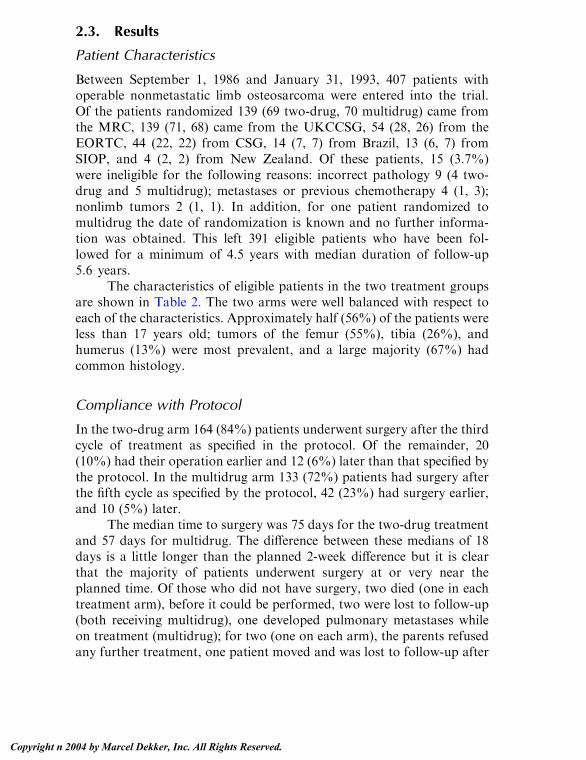
2.3. Results

Patient Characteristics

Between September 1, 1986 and January 31, 1993, 407 patients withoperable nonmetastatic limb osteosarcoma were entered into the trial.Of the patients randomized 139 (69 two-drug, 70 multidrug) came fromthe MRC, 139 (71, 68) came from the UKCCSG, 54 (28, 26) from theEORTC, 44 (22, 22) from CSG, 14 (7, 7) from Brazil, 13 (6, 7) fromSIOP, and 4 (2, 2) from New Zealand. Of these patients, 15 (3.7%)were ineligible for the following reasons: incorrect pathology 9 (4 two-drug and 5 multidrug); metastases or previous chemotherapy 4 (1, 3);nonlimb tumors 2 (1, 1). In addition, for one patient randomized tomultidrug the date of randomization is known and no further informa-tion was obtained. This left 391 eligible patients who have been fol-lowed for a minimum of 4.5 years with median duration of follow-up5.6 years.

The characteristics of eligible patients in the two treatment groupsare shown in Table 2. The two arms were well balanced with respect toeach of the characteristics. Approximately half (56%) of the patients wereless than 17 years old; tumors of the femur (55%), tibia (26%), andhumerus (13%) were most prevalent, and a large majority (67%) hadcommon histology.

Compliance with Protocol

In the two-drug arm 164 (84%) patients underwent surgery after the thirdcycle of treatment as specified in the protocol. Of the remainder, 20(10%) had their operation earlier and 12 (6%) later than that specified bythe protocol. In the multidrug arm 133 (72%) patients had surgery afterthe fifth cycle as specified by the protocol, 42 (23%) had surgery earlier,and 10 (5%) later.

The median time to surgery was 75 days for the two-drug treatmentand 57 days for multidrug. The difference between these medians of 18days is a little longer than the planned 2-week difference but it is clearthat the majority of patients underwent surgery at or very near theplanned time. Of those who did not have surgery, two died (one in eachtreatment arm), before it could be performed, two were lost to follow-up(both receiving multidrug), one developed pulmonary metastases whileon treatment (multidrug); for two (one on each arm), the parents refusedany further treatment, one patient moved and was lost to follow-up after



three cycles of chemotherapy (two-drug), and surgery was not done foran unspecified reason in one patient who went on to complete 19 cycles(multidrug).

The distribution of the (total) number of cycles actually received bypatients was summarized in Table 3. There was considerably morevariability in the total number of cycles administered in the multidrugregimen. In this regimen 97 patients (51%) received 18 or more cycles,125 (65%) 15 cycles or more, and 141 (73%) more than 12 cycles. Thereasons for failure to complete the assigned chemotherapy are given inTable 4. The numbers discontinuing treatment were very similar in the

Table 2 Characteristics of Eligible Patients by Treatment

Two-drug Multidrug Total

N % N % N %

Age

V11 43 22 25 13 68 1712–16 72 36 80 42 152 39z17 84 42 87 45 171 44

SexMale 131 66 130 68 261 67Female 68 34 62 32 130 33

Site of tumor

Femur 113 57 102 53 215 55Tibia 50 25 51 27 101 26Humerus 24 12 25 13 49 13

Fibula 9 5 10 5 19 5Radius 3 2 0 0 3 1Ulna 0 0 3 2 3 1

Calcaneus 0 0 1 1 1 0HistologyCommon 133 67 128 67 261 67Chondroblastic 25 13 19 10 44 11

Fibroblastic 23 12 20 10 43 11Osteoclast rich 4 2 4 2 8 2Telangiectatic 4 2 6 3 10 3

Anaplastic 4 2 12 6 16 4Small cell 2 1 0 0 2 1Osteoblastic 4 2 3 2 7 2

Total 199 192 391

Weeden et al.174


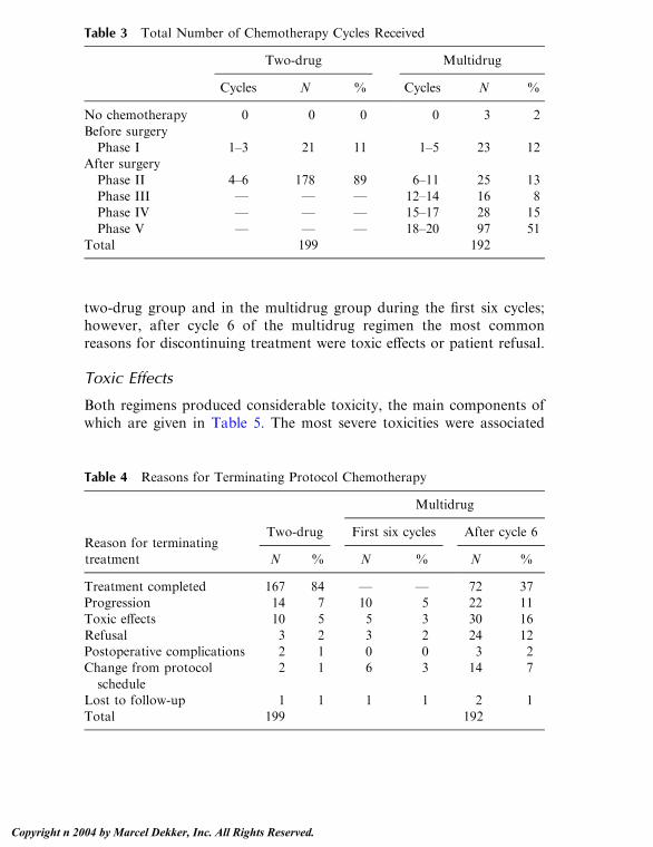
two-drug group and in the multidrug group during the first six cycles;however, after cycle 6 of the multidrug regimen the most commonreasons for discontinuing treatment were toxic effects or patient refusal.

Toxic Effects

Both regimens produced considerable toxicity, the main components ofwhich are given in Table 5. The most severe toxicities were associated

Table 3 Total Number of Chemotherapy Cycles Received

Two-drug Multidrug

Cycles N % Cycles N %

No chemotherapy 0 0 0 0 3 2

Before surgeryPhase I 1–3 21 11 1–5 23 12

After surgery

Phase II 4–6 178 89 6–11 25 13Phase III — — — 12–14 16 8Phase IV — — — 15–17 28 15

Phase V — — — 18–20 97 51Total 199 192

Table 4 Reasons for Terminating Protocol Chemotherapy

Multidrug

Two-drug First six cycles After cycle 6Reason for terminating

treatment N % N % N %

Treatment completed 167 84 — — 72 37Progression 14 7 10 5 22 11Toxic effects 10 5 5 3 30 16

Refusal 3 2 3 2 24 12Postoperative complications 2 1 0 0 3 2Change from protocol

schedule

2 1 6 3 14 7

Lost to follow-up 1 1 1 1 2 1Total 199 192



with the cisplatin/doxorubicin cycles of treatment in both arms. Severenausea and vomiting, thrombocytopenia, leucopenia, mucositis, andinfection were common. Liver function abnormalities were common afterhigh-dose methotrexate in the multidrug arm, but were not so prevalentduring later cycles. Severely impaired renal function was rare (2%). Therewere no deaths from cardiac toxic effects. Chemotherapy toxicity was amajor reason for dose reduction and delay, and for discontinuation ofchemotherapy.

Surgery

The surgical procedures planned at diagnosis for each patient, and theprocedure eventually carried out, are shown by treatment arm in Table 6.138 (69%) in the two-drug arm and 129 (67%) in the multidrug armactually underwent the surgery planned at diagnosis. Of 40 patients in thetwo-drug arm who were planned to undergo amputation, this was per-formed in only 22 while 17 were able to have a limb sparing procedure. Inthe multidrug arm 13 of 41 were spared the planned amputation.Conversely, of 141 patients scheduled for conservative surgery in the

Table 5 Serious (WHO Grade 3 or 4) Toxic Effects During Treatment

Multidrug

Two-drug First six cycles After cycle 6

N % N % N %

Leucopenia 150 75 35 19 124 73Thrombocytopenia 91 46 5 3 48 28Nausea and vomiting 148 74 85 85 112 66

Mucositis 40 20 11 6 23 14Alopecia 171 86 104 57 153 90Cardiac rhythm

disturbance

0 0 1 1 4 2

Infection 42 21 6 3 31 18Renal impairment 3 2 1 1 5 3

Liver 1 1 35 19 20 12Hearing loss 0 0 0 0 3 2Skin effects 1 1 1 1 3 2Neurotoxicity 1 1 1 1 1 1

Pulmonary 0 0 1 1 1 1

Weeden et al.176


two-drug arm, 19 (13%) had to have an amputation, while in the mul-tidrug arm the figures were 24 (18%) of 134.

Clinical Response

It was not possible to obtain data on response for eight patients (one two-drug, seven multidrug). The response rates in the two-drug and multidrugwere 117/198 (59%) and 85/185 (46%), respectively, with an odds ratio of2.02 (95% credible interval (CI) 1.34–3.07) in favor of the two-drug arm.Although the response rate differed according to type of histology (forexample, the highest response rates were observed in those with fibro-blastic tumors), the odds ratio for comparing the two treatments wasunaffected after adjustment for histology.

Histopathological Response

268 (69%) tumors were available for detailed analysis. The histopatho-logical response rate was similar in the two arms: 41 (30%) of 137 tumors

Table 6 Planned and Actual Surgery Received

Intended surgery

Actual surgery Amputation Prosthesis Rotation

Other

conservative Allograft Unknown Total

Two-drug

Amputation 22 19 1 1 0 2 45

Prosthesis 9 106 0 3 0 — 118

Rotation 3 1 2 0 0 — 6

Other

conservative

5 13 0 8 1 — 27

Allograft 0 0 0 0 0 — 0

None 1 2 0 0 0 — 3

Total 40 141 3 12 1 2 199

Multidrug

Amputation 27 24 1 3 0 1 56

Prosthesis 5 95 0 2 0 — 102

Rotation 0 1 0 0 0 — 1

Other

conservative

8 6 1 7 2 — 24

Allograft 0 2 0 0 0 — 2

None 1 6 0 0 0 — 7

Total 41 134 2 12 2 1 192



showed a good response in the two-drug group compared with 37 (29%)of 129 in the multidrug group (OR = 1.10, 95% CI 0.66-1.88).

Progression-Free Survival

Progression-free survival is shown in Figure 3 and was very similar in thetwo arms with an estimated value at 3 years after surgery of 47% (95%CI 42–52) and at 5 years after surgery of 44% (95% CI 39–49%). Therewas a high rate of tumor progression in the first year; 117 (56%) of the208 relapses or deaths occurred during that time. The hazard ratio (two-drug/multidrug) for risk of progression or death was 1.01 (95% CI 0.77–1.33).

Figure 3 Progression-free survival by treatment group.

Weeden et al.178


Survival

The analysis in this section assumes a noninformative prior distribution.Other prior distributions are considered in the Interpretation section thatfollows. The hazard ratio for risk of death was 0.94 (95% CI 0.69–1.27)in favor of the two-drug arm, representing a 2% (95% CI �8–12%)absolute difference in 5-year survival from 54% for the multidrug arm to56% for the two-drug arm (Figure 4). Adjustment of the treatmentcomparison for age, sex, tumor site, and initial pathology by means ofCox regression models made little difference to the estimate of the hazardratio. Preoperative histopathological response appears to be a major prog-nostic indicator for survival (Figure 5), although this result should be

Figure 4 Survival by treatment group.



treated with caution as histological response was determined after ran-domization. There was no evidence that the hazard ratio was different ingroupswith goodhistological response and thosewith apoor response. Thehazard ratio for treatment was 1.44 (95% CI 0.60–3.46) in the goodresponders and 1.05 (95% CI 0.71–1.54) in the poor responders.

2.4. Interpretation

Assuming an uninformative prior distribution, the hazard ratio for sur-vival comparing two-drug therapy to multidrug therapy is 0.94 (95% CI0.69–1.27) in favor of two-drug therapy. This represents a 6% reductionin the risk of death with the two-drug regimen. A total of 168 deaths

Figure 5 Survival by treatment and histopathological response.

Weeden et al.180


occurred in this trial. These results can be expressed in the form of anormal distribution with mean log(0.94) and variance 4/168. This dis-tribution is called the likelihood and is shown on the log hazard ratioscale in Figure 6.

The likelihood was combined with the various prior distributions(Figure 2) to form posterior distributions, shown in Figure 7. Theseposterior distributions represent the prior opinions taking into accountthe results of the trial. It is worth noting that these estimates of treatmentdifference are considerably more precise than those expressed in the priordistributions. This is the consequence of prior opinions being updated byevidence from the results of a randomized trial.

From the skeptical posterior distribution, the probability of therebeing any benefit to multidrug therapy is 36%, and the probability ofobserving an absolute benefit in 5-year survival of 5% or more is 7%, so askeptic is likely to feel that their initial caution was justified. An en-thusiast’s posterior probability of there being benefit to the multidrugtreatment would be 64%, but they would still have only a 22% proba-bility of a benefit of 5% or more.

The participating clinicians would only consider using the multi-drug treatment if the difference in 5-year survival was greater than thelower bound of their range of equivalence, and would adopt it routinely ifthe survival difference was greater than the upper bound. The posteriorprobabilities that the real treatment difference is greater than the lower

Figure 6 Likelihood distribution of the observed data on the log hazard ratio

(LHR) scale.



Figure 7 Posterior distributions, including the opinions of the seven participat-ing clinicians modified by the results of the trial. Vertical lines represent theboundaries of the range of equivalence.

Weeden et al.182


and upper bounds of the range of equivalence for each clinician areshown in Table 7. These probabilities vary considerably depending on theoutlook of the clinician involved.

Clinician 3, who was the most enthusiastic about the new treatment,may require the most convincing that there was little difference observedbetween the treatments. Combining his or her prior opinion with the datasuggested that his or her probability of the multidrug regimen beingclinically worthwhile was 63%. However, the posterior probability of theLHR exceeding the upper bound of the range of equivalence was only 9%and thus even clinician 3 would be unlikely to adopt multidrug therapyon the basis of these results. Clinician 7, who did not believe that multi-drug therapy would offer any survival benefit, would feel further vin-dicated by the result of the trial. According to that individual’s posteriordistribution, there is only a 1% chance that the multidrug regimen islikely to be clinically worthwhile. The maximum posterior probabilityover the seven participating clinicians that the effect of multidrug treat-ment exceeds their upper limit of the range of equivalence, and thereforeis clearly indicated, was only 0.09.

The group mean posterior distribution, which summarizes averageclinical opinion on the trial, suggests that multidrug therapy offers insuf-ficient survival benefit to warrant usage. The probability of the LHR ex-ceeding the minimum clinically worthwhile benefit (4% benefit tomultidrug) was 14%, and the probability of exceeding the upper boundof the range of equivalence (9% benefit) was 1%.

Table 7 Probability That the Log Hazard Ratio Is Greater Than theBoundaries of the Range of Equivalence for Each Clinician

Range of

equivalence

P (LHR >

lower bound)

P (LHR >

upper bound)

P (LHR liesin range of

equivalence)

Clinician 1 0–5 0.48 0.09 0.39Clinician 2 5–5 0.08 0.08 0.00Clinician 3 0–7 0.63 0.09 0.54

Clinician 4 5–10 0.05 <0.01 0.05Clinician 5 5–12 0.13 <0.01 0.13Clinician 6 10–15 0.01 <0.01 0.01

Clinician 7 5–10 0.01 <0.01 0.01Group mean 4–9 0.14 0.01 0.13



2.5. Discussion*

In rare tumors such as osteosarcoma, nonrandomized studies are usefulto show whether new treatments are feasible and effective. However, ma-jor differences in treatment policy must be assessed by randomized trials.One such major difference, between the complex and lengthy T10protocol and the shorter and simpler two-drug regimen, was the subjectof our randomized trial.

The reported results of Rosen using the T10 protocol in a non-randomized study (Rosen et al., 1982) were so much better than theresults reported from studies of simpler chemotherapy regimens [e.g., thefirst EOI study (Bramwell et al., 1992)], that a randomized comparisonwas demanded to settle the issue.

This trial found no evidence of a difference in progression-free oroverall survival in favor of the T10 protocol. The hazard ratio estimatedfrom the trial was 0.94, representing a 2% absolute reduction in the 5-year survival rate (i.e., a reduction from 56 to 54%). However, values ofthe hazard ratio from 0.69 up to 1.27 are feasible, equivalent to anythingfrom a 12% decrease to an 8% increase in the 5-year survival rate due tomultidrug treatment.

The social consequences of very lengthy chemotherapy regimens arequite severe in patients of this age group, many of whom are attendingschool or university courses. There is a substantial advantage to atreatment that takes only 18 weeks. The cost of drugs was substantiallygreater for the multidrug regimen (about $9000) than for the two-drugregimen (about $3000), and the bed occupancy rate was higher. Bothregimens were associated with considerable toxicity for the duration oftreatment. For these reasons, participating clinicians felt that to be clearlypreferable multidrug therapy needed to increase the 5-year survival rateby about 10% (see Table 1). The results of the trial indicate that such anincrease is highly unlikely.

Our Bayesian analysis demonstrates that this conclusion is robustto a wide variety of ‘‘starting positions’’ with regard to the likely benefitof the multidrug treatment. Table 7 shows that after the trial the posteriorprobability that multidrug treatment is clearly preferable to two-drug

*Author’s note: The original trial report (Souhami et al., 1997) provides a full discussion of

the results of this trial, and although the rest of the paper follows exactly the lines of an

intended medical publication, in this section we will reproduce only some of their more

general points and will add some extra points that result from the use of a Bayesian analysis.

Weeden et al.184


treatment was less than 0.1 for all the participating clinicians, despitetheir starting from varying positions of skepticism or enthusiasm.

Despite this conclusive result, the cure rate for osteosarcoma is stillunsatisfactory and further progress is necessary. The European Osteo-sarcoma Intergroup has shown that cisplatin and doxorubicin can beintensified further with the use of hemopoietic growth factors such asgranulocyte-colony stimulating factor (Ornadel et al., 1994), and thisapproach is the basis of the new treatment being tested in their currentrandomized trial. Since we have shown in our trial that shorter periods ofintensive treatment are as effective for osteosarcoma, dose intensificationbecomes a feasible option. Other drugs, such as ifosfamide, have activityin osteosarcoma, but no randomized comparison of the efficacy ofregimens including this drug have been reported. Future trials shouldaim to discover more effective ways of combining these agents.

3. EPILOGUE

In this chapter we have attempted to show by example how to report aclinical trial analyzed using Bayesian methods. The advantage of such anapproach in the present example is undoubtedly the sensitivity analysis inthe Interpretation section, which supports the conclusions drawn in theDiscussion and demonstrates their robustness. The availability of priorclinical opinion in this trial no doubt strengthens the sensitivity analysis.However, sensitivity analysis can be conducted without the elicitation ofprior opinion as shown in the calculation of the ‘skeptical’ and ‘enthu-siastic’ posterior distributions, and can be used in a similar manner tosupport or qualify the conclusions from a trial.

Bayesian analysis carries other advantages, particularly for trialmonitoring, and for the analysis of trials that terminate early for somereason. Those advantages are not seen in this particular trial which con-tinued until its recruitment goals were met and until all patients werefollowed for an adequate period. It might be instructive to repeat the pres-ent exercise for such an example.

The approach outlined in this chapter is not the only way thatBayesian methods can be used to analyze clinical trials. In a pair of recentpapers, Goodman argues that the p value approach to hypothesis testingis fundamentally flawed (Goodman, 1999a) and advocates basing infer-ence on the likelihood, or Bayes factor (Goodman, 1999b). The rationalefor this is to emphasize that Bayesian methods do have a solid, data-



based core and are not simply based on subjective opinion. However, theBayes factor in itself is not necessarily easy to interpret, and the ad-vantage of our method is that it provides a context for the trial resultswhich can be easily understood by the intended audience.

One of the criticisms that could be levelled at this paper is that thesections explaining the methodology and analysis of the trial are too long.We accept this argument, but feel it is necessary to give a detailed andhopefully understandable explanation of techniques that are still unfami-liar to a nonstatistical audience. If Bayesian methods become morepopular they will require as little explanation as Kaplan-Meier curves,the logrank test and Cox proportional hazards models in current trialreports.

The same criticism could be made of the Interpretation section. Wewould argue that a full explanation of how the trial results wouldinfluence participants who hold a wide range of opinions is one of theadvantages of these methods. It is also likely that the addition of theInterpretation section will lead to a proportionate reduction in the lengthof the Discussion section, which can be fully devoted to examining thewider implications of the trial results.

We hope that the example we present in this chapter will help toconvince investigators that it is quite possible to present a report of aclinical trial analyzed by Bayesian methods in a manner that will beacceptable and even welcomed by the clinical community, or at least willencourage them to try!

ACKNOWLEDGMENTS

We would like to thank the chairman of the European OsteosarcomaIntergroup, Professor Alan Craft, and the coordinator of this study, Pro-fessor Robert Souhami, for permission to use data and ideas from their1997 paper to produce our ‘‘medical paper.’’

REFERENCES

Abrams, K., Ashby, D., Errington, D. (1996). A Bayesian approach to Weibull

survival models—application to a cancer clinical trial. Lifetime Data Anal-ysis 2:159–174.

Bramwell, V. H. C., Burgers, M., Sneath, R., Souhami, R., van Oosterom, A. T.,

Weeden et al.186


Voute, P. A., Rouesse, J., Spooner, D., Craft, A. W., Somers, R., Pringle,

J., Malcolm, A. J., van der Eijken, J., Thomas, D., Uscinska, B., Machin,D., van Glabbeke, M. (1992). A comparison of two short intensivechemotherapy regimens in operable osteosarcoma of limbs in children and

young adults: The first study of the European Osteosarcoma Intergroup.Journal of Clinical Oncology 10:1579–1591.

Carlin, B. P., Sargent, D. J. (1996). Robust Bayesian approaches for clinical trials

monitoring. Statistics in Medicine 15:1093–1106.Eilber, F., Giuliano, A., Eckardt, J., Patterson, K., Moseley, S., Goodnight, J.

(1987). Adjuvant chemotherapy for osteosarcoma: a randomized prospec-tive trial. Journal of Clinical Oncology 5:21–26.

Fayers, P.M., Ashby, D., Parmar,M.K. B. (1997). Tutorial in Biostatistics: Bayes-ian data monitoring in clinical trials. Statistics in Medicine 16:1413–1430.

Freedman, L. S., Spiegelhalter, D. J. (1983). The assessment of subjective opinion

and its use in relation to stopping rules for clinical trials. The Statistician33:153–160.

Goodman, S. N. (1999a). Towards Evidence-Based Medical Statistics. 1: The P

Value Fallacy. Annals of Internal Medicine 130:995–1004.Goodman, S. N. (1999b). Towards Evidence-Based Medical Statistics. 2: The

Bayes Factor. Annals of Internal Medicine 130:1005–1013.

Greenhouse, J. B., Wasserman, L. (1995). Robust Bayesian methods for moni-toring clinical trials. Statistics in Medicine 14:1379–1391.

Hughes, M. D. (1993). Reporting Bayesian analysis of clinical trials. Statistics inMedicine 12:1651–1663.

Link, M. P., Goorin, A. M., Miser, A. W., Green, A. A., Pratt, C. B., Belasco, J.B., Pritchard, J., Malpas, J. S., Baker, A. R., Kirkpatrick, J. A., et al. Theeffect of adjuvant chemotherapy on relapse-free survival in patients with

osteosarcoma of the extremity. NewEngland Journal ofMedicine 314:1600–1606.

Machin, D., Campbell, M., Fayers, P., Pinol, A. (1997). Sample Size Tables for

Clinical Studies. 2nd ed. Oxford: Blackwell Science.Meyers, P. A., Heller, G.,Healey, J., Huvos, A., Lane, J.,Marcove, R., Applewhite,

A., Vlamis, V., Rosen, G. (1992). Chemotherapy for non-metastatic os-teogenic sarcoma: The Memorial Sloan-Kettering experience. Journal of

Clinical Oncology 10:5–15.Ornadel, D., Souhami, R. L., Whelan, J., Nooy, M., de Elvira, C. R., Pringle, J.,

Lewis, I., Steward, W. P., George, R., Bridgewater, J., Wierzbicki, R.,

Craft, A. W. (1994). Doxorubicin and cisplatin with granulocyte colonystimulating factor as adjuvant therapy for osteosarcoma: Phase II trial ofthe European Osteosarcoma Intergroup. Journal of Clinical Oncology

12:1842–1847.Parmar, M. K. B., Machin, D. (1995). Survival Analysis: A Practical Approach.

Chichester, England: Wiley.



Parmar, M. K. B., Spiegelhalter, D. J., Freedman, L. S. (1994). The CHART

trials: Bayesian design and monitoring in practice. Statistics in Medicine13:1297–1312.

Parmar, M. K. B., Ungerleider, R. S., Simon, R. (1996). Assessing whether to

perform a confirmatory randomized clinical trial. Journal of the NationalCancer Institute 88:1645–1651.

Parmar, M. K. B., Griffiths, G. O., Spiegelhalter, D. J., Souhami, R. L., Altman,

O. G., van der Scheven, E. (2001). Monitoring of large randomised clinicaltrials: a new approach with Bayesian methods. Lancet 358:375–381.

Rosen, G., Caparros, B., Huvos, A. G., Kosloff, C., Nirenberg, A., Cacavio, A.,Marcove, R. C., Lane, J. M., Mehta, B., Urban, C. (1982). Preoperative che-

motherapy for osteogenic sarcoma: selection of postoperative adjuvantchemotherapy based on the response of the primary tumor to preoperativechemotherapy. Cancer 49:1221–1230.

Simon, R., Freedman, L. S. (1997). Bayesian design and analysis of 2 � 2 factorialclinical trials. Biometrics 53:456–464.

Souhami, R. L., Craft, A. W., Van der Eijken, J. W., Nooij, M., Spooner, D.,

Bramwell, V. H. C., Wierzbicki, R., Malcolm, A. J., Kirkpatrick, A.,Uscinska, B.M., VanGlabbeke,M.,Machin, D. (1997). Randomized trial oftwo regimens of chemotherapy in operable osteosarcoma: a study of the

European Osteosarcoma Intergroup. Lancet 350:911–917.Spiegelhalter, D. J., Freedman, L. S., Parmar, M. K. B. (1993). Applying Bayesian

ideas in drug development and clinical trials. Statistics inMedicine 12: 1501–1511.

Spiegelhalter, D. J., Freedman, L. S., Parmar, M. K. B. (1994). Bayesian ap-proaches to randomized trials. Journal of the Royal Statistical Society A157:357–416.

Stangl, D. K., Greenhouse, J. B. (1998). Assessing placebo response usingBayesian hierarchical survival models. Lifetime Data Analysis 4:5–28.

Thall, P. F., Simon, R. M., Estey, E. H. (1996). New statistical strategy for

monitoring safety and efficacy in single-arm clinical trials. Journal ofClinical Oncology 14:296–303.

Tsiatis, A. A. (1981). The asymptotic joint distribution of the efficient scores testfor the proportional hazards model over time. Biometrika 68:311–315.

Winkler, K., Beron, G., Kotz, R., Salzer-Kuntschik, M., Beck, J., Beck, W.,Brandeis, W., Ebell, W., Erttmann, R., Gobel, U., et al. Neoadjuvantchemotherapy for osteogenic sarcoma: results of a cooperative German/

Austrian study. Journal of Clinical Oncology 2:617–624.

Weeden et al.188


10Methods Incorporating Compliancein Treatment Evaluation

Juni PalmgrenStockholm University and Karolinska Institutet, Stockholm, Sweden

Els GoetghebeurUniversity of Ghent, Ghent, Belgium

1. INTRODUCTION

As pointed out by Neyman (1923) and Fisher (1925), randomization is acornerstone of scientific experimentation. Traditional theories of inferencebased on randomization formally require that all experimental units com-ply with their assigned treatment. However, in studies involving humansubjects, noncompliance is common and the compliance patternmay differbetween treatment arms. The standard approach is to rely on the random-ization distribution as if compliance had been perfect, and thus to compareresponse distributions by assignment, ignoring information on compliance(Lee et al., 1991). This is often referred to as the intent-to-treat analysis.The intent-to-treat analysis does not, however, measure biologic efficacy,but rather programmatic effectiveness, which depends on the biologic ac-tion as well as on the compliance with the treatment regimen. As the num-ber of noncompliers increases, effectiveness will decrease regardless of thebiologic efficacy of the treatment.

Treatment effectiveness and treatment efficacy address distinctscientific questions, both of which are important. Biologic efficacy is, how-


ever, more likely to be reproducible in different populations and sub-groups. Similarly, potential effect modification is better assessed on theefficacy scale, since factors that modify the treatment effect may also in-fluence compliance. While the intent-to-treat analysis is usually straight-forward, acceptable approaches for estimating efficacy have been lacking.It is reasonable to assume that the treatment protocol presents a differentchallenge for compliance than the control protocol, and those who adhereto the protocol in the different treatment arms are not as a rule com-parable. This results in serious potential for selection bias if individualswho complete the treatment regimen are compared with controls whocomplete the control regimen.

The causal framework of Rubin (1978) and Holland (1986) providesnew tools for evaluating average treatment efficacy.Models are specified interms of potential responses and potential receipt of the experimental treat-ment, and a randomization-based inference procedure is used. In order toavoid selection bias comparison is made to the subgroup in the placeboarm that corresponds to the treatment compliers and not to the subgroupof placebo compliers. Although the individual treatment compliers in theplacebo arm cannot be identified, their average response can be comparedto the average response among similar treatment compliers in the treatedarm. The efficacy so estimated pertains to the subgroup of compliers, andextrapolation to the full population under study requires additional modelassumptions. Additional model assumptions are also needed if non-com-pliance is measured on an ordered categorical or continuous scale.

Our aim is to give a flavor of the recent development of methodologyfor estimating treatment efficacy when faced with nonrandom noncom-pliance. We focus on model specification for the two-group parallel trial,with one treatment arm and one placebo arm. Basic concepts are illus-trated using the Efron and Feldman (1991) data from the Lipid ResearchClinics Coronary Primary Prevention Trial (LRC-CPPT). This was aplacebo-controlled double-blind randomized clinical trial assessing theefficacy of cholestyramine for lowering cholesterol level and thereby reduc-ing coronary heart disease. The Lipid Research Clinic Program (1984)describes the complete study. Efron and Feldman estimated the efficacy oftreatment received by making a strong assumption for noncompliance:They assumed corresponding compliance quantiles in the treated and inthe control arm to have similar average treatment-free response distribu-tions. As argued by Albert and DeMets (1994) this nonselection assump-tion has considerable impact on the inferences drawn.

In Section 2 we dichotomize the nominal dose of cholestyraminereceived for the purpose of illustrating null versus full compliance. Those

Palmgren and Goetghebeur190


on the lower relative dose are treated as null compliers and those on thehigher relative dose as full compliers. Following Angrist, Imbens, andRubin (1996) we define a set of potential outcomes and present the con-cept of Local Average Treatment Effect (LATE), i.e., the average effectof treatment received on cholesterol reduction in the subgroup of com-pliers. Angrist, Imbens, and Rubin also emphasize that the randomizationindicator serves as a so-called instrumental variable, a well-known tool forhandling errors that are correlated with the explanatory variable in lineareconometric models. In Section 3 we dichotomize the response (choles-terol reduction) and recapture the procedure proposed by Sommer andZeger (1991) and Zeger (1998) for estimating biologic efficacy for a binaryresponse with null versus full compliance. We extend the argument toordered categorical compliance by elaborating on the Goetghebeur andMolenberghs (1996) analysis of the cholestyramine data. They presentefficacy estimates for partial dose in the subgroup of partial treatmentcompliers and for full dose in the subgroup of full treatment compliers.

When data on compliance with experimental treatment are moredetailed a parametric structural model may be used, which links the com-pliance information to the potential response data. The structural modelmay further include compliance-covariate interaction terms, whichdescribe differential efficacy in subgroups determined by values of mea-sured covariates. In Section 4 we present the main features of the structuralmean model used by Goetghebeur and Lapp (1997) for assessing bloodpressure reduction for 300 hypertensive patients randomized to treatmentor placebo. The blood pressure was measured on a continuous scale, andcompliance to treatment was assessed by the medical event monitoringsystem (MEMS) producing essentially continuous relative dose informa-tion. While the structural mean models handle responses measured on acontinuous scale, structural failure time models are useful for responsesmeasured on a time-to-event scale. In Section 5 we refer to several appli-cations of structural failure timemodels, and in Section 6 we sketch currentdirections for the development of models and procedures for nonrandomnoncompliance.

Inferences for the models discussed throughout this chapter relyheavily on the randomization distribution: conditional on any subspacespanned by covariates measured before randomization, the expecteddistribution for any pre-randomization characteristic should be iden-tical in the two trial arms. Two constructs are used as prerandomizationcharacteristics: the potential treatment compliance and the potential treat-ment-free response. These two constructs are assumed to exist as inherentfeatures of the individual prior to randomization. Treatment compliance

Methods Incorporating Compliance in Treatment Evaluation 191


is subsequently observed for those randomized to the treated arm, but forthose in the placebo arm it remains a latent construct. Treatment-freeresponse is observed for those who receive no treatment, and for othersit may be computed from a more or less complex structural model. Forthe models in Section 3 we formulate a multinomial likelihood with thecell probabilities parameterized to reflect similarity for treatment compli-ance and for treatment-free response, respectively, in the two trial arms.For the structural models in Sections 4 and 5 we set up estimatingequations that correspond to test statistics for testing equality of featuresof the distributions for the expected treatment-free response in the two trialarms.

In the treated arm the compliance subgroups may differ in terms ofmeasured covariates. We argue throughout that conditioning on cova-riates that simultaneously predict treatment compliance and placeboresponse improves the precision for estimating efficacy.

2. POTENTIAL OUTCOMES AND ‘‘‘‘‘‘‘‘‘‘‘‘‘‘CAUSAL’’’’’’’’’’’’’’ EFFECTS

2.1. Potential Outcomes

Figure 1 illustrates the observed cholesterol reduction for 337 patients inthe Lipid Research Clinics Coronary Prevention Trial (LRC-CPPT) as afunction of percentage of prescribed dose actually taken of cholestyr-amine and placebo, respectively. Smoothed curves are fit to the scatter-plots.

The data in Figure 1 were analyzed by Efron and Feldman (1991),who treated cholesterol reduction and dose as continuous variables andfocused on a linear model for the average reduction as function of doseand other covariates. For the same data Zeger (1998) used a dichoto-mized dose scale and response scale, and Goetghebeur and Molenberghs(1996) used an ordered categorical dose scale.

It is clear fromFigure 1 that the percentage of the dose actually takenvaries between the two treatment arms, with a tendency for higherpercentages in the placebo arm. Figure 1 also shows a steeper rise incholesterol reduction in the treated group as function of percentage ofprescribed dose. Although randomization guarantees overall comparabil-ity between the treated and the control arm, it is likely that individuals aredifferently distributed over the compliance axes in a fashion which maydirectly or indirectly be associated with cholesterol reduction. If selectionof this kind is present, it would be seriously misleading to draw conclusions



concerning efficacy from comparing the trend in cholesterol reduction forthe two panels in Figure 1.

Here we treat cholesterol reduction as a continuous response varia-ble, while the percentage of the nominal dose actually received is dichot-omized at 60%. Those below the cut point are treated as noncompliers andthose above the cutpoint as full compliers. This crude approximationserves the purpose of illustrating the null versus full compliance pattern.Let Ri = 1 and Ri = 0 indicate the assignment of individual i to thecholestyramine arm or to the control arm, respectively. For given assign-ment Ri, the individual receives a dose of cholestyramine as indicated by

Figure 1 Observed compliance-response relationship in the LRC-CPPT trial.



Di(Ri) = 0 (V60% of nominal dose) or 1 (>60%), and then experiences acholesterol reduction of Yi{Ri, Di(Ri)} units. Note that Di(Ri) refers to thedose received of the experimental treatment in the respective arms, and thatthe percentage of nominal placebo dose will not be used in the modelspecification. If the experimental treatment is not available in the placeboarm, thenDi(0)= 0 for all i. We refer toDi(Ri) andYi{Ri,Di(Ri)}, forRi=0or 1, as potential outcomes. The potential outcomes that get observed forany given individual i depends on the random assignment of treatment. Ifindividual i is assigned to experimental treatment, then Di(1) and Yi{1,Di(1)} are observed, and if assigned to placebo, thenDi(0) and Yi{0,Di(0)}are observed. Throughout we assume thatDi(Ri) andYi{Ri,Di(Ri)} dependonly onRi, the treatment assigned to individual i, and not on the treatmentassignment to other individuals under study. In the causal literature thisindependence assumption is called the stable unit treatment value assump-tion (Angrist, Imbens, and Rubin, 1996).

The double argument for the cholesterol reduction is useful formaking explicit the so-called exclusion restriction: Yi{Ri, Di(Ri)} =Yi{Di(Ri)} (Angrist, Imbens, and Rubin 1996). This restriction states thatany effect of Ri on Yi{Ri, Di(Ri)} must be via the effect of Di(Ri). Thetreatment assignment is thus assumed conditionally independent of theresponse, given the dose of the experimental treatment that was actuallyreceived. This exclusion restriction is plausible if the study was appropri-ately blinded, in which case the randomassignment per se is not expected toaffect the response. Under the exclusion restriction any comparison ofYi{Di(1)} with Yi{Di(0)}, i.e., the potential response for an individual i ifallocated to the treatment arm versus if allocated to the placebo arm, willdepend solely on the experimental treatment received in the respectivearms.

In studies with prolonged follow-up, postrandomization treatmentchanges for reasons other than non-compliance may occur. Distinctionsbetween direct and indirect effects of treatment are discussed by Green-land and Robins (1994) and by White and Pocock (1996). They are alsotaken up in Chapter 12 by Babiker and Walker on AIDS models.

2.2. Local Average Treatment Efficacy (LATE)

In Table 1 the difference in cholesterol reduction between the treated armand the control arm for an individual i is cross-classified according to thevalue of the potential treatment compliance variable Di(1) when assignedto the treatment arm, and Di(0) when assigned to placebo.



The category corresponding to Di(0) = Di(1) = 0 in Table 1 definesan individual who would never take the treatment, regardless of treatmentassignment. If the experimental treatment is available also in the placeboarm, then the categoryDi(0)=Di(1)= 1 defines an ‘‘always taker.’’Underthe exclusion restriction the never takers and the always takers contributenothing to an aggregated group difference in cholesterol reduction whencomparing the two trial arms. Following Angrist, Imbens, and Rubin(1996) we summarize the entries in Table 1 asYi{1,Di(1)}�Yi{0,Di(0)}=Yi{Di(1)}�Yi{Di(0)}, and forDi(0) =Di(1) this difference is zero. For thecategory Di(1) = 1, Di(0) = 0, i.e., for the compliers, the differenceYi{Di(1)} � Yi{Di(0)} is written Yi(1) � Yi(0), and for the category Di(1)= 0, Di(0) = 1, the defiers, i.e., those who always do the reverse of whattheir assignment requires, the difference is �{Yi(1) � Yi(0)}.

Referring to Table 1, the difference in cholesterol reduction for anindividual i as function of treatment arm allocation can be written in theform

Yif1;Dið1Þg � Yif0;Dið0Þg ¼ YifDið1Þg � YifDið0Þg¼ ½Yið1ÞDið1Þ þ Yið0Þf1�Dið1Þg� � ½Yið1ÞDið0Þ ð1Þ

þYið0Þf1�Dið0Þg� ¼ fYið1Þ � Yið0ÞgfDið1Þ �Dið0Þg:Before taking expectations the strong monotonicity assumption of Imbensand Angrist (1994) is invoked, which states thatDi(1)zDi(0) for all i, withinequality for at least one i. This monotonicity assumption excludes theexistence of defiers, and the proportion of compliers Pr{Di(1)�Di(0)= 1}equals the expected value E{Di(1) � Di(0)}, with E{Di(1) � Di(0)} > 0.When averaging both sides of the expression in (1), the always takers andthe never takers contribute nothing, and by excluding the existence of

Table 1 Treatment Arm Difference in Cholesterol Reduction Yi(1, Di(1)) �Yi(0, Di(0)), for an Individual i Classified by Di(1) and Di(0)

Di(0)

0 1

Di(1) 0 Yi(1, 0)�Yi(0, 0) = 0 Yi(1, 0)�Yi(0, 1) = �(Yi(1)�Yi(0))Never taker Defier

1 Yi(1, 1)�Yi(0, 0) = Yi(1)�Yi(0) Yi(1, 1)�Yi(0, 1) = 0

Complier Always taker



defiers, the average difference in response between treatment arms ‘asassigned’ has the form

E½Yif1;Dið1Þg � Yif0;Dið0Þg�¼ E½fYið1Þ � Yið0ÞgfDið1Þ �Dið0Þg�¼ EfYið1Þ � Yið0Þ j Dið1Þ �Dið0Þ ¼ 1gPrfDið1Þ �Dið0Þ ¼ 1g¼ EfYið1Þ � Yið0Þ j Dið1Þ �Dið0Þ ¼ 1gEfDið1Þ �Dið0Þg

and we can write the average difference in response among the compliersas

EfYið1Þ � Yið0Þ j Dið1Þ �Dið0Þ ¼ 1g

¼ E½Yif1;Dið1Þg � Yif0;Dið0Þg�EfDið1Þ �Dið0Þg :

ð2Þ

By virtue of the random assignment, the numerator in (2) is equal toE(Yj1) � E(Yj0), and the denominator is equal to E(Dj1) � E(Dj0), with jkindexing individuals assigned to arm k, for k = 0, 1. An estimate of theright-hand side of (2) is obtained by dividing the difference in meanresponse between the two treatment arms by the difference in the averageexperimental treatment received between the two treatment arms. Anestimator for the biologic treatment efficacy among compliers can thus becomputed from observable data, by dividing the intention-to-treat esti-mator of treatment effectiveness with the treatment arm difference in theproportion taking the experimental substance. Imbens and Angrist (1994)call this the Local Average Treatment Effect (LATE). Although thisaverage efficacy measure is estimable, it is in general not possible toidentify the latent subgroup of compliers (cf. Table 1) to which the effectpertains. This is particularly true if the experimental treatment is availablealso in the placebo arm, in which case the observed group of treatmentcompliers is a mixture of true compliers and always takers. If the experi-mental treatment is not available in the placebo arm, then the columnDi(0) = 1 in Table 1 vanishes, and the compliers are identified from theobserved entries in the treated arm.

In the LRC-CPPT-trial cholestyramine was not available for thoserandomized to placebo, i.e., Di(0) = 0 for all i, and thus neither ‘‘defiers’’nor ‘‘always takers’’ were possible. Those observed to comply with theassignment to cholestyramine in the treated arm are all ‘‘compliers’’ andthose observed not to comply with the assignment to experimentaltreatment are all ‘‘never takers.’’ For the cholestyramine data the



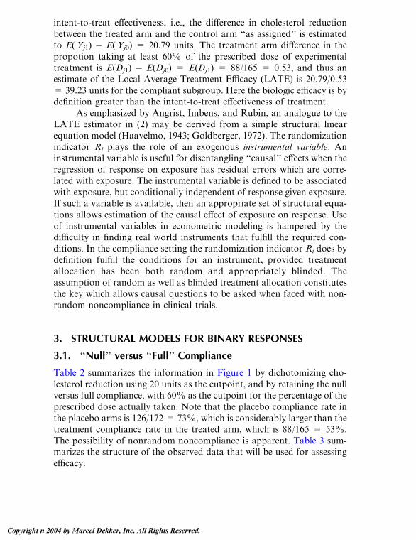
intent-to-treat effectiveness, i.e., the difference in cholesterol reductionbetween the treated arm and the control arm ‘‘as assigned’’ is estimatedto E(Yj1) � E(Yj0) = 20.79 units. The treatment arm difference in thepropotion taking at least 60% of the prescribed dose of experimentaltreatment is E(Dj1) � E(Dj0) = E(Dj1) = 88/165 = 0.53, and thus anestimate of the Local Average Treatment Efficacy (LATE) is 20.79/0.53= 39.23 units for the compliant subgroup. Here the biologic efficacy is bydefinition greater than the intent-to-treat effectiveness of treatment.

As emphasized by Angrist, Imbens, and Rubin, an analogue to theLATE estimator in (2) may be derived from a simple structural linearequation model (Haavelmo, 1943; Goldberger, 1972). The randomizationindicator Ri plays the role of an exogenous instrumental variable. Aninstrumental variable is useful for disentangling ‘‘causal’’ effects when theregression of response on exposure has residual errors which are corre-lated with exposure. The instrumental variable is defined to be associatedwith exposure, but conditionally independent of response given exposure.If such a variable is available, then an appropriate set of structural equa-tions allows estimation of the causal effect of exposure on response. Useof instrumental variables in econometric modeling is hampered by thedifficulty in finding real world instruments that fulfill the required con-ditions. In the compliance setting the randomization indicator Ri does bydefinition fulfill the conditions for an instrument, provided treatmentallocation has been both random and appropriately blinded. Theassumption of random as well as blinded treatment allocation constitutesthe key which allows causal questions to be asked when faced with non-random noncompliance in clinical trials.

3. STRUCTURAL MODELS FOR BINARY RESPONSES

3.1. ‘‘Null’’ versus ‘‘Full’’ Compliance

Table 2 summarizes the information in Figure 1 by dichotomizing cho-lesterol reduction using 20 units as the cutpoint, and by retaining the nullversus full compliance, with 60% as the cutpoint for the percentage of theprescribed dose actually taken. Note that the placebo compliance rate inthe placebo arms is 126/172 = 73%, which is considerably larger than thetreatment compliance rate in the treated arm, which is 88/165 = 53%.The possibility of nonrandom noncompliance is apparent. Table 3 sum-marizes the structure of the observed data that will be used for assessingefficacy.



In Table 3 placebo compliance categories are replaced by latentunobserved treatment compliance categories in the placebo arm. Theselection problem for compliance is thus avoided since by definition thecompliance categories in the two arms in Table 3 are comparable.

The observed data in Table 3 follow a multinomial distribution withfour cells in the treated arm, and a binomial distribution in the placeboarm. We write Pr {Di(1) = 1 j Ri = 1} = Pr {Di(1) = 1 j Ri = 0} = dand Pr {Yi(0) = 1 j Di(1) = 0, Ri = 0} = Pr {Yi(1) = 1 j Di(1) = 0,Ri = 1} = a0, to reflect that the distributions for expected treatmentcompliance and expected treatment-free response are similar in the twotrial arms, due to randomization. We further write Pr {Yi(0) = 1 j Di(1)= 1, Ri = 0} = a1 for the response probability in the subgroup ofpotential treatment compliers in the placebo arm. The corresponding

Table 2 Cross-Classification of Cholesterol Reduction (Y= 1 if at least 20 units;Y = 0 otherwise), Treatment Arm Assignment (R = 1 for treated arm; R = 0for control arm) and Compliance (V60%; >60%)

Placebo (R = 0) Treatment (R = 1)

Placebo compliance Treatment compliance

V60% >60% V60% >60%

0 42 98 140 50 16 66Y

1 4 28 32 27 72 99

46 126 172 77 88 165

Table 3 Data in Table 2 Used for Estimation of Efficacy Among Compliers

Placebo (R=0) Treatment (R=1)

Treatment compliance Treatment compliance

D=0 D=1 D=0 D=1

0 m00= ? m01= ? m0+=140 n00=50 n01=16 n0+=66Y

1 m10= ? m11= ? m1+=32 n10=27 n11=72 n1+=99

m+0=? m+1=? m++=172 n+0=77 n+1=88 n++=165



response probability in the treated arm is Pr {Yi(1) = 1 j Di(1) = 1, Ri =1}, and the risk of interest c is defined as the ratio

c ¼ PrfYið1Þ ¼ 1 j Dið1Þ ¼ 1;Ri ¼ 1gPrfYið0Þ ¼ 1 j Dið1Þ ¼ 1;Ri ¼ 0g :

Table 4 presents the multinomial cell probabilities for the observedand latent counts in Table 3. The risk parameter c simply captures theexcess risk in the subgroup Di(1) = 1 due to experimental treatmentactually received in the treated arm. The treated arm has 3 degrees offreedom and the placebo arm one degree of freedom for joint estimationof d, a0, a1, and c. The model is thus saturated with four parameters, all ofwhich are identifiable. Using the notation for the observed counts inTable 3 and for the expected counts in Table 4, we write the log likelihoodfunction l= lP + lT, with lT the contribution from the multinomial in thetreated arm

lT ¼ n00 logfð1� dÞð1� a0Þg þ n01 logfdð1� ca1Þgþ n10 logfð1� dÞa0g þ n11 logðdca1Þ

and lP the contribution from the binomial in the placebo arm

lP ¼ m0þ logfð1� dÞð1� a0Þ þ dð1� a1Þg þm1þ logfð1� dÞa0þ da1g:

Table 4 Expected Cell Probabilies for the Cross-Classification in Table 3,Assuming Similar Placebo Response and Treatment Compliance in the Two

Treatment Arms. (The relative risk c captures the treatment efficacy amongcompliers.)



D=0 D=1 D=0 D=1

0 (1 � d)(1 � a0) d(1 � a1) (1 � d)(1 � a0) d(1 � ca1)Y

1 (1 � d)a0 da1 (1 � d)a0 dca1

1 � d d 1 � d d



The maximum likelihood estimators have the form

a0 ¼ n10n00 þ n10

d ¼ n01 þ n11nþþ

a1 ¼ m11

m11 þ m01c ¼ n11

n11 þ n01a�11

with m11 ¼ m1þ � mþþnþþ

n10 and m01 ¼ m0þ � mþþnþþ

n00 . The estimated ex-pected cell counts for the cholestyramine data are given in Table 5, andthe corresponding estimates are a0 = 0.35, a1 = 0.042, d = 0.53, andc = 19.5.

A straightforward extension of the above model is obtained byconditioning on baseline covariates. For a vector of given baseline co-variate values Z, the expected counts have a similar structure as in Table4, parameterized in terms of a0(Z ), a1(Z ), d(Z ), and c(Z ). Differentsubsets of Z may be used for the different parameters. A rich set ofrestrictions on the parameter space may thus be tested using standardmethods for likelihood inference. For a product of binomial and multi-nomial likelihoods, where the cell probabilities are nonlinear functionsof the parameters of interest, it is convenient to use the relation to alikelihood of independent Poisson counts. The restrictions needed forthe estimated expected Poisson counts to be equivalent to the expectedproduct multinomial counts are inherent in the parameterization ofTable 4 (Palmgren and Ekholm, 1987). Baseline covariates of interestinclude the set of predictors for treatment compliance and for placeboresponse, denoted Z1 and Z2, respectively. To form a master set of

Table 5 Estimated Expected Cell Counts for the Multinomial Data Structure inTable 3, with Parameterization as in Table 4



D=0 D=1 D=0 D=1

0 m00=52.12 m01=87.88 m0+=140 n00=50 n01=16 n0+=66Y

1 m10=28.15 m11=3.85 m1+=32 n10=27 n11=72 n1+=99

m+0=80.27 m+1=91.73 m++=172 n+0=77 n+1=88 n++=165



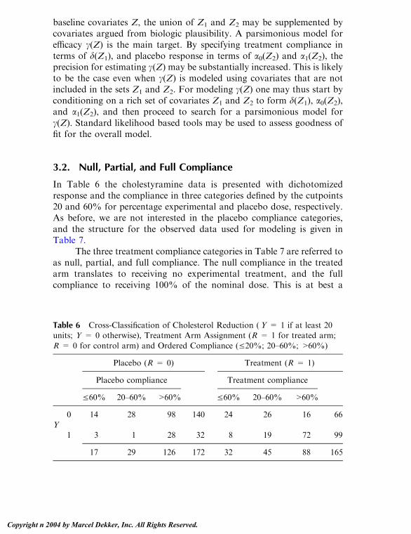
baseline covariates Z, the union of Z1 and Z2 may be supplemented bycovariates argued from biologic plausibility. A parsimonious model forefficacy c(Z) is the main target. By specifying treatment compliance interms of d(Z1), and placebo response in terms of a0(Z2) and a1(Z2), theprecision for estimating c(Z) may be substantially increased. This is likelyto be the case even when c(Z) is modeled using covariates that are notincluded in the sets Z1 and Z2. For modeling c(Z) one may thus start byconditioning on a rich set of covariates Z1 and Z2 to form d(Z1), a0(Z2),and a1(Z2), and then proceed to search for a parsimonious model forc(Z). Standard likelihood based tools may be used to assess goodness offit for the overall model.

3.2. Null, Partial, and Full Compliance

In Table 6 the cholestyramine data is presented with dichotomizedresponse and the compliance in three categories defined by the cutpoints20 and 60% for percentage experimental and placebo dose, respectively.As before, we are not interested in the placebo compliance categories,and the structure for the observed data used for modeling is given inTable 7.

The three treatment compliance categories in Table 7 are referred toas null, partial, and full compliance. The null compliance in the treatedarm translates to receiving no experimental treatment, and the fullcompliance to receiving 100% of the nominal dose. This is at best a

Table 6 Cross-Classification of Cholesterol Reduction (Y = 1 if at least 20units; Y = 0 otherwise), Treatment Arm Assignment (R = 1 for treated arm;

R = 0 for control arm) and Ordered Compliance (V20%; 20–60%; >60%)

Placebo (R = 0) Treatment (R = 1)

Placebo compliance Treatment compliance

V60% 20–60% >60% V60% 20–60% >60%

0 14 28 98 140 24 26 16 66Y

1 3 1 28 32 8 19 72 99

17 29 126 172 32 45 88 165



crude approximation for the cholestyramine trial, but serves the purposeof illustrating the model. The observed data follow a multinomialdistribution with six cells for the treated arm, and a binomial distributionfor the placebo arm. By virtue of the randomization, the distributions forthe expected treatment compliance and for the expected treatment freeresponse are again assumed similar in the two trial arms. This is reflectedin the parameterization Pr{Di(1) = k j Ri = 1} = Pr {Di(1) = k j Ri = 0}= dk, with Sk = 0

2 dk = 1, and Pr {Yi(0) = 1 j Di(1) = 0, Ri = 0} = Pr{Yi(1) = 1 j Di(1) = 0, Ri = 1} = a0. We further write Pr {Yi(0) = 1 jDi(1) = k, Ri = 0} = ak and Pr {Yi(1) = 1 j Di(1) = k, Ri = 1} = ckak,for k = 0, 1, 2. The two risk parameters of interest are

ck ¼prfYið1Þ ¼ 1 j Dið1Þ ¼ k;Ri ¼ 1gprfYið0Þ ¼ 1 j Dið1Þ ¼ k;Ri ¼ 0g k ¼ 1; 2:

Note that since treatment-free response is assumed equal in the twotreatment arms, c0 = 1 by definition, and c1 and c2 reflect respectively thepartial treatment efficacy in the group of partial compliers, and fulltreatment efficacy in the group of full compliers. Expressions for theexpected cell probabilities for the data structure in Table 7 are given inTable 8.

In the treated arm the multinomial distribution has 5 degrees offreedom and in the placebo arm the binomial distribution has 1 degree offreedom, resulting in a total of 6 degrees of freedom for estimating theseven parameters a0, a1, a2, d1, d2, c1, and c2 (c0 = 0, d0 = 1 � d1 � d2).The model is overparameterized and at least one additional restriction is

Table 7 Data in Table 6 Used for Estimation of Partial Efficacy Among Partial

Compliers and Full Efficacy Among Full Compliers



D=0 D=1 D=2 D=0 D=1 D=2

0 m00=? m01=? m02=? m0+=140 n00=24 n01=26 n02=16 n0+=66Y

1 m10=? m11=? m12=? m1+=32 n10=8 n11=19 n12=72 n1+=99

m+0=? m+1=? m+2=? m++=172 n+0=32 n+1=45 n+2=88 n++=165



needed for identification. Goetghebeur and Molenberghs (1996) suggest amodel in which the two parameters c1 and c2 are kept distinct, andinstead a set of intuitively reasonable, but rather complex second-orderparametric restrictions are put on the association between the treatmentcompliance and the response. This approach is feasible for the threeordered categories, null, partial and full compliance, but when a morerefined compliance scale is used, the Goetghebeur and Molenberghsessentially nonparametric relative risk model becomes intractable.

An alternative to the Goetghebeur and Molenberghs model for theordered categorical null, partial, and full compliance is to give the com-pliance categories numerical scores, k=0, 1, 2, and to use a linearmodel ofthe form ck = bVD(1), with D(1) = k. The structural parameter b captureshow a change in the level of experimental treatment received affects therisk. As argued earlier, it will be efficient for the estimation of the structuralparameter to stratify the data according to baseline covariates Z whichpredict both placebo response and treatment compliance. Furthermore,differential treatment efficacy over subgroups can be incorporated byadding effect modification by baseline covariates to the structural model.The extendedmodel takes the form ck= bVD(1)+ sVD(1) *Z, withD(1) *Zthe interaction term. These linear restrictions on the c parameters allow fora smooth conceptual transition from models presented for the binary andordered categorical compliance scales to structural models for compliancemeasured on a continuous scale. The latter approach is discussed inSections 4 and 5 and the dual role of baseline covariates as conditioning

Table 8 Expected Cell Probabilities for the Cross-Classification in Table 7 (Thedistribution of placebo response and treatment compliance is similar in the two

treatment arms, with d0 + d1 + d2 = 1. The relative risk parameters c1 and c2capture the treatment efficacy among partial and full compliers, respectively.)



D=0 D=1 D=2 D=0 D=1 D=2

0 d0(1�a0) d1(1�a1) d2(1�a2) d0(1�a0) d1(1�c1a1) d2(1�c2a2)Y

1 d0a0 d1a1 d2a2 d0a0 d1c1a1 d2c2a2

d0 d1 d2 d0 d1 d2



covariates in the estimationmodel and effect modifiers in the structural modelis further elaborated upon.

4. STRUCTURAL MEAN MODELS

4.1. The Model and Semiparametric Estimation

Continuous measures of exposure raise the problem of estimating theaverage effect of treatment over very detailed exposure levels. The ap-proach in Section 3 leads naturally to a structural meanmodel for inferenceregarding partial efficacy in this setting. LetD(R) be a possibly continuousand multidimensional measure of exposure to experimental treatmentfollowing assignment R, with D = 0 indicating no exposure. As before,both D(1) and D(0) are considered potential exposures, by design equallydistributed over randomized arms. In the special case where subjects on thecontrol arm have no access to experimental therapy, D(0) = 0, differentvalues of D are seen only on the treatment arm.

A linear structural model assuming the expected difference betweenpotential outcomes with and without treatment to be constant oversubgroups with different Z values is

EfYð1Þ � bVDð1Þ j Z;Dð1Þg ¼ EfYð0Þ j Z;Dð1Þg: ð3ÞIn words, after subtracting bVd from observed outcomes in the treatmentarm subset [Z = z, D(1) = d ] one recaptures expected treatment-freeoutcome for this subset. More generally, E{Y(1) � Y(0) j Z, D(1)} maydepend on Z as well as D(1), and a linear model respecting the zero doseconstraint can, for instance, take the form

EfYð1Þ � bVDð1Þ � sVðDð1Þ * ZÞ j Z;Dð1Þg¼ EfYð0Þ j Z;Dð1Þg

ð4Þ

where D(1) * Z refers to interaction terms between dose and baselinecovariates. Estimation for models (3) and (4) is not fundamentallydifferent. For ease of expression we develop the argument for the simplermodel (3) and refer to extensions in the discussion (cf. also Fischer-Lappand Goetghebeur, 1999).

Equation (3) does not enable straightforward least squares orlikelihood estimation. Although for given b the left-hand side is observ-able in the treatment arm, the placebo arm carries no direct informationon the association between observed (Y(0),Z) and the corresponding



latent D(1). Since the assumption of random noncompliance is not made,one cannot rely on E{Y(0)jZ, D(1)} = E{Y(0)jZ}, but unbiased estimatingequations follow from an equation implied by (3):

EfYð1Þ � bVDð1Þ j Zg ¼ EfYð0Þ j Zg: ð5ÞFor any choice of Z dependent weights, the weighted average of the left-hand side of (5) equals the similarly weighted average of the right-handside:

Ew½EfYð1Þ � bVDð1Þ j Zg� ¼ Ew½EfYð0Þ j Zg� ð6Þwhere Ew indicates the weighted mean. Due to randomization unbiasedestimates of the left- and right-hand sides of (6) can be derived from thetreatment and control arm, respectively. For fixed weights this leads tounbiased linear estimating equations for b which are easy to solve. Thecorresponding estimator b is consistent and asymptotically unbiasedunder mild regularity conditions, with covariance matrix estimated bythe sandwich estimator. This estimator b relies heavily on the random-ization assumption and can be seen as a dose-specific intent-to-treatestimator.

4.2. Efficiency

Efficiency is an issue in this semiparametric setting with no direct as-sumptions on the selectivity of compliance. Consider the extreme situationwhere no baseline covariates are measured. With just a single equation (5),structural models with more than one unknown parameter are unidenti-fied. In the special case of a single structural parameter however, equationE{Y(1)� bD(1)} = E{Y(0)} imposes no restrictions on the observed dataand can be solved by the (inefficient) instrumental variable estimatordescribed in Section 3. A good choice of weights in Eqs. (6) leads to moreefficient parameter estimates when the stricter assumption (5) holds.Optimal weights have been derived for general structural nested meanmodels by Robins (1994). Goetghebeur and Lapp (1997) suggest estima-tion of those weights in placebo-controlled trials using predictions ofplacebo outcome and treatment compliance from baseline covariates. Thebetter those predictions, the more precise the treatment effect estimates.The clear message for design is that good baseline predictors for com-pliance as well as for treatment-free response should be recorded toincrease information on dose-specific intent-to-treat estimators. Some-times, compliance measures taken over a run-in period during which all



subjects are given the same treatment yield good predictors for treatmentcompliance. Some have argued against run-in periods on placebo, how-ever, claiming it is incompatible with the informed consent obligation.Creative run-in designs which avoid the certainty of placebo for the entirerun-in period may provide an alternative that does not hamper accrualand resolves ethical concerns.

4.3. Implementation: An Example

That useful results can be obtained is illustrated by the blood pressureexamplepreviouslyanalyzedbyGoetghebeurandLapp(1997).Anewtreat-ment is compared with placebo in a double blind randomized blood pres-sure reduction trial, assigning patients to take one tablet daily. Drug intakeis electronically monitored over the experimental study period whichfollows a run-in on placebo. The dosing experience is subsequently sum-marized in a scalar D(1) representing the percentage of prescribed exper-imental drugwhich is taken. The experimental treatment is not available onthe control arm; henceD(0)=0.The responsemeasure of interest is changein blood pressure over the experimental study period (negative is good).An intent-to-treat analysis shows a highly significant difference betweenmean response on placebo, �3.54 mmHg (s.e. 1.49), and on treatment,�11.04 mmHg (s.e. 0.95). Table 9 shows the fit of three structural meanmodels with structural predictors: 1. {D(1)}, 2. {I{D(1) > 0}, D(1)}, 3.{D(1), D(1) * W}, where I{D(1) > 0} indicates whether any experimentaldrug was taken versus none at all and W represents body weight minus itssample average. The effect is modeled conditionally on baseline predictorsZ which include sex, height, weight, several run-in blood pressures and

Table 9 Estimated Structural Mean Models for Blood Pressure

Reduction, with D(1) the Percentage of Prescribed Dose ofActive Drug, W the Centered Body Weight, and I{D(1) > 0}an Indicator for Any Drug Taken or Not

Model Structural effects bS se(bS)

1. D(1) �7.41 1.84

2. I(D(1)>0) 15.90 13.38D(1) �24.83 14.88

3. D(1) �7.61 1.73

D(1)*W 0.36 0.14



their interaction with sex and height. This analysis is based on 54 availablepatients in the treatment arm and 51 in the placebo arm.

Model 1 estimates a linear dose effect quite precisely, but model 2requires more information to formally distinguish between a constanteffect of dose within the observed range and a linear effect. The fit sug-gests, however, that more variation in outcome is explained by the lineardose effect. Diagnostic plots constructed after fitting model 1 suggestedan interaction effect with baseline covariate W, centered body weight.Model 3 confirms a significant interaction: heavier people achieve lessreduction at the same dose level.

In general, once an identifiable structural mean model has been pro-posed, estimation is relatively straightforward. Implementation is achievedthrough just a few lines of code in Splus or SAS, for instance. However,without further assumptions on the selection mechanism, limited informa-tion makes parsimony for the structural model paramount. The challengein practice thus lies in proposing meaningful structural models and ininterpreting parameters correctly. The key question is:What aspect of drugexposure drives the treatment effect and how? Depending on the drug,different biologically plausible candidates present themselves. Besidespercentage of prescribed drug taken, compliance summaries may containlength and duration of drug holidays and other covariates related to timingand dose of drug actually taken.

5. STRUCTURAL DISTRIBUTION MODELS

Besides the mean difference, other contrasts between the distributions ofY(1) and Y(0) can be modeled. One then relies on the randomization as-sumption to demand equality of the (Y(1), Y(0), Z) distribution betweenarms rather than mere equality of means. Particularly for right censoredresponse data, comparing estimated distributions via Kaplan-Meiercurves rather than via means is a natural approach. Structural failuretime models based on accelerated failure time models were introduced byRobins and Tsiatis (1991). Mark and Robins (1993) use these to estimatethe effect of smoking cessation in the MRFIT study which randomizesover a life style intervention targeting multiple risk factors. Greenland andRobins (1994) compared high and low dose AZT in a trial which didrandomize over the high and low dose, but where differential adminis-tration of a third drug (PCP prophylaxis) over the two arms had takenplace post randomization. White et al. (1999) andWhite and Goetghebeur



(1998) examine the effect of treatment changes in randomized trials withlong-term follow-up (see also Chapter 12). Recently, Korhonen, Lairdand Palmgren (1999) and Korhonen and Palmgren (2001) have used thestructural accelerated failure time model to assess the effect of beta-carotene supplementation on right-censored times to death from all causesin the ATBC Study. Along the same lines, Korhonen et al. 2000 estimatethe effect of one dose of vitamin A on subsequent 4-month mortality inchildren under 6 months of age in a randomized, double-blind, placebo-controlled community trial in Nepal (West et al., 1995). Cluster random-ization is an added complexity in this vitamin A trial.

6. DISCUSSION

Naive interpretation of intent-to-treat estimators ignoring actual exposurebreeds poorly informed decisions (Goetghebeur and Shapiro, 1996).Incorporating exposure explicitly in an analysis bridges the gap between‘‘biological’’ and ‘‘statistical’’ models. This cannot be done, however,without some additional assumptions. Recent approaches avoid the ex-treme assumption of completely nonselective noncompliance. Rather, ran-domization-based estimators are constructed for models cast in terms ofpotential outcomes (latent variables). This chapter has introduced thebasic principle behind these estimators.

More general models than the ones presented here can be cast inthis framework and have been usefully implemented in clinical trials.When active treatment is received on several (all) arms of the trial, esti-mating equations are derived from equalities between arms of potentialtreatment-free distributions, none of which need to be directly observedon any one arm (Greenland and Robins, 1994). Repeated outcomes andsequentially randomized designs can be analyzed by structural nestedmean models or marginal structural models (Robins, Greenland, and Hu,1999; Robins, 1999). Also, Bayesian approaches were built on the causalformulation; see for instance, Imbens and Rubin (1997) and Hirano et al.(2000). Besides the hopes generated by all these tools, there are also haz-ards as pointed out by Pocock and Abdalla (1998).

Diagnostic tools for latent variable models are necessarily limited inpower. The model assumptions are sometimes subtle and must be wellunderstood. It is not generally recognized for instance, that once struc-tural (mean) models have been estimated, the (average) selection mech-anism is identified, for instance in model (5), by regressing Y(2) � bD(1)



on D(1) in the treatment arm. Sensitivity of conclusions to untestableassumptions must be explored. Another important concern in practiceregards data quality. Urquhart and De Klerk (1998) point out that goodmeasures of compliance are hard to get and Dunn (1999) emphasizes thatanalyses treating compliance as an explanatory variable should accountfor this.

It is reassuring that the structural analyses discussed here protectthe a-level when testing the null hypothesis of no difference betweenrandomized arms. However, the corresponding estimators rely in part onmodeling assumptions. For this reason, the traditional intent-to-treatanalysis will continue to hold a key position.

In summary, while structural estimators are potentially more mean-ingful, they are also more complex. It will take time to educate statis-ticians and clinicians alike to better understand their role. There is a needfor more practical experience and further theoretical development forinstance in the realm of design and sample size calculation, analysis ofequivalence studies, analysis of repeated outcome measures, the study ofdynamic treatment regimes (involving sequentially randomized designs tostudy treatment changes over time as a function of observed effects andcovariate evolutions), sensitivity analysis with respect to various modelassumptions, etc. In our view, the recent developments show excitingprospects for subject matter scientists as well as statisticians. Whenhandled with care, the new tools will lead to deeper insight into thenature of drug action in patient populations.

REFERENCES

Albert, J. M., DeMets, D. L. (1994). On a model-based approach to estimating

efficacy in clinical trials. Statistics in Medicine 13:2323–2335.Angrist, J. D., Imbens, G. W., Rubin, D. B. (1996). Identification of causal effects

using instrumental variables. With rejoinder. Journal of the American Sta-

tistical Association 91:444–471.Dunn, G. (1999). The problem of measurement error in modelling the effect of

compliance in a randomized trial. Statistics in Medicine 21:2863–2877.

Efron, B., Feldman, D. (1991). Compliance as an explanatory variable in clinicaltrials. Journal of the American Statistical Association 86:9–26.

Fischer-Lapp, K., Goetghebeur, E. (1999). Practical properties of structural meanmodels for the analysis of noncompliance data. Controlled Clinical Trials

20:531–546.Fisher, R. A. (1925). Statistical Methods for Research Workers. London: Olivier

and Boyd.



Goetghebeur, E., Lapp, K. (1997). The effect of treatment compliance in a

placebo-controlled trial: regression with unpaired data. Applied Statistics46:351–364.

Goetghebeur, E., Molenberghs, G. (1996). Causal inference in a placebo con-

trolled clinical trial with binary outcome and ordered compliance. Journalof the American Statistical Association 91:928–934.

Goetghebeur, E. J. T., Shapiro, S. H. (1996). Analyzing non-compliance in clini-

cal trials: Ethical imperative or mission impossible? Statistics in Medicine15:2813–2826.

Goldberger, A. S. (1972). Structural equation methods in the social sciences.Econometrica 40:979–1001.

Greenland, S., Robins, J. (1994). Adjusting for differential rates of PCP pro-phylaxis in high versus low dose AZT treatment arms in an AIDS ran-domized trial. Journal of the American Statistical Association 89:737–749.

Haavelmo, T. (1943). Statistical implications of a system of simultaneous esti-mating equations. Econometrica 11:1–12.

Hirano, K., Imbens, G. W., Rubin, D. B., Zhou, X. -H. (2000). Assessing the effect

of an influenza vaccine in an encouragement design. Biostatistics 1:69–88.Holland, P. W. (1986). Statistics and causal inference. Journal of the American

Statistical Association 81:945–970.

Imbens, G. W., Angrist, J. (1994). Identification and estimation of local averagetreatment effects. Econometrica 62:467–476.

Imbens, G. W., Rubin, D. B. (1997). Bayesian inference for causal effects in ran-domized experiments with noncompliance. Annals of Statistics 25:305–

327.Korhonen, P. A., Laird, N. M., Palmgren, J. (1999). Correcting for non-com-

pliance in randomized trials: An application to the ATBC Study. Statistics

in Medicine 18:2879–2897.Korhonen, P. A., Palmgren, J. (2002). Effect modification in a randomized trial

under non-ignorable non-compliance. Applied Statistics 51:115–133.

Korhonen, P., Loeys, T., Goetghebeur, E., Palmgren, J. (2000). Vitamin A andinfant mortality: beyond intention-to-treat in a randomized trial. LifetimeData Analysis 6:107–121.

Lee, Y. J., Ellenberg, J. H., Hirtz, D. G., Nelson, K. B. (1991). Analysis of clinical

trials by treatment actually received—Is it really an option? Statistics inmedicine 10:1595–1605.

The Lipid Research Clinic Program (1984). The Lipid Research Clinics Coronary

Primary Prevention Trial results, parts I and II. Journal of the AmericanMedical Association 251:351–374.

Mark, S. D., Robins, J. M. (1993). A method for the analysis of randomized trials

with compliance information—An application of the multiple risk factorintervention trial. Controlled clinical trials 14:79–97.

Neyman, J. (1923). On the application of probability theory to agricultural ex-



periments. Essay on principles. Section 9. 1923. [Translated in Statistical

Science 5, 465–480.]Palmgren, J., Ekholm, A. (1987). Exponential family nonlinear models for cate-

gorical data with errors of observation. Applied Stochastic Models and

Data Analysis 13:111–124.Pocock, S. J., Abdalla, M. (1998). The hope and the hazards of using compliance

data in randomized controlled trials. Statistics in Medicine 17:303–317.

Robins, J. M. (1994). Correcting for non-compliance in randomized trials usingstructural nested mean models. Communications in Statistics—Theory andMethods 23:2379–2412.

Robins, J. M. (1999). Marginal structural models versus structural nested mean

models as tools for causal inference. In: Halloran, M.E., Berry, D., eds.Statistical Models in Epidemiology: The Environment and Clinical Trials.IMA. Vol. 16. New York: Springer-Verlag, pp. 95–134.

Robins, J. M., Greenland, S., Hu, F. -C. (1999). Estimation of the causal effectof a time-varying exposure on the marginal mean of a repeated binary out-come. Journal of the American Statistical Association 94:708–712.

Robins, J. M., Tsiatis, A. A. (1991). Correcting for noncompliance in randomizedtrials using rank preserving structural failure time models. Communicationin Statistics—Theory and Methods 20:2609–2631.

Rubin, D. B. (1978). Bayesian inference for causal effects: The role of random-ization. The Annals of Statistics 7:34–58.

Sommer, A., Zeger, S. L. (1991). On estimating efficacy from clinical trials. Sta-tistics in Medicine 10:45–52.

Urquhart, J., De Klerk, E. (1998). Contending paradigms for the interpretation ofdata on patient compliance with therapeutic drug regimens. Statistics inMedicine 17:251–267.

West, K. P., Katz, J., Shrestha, S. R., LEclerq, S. C., Khatry, S. K., Pradhan, E.K., Adhikari, R., Wu, L. S. F., Pokhrel, R. P., Sommer, A. (1995). Mor-tality of infants less than 6 months of age supplemented with Vitamin A—

A randomized double-masked trial in Nepal. American Journal of ClinicalNutrition 62:143–148.

White, I. R., Babiker, A. G., Walker, S., Darbyshire, J. H. (1999). Randomiza-tion-based methods for correcting for treatment changes: Examples from

the Concorde trial. Statistics in Medicine 18:2617–2634.White, I. R., Goetghebeur, E. J. T. (1998). Clinical trials comparing two treat-

ment arm policies: which aspects of the treatment policies make a differ-

ence? Statistics in Medicine 17:319–340.White, I. R., Pocock, S. J. (1996). Statistical reporting of clinical trials with indi-

vidual changes from allocated treatment. Statistics in Medicine 115:249–

262.Zeger, S. (1998). Adjustment for noncompliance. In: Armitage, P., Colton, T., eds.

Encyclopedia of Biostatistics. Vol. 4. New York: Wiley, pp. 3006–3009.



11Analysis of Longitudinal Datawith Missingness*

Paul S. AlbertNational Cancer Institute, National Institutes of Health,Bethesda, Maryland, U.S.A.

Margaret C. Wuy

National Heart, Lung, and Blood Institute, National Institutes of Health,Bethesda, Maryland, U.S.A.

1. INTRODUCTION

The defining feature of a longitudinal clinical trial is that individuals aremeasured repeatedly across time. This is in contrast to many clinical trialsin which observations are taken at baseline and then perhaps at one follow-up time. In this chapter, we will make the distinction between longitudinalanalysis in which individuals are followed over time and multiple measure-ments are made, and survival analysis, in which individuals are followedand their time to event or censoring is analyzed. Our focus will be ondiscussing issues in missing data for longitudinal clinical trials in which theoutcome is measured repeatedly at follow-up visits.

* The portions of this chapter written by Margaret Wu were written in her private capacity.

The views expressed in the chapter do not necessarily represent the views of NIH, DHHS,

nor the United States.y Retired.


We will discuss three clinical trials in which the primary outcome isobserved repeatedly in a longitudinal setting and the repeated outcomes areoccasionally missing due to missed visits or censoring due to death or lossto follow-up (to be referred to as dropout). The scientific focus in all thesestudies is on evaluating the effect of treatment over time. These clinicaltrials will serve as motivation for methodological issues relating to analyz-ing longitudinal data in clinical trials withmissingness. These examples are:

1. The Intermittent Positive Pressure Breathing (IPPB) Trial (Inter-mittent Positive Pressure Trial Group, 1983). This was a ran-domized clinical trial that evaluated the effect of an intervention(IPPB) as compared with standard compressor nebulizer therapyon pulmonary function over time in 985 patients with obstructivepulmonary disease. The primary response was forced expiratoryvolume in 1 second (FEV1) measured at baseline and at 3 monthintervals over a 3 year period postrandomization (13 scheduledvisits including baseline). The outcomes are continuous withmany missing observations due to missed scheduled visits ordropout due to death and loss to follow-up. Approximately 23%of the patients died before the end of the study and 13.5%dropped out because they moved away or refused to return forfollow-up visits. In addition, almost all subjects have at least onemissed scheduled visit either before the occurrence of death orthe end of the study.

2. A three-arm randomized clinical trial to compare buprenorphinewith two doses of methadone for reducing opiate use in a groupof 162 addicts (Johnson et al., 1992). Sample sizes were 53, 55,and 54 patients in the buprenorphine, methadone 20 mg, andmethadone 40 mg groups, respectively. The outcomes of thistrial were a series of repeated binary responses of whether anindividual failed a urine test at each of three visits per week (onMonday, Wednesday, and Friday) over a 17 week period. Theserepeated responses are often missing due to missed visits or with-drawal from the study. More than 50% of the patients withdrewfrom the study before the end of the follow-up period. A sub-stantial number of patients occasionally missed visits but re-mained in the study.

3. A randomized trial of felbmate versus placebo for treating in-tractable partial epilepsy (Theodore et al., 1995). The study ran-domized 40 patients and the outcomes were repeated dailyseizure counts over a 3 day titration period and a 14 day follow-

Albert and Wu214


up period. Approximately one-half of the patients withdrewfrom the study prematurely. An inspection of average seizurefrequency by dropout time suggested that seizure frequencywas positively related to dropout time and that this relationshipmight be different in the two treatment groups.

There aremany other examples of clinical trials in which the outcomeis measured longitudinally. In Chapter 12, Babiker andWalker discuss theissue of analyzing repeated biological markers subject to informative cen-soring in an AIDS clinical trial. Other examples include cancer clinicaltrials in which quality-of-life assessments are measured repeatedly overfollow-up and may be subject to different informative censoring mecha-nisms in the treatment and control arms.

Before discussing methodology for analyzing longitudinal data withmissingness, we will briefly review the literature on longitudinal data. Thisreview is presented in Section 2. Section 3 discusses terminology, andSection 4 discusses the implications of various type types of missingnesson standard methodology for analyzing longitudinal data. General ap-proaches for analyzing longitudinal data with missingness are outlined inSection 5. We will analyze our motivating examples in Sections 6 to 8.Conclusions follow in Section 9.

2. METHODOLOGY FOR ANALYZINGLONGITUDINAL DATA

A review of methodology for analyzing longitudinal data in clinical trials ispresented by Albert (1999). This section summarizes much of that review.Methods for longitudinal data can be separated into three broad catego-ries: (1) simple univariate analyses of summary measures where the lon-gitudinal outcome are summarized by a single variable for each subject, (2)methods for continuous longitudinal data, (3) and methods for discretelongitudinal data.

2.1. Simple Univariate Analyses of Summary Measures

When the treatment comparisons reduce to comparing the averageresponses over follow-up time, a simple approach is to summarize eachperson’s longitudinal observations and compare these univariate measuresacross treatment groups (Pocock, 1983). These comparisons can be done

Analysis of Longitudinal Data with Missingness 215


with univariate statistical techniques (i.e., two-sample t tests or Wilcoxonrank sum tests) since there is only one summary measure per person andobservations on different subjects are independent. For the epilepsy clinicaltrial data, a comparison of average daily seizure frequency between treat-ment groups was performed (Theodore et al., 1995). In the analysis of theIPPB trial (Intermittent Positive Pressure Trial Group, 1983), the pro-gression of lung function over time was compared by testing differences inthe average individually estimated slopes between treatment groups. In theopiate clinical trial, the average individual proportions of positive urinetests were compared across treatment arms (Johnson et al., 1992). Uni-variate comparisons of means or slopes can be an attractive alternativeto complex modeling approaches. However, for highly imbalanced datacaused by missing observations, as in the three previous examples, thissimple comparison can be highly inefficient. This is demonstrated in Albert(1999) using IPPB clinical trial data. It is shown that an analysis based oncomparing individually estimated slopes between treatment groups is sub-stantially less efficient than an analysis based on a longitudinal model. Wepresent this example in detail in Section 6.

2.2. Longitudinal Methods for Gaussian Data

Various methodologies exist for analyzing longitudinal Gaussian data.Traditional multivariate techniques (Morrison, 1976) such as the Hotel-ling’s T 2, the multivariate analog of the t test for testing whether meanvectors are different in two samples, and profile analysis, a method fortesting for parallelism and differences between two mean vectors in multi-variate data, can be used to analyze continuous longitudinal data whenobservations are taken at the same time points on all subjects and thereare no missing data. This is rarely true in longitudinal clinical trials whereobservations are not taken at the same time points on all subjects and dataare often missing.

Alternatively, random effects models can be used to analyze longi-tudinal data. They provide a framework for analyzing longitudinal clinicaltrials data inwhich there is a sizable amount ofmissing observations (eitherdue to missed visits, loss to follow-up, or death). In the IPPB trial, forexample, scheduled follow-up visits at 3 month intervals were often missedor delayed and a large percentage of patient observations were censoreddue to death or dropout; only 77 out of 985 patients (8%) had completeequally spaced follow-up measurements.

Albert and Wu216


The random effects model is typically formulated in two stages. Con-ditional on each subject’s random effects, the model for the first stage is

Yij ¼ X Vij��þ Z Vij;i þ qij ð1Þwhere Xij and Zij are p and q element vectors of fixed and random effectscovariates, respectively, and qij are considered independent Gaussian withmean 0 and variance r2e , or can have an autoregressive moving average(ARMA) correlation structure. In the second stage, the random effects ;i

are assumed to have a multivariate normal distribution with covariancematrix D. The parameter vectors B and ;i measure the effect of fixed andrandom effect covariates on the mean responses. In a clinical trial, fixedeffects covariates may include treatment group, time, treatment by timeinteraction, or baseline characteristics, while only the intercept and timeeffects are included as random effects covariates. Tests of treatment effectsare usually constructed by testing for the significance of fixed effect co-variates corresponding to treatment. Laird and Ware (1982) discuss anestimation procedure which allows for highly irregularly spaced observa-tions where qij are independent. Chi and Reinsel (1989) discuss estimationwhen the qij’s follow an autogressive process.

2.3. Longitudinal Methods for Discrete Data

Many longitudinal clinical trials collect repeated outcomes which are notGaussian. The epilepsy and opiate clinical trials are examples in which therepeated responses are seizure counts and binary opiate-use responses atrepeated times post-randomization. Broadly speaking, models for discretelongitudinal data can be separated into three categories: marginal, randomeffects, and transition models.

Marginal models focus on estimating the effect of a set of covariateson the average response in a population. Liang and Zeger’s (1986) gener-alized estimating equation (GEE) approach is the seminal work in thisarea. They extend the generalized linear and quasi-likelihood models (Mc-Cullagh and Nelder, 1989), regression models for discrete and continuousoutcomes, to the longitudinal setting. Denote lij as the mean of the jthresponse on the ith subject. In the terminology of generalized linear mod-els, the mean can be related to a set of covariates through a link function,h, where h(lij) = h(E( yij)) = X Vij B. The relationship between the varianceand mean is specified as Var(Yij) = /g(lij) and the correlations on obser-



vations taken on the same subject are modeled by the function Corr(Yij,Yij) = q(A), where the parameter vector A characterizes this function.The approach is attractive in that both continuous and discrete responsevariables can be modeled by choosing h and g in an appropriate way. ForGaussian longitudinal data like FEV1 in the IPPB trial, h(lij) = lij andg(lij) = 1. For binary longitudinal data as in the opiate clinical trial, h andgmay be chosen as h(lij) = logit(lij) and g(lij) = lij(1� lij). For repeatedcount data like in our epilepsy clinical trial, h(lij) = log(lij) and g(lij) =lij. The appeal of the GEE approach is that although a model for thecorrelation and variance structure of the longitudinal observations mustbe specified, inferences are not sensitive to the assumed model. Liang andZeger propose the use of a robust variance estimator which produces thecorrect asymptotic inference even when the correlation structure is misspe-cified. Diggle, Liang, and Zeger (1993) apply the GEE approach to analyzean epilepsy clinical trial where the outcome is repeated seizure counts.

Random effects models have been proposed for modeling discretelongitudinal data (Zeger, Liang, and Albert, 1988, among others). Pa-tient-to-patient variability is modeled by adding random effects as linearpredictors in the regression terms in a generalized linear model. Theserandom effects models generalize the standard random effects models forGaussian data and are often referred to as generalized linear mixed mod-els. As in the linear mixed models discussed in the previous section, gen-eralized linear mixed models can be viewed in two stages. In the first stage,the mean response for the ith person is lij= h(Yijj;i) =X Vij B+Z Vij ;i, andthe conditional variance is specified as var(Yij) = /g(lij). In the secondstage, a distribution for the random effects is assumed to be normal withmean 0 and variance D. The generalized linear mixed model encompassesa wide range of random effects models. The linear mixed model, obtainedwith h(lij) = lij, can be used to analyze the IPPB trial data. A randomeffects model for logistic regression, obtained with h(lij) = logit(lij) andg(lij) = lij(1 � lij), can be used to analyze the opiate clinical trial data.Likewise, a random effects model for count data, obtained with h(lij) =log(lij) and g(lij) = lij, can be used to analyze the epilepsy trial data.These models have been discussed by a number of authors (Zeger, Liang,and Albert, 1988; Zeger and Karim, 1991; Breslow and Clayton, 1993,among others). Covariates such as treatment group can be interpreted asthe effect of treatment on an individual’s average response. This is in con-trast to marginal models where the effect of covariates is on the populationaveraged mean response. For this reason, Lindsey and Lambert (1997)have argued that random effects models are more appropriate thanmarginal models for analyzing data in longitudinal clinical trials.

Albert and Wu218


A third approach for analyzing longitudinal discrete data is transi-tional models. They examine the effect of covariates on the transition pat-terns in binary or categorical longitudinal data. Specifically, for binarydata, as in our opiate trial, these models reduce to lagging previousobservations in a logistic regression,

logitPðYit ¼ 1jYit�1;Yit�2; . . . ;Yit�qÞ ¼ X VitBþXqk ¼ 1

hkYit�k ð2Þ

where q is the order of theMarkov dependence (Cox, 1970). Thismodel hasbeen used to analyze the opiate trial data by Follmann (1994) and byAlbert(2000). Transitional models have been generalized to generalized linearmodel outcomes by Zeger and Qaqish (1988), and to ordinal data byDiggle, Liang, and Zeger (1993).

3. MISSINGNESS IN LONGITUDINAL CLINICAL TRIALS:TERMINOLOGY

There is a distinction between two types of missingness in longitudinalstudies: dropout and intermittently missed observations. Dropout refers tothe case when an individual ceases to participate in the study due to loss tofollow-up or death. Dropout occurs for both reasons in our examples.Dropout in the opiate trial occurs when patients refuse to participate (i.e.,return for scheduled visits) after being randomized in the study. Patients inthe epilepsy clinical trial drop out when they withdraw from the study andleave the hospital. Patients in the IPPB trial drop out because of death orrefusal to return for follow-up visits. Intermittent missingness occurs whenindividuals miss particular follow-up visits, but do not withdraw from thestudy. In the opiate clinical trial, many subjects miss particular visits andthen return for additional follow-up visits. In the IPPB data, many obser-vations are missed, followed by subjects returning and then dropping outfrom the study due to death or withdrawal from the study. Missing datamechanisms in which patients do not return after having missed an obser-vation are called monotonically missing mechanisms. Similarly, missingdata mechanisms in which patients return after having missed an obser-vation are called non-monotonic missing data mechanisms.

Missing data can be missing for various reasons which may relate tothe actual longitudinal responses. Little and Rubin (1987) classify missingdata into three categories. First, data are missing completely at random(MCAR) if the missing data mechanism is independent of both the ob-served and actual missing values. Second, data are said to be missing at



random (MAR) if the occurrence of missing data relates to the values ofthe observed responses, but not on the values of the missing observations.Last, data are missing nonrandomly if the probability of missing dependson the actual value of the missed observation. Little and Rubin (1987)have coined the phrase ignorable missingness to describe MCAR andMAR missing data mechanisms and nonignorable missingness to describenonrandomly missing data mechanisms in which the probability of miss-ingness depends on the actual value of the missed responses. The termsignorable and nonignorable missingness refer to the fact that likelihood-based methodology is insensitive to ignorable missing data mechanisms,but will be biased when missing data are nonignorable.

In longitudinal clinical trials, a special type of nonignorable miss-ingness called informative missingness is used to describe a missing datamechanism in which the distribution for both the repeated response andthe missing process are linked by common random effects. Models thatinduce informative missingness are called shared random effects models(Wu and Carroll, 1988; Follmann and Wu, 1995). These models arediscussed in detail in Section 5.3.

4. IMPLICATIONS OF MISSING DATA ONLONGITUDINAL METHODOLOGY

Most methods for the analysis of longitudinal data make valid inferencewith MCAR data. For MAR data, as was previously mentioned, like-lihood-based methods are valid. However, moment-based methods, suchas GEE, are biased. This point has been mentioned by various authors,including Liang and Zeger (1986) in their original paper on GEE. Rot-nitzky andWypij (1994) quantify this bias for GEE. Thus, recent method-ology for analyzing longitudinal data with missingness has focused onMAR data for GEE and nonignorable missingness for likelihood basedprocedures. We discuss these methodologies in Section 5.

5. MISSING DATA IN LONGITUDINAL CLINICALTRIALS: GENERAL APPROACHES

5.1. Analyses on Summary Measures

There have been various general approaches proposed for analyzinglongitudinal clinical trials data with missingness. We begin by discussing

Albert and Wu220


simple summary measures across groups. Dawson and Lagakos (1993)propose an approach which involves summarizing each individual’s lon-gitudinal outcome into a single summary measure, and then propose anon-parametric test which stratifies over the missing data patterns. Thisapproach is shown to have the correct type I error rate under a wide rangeof ignorable missing data patterns. The approach does, however, make therestrictive assumption that there are only a few missing data patternsand does not have the correct type I error rate when missingness is non-ignorable. Unstratified comparisons of summary measurements (e.g., thecomparison of individual summary measures across treatment groups)have the advantage of allowing for large numbers of missing data patternsand have the correct type I error rate under certain types of nonignor-able missingness. The disadvantage of unstratified tests, as mentioned byDawson (1994), is that they have substantially less power than stratifiedtests. In the IPPB study, for example, interest focuses on comparisonsof rate of change in FEV1 across treatment groups. There are too manymissing data patterns in this relatively long sequence to perform a stratifiedtest. Unstratified tests that compare summarymeasures between treatmentgroups can be done by estimating each individual slope and comparingthese slopes across treatment groups. The IPPB data was originally ana-lyzed in this way. Similarly, the original analysis in the epilepsy clinicaltrial was a comparison between average individual seizure frequency be-tween treatment arms. Wu and Carroll (1988) show that such an unstrat-ified comparison produces unbiased estimation of treatment effects evenunder certain types of nonignorable missing data mechanisms. They pointout, however, that tests based on these unstratified comparisons can havelow power, particularly in situations like the IPPB data where there is verylarge variation across individuals in the number of available observations.Wu and Carroll (1988) propose a modeling strategy for informative miss-ing data which does not suffer from this low power which will be discussedin Section 5.3.

Follmann, Wu, and Geller (1994) propose approaches for testingtreatment efficacy in clinical trials with repeated binary measurements withmissing data. The methods they discuss include (1) rank tests betweentreatment groups where the unit of analysis is each subject’s average ob-served binary response, (2) a combined test of missingness and efficacyusing a multivariate rank test (O’Brien, 1984), where the units of analysisare the subject’s average observed binary response along with the subject’sestimated proportion of missed visits, and (3) simple imputation wheremissed responses are replaced with positive responses (this method makes



the assumption that missed visits if they had been observed would haveresulted in positive opiate tests).

5.2. Selection Versus Pattern Mixture Models

Two very general classes of models have been proposed for modeling lon-gitudinal data with nonignorable missingness. Little (1995) discusses thedistinction between selection models and pattern mixture models formodeling longitudinal data with missingness. Denote Yi = ( yi1, yi2, . . . ,yin)V as the complete data vector for the ith subject, Mi as a vector of indi-cator variables which represent the missing data status, and Xi as a vectorof covariates which could include a treatment indicator as well as base-line or time-dependent covariates. For both classes of models, maximum-likelihood estimation involves parameterizing the joint density of thecomplete data and missing data indicator vector, f(Yi, Mi). For selectionmodels,

fðYi;MiAXiÞ ¼ gðYiAXiÞhðMiAYi;XiÞ: ð3ÞEstimation follows by maximizing the joint density of the observed dataand the missing data vetor, fðYo

i ;MiÞ ¼PðYo

i ;Ymi ;MiÞ, where Yo

i and Ymi

are vectors of observed and missed observations, respectively, and thesummation is taken over all possible occurrences of the binary missedobservations.

In selection models, the complete data distribution of the Yi’s isparameterized separately from the missing data mechanism conditional onthe complete-data vector. Parameters in this formulation have a naturalinterpretation. Parameters for g(Yi|Xi) address the scientific question ofinterest, namely, the effect of treatment on the complete-data vector Yi.Parameters for h(Mi|Yi, Xi) characterize the nonignorable missing datamechanism.

Various authors have proposed selection models in which the miss-ing data mechanism depends on the repeated responses Yi, either observedor missing. Diggle and Kenward (1994) propose a model for continuousGaussian data with nonignorable dropout. They parameterize g as a mul-tivariate Gaussian and h as a logistic regression which characterizes theprobability of dropping out at the jth time point. Specifically, the proba-bility of dropout is modeled as

logit Pðith subject drops out at time jÞ ¼ b0 þ b1yij þXqk ¼ 1

bkyij�k: ð4Þ

Albert and Wu222


For these dropout models, testing whether b1 = 0 would be a test ofwhether dropout was non-ignorable. Testing whether b1 = b2 = . . . = bq= 0 would be a test of whether dropout was completely at random.Molenberghs et al. (1997) extend this model to repeated ordinal data andpropose an E-M algorithm for parameter estimation. Troxel et al. (1998)proposes methodology for analyzing repeated continuous data with non-montone missingness (e.g., intermittent missingness). This methodology iswell suited for a situation where we have short sequences of continuousdata on each subject. In the spirit of these models, Albert (2000) propose atransitional model for binary data subject to nonignorable missingness.This work extends work by Conaway (1993) to allow for long sequences ofrepeated binary data with both nonignorable dropout and intermittentmissing data as in our opiate dependence trial. In (3), g is a transitionalmodel as in (2), and the dropout mechanism h is modeled as a three stateMarkov chain (states corresponding to the binary response observed, in-termittently missed, or dropout) which depends on the current value ofthe binary response. An E-M algorithm is implemented for parameter es-timation.

For pattern mixture models, the joint probability of Yi and Mi

given Xi is decomposed as

fðYi;MiAXiÞ ¼ gðYiAMi;XiÞhðMiAXiÞ ð5Þ

where h parameterizes the missing data pattern and g the complete-datadistribution conditional on the missing data pattern. For example, Littleand Wang (1996) propose a pattern mixture model for dropout in which gis a multivariate normal whose parameters are indexed by dropout time,and h is a multinomial which characterizes the marginal distributions ofdropout times. Inferences about treatment effect can be made by compar-ing the parameters of g across treatment groups (i.e., an analysis whichstratifies by dropout time) or by comparing functions of the marginalcomplete-data likelihood by averaging the g over the missing data pattern.In the case of a saturated model, this approach reduces to an unweightedanalysis.

5.3. Shared Random Effects Models and InformativeMissingness

In longitudinal clinical trials, repeated measures are often highly variableover time. Rather than modeling the missing data mechanism directly as a



function of Yi, as in the selection models discussed in the previous section,Wu and Carroll (1988) exploit the fact that we have repeated responses oneach individual to model the missing data mechanism in terms of featuresof an individual’s underlying response process. They proposemethodologyin which informative dropout is accounted for by introducing randomeffects that are shared between the model for the longitudinal observationsand the dropout mechanism. Thus, the missing data mechanism dependson an individual’s underlying response process as opposed to the actualresponses. Let di denote the dropout time for the ith subject. The jointdistribution of (Yi, di, BiAXi) can be factored as

fðYi; di;BiAXiÞ ¼ gðYiAXi;BiÞkðBiAXiÞhðdiAXi;Yi;BiÞ ð6Þ

where h(diAXi, Yi, Bi) is assumed to depend on Yi only through Bi, i.e.,h(diAXi, Yi, Bi) = h(diAXi, Bi).

These models were first proposed by Wu and Carroll (1988) formodeling nonignorable dropout and have been referred to as randomcoefficient selection models (Little, 1995). Wu and Carroll (1988) proposetheir methodology in the setting of a two group longitudinal clinical trialwhere interest focuses on comparing change over time in the presence ofinformative dropout. They proposed a random effects model with a ran-dom intercept and slope (e.g., a random vector Bi = (b1i, b2i)V for the ithsubject). The dropout mechanism was modeled as a multinomial withshared random effects incorporated through a probit link. Specifically, theprobability of the ith subject dropping out within the first j intervals is pa-rameterized as P(di V j) = pij = /(AVBi + a0j), where A= (a1, a2). Largepositive values of a1 or a2 correspond to the situation where those indi-viduals with large intercept or slopes tend to drop out of the study sooner.They propose jointly estimating the parameters of both probability mech-anisms using weighted least squares. Others have proposed shared randomeffects models of this type. Schluchter (1992) proposed an E-M algorithmfor maximum-likelihood estimation for a model where an individual’sslope and log survival are assumed multivariate normal. Mori et al. (1994)proposed a model where the slope of continuous repeated data is related tothe number of observations on each subject though a shared randomeffect. Similarly, Follmann and Wu (1995), Ten Have et al. (1998), andPulkstenis et al. (1998) have proposed shared random effects models for bi-nary longitudinal data subject to missingness. Albert and Follmann (2000)proposed a shared random effects model for repeated count data with in-formative dropout.

Albert and Wu224


Wu and Bailey (1989) proposed an alternative approach to accountfor informative dropout which conditions on the dropout times. In thisapproach, they model the joint distribution of Yi and Bi given di and Xi.Specifically,

fðYi;BiAdi;XiÞ ¼ gðYiABi; di;Xi; ÞmðBiAdi;XiÞ; ð7Þwhere g(YiABi, di, Xi) = g(YiABi, Xi). Little (1995) mentions that thisapproach fits into the class of models he calls random coefficient patternmixture models. Wu and Bailey (1989) illustrated that the shared randomeffects model (6) can be well approximated by the conditional models (7).They approximated Bi|di as normal with constant variance and with meangiven as a polynomial expression of di, where the variance and polynomialare estimated separately in the two treatment groups. Follmann and Wu(1995) proposed a conditional model for analyzing binary longitudinaldata with non-monotonic missing data mechanisms. Albert and Follmann(2000) proposed similar methodology for analyzing repeated count data.They developed three approaches: a full shared random effects model, alikelihood-based, conditional approach, and a GEE-based conditional ap-proach, and applied these approaches for analyzing the epilepsy clinicaltrial data.Wu andFollmann (1999) discussed a generalization of the condi-tional model tomore closely approximate the shared random effects modelwhen the missing data mechanism is generated through time-dependentshared random effects models.

The shared random effects models are inherently different from theselection models discussed in the previous section. Unlike the selectionmodels in which the missing data mechanism depends on actual (eitherobserved or missed) response values, the missing data mechanism for theshared random effects model depends on an individual’s propensity torespond (i.e, an individual’s random effect). The choice of model formu-lation may depend on the scientific problem. Longitudinal data in whichmissingness is believed to be related to the actual observations (such as theopiate trial in which addicts may miss visits because they took drugs andknow that there is a high likelihood that they would test positive) may bemore appropriately modeled with a selection model. Longitudinal datain which missingness is believed to be related to an individual’s diseaseprocess and not a particular realization of this process are better modeledby a shared random effects model. Shared random effects are particularlyappropriate for modeling longitudinal data in which the response is highlyvariable over time. Examples include the epilepsy and the IPPB clinicaltrials in which dropout and missingness are most likely related to an



individual’s underlying seizure process or chronic lung disease process, andnot to a particular daily seizure count or lung function measurement.

5.4. GEE with Missingness

As discussed previously, GEE is a useful method for analyzing discreteand continuous longitudinal data when the mean response is of primaryinterest. Unlike likelihood-based methodology, however, GEE producesbiased parameter estimates when data are missing at random. Rotnitzkyand Wypij (1994) developed expression which can be used to quantifythis bias in various settings. Robins et al. (1995) proposed an extensionof GEE that allows for unbiased parameter estimation for MAR data.They propose a class of weighted estimating equations which result inconsistent estimation of mean structure parameters with a correctly spec-ified missing data mechanism. Their approach reduces to a weighted ver-sion of GEE in which each element of the residual vector (Yi � Mi) isweighted by the inverse of the probability of having a positive response.Paik (1997) discusses alternative GEE based methodology that allows forunbiased parameter estimation for MAR data. She proposes imputationtechniques, in which missing observations are imputed in the data set.More recently Rotnitzky, et al. (1998) have proposed GEE estimation fornonignorable missingness.

6. ANALYZING LONGITUDINAL GAUSSIAN DATAWITH MISSINGNESS: IPPB TRIAL

The primary objective in this trial was to compare the rate of change in(FEV1) over time between standard nebulizer therapy and the experimen-tal IPPB treatment for patients with obstructive pulmonary disease. Thetrial was designed to test for a change in average slope between the twotreatment groups at the end of the study. Analysis was complicated by thelarge amount of potentially informative dropout (e.g., censoring due todeath or loss to follow-up) and intermittently missed observations. Themean number of missed observations is slightly smaller in the IPPB treat-ment group (3.65 out of 13 in the IPPB group and 4.56 out of 13 in thestandard compressor nebulizer therapy group; P< 0.001, Wilcoxon ranksun test). In addition, individual estimates of the slope of FEV1 (rate ofchange in FEV1) were positively correlated with the number of missedvisits for the IPPB group (Spearman r = .10, p = 0.04) and essentiallyuncorrelated for the standard therapy group (Spearman r = �0.03,

Albert and Wu226


p = .53). We examined the effect of treatment on linear change in FEV1

with three analyses. First, we fit a linear mixed model (Laird and Ware,1982) to these data. Second, we compared average individual estimatedslopes between the two treatment groups. Third, we fit a conditional modelwhich adjusts for potentially informative missingness.

We model the longitudinal FEV1 data with the linear mixed model.This approach results in valid inference if missingness is ignorable. Themodel is

Yij ¼ b0 þ b1tij þ b2Ti þ b3Titij þ ci0 þ ci1tij þ eij ð8Þwhere eij fN(0, r2

e ) and ;i = (ci0, ci1)V fiid N (0, D), Ti is equal to1 when the ith subject was randomized to IPPB treatment and equalto 0 when randomized to standard compressor nebulizer therapy, andtij is the time from randomization for the jth follow-up time on theith subject. The coefficient b1 measures change over time, b2 measuresthe treatment differences at baseline, and b3 the treatment differencesover time. The two random effects ci0 and ci1 reflect individual departurein baseline FEV1 measurements and slope, respectively. In addition, thediagonal elements in the random effects covariance matrix D summarizethe between subject variation in baseline and slope measurements.

We transformed the outcome variable to the log-scale since theoutcome was close to being normally distributed on that scale. We fit thismodel using the linear mixed models routine in SPLUS (SPLUS version4.0) The parameter estimates were: bh0 = �.0471 (SE = .0172), bh1 =�.00331 (SE = .000355), bh2 = .0203 (SE = .0241), and bh3 = �.00014(SE = .00049). The test of whether b3 is zero provides a test of treatmenteffect; the Z value was �.28, which suggests that there is no effect oftreatment on change in FEV1 over time.

An alternative to the linear mixed model analysis is a two-stage un-weighted analysis in which average individually estimated slopes arecompared across treatment arms. Although this approach is valid whenmissingness is informative (Wu and Bailey, 1989), it can be highly ineffi-cient because all subjects’ data are weighted equally (e.g., a subject withonly 2 observations gets the same weight in the analysis as a subject with13 observations). We compared the differences in the slope estimates be-tween the IPPB treatment group and the standard compressor nebulizertherapy group. The difference in average slope by the simple method wascomputed as �.0000605 (SE = .0010). We compare this value to our esti-mate of bh3 . Although both approaches result in insignificant effects, theresulting standard error in the simple two-stage approach was twice aslarge as the standard error obtained with the random effects approach.



In the third approach we condition on the number of missed obser-vations (Wu and Bailey (1989)). Denote mi as the number of missed obser-vation on the ith subject.We implement the conditional approach by fittingthe linear mixed model

Yij ¼ b0 þ b1tij þ b2Ti þ b3Titij þ b4mi þ b5Timi þ b6tijmi

þ b7Titijmi þ ci0 þ ci1tij þ eijð9Þ

where eij fN(0, j2e ) and ;i = (;i0, ;i1)V fiid N(0, D). This model was fit

using the linear mixed modeling routine in SPLUS. The effect of treat-ment on average slope can be assessed by comparing slope valuesaveraged over mi across treatment groups. Specifically, we can assessthis effect through the quantity b3 + [b6 (m.1 � m.0) + b7m.1 where m.1

and m.0 are the average number of missed observations in the IPPB andthe standard therapy groups, respectively. This was estimated as�.000640 and the standard error was estimated by bootstrap as .000677.

Each of the three approaches demonstrates a nonsignificant differ-ence between mean slopes (where the average slope is slightly morenegative in the IPPB treatment than in the standard compressor nebulizertherapy group) in the two treatment groups. These results are slightly dif-ferent from the previously reported results (Intermittent Positive PressureTrial Group, 1983), where the slopes were estimated as slightly morenegative in the standard treatment group than in the IPPB treatmentgroup. This small difference may be due to the fact that the prior compar-ison was based on analyzing FEV1 on the original scale and on weightingeach individual’s slope by the number of observations present.

For our three analyses, the standard error was smallest for the linearmixed model which does not account for potentially informative missing-ness. The standard error was approximately twice this value for the simpleunweighted analysis which adjusts for informative missingness. The con-ditional model which adjusts for informative missingness is substantiallymore efficient than the unweighted analysis (i.e., this standard error was0.68 times that of the unweighted analysis).

7. ANALYZING LONGITUDINAL BINARY DATAWITH MISSINGNESS: OPIATE TRIAL

The opiate clinical trial had substantial amounts of dropout and inter-mittent missingness and dropout. Over 50% of patients dropped out of

Albert and Wu228


the study prematurely. All patients had at least one intermittent missedvisit before dropping out or completing the study. We will focus on a keycomparison, the comparison of the low-dose methadone (20 mg) groupwith the experimental buprenorphine treatment group.

Follmann, Wu, and Geller (1994) discuss simple summary measurecomparisons for assessing treatment effect in the opiate trial. They showthat the estimated proportion of positive tests is correlated with the es-timated missing data rate, and that this correlation is greater in thebuprenorphine group (r = .51 and .18 in the buprenorphine and metha-done group, respectively). The average estimated proportion of positivetests (among nonmissed tests) was .49 and .69 in the buprenorphine andmethadone groups, while the average estimated proportion of missed visitswas .48 and .58 in these two groups, respectively. All tests of summarymeasures that involve the comparisons of the proportion of positive re-sponses between the two groups were statistically significant. Z values for(1) a rank tests of average proportion of positive responses, (2) tests of theaverage proportion of positive response or missing (simple imputation),and (3) O’Brien’s rank test (O’Brien, 1984) for the multiple endpoint ofproportion of positive responses and proportion of missed visits, were�3.01, �3.48, and �2.70, respectively.

Follmann and Wu (1995) propose a conditional model for forexamining treatment effect while adjusting for informative missingness.They fit the generalized linear mixed model

logit EðYijAbi;miÞ ¼ b0 þ b1Ti þ ð1� TiÞx0mi þ Tix1mi

þ ð1� TiÞb1i þ Tib2i;ð10Þ

where mi are the number of missed visits and bi is a vector of treatmentgroup specific random effects with mean 0 and a diagonal covariancematrix. In addition, the indicator Ti denotes whether a patient is in thebuprenophine group. Follmann and Wu (1995) propose parameter esti-mation assuming a nonparametric mixture for the random effects usingmethodology described by Follmann and Lambert (1989). More typically,a Gaussian mixture can be assumed and Gaussian quadrature can be usedfor parameter estimation (e.g., Ten Have et al., 1998). Inference abouttreatment efficacy can be made by averaging summary statistics over mi.Follmann and Wu (1995) assess treatment effect using the statistic

1

n1

XTi ¼ 1

EðYi1Abi;miÞ � 1

n0

XTi ¼ 0

EðYi1Abi;miÞ; ð11Þ



where n0 and n1 are the number of patients in group 0 and 1, respectively,and where bi are empirical Bayes estimates of the random effects. Standarderrors for this statistic were computed using the bootstrap. For the opiateclinical trial data a Z test based on the above statistic divided by itsstandard error was �3.85, which demonstrates a highly significant treat-ment effect.

An examination of the opiate trial data suggests that addicts mayhave periods without opiate-use separated by bouts of opiate-use. Albert(2000) develops a transitional model for binary longitudinal data whichallows for nonignorable intermittent missing data and dropout. This is aselection model where the complete data are modeled through a transi-tional model, and the missing data mechanism is modeled as a first orderMarkov chain whose parameters depend on the current response value.Unlike the approach of Follmann and Wu, 1995, intermittent missingnessis modeled separately from dropout, and the probability of missingness isassumed to depend on the actual value of the response (either observed ormissing), and not the propensity to have a positive response. In addition,this model adjusted for day-of-the-week effects. Specifically, the transi-tional model is

logit PðYit ¼ 1AYit�1Þ ¼ b0 þ b1Ti þ b2Monit þ b3Wedit

þ b4Yit�1 þ b5TiYit�1

ð12Þ

where Monit and Wedit are indicator functions which are 1 when the tthvisit for the ith subject is a Monday or Wednesday, respectively. The non-ignorable missing data mechanism is modeled with a multinomial logittransformation of the probability of changing missing data status overvisits. Specifically, we model

PðMit ¼ mAMit�1 ¼ l;YitÞ ¼ /ðl;mÞP3m ¼ 1 /ðl;mÞ

where /(l, l) is constrained to be 1, /(2, 0) = /(2, 1) = 0, and

/ðl;mÞ ¼ expðc0lm þ c1lmTi þ c2lmYit þ c3lmTiYitÞ; ð13Þand whereMit=0, 1, or 2 when the ith subject tth observation is observed,is missing intermittently, or is missing due to dropout, respectively.

Including treatment group Ti by response Yit interactions in (13)allows for different nonignorable missing data mechanisms in the twotreatment arms. These interaction terms were highly significant for the

Albert and Wu230


opiate data. A global test of treatment effect can be obtained by jointlytesting whether b1 and b5 are zero. A test of b5 equal to zero was not sig-nificant (Z=1.25) while a test of b1 was highly significant (Z=6.37). Thissuggests that the opiate process for patients on buprenophine is signifi-cantly different the process when patients are on methadone. The transi-tional model can then be used to derive summary measures of the opiate-use process that can be compared across treatment groups. Specifically, weestimated the average proportion of positive responses as .61 (SE = .055,obtained with a nonparametric bootstrap) and .34 (SE = .048) for themethadone and buprenorphine groups, respectively. In addition, weestimated the time to the first occurrence of a positive urine test 4 weeksafter randomization as 1.75 (SE= .31) and 4.48 (SE= .89) for the metha-done and buprenophine groups, respectively. These summary measuresdemonstrated a large beneficial effect of buprenophine over the standardmethadone treatment.

8. ANALYZING LONGITUDINAL COUNT DATAWITH DROPOUT: EPILEPSY CLINICAL TRIAL

Theodore et al. (1995) discussed this trial, which was designed to assess theeffect of Felbamate on seizure frequency in patients with intractable partialepilepsy. Patients recruited to this trial had difficulty controlling seizureswhile on their current antiseizure medications. Patients were taken off theirprior medications and randomized to either placebo (n= 21) or Felbmate(n=19). Treatment was titrated to full dosage over a 3 day period and pa-tients were followed to monitor daily seizure frequency over an additional14 day period. A complication of this trial was the large amount of dropoutand the large heterogeneity in seizure counts. Time to dropout was earlierin the placebo group, but the difference was not statistically significant( p= .21 with a log-rank test). Theodore et al. (1995) discuss various anal-yses including a rank test to compare the mean daily seizure countsbetween treatment groups. Albert and Follmann (2000) propose method-ology for analyzing repeated count data subject to informative dropout.In particular, a shared random effects model was developed where therepeated count data and the dropout mechanism were jointly modeledby including random effects which are shared between the two proba-bility mechanisms. In addition, conditional likelihood approaches (like-lihood and GEE methods) which condition on the dropout times weredeveloped.



We focus here on the likelihood-based conditional model. We fittedthe generalized linear mixed model (see Albert and Follmann (2000) fordetails),

logE½YitAbi; di� ¼ b0 þ b1Ti þ x1logðdiÞð1� TiÞþ g1logðdiÞTi þ ð1� TiÞbi1 þ Tibi2

ð14Þ

where the choice of a log transformation for the dropout time was made byexamining a plot of mean seizure counts by dropout times in each of thetwo treatment groups. The estimate of x1 in (14) was highly significant,while the estimate of g1 was not significant. This suggests that the infor-mative dropout mechanism is different in the two treatment arms. Treat-ment effect was assessed using a summary measure which was averagedover the dropout times. Specifically, the test statistic was based on

q ¼ ETi ¼ 1½logEðYi1AbiÞ� � ETi ¼ 0

½logEðYi1AbiÞ�: ð15ÞThe treatment effect q was estimated by averaging over the dropout times

q ¼XTi ¼ 1

E½logE½Yi1Adi; biÞAbi�=n1 �XTi ¼ 0

E½logE½Yi1Adi; bi�Abi�=n0;

ð16Þwhere

E½logE½Yi1Adi; biÞAbi� ¼ b0 þ b1Ti þ x1logðdiÞð1� TiÞþ g1logðdiÞTi

ð17Þ

and where n0 and n1 are the sample sizes in the placebo and treatmentgroups, respectively (n0= 19 and n1= 21). Standard errors were estimatedwith the bootstrap. The analysis in Albert and Follmann (2000) resulted ina Z statistic of 1.68, which was not statistically significant at the .05 level.Although the rank test suggested a significant effect, based on the analysiswith the conditional model, we should be cautious in concluding thatFelbamate is effective in this population. More studies are needed toconfirm the positive effect of Felbamate.

9. CONCLUSIONS

This chapter discusses recent methodology for analyzing longitudinal datasubject to missingness. We reviewed the various types of missing data and

Albert and Wu232


discussed how these types of missingness affect various methodologiesfor analyzing longitudinal data. We also discussed various techniques foranalyzing continuous and discrete longitudinal data in clinical trials sub-ject to ignorable and nonignorable missing data.

Data analysis in this paper was done using S-Plus (Version 6.0). S-Plus code for some of the examples in this paper is included in the ap-pendix of Albert (1999). In addition, a general discussion of software forthe analysis of longitudinal data is presented in section 7 of Albert (1999).

A major difficulty in analyzing longitudinal data with missingness isthat it is difficult to examine the adequacy of models for missingness.Diggle (1989) proposes a test for random dropouts in repeated continuouslongitudinal data that can be used to examine whether dropout dependson the past history of the observed process or occurs completely at ran-dom. However, it is well recognized that methods that account for non-ignorable missing data are very subject to modeling assumptions (Laird,1988; Little, 1995, and more recently, Scharfstein et al. (1999)). Thus, oneapproach for analyzing longitudinal clinical trial data with missingness isto model this missingness in various ways and examine the sensitivity ofthe treatment effect to these modeling assumptions (as we did with theIPPB and opiate clinical trials, for example). Consistent treatment effectsunder a wide range of missing data models will reassure the investigatorthat the treatment effect is most probably valid.

REFERENCES

Albert, P. S. (1999). Tutorial in Biostatistics: Longitudinal data analysis (repeatedmeasures) in clinical trials. Statistics in Medicine 18:1707–1732.

Albert, P. S. (2000). A transitional model for longitudinal binary data subject tononignorable missing data. Biometrics 56:602–608.

Albert, P. S., Follmann, D. A. (2000). Modeling repeated count data subject to

informative dropout. Biometrics 56:667–677.Breslow, N. E., Clayton, D. G. (1993). Approximate inference in generalized

linear mixed models. J. Amer. Statist. Assoc. 88:9–25.Chi, E. M., Reinsel, G. C. (1989). Models for longitudinal data with random

effects and AR(1) errors. J. Amer. Statisti. Assoc. 84:452–459.Conaway, M. R. (1993). Nonignorable nonresponse models for time-ordered

categorical variables. Applied Statistics 42:105–115.

Cox, D. R. (1970). The Analysis of Binary Data. London: Chapman and Hall.Dawson, J. P. (1994). Stratification of summary statistic tests according to miss-

ing data patterns. Statistics in Medicine 13:1853–1863.



Dawson, J. D., Lagakos, S. W. (1993). Size and power of two-sample tests of

repeated measures data. Biometrics 49:1022–1032.Diggle, P. J. (1989). Testing for random dropouts in repeated measurement data.


Diggle, P., Kenward, M. G. (1994). Informative drop-out in longitudinal dataanalysis. Applied Statistics 43:49–93.

Diggle, P. J., Liang, K. Y., Zeger, S. L. (1993). Analysis of Longitudinal Data.

London: Oxford University Press.Follmann, D. (1994). Modelling transitional and joint marginal distribution in

repeated categorical data. Statistics in Medicine 13:467–477.Follmann, D. A., Lambert, D. (1989). Generalized logistic regression by nonpara-

metric mixing. J. Amer. Statist. Assoc. 84:295–300.Follmann, D., Wu, M. (1995). An approximate generalized linear model with

random effects for informative missing data. Biometrics 51:151–168.

Follmann, D., Wu, M., Geller, N. L. (1994). Testing treatment efficacy in clinicaltrials with repeated binary measurements and missing observations. Com-mun. Statist. Theory Meth. 23:557–574.

Intermittent Positive Pressure Breathing Trial Group (1983). Intermittent posi-tive pressure breathing therapy of chronic obstructive pulmonary disease.Annals of Internal Medicine 99:612–630.

Johnson, R. E., Jaffe, J. H., Fudala, P. J. (1992). A controlled trial of Buprenor-phine treatment for opiate dependence. J. Amer. Medical Assoc. 267:2750–2755.

Laird, N. M. (1988). Missing data in longitudinal studies. Statistics in Medicine

7:305–315.Laird, N. M., Ware, J. H. (1982). Random-effects models for longitudinal data.


Liang, K. Y., Zeger, S. L. (1986). Longitudinal data analyis using generalizedlinear models. Biometrika 73:12–22.

Lindsey, J. K., Lambert, P. (1997). On the appropriateness of marginal models

for repeated measurements in clinical trials. Statistics in Medicine 17:447–469.

Little, R. J. A. (1995). Modeling the drop-out mechanism in repeated-measuresstudies. J. Amer. Statist. Assoc. 90:1112–1121.

Little, R. J. A., Rubin, D. B. (1987). Statistical Analysis with Missing Data. NewYork: Wiley.

Little, R. J. A., Wang, Y. (1996). Pattern-mixture models for multivariate in-

complete data with covariates. Biometrics 52:98–111.McCullagh, P., Nelder, J. A. (1989). Generalized Linear Models. London: Chap-

man and Hall.

Molenberghs, G., Kenward, M. G., Lesaffre, E. (1997). The analysis of longitu-dinal ordinal data with nonrandom drop-out. Biometrika 84:33–34.

Mori, M., Woolson, R. F., Woodworth, G. G. (1994). Slope estimation in the

Albert and Wu234


presence of informative right censoring: modeling the number of observa-

tions as a geometric random variable. Biometrics 50:39–50.Morrison, D. F. (1976). Multivariate Statistical Methods. New York: McGraw-

Hill.

O’Brien, P. C. (1984). Procedures for comparing samples with multiple endpoints.Biometrics 40:1079–1087.

Paik, M. C. (1997). The generalized estimating equations approach when data are

not missing completely at random. J. Amer. Statist. Assoc. 92:1320–1329.Pocock, S. J. (1983). Clinical Trials: A Practical Approach. New York: John

Wiley and Sons.Pulkstenis, E. P., Ten Have, T. R., Landis, J. R. (1998). Model for the analysis of

binary longitudinal pain data subject to informative dropout through re-medication. J. Amer. Statist. Assoc. 93:438–450.

Robins, J. M., Rotnitzky, A., Zhao, L. P. (1995). Analysis of semi-parametric

regression models for repeated outcomes in the presence of missing data.J. Amer. Statist. Assoc. 90:106–121.

Rotnitzky, A., Robins, J. M., Scharfstein, D. O. (1998). Semiparametric re-

gression for repeated outcomes with nonignorable nonresponse. J. Amer.Statist. Assoc. 93:1321–1339.

Rotnitzky, A., Wypij, D. (1994). A note on the bias of estimators with missing

data. Biometrics 50:1163–1170.Scharfstein, D. O., Rotnitzky, A., Robins, J. M. (1999). Adjusting for nonignor-

able dropout using semiparametric nonresponse models (with discussion).J. Amer. Statist. Assoc. 94:1096–1120.

Schluchter, M. D. (1992). Methods for the analysis of informatively censoredlongitudinal data. Statistics in Medicine 11:1861–1870.

MathSoft, Inc. (2003). S-Plus Version 6.0 User’s Guide. Seattle, WA: MathSoft,

Inc.Ten Have, T. R., Kunselman, A. R., Pulkstenis, E. P., Landis, J. R. (1998). Mixed

effects logistic regression models for longitudinal binary response data with

informative dropout. Biometrics 54:367–383.Theodore, W. H., Albert, P., Stertz, B., Malow, B., Ko, D., White, S., Flamini,

R., Ketter, T. (1995). Felbamate monotherapy: Implications for anti-epileptic drug development. Epilepsia 36:1105–1110.

Troxel, A. B., Lipsitz, S. R., Harrington, D. P. (1998). Marginal models for theanalysis of longitudinal measurements with nonignorable non-monotonemissing data. Biometrika 85:661–672.

Wu, M. C., Bailey, K. R. (1989). Estimation and comparison of changes in thepresence of informative right censoring: conditional linearmodel. Biometrics45:939–955.

Wu, M. C., Carroll, R. J. (1988). Estimation and comparison of changes in thepresence of informative right censoring by modeling the censoring process.Biometrics 44:175–188.



Wu, M. C., Follmann, D. A. (1999). Use of summary measures to adjust for

informative missingness in repeated data with random-effects. Biometrics55:75–84.

Zeger, S. L., Karim, M. R. (1991). Generalized linear models with random effects:

A Gibbs’ sampling approach. J. Amer. Statist. Assoc. 86:79–95.Zeger, S. L., Liang, K. Y., Albert, P. S. (1988). Models for longitudinal data: A

generalized estimating equations approach. Biometrics 44:1049–1060.

Zeger, S. L., Qaqish, B. (1988). Markov regression models for time-series: Aquasi-likelihood approach. Biometrics 44:1019–1031.

Albert and Wu236


12Statistical Issues Emerging fromClinical Trials in HIV Infection

Abdel G. Babiker and Ann Sarah WalkerMedical Research Council Clinical Trials Unit,London, England

1. INTRODUCTION

The first randomized trial of antiviral therapy in HIV type 1* infectionincluded 282 patients with AIDS or advanced AIDS-related complex(ARC) and was stopped early in 1986 after an average follow-up of 4months because of a substantial reduction in mortality in the group whoreceived zidovudine (ZDV) (Fischl et al., 1987). The era of anti-HIVtreatment had begun. This chapter will discuss some of the issues faced byclinical trialists and governmental regulatory agencies in the evaluation oftherapies for HIV disease over the subsequent years as new anti-HIVdrugs have been developed requiring evaluation in clinical trials.

A number of features specific to HIV infection have influenced trialdesign and interpretation. Even without treatment, the disease has a longasymptomatic phase, on average about 10 years. During this time HIV-infected individuals are essentially well although some laboratorymarkers,principally the CD4 lymphocyte count and viral load, as measured by HIVRNA in plasma or serum, are indicative of disease progression. As the

*Throughout, HIV will be used to denote HIV-1.


disease progresses, individuals become increasingly susceptible to a num-ber of different opportunistic infections and tumors, some of which are lifethreatening. They may also develop a number of nonspecific symptoms(e.g., fever and weight loss) and hematological and neurological symptomswhich may be due to the direct effect of HIV.

It is difficult to find exact parallels between HIV and other diseases.The design of current treatment strategies reflects present ideas aboutdevelopment of drug resistance which have much in common with thechemotherapy of tuberculosis and malignant tumors. However, the needfor long-term suppressive therapy, which is likely to be an essential featureof the management of the disease, has much in common with other chronicdiseases such as diabetes, hypertension, rheumatoid arthritis, ulcerativecolitis, and multiple sclerosis. An additional factor not present in manychronic diseases is the substantial toxicity and burden to the patient of thecurrent effective highly active antiretroviral therapies (HAART). In par-ticular, over the last few years it has become apparent that a substantialproportion of patients taking HAART long term are suffering frommetabolic abnormalities and/or significant fat redistribution (‘‘lipodys-trophy’’) that, in combination with other risk factors, may put them athigher risk of cardiovascular disease (Shevitz et al., 2001; Egger et al.,2001). The balance between assessing short-term effects of treatmentregimens and long-term effects of treatment strategies [essentially the dif-ference between testing the direct effect of a treatment regimen underidealized conditions (efficacy) and pragmatic trials of effectiveness whichassess the impact of a treatment regimen in clinical practice] has yet to befound.

Many of the issues discussed in other chapters, such as the analysis offailure time and longitudinal data, methods for multiple endpoints andearly stopping, and methods for assessing compliance, are highly relevantto clinical trials in HIV infection. HIV trials face several other practicalproblems which affect their design and analysis and may threaten theirsuccessful outcome (Ellenberg et al., 1992; Foulkes, 1998; Albert and Yun,2001).

As manyHIV-infected individuals take large numbers of drugs (bothantiretrovirals and prophylaxis), there has been considerable interest intrial designs which maximize the information gained on drugs whileminimizing the number of participants involved and the time spent oninferior drug combinations. Factorial designs are attractive to HIV re-search for two reasons. First, they are the only trial designs that allowinvestigation of synergistic or antagonistic interactions when these are

Babiker and Walker238


thought to exist: second, when interactions are assumed to be small, mul-tiple drug effects may be estimatedmore efficiently in one trial (DeGruttolaet al., 1998; Ellenberg et al., 1992; Schoenfeld, in Finkelstein and Schoen-feld, 1995). However, they do have lower power to detect interactions thanmain treatment effects. When the same endpoint is used to compare morethan one treatment regimen, the sample size required to assess one treat-ment effect must be inflated to incorporate the likely smaller number ofevents due to both effective treatments. For fixed power, the inflationfactor is the ratio of the probability of an event in a nonfactorial trial wherethere is only one effective treatment to the probability of an event in thefactorial trial where both treatments are effective. Therefore in a 2 � 2factorial trial, where treatments 1 and 2 have hazard ratios a and h,respectively, compared with placebo, and 1 � k is the event rate on thedouble placebo arm on which the sample size is based, the inflation factorcan be shown to be

2� ð2� p� paÞ4� p� pa � pb � pab

:

The inflation factor is only large when event rates are low and treatmentsmoderately efficacious. A practical (rather than statistical) method forreducing patient time spent on inferior drug combinations has been theincreasing use of coenrollment in more than one protocol of a clinical trialsorganization (Larntz et al., 1996). Coenrollment can be more realistic thanfactorial designs in HIV infection, where the type of interventions to betested depend on disease stage. However, factorial designs have greatpotential for trials in HIV infection, in particular in small populationssuch as children, and also to simultaneously assess different types oftreatment strategies, such as testing two regimens of antiretroviral drugstogether with two criteria for defining treatment failure and change oftreatment.

Regardless of general trial design, the endpoints used to evaluateanti-HIV therapy have changed markedly over the last 15 years. End-points used in HIV trials to date include mortality, various measures ofmorbidity, biological markers of disease progression (surrogate markers),and adverse events. Mortality is the natural choice of endpoint in thedefinitive evaluation of therapy in a fatal disease such as HIV. It is clearlyrelevant to patients, it is a unique endpoint, and all trial participants areat risk. However, trials using death as an endpoint need to be much largerand last longer than trials which use earlier endpoints. With the advent ofHAART in clinical practice from 1997 [usually consisting of at least two

Statistical Issues Emerging from Clinical Trials in HIV Infection 239


nucleoside analog reverse transcriptase inhibitors (NRTI), with an addi-tional drug which is usually either a nonnucleoside analog reverse tran-scriptase inhibitor or a protease inhibitor], the use of survival as theprimary outcome is likely to be impractical, except in patients with lateHIV disease.

As a result, the most commonly used clinical outcome measure istime to the first new AIDS-defining event or death. Delaying the onset ofthe first AIDS event and preventing subsequent new AIDS events iscertainly clinically relevant. However, two issues remain: (1) the impli-cations for the size and duration of the trial and (2) the composite natureof this endpoint. Although progression to a new AIDS-defining event ordeath is more common than mortality, with the advent of HAART thisendpoint is likely to be rare enough to still require large numbers ofpatients to be recruited and followed over a long period, particularly inearly HIV disease. However, several international trials with AIDS as aprimary clinical endpoint are currently recruiting patients (see, for exam-ple, Emery et al., 2002). Some trials in the early 1990s used other (non-AIDS) clinical events (such as AIDS-related complex, ARC) in additionto AIDS or death. These events may provide early evidence of a treat-ment effect, but their usefulness is questionable because they are largelysubjective relatively minor symptoms and are clinically much less im-portant than AIDS. AIDS-defining illnesses, in contrast, are more clin-ically relevant and can more easily be assessed objectively. However,the current definition of AIDS includes a variety of over 20 differentconditions including opportunistic infections and malignancies (Centersfor Disease Control, 1992) in addition to a CD4 cell count of less than200 cells/ml (ignored for the purpose of this discussion). A major issue inusing progression to a new AIDS defining event or death is the compositenature of this endpoint, which treats all events equally regardless of theirclinical significance. Furthermore, information on second or subsequentAIDS events are ignored (or sometimes not even collected) as is the totalnumber of events experienced by a participant. In the Delta trial (DeltaCoordinating Committee, 1996) a total of 1451 AIDS-defining events and498 deaths were observed in 2765 participants who were AIDS-free atentry. When the relative risks of death associated with different AIDSevents were simultaneously estimated from a Cox proportional hazardsmodel using the occurrence of these events as time-dependent covariates,the impact of the different types of AIDS events on mortality ranged be-tween no effect to an increase of about 20-fold. The composite endpointof progression to AIDS or death utilized 936 (48%) of the total observed



events. Thus one clear disadvantage of the composite endpoint of AIDSor death is that more than 50% of all events and the great majority ofsevere events have not been utilized. Methods for the analysis of multi-variate failure time data can be used to include all events in the analysis,and to investigate differences in treatment effects across different AIDSevents (see Section 2).

The use of biological markers of disease progression to assess differ-ent treatments is attractive because it may provide direct evidence oftreatment activity and lead to smaller and shorter trials. Disadvantagesin using markers to measure treatment effects include their large within-patient biological variability and problems with quality control. A morerelevant criticism is that a biological marker generally measures activity inonly one mechanism of action of a drug regimen, be it efficacy or toxicity.Furthermore, the choice of timing of marker measurements and finalclinical outcome will clearly affect the degree to which a marker measuresthe treatment effect on the clinical endpoint. There are a number ofexamples from other diseases where the inappropriate use of such sur-rogate markers has led to misleading conclusions and consequently to theinappropriate treatment of many patients, the most notable being the useof anti-arrhythmic drugs (see, for example, Fleming and DeMets, 1996).Candidate markers in HIV include CD4 lymphocyte count and viral loadmeasured by plasma or serum HIV RNA. CD4 lymphocytes are the maintarget of the HIV virus and a key part of the defence against infectionprovided by the immune system. Declining numbers of CD4 cells aretherefore associated with an increase in susceptibility to infections to whicha person would not usually succumb (opportunistic infections). HIV RNAlevels in plasma or serum directly measure the number of circulating copiesof the virus, and quantitative plasmaHIVRNAmeasurements are now themost commonly used primary outcome measures in phase III trials.Although the prognostic significance of both viral load and CD4 cell countis beyond dispute (Mellors et al., 1997), neither viral load nor CD4 cellcounts are particularly strong surrogates for clinical outcome in theevaluation of therapy (HIV Surrogate Marker Collaborative Group,2000). The assessment of surrogacy of biological markers is discussed inSection 3.1. However, even assuming surrogacy of a marker, a number ofissues of analysis remain. If a marker is analyzed as a continuous variable,then repeated measures methods must be employed and informativedropout accounted for (Section 3.2). HIV RNA levels are also oftenreported as below a limit of assay detectability, so this censoring ofcontinuous datamust also be considered. Alternatively, biological markers



can be synthesized into failure time data; in this case, methods for intervalcensored failure time data should be used (Section 3.3).

When drug regimens are taken over the long term, the relative con-tribution of toxicity and efficacy becomes more important, particularlywhen endpoints are markers of efficacy only, such as levels of HIV RNA.For example, since 1998 a sizeable proportion of individuals infected withHIV have begun to present with severe disturbances of metabolic param-eters and body fat redistribution or ‘‘lipodystrophy’’ (both at levels asso-ciated with increased cardiovascular disease risk) (Carr, 1999; Shevitz etal., 2001). The precise relationship between these changes and antiretro-viral therapy is currently unclear, although epidemiological studies areongoing (Friis-Moller, 2002). Toxicity data are a second example of mul-tivariate failure time data with the additional problems of sparse data. Themethods described in Section 2 can be used to investigate the effect oftreatment on the time to multiple adverse events, but may have little powerwhen there are small numbers of events.

Independently of the choice of endpoint, however, the long asymp-tomatic phase of HIV infection means that trials which are designed toevaluate the effectiveness of therapy in early disease need to have long-term follow-up. To date more than half of the published phase III trialswith clinical endpoints have a median follow-up of 1.5 years or less. Long-term trials are considered undesirable by many clinicians and patientgroups because of the urgency of making new treatments available, andthe rapid changes in perceptions about therapy. In addition, HIV drugs todate have demonstrated only transient benefit, and so the emphasis hasshifted to determining efficacy over short periods of time (particularly instudies sponsored by the pharmaceutical industry for regulatory purpo-ses). This is achieved through trials of relatively short duration usingendpoints such as biological markers which occur earlier in the diseaseand are thus more proximal to randomization. However, there is a clinicalneed for extra information beyond that required for regulatory purposes:It is precisely because the effect of treatment might be of only very shortduration that long-term follow-up is needed to assess durability of theeffect as well as the effectiveness of treatment strategies. The transientnature of the benefit of ZDV was only established after the completion oftrials with relatively longer duration [the Concorde trial (ConcordeCoordinating Committee 1994), and the extended follow-up of the ACTG019 (Volberding et al., 1994)]. This has been further confirmed by theextended follow-up of the Concorde and Opal trials (Joint Concorde andOpal Coordinating Committee 1998) and the overview of trials of ZDV in



asymptomatic and early symptomatic infection (HIV Trialists’ Collabo-rative Group, 1999). The difference between assessing biological efficacyand clinical effectiveness embodied in the difference between explanatoryand pragmatic trials (Schwarz and Lellouch, 1967) is central to thearguments for and against longer term follow-up (Schoenfeld, 1996) andthe level of agreement expected between short- and long-term results.

The third, and perhaps the most important, reason for short follow-up is the high rate of change from allocated trial therapy (noncomplianceor treatment change). In addition to toxicity and tolerability, the reasonsfor change from allocated treatment include perceived or actual treatmentfailure, desire to try new but perhaps unproven drugs, or simply the feelingof clinicians and participants that it is ‘‘time for a change.’’ Figure 1 showsthat the rate of withdrawal from allocated therapy for reasons other thandisease progression increases with follow-up but does not appear to dependon the therapy or the size of the trial. The effect of a large number oftreatment changes is to reduce the interest of some participants andinvestigators in the trial because of concerns that the initial treatment

Figure 1 Rate of withdrawal from allocated therapy for reasons other than dis-ease progression by median follow-up in antiretroviral trials with clinical end-

points in HIV infection. o, monotherapy with NRTIs; D, combination therapywith NRTIs; 5, combination therapy including a PI. The size of the symbol isproportional to the size of the trial.



effect might be diluted, the treatment comparison might be confoundedand therefore the trial will not provide useful results. That this view is notnecessarily correct and should not be used to justify early stopping of a trialof effectiveness is demonstrated by experience in the Delta trial, althoughthere is a clear difference between trials primarily concerned with estimat-ing efficacy rather than effectiveness in the way treatment changes areconsidered. Delta was a multinational double-blind randomized trialwhich compared the policy of dual therapy with ZDV plus didanosine(ddl) or zalcitabine (ddC) compared with the policy of monotherapy withZDV alone (median follow-up 30 months) (Delta Coordinating Commit-tee, 1996). More than 2000 patients had not had anti-HIV therapy priorto entry (Delta 1) and over 1000 had taken ZDV for at least 3 months(Delta 2). There was a high rate of change from allocated treatment in bothDelta 1 and Delta 2, with median time from randomization to stoppingblinded allocated treatment only about 15 months in Delta 1 (Figure 2).

Figure 2 Time from randomization to stopping blinded allocated treatment inDelta 1.



Largely because of this, but also because of ‘‘trial fatigue’’ and of theavailability of new drugs [notably lamivudine (3TC)], there was strongpressure to terminate Delta early. The Data and Safety Monitoring Com-mittee (DSMC) finally recommended termination of Delta 3 months be-fore its scheduled completion, not because of the negative impact of thehigh rate of treatment changes, but because of the clear evidence of thesuperiority of combination therapy. Table 1 shows that the effect of com-bination treatment on mortality in Delta 1 became increasingly apparent,and the magnitude of the treatment effect larger, with longer follow-up.Had the trial been stopped on the basis of the high rate of withdrawal fromallocated treatment, an important effect would have been missed. Thisunexpected result (an increasing effect of treatment at least during the first3 years in spite of a high rate of change from allocated therapy) may be dueto the fact that, like Concorde, Delta 1 addressed a generic question on theeffectiveness of a treatment policy (namely, initiation of treatment withcombination therapy or with monotherapy). Such questions may be morerobust to treatment changes of the magnitude observed in Delta, becausethe treatment changes are part of the policy.

Clearly statistical methods cannot be used to assess rapid changes intherapeutic options. However, transient benefit of anti-HIV therapy canbe investigated, at least in the setting of survival data, by either fittingflexible time-dependent treatment effects using natural cubic splines(Hess, 1994), or by considering weighted Schoenfeld residuals (Grambschand Therneau, 1994). Exploring the impact of treatment changes on theestimated treatment effect in a manner which avoids the introduction ofselection bias is considerably complex, and will be considered in detail inSection 4.

Table 1 Relative Risk of Death (RR) in ZDV+ ddl and ZDV+ ddCCompared to ZDV Alone by Follow-up Time in Delta 1

Years fromrandomization

Totaldeaths

ZDV+ ddl vs. ZDV ZDV+ ddC vs. ZDV

RR 95% CI RR 95% CI

0–1 49 .77 (.39–1.52) .78 (.40–1.53)

1–2 151 .60 (.40–.88) .71 (.49–1.03)2–3 137 .44 (.29–.67) .57 (.39–.85)



2. ANALYSIS OF MULTIPLE EVENTS

For the first decade of HIV trials, before the advent of effective therapies,the majority of trials used composite clinical endpoints such as AIDS ordeath. It soon became clear that analyses of these endpoints were placingundue emphasis on the events that tend to occur earlier in the naturalhistory of the disease. Events in a composite endpoint are likely to beheterogeneous in their effect on subsequent mortality, the physiologicalsystem they affect, their response to treatment, and their effect on quality oflife. If the majority of early events are less severe events that aremore easilytreated and have a relatively small impact on patients, then the relevance ofthe endpoint to clinical practice becomes questionable. In addition, iftreatment has a different impact on the different events, comparisons basedon the composite endpoint may be misleading. These issues were firstconsidered, in HIV infection at least, by Neaton et al. (1994). On the otherhand, large numbers of treatment changes after a first event in the com-posite endpoint mean that it is only possible to compare treatments interms of effectiveness not efficacy if events after the first are also included.A number of alternative methods to utilize the available information on allAIDS events have been proposed.

Mocroft et al. (1995) proposed a simple staging system based on ascore calculated as a function of the patient’s AIDS events and CD4 cellcount history up to this time. The proposed score is intuitive, objective,simple to calculate, and can be useful for patient management. However,the use of the score as an outcome measure in clinical trials is likely to giveundue emphasis to changes in CD4 count particularly when only a fewsevere AIDS events are observed. Although moderate changes in CD4count may be more predictive of mortality than some AIDS events, thepredictive ability of CD4 counts may be different in different treatmentgroups (Sec. 3.1).

Bjorling and Hodges (1997) suggested a rule-based ranking schemewhereby patients are ranked according to their clinical experiencethroughout follow-up and treatment groups are compared in terms ofthe ranks. This is intuitively similar to the rank-sum global test proposedby O’Brien for testing multiple endpoints (O’Brien, 1984). Several rankingrules were proposed, based on the total number, severity, and timing ofAIDS events. However, this approach can lead to inappropriate conclu-sions, particularly with heavy censoring, because the method forces a totalorder in constructing the ranks in a situation where only a partial orderingexists because of the censored observations. For example, in a trial with 10



deaths occurring early among 100 patients in one treatment group and noevents in 100 patients in the other group, the ranking method comparingscores with the Wilcoxon rank sum test leads to p= .36 while the logranktest gives p < .005.

Multivariate failure time data methods can also be used to analyzemultiple events in a composite endpoint such as AIDS (Neaton et al.,1994; Finkelstein et al., 1997; Walker et al., 2000). Available techniquesinclude marginal (Wei et al., 1989), frailty (Clayton and Cuzick, 1985;Klein, 1992), and conditional models (Prentice et al., 1981; Kay, 1984),reviewed in Wei and Glidden (1997).

2.1. Marginal Models

Marginal models fully respect the randomization in a clinical trial andare therefore most appropriate for treatment comparisons. In these mo-dels, the treatment effect on the hazard of progression to each event (orgroup of events) is of primary interest, while the correlations between thedifferent events are treated as nuisance parameters. The method of Wei etal. (1989) is based on standard proportional hazards partial likelihood fol-lowed by robust adjustment of the covariance matrix of the estimatedtreatment effect on the marginal hazards [similar to the generalized esti-mating equations (GEE) of Liang and Zeger (1986)]. For each individuali = 1, . . . , I the hazard of experiencing an event in group j = 1, . . . , J is

kijðtÞ ¼ k0jðtÞ expðbjziÞwith zi the treatment group indicator. A working assumption of inde-pendence between events is used to construct a working partial likelihoodand large sample martingale arguments are used to derive the varianceadjustment. This method can be used to compare the treatment groupswith respect to the hazard of progression to different events or groups ofevents, and is implemented in standard statistical software (SAS, STATA,S+). A summary treatment effect can be calculated from a weightedaverage of the treatment effect on the separate AIDS events (Wei et al.,1989). The choice of weights is arbitrary, but can depend on clinicalconsiderations. Wei et al. (1989) proposed weighting by the informationmatrix, while Neaton et al. (1994) proposed using subjective weightselicited from clinicians and patients. Adjustment for multiple testing canbe made based on the covariance matrix (see Chapter 6). However, withthese marginal multivariate models, Hughes (1997) has shown that the use



of events after the first may lead to loss in power in estimating event-specific treatment effects in some situations when a substantial number ofparticipants change their allocated treatment after the first event.

Based on the relative risk of mortality associated with the occurrenceof AIDS events, the AIDS events in Delta can be divided into two cat-egories, where AIDS II are events of poorer prognosis (relative risk ofdeath greater than 5: namely multifocal leukoencephalopathy, non-Hodg-kin’s and cerebral lymphomas, indeterminate cerebral lesions, HIV ence-phalopathy, and HIV wasting syndrome) and AIDS I consists of theremaining less severe events. The vast majority (81%) of first events wereAIDS I. The effect of randomized group on the cause-specific hazardsfor progression to AIDS I, AIDS II, and death are shown in Table 2,together with the composite endpoint analysis. Table 3 gives the parameter

Table 2 Cause-Specific Analysis for Progression to a First AIDS-Defining Eventor Death in Delta: Relative Risk (RR) for Participants Entering Without AIDS

ZDV+ ddl vs. ZDV ZDV+ ddC vs. ZDV

Event Total events log(RR) (se) log(RR) (se)

AIDS I 756 �.277 (.091) �.109 (.088)AIDS II 96 �.617 (.256) �.362 (.239)Death 84 .082 (.266) �.016 (.275)

First 936 �.279 (.081) �.132 (.078)

Table 3 Marginal Analysis of Multiple Endpoints for the ZDV + ddl VersusZDV Alone Comparison in Delta (for Participants Entering Without AIDS)

ZDV+ ddl vs. ZDV

Correlations

Total events log (RR) (se) AIDS I AIDS II

AIDS I 525 �.307 (.088)AIDS II 116 �.500 (.191) .21Death 342 �.346 (.109) .52 .45

Any 983 �.343 (.085) —First 624 �.281 (.081) — —



estimates (log relative risk) for the ZDV+ddl versus ZDV comparison inDelta from the multivariate marginal model, together with the correlationmatrix. The closed testing procedure of Marcus et al. (1976) applied to theestimates in Table 3 shows that ZDV+ddl significantly reduces the mar-ginal hazard to AIDS I, AIDS II, and death ( p < .02).

2.2. Frailty Models

Frailty models represent the association between events experienced bythe same individual as the effect of a single unobservable covariate (frailtywi), conditional upon which the times to the different events are assumedindependent. For each individual i = 1, . . . , I the hazard of experiencingan event in group j = 1, . . . , J is now

kijðtÞ ¼ k0jðtÞ expðbjziÞwi:

Semiparametric inference for multivariate failure time data was developedfor gamma-distributed frailties (Klein, 1992), although inverse Gaussianand positive stable frailties can also be used (Wang et al., 1995, Klein et al.1992). Parameter estimation proceeds via the EM algorithm (Dempster etal., 1977). A profile likelihood estimate is constructed for the baselinehazard, resulting in a likelihood for the effect of factors and the frailtyparameters similar to the partial likelihood. However, complex (numer-ical) maximization routines are required to estimate the parameters of thecontinuous frailty distributions. Further, standard errors should beadjusted for the use of the profile likelihood estimate for the nonpara-metric baseline hazard (Andersen et al., 1997).

Currently, a SAS macro is available for implementing the gammafrailty model (Klein and Moeschberger, 1997), but only with a commonnonparametric baseline hazard across event groups [k0j(t) = k0(t)bj]. Thisis clearly inappropriate for a composite endpoint such as AIDS or deathwhen the underlying rates vary substantially across the individual eventsmaking up the composite endpoint. A simpler semiparametric method ofestimation assumes the frailties come from a finite number of frailtysubpopulations, with the simplest form a binary frailty similar to thatproposed for multivariate binary data by Babiker and Cuzick (1994). Nowthe frailtywi=exp(cUi), whereUia {0, 1} withP(Ui=1)= h. This modelis estimable using standard software for Poisson regression (Walker, 1999).Table 4 gives the parameter estimates (log relative risk) for the ZDV+ddlversus ZDV comparison in Delta from the multivariate semiparametricbinary frailty model, together with the correlation matrix. Models with



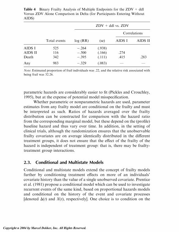
parametric hazards are considerably easier to fit (Pickles and Crouchley,1995), but at the expense of potential model misspecification.

Whether parametric or nonparametric hazards are used, parameterestimates from any frailty model are conditional on the frailty and mustbe interpreted as such. Ratios of hazards averaged over the frailtydistribution can be constructed for comparison with the hazard ratiofrom the corresponding marginal model, but these depend on the (profile)baseline hazard and thus vary over time. In addition, in the setting ofclinical trials, although the randomization ensures that the unobservablefrailty covariates are on average identically distributed in the differenttreatment groups, it does not ensure that the effect of the frailty of thehazard is independent of treatment group: that is, there may be frailty-treatment group interactions.

2.3. Conditional and Multistate Models

Conditional and multistate models extend the concept of frailty modelsfurther by conditioning treatment effects on more of an individuals’covariate history than the value of a single unobserved covariate. Prenticeet al. (1981) propose a conditional model which can be used to investigaterecurrent events of the same kind, based on proportional hazards modelsand conditional on the history of the event and covariate processes[denoted D(t) and X(t), respectively]. One choice is to condition on the

Table 4 Binary Frailty Analysis of Multiple Endpoints for the ZDV+ ddl

Versus ZDV Alone Comparison in Delta (for Participants Entering WithoutAIDS)

ZDV+ ddl vs. ZDV

Correlations

Total events log (RR) (se) AIDS I AIDS II

AIDS I 525 �.264 (.938)

AIDS II 116 �.500 (.166) .274Death 342 �.395 (.111) .415 .283

Any 983 �.329 (.083) — —

Note: Estimated proportion of frail individuals was .22, and the relative risk associated with

being frail was 32.26.



previous number of events experienced by the individual. The hazard forthe jth event in individual i is then

kijftADðtÞ;XðtÞg ¼ k0jðtÞ expðbjziÞ:Time can either be measured from randomization, or from the previousevent. This type of recurrence model can be fitted in any standard soft-ware which allows data to be input in the counting process formulationfor failure time data and simultaneously allows stratification of the base-line hazard (such as SAS, STATA, and S+).

Multistate models (Kay, 1984) extend these conditional modelsfurther to include conditioning information on the type rather than merelythe number of previous events. Separate proportional hazards models arespecified for transitions between any pair of events or group of events. Allestimated treatment effects must now be interpreted conditionally on theentire covariate history. Table 5 gives the parameter estimates (log relativerisk) for the ZDV+ddl versus ZDV comparison in Delta from the multi-state model. The effect of combination therapy on the overall rate of pro-gression to AIDS II events is much less clear from this model.

A distinction has to be drawn between accurately modelling diseaseprocesses and covariate effects, and presenting the likely effects of treat-ment in amanner which is easily understood by clinicians and patients, andapplied to clinical practice. For the latter marginal models remain themostappropriate for use in clinical trials, while for the former the simple frailtymodels present an alternative which is easy to interpret. Conditional andfrailty models provide a richer alternative for hypothesis generating.

Table 5 Multistate Analysis of Multiple Endpoints for the ZDV+ ddl VersusZDV Alone Comparison in Delta (for Participants Entering Without AIDS)

Transition ZDV+ ddl vs. ZDV

From To Total events Log (RR) (se)

Entry AIDS I 759 �.281 (.090)

Entry AIDS II 98 �.662 (.254)Entry Death 79 .216 (.281)

AIDS I AIDS IIa 67 �.155 (.293)AIDS I Deatha 284 �.311 (.147)

AIDS II Deatha 135 �.122 (.213)

a Timescale measured from previous event.



3. BIOLOGICAL MARKERS OF DISEASEPROGRESSION

Without a doubt, the greatest change in the design of HIV trials over thelast 15 years has been the move from clinical endpoints to the use ofendpoints based on biological markers of disease progression. The 1990ssaw substantial statistical interest in the validation of these markers assurrogates for clinical outcome. Eventually, however, the FDA and otherregulatory authorities decided to licence anti-HIV drugs on the basis oftheir effects on these markers rather than on clinical outcome. PlasmaHIVRNA measurements are now the most commonly used primary outcomemeasures in Phase III trials.

3.1. Surrogacy

A perfect surrogate for clinical outcome should satisfy the condition thata test of the null hypothesis of no treatment effect on the marker shouldalso be a valid test of the null hypothesis based on clinical outcome(Prentice 1989). This requires that

1. The ability of the marker to predict clinical outcome should beindependent of treatment.

2. The marker should capture any relationship, positive or neg-ative, between the treatment and clinical outcome.

In the Concorde trial (Concorde Coordinating Committee, 1994), imme-diate treatment with ZDV induced significant increases in CD4 count,which remained on average more than 30 cells/AL higher than in thedeferred treatment group for at least 3 years. Yet clinical outcome up to3 years showed no significant difference between the two treatment groupsin mortality or progression to AIDS or death, and with longer follow-upthere was a significant excess of deaths in the immediate group. Thus CD4does not seem to satisfy conditions 1 and 2. Neither of the Prentice con-ditions for surrogacy, condition 2 in particular, appear to be adequatelysatisfied by HIV RNA viral load. In the Delta trial, plasma and/or serumwas available for viral load assessment in about 40% of the participants.Compared to ZDV alone, the unadjusted relative risk (95% confidenceinterval, CI) of disease progression or death (after week 8) was 0.60 (0.46to 0.78) for ZDV + ddl and .66 (.51 – .85) for ZDV + ddC. After ad-justment for viral load at baseline and week 8, disease-free survival wassubstantially worse in the two combination groups relative to ZDV



monotherapy: the adjusted relative risks were 1.31 (1.00 to 1.71) and 1.52(1.15 to 2.02) respectively (Delta, 1999).

In practice a single marker that captures all of the treatment effect isunlikely to exist. A more realistic goal is to require that, in addition to thelack of interaction between treatment and marker in their effect on clinicaloutcome (1), the marker captures a substantial proportion of the treat-ment effect on the clinical endpoint. The statistical properties of theproportion of treatment effect explained by the marker (PTE) wereinvestigated by Freedman et al. (1992) and Lin et al. (1997) in the contextsof logistic regression and Cox proportional hazards regression, respec-tively. The marginal methods for the analysis of multivariate failure timedata described in Section 2 can be used to simultaneously model

kiðtAziÞ ¼ k01ðtÞ expðaziÞ ð1ÞkiðtAzi;XÞ ¼ k02ðtÞ expfbzi þ c XðtÞg ð2Þ

where zi is the treatment group indicator and X(t) represents the possiblytime-dependent history of the marker. Models (1) and (2) cannot strictlyhold simultaneously, but the first model, which is not conditional on themarker process, is assumed to correspond approximately to the inte-grated second model. This will hold provided either c E{X(t)} or �02(t) =R t

0 k02 (u) du is small. Under these conditions the PTE is defined byPTE = 1�h/a. Confidence intervals for the PTE can be obtained usingthe Delta method or Fieller’s theorem (Fieller, 1940). Using the Deltamethod, the variance of the PTE can be estimated by

r2 ¼ Vaa2

VbVa

þ ba

!2�2� b

a� Vab

Va

24 35where Va, Vh, and Vah are the elements of the robust variance matrix.Logrank based methods for estimating PTE have also been developedbased on the difference between logrank observed and expected eventsstratified by marker levels (DeMasi and Babiker 1998), avoiding theassumption of proportional hazards.

The PTE by serial CD4 cell counts for AIDS or death has beenestimated by Choi et al. (1993) and Lin et al. (1993) as �.01, .31, and �.13from three trials of ZDV (Volberding et al., 1990; Fischl et al., 1987; andFischl et al., 1990, respectively). The PTE by CD4 at weeks 16 and 8 forAIDS or death after this time point in the second two trials has also beenestimated at .46 (95% Cl –.14 to .08) and .28 (95% Cl .06 to .51)



respectively (Choi et al., 1993; Lin et al., 1997). CD4 cell counts over timeand at fixed time points therefore appear to be only an incompletesurrogate for clinical outcome.

Estimates of PTE clearly tend to be imprecise, and can even lieoutside the range of zero to one because PTE is related to the net effect oftreatment. A surrogate marker might be considered important if thelower confidence limit for the PTE exceeded a level such as .75 (since aperfect surrogate has PTE = 1). Lin et al. (1997) showed that the powerof detecting the lower confidence limit greater than .75 remained low, atonly 50% even when the treatment effect was about 8 standard deviationsin size. Therefore, reasonably precise estimation of the PTE is likely torequire that the effect of treatment on a clinical outcome be assessedmuch more precisely (with a smaller standard error) than needed to showa significant result on the clinical event itself. Such a trial would be likelyto be stopped early before such significant evidence accumulated in anycase. More importantly, even if PTE is estimated to be near 1 with a highdegree of confidence, this by itself does not guarantee that the marker is agood surrogate (DeGruttola et al., 1997). The reason is that if the treat-ment has a negative impact on clinical outcome through processes notmediated via the marker, a poor surrogate can have PTE close to 1. Thus,while these methods may lead to the identification of poor surrogates,they cannot validate surrogacy, which requires a more general under-standing of mechanisms of disease and drug action.

Rather than considering the PTE, Buyse and Molenberghs (1998)propose assessing the surrogacy of an endpoint (rather than a markerprocess) via the relative effect defined by RE= a/c, where c is the effect oftreatment on the surrogate endpoint,

kiðxAziÞ ¼ k03ðxÞ expðcziÞ:However, similarly to PTE, validating surrogate endpoints using the RErequires large numbers of observations.

Daniels and Hughes (1997) explored the issue of surrogacy by aBayesian meta-analysis of the correlation between treatment-inducedchanges in biological markers and treatment effect on clinical outcome.This is a more promising approach, although it may be limited by theamount and nature of data available from the trials. The estimated treat-ment difference on the clinical outcome uk and the marker response gk ineach trial, k= 1, . . . , I are assumed to follow a joint normal distribution,

ukgk

!fN

ukgk

� �;

j2k

Ukjkrk

Ukjkrkr2k

� ��



where sampling variation is represented by jk and rk. uk is assumed to berelated to ck through a simple linear fixed effects model, hk|ckfN(a+ bck,s2), leading to

hkck

!fN

aþ bckck

� �;

r2k þ s2

qkrkrk

qkrkrkr2k

� �� :

If themarker is a perfect surrogate, thenwe expecta=0,h p 0, and H 2=0.Noninformative priors are placed on the regression coefficients (a, h, gk), apositive prior is placed on H 2, and (jk

2, rk2, Uk) are replaced by their within

trial (empirical Bayes) estimates. Gibbs sampling is used for estimation(Gilks et al., 1996). This method allows for the fact that both clinicaloutcome and marker outcome are measured with error. Using this tech-nique to assess mean change and AUC (area under the curve) in CD4 andRNA as surrogates for progression to AIDS or death, CD4 andRNAwereconcluded to be jointly important as prognostic factors, but only partialsurrogates, for clinical outcome (HIV Surrogate Marker CollaborativeGroup, 2000). At 24 weeks change in CD4 alone accounted for 0.34 (95%Cl .16–.53) of the observed treatment effect, change in RNA accounted for0.45 (95% Cl .24–.67), and changes in both RNA and CD4 jointlyaccounted for 0.57 (95% Cl .31–.84) of the treatment effect on AIDS ordeath to 2 years.

3.2. Analysis of Biological Markers as ContinuousVariables

The majority of clinical trials in HIV disease now have biological markersas outcome measures, notably viral load as measured by HIV RNA, andthus (in the absence of sufficient information on surrogacy) evaluate theeffect of treatment on the markers of anti-HIV efficacy only. When mark-ers are treated as continuous outcome measures, methods for the analysisof longitudinal data must be used as in Chapter 11. Treatment groups arecompared in terms of the trajectory of the marker or a summary of such atrajectory. Possible summaries include

1. Level or change at a fixed time point2. Average level as measured by the area under the curve (AUC)3. Average slope of marker trajectory4. Time to achieve a given threshold level

However, participants are not followed beyond the end of the trial therapyinmanyHIV trials and so intention to treat has beenmore rarely used. The



rationale is that biological markers measure efficacy and that no efficacy isexpected after withdrawal from the trial regimen. This excludes eithercontinuing benefit from continuation of other therapy, or more impor-tantly leads to bias if one group with superior marker response stoptherapy more quickly due to toxicity. Data will often be incomplete due todropouts from toxicity or personal withdrawal and dropout will com-monly be informative (Touloumi et al., 2002). In the analysis of biologicalmarkers as continuous variables in the medical literature, dropout isgenerally handled either by basing analysis only on those with completedata, or by using the last observation carried forward (LOCF). Meanvalues at various time points after randomization can then be comparedusing pointwise tests. Clearly, more advanced methods of analysis of in-complete data are possible including GEE and multilevel models in stan-dard software such as SAS, Stata, and S+, as well as Bayesian methods(Raab and Parpia, 2001). However, none of the above methods addressesthe issue of informative dropout. More recently, longitudinal modelswhich explicitly include information on the dropout process have beendeveloped (see, for example, Diggle and Kenward, 1994; Touloumi, 1999;Hogan and Laird, 1997a, b). All these models for longitudinal data can beused with the intention-to-treat principle, assessing the effect on themarker of efficacy of the policy of giving the treatment regimens.

When comparing treatment groups in terms of change in HIV RNAfrom baseline, it is also important to recognize that the continuous dataitself is often censored (Hughes, 2000). In general, at any time point afterrandomization a number of HIV RNA measurements will be reported asless than the level of detectability of the assay, for example, RNA < 400or RNA< 50. Often this left censoring is ignored, assuming that RNA<400 is equivalent to RNA = 400. A number of appropriate statisticalmethods for parametric and nonparametric analysis of this type ofmeasurements are available (Hughes, 2000; Journot et al., 2001). Forexample, normal interval regression can be used, where the likelihoodcontribution for the interval censored data is the probability that the truevalue lies within the known interval, rather than the probability that itequals some fixed value (Long, 1997). Parametric or nonparametric failuretime methods can be used to incorporate the left censoring with thedependent variable RNA rather than time, and compare treatment groupsor calculate medians (Flandre et al., 2002). Gehan’s modification of theWilcoxon test (Gehan, 1965) can also be used as a nonparametric ranktest. Mixed models can be used to model longitudinal data incorporatingthis left censoring and informative dropouts (Lyles et al., 2000). More



complicated mixture models allowing for highly skewed data with extraprobability mass below the limit of detection of the assay have also beendeveloped but do not currently take informative dropout into account(Moulton et al., 2002).

3.3. Analysis of Biological Markers as Failure Time Data

Rather than comparing levels of biological markers over time or at arbi-trarily chosen time points, biological markers can also be used to definetime-to-event endpoints, for example, time to achieve either a prespecifiedfixed level, or percentage change from baseline. For example, a successfuloutcome can be defined as time to reach a threshold such as<50 copiesof HIV RNA per milliliter (or undetectable viral load on the assays), or atreatment failure can be defined as time to a rebound above baseline afterinitial reduction. An endpoint such as RNA rebound or failure of viralsuppression needs to take into account the likely trajectories of viral loaddecline in response to therapy: generally a window of 16–24 weeks has beenconsidered an appropriate period for viral load to drop to undetectablelevels (DeGruttola et al., 1998). How to account for unsuccessful or slowinitial response to treatment must also be considered (Gilbert et al., 2000).There is still a measure of arbitrariness in the definition of these endpointssince they are likely to depend on factors which may have no clinicalsignificance, such as the lower limit of quantification of the RNA assaychosen or a convenient round number.

In clinical trials RNA is generally only measured at specific timepoints post baseline (clinic visits) so that the exact time of occurrence of amarker defined endpoint is never known. A rigorous approach to theanalysis of time to virological failure therefore requires the use of intervalcensored failure data techniques. This is particularly important when dataare sparse, or the intervals between successive marker measurements arewide, since it is then that the most bias is likely to occur in approximationssuch as taking the failure time as the midpoint between visits or the firstvisit at which the event is observed to have already happened.

Suppose Ti denotes the unobserved marker event time, such as thetime that viral load first drops to undetectable levels. The observedinterval-censored data consists of an interval (Li, Ri) where Li is the timeof the last clinic visit with detectable viral load and Ri is the time viral loadwas first observed to be undetectable. If Ti could be observed exactly, thenLi = Ri, when Ti is left censored, Li = 0, and when Ti is right censored,Ri = l. Both semiparametric and parametric approaches have been



developed to estimate the effects of covariates such as treatment group onthe failure times Ti.

A (semiparametric) extension to Cox’s proportional hazards modelfor interval censored data was originally proposed by Finkelstein (1986)by parameterizing the cumulative baseline hazard in a sufficiently finemanner. Suppose that now sk denote times from trial entry such that all Li

and Ri are contained in the set of sk. Then the failure data log-likelihoodcan be expressed asX

i

logXk

cikexp��exp

�bzi þ ck�1

�� exp��exp

�bzi þ ck

��where

cik ¼ I��

sk�1; sk�o�Li;Ri

��; and

ck ¼ log �log�Pr�T > skAX ¼ 0

� �represents the cumulative baseline hazard. Newton-Raphson can be usedto maximize the log likelihood to simultaneously estimate h and g. Themajor disadvantage with this method is that the number of parameters tobe estimated (g) increases with the number of individuals unless the visittimes are fixed for all individuals. Rank-based methods and methodsbased on multiple imputation are also available but are considerably morecomplex computationally.

By imposing the relatively weak assumption of constant hazardsacross predefined time intervals a parametric model with a fixed number ofparameters can be fitted without imposing strong assumptions about therequired failure time distribution. Generalized linear model approaches toestimation in this model have been developed (Carsenten, 1996; Farring-don, 1996; Smith et al., 1997), extending the logistic model for rightcensored data of Efron (1988). Suppose the time axis is divided intointervals I1, . . . , Im with Ij = [tj � 1, tj] and with hazard a constant kjwithin each interval. Then the failure data likelihood is

Yi

exp �Xj

aijkj

!� 1� exp �

Xj

bijkj

!( )

where aij is the time in Ij in which patient i is known to not have had theevent, and bij is the time in Ij during which the event could have occurred.The hazards Ej are therefore the parameters of a generalized linear modelwith a log link and Bernoulli error. However, estimation using generalizedlinear models requires that the linear predictor is constrained to be positive



throughout the iterations. Sparse data or inappropriate intervals canproduce negative hazards. An alternative is to estimate the Ej using theEM algorithm (Lindsey and Ryan, 1998), where the complete data is theexact (unobserved) failure times for those who experienced the event andthe censoring times for those right censored. The complete data loglikelihood is thereforeX

j

ðDjlnkj � kjYjÞ

whereDj is the number of events in Ij and Yj is the person-time at risk in Ij.Poisson regression can therefore be used to estimate kj usingDj as responseand log Yj as offset. The conditional probability of a patient’s eventoccurring in an interval Ij and the conditional expected time at risk in Ijgiven current kj can be calculated by considering the location of (Li, Ri)with respect to Ij. These quantities can then be used in the Poissonregression. Standard errors can be estimated using methods such as Louis(1982) or Meng and Rubin (1991).

Finally, fully parametric failure time data models provide greaterstability when event data are sparse or intervals are wide (Lindsey, 1998;Lindsey and Ryan, 1998). However, this stability comes at the expense ofpotential model misspecification. Both nonparametric and parametricmethods have been recently extended to multivariate data (Betensky andFinkelstein, 1999; Goggins and Finkelstein, 2000).

An alternative to interval-censored failure time data analysis is togroup the data and use a discrete survival model; for example failure timeobservations Ri could be grouped by weeks from randomization (indexedby k below). A logistic model for the regression analysis of discrete failuretime data has been proposed by Sun (1997), relating the hazard of failureat discrete time point sk to covariates via

kk1� kk

¼ expðwkbzþ ckÞ

where wk is a prespecified weight used to construct tests. Under thismodel the failure data log–likelihood function is

Xi

logXk

cikYk�1

l¼ 1

f1þ expðwlbzi þ clÞg�1

" #expðwkbzi þ ckÞ

1þ expðwkbzi þ ckÞ� �

with cik= I{(sk � 1, sk)o (Li,Ri)} as before. h and g can be estimated usingNewton-Raphson maximization of the log likelihood, with standard



errors estimated from the Hessian. Interval-censored and discrete modelsfor the analysis of virologic endpoints have not been widely used so far.Instead, the time of the assay has been used as the true time of the event.

In the medical literature, analyses of virologic endpoints after ran-domization have often been based on comparison of proportions expe-riencing the endpoint by a fixed time T0, excluding participants whochange treatment or are lost to follow-up before T0 (standard on treat-ment analysis). More recently, a ‘‘noncompleter equals failure’’ analysis(NC=F) has been proposed as an attempt to include all participants in asimple manner. Under NC = F, patients who change treatment are in-cluded in the analysis and assumed to have failed at the time of dropout.This method is also likely to lead to biased estimates of the treatment effectif the reasons for dropout are different in the two treatment groups. As-suming that either none or all (NC=F) of those who change treatment orare lost to follow-up have events are extreme case analyses (although themost conservative extreme case approach would be to define noncomp-leter equals failure in the experimental treatment arm, and noncompleterequals success in the standard arm). A similar approach has recently beendescribed as a sensitivity method for assessing the effect of missing data(Molenberghs et al., 2001). If the number of noncompleters is substantialthere may be large differences between the methods in the absoluteproportions experiencing the event as well as in the differences betweenrandomized groups. If treatment changes are the reason for noncomple-tion, then some methods have been proposed to adjust for the treatmentchanges while retaining unbiased estimation of treatment differences.

4. ADJUSTING FOR CHANGES FROM ALLOCATEDTREATMENT

Analysis by the intent-to-treat (ITT) principle is generally accepted as themost appropriate for randomized controlled trials. All follow-up from alleligible patients are included in the analysis in the treatment group towhich they were originally assigned. In contrast, ‘‘on treatment’’ analysesare restricted to patients on allocated therapy at the time of analysis (sofollow-up is censored at the time of change from allocated therapy insurvival analysis). Clearly focusing on events that occur during theallocated treatment period or shortly after can lead to misleading results.Many trials in HIV infection only collect information until participantsstop allocated trial therapy, and therefore the only analysis possible is an



on-treatment analysis. It is important to note that only the intent-to-treat(ITT) analysis is unbiased under the null hypothesis of no treatmentdifference and that on treatment analyses can produce significantly biasedestimates of treatment effect for a variety of reasons, the most commonbeing that participants with worse prognosis are more likely to changetreatment in both treatment groups. Direct comparison of patients ac-cording to treatment actually received therefore incurs major selectionbias. However, several methods are available to adjust the ITT estimateof treatment effect for the treatment changes that occurred in a mannerwhich preserves the randomization. Thus the direct efficacy of the treat-ment regimens can be compared as intended, in addition to the effective-ness of the policy of applying the treatment regimens in practice (ITT).

Randomization-based methods for adjusting for treatment changesare also described in Chapter 10. Methods for adjusting for treatmentchanges at randomization have been proposed by Sommer and Zeger(1991) and Cuzick et al. (1997) for binary treatment outcomes, and byNewcombe (1988) for continuous outcomes. The difference in outcomeadjusting for treatment changes essentially equals the intention-to-treatdifference divided by the difference between the two treatment groups inthe proportion receiving the treatment as allocated. For treatment changeswhich can occur at any time, rather than only at randomization, a varietyof randomization-based methods using causal modelling have been devel-oped by Robins and coworkers (Robins and Tsiatis, 1991; Robins andGreenland, 1994;Mark and Robins, 1993;White and Goetghebeur, 1998).These models make no assumptions about the relationship between treat-ment changes and prognosis. A Stata macro is available for the simplestmodel, described below (White et al., 2002).

Only randomization-based methods for survival data will be con-sidered here. In brief, for a participant who experiences an event at timeTi, the treatment history, represented by time dependent covariate zi(t), isassumed to modify the true unobserved underlying lifetime Ui, in theabsence of treatment via the causal accelerated life model

Ui ¼Z Ti

0

exp�bTziðuÞ

�du:

The underlying lifetime is independent of treatment group, and thereforeh can be estimated using a logrank test for Ui. The point estimate is thevalue of h at which the logrank test for a difference between the treatmentgroups in Ui is 0, and the 95% confidence interval for h the range ofvalues for which the logrank test is not significant at the 5% level. The



test of h = 0 is the intention-to-treat logrank test, and therefore the pvalue is unchanged by the adjustment for treatment changes.

When not all patients experience the event of interest, censoring ofthe failure times by withdrawal or end of study depends on the treatmentactually received, and is therefore informative on the U scale. This is easyto see by considering individuals with detrimental treatment history(|bTzi(t)| >> 0): Individuals experiencing events just before their censor-ing time Ci would not have had these events observed if their treatmenthistory had been more favorable. Recensoring is one procedure fordealing with this informative censoring: Each Ui is ‘‘recensored’’ by theminimum censoring time over all time-dependent values of z(t) that werepossible within the ith patient’s randomized treatment group. Thus for apatient censored at Ci,

Ui ¼ min

Z Ti

0

exp�bTziðuÞ

�du; min

zðuÞ in ith group

Z ci

0

exp�bTzðuÞ�du� ��

:

Although such randomization-based methods are appealing in that theydo not introduce bias into the comparison of the treatment groups, theeffect of treatment from the accelerated failure time model h represents aratio by which time to event is extended in one treatment group. For ex-ample, with two treatment groups and without censoring, if z(t) indi-cates whether a patient is taking the experimental treatment at time t, thenUi = Ti

0 + ebTi1 where Ti

0 is the total time patient i spent on the stan-dard treatment and Ti

1 is the total time patient i spent on the experi-mental treatment. Then e�b is the factor by which time to event ismultiplied if a patient receives the experimental treatment continuouslycompared with continuously receiving the standard treatment. However,this is unfamiliar to many clinicians and statisticians who are more usedto expressing the treatment effect as a hazard ratio. The estimated timeratio in the accelerated life model can be used to ‘‘correct’’ the observedevent times Ti to those which would have been observed under the sce-nario represented by the treatment variable z(t), denoted Ti*. Forexample, with z(t) as above and ignoring treatment changes in the ex-perimental group, Ti* = Ti in the experimental treatment group, whereasin the standard group

Ti* ¼ Ti þ ðe�b � 1ÞT01i þ ðeb � 1ÞT10

i

where Timn is the time on the T scale that the treatment received was m but

would have been n under the scenario represented by z(t). T* is recensored



in a similar manner to U, and then a ‘‘corrected’’ hazard ratio can be es-timated using standard methods on T* for comparison with the standardintention-to-treat hazard ratios.

Example. In the Concorde trial participants were randomized to imme-diate ZDV or ZDV deferred until the onset of symptoms (ARC orAIDS). Many participants started open label ZDV before clinical diseaseprogression, mainly on the basis of persistently low CD4 counts after aprotocol amendment one year into the trial. The effect of these treatmentchanges is to make the two treatment arms more similar, that is, to movethe estimate of the treatment effect toward the null. Methods not basedon the randomization (such as proportional hazards modelling with ‘‘ontreatment’’ covariates) are subject to particularly large bias in Concorde,because in both groups by far the strongest predictor of starting ZDV isprognosis. Therefore comparing patients by whether or not they hadtaken ZDV is a comparison of prognosis, not the treatment armsthemselves (White et al., 1997). Using the accelerated failure time modelabove, there are several choices for the treatment history covariate z(t):

zITT (t) = 1 for immediate, 0 for deferred ZDVzNOW (t) = indicator of being on ZDV at time tzEVR (t) = indicator of being assigned to receive ZDV before

time t (that is, 1 for immediate or after open ZDVin deferred)

zEVP (t) = indicator of being assigned to receive ZDV beforetime t, other than at or after the onset of ARC orAIDS (that is, 1 for immediate, or after open ZDVin deferred if open ZDV before ARC or AIDS)

The concept of transient treatment effect can also be incorporated intothese models by restricting the effect of ZDV to only a limited period, forexample, by defining

zEVR1ðtÞ ¼ indicator of being assigned to receive ZDV within theprevious year at time t

and similarly for zEVP1(t). However, these treatment covariates do notcorrespond to the difference between the two treatment arms under anyscenario of treatment changes.

Table 6 shows the log time ratios for progression to the three ma-jor clinical endpoints in Concorde adjusted for the various scenariosdescribed above (White et al., 1998, 1999). Correcting for treatment



changes increased the estimated benefit of immediate ZDV in delayingprogression to ARC, AIDS, or death and the estimated disadvantage ofimmediate ZDV in accelerating death. Correspondingly, the confidenceintervals became wider, reflecting the increased uncertainty because of thetreatment changes and indicating the maximum effect that might havebeen missed in the trial. The necessity of some form of recensoring can beshown by considering proportional hazards models using treatmenthistory as covariates. Treatment history strongly predicts events on theT scale, the U scale, and the recensored U scale, but only predicts end offollow-up on the nonrecensored U scale, showing that censoring is in-formative on the U scale. Simulations show that in Concorde, failing torecensor incurs a small bias, but has little effect on the overall error in theestimation because the standard deviations of the recensored estimatorare larger.

5. CONCLUSIONS

Clinical trials in HIV over the first decade of antiretroviral therapy weremainly set up to evaluate two classes of anti-HIV drugs, the reverse tran-scriptase and protease inhibitors. The second decade of HIV clinical trialsis seeing a wider diversity as further classes of anti-HIV drugs becomeavailable (such as fusion inhibitors and immune modulators), strategy

Table 6 Semiparametric Adjustment for Changes from Allocated TrialTherapy in Concorde

ARC, AIDS,or death

EndpointAIDS or death Death

Scenario h 95% CI h 95% CI h 95% CI

ITT �.101 (�.245, .041) .004 (�.140, .137) .093 (�.028, .227)NOW �.262 (�.517, .061) .006 (�.308, .383) .414 (�.104, 2.082)

EVR �.178 (�.377, .041) .004 (�.274, .217) .172 (�.102, .858)EVP .004 (�.230, .178) .132 (�.078, .344)EVR1 �.870 (. , .134) .013 (. , .710) .750 (. , 1.260)

EVP1 .013 (�1.857, .554) .435 (�.534, .746)

Note: h is a log time ratio from the accelerated failure time model. Lower confidence limit is

missing when the logrank test statistic is greater than �1.96 at h = �3. For progression to

ARC, AIDS, or death, EVP is an identical scenario to EVR.



trials are designed to investigate order and length of administration of drugcombinations, salvage trials are developed for patients failing onHAART,and trials move into areas of nondrug interventions such as genotypic andphenotypic resistance testing. As individuals take HAART for increasingperiods of time, toxicity data are likely to play a more important role,particularly with the advent of reported metabolic dysfunction and lip-odystrophy. Methods which incorporate both efficacy and safety intotreatment comparisons may become more widely used (Tubert-Bitter etal., 1995; Thall and Cheng, 1999). It is also likely that the use of biologicalmarkers in making treatment decisions will be further refined, and thatmeasures of drug resistance will become trial endpoints. However, issuesdiscussed in this chapter such as choice of trial design and endpoints, theanalysis of biological markers and their interpretation, and compliancewill continue to be important and present new statistical challenges.

REFERENCES

Albert, J. M., Yun, H. (2001). Statistical advances in AIDS therapy trials.Statistical Methods in Medical Research 10:85–100.

Andersen, P. K., Klein, J. P., Knudsen, K. M., Tabanera y Palacios, R. (1997).Estimation of variance in Cox’s regression model with shared gamma frail-ties. Biometrics 53:1475–1484.

Babiker, A. G., Cuzick, J. (1994). A simple frailty model for family studies withcovariates. Statistics in Medicine 13:1679–1692.

Betensky, R. A., Finkelstein, D.M. (1999). A non-parametric maximum likelihoodestimator for bivariate interval censored data. Statistics in Medicine 18:

3089–3100.Bjorling, L. E., Hodges, J. S. (1997). Rule-based ranking schemes for antiretroviral

trials. Statistics in Medicine 16:1175–1191.

Buyse, M., Molenberghs, G. (1998). Criteria for the validation of surrogate end-points in randomized experiments. Biometrics 54:1014–1029.

Carr, A., Samaras, K., Thorisdottir, A., Kaufmann, G. R., Chisholm, D. J.,

Cooper, D. A. (1999). Diagnosis, prediction, and natural course of HIV-1protease-inhibitor-associated lipodystrophy, hyperlipidaemia, and diabetesmellitus: a cohort study. Lancet 353:2093–2099.

Carsenten, B. (1996). Regression models for interval censored survival data:

application to HIV infection in Danish homosexual men. Statistics inMedicine 15:2177–2189.

Centers for Disease Control (1992). 1993 revised classification system for HIV

infection and expanded surveillance case definition for AIDS among ado-lescents and adults. Mortality and Morbidity Weekly Report 41:1–19.



Choi, S., Lagakos, S. W., Schooley, R. T., Volberding, P. A. (1993). CD4 Lym-

phocytes are an incomplete surrogate marker for clinical progression inpersons with asymptomatic HIV infection taking zidovudine. Annals ofInternal Medicine 118:674–680.

Clayton, D., Cuzick, J. (1985). Multivariate generalizations of the proportionalhazards model. Journal of the Royal Statistical Society A 148:82–117.

Concorde Coordinating Committee (1994). Concorde: MRC/ANRS randomised

double-blind controlled trial of immediate and deferred zidovudine insymptom-free HIV infection. Lancet 343:871–882.

Cuzick, J., Edwards, R., Segnan, N. (1997). Adjusting for non-compliance andcontamination in randomized controlled trials. Statistics in Medicine 16:

1017–1029.Daniels, M. J., Hughes, M. D. (1997). Meta analysis for the evaluation of potential

surrogate markers. Statistics in Medicine 16:1965–1982.

DeGruttola, V., Fleming, T. R., Lin, D. Y., Coombs, R. (1997). Validating sur-rogate markers - are we being naive? Journal of Infectious Diseases 175:237–246.

DeGruttola, V., Hughes, M. D., Gilbert, P., Phillips, A. (1998). Trial design in theera of highly effective antiviral drug combinations for HIV infection. AIDS12(suppl A):S149–S156.

Delta Coordinating Committee (1996). Delta: a randomised double-blind con-trolled trial comparing combinations of zidovudine plus didanosine or zal-citabine with zidovudine alone in HIV-infected individuals. Lancet 348:283–291.

Delta Coordinating Committee and Virology Group (1999). An evaluation of HIVRNA and CD4 cell count as surrogates for clinical outcome. AIDS 13: 565–573.

DeMasi, R. A., Babiker, A. G. (1998). Nonparametric estimation of the propor-tion of treatment effect explained by a surrogate marker. Presented at the1998 ENAR conference, April 1, 1998.

Dempster, A. P., Laird, N.M., Rubin, D. R. (1977). Maximum likelihood from in-complete data via the EM algorithm. Journal of the Royal Statistical So-ciety B 39:1–38.

Diggle, P., Kenward, M. G. (1994). Informative drop-out in longitudinal analysis

(with discussion). Journal of the Royal Statistical Society C 43:49–93.Efron, B. (1988). Logistic regression, survival analysis and the Kaplan Meier

curve. Journal of the American Statistical Association 83:414–425.

Egger, M., Junghans, C., Friis-Moller, N., Lundgren, J. D. (2001). Highly activeantiretroviral therapy and coronary heart disease: the need for perspective.AIDS 15(Suppl. 5):S193–S201.

Ellenberg, S. S., Finkelstein, D. M., Schoenfeld, D. A. (1992). Statistical issuesarising in AIDS clinical trials (with discussion). Journal of the AmericanStatistical Association 87:562–583.



Emery, S., Abrams,D. I., Cooper, D. A., Darbyshire, J. H., Lane, H. C., Lundgren,

J. D., Neaton, J. D. (2002). The evaluation of subcutaneous Proleukin (R)(interleukin-2) in a randomized international trial: rationale, design, andmethods of ESPRIT. Controlled Clinical Trials 23:198–220.

Farringdon, C. P. (1996). Interval censored survival data: a generalised linearmodel approach. Statistics in Medicine 15:283–292.

Fieller, E. C. (1940). The biological standardisation of insulin. Journal of the

Royal Statistical Society 7:S1–S15.Finkelstein, D. M. (1986). A proportional hazards model for interval-censored

failure time data. Biometrics 42:845–854.Finkelstein, D. M., Schoenfeld, D. A., Stamenovic, E. (1997). Analysis of multi-

variate failure time data from an AIDS clinical trial. Statistics in Medicine16:951–961.

Fischl, M. A., Richman, D. D., Grieco, M. H., Gottlieb, M. S., Volberding, P. A.,

Laskin, O. L., Leedom, J. M., Groopman, J. E., Mildvan, D., Schooley,R. T., Jackson, G. G., Durack, D. T., King, D., the ZDV CollaborativeWorking Group. (1987). The efficacy of azidothymidine (ZDV) in the treat-

ment of patients with AIDS and AIDS-related complex: A double-blind,placebo-controlled trial. New England Journal of Medicine 317:185–191.

Fischl, M. A., Richman, D. D., Hansen, N., Collier, A. C., Carey, J. T., et al.

(1990). The safety and efficacy of zidovudine (AZT) in the treatment ofsubjects with mildly symptomatic human immunodeficiency virus type 1(HIV) infection. Annals of Internal Medicine 112:727–737.

Flandre, P., Durier, C., Descamps, D., Launay, O., Joly, V. (2002). On the use of

magnitude of reduction in HIV-1 RNA in clinical trials: Statistical analysisand potential biases. Journal of Acquired Immune Deficiency Syndromes30:59–64.

Fleming, T. R., DeMets, D. L. (1996). Surrogate endpoints in clinical trials: Arewe being misled? Annals of Internal Medicine 125:605–613.

Foulkes, M. A. (1998). Advances in HIV/AIDS statistical methodology over the

past decade. Statistics in Medicine 17:1–25.Freedman, L. S., Graubard, B. I., Schatzkin, A. (1992). Statistical validation of in-

termediate endpoints for chronic diseases. Statistics inMedicine 11:167–178.Friis-Moller, N., Weber, R., Reiss, P., Thiebaut, R., et al., for the DAD Study

Group. (2003) Cardiovascular disease risk factors in HIV patients—asso-ciation with antiretroviral therapy. Results from the DAD Study. AIDS17:1179–1193.

Gehan, E. A. (1965). A generalized two-sample Wilcoxon test for doubly censoreddata. Biometrika 52:620–653.

Gilbert, P. B., Ribaudo, H. J., Greenberg, L., Yu, G., Bosch, R. J., Tierney, C.,

Kuritzkes, D. R. (2000). Considerations in choosing a primary endpoint thatmeasures durability of virological suppression in an antiretroviral trial.AIDS 14:1961–1972.



Gilks, W. R., Richardson, S., Spiegelhalter, D. J. (1996). Markov Chain Monte

Carlo in practice. London: Chapman and Hall.Goggins, W. B., Finkelstein, D. M. (2000). A proportional hazards model for

multivariate interval-censored failure time data. Biometrics 56:940–943.

Grambsch, P. M., Therneau, T. M. (1994). Proportional hazards tests and diag-nostics based on weighted residuals. Biometrika 81:515–526.

Hess, K. R. (1994). Assessing time-by-covariate interactions in proportional haz-

ards regression models using cubic spline functions. Statistics in Medicine13:1045–1062.

HIV Surrogate Marker Collaborative Group (2000). Human Immunodeficiencyvirus type 1 RNA level and CD4 count as prognostic markers and surrogate

endpoints: a meta-analysis. AIDS Research and Human Retroviruses 16:1123–1133.

HIV Trialists’ Collaborative Group (1999). Zidovudine, didanosine and zalcita-

bine in the treatment of HIV infection: meta-analyses of the randomisedevidence. Lancet 353:2014–2025.

Hogan, J. W., Laird, N. M. (1997a). Mixture models for the joint distribution of

repeated measures and event times. Statistics in Medicine 16:239–257.Hogan, J. W., Laird, N. M. (1997b). Model-based approaches to analysing incom-

plete longitudinal and failure time data. Statistics in Medicine 16:259–272.

Hughes, M. D. (1997). Power considerations for clinical trials using multivariatetime-to-event data. Statistics in Medicine 16:865–882.

Hughes, M. D. (2000). Analysis and design issues for studies using censoredbiomarker measurements with an example of viral load measurements in

HIV clinical trials. Statistics in Medicine 19:3171–3191.Joint Concorde and Opal Coordinating Committee (1998). Long-term follow-up

of randomized trials of immediate versus deferred zidovudine in symptom-

free HIV infection. AIDS 12:1259–1265.Journot, V., Chene, G., Joly, P., Saves, M., Jacqmin-Gadda, H., Molina, J.-M.,

Salamon, R., the ALBI Study Group (2001). Viral load as a primary out-

come in Human Immunodeficiency Virus trials: a review of statisticalanalysis methods. Controlled Clinical Trials 22:639–658.

Kay, R. (1984). Multistate survival analysis: An application in breast cancer.Methods of Information in Medicine 23:157–162.

Klein, J. P. (1992). Semiparametric estimation of random effects using the Coxmodel based on the EM algorithm. Biometrics 48:795–806.

Klein, J. P., Moeschberger, M., Li, Y. H., Wang, S. T. (1992). Estimating random

effects in the Framingham Heart Study. In: Goel, P. K., Klein, J. P., eds.Survival Analysis: State of the Art. Boston: Kluwer Academic Publishers,pp. 99–120.

Klein, J. P., Moeschberger, M. L. (1997). Survival analysis: techniques forcensored and truncated data. New York: Springer-Verlag.

Larntz, K., Neaton, J. D., Wentworth, D. N., Yurik, T. (1996). Data analysis



issues for protocols with overlapping enrollment. Statistics in Medicine 15:

2445–2453.Liang, K-Y., Zeger, S. L. (1986). Longitudinal data analysis using generalized

linear models. Biometrika 73:13–22.

Lin, D. Y., Fischl, M. A., Schoenfeld, D. A. (1993). Evaluating the role of CD4-lymphocyte counts as surrogate endpoints in HIV clinical trials. Statistics inMedicine 12:835–842.

Lin, D. Y., Fleming, T. R., De Gruttola, V. (1997). Estimating the proportion oftreatment effect explained by a surrogate marker. Statistics in Medicine16:1515–1527.

Lindsey, J. C., Ryan, L. M. (1998). Methods for interval-censored data. Statistics

in Medicine 17:219–238.Lindsey, J. K. (1998). A study of interval censoring in parametric regression

models. Lifetime Data Analysis 4:329–354.

Long, J. S. (1997). Regression Models for Categorical and Limited DependentVariables. Thousand Oaks, CA: Sage Publications.

Louis, T. A. (1982). Finding the observed information matrix when using the EM

algorithm. Journal of the Royal Statistical Society B 44:226–233.Lyles, R. H., Lyles, C. M., Taylor, D. J. (2000). Random regression models for

human immunodeficiency virus ribonucleic acid data subject to left

censoring and informative dropouts. Applied Statistics 49:485–497.Marcus, R., Peritz, E., Gabriel, K. R. (1976). On closed testing procedures with

special reference to ordered analysis of variance. Biometrika 63:655–660.Mark, S. D., Robins, J. M. (1993). A method for the analysis of randomized trials

with compliance information: An application to the multiple risk factorintervention trial. Controlled Clinical Trials 14:79–97.

Mellors, J. W., Munoz, A., Giorgi, J. V., Margolick, J. B., Tassoni, C. J., Gupta,

P., Kingsley, L. A., Todd, J. A., Saah, A. J., Detels, R., Phair, J. P. (1997).Plasma viral load and CD4+ lymphocytes as prognostic markers of HIV-1infection. Annals of Internal Medicine 126:946–954.

Meng, X. L., Rubin, D. B. (1991). Using EM to obtain asymptotic variance-covariance matrices: the SEM algorithm. Journal of the AmericanStatistical Association 86:899–909.

Mocroft, A. J., Johnson, M. A., Sabin, C. A., Lipman, M., Elford, J., Emery, V.,

Morcinek, J., Youle, M., Janossy, G., Lee, C. A., Phillips, A. N. for theRoyal Free/Chelsea and Westminster Hospitals Collaborative Group.(1995). Staging System for clinical AIDS patients. Lancet 346:12–17.

Molenberghs, G., Kenward, M. G., Goetghebeur, E. (2001). Sensitivity analysisfor incomplete contingency tables: The Slovenian plebiscite case. AppliedStatistics 50:15–29.

Moulton, L. H., Curriero, F. C., Barroso, P. F. (2002). Mixture models for quan-titative HIV RNA data. Statistical Methods in Medical Research 11:317–325.



Neaton, J. D., Wentworth, D. N., Rhame, F., Hogan, C., Abrams, D. I., Deyton,

L. (1994). Considerations in choice of a clinical endpoint for AIDS clinicaltrials. Statistics in Medicine 13:2107–2125.

Newcombe, R. G. (1988). Explanatory and pragmatic estimates of the treatment

effect when deviations from allocated treatment occur. Statistics inMedicine 7:1179–1186.

O’Brien, P. C. (1984). Procedures for comparing samples with multiple endpoints.

Biometrics 40:1079–1087.Pickles, A., Crouchley, R. (1995). A comparison of frailty models for multivariate

survival data. Statistics in Medicine 14:1447–1461.Prentice, R. L., Williams, B. J., Peterson, A. V. (1981). On the regression analysis

of multivariate failure time data. Biometrika 68:373–379.Prentice, R. L. (1989). Surrogate endpoints in clinical trials: Definition and

operational criteria. Statistics in Medicine 8:431–440.

Raab, G. M., Parpia, T. (2001). Random effects models for HIV marker data:Practical approaches with currently available software. Statistical Methodsin Medical Research 10:101–116.

Robins, J. M., Tsiatis, A. A. (1991). Correcting for non-compliance in ran-domized trials using rank preserving structural failure time models.Communications in Statistics—Theory and Methods 20:2609–2631.

Robins, J. M., Greenland, S. (1994). Adjusting for differential rates ofprophylaxis therapy for PCP in high-dose versus low-dose AZT treatmentarms in an AIDS randomized trial. Journal of the American StatisticalAssociation 89:737–749.

Schoenfeld, D. A. (1995). Issues in the testing of drug combinations. In: Fin-kelstein, D. M., Schoenfeld, D. A., eds. AIDS Clinical Trials: Guidelinesfor Design and Analysis. New York: Wiley.

Schoenfeld, D. A. (1996). Long-term follow-up in AIDS clinical trials. Statisticsin Medicine 15:2366–2539.

Schwartz, D., Lellouch, J. (1967). Explanatory and pragmatic attitudes in thera-

peutic trials. Journal of Chronic Disease 20:637–648.Shevitz, A., Wanke, C. A., Falutz, J., Kotler, D. P. (2001). Clinical perspectives on

HIV-associated lipodystrophy syndrome: an update. AIDS 15:1917–1930.Smith, P. J., Thompson, T. J., Jereb, J. A. (1997). A model for interval-censored

tuberculosis outbreak data. Statistics in Medicine 16:485–496.Sommer, A., Zeger, S. L. (1991). On estimating efficacy from clinical trials. Sta-

tistics in Medicine 10:45–52.

Sun, J. (1997). Regression analysis of interval-censored failure time data. Sta-tistics in Medicine 16:497–504.

Thall, P. F., Cheng, S. C. (1999). Treatment comparisons based on two-

dimensional safety and efficacy alternatives in oncology. Biometrics 55:746–753.

Touloumi, G., Pocock, S. J., Babiker, A. G., Darbyshire, J. H. (1999). Estimation



and comparison of rates of change in longitudinal studies with informative

drop-outs. Statistics in Medicine 18:1215–1233.Touloumi, G., Pocock, S. J., Babiker, A. G., Darbyshire, J. H. (2002). Impact of

missing data due to selective drop-outs in cohort studies and clinical trials.

Epidemiology 13:347–355.Tubert-Bitter, P., Bloch, D. A., Raynauld, J. P. (1995). Comparing the bivariate

effects of toxicity and efficacy of treatments. Statistics in Medicine 14:1129–

1141.Volberding, P. A., Lagakos, S. W., Koch, M. A., Pettinelli, C. B., et al. (1990).

Zidovudine in asymptomatic HIV infection: a controlled trial in personswith fewer than 500 CD4-positive cells per cubic millimeter. New England

Journal of Medicine 322:941–949.Volberding, P. A., Lagakos, S. W., Grimes, J. M., Stein, D. S., Balfour, H. H.,

Reichman, R. C., Bartlett, J. A., Hirsch, M. S., Phair, J. P., Mitsuyasu, R.

T., Fischl, M. A., Soeiro, R., the AIDS Clinical Trials Group of the Na-tional Institute of Allergy and Infectious Diseases (1994). The duration ofzidovudine benefit in persons with asymptomatic HIV infection. Journal of

the American Medical Association 272:437–442.Walker, A. S. (1999).The analysis of multivariate failure time data with applica-

tion to multiple endpoints in trials in HIV infection. Unpublished PhD

thesis, University College, London.Walker, A. S., Babiker, A. G., Darbyshire, J. H. (2000). Analysis of multivariate

failure-time data from HIV clinical trials. Controlled Clinical Trials 21:75–93.

Wang, S. T., Klein, J. P., Moeschberger, M. L. (1995). Semi-parametric es-timation of covariate effects using the positive stable frailty model. AppliedStochastic Models and Data Analysis 11:121–133.

Wei, L. J., Lin, D. Y., Weissfeld, L. (1989). Regression analysis of multivariateincomplete failure time data by modelling marginal distributions. Journalof the American Statistical Association 84:1065–1073.

Wei, L. J., Glidden, D. V. (1997). An overview of statistical methods for multiplefailure time data in clinical trials. Statistics in Medicine 16:833–839.

White, I. P., Walker, A. S., Babiker, A. G., Darbyshire, J. H. (1997). Impact oftreatment changes on the interpretation of the Concorde trial. AIDS 11:999–

1006.White, I. R., Goetghebeur, E. J. T. (1998). Clinical trials comparing two treat-

ment policies: which aspect of the treatment policies make a difference?

Statistic in Medicine 17:319–339.White, I. R., Babiker, A. G., Walker, A. S., Darbyshire, J. H. (1999). Random-

ization-based methods for correcting for treatment changes: examples from

the Concorde trial. Statistics in Medicine 18:2617–2634.White, I. R., Walker, A. S., Babiker, A. G., Darbyshire, J. H. (2002). Strbee:

Randomization-based efficacy estimator. The Stata Journal 2:140–150.



Documents

ADVANCES IN CLINICAL TRIAL B IOSTATISTI CSthe-eye.eu/public/Books/BioMed/Advances in Clinical Trial...Bayesian Reporting of Clinical Trials Simon Weeden, Laurence S. Freedman, and