ADVANCES IN CHEMICAL PHYSICS - Институт ...ipmras.ru/UserFiles/publications/alp/Advances in Chemical Physics... · Advances in Chemical Physics, ... we note that there are

ADVANCES INCHEMICAL PHYSICS

Edited by

I. PRIGOGINE

Center for Studies in Statistical Mechanics and Complex SystemsThe University of Texas

Austin, Texasand

International Solvay InstitutesUniversite Libre de Bruxelles

Brussels, Belgium

and

STUART A. RICE

Department of Chemistryand

The James Franck InstituteThe University of Chicago

Chicago, Illinois

VOLUME 121

AN INTERSCIENCE PUBLICATION

JOHN WILEY & SONS, INC.

EDITORIAL BOARD

Bruce J. Berne, Department of Chemistry, Columbia University, New York,New York, U.S.A.

Kurt Binder, Institut fur Physik, Johannes Gutenberg-Universitat Mainz, Mainz,Germany

A. Welford Castleman, Jr., Department of Chemistry, The Pennsylvania StateUniversity, University Park, Pennsylvania, U.S.A.

David Chandler, Department of Chemistry, University of California, Berkeley,California, U.S.A.

M. S. Child, Department of Theoretical Chemistry, University of Oxford, Oxford,U.K.

William T. Coffey, Department of Microelectronics and Electrical Engineering,Trinity College, University of Dublin, Dublin, Ireland

F. Fleming Crim, Department of Chemistry, University of Wisconsin, Madison,Wisconsin, U.S.A.

Ernest R. Davidson, Department of Chemistry, Indiana University, Bloomington,Indiana, U.S.A.

Graham R. Fleming, Department of Chemistry, The University of California,Berkeley, California, U.S.A.

Karl F. Freed, The James Franck Institute, The University of Chicago, Chicago,Illinois, U.S.A.

Pierre Gaspard, Center for Nonlinear Phenomena and Complex Systems,Universite Libre de Bruxelles, Brussels, Belgium

Eric J. Heller, Department of Chemistry, Harvard-Smithsonian Center forAstrophysics, Cambridge, Massachusetts, U.S.A.

Robin M. Hochstrasser, Department of Chemistry, The University ofPennsylvania, Philadelphia, Pennsylvania, U.S.A.

R. Kosloff, The Fritz Haber Research Center for Molecular Dynamics and Depart-ment of Physical Chemistry, The Hebrew University of Jerusalem, Jerusalem,Israel

Rudolph A. Marcus, Department of Chemistry, California Institute of Tech-nology, Pasadena, California, U.S.A.

G. Nicolis, Center for Nonlinear Phenomena and Complex Systems, UniversiteLibre de Bruxelles, Brussels, Belgium

Thomas P. Russell, Department of Polymer Science, University of Massachusetts,Amherst, Massachusetts

Donald G. Truhlar, Department of Chemistry, University of Minnesota,Minneapolis, Minnesota, U.S.A.

John D. Weeks, Institute for Physical Science and Technology and Departmentof Chemistry, University of Maryland, College Park, Maryland, U.S.A.

Peter G. Wolynes, Department of Chemistry, University of California, San Diego,California, U.S.A.

CONTRIBUTORS TO VOLUME 121

Aleksij Aksimentiev, Computer Science Department, Material Science

Laboratory, Mitsui Chemicals, Inc., Sodegaura-City, Chiba, Japan

Michal Ben-Nun, Department of Chemistry and the Beckman Institute,

University of Illinois, Urbana, Illionis, U.S.A.

Paul Blaise, Centre d’Etudes Fondamentales, Universite de Perpignan,

Perpignan, France

Didier Chamma, Centre d’Etudes Fondamentales, Universite de Perpignan,

Perpignan, France

C. H. Chang, Institute of Atomic and Molecular Sciences, Academia Sinica,

Taipei, Taiwan, R.O.C.

R. Chang, Institute of Atomic and Molecular Sciences, Academia Sinica, Taipei,

Taiwan

D. S. F. Crothers, Theoretical and Computational Physics Research Division,

Department of Applied Mathematics and Theoretical Physics, Queen’s

University Belfast, Belfast, Northern Ireland

Marcin FiaLkowski, Institute of Physical Chemistry, Polish Academy of Science

and College of Science, Department III, Warsaw, Poland

M. Hayashi, Center for Condensed Matter Sciences, National Taiwan University,

Taipei, Taiwan

Olivier Henri-Rousseau, Centre d’Etudes Fondamentales, Universite de

Perpignan, Perpignan, France

Robert HoLyst, Institute of Physical Chemistry, Polish Academy of Science and

College of Science, Department III, Warsaw, Poland; and Labo de Physique,

Ecole Normale Superieure de Lyon, Lyon, France

F. C. Hsu, Department of Chemistry, National Taiwan University, Taipei, Taiwan

K.K.Liang, Institute ofAtomic andMolecular Sciences,AcademiaSinica, Taipei,

Taiwan

S. H. Lin, Department of Chemistry, National Taiwan University, Taipei, Taiwan,

R.O.C.; Institute ofAtomic andMolecular Sciences,AcademiaSinica, Taipei,

Taiwan, R.O.C.

v

AskoldN.Malakhov (deceased), Radiophysical Department, NizhnyNovgorod

State University, Nizhny Novgorod; Russia

Todd J. Martınez, Department of Chemistry and the Beckman Institute,

University of Illinois, Urbana, Illinois, U.S.A.

D. M. McSherry, Theoretical and Computational Physics Research Division,



S. F. C. O’Rourke, Theoretical and Computational Physics Research Division,



Andrey L. Pankratov, Institute for Physics of Microstructures of RAS, Nizhny

Novgorod, Russia

Y. J. Shiu, Institute of Atomic and Molecular Sciences, Academia Sinica, Taipei,

Taiwan

T.-S. Yang, Institute of Atomic andMolecular Sciences, Academia Sinica, Taipei,

Taiwan, R.O.C.

Arun Yethiraj, Department of Chemistry, University of Wisconsin, Madison,

Wisconsin, U.S.A.

J. M. Zhang, Institute of Atomic and Molecular Sciences, Academia Sinica,

Taipei, Taiwan

vi contributors to volume 121

INTRODUCTION

Few of us can any longer keep up with the flood of scientific literature, evenin specialized subfields. Any attempt to do more and be broadly educatedwith respect to a large domain of science has the appearance of tilting atwindmills. Yet the synthesis of ideas drawn from different subjects into new,powerful, general concepts is as valuable as ever, and the desire to remaineducated persists in all scientists. This series, Advances in ChemicalPhysics, is devoted to helping the reader obtain general information about awide variety of topics in chemical physics, a field that we interpret verybroadly. Our intent is to have experts present comprehensive analyses ofsubjects of interest and to encourage the expression of individual points ofview. We hope that this approach to the presentation of an overview of asubject will both stimulate new research and serve as a personalized learningtext for beginners in a field.

I. PrigogineStuart A. Rice

vii

CONTENTS

Ultrafast Dynamics and Spectroscopy of Bacterial

Photosynthetic Reaction Centers 1

By S. H. Lin, C. H. Chang, K. K. Liang, R. Chang, J. M. Zhang,

T.-S. Yang, M. Hayashi, Y. J. Shiu, and F. C. Hsu

Polymer Melts at Solid Surfaces 89

By Arun Yethiraj

Morphology of Surfaces in Mesoscopic Polymers, Surfactants,

Electrons, or Reaction–Diffusion Systems: Methods,

Simulations, and Measurements 141

By Aleksij Aksimentiev, Marcin Fialkowski, and Robert Holyst

Infrared Lineshapes of Weak Hydrogen Bonds:

Recent Quantum Developments 241

By Olivier Henri-Rousseau, Paul Blaise, and Didier Chamma

Two-Center Effects in Ionization by Ion-Impact

in Heavy-Particle Collisions 311

By S. F. C. O’Rourke, D. M. McSherry, and D. S. F. Crothers

Evolution Times of Probability Distributions

and Averages—Exact Solutions of the Kramers’ Problem 357

By Askold N. Malakhov and Andrey L. Pankratov

Ab Initio Quantum Molecular Dynamics 439

By Michal Ben-Nun and Todd J. Martınez

Author Index 513

Subject Index 531

EVOLUTION TIMES OF PROBABILITY

DISTRIBUTIONS AND AVERAGES—EXACT

SOLUTIONS OF THE KRAMERS’ PROBLEM

ASKOLD N. MALAKHOV (DECEASED)

Radiophysical Department, Nizhny Novgorod State University,

Nizhny Novgorod, Russia

ANDREY L. PANKRATOV

Institute for Physics of Microstructures of RAS, Nizhny Novgorod, Russia

CONTENTS

I. Introduction

II. Introduction into the Basic Theory of Random Processes

A. Continuous Markov Processes

B. The Langevin and the Fokker–Planck Equations

III. Approximate Approaches for Escape Time Calculation

A. The Kramers’ Approach and Temperature Dependence of the Prefactor

of the Kramers’ Time

B. Eigenvalues as Transition Rates

IV. The First Passage Time Approach

A. Probability to Reach a Boundary by One-Dimensional Markov Processes

B. Moments of the First Passage Time

V. Generalizations of the First Passage Time Approach

A. Moments of Transition Time

B. The Effective Eigenvalue and Correlation Time

C. Generalized Moment Expansion for Relaxation Processes

D. Differential Recurrence Relation and Floquet Approach

1. Differential Recurrence Relations

2. Calculation of Mean First Passage Times from Differential Recurrence Relations

3. Calculation of t by a Continued Fraction Method

Advances in Chemical Physics, Volume 121, Edited by I. Prigogine and Stuart A. Rice.ISBN 0-471-20504-4 # 2002 John Wiley & Sons, Inc.

357

E. The Approach by Malakhov and Its Further Development

1. Statement of the Problem

2. Method of Attack

3. Basic Results Relating to Relaxation Times

4. Basic Results Relating to Decay Times

5. Some Comments and Interdependence of Relaxation and Decay Times

6. Derivation of Moments of Transition Time

7. Timescales of Evolution of Averages and Correlation Time

VI. Time Evolution of Observables

A. Time Constant Potentials

1. Time Evolution of Survival Probability

2. Temporal Evolution of Averages

3. Discussion of Applicability of Single Exponential Approximation

B. Time Periodic Potentials: Resonant Activation and Suprathreshold Stochastic Resonance

VII. Conclusions

Acknowledgments

Appendix

References

I. INTRODUCTION

The investigation of temporal scales (transition rates) of transition processes in

various polystable systems driven by noise is a subject of great theoretical and

practical importance in physics (semiconductor [1,2] and Josephson electronics

[3], dynamics of magnetization of fine single-domain ferromagnetic particles

[4–7]), chemistry and biology (transport of biomolecules in cell compartments

and membranes [8], the motion of atoms and side groups in proteins [9], and the

stochastic motion along the reaction coordinates of chemical and biochemical

reactions [2,4,10–14]).

The first paper that was devoted to the escape problem in the context of the

kinetics of chemical reactions and that presented approximate, but complete,

analytic results was the paper by Kramers [11]. Kramers considered

the mechanism of the transition process as noise-assisted reaction and used

the Fokker–Planck equation for the probability density of Brownian particles to

obtain several approximate expressions for the desired transition rates. The main

approach of the Kramers’ method is the assumption that the probability current

over a potential barrier is small and thus constant. This condition is valid only if

a potential barrier is sufficiently high in comparison with the noise intensity. For

obtaining exact timescales and probability densities, it is necessary to solve the

Fokker–Planck equation, which is the main difficulty of the problem of

investigating diffusion transition processes.

The Fokker–Planck equation is a partial differential equation. In most cases,

its time-dependent solution is not known analytically. Also, if the Fokker–

Planck equation has more than one state variable, exact stationary solutions are

358 askold n. malakhov and andrey l. pankratov

very rare. That is why the most simple thing is to approximately obtain time

characteristics when analyzing dynamics of diffusion transition processes.

Considering the one-dimensional Brownian diffusion (Brownian motion in

the overdamped limit), we note that there are many different time characteris-

tics, defined in different ways (see review [1] and books [2,15,16])—for

example, decay time of metastable state or relaxation time to steady state. An

often used method of eigenfunction analysis [2,15–18], when the timescale (the

relaxation time) is supposed to be equal to an inverse minimal nonzero eigen-

value, is not applicable for the case of a large noise intensity because then higher

eigenvalues should be also taken into account. In one-dimensional Fokker–

Planck dynamics the moments of the first passage time (FPT) distribution can be

calculated exactly, at least expressed by integrals [19]. But during the FPTapproach,

absorbing boundaries have additionally to be introduced. Both eigenfunction

analysis and an FPT approach were widely used for describing different tasks in

chemical physics [20–29].

However, most concrete tasks (see examples, listed above) are described by

smooth potentials that do not have absorbing boundaries, and thus the moments

of FPT may not give correct values of timescales in those cases.

The aim of this chapter is to describe approaches of obtaining exact time

characteristics of diffusion stochastic processes (Markov processes) that are in

fact a generalization of FPT approach and are based on the definition of

characteristic timescale of evolution of an observable as integral relaxation time

[5,6,30–41]. These approaches allow us to express the required timescales and

to obtain almost exactly the evolution of probability and averages of stochastic

processes in really wide range of parameters. We will not present the

comparison of these methods because all of them lead to the same result due to

the utilization of the same basic definition of the characteristic timescales, but

we will describe these approaches in detail and outline their advantages in

comparison with the FPT approach.

It should be noted that besides being widely used in the literature definition

of characteristic timescale as integral relaxation time, recently ‘‘intrawell

relaxation time’’ has been proposed [42] that represents some effective

averaging of the MFPT over steady-state probability distribution and therefore

gives the slowest timescale of a transition to a steady state, but a description of

this approach is not within the scope of the present review.

II. INTRODUCTION INTO THE BASIC THEORYOF RANDOM PROCESSES

A. Continuous Markov Processes

This chapter describes methods of deriving the exact time characteristics of

overdamped Brownian diffusion only, which in fact corresponds to continuous

evolution times of probability distributions and averages 359

Markov process. In the next few sections we will briefly introduce properties of

Markov processes as well as equations describing Markov processes.

If we will consider arbitrary random process, then for this process the

conditional probability density Wðxn; tnjx1; t1; . . . ; xn�1; tn�1Þ depends on x1,

x2, . . . , xn�1. This leads to definite ‘‘temporal connexity’’ of the process, to

existence of strong aftereffect, and, finally, to more precise reflection of

peculiarities of real smooth processes. However, mathematical analysis of

such processes becomes significantly sophisticated, up to complete impossi-

bility of their deep and detailed analysis. Because of this reason, some

‘‘tradeoff’’ models of random processes are of interest, which are simple in

analysis and at the same time correctly and satisfactory describe real processes.

Such processes, having wide dissemination and recognition, are Markov

processes. Markov process is a mathematical idealization. It utilizes the

assumption that noise affecting the system is white (i.e., has constant spectrum

for all frequencies). Real processes may be substituted by a Markov process

when the spectrum of real noise is much wider than all characteristic

frequencies of the system.

A continuous Markov process (also known as a diffusive process) is

characterized by the fact that during any small period of time �t some small (of

the order offfiffiffiffiffiffi�tp

) variation of state takes place. The process xðtÞ is called a

Markov process if for any ordered n moments of time t1 < � � � < t < � � � < tn,

the n-dimensional conditional probability density depends only on the last fixed

value:

Wðxn; tnjx1; t1; . . . ; xn�1; tn�1Þ ¼ Wðxn; tnjxn�1; tn�1Þ ð2:1Þ

Markov processes are processes without aftereffect. Thus, the n-dimensional

probability density of Markov process may be written as

Wðx1; t1; . . . ; xn; tnÞ ¼ Wðx1; t1ÞYni¼2

Wðxi; tijxi�1; ti�1Þ ð2:2Þ

Formula (2.2) contains only one-dimensional probability density Wðx1; t1Þ and

the conditional probability density. The conditional probability density of

Markov process is also called the ‘‘transition probability density’’ because the

present state comprehensively determines the probabilities of next transitions.

Characteristic property of Markov process is that the initial one-dimensional

probability density and the transition probability density completely determine

Markov random process. Therefore, in the following we will often call different

temporal characteristics of Markov processes ‘‘the transition times,’’ implying

that these characteristics primarily describe change of the evolution of the

Markov process from one state to another one.


The transition probability density satisfies the following conditions:

1. The transition probability density is a nonnegative and normalized quantity:

Wðx; tjx0; t0Þ � 0;

ðþ1�1

Wðx; tjx0; t0Þ dx ¼ 1

2. The transition probability density becomes Dirac delta function for

coinciding moments of time (physically this means small variation of the

state during small period of time):

limt!t0

Wðx; tjx0; t0Þ ¼ dðx� x0Þ

3. The transition probability density fulfills the Chapman–Kolmogorov (or

Smoluchowski) equation:

Wðx2; t2jx0; t0Þ ¼ðþ1�1

Wðx2; t2jx1; t1ÞWðx1; t1jx0; t0Þ dx1 ð2:3Þ

If the initial probability density Wðx0; t0Þ is known and the transition

probability density Wðx; tjx0; t0Þ has been obtained, then one can easily

get the one-dimensional probability density at arbitrary instant of time:

Wðx; tÞ ¼ð1�1

Wðx0; t0ÞWðx; tjx0; t0Þ dx0 ð2:4Þ

B. The Langevin and the Fokker–Planck Equations

In the most general case the diffusive Markov process (which in physical

interpretation corresponds to Brownian motion in a field of force) is described

by simple dynamic equation with noise source:

dxðtÞdt¼ �d�ðx; tÞ

h dxþ xðtÞ ð2:5Þ

where xðtÞ may be treated as white Gaussian noise (Langevin force),

hxðtÞi ¼ 0; hxðtÞxðt þ tÞi ¼ Dðx; tÞdðtÞ, �ðxÞ is a potential profile, and h is

viscosity. The equation that has in addition the second time derivative of

coordinate multiplied by the mass of a particle is also called the Langevin

equation, but that one describes not the Markov process itself, but instead a set of

two Markov processes: xðtÞ and dxðtÞ=dt. Here we restrict our discussion by

considering only Markov processes, and we will call Eq. (2.5) the Langevin

equation, which in physical interpretation corresponds to overdamped Brownian

motion. If the diffusion coefficient Dðx; tÞ does not depend on x, then Eq. (2.5) is


called a Langevin equation with an additive noise source. For Dðx; tÞ dependingon x, one speaks of a Langevin equation with multiplicative noise source. This

distinction between additive and multiplicative noise may not be considered very

significant because for the one-variable case (2.5), for time-independent drift and

diffusion coefficients, and for Dðx; tÞ 6¼ 0, the multiplicative noise always

becomes an additive noise by a simple transformation of variables [2].

Equation (2.5) is a stochastic differential equation. Some required characteri-

stics of stochastic process may be obtained even from this equation either by

cumulant analysis technique [43] or by other methods, presented in detail in

Ref. 15. But the most powerful methods of obtaining the required characteristics

of stochastic processes are associated with the use of the Fokker–Planck

equation for the transition probability density.

The transition probability density of continuous Markov process satisfies to

the following partial differential equations (Wx0ðx; tÞ � Wðx; tjx0; t0Þ):

qWx0ðx; tÞqt

¼ � qqx

aðx; tÞWx0ðx; tÞ½ � þ q2

qx2Dðx; tÞ

2Wx0ðx; tÞ

� �ð2:6Þ

qWx0ðx; tÞqt0

¼ �aðx0; t0Þ qqx0

Wx0ðx; tÞ �Dðx0; t0Þ

2

q2

qx20Wx0ðx; tÞ ð2:7Þ

Equation (2.6) is called the Fokker–Planck equation (FPE) or forward

Kolmogorov equation, because it contains time derivative of final moment of

time t > t0 . This equation is also known as Smoluchowski equation. The second

equation (2.7) is called the backward Kolmogorov equation, because it contains

the time derivative of the initial moment of time t0 < t. These names are

associated with the fact that the first equation used Fokker (1914) [44] and

Planck (1917) [45] for the description of Brownian motion, but Kolmogorov [46]

was the first to give rigorous mathematical argumentation for Eq. (2.6) and he

was first to derive Eq. (2.7). The derivation of the FPE may be found, for

example, in textbooks [2,15,17,18].

The function aðx; tÞ appearing in the FPE is called the drift coefficient,

which, due to Stratonovich’s definition of stochastic integral, has the form [2]

aðx; tÞ ¼ �d�ðx; tÞh dx

� 1

2

dDðx; tÞdx

where the first term is due to deterministic drift, while the second term is called

the spurious drift or the noise-induced drift. It stems from the fact that during a

change of xðtÞ, also the coordinate of Markov process xðtÞ changes and thereforeDðxðtÞ; tÞxðtÞh i is no longer zero. In the case where the diffusion coefficient doesnot depend on the coordinate, the only deterministic drift term is present in the

drift coefficient.


Both partial differential equations (2.6) and (2.7) are linear and of the

parabolic type. The solution of these equations should be nonnegative and

normalized to unity. Besides, this solution should satisfy the initial condition:

Wðx; t j x0; t0Þ ¼ dðx� x0Þ ð2:8ÞFor the solution of real tasks, depending on the concrete setup of the problem,

either the forward or the backward Kolmogorov equation may be used. If the

one-dimensional probability density with known initial distribution deserves

needs to be determined, then it is natural to use the forward Kolmogorov

equation. Contrariwise, if it is necessary to calculate the distribution of the mean

first passage time as a function of initial state x0, then one should use the

backward Kolmogorov equation. Let us now focus at the time on Eq. (2.6) as

much widely used than (2.7) and discuss boundary conditions and methods of

solution of this equation.

The solution of Eq. (2.6) for infinite interval and delta-shaped initial

distribution (2.8) is called the fundamental solution of Cauchy problem. If the

initial value of the Markov process is not fixed, but distributed with the

probability density W0ðxÞ, then this probability density should be taken as the

initial condition:

Wðx; t0Þ ¼ W0ðxÞ ð2:9Þ

In this case the one-dimensional probability density Wðx; tÞ may be obtained in

two different ways.

1. The first way is to obtain the transition probability density by the solution

of Eq. (2.6) with the delta-shaped initial distribution and after that

averaging it over the initial distribution W0ðxÞ [see formula (2.4)].

2. The second way is to obtain the solution of Eq. (2.6) for one-dimensional

probability density with the initial distribution (2.9). Indeed, multiplying

(2.6) by Wðx0; t0Þ and integrating by x0 while taking into account (2.4),

we get the same Fokker–Planck equation (2.6).

Thus, the one-dimensional probability density of the Markov process fulfills the

FPE and, for delta-shaped initial distribution, coincides with the transition

probability density.

For obtaining the solution of the Fokker–Planck equation, besides the initial

condition one should know boundary conditions. Boundary conditions may be

quite diverse and determined by the essence of the task. The reader may find

enough complete representation of boundary conditions in Ref. 15.

Let us discuss the four main types of boundary conditions: reflecting,

absorbing, periodic, and the so-called natural boundary conditions that are much

more widely used than others, especially for computer simulations.


First of all we should mention that the Fokker–Planck equation may be

represented as a continuity equation:

qWðx; tÞqt

þ qGðx; tÞqx

¼ 0 ð2:10Þ

Here Gðx; tÞ is the probability current:

Gðx; tÞ ¼ aðx; tÞWðx; tÞ � 1

2

qqx

Dðx; tÞWðx; tÞ½ � ð2:11Þ

Reflecting Boundary. The reflecting boundary may be represented as an

infinitely high potential wall. Use of the reflecting boundary assumes that there

is no probability current behind the boundary. Mathematically, the reflecting

boundary condition is written as

Gðd; tÞ ¼ 0 ð2:12Þ

where d is the boundary point. Any trajectory of random process is reflected

when it contacts the boundary.

Absorbing Boundary. The absorbing boundary may be represented as an

infinitely deep potential well just behind the boundary. Mathematically, the

absorbing boundary condition is written as

Wðd; tÞ ¼ 0 ð2:13Þ

where d is the boundary point. Any trajectory of random process is captured

when it crosses the absorbing boundary and is not considered in the preboundary

interval. If there are one reflecting boundary and one absorbing boundary, then

eventually the whole probability will be captured by the absorbing boundary; and

if we consider the probability density only in the interval between two

boundaries, then the normalization condition is not fulfilled. If, however, we

will think that the absorbing boundary is nothing else but an infinitely deep

potential well and will take it into account, then total probability density (in

preboundary region and behind it) will be normalized.

Periodic Boundary Condition. If one considers Markov process in periodic

potential, then the condition of periodicity of the probability density may be

treated as boundary condition:

Wðx; tÞ ¼ Wðxþ X; tÞ ð2:14Þ


where X is the period of the potential. The use of this boundary condition is

especially useful for computer simulations.

Natural Boundary Conditions. If the Markov process is considered in infinite

interval, then boundary conditions at 1 are called natural. There are two

possible situations. If the considered potential at þ1 or �1 tends to �1(infinitely deep potential well), then the absorbing boundary should be supposed

at þ1 or �1, respectively. If, however, the considered potential at þ1 or �1tends to þ1, then it is natural to suppose the reflecting boundary at þ1 or

�1, respectively.

In conclusion, we can list several most widely used methods of solution of

the FPE [1,2,15–18]:

1. Method of eigenfunction and eigenvalue analysis

2. Method of Laplace transformation

3. Method of characteristic function

4. Method of exchange of independent variables

5. Numerical methods

III. APPROXIMATE APPROACHES FOR ESCAPETIME CALCULATION

A. The Kramers’ Approach and Temperature Dependenceof the Prefactor of the Kramers’ Time

The original work of Kramers [11] stimulated research devoted to calculation of

escape rates in different systems driven by noise. Now the problem of

calculating escape rates is known as Kramers’ problem [1,47].

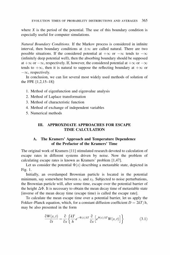
Let us consider the potential �ðxÞ describing a metastable state, depicted in

Fig. 1.

Initially, an overdamped Brownian particle is located in the potential

minimum, say somewhere between x1 and x2. Subjected to noise perturbations,

the Brownian particle will, after some time, escape over the potential barrier of

the height ��. It is necessary to obtain the mean decay time of metastable state

[inverse of the mean decay time (escape time) is called the escape rate].

To calculate the mean escape time over a potential barrier, let us apply the

Fokker–Planck equation, which, for a constant diffusion coefficient D ¼ 2kT=h,may be also presented in the form

qWðx; tÞqt

¼ qqx

kT

he��ðxÞ=kT

qqx

e�ðxÞ=kTWðx; tÞh i� �

ð3:1Þ


where we substituted aðxÞ ¼ �d�ðxÞhdx

, where k is the Boltzmann constant, T is the

temperature, and h is viscosity.

Let us consider the case when the diffusion coefficient is small, or, more

precisely, when the barrier height �� is much larger than kT . As it turns out,

one can obtain an analytic expression for the mean escape time in this limiting

case, since then the probability current G over the barrier top near xmax is very

small, so the probability density Wðx; tÞ almost does not vary in time,

representing quasi-stationary distribution. For this quasi-stationary state the

small probability current G must be approximately independent of coordinate x

and can be presented in the form

G ¼ � kT

he��ðxÞ=kT

qqx

e�ðxÞ=kTWðx; tÞh i� �

ð3:2Þ

Integrating (3.2) between xmin and d, we obtain

G

ðdxmin

e�ðxÞ=kT dx ¼ kT

he�ðxminÞ=kTWðxmin; tÞ � e�ðdÞ=kTWðd; tÞh i

ð3:3Þ

or if we assume that at x ¼ d the probability density is nearly zero (particles may

for instance be taken away that corresponds to absorbing boundary), we can

express the probability current by the probability density at x ¼ xmin, that is,

G ¼ kT

he�ðxminÞ=kTWðxmin; tÞ=

ðdxmin

e�ðxÞ=kT dx ð3:4Þ

Figure 1. Potential describing me-

tastable state.


If the barrier is high, the probability density near xmin will be given approxi-

mately by the stationary distribution:

Wðx; tÞ Wðxmin; tÞe� �ðxÞ��ðxminÞ½ �=kT ð3:5Þ

The probability P to find the particle near xmin is

P ¼ðx2x1

Wðx; tÞ dx Wðxmin; tÞe�ðxminÞ=kTðx2x1

e��ðxÞ=kT dx ð3:6Þ

If kT is small, the probability density becomes very small for x values

appreciably different from xmin, which means that x1 and x2 values need not be

specified in detail.

The escape time is introduced as the probability P divided by the probability

current G. Then, using (3.4) and (3.6), we can obtain the following expression

for the escape time:

t ¼ h

kT

ðx2x1

e��ðxÞ=kT dxðdxmin

e�ðxÞ=kT dx ð3:7Þ

Whereas the main contribution to the first integral stems from the region around

xmin, the main contribution to the second integral stems from the region around

xmax. We therefore expand�ðxÞ for the first and the second integrals according to

�ðxÞ �ðxminÞ þ 1

2�00ðxminÞðx� xminÞ2 ð3:8Þ

�ðxÞ �ðxmaxÞ � 1

2j�00ðxmaxÞjðx� xmaxÞ2 ð3:9Þ

We may then extend the integration boundaries in both integrals to 1 and thus

obtain the well-known Kramers’ escape time:

t ¼ 2phffiffiffiffiffiffiffiffiffiffiffiffiffiffiffiffiffiffiffiffiffiffiffiffiffiffiffiffiffiffiffiffiffiffiffiffiffi�00ðxminÞj�00ðxmaxÞj

p e��=kT ð3:10Þ

where�� ¼ �ðxmaxÞ � �ðxminÞ. As shown by Edholm and Leimar [48], one can

improve (3.10) by calculating the integrals (3.7) more accurately—for example,

by using the expansion of the potential in (3.8) and (3.9) up to the fourth-order

term. One can ask the question: What if the considered potential is such that

either �00ðxmaxÞ ¼ 0 or �00ðxminÞ ¼ 0? You may see that Kramers’ formula (3.10)

does not work in this case. This difficulty may be easily overcome because we

know how Kramers’ formula has been derived: We may substitute the required


potential into integrals in (3.7) and derive another formula, similar to Kramers’

formula:

t ¼ t0ðkTÞe��=kT ð3:11Þwhere the prefactor t0ðkTÞ is a function of temperature and reflects particular

shape of the potential. For example, one may easily obtain this formula for a

piecewise potential of the fourth order. Formula (3.11) for t0ðkTÞ ¼ const is also

known as the Arrhenius law.

Influence of the shape of potential well and barrier on escape times was

studied in detail in paper by Agudov and Malakhov [49].

In Table I, the temperature dependencies of prefactor t0ðkTÞ for potentialbarriers and wells of different shape are shown in the limiting case of small

temperature (note, that jxj1 means a rectangular potential profile). For the

considered functions �bðxÞ and �tðxÞ the dependence t0ðkTÞ vary from

t0 � ðkTÞ3 to t0 � ðkTÞ�1. The functions �bðxÞ and �tðxÞ are, respectively,potentials at the bottom of the well and the top of the barrier. As follows from

Table I, the Arrhenius law (3.11) [i.e. t0ðkTÞ ¼ const] occurs only for such

forms of potential barrier and well that 1=pþ 1=q ¼ 1. This will be the case for

a parabolic well and a barrier ( p ¼ 2, q ¼ 2), and also for a flat well ( p ¼ 1)

and a triangle barrier (q ¼ 1), and, vice versa, for a triangle well ( p ¼ 1) and a

flat barrier (q ¼ 1).

So, if one will compare the temperature dependence of the experimentally

obtained escape times of some unknown system with the temperature

dependence of Kramers’ time presented in Table I, one can make conclusions

about potential profile that describes the system.

B. Eigenvalues as Transition Rates

Another widely used approximate approach for obtaining transition rates is the

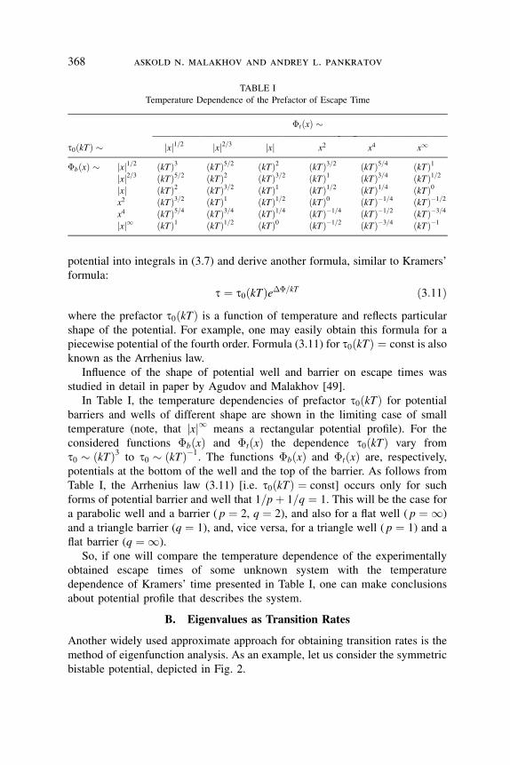
method of eigenfunction analysis. As an example, let us consider the symmetric

bistable potential, depicted in Fig. 2.

TABLE I

Temperature Dependence of the Prefactor of Escape Time

�tðxÞ �————————————————————————————————

t0ðkTÞ � jxj1=2 jxj2=3 jxj x2 x4 x1

�bðxÞ � jxj1=2 ðkTÞ3 ðkTÞ5=2 ðkTÞ2 ðkTÞ3=2 ðkTÞ5=4 ðkTÞ1jxj2=3 ðkTÞ5=2 ðkTÞ2 ðkTÞ3=2 ðkTÞ1 ðkTÞ3=4 ðkTÞ1=2jxj ðkTÞ2 ðkTÞ3=2 ðkTÞ1 ðkTÞ1=2 ðkTÞ1=4 ðkTÞ0x2 ðkTÞ3=2 ðkTÞ1 ðkTÞ1=2 ðkTÞ0 ðkTÞ�1=4 ðkTÞ�1=2x4 ðkTÞ5=4 ðkTÞ3=4 ðkTÞ1=4 ðkTÞ�1=4 ðkTÞ�1=2 ðkTÞ�3=4jxj1 ðkTÞ1 ðkTÞ1=2 ðkTÞ0 ðkTÞ�1=2 ðkTÞ�3=4 ðkTÞ�1


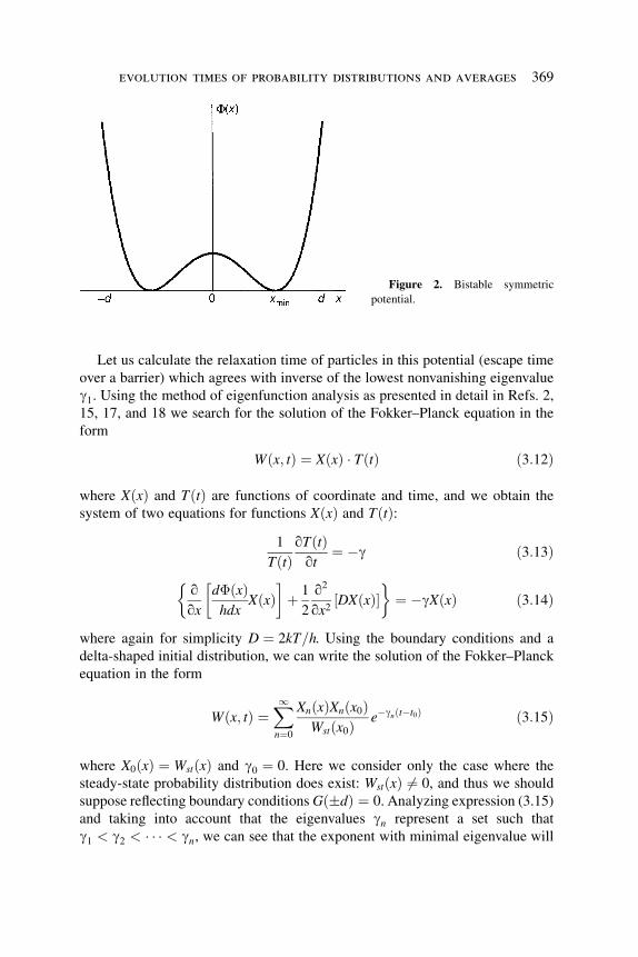
Let us calculate the relaxation time of particles in this potential (escape time

over a barrier) which agrees with inverse of the lowest nonvanishing eigenvalue

g1. Using the method of eigenfunction analysis as presented in detail in Refs. 2,

15, 17, and 18 we search for the solution of the Fokker–Planck equation in the

form

Wðx; tÞ ¼ XðxÞ � TðtÞ ð3:12Þ

where XðxÞ and TðtÞ are functions of coordinate and time, and we obtain the

system of two equations for functions XðxÞ and TðtÞ:1

TðtÞqTðtÞqt¼ �g ð3:13Þ

qqx

d�ðxÞhdx

XðxÞ� �

þ 1

2

q2

qx2DXðxÞ½ �

� �¼ �gXðxÞ ð3:14Þ

where again for simplicity D ¼ 2kT=h. Using the boundary conditions and a

delta-shaped initial distribution, we can write the solution of the Fokker–Planck

equation in the form

Wðx; tÞ ¼X1n¼0

XnðxÞXnðx0ÞWstðx0Þ e�gnðt�t0Þ ð3:15Þ

where X0ðxÞ ¼ WstðxÞ and g0 ¼ 0. Here we consider only the case where the

steady-state probability distribution does exist: WstðxÞ 6¼ 0, and thus we should

suppose reflecting boundary conditionsGðdÞ ¼ 0. Analyzing expression (3.15)

and taking into account that the eigenvalues gn represent a set such that

g1 < g2 < � � � < gn, we can see that the exponent with minimal eigenvalue will

Figure 2. Bistable symmetric

potential.


decay slower than the others and will thus reflect the largest timescale of decay

which equals the inversed minimal nonzero eigenvalue.

So, Eq. (3.14) with boundary conditions is the equation for eigenfunction

XnðxÞ of the nth order. For X0ðxÞ, Eq. (3.14) will be an equation for stationary

probability distribution with zero eigenvalue g0 ¼ 0, and for X1ðxÞ the equationwill have the following form:

qqx

kT

he��ðxÞ=kT

qqx

e�ðxÞ=kTX1ðxÞh i� �

¼ �g1X1ðxÞ ð3:16Þ

Integrating Eq. (3.16) and taking into account the reflecting boundary conditions

(probability current is equal to zero at the points d), we getkT

h

qqx

e�ðxÞ=kTX1ðxÞ ¼ �g1e�ðxÞ=kTðdx

X1ðzÞ dz ð3:17Þ

Integrating this equation once again, the following integral equation for

eigenfunction X1ðxÞ may be obtained:

X1ðxÞ ¼ e��ðxÞ=kT e�ðdÞ=kTX1ðdÞ � hg1kT

ðdx

e�ðyÞ=kT dyðdy

X1ðzÞ dz� �

ð3:18Þ

The eigenfunction X1ðxÞ belonging to the lowest nonvanishing eigenvalue must

be an odd function for the bistable potential, that is, X1ð0Þ ¼ 0. The integral

equation (3.18) together with reflecting boundary conditions determine the

eigenfunction X1ðxÞ and the eigenvalue g1. We may apply an iteration procedure

that is based on the assumption that the noise intensity is small compared to the

barrier height (this iteration procedure is described in the book by Risken [2]),

and we obtain the following expression for the required eigenvalue in the first-

order approximation:

g1 ¼ ðkT=hÞðd0

e�ðyÞ=kT dyðdy

e��ðzÞ=kT dz�

ð3:19Þ

For a small noise intensity, the double integral may be evaluated analytically and

finally we get the following expression for the escape time (inverse of the

eigenvalue g1) of the considered bistable potential:

tb ¼ phffiffiffiffiffiffiffiffiffiffiffiffiffiffiffiffiffiffiffiffiffiffiffiffiffiffiffiffiffiffiffiffi�00ðxminÞj�00ð0Þj

p e��=kT ð3:20Þ

The obtained escape time tb for the bistable potential is two times smaller than

the Kramers’ time (3.10): Because we have considered transition over the barrier

top x ¼ 0, we have obtained only a half.


IV. THE FIRST PASSAGE TIME APPROACH

The first approach to obtain exact time characteristics of Markov processes with

nonlinear drift coefficients was proposed in 1933 by Pontryagin, Andronov, and

Vitt [19]. This approach allows one to obtain exact values of moments of the

first passage time for arbitrary time constant potentials and arbitrary noise

intensity; moreover, the diffusion coefficient may be nonlinear function of

coordinate. The only disadvantage of this method is that it requires an artificial

introducing of absorbing boundaries, which change the process of diffusion in

real smooth potentials.

A. Probability to Reach a Boundary by One-DimensionalMarkov Processes

Let continuous one-dimensional Markov process xðtÞ at initial instant of time

t ¼ 0 have a fixed value xð0Þ ¼ x0 within the interval ðc; dÞ; that is, the initial

probability density is the delta function:

Wðx; 0Þ ¼ dðx� x0Þ; x0 2 ðc; dÞ

It is necessary to find the probability Qðt; x0Þ that a random process, having

initial value x0, will reach during the time t > 0 the boundaries of the interval

(c; d); that is, it will reach either boundary c or d: Qðt; x0Þ ¼Ð c�1Wðx; tÞ dxþÐþ1

dWðx; tÞ dx.

Instead of the probability to reach boundaries, one can be interested in the

probability

Pðt; x0Þ ¼ 1� Qðt; x0Þ

of nonreaching the boundaries c and d by Markov process, having initial value

x0. In other words,

Pðt; x0Þ ¼ Pfc < xðtÞ < d; 0 < t < Tg; x0 2 ðc; dÞ

where T ¼ Tðc; x0; dÞ is a random instant of the first passage time of boundaries

c or d.

We will not present here how to derive the first Pontryagin’s equation for the

probability Qðt; x0Þ or Pðt; x0Þ. The interested reader can see it in Ref. 19 or in

Refs. 15 and 18. We only mention that the first Pontryagin’s equation may be

obtained either via transformation of the backward Kolmogorov equation (2.7)

or by simple decomposition of the probability Pðt; x0Þ into Taylor expansion in

the vicinity of x0 at different moments t and t þ t, some transformations and

limiting transition to t! 0 [18].


The first Pontryagin’s equation looks like

qQðt; x0Þqt

¼ aðx0Þ qQðt; x0Þqx0þ Dðx0Þ

2

q2Qðt; x0Þqx02

ð4:1Þ

Let us point out the initial and boundary conditions of Eq. (4.1). It is obvious that

for all x0 2 ðc; dÞ the probability to reach boundary at t ¼ 0 is equal to zero:

Qð0; x0Þ ¼ 0; c < x0 < d ð4:2Þ

At the boundaries of the interval (i.e., for x0 ¼ c and x0 ¼ d ) the probability to

reach boundaries for any instant of time t is equal to unity:

Qðt; cÞ ¼ Qðt; dÞ ¼ 1 ð4:3Þ

This means that for x0 ¼ c, x0 ¼ d the boundary will be surely reached already at

t ¼ 0. Besides these conditions, usually one more condition must be fulfilled:

limt!1Qðt; x0Þ ¼ 1; c � x0 � d

expressing the fact that the probability to pass boundaries somewhen for a long

enough time is equal to unity.

The compulsory fulfillment of conditions (4.2) and (4.3) physically follows

from the fact that a one-dimensional Markov process is nondifferentiable; that

is, the derivative of Markov process has an infinite variance (instantaneous

speed is an infinitely high). However, the particle with the probability equals

unity drifts for the finite time to the finite distance. That is why the particle

velocity changes its sign during the time, and the motion occurs in an opposite

directions. If the particle is located at some finite distance from the boundary, it

cannot reach the boundary in a trice—the condition (4.2). On the contrary, if the

particle is located near a boundary, then it necessarily crosses the boundary—

the condition (4.3).

Let us mention that we may analogically solve the tasks regarding the

probability to cross either only the left boundary c or the right one d or

regarding the probability to not leave the considered interval ½c; d�. In this case,

Eq. (4.1) is valid, and only boundary conditions should be changed.

Also, one can be interested in the probability of reaching the boundary by a

Markov process, having random initial distribution. In this case, one should first

solve the task with the fixed initial value x0; and after that, averaging for all

possible values of x0 should be performed. If an initial value x0 is distributed in

the interval ðc1; d1Þ � ðc; dÞ with the probability W0ðx0Þ, then, following the

theorem about the sum of probabilities, the complete probability to reach


boundaries c and d is defined by the expression

QðtÞ ¼ðdc

Qðt; x0ÞW0ðx0Þ dx0 þ Pfc1 < x0 < c; t ¼ 0gþ Pfd < x0 < d1; t ¼ 0g ð4:4Þ

B. Moments of the First Passage Time

One can obtain an exact analytic solution to the first Pontryagin equation only in

a few simple cases. That is why in practice one is restricted by the calculation of

moments of the first passage time of absorbing boundaries, and, in particular, by

the mean and the variance of the first passage time.

If the probability density wTðt; x0Þ of the first passage time of boundaries c

and d exists, then by the definition [18] we obtain

wTðt; x0Þ ¼ qqtQðt; x0Þ ¼ � q

qtPðt; x0Þ ð4:5Þ

Taking a derivative from Eq. (4.1), we note that wTðt; x0Þ fulfills the following

equation:

qwTðt; x0Þqt

¼ aðx0Þ qwTðt; x0Þqx0

þ Dðx0Þ2

q2wTðt; x0Þqx02

ð4:6Þ

with initial and boundary conditions

wTð0; x0Þ ¼ 0; c < x0 < d

wTðt; cÞ ¼ wTðt; dÞ ¼ dðtÞ ð4:7Þ

for the case of both absorbing boundaries and

wTðt; dÞ ¼ dðtÞ; qwTðt; x0Þqx0

x0¼c¼ 0 ð4:8Þ

for the case of one absorbing (at the point d) and one reflecting (at the point c)

boundaries.

The task to obtain the solution to Eq. (4.6) with the above-mentioned initial

and boundary conditions is mathematically quite difficult even for simplest

potentials �ðx0Þ.Moments of the first passage time may be expressed from the probability

density wTðt; x0Þ as

Tn ¼ Tnðc; x0; dÞ ¼ð10

tnwTðt; x0Þ dt; n ¼ 1; 2; 3; . . . ð4:9Þ


Multiplying both sides of Eq. (4.6) by ei�t and integrating it for t going from 0 to

1, we obtain the following differential equation for the characteristic function

�ði�; x0Þ:

�i��ði�; x0Þ ¼ aðx0Þ q�ði�; x0Þqx0þ Dðx0Þ

2

q2�ði�; x0Þqx02

ð4:10Þ

where �ði�; x0Þ ¼Ð10

ei�twTðt; x0Þ dt.Equation (4.10) allows to find one-dimensional moments of the first passage

time. For this purpose let us use the well-known representation of the

characteristic function as the set of moments:

�ði�; x0Þ ¼ 1þX1n¼1

ði�Þnn!

Tnðc; x0; dÞ ð4:11Þ

Substituting (4.11) and its derivatives into (4.10) and equating terms of the same

order of i�, we obtain the chain of linear differential equations of the second

order with variable coefficients:

Dðx0Þ2

d2Tnðc; x0; dÞdx02

þ aðx0Þ dTnðc; x0; dÞdx0

¼ �n � Tn�1ðc; x0; dÞ ð4:12Þ

Equations (4.11) allow us to sequentially find moments of the first passage time

for n ¼ 1; 2; 3; . . . (T0 ¼ 1). These equations should be solved at the correspond-

ing boundary conditions, and by physical implication all moments Tnðc; x0; dÞmust have nonnegative values, Tnðc; x0; dÞ � 0.

Boundary conditions for Eq. (4.12) may be obtained from the corresponding

boundary conditions (4.7) and (4.8) of Eqs. (4.1) and (4.6). If boundaries c and d

are absorbing, we obtain the following from Eq. (4.7):

Tðc; c; dÞ ¼ Tðc; d; dÞ ¼ 0 ð4:13ÞIf one boundary, say c, is reflecting, then one can obtain the following from

Eq. (4.8):

Tðc; d; dÞ ¼ 0;qTðc; x0; dÞ

qx0

x0¼c¼ 0 ð4:14Þ

If we start solving Eq. (4.12) from n ¼ 1, then further moments Tnðc; x0; dÞ willbe expressed from previous moments Tmðc; x0; dÞ. In particular, for n ¼ 1; 2 we

obtain

Dðx0Þ2

d2T1ðc; x0; dÞdx02

þ aðx0Þ dT1ðc; x0; dÞdx0

þ 1 ¼ 0 ð4:15ÞDðx0Þ2

d2T2ðc; x0; dÞdx02

þ aðx0Þ dT2ðc; x0; dÞdx0

þ 2T1ðc; x0; dÞ ¼ 0 ð4:16Þ


Equation (4.15) was first obtained by Pontryagin and is called the second

Pontryagin equation.

The system of equations (4.12) may be easily solved. Indeed, making

substitution Z ¼ dTnðc; x0; dÞ=dx0 each equation may be transformed in the

first-order differential equation:

Dðx0Þ2

dZ

dx0þ aðx0ÞZ ¼ �n � Tn�1ðc; x0; dÞ ð4:17Þ

The solution of (4.17) may be written by quadratures:

Zðx0Þ ¼ dTnðc; x0; dÞdx0

¼ ejðx0Þ A�ðx0c

2nTn�1ðc; y; dÞDðyÞ e�jðyÞ dy

� �ð4:18Þ

where jðyÞ ¼ R 2aðyÞDðyÞ dy and A is an arbitrary constant, determined from

boundary conditions.

When one boundary is reflecting (e.g., c) and another one is absorbing

(e.g., d), then from (4.18) and boundary conditions (4.14) we obtain

Tnðc; x0; dÞ ¼ 2n

ðdx0

ejðxÞðxc

Tn�1ðc; y; dÞDðyÞ e�jðyÞ dy dx ð4:19Þ

Because dTnðc; x0; dÞ=dx0 < 0 for any c < x0 < d and dTnðc; x0; dÞ=dx0 ¼ 0 for

x0 ¼ c, and, as follows from (4.12), d2Tnðc; x0; dÞ=dx20 < 0 for x0 ¼ c, the

maximal value of the function Tnðc; x0; dÞ is reached at x0 ¼ c.

For the case when both boundaries are absorbing, the required moments of

the first passage time have more complicated form [18].

When the initial probability distribution is not a delta function, but some

arbitrary function W0ðx0Þ where x0 2 ðc; dÞ, then it is possible to calculate

moments of the first passage time, averaged over initial probability distribution:

Tnðc; dÞ ¼ðdc

Tnðc; x0; dÞW0ðx0Þ dx0 ð4:20Þ

We note that recently the equivalence between the MFPT and Kramers’ time was

demonstrated in Ref. 50.

V. GENERALIZATIONS OF THE FIRST PASSAGETIME APPROACH

A. Moments of Transition Time

As discussed in the previous section, the first passage time approach requires an

artificial introduction of absorbing boundaries; therefore, the steady-state


probability distribution in such systems does not exist, because eventually all

particles will be absorbed by boundaries. But in the large number of real

systems the steady-state distributions do exist, and in experiments there are

usually measured stationary processes; thus, different steady-state character-

istics, such as correlation functions, spectra, and different averages, are of

interest.

The idea of calculating the characteristic timescale of the observable

evolution as an integral under its curve (when the characteristic timescale is

taken as the length of the rectangle with the equal square) was adopted a long

time ago for calculation of correlation times and width of spectral densities (see,

e.g., Ref. 51). This allowed to obtain analytic expressions of linewidths [51] of

different types of oscillators that were in general not described by the Fokker–

Planck equation. Later, this definition of timescales of different observables was

widely used in the literature [5,6,14,24,30–41,52,53]. In the following we will

refer to any such defined characteristic timescale as ‘‘integral relaxation time’’

[see Refs. 5 and 6], but considering concrete examples we will also specify the

relation to the concrete observable (e.g., the correlation time).

However, mathematical evidence of such a definition of characteristic

timescale has been understood only recently in connection with optimal

estimates [54]. As an example we will consider evolution of the probability, but

the consideration may be performed for any observable. We will speak about the

transition time implying that it describes change of the evolution of the

transition probability from one state to another one.

The Transition Probability. Suppose we have a Brownian particle located at an

initial instant of time at the point x0, which corresponds to initial delta-shaped

probability distribution. It is necessary to find the probability Qc;dðt; x0Þ ¼Qðt; x0Þ of transition of the Brownian particle from the point c � x0 � d outside

of the considered interval (c; d) during the time t > 0 : Qðt; x0Þ ¼Ð c�1Wðx; tÞ dxþ Ðþ1

dWðx; tÞ dx. The considered transition probability Qðt; x0Þ

is different from the well-known probability to pass an absorbing boundary.

Here we suppose that c and d are arbitrary chosen points of an arbitrary

potential profile �ðxÞ, and boundary conditions at these points may be arbitrary:

Wðc; tÞ � 0, Wðd; tÞ � 0.

The main distinction between the transition probability and the probability to

pass the absorbing boundary is the possibility for a Brownian particle to come

back in the considered interval (c; d) after crossing boundary points (see, e.g.,

Ref. 55). This possibility may lead to a situation where despite the fact that a

Brownian particle has already crossed points c or d, at the time t!1 this

particle may be located within the interval (c; d). Thus, the set of transition

events may be not complete; that is, at the time t!1 the probability Qðt; x0Þmay tend to the constant, smaller than unity: lim

t!1Qðt; x0Þ < 1, as in the case


where there is a steady-state distribution for the probability density

limt!1Wðx; tÞ ¼ WstðxÞ 6¼ 0. Alternatively, one can be interested in the probability

of a Brownian particle to be found at the moment t in the considered interval

(c; d) Pðt; x0Þ ¼ 1� Qðt; x0Þ. In the following, for simplicity we will refer to

Qðt; x0Þ as decay probability and will refer to Pðt; x0Þ as survival probability.

Moments of Transition Time. Consider the probability Qðt; x0Þ of a Brownian

particle, located at the point x0 within the interval (c; d), to be at the time t > 0

outside of the considered interval. We can decompose this probability to the set

of moments. On the other hand, if we know all moments, we can in some cases

construct a probability as the set of moments. Thus, analogically to moments of

the first passage time we can introduce moments of transition time #nðc; x0; dÞtaking into account that the set of transition events may be not complete, that is,

limt!1Qðt; x0Þ < 1:

#nðc; x0; dÞ ¼ tnh i ¼Ð10

tnqQðt;x0Þ

qt dtÐ10

qQðt;x0Þqt dt

¼Ð10

tnqQðt;x0Þ

qt dt

Qð1; x0Þ � Qð0; x0Þ ð5:1Þ

Here we can formally denote the derivative of the probability divided by the

factor of normalization as wtðt; x0Þ and thus introduce the probability density of

transition time wc;dðt; x0Þ ¼ wtðt; x0Þ in the following way:

wtðt; x0Þ ¼ qQðt; x0Þqt

1

½Qð1; x0Þ � Qð0; x0Þ� ð5:2Þ

It is easy to check that the normalization condition is satisfied at such a definition,Ð10

wtðt; x0Þ dt ¼ 1. The condition of nonnegativity of the probability density

wtðt; x0Þ � 0 is, actually, the monotonic condition of the probability Qðt; x0Þ. Inthe case where c and d are absorbing boundaries the probability density of

transition time coincides with the probability density of the first passage time

wTðt; x0Þ:

wTðt; x0Þ ¼ qQðt; x0Þqt

ð5:3Þ

Here we distinguish wtðt; x0Þ and wTðt; x0Þ by different indexes t and T to note

again that there are two different functions and wtðt; x0Þ ¼ wTðt; x0Þ in the case

of absorbing boundaries only. In this context, the moments of the FPT are

Tnðc; x0; dÞ ¼ htni ¼ð10

tnqQðt; x0Þ

qtdt ¼

ð10

tnwTðt; x0Þ dt


Integrating (5.1) by parts, one can obtain the expression for the mean transition

time (MTT) #1ðc; x0; dÞ ¼ th i:

#1ðc; x0; dÞ ¼Ð10½Qð1; x0Þ � Qðt; x0Þ� dtQð1; x0Þ � Qð0; x0Þ ð5:4Þ

This definition completely coincides with the characteristic time of the probabi-

lity evolution introduced in Ref. 32 from the geometrical consideration, when the

characteristic scale of the evolution time was defined as the length of rectangle

with the equal square, and the same definition was later used in Refs. 33–35.

Similar ideology for the definition of the mean transition time was used in

Ref. 30. Analogically to the MTT (5.4), the mean square #2ðc; x0; dÞ ¼ ht2i ofthe transition time may also be defined as

#2ðc; x0; dÞ ¼ 2

Ð10

Ð1t½Qð1; x0Þ � Qðt; x0Þ� dt

� �dt

Qð1; x0Þ � Qð0; x0Þ ð5:5Þ

Note that previously known time characteristics, such as moments of FPT, decay

time of metastable state, or relaxation time to steady state, follow from moments

of transition time if the concrete potential is assumed: a potential with an

absorbing boundary, a potential describing a metastable state or a potential

within which a nonzero steady-state distribution may exist, respectively. Besides,

such a general representation of moments #nðc; x0; dÞ (5.1) gives us an oppor-

tunity to apply the approach proposed by Malakhov [34,35] for obtaining the

mean transition time and easily extend it to obtain any moments of transition

time in arbitrary potentials, so #nðc; x0; dÞ may be expressed by quadratures as it

is known for moments of FPT.

Alternatively, the definition of the mean transition time (5.4) may be

obtained on the basis of consideration of optimal estimates [54]. Let us define

the transition time # as the interval between moments of initial state of the

system and abrupt change of the function, approximating the evolution of its

probability Qðt; x0Þ with minimal error. As an approximation consider the

following function: cðt; x0; #Þ ¼ a0ðx0Þ þ a1ðx0Þ½1ðtÞ � 1ðt � #ðx0ÞÞ�. In the

following we will drop an argument of a0, a1, and the relaxation time #,assuming their dependence on coordinates of the considered interval c and d and

on initial coordinate x0. Optimal values of parameters of such approximating

function satisfy the condition of minimum of functional:

U ¼ðtN0

Qðt; x0Þ � cðt; x0; #Þ½ �2 dt ð5:6Þ

where tN is the observation time of the process. As it is known, a necessary

condition of extremum of parameters a0, a1, and # has the form

qUqa0¼ 0;

qUqa1¼ 0;

qUq#¼ 0 ð5:7Þ


It follows from the first condition thatðtN0

Qðt; x0Þ � a0 � a1½1ðtÞ � 1ðt � #Þ�f g dt ¼ 0

Transform this condition to the formðtN0

Qðt; x0Þ dt ¼ a0tN þ a1# ð5:8Þ

The condition of minimum of functional U on # may be written as

Qð#; x0Þ ¼ a0 þ a1=2 ð5:9Þ

Analogically, the condition of minimum of functional U on a1 isð#0

Qðt; x0Þ dt ¼ ða0 þ a1Þ# ð5:10Þ

The presented estimate is nonlinear, but this does not lead to significant troubles

in processing the results of experiments. An increase of the observation time tNallows us to adjust values of estimates, and slight changes of amplitudes a0 and

a1 and a shift of the moment of abrupt change # of the approximating function

are observed.

When considering analytic description, asymptotically optimal estimates are

of importance. Asymptotically optimal estimates assume infinite duration of the

observation process for tN !1. For these estimates an additional condition for

amplitude of a leap is superimposed: The amplitude is assumed to be equal to

the difference between asymptotic and initial values of approximating function

a1 ¼ Qð0; x0Þ � Qð1; x0Þ. The only moment of abrupt change of the function

should be determined. In such an approach the required quantity may be

obtained by the solution of a system of linear equations and represents a linear

estimate of a parameter of the evolution of the process.

To get an analytical solution of the system of equations (5.8), (5.9), and

(5.10), let us consider them in the asymptotic case tN !1. Here we should

take into account that the limit of a0 for tN !1 is Qð1; x0Þ. In asymptotic

form for tN !1, Eq. (5.8) is

# ¼Ð10½Qð1; x0Þ � Qðt; x0Þ� dtQð1; x0Þ � Qð0; x0Þ ð5:11Þ

Therefore, we have again arrived at (5.4), which, as follows from the above, is an

asymptotically optimal estimate. From the expression (5.9), another well-known


asymptotically optimal estimate immediately follows:

Qð#; x0Þ ¼ ðQð0; x0Þ þ Qð1; x0ÞÞ=2 ð5:12Þbut this estimate gives much less analytic expressions than the previous one. It

should be noted, that asymptotically optimal estimates are correct only for

monotonic evolutions of observables.

In many practical cases the MTT is a more adequate characteristic than the

MFPT. As an example (for details see the end of Section V.E.5), if we consider

the decay of a metastable state as a transition over a barrier top and we compare

mean decay time obtained using the notion of integral relaxation time (case of a

smooth potential without absorbing boundary) and the MFPT of the absorbing

boundary located at the barrier top, we obtain a twofold difference between

these time characteristics even in the case of a high potential barrier in

comparison with the noise intensity (5.120). This is due to the fact that the

MFPT does not take into account the backward probability current and therefore

is sensitive to the location of an absorbing boundary. For the considered

situation, if we will move the boundary point down from the barrier top, the

MFPT will increase up to two times and tend to reach a value of the

corresponding mean decay time which is less sensitive to the location of

the boundary point over a barrier top. Such weak dependence of the mean decay

time from the location of the boundary point at the barrier top or further is

intuitively obvious: Much more time should be spent to reach the barrier top

(activated escape) than to move down from the barrier top (dynamic motion).

Another important example is noise delayed decay (NDD) of unstable states

(see below Fig. 4, case N without potential barrier). It was assumed before that

the fluctuations can only accelerate the decay of unstable states [56]. However,

in Refs. 57–69 it was found that there are systems that may drop out of these

rules. In particular, in the systems considered in Refs. 57–69 the fluctuations can

considerably increase the decay time of unstable and metastable states. This

effect may be studied via MFPT (see, e.g., Ref. 64), but this characteristic

significantly underestimates it [69]. As demonstrated in Ref. 69, the NDD

phenomenon appears due to the action of two mechanisms. One of them is

caused by the nonlinearity of the potential profile describing the unstable state

within the considered interval. This mechanism is responsible for the resonant

dependence of MFPT on the noise intensity. Another mechanism is caused by

inverse probability current directed into the considered interval. The latter

cannot be accounted for by the MFPT method. In Refs. 34 and 69, asymptotic

expressions of the decay time of unstable states were obtained for small noise

intensities, and it has been demonstrated that if the first derivative of the

potential is negative (for the potential oriented as depicted in Fig. 4),

the fluctuations acting in dynamic systems always increase the decay time of

the unstable state in the limit of a small noise intensity.


Finally, for additional support of the correctness and practical usefulness of

the above-presented definition of moments of transition time, we would like to

mention the duality of MTT and MFPT. If one considers the symmetric

potential, such that �ð�1Þ ¼ �ðþ1Þ ¼ þ1, and obtains moments of

transition time over the point of symmetry, one will see that they absolutely

coincide with the corresponding moments of the first passage time if the

absorbing boundary is located at the point of symmetry as well (this is what we

call ‘‘the principle of conformity’’ [70]). Therefore, it follows that the

probability density (5.2) coincides with the probability density of the first

passage time: wtðt; x0Þ ¼ wTðt; x0Þ, but one can easily ensure that it is so,

solving the FPE numerically. The proof of the principle of conformity is given

in the appendix.

In the forthcoming sections we will consider several methods that have been

used to derive different integral relaxation times for cases where both drift and

diffusion coefficients do not depend on time, ranging from the considered mean

transition time and to correlation times and time scales of evolution of different

averages.

B. The Effective Eigenvalue and Correlation Time

In this section we consider the notion of an effective eigenvalue and the

approach for calculation of correlation time by Risken and Jung [2,31]. A

similar approach has been used for the calculation of integral relaxation time of

magnetization by Garanin et al. [5,6].

Following Ref. 2 the correlation function of a stationary process KðtÞ may be

presented in the following form:

KðtÞ ¼ Kð0ÞX1n¼1

Vn expð�lnjtjÞ ð5:13Þ

where matrix elements Vn are positive and their sum is one (for details see Ref. 2,

Section 12.3):

X1n¼1

Vn ¼ 1

The required correlation function (5.13) may be approximated by the single

exponential function

KeffðtÞ ¼ K2 expð�leff jtjÞ; 1

leff¼X1n¼1

Vn

lnð5:14Þ


which has the same area and the same value at t ¼ 0 as the exact expression. The

same basic idea was used in Refs. 5 and 6 for the calculation of integral

relaxation times of magnetization. The behavior of leff was studied in Refs. 71

and 72.

The correlation time, given by 1=leff, may be calculated exactly in the

following way. Let us define the normalized correlation function of a stationary

process by

�ðtÞ ¼ KðtÞ=Kð0ÞKðtÞ ¼ h�rðxðt0ÞÞ�rðxðt0 þ tÞÞi ð5:15Þ

�rðxðt0ÞÞ ¼ rðxðt0ÞÞ � hri

The subtraction of the average hri guarantees that the normalized correlation

function �ðtÞ vanishes for large times. Obviously, �ðtÞ is normalized according

to �ð0Þ ¼ 1. A correlation time may be defined by

tc ¼ð10

�ðtÞ dt ð5:16Þ

For an exponential dependence we then have �ðtÞ ¼ expð�t=tcÞ. For the

considered one-dimensional Markov process the correlation time may be found

in the following way. Alternatively to (5.15) the correlation function may be

written in the form

KðtÞ ¼ð�rðxÞ ~Wðx; tÞ dx ð5:17Þ

where ~Wðx; tÞ obeys the FPE (2.6) with the initial condition

~Wðx; 0Þ ¼ �rðxÞWstðxÞ ð5:18Þ

where WstðxÞ ¼ NDðxÞ expf

R 2aðxÞDðxÞ dxg is the stationary probability distribution.

Introducing

rðxÞ ¼ð10

~Wðx; tÞ dt ð5:19Þ

Eq. (5.16) takes the form

tc ¼ 1

Kð0Þð1�1

�rðxÞrðxÞ dx ð5:20Þ


Due to initial condition (5.18), rðxÞ must obey

��rðxÞWstðxÞ ¼ � d

dxaðxÞ þ d2

dx2DðxÞ2

� �rðxÞ ð5:21Þ

This equation may be integrated leading to

rðxÞ ¼ WstðxÞðx�1

2f ðx0ÞDðx0ÞWstðx0Þ dx

0 ð5:22Þ

with f ðxÞ given by

f ðxÞ ¼ �ðx�1

�rðxÞWstðxÞ dx ð5:23Þ

Inserting (5.22) into (5.20) we find, after integration by parts, the following

analytical expression for the correlation time:

tc ¼ 1

Kð0Þð1�1

2f 2ðxÞDðxÞWstðxÞ dx ð5:24Þ

C. Generalized Moment Expansion for Relaxation Processes

To our knowledge, the first paper devoted to obtaining characteristic time scales

of different observables governed by the Fokker–Planck equation in systems

having steady states was written by Nadler and Schulten [30]. Their approach is

based on the generalized moment expansion of observables and, thus, called the

‘‘generalized moment approximation’’ (GMA).

The observables considered are of the type

MðtÞ ¼ðdc

ðdc

f ðxÞWðx; t j x0Þgðx0Þ dx0 dx ð5:25Þ

where Wðx; t j x0Þ is the transition probability density governed by the Fokker–

Planck equation

qWðx; tÞqt

¼ qqx

WstðxÞ qqxDðxÞ

2WstðxÞ� ��

ð5:26Þ

gðx0Þ is initial probability distribution and f ðxÞ is some test function that

monitors the distribution at the time t. The reflecting boundary conditions at

points c and d are supposed, which leads to the existence of steady-state

probability distribution WstðxÞ:

WstðxÞ ¼ C

DðxÞ expðxx0

2aðxÞDðxÞ dx

� �ð5:27Þ

where C is the normalization constant.


The observable has initial value Mð0Þ ¼ f ðxÞg0ðxÞih and relaxes asympto-

tically to Mð1Þ ¼ h f ðxÞihg0ðxÞi. Here g0ðxÞ ¼ gðxÞ=WstðxÞ. Because the time

development of MðtÞ is solely due to the relaxation process, one needs to

consider only �MðtÞ ¼ MðtÞ �Mð1Þ.The starting point of the generalized moment approximation (GMA) is the

Laplace transformation of an observable:

�MðsÞ ¼ð10

�MðtÞe�st dt ð5:28Þ

�MðsÞ may be expanded for low and high frequencies:

�MðsÞ �s!0

X1n¼0

m�ðnþ1Þð�sÞn ð5:29Þ

�MðsÞ �s!1X1n¼0

mnð�1=sÞn ð5:30Þ

where the expansion coefficients mn, the ‘‘generalized moments,’’ are given by

mn ¼ ð�1Þnðdc

gðxÞ ðLþðxÞÞnf gb f ðxÞ dx ð5:31Þ

where f gb denotes operation in a space of functions that obey the adjoint

reflecting boundary conditions, and LþðxÞ is the adjoint Fokker–Planck operator:

LþðxÞ ¼ � aðxÞ qqxþ DðxÞ q

2

qx2

� �ð5:32Þ

In view of expansions (5.29) and (5.30), we will refer to mn, n � 0, as the high-

frequency moments and to mn, n < 0, as the low-frequency moments. The

moment m0 is identical to the initial value �MðtÞ and assumes the simple form:

m0 ¼ f ðxÞg0ðxÞi � h f ðxÞihg0ðxÞih ð5:33ÞFor negative n (see Ref. 30), the following recurrent expressions for the moments

m�n may be obtained:

m�n ¼ðdc

4 dx

WstðxÞðxc

WstðyÞDðyÞ m�ðn�1ÞðyÞ dy

ðyc

WstðzÞDðzÞ ðg0ðzÞ � hg0ðzÞiÞ dz ð5:34Þ

where

m�nðxÞ ¼ C �ðxc

dy

WstðyÞðyc

2WstðzÞDðzÞ m�ðn�1ÞðzÞ dz ð5:35Þ


where C is an integration constant, chosen to satisfy the orthogonality property.

For n ¼ 1

m�1 ¼ðdc

4dx

WstðxÞðxc

WstðyÞDðyÞ ð f ðyÞ � h f ðyÞiÞ dy

ðyc

WstðzÞDðzÞ ðg0ðzÞ � hg0ðzÞiÞ dz

ð5:36Þholds. Moments with negative index, which account for the low-frequency

behavior of observables in relaxation processes, can be evaluated by means of

simple quadratures. Let us consider now how the moments mn may be employed

to approximate the observable �MðtÞ.We want to approximate �MðsÞ by a Pade approximant �mðsÞ. The

functional form of �mðsÞ should be such that the corresponding time-dependent

function �mðtÞ is a series of N exponentials describing the relation of �MðtÞ to�Mð1Þ ¼ 0. This implies that �mðsÞ is an ½N � 1;N�-Pade approximant that

can be written in the form

�mðsÞ ¼XNn¼1

an=ðln þ sÞ ð5:37Þ

or, correspondingly,

�mðtÞ ¼XNn¼1

an expð�lntÞ ð5:38Þ

The function �mðsÞ should describe the low- and high-frequency behavior of

�MðsÞ to a desired degree. We require that �mðsÞ reproduces Nh high- and

Nl low-frequency moments. Because�mðsÞ is determined by an even number of

constants an and ln, one needs to choose Nh þ Nl ¼ 2N. We refer to the resulting

description as the ðNh;NlÞ-generalized-moment approximation (GMA). The

description represents a two-sided Pade approximation. The moments determine

the parameters an and ln through the relations

XNn¼1

anlmn ¼ mm ð5:39Þ

where m ¼ �Nl;�Nl þ 1; . . . ;Nh � 1.

Algebraic solution of Eq. (5.39) is feasible only for N ¼ 1; 2. For N > 2 the

numerical solution of (5.39) is possible by means of an equivalent eigenvalue

problem (for references see Ref. 30).

The most simple GMA is the ð1; 1Þ approximation which reproduces the

moments m0 and m1. In this case, the relaxation of �MðtÞ is approximated by a

single exponential

�MðtÞ ¼ m0 expð�t=tÞ ð5:40Þ


where t ¼ m�1=m0 is the mean relaxation time. As has been demonstrated in

Ref. 30 for a particular example of rectangular barrierless potential well, this

simple one-exponential approximation is often satisfactory and describes the

required observables with a good precision. We should note that this is indeed so

as will be demonstrated below.

D. Differential Recurrence Relation and Floquet Approach

1. Differential Recurrence Relations

A quite different approach from all other presented in this review has been

recently proposed by Coffey [41]. This approach allows both the MFPT and the

integral relaxation time to be exactly calculated irrespective of the number of

degrees of freedom from the differential recurrence relations generated by the

Floquet representation of the FPE.

In order to achieve the most simple presentation of the calculations, we shall

restrict ourselves to a one-dimensional state space in the case of constant

diffusion coefficient D ¼ 2kT=h and consider the MFPT (the extension of the

method to a multidimensional state space is given in the Appendix of Ref. 41).

Thus the underlying probability density diffusion equation is again the Fokker–

Planck equation (2.6) that for the case of constant diffusion coefficient we

present in the form:

qWðx; tÞqt

¼ 1

B

qqx

djðxÞdx

Wðx; tÞ� �

þ q2Wðx; tÞqx2

� �ð5:41Þ

where B ¼ 2=D ¼ h=kT and jðxÞ ¼ �ðxÞ=kT is the dimensionless potential.

Furthermore, we shall suppose that �ðxÞ is the symmetric bistable potential

(rotator with two equivalent sites)

�ðxÞ ¼ U sin2ðxÞ ð5:42Þ

Because the solution of Eq. (5.41) must be periodic in x that is Wðxþ 2pÞ ¼WðxÞ, we may assume that it has the form of the Fourier series

Wðx; tÞ ¼X1p¼�1

apðtÞeipx ð5:43Þ

where for convenience (noting that the potential has minima at 0, p and a central

maximum at p=2) the range of x is taken as �p=2 < x < 3p=2.On substituting Eq. (5.43) into Eq. (5.41) we have, using the orthogonality

properties of the circular functions,

_apðtÞ þ p2

BapðtÞ ¼ sp

B½ap�2ðtÞ � apþ2ðtÞ� ð5:44Þ


where 2s ¼ U=kT . The differential-recurrence relation for a�pðtÞ is from

Eq. (5.44)

_a�pðtÞ þ p2

Ba�pðtÞ ¼ sp

B½a�ðp�2ÞðtÞ � a�ðpþ2ÞðtÞ� ð5:45Þ

which is useful in the calculation that follows because the Fourier coefficients of

the Fourier cosine and sine series, namely,

Wðx; tÞ ¼ f0

2þX1p¼1

fpðtÞcosðpxÞ þX1p¼1

gpðtÞsinðpxÞ ð5:46Þ

corresponding to the complex series (5.43) are by virtue of Eqs. (5.44) and (5.45)

f�pðtÞ ¼ fpðtÞ ¼ 1

p

ð3p=2�p=2

Wðx; tÞcosðpxÞ dx

g�pðtÞ ¼ �gpðtÞ ¼ � 1

p

ð3p=2�p=2

Wðx; tÞ sinðpxÞ dxð5:47Þ

Thus Eq. (5.44) need only be solved for positive p.

We also remark that Eq. (5.44) may be decomposed into separate sets of

equations for the odd and even apðtÞ which are decoupled from each other.

Essentially similar differential recurrence relations for a variety of relaxation

problems may be derived as described in Refs. 4, 36, and 73–76, where the

frequency response and correlation times were determined exactly using scalar

or matrix continued fraction methods. Our purpose now is to demonstrate how

such differential recurrence relations may be used to calculate mean first

passage times by referring to the particular case of Eq. (5.44).

2. Calculation of Mean First Passage Times from Differential

Recurrence Relations

In order to illustrate how the Floquet representation of the FPE, Eq. (5.44), may

be used to calculate first passage times, we first take the Laplace transform of

Eq. (5.41) for the probability density (Yðx; sÞ ¼ Ð10

Wðx; tÞe�st dt; apðsÞ ¼Ð10

apðtÞe�st dt) which for a delta function initial distribution at x0 becomes

d 2Yðx; sÞdx 2

þ d

dx

djðxÞdx

Yðx; sÞ� �

� sBYðx; sÞ ¼ �Bdðx� x0Þ ð5:48Þ

The corresponding Fourier coefficients satisfy the differential recurrence

relations

sapðsÞ � expð�ipx0Þ2p

¼ spB½ap�2ðsÞ � apþ2ðsÞ� ð5:49Þ


The use of the differential recurrence relations to calculate the mean first passage

time is based on the observation that if in Eq. (5.48) one ignores the term sYðx; sÞ(which is tantamount to assuming that the process is quasi-stationary, i.e., all

characteristic frequencies associated with it are very small), then one has

d 2Yðx; sÞdx 2

þ d

dx

djðxÞdx

Yðx; sÞ� �

¼ �Bdðx� x0Þ ð5:50Þ

which is precisely the differential equation given by Risken for the stationary

probability if at x0 a unit rate of probability is injected into the system;

integrating Eq. (5.50) from x0 � E to x0 þ E leads to Gðx0 þ EÞ � Gðx0 � EÞ ¼ 1,

where G is the probability current given by Eq. (2.11).

The mean first passage time at which the random variable xðtÞ specifying the

angular position of the rotator first leaves a domain L defined by the absorbing

boundaries x1 and x2 where Wðx; tjx0; 0Þ and consequently Yðx; s ¼ 0jx0Þ �Y ðx; x0Þ vanishes may now be calculated because [see Eq. (8.5) of Ref. 2]

Tðx0Þ ¼ðx2x1

Yðx; x0Þ dx ð5:51Þ

Here we are interested in escape out of the domain L specified by a single cycle of

the potential that is out of a domain of length p that is the domain of the well.

Because the bistable potential of Eq. (5.42) has a maximum at x ¼ p=2 and

minima at x ¼ 0, x ¼ p, it will be convenient to take our domain as the interval

�p=2 < x < p=2. Thus we will impose absorbing boundaries at x ¼ �p=2,x ¼ p=2. Next we shall impose a second condition that all particles are initially

located at the bottom of the potential well so that x0 ¼ 0. The first boundary

condition (absorbing barriers at �p=2, p=2) implies that only odd terms in p in

the Fourier series will contribute to YðxÞ. While the second ensures that only the

cosine terms in the series will contribute because there is a null set of initial

values for the sine terms. Hence

Tðx0Þ ¼ Tð0Þis given by

Tð0Þ ¼ðp=2�p=2

X1p¼0

f2pþ1ð0Þcosð2pþ 1Þx dx ð5:52Þ

and the MFPT to go from �p=2 to 3p=2 which is the escape time is

te ¼ 2Tð0Þ ¼ 4X1p¼0

ð�1Þp2pþ 1

f2pþ1ð0Þ ð5:53Þ


In the high barrier limit in this particular problem the inverse escape time is the

Kramers’ escape rate.

3. Calculation of t by a Continued Fraction Method

The differential recurrence relations for f2pþ1ðtÞ are [4,77]

_f2pþ1ðtÞ þ ð2pþ 1Þ2B

f2pþ1ðtÞ ¼ sð2pþ 1ÞB

½ f2p�1ðtÞ � f2pþ3ðtÞ� ð5:54Þ

the solution of which for f1ðsÞ is [77]

f1ðsÞ ¼ B

sBþ ð1� sÞ þ sS3ðsÞ

� f1ð0Þ þX1p¼1

ð�1Þp2pþ 1

f2pþ1ð0ÞYpk¼1

S2kþ1ðsÞ" #

ð5:55Þ

where the continued fraction SpðsÞ is

SpðsÞ ¼ sp

sBþ p2 þ spSpþ2ðsÞð5:56Þ

and successive fpðsÞ, p > 1, are determined from [4,77]

fp ¼ Spfp�2 þ qp ð5:57Þwhere

qp ¼ fpð0ÞB� spqpþ2sBþ p2 þ spSpþ2

ð5:58Þ

whence

f3ðsÞ ¼ BS3ðsÞsBþ ð1� sÞ þ sS3ðsÞ

f1ð0Þ þX1p¼1

ð�1Þp2pþ 1

f2pþ1ð0ÞYpk¼1

S2kþ1ðsÞ" #

� B

s

X1p¼1

ð�1Þp2pþ 1

f2pþ1ð0ÞYpk¼1

S2kþ1ðsÞ" #

ð5:59Þ

where of course the f2pþ1ð0Þ are the initial values of f2pþ1ðtÞ. Since x0 is not anend point in the domain of integration the initial values are

f2pþ1ð0Þ ¼ 1

pcosð2pþ 1Þx0 ¼ 1

pð5:60Þ


because we suppose that x0 ¼ 0. All f2pþ1ðsÞ can now be written down in the

manner of f1ðsÞ and f2ðsÞ using Eqs. (5.57) and (5.58), with the calculations beingmuch simpler than those of the correlation time in Ref. 77 on account of the

rather simple initial condition of Eq. (5.60). This is unnecessary, however, as we

shall demonstrate. First we recall that for the purpose of the calculation of

Yðx; x0Þ the relevant quantity is the s ¼ 0 value of f2pþ1. Furthermore, the s ¼ 0

value of the continued fraction S2kþ1ðsÞ is [77]

S2kþ1ð0Þ ¼ s=ð2k þ 1Þ1þ ½s=ð2k þ 1Þ�S2kþ3ð0Þ

ð5:61Þ

the solution of which, which is finite at s ¼ 0, is

S2kþ1ð0Þ ¼Ikþð1=2ÞðsÞIk�ð1=2ÞðsÞ ð5:62Þ

where Ikþð1=2ÞðsÞ are the modified Bessel functions of the first kind of order

k þ 12. Thus just as in Ref. 77, f1ð0Þ may be written as

f1ð0Þ ¼ B

2sðe2s � 1Þ

X1p¼0

ð�1Þp2pþ 1

1

pLpðsÞ ð5:63Þ

where the LpðsÞ satisfy the recurrence relation

Lp�1ðsÞ � Lpþ1ðsÞ ¼ 2pþ 1

sLpðsÞ

LpðsÞ ¼Ipþð1=2ÞðsÞIð1=2ÞðsÞ

ð5:64Þ

The leading term in Eq. (5.63) arises because

B

ð1� sÞ þ sS3ð0Þ¼ B

ð1� sÞ þ sðIð3=2ÞðsÞ=Ið1=2ÞðsÞÞ¼ B

2sðe2s � 1Þ ð5:65Þ

In like manner we have

f3ð0Þ ¼ BS3ð0Þð1� sÞ þ sS3ð0Þ

1

p

X1p¼0

ð�1Þp2pþ 1

LpðsÞ � B

sp

X1p¼1

ð�1Þp2pþ 1

LpðsÞ ð5:66Þ


The large s limit (high barrier limit, 2s ¼ U=kT) of both Eqs. (5.63) and (5.66)

is the same, namely,

f1ð0Þ ¼ f3ð0Þ B

2se2s

p

X1p¼0

ð�1Þp2pþ 1

¼ B

8se2s ð5:67Þ

by the properties of the Riemann zeta function [78] [Eq. (5.67)] because

lims!1LpðsÞ ¼ 1

and because the second term in Eq. (5.66) decays as s�1 for large s. One may

also deduce from Eqs. (5.57) and (5.58) that the behavior of all f2pþ1ð0Þ for larges is the same. Thus we may write down Yðx; x0Þ in the high barrier limit as

Yðx; 0Þ B

8se2sX1p¼1

cosð2pþ 1Þx ð5:68Þ

which with Eq. (5.52) yields the following for the MFPT from x ¼ 0 to x ¼ p=2or �p=2:

TMFPT B

8se2sX1p¼0

2ð�1Þp2pþ 1

p2

B

8se2s ð5:69Þ

The escape time te out of the well that is the domain �p=2 < x < p=2 is

te 2TMFPT p4

B

2se2s ð5:70Þ

in agreement with the results of the Kramers theory [Eq. (102) of Ref. 77] and the

asymptotic expression for the smallest nonvanishing eigenvalue [79]. Equiva-

lently, the escape time in this case is the MFPT from �p=2 to 3p=2. In the

opposite limit when the potential barrier is zero, Eq. (5.53) becomes (again using

the properties of the Riemann zeta and Langevin functions)

te ¼ p2B8

ð5:71Þ

in agreement with the predictions of the Einstein theory of the Brownian

movement as adapted to the calculation of MFPTs by Klein [80] and in contrast

to the zero barrier value of the correlation time which is B.

E. The Approach by Malakhov and Its Further Development

Another approach for computing the transition times had been proposed by

Malakhov [34,35]. This approach also utilizes the definition of the desired


timescale as integral relaxation time and is based on obtaining the solution of

the Laplace transformed FPE as a set with respect to small Laplace parameter s

and allows us to obtain a wide variety of temporal characteristics of Markov

processes with time constant drift and diffusion coefficients and for a wide

variety of boundary conditions ranging from natural to periodic.

In this section we will consider this approach in detail for different types of

potential profiles jðxÞ ¼ �ðxÞ=kT , and to avoid cumbersome calculations we

present the analysis for the constant diffusion coefficient D ¼ 2kT=h, but theresults, of course, may be easily generalized for any DðxÞ 6¼ 0.

1. Statement of the Problem

It is convenient to present the Fokker–Planck equation in the following dimen-

sionless form:

qWðx; tÞqt

¼ � qGðx; tÞqx

¼ 1

B

qqx

djðxÞdx

Wðx; tÞ� �

þ q2Wðx; tÞqx2

� �ð5:72Þ

where B ¼ 2=D ¼ h=kT ; Gðx; tÞ is the probability current, and jðxÞ ¼2�ðxÞ=hD ¼ �ðxÞ=kT is the dimensionless potential profile.

We suppose that at initial instant t ¼ 0 all Brownian particles are located at

the point x ¼ x0, which corresponds to the initial conditionWðx; 0Þ ¼ dðx� x0Þ.The initial delta-shaped probability distribution spreads with time, and its later

evolution strongly depends on the form of the potential profile jðxÞ. We shall

consider the problem for the three archetypal potential profiles that are sketched

in Figs. 3–5.

If a potential profile is of the type I (see Fig. 3) when jðxÞ goes to plus

infinity fast enough at x! 1, there is the steady-state probability distribution

Wðx;1Þ ¼ Ae�jðxÞ; A ¼ 1=

ðþ1�1

exp ½�jðxÞ� dx > 0 ð5:73Þ

In this case our aim is to determine the relaxation time � that is the timescale of

the probability density evolution from the initial Wðx; 0Þ to the final value

Wðx;1Þ for any x 6¼ x0. On the other hand we may consider the probability

Pðt; x0Þ ¼ PðtÞ ¼ðdc

Wðx; tÞ dx ð5:74Þ

in a given interval [c; d], which in the following we shall call the decision interval,and seek the relaxation time of this probability PðtÞwhich changes from the initial

value Pð0Þ ¼ Ð dcWðx; 0Þ dx to the final one Pð1Þ ¼ Ð d

cW ðx;1Þ dx. A potential


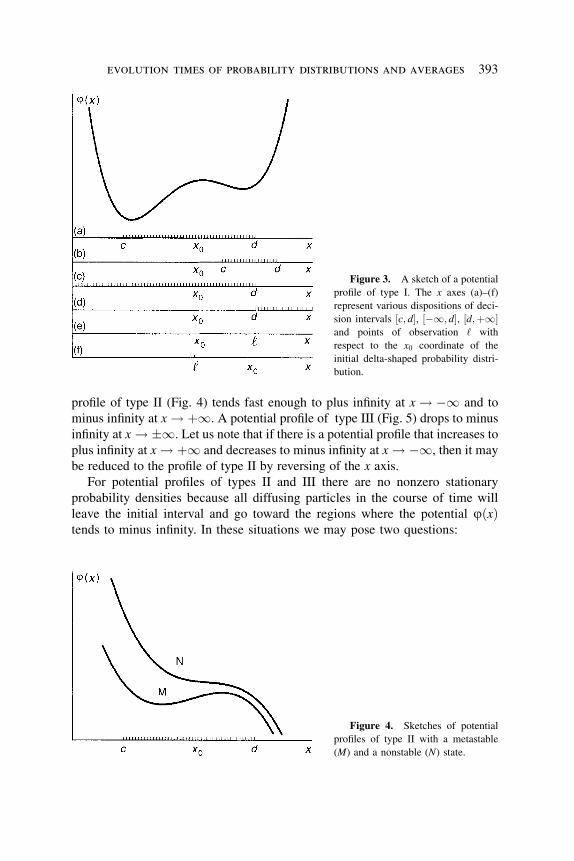
profile of type II (Fig. 4) tends fast enough to plus infinity at x! �1 and to

minus infinity at x! þ1. A potential profile of type III (Fig. 5) drops to minus

infinity at x! 1. Let us note that if there is a potential profile that increases to

plus infinity at x! þ1 and decreases to minus infinity at x! �1, then it may

be reduced to the profile of type II by reversing of the x axis.

For potential profiles of types II and III there are no nonzero stationary

probability densities because all diffusing particles in the course of time will

leave the initial interval and go toward the regions where the potential jðxÞtends to minus infinity. In these situations we may pose two questions:

Figure 3. A sketch of a potential

profile of type I. The x axes (a)–(f)

represent various dispositions of deci-

sion intervals ½c; d�, ½�1; d�, ½d;þ1�and points of observation ‘ with

respect to the x0 coordinate of the

initial delta-shaped probability distri-

bution.

Figure 4. Sketches of potential

profiles of type II with a metastable

(M) and a nonstable (N) state.


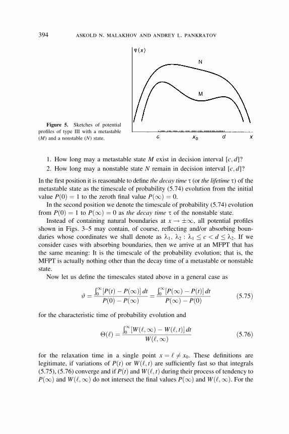
1. How long may a metastable state M exist in decision interval [c; d]?

2. How long may a nonstable state N remain in decision interval [c; d]?

In the first position it is reasonable to define the decay time t (or the lifetime t) of themetastable state as the timescale of probability (5.74) evolution from the initial

value Pð0Þ ¼ 1 to the zeroth final value Pð1Þ ¼ 0.

In the second position we denote the timescale of probability (5.74) evolution

from Pð0Þ ¼ 1 to Pð1Þ ¼ 0 as the decay time t of the nonstable state.

Instead of containing natural boundaries at x! 1, all potential profiles

shown in Figs. 3–5 may contain, of course, reflecting and/or absorbing boun-

daries whose coordinates we shall denote as l1; l2 : l1 � c < d � l2. If weconsider cases with absorbing boundaries, then we arrive at an MFPT that has

the same meaning: It is the timescale of the probability evolution; that is, the

MFPT is actually nothing other than the decay time of a metastable or nonstable

state.

Now let us define the timescales stated above in a general case as

# ¼Ð10½PðtÞ � Pð1Þ� dtPð0Þ � Pð1Þ ¼

Ð10½Pð1Þ � PðtÞ� dtPð1Þ � Pð0Þ ð5:75Þ

for the characteristic time of probability evolution and

�ð‘Þ ¼Ð10½Wð‘;1Þ �Wð‘; tÞ� dt

Wð‘;1Þ ð5:76Þ

for the relaxation time in a single point x ¼ ‘ 6¼ x0. These definitions are

legitimate, if variations of PðtÞ or Wð‘; tÞ are sufficiently fast so that integrals

(5.75), (5.76) converge and if PðtÞ andWð‘; tÞ during their process of tendency toPð1Þ and Wð‘;1Þ do not intersect the final values Pð1Þ and Wð‘;1Þ. For the

Figure 5. Sketches of potential

profiles of type III with a metastable

(M) and a nonstable (N) state.


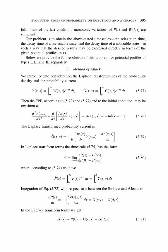
fulfillment of the last condition, monotonic variations of PðtÞ and Wð‘; tÞ aresufficient.

Our problem is to obtain the above-stated timescales—the relaxation time,

the decay time of a metastable state, and the decay time of a nonstable state—in

such a way that the desired results may be expressed directly in terms of the

given potential profiles jðxÞ.Below we provide the full resolution of this problem for potential profiles of

types I, II, and III separately.

2. Method of Attack

We introduce into consideration the Laplace transformations of the probability

density and the probability current

Yðx; sÞ ¼ð10

Wðx; tÞe�st dt; Gðx; sÞ ¼ð10

Gðx; tÞe�st dt ð5:77Þ

Then the FPE, according to (5.72) and (5.77) and to the initial condition, may be

rewritten as

d 2Yðx; sÞdx 2

þ d

dx

djðxÞdx

Yðx; sÞ� �

� sBYðx; sÞ ¼ �Bdðx� x0Þ ð5:78Þ

The Laplace transformed probability current is

Gðx; sÞ ¼ � 1

B

djðxÞdx

Yðx; sÞ þ dYðx; sÞdx

� �ð5:79Þ

In Laplace transform terms the timescale (5.75) has the form

# ¼ lims!0

sPðsÞ � Pð1Þs½Pð0Þ � Pð1Þ� ð5:80Þ

where according to (5.74) we have

PðsÞ ¼ð10

PðtÞe�st dt ¼ðdc

Yðx; sÞ dx

Integration of Eq. (5.72) with respect to x between the limits c and d leads to

dPðtÞdt¼ �

ðdc

qGðx; tÞqx

dx ¼ Gðc; tÞ � Gðd; tÞ

In the Laplace transform terms we get

sPðsÞ � Pð0Þ ¼ Gðc; sÞ � Gðd; sÞ ð5:81Þ


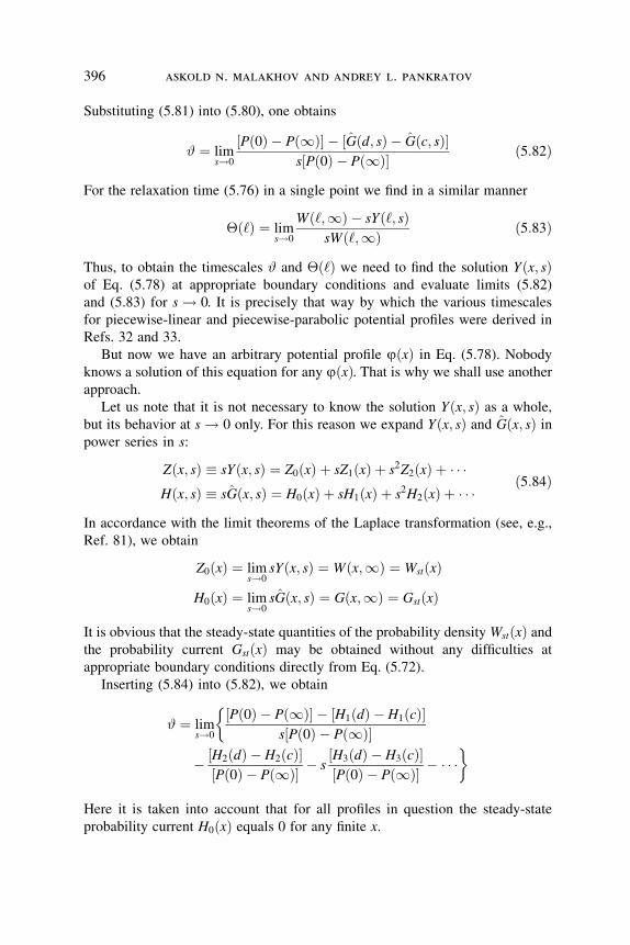
Substituting (5.81) into (5.80), one obtains

# ¼ lims!0

Pð0Þ � Pð1Þ½ � � ½Gðd; sÞ � Gðc; sÞ�s½Pð0Þ � Pð1Þ� ð5:82Þ

For the relaxation time (5.76) in a single point we find in a similar manner

�ð‘Þ ¼ lims!0

Wð‘;1Þ � sYð‘; sÞsWð‘;1Þ ð5:83Þ

Thus, to obtain the timescales # and �ð‘Þ we need to find the solution Yðx; sÞof Eq. (5.78) at appropriate boundary conditions and evaluate limits (5.82)

and (5.83) for s! 0. It is precisely that way by which the various timescales

for piecewise-linear and piecewise-parabolic potential profiles were derived in

Refs. 32 and 33.

But now we have an arbitrary potential profile jðxÞ in Eq. (5.78). Nobody

knows a solution of this equation for any jðxÞ. That is why we shall use another

approach.

Let us note that it is not necessary to know the solution Yðx; sÞ as a whole,

but its behavior at s! 0 only. For this reason we expand Yðx; sÞ and Gðx; sÞ inpower series in s:

Zðx; sÞ � sYðx; sÞ ¼ Z0ðxÞ þ sZ1ðxÞ þ s2Z2ðxÞ þ � � �Hðx; sÞ � sGðx; sÞ ¼ H0ðxÞ þ sH1ðxÞ þ s2H2ðxÞ þ � � �

ð5:84Þ

In accordance with the limit theorems of the Laplace transformation (see, e.g.,

Ref. 81), we obtain

Z0ðxÞ ¼ lims!0

sYðx; sÞ ¼ Wðx;1Þ ¼ WstðxÞH0ðxÞ ¼ lim

s!0sGðx; sÞ ¼ Gðx;1Þ ¼ GstðxÞ

It is obvious that the steady-state quantities of the probability density WstðxÞ andthe probability current GstðxÞ may be obtained without any difficulties at

appropriate boundary conditions directly from Eq. (5.72).

Inserting (5.84) into (5.82), we obtain

# ¼ lims!0

½Pð0Þ � Pð1Þ� � ½H1ðdÞ � H1ðcÞ�s½Pð0Þ � Pð1Þ�

�

� ½H2ðdÞ � H2ðcÞ�½Pð0Þ � Pð1Þ� � s

½H3ðdÞ � H3ðcÞ�½Pð0Þ � Pð1Þ� � � � �

�

Here it is taken into account that for all profiles in question the steady-state

probability current H0ðxÞ equals 0 for any finite x.


As will be demonstrated below for all profiles the following condition takes

place

H1ðdÞ � H1ðcÞ ¼ Pð0Þ � Pð1Þ ð5:85ÞConsequently, the desired timescale reads as follows:

# ¼ H2ðcÞ � H2ðdÞPð0Þ � Pð1Þ ð5:86Þ

Substituting (5.84) into (5.83), we find the relaxation time in a single point:

�ð‘Þ ¼ � Z1ð‘ÞWð‘;1Þ ¼ �

Z1ð‘ÞZ0ð‘Þ ð5:87Þ

Hence, to attain our aim it is necessary to calculate functions H2ðxÞ and Z1ðxÞ.Inserting (5.84) into (5.78) and (5.79), it is easy to write the following equations:

d

dx

dZ0

dxþ j0Z0

� �¼ 0 ðaÞ

d

dx

dZ1

dxþ j0Z1

� �¼ BZ0 � Bdðx� x0Þ ðbÞ ð5:88Þ

d

dx

dZ2

dxþ j0Z2

� �¼ BZ1 ðcÞ

..

. ...

H0 ¼ � 1

B

dZ0

dxþ j0Z0

� �ðaÞ

H1 ¼ � 1

B

dZ1

dxþ j0Z1

� �ðbÞ ð5:89Þ

H2 ¼ � 1

B

dZ2

dxþ j0Z2

� �ðcÞ

..

. ...

From (5.88) and (5.89) we obtain

dH0

dx¼ 0 ðaÞ

dH1

dx¼ �Z0 þ dðx� x0Þ ðbÞ

dH2

dx¼ �Z1 ðcÞ

..

. ...

ð5:90Þ


Combining Eqs. (5.88)–(5.90), one finds the closed equations for HðxÞ:dH0

dx¼ 0 ðaÞ

d2H1

dx2þ j0

dH1

dx¼ BH0 þ d

dxþ j0

� �dðx� x0Þ ðbÞ

d2H2

dx2þ j0

dH2

dx¼ BH1 ðcÞ

..

. ...

ð5:91Þ

When solving these equations it is necessary to take into account the boundary

conditions that are different for different types of potential profiles.

3. Basic Results Relating to Relaxation Times

Let us begin our consideration in detail from the derivation of the relaxation

time which implies that the potential profile jðxÞ of type I tends fast enough to

plus infinity at x! 1. In this case the boundary conditions are

Gð1; tÞ ¼ 0; that is, all functions HkðxÞ must be zero at x ¼ 1. According

to (5.73) the steady-state distribution equals

WstðxÞ ¼ Z0ðxÞ ¼ Ae�jðxÞ; A ¼ 1

�ðþ1�1

e�jðxÞ dx > 0

This situation is depicted in Fig. 3, where the decision interval [c; d] is chosen inaccordance with the concrete stated task and may involve or not involve the

initial distribution Wðx; 0Þ ¼ dðx� x0Þ.It is clear that the probability PðtÞ ¼ Ð d

cWðx; tÞ dx varies from Pð0Þ ¼ 1 or

Pð0Þ ¼ 0 to Pð1Þ ¼ AÐ dce�jðvÞ dv.

From Eq. (5.90b) it follows that

H1ðxÞ ¼ �Aðx�1

e�jðvÞ dvþ 1ðx� x0Þ þ C

where C is arbitrary constant and the unit step function 1ðxÞ is defined as

1ðxÞ ¼0; x < 0

1=2; x ¼ 0

1; x > 0

8><>:

The boundary conditions H1ð1Þ ¼ 0 lead to C ¼ 0. Hence

H1ðxÞ ¼ �FðxÞ þ 1ðx� x0Þ ð5:92Þ


where

FðxÞ ¼ A

ðx�1

e�jðvÞ dv ð5:93Þ

is the integral distribution function for the probability density WstðxÞ.It is easy to see that

H1ðdÞ � H1ðcÞ ¼�A Ð d

ce�jðvÞdvþ 1 ¼ Pð0Þ � Pð1Þ; c < x0 < d

�A Ð dce�jðvÞ dv ¼ Pð0Þ � Pð1Þ; x0 < c < d

(

Thus, condition (5.85) is true for potential profiles of type I, and therefore the

relaxation time � is really found according to (5.86).

The function H2ðxÞ may be found from (5.91c) taking into account (5.92)

and (5.93):

H2 ¼ C1FðxÞ þ B

ðx�1

e�jðuÞ duðu�1

ejðvÞ½1ðv� x0Þ � FðvÞ� dvþ C2

where C1 and C2 are arbitrary constants, which must be defined from boundary

conditions H2ð1Þ ¼ 0. As the result, we have C2 ¼ 0 and

C1 ¼ �Bðþ1�1


ejðvÞ½1ðv� x0Þ � FðvÞ� dv

Consequently,

H2ðxÞ ¼ B

ðx�1


ejðvÞ½1ðv� x0Þ � FðvÞ� dv�

�FðxÞðþ1�1



ð5:94Þ

By changing the integration order, one obtains

H2ðcÞ � H2ðdÞ ¼ B

APð1Þ

ðþ1�1

ejðvÞ½1ðv� x0Þ � FðvÞ�½1� FðvÞ� dv�

� Pð1Þðc�1

ejðvÞ½1ðv� x0Þ � FðvÞ� dv

�ðdc

ejðvÞ½1ðv� x0Þ � FðvÞ�½FðdÞ � FðvÞ� dv�

ð5:95Þ


The Initial Probability Distribution Is Within the Decision Interval. After some

transformations taking into account that c < x0 < d, we obtain finally

from (5.95) and from (see (5.86))

� ¼ H2ðcÞ � H2ðdÞ1� Pð1Þ

the following quantity of the relaxation time for the situation depicted in

Fig. 3(a):

� ¼ B

Að1� P1Þ ð1� P1Þðdc

ejðvÞFðvÞ½1� FðvÞ� dv�

þP1ðc�1

ejðvÞF2ðvÞ dvþ P1ð1d

ejðvÞ½1� FðvÞ�2 dv

�ð1� F2Þðx0c

ejðvÞFðvÞ dv� F1

ðdx0

ejðvÞ½1� FðvÞ� dv�

ð5:96Þ

where F1 ¼ FðcÞ, F2 ¼ FðdÞ; and P1 � Pð1Þ.In the particular case where c ¼ �1 (FðdÞ ¼ P1, FðcÞ ¼ 0) the relaxation

time is given by

� ¼ B

A

ðdx0


þ P1ð1� P1Þ

ð1d

ejðvÞ½1� FðvÞ�2 dv

�ðx0�1

ejðvÞF2ðvÞ dv)

ð5:97Þ

If, on the other hand, d ¼ 1 (FðdÞ ¼ 1, FðcÞ ¼ 1� P1) from (5.96), one finds

� ¼ B

A

ðx0c


þ P1ð1� P1Þ

ðc�1

ejðvÞF2ðvÞ dv

�ð1x0

ejðvÞ½1� FðvÞ�2 dv)

ð5:98Þ

In the case of the symmetry of the potential profile with respect to the coordinate

of the initial distribution x0 (which may be taken as x0 ¼ 0) and of the

symmetrical decision interval [�d;þd] from (5.96), one can obtain the following

expression for the relaxation time:

� ¼ B

A1

ðd0

ejðvÞf ðvÞ½1� f ðvÞ� dvþ P1ð1� P1Þ

ð1d

ejðvÞ½1� f ðvÞ�2 dv� �

ð5:99Þ


where a new function is introduced:

f ðxÞ ¼ A1

ðx0

e�jðvÞ dv; A�11 ¼ð10

e�jðvÞ dv; P1 ¼ f ðdÞ

As may be shown, the same relaxation time (5.99) will take place if the initial

distribution is located in an immediate vicinity of the origin (i.e., when x0 ¼ þ0)and when the reflecting wall is sited at the point x ¼ 0.

In the situation where there are two reflecting walls at the points l1 ¼ 0 and

l2 ¼ l and the decision interval is [c ¼ 0, d], so that 0 < x0 < d < l,expression (5.96) becomes (F1 ¼ 0, F2 ¼ P1)

� ¼ B

A2

ðd0

ejðvÞcðvÞ½1� cðvÞ� dv�

þ P1ð1� P1Þ

ðld

ejðvÞ½1� cðvÞ�2 dv

�ðx00

ejðvÞcðvÞ dv)

ð5:100Þ

where

cðxÞ ¼ A2

ðx0

e�jðvÞ dv; A�12 ¼ðl0

e�jðvÞ dv; P1 ¼ cðdÞ

The Initial Probability Distribution Lies Outside the Decision Interval. In this

case, which is depicted in Fig. 3(b), the chosen points c and d satisfy the

inequalities x0 < c < d. Because of Pð0Þ ¼ 0 the relaxation time is now

[see (5.86)]

� ¼ H2ðdÞ � H2ðcÞP1

ð5:101Þ

The numerator of this fraction is represented by (5.95) as before, but due to the

above-mentioned inequalities the relaxation time is expressed by another

formula (F1 ¼ FðcÞ, F2 ¼ FðdÞ):

� ¼ B

A

ðþ1�1

ejðvÞFðvÞ½1� FðvÞ� dv�ðx0�1

ejðvÞFðvÞ dv�

�ð1d

ejðvÞ½1� FðvÞ� dv

� 1

F2 � F1

ðdc

ejðvÞ½1� FðvÞ�½FðvÞ � F1� dv)

ð5:102Þ


In particular case where d ¼ 1 (F2 ¼ 1, P1 ¼ 1� F1)

� ¼ B

A

ðcx0

ejðvÞFðvÞ½1� FðvÞ� dvþ F1

1� F1

ð1c

ejðvÞ½1� FðvÞ�2 dv�

�ðx0�1

ejðvÞFðvÞ2 dv�

ð5:103Þ

The Relaxation Time in a Single Point. We turn now to formula (5.87). The

function Z1ðxÞ may be obtained in two ways: First, one can solve Eq. (5.88b),

second, one can use Eq. (5.90c) keeping in mind that the function H2ðxÞ isalready obtained [see formula (5.94)] and in addition it satisfies the required

boundary conditions (H2ð1Þ ¼ 0).

The second way is shorter. From (5.90c) and (5.94) we have

�Z1ðxÞ ¼ dH2ðxÞdx

¼ Be�jðxÞðx�1

e�jðvÞ½1ðv� x0Þ � FðvÞ� dv�

�Aðþ1�1



Hence, according to (5.87) and by changing the order of integration in the last

integral, the relaxation time may be expressed as

�ð‘Þ ¼ B

A

ð‘�1

ejðvÞ½1ðv� x0Þ � FðvÞ� dv�ðþ1�1

ejðvÞ½1ðv� x0Þ�

� FðvÞ�½1� FðvÞ� dv)

ð5:104Þ

Considering the relaxation time at the point x ¼ ‘ > x0 [Fig. 3(e)], one obtains

the following after some transformations:

�ð‘Þ ¼ B

A

ðþ1�1


�ðx0�1

ejðvÞFðvÞ dv

�ð1‘


ð5:105Þ

It is easy to check that the same relaxation time may be derived from expression

(5.102) for c � ‘ � d at c! ‘, d ! ‘.


For the case where ‘ < x0 [Fig. 3(f )] from (5.104) after some transforma-

tions, it follows that the relaxation time takes the form

�ð‘Þ ¼ B

A

ðþ1�1


�ð‘�1

ejðvÞFðvÞ dv

�ð1x0


ð5:106Þ

When comparing (5.106) with (5.105), it becomes evident that these expressions

coincide to make the interchange x0 $ ‘. This fact demonstrates the so-called

reciprocity principle: In any linear system, some effect does not vary if the

source (at position x ¼ x0) and the observation point (x ¼ ‘) will be inter-

changed. The linearity of our system is represented by the linearity of the

Fokker–Planck equation (5.72).

4. Basic Results Relating to Decay Times

Potential Profiles of Type II. Consider now the potential profiles of type II,

which may represent the occurrence of the metastable state or the nonstable

state (Fig. 4) and which tend to plus infinity at x! �1 and to minus infinity at

x! þ1. The boundary conditions are now Gð�1; tÞ ¼ 0 and Wðþ1; tÞ ¼ 0.

For this reason all functions HkðxÞ must be zero at x ¼ �1 and all functions

ZkðxÞ must be zero at x ¼ þ1. For such potential profiles the nonzero steady-

state distributions do not exist and consequently Z0ðxÞ � 0.

As for probability PðtÞ ¼ Ð dcWðx; tÞ dx, where c < x0 < d, it is evident that

Pð0Þ ¼ 1 and Pð1Þ ¼ 0. From (5.86) it follows that (denoting t as the decay

time of the metastable state or the decay time of the unstable state)

t ¼ H2ðcÞ � H2ðdÞ ð5:107Þ

From Eq. (5.90b) we get H1ðxÞ ¼ 1ðx� x0Þ and consequently condition (5.85) isfulfilled. From Eq. (5.91c) one can find

dH2ðxÞdx

¼ e�jðxÞ C1 þ B

ðx�1

ejðvÞ1ðv� x0Þ dv� �

ð5:108Þ

where C1 is an arbitrary constant.

Because Z1ðxÞ ¼ �dH2ðxÞ=dx [see Eq. (5.90c)] must be zero at x ¼ þ1, we

obtain

C1 ¼ �Bðþ1�1

ejðvÞ1ðv� x0Þ dv ¼ �Bðþ1x0

ejðvÞ dv


Consequently, the integration of Eq. (5.108) gives

H2ðxÞ ¼ B

ðx�1


ejðvÞ1ðv� x0Þ dv�

�ðþ1x0

ejðvÞ dv �ðx�1

e�jðvÞ dv�þ C2

Because of H2ð�1Þ ¼ 0, an arbitrary constant C2 must be zero.

After some transformations we have

H2ðxÞ ¼ B

Ð xx0ejðvÞ dv

Ð xve�jðuÞ du� Ð1

x0ejðvÞ dv � Ð x�1 e�jðuÞ du; x > x0

� Ð1x0

ejðvÞ dv � Ð x�1 e�jðuÞ du; x < x0

8<:

Hence, according to (5.107), taking into account that c < x0 < d, we finally

arrive at the exact expression of the escape time of the Brownian particles from

decision interval ½c; d� for an arbitrary potential profile jðxÞ of type II (Fig. 4):

t ¼ B

ðdx0

ejðvÞ dvðvc

e�jðuÞ duþð1d

ejðvÞ dv �ðdc

e�jðuÞ du� �

ð5:109Þ

In the case where the absorbing boundary is at x ¼ l2 > d, expression (5.109)

takes the form

t ¼ B

ðdx0

ejðvÞ dvðvc

e�jðuÞ duþðl2d

ejðvÞ dv �ðdc

e�jðuÞdu� �

ð5:110Þ

For the decision interval extended to the absorbing boundary (d ¼ l2) from

(5.110), one obtains

t ¼ B

ðl2x0

ejðvÞ dvðvc

e�jðuÞ du ð5:111Þ

If, in addition, c ¼ �1, we have come to the MFPT

t ¼ B

ðl2x0

ejðvÞ dvðv�1

e�jðuÞ du � Tðx0; l2Þ ð5:112Þ

that we have already mentioned. In other words, the MFPT coincides with the

decay time of the state existing in decision interval [�1; l2].


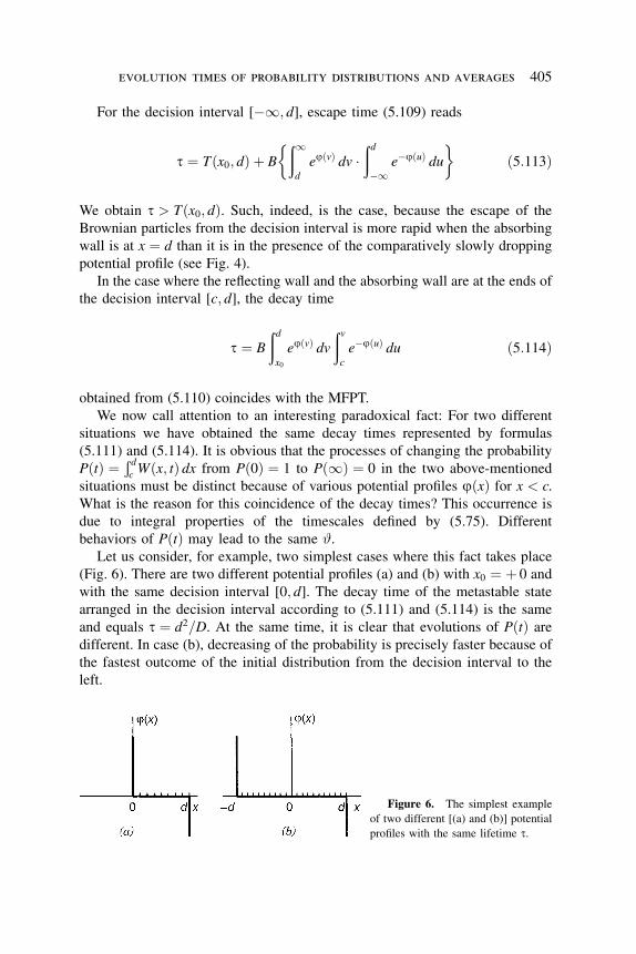
For the decision interval [�1; d], escape time (5.109) reads

t ¼ Tðx0; dÞ þ B

ð1d

ejðvÞ dv �ðd�1

e�jðuÞ du� �

ð5:113Þ

We obtain t > Tðx0; dÞ. Such, indeed, is the case, because the escape of the

Brownian particles from the decision interval is more rapid when the absorbing

wall is at x ¼ d than it is in the presence of the comparatively slowly dropping

potential profile (see Fig. 4).

In the case where the reflecting wall and the absorbing wall are at the ends of

the decision interval [c; d], the decay time

t ¼ B

ðdx0

ejðvÞ dvðvc

e�jðuÞ du ð5:114Þ

obtained from (5.110) coincides with the MFPT.

We now call attention to an interesting paradoxical fact: For two different

situations we have obtained the same decay times represented by formulas

(5.111) and (5.114). It is obvious that the processes of changing the probability

PðtÞ ¼ Ð dcWðx; tÞ dx from Pð0Þ ¼ 1 to Pð1Þ ¼ 0 in the two above-mentioned

situations must be distinct because of various potential profiles jðxÞ for x < c.

What is the reason for this coincidence of the decay times? This occurrence is

due to integral properties of the timescales defined by (5.75). Different

behaviors of PðtÞ may lead to the same #.Let us consider, for example, two simplest cases where this fact takes place

(Fig. 6). There are two different potential profiles (a) and (b) with x0 ¼ þ 0 and

with the same decision interval [0; d]. The decay time of the metastable state

arranged in the decision interval according to (5.111) and (5.114) is the same

and equals t ¼ d2=D. At the same time, it is clear that evolutions of PðtÞ aredifferent. In case (b), decreasing of the probability is precisely faster because of

the fastest outcome of the initial distribution from the decision interval to the

left.

Figure 6. The simplest example

of two different [(a) and (b)] potential

profiles with the same lifetime t.


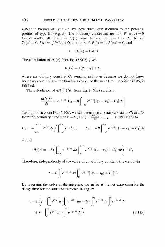
Potential Profiles of Type III. We now direct our attention to the potential

profiles of type III (Fig. 5). The boundary conditions are now Wð1Þ ¼ 0.

Consequently, all functions ZkðxÞ must be zero at x ¼ 1. As before,

Z0ðxÞ � 0, PðtÞ ¼ Ð dcWðx; tÞ dx, c < x0 < d, Pð0Þ ¼ 1, Pð1Þ ¼ 0, and

t ¼ H2ðcÞ � H2ðdÞ

The calculation of H1ðxÞ from Eq. (5.90b) gives

H1ðxÞ ¼ 1ðx� x0Þ þ C1

where an arbitrary constant C1 remains unknown because we do not know

boundary conditions on the functionsHkðxÞ. At the same time, condition (5.85) is

fulfilled.

The calculation of dH2ðxÞ=dx from Eq. (5.91c) results in

dH2ðxÞdx

¼ e�jðxÞ C2 þ B

ðx�1

ejðvÞ½1ðv� x0Þ þ C1� dv� �

Taking into account Eq. (5.90c), we can determine arbitrary constants C1 and C2

from the boundary conditions: �Z1ð1Þ ¼ dH2ðxÞdxjx¼1 ¼ 0. This leads to

C1 ¼ �ðþ1x0

ejðvÞ dvðþ1�1

ejðvÞ dv�

; C2 ¼ �Bðþ1�1

ejðvÞ½1ðv� x0Þ þ C1� dv

and to

H2ðxÞ ¼ �Bðx�1

e�jðuÞ duðþ1u

ejðvÞ½1ðv� x0Þ þ C1� dv� �

þ C3

Therefore, independently of the value of an arbitrary constant C3, we obtain

t ¼ B

ðdc

e�jðuÞ duð1u

ejðvÞ½1ðv� x0Þ þ C1� dv

By reversing the order of the integrals, we arrive at the net expression for the

decay time for the situation depicted in Fig. 5:

t ¼ B f1 �ðdx0

ejðvÞ dvðvc

e�jðuÞ du� f2 �ðx0c

ejðvÞ dvðvc

e�jðuÞ du�

þ f1 �ð1d

ejðvÞ dv �ðdc

e�jðuÞ du�

ð5:115Þ


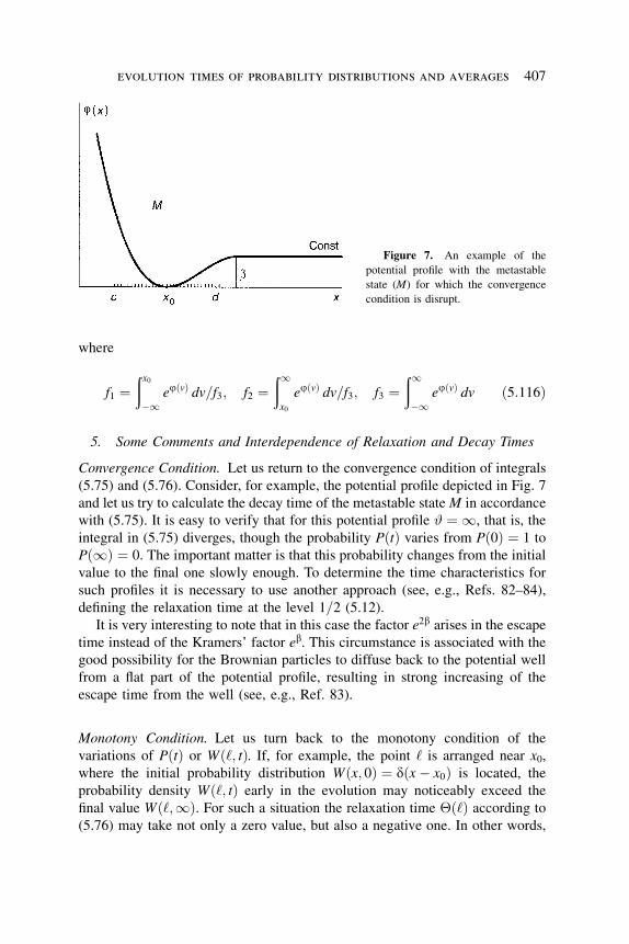
where

f1 ¼ðx0�1

ejðvÞ dv=f3; f2 ¼ð1x0

ejðvÞ dv=f3; f3 ¼ð1�1

ejðvÞ dv ð5:116Þ

5. Some Comments and Interdependence of Relaxation and Decay Times

Convergence Condition. Let us return to the convergence condition of integrals

(5.75) and (5.76). Consider, for example, the potential profile depicted in Fig. 7

and let us try to calculate the decay time of the metastable state M in accordance

with (5.75). It is easy to verify that for this potential profile # ¼ 1, that is, the

integral in (5.75) diverges, though the probability PðtÞ varies from Pð0Þ ¼ 1 to

Pð1Þ ¼ 0. The important matter is that this probability changes from the initial

value to the final one slowly enough. To determine the time characteristics for

such profiles it is necessary to use another approach (see, e.g., Refs. 82–84),

defining the relaxation time at the level 1=2 (5.12).

It is very interesting to note that in this case the factor e2b arises in the escape

time instead of the Kramers’ factor eb. This circumstance is associated with the

good possibility for the Brownian particles to diffuse back to the potential well

from a flat part of the potential profile, resulting in strong increasing of the

escape time from the well (see, e.g., Ref. 83).

Monotony Condition. Let us turn back to the monotony condition of the

variations of PðtÞ or Wð‘; tÞ. If, for example, the point ‘ is arranged near x0,

where the initial probability distribution Wðx; 0Þ ¼ dðx� x0Þ is located, the

probability density Wð‘; tÞ early in the evolution may noticeably exceed the

final value Wð‘;1Þ. For such a situation the relaxation time �ð‘Þ according to

(5.76) may take not only a zero value, but also a negative one. In other words,

Figure 7. An example of the

potential profile with the metastable

state (M) for which the convergence

condition is disrupt.


nonmonotony of PðtÞ or Wð‘; tÞ leads in accordance with (5.75) and (5.76) to

defective results. We analyze this situation with aid of a simple example.

Consider the potential profile depicted in Fig. 8. At the points x ¼ 0 and

x ¼ l the reflecting walls are arranged. The relaxation time at the point ‘ may

be calculated with the aid of (5.105), taking into account that jðxÞ ¼ 0,

x 2 ½0; l�:

�ð‘Þ ¼ B

A

ðl0

FðvÞ½1� FðvÞ� dv�ðx00

FðvÞ dv�ðl‘

½1� FðvÞ� dv� �

ð5:117Þ

Here

A�1 ¼ðl0

dv ¼ l; FðvÞ ¼ A

ðv0

dx ¼ v=l

As a result we have (B ¼ 2=D)

�ð‘Þ ¼ l2

3D1� 3

x0

l

�2�3 1� ‘

l

� �2( )

ð5:118Þ

Three terms in (5.117) correspond to three terms in (5.118).

We have obtained the relaxation time—that is, the time of attainment of the

equilibrium state or, in other words, the transition time to the stationary

distribution Wð‘;1Þ at the point ‘ in the rectangular potential profile. This time

depends on the delta-function position x0 and on the observation point location ‘.The relaxation time is maximal for x0 ¼ 0 and ‘ ¼ l—that is, when x0 and ‘

are widely spaced. If the distance between x0 and ‘ decreases, the relaxation

time goes down.

Figure 8. A rectangular potential

well.


But if the distance between x0 and ‘ is too small, expression (5.118) may give

�ð‘Þ ¼ 0 or even �ð‘Þ < 0. What does it mean? This signals that the condition

of monotonic variation of Wð‘; tÞ from zero to Wð‘;1Þ is broken and that the

obtained values of the relaxation times are false.

The special investigation has shown that, in particular, for x0 ¼ 0 the

relaxation time defined by (5.118) is true for ‘=l � 0:5. At the same time it

would be reasonable to take the first term in (5.118)—that is, � ¼ l2=3D—as

an upper bound for the relaxation time in the rectangular well to avoid the

difficulties with the possible nonmonotonic behavior of the Wð‘; tÞ regardless ofthe values x0 and ‘.

The same reasoning may be extended on all above-obtained results regarding

relaxation times, but with some care especially when there are no any potential

barriers between x0 and the observation point.

Some Common Interdependence of Relaxation Times. Consider an arbitrary

disposition of the initial distribution point x0 and the boundary point d [see

Fig. 3(c,d)]. We may take into account two decision intervals I1 ¼ ½�1; d� andI2 ¼ ½d;þ1� and define two probabilities:

P1ðtÞ ¼ðd�1

Wðx; tÞ dx; P2ðtÞ ¼ð1d

Wðx; tÞ dx

In line with these probabilities, we may introduce into consideration two

relaxation times �1 and �2 according to a common definition (5.75). From the

evident equality P1ðtÞ þ P2ðtÞ ¼ 1, it follows that �1 ¼ �2 for both d > x0 and

d < x0.

If there is the symmetrical potential profile jðxÞ ¼ jð�xÞ and the initial

distribution is located at the origin (i.e., x0 ¼ 0), then all results concerning the

relaxation times will be the same as for the potential profile in which the

reflecting wall is at x ¼ 0 and at x0 ¼ þ0. This coincidence of the relaxation

times may be proven in a common case taking into account that the probability

current at x ¼ 0 is equal to zero at any instant of time.

Interdependence Between Relaxation and Decay Times. Consider the potential

profile of type I which is symmetrical with respect to x ¼ d > 0 and where the

initial distribution is located at x0 ¼ 0 and the decision interval is [�1; d] (seeAppendix). The relaxation time that follows from (5.97) is

� ¼ B

A

ðd0

ejðvÞFðvÞ½1� FðvÞ� dv�ð0�1

ejðvÞF2ðvÞ dv�

þ FðdÞ1� FðdÞ

ð1d



This formula may be transformed into

� ¼ B

A

ðd0

ejðvÞFðvÞ dv�ðd�1

ejðvÞF2ðvÞ dv�

þ FðdÞ1� FðdÞ

ð1d


Because of the potential profile symmetry we have FðdÞ ¼ 1=2, Fðd � zÞ ¼1� Fðd þ zÞ and the second integral goes to

Ð1d

ejðvÞ½1� FðvÞ�2 dv. As a result,we have

� ¼ B

A

ðd0

ejðvÞFðvÞ dv ¼ B

ðd0

ejðvÞ dvðv�1

e�jðuÞ du ¼ Tð0; dÞ ð5:119Þ

Thus, we have proven the so-called principle of conformity which was

demonstrated for an arbitrary symmetrical potential profile of type I by another

more complicated way in Refs. 70 and 85.

Consider the bistable one-level system with symmetrical potential profile

jðxÞ ¼ jð�xÞ with respect to the origin, where the potential barrier of the

height b is located (Fig. 9). According to the principle of conformity and (5.119)

the relaxation time � of this bistable system (the decision interval is [�1; 0]) isequal to

� ¼ B

ð0�d

ejðvÞ dvðv�1

e�jðuÞ du ¼ Tð�d; 0Þ

If we will locate the absorbing wall at the point x ¼ d (the dashed line in Fig. 9),

the MFPT Tð�d; dÞ reads

Tð�d; dÞ ¼ B

ðd�d

ejðvÞ dvðv�1

e�jðuÞ du

After some transformations using the symmetrical properties of the potential

profile, one finds

Tð�d; dÞ ¼ 2Tð�d; 0Þ þ t0

where

t0 ¼ 2B

ðd0

ejðvÞ dvðv0

e�jðuÞ du


It may be shown that for the high enough potential barrier b� 1 the quantity t0is significantly smaller than 2Tð�d; 0Þ and we arrive at

� ¼ 1

2Tð�d;þdÞ ð5:120Þ

Expression (5.120) means that the relaxation time in an arbitrary symmetrical

one-level bistable system is two times smaller than the MFPT Tð�d;þdÞ—that

is, two times smaller than the decay time of the metastable state—shown with the

dashed line taken into account in Fig. 9.

This is concerned with the fact that in the case of the relaxation time, roughly

speaking only half of all Brownian particles should leave the initial potential

minimum to reach the equilibrium state, while for the profile of the decay time

case all particles should leave the initial minimum. Expression (5.120), of

course, is true only in the case of the sufficiently large potential barrier,

separating the stable states of the bistable system, when the inverse probability

current from the second minimum to the initial one may be neglected (see

Ref. 33).

The comparison with known results (e.g., Refs. 2, 20, 21, 86, and 87) for

variety of examples of metastable, bistable and periodic potentials was done in

Refs. 32–35 and 85.

6. Derivation of Moments of Transition Time

In this section we restrict our consideration by potentials of type II only (in this

case moments of transition time are moments of decay time). The approach,

considered above for derivation of the mean transition time may also be used to

obtain higher moments, given by Eq. (5.1).

Figure 9. A potential profile of

type I representing a one-level bistable

system. The dashed line shows the

absorbing wall.


Let us write in the explicit form the expressions for functions HnðxÞ (weremind that Hðx; sÞ ¼ sGðx; sÞ ¼ H0ðxÞ þ sH1ðxÞ þ s2H2ðxÞ þ � � �) using the

boundary conditions Wðþ1; tÞ ¼ 0 and Gð�1; tÞ ¼ 0 (H1ðxÞ ¼ 1ðx� x0Þ):

H2ðxÞ ¼ �Bðx�1

e�jðvÞð1v

ejðyÞ1ðy� x0Þ dy dv

HnðxÞ ¼ �Bðx�1

e�jðvÞð1v

ejðyÞHn�1ðyÞ dy dv; n ¼ 3; 4; 5; . . .

ð5:121Þ

As one can check, from formula (5.1) (taking the integral by parts and Laplace

transforming it using the property Pðx0; 0Þ � sPðx0; sÞ ¼ Gðd; sÞ � Gðc; sÞtogether with the expansion of Hðx; sÞ via HnðxÞ, one can obtain the following

expressions for moments of decay time [88]:

t1ðc; x0; dÞ ¼ �ðH2ðdÞ � H2ðcÞÞt2ðc; x0; dÞ ¼ 2ðH3ðdÞ � H3ðcÞÞt3ðc; x0; dÞ ¼ �2 � 3ðH4ðdÞ � H4ðcÞÞ; . . .tnðc; x0; dÞ ¼ ð�1Þnn!ðHnþ1ðdÞ � Hnþ1ðcÞÞ

ð5:122Þ

From these recurrent relations, one obtains the following expression for the

second moment in the case c ¼ �1 (c < x0 < d):

t2ð�1; x0; dÞ ¼ 2B2

(t1ð�1; x0; dÞ½ �2

þðd�1

e�jðxÞdx �ð1x0

ejðvÞðvd

e�jðuÞð1u

ejðzÞ dz du dv

�ðdx0

e�jðxÞðxx0

ejðvÞðvd

e�jðuÞð1u

ejðzÞ dz du dv dx

)ð5:123Þ

where t1ð�1; x0; dÞ is the first moment:

t1ð�1; x0; dÞ ¼ B

ðd�1

e�jðxÞdx �ð1x0

ejðvÞ dv�

�ðdx0

e�jðxÞðxx0

ejðvÞ dv dx�

ð5:124Þ

Instead of analyzing the structure and the properties of the second and higher

moments, in the next section, we will perform analysis of temporal evolution of

the survival probability.


7. Timescales of Evolution of Averages and Correlation Time

Analogically, one can apply the considered approach to derive timescales of

evolution of averages [89] and correlation time [90,91]. We will search for the

average mf ðtÞ in the form

mf ðtÞ ¼ f ðxÞh i ¼ðþ1�1

f ðxÞWðx; tÞ dx ð5:125Þ

As we have mentioned above, the FPE (5.72) is a continuity equation. To obtain

necessary average mf ðtÞ (5.125), let us multiply it by the function f ðxÞ andintegrate with respect to x from �1 to þ1. Then we get

dmf ðtÞdt¼ �

ðþ1�1

f ðxÞ qGðx; tÞqx

dx ð5:126Þ

This is already an ordinary differential equation of the first order ( f ðxÞ is a knowndeterministic function), but nobody knows how to find Gðx; tÞ.

Let us define the characteristic scale of time evolution of the average mf ðtÞ asan integral relaxation time:

tf ðx0Þ ¼Ð10

mf ðtÞ � mf ð1Þ� �

dt

mf ð0Þ � mf ð1Þ ð5:127Þ

Definition (5.127) as before is general in the sense that it is valid for any initial

condition. But here we restrict ourselves by the delta-shaped initial distribution

and consider tf ðx0Þ as a function of x0. For arbitrary initial distribution the

required timescale may be obtained from tf ðx0Þ by separate averaging of both

numerator and denominator mf ð0Þ � mf ð1Þ over initial distribution, because

mf ð0Þ is also a function of x0.

The restrictions of the definition (5.127) are the same as before: It gives

correct results only for monotonically evolving functions mf ðtÞ and mf ðtÞ shouldfastly enough approach its steady-state value mf ð1Þ for convergence of the

integral in (5.127).

Performing Laplace transform of formula (5.127), Eq. (5.126) (Laplace

transformation of (5.126) gives: smf ðsÞ � mf ð0Þ ¼ �Ðþ1�1 f ðxÞ½qGðx; sÞ=qx� dx,

where mf ðsÞ ¼Ð10

mf ðtÞe�stdt) and combining them, we obtain

tf ðx0Þ ¼ lims!0

smf ðsÞ � mf ð1Þs½mf ð0Þ � mf ð1Þ�

¼ lims!0

mf ð0Þ � mf ð1Þ �Ðþ1�1 f ðxÞ½qGðx; sÞ=qx� dx

s½mf ð0Þ � mf ð1Þ� ð5:128Þ

where Gðx; sÞ is the Laplace transformation of the probability current

Gðx; sÞ ¼ Ð10

Gðx; tÞe�st dt.


Introducing the function Hðx; sÞ ¼ sGðx; sÞ and expanding it into power

series in s, we restrict our computation by obtaining H2ðxÞ only, since it can be

demonstrated that

tf ðx0Þ ¼ �Ðþ1�1 f ðxÞ dH2ðxÞ½mf ð0Þ � mf ð1Þ� ð5:129Þ

Substituting the concrete form of H2ðxÞ (5.94) into formula (5.129), one can

obtain the characteristic scale of time evolution of any average mf ðtÞ for arbitrarypotential such that jð1Þ ¼ 1:

tf ðx0Þ ¼ B

mf ð0Þ � mf ð1Þð1�1

f ðxÞe�jðxÞðxx0

ejðuÞFðuÞ du dx�

�A

ð1�1

f ðxÞe�jðxÞdxð1�1

e�jðxÞðxx0

ejðuÞFðuÞ du dx

þA

ð1�1

f ðxÞe�jðxÞdxð1x0

e�jðxÞðxx0

ejðuÞdu dx

�ð1x0

f ðxÞe�jðxÞðxx0

ejðuÞ du dx�

ð5:130Þ

where FðxÞ is expressed by

FðuÞ ¼ðu�1

e�jðvÞ dv=ðþ1�1

e�jðvÞ dv ð5:131Þ

and A ¼ 1=Ðþ1�1 e�jðxÞdx.

Analogically, the correlation time as evolution time of the correlation

function KxðtÞ ¼ xðt0Þxðt0 þ tÞh i [90] or the correlation time of more general

function Kf ðtÞ ¼ f ðxðt0ÞÞf ðxðt0 þ tÞÞh i (in Ref. 91 the correlation time of

sinðxðtÞÞ has been computed) may be obtained. Here we present the correlation

time of KxðtÞ ¼ xðt0Þxðt0 þ tÞh i [90] defined as

tc ¼ 1

s2

ð10

½KxðtÞ � xh i2� dt ð5:132Þ

where s2 ¼ x2� �� xh i2. As can be demonstrated [90], the correlation time is

given by

tc ¼ B

As2

ðþ1�1

ejðuÞ½HðuÞ � xh iFðuÞ�2 du ð5:133Þ


where

HðxÞ ¼ðx�1

uWðuÞ du; xh i ¼ Hð1Þ; s2 ¼ðþ1�1ðu� uh iÞ2WðuÞ du

WðxÞ ¼ Ae�jðxÞ; A ¼ 1.ðþ1

�1e�jðxÞ dx

One can check that this result coincides with the result by Risken and Jung (5.24)

for the case of constant diffusion coefficient.

VI. TIME EVOLUTION OF OBSERVABLES

A. Time Constant Potentials

It is known that when the transition of an overdamped Brownian particle occurs

over a potential barrier high enough in comparison with noise intensity

��=kT � 1, time evolution of many observables (e.g., the probability of

transition or the correlation function) is a simple exponent � expð�t=tÞ [2,15],where t is the corresponding timescale (the mean transition time or the

correlation time). Such representation of an observable is evident, for example,

from the method of eigenfunction analysis. In this case the corresponding

timescale (mean transition time) gives complete information about the

probability evolution. The boundaries of validity of exponential approximation

of the probability were studied in Refs. 24 and 30. In Ref. 24 the authors

extended the mean first passage time to the case of ‘‘radiation’’ boundary

condition and for two barrierless examples demonstrated good coincidence

between exponential approximation and numerically obtained probability. In a

more general case the exponential behavior of observables was demonstrated in

Ref. 30 for relaxation processes in systems having steady states. Using the

approach of ‘‘generalized moment approximation,’’ the authors of Ref. 30

obtained the exact mean relaxation time to steady state (see Section V.C), and

for particular example of a rectangular potential well they demonstrated good

coincidence of exponential approximation with numerically obtained obser-

vables. They considered in Ref. 30 an example where the rectangular well did

not have a potential barrier, and the authors of that paper supposed that their

approach (and the corresponding formulas) should also give good approxima-

tion in tasks with diffusive barrier crossing for different examples of potentials

and in a wide range of noise intensity.

In this section we will analyze the validity of exponential approximation of

observables in wide range of noise intensity [88,89,91,92].

1. Time Evolution of Survival Probability

Let us perform the analysis of temporal evolution of the probability Pðt; x0Þ of aBrownian particle, located at the point x0 (t ¼ 0) within the interval (c; d), to be


at the time t > 0 inside the considered interval: Pðt; x0Þ ¼Ð dcWðx; tÞ dx

(survival probability). We suppose that c and d are arbitrary chosen points of

an arbitrary potential profile jðxÞ, and boundary conditions at these points may

be arbitrary: Wðc; tÞ � 0 and Wðd; tÞ � 0, and we restrict our consideration by

profiles of type II (Fig. 4).

The corresponding moments of decay time were obtained above (5.122). Let

us analyze in more detail their structure. One can represent the nth moment in

the following form:

tnðc; x0; dÞ ¼ n!tn1ðc; x0; dÞ þ rnðc; x0; dÞ ð6:1ÞThis is a natural representation of tnðc; x0; dÞ due to the structure of recurrent

formulas (5.121), which is seen from the particular form of the first and the

second moments given by (5.123) and (5.124). Using the approach, applied in the

paper by Shenoy and Agarwal [93] for analysis of moments of the first passage

time, it can be demonstrated that in the limit of a high barrier �j� 1

(�j ¼ ��=kT is the dimensionless barrier height) the remainders rnðc; x0; dÞ informula (6.1) may be neglected. For �j 1, however, a rigorous analysis

should be performed for estimation of rnðc; x0; dÞ. Let us suppose that the

remainders rnðc; x0; dÞ may be neglected in a wide range of parameters, and

below we will check numerically when our assumption is valid.

The cumulants [2,43] of decay time �n are much more useful for our purpose

to construct the probability Pðt; x0Þ—that is, the integral transformation of the

introduced probability density of decay time wtðt; x0Þ (5.2). Unlike the

representation via moments, the Fourier transformation of the probability

density (5.2)—the characteristic function—decomposed into the set of

cumulants may be inversely transformed into the probability density.

Analogically to the representation for moments (6.1), a similar representation

can be obtained for cumulants �n:

�nðc; x0; dÞ ¼ ðn� 1Þ!�n1ðc; x0; dÞ þ Rnðc; x0; dÞ ð6:2Þ

It is known that the characteristic function �ðo; x0Þ ¼Ð10

wtðt; x0Þe jot dt( j ¼ ffiffiffiffiffiffiffi�1p

) can be represented as the set of cumulants (wtðt; x0Þ ¼ 0 for t < 0):

�ðo; x0Þ ¼ expX1n¼1

�nðc; x0; dÞn!

ð joÞn" #

ð6:3Þ

In the case where the remainders Rnðc; x0; dÞ in (6.2) (or rnðc; x0; dÞ in (6.1)) may

be neglected, the set (6.3) may be summarized and inverse Fourier transformed:

wtðt; x0Þ ¼ e�t=t

tð6:4Þ


where t is the mean decay time [34,35] (tðc; x0; dÞ � t1 � �1):

tðc; x0; dÞ ¼ B

ðdx0

ejðxÞðxc

e�jðvÞ dv dxþð1d

ejðxÞdxðdc

e�jðvÞ dv� �

ð6:5Þ

This expression is a direct transformation of formula (5.124), where now c is

arbitrary, such that c < x0 < d.

Probably, a similar procedure was previously used (see Refs. 1 and 93–95)

for summation of the set of moments of the first passage time, when exponential

distribution of the first passage time probability density was demonstrated for

the case of a high potential barrier in comparison with noise intensity.

Integrating probability density (6.4), taking into account definition (5.2), we

get the following expression for the survival probability Pðt; x0Þ (Pð0; x0Þ ¼ 1,

Pð1; x0Þ ¼ 0):

Pðt; x0Þ ¼ expð�t=tÞ ð6:6Þ

where mean decay time t is expressed by (6.5). Probability (6.6) represents a

well-known exponential decay of a metastable state with a high potential barrier

[15]. Where is the boundary of validity of formula (6.6) and when can we neglect

rn and Rn in formulas (6.1) and (6.2)? To answer this question, we have

considered three examples of potentials having metastable states and have

compared numerically obtained survival probability Pðt; x0Þ ¼Ð dcWðx; tÞ dx

with its exponential approximation (6.6). We used the usual explicit difference

scheme to solve the FPE (5.72), supposing the reflecting boundary condition

Gðcb; tÞ ¼ 0 (cb < c) far above the potential minimum and the absorbing one

Wðdb; tÞ ¼ 0 (db > d) far below the potential maximum, instead of boundary

conditions at 1, such that the influence of phantom boundaries at cb and db on

the process of diffusion was negligible. The first considered system is described

by the potential �ðxÞ ¼ ax2 � bx3. We have taken the following particular

parameters: a ¼ 2 and b ¼ 1, which lead to the barrier height �� 1:2,c ¼ �2, d ¼ 2a=3b, and kT ¼ 0:5; 1; 3 (in computer simulations we set the

viscosity h ¼ 1). The corresponding curves of the numerically simulated

probability and its exponential approximation are presented in Fig. 10. In the

worse case when kT ¼ 1 the maximal difference between the corresponding

curves is 3:2%. For comparison, there is also presented a curve of exponential

approximation with the mean first passage time (MFPT) of the point d for kT ¼ 1

(dashed line). One can see that in the latter case the error is significantly larger.

The second considered system is described by the potential �ðxÞ ¼ ax4 � bx5.

We have taken the following particular parameters: a ¼ 1 and b ¼ 0:5, whichlead to the barrier height �� 1:3, c ¼ �1:5, d ¼ 4a=5b, and kT ¼ 0:5; 1; 3.The corresponding curves of the numerically simulated probability and its


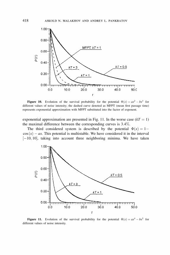
exponential approximation are presented in Fig. 11. In the worse case (kT ¼ 1)

the maximal difference between the corresponding curves is 3:4%.

The third considered system is described by the potential �ðxÞ ¼ 1�cosðxÞ � ax. This potential is multistable. We have considered it in the interval

½�10; 10�, taking into account three neighboring minima. We have taken

Figure 10. Evolution of the survival probability for the potential �ðxÞ ¼ ax2 � bx3 for

different values of noise intensity; the dashed curve denoted as MFPT (mean first passage time)

represents exponential approximation with MFPT substituted into the factor of exponent.

Figure 11. Evolution of the survival probability for the potential �ðxÞ ¼ ax4 � bx5 for

different values of noise intensity.


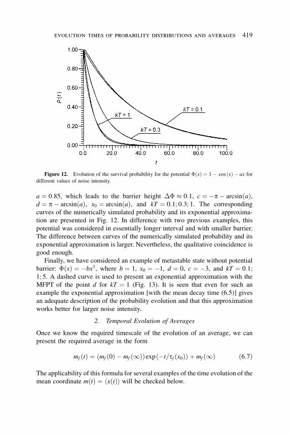
a ¼ 0:85, which leads to the barrier height �� 0:1, c ¼ �p� arcsinðaÞ,d ¼ p� arcsinðaÞ, x0 ¼ arcsinðaÞ, and kT ¼ 0:1; 0:3; 1. The corresponding

curves of the numerically simulated probability and its exponential approxima-

tion are presented in Fig. 12. In difference with two previous examples, this

potential was considered in essentially longer interval and with smaller barrier.

The difference between curves of the numerically simulated probability and its

exponential approximation is larger. Nevertheless, the qualitative coincidence is

good enough.

Finally, we have considered an example of metastable state without potential

barrier: �ðxÞ ¼ �bx3, where b ¼ 1, x0 ¼ �1, d ¼ 0, c ¼ �3, and kT ¼ 0:1;1; 5. A dashed curve is used to present an exponential approximation with the

MFPT of the point d for kT ¼ 1 (Fig. 13). It is seen that even for such an

example the exponential approximation [with the mean decay time (6.5)] gives

an adequate description of the probability evolution and that this approximation

works better for larger noise intensity.

2. Temporal Evolution of Averages

Once we know the required timescale of the evolution of an average, we can

present the required average in the form

mf ðtÞ ¼ ðmf ð0Þ � mf ð1ÞÞexpð�t=tf ðx0ÞÞ þ mf ð1Þ ð6:7Þ

The applicability of this formula for several examples of the time evolution of the

mean coordinate mðtÞ ¼ xðtÞh i will be checked below.

Figure 12. Evolution of the survival probability for the potential �ðxÞ ¼ 1� cos ðxÞ � ax for

different values of noise intensity.


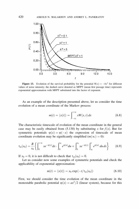
As an example of the description presented above, let us consider the time

evolution of a mean coordinate of the Markov process:

mðtÞ ¼ xðtÞh i ¼ðþ1�1

xWðx; tÞ dx ð6:8Þ

The characteristic timescale of evolution of the mean coordinate in the general

case may be easily obtained from (5.130) by substituting x for f ðxÞ. But forsymmetric potentials jðxÞ ¼ jð�xÞ the expression of timescale of mean

coordinate evolution may be significantly simplified (mð1Þ ¼ 0):

tmðx0Þ ¼ B

x0

ðþ10

xe�jðxÞdx �ðx00

ejðuÞduþðx00

xe�jðxÞðxx0

ejðuÞ du dx� �

ð6:9Þ

If x0 ¼ 0, it is not difficult to check that tmðx0Þ ¼ 0.

Let us consider now some examples of symmetric potentials and check the

applicability of exponential approximation:

mðtÞ ¼ xðtÞh i ¼ x0 expð�t=tmðx0ÞÞ ð6:10Þ

First, we should consider the time evolution of the mean coordinate in the

monostable parabolic potential jðxÞ ¼ ax2=2 (linear system), because for this

Figure 13. Evolution of the survival probability for the potential �ðxÞ ¼ �bx3 for different

values of noise intensity; the dashed curve denoted as MFPT (mean first passage time) represents

exponential approximation with MFPT substituted into the factor of exponent.


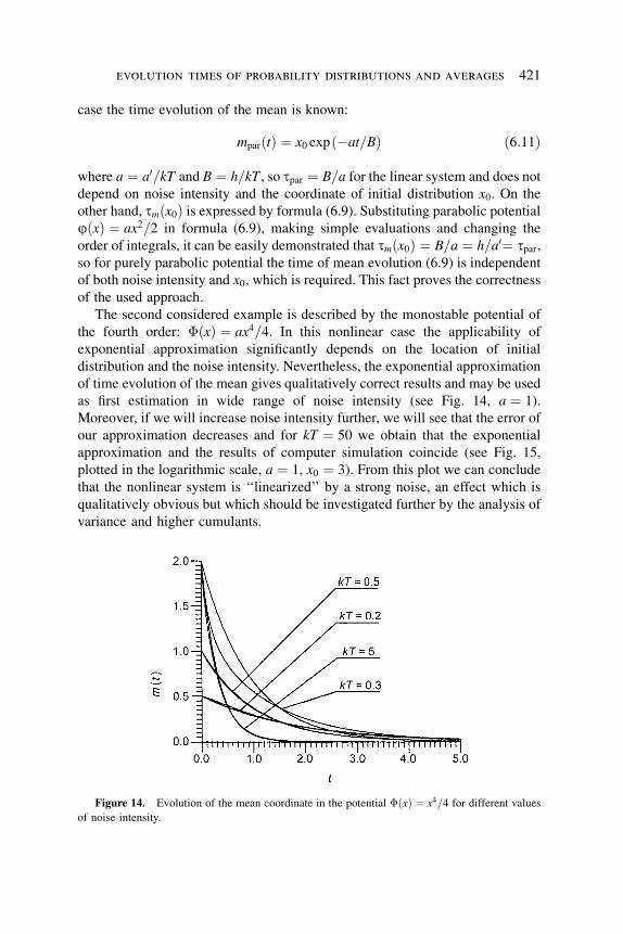
case the time evolution of the mean is known:

mparðtÞ ¼ x0 expð�at=BÞ ð6:11Þ

where a ¼ a0=kT and B ¼ h=kT , so tpar ¼ B=a for the linear system and does not

depend on noise intensity and the coordinate of initial distribution x0. On the

other hand, tmðx0Þ is expressed by formula (6.9). Substituting parabolic potential

jðxÞ ¼ ax2=2 in formula (6.9), making simple evaluations and changing the

order of integrals, it can be easily demonstrated that tmðx0Þ ¼ B=a ¼ h=a0¼ tpar,so for purely parabolic potential the time of mean evolution (6.9) is independent

of both noise intensity and x0, which is required. This fact proves the correctness

of the used approach.

The second considered example is described by the monostable potential of

the fourth order: �ðxÞ ¼ ax4=4. In this nonlinear case the applicability of

exponential approximation significantly depends on the location of initial

distribution and the noise intensity. Nevertheless, the exponential approximation

of time evolution of the mean gives qualitatively correct results and may be used

as first estimation in wide range of noise intensity (see Fig. 14, a ¼ 1).

Moreover, if we will increase noise intensity further, we will see that the error of

our approximation decreases and for kT ¼ 50 we obtain that the exponential

approximation and the results of computer simulation coincide (see Fig. 15,

plotted in the logarithmic scale, a ¼ 1, x0 ¼ 3). From this plot we can conclude

that the nonlinear system is ‘‘linearized’’ by a strong noise, an effect which is

qualitatively obvious but which should be investigated further by the analysis of

variance and higher cumulants.

Figure 14. Evolution of the mean coordinate in the potential �ðxÞ ¼ x4=4 for different values

of noise intensity.


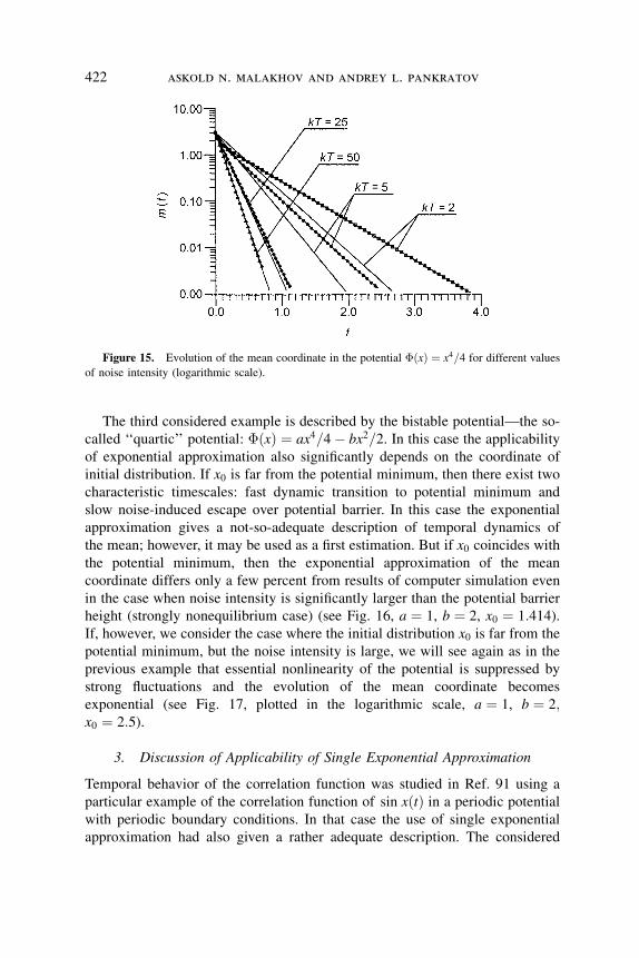
The third considered example is described by the bistable potential—the so-

called ‘‘quartic’’ potential: �ðxÞ ¼ ax4=4� bx2=2. In this case the applicability

of exponential approximation also significantly depends on the coordinate of

initial distribution. If x0 is far from the potential minimum, then there exist two

characteristic timescales: fast dynamic transition to potential minimum and

slow noise-induced escape over potential barrier. In this case the exponential

approximation gives a not-so-adequate description of temporal dynamics of

the mean; however, it may be used as a first estimation. But if x0 coincides with

the potential minimum, then the exponential approximation of the mean

coordinate differs only a few percent from results of computer simulation even

in the case when noise intensity is significantly larger than the potential barrier

height (strongly nonequilibrium case) (see Fig. 16, a ¼ 1, b ¼ 2, x0 ¼ 1:414).If, however, we consider the case where the initial distribution x0 is far from the

potential minimum, but the noise intensity is large, we will see again as in the

previous example that essential nonlinearity of the potential is suppressed by

strong fluctuations and the evolution of the mean coordinate becomes

exponential (see Fig. 17, plotted in the logarithmic scale, a ¼ 1, b ¼ 2;x0 ¼ 2:5).

3. Discussion of Applicability of Single Exponential Approximation

Temporal behavior of the correlation function was studied in Ref. 91 using a

particular example of the correlation function of sin xðtÞ in a periodic potential

with periodic boundary conditions. In that case the use of single exponential

approximation had also given a rather adequate description. The considered

Figure 15. Evolution of the mean coordinate in the potential �ðxÞ ¼ x4=4 for different values

of noise intensity (logarithmic scale).


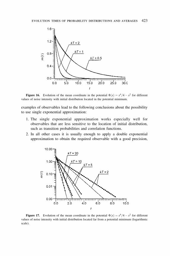
examples of observables lead to the following conclusions about the possibility

to use single exponential approximation:

1. The single exponential approximation works especially well for

observables that are less sensitive to the location of initial distribution,

such as transition probabilities and correlation functions.

2. In all other cases it is usually enough to apply a double exponential

approximation to obtain the required observable with a good precision,

Figure 16. Evolution of the mean coordinate in the potential �ðxÞ ¼ x4=4� x2 for different

values of noise intensity with initial distribution located in the potential minimum.

Figure 17. Evolution of the mean coordinate in the potential �ðxÞ ¼ x4=4� x2 for different

values of noise intensity with initial distribution located far from a potential minimum (logarithmic

scale).


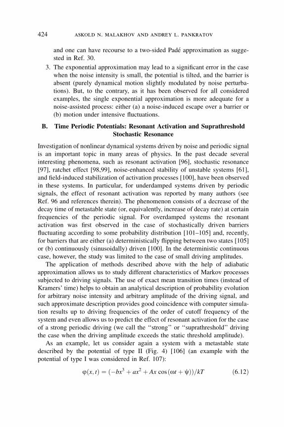
and one can have recourse to a two-sided Pade approximation as sugge-

sted in Ref. 30.

3. The exponential approximation may lead to a significant error in the case

when the noise intensity is small, the potential is tilted, and the barrier is

absent (purely dynamical motion slightly modulated by noise perturba-

tions). But, to the contrary, as it has been observed for all considered

examples, the single exponential approximation is more adequate for a

noise-assisted process: either (a) a noise-induced escape over a barrier or

(b) motion under intensive fluctuations.

B. Time Periodic Potentials: Resonant Activation and SuprathresholdStochastic Resonance

Investigation of nonlinear dynamical systems driven by noise and periodic signal

is an important topic in many areas of physics. In the past decade several

interesting phenomena, such as resonant activation [96], stochastic resonance

[97], ratchet effect [98,99], noise-enhanced stability of unstable systems [61],

and field-induced stabilization of activation processes [100], have been observed

in these systems. In particular, for underdamped systems driven by periodic

signals, the effect of resonant activation was reported by many authors (see

Ref. 96 and references therein). The phenomenon consists of a decrease of the

decay time of metastable state (or, equivalently, increase of decay rate) at certain

frequencies of the periodic signal. For overdamped systems the resonant

activation was first observed in the case of stochastically driven barriers

fluctuating according to some probability distribution [101–105] and, recently,

for barriers that are either (a) deterministically flipping between two states [105]

or (b) continuously (sinusoidally) driven [100]. In the deterministic continuous

case, however, the study was limited to the case of small driving amplitudes.

The application of methods described above with the help of adiabatic

approximation allows us to study different characteristics of Markov processes

subjected to driving signals. The use of exact mean transition times (instead of

Kramers’ time) helps to obtain an analytical description of probability evolution

for arbitrary noise intensity and arbitrary amplitude of the driving signal, and

such approximate description provides good coincidence with computer simula-

tion results up to driving frequencies of the order of cutoff frequency of the

system and even allows us to predict the effect of resonant activation for the case

of a strong periodic driving (we call the ‘‘strong’’ or ‘‘suprathreshold’’ driving

the case when the driving amplitude exceeds the static threshold amplitude).

As an example, let us consider again a system with a metastable state

described by the potential of type II (Fig. 4) [106] (an example with the

potential of type I was considered in Ref. 107):

jðx; tÞ ¼ ð�bx3 þ ax2 þ Ax cosðot þ cÞÞ=kT ð6:12Þ


with c an arbitrary phase. The particle is initially located in the potential well

near the minimum. In the course of time the potential barrier moves up and down

and the probability to find a particle in the minimum tends to zero. Again we are

interested in the evolution of the survival probability:

PðtÞ ¼ðd�1

Wðx; tÞ dx ð6:13Þ

where d is the coordinate of the barrier top at the instant of time when the barrier

height has its maximal value.

For the analysis of the resonant activation effect in the considered system it is

suitable to use as monitoring characteristic the first moment of the expansion of

the survival probability (6.13). If one decomposes the probability to the set of

moments as was done above for time-constant potentials, it can be demonstrated

that tðoÞ defined as

tðoÞ ¼Ð10½PðtÞ � Pð1Þ� dt½Pð0Þ � Pð1Þ� ð6:14Þ

is the first moment of such expansion [the mean decay time (MDT)]. In the

considered case, tðoÞ correctly describes the probability evolution (a compar-

ison of some characteristic scale of the probability evolution, e.g., decrease of the

probability e times, and the MDT provides rather good coincidence both for the

case of zero initial phase of driving and for the phase averaged characteristics).

In computer simulations the probability PðtÞ is obtained by solving the FPE

with the potential (6.12) for the following parameter values d ¼ ðaþffiffiffiffiffiffiffiffiffiffiffiffiffiffiffiffiffiffia2 þ 3Abp Þ=3b, a ¼ 1, b ¼ 1, A ¼ 1; 0:3; 0:1. For conveniencewe take the initialdistribution located at x0 ¼ 0 6¼ xmin (the phenomenon is quite insensitive to the

location of the initial condition). Let us consider first the case of zero phase

c ¼ 0. With this choice the potential barrier at the initial instant of time has

maximal height and is decreasing during the first half of the period. The

probability evolution for c ¼ 0 is depicted in Fig. 18 for kT ¼ 0:1, A ¼ 1

(strong driving) and for different values of the frequency, from which it is clear

that the decay of metastable state occurs earlier for o 1 than for other values.

This manifestation of the resonant activation is also seen in Fig. 19 where the

mean decay time for different values of the noise intensity is presented. We see

that the resonant activation is almost absent at large noise intensities (for kT ¼ 1

the effect has the order of error) and becomes stronger when the noise intensity

is decreased.

The complete curve tðoÞ in Fig. 19 is difficult to describe analytically, but

one can have recourse to the adiabatic approximation. This approximation has

been used in the context of stochastic resonance by many authors [96,108]. Here


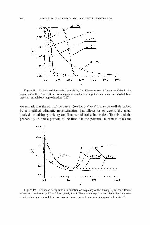
we remark that the part of the curve tðoÞ for 0 � o � 1 may be well-described

by a modified adiabatic approximation that allows us to extend the usual

analysis to arbitrary driving amplitudes and noise intensities. To this end the

probability to find a particle at the time t in the potential minimum takes the

Figure 18. Evolution of the survival probability for different values of frequency of the driving

signal, kT ¼ 0:1, A ¼ 1. Solid lines represent results of computer simulation, and dashed lines

represent an adiabatic approximation (6.15).

Figure 19. The mean decay time as a function of frequency of the driving signal for different

values of noise intensity, kT ¼ 0:5; 0:1; 0:05, A ¼ 1. The phase is equal to zero. Solid lines represent

results of computer simulation, and dashed lines represent an adiabatic approximation (6.15).


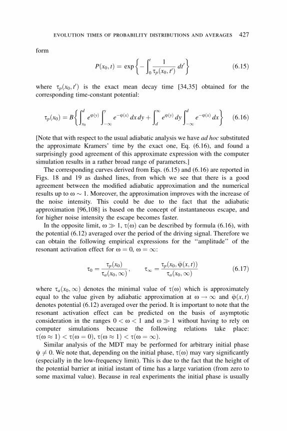
form

Pðx0; tÞ ¼ exp �ðt0

1

tpðx0; t0Þ dt0

� �ð6:15Þ

where tpðx0; t0Þ is the exact mean decay time [34,35] obtained for the

corresponding time-constant potential:

tpðx0Þ ¼ B

ðdx0

ejðyÞðy�1

e�jðxÞ dx dyþð1d

ejðyÞ dyðd�1

e�jðxÞ dx� �

ð6:16Þ

[Note that with respect to the usual adiabatic analysis we have ad hoc substituted

the approximate Kramers’ time by the exact one, Eq. (6.16), and found a

surprisingly good agreement of this approximate expression with the computer

simulation results in a rather broad range of parameters.]

The corresponding curves derived from Eqs. (6.15) and (6.16) are reported in

Figs. 18 and 19 as dashed lines, from which we see that there is a good

agreement between the modified adiabatic approximation and the numerical

results up to o � 1. Moreover, the approximation improves with the increase of

the noise intensity. This could be due to the fact that the adiabatic

approximation [96,108] is based on the concept of instantaneous escape, and

for higher noise intensity the escape becomes faster.

In the opposite limit, o� 1, tðoÞ can be described by formula (6.16), with

the potential (6.12) averaged over the period of the driving signal. Therefore we

can obtain the following empirical expressions for the ‘‘amplitude’’ of the

resonant activation effect for o ¼ 0, o ¼ 1:

t0 ¼ tpðx0Þtaðx0;1Þ ; t1 ¼ tpðx0; �jðx; tÞÞ

taðx0;1Þ ð6:17Þ

where taðx0;1Þ denotes the minimal value of tðoÞ which is approximately

equal to the value given by adiabatic approximation at o!1 and �jðx; tÞdenotes potential (6.12) averaged over the period. It is important to note that the

resonant activation effect can be predicted on the basis of asymptotic

consideration in the ranges 0 < o < 1 and o� 1 without having to rely on

computer simulations because the following relations take place:

tðo 1Þ < tðo ¼ 0Þ, tðo 1Þ < tðo ¼ 1Þ.Similar analysis of the MDT may be performed for arbitrary initial phase

c 6¼ 0. We note that, depending on the initial phase, tðoÞ may vary significantly

(especially in the low-frequency limit). This is due to the fact that the height of

the potential barrier at initial instant of time has a large variation (from zero to

some maximal value). Because in real experiments the initial phase is usually


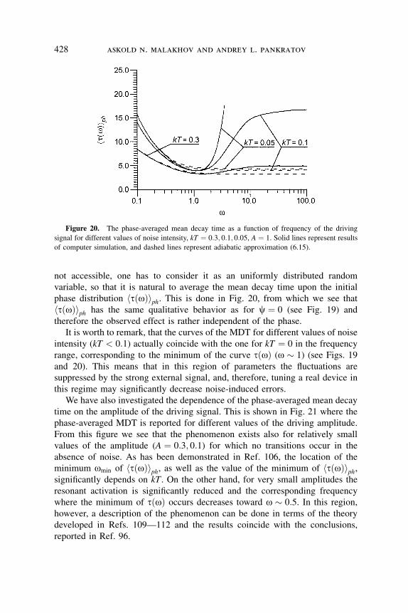
not accessible, one has to consider it as an uniformly distributed random

variable, so that it is natural to average the mean decay time upon the initial

phase distribution tðoÞh iph. This is done in Fig. 20, from which we see that

tðoÞh iph has the same qualitative behavior as for c ¼ 0 (see Fig. 19) and

therefore the observed effect is rather independent of the phase.

It is worth to remark, that the curves of the MDT for different values of noise

intensity (kT < 0:1) actually coincide with the one for kT ¼ 0 in the frequency

range, corresponding to the minimum of the curve tðoÞ (o � 1) (see Figs. 19

and 20). This means that in this region of parameters the fluctuations are

suppressed by the strong external signal, and, therefore, tuning a real device in

this regime may significantly decrease noise-induced errors.

We have also investigated the dependence of the phase-averaged mean decay

time on the amplitude of the driving signal. This is shown in Fig. 21 where the

phase-averaged MDT is reported for different values of the driving amplitude.

From this figure we see that the phenomenon exists also for relatively small

values of the amplitude (A ¼ 0:3; 0:1) for which no transitions occur in the

absence of noise. As has been demonstrated in Ref. 106, the location of the

minimum omin of tðoÞh iph, as well as the value of the minimum of tðoÞh iph,significantly depends on kT . On the other hand, for very small amplitudes the

resonant activation is significantly reduced and the corresponding frequency

where the minimum of tðoÞ occurs decreases toward o � 0:5. In this region,

however, a description of the phenomenon can be done in terms of the theory

developed in Refs. 109—112 and the results coincide with the conclusions,

reported in Ref. 96.

Figure 20. The phase-averaged mean decay time as a function of frequency of the driving

signal for different values of noise intensity, kT ¼ 0:3; 0:1; 0:05, A ¼ 1. Solid lines represent results

of computer simulation, and dashed lines represent adiabatic approximation (6.15).


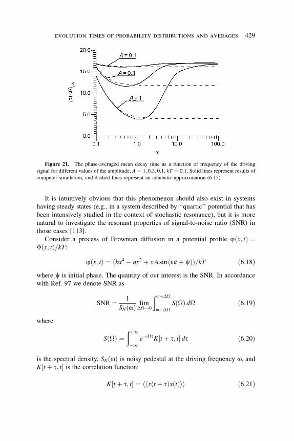
It is intuitively obvious that this phenomenon should also exist in systems

having steady states (e.g., in a system described by ‘‘quartic’’ potential that has

been intensively studied in the context of stochastic resonance), but it is more

natural to investigate the resonant properties of signal-to-noise ratio (SNR) in

those cases [113].

Consider a process of Brownian diffusion in a potential profile jðx; tÞ ¼�ðx; tÞ=kT :

jðx; tÞ ¼ ðbx4 � ax2 þ x Asinðot þ cÞÞ=kT ð6:18Þwhere c is initial phase. The quantity of our interest is the SNR. In accordance

with Ref. 97 we denote SNR as

SNR ¼ 1

SNðoÞ lim��!0

ðoþ��

o��

Sð�Þ d� ð6:19Þ

where

Sð�Þ ¼ðþ1�1

e�i�tK½t þ t; t� dt ð6:20Þ

is the spectral density, SNðoÞ is noisy pedestal at the driving frequency o, andK½t þ t; t� is the correlation function:

K½t þ t; t� ¼ xðt þ tÞxðtÞh ih i ð6:21Þ

Figure 21. The phase-averaged mean decay time as a function of frequency of the driving

signal for different values of the amplitude, A ¼ 1; 0:3; 0:1, kT ¼ 0:1. Solid lines represent results of

computer simulation, and dashed lines represent an adiabatic approximation (6.15).


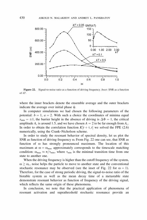
where the inner brackets denote the ensemble average and the outer brackets

indicate the average over initial phase c.In computer simulations we had chosen the following parameters of the

potential: b ¼ 1, a ¼ 2. With such a choice the coordinates of minima equal

xmin ¼ 1, the barrier height in the absence of driving is �� ¼ 1, the critical

amplitude Ac is around 1:5, and we have chosen A ¼ 2 to be far enough from Ac.

In order to obtain the correlation function K½t þ t; t� we solved the FPE (2.6)

numerically, using the Crank–Nicholson scheme.

In order to study the resonant behavior of spectral density, let us plot the

SNR as function of driving frequency o. From Fig. 22 one can see, that SNR as

function of o has strongly pronounced maximum. The location of this

maximum at o ¼ omax approximately corresponds to the timescale matching

condition: omax p=tmin, where tmin is the minimal transition time from one

state to another one.

When the driving frequency is higher than the cutoff frequency of the system,

o � oc, noise helps the particle to move to another state and the conventional

stochastic resonance may be observed (see the inset of Fig. 22 for o ¼ 1).

Therefore, for the case of strong periodic driving, the signal-to-noise ratio of the

bistable system as well as the mean decay time of a metastable state

demonstrate resonant behavior as function of frequency of the driving signal,

which reflects the same origin of these phenomena.

In conclusion, we note that the practical application of phenomena of

resonant activation and suprathreshold stochastic resonance provide an

Figure 22. Signal-to-noise ratio as a function of driving frequency. Inset: SNR as a function

of kT:


intriguing possibility to tune a concrete device in a regime with minimal noise-

induced error.

VII. CONCLUSIONS

In the frame of the present review, we discussed different approaches for

description of an overdamped Brownian motion based on the notion of integral

relaxation time. As we have demonstrated, these approaches allow one to

analytically derive exact time characteristics of one-dimensional Brownian

diffusion for the case of time constant drift and diffusion coefficients in arbitrary

potentials and for arbitrary noise intensity. The advantage of the use of integral

relaxation times is that on one hand they may be calculated for a wide variety of

desirable characteristics, such as transition probabilities, correlation functions,

and different averages, and, on the other hand, they are naturally accessible

from experiments.

Another important thing is that in many situations for the considered

diffusion processes these characteristic timescales give a rather good description

of observables via utilization of single exponential approximation. The

exponential approximation works especially well for observables that are less

sensitive to the location of initial distribution, such as transition probabilities

and correlation functions. In all other cases it is usually enough to apply double

exponential approximation to obtain the required observable with a good

precision, and one can have recourse to the two-sided Pade approximation as

suggested in Ref. 30. The exponential approximation may lead to a significant

error in the case where the noise intensity is small, the potential is tilted, and the

barrier is absent (purely dynamical motion slightly modulated by noise

perturbations). To the contrary, as has been observed for all considered

examples, the single exponential approximation is more adequate for a noise-

assisted process: either (a) noise-induced escape over a barrier or (b) motion

under intensive fluctuations. Moreover, these temporal characteristics are useful

for the description of diffusion processes in time-dependent potentials, where

one can have recourse to adiabatic approximation and obtain an adequate

description of an observable up to the cutoff frequency of the considered

system.

Finally we note that the presented approaches may be easily generalized for

the case of multidimensional systems with axial symmetry. The generalization

for arbitrary multidimensional potentials had been discussed in Refs. 41 and 114.

Acknowledgments

A. L. Pankratov wishes to thank the Department of Physics ‘‘E.R.Caianello’’ of the University of

Salerno, and he wishes to personally thank Professor M. Salerno for the offered position where part

of this work has been done. This work has been supported by the Russian Foundation for Basic


Research (Project N 00-02-16528, Project N 99-02-17544, and Project N 00-15-96620) and by the

Ministry of High Education of Russian Federation (Project N 992874).

APPENDIX: THE PRINCIPLE OF CONFORMITY

We consider the process of Brownian diffusion in a potential jðxÞ. The

probability density of a Brownian particle is governed by the FPE (5.72) with

delta-function initial condition. The moments of transition time are given by

(5.1).

Let us formulate the principle of conformity:

The moments of transition time of a dynamical system driven by noise,

described by arbitrary potential jðxÞ such that jð1Þ ¼ 1, symmetric

relatively to some point x ¼ d, with initial delta-shaped distribution, located at

the point x0 < d [Fig. A1(a)], coincides with the corresponding moments of the

first passage time for the same potential, having an absorbing boundary at the

point of symmetry of the original potential profile [Fig. A1(b)].

Let us prove that formula (4.19) (in this particular case for c ¼ �1) not only

gives values of moments of FPT of the absorbing boundary, but also expresses

moments of transition time of the system with noise, described by an arbitrary

symmetric with respect to the point d potential profile.

Figure A1. Potential profiles illustrating the principle of conformity.


Superpose the point of symmetry of the dimensionless potential profile with

the origin of the coordinate z ¼ x� d such that jð�zÞ ¼ jðzÞ and put

z0 ¼ x0 � d < 0. For the Laplace-transformed probability density Yðz; sÞ ¼Ð10

Wðz; tÞe�st dt from Eq. (5.72) we may write the following equation:

d 2Yðz; sÞdz 2

þ d

dz

djðzÞdz

Yðz; sÞ� �

� sBYðz; sÞ ¼ �Bdðz� z0Þ ð9:1Þ

Note that the probability current in Laplace transform terms is

Gðz; sÞ ¼ð10

Gðz; tÞe�st dt ¼ � 1

B

djðzÞdz

Yðz; sÞ þ dYðz; sÞdz

� �ð9:2Þ

Suppose that we know two linearly independent solutions UðzÞ ¼ Uðz; sÞ andVðzÞ ¼ Vðz; sÞ of the homogeneous equation corresponding to (9.1) (i.e., when

the right-hand side of Eq. (9.1) is equal to zero), such that UðzÞ ! 0 at z! þ1and VðzÞ ! 0 at z! �1. Because of symmetry of the function jðzÞ, theseindependent solutions may be also chosen as symmetrical, such that

Uð�zÞ ¼ VðzÞ, Uð0Þ ¼ Vð0Þ; ½dUðzÞ=dz�z¼0 ¼ �½dVðzÞ=dz�z¼0 < 0. In this

case the general solution of Eq. (9.1) may be represented as follows:

Yðz; sÞ ¼Y1ðzÞ þ y�ðzÞ; z � z0Y1ðzÞ þ yþðzÞ; z0 � z � 0

Y2ðzÞ; z � 0

8<: ð9:3Þ

where

Y1ðzÞ ¼ C1VðzÞ; Y2ðzÞ ¼ C2UðzÞy�ðzÞ ¼ B

W ½z0�Uðz0ÞVðzÞ; yþðzÞ ¼ B

W ½z0�Vðz0ÞUðzÞ

Here W ½z� ¼ UðzÞ dVðzÞdz� VðzÞ dUðzÞ

dzis Wronskian, and C1 and C2 are arbitrary

constants that may be found from the continuity condition of the probability

density and the probability current at the origin:

Y1ð0Þ þ yþð0Þ ¼ Y2ð0Þ; Gðz ¼ �0; sÞ ¼ Gðz ¼ þ0; sÞ ð9:4ÞCalculating from (9.4) the values of arbitrary constants and putting them into

(9.3), one can obtain the following value for the probability current Laplace

transform Gðz; sÞ (9.2) at the point of symmetry z ¼ 0:

Gð0; sÞ ¼ Vðz0ÞW ½z0�

dVðzÞdz

� �z¼0

ð9:5Þ


Actually, we can prove the principle of conformity step-by-step for all moments

of transition time (5.4),(5.5), and so on, but it is more simple to prove it for the

probability density of transition time wtðt; z0Þ (5.2). Taking the Laplace

transform from the expression (5.2) and noting that sQðs; z0Þ � Qð0; z0Þ ¼Gð0; sÞ, one can obtain the following formula for wtðs; z0Þ:

wtðs; z0Þ ¼ sQðs; z0Þ � Qð0; z0ÞQð1; z0Þ � Qð0; z0Þ ¼

Gð0; sÞQð1; z0Þ � Qð0; z0Þ ð9:6Þ

where Qðs; z0Þ ¼Ð10

Yðz; sÞ dz is the Laplace-transformed decay probability. In

our particular case Qð0; z0Þ ¼ 0, Qð1; z0Þ ¼ 1=2, because the steady-state

probability density Wðz;1Þ will spread symmetrically from both sides of the

point of symmetry z ¼ 0. Thus, combining (9.6) and (9.5) we obtain the

following formula for the Laplace-transformed probability density of transition

time:

wtðs; z0Þ ¼ 2Vðz0ÞW ½z0�

dVðzÞdz

� �z¼0

ð9:7Þ

Before finding the Laplace-transformed probability density wTðs; z0Þ of FPT for

the potential, depicted in Fig. A1(b), let us obtain the Laplace-transformed

probability density wtðs; z0Þ of transition time for the system whose potential is

depicted in Fig. A1(c). This potential is transformed from the original profile

[Fig. A1(a)] by the vertical shift of the right-hand part of the profile by step bwhich is arbitrary in value and sign. So far as in this case the derivative djðzÞ=dzin Eq. (9.1) is the same for all points except z ¼ 0, we can use again linear-

independent solutions UðzÞ and VðzÞ, and the potential jump that equals b at the

point z ¼ 0 may be taken into account by the new joint condition at z ¼ 0. The

probability current at this point is continuous as before, but the probability

densityWðz; tÞ has now the step, so the second condition of (9.4) is the same, but

instead of the first one we should write Y1ð0Þ þ yþð0Þ ¼ Y2ð0Þe�b. It gives newvalues of arbitrary constants C1 and C2 and a new value of the probability current

at the point z ¼ 0. Now the Laplace transformation of the probability current is

Gð0; sÞ ¼ 2Vðz0ÞW ½z0�ð1þ e�bÞ

dVðzÞdz

� �z¼0

ð9:8Þ

One can find that for the potential depicted in Fig. A1(c) the quantity Qð1; z0Þhas been also changed and now equals Qð1; z0Þ ¼ 1=ð1þ e�bÞ, while the

quantity of Qð0; z0Þ certainly, as before, is Qð0; z0Þ ¼ 0. It is easy to check that

the substitution of new values of Gð0; sÞ and Qð1; z0Þ into formula (9.6) gives

the same formula (9.7) for wtðs; z0Þ. Putting now b ¼ 1—that is, locating the


absorbing boundary at the point z ¼ 0 (x ¼ d)—we obtain the same formula

(9.7), not for the probability density of the transition time but for the probability

density of FPT wTðs; z0Þ. It is known that if the Laplace transformations of two

functions coincide, then their origins coincide too. So, if we substitute the

coinciding probability densities wtðt; z0Þ and wTðt; z0Þ into formula (5.1) [see

formulas (5.2) and (5.3)] for the cases of the symmetric potential profile and the

profile with the absorbing boundary at the point of symmetry, we should obtain

equal values for the moments of transition time and FPT.

Thus, we have proved the principle of conformity for both probability

densities and moments of the transition time of symmetrical potential profile

and FPT of the absorbing boundary located at the point of symmetry.

It is obvious that moments of FPT to the point 0 are the same for the profiles

depicted in Fig. A1. For moments of transition time, this coincidence is not so

easily understandable, and the fact that the principle of conformity is valid for

the potential depicted in Fig. A1(c) leads to an unusual conclusion: Neither the

quantity nor the sign of the potential step b influences the moments of the

transition time.

For the mean transition time, this fact may be explained in the following

way: If the transition process is going from up to down, then the probability

current is large, but it is necessary to fill the lower minimum by the larger part of

the probability to reach the steady state; if the transition process is going from

down to up, then the probability current is small, and it is necessary to fill the

upper minimum by the smaller part of the probability to reach the steady state.

The difference in the quantities of currents is completely compensated by

quantities of final probabilities of reaching the steady state.

An interested reader can easily check the principle of conformity

numerically and see that if the probability of the FPT QTðt; x0Þ [Fig. A1(b)]is known, then the decay probability Qtðt; x0Þ [Fig. A1(a)] is expressed as

Qtðt; x0Þ ¼ ½1þ QTðt; x0Þ�=2.Note finally that the principle of conformity, proved for delta-shaped initial

distribution of the probability density, may also be extended to arbitrary initial

distributions located within the considered interval Wðx; 0Þ ¼ WinðxÞ; x 2 ðc; dÞ.

References

1. P. Hanggi, P. Talkner, and M. Borkovec, Rev. Mod. Phys. 62, 251 (1990).

2. H. Risken, The Fokker–Planck Equation, 2nd ed., Springer Verlag, Berlin, 1989.

3. K. K. Likharev,Dynamics of Josephson Junctions and Circuits, Gordon and Breach, New York,

1986.

4. W. T. Coffey, Yu. P. Kalmykov, and J. T. Waldron, The Langevin Equation, World Scientific,

Singapore, 1996.

5. D. A. Garanin, V. V. Ishchenko, and L. V. Panina, Teor. Mat. Fiz. 82, 242 (1990) [Teor. Mat.

Phys. 82, 169 (1990)].


6. D. A. Garanin, Phys. Rev. E 54, 3250 (1996).

7. W. T. Coffey, D. S. F. Crothers, Yu. P. Kalmykov, and J. T. Waldron, Phys. Rev. B 51, 15947

(1995).

8. F. W. Weigel, Phys. Rep. 95, 283 (1983).

9. J. A. McCammon, Rep. Prog. Phys. 47, 1 (1984).

10. R. S. Berry, S. A. Rice, and J. Ross, Physical Chemistry, Wiley, New York, 1980.

11. H. Kramers, Physica 7, 284 (1940).

12. S. H. Northrup and J. T. Hynes, J. Chem. Phys. 69, 5264 (1978).

13. G. van der Zwan and J. T. Hynes, J. Chem. Phys. 77, 1295 (1982).

14. N. Agmon and J. J. Hopfield, J. Chem. Phys. 78, 6947 (1983).

15. C. W. Gardiner, Handbook of Stochastic Methods, Springer-Verlag, 1985.

16. N. G. van Kempen, Stochastic Process in Physics and Chemistry, 2nd ed., North-Holland,

Amsterdam, 1992.

17. R. L. Stratonovich, Topics of the Theory of Random Noise, Gordon and Breach, New York,

1963.

18. V. I. Tikhonov and M. A. Mironov, Markovian Processes, Sovetskoe Radio, Moscow, 1978, in

Russian.

19. L. A. Pontryagin, A. A. Andronov, and A. A. Vitt, Zh. Eksp. Teor. Fiz. 3, 165 (1933) [translated

by J. B. Barbour and reproduced in Noise in Nonlinear Dynamics, Vol. 1, F. Moss and P. V. E.

McClintock, eds., Cambridge University Press, Cambridge, 1989, p. 329.

20. R. S. Larson and M. D. Kostin, J. Chem. Phys. 69, 4821 (1978).

21. R. S. Larson, J. Chem. Phys. 81, 1731 (1984).

22. G. H. Weiss, Adv. Chem. Phys. 13, 1 (1967).

23. I. Oppenheim, K. E. Shuler, and G. H. Weiss, Stochastic Processes in Chemical Physics, MIT,

Cambridge, 1977.

24. A. Szabo, K. Schulten, and Z. Schulten, J. Chem. Phys. 72, 4350 (1980).

25. K. Schulten, Z. Schulten, and A. Szabo, J. Chem. Phys. 74, 4426 (1981).

26. V. Seshadri, B. J. West, and K. Lindenberg, J. Chem. Phys. 72, 1145 (1980).

27. B. J. West, K. Lindenberg, and V. Seshadri, J. Chem. Phys. 72, 1151 (1980).

28. J. Deutch, J. Chem. Phys. 73, 4700 (1980).

29. B. Carmeli and A. Nitzan, J. Chem. Phys. 76, 5321 (1982).

30. W. Nadler and K. Schulten, J. Chem. Phys. 82, 151 (1985).

31. P. Jung and H. Risken, Z. Phys. B 59, 469 (1985).

32. N. V. Agudov and A. N. Malakhov, Radiophys. Quantum Electron. 36, 97 (1993).

33. A. N. Malakhov and A. L. Pankratov, Physica A 229, 109 (1996).

34. A. N. Malakhov and A. L. Pankratov, Physica C 269, 46 (1996).

35. A. N. Malakhov, CHAOS 7, 488 (1997).

36. W. T. Coffey, Adv. Chem. Phys. 103, 259 (1998).

37. W. T. Coffey and D. S. F. Crothers, Phys. Rev. E 54, 4768 (1996).

38. Yu. P. Kalmykov, W. T. Coffey, and J. T. Waldron, J. Chem. Phys. 105, 2112 (1996).

39. Yu. P. Kalmykov, J. L. Dejardin, and W. T. Coffey, Phys. Rev. E 55, 2509 (1997).

40. W. T. Coffey, D. S. F. Crothers, and Yu. P. Kalmykov, Phys. Rev. E 55, 4812 (1997).

41. W. T. Coffey, J. Chem. Phys. 111, 8350 (1999).


42. I. Derenyi and R. D. Astumian, Phys. Rev. Lett. 82, 2623 (1999).

43. A. N. Malakhov, Cumulant Analysis of Random Non-Gaussian Processes and Its Transforma-

tions, Sovetskoe Radio, Moscow, 1978, in Russian.

44. A. D. Fokker, Ann. Phys. (Leipzig) 43, 310 (1915).

45. M. Planck, Sitzungsber. Preuss. Acad. Wiss. Phys. Math. Kl. 325 (1917).

46. A. N. Kolmogorov, Math. Ann. 104, 415 (1931).

47. V. I. Melnikov, Phys. Rep. 209, 1 (1991).

48. O. Edholm, O. Leimar, Physica A 98, 313 (1979).

49. N. V. Agudov and A. N. Malakhov, Appl. Nonlinear Dyn. 3, N3, 75 (1995) (in Russian).

50. P. Reimann, G. J. Schmid, and P. Hanggi, Phys. Rev. E 60, R1 (1999).

51. A. N. Malakhov, Fluctuations in Self-Oscillating Systems, Science, Moscow, 1968, in Russian.

52. M. San Miguel, L. Pesquera, M. A. Rodriguez, and A. Hernandez-Machado, Phys. Rev. A 35,

208 (1987).

53. W. Coffey, D. S. F. Crothers, Yu. P. Kalmykov, E. S. Massawe, and J. T. Waldron, Phys. Rev. E

49, 1869 (1994).

54. A. N. Malakhov and E. L. Pankratov, Radiophysics and Quantum Electonics, 44, 339 (2001).

55. Jose Luis Garsia-Palacios and Francisco J. Lazaro, Phys. Rev. B 58, 14937 (1998).

56. P. Colet, M. San Miguel, J. Casademunt, and J. M. Sancho, Phys. Rev. A 39, 149 (1989).

57. J. E. Hirsch, B. A. Huberman, and D. V. Scalapino, Phys. Rev. A 25, 519 (1982).

58. I. Dayan, M. Gitterman, and G. H. Weiss, Phys. Rev. A 46, 757 (1992).

59. M. Gitterman and G. H. Weiss, J. Stat. Phys. 70, 107 (1993).

60. J. M. Casado and M. Morillo, Phys. Rev. E 49, 1136 (1994).

61. R. N. Mantegna and B. Spagnolo, Phys. Rev. Lett. 76, 563 (1996).

62. R. N. Mantegna and B. Spagnolo, Int. J. Bifurcation Chaos Appl. Sci. Eng. 8, 783 (1998).

63. N. V. Agudov and A. N. Malakhov, Int. J. Bifurcation Chaos Appl. Sci. Eng. 5, 531 (1995).

64. N. V. Agudov, Phys. Rev. E 57, 2618 (1998).

65. M. Frankowicz and G. Nicolis, J. Stat. Phys. 33, 595 (1983).

66. M. Frankowicz, M. Malek Mansour, and G. Nicolis, Physica A 125, 237 (1984).

67. E. Arimondo, D. Dangoisse, and L. Fronzoni, Europhys. Lett. 4, 287 (1987).

68. J. Iwaniszewski, Phys. Rev. A 45, 8436 (1992).

69. N. V. Agudov and A. N. Malakhov, Phys. Rev. E 60, 6333 (1999).

70. A. L. Pankratov, Phys. Lett. A 234, 329 (1997).

71. F. T. Arecci, M. Giglio, and A. Sona, Phys. Lett. A 25, 341 (1967).

72. S. Chopra and L. Mandel, IEEE J. QE-8, 324 (1972).

73. W. T. Coffey, D. S. F. Crothers, J. L. Dormann, L. G. Geoghegan, and E. C. Kennedy, Phys.

Rev. B 58, 3249 (1998).

74. Yu. P. Kalmykov, S. V. Titov, and W. T. Coffey, Phys. Rev. B 58, 3267 (1998).

75. Yu. P. Kalmykov and S. V. Titov, Phys. Rev. Lett. 82, 2967 (1999).

76. W. T. Coffey, J. Chem. Phys. 93, 724 (1990).

77. W. T. Coffey, Yu. P. Kalmykov, E. S. Massawe, and J. T. Waldron, J. Chem. Phys. 99, 4011

(1993).

78. M. Abramowitz and I. Stegun, Handbook of Mathematical Functions, Dover, New York, 1964.

79. J. I. Lauritzen, Jr., and R. W. Zwanzig, Jr., Adv. Mol. Relax. Processes 5, 339 (1973).


80. G. Klein, Proc. R. Soc. London, Ser. A 211, 431 (1952).

81. G. Korn and T.Korn,Mathematical Handbook for Scientists and Engineers, McGraw-Hill, New

York, 1961.

82. A. N. Malakhov, Radiophys. Quantum Electron. 34, 451 (1991).

83. A. N. Malakhov, Radiophys. Quantum Electron. 34, 571 (1991).

84. Z. Bilkadi, J. D. Parsons, J. A. Mann, and R. D. Neumann, J. Chem. Phys. 72, 960 (1980).

85. A. N. Malakhov and A. L. Pankratov, Radiophys. Quantum Electron. 38, 167 (1995).

86. H. L. Frisch, V. Privman, C. Nicolis, and G. Nicolis, J. Phys. A: Math. Gen. 23, L1147 (1990).

87. M. Morsch, H. Risken, and H. Vollmer, Z. Phys. B 32, 245 (1979).

88. S. P. Nikitenkova and A. L. Pankratov, Preprint N adap-org/9811004 at http://xxx.lanl.gov.

89. A. L. Pankratov, Phys. Lett. A 255, 17 (1999).

90. A. A. Dubkov, A. N. Malakhov, and A. I. Saichev, Radiophys. Quantum Electron. 43, 335

(2000).

91. A. A. Antonov, A. L. Pankratov, A. V. Yulin, and J. Mygind, Phys. Rev. B 61, 9809 (2000).

92. S. P. Nikitenkova and A. L. Pankratov, Phys. Rev. E 58, 6964 (1998).

93. S. R. Shenoy and G. S. Agarwal, Phys. Rev. A 29, 1315 (1984).

94. R. Roy, R. Short, J. Durnin, and L. Mandel, Phys. Rev. Lett. 45, 1486 (1980).

95. K. Lindenberg and B. West, J. Stat. Phys. 42, 201 (1986).

96. P. Jung, Physics Rep. 234, 175 (1993).

97. For a review on stochastic resonance see L. Gammaitoni, P. Hanggi, P. Jung, and F. Marchesoni,

Rev. Mod. Phys. 70, 223 (1998) and references therein.

98. F. Julicher, A. Ajdari, and J. Prost, Rev. Mod. Phys. 69, 1269 (1997).

99. C. R. Doering, Physica A 254, 1 (1998).

100. N. G. Stocks and R. Manella, Phys. Rev. Lett. 80, 4835 (1998).

101. C. R. Doering and J. Godoua, Phys. Rev. Lett. 69, 2318 (1992).

102. M. Bier and R. Dean Astumian, Phys. Rev. Lett. 71, 1649 (1993).

103. P. Pechukas and P. Hanggi, Phys. Rev. Lett. 73, 2772 (1994).

104. P. Reimann and P. Hanggi, in Lectures on Stochastic Dynamics, Springer Series LNP 484,

Springer, New York, 1997, p. 127.

105. M. Boguna, J. M. Porra, J. Masoliver, and K. Lindenberg, Phys. Rev. E 57, 3990 (1998).

106. A. L. Pankratov and M. Salerno, Phys. Lett. A 273, 162 (2000).

107. A. L. Pankratov and M. Salerno, Phys. Rev. E 61, 1206 (2000).

108. T. Zhou, F. Moss, and P. Jung, Phys. Rev. A 42, 3161 (1990).

109. V. N. Smelyanskiy, M. I. Dykman, H. Rabitz, and B. E. Vugmeister, Phys. Rev. Lett. 79, 3113

(1997).

110. V. N. Smelyanskiy, M. I. Dykman, and B. Golding, Phys. Rev. Lett. 82, 3193 (1999).

111. D. G. Luchinsky, R. Mannella, P. V. E. McClintock, M. I. Dykman, and V. N. Smelyanskiy,

J. Phys. A: Math. Gen. 32, L321 (1999).

112. J. Lehmann, P. Reimann, and P. Hanggi, Phys. Rev. Lett. 84, 1639 (2000).

113. A. L. Pankratov, Phys. Rev. E, in press, cond-mat/0103448.

114. W. Nadler and K. Schulten, J. Chem. Phys. 84, 4015 (1986).


Documents

ADVANCES IN CHEMICAL PHYSICS - Институт ...ipmras.ru/UserFiles/publications/alp/Advances in Chemical Physics... · Advances in Chemical Physics, ... we note that there are