Embed Size (px)
Citation preview


ADVANCES IN BUSINESS AND
MANAGEMENT FORECASTING

ADVANCES IN BUSINESS ANDMANAGEMENT FORECASTING
Series Editor: Kenneth D. Lawrence
Recent Volumes:
Volume 1: Advances in Business and ManagementForecasting: Forecasting Sales
Volume 2: Advances in Business and ManagementForecasting: Forecasting
Volume 3: Advances in Business and ManagementForecasting
Volume 4: Advances in Business and ManagementForecasting
Volume 5: Advances in Business and ManagementForecasting

ADVANCES IN BUSINESS AND MANAGEMENT
FORECASTING VOLUME 6
ADVANCES IN BUSINESSAND MANAGEMENT
FORECASTING
EDITED BY
KENNETH D. LAWRENCENew Jersey Institute of Technology, Newark, USA
RONALD K. KLIMBERGSaint Joseph’s University, Philadelphia, USA
United Kingdom – North America – Japan
India – Malaysia – China

JAI Press is an imprint of Emerald Group Publishing Limited
Howard House, Wagon Lane, Bingley BD16 1WA, UK
First edition 2009
Copyright r 2009 Emerald Group Publishing Limited
Reprints and permission service
Contact: [email protected]
No part of this book may be reproduced, stored in a retrieval system, transmitted in any
form or by any means electronic, mechanical, photocopying, recording or otherwise
without either the prior written permission of the publisher or a licence permitting
restricted copying issued in the UK by The Copyright Licensing Agency and in the USA
by The Copyright Clearance Center. No responsibility is accepted for the accuracy of
information contained in the text, illustrations or advertisements. The opinions expressed
in these chapters are not necessarily those of the Editor or the publisher.
British Library Cataloguing in Publication Data
A catalogue record for this book is available from the British Library
ISBN: 978-1-84855-548-8
ISSN: 1477-4070 (Series)
Awarded in recognition ofEmerald’s productiondepartment’s adherence toquality systems and processeswhen preparing scholarlyjournals for print

CONTENTS
LIST OF CONTRIBUTORS ix
EDITORIAL BOARD xiii
PART I: FINANCIAL APPLICATIONS
COMPETITIVE SET FORECASTING IN THE HOTELINDUSTRY WITH AN APPLICATION TO HOTELREVENUE MANAGEMENT
John F. Kros and Christopher M. Keller 3
PREDICTING HIGH-TECH STOCK RETURNS WITHFINANCIAL PERFORMANCE MEASURES:EVIDENCE FROM TAIWAN
Shaw K. Chen, Chung-Jen Fu and Yu-Lin Chang 15
FORECASTING INFORMED TRADING ATMERGER ANNOUNCEMENTS: THE USE OFLIQUIDITY TRADING
Rebecca Abraham and Charles Harrington 37
USING DATA ENVELOPMENT ANALYSIS (DEA) TOFORECAST BANK PERFORMANCE
Ronald K. Klimberg, Kenneth D. Lawrence andTanya Lal
53
PART II: MARKETING AND DEMANDAPPLICATIONS
FORECASTING DEMAND USING PARTIALLYACCUMULATED DATA
Joanne S. Utley and J. Gaylord May 65v

FORECASTING NEW ADOPTIONS: A COMPARATIVEEVALUATION OF THREE TECHNIQUES OFPARAMETER ESTIMATION
Kenneth D. Lawrence, Dinesh R. Pai andSheila M. Lawrence
81
THE USE OF A FLEXIBLE DIFFUSION MODEL FORFORECASTING NATIONAL-LEVEL MOBILETELEPHONE AND INTERNET DIFFUSION
Kallol Bagchi, Peeter Kirs and Zaiyong Tang 93
FORECASTING HOUSEHOLD RESPONSE INDATABASE MARKETING: A LATENTTRAIT APPROACH
Eddie Rhee and Gary J. Russell 109
PART III: FORECASTING METHODSAND EVALUATION
A NEW BASIS FOR MEASURING AND EVALUATINGFORECASTING MODELS
Frenck Waage 135
FORECASTING USING INTERNAL MARKETS,DELPHI, AND OTHER APPROACHES: THEKNOWLEDGE DISTRIBUTION GRID
Daniel E. O’Leary 157
THE EFFECT OF CORRELATION BETWEENDEMANDS ON HIERARCHICAL FORECASTING
Huijing Chen and John E. Boylan 173
PART IV: OTHER APPLICATION AREASOF FORECASTING
ECONOMETRIC COUNT DATA FORECASTING ANDDATA MINING (CLUSTER ANALYSIS) APPLIED TOSTOCHASTIC DEMAND IN TRUCKLOAD ROUTING
Virginia M. Miori 191
CONTENTSvi

TWO-ATTRIBUTE WARRANTY POLICES UNDERCONSUMER PREFERENCES OF USAGE ANDCLAIMS EXECUTION
Amitava Mitra and Jayprakash G. Patankar 217
A DUAL TRANSPORTATION PROBLEM ANALYSISFOR FACILITY EXPANSION/CONTRACTIONDECISIONS: A TUTORIAL
N. K. Kwak and Chang Won Lee 237
MAKE-TO-ORDER PRODUCT DEMANDFORECASTING: EXPONENTIAL SMOOTHINGMODELS WITH NEURAL NETWORK CORRECTION
Mark T. Leung, Rolando Quintana andAn-Sing Chen
249
Contents vii

This page intentionally left blank

LIST OF CONTRIBUTORS
Rebecca Abraham Huizenga School of Business, NovaSoutheastern University, FortLauderdale, FL, USA
Kallol Bagchi Department of Information andDecision Sciences, University of TexasEl Paso, El Paso, TX, USA
John E. Boylan School of Business and Management,Buckingham Shire Chilton UniversityCollege, Buckinghamshire, UK
Yu-Lin Chang Department of Accounting andInformation Technology, Ling TungUniversity, Taiwan
An-Sing Chen College of Management,National Chung Cheng University,Ming-Hsiung, Chia-Yi, Taiwan
Huijing Chen Salford Business School, Universityof Salford, Salford, UK
Shaw K. Chen College of Business Administration,University of Rhode Island, RI, USA
Chung-Jen Fu College of Management, NationalYunlin University of Science andTechnology, Yunlin, Taiwan
Charles Harrington Huizenga School of Business, NovaSoutheastern University, FortLauderdale, FL, USA
ix

Christopher M. Keller Department of Marketing and SupplyChain Management, College of Business,East Carolina University, Greenville,NC, USA
Peeter Kirs Department of Information andDecision Sciences, University of TexasEl Paso, El Paso, TX, USA
Ronald K. Klimberg DSS Department, Haub School ofBusiness, Saint Joseph’s University,Philadelphia, PA, USA
John F. Kros Department of Marketing and SupplyChain Management, College of Business,East Carolina University, Greenville,NC, USA
N. K. Kwak Department of Decision Sciences andITM, Saint Louis University, St. Louis,MO, USA
Tanya Lal Haub School of Business, Saint Joseph’sUniversity, Philadelphia, PA, USA
Kenneth D. Lawrence School of Management, New JerseyInstitute of Technology, Newark,NJ, USA
Sheila M. Lawrence Management Science and InformationSystems, Rutgers Business School,Rutgers University, Piscataway,NJ, USA
Chang Won Lee School of Business, Hanyang University,Seoul, Korea
Mark T. Leung Department of Management Science,College of Business, University of Texasat San Antonio, San Antonio, TX, USA
J. Gaylord May Department of Mathematics, WakeForest University, Winston-Salem, NC,USA
LIST OF CONTRIBUTORSx

Virginia M. Miori DSS Department, Haub School ofBusiness, St. Joseph’s University,Philadelphia, PA, USA
Amitava Mitra Office of the Dean and Departmentof Management, College of Business,Auburn University, Auburn, AL, USA
Daniel E. O’Leary Levanthal School of Accounting,Marshall School of Business, Universityof Southern California, CA, USA
Dinesh R. Pai Management Science and InformationSystems, Rutgers Business School,Rutgers University, Newark, NJ, USA
Jayprakash G. Patankar Department of Management, TheUniversity of Akron, Akron, OH, USA
Rolando Quintana Department of Management Science,College of Business, University of Texasat San Antonio, San Antonio, TX, USA
Eddie Rhee Department of Business Administration,Stonehill College, Easton, MA, USA
Gary J. Russell Department of Marketing, TippieCollege of Business, University of Iowa,Iowa City, IA, USA
Zaiyong Tang Marketing and Decision SciencesDepartment, Salem State College, Salem,MA, USA
Joanne S. Utley School of Business and Economics,North Carolina A&T State University,Greensboro, NC, USA
Frenck Waage Department of Management Science andInformation Systems, University ofMassachusetts Boston, Boston, MA, USA
List of Contributors xi

This page intentionally left blank

EDITORIAL BOARD
Editors-in-Chief
Kenneth D. Lawrence Ronald KlimbergNew Jersey Institute of Technology Saint Joseph’s University
Senior Editors
Lewis Coopersmith Daniel O’LearyRider College University of Southern California
John Guerard Dinesh R. PaiAnchorage, Alaska Rutgers University
Douglas Jones Ramesh ShardaRutgers University Oklahoma State University
Stephen Kudbya William StewardNew Jersey Institute of Technology College of William and Mary
Sheila M. Lawrence Frenck WaageRutgers University University of Massachusetts
Virginia Miori David WhitlarkSaint Joseph’s University Brigham Young University
xiii

This page intentionally left blank

PART I
FINANCIAL APPLICATIONS

This page intentionally left blank

COMPETITIVE SET FORECASTING
IN THE HOTEL INDUSTRY WITH
AN APPLICATION TO HOTEL
REVENUE MANAGEMENT
John F. Kros and Christopher M. Keller
INTRODUCTION
Successful revenue management programs are found in industries wheremanagers can accurately forecast customer demand. Airlines, rental caragencies, cruise lines, and hotels are all examples of industries that havebeen associated with revenue management. All of these industries haveapplied revenue management, whether it be complex overbooking models inthe airline industry or simple price discrimination (i.e., having a tiered pricesystem for those making reservations ahead of time versus walk-ups) forhotels.
The travel and hospitality industry and the hotel industry in particularhas a history of employing revenue management to enhance profits. Theability to accurately set prices in response to forecasted demand is a centralmanagement performance tool. Individual hotel manager performance isgenerally base-lined on historical performance and a manager may be taskedwith driving occupancy higher than the previous year’s performance. In astable market environment, such benchmarking is reasonable. However, ifthe market changes by the entrance and exit of competitive hotels then such
Advances in Business and Management Forecasting, Volume 6, 3–14
Copyright r 2009 by Emerald Group Publishing Limited
All rights of reproduction in any form reserved
ISSN: 1477-4070/doi:10.1108/S1477-4070(2009)0000006001
3

benchmarking may be unfair to the individual manager and a poor plan formanagement. This chapter develops two models that forecast demand anddemonstrates for an existing data set how the entrance and exit ofcompetitive market hotels in some cases does and in some cases does notchange that forecasting demand. Understanding that the analysis of adynamic market environment sometimes necessitates a forecast change isuseful for improving the demand forecasts, which are critical to any revenuemanagement system.
HOTEL REVENUE MANAGEMENT
AND PERFORMANCE
The performance of hotel managers is measured along three principalcomponents: revenue, cost, and quality. Hotel managers set availabilityrestrictions and price for hotel rooms. Availability and price are theprincipal components of hotel revenue management. Of the threecomponents of hotel management performance, revenue management isthe single most controllably variable measure. Lee (1990) reported thataccurately forecasting demand is cornerstone to any revenue managementsystem and that a 10 percent improvement in forecast accuracy could resultin an increase in revenue of between 1.5 and 3.0 percent.
Most hotel managers do not control fixed investment costs and generallyspeaking any controllable variable costs tend to be relatively standardrates. Cost management thus does not have large managerial flexibility, butrather is a limited control responsibility for overall hotel performance.Quality measures of performance include customer satisfaction and qualityinspections. As with costs, measures of hotel quality performance aregenerally not widely variable, but rather are a limited control responsibilityfor overall hotel performance.
A number of researchers have studied hotel revenue management ingeneral. Bitran and Mondschein (1995) spoke about room allocation,Weatherford (1995) proposed a heuristic for booking of customers, Bakerand Collier (1999) compare five booking control policies. More specifically,forecasting in hotel revenue management has also been studied.Kimes (1999) studied the issue of hotel group forecasting accuracy andWeatherford and Kimes (2003) compare forecasting methods for hotelrevenue management. Schwartz and Cohen (2004) investigate the subjective
JOHN F. KROS AND CHRISTOPHER M. KELLER4

estimates of forecast uncertainty by hotel revenue managers, whereasWeatherford, Kimes, and Scott (2001) speak more quantitatively to theconcept of forecasting aggregation versus disaggregation in hotel revenuemanagement. Weatherford et al. (2001) determine that disaggregatedforecasts are much more accurate than in their aggregate form. Undertheir study, aggregation is done over average daily rate (ADR) and length-of-stay.
Rate class and length-of-stay are important variables that influence hotelperformance and in turn improved forecasting of these variables shouldassist in optimizing revenue. Along these dimensions, ceteris paribus, hotelmanagement is improved by increasing the performance measure. Forexample, higher rate classes generate higher revenue and longer lengths-of-stay generate greater revenue.
COMPARING REVENUE PERFORMANCE
OF COMPETING HOTELS
The revenue performance of an individual hotel’s revenue performance canbe compared with its competitors’ revenue performance using standardmarket data such as that provided by Smith Travel and Research (STAR).STAR reports are a widely used standard competitive market informationservice in the hotel industry. In a stable and nonchanging market, suchcomparisons can be used to assess individual performance of a hotelmanager. But, in many markets, new hotels are opened, old hotels areclosed, and existing hotels are rebranded (up or down). The dynamics ofthese market changes are generally reflected in the STAR reports. Thesedynamic market changes can seriously affect comparisons of an individualhotel and its competitive set.
The specific inclusion and exclusion of any hotel within the competitiveset may vary over time and the entrance and exit of hotels in a competitiveset is reflected in the STAR reports. This chapter considers an exploratoryassessment of whether or not a competitive set has been well-defined fora specific hotel and in turn how a competitive set could be forecast fora specific hotel in a dynamic marketplace. The data consists of competitiveperformance data for five distinct periods, representing changes in hotelcompetitors. The performance measures of the dynamic market areconsidered for whether or not the underlying competitive market has
Competitive Set Forecasting in Hotel Industry 5

significantly changed and this is particular important for assessingindividual hotel manager performance.
RESEARCH METHOD AND HOTEL DATA
This research examines hotel occupancy (OCC) and ADRs over a three-yearperiod. The principal observation that is being sought is that ADR andOCC exhibit a consistent relationship over the various time periods. That is,the demand for hotel rooms has not changed during the time period; onlythe supply has changed by the entrance and or exit of hotels in thecompetitive set. There has been research in the area regarding model-basedforecasting of hotel demand. Witt and Witt (1991b) present a literaturereview of published papers on forecasting tourism demand. They alsocompare the performance of time series and econometric models (Witt &Witt, 1991a). S-shaped models, based on Gompertz’ work (Harrington,1965), were used by Witt and Witt (1991a), and again by Riddington (1999)to model tourism demand. However, little other research has beencompleted incorporating such a model into the tourism area.
The data in the present chapter has five distinct periods overapproximately three years with each period containing a differentcompetitive set
(1) Period One: Data for an 8-month period, which includes 7 hotels with atotal of 763 rooms. This variable is denoted P1.
(2) Period Two: Data for an 11-month period, which includes 8 hotels witha total of 865 rooms, and includes the addition of a newly constructedbrand name hotel. This variable is denoted P2.
(3) Period Three: Data for a 5-month period, which includes 9 hotels with atotal of 947 rooms, and includes the addition of a newly constructedbrand name hotel. This variable is denoted P3.
(4) Period Four: Data for a 1-month period, which includes 8 hotels with atotal of 761 rooms, and includes the closing of an existing hotel. Thisvariable is denoted P4.
(5) Period Five: Data for a 10-month period, which includes 7 hotels with atotal of 666 rooms, and includes the removal of an existing hotel fromreporting within the competitive set. This variable is denoted P5.
The periods as listed above are sequential. That is, Period Two followsPeriod One, and Period Five follows Period Four. It should be noted thateach time period does not include each month, and that in general, each
JOHN F. KROS AND CHRISTOPHER M. KELLER6

month is included in only two or three of the relevant reporting periods. Thenonsystematic and nonseasonal changes in the market limit the standardtools that may be applied to the data. For example, one method forconsidering the periodic effects above would be to construct a multiplelinear regression model of demand that includes dummy variables for eachof the periods. Although the dummy variable methodology for evaluatingchanges in the market is useful, the underlying linear model is difficult toapply reasonable in the data for this case of hotel revenue management. Thefundamental issue with a linear approximation of demand is illustrated inFig. 1. Descriptively, the ‘‘problem’’ is that any multiple linear regressionmodel of demand is fundamentally ill-fitting.
This chapter uses a bases S-shaped model that begins with a slow startfollowed by rapid growth, which tails off as saturation approaches. As canbe seen in Fig. 1, when ADR versus OCC is analyzed, the relationshipdefinitely takes on an S-shape. Therefore, the basic Gompertz function wasemployed as the base function for modeling ADR versus OCC and is asfollows:
yðtÞ ¼ aebect
where y(t) ¼ EstOCC, a ¼ 100 (upper limit of % occupancy), bo0 and is acurve fitting parameter, co0 and is a measure of growth rate, and t ¼ ADR.
Fig. 1. Linear Estimate of Demand for the Data.
Competitive Set Forecasting in Hotel Industry 7
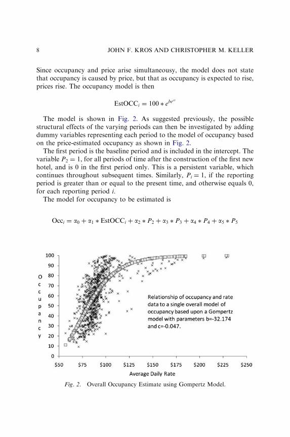
Since occupancy and price arise simultaneousy, the model does not statethat occupancy is caused by price, but that as occupancy is expected to rise,prices rise. The occupancy model is then
EstOCCi ¼ 100 � ebect
The model is shown in Fig. 2. As suggested previously, the possiblestructural effects of the varying periods can then be investigated by addingdummy variables representing each period to the model of occupancy basedon the price-estimated occupancy as shown in Fig. 2.
The first period is the baseline period and is included in the intercept. Thevariable P2 ¼ 1, for all periods of time after the construction of the first newhotel, and is 0 in the first period only. This is a persistent variable, whichcontinues throughout subsequent times. Similarly, Pi ¼ 1, if the reportingperiod is greater than or equal to the present time, and otherwise equals 0,for each reporting period i.
The model for occupancy to be estimated is
Occi ¼ a0 þ a1 � EstOCCi þ a2 � P2 þ a3 � P3 þ a4 � P4 þ a5 � P5
Fig. 2. Overall Occupancy Estimate using Gompertz Model.
JOHN F. KROS AND CHRISTOPHER M. KELLER8
The estimated parameters are
Occi ¼ 9:18þ 1:10 � EstOCCi � 13:78 � P2 � 10:96 � P3
þ 11:01 � P4 � 3:84 � P5
The t-statistics for the coefficient estimates are, respectively, 4.38, 32.19,�7.83, �7.75, 3.78, and �1.37. All of the coefficient estimates arestatistically significant at the 5% level with the exception of the fifth period,which has a p-value of 17%. Period 5 represented the removal of an existinghotel from the competitive data set and appears to not statisticallysignificantly affect the overall estimation. That is, Period 5 represented amere reporting change and not an actual supply change in the market.
Interestingly, each of the other three changes did significantly affect theestimate: two new constructions and the closing of an existing hotel. Theoverall results strongly suggest that the data as reported may in fact indicateunderlying changes in the market reported. As a consequence, conclusionsregarding hotel performance across the entire reporting period may not bedirectly justified and managerial performance structures that are basedstrictly on historical performance are not justified.
Since P2 and P3 represent increases in supply, then it is to be expected thatthe coefficient estimates are negative. Since P4 represents a decrease insupply, then it is to be expected that the coefficient estimate is positive. Thestatistical insignificance of the coefficient for P5 indicates that a merereporting change in the data does not affect the estimate of occupancy, andthat this variable may be removed from the estimated model.
A reduced model without this variable changes only slightly
Occi ¼ 9:28þ 1:10 � EstOCCi � 13:75 � P2 � 10:95 � P3 þ 7:51 � P4
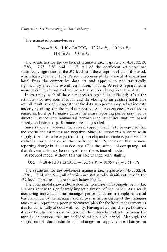
The t-statistics for the coefficient estimates are, respectively, 4.43, 32.14,�7.81, �7.74, and 5.31, all of which are statistically significant beyond the5% level. These results are shown below Fig. 3.
The basic model shown above does demonstrate that competitive marketchanges appear to significantly impact estimates of occupancy. As a resultmeasuring individual hotel manager performance on a simple historicalbasis is unfair to the manager and since it is inconsiderate of the changingmarket will represent a poor performance plan for the hotel management asit is fundamentally at odds with reality. Having noted this change, however,it may be also necessary to consider the interaction effects between themonths or seasons that are included within each period. Although thesimple model does indicate that changes in supply cause changes in
Competitive Set Forecasting in Hotel Industry 9
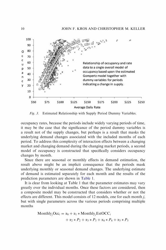
occupancy rates, because the periods include widely varying periods of time,it may be the case that the significance of the period dummy variables isa result not of the supply changes, but perhaps is a result that masks theunderlying demand changes associated with the included months of eachperiod. To address this complexity of interaction effects between a changingmarket and changing demand during the changing market periods, a secondmodel of occupancy is constructed that specifically considers occupancychanges by month.
Since there are seasonal or monthly effects in demand estimation, theresult above might be an implicit consequence that the periods maskunderlying monthly or seasonal demand changes. The underlying estimateof demand is estimated separately for each month and the results of theprediction parameters are shown in Table 1.
It is clear from looking at Table 1 that the parameter estimates may varygreatly over the individual months. Once these factors are considered, thena composite model may be constructed that considers whether or not theeffects are different. This model consists of 12 models, one for each month j,but with single parameters across the various periods comprising multiplemonths
MonthlyjOcci ¼ a0 þ a1 �MonthlyjEstOCCi
þ a2 � P2 þ a3 � P3 þ a4 � P4 þ a5 � P5
Fig. 3. Estimated Relationship with Supply Period Dummy Variables.
JOHN F. KROS AND CHRISTOPHER M. KELLER10
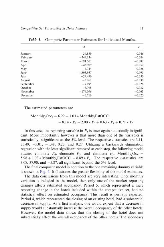
The estimated parameters are
MonthlyjOcci ¼ 6:22þ 1:03 �MonthlyjEstOCCi
� 8:14 � P2 � 2:00 � P3 þ 0:63 � P4 þ 0:71 � P5
In this case, the reporting variable in P5 is once again statistically insignifi-cant. More importantly however is that more than one of the variables isstatistically insignificant at the 5% level. The respective t-statistics are 3.11,35.49, �5.01, �1.48, 0.23, and 0.27. Utilizing a backwards eliminationregression with the least significant removed at each step, the following modelattains: eliminate P4; eliminate P5; and eliminate P3: MonthlyjOcci ¼5:98þ 1:03 �MonthlyjEstOCCi � 8:89 � P2. The respective t-statistics are3.08, 37.90, and �5.87, all significant beyond the 5% level.
The final composite model in addition to the one remaining dummy variableis shown in Fig. 4. It illustrates the greater flexibility of the model estimates.
The data conclusions from this model are very interesting. Once monthlyvariation is included in the model, then only one of the market reportingchanges affects estimated occupancy. Period 5, which represented a merereporting change in the hotels included within the competitive set, had nostatistical effect on estimated occupancy. This result is perhaps expected.Period 4, which represented the closing of an existing hotel, had a substantialdecrease in supply. As a first analysis, one would expect that a decrease insupply would substantially increase the overall occupancy of the other hotels.However, the model data shows that the closing of the hotel does notsubstantially affect the overall occupancy of the other hotels. The secondary
Table 1. Gompertz Parameter Estimates for Individual Months.
b c
January �34.839 �0.046
February �749.134 �0.084
March �591.507 �0.082
April �45.909 �0.052
May �4.744 �0.026
June �1,803.937 �0.095
July �29.490 �0.050
August �5.962 �0.030
September �7.495 �0.028
October �8.798 �0.032
November �174.096 �0.063
December �6.716 �0.025
Competitive Set Forecasting in Hotel Industry 11
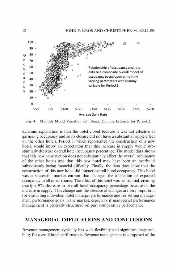
dynamic explanation is that the hotel closed because it was not effective atgarnering occupancy and so its closure did not have a substantial ripple effecton the other hotels. Period 3, which represented the construction of a newhotel, would imply an expectation that this increase in supply would sub-stantially decrease overall hotel occupancy percentage. The model data showsthat this new construction does not substantially affect the overall occupancyof the other hotels and that this new hotel may have been an overbuildsubsequently facing financial difficulty. Finally, the data does show that theconstruction of this new hotel did impact overall hotel occupancy. This hotelwas a successful market entrant that changed the allocation of expectedoccupancy to all other rooms. The effect of this hotel was substantial, creatingnearly a 9% decrease in overall hotel occupancy percentage because of theincrease in supply. This change and the absence of changes are very importantfor evaluating individual hotel manager performance and for setting manage-ment performance goals in the market, especially if managerial performancemanagement is generally structured on past comparative performance.
MANAGERIAL IMPLICATIONS AND CONCLUSIONS
Revenue management typically has wide flexibility and significant responsi-bility for overall hotel performance. Revenue management is composed of the
Fig. 4. Monthly Model Variation with Single Dummy Estimate for Period 2.
JOHN F. KROS AND CHRISTOPHER M. KELLER12

product of the occupancy and the price. If the demand relationship ofcustomers does not change over time and this is reasonable because hotelmanagers act as a set of revenue-maximizers. This means that regardless ofthe supply, the price–demand relationship will remain unchanged. Because ofthis, then a principal dimension for managerial performance enhancement isestimating the occupancy in relation to price and individual performancetargets for hotel managers may be base-lined on historical performance. Thatis, a hotel manager may be tasked with driving occupancy above the previousyear’s performance. In a stable market environment, such benchmarkingis reasonable. However, if the market changes by the entrance or exit ofcompetitive hotels, then such benchmarking may be unfair to the managerand a poor plan for the management. This chapter develops a method foranalyzing then the entrance and exit of hotels changes the competitive marketenvironment and the attendant effects on occupancy.
One of the things that remains unknown for future research is can amarket entrant or exit be accurately predicted of whether or not it will in thefuture, rather than in the past, affect performance. That is, this chapterevaluated ex-post the market changes which is useful for evaluatingperformance. In terms of future investment in new properties, what wouldbe especially valuable is a determination of whether or not the addition ofsupply would directly impact occupancy estimates.
Although historic comparisons are useful to assessing changing perfor-mance, in order to assess competitive performance it is necessary to comparehotel revenue performance to the hotel’s competitors’ revenue performance.In a broader sense, hotel managers are also interested in their relativeposition and performance to competitors in their market. The decomposi-tion of the relevant data into comparative changes for individual hotelswithin the present data set may also be a valuable avenue of future research.In any case, this chapter has developed and illustrated a method forconsidering occupancy effects on existing hotels with attendant changes inthe market supply illustrating both the existence of an increase in supplythat cause a decrease in overall occupancy, an increase in supply that doesnot cause a decrease in occupancy, and a decrease in supply that does notresult in an increase in occupancy.
REFERENCES
Baker, T. K., & Collier, D. A. (1999). A comparative revenue analysis of hotel yield
management heuristics. Decision Sciences, 30(1), 239–263.
Competitive Set Forecasting in Hotel Industry 13

Bitran, G. R., & Mondschein, S. (1995). An application of yield management to the hotel
industry considering multiple days stays. Operations Research, 43, 427–443.
Harrington, E. C. (1965). The desirability function. Industrial Quality Control, 21, 494–498.
Kimes, S. (1999). Group forecasting accuracy for hotels. Journal of the Operational Research
Society, 50(11), 1104–1110.
Lee, A. O. (1990). Airline reservations forecasting: Probabilistic and statistical model of the
booking process. Ph.D. Thesis, Massachusetts Institute of Technology.
Riddington, G. L. (1999). Forecasting ski demand: Comparing learning curve and varying
parameter coefficient approaches. Journal of Forecasting, 18, 205–214.
Schwartz, Z., & Cohen, E. (2004). Hotel revenue-management forecasting: Evidence of expert-
judgment bias. Cornell Hotel and Restaurant Administration Quarterly, 45(1), 85–98.
Weatherford, L. R. (1995). Length-of-stay heuristics: Do they really make a difference? Cornell
Hotel and Restaurant Administration Quarterly, 36(6), 70–79.
Weatherford, L. R., & Kimes, S. E. (2003). A comparison of forecasting methods for hotel
revenue management. International Journal of Forecasting, 19(3), 401–415.
Weatherford, L. R., Kimes, S. E., & Scott, D. (2001). Forecasting for hotel revenue
management: Testing aggregation against disaggregation. Cornell Hotel and Restaurant
Administration Quarterly, 42(6), 156–166.
Witt, S., & Witt, C. (1991a). Tourism forecasting: Error magnitude, direction of change error
and trend change error. Journal of Travel Research, 30, 26–33.
Witt, S., & Witt, C. (1991b). Forecasting tourism demand: A review of empirical research.
International Journal of Forecasting, 11, 447–475.
JOHN F. KROS AND CHRISTOPHER M. KELLER14
PREDICTING HIGH-TECH STOCK
RETURNS WITH FINANCIAL
PERFORMANCE MEASURES:
EVIDENCE FROM TAIWAN
Shaw K. Chen, Chung-Jen Fu and Yu-Lin Chang
ABSTRACT
A one-year-ahead price change forecasting model is proposed based on thefundamental analysis to examine the relationship between equity marketvalue and financial performance measures. By including book value andsix financial statement items in the valuation model, current firm valuecan be determined and the estimation error can predict the direction andmagnitude of future returns of a given portfolio. The six financialperformance measures represent both cash flows – cash flows fromoperations (CFO), cash flows from investing (CFI), and cash flows fromfinancing (CFF) – as well as net income – R&D expenditures (R&D),operating income (OI), and adjusted nonoperating income (ANOI). Thisstudy uses a 10-year sample of the Taiwan information electronic industry(1995–2004 with 2,465 firm-year observations). We find hedge portfolios(consisting of a long position in the most underpriced portfolio and anoffsetting short position in the most overpriced portfolio) provide anaverage annual return of 43%, more than three times the average annualstock return of 12.6%. The result shows the estimation error can be a
Advances in Business and Management Forecasting, Volume 6, 15–35
Copyright r 2009 by Emerald Group Publishing Limited
All rights of reproduction in any form reserved
ISSN: 1477-4070/doi:10.1108/S1477-4070(2009)0000006002
15

good stock return predictor; however, the return of hedge portfoliosgenerally decreases as the market matures.
1. INTRODUCTION
Fundamental analysis research is aimed at determining the value of firmsecurities by carefully examining critical value drivers (Lev & Thiagarajan,1993). The importance of analyzing the components of financial statementsin assessing firm value and future stock returns is widely highlighted infinancial statement analyses. Beneish, Lee, and Tarpley (2001) assertsecurities with a tendency to yield unpredictable returns are particularlyattractive to professional fund managers and investors and suggestfundamental analysis based on financial performance measures is morehelpful, in terms of correlation with future returns. Therefore, providingevidence on the association between financial performance measures andcontemporaneous stock prices or future price changes is an important issuefor academics and practice.
The evidence from researches shows stock prices do not completely reflectall publicly available information (Ou & Penman, 1989a; Fama, 1991; Sloan,1996; Frankel & Lee, 1998). Followed by Ball and Brown (1968) and Beaver(1968), many studies examine the association with stock returns to comparealternative accounting performance measures, such as earnings, accruals,operating cash flows, and so on. However, numerous prior valuationresearches suggest the market might be informationally inefficient and stockprices might take years before they entirely reflect available information. Thisleads to significant abnormal returns spread over several years byimplementing fundamental analysis trading strategies (Kothari, 2001).
The major goal of fundamental analysis is to assess firm value fromfinancial statements (Ou & Penman, 1989a). Using the components offinancial statements to help estimate a firm’s intrinsic value, the differencebetween the intrinsic value and the stock price can be examined whether itsuccessfully identifies those mispriced securities. Related research such as Ouand Penman (1989a, 1989b), Lev and Thiagarajan (1993), Abarbanell andBushee (1997, 1998), and Chen and Zhang (2007) predict future earningsand stock returns using financial measures within the income statement andbalance sheet. However, a number of studies present evidence investors donot correctly use available information in predicting future earningsperformance (Bernard & Thomas, 1989, 1990; Hand, 1990; Maines &
SHAW K. CHEN ET AL.16

Hand, 1996). Furthermore, the research in return predictability alsoprovides strong evidence challenging market efficiency (Ou & Penman,1989a, 1989b; Holthausen & Larcker, 1992; Sloan, 1996; Abarbanell &Bushee, 1997, 1998; Frankel & Lee, 1998).
In practice, the purpose of fundamental analysis research is to identifymispriced securities for investment decisions. Several empirical studiesdocument intrinsic values estimated using the residual income model to helppredict future returns (Lee, Myers, & Swaminathan, 1999). Kothari (2001)indicates the research on indicators of market mispricing produce largemagnitudes of abnormal returns and further suggests a good model ofintrinsic value should predictably generate abnormal returns. This raises theissue of how to precisely predict stock returns with financial performancemeasures based on the residual income model. Testing what kind offinancial performance measures should be embedded in the valuation modelis also important to investors.
Accruals and cash flows are the two financial measures most commonlyexamined. Prior related studies compared stock returns’ association withearnings, accruals, and cash flows, such as Rayburn (1986), Bowen,Burgstahler, and Daley (1986, 1987), and Bernard and Stober (1989). Thisstudy extends the research for value-relevant fundamentals to investigatehow the major components of financial statements enter the decisions ofmarket participants, and we highlight the research design correlating theunanticipated component with stock returns.
To perform fundamental analysis to examine the relationship betweenequity market value and key financial performance measures, we use bookvalue as the basic firm value measure and further decompose cash flows intocash flows from operations (CFO), cash flows from investing (CFI), andcash flows from financing (CFF), and net income into R&D expenditures(R&D), operating income (OI), and adjusted nonoperating income (ANOI)as additional performance measures. Applying these seven financialperformance measures (CFO, CFI, CFF, R&D, OI, ANOI and bookvalue) with the stock price, this study constructs fundamental valuationmodels, and the estimated errors can be used to predict future stock returns.Then, this study operates hedge portfolios of major high-tech companies inTaiwan based on ranked estimation errors involving a long position in themost underpriced stocks and an offsetting short position in the mostoverpriced stocks. The empirical results show the highest average one-yearholding-period return of the hedge portfolios is about 43%, much higherthan the risk-free rate and average stock return (12.6%) in the same period.Our finding suggests the estimation error of valuation model embedded in
Predicting High-Tech Stock Returns with Financial Performance Measures 17

these seven financial performance measures can be a good stock returnpredictor.
This study adds to the growing body of evidence indicating stock pricesreflect investors’ expectations about fundamental valuation attributes suchas earnings and cash flows. In particular, it further contributes in tworespects. First, we apply and confirm a model relying on characteristics ofthe underlying accounting process that are documented in texts on financialstatement analysis; second, our empirical findings suggest major compo-nents of earnings and cash flows will lead to better predictions of relativefuture cross-sectional stock returns.
The rest of this chapter is organized as follows. Section 2 discusses theliterature review and develops the hypotheses. Section 3 discusses theestimation procedures used to implement the valuation model and containsthe sample selection procedure, definition and measurement of the variables,respectively. Section 4 discusses the empirical results and analysis. Finalsection concludes with a summary of our findings and their implications.
2. LITERATURE REVIEW AND HYPOTHESES
Shareholders, investors, and lenders have an interest in evaluating the firmfor decision making. Firm’s current performance will be summarized in itsfinancial statements, and then the market assesses this information toevaluate the firm. This is consistent with the conceptual framework ofFinancial Accounting Standard Board (FASB) that financial statementsshould help investors and creditors in ‘‘assessing the amounts, timing, anduncertainty of future cash flows’’ (Kothari, 2001). A growing body ofrelated research shows stock prices do not fully reflect all publicly availableinformation. It implies that investor might irrationally decide the stockprice. Many studies further evaluate the ability of the models to explainstock prices. Penman and Sougiannis (1998) examine variations of themodel by means of ex-post realizations of earnings to proxy for ex anteexpectations. Dechow, Hutton, and Sloan (1999) investigate the modelsunder alternative specifications and examine the predictive power of themodels for cross-sectional stock returns in the US. Dechow (1994) furtherindicates prior research emphasizing on unexpected components of thefinancial performance measures is misplaced, and suggests researchersshould search for the best alternative measure in the valuation model toevaluate firm value.
SHAW K. CHEN ET AL.18
The evidence in prior research indicates earnings and cash flows are value-relevant. The relation between stock prices and earnings has been widelyresearched. In view of components of earnings, Robinson (1998) indicatesOI is a superior measure for firms to reflect the firm’s ability to sell itsproducts and evaluate firm’s operation performance. Furthermore, if thenon-productive and idle assets are disposed and managers make decisions ininvestor’s best interest, Fairfield, Sweeney, and Yohn (1996) suggest ANOIhas incremental predictive content of future profitability. Thus, both OI andANOI have a positive association with firm value. R&D is a particularlycritical element in the production function of firms in the informationelectronic industry. Evidence supports that R&D should be included as animportant independent variable in the valuation model for research-intensive firms. Hand (2003, 2005) finds equity values are positively relatedto R&D and supports the proposition that R&D is beneficial to the futuredevelopment of the firm. Chan, Lakonishok, and Sougiannis (1999) furthersuggest R&D intensity is associated with return volatility. In sum, as thecomponents of earnings increases, such as OI, ANOI, and R&D, the valueof the firm will increase.
For cash flows, Black (1998), Jorion and Talmor (2001), and Hand (2005)suggest that the CFI are value relevant. Firms wanting to increase theirlong-term competitive advantage will spend more on investment activities toengage in expansion and profit-generating opportunities. For this reason,firms will execute financial activities to raise sufficient funds excluding fromoperations. Jorion and Talmor (2001) suggest the ability to generate fundsfrom the outside affects the opportunity for firms’ continuous operationsand improvement. When the CFF is higher, it has a direct benefit on thevalue of the firm. Furthermore, CFO, as a measure of performance is lesssubject to distortion than the net income figure. Klein and Marquardt (2006)views CFO as the measure of the firm’s real performance.
In sum, the components of earnings or cash flows have differentimplications for assessing firm value. The evidence of prior studies supporta positive contemporaneous association of earnings and cash flows withstock returns (or stock prices), which is generally attributed to earnings andcash flows to summarize value-relevant information.
The well-known Ohlson’s (1995) residual income model decomposed theequity evaluation into book value, earning capitalization value, and presentvalue of ‘‘other information.’’ Ohlson (1995) states the importance of ‘‘otherinformation’’ and further points out other information is difficult tomeasure and operate, on the assumption investors on average could use thefinancial statements to capture the main value of other information in an
Predicting High-Tech Stock Returns with Financial Performance Measures 19

unbiased manner. By identifying the role of information from thecomponents of earnings and cash flows in the forecasting of future stockreturns and firm value, this study provides an expected setting in which tosupport and extend prior research.
On the other hand, numerous recent studies conclude the capital market isinefficient with respect to some areas (Fama, 1991; Beaver, 2002).1 Inaddition, Grossman and Stiglitz (1980) show the impossibility of informa-tion efficient markets when information is costly, and there is an equilibriumdegree of disequilibrium, price reflects the information of informedindividuals but only partially.
We expect the market perception of the relationship between the firmvalue and its components of financial statements on average are unbiased,but it will not always be completely reflected in stock prices in time for someindividual securities. Thus, we can evaluate the relationship between variousfinancial measures and firm value by regressing key components of financialstatements to the stock prices. Therefore, we infer financial performancemeasure stated earlier such as the R&D, OI, ANOI, CFF, CFI, and CFO isincreasing; it has a direct benefit on the value of the firm. By connectingstock price with book value and these six financial measures in the valuationmodel, we propose the estimation error of the fundamental value equationmay serve an indicator of the direction and magnitude of future stock returnand further examine its usefulness in predicting future stock returns in theTaiwan capital market.
This study expects incorporating more comprehensive and more precise(by focusing on the same industry) estimators should improve thepredictability in estimating those firm’s intrinsic values. So we can use theestimated coefficients of the variables in the regression to estimate each firm’s‘‘intrinsic values,’’ and compare it with the actual stock price to identifyoverpriced and underpriced stocks to investigate the issue related to thepredictability of future stock returns. From the evidence of prior research, attimes stock price deviate from their fundamental values and over time willslowly gravitate toward the fundamental values. If the stock prices aregravitating to their fundamental values, then the trading strategy of a hedgeportfolio formed by being on the long side of the underpriced stocks and onthe short side of the overpriced stocks will produce ‘‘abnormal return.’’
In sum, we expect the trading strategy taking a long position in firms withnegative estimation error and a short position in firms with positiveestimation error should generate abnormal stock returns. In additions, whenwe operate the trading strategy with relatively higher absolute estimationerrors, the more abnormal stock returns will be generated. Thus, we infer
SHAW K. CHEN ET AL.20

the more the estimation errors in the current year, the less the subsequentstock returns.
Hence we state the hypothesis as follows:
H1. There is a negative association between current year estimation errorsand subsequent stock returns.
3. RESEARCH DESIGN AND METHODOLOGY
3.1. Empirical Model and Variables Measurements
To examine the research hypothesis raised above, we first select variablesthat reflect levels of firm values. Following the residual income valuationmodel of Ohlson (1995) and Feltham and Ohlson (1995), this study furthermodifies the prediction model employed by Frankel and Lee (1998),Dechow et al. (1999), and Lee et al. (1999)2 to reexamine the relationbetween seven financial measures and firm value in the Taiwan capitalmarket.
The valuation model to examine the relationship between equity marketvalue and the various financial performance measures, decomposing cashflows into CFO, CFI, and CFF, and net income into R&D, OI, and ANOI,is presented as follows (for the definition and measurement of variables seeTable 1):
MVi ¼ b0 þ b1BVCi þ b2CFOi þ b3CFIi þ b4CFFi þ b5R&Di
þ b6OIi þ b7ANOIi þ �i
Given the discussion above, these variables should be positivelyassociated with expected stock prices,3 except for CFI, which may bepositively or negatively associated with expected stock prices, depending onthe situation.
After we use these seven variables to regress the stock price, we canestimate each firm’s fundamental values. Then, we use the error term (orestimation error) of the estimation equation to predict the next period stockreturn and expect there to be a negative relationship between the estimationerror and subsequent stock return (or stock price change) and furtherconstruct the trading strategy to invest in those mispriced stocks as rankedby their estimated errors. The estimation procedure is described in moredetail in Section 3.2.
Predicting High-Tech Stock Returns with Financial Performance Measures 21

3.2. The Estimation Procedures
The purpose of this study is to examine the possibility of temporary stockmispricing that can be systematically predicted by our particular valuationmodels. Thus, we consider whether the estimation errors derived from theseven financial performance measures implied in the valuation model areable to predict future stock returns. The estimation procedures taken in thisstudy are implemented as follows.
First, we assume the seven financial measures in the estimation modelstated earlier provide important information for determining current firm’svalue and can help predict future stock return, with error terms providingthe direction and magnitude of price changes. Thus, by regressing stockprice to the seven financial measures (BVC, CFO, CFI, CFF, R&D, OI, andANOI), we use the estimated coefficients of these variables in the regressionand estimate each firm’s ‘‘intrinsic values.’’
Table 1. Definition and Measurement of Variables.
Variables Measurement
Dependent variables
Market value of equity (MVit) The market value of equity of firm i at time t/
AVt�1
Independent variables
Book value of net assets except for
cash (BVCit)
The book value of equity less the change in the
cash account of firm i at time t/AVt�1
R&D expense (R&Dit) R&D expense of the firm i at time t/AVt�1
Operating income (OIit) (Gross profit�operating expenses) of firms i at
time t/AVt�1
Adjusted nonoperating income (ANOIit) (NIit�OIit�R&Dit)/AVt�1
Cash flows from operations (CFOit) Cash flows from operations activities of firm i at
time t/AVt�1
Cash flows from investing (CFIit) Cash flows from investing activities of firm i at
time t/AVt�1
Cash flows from financing (CFFit) Cash flows from financing activities of firm i at
time t/AVt�1
Other variables
Operating income before discontinued
and extraordinary items (NIit)
The operating income before discontinued and
extraordinary items of firms i at time t/AVt�1
Note: To allow for a cross-sectional aggregation and mitigate the impact of cross-sectional
difference in firm size, we deflate all of the variables for each year by the book value of assets at
the end of year t�1(AVt�1).
Source: Fu and Chang (2006, p.17).
SHAW K. CHEN ET AL.22

Second, compare each firm’s ‘‘intrinsic values’’ with actual stock price tocompute the error terms of valuation model and identify overpriced stocks(with positive error terms) and underpriced stocks (with negative errorterms).
Third, using the relative value of error terms as the return predictor, wedevelop a trading strategy, providing insight into the deviations from therational fundamental value expectations and actual stock prices.4 Theabsolute value of expected stock returns (error terms) are ranked from lowto high and then assigned to five hedge portfolios5 (or three hedgeportfolios) based on equal numbers. Therefore, quintile 1 portfolio isformed with the lowest ranked error terms; in contrast, quintile 5 portfolio isformed with the highest ranked error terms.
Finally, the study operates each hedge portfolio by going long on theunderpriced stocks and shorting the overpriced ones, and then calculates theaverage expected future annual portfolio return for each quintile portfoliofor the period of 1995–2004. So, for example, we expect the lowest quintile(Quintile 1) has the highest stock return average; in contrast, the highestquintile (Quintile 5) will have the lowest stock return average.6
In sum, by combining these variables in a prediction model, we developan estimate of the error terms in yearly subsequent stock return forecasts,and show this estimate has predictive power for cross-sectional returns.Then, the investors can gain the excess return from these hedge portfolios,and assess the relationship between stock price and these financial perfo-rmance measures and use the estimation error as a benchmark to forecastsubsequent stock prices changes or return.
3.3. Sample Selection
The sample companies are composed of publicly listed firms on the TaiwanStock Exchange (TSE) and Gre Tai Securities Market (the GTSM) companies.The companies’ financial data and the equity market value data are obtainedfrom the financial data of company profile of the Taiwan Economic Journal(TEJ) Data Bank. The criteria for sample selection are as follows:
(1) Sample firms are limited to information electronics industries.(2) For each year, companies without sufficient stock price or financial data
are excluded from this study.(3) Companies subject to full-delivery settlements and the de-listed
companies are excluded.
Predicting High-Tech Stock Returns with Financial Performance Measures 23

Eliminating firms due to lack of sufficient data gives a sample size of 2,465firm-years observations for the 10-year period from 1995 to 2004.
We focus on the information electronic industry in Taiwan for threereasons (1) The information electronic industry in Taiwan is the mostimportant and competitive industry; (2) Beneish et al. (2001) suggestprofessional analysts typically tend to focus on firms with the same industry;and (3) We can mitigate some problems of cross-sectional studies(Ittner, Larcker, & Randall, 2003). Furthermore, by incorporating morecomplete value drivers and more precise estimates of their coefficients in theprediction model in the same industry, we could improve our ability toexplain contemporaneous stock prices and therefore predict future stockreturns.
4. EMPIRICAL RESULTS AND ANALYSIS
4.1. Descriptive Statistics
In Table 2, we present the descriptive statistics for the full sample andannual samples. As we show in panel A of Table 2, the mean (median) ofMV are 18,680 (3,080) million New Taiwan dollars. The mean (median) ofCFO, CFI, and CFF are 1,281 (138), �1,531 (�209), and 452 (49) millionNew Taiwan dollars, respectively. On the other hand, the mean (median) ofR&D, OI, and ANOI are 269 (56), 785 (147), and –226 (–73) million NewTaiwan dollars, respectively. The mean (median) of Return is 16.95%(�0.74%). Panel B of Table 2 shows the mean (or median) of these variablesfor each year are quite diverse; implying there are divergent characteristicsamong those firms.
Table 3 reports the Spearman and Pearson correlations among selectedvariables. Except for CFI, the other six financial performance measures arepositively related to MV. As expected, in general, observed relations amongvariables are consistent with our expectations.
4.2. Empirical Results and Analysis
Our research purpose is to predict both the direction and the magnitude ofdeviations in the expectations of stock prices and to examine whethermarket value weighted average (or simple average) error terms in the
SHAW K. CHEN ET AL.24
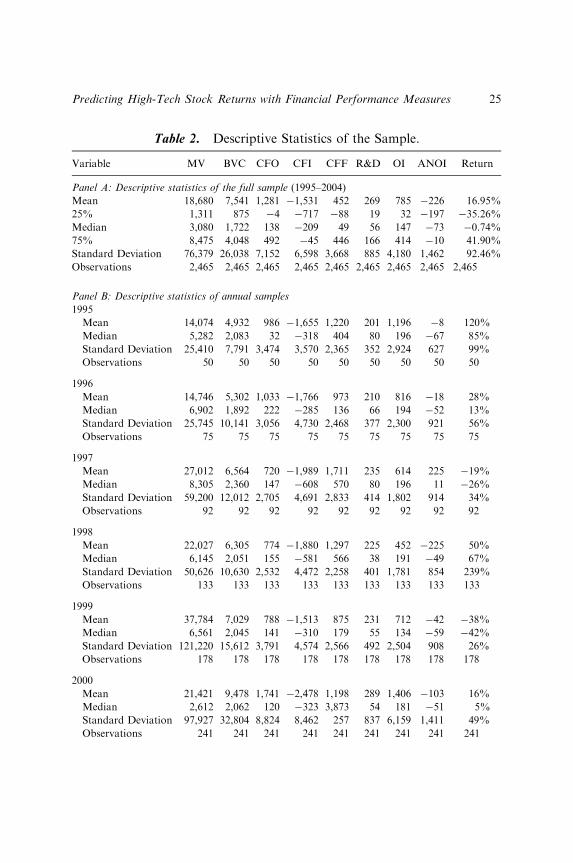
Table 2. Descriptive Statistics of the Sample.
Variable MV BVC CFO CFI CFF R&D OI ANOI Return
Panel A: Descriptive statistics of the full sample (1995–2004)
Mean 18,680 7,541 1,281 �1,531 452 269 785 �226 16.95%
25% 1,311 875 �4 �717 �88 19 32 �197 �35.26%
Median 3,080 1,722 138 �209 49 56 147 �73 �0.74%
75% 8,475 4,048 492 �45 446 166 414 �10 41.90%
Standard Deviation 76,379 26,038 7,152 6,598 3,668 885 4,180 1,462 92.46%
Observations 2,465 2,465 2,465 2,465 2,465 2,465 2,465 2,465 2,465
Panel B: Descriptive statistics of annual samples
1995
Mean 14,074 4,932 986 �1,655 1,220 201 1,196 �8 120%
Median 5,282 2,083 32 �318 404 80 196 �67 85%
Standard Deviation 25,410 7,791 3,474 3,570 2,365 352 2,924 627 99%
Observations 50 50 50 50 50 50 50 50 50
1996
Mean 14,746 5,302 1,033 �1,766 973 210 816 �18 28%
Median 6,902 1,892 222 �285 136 66 194 �52 13%
Standard Deviation 25,745 10,141 3,056 4,730 2,468 377 2,300 921 56%
Observations 75 75 75 75 75 75 75 75 75
1997
Mean 27,012 6,564 720 �1,989 1,711 235 614 225 �19%
Median 8,305 2,360 147 �608 570 80 196 11 �26%
Standard Deviation 59,200 12,012 2,705 4,691 2,833 414 1,802 914 34%
Observations 92 92 92 92 92 92 92 92 92
1998
Mean 22,027 6,305 774 �1,880 1,297 225 452 �225 50%
Median 6,145 2,051 155 �581 566 38 191 �49 67%
Standard Deviation 50,626 10,630 2,532 4,472 2,258 401 1,781 854 239%
Observations 133 133 133 133 133 133 133 133 133
1999
Mean 37,784 7,029 788 �1,513 875 231 712 �42 �38%
Median 6,561 2,045 141 �310 179 55 134 �59 �42%
Standard Deviation 121,220 15,612 3,791 4,574 2,566 492 2,504 908 26%
Observations 178 178 178 178 178 178 178 178 178
2000
Mean 21,421 9,478 1,741 �2,478 1,198 289 1,406 �103 16%
Median 2,612 2,062 120 �323 3,873 54 181 �51 5%
Standard Deviation 97,927 32,804 8,824 8,462 257 837 6,159 1,411 49%
Observations 241 241 241 241 241 241 241 241 241
Predicting High-Tech Stock Returns with Financial Performance Measures 25
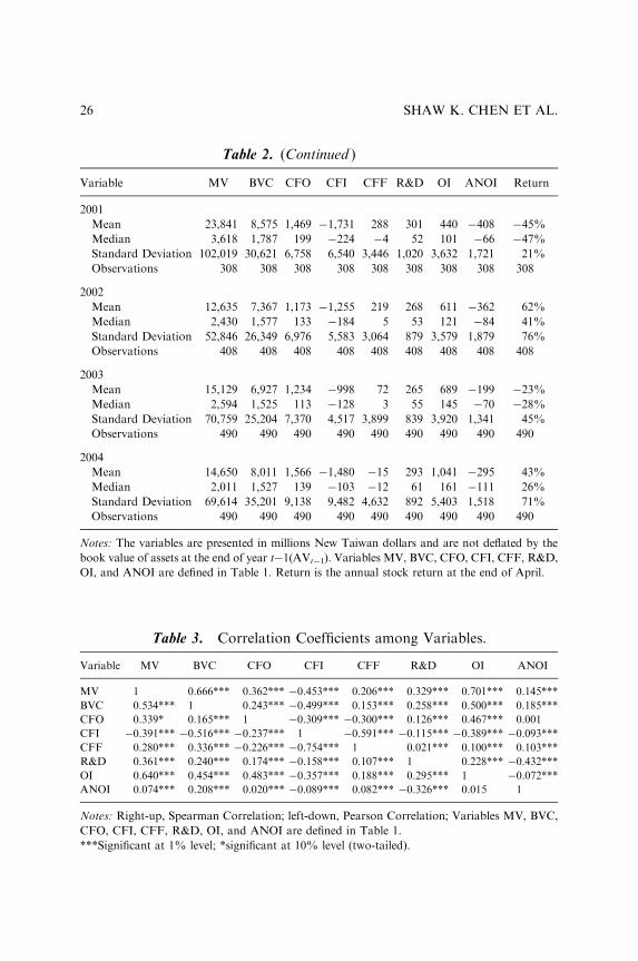
Table 3. Correlation Coefficients among Variables.
Variable MV BVC CFO CFI CFF R&D OI ANOI
MV 1 0.666*** 0.362*** �0.453*** 0.206*** 0.329*** 0.701*** 0.145***
BVC 0.534*** 1 0.243*** �0.499*** 0.153*** 0.258*** 0.500*** 0.185***
CFO 0.339* 0.165*** 1 �0.309*** �0.300*** 0.126*** 0.467*** 0.001
CFI �0.391*** �0.516*** �0.237*** 1 �0.591*** �0.115*** �0.389*** �0.093***
CFF 0.280*** 0.336*** �0.226*** �0.754*** 1 0.021*** 0.100*** 0.103***
R&D 0.361*** 0.240*** 0.174*** �0.158*** 0.107*** 1 0.228*** �0.432***
OI 0.640*** 0.454*** 0.483*** �0.357*** 0.188*** 0.295*** 1 �0.072***
ANOI 0.074*** 0.208*** 0.020*** �0.089*** 0.082*** �0.326*** 0.015 1
Notes: Right-up, Spearman Correlation; left-down, Pearson Correlation; Variables MV, BVC,
CFO, CFI, CFF, R&D, OI, and ANOI are defined in Table 1.
***Significant at 1% level; *significant at 10% level (two-tailed).
Table 2. (Continued )
Variable MV BVC CFO CFI CFF R&D OI ANOI Return
2001
Mean 23,841 8,575 1,469 �1,731 288 301 440 �408 �45%
Median 3,618 1,787 199 �224 �4 52 101 �66 �47%
Standard Deviation 102,019 30,621 6,758 6,540 3,446 1,020 3,632 1,721 21%
Observations 308 308 308 308 308 308 308 308 308
2002
Mean 12,635 7,367 1,173 �1,255 219 268 611 �362 62%
Median 2,430 1,577 133 �184 5 53 121 �84 41%
Standard Deviation 52,846 26,349 6,976 5,583 3,064 879 3,579 1,879 76%
Observations 408 408 408 408 408 408 408 408 408
2003
Mean 15,129 6,927 1,234 �998 72 265 689 �199 �23%
Median 2,594 1,525 113 �128 3 55 145 �70 �28%
Standard Deviation 70,759 25,204 7,370 4,517 3,899 839 3,920 1,341 45%
Observations 490 490 490 490 490 490 490 490 490
2004
Mean 14,650 8,011 1,566 �1,480 �15 293 1,041 �295 43%
Median 2,011 1,527 139 �103 �12 61 161 �111 26%
Standard Deviation 69,614 35,201 9,138 9,482 4,632 892 5,403 1,518 71%
Observations 490 490 490 490 490 490 490 490 490
Notes: The variables are presented in millions New Taiwan dollars and are not deflated by the
book value of assets at the end of year t�1(AVt�1). Variables MV, BVC, CFO, CFI, CFF, R&D,
OI, and ANOI are defined in Table 1. Return is the annual stock return at the end of April.
SHAW K. CHEN ET AL.26
valuation model have predictability in future returns of the five (or three)hedge portfolios.
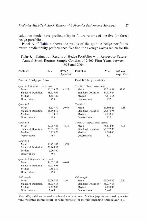
Panel A of Table 4 shows the results of the quintile hedge portfolios’return-predictability performance. We find the average excess return for the
Table 4. Estimation Results of Hedge Portfolios with Respect to FutureAnnual Stock Returns Sample Consists of 2,465 Firm-Years between
1995 and 2004.
Portfolios MVt MVWA
(Apr) (%)
Portfolios MVt MVWA
(Apr) (%)
Panel A: 5 hedge portfolios Panel B: 3 hedge portfolios
Quintile 1 (lowest error terms) Tercile 1 (lowest error terms)
Mean 15,639.72 42.25 Mean 13,216.84 37.82
Standard Deviation 38,126.91 Standard Deviation 34,925.24
Median 5,851.20 Median 4,816.55
Observations 493 Observations 822
Quintile 2 Tercile 2
Mean 8,523.50 30.63 Mean 11,894.26 17.88
Standard Deviation 16,192.59 Standard Deviation 28,110.95
Median 3,830.10 Median 4,053.50
Observations 493 Observations 822
Quintile 3 Tercile 3 (highest error terms)
Mean 12,967.22 18.55 Mean 35,634.03 4.01
Standard Deviation 25,321.97 Standard Deviation 95,572.92
Median 5,138.70 Median 8,384.00
Observations 493 Observations 821
Quintile 4
Mean 19,491.02 15.99
Standard Deviation 50,905.82
Median 5,208.90
Observations 493
Quintile 5 (highest error terms)
Mean 44,572.83 �0.69
Standard Deviation 113,556.98
Median 7,586.30
Observations 493
Full sample Full sample
Mean 20,267.32 12.6 Mean 20,267.32 12.6
Standard Deviation 66,337.68 Standard Deviation 66,337.68
Median 4,659.05 Median 4,659.05
Observations 2,465 Observations 2,465
Note: MVt is defined as market value of equity in time t. MVWA (Apr) is measured by market
value weighted average return of hedge portfolio for the year beginning April in year tþ1.
Predicting High-Tech Stock Returns with Financial Performance Measures 27

top quintile of hedge portfolios over the other stocks hedge portfolios is42.94% [ ¼ 42.25%�(�0.69%)] annually over the past 10 years. Theempirical result shows the annual average return of the hedge portfolio isover 40% by standing on the regression analysis residuals one year ahead,which is much higher than the average return (12.6%) of all samples.Meanwhile, the average return of hedge portfolio formed with theranked error terms is negatively related to error terms. This means theportfolios with smaller error terms (e.g., Quintile 1) gain higher averagereturn, which is consistent with our expectation. We also suggest these sevenfinancial performance measures can strongly explain not only the stockprices of those high-tech companies, but also help to predict future returnsin Taiwan.
Further analyzing by year, we also find the return of hedge port-folios during the forecast period shows seven of ten years are significantlypositive, and only one year is significantly negative (result from sensitivityanalysis is not listed here).7 However, as the influence of foreign capitalincreases and stock market matures, the returns of hedge portfolios becomerelatively smaller than ever.
Panel B of Table 4 shows the results of the tercile hedge portfolios’ return-predictability performance and also find Tercile 1, with lower ranked errorterms, still has the highest market value weighted average return; incontrast, Tercile 3, with higher ranked error terms, has the lowest marketvalue weighted average return.
In sum, the results support our hypothesis and imply firms’ currentyear estimation errors are negatively associated with subsequent stockreturns.
4.3. Sensitivity Analysis
To check the robustness of our results, we use both stock prices at the end ofJune and end of December, and further recompute portfolio annual returnbased on the weighted average of market value (market value weightedaverage) and weighted average sum of firms (simple average) respectively insensitivity analysis.
Panels A and B of Table 5 show the quintile and tercile hedge portfolios’return-predictability performance and reports the estimation results of theportfolios formed based on simple average and market value weightedaverage, respectively. From the results in Table 5, we have consistentconclusions as earlier stated that support our hypothesis.
SHAW K. CHEN ET AL.28
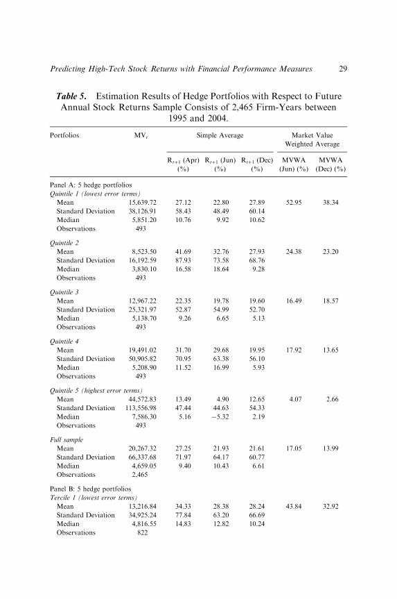
Table 5. Estimation Results of Hedge Portfolios with Respect to FutureAnnual Stock Returns Sample Consists of 2,465 Firm-Years between
1995 and 2004.
Portfolios MVt Simple Average Market Value
Weighted Average
Rtþ1 (Apr)
(%)
Rtþ1 (Jun)
(%)
Rtþ1 (Dec)
(%)
MVWA
(Jun) (%)
MVWA
(Dec) (%)
Panel A: 5 hedge portfolios
Quintile 1 (lowest error terms)
Mean 15,639.72 27.12 22.80 27.89 52.95 38.34
Standard Deviation 38,126.91 58.43 48.49 60.14
Median 5,851.20 10.76 9.92 10.62
Observations 493
Quintile 2
Mean 8,523.50 41.69 32.76 27.93 24.38 23.20
Standard Deviation 16,192.59 87.93 73.58 68.76
Median 3,830.10 16.58 18.64 9.28
Observations 493
Quintile 3
Mean 12,967.22 22.35 19.78 19.60 16.49 18.57
Standard Deviation 25,321.97 52.87 54.99 52.70
Median 5,138.70 9.26 6.65 5.13
Observations 493
Quintile 4
Mean 19,491.02 31.70 29.68 19.95 17.92 13.65
Standard Deviation 50,905.82 70.95 63.38 56.10
Median 5,208.90 11.52 16.99 5.93
Observations 493
Quintile 5 (highest error terms)
Mean 44,572.83 13.49 4.90 12.65 4.07 2.66
Standard Deviation 113,556.98 47.44 44.63 54.33
Median 7,586.30 5.16 �5.32 2.19
Observations 493
Full sample
Mean 20,267.32 27.25 21.93 21.61 17.05 13.99
Standard Deviation 66,337.68 71.97 64.17 60.77
Median 4,659.05 9.40 10.43 6.61
Observations 2,465
Panel B: 5 hedge portfolios
Tercile 1 (lowest error terms)
Mean 13,216.84 34.33 28.38 28.24 43.84 32.92
Standard Deviation 34,925.24 77.84 63.20 66.69
Median 4,816.55 14.83 12.82 10.24
Observations 822
Predicting High-Tech Stock Returns with Financial Performance Measures 29
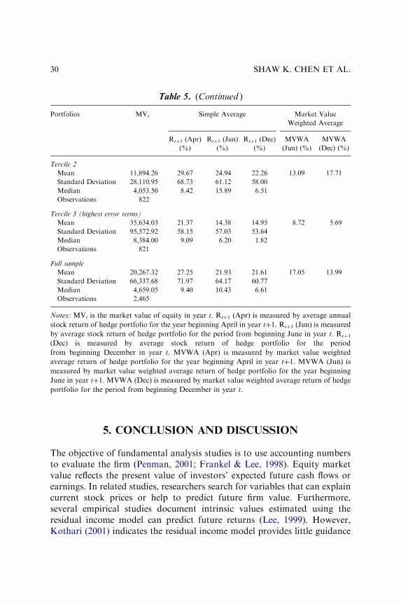
5. CONCLUSION AND DISCUSSION
The objective of fundamental analysis studies is to use accounting numbersto evaluate the firm (Penman, 2001; Frankel & Lee, 1998). Equity marketvalue reflects the present value of investors’ expected future cash flows orearnings. In related studies, researchers search for variables that can explaincurrent stock prices or help to predict future firm value. Furthermore,several empirical studies document intrinsic values estimated using theresidual income model can predict future returns (Lee, 1999). However,Kothari (2001) indicates the residual income model provides little guidance
Table 5. (Continued )
Portfolios MVt Simple Average Market Value
Weighted Average
Rtþ1 (Apr)
(%)
Rtþ1 (Jun)
(%)
Rtþ1 (Dec)
(%)
MVWA
(Jun) (%)
MVWA
(Dec) (%)
Tercile 2
Mean 11,894.26 29.67 24.94 22.26 13.09 17.71
Standard Deviation 28,110.95 68.73 61.12 58.00
Median 4,053.50 8.42 15.89 6.51
Observations 822
Tercile 3 (highest error terms)
Mean 35,634.03 21.37 14.38 14.95 8.72 5.69
Standard Deviation 95,572.92 58.15 57.03 53.64
Median 8,384.00 9.09 6.20 1.82
Observations 821
Full sample
Mean 20,267.32 27.25 21.93 21.61 17.05 13.99
Standard Deviation 66,337.68 71.97 64.17 60.77
Median 4,659.05 9.40 10.43 6.61
Observations 2,465
Notes: MVt is the market value of equity in year t. Rtþ1 (Apr) is measured by average annual
stock return of hedge portfolio for the year beginning April in year tþ1. Rtþ1 (Jun) is measured
by average stock return of hedge portfolio for the period from beginning June in year t. Rtþ1
(Dec) is measured by average stock return of hedge portfolio for the period
from beginning December in year t. MVWA (Apr) is measured by market value weighted
average return of hedge portfolio for the year beginning April in year tþ1. MVWA (Jun) is
measured by market value weighted average return of hedge portfolio for the year beginning
June in year tþ1. MVWA (Dec) is measured by market value weighted average return of hedge
portfolio for the period from beginning December in year t.
SHAW K. CHEN ET AL.30

in terms of why we should expect to predict future returns using estimatedintrinsic values.
This study extends and aims to apply fundamental analysis based onseven financial measures to predict high-tech stock returns, which can helpinvestors make investment decisions. The financial measures included in ourmodified residual income model are the major components of a firm’sfinancial statement. We use book value as a basic firm value measure anddecompose cash flows into CFO, CFI, and CFF, and net income into R&D,OI, and ANOI as additional performance measures. Including theseseven financial statement items in the valuation model can properlyexplain current firm value and help us predict future stock return throughusing the estimation errors to indicate the direction of one-year-ahead pricechanges.
For a sample of Taiwan information electronic firms, hedge portfoliosinvolved in the trading strategy are operated on the basis of rankedestimation errors in long and short positions. The highest average one-yearholding-period return of the hedge portfolios is about 43%, muchhigher than the risk free rate and average stock return (12.6%) in the sameperiod.
Thus, we modify the residual income model and find the results of thissimpler trading strategy approach can support the conclusion for thepredictability of R&D, OI, ANOI, CFI, CFF, and CFO in future stockreturns. The results also demonstrate the estimation error can be a goodstock return predictor, but the return of hedge portfolios generally decreasesas the market matures.
The results of this study deviate from the efficient market’s viewand show stock prices do not fully reflect all publicly available information.Our findings contribute to the finance and fundamental analysis literatureson the predictability of stock returns by documenting the returnpredictability of seven major financial performance measures, especially forthe informational electronic industry, which is high-tech and highlycompetitive.
Moreover, by recognizing the economic effect of past transactions andevents, past transactions have predictive ability for future events that thefinancial statements convey valuable information about firm’s future value.The components of cash flows and various earnings-related items reallyprovide significant explanatory power in relation to a firm’s market value.Thus, just as the FASB advocates, present and potential investors can relyon the accounting information in valuing the firm to improve investmentdecisions.
Predicting High-Tech Stock Returns with Financial Performance Measures 31

We recognize the limitations of this study that (1) cross-sectional returnpredictability tests of market efficiency cannot invariably examine long-horizon returns; (2) the determinants of expected return are likely to becorrelated with the portfolio formation procedure; (3) the survival bias anddata problems may be serious; and (4) the risk of the hedge portfolio couldnot be reduced to zero because of some restrictions on short sales in theTaiwan stock market.
NOTES
1. Fama (1991) indicates returns can be predictable from past returns, dividendyields, and various term-structure variables. Beaver (2002) also asserts capitalmarkets are inefficient with regard to at least three regions: postearningsannouncement drift, market-to-book ratios and its refinements, and contextualaccounting issues.2. Sloan (1996) suggests an analysis of this type can be used to detect mispriced
securities. Moreover, the related studies such as Frankel and Lee (1998), Dechowet al. (1999), and Lee et al. (1999), use the residual income model combinedwith analysts’ forecasts to estimate fundamental values and shows abnormal returnscan be earned. However, due to lack of reliable analysts’ forecasts data in Taiwan,this study adopts the components of cash flow and earnings to predict future stockprices.3. Major components of balance sheet and income statement are used instead
of aggregating book equity and net income to avoid the severe inferentialdistortions that can arise when evaluating the value relevance of financial statementsof fast growing, highly intangible-intensive companies (Zhang, 2001; Hand, 2004,2005).4. Because all listed companies in Taiwan announce their annual report and
financial statements before the end of April; this study adopts the stock prices of endof April as the actual annual stock price.5. The hedged portfolios in our trading strategy are formed annually by assigning
firms into quintiles based on the magnitude of the absolute value of error terms inyear t. Then equal-weighted stock returns are computed for each quintile portfolioover the subsequent year, beginning four months after the end of the fiscal year fromwhich the historical forecast data are obtained.6. In Taiwan stock market, the risk of this hedge portfolio could not be entirely
eliminated because of some restrictions on short sale of securities. Therefore, theinvestors still bear some uncertain risk even if they operate the trading strategythrough the short sale of Electronic Sector Index Futures.7. The hedged portfolio return summarizes the predictive ability of our model with
respect to future returns. Related statistical inference is conducted using the standarderror of the annual mean hedged portfolio returns over the 10 years in the sampleperiod.
SHAW K. CHEN ET AL.32

REFERENCES
Abarbanell, J., & Bushee, B. (1997). Fundamental analysis, future earnings, and stock prices.
Journal of Accounting Research, 35, 1–24.
Abarbanell, J., & Bushee, B. (1998). Abnormal returns to a fundamental analysis strategy. The
Accounting Review, 73, 19–45.
Ball, R., & Brown, P. (1968). An empirical evaluation of accounting income numbers. Journal
of Accounting Research, 6, 159–177.
Beaver, W. H. (1968). The information content of annual earnings announcements. Journal of
Accounting Research, 6, 67–92.
Beaver, W. H. (2002). Perspectives on recent capital market research. The Accounting Review,
77, 453–474.
Beneish, M. D., Lee, M. C., & Tarpley, R. L. (2001). Contextual fundamental ana-
lysis through the prediction of extreme returns. Review of Accounting Studies, 6,
165–189.
Bernard, V., & Stober, T. (1989). The nature and amount of information in cash flows and
accruals. The Accounting Review, 64, 624–652.
Bernard, V., & Thomas, J. (1989). Post-earnings announcement drift: Delayed price response or
risk premium? Journal of Accounting Research, 27, 1–36.
Bernard, V., & Thomas, J. (1990). Evidence that stock prices do not fully reflect the implicat-
ions of current earnings for future earnings. Journal of Accounting and Economics, 13,
305–340.
Black, E. L. (1998). Life-cycle impacts on the incremental value-relevance of earnings and cash
flow measures. Journal of Financial Statement Analysis, 4, 40–56.
Bowen, R., Burgstahler, D., & Daley, L. (1986). Evidence on the relationships between earnings
and various measures of cash flow. The Accounting Review, 61, 713–725.
Bowen, R., Burgstahler, D., & Daley, L. (1987). The incremental information content of accrual
versus cash flows. The Accounting Review, 62, 723–747.
Chan, K. C., Lakonishok, J., & Sougiannis, T. (1999). The stock market valuation of research
and development expenditures. Working Paper. University of Illinois.
Chen, P., & Zhang, G. (2007). How do accounting variables explain stock price movements?
Theory and evidence. Journal of Accounting and Economics, 43, 219–244.
Dechow, P. (1994). Accounting earnings and cash flows as measures of firm performance: The
role of accounting accruals. Journal of Accounting and Economics, 18, 3–42.
Dechow, P., Hutton, A., & Sloan, R. (1999). An empirical assessment of the residual income
valuation model. Journal of Accounting and Economics, 26, 1–34.
Fairfield, P. M., Sweeney, R. J., & Yohn, T. L. (1996). Accounting classification and the
predictive content of earnings. The Accounting Review, 71, 337–355.
Fama, E. F. (1991). Efficient capital market: II. Journal of Finance, 46, 1575–1617.
Feltham, G., & Ohlson, J. (1995). Valuation and clean surplus accounting for operating and
financial activities. Contemporary Accounting Research, 11, 689–731.
Frankel, R., & Lee, C. (1998). Accounting valuation, market expectation, and cross-sectional
stock returns. Journal of Accounting and Economics, 25, 283–319.
Fu, C. J., & Chang, Y. L. (2006). The impacts of life cycle on the value relevance of financial
performance measures: Evidence from Taiwan. Working Paper. 2006 Annual Meeting of
the American Accounting Association.
Predicting High-Tech Stock Returns with Financial Performance Measures 33

Grossman, S. J., & Stiglitz, J. E. (1980). On the impossibility of informationally efficient
markets. American Economic Review, 70, 393–408.
Hand, J. R. M. (1990). A test of the extended functional fixation hypothesis. The Accounting
Review, 65, 740–763.
Hand, J. R. M. (2003). The relevance of financial statements within and across private and
public equity markets. Working Paper. UNC Chapel Hill: Kenan-Flagler Business
School.
Hand, J. R. M. (2004). The market valuation of biotechnology firms and biotechnology R&D.
In: J. McCahery & L. Renneboog (Eds), Venture capital contraction and the valuation of
high-technology firms (pp. 251–280). UK: Oxford University Press.
Hand, J. R. M. (2005). The value relevance of financial statements in the venture capital market.
The Accounting Review, 80, 613–648.
Holthausen, R., & Larcker, D. (1992). The prediction of stock returns using financial statement
information. Journal of Accounting and Economics, 15, 373–411.
Ittner, C. D., Larcker, D. F., & Randall, T. (2003). Performance implications of strategic
performance measurement in financial service firms. Accounting, Organizations and
Society, 28, 715–741.
Jorion, P., & Talmor, E. (2001). Value relevance of financial and nonfinancial information in
emerging industries: The changing role of web traffic data. Working Paper. University of
California at Irvine.
Klein, A., & Marquardt, C. (2006). Fundamentals of accounting losses. The Accounting Review,
81, 179–206.
Kothari, S. P. (2001). Capital markets research in accounting. Journal of Accounting and
Economics, 31, 105–231.
Lee, C. (1999). Accounting-based valuation: Impact on business practices and research.
Accounting Horizons, 13, 413–425.
Lee, C., Myers, J., & Swaminathan, B. (1999). What is the intrinsic value of the Dow? Journal of
Finance, 54, 1693–1741.
Lev, B., & Thiagarajan, R. (1993). Fundamental information analysis. Journal of Accounting
Research, 31, 190–215.
Maines, L. A., & Hand, J. R. (1996). Individuals’ perceptions and misperceptions of time series
properties of quarterly earnings. The Accounting Review, 71, 317–336.
Ohlson, J. (1995). Earnings, book values and dividends in security valuation. Contemporary
Accounting Research, 11, 661–687.
Ou, J., & Penman, S. (1989a). Financial statement analysis and the prediction of stock returns.
Journal of Accounting and Economics, 11, 295–329.
Ou, J., & Penman, S. (1989b). Accounting measurement, price–earnings ratios, and the
information content of security prices. Journal of Accounting Research, 27, 111–152.
Penman, S. H. (2001). Financial statement analysis and security valuation (pp. 2–20). Irwin, NY:
McGraw-Hill.
Penman, S. H., & Sougiannis, T. (1998). A comparison of dividend, cash flow, and
earnings approaches to equity valuation. Contemporary Accounting Research, 15,
343–383.
Rayburn, J. (1986). The association of operating cash flow and accruals with security returns.
Journal of Accounting Research, 24, 112–133.
SHAW K. CHEN ET AL.34

Robinson, K. C. (1998). An examination of the influence of industry structure on the eight
alternative measures of new venture performance for high potential independent new
ventures. Journal of Business Venturing, 14, 165–187.
Sloan, R. (1996). Do stock prices fully reflect information in accruals and cash flows about
future earnings. The Accounting Review, 71, 289–315.
Zhang, X.-J. (2001). Accounting conservatism and the analysis of line items in earnings forecasting
and equity valuation. Working Paper. University of California, Berkeley.
Predicting High-Tech Stock Returns with Financial Performance Measures 35

This page intentionally left blank

FORECASTING INFORMED
TRADING AT MERGER
ANNOUNCEMENTS: THE USE
OF LIQUIDITY TRADING
Rebecca Abraham and Charles Harrington
ABSTRACT
We propose a novel method of forecasting the level of informed trading atmerger announcements. Informed traders typically take advantage oftheir knowledge of the forthcoming merger by trading heavily atannouncement. They trade on positive volume or informed buys for cashmergers and negative volume or informed sells for stock mergers. Inresponse, market makers set wider spreads and raise prices for informedbuys and lower prices for informed sells. As liquidity traders trade onthese prices, our vector autoregressive framework establishes the linkbetween informed trading and liquidity trading through price changes. Aslong as the link holds, informed trading may be detected by measuringlevels of liquidity trading. We observe the link during the �1 to þ1 periodfor cash mergers and �1 to þ5 period for stock mergers.
Advances in Business and Management Forecasting, Volume 6, 37–51
Copyright r 2009 by Emerald Group Publishing Limited
All rights of reproduction in any form reserved
ISSN: 1477-4070/doi:10.1108/S1477-4070(2009)0000006003
37

INTRODUCTION
The financial markets typically contain traders with different motivationsand trading strategies. Informed traders act on the basis of privilegedinformation. At earnings announcements, certain firms report earningssurprises, announcing earnings that are either higher or lower than analysts’forecasts. Dividend announcements involve the announcement that the firmis about to pay dividends or increase its dividend payout ratio. At mergerannouncements, target firms are perceived as valuable in that they aredesired by acquirers. Firms facing bankruptcies send negative signals intothe markets. Informed traders capitalize on their knowledge of the positivesignals generated by positive earnings surprises, dividend announcements,and rises in target firms’ prices by buying stock or call options, and sellingstock or buying put options on negative signals such as negative earningssurprises or forthcoming bankruptcies. In each case, the informed trader isaware of the firms’ performance and is capable of profiting from thatinformation. By definition, uninformed trading is termed noise trading.Black (1986) offers the following definition:
Noise trading is trading on noise as if it were information. People who trade on noise are
willing to trade even though from an objective point of view they would be better off not
trading. (Black, 1986, p. 529)
Uninformed traders, on the other hand, trade at random. They merelybuy and sell for their own inventory. Uninformed traders, also termedliquidity traders, are driven by the desire to maintain liquidity. Therefore, atmergers, earnings announcements, or dividend announcements, liquiditytraders trade to maintain an inventory of stock, or in response to pressurefrom their clients (liquidity traders are typically market makers andinstitutional traders). They are not motivated by the profit-making desiresof informed traders. If they take large positions, it is usually afterinformation about the event (merger or dividend announcement) hasbecome public with a view to satisfying their clients who wish to hold targetstock or stock on which dividends have just been announced.
The literature is replete with reports of trading by informed traders(Admati & Pfleiderer, 1988; Glosten & Milgrom, 1985; Kyle, 1985; Lee & Yi,2001) on different occasions. These papers also develop theoretical constructsby which the impact of informed traders on the markets may be derived.Market makers in the stock market buy and sell stock to traders at bid andask prices, respectively. If a trader wishes to purchase, the market makeroffers a variety of bid prices; likewise, if another trader wishes to sell the
REBECCA ABRAHAM AND CHARLES HARRINGTON38

market maker offers a variety of ask prices. The difference between the bid andask prices is termed the quoted spread. Setting of the spread is the mechanismby which market makers influence prices. For informed traders, the marketmaker, knowing the trader will profit at his (the market maker’s) expense, willset the spreads to be wide to cover losses. In contrast, for liquidity traders, themarket maker will set spreads to be narrow as losses are not expected to occur.It is the position of this chapter that the influence of spreads (based oninformed trading volumes) on prices will determine the volume of liquiditytrading. Accordingly, we focus on establishing a link between volumes ofinformed trading, price changes resulting from spread widths, and liquiditytrading as a means of forecasting the level of informed trading.
Why is it important to forecast levels of informed trading volume?Regulators in recent years have embarked on a campaign to reduce spreads.High spreads contribute to higher transactions prices for traders. Highertransactions prices suggest less market efficiency, higher costs to brokeragehouses and their clients for purchasing stock or options, and monopoly profitsfor market makers. Consequently, regulators have ordered the listing ofoptions on multiple exchanges so that competition between market makerswill drive down spreads and reduce transaction fees for options traders.At present, almost 80% of all traded options are listed on all six optionsexchanges (De Fontnouvelle, Fishe, & Harris, 2003). This outcome has beenachieved after passage of Rule 18-c by the Securities and Exchange Commiss-ion in 1981, banning uncompetitive practices, a lawsuit and settlement by theDepartment of Justice against the American Stock Exchange in 1989, and anoptions campaign on August–September 1989, designed to increase multiplelisting. As informed traders contribute to higher spreads, the ability toforecast levels of informed trading is of practical interest to regulatorstracking the incidence of rising spreads. From a theoretical standpoint, mostmodels of informed trading (Admati & Pfleiderer, 1988l; Bamber, Barron, &Stober, 1999) have viewed informed and liquidity trading as tangentiallylinked. It would be useful to establish a direct link between these two tradingactivities. It is to that purpose that this study is directed.
REVIEW OF LITERATURE
This chapter casts informed and liquidity trading in the context of mergerannouncements. Merger announcements have been studied extensively as avenue of information-based trading (for a review, see Cao, Chen, & Griffin,2005). However, the focus of merger research has been on the target firm.
Forecasting Informed Trading at Merger Announcements 39

Target firms rise in price with the announcement of a merger as the signal issent that they are in demand by acquirer firms. We wish to shift the focus toacquirer firms. The cornerstone of our work is the response by informedtraders to signals. Therefore, the signal should be as pure and unidirectionalas possible. If all mergers are considered as similar, there may be mixedsignals whose effects obliterate each other. One method of obtaining puresignals is by classifying mergers in terms of method of payment. Mitchell,Pulvino, and Stafford (2004) conceived of mergers as cash mergers if theacquirer paid cash for the acquisition or a stock (fixed-exchange ratio)merger if stock was exchanged in a fixed ratio at the time of closing. Cashmergers are viewed as positive in that the acquiring firm must have excesscash to spend on a purchase. Conversely, acquirers that engage in a stockexchange are viewed unfavorably as being devoid of financial resources. Atmerger announcement, Mitchell et al. (2004) observed significant positivecumulative abnormal returns (CAARs) on cash mergers and significantnegative CAARs on stock mergers. Intuitively, informed traders would usetheir privileged information of a positive signal on forthcoming cashmergers to purchase acquirer stock, or we would expect informed buyingvolume to rise at the time of announcement of a cash merger. In contrast,informed traders would use their privileged information of the negativesignal on stock mergers to sell acquirer stock at merger announcements.Therefore, at the time of merger announcement, typically, days �1 to þ1 ofthe merger, the volume of trading on both cash and stock acquirers may beexpected to rise significantly above normal trading volume.
H1a. CAARs due to elevated total volume of trading on cash acquirerswill be significantly positive during days �1 to þ1 of a mergerannouncement than during the benchmark period.
H1b. CAARs due to elevated total volume of trading on stock acquirerswill be significantly negative during days �1 to þ1 of a mergerannouncement than during the benchmark period.
Theoretical Framework
Easley and O’Hara (1992) propose a model of informed trading andliquidity trading that may be used as the basis for this study. They viewinformed traders as arriving in a continuous auction. Informed traders tradeon the same side of the market. For cash mergers, informed traders will buy
REBECCA ABRAHAM AND CHARLES HARRINGTON40

only while for stock mergers they will only sell. Informed traders trade inlarge sizes (Easley & O’Hara, 1992) as they wish to make as large a profit aspossible with a single trade. In fact, the large size characteristic of informedtrades led Heflin and Shaw (2005) to develop a method of detecting informedtrades by transaction. Informed traders also trade regularly until prices havereached a market equilibrium. Market makers, on the other hand, are in anadversarial position vis a vis informed traders. The increased trading ofinformed traders suggests larger losses to them as does large size trades. As faras the market maker is concerned, informed traders trading in block tradesreduce their profits substantially. In response, market makers will increasequoted spreads (ask price� bid price), or charge higher prices to informedtraders who wish to buy (as in cash mergers) and pay lower prices to informedtraders who wish to sell (as in stock mergers). This results in higher effectivespreads (trade price� [bid priceþ ask price]/2), which are the more relevantmeasures as they include the actual price at which trading took place.Therefore, trade prices will rise on buy orders for cash mergers and fall for sellorders with stock mergers. Information is thus impounded into prices.
However, informed traders are not the only traders in the market. Themarket maker is aware of the existence of uninformed or liquidity traders.As informed traders continue to trade, market makers will, over time, try toinfer the percentage of trading volume that is informed versus uninformed.The composition of trades may provide some information to the marketmaker. As the informed all trade on the same side of the market, thepercentage of such trades will indicate the proportion of informed tradingvolume. For cash mergers, all informed traders may be expected to buy.Uninformed traders will both buy and sell as they are purchasing and sellingat random. The buy trades may be attributed to informed and uninformedtraders. As informed traders are assumed to trade in large size only, whereassome of the uninformed may trade in large size, all small trades areeliminated. The only doubt remains on large trades, which may belong toboth informed or uninformed traders. Market makers can infer the existenceof informed traders by identifying large buy trades for cash mergers andlarge sell trades for stock mergers. Over time, with repeated purchases byinformed traders, market makers are able to identify the trades that areinformed. Accordingly, they will adjust spreads downward for trades thatare clearly uninformed trades, while maintaining high spreads for informedtrades. Soon after this occurs, information will no longer enter into pricesand prices will clear at an equilibrium level. This suggests that a multiperiodmodel is more appropriate, in that spread and price adjustments cannot takeplace instantaneously. It is possible that adjustments may take place on an
Forecasting Informed Trading at Merger Announcements 41

intraday basis or over the span of several days. In either case, empiricaltesting must use lagged structures to capture intraday price changes andspread analysis over several days to explore interday effects.
What is the reaction of liquidity traders? Liquidity traders are not novices.In fact, most of them are institutional traders. They just have differentmotivations for trading from the informed traders. They choose to purchaseand sell for reasons of ownership rather than acting to profit on the basis ofspecialized information. They are aware of spreads and transactions costs. Infact, the Easley and O’Hara (1992) model makes the assumption that there isa constant (nonincreasing) transaction cost that liquidity traders assume asthe model could not exist without liquidity traders. Liquidity traders acceptand pay higher prices for cash buys and earn lower amounts on sales in stockmergers. The question may be raised as to why they accept these conditions?Why do liquidity traders accept the higher spreads and unfavorable priceswhich are the market makers’ reaction to informed trading? Why do not theyleave the market (Black, 1986). Trueman (1988) advances the explanationthat investors view fund managers as being more productive, and in turninvest in a fund if the total volume of trading in the fund is large. To theinvestor, a large volume of trading suggests more information-based tradesand thereby higher fund profits. However, the investor does not know theproportion of trades that are information-based; he or she simply views thetotal amount of trading and assumes that a larger trading volume indicatesmore information-based trades. This provides an incentive for fundmanagers to engage in liquidity trading to send the signal to the investorthat he or she is actually making information-based trades, and therebyattract investor funds. Empirically, Kanodia, Bushman, and Dickhaut (1986)observed that managers do not forego unprofitable investment projects aswithdrawal would send the message that the manager’s information aboutthe outcome of the project was inaccurate. Trueman (1988) showed thatsecurity analysts may be unwilling to revise original erroneous estimates onreceiving new information due to the negative signal such action would sendabout the wisdom of the original forecast.
For our purposes, it is apparent that liquidity traders will continue to tradeeven at the unfavorable prices set by market makers in response to informedtrading. The volume of informed trading influences stock price changes to beeither positive (for cash mergers) or negative (for stock mergers). Those pricechanges will influence the level of liquidity trading. Assuming that liquiditytraders will continue to trade, i.e., that they continue to trade to attractfuture investment, they will pay higher prices for cash mergers and lowerprices for stock mergers. The trading volume of liquidity traders will depend
REBECCA ABRAHAM AND CHARLES HARRINGTON42

on the level of trading of informed traders. There is a three-step link withhigher informed buying (selling) resulting in higher (lower) stock pricechanges and in turn, higher liquidity trading as liquidity traders accept theadverse prices set by market makers responding to informed trading. It is thislink that this study tests, and which acts as a forecast of informed tradingusing liquidity trading volumes. This link maybe expected to weaken overtime, as market makers learn the pattern of informed trading and setdifferential spreads for informed and liquidity traders. Liquidity trading atthat point will no longer depend on informed trading and it will be no longerpossible to forecast the existence of informed trading using liquidity trades.
H2a. Liquidity buying volume for acquirer stock in cash mergers will bedirectly related to informed buying volume and stock price changes.Specifically, informed buying volume will increase future stock pricechanges, which will increase liquidity buying volume on days �1 to þ1 ofthe merger announcement.
H2b. Liquidity selling volume for acquirer stock in stock mergers will bedirectly related to informed selling volume and stock price changes.Specifically, informed selling volume will decrease future stock pricechanges, which will reduce liquidity buying volume on days �1 to þ1 ofthe merger announcement.
DATA AND SAMPLE CHARACTERISTICS
All cash and stock mergers for 2005 were obtained from FactsetMergerstat’s comprehensive database of worldwide merger transactions.Mergers were filtered by completion, as only acquisitions of complete firmswere included. Partial transfers including sales of divisions and assets werenot included. All foreign firms (either acquirer or target) were excluded.Although data is available for the past 25 years, only 1 year of data wasincluded as the vector autoregressions used to test Hypothesis 2 use intradaydata. Intraday data is extremely voluminous, with W10 million data pointsfor the sample period. All mergers were examined closely for method ofpayment, with only full cash purchases and fixed ratios of exchanges ofstock between target and acquirer being included. The final sample consistedof 66 cash mergers and 38 stock mergers. Intraday stock trade and quoteprices were obtained from the New York Stock Exchange’s TAQ (Trade andQuotes) database. TAQ provided intraday bid and ask quotes for each trade
Forecasting Informed Trading at Merger Announcements 43
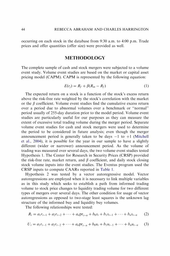
occurring on each stock in the database from 9:30 a.m. to 4:00 p.m. Tradeprices and offer quantities (offer size) were provided as well.
METHODOLOGY
The complete sample of cash and stock mergers were subjected to a volumeevent study. Volume event studies are based on the market or capital assetpricing model (CAPM). CAPM is represented by the following equation:
EðrjÞ ¼ Rf þ bðRm � Rf Þ (1)
The expected return on a stock is a function of the stock’s excess returnabove the risk-free rate weighted by the stock’s correlation with the marketor the b coefficient. Volume event studies find the cumulative excess returnover a period due to abnormal volumes over a benchmark or ‘‘normal’’period usually of 255-day duration prior to the model period. Volume eventstudies are particularly useful for our purposes as they can measure theextent of excessive total trading volume during the merger period. Separatevolume event studies for cash and stock mergers were used to determinethe period to be considered in future analysis; even though the mergerannouncement period is generally taken to be days �1 to þ1 (Mitchellet al., 2004), it is possible for the year in our sample to have a slightlydifferent (wider or narrower) announcement period. As the volume oftrading was measured over several days, the two volume event studies testedHypothesis 1. The Center for Research in Security Prices (CRSP) providedthe risk-free rate, market return, and b coefficient, and daily stock closingstock volume inputs into the event studies. The Eventus program used theCRSP inputs to compute CAARs reported in Table 1.
Hypothesis 2 was tested by a vector autoregressive model. Vectorautoregressions are employed when it is necessary to link multiple variablesas in this study which seeks to establish a path from informed tradingvolume to stock price changes to liquidity trading volume for two differenttypes of mergers over several days. The other condition for usage of vectorautoregressions as opposed to two-stage least squares is the unknown lagstructure of the informed buy and liquidity buy volumes.
The following relationships were tested:
Rt ¼ a1rt�1 þ a2rt�2 þ � � � þ anprt�n þ b0st þ b1st�1 þ � � � þ bnst�n (2)
Ut ¼ a1rt�1 þ a2rt�2 þ � � � þ anprt�n þ b0ut þ b1ut�1 þ � � � þ bnut�n (3)
REBECCA ABRAHAM AND CHARLES HARRINGTON44

where Rt is the contemporaneous and lagged stock price changes; st theinformed buy volume for cash mergers and informed sell volume for stockmergers at time t; and Ut the liquidity buy volume for cash mergers andliquidity sell volume for stock mergers at time t.
Input variables into the vector autoregression included an intraday stockprice change series, informed trading volume, and liquidity trading volume.The stock price change series was constructed by finding the mean stockprices for each 5-min interval from 9:30 a.m. to 4:00 p.m. for each day in themerger announcement period. The difference between consecutive meanprices was obtained to get a change series. Z scores were computed byfinding the difference between each stock price change and mean dailychanges and dividing by the standard deviation of daily stock price changes.This procedure was considered necessary to smooth out the autocorrelationof daily stock price change data. Heflin and Shaw’s (2005) methodologywas used to differentiate between informed and liquidity trades. Theyargued that a trade size/offer quantity ratioo1 indicated an informed trade,whereas that above 1 indicated a liquidity trade. Their rationale was thatinformed traders prefer to trade in large size, but market makers will seek tolimit the size of informed trade so that the market makers will only permittrades with sizes below the offer quantity to be completed. For liquiditytrades, market makers will permit large trades, which are above the offerquantity. Accordingly, we computed trade size/offer quantity ratios for alltrades for each day in the announcement period, differentiating them as
Table 1. Results of Volume Event Studies of Cash and Stock Mergers.
Cash Mergers Stock Mergers
Event window CAAR Patell Z Event window CAAR Patell Z
�1, 0 42.02% 1.927* �1, 0 247.95% 25.953***
Day CAAR Patell Z Day CAAR Patell Z
�1 �20.45% 0.043 �1 �27.75% 0.455
0 62.46 2.682*** 0 275.70 36.249*
1 8.42 5.936*** 1 86.97 17.873***
2 14.17 6.211***
3 �16.32 4.77***
4 �11.79 3.772***
5 �0.64 3.776***
*po.01; ***po.001.
Forecasting Informed Trading at Merger Announcements 45
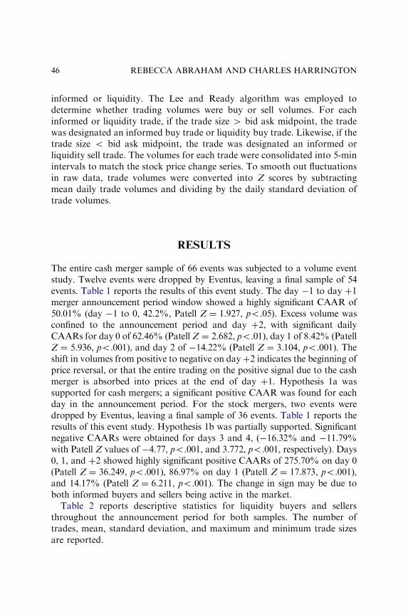
informed or liquidity. The Lee and Ready algorithm was employed todetermine whether trading volumes were buy or sell volumes. For eachinformed or liquidity trade, if the trade size W bid ask midpoint, the tradewas designated an informed buy trade or liquidity buy trade. Likewise, if thetrade size o bid ask midpoint, the trade was designated an informed orliquidity sell trade. The volumes for each trade were consolidated into 5-minintervals to match the stock price change series. To smooth out fluctuationsin raw data, trade volumes were converted into Z scores by subtractingmean daily trade volumes and dividing by the daily standard deviation oftrade volumes.
RESULTS
The entire cash merger sample of 66 events was subjected to a volume eventstudy. Twelve events were dropped by Eventus, leaving a final sample of 54events. Table 1 reports the results of this event study. The day �1 to day þ1merger announcement period window showed a highly significant CAAR of50.01% (day �1 to 0, 42.2%, Patell Z ¼ 1.927, po.05). Excess volume wasconfined to the announcement period and day þ2, with significant dailyCAARs for day 0 of 62.46% (Patell Z ¼ 2.682, po.01), day 1 of 8.42% (PatellZ ¼ 5.936, po.001), and day 2 of �14.22% (Patell Z ¼ 3.104, po.001). Theshift in volumes from positive to negative on dayþ2 indicates the beginning ofprice reversal, or that the entire trading on the positive signal due to the cashmerger is absorbed into prices at the end of day þ1. Hypothesis 1a wassupported for cash mergers; a significant positive CAAR was found for eachday in the announcement period. For the stock mergers, two events weredropped by Eventus, leaving a final sample of 36 events. Table 1 reports theresults of this event study. Hypothesis 1b was partially supported. Significantnegative CAARs were obtained for days 3 and 4, (�16.32% and �11.79%with Patell Z values of �4.77, po.001, and 3.772, po.001, respectively). Days0, 1, and þ2 showed highly significant positive CAARs of 275.70% on day 0(Patell Z ¼ 36.249, po.001), 86.97% on day 1 (Patell Z ¼ 17.873, po.001),and 14.17% (Patell Z ¼ 6.211, po.001). The change in sign may be due toboth informed buyers and sellers being active in the market.
Table 2 reports descriptive statistics for liquidity buyers and sellersthroughout the announcement period for both samples. The number oftrades, mean, standard deviation, and maximum and minimum trade sizesare reported.
REBECCA ABRAHAM AND CHARLES HARRINGTON46
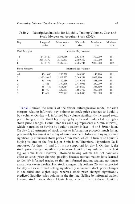
Table 3 shows the results of the vector autoregressive model for cashmergers relating informed buy volume to stock price changes to liquiditybuy volume. On day �1, informed buy volume significantly increased stockprice changes in the third lag. Buying by informed traders led to higherstock price changes 15min later (as each lag represents a 5-min interval),which in turn led to buying by liquidity traders in lags 1–6 or 5–30min later.On day 0, adjustments of stock prices to information proceeds much faster,presumably because it is the day of announcement. Informed buying volumesignificantly influences stock prices 5min later, which in turn raise liquiditybuying volume in the first lag or 5min later. Therefore, Hypothesis 2a issupported for days �1 and 0. It is not supported for day 1. On day 1, thestock price changes significantly increase liquidity buy volume in the firstlag, or 5min later. However, informed buying volume has not have anyeffect on stock price changes, possibly because market makers have learnedto identify informed trades, so that an informed trading strategy no longerguarantees excess profits. For stock mergers, Hypothesis 2b was supportedfor day �1 as informed selling significantly influenced stock price changesin the third and eighth lags, whereas stock price changes significantlypredicted liquidity sales volume in the first lag. Selling by informed traderslowered stock prices about 15min later, which in turn induced liquidity
Table 2. Descriptive Statistics for Liquidity Trading Volumes, Cash andStock Mergers on Acquirer Stock (2005).
Day Range of
trades
Mean trade
size
SD trade
size
Maximum
size
Minimum
size
Cash Mergers Informed Buy Volume
�1 124–2,429 2,273.766 3,836.35 500,000 101
0 216–3,379 2,312.493 2,909.312 500,000 101
1 19–3,172 2,507.624 2,786.744 2,000,000 102
Stock Mergers Informed Sell Volume
�1 45–1,680 1,255.278 646.996 143,100 101
0 1,320–3,615 2,519.937 2,569.231 2,013,100 101
1 45–1,406 1,820.686 1,489.293 248,600 101
2 9–883 1,539.899 1,416.966 250,000 101
3 35–1,457 1,615.354 1,142.617 338,800 101
4 41–779 1,629.203 1,685.792 212,000 101
5 45–652 1,923.973 2,268.493 900,000 101
Forecasting Informed Trading at Merger Announcements 47
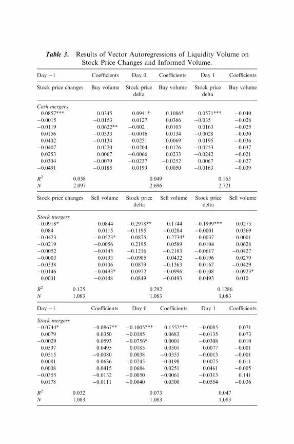
Table 3. Results of Vector Autoregressions of Liquidity Volume onStock Price Changes and Informed Volume.
Day �1 Coefficients Day 0 Coefficients Day 1 Coefficients
Stock price changes Buy volume Stock price
delta
Buy volume Stock price
delta
Buy volume
Cash mergers
0.0857*** 0.0345 0.0941* 0.1086* 0.0571*** �0.040
�0.0015 �0.0153 0.0127 0.0366 �0.035 �0.028
�0.0119 0.0622** �0.002 0.0103 0.0163 �0.025
0.0156 �0.0333 �0.0016 0.0134 �0.0028 �0.030
0.0402 �0.0134 0.0251 0.0069 0.0195 �0.036
�0.0407 0.0220 �0.0204 �0.0126 �0.0253 �0.037
0.0253 0.0067 �0.0066 0.0233 �0.0242 �0.021
0.0304 �0.0079 �0.0237 �0.0252 0.0067 �0.027
�0.0491 �0.0185 0.0199 0.0050 �0.0163 �0.039
R2 0.058 0.049 0.163
N 2,097 2,696 2,721
Stock price changes Sell volume Stock price
delta
Sell volume Stock price
delta
Sell volume
Stock mergers
�0.0918* 0.0844 �0.2978** 0.1744 �0.1999*** 0.0275
0.084 0.0115 �0.1195 �0.0284 �0.0001 0.0569
�0.0423 �0.0523* 0.0875 �0.2734* �0.0037 �0.0001
�0.0219 �0.0056 0.2195 0.0589 0.0104 0.0628
�0.0052 �0.0145 �0.1216 �0.2183 �0.0617 �0.0427
�0.0003 0.0193 �0.0905 0.0432 �0.0196 0.0279
�0.0338 0.0106 0.0879 �0.1363 0.0167 �0.0429
�0.0146 �0.0493* 0.0972 �0.0996 �0.0108 �0.0923*
0.0001 �0.0148 0.0849 �0.0493 0.0493 0.010
R2 0.125 0.292 0.1286
N 1,083 1,083 1,083
Day �1 Coefficients Day 0 Coefficients Day 1 Coefficients
Stock mergers
�0.0744* �0.0867** �0.1005*** 0.1552*** �0.0085 0.071
0.0079 0.0350 �0.0185 0.0683 �0.0135 0.073
�0.0029 0.0593 �0.0756* 0.0001 �0.0308 0.010
0.0597 0.0495 0.0185 0.0501 0.0077 �0.001
0.0515 �0.0080 0.0038 �0.0355 �0.0013 �0.001
0.0081 0.0636 �0.0245 �0.0198 0.0075 �0.011
0.0008 0.0415 0.0684 0.0251 0.0461 �0.005
�0.0355 �0.0132 �0.0050 �0.0061 �0.0313 0.141
0.0178 �0.0111 �0.0040 0.0300 �0.0554 �0.036
R2 0.032 0.073 0.047
N 1,083 1,083 1,083
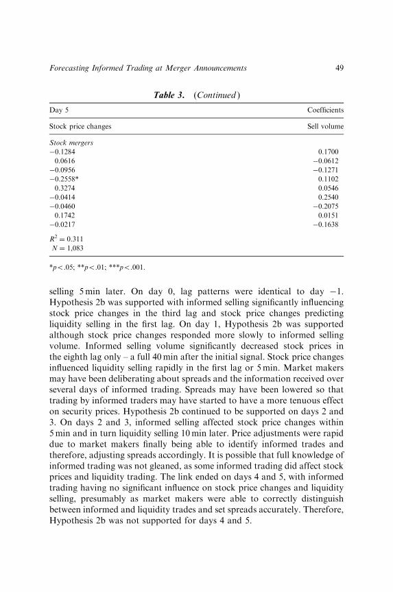
selling 5min later. On day 0, lag patterns were identical to day �1.Hypothesis 2b was supported with informed selling significantly influencingstock price changes in the third lag and stock price changes predictingliquidity selling in the first lag. On day 1, Hypothesis 2b was supportedalthough stock price changes responded more slowly to informed sellingvolume. Informed selling volume significantly decreased stock prices inthe eighth lag only – a full 40min after the initial signal. Stock price changesinfluenced liquidity selling rapidly in the first lag or 5min. Market makersmay have been deliberating about spreads and the information received overseveral days of informed trading. Spreads may have been lowered so thattrading by informed traders may have started to have a more tenuous effecton security prices. Hypothesis 2b continued to be supported on days 2 and3. On days 2 and 3, informed selling affected stock price changes within5min and in turn liquidity selling 10min later. Price adjustments were rapiddue to market makers finally being able to identify informed trades andtherefore, adjusting spreads accordingly. It is possible that full knowledge ofinformed trading was not gleaned, as some informed trading did affect stockprices and liquidity trading. The link ended on days 4 and 5, with informedtrading having no significant influence on stock price changes and liquidityselling, presumably as market makers were able to correctly distinguishbetween informed and liquidity trades and set spreads accurately. Therefore,Hypothesis 2b was not supported for days 4 and 5.
Day 5 Coefficients
Stock price changes Sell volume
Stock mergers
�0.1284 0.1700
0.0616 �0.0612
�0.0956 �0.1271
�0.2558* 0.1102
0.3274 0.0546
�0.0414 0.2540
�0.0460 �0.2075
0.1742 0.0151
�0.0217 �0.1638
R2¼ 0.311
N ¼ 1,083
*po.05; **po.01; ***po.001.
Table 3. (Continued )
Forecasting Informed Trading at Merger Announcements 49

CONCLUSIONS AND RECOMMENDATIONS FOR
FUTURE RESEARCH
This study has provided empirical proof of the Easley and O’Hara (1992)model. Informed buying and selling volumes act to increase or decreasestock price changes which affect liquidity trading. By examining the patternof relationships defined by our vector autoregressions, it is possible toforecast the actions of informed traders over the merger announcementperiod. As long as the link between informed trading, stock price changes,and liquidity trading holds, market makers in the stock market at mergerannouncements are setting high spreads, raising bid and ask quotes, andimpounding information into prices. In other words, market makers areresponding to the actions of informed traders, or informed trading is drivingprices and uninformed trades. This occurred throughout the �1 to þ1merger announcement period for cash mergers. For stock mergers, thesituation was found to be inherently more complex. For days �1 to þ1,informed traders influenced stock price changes and liquidity trading. Ondays 2 and 3, there was rapid inclusion of informed trading in stock prices asstock prices achieved equilibrium rapidly. The existence of some marketimperfection was apparent in that some trading on privileged informationdid have an impact on security prices. However, it is evident that marketmakers were beginning to infer patterns of informed trading and distinguishthem from liquidity trading. Spreads began to be adjusted downwards, andexcessive profits were not as easily available to informed traders as on theprevious days. On days 4 and 5, all excess profits disappeared as marketmakers finally adjusted spreads to equilibrium prices and liquidity traderswere subject to transaction costs that reflected their true values. This studyhas provided the first evidence of trading patterns for informed and liquiditytraders during merger announcements, where the type of merger or methodof payment forms the basis of demarcation. We have found that spreads andprices do not adjust to equilibrium levels for cash mergers during theannouncement period. For stock mergers, they adjust over a longer period,i.e., during the fourth and fifth days. Hypothesis 1b was partly supported forstock mergers with shifts from significant positive to negative CAARsduring the day 0 to þ5 period. It is possible that there are multiple groups ofinformed or liquidity traders. Future autoregressive models should includedifferent types of liquidity traders and trace their activity to different groupsof informed traders.
REBECCA ABRAHAM AND CHARLES HARRINGTON50

Easley and O’Hara (1992) identify the spread as the key linking variablebetween informed and liquidity traders. In their theoretical model, marketmakers respond to increased trading by informed traders by setting thespread to have higher widths. The width gets adjusted downwards asmarket makers obtain more information about the identity of informedand liquidity trades. The width of the spread is a proxy for the extent ofuncertainty the market maker feels about his profits. It may be advisableto enter the spread in the vector autoregressive model in lieu of prices, as itis a direct measure of the actions of the market maker in setting prices,rather than our more indirect measure of the price changes resulting fromthose spreads. The study may then be extended to dividends and earningsannouncements as other information-based events in which informedtrading may be forecasted by examining levels of uninformed trading.
REFERENCES
Admati, A. R., & Pfleiderer, P. (1988). A theory of intraday patterns: Volume and price
variability. Review of Financial Studies, 1, 3–40.
Bamber, L. S., Barron, O. E., & Stober, T. L. (1999). Differential interpretations and trading
volume. Journal of Financial and Quantitative Analysis, 34, 369–386.
Black, F. (1986). Noise. Journal of Finance, 41, 529–543.
Cao, C., Chen, C., & Griffin, T. (2005). Informational content of option volume prior to
takeover. Journal of Business, 78, 1073–1109.
De Fontnouvelle, P., Fishe, P., & Harris, J. H. (2003). The behavior of bid-ask spreads and
volume in options markets during the competition for listings in 1999. Journal of
Finance, 58, 2437–2464.
Easley, D. O., & O’Hara, M. (1992). Adverse selection and large trade volume: The implications
for market efficiency. Journal of Financial and Quantitative Analysis, 27, 185–208.
Glosten, L., & Milgrom, P. (1985). Bid, ask, and transaction prices in a specialist market with
heterogeneously informed traders. Journal of Financial Economics, 14, 71–100.
Heflin, F., & Shaw, K. W. (2005). Trade size and informed trading: Which trades are ‘‘big’’?
Journal of Financial Research, 28, 133–163.
Kanodia, C., Bushman, R., & Dickhaut, J. (1986). Private information and rationality in the
sunk costs phenomenon. Working Paper. University of Minnesota.
Kyle, A. S. (1985). Continuous auctions and insider trading. Econometrica, 53, 1315–1335.
Lee, J., & Yi, C. H. (2001). Trade size and information-motivated trading in options and stock
markets. Journal of Financial and Quantitative Analysis, 36, 485–501.
Mitchell, M., Pulvino, T., & Stafford, E. (2004). Price pressure around mergers. Journal of
Finance, 59, 31–63.
Trueman, B. (1988). A theory of noise trading in securities markets. Journal of Finance, 43,
83–95.
Forecasting Informed Trading at Merger Announcements 51

This page intentionally left blank
USING DATA ENVELOPMENT
ANALYSIS (DEA) TO FORECAST
BANK PERFORMANCE
Ronald K. Klimberg, Kenneth D. Lawrence and
Tanya Lal
ABSTRACT
Forecasting is an important tool used by businesses to plan and evaluatetheir operations. One of the most commonly used techniques forforecasting is regression analysis. Often forecasts are produced for aset of comparable units which could be individuals, groups, departments,or companies that perform similar activities such as a set of banks, agroup of mangers, and so on. We apply a methodology that includes a newvariable, the comparable unit’s data envelopment analysis relativeefficiency, into the regression analysis. This chapter presents the resultsof applying this methodology to the performance of commercial banks.
INTRODUCTION
Quantitative forecasting models, even rather sophisticated models, are easierto develop and use today as a result of our improving computer technology.These quantitative forecasting techniques use historical data to predict thefuture. Most quantitative forecasting techniques can be categorized into either
Advances in Business and Management Forecasting, Volume 6, 53–61
Copyright r 2009 by Emerald Group Publishing Limited
All rights of reproduction in any form reserved
ISSN: 1477-4070/doi:10.1108/S1477-4070(2009)0000006004
53
time series approaches or causal models. Time series forecasting techniquesare forecasting techniques that only use the time series data itself and not anyother data to build the forecasting models. These time series approachesisolate and measure the impact of the trend, seasonal, and cyclical time seriescomponents. Causal models use a set of predictor/independent variables,possibly also including the time series components, which are believed toinfluence the forecasted variable. One of the most popular causal modelapproach is regression analysis. Regression techniques employ the statisticalmethod of least squares to establish a statistical relationship between theforecasted variable and the set of predictor/independent variables.
Many forecasting situations involve producing forecasts for comparableunits. A comparable unit could be an individual, group of individuals, adepartment, a company, and so on. Each comparable unit should beperforming similar set of tasks. When applying regression analysis, theestablished statistical relationship is an average relationship using one set ofweights assigned to the predictor/independent variables. However, whenregression is applied to a set of comparable units the relative weight/importance of each of the predictor/independent variables will most likelyvary from comparable unit to comparable unit. For example, if advertisingis an independent variable, one comparable unit might emphasizeadvertising more (or less) than other comparable units. Either way is notnecessarily better nor worse, it is just how that particular comparable unitemphasizes advertising. As a result, in some cases, the regression modelcould provide forecast estimates that are too high or too low.
In this chapter, we will apply and extend some of our recent previouswork, Klimberg, Lawrence, and Lawrence (2005, 2008), in which we intro-duced a methodology that incorporates into the regression forecastinganalysis a new variable that captures the unique weighting of each compa-rable unit. This new variable is the relative efficiency of each comparableunit that is generated by a nonparametric technique called data envelopmentanalysis (DEA). The next section provides a brief introduction to DEA.Subsequently, the methodology is discussed and the results of applying ourmethodology to a data set of commercial banks are presented. Finally, theconclusions and future extensions are discussed.
DATA ENVELOPMENT ANALYSIS (DEA)
DEA utilizes linear programming to produce measures of the relativeefficiency of comparable units that employ multiple inputs and outputs.
RONALD K. KLIMBERG ET AL.54
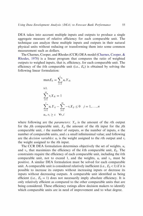
DEA takes into account multiple inputs and outputs to produce a singleaggregate measure of relative efficiency for each comparable unit. Thetechnique can analyze these multiple inputs and outputs in their naturalphysical units without reducing or transforming them into some commonmeasurement such as dollars.
The Charnes, Cooper, and Rhodes (CCR) DEAmodel (Charnes, Cooper, &Rhodes, 1978) is a linear program that compares the ratio of weightedoutputs to weighed inputs, that is, efficiency, for each comparable unit. Theefficiency of the kth comparable unit (i.e., Ek) is obtained by solving thefollowing linear formulation:
maxEk ¼Xtr¼1
urYrk
s:t:
Xmi¼1
viXik ¼ 1
Xtr¼1
urYrj �Xmi¼1
�viXij � 0 j ¼ 1; . . . ; n
ur; vi � � 8r; i
where following are the parameters: Yrj is the amount of the rth outputfor the jth comparable unit, Xij the amount of the ith input for the jthcomparable unit, t the number of outputs, m the number of inputs, n thenumber of comparable units, and e a small infinitesimal value; and followingare the decision variables: ur is the weight assigned to the rth output and vithe weight assigned to the ith input.
The CCR DEA formulation determines objectively the set of weights, urand vi, that maximizes the efficiency of the kth comparable unit, Ek. Theconstraints require the efficiency of each comparable unit, including the kthcomparable unit, not to exceed 1, and the weights, ur and vi, must bepositive. A similar DEA formulation must be solved for each comparableunit. A comparable unit is considered relatively inefficient (i.e., Eko1) if it ispossible to increase its outputs without increasing inputs or decrease itsinputs without decreasing outputs. A comparable unit identified as beingefficient (i.e., Ek ¼ 1) does not necessarily imply absolute efficiency. It isonly relatively efficient as compared to the other comparable units that arebeing considered. These efficiency ratings allow decision makers to identifywhich comparable units are in need of improvement and to what degree.
Using Data Envelopment Analysis (DEA) to Forecast Bank Performance 55
Each efficiency score measures the relative efficiency of the comparableunit. These efficiency scores can be used to evaluate performance of thecomparable units and provide benchmarks. Nevertheless, besides eachefficiency score being composed of a different set of inputs and outputsvalues, each comparable unit’s efficiency score includes a unique set ofweights. The DEA process attempts to find objectively the set of weights thatwill maximize a comparable unit’s efficiency. Therefore, the DEA model hasselected the best possible set of weights for each comparable unit. Thevariation of these weights from one comparable unit to the other comparableunit allows each comparable unit to have its own unique freedom toemphasize the importance of each of these input and output variables in theirown way. How well they do this is measured by the efficiency score.
Since the Charnes et al.’s 1978 paper, there have been thousands oftheoretical contributions and practical applications in various fields usingDEA. DEA has been applied to many diverse areas such as health care,military operations, criminal courts, university departments, banks, electricutilities mining operations, and manufacturing productivity (Klimberg &Kern, 1992; Seiford, 1996; Seiford & Thrall, 1990).
REGRESSION FORECASTING METHODOLOGY
Our regression forecasting methodology is designed to be applied to ahistorical data set of multiple input and output variables from a set ofcomparable units (Klimberg et al., 2005, 2008). The methodology is a three-step process. The first step selects a dependent variable and if necessaryreduces the number of input and output variables. Basically, one outputvariable is identified to be the principal/critical variable that will be needed tobe forecasted, for example, sales, production, or demand. If the number ofinput and output variables is relatively large, similar to the goal in multipleregression, we follow the principle of parsimony and try to build a model thatincludes the least number of variables, which sufficiently explains the depen-dent variable. In DEA, the combined total of inputs and outputs includedin the model should be no more than half the number of comparable unitsbeing compared in the analysis (Boussofiane, Dyson, & Thanassoulis, 1991;Golany & Roll, 1989). Golany and Roll (1989) suggest employing bothqualitative and quantitative (including stepwise regression) techniques toidentify the significant set of input and output variables. The second step is torun the DEA for each comparable unit using the identified significant inputand output variables. We use these efficiency scores as surrogate measures of
RONALD K. KLIMBERG ET AL.56

the unique emphasis of the variables and of performance. The last step usesthe principal/critical output variable as the regression-dependent variable, allthe significant input variables plus the DEA efficiency score as regression-independent variables, and run a multiple regression. This regression modelwith the DEA efficiency variable should be superior, that is, should have asignificantly lower standard error of the mean and increase R2, to theregression model without the DEA efficiency score variable.
EXAMPLE
Commercial banks are defined as ‘‘those banks whose business is derivedprimarily from commercial operations but which are also present in the retailbanking and small and medium industry sectors’’ (Datamonitor, 2007). As of2007, the commercial banking industry in the United States had a marketvalue of $502.7 billion and was projected to grow by 23.7% to $622 billion in2011 (Datamonitor, 2007). The different banks in the industry serve the samerange of clients and offer the same services and therefore have limitedcompetitive advantage on those fronts. Most companies derive competitiveadvantage from pricing and market reach. This has caused a trend towardconsolidation in the industry. Since the balance of risk and return is crucialto profitability in commercial banking, consolidation has raised concernsabout whether the large scale of some of the companies in the industry allowsfor proper oversight and regulation of risk.
Revenue is derived from two sources, interest income on deposits andnoninterest income such as fees and commissions. Typically 50% or more ofcommercial banks’ operating costs can be due to employee compensation.This is because of a need to have a large street branch presence and tocompetitively compensate higher level employees such as asset managerswho are in high demand (Datamonitor, 2007).
Monitoring the performance of commercial banks is important to severalparties. Customers are concerned about the safety of their deposits andaccess to affordable credit; shareholders are concerned about returns ontheir investment; managers are concerned with profitability; and finallyregulators are concerned owing to the banks’ role in the economy as themain source of financial intermediation and as custodians of a large portionof the nation’s cash (Data Envelopment Analysis and Commercial BankPerformance: A Primer With Applications to Missouri Banks, 1992).Historically financial ratios such as return on assets (ROA) or return oninvestment (ROI) have been used to measure bank’s performance. Although
Using Data Envelopment Analysis (DEA) to Forecast Bank Performance 57
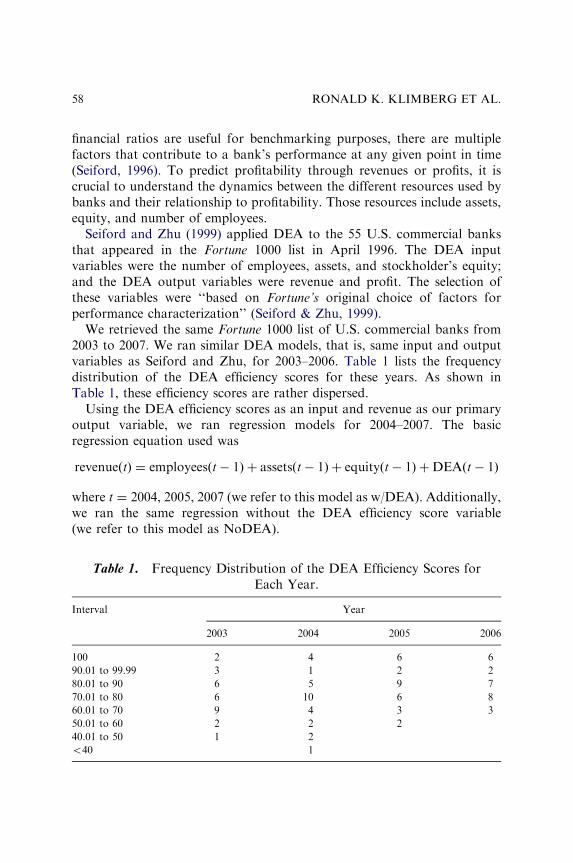
financial ratios are useful for benchmarking purposes, there are multiplefactors that contribute to a bank’s performance at any given point in time(Seiford, 1996). To predict profitability through revenues or profits, it iscrucial to understand the dynamics between the different resources used bybanks and their relationship to profitability. Those resources include assets,equity, and number of employees.
Seiford and Zhu (1999) applied DEA to the 55 U.S. commercial banksthat appeared in the Fortune 1000 list in April 1996. The DEA inputvariables were the number of employees, assets, and stockholder’s equity;and the DEA output variables were revenue and profit. The selection ofthese variables were ‘‘based on Fortune’s original choice of factors forperformance characterization’’ (Seiford & Zhu, 1999).
We retrieved the same Fortune 1000 list of U.S. commercial banks from2003 to 2007. We ran similar DEA models, that is, same input and outputvariables as Seiford and Zhu, for 2003–2006. Table 1 lists the frequencydistribution of the DEA efficiency scores for these years. As shown inTable 1, these efficiency scores are rather dispersed.
Using the DEA efficiency scores as an input and revenue as our primaryoutput variable, we ran regression models for 2004–2007. The basicregression equation used was
revenueðtÞ ¼ employeesðt� 1Þ þ assetsðt� 1Þ þ equityðt� 1Þ þDEAðt� 1Þ
where t ¼ 2004, 2005, 2007 (we refer to this model as w/DEA). Additionally,we ran the same regression without the DEA efficiency score variable(we refer to this model as NoDEA).
Table 1. Frequency Distribution of the DEA Efficiency Scores forEach Year.
Interval Year
2003 2004 2005 2006
100 2 4 6 6
90.01 to 99.99 3 1 2 2
80.01 to 90 6 5 9 7
70.01 to 80 6 10 6 8
60.01 to 70 9 4 3 3
50.01 to 60 2 2 2
40.01 to 50 1 2
o40 1
RONALD K. KLIMBERG ET AL.58
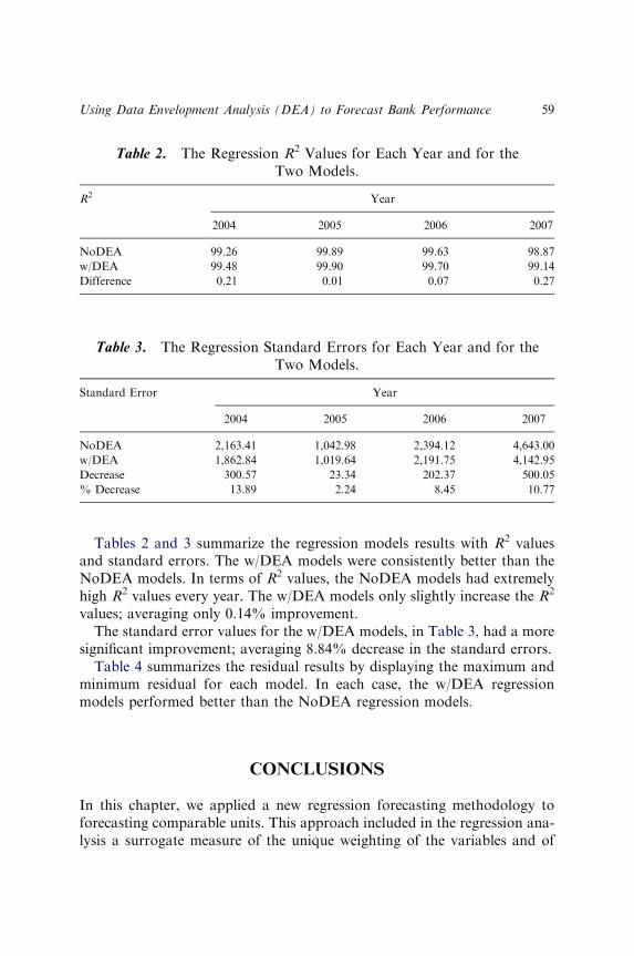
Tables 2 and 3 summarize the regression models results with R2 valuesand standard errors. The w/DEA models were consistently better than theNoDEA models. In terms of R2 values, the NoDEA models had extremelyhigh R2 values every year. The w/DEA models only slightly increase the R2
values; averaging only 0.14% improvement.The standard error values for the w/DEA models, in Table 3, had a more
significant improvement; averaging 8.84% decrease in the standard errors.Table 4 summarizes the residual results by displaying the maximum and
minimum residual for each model. In each case, the w/DEA regressionmodels performed better than the NoDEA regression models.
CONCLUSIONS
In this chapter, we applied a new regression forecasting methodology toforecasting comparable units. This approach included in the regression ana-lysis a surrogate measure of the unique weighting of the variables and of
Table 2. The Regression R2 Values for Each Year and for theTwo Models.
R2 Year
2004 2005 2006 2007
NoDEA 99.26 99.89 99.63 98.87
w/DEA 99.48 99.90 99.70 99.14
Difference 0.21 0.01 0.07 0.27
Table 3. The Regression Standard Errors for Each Year and for theTwo Models.
Standard Error Year
2004 2005 2006 2007
NoDEA 2,163.41 1,042.98 2,394.12 4,643.00
w/DEA 1,862.84 1,019.64 2,191.75 4,142.95
Decrease 300.57 23.34 202.37 500.05
% Decrease 13.89 2.24 8.45 10.77
Using Data Envelopment Analysis (DEA) to Forecast Bank Performance 59
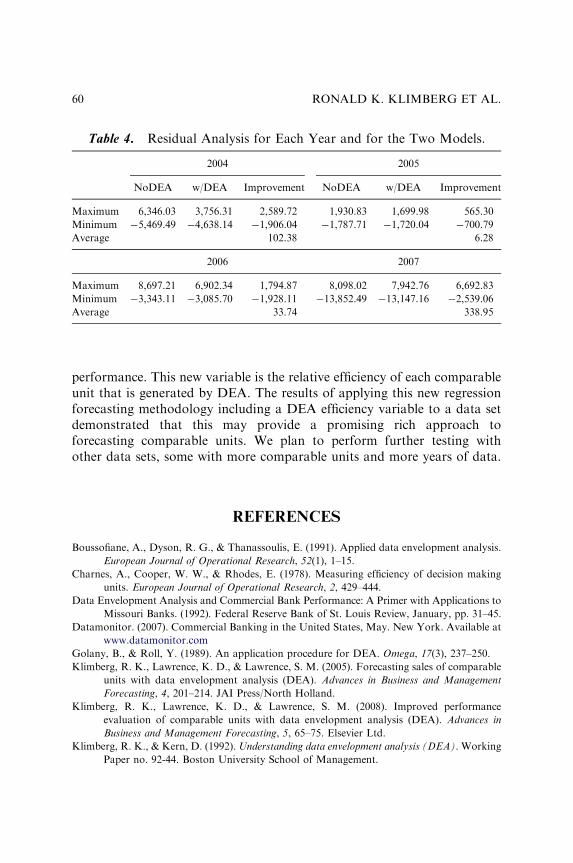
performance. This new variable is the relative efficiency of each comparableunit that is generated by DEA. The results of applying this new regressionforecasting methodology including a DEA efficiency variable to a data setdemonstrated that this may provide a promising rich approach toforecasting comparable units. We plan to perform further testing withother data sets, some with more comparable units and more years of data.
REFERENCES
Boussofiane, A., Dyson, R. G., & Thanassoulis, E. (1991). Applied data envelopment analysis.
European Journal of Operational Research, 52(1), 1–15.
Charnes, A., Cooper, W. W., & Rhodes, E. (1978). Measuring efficiency of decision making
units. European Journal of Operational Research, 2, 429–444.
Data Envelopment Analysis and Commercial Bank Performance: A Primer with Applications to
Missouri Banks. (1992). Federal Reserve Bank of St. Louis Review, January, pp. 31–45.
Datamonitor. (2007). Commercial Banking in the United States, May. New York. Available at
www.datamonitor.com
Golany, B., & Roll, Y. (1989). An application procedure for DEA. Omega, 17(3), 237–250.
Klimberg, R. K., Lawrence, K. D., & Lawrence, S. M. (2005). Forecasting sales of comparable
units with data envelopment analysis (DEA). Advances in Business and Management
Forecasting, 4, 201–214. JAI Press/North Holland.
Klimberg, R. K., Lawrence, K. D., & Lawrence, S. M. (2008). Improved performance
evaluation of comparable units with data envelopment analysis (DEA). Advances in
Business and Management Forecasting, 5, 65–75. Elsevier Ltd.
Klimberg, R. K., & Kern, D. (1992). Understanding data envelopment analysis (DEA). Working
Paper no. 92-44. Boston University School of Management.
Table 4. Residual Analysis for Each Year and for the Two Models.
2004 2005
NoDEA w/DEA Improvement NoDEA w/DEA Improvement
Maximum 6,346.03 3,756.31 2,589.72 1,930.83 1,699.98 565.30
Minimum �5,469.49 �4,638.14 �1,906.04 �1,787.71 �1,720.04 �700.79
Average 102.38 6.28
2006 2007
Maximum 8,697.21 6,902.34 1,794.87 8,098.02 7,942.76 6,692.83
Minimum �3,343.11 �3,085.70 �1,928.11 �13,852.49 �13,147.16 �2,539.06
Average 33.74 338.95
RONALD K. KLIMBERG ET AL.60

Seiford, L. M. (1996). Data envelopment analysis: The evaluation of the state of the art
(1978–1995. The Journal of Productivity Analysis, 9, 99–137.
Seiford, L. M., & Thrall, R. M. (1990). Recent developments in DEA: The mathematical
programming approach to frontier analysis. Journal of Econometric, 46, 7–38.
Seiford, L. M., & Zhu, J. (1999). Profitability and marketability of the top 55 U.S. commercial
banks. Management Science, 45(9), 1270–1288.
Using Data Envelopment Analysis (DEA) to Forecast Bank Performance 61

This page intentionally left blank

PART II
MARKETING AND DEMAND
APPLICATIONS

This page intentionally left blank
FORECASTING DEMAND
USING PARTIALLY
ACCUMULATED DATA
Joanne S. Utley and J. Gaylord May
ABSTRACT
This chapter uses advance order data from an actual manufacturing shopto develop and test a forecast model for total demand. The proposedmodel made direct use of historical time series data for total demand andtime series data for advance orders. Comparison of the proposed model tocommonly used approaches showed that the proposed model exhibitedgreater forecast accuracy.
INTRODUCTION
In many businesses, a portion of the demand for a future time period may beknown due to advance customer orders. For example, at any point in time,hotel reservations provide partial information about the customer demandthat will actually be realized in future time periods. Similarly, in a manu-facturing shop, firm orders to date with customer designated lead timesallow the manufacturer to know with certainty a portion of the actualdemand in future time periods.
Advances in Business and Management Forecasting, Volume 6, 65–80
Copyright r 2009 by Emerald Group Publishing Limited
All rights of reproduction in any form reserved
ISSN: 1477-4070/doi:10.1108/S1477-4070(2009)0000006005
65

Past research has shown that if a forecaster can utilize this kind of partialdemand information in developing a forecast, he has the opportunity toproduce a more accurate forecast than if he relied on historical data alone(Kekre, Morton, & Smunt, 1990). Past research has also suggested that theforecast methodology should not be so complex that it would be difficult toimplement in practice (Guerrero & Elizondo, 1997). This chapter proposes aforecast model, which is straightforward in approach and relatively easy toimplement. The proposed model utilizes both partial demand data andhistorical time series data to forecast customer demand.
This chapter is organized as follows. The following section provides anoverview of forecast methods which use advance customer order data. The‘‘Case Study’’ section describes the forecast model devised by the authors. Itillustrates the application of the proposed model at an actual manufacturingcompany and develops alternative forecasts through commonly usedapproaches. The accuracy of the proposed forecast model is then comparedto the accuracy of the standard models. The chapter concludes with adiscussion of the research findings and suggestions for future research.
OVERVIEW OF THE LITERATURE
One of the earliest methods of forecasting with partial data was proposed byMurray and Silver (1966) to address the style goods problem. In thisproblem, there is a finite selling period for the item, sales vary in a seasonaland somewhat predictable pattern, and the item can be bought or producedonly on a limited number of occasions. Murray and Silver (1966) noted thatalthough there is initially great uncertainty about the sales potential of theitem, the manager can improve the forecast as sales become known overtime. Murray and Silver (1966) utilized a dynamic programming model inwhich each state represented both the amount of unsold inventory andcurrent knowledge of sales. Green and Harrison (1973) also used Bayesianmethods to solve the style goods problem. Their approach was utilized in amail order company to forecast sales for a sample of 93 different types ofdresses. Guerrero and Elizondo (1997) have noted that these early studiesadopted a Bayesian perspective to the problem because information onfuture demand was extremely limited. Guerrero and Elizondo (1997, p. 879)also observed that a major difficulty with this approach is that ‘‘the resultingmethods usually require a large amount of expertise from the analyst toimplement them.’’
JOANNE S. UTLEY AND J. GAYLORD MAY66

Bestwick’s (1975) study was the first in the forecasting literature toinvestigate a simpler alternative to Bayesian type models. Bestwick’s (1975)approach utilized a multiplicative model, which assumed that total demandfor a future time period t can be found at an earlier time period t�h bydividing the advance orders for period t, booked h or more periods ahead,by a cumulative proportion Ch. The cumulative proportion Ch can beinterpreted as the percent of total actual demand for a time period realizedthrough accumulated customer orders, h periods in advance. For example, ifa manager knows that at time t�h, 25% of the total demand for period t willalready be known, and if the sum of the advance orders for period t ¼ 100units, then the forecast for period t is 100/.25 ¼ 400 units.
Bestwick (1975) used his multiplicative model in conjunction with aforecast monitoring procedure, which included traditional elements ofstatistical process control such as cusum techniques, the mean chart, and thesampling distribution of the range. Bestwick (1975) reported that hismethodology was successfully implemented in a number of areas includingdemand forecasting, inventory control, budgeting, production control, andturnover analysis. Today, the multiplicative model remains popular in boththe private and public sector (Kekre et al., 1990). Its simplicity continues tomake it attractive to managers who lack the technical expertise or financialresources needed to implement more sophisticated forecast models.
Despite its popularity, Bestwick’s (1975) multiplicative model does exhibitsome shortcomings. First, this approach assumes that each cumulativeproportion Ch will remain constant over time; however, drift in the Ch
values can often occur in practice. Second, this model does not use the totaldemand time series directly in the forecast. Thus, the simple multiplicativemodel is not particularly responsive to changes in total demand (Bodily &Freeland, 1988). Finally, the accuracy of the multiplicative method is notonly a function of the stability of the Ch values but also their accuracy. Theaccuracy of the Ch values tends to decline as h increases. When hWL, themaximum customer specified lead time, the forecaster cannot continue touse this method since no customer order data will exist this far in advance(Kekre et al., 1990).
Kekre et al. (1990) addressed the problem of variability of the cumulativeproportions in Bestwick’s model by using exponential smoothing to updatethe Ch values. They used partially known demand data from a printing firmto test their model, assuming a 5-day forecast horizon. Kekre et al. (1990)found that the multiplicative model outperformed a simple exponentialsmoothing model that used time series data for total demand. They alsoexamined an additive model for partial demand data. The additive model
Forecasting Demand Using Partially Accumulated Data 67
assumed that a forecast for total demand could be found by adding theknown portion of demand for a future time period with the smoothedunknown portion of demand for the future time period. Unlike thesmoothed multiplicative model, the additive model assumes that the knownportion of demand contains no information about the unknown portion ofdemand (Kekre et al., 1990).
Kekre et al. (1990) found that both the smoothed multiplicative andadditive models performed better than traditional exponential smoothingfor a planning horizon of four periods or less, even if random demandshocks occurred. Kekre et al. (1990, p. 123) also reported that the smoothedadditive model was more appropriate for long lead times than themultiplicative approach and observed that the smoothed additive model‘‘becomes indistinguishable from exponential smoothing as the lead timeincreases.’’ They concluded their paper by suggesting that future researchcould focus on the combination of multiplicative and additive techniquesthrough regression analysis.
Bodily and Freeland (1988) argued that alternatives to the simple andsmoothed multiplicative models were needed, especially since both modelsfail to use the total demand time series directly. Using simulated bookingand shipment data, Bodily and Freeland (1988) tested six partial demandforecast models. The first two models were the simple multiplicative modeland the smoothed multiplicative model discussed earlier. The third modelcombined smoothed shipments with fixed Ch factors, whereas the fourthmodel combined smoothed shipments with smoothed Ch factors. The fifthand sixth models used Bayesian shipments with fixed Ch factors andsmoothed Ch factors, respectively. Results of the model comparisonsshowed that the smoothed multiplicative model performed the best overall.
In a later paper, Guerrero and Elizondo (1997) used least squaresestimation to forecast total demand with partially accumulated data. Theirmodel specified a set of L linear regressions, where L is the longest lead timeof the forecast. Guerrero and Elizondo (1997) used both Kekre et al.’s(1990) data set and data on the Mexican economy to compare the accuracyof their approach to that of algorithmic solutions. They reported that theirstatistical approach was more accurate for all lead times.
A recent paper by Waage (2006) used a stochastic dynamic model toforecast demand with advance order data. The model combined twoinformation sources (1) an econometric sales forecast and (2) partiallyknown information about customer orders for future time periods. Waage(2006) applied his model to the problem of forecasting sales for specialpurpose computers. Waage (2006, p. 24) reported that the sales forecast
JOANNE S. UTLEY AND J. GAYLORD MAY68

produced by his model converged on the actual sales trajectory even beforethe actual trajectory was known.
The forecast models summarized in this section reflect varying degrees ofcomplexity and forecast accuracy. Although some companies may prefer toimplement more sophisticated forecast models when partial order data areavailable, other business, particularly smaller businesses, may preferapproaches that are simpler and require less expertise. The next section ofthis chapter will describe a forecast approach that is relatively simple to useyet exploits the availability of both advance order data and time series datafor total demand.
CASE STUDY
An electronics component manufacturer located in the southeast UnitedStates provided the research context for this study. Although the companyproduces a variety of products, order data for a single product, referredto as product (A), will be used to illustrate the forecast model. Analysis of9 months of historical data for this product showed that each customerorder included a requested delivery date (or customer designated lead time)in addition to the order quantity. Designated lead times typically rangedfrom 1 to 4 months, although a lead time of 5 or 6 months would occa-sionally be requested. A customer’s order quantity and designated lead timedid not remain constant over time; instead, they varied with each order.
The manufacturer wished to forecast total demand for a 6 monthplanning horizon (months 10–15) by using the partial order data it alreadypossessed at the end of month 9. The authors developed the model shownin Exhibit 1 to make use of both the partial order data available for months1–13 and the total demand data for months 1–9 in preparing the forecasts.The remainder of this section will use these data to illustrate conceptscontained in the model’s design.
For a particular product, we will consider all customer orders that arerequested for delivery in a specific time period (t). This demand may bedistributed with respect to the lead times supplied by the customer. Table 1shows such a distribution of orders for product (A), which was actuallyreceived by the manufacturing company.
Let t be a particular time period and h be a designated number of suchperiods. D(t,h) shall denote the sum of customer demands for period (t),which have lead times Zh. As an example, in Table 1, let t correspond tomonth (4) of 2005. For this request date, orders were received from month
Forecasting Demand Using Partially Accumulated Data 69
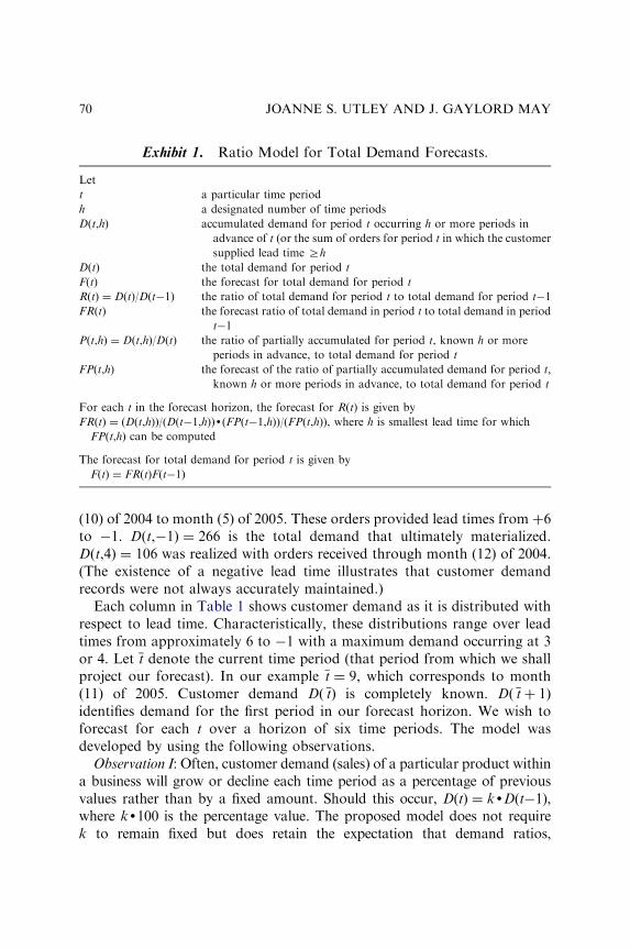
(10) of 2004 to month (5) of 2005. These orders provided lead times from þ6to �1. D(t,�1) ¼ 266 is the total demand that ultimately materialized.D(t,4) ¼ 106 was realized with orders received through month (12) of 2004.(The existence of a negative lead time illustrates that customer demandrecords were not always accurately maintained.)
Each column in Table 1 shows customer demand as it is distributed withrespect to lead time. Characteristically, these distributions range over leadtimes from approximately 6 to �1 with a maximum demand occurring at 3or 4. Let t denote the current time period (that period from which we shallproject our forecast). In our example t ¼ 9, which corresponds to month(11) of 2005. Customer demand Dð tÞ is completely known. Dð tþ 1Þidentifies demand for the first period in our forecast horizon. We wish toforecast for each t over a horizon of six time periods. The model wasdeveloped by using the following observations.
Observation I: Often, customer demand (sales) of a particular product withina business will grow or decline each time period as a percentage of previousvalues rather than by a fixed amount. Should this occur, D(t) ¼ kdD(t�1),where kd100 is the percentage value. The proposed model does not requirek to remain fixed but does retain the expectation that demand ratios,
Exhibit 1. Ratio Model for Total Demand Forecasts.
Let
t a particular time period
h a designated number of time periods
D(t,h) accumulated demand for period t occurring h or more periods in
advance of t (or the sum of orders for period t in which the customer
supplied lead time Zh
D(t) the total demand for period t
F(t) the forecast for total demand for period t
R(t) ¼ D(t)/D(t�1) the ratio of total demand for period t to total demand for period t�1
FR(t) the forecast ratio of total demand in period t to total demand in period
t�1
P(t,h) ¼ D(t,h)/D(t) the ratio of partially accumulated for period t, known h or more
periods in advance, to total demand for period t
FP(t,h) the forecast of the ratio of partially accumulated demand for period t,
known h or more periods in advance, to total demand for period t
For each t in the forecast horizon, the forecast for R(t) is given by
FR(t) ¼ (D(t,h))/(D(t�1,h))d(FP(t�1,h))/(FP(t,h)), where h is smallest lead time for which
FP(t,h) can be computed
The forecast for total demand for period t is given by
F(t) ¼ FR(t)F(t�1)
JOANNE S. UTLEY AND J. GAYLORD MAY70
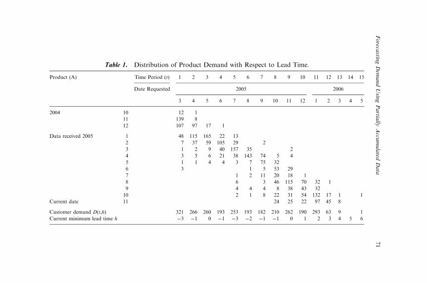
Table 1. Distribution of Product Demand with Respect to Lead Time.
Product (A) Time Period (t) 1 2 3 4 5 6 7 8 9 10 11 12 13 14 15
Date Requested 2005 2006
3 4 5 6 7 8 9 10 11 12 1 2 3 4 5
2004 10 12 1
11 139 8
12 107 97 17 1
Data received 2005 1 48 115 165 22 13
2 7 37 59 105 29 2
3 1 2 9 40 157 35 2
4 3 5 6 21 38 143 74 5 4
5 1 1 4 4 3 7 75 32
6 3 1 5 53 29
7 1 2 11 20 18 1
8 6 3 46 115 70 32 1
9 4 4 4 8 38 43 32
10 2 1 8 22 31 54 132 17 1 1
Current date 11 24 25 22 97 45 8
Customer demand D(t,h) 321 266 260 193 253 193 182 210 262 190 293 63 9 1
Current minimum lead time h �3 �1 0 �1 �3 �2 �1 �1 0 1 2 3 4 5 6
Foreca
stingDem
andUsin
gPartia
llyAccu
mulated
Data
71
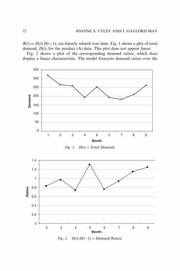
R(t) ¼ D(t)/D(t�1), are linearly related over time. Fig. 1 shows a plot of totaldemand, D(t), for the product (A) data. This plot does not appear linear.
Fig. 2 shows a plot of the corresponding demand ratios, which doesdisplay a linear characteristic. The model forecasts demand ratios over the
0
50
100
150
200
250
300
350
2 6 8
Month
Dem
and
1 3 4 5 97
Fig. 1. D(t) ¼ Total Demand.
0
0.2
0.4
0.6
0.8
1
1.2
1.4
2 6 7 8 9Month
Rat
ios
3 54
Fig. 2. D(t)/D(t�1) ¼ Demand Ratios.
JOANNE S. UTLEY AND J. GAYLORD MAY72

six period horizon. A final calculation converts these ratios into a forecast ofdemand. This conversion uses the recursive formula: F(t) ¼ FR(t)dF(t�1).
Observation II: As explained in the ‘‘Overview of the Literature’’ section,the basic multiplicative model customarily assumes that D(t,h)/D(t), thepercent of total demand for period t with a lead time Zh, remains constantover time. Examination of product (A) data showed that, for fixed h,P(t,h) ¼ D(t,h)/D(t) does not remain stationary. As shown in Table 2, thepercent of total demand declines as the time periods advance.
To forecast D(t)/D(t�1) over time periods 10, 11, 12, 13 where lead timedemand exists, we must first forecast P(t,h) for h ¼ 1, 2, 3, 4. These forecastswere obtained using exponential smoothing. They are shown in Table 2 inrows 10–13. Let FP(t,h) denote these forecast values. We estimateD(t,h)/D(t) ¼ FP(t,h) or D(t) ¼ D(t,h)/FP(t,h). For each t, we use thesmallest h for which FP(t,h) can be computed. We have
DðtÞ
Dðt� 1Þ�
Dðt; hÞ
Dðt� 1; hÞdFPðt� 1; hÞ
FPðt; hÞ¼ FRðtÞ; where t ¼ 10; 11; 12; 13
These forecasts of demand ratios are shown in the right most column ofTable 2. Fig. 3 shows a plot of these four lead time ratios, which appear as acontinuation of the ratios shown in Fig. 2.
Observation III: Time periods 14 and 15 are in the forecast horizon but donot have partially accumulated demand data. To obtain ratio forecasts forthese two periods, exponential smoothing was applied to the existing ratios.These smoothed ratios are plotted in Fig. 4 and their values are displayed inTable 3.
The smoothed ratios for periods 14 and 15 together with the lead timeratios for periods 10, 11, 12 and 13 form the ratio forecasts over the sixperiod horizon. All of these ratios are shown in Table 3.
Table 4 shows the results of converting the complete ratio forecasts intototal demand forecasts. Also shown is the complete demand that actuallymaterialized after the 6-month horizon had transpired.
Fig. 5 plots a comparison of the actual demand with the forecast ofdemand obtained from converting the ratio forecasts. Over the 4-month leadtime, a ‘‘seasonal pattern’’ existed for product (A) due to budget considera-tions of the customers. There was a decline in demand for December (period10) followed by a sharp increase in January and a subsequent decline inFebruary and March. This pattern was anticipated in November (currenttime period 9) using lead time ratios.
Forecasting Demand Using Partially Accumulated Data 73
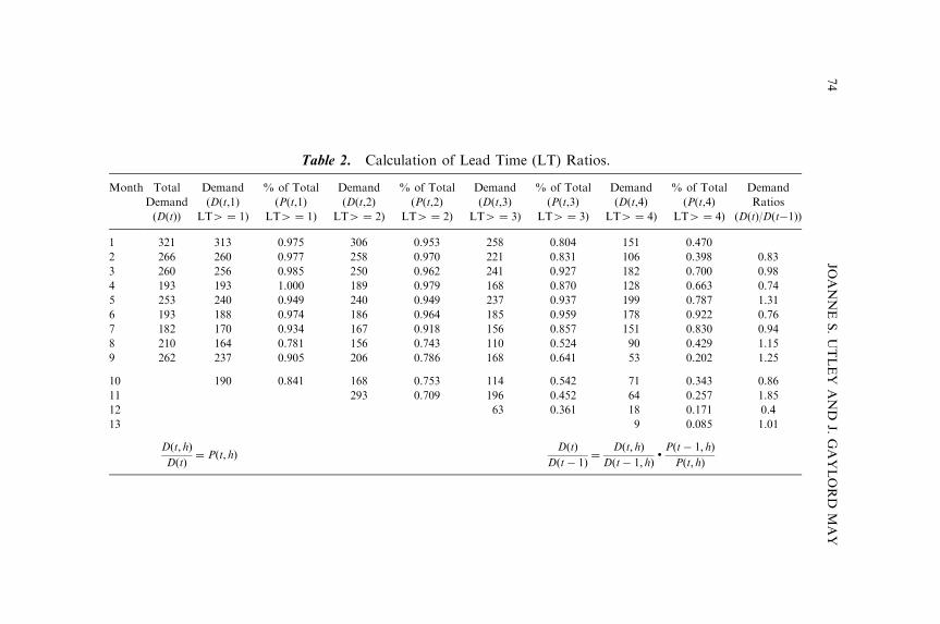
Table 2. Calculation of Lead Time (LT) Ratios.
Month Total Demand
(D(t,1)
LTW ¼ 1)
% of Total
(P(t,1)
LTW ¼ 1)
Demand
(D(t,2)
LTW ¼ 2)
% of Total
(P(t,2)
LTW ¼ 2)
Demand
(D(t,3)
LTW ¼ 3)
% of Total
(P(t,3)
LTW ¼ 3)
Demand
(D(t,4)
LTW ¼ 4)
% of Total
(P(t,4)
LTW ¼ 4)
Demand
Demand
(D(t))
Ratios
(D(t)/D(t�1))
1 321 313 0.975 306 0.953 258 0.804 151 0.470
2 266 260 0.977 258 0.970 221 0.831 106 0.398 0.83
3 260 256 0.985 250 0.962 241 0.927 182 0.700 0.98
4 193 193 1.000 189 0.979 168 0.870 128 0.663 0.74
5 253 240 0.949 240 0.949 237 0.937 199 0.787 1.31
6 193 188 0.974 186 0.964 185 0.959 178 0.922 0.76
7 182 170 0.934 167 0.918 156 0.857 151 0.830 0.94
8 210 164 0.781 156 0.743 110 0.524 90 0.429 1.15
9 262 237 0.905 206 0.786 168 0.641 53 0.202 1.25
10 190 0.841 168 0.753 114 0.542 71 0.343 0.86
11 293 0.709 196 0.452 64 0.257 1.85
12 63 0.361 18 0.171 0.4
13 9 0.085 1.01
Dðt; hÞ
DðtÞ¼ Pðt; hÞ
DðtÞ
Dðt� 1Þ¼
Dðt; hÞ
Dðt� 1; hÞdPðt� 1; hÞ
Pðt; hÞ
JOANNE
S.UTLEY
AND
J.GAYLORD
MAY
74
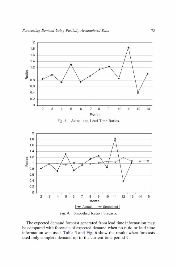
The expected demand forecast generated from lead time information maybe compared with forecasts of expected demand when no ratio or lead timeinformation was used. Table 5 and Fig. 6 show the results when forecastsused only complete demand up to the current time period 9.
0
0.2
0.4
0.6
0.8
1
1.2
1.4
1.6
1.8
2
2 3 4 9 10 11 12 13
Month
Rat
ios
5 6 7 8
Fig. 3. Actual and Lead Time Ratios.
0
0.2
0.4
0.6
0.8
1
1.2
1.4
1.6
1.8
2
2 7 8 10 11 12 13 14 15Month
Rat
ios
Actual Smoothed
3 4 5 6 9
Fig. 4. Smoothed Ratio Forecasts.
Forecasting Demand Using Partially Accumulated Data 75
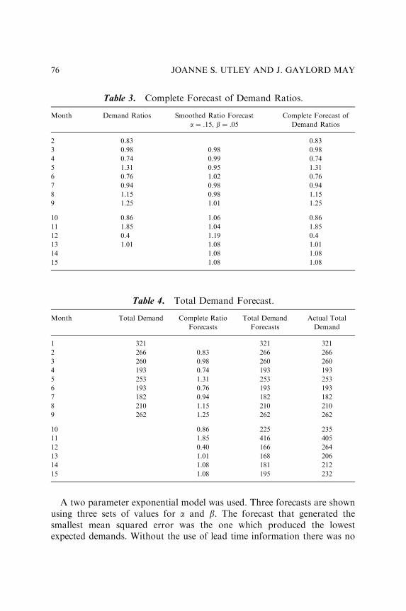
A two parameter exponential model was used. Three forecasts are shownusing three sets of values for a and b. The forecast that generated thesmallest mean squared error was the one which produced the lowestexpected demands. Without the use of lead time information there was no
Table 3. Complete Forecast of Demand Ratios.
Month Demand Ratios Smoothed Ratio Forecast
a ¼ .15, b ¼ .05
Complete Forecast of
Demand Ratios
2 0.83 0.83
3 0.98 0.98 0.98
4 0.74 0.99 0.74
5 1.31 0.95 1.31
6 0.76 1.02 0.76
7 0.94 0.98 0.94
8 1.15 0.98 1.15
9 1.25 1.01 1.25
10 0.86 1.06 0.86
11 1.85 1.04 1.85
12 0.4 1.19 0.4
13 1.01 1.08 1.01
14 1.08 1.08
15 1.08 1.08
Table 4. Total Demand Forecast.
Month Total Demand Complete Ratio
Forecasts
Total Demand
Forecasts
Actual Total
Demand
1 321 321 321
2 266 0.83 266 266
3 260 0.98 260 260
4 193 0.74 193 193
5 253 1.31 253 253
6 193 0.76 193 193
7 182 0.94 182 182
8 210 1.15 210 210
9 262 1.25 262 262
10 0.86 225 235
11 1.85 416 405
12 0.40 166 264
13 1.01 168 206
14 1.08 181 212
15 1.08 195 232
JOANNE S. UTLEY AND J. GAYLORD MAY76
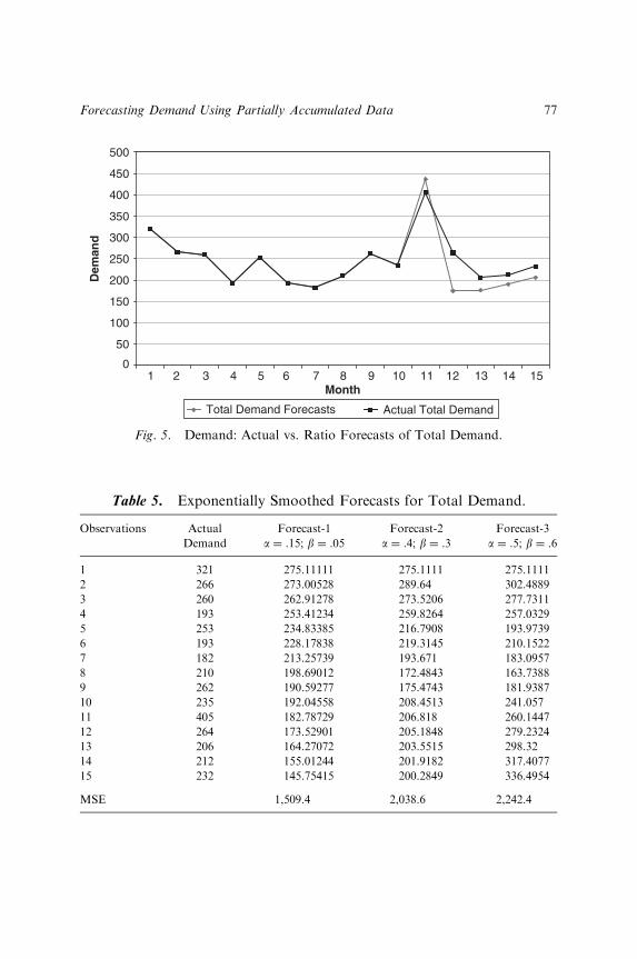
0
50
100
150
200
250
300
350
400
450
500
1 3 4 5 7 9 10 11 12 13 14 15Month
Dem
and
Total Demand Forecasts Actual Total Demand
862
Fig. 5. Demand: Actual vs. Ratio Forecasts of Total Demand.
Table 5. Exponentially Smoothed Forecasts for Total Demand.
Observations Actual Forecast-1 Forecast-2 Forecast-3
Demand a ¼ .15; b ¼ .05 a ¼ .4; b ¼ .3 a ¼ .5; b ¼ .6
1 321 275.11111 275.1111 275.1111
2 266 273.00528 289.64 302.4889
3 260 262.91278 273.5206 277.7311
4 193 253.41234 259.8264 257.0329
5 253 234.83385 216.7908 193.9739
6 193 228.17838 219.3145 210.1522
7 182 213.25739 193.671 183.0957
8 210 198.69012 172.4843 163.7388
9 262 190.59277 175.4743 181.9387
10 235 192.04558 208.4513 241.057
11 405 182.78729 206.818 260.1447
12 264 173.52901 205.1848 279.2324
13 206 164.27072 203.5515 298.32
14 212 155.01244 201.9182 317.4077
15 232 145.75415 200.2849 336.4954
MSE 1,509.4 2,038.6 2,242.4
Forecasting Demand Using Partially Accumulated Data 77
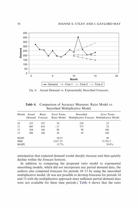
anticipation that expected demand would sharply increase and then quicklydecline within the forecast horizon.
In addition to comparing the proposed ratio model to exponentialsmoothing models, which did not incorporate any partial demand data, theauthors also computed forecasts for periods 10–13 by using the smoothedmultiplicative model. (It was not possible to develop forecasts for periods 14and 15 with the multiplicative approach since sufficient partial demand datawere not available for these time periods.) Table 6 shows that the ratio
0
50
100
150
200
250
300
350
400
450
0 5 10 15 20Month
Dem
and
Demand Fore-1 Fore-2 Fore-3
Fig. 6. Actual Demand vs. Exponentially Smoothed Forecasts.
Table 6. Comparison of Accuracy Measures: Ratio Model vs.Smoothed Multiplicative Model.
Month Actual
Demand
Ratio
Forecast
Error Terms
Ratio Model
Smoothed
Multiplicative Forecast
Error Terms
Multiplicative Model
10 235 225 10 210 25
11 405 416 �11 373 32
12 264 166 98 98 166
13 206 168 38 45 168
MAD 39.25 96
MSE 2,817.25 13,781.5
MAPE 15.7% 39.9%
JOANNE S. UTLEY AND J. GAYLORD MAY78
model outperformed the smoothed multiplicative model on all three accuracymeasures: the mean absolute deviation (MAD; 39.25 vs. 96, respectively),the mean squared error (MSE; 2817.25 vs. 13781.5, respectively), and themean absolute percent error (MAPE; 15.7% and 39.9%, respectively).
DISCUSSION
Results from this study indicated that despite the very limited partial orderdata available for the second half of the forecast horizon, the ratio methodoutperformed the exponential smoothing models, which utilized only totaldemand time series data. Results also established the superiority of the ratiomethod over the smoothed multiplicative approach in this research context.There are several reasons why the ratio method outperformed the otherapproaches in this research context. First, the use of total demand ratios incomputing the forecasts produced a smoothing effect on the data, therebyleading to greater forecast accuracy. Second, unlike the multiplicativeapproach, the ratio method made direct use of both the historical values andforecasted values of the total demand time series. Third, in contrast to theexponential smoothing models, the ratio model exploited the availability ofthe partially known order data.
The results presented in this chapter serve only to illustrate the proposedforecast model. Larger data sets and additional research contexts are neededto better study the effectiveness of the model. In addition, alternativeforecast methodologies that are more complex than the smoothed multi-plicative model or the exponentially smoothed model could be used forcomparison purposes.
This study developed a forecast model for only one product made by themanufacturer. Also, the customer-specified lead times were specified inmonths. However, the results obtained suggest that the model could beapplied to other products and services and that the customer-designatedlead times period could be much shorter – perhaps weeks or even days.
REFERENCES
Bestwick, P. (1975). A forecast monitoring and revision system for top management.
Operational Research Quarterly, 26, 419–429.
Bodily, S., & Freeland, J. (1988). A simulation of techniques for forecasting shipments using
firm order-to-date. Journal of the Operational Research Society, 39(9), 833–846.
Forecasting Demand Using Partially Accumulated Data 79

Green, M., & Harrison, P. (1973). Fashion forecasting for a mail order company using a
Bayesian approach. Operational Research Quarterly, 24, 193–205.
Guerrero, V., & Elizondo, J. (1997). Forecasting a cumulative variable using its partially
accumulated data. Management Science, 43(6), 879–889.
Kekre, S., Morton, T., & Smunt, T. (1990). Forecasting using partially known demands.
International Journal of Forecasting, 6, 115–125.
Murray, G., & Silver, E. (1966). A Bayesian analysis of the style goods problem. Management
Science, 12(11), 785–797.
Waage, F. (2006). Extracting forecasts from advance orders. Advances in Business and
Management Forecasting, 4, 13–26.
JOANNE S. UTLEY AND J. GAYLORD MAY80
FORECASTING NEW ADOPTIONS:
A COMPARATIVE EVALUATION
OF THREE TECHNIQUES OF
PARAMETER ESTIMATION
Kenneth D. Lawrence, Dinesh R. Pai and
Sheila M. Lawrence
ABSTRACT
Forecasting sales for an innovation before the product’s introduction is anecessary but difficult task. Forecasting is a crucial analytic tool whenassessing the business case for internal or external investments in newtechnologies. For early stage investments or internal business cases fornew products, it is essential to have some understanding of the likelydiffusion of the technology. Diffusion of innovation models are importanttools for effectively assessing the merits of investing in technologies thatare new or novel and do not have prima facie, predictable patterns of useruptake. Most new product forecasting models require the estimation ofparameters for use in the models. In this chapter, we evaluate threetechniques to determine the parameters of the Bass diffusion model byusing an example of a new movie.
Advances in Business and Management Forecasting, Volume 6, 81–91
Copyright r 2009 by Emerald Group Publishing Limited
All rights of reproduction in any form reserved
ISSN: 1477-4070/doi:10.1108/S1477-4070(2009)0000006006
81
INTRODUCTION
Forecasting new adoptions after a product introduction is an importantmarketing problem. The Bass model for forecasting is most appropriate forforecasting sales of an innovation (more generally, a new product) where noclosely competing alternatives exist in the marketplace. Managers needsuch forecasts for new technologies or major product innovations beforeinvesting significant resources in them.
The Bass model offers a good starting point for forecasting the long-termsales pattern of new technologies and new durable products under two typesof conditions (Lawrence & Geurts, 1984; Lilien & Rangaswamy, 2006).
(1) The firm has recently introduced the product or technology and hasobserved its sales for a few time periods; or
(2) The firm has not yet introduced the product or technology, but it issimilar in some way to existing products or technologies whose saleshistory is known.
In this chapter, we introduce a forecasting model developed by FrankBass that has proven to be particularly effective in forecasting the adoptionof innovative and new technologies in the market place. We then use threetechniques: nonlinear programming (NLP), linear regression (LR), andminimizing the sum of deviations to estimate the parameters of the Bassmodel and compare their performance using dataset of a new movie (Bass,1969; Bass, 1993).
LITERATURE REVIEW
Rogers (1962) discussed the theory of adoption and diffusion of newproducts at length. The innovation adoption curve of Rogers classifiesadopters of innovations into various categories, based on the idea thatcertain individuals are inevitably more open to adaptation than others. Thevarious categories of adopters specified in the literature are (1) innovators,(2) early adopters, (3) early majority, (4) late majority, and (5) laggards(Fig. 1). The theory suggests that innovators are individuals who adopt newproducts independently of the decisions of other individuals in a socialsystem. The literature aggregates groups (2) through (5) aforementioned anddefines them as imitators (Bass, 1969). Imitators are adopters who areinfluenced in the timing of adoption by various external factors.
KENNETH D. LAWRENCE ET AL.82
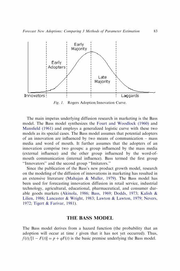
The main impetus underlying diffusion research in marketing is the Bassmodel. The Bass model synthesizes the Fourt and Woodlock (1960) andMansfield (1961) and employs a generalized logistic curve with these twomodels as its special cases. The Bass model assumes that potential adoptersof an innovation are influenced by two means of communication – massmedia and word of mouth. It further assumes that the adopters of aninnovation comprise two groups: a group influenced by the mass media(external influence) and the other group influenced by the word-of-mouth communication (internal influence). Bass termed the first group‘‘Innovators’’ and the second group ‘‘Imitators.’’
Since the publication of the Bass’s new product growth model, researchon the modeling of the diffusion of innovations in marketing has resulted inan extensive literature (Mahajan & Muller, 1979). The Bass model hasbeen used for forecasting innovation diffusion in retail service, industrialtechnology, agricultural, educational, pharmaceutical, and consumer dur-able goods markets (Akinola, 1986; Bass, 1969; Dodds, 1973; Kalish &Lilien, 1986; Lancaster & Wright, 1983; Lawton & Lawton, 1979; Nevers,1972; Tigert & Farivar, 1981).
THE BASS MODEL
The Bass model derives from a hazard function (the probability that anadoption will occur at time t given that it has not yet occurred). Thus,f ðtÞ= 1� FðtÞ½ � ¼ pþ qFðtÞ is the basic premise underlying the Bass model.
Fig. 1. Rogers Adoption/Innovation Curve.
Forecast New Adoptions: Comparing 3 Methods of Parameter Estimation 83
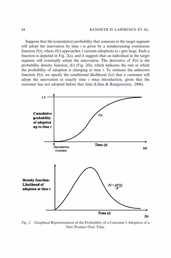
Suppose that the (cumulative) probability that someone in the target segmentwill adopt the innovation by time t is given by a nondecreasing continuousfunction F(t), where F(t) approaches 1 (certain adoption) as t gets large. Such afunction is depicted in Fig. 2(a), and it suggests that an individual in the targetsegment will eventually adopt the innovation. The derivative of F(t) is theprobability density function, f(t) (Fig. 2(b), which indicates the rate at whichthe probability of adoption is changing at time t. To estimate the unknownfunction F(t), we specify the conditional likelihood L(t) that a customer willadopt the innovation at exactly time t since introduction, given that thecustomer has not adopted before that time (Lilien & Rangaswamy, 2006).
Fig. 2. Graphical Representation of the Probability of a Customer’s Adoption of a
New Product Over Time.
KENNETH D. LAWRENCE ET AL.84
The conditional likelihood that a customer will adopt the innovationexactly at time t since introduction, given that the customer has not adoptedbefore that time is (Lawrence & Lawton, 1981)
LðtÞ ¼f ðtÞ
1� FðtÞ(1)
where F(t) is a nondecreasing function, probability that someone in thetarget segment will adopt the innovation by time t; and f(t) the rate at whichthe probability of adoption is changing at time t.
Bass (1969) proposed that L(t) be defined to be equal to
LðtÞ ¼ pþq
mCðtÞ (2)
where C(t) is the number of customers (or a multiple of that number, such assales) who have already adopted the innovation by time t.
Following are the three parameters of the model that must be estimated:
m – A parameter representing the total number of customers in the adoptingtarget segment, all of whom will eventually adopt the product. A companyintroducing a new product is obviously interested in the value of thisparameter.q – Coefficient of imitation (or coefficient of internal influence). Thisparameter measures the likelihood of adoption due to a potential adopterbeing influenced by someone who has already adopted the product.It measures the ‘‘word-of-mouth’’ effect influencing purchases.p – Coefficient of innovation (or coefficient of external influence). Thisparameter measures the likelihood of adoption, assuming no influencefrom someone who has already purchased (adopted) the product. It is thelikelihood of someone adopting the product due to her or his own interestin the innovation.
Let Ct�1 be the number of people (or a multiple of that number, such assales) who have adopted the product through time t�1. Therefore, m�Ct�1
is the number of potential adopters remaining at time t�1. We refer to timeinterval between time t�1 and time t as time period t.
The likelihood of adoption due to imitation is
qCt�1
m
� �
where Ct�1/m is the fraction of the number of people estimated to adopt theproduct by time t�1.
Forecast New Adoptions: Comparing 3 Methods of Parameter Estimation 85
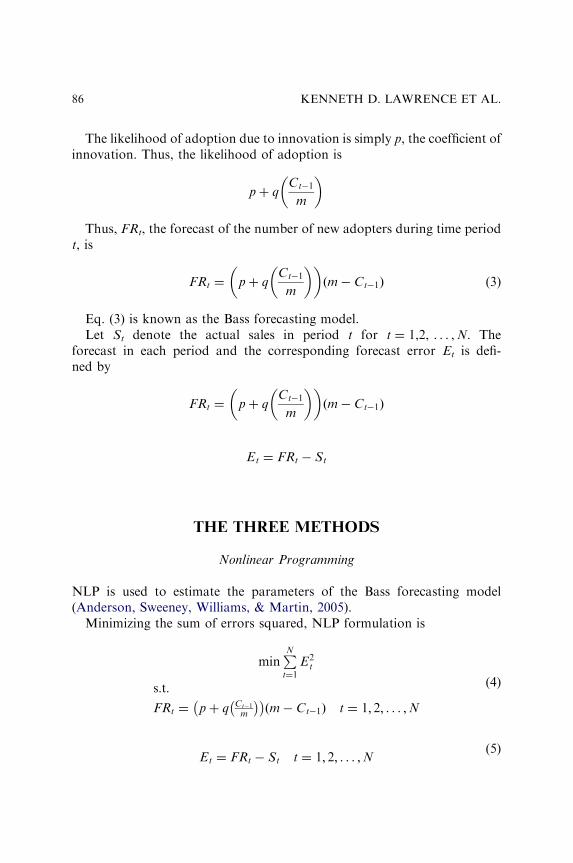
The likelihood of adoption due to innovation is simply p, the coefficient ofinnovation. Thus, the likelihood of adoption is
pþ qCt�1
m
� �
Thus, FRt, the forecast of the number of new adopters during time periodt, is
FRt ¼ pþ qCt�1
m
� �� �ðm� Ct�1Þ (3)
Eq. (3) is known as the Bass forecasting model.Let St denote the actual sales in period t for t ¼ 1,2, . . . ,N. The
forecast in each period and the corresponding forecast error Et is defi-ned by
FRt ¼ pþ qCt�1
m
� �� �ðm� Ct�1Þ
Et ¼ FRt � St
THE THREE METHODS
Nonlinear Programming
NLP is used to estimate the parameters of the Bass forecasting model(Anderson, Sweeney, Williams, & Martin, 2005).
Minimizing the sum of errors squared, NLP formulation is
minPNt¼1
E2t
s:t:
FRt ¼ pþ q Ct�1
m
� �� �ðm� Ct�1Þ t ¼ 1; 2; . . . ;N
(4)
Et ¼ FRt � St t ¼ 1; 2; . . . ;N(5)
KENNETH D. LAWRENCE ET AL.86
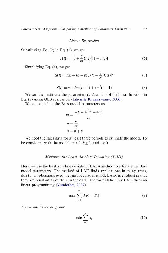
Linear Regression
Substituting Eq. (2) in Eq. (1), we get
f ðtÞ ¼ pþq
mCðtÞ
h i1� FðtÞ½ � (6)
Simplifying Eq. (6), we get
SðtÞ ¼ pmþ ðq� pÞCðtÞ �q
NCðtÞ½ �
2 (7)
SðtÞ ¼ aþ bmðt� 1Þ þ cm2ðt� 1Þ (8)
We can then estimate the parameters (a, b, and c) of the linear function inEq. (8) using OLS regression (Lilien & Rangaswamy, 2006).
We can calculate the Bass model parameters as
m ¼�b�
ffiffiffiffiffiffiffiffiffiffiffiffiffiffiffiffiffiffib2 � 4ac
p2c
p ¼a
m
q ¼ pþ b
We need the sales data for at least three periods to estimate the model. Tobe consistent with the model, mW0, bZ0, and co0
Minimize the Least Absolute Deviation (LAD)
Here, we use the least absolute deviation (LAD) method to estimate the Bassmodel parameters. The method of LAD finds applications in many areas,due to its robustness over the least squares method. LADs are robust in thatthey are resistant to outliers in the data. The formulation for LAD throughlinear programming (Vanderbei, 2007)
minXNt¼1
jFRt � Stj (9)
Equivalent linear program:
minXNt¼1
dt (10)
Forecast New Adoptions: Comparing 3 Methods of Parameter Estimation 87
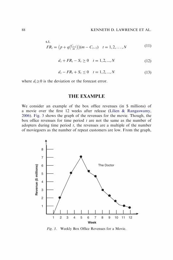
s:t:
FRt ¼ pþ q Ct�1
m
� �� �ðm� Ct�1Þ t ¼ 1; 2; . . . ;N (11)
dt þ FRt � St � 0 t ¼ 1; 2; :::;N (12)
dt � FRt þ St � 0 t ¼ 1; 2; :::;N (13)
where dtZ0 is the deviation or the forecast error.
THE EXAMPLE
We consider an example of the box office revenues (in $ millions) ofa movie over the first 12 weeks after release (Lilien & Rangaswamy,2006). Fig. 3 shows the graph of the revenues for the movie. Though, thebox office revenues for time period t are not the same as the number ofadopters during time period t, the revenues are a multiple of the numberof moviegoers as the number of repeat customers are low. From the graph,
8
7
The Doctor6
5
4
3
2
1
1 4 6 9 10 11 12
Rev
enu
e ($
mill
ion
s)
Week
87532
Fig. 3. Weekly Box Office Revenues for a Movie.
KENNETH D. LAWRENCE ET AL.88
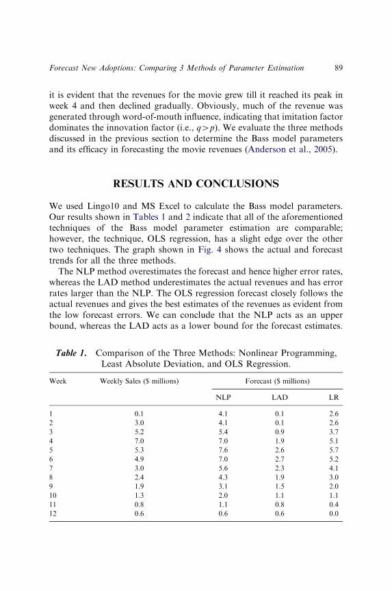
it is evident that the revenues for the movie grew till it reached its peak inweek 4 and then declined gradually. Obviously, much of the revenue wasgenerated through word-of-mouth influence, indicating that imitation factordominates the innovation factor (i.e., qWp). We evaluate the three methodsdiscussed in the previous section to determine the Bass model parametersand its efficacy in forecasting the movie revenues (Anderson et al., 2005).
RESULTS AND CONCLUSIONS
We used Lingo10 and MS Excel to calculate the Bass model parameters.Our results shown in Tables 1 and 2 indicate that all of the aforementionedtechniques of the Bass model parameter estimation are comparable;however, the technique, OLS regression, has a slight edge over the othertwo techniques. The graph shown in Fig. 4 shows the actual and forecasttrends for all the three methods.
The NLP method overestimates the forecast and hence higher error rates,whereas the LAD method underestimates the actual revenues and has errorrates larger than the NLP. The OLS regression forecast closely follows theactual revenues and gives the best estimates of the revenues as evident fromthe low forecast errors. We can conclude that the NLP acts as an upperbound, whereas the LAD acts as a lower bound for the forecast estimates.
Table 1. Comparison of the Three Methods: Nonlinear Programming,Least Absolute Deviation, and OLS Regression.
Week Weekly Sales ($ millions) Forecast ($ millions)
NLP LAD LR
1 0.1 4.1 0.1 2.6
2 3.0 4.1 0.1 2.6
3 5.2 5.4 0.9 3.7
4 7.0 7.0 1.9 5.1
5 5.3 7.6 2.6 5.7
6 4.9 7.0 2.7 5.2
7 3.0 5.6 2.3 4.1
8 2.4 4.3 1.9 3.0
9 1.9 3.1 1.5 2.0
10 1.3 2.0 1.1 1.1
11 0.8 1.1 0.8 0.4
12 0.6 0.6 0.6 0.0
Forecast New Adoptions: Comparing 3 Methods of Parameter Estimation 89
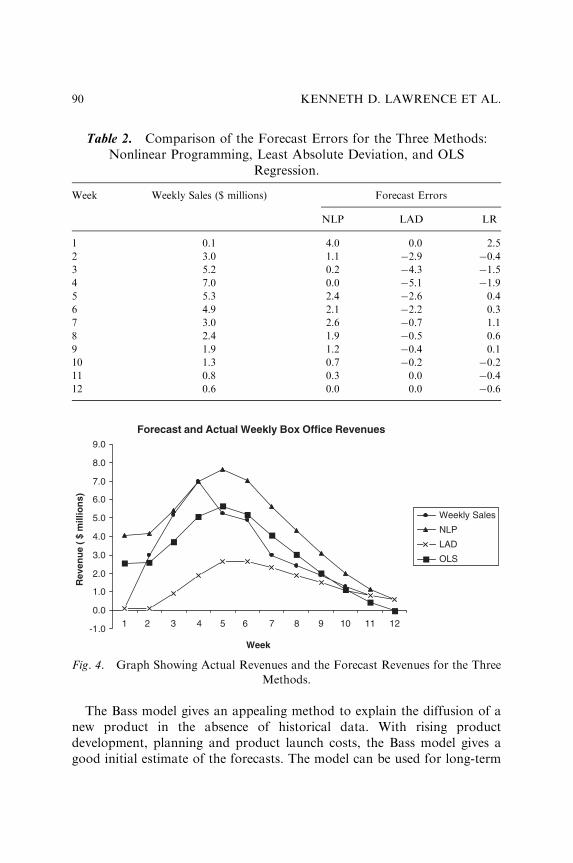
The Bass model gives an appealing method to explain the diffusion of anew product in the absence of historical data. With rising productdevelopment, planning and product launch costs, the Bass model gives agood initial estimate of the forecasts. The model can be used for long-term
Table 2. Comparison of the Forecast Errors for the Three Methods:Nonlinear Programming, Least Absolute Deviation, and OLS
Regression.
Week Weekly Sales ($ millions) Forecast Errors
NLP LAD LR
1 0.1 4.0 0.0 2.5
2 3.0 1.1 �2.9 �0.4
3 5.2 0.2 �4.3 �1.5
4 7.0 0.0 �5.1 �1.9
5 5.3 2.4 �2.6 0.4
6 4.9 2.1 �2.2 0.3
7 3.0 2.6 �0.7 1.1
8 2.4 1.9 �0.5 0.6
9 1.9 1.2 �0.4 0.1
10 1.3 0.7 �0.2 �0.2
11 0.8 0.3 0.0 �0.4
12 0.6 0.0 0.0 �0.6
Forecast and Actual Weekly Box Office Revenues
-1.0
0.0
1.0
2.0
3.0
4.0
5.0
6.0
7.0
8.0
9.0
1 2 3 4 5 7 9 10 11 12
Week
Rev
enu
e (
$ m
illio
ns)
Weekly Sales
NLP
LAD
OLS
86
Fig. 4. Graph Showing Actual Revenues and the Forecast Revenues for the Three
Methods.
KENNETH D. LAWRENCE ET AL.90
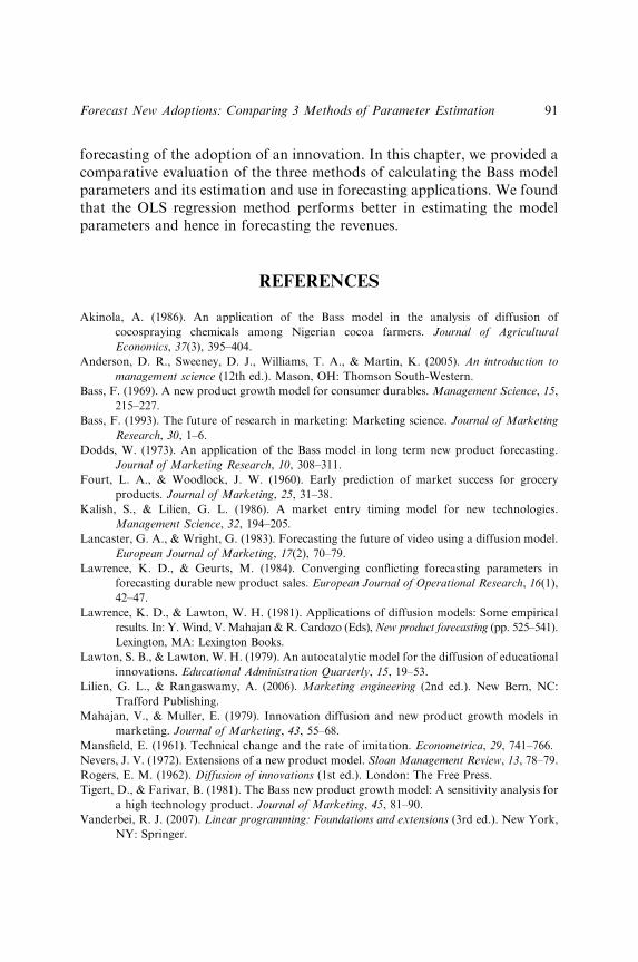
forecasting of the adoption of an innovation. In this chapter, we provided acomparative evaluation of the three methods of calculating the Bass modelparameters and its estimation and use in forecasting applications. We foundthat the OLS regression method performs better in estimating the modelparameters and hence in forecasting the revenues.
REFERENCES
Akinola, A. (1986). An application of the Bass model in the analysis of diffusion of
cocospraying chemicals among Nigerian cocoa farmers. Journal of Agricultural
Economics, 37(3), 395–404.
Anderson, D. R., Sweeney, D. J., Williams, T. A., & Martin, K. (2005). An introduction to
management science (12th ed.). Mason, OH: Thomson South-Western.
Bass, F. (1969). A new product growth model for consumer durables. Management Science, 15,
215–227.
Bass, F. (1993). The future of research in marketing: Marketing science. Journal of Marketing
Research, 30, 1–6.
Dodds, W. (1973). An application of the Bass model in long term new product forecasting.
Journal of Marketing Research, 10, 308–311.
Fourt, L. A., & Woodlock, J. W. (1960). Early prediction of market success for grocery
products. Journal of Marketing, 25, 31–38.
Kalish, S., & Lilien, G. L. (1986). A market entry timing model for new technologies.
Management Science, 32, 194–205.
Lancaster, G. A., & Wright, G. (1983). Forecasting the future of video using a diffusion model.
European Journal of Marketing, 17(2), 70–79.
Lawrence, K. D., & Geurts, M. (1984). Converging conflicting forecasting parameters in
forecasting durable new product sales. European Journal of Operational Research, 16(1),
42–47.
Lawrence, K. D., & Lawton, W. H. (1981). Applications of diffusion models: Some empirical
results. In: Y.Wind, V.Mahajan & R. Cardozo (Eds),New product forecasting (pp. 525–541).
Lexington, MA: Lexington Books.
Lawton, S. B., & Lawton, W. H. (1979). An autocatalytic model for the diffusion of educational
innovations. Educational Administration Quarterly, 15, 19–53.
Lilien, G. L., & Rangaswamy, A. (2006). Marketing engineering (2nd ed.). New Bern, NC:
Trafford Publishing.
Mahajan, V., & Muller, E. (1979). Innovation diffusion and new product growth models in
marketing. Journal of Marketing, 43, 55–68.
Mansfield, E. (1961). Technical change and the rate of imitation. Econometrica, 29, 741–766.
Nevers, J. V. (1972). Extensions of a new product model. Sloan Management Review, 13, 78–79.
Rogers, E. M. (1962). Diffusion of innovations (1st ed.). London: The Free Press.
Tigert, D., & Farivar, B. (1981). The Bass new product growth model: A sensitivity analysis for
a high technology product. Journal of Marketing, 45, 81–90.
Vanderbei, R. J. (2007). Linear programming: Foundations and extensions (3rd ed.). New York,
NY: Springer.
Forecast New Adoptions: Comparing 3 Methods of Parameter Estimation 91

This page intentionally left blank

THE USE OF A FLEXIBLE
DIFFUSION MODEL FOR
FORECASTING NATIONAL-LEVEL
MOBILE TELEPHONE AND
INTERNET DIFFUSION
Kallol Bagchi, Peeter Kirs and Zaiyong Tang
INTRODUCTION
Much attention has been given to adoption and diffusion, defined as thedegree of market penetration, of Information and CommunicationsTechnologies (ICT) in recent years (Carter, Jambulingam, Gupta, & Melone,2001; Kiiski & Pohjola, 2002; Milner, 2003; Benhabib & Spiegel, 2005). Thetheory of diffusion of innovations considers how a new idea spreadsthroughout the market over time. The ability to accurately predict newproduct diffusion is of concern to designers, marketers, managers, andresearchers alike. However, although the diffusion process of new productsis generally accepted as following an s-curve pattern, where diffusion startsslowly, grows exponentially, peaks, and then declines (as shown in Fig. 1),there is considerable disagreement about what factors affect diffusion andhow to measure diffusion rates (Bagchi, Kirs, & Lopez, 2008).
Advances in Business and Management Forecasting, Volume 6, 93–107
Copyright r 2009 by Emerald Group Publishing Limited
All rights of reproduction in any form reserved
ISSN: 1477-4070/doi:10.1108/S1477-4070(2009)0000006007
93

Diffusion of technology products varies considerably across nations. Forexample, mobile phone growth has been spectacular in nations in generalbut particularly in nations such as India and China where usage increasedfrom 3.53 and 65.82 per 1,000 in 2000 to 214.77 and 414.62 per 1,000 in2007, respectively. Worldwide, the pattern of diffusion varies greatly.Mobile phone penetration for selected nations, or groups of nations, is givenin Fig. 2; Internet penetration is given in Fig. 3. As the figures show, thelevel of diffusion, as well as the rate of diffusion (the speed at whichpenetration occurs), can greatly vary between regions.
Forecasting models are aimed at predicting future observations with ahigh degree of accuracy (Shmueli & Koppius, 2008). Diffusion models areused to forecast new product adoptions (Mahajan, Muller, & Bass, 1995)and the emphasis is on predicting the ultimate level of penetration(saturation) and the rate of approach to saturation. Diffusion models canalso be considered a type of explanatory model, and have been used toclarify differences in national technology adoptions, based on estimatedparameter values. Diffusion models thus not only yield good forecastingestimates; they generate parameter values, which can be used to explaindifference in diffusion patterns.
Diffusion modeling studies try to explain and analyze patterns ofinnovation diffusion, usually over time and across a population of potentialadopters, and forecast diffusion levels and rates. The emphasis is onpredicting the ultimate level of penetration and the rate of approach tosaturation. Observations of diffusion or percentages of diffusion are
Fig. 1. New Product Diffusion.
KALLOL BAGCHI ET AL.94
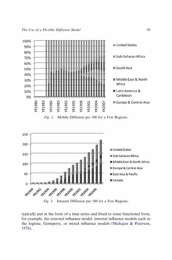
typically put in the form of a time series and fitted to some functional form,for example, the external influence model, internal influence models such asthe logistic, Gompertz, or mixed influence models (Mahajan & Peterson,1978).
Fig. 3. Internet Diffusion per 100 for a Few Regions.
Fig. 2. Mobile Diffusion per 100 for a Few Regions.
The Use of a Flexible Diffusion Model 95

Diffusion models with time varying parameters, such as the Von Bertalanffy(BERT) model (Bertalanffy, 1957) are called flexible models, and havepreviously been used to examine the diffusion process of an innovation (Hu,Saunders, & Gebelt, 1997). Incorporating time-variation in the parameters(b and y, to be discussed later) of a diffusion model usually yields better esti-mates than time invariant models (Easingwood, 1989; Radas, 2005). By incor-porating prior estimates of unknown parameters and updating initial estimatesas new data become available, time-varying estimation procedures often canprovide better early forecasts (Xie, Song, Sirbu, & Qiong Wang, 1997).
The role of ICT in economic development of a nation has been studiedpreviously, in both developed and developing nations (Wong, 2002; SridharKala, & Sridhar, 2003). It is generally agreed that investment in ICTpositively influences the economic growth of a nation by reducing trans-action costs and increasing output for firms in various sectors of theeconomy, which in turn promotes more investments in ICT (Roller &Waverman, 2001). In the present study, the diffusion of two technologies,mobile and the Internet, are investigated across different nations. These twotechnologies could be crucial for a country’s economic growth and are atdifferent stages in the product development life cycle. The Internet hasbecome a new standard outlet for doing business in developed nations. Inmany developed nations, mobile phone growth has already exceeded 1 peruser (The World Bank database, 2008). Expanding mobile networks bringsin more customers, better foreign investments, and increase revenues for thegovernment. According to a McKinsey & Company study, raising wirelesspenetration by 10% points can lead to an increase in gross domestic product(GDP) of about 0.5%, or around $12 billion for an economy the size ofChina (Dalka, 2007). Accurate forecasts of these technologies are, therefore,important to managers and government policy makers. Inaccurate forecastsin mobile handset as well as network equipment market can cost millions ofdollars in losses (Wenrong, Xie, & Tsui, 2006).
It is the aim of this study to attempt to answer the following questions:
How well does a flexible diffusion model such as BERT forecast thediffusion of two ICTs, the Internet and mobile, in different nations? Inparticular, how do these forecasts compare with traditional andnontraditional forecasting schemes? What parameter values for b and y of the BERT model can be obtainedfor mobile phone and Internet diffusion in various nations? Are thesevalues different for developing and developed nations for both of theproducts? For the two ICT products?
KALLOL BAGCHI ET AL.96

What kind of analysis/interpretation we can make from these forecasts,which otherwise would be difficult to do with traditional forecastingmodels? For example, can the results be used to see whether decisions canbe made to introduce a new IT product in different nations?
NATIONAL DIFFUSION OF ICT
It is generally accepted that national ICT diffusions can, in large part, beexplained by country-specific factors such as demographic, economic, regu-latory, infrastructural, educational, and affordability factors (Bagchi et al.,2008). In the same study, the authors also found that the impact of pricedecreases was positive and significant in all regions and for both telephoneand mobile phone diffusion. Dedrick, Goodman, and Kraemer (1995) alsoused nation-specific analysis to investigate the factors responsible for thedifferences in ICT diffusion among nine culturally and geographicallydiverse small, developed nations. They concluded that the level of economicdevelopment, basic education system, infrastructure, investment in ICT, andgovernment policies were reasons for different ICT diffusions among thecountries. Watson and Myers (2001) used the Ein-Dor, Myers, and Raman(1997) approach to investigate the ICT industry and ICT diffusion inFinland and New Zealand using 1998 data. They concluded that althoughthe two countries were similar in many ways, Finland’s ICT diffusion out-paced New Zealand’s due to government promotion of ICT, research anddevelopment in private sector, and an ICT-based education system.
In a previous paper (Bagchi, Kirs, & Udo, 2006), the authors contrastedmobile phone, PC, and Internet diffusion levels and rates between developedand developing nations and found a number of differences in factorsresponsible for such diffusions between the two groups. For developednations the most significant factors influencing ICT diffusion rates werehuman development, urbanization, and institutional factors. Humandevelopment, as conceived by the United Nations Development Programme(UNDP, 1990), is a composite index of normalized measures of life expec-tancy, literacy, educational attainment, and GDP per capita for countriesworldwide. Institutional factors, or the Economic Freedom of the World(EFW) index, is a composite index containing 38 components designed tomeasure the degree to which a nation’s institutions and policies are consi-stent with voluntary exchange, protection of property rights, open markets,and minimal regulation of economic activity (Gwartney & Lawson, 2003;
The Use of a Flexible Diffusion Model 97
Walker, 1988). In contrast, for developing countries, the significant factorsinfluencing ICT diffusion rates included ICT infrastructure, humandevelopment, and income disparity.
Although it can be anticipated that developed countries can initially besttake advantage of innovative technologies due to purchasing power, theassumption that established technology diffusion rate in developed countriesis always faster than in lesser developed countries may be misplaced, at leastin a later stage of diffusion. Gruber and Verboven (1998) showed that lateradopting countries have faster diffusion rates in some stages, in accordancewith diffusion theory, implying that developing countries can takeadvantage of a ‘‘leap-frog’’ affect (Davison, Vogel, Harris, & Jones, 2000)by applying an ‘‘investment-based growth strategy’’ (Acemoglu, Aghion, &Zilibotti, 2002). As national scenarios for technology diffusion widely vary,diffusion models such as flexible ones that assume asymmetric diffusionpatterns could be more appropriate for modeling technological diffusions indifferent nations. The parameters of the diffusion model can be expected tohave significantly different values for developing and developed nationdiffusion scenarios.
DIFFUSION MEASUREMENT
Although there are a number of diffusion model estimation procedures,Mahajan, Muller, and Bass (1990) offer two basic model classes: Time-Invariant Estimation Procedures (TIEP) and Time-Varying EstimationProcedures (TVEP). In TIEP, the output does not depend explicitly ontime and includes conventional estimation methods such as ordinary leastsquare (OLS) (Bass, 1969), maximum likelihood estimation (MLE)(Schmittlein & Mahajan, 1982), and nonlinear least squares (NLS)(Srinivasan & Mason, 1986). However, according to Xie et al. (1997), thereare two common limitations inherent in TIEP. First, to obtain stable androbust parameter estimates, TIEP often require data to include the peaksales (Mahajan et al., 1990). TIEP are also not helpful in forecasting a newproduct diffusion since they require observable data to be collected overtime; by the time sufficient data have been collected, it may be too late foradequate forecasting or planning. Second, TIEP can be applied only to adiscrete form of a diffusion model or to a solution to a diffusion model.These discrete forms can often result in biased and high variance estimates.
TVEP have been introduced to overcome some of these limitations ofTIEP (Mahajan et al., 1990). TVEPs start with a prior estimate of unknown
KALLOL BAGCHI ET AL.98
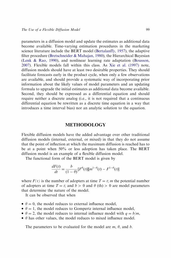
parameters in a diffusion model and update the estimates as additional databecome available. Time-varying estimation procedures in the marketingscience literature include the BERT model (Bertalanffy, 1957), the adaptivefilter procedure (Bretschneider & Mahajan, 1980), the Hierarchical Bayesian(Lenk & Rao, 1990), and nonlinear learning rate adaptation (Bousson,2007). Flexible models fall within this class. As Xie et al. (1997) note,diffusion models should have at least two desirable properties. They shouldfacilitate forecasts early in the product cycle, when only a few observationsare available, and should provide a systematic way of incorporating priorinformation about the likely values of model parameters and an updatingformula to upgrade the initial estimates as additional data become available.Second, they should be expressed as a differential equation and shouldrequire neither a discrete analog (i.e., it is not required that a continuousdifferential equation be rewritten as a discrete time equation in a way thatintroduces a time interval bias) nor an analytic solution to the equation.
METHODOLOGY
Flexible diffusion models have the added advantage over other traditionaldiffusion models (internal, external, or mixed) in that they do not assumethat the point of inflection at which the maximum diffusion is reached has tobe at a point when 50% or less adoption has taken place. The BERTdiffusion model is an example of a flexible diffusion model.
The functional form of the BERT model is given by
dFðtÞ
dt¼
b
ð1� yÞ½FyðtÞ�½m1�yðtÞ � F1�yðtÞ�
where F(t) is the number of adopters at time T ¼ t; m the potential numberof adopters at time T ¼ t; and bW 0 and y (th)W 0 are model parametersthat determine the nature of the model.
It can be observed that when
y ¼ 0, the model reduces to external influence model, y ¼ 1, the model reduces to Gompertz internal influence model, y ¼ 2, the model reduces to internal influence model with q ¼ b/m, y has other values, the model reduces to mixed influence model.
The parameters to be evaluated for the model are m, y, and b.
The Use of a Flexible Diffusion Model 99

TEST SCHEMES
The methodology consisted of running nonlinearly the flexible model inExcel Solver and running standard forecasting techniques such asexponential smoothing (ES) and moving averages (MA) using SPSS(Kendrick, Mercado, & Amman, 2006). The parameter values of the BERTdiffusion model were obtained for developing and developed nations afterrunning the Excel Solver, and suitable statistical tests were conducted forsignificant differences in values across the set of nations.
For forecasting purposes, separate year data (2007) were used. For in-sample and out-of-sample forecast comparisons, six regions and twotechnologies were selected. The selection was based on sum of squares oferrors (SSE) values of the BERT model fits and two regions each wereselected for best, worst, and middle-level values of SSEs for each technology.Two standard forecasting procedures, ES and MA were selected. The ESprocedure computes forecasts for time series data using exponentiallyweighted averages. The number of periods in the MA procedure was selectedto remove seasonal effect. To keep calculations manageable, for ES, a middlevalue of smoothing constant/damping factor (0.30) was selected; in practice,the values of a smoothing constant typically range from 0.05 to 0.60(Statistix for Windows, 1996). For MA, the number of periods selectedwas 3. The data from 2007 was used for out-of-sample forecasting andsquared difference was computed (DiffSE07). For in-sample forecasting, thesum of squares of all forecast differences from different years was computed(DiffSE90-06) for comparison among various forecasting methods.
DATA
All data was obtained from The World Bank database (2008). The dataconsists of time series data of yearly Internet and the mobile diffusions per 100residents from 24 groups of nations/regions/nations. All the definitions ofgroups can be found in The World Bank database (2008). The groups areof two types – region- and economy-based. Although, there is some overlapof nations in various groups, the groups are by themselves representative ofdeveloping and developed sets of nations. Large nations such as India andChina, as well as developed nations such as the U.S, the U.K., and Australia,were also included to maintain representation of the entire world, and becausethese two technologies have been extensively adopted in these nations. Internetdata were from 1990 to 2006 and the mobile data were from 1987 to 2006.
KALLOL BAGCHI ET AL.100
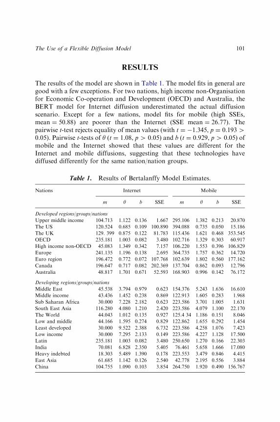
RESULTS
The results of the model are shown in Table 1. The model fits in general aregood with a few exceptions. For two nations, high income non-Organisationfor Economic Co-operation and Development (OECD) and Australia, theBERT model for Internet diffusion underestimated the actual diffusionscenario. Except for a few nations, model fits for mobile (high SSEs,mean ¼ 50.88) are poorer than the Internet (SSE mean ¼ 26.77). Thepairwise t-test rejects equality of mean values (with t ¼ �1.345, p ¼ 0.193W0.05). Pairwise t-tests of y (t ¼ 1.08, pW 0.05) and b (t ¼ 0.929, p W 0.05) ofmobile and the Internet showed that these values are different for theInternet and mobile diffusions, suggesting that these technologies havediffused differently for the same nation/nation groups.
Table 1. Results of Bertalanffy Model Estimates.
Nations Internet Mobile
m y b SSE m y b SSE
Developed regions/groups/nations
Upper middle income 104.713 1.122 0.136 1.667 295.106 1.382 0.213 20.870
The US 120.524 0.685 0.109 100.890 394.088 0.735 0.050 15.186
The UK 129. 399 0.875 0.122 81.783 115.436 1.621 0.468 353.545
OECD 235.181 1.003 0.082 3.480 102.716 1.329 0.303 60.917
High income non-OECD 45.083 1.349 0.342 7.157 106.220 1.553 0.396 106.829
Europe 241.135 1.196 0.138 2.695 364.735 1.757 0.362 14.720
Euro region 196.472 0.772 0.072 107.768 102.639 1.802 0.560 177.162
Canada 196.647 0.717 0.082 202.369 137.704 0.862 0.093 12.796
Australia 48.817 1.701 0.671 52.593 168.903 0.996 0.142 76.172
Developing regions/groups/nations
Middle East 45.538 3.794 0.979 0.623 154.376 5.243 1.636 16.610
Middle income 43.436 1.452 0.238 0.869 122.913 1.605 0.283 1.968
Sub Saharan Africa 30.000 7.228 2.182 0.623 223.586 3.701 1.005 1.631
South East Asia 116.280 4.080 1.210 2.420 223.586 4.079 1.100 22.170
The World 44.043 1.012 0.135 0.927 125.4 34 1.186 0.151 8.046
Low and middle 44.166 1.595 0.274 0.829 122.862 1.655 0.292 1.454
Least developed 30.000 9.522 2.388 6.732 223.586 4.258 1.076 7.423
Low income 30.000 7.295 2.133 0.149 223.586 4.227 1.128 17.500
Latin 235.181 1.003 0.082 3.480 250.650 1.270 0.166 22.303
India 70.081 6.828 2.350 5.405 76.461 5.658 1.666 17.080
Heavy indebted 18.303 5.489 1.390 0.178 223.553 3.479 0.846 4.415
East Asia 61.685 1.142 0.126 2.540 42.778 2.195 0.556 3.884
China 104.755 1.090 0.103 3.854 264.750 1.920 0.490 156.767
The Use of a Flexible Diffusion Model 101
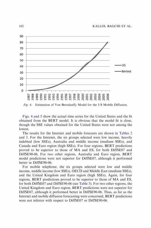
Figs. 4 and 5 show the actual time series for the United States and the fitobtained from the BERT model. It is obvious that the model fit is close,though the SSE values obtained for the United States were not among thelowest.
The results for the Internet and mobile forecasts are shown in Tables 2and 3. For the Internet, the six groups selected were low income, heavilyindebted (low SSEs), Australia and middle income (medium SSEs), andCanada and Euro region (high SSEs). For four regions, BERT predictionsproved to be superior to those of MA and ES, for both DiffSE07 andDiffSE90-06. For two other regions, Australia and Euro region, BERTmodel predictions were not superior for DiffSE07, although it performedbetter in DiffSE90-06.
For mobile telephone, the six groups selected were low and middleincome, middle income (low SSEs), OECD and Middle East (medium SSEs),and the United Kingdom and Euro region (high SSEs). Again, for fourregions, BERT predictions proved to be superior to those of MA and ES,for both DiffSE07 and DiffSE90-06 (see Table 3). For two other regions, theUnited Kingdom and Euro region, BERT predictions were not superior forDiffSE07, although it performed better in DiffSE90-06. Thus, as far as theInternet and mobile diffusion forecasting were concerned, BERT predictionswere not inferior with respect to DiffSE07 or DiffSE90-06.
Fig. 4. Estimation of Von Bertalanffy Model for the US Mobile Diffusion.
KALLOL BAGCHI ET AL.102
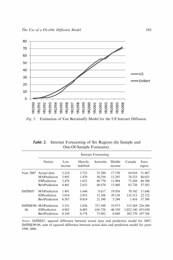
Fig. 5. Estimation of Von Bertalanffy Model for the US Internet Diffusion.
Table 2. Internet Forecasting of Six Regions (In Sample andOut-Of-Sample Forecasts).
Internet Forecasting
Nation Low
income
Heavily
indebted
Australia Middle
income
Canada Euro
region
Year 2007 Actual data 5.214 2.752 53.280 17.750 84.910 51.467
MAPrediction 3.993 1.470 50.350 13.285 76.523 48.025
ESPrediction 3.478 1.033 49.770 11.494 73.269 46.700
BertPrediction 4.461 2.633 48.670 15.460 83.720 57.582
DiffSE07 MAPrediction 1.491 1.644 8.617 19.936 70.342 11.846
ESPrediction 3.014 2.955 12.366 39.138 135.513 22.722
BertPrediction 0.567 0.014 21.390 5.244 1.416 37.396
DiffSSE90-
06
MAPrediction 2.531 2.856 337.309 19.973 515.269 226.580
ESPrediction 4.982 0.485 656.758 40.350 1,022.140 453.030
BertPrediction 0.149 0.178 73.982 0.869 202.370 107.768
Notes: DiffSE07, squared difference between actual data and prediction model for 2007;
DiffSSE90-06, sum of squared difference between actual data and prediction model for years
1990–2006.
The Use of a Flexible Diffusion Model 103

DISCUSSIONS AND CONCLUSION
This research provides some answers to the research questions posed in the‘‘Introduction’’ section. Traditional diffusion models can be inadequate tomodel the technology product diffusion in various nations. The traditionaldiffusion models (internal, external, and mixed) cater to standard distribu-tion pattern of product diffusion over time. Diffusion models for technologydiffusion in various nations must be more flexible to capture the variety ofdifferent patterns in different nations that may exist, depending on thevarious national conditions prevalent during the period of diffusion.
The results showed that a flexible diffusion model such as BERT canindeed model the diffusion of the ICT products more realistically in bothdeveloped and developing nations. The model predictions, in most cases,were better than traditional forecasting schemes such as ES or MA. For thetwo technologies, 4 out of 6 out-of-sample BERT forecasts emerged asbetter. Although not shown in this research, the BERT model predictionswere, in most cases, also better than those from the Bass model (Bass, 1969).
The parameter values were also different for these two sets of nationgroups, developing and developed. Table 1 shows that developing nations in
Table 3. Mobile Forecasting of six Regions (In Sample andOut-Of-Sample Forecasts).
Mobile Forecasting
Nation Middle
East and
North
Africa
OECD Low and
mid
income
Middle
income
UK Euro
region
Year 2007 Actual data 50.7 94.995 41.503 46.594 117.950 107.685
MAPrediction 35.940 90.702 32.877 34.858 113.932 103.994
ESPrediction 29.950 89.018 29.424 38.228 112.072 102.609
BertPrediction 48.333 93.254 41.398 47.769 112.179 100.999
DiffSE07 MAPrediction 217.869 18.430 74.408 137.734 16.144 13.623
ESPrediction 430.500 35.725 145.902 69.990 34.551 25.766
BertPrediction 5.603 3.031 0.011 1.381 33.304 44.703
DiffSSE90-06 MAPrediction 213.632 651.179 139.834 187.477 1,451.874 1,189.536
ESPrediction 414.820 1,296.889 275.922 369.475 2,818.429 2,330.951
BertPrediction 16.614 61.674 1.454 1.968 353.545 177.162
Notes: DiffSE07, squared difference between actual data and prediction model for 2007;
DiffSSE90-06, sum of squared difference between actual data and prediction model for years
1990–2006.
KALLOL BAGCHI ET AL.104

general, had greater values in b and y. One interpretation of this result couldbe that the diffusion pattern of these technologies in developing nationsrequires more word-of-mouth and promotional effort as not many peopleare ready to adopt these products due to differences in developing nation’ssocial, institutional, and economic conditions. At the same time, in manydeveloping nations the potential for high diffusion of these products exists(as the values of m show).
The parameter values also showed that for each nation or nation-group,mobile diffusion has progressed differently than the Internet diffusion. Thisis because, in general, Internet subscriptions per 100 individuals have beenslower than mobile diffusion per 100. Price could be one of the major factorsfor such differences of diffusions in a same nation/set of nations (Bagchiet al., 2008). To give some concrete examples of how the diffusions havediffered, consider the diffusion of two technologies of two nation sets atextreme economic ends: heavily indebted poor nations and high incomenations. From the period 1990 to 2007, mobile diffusion has progressed inthe heavily indebted poor nations and high-income nations from base valuesof 0 and 1.16, respectively, to 15.77 and 96.99, respectively. For the Internet,during the same period, high income nations registered a much slowerincrease from 0.28 to 63.53 and heavily indebted poor nations registered asimilar slower increase from 0 to 2.75 (The World Bank database, 2008).Although a few situations can be found where the Internet diffused fasterthan mobile phones during the same time period (Canada is an example), formost nations the reverse has been the case.
The results from the BERT model indicate that it can be used effectivelyin predicting the diffusion of these technologies in different nations and themodel may yield better results in many cases than the traditional ES or MAschemes or the standard Bass model of diffusion. For a successful diffusionof the product in any nation, a manager needs to additionally investigate therelationship of model parameter values to various types of existing social,institutional, and economic factors in a nation. Future research can alsorelate the model parameters b and y more specifically to business situations(Radas, 2005).
REFERENCES
Acemoglu, D., Aghion, P., & Zilibotti, F. (2002). Distance to frontier, selection, and economic
growth. NBER Working Paper 9066, National Bureau of Economic Research, Inc.
Bagchi, K., Kirs, P. J., & Lopez, F. (2008). The impact of price on cell phone and telephone
diffusion in four groups of nations. Information & Management, 45, 183–193.
The Use of a Flexible Diffusion Model 105

Bagchi, K., Kirs, P. J., & Udo, G. (2006). A comparison of factors impacting ICT growth rates
in developing and industrialized countries. In: E. Trauth, D. Howcroft, T. Butler,
B. Fitzgerald, & J. DeGross (Eds), IFIP International Federation for Information
Processing, Volume 208. Social inclusion: Societal and organizational implications for
information systems (pp. 37–50). Boston: Springer.
Bass, F. M. (1969). A new product growth model for consumer durable. Management Science,
15, 215–227.
Benhabib, J., & Spiegel, M. M. (2005). Human capital and technology diffusion. Handbook of
Economic Growth, 1(Part A), 935–966.
Bertalanffy, L. Von. (1957). Quantitative laws in metabolism and growth. Quarterly Review of
Biology, 32, 217–231.
Bousson, K. (2007). Time-varying parameter estimation with application to trajectory tracking.
Aircraft Engineering and Aerospace Technology, 79(4), 406–413.
Bretschneider, S. I., & Mahajan, V. (1980). Adaptive technological substitution models.
Technological Forecasting & Social Change, 18(2), 129–139.
Carter, F. J., Jambulingam, T., Gupta, V. K., & Melone, N. (2001). Technological innovat-
ions: A framework for communicating diffusion effects. Information & Management, 5,
277–287.
Dalka, D. (2007). Mobile phone usage creates economic growth in developing nations (Available at
http://www.daviddalka.com/createvalue/2007/01/28/mobile-phone-usage-creates-economic-
growth-in-developing-nations/).
Davison, R., Vogel, D., Harris, R., & Jones, N. (2000). Technology leapfrogging in developing
countries: An inevitable luxury? The Electronic Journal on Information Systems in
Developing Countries, 5, 1–10.
Dedrick, J. L., Goodman, S. E., & Kraemer, K. L. (1995). Little engines that could: Computing
in small energetic countries. Communications of ACM, 38(5), 21–26.
Easingwood, C. (1989). An analogical approach to the long-term forecasting of major new
product sales. International Journal of Forecasting, 5, 69–82.
Ein-Dor, P., Myers, M. D., & Raman, K. S. (1997). Information technology in three small
developed countries. Journal of Management Information Systems, 13(4), 61–89.
Gruber, H., & Verboven, F. (1998). The diffusion of mobile telecommunications services in
the European union. Discussion Paper 138. Center for Economic Research, Tilburg
University.
Gwartney, J., & Lawson, R. (2003). Economic freedom of the world: 2003 annual report.
Vancouver: The Fraser Institute.
Hu, Q., Saunders, C., & Gebelt, M. (1997). Research report. Diffusion of information systems
outsourcing: A reevaluation of influence sources. Information Systems Research, 8, 288–301.
Kendrick, D., Mercado, P., & Amman, H. (2006). Computational economics. Princeton, NJ:
Princeton University Press.
Kiiski, S., & Pohjola, M. (2002). Cross country diffusion of the internet. Information Economics
and Policy, 14(2), 297–310.
Lenk, P. J., & Rao, A. G. (1990). New models from old: Forecasting product adoption by
hierarchical Bayes procedures. Marketing Science, 9(1), 42–53.
Mahajan, V., Muller, E., & Bass, F. M. (1990). New product diffusion models in marketing:
A review and directions for re-search. Journal of Marketing, 54, 1–26.
Mahajan, V., Muller, E., & Bass, F. M. (1995). Diffusion of new products: Empirical
generalizations and managerial uses. Marketing Science, 14(3), G79–G88.
KALLOL BAGCHI ET AL.106

Mahajan, V., & Peterson, R. (1978) Models for innovation diffusion. Sage University Paper
series on Quantitative Applications in the Social Sciences (2nd ed.). Beverly Hills and
London: Sage.
Milner, H. V. (2003). The global spread of the internet: The role of international diffusion
pressures in technology adoption. New York: Columbia University.
Radas, S. (2005). Diffusion models in marketing: How to incorporate the effect of external
influence? Economic Trends and Economic Policy, 15(105), 31–51.
Roller, L. H., & Waverman, L. (2001). Telecommunications infrastructure and economic
development: A simultaneous approach. American Economic Review, 91(4), 909–923.
Schmittlein, D. C., & Mahajan, V. (1982). Maximum likelihood estimation for an innovation
diffusion model of new product acceptance. Marketing Science, I, 57–78.
Shmueli, G., & Koppius, O. (2008). Contrasting predictive and explanatory modeling in IS
research. Robert H. Smith School Research Paper no. RHS 06-058. Available at http://
ssrn.com/abstract ¼ 1112893
Sridhar Kala, S., & Sridhar, V. (2003). The effect of telecommuting on suburbanisation:
Empirical evidence. Journal of Regional Analysis and Policy, 33(1), 1–25.
Srinivasan, V., & Mason, C. (1986). Nonlinear least squares estimation of new product
diffusion models. Marketing Science, 5, 169–178.
Statistix for Windows. (1996). Analytical Software, ISBN 1-881789-04-7.
The World Bank database. (2008). Available at http://www.devdata.worldbank.org
UNDP. (1990). World Development Report 1990. Oxford: UNDP.
Walker, M. A. (Ed.) (1988). Freedom, democracy, and economic welfare. Vancouver: The Fraser
Institute.
Watson, R., & Myers, M. D. (2001). IT industry success in small countries: The case of Finland
and New Zealand. Journal of Global Information Management, 9(2), 4–14.
Wenrong, W., Xie, M., Tsui, K. (2006). Forecasting of mobile subscriptions in Asia pacific
using bass diffusion model. Proceedings 2006 IEEE International Conference on
Management of Innovation and Technology, Singapore (pp. 300–303).
Wong, P.-K. (2002). ICT production and diffusion in Asia: Digital dividends or digital divide?
Information Economics and Policy, 14, 167–187.
Xie, J. X., Song, M., Sirbu, M., & Qiong Wang, Q. (1997). Kalman filter estimation of new
product diffusion models. Journal of Marketing Research, 34(3), 378–393.
The Use of a Flexible Diffusion Model 107

This page intentionally left blank
FORECASTING HOUSEHOLD
RESPONSE IN DATABASE
MARKETING: A LATENT
TRAIT APPROACH
Eddie Rhee and Gary J. Russell
ABSTRACT
Database marketers often select households for individual marketingcontacts using information on past purchase behavior. One of the mostcommon methods, known as RFM variables approach, ranks householdsaccording to three criteria: the recency of the latest purchase event, thelong-run frequency of purchases, and the cumulative dollar expenditure.We argue that RFM variables approach is an indirect measure of thelatent purchase propensity of the customer. In addition, the use of RFMinformation in targeting households creates major statistical problems(selection bias and RFM endogeneity) that complicate the calibration offorecasting models. Using a latent trait approach to capture a household’spropensity to purchase a product, we construct a methodology that notonly measures directly the latent propensity value of the customer, butalso avoids the statistical limitations of the RFM variables approach. Theresult is a general household response forecasting and scoring approachthat can be used on any database of customer transactions. We apply our
Advances in Business and Management Forecasting, Volume 6, 109–131
Copyright r 2009 by Emerald Group Publishing Limited
All rights of reproduction in any form reserved
ISSN: 1477-4070/doi:10.1108/S1477-4070(2009)0000006008
109

methodology to a database from a charitable organization and show thatthe forecasting accuracy of the new methodology improves upon thetraditional RFM variables approach.
INTRODUCTION
Database marketing is an increasingly important aspect of the managementof traditional catalog retailers (such as Lands’ End) and e-commerce firms(such as Amazon.com). In database marketing, the manager has access to ahousehold database detailing each interaction with the firm over a period oftime. The task of the marketing manager is to use the database informationto develop predictive models of household purchasing, and then to targetsegments of households for specific marketing programs (Winer, 2001;Berger & Nasr, 1998; Hughes, 1996).
Scoring Households Using RFM
Firms frequently use household purchase characteristics, collectively knownas RFM variables, in selecting the best households for marketingsolicitations (Hughes, 1996). Recency (R) is defined as the number ofperiods since the most recent purchase. Frequency (F) is defined as the totalnumber of purchases. Monetary value (M) is defined as the dollar amountthat the household has spent to date. Conceptually, RFM variables are usedfor forecasting because past purchase behavior is often a reliable guide tofuture purchase behavior (Schmid & Weber, 1997; Rossi, McCulloch, &Allenby, 1996). The predictive power of the three variables is traditionallyknown as having the rank order: recency is the best predictor, followed byfrequency, and then monetary value (David Sheppard Associates, Inc.,1999). Forecasting the customer’s response likelihood using RFM variablesis widely accepted by database marketers as an easy and useful way ofpredicting behavior from a customer database.
RFM information is inserted into predictive models. For example, RFMvalues can be used as independent variables in a probit or logit responsemodel. Additional procedures drawn from the data mining literature, suchas decision trees and neural networks, can also be used to link RFM valuesto buying behavior (Berry & Linoff, 2000).
EDDIE RHEE AND GARY J. RUSSELL110

Statistical Problems Induced by RFM
The use of RFM in response modeling appears straightforward on thesurface but important statistical problems arise.
The first problem is known as selection bias. Simply put, selection biasarises when the researcher uses a nonrandomly selected sample to estimatebehavioral relationships (Heckman, 1979). If the firm selects households formailings based on a nonrandom selection rule (such as the RFM variables),a study that only analyzes the selected households generates biased results.This bias arises from the fact that the researcher does not observe thebehavior of nonselected households. Selection bias is a special type ofmissing data problem that can only be controlled by formally analyzing theway that the firm selects customers for marketing solicitations.
The second problem, known as RFM endogeneity, occurs when RFMvalues not only represent the past response behavior of the households, butalso reflect the past selection decision of the firm. For instance, if a householdis not selected to receive a marketing offer (and the household has no way torespond to the offer otherwise), the recency (the number of periods since thelast purchase) will be larger and the frequency and the monetary value will besmaller, than the values of these same variables for a comparable householdwho received the solicitation. If the firm consistently ignores the householdfor any reason, the RFM values of this household will deteriorate regardlessof the true propensity to respond. In formal statistical terms, it can be shownthat RFM endogeneity yields incorrect parameter estimates in a predictivemodel due to unobserved correlations between the RFM variables and theerror in the model (see, e.g., Davidson & MacKinnon, 1993).
The marketing science community has gradually begun to recognize thesestatistical problems. Industry standard procedures (such as RFM probitregression) and the early model of Bult and Wansbeek (1995) ignore theseproblems entirely. Jonker, Paap, and Frances (2000) addresses selection biasby relating RFM variables to both household selection and householdresponse. However, because RFM values appear in the specification, issuesof endogeneity are not addressed. Studies by Bitran and Mondschein (1996)and Gonul and Shi (1998) provide an approach to dealing with RFMendogeneity. By replacing observed RFM values with predicted values, theseauthors construct an instrumental variables methodology (see Davidson &MacKinnon, 1993) that corrects for potential parameter biases. In theapplications discussed by these authors, households are able to buy productseven if a marketing solicitation is not received. Accordingly, parameterbiases due to selection bias are not relevant and are not addressed.
Forecasting Household Response in Database Marketing 111
Latent Trait Scoring Model
This research builds on existing work by developing an approach tohousehold scoring, which corrects for both selection bias and RFMendogeneity. In contrast to earlier studies, we assume that each householdhas a latent (unobserved) propensity to respond that cannot be adequatelycaptured using RFM variables. Latent trait models have a long history inpsychometric studies of psychological constructs such as verbal andquantitative ability (see, e.g., Lord & Novick, 1968; Fischer & Molenarr,1995; Langeheine & Rost, 1988). These models have also found marketingscience applications in survey research (Balasubramanian & Kamakura,1989), coupon redemption (Bawa, Srinivasan, & Srivastava, 1997), andcross-selling of financial services (Kamakura, Ramaswami, & Srivastava,1991). Although latent trait models can be regarded as a type of randomcoefficient heterogeneity model (Allenby & Rossi, 1999), they are bestviewed as a method of measuring a psychological trait. In this research, weview household scoring as a research procedure designed to estimate ahousehold’s propensity to respond to marketing solicitations by the firm.
Our model is based on the assumption that both the firm’s selection ruleand the household’s response behavior provide indirect indications of thehousehold’s latent propensity. The notion here is that the firm does notselect households for mailings using either a census (all households) or arandom process (probability sample of households). Instead, the firm selectshouseholds using some process that takes into account the likelihood thatthe household will respond favorably. We do not, however, assume that theselection process is necessarily optimal. The key advantage of this approachis generality: the researcher can estimate a household response model onexisting databases in which the firm has attempted to optimize customercontact policy. As we show subsequently, we are able to measure eachhousehold’s true propensity to respond and examine the effectiveness of thefirm’s current contact policy.
The remainder of the chapter is organized as follows. We first detail ournew model, discussing the need to consider both household response and thefirm’s household selection rule simultaneously. We demonstrate that ourlatent trait specification can be formulated as a Hierarchical Bayes modeland estimated using Monte Carlo simulation technologies. The newmethodology is then applied in an analysis of the customer database of anonprofit organization. We show that the model provides forecasts with alevel of accuracy better than a benchmark RFM probit model. We concludewith a discussion of future research opportunities.
EDDIE RHEE AND GARY J. RUSSELL112
LATENT TRAIT MODEL OF RESPONSE
PROPENSITY
The chapter begins by describing the structure of a general model ofhousehold choice behavior in a database marketing context. Instead ofrelying on RFM variables to measure the propensity of each household torespond to marketing solicitation, we assume the existence of a household-specific latent trait that impacts the household’s probability of responding toa solicitation. This same latent variable is also assumed to impact the firm’slikelihood of targeting the household. By developing the model in thismanner, we correct for selection bias (if present) and avoid issues of RFMendogeneity. The result is a general model of household purchase behaviorthat takes into account potential limitations of the RFM variablesapproach.
Propensity to Respond
Propensity to respond is defined here as a household characteristic thatreflects the household’s inherent interest in the firm’s product offering. Weassume that this propensity has two components: a long-run componentthat varies only by household and a short-run component that varies overhouseholds and time. Implicitly, the long-run component accounts forheterogeneity in response across households, whereas the short-runcomponent accounts for temporal variation in response propensity withinhouseholds.
Let th,t denote the propensity to respond of household h at time t. Wedefine this construct according to the following equation:
th;t ¼ d1mh þ d2 YRðh;t�1Þ (1)
where YR(h,t�1) ¼ 1 if the household responded to the previous solicitation,and 0 otherwise. Furthermore, we assume that the long-run component isnormally distributed across the household population as
mh NðXhg; 1:0Þ (2)
where Xh denotes a set of demographic variables for household h.This formulation has two key properties. First, th,t changes over time
depending on whether or not the household purchased at the previous time
Forecasting Household Response in Database Marketing 113

point. Note that nonpurchase at time t�1 could be due to a rejection of theprevious offer. Alternatively, the household may have not been given anopportunity to purchase the product. In our formulation, it is not necessaryto distinguish between these two cases. Rather, similar to models of choiceinertia found in grocery scanner data applications (Seetharaman &Chintagunta, 1998; Jeuland, 1979), we assume that the act of purchasinga product at one time point has an impact on future behavior, regardless ofwhy the product was purchased. Note that the parameter on the laggedcomponent (d2) can be either positive or negative. Thus, the impact of theshort-term component can either enhance or diminish purchasing at the nextperiod.
The normal distribution characterizing the long-run component isintended to allow for heterogeneity in response across households. Notethat this distribution has a mean that depends on demographics and avariance set to one. Intuitively, this formulation states that the long-runcomponent depends in part on demographics, and in part on other(unobserved) household characteristics. Setting the variance of this distribu-tion to one can be accomplished without loss of generality. This restrictionis necessary for model identification and does not impact the fit of themodel.
Modeling the Firm’s Targeting Decision
We assume that the firm is attempting to optimize its targeting policy usingsome information in the household database. This information may or maynot be RFM variables. We assume that the firm’s rule has some validity andis correlated to some extent with th,t the household’s propensity to respond.We stress that this assumption does not imply that the firm actually observesth,t. Rather, the expression displayed later for the firm’s selection rule issimply a formal way of stating that households are not necessarily selectedat random. During model estimation, the researcher learns the extentto which the current targeting policy is based on some knowledge ofhousehold’s true propensity to respond. In the language of econometrictheory, our model of the firm’s targeting policy is a limited informationspecification – not a structural specification.
To model this process, we assume that the firm’s decision to target ahousehold depends on the attractiveness of the household to the firm. Definethe attractiveness of a household h to the firm at time t as US(h,t). Weassume that the firm makes a product offer to this household (YS(h,t) ¼ 1)
EDDIE RHEE AND GARY J. RUSSELL114
if US(h,t) is greater than zero. Otherwise, YS(h,t) ¼ 0. Hence, US(h,t) is a latentvariable that drives the observed targeting policy of the firm.
To complete the specification, we assume that the deterministic part ofUS(h,t) is a linear function of the household’s propensity to respond th,tdefined in Eq. (1). This leads to the model
USðh;tÞ ¼ a0 þ a1mh þ a2 YRðh;t�1Þ þ �S h; t; �S h;t Nð0; 1Þ (3)
where the normally distributed error �S h;t Nð0; 1Þ has mean 0 andvariance 1.
The assumption that the variance of the error is equal to 1 is necessary formodel identification; it has no impact on model fit.
We again emphasize that this expression does not imply that the firmknows the household propensity to respond as measured by th,t. All that thisexpression states is that the attractiveness of a household to the firm iscorrelated to some extent with the household’s propensity to respond. Thisspecification of the household selection process is identical to that of aprobit model for the binary variable YS(h,t). Intuitively, this model allows forthe possibility that households that are selected are likely to be betterprospects for the firm.
Modeling Household Response
In an analogous fashion, we assume that the household’s decision torespond to a product offer depends on the attractiveness (or utility) of theoffering. Define the attractiveness of a marketing offering to household hat time t as UR(h,t). We assume that the household buys the product(YR(h,t) ¼ 1) if UR(h,t) is greater than zero. Otherwise, YR(h,t) ¼ 0. Hence,UR(h,t) is a latent variable that determines the response behavior of thehousehold.
Given our definition of the household response propensity, we assumethat
URðh;tÞ ¼ b0 þ b1 mh þ b2YRðh;t�1Þ þ �R h;t; �R h;t Nð0; 1Þ (4)
where the normally distributed error �R h;t Nð0; 1Þ has mean 0 andvariance 1. Again, for model identification reasons, we can set the varianceof the error to 1 without loss of generality. Intuitively, this specificationamounts to the assumption that the deterministic part of UR(h,t) is a linearfunction of the household’s propensity to respond th,t defined in Eq. (1).
Forecasting Household Response in Database Marketing 115

Because the error in this expression is normally distributed, the model forthe household purchase variable is a probit model, conditional upon the long-and short-run elements of the propensity to respond construct. It should benoted that this model is only applied to households who are targeted by thefirm. Households who do not receive a product offer cannot buy the product.For these households, YR(h,t) must be equal to 0. Stated differently, we canonly estimate the response model over the set of households at a particulartime point who receive a product offer from the firm.
Properties of the Errors
To complete the specification of the model, we make two key assumptionsabout the errors in the firm targeting equation and the household responseequation. First, we assume that these errors are mutually independentat each time point. Second, we assume that these errors are independentover time.
The first assumption amounts to the notion of conditional independence.The intuition is that the household’s propensity to respond drives both firmbehavior and household behavior. Consequently, conditional on the valuesof mh and YR(h,t�1), we can assume that the selection and response errorterms in this model are independent. Since different values of mh andYR(h,t�1) lead to different values of selection and response, our model impliesa natural correlation between observed selection and observed responseacross the household population. In other words, conditional independenceallows for a simpler representation of the choice process without sacrificingthe reality that selection and response are correlated. Conditional indepen-dence is a key element of model construction both in psychometrics (Lord &Novick, 1968; Fischer & Molenarr, 1995; Langeheine & Rost, 1988) andmarketing science (e.g., Kamakura & Russell, 1989; Rossi et al., 1996).
The second assumption is necessary to prevent endogeneity issues fromentering the model through the lagged response variable. Lagged responseYR(h,t�1) is already modeled in the system by the selection and responseequations at time t�1. Given the value of propensity to respond at theprevious period, the probability that YR(h,t�1) equals one is a product of theprobability of selection and the probability of response in period t�1.Consequently, in the context of the response model, the observed laggedresponse is only correlated with the error terms in previous time periods(i.e., periods t�2, t�3, t�4). Since the error terms are assumed independentover time, the lagged response YR(h,t�1) cannot be correlated with the error
EDDIE RHEE AND GARY J. RUSSELL116

terms in the current period (eS h,t or eR h,t). Thus, the inclusion of YR(h,t�1) inthe model does not create endogeneity problems.
It is important to notice that the model developed here does not sufferfrom the problems of selection bias and endogeneity noted in our earlierdiscussion of RFM models. Both mh and YR(h,t�1) are independent of theerrors in the selection and response models (Eqs. (3) and (4)), thus elimina-ting endogeneity from the specification. Moreover, as explained byHeckman (1979), biases in parameter estimation due to selection bias areentirely due to a nonzero correlation between the errors of the selection andresponse equations. Because the errors eS h,t and eR h,t are contemporane-ously independent, selection bias is not present in the estimates generatedfrom our model.
Model Estimation
The proposed model (Eqs. (2)–(4)) is a two-equation probit system with anunderlying latent variable measuring the response propensity of eachhousehold. (The definition of the propensity to respond construct (Eq. (1))is used to motivate the structure of the model, but the d1 and d2 coefficientsare not explicitly estimated by our algorithm.) We calibrate the model byformulating the estimation problem using Hierarchical Bayes concepts andemploying Markov Chain Monte Carlo (MCMC) technology to simulatedraws from the posterior distribution of parameters (Gelman, Carlin, Stern, &Rubin, 1996). Details on the algorithm are presented in the appendix.
The convergence of the MCMC algorithm was checked using a proceduredeveloped by Geweke (2001). In Geweke’s approach, a second simulation,which uses a different (nonstandard) logic to draw the simulated values, isconducted following the initial MCMC analysis of the data. BecauseGeweke (2001) proves that the initial and the new simulation constituteMarkov chains with the same stationary point, the researcher is able tocheck convergence by verifying that the posterior means and variances fromthe two simulations are the same. The results reported in this chapter passedthis stringent convergence test.
APPLICATION
To understand the properties of the propensity to respond model, we use acustomer database from a nonprofit organization. Our intention here is to
Forecasting Household Response in Database Marketing 117
contrast the latent trait approach to a predictive model based solely onRFM. It is important to understand that the propensity to respond modeldoes not make any use of traditional RFM variables. This difference isimportant because it allows us to compare the industry standard RFMapproach to a formulation that ignores RFM variables. From a substantivepoint of view, this application is also designed to show that the propensity torespond model yields insights into the response characteristics of differenttypes of mail solicitations used by the firm and the operating characteristicsof the firm’s current household selection policy.
Data Description
The data consist of the transaction records of a nonprofit organization thatuses direct mail to solicit contributions from donors. Data are taken fromthe period October 1986 through June 1995. There is one record per pastdonor. Each record contains information on donor identification, postalcode, donation history, and solicitation dates. Since the contribution codesand solicitation codes match, each contribution can be traced to a specificsolicitation type and date.
We selected a random sample of 1,065 households for our analysis. Sincewe need a start-up time period to define RFM values, the final calibrationsample contains 20 solicitations during the period from July 1991 to October1994. The holdout sample for verification of the results contains foursolicitations potentially available to these households during the periodfrom November 1994 to March 1995. Overall, households receive mailingsfrom as few as two times to as many as 11 times across 20 time periods.
A preliminary analysis of household donation behavior showed that theamount of money donated by household varies little over time. Forexample, if a given household donates $5 on one occasion, the household isvery likely to donate $5 on every donation occasion. This fact allows us toregard the amount of the donation as a stable characteristic of thehousehold, and concentrate only on the probability that the householddecides to make a donation. Thus, the use of our model – a model thatfocuses only on the incidence of selection and response (YS(h,t) and YR(h,t)) –is entirely appropriate for this application.
There are four major solicitation types, types A, B, C, and a miscellaneoustype. Type A is the major solicitation type that shows the most frequent andregular mailings every three to six months. Type B includes the holidaymailings of December and January. Types C and miscellaneous are less
EDDIE RHEE AND GARY J. RUSSELL118
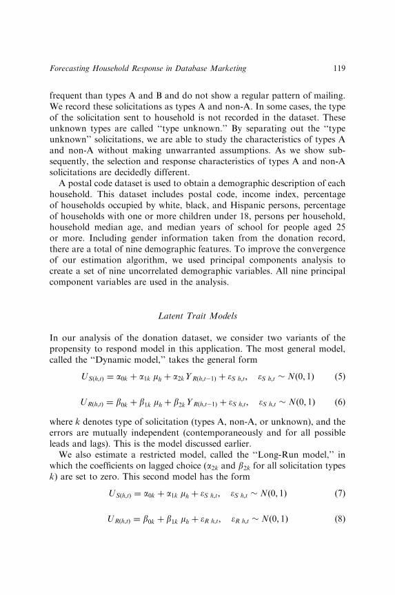
frequent than types A and B and do not show a regular pattern of mailing.We record these solicitations as types A and non-A. In some cases, the typeof the solicitation sent to household is not recorded in the dataset. Theseunknown types are called ‘‘type unknown.’’ By separating out the ‘‘typeunknown’’ solicitations, we are able to study the characteristics of types Aand non-A without making unwarranted assumptions. As we show sub-sequently, the selection and response characteristics of types A and non-Asolicitations are decidedly different.
A postal code dataset is used to obtain a demographic description of eachhousehold. This dataset includes postal code, income index, percentageof households occupied by white, black, and Hispanic persons, percentageof households with one or more children under 18, persons per household,household median age, and median years of school for people aged 25or more. Including gender information taken from the donation record,there are a total of nine demographic features. To improve the convergenceof our estimation algorithm, we used principal components analysis tocreate a set of nine uncorrelated demographic variables. All nine principalcomponent variables are used in the analysis.
Latent Trait Models
In our analysis of the donation dataset, we consider two variants of thepropensity to respond model in this application. The most general model,called the ‘‘Dynamic model,’’ takes the general form
USðh;tÞ ¼ a0k þ a1k mh þ a2kYRðh;t�1Þ þ �S h;t; �S h;t Nð0; 1Þ (5)
URðh;tÞ ¼ b0k þ b1k mh þ b2kYRðh;t�1Þ þ �S h;t; �S h;t Nð0; 1Þ (6)
where k denotes type of solicitation (types A, non-A, or unknown), and theerrors are mutually independent (contemporaneously and for all possibleleads and lags). This is the model discussed earlier.
We also estimate a restricted model, called the ‘‘Long-Run model,’’ inwhich the coefficients on lagged choice (a2k and b2k for all solicitation typesk) are set to zero. This second model has the form
USðh;tÞ ¼ a0k þ a1k mh þ �S h;t; �S h;t Nð0; 1Þ (7)
URðh;tÞ ¼ b0k þ b1k mh þ �R h;t; �R h;t Nð0; 1Þ (8)
Forecasting Household Response in Database Marketing 119
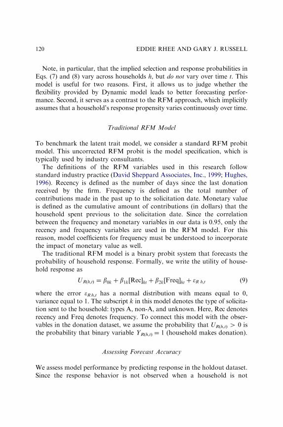
Note, in particular, that the implied selection and response probabilities inEqs. (7) and (8) vary across households h, but do not vary over time t. Thismodel is useful for two reasons. First, it allows us to judge whether theflexibility provided by Dynamic model leads to better forecasting perfor-mance. Second, it serves as a contrast to the RFM approach, which implicitlyassumes that a household’s response propensity varies continuously over time.
Traditional RFM Model
To benchmark the latent trait model, we consider a standard RFM probitmodel. This uncorrected RFM probit is the model specification, which istypically used by industry consultants.
The definitions of the RFM variables used in this research followstandard industry practice (David Sheppard Associates, Inc., 1999; Hughes,1996). Recency is defined as the number of days since the last donationreceived by the firm. Frequency is defined as the total number ofcontributions made in the past up to the solicitation date. Monetary valueis defined as the cumulative amount of contributions (in dollars) that thehousehold spent previous to the solicitation date. Since the correlationbetween the frequency and monetary variables in our data is 0.95, only therecency and frequency variables are used in the RFM model. For thisreason, model coefficients for frequency must be understood to incorporatethe impact of monetary value as well.
The traditional RFM model is a binary probit system that forecasts theprobability of household response. Formally, we write the utility of house-hold response as
URðh;tÞ ¼ b0k þ b1k½Rec�ht þ b2k½Freq�ht þ �R h;t (9)
where the error eRh,t has a normal distribution with means equal to 0,variance equal to 1. The subscript k in this model denotes the type of solicita-tion sent to the household: types A, non-A, and unknown. Here, Rec denotesrecency and Freq denotes frequency. To connect this model with the obser-vables in the donation dataset, we assume the probability that UR(h,t) W 0 isthe probability that binary variable YR(h,t) ¼ 1 (household makes donation).
Assessing Forecast Accuracy
We assess model performance by predicting response in the holdout dataset.Since the response behavior is not observed when a household is not
EDDIE RHEE AND GARY J. RUSSELL120
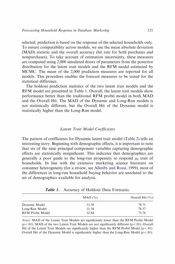
selected, prediction is based on the response of the selected households only.To ensure comparability across models, we use the mean absolute deviation(MAD) statistic and the overall accuracy (hit rate for both purchases andnonpurchases). To take account of estimation uncertainty, these measuresare computed using 2,000 simulated draws of parameters from the posteriordistribution for the latent trait models and the RFM model estimated byMCMC. The mean of the 2,000 prediction measures are reported for allmodels. This procedure enables the forecast measures to be tested for thestatistical difference.
The holdout prediction statistics of the two latent trait models and theRFM model are presented in Table 1. Overall, the latent trait models showperformance better than the traditional RFM probit model in both MADand the Overall Hit. The MAD of the Dynamic and Long-Run models isnot statistically different, but the Overall Hit of the Dynamic model isstatistically higher than the Long-Run model.
Latent Trait Model Coefficients
The pattern of coefficients for Dynamic latent trait model (Table 2) tells aninteresting story. Beginning with demographic effects, it is important to notethat six of the nine principal component variables capturing demographiceffects are statistically insignificant. This indicates that demographics aregenerally a poor guide to the long-run propensity to respond mh trait ofhouseholds. In line with the extensive marketing science literature onconsumer heterogeneity (for a review, see Allenby and Rossi, 1999), most ofthe differences in long-run household buying behavior are unrelated to theset of demographics available for analysis.
Table 1. Accuracy of Holdout Data Forecasts.
MAD (%) Overall Hit (%)
Dynamic Model 31.30 78.71
Long-Run Model 31.34 78.57
RFM Probit Model 32.84 75.76
Notes: MAD of the Latent Trait Models are significantly lower than the RFM Probit Model
(po.01). MAD of the two Latent Trait Models are not significantly different (po.01). Overall
Hit of the Latent Trait Models are significantly higher than the RFM Probit Model (po.01).
Overall Hit of the Dynamic Model is significantly higher than the Long-Run Model (po.01).
Forecasting Household Response in Database Marketing 121
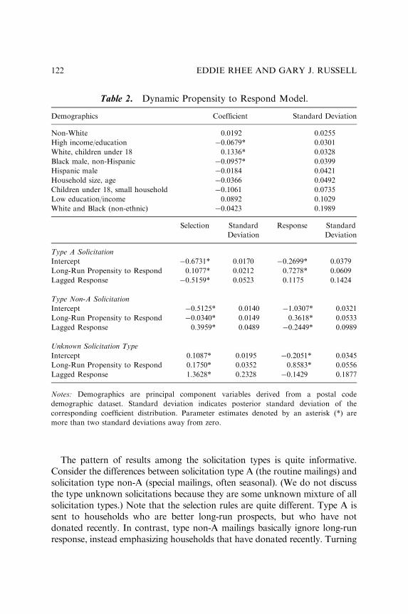
The pattern of results among the solicitation types is quite informative.Consider the differences between solicitation type A (the routine mailings) andsolicitation type non-A (special mailings, often seasonal). (We do not discussthe type unknown solicitations because they are some unknown mixture of allsolicitation types.) Note that the selection rules are quite different. Type A issent to households who are better long-run prospects, but who have notdonated recently. In contrast, type non-A mailings basically ignore long-runresponse, instead emphasizing households that have donated recently. Turning
Table 2. Dynamic Propensity to Respond Model.
Demographics Coefficient Standard Deviation
Non-White 0.0192 0.0255
High income/education �0.0679* 0.0301
White, children under 18 0.1336* 0.0328
Black male, non-Hispanic �0.0957* 0.0399
Hispanic male �0.0184 0.0421
Household size, age �0.0366 0.0492
Children under 18, small household �0.1061 0.0735
Low education/income 0.0892 0.1029
White and Black (non-ethnic) �0.0423 0.1989
Selection Standard
Deviation
Response Standard
Deviation
Type A Solicitation
Intercept �0.6731* 0.0170 �0.2699* 0.0379
Long-Run Propensity to Respond 0.1077* 0.0212 0.7278* 0.0609
Lagged Response �0.5159* 0.0523 0.1175 0.1424
Type Non-A Solicitation
Intercept �0.5125* 0.0140 �1.0307* 0.0321
Long-Run Propensity to Respond �0.0340* 0.0149 0.3618* 0.0533
Lagged Response 0.3959* 0.0489 �0.2449* 0.0989
Unknown Solicitation Type
Intercept 0.1087* 0.0195 �0.2051* 0.0345
Long-Run Propensity to Respond 0.1750* 0.0352 0.8583* 0.0556
Lagged Response 1.3628* 0.2328 �0.1429 0.1877
Notes: Demographics are principal component variables derived from a postal code
demographic dataset. Standard deviation indicates posterior standard deviation of the
corresponding coefficient distribution. Parameter estimates denoted by an asterisk (*) are
more than two standard deviations away from zero.
EDDIE RHEE AND GARY J. RUSSELL122
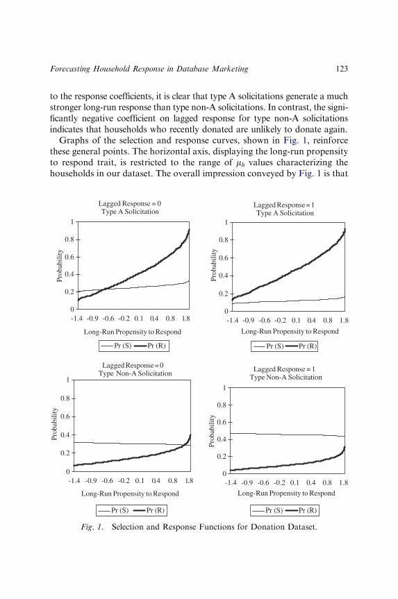
to the response coefficients, it is clear that type A solicitations generate a muchstronger long-run response than type non-A solicitations. In contrast, the signi-ficantly negative coefficient on lagged response for type non-A solicitationsindicates that households who recently donated are unlikely to donate again.
Graphs of the selection and response curves, shown in Fig. 1, reinforcethese general points. The horizontal axis, displaying the long-run propensityto respond trait, is restricted to the range of mh values characterizing thehouseholds in our dataset. The overall impression conveyed by Fig. 1 is that
Lagged Response = 0Type A Solicitation
0
0.2
0.4
0.6
0.8
1
-1.4 -0.9 -0.6 -0.2 0.1 0.4 0.8 1.8
Long-Run Propensity to Respond
Prob
abili
ty
Pr (S) Pr (R)
Lagged Response = 1Type A Solicitation
0
0.2
0.4
0.6
0.8
1
-1.4 -0.9 -0.6 -0.2 0.1 0.4 0.8 1.8
Long-Run Propensity to Respond
Prob
abili
ty
Pr (S) Pr (R)
Lagged Response = 0Type Non-A Solicitation
0
0.2
0.4
0.6
0.8
1
-1.4 -0.9 -0.6 -0.2 0.1 0.4 0.8 1.8
Long-Run Propensity to Respond
Prob
abili
ty
Pr (S) Pr (R)
Lagged Response = 1Type Non-A Solicitation
0
0.2
0.4
0.6
0.8
1
-1.4 -0.9 -0.6 -0.2 0.1 0.4 0.8 1.8
Long-Run Propensity to Respond
Prob
abili
ty
Pr (S) Pr (R)
Fig. 1. Selection and Response Functions for Donation Dataset.
Forecasting Household Response in Database Marketing 123
the decision to donate to this charitable organization is closely tied to thevalue of the propensity to respond measure. This, of course, is how themodel is constructed. However, Fig. 1 also shows that the decision to mail asolicitation to a household depends very weakly on this trait. Managers,instead, seem to base mailing policy primarily on whether the household hasdonated in the recent past.
Substantively, these results suggest that type A solicitations work betterfor this charity because managers wait for a period of time after a donationbefore sending out a new solicitation and attempt to target households withlong-run interests in the charity. In contrast, the type non-A solicitations aremailed out in a more opportunistic fashion, relying more on short-runresponse. It is possible that the firm views type A solicitations more in termsof household retention, and the type non-A solicitations more in terms ofhousehold acquisition. Nevertheless, given the response pattern for the typenon-A solicitations, the current mailing policy for type non-A (mailing tothose who have recently responded) is clearly counterproductive. Thisobservation, along with the fact that the mailing policy of the routine type Asolicitations is weakly linked to the household propensity trait, stronglyargues that the firm’s mailing policy could be improved by using theestimated propensity to respond as a guideline for mailing.
Summary
RFM variables are best regarded as behavioral indicators of an underlyinginterest in the firm’s product or service. In this case, the product is the causeof the charitable organization. Although RFM variables provide someinformation on a household’s propensity to respond trait, RFM variablesare also impacted by the mailing policy selected by managers. The latenttrait approach is superior in the sense that it separates the household trait(the decision to respond to a solicitation) from behavioral responses to thetrait (the manager’s decision to contact a household). Moreover, this trait isa stable characteristic of the household which cannot be affected by the firm.
CONCLUSION
This study develops a general procedure for estimating the responseprobabilities of households in database marketing. The proposed approach,based on a simultaneous selection–response formulation, assumes that each
EDDIE RHEE AND GARY J. RUSSELL124
household has a latent propensity to respond that impacts both the firm’sdecision to mail a solicitation and the household’s decision to respond to asolicitation. Inclusion of the selection decision of the firm in the modelrecognizes the potential for selection bias; the propensity to respondconstruct solves the problem of endogeneity of RFM. Our empirical analysisshowed that the Dynamic model yielded the best forecasting results. Thelatent trait model generates exogenous measures of the long-run propensityto respond to each household and provides the researcher with a tool tounderstand the effectiveness of current household solicitation policy.
Contributions of Research
Although recency, frequency, and monetary value are intuitively reasonableways of measuring the attractiveness of households, constructing a predictivemodel using RFM variables is problematic. The underlying problem is thatthe RFM variables in a database are functions of both the household’sinterest in the product category and the firm’s mailing policy. That is, ahousehold’s RFM profile depends on characteristics of the both thehousehold and the firm. From a statistical point of view, this confoundingof household behavior and firm decision behavior is particularly worrisome.
The proposed model, by explicitly considering the rule of householdselection rules in generating the dataset, calibrates a household responsemodel that can be generalized to future datasets. This generalizability is dueto the fact that our model is free from the selection bias and RFMendogeneity problems that affect most conventional methodologies. Usingthe response coefficients from the model output along with knowledge of thehousehold trait value and lagged response behavior YR(h,t�1), a researchercan predict response behavior in a future scenario in which the firm’sdecision rules have changed. A major strength of the model is its ability torecover the true response characteristics of households from a customerdatabase, even when the firm has attempted to optimize the mailing ofsolicitations. In principle, this is not possible with the RFM approachbecause the observed RFM profile depends on both past purchase behaviorand whether or not managers selected the household for mailings.
Limitations and Extensions
Our model has several limitations, all of which provide avenues for futureresearch. The current model predicts only the incidence of selection and
Forecasting Household Response in Database Marketing 125

response. The most obvious extension is the construction of a model thatpredicts both probability of response and the dollar donation (orexpenditure). This could be accomplished by changing the responseequation to a Tobit model (Davidson & MacKinnon, 1993), in which thelatent propensity to respond drives both incidence and dollar amount. Thecurrent model is also limited to the prediction of one response perhousehold. Clearly, most catalog retailers sell a large array of products.These retailers often develop specialty catalogs emphasizing subsets of theproduct line, and target these catalogs to various segments in the customerdatabase. By constructing a set of correlated latent response variables fordifferent product subsets, the model could be further generalized to considerthe basket of purchases made by a household. Taken together, thesegeneralizations would permit the analyst to develop a global choice modelfor use by a multiple-category catalog retailer.
ACKNOWLEDGMENT
The authors thank the Direct Marketing Educational Foundation forproviding access to the data used in this study. The authors also thankProfessor John Geweke of the Department of Economics, University ofIowa, for many helpful suggestions on model specification and estimation.
REFERENCES
Allenby, G. M., & Rossi, P. E. (1999). Marketing models of consumer heterogeneity. Journal of
Econometrics, 89, 57–78.
Balasubramanian, S. K., & Kamakura, W. A. (1989). Measuring consumer attitudes toward the
marketplace with tailored interviews. Journal of Marketing Research, 26(August),
311–326.
Bawa, K., Srinivasan, S. S., & Srivastava, R. K. (1997). Coupon attractiveness and coupon
proneness: A framework for modeling coupon redemption. Journal of Marketing
Research, 34(November), 517–525.
Berger, P. D., & Nasr, N. (1998). Customer lifetime value: Marketing models and applications.
Journal of Interactive Marketing, 12(Winter), 17–30.
Berry, M. J., & Linoff, G. S. (2000). Mastering data mining: The art and science of household
relationship management. New York: Wiley.
Bitran, G. R., & Mondschein, S. V. (1996). Mailing decisions in the catalog sales industry.
Management Science, 42(9), 1364–1381.
Bult, J. R., & Wansbeek, T. (1995). Optimal selection for direct mail. Marketing Science, 14(4),
378–394.
EDDIE RHEE AND GARY J. RUSSELL126

David Sheppard Associates, Inc. (1999). The new direct marketing: How to implement a profit-
driven database marketing strategy. Boston: McGraw-Hill.
Davidson, R., & MacKinnon, J. G. (1993). Estimation and inference in econometrics. New York:
Oxford University Press.
Fischer, G. H., & Molenarr, I. W. (1995). Rasch models: Foundations, recent developments and
applications. New York: Springer.
Gelfand, A. E., & Smith, A. F. M. (1990). Sampling based approaches to calculating marginal
densities. Journal of the American Statistical Association, 85(2), 398–409.
Gelman, A., Carlin, J., Stern, H., & Rubin, D. (1996). Bayesian data analysis. New York:
Chapman and Hall.
Geweke, J. F. (2001). Getting it right: Checking for errors in likelihood based inference. Working
Paper. Department of Economics, University of Iowa.
Geweke, J. F. (2003). Contemporary Bayesian econometrics and statistics. Working Monograph.
Department of Economics, University of Iowa.
Gonul, F., & Shi, M. Z. (1998). Optimal mailing of catalogs: A new methodology using esti-
mable structural dynamic programming models. Management Science, 44(9), 1249–1262.
Heckman, J. J. (1979). Sample selection bias as a specification error. Econometrica, 47(1),
153–161.
Hughes, A. M. (1996). Boosting response with RFM. Marketing Tools, 5, 4–10.
Jeuland, A. P. (1979). Brand choice inertia as one aspect of the notion of brand loyalty.
Management Science, 25(July), 671–682.
Jonker, J. J., Paap, R., & Frances, P. H. (2000). Modeling charity donations: Target selection,
response time and gift size. Economic Institute Report 2000-07/A. Erasmus University
Rotterdam.
Kamakura, W. A., Ramaswami, S. N., & Srivastava, R. K. (1991). Applying latent trait
analysis in the evaluation of prospects for cross-selling of financial services. International
Journal of Research in Marketing, 8(4), 329–349.
Kamakura, W. A., & Russell, G. J. (1989). A probabilistic choice model for market
segmentation and elasticity structure. Journal of Marketing Research, 26(November),
271–390.
Langeheine, R., & Rost, J. (1988). Latent trait and latent class models. New York: Plenum.
Lord, F. M., & Novick, M. R. (1968). Statistical theories of mental test scores. Reading, MA:
Addison-Wesley.
Robert, C. P., & Casella, G. (1999). Monte Carlo statistical methods. New York: Springer-
Verlag.
Rossi, P. E., McCulloch, R., & Allenby, G. (1996). The value of household information in
target marketing. Marketing Science, 15(Summer), 321–340.
Schmid, J., & Weber, A. (1997). Desktop database marketing. Chicago, IL: NTC Business
Books.
Seetharaman, P. B., & Chintagunta, P. K. (1998). A model of inertia and variety-seeking with
marketing variables. International Journal of Research in Marketing, 15(1), 1–17.
Winer, R. S. (2001). A framework for customer relationship management. California
Management Review, 43(Summer), 89–105.
Forecasting Household Response in Database Marketing 127
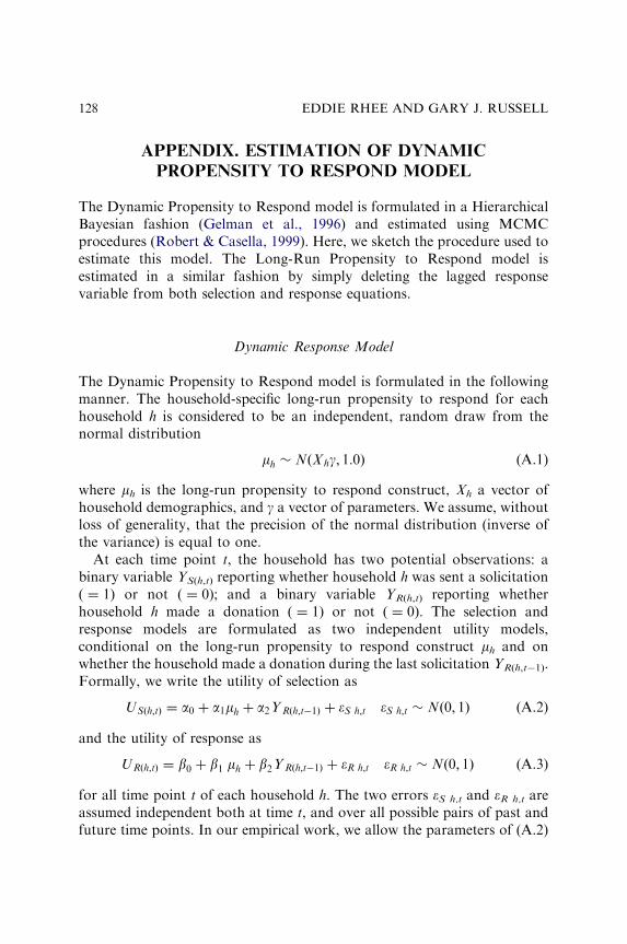
APPENDIX. ESTIMATION OF DYNAMIC
PROPENSITY TO RESPOND MODEL
The Dynamic Propensity to Respond model is formulated in a HierarchicalBayesian fashion (Gelman et al., 1996) and estimated using MCMCprocedures (Robert & Casella, 1999). Here, we sketch the procedure used toestimate this model. The Long-Run Propensity to Respond model isestimated in a similar fashion by simply deleting the lagged responsevariable from both selection and response equations.
Dynamic Response Model
The Dynamic Propensity to Respond model is formulated in the followingmanner. The household-specific long-run propensity to respond for eachhousehold h is considered to be an independent, random draw from thenormal distribution
mh NðXhg; 1:0Þ (A.1)
where mh is the long-run propensity to respond construct, Xh a vector ofhousehold demographics, and g a vector of parameters. We assume, withoutloss of generality, that the precision of the normal distribution (inverse ofthe variance) is equal to one.
At each time point t, the household has two potential observations: abinary variable YS(h,t) reporting whether household h was sent a solicitation( ¼ 1) or not ( ¼ 0); and a binary variable YR(h,t) reporting whetherhousehold h made a donation ( ¼ 1) or not ( ¼ 0). The selection andresponse models are formulated as two independent utility models,conditional on the long-run propensity to respond construct mh and onwhether the household made a donation during the last solicitation YR(h,t�1).Formally, we write the utility of selection as
USðh;tÞ ¼ a0 þ a1mh þ a2YRðh;t�1Þ þ �S h;t �S h;t Nð0; 1Þ (A.2)
and the utility of response as
URðh;tÞ ¼ b0 þ b1 mh þ b2YRðh;t�1Þ þ �R h;t �R h;t Nð0; 1Þ (A.3)
for all time point t of each household h. The two errors eS h,t and eR h,t areassumed independent both at time t, and over all possible pairs of past andfuture time points. In our empirical work, we allow the parameters of (A.2)
EDDIE RHEE AND GARY J. RUSSELL128

and (A.3) to depend on the type of solicitation sent by the firm. However, tosimplify the exposition here, we ignore this feature of the model in theequations later.
We observe a mailing to a household (YS(h,t) ¼ 1) when the utility ofselection is greater than zero, and no mailing (YS(h,t) ¼ 0) when the utility ofselection is less than or equal to zero. In a similar fashion, we observe adonation (YR(h,t) ¼ 1) when the utility of response is greater than zero, andno donation (YR(h,t) ¼ 0) when the utility of response is less than or equal tozero. Eqs. (A.2) and (A.3) form a two-equation binary probit system inwhich selection and response variables are independent, conditional on thevalues of mh and YR(h,t�1).
Note that when YS(h,t) ¼ 0 (no mailing to the household), then we mustobserve that YR(h,t) ¼ 0 (no donation is made). That is, when the householdis not sent a mailing, we observe no response, but do not know whether ornot the household would have responded if given the opportunity. For thisreason, it is necessary to regard the donation response as missing wheneverYS(h,t) ¼ 0. Accordingly, in the development below, it is understood that Eq.(A.3) is dropped from the model for all combinations of h and t for whichYS(h,t) ¼ 0.
Prior Distributions
The prior distributions for g, a, and b are assumed to be normal. Diffusepriors are chosen to allow the observed data to dominate the analysis.Specifically, we assume that gBN[0, U025 I(d )], aBN[0, U025 I(3)], andbBN[0, U025 I(3)] where d is the number of demographic variables and I(z)denotes a (square) identity matrix of dimension z. Note that we are usingBayesian convention of writing a normal distribution as N(m, p) where m isthe mean and p the precision (the inverse of the variance).
Full Conditional Distributions
After constructing the posterior distribution for the model, we derive the fullconditional distributions of the parameters. This leads to the followingrelations:
f ½mjelse� N½meanðmÞ;precðmÞ� (A.4)
Forecasting Household Response in Database Marketing 129

where mean(m) ¼ prec(m)�1 {X gþSt(a1US)� a0a1T�St(a1a2Y)þSt(b1UR)�b0b1T�St(b1b2Y)} and prec(m) ¼ (1þ a1
2Tþ b12T)*I(H). Here, mean( � ) and
prec( � ) are the mean and precision of a normal distribution, X is (H� d)matrix of demographics, US and UR are (H�T) matrices of utility ofselection and utility of response, respectively, Y is (H�T) matrix of laggedresponse, and H the number of households, and T the number of timeperiods.
f ½gjelse� N½meanðgÞ;precðgÞ� (A.5)
where mean(g) ¼ prec(g)�1 {Xumþ0(d� 1) (.025)}, prec(g) ¼ XuXþ(.025) I(d),and 0(d� 1) is (d� 1) vector of zeros.
f ½USjelse� truncated N½ �US; IðH*TÞ� (A.6)
where the elements of (H�T) matrix of �US are obtained from thedeterministic elements on the right-hand side of Eq. (A.2). The notationtruncated N(a,b) denotes a truncated normal with upper bound ¼ 0 ifYS(h,t) ¼ 0 and lower bound ¼ 0 if YS(h,t) ¼ 1.
f ½URjelse� truncated N½ �UR; IðH*TÞ� (A.7)
where the elements of (H�T) matrix of �UR are obtained from thedeterministic elements on the right-hand side of Eq. (A.3). The notationtruncated N(a,b) denotes a truncated normal with upper bound ¼ 0 ifYR(h,t) ¼ 0 and lower bound ¼ 0 if YR(h,t) ¼ 1.
f ½ajelse� N½meanðaÞ; precðaÞ� (A.8)
where mean(a) ¼ prec(a)�1 {mY*uUS*þ0(3� 1) (.025)} and prec(a) ¼ mY*umY*þ
(.025)I(3). Here, mY* is (H*T� 3) matrix that contains a (H*T� 1) vector ofones, a vector of mðH � TÞ, and a (H*T� 1) vector of YR(h,t). US
* is US
ðH � TÞ vector. 0(3� 1) is (3� 1) vector of zeroes.
f ½bjelse� N½meanðbÞ; precðbÞ� (A.9)
where mean(b) ¼ prec(b)�1 {mY*uUR*þ0(3� 1) (.025)} and prec(b) ¼ mY*u
mY*þ(.025)I(3).Here, mY* is (H*T� 3) matrix that contains a (H*T� 1) vector of ones, a
vector of mðH � TÞ and a (H*T� 1) vector of YR(h,t�1). UR* is UR ðH � TÞ
vector. 0(3� 1) is (3� 1) vector of zeros.
EDDIE RHEE AND GARY J. RUSSELL130

Markov Chain Monte Carlo Algorithm
To estimate the parameters of the model, we use the Gibbs Sampler(Gelfand & Smith, 1990). Starting with the vector of long-run propensity torespond parameters m in Eq. (A.4), we successively sample the parametersfrom each equation in turn (i.e., sample the parameters of Eqs. (A.4)–(A.9)in order, then repeat the sequence). The stationary point of this MarkovChain contains the model parameters (Gelman et al., 1996).
For each of the models, we ran a chain of 20,000 simulates. We used thelast 5,000 simulates to compute posterior means and variances. Theconvergence of this algorithm was checked using a procedure developedby Geweke (2001, 2003). In this approach, a second simulation, which uses adifferent (nonstandard) logic to draw the simulated values, is conducted.Because the underlying theory indicates that the initial and the newsimulation constitute Markov chains with the same stationary point, theresearcher can check convergence by verifying that the posterior means andvariances of the two simulations are the same. The results reported in thischapter passed this stringent convergence test.
Forecasting Household Response in Database Marketing 131

This page intentionally left blank

PART III
FORECASTING METHODS AND
EVALUATION

This page intentionally left blank

A NEW BASIS FOR MEASURING
AND EVALUATING
FORECASTING MODELS
Frenck Waage
ABSTRACT
Assume that we generate forecasts from a model y ¼ cxþdþ x. Theconstants ‘‘c’’ and ‘‘d’’ are placement parameters estimated fromobservations on x and y, and x is the residual error variable.
Our objective is to develop a method for accurately measuring andevaluating the risk profile of a forecasted variable y. To do so, it isnecessary to first obtain an accurate representation of the histogram of aforecasting model’s residual errors. That is not always so easy because thehistogram of the residual xmay be symmetric, or it may be skewed to eitherthe left of or to the right of its mode. We introduce the probability densityfunction (PDF) family of functions because it is versatile enough to fit anyresidual’s locus be it skewed to the left, symmetric about the mean, orskewed to the right. When we have measured the residual’s density, we showhow to correctly calculate the risk profile of the forecasted variable y fromthe density of the residual using the PPD function. We achieve the desiredand accurate risk profile for y that we seek. We conclude the chapter bydiscussing how a universally followed paradigm leads to misstating the riskprofile and to wrongheaded decisions by too freely using the symmetricGauss–normal function instead of the PPD function. We expect that thischapter will open up many new avenues of progress for econometricians.
Advances in Business and Management Forecasting, Volume 6, 135–155
Copyright r 2009 by Emerald Group Publishing Limited
All rights of reproduction in any form reserved
ISSN: 1477-4070/doi:10.1108/S1477-4070(2009)0000006009
135

1. INTRODUCTION
A forecast predicts the future consequences of present choices, and estimatesthe probability of each consequence occurring, which is the risk profile ofthe forecast. Mathematical forecasting models take many forms including,but not limited to, the following:
y ¼ f ðxÞ þ x
yt ¼ f ðyt�1; yt�1; yt�3Þ þ x
yt ¼ f ðyt�1Þ þ f ðxÞ þ x
We shall, in this chapter, let the very general formulation of a forecastingmodel y ¼ f (x)þ x represent any of the functions that might be used inpractice. The variable y is the dependent random variable whose values areto be forecasted, the term f(x) is an arbitrary function of x and also possiblyof lagged y variables, xmeasures the driving forces behind y, and xmeasuresthe model’s residual errors. Once a forecasting model has been finalized, itsresidual or forecasting errors x are calculated from x ¼ y� f(x). Mathema-tical forecasting functions are discussed by Makridakis and Wheelwright(1978), Granger (1980), Levenbach and Cleary (1981), Cleary andLevenbach (1982), Box and Cox (1964), Graybill (1961), Mosteller andTukey (1977), Neter, Kutner, Wassermann, and Nachtsheim (1996),Render, Stair, and Hanna (2006), and Weisberg (1985).
To obtain the risk profile of the forecast, first calculate the probabilitydensity, or histogram, of the forecasting model’s residual errors. Second,identify a mathematical function that accurately fits the observed residualdensity or its histogram. This mathematical function measures theprobability density of the residuals. From the now known residual densityfunction calculate the probability density of the forecasted variable y. Thedensity of y is the risk profile of the forecasted variable y. There are two basicapproaches to identify the mathematical function, which most accurately fitsthe histogram of the residuals. These two approaches are now discussed.
Approach 1: Fit every known PDF, one at a time to the observed residualhistogram. This includes fitting all of the normal, the Poisson, the binomial,the Weibull, the beta, the gamma, and many more to the histogram.The address on Internet http://wikipedia.org/wiki/Probability-distributionpresents an adequate listing. The advantage with this approach is that amathematical function will be identified, which provides the best fit. Thedisadvantage is that a very considerable amount of time will be consumedfinding it.
FRENCK WAAGE136

Approach 2: Identify a single family of functions, which alone can take allof the different loci that it takes many individual functions to reveal inApproach 1. This one family of functions too is capable of supplying thelocus, which best fits the residuals’ histogram. The advantage of fitting onlyone family of functions is that only the function’s placement parametersneed to be estimated. The time consumed in doing this may be short. Thedisadvantage includes that statistical tests and confidence statementsmay have to be developed for this new function, and this may be bothtime consuming and demanding.
The purpose of this chapter is to introduce the single family of functionsalluded to by Approach 2. That function is a polynomial probability densitythat we shall name PPD. By varying its placement parameters it will alonetake all of the different loci that Approach 1 needs many functions toidentify. The integral defined by Eq. (4) is the fundamental relationship.Cross-multiplications on Eq. (4) generate Eq. (5). Eq. (5) is the PPDfunction we introduce and discuss in this chapter. It possesses singly thecapabilities to take all the different loci, which Approach 1 can deliver onlywith the help from very many different functions, by simply varying itsplacement parameters.
This chapter
(1) develops methods for fitting the new PPD function to any residual’shistogram. The fitted PPD is the probability density of the residuals x;
(2) calculates the PDF of the random forecasted variable y from the knownprobability density of the forecasting model’s residuals x. This PDF of yis the risk profile of the forecasted variable y; and
(3) demonstrates effective ways of using the risk profile in decision making.
The first step in this program is to develop the residual’s histogram. How todo this is discussed next.
2. MEASURING THE HISTOGRAM OF THE
RESIDUALS n
The forecasts of yt for time period t are generated from a model yt ¼f(xt)þ xt. The residual errors of model are calculated from xt ¼ yt � f(xt).The histogram of the residual errors is calculated by ordering the values of xfrom x’s lower bound L to its upper bound M. The interval from L to M issubdivided into cells of equal width. Each observed x value is placed in the
A New Basis for Measuring and Evaluating Forecasting Models 137

appropriate cell. The number of x values in each cell is counted. The cellcount is converted into percentages of the total number of observed x values.The percentages sum to 100%. This defines the histogram, and it can now bevisualized. Graph the cell percentages along the ordinate axis and the cellwidths (or cell midpoints) along the abscissa. The resulting graph reveals theresidual’s histogram.
2.1. An Application: Measuring the Residuals’ Histogram
The linear regression model (1) was created from the 104 observations on xand y that have been tabulated in Table A1 in Appendix.
yt ¼0:24883xt þ 4:11807
ð0:2216Þ ð0:0036Þ
18:58 67:90
(1)
where values in parentheses represent standard errors and 18.58 and 67.90represent t-values.
xt ¼ yt � 0:24883 xt � 4:11807 (2)
The regression statistics are
r2 ¼ 0:978; standard error ¼ 1:121914; varianceðxÞ ¼ 1:258691;
F ¼ 4610:8; EðxÞ ¼ �0:0135(3)
Using judgment, we determined that Lx ¼ � 4.0 and Mx ¼ þ 2.4. Theresidual therefore has a finite range defined by � 4.0r xr 2.4. Fig. 1depicts the residual’s histogram and density. That histogram is visuallyskewed to the left.
We now seek a mathematical function that will correctly represent thelocus of this histogram.
3. FITTING A MATHEMATICAL FUNCTION TO
THE HISTOGRAM
To identify the function, which fits any given histogram best, we shall applyApproach 2. We shall create a single family of functions, which is so versatilein its capability to take different loci that it provides the best fit to any givenhistogram. This function is fundamentally defined by the integral (4).
FRENCK WAAGE138
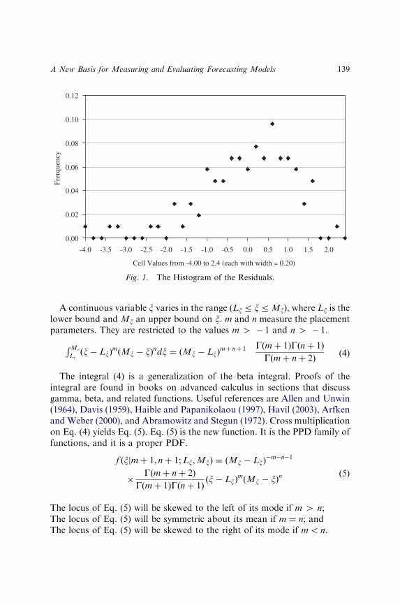
A continuous variable x varies in the range (Lxr xrMx), where Lx is thelower bound and Mx an upper bound on x. m and n measure the placementparameters. They are restricted to the values m W � 1 and n W � 1.
RM�
L�ðx� LxÞ
mðMx � xÞndx ¼ ðMx � LxÞ
mþ nþ 1 Gðmþ 1ÞGðnþ 1Þ
Gðmþ nþ 2Þ(4)
The integral (4) is a generalization of the beta integral. Proofs of theintegral are found in books on advanced calculus in sections that discussgamma, beta, and related functions. Useful references are Allen and Unwin(1964), Davis (1959), Haible and Papanikolaou (1997), Havil (2003), Arfkenand Weber (2000), and Abramowitz and Stegun (1972). Cross multiplicationon Eq. (4) yields Eq. (5). Eq. (5) is the new function. It is the PPD family offunctions, and it is a proper PDF.
f ðxjmþ 1; nþ 1;Lx;MxÞ ¼ ðMx � LxÞ�m�n�1
�Gðmþ nþ 2Þ
Gðmþ 1ÞGðnþ 1Þðx� LxÞ
mðMx � xÞn
(5)
The locus of Eq. (5) will be skewed to the left of its mode if m W n;The locus of Eq. (5) will be symmetric about its mean if m ¼ n; andThe locus of Eq. (5) will be skewed to the right of its mode if mo n.
0.00
0.02
0.04
0.06
0.08
0.10
0.12
-4.0 -3.5 -3.0 -2.5 -2.0 -1.5 -1.0 -0.5 0.0 0.5 1.0 1.5 2.0
Cell Values from -4.00 to 2.4 (each with width = 0.20)
Frer
quen
cy
Fig. 1. The Histogram of the Residuals.
A New Basis for Measuring and Evaluating Forecasting Models 139
Along the abscissa, the values of x are concentrated on the intervalLx rxrMx.
Integral (4) is not new. It has, however, not been used to any extent whichI have been able to detect in regression modeling or in management sciencemodeling. I consider Eq. (5) therefore to be new and unknown to thesesciences. It is a significant function, because it can do most of the estimationwork on symmetric forms that the normal function can do. And, it can domost of the estimation work on skew forms, which the normal functioncannot do. The function should therefore attract considerable interest onceit has been brought to light. This function is discussed by Lebedev (1972),Wilson (1912), and Hildebrand (1962). When the placement parameters mand n are known, the expected value of x, E(x), and the variance of x, V(x) ofEq. (5) are calculated from formulas (6) and (7). The formulas are calculateddirectly from Eq. (5) using the definitions of expectation and variance.Methods of calculating the moments are discussed by Green and Carroll(1978), Hair, Black, Babin, Anderson, and Tatham (2006), Harris (2001)and Wilks (1962).
EðxÞ ¼ ðMx � LxÞðmþ 1Þ
ðmþ nþ 2Þ
� �þ Lx (6)
VðxÞ ¼ ðMx � LxÞ2 ðmþ 1Þðnþ 1Þ
ðmþ nþ 2Þ2ðmþ nþ 3Þ(7)
We will now discuss two practical methods for fitting the PPD definedby Eq. (5) to any observed histogram: method A and method B. A vastliterature addresses the problem of fitting mathematical functions toobservations. Some of the useful references are: Brownlee (1965), Danieland Wood (1999), Maddala (1977), Render, Stair, and Balakrishnan (2006),Kendall (1951), Kendall and Stuart (1958), Feller (1957), Feller (1966),Hines and Montgomery (1972), and Wilks (1962).
3.1. Using the PPB Function and Fitting Method A
The problem we confront is: Find the values of m and n in Eq. (5), whichminimize the sum of squared differences between the locus of Eq. (5) whenthese values for m and n are used, and the locus of the observed histogramwhen L and M are known constants. This method requires that we solve
FRENCK WAAGE140
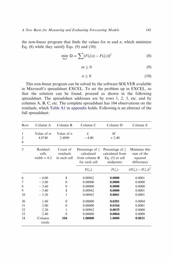
the non-linear program that finds the values for m and n, which minimizeEq. (8) while they satisfy Eqs. (9) and (10).
minm;n
O ¼XðFðxoÞ � FðxcÞÞ2 (8)
m � 0 (9)
n � 0 (10)
This non-linear program can be solved by the software SOLVER availablein Microsoft’s spreadsheet EXCEL. To set the problem up in EXCEL, sothat the solution can be found, proceed as shown in the followingspreadsheet. The spreadsheet addresses are by rows 1, 2, 3, etc. and bycolumns A, B, C, etc. The complete spreadsheet has 104 observations on theresiduals, which Table A1 in appendix holds. Following is an abstract of thefull spreadsheet:
Row Column A Column B Column C Column D Column E
1 Value of m Value of n L M
2 4.8748 2.4890 � 4.00 þ 2.40
4
5 Residual
cells
width ¼ 0.2
Count of
residuals
in each cell
Percentage of xcalculated
from column B
for each cell
Percentage of xcalculated from
Eq. (5) at cell
midpoints
Minimize this
sum of the
squared
differences
F(xo) F(xc) (F(xo)�F(xc))2
6 � 4.00 1 0.00962 0.0000 0.0001
7 � 3.80 0 0.00000 0.0000 0.0000
8 � 3.60 0 0.00000 0.0000 0.0000
9 � 3.40 1 0.00962 0.0000 0.0001
10 � 3.20 1 0.00962 0.0001 0.0001
30 1.80 0 0.00000 0.0201 0.0004
31 2.00 0 0.00000 0.0104 0.0001
32 2.20 1 0.00962 0.0035 0.0000
33 2.40 0 0.00000 0.0004 0.0000
34 Column
totals
104 1.00000 1.0000 0.0031
A New Basis for Measuring and Evaluating Forecasting Models 141

1. Complete, by calculating them, spreadsheet columns A–E.2. Enter in row 1 the text shown in columns A–D. Enter the values shown in
row 2 columns A–D. L ¼ � 4.00 and M ¼ þ 2.4 are lower and upperbounds on the residual. They do not change. Enter in A2 and B2 thearbitrary starting values m ¼ 1.00 and n ¼ 1.00, which the solutionalgorithm SOLVER needs to start. The solution software SOLVER willuse these in its first ‘‘round,’’ and find better values in each subsequent roundterminating the algorithm after many ‘‘rounds’’ on the optimal values for mand n. These optimal values are those that will minimize the sum of squareddifferences in column E, and those we seek. The optimal values of m and nwill be placed in addresses A2 and B2 replacing the initial starting values.
3. In EXCEL, the software SOLVER will find the desired values of m and n.To find the optimal solutions for m and n using SOLVER in EXCEL,proceed as follows.
4. Complete all entries in the table shown above for all rows and allcolumns A–E.
5. In EXCEL, click on TOOLS. Under TOOLS, click on SOLVER or onPREMIUM SOLVER. A Window labeled SOLVER PARAMETERSopens on your screen. Type the following information into this window:
Where it says Set Target Cell type the addresses that hold the sum ofthe squared differences, which you intend to minimize. Above that is$E$34 (Column E, Row 34). This is your objective to be minimized Next, click on the MIN button because you wish to minimize the sumof squares in $E$34. Where it says By Changing Cells type the address where the values form and n are. Above that is $A$2:$B$2. This is the address that holdsthe starter values for m and n. It is also where the optimal values for mand n will be placed by the software program. Where it says Subject to constraints click on ‘‘Add’’ and type in$A$2Z0.00, then click on ‘‘Add ’’ again and enter $B$2Z0.00, andthen click on ‘‘OK’’. Click on the button OPTIONS. Under OPTIONS click on ASSUMENON-NEGATIVE then on OK. Finally, to get the software to calculate the optimal values of m and n,click on the button SOLVE in the upper right corner of the SOLVERPARAMETERS window. SOLVER calculates the sum of squares foreach allowed pair (m, n). It finds the pair (m, n) that generates thesmallest sum. It prints the optimal pair in the location A2 for m andB2 for n. These are the minimizing values for m and n, which you seek.The minimized sum of squared differences is keyed in address $E$34.
FRENCK WAAGE142
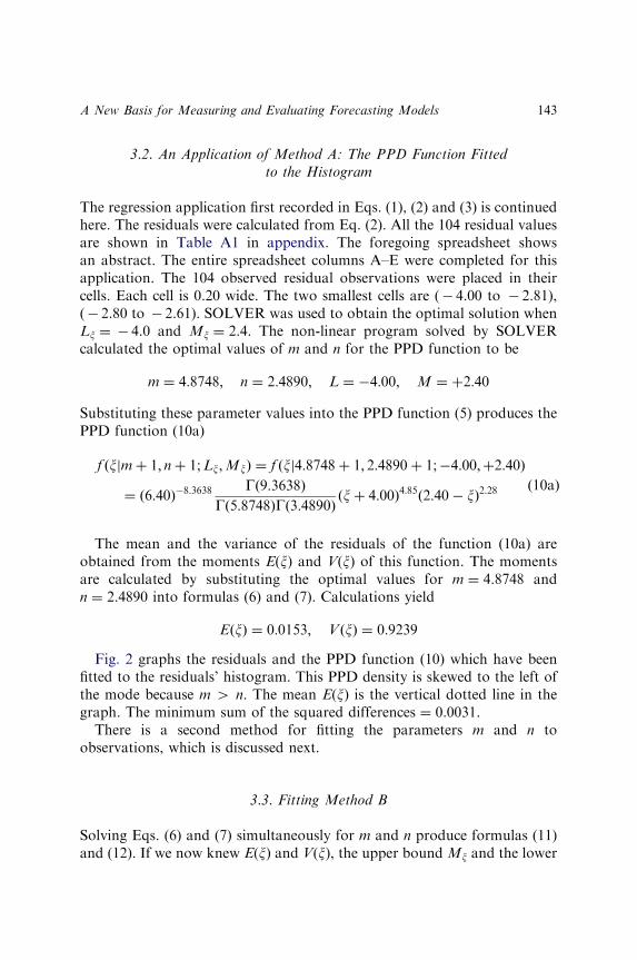
3.2. An Application of Method A: The PPD Function Fittedto the Histogram
The regression application first recorded in Eqs. (1), (2) and (3) is continuedhere. The residuals were calculated from Eq. (2). All the 104 residual valuesare shown in Table A1 in appendix. The foregoing spreadsheet showsan abstract. The entire spreadsheet columns A–E were completed for thisapplication. The 104 observed residual observations were placed in theircells. Each cell is 0.20 wide. The two smallest cells are (� 4.00 to � 2.81),(� 2.80 to � 2.61). SOLVER was used to obtain the optimal solution whenLx ¼ � 4.0 and Mx ¼ 2.4. The non-linear program solved by SOLVERcalculated the optimal values of m and n for the PPD function to be
m ¼ 4:8748; n ¼ 2:4890; L ¼ �4:00; M ¼ þ2:40
Substituting these parameter values into the PPD function (5) produces thePPD function (10a)
f ðxjmþ 1; nþ 1;Lx;MxÞ ¼ f ðxj4:8748þ 1; 2:4890þ 1;�4:00;þ2:40Þ
¼ ð6:40Þ�8:3638Gð9:3638Þ
Gð5:8748ÞGð3:4890Þðxþ 4:00Þ4:85ð2:40� xÞ2:28
ð10aÞ
The mean and the variance of the residuals of the function (10a) areobtained from the moments E(x) and V(x) of this function. The momentsare calculated by substituting the optimal values for m ¼ 4.8748 andn ¼ 2.4890 into formulas (6) and (7). Calculations yield
EðxÞ ¼ 0:0153; VðxÞ ¼ 0:9239
Fig. 2 graphs the residuals and the PPD function (10) which have beenfitted to the residuals’ histogram. This PPD density is skewed to the left ofthe mode because m W n. The mean E(x) is the vertical dotted line in thegraph. The minimum sum of the squared differences ¼ 0.0031.
There is a second method for fitting the parameters m and n toobservations, which is discussed next.
3.3. Fitting Method B
Solving Eqs. (6) and (7) simultaneously for m and n produce formulas (11)and (12). If we now knew E(x) and V(x), the upper bound Mx and the lower
A New Basis for Measuring and Evaluating Forecasting Models 143
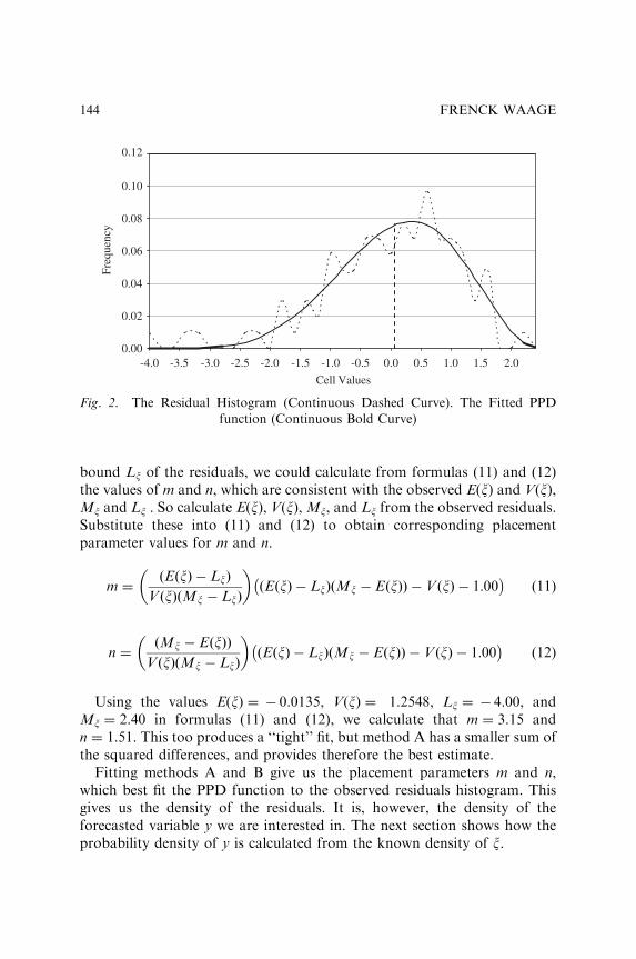
bound Lx of the residuals, we could calculate from formulas (11) and (12)the values of m and n, which are consistent with the observed E(x) and V(x),Mx and Lx . So calculate E(x), V(x),Mx, and Lx from the observed residuals.Substitute these into (11) and (12) to obtain corresponding placementparameter values for m and n.
m ¼ðEðxÞ � LxÞ
VðxÞðMx � LxÞ
� �ðEðxÞ � LxÞðMx � EðxÞÞ � VðxÞ � 1:00� �
(11)
n ¼ðMx � EðxÞÞ
VðxÞðMx � LxÞ
� �ðEðxÞ � LxÞðMx � EðxÞÞ � VðxÞ � 1:00� �
(12)
Using the values E(x) ¼ � 0.0135, V(x) ¼ 1.2548, Lx ¼ � 4.00, andMx ¼ 2.40 in formulas (11) and (12), we calculate that m ¼ 3.15 andn ¼ 1.51. This too produces a ‘‘tight’’ fit, but method A has a smaller sum ofthe squared differences, and provides therefore the best estimate.
Fitting methods A and B give us the placement parameters m and n,which best fit the PPD function to the observed residuals histogram. Thisgives us the density of the residuals. It is, however, the density of theforecasted variable y we are interested in. The next section shows how theprobability density of y is calculated from the known density of x.
0.00
0.02
0.04
0.06
0.08
0.10
0.12
-4.0 -3.5 -3.0 -2.5 -2.0 -1.5 -1.0 -0.5 0.0 0.5 1.0 1.5 2.0
Cell Values
Freq
uenc
y
Fig. 2. The Residual Histogram (Continuous Dashed Curve). The Fitted PPD
function (Continuous Bold Curve)
FRENCK WAAGE144

4. CALCULATING THE DENSITY OF Y FROM
THAT OF n
The variables y and x are linked by a model y ¼ f(x)þ x, or equivalently, byx ¼ y� ax� b. To calculate the probability density of y from the knowndensity of x, execute the following operations:
Step 1. Calculate the Jacobi transform |J| ¼ @x/@y from Eq. (2). TheJacobi transform |J| ¼ @x/@y ¼ 1.00. The Jacobi transform is discussed byBrownlee (1965), Yamane (1962), and Hines and Montgomery (1972).
Step 2. Substitute the residual function x ¼ y� ax� b given by Eq. (2)into the PPD function (5) in order to eliminate x from Eq. (5) and tointroduce y into it. The polynomial term in Eq. (5) will become(y� ax� b�Lx)
m(Mx� yþ axþ b)n.
Step 3. Simplify this polynomial term by defining the lower bound of y tobe Ly axþ bþLx and the upper bound on y My axþ bþMx. Usingthese expressions for Ly and My in the polynomial terms, we obtain thesimplified expression given by (y�Ly)
m(My� y)n.
Step 4. Obtain the PDF of y by executing the operations in Eq. (13).Eq. (13) is the probability density of the forecasted variable Y, and it givesus the risk profile of the forecast y.
gðyÞdy ¼ gð f ðyÞÞjJjdy ¼ gðyjmþ 1; nþ 1; x;Ly;MyÞdy
¼ ðMy � LyÞ�m�n�1 Gðmþ nþ 2Þ
Gðmþ 1ÞGðnþ 1Þ½ðy� LyÞ�
m½ðMy � yÞ�n(13)
My ¼ axþ bþMx is the upper bound on y, andLy ¼ axþ bþLx is the lower bound on y.
For each possible ‘‘x’’ in the regression Eq. (1), there exists a densityfunction that measures the probability of any y value occurring for thatgiven x value. The kernel of Eq. (5) and of Eq. (13) has the same form.We can therefore use formulas (6) and (7) to calculate E(y) and V(y) forEq. (13) using the known m and n, but replacing the bounds Lx and Mx
in the formulas with the new bounds for y, Ly, and My. Formulas (11)and (12) calculate m and n using E(y), V(y), My, and Ly in lieu of E(x), V(x),Mx, and Lx. Eq. (12) is the desired risk profile of the forecasted valuesfor y.
A New Basis for Measuring and Evaluating Forecasting Models 145

4.1. An Application: Calculating the Density of y from the Density of x
Using the results from the regression analysis from Eqs. (1), (2) and (3), wecalculate the upper bound My and the lower bound Ly of y.
Ly ¼ axþ bþ L� ¼ 0:24883xþ 4:11807� 4:00 ¼ 0:24883xþ 0:11807
My ¼ axþ bþM� ¼ 0:24883xþ 4:11807þ 2:40 ¼ 0:24883xþ 6:51807
The continuous random forecasted variable y varies in the finite rangebounded by
Ly ¼ 0:11807þ 0:24883x � y � 6:51807þ 0:24883x ¼My
The optimal placement parameters remain unchanged as m ¼ 4.8748,n ¼ 2.4890.
The density function of y is skewed to the left of the mode because mW n.Use these values in Eq. (13) to obtain the PPD density, which governs y.It is given by Eq. (14).
gðyjmþ 1; nþ 1; x;Ly;MyÞ ¼ g yj4:8748þ 1; 2:4890þ 1; 0:11807ð
þ 0:24883x; 6:51807þ 0:24883xÞ
¼ ð6:4Þ�8:3638Gð9:3638Þ
Gð5:8748ÞGð3:4890Þ
� ½ðy� 0:118� 0:2488xÞ�4:8748
� ½ð6:518þ 0:2488x� yÞ�2:489
(14)
Knowing that m ¼ 4.8748 and n ¼ 2.4890, we calculate the expectationE(y) and the variance V(y) from formulas (6) and (7). The results areE(y) ¼ 4.11807þ 0.24883x, V(y) ¼ 1.23449, and the standard deviation issy ¼ 1.12191. Fig. 3 plots Eq. (14) for the arbitrary value x ¼ 50.
5. A CURRENT PARADIGM FREQUENTLY LEADS
TO AN ERRONEOUS RISK PROFILE OF THE
FORECASTED VARIABLE Y AND TO
WRONGHEADED DECISIONS
First, recollect the possible loci the residuals can take. Earlier, we haveexplained the method for accurately calculating the risk profile (the accurate
FRENCK WAAGE146
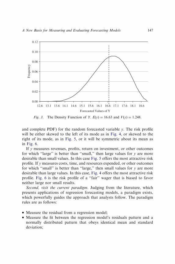
and complete PDF) for the random forecasted variable y. The risk profilewill be either skewed to the left of its mode as in Fig. 4, or skewed to theright of its mode, as in Fig. 5, or it will be symmetric about its mean asin Fig. 6.
If y measures revenues, profits, return on investment, or other outcomesfor which ‘‘large’’ is better than ‘‘small,’’ then large values for y are moredesirable than small values. In this case Fig. 5 offers the most attractive riskprofile. If ymeasures costs, time, and resources expended, or other outcomesfor which ‘‘small’’ is better than ‘‘large,’’ then small values for y are moredesirable than large values. In this case, Fig. 4 offers the most attractive riskprofile. Fig. 6 is the risk profile of a ‘‘fair’’ wager that is biased to favorneither large nor small results.
Second, visit the current paradigm. Judging from the literature, whichpresents applications of regression forecasting models, a paradigm exists,which powerfully guides the approach that analysts follow. The paradigmrules are as follows:
Measure the residual from a regression model; Measure the fit between the regression model’s residuals pattern and anormally distributed pattern that obeys identical mean and standarddeviation;
0.00
0.02
0.04
0.06
0.08
0.10
0.12
12.6 13.1 13.6 14.1 14.6 15.1 15.6 16.1 16.6 17.1 17.6 18.1 18.6
Forecasted Values of Y
Freq
uenc
y
Fig. 3. The Density Function of Y. E(y) ¼ 16.63 and V(y) ¼ 1.248.
A New Basis for Measuring and Evaluating Forecasting Models 147
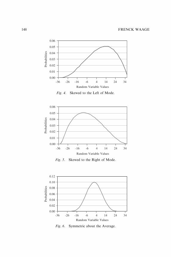
0.00
0.01
0.02
0.03
0.04
0.05
0.06
-36 -26 -16 -6 4 14 24 34
Random Variable Values
Prob
abili
ties
Fig. 4. Skewed to the Left of Mode.
0.00
0.01
0.02
0.03
0.04
0.05
0.06
-36 -26 -16 -6 4 14 24 34
Random Variable Values
Prob
abili
ties
Fig. 5. Skewed to the Right of Mode.
0.00
0.02
0.04
0.06
0.08
0.10
0.12
-36 -26 -16 -6 4 14 24 34
Random Variable Values
Prob
abili
ties
Fig. 6. Symmetric about the Average.
FRENCK WAAGE148

Judge from the measured fit if the agreement between the two is ‘‘closeenough.’’ If the two are judged to be ‘‘close enough,’’ the residual ‘‘can beconsidered’’ normally distributed; and The rest of the analysis of the regression model’s forecasts will be basedon statistical tests, confidence limits, and inferences from the normaldistribution.
When the residual’s histogram is symmetric about the mean, theparadigm may give wise guidance. Beware, however, that the mathemati-cally astute knows that the normal density function does not fit very wellmany of the symmetric loci, which occur. But, when the residual’s histogramis skewed, the paradigm guides the analysts to commit errors, often seriouserrors, and sometimes errors with disastrous consequences.
Third, we make our point through an application. In this section, weshall demonstrate the errors that can be committed when the regression’sresidual distribution is wrongly approximated by the normal function.We shall use as our standard the histogram of the residuals from regres-sion model (1), graphed in Fig. 1 and correctly measured by thePPD function (10). The risk profile of y in model (1) is correctly measuredby the PPD function (14). Therefore, Eqs. (10) and (14) are our referencepoints.
The normal approximation of the density of the forecasted variable y. Thedescriptive statistics of the residuals governed by the PPD function (10)are E(x) ¼ 0.0153, V(x) ¼ 0.9239, a standard deviation sx ¼ 1.12, a lowerbound Lx ¼ � 4.00, and an upper bound Mx ¼ 2.40. The normal functionfitted to these statistics is given by Eq. (15), except for the finite upper andlower bounds of x. The normal distribution has infinite bounds.
Nðxjmx; sxÞ ¼1
1:12p2p
eð1=2Þ½ðx�ð�0:0135ÞÞ=1:12�2
�1 � y � þ1 ð15Þ
Eq. (15) defines the normal approximation to the observed density ofthe residuals x. But it is the density of y we are interested in. To derive thedensity of the variable y from the known normal density (15) of the variablex, proceed as follows. Substitute the mean E(y) ¼ 4.1199þ 0.24883x of theregression model (1), and the model’s standard deviation sy ¼ 1.12 into (15).Multiply the result by the Jacobi transform |J| ¼ qx/qy ¼ 1.00, and obtainthe normal density of y given by (16).
NðyjEðyÞ; syÞ ¼1
1:12p2p
eð1=2Þ½ðy� 0:24883x� 4:1199Þ=1:12�2 �1 � y � þ1 ð16Þ
A New Basis for Measuring and Evaluating Forecasting Models 149
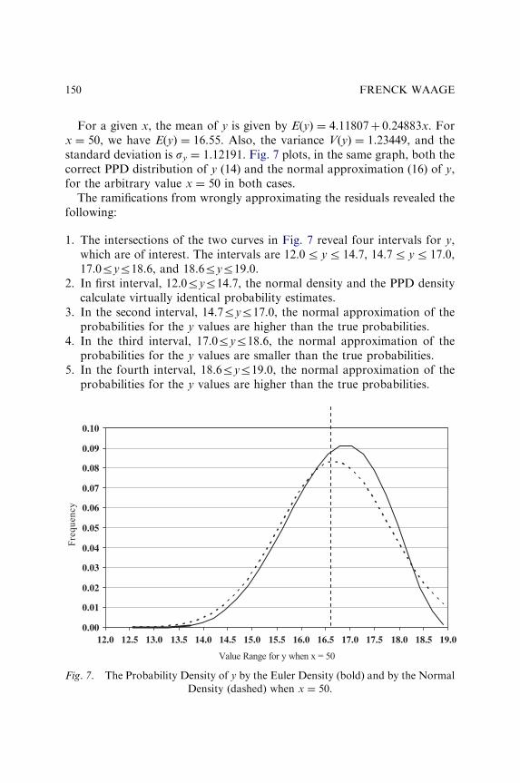
For a given x, the mean of y is given by E(y) ¼ 4.11807þ 0.24883x. Forx ¼ 50, we have E(y) ¼ 16.55. Also, the variance V(y) ¼ 1.23449, and thestandard deviation is sy ¼ 1.12191. Fig. 7 plots, in the same graph, both thecorrect PPD distribution of y (14) and the normal approximation (16) of y,for the arbitrary value x ¼ 50 in both cases.
The ramifications from wrongly approximating the residuals revealed thefollowing:
1. The intersections of the two curves in Fig. 7 reveal four intervals for y,which are of interest. The intervals are 12.0r yr 14.7, 14.7r yr 17.0,17.0ryr18.6, and 18.6ryr19.0.
2. In first interval, 12.0ryr14.7, the normal density and the PPD densitycalculate virtually identical probability estimates.
3. In the second interval, 14.7ryr17.0, the normal approximation of theprobabilities for the y values are higher than the true probabilities.
4. In the third interval, 17.0ryr18.6, the normal approximation of theprobabilities for the y values are smaller than the true probabilities.
5. In the fourth interval, 18.6ryr19.0, the normal approximation of theprobabilities for the y values are higher than the true probabilities.
0.00
0.01
0.02
0.03
0.04
0.05
0.06
0.07
0.08
0.09
0.10
12.0 12.5 13.0 13.5 14.0 14.5 15.0 15.5 16.0 16.5 17.0 17.5 18.0 18.5 19.0
Value Range for y when x = 50
Fre
qu
en
cy
Fig. 7. The Probability Density of y by the Euler Density (bold) and by the Normal
Density (dashed) when x ¼ 50.
FRENCK WAAGE150
6. These discrepancies have ramifications. Suppose that a decision makerseeks wagers that offer high values of y with favorable probabilities(e.g., high Revenues, high profits, ROI). The normal approximation willbe misleading the decision maker in intervals two, three, and four, andtherefore for the wager as a whole.
7. Suppose that a decision maker seeks wagers that offer low values of ywith favorable probabilities (e.g., low costs, low resource use). Thenormal approximation will similarly be misleading the decision maker inintervals two, three, and four.
8. The conclusions will be the same for a density function of y, which isskewed to the right.
9. Only in the case of symmetric densities for y will the normalapproximation serve well, but not in all such cases.
Here then is a way to understand the ramifications that do not fit theresidual density correctly can lead to. To give correct guidance to thedecision makers, the policy makers, or the strategy makers, the correctdensity of y has to be known. It implies that the density of the residual’shistogram must be correctly measured. This chapter shows that using thePPD family of functions will deliver highly accurate representations of therisk profile of the forecasted variable y.
6. CONCLUSION
Our objective was to develop a method for accurately calculating therisk profile of a forecasted variable. To accurately measure the risk profileof a forecasted variable y, it is necessary to first obtain an accuraterepresentation of the histogram of a forecasting model’s residual errors.The histogram of the residual x in a forecasting model y ¼ f(x)þ x maybe symmetric, or it may be skewed to either the left of or the right of itsmode. To accurately represent the locus of any histogram, we introducedthe PDF family of functions. That function is capable of correctly measu-ring the residual’s histogram – be it skewed to the left, symmetric about themean, or skewed to the right. From the residual’s density, we correctlycalculate the risk profile of the forecasted variable y from the density of theresidual using the PPD function. We end up with the desired and accuraterisk profile.
We discussed a universally followed paradigm that sometimes leads tomisstating the risk profile and wrongheaded decisions. The paradigm guides
A New Basis for Measuring and Evaluating Forecasting Models 151
the analysts to approximate almost all histograms and densities with theGauss–normal function. This chapter should open up many new avenuesof progress for econometricians. The new PPD family of functions maystimulate many professional papers, each of which will have the power todevelop econometric theory and applications further.
REFERENCES
Abramowitz, M., & Stegun, I. (Eds). (1972). Handbook of mathematical functions with formulas,
graphs and mathematical tables. New York: Dover.
Allen, G., & Unwin, L. (1964). The universal encyclopedia of mathematics. New York: Simon
and Schuster.
Arfken, G., & Weber, H. (2000). Mathematical methods for physicists. Harcourt: Academic
Press.
Box, G. E. P., & Cox, D. R. (1964). An analysis of transformations. Journal of the Royal
Statistical Society B, 26, 211–243.
Brownlee, K. A. (1965). Statistical theory and methodology in science and engineering (2nd ed.).
New York: Wiley.
Cleary, J., & Levenbach, H. (1982). The professional forecaster: The forecasting process through
data analysis. Belmont, CA: Lifetime Learning Publications, A Division of Wadsworth,
Inc.
Daniel, C., & Wood, F. S. (1999). Fitting equations to data (2nd ed). New York: Wiley-
Interscience.
Davis, P. J. (1959). Leonard Euler’s integral: A historical profile of the gamma function.
American Mathematical Monthly, 66, 849–869.
Feller, W. (1957). An introduction to probability theory and its applications (Vol. 1). New York:
Wiley.
Feller, W. (1966). An introduction to probability theory and its applications (Vol. 2). New York:
Wiley.
Granger, C. W. (1980). Forecasting in business and economics. New York, NY: Academic Press.
Graybill, F. A. (1961). An introduction to linear statistical models. New York, NY: McGraw-Hill
Book Company.
Green, P. E., & Carroll, J. D. (1978). Mathematical tools for applied multivariate analysis.
New York: Academic Press.
Haible, B., & Papanikolaou, T. (1997). Fast multiprecision evaluation of series of rational
numbers. Technical Report No. TI-7/97. Darmstadt University of Technology,
Germany.
Hair, J. F., Jr., Black, W. C., Babin, B. J., Anderson, R. E., & Tatham, R. L. (2006).
Multivariate data analysis. Upper Saddle river, NJ: Pearson/Prentice-Hall.
Harris, R. J. (2001). A primer of multivariate statistics (3rd ed). Hillsdale, NJ: Lawrence
Erlbaum Associates.
Havil, J. (2003). Gamma, exploring Euler’s constant. ISBN 0-691-09983-9 (c).
Hildebrand, F. B. (1962). Advanced calculus for applications. Englewood Cliffs, NJ: Prentice-
Hall.
FRENCK WAAGE152

Hines, W. W., & Montgomery, D. C. (1972). Probability and statistics in engineering and
management science (3rd ed.). New York, NY: Wiley.
Kendall, M. G. (1951). The advanced theory of statistics (3rd ed., Vol. 2). New York, NY:
Hafner Publishing Company.
Kendall, M. G., & Stuart, A. (1958). The advanced theory of statistics (Vol. 1).
Lebedev, N. N. (1972). Special functions and their applications (Translated and edited by R. A.
Silverman). New York, NY: Dover Publications, Inc.
Levenbach, H., & Cleary, J. (1981). The beginning forecaster: The forecasting process through
data analysis. Belmont, CA: Lifetime Learning Publications.
Maddala, G. S. (1977). Econometrics. New York: McGraw-Hill Book Company.
Makridakis, S., & Wheelwright, S. (1978). Forecasting, methods and applications. New York:
Wiley.
Mosteller, F., & Tukey, J. W. (1977). Data analysis and regression. Reading, MA: Addison-
Wesley.
Neter, J., Kutner, M. H., Wassermann, W., & Nachtsheim, C. J. (1996). Applied linear
regression models (3rd ed.). Homewood, IL: Irwin.
Render, B., Stair, R. M., & Balakrishnan, R. (2006). Managerial decision modeling with
spreadsheets (2nd ed.). Upper Saddle river, NJ: Prentice-Hall.
Render, B., Stair, R. M., & Hanna, M. (2006). Quantitative analysis for management (9th ed.).
Upper Saddle river, NJ: Prentice-Hall.
Weisberg, S. (1985). Applied linear regression. New York: Wiley.
Wilks, S. S. (1962). Mathematical statistics. New York, NY: Wiley.
Wilson, E. B. (1912). Advanced calculus. (Chapter 14). Fort Dix, NJ: Ginn and Company.
Yamane, T. (1962). Mathematics for economists, an elementary survey. Englewood Cliffs, NJ:
Prentice-Hall.
A New Basis for Measuring and Evaluating Forecasting Models 153
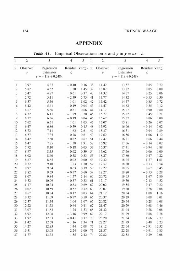
APPENDIX
Table A1. Empirical Observations on x and y in y ¼ axþ b.
1 2 3 4 5
x Observed
y
Regression
Estimates
y ¼ 4.119þ 0.248x
Residual
xVar(x)
1 3.97 4.37 � 0.40 0.16
2 5.82 4.62 1.20 1.45
3 5.47 4.87 0.61 0.37
4 2.72 5.11 � 2.39 5.73
5 6.37 5.36 1.01 1.02
6 5.42 5.61 � 0.19 0.04
7 6.67 5.86 0.81 0.66
8 4.32 6.11 � 1.79 3.20
9 6.17 6.36 � 0.19 0.04
10 7.62 6.61 1.01 1.03
11 6.47 6.86 � 0.39 0.15
12 8.72 7.11 1.62 2.61
13 6.57 7.35 � 0.78 0.61
14 8.42 7.60 0.82 0.67
15 6.47 7.85 � 1.38 1.91
16 7.92 8.10 � 0.18 0.03
17 8.97 8.35 0.62 0.39
18 8.02 8.60 � 0.58 0.33
19 8.87 8.85 0.02 0.00
20 10.32 9.10 1.23 1.50
21 9.97 9.34 0.63 0.39
22 8.82 9.59 � 0.77 0.60
23 8.07 9.84 � 1.77 3.14
24 9.52 10.09 � 0.57 0.33
25 11.17 10.34 0.83 0.69
26 10.02 10.59 � 0.57 0.32
27 10.67 10.84 � 0.17 0.03
28 10.32 11.09 � 0.77 0.59
29 12.37 11.34 1.04 1.07
30 12.22 11.58 0.64 0.41
31 13.07 11.83 1.24 1.53
32 8.92 12.08 � 3.16 9.99
33 11.92 12.33 � 0.41 0.17
34 11.42 12.58 � 1.16 1.34
35 14.27 12.83 1.44 2.08
36 15.31 13.08 2.24 5.00
37 11.77 13.33 � 1.55 2.42
1 2 3 4 5
x Observed
y
Regression
Estimates
y ¼ 4.119þ 0.248x
Residual
xVar(x)
38 14.42 13.57 0.85 0.72
39 13.87 13.82 0.05 0.00
40 14.32 14.07 0.25 0.06
41 13.77 14.32 � 0.55 0.30
42 15.42 14.57 0.85 0.72
43 14.47 14.82 � 0.35 0.12
44 14.17 15.07 � 0.90 0.80
45 15.77 15.32 0.45 0.21
46 15.62 15.57 0.06 0.00
47 16.07 15.81 0.26 0.07
48 15.92 16.06 � 0.14 0.02
49 15.37 16.31 � 0.94 0.89
50 17.62 16.56 1.06 1.12
51 17.47 16.81 0.66 0.44
52 16.92 17.06 � 0.14 0.02
53 16.37 17.31 � 0.94 0.88
54 17.62 17.56 0.06 0.00
55 18.27 17.80 0.47 0.22
56 19.32 18.05 1.27 1.61
57 17.57 18.30 � 0.73 0.54
58 19.22 18.55 0.67 0.45
59 18.27 18.80 � 0.53 0.28
60 20.72 19.05 1.67 2.80
61 17.17 19.30 � 2.13 4.52
62 20.02 19.55 0.47 0.22
63 20.07 19.80 0.28 0.08
64 21.12 20.04 1.08 1.16
65 20.37 20.29 0.08 0.01
66 20.82 20.54 0.28 0.08
67 21.47 20.79 0.68 0.46
68 21.32 21.04 0.28 0.08
69 22.17 21.29 0.88 0.78
70 23.20 21.54 1.66 2.77
71 22.27 21.79 0.48 0.23
72 18.12 22.04 � 3.91 15.32
73 21.37 22.28 � 0.91 0.83
74 22.82 22.53 0.29 0.08
FRENCK WAAGE154
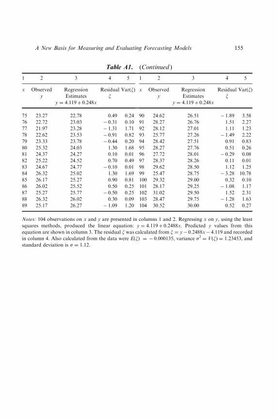
Table A1. (Continued )
1 2 3 4 5
x Observed
y
Regression
Estimates
y ¼ 4.119þ 0.248x
Residual
xVar(x)
75 23.27 22.78 0.49 0.24
76 22.72 23.03 � 0.31 0.10
77 21.97 23.28 � 1.31 1.71
78 22.62 23.53 � 0.91 0.82
79 23.33 23.78 � 0.44 0.20
80 25.32 24.03 1.30 1.68
81 24.37 24.27 0.10 0.01
82 25.22 24.52 0.70 0.49
83 24.67 24.77 � 0.10 0.01
84 26.32 25.02 1.30 1.69
85 26.17 25.27 0.90 0.81
86 26.02 25.52 0.50 0.25
87 25.27 25.77 � 0.50 0.25
88 26.32 26.02 0.30 0.09
89 25.17 26.27 � 1.09 1.20
1 2 3 4 5
x Observed
y
Regression
Estimates
y ¼ 4.119þ 0.248x
Residual
xVar(x)
90 24.62 26.51 � 1.89 3.58
91 28.27 26.76 1.51 2.27
92 28.12 27.01 1.11 1.23
93 25.77 27.26 � 1.49 2.22
94 28.42 27.51 0.91 0.83
95 28.27 27.76 0.51 0.26
96 27.72 28.01 � 0.29 0.08
97 28.37 28.26 0.11 0.01
98 29.62 28.50 1.12 1.25
99 25.47 28.75 � 3.28 10.78
100 29.32 29.00 0.32 0.10
101 28.17 29.25 � 1.08 1.17
102 31.02 29.50 1.52 2.31
103 28.47 29.75 � 1.28 1.63
104 30.52 30.00 0.52 0.27
Notes: 104 observations on x and y are presented in columns 1 and 2. Regressing x on y, using the least
squares methods, produced the linear equation: y ¼ 4.119þ 0.2488x. Predicted y values from this
equation are shown in column 3. The residual x was calculated from x ¼ y� 0.2488x� 4.119 and recorded
in column 4. Also calculated from the data were E(x) ¼ � 0.000135, variance s2 ¼ V(x) ¼ 1.23453, and
standard deviation is s ¼ 1.12.
A New Basis for Measuring and Evaluating Forecasting Models 155

This page intentionally left blank

FORECASTING USING INTERNAL
MARKETS, DELPHI, AND OTHER
APPROACHES: THE KNOWLEDGE
DISTRIBUTION GRID
Daniel E. O’Leary
ABSTRACT
Much forecasting is done by experts, who either make the forecaststhemselves or who do opinion research to gather such forecasts. This isconsistent with previous knowledge management research that typicallyhas focused on directly soliciting knowledge from those with greaterrecognized expertise.
However, recent research has found that in some cases, electronicmarkets, whose participants are not necessarily individual experts, oftenhave been found to be more effective aggregated forecasters. Thissuggests that knowledge management take a similar tact and expand theperspective to include internal markets. As a result, this chapter extendsthe use of internal markets to be included in knowledge management, thusexpanding the base of knowledge to gathering from nonexperts.
In particular, in this paper I examine the use of human expertise andopinion as a basis to forecast a range of different events. This chapter usesa ‘‘knowledge distribution grid’’ as a basis for understanding which kindof forecasting tool is appropriate for particular forecasting situations. Weexamine a number of potential sources of forecast information, including
Advances in Business and Management Forecasting, Volume 6, 157–172
Copyright r 2009 by Emerald Group Publishing Limited
All rights of reproduction in any form reserved
ISSN: 1477-4070/doi:10.1108/S1477-4070(2009)0000006010
157

knowledge acquisition, Delphi techniques, and internal markets. Each isseen as providing forecasting information for unique settings.
1. INTRODUCTION
Some forecasting questions, such as ‘‘Who will be elected President?’’ or‘‘Who will win the Olympic Medal in Water Polo?’’ can use expert opinion,general opinion polls, or electronic markets as a basis of forecasting. Recentresults have found that although expert opinion and opinion polls mightreceive the most publicity in the media, electronic markets are likely toprovide a more accurate forecast of what will happen.
The same approaches might be used to address similar enterprise orcorporate forecasting problems. As a result, it is probably not surprisingthat recent results have found that corporate internal markets provideinsight that often is better than expert opinion.
However, having nonexperts, use internal virtual dollars to help developforecasts, to assist corporations is a break from the classic approach, basedon having experts forecast events.
1.1. Knowledge Management and Forecasting
Knowledge management systems generally gather knowledge from experts.For example, as seen in O’Leary (2008a, 2008b), the classic notion of expertsystems and even new artifacts, such as Wikis, are based on the notion thatsome people know more than others and the knowledge managementsystems let them share that knowledge.
Further, historically, knowledge management has been backwardlooking, accumulating knowledge about what has occurred. For example,for consultants, knowledge management systems may gather proposals ofprevious engagements or summaries of actual engagements as keysummaries of knowledge. Furthermore, other documents, such as newsarticles are likely to be accessible in such systems. Accordingly, virtually allthe so-called knowledge management resources are backward looking.Knowledge is summarized for expert decision makers and they use thathistorical information to anticipate future events. The systems rarelyprovide forward-looking information, such as forecasts. Instead, experts use
DANIEL E. O’LEARY158

the knowledge in the systems to generate forward-looking views andforecasts.
1.2. Internal Prediction Markets
However, recently enterprises and other organizations have begun to useinternal markets to anticipate and forecast future events. For example(Wolfers & Zitzewitz, 2004), the Department of Defense was interested inknowing questions such as ‘‘Will the U.S. Military withdraw from country Ain two years or less?’’
Hewlett-Packard was one of the first companies to use such internalprediction markets (e.g., Totty, 2006). In 1996, they were concerned withhow well such markets could forecast monthly printer sales. Approximately15–20 people from various parts of the company were chosen to be a part ofthe market. Participants were given some cash and securities that wereconstructed to represent various monthly printer sales forecasts. In theirmarket, only the winning sales number paid off to the participants. Usingthis internal market approach, the markets beat the experts 6 out of 8 times.
1.3. Expert vs. Nonexpert and Historic vs. Future
Accordingly, internal markets provide an approach that allows us to changethe focus of knowledge management from just gathering knowledge fromexperts to a broader base of users (nonexpert). In addition, internal marketsallow us to change our focus from a historical one to a view aimed atforecasting the future, rather than a historical view, summarizing the past.These results are summarized in Fig. 1.
1.4. Purpose of this Chapter
As a result, we need to understand those conditions under which to usealternative knowledge management approaches, particularly in forecastingof future events. Thus, this chapter is concerned with analyzing differentapproaches to gather human opinion and information as to the possibleoccurrence of future events.
Forecasting the answers to difficult problems often depends on asking theright person or group of people the right question. However, knowing which
Forecasting Using Internal Markets, Delphi and Other Approaches 159

approach to use is not always clear. Thus, the remaining purpose of thischapter is to outline two ‘‘knowledge distribution grids’’ that can be used tohelp determine which approach to forecasting is appropriate for particularsituations, based on different characteristics of knowledge.
1.5. Outline of this Chapter
Section 2 examines notions of shallow knowledge vs. deep knowledge,whereas Section 3 examines distributed knowledge vs. concentrated knowl-edge. Section 4 examines a number of approaches used to gather knowledgein the different settings. Section 5 brings together Sections 2–4, andgenerates a knowledge distribution grid that allows us to better understandwhich approaches are useful for different forecasting opportunities in thecases of shallow and deep knowledge and distributed knowledge andconcentrated knowledge. Section 6 extends the knowledge characteristics todynamic and stable, and deterministic and probabilistic. Section 7 reviewssome limitations of forecasting approaches, whereas Section 8 provides abrief summary of the chapter, and examines some contributions of thechapter and analyzes some potential extensions.
Fig. 1. Knowledge Management and Internal Markets.
DANIEL E. O’LEARY160

2. SHALLOW KNOWLEDGE VS. DEEP KNOWLEDGE
Different people may have knowledge about an area based on a range offactors, including ability, education, or experience. Further, knowledge maybe distributed to a broad range or a small group of users. Thus, thatknowledge may be distributed in varying depths to a range of users. Thepurpose of this section is to briefly discuss the first dichotomy, shallow anddeep knowledge, and then examine some of the implications of thatdichotomy.
2.1. Shallow Knowledge
In many cases, individuals have only shallow knowledge about particularissues. At the extreme, as noted by Hayek (1945, pp. 521–522)
there is beyond question a body of very important but unorganized knowledge which
cannot possibly be called scientific in the sense of knowledge of general rules: the
knowledge of the particular circumstances of time and place . . . (and that individuals
have) . . . special knowledge of circumstances of the fleeting moment, not known to
others.
According to this description, there is asymmetric knowledge, particu-larly, in the case of knowledge that appears to describe events orcontemporary activity. In particular, the knowledge is not general scientificknowledge. Further, that knowledge is distributed to a number of people,and the knowledge that people have may be relatively shallow.
In particular, knowledge is considered to be shallow if it is not connectedto other ideas or if it is only loosely connected to other knowledge. Anotherview is that knowledge is shallow if it is more data than knowledge, or if thatknowledge is or can be ‘‘compiled.’’ For example, Chandrasekaran andMittal (1999) suggested that if the knowledge can be put in a table (i.e., aclassic table lookup) then that knowledge can be compiled and thecorresponding knowledge is not particularly deep.
2.2. Deep Knowledge
Knowledge is regarded as ‘‘deep’’ if central or key issues in a discipline needto be understood to understand the issues at hand. Further, generally,knowledge has greater depth if it is connected to other ideas.
Forecasting Using Internal Markets, Delphi and Other Approaches 161

Deep knowledge also has been thought to be based on ‘‘first principles’’(e.g., Reiter, 1987; Chandrasekaran & Mittal, 1999), rather than just basedon causal knowledge. First principles provide a basis to reason from orabout a set of issues. As an example, in the case of diagnostic systems, firstprinciples ultimately employ a description of some system and observationsof the behavior of the system and then reasons as to why the system mayhave failed.
Organizations are aware of and encourage cultivation of deep knowledge.For example, professional service firms have consulting ‘‘experts’’ inparticular areas. A review of most consultants’ resumes will rapidly tellyou their areas of expertise. Universities are famous for having faculties thathave deep knowledge in what can sometimes be very narrow areas.Oftentimes professional certifications can be issued to indicate that a level ofdepth and breadth in knowledge has been attained by an individual, forexample, ‘‘certified public accountant’’ (CPA).
2.3. Shallow Knowledge vs. Deep Knowledge
One view of knowledge is that it comes in ‘‘chunks’’ (Anderson & Lebiere,1998). Deep knowledge takes more ‘‘chunks’’ to be captured or described.Further, if there are numerous links between the chunks, rather than fewer,then that is another indication of deep knowledge. Thus, number of‘‘chunks’’ provides one measure of the depth.
Research and other activities might change the classification bygenerating additional links or influencing the chunks. Potentially shallowknowledge may be made deeper if fragmented notions are connected orlinked to other possibly related ideas. Alternatively, deep knowledge may bemade shallower if it can be decomposed into relatively unconnected chunks.
2.4. Implications of Shallow vs. Deep Knowledge
One of the key tenets to system sciences (Ashby, 1956; Weick, 1969, p. 44) isthat ‘‘it takes variety to destroy variety,’’ or ‘‘it takes equivocality to removeequivocality.’’ Thus, to paraphrase, ‘‘it takes shallow knowledge to captureshallow knowledge and deep knowledge to capture deep knowledge.’’ If theknowledge of concern is shallow, rather than deep, then representation ofthe knowledge is likely to be easier. In addition, if the knowledge is shallow,then the basic approach used to capture shallow knowledge is likely to be
DANIEL E. O’LEARY162

more straightforward. Further, capturing deep knowledge is likely to bemore time consuming, and require greater resources.
2.5. Deep Knowledge and Internal Prediction Markets
In some settings deep knowledge is necessary to be able to attain anappropriate level of insight to a problem, even when using internalprediction markets. For example, if we are trying to forecast a flu epidemicthis fall then knowledge of current viruses in circulation and the diffusion ofthose over time would be helpful at understanding the issue; otherwise,responses are likely to be little more than a random guess. Shallowknowledge of a problem, even if it is aggregated with knowledge of others isnot likely to facilitate forecasting.
3. DISTRIBUTED KNOWLEDGE VS.
CONCENTRATED KNOWLEDGE
In general, knowledge about forecasting events of interest can be what wecall ‘‘distributed’’ among members of a population, such as an enterprise, orit can be concentrated in the hands of a relative few. The extent to whichknowledge is distributed or concentrated can influence which approach isused to gather that knowledge.
3.1. Distributed Knowledge
Hayek (1945, p. 519) argues that much knowledge (in particular, knowledgeof circumstances) is not ‘‘concentrated,’’ but instead is what we will call‘‘distributed,’’
The peculiar character of the problem of a rational economic order is determined
precisely by the fact that the knowledge of the circumstances of which we must make use
never exists in concentrated or integrated form, but solely as dispersed bits of incomplete
and frequently contradictory knowledge which all of the separate individuals possess.
With some members knowing some things that others do not, this resultsin ‘‘information asymmetry.’’ Thus, with distributed knowledge, as noted byHayek (1945, p. 520) ‘‘knowledge (is) not given to anyone in its totality.’’
Forecasting Using Internal Markets, Delphi and Other Approaches 163

3.2. Concentrated Knowledge
Hayek (1945) was specifically concerned with settings where a central groupmade decisions and set prices for the overall economy, rather than lettingmarket forces determine prices. However, the concern generalizes toenterprises where, a central group of managers makes many decisions,rather than letting a broad range of users in the enterprise determine whatshould be done. Although some knowledge is concentrated in a few experts,much knowledge is distributed to a broad range of people in the enterprise.As a result, a critical characteristic of knowledge is whether knowledge isdistributed in many different people or if knowledge is concentrated in a fewspecialists, and ultimately how the enterprise addresses this issue.
Concentrated knowledge refers to situations where expertise in aparticular area is accomplished. There are numerous measures ofconcentration in different professional fields. For example, in accounting,there are numerous certifications, such as a CPA or certified managementaccountant (CMA). In education, various degree levels, for example, Ph.D.,also denote concentration of knowledge.
In some economic systems, concentrated knowledge is assumed of centralplanners. In sporting events, odds makers (e.g., those from Las Vegas) areconsidered a concentrated source of knowledge. Other such assumedconcentrated settings include planning departments or strategic planners.
3.3. Implications of Distributed or Concentrated Knowledge
In either case if we wish to manage the knowledge and make good decisionswe need to determine the extent to which knowledge is either concentratedor distributed. The extent to which knowledge is concentrated or distributedinfluences the approaches that we will use to gather that knowledge. Thus,there are implications if the knowledge is distributed or concentrated.
If the knowledge is concentrated, then approaches to gather theknowledge would focus only on the small group with the residentknowledge. If we wish to be unobtrusive, then we could gather knowledgeor implied knowledge from what people do. As a result, in the case ofconsultants, we could gather documents that consultants have generatedand make those documents available to others, for example, engagementproposals and summaries. If the knowledge is concentrated into only a smallgroup, then using an internal market to gather knowledge is not likely to beeffective for various reasons discussed in the following text.
DANIEL E. O’LEARY164

With distributed knowledge one must use approaches that tap into theasymmetric knowledge available to the many knowledgeable participants. Ifthe knowledge is distributed, then gathering knowledge must take a differenttact that tries to assemble the knowledge into an aggregated totality of sorts.In the case of forecasts, one such approach is internal markets, where we tryto generate a solution that incorporates all of the disparate knowledge,through the choice of one alternative over another or an indexrepresentative of the choice concern.
3.4. Knowledge Diffusion
Knowledge is more likely to diffuse if there are so-called ‘‘network effects’’that are dependent on communication and distributed knowledge. Thus,distributed knowledge seems more likely to diffuse, and more likely todiffuse more rapidly, than concentrated knowledge.
4. KNOWLEDGE GATHERING FOR FORECASTING
One of Hayek’s (1945, p. 520) key concerns was with investigating ‘‘what isthe best way of utilizing knowledge initially dispersed among all the people(as) is at least one of the main problems of economic policy – or of designingan efficient economic system.’’ This chapter is basically concerned with thesame issue. In particular, there are a number of ways to gather knowledgethat could be used for forecasting, including the following.
4.1. ‘‘Man on the Street’’ Interview (One Person or More)
A well-known approach to gathering knowledge is to interview the random‘‘man on the street,’’ in an attempt to gather opinion or general knowledgeof the populace. Such opinions could provide interviewers with an insightinto a number of issues, such as would a particular product sell or whomight win the presidential elections. Unfortunately, such interviews may ormay not be successful at gathering the opinions desired, in part based on thelimited sample, and the particular opinion.
The next step to generalization of ‘‘man on the street’’ interviews is toexpand the sample size and gather opinion from a broader base ofparticipants, and then aggregate their responses. Unfortunately, aggregation
Forecasting Using Internal Markets, Delphi and Other Approaches 165

is not an easy and noncontroversial issue. Given a base of opinions, how dowe aggregate?
In general, opinion polls do not seek out those with any particularly deepexpertise, but instead, seek a reasonable sample of some particularpopulation. For example on college campuses, not surprisingly, frequently,the concern is with the opinion of the student population.
4.2. Knowledge Acquisition (1–10 People)
The development of the so-called ‘‘expert systems’’ and ‘‘knowledge-basedsystems’’ led to the analysis of what became known as knowledgeacquisition, generally from a single expert (e.g., Rose, 1988). Enterprisesgenerated a number of clever approaches to capture knowledge, such asvideotaping events or the transfer of information between human actors(e.g., Kneale, 1986; Shpilberg, Graham, & Schatz, 1986) and those inte-rested in being able to capture the knowledge.
However, over time there has been an interest in acquiring knowledgefrom multiple experts, rather than just a single expert. In the case ofknowledge acquisition, ‘‘multiple’’ typically meant 2, 3, or 4, and rarelymore than 10 (e.g., O’Leary, 1993; O’Leary, 1997). With multiple experts insuch small samples, comes concerns as to whether the experts are from thesame paradigm and whether the combination of expertise from differentparadigms is sensible, and if it is sensible, how those multiple judgmentsshould be combined.
4.3. Delphi Technique (5–30 People)
The Delphi technique (Dalkey, 1969; Green, Armstrong, & Graefe, 2007) isused to generate opinion, typically from expert. Using a three-step approachof gathering anonymous responses, controlling information feedback in anumber of iterations, and aggregating opinions, the technique has beenprimarily used to generate consensus among a set of experts. The initialinvestigations used between 11 and 30 members in the group, but otherinvestigations have used as few as 5. As a result, generally, this approach isused when the available expertise is distributed to a sufficiently large numberof agents. In addition, this approach is used when there are time andresources to iteratively go back and forth with the experts to gradually elicitgroup consensus.
DANIEL E. O’LEARY166

4.4. Enterprise or Internal Prediction Markets (20 or More People)
Enterprise markets, also known as ‘‘internal prediction markets’’ can beused to gather knowledge for forecasting a wide range of issues. Althoughinternal prediction markets are not known as a knowledge management tool,in some cases they likely offer the best opportunity for gathering knowledge.
For example, recently internal prediction markets have been used toexamine such issues as ‘‘Will our store in Shanghai open on time?’’ Suchmarkets are ‘‘enterprise markets’’ since they are used by enterprise toforecast the future.
Internal prediction markets can be ‘‘informed markets’’ where theparticipants are those with more experience or knowledge about a particulararea. Informed markets are necessary when the topic requires deepknowledge. For example, a market aimed at forecasting flu virus mutationlikely necessarily would be an expert group.
5. A KNOWLEDGE DISTRIBUTION GRID
Our discussion about shallow knowledge vs. deep knowledge anddistributed knowledge vs. concentrated knowledge, and knowledge gather-ing for forecasting is summarized in Fig. 2. Each axis has one of the twocharacteristics on it, yielding four different settings. It is referred to as aknowledge distribution grid because it provides view as to where knowledgeis distributed and tools for gathering knowledge in different settings.
5.1. Gathering vs. Communicating
To this point, we have focused on gathering knowledge – whether dispersedor concentrated. However, in addition, the approaches provide differentialcommunication devises between the sources of the knowledge and ultimatelystructuring the knowledge in a usable forecast form.
For example, when compared to markets, some authors think that Delphimay be easier to maintain confidentiality (e.g., Green et al., 2007) and thatDelphi is more difficult to manipulate. Further, because Delphi is groundedin feedback, the approach is a bit more efficient than markets because otherparticipants directly benefit from research of other participants that surfaceas feedback. This is in contrast with markets where participants each need todo their own research.
Forecasting Using Internal Markets, Delphi and Other Approaches 167
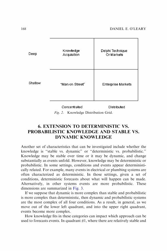
6. EXTENSION TO DETERMINISTIC VS.
PROBABILISTIC KNOWLEDGE AND STABLE VS.
DYNAMIC KNOWLEDGE
Another set of characteristics that can be investigated include whether theknowledge is ‘‘stable vs. dynamic’’ or ‘‘deterministic vs. probabilistic.’’Knowledge may be stable over time or it may be dynamic, and changesubstantially as events unfold. However, knowledge may be deterministic orprobabilistic. In some settings, conditions and events appear deterministi-cally related. For example, many events in electrical or plumbing systems areoften characterized as deterministic. In those settings, given a set ofconditions, deterministic forecasts about what will happen can be made.Alternatively, in other systems events are more probabilistic. Thesedimensions are summarized in Fig. 3.
If we suppose that dynamic is more complex than stable and probabilisticis more complex than deterministic, then dynamic and probabilistic systemsare the most complex of all four conditions. As a result, in general, as wemove out of the lower left quadrant, and into the upper right quadrant,events become more complex.
How knowledge fits in these categories can impact which approach can beused to forecasts events. In quadrant #1, where there are relatively stable and
Fig. 2. Knowledge Distribution Grid.
DANIEL E. O’LEARY168
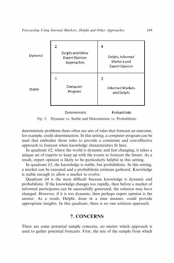
deterministic problems there often are sets of rules that forecast an outcome,for example, credit determination. In this setting, a computer program can beused that embodies those rules to provide a consistent and cost-effectiveapproach to forecast when knowledge characteristics fit here.
In quadrant #2, where the world is dynamic and fast changing, it takes aunique set of experts to keep up with the events to forecast the future. As aresult, expert opinion is likely to be particularly helpful in this setting.
In quadrant #3, the knowledge is stable, but probabilistic. In this setting,a market can be executed and a probabilistic estimate gathered. Knowledgeis stable enough to allow a market to evolve.
Quadrant #4 is the most difficult because knowledge is dynamic andprobabilistic. If the knowledge changes too rapidly, then before a market ofinformed participants can be successfully generated, the solution may havechanged. However, if it is too dynamic, then perhaps expert opinion is theanswer. As a result, Delphi, done in a time manner, could provideappropriate insights. In this quadrant, there is no one solution approach.
7. CONCERNS
There are some potential sample concerns, no matter which approach isused to gather potential forecasts. First, the size of the sample from which
Fig. 3. Dynamic vs. Stable and Deterministic vs. Probabilistic.
Forecasting Using Internal Markets, Delphi and Other Approaches 169

the knowledge and forecasts is gathered is critical to generating anappropriate view of the future. With internal markets, this issue is referredto under the notion of ‘‘thin markets’’ where there are too few traders toguarantee an effective and efficient market. Probably not unexpectedly,when using internal markets, in general, larger markets are better. However,if the sample size gets too large, then Delphi can bog down.
Second, sample bias from the population investigated has been consideredby researchers in most of these disciplines. In general, the smaller thepopulation is being drawn from, the bigger is the potential problem of bias.However, in some of the approaches discussed earlier, for example, in thecase of knowledge acquisition, the problem has been largely ignored.
Third, there is the potential for conflicts between points of view. In thearena of knowledge acquisition, O’Leary (1993, 1997) has investigated thisissue. As part of the concern of knowledge acquisition from multipleexperts, there has been concern with the so-called ‘‘paradigm myopia.’’ Inthat setting, with few experts as the basis of the knowledge used, any bias islikely to be reflected in the forecast that is made. Similarly, when usingDelphi, a diverse opinion set can drive the group to generate uniquesolutions or deadlock them.
8. SUMMARY, CONTRIBUTIONS, AND EXTENSIONS
This chapter has differentiated characteristics of knowledge along a numberof dimensions and investigated those dichotomous characteristics, including
expert vs. non-expert and historic vs. future, deep vs. shallow and concentrated vs. distributed, dynamic vs. stable and deterministic vs. probabilistic.
Using those characteristic pairs, we analyzed settings where differentapproaches were more appropriate than others. In particular, we generatedthe knowledge distribution grid, and used the grid to differentiate betweendifferent approaches that might be used for forecasting future events. Fourdifferent basic approaches were discussed: ‘‘man-on-the-street,’’ ‘‘knowledgeacquisition,’’ Delphi technique, and internal prediction markets. Marketswere labeled as ‘‘informed’’ for those involving experts, and ‘‘enterprise’’ forthose internally conducted by enterprises to address issues of direct concernto the enterprise.
DANIEL E. O’LEARY170

8.1. Contributions
This chapter has extended knowledge management to be forward lookingand to include internal markets as a means of gathering knowledge from abroad base of users. Virtually all previous knowledge management hasfocused on knowledge management as a medium to capture historicalinformation. Further, internal markets have been ignored as a knowledgemanagement tool. In addition, comparison of internal markets toapproaches such as Delphi, have received little attention.
This chapter provides three distinct sets of grids featuring differentknowledge characteristics. Each of those grids provides the ability toinvestigate knowledge characteristics, and how those knowledge character-istics influence different approaches to gathering information for forecastingfuture events.
8.2. Extensions
This research can be extended in a number of directions. First, we couldexpand the number of methods examined in Section 4. For example, otherapproaches, such as using surveys to gather knowledge and opinions couldbe generated. Second, the discussion in this chapter has suggested that thetime and resources available also influence the choice of an approach toforecast the future. Compiled expertise would be a rapid approach, butrunning an internal market while investigating time constrained issues is notlikely to provide timely returns. Third, in some cases there appear to bemultiple feasible approaches to problems. For example, Delphi and internalmarkets both seem feasible with approximately 20 or more people and anexpert environment. However, it is not clear which approaches provide the‘‘best results.’’ As a result, the two approaches could be compared for whichworks best under which conditions, and the strengths and weaknesses ofeach could be more fully fleshed out.
REFERENCES
Anderson, J., & Lebiere, C. (1998). The atomic components of thought. Mahwah, NJ: Lawrence
Erlbaum and Associates.
Ashby, W. R. (1956). An introduction to cybernetics. New York: Wiley.
Chandrasekaran, B., & Mittal, S. (1999). Deep versus compiled knowledge approaches to
diagnostic problem solving. International Journal of Human Computer Studies, 51,
357–368.
Forecasting Using Internal Markets, Delphi and Other Approaches 171

Dalkey, N. C. (1969). The delphi method: An experimental study of group opinion, June. Rand
Report RM-5888-PR. Available at http://www.rand.org/pubs/research_memoranda/
2005/RM5888.pdf
Green, K. C., Armstrong, J. S., & Graefe, A. (2007). Methods to elicit forecasts from groups:
Delphi and prediction markets compared, August 31. MPRA Paper 4663.
Hayek, F. (1945). The use of knowledge in society. The American Economic Review,
XXXV(September 4), 519–530.
Kneale, D. (1986). How Coopers & Lybrand put expertise into its computers. The Wall Street
Journal (November 14).
O’Leary, D. E. (1993). Determining differences in expert judgment. Decision Sciences, 24(2),
395–407.
O’Leary, D. E. (1997). Validation of computational models based on multiple heterogeneous
knowledge sources. Computational and Mathematical Organization Theory, 3(2), 75–90.
O’Leary, D. E. (2008a). Expert systems. In: B. Wah (Ed.), Encyclopedia of computer science.
New York, USA: Wiley.
O’Leary, D. E. (2008b). Wikis: From each according to his knowledge. Computer, 41(2), 34–41.
Reiter, R. (1987). A theory of diagnosis from first principles. Artificial Intelligence, 32, 57–95.
Rose, F. (1988). An ‘electronic’ clone of a skilled engineer is very hard to create. The Wall Street
Journal (August 12).
Shpilberg, D., Graham, L., & Schatz, H. (1986). Expertax: An expert system for corporate tax
accrual and planning. Expert Systems, 3(3), 136–151.
Totty, M. (2006). Business solutions. The Wall Street Journal (June 19), R9.
Weick, K. (1969). The social psychology of organizing. Addison-Wesley: Reading, MA.
Wolfers, J., & Zitzewitz, E. (2004). Prediction markets. Journal of Economic Perspectives, 18(2),
107–126.
DANIEL E. O’LEARY172
THE EFFECT OF CORRELATION
BETWEEN DEMANDS ON
HIERARCHICAL FORECASTING
Huijing Chen and John E. Boylan
ABSTRACT
The forecasting needs for inventory control purposes are hierarchical.For stock keeping units (SKUs) in a product family or a SKU storedacross different depot locations, forecasts can be made from the individualseries’ history or derived top–down. Many discussions have been found inthe literature, but it is not clear under what conditions one approach isbetter than the other. Correlation between demands has been identified asa very important factor to affect the performance of the two approaches,but there has been much confusion on whether it is positive or negativecorrelation. This chapter summarises the conflicting discussions in theliterature, argues that it is negative correlation that benefits the top–downor grouping approach, and quantifies the effect of correlation throughsimulation experiments.
INTRODUCTION
Many organisations operate in a multi-item, multi-level environment. Ingeneral, they have to ‘‘cope with well over 100 time series with numbers over
Advances in Business and Management Forecasting, Volume 6, 173–188
Copyright r 2009 by Emerald Group Publishing Limited
All rights of reproduction in any form reserved
ISSN: 1477-4070/doi:10.1108/S1477-4070(2009)0000006011
173

10,000 being quite common’’ (Fildes & Beard, 1992). These time series areoften related. For example, a company may group similar products inproduct families according to specifications, colours, sizes, etc. Alterna-tively, in a multi-echelon inventory system, a stock-keeping unit’s sales maybe recorded in many different locations at varying levels of aggregation.Therefore, in such cases, the data available and the need for forecasts arehierarchical.
A substantial part of the forecasting literature has been devoted to modelsand methods for single time series. However, as indicated earlier, the short-term forecasting need for production and inventory control purposes is toaddress a large amount of series simultaneously. Duncan, Gorr, andSzczypula (1993) argued that ‘‘forecasting for a particular observational unitshould be more accurate if effective use is made of information, not onlyfrom a time series on that observational unit, but also from time series onsimilar observational units.’’
There have been many discussions on group forecasting in the literature.However, no clear conclusions have been reached on the conditions underwhich the grouping approach is better than the individual approach.Correlation between demands has been identified as a very important factor,but there has been much confusion about whether positive or negativecorrelation would benefit grouping. This chapter is presented as follows:contrasting arguments are discussed in the next section; then the findings onthe role of correlation from simulation experiments are presented; and,finally, the chapter is summarised with our conclusions. The overall purposeof this chapter is to dispel some of the confusion in the literature on howcorrelation affects the grouping approach.
DEBATES AND CONFUSION IN THE LITERATURE
It is well recognised that to obtain better forecasts, one should make betteruse of available forecasting series. Some practitioners such as Muir (1983),McLeavey and Narasimhan (1985), and Fogarty and Hoffmann (1983) haveargued that forecasting an aggregate and then allocating it to items is moreaccurate than generating individual forecasts. Their argument was that thetop–down approach resulted in more accurate predictions since aggregatedata were more stable.
Schwarzkopf, Tersine, and Morris (1988) pointed out two problems ofusing the top–down approach: model incompleteness and positive correla-tion. They argued that the aggregate model may not completely describe the
HUIJING CHEN AND JOHN E. BOYLAN174

processes in the individual series, that is, there were model differencesamong the series. When the total forecast was disaggregated back to theitem level, correlated errors were produced. They commented that ‘‘thismodelling error can be quite large and may override the more precisepotential of top–down forecasts’’ (Schwarzkopf et al., 1988). The same pointwas also made by Shlifer and Wolff (1979). The second problem was that ifthere was a strong positive correlation in demand for items in a group, thevariance for the aggregate was increased by the amount of the covarianceterm. Schwarzkopf et al. (1988) advanced our understanding of some of thereasons why the top–down approach does not always lead to a moreaccurate subaggregate forecast.
Top–down forecasts have to be treated with caution. If the individualseries follow different demand generating processes, then the aggregatemodel does not reflect any of those individual processes. Although theaggregate data are less noisy, it does not always result in more accuratesubaggregate forecasts. Even when the modelling difference is not an issue,there is an additional problem of the disaggregation mechanism to beapplied.
One way to get around these problems is to group seasonal homogeneousseries. From a classical decomposition point of view, demand consists oflevel, trend, seasonality and noise. In a group of items, levels can be varying.Trends can be upwards or downwards and can have various degrees.However, seasonality is often more stable as it is affected by weather andcustoms. Chatfield (2004) pointed out that seasonal indices are usuallyassumed to change slowly through time, so that StESt�q, where q is theseasonal cycle. It makes more sense to use the grouping approach toestimate seasonality than to estimate level and trend as there is an issue ofmodelling difference. The problem of an appropriate disaggregationmechanism can also be avoided. For multiplicative seasonality, nodisaggregation mechanism is needed as seasonality is relative to the mean.For an additive model with common seasonal components across the group,a simple average can be used as the disaggregation method. Although it isdifficult to apply the grouping approach in general, we found it helpful inseasonal demand forecasting, that is, estimating level and trend individuallybut seasonality from the group.
Correlation has been identified as a very important factor to affect thegrouping and individual approaches, but there has been some confusionabout whether positive or negative correlation benefits grouping. Duncan,Gorr, and Szczypula (1998) argued for positive correlation. They claimedthat analogous series should correlate positively (co-vary) over time.
The Effect of Correlation between Demands on Hierarchical Forecasting 175

Then the co-variation would be able to ‘‘add precision to model estimatesand to adapt quickly to time-series pattern changes’’. However, Schwarzkopfet al. (1988) supported negative correlation as the covariance term wasincreased by positive correlation. The confusion lies in the distinctionbetween a common model and varied models. Given the same model, it isnegative correlation between series that reduces variability of the total andfavours the top–down approach. However, the more consistent the modelforms are, the more this favours the grouping approach; and consistencyof model forms is associated with positive correlations between series, notnegative correlations. Duncan et al. (1998) also identified the associationbetween consistency of model forms and positive correlations. However,positive correlations should not be used to identify whether different seriesfollow the same model, as sometimes the positive correlations may beincurred by a trend component, rather than the model form. Therefore,checks should be made on the consistency of models using other diagnostics,before employing correlation analysis to establish whether a grouped orindividual approach is preferable.
SIMULATION EXPERIMENTS
We used simulation experiments to examine the effect of correlationbetween demands on forecasting performance of the grouping andindividual approaches. It is argued that it is negative correlation that willbenefit the grouping approach when a common model is assumed; the mainpurpose of the simulation experiments is to quantify the effect.
Two simple models are assumed to generate demand
Yi;th ¼ miSh þ �i;th (1)
Yi;th ¼ mi þ Sh þ �i;th (2)
where i is a suffix representing the stock keeping unit (SKU) or the location,suffix t the year and t ¼ 1, 2, . . . , r (where r is the number of years’ datahistory), suffix h the seasonal period and h ¼ 1, 2, . . . , q (where q is thelength of the seasonal cycle), Y the demand, mi the underlying mean for theith SKU or location and is assumed to be constant over time but differentfor different SKUs or locations, Sh a seasonal index at seasonal period h(it is unchanging from year to year and the same for all SKUs or loca-tions under consideration), ei,th a random disturbance term for the ith
HUIJING CHEN AND JOHN E. BOYLAN176
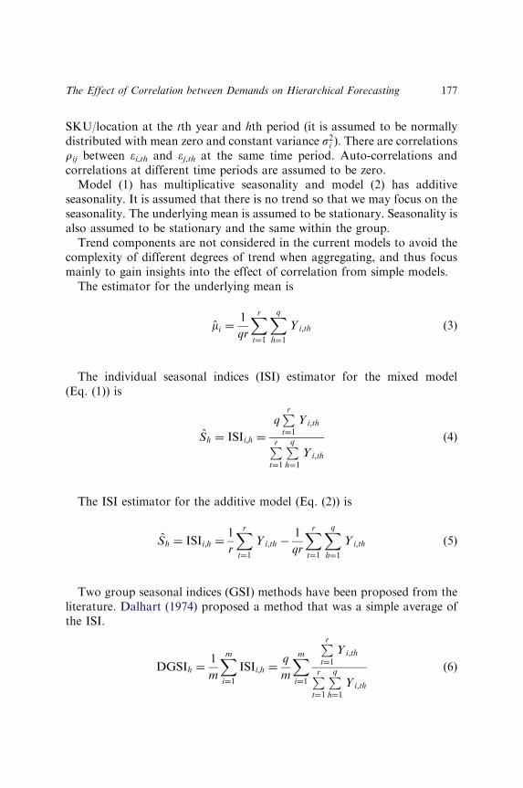
SKU/location at the tth year and hth period (it is assumed to be normallydistributed with mean zero and constant variance s2i ). There are correlationsrij between ei,th and ej,th at the same time period. Auto-correlations andcorrelations at different time periods are assumed to be zero.
Model (1) has multiplicative seasonality and model (2) has additiveseasonality. It is assumed that there is no trend so that we may focus on theseasonality. The underlying mean is assumed to be stationary. Seasonality isalso assumed to be stationary and the same within the group.
Trend components are not considered in the current models to avoid thecomplexity of different degrees of trend when aggregating, and thus focusmainly to gain insights into the effect of correlation from simple models.
The estimator for the underlying mean is
mi ¼1
qr
Xrt¼1
Xqh¼1
Yi;th (3)
The individual seasonal indices (ISI) estimator for the mixed model(Eq. (1)) is
Sh ¼ ISIi;h ¼
qPrt¼1
Yi;th
Prt¼1
Pqh¼1
Yi;th
(4)
The ISI estimator for the additive model (Eq. (2)) is
Sh ¼ ISIi;h ¼1
r
Xrt¼1
Yi;th �1
qr
Xrt¼1
Xqh¼1
Yi;th (5)
Two group seasonal indices (GSI) methods have been proposed from theliterature. Dalhart (1974) proposed a method that was a simple average ofthe ISI.
DGSIh ¼1
m
Xmi¼1
ISIi;h ¼q
m
Xmi¼1
Prt¼1
Yi;th
Prt¼1
Pqh¼1
Yi;th
(6)
The Effect of Correlation between Demands on Hierarchical Forecasting 177
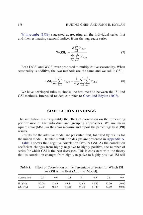
Withycombe (1989) suggested aggregating all the individual series firstand then estimating seasonal indices from the aggregate series
WGSIh ¼
qPrt¼1
YA;th
Prt¼1
Pqh¼1
YA;th
(7)
Both DGSI and WGSI were proposed to multiplicative seasonality. Whenseasonality is additive, the two methods are the same and we call it GSI.
GSIh1
mr
Xrt¼1
YA;th �1
mqr
Xrt¼1
Xqh¼1
YA;th (8)
We have developed rules to choose the best method between the ISI andGSI methods. Interested readers can refer to Chen and Boylan (2007).
SIMULATION FINDINGS
The simulation results quantify the effect of correlation on the forecastingperformance of the individual and grouping approaches. We use meansquare error (MSE) as the error measure and report the percentage best (PB)results.
Results for the additive model are presented first, followed by results forthe mixed model. Detailed simulation designs are presented in Appendix A.
Table 1 shows that negative correlation favours GSI. As the correlationcoefficient changes from highly negative to highly positive, the number ofseries for which GSI is the best decreases. This is consistent with the theorythat as correlation changes from highly negative to highly positive, ISI will
Table 1. Effect of Correlation on the Percentage of Series for Which ISIor GSI is the Best (Additive Model).
Correlation �0.9 �0.6 �0.3 0 0.3 0.6 0.9
ISI (%) 40.00 41.43 43.84 45.63 48.57 50.00 50.00
GSI (%) 60.00 58.57 56.16 54.38 51.43 50.00 50.00
HUIJING CHEN AND JOHN E. BOYLAN178
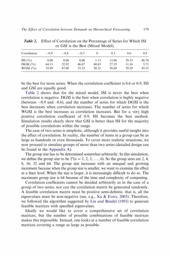
be the best for more series. When the correlation coefficient is 0.6 or 0.9, ISIand GSI are equally good.
Table 2 shows that for the mixed model, ISI is never the best whencorrelation is negative. DGSI is the best when correlation is highly negative(between �0.9 and –0.6), and the number of series for which DGSI is thebest decreases when correlation increases. The number of series for whichWGSI is the best increases as correlation increases. But for a very highpositive correlation coefficient of 0.9, ISI becomes the best method.Simulation results clearly show that GSI is better than ISI for the majorityof possible correlations within the range.
The case of two series is simplistic, although it provides useful insight intothe effect of correlation. In reality, the number of items in a group can be aslarge as hundreds or even thousands. To cover more realistic situations, wenow proceed to simulate groups of more than two series (detailed design canbe found in the Appendix A).
The group size has to be determined somewhat arbitrarily. In this simulation,we define the group size to be 2n(n ¼ 1, 2, 3, . . . , 6). So the group sizes are 2, 4,8, 16, 32 and 64. The group size increases with an unequal and growingincrement because when the group size is smaller, we want to examine the effectat a finer level. When the size is larger, it is increasingly difficult to do so. Themaximum group size is 64 because of the time and complexity of computing.
Correlation coefficients cannot be decided arbitrarily as in the case of agroup of two series, nor can the correlation matrix be generated randomly.A feasible correlation matrix must be positive semi-definite, that is, all theeigenvalues must be non-negative (see, e.g., Xu & Evers, 2003). Therefore,we followed the algorithm suggested by Lin and Bendel (1985) to generatefeasible matrices with specified eigenvalues.
Ideally we would like to cover a comprehensive set of correlationmatrices, but the number of possible combinations of feasible matricesmakes this impossible. Instead, one looks at a number of feasible correlationmatrices covering a range as large as possible.
Table 2. Effect of Correlation on the Percentage of Series for Which ISIor GSI is the Best (Mixed Model).
Correlation �0.9 �0.6 �0.3 0 0.3 0.6 0.9
ISI (%) 0.00 0.00 0.00 1.13 13.96 29.55 48.78
DGSI (%) 64.11 52.92 46.67 40.65 27.35 11.16 5.71
WGSI (%) 35.89 47.08 53.33 58.21 58.69 59.29 45.51
The Effect of Correlation between Demands on Hierarchical Forecasting 179
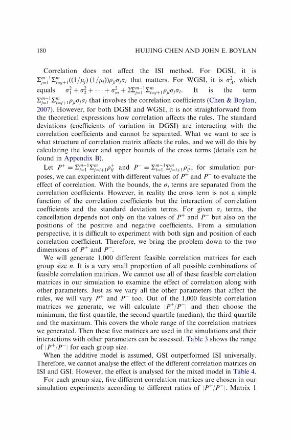
Correlation does not affect the ISI method. For DGSI, it is
Sm�1j¼1 Sm
l¼jþ1ðð1=mjÞ ð1=mlÞÞrjlsjsl that matters. For WGSI, it is s2A, which
equals s21 þ s22 þ � � � þ s2m þ 2Sm�1j¼1 Sm
l¼jþ1rjlsjsl. It is the term
Sm�1j¼1 Sm
l¼jþ1rjlsjsl that involves the correlation coefficients (Chen & Boylan,
2007). However, for both DGSI and WGSI, it is not straightforward fromthe theoretical expressions how correlation affects the rules. The standarddeviations (coefficients of variation in DGSI) are interacting with thecorrelation coefficients and cannot be separated. What we want to see iswhat structure of correlation matrix affects the rules, and we will do this bycalculating the lower and upper bounds of the cross terms (details can befound in Appendix B).
Let Pþ ¼ Sm�1i¼1 Sm
j¼iþ1rþij and P� ¼ Sm�1
i¼1 Smj¼iþ1r
�ij ; for simulation pur-
poses, we can experiment with different values of Pþ and P� to evaluate theeffect of correlation. With the bounds, the si terms are separated from thecorrelation coefficients. However, in reality the cross term is not a simplefunction of the correlation coefficients but the interaction of correlationcoefficients and the standard deviation terms. For given si terms, thecancellation depends not only on the values of Pþ and P� but also on thepositions of the positive and negative coefficients. From a simulationperspective, it is difficult to experiment with both sign and position of eachcorrelation coefficient. Therefore, we bring the problem down to the twodimensions of Pþ and P�.
We will generate 1,000 different feasible correlation matrices for eachgroup size n. It is a very small proportion of all possible combinations offeasible correlation matrices. We cannot use all of these feasible correlationmatrices in our simulation to examine the effect of correlation along withother parameters. Just as we vary all the other parameters that affect therules, we will vary Pþ and P� too. Out of the 1,000 feasible correlationmatrices we generate, we will calculate |Pþ/P�| and then choose theminimum, the first quartile, the second quartile (median), the third quartileand the maximum. This covers the whole range of the correlation matriceswe generated. Then these five matrices are used in the simulations and theirinteractions with other parameters can be assessed. Table 3 shows the rangeof |Pþ/P�| for each group size.
When the additive model is assumed, GSI outperformed ISI universally.Therefore, we cannot analyse the effect of the different correlation matrices onISI and GSI. However, the effect is analysed for the mixed model in Table 4.
For each group size, five different correlation matrices are chosen in oursimulation experiments according to different ratios of |Pþ/P�|. Matrix 1
HUIJING CHEN AND JOHN E. BOYLAN180
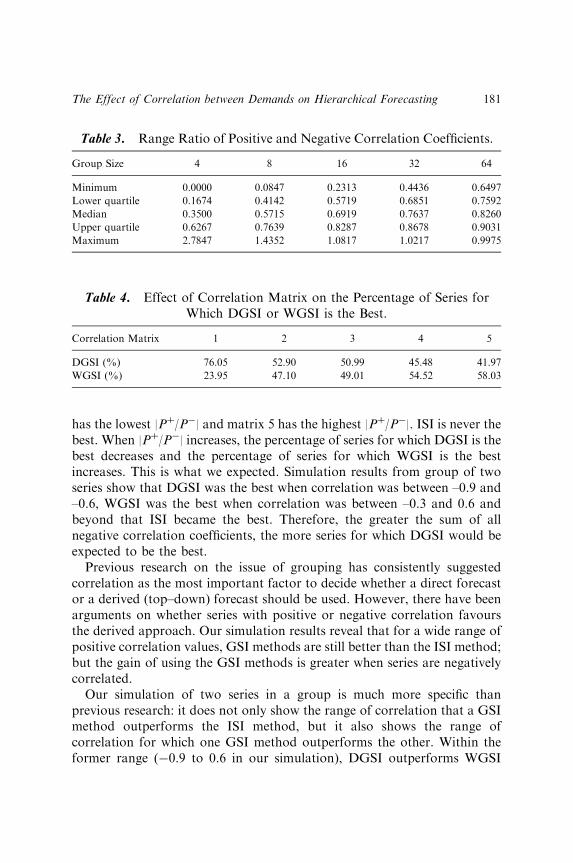
has the lowest |Pþ/P�| and matrix 5 has the highest |Pþ/P�|. ISI is never thebest. When |Pþ/P�| increases, the percentage of series for which DGSI is thebest decreases and the percentage of series for which WGSI is the bestincreases. This is what we expected. Simulation results from group of twoseries show that DGSI was the best when correlation was between –0.9 and–0.6, WGSI was the best when correlation was between –0.3 and 0.6 andbeyond that ISI became the best. Therefore, the greater the sum of allnegative correlation coefficients, the more series for which DGSI would beexpected to be the best.
Previous research on the issue of grouping has consistently suggestedcorrelation as the most important factor to decide whether a direct forecastor a derived (top–down) forecast should be used. However, there have beenarguments on whether series with positive or negative correlation favoursthe derived approach. Our simulation results reveal that for a wide range ofpositive correlation values, GSI methods are still better than the ISI method;but the gain of using the GSI methods is greater when series are negativelycorrelated.
Our simulation of two series in a group is much more specific thanprevious research: it does not only show the range of correlation that a GSImethod outperforms the ISI method, but it also shows the range ofcorrelation for which one GSI method outperforms the other. Within theformer range (�0.9 to 0.6 in our simulation), DGSI outperforms WGSI
Table 3. Range Ratio of Positive and Negative Correlation Coefficients.
Group Size 4 8 16 32 64
Minimum 0.0000 0.0847 0.2313 0.4436 0.6497
Lower quartile 0.1674 0.4142 0.5719 0.6851 0.7592
Median 0.3500 0.5715 0.6919 0.7637 0.8260
Upper quartile 0.6267 0.7639 0.8287 0.8678 0.9031
Maximum 2.7847 1.4352 1.0817 1.0217 0.9975
Table 4. Effect of Correlation Matrix on the Percentage of Series forWhich DGSI or WGSI is the Best.
Correlation Matrix 1 2 3 4 5
DGSI (%) 76.05 52.90 50.99 45.48 41.97
WGSI (%) 23.95 47.10 49.01 54.52 58.03
The Effect of Correlation between Demands on Hierarchical Forecasting 181
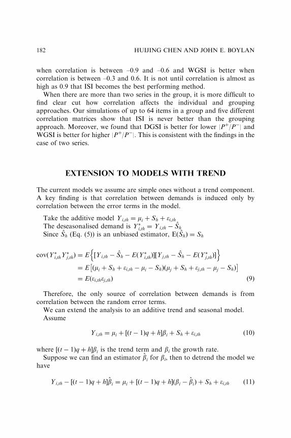
when correlation is between –0.9 and –0.6 and WGSI is better whencorrelation is between –0.3 and 0.6. It is not until correlation is almost ashigh as 0.9 that ISI becomes the best performing method.
When there are more than two series in the group, it is more difficult tofind clear cut how correlation affects the individual and groupingapproaches. Our simulations of up to 64 items in a group and five differentcorrelation matrices show that ISI is never better than the groupingapproach. Moreover, we found that DGSI is better for lower |Pþ/P�| andWGSI is better for higher |Pþ/P�|. This is consistent with the findings in thecase of two series.
EXTENSION TO MODELS WITH TREND
The current models we assume are simple ones without a trend component.A key finding is that correlation between demands is induced only bycorrelation between the error terms in the model.
Take the additive model Yi;th ¼ mi þ Sh þ �i;thThe deseasonalised demand is Y�i;th ¼ Yi;th � Sh
Since Sh (Eq. (5)) is an unbiased estimator, EðShÞ ¼ Sh
covðY�i;thY�j;thÞ ¼ E ½Yi;th � Sh � EðY�i;thÞ�½Yj;th � Sh � EðY�j;thÞ�
n o
¼ E ðmi þ Sh þ �i;th � mi � ShÞðmj þ Sh þ �j;th � mj � ShÞ� �
¼ Eð�i;th�j;thÞ ð9Þ
Therefore, the only source of correlation between demands is fromcorrelation between the random error terms.
We can extend the analysis to an additive trend and seasonal model.Assume
Yi;th ¼ mi þ ½ðt� 1Þqþ h�bi þ Sh þ �i;th (10)
where ½ðt� 1Þqþ h�bi is the trend term and bi the growth rate.Suppose we can find an estimator bi for bi, then to detrend the model we
have
Yi;th � ½ðt� 1Þqþ h�bi ¼ mi þ ½ðt� 1Þqþ h�ðbi � biÞ þ Sh þ �i;th (11)
HUIJING CHEN AND JOHN E. BOYLAN182
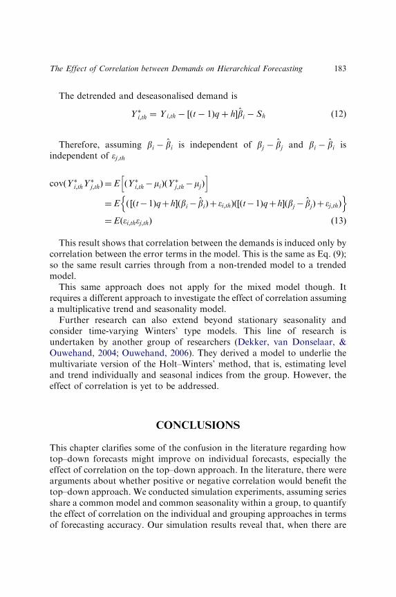
The detrended and deseasonalised demand is
Y�i;th ¼ Yi;th � ½ðt� 1Þqþ h�bi � Sh (12)
Therefore, assuming bi � bi is independent of bj � bj and bi � bi isindependent of ej,th
covðY�i;thY�j;thÞ ¼E ðY�i;th�miÞðY
�j;th�mjÞ
h i
¼E ð ½ðt�1Þqþh�ðbi� biÞþ �i;thÞð½ðt�1Þqþh�ðbj� bjÞþ �j;thÞn o
¼Eð�i;th�j;thÞ ð13Þ
This result shows that correlation between the demands is induced only bycorrelation between the error terms in the model. This is the same as Eq. (9);so the same result carries through from a non-trended model to a trendedmodel.
This same approach does not apply for the mixed model though. Itrequires a different approach to investigate the effect of correlation assuminga multiplicative trend and seasonality model.
Further research can also extend beyond stationary seasonality andconsider time-varying Winters’ type models. This line of research isundertaken by another group of researchers (Dekker, van Donselaar, &Ouwehand, 2004; Ouwehand, 2006). They derived a model to underlie themultivariate version of the Holt–Winters’ method, that is, estimating leveland trend individually and seasonal indices from the group. However, theeffect of correlation is yet to be addressed.
CONCLUSIONS
This chapter clarifies some of the confusion in the literature regarding howtop–down forecasts might improve on individual forecasts, especially theeffect of correlation on the top–down approach. In the literature, there werearguments about whether positive or negative correlation would benefit thetop–down approach. We conducted simulation experiments, assuming seriesshare a common model and common seasonality within a group, to quantifythe effect of correlation on the individual and grouping approaches in termsof forecasting accuracy. Our simulation results reveal that, when there are
The Effect of Correlation between Demands on Hierarchical Forecasting 183
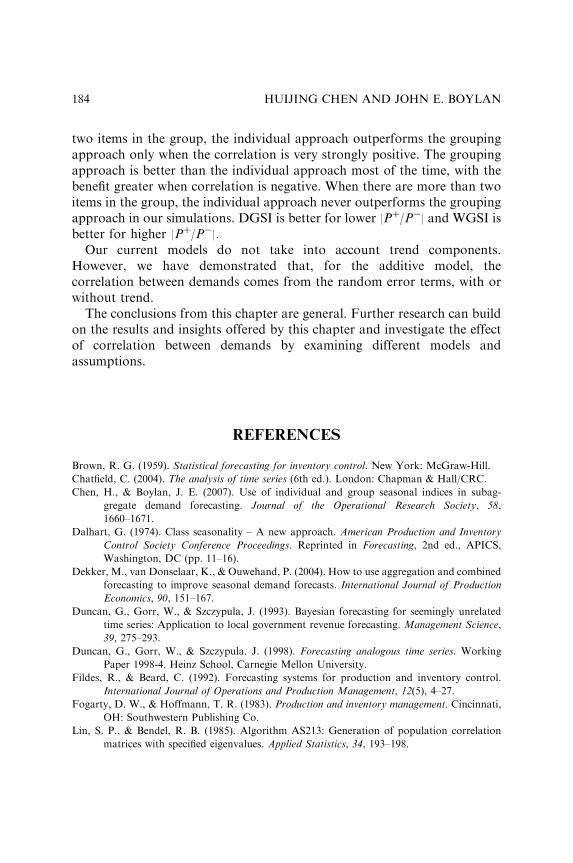
two items in the group, the individual approach outperforms the groupingapproach only when the correlation is very strongly positive. The groupingapproach is better than the individual approach most of the time, with thebenefit greater when correlation is negative. When there are more than twoitems in the group, the individual approach never outperforms the groupingapproach in our simulations. DGSI is better for lower |Pþ/P�| and WGSI isbetter for higher |Pþ/P�|.
Our current models do not take into account trend components.However, we have demonstrated that, for the additive model, thecorrelation between demands comes from the random error terms, with orwithout trend.
The conclusions from this chapter are general. Further research can buildon the results and insights offered by this chapter and investigate the effectof correlation between demands by examining different models andassumptions.
REFERENCES
Brown, R. G. (1959). Statistical forecasting for inventory control. New York: McGraw-Hill.
Chatfield, C. (2004). The analysis of time series (6th ed.). London: Chapman & Hall/CRC.
Chen, H., & Boylan, J. E. (2007). Use of individual and group seasonal indices in subag-
gregate demand forecasting. Journal of the Operational Research Society, 58,
1660–1671.
Dalhart, G. (1974). Class seasonality – A new approach. American Production and Inventory
Control Society Conference Proceedings. Reprinted in Forecasting, 2nd ed., APICS,
Washington, DC (pp. 11–16).
Dekker, M., van Donselaar, K., & Ouwehand, P. (2004). How to use aggregation and combined
forecasting to improve seasonal demand forecasts. International Journal of Production
Economics, 90, 151–167.
Duncan, G., Gorr, W., & Szczypula, J. (1993). Bayesian forecasting for seemingly unrelated
time series: Application to local government revenue forecasting. Management Science,
39, 275–293.
Duncan, G., Gorr, W., & Szczypula. J. (1998). Forecasting analogous time series. Working
Paper 1998-4. Heinz School, Carnegie Mellon University.
Fildes, R., & Beard, C. (1992). Forecasting systems for production and inventory control.
International Journal of Operations and Production Management, 12(5), 4–27.
Fogarty, D. W., & Hoffmann, T. R. (1983). Production and inventory management. Cincinnati,
OH: Southwestern Publishing Co.
Lin, S. P., & Bendel, R. B. (1985). Algorithm AS213: Generation of population correlation
matrices with specified eigenvalues. Applied Statistics, 34, 193–198.
HUIJING CHEN AND JOHN E. BOYLAN184

McLeavey, D. W., & Narasimhan, S. L. (1985). Production planning and inventory control.
Boston, MA: Allyn and Bacon, Inc.
Muir, J. W. (1983). Problems in sales forecasting needing pragmatic solutions. APICS
Conference Proceedings (pp. 4–7).
Ouwehand, P. (2006). Forecasting with group seasonality. Unpublished PhD thesis, Technische
Universiteit Eindhoven, The Netherlands.
Schwarzkopf, A. B., Tersine, R. J., & Morris, J. S. (1988). Top–down versus bottom-up
forecasting strategies. International Journal of Production Research, 26, 1833–1843.
Shlifer, E., & Wolff, R. W. (1979). Aggregation and proration in forecasting. Management
Science, 25, 594–603.
Withycombe, R. (1989). Forecasting with combined seasonal indices. International Journal of
Forecasting, 5, 547–552.
Xu, K., & Evers, P. T. (2003). Managing single echelon inventories through demand
aggregation and the feasibility of a correlation matrix. Computers and Operations
Research, 30, 297–308.
APPENDIX A. SIMULATION DESIGNS
Two Series
Quarterly seasonality was assumed in the simulations with four differentseasonal profiles as shown in Tables A1 and A2.
Table A1. Seasonal Profiles for the Additive Model.
Q1 Q2 Q3 Q4
No seasonality (NS) 0 0 0 0
Weak seasonality (WS) �5 �10 5 10
Low, low, low, high (LLLH) �20 �15 �15 50
Low, high, low, high (LHLH) �25 25 �25 25
Table A2. Seasonal Profiles for the Mixed Model.
Q1 Q2 Q3 Q4
No seasonality (NS) 1 1 1 1
Weak seasonality (WS) 0.9 0.8 1.1 1.2
Low, low , low, high (LLLH) 0.6 0.7 0.7 2
Low, high, low, high (LHLH) 0.5 1.5 0.5 1.5
The Effect of Correlation between Demands on Hierarchical Forecasting 185

The aim is not to attain comprehensiveness of seasonal profiles, but tochoose a few commonly occurring profile shapes to check whether theyaffect the rules. WS represents a weak seasonality and LLLH represents asituation where there is a single very high season (e.g., in the final quarter ofthe year, with higher demand before Christmas). LHLH representsalternative low and high seasons.
The underlying mean for one item is fixed to be 50, and the mean of theother item in the group varies. It can take a value of 50, 100, 200, 300, 400,500, 5,000 or 50,000, representing a ratio of 1, 2, 4, 6, 8, 10, 100 or 1,000.
Variances of the random error terms in the models are generated usingpower laws of the form s2 ¼ amb, where m is the underlying mean, and a andb are constants (Brown, 1959). Our preliminary results agreed with Shliferand Wolff (1979) that the a parameter does not affect the rules because itappears on both sides of the rule and can be cancelled out. Therefore, onlythe b parameter is allowed to vary in these power laws. We choose a to be0.5 and b to be 1.2, 1.4, 1.6 or 1.8.
Variances of series of a group may follow power laws, but different seriesin a group may not follow the same power law. Therefore, we also simulatesituations in which non-universal power laws are applied on a group. Series1 in the group follows one law and series 2 follows the other law.
Series 1: s2i ¼ 0:75� 0:5m1:5i
Series 2: s2i ¼ 1:25� 0:5m1:5i
Alternatively, it may be assumed that the series follow no power laws. Inthis case, various combinations of mean and variance values have been iden-tified, somewhat arbitrarily, for experimentation, as shown in Table A3.
Table A3. Arbitrary Variance Values.
Mean 1 50 50 50 50 50 50 50 50
Mean 2 50 100 200 300 400 500 5,000 50,000
No law
Low V1 100 100 100 100 100 100 100 100
Low V2 100 225 1,600 2,500 3,600 4,900 62,500 1,562,500
Low V1 100 100 100 100 100 100 100 100
High V2 400 900 4900 8100 10000 22500 490000 49000000
High V1 400 400 400 400 400 400 400 400
Low V2 100 225 1600 2500 3600 4900 62500 1562500
High V1 400 400 400 400 400 400 400 400
High V2 400 900 4900 8100 10000 22500 490000 49000000
HUIJING CHEN AND JOHN E. BOYLAN186
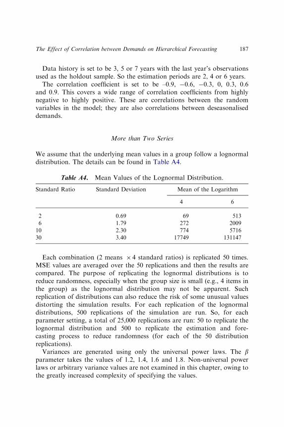
Data history is set to be 3, 5 or 7 years with the last year’s observationsused as the holdout sample. So the estimation periods are 2, 4 or 6 years.
The correlation coefficient is set to be –0.9, �0.6, �0.3, 0, 0.3, 0.6and 0.9. This covers a wide range of correlation coefficients from highlynegative to highly positive. These are correlations between the randomvariables in the model; they are also correlations between deseasonaliseddemands.
More than Two Series
We assume that the underlying mean values in a group follow a lognormaldistribution. The details can be found in Table A4.
Table A4. Mean Values of the Lognormal Distribution.
Standard Ratio Standard Deviation Mean of the Logarithm
4 6
2 0.69 69 513
6 1.79 272 2009
10 2.30 774 5716
30 3.40 17749 131147
Each combination (2 means � 4 standard ratios) is replicated 50 times.MSE values are averaged over the 50 replications and then the results arecompared. The purpose of replicating the lognormal distributions is toreduce randomness, especially when the group size is small (e.g., 4 items inthe group) as the lognormal distribution may not be apparent. Suchreplication of distributions can also reduce the risk of some unusual valuesdistorting the simulation results. For each replication of the lognormaldistributions, 500 replications of the simulation are run. So, for eachparameter setting, a total of 25,000 replications are run: 50 to replicate thelognormal distribution and 500 to replicate the estimation and fore-casting process to reduce randomness (for each of the 50 distributionreplications).
Variances are generated using only the universal power laws. The bparameter takes the values of 1.2, 1.4, 1.6 and 1.8. Non-universal powerlaws or arbitrary variance values are not examined in this chapter, owing tothe greatly increased complexity of specifying the values.
The Effect of Correlation between Demands on Hierarchical Forecasting 187
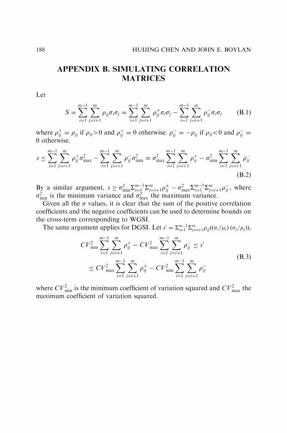
APPENDIX B. SIMULATING CORRELATION
MATRICES
Let
S ¼Xm�1i¼1
Xmj¼iþ1
rijsisj ¼Xm�1i¼1
Xmj¼iþ1
rþij sisj �Xm�1i¼1
Xmj¼iþ1
r�ij sisj (B.1)
where rþij ¼ rij if rijW0 and rþij ¼ 0 otherwise. r�ij ¼ �rij if rijo0 and r�ij ¼0 otherwise.
s �Xm�1i¼1
Xmj¼iþ1
rþij s2max �
Xm�1i¼1
Xmj¼iþ1
r�ij s2min ¼ s2max
Xm�1i¼1
Xmj¼iþ1
rþij � s2min
Xm�1i¼1
Xmj¼iþ1
r�ij
(B.2)
By a similar argument, s � s2minSm�1i¼1 Sm
j¼iþ1rþij � s2maxS
m�1i¼1 Sm
j¼iþ1r�ij , where
s2min is the minimum variance and s2max the maximum variance.Given all the s values, it is clear that the sum of the positive correlation
coefficients and the negative coefficients can be used to determine bounds onthe cross-term corresponding to WGSI.
The same argument applies for DGSI. Let s0 ¼ Sm�1i¼1 Sm
j¼iþ1rijððsi=miÞ ðsj=mjÞÞ,
CV2min
Xm�1i¼1
Xmj¼iþ1
rþij � CV2max
Xm�1i¼1
Xmj¼iþ1
r�ij � s0
� CV2max
Xm�1i¼1
Xmj¼iþ1
rþij � CV2min
Xm�1i¼1
Xmj¼iþ1
r�ij
(B.3)
where CV2min is the minimum coefficient of variation squared and CV2
max themaximum coefficient of variation squared.
HUIJING CHEN AND JOHN E. BOYLAN188

PART IV
OTHER APPLICATION AREAS OF
FORECASTING

This page intentionally left blank

ECONOMETRIC COUNT DATA
FORECASTING ANDDATAMINING
(CLUSTER ANALYSIS) APPLIED TO
STOCHASTIC DEMAND IN
TRUCKLOAD ROUTING
Virginia M. Miori
ABSTRACT
The challenge of truckload routing is increased in complexity by theintroduction of stochastic demand. Typically, this demand is generalizedto follow a Poisson distribution. In this chapter, we cluster the demanddata using data mining techniques to establish the more acceptabledistribution to predict demand. We then examine this stochastic truckloaddemand using an econometric discrete choice model known as a countdata model. Using actual truckload demand data and data from thebureau of transportation statistics, we perform count data regressions.Two outcomes are produced from every regression run, the predicteddemand between every origin and destination, and the likelihood that thatdemand will occur. The two allow us to generate an expected valueforecast of truckload demand as input to a truckload routing formulation.The negative binomial distribution produces an improved forecast over thePoisson distribution.
Advances in Business and Management Forecasting, Volume 6, 191–216
Copyright r 2009 by Emerald Group Publishing Limited
All rights of reproduction in any form reserved
ISSN: 1477-4070/doi:10.1108/S1477-4070(2009)0000006012
191

1. INTRODUCTION
This chapter brings together the application areas of truckload routing andeconometric count data analysis, whereas data mining provides a basis forselection of the statistical distribution underlying the count data regression.The combination provides the opportunity to solve the stochastic truckloadrouting problem (TRP) to optimality. Individually these areas have beenresearched; however, they have not been examined collectively. Theliterature presented therefore represents distinct areas of research.
The triplet model formulation was presented by Miori (2006) as analternative to allow solution of the TRP through the means of dynamicprogramming. This formulation examined demand in combination with anynecessary empty movements that would be incurred. An alternativerepresentation of stochastic demand is easily facilitated through thisreformulation.
Arunapuram, Mathur, and Solow (2003) noted that truckload carrierswere faced with a difficult problem. They present a new branch and boundalgorithm for solving an integer programming formulation of this vehiclerouting problem with full truckloads (VRPFL). Time window and waitingcost constraints were also represented in the problem formulation. Theresulting efficiency of the method was due to a column generation schemethat exploited the special structure of the problem. The column generationwas used to solve the linear relaxation problems that arose at the nodes. Theobjective in solving the VRPFL was to find feasible routes that minimizedcost. They noted that minimizing the total cost was equivalent to minimizingthe cost of traveling empty.
Chu (2004) presented a heuristic that applied to both the VRP and theTRP (less-than-truckload versus truckload applications). The focus of thepaper was a heuristic technique, based on a mathematical model, used forsolution generation for a private fleet of vehicles. Outside carriers thatprovided less-than-truckload (LTL) service could be employed in thesolution. In this paper, Chu addressed the problem of routing a fixednumber of trucks with limited capacity from a depot to customers. Theobjective was the minimization of total cost.
The TL-LTL heuristic developed in this paper was designed not only tobuild routes, but also to select the appropriate mode. The first step was theselection of customers to be served by mode. LTL customers werestripped out and routes built using the classic Clarke and Wright (1964)algorithm. The final step was swapping customers between and withinroutes. Though this paper addressed the TRP, its primary focus was on the
VIRGINIA M. MIORI192

LTL mode and in fact replicated a typical ‘‘cluster first-route second’’approach.
Gronalt, Hartl, and Reimann (2003) used a savings-based approach to theTRP with time window constraints. The objective was to minimize emptyvehicle movements that generate no revenue. They provided an exactformulation of the problem and calculated a lower bound on the solutionbased on a relaxed formulation using network flows. They further presentedfour different savings-based heuristics for the problem. There were generallytwo different problem classes. The first was concerned with dynamic carrierallocation and the second class of problems dealt with the pickup anddelivery of orders by a fleet of vehicles. This problem belonged to the secondclass.
Gronalt et al. strived for the goal of minimizing empty vehicle movementsfor the truckload portion of the shipments. The results were extended to amultidepot problem as well. The algorithms included the savings algorithm,the opportunity savings algorithm that incorporated opportunity costs intocalculation of savings values, and the simultaneous savings approach thataccepted a number of savings combinations at each iteration that satisfy agiven condition.
The TRP has also been addressed in the literature as a multivehicletruckload pickup and delivery problem. Yang, Jaillet, and Mahmassani(2000) presented a problem in which every job’s arrival time, duration, anddeadline are known. They considered the most general cost structure andemployed alternate linear coefficients to represent different cost emphaseson trucks’ empty travel distances, jobs with delayed completion times, andthe rejection of jobs. Note again that this problem did not require allpotential loads to be serviced. The problem was presented first as an off-lineproblem with cost minimization as its objective. A rolling horizon and real-time policies were then introduced.
The authors examined a specific stochastic and dynamic vehicle routingproblem. They devised heuristic stationary policies to be used by thedispatcher for each situation, at each decision epoch. The policies werebased on observations of the off-line problem and were intended to preemptempty movements. If a vehicle was already en route to a job, it could bedispatched to serve another job based on these rules. A series of simulationsshowed that the policies developed were very efficient.
Cameron and Trivedi (1986) discussed count data analysis in the premierissue of the Journal of Applied Econometrics. This work examined Poisson,compound Poisson, negative binomial, and more generalized models ofcount data. Their work continued and culminated in the publication of a
Econometric Count Data Forecasting and Data Mining 193

seminal text in the area (Cameron & Trivedi, 1998). Greene (2003) andAgresti (2002) both presented and applied count data models in text format.
Data mining, specifically clustering of data, has been used in areasextending from quality analysis, traffic safety to demand forecasting. BaFail(2004) forecasted demand of airline travelers in Saudi Arabia. Neuralnetworks were applied to 10 years of demand data. Bansal, Vadhavkar, andGupta (1998) used traditional statistical techniques to determine the bestneural network method to use for inventory forecasting in a large medicaldistribution company.
The area of count data models applied to stochastic demand in the freighttransportation industry has been the subject of little or no research. As such,the literature presented here represents alternate application areas for countdata models in an effort to draw parallels between the application areas.
Arunapuram et al. (2003) treated the demand deterministically, thusrequiring no distribution assumptions. Powell (1996) considered the stochasticdemand associated with truckload transportation and presented a multistagemodel to address it. He did not however offer a specification of distribution ofdemand. Frantzaskakis and Powell (1990) assumed a Poisson distributionof demand with a mean equal to the historical frequency.
Recreational travel was analyzed according to household factors, typicalfrequency of travel and ethnicity by Bowker and Leeworthy (1998). Haab(2003) examined recreational travel demand with consideration of temporalcorrelation between trips. Hellstrom (2006) studied tourism demand inSweden again according to number of leisure trips and number of overnightstays using count data. Jang (2005) used count data modeling to generatetrips, based on socioeconomic characteristics, as a way of overcoming theinherent shortcomings of linear regression. He first applied the Poissonregression model only to find overdispersion, thus turning to the negativebinomial model as the ultimate representation. Ledesma, Navarro, andPerez-Rodriguez (2005) used count data modeling to examine the hypothesisthat repeated visits to the same location was actually the result ofasymmetrical information. A left-truncated Poisson regression was applied.
Chakraborty and Keith (2000) used truncated count data travel costdemand models to estimate the demand for and value of mountain biking inMoab, Utah. Both truncated Poisson and truncated negative binomialdistributions were used to determine that mountain biking had a highervalue to the area than other recreational activities.
Puig (2003) presented the aspects of the Poisson distribution that make itthe most widely used distribution in count data analysis: it is closed underaddition and the sample mean is actually the maximum likelihood estimator
VIRGINIA M. MIORI194
(MLE) of the mean of the distribution. Other discrete distributions with twoparameters were discussed in an effort to find these same aspects and thusprovide an alternate distribution for count data analysis. The generalHermite distribution was discussed at great length though it is only partiallyclosed under addition. The Poisson distribution is a subfamily of the generalHermite distribution. Puig and Valero (2006) carried this discussion fartherand characterized all two-parameter discrete distributions that are alsopartially closed under addition. They limited consideration to only thosedistributions for which the sample mean was the same as the MLE of themean. The count data models included the negative binomial, Neyman A,Polya Aeppli, Poisson-inverse Gaussian, Thomas, and general Hermite. Theauthors also presented a theorem that allows extension to other two-parameter discrete distributions for use in count data models.
Negative binomial regressions have also been employed in assessingintersection-accident frequencies. Poch and Mannering (1996) looked atintersections in Bellevue, Washington. Rather than using the count datamodel with a negative binomial distribution underlying the regression, theyused a maximum likelihood estimation procedure. Karlaftis and Tarko(1998) discussed improved accident models using panel data. Rather thanemploying the Poisson distribution, which has been the source of criticism,they employed clustering of the data and subsequently applied multiplenegative binomial distributions to represent the accident frequency data.
2. TRP TRIPLET FORMULATION
The most basic assumption of the TRP is that freight is delivered by truck,in full truckload quantities. This means that a full truckload quantity isdefined as a single unit of demand and may not be split between multiplevehicles.
The formulation utilizes a triplet concept rather than a lane concept(Miori, 2006). A node triplet is composed of two origin/destination pairs insuccession in which the first destination location is the same as the secondorigin location. It may be made up of two loaded movements, one emptymovement and one loaded movement or two empty movements.
The TRP typically results in a loaded lane (origin/destination pair)movement followed by an empty lane movement. The movements are tiedtogether and a logical connection between the associated loaded and emptymovements is created. The cost of the triplet is therefore the sum of the costs
Econometric Count Data Forecasting and Data Mining 195

of the individual movements. The transit and work times are the sums of thetransit and work times of the individual movements.
Traditionally, a route is composed of a series of lanes to be serviced by asingle vehicle. We extend the notion of a route to consider a series of triplets.We must begin and end a route at the same node, known as a domicile.A route is therefore composed of a sequence of triplets. Within any routethat’s generated, the final node of a triplet must match the subsequent tripletorigin (first node). This organization of these locations has been chosen toconsider the opportunity cost of each movement.
Time conditions are placed on the handling of freight by the customers.Loads must be picked up and delivered on particular days of the weekduring specified times of the day. Some customers will be more restrictivethan others in specifying their time windows.
The remaining conditions are imposed by the Department of Transporta-tion (DOT). Restrictions are placed on the number of driving hours in agiven week and number of work hours in a given week.
A primary advantage of the triplet formulation is a more naturaltreatment of variation in length and cost of empty movements. Stochasticdemand is however still present.
The first terms in the TRP notation require no subscripts. They addressparameters set by the data itself and the carrier preference within DOThours of service restrictions for number of hours allowed on a tour.
N The number of nodes.V The number of vehicles.H Total allowed transit hours per route.
The time window specifications are particular to the location of eachnode. These require the subscript i, where i ¼ 1, . . . ,N.
Di Departure time from node.[ei,li] Early and late arrival times for node i.
The demand for service and the travel time are provided for each lanepair. Lanes are designated as ij, where i ¼ 1, . . . ,N and j ¼ 1, . . . ,N.
yij 1 if lane ij represents loaded movement.0 otherwise.
tij Travel time between node i and j.
VIRGINIA M. MIORI196
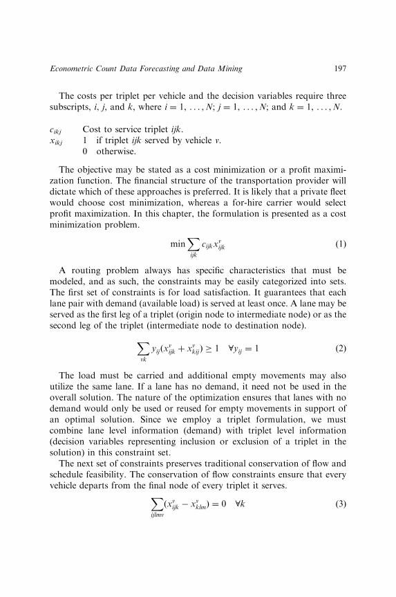
The costs per triplet per vehicle and the decision variables require threesubscripts, i, j, and k, where i ¼ 1, . . . ,N; j ¼ 1, . . . ,N; and k ¼ 1, . . . ,N.
cikj Cost to service triplet ijk.xikj 1 if triplet ijk served by vehicle v.
0 otherwise.
The objective may be stated as a cost minimization or a profit maximi-zation function. The financial structure of the transportation provider willdictate which of these approaches is preferred. It is likely that a private fleetwould choose cost minimization, whereas a for-hire carrier would selectprofit maximization. In this chapter, the formulation is presented as a costminimization problem.
minXijk
cijkxvijk (1)
A routing problem always has specific characteristics that must bemodeled, and as such, the constraints may be easily categorized into sets.The first set of constraints is for load satisfaction. It guarantees that eachlane pair with demand (available load) is served at least once. A lane may beserved as the first leg of a triplet (origin node to intermediate node) or as thesecond leg of the triplet (intermediate node to destination node).
Xvk
yijðxvijk þ xvkijÞ � 1 8yij ¼ 1 (2)
The load must be carried and additional empty movements may alsoutilize the same lane. If a lane has no demand, it need not be used in theoverall solution. The nature of the optimization ensures that lanes with nodemand would only be used or reused for empty movements in support ofan optimal solution. Since we employ a triplet formulation, we mustcombine lane level information (demand) with triplet level information(decision variables representing inclusion or exclusion of a triplet in thesolution) in this constraint set.
The next set of constraints preserves traditional conservation of flow andschedule feasibility. The conservation of flow constraints ensure that everyvehicle departs from the final node of every triplet it serves.X
ijlmv
ðxvijk � xvklmÞ ¼ 0 8k (3)
Econometric Count Data Forecasting and Data Mining 197
The schedule feasibility constraints ensure a logical progression throughthe routes (a vehicle may not depart before its arrival), and forces adherenceto time constraints (time windows are satisfied for the pickup and deliverypoints as well as the domicile). Because time windows address individuallocations, the time window constraints reflect the individual nodes and notthe entire triplet. These are standard constraints used in the TRP.
Di þ tij � Dj 8i; j (4)
ei � Di � li 8i (5)
The remaining constraint set ensures that the routes satisfy the DOTregulations for single drivers. Each route is restricted to a maximum numberof hours in transit. The DOT recently revised these regulations, but the newregulations have been challenged. The model discussed in this chapter allowsfor flexibility in the statement of these constraints to reflect this uncertainty.X
ijk
ðtij þ tjkÞ xvijk � H 8v (6)
The decision variables must take on binary values.
xvijk 2 f0; 1g (7)
3. DATA PREPARATION
The need for a large volume of data that accurately represents nationalfreight volumes arises from the use of data mining cluster analysis and theeconometric count data model. The cluster analysis revealed only four fieldsin the load-specific data that contributed to the cluster structures. The countdata model, however, combines the use of national freight flow informationwith load-specific data that represents the truckload freight operation underconsideration. The national freight data was gathered from the Bureau ofTransportation Statistics (BTS), whereas the carrier-specific data wascollected from truckload freight operations with domiciles in 14 differentcities. We first discuss the BTS data.
3.1. Bureau of Transportation Statistics Data
Within the BTS, freight surveys are completed approximately every fiveyears. This cross-sectional data is quite extensive and covers freight
VIRGINIA M. MIORI198

volumes, hazardous material issues, safety, and limitations specific to mode.The Commodity Flow Surveys within Intermodal Transportation Databaseand the Highway Data Library contain numerous tables applicable totruckload transportation. This data came specifically from two tables thatcontain outbound and inbound shipment characteristics.
The BTS eliminated data records with anomalies and errors beforepublishing its data. Therefore, an imbalance exists in the freight volumereported. The overall freight supply exceeds the freight demand. Beforecompleting any analysis that relies on balance of freight, the inequity mustbe resolved. The freight supply was scaled to eliminate the appearance offreight that traveled the country indefinitely.
The selected tables contain data that reflect specific origins anddestinations for freight. These origins and destinations include all majormetropolitan areas within the 50 states as well as rural and less populatedareas. Inbound and outbound freight volumes for each location within everystate are reported.
The volumes of freight inbound to each location and the volumes offreight outbound from each location provide the first useful application ofthe BTS data. These values are used in the subsequent count data model asexplanatory variables. In addition, the data is used to generate indices forsupply/demand centers at each metropolitan area. Note that theseaccumulations of data were all produced using the scaled supply figuresand the reported demand figures.
The supply/demand index points to the nature of the particularmetropolitan or rural area. A strict demand center is one in which allfreight is delivered to that location, but none is available for pick-up. It isdesignated by an index of 1.00. A strict supply center is just the opposite. It isone in which no freight is destined for that location, but freight is alwaysavailable to be shipped. An index of �1.00 is designated for a supply center.A completely balanced location will have an index of 0.00. The supply/demand index may therefore fall anywhere in the interval from�1.00 to 1.00.
The BTS data represents 138 metropolitan areas or regions in the UnitedStates, including Alaska and Hawaii (i ¼ 1, . . . , 138). The supply/demandindex is determined using the following formula:
indexi ¼demandi ðtonsÞ � scaled supplyi ðtonsÞ
demandi ðtonsÞ þ scaled supplyi ðtonsÞ(8)
The final supply/demand indices were cross-referenced with the load-specific data to be discussed next.
Econometric Count Data Forecasting and Data Mining 199

3.2. Load-Specific Truckload Data
The second data source contained information on a load-by-load basis. Theoriginal database contained over 34,000 records that included date, origin,volume, number of truckloads, and mileage traveled for each load. Therewere 15 origin terminal locations. There were no specific destination namesprovided in the data, but there were nongeographic destination designa-tions. Using mileage, origin locations, and overall demand patterns, we wereable to triangulate 50 destinations.
The discernment of the destination then allowed the preparation of datafor the cluster analysis and the count data model to continue. Each originand destination was matched with its supply/demand index. In addition, theoutbound volume for each origin and the inbound volumes for eachdestination were also matched.
On the basis of date, each record was assigned additional variables whichreflected the day of week and the quarter of the year in which the load wascarried. These variables were further used to create a series of dummyvariables as required to model the timeframe. Note that each of the timewindow dummy variables corresponds directly to the level of the decisiontree in which a load might be serviced.
The chosen aggregation method accumulated loads by origin, destination,and date. The minimum value for demand is a single truckload. To matchdemand data to either the Poisson or negative binomial distributions, weperformed a linear transformation of the data by decrementing the numberof loads by one (Fig. 1). The mean and variance of the decremented data donot appear to be the same resulting in a violation of that property of thePoisson distribution. This difference between the mean and variance leads tothe possibility of overdispersion in the data.
The issue of unequal mean and variance drives us to consider the negativebinomial as a basis for the count data model. We cannot make a completeassessment of the equality from the descriptive statistics. We can howevertest for the equality as we apply both the Poisson and negative binomialregressions. Further, by clustering our data using data mining, we are ableto examine the equal mean and variance property in detail.
4. DATA MINING: CLUSTERING METHODS
Research conducted on the TRP with stochastic demand has typicallygeneralized demand to a Poisson distribution. Rather than making this
VIRGINIA M. MIORI200
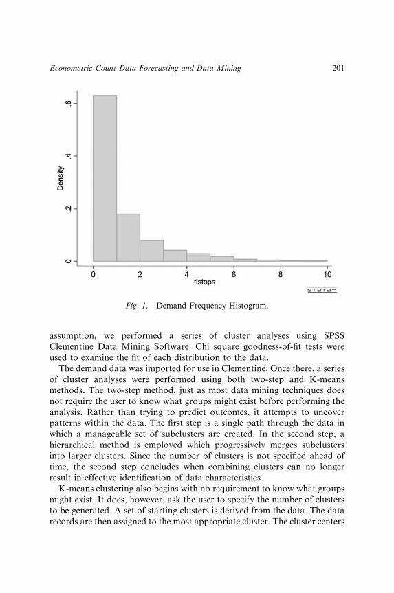
assumption, we performed a series of cluster analyses using SPSSClementine Data Mining Software. Chi square goodness-of-fit tests wereused to examine the fit of each distribution to the data.
The demand data was imported for use in Clementine. Once there, a seriesof cluster analyses were performed using both two-step and K-meansmethods. The two-step method, just as most data mining techniques doesnot require the user to know what groups might exist before performing theanalysis. Rather than trying to predict outcomes, it attempts to uncoverpatterns within the data. The first step is a single path through the data inwhich a manageable set of subclusters are created. In the second step, ahierarchical method is employed which progressively merges subclustersinto larger clusters. Since the number of clusters is not specified ahead oftime, the second step concludes when combining clusters can no longerresult in effective identification of data characteristics.
K-means clustering also begins with no requirement to know what groupsmight exist. It does, however, ask the user to specify the number of clustersto be generated. A set of starting clusters is derived from the data. The datarecords are then assigned to the most appropriate cluster. The cluster centers
Fig. 1. Demand Frequency Histogram.
Econometric Count Data Forecasting and Data Mining 201
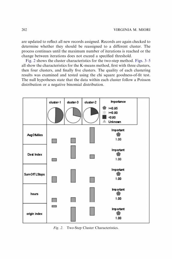
are updated to reflect all new records assigned. Records are again checked todetermine whether they should be reassigned to a different cluster. Theprocess continues until the maximum number of iterations is reached or thechange between iterations does not exceed a specified threshold.
Fig. 2 shows the cluster characteristics for the two-step method. Figs. 3–5all show the characteristics for the K-means method, first with three clusters,then four clusters, and finally five clusters. The quality of each clusteringresults was examined and tested using the chi square goodness-of-fit test.The null hypotheses state that the data within each cluster follow a Poissondistribution or a negative binomial distribution.
Fig. 2. Two-Step Cluster Characteristics.
VIRGINIA M. MIORI202
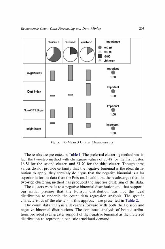
The results are presented in Table 1. The preferred clustering method was infact the two-step method with chi square values of 20.48 for the first cluster,16.58 for the second cluster, and 51.70 for the third cluster. Though thesevalues do not provide certainty that the negative binomial is the ideal distri-bution to apply, they certainly do argue that the negative binomial is a farsuperior fit for the data than the Poisson. In addition, the results argue that thetwo-step clustering method has produced the superior clustering of the data.
The clusters were fit to a negative binomial distribution and that supportsour initial premise that the Poisson distribution was not the idealdistribution to underlie the count data regression analysis. The specificcharacteristics of the clusters in this approach are presented in Table 2.
The count data analysis still carries forward with both the Poisson andnegative binomial distributions. The continued analysis of both distribu-tions provided even greater support of the negative binomial as the preferreddistribution to represent stochastic truckload demand.
Fig. 3. K-Mean 3 Cluster Characteristics.
Econometric Count Data Forecasting and Data Mining 203
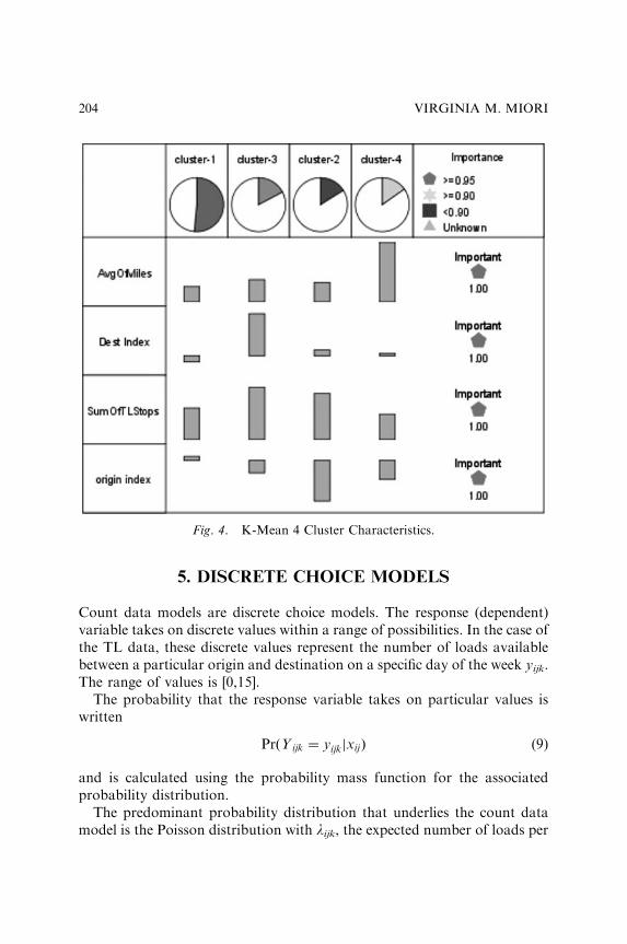
5. DISCRETE CHOICE MODELS
Count data models are discrete choice models. The response (dependent)variable takes on discrete values within a range of possibilities. In the case ofthe TL data, these discrete values represent the number of loads availablebetween a particular origin and destination on a specific day of the week yijk.The range of values is [0,15].
The probability that the response variable takes on particular values iswritten
PrðYijk ¼ yijkjxijÞ (9)
and is calculated using the probability mass function for the associatedprobability distribution.
The predominant probability distribution that underlies the count datamodel is the Poisson distribution with lijk, the expected number of loads per
Fig. 4. K-Mean 4 Cluster Characteristics.
VIRGINIA M. MIORI204
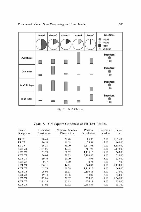
Fig. 5. K-5 Cluster.
Table 1. Chi Square Goodness-of-Fit Test Results.
Cluster
Designation
Geometric
Distribution
Negative Binomial
Distribution
Poisson
Distribution
Degrees of
Freedom
Cluster
size
TS C1 20.48 20.48 85.35 3.00 2,076.00
TS C2 16.58 16.58 75.38 3.00 860.00
TS C3 56.21 51.70 6,371.98 10.00 1,180.00
KC5 C1 134.05 142.75 561.93 7.00 2,113.00
KC5 C2 61.79 61.79 1,155.15 9.00 663.00
KC5 C3 26.04 21.33 2,180.85 8.00 710.00
KC5 C4 19.70 19.70 73.95 3.00 623.00
KC5 C5 0.37 0.00 0.74 0.00 7.00
KC4 C1 136.11 144.11 564.82 7.00 2,119.00
KC4 C2 61.79 61.79 1,155.15 8.00 663.00
KC4 C3 26.04 21.33 2,180.85 8.00 710.00
KC4 C4 19.38 19.38 73.07 3.00 624.00
KC3 C1 119.86 122.37 679.55 7.00 2,545.00
KC3 C2 115.13 115.13 974.18 8.00 920.00
KC3 C3 17.92 17.92 2,383.34 9.00 651.00
Econometric Count Data Forecasting and Data Mining 205

day, as the response variable. Each value of the response variable isconsidered to have been drawn from a Poisson distribution with the mean oflijk. When the Poisson distribution is used, the property that mean andvariance of the distribution are equal applies.
The Poisson regression may not always provide the best fit for data beingmodeled. The Poisson model has the property of equal mean and variance ofthe data. If instead, the variance exceeds the mean, we conclude that thedata is overdispersed. If the variance is exceeded by the mean, we concludethat the data is underdispersed. The risk of overdispersion is significant.A comparison of the sample mean and the sample variance can provide astrong indication of the magnitude of the overdispersion.
The Poisson regression is in fact nested within an alternate distributionapplied to count data models, the negative binomial distribution. Thenegative binomial provides greater flexibility in modeling the variance thanthe Poisson. Owing to this nesting, we can perform a hypothesis test todetermine whether the Poisson distribution is appropriate.
5.1. Independent Variables
Historic demand patterns may be broken down into base demand andseasonal fluctuations. The base demand allows lanes (origin/destinationpairs) to be compared to each other and even placed on a ratio scale.Seasonal or cyclical fluctuations will be considered uniquely for each lane.In this analysis, we will first consider two indicators of base demand, thedemand for freight leaving the load origin (origloadsout) and the demandfor freight entering the load destination (destloadsin). We also include aseasonal adjustment that necessitates the use of seasonal dummy variables(seasonQ2, seasonQ3, seasonQ4). When using dummy variables, we avoidcollinearity by specifying one fewer variable than circumstances to be
Table 2. Two-Step Cluster Characteristics.
Cluster 1 Mean Cluster 2 Mean Cluster 3 Mean
Miles 339.59 1,273.967 403.037
Destination Index �0.03 0.044 0.149
Hours 6.792 25.479 8.075
Origin Index 0.014 �0.067 �0.116
Demand 1.385 1.235 3.031
VIRGINIA M. MIORI206

represented. Therefore, dummy variables representing Q2, Q3, and Q4 areincluded in the model, whereas Q1 is considered the base timeframe.
We turn our attention next to the characteristics of the origins (origctr)and destinations (destctr) for each load. Every location considered in arouting scenario may be viewed at the extremes as a supply center or ademand center. We designate a strict demand center (no available loads todepart from the location) with a 1.00. A strict supply center (no availableloads destined for the location) with a �1.00. A 0.00 represents a balancedlocation with equal availability of loads destined for and departing fromthat location. Most locations will fall somewhere else along the continuumfrom �1.00 to 1.00.
The distance traveled to deliver each load (dist) is taken into considerationas well. A number of issues arise from the inclusion of very long hauls. Thisportion of the analysis, however, is concerned only with the predictivenature of distance. Rather than incur a very long and costly movement,many companies will try to source the load from an alternate location. Wetherefore anticipate a decline in number of loads as distance increases.Owing to the overhead of truckload travel, there also tend to be fewer loadscarried short distances. (LTL compares more favorably for short distances.)The nature of truckload transportation is that there is a lower frequencyassociated with loads traveling very short or very long distances. For thisreason, we will also include a variable for squared (distsq) distance andcubed distance (distcb).
The time windows that exist in the TL mode are typically specified on aday-by-day basis and represent when the load must depart from its originrather than when it must arrive at its destination. Receipt of freight occursprimarily on weekdays, but may have occasion to occur on weekends aswell. Therefore, we consider all days of the week. On the basis of this, timewindows may be modeled using two dummy variables for the three timewindows of the week: Monday–Tuesday, Wednesday–Thursday, andFriday–Saturday
(TimeWin2, TimeWin3). Time windows are the single factor that willresult in variation in the probabilities generated by the count data model.
We now integrate both the dependent and independent variables into thelog linear model specification of lijk. It takes the following form:
ln lijk ¼ b0 þ b1TimeWin2þ b2TimeWin3þ b3distþ b4origctr
þ b5destctrþ b6origloadsoutþ b7destloadsinþ b8seasonQ2
þ b9seasonQ3þ b10seasonQ4þ b11distsqþ b12distcb
(10)
Econometric Count Data Forecasting and Data Mining 207
6. REGRESSION DATA ANALYSIS
The aggregate truckload data combined with the indices produced from theBTS data provide the base data for the analysis. Before the completion ofthe regression, we generate and examine descriptive statistics on our fields toinitiate a better understanding of the data.
Descriptive statistics for the truckload demand over all of the data mustbe generated as well as descriptive statistics for the truckload demand forload origin and destination pairs within the aggregated data. The descriptivestatistics provide the first clue as to which type of regression may be moreeffective as the underlying distribution in the count data model.
6.1. Use of Stata
Stata Version 8 is the software product used in the count data model and theassociated analysis. Stata is a statistical package used heavily inepidemiological and econometric analysis. It provides most capabilitiesnecessary for data analysis, data management, and graphics. The count datamodel may be evaluated using the Poisson distribution or either of thenegative binomial distributions.
6.2. Analysis Procedure
On examination of the overall histogram in Fig. 1, it became a possibilitythat the Poisson distribution might not be suitable for the count data modeldue to the high concentration of zero observations. Recall that we havedecremented the demand by one in order to allow for analysis using aPoisson or negative binomial regression. We cannot make a definitiveconclusion based solely on the histogram; therefore, we begin to supplementour knowledge through the generation of descriptive statistics. Thesedescriptive statistics are presented in Appendix A. If the mean and varianceof the truckload demand in the data appear to differ, one is directed towardthe negative binomial distribution as a base for the count data model: if theyappear consistent, the Poisson regression is indicated.
We have already discussed the examination of aggregate data as well asexamination of data grouped by origin/destination pair. Both approachesprovide valuable information. The success of one approach beyond theother will be a reflection of the nature of the specific data used in any
VIRGINIA M. MIORI208
analysis. Running all data together in aggregate form allows the evaluationof the significance of the independent variables in the regression. Looking atindividual origin/destination pairs relies on our acceptance of an assumptionof conditional independence, but allows the focus to fall entirely on the timewindows and seasonality associated with each load.
Ultimately, both approaches offer insight into the data and bothapproaches must be used in order to determine how to best model thedata. Once regression coefficients have been established, the predictedcounts may be generated as well as the mass functions that provide theprobability that a particular number of loads occurs.
6.3. Count Data Model Results
Before completing the count data analysis, we must generate the supply anddemand indices from the BTS data. Overall, the freight flows in the UnitedStates are really quite balanced. On calculation and examination of thesupply/demand indices, we discover that over 60 percent of the locationscontained in the database have supply/demand indices that fall between�0.10 and 0.10. Less than 7 percent of these locations have indices that fallbelow �0.50 or above 0.50.
All other data required for the count data regression was pulled directlyfrom the lane-specific truckload database or from the general BTSsummary. The field of greatest interest is truckload demand. We againexamine the demand histogram, Fig. 1, providing initial justification forconsideration of the Poisson or negative binomial regression.
The histogram provided evidence and a starting point. The analysiscontinued with the calculation of descriptive statistics. It providedindications that the Poisson regression may not be suitable to representthe truckload demand data. Recall that the primary reason to discard thePoisson regression was overdispersion. The difference between the mean andthe variance of this data appeared to be significant enough to point us in thedirection of the negative binomial.
To test the hypothesis and make the determination of the appropriatedistribution, the first run performed in Stata was the Poisson regression onall independent variables. The output from this series of runs is found inAppendix B. Several of the variables showed p values that indicated a lackof significance. More importantly, however, the incredibly high chi squaredstatistic of over 1,379, and its associated p value of 0 indicated that we reject
Econometric Count Data Forecasting and Data Mining 209
the null hypothesis and conclude that the data did not follow a Poissondistribution. We indeed appeared to suffer from overdispersion.
The appropriate follow-up analysis was to perform a negative binomialregression using the NB2 model on that same data. There are other morecomplicated distributions that serve as bases for the count data regressionanalysis, but the burden of application is significant and the results do nothave direct interpretations.
The preliminary run of the NB2 regression again included all of theindependent variables. The dummy variables for Quarter4, Window2, andWindow3 and the distance variable were found to be insignificant. In theensuing run, the insignificant variables were eliminated but the distancevariable remained. Recall that the regression included distance, and higherorder terms of the distance in anticipation of a nonlinear relationshipbetween distance and demand. Therefore, the distance variable remained inthe regression despite its apparent insignificance.
In the remaining count data run, the negative binomial NB2 model wasagain evaluated. All of the independent variables remained significant withthe exception of the distance variable. The next step was a hypothesis test ofthe Poisson distribution. The null hypothesis stated that a ¼ 0, indicatingthat the underlying distribution was indeed a Poisson distribution. Thevalue of a generated was 1.5105. The p-value of the likelihood ratio test ofa ¼ 0 was equal to zero. Therefore, we rejected the null hypothesis andassumed that the underlying distribution was not Poisson, but was negativebinomial.
The negative binomial count data regression was then used as the base forcalculating expected counts and probabilities for every origin/destinationpair within the data. The expected counts were easily generated within Stata.The probabilities, however, required the development of a Cþþ program.The probability mass function for the negative binomial distribution wasembedded into this code and therefore used to generate the likelihood orprobability associated with each count. The counts and probabilities maynow be integrated into any continuing analysis.
7. CONCLUSIONS AND FUTURE RESEARCH
The use of data mining techniques and an econometric count data model toforecast for the TRP offers many advantages. More characteristics of thedemand patterns are considered as well as direct consideration of timewindows without inclusion of time window constraints in the TRP. It also
VIRGINIA M. MIORI210

opens the door to the use of the forecast in a more sophisticated fashion, asan expected value. It facilitates the eventual solution of the TRP usingdynamic programming.
In this research, cluster analysis provided strong supporting evidence thatthe Poisson distribution is unsuitable for representation of stochasticdemand data. It also provided sufficient evidence to conclude that thenegative binomial distribution provided a solid fit. A single regression wasperformed to generate the forecasted demand. We may extend this researchto create individual count data regression models for each of the demandclusters.
REFERENCES
Agresti, A. (2002). Categorical data analysis (2nd ed.). Somerset, NJ: Wiley.
Arunapuram, S., Mathur, K., & Solow, D. (2003). Vehicle routing and scheduling with full
truckloads. Transportation Science, 37(2), 170–182.
BaFail, A. O. (2004). Applying data mining techniques to forecast number of airline passenger
in Saudi Arabia (Domestic and international travels). Journal of Air Transportation, 9(1),
100–115.
Bansal, K., Vadhavkar, S., & Gupta, A. (1998). Neural networks based forecasting techniques
for inventory control applications. Data Mining and Knowledge Discovery, 2, 97–102.
Bowker, J. M., & Leeworthy, V. R. (1998). Accounting for ethnicity in recreation demand:
A flexible count data approach. Journal of Leisure Research, 30(1), 64–78.
Cameron, A. C., & Trivedi, P. K. (1986). Econometric models based on count data:
Comparisons and applications of some estimators and tests. Journal of Applied
Econometrics, 1, 29–53.
Cameron, A. C., & Trivedi, P. K. (1998). Regression analysis of count data. Cambridge, UK:
Cambridge University Press.
Chakraborty, K., & Keith, J. E. (2000). Estimating the recreation demand and economic value
of mountain biking in Moab, Utah: An application of count data models. Journal of
Environmental Planning and Management, 43(4), 461–469.
Chu, C.-W. (2004). A heuristic algorithm for the truckload and less-than-truckload problem.
European Journal of Operational Research, 1–11.
Clarke, G., & Wright, J. W. (1964). Scheduling of vehicles from a central dept to a number of
delivery points. Operations Research, 12, 568–581.
Frantzaskakis, L. F., & Powell, W. B. (1990). A successive linear approximation procedure for
stochastic, dynamic vehicle allocation problems. Transportation Science, 24(1), 40–57.
Greene, W. H. (2003). Econometric analysis (5th ed.). Upper Saddle River, NJ: Prentice Hall.
Gronalt, M., Hartl, R. F., & Reimann, M. (2003). New savings based algorithms for time
constrained pickup and delivery of full truckloads. European Journal of Operational
Research, 151, 520–535.
Haab, T. C. (2003). Temporal correlation in recreation demand models with limited data.
Journal of Environmental Economics and Management, 45, 195–212.
Econometric Count Data Forecasting and Data Mining 211

Hellstrom, J. (2006). A bivariate count data model for household tourism demand. Journal of
Applied Econometrics, 21(2), 213–227.
Jang, T. Y. (2005). Count data models for trip generation. Journal of Transportation
Engineering, 131(6), 444–450.
Karlaftis, M. G., & Tarko, A. P. (1998). Heterogeneity considerations in accident modeling.
Accident Analysis and Prevention, 30(4), 425–433.
Ledesma, F. J., Navarro, M., & Perez-Rodriguez, J. V. (2005). Return to tourist destination.
Is it reputation, after all? Applied Economics, 37, 2055–2065.
Miori, V. M. (2006). A novel approach to the continuous flow truckload routing problem. In:
K. Lawrence & R. Klimberg (Eds), Applications of management science: In productivity,
finance, and operations (Vol. 12, pp. 145–155). The Netherlands: Amsterdam.
Poch, M., & Mannering, F. (1996). Negative binomial analysis of intersection-accident
frequencies. Journal of Transportation Engineering, 105–113.
Powell, W. B. (1996). A stochastic formulation of the dynamic assignment problem, with an
application to truckload motor carriers. Transportation Science, 30(3), 195–219.
Puig, P. (2003). Characterizing additively closed discrete models by a property of their MLEs,
with an application to generalized hermite distributions. Journal of the American
Statistical Association, 98, 687–692.
Puig, P., & Valero, J. (2006). Count data distributions: Some characterizations with
applications. Journal of the American Statistical Association, 101(473), 332–340.
Yang, J., Jaillet, P., & Mahmassani, H. S. (2000). Study of a real-time multi-vehicle truckload
pickup-and-delivery problem. Research funded by NSF grant DMI-9713682.
VIRGINIA M. MIORI212

APPENDIX A. STATA OUTPUT: DESCRIPTIVE
STATISTICS
Econometric Count Data Forecasting and Data Mining 213
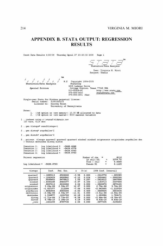
APPENDIX B. STATA OUTPUT: REGRESSION
RESULTS
VIRGINIA M. MIORI214
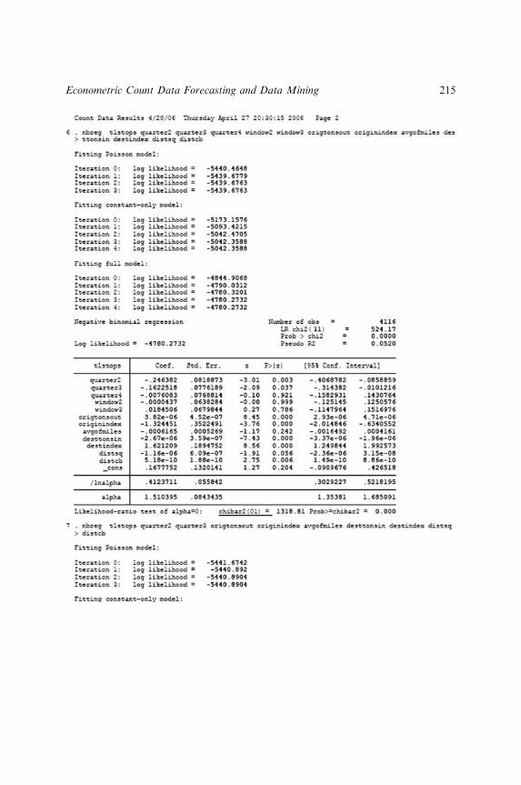
Econometric Count Data Forecasting and Data Mining 215
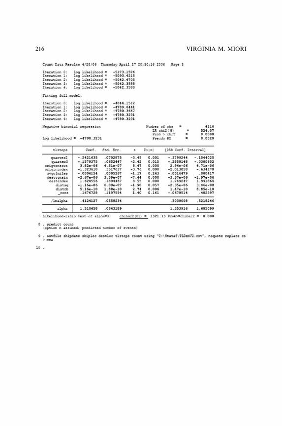
VIRGINIA M. MIORI216

TWO-ATTRIBUTE WARRANTY
POLICIES UNDER CONSUMER
PREFERENCES OF USAGE AND
CLAIMS EXECUTION
Amitava Mitra and Jayprakash G. Patankar
ABSTRACT
Warranty policies for certain products, such as automobiles, often involveconsideration of two attributes, for example, time and usage. Sinceconsumers are not necessarily homogeneous in their use of the product,such policies provide protection to users of various categories. In thischapter, product usage at a certain time is linked to the product agethrough a variable defined as usage rate. This variable, usage rate, isassumed to be a random variable with a specified probability distribution,which permits modeling of a variety of customer categories. Anotherfeature of the chapter is to model the propensity to execute the warranty,in the event of a failure within specified parameter values (say time orusage). In a competitive market, alternative product/warranty offeringsmay reduce the chances of exercising the warranty. This chapterinvestigates the impact of warranty policy parameters with the goal ofmaximizing market share, subject to certain constraints associated withexpected warranty costs per unit not exceeding a desirable level.
Advances in Business and Management Forecasting, Volume 6, 217–235
Copyright r 2009 by Emerald Group Publishing Limited
All rights of reproduction in any form reserved
ISSN: 1477-4070/doi:10.1108/S1477-4070(2009)0000006013
217

INTRODUCTION
A majority of consumer products provide some sort of assurance to theconsumer regarding the quality of the product sold. This assurance, in theform of a warranty, is offered at the time of sale. The Magnuson–MossWarranty Act of 1975 (US Federal Trade Commission Improvement Act,1975) also mandates that manufacturers must offer a warranty for allconsumer products sold for more than 15 dollars. The warranty statementassures consumers that the product will perform its function to theirsatisfaction up to a given amount of time (i.e., warranty period) from thedate of purchase. Manufacturers offer many different types of warrantiesto promote their products. Thus, warranties have become a significantpromotional tool for manufacturers. Warranties also limit the manufac-turers’ liability in the case of product failure beyond warranty period.
Taxonomy of the different types of warranty policies may be found in thework of Blischke and Murthy (1994). Considering warranty policies thatdo not involve product development after sale, policies exist for a singleitem or for a group of items. With our focus on single items, policies maybe subdivided into the two categories of nonrenewing and renewing. In arenewing policy, if an item fails within the warranty time, it is replaced bya new item with a new warranty. In effect, warranty beings anew with eachreplacement. On the other hand, for a nonrenewing policy, replacement ofa failed item does not alter the original warranty. Within each of these twocategories, policies may be subcategorized as simple or combination.Examples of a simple policy are those that incorporate replacement or repairof the product, either free or on a pro rata basis. The proportion of thewarranty time that the product was operational is typically used as a basisfor determining the cost to the customer for a pro rata warranty. Givenlimited resources, management has to budget for warranty repair costs andthereby determine appropriate values of the warranty parameters of, say,time and usage.
Although manufacturers use warranties as a competitive strategy to boosttheir market share, profitability, and image, they are by no means cheap.Warranties cost manufacturers a substantial amount of money. The costof a warranty program must be estimated precisely and its effect on thefirm’s profitability must be studied. Manufacturers plan for warranty coststhrough the creation of a fund for warranty reserves. These funds are setaside at the beginning of the sales period to meet product replacement orrepair obligations that occur while the product is under warranty. Anestimate of the expected warranty costs is thus essential for management to
AMITAVA MITRA AND JAYPRAKASH G. PATANKAR218

plan for warranty reserves. For the warranty policy considered, we assumethat the product will be repaired if failure occurs within a specified time andthe usage is less than a specified amount. Such a two-dimensional policy isfound for products such as automobiles where the warranty coverage isprovided for a time period; say five years, and a usage limit of, say, 50,000miles. In this chapter, we assume minimal repair, that is, the failure rate ofthe product on repair remains the same as just before failure. Further, therepair time is assumed to be negligible.
LITERATURE REVIEW
Estimation of warranty costs has been studied extensively in the literature.Menke (1969) estimated expected warranty costs for a single sale for a linearpro rata and lump-sum rebate plan for nonrenewable policies. Anexponential failure distribution was assumed. A drawback of his study wasthat he ignored the time value of money. Since warranty costs are incurredin the future, it is important that they be discounted using a properdiscounting rate. Amato and Anderson (1976) extended Menke’s modelto allow for discounting and price adjustments. Discounting may causethe product price to fall in real terms and be more competitive in themarketplace. Whereas these models estimate costs based on a selectedwarranty period, the formulation by Lowerre (1968) was motivated by themanufacturer’s concern. His model determined the warranty time assumingthat a selected percentage of revenue is used to meet warranty claims, thusproviding the manufacturer with some guidelines for selecting the warrantyperiod. Heschel (1971) developed his model with the consumer in mind.He found the expected repair cost to the consumer over the life of theproduct. His model assumed a full rebate for an initial period followed by apro rata rebate.
Blischke and Scheuer (1975) considered the costs of two types of warrantypolicies, namely, the free-replacement and pro rata policy under differenttime-to-failure distributions. In a separate paper, Blischke and Scheuer(1981) applied renewal theory to estimate warranty costs for the two typesof renewable warranty policies. They assumed that the buyer purchases anidentical replacement when an item in service fails at the end of the warrantyperiod. Patankar and Worm (1981) developed prediction intervals forwarranty reserves and cash flows associated with linear pro rata and lumpsum rebate plans. They developed confidence intervals on total warrantyreserves and cash flows. Upper bounds on cash flows and warranty reserves
Two-Attribute Warranty Policies 219
are determined to analyze the uncertainty or risk involved. Using aMarkovian approach, Balachandran, Maschmeyer, and Livingstone (1981)estimated the repair and replacement cost of a warranty program. Theyassumed an exponential failure distribution since its failure rate is constant.
Mamer (1982) estimated short-run total costs and long-run average costsof products under warranty. He studied pro rata and free-replacementwarranty policies under different failure distributions (such as new-better-than-used) and showed that the expected warranty costs depends on themean of the product lifetime distribution and its failure rate. Mamerconsidered pro rata and free-replacement warranties. He assumed that acustomer purchases a new product instantaneously during the product lifecycle. This provides a good assumption for using renewal theory. Cost of thereplacement depends on the type of rebate offered. Mamer (1987) laterexpanded his previous research with present value analysis and analyzedthe trade-off between warranty and quality control. He considered threewarranty policies: ordinary replacement (OR), free replacement (FR), andpro rata replacement (PR). In OR, an item is replaced and warranty isoffered only up to the original warranty period. In FR, a new warranty isoffered when an item is replaced. The new warranty is the same as theoriginal warranty. In PR, the consumer is charged based on time of failure,and a new warranty, the same as the original is offered.
Blacer and Sahin (1986) estimated warranty costs under free-replacementand pro rata warranty policies using renewal theory. They used the conceptof a renewal process to estimate warranty costs over the product lifecycle for pro rata and free-replacement warranties and computed first andsecond cost moments using gamma, exponential, and mixed exponentialfailure distributions. Frees and Nam (1988) found expressions for expectedwarranty costs in terms of distribution functions. They considered the free-replacement and pro rata policies to estimate warranty costs, wherewarranties are renewed under certain conditions. They concluded that it isvery difficult to estimate renewal functions, and, therefore, warranty costsmathematically and suggest a couple of approximations. They used newbetter than used (NBU) distribution and straight-line approximation (SLA)methods. They found that SLA gives a very good approximation to theestimations provided by Nguyen and Murthy (1984a, 1984b). The drawbackof Nguygen and Murthy’s model was that they assumed a monotonic failurerate for lifetime distributions.
Frees (1988) showed that estimating warranty costs is similar toestimating renewal functions in renewal theory. He also estimated thevariability of warranty costs using parametric and nonparametric methods.
AMITAVA MITRA AND JAYPRAKASH G. PATANKAR220

Tapiero and Posner (1988) presented an alternative approach to modeling ofwarranty reserves. Thomas (1989) found the expected warranty reserve costper unit with discounting for failure distributions that included the uniform,gamma, and Weibull. Patankar and Mitra (1995) studied the effect of partialexecution of warranty and its impact on warranty costs to model differentfactors that influence consumer behavior in exercising their warranty rights.Mitra and Patankar (1997) considered warranty programs that offercustomers the option to renew warranty, after an initial warranty period,for a certain premium. The effect of such warranty programs on marketshare and warranty costs is investigated.
A good review of the various warranty policies is found in Blischke andMurthy (1992). Murthy and Blischke (1992a) provide a comprehensiveframework of analyses in product warranty management and furtherconduct a detailed review of mathematical models (Murthy & Blischke,1992b) in this research area. A thorough treatment of warranty cost modelsand analysis of specific types of warranty policies, along with operationaland engineering aspects of product warranties, is found by Blischke andMurthy (1994). The vast literature in warranty analysis is quite disjoint. Agap exists between researchers from different disciplines. With the objectiveof bridging this gap, Blischke and Murthy (1996) provided a comprehensivetreatise of consumer product warranties viewed from different disciplines.In addition to providing a history of warranty, the handbook presents topicssuch as warranty legislation and legal actions; statistical, mathematical, andengineering analysis; cost models; and the role of warranty in marketing,management, and society.
Murthy and Djamaludin (2002) provided a literature review of warrantypolicies for new products. As each new generation of product usuallyincreases in complexity to satisfy consumer needs, customers are initiallyuncertain about its performance and may rely on warranties to influencetheir product choice. Additionally, servicing of warranty, whether to repairor replace the product by a new one, influences the expected cost to themanufacturer (Jack & Murthy, 2001). Wu, Lin, and Chou (2006) considereda model for manufacturers to determine optimal price and warranty lengthto maximize profit based on a chosen life cycle for a free renewal warrantypolicy. Huang, Liu, and Murthy (2007) developed a model to determinethe parameters of product reliability, price, and warranty strategy thatmaximize integrated profit for repairable products sold under a FR repairwarranty strategy.
The majority of past research has dealt with a single-attribute warrantypolicy, where the warranty parameter is typically the time since purchase of
Two-Attribute Warranty Policies 221
the product. Singpurwalla (1987) developed an optimal warranty policybased on maximization of expected utilities involving both profit and costs.A bivariate probability model involving time and usage as warranty criteriawas incorporated. One of the first studies among two-dimensional warrantypolicies using a one-dimensional approach is that by Moskowitz andChun (1988). Product usage was assumed to be a linear function of the ageof the product. Singpurwalla and Wilson (1993, 1998) model time to failure,conditional on total usage. By choosing a distribution for total usage, theyderive a two-dimensional distribution for failure using both age and usage.Singpurwalla (1992) also considers modeling survival in a dynamic environ-ment with the usage rate changing dynamically. Moskowitz and Chun(1994) used a Poisson regression model to determine warranty costs fortwo-dimensional warranty policies. They assumed that the total numberof failures is Poisson distributed whose parameter can be expressed as aregression function of age and usage of a product. Murthy, Iskander, andWilson (1995) used several types of bivariate probability distributionsin modeling product failures as a random point process on the two-dimensional plane and considered free-replacement policies. Eliashberg,Singpurwalla, and Wilson (1997) considered the problem of assessingthe size of a reserve needed by the manufacturer to meet future warrantyclaims in the context of a two-dimensional warranty. They developed aclass of reliability models that index failure by two scales, such as time andusage. Usage is modeled as a covariate of time. Gertsbakh and Kordonsky(1998) reduced usage and time to a single scale, using a linear relationship.Ahn, Chae, and Clark (1998) used a similar concept using a logarithmictransformation.
Chun and Tang (1999) found warranty costs for a two-attribute warrantymodel by considering age and usage of the product as warranty parameters.They provided warranty cost estimation for four different warranty policies;rectangular, L-shaped, triangular, and iso-cost, and performed sensitivityanalysis on discount rate, usage rate, and warranty terms to determine theireffects on warranty costs. Kim and Rao (2000) considered a two-attributewarranty model for nonrepairable products using a bivariate exponentialdistribution to explain item failures. Analytical expressions for warrantycosts are derived using Downtone’s bivariate distribution. They demonstratethe effect of correlation between usage and time on warranty costs. A two-dimensional renewal process is used to estimate warranty costs. Hsiung andShen (2001) considered the effect of warranty costs on optimization of theeconomic manufacturing quality (EMQ). As a process deteriorates overtime, it produces defective items that incur reworking costs (before sale) or
AMITAVA MITRA AND JAYPRAKASH G. PATANKAR222

warranty repair costs (after sale). The objective of their paper is to determinethe lot size that will minimize total cost per unit of time. The total cost perunit of time includes set up cost, holding cost, inspection cost, reworkedcost, and warranty costs. Sensitivity analysis is performed on various coststo determine an optimum production lot size. Yeh and Lo (2001) exploredthe effect of preventive maintenance actions on expected warranty costs. Amodel is developed to minimize such costs. Providing a regular preventivemaintenance within the warranty period increases maintenance cost to theseller, but the expected warranty cost is significantly reduced. An algorithmis developed that determines an optimal maintenance policy. Lam and Lam(2001) developed a model to estimate expected warranty costs for awarranty that includes a free repair period and an extended warrantyperiod. Consumers have an option to renew warranty after the free repairperiod ends. The choice of consumers has a significant effect on the expectedwarranty costs and determination of optimal warranty policy.
The model developed in this chapter is unique from those considered inthe past in several aspects. In the context of a two-attribute policy (say timeand usage) where a failed item is repaired or replaced, to model a varietyof consumers, usage rate is considered to be a random variable with aprobability distribution. Another unique contribution is the modeling ofthe customer’s propensity to exercise warranty, in the event of a productfailure within the stipulated parameters of the warranty policy. This isincorporated through the development of a warranty execution function,which represents a more realistic model. Since all consumers may notnecessarily exercise warranty claims, the impact of this warranty executionfunction will lead to a downward adjustment in the expected warrantycosts. This, in turn, will reflect a smaller accrued liability on the financialstatements of the firm.
The model considered in this chapter is also unique from the others in itsability to deal with current markets (that also includes gray markets) andenterprise warranty programs. Gray-market products are those that areoffered for sale by unauthorized third parties. Although gray marketproducts are not illegal, since they are sold outside of the normaldistribution channels of the original equipment manufacturer (OEM), amanufacturer may not honor the warranty. On the one hand, althoughconsumers may buy the product at a lower purchase price in the greymarket, the assurance of receiving warranty-related service is slim. Hence, incase of product failure within the warranty period, customer satisfactionwith the OEM will be hurt, impacting future sales and market share of theOEM.
Two-Attribute Warranty Policies 223

By incorporating a ‘‘warranty execution function’’ in the formulation(described later by Eqs. (5)–(8)), the chapter has the ability to model ‘‘fewer’’executions of warranty, in case the product is obtained through the graymarket. In particular, two parameters, the time up to which full warrantyexecution takes place (tc), and the warranty attrition rate (d), may beadequately selected to model product purchased from gray markets. If theOEM has an idea of the proportion of sales that is from gray markets, it willassist in a better forecast of expected warranty costs. When the OEMdefinitely does not honor warranty for gray market products, it will forcethe parameter tc to be zero. Alternatively, if the OEM provides limitedwarranty support and service, this may lead to a choice of the parameter tcto be some small value, greater than zero.
The choice of the warranty execution attrition rate parameter, d, is alsoinfluenced if the product is from gray markets. When the consumer issuspect about the warranty being honored, it leads to selection of d thatpermits rapid attrition. Thus, small values of d could be used to model thissituation, compared to the case where the product is purchased throughauthorized distributors or retailers.
Another feature of the existing chapter is the ability to model enterprisewarranty programs. Such programs are generally flexible and more generousand provide service and support that extends the original warrantycoverage. Associated with the enterprise warranty program is the emergenceof service contract providers that underwrite these policies. These providersmanage the claims processing through a warranty management systemthat is timely and responsive to the customer. Significant reduction inthe time to process warranties may also take place, leading to improvedcustomer satisfaction. The warranty execution function, incorporated inthis model, can incorporate the impact of enterprise warranty programson warranty costs. First, the time up to which full warranty executiontakes place (tc), will normally increase in such a program. Second, due toimproved customer satisfaction associated with such enterprise programs,the warranty execution attrition rate parameter (d) will be influencedsuch that there is a lower attrition. Hence, large values of the parameter dcould be appropriately selected to model such situations. Lastly, theprobability distribution of the parameter, tc, could be affected by suchprograms. The mean value of tc tends to be larger. The variability ofthe distribution of tc could be smaller, compared to a regular warrantyprogram, due to consistency in customer satisfaction. This can be modeledthrough adequate selection of the parameters a and b (as represented byEq. (6)).
AMITAVA MITRA AND JAYPRAKASH G. PATANKAR224
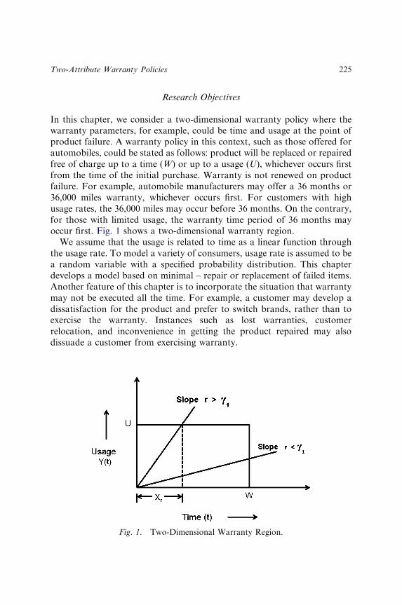
Research Objectives
In this chapter, we consider a two-dimensional warranty policy where thewarranty parameters, for example, could be time and usage at the point ofproduct failure. A warranty policy in this context, such as those offered forautomobiles, could be stated as follows: product will be replaced or repairedfree of charge up to a time (W) or up to a usage (U), whichever occurs firstfrom the time of the initial purchase. Warranty is not renewed on productfailure. For example, automobile manufacturers may offer a 36 months or36,000 miles warranty, whichever occurs first. For customers with highusage rates, the 36,000 miles may occur before 36 months. On the contrary,for those with limited usage, the warranty time period of 36 months mayoccur first. Fig. 1 shows a two-dimensional warranty region.
We assume that the usage is related to time as a linear function throughthe usage rate. To model a variety of consumers, usage rate is assumed to bea random variable with a specified probability distribution. This chapterdevelops a model based on minimal – repair or replacement of failed items.Another feature of this chapter is to incorporate the situation that warrantymay not be executed all the time. For example, a customer may develop adissatisfaction for the product and prefer to switch brands, rather than toexercise the warranty. Instances such as lost warranties, customerrelocation, and inconvenience in getting the product repaired may alsodissuade a customer from exercising warranty.
Fig. 1. Two-Dimensional Warranty Region.
Two-Attribute Warranty Policies 225
In this chapter, we develop a model from the manufacturer’s perspective.Using consumer conditions of usage and preferences on execution ofwarranty claims in the event of product failure within the specified boundsof warranty parameters, expected warranty costs are determined. Themanufacturer typically has an idea of the maximum bound, of expectedwarranty costs to sales, that should not be exceeded. Using this as aconstraint, in addition to upper and lower bounds on the price, warrantytime, and usage, optimal parameter values are determined based onmaximizing market share.
MODEL DEVELOPMENT
The following notation is used in the chapter:
W Warranty period offered in warranty policyU Usage limit offered in warranty policyR Usage ratet Instant of timeY(t) Usage at time tl(t|r) Failure intensity function at time t given R ¼ rtc Time up to which full warranty execution takes placem(t|tc) Conditional warranty execution function at time t given tcq(tc) Probability density function of tcN(W, U|r) Number of failures under warranty given R ¼ rc Unit product pricecs Unit cost of repair or replacementQ Market share for a given policy
Relationship Between Warranty Attributes
We assume that the two attributes, say time and usage, are related linearlythrough the usage rate, which is a random variable. Denoting Y(t) to be theusage at time t and X(t) the corresponding age, we have
YðtÞ ¼ RXðtÞ (1)
where R is the usage rate. It is assumed that all items that fail within theprescribed warranty parameters are minimally repaired and the repair timeis negligible. In this context, X(t) ¼ t.
AMITAVA MITRA AND JAYPRAKASH G. PATANKAR226

Distribution Function of Usage Rage
To model a variety of customers, R is assumed to be a random variable withprobability density function given by g(r). The following distributionfunctions of R are considered in this chapter:
(a) R has a uniform distribution over (a1, b1):This models a situation where the usage rate is constant across allcustomers. The density function of R is given by
gðrÞ ¼1
b1 � a1; a1 � r � b1
¼ 0; otherwise ð2Þ
(b) R has a gamma distribution function:This may be used for modeling a variety of usage rates among thepopulation of consumers. The shape of the gamma distribution functionis influenced by the selection of its parameters. When the parameter, p,is equal to 1, it reduces to the exponential distribution. The densityfunction is given by
gðrÞ ¼e�rrp�1
GðpÞ; 0 � ro1; p40 (3)
Failure Rate
Failures are assumed to occur according to a Poisson process where itis assumed that failed items are minimally repaired. If the repair time is small,it can be approximated as being zero. Since the failure rate is unaffected byminimal repair, failures over time occur according to a nonstationary Poissonprocess with intensity function l(t) equal to the failure rate.
Conditional on the usage rate R ¼ r, let the failure intensity function attime t be given by
lðtjrÞ ¼ y0 þ y1rþ ðy2 þ y3rÞt (4)
(1) Stationary Poisson process:Under this situation, the intensity function l(t|r) is a deterministicquantity as a function of t when y2 ¼ y3 ¼ 0. This applies to manyelectronic components that do not deteriorate with age and failures aredue to pure chance. The failure rate in this case is constant.
Two-Attribute Warranty Policies 227

(2) Nonstationary Poisson process:This models the more general situation where the intensity functionchanges as a function of t. It is appropriate for products andcomponents with moving parts where the failure rate may increasewith time of usage. In this case y2 and y3 are not equal to zero.
Warranty Execution Function
A variety of reasons, as mentioned previously, may prevent the fullexecution of warranty. The form of the weight function, which describeswarranty execution, could be influenced by factors such as the warrantytime, usage limit, warranty attrition due to costs of executing the warranty,and the product class as to whether they are expensive.
Fig. 2 shows a conditional warranty execution function, m(t|tc). It isassumed that full execution will take place if trtc. Beyond tc, the conditionalexecution function decreases exponentially with t. Eq. (5) represents m(t|tc):
mðtjtcÞ ¼ 1; 0ot � tc
¼ exp �ðt� tcÞ=d� �
; tc � t �W
¼ 0; t4W
(5)
The parameter d in Eq. (5) is a measure of the rate of warranty attritiondue to some of the reasons discussed previously. As d increases, the rate ofwarranty attrition decreases, leading to an increase in the value of theconditional warranty execution function.
Fig. 2. Conditional Warranty Execution Function.
AMITAVA MITRA AND JAYPRAKASH G. PATANKAR228

Note that if tc ¼W, we have full warranty execution. To modelheterogeneity in customer behavior in warranty execution, the distributionof tc is assumed to be given by a gamma distribution
qðtcÞ ¼ba
GðaÞexpð�btcÞta�1c (6)
The choice of the parameter values of a and b, that determine thedistribution of tc will be influenced by the current market and enterpriseenvironment. Note that for a gamma distribution the mean and varianceare given by a/b and a/b2, respectively. For products purchased in graymarkets, the mean of tc will be small, implying small values of a and largevalues of b. Alternatively, for enterprise warranty programs, the mean of tcwill be larger, relative to the traditional warranty program. This may beaccomplished through selection of large values of a and small values of b.However, since the variability in the distribution of tc will be smaller thanthat of a traditional warranty program, a judicious choice of a and b willhave to be made. Although increasing the value of b will reduce the varianceof tc, it will also reduce the mean of tc. Thus, based on market conditions, aand b may have to be jointly selected such that the existing environment onthe mean and variance of tc are modeled appropriately.
Now, m(t), the warranty execution function is found by compoundingm(t|tc) with q(tc) as follows:
mðtÞ ¼
ZmðtjtcÞqðtcÞdtc (7)
Here, the exponential distribution, which is a special case of the gamma dis-tribution (when a ¼ 1) is used for q(tc) to derive the results. Thus, we have
mðtÞ ¼
Z t
tc¼0
b exp �ðt� tcÞ=d� btc� �
dtc þ
Z W
tc¼t
b exp �ðbtcÞ½ �dtc
¼ ½expð�btÞ � expð�bWÞ� þb expð�t=dÞðb� 1=dÞ
½1� exp½�ðb� 1=dÞt��
(8)
Market Share
The market share function (Q) is formulated so as to be bounded between0 and 1. It is developed to decrease exponentially with respect to productprice (c), increase exponentially with warranty time (W) as well as usage
Two-Attribute Warranty Policies 229
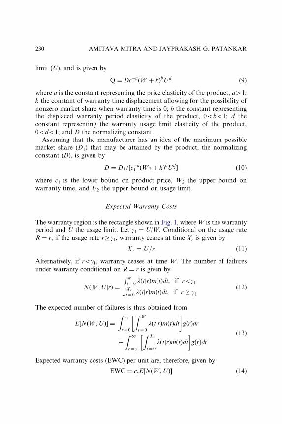
limit (U), and is given by
Q ¼ Dc�aðW þ kÞbUd (9)
where a is the constant representing the price elasticity of the product, aW1;k the constant of warranty time displacement allowing for the possibility ofnonzero market share when warranty time is 0; b the constant representingthe displaced warranty period elasticity of the product, 0obo1; d theconstant representing the warranty usage limit elasticity of the product,0odo1; and D the normalizing constant.
Assuming that the manufacturer has an idea of the maximum possiblemarket share (D1) that may be attained by the product, the normalizingconstant (D), is given by
D ¼ D1=½c�a1 ðW2 þ kÞbUd
2 � (10)
where c1 is the lower bound on product price, W2 the upper bound onwarranty time, and U2 the upper bound on usage limit.
Expected Warranty Costs
The warranty region is the rectangle shown in Fig. 1, whereW is the warrantyperiod and U the usage limit. Let g1 ¼ U/W. Conditional on the usage rateR ¼ r, if the usage rate rZg1, warranty ceases at time Xr is given by
Xr ¼ U=r (11)
Alternatively, if rog1, warranty ceases at time W. The number of failuresunder warranty conditional on R ¼ r is given by
NðW ;UjrÞ ¼
R wt¼ 0 lðtjrÞmðtÞdt; if rog1RXr
t¼ 0 lðtjrÞmðtÞdt; if r � g1(12)
The expected number of failures is thus obtained from
E NðW ;UÞ½ � ¼
Z g1
r¼ 0
Z W
t¼ 0
lðtjrÞmðtÞdt
gðrÞdr
þ
Z 1r¼ g1
Z Xr
t¼ 0
lðtjrÞmðtÞdt
gðrÞdr
(13)
Expected warranty costs (EWC) per unit are, therefore, given by
EWC ¼ csE½NðW ;UÞ� (14)
AMITAVA MITRA AND JAYPRAKASH G. PATANKAR230

whereas the expected warranty costs per unit sales (ECU) are obtained from
ECU ¼ ðcs=cÞE½NðW ;UÞ� (15)
Mathematical Model
We first consider the constraints that must be satisfied for the decisionvariables of product price, warranty time, and warranty usage limit. Amanufacturer having knowledge of the unit cost of production and a desirableprofit margin can usually identify a minimum price, below which it would notbe feasible to sell the product. Similarly, knowing the competition, it has anotion of the maximum price that the product should be priced at. Usinga similar rationale, a manufacturer might be able to specify minimum andmaximum bounds on the warranty time and usage limit to be offered with theproduct. So, the constraints on the policy parameters are
c1 � c � c2
W1 �W �W2
U1 � U � U2
(16)
where c1 is the minimum product price, c2 the maximum product price,W1 the minimum warranty period,W2 the maximum warranty period, U1 theminimum usage limit, and U2 the maximum usage limit.
The manufacturer has an objective of maximizing market share. However,the manufacturer cannot indefinitely increase the warranty time or usagelimit to do so, since expected warranty costs increase with the values of theseparameters. A manufacturer may typically be constrained on the expectedwarranty costs per unit sales. Hence, the model is formulated as follows:
max Q
s:t:
ECU � a1
(17)
and Eq. (16) on the parameter constraints.
RESULTS
The application of the proposed model is demonstrated through somesample results using selected values of the model parameters. Owing to the
Two-Attribute Warranty Policies 231
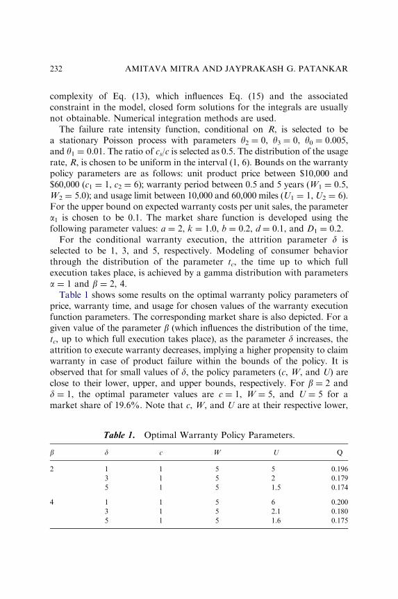
complexity of Eq. (13), which influences Eq. (15) and the associatedconstraint in the model, closed form solutions for the integrals are usuallynot obtainable. Numerical integration methods are used.
The failure rate intensity function, conditional on R, is selected to bea stationary Poisson process with parameters y2 ¼ 0, y3 ¼ 0, y0 ¼ 0.005,and y1 ¼ 0.01. The ratio of cs/c is selected as 0.5. The distribution of the usagerate, R, is chosen to be uniform in the interval (1, 6). Bounds on the warrantypolicy parameters are as follows: unit product price between $10,000 and$60,000 (c1 ¼ 1, c2 ¼ 6); warranty period between 0.5 and 5 years (W1 ¼ 0.5,W2 ¼ 5.0); and usage limit between 10,000 and 60,000 miles (U1 ¼ 1,U2 ¼ 6).For the upper bound on expected warranty costs per unit sales, the parametera1 is chosen to be 0.1. The market share function is developed using thefollowing parameter values: a ¼ 2, k ¼ 1.0, b ¼ 0.2, d ¼ 0.1, and D1 ¼ 0.2.
For the conditional warranty execution, the attrition parameter d isselected to be 1, 3, and 5, respectively. Modeling of consumer behaviorthrough the distribution of the parameter tc, the time up to which fullexecution takes place, is achieved by a gamma distribution with parametersa ¼ 1 and b ¼ 2, 4.
Table 1 shows some results on the optimal warranty policy parameters ofprice, warranty time, and usage for chosen values of the warranty executionfunction parameters. The corresponding market share is also depicted. For agiven value of the parameter b (which influences the distribution of the time,tc, up to which full execution takes place), as the parameter d increases, theattrition to execute warranty decreases, implying a higher propensity to claimwarranty in case of product failure within the bounds of the policy. It isobserved that for small values of d, the policy parameters (c, W, and U) areclose to their lower, upper, and upper bounds, respectively. For b ¼ 2 andd ¼ 1, the optimal parameter values are c ¼ 1, W ¼ 5, and U ¼ 5 for amarket share of 19.6%. Note that c, W, and U are at their respective lower,
Table 1. Optimal Warranty Policy Parameters.
b d c W U Q
2 1 1 5 5 0.196
3 1 5 2 0.179
5 1 5 1.5 0.174
4 1 1 5 6 0.200
3 1 5 2.1 0.180
5 1 5 1.6 0.175
AMITAVA MITRA AND JAYPRAKASH G. PATANKAR232
upper, and upper bounds, respectively. As d increases, for a given b, theoptimal value of U moves away from its upper bound. If no constraint hadbeen placed on ECU, the market share could be improved by increasing theusage limit further. But, since the company has to manage its expectedwarranty costs, the constrained optimization problem leads to a more manage-able and feasible solution. As the warranty execution parameter, d, increases,since the chances of warranty execution increases, expected warranty costswill go up. Thus, management may not be able to simultaneously increaseboth the warranty period or the usage limit to their upper bounds, so as tocontain the expected warranty costs per unit sales below the chosen bound. Asobserved from Table 1, with an increase in the value of d, the usage limit (U) isfound to decrease, which subsequently results in a smaller market share.
CONCLUSIONS
The chapter has considered a two-dimensional warranty policy with theobjective of assisting the manufacturer in selecting parameter values ofunit product price, warranty time, and usage limit. Since manufacturersoperate within resource constraints, it usually has to plan for expectedwarranty costs. Such costs are influenced by the warranty period and usagelimit. Thus, although it may be desirable to increase the values of theseparameters, to increase market share relative to competitors, it is not alwaysfeasible to do so based on expected warranty costs per unit.
An important insight has been the inclusion of the propensity to claima warranty on part of the consumer. Consumer behavior is influenced byseveral factors such as new product development, products offered bycompetitors, the ease or difficulty of filing a claim, and the cost associatedwith such filing, among others. Additionally, since consumers may vary intheir usage of the product, the usage rage has been modeled using a randomvariable with a selected probability distribution.
Several avenues of extension to this research exist. One could explore thestudy of enterprise warranty programs where an expanded warranty policyis offered to the customer at the time of purchase or even thereafter.Such policies are purchased through the payment of a premium and couldbe administered by the manufacturer or typically a third party. The impactof these enterprise warranty programs is to increase market share. However,expected warranty costs over the entire range of the policy also increases.Thus, a net revenue per unit sales approach could be pursued to determinethe optimal warranty policy parameters in this context.
Two-Attribute Warranty Policies 233
REFERENCES
Ahn, C. W., Chae, K. C., & Clark, G. M. (1998). Estimating parameters of the power law
process with two measures of failure rate. Journal of Quality Technology, 30, 127–132.
Amato, N. H., & Anderson, E. E. (1976). Determination of warranty reserves: An extension.
Management Science, 22(12), 1391–1394.
Balachandran, K. R., Maschmeyer, R. A., & Livingstone, J. L. (1981). Product warranty
period: A Markovian approach to estimation and analysis of repair and replacement
costs. Accounting Review, 56, 115–124.
Blacer, Y., & Sahin, I. (1986). Replacement costs under warranty: Cost moments and time
variability. Operations Research, 34, 554–559.
Blischke, W. R., & Murthy, D. N. P. (1992). Product warranty management – I: A taxonomy
for warranty policies. European Journal of Operations Research, 62, 127–148.
Blischke, W. R., & Murthy, D. N. P. (1994).Warranty cost analysis. New York: Marcel Dekker,
Inc.
Blischke, W. R., & Murthy, D. N. P. (Eds). (1996). Product warranty handbook. New York:
Marcel Dekker, Inc.
Blischke, W. R., & Scheuer, E. M. (1975). Calculation of the warranty cost policies as a function
of estimated life distributions. Naval Research Logistics Quarterly, 22(4), 681–696.
Blischke, W. R., & Scheuer, E. M. (1981). Applications of renewal theory in analysis of free-
replacement warranty. Naval Research Logistics Quarterly, 28, 193–205.
Chun, Y. H., & Tang, K. (1999). Cost analysis of two-attribute warranty policies based on the
product usage rate. IEEE Transactions on Engineering Management, 46(2), 201–209.
Eliashberg, J., Singpurwalla, N. D., & Wilson, S. P. (1997). Calculating the warranty reserve
for time and usage indexed warranty. Management Science, 43(7), 966–975.
Frees, E. W. (1988). Estimating the cost of a warranty. Journal of Business and Economic
Statistics, 1, 79–86.
Frees, E. W., & Nam, S. H. (1988). Approximating expected warranty cost. Management
Science, 43, 1441–1449.
Gertsbakh, I. B., & Kordonsky, K. B. (1998). Parallel time scales and two-dimensional
manufacturer and individual customer warranties. IIE Transactions, 30, 1181–1189.
Heschel, M. S. (1971). How much is a guarantee worth? Industrial Engineering, 3(5), 14–15.
Hsiung, C., & Shen, S. H. (2001). The effects of the warranty cost on the imperfect EMQ
model with general discrete shift distribution. Production Planning and Control, 12(6),
621–628.
Huang, H. Z., Liu, Z. J., & Murthy, D. N. P. (2007). Optimal reliability, warranty and price for
new products. IIE Transactions, 39, 819–827.
Jack, N., & Murthy, D. N. P. (2001). Servicing strategies for items sold with warranty. Journal
of Operational Research, 52, 1284–1288.
Kim, H. G., & Rao, B. M. (2000). Expected warranty cost of two-attribute free replacement
warranties based on a bivariate exponential distribution. Computers and Industrial
Engineering, 38, 425–434.
Lam, Y., & Lam, P. K. W. (2001). An extended warranty policy with options open to the
consumers. European Journal of Operational Research, 131, 514–529.
Lowerre, J. M. (1968). On warranties. Journal of Industrial Engineering, 19(3), 359–360.
Mamer, J. W. (1982). Cost analysis of pro rata and free-replacement warranties. Naval Research
Logistics Quarterly, 29(2), 345–356.
AMITAVA MITRA AND JAYPRAKASH G. PATANKAR234

Mamer, J. W. (1987). Discounted and per unit costs of product warranty. Management Science,
33(7), 916–930.
Menke, W. W. (1969). Determination of warranty reserves. Management Science, 15(10),
542–549.
Mitra, A., & Patankar, J. G. (1997). Market share and warranty costs for renewable warranty
programs. International Journal of Production Economics, 50, 155–168.
Moskowitz, H., & Chun, Y. H. (1988). A Bayesian approach to the two-attribute warranty policy.
Paper No. 950. Krannert Graduate School of Management, Purdue University, West
Lafayette, IN.
Moskowitz, H., & Chun, Y. H. (1994). A Poisson regression model for two-attribute warranty
policies. Naval Research Logistics, 41, 355–376.
Murthy, D. N. P., & Blischke, W. R. (1992a). Product warranty management – II: An
integrated framework for study. European Journal of Operations Research, 62, 261–281.
Murthy, D. N. P., & Blischke, W. R. (1992b). Product warranty management – III: A review of
mathematical models. European Journal of Operations Research, 62, 1–34.
Murthy, D. N. P., & Djamaludin, I. (2002). New product warranty: A literature review.
International Journal of Production Economics, 79, 231–260.
Murthy, D. N. P., Iskander, B. P., & Wilson, R. J. (1995). Two dimensional failure
free warranty policies: Two dimensional point process models. Operations Research, 43,
356–366.
Nguyen, D. G., & Murthy, D. N. P. (1984a). A general model for estimating warranty costs for
repairable products. IIE Transactions, 16(4), 379–386.
Nguyen, D. G., & Murthy, D. N. P. (1984b). Cost analysis of warranty policies. Naval Research
Logistics Quarterly, 31, 525–541.
Patankar, J. G., & Mitra, A. (1995). Effects of warranty execution on warranty reserve costs.
Management Science, 41, 395–400.
Patankar, J. G., & Worm, G. H. (1981). Prediction intervals for warranty reserves and cash
flow. Management Science, 27(2), 237–241.
Singpurwalla, N. D. (1987). A strategy for setting optimal warranties. Report TR-87/4. Institute
for Reliability and Risk Analysis, School of Engineering and Applied Science, George
Washington University, Washington, DC.
Singpurwalla, N. D. (1992). Survival under multiple time scales in dynamic environments. In:
J. P. Klein & P. K. Goel (Eds), Survival analysis: State of the art (pp. 345–354).
Singpurwalla, N. D., & Wilson, S. P. (1993). The warranty problem: Its statistical and game
theoretic aspects. SIAM Review, 35, 17–42.
Singpurwalla, N. D., & Wilson, S. P. (1998). Failure models indexed by two scales. Advances in
Applied Probability, 30, 1058–1072.
Tapiero, C. S., & Posner, M. J. (1988). Warranty reserving. Naval Research Logistics Quarterly,
35, 473–479.
Thomas, M. U. (1989). A prediction model for manufacturer warranty reserves. Management
Science, 35, 1515–1519.
US Federal Trade Commission Improvement Act. (1975). 88 Stat 2183, 101–112.
Wu, C. C., Lin, P. C., & Chou, C. Y. (2006). Determination of price and warranty length for a
normal lifetime distributed product. International Journal of Production Economics, 102,
95–107.
Yeh, R. H., & Lo, H. C. (2001). Optimal preventive maintenance warranty policy for repairable
products. European Journal of Operational Research, 134, 59–69.
Two-Attribute Warranty Policies 235

This page intentionally left blank

A DUAL TRANSPORTATION
PROBLEM ANALYSIS FOR
FACILITY EXPANSION/
CONTRACTION DECISIONS:
A TUTORIAL
N. K. Kwak and Chang Won Lee
ABSTRACT
A dual transportation analysis is considered as a strategic matter forplant facility expansion/contraction decision making in manufactu-ring operations. The primal-dual problem is presented in a generalizedmathematical form. A practical technique of generating the dual solutionis illustrated with a plant facility expansion/contraction example as atutorial. Demand forecasting is performed based on the time series datawith seasonal variation adjustments. The dual solution helps facilitateoperations decision making by providing useful information.
1. INTRODUCTION
A plethora of information on plant facility location analysis has appearedin the existing literature (Klamroth, 2002; Sule, 1988). The location selection
Advances in Business and Management Forecasting, Volume 6, 237–248
Copyright r 2009 by Emerald Group Publishing Limited
All rights of reproduction in any form reserved
ISSN: 1477-4070/doi:10.1108/S1477-4070(2009)0000006014
237
methods can be categorized as following: (1) factor listing/scoring method,(2) analytical hierarchy process (AHP), (3) mathematical programmingmethods, (4) simulation methods, and (5) heuristic algorithms.
In the factor listing/scoring method, decision makers identify and selectthe factors favorable for business expansion and rank them (Keeney, 1994).The AHP, developed by Saaty (1980), is a method of comparing andranking decision alternatives and select the best one in location and strategicacquisition decision making (Bowen, 1995; Tavana & Banerjee, 1995;Klorpela & Truominen, 1996; Badri, 1999). Mathematical programmingrefers to a group of mathematical techniques used for optimal solutionssubject to a set of decision constraints in facility location analysis. Itincludes linear programming, integer programming, dynamic programming,multicriteria decision-making methods, and data envelopment analysis(DEA), (Kwak, 1973; Erlenkotten, 1978; Kwak & Schniederjans, 1985;Sinha & Sastry, 1987; Current, Min, & Schilling, 1990; Revelle & Laporte,1996; Korhonen & Syrjanen, 2004; Drezner & Hamacher, 2004; Campbell,Ernst, & Krishnamoorthy, 2005; Farahani & Asgari, 2007; Ho, Lee, & Ho,2008). Simulation methods refer to the collection of methodologies used inthe Monte Carlo simulation process. They are generally computer-basedapproaches to decision making, which replicate behavior of an opera-tions system (Mehrez, Sinuany-Stern, Arad-Geva, & Binyamin, 1996;Quarterman, 1998; Schniederjans, 1999). Heuristic algorithms employ theuse of some intuitive rules or guidelines to generate new strategies, whichyield improved solutions. Some of the heuristic algorithms that can be usedfor facility expansion analysis are Tabu search algorithm (Glover, 1990),and genetic algorithm (Jaramillio, Bhadury, & Batta, 2002).
In this study, the dual transportation-problem approach is considered forfacility expansion/contraction decision making and demand forecasting withan illustrative case example.
2. A DUALITY ANALYSIS OF THE
TRANSPORTATION PROBLEM
The transportation problem, as a special case of linear programming, hasbeen analyzed in various forms in operations research/management scienceliterature. Most existing analyses deal with only one aspect of theoptimization procedure, known as the primal problem. In addition to theprimal aspect, every transportation problem has another related aspect,known as the dual problem. The dual aspect of the transportation problem
N. K. KWAK AND CHANG WON LEE238
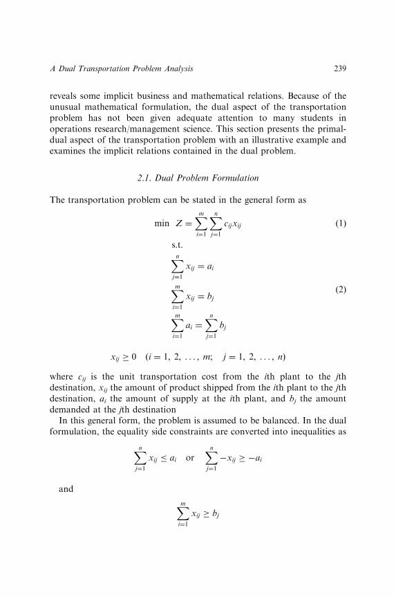
reveals some implicit business and mathematical relations. Because of theunusual mathematical formulation, the dual aspect of the transportationproblem has not been given adequate attention to many students inoperations research/management science. This section presents the primal-dual aspect of the transportation problem with an illustrative example andexamines the implicit relations contained in the dual problem.
2.1. Dual Problem Formulation
The transportation problem can be stated in the general form as
min Z ¼Xmi¼1
Xnj¼1
cijxij (1)
s:t:
Xnj¼1
xij ¼ ai
Xmi¼1
xij ¼ bj
Xmi¼1
ai ¼Xnj¼1
bj
(2)
xij � 0 ði ¼ 1; 2; . . . ; m; j ¼ 1; 2; . . . ; nÞ
where cij is the unit transportation cost from the ith plant to the jthdestination, xij the amount of product shipped from the ith plant to the jthdestination, ai the amount of supply at the ith plant, and bj the amountdemanded at the jth destination
In this general form, the problem is assumed to be balanced. In the dualformulation, the equality side constraints are converted into inequalities as
Xnj¼1
xij � ai orXnj¼1
�xij � �ai
and
Xmi¼1
xij � bj
A Dual Transportation Problem Analysis 239

These changes do not violate the supply and demand conditions, becauseeach of the i plants cannot supply a greater amount than it produces andeach of the j destinations receives at least the amount demanded.
The dual problem is formulated as
max Z0 ¼Xnj¼1
bjzj �Xmi¼1
aiyi (3)
s:t:
zj � yi � cij(4)
yi; zj � 0 ði ¼ 1; 2; . . . ;m; j ¼ 1; 2; . . . ; nÞ
where yi and zj are the dual decision variables representing the supply anddemand requirement restrictions, respectively.
Since Z ¼ Zu in the optimal solution, Eq. (5) can be obtained fromEqs. (1) and (3)
Xmi¼1
Xnj¼1
cijxij ¼Xnj¼1
bjzj �Xmi¼1
aiyi (5)
Substitution of ai and bj values in Eq. (2) into Eq. (5) yields
Xmi¼1
Xnj¼1
cijxij þXmi¼1
ðyiXnj¼1
xijÞ �Xnj¼1
ðzjXmi¼1
xijÞ ¼ 0
or
Xmi¼1
Xnj¼1
xij ðcij þ yi � zjÞ ¼ 0 (6)
Since xijZ0 and (cijþyi�zj)Z0, the following relations can be found fromEq. (6):
zj ¼ cij þ yi if xij40
zj � cij þ yi if xij ¼ 0(7)
Here, the dual variables yi and zj are interpreted as the value of theproduct, free on board (fob) at the ith plant and its delivered value at the jth
N. K. KWAK AND CHANG WON LEE240

destination, respectively. Thus, the delivered values at the destinations areequal to the values at the origins plus the unit transportation costs.
3. AN ILLUSTRATIVE CASE EXAMPLE
A logistics company in this study is a leading independent provider offactory-to-dealer transportation solutions in Korea. The company dealswith various products and distributors, such as agricultural and relatedequipments. The company’s mission statement is to give customerscompetitive advantages through logistics expertise, adequate marketforecasting, and local knowledge. The company has four plants: Busan(A), Inchon (B), Kunsan (C), and Mokpo (D). There are five dealer–distributors in the different markets. The company distributes farm andrelated equipments by means of inland and sea transportation modes.
The company management is concerned about recent turbulence in theglobal economy, which affects the domestic market performance, especiallydue to the seasonally varied demand for the products. Therefore, the generalmanagerial concern is to find the best practice in transportation services to thedealer–distributors while minimizing the total transportation cost, as well asfulfilling their needs. Data templates were derived from the company recordwith some modifications to ensure the corporate security in the competitive
Table 1. Transportation Table.
Dstn.*
PlantI II III IV V Supply
A13
x11
18
x12
12
x13
15
x14
13
x1540
B15
x21
15
x22
10
x23
17
x24
10
x2550
C12
x31
12
x32
10
x33
16
x34
23
x3560
D19
x41
20
x42
17
x43
25
x44
15 x 50
Demand 40 50 30 30 50 200
*Destination (Dstn) = Dealer-Distributor
45
A Dual Transportation Problem Analysis 241
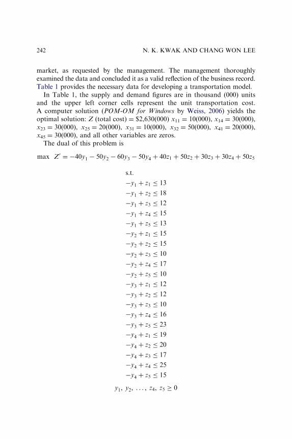
market, as requested by the management. The management thoroughlyexamined the data and concluded it as a valid reflection of the business record.Table 1 provides the necessary data for developing a transportation model.
In Table 1, the supply and demand figures are in thousand (000) unitsand the upper left corner cells represent the unit transportation cost.A computer solution (POM-OM for Windows by Weiss, 2006) yields theoptimal solution: Z (total cost) ¼ $2,630(000) x11 ¼ 10(000), x14 ¼ 30(000),x23 ¼ 30(000), x25 ¼ 20(000), x31 ¼ 10(000), x32 ¼ 50(000), x41 ¼ 20(000),x45 ¼ 30(000), and all other variables are zeros.
The dual of this problem is
max Z0 ¼ �40y1 � 50y2 � 60y3 � 50y4 þ 40z1 þ 50z2 þ 30z3 þ 30z4 þ 50z5
s:t:
�y1 þ z1 � 13
�y1 þ z2 � 18
�y1 þ z3 � 12
�y1 þ z4 � 15
�y1 þ z5 � 13
�y2 þ z1 � 15
�y2 þ z2 � 15
�y2 þ z3 � 10
�y2 þ z4 � 17
�y2 þ z5 � 10
�y3 þ z1 � 12
�y3 þ z2 � 12
�y3 þ z3 � 10
�y3 þ z4 � 16
�y3 þ z5 � 23
�y4 þ z1 � 19
�y4 þ z2 � 20
�y4 þ z3 � 17
�y4 þ z4 � 25
�y4 þ z5 � 15
y1; y2; . . . ; z4; z5 � 0
N. K. KWAK AND CHANG WON LEE242
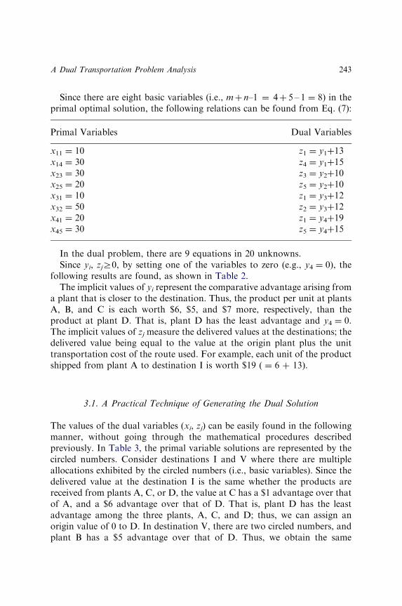
Since there are eight basic variables (i.e., mþ n–1 ¼ 4þ 5 – 1 ¼ 8) in theprimal optimal solution, the following relations can be found from Eq. (7):
Primal Variables Dual Variables
x11 ¼ 10 z1 ¼ y1þ13x14 ¼ 30 z4 ¼ y1þ15x23 ¼ 30 z3 ¼ y2þ10x25 ¼ 20 z5 ¼ y2þ10x31 ¼ 10 z1 ¼ y3þ12x32 ¼ 50 z2 ¼ y3þ12x41 ¼ 20 z1 ¼ y4þ19x45 ¼ 30 z5 ¼ y4þ15
In the dual problem, there are 9 equations in 20 unknowns.Since yi, zjZ0, by setting one of the variables to zero (e.g., y4 ¼ 0), the
following results are found, as shown in Table 2.The implicit values of yi represent the comparative advantage arising from
a plant that is closer to the destination. Thus, the product per unit at plantsA, B, and C is each worth $6, $5, and $7 more, respectively, than theproduct at plant D. That is, plant D has the least advantage and y4 ¼ 0.The implicit values of zj measure the delivered values at the destinations; thedelivered value being equal to the value at the origin plant plus the unittransportation cost of the route used. For example, each unit of the productshipped from plant A to destination I is worth $19 ( ¼ 6 þ 13).
3.1. A Practical Technique of Generating the Dual Solution
The values of the dual variables (xi, zj) can be easily found in the followingmanner, without going through the mathematical procedures describedpreviously. In Table 3, the primal variable solutions are represented by thecircled numbers. Consider destinations I and V where there are multipleallocations exhibited by the circled numbers (i.e., basic variables). Since thedelivered value at the destination I is the same whether the products arereceived from plants A, C, or D, the value at C has a $1 advantage over thatof A, and a $6 advantage over that of D. That is, plant D has the leastadvantage among the three plants, A, C, and D; thus, we can assign anorigin value of 0 to D. In destination V, there are two circled numbers, andplant B has a $5 advantage over that of D. Thus, we obtain the same
A Dual Transportation Problem Analysis 243
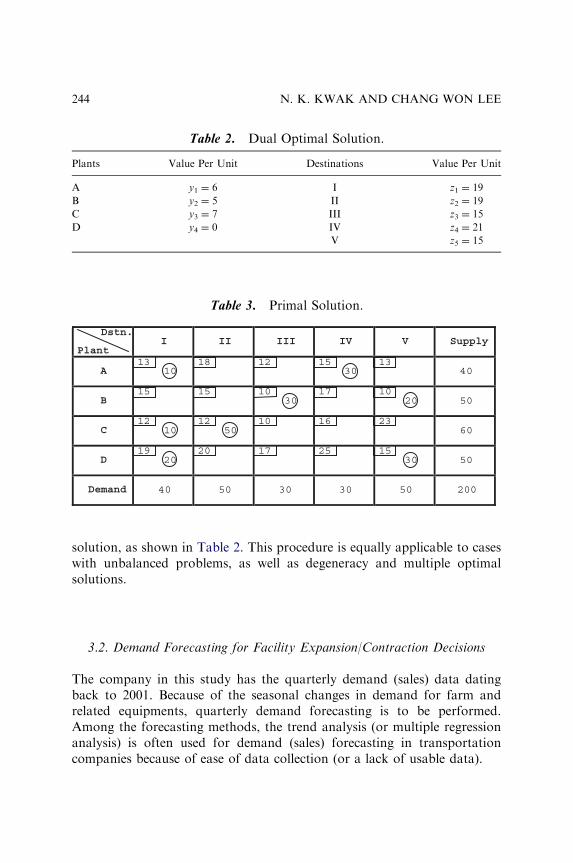
solution, as shown in Table 2. This procedure is equally applicable to caseswith unbalanced problems, as well as degeneracy and multiple optimalsolutions.
3.2. Demand Forecasting for Facility Expansion/Contraction Decisions
The company in this study has the quarterly demand (sales) data datingback to 2001. Because of the seasonal changes in demand for farm andrelated equipments, quarterly demand forecasting is to be performed.Among the forecasting methods, the trend analysis (or multiple regressionanalysis) is often used for demand (sales) forecasting in transportationcompanies because of ease of data collection (or a lack of usable data).
Table 2. Dual Optimal Solution.
Plants Value Per Unit Destinations Value Per Unit
A y1 ¼ 6 I z1 ¼ 19
B y2 ¼ 5 II z2 ¼ 19
C y3 ¼ 7 III z3 ¼ 15
D y4 ¼ 0 IV z4 ¼ 21
V z5 ¼ 15
Table 3. Primal Solution.
Dstn.
PlantI II III IV V Supply
A13
1018 12 15
3013
40
B15 15 10
3017 10
20 50
C12
1012
5010 16 23
60
D19
2020 17 25 15
30 50
Demand 40 50 30 30 50 200
N. K. KWAK AND CHANG WON LEE244
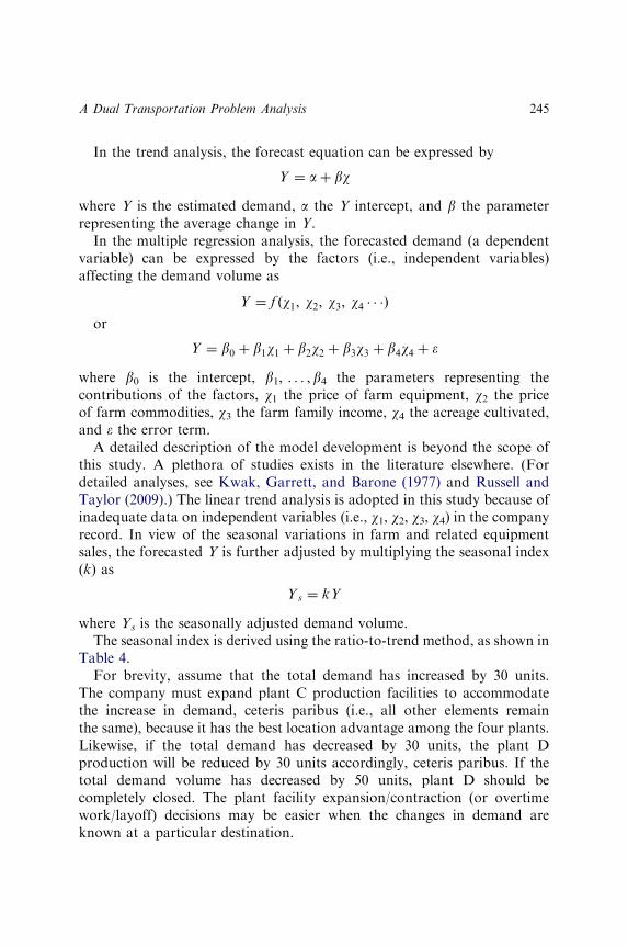
In the trend analysis, the forecast equation can be expressed by
Y ¼ aþ bw
where Y is the estimated demand, a the Y intercept, and b the parameterrepresenting the average change in Y.
In the multiple regression analysis, the forecasted demand (a dependentvariable) can be expressed by the factors (i.e., independent variables)affecting the demand volume as
Y ¼ f ðw1; w2; w3; w4 � � �Þ
or
Y ¼ b0 þ b1w1 þ b2w2 þ b3w3 þ b4w4 þ �
where b0 is the intercept, b1, . . . , b4 the parameters representing thecontributions of the factors, w1 the price of farm equipment, w2 the priceof farm commodities, w3 the farm family income, w4 the acreage cultivated,and e the error term.
A detailed description of the model development is beyond the scope ofthis study. A plethora of studies exists in the literature elsewhere. (Fordetailed analyses, see Kwak, Garrett, and Barone (1977) and Russell andTaylor (2009).) The linear trend analysis is adopted in this study because ofinadequate data on independent variables (i.e., w1, w2, w3, w4) in the companyrecord. In view of the seasonal variations in farm and related equipmentsales, the forecasted Y is further adjusted by multiplying the seasonal index(k) as
Ys ¼ kY
where Ys is the seasonally adjusted demand volume.The seasonal index is derived using the ratio-to-trend method, as shown in
Table 4.For brevity, assume that the total demand has increased by 30 units.
The company must expand plant C production facilities to accommodatethe increase in demand, ceteris paribus (i.e., all other elements remainthe same), because it has the best location advantage among the four plants.Likewise, if the total demand has decreased by 30 units, the plant Dproduction will be reduced by 30 units accordingly, ceteris paribus. If thetotal demand volume has decreased by 50 units, plant D should becompletely closed. The plant facility expansion/contraction (or overtimework/layoff) decisions may be easier when the changes in demand areknown at a particular destination.
A Dual Transportation Problem Analysis 245
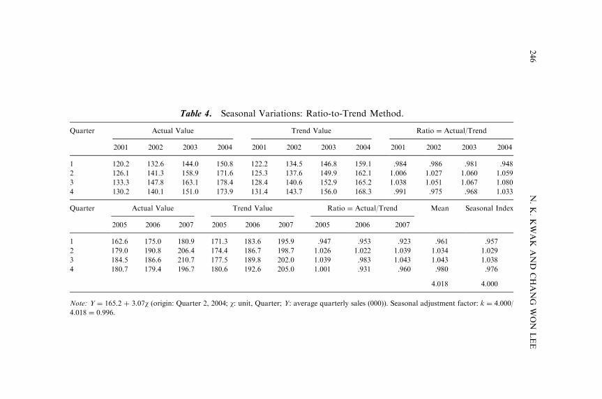
Table 4. Seasonal Variations: Ratio-to-Trend Method.
Quarter Actual Value Trend Value Ratio ¼ Actual/Trend
2001 2002 2003 2004 2001 2002 2003 2004 2001 2002 2003 2004
1 120.2 132.6 144.0 150.8 122.2 134.5 146.8 159.1 .984 .986 .981 .948
2 126.1 141.3 158.9 171.6 125.3 137.6 149.9 162.1 1.006 1.027 1.060 1.059
3 133.3 147.8 163.1 178.4 128.4 140.6 152.9 165.2 1.038 1.051 1.067 1.080
4 130.2 140.1 151.0 173.9 131.4 143.7 156.0 168.3 .991 .975 .968 1.033
Quarter Actual Value Trend Value Ratio ¼ Actual/Trend Mean Seasonal Index
2005 2006 2007 2005 2006 2007 2005 2006 2007
1 162.6 175.0 180.9 171.3 183.6 195.9 .947 .953 .923 .961 .957
2 179.0 190.8 206.4 174.4 186.7 198.7 1.026 1.022 1.039 1.034 1.029
3 184.5 186.6 210.7 177.5 189.8 202.0 1.039 .983 1.043 1.043 1.038
4 180.7 179.4 196.7 180.6 192.6 205.0 1.001 .931 .960 .980 .976
4.018 4.000
Note: Y ¼ 165.2 þ 3.07w (origin: Quarter 2, 2004; w: unit, Quarter; Y: average quarterly sales (000)). Seasonal adjustment factor: k ¼ 4.000/
4.018 ¼ 0.996.
N.K.KWAK
AND
CHANG
WON
LEE
246
4. CONCLUDING REMARKS
The dual transportation problem was analyzed for plant facility expansion/contraction decision making in manufacturing operations, along withdemand forecasting with an illustrative case example. This duality analysisof transportation problem is equally applicable to other resource allocationsproblems in business and industry. In manufacturing operations, the firm’saccounting personnel can be assigned to a variety of jobs (e.g., accountsreceivables, accounts payable, sales auditing, payroll) when the problem isformulated and presented in transportation matrix format. The qualifica-tions of the accounting personnel can be implicitly rated for effective controland better operations management.
REFERENCES
Badri, M. A. (1999). Combining the analytic hierarchy process and goal programming for
global facility-allocation problem. International Journal of Production Economics, 62,
237–248.
Bowen, W. M. (1995). A Thurstonian comparison of the analytic hierarchy process and
probabilistic multidimensional scaling through application to the nuclear waste site
selection decision. Socio-economic Planning Science, 29, 151–164.
Campbell, J. F., Ernst, A. T., & Krishnamoorthy, M. (2005). Hub arc location problems:
Part 1 – Introduction and results. Management Science, 51, 1540–1555.
Current, J. H., Min, H., & Schilling, D. (1990). Multiobjective analysis of facility location
decisions. European Journal of Operational Research, 49, 295–308.
Drezner, Z., & Hamacher, H. (2004). Facility location: Application and theory. Berlin, Germany:
Verlag.
Erlenkotten, D. (1978). A dual-based procedure for uncapacitated facility location. Operations
Research, 26, 992–1009.
Farahani, R. Z., & Asgari, N. (2007). Combination of MCDM and converging techniques in a
hierarchical model for facility location: A case study. European Journal of Operational
Research, 176, 1839–1858.
Glover, F. (1990). A Tabu search: A tutorial. Interfaces, 20, 74–94.
Ho, W., Lee, C. K. M., & Ho, G. T. S. (2008). Optimization of the facility location-allocation
problem in a customer-driven supply chain. Operations Management Research, 1, 69–79.
Jaramillio, J. H., Bhadury, J., & Batta, R. (2002). On the use of generic algorithms to solve
location problems. Computers & Operations Research, 29, 761–779.
Keeney, R. L. (1994). Using values in operations research. Operations Research, 42, 793–813.
Klamroth, K. (2002). Single facility location problems with barriers. Berlin, Germany: Springer
Verlag.
Klorpela, J., & Truominen, M. (1996). A decision aid in warehouse site selection. International
Journal of Production Economics, 45, 169–181.
A Dual Transportation Problem Analysis 247

Korhonen, P., & Syrjanen, M. (2004). Resource allocation based on efficiency analysis.
Management Science, 50, 1134–1144.
Kwak, N. K. (1973). Mathematical programming with business applications. New York:
McGraw-Hill.
Kwak, N. K., Garrett, W. A., & Barone, S. (1977). Stochastic model of demand forecasting for
technical manpower. Management Science, 23, 1089–1098.
Kwak, N. K., & Schniederjans, M. J. (1985). A goal programming model as an aid to facility
location analysis. Computers & Operations Research, 12, 151–161.
Mehrez, A., Sinuany-Stern, Z., Arad-Geva, T., & Binyamin, S. (1996). On the implementation
of quantitative facility location models: The case of a hospital in a rural region. Journal
of the Operational Research Society, 47, 612–626.
Quarterman, L. (1998). Points to consider in selecting facilities planning software. ITE
Solutions, 30, 42049.
Revelle, C. S., & Laporte, G. (1996). The plant location plan: New models and research
prospects. Operations Research, 44, 864–874.
Russell, R. S., & Taylor, B. W., III. (2009). Operations management. New York: Wiley.
Saaty, T. L. (1980). The analytic hierarchy process. New York: McGraw-Hill.
Schniederjans, M. J. (1999). International facility acquisition and location analysis. Westport,
CT: Quorum Books.
Sinha, S. B., & Sastry, S. V. C. (1987). A goal programming model to resolve a site location
problem. Interfaces, 12, 251–256.
Sule, D. R. (1988). Manufacturing facilities: Location, planning, and design. Boston, MA: PWS-
Kent Publishing.
Tavana, M., & Banerjee, S. (1995). Evaluating strategic alternatives: An analytic hierarchy
process. Computers & Operations Research, 22, 731–743.
Weiss, H. J. (2006). POM-QM for windows (Version 3). Upper Saddle River, NJ: Pearson/
Prentice Hall.
N. K. KWAK AND CHANG WON LEE248
MAKE-TO-ORDER PRODUCT
DEMAND FORECASTING:
EXPONENTIAL SMOOTHING
MODELS WITH NEURAL
NETWORK CORRECTION
Mark T. Leung, Rolando Quintana and
An-Sing Chen
ABSTRACT
Demand forecasting has long been an imperative tenet in productionplanning especially in a make-to-order environment where a typicalmanufacturer has to balance the issues of holding excessive safety stocksand experiencing possible stockout. Many studies provide pragmaticparadigms to generate demand forecasts (mainly based on smoothingforecasting models.) At the same time, artificial neural networks (ANNs)have been emerging as alternatives. In this chapter, we propose a two-stage forecasting approach, which combines the strengths of a neuralnetwork with a more conventional exponential smoothing model. In thefirst stage of this approach, a smoothing model estimates the series ofdemand forecasts. In the second stage, general regression neural network(GRNN) is applied to learn and then correct the errors of estimates. Ourempirical study evaluates the use of different static and dynamic
Advances in Business and Management Forecasting, Volume 6, 249–266
Copyright r 2009 by Emerald Group Publishing Limited
All rights of reproduction in any form reserved
ISSN: 1477-4070/doi:10.1108/S1477-4070(2009)0000006015
249

smoothing models and calibrates their synergies with GRNN. Variousstatistical tests are performed to compare the performances of the two-stage models (with error correction by neural network) and those of theoriginal single-stage models (without error-correction by neural net-work). Comparisons with the single-stage GRNN are also included.Statistical results show that neural network correction leads to improve-ments to the forecasts made by all examined smoothing models and canoutperform the single-stage GRNN in most cases. Relative performancesat different levels of demand lumpiness are also examined.
1. INTRODUCTION
Demand forecasting has long been an imperative tenet in productionplanning. In a make-to-order environment where production schedulesgenerally follow the fulfillment of orders, a typical manufacturer still has tobalance the paradoxical issues of producing too much which leads toexcessive inventory and producing inadequately which causes backlog.Either of the two scenarios can often result in higher cost and more waste.Hence, it would be advantageous for a manufacturer to obtain accurateestimates of demand orders (volumes) even before the orders are actuallyreceived. In light of this practical need, many studies have formulatedpragmatic paradigms to generate demand forecasts using a wide spectrum ofmethods and models. Nevertheless, it seems that most of the conventionalproduction forecasting models adopted mainly align with the stream ofexponential smoothing forecasting. Over the past decade, more innovativemodels have been emerging as alternatives due to the advancement ofcomputational intelligence. One of such stream of research is the use ofartificial neural networks (ANNs), which has been applied to solve problemsencountered in different manufacturing settings including productionscheduling, cell design and formation, quality control, and cost estimation.
In this study, we apply ANN to forecast demand orders based onhistorical (observable) data as well as to improve the forecasts made byother models. In other words, ANN is used to correct the errors of a basemodel’s forecasts in a two-stage adaptive forecasting framework. Conven-tional exponential smoothing models are chosen and facilitate as the basismodels in this forecasting research because of their popularity amongindustrial practitioners and academic circle. Because of the existence ofdifferent approaches and adaptations of the smoothing concept, we
MARK T. LEUNG ET AL.250

explicitly consider two groups of smoothing models – one that is basedon static model parameters, which do not autonomously change over timeand the other that utilizes dynamically self-adjusted smoothing controlconstants. The static models are simpler but may be subject to a slowerresponse rate. On the other hand, the more mathematically complexdynamic models should create better forecasts. With the current computertechnology, these models can be easily implemented.
Thus, the demand forecasting study consists of single- and two-stagemodels. The single-stage models include static and dynamic smoothingmodels and a neural network, namely, general regression neural network(GRNN). Each of the two-stage models is made up of a smoothing modeland GRNN. Essentially, a smoothing model is used as a basis and forms theseries of demand estimates in the first stage of forecasting. Consequently,GRNN is employed to ‘‘learn’’ the error residuals of these estimates andmakes proper adjustments (corrections) to the estimates. Our conjecture isthat the two-stage forecasting models with error correction capabilityshould perform better than the single-stage models. Another purpose of thischapter is to show that the use of neural network in error correction in thistwo-stage framework can lead to improvement in the original forecasts evengenerated by the neural network itself. It is because neural network mostlysuffers the issue of unexplored (untrained) state space due to its weaknessin extrapolation. An exponential smoothing model, which is capable ofextrapolating into unknown state space, can alleviate this weakness. Hence,combining a smoothing model with a neural network may create synergyin forecasting. All single- and two-stage models are evaluated accordingto a spectrum of measures such as root mean squared error (RMSE),improvement ratios (IRs) over the base model and the single-stage neuralnetwork, information contents, forecast bias and proportion. The empiricalanalysis also evaluates the relative performances of models at differentlevels of demand lumpiness or volatility. It is believed that the higher thelumpiness, the more uncertainty associated with demand orders and therebythe more deterioration to a model’s forecasting capacity.
The chapter is organized as follows. In Section 2, a conceptual back-ground of the single-stage forecasting models is briefly summarized. Thisincludes three conventional static and two dynamically self-adjusted smooth-ing models, as well as GRNN, the neural network employed in the secondstage of the two-stage forecasting framework. In Section 3, the methodologiesfor both single- and two-stage forecasting are explained. The section alsodescribes the data set and the horizons for model estimation and performanceevaluation. Moreover, criteria for data categorization with respect to demand
Make-to-Order Product Demand Forecasting 251
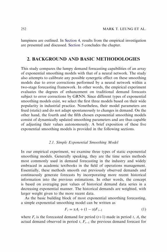
lumpiness are outlined. In Section 4, results from the empirical investigationare presented and discussed. Section 5 concludes the chapter.
2. BACKGROUND AND BASIC METHODOLOGIES
This study compares the lumpy demand forecasting capabilities of an arrayof exponential smoothing models with that of a neural network. The studyalso attempts to calibrate any possible synergetic effect on these smoothingmodels due to error corrections performed by a neural network within atwo-stage forecasting framework. In other words, the empirical experimentevaluates the degrees of enhancement on traditional demand forecastssubject to error corrections by GRNN. Since different types of exponentialsmoothing models exist, we select the first three models based on their widepopularity in industrial practice. Nonetheless, their model parameters arefixed (static) and do not adapt spontaneously to changes in demand. On theother hand, the fourth and the fifth chosen exponential smoothing modelsconsist of dynamically updated smoothing parameters and are thus capableof adjusting their values autonomously. A brief exposition of these fiveexponential smoothing models is provided in the following sections.
2.1. Simple Exponential Smoothing Model
In our empirical experiment, we examine three types of static exponentialsmoothing models. Generally speaking, they are the time series methodsmost commonly used in demand forecasting in the industry and widelyembraced in academic textbooks in the field of operations management.Essentially, these methods smooth out previously observed demands andcontinuously generate forecasts by incorporating more recent historicalinformation into the previous estimations. In other words, the conceptis based on averaging past values of historical demand data series in adecreasing exponential manner. The historical demands are weighted, withlarger weight given to the more recent data.
As the basic building block of most exponential smoothing forecasting,a simple exponential smoothing model can be written as
Ft ¼ aAt þ ð1� aÞFt�1 (1)
where Ft is the forecasted demand for period (tþ1) made in period t, At theactual demand observed in period t, Ft�1 the previous demand forecast for
MARK T. LEUNG ET AL.252
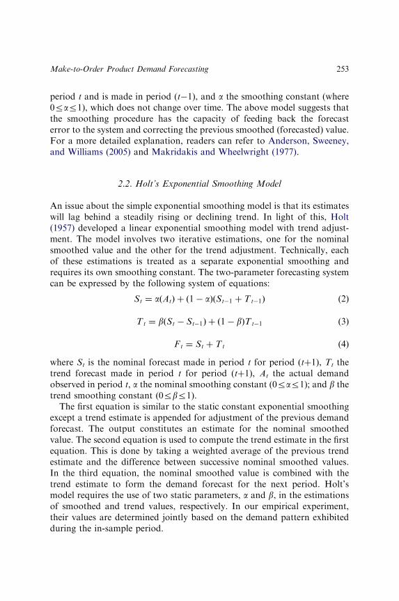
period t and is made in period (t�1), and a the smoothing constant (where0rar1), which does not change over time. The above model suggests thatthe smoothing procedure has the capacity of feeding back the forecasterror to the system and correcting the previous smoothed (forecasted) value.For a more detailed explanation, readers can refer to Anderson, Sweeney,and Williams (2005) and Makridakis and Wheelwright (1977).
2.2. Holt’s Exponential Smoothing Model
An issue about the simple exponential smoothing model is that its estimateswill lag behind a steadily rising or declining trend. In light of this, Holt(1957) developed a linear exponential smoothing model with trend adjust-ment. The model involves two iterative estimations, one for the nominalsmoothed value and the other for the trend adjustment. Technically, eachof these estimations is treated as a separate exponential smoothing andrequires its own smoothing constant. The two-parameter forecasting systemcan be expressed by the following system of equations:
St ¼ aðAtÞ þ ð1� aÞðSt�1 þ Tt�1Þ (2)
Tt ¼ bðSt � St�1Þ þ ð1� bÞTt�1 (3)
Ft ¼ St þ Tt (4)
where St is the nominal forecast made in period t for period (tþ1), Tt thetrend forecast made in period t for period (tþ1), At the actual demandobserved in period t, a the nominal smoothing constant (0rar1); and b thetrend smoothing constant (0rbr1).
The first equation is similar to the static constant exponential smoothingexcept a trend estimate is appended for adjustment of the previous demandforecast. The output constitutes an estimate for the nominal smoothedvalue. The second equation is used to compute the trend estimate in the firstequation. This is done by taking a weighted average of the previous trendestimate and the difference between successive nominal smoothed values.In the third equation, the nominal smoothed value is combined with thetrend estimate to form the demand forecast for the next period. Holt’smodel requires the use of two static parameters, a and b, in the estimationsof smoothed and trend values, respectively. In our empirical experiment,their values are determined jointly based on the demand pattern exhibitedduring the in-sample period.
Make-to-Order Product Demand Forecasting 253
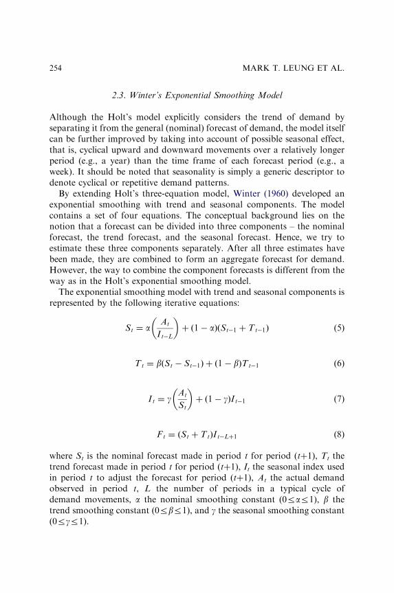
2.3. Winter’s Exponential Smoothing Model
Although the Holt’s model explicitly considers the trend of demand byseparating it from the general (nominal) forecast of demand, the model itselfcan be further improved by taking into account of possible seasonal effect,that is, cyclical upward and downward movements over a relatively longerperiod (e.g., a year) than the time frame of each forecast period (e.g., aweek). It should be noted that seasonality is simply a generic descriptor todenote cyclical or repetitive demand patterns.
By extending Holt’s three-equation model, Winter (1960) developed anexponential smoothing with trend and seasonal components. The modelcontains a set of four equations. The conceptual background lies on thenotion that a forecast can be divided into three components – the nominalforecast, the trend forecast, and the seasonal forecast. Hence, we try toestimate these three components separately. After all three estimates havebeen made, they are combined to form an aggregate forecast for demand.However, the way to combine the component forecasts is different from theway as in the Holt’s exponential smoothing model.
The exponential smoothing model with trend and seasonal components isrepresented by the following iterative equations:
St ¼ aAt
It�L
� �þ ð1� aÞðSt�1 þ Tt�1Þ (5)
Tt ¼ bðSt � St�1Þ þ ð1� bÞTt�1 (6)
I t ¼ gAt
St
� �þ ð1� gÞI t�1 (7)
Ft ¼ ðSt þ TtÞI t�Lþ1 (8)
where St is the nominal forecast made in period t for period (tþ1), Tt thetrend forecast made in period t for period (tþ1), It the seasonal index usedin period t to adjust the forecast for period (tþ1), At the actual demandobserved in period t, L the number of periods in a typical cycle ofdemand movements, a the nominal smoothing constant (0rar1), b thetrend smoothing constant (0rbr1), and g the seasonal smoothing constant(0rgr1).
MARK T. LEUNG ET AL.254
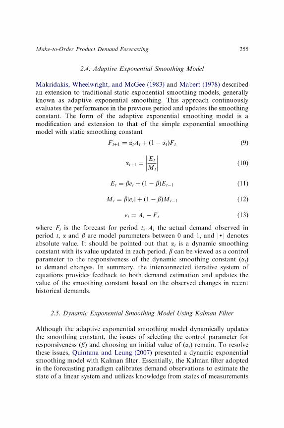
2.4. Adaptive Exponential Smoothing Model
Makridakis, Wheelwright, and McGee (1983) and Mabert (1978) describedan extension to traditional static exponential smoothing models, generallyknown as adaptive exponential smoothing. This approach continuouslyevaluates the performance in the previous period and updates the smoothingconstant. The form of the adaptive exponential smoothing model is amodification and extension to that of the simple exponential smoothingmodel with static smoothing constant
Ftþ1 ¼ atAt þ ð1� atÞFt (9)
atþ1 ¼Et
Mt
�������� (10)
Et ¼ bet þ ð1� bÞEt�1 (11)
Mt ¼ b etj j þ ð1� bÞMt�1 (12)
et ¼ At � Ft (13)
where Ft is the forecast for period t, At the actual demand observed inperiod t, a and b are model parameters between 0 and 1, and |d| denotesabsolute value. It should be pointed out that at is a dynamic smoothingconstant with its value updated in each period. b can be viewed as a controlparameter to the responsiveness of the dynamic smoothing constant (at)to demand changes. In summary, the interconnected iterative system ofequations provides feedback to both demand estimation and updates thevalue of the smoothing constant based on the observed changes in recenthistorical demands.
2.5. Dynamic Exponential Smoothing Model Using Kalman Filter
Although the adaptive exponential smoothing model dynamically updatesthe smoothing constant, the issues of selecting the control parameter forresponsiveness (b) and choosing an initial value of (at) remain. To resolvethese issues, Quintana and Leung (2007) presented a dynamic exponentialsmoothing model with Kalman filter. Essentially, the Kalman filter adoptedin the forecasting paradigm calibrates demand observations to estimate thestate of a linear system and utilizes knowledge from states of measurements
Make-to-Order Product Demand Forecasting 255
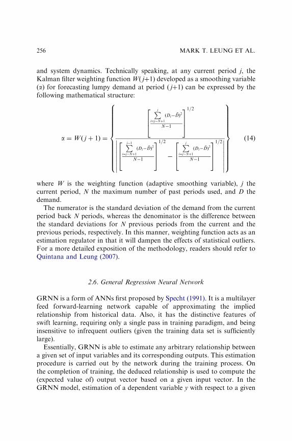
and system dynamics. Technically speaking, at any current period j, theKalman filter weighting functionW( jþ1) developed as a smoothing variable(a) for forecasting lumpy demand at period ( jþ1) can be expressed by thefollowing mathematical structure:
a ¼Wð j þ 1Þ ¼
Pji¼j�Nþ1
ðDi� �DÞ2
N�1
264
3751=2
Pj�1i¼j�Nþ1
ðDi� �DÞ2
N�1
264
3751=2
�
Pji¼j�Nþ1
ðDi� �DÞ2
N�1
264
3751=2
��������
��������
8>>>>>>>>>>><>>>>>>>>>>>:
9>>>>>>>>>>>=>>>>>>>>>>>;
(14)
where W is the weighting function (adaptive smoothing variable), j thecurrent period, N the maximum number of past periods used, and D thedemand.
The numerator is the standard deviation of the demand from the currentperiod back N periods, whereas the denominator is the difference betweenthe standard deviations for N previous periods from the current and theprevious periods, respectively. In this manner, weighting function acts as anestimation regulator in that it will dampen the effects of statistical outliers.For a more detailed exposition of the methodology, readers should refer toQuintana and Leung (2007).
2.6. General Regression Neural Network
GRNN is a form of ANNs first proposed by Specht (1991). It is a multilayerfeed forward-learning network capable of approximating the impliedrelationship from historical data. Also, it has the distinctive features ofswift learning, requiring only a single pass in training paradigm, and beinginsensitive to infrequent outliers (given the training data set is sufficientlylarge).
Essentially, GRNN is able to estimate any arbitrary relationship betweena given set of input variables and its corresponding outputs. This estimationprocedure is carried out by the network during the training process. Onthe completion of training, the deduced relationship is used to compute the(expected value of) output vector based on a given input vector. In theGRNN model, estimation of a dependent variable y with respect to a given
MARK T. LEUNG ET AL.256

vector of independent variables X can be regarded as finding the expectedvalue of y conditional on the value of X. The following equation summarizesthis statistical concept:
E yjX½ � ¼
R1�1
yf ðX; yÞdyR1�1
f ðX; yÞdy(15)
where y is the output value estimated by GRNN, X the input vector for theestimation of y; and f(X, y) the joint probability density function of X and ylearned by GRNN from the available training data set.
Justifications for the choice and use of GRNN architectural design forneural network forecasting in this study are primarily due to its relativesimplicity in training and its rather encouraging results and stable perfor-mances found by other studies. For the sake of brevity, readers can referto Wasserman (1993) for a complete explanation of the foundation andoperational logic of this specific design of neural network model.
3. FORECASTING DEMAND
3.1. Data and Single-Stage Forecasting of Demand
Our data set is based on an industrial consulting project with a Mexicanproduction facility supplying parts to major automobile manufacturers.Demand order information of more than 400 SKUs was obtained from themanagement. For the sake of a more focused experiment, only observationsof the items with the 10 largest aggregate demand volumes in each lumpinesscategory are used in our comparative evaluation. There are three categoriesof lumpiness, representing different levels of demand order volatility. Toclassify the level of lumpiness, the manufacturing company defines a ‘‘low’’lumpy environment as one within 71 standard deviation from the meandemand. Medium and high lumpiness are defined as within 72 and beyond72 standard deviations from the mean, respectively.
The provided weekly demand data run from January 1997 to December2005.1 In our empirical experiment, the historical data series is divided intotwo sample periods – the estimation (in-sample) and the test (out-of-sample)periods. The estimation period covers observations from January 1997 toDecember 2002 and is used for establishment of smoothing parametersin various single-stage (fixed constant, Holt’s, Winter’s, and Kalman filter)models. It also serves as the training period for the single-stage GRNN
Make-to-Order Product Demand Forecasting 257
forecasting and the two-stage GRNN adaptive error correction. Moreover,the first year in the estimation period is reserved as an initialization periodfor estimations by the Holt’s smoothing, the Winter’s smoothing, and bothsingle- and two-stage GRNN models. On the basis of an assessment ofperformances in the estimation period, the specification of each model typeis selected and subject to out-of-sample testing. The three-year test periodgoes from January 2003 to December 2005 and is reserved strictly for thepurpose of performance evaluation.
3.2. Two-Stage Demand Forecasting with Error Correction
Given its demonstrated performance, the two-stage error correctionframework described by Chen and Leung (2004) for foreign exchangeforecasting is modified and adapted to our problem environment. For thetwo-stage demand forecasting, a smoothing model is estimated and then itsforecasts are subsequently corrected by GRNN. In the first stage, eachof the five static and dynamic exponential smoothing models is estimatedbased on the paradigm described in the previous section. After that,residuals for the in-sample forecasts from January 19982 to December 2002are computed. GRNN is applied to estimate the error distribution. As wemove forward into the out-of-sample period, new forecasts are generatedfrom the smoothing model and new residuals are produced. Hence, as thedata of a week become observable, the residual associated with that weekcan be generated by subtracting the demand forecast from the newlyobserved demand, which is now observable. The training set is then updatedby incorporating this newly computed residual and eliminating the oldestresidual observation. Then, GRNN is retrained using the updated residualseries. The forecast for the expected residual of following week is thengenerated using the retrained GRNN. An error-corrected demand forecastfor the following week can be attained by adding the following week’sforecasted residual to the original single-stage forecast computed by thesmoothing model. This two-stage forecasting paradigm is repeated for thefive smoothing models.
4. RESULTS
Out-of-sample performances of the forecasting models in our empiricalstudy are tabulated in Table 1. The results with respect to RMSE are
MARK T. LEUNG ET AL.258
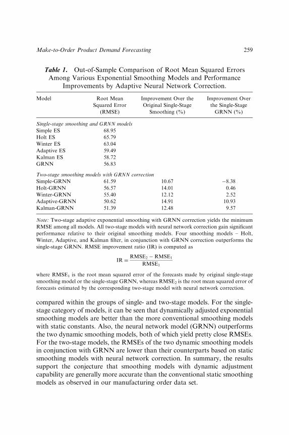
compared within the groups of single- and two-stage models. For the single-stage category of models, it can be seen that dynamically adjusted exponentialsmoothing models are better than the more conventional smoothing modelswith static constants. Also, the neural network model (GRNN) outperformsthe two dynamic smoothing models, both of which yield pretty close RMSEs.For the two-stage models, the RMSEs of the two dynamic smoothing modelsin conjunction with GRNN are lower than their counterparts based on staticsmoothing models with neural network correction. In summary, the resultssupport the conjecture that smoothing models with dynamic adjustmentcapability are generally more accurate than the conventional static smoothingmodels as observed in our manufacturing order data set.
Table 1. Out-of-Sample Comparison of Root Mean Squared ErrorsAmong Various Exponential Smoothing Models and Performance
Improvements by Adaptive Neural Network Correction.
Model Root Mean
Squared Error
(RMSE)
Improvement Over the
Original Single-Stage
Smoothing (%)
Improvement Over
the Single-Stage
GRNN (%)
Single-stage smoothing and GRNN models
Simple ES 68.95
Holt ES 65.79
Winter ES 63.04
Adaptive ES 59.49
Kalman ES 58.72
GRNN 56.83
Two-stage smoothing models with GRNN correction
Simple-GRNN 61.59 10.67 �8.38
Holt-GRNN 56.57 14.01 0.46
Winter-GRNN 55.40 12.12 2.52
Adaptive-GRNN 50.62 14.91 10.93
Kalman-GRNN 51.39 12.48 9.57
Note: Two-stage adaptive exponential smoothing with GRNN correction yields the minimum
RMSE among all models. All two-stage models with neural network correction gain significant
performance relative to their original smoothing models. Four smoothing models – Holt,
Winter, Adaptive, and Kalman filter, in conjunction with GRNN correction outperforms the
single-stage GRNN. RMSE improvement ratio (IR) is computed as
IR ¼RMSE2 �RMSE1
RMSE1
where RMSE1 is the root mean squared error of the forecasts made by original single-stage
smoothing model or the single-stage GRNN, whereas RMSE2 is the root mean squared error of
forecasts estimated by the corresponding two-stage model with neural network correction.
Make-to-Order Product Demand Forecasting 259

Table 1 also compares two- and single-stage models by evaluating theimprovement of GRNN error correction used in a two-stage model overits single-stage counterpart without error correction. Specifically, the IR iscomputed by the difference between the RMSE of a two-stage model andthat of its single-stage counterpart without correction divided by the RMSEof the single-stage counterpart without correction. This computation can beexpressed as follow:
IR ¼RMSE2 �RMSE1
RMSE1(16)
where RMSE1 is the RMSE of the forecasts made by original single-stagesmoothing model or the single-stage GRNN, whereas RMSE2 is the RMSEof forecasts estimated by the corresponding two-stage model with neuralnetwork correction.
As shown in Table 1, the computed ratios indicate that a minimumof 10% improvement can be obtained across all smoothing modelswhen neural network error correction is used. This finding reveals thesynergetic effect of combining a smoothing model with neural networkin demand forecasting. In addition, improvement over the single-stageGRNN is also computed for each two-stage smoothing model. Unliketheir improvements over the original single-stage smoothing models,the improvements over single-stage GRNN may or may not be signifi-cantly greater than zero. Nonetheless, an examination of the RMSEssuggests that significant improvements over GRNN are attained in thecases of dynamic smoothing models with neural network correction. Thisobservation may be attributed to the excellent performance of the single-stage GRNN model in the forecasting of the out-of-sample demandseries. Essentially, the better forecasts from GRNN make the poorlyperformed two-stage models based on static constants more difficult tocatch up even neural network error correction is adopted. Among all testedmodels, adaptive exponential smoothing model with GRNN correctionleads to the best set of out-of-sample forecasts (with RMSE ¼ 50.62.)Besides, this two-stage model captures the largest improvement relativeto both the original single-stage adaptive exponential model and thesingle-stage GRNN.
In light of these findings, we conduct informational content tests to cross-examine and validate the better performances induced by neural networkerror correction. The informational content test developed by Fair and
MARK T. LEUNG ET AL.260

Shiller (1990) involves running regressions of the realized correlation on aconstant and a pair of demand forecasts. The regression equation is
Ztþ1 ¼ aþ bZe1t;tþ1 þ gZe
2t;tþ1 þ mt (17)
where Ze1t;tþ1is the one-week ahead forecast made by model 1 at time t, and
Ze2t;tþ1is the one-week ahead forecast made by model 2 at time t. In addition,
because of potential multicollinearity, Wald tests are performed on twopossible restrictions: first, that the coefficient on the benchmark model(model 1) is equal to zero; and second, that the coefficient on the errorcorrection model being tested (model 2) is equal to zero. Wald test statistic isbased on w2 distribution. For methodological details of the empirical test,readers can refer to the original article.
Table 2 reports the results of the informational content tests. In panel A,the single-stage GRNN is compared with its two-stage counterpartswith adaptive error correction by GRNN. According to the Wald tests,all two-stage models with GRNN correction are significant at the 10% level,indicating that the out-of-sample forecasts from each of these two-stagemodels contain information not revealed in the single-stage GRNNforecasts. On the contrary, the vice versa is not correct, that is, forecastsfrom the single-stage GRNN model does not contain additional informa-tion beyond the forecasts generated by the two-stage models. Since alltwo-stage models involve GRNN correction in the second stage, the resultsfrom the informational content tests show the usefulness of error correc-tion and the capacity of neural network on the analysis (and prediction)of demand residuals. Further, this observation is possibly a consequence ofthe weakness in extrapolation commonly associated with neural networkforecasting.
In Table 1, we conclude that the adaptive exponential smoothing modelwith GRNN correction yields the best result among the demand forecastingmodels in the study. Hence, it is logical to compare its performance withthose of the other two-stage correction models using the informationalcontent tests. Panel B (Table 2) points out mixed results based on the Waldtests. Adaptive exponential smoothing with correction generates forecastswith information not contained in the forecasts from the two-stage modelsbuilt on simple and Holt’s exponential smoothing. However, its forecastsdo not have the informational advantage over the two-stage models basedon the Winter’s and the Kalman filter exponential smoothing. Besides, theforecasts from the Winter’s smoothing model with correction demonstrates
Make-to-Order Product Demand Forecasting 261
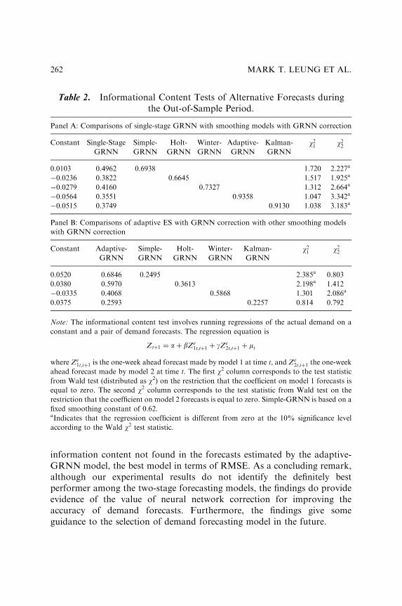
information content not found in the forecasts estimated by the adaptive-GRNN model, the best model in terms of RMSE. As a concluding remark,although our experimental results do not identify the definitely bestperformer among the two-stage forecasting models, the findings do provideevidence of the value of neural network correction for improving theaccuracy of demand forecasts. Furthermore, the findings give someguidance to the selection of demand forecasting model in the future.
Table 2. Informational Content Tests of Alternative Forecasts duringthe Out-of-Sample Period.
Panel A: Comparisons of single-stage GRNN with smoothing models with GRNN correction
Constant Single-Stage
GRNN
Simple-
GRNN
Holt-
GRNN
Winter-
GRNN
Adaptive-
GRNN
Kalman-
GRNNw21 w22
0.0103 0.4962 0.6938 1.720 2.227a
�0.0236 0.3822 0.6645 1.517 1.925a
�0.0279 0.4160 0.7327 1.312 2.664a
�0.0564 0.3551 0.9358 1.047 3.342a
�0.0515 0.3749 0.9130 1.038 3.183a
Panel B: Comparisons of adaptive ES with GRNN correction with other smoothing models
with GRNN correction
Constant Adaptive-
GRNN
Simple-
GRNN
Holt-
GRNN
Winter-
GRNN
Kalman-
GRNNw21 w22
0.0520 0.6846 0.2495 2.385a 0.803
0.0380 0.5970 0.3613 2.198a 1.412
�0.0335 0.4068 0.5868 1.301 2.086a
0.0375 0.2593 0.2257 0.814 0.792
Note: The informational content test involves running regressions of the actual demand on a
constant and a pair of demand forecasts. The regression equation is
Ztþ1 ¼ aþ bZe1t;tþ1 þ gZe
2t;tþ1 þ mt
where Ze1t;tþ1 is the one-week ahead forecast made by model 1 at time t, and Ze
2t;tþ1 the one-week
ahead forecast made by model 2 at time t. The first w2 column corresponds to the test statistic
from Wald test (distributed as w2) on the restriction that the coefficient on model 1 forecasts is
equal to zero. The second w2 column corresponds to the test statistic from Wald test on the
restriction that the coefficient on model 2 forecasts is equal to zero. Simple-GRNN is based on a
fixed smoothing constant of 0.62.aIndicates that the regression coefficient is different from zero at the 10% significance level
according to the Wald w2 test statistic.
MARK T. LEUNG ET AL.262
Encouraged by the effectiveness of neural network correction inexponential smoothing forecasting of demand, we compare the relativeforecasting strengths of various models with respect to the levels ofdemand lumpiness, which have already been defined and explained in‘‘Data and Single-Stage Forecasting of Demand’’ section. Specifically, weperform Theil’s (1966) decomposition tests to examine the characteristics ofthe out-of-sample forecasts estimated by the models. The Theil’s decom-position test is conducted by regressing the actual observed demand on aconstant and the demand forecast estimated by a particular model
At ¼ aþ bDt þ �t (18)
where At is the actual demand at period t, Dt the forecasted demandfor period t made at period t�1, and et the error term. The constanta (bias coefficient) should be insignificantly different from zero andthe coefficient b for estimated demand (regression proportion co-efficient) should be insignificantly different from one for the forecast to beacceptable.
Results of the decomposition test are displayed in Table 3. It shouldbe noted that the superior a and b denote that the bias coefficient (a) andthe proportion coefficient (b) are insignificantly different from 0 and 1,respectively. At low lumpiness level, the two-stage models with GRNNcorrection perform well in terms of insignificant bias (a ¼ 0) and parallelproportion to actual demand (b ¼ 1). This conclusion still holds forforecasting demand at the moderate lumpiness level except for the two-stagemodel based on simple exponential smoothing. However, when demandbecomes highly lumpy or volatile, only a few models generate goodforecasts. GRNN is the only single-stage model, which yields forecasts witha bias insignificantly different from zero and, at the same time, a proportioncoefficient insignificantly different from one. For the two-stage models,dynamic adaptive and Kalman filter exponential smoothing with GRNNare the two constructs satisfying the evaluation criteria. Performances oftwo-stage models built on static smoothing models drastically deterioratewhen demand becomes highly lumpy. It is suspected that the dynamicallyadjusted smoothing constants adopted in these two models instigate swiftadaptation and thus are better coping with more uncertain demandfluctuations during volatile periods. Again, the results echo the superiorperformances of adaptive-GRNN and Kalman-GRNN reported in previoustables.
Make-to-Order Product Demand Forecasting 263
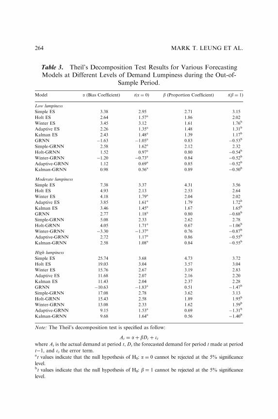
Table 3. Theil’s Decomposition Test Results for Various ForecastingModels at Different Levels of Demand Lumpiness during the Out-of-
Sample Period.
Model a (Bias Coefficient) t(a ¼ 0) b (Proportion Coefficient) t(b ¼ 1)
Low lumpiness
Simple ES 3.38 2.95 2.71 3.15
Holt ES 2.64 1.57a 1.86 2.02
Winter ES 3.45 3.12 1.61 1.76b
Adaptive ES 2.26 1.35a 1.48 1.31b
Kalman ES 2.43 1.48a 1.39 1.17b
GRNN �1.63 �1.05a 0.83 �0.53b
Simple-GRNN 2.58 1.62a 2.12 2.32
Holt-GRNN 1.52 0.97a 0.80 �0.54b
Winter-GRNN �1.20 �0.73a 0.84 �0.52b
Adaptive-GRNN 1.12 0.69a 0.85 �0.52b
Kalman-GRNN 0.98 0.56a 0.89 �0.50b
Moderate lumpiness
Simple ES 7.38 3.37 4.31 3.56
Holt ES 4.93 2.13 2.53 2.64
Winter ES 4.18 1.79a 2.04 2.02
Adaptive ES 3.85 1.61a 1.79 1.72b
Kalman ES 3.46 1.45a 1.67 1.65b
GRNN 2.77 1.18a 0.80 �0.68b
Simple-GRNN 5.08 2.33 2.62 2.78
Holt-GRNN 4.05 1.71a 0.67 �1.06b
Winter-GRNN �3.30 �1.37a 0.76 �0.87b
Adaptive-GRNN 2.72 1.17a 0.86 �0.55b
Kalman-GRNN 2.58 1.08a 0.84 �0.55b
High lumpiness
Simple ES 25.74 3.68 4.73 3.72
Holt ES 19.03 3.04 3.57 3.04
Winter ES 15.76 2.67 3.19 2.83
Adaptive ES 11.68 2.07 2.16 2.20
Kalman ES 11.43 2.04 2.37 2.28
GRNN �10.63 �1.83a 0.51 �1.47b
Simple-GRNN 17.08 2.78 3.62 3.13
Holt-GRNN 15.43 2.58 1.89 1.95b
Winter-GRNN 13.08 2.33 1.62 1.59b
Adaptive-GRNN 9.15 1.53a 0.69 �1.31b
Kalman-GRNN 9.68 1.64a 0.56 �1.40b
Note: The Theil’s decomposition test is specified as follow:
At ¼ aþ bDt þ �twhere At is the actual demand at period t, Dt the forecasted demand for period t made at period
t�1, and et the error term.at values indicate that the null hypothesis of H0: a ¼ 0 cannot be rejected at the 5% significance
level.bt values indicate that the null hypothesis of H0: b ¼ 1 cannot be rejected at the 5% significance
level.
MARK T. LEUNG ET AL.264

5. CONCLUSIONS
In this chapter, we compare the lumpy demand forecasting capabilities of anarray of exponential smoothing models with that of GRNN. The study alsoattempts to calibrate any possible synergetic effect on these smoothingmodels due to error corrections performed by a neural network within a two-stage forecasting framework. In other words, our empirical experimentevaluates the degrees of enhancement on traditional demand forecastssubject to error corrections by GRNN. The exponential smoothing modelsconsidered in this study belong to two types, static models with constantparameters and dynamic models with self-adjusted smoothing constants. Thisarray of five smoothing models serves as the basis of the two-stage forecastingframework and creates the first-cut demand estimates. In the second stage,these forecasts are corrected by the error residuals estimated by GRNN.
Results of the experiment indicate that forecasting accuracy of all (staticand dynamic) smoothing models can be improved by GRNN correction.This is a supporting evidence of the synergy realized by combining thecapacity of conventional forecasting model with neural network. Resultsalso reveal that two-stage models probably perform better than just thesingle-stage GRNN. In addition, the study explores the overlapping ofinformation contents between single-stage GRNN and two-stage modelswith GRNN correction. It is shown that the forecasts from all two-stagemodels possess information not revealed in the single-stage GRNN. Thisobservation is possibly a consequence of the weakness in extrapolationcommonly associated with neural network forecasting.
Furthermore, the study examines the consistency of performances acrossdifferent levels of demand lumpiness. It is found that the superior per-formances of the two-stage models persist when demand shifts from low tomoderate levels of lumpiness. However, only the dynamic adaptive andKalman filter smoothing models retain their good performances at highlylumpy demand level. Other two-stage models involving static exponentialsmoothing (fixed constants) do not perform up to parity when demand isvolatile. The implication is that the forecasting system can handle a certaindegree of demand changes without explicit human intervention and thatcomputational intelligence may help alleviate the issue of high demanduncertainty and lumpiness.
NOTES
1. The production facility was closed in the last week of December and the firstweek of January every year in observance of the holidays.
Make-to-Order Product Demand Forecasting 265

2. The first year (1997) in the estimation period is reserved as an initializationperiod for various exponential smoothing models.
REFERENCES
Anderson, D. R., Sweeney, D. J., & Williams, T. A. (2005). An introduction to management
science: Quantitative approaches to decision making (11th ed.). Mason, OH: Thomson
South-Western.
Chen, A. S., & Leung, M. T. (2004). Regression neural network for error correction in foreign
exchange forecasting and trading. Computers and Operations Research, 31, 1049–1068.
Fair, R., & Shiller, R. (1990). Comparing information in forecasts from econometric models.
American Economic Review, 80, 375–389.
Holt, C. C. (1957). Forecasting seasonal and trends by exponential weighted moving averages.
Office of Naval Research, Memorandum no. 52.
Mabert, V. A. (1978). Forecast modification based upon residual analysis: A case study of check
volume estimation. Decision Sciences, 9, 285–296.
Makridakis, S., & Wheelwright, S. C. (1977). Interactive forecasting. Palo Alto, CA: Scientific
Press.
Makridakis, S., Wheelwright, S. C., & McGee, V. E. (1983). Forecasting: Methods and
applications (2nd ed.). New York: Wiley.
Quintana, R., & Leung, M. T. (2007). Adaptive exponential smoothing versus conventional
approaches for lumpy demand forecasting: Case of production planning for a
manufacturing line. International Journal of Production Research, 45, 4937–4957.
Specht, D. (1991). A general regression neural network. IEEE Transactions on Neural Networks,
2, 568–576.
Theil, H. (1966). Applied economic forecasting. Amsterdam: North Holland.
Wasserman, P. D. (1993). Advanced methods in neural computing. New York: Van Nostrand
Reinhold.
Winter, P. R. (1960). Forecasting sales by exponentially weighted moving averages. Management
Science, 6, 324–342.
MARK T. LEUNG ET AL.266