Embed Size (px)
Citation preview

Journal of Probability and Statistics
Advances in Applied Econometrics
Guest Editors: Efthymios M. Tsionas, William Greene, and Kajal Lahiri

Advances in Applied Econometrics
Journal of Probability and Statistics
Advances in Applied Econometrics
Guest Editors: Efthymios M. Tsionas, William Greene,and Kajal Lahiri

Copyright q 2011 Hindawi Publishing Corporation. All rights reserved.
This is a special issue published in “Journal of Probability and Statistics.” All articles are open access articles distributedunder the Creative Commons Attribution License, which permits unrestricted use, distribution, and reproduction in anymedium, provided the original work is properly cited.

Editorial BoardM. F. Al-Saleh, JordanV. V. Anh, AustraliaZhidong Bai, ChinaIshwar Basawa, USAShein-chung Chow, USADennis Dean Cox, USAJunbin B. Gao, AustraliaArjun K. Gupta, USA
Debasis Kundu, IndiaNikolaos E. Limnios, FranceChunsheng Ma, USAHung T. Nguyen, USAM. Puri, USAJose Marıa Sarabia, SpainH. P. Singh, IndiaMan Lai Tang, Hong Kong
Robert J. Tempelman, USAA. Thavaneswaran, CanadaP. van der Heijden, The NetherlandsRongling Wu, USAPhilip L. H. Yu, Hong KongRicardas Zitikis, Canada

Contents
Advances in Applied Econometrics, Efthymios M. Tsionas, William Greene, and Kajal LahiriVolume 2011, Article ID 978530, 2 pages
Some Recent Developments in Efficiency Measurement in Stochastic Frontier Models,Subal C. Kumbhakar and Efthymios G. TsionasVolume 2011, Article ID 603512, 25 pages
Estimation of Stochastic Frontier Models with Fixed Effects through Monte Carlo MaximumLikelihood, Grigorios Emvalomatis, Spiro E. Stefanou, and Alfons Oude LansinkVolume 2011, Article ID 568457, 13 pages
Panel Unit Root Tests by Combining Dependent P Values: A Comparative Study,Xuguang Sheng and Jingyun YangVolume 2011, Article ID 617652, 17 pages
Nonparametric Estimation of ATE and QTE: An Application of Fractile Graphical Analysis,Gabriel V. Montes-RojasVolume 2011, Article ID 874251, 23 pages
Estimation and Properties of a Time-Varying GQARCH(1,1)-M Model, Sofia Anyfantaki andAntonis DemosVolume 2011, Article ID 718647, 39 pages
The CSS and The Two-Staged Methods for Parameter Estimation in SARFIMA Models,Erol Egrioglu, Cagdas Hakan Aladag, and Cem KadilarVolume 2011, Article ID 691058, 11 pages
Hindawi Publishing CorporationJournal of Probability and StatisticsVolume 2011, Article ID 978530, 2 pagesdoi:10.1155/2011/978530
EditorialAdvances in Applied Econometrics
Efthymios G. Tsionas,1 William Greene,2 and Kajal Lahiri3
1 Department of Economics, Athens University of Economics and Business, 10434 Athens, Greece2 Department of Economics, Stern School of Business, New York University, New York, NY 10012, USA3 Department of Economics, University at Albany, State University of New York, Albany, NY 12222, USA
Correspondence should be addressed to Efthymios G. Tsionas, [email protected]
Received 29 November 2011; Accepted 29 November 2011
Copyright q 2011 Efthymios G. Tsionas et al. This is an open access article distributed underthe Creative Commons Attribution License, which permits unrestricted use, distribution, andreproduction in any medium, provided the original work is properly cited.
The purpose of this special issue is to bring together some contributions in mainly two fields:time series analysis and estimation of technical inefficiency. The fields are important in ap-plied econometrics as they have attracted a lot of interest in recent years. In time seriesanalysis, the analysis focuses on seasonal ARIMA models and the GQARCH-M model. Inefficiency estimation a review is provided and a paper that deals with estimation of frontiermodels with fixed effects. Moreover, the special issue includes a paper on panel unit rootingtesting and a paper on nonparametric estimation of treatment effects.
In “Some recent developments in efficiency measurement in stochastic frontier models” by S. C.Kumbhakar and E. G. Tsionas, addressed are some of the recent developments in efficiencymeasurement using stochastic frontier (SF) models in some selected areas. The followingthree issues are discussed in detail. First, estimation of SF models with input-orientedtechnical efficiency. Second, estimation of latent class models to address technologicalheterogeneity as well as heterogeneity in economic behavior. Finally, estimation of SF modelsusing local maximum likelihood methods. Estimation of some of these models in the pastwas considered to be too difficult. The authors focus on the advances that have been made inrecent years to estimate some of these so-called difficult models. They complement these withsome developments in other areas as well. The reader is advised to consult Greene (2008) fora comprehensive review of stochastic frontier models.
G. Emvalomatis et al., in their paper “Estimation of stochastic frontier models with fixedeffects through Monte Carlo maximum likelihood,” propose a procedure for choosing appropriatedensities for integrating the incidental parameters from the likelihood function in a generalcontext. The densities are based on priors that are updated using information from thedata and are robust for possible correlation of the group-specific constant terms with theexplanatory variables. Monte Carlo’s experiments are performed in the specific context ofstochastic frontier models to examine and compare the sampling properties of the proposed
2 Journal of Probability and Statistics
estimator with those of the random effects and correlated random-effect estimators. Theresults suggest that the estimator is unbiased even in short panels. An application to a cross-country panel of EU manufacturing industries is presented as well. The proposed estimatorproduces a distribution of efficiency scores suggesting that these industries are highlyefficient, while the other estimators suggest much poorer performance.
In “Nonparametric estimation of ATE and QTE: an application of fractile graphical analysis,”G. V. Montes-Rojas constructs nonparametric estimators for average and quantile treatmenteffects using fractile graphical analysis, under the identifying assumption that selection totreatment is based on observable characteristics. The proposed method has two steps: first,the propensity score is estimated, and, second, a blocking estimation procedure using thisestimate is used to compute treatment effects. In both cases, the estimators are proved to beconsistent. Monte Carlo results show a better performance than other procedures based onthe propensity score. These estimators are applied to a job training dataset.
In “Estimation and properties of a time-varying GQARCH(1,1)-M model,” S. Anyfantakiand A. Demos outline the issues arising from time-varying GARCH-M models and suggestto employ aMarkov’s chainMonte Carlo algorithmwhich allows the calculation of a classicalestimator via the simulated EM algorithm or a simulated Bayesian solution in only O(T)computational operations, where T is the sample size. The theoretical dynamic properties ofa time-varying GQARCH(1,1)-M are derived. They discuss them and apply the suggestedBayesian estimation to three major stock markets.
In “The CSS and the two-staged methods for parameter estimation in SARFIMA models,”E. Egrioglu et al. focus on analysis of seasonal autoregressive fractionally integrated movingaverage (SARFIMA)models. Two methods, which are conditional sum of squares (CSS) andtwo-staged methods introduced by Hosking (1984), are proposed to estimate the parametersof SARFIMA models. However, no simulation study has been conducted in the literature.Therefore, it is not known how these methods behave under different parameter settings andsample sizes in SARFIMA models. The aim of this study is to show the behavior of thesemethods by a simulation study. According to results of the simulation, advantages anddisadvantages of both methods under different parameter settings and sample sizes arediscussed by comparing the root mean square error (RMSE) obtained by the CSS and two-staged methods. As a result of the comparison, it is seen that CSS method produces betterresults than those obtained from two-staged method.
In “Panel unit root tests by combining dependent P values: a comparative study,” X. Shengand J. Yang conduct a systematic comparison of the performance of four commonly usedP -value combination methods applied to panel unit root tests: the original Fisher test, themodified inverse normal method, Simes’ test, and the modified truncated product method(TPM). The simulation results show that under cross-sectional dependence, the originalFisher test is severely oversized, but the other three tests exhibit good size properties. Sims’test is powerful when the total evidence against the joint null hypothesis is concentrated inone or very few of the tests being combined, but the modified inverse normal method and themodified TPM have good performance when evidence against the joint null is spread amongmore than a small fraction of the panel units. The differences are further illustrated throughone empirical example on testing purchasing power parity using a panel of OECD quarterlyreal exchange rates.
Efthymios G. TsionasWilliam Greene
Kajal Lahiri
Hindawi Publishing CorporationJournal of Probability and StatisticsVolume 2011, Article ID 603512, 25 pagesdoi:10.1155/2011/603512
Review ArticleSome Recent Developments in EfficiencyMeasurement in Stochastic Frontier Models
Subal C. Kumbhakar1 and Efthymios G. Tsionas2
1 Department of Economics, State University of New York, Binghamton, NY 13902, USA2 Department of Economics, Athens University of Economics and Business, 76 Patission Street,104 34 Athens, Greece
Correspondence should be addressed to Subal C. Kumbhakar, [email protected]
Received 13 May 2011; Accepted 2 October 2011
Academic Editor: William H. Greene
Copyright q 2011 S. C. Kumbhakar and E. G. Tsionas. This is an open access article distributedunder the Creative Commons Attribution License, which permits unrestricted use, distribution,and reproduction in any medium, provided the original work is properly cited.
This paper addresses some of the recent developments in efficiency measurement using stochasticfrontier (SF) models in some selected areas. The following three issues are discussed in details.First, estimation of SF models with input-oriented technical efficiency. Second, estimation of latentclass models to address technological heterogeneity as well as heterogeneity in economic behavior.Finally, estimation of SF models using local maximum likelihood method. Estimation of some ofthese models in the past was considered to be too difficult. We focus on the advances that havebeen made in recent years to estimate some of these so-called difficult models. We complementthese with some developments in other areas as well.
1. Introduction
In this paper we focus on three issues. First, we discuss issues (mostly econometric) relatedto input-oriented (IO) and output-oriented (OO) measures of technical inefficiency andtalk about the estimation of production functions with IO technical inefficiency. We discussimplications of the IO and OOmeasures from both the primal and dual perspectives. Second,the latent class (finite mixing) modeling approach is extended to accommodate behavioralheterogeneity. Specifically, we consider profit- (revenue-) maximizing and cost-minimizingbehaviors with technical inefficiency. In our mixing/latent class model, first we consider asystem approach in which some producers maximize profit while others simply minimizecost, and then we use a distance function approach, and mix the input and output distancefunctions (in which it is assumed, at least implicitly, that some producers maximize revenuewhile others minimize cost). In the distance function approach the behavioral assumptionsare not explicitly taken into account. The prior probability in favor of profit (revenue)maximizing behavior is assumed to depend on some exogenous variables. Third, we considerstochastic frontier (SF) models that are estimated using local maximum likelihood (LML)
2 Journal of Probability and Statistics
method to address the flexibility issue (functional form, heteroskedasticity, and determinantsof technical inefficiency).
2. The IO and OO Debate
The technology (with or without inefficiency) can be looked at from either a primal or adual perspective. In a primal setup two measures of technical efficiency are mostly usedin the efficiency literature. These are (i) input-oriented (IO) technical inefficiency and (ii)output oriented (OO) technical inefficiency.1 There are some basic differences between the IOand OO models so far as features of the technology are concerned. Although some of thesedifferences and their implications are well-known except for Kumbhakar and Tsionas [1], noone has estimated a stochastic production frontier model econometrically with IO technicalinefficiency using cross-sectional data.2 Here we consider estimation of a translog productionmodel with IO technical inefficiency.
2.1. The IO and OO Models
Consider a single output production technology where Y is a scalar output and X is a vectorof inputs. Then the production technology with the IO measure of technical inefficiency canbe expressed as
Yi = f(Xi ·Θi), i = 1, . . . , n, (2.1)
where Yi is a scalar output, Θi ≤ 1 is IO efficiency (a scalar), Xi is the J × 1 vector of inputs,and i indexes firms. The IO technical inefficiency for firm i is defined as lnΘi ≤ 0 and isinterpreted as the rate at which all the inputs can be reduced without reducing output. Onthe other hand, the technology with the OO measure of technical inefficiency is specified as
Yi = f(Xi) ·Λi, (2.2)
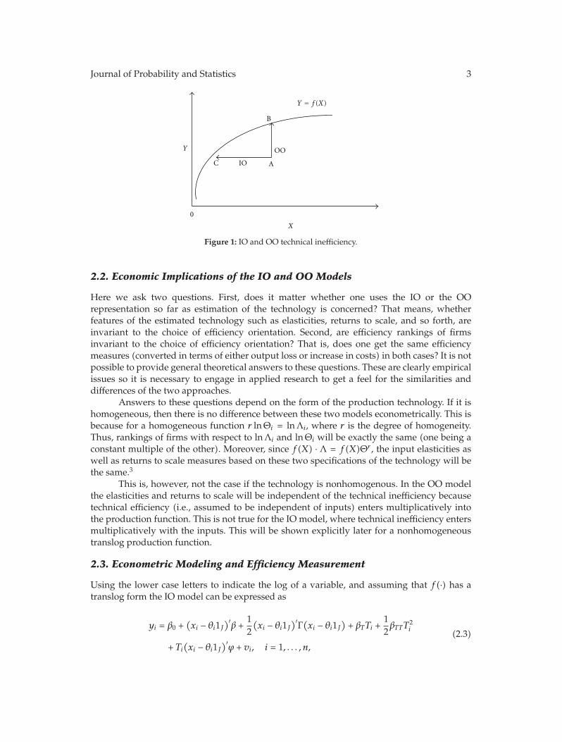
where Λi ≤ 1 represents OO efficiency (a scalar), and lnΛi ≤ 0 is defined as OOtechnical inefficiency. It shows the percent by which actual output could be increased withoutincreasing inputs (for more details, see Figure 1).
It is clear from (2.1) and (2.2) that if f(·) is homogeneous of degree r thenΘri = Λi, that
is, independent of X and Y . If homogeneity is not present their relationship will depend onthe input quantities and the parametric form of f(·).
We now show the IO and OO measures of technical efficiency graphically. Theobserved production plan (Y,X) is indicated by the point A. The vertical length ABmeasures OO technical inefficiency, while the horizontal distance AC measures IO technicalinefficiency. Since the former measures percentage loss of output while the latter measurespercentage increase in input usage in moving to the production frontier starting from theinefficient production plan indicated by point A, these two measures are, in general, notdirectly comparable. If the production function is homogeneous, then one measure is aconstant multiple of the other, and they are the same if the degree of homogeneity is one.In the more general case, they are related in the following manner: f(X) ·Λ = f(XΘ).
Although we consider technologies with a single output, the IO and OO inefficiencycan be discussed in the context of multiple output technologies as well.
Journal of Probability and Statistics 3
Y
Y
= f (X)
B
OO
A
0
C IO
X
Figure 1: IO and OO technical inefficiency.
2.2. Economic Implications of the IO and OO Models
Here we ask two questions. First, does it matter whether one uses the IO or the OOrepresentation so far as estimation of the technology is concerned? That means, whetherfeatures of the estimated technology such as elasticities, returns to scale, and so forth, areinvariant to the choice of efficiency orientation. Second, are efficiency rankings of firmsinvariant to the choice of efficiency orientation? That is, does one get the same efficiencymeasures (converted in terms of either output loss or increase in costs) in both cases? It is notpossible to provide general theoretical answers to these questions. These are clearly empiricalissues so it is necessary to engage in applied research to get a feel for the similarities anddifferences of the two approaches.
Answers to these questions depend on the form of the production technology. If it ishomogeneous, then there is no difference between these two models econometrically. This isbecause for a homogeneous function r lnΘi = lnΛi, where r is the degree of homogeneity.Thus, rankings of firms with respect to lnΛi and lnΘi will be exactly the same (one being aconstant multiple of the other). Moreover, since f(X) · Λ = f(X)Θr , the input elasticities aswell as returns to scale measures based on these two specifications of the technology will bethe same.3
This is, however, not the case if the technology is nonhomogenous. In the OO modelthe elasticities and returns to scale will be independent of the technical inefficiency becausetechnical efficiency (i.e., assumed to be independent of inputs) enters multiplicatively intothe production function. This is not true for the IO model, where technical inefficiency entersmultiplicatively with the inputs. This will be shown explicitly later for a nonhomogeneoustranslog production function.
2.3. Econometric Modeling and Efficiency Measurement
Using the lower case letters to indicate the log of a variable, and assuming that f(·) has atranslog form the IO model can be expressed as
yi = β0 +(xi − θi1J
)′β +
12(xi − θi1J
)′Γ(xi − θi1J
)+ βTTi +
12βTTT
2i
+ Ti(xi − θi1J
)′ϕ + vi, i = 1, . . . , n,
(2.3)
4 Journal of Probability and Statistics
where yi is the log of output, 1J denotes the J ×1 vector of ones, xi is the J ×1 vector of inputsin log terms, Ti is the trend/shift variable, β0, βT and βTT are scalar parameters, β, ϕ are J × 1parameter vectors, Γ is a J × J symmetric matrix containing parameters, and vi is the noiseterm. To make θ nonnegative we defined it as − lnΘ = θ.
We rewrite the IO model above as
yi =(β0 + x′
iβ +12x′iΓxi + βTTi +
12βTTT
2i + x
′iϕTi
)− g(θi, xi) + vi, i = 1, . . . , n, (2.4)
where g(θi, xi) = −[(1/2)θ2iΨ − θΞi], Ψ = 1′jΓ1J , and Ξi = 1′j(β + Γxi + ϕTi), i = 1, . . . , n. Notethat if the production function is homogeneous of degree r, then Γ1J = 0, 1′Jβ = r, and 1′Jϕ =0. In such a case the g(θi, xi) function becomes a constant multiple of θ, (namely, [(1/2)θ2iΨ−θΞi] = −rθi), and consequently, the IO model cannot be distinguished from the OO model.The g(θi, xi) function shows the percent by which output is lost due to technical inefficiency.For a well-behaved production function g(θi, xi) ≥ 0 for each i.
The OO model, on the other hand, takes a much simpler form, namely,
yi =(β0 + x′
iβ +12x′iΓxi + βTTi +
12βTTT
2i + x
′iϕTi
)− λi + vi, i = 1, . . . , n, (2.5)
where we defined − lnΛ = λ to make it nonnegative.4 The OO model in this form is theone introduced by Aigner et al. [2] and Meeusen and van den Broeck [3], and since then ithas been used extensively in the efficiency literature. Here we follow the framework used inKumbhakar and Tsionas [1]when θ is random.5
We write (2.4)more compactly as
yi = z′iα +12θ2iΨ − θΞi + vi, i = 1, . . . , n. (2.6)
Both Ψ and Ξi are functions of the original parameters, and Ξi also depends on the data (xiand Ti).
Under the assumption that vi ∼ N(0, σ2) and θi is distributed independently of vi withthe density function f(θi;ω), where ω is a parameter, the probability density function of yican be expressed as
f(yi;μ
)=
(2πσ2
)−1/2 ∫∞
0exp
⎡
⎣−(yi − z′iα − (1/2)θ2iΨ + θiΞi
)2
2σ2
⎤
⎦f(θi;ω)dθi, i = 1, . . . , n,
(2.7)
where μ denotes the entire parameter vector.We consider a half-normal and an exponential specification for the density f(θi;ω),
namely,
f(θi;ω) =
(πω2
2
)−1/2exp
(
− θ2i2ω2
)
, θi ≥ 0,
f(θi;ω) = ω exp(−ωθi), θi ≥ 0.
(2.8)
Journal of Probability and Statistics 5
The likelihood function of the model is then
l(μ;y,X
)=
n∏
i=1
f(yi;μ
), (2.9)
where f(yi;μ) has been defined above. Since the integral defining f(yi;μ) is not available inclosed form we cannot find an analytical expression for the likelihood function. However, wecan approximate the integrals using a simulation as follows. Suppose θi,(s), s = 1, . . . , S is arandom sample from f(θi;ω). Then it is clear that
f(yi;μ
) ≈ f(yi;μ) ≡ S−1
S∑
s=1
exp
⎡
⎢⎣−
(yi − z′iα − (1/2)θ2i,(s)Ψ + θi,(s)Ξi
)2
2σ2
⎤
⎥⎦, (2.10)
and an approximation of the log-likelihood function is given by
log l ≈n∑
i=1
log f(yi;μ
), (2.11)
which can be maximized by numerical optimization procedures to obtain the ML estimator.For the distributions we adopted, random number generation is trivial, so implementing theSML estimator is straightforward.6
Inefficiency estimation is accomplished by considering the distribution of θi condi-tional on the data and estimated parameters
f(θi | μ, Di
) ∝ exp
⎡
⎢⎣−
(yi − z′iα − (1/2)θ2i Ψ + Ξiθi
)2
2σ2
⎤
⎥⎦f(θi; ω), i = 1, . . . , n, (2.12)
where a tilde denotes the ML estimate, andDi = [xi, Ti] denotes the data. For example, whenf(θi; ω) is half-normal we get
f(θi | μ, y, X
) ∝ exp
⎡
⎢⎣−
(yi − z′iα − (1/2)θ2i Ψ + θiΞi
)2
2σ2− θ2i2ω2
⎤
⎥⎦, θi ≥ 0, i = 1, . . . , n.
(2.13)
This is not a known density, and even the normalizing constant cannot be obtained in closedform. However, the first two moments and the normalizing constant can be obtained bynumerical integration, for example, using Simpson’s rule.
To make inferences on efficiency, define efficiency as ri = exp(−θi) and obtain thedistribution of ri and its moments by changing the variable from θi to ri. This yields
fr(ri | μ, Di
)= r−1i f
(− ln ri | μ, y, X), 0 < ri ≤ 1, i = 1, . . . , n. (2.14)

6 Journal of Probability and Statistics
The likelihood function for the OOmodel is given in Aigner et al. [2] (hereafter ALS).7
TheMaximum likelihoodmethod for estimating the parameters of the production function inthe OO models are straightforward and have been used extensively in the literature startingfrom ALS.8 Once the parameters are estimated, technical inefficiency (λ) is estimated fromE(λ | (v − λ))—the Jondrow et al. [4] formula. Alternatively, one can estimate technicalefficiency from E(e−λ | (v − λ)) using the Battese and Coelli [5] formula. For an application ofthis approach see Kumbhakar and Tsionas [1].
2.4. Looking Through the Dual Cost Functions
2.4.1. The IO Approach
We now examine the IO and OO models when behavioral assumptions are explicitlyintroduced. First, we examine themodels when producersminimize cost to produce the givenlevel of output(s). The objective of a producer is to
Min. w′X
subject to Y = f(X ·Θ)(2.15)
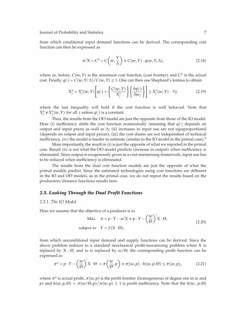
from which conditional input demand functions can be derived. The corresponding costfunction can then be expressed as
w′X = Ca =C(w,Y )
Θ, (2.16)
where C(w,Y ) is the minimum cost function (cost frontier) and Ca is the actual cost. Finally,one can use Shephard’s lemma to obtain Xa
j = X∗j (w,Y )/Θ ≥ X∗
j (w,Y ) for all j, where thesuperscripts a and ∗ indicate actual and cost-minimizing levels of input Xj .
Thus, the IO model implies (i) a neutral shift in the cost function which in turnimplies that RTS and input elasticities are unchanged due to technical inefficiency, (ii) anequiproportional increase (at the rate given by θ) in the use of all inputs due to technicalinefficiency, irrespective of the output level and input prices.
To summarize, result (i) is just the opposite of what we obtained in the primal case(see [6]). Result (ii) states that when inefficiency is reduced firms will move horizontally tothe frontier (as expected by the IO model).
2.4.2. The OO Model
Here the objective function is written as
Min. w′X
subject to Y = f(X) ·Λ(2.17)
Journal of Probability and Statistics 7
from which conditional input demand functions can be derived. The corresponding costfunction can then be expressed as
w′X = Ca = C(w,
Y
Λ
)≡ C(w,Y ) · q(w,Y,Λ), (2.18)
where as, before, C(w,Y ) is the minimum cost function (cost frontier) and Ca is the actualcost. Finally, q(·) = C(w,Y/Λ)/C(w,Y ) ≥ 1. One can then use Shephard’s lemma to obtain
Xaj = X∗
j (w,Y )
[
q(·) +{C(w,Y )X∗j
}{∂q(·)∂wj
}]
≥ X∗j (w,Y ) ∀j, (2.19)
where the last inequality will hold if the cost function is well behaved. Note thatXaj /=X
∗j (w,Y ) for all j unless q(·) is a constant.Thus, the results from the OO model are just the opposite from those of the IO model.
Here (i) inefficiency shifts the cost function nonneutrally (meaning that q(·) depends onoutput and input prices as well as Λ; (ii) increases in input use are not equiproportional(depends on output and input prices); (iii) the cost shares are not independent of technicalinefficiency, (iv) the model is harder to estimate (similar to the IO model in the primal case).9
More importantly, the result in (i) is just the opposite of what we reported in the primalcase. Result (ii) is not what the OO model predicts (increase in output) when inefficiency iseliminated. Since output is exogenously given in a cost-minimizing framework, input use hasto be reduced when inefficiency is eliminated.
The results from the dual cost function models are just the opposite of what theprimal models predict. Since the estimated technologies using cost functions are differentin the IO and OO models, as in the primal case, we do not repeat the results based on theproduction/distance functions results here.
2.5. Looking Through the Dual Profit Functions
2.5.1. The IO Model
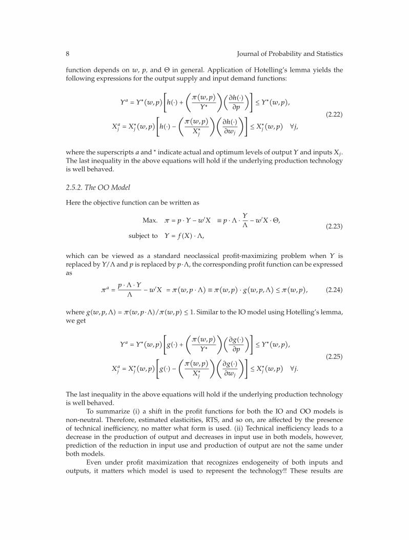
Here we assume that the objective of a producer is to
Max. π = p · Y −w′X ≡ p · Y −(w
Θ
)′X ·Θ,
subject to Y = f(X ·Θ),(2.20)
from which unconditional input demand and supply functions can be derived. Since theabove problem reduces to a standard neoclassical profit-maximizing problem when X isreplaced by X · Θ, and w is replaced by w/Θ, the corresponding profit function can beexpressed as
πa = p · Y −(w
Θ
)′X ·Θ = π
(w
Θ, p
)≡ π(
w, p) · h(w, p,Θ) ≤ π(
w, p), (2.21)
where πa is actual profit, π(w, p) is the profit frontier (homogeneous of degree one in w andp) and h(w, p,Θ) = π(w/Θ, p)/π(w, p) ≤ 1 is profit inefficiency. Note that the h(w, p,Θ)
8 Journal of Probability and Statistics
function depends on w, p, and Θ in general. Application of Hotelling’s lemma yields thefollowing expressions for the output supply and input demand functions:
Ya = Y ∗(w, p)[
h(·) +(π(w, p
)
Y ∗
)(∂h(·)∂p
)]
≤ Y ∗(w, p),
Xaj = X∗
j
(w, p
)[
h(·) −(π(w, p
)
X∗j
)(∂h(·)∂wj
)]
≤ X∗j
(w, p
) ∀j,(2.22)
where the superscripts a and ∗ indicate actual and optimum levels of output Y and inputsXj .The last inequality in the above equations will hold if the underlying production technologyis well behaved.
2.5.2. The OO Model
Here the objective function can be written as
Max. π = p · Y −w′X ≡ p ·Λ · YΛ
−w′X ·Θ,
subject to Y = f(X) ·Λ,(2.23)
which can be viewed as a standard neoclassical profit-maximizing problem when Y isreplaced by Y/Λ and p is replaced by p ·Λ, the corresponding profit function can be expressedas
πa =p ·Λ · Y
Λ−w′X = π
(w, p ·Λ) ≡ π(
w, p) · g(w, p,Λ) ≤ π(
w, p), (2.24)
where g(w, p,Λ) = π(w, p ·Λ)/π(w, p) ≤ 1. Similar to the IOmodel using Hotelling’s lemma,we get
Ya = Y ∗(w, p)[
g(·) +(π(w, p
)
Y ∗
)(∂g(·)∂p
)]
≤ Y ∗(w, p),
Xaj = X∗
j
(w, p
)[
g(·) −(π(w, p
)
X∗j
)(∂g(·)∂wj
)]
≤ X∗j
(w, p
) ∀j.(2.25)
The last inequality in the above equations will hold if the underlying production technologyis well behaved.
To summarize (i) a shift in the profit functions for both the IO and OO models isnon-neutral. Therefore, estimated elasticities, RTS, and so on, are affected by the presenceof technical inefficiency, no matter what form is used. (ii) Technical inefficiency leads to adecrease in the production of output and decreases in input use in both models, however,prediction of the reduction in input use and production of output are not the same underboth models.
Even under profit maximization that recognizes endogeneity of both inputs andoutputs, it matters which model is used to represent the technology!! These results are
Journal of Probability and Statistics 9
different from those obtained under the primal models and from the cost minimizationframework. Thus, it matters (both theoretically and empirically) whether one uses an input-or output-oriented measure of technical inefficiency.
3. Latent Class Models
3.1. Modeling Technological Heterogeneity
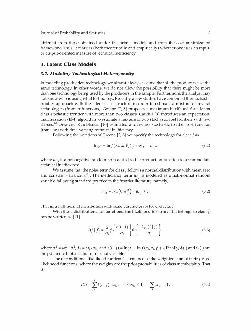
In modeling production technology we almost always assume that all the producers use thesame technology. In other words, we do not allow the possibility that there might be morethan one technology being used by the producers in the sample. Furthermore, the analyst maynot knowwho is using what technology. Recently, a few studies have combined the stochasticfrontier approach with the latent class structure in order to estimate a mixture of severaltechnologies (frontier functions). Greene [7, 8] proposes a maximum likelihood for a latentclass stochastic frontier with more than two classes. Caudill [9] introduces an expectation-maximization (EM) algorithm to estimate a mixture of two stochastic cost frontiers with twoclasses.10 Orea and Kumbhakar [10] estimated a four-class stochastic frontier cost function(translog) with time-varying technical inefficiency.
Following the notations of Greene [7, 8] we specify the technology for class j as
lnyi = ln f(xi, zi, βj
)|j + vi|j − ui|j , (3.1)
where ui|j is a nonnegative random term added to the production function to accommodatetechnical inefficiency.
We assume that the noise term for class j follows a normal distribution with mean zeroand constant variance, σ2
vj . The inefficiency term ut|j is modeled as a half-normal randomvariable following standard practice in the frontier literature, namely,
ui|j ∼N+
(0, ω2
j
)ui|j ≥ 0. (3.2)
That is, a half-normal distribution with scale parameter ωj for each class.With these distributional assumptions, the likelihood for firm i, if it belongs to class j,
can be written as [11]
l(i | j) =
2σjφ
{ε(i | j)
σj
}
Φ
{
−λjε(i | j)
σj
}
, (3.3)
where σ2j = ω2
j +σ2j , λj = ωj/σvj and ε(i | j) = lnyi − ln f(xi, zi, βj)|j . Finally, φ(·) andΦ(·) are
the pdf and cdf of a standard normal variable.The unconditional likelihood for firm i is obtained as the weighted sum of their j-class
likelihood functions, where the weights are the prior probabilities of class membership. Thatis,
l(i) =J∑
j=1
l(i | j) · πij , 0 ≤ πij ≤ 1,
∑
j
πijt = 1, (3.4)
10 Journal of Probability and Statistics
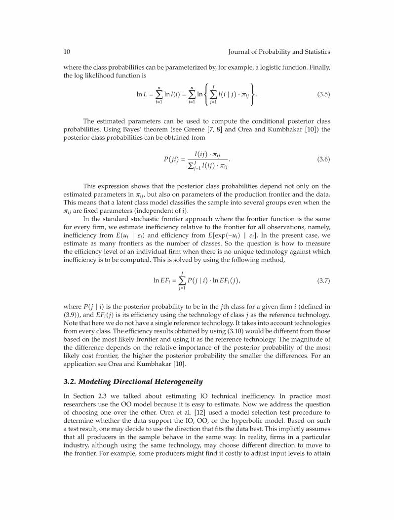
where the class probabilities can be parameterized by, for example, a logistic function. Finally,the log likelihood function is
lnL =n∑
i=1
ln l(i) =n∑
i=1
ln
⎧⎨
⎩
J∑
j=1
l(i | j) · πij
⎫⎬
⎭. (3.5)
The estimated parameters can be used to compute the conditional posterior classprobabilities. Using Bayes’ theorem (see Greene [7, 8] and Orea and Kumbhakar [10]) theposterior class probabilities can be obtained from
P(ji)=
l(ij) · πij
∑Jj=1 l
(ij) · πij
. (3.6)
This expression shows that the posterior class probabilities depend not only on theestimated parameters in πij , but also on parameters of the production frontier and the data.This means that a latent class model classifies the sample into several groups even when theπij are fixed parameters (independent of i).
In the standard stochastic frontier approach where the frontier function is the samefor every firm, we estimate inefficiency relative to the frontier for all observations, namely,inefficiency from E(ui | εi) and efficiency from E[exp(−ui) | εi]. In the present case, weestimate as many frontiers as the number of classes. So the question is how to measurethe efficiency level of an individual firm when there is no unique technology against whichinefficiency is to be computed. This is solved by using the following method,
lnEFi =J∑
j=1
P(j | i) · lnEFi
(j), (3.7)
where P(j | i) is the posterior probability to be in the jth class for a given firm i (defined in(3.9)), and EFi(j) is its efficiency using the technology of class j as the reference technology.Note that here we do not have a single reference technology. It takes into account technologiesfrom every class. The efficiency results obtained by using (3.10)would be different from thosebased on the most likely frontier and using it as the reference technology. The magnitude ofthe difference depends on the relative importance of the posterior probability of the mostlikely cost frontier, the higher the posterior probability the smaller the differences. For anapplication see Orea and Kumbhakar [10].
3.2. Modeling Directional Heterogeneity
In Section 2.3 we talked about estimating IO technical inefficiency. In practice mostresearchers use the OO model because it is easy to estimate. Now we address the questionof choosing one over the other. Orea et al. [12] used a model selection test procedure todetermine whether the data support the IO, OO, or the hyperbolic model. Based on sucha test result, one may decide to use the direction that fits the data best. This implictly assumesthat all producers in the sample behave in the same way. In reality, firms in a particularindustry, although using the same technology, may choose different direction to move tothe frontier. For example, some producers might find it costly to adjust input levels to attain
Journal of Probability and Statistics 11
the production frontier, while for others it might be easier to do so. This means that someproducers will choose to shrink their inputs while others will augment the output level. Insuch a case imposing one direction for all sample observations is not efficient. The otherpractical problem is that no one knows in advance, which producers are following whatdirection. Thus, we cannot estimate the IO model for one group and the OO model foranother.
The advantage of the LCM is that it is not necessary to impose a priori criterion toidentify which producers are in what class. Moreover, we can formally examine whethersome exogenous factors are responsible for choosing the input or the output direction bymaking the probabilities function of exogenous variables. Furthermore, when panel data isavailable, we do not need to assume that producers follow one direction for all the time, sowe can accommodate switching behaviour and determine when they go in the input (output)direction.
3.2.1. The Input-Oriented Model
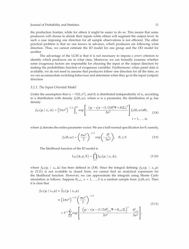
Under the assumption that vi ∼ N(0, σ2), and θi is distributed independently of vi, accordingto a distribution with density fθ(θi;ω), where ω is a parameter, the distribution of yi hasdensity
fIO(yi | zi,Δ
)=
(2πσ2
)−1/2 ∫∞
0exp
⎡
⎣−(yi − z′iα − (1/2)θ2iΨ + θiΞi
)2
2σ2
⎤
⎦fθ(θi;ω)dθi,
i = 1, . . . , n,
(3.8)
whereΔ denotes the entire parameter vector.We use a half-normal specification for θ, namely,
fθ(θi;ω) =
(πω2
2
)−1/2exp
(
− θ2i2ω2
)
, θi ≥ 0. (3.9)
The likelihood function of the IO model is
LIO(Δ;y,X
)=
n∏
i=1
fIO(yi | zi,Δ
), (3.10)
where fIO(yi | zi,Δ) has been defined in (3.8). Since the integral defining fIO(yi | zi, μ)in (3.11) is not available in closed form, we cannot find an analytical expression forthe likelihood function. However, we can approximate the integrals using Monte Carlosimulation as follows. Suppose θi,(s), s = 1, . . . , S is a random sample from fθ(θi;ω). Thenit is clear that
fIO(yi | zi, μ
) ≈ fIO(yi | zi, μ
)
≡(2πσ2
)−1/2(πω2
2
)−1/2
× S−1S∑
s=1
exp
⎡
⎢⎣−
(yi − z′iα − (1/2)θ2i,(s)Ψ + θi,(s)Ξi
)2
2σ2−θ2i,(s)
2ω2
⎤
⎥⎦,
(3.11)
12 Journal of Probability and Statistics
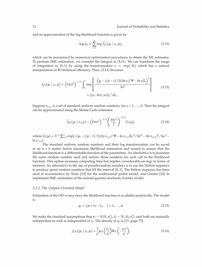
and an approximation of the log-likelihood function is given by
log lIO ≈n∑
i=1
log fIO(yi | zi, μ
), (3.12)
which can be maximized by numerical optimization procedures to obtain the ML estimator.To perform SML estimation, we consider the integral in (3.11). We can transform the rangeof integration to [0, 1] by using the transformation ri = exp(−θi) which has a naturalinterpretation as IO technical efficiency. Then, (3.11) becomes
fIO(yi | zi, μ
)=
(2πσ2
)−1/2 ∫1
0exp
⎡
⎢⎣−
(yi − z′iα − (1/2)(ln ri)
2Ψ − ln riΞi)2
2σ2
⎤
⎥⎦
× fθ(− ln ri;ω)r−1i dri.
(3.13)
Suppose ri,(s) is a set of standard uniform random numbers, for s = 1, . . . , S. Then the integralcan be approximated using the Monte Carlo estimator
fIO(yi | zi, μ
)=
(2πσ2
)−1/2(πω2
2
)−1/2Gi
(μ), (3.14)
where Gi(μ) = S−1 ∑Ss=1 exp[−(yi − z′iα − (1/2)(ln ri,(s))
2Ψ − ln ri,(s)Ξi)2/2σ2 − (ln ri,(s))
2/2ω2 −ln ri,(s)].
The standard uniform random numbers and their log transformation can be savedin an n × S matrix before maximum likelihood estimation and reused to ensure that thelikelihood function is a differentiable function of the parameters. An alternative is to maintainthe same random number seed and redraw these numbers for each call to the likelihoodfunction. This option increases computing time but implies considerable savings in terms ofmemory. An alternative to the use of pseudorandom numbers is to use the Halton sequenceto produce quasi-random numbers that fill the interval [0, 1]. The Halton sequence has beenused in econometrics by Train [13] for the multinomial probit model, and Greene [14] toimplement SML estimation of the normal-gamma stochastic frontier model.
3.2.2. The Output-Oriented Model
Estimation of the OO is easy since the likelihood function is available analytically. The modelis
yi = z′iα + vi − λi, i = 1, . . . , n. (3.15)
We make the standard assumptions that vi ∼ N(0, σ2v), λi ∼ N+(0, σ2
λ), and both are mutually
independent as well as independent of zi. The density of yi is [11, page 75]
fOO(yi | zi, μ
)=
2ρϕN
(eiρ
)ΦN
(−eiτρ
), (3.16)

Journal of Probability and Statistics 13
where ei = yi − z′iα, ρ2 = σ2v + σ
2λ, τ = σλ/σv, and φN and ΦN denote the standard normal pdf
and cdf, respectively. The log likelihood function of the model is
ln lOO(μ;y,Z
)= n ln
(2ρ
)− n
2ln
(2πρ2
)− 12ρ2
n∑
i=1
e2i +n∑
i=1
lnΦN
(−eiτρ
). (3.17)
3.3. The Finite Mixture (Latent Class) Model
The IO and OO models can be embedded in a general model that allows model choice foreach observation in the absence of sample separation information. Specifically, we assumethat each observation yi is associated with the OO class with probability p, and with the IOclass with probability 1 − p. To be more precise, we have the model
yi = z′iα − λi + vi, i = 1, . . . , n, (3.18)
with probability p, and the model
yi = z′iα +12θ2iΨ − θiΞi + vi, i = 1, . . . , n, (3.19)
with probability 1 − p, where the stochastic elements obey the assumptions that we statedpreviously in connection with the OO and IO models. Notice that the technical parameters,α, are the same in the two classes. Denote the parameter vector by ψ = [α′, σ2, ω2, σ2
v, σ2λ, p]
′.The density of yi will be
fLCM(yi | zi, ψ
)= p · fOO
(yi | zi,O
)+(1 − p)fIO
(yi | zi,Δ
), i = 1, . . . , n, (3.20)
where O = [α′, σ2, ω2]′, andΔ = [α′, σ2v, σ
2λ] are subsets of ψ. The log likelihood function of the
model is
log lLCM(ψ;y,Z
)=
n∑
i=1
ln fLCM(yi | zi, ψ
)=
n∑
i=1
ln[p · fOO
(yi | zi,O
)+(1 − p)fIO
(yi | zi,Δ
)].
(3.21)
The log likelihood function depends on the IO density fIO(yi | zi,Δ), which is not availablein closed form but can be obtained with the aid of simulation using the principles presentedpreviously to obtain
log lLCM(ψ;y,Z
)=
n∑
i=1
ln fLCM(yi | zi, ψ
)=
n∑
i=1
ln[pfOO
(yi | zi,O
)+(1 − p)fIO
(yi | zi,Δ
)],
(3.22)
where fIO(yi | zi,Δ) has been defined in (3.14) and fOO(yi | zi,O) in (3.16). This log likelihoodfunction can be maximized using standard techniques to obtain the SML estimates of theLCM.
14 Journal of Probability and Statistics
3.3.1. Technical Efficiency Estimation in the Latent Class Model
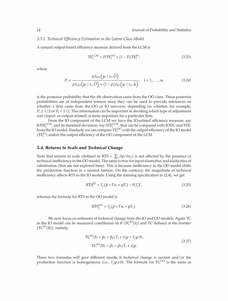
A natural output-based efficiency measure derived from the LCM is
TELCMi = PiTEOO
i + (1 − Pi)TEIOi , (3.23)
where
Pi =pfOO
(yi | zi, O
)
pfOO
(yi | zi, O
)+(1 − p)fIO
(yi | zi, Δ
) , i = 1, . . . , ·n, (3.24)
is the posterior probability that the ith observation came from the OO class. These posteriorprobabilities are of independent interest since they can be used to provide inferences onwhether a firm came from the OO or IO universe, depending on whether, for example,Pi ≥ 1/2 or Pi < 1/2. This information can be important in deciding which type of adjustmentcost (input- or output-related) is more important for a particular firm.
From the IO component of the LCM we have the IO-related efficiency measure, sayIOTELCM
i , and its standard deviation, say STELCMi , that can be compared with IOTEi and STEi
from the IOmodel. Similarly we can compare TEOOi with the output efficiency of the IOmodel
(TEIOi ) and/or the output efficiency of the OO component of the LCM.
3.4. Returns to Scale and Technical Change
Note that returns to scale (defined as RTS =∑
j ∂y/∂xj) is not affected by the presence oftechnical inefficiency in the OOmodel. The same is true for input elasticities and elasticities ofsubstitution (that are not explored here). This is because inefficiency in the OO model shiftsthe production function in a neutral fashion. On the contrary, the magnitude of technicalinefficiency affects RTS in the IO models. Using the translog specification in (2.4), we get
RTSIOi = 1′J(β + Γxi + ϕTi
) − θi1′JΓ, (3.25)
whereas the formula for RTS in the OO model is
RTSOOi = 1′J
(β + Γxi + ϕTi
). (3.26)
We now focus on estimates of technical change from the IO and OOmodels. Again TCin the IO model can be measured conditional on θ (TCIO(I)) and TC defined at the frontier(TCIO(II)), namely,
TCIO(I) = βT + βTTTi + x′iϕ + 1′Jϕ θi,
TCIO(II) = βT + βTTTi + x′iϕ.
(3.27)
These two formulas will give different results if technical change is neutral and/or theproduction function is homogeneous (i.e., 1′Jϕ /= 0). The formula for TCOO is the same as

Journal of Probability and Statistics 15
TCIO(II) except for the fact that the estimated parameters in (3.3) are from the IO model,whereas the parameters to compute TCOO are from the OO model.
It should be noted that in the LCM we enforce the restriction that the technicalparameters, α, are the same in the IO and OO components of the mixture. This impliesthat RTS and TC will be the same in both components if we follow the first approach, butthey will be different if we follow the second approach. In the second approach, a singlemeasure of RTS and TC can be defined as the weighted average of both measures usingthe posterior probabilities, Pi, as weights. To be more precise, suppose RTSIO,LCM
i (II) is thetype II RTS measure derived from the IO component of the LCM, and RTSOO,LCM
i is the RTSmeasure derived from the OO component of the LCM. The overall LCMmeasure of RTS willbe RTSLCMi = PiRTS
OO,LCMi + (1 − Pi)RTSIO,LCM
i . Similar methodology is followed for the TCmeasure.
4. Relaxing Functional form Assumptions (SF Model with LML)
In this section we introduce the LML methodology [15] in estimating SF models in such away that many of the limitations of the SF models originally proposed by Aigner et al. [2],Meeusen and van den Broeck [3], and their extensions in the last two and a half decadesare relaxed. Removal of all these deficiencies generalizes the SF models and makes themcomparable to the DEA models. Moreover, we can apply standard econometric tools toperform estimation and draw inferences.
To fix ideas, suppose we have a parametric model that specifies the density of anobserved dependent variable yi conditional on a vector of observable covariates xi ∈ X ⊆ Rk,a vector of unknown parameters θ ∈ Θ ⊆ Rm, and let the density be l(yi;xi, θ). The parametricML estimator is given by
θ = arg maxθ∈Θ
:n∑
i=1
ln l(yi;xi, θ
). (4.1)
The problem with the parametric ML estimator is that it relies heavily on theparametric model that can be incorrect if there is uncertainty regarding the functional formof the model, the density, and so forth. A natural way to convert the parametric model toa nonparametric one is to make the parameter θ a function of the covariates xi. Within LMLthis is accomplished as follows. For an arbitrary x ∈ X, the LML estimator solves the problem
θ(x) = arg maxθ∈Θ
:n∑
i=1
ln l(yi;xi, θ
)KH(xi − x), (4.2)
where KH is a kernel that depends on a matrix bandwidth H. The idea behind LML is tochoose an anchoring parametric model and maximize a weighted log-likelihood functionthat places more weight to observations near x rather than weight each observation equally,as the parametric ML estimator would do.11 By solving the LML problem for several pointsx ∈ X, we can construct the function θ(x) that is an estimator for θ(x), and effectively wehave a fully general way to convert the parametric model to a nonparametric approximationto the unknown model.
Suppose we have the following stochastic frontier cost model:
yi = x′iβ + vi + ui, vi ∼ N
(0, σ2
), ui ∼ N
(μ,ω2
), ui ≥ 0, for i = 1, . . . , n, β ∈ Rk, (4.3)
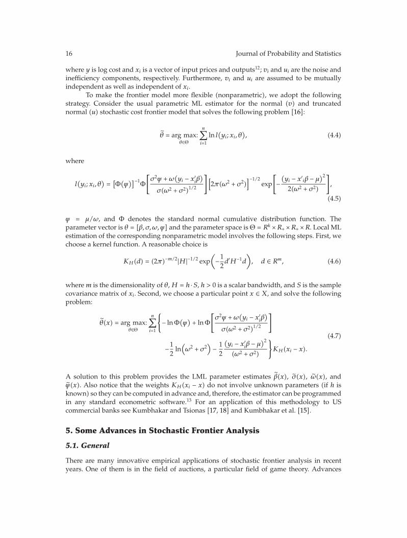
16 Journal of Probability and Statistics
where y is log cost and xi is a vector of input prices and outputs12; vi and ui are the noise andinefficiency components, respectively. Furthermore, vi and ui are assumed to be mutuallyindependent as well as independent of xi.
To make the frontier model more flexible (nonparametric), we adopt the followingstrategy. Consider the usual parametric ML estimator for the normal (v) and truncatednormal (u) stochastic cost frontier model that solves the following problem [16]:
θ = arg maxθ∈Θ
:n∑
i=1
ln l(yi;xi, θ
), (4.4)
where
l(yi;xi, θ
)=
[Φ(ψ)]−1Φ
[σ2ψ +ω
(yi − x′
iβ)
σ(ω2 + σ2)1/2
][2π(ω2 + σ2)
]−1/2exp
[
−(yi − x′
iβ − μ)2
2(ω2 + σ2)
]
,
(4.5)
ψ = μ/ω, and Φ denotes the standard normal cumulative distribution function. Theparameter vector is θ = [β, σ,ω, ψ] and the parameter space isΘ = Rk ×R+ ×R+ ×R. Local MLestimation of the corresponding nonparametric model involves the following steps. First, wechoose a kernel function. A reasonable choice is
KH(d) = (2π)−m/2|H|−1/2 exp(−12d′H−1d
), d ∈ Rm, (4.6)
wherem is the dimensionality of θ,H = h ·S, h > 0 is a scalar bandwidth, and S is the samplecovariance matrix of xi. Second, we choose a particular point x ∈ X, and solve the followingproblem:
θ(x) = arg maxθ∈Θ
:n∑
i=1
{
− lnΦ(ψ)+ lnΦ
[σ2ψ +ω
(yi − x′
iβ)
σ(ω2 + σ2)1/2
]
−12ln
(ω2 + σ2
)− 12
(yi − x′
iβ − μ)2
(ω2 + σ2)
}
KH(xi − x).(4.7)
A solution to this problem provides the LML parameter estimates β(x), σ(x), ω(x), andψ(x). Also notice that the weights KH(xi − x) do not involve unknown parameters (if h isknown) so they can be computed in advance and, therefore, the estimator can be programmedin any standard econometric software.13 For an application of this methodology to UScommercial banks see Kumbhakar and Tsionas [17, 18] and Kumbhakar et al. [15].
5. Some Advances in Stochastic Frontier Analysis
5.1. General
There are many innovative empirical applications of stochastic frontier analysis in recentyears. One of them is in the field of auctions, a particular field of game theory. Advances
Journal of Probability and Statistics 17
and empirical applications in this field are likely to accumulate rapidly and contributepositively to the advancement of empirical Game theory and empirical IO. Kumbhakar etal. [19] propose Bayesian analysis of an auction model where systematic over-bidding andunder-bidding is allowed. Extensive simulations are used to show that the new techniquesperformwell and ignoringmeasurement error or systematic over-bidding and under-biddingis important in the final results.
Kumbhakar and Parmeter [20] derive the closed-form likelihood and associatedefficiency measures for a two-sided stochastic frontier model under the assumption ofnormal-exponential components. The model receives an important application in the labormarket where employees and employers have asymmetric information, and each one triesto manipulate the situation to his own advantage, Employers would like to hire for lessand employees to obtain more in the bargaining process. The precise measurement of thesecomponents is, apparently, important.
Kumbhakar et al. [21] acknowledge explicitly the fact that certain decision makingunits can be fully (i.e., 100%) efficient, and propose a new model which is a mixture of (i)a half-normal component for inefficient firms and (ii) a mass at zero for efficient firms. Ofcourse, it is not known in advance which firms are fully efficient or not. The authors proposeclassical methods of inference organized around maximum likelihood and provide extensivesimulations to explore the validity and relevance of the new techniques under various datagenerating processes.
Tsionas [22] explores the implications of the convolution ε = v + u in stochasticfrontier models. The fundamental point is that even when the distributions of the errorcomponents are nonstandard (e.g., Student-t and half-Student or normal and half-Student,gamma, symmetric stable, etc.) it is possible to estimate the model by ML estimation via thefast Fourier transform (FFT) when the characteristic functions are available in closed form.These methods can also be used in mixture models, input-oriented efficiency models, two-tiered stochastic frontiers, and so forth. The properties of ML and some GLS techniques areexplored with an emphasis on the normal-truncated normal model for which the likelihoodis available analytically and simulations are used to determine various quantities that mustbe set in order to apply ML by FFT.
Starting with Annaert et al. [23], stochastic frontier models have been applied verysuccessfully in finance, especially the important issue of mutual funds performance. Schaeferand Maurer [24] apply these techniques to German funds to find that they “may be able toreduce its costs by 46 to 74% when compared with the best-practice complex in the sample.”Of course, much remains to be done in this area and connect more closely stochastic frontiermodels with practical finance and better mutual fund performance evaluation.
5.2. Panel Data
Panel data have always been a source of inspiration and new models in stochastic frontieranalysis. Roughly speaking, panel data are concerned with models of the form yit = αi+x′
itβ+vit, where the αi’s are individual effects, random or fixed, xit is a k × 1 vector of covariates, βis a k × 1 parameter vector and, typically, the error term vit ∼ iidN(0, σ2
v).An important contribution in panel data models of efficiency is the incorporation
of factors, as in Kneip et al. [25]. Factors arise from the necessity of incorporating morestructure into frontier models, a point that is clear after Lee and Schmidt [26]. The authorsuse smoothing techniques to perform the econometric analysis of the model.
18 Journal of Probability and Statistics
In recent years, the focus of the profession has shifted from the fixed effects model(e.g., Cornwell et al. [27]) to a so-called “true fixed effects model” (TFEM) first proposedby Greene [28]. Greene’s model is yit = αi + x′
itβ + vit ± uit, where uit ∼ iidN+(0, σ2v). In
this model, the individual effects are separated from technical inefficiency. Similar modelshave been proposed previously by Kumbhakar [29] and Kumbhakar and Hjalmarsson [30],although in these models firm-effects were treated as persistent inefficiency. Greene showsthat the TFEM can be estimated easily using special Gauss-Newton iterations without theneed to explicitly introduce individual dummy variables, which is prohibitive if the numberof firms (N) is large. As Greene [28] notes: “the fixed and random effects estimators force any timeinvariant cross unit heterogeneity into the same term that is being used to capture the inefficiency.Inefficiency measures in these models may be picking up heterogeneity in addition to or even instead ofinefficiency.” For important points and applications see Greene [8, 31].
Greene’s [8] findings are somewhat at odds with the perceived incidental parametersproblem in thismodel, as he himself acknowledges. His findingsmotivated a body of researchthat tries to deal with the incidental parameters problem in stochastic frontier models and,of course, efficiency estimation. The incidental parameters problem in statistics began withthe well-known contribution of Neyman and Scott [32] (see also [33]). In stochastic frontiermodels of the form: yit = αi + x′
itβ + vit, for i = 1, . . . ,N and t = 1, . . . , T . The essence of theproblem is that asN gets large, the number of unknown parameters (the individual effects αi,i = 1, . . . ,N) increase at the same rate so consistency cannot be achieved. Another route to theincidental parameters problem is well-known in the efficiency estimation with cross-sectionaldata (T = 1), where JLMS estimates are not consistent.
To appreciate better the incidental parameters problem, the TFEM implies a densityfor the ith unit, say
pi(αi, δ;Yi) ≡ pi(αi, β, σ,ω;Yi
), where Yi =
[y′i, x
′i
]′ is the data. (5.1)
The problem is that the ML estimator
maxα1,...,αn,δ
:n∑
i=1
pi(αi, δ;Yi) = maxδ
:n∑
i=1
pi(αi, δ;Yi) (5.2)
is not consistent. The source of the problem is that the concentrated likelihood using αi (theML estimator) will not deliver consistent estimators for all elements of δ.
In frontier models we know that ML estimators for β and σ2 + ω2 seem to be alrightbut the estimator for ω or the ratio λ = ω/σ can be wrong. This is also validated in a recentpaper by Chen et al. [34].
There are some approaches to correct such biases in the literature on nonlinear paneldata models.
(i) Correct the bias to first order using a modified score (first derivatives of loglikelihood).
(ii) Use a penalty function for the log likelihood. This can of course be related to [2]above.
(iii) Apply panel jackknife. Satchachai and Schmidt [35] has done that recently ina model with fixed effects but without one-sided component. He derives someinteresting results regarding convergence depending on whether we have ties or
Journal of Probability and Statistics 19
not. First differencing produces O(T−1) but with ties we have O(T−1/2) (for theestimator applied when you have a tie).
(iv) In line with (ii) one could use a modified likelihood of the form p∗i (δ;Yi) =∫pi(αi, δ;Yi)w(αi)dαi, where w(αi) is some weighting function for which it is clear
that there is a Bayesian interpretation.Since Greene [8] derived a computationally efficient algorithm for the true fixed effects
model, one would think that application of panel jackknife would reduce the first order biasof the estimator and for empirical purposes this might be enough. For further reductions inthe bias there remains only the possibility of asymptotic expansions along the lines of relatedwork in nonlinear panel data models. This point has not been explored in the literature but itseems that it can be used profitably.
Wang and Ho [36] show that “first-difference and within-transformation can beanalytically performed on this model to remove the fixed individual effects, and thus theestimator is immune to the incidental parameters problem.” The model is, naturally, lessgeneral than a standard stochastic frontier model in that the authors assume uit = f(z′itδ)u
+i ,
where u+i is a positive half-normal random variable and f() is a positive function. In thismodel, the dynamics of inefficiency are determined entirely by the function f() and thecovariates that enter into this function.
Recently, Chen et al. [34] proposed a new estimator for the model. If the model isyit = αi + x′
itβ + vit − uit, deviation from the mean gives
yit = x′itβ + vit − uit. (5.3)
Given β = βOLS, we have eit ≡ yit − x′itβ = vit − uit, when eit = “data.” The distribution of eit =
vit − uit, belongs to the family of the multivariate closed skew-normal (CSN), so estimating λand σ is easy. Of course, the multivariate CSN depends on evaluating a multivariate normalintegral in RT+1. With T > 5, this is not a trivial problem (see [37]).
There is reason to believe that “average likelihood” or a fully Bayesian approachcan perform much better relative to sampling-theory treatments. Indeed, the true fixedeffects model is nothing but another instance of the incidental parameters problem. Recentadvances suggest that the best treatment can be found in “average” or “integrated” likelihoodfunctions. For work in this direction, see Lancaster [33] and Arellano and Bonhomme[38], Arellano and Hahn [39, 40], Berger et al. [41], and Bester and Hansen [42, 43]. Theperformance of such methods in the context of TFE remains to be seen.
Tsionas and Kumbhakar [44] propose a full Bayesian solution to the problem. Theapproach is obvious in a sense, since the TFEM can be cast as a hierarchical model. Theauthors show that the obvious parameterization of the model does not perform well insimulated experiments and, therefore, they propose a new parameterization that is shownto effectively eliminate the incidental parameters problem. They also extend the TFEM tomodels with both individual and time effects. Of course, the TFEM is cast in terms of arandom effects model so it is at first sight not directly related to [35].
6. Thoughts on Current State of Efficiency Estimation and Panel Data
6.1. Nature of Individual Effects
If we think about the model: yit = αi + x′itβ + vit + uit, uit ≥ 0, asN → ∞ one natural question
is: Do we really expect ourselves to be so agnostic about the fixed effects as to allow αn+1 to
20 Journal of Probability and Statistics
be completely different from what we already know about α1, . . . , αn? This is rarely the case.But we do not adopt the true fixed effects model for that reason. There are other reasons. Ifwe ignore this choice we can adopt a finite mixture of normal distribution for the effects.
In principle this can approximate well any distribution of the effects, so with enoughlatent classes we should be able to approximate the weight function w(αi) quite well. Thatwould pose some structure in the model, it would avoid the incidental parameters problem(if the number of classes grows slowly and at a lower rate thanN) so for fixed T there shouldbe no significant bias. For really small T a further bias correction device like asymptoticexpansions or the jackknife could be used.
Since we do not adopt the true fixed effects model for that reason, why do we adopt it?Because the effects and the regressors are potentially correlated in a random effect frameworkso it is preferable to think of them as parameters. It could be that αi = h(xi1, . . . , xiT ), orperhaps αi = H(xi), when xi = T−1 ∑T
t=1 xit. Mundlak [45] first wrote about this model. Insome cases it makes sense. Consider the alternative model:
yit = αit + x′itβ + vit + uit,
αit = α(1 − ρ) + ραit−1 + x′
itγ + εit.(6.1)
Under stationarity we have the same implications with Mundlak’s original model butin many cases it makes much more sense: mutual fund rating and evaluation is one of them.But even if we stay with Mundlak’s original specification, many other possibilities are open.For small T , the most interesting case, approximation of αi = h(xi1, . . . , xiT ) by some flexiblefunctional form should be enough for practical purposes. By “practical purposes” we meanbias reduction to order O(T−1) or better. If the model becomes
yit = αi + x′itβ + vit + uit = h(xi1, . . . , xiT ) + x
′itβ + vit + uit, t = 1, . . . , T, (6.2)
adaptation of known nonparametric techniques should provide that rate of convergence.Reduction to
yit = αi + x′itβ + vit + uit = H(xi) + x′
itβ + vit + uit, t = 1, . . . , T, (6.3)
would facilitate the analysis considerably without sacrificing the rate. It is quite probable thath or H should be low order polynomials or basis functions with some nice properties (e.g.,Bernstein polynomials are nice) that can overcome the incidental parameters problem.
6.2. Random Coefficient Models
Consider yit = αi+x′itβi+vit+uit ≡ z′itγi+vit+uit [46]. Typically we assume that γi ∼ iidNK(γ,Ω).
For small to moderate panels (say T = 5 to 10) adaptation of the techniques in the paper byChen et al. [34] would be quite difficult to implement in the context of fixed effects. Theconcern is again with evaluation of (T + 1)-dimensional normal integrals, when T is large.Here, again we are subject to the incidental parameters problem—we never really escape the“small sample” situation.

Journal of Probability and Statistics 21
One way to proceed is the so-called CAR (conditionally autoregressive) prior (model)of the form:
γi | γj ∼N(γj , ϕ
2ij
)∀i /= j, logϕ2
ij = δ0 + δ1∥∥wi −wj
∥∥, if γi is scalar (the TFEM).
(6.4)
In themultivariate case wewould need something like the BEKK factorization of a covariancematrix as in multivariate GARCH processes. The point is that the coefficients cannot be toodissimilar and their degree of dissimilarity depends on a parameter ϕ2 that can be made afunction of covariates, if any. Under different DGPs, it would be interesting to know how theBayesian estimator of this model behaves in practice.
6.3. More on Individual Effects
Related to the above discussion, it is productive to think about sources, that is, where theseαis or γis come from. Of course we haveMundlak’s [45] interpretation in place. In practice wehave different technologies (represented by cost functions, say). The standard cost functionyit = α0 +x′
itβ+vit with input-oriented technical inefficiency results in yit = α0 +x′itβ+vit +uit,
uit ≥ 0. Presence of allocative inefficiency results in a much more complicated model: yit =α0 + x′
itβ + vit + uit + Git(xit, β, ξit) where ξit is the vector of price distortions (see [47, 48]). Sounder some reasonable economic assumptions and common technology we end up with anonlinear effects model through the G(·) function. Of course one can apply the TFEM herebut that would not correspond to the true DGP. So the issues of consistency are at stake.
It is hard to imagine a situation where in a TFEM, yit = αi +x′itβ+vit +uit the αis can be
anything and they are subjected to no “similarity” constraints. We can, of course, accept thatαi ≈ α0+Git(xit, β, ξit), so at least for the translog we should have a rough guide on what theseeffects represent under allocative inefficiency first-order approximations to the complicatedG term are available when the ξits are small. Of course then one has to think about the natureof the allocative distortions but at least that’s an economic problem.
6.4. Why a Bayesian Approach?
Chen et al.’s transformation that used the multivariate CSN is one class of transformations,but there are many transformations that are possible because the TFEM does not havethe property of information orthogonality [33]. The “best” transformation, the one thatis “maximally bias reducing,” cannot be taking deviations from the means because theinformation matrix is not block diagonal with respect to (αi, λ = ω/σ = signal/noise). Othertransformations would be more effective and it is not difficult to find them, in principle.
Recently Tsionas and Kumbhakar [44] considered a different model, namely, yit =αi + δ+i + x′
itβ + vit + uit, where δ+i ≥ 0 is persistent inefficiency. They have used a Bayesianapproach. Colombi et al. [49] used the same model but used classical (ML) approach toestimate the parameters as well as the inefficiency components. The finite sample propertiesof the Bayes estimators (posterior means and medians) in Tsionas and Kumbhakar [44]werefound to be very good for small samples with λ values typically encountered in practice(of course one needs to keep λ away from zero in the DGP). The moral of the story is thatin the random effects model, an integrated likelihood approach based on reasonable priors,
22 Journal of Probability and Statistics
a nonparametric approach based on low-order polynomials or a finite mixture model mightprovide an acceptable approximation to parameters like λ.
Coupled with a panel jack knife device these approaches can be really effective inmitigating the incidental parameters problem. For one, in the context of TFE, we do notknow how the Chen et al. [34] estimator would behave under strange DGPs-under strangeprocesses for the incidental parameters that is. We have some evidence from Monte Carlobut we need to think about more general “mitigating strategies.” The integrated likelihoodapproach is one, and is close to a Bayesian approach. Finite mixtures also hold great promisesince they have good approximating properties. The panel jack knife device is certainlysomething to think about. Also analytical devices for bias reduction to order O(T−1) orO(T−2) are available from the likelihood function of the TFEM (score and information). Theirimplementation in software should be quite easy.
7. Conclusions
In this paper we presented some new techniques to estimate technical inefficiency usingstochastic frontier technique. First, we presented a technique to estimate a nonhomogeneoustechnology using the IO technical inefficiency. We then discussed the IO and OO controversyin the light of distance functions, and the dual cost and profit functions. The second part of thepaper addressed the latent class-modeling approach incorporating behavioral heterogeneity.The last part of the paper addressed LML method that can solve the functional form issue inparametric stochastic frontier. Finally, we added a section that deals with some very recentadvances.
Endnotes
1. Another measure is hyperbolic technical inefficiency that combines both the IO and OOmeasures in a special way (see, e.g., [50], Cuesta and Zofio (1999), [12]). This measure isnot as popular as the other two.
2. On the contrary, the OO model has been estimated by many authors using DEA (see,e.g., [51] and references cited in there).
3. Alvarez et al. [52] addressed these issues in a panel data framework with time invarianttechnical inefficiency (using a fixed effects models).
4. The above equation gives the IO model (when the production function is homogeneous)by labeling λi = rθi.
5. Alvarez et al. [52] estimated an IO primal model in a panel data model where technicalinefficiency is assumed to be fixed and parametric.
6. Greene [14] used SML for the OO normal-gamma model.
7. See also Kumbhakar and Lovell [11, pages 74–82] for the log-likelihood functions underboth half-normal and exponential distributions for the OO technical inefficiency term.
8. It is not necessary to use the simulated ML method to estimate the parameters of thefrontier models if the technical inefficiency component is distributed as half-normal,truncated normal, or exponential along with the normality assumption on the noisecomponent. For other distributions, for example, gamma for technical inefficiency andnormal for the noise component the standard ML method may not be ideal (see Greene
Journal of Probability and Statistics 23
[14] who used the simulated ML method to estimate OO technical efficiency in thegamma-normal model).
9. Atkinson and Cornwell [53] estimated translog cost functions with both input-and output-oriented technical inefficiency using panel data. They assumed technicalinefficiency to be fixed and time invariant. See also Orea et al. [12].
10. See, in addition, Beard et al. [54, 55] for applications using a non-frontier approach. Forapplications in social sciences, see, Hagenaars and McCutcheon [56]. Statistical aspectsof the mixing models are dicussed in details in Mclachlan and Peel [57].
11. LML estimation has been proposed by Tibshirani [58] and has been applied by Gozaloand Linton [59] in the context of nonparametric estimation of discrete response models.
12. The cost function specification is discussed in details in Section 5.2.
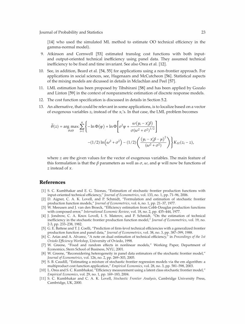
13. An alternative, that could be relevant in some applications, is to localize based on a vectorof exogenous variables zi instead of the xi’s. In that case, the LML problem becomes
θ(z) = arg maxθ∈Θ
:n∑
i=1
{
− lnΦ(ψ)+ lnΦ
[
σ2ψ +ω(yi − x′
iβ)
σ(ω2 + σ2)1/2
]
−(1/2) ln(ω2 + σ2
)− (1/2)
((yi − x′
iβ − μ)2
(ω2 + σ2)
)}
KH(zi − z),
where z are the given values for the vector of exogenous variables. The main feature ofthis formulation is that the β parameters as well as σ, ω, and ψ will now be functions ofz instead of x.
References
[1] S. C. Kumbhakar and E. G. Tsionas, “Estimation of stochastic frontier production functions withinput-oriented technical efficiency,” Journal of Econometrics, vol. 133, no. 1, pp. 71–96, 2006.
[2] D. Aigner, C. A. K. Lovell, and P. Schmidt, “Formulation and estimation of stochastic frontierproduction function models,” Journal of Econometrics, vol. 6, no. 1, pp. 21–37, 1977.
[3] W. Meeusen and J. van den Broeck, “Efficiency estimation from Cobb-Douglas production functionswith composed error,” International Economic Review, vol. 18, no. 2, pp. 435–444, 1977.
[4] J. Jondrow, C. A. Knox Lovell, I. S. Materov, and P. Schmidt, “On the estimation of technicalinefficiency in the stochastic frontier production function model,” Journal of Econometrics, vol. 19, no.2-3, pp. 233–238, 1982.
[5] G. E. Battese and T. J. Coelli, “Prediction of firm-level technical efficiencies with a generalized frontierproduction function and panel data,” Journal of Econometrics, vol. 38, no. 3, pp. 387–399, 1988.
[6] C. Arias and A. Alvarez, “A note on dual estimation of technical efficiency,” in Proceedings of the 1stOviedo Efficiency Workshop, University of Oviedo, 1998.
[7] W. Greene, “Fixed and random effects in nonlinear models,” Working Paper, Department ofEconomics, Stern School of Business, NYU, 2001.
[8] W. Greene, “Reconsidering heterogeneity in panel data estimators of the stochastic frontier model,”Journal of Econometrics, vol. 126, no. 2, pp. 269–303, 2005.
[9] S. B. Caudill, “Estimating a mixture of stochastic frontier regression models via the em algorithm: amultiproduct cost function application,” Empirical Economics, vol. 28, no. 3, pp. 581–598, 2003.
[10] L. Orea and S. C. Kumbhakar, “Efficiencymeasurement using a latent class stochastic frontier model,”Empirical Economics, vol. 29, no. 1, pp. 169–183, 2004.
[11] S. C. Kumbhakar and C. A. K. Lovell, Stochastic Frontier Analysis, Cambridge University Press,Cambridge, UK, 2000.
24 Journal of Probability and Statistics
[12] L. Orea, D. Roibas, and A. Wall, “Choosing the technical efficiency orientation to analyze firms’technology: a model selection test approach,” Journal of Productivity Analysis, vol. 22, no. 1-2, pp. 51–71, 2004.
[13] K. E. Train,Discrete Choice Methods with Simulation, Cambridge University Press, Cambridge, UK, 2ndedition, 2009.
[14] W. H. Greene, “Simulated likelihood estimation of the normal-gamma stochastic frontier function,”Journal of Productivity Analysis, vol. 19, no. 2-3, pp. 179–190, 2003.
[15] S. C. Kumbhakar, B. U. Park, L. Simar, and E. G. Tsionas, “Nonparametric stochastic frontiers: a localmaximum likelihood approach,” Journal of Econometrics, vol. 137, no. 1, pp. 1–27, 2007.
[16] R. E. Stevenson, “Likelihood functions for generalized stochastic frontier estimation,” Journal ofEconometrics, vol. 13, no. 1, pp. 57–66, 1980.
[17] S. C. Kumbhakar and E. G. Tsionas, “Scale and efficiency measurement using a semiparametricstochastic frontier model: evidence from the U.S. commercial banks,” Empirical Economics, vol. 34,no. 3, pp. 585–602, 2008.
[18] S. C. Kumbhakar and E. Tsionas, “Estimation of cost vs. profit systems with and without technicalinefficiency,” Academia Economic Papers, vol. 36, pp. 145–164, 2008.
[19] S. Kumbhakar, C. Parmeter, and E. G. Tsionas, “Bayesian estimation approaches to first-priceauctions,” to appear in Journal of Econometrics.
[20] S. C. Kumbhakar and C. F. Parmeter, “The effects of match uncertainty and bargaining on labormarket outcomes: evidence from firm and worker specific estimates,” Journal of Productivity Analysis,vol. 31, no. 1, pp. 1–14, 2009.
[21] S. Kumbhakar, C. Parmeter, and E. G. Tsionas, “A zero inflated stochastic frontier model,”unpublished.
[22] E. G. Tsionas, “Maximum likelihood estimation of non-standard stochastic frontier models by theFourier transform,” to appear in Journal of Econometrics.
[23] J. Annaert, J. Van den Broeck, and R. V. Vennet, “Determinants of mutual fund underperformance:a Bayesian stochastic frontier approach,” European Journal of Operational Research, vol. 151, no. 3, pp.617–632, 2003.
[24] A. Schaefer, R. Maurer et al., “Cost efficiency of German mutual fund complexes,” SSRN workingpaper, 2010.
[25] A. Kneip, W. H. Song, and R. Sickles, “A new panel data treatment for heterogeneity in time trends,”to appear in Econometric Theory.
[26] Y. H. Lee and P. Schmidt, “A production frontier model with flexible temporal variation in technicalinefficiency,” in The Measurement of Productive Efficiency: Techniques and Applications, H. O. Fried, C. A.K. Lovell, and S. S. Schmidt, Eds., Oxford University Press, New York, NY, USA, 1993.
[27] C. Cornwell, P. Schmidt, and R. C. Sickles, “Production frontiers with cross-sectional and time-seriesvariation in efficiency levels,” Journal of Econometrics, vol. 46, no. 1-2, pp. 185–200, 1990.
[28] W. Greene, “Fixed and random effects in stochastic frontier models,” Journal of Productivity Analysis,vol. 23, no. 1, pp. 7–32, 2005.
[29] S. C. Kumbhakar, “Estimation of technical inefficiency in panel data models with firm- and time-specific effects,” Economics Letters, vol. 36, no. 1, pp. 43–48, 1991.
[30] S. C. Kumbhakar and L. Hjalmarsson, “Technical efficiency and technical progress in Swedish dairyfarms,” in The Measurement of Productive Efficiency—Techniques and Applications, H. O. Fried, C. A. K.Lovell, and S. S. Schmidt, Eds., pp. 256–270, Oxford University Press, Oxford, UK, 1993.
[31] W. Greene, “Distinguishing between heterogeneity and inefficiency: stochastic frontier analysis of theWorld Health Organization’s panel data on national health care systems,” Health Economics, vol. 13,no. 10, pp. 959–980, 2004.
[32] J. Neyman and E. L. Scott, “Consistent estimates based on partially consistent observations,”Econometrica. Journal of the Econometric Society, vol. 16, pp. 1–32, 1948.
[33] T. Lancaster, “The incidental parameter problem since 1948,” Journal of Econometrics, vol. 95, no. 2, pp.391–413, 2000.
[34] Y.-Y. Chen, P. Schmidt, and H.-J. Wang, “Consistent estimation of the fixed effects stochastic frontiermodel,” in Proceedings of the the European Workshop on Efficiency and Productivity Analysis (EWEPA ’11),Verona, Italy, 2011.
Journal of Probability and Statistics 25
[35] P. Satchachai and P. Schmidt, “Estimates of technical inefficiency in stochastic frontier models withpanel data: generalized panel jackknife estimation,” Journal of Productivity Analysis, vol. 34, no. 2, pp.83–97, 2010.
[36] H. J. Wang and C. W. Ho, “Estimating fixed-effect panel stochastic frontier models by modeltransformation,” Journal of Econometrics, vol. 157, no. 2, pp. 286–296, 2010.
[37] A. Genz, “An adaptive multidimensional quadrature procedure,” Computer Physics Communications,vol. 4, no. 1, pp. 11–15, 1972.
[38] M. Arellano and S. Bonhomme, “Robust priors in nonlinear panel data models,” Working paper,CEMFI, Madrid, Spain, 2006.
[39] M. Arellano and J. Hahn, “Understanding bias in nonlinear panel models: some recent develop-ments,” in Advances in Economics and Econometrics, Ninth World Congress, R. Blundell, W. Newey, andT. Persson, Eds., Cambridge University Press, 2006.
[40] M. Arellano and J. Hahn, “A likelihood-based approximate solution to the incidental parameterproblem in dynamic nonlinear models with multiple effects,” Working Papers, CEMFI, 2006.
[41] J. O. Berger, B. Liseo, and R. L. Wolpert, “Integrated likelihood methods for eliminating nuisanceparameters,” Statistical Science, vol. 14, no. 1, pp. 1–28, 1999.
[42] C. A. Bester and C. Hansen, “A penalty function approach to bias reduction in non-linear panelmodels with fixed effects,” Journal of Business and. Economic Statistics, vol. 27, pp. 29–51, 2009.
[43] C. A. Bester and C. Hansen, “Bias reduction for Bayesian and frequentist estimators,” unpublished.[44] E. G. Tsionas, S. C. Kumbhakar et al., “Firm-heterogeneity, persistent and transient technical
inefficiency,” MPRA REPEC working paper, 2011.[45] Y. Mundlak, “Empirical production function free of management bias,” Journal of Farm Economics, vol.
43, no. 1, pp. 44–56, 1961.[46] E. G. Tsionas, “Stochastic frontier models with random coefficients,” Journal of Applied Econometrics,
vol. 17, no. 2, pp. 127–147, 2002.[47] S. C. Kumbhakar, “Modeling allocative inefficiency in a translog cost function and cost share
equations: an exact relationship,” Journal of Econometrics, vol. 76, no. 1-2, pp. 351–356, 1997.[48] S. C. Kumbhakar and E. G. Tsionas, “Measuring technical and allocative inefficiency in the translog
cost system: a Bayesian approach,” Journal of Econometrics, vol. 126, no. 2, pp. 355–384, 2005.[49] R. Colombi, G. Martini, and G. Vittadini, “A stochastic frontier model with short-run and long-
run inefficiency random effects,” Working Papers, Department of Economics and TechnologyManagement, University of Bergamo, 2011.
[50] R. Fare, S. Grosskopf, and C. A. K. Lovell, The Measurement of Efficiency of Production, Kluwer NijhoffPublishing, Boston, Mass, USA, 1985.
[51] S. C. Ray, Data Envelopment Analysis, Cambridge University Press, Cambridge, UK, 2004.[52] A. Alvarez, C. Arias, and S. C. Kumbhakar, Empirical Consequences of Direction Choice in Technical
Efficiency Analysis, SUNY, Binghamton, NY, USA, 2003.[53] S. E. Atkinson and C. Cornwell, “Estimation of output and input technical efficiency using a flexible
functional form and panel data,” International Economic Review, vol. 35, pp. 245–256, 1994.[54] T. Beard, S. Caudill, and D. Gropper, “Finite mixture estimation of multiproduct cost functions,”
Review of Economics and Statistics, vol. 73, pp. 654–664, 1991.[55] T. R. Beard, S. B. Caudill, and D. M. Gropper, “The diffusion of production processes in the U.S.
Banking industry: a finite mixture approach,” Journal of Banking and Finance, vol. 21, no. 5, pp. 721–740, 1997.
[56] J. A. Hagenaars and A. L. McCutcheon, Applied Latent Class Analysis, Cambridge University Analysis,New York, NY, USA, 2002.
[57] G. McLachlan and D. Peel, Finite Mixture Models, Wiley Series in Probability and Statistics: AppliedProbability and Statistics, Wiley-Interscience, New York, NY, USA, 2000.
[58] R. Tibshirani, Local likelihood estimation, Ph.D. thesis, Stanford University, 1984.[59] P. Gozalo and O. Linton, “Local nonlinear least squares: using parametric information in
nonparametric regression,” Journal of Econometrics, vol. 99, no. 1, pp. 63–106, 2000.
Hindawi Publishing CorporationJournal of Probability and StatisticsVolume 2011, Article ID 568457, 13 pagesdoi:10.1155/2011/568457
Research ArticleEstimation of Stochastic FrontierModels with Fixed Effects through MonteCarlo Maximum Likelihood
Grigorios Emvalomatis,1 Spiro E. Stefanou,1, 2
and Alfons Oude Lansink1
1 Business Economics Group, Wageningen University, 6707 KN Wageningen, The Netherlands2 Department of Agricultural Economics and Rural Sociology, The Pennsylvania State University,University Park, PA 16802, USA
Correspondence should be addressed to Grigorios Emvalomatis, [email protected]
Received 30 June 2011; Accepted 31 August 2011
Academic Editor: Mike Tsionas
Copyright q 2011 Grigorios Emvalomatis et al. This is an open access article distributed underthe Creative Commons Attribution License, which permits unrestricted use, distribution, andreproduction in any medium, provided the original work is properly cited.
Estimation of nonlinear fixed-effects models is plagued by the incidental parameters problem.This paper proposes a procedure for choosing appropriate densities for integrating the incidentalparameters from the likelihood function in a general context. The densities are based on priorsthat are updated using information from the data and are robust to possible correlation ofthe group-specific constant terms with the explanatory variables. Monte Carlo experiments areperformed in the specific context of stochastic frontier models to examine and compare thesampling properties of the proposed estimator with those of the random-effects and correlatedrandom-effects estimators. The results suggest that the estimator is unbiased even in short panels.An application to a cross-country panel of EU manufacturing industries is presented as well. Theproposed estimator produces a distribution of efficiency scores suggesting that these industries arehighly efficient, while the other estimators suggest much poorer performance.
1. Introduction
The incidental parameters problem was formally defined and studied by Neyman and Scott[1]. In general, the problem appears in many models for which the number of parameters tobe estimated grows with the number of observations. In such a model, even parameters thatare common to all observations cannot be consistently estimated due to their dependenceon observation- or group-specific parameters. In econometrics, the issue appears to be more

2 Journal of Probability and Statistics
relevant in panel-data models where the incidental parameters—although not as muchparameters as latent data—represent group-specific intercepts. In this setting, the numberof incidental parameters grows linearly with the cross-sectional dimension of the panel.Evidence on the inconsistency of estimators when the problem is ignored are available fordiscrete choice models [2], the Tobit [3], and the stochastic frontier models [4, 5].
Lancaster [6] identified three axes around which the proposed solutions concentrate:(i) integrate the incidental parameters out from the likelihood based on an assumed density,(ii) replace the incidental parameters in the likelihood function by their maximum-likelihoodestimates andmaximize the resulting profile with respect to the common parameters, and (iii)transform the incidental parameters in a way that they become approximately orthogonal tothe common parameters, and then integrate them from the likelihood using a uniform prior.
In the case of integrated likelihood, the Bayesian approach is straightforward:formulate a prior for each incidental parameter and use this prior to integrate them from thelikelihood. As pointed out by Chamberlain [7], such a procedure does not provide a definitesolution to the problem. When the number of incidental parameters grows, the number ofpriors placed on these parameters will grow as well and, therefore, the priors will never bedominated by the data. It appears, however, that this is the best that could be done. In theend, the problem of incidental parameters becomes one of choosing appropriate priors.
There exists no direct counterpart to the Bayesian approach in frequentist statistics.Instead, a random-effects formulation of the problem could be used [4, 5]. In this setting,the incidental parameters are integrated from the likelihood based on a “prior” density.However, this density is not updated by the data in terms of its shape, but only in terms of itsparameters. As such, it cannot be considered a prior in the sense the term is used in a Bayesianframework. (The usual practice is to use a normal density as a “prior” which does not dependon the data.) This random-effects formulation will produce a fixed-T consistent estimator aslong as the true underlying data-generating process is such that the group-specific parametersare uncorrelated with the regressors.
Allowing for the incidental parameters to be correlated with the regressors, Abdulaiand Tietje [8] use Mundlak’s [9] view on the relationship between fixed- and random-effectsestimators, in the context of a stochastic frontier model. Although this approach is likely tomitigate the bias of the random-effects estimator, there is no evidence on how Mundlak’sestimator performs in nonlinear models.
This study proposes a different method for integrating the incidental parameters fromthe likelihood in a frequentist setting. In panel-data models, the incidental parameters aretreated as missing data and the approach developed by Gelfand and Carlin [10] is used toupdate a true prior (in the Bayesian sense) on the incidental parameters using informationfrom the data. The formulated posterior is then used to integrate the incidental parametersfrom the likelihood.
The rest of the paper is organized as follows: in Section 2, the proposed estimatoris developed in a general framework and related to existing frequentist and Bayesianestimators. The following section discusses some practical considerations and possiblecomputational pitfalls. Section 4 presents a set of Monte Carlo experiments in the specificcontext of stochastic frontier models. The sampling properties of the proposed estimatorare compared to those of the linear fixed effects, random effects, and random effects withMundlak’s approach. The next section provides an application of the estimators to a datasetof EU manufacturing industries, while Section 6 presents some concluding comments.
Journal of Probability and Statistics 3
2. Monte Carlo Maximum Likelihood in Panel Data Models
We consider the following general formulation of a panel-data model:
yit = z′iγ + x′itβ + εit, (2.1)
where yit and xit are time-varying observed data. The zis are time-invariant and unobserveddata, which are potentially correlated with the xis. Since the zis are unobserved, they will beabsorbed in the group-specific constant term. The estimable model becomes
yit = αi + x′itβ + εit. (2.2)
The view of the fixed effects as latent data rather than parameters justifies, from a frequentistperspective, the subsequent integration of the αis from the likelihood function. The nature ofthe dependent variable (discrete, censored, etc.) and different distributional assumptions onε give rise to an array of econometric models.
In such a model, it is usually straightforward to derive the density of the dependentvariable conditional on the independent and the group-specific intercept. Let yi and xi be thevector and matrix of the stacked data for group i. The contribution to the likelihood of the ithgroup conditional on αi is
L(θ | yi, xi, αi) = f(yi | xi,θ, αi), (2.3)
where f(yit | xit,θ, αi) is easy to specify. Maximum likelihood estimation is based on thedensity of observed data; that is, on the density of yi marginally with respect to αi. In anintegrated-likelihood approach, the fixed effects are integrated out from the joint density ofyi and αi. We follow Gelfand and Carlin [10] to derive an appropriate density according towhich such an integration can be carried out by writing the density of the data marginallywith respect to the fixed effects as
f(yi | xi,θ) = f(yi | xi,ψ)∫
Ai
f(yi, αi | xi,θ)f(yi, αi | xi,ψ)f(αi | yi, xi,ψ)dαi, (2.4)
where ψ is any point in the parameter space of θ.It is obvious from this formulation that f(yi, αi | xi,ψ) plays the role of an importance
density for the evaluation of the integral. However, it is a very specific importance density: ithas the same functional form as the unknown f(yi, αi | xi,θ), but is evaluated at any chosen(by the researcher) point ψ . The same functional form of the integrand and the importancedensity can be exploited to reach a form in which, under some additional assumptions, everydensity will be known or easy to assume a functional form for it. Typically, the integral in (2.4)would be evaluated by simulation. For this formulation of themarginal likelihood, Geyer [11]showed that, under loose regularity conditions, the Monte Carlo likelihood hypoconvergesto the theoretical likelihood and the Monte Carlo maximum likelihood estimates converge tothe maximum likelihood estimates with probability 1.
4 Journal of Probability and Statistics
The joint density of yi and αi can be written as the product of the known (from (2.3))conditional likelihood and the marginal density of αi. Then, (2.4) becomes
f(yi | xi,θ) = f(yi | xi,ψ)∫
Ai
f(yi | xi,θ, αi)p(αi | xi,θ)f(yi | xi,ψ , αi)p(αi | xi,ψ)f(αi | yi, xi,ψ)dαi. (2.5)
The following assumption is imposed on the data-generating process:
p(αi | xi,θ) = p(αi | xi,ψ) ∀αi ∈ Ai. (2.6)
In words, this assumption means that the way αi and xi are related does not depend on θ.One may think of this as the relationship between αi and xi being determined by a set ofparameters η, prior to the realization of yi. (In mathematical terms, this would require thatf(yi, αi | xi,θ, η) = f(yi | xi,θ, αi) × p(αi | xi, η).) This implies that the set of parameters thatenter the distribution of αi conditionally on xi, but unconditionally on yi, is disjoint of θ.
In practice and depending on the application at hand, this assumption may or maynot be restrictive. Consider, for example, the specification of a production function where yis output, x is a vector of inputs, and a represents the effect of time-invariant unobservedcharacteristics, such as the location of the production unit, on output. The assumption statedin (2.6) implies that, although location may affect the levels of input use, the joint density oflocation and inputs does not involve the marginal productivity of inputs. On the other hand,conditionally on output, the density of α does involve the marginal productivity coefficients,since this conditional density is obtained by applying Bayes’ rule on f(yi | xi,θ, αi).
Under the assumption stated in (2.6), (2.5) can be simplified to
L(θ | yi, xi) = f(yi | xi,ψ)∫
Ai
f(yi | xi,θ, αi)f(yi | xi,ψ , αi)f(αi | yi, xi,ψ)dαi. (2.7)
Theoretically, f(αi | yi, xi,ψ) can be specified in a way that takes into account anyprior beliefs on the correlation between the constant terms and the independent variables.Then, the integral can be evaluated by simulation. Practically, however, there is no guidanceon how to formulate these beliefs. Furthermore, the choice of f(αi | yi, xi,ψ) is not updatedduring the estimation process and it is not truly a prior, just as in frequentist random effects.Alternatively, we can only specify the marginal density of αi and use Bayes’ rule to get
f(αi | yi, xi,ψ) ∝ L(ψ | yi, xi, αi) × p(αi | xi,ψ). (2.8)
Again, there is not much guidance on how to specify p(αi | xi,ψ). (Additionally, in order tobe consistent with assumption (2.6), we need to assume a density for αi that does not involveψ .) But now the issue is not as important: it is f(αi | yi, xi,ψ) and not the assumed p(αi | xi,ψ)that is used for the integration. That is, p(αi | xi,ψ) is a prior in the Bayesian sense of the termsince it is filtered through the likelihood for a given ψ before it is used for the integration.Accordingly, f(αi | yi, xi,ψ) is the posterior density of αi.
Journal of Probability and Statistics 5
Before examining the role of the prior in the estimation, we note that the frequentistrandom-effects approach can be derived by using (2.8) to simplify (2.7). If αi is assumedto be independent of xi and the parameters of its density are different from ψ , thenthe unconditional likelihood does not depend on ψ and the estimator becomes similar tothe one Greene [4] suggests
L(θ | yi, xi) =∫
Ai
f(yi | xi,θ, αi)p(αi)dαi. (2.9)
It is apparent that there is an advantage in basing the estimation on the likelihoodfunction in (2.7) rather than (2.9). By sampling from f(αi | yi, xi,ψ) instead of p(αi), we areusing information contained in the data on the way αi is correlated with xi. For example,we may assume that in the prior αi is normally or uniformly distributed and that it isindependent of the data. But even this prior independence assumption will not imposeindependence in the estimation, because of the filtering of the prior through the likelihood in(2.8).
As it is the case in Bayesian inference, the role of the prior density of αi diminishes withthe increase in the number of time observations per group. But the short time dimension of thepanel is the original cause of the incidental parameters problem. The estimator proposed hereis still subject to the critique that was developed for the corresponding Bayesian estimator:the density of the data will not dominate the prior asN → ∞with T held fixed. On the otherhand, when the true data-generating process is such that the group-specific constant termsare correlated with the independent variables, the method proposed here will mitigate thebias from which the random-effects estimator suffers.
3. Calculations and Some Practical Considerations
The first step in the application of the MC maximum likelihood estimator developed in theprevious section is to sample from the posterior of αi given ψ . Since this posterior densityinvolves the likelihood function, its functional formwill, in general, not resemble the kernel ofany known distribution. But, this posterior is unidimensional for every αi and simple randomsampling techniques, such as rejection sampling, can be used. Of course, the Metropolis-Hastings algorithm provides a more general framework for sampling from any distribution.In the context of the posterior in (2.8), a Metropolis-Hastings algorithm could be used toconstruct a Markov chain for each αi, while holding ψ fixed.
Given thatM random numbers are drawn from the posterior of each αi, the simulatedlikelihood function for the entire dataset can be written as
L(θ | y,X,α) =[
N∏
i=1
f(yi | xi,ψ)]⎡
⎣N∏
i=1
1M
M∑
j=1
f(yi | xi,θ, αij
)
f(yi | xi,ψ , αij
)
⎤
⎦, (3.1)
where αij is the jth draw from f(αi | yi, xi,ψ). The MC likelihood function can be maximizedwith respect to θ. The first term in the product is constant with respect to θ and can be ignoredduring the optimization. The relevant part of the simulated log-likelihood is
log L(θ | y,X,α) =N∑
i=1
log
⎡
⎣ 1M
M∑
j=1
f(yi | xi,θ, αij
)
f(yi | xi,ψ , αij
)
⎤
⎦. (3.2)
6 Journal of Probability and Statistics
One practical issue that remains to be resolved is the choice of ψ . Theoretically, thischoice should not matter. In practice, however, when the calculations are carried on finite-precision machines, it does. In principle, f(yi, αi | xi,ψ) should mimic the shape of f(yi, αi |xi,θ), as it plays the role of an importance density for the evaluation of the integral in (2.4).If ψ is chosen to be far away from θ, then the two densities will have probability mass overdifferent locations and the ratio in (3.2) will be ill behaved in the points of the parameterspace where the proposal density approaches zero, while the likelihood does not.
Gelfand and Carlin [10] propose solving this problem by choosing an initial ψ andrunning some iterations by replacing ψ with the MCmaximum likelihood estimates from theprevious step. In the final step, the number of samples is increased to reduce the Monte Carlostandard errors. The estimator produced by this iterative procedure has the same theoreticalproperties as an estimator obtained by choosing any arbitrary ψ . On the other hand, thisiterative procedure introduces another problem: if during this series of iterationsψ convergesto the value of θ supported by the data, then in the subsequent iteration the ratio in (3.2)willbe approximately unity. (In practice, the simulated likelihood will never be exactly one dueto the noise introduced through the random sampling.)As a consequence, the MC likelihoodfunction will no longer depend on θ or at least it will be very flat. This leads to numericalcomplications that now have to do with the routine used for maximizing the likelihood. Away to overcome this problem is by introducing some noise to the estimate of θ from iteration,say k, before using it in place of ψ for iteration k + 1. Additionally, increasing the varianceparameter(s) contained in ψ will result in the proposal density having heavier tails than thelikelihood, alleviating in this way the numerical instability problem in the ratio of the twodensities.
4. Monte Carlo Experiments
In this section, we perform a set of Monte Carlo experiments on the stochastic frontiermodel [12, 13]. Wang and Ho [14] have analytically derived the likelihood function for theclass of stochastic frontiers models that have the scaling property [15] by using within andfirst-difference transformations. Instead of restricting attention to this class of models, theformulation proposed by Meeusen and van den Broeck [13] is used here
yit = αi + x′itβ + vit − uit, (4.1)
where the noise component of the error term is assumed to follow a normal distributionwith mean zero and variance σ2
v, while the inefficiency component of the error is assumed tofollow an exponential distribution with rate λ. The technical efficiency score for observationi in period t is defined as TEit = exp{−uit} and assumes values on the unit interval.
Under the described specification and assuming independence over t, the contributionof group i to the likelihood conditional on the fixed effects is
f(yi | xi,θ, αi) ≡ L(θ | yi, xi, αi)
=T∏
t=1
1λΦ(− εitσv
− σvλ
)exp{εitλ
+12
(σvλ
)2},
(4.2)
Journal of Probability and Statistics 7
where εit = yit − αi − x′itβ and θ = [β′ logσ2v logλ2]′. A major objective of an application of
a stochastic frontier model is usually the estimation not only of the model’s parameters, butalso of the observation-specific efficiency scores. These estimates can be obtained as
E(e−uit | εit
)=
Φ((μit/σv
) − σv)
Φ(μit/σv
) exp
{
−μit +σ2v
2
}
, (4.3)
where μit = −εit − σ2v/λ.
Three experiments are performed for panels of varying length (T = 4, 8, and 16), whilekeeping the total number of observations (cross-section and time dimensions combined)fixed at 2000. The sampling properties of four estimators are examined: (i) linear fixedeffects within estimator, (ii) MC maximum likelihood, (iii) simple random effects, and (iv)correlated random effects using Mundlak’s approach.
The data are generated in the following sequence:
(i) N αis are drawn from a normal distribution with mean zero and variance 2,
(ii) for each i, T draws are obtained from a normal distribution with mean αi + (1/2)α2iand standard deviation equal to 1/2 for two independent variables, x1 and x2,
(iii) NT draws are obtained from a normal distribution with zero mean and standarddeviation equal to 0.3 for vit,
(iv) NT draws are obtained from an exponential distribution with rate equal to 0.3 foruit,
(v) the dependent variable is constructed as yit = αi + 0.7x1,i + 0.4x2,i + vit − uit.For theMCmaximum likelihood estimator, uniform priors are assumed for the αis and
their integration from the likelihood is based on 3000 random draws from their posterior.These draws are obtained using a Metropolis-Hastings random-walk algorithm. For therandom-effects estimators, each αi is assumed to follow a normal distribution with meanμ and variance σ2
α. Integration of the unobserved effects for the random-effects estimator,is carried using Gaussian quadratures. (Although integration of the unobserved effects canbe carried using simulation as suggested by Greene [4], under normally distributed αi’sintegration through a Gauss-Hermite quadrature reduces computational cost substantially.)
Table 1 presents the means, mean squared errors, and percent biases for the fourestimators, based on 1000 repetitions. The linear fixed-effects estimator is unbiased withrespect to the slope parameters, as well as with respect to the standard deviation ofthe composite error term. This estimator, however, cannot distinguish between the twocomponents of the error. Nevertheless, it can be used to provide group-specific but time-invariant efficiency scores using the approach of Schmidt and Sickles [16]. This approach hasthe added disadvantage of treating all unobserved heterogeneity as inefficiency.
On the other hand, as expected, the simple random-effects estimator is biased withrespect to the slope parameters. Interestingly, however, the bias is much smaller for thevariance parameter of the inefficiency component of the error term. This suggests that onemay use the simple random-effects estimator to obtain an indication of the distribution ofthe industry-level efficiency even in the case where the group effects are correlated with theindependent variables.
The MC maximum likelihood and the correlated random-effects estimators arevirtually unbiased both with respect to the slope and the variance parameters, even for small
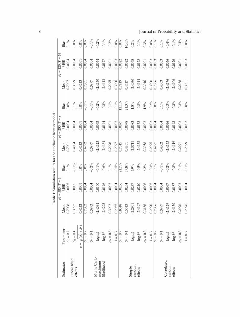
8 Journal of Probability and Statistics
Table
1:Simulationresu
ltsforthestocha
sticfron
tier
mod
el.
N=500,T=4
N=250,T=8
N=125,T=16
Estim
ator
Parameter
Mean
MSE
Bias
Mean
MSE
Bias
Mean
MSE
Bias
Linearfix
edeff
ects
β1=0.7
0.7008
0.0005
0.1%
0.7001
0.0004
0.0%
0.7007
0.0004
0.1%
β2=0.4
0.3997
0.0005
−0.1%
0.4004
0.0004
0.1%
0.3999
0.0004
0.0%
σ=√(σ
2 v+λ2 )
0.4242
0.0001
0.0%
0.4243
0.0001
0.0%
0.4243
0.0001
0.0%
Mon
teCarlo
max
imum
likelihoo
d
β1=0.7
0.7002
0.0004
0.0%
0.6992
0.0004
−0.1%
0.7001
0.0004
0.0%
β2=0.4
0.3993
0.0004
−0.2%
0.3997
0.0004
−0.1%
0.3997
0.0004
−0.1%
logσ2 v
−2.4094
0.0100
−0.1%
−2.4123
0.0065
−0.2%
−2.4130
0.0054
−0.2%
logλ2
−2.4225
0.0196
−0.6%
−2.4134
0.0144
−0.2%
−2.4112
0.0127
−0.1%
σv=0.3
0.3002
0.0002
0.1%
0.2996
0.0001
−0.1%
0.2995
0.0001
−0.2%
λ=0.3
0.2985
0.0004
−0.5%
0.2997
0.0003
−0.1%
0.3000
0.0003
0.0%
Simple
rand
omeff
ects
β1=0.7
0.8518
0.0236
21.7%
0.7845
0.0077
12.1%
0.7419
0.0022
6.0%
β2=0.4
0.5513
0.0234
37.8%
0.4851
0.0078
21.3%
0.4417
0.0022
10.4%
logσ2 v
−2.2901
0.0237
4.9%
−2.3711
0.0083
1.5%
−2.4030
0.0055
0.2%
logλ2
−2.4197
0.0210
−0.5%
−2.4152
0.0153
−0.3%
−2.4114
0.0128
−0.1%
σv=0.3
0.3186
0.0006
6.2%
0.3058
0.0002
1.9%
0.3010
0.0001
0.3%
λ=0.3
0.2990
0.0005
−0.3%
0.2995
0.0003
−0.2%
0.3000
0.0003
0.0%
Correlated
rand
omeff
ects
β1=0.7
0.7006
0.0004
0.1%
0.6997
0.0004
0.0%
0.7006
0.0003
0.1%
β2=0.4
0.3997
0.0004
−0.1%
0.4002
0.0004
0.1%
0.4003
0.0003
0.1%
logσ2 v
−2.4129
0.0097
−0.2%
−2.4153
0.0066
−0.3%
−2.4176
0.0056
−0.4%
logλ2
−2.4150
0.0187
−0.3%
−2.4119
0.0143
−0.2%
−2.4106
0.0126
−0.1%
σv=0.3
0.2996
0.0002
−0.1%
0.2991
0.0002
−0.3%
0.2988
0.0001
−0.4%
λ=0.3
0.2996
0.0004
−0.1%
0.2999
0.0003
0.0%
0.3001
0.0003
0.0%
Journal of Probability and Statistics 9
T . Furthermore, the mean squared errors of both estimators decrease as the time dimensionof the panel increases. For the MC maximum likelihood estimator this can be attributed tothe fact that as T increases more information per group is used to formulate the posterior ofαi.
Obtaining estimates of observation-specific efficiency scores involves first generatingestimates of the group intercepts. Estimates of the group effects can be obtained for therandom-effects estimators using group averages of the dependent and independent variables,accounting at the same time for the skewness of the composite error term [14]. On theother hand, the MC maximum likelihood estimator can provide estimates of the αis bytreating them as quantities to be estimated by simulation after the estimation of the commonparameters of the model. In both estimators, the αis and θ are replaced in (4.3) by their pointestimates to obtain estimates of the observation-specific efficiency scores.
Nevertheless, both the random-effects and the MC maximum likelihood estimators ofthe αis are only T consistent. A different approach, which is consistent with treating the αisas missing data, is to integrate them from the expectation in (4.3). That is, one may obtain theexpectation of e−uit | εit unconditionally on the missing data. In this way, the uncertaintyassociated with the αis is accommodated when estimating observation-specific efficiencyscores. The integration of the αis is achieved using the following procedure:
(1) draw M samples from f(αi | yi, xi, θ) where θ is either the random-effects or theMC maximum likelihood point estimate,
(2) for each draw j = 1, 2, . . . ,M, evaluate E(e−uit | εit,j), where εit,j = yit − αi,j − x′itβ,
(3) take the sample mean of the E(e−uit | εit,j)s over j.By the law of iterated expectations, this sample mean will converge to the unconditionalexpectation of e−uit | εit,j . (In the random-effects model, integration can also be performed byquadratures rather than simulation.)
Figure 1 presents scatter plots of the actual versus the predicted efficiency scores forthe MC maximum likelihood and the correlated random-effects estimators for a particularMonte Carlo repetition. Apart from the known problem of underestimating the scores ofhighly efficient observations, the approach of integrating the αis from the expectation ofe−uit | εit produces good predictions for the efficiency scores for the MC maximum likelihoodestimator. On the other hand, the predictions of the correlated random-effects estimatorare more dispersed around the 45◦ line. The MC maximum likelihood estimator has anadvantage over the random-effects estimator because it does not need to specify a systematicrelationship between the group effects and the independent variables. In other words, thequality of the estimates of the efficiency scores from the random-effects estimator deterioratesif there is a lot of noise in the relationship between the group effects and the group means ofthe independent variables.
5. Application
This section presents an application of the estimators discussed in this paper to a panel ofEuropean manufacturing industries. The dataset comes from the EU-KLEMS project [17] andcovers the period from 1970 to 2007. It contains annual information at the country level forindustries classified according to the 4-digit NACE revision 2 system. The part of the datasetused for the application covers 10 manufacturing industries for 6 countries for which therequired data series are complete (Denmark, Finland, Italy, Spain, The Netherlands, and UK).
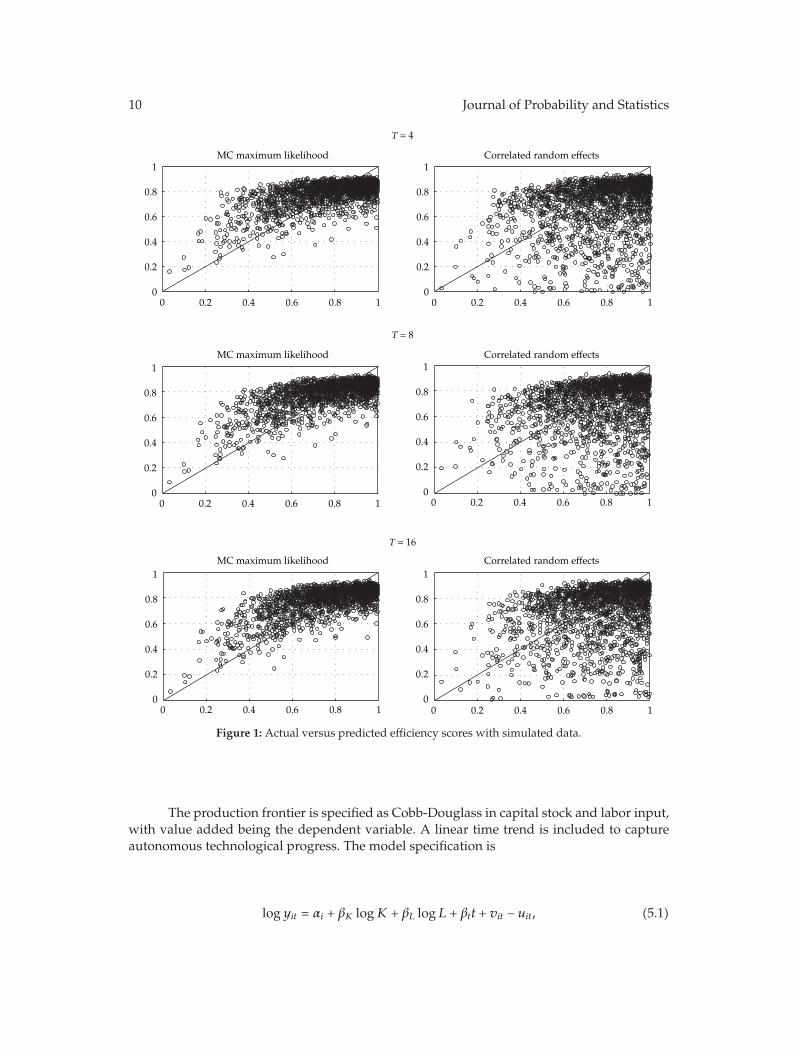
10 Journal of Probability and Statistics
0
0.2
0.4
0.6
0.8
1
0 0.2 0.4 0.6 0.8 10
0.2
0.4
0.6
0.8
1
0 0.2 0.4 0.6 0.8 1
0
0.2
0.4
0.6
0.8
1
0 0.2 0.4 0.6 0.8 10
0.2
0.4
0.6
0.8
1
0 0.2 0.4 0.6 0.8 1
0
0.2
0.4
0.6
0.8
1
0 0.2 0.4 0.6 0.8 10
0.2
0.4
0.6
0.8
1
0 0.2 0.4 0.6 0.8 1
T = 4
T = 8
T = 16
Correlated random effectsMCmaximum likelihood
MCmaximum likelihood Correlated random effects
Correlated random effectsMCmaximum likelihood
Figure 1: Actual versus predicted efficiency scores with simulated data.
The production frontier is specified as Cobb-Douglass in capital stock and labor input,with value added being the dependent variable. A linear time trend is included to captureautonomous technological progress. The model specification is
logyit = αi + βK logK + βL logL + βtt + vit − uit, (5.1)

Journal of Probability and Statistics 11
Table 2: Results for the EU-KLEMS model.
Linear fixed effects MC maximum likelihood Simple random effects Correlated random effects
βK 0.3262 0.2687 0.3478 0.1833βL 0.7265 0.7323 0.6134 0.7388βt 0.0202 0.0211 0.0173 0.0224σv — 0.0755 0.0796 0.0705λ — 0.2057 0.2033 0.2087
where it is assumed that vit ∼ N(0, σ2v) and uit ∼ Exp(λ). Each industry in each country is
treated as a group with its own intercept, but the production technologies of all industriesacross all countries are assumed to be represented by the same slope parameters.
The model is estimated using the linear fixed-effects, MC maximum likelihood, andsimple and correlated random-effects estimators. The results are presented in Table 2. Giventhat under the strict model specification the group effects are expected to be correlatedwith the regressors, it does not come as a surprise that relatively large discrepanciesbetween the parameter estimates of the linear fixed-effects and the simple random-effectsestimators appear. Nonnegligible discrepancies are also observed between the linear fixed-effects estimate of βK and the corresponding estimates from the estimators that account forpossible correlation between the group effects and the independent variables. Although thisresult appears to be in contrast with the findings of the Monte Carlo simulations, we needto keep in mind that the Monte Carlo findings are valid for the estimators on average,while the application considers a single dataset where particularities could lead to thesediscrepancies. For example, limited within variation in the capital and labor variables couldinduce multicollinearity and render the point estimates less precise.
On the other hand, all three estimators that can distinguish between noise andinefficiency effects produce very similar parameter estimates for the variances of the twoerror terms. The estimates of the parameter associated with the time trend suggest that theindustries experience, on average, productivity growth at a rate slightly larger than 2%.
Figure 2 presents kernel density estimates of the observation-specific technicalefficiency scores obtained by integrating the group effects from the expectation in (4.3)using the MC maximum likelihood and the two random-effects estimators. It appears thatonly the MC maximum likelihood estimator produces a distribution of technical efficiencyscores similar to the original assumptions imposed by the model, with the majority of theindustries being highly efficient. On the other hand, the simple random-effects estimatoryields a bimodal distribution of efficiency scores.
6. Conclusions and Further Remarks
This paper proposes a general procedure for choosing appropriate densities for frequentistintegrated-likelihood methods in panel data models. The proposed method requires theplacement of priors on the density of the group-specific constant terms. These priors,however, are updated during estimation and in this way their impact on the final parameterestimates is minimized.
A set of Monte Carlo experiments were conducted to examine the sampling propertiesof the proposed estimator and to compare them with the properties of existing relevantestimators. Although the experiments were conducted in the specific context of a stochastic
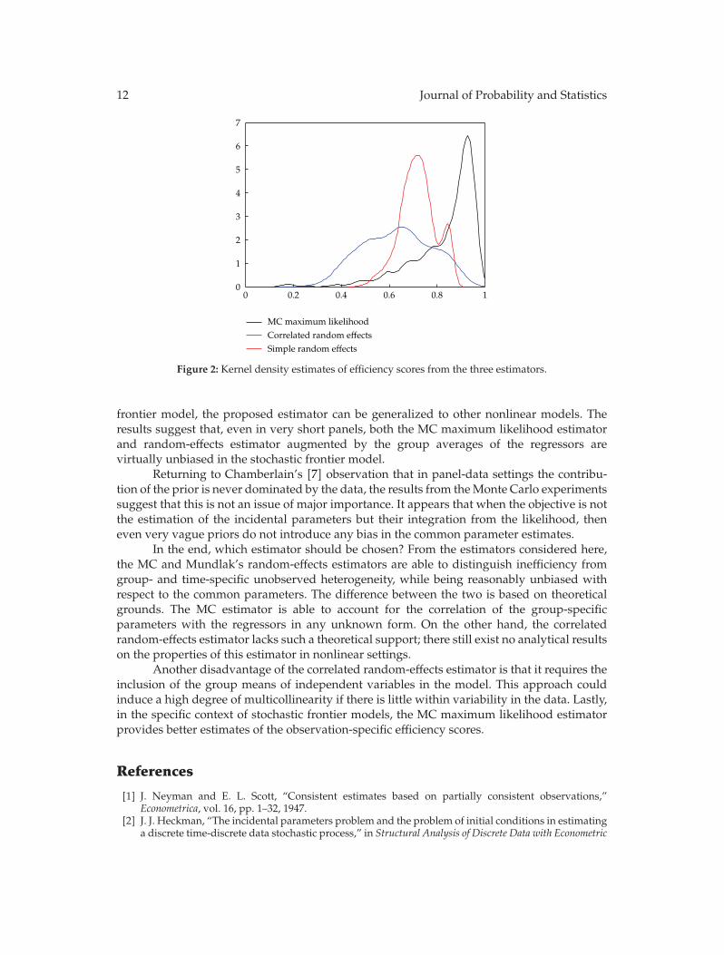
12 Journal of Probability and Statistics
0
1
2
3
4
5
6
7
0 0.2 0.4 0.6 0.8 1
MCmaximum likelihoodCorrelated random effectsSimple random effects
Figure 2: Kernel density estimates of efficiency scores from the three estimators.
frontier model, the proposed estimator can be generalized to other nonlinear models. Theresults suggest that, even in very short panels, both the MC maximum likelihood estimatorand random-effects estimator augmented by the group averages of the regressors arevirtually unbiased in the stochastic frontier model.
Returning to Chamberlain’s [7] observation that in panel-data settings the contribu-tion of the prior is never dominated by the data, the results from theMonte Carlo experimentssuggest that this is not an issue of major importance. It appears that when the objective is notthe estimation of the incidental parameters but their integration from the likelihood, theneven very vague priors do not introduce any bias in the common parameter estimates.
In the end, which estimator should be chosen? From the estimators considered here,the MC and Mundlak’s random-effects estimators are able to distinguish inefficiency fromgroup- and time-specific unobserved heterogeneity, while being reasonably unbiased withrespect to the common parameters. The difference between the two is based on theoreticalgrounds. The MC estimator is able to account for the correlation of the group-specificparameters with the regressors in any unknown form. On the other hand, the correlatedrandom-effects estimator lacks such a theoretical support; there still exist no analytical resultson the properties of this estimator in nonlinear settings.
Another disadvantage of the correlated random-effects estimator is that it requires theinclusion of the group means of independent variables in the model. This approach couldinduce a high degree of multicollinearity if there is little within variability in the data. Lastly,in the specific context of stochastic frontier models, the MC maximum likelihood estimatorprovides better estimates of the observation-specific efficiency scores.
References
[1] J. Neyman and E. L. Scott, “Consistent estimates based on partially consistent observations,”Econometrica, vol. 16, pp. 1–32, 1947.
[2] J. J. Heckman, “The incidental parameters problem and the problem of initial conditions in estimatinga discrete time-discrete data stochastic process,” in Structural Analysis of Discrete Data with Econometric

Journal of Probability and Statistics 13
Applications, C. F. Manski and D. McFadden, Eds., pp. 179–195, MIT Press, Cambridge, Mass, USA,1981.
[3] W. Greene, “Fixed effects and bias due to the incidental parameters problem in the tobit model,”Econometric Reviews, vol. 23, no. 2, pp. 125–147, 2004.
[4] W. Greene, “Fixed and random effects in stochastic frontier models,” Journal of Productivity Analysis,vol. 23, no. 1, pp. 7–32, 2005.
[5] W. Greene, “Reconsidering heterogeneity in panel data estimators of the stochastic frontier model,”Journal of Econometrics, vol. 126, no. 2, pp. 269–303, 2005.
[6] T. Lancaster, “The incidental parameter problem since 1948,” Journal of Econometrics, vol. 95, no. 2, pp.391–413, 2000.
[7] G. Chamberlain, “Panel data,” in Handbook of Econometrics, Z. Griliches and M. D. Intriligator, Eds.,vol. 2, pp. 1247–1313, North-Holland, Amsterdam, The Netherland, 1984.
[8] A. Abdulai and H. Tietje, “Estimating technical efficiency under unobserved heterogeneity withstochastic frontier models: Application to northern German dairy farms,” European Review ofAgricultural Economics, vol. 34, no. 3, pp. 393–416, 2007.
[9] Yair Mundlak, “On the pooling of time series and cross section data,” Econometrica, vol. 46, no. 1, pp.69–85, 1978.
[10] A. E. Gelfand and B. P. Carlin, “Maximum-likelihood estimation for constrained- or missing-datamodels,” The Canadian Journal of Statistics, vol. 21, no. 3, pp. 303–311, 1993.
[11] C. J. Geyer, “On the convergence of Monte Carlo maximum likelihood calculations,” Journal of theRoyal Statistical Society B, vol. 56, no. 1, pp. 261–274, 1994.
[12] D. Aigner, C. A. K. Lovell, and P. Schmidt, “Formulation and estimation of stochastic frontierproduction function models,” Journal of Econometrics, vol. 6, no. 1, pp. 21–37, 1977.
[13] W. Meeusen and J. van den Broeck, “Efficiency estimation from Cobb-Douglas production functionswith composed error,” International Economic Review, vol. 18, pp. 435–444, 1977.
[14] H.-J. Wang and C.-W. Ho, “Estimating fixed-effect panel stochastic frontier models by modeltransformation,” Journal of Econometrics, vol. 157, no. 2, pp. 286–296, 2010.
[15] A. Alvarez, C. Amsler, L. Orea, and P. Schmidt, “Interpreting and testing the scaling property inmodels where inefficiency depends on firm characteristics,” Journal of Productivity Analysis, vol. 25,no. 3, pp. 201–212, 2006.
[16] P. Schmidt and R. C. Sickles, “Production frontiers and panel data,” Journal of Business & EconomicStatistics, vol. 2, no. 4, pp. 367–374, 1984.
[17] M. O’Mahony and M. P. Timmer, “Output, input and productivity measures at the industry level: theEU KLEMS database,” Economic Journal, vol. 119, no. 538, pp. F374–F403, 2009.
Hindawi Publishing CorporationJournal of Probability and StatisticsVolume 2011, Article ID 617652, 17 pagesdoi:10.1155/2011/617652
Research ArticlePanel Unit Root Tests by Combining Dependent PValues: A Comparative Study
Xuguang Sheng1 and Jingyun Yang2
1 Department of Economics, American University, Washington, DC 20016, USA2 Department of Biostatistics and Epidemiology, University of Oklahoma Health Sciences Center,Oklahoma City, OK 73104, USA
Correspondence should be addressed to Xuguang Sheng, [email protected] Jingyun Yang, [email protected]
Received 27 June 2011; Accepted 25 August 2011
Academic Editor: Mike Tsionas
Copyright q 2011 X. Sheng and J. Yang. This is an open access article distributed under theCreative Commons Attribution License, which permits unrestricted use, distribution, andreproduction in any medium, provided the original work is properly cited.
We conduct a systematic comparison of the performance of four commonly used P valuecombination methods applied to panel unit root tests: the original Fisher test, the modified inversenormal method, Simes test, and the modified truncated product method (TPM). Our simulationresults show that under cross-section dependence the original Fisher test is severely oversized, butthe other three tests exhibit good size properties. Simes test is powerful when the total evidenceagainst the joint null hypothesis is concentrated in one or very few of the tests being combined,but the modified inverse normal method and the modified TPM have good performance whenevidence against the joint null is spread among more than a small fraction of the panel units. Thesedifferences are further illustrated through one empirical example on testing purchasing powerparity using a panel of OECD quarterly real exchange rates.
1. Introduction
Combining significance tests, or P values, has been a source of considerable research instatistics since Tippett [1] and Fisher [2]. (For a systematic comparison of methods forcombining P values from independent tests, see the studies by Hedges and Olkin [3] andLoughin [4].) Despite the burgeoning statistical literature on combining P values, thesetechniques have not been used much in panel unit root tests until recently. Maddala andWu [5] and Choi [6] are among the first who attempted to test unit root in panels bycombining independent P values. More recent contributions include those by Demetrescuet al. [7], Hanck [8], and Sheng and Yang [9]. Combining P values has several advantagesover combination of test statistics in that (i) it allows different specifications, such as different
2 Journal of Probability and Statistics
deterministic terms and lag orders, for each panel unit, (ii) it does not require a panel to bebalanced, and (iii) observed P values derived from continuous test statistics have a uniformdistribution under the null hypothesis regardless of the test statistic or distribution fromwhich they arise, and thus it can be carried out for any unit root test derived.
While the formulation of the joint null hypothesis (H0: all of the time series in the panelare nonstationary) is relatively uncontroversial, the specification of the alternative hypothesiscritically depends on what assumption one makes about the nature of the heterogeneity ofthe panel. (Recent contributions include O’Connell [10], Phillips and Sul [11], Bai and Ng[12], Chang [13], Moon and Perron [14] and Pesaran [15].) The problem of selecting a testis complicated by the fact that there are many different ways in which H0 can be false. Ingeneral, we cannot expect one test to be sensitive to all possible alternatives, so that no singleP value combinationmethod is uniformly the best. The goal of this paper is tomake a detailedcomparison, via both simulations and empirical examples, of some commonly used P valuecombination methods, and to provide specific recommendation regarding their use in panelunit root tests.
The plan of the paper is as follows. Section 2 briefly reviews the methods ofcombining P values. Small sample performance of these methods is investigated in Section 3using Monte Carlo simulations. Section 4 provides the empirical applications, and Section 5concludes the paper.
2. P Value Combination Methods
Consider the model
yit = (1 − αi)μi + αiyi,t−1 + εit, i = 1, . . . ,N; t = 1, . . . , T. (2.1)
Heterogeneity in both the intercept and the slope is allowed in (2.1). This specification iscommonly used in the literature, see the work of Breitung and Pesaran [16] for a recentreview. Equation (2.1) can be rewritten as
Δyit = −φiμi + φiyi,t−1 + εit, (2.2)
where Δyit = yit − yi,t−1 and φi = αi − 1.The null hypothesis is
H0 : φ1 = φ2 = · · · = φN = 0, (2.3)
and the alternative hypothesis is
H1 : φ1 < 0, φ2 < 0, . . . , φN0 < 0, N0 ≤N. (2.4)
Let Si,Ti be a test statistic for the ith unit of the panel in (2.2), and let the correspondingP value be defined as pi = F(Si,Ti), where F(·) denotes the cumulative distribution function(c.d.f.) of Si,Ti . We assume that, under H0, Si,Ti has a continuous distribution function.This assumption is a regularity condition that ensures a uniform distribution of the P

Journal of Probability and Statistics 3
values, regardless of the test statistic or distribution from which they arise. Thus, P valuecombinations are nonparametric in the sense that they do not depend on the parametric formof the data. The nonparametric nature of combined P values gives them great flexibility inapplications.
In the rest of this section, we briefly review the P value combination methods in thecontext of panel unit root tests. The first test, proposed by Fisher [2], is defined as
P = −2N∑
i=1
ln(pi), (2.5)
which has an χ2 distribution with 2N degrees of freedom under the assumption of cross-section independence of the P values. Maddala and Wu [5] introduced this method to thepanel unit root tests, and Choi [6]modified it to the case of infiniteN.
Inverse normal method, attributed to Stouffer et al. [17], is another often used methoddefined as
Z =1√N
N∑
i=1
Φ−1(pi), (2.6)
where Φ(·) is the c.d.f. of the standard normal distribution. UnderH0, Z ∼ N(0, 1). Choi [6]first applied this method to the panel unit root tests assuming cross-section independenceamong the panel units. To account for cross-section dependence, Hartung [18] developed amodified inverse normal method by assuming a constant correlation across the probits ti,
cov(ti, tj)= ρ, for i /= j, i, j = 1, . . . ,N, (2.7)
where ti = Φ−1(pi). He proposed to estimate ρ in finite samples by
ρ� = max(− 1N − 1
, ρ
), (2.8)
where ρ = 1 − (1/N − 1)∑N
i=1(ti − t)2 and t = (1/N)∑N
i=1 ti. The modified inverse normal teststatistic is formed as
Z∗ =∑N
i=1 ti√N +N(N − 1)
[ρ� + κ
√2/(n + 1)
(1 − ρ�)
] , (2.9)
where κ = 0.1(1 + 1/(N − 1) − ρ�) is a parameter designed to improve the small sampleperformance of the test statistic. Under the null hypothesis, Z∗ ∼ N(0, 1). Demetrescu et al.[7] showed that this methodwas robust to certain deviations from the assumption of constantcorrelation between probits in the panel unit root tests.
4 Journal of Probability and Statistics
A third method, proposed by Simes [19] as an improved Bonferroni procedure, isbased on the ordered P values, denoted by p(1) ≤ p(2) ≤ · · · ≤ p(N). The joint hypothesisH0 is rejected if
p(i) ≤ iα
N, (2.10)
for at least one i = 1, . . . ,N. This procedure has a type I error equal to αwhen the test statisticsare independent. Hanck [8] showed that Simes test was robust to general patterns of cross-sectional dependence in the panel.
The fourth method is Zaykin et al.’s [20] truncated product method (TPM), whichtakes the product of all those P values that do not exceed some prespecified value τ . TheTPM is defined as
W =N∏
i=1
pI(pi≤τ)i , (2.11)
where I(·) is the indicator function. Note that setting τ = 1 leads to Fisher’s originalcombination method, which could lose power in cases when there are some very large Pvalues. This can happen when some series in the panel are clearly nonstationary such thatthe resulting P -values are close to 1, and some are clearly stationary such that the resultingP values are close to 0. Ordinary combination methods could be dominated by the large Pvalues. The TPM removes these large P values through truncation, thus eliminating the effectthat they could have on the resulting test statistic.
When all the P values are independent, there exists a closed form of the distributionfor W under H0. When the P values are dependent, Monte Carlo simulation is needed toobtain the empirical distribution of W . Sheng and Yang [9] modify the TPM to allow for acertain degree of correlation among the P values. Their procedure is as follows.
Step 1. CalculateW∗ using (2.11). Set A = 0.
Step 2. Estimate the correlation matrix, Σ, for P values. Following Hartung [18] andDemetrescu et al. [7], they assume a constant correlation between the probits ti and tj ,
cov(ti, tj)= ρ, for i /= j, i, j = 1, . . . ,N, (2.12)
where ti = Φ−1(pi) and tj = Φ−1(pj). ρ can be estimated in finite samples according to (2.8).
Step 3. The distribution ofW∗ is calculated based on the following Monte Carlo simulations.
(a) Draw pseudorandom probits from the normal distribution with mean zero and theestimated correlation matrix, Σ, and transform them back through the standardnormal c.d.f., resulting inN P -values, denoted by p1, p2, . . . , pN .
(b) Calculate W =∏N
i=1pI(pi≤τ)i .
(c) If W ≤W∗, increment A by one.
(d) Repeat steps (a)–(c) B times.
(e) The P value forW∗ is given by A/B.
Journal of Probability and Statistics 5
3. Monte Carlo Study
In this sectionwe compare the finite sample performance of the P value combinationmethodsintroduced in Section 2.We consider “strong” cross-section dependence, driven by a commonfactor, and “weak” cross-section dependence due to spatial correlation.
3.1. The Design of Monte Carlo
First we consider dynamic panels with fixed effects but no linear trends or residual serialcorrelation. The data-generating process (DGP) in this case is given by
yit = (1 − αi)μi + αiyi,t−1 + εit, (3.1)
where
εit = γift + ξit, (3.2)
for i = 1, . . . ,N, t = −50,−49, . . . , T . The initial values yi,−50 are set to be 0 for all i. Theindividual fixed effect μi, the common factor ft, the factor loading γi, and the error term ξitare independent of each other with μi ∼ i.i.dN(0, 1), ft ∼ i.i.dN(0, σ2
f), γi ∼ i.i.d U[0, 3], andξit ∼ i.i.dN(0, 1).
Remark 3.1. Setting σ2f = 0, we explore the properties of the tests under cross-section
independence, and, with σ2f
= 10, we explore the performance of the tests under “high”cross-section dependence. In the latter case, the average pairwise correlation coefficient of εitand εjt is 70%, representing a strong cross-section correlation in practice.
Next we allow for deterministic trends in the DGP and the Dickey-Fuller (DF)regressions. For this case yit is generated as follows:
yit = κi + (1 − αi)λit + αiyi,t−1 + εit, (3.3)
with κi ∼ i.i.d U[0, 0.02] and λi ∼ i.i.d U[0, 0.02]. This ensures that yit has the same averagetrend properties under the null and the alternative hypotheses. The errors εit are generatedaccording to (3.2) with σ2
f= 10, representing the scenario of high cross-section correlation.
To examine the impact of residual serial correlation, we consider a number ofexperiments, where the errors ξit in (3.2) are generated as
ξit = ρiξi,t−1 + eit, (3.4)
with eit ∼ i.i.d N(0, 1). Following Pesaran [15], we choose ρi ∼ i.i.d U[0.2, 0.4] for positiveserial correlations and ρi ∼ i.i.d U[−0.4,−0.2] for negative serial correlations. We use thisDGP to check the robustness of the tests to alternative residual correlation models and to theheterogeneity of the coefficients, ρi.
Finally we explore the performance of the tests under spatial dependence. We considertwo commonly used spatial error processes: the spatial autoregressive (SAR) and the spatial
6 Journal of Probability and Statistics
moving average (SMA). Let εt be theN × 1 error vector in (3.1). In SAR, it can be expressedas
εt = θ1WNεt + υt = (IN − θ1WN)−1υt, (3.5)
where θ1 is the spatial autoregressive parameter, WN is an N × N known spatial weightsmatrix, and υt is the error component which is assumed to be distributed independentlyacross cross-section dimension with constant variance σ2
υ. Then the fullNT ×NT covariancematrix is
ΩSAR = σ2υ
[IT ⊗
(B′NBN
)−1], (3.6)
where BN = IN − θ1WN . In SMA, the error vector εt can be expressed as
εt = θ2WNυt + υt = (IN + θ2WN)υt, (3.7)
with θ2 being the spatial moving average parameter. Then the fullNT×NT covariance matrixbecomes
ΩSMA = σ2υ
[IT ⊗
(IN + θ2
(WN +W ′
N
)+ θ22WNW
′N
)]. (3.8)
Without loss of generality, we let σ2υ = 1. We consider the spatial dependence with θ1 = 0.8
and θ2 = 0.8. The average pairwise correlation coefficient of εit and εjt is 4%–22% for SARand 2%–8% for SMA, representing a wide range of cross-section correlations in practice. Thespatial weight matrix WN is specified as a “1 ahead and 1 behind” matrix with the ith row,1 < i < N, of this matrix having nonzero elements in positions i + 1 and i − 1. Each row of thismatrix is normalized such that all its nonzero elements are equal to 1/2.
For all of DGPs considered here, we use
αi
⎧⎨
⎩
∼ i.i.d. U[0.85, 0.95] for i = 1, . . . ,N0, where N0 = δ ·N,
= 1 for i =N0 + 1, . . . ,N,(3.9)
where δ indicates the fraction of stationary series in the panel, varying in the interval 0-1.As a result, changes in δ allow us to study the impact of the proportion of stationary serieson the power of tests. When δ = 0, we explore the size of tests. We set δ = 0.1, 0.5 and 0.9to examine the power of the tests under heterogeneous alternatives. The tests are one-sidedwith the nominal size set at 5% and conducted for all combinations ofN and T = 20, 50, and100. (We also conduct the simulations with the nominal size set at 1% and 10%. The resultsare qualitatively similar to those at the 5% level, and thus are not reported here.) The resultsare obtained with MATLAB using M = 2000 simulations. To calculate the empirical criticalvalue for the modified TPM, we run additional B = 1000 replications within each simulation.
We calculate the augmented Dickey-Fuller (ADF) t statistics. The number of lags in theADF regressions is selected according to the recursive t-test procedure. (Start with an upperbound, kmax = 8, on k. If the last included lag is significant, choose k = kmax, if not, reduce k
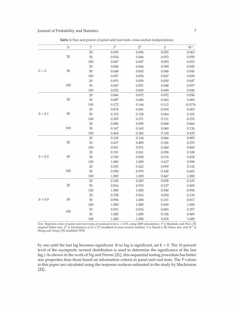
Journal of Probability and Statistics 7
Table 1: Size and power of panel unit root tests: cross-section independence.
N T P Z∗ S W∗
δ = 0
2020 0.059 0.056 0.052 0.06350 0.054 0.046 0.053 0.050100 0.047 0.047 0.053 0.052
5020 0.040 0.044 0.050 0.04550 0.048 0.045 0.048 0.045100 0.057 0.054 0.047 0.058
10020 0.051 0.050 0.050 0.04750 0.047 0.051 0.048 0.057100 0.052 0.045 0.049 0.049
δ = 0.1
2020 0.066 0.072 0.052 0.05650 0.087 0.080 0.062 0.083100 0.172 0.144 0.112 0.0174
5020 0.074 0.081 0.054 0.06550 0.123 0.128 0.064 0.102100 0.303 0.251 0.121 0.276
10020 0.080 0.085 0.048 0.06650 0.167 0.165 0.060 0.126100 0.464 0.366 0.130 0.435
δ = 0.5
2020 0.120 0.144 0.066 0.08350 0.417 0.489 0.106 0.253100 0.951 0.931 0.360 0.860
5020 0.181 0.261 0.058 0.10850 0.749 0.838 0.119 0.454100 1.000 1.000 0.417 0.998
10020 0.292 0.422 0.059 0.14250 0.950 0.979 0.108 0.683100 1.000 1.000 0.447 1.000
δ = 0.9
2020 0.182 0.283 0.058 0.10550 0.816 0.933 0.127 0.495100 1.000 1.000 0.580 0.994
5020 0.358 0.562 0.054 0.15450 0.994 1.000 0.151 0.817100 1.000 1.000 0.649 1.000
100 20 0.591 0.834 0.069 0.25750 1.000 1.000 0.156 0.969100 1.000 1.000 0.676 1.000
Note. Rejection rates of panel unit root tests at nominal level α = 0.05, using 2000 simulations. P is Maddala and Wu’s [5]original Fisher test, Z∗ is Demetrescu et al.’s [7] modified inverse normal method, S is Hanck’s [8] Simes test, and W∗ isSheng and Yang’s [9]modified TPM.
by one until the last lag becomes significant. If no lag is significant, set k = 0. The 10 percentlevel of the asymptotic normal distribution is used to determine the significance of the lastlag.)As shown in the work of Ng and Perron [21], this sequential testing procedure has bettersize properties than those based on information criteria in panel unit root tests. The P valuesin this paper are calculated using the response surfaces estimated in the study by Mackinnon[22].
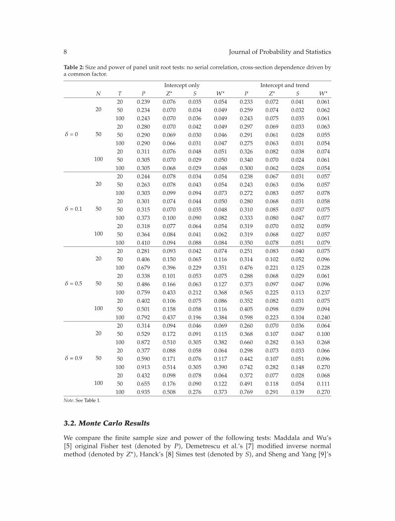
8 Journal of Probability and Statistics
Table 2: Size and power of panel unit root tests: no serial correlation, cross-section dependence driven bya common factor.
Intercept only Intercept and trendN T P Z∗ S W∗ P Z∗ S W∗
δ = 0
2020 0.239 0.076 0.035 0.054 0.233 0.072 0.041 0.06150 0.234 0.070 0.034 0.049 0.259 0.074 0.032 0.062100 0.243 0.070 0.036 0.049 0.243 0.075 0.035 0.061
5020 0.280 0.070 0.042 0.049 0.297 0.069 0.033 0.06350 0.290 0.069 0.030 0.046 0.291 0.061 0.028 0.055100 0.290 0.066 0.031 0.047 0.275 0.063 0.031 0.054
10020 0.311 0.076 0.048 0.051 0.326 0.082 0.038 0.07450 0.305 0.070 0.029 0.050 0.340 0.070 0.024 0.061100 0.305 0.068 0.029 0.048 0.300 0.062 0.028 0.054
δ = 0.1
2020 0.244 0.078 0.034 0.054 0.238 0.067 0.031 0.05750 0.263 0.078 0.043 0.054 0.243 0.063 0.036 0.057100 0.303 0.099 0.094 0.073 0.272 0.083 0.057 0.078
5020 0.301 0.074 0.044 0.050 0.280 0.068 0.031 0.05850 0.315 0.070 0.035 0.048 0.310 0.085 0.037 0.075100 0.373 0.100 0.090 0.082 0.333 0.080 0.047 0.077
10020 0.318 0.077 0.064 0.054 0.319 0.070 0.032 0.05950 0.364 0.084 0.041 0.062 0.319 0.068 0.027 0.057100 0.410 0.094 0.088 0.084 0.350 0.078 0.051 0.079
δ = 0.5
2020 0.281 0.093 0.042 0.074 0.251 0.083 0.040 0.07550 0.406 0.150 0.065 0.116 0.314 0.102 0.052 0.096100 0.679 0.396 0.229 0.351 0.476 0.221 0.125 0.228
5020 0.338 0.101 0.053 0.075 0.288 0.068 0.029 0.06150 0.486 0.166 0.063 0.127 0.373 0.097 0.047 0.096100 0.759 0.433 0.212 0.368 0.565 0.225 0.113 0.237
10020 0.402 0.106 0.075 0.086 0.352 0.082 0.031 0.07550 0.501 0.158 0.058 0.116 0.405 0.098 0.039 0.094100 0.792 0.437 0.196 0.384 0.598 0.223 0.104 0.240
δ = 0.9
2020 0.314 0.094 0.046 0.069 0.260 0.070 0.036 0.06450 0.529 0.172 0.091 0.115 0.368 0.107 0.047 0.100100 0.872 0.510 0.305 0.382 0.660 0.282 0.163 0.268
5020 0.377 0.088 0.058 0.064 0.298 0.073 0.033 0.06650 0.590 0.171 0.076 0.117 0.442 0.107 0.051 0.096100 0.913 0.514 0.305 0.390 0.742 0.282 0.148 0.270
10020 0.432 0.098 0.078 0.064 0.372 0.077 0.028 0.06850 0.655 0.176 0.090 0.122 0.491 0.118 0.054 0.111100 0.935 0.508 0.276 0.373 0.769 0.291 0.139 0.270
Note. See Table 1.
3.2. Monte Carlo Results
We compare the finite sample size and power of the following tests: Maddala and Wu’s[5] original Fisher test (denoted by P), Demetrescu et al.’s [7] modified inverse normalmethod (denoted by Z∗), Hanck’s [8] Simes test (denoted by S), and Sheng and Yang [9]’s
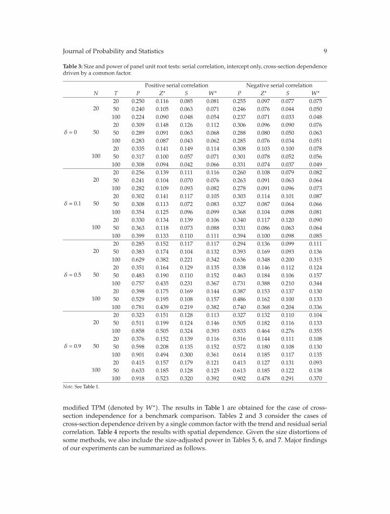
Journal of Probability and Statistics 9
Table 3: Size and power of panel unit root tests: serial correlation, intercept only, cross-section dependencedriven by a common factor.
Positive serial correlation Negative serial correlationN T P Z∗ S W∗ P Z∗ S W∗
δ = 0
2020 0.250 0.116 0.085 0.081 0.255 0.097 0.077 0.07550 0.240 0.105 0.063 0.071 0.246 0.076 0.044 0.050100 0.224 0.090 0.048 0.054 0.237 0.071 0.033 0.048
5020 0.309 0.148 0.126 0.112 0.306 0.096 0.090 0.07650 0.289 0.091 0.063 0.068 0.288 0.080 0.050 0.063100 0.283 0.087 0.043 0.062 0.285 0.076 0.034 0.051
10020 0.335 0.141 0.149 0.114 0.308 0.103 0.100 0.07850 0.317 0.100 0.057 0.071 0.301 0.078 0.052 0.056100 0.308 0.094 0.042 0.066 0.331 0.074 0.037 0.049
δ = 0.1
2020 0.256 0.139 0.111 0.116 0.260 0.108 0.079 0.08250 0.241 0.104 0.070 0.076 0.263 0.091 0.063 0.064100 0.282 0.109 0.093 0.082 0.278 0.091 0.096 0.073
5020 0.302 0.141 0.117 0.105 0.303 0.114 0.101 0.08750 0.308 0.113 0.072 0.083 0.327 0.087 0.064 0.066100 0.354 0.125 0.096 0.099 0.368 0.104 0.098 0.081
10020 0.330 0.134 0.139 0.106 0.340 0.117 0.120 0.09050 0.363 0.118 0.073 0.088 0.331 0.086 0.063 0.064100 0.399 0.133 0.110 0.111 0.394 0.100 0.098 0.085
δ = 0.5
2020 0.285 0.152 0.117 0.117 0.294 0.136 0.099 0.11150 0.383 0.174 0.104 0.132 0.393 0.169 0.093 0.136100 0.629 0.382 0.221 0.342 0.636 0.348 0.200 0.315
5020 0.351 0.164 0.129 0.135 0.338 0.146 0.112 0.12450 0.483 0.190 0.110 0.152 0.463 0.184 0.106 0.157100 0.757 0.435 0.231 0.367 0.731 0.388 0.210 0.344
10020 0.398 0.175 0.169 0.144 0.387 0.153 0.137 0.13050 0.529 0.195 0.108 0.157 0.486 0.162 0.100 0.133100 0.781 0.439 0.219 0.382 0.740 0.368 0.204 0.336
δ = 0.9
2020 0.323 0.151 0.128 0.113 0.327 0.132 0.110 0.10450 0.511 0.199 0.124 0.146 0.505 0.182 0.116 0.133100 0.858 0.505 0.324 0.393 0.833 0.464 0.276 0.355
5020 0.376 0.152 0.139 0.116 0.316 0.144 0.111 0.10850 0.598 0.208 0.135 0.152 0.572 0.180 0.108 0.130100 0.901 0.494 0.300 0.361 0.614 0.185 0.117 0.135
10020 0.415 0.157 0.179 0.121 0.413 0.127 0.131 0.09350 0.633 0.185 0.128 0.125 0.613 0.185 0.122 0.138100 0.918 0.523 0.320 0.392 0.902 0.478 0.291 0.370
Note. See Table 1.
modified TPM (denoted by W∗). The results in Table 1 are obtained for the case of cross-section independence for a benchmark comparison. Tables 2 and 3 consider the cases ofcross-section dependence driven by a single common factor with the trend and residual serialcorrelation. Table 4 reports the results with spatial dependence. Given the size distortions ofsome methods, we also include the size-adjusted power in Tables 5, 6, and 7. Major findingsof our experiments can be summarized as follows.
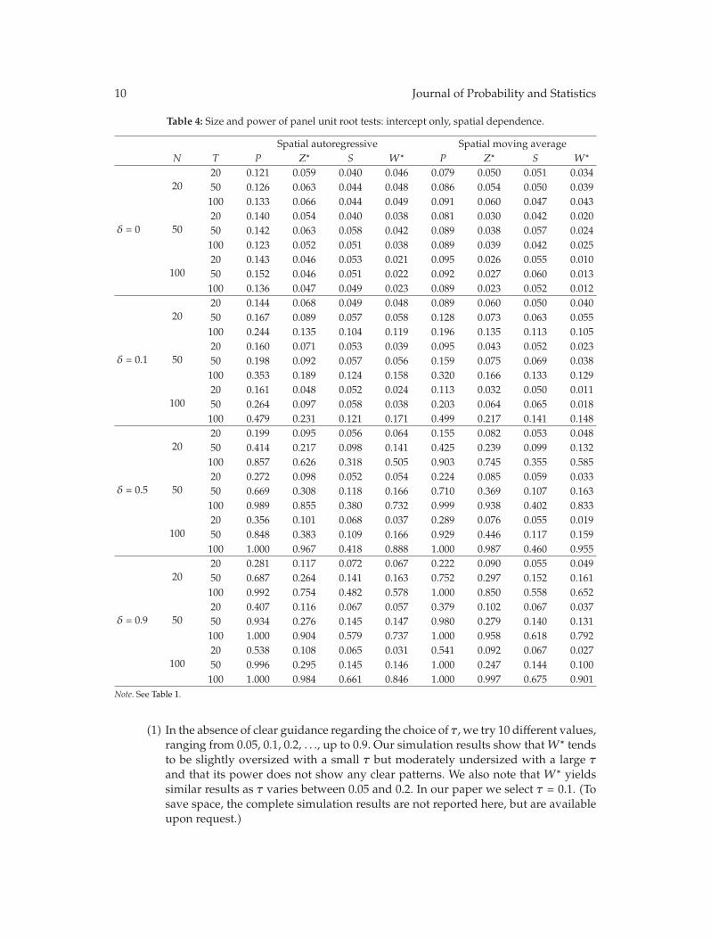
10 Journal of Probability and Statistics
Table 4: Size and power of panel unit root tests: intercept only, spatial dependence.
Spatial autoregressive Spatial moving averageN T P Z∗ S W∗ P Z∗ S W∗
δ = 0
2020 0.121 0.059 0.040 0.046 0.079 0.050 0.051 0.03450 0.126 0.063 0.044 0.048 0.086 0.054 0.050 0.039100 0.133 0.066 0.044 0.049 0.091 0.060 0.047 0.043
5020 0.140 0.054 0.040 0.038 0.081 0.030 0.042 0.02050 0.142 0.063 0.058 0.042 0.089 0.038 0.057 0.024100 0.123 0.052 0.051 0.038 0.089 0.039 0.042 0.025
10020 0.143 0.046 0.053 0.021 0.095 0.026 0.055 0.01050 0.152 0.046 0.051 0.022 0.092 0.027 0.060 0.013100 0.136 0.047 0.049 0.023 0.089 0.023 0.052 0.012
δ = 0.1
2020 0.144 0.068 0.049 0.048 0.089 0.060 0.050 0.04050 0.167 0.089 0.057 0.058 0.128 0.073 0.063 0.055100 0.244 0.135 0.104 0.119 0.196 0.135 0.113 0.105
5020 0.160 0.071 0.053 0.039 0.095 0.043 0.052 0.02350 0.198 0.092 0.057 0.056 0.159 0.075 0.069 0.038100 0.353 0.189 0.124 0.158 0.320 0.166 0.133 0.129
10020 0.161 0.048 0.052 0.024 0.113 0.032 0.050 0.01150 0.264 0.097 0.058 0.038 0.203 0.064 0.065 0.018100 0.479 0.231 0.121 0.171 0.499 0.217 0.141 0.148
δ = 0.5
2020 0.199 0.095 0.056 0.064 0.155 0.082 0.053 0.04850 0.414 0.217 0.098 0.141 0.425 0.239 0.099 0.132100 0.857 0.626 0.318 0.505 0.903 0.745 0.355 0.585
5020 0.272 0.098 0.052 0.054 0.224 0.085 0.059 0.03350 0.669 0.308 0.118 0.166 0.710 0.369 0.107 0.163100 0.989 0.855 0.380 0.732 0.999 0.938 0.402 0.833
10020 0.356 0.101 0.068 0.037 0.289 0.076 0.055 0.01950 0.848 0.383 0.109 0.166 0.929 0.446 0.117 0.159100 1.000 0.967 0.418 0.888 1.000 0.987 0.460 0.955
δ = 0.9
2020 0.281 0.117 0.072 0.067 0.222 0.090 0.055 0.04950 0.687 0.264 0.141 0.163 0.752 0.297 0.152 0.161100 0.992 0.754 0.482 0.578 1.000 0.850 0.558 0.652
5020 0.407 0.116 0.067 0.057 0.379 0.102 0.067 0.03750 0.934 0.276 0.145 0.147 0.980 0.279 0.140 0.131100 1.000 0.904 0.579 0.737 1.000 0.958 0.618 0.792
10020 0.538 0.108 0.065 0.031 0.541 0.092 0.067 0.02750 0.996 0.295 0.145 0.146 1.000 0.247 0.144 0.100100 1.000 0.984 0.661 0.846 1.000 0.997 0.675 0.901
Note. See Table 1.
(1) In the absence of clear guidance regarding the choice of τ , we try 10 different values,ranging from 0.05, 0.1, 0.2, . . ., up to 0.9. Our simulation results show thatW∗ tendsto be slightly oversized with a small τ but moderately undersized with a large τand that its power does not show any clear patterns. We also note that W∗ yieldssimilar results as τ varies between 0.05 and 0.2. In our paper we select τ = 0.1. (Tosave space, the complete simulation results are not reported here, but are availableupon request.)

Journal of Probability and Statistics 11
Table 5: Size-adjusted power of panel unit root tests: no serial correlation, cross-section dependence drivenby a common factor.
Intercept only Intercept and trendN T P Z∗ W∗ P Z∗ W∗
δ = 0.1
2020 0.043 0.046 0.044 0.038 0.052 0.03750 0.048 0.056 0.049 0.049 0.050 0.050100 0.062 0.084 0.063 0.066 0.062 0.064
5020 0.061 0.063 0.061 0.047 0.046 0.04750 0.053 0.054 0.054 0.042 0.046 0.040100 0.066 0.080 0.058 0.056 0.062 0.053
10020 0.099 0.121 0.094 0.052 0.058 0.05250 0.043 0.051 0.042 0.046 0.045 0.046100 0.065 0.069 0.065 0.058 0.067 0.055
δ = 0.5
2020 0.044 0.071 0.042 0.045 0.056 0.04650 0.070 0.116 0.068 0.062 0.075 0.058100 0.200 0.349 0.207 0.123 0.163 0.110
5020 0.057 0.080 0.057 0.052 0.056 0.04750 0.085 0.133 0.076 0.051 0.062 0.041100 0.161 0.348 0.160 0.116 0.182 0.099
10020 0.114 0.154 0.119 0.048 0.053 0.04750 0.069 0.123 0.064 0.057 0.068 0.054100 0.189 0.355 0.189 0.099 0.169 0.086
δ = 0.9
2020 0.059 0.050 0.058 0.061 0.061 0.06050 0.140 0.114 0.137 0.088 0.077 0.084100 0.456 0.433 0.431 0.250 0.201 0.231
5020 0.084 0.073 0.082 0.054 0.053 0.05350 0.150 0.114 0.144 0.087 0.073 0.081100 0.453 0.424 0.422 0.243 0.225 0.222
10020 0.144 0.151 0.131 0.054 0.051 0.05450 0.143 0.129 0.136 0.088 0.070 0.086100 0.446 0.395 0.414 0.208 0.198 0.191
Note. The power is calculated at the exact 5% level. The 5% critical values for these tests are obtained from their finite sampledistributions generated by 2000 simulations for sample sizes T = 20, 50, and 100. P is Maddala and Wu’s [5] original Fishertest, Z∗ is Demetrescu et al.’s [7] modified inverse normal method, andW∗ is Sheng and Yang’s [9] modified TPM.
(2) With no cross-section dependence, all the tests yield good empirical size, close to the5% nominal level (Table 1). As expected, P test shows severe size distortions undercross-section dependence driven by a common factor or by spatial correlations.For a common factor with no residual serial correlation, while Z∗ test is mildlyoversized and S test is slightly undersized, W∗ test shows satisfactory sizeproperties (Table 2). The presence of serial correlation leads to size distortions forall statistics when T is small, which even persist when T = 100 for P and Z∗ tests.On the contrary, S and W∗ tests exhibit good size properties with T = 50 and 100(Table 3). Under spatial dependence, S test performs the best in terms of size, whileZ∗ andW∗ tests are conservative for largeN (Table 4).
(3) All the tests become more powerful asN increases, which justifies the use of paneldata in unit root tests. When a linear time trend is included, the power of all the

12 Journal of Probability and Statistics
Table 6: Size-adjusted power of panel unit root tests: serial correlation, intercept only, cross-sectiondependence driven by a common factor.
Positive correlation Negative correlationN T P Z∗ W∗ P Z∗ W∗
δ = 0.1
2020 0.041 0.051 0.043 0.042 0.048 0.04150 0.053 0.054 0.050 0.043 0.054 0.042100 0.062 0.065 0.057 0.067 0.077 0.066
5020 0.042 0.058 0.043 0.050 0.053 0.04850 0.059 0.069 0.063 0.053 0.058 0.053100 0.058 0.075 0.052 0.056 0.066 0.054
10020 0.045 0.058 0.041 0.044 0.051 0.04450 0.056 0.061 0.052 0.063 0.061 0.065100 0.054 0.067 0.053 0.069 0.083 0.065
δ = 0.5
2020 0.040 0.056 0.040 0.045 0.064 0.03950 0.072 0.100 0.069 0.069 0.117 0.059100 0.188 0.255 0.199 0.158 0.298 0.150
5020 0.049 0.059 0.048 0.051 0.093 0.04550 0.081 0.120 0.083 0.068 0.127 0.058100 0.207 0.302 0.210 0.168 0.309 0.150
10020 0.051 0.054 0.046 0.037 0.084 0.03350 0.100 0.124 0.095 0.071 0.121 0.063100 0.209 0.330 0.221 0.148 0.345 0.127
δ = 0.9
2020 0.058 0.060 0.056 0.066 0.066 0.06550 0.153 0.083 0.148 0.119 0.110 0.114100 0.424 0.242 0.391 0.390 0.384 0.376
5020 0.068 0.054 0.066 0.065 0.069 0.06150 0.162 0.078 0.156 0.136 0.130 0.134100 0.454 0.262 0.415 0.376 0.376 0.352
10020 0.062 0.052 0.061 0.058 0.063 0.05750 0.169 0.088 0.157 0.135 0.114 0.135100 0.431 0.268 0.411 0.358 0.371 0.326
Note. See Table 5.
tests decreases substantially. Also notable is the fact that the power of tests increaseswhen the proportion of stationary series increases in the panel.
(4) Compared to the other three tests, the size-unadjusted power of S test is somewhatdisappointing here. An exception is that, when only very few series are stationary, Stest becomes most powerful. When the proportion of stationary series in the panelincreases, however, S test is outperformed by other tests. For example, in the caseof no cross-section dependence in Table 1 with δ = 0.9, N = 100, and T = 50, thepower of S test is 0.156, and, in contrast, all other tests have power close to 1.
(5) Because P test has severe size distortions, we only compare Z∗ and W∗ tests interms of size-adjusted power. (The power is calculated at the exact 5% level. The5% critical values for these tests are obtained from their finite sample distributionsgenerated by 2000 simulations for sample size T = 20, 50, and 100. Since Hanck’s [8]test does not have an explicit form of finite sample distribution, we do not calculateits size-adjusted power.) With the cross-section dependence driven by a common
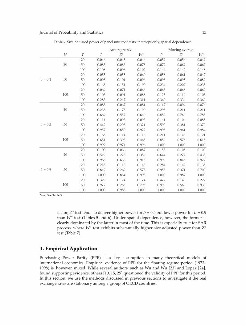
Journal of Probability and Statistics 13
Table 7: Size-adjusted power of panel unit root tests: intercept only, spatial dependence.
Autoregressive Moving averageN T P Z∗ W∗ P Z∗ W∗
δ = 0.1
2020 0.046 0.048 0.046 0.059 0.056 0.04950 0.085 0.083 0.078 0.072 0.069 0.067100 0.108 0.096 0.102 0.144 0.142 0.148
5020 0.055 0.055 0.060 0.058 0.061 0.04750 0.098 0.101 0.096 0.098 0.095 0.089100 0.165 0.151 0.190 0.234 0.207 0.235
10020 0.069 0.071 0.066 0.065 0.068 0.06250 0.103 0.091 0.088 0.125 0.119 0.105100 0.283 0.247 0.311 0.360 0.334 0.369
δ = 0.5
2020 0.088 0.067 0.081 0.117 0.094 0.07650 0.238 0.178 0.190 0.298 0.211 0.211100 0.669 0.557 0.640 0.852 0.760 0.785
5020 0.114 0.093 0.093 0.141 0.104 0.08550 0.442 0.298 0.321 0.593 0.381 0.379100 0.957 0.850 0.922 0.995 0.961 0.984
10020 0.168 0.114 0.116 0.211 0.146 0.12150 0.654 0.393 0.465 0.859 0.578 0.615100 0.999 0.974 0.996 1.000 1.000 1.000
δ = 0.9
2020 0.100 0.066 0.087 0.158 0.105 0.10050 0.519 0.223 0.359 0.644 0.272 0.438100 0.968 0.636 0.918 0.999 0.845 0.977
5020 0.218 0.113 0.143 0.284 0.142 0.13550 0.812 0.269 0.578 0.958 0.371 0.709100 1.000 0.864 0.998 1.000 0.987 1.000
10020 0.329 0.124 0.174 0.472 0.143 0.22750 0.977 0.285 0.795 0.999 0.569 0.930100 1.000 0.988 1.000 1.000 1.000 1.000
Note. See Table 5.
factor, Z∗ test tends to deliver higher power for δ = 0.5 but lower power for δ = 0.9than W∗ test (Tables 5 and 6). Under spatial dependence, however, the former isclearly dominated by the latter in most of the time. This is especially true for SARprocess, where W∗ test exhibits substantially higher size-adjusted power than Z∗
test (Table 7).
4. Empirical Application
Purchasing Power Parity (PPP) is a key assumption in many theoretical models ofinternational economics. Empirical evidence of PPP for the floating regime period (1973–1998) is, however, mixed. While several authors, such as Wu and Wu [23] and Lopez [24],found supporting evidence, others [10, 15, 25] questioned the validity of PPP for this period.In this section, we use the methods discussed in previous sections to investigate if the realexchange rates are stationary among a group of OECD countries.

14 Journal of Probability and Statistics
Table 8: Unit root tests for 27 OECD real exchange rates.
US dollar real exchange rate Deutchemark real exchange rateCountry k P value Simes criterion Country k P value Simes criterionNew Zealand 8 0.008 0.002 Mexico 3 0.006 0.002Sweden 8 0.053 0.004 Iceland 0 0.010 0.004United Kingdom 7 0.055 0.006 Australia 3 0.012 0.006Finland 7 0.058 0.007 Korea 0 0.014 0.007Spain 8 0.061 0.009 Canada 7 0.040 0.009Mexico 3 0.066 0.011 Sweden 0 0.074 0.011Iceland 8 0.069 0.013 United States 4 0.148 0.013Switzerland 4 0.071 0.015 New Zealand 0 0.171 0.015France 4 0.080 0.017 Finland 6 0.232 0.017Netherlands 4 0.099 0.019 Turkey 8 0.241 0.019Austria 4 0.102 0.020 Netherlands 1 0.415 0.020Italy 4 0.103 0.022 Norway 7 0.417 0.022Belgium 4 0.135 0.024 Spain 0 0.459 0.024Korea 0 0.138 0.026 France 0 0.564 0.026Germany 4 0.148 0.028 Italy 0 0.565 0.028Greece 4 0.150 0.030 Poland 5 0.579 0.030Norway 7 0.167 0.031 Hungary 4 0.612 0.031Denmark 3 0.206 0.033 Belgium 0 0.618 0.033Ireland 7 0.235 0.035 Luxembourg 0 0.655 0.035Japan 4 0.246 0.037 Japan 5 0.656 0.037Luxembourg 3 0.276 0.039 United Kingdom 0 0.697 0.039Portugal 8 0.332 0.041 Denmark 0 0.698 0.041Australia 3 0.386 0.043 Ireland 0 0.708 0.043Poland 0 0.414 0.044 Austria 0 0.720 0.044Turkey 8 0.418 0.046 Switzerland 8 0.733 0.046Canada 6 0.580 0.048 Portugal 0 0.786 0.048Hungary 0 0.816 0.050 Greece 5 0.880 0.050P 0.097 0.015Z∗ 0.095 0.016W∗ 0.257 0.002Note. Simes criterion is calculated using the 5% significance level.
The log real exchange rate between country i and the US is given by
qit = sit − pus,t + pit, (4.1)
where sit is the nominal exchange rate of the ith country’s currency in terms of US dollarand pus,t and pit are consumer price indices in the US and country i, respectively. All thesevariables are measured in natural logarithms. We use quarterly data from 1973 : 1 to 1998 : 2for 27 OECD countries, as listed in Table 8. (Two countries, Czech Republic and SlovakRepublic, are excluded from our analysis, since their data span a very limited period of time,starting at 1993 : 1.) All data are obtained from the IMF’s International Financial Statistics.(Note that, for Iceland, the consumer price indices are missing during 1982:Q1–1982:Q4 in

Journal of Probability and Statistics 15
the original data. We filled out this gap by calculating the level of CPI from its percentagechanges in the IMF database.)
As the first stage in our analysis we estimated individual ADF regressions:
Δqit = μi + φiqi,t−1 +ki∑
j=1
ϕijΔqi,t−j + εit, i = 1, . . . ,N; t = ki + 2, . . . , T. (4.2)
The null and alternative hypotheses for testing PPP are specified in (2.3) and (2.4),respectively. The selected lags and the P values are reported in Table 8. The results in theleft panel show that the ADF test does not reject the unit root null of real exchange rate atthe 5% level except for New Zealand. As a robustness check, we investigated the impact ofa change in numeraire on the results. The right panel reports the estimation results whenthe Deutsche mark is used as the numeraire. Out of 27 countries, only 5—Mexico, Iceland,Australia, Korea, and Canada—reject the null of unit root at the 5% level.
As is well known, the ADF test has low power with a short time span. Exploring thecross-section dimension is an alternative. However, if a positive cross-section dependence isignored, panel unit root tests can also lead to spurious results, as pointed out by O’Connell[10]. As a preliminary check, we compute the pairwise cross-section correlation coefficientsof the residuals from the above individual ADF regressions, ρij . The simple average of thesecorrelation coefficients is calculated, according to Pesaran [26], as
ρ =2
N(N − 1)
N−1∑
i=1
N∑
j=i+1
ρij . (4.3)
The associated cross-section dependence (CD) test statistic is calculated using
CD =
√2T
N(N − 1)
N−1∑
i=1
N∑
j=i+1
ρij . (4.4)
In our sample ρ is estimated as 0.396 and 0.513 when US dollar and Deutchemark areconsidered as the numeraire, respectively. The CD statistics, 71.137 for the former and 93.368for the latter, strongly reject the null of no cross-section dependence at the conventionalsignificance level.
Now turning to panel unit root tests, Simes test does not reject the unit root null,regardless of which numeraire, US dollar or Deutchemark, is used. However, the evidenceis mixed, as illustrated by other test statistics. For 27 OECD countries as a whole, we findsubstantial evidence against the unit root null with Deutchemark but not with US dollar. Insummary, our results from panel unit root tests are numeraire specific, consistent with Lopez[24], and provide mixed evidence in support of PPP for the floating regime period.
5. Conclusion
We conduct a systematic comparison of the performance of four commonly used P -valuecombination methods applied to panel unit root tests: the original Fisher test, the modified
16 Journal of Probability and Statistics
inverse normal method, Simes test, and the modified TPM.Monte Carlo evidence shows that,in the presence of both “strong” and “weak” cross-section dependence, the original Fisher testis severely oversized but the other three tests exhibit good size properties with moderate andlarge T . In terms of power, Simes test is useful when the total evidence against the joint nullhypothesis is concentrated in one or very few of the tests being combined, and the modifiedinverse normal method and the modified TPM perform well when evidence against the jointnull is spread amongmore than a small fraction of the panel units. Furthermore, under spatialdependence, the modified TPM yields the highest size-adjusted power. We investigate thePPP hypothesis for a panel of OECD countries and find mixed evidence.
The results of this work provide practitioners with guidelines to follow for selectingan appropriate combination method in panel unit root tests. A worthwhile extension wouldbe to develop bootstrap P value combination methods that are robust to general forms ofcross-section dependence in panel data. This issue is currently under investigation by theauthors.
Acknowledgment
The authors have benefited greatly from discussions with Kajal Lahiri and Dmitri Zaykin.They also thank the guest editor Mike Tsionas and an anonymous referee for helpfulcomments. The usual disclaimer applies.
References
[1] L. H. C. Tippett, The Method of Statistics, Williams and Norgate, London, UK, 1931.[2] R. A. Fisher, Statistical Methods for Research Workers, Oliver and Boyd, London, UK, 4th edition, 1932.[3] L. V. Hedges and I. Olkin, Statistical Methods for Meta-Analysis, Academic Press, Orlando, Fla, USA,
1985.[4] T. M. Loughin, “A systematic comparison of methods for combining -values from independent tests,”
Computational Statistics & Data Analysis, vol. 47, no. 3, pp. 467–485, 2004.[5] G. S. Maddala and S. Wu, “A comparative study of unit root tests with panel data and a new simple
test,” Oxford Bulletin of Economics and Statistics, vol. 61, pp. 631–652, 1999.[6] I. Choi, “Unit root tests for panel data,” Journal of International Money and Finance, vol. 20, no. 2, pp.
249–272, 2001.[7] M. Demetrescu, U. Hassler, and A. I. Tarcolea, “Combining significance of correlated statistics with
application to panel data,” Oxford Bulletin of Economics and Statistics, vol. 68, no. 5, pp. 647–663, 2006.[8] C. Hanck, “Intersection test for panel unit roots,” Econometric Reviews. In press.[9] X. Sheng and J. Yang, “A simple panel unit root test by combining dependent p-values,” SSRN
working paper, no. 1526047, 2009.[10] P. G. J. O’Connell, “The overvaluation of purchasing power parity,” Journal of International Economics,
vol. 44, no. 1, pp. 1–19, 1998.[11] P. C. B. Phillips and D. Sul, “Dynamic panel estimation and homogeneity testing under cross section
dependence,” Econometrics Journal, vol. 6, no. 1, pp. 217–259, 2003.[12] J. Bai and S. Ng, “A PANIC attack on unit roots and cointegration,” Econometrica, vol. 72, no. 4, pp.
1127–1177, 2004.[13] Y. Chang, “Bootstrap unit root tests in panels with cross-sectional dependency,” Journal of
Econometrics, vol. 120, no. 2, pp. 263–293, 2004.[14] H. R. Moon and B. Perron, “Testing for a unit root in panels with dynamic factors,” Journal of
Econometrics, vol. 122, no. 1, pp. 81–126, 2004.[15] M. H. Pesaran, “A simple panel unit root test in the presence of cross-section dependence,” Journal of
Applied Econometrics, vol. 22, no. 2, pp. 265–312, 2007.

Journal of Probability and Statistics 17
[16] J. Breitung and M. H. Pesaran, “Unit root and cointegration in panels,” in The Econometrics of PanelData: Fundamentals and Recent Developments in Theory and Practice, L. Matyas and P. Sevestre, Eds., pp.279–322, Kluwer Academic Publishers, Boston, Mass, USA, 2008.
[17] S. A. Stouffer, E. A. Suchman, L. C. DeVinney, S. A. Star, and R. M. Williams Jr., The American Soldier,vol. 1 of Adjustment during Army Life, Princeton University Press, Princeton, NJ, USA, 1949.
[18] J. Hartung, “A note on combining dependent tests of significance,” Biometrical Journal, vol. 41, no. 7,pp. 849–855, 1999.
[19] R. J. Simes, “An improved Bonferroni procedure for multiple tests of significance,” Biometrika, vol. 73,no. 3, pp. 751–754, 1986.
[20] D. V. Zaykin, L. A. Zhivotovsky, P. H. Westfall, and B. S. Weir, “Truncated product method forcombining P-values,” Genetic Epidemiology, vol. 22, no. 2, pp. 170–185, 2002.
[21] S. Ng and P. Perron, “Unit root tests in ARMAmodels with data-dependent methods for the selectionof the truncation lag,” Journal of the American Statistical Association, vol. 90, no. 429, pp. 268–281, 1995.
[22] J. G. Mackinnon, “Numerical distribution functions for unit root and cointegration tests,” Journal ofApplied Econometrics, vol. 11, no. 6, pp. 601–618, 1996.
[23] J.-L. Wu and S. Wu, “Is purchasing power parity overvalued?” Journal of Money, Credit and Banking,vol. 33, pp. 804–812, 2001.
[24] C. Lopez, “Evidence of purchasing power parity for the floating regime period,” Journal ofInternational Money and Finance, vol. 27, no. 1, pp. 156–164, 2008.
[25] I. Choi and T. K. Chue, “Subsampling hypothesis tests for nonstationary panels with applications toexchange rates and stock prices,” Journal of Applied Econometrics, vol. 22, no. 2, pp. 233–264, 2007.
[26] M.H. Pesaran, “General diagnostic tests for cross section dependence in panels,” Cambridge workingpapers in economics, no. 435, University of Cambridge, 2004.

Hindawi Publishing CorporationJournal of Probability and StatisticsVolume 2011, Article ID 874251, 23 pagesdoi:10.1155/2011/874251
Research ArticleNonparametric Estimation of ATE and QTE:An Application of Fractile Graphical Analysis
Gabriel V. Montes-Rojas
Department of Economics, City University London, D306 Social Sciences Building, Northampton Square,London EC1V 0HB, UK
Correspondence should be addressed to Gabriel V.Montes-Rojas, [email protected]
Received 3 May 2011; Accepted 28 July 2011
Academic Editor: Mike Tsionas
Copyright q 2011 Gabriel V. Montes-Rojas. This is an open access article distributed under theCreative Commons Attribution License, which permits unrestricted use, distribution, andreproduction in any medium, provided the original work is properly cited.
Nonparametric estimators for average and quantile treatment effects are constructed using FractileGraphical Analysis, under the identifying assumption that selection to treatment is based onobservable characteristics. The proposed method has two steps: first, the propensity score isestimated, and, second, a blocking estimation procedure using this estimate is used to computetreatment effects. In both cases, the estimators are proved to be consistent. Monte Carlo resultsshow a better performance than other procedures based on the propensity score. Finally, theseestimators are applied to a job training dataset.
1. Introduction
Econometric methods for estimating the effects of certain programs (such as job searchassistance or classroom teaching programs) has been widely developed since the pioneeringwork of Ashenfelter [1], LaLonde [2], and others. In this case, a treatment refers to acertain program whose benefits are potentially obtainable by those selected for participation(treated), and it has no effect on a control group (nontreated).
Estimating average treatment effects (ATEs), which refers to the mean effect of theprogram on a given outcome variable in parametric and nonparametric environments (see[3, 4]), has been a central issue in the literature. Lehmann [5] and Doksum [6] introduced theconcept of quantile treatment effects (QTEs) as the difference of the quantiles of the treatedand control outcome distributions. In this case, it is implicitly assumed that individuals havean intrinsic heterogeneity which cannot be controlled for using observables. Bitler et al. [7]discuss the costs of focusing on average treatment estimation instead of other statistics.
2 Journal of Probability and Statistics
Provided that in nonexperimental settings selection into treatment is not random,ordinary least squares (OLSs) and quantile regression techniques are inconsistent. As statedby Heckman and Navarro-Lozano [8], three different approaches were used to overcome thisproblem. First, the control function approach explicitly models the selection mechanism andits relation to the outcome equation; second, instrumental variables; third, local estimationand aggregation. In the latter, under the unconfoundedness assumption, which states thatconditional on a given set of exogenous covariates (observables) treatment occurrence is sta-tistically independent of the potential outcomes, local unbiased estimates can be obtained byconditioning on this set of covariates. The identification strategies that we follow relies on thisassumption. Rosenbaum and Rubin [9, 10] show that, adjusting solely for differences betweentreated and control units in a scalar function of the pretreatment covariates, the propensityscore also removes the entire bias associated with differences in pre-treatment variables.
Several estimation methods have been proposed for estimating ATE by conditioningon the propensity score. Matching estimators are widely used in empirical settings andin particular propensity score matching. In this case, each treated (nontreated) individual ismatched to a nontreated (treated) individual (or aggregate of individuals) by means of theirproximity in terms of the propensity score. Only in a few cases matching on more thanone dimension has been used (see, e.g., [11]) because of the computational burden thatmultivariate matching requires. Moreover, Hirano et al.’s [12]method uses a series estimatorof the propensity score to obtain efficient (in the sense of Hahn [13]) ATE estimators.
Estimation of QTE has been developed using the minimization of convex checkfunctions as in Koenker and Bassett [14]. Abadie et al. [15] and Chernozhukov and Hansen[16, 17] develop this methodology using instrumental variables. On the other hand, Firpo[18] does not require instrumental variables, and his methodology follows a two-stepprocedure: in the first stage, he estimates the propensity score using a series estimator, while,in the second, he uses a weighted quantile regression method. Bitler et al. [7] compute QTEusing the empirical distribution function and derives an equivalent estimator. Diamond [19]uses matching to construct comparable treated and nontreated groups, and, then computesthe difference between the matched sample quantiles.
An alternative source of heterogeneity comes from the consideration of observablesonly. Treatment effects may vary depending on the amount of human capital or on the incomeand job status of their families. Differences in terms of these covariates determines that onemay be interested in the conditional treatment effect that is conditional on some value ofthe observables. For instance, in terms of the propensity score, individuals are more likely toreceive a treatment may have a different effect than those are less likely to receive it. As weshow in this paper, how observables are treated determines differences in the parameter ofinterest for QTE but not for ATE. We define the average conditional quantile treatment effectas our parameter of interest, which can be described as the average of local QTEs. Thisparameter is equivalent to the standard unconditional QTE only in the case that the quantiletreatment effect is constant.
In many cases, one would be more interested in the dependence of the outcome vari-able on the fractiles (i.e., quantiles) of the covariates rather than the covariates themselves.Mahalanobis’s [20] fractile graphical analysis (FGA)methodology was developed to accountfor this heterogeneity in observables. This method has awaken recent interest in the literatureas a nonparametric regression technique [21, 22].
For our purposes, this methodology can be used as an alternative to matching, and itallows not only for estimating average but also quantile treatment effects. The idea is simple:divide the covariates space into fractiles, and obtain the conditional regression (or quantile)
Journal of Probability and Statistics 3
by a step function. Provided that the number of fractile groups increases with the number ofobservations, we obtain consistent estimates of these functions, as the local estimators wouldsatisfy the unconfoundedness assumption (quoting Koenker and Hallock [23, page 147]:“(...) segmenting the sample into subsets defined according to the conditioning covariatesis always a valid option. Indeed, such local fitting underlies all nonparametric quantileregression approaches. In the most extreme cases, we have p distinct cells correspondingto different settings of the covariate vector, x, and quantile regression reduces simply tocomputing univariate quantiles for each of these cells.”)
FGA can be viewed as a histogram-type smoother, and it shares the convergence rateof histograms as opposed to kernel-based methods that have a better performance. In theclassification of Imbens [4], it can be associated with the “blocking on the propensity score”methods. An advantage of this procedure is that only the number of fractile groups needs tobe chosen as a smoothing parameter.
In spirit, this method is very similar to matching. The latter matches every treatedindividual to a control (nontreated) individual whose characteristics are similar. Then, usingthe unconfoundedness assumption, it integrates over the covariates as the matched sampleis similar to the treated. FGA decomposes the covariates distribution into fractiles. Thenwithin each fractile, treated and nontreated individuals are compared. Finally, it integratesover the covariates (in this case over the fractile groups) as matching does. However,this nonparametric technique allows us to recover the complete graph for the conditionalexpectation or quantiles. In the latter, we show that the graph contains more informationthan the comparison of treated and nontreated separately.
The propensity score FGA estimators are compared to other estimators based on thepropensity score. In particular we compare it to propensity score matching estimators andHirano et al.’s [12] estimator for ATE and to Firpo’s [18] for QTE.
The paper is organized as follows. Section 2 describes the general framework anddefines the parameters of interest. Section 3 reviews the literature on FGA. Section 4 derivesATE estimators, and Section 5 does it for QTE. Section 6 presentsMonte Carlo evidence on theperformance of these estimators, while Section 7 applies them to a well-known job trainingdataset. Conclusions appear in Section 8.
2. A General Setup for Nonrandom Experiments andMain Estimands
2.1. Unconditional Treatment Effects
To more formally characterize the model we follow the potential-outcome notation used inImbens [4], which dates back to Fisher [24], Splawa-Neyman [25], and Rubin [26–28], and itis standard in the literature.
Consider N individuals indexed by i = 1, 2, . . . ,N who may receive a certain“treatment” (e.g., receiving job training), indicated by the binary variable Wi = 0, 1. Eachindividual has a pair of potential outcomes (Y1i, Y0i) that corresponds to the outcome withand without treatment, respectively. The fundamental problem, of course, is the inability toobserve at the same time the same individual both with and without the treatment effect; thatis, we only observe Yi = Wi × Y1i + (1 −Wi) × Y0i and a set of exogenous variables Xi. We areinterested in measuring the “effect” of the W-treatment (e.g., whether job training increasessalaries or the chances of being employed).
4 Journal of Probability and Statistics
A parameter of interest is the average treatment effect, ATE,
δ = E[Y1 − Y0] (2.1)
which tells us whether, on average theW-treatment has an effect on the population.The key identification assumption is the unconfoundedness assumption(Rosenbaum and
Rubin [9] called this strongly ignorable treatment assignment assumption, Heckman etal. [29] and Lechner [30, 31] conditional independence assumption) [9, 28], which statesthat conditional on the exogenous variables, the treatment indicator is independent of thepotential outcomes. More formally, see the following assumption .
Assumption 2.1 (unconfoundedness). Consider
W ⊥ (Y1, Y0) | X, (2.2)
where ⊥ denotes statistical independence. Under this assumption we can identify the ATE(see, [4]) if both treated and nontreated have a common support, that is, comparable X-values
δ = E[Y1 − Y0] = EX[E[Y1 − Y0 | X]]
= EX[E[Y1 | X,W = 1]] − EX[E[Y0 | X,W = 0]]
= EX[E[Y | X,W = 1]] − EX[E[Y | X,W = 0]].
(2.3)
In some cases, we are interested not only in the average effect but also in the effecton a subgroup of the population. Average treatment effects do not fully describe all thedistributional features of theW-treatment. For instance, high-ability individuals may benefitdifferently fromprogramparticipation than low-ability ones, even if they have the same valueof covariates. This determines that the effect of a certain treatment would vary accordingto unobservable characteristics. A parameter of interest in the presence of heterogeneoustreatment effects is the quantile treatment effect (QTE). As originally defined in the studiesbyDoksum [6] and Lehmann [5], the QTE corresponds, for any fixed percentile, to thehorizontal distance between two cumulative distribution functions. Let F0 and F1 be thecontrol and treated distribution of a certain outcome, and let Δ(y) denote the horizontaldistance at y between F0 and F1, that is, F0(y) = F1(y + Δ(y)) or Δ(y) = F−1
1 (F0(y)) − y.We can express this effect not in terms of y but on the quantiles of the same variable, and theQTE is then
δτ = Δ(F−10 (τ)
)= F−1
1 (τ) − F−10 (τ) ≡ Qτj −Qτj , (2.4)
where Qτj , j = 0, 1 are the quantiles of the treated and nontreated outcome distributions.The key identification assumption here is the rank invariance assumption (which is
implied by the unconfoundedness assumption): in both treatment statuses, all individualswould mantain their rank in the distribution (see [29], for a general discussion about this
Journal of Probability and Statistics 5
assumption). Therefore, using a similar argument as in the ATE case, Firpo [18] shows thatthis assumption provides a way of identifying the QTE:
τ = E[P[Y1 ≤ Qτ1 | X]] = E[P[Y0 ≤ Qτ0 | X]]
= E[P[Y ≤ Qτ1 | X,W = 1]] = E[P[Y ≤ Qτ0 | X,W = 0]],(2.5)
where the last two expectations can be estimated from the observable data.
In both cases, Assumption 2.1 suggests that, by constructing cells of homogenousvalues of X, we would be able to get an unbiased estimate of the treatment effect. Howeverthis becomes increasingly difficult and computationally impossible as the dimension of Xincreases. Rosenbaum and Rubin [9] argue that the unconfoundedness assumption can berestated in terms of the propensity score, p(X) ≡ P[W = 1 | X = x], under the followingassumption.
Assumption 2.2 (common support). For all x ∈ domain(X), we have that
0 < p ≤ p(x) ≤ p < 1. (2.6)
In this case, we have the following lemma.
Lemma 2.3. Assumptions 2.1 and 2.2 imply that
W ⊥ (Y1, Y0) | p(X). (2.7)
Proof. See the work by Rosenbaum and Rubin [9].
Therefore, the problem can be reduced to the dimension of p(X). Through this paperwe consider estimators based only on the propensity score.
2.2. Conditional Treatment Effects
Let Yj(X) = E[Yi | X] and Fj(· | X), j = 0, 1 be the outcome distribution functions conditionalon X, and letH(·) be the distribution function of X. Then the ATE can be defined as
∫[∫Y1(X)dH(X)
]dF1(Y1) −
∫[∫Y0(X)dH(X)
]dF0(Y0)
=∫[∫
Y1(X)dF1(Y1 | X) −∫Y0(X)dF0(Y0 | X)
]dH(X).
(2.8)
Therefore, ATE can be obtained by comparing the unconditional mean outcome for thetreated and nontreated or by obtaining first the conditional ATE and then integrating over thecovariates space.
6 Journal of Probability and Statistics
Now define
Qτj(x) = F−1j (τ | X = x) ≡ inf
{Yj : Fj
(Yj | X = x
) ≥ τ}, j = 0, 1, (2.9)
as the conditional τth quantile. In general
EX[Qτj(X)
]/=Qτj , j = 0, 1. (2.10)
In other words, the above equivalence cannot be applied to QTE: comparing theunconditional quantiles of the outcome distributions is not equivalent to computing theconditional quantiles and then aggregating. Chernozhukov and Hansen [16, 17] define theconditional quantile treatment effect (CQTE) as
δτ(x) = Qτ1(x) −Qτ0(x). (2.11)
Define the average conditional quantile treatment effect (ACQTE) as
δτ = EX[Qτ1(X) −Qτ0(X)]. (2.12)
Strictly speaking, differences inQτ1(X)−Qτ0(X) can either be attributed to differencesin the treatment effect or differences in the effect of the X’s on the treated and nontreated.For instance, in a linear regression setup, we may have Qτj(X) = α(τ,X)j + β(τ, j)X, j =0, 1. In the job training example, we may have that training increases salaries and returns toschooling, where years of schooling are X. However, in general, both parameters cannot beidentified separately, and the literature often attributes to the treatment the whole conditionaldifference, that is, β(τ, j) = β(τ), j = 0, 1.
In order to see these differences consider the following simple example with oneoutcome variable. Let X be a uniform random variable on (0, 1), and let
Y (X) =
⎧⎪⎪⎨
⎪⎪⎩
0 with prob. 0.50.5 with prob. 0.50.5 with prob. 0.51 with prob. 0.5
if X ≤ 0.5,
if X > 0.5.(2.13)
Here note that E[Y ] = E[EX[Y ]] by the Law of Iterated Expectations. Let Qτ be thequantile of the Y distribution, and let Qτ(X) be the conditional quantile of Y conditional onX. In this case,
Qτ =
⎧⎪⎪⎪⎨
⎪⎪⎪⎩
0 if τ < 0.25,
0.5 if 0.25 ≤ τ < 0.75,
1 if τ ≥ 0.75.
(2.14)
Journal of Probability and Statistics 7
But,
EX[Qτ(X)] =
⎧⎨
⎩
0.25 if τ < 0.5,
0.75 if τ ≥ 0.5.(2.15)
This determines that recovering the complete graph {X,Qτj(X)}, j = 0, 1, providesadditional information that cannot be recovered by computing unconditional quantiles. Firpo[18], Bitler et al. [7], and Diamond’s [19] estimators obtain unconditional quantiles becausetheir estimators compute the difference between the treated and nontreated quantiles.
If we add X to the model and the treatment effect is constant across X, then we havethe following expression:
Qτ(X) = α(τ) + β(τ)1[X > 0.5] = 0.5 + 0.5 × 1[X > 0.5], ∀τ. (2.16)
However, in this case, we would be attributing no difference across quantiles. If weconsider differences in the treatment effect across X
Qτ(X) = α(τ,X) =
⎧⎪⎪⎨
⎪⎪⎩
0 if τ < 0.50.5 if τ ≥ 0.50.5 if τ < 0.51 if τ ≥ 0.5
if X ≤ 0.5,
if X > 0.5.(2.17)
We assume that Yj(·), Qτj(·), j = 0, 1, can be expressed as a function of p. In particular,for QTE, we assume that the CQTE is of the form Qτ1(p) −Qτ0(p) = α(τ, p), and therefore theACQTE becomes
δτ = Ep[Qτ1(p) −Qτ0
(p)]
= Ep[δτ(p)], (2.18)
which is our parameter of interest.
3. Fractile Graphical Analysis
Fractile graphical analysis (FGA) is a nonparametric estimation method developed firstby Mahalanobis [20] based on conditioning on the fractiles of the X’s. It was specificallydesigned to compare two populations, where the X variable was influenced by inflationand therefore not directly comparable. It has the same properties as other histogram-typeestimators [32]. Moreover, Bhattacharya [33] developed a conditional quantile estimationmethod based on FGA. Our proposal is to use FGA to develop estimators for both ATE andQTE. FGA produces a histogram-type smoother by blocking on the fractiles (i.e., quantiles)of the propensity score.
FGA was originally developed for one covariate (i.e., dim(X) = 1), but Bhattacharya[33] and others showed that it can be extended to more covariates. However, we will onlyconsider FGA based on a single covariate, the propensity score. One-dimensional FGA allowsus to recover the graphs {p, γ(p)}, where γ is any function of the propensity score.
8 Journal of Probability and Statistics
Assume first that the propensity score is known and it has a distribution functionH(p). Further, assume that H(·) is continuous and strictly increasing, and p satisfiesAssumption 2.2. Construct R fractile groups (indexed by r) on the propensity score:
Irp ={p ∈[p, p]: ξ(r−1)/R < p ≤ ξr/R, ξ(r−1)/R = H−1
(r − 1R
), ξr/R = H−1
( rR
)},
r = 1, 2, . . . , R,
(3.1)
whereH−1(τ) = inf{p : H(p) ≥ τ}.Each fractile group contains a similar number of observations (i.e., about N/R), and
it has an associated interval on the domain of p defined by the order statistics (ξ(r−1)/R, ξr/R],such that P[p ∈ (ξ(r−1)/R, ξr/R]] � 1/R. As the number of fractiles increases, the divergencein terms of p for all observations within the same fractile group becomes smaller, andtherefore we would be gradually constructing groups with the same p-characteristics. Inthat case, estimates within each fractile group asymptotically satisfy the unconfoundednessassumption, provided that the conditioning set converges to a single propensity score value.
The following lines provide a short review of the asymptotic properties of FGA, whichcan be found in the studies by Bhattacharya and Muller [32] and Bera and Gosh [21]. Letg(p) = E[Y | P = p] and σ2(p) = VAR[Y | P = p] be the conditional expectation and variancein terms of the propensity score, and consider the following notation: h(t) = g ◦H−1(t) andk(t) = σ2 ◦ H−1(t) for t = (r − 1 + α)/R with 0 ≤ α ≤ 1. Suppose that h(·) has boundedsecond derivative and k(·) has bounded first derivative. Then, as N → ∞ and R → ∞ sothat R/N → 0 for fixed t, the bias and the variance of an FGA estimator of h(t), h(t) become
BIAS: E[h(t) − h(t)
]= −(2R)−1h′(t)[1 + o(1)] = O
(1R
),
VARIANCE: VAR[h(t)]=(R
N
)[(1 − α)2 + α2
]k(t)[1 + o(1)] = O
(R
N
),
(3.2)
so that the mean-squared error of h is
MSE: MSE[h(t)]=[(
4R2)2(
h′(t))+(R
N
){(1 − α)2 + α2
}k(t)][1 + o(1)], (3.3)
where 0 ≤ α = Rt − [Rt] < 1. Therefore, the best rate of convergence of fractile graphs isobtained by letting R = O(N1/3), which yields a rate of O(N−2/3) for the Integrated MSE.
If p is not known, then it has to be estimated. In practice any estimate p = p + op(1)removes the bias. However, they will differ in the variance of the estimator, provided that thefirst stage (i.e., the estimation of the propensity score) needs to be taken into account. Hahn[13] shows that, by using the estimated propensity score, instead of the true propensity score,efficiency is achieved. Hirano et al. [12] and Firpo [18] use a semiparametric series estimatorof the propensity score which produces this result.
We impose the following assumption regarding the use of the estimated propensityscore.
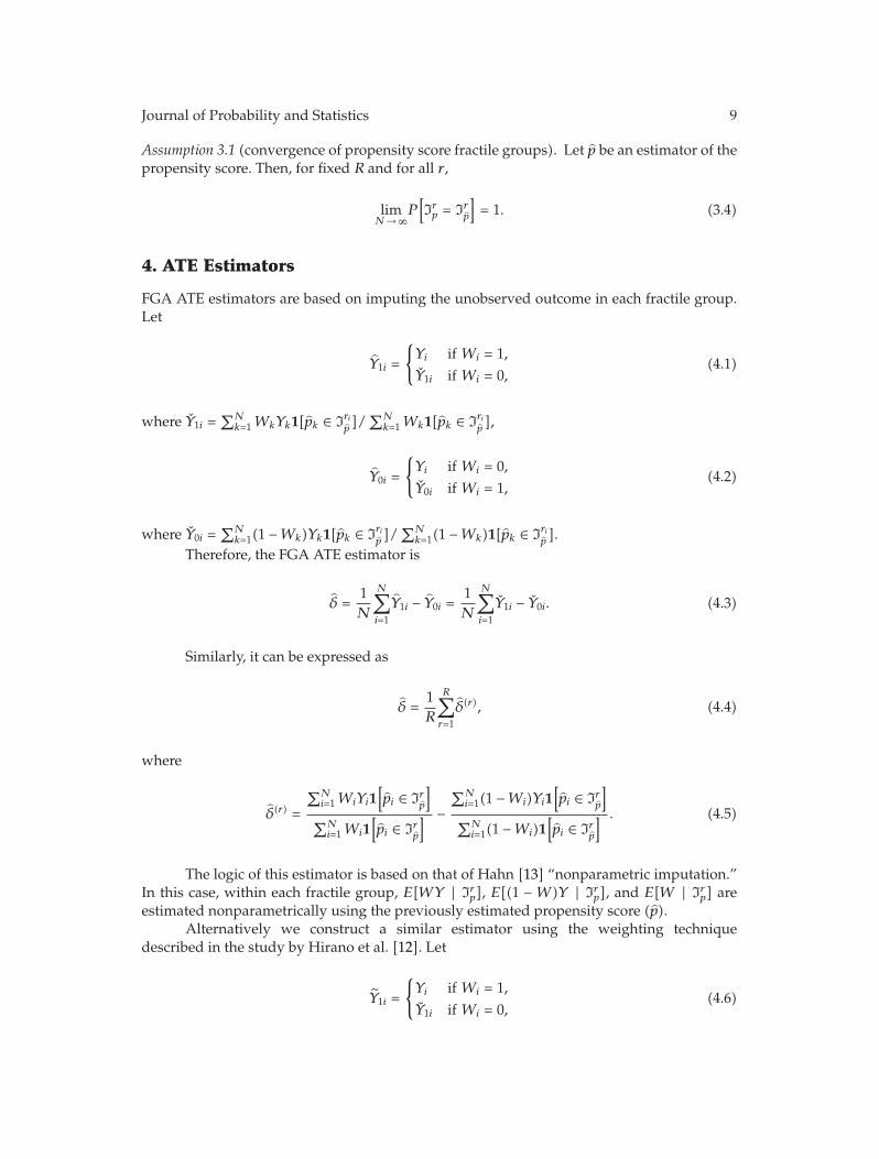
Journal of Probability and Statistics 9
Assumption 3.1 (convergence of propensity score fractile groups). Let p be an estimator of thepropensity score. Then, for fixed R and for all r,
limN→∞
P[Irp = Irp
]= 1. (3.4)
4. ATE Estimators
FGA ATE estimators are based on imputing the unobserved outcome in each fractile group.Let
Y1i =
{Yi if Wi = 1,Y1i if Wi = 0,
(4.1)
where Y1i =∑N
k=1WkYk1[pk ∈ Irip]/∑N
k=1Wk1[pk ∈ Irip],
Y0i =
{Yi if Wi = 0,Y0i if Wi = 1,
(4.2)
where Y0i =∑N
k=1(1 −Wk)Yk1[pk ∈ Irip]/∑N
k=1(1 −Wk)1[pk ∈ Irip].
Therefore, the FGA ATE estimator is
δ =1N
N∑
i=1
Y1i − Y0i =1N
N∑
i=1
Y1i − Y0i. (4.3)
Similarly, it can be expressed as
δ =1R
R∑
r=1
δ(r), (4.4)
where
δ(r) =
∑Ni=1WiYi1
[pi ∈ Ir
p
]
∑Ni=1Wi1
[pi ∈ Ir
p
] −∑N
i=1(1 −Wi)Yi1[pi ∈ Ir
p
]
∑Ni=1(1 −Wi)1
[pi ∈ Ir
p
] . (4.5)
The logic of this estimator is based on that of Hahn [13] “nonparametric imputation.”In this case, within each fractile group, E[WY | Irp], E[(1 − W)Y | Irp], and E[W | Irp] areestimated nonparametrically using the previously estimated propensity score (p).
Alternatively we construct a similar estimator using the weighting techniquedescribed in the study by Hirano et al. [12]. Let
Y1i =
{Yi if Wi = 1,Y1i if Wi = 0,
(4.6)

10 Journal of Probability and Statistics
where Y1i =∑N
k=1(WkYk/pk)1[pk ∈ Irip],
Y0i =
{Yi if Wi = 0,Y0i if Wi = 1,
(4.7)
where Y0i =∑N
k=1((1 −Wk)Yk/(1 − pk))1[pk ∈ Irip].
Then
δ =1R
R∑
r=1
δ(r), (4.8)
where
δ(r) =R
N
N∑
i=1
Wi
piYi1[pi ∈ Irp
]− R
N
N∑
i=1
1 −Wi
1 − pi Yi1[pi ∈ Irp
]. (4.9)
This estimator suffers from the same problems of Hirano et al.’s [12] estimator; thatis, the presence of occasional high/low values of the propensity score produces a very badempirical performance.
The following theorem shows that the FGA ATE estimators are consistent. Theintuition behind the proof is that, as N increases, and R does it but at a smaller rate, eachfractile group will have individuals with similar propensity score values. In the limit, thedifferences among them is negligible, and therefore the unconfoundedness assumption canbe applied. In this case, the local (i.e., for a given propensity score value) ATE can beobtained by constructing the difference of the average treated and control individuals withthat propensity score value.
Theorem 4.1 (consistency of ATE estimator). Consider Assumptions 2.1, 2.2, and 3.1, and assumethat
(1) the distribution functions of p and (Y1, Y0) | p are continuous and strictly increasing.
(2) E[Y 21 ] <∞, E[Y 2
0 ] <∞.
Then, δ P→ δ and δ P→ δ asN,R → ∞, R/N → 0.
Proof. See Appendix A.1.
5. QTE Estimators
Define the within fractile conditional quantiles:
Q(r)τ1 = argmin
q
∑Ni=1 1[pi ∈ Ir
p
]Wi
(Yi − q
)(τ − 1[Yi ≤ q
])
∑Ni=1 1[pi ∈ Ir
p
]Wi
,
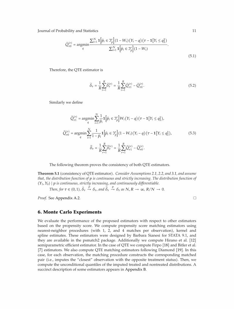
Journal of Probability and Statistics 11
Q(r)τ0 = argmin
q
∑Ni=1 1[pi ∈ Ir
p
](1 −Wi)
(Yi − q
)(τ − 1[Yi ≤ q
])
∑Ni=1 1[pi ∈ Ir
p
](1 −Wi)
.
(5.1)
Therefore, the QTE estimator is
δτ =1R
R∑
r=1
δ(r)τ =
1R
R∑
r=1
Q(r)τ1 − Q(r)
τ0 . (5.2)
Similarly we define
Q(r)τ1 = argmin
q
N∑
i=1
1pi1[pi ∈ Irp
]Wi
(Yi − q
)(τ − 1[Yi ≤ q
]),
Q(r)τ0 = argmin
q
N∑
i=1
11 − pi 1
[pi ∈ Irp
](1 −Wi)
(Yi − q
)(τ − 1[Yi ≤ q
]),
δτ =1R
R∑
r=1
δ(r)τ =
1R
R∑
r=1
Q(r)τ1 − Q(r)
τ0 .
(5.3)
The following theorem proves the consistency of both QTE estimators.
Theorem 5.1 (consistency of QTE estimator). Consider Assumptions 2.1, 2.2, and 3.1, and assumethat, the distribution function of p is continuous and strictly increasing. The distribution function of(Y1, Y0) | p is continuous, strictly increasing, and continuously differentiable.
Then, for τ ∈ (0, 1), δτP→ δτ , and δτ
P→ δτ asN,R → ∞, R/N → 0.
Proof. See Appendix A.2.
6. Monte Carlo Experiments
We evaluate the performance of the proposed estimators with respect to other estimatorsbased on the propensity score. We compute propensity score matching estimators usingnearest-neighbor procedures (with 1, 2, and 4 matches per observation), kernel andspline estimates. These estimators were designed by Barbara Sianesi for STATA 9.1, andthey are available in the psmatch2 package. Additionally we compute Hirano et al. [12]semiparametric efficient estimator. In the case of QTE we compute Firpo [18] and Bitler et al.[7] estimators. We also compute QTE matching estimators following Diamond [19]. In thiscase, for each observation, the matching procedure constructs the corresponding matchedpair (i.e., imputes the “closest” observation with the opposite treatment status). Then, wecompute the unconditional quantiles of the imputed treated and nontreated distributions. Asuccinct description of some estimators appears in Appendix B.
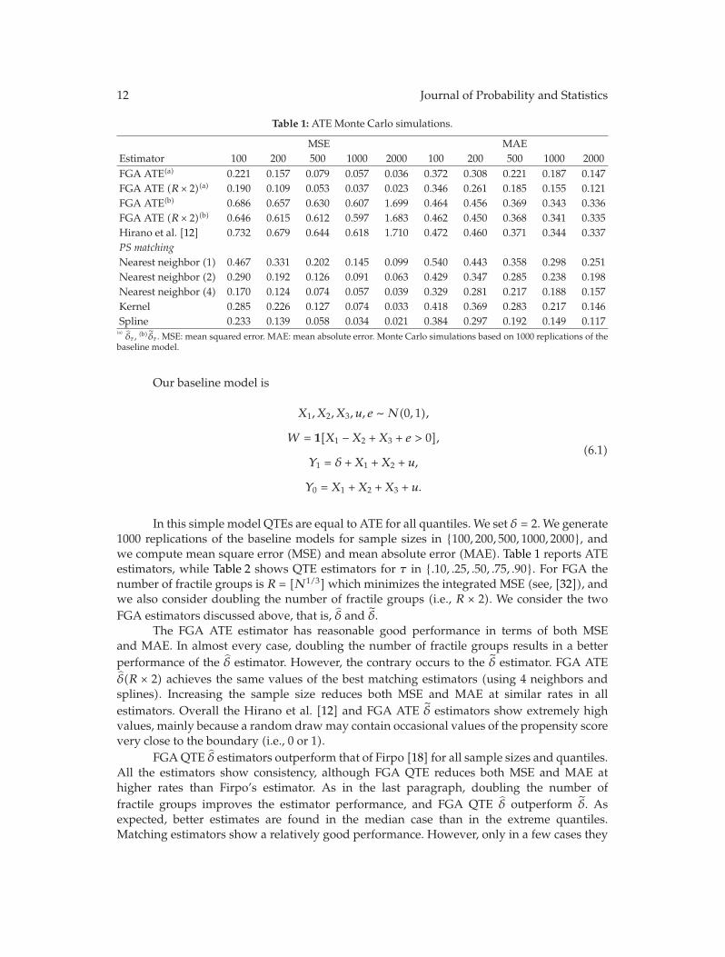
12 Journal of Probability and Statistics
Table 1: ATE Monte Carlo simulations.
MSE MAEEstimator 100 200 500 1000 2000 100 200 500 1000 2000FGA ATE(a) 0.221 0.157 0.079 0.057 0.036 0.372 0.308 0.221 0.187 0.147FGA ATE (R × 2)(a) 0.190 0.109 0.053 0.037 0.023 0.346 0.261 0.185 0.155 0.121FGA ATE(b) 0.686 0.657 0.630 0.607 1.699 0.464 0.456 0.369 0.343 0.336FGA ATE (R × 2)(b) 0.646 0.615 0.612 0.597 1.683 0.462 0.450 0.368 0.341 0.335Hirano et al. [12] 0.732 0.679 0.644 0.618 1.710 0.472 0.460 0.371 0.344 0.337PS matchingNearest neighbor (1) 0.467 0.331 0.202 0.145 0.099 0.540 0.443 0.358 0.298 0.251Nearest neighbor (2) 0.290 0.192 0.126 0.091 0.063 0.429 0.347 0.285 0.238 0.198Nearest neighbor (4) 0.170 0.124 0.074 0.057 0.039 0.329 0.281 0.217 0.188 0.157Kernel 0.285 0.226 0.127 0.074 0.033 0.418 0.369 0.283 0.217 0.146Spline 0.233 0.139 0.058 0.034 0.021 0.384 0.297 0.192 0.149 0.117
(a)δτ , (b)δτ . MSE: mean squared error. MAE: mean absolute error. Monte Carlo simulations based on 1000 replications of the
baseline model.
Our baseline model is
X1, X2, X3, u, e ∼N(0, 1),
W = 1[X1 −X2 +X3 + e > 0],
Y1 = δ +X1 +X2 + u,
Y0 = X1 +X2 +X3 + u.
(6.1)
In this simple model QTEs are equal to ATE for all quantiles. We set δ = 2. We generate1000 replications of the baseline models for sample sizes in {100, 200, 500, 1000, 2000}, andwe compute mean square error (MSE) and mean absolute error (MAE). Table 1 reports ATEestimators, while Table 2 shows QTE estimators for τ in {.10, .25, .50, .75, .90}. For FGA thenumber of fractile groups is R = [N1/3]which minimizes the integrated MSE (see, [32]), andwe also consider doubling the number of fractile groups (i.e., R × 2). We consider the twoFGA estimators discussed above, that is, δ and δ.
The FGA ATE estimator has reasonable good performance in terms of both MSEand MAE. In almost every case, doubling the number of fractile groups results in a betterperformance of the δ estimator. However, the contrary occurs to the δ estimator. FGA ATEδ(R × 2) achieves the same values of the best matching estimators (using 4 neighbors andsplines). Increasing the sample size reduces both MSE and MAE at similar rates in allestimators. Overall the Hirano et al. [12] and FGA ATE δ estimators show extremely highvalues, mainly because a random drawmay contain occasional values of the propensity scorevery close to the boundary (i.e., 0 or 1).
FGAQTE δ estimators outperform that of Firpo [18] for all sample sizes and quantiles.All the estimators show consistency, although FGA QTE reduces both MSE and MAE athigher rates than Firpo’s estimator. As in the last paragraph, doubling the number offractile groups improves the estimator performance, and FGA QTE δ outperform δ. Asexpected, better estimates are found in the median case than in the extreme quantiles.Matching estimators show a relatively good performance. However, only in a few cases they
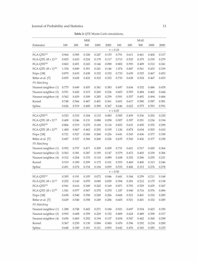
Journal of Probability and Statistics 13
Table 2: QTE Monte Carlo simulations.
MSE MAE
Estimator 100 200 500 1000 2000 100 200 500 1000 2000
τ = 0.10
FGA QTE(a) 0.964 0.585 0.328 0.247 0.155 0.791 0.611 0.461 0.404 0.317
FGA QTE (R × 2)(a) 0.825 0.433 0.224 0.178 0.117 0.713 0.525 0.379 0.339 0.279
FGA QTE(b) 0.863 0.491 0.243 0.146 0.090 0.802 0.593 0.409 0.312 0.241
FGA QTE (R × 2)(b) 1.334 0.849 0.391 0.241 0.146 1.074 0.847 0.561 0.433 0.339
Firpo [18] 0.879 0.633 0.438 0.332 0.332 0.733 0.639 0.525 0.467 0.453
Bitler et al. [7] 0.835 0.628 0.432 0.332 0.332 0.733 0.638 0.524 0.467 0.453
PS Matching
Nearest neighbor (1) 0.775 0.649 0.455 0.341 0.383 0.697 0.636 0.532 0.486 0.478
Nearest neighbor (2) 0.551 0.442 0.315 0.269 0.236 0.603 0.555 0.484 0.462 0.444
Nearest neighbor (4) 0.562 0.429 0.309 0.285 0.259 0.591 0.557 0.492 0.494 0.484
Kernel 0.748 0.566 0.467 0.401 0.361 0.691 0.617 0.580 0.587 0.581
Spline 0.626 0.519 0.400 0.389 0.367 0.646 0.622 0.575 0.593 0.591
τ = 0.25
FGA QTE(a) 0.523 0.333 0.184 0.133 0.083 0.585 0.459 0.336 0.292 0.230
FGA QTE (R × 2)(a) 0.409 0.246 0.131 0.088 0.058 0.507 0.397 0.291 0.236 0.194
FGA QTE(b) 0.866 0.519 0.270 0.169 0.116 0.823 0.631 0.450 0.352 0.290
FGA QTE (R × 2)(b) 1.400 0.867 0.462 0.292 0.195 1.126 0.874 0.634 0.503 0.410
Firpo [18] 0.721 0.527 0.360 0.268 0.226 0.641 0.543 0.436 0.377 0.338
Bitler et al. [7] 0.687 0.527 0.360 0.268 0.226 0.635 0.543 0.436 0.377 0.338
PS Matching
Nearest neighbor (1) 0.952 0.757 0.471 0.309 0.209 0.731 0.621 0.517 0.420 0.364
Nearest neighbor (2) 0.563 0.381 0.287 0.195 0.147 0.579 0.472 0.403 0.339 0.306
Nearest neighbor (4) 0.312 0.204 0.153 0.110 0.089 0.438 0.352 0.296 0.255 0.231
Kernel 0.519 0.390 0.299 0.175 0.101 0.553 0.469 0.400 0.313 0.246
Spline 0.491 0.274 0.154 0.104 0.095 0.533 0.406 0.312 0.276 0.278
τ = 0.50
FGA QTE(a) 0.305 0.191 0.105 0.072 0.046 0.441 0.344 0.259 0.211 0.168
FGA QTE (R × 2)(a) 0.252 0.143 0.070 0.049 0.029 0.394 0.301 0.212 0.175 0.138
FGA QTE(b) 0.941 0.616 0.349 0.242 0.169 0.871 0.703 0.529 0.435 0.367
FGA QTE (R × 2)(b) 1.541 0.977 0.567 0.370 0.270 1.187 0.940 0.716 0.576 0.496
Firpo [18] 0.658 0.540 0.358 0.249 0.206 0.606 0.521 0.401 0.332 0.285
Bitler et al. [7] 0.629 0.540 0.358 0.249 0.206 0.603 0.521 0.401 0.332 0.285
PS Matching
Nearest neighbor (1) 1.288 0.748 0.443 0.271 0.184 0.921 0.697 0.534 0.423 0.350
Nearest neighbor (2) 0.993 0.608 0.359 0.229 0.152 0.809 0.624 0.489 0.390 0.317
Nearest neighbor (4) 0.656 0.465 0.292 0.194 0.137 0.654 0.547 0.442 0.360 0.298
Kernel 0.367 0.250 0.130 0.084 0.060 0.476 0.396 0.292 0.234 0.200
Spline 0.648 0.349 0.181 0.121 0.093 0.642 0.476 0.343 0.285 0.235
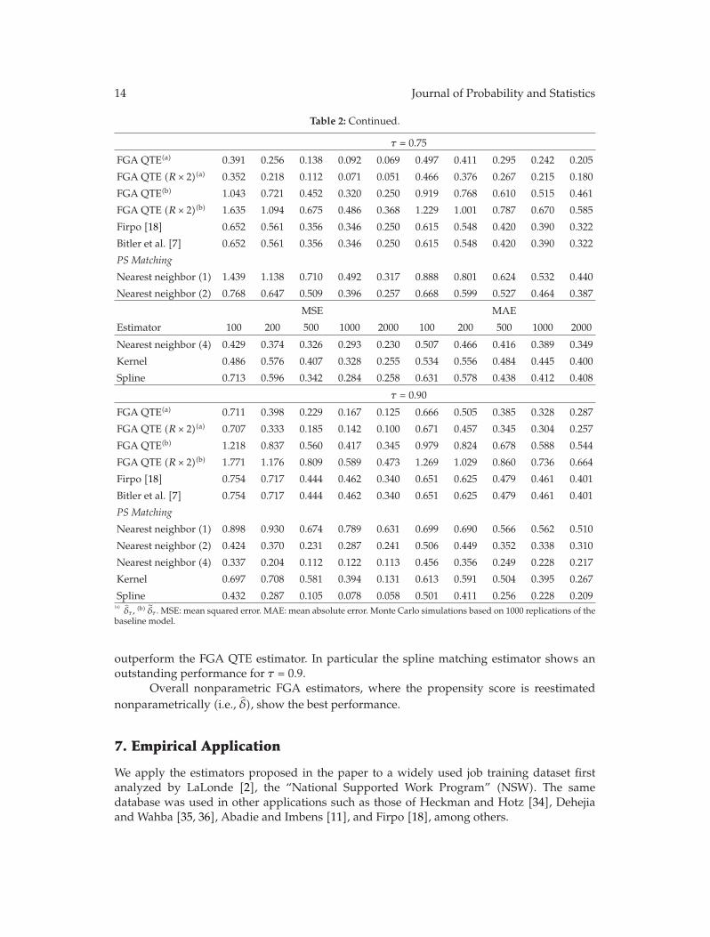
14 Journal of Probability and Statistics
Table 2: Continued.
τ = 0.75
FGA QTE(a) 0.391 0.256 0.138 0.092 0.069 0.497 0.411 0.295 0.242 0.205
FGA QTE (R × 2)(a) 0.352 0.218 0.112 0.071 0.051 0.466 0.376 0.267 0.215 0.180
FGA QTE(b) 1.043 0.721 0.452 0.320 0.250 0.919 0.768 0.610 0.515 0.461
FGA QTE (R × 2)(b) 1.635 1.094 0.675 0.486 0.368 1.229 1.001 0.787 0.670 0.585
Firpo [18] 0.652 0.561 0.356 0.346 0.250 0.615 0.548 0.420 0.390 0.322
Bitler et al. [7] 0.652 0.561 0.356 0.346 0.250 0.615 0.548 0.420 0.390 0.322
PS Matching
Nearest neighbor (1) 1.439 1.138 0.710 0.492 0.317 0.888 0.801 0.624 0.532 0.440
Nearest neighbor (2) 0.768 0.647 0.509 0.396 0.257 0.668 0.599 0.527 0.464 0.387
MSE MAE
Estimator 100 200 500 1000 2000 100 200 500 1000 2000
Nearest neighbor (4) 0.429 0.374 0.326 0.293 0.230 0.507 0.466 0.416 0.389 0.349
Kernel 0.486 0.576 0.407 0.328 0.255 0.534 0.556 0.484 0.445 0.400
Spline 0.713 0.596 0.342 0.284 0.258 0.631 0.578 0.438 0.412 0.408
τ = 0.90
FGA QTE(a) 0.711 0.398 0.229 0.167 0.125 0.666 0.505 0.385 0.328 0.287
FGA QTE (R × 2)(a) 0.707 0.333 0.185 0.142 0.100 0.671 0.457 0.345 0.304 0.257
FGA QTE(b) 1.218 0.837 0.560 0.417 0.345 0.979 0.824 0.678 0.588 0.544
FGA QTE (R × 2)(b) 1.771 1.176 0.809 0.589 0.473 1.269 1.029 0.860 0.736 0.664
Firpo [18] 0.754 0.717 0.444 0.462 0.340 0.651 0.625 0.479 0.461 0.401
Bitler et al. [7] 0.754 0.717 0.444 0.462 0.340 0.651 0.625 0.479 0.461 0.401
PS Matching
Nearest neighbor (1) 0.898 0.930 0.674 0.789 0.631 0.699 0.690 0.566 0.562 0.510
Nearest neighbor (2) 0.424 0.370 0.231 0.287 0.241 0.506 0.449 0.352 0.338 0.310
Nearest neighbor (4) 0.337 0.204 0.112 0.122 0.113 0.456 0.356 0.249 0.228 0.217
Kernel 0.697 0.708 0.581 0.394 0.131 0.613 0.591 0.504 0.395 0.267
Spline 0.432 0.287 0.105 0.078 0.058 0.501 0.411 0.256 0.228 0.209(a)δτ , (b) δτ . MSE: mean squared error. MAE: mean absolute error. Monte Carlo simulations based on 1000 replications of the
baseline model.
outperform the FGA QTE estimator. In particular the spline matching estimator shows anoutstanding performance for τ = 0.9.
Overall nonparametric FGA estimators, where the propensity score is reestimatednonparametrically (i.e., δ), show the best performance.
7. Empirical Application
We apply the estimators proposed in the paper to a widely used job training dataset firstanalyzed by LaLonde [2], the “National Supported Work Program” (NSW). The samedatabase was used in other applications such as those of Heckman and Hotz [34], Dehejiaand Wahba [35, 36], Abadie and Imbens [11], and Firpo [18], among others.
Journal of Probability and Statistics 15
The program was designated as a random experiment for applicants who if selectedwould had received work experience (treatment) in a wide range of possible activities, likelearning to operate a restaurant, a child care, or a construction work, for a period not exceed-ing twelve months. Eligible participants were targeted from recipients of AFDC, formeraddicts, former offenders, and young school dropouts. Candidates eligible for the NSWwererandomized into the program between March 1975 and July 1977. The NSW data set consistsof information on earnings and employment in 1978 (outcome variables), whether treated ornot, information on earnings and employment in 1974 and 1975, and background character-istics such as education, ethnicity, marital status, and age. We use the database provided byGuido Imbens (http://www.economics.harvard.edu/faculty/imbens/software imbens/),which consists of 455 individuals, 185 treated, and 260 control observations. This particularsubset is the one constructed by Dehejia and Wahba [35] and described there in more detail.
We will focus on the possible effect on participants’ earnings in 1978 (if any); thatis, we answer the following question: what is the effect of this particular training programon future earnings? Provided that earnings is a continuous variable, we would be able toapply quantile analysis. A main drawback of this variable is that those unemployed in 1978report earnings of zero. In 1978, 92 control and 45 treated individuals were unemployed. Theaverage (standard deviation) of earnings in 1978 is $5300 ($6631), which breaks into $6349($578) for treated and $4554 ($340) for control individuals. Without considering covariates,the difference between treated and nontreated is $1794 ($671), which in a two-sample t-test rejects the null hypothesis of equal values (t-stat 2.67, P value 0.0079). We also observedifferences in terms of the percentiles in the earnings distribution. The 10th percentile for thetreated (control) is $0 ($0); the 25th percentile $485 ($0); the median is $4232 ($3139); the 75thpercentile $9643 ($7292) ; and the 90th percentile is $14582 ($11551). Therefore, assumingthe rank invariance property discussed above, higher quantiles of the earnings distributionseems to be associated with larger treatment effects.
The propensity score is estimated by a probit model, where the dependent variableis participation and the covariates used are the individual characteristics and employmentand earnings in 1974 and 1975. Note that the propensity score is of no particular interest byitself, provided that participants were randomly selected in the experiment. In this case, noparticular covariate is individually significant, and a likelihood ratio test of joint significancegets chi-squared (8) = 8.30, P value = 0.4050.
As we mention above, a common support in the propensity score domain is necessaryto make meaningful comparisons among treated and nontreated individuals. The empiricalrelevance of this assumption was pointed out by Heckman et al. [37], and it was identifiedas one of the major sources of bias. In our case, this has special importance since consistentestimates of treatment effect requires that both the number of treated and control is eventuallylarge enough to apply large sample theory. Moreover, if there are no treated (controls) ina given fractile group, no within fractile estimate can be obtained. We use two differenttrimming procedures. First, provided that we may assume that F1(p) ≤ F0(p), we onlyconsider propensity score values in the range
p∗ = minp
(pi,Wi = 1
) ≤ p ≤ maxp
(pi,Wi = 0
)= p∗. (7.1)
By doing this we drop 8 observations, and we refer to this sample as Trim 1. We alsotrim 2.5% in each tail of the propensity score distribution (Trim 2) dropping 23 observations.
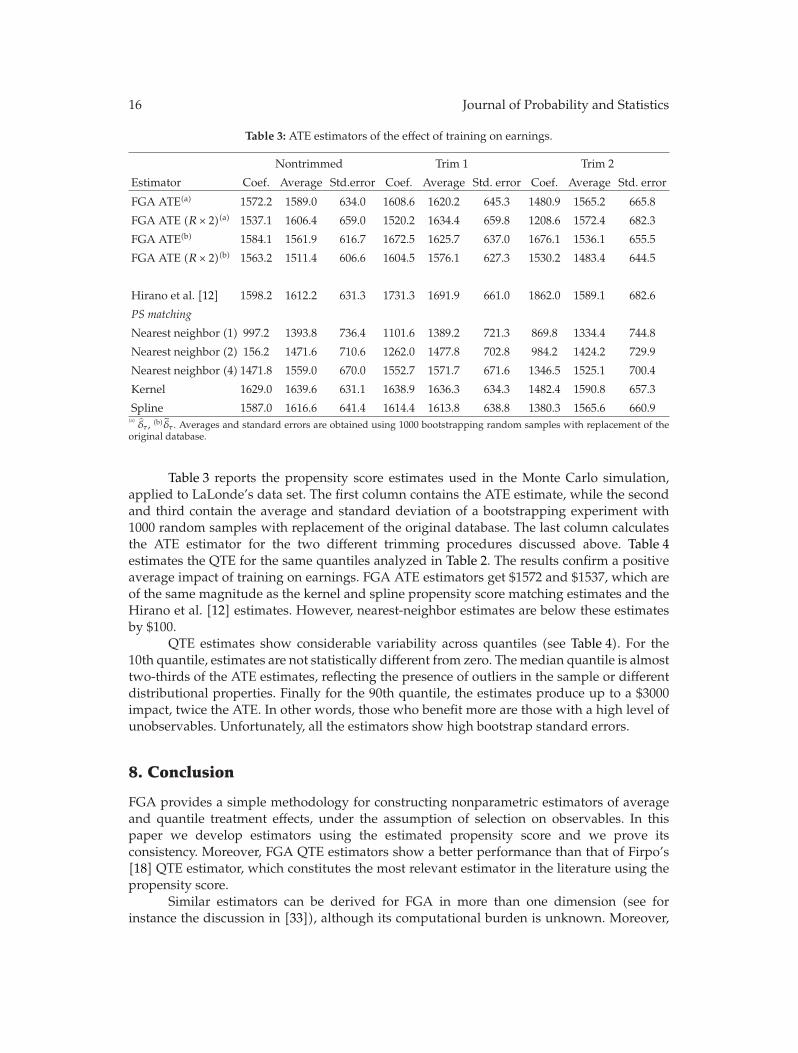
16 Journal of Probability and Statistics
Table 3: ATE estimators of the effect of training on earnings.
Nontrimmed Trim 1 Trim 2
Estimator Coef. Average Std.error Coef. Average Std. error Coef. Average Std. error
FGA ATE(a) 1572.2 1589.0 634.0 1608.6 1620.2 645.3 1480.9 1565.2 665.8
FGA ATE (R × 2)(a) 1537.1 1606.4 659.0 1520.2 1634.4 659.8 1208.6 1572.4 682.3
FGA ATE(b) 1584.1 1561.9 616.7 1672.5 1625.7 637.0 1676.1 1536.1 655.5
FGA ATE (R × 2)(b) 1563.2 1511.4 606.6 1604.5 1576.1 627.3 1530.2 1483.4 644.5
Hirano et al. [12] 1598.2 1612.2 631.3 1731.3 1691.9 661.0 1862.0 1589.1 682.6
PS matching
Nearest neighbor (1) 997.2 1393.8 736.4 1101.6 1389.2 721.3 869.8 1334.4 744.8
Nearest neighbor (2) 156.2 1471.6 710.6 1262.0 1477.8 702.8 984.2 1424.2 729.9
Nearest neighbor (4) 1471.8 1559.0 670.0 1552.7 1571.7 671.6 1346.5 1525.1 700.4
Kernel 1629.0 1639.6 631.1 1638.9 1636.3 634.3 1482.4 1590.8 657.3
Spline 1587.0 1616.6 641.4 1614.4 1613.8 638.8 1380.3 1565.6 660.9(a)δτ , (b)δτ . Averages and standard errors are obtained using 1000 bootstrapping random samples with replacement of the
original database.
Table 3 reports the propensity score estimates used in the Monte Carlo simulation,applied to LaLonde’s data set. The first column contains the ATE estimate, while the secondand third contain the average and standard deviation of a bootstrapping experiment with1000 random samples with replacement of the original database. The last column calculatesthe ATE estimator for the two different trimming procedures discussed above. Table 4estimates the QTE for the same quantiles analyzed in Table 2. The results confirm a positiveaverage impact of training on earnings. FGA ATE estimators get $1572 and $1537, which areof the same magnitude as the kernel and spline propensity score matching estimates and theHirano et al. [12] estimates. However, nearest-neighbor estimates are below these estimatesby $100.
QTE estimates show considerable variability across quantiles (see Table 4). For the10th quantile, estimates are not statistically different from zero. Themedian quantile is almosttwo-thirds of the ATE estimates, reflecting the presence of outliers in the sample or differentdistributional properties. Finally for the 90th quantile, the estimates produce up to a $3000impact, twice the ATE. In other words, those who benefit more are those with a high level ofunobservables. Unfortunately, all the estimators show high bootstrap standard errors.
8. Conclusion
FGA provides a simple methodology for constructing nonparametric estimators of averageand quantile treatment effects, under the assumption of selection on observables. In thispaper we develop estimators using the estimated propensity score and we prove itsconsistency. Moreover, FGA QTE estimators show a better performance than that of Firpo’s[18] QTE estimator, which constitutes the most relevant estimator in the literature using thepropensity score.
Similar estimators can be derived for FGA in more than one dimension (see forinstance the discussion in [33]), although its computational burden is unknown. Moreover,
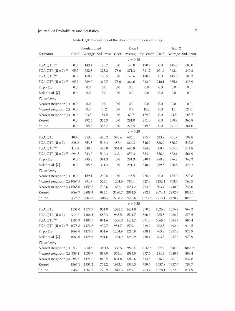
Journal of Probability and Statistics 17
Table 4: QTE estimators of the effect of training on earnings.
Nontrimmed Trim 1 Trim 2
Estimator Coef. Average Std. error Coef. Average Std. error Coef. Average Std. error
τ = 0.10
FGA QTE(a) 0.0 149.4 188.2 0.0 146.8 190.9 0.0 145.5 183.0
FGA QTE (R × 2)(a) 95.7 382.5 325.2 78.0 371.3 311.2 101.9 392.4 340.2
FGA QTE(b) 0.0 150.9 190.5 0.0 148.6 190.9 0.0 145.0 185.2
FGA QTE (R × 2)(b) 95.7 369.7 317.7 78.0 364.6 312.0 240.1 385.1 335.9
Firpo [18] 0.0 0.0 0.0 0.0 0.0 0.0 0.0 0.0 0.0
Bitler et al. [7] 0.0 0.0 0.0 0.0 0.0 0.0 0.0 0.0 0.0
PS matching
Nearest neighbor (1) 0.0 0.0 0.0 0.0 0.0 0.0 0.0 0.0 0.0
Nearest neighbor (2) 0.0 0.7 15.2 0.0 0.7 15.2 0.0 1.1 21.0
Nearest neighbor (4) 0.0 73.8 184.5 0.0 69.7 179.3 0.0 74.5 188.7
Kernel 0.0 292.5 356.3 0.0 281.0 351.0 0.0 298.9 365.8
Spline 0.0 295.3 355.7 0.0 278.5 349.5 0.0 291.2 361.0
τ = 0.25
FGA QTE 409.6 653.5 480.2 376.4 686.1 475.9 623.2 701.7 502.8
FGA QTE (R × 2) 628.8 853.5 546.4 487.4 864.3 540.9 836.9 880.2 547.8
FGA QTE(b) 414.2 649.8 488.0 361.9 685.8 484.2 500.9 705.8 511.8
FGA QTE (R × 2)(b) 694.5 843.3 546.3 363.1 853.3 554.6 856.6 872.1 561.9
Firpo [18] 0.0 295.8 341.3 0.0 291.3 340.4 289.8 276.8 343.2
Bitler et al. [7] 0.0 295.8 341.3 0.0 291.3 340.4 289.8 276.8 343.2
PS matching
Nearest neighbor (1) 0.0 159.1 290.8 0.0 145.5 278.6 0.0 134.9 273.8
Nearest neighbor (2) 1067.5 804.7 523.1 1254.6 783.1 527.8 1152.1 763.5 763.5
Nearest neighbor (4) 1568.0 1455.8 738.6 1682.1 1454.2 733.0 803.4 1440.0 748.0
Kernel 3068.7 2808.3 986.1 3180.7 2864.5 992.4 3074.4 2892.7 1036.1
Spline 2628.7 2363.8 1019.7 2708.2 2486.6 1023.5 2715.1 2470.7 1053.1
τ = 0.50
FGA QTE 1131.0 1379.9 851.0 1321.2 1404.8 870.5 1026.0 1376.2 869.2
FGA QTE (R × 2) 914.2 1466.4 887.3 965.5 1501.7 866.6 385.5 1488.7 873.5
FGA QTE(b) 1193.9 1403.5 871.6 1306.0 1432.7 891.8 1066.3 1384.7 883.4
FGA QTE (R × 2)(b) 1078.8 1476.8 939.7 981.7 1509.1 919.9 262.5 1492.6 916.5
Firpo [18] 1063.0 1178.5 901.6 1254.9 1260.9 938.1 763.8 1257.8 973.9
Bitler et al. [7] 1063.0 1178.5 901.6 1254.9 1260.9 938.1 763.8 1257.8 973.9
PS matching
Nearest neighbor (1) 5.2 910.5 1034.6 368.5 984.4 1042.5 77.5 990.4 1066.2
Nearest neighbor (2) 388.1 1050.9 859.9 563.4 1093.0 877.5 284.4 1088.4 898.4
Nearest neighbor (4) 695.5 1171.6 810.5 801.8 1210.6 814.5 616.7 1201.0 842.8
Kernel 1567.1 1351.2 752.2 1643.1 1365.3 759.6 1587.8 1357.7 783.7
Spline 846.6 1261.7 776.9 1843.3 1259.1 783.4 1578.1 1272.3 811.9
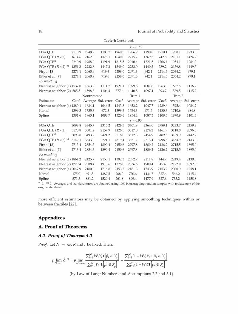
18 Journal of Probability and Statistics
Table 4: Continued.
τ = 0.75FGA QTE 2110.9 1948.9 1180.7 1960.5 1986.9 1190.8 1710.1 1950.1 1233.8FGA QTE (R × 2) 1614.6 2162.8 1376.1 1640.0 2215.2 1369.5 742.6 2131.1 1424.7FGA QTE(b) 2240.9 1968.0 1191.9 1815.5 2010.4 1221.5 1706.4 1954.1 1264.7FGA QTE (R × 2)(b) 1351.3 2222.8 1447.2 1549.0 2253.0 1440.5 789.2 2159.8 1449.7Firpo [18] 2274.1 2060.9 919.6 2258.0 2071.3 942.1 2214.5 2034.2 979.1Bitler et al. [7] 2274.1 2060.9 919.6 2258.0 2071.3 942.1 2214.5 2034.2 979.1PS matchingNearest neighbor (1) 1537.0 1663.9 1111.7 1921.1 1699.6 1081.8 1263.0 1637.5 1116.7Nearest neighbor (2) 585.5 1598.8 1106.4 877.6 1640.8 1097.4 393.7 1589.5 1115.2
Nontrimmed Trim 1 Trim 2Estimator Coef. Average Std. error Coef. Average Std. error Coef. Average Std. errorNearest neighbor (4) 1280.1 1634.1 1046.5 1243.8 1653.2 1047.7 1239.6 1595.4 1084.2Kernel 1399.3 1735.3 972.3 1399.5 1754.3 971.5 1180.6 1710.6 984.8Spline 1381.6 1963.1 1088.7 1320.6 1954.4 1087.3 1108.5 1870.9 1101.3
τ = 0.90FGA QTE 3093.8 3345.7 2315.2 3426.5 3401.9 2364.0 2789.1 3233.7 2459.3FGA QTE (R × 2) 3170.8 3301.2 2157.9 4126.5 3317.0 2174.2 4161.9 3118.0 2096.5FGA QTE(b) 3093.8 3493.2 2421.2 3518.0 3512.3 2454.9 3189.5 3189.9 2442.7FGA QTE (R × 2)(b) 3142.1 3343.0 2221.1 4819.4 3351.2 2213.4 3998.6 3154.9 2133.0Firpo [18] 2713.4 2854.3 1890.4 2150.6 2797.8 1889.2 2126.2 2715.5 1895.0Bitler et al. [7] 2713.4 2854.3 1890.4 2150.6 2797.8 1889.2 2126.2 2715.5 1895.0PS matchingNearest neighbor (1) 1861.2 2425.7 2150.1 1392.3 2372.7 2111.8 444.7 2249.4 2130.0Nearest neighbor (2) 1279.4 2388.4 1915.6 1278.0 2336.6 1900.4 45.4 2172.0 1892.5Nearest neighbor (4) 2047.9 2180.9 1716.8 2153.7 2181.3 1743.9 2153.7 2030.9 1758.1Kernel 175.0 691.5 1389.5 208.0 770.6 1431.7 327.6 566.2 1415.4Spline 571.5 881.2 1520.4 261.8 899.4 1477.9 327.6 755.2 1458.8
(a)δτ , (b) δτ . Averages and standard errors are obtained using 1000 bootstrapping random samples with replacement of the
original database.
more efficient estimators may be obtained by applying smoothing techniques within orbetween fractiles [22].
Appendices
A. Proof of Theorems
A.1. Proof of Theorem 4.1
Proof. LetN → ∞, R and r be fixed. Then,
p limN→∞
δ(r) = p limN→∞
∑Ni=1WiYi1
[pi ∈ Ir
p
]
∑Ni=1Wi1
[pi ∈ Ir
p
] −∑N
i=1(1 −Wi)Yi1[pj ∈ Ir
p
]
∑Ni=1(1 −Wi)1
[pi ∈ Ir
p
]
(by Law of Large Numbers and Assumptions 2.2 and 3.1
)

Journal of Probability and Statistics 19
=E[W × Y | Irp
]
P[W | Irp
] −E[(1 −W) × Y | Irp
]
P[(1 −W) | Irp
]
=E[E[W × Y | p] | Irp
]
P[W | Irp
] −E[E[(1 −W) × Y | p] | Irp
]
P[(1 −W) | Irp
]
(by Law of Iterated Expectations
)
=E[E[W | p] × E[Y1 | p
] | Irp]
P[W | Irp
] −E[E[(1 −W) | p] × E[Y0 | p
] | Irp]
P[(1 −W) | Irp
]
(by Assumption 1.2
).
(A.1)
Let E[Wp] = p, P[WIrp] ≡ p(r), E[Y1p] = g1(p), E[Y0 | p] = g0(p), δ(r) = E[Y1 − Y0 | Irp].Then
∣∣∣∣p limN→∞
δ(r) − δ(r)∣∣∣∣ =
∣∣∣∣∣∣∣
E[(p − p(r)
)g1(p) | Irp
]
p(r)+E[(p − p(r)
)g0(p) | Irp
]
1 − p(r)
∣∣∣∣∣∣∣
=
∣∣∣∣∣∣∣
COV[p; g1(p) | Irp
]
p(r)+COV
[p; g0(p) | Irp
]
1 − p(r)
∣∣∣∣∣∣∣
≤√VAR[p | Irp
] × C(r),
(A.2)
where
C(r) =
⎛
⎜⎝
√VAR[g1(p)Irp]
p(r)+
√VAR[g0(p)Irp]
1 − p(r)
⎞
⎟⎠. (A.3)
Now let R,N → ∞, R/N → 0. Then
∣∣∣∣p limN→∞
δ − δ∣∣∣∣ =
∣∣∣∣∣p limN→∞
1R(N)
R(N)∑
r=1
(δ(r) − δ(r)
)∣∣∣∣∣
≤ limN→∞
1R(N)
R(N)∑
r=1
√VAR[p | Irp
]C(r)
≤ limN→∞
maxr√VAR[p | Irp
]C(r).
(A.4)
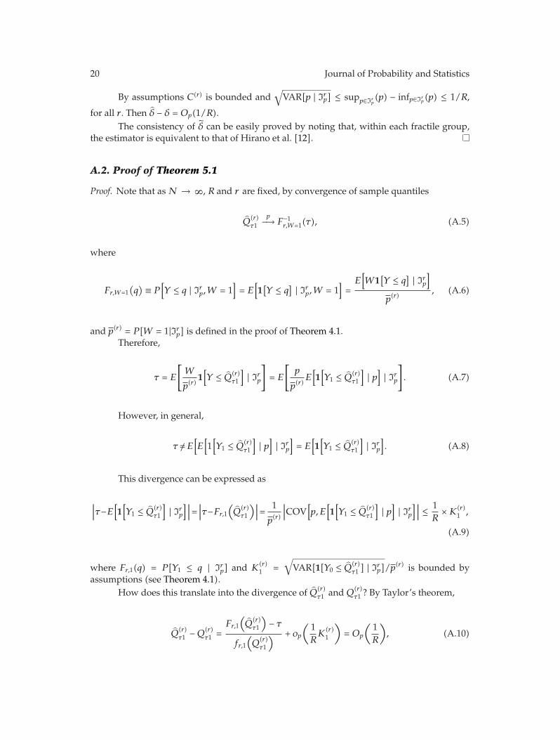
20 Journal of Probability and Statistics
By assumptions C(r) is bounded and√VAR[p | Irp] ≤ supp∈Ir
p(p) − infp∈Ir
p(p) ≤ 1/R,
for all r. Then δ − δ = Op(1/R).The consistency of δ can be easily proved by noting that, within each fractile group,
the estimator is equivalent to that of Hirano et al. [12].
A.2. Proof of Theorem 5.1
Proof. Note that asN → ∞, R and r are fixed, by convergence of sample quantiles
Q(r)τ1
p−→ F−1r,W=1(τ), (A.5)
where
Fr,W=1(q) ≡ P
[Y ≤ q | Irp,W = 1
]= E[1[Y ≤ q] | Irp,W = 1
]=E[W1[Y ≤ q] | Irp
]
p(r), (A.6)
and p(r) = P[W = 1|Irp] is defined in the proof of Theorem 4.1.Therefore,
τ = E
[W
p(r)1[Y ≤ Q(r)
τ1
]| Irp]
= E
[p
p(r)E[1[Y1 ≤ Q(r)
τ1
]| p]| Irp]
. (A.7)
However, in general,
τ /=E[E[1[Y1 ≤ Q(r)
τ1
]| p]| Irp]= E[1[Y1 ≤ Q(r)
τ1
]| Irp]. (A.8)
This divergence can be expressed as
∣∣∣τ−E[1[Y1 ≤ Q(r)
τ1
]| Irp]∣∣∣=∣∣∣τ−Fr,1
(Q
(r)τ1
)∣∣∣=1
p(r)
∣∣∣COV[p, E[1[Y1 ≤ Q(r)
τ1
]| p]| Irp]∣∣∣ ≤ 1
R×K(r)
1 ,
(A.9)
where Fr,1(q) = P[Y1 ≤ q | Irp] and K(r)1 =
√VAR[1[Y0 ≤ Q(r)
τ1 ] | Irp]/p(r) is bounded byassumptions (see Theorem 4.1).
How does this translate into the divergence of Q(r)τ1 and Q(r)
τ1 ? By Taylor’s theorem,
Q(r)τ1 −Q(r)
τ1 =Fr,1(Q
(r)τ1
)− τ
fr,1(Q
(r)τ1
) + op(1RK
(r)1
)= Op
(1R
), (A.10)
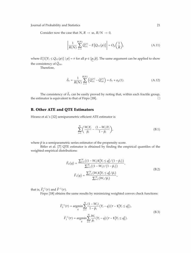
Journal of Probability and Statistics 21
Consider now the case thatN,R → ∞, R/N → 0,
∣∣∣∣∣
1R(N)
R(N)∑
r=1
Q(r)τ1 − E[Qτ1
(p)]∣∣∣∣∣= Op
(1R
), (A.11)
where E[1[Y1 ≤ Qτ1(p)] | p] = τ for all p ∈ [p, p]. The same argument can be applied to show
the consistency of Qτ0.Therefore,
δτ =1
R(N)
R(N)∑
r=1
(Q
(r)τ1 − Q(r)
τ0
)= δτ + op(1). (A.12)
The consistency of δτ can be easily proved by noting that, within each fractile group,the estimator is equivalent to that of Firpo [18].
B. Other ATE and QTE Estimators
Hirano et al.’s [12] semiparametric efficient ATE estimator is
N∑
i=1
(WiYipi
− (1 −Wi)Yi1 − pi
), (B.1)
where p is a semiparametric series estimator of the propensity score.Bitler et al. [7] QTE estimator is obtained by finding the empirical quantiles of the
weighted empirical distributions:
F0(q)=∑N
i=1((1 −Wi)1
[Yi ≤ q
]/(1 − pi
))
∑Ni=1((1 −Wi)/
(1 − pi
)) ,
F1(q)=∑N
i=1(Wi1[Yi ≤ q
]/pi)
∑Ni=1(Wi/pi
) ,
(B.2)
that is, F−10 (τ) and F−1(τ).
Firpo [18] obtains the same results by minimizing weighted convex check functions:
F−10 (τ) = argmin
q
N∑
i=1
(1 −Wi)1 − pi
(Yi − q
)(τ − 1[Yi ≤ q
]),
F−11 (τ) = argmin
q
N∑
i=1
Wi
pi
(Yi − q
)(τ − 1[Yi ≤ q
]).
(B.3)
22 Journal of Probability and Statistics
Acknowledgment
The author is grateful to Anil Bera, Antonio Galvao, and Todd Elder for helpful comments.
References
[1] O. Ashenfelter, “Estimating the effect of training programs on earnings,” Review of Economics andStatistics, vol. 60, no. 1, pp. 47–57, 1978.
[2] R. LaLonde, “Evaluating the econometric evaluations of training programs with experimental data,”American Economic Review, vol. 76, no. 4, pp. 604–620, 1986.
[3] J. D. Angrist and A. Krueger, “Empirical strategies in labor economics,” in Handbook of LaborEconomics, O. Ashenfelter and D. Card, Eds., vol. ume 1, pp. 1277–1366, Elsevier, New York, NY,USA, 1st edition, 1999.
[4] G. W. Imbens, “Nonparametric estimation of average treatment effects under exogeneity: a review,”Review of Economics and Statistics, vol. 86, no. 1, pp. 4–29, 2004.
[5] E. L. Lehmann, Nonparametrics: Statistical Methods Based on Ranks, Holde-Bay, San Francisco, Calif,USA, 1st edition, 2006.
[6] K. Doksum, “Empirical probability plots and statistical inference for nonlinear models in the two-sample case,” The Annals of Statistics, vol. 2, pp. 267–277, 1974.
[7] M. P. Bitler, J. B. Gelbach, and H. W. Hoynes, “What mean impacts miss: distributional effects ofwelfare reform experiments,” American Economic Review, vol. 96, no. 4, pp. 988–1012, 2006.
[8] J. Heckman and S. Navarro-Lozano, “Using matching, instrumental variables, and control functionsto estimate economic choice models,” Review of Economics and Statistics, vol. 86, no. 1, pp. 30–57, 2004.
[9] P. R. Rosenbaum and D. B. Rubin, “The central role of the propensity score in observational studiesfor causal effects,” Biometrika, vol. 70, no. 1, pp. 41–55, 1983.
[10] P. R. Rosenbaum and D. B. Rubin, “Reducing bias in observational studies using subclassification onthe propensity score,” Journal of the American Statistical Society, vol. 79, no. 387, pp. 516–524, 1984.
[11] A. Abadie and G. W. Imbens, “Simple and bias-corrected matching estimators for average treatmenteffects,” NBER Technical Working Paper 0283, National Bureau of Economic Research, Cambridge,Mass, USA, 2002.
[12] K. Hirano, G. W. Imbens, and G. Ridder, “Efficient estimation of average treatment effects using theestimated propensity score,” Econometrica, vol. 71, no. 4, pp. 1161–1189, 2003.
[13] J. Hahn, “On the role of the propensity score in efficient semiparametric estimation of averagetreatment effects,” Econometrica, vol. 66, no. 2, pp. 315–331, 1998.
[14] R. Koenker and G. Bassett,, “Regression quantiles,” Econometrica, vol. 46, no. 1, pp. 33–50, 1978.[15] A. Abadie, J. Angrist, and G. Imbens, “Instrumental variables estimates of the effect of subsidized
training on the quantiles of trainee earnings,” Econometrica, vol. 70, no. 1, pp. 91–117, 2002.[16] V. Chernozhukov and C. Hansen, “The effects of 401(k) participation on the wealth distribution: an
instrumental quantile regression analysis,” Review of Economics and Statistics, vol. 86, no. 3, pp. 735–751, 2004.
[17] V. Chernozhukov and C. Hansen, “An IV model of quantile treatment effects,” Econometrica, vol. 73,no. 1, pp. 245–261, 2005.
[18] S. Firpo, “Efficient semiparametric estimation of quantile treatment effects,” Econometrica, vol. 75, no.1, pp. 259–276, 2007.
[19] A. Diamond, Reliable estimation of average and quantile causal effects in non-experimental settings, HarvardUniversity, Cambridge, Mass, USA, 2005.
[20] P. C. Mahalanobis, “A method fractile graphical analysis,” Econometrica, vol. 28, no. 2, pp. 325–351,1960.
[21] A. K. Bera and A. Gosh, Fractile Regression and Its Applications, University of Illinois at Urbana-Champaign, Champaign, Ill, USA, 2006.
[22] B. Sen, “Estimation and comparison of fractile graphs using kernel smoothing techniques,” Sankhya.The Indian Journal of Statistics, vol. 67, no. 2, pp. 305–334, 2005.
[23] R. Koenker and K. F. Hallock, “Quantile regression,” Journal of Economic Perspectives, vol. 15, no. 4, pp.143–156, 2001.
[24] R. Fisher, The Design of Experiments, Boyd, London, UK, 1935.[25] J. Splawa-Neyman, “On the application of probability theory to agricultural experiments. Essay on
principles. Section 9,” Statistical Science, vol. 5, no. 4, pp. 465–480, 1990.
Journal of Probability and Statistics 23
[26] D. B. Rubin, “Estimating causal effects of treatments in randomized and nonrandomized studies,”Journal of Educational Psychology, vol. 66, no. 5, pp. 688–701, 1974.
[27] D. B. Rubin, “Assignment to a treatment group on the basis of a covariate,” Journal of EducationalStatistics, vol. 2, no. 1, pp. 1–26, 1977.
[28] D. B. Rubin, “Bayesian inference for causal effects: the role of randomization,” The Annals of Statistics,vol. 6, no. 1, pp. 34–58, 1978.
[29] J. J. Heckman, H. Ichimura, and P. E. Todd, “Matching as an econometric evaluation estimator:evidence from evaluating a job training programme,” Review of Economic Studies, vol. 64, no. 4, pp.605–654, 1997.
[30] M. Lechner, “Earnings and employment effects of continuous off-the-job training in East Germanyafter unification,” Journal of Business and Economic Statistics, vol. 17, no. 1, pp. 74–90, 1999.
[31] M. Lechner, “An evaluation of public-sector-sponsored continuous vocational training programs inEast Germany,” Journal of Human Resources, vol. 35, no. 2, pp. 347–375, 2000.
[32] P. K. Bhattacharya andH.-G. Muller, “Asymptotics for nonparametric regression,” Sankhya. The IndianJournal of Statistics. Series A, vol. 55, no. 3, pp. 420–441, 1993.
[33] P. K. Bhattacharya, “On an analog of regression analysis,” Annals of Mathematical Statistics, vol. 34, pp.1459–1473, 1963.
[34] J. J. Heckman and V. Hotz, “Choosing among alternative nonexperimental methods for estimatingthe impact of social programs: the case of manpower training,” Journal of the American StatisticalAssociation, vol. 84, no. 408, pp. 862–874, 1989.
[35] R. H. Dehejia and S. Wahba, “Causal effects in nonexperimental studies: reevaluating the evaluationof training programs,” Journal of the American Statistical Association, vol. 94, no. 448, pp. 1053–1062,1999.
[36] R. H. Dehejia and S. Wahba, “Propensity score-matching methods for nonexperimental causalstudies,” Review of Economics and Statistics, vol. 84, no. 1, pp. 151–161, 2002.
[37] J. J. Heckman, H. Ichimura, and P. Todd, “Matching as an econometric evaluation estimator,” Reviewof Economic Studies, vol. 65, no. 2, pp. 261–294, 1998.
Hindawi Publishing CorporationJournal of Probability and StatisticsVolume 2011, Article ID 718647, 39 pagesdoi:10.1155/2011/718647
Research ArticleEstimation and Properties of a Time-VaryingGQARCH(1,1)-M Model
Sofia Anyfantaki and Antonis Demos
Athens University of Economics and Business, Department of International and EuropeanEconomic Studies, 10434 Athens, Greece
Correspondence should be addressed to Antonis Demos, [email protected]
Received 16 May 2011; Accepted 14 July 2011
Academic Editor: Mike Tsionas
Copyright q 2011 S. Anyfantaki and A. Demos. This is an open access article distributed underthe Creative Commons Attribution License, which permits unrestricted use, distribution, andreproduction in any medium, provided the original work is properly cited.
Time-varying GARCH-Mmodels are commonly used in econometrics and financial economics. Yetthe recursive nature of the conditional variance makes exact likelihood analysis of these modelscomputationally infeasible. This paper outlines the issues and suggests to employ a Markov chainMonte Carlo algorithm which allows the calculation of a classical estimator via the simulated EMalgorithm or a simulated Bayesian solution in onlyO(T) computational operations, where T is thesample size. Furthermore, the theoretical dynamic properties of a time-varying GQARCH(1,1)-Mare derived. We discuss them and apply the suggested Bayesian estimation to three major stockmarkets.
1. Introduction
Time series data, emerging from diverse fields appear to possess time-varying second con-ditional moments. Furthermore, theoretical results seem to postulate quite often, specificrelationships between the second and the first conditional moment. For instance, in the stockmarket context, the first conditional moment of stock market’s excess returns, given someinformation set, is a possibly time-varying, linear function of volatility (see, e.g., Merton [1],Glosten et al. [2]). These have led to modifications and extensions of the initial ARCHmodelof Engle [3] and its generalization by Bollerslev [4], giving rise to a plethora of dynamicheteroscedasticity models. These models have been employed extensively to capture the timevariation in the conditional variance of economic series, in general, and of financial timeseries, in particular (see Bollerslev et al. [5] for a survey).
Although the vast majority of the research in conditional heteroscedasticity is beingprocessed aiming at the stylized facts of financial stock returns and of economic time series
2 Journal of Probability and Statistics
in general, Arvanitis and Demos [6] have shown that a family of time-varying GARCH-Mmodels can in fact be consistent with the sample characteristics of time series describing thetemporal evolution of velocity changes of turbulent fluid and gas molecules. Despite thefact that the latter statistical characteristics match in a considerable degree their financialanalogues (e.g., leptokurtosis, volatility clustering, and quasi long-range dependence inthe squares are common), there are also significant differences in the behavior of thebefore mentioned physical systems as opposed to financial markets (examples are theanticorrelation effect and asymmetry of velocity changes in contrast to zero autocorrelationand the leverage effect of financial returns) (see Barndorff-Nielsen and Shephard [7] as wellas Mantegna and Stanley [8, 9]). It was shown that the above-mentioned family of modelscan even create anticorrelation in the means as far as an AR(1) time-varying parameter isintroduced.
It is clear that from an econometric viewpoint it is important to study how to efficientlyestimate models with partially unobserved GARCH processes. In this context, our maincontribution is to show how to employ themethod proposed in Fiorentini et al. [10] to achieveMCMC likelihood-based estimation of a time-varying GARCH-Mmodel bymeans of feasibleO(T) algorithms, where T is the sample size. The crucial idea is to transform the GARCHmodel in a first-order Markov’s model. However, in our model, the error term enters the in-mean equation multiplicatively and not additively as it does in the latent factor models ofFiorentini et al. [10]. Thus, we show that their method applies to more complicated models,as well.
We prefer to employ a GQARCH specification for the conditional variance (Engle [3]and Sentana [11]) since it encompasses all the existing restricted quadratic variance functions(e.g., augmented ARCH model), its properties are very similar to those of GARCH models(e.g., stationarity conditions) but avoids some of their criticisms (e.g., very easy to generalizeto multivariate models). Moreover, many theories in finance involve an explicit tradeoffbetween the risk and the expected returns. For that matter, we use an in-mean model whichis ideally suited to handling such questions in a time series context where the conditionalvariance may be time varying. However, a number of studies question the existence of apositive mean/variance ratio directly challenging themean/variance paradigm. In Glosten etal. [2]when they explicitly include the nominal risk free rate in the conditioning informationset, they obtain a negative ARCH-M parameter. For the above, we allow the conditionalvariance to affect the mean with a possibly time varying coefficient which we assume forsimplicity that it follows an AR(1) process. Thus, our model is a time-varying GQARCH-M-AR(1) model.
As we shall see in Section 2.1, this model is able to capture the, so-called, stylized factsof excess stock returns. These are (i) the sample mean is positive and much smaller thanthe standard deviation, that is, high coefficient of variation, (ii) the autocorrelation of excessreturns is insignificant with a possible exception of the 1st one, (iii) the distribution of returnsis nonnormal mainly due to excess kurtosis and may be asymmetry (negative), (iv) thereis strong volatility clustering, that is, significant positive autocorrelation of squared returnseven for high lags, and (v) the so-called leverage effect; that is, negative errors increase futurevolatility more than positive ones of the same size.
The structure of the paper is as follows. In Section 2, we present the model andderive the theoretical properties the GQARCH(1,1)-M-AR(1) model. Next, we reviewBayesian and classical likelihood approaches to inference for the time-varying GQARCH-M model. We show that the key task (in both cases) is to be able to produce consistentsimulators and that the estimation problem arises from the existence of two unobserved
Journal of Probability and Statistics 3
processes, causing exact likelihood-based estimations computationally infeasible. Hence,we demonstrate that the method proposed by Fiorentini et al. [10] is needed to achievea first-order Markov’s transformation of the model and thus, reducing the computationsfrom O(T2) to O(T). A comparison of the efficient (O(T) calculations) and the inefficient(O(T2) ones) simulator is also given. An illustrative empirical application on weeklyreturns from three major stock markets is presented in Section 4, and we conclude inSection 5.
2. GQARCH(1,1)-M-AR(1) Model
The definition of our model is as follows.
Definition 2.1. The time-varying parameter GQARCH(1,1)-M-AR(1)model:
rt = δtht + εt, εt = zth1/2t , (2.1)
where
δt =(1 − ϕ)δ + ϕδt−1 + ϕuut, (2.2)
ht = ω + α(εt−1 − γ
)2 + βht−1, (2.3)
zt � i.i.d. N(0, 1), ut � i.i.d. N(0, 1), ut, zt are independent for all t′s, and where {rt}Tt=1 arethe observed excess returns, T is the sample size, {δt}Tt=1 is an unobserved AR(1) processindependent (with δ0 = δ) of {εt}Tt=1, and {ht}Tt=1 is the conditional variance (with h0 equalto the unconditional variance and ε0 = 0) which is supposed to follow a GQARCH(1,1). It isobvious that δt is the market price of risk (see, e.g., Merton [1] Glosten at al. [2]). Let us callFt−1 the sequence of natural filtrations generated by the past values of {εt} and {rt}.
Modelling the theoretical properties of this model has been a quite important issue.Specifically, it would be interesting to investigate whether this model can accommodate themain stylized facts of the financial markets. On other hand, the estimation of the modelrequires its transformation into a first-order Markov’s model to implement the method ofFiorentini et al. [10]. Let us start with the theoretical properties.
2.1. Theoretical Properties
Let us consider first the moments of the conditional variance ht, needed for the moments ofrt. The proof of the following lemma is based on raising ht to the appropriate power, in (2.3),and taking into account that E(z4t ) = 3, E(z6t ) = 15 and E(z8t ) = 105.
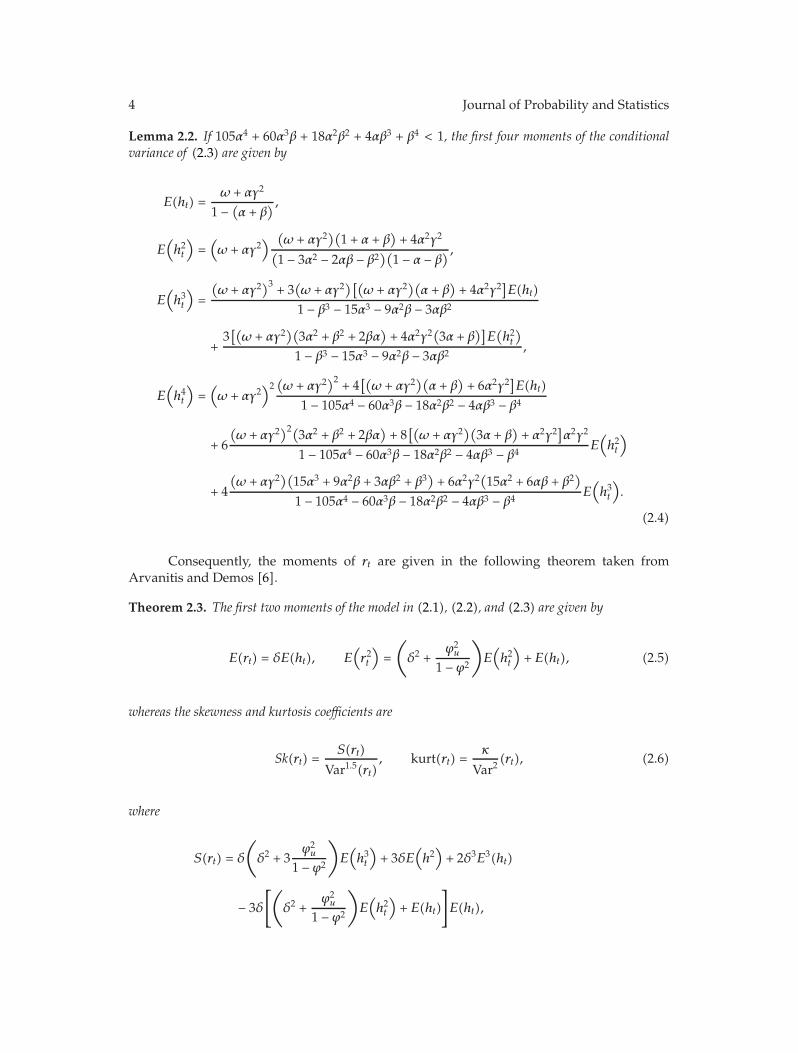
4 Journal of Probability and Statistics
Lemma 2.2. If 105α4 + 60α3β + 18α2β2 + 4αβ3 + β4 < 1, the first four moments of the conditionalvariance of (2.3) are given by
E(ht) =ω + αγ2
1 − (α + β) ,
E(h2t
)=(ω + αγ2
) (ω + αγ2
)(1 + α + β
)+ 4α2γ2
(1 − 3α2 − 2αβ − β2)(1 − α − β) ,
E(h3t
)=
(ω + αγ2
)3 + 3(ω + αγ2
)[(ω + αγ2
)(α + β
)+ 4α2γ2
]E(ht)
1 − β3 − 15α3 − 9α2β − 3αβ2
+3[(ω + αγ2
)(3α2 + β2 + 2βα
)+ 4α2γ2
(3α + β
)]E(h2t)
1 − β3 − 15α3 − 9α2β − 3αβ2,
E(h4t
)=(ω + αγ2
)2(ω + αγ2
)2 + 4[(ω + αγ2
)(α + β
)+ 6α2γ2
]E(ht)
1 − 105α4 − 60α3β − 18α2β2 − 4αβ3 − β4
+ 6
(ω + αγ2
)2(3α2 + β2 + 2βα)+ 8[(ω + αγ2
)(3α + β
)+ α2γ2
]α2γ2
1 − 105α4 − 60α3β − 18α2β2 − 4αβ3 − β4 E(h2t
)
+ 4
(ω + αγ2
)(15α3 + 9α2β + 3αβ2 + β3
)+ 6α2γ2
(15α2 + 6αβ + β2
)
1 − 105α4 − 60α3β − 18α2β2 − 4αβ3 − β4 E(h3t
).
(2.4)
Consequently, the moments of rt are given in the following theorem taken fromArvanitis and Demos [6].
Theorem 2.3. The first two moments of the model in (2.1), (2.2), and (2.3) are given by
E(rt) = δE(ht), E(r2t
)=
(
δ2 +ϕ2u
1 − ϕ2
)
E(h2t
)+ E(ht), (2.5)
whereas the skewness and kurtosis coefficients are
Sk(rt) =S(rt)
Var1.5(rt), kurt(rt) =
κ
Var2(rt), (2.6)
where
S(rt) = δ
(
δ2 + 3ϕ2u
1 − ϕ2
)
E(h3t
)+ 3δE
(h2)+ 2δ3E3(ht)
− 3δ
[(
δ2 +ϕ2u
1 − ϕ2
)
E(h2t
)+ E(ht)
]
E(ht),

Journal of Probability and Statistics 5
κ =
(
δ4 + 6δ2ϕ2u
1 − ϕ2+ 3
ϕ4u
(1 − ϕ2
)2
)
E(h4t
)+ 3δ2
[2 − δ2E(ht)
]E3(ht)
+ 6
(
δ2 +ϕ2u
1 − ϕ2
)
E(h3t
)− 4δ2
(
δ2 +3ϕ2
u
1 − ϕ2
)
E(h3t
)E(ht)
+
{
6δ2[(
δ2 +ϕ2u
1 − ϕ2
)
E(h) − 2
]
E(h) + 3
}
E(h2t
),
(2.7)
and E(ht), E(h2t ), E(h3t ), and E(h4t ) are given in Lemma 2.2.
In terms of stationarity, the process {rt} is 4th-order stationary if and only if
∣∣ϕ∣∣ < 1, 105α4 + 60α3β + 18α2β2 + 4αβ3 + β4 < 1. (2.8)
These conditions are the same as in Arvanitis and Demos [6], indicating that the presence ofthe asymmetry parameter, γ , does not affect the stationarity conditions (see also Bollerslev[4] and Sentana [11]). Furthermore, the 4th-order stationarity is needed as we would liketo measure the autocorrelation of the squared rt’s (volatility clustering), as well as thecorrelation of r2t and rt−1 (leverage effect). The dynamic moments of the conditional varianceand those between the conditional variance ht and the error εt are given in the following twolemmas (for a proof see Appendix B).
Lemma 2.4. Under the assumption of Lemma 2.2, one has that
Cov(ht, ht−k) =(α + β
)kV (ht),
Cov(h2t , ht−k
)= Ak
[E(h3t
)− E
(h2t
)E(ht)
]+
(α + β
)k −Ak
(α + β
) −A BV (ht),
Cov(ht, h
2t−k)=(α + β
)k[E(h3t−1
)− E
(h2t−1
)E(ht−1)
],
Cov(h2t , h
2t−k)= AkV
(h2t
)+ B
(α + β
)k −Ak
(α + β
) −A[E(h3t
)− E
(h2t
)E(ht)
],
(2.9)
where A = 3α2 + β2 + 2αβ and B = 2[2α2γ2 + (ω + αγ2)(α + β)].
Lemma 2.5.
Cov(ht, εt−k) = E(htεt−k) = −2αγ(α + β)k−1
E(ht),
Cov(htht−k, εt−k) = E(htht−kεt−k) = −2αγ(α + β)k−1
E(h2t−1
),
Cov(ht, ε
2t−k)=(α + β
)kV (ht) + 2α
(α + β
)k−1E(h2t
),
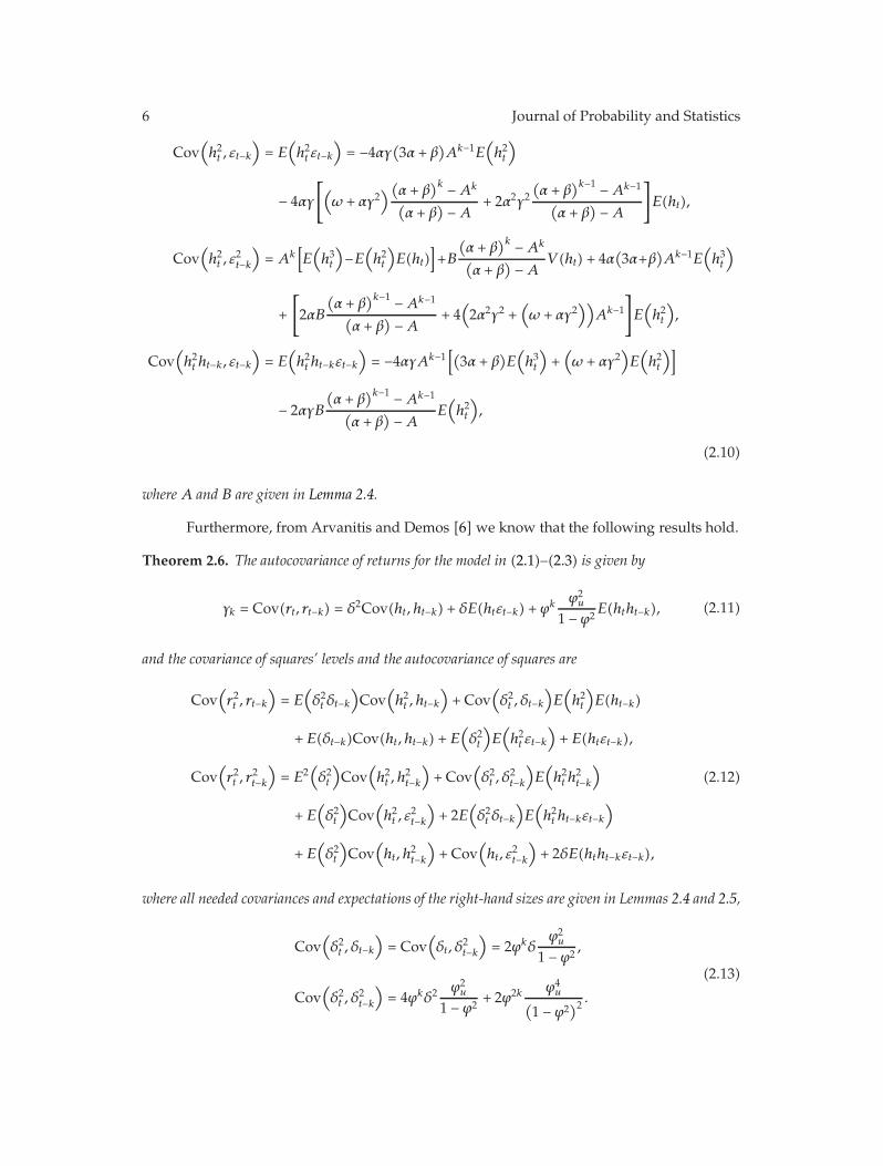
6 Journal of Probability and Statistics
Cov(h2t , εt−k
)= E
(h2t εt−k
)= −4αγ(3α + β
)Ak−1E
(h2t
)
− 4αγ
[(ω + αγ2
)(α + β)k −Ak
(α + β
) −A + 2α2γ2(α + β
)k−1 −Ak−1(α + β
) −A
]
E(ht),
Cov(h2t , ε
2t−k)= Ak
[E(h3t
)−E(h2t
)E(ht)
]+B
(α + β
)k −Ak
(α + β
) −A V (ht) + 4α(3α+β
)Ak−1E
(h3t
)
+
[
2αB
(α + β
)k−1 −Ak−1(α + β
) −A + 4(2α2γ2 +
(ω + αγ2
))Ak−1
]
E(h2t
),
Cov(h2t ht−k, εt−k
)= E
(h2t ht−kεt−k
)= −4αγAk−1
[(3α + β
)E(h3t
)+(ω + αγ2
)E(h2t
)]
− 2αγB
(α + β
)k−1 −Ak−1(α + β
) −A E(h2t
),
(2.10)
where A and B are given in Lemma 2.4.
Furthermore, from Arvanitis and Demos [6] we know that the following results hold.
Theorem 2.6. The autocovariance of returns for the model in (2.1)–(2.3) is given by
γk = Cov(rt, rt−k) = δ2Cov(ht, ht−k) + δE(htεt−k) + ϕkϕ2u
1 − ϕ2E(htht−k), (2.11)
and the covariance of squares’ levels and the autocovariance of squares are
Cov(r2t , rt−k
)= E
(δ2t δt−k
)Cov
(h2t , ht−k
)+ Cov
(δ2t , δt−k
)E(h2t
)E(ht−k)
+ E(δt−k)Cov(ht, ht−k) + E(δ2t
)E(h2t εt−k
)+ E(htεt−k),
Cov(r2t , r
2t−k)= E2
(δ2t
)Cov
(h2t , h
2t−k)+ Cov
(δ2t , δ
2t−k)E(h2t h
2t−k)
+ E(δ2t
)Cov
(h2t , ε
2t−k)+ 2E
(δ2t δt−k
)E(h2t ht−kεt−k
)
+ E(δ2t
)Cov
(ht, h
2t−k)+ Cov
(ht, ε
2t−k)+ 2δE(htht−kεt−k),
(2.12)
where all needed covariances and expectations of the right-hand sizes are given in Lemmas 2.4 and 2.5,
Cov(δ2t , δt−k
)= Cov
(δt, δ
2t−k)= 2ϕkδ
ϕ2u
1 − ϕ2 ,
Cov(δ2t , δ
2t−k)= 4ϕkδ2
ϕ2u
1 − ϕ2 + 2ϕ2k ϕ4u
(1 − ϕ2
)2 .
(2.13)
Journal of Probability and Statistics 7
From the above theorems and lemmas it is obvious that our model can accommodateall stylized facts. For example, negative asymmetry is possible; volatility clustering and theleverage effect (negative Cov(ht, εt−k)) can be accommodated, and so forth. Furthermore, themodel can accommodate negative autocorrelations, γk, something that is not possible forthe GARCH-M model (see Fiorentini and Sentana [12]). Finally, another interesting issueis the diffusion limit of the time-varying GQARCH-M process. As already presented byArvanitis [13], the weak convergence of the Time-varying GQARCH(1,1)-M coincides withthe general conclusions presented elsewhere in the literature. These are that weak limitsof the endogenous volatility models are exogenous (stochastic volatility) continuous-timeprocesses. Moreover, Arvanitis [13] suggests that there is a distributional relation betweenthe GQARCH model and the continuous-time Ornstein-Uhlenbeck models with respect toappropriate nonnegative Levy’s processes.
Let us turn our attention to the estimation of our model. We will show that estimatingour model is a hard task and the use of well-knownmethods such as the EM-algorithm cannothandle the problem due to the huge computational load that such methods require.
3. Likelihood-Inference: EM and Bayesian Approaches
The purpose of this section is the estimation of the time-varying GQARCH(1,1)-M model.Since our model involves two unobserved components (one from the time-varying in-meanparameter and one from the error term), the estimation method required is an EM andmore specifically a simulated EM (SEM), as the expectation terms at the E step cannot becomputed. The main modern way of carrying out likelihood inference in such situations isvia a Markov chain Monte Carlo (MCMC) algorithm (see Chib [14] for an extensive review).This simulation procedure can be used either to carry out Bayesian inference or to classicallyestimate the parameters by means of a simulated EM algorithm.
The idea behind the MCMC methods is that in order to sample a given probabilitydistribution, which is referred to as the target distribution, a suitable Markov chain isconstructed (using a Metropolis-Hasting (M-H) algorithm or a Gibbs sampling method)with the property that its limiting, invariant distribution is the target distribution. In mostproblems, the target distribution is absolutely continuous, and as a result the theory ofMCMC methods is based on that of the Markov chains on continuous state spaces [15]. Thismeans that by simulating theMarkov chain a large number of times and recording its values asample of (correlated) draws from the target distribution can be obtained. It should be notedthat the Markov chain samplers are invariant by construction, and, therefore, the existence ofthe invariant distribution does not have to be checked in any particular application of MCMCmethod.
The Metropolis-Hasting algorithm (M-H) is a general MCMC method to producesample variates from a given multivariate distribution. It is based on a candidate generatingdensity that is used to supply a proposal value that is accepted with probability given as theratio of the target density times the ratio of the proposal density. There are a number of choicesof the proposal density (e.g., randomwalk M-H chain, independence M-H chain, tailored M-H chain) and the components may be revised either in one block or in several blocks. AnotherMCMCmethod, which is special case of the multiple block M-Hmethod with acceptance ratealways equal to one, is called the Gibbs sampling method and was brought into statisticalprominence by Gelfand and Smith [16]. In this algorithm, the parameters are grouped intoblocks, and each block is sampled according to the full conditional distribution denoted as
8 Journal of Probability and Statistics
π(φt/φ/t). By Bayes’ theorem, we have π(φt/φ/t) ∝ π(φtφ/t), the joint distribution of allblocks, and so full conditional distributions are usually quite simply derived. One cycle ofthe Gibbs sampling algorithm is completed by simulating {φt}pt=1, where p is the numberof blocks, from the full conditional distributions, recursively updating the conditioningvariables as one moves through each distribution. Under some general conditions, it isverified that the Markov chain generated by the M-H or the Gibbs sampling algorithmconverges to the target density as the number of iterations becomes large.
Within the Bayesian framework, MCMC methods have proved very popular, and theposterior distribution of the parameters is the target density (see [17]). Another applicationof the MCMC is the analysis of hidden Markov’s models where the approach relies onaugmenting the parameter space to include the unobserved states and simulate the targetdistribution via the conditional distributions (this procedure is called data augmentation andwas pioneered by Tanner and Wong [18]). Kim et al. [19] discuss an MCMC algorithm of thestochastic volatility (SV)model which is an example of a state space model in which the statevariable ht (log-volatility) appears non-linearly in the observation equation. The idea is toapproximate the model by a conditionally Gaussian state space model with the introductionof multinomial random variables that follow a seven-point discrete distribution.
The analysis of a time-varying GQARCH-Mmodel becomes substantially complicatedsince the log-likelihood of the observed variables can no longer be written in closed form.In this paper, we focus on both the Bayesian and the classical estimation of the model.Unfortunately, the non-Markovian nature of the GARCH process implies that each time wesimulate one error we implicitly change all future conditional variances. As pointed out byShephard [20], a regrettable consequence of this path dependence in volatility is that standardMCMC algorithms will evolve in O(T2) computational load (see [21]). Since this cost has tobe borne for each parameter value, such procedures are generally infeasible for large financialdatasets that we see in practice.
3.1. Estimation Problem: Simulated EM Algorithm
As mentioned already, the estimation problem arises because of the fact that we have twounobserved processes. More specifically, we cannot write down the likelihood function inclosed form since we do not observe both εt and δt. On the other hand, the conditional log-likelihood function of our model assuming that δt were observed would be the following:
�(r,δ | φ,F0
)= ln p
(r | δ, φ,F0
)+ ln p
(δ | φ,F0
)
= −T ln 2π − 12
T∑
t=1
lnht − 12
T∑
t=1
(εt)2
ht
− T
2ln(ϕ2u
)− 12
T∑
t=1
(δt − δ
(1 − ϕ) − ϕδt−1
)2
ϕ2u
,
(3.1)
where r = (r1, . . . , rT)′, δ = (δ1, . . . , δT)′, and h = (h1, . . . , hT )′.However, the δt’s are unobserved, and, thus, to classically estimate the model, we have
to rely on an EMalgorithm [22] to obtain estimates as close to the optimum as desired.At eachiteration, the EM algorithm obtains φ(n+1), where φ is the parameter vector, by maximizing
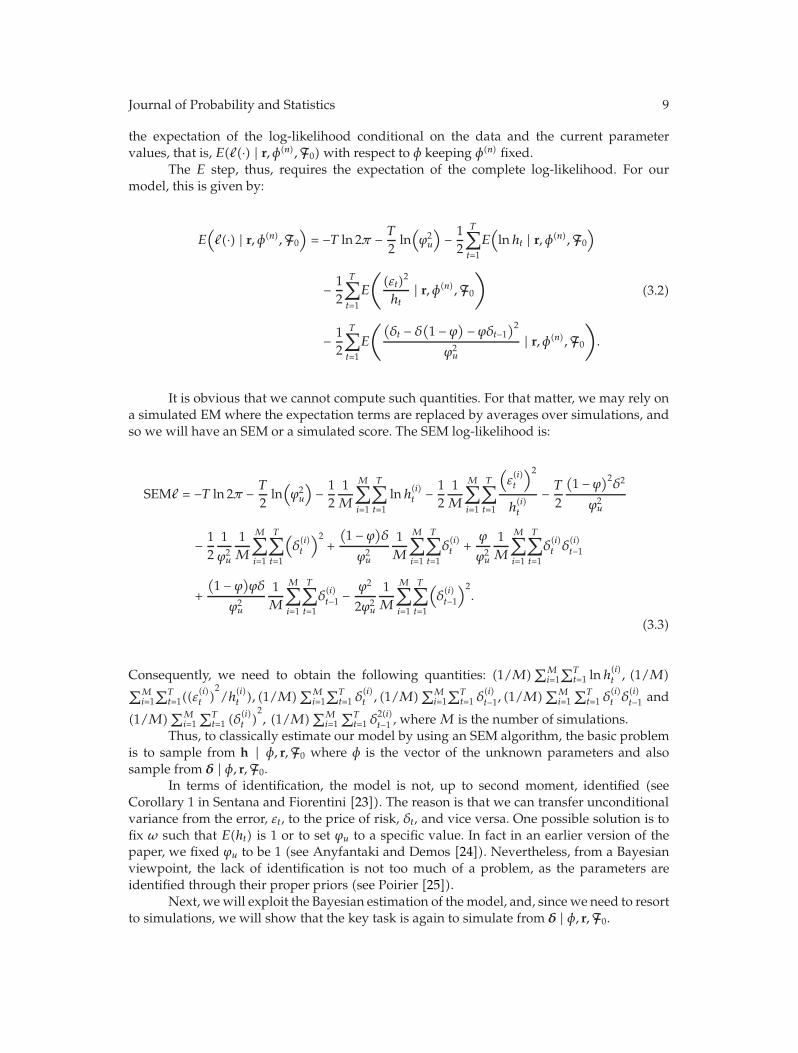
Journal of Probability and Statistics 9
the expectation of the log-likelihood conditional on the data and the current parametervalues, that is, E(�(·) | r, φ(n),F0) with respect to φ keeping φ(n) fixed.
The E step, thus, requires the expectation of the complete log-likelihood. For ourmodel, this is given by:
E(�(·) | r, φ(n),F0
)= −T ln 2π − T
2ln(ϕ2u
)− 12
T∑
t=1
E(lnht | r, φ(n),F0
)
− 12
T∑
t=1
E
((εt)2
ht| r, φ(n),F0
)
− 12
T∑
t=1
E
((δt − δ
(1 − ϕ) − ϕδt−1
)2
ϕ2u
| r, φ(n),F0
)
.
(3.2)
It is obvious that we cannot compute such quantities. For that matter, we may rely ona simulated EM where the expectation terms are replaced by averages over simulations, andso we will have an SEM or a simulated score. The SEM log-likelihood is:
SEM� = −T ln 2π − T
2ln(ϕ2u
)− 12
1M
M∑
i=1
T∑
t=1
lnh(i)t − 12
1M
M∑
i=1
T∑
t=1
(ε(i)t
)2
h(i)t
− T
2
(1 − ϕ)2δ2ϕ2u
− 12
1ϕ2u
1M
M∑
i=1
T∑
t=1
(δ(i)t
)2+
(1 − ϕ)δϕ2u
1M
M∑
i=1
T∑
t=1
δ(i)t +
ϕ
ϕ2u
1M
M∑
i=1
T∑
t=1
δ(i)t δ
(i)t−1
+
(1 − ϕ)ϕδϕ2u
1M
M∑
i=1
T∑
t=1
δ(i)t−1 −
ϕ2
2ϕ2u
1M
M∑
i=1
T∑
t=1
(δ(i)t−1)2.
(3.3)
Consequently, we need to obtain the following quantities: (1/M)∑M
i=1∑T
t=1 lnh(i)t , (1/M)
∑Mi=1∑T
t=1((ε(i)t )
2/h
(i)t ), (1/M)
∑Mi=1∑T
t=1 δ(i)t , (1/M)
∑Mi=1∑T
t=1 δ(i)t−1, (1/M)
∑Mi=1∑T
t=1 δ(i)t δ
(i)t−1 and
(1/M)∑M
i=1∑T
t=1 (δ(i)t )
2, (1/M)
∑Mi=1∑T
t=1 δ2(i)t−1 , whereM is the number of simulations.
Thus, to classically estimate our model by using an SEM algorithm, the basic problemis to sample from h | φ, r,F0 where φ is the vector of the unknown parameters and alsosample from δ | φ, r,F0.
In terms of identification, the model is not, up to second moment, identified (seeCorollary 1 in Sentana and Fiorentini [23]). The reason is that we can transfer unconditionalvariance from the error, εt, to the price of risk, δt, and vice versa. One possible solution is tofix ω such that E(ht) is 1 or to set ϕu to a specific value. In fact in an earlier version of thepaper, we fixed ϕu to be 1 (see Anyfantaki and Demos [24]). Nevertheless, from a Bayesianviewpoint, the lack of identification is not too much of a problem, as the parameters areidentified through their proper priors (see Poirier [25]).
Next, we will exploit the Bayesian estimation of the model, and, since we need to resortto simulations, we will show that the key task is again to simulate from δ | φ, r,F0.

10 Journal of Probability and Statistics
3.2. Simulation-Based Bayesian Inference
In our problem, the key issue is that the likelihood function of the sample p(r | φ,F0) isintractable which precludes the direct analysis of the posterior density p(φ | r,F0). Thisproblem may be overcome by focusing instead on the posterior density of the model usingBayes’ rule:
p(φ,δ | r) ∝ p(φ,δ)p(r | φ,δ) ∝ p(δ | φ)p(φ)p(r | φ,δ), (3.4)
where
φ =(δ, ϕ, ϕu, α, β, γ, ω
)′. (3.5)
Now,
p(δ | φ) =
T∏
t=1
p
(δtδ, ϕ, ϕ2
u
)=
T∏
t=1
1√2πϕ2
u
exp
(
−(δt − δ
(1 − ϕ) − ϕδt−1
)2
2ϕ2u
)
. (3.6)
On the other hand,
p(r | φ,δ) =
T∏
t=1
p
(rt
{rt−1} ,δ, φ)
=T∏
t=1
1√2πht
exp
(
− ε2t2ht
)
(3.7)
is the full-information likelihood. Once we have the posterior density, we get the parameters’marginal posterior density by integrating the posterior density. MCMC is one way ofnumerical integration.
The Hammersley-Clifford theorem (see Clifford [26]) says that a joint distributioncan be characterized by its complete conditional distribution. Hence, given initial values{δt}(0), φ(0), we draw {δt}(1) from p({δt}(1) | r, φ(0)) and then φ(1) from p(φ(1) | {δt}(1), r).Iterating these steps, we finally get ({δt}(i), φ(i))
M
i=1, and under mild conditions it is shownthat the distribution of the sequence converges to the joint posterior distribution p(φ,δ | r).
The above simulation procedure may be carried out by first dividing the parametersinto two blocks:
φ1 =(δ, ϕ, ϕ2
u
),
φ2 =(α, β, γ, ω
),
(3.8)
Then the algorithm is described as follows.
(1) Initialize φ.
(2) Draw from p(δt | δ/= t, r, φ).(3) Draw from p(φ | δ, r) in the following blocks:
(i) draw from p(φ1 | δ, r) using the Gibbs sampling. This is updated in one block;
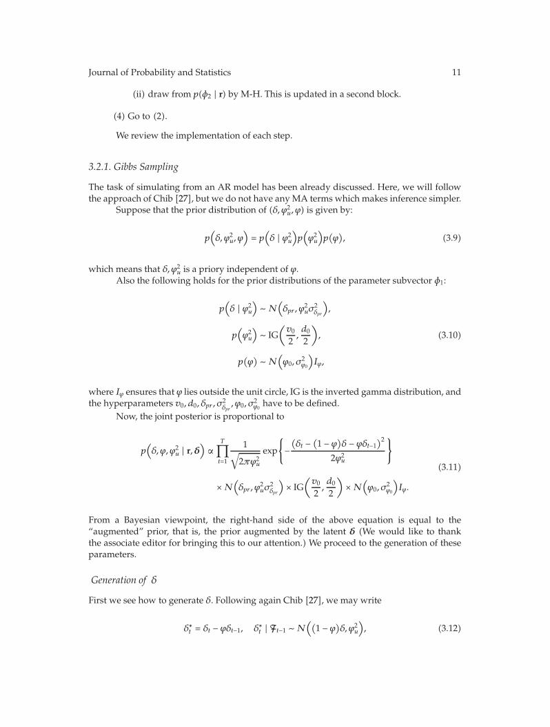
Journal of Probability and Statistics 11
(ii) draw from p(φ2 | r) by M-H. This is updated in a second block.
(4) Go to (2).
We review the implementation of each step.
3.2.1. Gibbs Sampling
The task of simulating from an AR model has been already discussed. Here, we will followthe approach of Chib [27], but we do not have any MA terms which makes inference simpler.
Suppose that the prior distribution of (δ, ϕ2u, ϕ) is given by:
p(δ, ϕ2
u, ϕ)= p(δ | ϕ2
u
)p(ϕ2u
)p(ϕ), (3.9)
which means that δ, ϕ2u is a priory independent of ϕ.
Also the following holds for the prior distributions of the parameter subvector φ1:
p(δ | ϕ2
u
)∼ N
(δpr , ϕ
2uσ
2δpr
),
p(ϕ2u
)∼ IG
(v02,d02
),
p(ϕ) ∼ N
(ϕ0, σ
2ϕ0
)Iϕ,
(3.10)
where Iϕ ensures that ϕ lies outside the unit circle, IG is the inverted gamma distribution, andthe hyperparameters v0, d0, δpr , σ2
δpr, ϕ0, σ2
ϕ0have to be defined.
Now, the joint posterior is proportional to
p(δ, ϕ, ϕ2
u | r,δ)∝
T∏
t=1
1√2πϕ2
u
exp
{
−(δt −
(1 − ϕ)δ − ϕδt−1
)2
2ϕ2u
}
×N(δpr , ϕ
2uσ
2δpr
)× IG
(v02,d02
)×N
(ϕ0, σ
2ϕ0
)Iϕ.
(3.11)
From a Bayesian viewpoint, the right-hand side of the above equation is equal to the“augmented” prior, that is, the prior augmented by the latent δ (We would like to thankthe associate editor for bringing this to our attention.) We proceed to the generation of theseparameters.
Generation of δ
First we see how to generate δ. Following again Chib [27], we may write
δ∗t = δt − ϕδt−1, δ∗t | Ft−1 ∼N((
1 − ϕ)δ, ϕ2u
), (3.12)
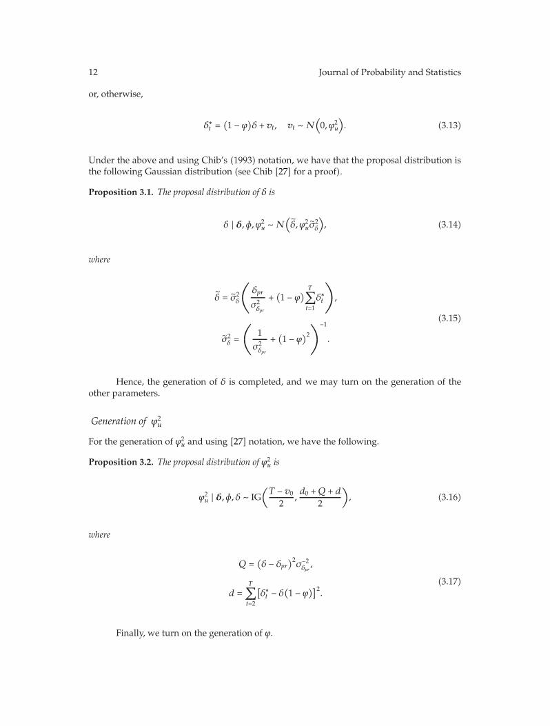
12 Journal of Probability and Statistics
or, otherwise,
δ∗t =(1 − ϕ)δ + vt, vt ∼ N
(0, ϕ2
u
). (3.13)
Under the above and using Chib’s (1993) notation, we have that the proposal distribution isthe following Gaussian distribution (see Chib [27] for a proof).
Proposition 3.1. The proposal distribution of δ is
δ | δ, φ, ϕ2u ∼N
(δ, ϕ2
uσ2δ
), (3.14)
where
δ = σ2δ
⎛
⎝ δpr
σ2δpr
+(1 − ϕ)
T∑
t=1
δ∗t
⎞
⎠,
σ2δ =
⎛
⎝ 1σ2δpr
+(1 − ϕ)2
⎞
⎠
−1
.
(3.15)
Hence, the generation of δ is completed, and we may turn on the generation of theother parameters.
Generation of ϕ2u
For the generation of ϕ2u and using [27] notation, we have the following.
Proposition 3.2. The proposal distribution of ϕ2u is
ϕ2u | δ, φ, δ ∼ IG
(T − v0
2,d0 +Q + d
2
), (3.16)
where
Q =(δ − δpr
)2σ−2δpr,
d =T∑
t=2
[δ∗t − δ
(1 − ϕ)]2.
(3.17)
Finally, we turn on the generation of ϕ.

Journal of Probability and Statistics 13
Generation of ϕ
For the generation of ϕ, we follow again Chib [27] and write
δt =(1 − ϕ)δ − ϕδt−1 + vt, vt ∼N
(0, ϕ2
u
). (3.18)
We may now state the following proposition (see Chib [27] for a proof).
Proposition 3.3. The proposal distribution of ϕ is
ϕ2 | δ, δ, ϕ2u ∼ N
(ϕ, σ2
ϕ
), (3.19)
where
ϕ = σ2ϕ
(
σ−2ϕ0ϕ0 + ϕ−2
u
T∑
t=1
(δt−1 − δ)(δt − δ))
,
σ−2ϕ = σ−2
ϕ0+ ϕ−2
u
T∑
t=1
(δt−1 − δ)2.(3.20)
The Gibbs sampling scheme has been completed, and the next step of the algorithmrequires the generation of the conditional variance parameters via an M-H algorithm whichis now presented.
3.2.2. Metropolis-Hasting
Step (3)-(ii) is the task of simulating from the posterior of the parameters of a GQARCH-M process. This has been already addressed by Kim et al. [19], Bauwens and Lubrano [28],Nakatsuma [29], Ardia [30] and others.
First, we need to decide on the priors. For the parameters α, β, γ, ω, we use normaldensities as priors:
p(α) ∼ N(μα,Σα)Iα,
p(β) ∼ N
(μβ, σ
2β
)Iβ
(3.21)
and similarly
p(γ) ∼N
(μγ , σ
2γ
), (3.22)
where α = (ω, α)′, Iα, Iβ are the indicators ensuring the constraints α > 0, α + β < 1 and β > 0,α + β < 1, respectively. μ., σ2
. are the hyperparameters.

14 Journal of Probability and Statistics
We form the joint prior by assuming prior independence between α, β, γ , and the jointposterior is then obtained by combining the joint prior and likelihood function by Bayes’ rule:
p(α, β, γ | r) ∝
T∏
t=1
1√2πht
exp
(
− ε2t2ht
)
×N(μα,Σα)Iα ×N
(μβ, σ
2β
)Iβ ×N
(μγ , σ
2γ
).
(3.23)
For the M-H algorithm, we use the following approximated GARCH model as inNakatsuma [29] which is derived by the well-known property of GARCH models [4]:
ε2t = ω + α(εt−1 − γ
)2 + βε2t−1 +wt − βwt−1, (3.24)
where wt = ε2t − ht withwt ∼N(0, 2h2t ).Then the corresponding approximated likelihood is written as
p(ε2 | δ, r, φ2
)=
T∏
t=1
12ht
√π
exp
⎡
⎢⎣−
(ε2t −ω − α(εt−1 − γ
)2 − βε2t−1 + βwt−1)2
4h2t
⎤
⎥⎦, (3.25)
and the generation of α, β, γ is based on the above likelihood where we update {ht} eachtime after the corresponding parameters are updated. The generation of the four varianceparameters is given.
Generation of α
For the generation of α, we first note that wt in (3.32), below, can be written as a linear func-tion of α:
wt = ε2t − ζtα, (3.26)
where ζt = [ιt, ε2t ] with
ε2t = ε2t − βε2t−1,
ε2t = ε2t + βε
2t−1,
ε2t =(εt−1 − γ
)2 + βε2t−1,
ιt = 1 + βιt−1.
(3.27)
Now, let the two following vectors be
Yα =[ε21, . . . , ε
2T
]′,
Xα =[ζ′1, . . . , ζ
′T
]′.
(3.28)

Journal of Probability and Statistics 15
Then the likelihood function of the approximated model is rewritten as
p(ε2 | r,δ, φ2
)=
T∏
t=1
1√2π(2h2t
) exp
⎡
⎢⎣−
(ε2t − ζtα
)2
2(2h2t
)
⎤
⎥⎦. (3.29)
Using this we have the following proposal distribution of α (see Nakatsuma [29] orArdia [30] for a proof).
Proposition 3.4. The proposal distribution of α is
α | Y,X,Σ, φ2−α ∼N(μα, Σα
)Iα, (3.30)
where μα = Σα(X′αΛ
−1Yα + Σ−1α μα), Σα = (X′
αΛ−1Xα + Σ−1
α )−1, and Λ = diag(2h21, . . . , 2h2T). Iα
imposes the restriction that α > 0 and α + β < 1.Hence a candidate α is sampled from this proposal density and accepted with probability:
min
{p(α, β, γ | δ, r)q(α∗ | α, β, γ,δ, r)
p(α∗, β, γ | δ, r)q(α | α∗, β, γ,δ, r
) , 1
}
, (3.31)
where α∗ is the previous draw.
Similar procedure is used for the generation of β and γ .
Generation of β
Following Nakatsuma [29], we linearizewt by the first-order Taylor expansion
wt
(β) ≈ wt
(β∗)+ ξt
(β∗)(β − β∗), (3.32)
where ξt is the first-order derivative of wt(β) evaluated at β∗ the previous draw of the M-Hsampler.
Define as
rt = wt
(β∗)+ gt
(β∗)β∗, (3.33)
where gt(β∗) = −ξt(β∗) which is computed by the recursion:
gt = ε2t−1 −wt−1 + β∗gt−1, (3.34)
ξt = 0 for t ≤ 0 [30]. Then,
wt
(β) ≈ rt − gt
(β)β. (3.35)
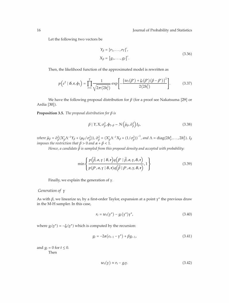
16 Journal of Probability and Statistics
Let the following two vectors be
Yβ = [r1, . . . , rT]′,
Xβ =[g1, . . . , gT
]′.
(3.36)
Then, the likelihood function of the approximated model is rewritten as
p(ε2 | δ, r, φ2
)=
T∏
t=1
1√2π(2h2t
) exp
[
−{wt
(β∗)+ ξt
(β∗)(β − β∗)}2
2(2h2t
)
]
. (3.37)
We have the following proposal distribution for β (for a proof see Nakatsuma [29] orArdia [30]).
Proposition 3.5. The proposal distribution for β is
β | Y,X, σ2β, φ2−β ∼ N
(μβ, σ
2β
)Iβ, (3.38)
where μβ = σ2β(X′
βΛ−1Yβ + (μβ/σ2
β)), σ2
β= (X′
βΛ−1Xβ + (1/σ2
β))−1, and Λ = diag(2h41, . . . , 2h
4T). Iβ
imposes the restriction that β > 0 and α + β < 1.Hence, a candidate β is sampled from this proposal density and accepted with probability:
min
⎧⎨
⎩
p(β, α, γ | δ, r
)q(β∗ | β, α, γ,δ, r
)
p(β∗, α, γ | δ, r)q
(β | β∗, α, γ,δ, r
) , 1
⎫⎬
⎭(3.39)
Finally, we explain the generation of γ .
Generation of γ
As with β, we linearize wt by a first-order Taylor, expansion at a point γ ∗ the previous drawin the M-H sampler. In this case,
rt = wt
(γ ∗) − gt
(γ ∗)γ ∗, (3.40)
where gt(γ ∗) = −ξt(γ ∗) which is computed by the recursion:
gt = −2α(εt−1 − γ ∗)+ βgt−1, (3.41)
and gt = 0 for t ≤ 0.Then
wt
(γ) ≈ rt − gtγ. (3.42)
Journal of Probability and Statistics 17
Let again
Yγ = [r1, . . . , rT]′,
Xγ =[g1, . . . , gT
]′ (3.43)
and the likelihood function of the approximated model is rewritten as
p(ε2 | δ, r, φ2
)=
T∏
t=1
1√2π(2h2t
) exp
[
−{wt
(γ ∗) − gt
(γ ∗)γ ∗}2
2(2h2t
)
]
. (3.44)
Thus, we have the following proposal distribution for γ (for proof see Nakatsuma [29]and Ardia [30]).
Proposition 3.6. The proposal distribution of γ is
γ | Y,X, σ2γ , φ2−γ ∼N
(μγ , σ
2γ
), (3.45)
where μγ = σ2γ (X′
γΛ−1Yγ + (μγ/σ2γ )), σ2
γ = (X′γΛ−1Xγ + (1/σ2
γ ))−1, and Λ = diag(2h41, . . . , 2h
4T). A
candidate γ is sampled from this proposal density and accepted with probability:
min
{p(γ , α, β | δ, r)q(γ ∗ | γ , α, β,δ, r)
p(γ ∗, α, β | δ, r)q(γ | γ ∗, α, β,δ, r) , 1
}
. (3.46)
The algorithm described above is a special case of a MCMC algorithm, which con-verges as it iterates, to draws from the required density p(φ,δ | r). Posterior momentsand marginal densities can be estimated (simulation consistently) by averaging the relevantfunction of interest over the sample variates. The posterior mean of φ is simply estimated bythe sample mean of the simulated φ values. These estimated values can be made arbitrarilyaccurate by increasing the simulation sample size. However, it should be remembered thatsample variates from an MCMC algorithm are a high dimensional (correlated) sample fromthe target density, and sometimes the serial correlation can be quite high for badly behavedalgorithms.
All that remains, therefore, is step (2). Thus, from the above, it is seen that the maintask is again as with the classical estimation of the model, to simulate from δ | φ, r,F0.
3.2.3. MCMC Simulation of ε | φ, r,F0
For a given set of parameter values and initial conditions, it is generally simpler to simulate{εt} for t = 1, . . . , T and then compute {δt}Tt=1 than to simulate {δt}Tt=1 directly. For that matter,we concentrate on simulators of εt given r and φ. We set the mean and the variance of ε0equal to their unconditional values, and, given that ht is a sufficient statistic for Ft−1 andthe unconditional variance is a deterministic function of φ, F0 can be eliminated from theinformation set without any information loss.
18 Journal of Probability and Statistics
Now sampling from p(ε | r, φ) ∝ p(r | ε, φ)p(ε | φ) is feasible by using an M-Halgorithm where we update each time only one εt leaving all the other unchanged [20]. Inparticular, let us write the nth iteration of a Markov chain as εnt . Then we generate a potentialnew value of the Markov chain εnewt by proposing from some candidate density g(εt | εn\t, r, φ)where εn\t = {εn+11 , . . . , εn+1t−1 , ε
nt+1, . . . , ε
nT} which we accept with probability
min
⎡
⎢⎣1,
p(εnewt | εn\t, r, φ
)g(εnewt | εn\t, r, φ
)
p(εnt | εn\t, r, φ
)g(εnt | εn\t, r, φ
)
⎤
⎥⎦. (3.47)
If it is accepted then, we set εn+1t = εnewt and otherwise we keep εn+1t = εnt . Althoughthe proposal is much better since it is only in a single dimension, each time we considermodifying a single error we have to compute:
p(εnewt | εn\t, r, φ
)
p(εnt | εn\t, r, φ
) =p(rt | εnewt , hnew,tt , φ
)p(εnewt | hnew,tt , φ
)p(rt | hn,tt , φ
)
p(rt | hnew,tt , φ
)p(rt | εnt , hn,tt , φ
)p(εnewt | hn,tt , φ
)
∗T∏
s=t+1
p(rs | εrs, hnew,ts , φ
)p(εrs | hnew,ts , φ
)p(rs | hn,ts , φ
)
p(rs | hnew,ts , φ
)p(rs | εns , hn,ts , φ
)p(εns | hn,ts , φ
)
=p(rt | εnewt , hnew,tt , φ
)p(εnewt | hnew,tt , φ
)
p(rt | εnt , hn,tt , φ
)p(εnewt | hn,tt , φ
)
∗T∏
s=t+1
p(rs | εns , hnew,ts , φ
)p(εns | hnew,ts , φ
)
p(rs | εns , hn,ts , φ
)p(εns | hn,ts , φ
) ,
(3.48)
where for s = t + 1, . . . , T ,
hnew,ts = V(εs | εns−1, εns−2, . . . , εnt+1, εnewt , εn+1t−1 , . . . , ε
n+11
),
hn,ts = V(εs | εns−1, εns−2, . . . , εnt+1, εnt , εn+1t−1 , . . . , ε
n+11
) (3.49)
while
hnew,tt = hn,tt . (3.50)
Nevertheless, each time we revise one εt, we have also to revise T − t conditionalvariances because of the recursive nature of the GARCH model which makes hnew,ts dependupon εnewt for s = t + 1, . . . , T . And since t = 1, . . . , T , it is obvious that we need to calculateT2 normal densities, and so this algorithm is O(T2). And this should be done for every φ. To

Journal of Probability and Statistics 19
avoid this huge computational load, we show how to use the method proposed by Fiorentiniet al. [10] and so do MCMC with only O(T) calculations. The method is described in thefollowing subsection.
3.3. Estimation Method Proposed: Classical and Bayesian Estimation
The method proposed by Fiorentini et al. [10] is to transform the GARCH model into a first-order Markov’s model and so do MCMC with only O(T) calculations. Following their trans-formation, we augment the state vector with the variables ht+1 and then sample the jointMarkov process {ht+1, st} | r, φ ∈ Ft where
st = sign(εt − γ
), (3.51)
so that st = ±1 with probability one. Themapping is one to one and has no singularities. Morespecifically, if we know {ht+1} and ϕ, then we know the value of
(εt − γ
)2 =ht+1 −ω − βht
α∀t ≥ 1. (3.52)
Hence the additional knowledge of the signs of (εt − γ)would reveal the entire path of{εt} so long as h0 (which equals the unconditional value in our case) is known, and, thus, wemay now reveal also the unobserved random variable {δt} | r, φ, {ht+1}.
Now we have to sample from
p({st, ht+1} | r, φ
) ∝T∏
t=1
p(st | ht+1, ht, φ
)p(ht+1 | ht, φ
)p(rt | st, ht, ht+1, φ
), (3.53)
where the second and the third term come from the model, and the first comes from the factthat εt | Ft−1 ∼N(0, ht) but εt | {ht+1},Ft−1 takes values
εt = γ ± dt, (3.54)
where
dt =
√ht+1 −ω − βht
α. (3.55)
From the above, it is seen that we should first simulate {ht+1} | r, φ since we do notalter the volatility process when we flip from st = −1 to st = 1 (implying that the signs do notcause the volatility process), but we do alter εt and then simulate {st} | {ht+1}, r, φ. The secondstep is a Gibbs sampling scheme whose acceptance rate is always one and also conditional on{ht+1}, r, φ the elements of {st} are independent which further simplifies the calculations. Weprefer to review first the Gibbs sampling scheme and then the simulation of the conditionalvariance.
20 Journal of Probability and Statistics
3.3.1. Simulations of {st} | {ht+1}, r, φFirst, we see how to sample from {st} | {ht+1}, r, φ. To obtain the required conditionallyBernoulli distribution, we establish first some notation. We have the following (seeAppendix A):
ct =1√vt|rt,ht
[
ϕ
(γ + dt − εt|rt,ht√
vt|rt,ht
)
+ ϕ
(γ − dt − εt|rt,ht√
vt|rt,ht
)]
,
εt|rt,ht = E(εt | rt, ht) =(1 − ϕ2)(rt − δht)ϕ2uht + 1 − ϕ2
, vt|rt,ht = Var(εt | rt, ht) =ϕ2uh
2t
ϕ2uht + 1 − ϕ2
.
(3.56)
Using the above notation, we see that the probability of drawing st = 1 conditional on{ht+1} is equal to the probability of drawing εt = γ + dt conditional on ht+1, ht, rt, φ, where dtis given by (3.70), which is given by
p(st = 1 | {ht+1}, r, φ
)= p(εt = γ + dt | ht+1, ht, rt, φ
)
=1
ct√vt/rt,ht
ϕ
(γ + dt − εt/rr ,ht√
vt/rt,ht
).
(3.57)
Similarly for the probability of drawing st = −1. Both of these quantities are easy tocompute; for example,
ϕ
(γ + dt − εt/rr ,ht√
vt/rt,ht
)=
1√2π
exp
{
−12
(γ + dt − εt/rr ,ht√
vt/rt,ht
)2}
(3.58)
and so we may simulate {st} | {ht+1}, r, φ using a Gibbs sampling scheme. Specifically, sinceconditional on {ht+1}, r, φ the elements of {st} are independent, we actually draw from themarginal distribution, and the acceptance rate for this algorithm is always one.
The Gibbs sampling algorithm for drawing {st} | {ht+1}, r, φ may be described asbelow.
(1) Specify an initial value s(0) = (s(0)1 , . . . , s(0)T ).
(2) Repeat for k = 1, . . . ,M.
(a) Repeat for t = 0, . . . , T − 1.(i) Draw s(k) = 1 with probability,
1ct√vt/rt,ht
ϕ
(γ + dt − εt/rr ,ht√
vt/rt,ht
), (3.59)
and s(k) = −1 with probability,
1 − 1ct√vt/rt,ht
ϕ
(γ + dt − εt/rr ,ht√
vt/rt,ht
). (3.60)
(3) Return the values {s(1), . . . , s(M)}.
Journal of Probability and Statistics 21
3.3.2. Simulations of {ht+1} | r, φ (Single Move Samplers)
On the other hand, the first step involves simulating from {ht+1} | r, φ. To avoid large de-pendence in the chain, we use an M-H algorithm where we simulate one ht+1 at a timeleaving the others unchanged [20, 31]. So if (ht+1)n is the current value of the nth iterationof a Markov chain, then we draw a candidate value of the Markov chain hnewt+1 by proposingit from a candidate density (proposal density) g(ht+1 | (h)n/t+1, r, φ) where (h)n/t+1 ={hn+11 , hn+12 , . . . , hn+1t , hnt+2, . . . , h
nT+1}. We set (ht+1)
n+1 = (ht+1)new with acceptance probability
min
[
1,p(hnewt+1 | (h)n/t+1, r, φ
)g(hnt+1 | (h)n/t+1, r, φ
)
p(hnt+1 | (h)n/t+1, r, φ
)g(hnewt+1 | (h)n/t+1, r, φ
)
]
, (3.61)
where we have used the fact that
p(h | r, φ) = p((h)/t | r, φ
)p(ht | (h)/t, r, φ
). (3.62)
However, we may simplify further the acceptance rate. More specifically, we have that
p(ht+1 | (h)/t+1, r, φ
) ∝ p(ht+2 | ht+1, φ)p(ht+1 | ht, φ
)p(rt+1 | ht+2, ht+1, φ
)p(rt | ht+1, ht, φ
).
(3.63)
Now, since the following should hold:
ht+1 ≥ ω + βht (3.64)
and similarly
ht+1 ≤ β−1(ht+2 −ω), (3.65)
we have the support of the conditional distribution of ht+1 given that ht is bounded frombelow by ω + βht, and the same applies to the distribution of ht+2 given ht+1 (lower limitcorresponds to dt = 0 and the upper limit to dt+1 = 0). This means that the range of valuesof ht+1 compatible with ht and ht+2 in the GQARCH case is bounded from above and below;that is:
ht+1 ∈[ω + βht, β−1(ht+2 −ω)
]. (3.66)
From the above, we understand that it makes sense to make the proposal to obey thesupport of the density, and so it is seen that we can simplify the acceptance rate by setting
g(ht+1 | (h)/t+1, r, φ
)= p(ht+1 | ht, φ
)(3.67)
appropriately truncated from above (since the truncation from below will automatically besatisfied). But the above proposal density ignores the information contained in rt+1, and so
22 Journal of Probability and Statistics
according to Fiorentini et al. [10] we can achieve a substantially higher acceptance rate if wepropose from
g(ht+1 | (h)/t+1, r, φ
)= p(ht+1 | rt, ht, φ
). (3.68)
A numerically efficient way to simulate ht+1 from p(ht+1 | rt, ht, φ) is to sample anunderlying Gaussian random variable doubly truncated by using an inverse transformmeth-od. More specifically, we may draw
εt | rt, ht, φ ∼N((
1 − ϕ2)(rt − δht)ϕ2uht + 1 − ϕ2
,ϕ2uh
2t
ϕ2uht + 1 − ϕ2
)
(3.69)
doubly truncated so that it remains within the following bounds:
εnewt ∈ [γ − lt, γ + lt], (3.70)
where
lt =
√ht+2 −ω − βω − β2ht
βα, (3.71)
using an inverse transform method and then compute
hnewt+1 = ω + α(εnewt − γ)2 + βht, (3.72)
which in turn implies a real value for dnewt+1 =
√(ht+2 −ω − βhnewt+1 )/α and so guarantees that
hnewt+1 lies within the acceptance bounds.The inverse transform method to draw the doubly truncated Gaussian random vari-
able first draws a uniform random number
u ∼ U(0, 1) (3.73)
and then computes the following:
u = (1 − u)Φ
⎛
⎜⎝γ − lt −
((1 − ϕ2)(rt − δht)/
(ϕ2uht + 1 − ϕ2))
√ϕ2uh
2t /(ϕ2uht + 1 − ϕ2
)
⎞
⎟⎠
+ uΦ
⎛
⎜⎝γ + lt −
((1 − ϕ2)(rt − δht)/
(ϕ2uht + 1 − ϕ2))
√ϕ2uh
2t /(ϕ2uht + 1 − ϕ2
)
⎞
⎟⎠.
(3.74)
Journal of Probability and Statistics 23
A draw is then given by
εnewt = Φ−1(u). (3.75)
However, if the bounds are close to each other (the degree of truncation is small) theextra computations involved make this method unnecessarily slow, and so we prefer to usethe accept-reject method where we draw
εnewt | rt, ht, φ ∼ N((
1 − ϕ2)(rt − δht)ϕ2uht + 1 − ϕ2
,ϕ2uh
2t
ϕ2uht + 1 − ϕ2
)
(3.76)
and accept the draw if γ − lt ≤ εnewt ≤ γ + lt, and otherwise we repeat the drawing (this methodis inefficient if the truncation lies in the tails of the distribution). It may be worth assessingthe degree of truncation first, and, depending on its tightness, choose one simulation methodor the other.
The conditional density of εnewt will be given according to the definition of a truncatednormal distribution:
p(εnewt | ∣∣εnewt − γ∣∣ ≤ lt, rt, ht, φ
)=
1√vt/rt,ht
ϕ
(εnewt − εt/rr ,ht√
vt/rt,ht
)
×[Φ(γ + lt − εt/rr ,ht√
vt/rt,ht
)−Φ
(γ − lt − εt/rr ,ht√
vt/rt,ht
)]−1,
(3.77)
where Φ(·) is the cdf of the standard normal.By using the change of variable formula, we have that the density of hnewt+1 will be
p(hnewt+1 | hnewt+1 ∈
[ω + βht, β−1(ht+2 −ω)
], rt, ht, φ
)
=cnewt∣∣2αdnew
t
∣∣ ×[Φ(γ + lt − εt/rr ,ht√
vt/rt,ht
)−Φ
(γ − lt − εt/rr ,ht√
vt/rt,ht
)]−1.
(3.78)
Using Bayes theorem we have that the acceptance probability will be
min
(
1,p(ht+2 | hnewt+1 , rt+1, φ
)p(rt+1 | hnewt+1 , φ
)
p(rt+1 | hnt+1, φ
)p(ht+2 | hnt+1, rt+1, φ
)
)
. (3.79)
Since the degree of truncation is the same for old and new, the acceptance probabilitywill be
min
(
1,p(rt+1 | hnewt+1
)
p(rt+1 | hnt+1
)cnewt+1
cnt+1
dnt+1dnewt+1
)
, (3.80)
24 Journal of Probability and Statistics
where p(rt+1 | ht+1) is a mixture of two univariate normal densities so
rt+1 | ht+1 ∼N(
δht+1,
(ϕ2u
1 − ϕ2ht+1 + 1
)
ht+1
)
. (3.81)
Hence,
p(rt+1 | hnt+1
)=
1√2π((ϕ2u/(1 − ϕ2
))hnt+1 + 1
)hnt+1
exp
(
−(rt+1 − δhnt+1
)2
2((ϕ2u/(1 − ϕ2
))hnt+1 + 1
)hnt+1
)
,
(3.82)
and the acceptance probability becomes
min
⎡
⎢⎣1,
(hnt+1hnewt+1
)3/2√hnt+2 −ω − βhnt+1
√hnt+2 −ω − βhnewt+1
κ(hnewt+1
)
κ(hnt+1
)
⎤
⎥⎦, (3.83)
where
κ(hit+1
)= exp
⎡
⎢⎢⎢⎢⎢⎢⎢⎣
−(rt+1 − δhit+1
)2
2
(ϕ2u
1 − ϕ2hit+1 + 1
)
hit+1
−
ϕ2u
1 − ϕ2hit+1 + 1
2ϕ2u
1 − ϕ2
(hit+1
)2
⎛
⎜⎜⎜⎜⎜⎜⎜⎝
⎛
⎜⎜⎜⎝γ − rt+1 − δhit+1
ϕ2u
1 − ϕ2hit+1 + 1
⎞
⎟⎟⎟⎠
2
+hrt+2 −ω − βhit+1
α
⎞
⎟⎟⎟⎟⎟⎟⎟⎠
⎤
⎥⎥⎥⎥⎥⎥⎥⎦
×
⎡
⎢⎢⎢⎢⎢⎢⎢⎢⎢⎢⎢⎢⎢⎢⎣
1 + exp
⎡
⎢⎢⎢⎣2
ϕ2u
1 − ϕ2hit+1 + 1
ϕ2u
1 − ϕ2
(hit+1
)2
⎛
⎜⎜⎜⎝γ − rt+1 − δhit+1
ϕ2u
1 − ϕ2hit+1 + 1
⎞
⎟⎟⎟⎠
√hnt+2 −ω − βhit+1
α
⎤
⎥⎥⎥⎦
exp
⎡
⎢⎢⎢⎣
ϕ2u
1 − ϕ2hit+1 + 1
ϕ2u
1 − ϕ2
(hit+1
)2
⎛
⎜⎜⎜⎝γ − rt+1 − δhit+1
ϕ2u
1 − ϕ2hit+1 + 1
⎞
⎟⎟⎟⎠
√hnt+2 −ω − βhit+1
α
⎤
⎥⎥⎥⎦
⎤
⎥⎥⎥⎥⎥⎥⎥⎥⎥⎥⎥⎥⎥⎥⎦
.
(3.84)
Overall the MCMC of {ht+1} | r, φ includes the following steps.
(1) Specify an initial value {h(0)}.(2) Repeat for n = 1, . . . ,M.
(a) Repeat for t = 0, . . . , T − 1.
Journal of Probability and Statistics 25
(i) Use an inverse transform method to simulate
εnewt | rt, ht, φ ∼ N((
1 − ϕ2)(rt − δht)ϕ2uht + 1 − ϕ2
,ϕ2uh
2t
ϕ2uht + 1 − ϕ2
)
(3.85)
doubly truncated.(ii) Calculate
hnewt+1 = ω + α(εct − γ
)2 + βht. (3.86)
Steps (2)(a)(i) and (2)(a)(ii) are equivalent to draw
(ht+1)new ∼ p(hnewt+1 | rt, ht, φ)
(3.87)
appropriately truncated.(iii) Calculate
αr = min
[
1,p(rt+1 | hnewt+1
)
p(rt+1 | hnt+1
)cnewt+1
cnt+1
dnt+1dnewt+1
]
. (3.88)
(iv) Set
(ht+1)n+1 =
⎧⎨
⎩
(ht+1)new if Unif(0, 1) ≤ αr(ht+1)n otherwise
(3.89)
Remark 3.7. Every time we change ht+1, we calculate only one normal density since the trans-formation is Markovian, and, since t = 0, . . . , T − 1, we need O(T) calculations.
Notice that if we retain hnewt+1 , then εnewt is retained and we will not need to simulate stat a later stage. In fact we only need to simulate st at t = T since we need to know εT . Thefinal step involves computing
δ(n)t+1 =
rt+1 − ε(n)t+1
h(n)t+1
, t = 0, . . . , T − 1, n = 1, . . . ,M. (3.90)
Using all the above simulated values, we may now take average of simulations andcompute the quantities needed for the SEM algortihm. As for the Bayesian inference, havingcompleted Step (2) we may now proceed to the Gibbs sampling and M-H steps to obtaindraws from the required posterior density. Thus, the first-order Markov transformation ofthe model made feasible an MCMC algorithm which allows the calculation of a classicalestimator via the simulated EM algorithm and a simulation-based Bayesian inference inO(T)computational operations.

26 Journal of Probability and Statistics
3.4. A Comparison of the Simulators
In order to compare the performance of the inefficient and the efficient MCMC samplerintroduced in the previous subsection, we have generated realizations of size T = 240 forthe simple GQARCH(1,1)-M-AR(1) model with parameters δ = 0.1, ϕ = 0.85, α = 0.084,β = 0.688, γ = 0.314 (which are centered around typical values that we tend to see in theempirical literature). We first examine the increase in the variance of the sample mean of εtacross 500,000 simulations due to the autocorrelation in the drawings relative to an ideal butinfeasible independent sampler.
We do so by recording the inefficient ratios for the observations t = 80 and t = 160using standard spectral density techniques. In addition, we record the mean acceptanceprobabilities over all observations and the average CPU time needed to simulate onecomplete drawing. The behavior of the two simulators is summarized in Table 1 and isvery much as one would expect. The computationally inefficient sampler shows high serialcorrelation for both t = 80 and t = 160 and a low acceptance rate for each individual t.Moreover, it is extremely time consuming to compute even though our sample size is fairlysmall. In fact, when we increase T from 240 to 2400, and 24000 the average CPU time increasesby a factor of 100 and 10000, respectively, as opposed to 10 and 100 for the other one (theefficient), which makes it impossible to implement in most cases of practical interest. On theother hand, the single-move efficient sampler produces results much faster, with a reasonablyhigh acceptance rate but more autocorrelation in the drawings for t = 160.
4. Empirical Application: Bayesian Estimation ofWeekly Excess Returns from Three Major Stock Markets:Dow-Jones, FTSE, and Nikkei
In this section we apply the procedures described above to weekly excess returns from threemajor stock markets: Dow-Jones, FTSE, and Nikkei for the period of the last week of 1979:8 tothe second to the last week of 2008:5 (1,500 observations). To guarantee 0 ≤ β ≤ 1 − α ≤ 1 andto ensure that ω > 0 we also used some accept-reject method for the Bayesian inference. Thismeans that, when drawing from the posterior (as well as from the prior), we had to ensurethat α, β > 0, α + β < 1 and ω > 0.
In order to implement our proposed Bayesian approach, we first have to specify thehyperparameters that characterize the prior distributions of the parameters. In this respect,our aim is to employ informative priors that would be in accordance with the “receivedwisdom.” In particular, for all data sets, we set the prior mean for β equal to 0.7, and fora, ω, and γ we decided to set their prior means equal to 0.15, 0.4, and 0.0, respectively. Wehad also to decide on the prior mean of δ. We set its prior mean equal to 0.05, for all markets.These prior means imply an annual excess return of around 4%, which is a typical value forannualized stock excess returns. Finally, we set the prior mean of ϕ equal to 0.75, of ϕ2
u equalto 0.01, and the hyperparameters ν0 and do equal to 1550 and 3, respectively, for all threedatasets, something which is consistent with the “common wisdom” of high autocorrelationof the price of risk. We employ a rather vague prior and set its prior variance equal to 10,000for all datasets.
We ran a chain for 200,000 simulations for the three datasets and decided to use everytenth point, instead of all points, in the sample path to avoid strong serial correlation. Theposterior statistics for the Dow-Jones, FTSE, and Nikkey are reported in Table 2. Inefficiency

Journal of Probability and Statistics 27
Table 1: Comparison between the efficient and inefficient MCMC simulator.
MAP IR Time (CPU effort)
t = 80 t = 160 T = 240 T = 2400 T = 24000
Inefficient 0.16338 45.1748 47.3602 0.031250 4.046875 382.05532
Single-move 0.60585 8.74229 110.245 0.001000 0.015625 0.1083750Note: MAP denotes mean acceptance probability over the whole sample, while IR refers to inefficiency ratio of the MCMCdrawings at observations 80 and 160. Time refers to the total CPU time (in seconds) taken to simulate one completedrawing.
Table 2: Bayesian inference results.
Dow-Jones PM PSD φ0.5 φmin φmax IF
δ 0.052 0.041 0.054 −0.048 0.103 3.001
ϕ 0.812 0.082 0.854 −0.992 0.999 2.115
ϕ2u 0.010 0.034 0.013 0.002 0.018 1.509
ω 0.405 0.071 0.461 0.004 0.816 2.367
α 0.152 0.040 0.291 0.001 0.873 1.048
β 0.651 0.168 0.629 0.003 0.984 2.994
γ 0.392 0.112 0.393 −0.681 0.418 5.108
FTSE PM PSD φ0.5 φmin φmax IF
δ 0.059 0.036 0.059 −0.051 0.395 3.111
ϕ 0.811 0.096 0.839 −0.809 0.999 2.154
ϕ2u 0.009 0.029 0.012 0.005 0.017 1.995
ω 0.205 0.087 0.398 0.003 0.995 1.457
α 0.140 0.055 0.187 0.001 0.931 3.458
β 0.682 0.153 0.701 0.001 0.988 2.721
γ 0.374 0.102 0.381 −0.615 0.401 1.254
Nikkei PM PSD φ0.5 φmin φmax IF
δ 0.068 0.051 0.068 −0.064 0.211 2.998
ϕ 0.809 0.090 0.837 −0.831 0.999 1.211
ϕ2u 0.010 0.031 0.010 0.004 0.019 2.001
ω 0.195 0.079 0.228 0.004 0.501 2.789
α 0.149 0.052 0.197 0.001 0.893 3.974
β 0.634 0.119 0.645 0.006 0.989 1.988
γ 0.408 0.123 0.409 −0.587 0.487 4.007Note: PM denotes posterior mean, PSD posterior standard deviation, φ0.5 posterior median, φmin posterior minimum, φmaxposterior maximum, and IF inefficiency factor.
factors are calculated using a Parzen window equal to 0.1T (where, recall, T is the numberof observations) and indicate that the M-H sampling algorithm has converged and wellbehaved (This is also justified by the ACFs of the draws. However, they are not presentedfor space considerations and are available upon request.)With the exception of the constantsδ and the ϕ2
u’s, there is low uncertainty with the estimation of the parameters. The estimatedpersistence, α + β, for all three markets is close to 0.8 with the highest being the one of
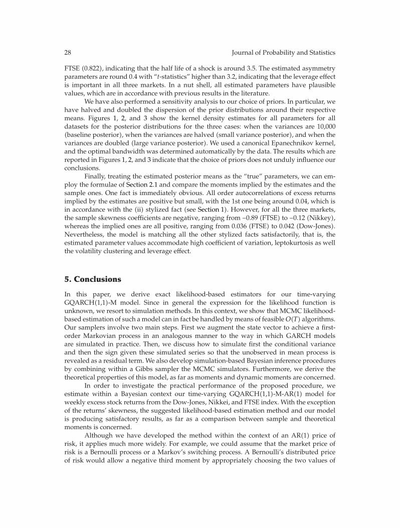
28 Journal of Probability and Statistics
FTSE (0.822), indicating that the half life of a shock is around 3.5. The estimated asymmetryparameters are round 0.4 with “t-statistics” higher than 3.2, indicating that the leverage effectis important in all three markets. In a nut shell, all estimated parameters have plausiblevalues, which are in accordance with previous results in the literature.
We have also performed a sensitivity analysis to our choice of priors. In particular, wehave halved and doubled the dispersion of the prior distributions around their respectivemeans. Figures 1, 2, and 3 show the kernel density estimates for all parameters for alldatasets for the posterior distributions for the three cases: when the variances are 10,000(baseline posterior), when the variances are halved (small variance posterior), and when thevariances are doubled (large variance posterior). We used a canonical Epanechnikov kernel,and the optimal bandwidth was determined automatically by the data. The results which arereported in Figures 1, 2, and 3 indicate that the choice of priors does not unduly influence ourconclusions.
Finally, treating the estimated posterior means as the “true” parameters, we can em-ploy the formulae of Section 2.1 and compare the moments implied by the estimates and thesample ones. One fact is immediately obvious. All order autocorrelations of excess returnsimplied by the estimates are positive but small, with the 1st one being around 0.04, which isin accordance with the (ii) stylized fact (see Section 1). However, for all the three markets,the sample skewness coefficients are negative, ranging from −0.89 (FTSE) to −0.12 (Nikkey),whereas the implied ones are all positive, ranging from 0.036 (FTSE) to 0.042 (Dow-Jones).Nevertheless, the model is matching all the other stylized facts satisfactorily, that is, theestimated parameter values accommodate high coefficient of variation, leptokurtosis as wellthe volatility clustering and leverage effect.
5. Conclusions
In this paper, we derive exact likelihood-based estimators for our time-varyingGQARCH(1,1)-M model. Since in general the expression for the likelihood function isunknown, we resort to simulation methods. In this context, we show that MCMC likelihood-based estimation of such amodel can in fact be handled bymeans of feasibleO(T) algorithms.Our samplers involve two main steps. First we augment the state vector to achieve a first-order Markovian process in an analogous manner to the way in which GARCH modelsare simulated in practice. Then, we discuss how to simulate first the conditional varianceand then the sign given these simulated series so that the unobserved in mean process isrevealed as a residual term. We also develop simulation-based Bayesian inference proceduresby combining within a Gibbs sampler the MCMC simulators. Furthermore, we derive thetheoretical properties of this model, as far as moments and dynamic moments are concerned.
In order to investigate the practical performance of the proposed procedure, weestimate within a Bayesian context our time-varying GQARCH(1,1)-M-AR(1) model forweekly excess stock returns from the Dow-Jones, Nikkei, and FTSE index. With the exceptionof the returns’ skewness, the suggested likelihood-based estimation method and our modelis producing satisfactory results, as far as a comparison between sample and theoreticalmoments is concerned.
Although we have developed the method within the context of an AR(1) price ofrisk, it applies much more widely. For example, we could assume that the market price ofrisk is a Bernoulli process or a Markov’s switching process. A Bernoulli’s distributed priceof risk would allow a negative third moment by appropriately choosing the two values of
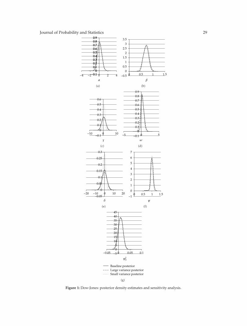
Journal of Probability and Statistics 29
α
−0.10
0.10.20.30.40.50.60.70.80.9
−4 −2 0 2 4−0.10
0.10.20.30.40.50.60.70.80.9
(a)
β
−0.50
0.51
1.52
2.53
3.5
0 0.5 1 1.5
(b)
γ
−0.10
0.1
0.2
0.3
0.4
0.5
0.6
−10 0 10
(c)
ω
−5 0 5−0.10
0.10.20.30.40.50.60.70.80.9
(d)
δ
−0.050
0.05
0.1
0.15
0.2
0.25
0.3
−20 −10 0 10 20
(e)
ϕ
−10
1
2
3
4
5
6
7
0 0.5 1 1.5
(f)
Baseline posteriorLarge variance posteriorSmall variance posterior
ϕ2u
−5051015202530354045
−0.05 0 0.05 0.1
(g)
Figure 1: Dow-Jones: posterior density estimates and sensitivity analysis.
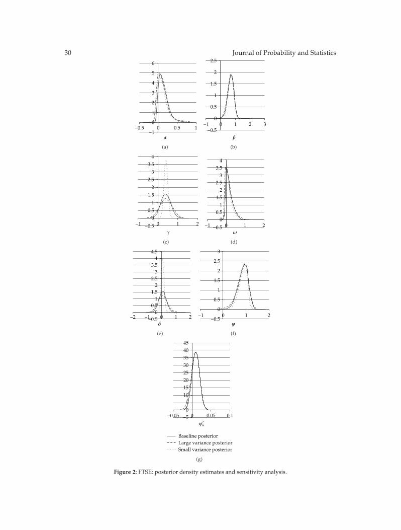
30 Journal of Probability and Statistics
α−10
1
2
3
4
5
6
−0.5 0 0.5 1
(a)
β
−0.5
0
0.5
1
1.5
2
2.5
−1 0 1 2 3
(b)
γ−0.5
0
0.5
1
1.5
2
2.5
3
3.5
4
−1 0 1 2
(c)
ω−0.5
00.51
1.52
2.53
3.54
−1 0 1 2
(d)
δ−0.5
00.51
1.52
2.53
3.54
4.5
−2 −1 0 1 2
(e)
ϕ−0.5
0
0.5
1
1.5
2
2.5
3
−1 0 1 2
(f)
ϕ2u
−5051015202530354045
−0.05 0 0.05 0.1
Baseline posteriorLarge variance posteriorSmall variance posterior
(g)
Figure 2: FTSE: posterior density estimates and sensitivity analysis.
Journal of Probability and Statistics 31
α−1
0
1
2
3
4
5
−1 0 1 2
(a)
β
−1 0 1 2
−0.5
0
0.5
1
1.5
2
(b)
γ
−0.50
0.51
1.52
2.53
3.54
4.5
−2 0 2
(c)
−1 0 1 2
ω
−10
1
2
3
4
5
6
(d)
δ
−0.20
0.20.40.60.81
1.21.41.61.8
−2 −1 0 1 2
(e)
−1 0 1 2
ϕ
−0.50
0.51
1.52
2.53
3.54
4.5
(f)
ϕ2u
−5051015202530354045
−0.05 0 0.05 0.1
Baseline posteriorLarge variance posteriorSmall variance posterior
(g)
Figure 3: Nikkei: posterior density estimates and sensitivity analysis.
32 Journal of Probability and Statistics
the in-mean process. However, this would make all computations much more complicated.In an earlier version of the paper, we assumed that the market price of risk follows a normaldistribution, and we applied both the classical and the Bayesian procedure to three stockmarkets (where we decided to set the posterior means as initial values for the simulatedEM algorithm). The results suggested that the Bayesian and the classical procedures are quitein agreement (see Anyfantaki and Demos [24]).
Finally, it is known that (e.g., [32, pages 84 and 85]) the EM algorithm slows downsignificantly in the neighborhood of the optimum. As a result, after some initial EM iterations,it is tempting to switch to a derivative-based optimization routine, which is more likely toquickly converge to the maximum. EM-type arguments can be used to facilitate this switchby allowing the computation of the score. In particular, it is easy to see that
E
(∂ ln p
(δ | r, φ,F0
)
∂φ| r, φ(n),F0
)
= 0, (5.1)
so it is clear that the score can be obtained as the expected value given r, φ,F0 of the sumof the unobservable scores corresponding to ln p(r | δ, φ,F0) and ln p(δ | φ,F0). This couldbe very useful for the classical estimation procedure, not presented here, as even though ouralgorithm is an O(T) one, it is still rather slow. We leave these issues for further research.
Appendices
A. Proof of (3.69) and (3.82)
Proof of Equation (3.69). This is easily derived using the fact that
rt = δtht + εt, (A.1)
where
rt | ht ∼ N(
δht,
(ϕ2u
1 − ϕ2ht + 1
)
ht
)
, (A.2)
and, consequently,
(εt
rt
)
| ht ∼ N
⎛
⎜⎜⎝
(0
δht
)
,
⎛
⎜⎜⎝
ht ht
ht
(ϕ2u
1 − ϕ2ht + 1
)
ht
⎞
⎟⎟⎠
⎞
⎟⎟⎠, (A.3)
Journal of Probability and Statistics 33
and, thus; from the definition of the bivariate normal,
E(εt | rt, ht) =(1 − ϕ2)(rt − δht)ϕ2uht + 1 − ϕ2
,
Var(εt | rt, ht) =ϕ2uh
2t
ϕ2uht + 1 − ϕ2
.
(A.4)
Consequently,
εt | rt, ht, φ ∼N((
1 − ϕ2)(rt − δht)ϕ2uht + 1 − ϕ2
,ϕ2uh
2t
ϕ2uht + 1 − ϕ2
)
. (A.5)
Proof of Equation (3.82). We have that
p(rt+1 | hrt+1
)=
1√2π((ϕ2u/(1 − ϕ2
))hrt+1 + 1
)hrt+1
exp
(
−(rt+1 − δhrt+1
)2
2((ϕ2u/(1 − ϕ2
))hrt+1 + 1
)hrt+1
)
,
(A.6)
and, thus,
p(rt+1 | hnewt+1
)
p(rt+1 | hrt+1
) =
√((ϕ2u/(1 − ϕ2
))hrt+1 + 1
)hrt+1
√((ϕ2u/(1 − ϕ2
))hnewt+1 + 1
)hnewt+1
× exp
( (rt+1 − δhrt+1
)2
2((ϕ2u/(1 − ϕ2
))hrt+1 + 1
)hrt+1
−(rt+1 − δhnewt+1
)2
2((ϕ2u/(1 − ϕ2
))hnewt+1 + 1
)hnewt+1
)
.
(A.7)
Also,
drt+1 =
√hrt+2 −ω − βhrt+1
α, (A.8)
and so
drt+1dnewt+1
=
√hrt+2 −ω − βhrt+1
√hrt+2 −ω − βhnewt+1
. (A.9)

34 Journal of Probability and Statistics
Moreover,
cnewt+1
crt+1=
hrt+1
√ϕ2uh
newt+1 + 1 − ϕ2
⎡
⎢⎢⎢⎢⎢⎢⎢⎢⎢⎢⎢⎢⎢⎣
exp
⎛
⎜⎜⎜⎜⎜⎜⎜⎝
−
(ϕ2uh
newt+1 + 1 − ϕ2)
2ϕ2uh
new2t+1
⎛
⎜⎜⎜⎜⎜⎜⎜⎝
γ+
√√√√hrt+2 −ω − βhnewt+1
α
−
(1 − ϕ2)(rt+1 − δhnewt+1
)
(ϕ2uh
newt+1 + 1 − ϕ2
)
⎞
⎟⎟⎟⎟⎟⎟⎟⎠
2⎞
⎟⎟⎟⎟⎟⎟⎟⎠
+ exp
⎛
⎜⎜⎜⎜⎜⎜⎜⎝
−
(ϕ2uh
newt+1 + 1 − ϕ2)
2ϕ2uh
new2t+1
⎛
⎜⎜⎜⎜⎜⎜⎜⎝
γ−
√√√√h
rt+2 −ω − βhnewt+1
α
−
(1 − ϕ2)(rt+1 − δhnewt+1
)
(ϕ2uh
newt+1 + 1 − ϕ2
)
⎞
⎟⎟⎟⎟⎟⎟⎟⎠
2⎞
⎟⎟⎟⎟⎟⎟⎟⎠
⎤
⎥⎥⎥⎥⎥⎥⎥⎥⎥⎥⎥⎥⎥⎦
hnewt+1
√ϕ2uh
rt+1 + 1 − ϕ2
⎡
⎢⎢⎢⎢⎢⎢⎢⎢⎢⎢⎢⎢⎢⎣
exp
⎛
⎜⎜⎜⎜⎜⎜⎜⎝
−
(ϕ2uh
rt+1 + 1 − ϕ2)
2ϕ2uh
r2t+1
⎛
⎜⎜⎜⎜⎜⎜⎜⎝
γ+
√√√√h
rt+2 −ω − βhrt+1
α
−
(1 − ϕ2)(rt+1 − δhrt+1
)
(ϕ2uh
rt+1 + 1 − ϕ2
)
⎞
⎟⎟⎟⎟⎟⎟⎟⎠
2⎞
⎟⎟⎟⎟⎟⎟⎟⎠
+ exp
⎛
⎜⎜⎜⎜⎜⎜⎜⎝
−
(ϕ2uh
rt+1 + 1 − ϕ2)
2ϕ2uh
r2t+1
⎛
⎜⎜⎜⎜⎜⎜⎜⎝
γ−
√√√√h
rt+2 −ω − βhrt+1
α
−
(1 − ϕ2)(rt+1 − δhrt+1
)
(ϕ2uh
rt+1 + 1 − ϕ2
)
⎞
⎟⎟⎟⎟⎟⎟⎟⎠
2⎞
⎟⎟⎟⎟⎟⎟⎟⎠
⎤
⎥⎥⎥⎥⎥⎥⎥⎥⎥⎥⎥⎥⎥⎦
.
(A.10)
And the result comes straightforward.
B. Dynamic Moments of the Conditional Variance
We have
Cov(ht, ht−k) = αCov(ε2t−1, ht−k
)− 2αγCov(εt−1, ht−k) + βCov(ht−1, ht−k)
=(α + β
)Cov(ht−1, ht−k) = · · · = (α + β
)kV (ht),
E(htεt−k) = αE(ε2t−1εt−k
)− 2αγE(εt−1εt−k) + βE(ht−1εt−k)
=(α + β
)E(ht−1εt−k) = · · · = (α + β
)k−1E(ht−k+1εt−k)
= −2αγ(α + β)k−1
E(ht−1),
(B.1)
since
E(htεt−1) = E(αε3t−1 − 2αγε2t−1 + βht−1εt−1
)
= −2αγE(ε2t−1
)= −2αγE(ht−1).
(B.2)

Journal of Probability and Statistics 35
Also,
Cov(h2t , ht−k
)= ACov
(h2t−1, ht−k
)+ BCov(ht−1, ht−k)
= A2Cov(h2t−2, ht−k
)+ABCov(ht−2, ht−k) + BCov(ht−1, ht−k)
= · · · = Ak−1Cov(h2t−k+1, ht−k
)+Ak−2BCov(ht−k+1, ht−k)
+ · · · +ABCov(ht−2, ht−k) + BCov(ht−1, ht−k)
= Ak−1Cov(h2t−k+1, ht−k
)+(α + β
)B
(α + β
)k−1 −Ak−1(α + β
) −A V (ht)
= Ak[E(h3t−1
)− E
(h2t−1
)E(ht−1)
]+
(α + β
)k −Ak
(α + β
) −A BV (ht),
(B.3)
as
Cov(h2t , ht−1
)= A
[E(h3t−1
)− E
(h2t−1
)E(ht−1)
]+ BV (ht−1), (B.4)
where A = 3α2 + β2 + 2αβ and B = 2[2α2γ2 + (ω + αγ2)(α + β)].Furthermore,
E(h2t εt−k
)= AE
(h2t−1εt−k
)+ BE(ht−1εt−k)
= A2E(h2t−2εt−k
)+ABE(ht−2εt−k) + BE(ht−1εt−k)
= · · · = Ak−1E(h2t−k+1εt−k
)− 2αγB
[Ak−2 + · · · +A(α + β
)k−3 +(α + β
)k−2]E(ht−1)
= −4αγ(3α + β)Ak−1E
(h2t−1
)
− 4αγ
[(ω + αγ2
)(α + β)k −Ak
(α + β
) −A + 2α2γ2(α + β
)k−1 −Ak−1(α + β
) −A
]
E(ht−1),
(B.5)
as
E(h2t εt−1
)= −4αγ(3α + β
)E(h2t−1
)− 4(ω + αγ2
)αγE(ht−1). (B.6)
Also we have that
Cov(ht, h
2t−k)=(α + β
)Cov
(ht−1, h2t−k
)
=(α + β
)k[E(h3t−1
)− E
(h2t−1
)E(ht−1)
],
(B.7)

36 Journal of Probability and Statistics
as
Cov(ht, h
2t−1)=(α + β
)[E(h3t−1
)− E
(h2t−1
)E(ht−1)
]. (B.8)
Now,
Cov(h2t , h
2t−k)= ACov
(h2t−1, h
2t−k)+ BCov
(ht−1, h2t−k
)
= A2Cov(h2t−2, h
2t−k)+ABCov
(ht−2, h2t−k
)+ BCov
(ht−1, h2t−k
)
= · · · = Ak−1Cov(h2t−k+1, h
2t−k)+Ak−1BCov
(ht−k+1, h2t−k
)
+ · · · +ABCov(ht−2, h2t−k
)+ BCov
(ht−1, h2t−k
)
= AkV(h2t−1
)+ B
(α + β
)k −Ak
(α + β
) −A[E(h3t−1
)− E
(h2t−1
)E(ht−1)
],
(B.9)
as
Cov(h2t , h
2t−1)= AV
(h2t−1
)+ B
[E(h3t−1
)− E
(h2t−1
)E(ht−1)
]. (B.10)
Further,
Cov(ht, ε
2t−k)=(α + β
)Cov
(ht−1, ε2t−k
)
=(α + β
)k−1Cov(ht−k+1, ε2t−k
)
=(α + β
)kV (ht−1) + 2α
(α + β
)k−1E(h2t
),
(B.11)
as
Cov(ht, ε
2t−1)= α
[2E(h2t
)+ V (ht−1)
]+ βV (ht−1)
=(α + β
)V (ht−1) + 2αE
(h2t
).
(B.12)
Further
Cov(h2t , ε
2t−k)= ACov
(h2t−1, ε
2t−k)+ BCov
(ht−1, ε2t−k
)
= ACov(h2t−2, ε
2t−k)+ABCov
(ht−2, ε2t−k
)+ BCov
(ht−1, ε2t−k
)
= · · · = Ak−1Cov(h2t−k+1, ε
2t−k)+Ak−2BCov
(ht−k+1, ε2t−k
)
+ · · · +ABCov(ht−2, ε2t−k
)+ BCov
(ht−1, ε2t−k
)
Journal of Probability and Statistics 37
= Ak−1Cov(h2t−k+1, ε
2t−k)+ B
(α + β
)(α + β
)k−1 −Ak−1(α + β
) −A V (ht−1)
+ 2αB
(α + β
)k−1 −Ak−1(α + β
) −A E(h2t
)
= Ak[E(h3t−1
)− E
(h2t−1
)E(ht−1)
]+ B
(α + β
)k −Ak
(α + β
) −A V (ht−1)
+ 4α(3α + β
)Ak−1E
(h3t−1
)
+
[
2αB
(α + β
)k−1 −Ak−1(α + β
) −A + 4(2α2γ2 +
(ω + αγ2
))Ak−1
]
E(h2t
),
(B.13)
as
Cov(h2t , ε
2t−1)= A
[E(h3t−1
)− E
(h2t−1
)E(ht−1)
]+ 4α
(3α + β
)E(h3t−1
)
+ 4(2α2γ2 +
(ω + αγ2
))E(h2t
)+ BV (ht).
(B.14)
Further,
E(htht−kεt−k) =(α + β
)E(ht−1ht−kεt−k) = · · · = (α + β
)k−1E(ht−k+1ht−kεt−k)
= −2αγ(α + β)k−1
E(h2t−1
),
(B.15)
as
E(htht−1εt−1) = −2αγE(h2t−1
). (B.16)
Finally,
E(h2t ht−kεt−k
)= AE
(h2t−1ht−kεt−k
)+ BE(ht−1ht−kεt−k)
= · · · = Ak−1E(h2t−k+1ht−kεt−k
)+Ak−2BE(ht−k+1ht−kεt−k)
+ · · · +ABE(ht−2ht−kεt−k) + BE(ht−1ht−kεt−k)
= −4αγAk−1[(3α + β
)E(h3t−1
)+(ω + αγ2
)E(h2t−1
)]
− 2αγB
(α + β
)k−1 −Ak−1(α + β
) −A E(h2t−1
),
(B.17)
38 Journal of Probability and Statistics
as
E(h2t ht−1εt−1
)= −4αγ(3α + β
)E(h3t−1
)− 4(ω + αγ2
)αγE
(h2t−1
). (B.18)
Acknowledgments
The authors would like to thank S. Arvanitis, G. Fiorentini, and E. Sentana for their valuablecomments. We wish also to thank the participants of the 7th Conference on Researchon Economic Theory and Econometrics (Naxos, July 2008), the 14th Spring Meeting ofYoung Economists (Istanbul, April 2009), the Doctoral Meeting of Montpellier (D.M.M.) inEconomics, Management and Finance (Montpellier, May 2009), the 2nd Ph.D. Conference inEconomics 2009, in Memory of Vassilis Patsatzis (Athens, May 2009), the 3rd InternationalConference in Computational and Financial Econometrics (Limassol, October 2009), the 4thInternational Conference in Computational and Financial Econometrics (London, December2010) and the seminar participants at the Athens University of Economics and Business foruseful discussions. They acknowledge Landis Conrad’s help for the collection of the data.Finally, they greatly benefited by the comments of the Associate Editor and an anonymousreferee.
References
[1] R. C. Merton, “Stationarity and persistence in the GARCH (1,1) model,” Econometric Theory, vol. 6,no. 3, pp. 318–334, 1980.
[2] L. R. Glosten, R. Jaganathan, and D. E. Runkle, “On the relation between the expected value and thevolatility of the nominal excess return on stocks,” Journal of Finance, vol. 48, no. 5, pp. 1101–1801, 1993.
[3] R. F. Engle, “Autoregressive conditional heteroscedasticity with estimates of the variance of UnitedKingdom inflation,” Econometrica, vol. 50, no. 4, pp. 987–1007, 1982.
[4] T. Bollerslev, “Generalized autoregressive conditional heteroskedasticity,” Journal of Econometrics, vol.31, no. 3, pp. 307–327, 1986.
[5] T. Bollerslev, R. Y. Chou, and K. F. Kroner, “ARCH modeling in finance: a review of the theory andempirical evidence,” Journal of Econometrics, vol. 52, no. 1-2, pp. 5–59, 1992.
[6] S. Arvanitis and A. Demos, “Time dependence and moments of a family of time-varying parameterGARCH in mean models,” Journal of Time Series Analysis, vol. 25, no. 1, pp. 1–25, 2004.
[7] O. E. Barndorff-Nielsen and N. Shephard, Modelling by Levy Processes for Financial Econometrics,Nuffield College Economics Working Papers, Oxford University, London, UK, 2000, D.P. No 2000-W3.
[8] R. N. Mantegna and H. E. Stanley, “Turbulence and financial markets,” Nature, vol. 383, no. 6601, pp.587–588, 1996.
[9] R.N.Mantegna andH. E. Stanley,An Introduction to Econophysics Correlations and Complexity in Finance,Cambridge University Press, Cambridge, UK, 2000.
[10] G. Fiorentini, E. Sentana, and N. Shephard, “Likelihood-based estimation of latent generalized ARCHstructures,” Econometrica, vol. 72, no. 5, pp. 1481–1517, 2004.
[11] E. Sentana, “Quadratic ARCH models,” The Review of Economic Studies, vol. 62, no. 4, pp. 639–661,1995.
[12] G. Fiorentini and E. Sentana, “Conditional means of time series processes and time series processesfor conditional means,” International Economic Review, vol. 39, no. 4, pp. 1101–1118, 1998.
[13] S. Arvanitis, “The diffusion limit of a TVP-GQARCH-M(1,1) model,” Econometric Theory, vol. 20, no.1, pp. 161–175, 2004.
[14] S. Chib, “Markov chain monte carlo methods: computation and Inference,” in Handbook ofEconometrics, J. J. Heckman and E. Leamer, Eds., vol. 5, pp. 3569–3649, North-Holland, Amsterdam,The Netherlands, 2001.
[15] S. P. Meyn and R. L. Tweedie, Markov Chains and Stochastic Stability, Springer, New York, NY, USA,1993.

Journal of Probability and Statistics 39
[16] A. E. Gelfand and A. F. M. Smith, “Sampling-based approaches to calculating marginal densities,”Journal of the American Statistical Association, vol. 85, no. 410, pp. 398–409, 1990.
[17] L. Tierney, “Markov chains for exploring posterior distributions,” The Annals of Statistics, vol. 22, no.4, pp. 1701–1728, 1994.
[18] M. A. Tanner and W. H. Wong, “The calculation of posterior distributions by data augmentation,”Journal of the American Statistical Association, vol. 82, no. 398, pp. 528–540, 1987.
[19] S. Kim, N. Shephard, and S. Chib, “Stochastic volatility: likelihood inference and comparison withARCHmodels,” Review of Economic Studies, vol. 65, no. 3, pp. 361–393, 1998.
[20] N. Shephard, “Statistical aspects of ARCH and stochastic volatility,” in Time Series Models inEconometrics, Finance and Other Fields, D. R. Cox, D. V. Hinkley, and O. E. B. Nielsen, Eds., pp. 1–67,Chapman & Hall, London, UK, 1996.
[21] S. G. Giakoumatos, P. Dellaportas, and D. M. Politis, Bayesian Analysis of the Unobserved ARCH Model,vol. 15, Department of Statistics, Athens University of Economics and Business, Athens, Greece, 1999.
[22] A. P. Dempster, N. Laird, and D. B. Rubin, “Maximum likelihood from incomplete data via the EMalgorithm,” Journal of the Royal Statistical Society B, vol. 39, no. 1, pp. 1–38, 1977.
[23] E. Sentana and G. Fiorentini, “Identification, estimation and testing of conditionally heteroskedasticfactor models,” Journal of Econometrics, vol. 102, no. 2, pp. 143–164, 2001.
[24] S. Anyfantaki and A. Demos, “Estimation of a time-varying GQARCH(1,1)-M model,” Workingpaper, 2009, http://www.addegem-asso.fr/docs/PapersDMM2009/2.pdf.
[25] D. J. Poirier, “Revising beliefs in nonidentified models,” Econometric Theory, vol. 14, no. 4, pp. 483–509,1998.
[26] P. Clifford, “Markov random fields in statistics,” in Disorder in Physical Systems: A Volume in Honor ofJohn M. Hammersley, G. Grimmett and D. Welsh, Eds., pp. 19–32, Oxford University Press, 1990.
[27] S. Chib, “Bayes regression with autoregressive errors,” Journal of Econometrics, vol. 58, no. 3, pp. 275–294, 1993.
[28] L. Bauwens and M. Lubrano, “Bayesian inference on Garch models using the Gibbs sampler,”Econometrics Journal, vol. 1, no. 1, pp. C23–C46, 1998.
[29] T. Nakatsuma, “Bayesian analysis of ARMA-GARCHmodels: a Markov chain sampling approach,”Journal of Econometrics, vol. 95, no. 1, pp. 57–69, 2000.
[30] D. Ardia, “Bayesian estimation of a Markov-switching threshold asymmetric GARCH model withstudent-t innovations,” The Econometrics Journal, vol. 12, no. 1, pp. 105–126, 2009.
[31] S. X. Wei, “A censored-GARCHmodel of asset returns with price limits,” Journal of Empirical Finance,vol. 9, no. 2, pp. 197–223, 2002.
[32] M. A. Tanner, Tools for Statistical Inference: Methods for the Exploration of Posterior Distributions andLikelihood Function, Springer, New York, NY, USA, 3rd edition, 1996.
Hindawi Publishing CorporationJournal of Probability and StatisticsVolume 2011, Article ID 691058, 11 pagesdoi:10.1155/2011/691058
Review ArticleThe CSS and The Two-Staged Methods forParameter Estimation in SARFIMA Models
Erol Egrioglu,1 Cagdas Hakan Aladag,2 and Cem Kadilar2
1 Department of Statistics, Ondokuz Mayis University, 55139 Samsun, Turkey2 Department of Statistics, Hacettepe University, Beytepe, 06800 Ankara, Turkey
Correspondence should be addressed to Erol Egrioglu, [email protected]
Received 19 May 2011; Accepted 1 July 2011
Academic Editor: Mike Tsionas
Copyright q 2011 Erol Egrioglu et al. This is an open access article distributed under the CreativeCommons Attribution License, which permits unrestricted use, distribution, and reproduction inany medium, provided the original work is properly cited.
Seasonal Autoregressive Fractionally Integrated Moving Average (SARFIMA) models are used inthe analysis of seasonal long memory-dependent time series. Two methods, which are conditionalsum of squares (CSS) and two-staged methods introduced by Hosking (1984), are proposed toestimate the parameters of SARFIMA models. However, no simulation study has been conductedin the literature. Therefore, it is not known how these methods behave under different parametersettings and sample sizes in SARFIMA models. The aim of this study is to show the behaviorof these methods by a simulation study. According to results of the simulation, advantages anddisadvantages of both methods under different parameter settings and sample sizes are discussedby comparing the root mean square error (RMSE) obtained by the CSS and two-staged methods.As a result of the comparison, it is seen that CSS method produces better results than thoseobtained from the two-staged method.
1. Introduction
In the recent years, there have been a lot of studies about Autoregressive FractionallyIntegrated Moving Average (ARFIMA) models in the literature. However, most of timeseries in real life may have seasonality, in addition to long-term structure. Therefore,SARFIMA models have been introduced to model such time series. Generally, SARFIMA(p, d, q)(P,D,Q)s process is given in the following form:
φ(B)Φ(B)(1 − B)d(1 − Bs)DXt = Θ(B)θ(B)et, (1.1)
where Xt is a time series, B is the back shift operator, such as BiXt = Xt−i, s is the seasonallag, d andD represent the nonseasonal and seasonal fractionally differences; respectively, et is

2 Journal of Probability and Statistics
a white noise process and has normal distribution (N(0, σ2e)), and φ(B),Φ(B), θ(B), and Θ(B)
are given by
φ(B) =(1 − φ1B − · · · − φpBP
),
θ(B) =(1 + θ1B + · · · + θqBq
),
Φ(B) =(1 −Φ1B
s − · · · −ΦpBps),
Θ(B) =(1 + Θ1B + · · · + ΘqB
qs),
(1.2)
where p, q and P,Q are the orders of the nonseasonal and seasonal parameters, respectively.Baillie [1] and Hassler and Wolters [2] examined the basic characteristics of ARFIMA
models, while some significant contributions to the SARFIMA models were presented byGiraitis and Leipus [3], Arteche and Robinson [4], Chung [5], Velasco and Robinson [6],Giraitis et al. [7], and Haye [8]. When all parameters are different from zero in (1.1) andwhen some parameters such as p, q, P,Q are equal to zero, different parameter estimationmethods are compared by performing simulation studies in the literature [9–11].
Seasonal long-term structure exists in time series in various study fields such as thecumulative money series in Porter-Hudak [12], the IBM input series in Ray [13], and the NileRiver data in Montanari et al. [14]. Candelon and Gil-Alana [15] forecasted the industrialproduction index of countries in South America by employing the SARFIMA models. Gil-Alana [16] found that the GDP series in Germany, Italy, and Denmark had a structure whichwas suitable to use SARFIMA models.
Brietzke et al. [17] utilized Durbin-Levinson algorithm for the p = q = P = Q = d = 0model. Ray [13] modified the method proposed by Hosking [18] and used this modifiedmethod for a special SARFIMA process having two different seasonal difference parameters.Darne et al. [19] adapted the method, proposed for ARFIMA by Chung and Baillie [20], toSARFIMAmodels. However, the properties of the CSS method employed in Darne et al. [19]have not been examined by a simulation study yet.
Arteche and Robinson [4] introduced a semiparametric method based on spectraldensity functions while estimating parameters for SARFIMAmodel in the case of d = 0. GPHmethod used in ARFIMA is extended to be used in SARFIMAmodels for p = q = P = Q = d =0 by Porter-Hudak [12], and GPH estimator has been modified by Ooms and Hassler [21].Also, a simulation study for different values of d,D, s, and sample size has been conductedusing GPH, Whittle and Exact Maximum likelihood (EML) by Reisen et al. [9, 10] and Palmaand Chan [11]. In addition to these studies, many methods for determining seasonal long-term structure have been proposed by Hassler and Wolters [22], Gil-Alana and Robinson[23], Arteche [24], and Gil-Alana [25, 26].
We examine the properties of the CSS and two staged estimation methods by asimulation study in which both methods are compared based on various parameter settingsand sample sizes. In the simulation study, a specific form of the model given in (1.1) in whichp, d, and q are equal to zero is examined by using the both CSS and two staged estimationmethods. This model can also be expressed as SARFIMA (P,D,Q)s. After simulation studywas conducted, the results obtained from the CSS and two staged estimation methods arecompared, and it is observed that better results are obtained when the CSS method isemployed.
Journal of Probability and Statistics 3
The outline of this study is as follows. Section 2 contains brief information related toSARFIMAmodels. The CSS method and two staged methods are explained in Sections 3 and4, respectively. The outline of the simulation study and the results are given in Section 5.Finally, the results obtained from the simulation study are summarized in the last section.
2. SARFIMA Models
When p, q, d, P , and Q are set to zero in model (1.1), this model is called as SeasonalFractionally Integrated (SFI) model. The SFI model was firstly introduced by Arteche andRobinson [4], and basic information about the model can be found in Baillie [1]. SFI modelcan be given by
(1 − Bs)DXt = et. (2.1)
Infinite moving average presentation of the model (2.1) is as follows:
Xt = Ψ(Bs)et =∞∑
k=0
ψket−sk, (2.2)
where ψk = Γ(k +D)/(Γ(D)Γ(k + 1)), (ψk ∼ kD−1/Γ(D), for k → ∞).Infinite autoregressive presentation of the model (2.1) is as follows:
Π(Bs)Xt =∞∑
k=0
πkXt−sk = et, (2.3)
where πk = Γ(k −D)/(Γ(−D)Γ(k + 1)), (πk = k−D−1/Γ(−D), for k → ∞).For model (2.1), autocovariance and autocorrelation functions can be, respectively,
written as follows:
γ(sk) =(−1)kΓ(1 − 2D)
Γ(k −D + 1)Γ(1 − k −D)σ2e , k = 1, 2, . . . , (2.4)
ρ(sk) =Γ(1 −D)Γ(k +D)Γ(D)Γ(k −D + 1)
, k = 1, 2, . . . , (2.5)
when
k −→ ∞, ρ(sk) ∼ Γ(1 −D)Γ(D)
k2D−1. (2.6)
For model (2.1), spectral density function is as follows:
f(ω) =σ2e
2π
[2 sin
(sω2
)]−2D, 0 < ω ≤ π. (2.7)
Note that the spectral density function is infinite at the frequencies 2πν/s, ν = 1, . . . , [s/2].
4 Journal of Probability and Statistics
When p, q, d, D, P , and Q are different from zero in model (1.1), closed formfor autocovariances cannot be determined. However, some methods, such as the splittingmethod presented by Bertelli and Caporin [27], employed to calculate autocovariances ofARFIMA models, can also be used for those in SARFIMA models.
Let γ1(·) denote the autocovariance function of SARFIMA (p, d, q)(P,D,Q)s models.Autocovariances are calculated in terms of splitting method as follows:
γ1(k) =−m∑
h=−mγ2(h)γ3(k − h). (2.8)
γ2(·) and γ3(·) are autocovariances functions for SARFIMA (p, 0, q)(P, 0, Q)s and SARFIMA(0, d, 0)(0, D, 0)s models, respectively. γ3(·) is calculated using splitting method given in afollowing expression:
γ3(k) =−m∑
h=−mγ4(h)γ5(k − h). (2.9)
γ4(·) and γ5(·) are autocovariances functions for SARFIMA (0, 0, 0)(0, D, 0)s and SARFIMA(0, d, 0) × (0, 0, 0)s models, respectively. The closed form for γ4(·) is given in (2.4). Theautocovariances of γ5(·) are autocovariances of fractionally integrated process and the closedform is given by [28] as follows:
γ5(k) =(−1)kΓ(1 − 2d)
Γ(k − d + 1)Γ(1 − k − d)σ2e . (2.10)
To generate series, which are appropriate for SARFIMA (P,D,Q)s models, the followingalgorithm is applied.
Step 1. Generate Z = (z1, . . . , zn)T random variable vector with standard normal distribution.
Step 2. Obtain the matrix Σn = [γ(i − j)], i, j = 1, . . . , n by utilizing the expression (2.4).
Step 3. Split the covariance matrix as follows: Σ = LLT where, L is a lower triangular matrix.
This splitting is called Cholesky. It is possible to obtain Cholesky decompositionof positive definite and symmetric matrices. Note that matrix Σn is positive definite andsymmetric.
Step 4. Obtain series X = (X1, . . . , Xn)T by using X = (X1, . . . , Xn)
T = LZ formula. X =(X1, . . . , Xn) has a suitable structure for SARFIMA (0, D, 0)s model.
Step 5. Generate series according to SARMA (P,Q)s model by taking X = (X1, . . . , Xn) aserror series. By this way, the new generated series have the structure of SARFIMA (P,D,Q)s.This algorithm is easily extended to SARFIMA (p, d, q)(P,D,Q)s model.
Journal of Probability and Statistics 5
3. The Two-Staged Method
The two-staged method can be used to estimate the parameters of SARFIMA (P,D,Q)smodel. In the first phase of this method, it is assumed that the time series has a suitablestructure to use the SARFIMA (0, D, 0)s model, and seasonal fractionally difference parameterD is estimated. In the second phase, estimation of the parameter, EML method given below,can be employed.
Theoretical autocovariance and autocorrelation functions for SARFIMA (0, D, 0)smodel are shown in (2.4) and (2.5) respectively. Let time series Xt have n observations(x1, . . . , xn), and let Ω represent the autocorrelation matrix of x1, . . . , xn. Therefore, thelikelihood function of x1, . . . , xn is as follows:
L(D) = (2π)−n/2|Ω|−1/2 exp{−12X′Ω−1X
}. (3.1)
Cholesky decomposition is used for the matrix Ω as multiplication of lower and uppertriangular matrices in calculation of the likelihood function. Instead of calculating the inverseofmatrixΩ (n×n), inverses of lower and upper triangularmatrices are calculated by using thedecomposition. Thus, the decomposition decreases computational difficulty and calculationtime. Cholesky decomposition of the matrix Ω is written as follows:
Ω = LL′. (3.2)
Let W = L−1X, and it can be written
X′Ω−1X = X′(LL′)−1X =(L−1X
)′(L−1X
)= W′W
|Ω|−1/2 = ∣∣LL′∣∣−1/2 = |L|−1.(3.3)
Thus, (3.1) can be rewritten as
P
(D
X
)= exp (2π)−n/2|L|−1 exp
{−12W′W
}. (3.4)
The likelihood function given in (3.4) is maximized in terms of seasonal fractionally differ-ence parameter by using an optimization algorithm. After seasonal fractionally differenceparameter is estimated by using EML, the rest of the parameters of SARMA (P,Q)s modelare estimated in the second phase by using the classic method. In the second phase, the orderof the seasonal model can be determined by using the Box-Jenkins approach. Therefore, thetwo-staged method can be summarized as follows.
Phase 1. Estimate the parameter D by assuming the time series suitable for SARFIMA(0, D, 0)s.
Phase 2. Estimate seasonal autoregressive and moving average parameters by using the Box-Jenkins methodology.
6 Journal of Probability and Statistics
4. The CSS Method
Chung and Baillie [20] proposed a method based on minimization of conditional sum ofsquare. This method can be used for SARFIMA (p, d, q)(P,D,Q)s models. Conditional sumof square method for SARFIMA model is as follows:
S =(12
)log
(σ2ε
)+(
12σ2
ε
) n∑
t=1
{θ−1(B)Θ−1(B)φ(B)Φ(B)(1 − B)d(1 − Bs)DXt
}2. (4.1)
In the CSS method, firstly, seasonal fractionally difference procedure is executed for Xt.Secondly, fractionally difference procedure is executed for (1 − Bs)DXt. Thirdly, SARMAfiltering is applied to (1 − B)d(1 − Bs)DXt. By calculating sum of squares of this obtainedseries (θ−1(B)Θ−1(B)φ(B)Φ(B)(1 − B)d(1 − Bs)DXt), conditional sum of square is calculatedfor a fixed value of σ2
e and D. Chung and Baillie [20] also emphasize that the estimations ofparameters obtained by the CSS method have less bias when the mean value of the series isknown. It is easy to use the CSSmethod because it does not need to calculate autocovariances.In the literature, the CSS method for the SARFIMA (P,D,Q)s model has been used only byDarne et al. [19].
5. Simulation Study
In this section, the parameters of SARFIMA (P,D,Q)s model are estimated by using the CSSand the two-staged methods separately under different parameter settings and sample sizes.Also, the advantages and the disadvantages of both methods are discussed.
The algorithm, whose steps are given in Section 2, is used to generate variousSARFIMA (P,D,Q)s models. SARFIMA (1, D, 0)s and SARFIMA (0, D, 1)s models areemphasized in the simulation study. For SARFIMA (1, D, 0)s model, 36 different cases areexamined such as seasonal fractionally difference D = 0.1, 0.2, 0.3, seasonal autoregressiveparameter Φ = 0.3, 0.7, (−0.3), (−0.7), sample sizes n = 120, 240, 360, and period s = 4.Similarly, the same parameters are also used for SARFIMA (0, D, 1)s model by taking Θ =0.3, 0.7, (−0.3), (−0.7). For each case, 1000 time series are generated, so totally we generate72000 time series. The parameters of the generated time series are estimated by using boththe CSS and two-staged methods whose results are summarized in Tables 1 and 2. For each1000 time series, the mean, standard deviation, and root mean square error (RMSE) values ofestimated parameters are exhibited in these tables. RMSE values are computed by
RMSE =
√√√√
∑1000i=1
(βi − βi
)2
1000,
(5.1)
where βi and βi denote the real and estimated values of parameter, respectively.In Table 1, for SARFIMA (1, D, 0)s model, the simulation results for different values
of Φ and sample size n are shown when the CSS and the two-stage methods are executed.From this table, for CSS method, we observe that RMSE values have sharply decreased forthe estimated parameters of seasonal fractional difference and seasonal autoregressive, whenthe sample size increases. It is also seen that the values of RMSE do not change much whether
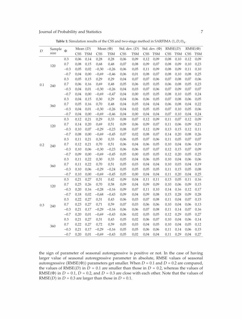
Journal of Probability and Statistics 7
Table 1: Simulation results of the CSS and two-stage method in SARFIMA (1, D, 0)4.
DSamplesize Φ
Mean (D) Mean (Φ) Std. dev. (D) Std. dev. (Φ) RMSE(D) RMSE(Φ)CSS TSM CSS TSM CSS TSM CSS TSM CSS TSM CSS TSM
0.1
120
0.3 0,06 0,14 0,28 0,28 0,06 0,09 0,12 0,09 0,08 0,10 0,12 0,090.7 0,08 0,15 0,68 0,48 0,07 0,08 0,09 0,07 0,08 0,09 0,10 0,23−0.3 0,05 0,02 −0,30 −0,26 0,06 0,05 0,11 0,09 0,08 0,09 0,11 0,10−0.7 0,04 0,00 −0,69 −0,46 0,06 0,01 0,08 0,07 0,08 0,10 0,08 0,25
240
0.3 0,05 0,15 0,29 0,29 0,04 0,07 0,07 0,06 0,07 0,08 0,07 0,060.7 0,06 0,16 0,69 0,48 0,05 0,06 0,05 0,05 0,06 0,08 0,05 0,23−0.3 0,04 0,01 −0,30 −0,26 0,04 0,03 0,07 0,06 0,07 0,09 0,07 0,07−0.7 0,04 0,00 −0,69 −0,47 0,04 0,00 0,05 0,05 0,08 0,10 0,05 0,24
360
0.3 0,04 0,15 0,30 0,29 0,04 0,06 0,06 0,05 0,07 0,08 0,06 0,050.7 0,05 0,16 0,70 0,48 0,04 0,05 0,04 0,04 0,06 0,08 0,04 0,22−0.3 0,04 0,01 −0,30 −0,26 0,04 0,02 0,05 0,05 0,07 0,10 0,05 0,06−0.7 0,04 0,00 −0,69 −0,46 0,04 0,00 0,04 0,04 0,07 0,10 0,04 0,24
0.2
120
0.3 0,12 0,21 0,29 0,33 0,08 0,07 0,12 0,09 0,11 0,07 0,12 0,090.7 0,14 0,20 0,69 0,51 0,09 0,06 0,09 0,07 0,11 0,06 0,09 0,21−0.3 0,10 0,07 −0,29 −0,23 0,08 0,07 0,12 0,09 0,13 0,15 0,12 0,11−0.7 0,08 0,00 −0,69 −0,45 0,07 0,02 0,08 0,07 0,14 0,20 0,08 0,26
240
0.3 0,11 0,21 0,30 0,33 0,06 0,05 0,07 0,06 0,11 0,05 0,07 0,070.7 0,12 0,21 0,70 0,51 0,06 0,04 0,06 0,05 0,10 0,04 0,06 0,19−0.3 0,10 0,06 −0,30 −0,23 0,06 0,06 0,07 0,07 0,12 0,15 0,07 0,09−0.7 0,09 0,00 −0,69 −0,45 0,05 0,00 0,05 0,05 0,12 0,20 0,05 0,25
360
0.3 0,11 0,22 0,30 0,33 0,05 0,04 0,06 0,05 0,10 0,04 0,06 0,060.7 0,11 0,22 0,70 0,51 0,05 0,03 0,04 0,04 0,10 0,03 0,04 0,19−0.3 0,10 0,06 −0,29 −0,24 0,05 0,05 0,05 0,05 0,11 0,15 0,05 0,08−0.7 0,10 0,00 −0,69 −0,45 0,05 0,00 0,04 0,04 0,11 0,20 0,04 0,25
0.3
120
0.3 0,21 0,27 0,31 0,42 0,09 0,04 0,11 0,11 0,13 0,05 0,11 0,160.7 0,25 0,26 0,70 0,58 0,09 0,04 0,09 0,09 0,10 0,06 0,09 0,15−0.3 0,20 0,16 −0,28 −0,16 0,09 0,07 0,11 0,10 0,14 0,16 0,12 0,17−0.7 0,18 0,02 −0,68 −0,43 0,09 0,04 0,09 0,08 0,15 0,28 0,09 0,28
240
0.3 0,22 0,27 0,31 0,43 0,06 0,03 0,07 0,08 0,11 0,04 0,07 0,150.7 0,23 0,27 0,71 0,59 0,07 0,03 0,06 0,06 0,10 0,04 0,06 0,13−0.3 0,21 0,17 −0,29 −0,16 0,06 0,06 0,07 0,08 0,11 0,14 0,07 0,16−0.7 0,20 0,01 −0,69 −0,43 0,06 0,02 0,05 0,05 0,12 0,29 0,05 0,27
360
0.3 0,21 0,27 0,31 0,43 0,05 0,02 0,06 0,07 0,10 0,04 0,06 0,140.7 0,22 0,27 0,72 0,59 0,05 0,03 0,04 0,05 0,10 0,04 0,05 0,12−0.3 0,21 0,17 −0,29 −0,16 0,05 0,05 0,06 0,06 0,11 0,14 0,06 0,15−0.7 0,20 0,01 −0,69 −0,43 0,05 0,02 0,04 0,04 0,11 0,29 0,04 0,27
the sign of parameter of seasonal autoregressive is positive or not. In the case of havinglarger value of seasonal autoregressive parameter in absolute, RMSE values of seasonalautoregressive (RMSE(Φ)) parameters get smaller. When D = 0.1 and D = 0.2 are compared,the values of RMSE(D) in D = 0.1 are smaller than those in D = 0.2, whereas the values ofRMSE(Φ) in D = 0.1, D = 0.2, and D = 0.3 are close with each other. Note that the values ofRMSE(D) in D = 0.3 are larger than those in D = 0.1.
8 Journal of Probability and Statistics
According to Table 1, when the two-staged method is executed, it is observed thatthe sample size does not affect significantly the values of RMSE, especially for RMSE(Φ)when Φ = −0.7. However, when the absolute value estimated of seasonal autoregressiveparameter increases, the values of RMSE(Φ) increase dramatically in D = 0.1 and D =0.2. The values of RMSE(D) are not affected by both the sign and magnitude of seasonalautoregressive parameter, especially in D = 0.1. It is worth to point out that the values ofRMSE(D) are quite larger for the negative values of seasonal autoregressive parameters inboth D = 0.2 and D = 0.3. It can be inferred from the comparison between D = 0.1 andD = 0.2 that for the negative values of seasonal autoregressive parameter, both the valuesof RMSE(D) and RMSE(Φ) increase gradually while D is increasing. Especially, the valuesof RMSE(Φ) in D = 0.3 get the biggest values when the seasonal autoregressive parameteris negative. Therefore, for the negative values of seasonal autoregressive parameters, we cansay that the estimation error gets bigger while the order of seasonal fractional difference isincreasing.
In Table 2, for the SARFIMA (0, D, 1)s model, the simulation results for different valuesof parameter Θ and sample size n are shown for the CSS and two-staged methods. From thistable, we observe that RMSE values have decreased for the estimated parameters of seasonalfractional difference and seasonal moving average, when the sample size increases, the CSSmethod is executed. It is also seen that the values of RMSE do not change much whetherthe sign of parameter of seasonal moving average is positive or not. In the case of havinglarger value of seasonal moving average parameter for the negative values, RMSE valuesfor seasonal fractionally difference (RMSE(D)) are smaller. When we compare D = 0.1 withD = 0.2, the values of RMSE(D) in D = 0.1 are smaller than those in D = 0.2, whereas thevalues of RMSE(Θ) among D = 0.1, D = 0.2, and D = 0.3 are close with each other. Note thatthe values of RMSE(D) in D = 0.3 are larger than those in D = 0.1.
When Table 2 is examined, it is observed that the values of RMSE(Θ) decrease whensample size increases for two-staged method. However, there is no positive or negativerelations between the value of seasonal moving average parameter and the values ofRMSE(D) and RMSE(Θ) when two-stage method is executed. We would like to remark thatRMSE(Θ) has the smallest value in each sample size for Θ = 0.7 and that values of RMSE(D)are quite big for the negative values of seasonal moving average parameter with respect toits positive values when D = 0.2, and 0.3 in Table 2.
6. Discussions
In the literature, the two-staged method is a widely used method to estimate parameters ofSARFIMA models. Although there is another method called CSS, this method has not beenemployed to estimate the parameters of SARFIMAmodel. In this study, the CSS and the two-stagedmethods are employed to estimate parameters of the SARFIMAmodels by conductinga simulation study, and by this way the properties of these two methods are examined underdifferent parameter settings and sample sizes.
From the results of the simulation, we deduce that when the sample size increases,the CSS method gives more accurate estimates. Besides, we can infer that when seasonalautoregressive parameter in SARFIMA (1, D, 0)4 model gets close to 1 or −1, the parameterestimates of the CSS method have less error. The CSS method produces quite good estimatesfor D when the seasonal autoregressive parameter in SARFIMA (1, D, 0)4 model and theseasonal moving average parameter in SARFIMA (0, D, 1)4 model are positive.
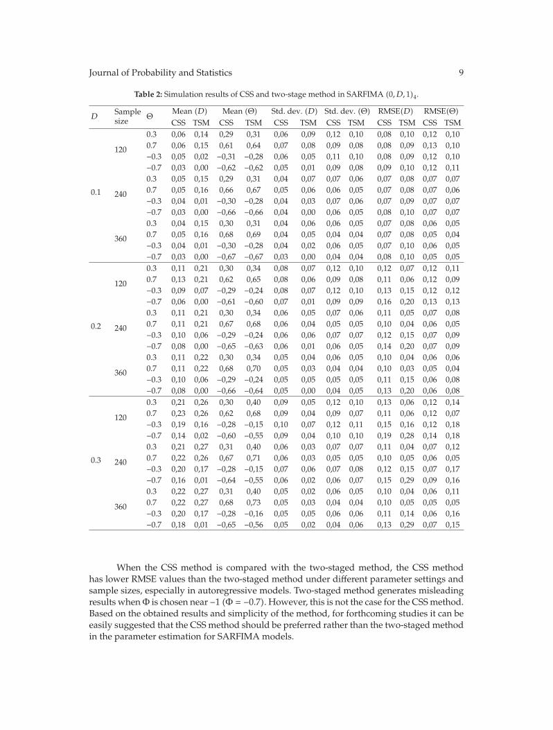
Journal of Probability and Statistics 9
Table 2: Simulation results of CSS and two-stage method in SARFIMA (0, D, 1)4.
DSamplesize Θ
Mean (D) Mean (Θ) Std. dev. (D) Std. dev. (Θ) RMSE(D) RMSE(Θ)CSS TSM CSS TSM CSS TSM CSS TSM CSS TSM CSS TSM
0.1
120
0.3 0,06 0,14 0,29 0,31 0,06 0,09 0,12 0,10 0,08 0,10 0,12 0,100.7 0,06 0,15 0,61 0,64 0,07 0,08 0,09 0,08 0,08 0,09 0,13 0,10−0.3 0,05 0,02 −0,31 −0,28 0,06 0,05 0,11 0,10 0,08 0,09 0,12 0,10−0.7 0,03 0,00 −0,62 −0,62 0,05 0,01 0,09 0,08 0,09 0,10 0,12 0,11
240
0.3 0,05 0,15 0,29 0,31 0,04 0,07 0,07 0,06 0,07 0,08 0,07 0,070.7 0,05 0,16 0,66 0,67 0,05 0,06 0,06 0,05 0,07 0,08 0,07 0,06−0.3 0,04 0,01 −0,30 −0,28 0,04 0,03 0,07 0,06 0,07 0,09 0,07 0,07−0.7 0,03 0,00 −0,66 −0,66 0,04 0,00 0,06 0,05 0,08 0,10 0,07 0,07
360
0.3 0,04 0,15 0,30 0,31 0,04 0,06 0,06 0,05 0,07 0,08 0,06 0,050.7 0,05 0,16 0,68 0,69 0,04 0,05 0,04 0,04 0,07 0,08 0,05 0,04−0.3 0,04 0,01 −0,30 −0,28 0,04 0,02 0,06 0,05 0,07 0,10 0,06 0,05−0.7 0,03 0,00 −0,67 −0,67 0,03 0,00 0,04 0,04 0,08 0,10 0,05 0,05
0.2
120
0.3 0,11 0,21 0,30 0,34 0,08 0,07 0,12 0,10 0,12 0,07 0,12 0,110.7 0,13 0,21 0,62 0,65 0,08 0,06 0,09 0,08 0,11 0,06 0,12 0,09−0.3 0,09 0,07 −0,29 −0,24 0,08 0,07 0,12 0,10 0,13 0,15 0,12 0,12−0.7 0,06 0,00 −0,61 −0,60 0,07 0,01 0,09 0,09 0,16 0,20 0,13 0,13
240
0.3 0,11 0,21 0,30 0,34 0,06 0,05 0,07 0,06 0,11 0,05 0,07 0,080.7 0,11 0,21 0,67 0,68 0,06 0,04 0,05 0,05 0,10 0,04 0,06 0,05−0.3 0,10 0,06 −0,29 −0,24 0,06 0,06 0,07 0,07 0,12 0,15 0,07 0,09−0.7 0,08 0,00 −0,65 −0,63 0,06 0,01 0,06 0,05 0,14 0,20 0,07 0,09
360
0.3 0,11 0,22 0,30 0,34 0,05 0,04 0,06 0,05 0,10 0,04 0,06 0,060.7 0,11 0,22 0,68 0,70 0,05 0,03 0,04 0,04 0,10 0,03 0,05 0,04−0.3 0,10 0,06 −0,29 −0,24 0,05 0,05 0,05 0,05 0,11 0,15 0,06 0,08−0.7 0,08 0,00 −0,66 −0,64 0,05 0,00 0,04 0,05 0,13 0,20 0,06 0,08
0.3
120
0.3 0,21 0,26 0,30 0,40 0,09 0,05 0,12 0,10 0,13 0,06 0,12 0,140.7 0,23 0,26 0,62 0,68 0,09 0,04 0,09 0,07 0,11 0,06 0,12 0,07−0.3 0,19 0,16 −0,28 −0,15 0,10 0,07 0,12 0,11 0,15 0,16 0,12 0,18−0.7 0,14 0,02 −0,60 −0,55 0,09 0,04 0,10 0,10 0,19 0,28 0,14 0,18
240
0.3 0,21 0,27 0,31 0,40 0,06 0,03 0,07 0,07 0,11 0,04 0,07 0,120.7 0,22 0,26 0,67 0,71 0,06 0,03 0,05 0,05 0,10 0,05 0,06 0,05−0.3 0,20 0,17 −0,28 −0,15 0,07 0,06 0,07 0,08 0,12 0,15 0,07 0,17−0.7 0,16 0,01 −0,64 −0,55 0,06 0,02 0,06 0,07 0,15 0,29 0,09 0,16
360
0.3 0,22 0,27 0,31 0,40 0,05 0,02 0,06 0,05 0,10 0,04 0,06 0,110.7 0,22 0,27 0,68 0,73 0,05 0,03 0,04 0,04 0,10 0,05 0,05 0,05−0.3 0,20 0,17 −0,28 −0,16 0,05 0,05 0,06 0,06 0,11 0,14 0,06 0,16−0.7 0,18 0,01 −0,65 −0,56 0,05 0,02 0,04 0,06 0,13 0,29 0,07 0,15
When the CSS method is compared with the two-staged method, the CSS methodhas lower RMSE values than the two-staged method under different parameter settings andsample sizes, especially in autoregressive models. Two-staged method generates misleadingresults whenΦ is chosen near −1 (Φ = −0.7). However, this is not the case for the CSSmethod.Based on the obtained results and simplicity of the method, for forthcoming studies it can beeasily suggested that the CSS method should be preferred rather than the two-staged methodin the parameter estimation for SARFIMA models.
10 Journal of Probability and Statistics
References
[1] R. T. Baillie, “Long memory processes and fractional integration in econometrics,” Journal of Econo-metrics, vol. 73, no. 1, pp. 5–59, 1996.
[2] U. Hassler and J. Wolters, “On the power of unit root tests against fractional alternatives,” EconomicsLetters, vol. 45, no. 1, pp. 1–5, 1994.
[3] L. Giraitis and R. Leipus, “A generalized fractionally differencing approach in long-memory model-ing,” Lithuanian Mathematical Journal, vol. 35, no. 1, pp. 53–65, 1995.
[4] J. Arteche and P. M. Robinson, “Semiparametric inference in seasonal and cyclical long memoryprocesses,” Journal of Time Series Analysis, vol. 21, no. 1, pp. 1–25, 2000.
[5] C.-F. Chung, “A generalized fractionally integrated autoregressive moving-average process,” Journalof Time Series Analysis, vol. 17, no. 2, pp. 111–140, 1996.
[6] C. Velasco and P. M. Robinson, “Whittle pseudo-maximum likelihood estimation for nonstationarytime series,” Journal of the American Statistical Association, vol. 95, no. 452, pp. 1229–1243, 2000.
[7] L. Giraitis, J. Hidalgo, and P. M. Robinson, “Gaussian estimation of parametric spectral density withunknown pole,” The Annals of Statistics, vol. 29, no. 4, pp. 987–1023, 2001.
[8] M. O. Haye, “Asymptotic behavior of the empirical process for Gaussian data presenting seasonallong-memory,” European Series in Applied and Industrial Mathematics, vol. 6, pp. 293–309, 2002.
[9] V. A. Reisen, A. L. Rodrigues, and W. Palma, “Estimating seasonal long-memory processes: a MonteCarlo study,” Journal of Statistical Computation and Simulation, vol. 76, no. 4, pp. 305–316, 2006.
[10] V. A. Reisen, A. L. Rodrigues, and W. Palma, “Estimation of seasonal fractionally integratedprocesses,” Computational Statistics & Data Analysis, vol. 50, no. 2, pp. 568–582, 2006.
[11] W. Palma and N. H. Chan, “Efficient estimation of seasonal long-range-dependent processes,” Journalof Time Series Analysis, vol. 26, no. 6, pp. 863–892, 2005.
[12] S. Porter-Hudak, “An application of the seasonal fractionally differenced model to the monetaryaggregates,” Journal of American Statistical Association, vol. 85, no. 410, pp. 338–344, 1990.
[13] B. K. Ray, “Long-range forecasting of IBM product revenues using a seasonal fractionally differencedARMA model,” International Journal of Forecasting, vol. 9, no. 2, pp. 255–269, 1993.
[14] A. Montanari, R. Rosso, and M. S. Taqqu, “A seasonal fractional ARIMA model applied to the NileRiver monthly flows at Aswan,”Water Resources Research, vol. 36, no. 5, pp. 1249–1259, 2000.
[15] B. Candelon and L. A. Gil-Alana, “Seasonal and long-run fractional integration in the IndustrialProduction Indexes of some Latin American countries,” Journal of Policy Modeling, vol. 26, no. 3,pp. 301–313, 2004.
[16] L. A. Gil-Alana, “Seasonal long memory in the aggregate output,” Economics Letters, vol. 74, no. 3,pp. 333–337, 2002.
[17] E. H. M. Brietzke, S. R. C. Lopes, and C. Bisognin, “A closed formula for the Durbin-Levinson’salgorithm in seasonal fractionally integrated processes,” Mathematical and Computer Modelling, vol.42, no. 11-12, pp. 1191–1206, 2005.
[18] J. R.M. Hosking, “Modeling persistence in hydrological time series using fractional differencing,”Water Resources Research, vol. 20, no. 12, pp. 1898–1908, 1984.
[19] O. Darne, V. Guiraud, andM. Terraza, “Forecasts of the Seasonal Fractional Integrated Series,” Journalof Forecasting, vol. 23, no. 1, pp. 1–17, 2004.
[20] C.-F. Chung and R. T. Baillie, “Small sample bias in conditional sum-of-squares estimators offractionally integrated ARMAmodels,” Empirical Economics, vol. 18, no. 4, pp. 791–806, 1993.
[21] M. Ooms and U. Hassler, “On the effect of seasonal adjustment on the log-periodogram regression,”Economics Letters, vol. 56, no. 2, pp. 135–141, 1997.
[22] U. Hassler and J. Wolters, “Longmemory in inflation rates: international evidence,” Journal of Business& Economic Statistics, vol. 13, no. 1, pp. 37–45, 1995.
[23] L. A. Gil-Alana and P. M. Robinson, “Testing of seasonal fractional integration in UK and Japaneseconsumption and income,” Journal of Applied Econometrics, vol. 16, no. 2, pp. 95–114, 2001.
[24] J. Arteche, “Semiparametric robust tests on seasonal or cyclical long memory time series,” Journal ofTime Series Analysis, vol. 23, no. 3, pp. 251–285, 2002.
[25] L. A. Gil-Alana, “Seasonal misspecification in the context of fractionally integrated univariate timeseries,” Computational Economics, vol. 22, no. 1, pp. 65–74, 2003.

Journal of Probability and Statistics 11
[26] L. Gil-Alana, “Modelling seasonality with fractionally integrated processes,” Tech. Rep. number, 2003.[27] S. Bertelli andM. Caporin, “A note on calculating autocovariances of long-memory processes,” Journal
of Time Series Analysis, vol. 23, no. 5, pp. 503–508, 2002.[28] J. Beran, Statistics for Long-Memory Processes, vol. 61, Chapman & Hall/CRC, New York, NY, USA,
1994.