SSERC 2014/15

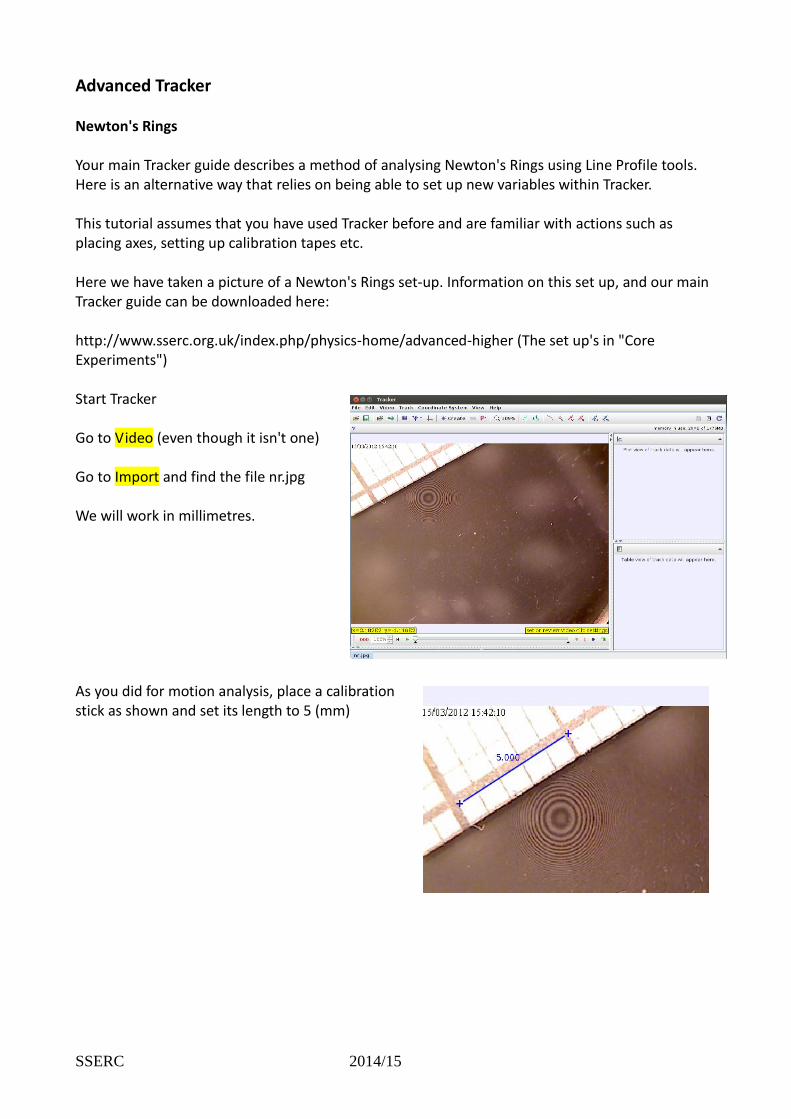
Advanced Tracker Newton's Rings Your main Tracker guide describes a method of analysing Newton's Rings using Line Profile tools. Here is an alternative way that relies on being able to set up new variables within Tracker. This tutorial assumes that you have used Tracker before and are familiar with actions such as placing axes, setting up calibration tapes etc. Here we have taken a picture of a Newton's Rings set-up. Information on this set up, and our main Tracker guide can be downloaded here: http://www.sserc.org.uk/index.php/physics-home/advanced-higher (The set up's in "Core Experiments") Start Tracker Go to Video (even though it isn't one) Go to Import and find the file nr.jpg We will work in millimetres. As you did for motion analysis, place a calibration stick as shown and set its length to 5 (mm)

SSERC 2014/15

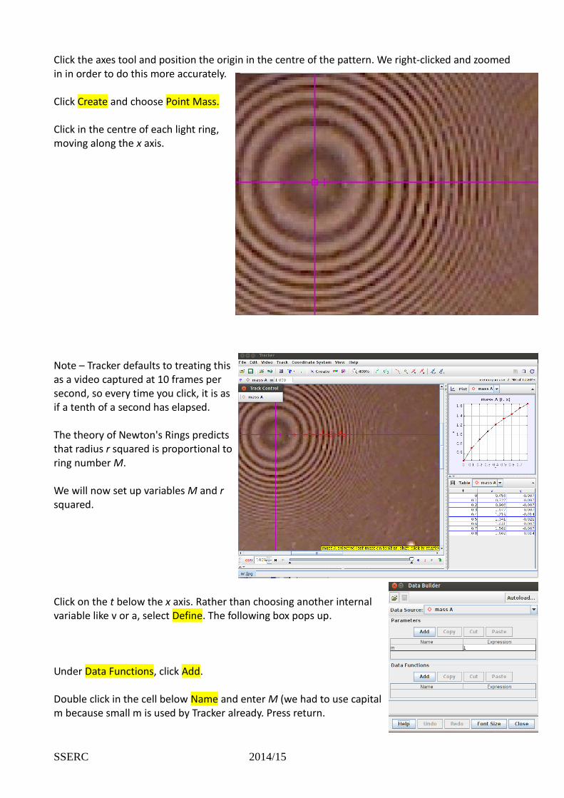
Click the axes tool and position the origin in the centre of the pattern. We right-clicked and zoomed in in order to do this more accurately. Click Create and choose Point Mass. Click in the centre of each light ring, moving along the x axis. Note – Tracker defaults to treating this as a video captured at 10 frames per second, so every time you click, it is as if a tenth of a second has elapsed. The theory of Newton's Rings predicts that radius r squared is proportional to ring number M. We will now set up variables M and r squared. Click on the t below the x axis. Rather than choosing another internal variable like v or a, select Define. The following box pops up. Under Data Functions, click Add. Double click in the cell below Name and enter M (we had to use capital m because small m is used by Tracker already. Press return.

SSERC 2014/15

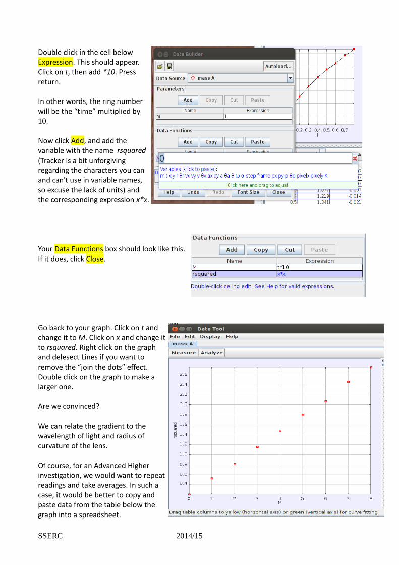
Double click in the cell below Expression. This should appear. Click on t, then add *10. Press return. In other words, the ring number will be the “time” multiplied by 10. Now click Add, and add the variable with the name rsquared (Tracker is a bit unforgiving regarding the characters you can and can't use in variable names, so excuse the lack of units) and the corresponding expression x*x. Your Data Functions box should look like this. If it does, click Close. Go back to your graph. Click on t and change it to M. Click on x and change it to rsquared. Right click on the graph and delesect Lines if you want to remove the “join the dots” effect. Double click on the graph to make a larger one. Are we convinced? We can relate the gradient to the wavelength of light and radius of curvature of the lens. Of course, for an Advanced Higher investigation, we would want to repeat readings and take averages. In such a case, it would be better to copy and paste data from the table below the graph into a spreadsheet.

SSERC 2014/15

Measuring g by flow rate.

The following theory is consistent with Bernoulli’s theorem, but has been

recast in terms more accessible to an Advanced Higher student.

Note that we will use non-standard units of cm³ and cm s¯¹ for

convenience.

Imagine water emerging from a tap at a rate of X cm³ s¯¹

Suppose the water has a velocity of u cm s¯¹

Suppose the stream has a radius of r1 at this point

The cross sectional area A1 of the stream is therefore π r12

It follows that the volume of water per second X = A1u.

Rearranging: u = X/A1

As the water streams downwards, it will speed up. The volume per second X will not change – if

X cm³ leaves the tap per second, X cm³ enters the sink every second.

Suppose that at some point, the velocity of the water has increased to v.

v = X/A2 where A2 is the cross sectional area of the stream at this point.

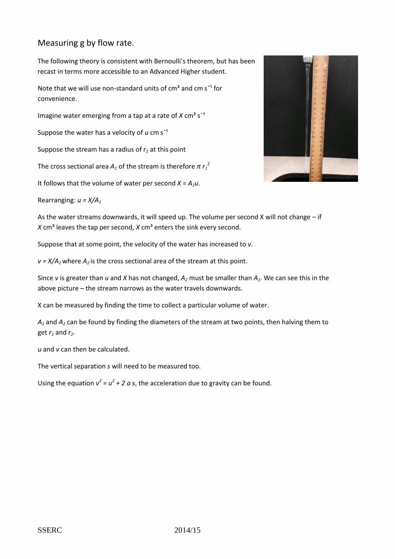
Since v is greater than u and X has not changed, A2 must be smaller than A1. We can see this in the

above picture – the stream narrows as the water travels downwards.

X can be measured by finding the time to collect a particular volume of water.

A1 and A2 can be found by finding the diameters of the stream at two points, then halving them to

get r1 and r2.

u and v can then be calculated.

The vertical separation s will need to be measured too.

Using the equation v2 = u2 + 2 a s, the acceleration due to gravity can be found.

SSERC 2014/15

Making measurements

We have seen advice stating that a travelling microscope should be used to find the diameter of the

stream. We have two alternative methods. Both involve photographing the stream with a ruler

alongside it. The ruler must be in the same plane as the stream.

The photograph can then be projected and measurements made. These measurements are then

scaled, the scale being determined by the ruler.

Alternatively, the photograph can be loaded into the free Tracker application.

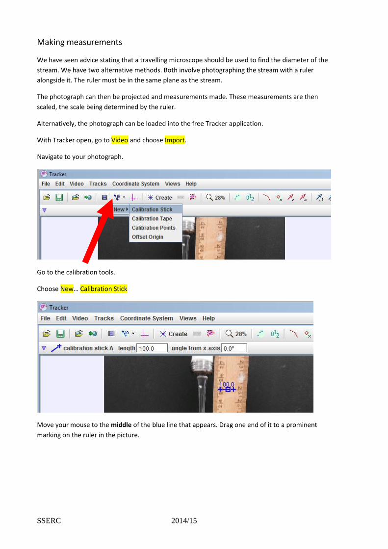
With Tracker open, go to Video and choose Import.

Navigate to your photograph.

Go to the calibration tools.

Choose New… Calibration Stick

Move your mouse to the middle of the blue line that appears. Drag one end of it to a prominent

marking on the ruler in the picture.

SSERC 2014/15

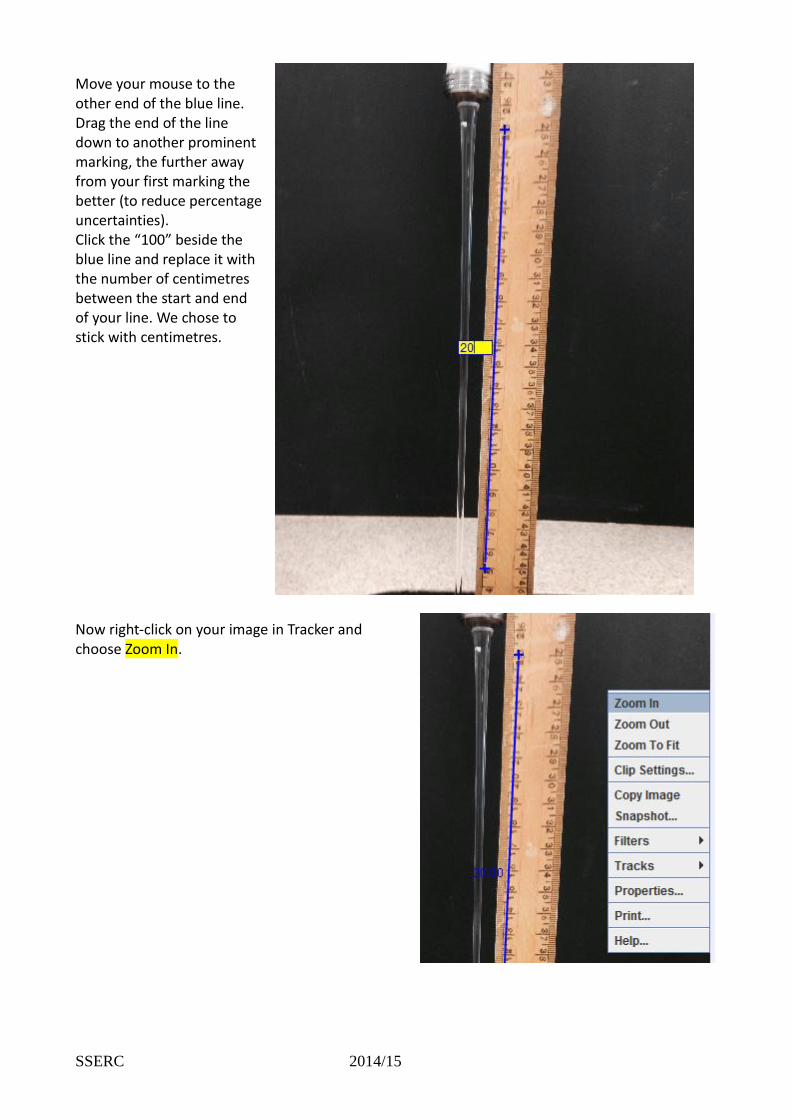
Move your mouse to the other end of the blue line. Drag the end of the line down to another prominent marking, the further away from your first marking the better (to reduce percentage uncertainties). Click the “100” beside the blue line and replace it with the number of centimetres between the start and end of your line. We chose to stick with centimetres. Now right-click on your image in Tracker and choose Zoom In.

SSERC 2014/15

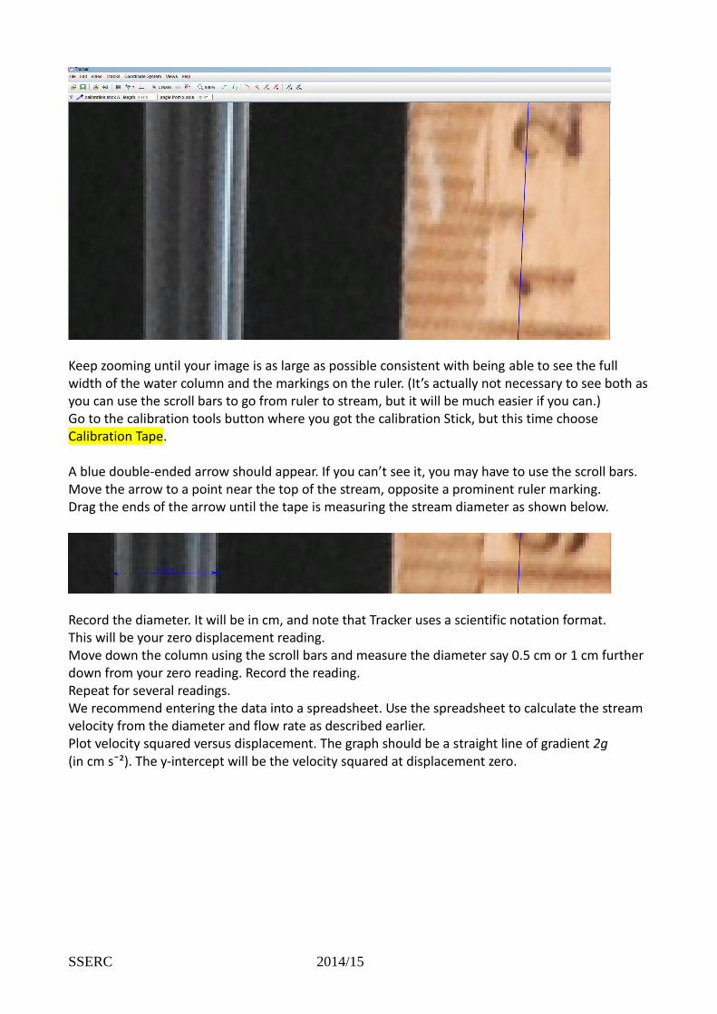
Keep zooming until your image is as large as possible consistent with being able to see the full width of the water column and the markings on the ruler. (It’s actually not necessary to see both as you can use the scroll bars to go from ruler to stream, but it will be much easier if you can.) Go to the calibration tools button where you got the calibration Stick, but this time choose Calibration Tape. A blue double-ended arrow should appear. If you can’t see it, you may have to use the scroll bars. Move the arrow to a point near the top of the stream, opposite a prominent ruler marking. Drag the ends of the arrow until the tape is measuring the stream diameter as shown below.

Record the diameter. It will be in cm, and note that Tracker uses a scientific notation format. This will be your zero displacement reading. Move down the column using the scroll bars and measure the diameter say 0.5 cm or 1 cm further down from your zero reading. Record the reading. Repeat for several readings. We recommend entering the data into a spreadsheet. Use the spreadsheet to calculate the stream velocity from the diameter and flow rate as described earlier. Plot velocity squared versus displacement. The graph should be a straight line of gradient 2g (in cm s¯²). The y-intercept will be the velocity squared at displacement zero.

SSERC 2014/15

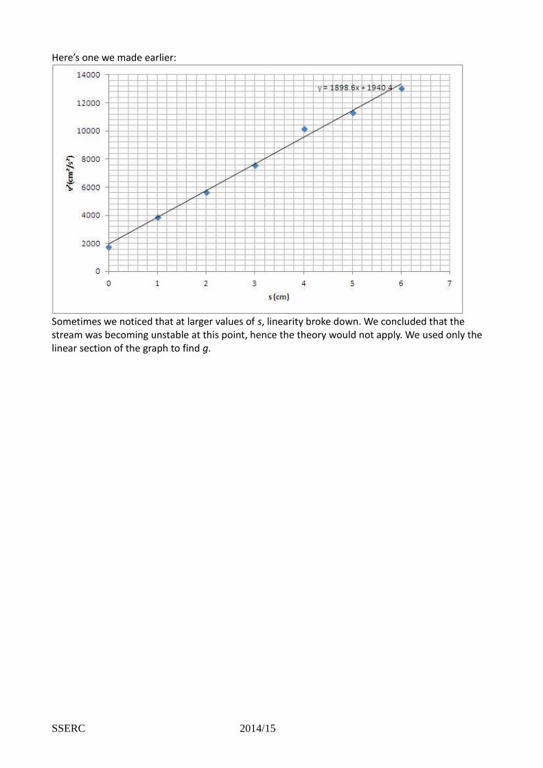
Here’s one we made earlier:

Sometimes we noticed that at larger values of s, linearity broke down. We concluded that the stream was becoming unstable at this point, hence the theory would not apply. We used only the linear section of the graph to find g.

SSERC 2014/15

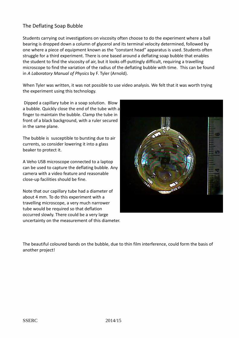
The Deflating Soap Bubble Students carrying out investigations on viscosity often choose to do the experiment where a ball bearing is dropped down a column of glycerol and its terminal velocity determined, followed by one where a piece of equipment known as the “constant head” apparatus is used. Students often struggle for a third experiment. There is one based around a deflating soap bubble that enables the student to find the viscosity of air, but it looks off-puttingly difficult, requiring a travelling microscope to find the variation of the radius of the deflating bubble with time. This can be found in A Laboratory Manual of Physics by F. Tyler (Arnold). When Tyler was written, it was not possible to use video analysis. We felt that it was worth trying the experiment using this technology. Dipped a capillary tube in a soap solution. Blow a bubble. Quickly close the end of the tube with a finger to maintain the bubble. Clamp the tube in front of a black background, with a ruler secured in the same plane. The bubble is susceptible to bursting due to air currents, so consider lowering it into a glass beaker to protect it. A Veho USB microscope connected to a laptop can be used to capture the deflating bubble. Any camera with a video feature and reasonable close-up facilities should be fine. Note that our capillary tube had a diameter of about 4 mm. To do this experiment with a travelling microscope, a very much narrower tube would be required so that deflation occurred slowly. There could be a very large uncertainty on the measurement of this diameter. The beautiful coloured bands on the bubble, due to thin film interference, could form the basis of another project!

SSERC 2014/15

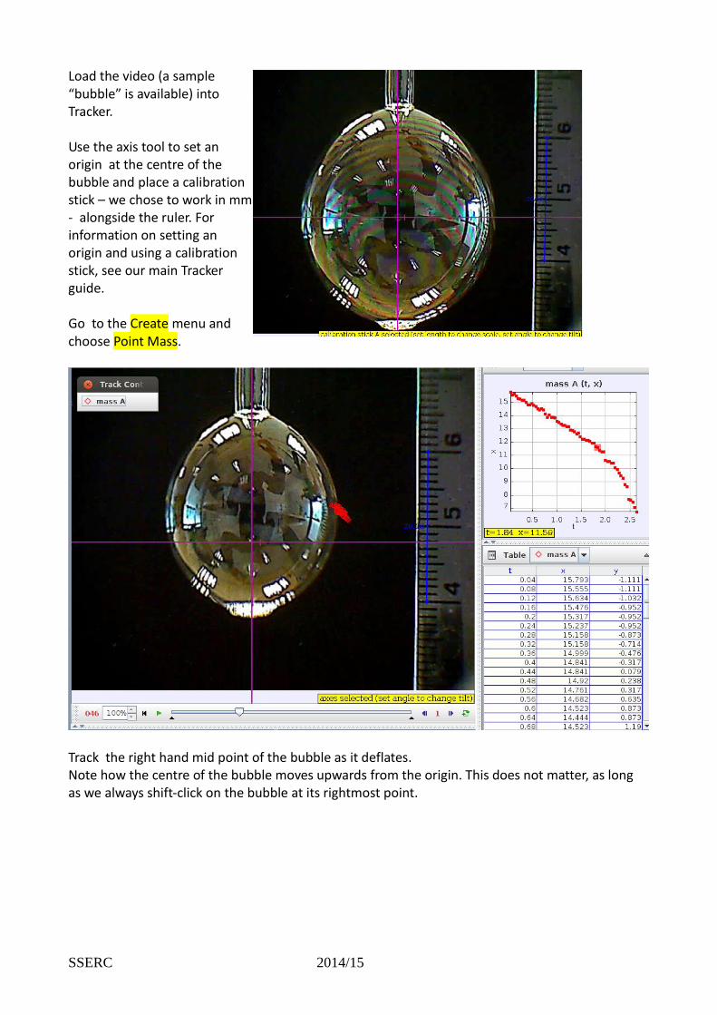
Load the video (a sample “bubble” is available) into Tracker. Use the axis tool to set an origin at the centre of the bubble and place a calibration stick – we chose to work in mm - alongside the ruler. For information on setting an origin and using a calibration stick, see our main Tracker guide. Go to the Create menu and choose Point Mass.

Track the right hand mid point of the bubble as it deflates. Note how the centre of the bubble moves upwards from the origin. This does not matter, as long as we always shift-click on the bubble at its rightmost point.

SSERC 2014/15

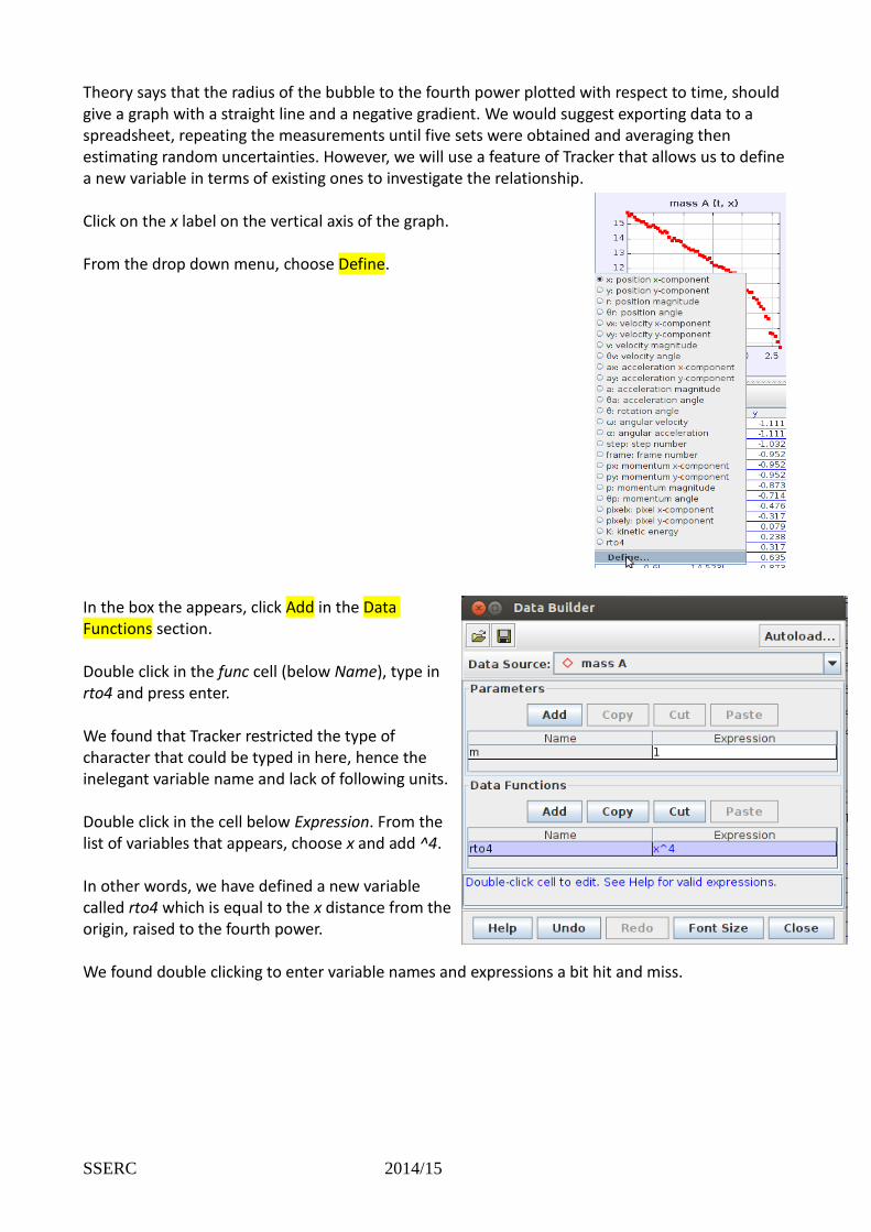
Theory says that the radius of the bubble to the fourth power plotted with respect to time, should give a graph with a straight line and a negative gradient. We would suggest exporting data to a spreadsheet, repeating the measurements until five sets were obtained and averaging then estimating random uncertainties. However, we will use a feature of Tracker that allows us to define a new variable in terms of existing ones to investigate the relationship. Click on the x label on the vertical axis of the graph. From the drop down menu, choose Define. In the box the appears, click Add in the Data Functions section. Double click in the func cell (below Name), type in rto4 and press enter. We found that Tracker restricted the type of character that could be typed in here, hence the inelegant variable name and lack of following units. Double click in the cell below Expression. From the list of variables that appears, choose x and add ^4. In other words, we have defined a new variable called rto4 which is equal to the x distance from the origin, raised to the fourth power. We found double clicking to enter variable names and expressions a bit hit and miss.

SSERC 2014/15

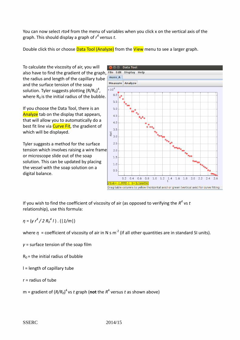
You can now select rto4 from the menu of variables when you click x on the vertical axis of the graph. This should display a graph of r4 versus t. Double click this or choose Data Tool (Analyze) from the View menu to see a larger graph. To calculate the viscosity of air, you will also have to find the gradient of the graph, the radius and length of the capillary tube and the surface tension of the soap solution. Tyler suggests plotting (R/R0)4, where R0 is the initial radius of the bubble. If you choose the Data Tool, there is an Analyze tab on the display that appears, that will allow you to automatically do a best fit line via Curve Fit, the gradient of which will be displayed. Tyler suggests a method for the surface tension which involves raising a wire frame or microscope slide out of the soap solution. This can be updated by placing the vessel with the soap solution on a digital balance. If you wish to find the coefficient of viscosity of air (as opposed to verifying the R4 vs t relationship), use this formula: η = (γ r4 / 2 R0

4 l ) . (|1/m|) where η = coefficient of viscosity of air in N s m-2 (if all other quantities are in standard SI units). γ = surface tension of the soap film R0 = the initial radius of bubble l = length of capillary tube r = radius of tube m = gradient of (R/R0)4 vs t graph (not the R4 versus t as shown above)