Embed Size (px)
Citation preview

Advanced Tools in MacroeconomicsContinuous time models (and methods)
Pontus Rendahl
August 21, 2017

Introduction
I In this lecture we will take a look at models incontinuous, as opposed to discrete, time.
I There are some advantages and disadvantagesI Advantages: Can give closed form solutions even when
they do not exist for the discrete time counterpart. Canbe very fast to solve. Trendier than sourdough bread,fixed gear bicycles, and skinny jeans combined (so if youdo continuous time you need neither).
I Disadvantages: Intuition is a bit tricky. Contractionmapping theorems / convergence results go out thewindow (but can be somewhat brought back). The lattercan create issues for numerical computing. Difficult todeal with certain end-conditions (like finite lives etc.)

Plan for today
I Continuous time methods and models are not as welldocumented as the discrete time cases.
I Proceed through a series of examples
1. The Solow growth model (!)2. The (stochastic) Ramsey growth model3. A monetary economy4. Search and matching
I How to solve (turns out to be pretty easy, and we canapply methods we know from earlier parts of the course)

Plan for tomorrow
I Speeding things up and making it more robustI Little tips and tricks
I Heterogenous agent models in continuous timeI Focus on the Aiyagari model
I Useful list of papers to read
1. “Finite?Difference Methods for Continuous?TimeDynamic Programming” by Candler 2001
2. http://www.princeton.edu/ moll/HACT.pdf
3. http://www.princeton.edu/ moll/WIMM.pdf

The Solow growth model
I The Solow growth model is characterized by the followingequations
Yt = Kαt (AtNt)
1−α
Kt+1 = It + (1− δ)Kt
St = sYt
It = St
At+1 = (1 + g)At
Nt+1 = (1 + η)Nt
I To solve this model we rewrite it in intensive form
xt =Xt
AtNt, for X = {Y ,K , S , I}
The Solow growth model
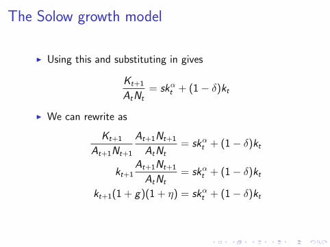
I Using this and substituting in gives
Kt+1
AtNt= skαt + (1− δ)kt
I We can rewrite as
Kt+1
At+1Nt+1
At+1Nt+1
AtNt= skαt + (1− δ)kt
kt+1At+1Nt+1
AtNt= skαt + (1− δ)kt
kt+1(1 + g)(1 + η) = skαt + (1− δ)kt

The Solow growth model
I Ta-daa!
kt+1 =skαt
(1 + g)(1 + η)+
(1− δ)kt(1 + g)(1 + η)
I Balanced growth: kt+1 = kt = k
k =
(g + η + gη + δ
s
) 1α−1
I This is not textbook stuff. Why? Discrete time. Moreelegant solution in continuous time.
The Solow growth model
I Continuous time is not a state in itself, but is the effectof a limit. A derivative is a limit, an integral is a limit, thesum to infinity is a limit, and so on.
I Continuous time is the name we use for the behavior ofan economy as intervals between time periods approacheszero.

The Solow growth model
I The right approach is therefore to derive this behavior asa limit (much like you probably derived derivatives fromits limit definition in high school).
I Eventually you may get so well versed in the limitbehavior that you can set it up directly (like you can saythat the derivative of ln x is equal to 1/x, withoutcalculating limε→0(ln(x + ε)− ln(x))/ε)
I I’m not there yet. I have to do this the complicated way.People like Ben Moll at Princeton is. Take a look at hislecture notes on continuous time stuff. They are great.

The Solow growth model
I Back to the model.
I Suppose that before the length of each time period wasone month. Now we want to rewrite the model on abiweekly frequency.
I It seems reasonable to assume that in two weeks weproduce half as much as we do in one month:Yt = 0.5Kα
t (AtNt)1−α.
I It also seems reasonable that capital depreciates slower,i.e. 0.5δ.

The Solow growth model
I Notice that we still have Nt worker and Kt units ofcapital: Stocks are not affected by the length of timeintervals (although the accumulation of them will).
I The propensity to save is the same, but with half of theincome saving is halved too (and therefore investment)
I What happens to the exogenous processes for At and Nt?

The Solow growth model
I Before
At+1 = (1 + g)At , Nt+1 = (1 + η)Nt
I Now
At+0.5 = (1 + 0.5g)At , Nt+0.5 = (1 + 0.5η)Nt
or
At+0.5 = e0.5gAt , Nt+0.5 = e0.5ηNt ?

The Solow growth model
I It turns out that this choice does not matter much for ourpurpose
I Suppose that the time period is not one month but∆× one month. And suppose that
At+∆ = (1 + ∆g)At
I Rearrange
At+∆ − At
∆= gAt .
I And take limit ∆→ 0
At = gAt
The Solow growth model
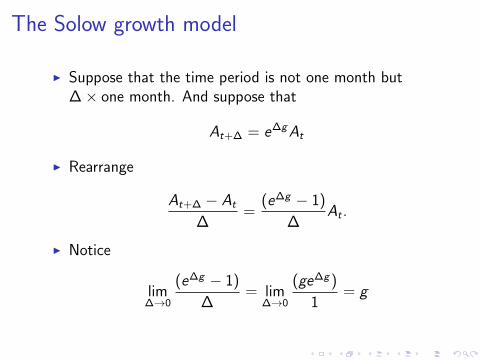
I Suppose that the time period is not one month but∆× one month. And suppose that
At+∆ = e∆gAt
I Rearrange
At+∆ − At
∆=
(e∆g − 1)
∆At .
I Notice
lim∆→0
(e∆g − 1)
∆= lim
∆→0
(ge∆g )
1= g

The Solow growth model
I So
lim∆→0
(e∆g − 1)
∆At = gAt
and thus
At = gAt
I Therefore, it doesn’t matter if At+∆ = (1 + ∆g)At orAt+∆ = e∆gAt . The limits are the same.

The Solow growth model
I Solow growth model in ∆ units of time
Yt = ∆Kαt (AtNt)
1−α
Kt+∆ = It + (1−∆δ)Kt
St = sYt
It = St
At+∆ = (1 + ∆g)At
Nt+∆ = (1 + ∆η)Nt

The Solow growth model
I Substitute and rearrange as before
Kt+∆
At+∆Nt+∆
At+∆Nt+∆
AtNt= s∆kαt + (1−∆δ)kt
kt+∆At+∆Nt+∆
AtNt= s∆kαt + (1−∆δ)kt
kt+∆(1 + ∆g)(1 + ∆η) = s∆kαt + (1−∆δ)kt

The Solow growth model
I Simplify and rearrange
kt+∆(1+∆g)(1 + ∆η) = s∆kαt + (1−∆δ)kt
⇒ kt+∆ − kt = s∆kαt −∆δkt −∆(g + η + ∆gη)kt+∆
⇒ kt+∆ − kt∆
= skαt − δkt − (g + η + ∆gη)kt+∆
I Take limits ∆→ 0
kt = skαt − (g + η + δ)kt
I With steady state
k =
(g + η + δ
s
) 1α−1

The Solow growth model: Solution
I How do you solve this model?
I The equation
kt = skαt − (g + η + δ)kt
is an ODE.
I Declare it as a function with respect to time, t, andcapital, k , in Matlab as
solow = @(t, k) skα − (g + η + δ)k;
I The simulate it for, say 100 units of time, with initialcondition k0 as
[time, capital] = ode45(solow, [0 100], k0);

The Solow growth model: Solution
0 50 100
Outp
ut
-1
0
1
2
0 50 100
Capital
-2
-1
0
1
2
Time (years)
0 50 100
Inves
tmen
t
-3
-2
-1
0
1
Time (years)
0 50 100
Con
sum
ption
-1
0
1
Solow growth model: Saving like China
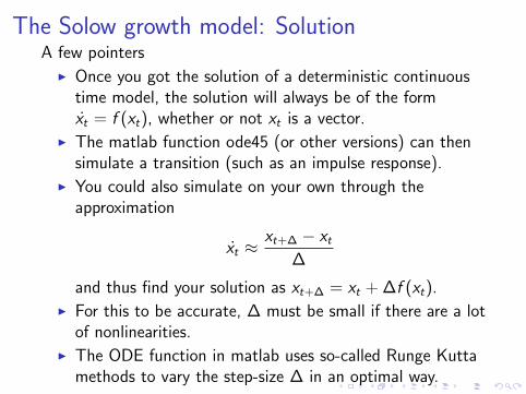
The Solow growth model: SolutionA few pointers
I Once you got the solution of a deterministic continuoustime model, the solution will always be of the formxt = f (xt), whether or not xt is a vector.
I The matlab function ode45 (or other versions) can thensimulate a transition (such as an impulse response).
I You could also simulate on your own through theapproximation
xt ≈xt+∆ − xt
∆
and thus find your solution as xt+∆ = xt + ∆f (xt).I For this to be accurate, ∆ must be small if there are a lot
of nonlinearities.I The ODE function in matlab uses so-called Runge Kutta
methods to vary the step-size ∆ in an optimal way.

The Ramsey growth model
I Now consider the Ramsey growth model (without growth)
v(kt) = maxct ,kt+1
{u(ct) + (1− ρ)v(kt+1)}
s.t. ct + kt+1 = kαt + (1− δ)kt
I In ∆ units of time
v(kt) = maxct ,kt+∆
{∆u(ct) + (1−∆ρ)v(kt+∆)}
s.t. ∆ct + kt+∆ = ∆kαt + (1−∆δ)kt

The Ramsey growth model
I Notice that all flows change when the length of the timeperiod on which they are defined changes. Stocks, k , arethe same.
I I discount the future with 1−∆ρ instead of (1− ρ) (orwith e−∆ρ instead of eρ, but these are, in the limit,equivalent).
I One funny thing: Consumption, c , is still “monthly”consumption, but it now only cost ∆ as much, and I onlyget a ∆ fraction of the utility!
I These assumptions are for technical reasons, and it will(hopefully) soon be clear why they are made.
The Ramsey growth model
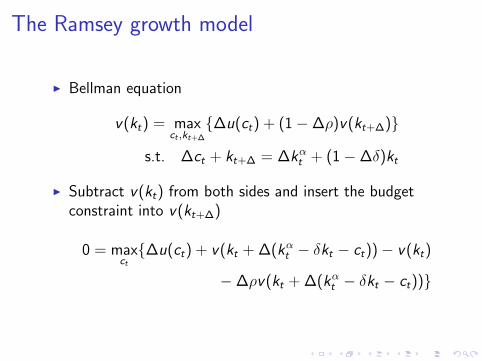
I Bellman equation
v(kt) = maxct ,kt+∆
{∆u(ct) + (1−∆ρ)v(kt+∆)}
s.t. ∆ct + kt+∆ = ∆kαt + (1−∆δ)kt
I Subtract v(kt) from both sides and insert the budgetconstraint into v(kt+∆)
0 = maxct{∆u(ct) + v(kt + ∆(kαt − δkt − ct))− v(kt)
−∆ρv(kt + ∆(kαt − δkt − ct))}

The Ramsey growth model
I From before
0 = maxct{∆u(ct) + v(kt + ∆(kαt − δkt − ct))− v(kt)
−∆ρv(kt + ∆(kαt − δkt − ct))}
I Divide by ∆
0 = maxct{u(ct) +
v(kt + ∆(kαt − δkt − ct))− v(kt)
∆
− ρv(kt + ∆(kαt − δkt − ct))}

The Ramsey growth model
I From before
0 = maxct{u(ct) +
v(kt + ∆(kαt − δkt − ct))− v(kt)
∆
− ρv(kt + ∆(kαt − δkt − ct))}
I Take limit ∆→ 0 and rearrange
ρv(kt) = maxct{u(ct) + v ′(kt)(kαt − δkt − ct)}
I This is know as the Hamilton-Jacobi-Bellman (HJB)equation.
The Ramsey growth model: Solving
I Dropping time notation we have
ρv(k) = maxc{u(c) + v ′(k)(kα − δk − c)}
I This is simple to solve and (can be) blazing fast!
I Why fast? Maximization is trivial: First order condition
u′(c) = v ′(k)
I So if we know v ′(k) we know optimal c without searchingfor it!
The Ramsey growth model: Solving
I Dropping time notation we have
ρv(k) = maxc{u(c) + v ′(k)(kα − δk − c)}
I This is simple to solve and (can be) blazing fast!
I Why fast? Maximization is trivial: First order condition
u′(c) = v ′(k)
I So if we know v ′(k) we know optimal c without searchingfor it!

The Ramsey growth model: Solving
I How do we find v ′(k)?
I Suppose we have hypothetical values of v(k) on auniformly spaced grid of k , K = {k0, k1, . . . , kN} withstepsize ∆k .
I We can then approximate v ′(k) at gridpoint ki (i 6= 1,N)as
v ′(ki) = 0.5(v(ki+1)− v(ki))/∆k
+ 0.5(v(ki)− v(ki−1))/∆k
or
v ′(ki) =v(ki+1)− v(ki−1)
2∆k
The Ramsey growth model: Solving
I and for k1 and kN
v ′(k1) = (v(k2)− v(k1))/∆k
and
v ′(kN) = (v(kN)− v(kN−1))/∆k
I There are many ways of doing this. If you have a vectorof v(k) values – call it V – then dV=gradient(V)/dk.

The Ramsey growth model: Solving
I I prefer an alternative method.
I Construct the matrix D as
D =
−1/dk 1/dk 0 0 . . . 0−0.5/dk 0 0.5/dk 0 . . . 0
0 −0.5/dk 0 0.5/dk . . . 0...
......
.... . . 0
0 0 0 0 −1/dk 1/dk
I Then
v ′(k) ≈ D × v(k)

The Ramsey growth model: Solving
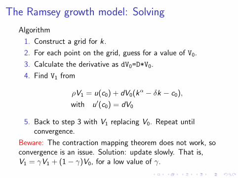
Algorithm
1. Construct a grid for k .
2. For each point on the grid, guess for a value of V0.
3. Calculate the derivative as dV0=D*V0.
4. Find V1 from
ρV1 = u(c0) + dV0(kα − δk − c0),
with u′(c0) = dV0
5. Back to step 3 with V1 replacing V0. Repeat untilconvergence.
Beware: The contraction mapping theorem does not work, soconvergence is an issue. Solution: update slowly. That is,V1 = γV1 + (1− γ)V0, for a low value of γ.
The Ramsey growth model: Solving
Algorithm
1. Construct a grid for k .
2. For each point on the grid, guess for a value of V0.
3. Calculate the derivative as dV0=D*V0.
4. Find V1 from
ρV1 = u(c0) + dV0(kα − δk − c0),
with u′(c0) = dV0
5. Back to step 3 with V1 replacing V0. Repeat untilconvergence.
Beware: The contraction mapping theorem does not work, soconvergence is an issue. Solution: update slowly. That is,V1 = γV1 + (1− γ)V0, for a low value of γ.

The Ramsey growth model: Solving
Alternative algorithm
1. Construct a grid for k .
2. For each point on the grid, guess for a value of V0.
3. Calculate the derivative as dV0=D*V0.
4. Find V1 from
V1 = Γ(u(c0) + dV0(kα − δk − c0)− ρV0) + V0,
with u′(c0) = dV0
5. Back to step 3 with V1 replacing V0. Repeat untilconvergence.
We will take a look at an alternative way of doing thingstomorrow.

The Ramsey growth model: Solving
Alternative vs. standard algorithm
I But to me they sort of look the same
I I.e.
V1 = γ1
ρ(u(c0) + dV0(kα − δk − c0)) + (1− γ)V0
=γ
ρ(u(c0) + dV0(kα − δk − c0)− ρV0) + V0
I So as long as γρ
= Γ they should be identical.

The Ramsey growth model: Euler equation
I Let’s go back to the HJB equation.
ρv(k) = u(c) + v ′(k)(kα − δk − c)
with u′(c) = v ′(k)
I Thus
ρv ′(k) = v ′′(k)(kα − δk − c) + v ′(k)(αkα−1 − δ)
I And
v ′′(k) = u′′(c)c ′(k)
The Ramsey growth model: Euler equation
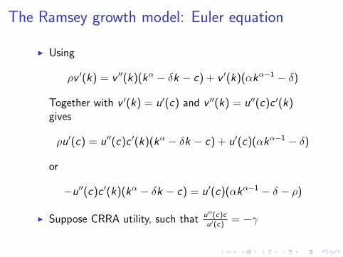
I Using
ρv ′(k) = v ′′(k)(kα − δk − c) + v ′(k)(αkα−1 − δ)
Together with v ′(k) = u′(c) and v ′′(k) = u′′(c)c ′(k)gives
ρu′(c) = u′′(c)c ′(k)(kα − δk − c) + u′(c)(αkα−1 − δ)
or
−u′′(c)c ′(k)(kα − δk − c) = u′(c)(αkα−1 − δ − ρ)
I Suppose CRRA utility, such that u′′(c)cu′(c)
= −γ

The Ramsey growth model: Euler equation
I Then the last equation
−u′′(c)c ′(k)(kα − δk − c) = u′(c)(αkα−1 − δ − ρ)
is equal to
γc ′(k)
c(kα − δk − c) = (αkα−1 − δ − ρ)
I This is the Euler equation in continuous time.

The Ramsey growth model: Euler equationBefore we attempt to solve the Euler equation, recall that wehad
kt+∆ + ∆ct = ∆kαt + (1−∆δ)kt
rearrange
kt+∆ − kt = ∆(kαt − δkt − ct)
Divide with ∆ and take limit ∆→ 0 to get
kt = kαt − δkt − ct
Or dropping time notation
k = kα − δk − c

The Ramsey growth model: Euler equationI Our Euler equation is
c ′(k)
c(kα − δk − c) =
1
γ(αkα−1 − δ − ρ)
or now
γc ′(k)
ck = (αkα−1 − δ − ρ)
I What is c ′(k)k? Recall chain rule
c =∂ct∂t
=∂ct∂k
∂k
∂t= c ′(k)k
I Thus
c
c=
1
γ(αkα−1 − δ − ρ)

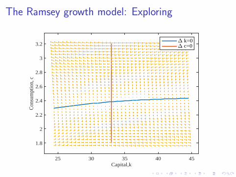
The Ramsey growth model: Exploring
I Two equations
c =c
γ(αkα−1 − δ − ρ)
k = kα − δk − c
I Nullclines
0 = αkα−1 − δ − ρ0 = kα − δk − c

The Ramsey growth model: Exploring
Capital,k25 30 35 40 45
Con
sum
ptio
n, c
1.8
2
2.2
2.4
2.6
2.8
3
3.2" k=0" c=0
The Ramsey growth model: Exploring
Capital,k25 30 35 40 45
Con
sum
ptio
n, c
1.8
2
2.2
2.4
2.6
2.8
3
3.2" k=0" c=0
The Ramsey growth model: Exploring
Capital,k25 30 35 40 45
Con
sum
ptio
n, c
1.8
2
2.2
2.4
2.6
2.8
3
3.2" k=0" c=0Explosive paths

The Ramsey growth model: Exploring
Capital,k25 30 35 40 45
Con
sum
ptio
n, c
1.8
2
2.2
2.4
2.6
2.8
3
3.2" k=0" c=0Explosive pathsSaddle path
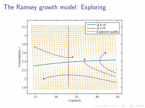
The Ramsey growth model: Exploring
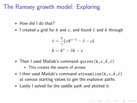
I How did I do that?
I I created a grid for k and c , and found c and k through
c =c
γ(αkα−1 − δ − ρ)
k = kα − δk − c
I Then I used Matlab’s command quiver(k,c,k,c)I This creates the swarm of arrows
I I then used Matlab’s command streamline(k,c,k,c)at various starting values to get the explosive paths.
I Lastly I solved for the saddle path and plotted it.

The Ramsey growth model: Euler equation solution
I Back to the “recursive” Euler
c ′(k)
c(kα − δk − c) =
1
γ(αkα−1 − δ − ρ)
I Solve for c
c =c ′(k)(kα − δk)
1γ
(αkα−1 − δ − ρ) + c ′(k)
The Ramsey growth model: Euler equation solution
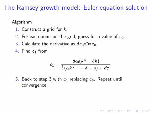
Algorithm
1. Construct a grid for k .
2. For each point on the grid, guess for a value of c0.
3. Calculate the derivative as dc0=D*c0.
4. Find c1 from
c1 =dc0(kα − δk)
1γ
(αkα−1 − δ − ρ) + dc0
5. Back to step 3 with c1 replacing c0. Repeat untilconvergence.
Beware: No guaranteed convergence. Update slowly. Fewergridpoints appears to provide some stability.

The Ramsey growth model: Euler equation solution
Algorithm
1. Construct a grid for k .
2. For each point on the grid, guess for a value of c0.
3. Calculate the derivative as dc0=D*c0.
4. Find c1 from
c1 =dc0(kα − δk)
1γ
(αkα−1 − δ − ρ) + dc0
5. Back to step 3 with c1 replacing c0. Repeat untilconvergence.
Beware: No guaranteed convergence. Update slowly. Fewergridpoints appears to provide some stability.

The Ramsey growth model: Solution
kt
4 5 6 7 8 9
_ kt
-0.25
-0.2
-0.15
-0.1
-0.05
0
0.05
0.1
0.15
0.2
Value function iteration
Euler equation iteration
Figure: Comparison of solution methods.

The Ramsey growth model: Solution
Time (quarters)
0 10 20 30 40 50 60 70 80 90 100
Cap
ital
6.25
6.3
6.35
6.4
6.45
6.5
6.55
6.6
6.65Comparison
Euler equation iteration
Value function iteration
Figure: Comparison of solution methods.
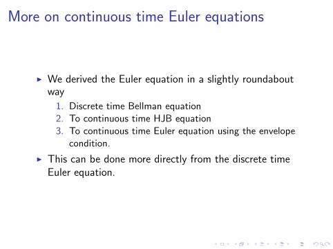
More on continuous time Euler equations
I We derived the Euler equation in a slightly roundaboutway
1. Discrete time Bellman equation2. To continuous time HJB equation3. To continuous time Euler equation using the envelope
condition.
I This can be done more directly from the discrete timeEuler equation.
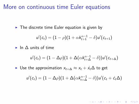
More on continuous time Euler equations
I The discrete time Euler equation is given by
u′(ct) = (1− ρ)(1 + αkα−1t+1 − δ)u′(ct+1)
I In ∆ units of time
u′(ct) = (1−∆ρ)(1 + ∆(αkα−1t+∆ − δ))u′(ct+∆)
I Use the approximation xt+∆ ≈ xt + xt∆ to get
u′(ct) = (1−∆ρ)(1 + ∆(αkα−1t+∆ − δ))u′(ct + ct∆)

More on continuous time Euler equations
u′(ct) = (1−∆ρ)(1 + ∆(αkα−1t+∆ − δ))u′(ct + ct∆)
I Move the u′(ct + ct∆) term to the left-hand side andexpand
u′(ct)− u′(ct + ct∆)
= ∆[αkα−1t+∆ − δ − ρ− ρ∆(αkα−1
t+∆ − δ)]u′(ct + ct∆)
I Divide by ∆ and take limits ∆→ 0
−u′′(ct)ct = [αkα−1t − δ − ρ]u′(ct)

More on continuous time Euler equations
−u′′(ct)ct = [αkα−1t − δ − ρ]u′(ct)
I Lastly, use the CRRA property to get
ctct
=1
γ[αkα−1
t − δ − ρ]

More on continuous time Euler equations
I Now consider a stochastic model with a “good”, g , and a“bad”, b, state
u′(cgt ) = (1−ρ)[(1−p)(1+zgt+1α(kgt+1)α−1−δ)u′(cgt+1)
+ p(1 + zbt+1α(kbt+1)α−1 − δ)u′(cbt+1)]
and
u′(cbt ) = (1−ρ)[(1−q)(1 +zgt+1α(kgt+1)α−1−δ)u′(cgt+1)
+ q(1 + zbt+1α(kbt+1)α−1 − δ)u′(cbt+1)]
I We will focus on the good state (the treatment of thebad state is symmetric)
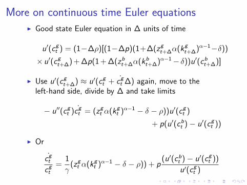
More on continuous time Euler equationsI Good state Euler equation in ∆ units of time
u′(cgt ) = (1−∆ρ)[(1−∆p)(1+∆(zgt+∆α(kgt+∆)α−1−δ))
× u′(cgt+∆) + ∆p(1 + ∆(zbt+∆α(kbt+∆)α−1− δ))u′(cbt+∆)]
I Use u′(cgt+∆) ≈ u′(cgt + cgt ∆) again, move to theleft-hand side, divide by ∆ and take limits
− u′′(cgt )cgt = (zgt α(kgt )α−1 − δ − ρ))u′(cgt )
+ p(u′(cbt )− u′(cgt ))
I Or
cgtcgt
=1
γ(zgt α(kg
t )α−1 − δ − ρ)) + p(u′(cbt )− u′(cgt ))
u′(cgt )

More on continuous time Euler equations
I For the bad state
cbtcbt
=1
γ(zbt α(kb
t )α−1 − δ − ρ)) + q(u′(cbt )− u′(cgt ))
u′(cbt )
I These can be solved using the previous methods. Theonly difference is that we now iterate on two equationsinstead of one. But the procedure is the same.
More on continuous time Euler equations
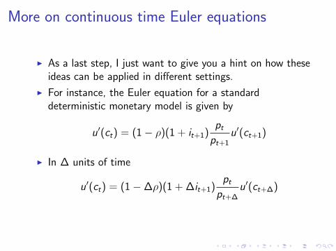
I As a last step, I just want to give you a hint on how theseideas can be applied in different settings.
I For instance, the Euler equation for a standarddeterministic monetary model is given by
u′(ct) = (1− ρ)(1 + it+1)ptpt+1
u′(ct+1)
I In ∆ units of time
u′(ct) = (1−∆ρ)(1 + ∆it+1)pt
pt+∆u′(ct+∆)

More on continuous time Euler equations
I Use the approximations u′(ct+∆) ≈ u′(ct + ct∆), andpt ≈ pt+∆ − pt∆ and rewrite
u′(ct) = (1−∆ρ)(1 + ∆it+∆)pt+∆ − pt∆
pt+∆u′(ct + ct∆)
I Expand
u′(ct) = (1−∆ρ + ∆it+∆ −∆2it+∆ρ)(1− pt∆
pt+∆)u′(ct + ct∆)
I Thus
u′(ct)− u′(ct + ct∆) = (−∆ρ + ∆it+∆ −∆2it+∆ρ)
× (1− pt∆
pt+∆)u′(ct + ct∆)− pt∆
pt+∆u′(ct + ct∆)

More on continuous time Euler equationsI Previous equation
u′(ct)− u′(ct + ct∆) = (−∆ρ + ∆it+∆ −∆2it+∆ρ)
× (1− pt∆
pt+∆)u′(ct + ct∆)− pt∆
pt+∆u′(ct + ct∆)
I Divide by ∆
u′(ct)− u′(ct + ct∆)
∆= (−ρ + it+∆ −∆it+∆ρ)
× (1− pt∆
pt+∆)u′(ct + ct∆)− pt
pt+∆u′(ct + ct∆)
I And take limit ∆→ 0
ctct
=1
γ(it −
ptpt− ρ)

The Mortensen-Pissarides model
I Continuous time is frequently used in the theoretical laborliterature.
I In the remainder of this lecture I will go through theworkhorse model developed by Christopher Pissarides andDale Mortensen.
I In today’s exercise you will be asked to solve this model.

The Mortensen-Pissarides model
I Continuous time is frequently used in the theoretical laborliterature.
I In the remainder of this lecture I will go through theworkhorse model developed by Christopher Pissarides andDale Mortensen.
I In today’s exercise you will be asked to solve this model.

The Mortensen-Pissarides model: Workers
I In the simplest case workers are risk-neutral and value ajob according to
Vt = wt + (1− ρ)[(1− δ)Vt+1 + δUt+1]
I The value of being unemployed is given by
Ut = b + (1− ρ)[(1− ft+1)Ut+1 + ft+1Vt+1]
I The variables wt and ft+1 will be endogenouslydetermined, but we will, for the moment, treat them asexogenous.

The Mortensen-Pissarides model: Workers
I Let’s rewrite these equations in ∆ units of time
Vt = ∆wt + (1−∆ρ)[(1−∆δ)Vt+∆ + ∆δUt+∆]
Ut = ∆b + (1−∆ρ)[(1−∆ft+∆)Ut+1 + ∆ft+∆Vt+1]
I Or
Vt − Vt+∆ = ∆wt −∆[δ + ρ−∆δρ]Vt+∆
+ (1−∆ρ)∆δUt+∆
Ut − Ut+∆ = ∆b −∆[ft+∆ + ρ−∆ft+∆ρ]Ut+∆
+ (1−∆ρ)∆ft+∆Vt+∆

The Mortensen-Pissarides model: Workers
I Dividing through by ∆ gives
Vt − Vt+∆
∆= wt − [δ + ρ−∆δρ]Vt+∆
+ (1−∆ρ)δUt+∆
Ut − Ut+∆
∆= b − [ft+∆ + ρ−∆ft+∆ρ]Ut+∆
+ (1−∆ρ)ft+∆Vt+∆
I And taking limits ∆→ 0 yields
−Vt = wt − (δ + ρ)Vt + δUt
−Ut = b − (ft + ρ)Ut + ftVt

The Mortensen-Pissarides model: Workers
I These equations are commonly written as
ρVt = wt + Vt + δ(Ut − Vt)
ρUt = b + Ut + ft(Vt − Ut)
I Define the surplus of having a job as St = Vt −Ut , that is
(ρ + δ + ft)St = wt − b + St

The Mortensen-Pissarides model: Firms
I The value to a firm of having an employed worker is
Jt = zt − wt + (1− ρ)[(1− δ)Jt+1 + δWt+1]
I We will assume free entry, such that Wt = 0 for all t.
I Following the same procedure as before we find that incontinuous time
(ρ + δ)Jt = zt − wt + Jt

The Mortensen-Pissarides model: Wages
I Collecting equations
ρSt = wt − b + St + (δ + ft)St
ρJt = zt − wt + Jt − δJt
I Wages are set according to Nash bargaining, which arerenegotiated period-by-period
wt = argmax{Jηt S1−ηt }
I First order condition
ηSt = (1− η)Jt

The Mortensen-Pissarides model: Wages
I Expanding
η(wt − b + St + (δ + ft)St) = (1− η)(zt − wt + Jt − δJt)
and using the fact that
St =1− ηη
Jt , and St =1− ηη
Jt
gives
wt = ηb + (1− η)zt + ft(1− η)Jt
I Inserting into the firm’s value function gives
ρJt = η(zt − b) + Jt − (ft(1− η) + δ)Jt

The Mortensen-Pissarides model: Matching
I Suppose that there are vt vacancies posted and utunemployed individuals. Then the measure of matches ina given period is given as
Mt = ∆ψvωt u1−ωt
I The probability that an unemployed individual finds a job,∆ft , is then given as
∆ft =Mt
ut= ∆ψθωt , with θ =
vtut

The Mortensen-Pissarides model: Matching
I The probability that a vacant position is filled, ∆ht , isthen given as
∆ht =Mt
vt= ∆ψθω−1
t
I Suppose the cost of posting a vacancy is given by ∆κ.Free entry then ensures that
κ = htJt
I To see this more clearly, a firm that is considering postinga vacancy faces the optimization problem
maxvt,i{−κ∆vt,i + vt,i∆htJt}

The Mortensen-Pissarides model: Matching
I Lastly, employment, nt = 1− ut , satisfies the law ofmotion
nt+∆ = (1− nt)∆ft + (1−∆δ)nt
which can be rearranged to
nt+∆ − nt∆
= (1− nt)ft − δnt
taking limits
nt = (1− nt)ft − δnt
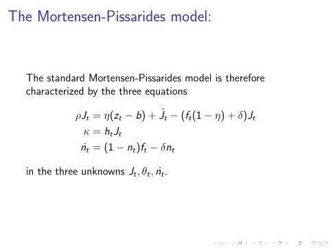
The Mortensen-Pissarides model:
The standard Mortensen-Pissarides model is thereforecharacterized by the three equations
ρJt = η(zt − b) + Jt − (ft(1− η) + δ)Jt
κ = htJt
nt = (1− nt)ft − δnt
in the three unknowns Jt , θt , nt .