Advanced structural and geotechnical analyses for offshore ... · models for different soil types needed. Most existing constitutive models not practical for performing 3D FEA under

Advanced structural and geotechnical analyses

for offshore monopile design: a case study

Go to insert header and footer under

▪ Case study to be presented on

design of Monopile foundation;

▪ Specific planned stop points for

round table discussions;

▪ Round table image presented on

slides where discussions to be held;

▪ Please get involved!

Round Table Format


1.Introduction and

Project Background

2.Overview of Support

Structure Design

Approach

3.Overview of

Geotechnical

Approach

4.3D FEA and

Constitutive Model

5.Geotechnical Analysis

and Soil Reaction

Curve Development

6.Overview of

Structural Approach

Contents

7.Results and

Comparisons

8.Conclusions and Way

Forward

1. Introduction and Project Background


Project BackgroundProject Information

Project Name

Project Type Offshore Wind Farm

235 MW and 252 MW

Scope of Work Offshore High Voltage Substation

Support Structures

Owner

Offshore Contactor

Fabrication Contractor

HV Electrical Contractor


Site ConditionsMetocean Information

Water depth 35m

Max. wave height 12.5m

Wind speed c. 35 m/s

Current velocity 1.1 m/s

Soil Information

0 – 4 m bsf Medium dense SAND

4 – 28 m bsf High strength CLAY


35 – 45 m bsf High strength CLAY



Project Background

Structural Concept

Topside Weight 1150t

Support Structure 7.5m Diameter Monopile – Transition Piece

MP-TP Connection Bolted Flange (grouted skirt)

Cable Deck Integrated

J-tubes External cage mounted on MP

Boat Landings 2 boat landings + access infrastructure

Installation Method Direct drive on-flange

Piling Hammer IHC S-4000Mudline

Transition Piece

Grouted Skirt

Monopile

Transition

Piece Girder

Topside

Boat Landing

J-Tube Cage

Cable Deck

2. Overview of Support Structure Design Approach


Overview of Support Structure Design ApproachGlobal Structure - Limit State Verification

Ultimate and Accidental

Limit State

Dynamic excitation

Non-linear pile interaction

Buckling phenomenon

Directional hydrodynamics

Large deflection (P-Δ)

Ringing interaction

(hydrodynamic)

Fatigue and Serviceability

Limit State

Diffraction

Directional hydrodynamics

Bi-modal swell seas

Significant driving fatigue

Acceleration / motion limits

3. Overview of Geotechnical Approach

▪ Over last 5 to 10 years significant research shown that using design methods typically employed for slender piles of jacket structures not appropriate (e.g. using only p-y curves in 1D model)

▪ New methods recently proposed include additional soil reaction curves in 1D model (PISA Method)

▪ This presentation presents real application of PISA approach to monopile design project

Overview of Geotechnical Approach

H

Distributed lateral load p(z,y)

Distributed moment m(z,𝜃)

Base moment M(𝜃 at base)

Base shear

S(y at base)

zy

2

Overview of Geotechnical Approach

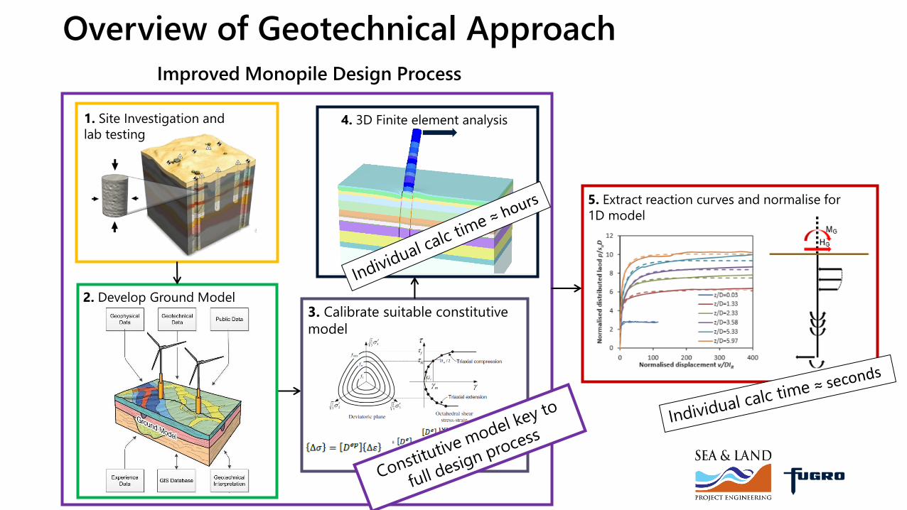
3. Calibrate suitable constitutive

model

Improved Monopile Design Process

1. Site Investigation and

lab testing

2. Develop Ground Model

4. 3D Finite element analysis

5. Extract reaction curves and normalise for

1D model

4. 3D FEA and Constitutive Model

What is a constitutive soil model?

▪ The constitutive soil model is a

mathematical representation of the

mechanical behaviour of the soil

and is fundamental part of FEA of a

geotechnical problem.

Constitutive Model

Is it important?

▪ Yes… it controls the response of the

FEA prediction!

Constitutive Model

Source Code

UDSM

Wrapper

Code

UMAT

Wrapper

Code

Often Important to implement

bespoke soil models to capture the

soil response. Library of bespoke

models for different soil types needed.

▪ Most existing constitutive models

not practical for performing 3D

FEA under cyclic loading

▪ Parallel Iwan Multi-Surface (PIMS)

model developed

▪ Multi-surface models historically

not used due to computational

cost

▪ New practical model termed the

Parallel Iwan Multi-Surface (PIMS)

model developed and

implemented in 3D FEA (Plaxis &

Abaqus) for design FEA

Fugro PIMS Model

Captures site specific

cyclic degradation

esponse

Multi Surface

Anisotropic Model

Reference: Whyte S, Burd H, Martin C, Rattley M. 2019. A

practical total stress multi-surface cyclic degradation plasticity

model. Computers and Geotechnics Journal (Accepted)

Fugro PIMS Model Calibration

-350

-250

-150

-50

50

150

250

350

0 2 4 6 8 10 12 14 16

CUc, k0=1, p'=121kPa (Zdravkovic et al., 2018) CUe, k0=1.3, p'=159 kPa (Fugro Database)

CUc, k0=1.5, p'=32 kPa (Fugro Database) CUc, k0=1.5, p'=130kPa (Fugro Datatbase)

Model Simulation

G0 = 109MPasuc = 136 kPa




(kP

a)

(%)

0 50 100 150 200

0

0.2

0.4

0.6

0.8

1

1.2

Fugro Bolders Bank Undrained Triaxial

Compression Database (x10 Tests)

Calibrated Stress-Strain Backbone Curve

(

-)

(-)

0

2

4

6

8

10

12

0 100 200 300

Dep

th (

m)

G0 (MPa)

BE vh (PISA)

BE hh (PISA)

SCPT1 (PISA)

SCPT2 (PISA)

Weathered till

Unweathered till

(b)

0

2

4

6

8

10

12

0 100 200 300

Dep

th (

m)

suc (kPa)

CUc - historic data

HSV (PISA)

CUc 38mm (PISA)

CUc 100mm (PISA)

FEA Profile

Weathered till

Unweathered till

(a)

1. Calibrate to Normalised Triaxial

extension and compression test data

2. Determine local design profiles

3. Review of model performance to individual

laboratory tests

Fugro PIMS Model Performance

Why go to this trouble?

Pile Load Tests

3D FEA

http://www.eng.ox.ac.uk/geotech/research/PISA/FieldTests

Byrne et al. (2017)

▪ Constitutive soil model used within FEA VERY important, particularly for

complex soil types outside of standard practice!

▪ Fugro PIMS model shows good comparison

to field test data.


▪ How important is the constitutive

model?

▪ What models are being used for

different soil types etc.?

▪ Analysis run time issues with

complex models?

▪ Issue of models becoming black

box tools making certification

difficult?

▪ Difficulty of parameterisation of

models for large wind farms?

Constitutive Models

5. Geotechnical Analysis and Soil Reaction Curve Development

0

5000

10000

15000

20000

25000

0 0.2 0.4 0.6 0.8

Pile

He

ad L

oa

d [

kN

]

Seabed Level Displacement [m]

3D FEA Model

1D Site Specific PISA Model

1D API/DNV p-y Model

▪ Calibration 3D FEA runs performed

to develop site specific reaction

curves

▪ 8 hour run time per 3D FEA

calibration model

▪ 1D model shows very good

comparison to 3D FEA model

▪ API p-y approach shown to be

highly conservative at Seastar site

Seastar Monopile FEA – Monotonic

1D site specific model

1D API p-y model

H3D FE model

Seastar Monopile FEA – Cyclic

1) Calibration to laboratory testing of soils


Byrne et al. (2017)

Laboratory data PIMS model simulation

Cyclic Simple Shear

τxy

3) 3D FEA applying site specific storm4) Extract cyclic degraded reactions

curves for 1D model

0

100

200

300

400

500

0 200 400 600

Mo

me

nt

at M

ud

lin

e (M

Nm

)

Time (s)

Deg

rad

ati

on

Fact

or,

(-)

1.00

0.75

0.50

H

2) Site specific load time history


▪ Experiences of using numerically

derived reaction curves for design?

▪ Experience of using PISA method?

▪ Challenges using such approaches?

▪ Considering layered soils?

▪ How to considering cyclic loading?

Monopile Design Methods

6. Structural Design Overview


ULS Structural Analysis

ULS Time Domain Analysis

Water Level

High Low

Wave Period

Upper Bound

Lower Bound

Seed No.

1

2

34

512

Directions

Topsides Weight

Maximum Mass

Minimum Mass

▪ Iterative pile linearization method

(95th percentile)

▪ Iterative P-Δ loading

▪ Linear buckling

▪ Diffraction (MacCamy – Fuchs)

▪ High-order non-linear wave

▪ 5,800,000 code checks960

simulations


FLS Structural Analysis

▪ Multiple options available for

OHVS Structures

▪ Varying level of complexity and

run time

▪ Limited control over detailed

inputs in commercial software

▪ Which method to use and why?

Time domain

analysis = 50

hours sim.

Frequency

domain spectral

= 20 mins sim.

Time domain

spectral = 2 hours

Time Domain vs Frequency Domain Analysis



Basic Approach

vs

Advanced Approach

▪ Constant hydrodynamic

coefficients vs. directional and

frequency dependent.

▪ Constant stretching vs Wheeler

stretching of wave kinematics

▪ MacCamy-Fuchs Diffraction (w.

phase lag)

Frequency Domain Spectral Analysis

Complex harmonic

regular waves SOLVE

Stress transfer

function

Frequency domain

dynamic analysis –

direct steady state

solution

Deterministic

regular wavesSOLVE

Stress transfer

function

Time domain


direct time

integration solutionTime [s]

Time Domain Spectral Analysis



Advanced Approach

▪ Significantly improved control

over the hydrodynamic load

calculations.

▪ Instantaneous directional, Re and

KC dependent wave force

calculation

▪ MacCamy-Fuchs diffraction

(without phase lag acceleration)

Time Domain Spectral Analysis

𝑴 ሷ𝒙 + 𝑪 ሶ𝒙 + ⋯𝑲 𝒙 = 𝒇(𝒕)𝑉𝑖 Streamlines

0.0

0.5

1.0

1.5

2.0

0 0.5 1 1.5 2

DR

AG

CO

EFFIC

IEN

TC

D[-

]

WAVE FREQUENCY [HZ]

0.0

0.5

1.0

1.5

2.0

0 0.5 1 1.5 2

INER

TIA

CO

EFFIC

IEN

T C

M[-

]

WAVE FREQUENCY [HZ]

Deterministic

regular wavesSOLVE

Stress transfer

function



Time Domain – Time Integration

Wave spectrumIrregular seastate

wavesSolve

Rainflow

counting

Stress

histogram

Damage via

stress

histogram

Time domain


direct time

integration solutionAdvanced Approach

▪ Instantaneous directional, Re and

KC dependent wave force

▪ Wheeler stretching of wave

kinematics

▪ Exact solution to MacCamy-Fuchs

diffraction (with phase lag

acceleration)

▪ Direction and frequency

dependent wave force per

structural member

Nominal -0.08 -0.07 -0.06 -0.05 -0.04 -0.03 -0.02 -0.01 0.01 0.02 0.03 0.04 0.05 0.06 0.07

0.01 120.26 563.02 0.00 6085.26 5089.10 27581.80 ######## ######## ######## 70463.66 62075.76 1789.48 4950.46 4.07 0.00

0.02 0.00 0.00 0.00 0.00 10582.64 49403.13 98006.36 ######## ######## ######## 41778.20 2385.92 1100.08 0.00 0.00

0.03 0.00 0.00 0.00 1104.15 22477.15 16154.63 40391.91 ######## ######## 56012.70 60578.07 2547.10 374.44 0.00 0.00

0.04 0.00 0.00 4.07 496.74 0.00 110.10 73618.86 ######## ######## 81888.77 37893.34 20448.52 8.14 0.00 0.00

0.05 0.00 0.00 0.00 114.18 0.00 19347.72 55176.14 ######## ######## 66539.99 15357.37 689.40 6081.19 0.00 0.00

0.06 0.00 0.00 0.00 0.00 3367.20 7801.61 40747.61 ######## ######## ######## 1104.15 2486.05 0.00 0.00 0.00

0.07 0.00 0.00 0.00 0.00 4.07 12122.04 24042.18 ######## ######## ######## 2628.51 1108.24 563.02 0.00 0.00

0.08 0.00 0.00 0.00 0.00 0.00 6391.40 89580.43 ######## ######## 93578.41 3674.23 0.00 0.00 0.00 0.00

0.09 0.00 0.00 0.00 0.00 120.26 3429.30 93695.29 ######## ######## 82508.74 21460.57 492.69 374.44 0.00 0.00

0.10 0.00 0.00 0.00 0.00 281.51 366.87 64871.26 ######## ######## ######## 8100.82 20.38 0.00 0.00 0.00

0.11 0.00 0.00 0.00 0.00 0.00 114.18 83642.46 ######## ######## 75295.78 811.70 0.00 4.07 0.00 0.00

0.12 0.00 0.00 0.00 0.00 0.00 2590.83 70400.13 ######## ######## 76765.49 2163.92 122.31 4.07 0.00 0.00

0.13 0.00 0.00 0.00 0.00 0.00 20379.62 ######## ######## ######## 61615.33 22574.11 101.95 0.00 0.00 0.00

0.14 0.00 0.00 0.00 0.00 0.00 4044.29 48969.90 ######## ######## ######## 1320.67 0.00 8.16 0.00 0.00

0.15 0.00 0.00 0.00 0.00 0.00 2416.72 ######## ######## ######## ######## 11170.48 285.60 0.00 4.07 0.00

0.16 0.00 0.00 0.00 0.00 4.07 2097.12 31412.96 ######## ######## 25078.36 803.51 1515.52 0.00 0.00 0.00

0.17 0.00 0.00 0.00 0.00 1100.08 26738.09 33321.84 ######## ######## 9284.41 386.67 3040.60 550.04 0.00 0.00

0.18 0.00 0.00 0.00 0.00 374.44 15958.65 47361.59 ######## ######## 67178.20 20.39 1104.15 61.15 187.22 0.00

0.19 0.00 0.00 0.00 4.07 1474.52 571.19 67305.06 ######## ######## 61515.64 0.00 285.58 50.97 0.00 0.00

0.20 0.00 0.00 0.00 0.00 567.12 9968.32 20794.52 ######## ######## 20885.20 567.10 378.51 0.00 4.08 2.04

0.21 0.00 0.00 0.00 0.00 0.00 15666.94 47050.24 ######## ######## 12861.83 0.00 4.07 0.00 0.00 0.00

0.22 0.00 0.00 0.00 4.07 0.00 1328.41 29413.47 ######## 80846.61 19556.10 378.51 0.00 0.00 0.00 2.04

0.23 0.00 0.00 0.00 0.00 2282.16 9190.72 35388.21 48453.48 75707.71 4215.84 0.00 0.00 0.00 0.00 0.00

0.24 0.00 0.00 0.00 0.00 0.00 3243.09 20147.15 ######## 62641.85 27877.77 1100.08 4.07 0.00 0.00 0.00

0.25 0.00 0.00 0.00 0.00 2404.46 8.16 33164.25 35936.41 26575.79 12242.27 384.63 0.00 0.00 0.00 0.00

0.26 0.00 0.00 0.00 0.00 1478.59 3358.24 40572.36 46093.34 69270.84 1946.66 0.00 0.00 0.00 0.00 0.00

0.27 0.00 0.00 0.00 0.00 0.00 2414.64 18046.86 2416.09 29341.89 7780.65 8.14 0.00 0.00 0.00 0.00

0.28 0.00 0.00 0.00 0.00 224.25 3011.28 9923.17 65018.93 47196.95 22268.78 1145.15 0.00 0.00 0.00 0.00

0.29 0.00 0.00 0.00 0.00 374.44 567.10 7103.28 12475.38 24272.01 11457.89 61.15 0.00 0.00 0.00 0.00

0.30 0.00 0.00 0.00 4.07 1112.31 11900.14 9474.50 22868.14 13900.40 6187.21 3040.60 0.00 0.00 0.00 0.00

0.31 0.00 0.00 0.00 0.00 101.95 4420.78 14259.37 17465.92 2409.83 9239.42 601.01 0.00 0.00 0.00 0.00

0.32 0.00 0.00 0.00 0.00 61.15 1784.66 3254.94 8298.38 35343.29 2489.87 281.51 0.00 0.00 0.00 0.00

0.33 0.00 0.00 0.00 0.00 4.07 656.06 1898.02 12800.43 13605.40 6085.26 195.38 4.08 0.00 0.00 0.00

0.34 0.00 0.00 0.00 0.00 4.07 1026.42 2097.12 9789.97 1766.28 244.57 4.07 0.00 0.00 0.00 0.00

0.35 0.00 0.00 0.00 0.00 12.23 4057.55 65.23 4088.50 12185.75 4.07 567.10 2.04 0.00 0.00 0.00

0.36 0.00 0.00 0.00 0.00 612.63 8404.34 1149.24 4299.88 2321.89 238.46 6.11 0.00 0.00 0.00 0.00

0.37 0.00 0.00 0.00 0.00 0.00 666.16 10512.19 3389.03 4800.81 4.07 4.07 0.00 0.00 0.00 0.00

0.38 0.00 0.00 0.00 0.00 0.00 22732.73 772.17 8283.88 2568.79 0.00 0.00 0.00 0.00 0.00 0.00

0.39 0.00 0.00 0.00 4.08 0.00 8.14 5224.36 1307.09 163.10 0.00 0.00 0.00 0.00 0.00 0.00

0.40 0.00 0.00 0.00 0.00 4.07 1145.15 6472.79 4250.77 130.44 0.00 0.00 0.00 0.00 0.00 0.00

0.41 0.00 0.00 0.00 0.00 285.58 0.00 924.48 391.61 0.00 668.25 0.00 0.00 0.00 0.00 0.00

0.42 0.00 0.00 0.00 2.04 0.00 3164.93 1703.35 484.54 936.09 0.00 0.00 0.00 0.00 0.00 0.00

0.43 0.00 0.00 0.00 2.04 4.07 1058.74 16.32 10.19 618.07 50.97 0.00 0.00 0.00 0.00 0.00

0.44 0.00 0.00 0.00 0.00 0.00 1547.63 3670.88 8.16 0.00 120.26 0.00 0.00 0.00 0.00 0.00

0.45 0.00 0.00 0.00 0.00 0.00 0.00 0.00 378.51 0.00 0.00 0.00 0.00 0.00 0.00 0.00

0.46 0.00 0.00 0.00 0.00 118.21 4.07 554.11 0.00 187.22 0.00 0.00 0.00 0.00 0.00 0.00

0.47 0.00 0.00 0.00 0.00 281.51 374.44 59.12 12.23 405.85 2.04 4.08 0.00 0.00 0.00 0.00

0.48 0.00 0.00 0.00 0.00 0.00 305.43 59.12 4.07 2.04 0.00 0.00 0.00 0.00 0.00 0.00

0.49 0.00 0.00 0.00 0.00 0.00 0.00 0.00 0.00 6.11 0.00 0.00 0.00 0.00 0.00 0.00

0.50 0.00 0.00 0.00 0.00 0.00 0.00 187.22 0.00 0.00 0.00 0.00 0.00 0.00 0.00 0.00

0.51 0.00 0.00 0.00 0.00 0.00 281.51 4.08 281.51 0.00 0.00 0.00 0.00 0.00 0.00 0.00

0.52 0.00 0.00 0.00 0.00 0.00 0.00 281.51 4.07 2.04 0.00 2.04 0.00 0.00 0.00 0.00

0.53 0.00 0.00 0.00 0.00 4.07 0.00 0.00 8.15 2.04 0.00 0.00 0.00 0.00 0.00 0.00

0.54 0.00 0.00 0.00 0.00 0.00 0.00 0.00 0.00 0.00 0.00 0.00 0.00 0.00 0.00 0.00

0.55 0.00 0.00 0.00 0.00 0.00 2.04 2.04 0.00 0.00 0.00 0.00 0.00 0.00 0.00 0.00

0.56 0.00 0.00 0.00 0.00 0.00 0.00 2.04 0.00 0.00 0.00 0.00 0.00 0.00 0.00 0.00

0.57 0.00 0.00 0.00 0.00 0.00 0.00 0.00 2.04 0.00 0.00 0.00 0.00 0.00 0.00 0.00


▪ Structural-geotechnical interfacing

issues?

▪ Understanding of the impacts of

linearising pile-soil model. How

should this be done?

▪ State-of-the-art hydrodynamic

modelling. What are the key

phenomena / areas to look at?

▪ Limitations of commercial software

and their impact on the design.

What is the solution?

Structural Design

7. Results and Comparison


ULS Structural Analysis

Basic API Approach

vs.

Advanced PISA-type

▪ Significant increase in foundation

stiffness (1st mode)

▪ Significant reduction in monopile

design length

▪ Significant reduction in weight

Time Domain Analysis

Basic

1st Mode (Tn) = 2.62s

Mudline Moment = 476 MNm

Mudline Shear = 14.8 MN

Design Penetration= 39m

Monopile Weight = 1061t

Advanced PISA-type

1st Mode (Tn) = 2.44s

ΔTn = -7%

Mudline Moment = 427 MNm

ΔM = -10%

Mudline Shear = 14.0 MN

ΔV = -6%

Design Penetration = 30m

ΔP = -23%

Monopile Weight = 956t

ΔW = -10%

Conclusions

1

2

3

4

5

6

7

8

9

10

11

12

13

14

15

1

2

3

4

5

6

7

8

9

10

11

12

13

14

15

▪ Structural Engineers and Software

Developers needs to keep up

with geotechnical advancements

▪ Needs a truly collaborative or JV

GeoStructural approach to realise

potential full savings

▪ Demonstrated that significant de-

risking and cost saving possible

▪ Further savings possible

▪ Saving for 1 Monopile scaled to

100 Monopiles are significant

Basic Design Approach Advanced Integrated Geotechnical-

Structural Design Approach

▪ Savings being realised in Europe?

▪ Further optimisation possible?

▪ Better understanding of cyclic

loading needed?

▪ Next steps?

Monopile Design Optimisation

Documents

Advanced structural and geotechnical analyses for offshore ... · models for different soil types needed. Most existing constitutive models not practical for performing 3D FEA under