Embed Size (px)
Citation preview

POLITECNICO DI MILANO DEPARTMENT OF ENERGY
DOCTORAL PROGRAMME IN ELECTRICAL ENGINEERING
ADVANCED STATE ESTIMATION IN DISTRIBUTION SYSTEMS
Doctoral Dissertation of: Milos Subasic
Supervisor: Prof. Cristian Bovo
Tutor: Prof. Cristian Bovo
The Chair of the Doctoral Program: Prof. Alberto Berizzi
2011-2014 – XXVII cycle


Acknowledgements
Firstly, I would like to thank to Prof. Alberto Berizzi for having a faith in
my capabilities and giving me an opportunity to study and develop myself
as a researcher during doctorate at Politecnico di Milano. I would also
like to express the gratitude for his immediate help and advices in many
stressful situations.
Secondly, my deep gratitude goes to my supervisor, Prof. Cristian Bovo
for his sincere interest in my development and close attention he gave to
my work and for having faith in me even when I wasn’t sure about my
capabilities. I wish also to thank him for enabling me to take part in the
development of big project with the industry during my PhD. Without his
guidance, ideas and expertize, I wouldn’t be where I am now.
Finally, big thanks go to my older colleague, Valentin Ilea, for every-day
involvement in my growth as a researcher and all the advices, help and
support he gave me. His expertize was an inspiration for me and it tackled
me to improve myself.
I would like to express my deepest gratitude for the support and love of
my family. Growing up in a family of teachers and engineers is a great
privilege. I can never thank my parents and grandparents enough for their
encouragement and love. Individual attention from my mother, Gordana,
an expert in early childhood education, was an enormous advantage. I am
also grateful for the love and encouragement of my grandmother,
Nadežda, whose teaching and literature knowledge was instrumental to
my education. My gratitude also goes to my other grandmother, Nevenka,
whose fighting through life and diligence was an inspiration for me. As a
second-generation power engineer, I am proud to follow in the footsteps
of my father, Zoran.
My father’s power engineering background and his encouragement for
learning math, physics and science provided a strong foundation for
educational success. Love and encouragement of my grandfather, high
school teacher, was a constant source of support throughout my
education. He is fondly remembered and greatly missed. I am further
thankful for the camaraderie and support of my brother, Nikola, who is
also studying engineering.


I
Abstract
This research is composed of two major topics; first, the development
of the State Estimation function for distribution systems and second, on of
Measurement Equipment Placement for the sake of improvement of
observability of distribution network.
The traditional vertically integrated structure of the electric utility has
been deregulated in recent years particularly by adopting the competitive
market paradigm in many countries around the world. The market-
governed electrical business and the Renewable Energy Sources (RES)
have changed significantly the power flows in distribution networks.
On the other side, the evolution of the distribution systems seen
through the remarkable expansion of dispersed generation plants
connected to the medium and low voltage network is one of the main
challenges. The growth of the dispersed generation is causing a profound
change of the distribution systems in the technical, legal and regulatory
aspects; most likely the Distribution System Operators (DSOs) will more
and more take, on local dimensions, tasks and responsibilities of the role
assigned on a national scale to the operator of the electricity transmission
network. In other words, the DSO will become a sort of a “local
dispatcher” and will involve its real/passive customers in activities related
to the network management and optimization. This, obviously, requires a
deep review of the regulatory framework.
In this sense, definition of “Smart Grid”, now usually in use, appears
reduced as it focuses only on the appearance of the network, while it is
more appropriate to speak about “Smart Distribution System” (SDS),
extending the involvement also to network users. Among the various
initiatives that the distributor must undertake in order to adapt the
methods of planning, management and analysis of operation of the
network, acquisition of dedicated tools and the related infrastructure plays
a crucial role.
Most distributed energy resources (DER) can be disposed in the
distribution network and to be accessible to provide network support,
DER must co-ordinate with the rest of the power system without affecting
other costumers. The capability of DER to provision ancillary services
will depend on factors such as DER location and number of resources
integrated to the grid. Most of the benefits relying on ancillary services
will be directly dependent upon the location whereas as the penetration of
DER increases, it will impact not only the distribution system capacity
restraints but the voltage and frequency stability of the interconnected
DER units.
From the infrastructural point of view, there is a clear need of

II
enhancing the observability of the network, now generally limited to the
HV/MV substation and the preparation of appropriate channels of
communication with the users.
Software tools evolution includes the enhancements of the SCADA
side for managing the new devices and information coming from the
network on one side. In addition, a new family of software applications is
being developed to support in both real-time operation and the planning
phase.
At this point, the specific software tools for both real-time
management and planning of the distribution network need to be
developed. To implement these, the developer has to have in mind all the
above stated limitations and challenges of modern systems. This thesis
will provide tools for improvement of the observability of the distribution
systems and optimal planning of network for the same cause.

III
Contents
List of Figures ....................................................................................... VII
List of Tables ........................................................................................... IX
1. Introduction .......................................................................................... 1
1.1 Motivation............................................................................................................ 1
1.2 Organization ........................................................................................................ 4
1.3 Contributions ....................................................................................................... 5
2. Active Distribution System Management .......................................... 7
2.1 Integration of Distributed Generation: A Key Challenge for DSOs .................... 8
2.1.1 Distributed Generation: Facts and Figures ................................................ 8
2.1.2 Key Challenges for Current Distribution Networks ................................ 10
2.1.2.1 Network reinforcement ................................................................... 10
2.1.2.2 Distribution Network Operation ..................................................... 12
2.1.2.3 Traditional Design of Distribution Networks ................................. 16
2.2 Active Distribution Networks ............................................................................ 17
2.2.1 Key Building Blocks ............................................................................... 17
2.2.2 Distribution Network Development, Planning, Access and Connection . 21
2.2.2.1 Coordinated Network Development ............................................... 21
2.2.2.2 Connection ...................................................................................... 22
2.2.3 Active Distribution Network Operation .................................................. 22
2.2.3.1 DSO System Services ..................................................................... 23
2.2.3.2 Information Exchange .................................................................... 25
2.2.3.3 Voltage Control .............................................................................. 26
2.2.4 Technical Development: Towards Flexible Distribution Systems ....... 29
2.3 Implications for Regulation and Market Design ............................................ 30
2.4 Conclusions........................................................................................................ 31
3. Classical State Estimation ................................................................. 35
3.1 Introduction........................................................................................................ 35
3.2 Power System Static State Estimation ............................................................... 36

IV
3.2.1 Nonlinear Measurement Model ............................................................... 36
3.2.2 Weighted least squares method ............................................................... 38
3.3 Gauss-Newton Method ...................................................................................... 39
3.3.1 Linearization of the Measurement Model ............................................... 40
3.3.2 Computational Aspects ........................................................................... 42
3.3.3 Algorithm ................................................................................................ 43
3.3.3 Decoupled Estimators ............................................................................. 43
3.3.3.1 Decoupling of the algorithm ........................................................... 45
3.3.3.2 Decoupling of the Model ................................................................ 46
3.4 Bad Data Processing .......................................................................................... 46
3.4.1 Bad Data Detection ................................................................................. 47
3.4.2 Bad Data Identification ........................................................................... 51
3.4.3 Multiple Bad Data Processing ................................................................. 51
3.5 Observability Analysis ....................................................................................... 52
3.5.1 Concepts and Solution Method ............................................................... 52
3.5.2 Topological Observability ....................................................................... 54
3.5.2.1 P – 𝜹 and Q – V observability ........................................................ 54
3.5.2.2 Algorithm ....................................................................................... 55
3.5.2.3 Measures of Magnitude of Voltage ............................................. 56
3.6 Conclusions........................................................................................................ 57
4. Distribution System State Estimation .............................................. 59
4.1 Introduction and Motivation .............................................................................. 59
4.1.1 The Impact of Dispersed Generation on Distributed Networks .............. 61
4.1.1.1 Voltage Regulation and Losses....................................................... 61
4.1.1.2 Voltage Flicker ............................................................................... 63
4.1.1.3 Harmonics ....................................................................................... 63
4.1.1.4 Impact on Short Circuit Levels ....................................................... 64
4.1.1.5 Grounding and Transformer Interface ............................................ 64
4.1.1.6 Islanding ......................................................................................... 65
4.1.1.7 Intentional Islanding for Reliability ................................................ 65
4.1.1.8 Bidirectional Power Flow and Protection System .......................... 66
4.1.1.9 Hosting Capacity ............................................................................ 66
4.2 Bibliography review .......................................................................................... 67
4.2.1 Critical review of the proposed bibliography .......................................... 78
4.3 Distribution System State Estimation ................................................................ 78
4.3.1 Available Information ............................................................................. 79
4.3.2 Simplified State Estimation (SSE) Function ........................................... 81
4.3.2.1 General Approach ........................................................................... 81
4.3.2.2 Tap Ratio Computation................................................................... 83
4.3.2.2.1 2-Winding transformer ........................................................ 83
4.3.2.2.2 3-Winding Transformer ....................................................... 84
4.3.2.3 Losses approximation formula ....................................................... 85

V
4.3.2.4 The Non-Optimized Approach to Compute 𝑃𝑓,𝑖/𝑘𝑒𝑠𝑡 and 𝑄𝑓,𝑖/𝑘
𝑒𝑠𝑡 ......... 87
4.3.2.4.1 Aligning the Current Magnitudes – the cp Factor ................ 88
4.3.2.4.2 Phase Correction and Power Flow Inversion Check ........... 89
4.3.2.4.3 Power Residual Manipulation ............................................. 92
4.3.2.5 The Optimization Approach to Compute 𝑃𝑓,𝑖/𝑘𝑒𝑠𝑡 and 𝑄𝑓,𝑖/𝑘
𝑒𝑠𝑡 ............. 94
4.3.2.6 Load and Generation Profiles Update ............................................. 98
4.3.3 Simplified State Estimation Simulation Results .................................... 100
4.3.3.1 The non-optimized approach to compute 𝑃𝑓,𝑖/𝑘𝑒𝑠𝑡 and 𝑄𝑓,𝑖/𝑘
𝑒𝑠𝑡 ........... 100
4.3.3.1.1 Performance analysis of each step of the NO approach .... 100
4.3.3.1.2 Performance and limitations of the NO approach ............. 102
4.3.3.2 The Optimization Approach ......................................................... 106
4.3.4 Implementation Aspects Regarding the SSE ......................................... 107
4.3.5 Advanced State Estimation (ASE) function .......................................... 108
4.3.5.1 Vector of State Variables and Objective Function Definition ...... 109
4.3.5.2 Equality Constraints of the Problem ............................................. 111
4.3.5.2.1 Power Flow Equations ...................................................... 111
4.3.5.2.2 Measured Voltage Constraints .......................................... 112
4.3.5.2.3 Measured Current Constraints ........................................... 112
4.3.5.2.4 Measured Power Constraints ............................................. 113
4.3.5.2.5 Upper and Lower Bounds.................................................. 114
4.3.6 Implementation Aspects Regarding the ASE ........................................ 114
4.3.7 Advanced State Estimation Simulation Results .................................... 114
4.3.7.1 9-bus Test System ......................................................................... 114
4.3.7.2 69-bus Test System ....................................................................... 117
5. Optimization of Measurement Equipment Placement ................. 122
5.1 Problem Definition and Importance ................................................................. 122
5.2 Bibliography review ........................................................................................ 123
5.2.1 Critical review of the proposed bibliography ........................................ 140
5.3 Optimization of Measurement Equipment Placement Mathematical Model ... 141
5.4 Evolutionary Algorithms for Large-Scale Problems ........................................ 144
5.4.1 Evolutionary Algorithms vs. Classical Techniques ............................... 144
5.4.2 Introduction to Evolutionary Algorithms .............................................. 145
5.4.3 Diversification of Evolutionary Algorithms .......................................... 146
5.4.4 Detailed Structure of Evolutionary Algorithm ...................................... 148
5.4.4.1 Fitness Function ............................................................................ 148
5.4.4.2 Initialization .................................................................................. 149
5.4.4.3 Selection ....................................................................................... 150
5.4.4.4 Crossover ...................................................................................... 151
5.4.4.5 Mutation ....................................................................................... 152
5.4.4.6 Replacement ................................................................................. 152
5.4.5 Genetic Algorithms as Optimization Tool............................................. 153
5.5 Optimization of Measurement Equipment Placement Method ........................ 155

VI
5.5.1 Structure of the OMEP algorithm.......................................................... 155
5.5.1.1 Candidate Bus and Measurement Configuration .......................... 155
5.5.1.2 Coding Approaches ...................................................................... 156
5.5.1.2.1 Integer Coding Technique ................................................. 156
5.5.1.2.2 Binary Coding Technique ................................................. 157
5.5.1.2.3 Binary Coding Technique with Whole SS Approach ........ 158
5.5.1.3 Fitness Function ............................................................................ 159
5.5.1.4 Sorting Procedure ......................................................................... 160
5.5.1.5 Crowding Distance ....................................................................... 160
5.5.1.6 Selection ....................................................................................... 161
5.5.1.6.1 Tournament Selection ....................................................... 161
5.5.1.6.2 Fitness scaling-based Roulette Wheel Selection ............... 162
5.5.1.6.3 Fine Grained Tournament Selection .................................. 163
5.5.1.6.4 Stochastic Universal Sampling Selection .......................... 164
5.5.1.7 Crossover ...................................................................................... 164
5.5.1.7.1 Partially Matched Crossover ............................................. 165
5.5.1.7.2 Scattered Crossover ........................................................... 166
5.5.1.8 Mutation ....................................................................................... 166
5.5.1.8.1 Mutation Matrix Approach ................................................ 167
5.5.1.8.2 Uniform Mutation ............................................................. 167
5.5.1.9 Replacement ................................................................................. 167
5.5.2 Single-objective OMEP Results ............................................................ 168
5.5.2.1 Test of the Algorithm Convergence Quality ................................. 168
5.5.2.2 Test of the Algorithm Properties .................................................. 170
5.5.2.3 Comparison of Integer and Binary Approaches ............................ 171
5.5.2.3.1 29-bus DN Tests ................................................................ 171
5.5.2.3.2 69-bus DN Tests ................................................................ 175
5.5.2.3.3 272-bus DN Tests .............................................................. 179
5.5.3 General Design Strategy of OMEP in DNs ........................................... 180
5.6 Advanced Optimization of Measurement Equipment Placement Method ....... 187
5.6.1 Genetic Multi-Objective Optimization (GMOO) .................................. 188
5.6.1.1 Principle of GMOO’s Search ........................................................ 189
5.6.1.2 Generating Classical Methods and GMOO .................................. 190
5.6.2 Elitist Non-dominated Sorting GA or NSGA-II .................................... 192
5.6.3 Application of Advanced OMEP – Voltage Observability ................... 193
5.6.3.1 Voltage Observability: 29-bus DN Test ....................................... 194
5.6.3.2 Voltage Observability: 69-bus DN Test ....................................... 196
6. Conclusion and Future Work .......................................................... 198
6.1 Conclusion ....................................................................................................... 198
6.2 Future Work ..................................................................................................... 200
Bibliography ......................................................................................... 201

VII
List of Figures 1.1 Distribution systems of Europe in numbers ......................................................... 2 2.1 Distributed generation installed capacity and peak demand in Galicia, Spain ..... 9 2.2 Installed capacity of photovoltaic installations in the E.ON Bayern grid ............ 10 2.3 PFs between transmission and distribution network in Italy, 2010- 2012 ........... 11 2.4 Relation between the degree of DG penetration and grid losses .......................... 12 2.5 Instability in distribution system .......................................................................... 13 2.6 Current DSO network .......................................................................................... 16 2.7 Three-Step Evolution of Distribution Systems .................................................... 18 2.8 DSO interactions with markets & TSO at different time frames ......................... 19 2.9 Market and network operations............................................................................ 24 2.10 Information Exchange Today and in the Future .................................................. 26 3.1 Linear regression - geometrical illustration ......................................................... 39 3.2 Chi-squared probability density function with 8 degrees of freedom .................. 49 3.3 Density probability function of the χ2 distribution is 3 degrees of freedom ........ 50 3.4 Treatment of the voltage magnitude measurements in the analysis of the Q–V observability ........................................................................................................ 56 3.5 Role of State Estimation in power system control and operation ........................ 57 4.1 Voltage profiles with and without DG ................................................................. 62 4.2 Voltage Deviation vs. Load error at critical bus of the DN ................................. 73 4.3 Concept of performing synchronized measurements for DS ............................... 74 4.4 Gaussian mixture approximation of the density ................................................... 77 4.5 Available information in a primary substation of a DS grid ................................ 80 4.6 Available information in secondary substations of a DS grid .............................. 81 4.7 2-Winding transformer model .............................................................................. 84 4.8 3-Winding transformer model .............................................................................. 84 4.9 Losses approximation .......................................................................................... 86 4.10 Generic 4-feeders DN .......................................................................................... 88 4.11 SSE application on a four feeders DN: initial data .............................................. 88 4.12 SSE application on a four feeders DN: step one .................................................. 88 4.13 SSE application on a four feeders DN: final step ................................................ 90 4.14 Upper and lower boundaries ................................................................................ 93 4.15 Residual manipulation ......................................................................................... 94 4.16 Test DN ................................................................................................................ 101 4.17 The 9-bus distribution network ............................................................................ 115 4.18 Voltage magnitude at bus 8: real vs standard profiles ......................................... 115 4.19 Voltage magnitude at bus 8: real vs OP solution (Case III) ................................. 117 4.20 The 69-bus distribution network: Configuration I ............................................... 118 4.21 End-feeder buses voltage magnitude mean estimation error: Case III ................. 119 4.22 End-feeder buses voltage magnitude standard deviation: Case III ...................... 119 4.23 End-feeder buses voltage angle mean estimation error: Case III ......................... 120 4.24 End-feeder buses voltage angle standard deviation: Case III............................... 120 5.1 Flow chart of the optimization algorithm for the OMEP in DNs ......................... 132 5.2 Flow chart to locate potential measurement points for SE ................................... 134 5.3 Voltage and angle error ellipse: errors are (a) correlated, (b) uncorrelated ......... 136 5.4 Population classification into fronts ..................................................................... 139

VIII
5.5 Flow chart of the problem solution ...................................................................... 144 5.6 Illustration of the evolutionary approach to optimization .................................... 146 5.7 Two examples of complex representations - (Left) A graph representing a neural network. (Right) A tree representing a fuzzy rule ..................................... 152 5.8 Two examples of crossover on bit-strings: single-point crossover (left) and uniform crossover (right) .................................................................................... 147 5.9 Bus candidate ....................................................................................................... 156 5.10 Integer coding GA ............................................................................................... 157 5.11 Binary coding GA ................................................................................................ 157 5.12 Binary coding GA with whole search space approach ......................................... 158 5.13 Selection strategy with tournament mechanism ................................................... 162 5.14 Roulette – wheel selection; without fitness scaling - left and with fitness scaling - right ....................................................................................................... 163 5.15 Stochastic universal sampling .............................................................................. 166 5.16 Scattered crossover .............................................................................................. 166 5.17 29-bus test DN with optimal measurement configuration ................................... 169 5.18 Manipulations of the optimal configuration ......................................................... 169 5.19 DN with (a) 5 old and 5 new optimally placed units and (b) 10 new units .......... 170 5.20 Comparison of algorithms – good initial fitness of the population ...................... 173 5.21 Comparison of algorithms – bad initial fitness of the population ........................ 173 5.22 Comparison of binary coding GAs – good initial fitness of the population ......... 174 5.23 Comparison of binary coding GAs – bad initial fitness of the population ........... 174 5.24 69-bus distribution network ................................................................................. 176 5.25 Optimal locations for (a) 15, (b) 22 and (c) 30 measurement equipment ............ 176 5.26 Comparison of integer coding GAs – 15 measurements configuration ............... 177 5.27 Comparison of integer coding GAs – 22 measurements configuration ............... 177 5.28 Comparison of integer coding GAs – 30 measurements configuration ............... 178 5.29 Comparison of the two best integer approaches – 272-bus DN ........................... 180 5.30 Comparison of the two best integer approaches – last 200 generations ............... 180 5.31 48-bus test DN with equal loads .......................................................................... 181 5.32 Voltage objective function without primary substation measurements (5 meas. points) – equal loads ............................................................................................ 182 5.33 Voltage objective function with primary substation measurements (5 meas. points) – equal loads ........................................................................................... 183 5.34 Voltage objective function with primary substation measurements (10 meas. points) – equal loads ............................................................................................ 184 5.35 48-bus test DN with unequal loads ...................................................................... 184 5.36 Voltage objective function without primary substation measurements (5 meas. points) – unequal loads ........................................................................................ 185 5.37 Voltage objective function with primary substation measurements (5 meas. points) – unequal loads ........................................................................................ 186 5.38 Voltage objective function with primary substation measurements (10 meas. points) – unequal loads ........................................................................................ 187 5.39 A set of points and the first non-dominated front ................................................ 189 5.40 Generative MCDM methodology employs multiple, independent single- objective optimizations ........................................................................................ 191 5.41 Schematic of the NSGA-II procedure .................................................................. 193 5.42 The crowding distance calculation ....................................................................... 193 5.43 Voltage observability in DN ................................................................................ 194 5.44 Comparison of weighted and NSGA-II approach for voltage observability (29- bus DN) ................................................................................................................ 195 5.45 Comparison of weighted and NSGA-II approach for voltage observability (69- bus DN) ................................................................................................................ 197

IX
List of Tables 2.1 Common voltage connection levels for different types of DG/RES .................... 9 2.2 Three-Step Evolution of Distribution Systems in detail ...................................... 20 2.3 Voltage control in current distribution networks ................................................. 27 2.4 Technology options for distribution network development ................................. 30 4.1 Technology options for DN development ............................................................ 60 4.2 Approximation of losses – test feeders data ......................................................... 86 4.3 Estimation results after using cp factor................................................................. 101 4.4 Estimation results after using cp factor and phase correction ............................... 101 4.5 Estimation results after completion of SSE ......................................................... 102 4.6 Case 1: without residual manipulation – normal operation .................................. 103 4.7 Case 1: with residual manipulation – normal operation ....................................... 103 4.8 Case 2: without residual manipulation – normal operation .................................. 103 4.9 Case 2: with residual manipulation – normal operation ....................................... 104 4.10 Case 3: without residual manipulation – disturbed operation .............................. 104 4.11 Case 3: with residual manipulation – disturbed operation ................................... 105 4.12 Case 4: without residual manipulation – disturbed operation .............................. 105 4.13 Case 4: with residual manipulation – disturbed operation ................................... 105 4.14 Case 1. only load - optimization method ............................................................. 106 4.15 Case 2. generation and load - optimization method ............................................. 107 4.16 Upper and lower bounds for the optimization problem variables ........................ 114 4.17 9-bus DN observability based on the standard profiles in % ............................... 115 4.18 Power injections observability based on the standard profiles in % .................... 116 4.19 9-bus DN estimate errors with respect to the exact measurements ...................... 116 4.20 9-bus DN observability based on the optimization procedure ............................. 117 4.21 69-bus DN estimate errors with respect to the exact measurements .................... 119 4.22 69-bus DN estimate errors with respect to the exact measurements .................... 121 5.1 Test of the Algorithm Convergence Quality ........................................................ 170 5.2 Test of the Algorithm Properties .......................................................................... 171 5.3 Types of the approaches used for tests – 29-bus DN ........................................... 172 5.4 Types of the approaches used for tests – 69-bus DN ........................................... 175 5.5 Convergence quality of the algorithms – 15 measurements configuration .......... 178 5.6 Convergence quality of the algorithms – 22 measurements configuration .......... 178 5.7 Convergence quality of the algorithms – 22 measurements configuration .......... 179


1
CHAPTER 1
1. Introduction
1.1 Motivation
Widespread electrification has been classified as one of the greatest
engineering achievements of the 20th century by the National Academy of
Engineering [1]. As electrical energy systems are closely connected to most
aspects of modern society, electric service interruptions are extremely
burdensome and expensive; a 2006 study estimated that the national annual
cost of power interruptions in Italy is € 267.8 million [2]. Improving electric
system reliability is therefore a major research emphasis.
Grid operators must ensure reliable electric service and preventing
blackouts. That requires supplying consumers’ load demands while remaining
within both physical and engineering constraints of the network and
connected facilities. As for many engineering systems, operating in a secure
region far from potential failure points (i.e., operation with sufficient stability
margins) is desired for maintaining reliability. This is particularly important in
electric power systems due to the inherent uncertainty resulting from, for
instance, uncontrollable customer load demands, uncertain system parameters,
and the potential for unexpected outages of generation and transmission
facilities.
Inability to maintain sufficient stability margins may result in
uncontrolled operation, potentially leading to voltage collapse and wide-scale
blackouts, as occurred in the September 2003 blackout in Italy that affected
57 million people nationwide and had estimated cost of € 120 million [3].
Not only reliability, but also economic operation of electrical power
systems is a major concern of power system engineers. To emphasize the
importance of the economic operation of power systems, following numbers
of the power distribution in Europe should be considered [126]:
€ 400 billion of investments by 2020;
2 400 electricity distribution companies;
260 million connected customers, of which 99% are residential customers

1. Introduction
2
and small businesses;
240 000 people are employed;
2 700 TWh of energy distributed.
Fig. 1.1 offers some more numbers regarding distribution systems of
Europe explaining how huge electrical business is and by that further
emphasizing the importance of economic operation of systems and size of the
market.
(a)
(b)
Figure 1.1: Distribution systems of Europe in numbers (a) left portion and (b) right portion
To concretize to nation level, with the large size of the power system
industry in Italy (as one measure of industry size, electric industry revenues of

1.1 Motivation
3
Enel, Italian electrical utility company, were € 80.5 billion in 2013 [4]),
improvements in power system economics have the potential for significant
impacts.
Many aspects of electric power systems are optimized to reduce costs and
enable the management of the network in automated manner. However,
physical and organizational issues related to modern power systems unable
this. Historically, power systems have been vertically governed systems with
clearly distinctive subsystems – generation, transmission and distribution.
Distribution Networks (DNs) have been planned, designed, and operated as
passive systems i.e. systems with no generation. The recent large growth of
dispersed generators (DG) in the DNs represents a major challenge: the
distribution companies have to start behaving as a local DSO similarly to the
Transmission System Operators (TSOs). In other words, the Distribution
Company will become a sort of “local dispatcher” and will involve its
real/passive customers in activities related to the network management and
optimization. Thus, a key element in the future DNs will be achieving and
maintaining the observability of the network to provide inputs to various DSO
functions such as voltage and power flow control.
In this sense, the DSO must undertake various initiatives in order to adapt
the methods of planning, management and analysis of operation of the
network to the new context. For all of this to be possible, it is mandatory for
the DSO to possess a thorough real-time knowledge of the system state. The
solution at hand would be the use of the least square based SE techniques used
for a very long time by the TSOs. However, the percentage of investments
into measurement equipment is much more reduced than the increase of DG
penetration and the situation is very similar to the past: a limited set of
measurements in the primary substations and sometimes in secondary
substations are available. Moreover, the equipment is mostly old and the
precision class is inappropriate for classical state estimation as it was installed
for other purposes, (e.g. input signal for the protection systems). Then, the
measurements are not synchronized but averaged and collected at different
moments. On the other hand, it is not physically possible to install
measurement equipment in many buses of a real DN as they are buried
welded junctions between various cables. All these make impossible the
application of classical SE techniques adopted for the transmission system, as
there is no sufficient redundancy, synchronization and statistical
characterization of the available information.
Thus, the application of a complete state-estimation technique similar to
the ones used by the TSOs is impossible. However, many approaches tend to
use the traditional least square methods by introducing a large number of
pseudo-measurements for loads and generators. But in real DNs, the loads and
generators profiles are estimated profiles based on the past yearly energy
consumption. This means that there is no statistical information available
about them so it is impossible to correctly use them as pseudo-measurements
in a least square approach.
Hence, it is necessary to design innovative techniques to improve as much
as possible the observability of the DS. Such approaches need to be robust and
computationally fast as they should run on-line under a single control center
on many different DNs with hundreds of buses. This dissertation discusses the
research about the State Estimation (SE) function in DNs that tackles the

1. Introduction
4
problem of network observability and therefore represents the core function
for managing power systems.
Improvement of the observability of the DN in a way to obtain as accurate
as possible representation of the network state give promising results but its
impact is still not sufficient with the perspective of further penetration of DGs
and increased need to make automatic control actions. So, even though DSOs
are reluctant to do so because of the expenses, investments into the new
measurement equipment are the matter of necessity. The measurement
equipment should be placed optimally throughout the network to ensure the
best possible attainable observability with the least possible number of new
measurement locations to diminish the expenses.
The problem of the determination of the best locations of the
measurement equipment for state estimation is known as the problem of
Optimal Measurement Equipment Placement (OMEP). With every additional
instrument, assessment of state is improved, but there are economical and
physical boundaries related to the number of additional equipment: it is
necessary to find the minimum number of additional instruments that, when
placed in optimal locations, enable maximal network observability.
Therefore, the attention of the dissertation is directed as well towards the
OMEP function, which aim is to improve the observability of the DN and thus
further improve the results obtained by SE algorithm.
1.2 Organization
This dissertation is organized around two major themes: 1) State
Estimation function in DN that is used for improvement of observability of
Distribution Systems (DSs) and 2) Optimization of Measurement Placement
function which is a planner function, helping DSOs to optimally plan new
network or improvement of the existing one by introducing new measurement
equipment in certain points of the network.
Chapter 2 provides the description of Active Distribution System
Management paradigm, analyzing in detail the changes in modern DS
regarding DG penetration and key changes in DN of today. This chapter
explains why the development of new DMS is necessary and where is the
crucial space for the research developed in this dissertation in modern power
systems.
Chapter 3 formulates the classical State Estimation function, offering the
mathematical model and fields of implementation. It also explains how
distribution systems are different from the transmission ones and why they
require different approach regarding State Estimation function.
Chapter 4 presents the State Estimation in Distribution Network approach
that has been developed during the PhD research by Departmental R&D
group. Detailed description of the problem, methodology and mathematical
system is provided. An innovative approach is proposed: it consists in
minimizing the sum of the squares of the differences between measured and
estimated values of the quantities provided by the measurement equipment
present in the system. The proposed technique is based on the Interior Point
method. The benefits of the approach in terms of observability improvement
are illustrated by simulations involving realistic MV distribution system
models. The results presented in the paper represent a part of the INGRID 2

1.3 Contributions
5
project, which is the product of the collaboration among Politecnico di
Milano, SIEMENS SpA and Università degli Studi di Milano and represents a
tool developed to answer the above mention needs of the Distribution System
Operator (DSO).
Chapter 5 introduces and develops the idea of General OMEP problem.
The aim of the proposed methodology is to improve the observability of the
DN. In obtaining the results, innovative evolutionary technique was used in its
two forms of coding – integer and binary. Also, different approaches
regarding the evolution process have been exploited. The chapter presents
these different approaches and compares the results obtained to determine the
best one. Also, the comparisons and the benefits of the approaches are
illustrated by simulations involving realistic MV distribution system models.
In continuance, multi-objective OMEP model is developed and discussed
enabling its further exploitation due to vast DSOs requirements. This type of
OMEP was named Advanced OMEP and it involves adaptations of objective
function (OF) of the problem in order to adapt to the previously mentioned
requirements.
Chapter 6 summarizes the developments and discusses future work.
Proposed areas of future work include OMEP function further utilization and
general design strategy of measurement placement throughout DNs.
Chapter 8 is appendix of the dissertation offering bibliographical
references, data of the test network, etc.
1.3 Contributions
The contributions of this dissertation can be organized in two major areas:
1) modelling, computational and industrial advances of SE function developed
specifically for the specific nature of DNs 2) theoretical, computational and
industrial advances of developed OMEP function.
The main modelling contribution of SE function is its innovative and
complete approach for DN observability improvement that does not rely on a
methodology developed for transmission networks. The second modelling
contribution lies in its mathematical model specially designed for DN that
takes into account many limitations of today’s DSs. Also, developed SE
solution is capable of adaptation to different types of DNs and available
realistic low quality measurement equipment so it can operate in its non-
optimization or optimization module. Model is made in a way that it can
bypass the improbabilities introduced by realistic DG and still obtain high
level of observability.
The developed approach is computationally advanced and fast. It is
designed to accept complex inputs and process them, giving the result at the
time frames completely suitable for on-line operations.
As the consequence, this software solution is suitable for broad
applicability in electrical industry and as a matter of fact, it is already running
on a number of pilot projects all over Italy. As its model is made in a way it
can process different type of network inputs, it is a necessary part of
Distribution Management System (DMS) software as it enables much needed
knowledge about DSs in order for DSO to make control actions.

1. Introduction
6
The first theoretical contribution of OMEP lays within its pioneering
approach for solution of this type of problem. The algorithm is completely
functional for planning of realistic DS. Tests on the large number of networks,
case scenarios, different configurations and inputs also offer the theoretical
design strategy of measurement equipment placement in generalized DN.
Further on, an implementation of evolutionary technique for this type of a
problem has proven to be very successful and promising also for other similar
types of problems.
Taking into account that this is a planning problem, computational time
was not an immensely important issue, but developers made sure that time
consumption is still optimal and even with the larger DNs (hundreds of
buses), problem was converging within satisfactory time frame.
The potential for industrial exploitation of the OMEP solution is huge.
This function will be in a very near future essential for planning of new DNs
or improvement of the existing ones. As the economic criterion is behind any
decision made in electrical industry and every decision is quite expensive, this
software solution can provide much needed information to DSOs and/or
investors. Exactly its modular and easily adjustable nature offers the
possibility to DSOs to investigate different criteria and objectives that are
valuable in making a decision and enforce these into the software solutions as
an input. This software solution can serve to significantly improve the
observability of the DN with the limitation of imposed economic constraints.

7
CHAPTER 2
2. Active Distribution System Management The expansion of decentralized and intermittent renewable generation
capacities introduces new challenges to ensuring the reliability and quality of
power supply. Most of these new generators (both in number and capacity)
are being connected to distribution networks – which is a trend that will
continue in the coming years.
This situation has profound implications for DSOs. Until recently, DSOs
designed and operated distribution networks through a top-down approach.
Predictable flows in the electricity network did not require extensive
management and monitoring tools.
But this model is changing. Higher shares of dispersed energy sources
lead to unpredictable network flows, greater variations in voltage, and
different network reactive power characteristics. Local grid constraints can
occur more frequently, adversely affecting the quality of supply. On the other
side, DSOs are expected to continue to operate their networks in a secure way
and to provide high-quality service to their customers.
Distribution management will allow grids to integrate Dispersed Energy
Resources (DER) efficiently by leveraging the inherent characteristics of this
type of generation. The growth of DER requires changes to how distribution
networks are planned and operated. Bi-directional flows need to be taken into
account: they must be monitored, simulated and managed.
The chapter sets out implications for the tasks of system operators (TSOs
and DSOs) and DG/RES operators and outlines options for system planning
and development, system operation, and information exchange, thereby
opening the door for further analysis. It focuses on outstanding technical
issues and necessary operational requirements and calls for adequate
regulatory mechanisms that would pave the way for these solutions.

2.1 Integration of Distributed Generation: A Key Challenge for DSOs
8
2.1 Integration of Distributed Generation: A Key Challenge
for DSOs DER includes dispersed/decentralized generation (DG) and distributed
energy storage (DES). With the EU on its way to meeting a 20% target for
RES in total energy consumption by 2020, the share of electricity supply from
RES is on the rise. Intermittent RES like solar and wind add an additional
variable to the system that will require more flexibility from generation
(including RES) and demand and investments in network infrastructure. Such
intermittent RES will be connected largely to European distribution systems.
At the same time, electrification of transport will be needed to further
decarbonize the economy. For a significant deployment of electric vehicles by
2050, Europe needs to target a 10% share of electric vehicles by 2020. These
vehicles will need to be charged through the electrical system. Together with
the electrification of heating and cooling, these trends will contribute to
further evolution of European power systems.
2.1.1 Distributed Generation: Facts and Figures
Dispersed/decentralized generation (DG) are generating plants connected
to the DN, often with small to medium installed capacities, as well as medium
to larger renewable generation units. Due to high “numbers”, they are
important compared to the “size” of the DN. In addition to meeting on-site
needs, they export the excess electricity to the market via the local distribution
network. DG is often operated by smaller power producers or so-called
prosumers.
Unlike centralized generation, which is dispatched in a market frame
under the technical supervision of TSOs, small DG is often fully controlled by
the owners themselves. The technologies include engines, wind turbines, fuel
cells and photovoltaic (PV) systems and all micro-generation technologies. In
addition to intermittent RES, an important share of DG is made up of
combined heat and power generation (CHP), based on either renewables
(biomass) or fossil fuels. A portion of the electricity produced is used on site,
and any remainder is fed into the grid. By contrast, in case of CHP the
generated heat is always used locally, as heat transport is costly and entails
relatively large losses. Table 2.1 provides an overview of generation types
usually connected at different distribution voltage levels.

2. Active Distribution System Management
9
Table 2.1: Common voltage connection levels for different types of DG/RES
The following examples demonstrate that a move from simple DG
connection to DG integration is a must already today in some countries. As
illustrated in Fig. 2.1, in Galicia, Spain, the installed capacity of DG
connected to the distribution networks of Union Fenosa Distribución (2,203
MW) represents 120% of the area’s total peak demand (1,842 MW) [5].
Figure 2.1: Distributed generation installed capacity and peak demand in Galicia, Spain [5]
In the regional distribution network in the south of Germany (see Figure
2.2), the installed capacity of intermittent renewable DG already represents a
large percentage of the peak load. In many places, the DG output of
distribution networks already exceeds local load – sometimes by multiple
times. From the TSO point of view, the DSO network then looks like ‘a large
generator’ in periods with high RES production [6].
Usual connection
voltage level Generation technology
HV
(usually 38-150 kV)
Large industrial CHP
Large-scale hydro
Offshore and onshore wind parks
Large PV
MV
(usually 10-36 kV)
Onshore wind parks
Medium-scale hydro
Small industrial CHP
Tidal wave systems
Solar, thermal and geothermal
systems
Large PV
LV (<1 kV) Small individual PV, Small-scale
hydro, Micro CHP, Micro wind

2.1 Integration of Distributed Generation: A Key Challenge for DSOs
10
Figure 2.2: Installed capacity of photovoltaic installations in the E.ON Bayern grid
In 2014, 20 GW of PV were connected to Italian distribution grids (Enel
Distribuzione), with additional 10GW of wind generation. It is the highest
yearly increase in distributed generation connected to the grid worldwide
[131].
In northwest Ireland with a peak demand of 160 MW, 307.75 MW of
distributed wind generation are already connected to the distribution system in
2013, and a further 186 MW are contracted or planned. Beyond this, another
640 MW of applications have been submitted [132].
2.1.2 Key Challenges for Current Distribution Networks
In theory, due to its proximity to the loads, dispersed generation should
contribute to the security of supply, power quality, reduction of transmission
and distribution peak load and congestion, avoidance of network
overcapacity, reduced need for long distance transmission, postponement of
network investments and reduction in distribution grid losses (via supplying
real power to the load and managing voltage and reactive power in the grid).
In reality, integrating dispersed generation into DN represents a capacity
challenge due to DG production profiles, location and firmness. DG is not
always located close to load and DG production is mostly non-dispatchable
(cannot control its own output). Therefore, production does not always stand
in parallel with demand (stochastic regime) and DG does not necessarily
generate when the distribution network is constrained. In addition, power
injections to higher voltage levels need to be considered where the local
capacity exceeds local load. This poses important challenges for both DN
development and operation [7].
2.1.2.1 Network reinforcement
The ability of DG to produce electricity close to the point of consumption
mitigates the need to use network capacity for transport over longer distances
during certain hours. However, the need to design the DN for peak load
remains undiminished and the overall network cost may even increase. For
example, peak residential demand frequently corresponds to moments of no

2. Active Distribution System Management
11
PV production. Figure 2.3 shows the situation in the southern Italian region of
Puglia. It indicates the incredible increase in the power installed and energy
produced from PVs in recent years and the subsequent evolution of power
flows at the connection point between the transmission network and the
distribution network. As the peak load corresponds to literally zero PV
production, there is no reduction in investment (“netting” generation and
demand) [4].
MW Power flow at TN -> DN (MV) May
Mon-Fri Sat Sun
Figure 2.3: Power flows between transmission and distribution network in Italy, 2010- 2012
(Source: Enel Distribuzione)
Generally speaking, DNs have to be prepared for all possible
combinations of production and load situations. They are designed for a peak
load that often only occurs for a few hours per year, in what this dissertation
refers to as the fit-and-forget approach. Even constraints of short duration
trigger grid adaptations (e.g. reinforcement). DNs have always been designed
in this way, but with DG, the utilization rate of network assets declines even
more.
Network connection studies and schemes for generators are designed to
guarantee that under normal operation all capacity can be injected at any time
of the year. The current European regulatory framework provides for priority
and guaranteed network access for electricity from RES (Art. 16 of RES
Directive 2009/28/EC) and RES-based CHP (Art. 14 of the new Energy
Efficiency Directive 2012/27/EC). RES-E is mostly connected on a
firm/permanent network access basis (but cannot be considered as firm for
such design purposes). Generation and load of equivalent sizes imply different
design criteria as e.g. wind and PV has lower diversity than load. In addition,
wider cables to lower the voltage might be needed. Overall, this can lead to
higher reinforcement cost and thus a rise in CAPital EXpenditure (CAPEX)1
for DSOs and/or higher connection costs for DG developers.
1 CAPEX - Funds used by a company to acquire or upgrade physical assets such as property, industrial buildings or
equipment. This type of outlay is made by companies to maintain or increase the scope of their operations. These
expenditures can include everything from repairing a roof to building a brand new factory.
2.1 Integration of Distributed Generation: A Key Challenge for DSOs
12
The contribution of DG to the deferral of network investments holds true
only for a relatively small amount and size of DG and for predictable and
controllable primary sources [8],[9].
The lead time needed to realize generation investment is usually shorter
than that for grid reinforcement. Article 25.7 of Directive 2009/72/EC
requires DSOs to take into account DER and conventional assets when
planning their networks. This may be complicated when applications for
connection are submitted at short notice and DSOs receive no information on
connection to private networks. Situations will occur when DSOs have large
amounts of DER connected to their network and the resulting net demand
seen further up the system hierarchy is lowered. Virtual saturation – a
situation when the entire capacity is reserved by plants queuing for connection
that may not eventually materialize – may also occur as generator plans
cannot be firm before the final investment decision. However, even in the
cases when the project is not built, it occupies an idle capacity which may
lead new grid capacity requests to face increased costs if case network
reinforcements are needed. Temporary lack of network capacity may result in
‘queuing’ and long waiting times, delaying grid connection of new generators
[10].
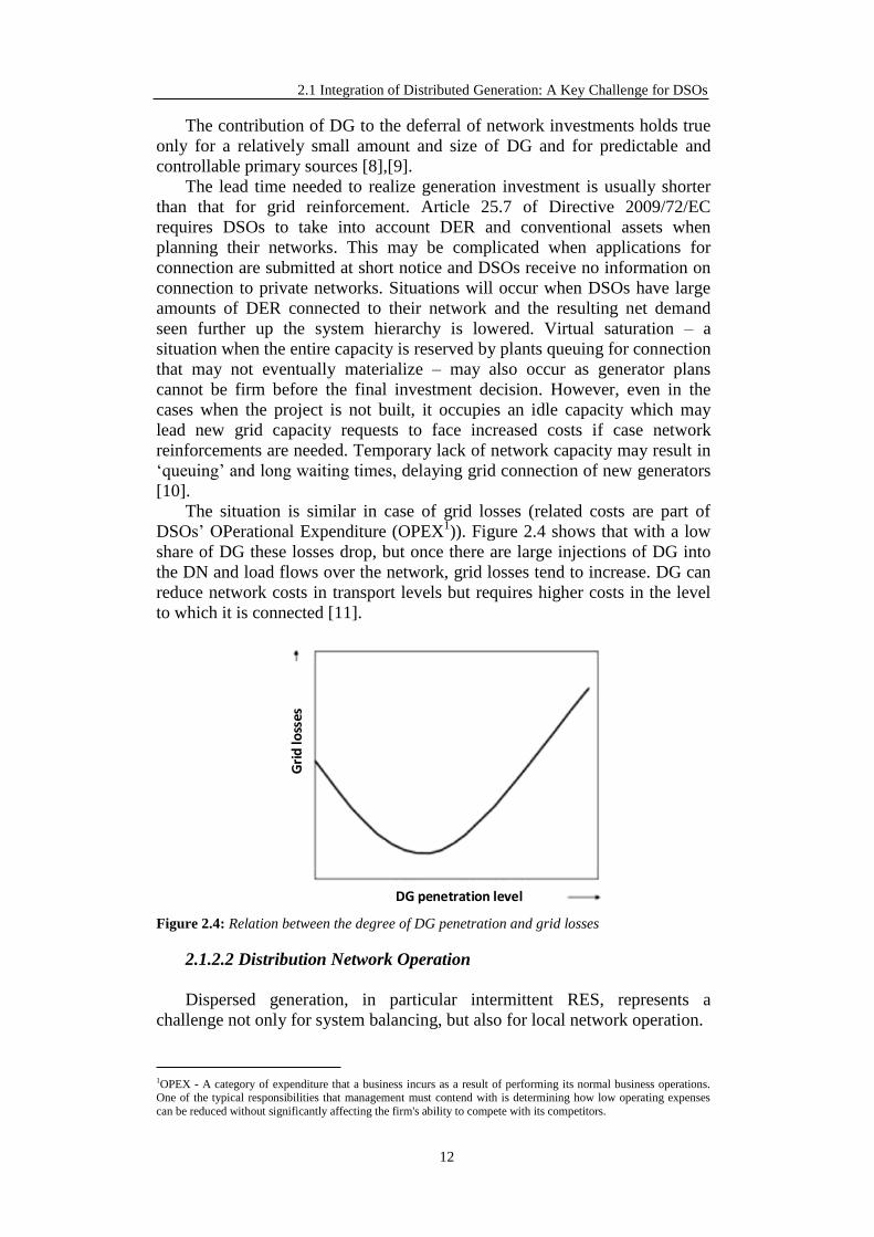
The situation is similar in case of grid losses (related costs are part of
DSOs’ OPerational Expenditure (OPEX1)). Figure 2.4 shows that with a low
share of DG these losses drop, but once there are large injections of DG into
the DN and load flows over the network, grid losses tend to increase. DG can
reduce network costs in transport levels but requires higher costs in the level
to which it is connected [11].
DG penetration level
Gri
d lo
sses
Figure 2.4: Relation between the degree of DG penetration and grid losses
2.1.2.2 Distribution Network Operation
Dispersed generation, in particular intermittent RES, represents a
challenge not only for system balancing, but also for local network operation.
1OPEX - A category of expenditure that a business incurs as a result of performing its normal business operations. One of the typical responsibilities that management must contend with is determining how low operating expenses
can be reduced without significantly affecting the firm's ability to compete with its competitors.
2. Active Distribution System Management
13
The security and hosting capacity of the DS is determined by voltage
(statutory limits for the maximum and minimum voltage ensure that voltage is
kept within the proper margins and is never close to the technical limits of the
grid) and the physical current limits of the network (thermal rates of lines,
cables, transformers that determine the possible power flow).
DS can be driven out of its defined legal and/or physical operating
boundaries due to one or both of the following:
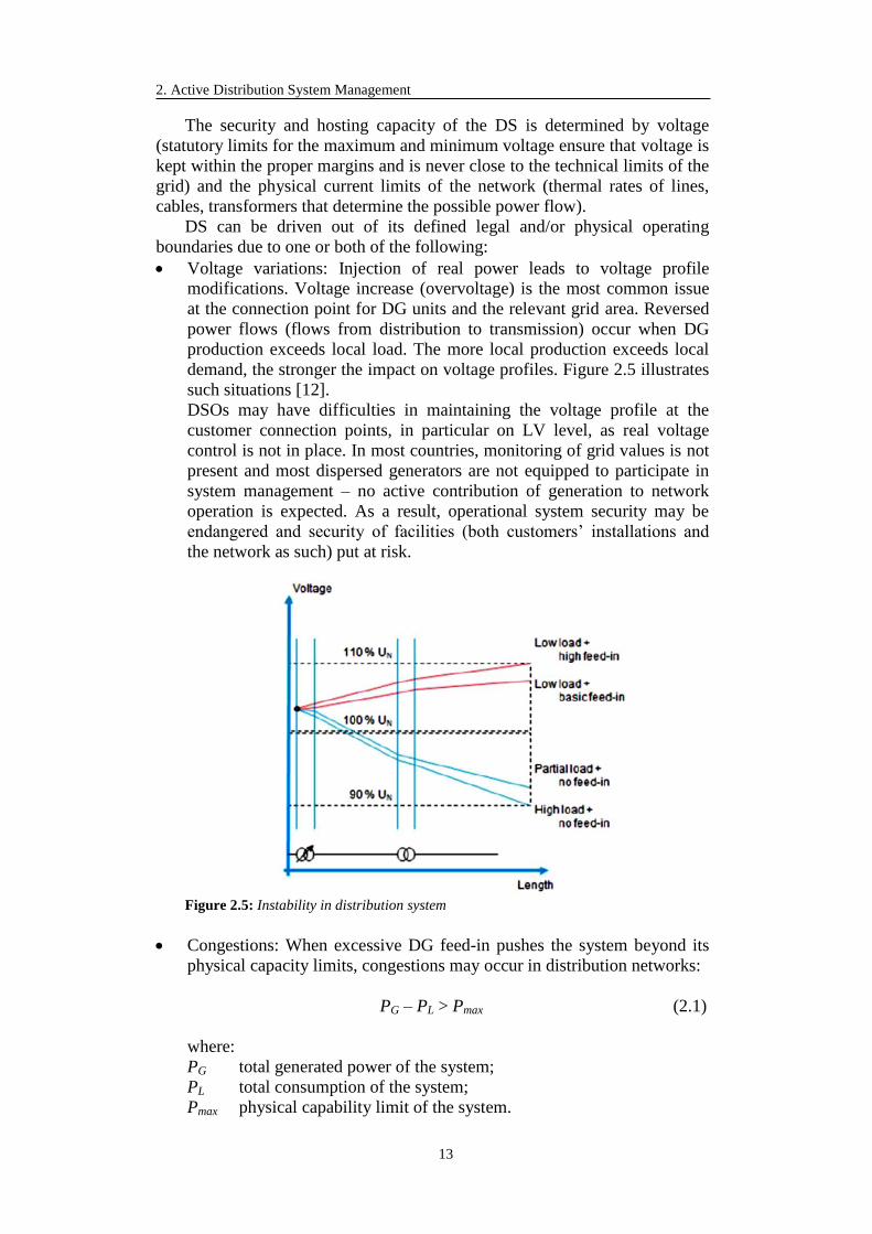
Voltage variations: Injection of real power leads to voltage profile
modifications. Voltage increase (overvoltage) is the most common issue
at the connection point for DG units and the relevant grid area. Reversed
power flows (flows from distribution to transmission) occur when DG
production exceeds local load. The more local production exceeds local
demand, the stronger the impact on voltage profiles. Figure 2.5 illustrates
such situations [12].
DSOs may have difficulties in maintaining the voltage profile at the
customer connection points, in particular on LV level, as real voltage
control is not in place. In most countries, monitoring of grid values is not
present and most dispersed generators are not equipped to participate in
system management – no active contribution of generation to network
operation is expected. As a result, operational system security may be
endangered and security of facilities (both customers’ installations and
the network as such) put at risk.
Figure 2.5: Instability in distribution system
Congestions: When excessive DG feed-in pushes the system beyond its
physical capacity limits, congestions may occur in distribution networks:
PG – PL > Pmax (2.1)
where:
PG total generated power of the system;
PL total consumption of the system;
Pmax physical capability limit of the system.

2.1 Integration of Distributed Generation: A Key Challenge for DSOs
14
This may lead to necessary emergency actions to interrupt/constrain off
generation feed-in or supply. A similar situation can occur in case of
excessive demand on the system (PL - PG> Pmax). This could apply to high
load originated e.g. by charging of electric vehicles, heat pumps and
electrical HVAC (heating ventilation and air-conditioning).
Generation curtailment is used in cases of system security related events (i.e.
congestion or voltage rise). The regulatory basis for generation curtailment in
such emergency situations differs across Europe. In some countries (e.g. in
Italy, Spain, Ireland), the control of DG curtailment is de facto in TSO hands:
the DSO can ask the TSO, who is able to control real power of DG above a
certain installed capacity, to constrain DG if there is a local problem. As the
TSO is not able to monitor DN conditions (voltage, flows), DSOs can only
react to DG actions [15]. This can result in deteriorating continuity on the
distribution system which will impact both demand customers and DG.
In systems with a high penetration of DG, both types of unsecure
situations already occur today. As a result, DSOs with high shares of DG in
their grids already face challenges in meeting some of their responsibilities.
These challenges are expected to become more frequent, depending on the
different types of connected resources, their geographic location and the
voltage level of the connection.
Active network and reversed power flow: The introduction of DG on to
the DN impacts upon power flows, voltage conditions and fault current
levels [133]. These impacts can be positive, such as reduction of voltages
sags and release of additional network capacity, but can negatively
impact on the protection systems. DG introduces additional sources of
fault current, which may increase the total fault level within the network,
while possibly altering the magnitude and direction of fault currents
measured by the protection systems. The contribution of one single DG is
normally relatively insignificant, but the aggregate contribution of many
DG units can lead to a number of problems such as: blinding, false
tripping and loss of grading.
To summarize, the key challenges for DSOs include:
Increased need for network reinforcement to accommodate new DG
connections:
Network operators are expected to provide an unconditional firm
connection which may cause delays or increase costs for connecting
dispersed generation;
Increased complexity for extension (including permitting procedures)
and maintenance of the grid may require temporary limitation for
connection of the end customers.
Problems with operation of the distribution grid:
Local power quality/operational problems, in particular variations in
voltage but also fault levels and system perturbations like harmonics
or flickers;
Rising local congestions when flows exceed the existing maximum
2. Active Distribution System Management
15
capacity, which may result in interruptions of generation feed-in or
supply;
Longer restoration times after network failure due to an increased
number and severity of such faults.
Current DSO responsibilities are the following:
Distribution planning, system development, connection & provision of
network capacity
DSOs are in charge of developing their network. They design new lines
and substations and ensure that they are delivered or that existing ones are
reinforced to enable connection of load and decentralized power
production. Depending on the size of a DG/RES & DER system, DSOs
may require a new connection at a particular voltage level. They are
obliged to provide third party access to all end customers and provide
network users with all information they need for efficient access and use
of the distribution system. They may refuse access to the grid only when
they can prove that they lack the necessary network capacity (Art. 32 of
Directive 2009/72/EC).
Distribution network operation/management and support in system
operation
DSOs maintain the system security and quality of service in DNs. This
includes control, monitoring and supervision, as well as scheduled and
non-scheduled outage management. DSOs are responsible for operations
directly involving their own customers. They support the TSOs, who are
typically in charge of overall system security, when necessary in a
predefined manner, either automatically or manually (e.g. through load
shedding in emergency situations). A common basis for these rules is
now being set in the EU-wide network codes (operational security,
balancing, congestion management, etc.).
Power flow management: Ensuring high reliability and quality in their
networks
Continuity and capacity: DSOs are subject to technical performance
requirements for quality of service including continuity of supply
(commonly assessed by zonal indexes such as average duration of
interruptions per customer per year (SAIDI) and average number of
interruptions per customer per year (SAIFI) or individual indexes
like number and duration of interruptions) and power quality laid out
in national law, standards and grid codes. They are also responsible
for voltage quality in distribution networks (maintaining voltage
fluctuations on the system within given limits). In planning, the DSO
ensures that networks are designed to maintain these standards
regardless of power flow conditions. However in cases of network
faults, planned outages or other erroneous events, the DSO must
undertake switching actions so that adequate supply quality is
maintained. Up until now, this has been rather static, increasingly
automation or remote switching will need to be undertaken to ensure
near real-time fault isolation and restoration of supply.
Voltage and reactive power: Voltage quality is impacted by the
electrical installations of connected network users. Thus the task of

2.1 Integration of Distributed Generation: A Key Challenge for DSOs
16
the DSO in ensuring voltage quality must account also for the actions
of network users, adding complexity and the need for both real-time
measurement and mitigating resources (i.e. on-load voltage control)
and strict network connection criteria. European standard EN 50160
specifies that the maximum and minimum voltage at each service
connection point must allow an undisturbed operation of all
connected devices. Voltage at each connection should thus be in the
range of ± 10% of the rated voltage under normal operating
conditions. In some countries, compliance with these or other
specified national voltage quality requirements that can be even more
restrictive represents part of DSOs’ contractual obligations and
quality regulation. In some countries, network operators are required
to compensate customers in case the overall voltage quality limits are
breached.
2.1.2.3 Traditional Design of Distribution Networks
The fundamental topological design of traditional distribution grids has
not changed much over the past decades. Up until recently, DSOs have
distributed energy and designed their grids on a top-down basis.
Under the paradigm “networks follow demand”, their primary role was to
deliver energy flowing in one direction, from the transmission substation
down to end users. This approach makes use of very few monitoring
equipment and is suitable for distribution networks with predictable flows.
Because of the different development of electrification, distribution
networks characteristics differ from country to country. Voltage rate levels are
usually distinguished as LV, MV or HV. As shown in Figure 2.6, the level of
supervision, control and simulation in HV distribution networks is close to
that of TSOs in their networks. MV and LV networks are mostly rather
passive – here DSOs lack network visibility and control. The lower the
monitoring level are, the lower the operational flexibility is.
Figure 2.6: Current DSO network

2. Active Distribution System Management
17
Traditional distribution networks have different characteristics in
topology (meshed or radial), operation type (meshed or radial), number of
assets and customers, operational flexibility and monitoring level:
HV networks (also called sub-transmission) are very similar to
transmission networks. The topological design of the grid is meshed and
may be operated as radial or meshed depending on the situation. HV
networks are operated in a similar way all around Europe: N-1 or N-2
contingency criteria are usually used for rural and urban areas,
respectively. The monitoring level at HV is very high. DSOs operating
HV grids are able to supervise and control the HV network from the
control room centers.
MV distribution networks significantly differ in their characteristics with
respect to urban and rural grids. Mostly, meshed topology is used that can
be operated either as meshed (closed loop) or radial (open loop). In some
countries or depending on the network type in a region, MV operation
may always be radial. A high density of loads and relatively high demand
typically causes high equipment load factors (transformers, cables) for
urban areas. Rural areas are characterized by larger geographical
coverage and lower load density and thus longer lines, high network
impedances and lower equipment load factors. The proportion of
European MV networks with remote monitoring, control and automated
protection/fault sectionalization is currently low but increasing by
necessity.
LV networks are usually radially operated. Similar to MV networks,
urban and rural LV networks have different characteristics. The
proportion of LV monitoring and control is typically even lower than in
MV. Measurements usually rely on aggregated information from
substations and are only available with a significant time lag. Profile
information will not be available.
2.2 Active Distribution Networks
Once DG in distribution networks surpasses a particular level, building
distribution networks able to supply all load & DG within the existing quality
of service requirements will frequently be too expensive and inefficient. For
example, in many places the network would only be constrained for few hours
per year. In addition, the security of supply and quality of service problems
will no longer be limited to specific situations.
Integrating the high amount of existing and projected DG and, later, other
DER will require new Information and Communication Technology (ICT)
solutions and an evolution of the regulatory framework for both network
operators and users. Network planning and operation methodologies need to
be revised to take the new solutions into account.
2.2.1 Key Building Blocks
There is no unique solution because DNs are rather heterogeneous in
terms of grid equipment and DG density at different voltage levels. Every DN

2.2 Active Distribution Networks
18
should be assessed individually in terms of its network structure (e.g.
customers and connected generators) and public infrastructures (e.g. load and
population density). Nevertheless, the needed development towards future
distribution systems which meet the needs of all customers can be described
in the three schematic steps pictured below (Fig. 2.7): from (1) passive
network via (2) reactive network integration to (3) active system management.
Figure 2.7: Three-Step Evolution of Distribution Systems [134]
1. Passive distribution networks make use of the so-called “fit and
forget” approach [134]. This approach indicates resolving all issues at
the planning stage, which may lead to an oversized network. DSOs
provide firm capacity (firm grid connection and access) that may not be
fully used anymore due to local consumption of the electricity produced
by DG. This approach has the advantage of requiring low flexibility,
control and supervision, but is possible to implement only for a network
with very low DER penetration. Once DER penetration rises, the system
cannot be designed to cater for all contingencies without very significant
investment in basic network infrastructure, making this approach less
economical.
2. Reactive network integration is often characterized by the “only
operation” approach. This approach is used today in some countries
with a high share of DG. The regulation requires connecting as much DG
as possible with no restrictions. Congestions (or other grid problems) are
solved at the operation stage by restricting both load and generation. This
solution could restrict DG injections during many hours per year and lead
to negative business case for DG if they are not remunerated for the
restrictions [134]. Already today, some pioneering countries in this field
with high DG penetration levels can be considered as having reached the
interim “reactive network integration” stage at which DSOs solve
problems once they occur (largely only in operation).
3. The active approach would allow for interaction between planning,
access & connection and operational timeframes. Different levels of
connection firmness and real-time flexibility can reduce investment
needs. The existing hosting capacity of the distribution network can be
used more optimally if other options including ICT, connection &

2. Active Distribution System Management
19
operational requirements that guarantee adequate performance of DER
towards the system (i.e. via grid codes) and market-based procurement of
ancillary services from DER are considered [134]. Operational planning
of DNs (similar to that at transmission level) would be in place in
networks with high DER shares in order to incentivize dispatch in a way
that is compatible with the network. Improved network capacity planning
and congestion management at distribution level at different times and
locations will be required to maximize the level of generation which is
injected in the most economical way for all parties, while maintaining
network stability. DSOs must have tools for overseeing maintenance of
network standards. Additionally they should have the possibility to buy
flexibility from DG and load in order to optimize network availability in
the most economic manner or to manage network conditions which are
outside the contracted connection of the customers. DSOs should have
the possibility to buy flexibility from DG and load on so-called
“flexibility platforms” in order to solve grid constraints. The network
reinforcement could be deferred until the moment when it becomes more
cost-effective than the on-going cost of procuring services from DER
[13]. Interactions between DSOs, TSOs and market actors at different
stages are depicted in Figure 2.8:
Network capacity
management
Security Congestion
management
Reconstitution of flows and a posteriori analysis
of congestions
Forecasts & schedules of production and consumption & outages
Simulations and network calculations
Detection of constraints (U, I)
Search for solutions
Adjustment interactions with the market, i.e. commercial aggregators
Interactions with TSO Pre-emptive network
actions (voltage set-points and network configuration) to mitigate constraints
Interactions with TSO, commercial aggregators, suppliers
Adjustment of network control points where this can mitigate congestions
Years - Months D - 1 H - 1 Real Time H + 1
Real time negotiations with the actors
Detection of constraints
Proposals of manual actions Automatic actions
Figure 2.8: DSO interactions with markets & TSO at different time frames [134]
Using the active system management approach would enable maximal
integration of DER, making the most of the existing grid while enabling
DSOs to fulfil the security standards and enabling DER to find the right
conditions for their business plan in the most cost-effective way. Table 2.2
highlights the key features of each phase, broken down into the different
“layers”: development & planning, operations, information exchange and
technical development. The subsequent sections of the chapter discuss the
active system management approach within the individual layers in detail.

2.2 Active Distribution Networks
20
Table 2.2: Three-Step Evolution of Distribution Systems in detail [134]
Layer Passive DN Re-active DN
integration Active DS management
Net
wo
rk d
evel
op
men
t
(pla
nn
ing
, co
nn
ecti
on
&
acce
ss)
Fit and forget
approach:
everything “solved”
at the planning
stage
Only operation
approach:
connection with no
restrictions and
solutions at the
operations stage
Or
Fit and forget
approach
Combined planning and
operational solutions:
Active capacity and loss
management through
commercial interaction
with market actors
selling
flexibility services
Connection and access
criteria combined with
operation tools to
manage
DER
Flexibility support from
DSO to TSO and from
TSO to DSO when
required
New system services for
DSOs arranged via
commercial ancillary
services and grid codes.
Net
wo
rk o
per
atio
n
Low monitoring &
control of DG RES,
often only by the
TSO
Missing rules &
services for
DG contribution to
quality of service,
security of supply
& firmness
Emergency
generation
curtailment by DSO
Active voltage
control distribution
networks. Grid codes
for DG to meet
connection criteria
and be able of voltage
based
control and reactive
power contribution
Info
rmat
ion
ex
chan
ge
Little information
exchange from
TSOs/DER to
DSOs (small DER
do not send
information)
High-level
information exchange
from TSOs/DER to
DSOs
Structured and organized
off-line and where
needed real-time
information exchange
(standardized interfaces
with DER required)
Tec
hn
ical
dev
elo
pm
ent
Net
wo
rk
Limited monitoring
& control
capabilities (usually
only HV)
Conventional
SCADA for HV
network and
DMS/OMS for
MV and LV
Increased monitoring
and control at HV &
MV via
telecommunications
SCADA/DMS/OMS
with the measurement
of certain new DG
Increased monitoring,
simulation and control
down to LV via
telecommunications
Advanced Distribution
Management Systems13
for DSOs/ SCADA and
Distribution
Management System
(DMS)
DE
R
DG often not
prepared for power
factor control
Storage & EV not
developed
Enhanced DG
protection systems/
inverters enabling
voltage & reactive
power control
Configurable settings:
e.g. protection / fault ride
through settings, voltage
droop
Presence of storage &
EVs

2. Active Distribution System Management
21
2.2.2 Distribution Network Development, Planning, Access and
Connection
2.2.2.1 Coordinated Network Development
DSOs should be able to plan their grids well in advance to prevent
bottlenecks in the most cost-effective way. Data acquired within DN
monitoring and information exchange with TSOs and distributed energy
resources could be very beneficial in this respect.
In addition, every connection request should be analyzed and considered
in the planning process in order to maximize the utilization of the existing
network. According to the traditional regulatory approach to connection
requests analysis currently applied in most countries, the network operator
performs an individual analysis and provides an individual solution to each
connection. The first connections may use the available capacity of the
existing network. But once there is an increased demand for new DG
connections in the same area and the available network capacity is limited,
this approach is not always optimal from the overall cost and network
development perspective.
One way to tackle this issue is to allow for coordination of all relevant
actors, including network operators, investors and local authorities in the
analysis of connection requests. One of the examples is the approach made in
Spain [14]. To rationalize the RES expansion and optimize the available
energy resources, some Spanish regions created so-called "Evacuation
Boards". They are characterized by a coordinated grid connection request
process. RES installation plans are deployed and coordinated between the
administration, RES investors and transmission and distribution system
operators. In these evacuation boards the TSO or DSO do not receive
individual requests; they are collected by the Regional Administration and
after a validation process submitted for an aggregated analysis to be made
together by the DSO & TSO. The positive impact of the new networks for
consumption (extra capacity for consumers) is also considered. In addition to
the cost-sharing mechanism (proportionally to the capacity assigned to each
RES project), the covenants for the development of such infrastructures
contain the necessary guarantees, payment and execution terms. Benefits of
this approach include overall minimized costs of network development and
project, reduction of project risks thanks to the possibility to correctly analyze
both the costs and timetables needed for the different RES penetration
scenarios, and reduced time for acquiring all necessary administrative permits.
Coordination between TSOs and DSOs is likely to play a particular role.
Whilst in some cases modifications required by DSOs from TSOs or vice
versa do not considerably affect the capabilities of one or the other to
maintain their network performance, the impact may be substantial in other
cases. For example, when the HV or EHV (extreme-high voltage) network is
saturated, connection of generation to the MV network cannot be planned
without taking into account the conditions at HV network. An optimal
network development is also a key to minimize losses in the electrical system.
Transmission or distribution network conditions which require regular (or
conditional) exchange of information between TSOs and DSOs should be

2.2 Active Distribution Networks
22
defined. Standard reciprocal data exchange arrangements about the expected
development of generation/load at the different voltage levels and about the
network reinforcements needed at the TSO level, not directly related to the
lower voltage planning activities, should be put in place.
2.2.2.2 Connection
For proper integration into the network, distributed generation needs to
fulfil minimum technical criteria: the equipment and its protective relays must
be able to resist voltage dips and prevent islanding and there should be
separate metering for production and consumption. DG should also be
subjected to the same costs as other generators, including adequate connection
fees. DSOs must know what is on-line when they are working to prevent
accidents. Therefore, they should have a possibility to verify compliance with
requirements. DG should thus “be registered” with the DSO, and remote
disconnection by the DSO to prevent damage to facilities of other clients
while maneuvering should be technically possible under conditions defined by
regulation. To secure safe operation of the distribution grid, DSOs should also
be able to define control schemes and settings for generators connected to
their grids, in coordination with the TSO where necessary in order to ensure
compliance with overall system requirements.
2.2.3 Active Distribution Network Operation
Dispersed generation should be incentivized to sell their production into
the electricity market. Aggregation of DG in form of so-called Virtual Power
Plants (VPPs), flexible loads and possibly decentralized storage is expected to
play an important role in facilitating access of small customers to the market
and addressing the uncertainty of availability and providing enhanced
capability to manage the risk of not being able to meet the contracted
scheduled output. The aggregator role could also be taken up by electricity
service companies (ESCO) or suppliers. The aggregator is to provide an
interface between DER and other market actors and system operators. In
addition, DG should be obliged to meet scheduling, nomination and balancing
obligations as other power generators do, including payment of balancing
charges. DG should also be responsible for their imbalances on equal terms
with other Balancing Responsible Parties. It is highly beneficial for system
stability and cost reduction if variable RES technologies are incentivized to
reduce forecast errors and to minimize imbalances in the market and take up
necessary responsibilities towards the system as other generation technologies
do [15].
The network plays an important service role of supporting the market.
Operational barriers may arise, characterized by one or more violations of the
physical, operational, or policy constraints under which the grid operates in
the normal state or under contingency cases. They are transient – associated
with a specified point in time. As such, they may be detected before or during
the day-ahead, the hour-ahead markets or during real-time system operation.
In order to facilitate secure network operation and smooth functioning of the
future market with high DER penetration, DSOs need to become active

2. Active Distribution System Management
23
operators of their networks. This means that they need adequate tools to
operate their networks. In order to facilitate this, they need to know the state
of the network in each time. In addition, network users need to actively
participate in network usage optimization. In this way, the possible above
mentioned violations can be eliminated.
2.2.3.1 DSO System Services
Active DSOs should be allowed to coordinate the offering of new system
services, as required by the new Energy Efficiency Directive (Art 15.1 of
2012/27/EC) while ensuring the security, integrity and quality of supply in
their networks. The DSO is best placed to facilitate this mechanism as the data
need to be gathered at substation level and in-depth knowledge of the grid
layout and its behavior is required. Moreover, the DSO has a legal
responsibility to ensure that such technical constraints are mitigated.
The blue area in Figure 2.9 schematically outlines the stages in the
electricity market in which the network operators do not interfere, but act as
mere behind-the-scene facilitators. The green area depicts the system services
that are to be administrated by network operators (for both transmission and
distribution system needs). Such system services could be defined in grid
codes (voltage and reactive power contribution) or procured as ancillary
services from DER within a transparent and non-discriminatory regulatory
framework.
Today, ancillary services are procured by the TSO, largely from large
power producers, to manage the system as whole. In near future, flexibility
platforms where flexibility is offered (usually via aggregators) to DSOs for
relieving congestion in their networks but also to TSOs to provide balancing
and dispatching in transmission grids will play an important role, in particular
for close to real-time flexibility.
Italy is one of the pioneering countries in promoting standards for
procurements of generating resources for ancillary services, with special
referral to the dispersed uncontrollable generation. Document 354/2013/R/eel
provides the guideline for such an action [16]. There is a persistent action to
make the most of the technological development that is happening in these
years. Therefore, the units for production of electrical energy from renewable
sources and energy storage systems (whether in electrochemical battery,
hydraulic, compressed air, etc.) must promote, in relation to the conditions of
economic efficiency of these technological developments, a system in which
all networks gradually become smart, in relation to the conditions of
development of DG. Gradually, all plants need to become eligible to provide
network services. This is in relation to the possibility that the various
technologies are subjects to the charges for the supply of those network
services that are not able to provide at the moment. In general, it is the entire
electrical system that must become "smarter" and which must be able to
operate in order to exploit in the most efficient performance of each of the
technologies of use of the sources of energy available.
Such a system will make more efficient use of DG, and the development
of ancillary services in DNs such that distributed generation can actively
participate in the management of the power system. This seems necessary in a

2.2 Active Distribution Networks
24
context where an increasing share of the hourly load is met by the distributed
generation that does not provide the same network services and amending the
profile of the residual load daily (that is covered by the significant production
units) to the point reset it in a few hours, and in some areas.
The regulatory action conducted so far has enabled undoubtedly
important steps forward, bringing Italy between the countries at the forefront
of integration of non-programmable renewable and dispersed generation. This
corresponds to the primary interest of Italy, which boasts one of the highest
degrees of penetration of these systems.
Figure 2.9: Market and network operations [134]
Distribution congestion
Security congestion management would be used to solve the technical
constraints at distribution level close to real-time in the alert state. In these
defined cases, the DSO could deviate from the merit order, but ex-post
justification and compensation should be provided. This could be executed by
pre-agreed contracts for instance. The DSO should then pay the “up
regulating” cost elsewhere in the system, and should remunerate the
downward cost to the local generator that is constrained off in his grid
(including the missed income from the support scheme and the costs of
keeping balanced position).
Emergencies
Emergency tools including direct load management (load shedding) and
emergency DG curtailment should be used only in well-defined emergency
states/once the contracted options are exhausted. When the grid stability is at
risk, DSOs should be able to act physically to control and constrain off both
local consumption and production (as is already the case in some countries –

2. Active Distribution System Management
25
e.g. Germany or Sweden). Priority access rules should not restrict network
operators’ ability to flexibly respond to emergency situations.
Any action on DN users requested by the TSO should be agreed with the
DSO as system operators. TSOs should not act on any individual DER
connected to the DS. Any direct order from the TSO to DER embedded in
distribution networks targeted to safeguard operation of the system will be
executed by the DSO, not the TSO.
2.2.3.2 Information Exchange
Today, DSOs have don’t possess systems installed for acquiring data
from DG of smaller size in particular. In some cases, the TSO receives
information from DG in real time while DSOs do not have real-time access to
this information. There is not usually an operational exchange between the
TSO and the DSO.
In the future, a well-structured and organized information exchange
between relevant actors will be necessary to operate the distribution network
with high DG penetration in real-time or close to real time (Fig. 2.10). This
form of information exchange will be used for DSO planning and asset
management purposes (to optimize network capacity and availability in the
most economic manner) while ensuring that all customers feel the absolute
minimum impact of DG on power quality and continuity. It is the first and
potentially most effective step which can be taken to reduce the cost of DG
connection and integration [17].
At the transmission level, generators already send schedules to the TSO
for system balance purposes and to guarantee that their realization is
technically possible. In systems with high DG penetration, the DSO will need
information about DG forecast, schedules and active dispatch to improve their
visibility and to assist with real-time or close to real-time management of the
distribution network including local network constraints. DSOs should have
managed access to communication and monitoring assets of DG to collect
information that will be necessary for operation of their networks. The
granularity of the data exchange will depend on the size of the generating unit.
The necessary information should be then exchanged between the DSO and
the TSO (in both directions). DSOs should provide the TSO with information
on active power that the TSO needs to facilitate secure system operation.
DSOs operating sub-transmission networks may also require TSO information
in real time.
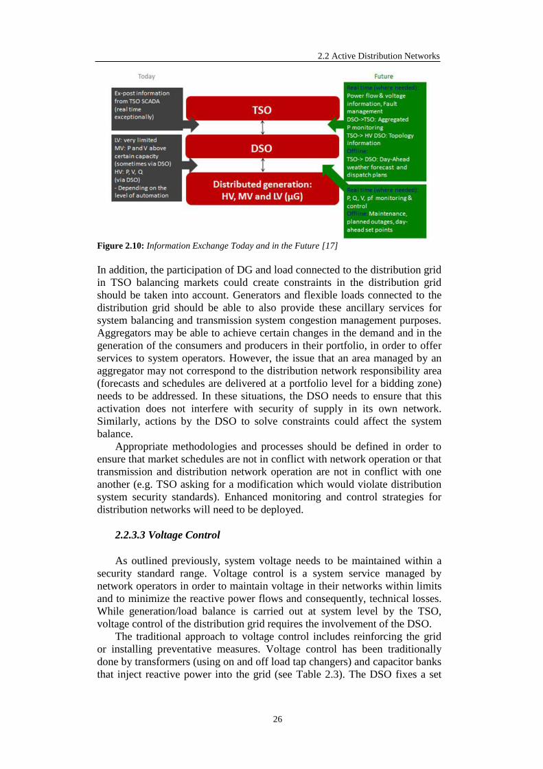
2.2 Active Distribution Networks
26
Figure 2.10: Information Exchange Today and in the Future [17]
In addition, the participation of DG and load connected to the distribution grid
in TSO balancing markets could create constraints in the distribution grid
should be taken into account. Generators and flexible loads connected to the
distribution grid should be able to also provide these ancillary services for
system balancing and transmission system congestion management purposes.
Aggregators may be able to achieve certain changes in the demand and in the
generation of the consumers and producers in their portfolio, in order to offer
services to system operators. However, the issue that an area managed by an
aggregator may not correspond to the distribution network responsibility area
(forecasts and schedules are delivered at a portfolio level for a bidding zone)
needs to be addressed. In these situations, the DSO needs to ensure that this
activation does not interfere with security of supply in its own network.
Similarly, actions by the DSO to solve constraints could affect the system
balance.
Appropriate methodologies and processes should be defined in order to
ensure that market schedules are not in conflict with network operation or that
transmission and distribution network operation are not in conflict with one
another (e.g. TSO asking for a modification which would violate distribution
system security standards). Enhanced monitoring and control strategies for
distribution networks will need to be deployed.
2.2.3.3 Voltage Control
As outlined previously, system voltage needs to be maintained within a
security standard range. Voltage control is a system service managed by
network operators in order to maintain voltage in their networks within limits
and to minimize the reactive power flows and consequently, technical losses.
While generation/load balance is carried out at system level by the TSO,
voltage control of the distribution grid requires the involvement of the DSO.
The traditional approach to voltage control includes reinforcing the grid
or installing preventative measures. Voltage control has been traditionally
done by transformers (using on and off load tap changers) and capacitor banks
that inject reactive power into the grid (see Table 2.3). The DSO fixes a set

2. Active Distribution System Management
27
point and prepares scenarios/ranges for different voltages within which the
voltage must be maintained.
Table 2.3: Voltage control in current distribution networks
HV Usually power transformers with on-load tap changers
Capacitors frequently used to control the voltage
MV No analogue values in secondary substations obtained in real time (typically
analogue values only at MV feeders)
MV networks connected to HV through a power transformer with on-load tap
changer
Capacitors can be commonly found also in these substations to improve the
power factor
Voltage set points specified at MV substation busbars
LV MV/LV transformers may be fixed ratio (i.e. have not tap changers) or have
off-load tap changers, manually controlled. Taps selected to compensate the
effect of MV voltage drops at LV levels (passive approach).
These tap-changers operate only a few times during transformers lifetime
Sometimes capacitors are installed in consumer facilities to meet power factor
regulations
New controllable MV/LV transformers are emerging but expensive
As the penetration of DG in networks increases, it is no longer possible to
ensure sustained system security without some dynamic resources, including
reactive power compensation and active voltage control. The DSO’s role in
ensuring not only that adequate network capacity is available for all connected
customers (demand and load) under all conditions, but also in managing
voltage and reactive power flows on distribution networks is becoming more
complex.
Two technical considerations for voltage control in distribution networks
include:
1. With high DG penetration, active power becomes a significant driver for
voltages changes in MV and LV networks (the kW-V effect is more
significant than the kVAr-V effect). The lower the distribution voltage
level, the higher this effect [18].
2. In MV and LV networks, the active power effect may not be always
neutralized by the reactive power injections/withdrawals available in the
system. To regulate voltage, DSO should be able to control reactive
power and in some cases also active power.
In high-voltage networks, DSOs will be able to maintain the voltage
within the security standards if they have the means to manage reactive power
flows. Real power will not cause voltage deviation under normal operation.
On the other hand, at medium and low voltage levels, real power changes due
to DG feed-in cause voltage rises (especially in cables) [18]. Distributed
generation changes voltage triangle design and as a result, both scenarios with
and without DG have to be considered. Reactive power may help compensate
the real power effect but may not be sufficient to neutralize it.
As reactive power cannot be transported over long distances and as many
regions with high DG penetration (thus voltage control challenges) have no
conventional sources of reactive power, managing voltage on a local or sub-
regional basis could be the most economically viable solution for the entire

2.2 Active Distribution Networks
28
electricity system. For these purposes, the DSO should be able to sectionalize
its networks, to actively interact with DG to request supply voltage control
and reactive dispatch or to exploit active demand services over the
distribution network to solve operational problems. Clear interface conditions
and an agreed operational framework at the interface between TSO and DSO
are also necessary (including parameters for TSO-DSO interface nodes).
Innovative approaches to voltage control should be explored. Experiences
from several European countries show that compensation at the TSO-DSO
connection point may not be flexible enough in case of emergency. The
increasing DG penetration requires continuous adaption of the capacities at
the connection points [135]. Voltage control requires a system approach that
would include minimizing system losses, optimizing network investments and
coordinating the necessary operational windows and control actions between
the individual TSO and DSO, with particular attention to cases of emergency.
Solutions on the network side and on the network users’ side should be
considered:
Network contribution
There are cases where HV voltage control cannot be achieved in a manner
which maintains both transmission and distribution security without additional
reactive power resources on the network. Investments in new analytical,
control and monitoring expertise and facilities in MV and LV (like power
electronics, real time supervision) may be required. For example, satellite
cables with large diameters could drastically reduce voltage rise within the
grid [19]. Alternatively, voltage controlled MV/LV transformers can be
installed in order to decouple the voltage rise within the MV and the LV
networks caused by RES feed-in. These innovative network techniques would
need to be considered and allowed within regulation.
Combination of both solutions
A combination of both solutions may be used. Studies show that in some
situations even a contribution by distributed generation will not be able to
maintain the voltage within limits [20]. Both to minimize any impact (real
power generation) on DG and to ensure that TSO-DSO interface standards
can be maintained for system stability, it may thus be necessary that
additional reactive resources are installed in DNs. The contribution of the
system operators or DG to these resources must be reflective of the particular
network issue being addressed and the beneficiaries of the installation. It may
also be necessary in future for DG which will displace reactive power
resources to also contribute to the reactive power facilities on its hosting
networks so as to maximize its potential to deliver real power. This is already
the case with larger (industrial) demand facilities that are required to follow
strict power factor regulations. Where this solution is considered the most
cost-effective, generators should be required to comply with minimum
connection & operational requirements necessary for managing distribution
network stability. On the other hand, DG contribution to loss minimization
may be compensated on a commercial basis.
Reduction of real power that might be technically necessary to manage
the network voltage and avoid complete generation disconnection should be

2. Active Distribution System Management
29
used only when other solutions have been exhausted. Congestion management
would apply in this case, with emergency DG curtailment only if necessary.
So, the recommendations are the following:
Active DSOs should be allowed to coordinate the offering of new system
services. Such system services could be procured as ancillary services
from DER or defined in grid codes (voltage and reactive power
contribution);
Flexibility platforms where flexibility is offered (either directly by larger
DG/load or via aggregators which group a large number of DG and loads)
to DSOs (but also to TSOs to provide balancing and redispatching in
transmission grids) could play an important role for close to real-time
flexibility in particular;
DSOs should be included in the information exchange about:
o planned location/connection/clustering of contracted customers
(aggregators);
o forecasts and schedules necessary for dealing with local grid
constraints;
Appropriate methodologies and tools for these purposes should be
developed;
Voltage control requires a system approach considering transmission and
distribution networks. Coordination between DSO and TSO at the
interface point should aim at reactive power optimization and minimizing
system investments and losses;
DG contribution to voltage control, probably in combination with
network solutions, is likely to play an important role in keeping DNs
stable. Where this solution proves to be the most cost-effective one,
generators connected to the DN above a certain capacity should be
required to have reactive power capabilities in line with those for
transmission connected RES, adapted to the connection level and
capacity.
2.2.4 Technical Development: Towards Flexible Distribution Systems
With a rising share of DER, monitoring, control strategies and advanced
protection systems in MV and LV distribution networks will have to develop
in order to enable DSOs to:
Determine and forecast grid capacity and bottlenecks;
Supervise and control power flows and voltage in their networks;
Enable the new operations at the distribution level (including non-
discrimination and effective real-time grid capacity monitoring and
management of injections/withdrawals);
Enable congestion management and voltage control procedure in
distribution networks;
Enhance the distribution grid hosting capability.
This solution should not be taken up in isolation from other options such as
services from DERs to help manage the DS mentioned above. The route to the
future energy system will incorporate both aspects. The most economically
efficient solution will depend on the topology, load and generation profiles

Implications for Regulation and Market Design
30
within a given DS. A two-level approach might be adopted: larger DG (with a
defined installed capacity and level of connection) could be monitored and
tele-controlled while other DER may not be dispatchable and should be
forecast and monitored by the DSO on an aggregated basis at the substation
level.
Technology options for development of the abovementioned options are
outlined in Table 2.4. In addition, new design ideas such as “satellite cables”
and dynamic line rating (DLR) are being tested. With DLR, real-time
information, for example the temperature of the conductor or the wind speed,
can be used to calculate a temporary rating of a line, thus allowing more
power to flow. This technology increases the utilization of the line and also
allows more RES to be integrated than if static ratings were used. Smart
meters will provide relevant monitoring functionalities, such as real-time local
voltage and load data that will be of high importance in DN management
processes and systems.
Table 2.4: Technology options for distribution network development
Function Medium Voltage Low Voltage
Monitoring
Current, voltage, fault
passage indicators and other
sensors
Centralization of information
via secondary substations
Control Remotely controllable
reclosers, switches
automated protection / fault
sectionalization – remote
monitored fault detectors
Voltage or power factor set
points to DGs
Controllable MV/LV
transformers (with centralized
or decentralized sensors)
2.3 Implications for Regulation and Market Design
The transition towards more active DNs requires the development of
technology as well as requirements for both network operators and network
users to contribute to system security. Appropriate commercial and regulatory
frameworks need to be put in place.
As mentioned above, the new Energy Efficiency Directive (Art 15.1 of
2012/27/EC) provides a good baseline for setting up system services at
distribution level that will allow for an energy efficient use of infrastructure.
Its appropriate implementation is thus crucial.
In addition, regulation and a flexibility market model should be further
developed to address the following issues:
Principles and methods for defining system states within the so-called
‘traffic lights concept’: boundaries between the green, yellow
(procurement of flexibility from markets) and red zones (emergency state
with non-commercial services) should be defined depending on physical
operating boundaries of a system, including methodologies of how they
will be monitored, calculated and audited.
Regulations for governing the most cost-efficient solutions: Regulatory
mechanisms for governing, when the investment delaying is more cost-
effective than active distribution approach, should be elaborated, for

2. Active Distribution System Management
31
example in order to ensure that network development occurs when
excursions to the yellow and red operating states become too frequent.
Active system management will affect the amount and structure of
operational expenditure and would replace some CAPEX with OPEX.
DSOs should be able to look at the business case for both the investment
solution (CAPEX) and the service-based solution (OPEX), or a mixture
of the two, and decide which is preferable. Adoption of a regulatory
mechanism is necessary to integrate this approach in the grid fee
calculation. DSOs need to be provided with adequate remuneration for
the most adequate solution: investment or active system management
tools including procurement of flexibility services from network users.
New roles and relationships between different actors in the market: In
particular, the role of flexibility providers (to be taken up by
aggregators/suppliers/ESCOs) and the relationship between these
flexibility providers and network operators, suppliers, the balance
responsible party (BRP) and the local customer/local producer should be
addressed.
Interaction between the DSO and the market: How will the DSO have
visibility of what is happening on the market side that may impact on the
DSO network and cause constraints in the short or long term? For
example, a flexibility provider may have a contract to provide reserves to
the TSO, but needs to use the DS to which its resources are connected to
deliver this service. However, a bottleneck on the DS may prevent this
delivery. These technical aspects of flexibility markets require further
investigation.
Measurement/determination of “non-produced” and “non-consumed”
energy is an important related issue: unlike consumed and produced
energy, saying how much a generator has “not produced” when he
reduced his production on demand of e.g. an aggregator is rather difficult,
and appropriate methodologies have to be developed and implemented.
Knowledge of the initial schedule is important in this respect.
Revision of planning guidelines for distribution network development:
Revision of these rules should be reconsidered in order to account for
ancillary services that the DSO can procure. Are deterministic security
standards such as the N-1 criterion appropriate or should they move to
being more probabilistic and based on reasonable risk of expected energy
not served in order to maintain high reliability while minimizing over-
investment in redundant capacity?
Establishment of contingency assessment and outage management
(organization and coordination of outages) rules for DNs and their users.
2.4 Conclusions
1. Secure and cost-effective integration of DER requires a rethink of how
distribution grids are planned and operated
Distribution networks are currently coping with the rapid increases in
decentralized RES feed-in that Europe is experiencing. Decentralized feed-in
of RES has already started to outstrip local demand in some European

2.4 Conclusions
32
regions. This growth can be quite rapid, as the increased feed-in often occurs
in rural areas with little demand. Building sources of production close to
consumption does not reduce DN cost. The network still has to be designed to
supply maximum demand for situations when there is no DG production. In
addition, operation of such a system becomes more complex. Once the share
of decentralized RES passes a certain point, it overburdens the local
distribution grid. DSOs are therefore increasingly facing voltage problems and
grid congestions.
2. DSOs need tools that allow them to become real system operators
DSOs are responsible for developing their grids efficiently and providing
quality of service for end customers. But in order to satisfy these
responsibilities in the changing context of DER/DG, DSOs need adequate
new tools. On one side, advanced software solutions are necessary for
managing the DN in optimized way. Then, system services at the distribution
level are key in this respect. Such services include the participation of
decentralized generators in voltage and reactive power management,
distribution network capacity management and congestion management, and
information exchange between TSOs, DSOs and DER.
Distribution network capacity management involves taking services from
DER into account in the planning stage to optimize investments and ensure
that infrastructure is only extended when it is more cost-efficient than
procuring services from DER.
3. Optimizing DER management through flexibility services should be
explored
Traditional methods of grid expansion reinforce the network so that it
may bear maximum feed-in from distributed generation. However, such
maximum capacity is only required for a short period of time each year. While
this approach will remain important, it may therefore not always be the most
optimal and cost-effective solution – not least because new lines often face
problems of public acceptance.
New solutions must be developed to enhance the hosting capacity of the
distribution grid; minimizing situations when DG feed-in has to be reduced or
new connections have to be denied. Such solutions include new network
technologies and design concepts, the contribution of generation to system
performance, and access to flexibility services provided by DG operators,
storage and demand response. Their flexibility could be procured on a
competitive basis via flexibility platforms and be offered to DSOs, but also to
TSOs as a way of managing redispatching issues in transmission grids. They
should be used whenever it is most efficient.
4. One-size-does-not-fit-all: different distribution networks require different
solutions
While best practice sharing is desirable, the most economically efficient
solution will depend on the topology, demand and generation profiles within a
given distribution system. The route to the future energy system will probably
incorporate aspects of each of the above mentioned solutions. The regulatory

2. Active Distribution System Management
33
framework should grant DSOs enough flexibility to determine the most
appropriate solution for their network. Methods of prioritizing and selecting
the most cost-effective solutions should be further investigated.
5. Coordination among all relevant stakeholders is the key
A system-wide approach to DG and network development is needed. For
instance, all stakeholders must be involved in analyzing grid connection
requests. This will lower the costs of network development and connection
while reducing connection waiting times for new users compared to business
as usual.
6. Take into account lessons learnt from smart grid demonstration projects
Europe already has experience of smart grid demonstration projects worth
more than €5.5 billion [21]. The future large-scale deployment of smart grids
should reflect best practices from these projects and already implemented
solutions. European network codes are currently being designed and will
include requirements for distribution network users. They should take into
account latest improvements on the ground and not close the door to the
implementation of new, proven innovation in distribution networks.
Standardization plays a key role in facilitating these solutions.
7. Tap into the potential of aggregation
Aggregators will act as possible middlemen for many small DG and load
customers, offering the flexibility options they buy from their clients to TSOs
and DSOs. A market model should be developed to unlock the potential of
such aggregation and new roles and relationships between new and existing
actors should be defined. This will enable demand, DG and storage resources
to participate in the markets for energy and ancillary services.
8. Equip DSOs with the tools they need to ensure quality of service and to
facilitate the market
Establishment of system services at distribution level calls for adequate
supporting tools that allow DSOs to operate their networks in a “more active”
way. Such tools should include access to technical data and further
development of the ICT systems essential for operational control of the grid.
It is the basic task of DSOs to guarantee security in their grids and to
support the security of the system as a whole. They are also in the best
position to plan and manage the new opportunities and risks related to the
grid. They should thus act as facilitators for flexibility platforms which will
allow generators, suppliers and consumers to offer network services either
directly or via aggregators.
DSOs are also best suited to manage operational data of distribution
network users and pass it to TSOs in an appropriate form and in the cost-
effective manner if needed.
The flexibility market and European rules for system operation should not
be designed in isolation. Technical and commercial data will become more
interrelated. Operational rules have an impact on market rules. EU network
codes that redefine operational and balancing rules will have implications for

2.4 Conclusions
34
procurement of flexibility services from DG, decentralized storage and
flexible loads and should therefore be designed to facilitate it.
9. Review connection and access regimes for distributed energy resources
A review of grid access regimes, including priority and guaranteed grid
access for renewables is becoming increasingly necessary. Currently such
rules prevent grid and market operators from implementing cost-effective
solutions to avoid grid congestion. Instead, they trigger inefficient
investments in grid extension based on rare situations.
Variable network access contracts or alternatives involving close to real-
time operation might be part of the solution. They would allow for limiting
DG injection by the grid operator based on an agreement with the producer
concerned, who would be remunerated, or at the initiative of the producer on
the basis of market prices and/or local flexibility mechanisms.
Priority access rules for DER also should not prevent network operators
from responding flexibly to emergency situations.
10. Design regulation to include network solutions beyond simple
“investment in copper”
DSO regulation should be adjusted to encourage the transformation of
DNs into actively managed DSs wherever this is the most economical
solution. Faced with new challenges posed by DER, DSOs could design and
operate their networks more efficiently if national regulation defines cost-
efficiency more broadly. The expected replacement of part of CAPEX by
OPEX should be taken into account and DSOs should be provided with an
adequate reward for CAPEX and improved evaluation of OPEX. DSOs
should receive an adequate rate of return on their network investments
without time delay.
In addition, the current approach to network development should be
reconsidered: DSOs should be able to take into account DER and
conventional assets when planning their networks (as required by Article 25.7
of Directive 2009/72/EC).

35
CHAPTER 3
3. Classical State Estimation
3.1 Introduction
Power systems are operated by system operators from the area control
centers. The main goal of the system operator is to maintain the system in the
normal secure state as the operating conditions vary during the daily
operation. Accomplishing this goal requires continuous monitoring of the
system conditions, identification of the operating state and determination of
the necessary preventive or corrective actions in case the system state is found
to be insecure. This sequence of actions is referred to as the security analysis
of the system.
The first stop of security analysis is to monitor the current state of the
system. This involves acquisition of measurements from all parts of the
system and then processing them in order to determine the system state. The
measurements may be both of analog and digital (on/off status of devices)
type. Substations are equipped with devices called remote terminal units
(RTU) which collect various types of measurements from the field and are
responsible for transmitting them to the control center. More recently, the so-
called intelligent electronic devices (IED) are replacing or complementing the
existing RTUs. It is possible to have a mixture of these devices connected to a
local area network (LAN) along with a SCADA front end computer, which
supports the communication of the collected measurements to the host
computer at the control center. The SCADA host computer at the control
center receives measurements from all the monitored substations' SCADA
systems via one of many possible types of communication links such as fiber
optics, satellite, power line connection (PLC), etc.
Measurements received at the control center will include line and
transformer power flows, bus voltage and line current magnitudes, generator
outputs, loads, circuit breaker and switch status information, transformer tap
positions, and switchable capacitor bank values. These raw data and
measurements are processed by the state estimator in order to filter the

3.2 Power System Static State Estimation
36
measurement noise and detect gross errors. State estimator solution will
provide an optimal estimate of the system state based on the available
measurements and on the assumed system model. This will then be passed on
to all the energy management system (EMS) application functions such as the
contingency analysis, automatic generation control, load forecasting and
optimal power now, etc. The same information will also be available via a
LAN connection to the corporate offices where other planning and analysis
functions can be executed off-line.
Static state estimation refers to the procedure of obtaining the voltage
phasors at all of the system buses at a given point in time. This can be
achieved by direct means which involve very accurate synchronized phasor
measurements of all bus voltages in the system. However, such an approach
would be very vulnerable to measurement errors or telemetry failures. Instead,
state estimation procedure makes use of a set of redundant measurements in
order to filter out such errors and find an optimal estimate. The measurements
may include not only the conventional power and voltage measurements, but
also those others such as the current magnitude or synchronized voltage
phasor measurements as well. Simultaneous measurement of quantities at
different parts of the system is practically impossible; hence a certain amount
of time skew between measurements is commonly tolerated. This tolerance is
justified due to the slowly varying operating conditions of the power systems
under normal operating conditions.
The definition of the system state usually includes the steady state bus
voltage phasors only. This implies that the network topology and parameters
are perfectly known. However, errors in the network parameters or topology
do exist occasionally, due to various reasons such as unreported outages,
transmission line sags on hot days, etc.
The foregoing concerns were first recognized and subsequently addressed
by Fred Schweppe, who proposed the idea of state estimation in power
systems [22],[23],[24]. Introduction of the state estimation function broadened
the capabilities of the SCADA system computers, leading to the establishment
of the EMS, which would now be equipped with, among other application
functions, an on-line State Estimator (SE) [25].
3.2 Power System Static State Estimation
3.2.1 Nonlinear Measurement Model
A power system with N buses is considered, where m quantities are
measured and whose topology and parameters are known. Under these
conditions, if the complex bus voltages are known, it is possible to determine
any power flow in the transmission network and/or any bus power injection.
This is the reason why the complex bus voltages are named state variables of
the power system.
The set of m measurements taken along the electrical network and the
measurement errors are related through the following model [26]:
z = z0 + 𝜼 (3.1)

3. Classical State Estimation
37
where, z is a (m × 1) vector of the measurements; z0 is a (m × 1) vector of the
actual measurements, which is a function of the actual power system state and
η is a (m × 1) random vector which models the measurement errors
(inaccuracy of the meters, errors of transformers as measurement instruments,
communication errors, effects of analog-digital conversion, etc.).
The actual values of state variables of the power system, and
consequently the actual value of the measured quantities, are unknown. In
order to estimate the power network state, it is necessary to make certain
assumptions about the measurement model and using the relationship between
the measurements and the estimated states. With respect to the measurements,
it is observed that all meters have an error whose magnitude is related to its
accuracy level. Under normal circumstances, the magnitude of this error is
situated within a tolerable range and does not deteriorate the measurement. In
addition, the error of a meter does not affect the measurement taken by
another meter. For this reason, it is assumed that the vector of measurement
errors has a Gaussian (normal) distribution 𝐸(𝜂), with zero mean and a
covariance matrix R, which is analytically expressed as:
𝐸(𝜼) = 0 𝐸(𝜼𝜼𝑡) = R (3.2)
where R is a diagonal matrix, indicating that measurement errors are not inter-
related. The diagonal elements of this matrix are the variances of the
measurement errors, which are usually expressed as a function of the full
scale value of meters.
The actual values of the measurements and the actual states are related by:
z0 = h(x) (3.3)
where h(x) is a vector composed of m nonlinear functions of the system state,
based on Kirchhoff’s and Ohm’s laws and x is the vector of power system
states, which for a power system with N buses is a n = 2N − 1 column vector
(only the reference angle is not included in the vector of system states). Under
these assumptions the measurement model of Eq. (3.1) is re-written as:
z = h(x) + 𝜼
𝐸(𝜼) = 0; 𝐸(𝜼𝜼𝑡) = R (3.4)
The measurements typically include real and reactive power flows in the
transmission, real and reactive power injections in the buses, and voltage
magnitudes. The magnitude of the current in transmission lines could also be
monitored, but this practice is not the usual in HV transmission systems.
Another important aspect is related to the number and location of the
measurements in the electrical network. The degree of redundancy of the
measurement set is denoted by 𝜌 and defined as:
𝜌 ≜𝑚
𝑛=
𝑚
2𝑁 − 1
Observe that a necessary (but not sufficient) condition to estimate the
state of the power system is: m ≥ n, or ρ ≥ 1.0. In addition to a good
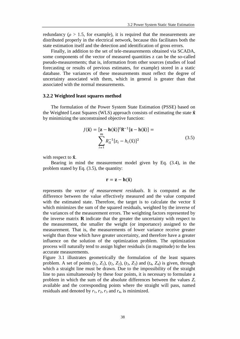
3.2 Power System Static State Estimation
38
redundancy (ρ > 1.5, for example), it is required that the measurements are
distributed properly in the electrical network, because this facilitates both the
state estimation itself and the detection and identification of gross errors.
Finally, in addition to the set of tele-measurements obtained via SCADA,
some components of the vector of measured quantities z can be the so-called
pseudo-measurements; that is, information from other sources (studies of load
forecasting or results of previous estimates, for example) stored in a static
database. The variances of these measurements must reflect the degree of
uncertainty associated with them, which in general is greater than that
associated with the normal measurements.
3.2.2 Weighted least squares method
The formulation of the Power System State Estimation (PSSE) based on
the Weighted Least Squares (WLS) approach consists of estimating the state
by minimizing the unconstrained objective function:
𝐽(x) = [𝐳 − 𝐡()]𝑡R−1[z − h(x)] =
∑𝑅𝑖𝑖−1[𝑧𝑖 − ℎ𝑖(x)]
2
𝑚
𝑖=1
(3.5)
with respect to .
Bearing in mind the measurement model given by Eq. (3.4), in the
problem stated by Eq. (3.5), the quantity:
𝐫 = 𝐳 − 𝐡(x)
represents the vector of measurement residuals. It is computed as the
difference between the value effectively measured and the value computed
with the estimated state. Therefore, the target is to calculate the vector x which minimizes the sum of the squared residuals, weighted by the inverse of
the variances of the measurement errors. The weighting factors represented by
the inverse matrix R indicate that the greater the uncertainty with respect to
the measurement, the smaller the weight (or importance) assigned to the
measurement. That is, the measurements of lower variance receive greater
weight than those which have greater uncertainty, and therefore have a greater
influence on the solution of the optimization problem. The optimization
process will naturally tend to assign higher residuals (in magnitude) to the less
accurate measurements.
Figure 3.1 illustrates geometrically the formulation of the least squares
problem. A set of points (t1, Z1), (t2, Z2), (t3, Z3) and (t4, Z4) is given, through
which a straight line must be drawn. Due to the impossibility of the straight
line to pass simultaneously by these four points, it is necessary to formulate a
problem in which the sum of the absolute differences between the values Zi
available and the corresponding points where the straight will pass, named
residuals and denoted by r1, r2, r3 and r4, is minimized.

3. Classical State Estimation
39
Figure 3.1: Linear regression - geometrical illustration
3.3 Gauss-Newton Method
The PSSE can be formulated as a weighted least squares problem
expressed as:
minx𝐽(x) = [𝐳 − 𝐡()]𝑡R−1[z − h(x)] (3.6)
where x is the vector of state variables, z is the vector of measurements and R
is the covariance matrix of the measurement errors.
The optimality condition for the problem stated by Eq. (3.6) is expressed
by:
𝜕𝐽
𝜕𝑥|𝐱=
= 0 ⇒ 𝐇𝑡()𝐑−1[𝐳 − 𝐡()] = 0 (3.7)
where 𝐇() =𝜕h(x)
𝜕x|𝐱=x
is the matrix of first derivatives of the non-linear
functions h(x), calculated at the point . Despite the minimization of the
function expressed by Eq. (3.6) does not involve constraints, the search for the
solution of the least squares problem presents considerable difficulty. The
index to be optimized is a quadratic function, expressed in terms of a vector of
non-linear equations relating the state variables and the measurements.
Additionally, Eq. (3.7), which represents the optimality conditions, has no
closed solution and therefore requires the use of iterative methods. Several
numerical methods could be applied to solve a problem of this type. However,
the quadratic nature of the objective function and the absence of constraints
make this optimization problem appropriate to the solution by the Newton’s
method, described in following subchapter.

3.3 Gauss-Newton Method
40
3.3.1 Linearization of the Measurement Model
The application of iterative methods to solve the non-linear optimization
problem expressed by Eq. (3.6) requires the current estimate of the state
vector to be updated with successive corrections given by:
x𝑘+1 = x𝑘 + Δx (3.8)
In order to determine the increment Δ𝐱 of Eq. (3.8), the linearization of 𝐡(𝐱)
around the point x𝑘, in the direction (𝐱 − x𝑘), should be considered:
h(x𝑘 + Δx)≈h(x𝑘) + H(x𝑘)(x − x𝑘) (3.9)
where all terms have been previously defined.
The replacement of this equation in z = h(x) + η provides:
z − h(x𝑘) = H(x𝑘)(x − x𝑘) + 𝜼
which stands for the linearized measurement model and whose compact form
is given by:
Δz = H(x𝑘)Δx + 𝜼
𝐸(𝜼) = 0; 𝐸(𝜼𝜼𝑡) = R
where Δz = z − h(x𝑘) is the vector of measurement residuals and Δx =(𝐱 − 𝑘).
In terms of the linearized measurement model, the objective function of
the least squares problem of Eq. (3.6) is expressed as:
𝐽(Δ𝐱) = [Δ𝐳 − H(x𝑘)Δx]𝑡𝐑−1[Δ𝐳 − H(x𝑘)Δx]
and the corresponding optimality condition is given by:
𝜕𝐽
𝜕Δ𝐱|𝐱=𝑘
= 0 ⟹ 𝐇t(x𝑘)𝐑−1[Δ𝐳 − H(x𝑘)Δx] = 0
Or alternatively:
[𝐇t(x𝑘)𝐑−1𝐇(x𝑘)]Δx=𝐇t(x𝑘)𝐑−1Δz (3.10)
The expression (3.10) is called Gauss Normal Equation and represents the
linear system to be solved at each iteration for the determination of the
increment Δx of the state vector. This correction can also be determined by
using the Gauss-Newton iterative method. In this case, the function J(x) of
Eq. (3.6) is expanded in Taylor series, around the point x𝑘, along the direction
Δx, to the second order term, that is:

3. Classical State Estimation
41
𝐽(x𝑘 + Δx) = 𝐽(x𝑘) +𝜕𝐽(𝐱)𝑡
𝜕𝐱|𝐱=x𝑘
Δx +1
2Δ𝐱𝑡
𝜕2𝐽(𝐱)
𝜕𝐱2|𝐱=x𝑘
Δx
where: 𝜕𝐽(𝐱)
𝜕𝐱|𝐱=x𝑘
and 𝜕2𝐽(𝐱)
𝜕𝐱2|𝐱=x𝑘
are respectively the vector of first derivatives
and the matrix of second derivatives of the function J(x) with respect to x,
calculated in point that represents the current estimate x𝑘.
The minimum of the function 𝐽(x𝑘 + Δx) is obtained by differentiating
this function with respect to Δx and making the result equal to zero, that is:
𝜕𝐽
𝜕(Δ𝐱)=𝜕𝐽(𝐱)𝑡
𝜕𝐱|𝐱=x𝑘
+𝜕2𝐽(𝐱)
𝜕𝐱2|𝐱=x𝑘
Δx = 0
or alternatively:
𝜕2𝐽(𝐱)
𝜕𝐱2|𝐱=x𝑘
Δx = −𝜕𝐽(𝐱)𝑡
𝜕𝐱|𝐱=x𝑘
(3.11)
The gradient vector 𝜕𝐽(𝐱)
𝜕𝐱|𝐱=x𝑘
is given by:
𝜕𝐽(𝐱)
𝜕𝐱|𝐱=x𝑘
= (𝜕[𝐳 − 𝐡()]𝑡𝐑−1[𝐳 − 𝐡()]
𝜕𝐱)|𝐱=x𝑘
=
= −2(𝜕𝐡(𝐱)
𝜕𝐱)𝑡
|𝐱=x𝑘
𝐑−1[𝐳 − 𝐡()]|𝐱=x𝑘
= −2𝐇(𝑘)𝑡𝐑−1Δz
(3.12)
where 𝐇(𝑘) and Δz were previously defined.
The application of the same procedure to compute the matrix of second
derivatives of J(x) provides:
𝜕2𝐽(𝐱)
𝜕𝐱2|𝐱=x𝑘
=𝜕
𝜕𝐱[−2 (
𝜕𝐡(𝐱)
𝜕𝐱)𝐑−1[𝐳 − 𝐡()]]|
𝐱=x𝑘
Supposing that in the neighborhood of the solution the variations of the
matrix H(x) are negligible, that is:
𝐇(𝐱) =𝜕𝐡(𝐱)
𝜕𝐱≈ 𝑐𝑜𝑛𝑠𝑡𝑎𝑛𝑡
then:
𝜕2𝐽(𝐱)
𝜕𝐱2|𝐱=x𝑘
≈ 2𝐇𝑡(𝑘)𝐑−1𝐇(𝑘)
such that Eq. (3.11) is rewritten as:
𝐇𝑡(x𝑘)𝐑−1𝐇(x𝑘) Δx = 𝐇𝑡(x𝑘)𝐑−1Δz (3.13)

3.3 Gauss-Newton Method
42
which is the same expression obtained with the linearized measurement
model.
3.3.2 Computational Aspects
The matrix R of Eq. (3.13) is diagonal. For this reason, the product matrix
(HtR
−1H), named Gain or Information matrix, is approximately twice more
dense than the matrix H. Additionally, the matrix H is sparse and thus the
information matrix has a number of non-zero elements which allows the use
of sparse techniques. In addition, this matrix is symmetrical in structure and
numerical values and positive semidefinite, which facilitates their
factorization [27].
The elements of the Jacobian matrix H(𝑘) are obtained by deriving the
expressions of h(x) with respect to the state vector x. Despite the simplicity of
these derivatives, the calculation of their numerical values demands a
reasonable computational effort, since it is performed repeatedly during the
iterations.
The iterative process starts at an initial estimate 0 and computes
increments in the state variables Δ by solving the linear system of Eq. (3.13)
at each iteration. The state vector is updated according to Eq. (3.8), until the
convergence criterion is satisfied, that is:
max|∆𝑖| ≤ 휀 (3.14)
where 휀 is a pre-specified tolerance. This criterion indicates that the iterative
process is finished when the magnitude of adjustments in the state variables is
negligible. Another important aspect of the problem represented by the
normal equation (3.13) is that it has a tendency to numerical ill-conditioning.
This can be verified by analyzing the number of conditioning of the matrix of
information. The spectral conditioning number of a matrix C is defined as:
𝐶𝑜𝑛𝑑(𝐂) =𝜎𝑀𝜎𝑚
(3.15)
where 𝜎𝑀 and 𝜎𝑚 are respectively the maximum and the minimum
eigenvalues of matrix C.
The index Cond (C) provides a measurement of how small disturbances
in matrix C affect the solution of the linear system Cx = b. With respect to the
Gauss Normal equation it can be proved that:
𝐶𝑜𝑛𝑑(𝐇𝑡𝐇) = (𝐶𝑜𝑛𝑑(𝐇))2
that is, if H is numerically ill-conditioned, matrix HtH will have a worse
numerical conditioning.
The linear system of Eq. (3.13) can be solved by applying the method of
Cholesky and the 2nd method of Tinney (also known as minimum degree
algorithm). The procedure for obtaining the solution of the normal equation
can be summarized in the following steps:

3. Classical State Estimation
43
Decompose the information matrix A = [HtR
−1H] (symmetrical and
positive definite), via Cholesky method, in A = LtL
Perform inverse substitution in the linear system Lty = b, to obtain y
(where b = HtR
−1Δz), and direct substitution in the linear system LΔx = y
to obtain x.
Since the structure of the information matrix is not modified during the
iterative process, the ordering and the structure of matrix A can be determined
only once, which speeds up the computational process, since the solution
method is iterative and requires multiple solutions of the normal equation.
3.3.3 Algorithm
The state estimation through Gauss-Newton method can be summarized
in the following sequence of steps:
1. determine the structure of the Jacobian matrix H(𝐱) and information
matrix [HtR
−1H] and the ordering scheme of the information matrix;
2. specify an initial estimate for the state variables vector 0;
3. calculate the numerical values of H(𝑘), 𝐇𝑡(𝑘)𝐑−1𝐇(𝑘), Δz = 𝐳 − 𝐡(x𝑘) and 𝐛 = 𝐇𝑡(𝑘)𝐑−1Δz;
4. factorize the information matrix [HtR
−1H] = LL
t;
5. solve the linear system 𝐋𝐋𝑡Δ𝐱𝑘 = 𝐛;
6. update the state variables vector 𝑘+1 = k + Δ𝐱k
7. check convergence: if max|∆𝑖| ≤ 휀 (generally 휀 = 10−4 𝑝𝑢 ), compute
the power flows in the transmission lines and the power injections and
finish the iterative process.
8. make k = k + 1 and return to step 3;
It is noted that in the last iterations of the iterative process the changes in
the numerical values of the matrix H are practically negligible, which allows
you to keep this matrix constant during some iterations. This strategy reduces
the computational effort demanded by the iterative process, provided that in
the final iterations only the calculation of Δz = 𝐡((𝑘)) − 𝐳 and 𝐛 =
𝐇t(k)𝐑−1Δz is required.
3.3.3 Decoupled Estimators
The decoupled estimators are based on the same approximations of the
fast decoupled power flow. The main characteristics of these estimators are
the exploration of the Pδ − QV decoupling and the use of constant matrices
(information matrix 𝐇𝑡()𝐑−1𝐇() and/or Jacobian matrix H) [28].
To show how the decoupling Pδ − QV can be explored in the state
estimation algorithms, suppose that the vector of measurements is partitioned
as:
𝐳 = [𝐳𝑃𝐳𝑄] =
[ 𝐭𝐩𝐮𝐪𝐕]

3.3 Gauss-Newton Method
44
where, zP corresponds to p and t, which are the vector of the real power
injection and real power flow measurements, respectively; and zQ corresponds
to u, q and V, which represent the vectors of the reactive power injection,
reactive power flow, and voltage magnitude measurements.
By adopting a similar partition to the non-linear functions that relate the
measurements to the states and to the measurement errors, the measurement
model can be expressed as:
[𝐳𝑃𝐳𝑄] = [
𝐡(𝐱)𝑃𝐡(𝐱)𝑄
] + [𝜼𝑃𝜼𝑄]
with:
𝐸 [𝜼𝑃𝜼𝑄] = 0 𝐸 [
𝜼𝑃𝜼𝑄] [𝜼𝑃𝜼𝑄]𝑡
= [𝐑𝑃 00 𝐑𝑄
]
where, h(x)P , h(x)Q, ηP and ηQ are the vectors of non-linear functions and the
vectors of the measurement errors corresponding to the real and reactive
measurements, respectively; RP and RQ represent the sub-matrices of
covariance measurement errors associated with the real and reactive
measurements, respectively. The Jacobian matrix of the non-linear functions
h(x)P and h(x)Q, corresponding to this non-linear measurement model can be
written as:
𝐇(V, 𝛿) = [𝐇𝑃𝛿 𝐇𝑃𝑉𝐇𝑄𝛿 𝐇𝑄𝑉
] (3.16)
where 𝐇𝑃𝛿 =𝜕𝐡(𝐱)𝑃
𝜕𝜹 and 𝐇𝑃𝑉 =
𝜕𝐡(𝐱)𝑃
𝜕𝐕 are the sub-matrices of first derivatives
of the functions h(x)P (related to the real measurements) with respect to the
angle and magnitude of the complex bus voltages; and 𝐇𝑄𝛿 =𝜕𝐡(𝐱)𝑄
𝜕𝜹 and
𝐇𝑃𝑉 =𝜕𝐡(𝐱)𝑄
𝜕𝐕 are the sub-matrices of first derivatives of the functions h(x)Q
(related to the reactive measurements) with respect to the angle and
magnitude of the complex bus voltages.
According to the previous partitioning, the information matrix [HtR
−1H]
can be rewritten as:
[𝐇𝑃𝛿𝒕 𝐇𝑄𝛿
𝒕
𝐇𝑃𝑉𝒕 𝐇𝑄𝑉
𝒕 ] [𝐑𝑃 00 𝐑𝑄
] [𝐇𝑃𝛿 𝐇𝑃𝑉𝐇𝑄𝛿 𝐇𝑄𝑉
]
such that, the matrix product indicated in the last equation provides:
[𝐇𝑃𝛿𝒕 𝐑𝑃
−1𝐇𝑃𝛿 + 𝐇𝑄𝛿𝒕 𝐑𝑄
−1𝐇𝑄𝛿 𝐇𝑃𝛿𝒕 𝐑𝑃
−1𝐇𝑃𝑉 + 𝐇𝑄𝛿𝒕 𝐑𝑄
−1𝐇𝑄𝑉
𝐇𝑃𝑉𝒕 𝐑𝑃
−1𝐇𝑃𝛿 + 𝐇𝑄𝑉𝒕 𝐑𝑄
−1𝐇𝑄𝛿 𝐇𝑃𝑉𝒕 𝐑𝑃
−1𝐇𝑃𝑉 + 𝐇𝑄𝑉𝒕 𝐑𝑄
−1𝐇𝑄𝑉]
or in a compact form:
[𝐀𝑃𝛿 𝐀𝑃𝑉𝐀𝑄𝛿 𝐀𝑄𝑉
]
where:
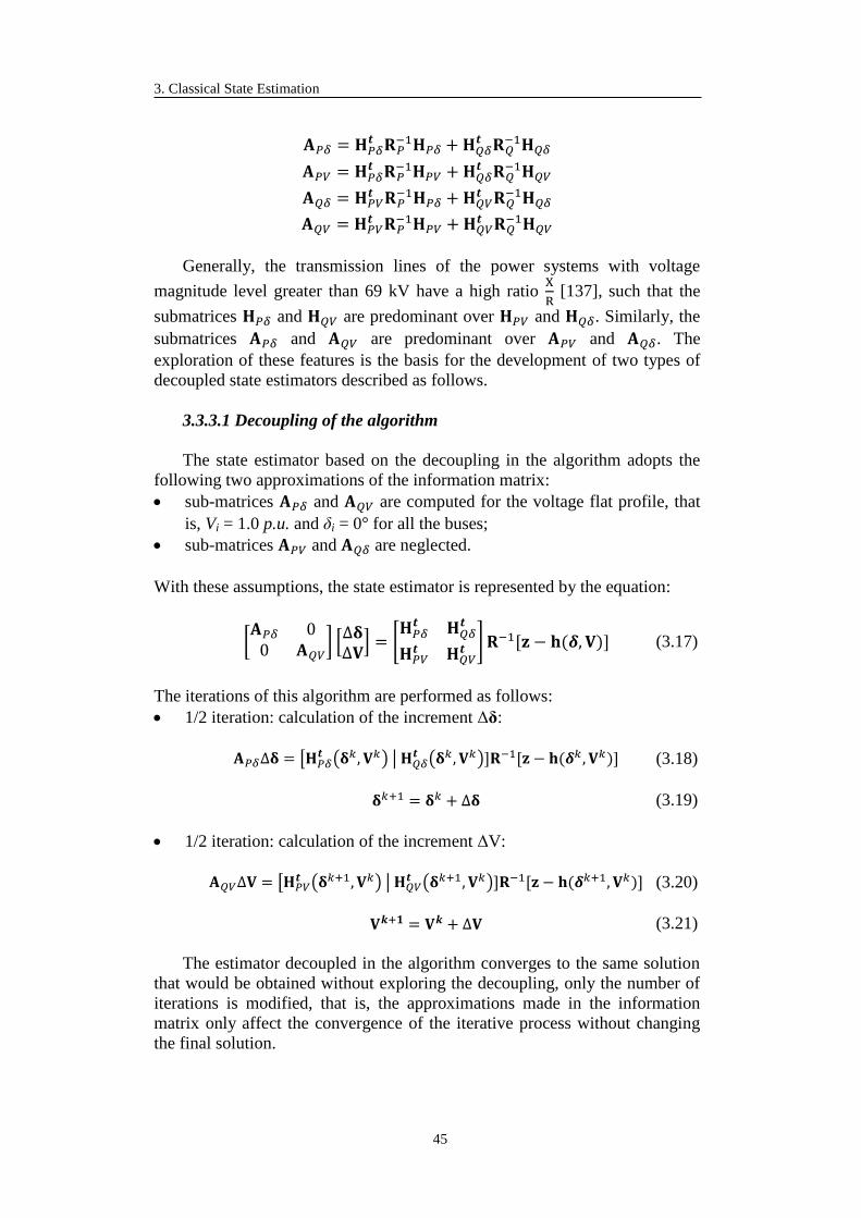
3. Classical State Estimation
45
𝐀𝑃𝛿 = 𝐇𝑃𝛿𝒕 𝐑𝑃
−1𝐇𝑃𝛿 + 𝐇𝑄𝛿𝒕 𝐑𝑄
−1𝐇𝑄𝛿
𝐀𝑃𝑉 = 𝐇𝑃𝛿𝒕 𝐑𝑃
−1𝐇𝑃𝑉 + 𝐇𝑄𝛿𝒕 𝐑𝑄
−1𝐇𝑄𝑉
𝐀𝑄𝛿 = 𝐇𝑃𝑉𝒕 𝐑𝑃
−1𝐇𝑃𝛿 + 𝐇𝑄𝑉𝒕 𝐑𝑄
−1𝐇𝑄𝛿
𝐀𝑄𝑉 = 𝐇𝑃𝑉𝒕 𝐑𝑃
−1𝐇𝑃𝑉 + 𝐇𝑄𝑉𝒕 𝐑𝑄
−1𝐇𝑄𝑉
Generally, the transmission lines of the power systems with voltage
magnitude level greater than 69 kV have a high ratio X
R [137], such that the
submatrices 𝐇𝑃𝛿 and 𝐇𝑄𝑉 are predominant over 𝐇𝑃𝑉 and 𝐇𝑄𝛿. Similarly, the
submatrices 𝐀𝑃𝛿 and 𝐀𝑄𝑉 are predominant over 𝐀𝑃𝑉 and 𝐀𝑄𝛿. The
exploration of these features is the basis for the development of two types of
decoupled state estimators described as follows.
3.3.3.1 Decoupling of the algorithm
The state estimator based on the decoupling in the algorithm adopts the
following two approximations of the information matrix:
sub-matrices 𝐀𝑃𝛿 and 𝐀𝑄𝑉 are computed for the voltage flat profile, that
is, Vi = 1.0 p.u. and δi = 0° for all the buses;
sub-matrices 𝐀𝑃𝑉 and 𝐀𝑄𝛿 are neglected.
With these assumptions, the state estimator is represented by the equation:
[𝐀𝑃𝛿 00 𝐀𝑄𝑉
] [Δ𝛅Δ𝐕] = [
𝐇𝑃𝛿𝒕 𝐇𝑄𝛿
𝒕
𝐇𝑃𝑉𝒕 𝐇𝑄𝑉
𝒕 ] 𝐑−1[𝐳 − 𝐡(𝜹, 𝐕)] (3.17)
The iterations of this algorithm are performed as follows:
1/2 iteration: calculation of the increment Δδ:
𝐀𝑃𝛿Δ𝛅 = [𝐇𝑃𝛿𝒕 (𝛅𝑘, 𝐕𝑘) | 𝐇𝑄𝛿
𝒕 (𝛅𝑘, 𝐕𝑘)]𝐑−1[𝐳 − 𝐡(𝜹𝑘 , 𝐕𝑘)] (3.18)
𝛅𝑘+1 = 𝛅𝑘 + Δ𝛅 (3.19)
1/2 iteration: calculation of the increment ΔV:
𝐀𝑄𝑉Δ𝐕 = [𝐇𝑃𝑉𝒕 (𝛅𝑘+1, 𝐕𝑘) | 𝐇𝑄𝑉
𝒕 (𝛅𝑘+1, 𝐕𝑘)]𝐑−1[𝐳 − 𝐡(𝜹𝑘+1, 𝐕𝑘)] (3.20)
𝐕𝒌+𝟏 = 𝐕𝒌 + Δ𝐕 (3.21)
The estimator decoupled in the algorithm converges to the same solution
that would be obtained without exploring the decoupling, only the number of
iterations is modified, that is, the approximations made in the information
matrix only affect the convergence of the iterative process without changing
the final solution.

3.4 Bad Data Processing
46
3.3.3.2 Decoupling of the Model
In this case, the approximations are adopted in the Jacobian matrix H, that is:
the Jacobian matrix is calculated for V = 1.0 p.u. and δ = 0° for all buses;
sub-matrices 𝐇𝑃𝑉 and 𝐇𝑄𝛿 are neglected;
the series resistance of the transmission lines are neglected in the
computation of the sub-matrix 𝐇𝑃𝛿.
With these approximations, matrix H(V, δ) is expressed as:
𝐇(𝐕, 𝜹) = [𝐇𝑃𝛿 00 𝐇𝑄𝑉
] (3.22)
and the iterations of this algorithm are performed as follows:
1/2 iteration: computation of the increment Δδ:
𝐀𝑃𝛿′ Δ𝛅 = 𝐇𝑃𝛿
𝑡 𝐑𝑃−1[𝐳𝑃 − 𝐡𝑃(𝜹
𝑘, 𝐕𝑘)] (3.23)
𝛅𝑘+1 = 𝛅𝑘 + Δ𝛅 (3.24)
1/2 iteration: computation of the increment ΔV:
𝐀𝑄𝑉′ Δ𝐕 = 𝐇𝑄𝑉
𝑡 𝐑𝑄−1[𝐳𝑄 − 𝐡𝑄(𝜹
𝑘+1, 𝐕𝑘)] (3.25)
𝐕𝑘+1 = 𝐕𝑘 + Δ𝐕 (3.26)
where the sub-matrices 𝐀𝑃𝛿′ and 𝐀𝑄𝑉
′ are computed by taking into account
only 𝐇𝑃𝛿, 𝐑𝑃, 𝐇𝑄𝑉 and 𝐑𝑄 respectively, that is:
𝐀𝑃𝛿′ = 𝐇𝑃𝛿
𝑡 𝐑𝑃−1𝐇𝑃𝛿
𝐀𝑄𝑉′ = 𝐇𝑄𝑉
𝑡 𝐑𝑄−1𝐇𝑄𝑉
The approximations used in estimator decoupled in the model can change
the final solution. However, these changes tend to be negligible if the level of
magnitude of system voltage is sufficiently high (EHV for example).
3.4 Bad Data Processing
In the context of the PSSE, gross measurements are those with a degree of
inaccuracy much larger than it is supposed in the measurement model. These
bad data result from errors in the communication devices, inaccurate meters,
modelling of pseudo-measurements etc. The presence of errors in the set of
measurements processed by the state estimator obviously damages the
estimates. Since the estimator based on the least squares formulation
minimizes the weighted sum of the squared residuals, the residuals with large
magnitudes associated with the gross measurements will have a large effect
on the final estimates of the state variables. The data more evidently
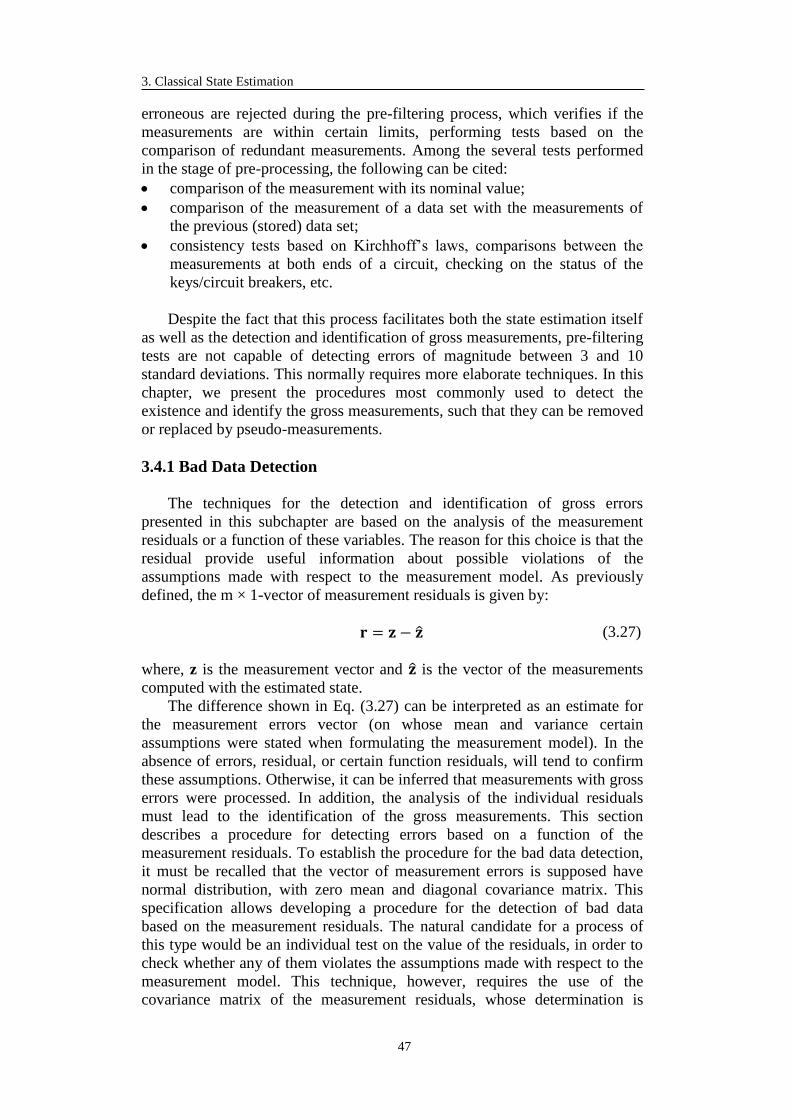
3. Classical State Estimation
47
erroneous are rejected during the pre-filtering process, which verifies if the
measurements are within certain limits, performing tests based on the
comparison of redundant measurements. Among the several tests performed
in the stage of pre-processing, the following can be cited:
comparison of the measurement with its nominal value;
comparison of the measurement of a data set with the measurements of
the previous (stored) data set;
consistency tests based on Kirchhoff’s laws, comparisons between the
measurements at both ends of a circuit, checking on the status of the
keys/circuit breakers, etc.
Despite the fact that this process facilitates both the state estimation itself
as well as the detection and identification of gross measurements, pre-filtering
tests are not capable of detecting errors of magnitude between 3 and 10
standard deviations. This normally requires more elaborate techniques. In this
chapter, we present the procedures most commonly used to detect the
existence and identify the gross measurements, such that they can be removed
or replaced by pseudo-measurements.
3.4.1 Bad Data Detection
The techniques for the detection and identification of gross errors
presented in this subchapter are based on the analysis of the measurement
residuals or a function of these variables. The reason for this choice is that the
residual provide useful information about possible violations of the
assumptions made with respect to the measurement model. As previously
defined, the m × 1-vector of measurement residuals is given by:
𝐫 = 𝐳 − (3.27)
where, z is the measurement vector and is the vector of the measurements
computed with the estimated state.
The difference shown in Eq. (3.27) can be interpreted as an estimate for
the measurement errors vector (on whose mean and variance certain
assumptions were stated when formulating the measurement model). In the
absence of errors, residual, or certain function residuals, will tend to confirm
these assumptions. Otherwise, it can be inferred that measurements with gross
errors were processed. In addition, the analysis of the individual residuals
must lead to the identification of the gross measurements. This section
describes a procedure for detecting errors based on a function of the
measurement residuals. To establish the procedure for the bad data detection,
it must be recalled that the vector of measurement errors is supposed have
normal distribution, with zero mean and diagonal covariance matrix. This
specification allows developing a procedure for the detection of bad data
based on the measurement residuals. The natural candidate for a process of
this type would be an individual test on the value of the residuals, in order to
check whether any of them violates the assumptions made with respect to the
measurement model. This technique, however, requires the use of the
covariance matrix of the measurement residuals, whose determination is

3.4 Bad Data Processing
48
computationally expensive. Considering that the bad data processing is
performed on line after each SE, it is concluded that the individual
examination of residual would not be a computationally efficient technique
for simple detection of gross measurements. Even so, if the presence of these
measurements is detected, a possible methodology for the identification of
gross errors is based on the covariance matrix of the measurement residuals,
as will be subsequently shown. The computational difficulties associated with
the individual analysis of the measurement residuals lead to the search for a
test based on an observable function of the residuals, whose behavior in the
presence and in the absence of gross errors is clearly distinct. The weighted
sum of the squared residuals is a function that satisfies this condition, that is,
if there are gross measurements in the measurement set, J() tends to assume
higher values than when such measurements are absent. Thus, taking as a
basis the value of the weighted sum of the squared residuals, some conclusion
can be stated about the presence of errors. Since both the residual and the
weighted sum of the squared residuals are random variables it is reasonable to
establish a type of detection test based on the statistical properties of these
variables. The analytical formulation of the detection process errors is based
on a statistical hypotheses test for which the following settings are required:
Statistical hypothesis: assumption about the probabilistic distribution of
one or a set of random variables;
Basic hypothesis (Null hypothesis), H0: main hypothesis;
Alternative hypothesis, H1: complement of the basic hypothesis H0, that
is, if H0 is false, H1 is true, and vice-versa;
Hypothesis test: procedure to decide if the hypothesis H0 must be
accepted or rejected.
The Hypothesis Test theory defines two types of errors:
Type I Error: rejection of the basic hypothesis H0 when it is true;
Type II Error: acceptance of the basic hypothesis H0 when it is false.
The false alarm probability, denoted α, is the probability of having a type
I error (α is considered the significance level of the test). Similarly, β
represents the probability of error type II. The quantity (1−β) represents the
probability of the basic assumption H0 to be rejected when it is false. This
quantity is called power function of the hypothesis test. The application of the
hypothesis test consists of reducing as much as possible the probability of
false alarm α and the probability of error type II β. For this reason, fixed α in
pre-specified in a low value (between 0.01 and 0.1, for example) and the
power function (1−β) is maximized over all the alternatives. This requires an
observable function of the random variables, which behaves differently under
the conditions of basic and alternative assumptions. This difference in
behavior is used to design the test. For example, suppose that S is a statistical
function that tends to assume lower values when the basic assumption is true
than when it is false. From a probability of false alarm α fixed at a small value
and the probability density function of the variables in this study, a threshold
K can be determined, so that the test will be positive if S > K and negative
otherwise. Then it is considered that the test results have a significance level

3. Classical State Estimation
49
of (100×α). In the case of PSSE, for the application of the test of Hypotheses
assumed that:
the vector of measurement errors has normal distribution with zero mean
and covariance matrix R diagonal;
the structure and the parameters of the network are known;
the measurement model is linearized at a point close the solution.
Under these conditions, the weighted sum of the squared residual has a
chi-square distribution (denoted χ2) with m−n degrees of freedom, where m
and n are respectively the number of measurements and the number of states.
Fig. 3.2 shows the probability density function of the chi-square distribution
with eight degrees of freedom. Note that this function is defined only for
positive values, and it is asymmetrical. In the presence of gross errors, the
previous assumptions become false and the weighted sum of the squared
residual does not present the chi-square distribution, tending to assume high
values.
Value of J(x)
d.p
.f o
f o
f J(
x)
Figure 3.2: Chi-squared probability density function with 8 degrees of freedom
In terms of the previously mentioned assumptions, the problem of
detecting errors is established in accordance with the following hypothesis
test:
basic assumption H0: the weighted sum of the squared residuals J()
presents the χ2 distribution;
alternative hypothesis, H1: the basic assumption is false.
Based on the probability of false alarm, it is possible to establish a
threshold K, such that:
𝑃(𝐽(x) > 𝐾 | 𝐽(x) presents the distribution χ2) = α (3.28)
where P(a > b|c) represents the probability that a is greater than b assuming
that c is true.
As shown in Fig. 3.2, the probability α and its complement (1−α) may be
interpreted as areas under the curve of density probability function of J().
Note that the specification of α determines uniquely the threshold K, that is:

3.4 Bad Data Processing
50
𝐾 = 𝜒𝑚−𝑛;1−𝛼2 (3.29)
where 𝜒𝑚−𝑛;1−𝛼2 denotes the percentile (1−α) of the χ
2-distribution with (m−n)
degrees of freedom. In summary, the test for the error detection based on the
weighted sum of the squared residuals consists in comparing the value of J()
with the value K, obtained from the cumulative χ2 distribution with (m − n)
degrees of freedom and probability of false alarm equal to α. If J() > K, then
there is evidence that there are gross measurements in the measurement set. If
the number of degrees of freedom becomes high (in practice, greater than 30),
which occurs frequently in the case of PSSE, the χ2 distribution tends to
behave as a Gaussian distribution with mean (m − n) and variance 2(m − n).
This is illustrated in Fig. 3.3, which verifies that, as the number of degrees of
freedom ℓ increases, the curve will tend to symmetry with respect to the
average.
Figure 3.3: Density probability function of the χ
2 distribution is 3 degrees of freedom [138]
For values of ℓ higher than 30, it is possible to demonstrate that the quantity:
𝐽() − (𝑚 − 𝑛)
√2(𝑚 − 𝑛) (3.30)
tends to the standard normal distribution, so that the percentiles of this
distribution can be used instead of those obtained from the χ2 distribution to
determine K. In this case K is expressed analytically as:
Φ(𝐾 − (𝑚 − 𝑛)
√2(𝑀 − 𝑁)) = 1 − 𝛼 (3.31)
where Φ(∙) is the cumulative standard normal distribution. The test for the
bad data detection can be summarized in the following steps:
calculate the weighted sum of the squared residuals J(x) after the state
estimation;
compare J() with the threshold K, obtained (a) the χ2 distribution with
(m − n) degrees of freedom and probability of false alarm α or, from the
standard normal distribution if (m − n) > 30, by Eq. (3.31):

3. Classical State Estimation
51
o if J() > K, it is concluded that there is at least one bad data in the
measurement set;
o if J() ≤ K, it is concluded that there is no bad data in the
measurement set.
3.4.2 Bad Data Identification
Based on the results of the bad data detection test, two alternatives can be
taken. If the test does not indicate the existence of such measurements, the
estimation process is finished. Otherwise, the gross measurements must be
identified, which requires the individual examination of measurement
residuals. If there is only a single gross measurement, a possible strategy of
identification could be based on the determination of maximum residual, with
the expectation that this would correspond to the gross measurements.
However, this is not necessarily true, because meters of different types have
different accuracy levels, such that the variances of the measurements can be
significantly affected. In addition, there is the possibility that the residual are
correlated, so that the effect of a gross error associated with a measurement
can spread over the residual of other quantities. These difficulties are
overcome by using the Method of Maximum Normalized Residuals [28],[29].
3.4.3 Multiple Bad Data Processing
The simplest case of bad data processing is that of a single gross
measurement. The identification procedure most often used is the one in
which it is assumed that the gross measurement is that corresponding to the
maximum normalized measurement residual (in magnitude), after being
verified the presence of bad data in the measurement set. Further about this
problem can be found in literature [30].
However, more realistic and more frequent situations are not those
relative to the existence of a simple gross error (GE). On the contrary,
practical situations are characterized by the occurrence of multiple gross
measurements, interactive or not. In the case of multiple non-interactive
errors, the application of a generalized Method of Maximum Normalized
Residuals may be sufficient to correctly identify the gross measurements [31].
In case of multiple interactive bad data, this generalization can be non-
effective, producing results which are not consistent with the reality. This
happens because the residuals are linear combinations of the measurement
errors. Therefore, there is not, necessarily, a unique correspondence between
the residual with larger magnitudes and the larger measurement errors, and for
this reason the gross measurements may not be those relating to maximum
normalized residuals.
There are numerous ways to process the multiple bad data. One of those,
Identification by elimination, corresponds to an extension of the procedure
adopted in the case of simple gross errors for the case of multiple gross errors
[32]. The second one, Identification based on hypothesis test, is based on set
of suspect measurements selected in the measurement set, and applies
procedures based on hypothesis tests to refine this set [33].

3.5 Observability Analysis
52
3.5 Observability Analysis
The problem of observability of power systems consists essentially in
determining whether the measurements that compose a given set provide
sufficient information for the SE of the power system. The analysis of
observability is particularly important during the real time operation of the
power system, because its results can determine changes in the procedures for
estimating the state variables.
In the case of deficiency of the measurement set for example, the
observability analysis must provide subsidies for, in a subsequent step,
proceeding to the estimation of states of the observable components (islands)
of the power system. Alternatively, it is possible to establish procedures for
allocating appropriate pseudo-measurements which, once added to the
deficient measurement set, will allow the recovery of the observability of the
system as a whole.
Another important by-product of the analysis of observability is the
determination of critical measurements and critical pairs. Their correct
identification is important both to indicate points of reinforcement of the
measurement set and to the processing of gross errors.
The routines for determination of observability are also useful as a tool
for design of the measurement set. In this case, it must guarantee the
achievement of reliable estimates even if some measurements are lost during
the power system operation, due to the failure of the data transmission system
or by the elimination resulting from the processing of gross errors. The tests
of observability can be used to evaluate the measurement set and indicate
where these must be reinforced, through the addition of new measurements.
3.5.1 Concepts and Solution Method
Consider a measurement set M of a power system for state estimation
purposes. It is assumed that the measurements are real and reactive power
injections in the buses, real and reactive power flows in the transmission lines
and bus voltage magnitude. The concept of power system observability is
formally expressed by the following definition:
Definition 3.1 A power system is observable, from the point of view of the
static state estimation, with respect to a given set of measurements M if the
state variables of the power system (magnitudes and angles of the bus
voltages) may be determined by processing the measurements of M through a
state estimator. Otherwise, the power system is considered non-observable
with respect to M.
The definition above, although clear, it is not operational for the purposes
of observability analysis. For this reason, it is necessary to characterize the
concept of observability in terms of certain matrices and graphs associated
with the network topology and the measurement set, which will be introduced
as follows.
As previously seen, the weighted least squares approach provides an
estimate for the increments Δx, obtained through the minimization of the
objective function:

3. Classical State Estimation
53
𝐽(∆𝐱) = [∆𝐳 − 𝐇∆𝐱]𝑡𝐑−1[∆𝐳 − 𝐇∆𝐱] (3.32)
where, for the sake of simplicity, the argument of H(.) has been eliminated.
The final solution of the state estimation problem states is obtained through an
iterative procedure in which Δx is calculated at each iteration by solving the
so-called Gauss normal equation:
𝐆∆x = 𝐇𝑡𝐑−1∆𝐳 (3.33)
where:
𝐆 = 𝐇𝑡𝐑−1𝐇 (3.34)
is the information or gain matrix defined in subchapter 3.2.
From the definition introduced earlier in this section, it is clear the
relationship between the observability and the features of the matrix G. In
fact, aiming at solving the normal equation, it is necessary that the
information matrix G is non-singular. Given that the covariance matrix of the
errors of measurement R is generally supposed diagonal and non-singular,
which implies that the Jacobian matrix H must have full rank, that is, as m>n,
the rank of H must be equal to n. Therefore, it is necessary to have at least a
subset of M composed by n measurements, such that the n corresponding rows
of the Jacobian matrix are linearly independent. This leads to the definitions
of observability presented as follows.
Definition 3.2 A power system is algebraically observable with respect to a
set of measurements M, if the Jacobian matrix H has rank equal to n, which is
the dimension of the vector of state variables x.
According to this definition, the algebraic observability depends on the
operation point used for the linearization of the measurement model.
Reference [34] assumes that this operation point is the flat bus voltage profile
(magnitudes and angles of all bus voltages equal to 1.0 p.u. and 0.0 rad,
respectively), in addition to the decoupled approximation for H proposed by
[23]. In spite of a power system being algebraically observable, it is possible
that during the iterative solution process, numerical problems eventually
prevent the convergence, due to the poor conditioning of the matrix H or due
to the actual state being too far away from the initial estimates. To take this
fact into account, it introduces the following definition:
Definition 3.3 A power system is numerically observable with respect to M if
the estimates for all states can be obtained through iterative solution starting
from initial state estimates equal to 1.0 p.u. for the magnitudes and 0.0 rad for
the angles of the bus voltages.
Therefore, it can be inferred that although the numerical observability
implies in algebraic observability, the reciprocal is in general not true. Testing
the numerical observability is equivalent to solve the problem of static state
estimation from the flat voltage profile, for a given measurement set M. The
methods based on triangular factorization proposed in [35] are in reality the

3.5 Observability Analysis
54
verification of the numerical observability, which are already implemented in
the proper solution process of the normal equation. Another possible test for
analyzing the power system observability could be the calculation (in floating-
point) of the rank of the Jacobian matrix, which would provide information
about the algebraic observability. Although several algorithms suitable for
calculating the rank of an array are available [36], the cpu time required for
this purpose is not compatible with real-time applications. In addition, they do
not indicate the points of the power network at which the measurement set
might require reinforcement, nor about observable islands.
Clements-Wollenberg method was the first specifically developed method
for the analysis of the topological observability, based on the network
topology and the location of the measurements, and therefore not using
calculations in floating point. It is a heuristic method, which is based on
principles drawn from the experience in the analysis of electrical networks
[37]. In spite of its undeniable appeal to physical understanding of the
problem of observability, the method of Clements-Wollenberg is essentially
heuristic. Consequently, the method provides conservative results in some
cases, that is, the power network can be classified as non-observable when the
power system is in reality observable. The method for observability analysis
presented as follows supplies the deficiencies of the algorithm of Clements
and Wollenberg, being supported by a more solid theoretical foundation.
3.5.2 Topological Observability
3.5.2.1 P – 𝜹 and Q – V observability
The introduction of the notions of the observability P − δ and the
observability Q − V, which are important for the investigation of topological
observability, implies the decomposition of the problem into two sub-
problems. This decoupling is similar to that used in formulation of the fast
decoupled power flow problem. It recognizes that the measurements of real
power convey a greater quantity of information about the voltage angles.
Conversely, reactive power measurements provide more information about
the voltage magnitude. Taking into account the P − δ/Q − V decoupling and
assuming that the relationship reactance/resistance of the series impedances of
the transmission lines is much greater than 1.0, the following model of
decoupled measurement is developed [136]:
𝐳𝑃 = 𝐇𝑃𝜹 + 𝜼𝑃 (3.35)
𝐳𝑄 = 𝐇𝑄𝑽 + +𝐤 + 𝜼𝑄 (3.36)
The vector zP is composed by measurements of real power injections and
flows, and the vector zQ contains the measurements of voltage magnitude,
reactive power injections and flows. The corresponding measurement errors
are represented by ηP and ηQ. Vector k can be obtained from reference [136].
The vectors δ and V contains N − 1 bus voltage angles and N bus voltage
magnitudes, respectively. The constant vector k depends on the shunt
admittances of the transmission lines. Finally, the matrices HP and HQ depend

3. Classical State Estimation
55
basically on the measurement set, the topology of the electrical network and
the series admittances of the transmission lines. From Eqs. (3.35) and (3.36),
one can state that:
Definition 3.4 A power system composed by N buses is P−δ/Q−V)
algebraically observable with respect to the real (reactive) measurement sets,
if and only if the rank of the matrix HP (HQ) is equal to N − 1 (N).
If there is no parity between the real and reactive measurement sets, the
problems of P − δ and Q − V observability must be analyzed separately. A
difficulty that arises in this case is the asymmetry introduced by the
measurements of voltage magnitude, without similar on sub-problem P − δ.
However, this type of measurement can be replaced by reactive power flow
measurement in a fictitious transmission line, connecting the bus where
measurement of the voltage magnitude is taken to a reference bus [38],[39].
Therefore, in general, any algorithm for analysis of observability should be
executed twice for the same system. However, the measurement sets used in
practice normally present the measurements of power injection and power
flow taken in pairs real/reactive. If the voltage magnitude measurement is
considered only in the reference bus, the conclusions about the observability P
− δ and Q − V can be obtained from a single application of the algorithm of
observability. Without loss of generality, this chapter considers that the
measurements of power injections and flows are taken in pairs.
3.5.2.2 Algorithm
This subchapter deals with a combinatory algorithm for the determination
of topological observability. The algorithm in question is derived from the
work described in [40]. The method is based on the formulation of the
problem of topological observability in terms of graph of the system
measurement, Z, associated with a given measurement set M, whose vertices
and edges are defined as follows:
1. The vertices of Z are the same vertices of the graph of network;
2. If the flow in the line i−j is measured, then the vertices i and j in Z are
connected by an edge that will be associated with that measure of edge
flow (flow);
3. If the injection in bus i is measured, the vertex i in Z will be connected to
each of its adjacent vertices by edges that will all be associated with the
measurement of the power injection (edges of injection).
The graph of measurement contains, therefore, all the possible edges that
may be associated with the measurements on M. Once this subgraph is
determined, the problem of topological observability analysis may be thus
enunciated: investigate the existence of a spanning tree in graph of
measurements, considering the constraint that this tree may not contain more
than one edge associated to a given measure.
A tree with these characteristics is clearly an observable spanning tree of
the graph of the network associated with the M. The proposed algorithm is
able to find such tree whenever it exists, as well as detects promptly the cases
in which it does not exist.

3.5 Observability Analysis
56
3.5.2.3 Measures of Magnitude of Voltage
If the parity between real and reactive measurements is not verified, the
problems of observability P − δ and Q − V must be analyzed separately. In
addition, the presence of multiple measurements of voltage magnitude in the
system must be properly taken into account, because these measurements
significantly influence the analysis of observability Q − V. Van Cutsen and
Gailly [38] showed that the voltage measurements can be represented (in
which concerns the analysis of topological observability only) by reactive
flow in a transmission line, with a fictitious unitary susceptance, connecting
the bus where the voltage is measured to the earth. It becomes necessary
therefore to include an additional bus representing the reference, so that from
the point of view of observability Q − V, the network becomes contain N + 1
buses. Consequently, an observable spanning tree for analysis Q − V should
contain N branches. To illustrate the effect of voltage measurements in the
analysis of observability Q − V, consider the Fig. 3.4, which represents an
electrical network in which only reactive measurements (q, u and v) are
represented. Note that only the power injections and power flows do not
guarantee the Q − V observability. However, the voltage measurements allow
you to find a spanning tree that includes observable in the land, which is
shown in Fig. 3.4.
Figure 3.4: Treatment of the voltage magnitude measurements in the analysis of the Q−V
observability
Finally, it appears that the method described above for the representation
of voltage measurements in the analysis of observability is consistent with the
fact that widely known that, even when the measurements of power are made
to pairs real/reactive, there is need to have at least a voltage magnitude
measurement to estimate the states. In fact, only in this case is that if one can
connect the observable ground in the spanning tree analysis of observability Q
– V.
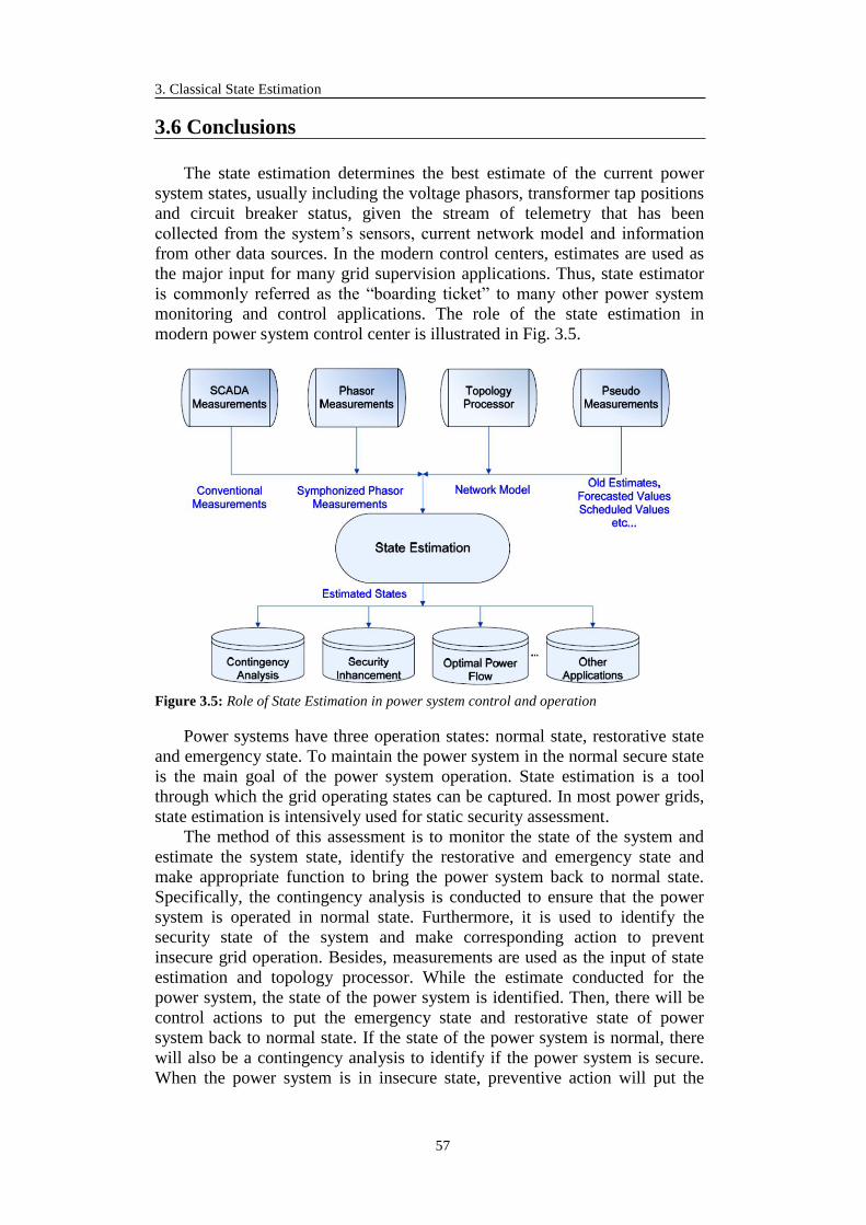
3. Classical State Estimation
57
3.6 Conclusions
The state estimation determines the best estimate of the current power
system states, usually including the voltage phasors, transformer tap positions
and circuit breaker status, given the stream of telemetry that has been
collected from the system’s sensors, current network model and information
from other data sources. In the modern control centers, estimates are used as
the major input for many grid supervision applications. Thus, state estimator
is commonly referred as the “boarding ticket” to many other power system
monitoring and control applications. The role of the state estimation in
modern power system control center is illustrated in Fig. 3.5.
Figure 3.5: Role of State Estimation in power system control and operation
Power systems have three operation states: normal state, restorative state
and emergency state. To maintain the power system in the normal secure state
is the main goal of the power system operation. State estimation is a tool
through which the grid operating states can be captured. In most power grids,
state estimation is intensively used for static security assessment.
The method of this assessment is to monitor the state of the system and
estimate the system state, identify the restorative and emergency state and
make appropriate function to bring the power system back to normal state.
Specifically, the contingency analysis is conducted to ensure that the power
system is operated in normal state. Furthermore, it is used to identify the
security state of the system and make corresponding action to prevent
insecure grid operation. Besides, measurements are used as the input of state
estimation and topology processor. While the estimate conducted for the
power system, the state of the power system is identified. Then, there will be
control actions to put the emergency state and restorative state of power
system back to normal state. If the state of the power system is normal, there
will also be a contingency analysis to identify if the power system is secure.
When the power system is in insecure state, preventive action will put the

3.6 Conclusions
58
system back to normal secure state, which is the ideal state of the power
system.
The SE solution determines the optimal estimate of the system state,
which is composed of complex bus voltages in the entire power system. The
estimates based on the network model and the gathered measurements from
the system. Moreover, state estimation provides the best estimates for all the
line flows, loads, transformer taps, and generator outputs. The typical
functions of state estimation are topology processor, observability analysis,
state estimation solution, bad data processing and parameters and structural
error processing. Firstly, the topology processor gathers status for the circuit
breakers and switches, and produces the one-line diagram of the system.
Secondly, Observability analysis determines if a state estimation solution for
the entire system can be obtained by the available set of measurements and
the identified network topology. Besides, it could identify the unobservable
branches and the observable islands in the system if any exist. Thirdly, bad
data processing detects the existence of gross errors in the measurement set. It
identifies and eliminates bad measurements provided that there is enough
redundancy in the measurement configuration. Lastly, parameter and
structural error processing estimates various network parameters, such as
transmission line model parameters, transformer tap changer parameters,
shunt capacitor or reactor parameters using the measurements as known
values. Besides this functionality, structural errors in the network
configuration as the erroneous breaker status can be identified provided that
there is enough measurement redundancy.

59
CHAPTER 4
4. Distribution System State Estimation
4.1 Introduction and Motivation
High penetration of DG is currently limited by the passive operating
methods of DN. Automatic Voltage Control (AVC) with current
compounding applied to distribution transformers usually assumes a simple
R+jX or Z∠θ network model which, combined with radial power flow, allows
the AVC system to maintain the voltage of the network within limits. When
DNs become real, this network and load model no longer applies. With the
export of power from the generating station a voltage difference is often
created. The resultant voltage rise along the feeder from the substation to the
DG can cause the feeder voltage to exceed its upper limit [41].
The DG has to provide ancillary services (to solve local and global issues
– frequency, reserve, voltage regulation, congestion management). Therefore
the DS will assume the role of DSO. Premise of this is the knowledge of the
network. For this reason, SE applied to DN is a main tool to improve the
effects of DG penetration as an improved knowledge of the network
condition, or state, is required. Usually, at distribution level, insufficient
measurements are taken to allow satisfactory control, so measurement is
extended through the use of SE techniques.
As previously elaborated, SE has been widely used on TNs to assess the
network operating conditions given a set of redundant measurements. Since
not only the redundancy cannot be obtained, but also the number of
measurement equipment is limited in DNs, distribution SE algorithms in
most of the approaches use a large number of load pseudo-measurements.
When transferring the techniques of SE to DNs, there are additional
aspects that must be considered. They focus on the causes of ill-
conditioning of the gain matrix G, which can lead to poor convergence, or
non-convergence, of the iterative state estimator.

4.1 Introduction and Motivation
60
Following issues regarding SE must be analyzed when designing the
Distribution System State Estimation (DSSE):
Pseudo-measurements. The distribution state estimator is expected to
have a large number of load pseudo-measurements or to use some
other innovative technique. Authors in [42] suggest that this may cause
problems of instability due to increased poor conditioning of the gain
matrix.
Network Impedances. Adjacent long and short lines (i.e. large and small
impedances) are also a source of ill-conditioning [43]. The authors
proposed an orthogonal decomposition method. This feature of SE can be
expected to have an effect where there are very low impedance lines
coupling busses.
Virtual Measurements. The combination of measurements with very
large and very small weighting factors leads to ill-conditioning of the
gain matrix G [44]. The use of equality constraints to fix known values,
e.g. zero injection at a non-load bus, can improve numerical stability.
Scaling. Poor scaling of measurement values has been identified as
another cause of ill-conditioning of the gain matrix [45]. While this is
satisfactory for Transmission System State Estimation (TSSE), the above
suggests that for distribution state estimate on the base should be reduced.
Adding to the complexity of the problem is the existence of the significant
differences in the characteristics of typical DNs compared to typical TNs that
are summarized in the Table 4.1 below [46]:
Table 4.1: Technology options for DN development
Characteristics Transmission Distribution
Topology Generally extensively
meshed and must be
analyzed as a whole
Generally many
independent substations,
each supplying several
radial feeders. Can be
analyzed as multiple
independent islands
Phase unbalance The degree of unbalance is
generally sufficiently small
that it can be ignored and
only positive sequence
analyzed
The degree of unbalance
may be quite large and
each phase should be in
that case considered
independently
SCADA Measurements A high percentage of
devices have
measurements. Significant
part of the network has
measurement redundancy
and is mathematically
observable
Generally has many more
load points than
measurements. Practically
speaking, there is usually
no measurement
redundancy and,
considering SCADA
measurements only, is
highly unobservable
Network Size vs
Investments
A typical network size
ranges from few hundred
busses to one or two
thousand
A typical network size
ranges from 10 000 to
100 000 electrical nodes

4. Distribution System State Estimation
61
Finally, apart from the already described physical and technological
characteristics of DNs, increased penetration of DGs is leaving multiple prints
in operational issues of DNs. It is necessary to briefly describe the changes
that DG is inducing in modern systems which points out once again the
importance of DSSE.
4.1.1 The Impact of Dispersed Generation on Distributed Networks
DG is playing an increasing role in the electric power system of todays.
DG is by definition limited in size (roughly 10 MW or less) [47] and
interconnected at the substation, distribution feeder or customer load levels.
DG technologies include photovoltaics, wind turbines, fuel cells, small and
micro sized turbine packages, stirling-engine based generators, and internal
combustion engine-generators. These technologies have already entered in a
period of rapid expansion and commercialization. With so much new DG
being installed, it is critical to assess the power system impacts accurately so
that these units can be applied in a manner that avoids causing degradation of
power quality, reliability, and control of the utility system [47].
The introduction of generation sources on the DS can significantly impact
the flow of power and voltage conditions at customers and utility equipment.
These impacts may manifest themselves either positively or negatively
depending on the DS operating characteristics and the DG characteristics.
Positive impacts are generally called “system support benefits” and include:
Voltage support and improved power quality;
Loss reduction;
Transmission and distribution capacity release;
Deferments of new or upgraded transmission and distribution
infrastructure;
Improved utility system reliability.
Achieving the above benefits is in practice much more difficult than it is
often realized. The DG sources must be reliable, dispatchable, of the proper
size and at the proper locations. They must also meet various other operating
criteria. Since many DGs will not be utility owned or will be variable energy
sources such as solar and wind, there is no guarantee that these conditions will
be satisfied and that the full system support benefits will be realized. In fact,
power system operations may be adversely impacted by the introduction of
DG if certain minimum standards for control, installation and placement are
not maintained. This subchapter is focusing on the voltage quality, loss
reduction and reliability factors associated with DG.
4.1.1.1 Voltage Regulation and Losses
Radial DSs are normally regulated using load-tap-changing transformers
at substations, supplementary line regulators on feeders, and switched
capacitors on feeders. Voltage regulation practice is based on radial power
flows from the substation to the loads while DG sometimes introduces
reversed power flows that interfere with the effectiveness of standard voltage
regulation practice.

4.1 Introduction and Motivation
62
If a DG unit is applied just downstream of a voltage regulator or on-load
tap changing (LTC) transformer that is using considerable line drop
compensation, then the regulation controls will be unable to properly measure
feeder demand (Fig. 4.2). With DG, the voltage becomes lower on the feeder.
In this case, the voltage is reduced because the DG reduces the observed load
at the line drop compensator control. This can confuse the regulator into
setting a voltage lower than is required to maintain adequate service levels at
the tail end of the feeder. This is the opposite effect of “voltage support”, a
commonly touted benefit of DG.
Figure 4.1: Voltage profiles with and without DG [47]
DG may also result in high voltage at some electric customers. For
example, a small residential DG system that shares a common distribution
transformer with several other residences may raise the voltage on the
secondary enough to cause high voltage at these customers. The presence of
the DG may introduce reverse power flow to counteract this normal voltage
drop, perhaps even raising voltage somewhat, and the service voltage may
actually be higher at the customer services than on the primary side of the
distribution transformer.
The preceding examples have shown ways that both high and low service
voltage can occur due to the incompatibility of DG with the radial power flow
based voltage regulation approach used on most utility systems. As a result,
the DG influence on voltage for any potential application should always be
assessed to insure that no customers will be adversely impacted.
In essentially all cases, the impact on the feeder will be negligible for any
individual residential scale DG unit (<10 kW) [47]. However, when the
aggregate capacity of many small units deployed reaches a critical threshold
or when the capacity of a single unit is large enough, then the knowledge of
the network state and voltage regulation studies are desirable to insure that the
feeder voltage will be maintained within appropriate limits. The aggregate DG
capacity threshold, for which studies become appropriate, depends on many
factors. DG will also impact losses on the feeder. DG units should be placed
at optimal locations where they provide the best reduction in feeder losses. In

4. Distribution System State Estimation
63
that manner it would be planned and called distributed generation. However,
DG is installed where there are customers. The connection point is generally
the nearest point to the network. This is why it is referred as dispersed.
4.1.1.2 Voltage Flicker
DG may cause noticeable voltage flicker. Flicker can be either a simple
issue or a complex issue as far as its analysis and mitigation are concerned.
From the simple perspective, it can be the result of starting a machine (e.g.
induction generator) or step changes in DG output which result in a significant
voltage change on the feeder. If a generator starts, or its output fluctuates
frequently enough, flicker of lighting loads may be noticeable to customers.
Mitigation approaches include reduced voltage starts on induction
generators as well as speed matching. Synchronous generators might require
tighter synchronization and voltage matching. A less technical approach to
reduce flicker involves placing constraints on when and how often DG
operators may start and change the output of DG systems. In the case of wind
and solar energy systems, the outputs will fluctuate significantly as the sun
and wind intensity change.
Determination of the risk of flicker problems due to basic generator
starting conditions or output fluctuations is fairly straightforward using the
flicker curve approach, particularly if the rate of these fluctuations is well
defined, the fluctuations are “step” changes and there are no complex dynamic
interactions of equipment. The dynamic behavior of machines and their
interactions with upstream voltage regulators and generators can complicate
matters considerably. For example, it is possible for output fluctuations of a
DG (even smoother ones from solar or wind systems) to cause hunting of an
upstream regulator and, while the DG fluctuations alone may not create
visible flicker, the hunting regulator may create visible flicker. Thus, flicker
can involve factors beyond simply starting and stopping of generation
machines or their basic fluctuations. Dealing with these interactions requires
an analysis that is far beyond the ordinary voltage drop calculation performed
for generator starting.
4.1.1.3 Harmonics
Many generating like wind power plants or PV units are connected to the
grid via inverter. The inverters are the main contributors to the insertion of the
harmonics in the grid. Although the contribution of a single converter might
seem insignificant because of the power of the DG it is connected to,
contribution of many units can insert big distortion. Nowadays, inverters are
designed with IGBT (Insulated Gate Bipolar Transistor) technology that use
pulse width modulation to generate the injected “pure” sinusoidal wave. This
new technology produces a cleaner output with fewer harmonic that should
satisfy the IEEE 1547-2003 standards [139]. Rotating generators such as
synchronous generators can be another source of harmonics. Depending on
the design of the generator windings (pitch of the coils), core non-linearity,
grounding and other factors, significant harmonics can occur. The grounding
arrangement of the generator and step-up transformer will play a major role in

4.1 Introduction and Motivation
64
limiting the feeder penetration of harmonics. Arrangements can be selected to
block or reduce third harmonic injection to the utility system. This would tend
to confine it to the DG site only.
For larger DG units or cases involving complex harmonic problems,
measurements and modeling of the system harmonics may be required to
assess conditions. Any analysis should consider the impact of DG currents on
the background utility voltage distortion levels. The limits for utility voltage
distortion are 5% for total harmonic distortion (THD) and 3% for any
individual harmonic [47].
4.1.1.4 Impact on Short Circuit Levels
Studies of the impact of DG on the network faults current indicate that
DG may invalidate overcurrent protection. DG may affect the operation of
existing DNs by providing flows of fault currents which were not expected
when the protection was originally designed. In practice, the presence of DG
may result in increased fault currents which depend on capacity, penetration,
technology, interface of the DG, and system voltage prior to the fault.
The fault contribution from a single small DG unit is not large, however,
the aggregate contributions of many small units, or a few large units, can alter
the short circuit levels enough to cause fuse-breaker miscoordination. This
could affect the reliability and safety of the DS [47].
For inverters, the fault contributions will depend on the maximum current
level and duration for which the inverter manufacturer’s current limiter is set
to respond. For most induction generators, the significant current would only
last a few cycles and would be determined by dividing the pre-fault voltage by
the transient reactance of the machine. Even though a period of few cycles is a
short time, it is long enough to impact fuse-breaker coordination and breaker
duties in some cases.
The current contribution from DG units is enough to impact fuse
coordination in some cases, especially in weaker parts of the system. The
contributions will decrease with the increase of generator’s distance from the
fault. The configuration and impedance of the DG site step-up transformer
will also play a role.
4.1.1.5 Grounding and Transformer Interface
DG must be applied with a transformer configuration and grounding
arrangement compatible with the utility system to which it is to be connected.
Otherwise, voltage swells and over-voltages may be imposed on the utility
system that damage utility or customer equipment.
Use of a DG source that does not appear as an effectively grounded
source connected to such systems may lead to over-voltages during line to
ground faults on the utility system. This condition is especially dangerous if a
generation island develops and continues to serve a group of customers on a
faulted DS [47].
To avoid problems, all DG sources on multi-grounded neutral systems
that are large enough to sustain an island should present themselves to the
utility system as an effectively grounded source. If they do not, they should

4. Distribution System State Estimation
65
use appropriate protective relaying to detect primary side ground fault over-
voltages and quickly trip off-line (instantaneous trip).
4.1.1.6 Islanding
Islanding occurs when the DG (or group of DGs) continues to energize a
portion of the utility system that has been separated from the main utility
system. Islanding can occur only if the generator(s) can self-excite and sustain
the load in the islanded section. In most cases it is not desirable for a DG to
island with any part of the utility system because this can lead to safety and
power quality problems that will affect the utility system and loads. Islanding
also increases the likelihood that DG sources may be allowed to subject the
island to out of range voltage and frequency conditions during its existence.
And it can pose a serious safety threat during downed conductors and utility
repair operations since the public and utility workers may be exposed to
circuits that otherwise would be de-energized. Finally, islanding can hinder
service restoration by requiring line crews to spend extra time disabling the
island conditions. This will impact reliability indices such as SAIDI.
To prevent islanding, a DG unit operating in parallel with the utility
system should in a timely manner sense a significant voltage sag or
discontinuity of service on the utility side and disconnect from the system.
Voltage and frequency relays are used as a means of anti-island
protection. In most cases, if a generator becomes islanded, it will not be able
to satisfy the sudden change in its load without a significant change in voltage
and/or frequency and the relays will trip the unit off-line. This type of anti-
islanding protection is called “passive.” Passive protection can be deceived if
the generator is able to carry the load of the island without a substantial
change in voltage or frequency so, as a further safeguard; many smaller
inverters today also use what is called “active” anti-islanding protection. One
common “active” approach is for the inverter to be “tuned” to operate while
islanded at a frequency other than nominal value [47].
Since islanding can cause severe voltage quality and reliability problems,
the proper use and setting of anti-islanding controls is one of the more
important issues for DG installations. Of course, for this action to take place,
the network operator must, in every moment, be aware of the state of the DN.
Today, the way to avoid unwanted islanding is to disconnect the DG
through the interface breakers, operated by minimum/maximum
voltage/frequency relays, i.e., by local information only.
This requirement results in restrictive protection settings which, in many
cases, determine the unsuitable breaker operation e.g., due to instability
conditions of the electrical system. In such cases, the DG could be shed when
it is necessary to stabilize the system [145]. The only way to overcome this
problem is to set up an adequate communication system between the
distributor substation and the DG.
4.1.1.7 Intentional Islanding for Reliability
The implementation of DG can increase reliability of electric service if
units are configured to provide “backup-islands” during upstream utility

4.1 Introduction and Motivation
66
source outages. To be effective this requires reliable DG units and careful
coordination of utility sectionalizing and protection equipment [47].
A DG assigned to carry the island must be able to restart and pick up the
island load after the switch has opened. Power flow analysis of island
scenarios must be performed to insure that proper voltage regulation is
maintained and to establish that the DG can handle inrush during “starting” of
the island. The DG unit must be able to follow load during islanded operation
and the switch will need to sense if a fault current has occurred downstream of
the switch location and send a signal to block islanding if a fault has occurred
within the island zone. When utility power is restored on the utility side, the
switch must not close unless the utility and “island” are tightly in
synchronism. This requires measuring the voltage on both sides of the switch
and transmitting that information to the DG unit supporting the island so that
it can “synchronize” with the utility and allow reconnection.
4.1.1.8 Bidirectional Power Flow and Protection System
The presence of DG connected to DNs changes the typical operating
conditions. In particular, the inversion of the PF on the MV/LV transformers
could occur. In the passive DNs, the power flows typically from MV to LV
systems, and the protection systems are based on this assumption. When the
power produced by the DG is higher than that power required by the local
loads, the LV network seen from the MV side could be considered as a
generating unit connected to the MV system. The frequency of this situation
will increase with high RES penetration [144].
The protection systems currently in operation in the LV networks are not
able to handle bidirectional PFs: in the presence of bidirectional PFs, they are
likely to behave unsuitably in the selection of the fault point. This can result
in unwanted islanding of a portion of the LV system, supplied by the DG,
which could be not acceptable for safety reasons.
4.1.1.9 Hosting Capacity
As already underlined, the increase in DG penetration may have an
adverse influence on several power quality parameters and, in a wider
perspective, a direct impact on the management and control of distribution
grids, and finally, on the whole power system security. To quantify the impact
of increasing penetration of DG on the power system, the Hosting Capacity
(HC) approach was developed. The basis of this approach is a clear
understanding of the technical requirements that the customer places on the
system (i.e. quality and reliability) and the requirements that the system
operator may place on individual customers to guarantee reliable and high-
quality operation of the system. By definition, HC is the maximum DG
penetration at which the power system operates satisfactorily and it is
determined by comparing some performance indices with predefined bounds,
which are selected in order to represent the limit of secure operation of the
power system [141]. The performance indices are calculated as a function of
the DG penetration level, and the HC is the DG penetration level at which at
least one performance index reaches upper/lower bound.
4. Distribution System State Estimation
67
Technical rule EN 50160 [142] introduces some reference terms that
could be adapted in order to set the performance indices limit, however,
especially with respect to power quality issues, it lacks a common accepted
approach. An overview of the state-of-the-art on power quality indices can be
found in [143].
From all previously stated, it is obvious that DSSE with other functions of
modern DMS are having a huge importance in DNs even now and this trend
will only increase in the future. Together with the already described
circumstances of active DNs that rely on DSSE in Chapter 2 of this
dissertation, here will be briefly underlined some of the other key features of
this function.
Optimal operation of DNs comprises of the economics, quality and
reliability of distributed energy. One of the most important tools that enable
optimal operation of DNs in all its features is monitoring of the system and
DSSE is the software tool that enables it. Knowing the state of the DNs is a
base to other DS control functions:
real time reliability system and reconfiguration network for reliability
improvement;
VAR management in the DNs for minimizing the losses;
reconfiguration of the network for optimal power flow;
fault management in the DNs for the reduction of customers’
interruption duration;
short time load forecasting in DN;
energy management and load management of the DNs.
Nowadays, DSSE is a field of a significant scientific interest and many
authors have been dealing with this subject. As already pointed out, many
approaches have been based on the adaptation of Transmission System
State Estimation (TSSE) to DN environment. Following subchapter
addresses some of the key developments in the field of DSSE.
4.2 Bibliography review
Since the pioneering work of F.C. Schweppe in 1970 [48], SE has become
a key function in supervisory control and planning of electric power grids. It
serves to monitor the state of the grid and enables energy management
systems (EMS) to perform various important control and planning tasks such
as establishing near real-time network models for the grid, optimizing power
flows, and bad data detection/analysis. Another example of the utility of SE is
the SE-based reliability/security assessment deployed to analyze
contingencies and determine necessary corrective actions against possible
failures in the power systems.
In view of the ongoing development of a “smarter” grid, more research on
SE is needed to meet the challenges that the envisioned smart grid
functionalities present. Among others, environmental compliance, energy
conservation, and improved dependability, reliability, and security will
impose additional constraints on SE and require improved performance in

4.2 Bibliography review
68
terms of response time and robustness [49]. In this subchapter, a brief survey
drown out from extensive bibliography research of SE developed technologies
will be provided and also examined the challenges and opportunities
presented by the evolution of the legacy grid into a smarter grid.
Research presented by M. E. Baran and A. W. Kelley in [50] bring the
first steps towards development of DSSE. In conventional operation of a DS,
there is very little real-time information available to monitor the system; the
voltage and the power supplied to the feeders at the substation are usually the
only realtime measurements available to DSOs at distribution control centers.
However, more extensive real-time monitoring and control is needed for
effective operation of the system and for good quality of service to the
customers. In addition to monitoring and control of switches and control
devices, detailed real-time load data is needed for real-time monitoring and
control purposes. Unfortunately, this data is not currently available and
historical data about the customer loads is used to forecast the loads [51].
Obviously, the accuracy of historical data may not be good enough for real-
time applications.
Since it is not possible to measure every quantity and telemeter it to the
control center, only a limited number of real-time measurements will be
available at the control center. Then the problem becomes determining the
operating point of the system as accurately as possible based on these limited
measurements.
When there are only a few measurements, power flow analysis can be
used to obtain an approximate solution by scaling the forecasted loads such
that the power flow results match the measurements. To improve the accuracy
of load data, however, more real-time measurements are needed so that the
validity of the forecasted load data can be checked and corrected if necessary.
Authors proposed using of SE for this purpose.
The main function of SE is to minimize the errors and inconsistencies that
may exist in data. A state estimator can "smooth out" small errors in meter
readings, detect and identify gross measurement errors, and "fill-in" meter
readings that have failed due to communication failures [52].
The main point of reference [50] is to develop a SE method that can be
used in monitoring of a distribution feeder in real-time. The authors relied
strongly on classical TSSE approach with adjustments taking into account the
specific nature of DNs like representation of feeders and deficiency of real-
time measurements. Three-phase approach has been utilized in this research.
An investigation of the measurement functions will reveal that all the
functions, except the one corresponding to the voltage magnitude
measurement, are nonlinear functions of state variables. These functions are
more complex than the single-phase case, since they not only contain product
terms between neighboring nodes, but also cross product terms between
phases. This indicates that the Jacobian H corresponding to the measurement
equations will not be constant (i.e., the elements of Jacobian will depend on
state variables, x). However, it is very desirable to have a constant Jacobian
for computational efficiency, since then the normal equations will be easier to
construct and solve iteratively. For this purpose, authors tried to approximate
the Jacobian by simplifying its elements.

4. Distribution System State Estimation
69
For SE to be effective, a minimum amount of real-time data is necessary.
In this research, the power supplied to the feeders and voltage measurements
at the substation are the only real-time measurements available at distribution
level. Some feeders may have a few branch current or power measurements
also. Considering the data required for power flow analysis as the minimum
data, and taking distribution transformer primaries as load points, this real-
time data is not enough for SE. Therefore, authors propose to use historical
load data to forecast the loads since it is an approach commonly used by
utilities. These forecasted data are used as pseudo-measurements,
measurements that are less accurate than actual measurements, to supplement
for the real-time data available for SE.
The minimum data assumed to be available will satisfy the so-called
topological observability when it is applied on a per-phase basis. However,
the mutual terms in three-phase analysis and current magnitude measurements
may require the check for numerical observability which corresponds to the
gain matrix being non-singular. Numerical observability can be checked
during the LDU factorization of the gain matrix, G; if any of the pivots
become very small then this is an indication that the gain matrix may be
singular, hence the system may not be observable.
Results indicate that SE with limited measurements improves the
accuracy of the load only marginally when the forecasted load data is properly
scaled. In continuance, results indicate that SE has good convergence
characteristics even with very limited measurements. Test results also indicate
that SE can improve the forecasted load data by using real-time
measurements. However, the effectiveness of SE mainly depends on the
accuracy of the forecasted loads when there are only limited real-time
measurements. It is also observed that power flow measurements are more
effective in bad data identification than current measurements. It is the hope
of these authors that as more real-time measurements become available at
distribution level, SE will be used for feeder monitoring as widely as it is used
for monitoring of TNs today.
The development of the DSSE was further tackled by the same authors in
[53]. The main focus of this research was to develop a computationally
efficient SE method that is tailored for monitoring of distribution feeders in
real-time. A branch-current-based three-phase SE method was developed. The
method can handle radial and weakly meshed feeders which may have a few
loops created by closing some normally-open tie or line switches. The method
is computationally more efficient and more insensitive to line parameters than
the conventional node-voltage-based SE methods. This improvement mainly
comes from the fact that the branch current formulation decouples the SE
problem into three sub-problems, one for each phase. Furthermore, a simple
rule based feeder network reduction method is proposed in this research to
further improve the computational efficiency of SE without sacrificing
accuracy.
The branch-current-based SE method, like conventional node-voltage-
based SE methods, is based on the weighted least square (WLS) approach.
Rather than using the node voltages as the system state, the proposed method
uses the branch currents and solves the following WLS problem to obtain an
estimate of the system operating point defined by the system state x:
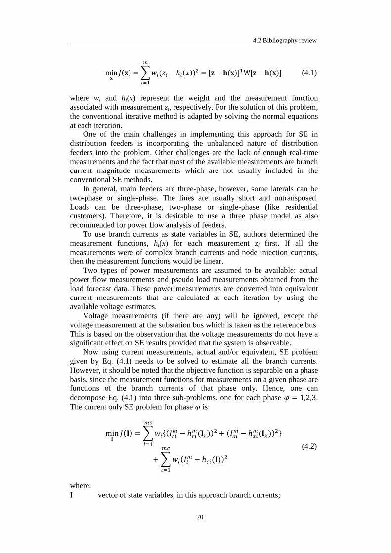
4.2 Bibliography review
70
min𝐱𝐽(𝐱) =∑𝑤𝑖(𝑧𝑖 − ℎ𝑖(𝑥))
2 = [𝐳 − 𝐡(𝐱)]TW[𝐳 − 𝐡(𝐱)]
𝑚
𝑖=1
(4.1)
where wi and hi(x) represent the weight and the measurement function
associated with measurement zi, respectively. For the solution of this problem,
the conventional iterative method is adapted by solving the normal equations
at each iteration.
One of the main challenges in implementing this approach for SE in
distribution feeders is incorporating the unbalanced nature of distribution
feeders into the problem. Other challenges are the lack of enough real-time
measurements and the fact that most of the available measurements are branch
current magnitude measurements which are not usually included in the
conventional SE methods.
In general, main feeders are three-phase, however, some laterals can be
two-phase or single-phase. The lines are usually short and untransposed.
Loads can be three-phase, two-phase or single-phase (like residential
customers). Therefore, it is desirable to use a three phase model as also
recommended for power flow analysis of feeders.
To use branch currents as state variables in SE, authors determined the
measurement functions, hi(x) for each measurement zi first. If all the
measurements were of complex branch currents and node injection currents,
then the measurement functions would be linear.
Two types of power measurements are assumed to be available: actual
power flow measurements and pseudo load measurements obtained from the
load forecast data. These power measurements are converted into equivalent
current measurements that are calculated at each iteration by using the
available voltage estimates.
Voltage measurements (if there are any) will be ignored, except the
voltage measurement at the substation bus which is taken as the reference bus.
This is based on the observation that the voltage measurements do not have a
significant effect on SE results provided that the system is observable.
Now using current measurements, actual and/or equivalent, SE problem
given by Eq. (4.1) needs to be solved to estimate all the branch currents.
However, it should be noted that the objective function is separable on a phase
basis, since the measurement functions for measurements on a given phase are
functions of the branch currents of that phase only. Hence, one can
decompose Eq. (4.1) into three sub-problems, one for each phase 𝜑 = 1,2,3.
The current only SE problem for phase 𝜑 is:
min𝐈𝐽(𝐈) =∑𝑤𝑖(𝐼𝑟𝑖
𝑚 − ℎ𝑟𝑖𝑚(𝐈𝑟))
2 + (𝐼𝑥𝑖𝑚 − ℎ𝑥𝑖
𝑚(𝐈𝑥))2
𝑚𝑠
𝑖=1
+∑𝑤𝑖(𝐼𝑖𝑚 − ℎ𝑐𝑖(𝐈))
2
𝑚𝑐
𝑖=1
(4.2)
where:
𝐈 vector of state variables, in this approach branch currents;

4. Distribution System State Estimation
71
𝐼𝑟𝑖𝑚 equivalent current measurement of the real power measurement;
𝐼𝑥𝑖𝑚 equivalent current measurement of the reactive power measurement;
ℎ𝑟𝑖𝑚(𝐈𝑟) measurement function of the real part of the equivalent current
measurement;
ℎ𝑥𝑖𝑚(𝐈𝑥) measurement function of the imaginary part of the equivalent current
measurement;
𝐼𝑖𝑚 current measurement;
ℎ𝑐𝑖(𝐈) measurement function of branch current magnitude measurement;
The two summation terms in the objective function are for the power and the
current measurements.
The current only SE problem given by Eq. (4.2) is solved together with
the voltage update procedure forward sweep to obtain the SE solution. This
iterative process involves the following steps at each iteration k:
Step 1. Given the node voltages V𝑘−𝑙, convert power measurements into
equivalent current measurements.
Step 2. Use current measurements to obtain an estimate of branch currents
𝜑𝑘 = [𝑟,𝜑
𝑘 𝑥,𝜑 𝑘 ] by solving the current only SE problem given by Eq.
(4.2) for each phase 𝜑 = 1,2,3.
Step 3. Given the branch currents, update the node voltage Vk by the forward
sweep procedure.
Step 4. Check for convergence; if two successive updates of branch currents
are less than a convergence tolerance, stop, otherwise go to step 1.
Test results indicate that the method has superior performance compared
to the conventional node-voltage-based methods both in terms of computation
speed and memory requirements. The method is specially tailored for weakly
meshed DSs which are radial or have a few loops. Another advantage of the
method is its insensitivity to line parameters, which improves both its
convergence and bad data handling performance. Finally, it is shown that the
proposed feeder reduction method is very effective in improving the
computation speed and filtering properties of the method without sacrificing
accuracy.
Research of C. N. Lu, J. H. Teng and W. H. E. Liu [54] is another three-
phase DSSE approach. Authors point out that, due to the requirements of
filtering measurement data and having real-time system states for on-line
operation, the need for a DSSE is more than justified.
In addition to the network data, DSO also needs a set of redundant
measurements to obtain an estimate of the system states. In a fully automated
system the measurements are sufficient for SE. However, in the current stage
of distribution system automation (DSA), the number of meters installed in
the system is low and may not be sufficient for SE, i.e. the system may not be
completely observable. In order to obtain an SE under this condition,
techniques have to be developed to provide additional data (i.e. pseudo-
measurements) to the estimator.
Authors mitigate the problem of redundancy by introducing speial three-
phase SE algorithm based on normal equation method. A new rectangular
form SE based on current instead of power, is introduced. The proposed

4.2 Bibliography review
72
algorithm can be used to handle many types of measurements. It is applicable
to the current magnitude measurements that are often found in the distribution
sysrem telemetry. The three-phase network models and mathematical
formulation of the method are described in this paper.
Authors point out that historical data are available and can be utilized to
forecast the loadings of feeders and distribution transformers. These data are
treated as pseudo-measurements. Loads in a DS are usually classified as three
general types of customers. they are the residential, industrial and commercial
customers. Typical load pattern or daily load curve of each type of customer
can be obtained by electric load synthesis or load survey technique [55]. The
load composition of each distribution transformer can be calculated according
to the energy consumption of all customers served by the transformer. By
using the load patterns and the derived load composition, an hourly load of
distribution transformer can be estimated and used as a pseudo-measurement.
Authors use similar model as the one presented in reference [53] - SE
formulation based on current instead of power. The proposed formulation can
handle all types of measurements. In each iteration of SE, power
measurements are converted into their equivalent currents. The authors also
make a similar observation regarding the observability and how to obtain it.
The measurement data are simulated by using a three-phase power flow
solution. Noise is added to each measurement and weights of measurements
are given. Noise is added randomly to the actual and pseudo-measurements
and is at the ranges of ±10% and ±30% respectively. Two different weights
are given to the measurements, one for the actual measurements and the other
one for the pseudo-measurements. The weights are 1/3 and 1/50 respectively.
Since measurement noise is included randomly in the measurements,
±10% and ±30% respectively, for actual and pseudo-measurements, the final
SE solutions will not be the same as the power flow solution. The results of
research indicated that even with only the pseudo-measurements, the
proposed algorithm can provide an SE solution. However, due to the low
accuracy of the pseudo-measurements, the solution is bad when we compare it
with the base case power flow solution. This estimated solution can be
improved by adding real-time measurements to the measurement set.
Test results of this research have shown that the proposed rectangular
form current based formulatuon is a suitable choice for the DSSE. Authors
conclude that more investigation is required in order to determine other
techniques that may faciliate the performance and accuracy requirements of
the DSSE.
Ke Li in [56] introduces the concept of stochastic results of DSSE and a
detailed analysis. Author points out that due to the large number of customers,
it is impractical to monitor distribution systems in real-time at every customer
location. A practical DSSE scheme must be based on substation
measurements, few critical circuit measurements and a large number of
customer load estimates. A DSE should be a three-phase model to represent
the unbalance phase load and phase configuration, instead of the single phase
model in TSSE.
The DSSE study also requires an appropriate load model in order to
represent each customer or group of customers, which can include a mixture
of residential, commercial and industrial load. Due to the uncertain behavior

4. Distribution System State Estimation
73
of customer loads, each load can not be represented by a deterministic
quantity. The customer load can be represented by pseudo-measurement, an
expected value with an associated deviation. The limited real-time
measurements and numerous customer loads of the lower voltage level in DS
dramatically increase the uncertainties of system states; therefore, the
traditional deterministic model of distribution power flow studies could lead
to incorrect results.
The proposed DSSE model requires the information of the DS
configuration, real-time measurements and customer load pseudo-
measurements. The system configuration information illustrates the
connections of circuits and buses of the power DS as well as the switch status.
Real-time measurements include the real and reactive power flow, bus voltage
magnitudes, and the line current magnitudes. Customer load pseudo-
measurements are obtained from the knowledge of the customers. The authors
also uses LWS approach to solve DSSE.
The bus load errors vary from 20% to 50% with different type of
customers. For instance, the industrial type load (particularly with larger
customers) can be estimated more accurately so it has lower variance. The
residential type load is diflicult to be estimated so the higher variances can be
selected. The commercial type load is generally between the above two type
loads.
The standard deviations of customer load pseudo-measurements and real-
time measurements are two of the system parameters affecting the system
state deviations. Figure 4.2 depicts the influence on the system critical voltage
at bus 5 of the test from this research due to the changing the customer load
pseudo-measurement errors from 10% to 50%. The bus voltage deviation
appears to be a linear function of the customer load pseudo-measurements
according to this figure. It can be concluded how increasing the load
measurement accuracy will improve the estimated deviations of the bus
voltage.
Figure 4.2: Voltage Deviation vs. Load error at critical bus of the DN [56]
The results of this research lead to the conclusion that the change of real-
time measurement deviation has little influence on the bus farther away from
the substation, but a large influence at the bus near the substation. To improve
the voltage deviation at the voltage critical bus, the method of increasing
measurement accuracy for customer load is a better choice.
The additional real-time measurements will improve the estimating
accuracy. Generally, it is more economical to install the bus voltage

4.2 Bibliography review
74
measurement as opposed to a line measurement to decrease the estimated
deviation of the bus voltage magnitude.
The research of A. P. S. Meliopoulos and F. Zhang in [57] provides an
estimate of the total electric load for each distribution circuit without the
requirement of knowledge of the individual loads along the circuit. Authors
noted that the use of low weights for historical data is meaningless if these
data represent critical measurements. These methods require extensive field
tuning to achieve reasonable performance. The distributed nature of loads in a
DS, i.e. distributed load, deserves special attention. The proper
implementation of DMS functions requires the knowledge of the distributed
load [58]. A SCADA system which measures all the components of the
distributed load may be prohibitively expensive. For this reason, authors of
the paper propose a method which estimates the total electric load from
measurements placed at strategic points along the DS without knowledge of
the individual loads along the circuit. This structure and approach does not
exclude measurements of individual electric loads, i.e. large industrial
customers or other key load components.
Authors form their research on three-phase power flow model for DS and
then DSSE is formulated based on WLS approach followed by an extension of
the traditional topological observability analysis method and quantitative
measures to asses the performance of the SE method. This paper introduces
the methodology of phasor measurement units (PMUs). A conceptual view of
the system using PMUs is depicted in Figure 4.3. The figure illustrates the use
of the Global Positioning System (GPS) as an absolute time reference. As an
example, the figure shows a PMU which is capable of communicating with
the GPS to provide an absolute time reference with a nominal accuracy of 1
microsecond. Subsequently, a synchroruzing signal is transmitted via radio to
all data acquisition systems (DAS) which may be dispersed throughout a DS.
Global Time
Reference
(GPS)
Master Station
DASRadio
T/RPMU
Radio
T/RDAS
Radio
T/R
Figure 4.3: Concept of performing synchronized measurements for DS [57]

4. Distribution System State Estimation
75
In any SE problem, the question of observability is very important. For
DS observability analysis, the conventional topological method [34] cannot be
used directly because the definition of system state is not the same as in the
traditional sense and not all buses are three phase buses. Existing topological
observability algorithms, with small modifications, are used for the part of the
system which satisfies the following measurement selection condition:
the voltage measurement is selected such that if there is a voltage
measurement for one of the phases of a bus, then there is a voltage
measurement for all other phases of the bus;
the current measurement is selected such that if there is a current
measurement for one of the phases of a transmission or distribution line,
then there is a current measurement for all other phases of the
transmission or distribution line.
Authors note that while the voltage state variables exhibit very small
errors, the load current state variables exhibit substantially larger errors. It is
important to note here that the use of uniformly distributed measurement error
substantially contributes to these large errors. The results suggest that
improvements in estimating the electric load require improvements in the
accuracy of the measurement system.
The research developed in [59] is aimed towards development of robust
three-phase SE. Its extension to observability analysis and bad data processing
is also discussed. Method uses forward and backward propagation scheme to
estimate line flows, node voltages and loads at each node, based on the
measured quantities.
Author points out that conventional state estimation methods based on
least square method technique may fail to give solution to the DSSE in many
cases due to ill-conditioned gain matrix and Jacobian matrices. Also these
methods are applicable to system with lower number of nodes and lower r/x
ratio of lines and computationally are not efficient. In this paper a new
formulation and solution algorithm for solving SE is proposed for three-phase
unbalanced DSs. In the proposed technique, the observability routine decides
if the measurement set is suficient to allow the computation of the SE. Bad
measurement data are detected, eliminated and replaced by pseudo or
calculated values.
The algorithm developed for this research checks the measurement
values. If the measurements are not available, then the values are either
calculated or pseudo-measurements are provided. Selections of pseudo-
measurements, filling of missing data, providing appropriate weightage are
the functions of the observability analysis algorithm. Backward propagation is
used to calculate branch currents, branch flows and average of calculated and
measured branch flows providing weights. During the iterative process the
bad data is detected and replaced by pseudo or calculated values.
Bad data processor detects the presence of bad data (gross error) in the
measurement set. After bad data is detected, it identifies which measurements
are erroneous. These are eliminated from the set of measurements to be
utilized for the SE and suitable values are replaced. In this approach, the
difference between the measured and calculated values are calculated during
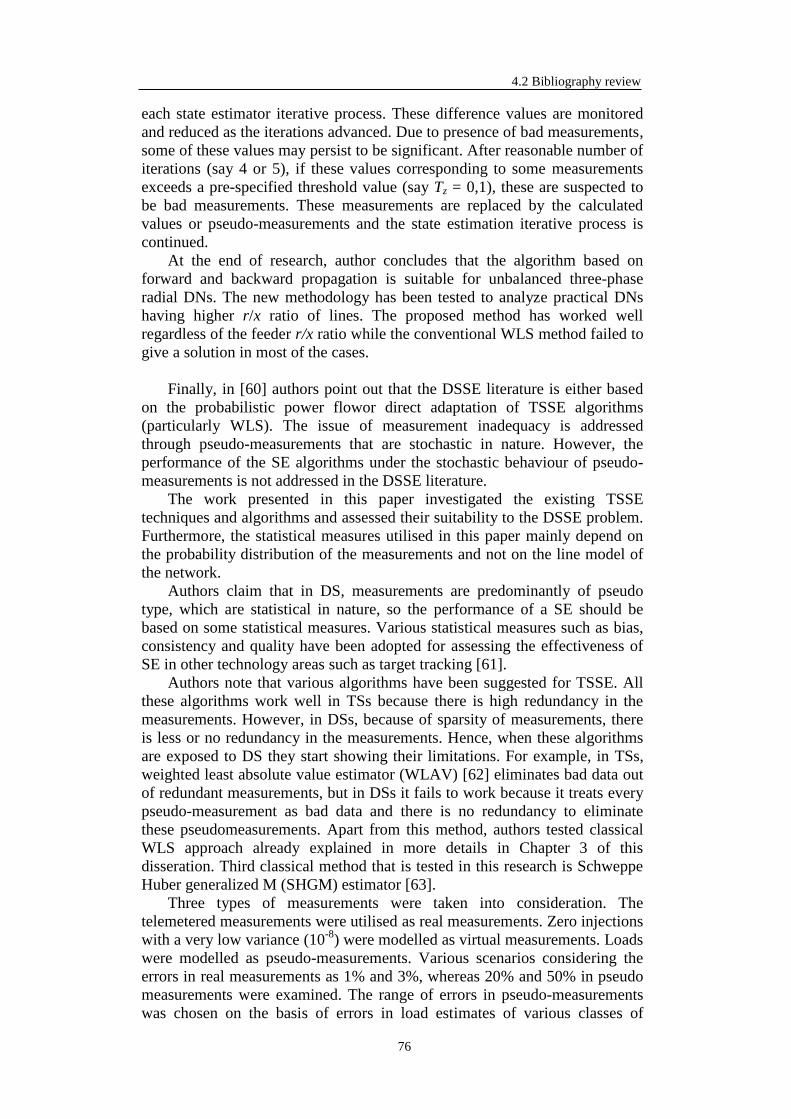
4.2 Bibliography review
76
each state estimator iterative process. These difference values are monitored
and reduced as the iterations advanced. Due to presence of bad measurements,
some of these values may persist to be significant. After reasonable number of
iterations (say 4 or 5), if these values corresponding to some measurements
exceeds a pre-specified threshold value (say Tz = 0,1), these are suspected to
be bad measurements. These measurements are replaced by the calculated
values or pseudo-measurements and the state estimation iterative process is
continued.
At the end of research, author concludes that the algorithm based on
forward and backward propagation is suitable for unbalanced three-phase
radial DNs. The new methodology has been tested to analyze practical DNs
having higher r/x ratio of lines. The proposed method has worked well
regardless of the feeder r/x ratio while the conventional WLS method failed to
give a solution in most of the cases.
Finally, in [60] authors point out that the DSSE literature is either based
on the probabilistic power flowor direct adaptation of TSSE algorithms
(particularly WLS). The issue of measurement inadequacy is addressed
through pseudo-measurements that are stochastic in nature. However, the
performance of the SE algorithms under the stochastic behaviour of pseudo-
measurements is not addressed in the DSSE literature.
The work presented in this paper investigated the existing TSSE
techniques and algorithms and assessed their suitability to the DSSE problem.
Furthermore, the statistical measures utilised in this paper mainly depend on
the probability distribution of the measurements and not on the line model of
the network.
Authors claim that in DS, measurements are predominantly of pseudo
type, which are statistical in nature, so the performance of a SE should be
based on some statistical measures. Various statistical measures such as bias,
consistency and quality have been adopted for assessing the effectiveness of
SE in other technology areas such as target tracking [61].
Authors note that various algorithms have been suggested for TSSE. All
these algorithms work well in TSs because there is high redundancy in the
measurements. However, in DSs, because of sparsity of measurements, there
is less or no redundancy in the measurements. Hence, when these algorithms
are exposed to DS they start showing their limitations. For example, in TSs,
weighted least absolute value estimator (WLAV) [62] eliminates bad data out
of redundant measurements, but in DSs it fails to work because it treats every
pseudo-measurement as bad data and there is no redundancy to eliminate
these pseudomeasurements. Apart from this method, authors tested classical
WLS approach already explained in more details in Chapter 3 of this
disseration. Third classical method that is tested in this research is Schweppe
Huber generalized M (SHGM) estimator [63].
Three types of measurements were taken into consideration. The
telemetered measurements were utilised as real measurements. Zero injections
with a very low variance (10-8
) were modelled as virtual measurements. Loads
were modelled as pseudo-measurements. Various scenarios considering the
errors in real measurements as 1% and 3%, whereas 20% and 50% in pseudo
measurements were examined. The range of errors in pseudo-measurements
was chosen on the basis of errors in load estimates of various classes of
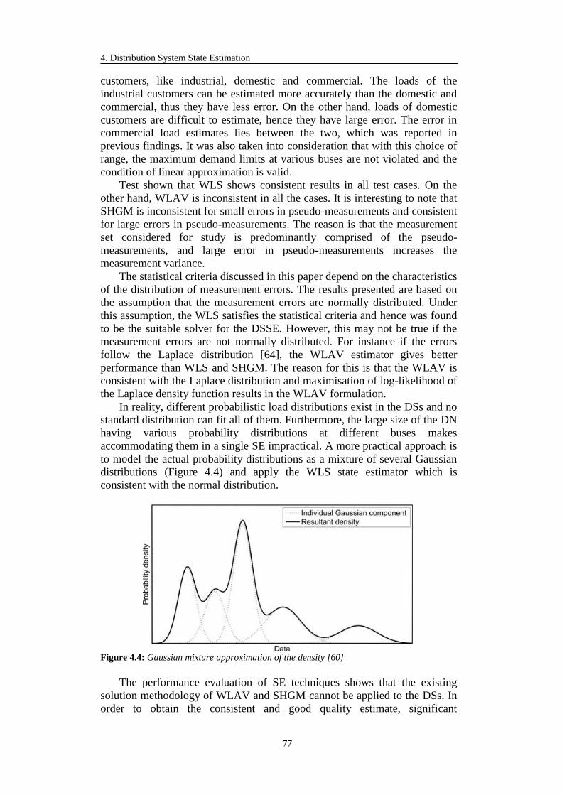
4. Distribution System State Estimation
77
customers, like industrial, domestic and commercial. The loads of the
industrial customers can be estimated more accurately than the domestic and
commercial, thus they have less error. On the other hand, loads of domestic
customers are difficult to estimate, hence they have large error. The error in
commercial load estimates lies between the two, which was reported in
previous findings. It was also taken into consideration that with this choice of
range, the maximum demand limits at various buses are not violated and the
condition of linear approximation is valid.
Test shown that WLS shows consistent results in all test cases. On the
other hand, WLAV is inconsistent in all the cases. It is interesting to note that
SHGM is inconsistent for small errors in pseudo-measurements and consistent
for large errors in pseudo-measurements. The reason is that the measurement
set considered for study is predominantly comprised of the pseudo-
measurements, and large error in pseudo-measurements increases the
measurement variance.
The statistical criteria discussed in this paper depend on the characteristics
of the distribution of measurement errors. The results presented are based on
the assumption that the measurement errors are normally distributed. Under
this assumption, the WLS satisfies the statistical criteria and hence was found
to be the suitable solver for the DSSE. However, this may not be true if the
measurement errors are not normally distributed. For instance if the errors
follow the Laplace distribution [64], the WLAV estimator gives better
performance than WLS and SHGM. The reason for this is that the WLAV is
consistent with the Laplace distribution and maximisation of log-likelihood of
the Laplace density function results in the WLAV formulation.
In reality, different probabilistic load distributions exist in the DSs and no
standard distribution can fit all of them. Furthermore, the large size of the DN
having various probability distributions at different buses makes
accommodating them in a single SE impractical. A more practical approach is
to model the actual probability distributions as a mixture of several Gaussian
distributions (Figure 4.4) and apply the WLS state estimator which is
consistent with the normal distribution.
Figure 4.4: Gaussian mixture approximation of the density [60]
The performance evaluation of SE techniques shows that the existing
solution methodology of WLAV and SHGM cannot be applied to the DSs. In
order to obtain the consistent and good quality estimate, significant

4.3 Distribution System State Estimation
78
modifications are required in these algorithms. WLS gives consistent and
better quality performance when applied to DSs. Hence, authors found out
that out of the three approaches, WLS is the most suitable solver for the DSSE
problem. The WLS works well if the noise characteristics are known. In the
absence of this knowledge, either the WLS needs to be modified or a new
class of algorithms needs to be introduced.
4.2.1 Critical review of the proposed bibliography
As one can see for the stated brief bibliography review, many researchers
have addressed the issues of DN observability and State Estimation (SE)
proposing different approaches. Many approaches, such as in [50],[53]-[56]
tend to use the traditional least square methods by introducing a large number
of pseudo-measurements for loads and generators. But in real DNs the loads
and generators profiles are determined based on the annual energy
consumption from the previous years [65]. This means that there is no
statistical information available so it is impossible to correctly use them as
pseudo-measurements.
Introducing a large number of pseudo-measurements is meaningless if
these represent critical measurements. Trying to achieve the minimum
redundancy by adding the large number of pseudo-measurements will
deteriorate the quality of SE applied to DN. Some approaches, such as in [57]
propose using the Phasor Measurement Units (PMUs), but this type of
equipment is expensive and most of the DSOs do not use it. Last, a three or
multi-phase approach [50],[53],[54],[56]-[59] is not applicable for real MV
grids: the loads are generally balanced and the cables parameters (especially
mutual coupling) are not known [65]. Results stated in [53] are based on the
exclusion of voltage measurements and this is justified by the fact this type of
measurements don’t have significant effect on SE results provided that the
system is observable. However, DS is not observable.
Hence, it is necessary to design suitable innovative techniques to improve
as much as possible the observability of the DN. The aim of the proceeding
subchapters of this chapter is to provide these techniques for DSSE.
4.3 Distribution System State Estimation
The evolution of DSs sees in the remarkable expansion of the DG plants
connected to the medium and low voltage networks one of the main
challenge. The growth of DG will cause a profound change of the DS in the
technical, legal and regulatory aspects; most likely the distribution company
will more and more undertake, on local scale, tasks and responsibilities of the
role assigned on a national scale to the operator of the electricity transmission
network, becoming thus a DSO. In other words, the distribution company will
become a sort of “local dispatcher” and will involve its active/passive
customers in activities related to the network management and optimization;
obviously, this requires a deep review of the regulatory framework.
In this sense, the DSO must undertake various initiatives in order to adapt
the methods of planning, management and analysis of operation of the
network. For all of this to be possible it is mandatory for the DSO to possess a

4. Distribution System State Estimation
79
thorough real-time knowledge of the system state. The solution at hand would
be the use of the least square based SE techniques used for a very long time
by the TSOs. However, in nowadays DSs, the pace of investments into
measurement equipment is much more reduced than the increase of DG
penetration and the situation is very similar to the past when the DS were
passive. Thus, only a limited set of measurements in the primary substations
and, sometimes, in some secondary substations are available. Then, the
equipment is mostly old and the precision class is inappropriate for applying
state estimation as it was installed for other purposes, (e.g. input signal for the
protection systems). All these factors make the DS lack of redundancy or, in
other words, to have sub-unitary redundancy. Moreover, the data acquisition
process of these measurements is qualitatively poor: the measurements are
not always synchronized but averaged and collected in different moments so,
is very hard to statistically characterize them.
Thus, the application of a complete SE technique similar to the ones used
by the TSOs is impossible. However, many approaches, as already explained,
tend to use the traditional least square methods by introducing a large number
of pseudo-measurements for loads and generators. Nevertheless, in real DSs,
the loads and generators profiles are estimated profiles based on the past
yearly energy consumption. This means that there is no statistical information
available about them, so it is impossible to correctly use them as pseudo-
measurements in a least square approach.
Hence, it is necessary to design innovative techniques to improve as much
as possible the observability of the DS. Such approaches need to be robust and
computationally fast as they should run on-line for many networks. In this
chapter, various approaches that depend on the available measurements in the
DS were exposed. The degree of their complexity increases with the number
of available measurements. As mentioned in the Chapter 1, INGRID project,
which was specifically developed for automated control software package for
DSO, comprises SE function [66] which will be developed in details in the
following subchapters.
4.3.1 Available Information
The information currently available to the DSO is of two types (Fig. 4.5):
(i) estimated load and generation profiles and (ii) a set of measurements at the
primary substation level and, sometimes, at the secondary substation level. In
what regards the first category, the real and reactive power demand (𝑃𝐿0, 𝑄𝐿
0)
and the generation (𝑃𝐺0, 𝑄𝐺
0) profiles are known through an appropriate
processing of the historical data that gives "standard" curves for various loads
and generators based on the annual energy consumption. This information is
far from being accurate which implies that in the majority of cases the PF
results obtained using these data are not consistent with the actual operation
and hence no decision regarding the control and management of the DS can
be taken.
However, every 10-15 minutes, a set of measurements in the primary
substation of the DS is available as averaged values over the considered
period of time (Fig. 4.5):
voltage magnitude at the HV busbar (𝑉𝐻𝑉𝑚 );
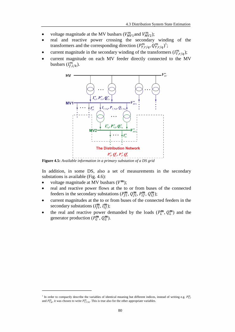
4.3 Distribution System State Estimation
80
voltage magnitude at the MV busbars (𝑉𝑀𝑉1𝑚 and 𝑉𝑀𝑉2
𝑚 );
real and reactive power crossing the secondary winding of the
transformers and the corresponding direction (𝑃𝑇,𝑟/𝑞𝑚 , 𝑄𝑇,𝑟/𝑞
𝑚 )1;
current magnitude in the secondary winding of the transformers (𝐼𝑇,𝑟/𝑞𝑚 );
current magnitude on each MV feeder directly connected to the MV
busbars (𝐼𝑓,𝑖/𝑘𝑚 ).
Figure 4.5: Available information in a primary substation of a DS grid
In addition, in some DS, also a set of measurements in the secondary
substations is available (Fig. 4.6):
voltage magnitude at MV busbars (𝑉𝐦);
real and reactive power flows at the to or from buses of the connected
feeders in the secondary substations (𝑃𝑓𝑡𝐦, 𝑄𝑓𝑡
𝐦 , 𝑃𝑡𝑓𝐦, 𝑄𝑡𝑓
𝐦);
current magnitudes at the to or from buses of the connected feeders in the
secondary substations (𝐼𝑓𝑡𝐦, 𝐼𝑡𝑓
𝐦);
the real and reactive power demanded by the loads (𝑃𝐿𝐦, 𝑄𝐿
𝐦) and the
generator production (𝑃𝐺𝐦, 𝑄𝐺
𝐦).
1 In order to compactly describe the variables of identical meaning but different indices, instead of writing e.g. 𝑃𝑇,𝑟𝑚
and 𝑃𝑇,𝑞𝑚 , it was chosen to write 𝑃𝑇,𝑟/𝑞
𝑚 . This is true also for the other appropriate variables.
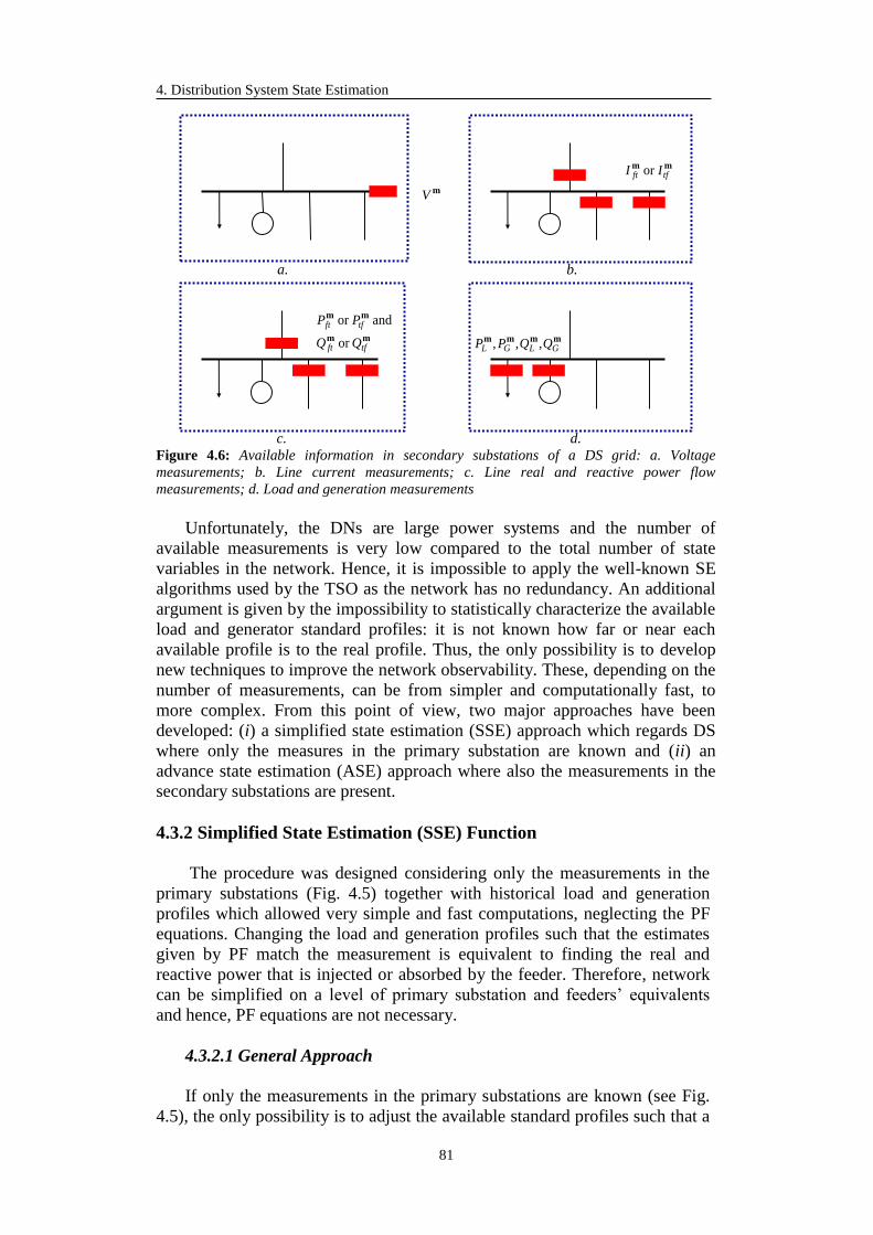
4. Distribution System State Estimation
81
mmtfft II or
mV
mm
mm
tfft
tfft
PP
or
and or
mmmmGLGL QQPP ,,,
a. b.
c. d.
Figure 4.6: Available information in secondary substations of a DS grid: a. Voltage
measurements; b. Line current measurements; c. Line real and reactive power flow
measurements; d. Load and generation measurements
Unfortunately, the DNs are large power systems and the number of
available measurements is very low compared to the total number of state
variables in the network. Hence, it is impossible to apply the well-known SE
algorithms used by the TSO as the network has no redundancy. An additional
argument is given by the impossibility to statistically characterize the available
load and generator standard profiles: it is not known how far or near each
available profile is to the real profile. Thus, the only possibility is to develop
new techniques to improve the network observability. These, depending on the
number of measurements, can be from simpler and computationally fast, to
more complex. From this point of view, two major approaches have been
developed: (i) a simplified state estimation (SSE) approach which regards DS
where only the measures in the primary substation are known and (ii) an
advance state estimation (ASE) approach where also the measurements in the
secondary substations are present.
4.3.2 Simplified State Estimation (SSE) Function
The procedure was designed considering only the measurements in the
primary substations (Fig. 4.5) together with historical load and generation
profiles which allowed very simple and fast computations, neglecting the PF
equations. Changing the load and generation profiles such that the estimates
given by PF match the measurement is equivalent to finding the real and
reactive power that is injected or absorbed by the feeder. Therefore, network
can be simplified on a level of primary substation and feeders’ equivalents
and hence, PF equations are not necessary.
4.3.2.1 General Approach
If only the measurements in the primary substations are known (see Fig.
4.5), the only possibility is to adjust the available standard profiles such that a

4.3 Distribution System State Estimation
82
PF computation delivers a set of results that matches the available
measurements. In this regard, it can be generally proceed as follows [67],[68]:
1) adjust the tap ratio of the HV/MV transformers according to the available
measurements;
2) perform a PF using the historical and actual profiles and the HV bus as
the slack bus (𝑉𝑠𝑙𝑎𝑐𝑘 = 𝑉𝐻𝑉𝑚 ) to obtain the initial currents and powers
absorbed by the feeders (𝐼𝑓,𝑖/𝑘0 , 𝑃𝑓,𝑖/𝑘
0 , 𝑄𝑓,𝑖/𝑘0 ); the initial power losses in
the feeders (𝑃𝑙𝑜𝑠𝑠_𝑓,𝑖/𝑘0 , 𝑄𝑙𝑜𝑠𝑠_𝑓,𝑖/𝑘
0 ) and MV1/MV2 transformers
(𝑃𝑙𝑜𝑠𝑠_𝑇,𝑞0 , 𝑄𝑙𝑜𝑠𝑠_𝑇,𝑞
0 ); the initial voltages at the substation MV busbars
(𝑉𝑀𝑉10 and 𝑉𝑀𝑉2
0 ) and the initial currents and powers flowing through the
transformers (𝐼𝑇,𝑖/𝑘0 and 𝑃𝑇,𝑖/𝑘
0 , 𝑄𝑇,𝑖/𝑘0 ) (Fig. 4.5);
3) substitute the DN feeders with equivalent loads (𝑃𝑓,𝑖/𝑘 and 𝑄𝑓,𝑖/𝑘) and
adjust them to 𝑃𝑓,𝑖/𝑘𝑒𝑠𝑡 and 𝑄𝑓,𝑖/𝑘
𝑒𝑠𝑡 such that the variables in the primary
substation match the measurements. Of course, as the feeders can be
active, these equivalent loads can also have negative values;
4) modify the generation and load profiles to 𝑃𝐿𝑒𝑠𝑡 , 𝑄𝐿
𝑒𝑠𝑡, 𝑃𝐺𝑒𝑠𝑡, 𝑄𝐺
𝑒𝑠𝑡 such to
obtain 𝑃𝑓,𝑖/𝑘𝑒𝑠𝑡 and 𝑄𝑓,𝑖/𝑘
𝑒𝑠𝑡 , then perform a new PF to obtain the estimated
values of the measured quantities. If the errors between the estimates and
the measurements are not well contained, go back to point 2). Otherwise,
retain as the final load/generation profiles.
To correctly modify the generation and load profiles it is necessary to
accurately estimate the power losses in the feeders corresponding to the new
profile. Since the power losses are proportional to the square of the current a
good approximation of the power losses in the feeders was found to be:
𝑃𝑙𝑜𝑠𝑠_𝑓,𝑖/𝑘𝑒𝑠𝑡 = 𝑐𝑃,𝑖/𝑘
2 ∙ 𝑃𝑙𝑜𝑠𝑠_𝑓,𝑖/𝑘0
𝑄𝑙𝑜𝑠𝑠_𝑓,𝑖/𝑘𝑒𝑠𝑡 = 𝑐𝑃,𝑖/𝑘
2 ∙ 𝑄𝑙𝑜𝑠𝑠_𝑓,𝑖/𝑘0
(4.3)
where cP is the power coefficient, computed as:
𝑐𝑃,𝑖/𝑘 = 𝑉𝑀𝑉2,1𝑚 ∙ 𝐼𝑓,𝑖/𝑘
𝑚 /𝑉𝑀𝑉2,10 ∙ 𝐼𝑓,𝑖/𝑘
0 (4.4)
Finally, an important assumption on which the algorithms from this
dissertation rely is that once the current and power estimates match the
measurements, also the resulting voltages estimates will automatically match
the measurements. The hypothesis is valid as the primary substation is
analogous to a very small radial network were the slack voltage and the loads
are known. This assumption validates the approximation of Eq. (4.3) and
allows the proposed procedures to focus only on the current and power
measurements.
While the second step of the above procedure is obvious, steps 1), 3) and
4) will be developed in the former subchapter. The core of the above
methodology is given by step 3) for which two algorithms can be defined:
one, very fast, based on simple computations and another one,
computationally slower, based on optimization techniques. Both approaches

4. Distribution System State Estimation
83
have their advantages and disadvantages and they are both going to be
exposed in the following subchapters.
4.3.2.2 Tap Ratio Computation
To solve the PF problem, it is necessary to define many input data: real
and reactive power required by the loads and produced by each generating
unit, the topology of the network, the electrical data of each component and
the magnitude of voltage of the HV busbar of the primary station. Another
important information is the tap changer position of the HV/MV transformer.
Generally, for this type of device, 20 different positions are available, but,
due to technical limitation there is not the possibility to communicate the
position of the tap changer. In particular, the bit number available to code the
position is very limited. Therefore, it is essential to define a procedure able to
compute the tap change position of the transformer; otherwise, the PF results
could be significantly different from the real values.
To overcome this problem, a specific procedure, invoked before the SE
function, has been developed. It permits to compute the tap change position
for 2 o 3 winding transformer starting from the measured data obtained in real
time.
4.3.2.2.1 2-Winding transformer
The 2-Winding transformer is represented according to the circuit scheme
reported in Fig. 4.5. To compute the tap changer position, the following data
is necessary:
the real and reactive power at the MV level of the transformer;
the voltage magnitude at both HV and MV level.
Using this information, it is possible to apply the Boucherot theorem
starting from the voltage magnitude of MV busbar (section A in Fig. 4.7) to
compute the voltage of section B. Then, using the information about the
magnitude voltage of HV busbar (section C) it is possible to compute the tap
change ratio with the following equation:
𝑘 = 𝑉𝐶/𝑉𝐵 (4.5)
Obviously, in order to apply this procedure, it is mandatory to know the
values of the real and reactive power given by the transformer to the MV
network. Without this information, it is not possible to compute the tap
change ratio.
Moreover, the numerical result given by this procedure is influenced by
the measure errors that affect the input data.
A particular situation can occur when the measurement data is given at
section C (Fig. 4.7).

4.3 Distribution System State Estimation
84
Figure 4.7: 2-Winding transformer model
In this case, it is necessary to perform an iterative Boucherot following the
steps:
1. Based on the initial value of the tap, compute a first estimate for the
voltage in section B, 𝑉𝐵0 , according to the above equation;
2. Perform Boucherot to determine 𝑉𝐴𝑘, where 𝑘 is the index of current
iteration;
3. Compute the error between 𝑉𝐴𝑘 and the measured value 𝑉𝐴
𝑚: ∆𝑉𝑘 = 𝑉𝐴𝑚 −
𝑉𝐴𝑘;
4. If ∆𝑉𝑘 > 𝑡𝑜𝑙 then update the voltage in section B as: 𝑉𝐵𝑘+1 = 𝑉𝐵
𝑘 + ∆𝑉𝑘
and redo steps 2-4;
5. If ∆𝑉𝑘 ≤ 𝑡𝑜𝑙 then compute the correct value of the tap ratio as:
𝑘 = 𝑉𝐶𝑚/𝑉𝐵
𝑚 (4.6)
The iterative procedure was tested for various stressed situations and
proved to be delivering very good results within insignificant computation
time.
4.3.2.2.2 3-Winding Transformer
The procedure developed for the 2-Winding transformer is not directly
applicable to 3-Winding transformer. 3-Winding transformer is represented in
according with Fig. 4.8; therefore it is necessary to compute two tap change
ration. For example, for an HV/MV1/MV2 transformer, the two tap rations
are respectively between HV/MV1 and HV/MV2.
Figure 4.8: 3-Winding transformer model
k
R+jX
Y0/2 Y0/2
Sec C Sec B Sec A
VC VB V
A
PT QT
k1
k2
VA
PA
QA
Sec A
VB
PB
QB
Sec B
VC
VD
VE
PE
QE
Sec E V
F
Sec F
R1+jX1
R2+jX
2
R3+ jX3
Y0/2 Y0/2

4. Distribution System State Estimation
85
Also, in this case, the following data are necessary to compute the values
of the two tap ratios, k1 and k2:
the real and reactive power at the both MV levels of the transformer;
the voltage magnitude at HV, MV1 and MV2.
In according with the symbols used in Fig. 4.7, k1 and k2 are given by the
following equation:
𝑘1 = 𝑉𝐸/𝑉𝐶
𝑘2 = 𝑉𝐸/𝑉𝐷 (4.7)
Therefore, it is necessary to compute the following magnitude voltages:
VC, VD and VE. Starting from the section A and applying the theorem of
Boucherot, it is possible to compute the value of VC. The same is true for
section B and D.
Then, VE should be computed. In this case, it is possible to compute PE
and QE applying the balance equation for real and reactive power at this
section taking into account that k1 and k2 represent an ideal transformer:
𝑃𝐸 = 𝑃𝐶 + 𝑃𝐷
𝑄𝐸 = 𝑄𝐶 + 𝑄𝐷 (4.8)
Now, it is possible to use the information given by the voltage magnitude
of section F to implement an interactive Boucherot procedure. In other words,
it is possible to assign to VE an initial value (𝑉E0 = 1 in per unit) and applying
Boucherot from section E to section F, it is possible to compute VF and
compare this value with the voltage measured in real time, 𝑉𝐹_𝑚𝑒𝑎𝑠:
∆𝑉 = 𝑉𝐹𝑚 − 𝑉𝐹 (4.9)
Then, 𝑉𝐸 is update in according to the following equation:
𝑉𝐸𝑘+1 = 𝑉𝐸
𝑘 − ∆𝑉𝑘 (4.10)
After that, it is possible to repeat the procedure until V is lower or equal
to a given tolerance (i.e. 1 ∙ 10−7 in p.u.). Finally, adopting the VE given by
this procedure, k1 and k2 are computed. The time required to execute this
interactive procedure is negligible.
4.3.2.3 Losses approximation formula
Subchapter 4.3.2.1 reports that in order to correctly modify the generation
and load profiles, it is necessary to accurately estimate the power losses in the
feeders corresponding to the new profile. An approximation of the power
losses in the feeders was offered. At this point, the justification of the
proposed approximation is given.
To avoid the computation of the PF to get the exact value of the losses, it
is required to be able to obtain a good approximation with the available
information (initial value of the losses, 𝑃𝑙𝑜𝑠𝑠_𝑓,𝑖/𝑘0 , 𝑄𝑙𝑜𝑠𝑠_𝑓,𝑖/𝑘
0 , initial apparent
power absorbed by the feeder, available measurements, etc.). Power losses are

4.3 Distribution System State Estimation
86
made up from two components – longitudinal losses that are proportional to
the square of the current absorbed by the feeder and shunt losses that are
proportional to the square of the voltage. Taking this into consideration, the
change in losses from a known initial point to another unknown point in terms
of PF results was roughly estimated by considering it equal to the square of
the apparent power ratio between these operating points and Eq. (4.3) was
derived. In this way, both longitudinal and shunt losses have been
incorporated without the need to compute time-consuming PFs during the
convergence of the state estimation algorithm.
This claim is proven by testing it on feeders with various topologies and
load/generation characteristics. The data for some tested the feeders is given
in Table 4.2.
Table 4.2: Approximation of losses – test feeders data
Feeder A B C D
No. buses 14 28 90 20
A𝑓,𝑖/𝑘0 [kVA] 1080.71 852.06 1114.54 385.01
𝑃𝑙𝑜𝑠𝑠_𝑓,𝑖/𝑘0 [kW] 3.39 1.00 20.42 0.98
𝑃𝑙𝑜𝑠𝑠_𝑓,𝑖/𝑘0 /A𝑓,𝑖/𝑘
0 [%] 0.31 0.12 1.83 0.25
Table reports 4 feeders of different lengths, different number of buses and
ratios between load and generation. Apparent powers absorbed by the feeders,
their real power loss and ratio between power loss and feeder’s apparent
power is also reported for the initial point.
Further, tests were run to evaluate the quality of estimation for the real
power losses as follows: with the initial PF, exact A𝑓,𝑖/𝑘0 and 𝑃𝑙𝑜𝑠𝑠_𝑓,𝑖/𝑘
0 have been
obtained. Then loads and generation in each bus of the feeder were modified
in order to obtain higher value of A𝑓,𝑖/𝑘0
(approximately 10%, 20%, … higher
value). Another PF was run to get the exact value of the new 𝐴𝑓,𝑖/𝑘 and
𝑃𝑙𝑜𝑠𝑠_𝑓,𝑖/𝑘. Using the Eqs. (4.3) and (4.4), the factor 𝑐𝑝𝑓 and estimation of the
losses were computed and then the estimation was compared with the exact
value of the losses obtained by PF – the relative error in estimation was
obtained (). The results are summarized in Fig. 4.9.
Figure 4.9: Losses approximation
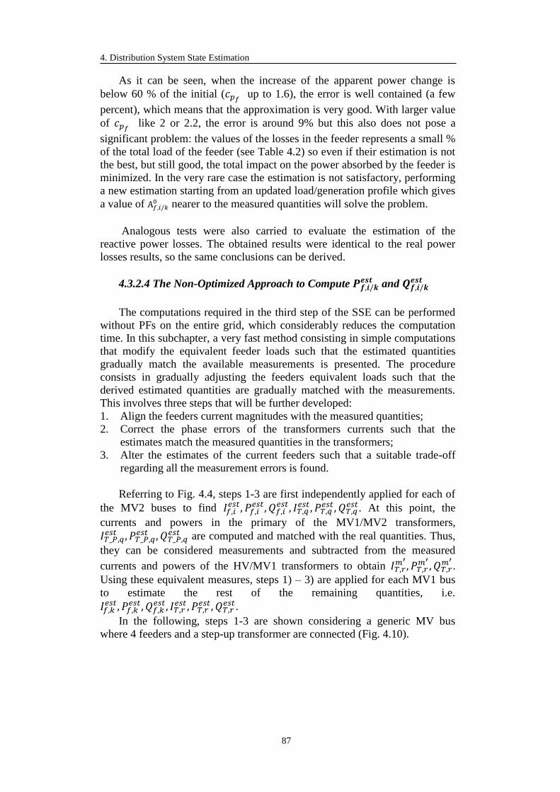
4. Distribution System State Estimation
87
As it can be seen, when the increase of the apparent power change is
below 60 % of the initial (𝑐𝑝𝑓 up to 1.6), the error is well contained (a few
percent), which means that the approximation is very good. With larger value
of 𝑐𝑝𝑓 like 2 or 2.2, the error is around 9% but this also does not pose a
significant problem: the values of the losses in the feeder represents a small %
of the total load of the feeder (see Table 4.2) so even if their estimation is not
the best, but still good, the total impact on the power absorbed by the feeder is
minimized. In the very rare case the estimation is not satisfactory, performing
a new estimation starting from an updated load/generation profile which gives
a value of A𝑓,𝑖/𝑘0 nearer to the measured quantities will solve the problem.
Analogous tests were also carried to evaluate the estimation of the
reactive power losses. The obtained results were identical to the real power
losses results, so the same conclusions can be derived.
4.3.2.4 The Non-Optimized Approach to Compute 𝑷𝒇,𝒊/𝒌𝒆𝒔𝒕 and 𝑸𝒇,𝒊/𝒌
𝒆𝒔𝒕
The computations required in the third step of the SSE can be performed
without PFs on the entire grid, which considerably reduces the computation
time. In this subchapter, a very fast method consisting in simple computations
that modify the equivalent feeder loads such that the estimated quantities
gradually match the available measurements is presented. The procedure
consists in gradually adjusting the feeders equivalent loads such that the
derived estimated quantities are gradually matched with the measurements.
This involves three steps that will be further developed:
1. Align the feeders current magnitudes with the measured quantities;
2. Correct the phase errors of the transformers currents such that the
estimates match the measured quantities in the transformers;
3. Alter the estimates of the current feeders such that a suitable trade-off
regarding all the measurement errors is found.
Referring to Fig. 4.4, steps 1-3 are first independently applied for each of
the MV2 buses to find 𝐼𝑓,𝑖𝑒𝑠𝑡, 𝑃𝑓,𝑖
𝑒𝑠𝑡, 𝑄𝑓,𝑖𝑒𝑠𝑡, 𝐼𝑇,𝑞
𝑒𝑠𝑡, 𝑃𝑇,𝑞𝑒𝑠𝑡, 𝑄𝑇,𝑞
𝑒𝑠𝑡. At this point, the
currents and powers in the primary of the MV1/MV2 transformers,
𝐼𝑇_𝑃,𝑞𝑒𝑠𝑡 , 𝑃𝑇_𝑃,𝑞
𝑒𝑠𝑡 , 𝑄𝑇_𝑃,𝑞𝑒𝑠𝑡 are computed and matched with the real quantities. Thus,
they can be considered measurements and subtracted from the measured
currents and powers of the HV/MV1 transformers to obtain 𝐼𝑇,𝑟𝑚′, 𝑃𝑇,𝑟
𝑚′, 𝑄𝑇,𝑟
𝑚′.
Using these equivalent measures, steps 1) – 3) are applied for each MV1 bus
to estimate the rest of the remaining quantities, i.e.
𝐼𝑓,𝑘𝑒𝑠𝑡, 𝑃𝑓,𝑘
𝑒𝑠𝑡 , 𝑄𝑓,𝑘𝑒𝑠𝑡, 𝐼𝑇,𝑟
𝑒𝑠𝑡, 𝑃𝑇,𝑟𝑒𝑠𝑡, 𝑄𝑇,𝑟
𝑒𝑠𝑡.
In the following, steps 1-3 are shown considering a generic MV bus
where 4 feeders and a step-up transformer are connected (Fig. 4.10).
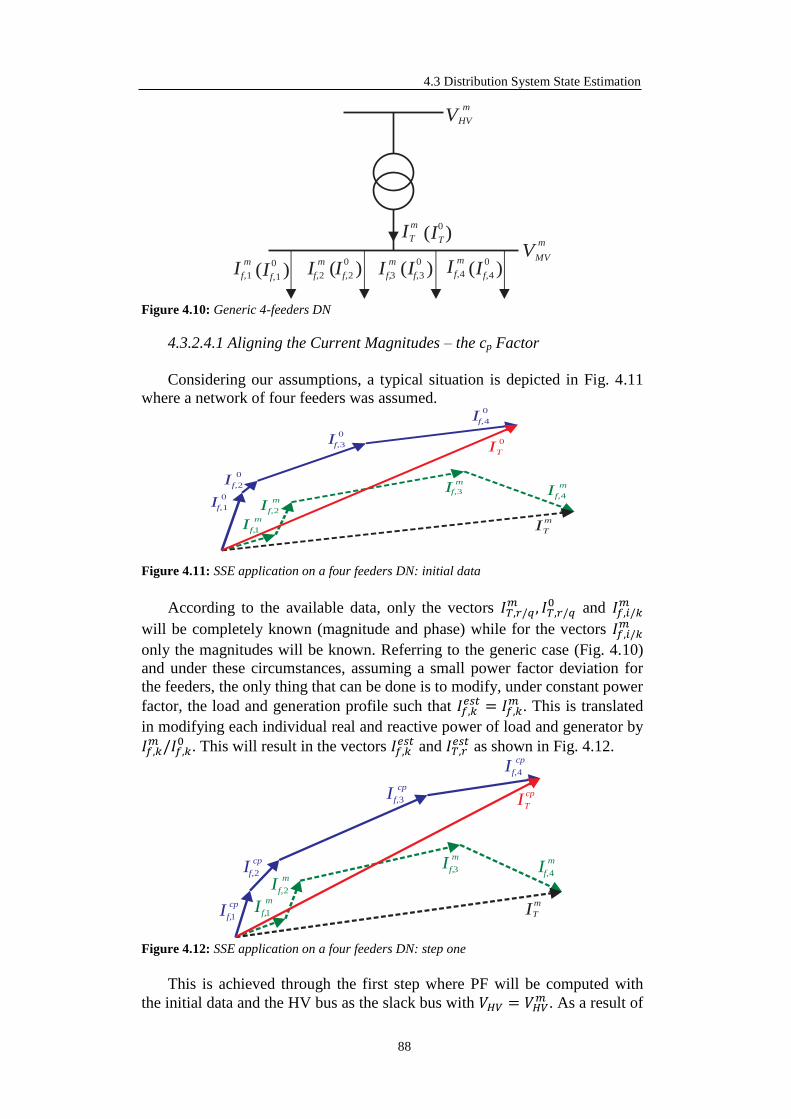
4.3 Distribution System State Estimation
88
Figure 4.10: Generic 4-feeders DN
4.3.2.4.1 Aligning the Current Magnitudes – the cp Factor
Considering our assumptions, a typical situation is depicted in Fig. 4.11
where a network of four feeders was assumed.
Figure 4.11: SSE application on a four feeders DN: initial data
According to the available data, only the vectors 𝐼𝑇,𝑟/𝑞𝑚 , 𝐼𝑇,𝑟/𝑞
0 and 𝐼𝑓,𝑖/𝑘𝑚
will be completely known (magnitude and phase) while for the vectors 𝐼𝑓,𝑖/𝑘𝑚
only the magnitudes will be known. Referring to the generic case (Fig. 4.10)
and under these circumstances, assuming a small power factor deviation for
the feeders, the only thing that can be done is to modify, under constant power
factor, the load and generation profile such that 𝐼𝑓,𝑘𝑒𝑠𝑡 = 𝐼𝑓,𝑘
𝑚 . This is translated
in modifying each individual real and reactive power of load and generator by
𝐼𝑓,𝑘𝑚 /𝐼𝑓,𝑘
0 . This will result in the vectors 𝐼𝑓,𝑘𝑒𝑠𝑡 and 𝐼𝑇,𝑟
𝑒𝑠𝑡 as shown in Fig. 4.12.
Figure 4.12: SSE application on a four feeders DN: step one
This is achieved through the first step where PF will be computed with
the initial data and the HV bus as the slack bus with 𝑉𝐻𝑉 = 𝑉𝐻𝑉𝑚 . As a result of
VHV
m
VMV
mIT
m
(IT )0
If,1
m
(If,1 )0 If,2
m(If, 2 )
0If,3
m(If, 3 )
0 If,4
m
(If,4 )0
IT
m
If, 3
m
If, 4
m
If, 2
m
If,1
m
If, 1
0
If,2
0
If,3
0
If,4
0
IT
0
IT
m
If, 3
m
If,4
m
If, 2
m
If,1
m
If, 1
cp
If, 2
cp
If, 3
cp
If, 4
cp
IT
cp

4. Distribution System State Estimation
89
former computation, all the relevant quantities of the system such as
𝑉𝑀𝑉0 , 𝐼𝑓,𝑖/𝑘
0 , 𝑃𝑙𝑜𝑠𝑠_𝑓,𝑖/𝑘0 will be obtained. These quantities represent the starting
point for later computations.
In order to distinguish between physical measured value of a certain
quantity and the actual value of the non-measured quantity, different
subscripts are used: m for the former and act for the later one. Assuming that
𝑐𝑜𝑠𝜑𝑓 = 𝑐𝑜𝑛𝑠𝑡, the actual and initial apparent powers absorbed by feeder i or
k are:
𝐴𝑓,𝑖/𝑘𝑎𝑐𝑡 =
∑ 𝑃𝐿,𝑙𝑎𝑐𝑡
𝑙∈𝑙𝑜𝑎𝑑_𝑓,𝑖/𝑘 + 𝑃𝑙𝑜𝑠𝑠_𝑓,𝑖/𝑘𝑎𝑐𝑡
𝑐𝑜𝑠𝜑𝑓= √3𝑉𝑀𝑉
𝑚 𝐼𝑓𝑚 (4.11)
𝐴𝑓,𝑖/𝑘0 =
∑ 𝑃𝐿,𝑙0
𝑙∈𝑙𝑜𝑎𝑑_𝑓,𝑖/𝑘 + 𝑃𝑙𝑜𝑠𝑠_𝑓,𝑖/𝑘0
𝑐𝑜𝑠𝜑𝑓= √3𝑉𝑀𝑉
0 𝐼𝑓0 (4.12)
where:
∑ 𝑃𝐿,𝑙𝑎𝑐𝑡
𝑙∈𝑙𝑜𝑎𝑑_𝑓,𝑖/𝑘 total actual real power of the load pertaining to feeder i or
k;
𝑃𝑙𝑜𝑠𝑠_𝑓,𝑖/𝑘𝑎𝑐𝑡 actual losses pertaining to the feeder i or k;
∑ 𝑃𝐿,𝑙0
𝑙∈𝑙𝑜𝑎𝑑_𝑓,𝑖/𝑘 total initial real power of the load pertaining to feeder i or
k;
𝑃𝑙𝑜𝑠𝑠_𝑓,𝑖/𝑘0 initial losses pertaining to the feeder i or k;
Dividing the quantities given by Eq. (4.11) and Eq. (4.12), 𝑐𝑝𝑓 for each feeder
i or k is computed:
𝑐𝑝𝑓 =∑ 𝑃𝐿,𝑙
𝑎𝑐𝑡𝑙∈𝑙𝑜𝑎𝑑_𝑓,𝑖/𝑘 + 𝑃𝑙𝑜𝑠𝑠_𝑓,𝑖/𝑘
𝑎𝑐𝑡
∑ 𝑃𝐿,𝑙0
𝑙∈𝑙𝑜𝑎𝑑_𝑓,𝑖/𝑘 + 𝑃𝑙𝑜𝑠𝑠_𝑓,𝑖/𝑘0 =
𝑉𝑀𝑉𝑚 𝐼𝑓
𝑚
𝑉𝑀𝑉0 𝐼𝑓
0 (4.13)
Now, by updating initial variables, feeder powers are obtained:
𝑃𝑓
𝑐𝑝 = 𝑐𝑝𝑓 ∙ 𝑃𝑓0
𝑄𝑓
𝑐𝑝 = 𝑐𝑝𝑓 ∙ 𝑄𝑓0
(4.14)
4.3.2.4.2 Phase Correction and Power Flow Inversion Check
At this point, the currents in the inputs of the feeders have been aligned in
magnitude, i.e. 𝐼𝑓,𝑖/𝑘𝑒𝑠𝑡 ≃ 𝐼𝑓,𝑖/𝑘
𝑚 , but there can be a noticeable phase error
between the vectors 𝐼𝑇𝑒𝑠𝑡 and 𝐼𝑇
𝑚. This error can be easily minimized by
shifting the angle of each 𝐼𝑓,𝑖/𝑘𝑒𝑠𝑡 vector with the respective phase error, i.e. with
∠(𝐼𝑇𝑒𝑠𝑡, 𝐼𝑇
𝑚). In our particular generic case the situation is depicted in Fig.
4.13.
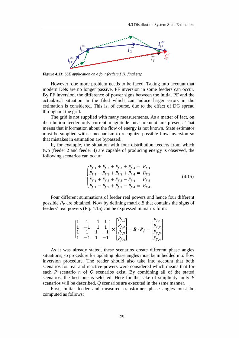
4.3 Distribution System State Estimation
90
Figure 4.13: SSE application on a four feeders DN: final step
However, one more problem needs to be faced. Taking into account that
modern DNs are no longer passive, PF inversion in some feeders can occur.
By PF inversion, the difference of power signs between the initial PF and the
actual/real situation in the filed which can induce larger errors in the
estimation is considered. This is, of course, due to the effect of DG spread
throughout the grid.
The grid is not supplied with many measurements. As a matter of fact, on
distribution feeder only current magnitude measurement are present. That
means that information about the flow of energy is not known. State estimator
must be supplied with a mechanism to recognize possible flow inversion so
that mistakes in estimation are bypassed.
If, for example, the situation with four distribution feeders from which
two (feeder 2 and feeder 4) are capable of producing energy is observed, the
following scenarios can occur:
𝑃𝑓,1 + 𝑃𝑓,2 + 𝑃𝑓,3 + 𝑃𝑓,4 = 𝑃𝑇,1𝑃𝑓,1 − 𝑃𝑓,2 + 𝑃𝑓,3 + 𝑃𝑓,4 = 𝑃𝑇,2𝑃𝑓,1 + 𝑃𝑓,2 + 𝑃𝑓,3 − 𝑃𝑓,4 = 𝑃𝑇,3𝑃𝑓,1 − 𝑃𝑓,2 + 𝑃𝑓,3 − 𝑃𝑓,4 = 𝑃𝑇,4
(4.15)
Four different summations of feeder real powers and hence four different
possible 𝑃𝑇 are obtained. Now by defining matrix B that contains the signs of
feeders’ real powers (Eq. 4.15) can be expressed in matrix form:
[
1 11 −1
1 11 1
1 11 −1
1 −11 −1
] ×
[ 𝑃𝑓,1𝑃𝑓,2𝑃𝑓,3𝑃𝑓,4]
= 𝑩 ∙ 𝑷𝑓 =
[ 𝑃𝑇,1𝑃𝑇,2𝑃𝑇,3𝑃𝑇,4]
As it was already stated, these scenarios create different phase angles
situations, so procedure for updating phase angles must be imbedded into flow
inversion procedure. The reader should also take into account that both
scenarios for real and reactive powers were considered which means that for
each P scenario n of Q scenarios exist. By combining all of the stated
scenarios, the best one is selected. Here for the sake of simplicity, only P
scenarios will be described. Q scenarios are executed in the same manner.
First, initial feeder and measured transformer phase angles must be
computed as follows:
IT
m
If, 1
est
If,2
est
If,3
estIf, 4
est
IT
est

4. Distribution System State Estimation
91
𝜑𝑓0 = ∠(𝑃𝑓,𝑖/𝑘
0 + 𝑗𝑄𝑓,𝑖/𝑘0 )
𝜑𝑇𝑚 = ∠(𝑃𝑇
𝑚 + 𝑗𝑄𝑇𝑚)
(4.16)
Then, from already computed values of 𝑃𝑓,𝑖/𝑘0 and 𝑄𝑓,𝑖/𝑘
0 , 𝐴𝑓,𝑖/𝑘
𝑐𝑝 can be
obtained in the following manner:
𝐴𝑓,𝑖/𝑘
𝑐𝑝 = √(𝑐𝑝𝑓𝑃𝑓,𝑖/𝑘0 )
2
+ 𝑗 (𝑐𝑝𝑓𝑄𝑓,𝑖/𝑘0 )
2
(4.17)
Using matrix B for a certain case, 𝑃𝑇 can be obtained as follows:
𝑃𝑇 = 𝑩 ∙ 𝑃𝑓𝑐𝑝
(4.18)
Next, using the loop, all the rows of matrix B will be examined, computing
the following:
𝜑𝑇𝑒𝑠𝑡 = ∠(𝑃𝑇 + 𝑗𝑄𝑇) (4.19)
Using Eqs. (4.16) and (4.19) phase error Δ𝜑𝑓,𝑖/𝑘 can be acquired:
Δ𝜑𝑓,𝑖/𝑘 = 𝜑𝑇𝑚 − 𝜑𝑇
𝑒𝑠𝑡 (4.20)
Now, as already mentioned, new estimate of feeder’s phase angle will be
obtained using this phase error Δ𝜑𝑓,𝑖/𝑘:
𝜑𝑓,𝑖/𝑘𝑒𝑠𝑡 = 𝜑𝑓,𝑖/𝑘
0 + Δ𝜑𝑓,𝑖/𝑘 (4.21)
Using Eq. (4.21), new estimates of real and reactive powers can be
computed as following:
𝑃𝑓,𝑖/𝑘𝑒𝑠𝑡 = 𝐴
𝑓
𝑐𝑝 ∙ cos (𝜑𝑓,𝑖/𝑘𝑒𝑠𝑡 )
𝑄𝑓,𝑖/𝑘𝑒𝑠𝑡 = 𝐴
𝑓
𝑐𝑝 ∙ sin(𝜑𝑓,𝑖/𝑘𝑒𝑠𝑡 )
(4.22)
Corrected values of real and reactive transformer’s powers can be
obtained using Eq. (4.22):
𝑃𝑇𝑐𝑜𝑟 = ∑ 𝑃𝑓,𝑖/𝑘
𝑒𝑠𝑡
𝑛𝑓
𝑖/𝑘=1
𝑄𝑇𝑐𝑜𝑟 = ∑ 𝑄𝑓,𝑖/𝑘
𝑒𝑠𝑡
𝑛𝑓
𝑖/𝑘=1
(4.23)
where:
𝑛𝑓 number of feeders supplied by the considered transformer.

4.3 Distribution System State Estimation
92
At the end of the loop, by combining P and Q scenarios as already stated,
errors of real and reactive power of the transformer can be acquired using Eq.
(4.23) and the measured values:
Δ𝑃𝑇 = 𝑃𝑇
𝑚 − 𝑃𝑇𝑐𝑜𝑟
Δ𝑄𝑇 = 𝑄𝑇𝑚 − 𝑄𝑇
𝑐𝑜𝑟 (4.24)
Finally, the scenario with the smallest error given by Eq. (4.24) is chosen
and the flow direction is set according to that scenario.
4.3.2.4.3 Power Residual Manipulation
Next step in improving state estimation requires certain compromises. As
an effect of our hypothesis that 𝐼𝑓,𝑖/𝑘𝑒𝑠𝑡 ≃ 𝐼𝑓,𝑖/𝑘
𝑚 , errors on feeders will be almost
zero. These vectors are not equal because in the above equations the
estimation of the losses is used. While for feeders almost perfect estimation
can be obtained, errors on the transformers quantities can be noticeable. Now
it is the time to distribute the errors from the transformers to the feeders.
If feeder’s estimates tolerance is set to 1%, for example, great
improvement of transformer’s estimates can be obtained.
The procedure starts with defining transformer errors of real and reactive
power estimates. First it is necessary to compute new transformer power
estimate in respect with the powers obtained in the previous step of the
process:
𝑃𝑇𝑒𝑠𝑡′ = ∑ 𝑃𝑓,𝑖/𝑘
𝑒𝑠𝑡
𝑛𝑓
𝑖/𝑘=1
𝑄𝑇𝑒𝑠𝑡′ = ∑ 𝑄𝑓,𝑖/𝑘
𝑒𝑠𝑡
𝑛𝑓𝑒𝑒𝑑𝑒𝑟𝑠
𝑖/𝑘=1
(4.25)
Then, using Eq. (4.25) and measured values of the measured transformer
powers, the errors Δ𝑃𝑇′ and Δ𝑄𝑇
′ are computed:
Δ𝑃𝑇
′ = 𝑃𝑇𝑚 − 𝑃𝑇
𝑒𝑠𝑡′
Δ𝑄𝑇′ = 𝑃𝑇
𝑚 −𝑄𝑇𝑒𝑠𝑡′
(4.26)
The idea is to distribute the errors Δ𝑃𝑇′ and Δ𝑄𝑇
′ on feeders as much as
possible taking into account the tolerance mentioned before. This will be done
using the vectors Δ𝑃𝑓,𝑖/𝑘 and Δ𝑄𝑓,𝑖/𝑘 that are bounded by the “capacity” of the
feeder as follows:
Δ𝑃𝑓,𝑘 =|𝑃𝑓,𝑖/𝑘𝑒𝑠𝑡 |
∑ 𝑃𝑓,𝑖/𝑘𝑒𝑠𝑡𝑛𝑓
𝑘=1
Δ𝑃𝑇′
Δ𝑄𝑓,𝑘 =|𝑄𝑓,𝑖/𝑘
𝑒𝑠𝑡 |
∑ 𝑄𝑓,𝑖/𝑘𝑒𝑠𝑡𝑛𝑓
𝑘=1
Δ𝑄𝑇′
(4.27)

4. Distribution System State Estimation
93
where 𝑘 = 1,… , 𝑛𝑓.
In this way, power errors on each feeder have been set according to their
“capacity”, or to be more precise, their sharing in the total amount of real and
reactive power.
The strategy was to diminish first the error on the reactive power as much
as possible and then to “push” the rest to the real power error estimates. It will
be seen later in results provided that greater improvements were obtained in
this way.
Procedure is taking into account all the situations regarding the sign of the
real and reactive powers of feeders (𝑃𝑓,𝑖/𝑘 ≤ 0, 𝑃𝑓,𝑖/𝑘 ≥ 0,𝑄𝑓,𝑖/𝑘 ≤ 0,𝑄𝑓,𝑖/𝑘 ≥
0) and also respective amounts of power propagated from
transformer (∆𝑃𝑓,𝑖/𝑘 ≤ 0, ∆𝑃𝑓,𝑖/𝑘 ≥ 0, ∆𝑄𝑓,𝑖/𝑘 ≤ 0, ∆𝑄𝑓,𝑖/𝑘 ≥ 0).
Thus, depending on the case, the real and reactive power limits are
depicted according to Fig. 4.14 (two circles depict lower and upper feeders’
apparent power bound, 0.99𝐴𝑓,𝑖/𝑘 and 1.01𝐴𝑓,𝑖/𝑘 respectively):
Figure 4.14: Upper and lower boundaries
To illustrate the procedure, the example where both 𝑃𝑓,𝑖/𝑘𝑒𝑠𝑡 and 𝑄𝑓,𝑖/𝑘
𝑒𝑠𝑡 are
positive will be considered, with ∆𝑄𝑓,𝑖/𝑘𝑒𝑠𝑡 > 0 and ∆𝑃𝑓,𝑖/𝑘
𝑒𝑠𝑡 < 0. Procedure first
tries to set as much as it can of reactive power residual ∆𝑄𝑓,𝑖/𝑘𝑒𝑠𝑡 and as
∆𝑄𝑓,𝑖/𝑘𝑒𝑠𝑡 + ∆𝑄𝑟𝑒𝑠 < ∆𝑄𝑓,𝑖/𝑘
𝑚𝑎𝑥 , it has enough “space” to allocate it. ∆𝑄𝑟𝑒𝑠 denotes
power residual from operations with the previous feeder. Once ∆𝑄𝑓,𝑖/𝑘𝑒𝑠𝑡 is
allocated, ∆𝑃𝑓,𝑖/𝑘𝑒𝑠𝑡 can also be allocated, completely or partially. As ∆𝑃𝑓,𝑖/𝑘
𝑒𝑠𝑡 <
0, if ∆𝑃𝑓,𝑖/𝑘𝑒𝑠𝑡 + ∆𝑃𝑟𝑒𝑠 < ∆𝑃𝑓,𝑖/𝑘
𝑚𝑖𝑛 , only part of it can be allocated, the rest is
stored in ∆𝑃𝑟𝑒𝑠 and will be transferred to the operations with next feeder. If
1.01 Af,i/k
0.99 Af,i/k
est
est
Pmin1P
max2 Pmin2
Qmax1
Qmin1
Qmax2
Qmin2
A f,i/k
est
Pmax1
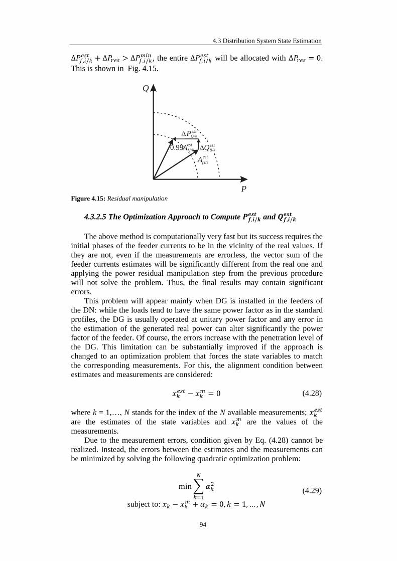
4.3 Distribution System State Estimation
94
∆𝑃𝑓,𝑖/𝑘𝑒𝑠𝑡 + ∆𝑃𝑟𝑒𝑠 > ∆𝑃𝑓,𝑖/𝑘
𝑚𝑖𝑛 , the entire ∆𝑃𝑓,𝑖/𝑘𝑒𝑠𝑡 will be allocated with ∆𝑃𝑟𝑒𝑠 = 0.
This is shown in Fig. 4.15.
Figure 4.15: Residual manipulation
4.3.2.5 The Optimization Approach to Compute 𝑷𝒇,𝒊/𝒌𝒆𝒔𝒕 and 𝑸𝒇,𝒊/𝒌
𝒆𝒔𝒕
The above method is computationally very fast but its success requires the
initial phases of the feeder currents to be in the vicinity of the real values. If
they are not, even if the measurements are errorless, the vector sum of the
feeder currents estimates will be significantly different from the real one and
applying the power residual manipulation step from the previous procedure
will not solve the problem. Thus, the final results may contain significant
errors.
This problem will appear mainly when DG is installed in the feeders of
the DN: while the loads tend to have the same power factor as in the standard
profiles, the DG is usually operated at unitary power factor and any error in
the estimation of the generated real power can alter significantly the power
factor of the feeder. Of course, the errors increase with the penetration level of
the DG. This limitation can be substantially improved if the approach is
changed to an optimization problem that forces the state variables to match
the corresponding measurements. For this, the alignment condition between
estimates and measurements are considered:
𝑥𝑘𝑒𝑠𝑡 − 𝑥𝑘
𝑚 = 0 (4.28)
where k = 1,…, N stands for the index of the N available measurements; 𝑥𝑘𝑒𝑠𝑡
are the estimates of the state variables and 𝑥𝑘𝑚 are the values of the
measurements.
Due to the measurement errors, condition given by Eq. (4.28) cannot be
realized. Instead, the errors between the estimates and the measurements can
be minimized by solving the following quadratic optimization problem:
min∑𝛼𝑘
2
𝑁
𝑘=1
subject to: 𝑥𝑘 − 𝑥𝑘𝑚 + 𝛼𝑘 = 0, 𝑘 = 1,… , 𝑁
(4.29)
P
Af,i/k
Q
Qf
Pf,i/k
0.99A f,i/k
est
est
est
est,i/k

4. Distribution System State Estimation
95
𝑓(𝐱) = 0
𝑔(𝐱) ≤ 0
where 𝐱 = [𝑥1…𝑥𝑘]𝑇, αk are the slack variables standing for the absolute
error between the k-th state variable, 𝑥𝑘, and the k-th measurement.
In the above model, first set of constraints will force the state variables to
fit the associated measurements while the following sets of constraint 𝑓(𝐱) and 𝑔(𝐱) represents various technical constraints in the primary substations of
the DS.
When defining the optimization problem according to (4.29), the
measured currents through the transformers can be neglected: once the powers
and the voltage estimates in the transformers are matched with the
measurements, also the corresponding currents will be automatically matched.
Moreover, considering the assumption previously made, also the voltage
measurements can be neglected and the measured magnitude of the apparent
powers absorbed by the feeders, Af,i and Af,k, can be derived from the voltage
and current measurements. Thus, an optimization problem where only the
states associated with the power measurements need to be fit is obtained. The
objective function can thus be written as:
min∑𝛼𝑃𝑇,𝑟2 +∑𝛼𝑄𝑇,𝑟
2 +∑𝛼𝐴𝑓,𝑘2 +
𝑁𝑓1
𝑘=1
𝑁𝑇1
𝑟=1
𝑁𝑇1
𝑟=1
∑ 𝛼𝑃𝑇,𝑞2 +∑𝛼𝑄𝑇,𝑞
2 +∑𝛼𝐴𝑓,𝑖2
𝑁𝑓2
𝑖=1
𝑁𝑇2
𝑞=1
𝑁𝑇2
𝑞=1
(4.30)
where:
𝑁𝑇1 the number of HV/MV1 transformers;
𝑁𝑇2 the number of MV1/MV2 transformers;
𝑁𝑓1 the number of feeders connected to the MV1 buses;
𝑁𝑓2 the number of feeders connected to the MV2 buses;
𝛼𝑃𝑇,𝑟/𝑞 the slack variables associated to 𝑃𝑇,𝑟/𝑞𝑚 ;
𝛼𝑄𝑇,𝑟/𝑞 the slack variables associated to 𝑄𝑇,𝑟/𝑞𝑚 ;
𝛼𝐴𝑓,𝑘,𝑖 the slack variable associated to the measured magnitude of the
apparent powers absorbed by the feeders connected to the MV1 and
MV2 buses, respectively.
The above objective function is subject to various constraints of both
types. The following can be written regarding the measurements in the
transformers and feeders connected to the MV1 buses:
𝑃𝑇,𝑟 − 𝑃𝑇,𝑟𝑚 + 𝛼𝑃𝑇,𝑟 = 0
𝑄𝑇,𝑟 − 𝑄𝑇,𝑟𝑚 + 𝛼𝑄𝑇,𝑟 = 0
𝐴𝑓,𝑘 − 𝐴𝑓,𝑘𝑚 + 𝛼𝐴𝑓,𝑘 = 0
(4.31)
where 𝑃𝑇,𝑟, 𝑄𝑇,𝑟 and 𝐴𝑓,𝑘 are the state variables associated with the 𝑃𝑇,𝑟𝑚 , 𝑄𝑇,𝑟
𝑚
and 𝐴𝑓,𝑘𝑚 measurements, and 𝐴𝑓,𝑘
𝑚 is computed as:

4.3 Distribution System State Estimation
96
𝐴𝑓,𝑘𝑚 = √3𝑉𝑀𝑉1
𝑚 ∙ 𝐼𝑓,𝑘𝑚 (4.32)
In addition, the MV1 feeder equivalent loads, 𝑃𝑓,𝑘 and 𝑄𝑓,𝑘, and the real
and reactive powers in the primary of the MV1/MV2 transformers need to be
aligned with the corresponding apparent powers:
𝑃𝑓,𝑘2 + 𝑄𝑓,𝑘
2 − 𝐴𝑓,𝑘2 = 0
𝑃𝑇_𝑃,𝑞2 + 𝑄𝑇_𝑃,𝑞
2 − 𝐴𝑇_𝑃,𝑞2 = 0
(4.33)
where 𝑃𝑇_𝑃,𝑞, 𝑄𝑇_𝑃,𝑞 and 𝐴𝑇_𝑃,𝑞 are the real, reactive and apparent powers in
the primary of the MV1/MV2 transformers, respectively (see Fig. 4.5).
In order to completely describe the MV1 buses, constraints regarding the
real and reactive power balance at these buses are added to the model:
∑𝑃𝑓,𝑘
𝑁𝑓1
𝑘=1
+∑𝑃𝑇_𝑃,𝑞 +∑𝑃𝑇,𝑟 = 0
𝑁𝑇1
𝑟=1
𝑁𝑇2
𝑞=1
∑𝑄𝑓,𝑘
𝑁𝑓1
𝑘=1
+∑𝑄𝑇_𝑃,𝑞 +∑𝑄𝑇,𝑟 = 0
𝑁𝑇1
𝑟=1
𝑁𝑇2
𝑞=1
(4.34)
In analogy with the MV1 buses constraints given by Eqs. (4.31) – (4.34),
a set of constraints for the MV2 buses can be defined as:
𝑃𝑇,𝑞 − 𝑃𝑇,𝑞𝑚 + 𝛼𝑃𝑇,𝑞 = 0
𝑄𝑇,𝑞 − 𝑄𝑇,𝑞𝑚 + 𝛼𝑄𝑇,𝑞 = 0
𝐴𝑓,𝑖 − 𝐴𝑓,𝑖𝑚 + 𝛼𝐴𝑓,𝑖 = 0
(4.35)
𝑃𝑓,𝑖2 + 𝑄𝑓,𝑖
2 − 𝐴𝑓,𝑖2 = 0 (4.36)
∑𝑃𝑓,𝑖 +
𝑁𝑓2
𝑖=1
∑𝑃𝑇,𝑞 = 0
𝑁𝑇2
𝑞=1
∑𝑄𝑓,𝑖 +
𝑁𝑓2
𝑖=1
∑𝑄𝑇,𝑞 = 0
𝑁𝑇2
𝑞=1
(4.37)
where 𝑃𝑇,𝑞, 𝑄𝑇,𝑞 and 𝐴𝑓,𝑖 are the state variables associated with the 𝑃𝑇,𝑞𝑚 , 𝑄𝑇,𝑞
𝑚
and 𝐴𝑓,𝑞𝑚 measurements. 𝐴𝑓,𝑞
𝑚 is computed as:
𝐴𝑓,𝑞𝑚 = √3𝑉𝑀𝑉2
𝑚 ∙ 𝐼𝑓,𝑖𝑚 (4.38)
Finally, for the model to be consistent, it is necessary to define a set of
constraints that link the MV2 buses variables to the MV1 buses variables.
These are the power balance equations between the primary and the secondary
windings of the MV1/MV2 transformers:

4. Distribution System State Estimation
97
𝑃𝑇_𝑃,𝑞 − 𝑃𝑇,𝑞 − 𝑃𝑙𝑜𝑠𝑠_𝑇,𝑞 − 𝑃𝑠ℎ_𝑙𝑜𝑠𝑠_𝑇,𝑞 = 0
𝑄𝑇_𝑃,𝑞 − 𝑄𝑇,𝑞 − 𝑄𝑙𝑜𝑠𝑠_𝑇,𝑞 − 𝑄𝑠ℎ_𝑙𝑜𝑠𝑠_𝑇,𝑞 = 0 (4.39)
where 𝑃𝑙𝑜𝑠𝑠_𝑇,𝑞 and 𝑄𝑙𝑜𝑠𝑠_𝑇,𝑞 are the real and reactive power losses along the
MV1/MV2 transformers, respectively; while 𝑃𝑠ℎ_𝑙𝑜𝑠𝑠_𝑇,𝑞 and 𝑄𝑠ℎ_𝑙𝑜𝑠𝑠_𝑇,𝑞 are
the real and reactive power losses in the shunt elements of the MV1/MV2
transformers, respectively.
To compute 𝑃𝑙𝑜𝑠𝑠_𝑇,𝑞 and 𝑄𝑙𝑜𝑠𝑠_𝑇,𝑞 a formulation similar to Eq. (4.3) can
be used, these time the defined equations are exact as they involve a single
network element:
𝑃𝑙𝑜𝑠𝑠_𝑇,𝑞 = (𝐴𝑇_𝑝,𝑞
𝐴𝑇_𝑝,𝑞0 )
2
∙ 𝑃𝑙𝑜𝑠𝑠_𝑇,𝑞0
𝑃𝑙𝑜𝑠𝑠_𝑇,𝑞 = (𝐴𝑇_𝑝,𝑞
𝐴𝑇_𝑝,𝑞0 )
2
∙ 𝑃𝑙𝑜𝑠𝑠_𝑇,𝑞0
(4.40)
The shunt losses mainly depend on the square of the voltage and,
considering the adopted hypothesis regarding the voltages, these losses can be
considered constant quantities given by:
𝑃𝑠ℎ_𝑙𝑜𝑠𝑠_𝑇,𝑞 = (𝑉𝑀𝑉1𝑚
𝑉𝑀𝑉10 )
2
∙ 𝑃𝑠ℎ_𝑙𝑜𝑠𝑠_𝑇,𝑞0
𝑄𝑠ℎ_𝑙𝑜𝑠𝑠_𝑇,𝑞 = (𝑉𝑀𝑉1𝑚
𝑉𝑀𝑉10 )
2
∙ 𝑄𝑠ℎ_𝑙𝑜𝑠𝑠_𝑇,𝑞0
(4.41)
In order to assure that the optimization problem converges to a realistic
operating point, the control variables need to be lower and upper bounded. For
this optimization problem various limits are defined such to fulfill the
technical requirements of the analyzed system. Thus, these limits are defined
considering: the capability limits of the installed generators, the capacitive
currents of the feeders, the maximum currents of the branches connected to
the primary substation and the direction of the power flows as suggested by
the corresponding measurements. Feeder power limits, therefore, are:
−∑𝑃𝑔𝑚𝑎𝑥 ≤ 𝑃𝑓 ≤ 1.5 ⋅ |𝐴𝑓
𝑚𝑎𝑥|
−∑𝑄𝑔𝑚𝑎𝑥 −𝑄𝑐𝑎𝑏𝑙𝑒𝑠 ≤ 𝑄𝑓 ≤ 1.5 ⋅ |𝐴𝑓
𝑚𝑎𝑥|
0 ≤ 𝐴𝑓 ≤ 1.5 ⋅ |𝐴𝑓𝑚𝑎𝑥|
(4.42)
Generally, upper bound is defined by maximal thermal current (𝐴𝑓𝑚𝑎𝑥 =
√3𝑉𝐼𝑓𝑚𝑎𝑥) of the feeder. But, in this case, the point is on the SE, so cases with
powers exceeding maximal values can occur, this bound has numerical nature
(augmentation of 50%).
As 𝑃𝑓 is absorbed power, lower bound is given by the maximum
generation capability of the feeder with appropriate sign. Lower bound of 𝑄𝑓

4.3 Distribution System State Estimation
98
is composed of two terms. The first one corresponds to the maximum
generation capability of the feeder with appropriate sign, while the other takes
into account estimated reactive power of the network when it is empty. As it
is injected power, the sign is negative. Minimal value for 𝐴𝑓 is 0.
Real and reactive power flows through transformers are limited as
follows:
0.5𝑃𝑇
𝑚 ≤ 𝑃𝑇 ≤ 1.5𝑃𝑇𝑚
0.5𝑄𝑇𝑚 ≤ 𝑄𝑇 ≤ 1.5𝑄𝑇
𝑚 (4.43)
Upper and lower limits of transformer power flows are given by large
bands (±50%) of the measurement errors.
Moreover, large limits are defined for the slack variables as there is no
knowledge about the quality of the measurements so they are actually free
variables, but they are minimized in objective function. Upper and lower
limits for slack variables are in per unit as follows:
−10 ≤ 𝛼 ≤ 10 (4.44)
4.3.2.6 Load and Generation Profiles Update
After completing the procedures for improving the SE and obtaining the
estimates for the feeder equivalent loads, the loads and generation profiles
need to be updated such that a new PF will turn the estimated quantities. For
this, the total quantity to be split to each feeder’s loads and generators is:
∆𝑃𝑓,𝑖/𝑘
𝑡𝑜𝑡 = 𝑃𝑓,𝑖/𝑘𝑒𝑠𝑡 − 𝑃𝑓,𝑖/𝑘
0 − (𝑐𝑃𝑓2 − 1) ∙ 𝑃𝑙𝑜𝑠𝑠_𝑓,𝑖/𝑘
0
∆𝑄𝑓,𝑖/𝑘𝑡𝑜𝑡 = 𝑄𝑓,𝑖/𝑘
𝑒𝑠𝑡 − 𝑄𝑓,𝑖/𝑘0 − (𝑐𝑃𝑓
2 − 1) ∙ 𝑄𝑙𝑜𝑠𝑠_𝑓,𝑖/𝑘0 − (
𝑉𝑀𝑉𝑚
𝑉𝑀𝑉0 )
2
∙ 𝑄𝑠ℎ_𝑙𝑜𝑠_𝑓,𝑖/𝑘0
(4.45)
In this equation 𝑃𝑓,𝑖/𝑘𝑒𝑠𝑡 denotes the estimate of feeder’s real power obtained
using proposed procedures, 𝑃𝑓,𝑖/𝑘0 denotes initial power of the feeder, 𝑃𝑙𝑜𝑠𝑠_𝑓,𝑖/𝑘
0 are
the initial real power losses in the feeders. The same can be said regarding the
reactive powers adding that 𝑄𝑠ℎ_𝑙𝑜𝑠_𝑓,𝑖/𝑘0 is the initial power produced by the shunt
capacitance of the feeders.
Now updating the load and generation profiles can start.
First, the total quantity of real power to be assigned to loads and generators will
be computed as:
∆𝑃𝐿_𝑡𝑜𝑡_𝑓,𝑖/𝑘 =∑ 𝑃𝐿,𝑙
0𝑙∈𝑙𝑜𝑎𝑑_𝑓,𝑖/𝑘
∑ 𝑃𝐿,𝑙0
𝑙∈𝑙𝑜𝑎𝑑_𝑓,𝑖/𝑘 +∑ 𝑃𝐺,𝑔0
𝑔∈𝑔𝑒𝑛_𝑓,𝑖/𝑘
∆𝑃𝑓,𝑖/𝑘𝑡𝑜𝑡
∆𝑃𝐺_𝑡𝑜𝑡_𝑓,𝑖/𝑘 = −∑ 𝑃𝐺,𝑔
0𝑔∈𝑔𝑒𝑛_𝑓,𝑖/𝑘
∑ 𝑃𝐿,𝑙0
𝑙∈𝑙𝑜𝑎𝑑_𝑓,𝑖/𝑘 + ∑ 𝑃𝐺,𝑔0
𝑔∈𝑔𝑒𝑛_𝑓,𝑖/𝑘
∆𝑃𝑓,𝑖/𝑘𝑡𝑜𝑡
(4.46)
where ∑ 𝑃𝐿,𝑙0
𝑙∈𝑙𝑜𝑎𝑑_𝑓,𝑖/𝑘 presents the total initial real power of the loads
pertaining to feeder i or k; and ∑ 𝑃𝐿,𝑙0
𝑙∈𝑙𝑜𝑎𝑑_𝑓,𝑖/𝑘 + ∑ 𝑃𝐺,𝑔0
𝑔∈𝑔𝑒𝑛_𝑓,𝑖/𝑘 is the total
initial real power. ∑ 𝑃𝐺,𝑔0
𝑔∈𝑔𝑒𝑛_𝑓,𝑖/𝑘 represents the total initial real power of

4. Distribution System State Estimation
99
the generators pertaining to feeder i or k; The minus sign comes from the
premise that 𝑃𝑓,𝑖/𝑘 = ∑𝑃𝐿,𝑖/𝑘 − ∑𝑃𝐺,𝑖/𝑘.
Next, ∆𝑃𝐺_𝑡𝑜𝑡_𝑓,𝑖/𝑘 will be assigned to each generator in the feeder
according to the sign of ∆𝑃𝐺_𝑡𝑜𝑡_𝑓,𝑖/𝑘 and the capability of each generator:
1. ∆𝑃𝐺_𝑡𝑜𝑡_𝑓,𝑖/𝑘 > 0 and ∆𝑃𝐺_𝑡𝑜𝑡_𝑓,𝑖/𝑘 > ∑(𝑃𝐺_𝑓,𝑖/𝑘𝑚𝑎𝑥 − 𝑃𝐺_𝑓,𝑖/𝑘
0 ):
𝑃𝐺_𝑓,𝑖/𝑘𝑒𝑠𝑡 = 𝑃𝐺_𝑓,𝑖/𝑘
𝑚𝑎𝑥
∆𝑃𝐿_𝑟𝑒𝑠_𝑓,𝑖/𝑘 = −(∆𝑃𝐺_𝑡𝑜𝑡_𝑓,𝑖/𝑘 −∑𝑃𝐺_𝑓,𝑖/𝑘𝑚𝑎𝑥 )
(4.47)
To be noted that we forced 𝑃𝐺_𝑓,𝑖/𝑘𝑒𝑠𝑡 to the maximum value, but as
∆𝑃𝐺_𝑡𝑜𝑡_𝑓,𝑖/𝑘 is higher, there will be some residual left, ∆𝑃𝐿_𝑟𝑒𝑠_𝑓,𝑖/𝑘 which will
be later assigned to the loads. As a result, ∆𝑃𝐿_𝑡𝑜𝑡_𝑓,𝑖/𝑘 will be updated in
following manner: ∆𝑃𝐿_𝑡𝑜𝑡_𝑓,𝑖/𝑘 = ∆𝑃𝐿_𝑡𝑜𝑡_𝑓,𝑖/𝑘 + ∆𝑃𝐿_𝑟𝑒𝑠_𝑓,𝑖/𝑘.
2. ∆𝑃𝐺_𝑡𝑜𝑡_𝑓,𝑖/𝑘 < 0 and |∆𝑃𝐺_𝑡𝑜𝑡_𝑓,𝑖/𝑘| > ∑(𝑃𝐺_𝑓,𝑖/𝑘0 − 𝑃𝐺_𝑓,𝑖/𝑘
𝑚𝑖𝑛 ):
𝑃𝐺_𝑓,𝑖/𝑘𝑒𝑠𝑡 = 𝑃𝐺_𝑓,𝑖/𝑘
𝑚𝑖𝑛
∆𝑃𝐿_𝑟𝑒𝑠_𝑓,𝑖/𝑘 = −(∑𝑃𝐺_𝑓,𝑖/𝑘𝑚𝑖𝑛 −∆𝑃𝐺_𝑡𝑜𝑡_𝑓,𝑖/𝑘)
(4.48)
3. ∆𝑃𝐺_𝑡𝑜𝑡_𝑓,𝑖/𝑘 > 0 and ∆𝑃𝐺_𝑡𝑜𝑡_𝑓,𝑖/𝑘 ≤ ∑(𝑃𝐺_𝑓,𝑖/𝑘𝑚𝑎𝑥 − 𝑃𝐺_𝑓,𝑖/𝑘
0 ):
In this case 𝑃𝐺_𝑓,𝑖/𝑘𝑒𝑠𝑡 is computed such that ∆𝑃𝐺_𝑡𝑜𝑡 is distributed according
to the capability of each generator with respect to the total available
regulation band:
𝑃𝐺_𝑓,𝑖/𝑘𝑒𝑠𝑡 = 𝑃𝐺_𝑓,𝑖/𝑘
0 +𝑃𝐺_𝑓,𝑖/𝑘𝑚𝑎𝑥 − 𝑃𝐺_𝑓,𝑖/𝑘
0
∑(𝑃𝐺_𝑓,𝑖/𝑘𝑚𝑎𝑥 − 𝑃𝐺_𝑓,𝑖/𝑘
0 )∆𝑃𝐺_𝑡𝑜𝑡_𝑓,𝑖/𝑘 (4.49)
Next, ∆𝑃𝐿_𝑡𝑜𝑡_𝑓,𝑖/𝑘 can be assigned to each individual load according to:
𝑃𝐿_𝑓,𝑖/𝑘𝑒𝑠𝑡 = 𝑃𝐿_𝑓,𝑖/𝑘
0 +𝑃𝐿_𝑓,𝑖/𝑘0
∑𝑃𝐿_𝑓,𝑖/𝑘0 ∆𝑃𝐿_𝑡𝑜𝑡_𝑓,𝑖/𝑘 (4.50)
As for the real powers, the total quantity of real power to be assigned to
loads and generators will be computed as:
∆𝑄𝐿_𝑡𝑜𝑡_𝑓,𝑖/𝑘 =∑ 𝑄𝐿,𝑙
0𝑙∈𝑙𝑜𝑎𝑑_𝑓,𝑖/𝑘
∑ 𝑄𝐿,𝑙0
𝑙∈𝑙𝑜𝑎𝑑_𝑓,𝑖/𝑘 + ∑ 𝑄𝐺,𝑔0
𝑔∈𝑔𝑒𝑛_𝑓,𝑖/𝑘
∆𝑄𝑓,𝑖/𝑘𝑡𝑜𝑡
∆𝑄𝐺_𝑡𝑜𝑡_𝑓,𝑖/𝑘 = −∑ 𝑄𝐺,𝑔
0𝑔∈𝑔𝑒𝑛_𝑓,𝑖/𝑘
∑ 𝑄𝐿,𝑙0
𝑙∈𝑙𝑜𝑎𝑑_𝑓,𝑖/𝑘 + ∑ 𝑄𝐺,𝑔0
𝑔∈𝑔𝑒𝑛_𝑓,𝑖/𝑘
∆𝑄𝑓,𝑖/𝑘𝑡𝑜𝑡
(4.51)
where ∑ 𝑄𝐿,𝑙0
𝑙∈𝑙𝑜𝑎𝑑_𝑓,𝑖/𝑘 presents the total initial reactive power of the loads
pertaining to feeder i or k; and ∑ 𝑄𝐿,𝑙0
𝑙∈𝑙𝑜𝑎𝑑_𝑓,𝑖/𝑘 +∑ 𝑄𝐺,𝑔0
𝑔∈𝑔𝑒𝑛_𝑓,𝑖/𝑘 is the total
initial reactive power. ∑ 𝑄𝐺,𝑔0
𝑔∈𝑔𝑒𝑛_𝑓,𝑖/𝑘 represents the total initial reactive

4.3 Distribution System State Estimation
100
power of the generators pertaining to feeder i or k; The minus sign comes
from the premise that 𝑄𝑓,𝑖/𝑘 = ∑𝑄𝐿,𝑖/𝑘 − ∑𝑄𝐺,𝑖/𝑘.
Next, ∆𝑄𝐺_𝑡𝑜𝑡_𝑓,𝑖/𝑘 will be assigned to each generator in the feeder
according to the sign of ∆𝑄𝐺_𝑡𝑜𝑡_𝑓,𝑖/𝑘 and the capability of each generator:
4. ∆𝑄𝐺_𝑡𝑜𝑡_𝑓,𝑖/𝑘 > 0 and ∆𝑄𝐺_𝑡𝑜𝑡_𝑓,𝑖/𝑘 > ∑(𝑄𝐺_𝑓,𝑖/𝑘𝑚𝑎𝑥 − 𝑄𝐺_𝑓,𝑖/𝑘
0 ):
𝑄𝐺_𝑓,𝑖/𝑘𝑒𝑠𝑡 = 𝑄𝐺_𝑓,𝑖/𝑘
𝑚𝑎𝑥
∆𝑄𝐿_𝑟𝑒𝑠_𝑓,𝑖/𝑘 = −(∆𝑄𝐺_𝑡𝑜𝑡_𝑓,𝑖/𝑘 −∑𝑄𝐺_𝑓,𝑖/𝑘𝑚𝑎𝑥 )
(4.52)
To be noted that we forced 𝑄𝐺_𝑓,𝑖/𝑘𝑒𝑠𝑡 to the maximum value, but as
∆𝑄𝐺_𝑡𝑜𝑡_𝑓,𝑖/𝑘 is higher, there will be some residual left, ∆𝑄𝐿_𝑟𝑒𝑠_𝑓,𝑖/𝑘 which will
be later assigned to the loads. As a result, ∆𝑄𝐿_𝑡𝑜𝑡_𝑓,𝑖/𝑘 will be updated in
following manner: ∆𝑄𝐿_𝑡𝑜𝑡_𝑓,𝑖/𝑘 = ∆𝑄𝐿_𝑡𝑜𝑡_𝑓,𝑖/𝑘 + ∆𝑄𝐿_𝑟𝑒𝑠_𝑓,𝑖/𝑘.
5. ∆𝑄𝐺_𝑡𝑜𝑡_𝑓,𝑖/𝑘 < 0 and |∆𝑄𝐺_𝑡𝑜𝑡_𝑓,𝑖/𝑘| > ∑(𝑄𝐺_𝑓,𝑖/𝑘0 − 𝑄𝐺_𝑓,𝑖/𝑘
𝑚𝑖𝑛 ):
𝑄𝐺_𝑓,𝑖/𝑘𝑒𝑠𝑡 = 𝑄𝐺_𝑓,𝑖/𝑘
𝑚𝑖𝑛
∆𝑄𝐿_𝑟𝑒𝑠_𝑓,𝑖/𝑘 = −(∑𝑄𝐺_𝑓,𝑖/𝑘𝑚𝑖𝑛 −∆𝑄𝐺_𝑡𝑜𝑡_𝑓,𝑖/𝑘)
(4.53)
6. ∆𝑄𝐺_𝑡𝑜𝑡_𝑓,𝑖/𝑘 > 0 and ∆𝑄𝐺_𝑡𝑜𝑡_𝑓,𝑖/𝑘 ≤ ∑(𝑄𝐺_𝑓,𝑖/𝑘𝑚𝑎𝑥 − 𝑄𝐺_𝑓,𝑖/𝑘
0 ):
In this case 𝑄𝐺_𝑓,𝑖/𝑘𝑒𝑠𝑡 is computed such that ∆𝑄𝐺_𝑡𝑜𝑡 is distributed according
to the capability of each generator with respect to the total available
regulation band:
𝑄𝐺_𝑓,𝑖/𝑘𝑒𝑠𝑡 = 𝑄𝐺_𝑓,𝑖/𝑘
0 +𝑄𝐺_𝑓,𝑖/𝑘𝑚𝑎𝑥 − 𝑄𝐺_𝑓,𝑖/𝑘
0
∑(𝑄𝐺_𝑓,𝑖/𝑘𝑚𝑎𝑥 − 𝑄𝐺_𝑓,𝑖/𝑘
0 )∆𝑄𝐺_𝑡𝑜𝑡_𝑓,𝑖/𝑘 (4.54)
Next, ∆𝑄𝐿_𝑡𝑜𝑡_𝑓,𝑖/𝑘 can be assigned to each individual load according to:
𝑄𝐿_𝑓,𝑖/𝑘𝑒𝑠𝑡 = 𝑄𝐿_𝑓,𝑖/𝑘
0 +𝑄𝐿_𝑓,𝑖/𝑘0
∑𝑄𝐿_𝑓,𝑖/𝑘0 ∆𝑄𝐿_𝑡𝑜𝑡_𝑓,𝑖/𝑘 (4.55)
4.3.3 Simplified State Estimation Simulation Results
4.3.3.1 The non-optimized approach to compute 𝑷𝒇,𝒊/𝒌𝒆𝒔𝒕 and 𝑸𝒇,𝒊/𝒌
𝒆𝒔𝒕
4.3.3.1.1 Performance analysis of each step of the non-optimized
approach
Some results of the non-optimized SSE will be presented here to clarify
the advantages it offers and how much of the improvement is achieved step by
step.
The performance of the SSE algorithm is analyzed by applying each step
of the defined procedure. The test network contains 154 buses and 155

4. Distribution System State Estimation
101
branches and the primary substation consists of two parallel HV/MV
transformers feeding 4 distribution feeders, among which the third has
installed generators. In order to test the procedure, 1000 sets of measurements
were created starting from standard profiles as follows: (i) the load/generation
profiles were randomly varied according to a specified uncertainty, then (ii)
the PF was performed and the set of measures extracted. Then, the SSE was
run starting from the standard data and the set of measures. The tests are
carried out assuming a load and generation profiles uncertainty of 40% and an
uncertainty of the power factor of each component of 5%. Test DN is shown
in Fig (4.16):
Figure 4.16: Test DN
First set of tables (Table 4.3) presents the results of estimator just with
using the cp factor, without phase correction nor residual manipulation.
Table 4.3: Estimation results after using cp factor
The following set of tables (Table 4.4) refers to results obtained by using
cp factor and phase correction procedure.
Table 4.4: Estimation results after using cp factor and phase correction
The last set of tables (Table 4.5) refers to results obtained using complete
solution offered by the SSE.

4.3 Distribution System State Estimation
102
Table 4.5: Estimation results after completion of SSE
As seen in first set of tables, both average and maximal errors of feeders’
current estimates are very small and this is due to the fact that 𝐼𝑓𝑒𝑒𝑑𝑒𝑟,𝑘𝑒𝑠𝑡 ≃
𝐼𝑓𝑒𝑒𝑑𝑒𝑟,𝑘𝑚 . The error, however, is not null because losses of feeders are
estimated, not known values, as stated before. The errors of the transformers’
estimates present the main problem. By aligning the current magnitudes, the
estimation was not very successful. That’s why phase correction procedure
with power flow inversion detection was introduced. It is obvious from the
second set of tables that improvement gained this way is considerable. For
example, in the first set of tables, maximal errors on real and reactive power
estimates of the transformers are 4.51% and 6.99% respectively. After phase
correction procedure with power flow inversion detection, these have been
reduced to 0.658% and 0.659% respectively. Also, reader can see that
outstanding improvement has been achieved regarding average errors on the
transformers in this step, decrease from 1.72% to 0.241% regarding real
power, and from 2.26% to 0.241% regarding reactive power.
To further improve the estimation and reduce errors even more, we have
introduced power residual manipulation. After this, maximal errors on real
and reactive power estimates of the transformers were 0.125% and 0.029%
respectively. Taking into account that after aligning the current magnitudes
procedure they were 4.51% and 6.99% respectively, this presents remarkable
result. Regarding average errors, improvements have also been gained, from
0.241% to 0.041% for real power and from 0.241% to 0.009% for reactive
power. But, as a result of using power residual manipulation procedure,
feeders’ current errors have been increased to maximal of 0.691%, but in any
case it remains small.
4.3.3.1.2 Performance and limitations of the non-optimized approach
Following results refer to performance of proposed DSSE in different
network scenarios.
First set of data refers to load power uncertainty of 40% for each load
randomly, and also power factor uncertainty of 5% for each load randomly
which can be observed as “normal” state of the network operation, at its
normal operation boundary. Thousand simulations have been run.
Results will be given for two types of generation in the third feeder –
generation of 50 kW in comparison with 225 kW of consumption and 550 kW
of generation with 225 kW of consumption. This is done to show how
generation in DN induces larger errors in estimation. For each set of data, the
results will be presented without and with procedure of residuals
manipulation.

4. Distribution System State Estimation
103
Case 1: feeder 3 – load 225 kW, generation 50 kW - normal operation
(Table 4.6 and Table 4.7)
Table 4.6: Case 1: without residual manipulation – normal operation
Table 4.7: Case 1: with residual manipulation – normal operation
It can be easily seen that even without using residual manipulation
procedure, results obtained are below 1% for average but also maximal error
on transformer and feeder estimates. Of courses, results obtained by using this
procedure are of better quality but it’s practical use will be more pronounced
with larger amount of generation. Also, it can be observed that feeders’
current estimates are worse in later table, as already explained.
Case 2: feeder 3 – load 225 kW, generation 550 kW - normal operation
(Table 4.8 and Table 4.9)
Table 4.8: Case 2: without residual manipulation – normal operation

4.3 Distribution System State Estimation
104
Table 4.9: Case 2: with residual manipulation – normal operation
Case 2 introduces significant amount of generation in the third feeder and,
as the effect of that, one can see that errors on all the estimates have grown
significantly. As an effect of using proposed procedure of residual
manipulation, errors on reactive power of the transformers have been
decreased for roughly 3.5% which is an considerable amount (maximal
value), but as a result of that not much could be done regarding real power. It
can be also observed that average values, however, are good because they
decreased from 1.44% to 0.694% for real and 0.157% for reactive power.
Second set of data refer to load power uncertainty of 80% for each load
randomly, and also power factor uncertainty of 10% for each load randomly
which can be observed as very bad initial data. Thousand simulations have
been run.
Results will be given for two types of generation in the third feeder –
generation of 50 kW in comparison with 225 kW of consumption and 550 kW
of generation with 225 kW of consumption. This is done to show how
generation in distribution network induces larger errors in estimation. For
each set of data, presented will be the results without and with procedure of
residuals manipulation.
Case 3: feeder 3 – load 225 kW, generation 50 kW - disturbed operation
(Table 4.10 and Table 4.11)
Table 4.10: Case 3: without residual manipulation – disturbed operation

4. Distribution System State Estimation
105
Table 4.11: Case 3: with residual manipulation – disturbed operation
It can be seen that in this case as a result of increased uncertainty in both
power of the load and power factor, results are much worse than in Case 1.
Although average errors of transformers’ estimates stay below 1%, maximal
error on transformers’ real power is little above this border. Other results are
good.
This set of results present the actual limitation of proposed method which
will be even more enhanced in last Case 4 with significant amount of
generation.
Case 4: feeder 3 – load 225 kW, generation 550 kW - disturbed operation
(Table 4.12 and Table 4.13)
Table 4.12: Case 4: without residual manipulation – disturbed operation
Table 4.13: Case 4: with residual manipulation – disturbed operation
Case 4 introduces significant amount of generation in the third feeder and
as the effect of that reader can see that errors on all the estimates have grown

4.3 Distribution System State Estimation
106
significantly. As a result of larger uncertainty of load, errors are much higher
than in Case 2. As an effect of using proposed procedure of residual
manipulation, errors on reactive power of the transformers have been
decreased for roughly 2.2% which is an considerable amount (average value),
but as a result of that not much could be done regarding real power, from
3.36% to 2.73%. But, maximal errors of power estimates on transformers are
much higher than 1%, even with using proposed procedure of residual
manipulation.
This leads to acknowledging the limitation of the SSE. It can be used well
in normal conditions with very high performances regarding results and time
consumption but in case of very bad initial data, optimization procedure must
be used. It should be also pointed that the computational time needed for this
procedure is insignificant with respect to a PF computation. Therefore, from
computation point of view, two PF computations are dominant (the average
time is less than 0.005 seconds).
4.3.3.2 The Optimization Approach
In this subchapter, the results of the optimization procedure for some
cases in which the simple, non-optimization, approach gives bad results in
terms of errors between the estimated and the measured values will be
provided. These tests were made using the same network and assumptions as
previously (Fig. 4.16). The computational time depends on the number of
variables and constraints of the problem. In the following tests the
optimization model consists of 28 variables and 14 constraints.
In the first case, we considered the network containing no generation and
an uncertainty of the load profiles of 80% and of the power factor of each load
of 10%. The results of the 1000 simulations are reported in Table 4.14. As it
can be seen, the errors are very small and due only to the approximation of the
final power losses in the feeders and transformers. The average simulation
time for the optimization procedure is 0.054 s, much longer than the simple
method, but still contained.
Table 4.14: Case 1. only load - optimization method
Next, generators were introduced in one of the feeders and many cases
where simulated. Further, the most severe case is going to be reported. In this
case the uncertainty of the load and generation profiles is 80% and of the
power factor of each load and generator is 10%. Table 4.15 depicts the results
of the 1000 simulations. Also this time the errors are very small. However,

4. Distribution System State Estimation
107
one can notice a slightly high error in the maximum value of PT1 and PT2. This
is because in this situation the real generated power almost balances the real
load, so the real power flows in the AT/MT transformers are almost null. In
the same time, the feeders are highly loaded and therefore the error introduced
by the approximation of the losses in the feeders has a high impact on the very
small real power flow in the transformers. However, the difference in kW
between the measured and the computed PT1 and PT2 is very small, i.e. 0.2 kW
of difference with respect to PT1_m = PT2_m ≈ 40 kW.
Table 4.15: Case 2. generation and load - optimization method
This time, the average simulation time of the optimization procedure was
0.059 s, a value similar to the previous one. Generally, the average simulation
time for all the tests made with this network was ≈ 0.06 s, so well contained.
These tests, allow us to conclude that the optimization can provide very
good results in all the situations. However, since the simulation time of the
optimization procedure is much higher than the simple method (≈ 0.06 s over
≈ 0.005 s) and since the simple method gives good results in many situations,
it was chosen as a general strategy to perform the optimization only when the
simple approach gives unacceptable results. With the tests done here, the
maximum admissible error between computed values by the simple method
and the measurements was set to 1%.
4.3.4 Implementation Aspects Regarding the SSE
The previously presented function was implemented in the MATLAB
environment. The SSE cannot be run if one or more of previously stated
measurements is/are missing:
If 𝑉𝐻𝑉𝑚 is missing, both PF and SE functions cannot be run correctly
because they would lack the real setting of slack bus voltage;
If one of the following quantities is missing: 𝑉𝐻𝑉𝑚 or 𝑉𝑀𝑉1/2
𝑚 it is
impossible to estimate the position of HV/MV transformer’s tap changer
which is crucial for obtaining good PF and as a consequence SE solution;
If 𝑉𝑀𝑉1/2𝑚 is missing it is impossible to obtain high quality SE solution
since it becomes impossible to compute the actual apparent power
absorbed by the feeder (𝐴𝑓,𝑝/𝑞𝑚 = √3𝑉𝑀𝑉1/2
𝑚 ⋅ 𝐼𝑓,𝑝/𝑞𝑚 ) and, hence, it is
impossible to adjust 𝑃𝑓,𝑝/𝑞 and 𝑄𝑓,𝑝/𝑞 such to obtain 𝐴𝑓,𝑝/𝑞𝑚 and 𝑃𝑇
𝑚 and
𝑄𝑇𝑚, respectively;
4.3 Distribution System State Estimation
108
If 𝑃𝑇𝑚 or 𝑄𝑇
𝑚 is missing, SE cannot give the solution of the problem
because powers obtained as a solution in feeder level cannot be compared
to a measured value on transformer level and changed accordingly;
If some of the values from 𝐼𝑓,𝑝/𝑞𝑚 are missing, solutions obtained by SE
function on feeder level can turn the solution with a very large error as it
will not match the values of powers on MV level of transformer.
4.3.5 Advanced State Estimation (ASE) function
The presence of measurements at the secondary substations of the DS
forces the change of the approach as now it is required to constraint the state
estimation procedure with the PF equations, making the procedure more
computationally burdened. In these regards, an optimization based procedure
is proposed to improve the observability of the DS in the presence of
measurements in the secondary substations. In brief, the optimization problem
is defined as the minimization of the sum of the squares of the differences
between measured and estimated values – the slack variables αi – so as to
satisfy the PF equations. The mathematical model of the optimization problem
can be generally written as follows [68]:
min∑(𝛼𝑖𝑥𝑖𝑚)
2𝑁𝑚
𝑖=1
Subject to:
𝑓𝑃(𝑉𝑀, 𝑉𝐴, 𝐱𝐞𝐬𝐭) = 0
𝑓𝑄(𝑉𝑀, 𝑉𝐴, 𝐱𝐞𝐬𝐭) = 0
𝐱𝐦 − 𝐱𝐞𝐬𝐭 + 𝜶 = 0
(4.56)
where:
𝛼𝑖 contained in the vector 𝛂, are the slack variables;
𝑁𝑚 is the number of available measurements;
𝑓𝑃 and 𝑓𝑄 are the PF equations;
𝑥𝑖𝑚 contained in the vector 𝐱𝐦, are the available measurements in the
considered DN;
𝐱𝐞𝐬𝐭 is the vector of the state variables;
𝑉𝑀 and 𝑉𝐴 are the vectors of the bus voltage magnitudes and phases,
excluding the slack bus.
In the objective function (OF) of Eq. (4.56), the slack variables, αi, are
scaled with respect to the measured quantities: in the absence of any statistical
information regarding the quality of the measurements, in particular the type
of distribution and the standard deviation of the measurements with respect to
the exact value, it is very difficult to properly weight the slack variables in the
OF. Introducing typical values for the standard deviations may force the
optimization solver to give unrealistic results in many cases. If particular
network measurement 𝑥𝑖𝑚 → 0, 𝛼𝑖 cannot be scaled according to the value of
the measurement (as it would have potentially infinite value), so in this case
measurement value is replaced with properly chosen small reference value
which depends on which particular quantity it is.

4. Distribution System State Estimation
109
Moreover, defining an OF as the sum of the squares of αi may give many
bad results since the absolute errors would be minimized without taking into
account that various measurements in the DN can be very different in terms of
numerical values, i.e. 10 to 1000 times different. This could give very high
relative errors between the estimates and corresponding measurements. Thus,
minimizing the OF in Eq. (4.), which ideally is zero, will minimize the
relative error between the measured and the estimated values in a balance
manner.
4.3.5.1 Vector of State Variables and Objective Function Definition
In defining the particular shape of model given by Eq. (4.56) one can
observe from Figs. (4.) and (4.) that the types of measurements that are
available in the secondary substations coincide with the ones available in the
primary substation. Thus, a unified set of measurements can be considered
and the vector of variables associated with this set can be defined as:
𝐱𝐞𝐬𝐭 = [𝑉𝑀 𝑉𝐴 𝐼𝑓𝑡_𝑟𝑒 𝐼𝑓𝑡_𝑖𝑚 𝐼𝑡𝑓_𝑟𝑒 𝐼𝑡𝑓_𝑖𝑚 𝑃𝑓𝑡 𝑄𝑓𝑡 𝑃𝑡𝑓 𝑄𝑡𝑓] (4.57)
where:
𝑉𝑀 the vector of bus voltage magnitudes in p.u. excluding the slack bus;
𝑉𝐴 the vector of bus voltage phase angles in p.u. excluding the slack bus;
𝐼𝑓𝑡_𝑟𝑒 the vector of real parts of branch currents with existing current
measurements in p.u. in from – to direction;
𝐼𝑓𝑡_𝑖𝑚 the vector of imaginary parts of branch currents with existing current
measurements in p.u. in from – to direction;
𝐼𝑡𝑓_𝑟𝑒 the vector of real parts of branch currents with existing current
measurements in p.u. in to – from direction;
𝐼𝑡𝑓_𝑖𝑚 the vector of imaginary parts of branch currents with existing current
measurements in p.u. in to – from direction;
𝑃𝑓𝑡 the vector of branch real powers with existing power measurements
in p.u. in from – to direction;
𝑄𝑓𝑡 the vector of branch reactive powers with existing power
measurements in p.u. in from – to direction;
𝑃𝑡𝑓 the vector of branch real powers with existing power measurements
in p.u. in to – from direction;
𝑄𝑡𝑓 the vector of branch reactive powers with existing power
measurements in p.u. in to – from direction.
Thus, the vector of slack variables consists of:
𝛂 = [𝛼𝑃 𝛼𝑄 𝛼𝑉 𝛼𝐼𝑓𝑡 𝛼𝐼𝑡𝑓 𝛼𝑃𝑓𝑡 𝛼𝑄𝑓𝑡 𝛼𝑃𝑡𝑓 𝛼𝑄𝑡𝑓] (4.58)
where:
𝛼𝑃 the vector of slack variables associated with the measured real power
injections of the non-empty busses;
𝛼𝑄 the vector of slack variables associated with the measured reactive
power injections of the non-empty busses;

4.3 Distribution System State Estimation
110
𝛼𝑉 the vector of slack variables pertaining to the voltage magnitude of
the busses with voltage measurement equipment;
𝛼𝐼𝑓𝑡 the vector of slack variables pertaining to the current in from – to
direction of the busses with current measurement equipment;
𝛼𝐼𝑡𝑓 the vector of slack variables pertaining to the current in to – from
direction of the busses with current measurement equipment;
𝛼𝑃𝑓𝑡 the vector of slack variables pertaining to the real power in from – to
direction of the busses with power measurement equipment;
𝛼𝑄𝑓𝑡 the vector of slack variables pertaining to the reactive power in from
– to direction of the busses with power measurement equipment;
𝛼𝑃𝑡𝑓 the vector of slack variables pertaining to the real power in to – from
direction of the busses with power measurement equipment;
𝛼𝑄𝑡𝑓 the vector of slack variables pertaining to the reactive power in to –
from direction of the busses with power measurement equipment.
The solution of DSSE problem is obtaining an accurate as possible picture
of the network which means in ideal case equaling estimates with measured
values of different quantities throughout the network. The difficulty is that
number of measurements is limited so the differences between estimated and
measured values will exist. The task is that differences be as small as possible
so this is why the estimator’s objective function is the minimization of sum of
squares of these differences which are represented by the slack variables. The
objective function is the following:
min𝑓 = min ∑ (𝛼𝑃𝑘
𝑃𝐺𝑘𝑚 − 𝑃𝐿𝑘
𝑚)
2
+
𝑁𝑚_𝑏𝑢𝑠
𝑘=1
∑ (𝛼𝑄𝑘
𝑄𝐺𝑘𝑚 − 𝑄𝐿𝑘
𝑚)
2𝑁𝑚_𝑏𝑢𝑠
𝑘=1
+ ∑ (𝛼𝑉𝐼𝑃𝑄𝑘𝑉𝐼𝑃𝑄𝑘
𝑚)
2𝑁𝑚_𝑉𝐼𝑃𝑄
𝑘=1
(4.59)
where:
𝑁𝑚_𝑏𝑢𝑠 the number of buses with completely measured injected powers (see
Fig. 4., d);
𝑁𝑚_𝑉𝐼𝑃𝑄 the total number of voltage and branch powers and currents
measurements (see Fig. 4.);
𝛼𝑉𝐼𝑃𝑄 vector holding 𝛼𝑉, 𝛼𝐼𝑏𝑟𝑎𝑛𝑐ℎ , 𝛼𝑃𝑏𝑟𝑎𝑛𝑐ℎ , 𝛼𝑄𝑏𝑟𝑎𝑛𝑐ℎ;
𝑉𝐼𝑃𝑄𝑚 vector holding the voltage and branch measurements.
The other quantities have been defined in subchapter 4.3.1.
It should be noted that regarding the real and reactive power injections,
only the slacks pertaining to buses with completely known load and
generation are included into Eq. (4.59) since only these measurements can be
matched.

4. Distribution System State Estimation
111
4.3.5.2 Equality Constraints of the Problem
Every optimization problem is a subject to a certain number of linear
and/or nonlinear constraints. These constraints ensure the technical or
physical limitations of the problem so the problem itself represents as real as
possible the picture of the system. Following are the constraints adopted in
our SE problem.
4.3.5.2.1 Power Flow Equations
SE uses the initial values of the problem obtained directly from the PF
which means that PF equations represent the first constraint of the problem.
This is a nonlinear constraint. We have to distinguish between:
1. Buses without connected load and generation, i.e. empty buses:
𝑓𝑃𝑘(𝑉𝑀, 𝑉𝐴) = 0
𝑓𝑄𝑘(𝑉𝑀, 𝑉𝐴) = 0 (4.60)
2. Buses with connected loads and/or generators but partially measured or
not measured at all, such that the resulted nodal injected power is not
known:
𝑃𝑘0 − 𝑓𝑃𝑘(𝑉𝑀, 𝑉𝐴) + 𝛼𝑃𝑘 = 0
𝑄𝑘0 − 𝑓𝑄𝑘(𝑉𝑀, 𝑉𝐴) + 𝛼𝑄𝑘 = 0
(4.61)
In this case the slack variables are not present in the OF given by Eq.
(4.59) since the injected powers are not completely measured; however
their lower bounds (LB) and upper bounds (UB) are defined in
accordance to the measured data. These bounds can be find in Table 4.15.
In Eqs. (4.60) and (4.61):
𝑓𝑃𝑘(𝑉𝑀, 𝑉𝐴) real power of the k-th bus which is the result of the state
estimation’s appropriate iteration and is the function of bus
voltage magnitude and phase angle;
𝑓𝑄𝑘(𝑉𝑀, 𝑉𝐴) reactive power of the k-th bus which is the result of the state
estimation’s appropriate iteration and is the function of bus
voltage magnitude and phase angle;
𝑃𝑘0 initial real power of the k-th bus corresponding to the initial
estimated profiles. Power injection stands for the difference
between generation and load of the network buses;
𝑄𝑘0 initial reactive power of the k-th bus gained as the result of
the computation of complex bus power injection matrix;
𝛼𝑃𝑘 slack variables of real power of the k-th bus;
𝛼𝑄𝑘 slack variables of reactive power of the k-th bus.
3. Buses with connected loads and/or generation which are all measured. In
this case, the nodal injected power can be considered completely known:
𝑃𝑘𝑚 and 𝑄𝑘
𝑚:

4.3 Distribution System State Estimation
112
𝑃𝑘𝐦 − 𝑓𝑃𝑘(𝑉𝑀, 𝑉𝐴) + 𝛼𝑃𝑘 = 0
𝑄𝑘𝐦 − 𝑓𝑄𝑘(𝑉𝑀, 𝑉𝐴) + 𝛼𝑄𝑘 = 0
(4.62)
Accordingly, the slack variables are present in the objective function
and are subject of upper and lower bounds determined by the errors of the
measurement apparatus:
−휀𝑃𝑘
𝐦 ⋅ 𝑃𝑘𝐦 ≤ 𝛼𝑃𝑘 ≤ 휀𝑃𝑘
𝐦 ⋅ 𝑃𝑘𝐦
−휀𝑄𝑘𝐦 ⋅ 𝑄𝑘
𝐦 ≤ 𝛼𝑄𝑘 ≤ 휀𝑄𝑘𝐦 ⋅ 𝑄𝑘
𝐦 (4.63)
where 휀𝑃𝑘𝐦 and 휀𝑄𝑘
𝐦 are the errors that take into account the total
measurement errors.
4.3.5.2.2 Measured Voltage Constraints
For the buses of the network where a voltage measurement equipment is
present, the following constraint must be respected:
𝑉𝑀,𝑘 − 𝑉𝑘𝐦 + 𝛼𝑉𝑘 = 0 (4.64)
where:
𝑉𝑀,𝑘 - voltage magnitude of the k-th bus which is the result of the state
estimation’s appropriate iteration;
𝑉𝑘𝐦 - measured voltage of the k-th bus;
𝛼𝑉𝑘 - slack variable of voltage of the k-th bus.
4.3.5.2.3 Measured Current Constraints
For the buses of the network where there is present current measurement
equipment (from-to and/or to-from direction), following constraints must be
respected:
𝐼𝑓𝑡_𝑟𝑒 − 𝑅𝑒(𝑌𝑓 ⋅ 𝑉) = 0
𝐼𝑓𝑡_𝑖𝑚 − 𝐼𝑚(𝑌𝑓 ⋅ 𝑉) = 0
𝐼𝑡𝑓_𝑟𝑒 − 𝑅𝑒(𝑌𝑡 ⋅ 𝑉) = 0
𝐼𝑡𝑓_𝑖𝑚 − 𝐼𝑚(𝑌𝑡 ⋅ 𝑉) = 0
(4.65)
Eqs. (4.65) which pertain to the branch current constraints are then used
to compute the current measurement constraints given by Eqs. (4.66) as
follows:
√𝐼𝑓𝑡_𝑟𝑒2 + 𝐼𝑓𝑡_𝑖𝑚
2 − 𝐼𝑓𝑡𝐦 + 𝛼𝐼𝑓𝑡 = 0
√𝐼𝑡𝑓_𝑟𝑒2 + 𝐼𝑡𝑓_𝑖𝑚
2 − 𝐼𝑡𝑓𝐦 + 𝛼𝐼𝑡𝑓 = 0
(4.66)

4. Distribution System State Estimation
113
where:
𝑉 the vector of the complex bus voltages; 𝑉 = 𝑉𝑀𝑒𝑗𝑉𝐴;
𝑌𝑓 the branch admittance matrix computed according to the from buses of
the considered branches;
𝑌𝑡 the branch admittance matrix computed according to the “to” buses of the
considered branches;
𝐼𝑓𝑡𝐦 measured branch current in from-to direction;
𝐼𝑡𝑓𝐦 measured branch current in to-from direction.
For the structure of 𝑌𝑓 and 𝑌𝑡, it is suggested to refer to MATPOWER
software package [140].
The set of constraints given by Eqs. (4.65) and (4.66) is defined only for
the branches where measurements are available.
4.3.5.2.4 Measured Power Constraints
For the buses of the network where there is present real and reactive
power measurement equipment (from-to and/or to-from direction), following
constraints must be respected:
𝑃𝑓𝑡 − 𝑅𝑒 (𝑉𝑓 ⋅ 𝑐𝑜𝑛𝑗(𝑌𝑓 ⋅ 𝑉)) = 0
𝑄𝑓𝑡 − 𝐼𝑚 (𝑉𝑓 ⋅ 𝑐𝑜𝑛𝑗(𝑌𝑓 ⋅ 𝑉)) = 0
𝑃𝑡𝑓 − 𝑅𝑒(𝑉𝑡 ⋅ 𝑐𝑜𝑛𝑗(𝑌𝑡 ⋅ 𝑉)) = 0
𝑄𝑡𝑓 − 𝐼𝑚(𝑉𝑡 ⋅ 𝑐𝑜𝑛𝑗(𝑌𝑡 ⋅ 𝑉)) = 0
(4.67)
Eqs. (4.67) which pertain to the branch power constraints are then used to
compute power measurement constraints given by Eqs. (4.68) as follows:
𝑃𝑓𝑡 − 𝑃𝑓𝑡𝐦 + 𝛼𝑃𝑓𝑡 = 0
𝑄𝑓𝑡 − 𝑄𝑓𝑡𝐦 + 𝛼𝑄𝑓𝑡 = 0
𝑃𝑡𝑓 − 𝑃𝑡𝑓𝐦 + 𝛼𝑃𝑡𝑓 = 0
𝑄𝑡𝑓 − 𝑄𝑡𝑓𝐦 + 𝛼𝑄𝑡𝑓 = 0
(4.68)
where:
𝑃𝑓𝑡𝐦 - measured real power of the branch in from-to direction;
𝑄𝑓𝑡𝐦 - measured reactive power of the branch in from-to direction;
𝑃𝑡𝑓𝐦 - measured real power of the branch in to-from direction;
𝑄𝑡𝑓𝐦 - measured reactive power of the branch in to-from direction.
Constraints given by Eqs. (4.67) are nonlinear while constraints (4.68)
constraints are linear. The set of constraints given by Eqs. (4.67) and (4.68) is
defined only for the branches where measurements are available.

4.3 Distribution System State Estimation
114
4.3.5.2.5 Upper and Lower Bounds
To prevent the convergence of the defined optimization problem (OP) to
technically unfeasible operating points (e.g. operating points in which the DN
would be disconnected from the main grid due to the protection actions)
appropriate lower and upper bounds have been adopted for the variables of the
OP as shown in Table 4.16. These values are set according to the DSO criteria
and expressed in per. Since the powers in DN buses are generally at maximum
few hundreds of kVA, the limits in Table 4.16 were set such to provide large
margins for any DN.
Table 4.16: Upper and lower bounds for the optimization problem variables
Variable Lower Bound Upper Bound
𝑉𝑀 1.1 p.u. 0.9 p.u.
𝑉𝐴 −𝜋/2 𝜋/2
𝐼𝑓𝑡_𝑟𝑒, 𝐼𝑓𝑡_𝑖𝑚 , 𝐼𝑡𝑓_𝑟𝑒,
𝐼𝑡𝑓_𝑖𝑚, 𝑃𝑓𝑡, 𝑄𝑓𝑡, 𝑃𝑡𝑓, 𝑄𝑡𝑓 0.05 0.05
𝛼𝑃, 𝛼𝑄 10 or −휀𝑃𝑘
𝐦 ⋅
𝑃𝑘𝐦/𝑄𝑘
𝐦 10 or 휀𝑃𝑘
𝐦 ⋅ 𝑃𝑘𝐦/𝑄𝑘
𝐦
VIPQ 0.05 0.05
4.3.6 Implementation Aspects Regarding the ASE
The proposed optimization model was implemented in MATLAB and the
“fmincon” native function was used to find the solution to the OP. In order to
facilitate and reduce the computation time, the constraints and OF gradients
and hessians were defined.
It should be noted that at least one voltage measurement and branch
current or power measurement is required to run the ASE. In the absence of
this minimum required information, running the ASE is meaningless.
4.3.7 Advanced State Estimation Simulation Results
To evaluate the performances of the optimization model many different
DNs were tested in various measurement configurations. The test procedure
involved generating a large number of measurement scenarios: large
deviations were introduced in the standard load/generation profiles using a
standard uniform distribution set to generate random numbers in the range of
±80% of the initial quantities; then PF were run to obtain the measurements.
Once the set of measurements was obtained, noise was added to the measured
values using a standard uniform distribution set to generate random numbers
in various ranges with respect to the initial quantities. In the following
subchapters, representative tests are reported.
4.3.7.1 9-bus Test System
The first investigated DN is the small grid depicted in Fig. 4.17. This test
system was chosen to emphasize in details the features of the proposed
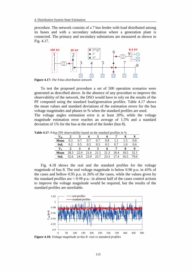
4. Distribution System State Estimation
115
procedure. The network consists of a 7 bus feeder with load distributed among
its buses and with a secondary substation where a generation plant is
connected. The primary and secondary substations are measured as shown in
Fig. 4.17.
Figure 4.17: The 9-bus distribution network
To test the proposed procedure a set of 500 operation scenarios were
generated as described above. In the absence of any procedure to improve the
observability of the network, the DSO would have to rely on the results of the
PF computed using the standard load/generation profiles. Table 4.17 shows
the mean values and standard deviations of the estimation errors for the bus
voltage magnitudes and phases in % when the standard profiles are used.
The voltage angles estimation error is at least 20%, while the voltage
magnitude estimation error reaches an average of 1.5% and a standard
deviation of 1% for the bus at the end of the feeder (bus 8).
Table 4.17: 9-bus DN observability based on the standard profiles in %
VM 2 3 4 5 6 7 8 9
Mean 0.3 0.7 0.7 0.7 0.8 1.1 1.5 0.8
Std. 0.2 0.5 0.5 0.5 0.5 0.7 1.0 0.6
VA 2 3 4 5 6 7 8 9
Mean 28.3 22.0 21.6 21.5 21.3 18.4 18.5 32.1
Std. 52.6 24.9 23.9 23.7 23.3 17.4 16.5 79.0
Fig. 4.18 shows the real and the standard profiles for the voltage
magnitude of bus 8. The real voltage magnitude is below 0.96 p.u. in 43% of
the cases and bellow 0.95 p.u. in 26% of the cases, while the values given by
the standard profiles are ≈ 0.98 p.u.: in almost half of the cases control actions
to improve the voltage magnitude would be required, but the results of the
standard profiles are unreliable.
Figure 4.18: Voltage magnitude at bus 8: real vs standard profiles
1 2
3 4
150 kV 20 kV
5
6
78
9 8.4 kVP Q
m m/
Im
Vm

4.3 Distribution System State Estimation
116
Table 4.18 shows the mean values and standard deviations of the
estimation errors for the power injections at bus 1 and 9 in % when the
standard profiles are used. The values of Table 4.18 are very high as the error
of the standard profiles in terms of load and generation are up to 80% for each
single load or generator. Table 4.18 shows that the estimation of both the
power exchange with the HV grid and the power produced by the generator
plant is very bad and, in consequence, no control action is possible to improve
the voltage profile of the feeder.
Table 4.18: Power injections observability based on the standard profiles in %
P 1 9
Mean 27.9 398.5
Std. 52.1 1595.2
Q 1 9
Mean 174.7 303.5
Std. 462.2 1063.7
In conclusion, the DN is unobservable and uncontrollable if only the
standard profiles are considered. The proposed OP is run for the 500 scenarios
in three cases:
1. Case I: the exact measurements are used;
2. Case II: the voltage measurements are perturbed by maximum ±1% while
the remaining measurements by maximum ±3%;
3. Case III: the voltage measurements are perturbed by maximum ±2%
while the remaining measurements by maximum ±5%.
The voltage measurement is generally more precise than other
measurements, hence the values reported above. Table 4.19 depicts the mean
values and standard deviations of the estimate errors for the measured
quantities with respect to the exact values of the measures for all the cases. In
Case I, when the measurements are exact, the estimates match very well the
measured values, the errors being insignificant. When noise is introduced in
the measurement profile (Case II and III), the procedure converges to a point
where the estimate errors are as close as possible to the exact measurements,
the errors being congruent with the introduced noise.
Table 4.19: 9-bus DN estimate errors with respect to the exact measurements % Case I Case II Case III
Measure Mean Std. Mean Std. Mean Std.
VM2 2E-7 7E-7 5E-3 5E-3 8E-3 8E-3
VM6 5E-3 6E-3 6E-2 4E-2 7E-2 5E-2
I2,3 8E-5 6E-4 1.0 0.7 1.7 1.2
P6,7 3E-5 3E-4 1.2 0.8 1.9 1.3
P2,1 8E-5 6E-4 1.1 0.7 1.8 1.2
P6,5 3E-5 2E-4 1.1 0.7 1.8 1.3
P6,9 2E-5 3E-4 1.3 0.9 2.2 1.4
Q6,7 1E-5 1E-4 1.2 0.8 2.0 1.4
Q2,1 4E-5 2E-4 1.5 0.9 2.6 1.4
Q6,5 1E-5 8E-5 1.2 0.8 2.0 1.3
Q6,9 7E-6 5E-5 1.4 0.9 2.2 1.4
P6 3E-5 2E-4 1.4 0.8 2.3 1.4
Q6 3E-5 3E-4 1.3 0.8 2.1 1.4
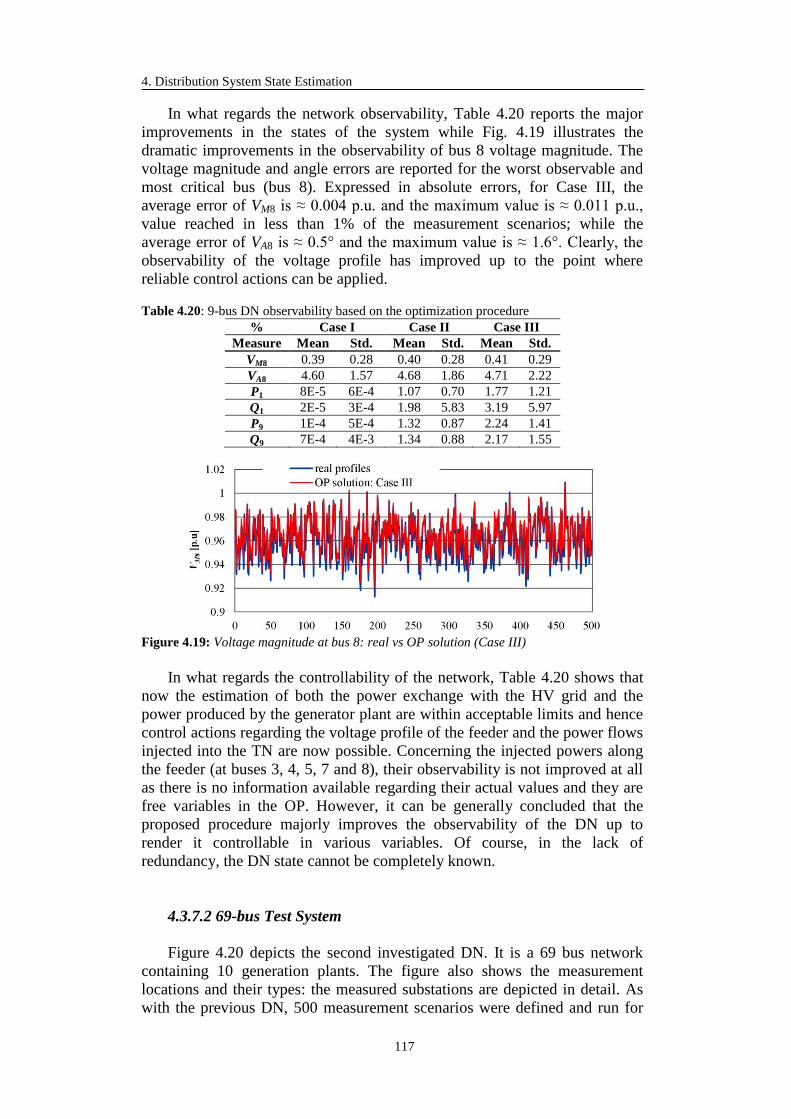
4. Distribution System State Estimation
117
In what regards the network observability, Table 4.20 reports the major
improvements in the states of the system while Fig. 4.19 illustrates the
dramatic improvements in the observability of bus 8 voltage magnitude. The
voltage magnitude and angle errors are reported for the worst observable and
most critical bus (bus 8). Expressed in absolute errors, for Case III, the
average error of VM8 is ≈ 0.004 p.u. and the maximum value is ≈ 0.011 p.u.,
value reached in less than 1% of the measurement scenarios; while the
average error of VA8 is ≈ 0.5° and the maximum value is ≈ 1.6°. Clearly, the
observability of the voltage profile has improved up to the point where
reliable control actions can be applied.
Table 4.20: 9-bus DN observability based on the optimization procedure % Case I Case II Case III
Measure Mean Std. Mean Std. Mean Std.
VM8 0.39 0.28 0.40 0.28 0.41 0.29
VA8 4.60 1.57 4.68 1.86 4.71 2.22
P1 8E-5 6E-4 1.07 0.70 1.77 1.21
Q1 2E-5 3E-4 1.98 5.83 3.19 5.97
P9 1E-4 5E-4 1.32 0.87 2.24 1.41
Q9 7E-4 4E-3 1.34 0.88 2.17 1.55
Figure 4.19: Voltage magnitude at bus 8: real vs OP solution (Case III)
In what regards the controllability of the network, Table 4.20 shows that
now the estimation of both the power exchange with the HV grid and the
power produced by the generator plant are within acceptable limits and hence
control actions regarding the voltage profile of the feeder and the power flows
injected into the TN are now possible. Concerning the injected powers along
the feeder (at buses 3, 4, 5, 7 and 8), their observability is not improved at all
as there is no information available regarding their actual values and they are
free variables in the OP. However, it can be generally concluded that the
proposed procedure majorly improves the observability of the DN up to
render it controllable in various variables. Of course, in the lack of
redundancy, the DN state cannot be completely known.
4.3.7.2 69-bus Test System
Figure 4.20 depicts the second investigated DN. It is a 69 bus network
containing 10 generation plants. The figure also shows the measurement
locations and their types: the measured substations are depicted in detail. As
with the previous DN, 500 measurement scenarios were defined and run for

4.3 Distribution System State Estimation
118
the 3 defined cases. Moreover, 3 configurations for the measurement types
and locations were defined:
1. Configuration I: the base case depicted in Fig. 4.20;
2. Configuration II: same as Configuration I, but with the current
measurements changed to power measurements;
3. Configuration III: same as Configuration III, but with branch power
measurements added at substations 57, 59 and 62.
Figure 4.20: The 69-bus distribution network: Configuration I
Table 4.21 shows the results of the OP for all the defined measurement
configurations and cases in terms of mean relative errors of the estimates with
respect to the measurements and their standard deviations. Since there is a
large number of measurements, only the worst results are shown for each type
of measurements: generally, the estimate errors are much smaller than the
reported maximum case. The results of Table 4.21 show that the procedure
has found very good solutions where the estimates are as close as possible to
the exact measurements, the errors being congruent with the introduced noise.
1 150 kV
2
3
4
5
6
7
8
9
10
11
12
13
14
15
16
17
18
19
20
21
22
23
24
25
26
27
28
2930
31
32
3334
35
36
37
38
39
40
41
42
43
44
45
46
47
48
49
51
50
53
5455
5657
5859
60
61
62
63
6465
66
67
68
69
52
20 kV
P Qm m/
Im
Vm

4. Distribution System State Estimation
119
Table 4.21: 69-bus DN estimate errors with respect to the exact measurements Configuration I
% Case I Case II Case III
Measure Mean Std. Mean Std. Mean Std.
VM62 2E-2 1E-2 0.3 0.2 0.4 0.3
I3,36 1E-3 5E-4 1.6 0.9 2.6 1.4
P8,51 1E-4 7E-5 1.5 0.8 2.5 1.4
Q8,51 2E-4 6E-5 1.6 0.9 2.5 1.4
P62 5E-5 4E-5 1.5 0.9 2.7 1.5
Q62 4E-5 3E-5 1.5 0.8 2.4 1.4
Configuration II
VM62 2E-2 2E-2 0.3 0.2 0.4 0.3
P8,51 2E-4 5E-5 1.5 0.8 2.5 1.4
Q8,51 2E-4 5E-5 1.5 0.9 2.6 1.4
P62 6E-5 4E-5 1.5 0.9 2.5 1.5
Q62 5E-5 3E-5 1.5 0.9 2.4 1.5
Configuration III
VM62 4E-2 3E-2 1E-1 1E-1 1E-1 1E-1
P8,51 1E-4 6E-5 1.5 0.9 2.3 1.4
Q8,51 1E-4 6E-5 1.5 0.9 2.4 1.5
P43 2E-5 4E-5 1.5 0.9 2.6 1.4
Q43 1E-5 1E-5 1.5 0.9 2.5 1.5
Regarding the observability of the network, Figs. 4.21 ÷ 4.24 depict the
estimation errors in terms of means and standard deviation for the voltage
magnitudes and phases of the buses at the end of the main feeder, i.e. bus 27,
and of its deviations (secondary feeders), i.e. buses 35, 46, 50, 52, 65, 67, 69.
The results are shown for all the measurement configurations, including also
the results given by the standard profiles, for the case with the most severe
measurement noise (Case III).
Figure 4.21: End-feeder buses voltage magnitude mean estimation error: Case III
Figure 4.22: End-feeder buses voltage magnitude standard deviation: Case III
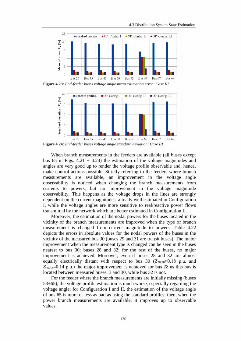
4.3 Distribution System State Estimation
120
Figure 4.23: End-feeder buses voltage angle mean estimation error: Case III
Figure 4.24: End-feeder buses voltage angle standard deviation: Case III
When branch measurements in the feeders are available (all buses except
bus 65 in Figs. 4.21 ÷ 4.24) the estimation of the voltage magnitudes and
angles are very good up to render the voltage profile observable and, hence,
make control actions possible. Strictly referring to the feeders where branch
measurements are available, an improvement in the voltage angle
observability is noticed when changing the branch measurements from
currents to powers, but no improvement in the voltage magnitude
observability. This happens as the voltage drops in the lines are strongly
dependent on the current magnitudes, already well estimated in Configuration
I, while the voltage angles are more sensitive to real/reactive power flows
transmitted by the network which are better estimated in Configuration II.
Moreover, the estimation of the nodal powers for the buses located in the
vicinity of the branch measurements are improved when the type of branch
measurement is changed from current magnitude to powers. Table 4.22
depicts the errors in absolute values for the nodal powers of the buses in the
vicinity of the measured bus 30 (buses 29 and 31 are transit buses). The major
improvement when the measurement type is changed can be seen in the buses
nearest to bus 30: buses 28 and 32; for the rest of the buses, no major
improvement is achieved. Moreover, even if buses 28 and 32 are almost
equally electrically distant with respect to bus 30 (Z28,30≈0.18 p.u. and
Z30,32≈0.14 p.u.) the major improvement is achieved for bus 28 as this bus is
located between measured buses: 3 and 30, while bus 32 is not.
For the feeder where the branch measurements are initially missing (buses
53÷65), the voltage profile estimation is much worse, especially regarding the
voltage angle: for Configuration I and II, the estimation of the voltage angle
of bus 65 is more or less as bad as using the standard profiles; then, when the
power branch measurements are available, it improves up to observable
values.

4. Distribution System State Estimation
121
Table 4.22: 69-bus DN estimate errors with respect to the exact measurements Case II
kW/kVar Configuration I Configuration II
Measure Mean Std. Mean Std.
P28 15.8 13.8 2.2 1.6
Q28 13.5 9.0 1.6 1.1
P32 7.2 5.7 4.7 3.6
Q32 7.0 5.5 3.7 2.7
P33 9.5 7.9 7.3 4.9
Q33 6.0 4.3 5.3 3.5
P34 10.4 4.8 8.8 5.6
Q34 8.9 5.7 7.6 3.4
Regarding the controllability of the network, all the generation plants and
the power exchange with the HV network are measured and the estimation of
their output is very good (see Fig. 4.20 and Table 4.21). Therefore, the voltage
profile and the power exchange with the HV grid are controllable through the
adjustment of the generation plants output.

122
CHAPTER 5
5. Optimization of Measurement Equipment Placement
5.1 Problem Definition and Importance
The operation philosophy for power systems has been changing in the
deregulated business environment. A key objective is now to improve
operational efficiency through better utilization of network capacity. Another
important goal is to accommodate a considerable portion of the DG within an
overall MW/MVAr transaction portfolio. This requires the monitoring and
control of the network by means of a modern DMS at substation level. DSSE
should obviously be at the center of the DMS technology. However, a large
part of the system, particularly the distribution segment, continues to operate
in an unmonitored fashion, adversely affecting the accuracy and quality of the
SE and therefore its usefulness. This introduces bottlenecks in carrying out a
range of substation and feeder automation tasks that rely on the quality of the
DSSE.
Voltage, current and power flows are typically measured in a secondary
busbar of primary substation; virtually no monitoring is carried out further
down at the secondary substation level. The loads are not measured; instead
they are modeled as pseudo-measurements constructed from the historical and
sample load profiles [56],[70]. Since pseudo-measurements are high-variance
estimates of the loads, the quality of the estimated voltages and angles at each
bus is poor if the number of pseudo-measurements is large.
Therefore, an innovative tool that improves the observability of the DNs
considering few measurements has been proposed by the authors in [68],[69].
The developed algorithm bypasses the lack of redundancy and statistical
information regarding the measurements in the DN, but, the quality of the
results strongly depends on the quality of the measurements and location of
the equipment.
As the investments into measurement equipment are low compared to the
increase of DG penetration [68], the DN infrastructure of today has not
changed much with respect to the past: a limited set of measurements in the

5. Optimization of Measurement Equipment Placement
123
primary substations and in some secondary substations are available. The
equipment is mostly old and the precision class is inappropriate for classical
state estimation as it was installed for other purposes, (e.g. input signal for the
protection systems). Moreover, the measurements are not synchronized but
averaged and collected at different moments. Improvement of the
observability of the DN in a way to obtain as accurate as possible
representation of the network state can give results but its impact is still not
sufficient with the perspective of further penetration of DGs and increased
need to make automatic control actions. So, even though DSOs are reluctant
to do so because of the expenses, investments into the new measurement
equipment are the matter of necessity. The measurement equipment should be
placed optimally throughout the network to ensure the best possible attainable
observability with the least possible number of new measurement locations to
diminish the expenses.
The problem of the determination of the best locations of the
measurement equipment for state estimation is known as the problem of
Optimal Measurement Equipment Placement (OMEP). With every additional
instrument, assessment of state is improved, but there are economical and
physical boundaries related to the number of additional equipment: it is
necessary to find the minimum number of additional instruments that, when
placed in optimal locations, enable maximal network observability. These
issues have been addressed in the literature, at transmission level. But little
attention has been paid to measurement equipment placement at the
distribution level. Research reported in the literature concerning measurement
placement fall, broadly speaking, into two categories:
the improvement of the network observability;
the minimization of the errors in the estimates.
5.2 Bibliography review
The topic of this chapter is not a new one, but as with SE, little attention
in the past was dedicated to the problem of OMEP in DS. The reason is that,
in the past, operators knew the behavior of the DN well enough to render
control actions and most of the issues regarding DN were solved by the
manipulations on the primary substation, in most of the cases by adapting
voltage to ensure normal operation of the network. However, this is no longer
sufficient and new equipment must be installed to ensure the observability of
the larger portion of the DS and also to make possible automatic control
actions that are crucial for the optimal operation of the network.
Highly precise and automated actions needed nowadays in DN are the
result of the increased penetration of DGs that completely changed the picture
of the system as known before. Also, changes already described in Chapter 2,
regarding the functionalities of DS are further pointing out that with other
investments in DN, measurement equipment needs to have a central position.
The description of the proposed approaches will start with the ones that
are developed for TS, and then proceed to a few pioneering approaches,
specially designed for DS.

5.2 Bibliography review
124
The research of B. Gou and A. Abur [71] proposes a fast method for
multiple measurement placement for systems that are found to be
unobservable. The method uses a test matrix whose leading dimension is
determined by the rank deficiency of the gain matrix.
Authors notice that observability analysis of power systems involves
checking the rank of the state estimation gain matrix G, which is sparse,
symmetric and positive definite for observable systems. This can be
accomplished by topological [34] or by numerical [43] methods. If the gain
matrix is found to be singular, then all observable islands need to be identified
and power injection pseudo-measurements will have to be introduced in order
to merge these islands into a single observable island for the entire system.
The process of choosing the right set of additional measurements for this
purpose is referred to as the measurement equipment placement.
Pseudo-measurements are typically generated from load forecasts,
scheduled generation data, or some other source with a degree of uncertainty.
Hence, pseudo-measurements are usually of injection type.
The main idea behind the proposed method is the use of the test matrix, in
order to simultaneously process the candidate measurements and make the
final selection in a noniterative and fast manner.
The measurement placement algorithm presented in this research is based
on the observability analysis method. One should consider the real power
versus phase angle part of the linearized and decoupled measurement
equation. This is obtained by using the first order approximation of the
decoupled nonlinear measurement equation around the operating point:
𝑧 = 𝐇𝜃 + 𝑒 (5.1)
where:
𝑧 mismatch between the measured and calculated real power
measurements;
𝐻 decoupled Jacobian of the real power measurements versus all bus phase
angles;
𝜃 incremental change in the bus phase angles at all buses including the
slack bus;
𝑒 measurement error vector.
The decoupled gain matrix for the real power measurements can be
formed as:
𝐆 = 𝐇T𝐇 (5.2)
where measurement covariance error matrix is assumed to be the identity
matrix without loss of generality.
The symmetric matrix G can be decomposed into its Cholesky factors
LDLT where the diagonal factor D, may have one or more zeros on its
diagonal. Taking the inverse of L and collecting only those rows of L-1
corresponding to the zero diagonals of D, we can form a rectangular
submatrix which is called the “test” matrix and denoted by W.

5. Optimization of Measurement Equipment Placement
125
The following algorithm can then be used to determine all the observable
islands simultaneously:
Step 1. Form the gain matrix G and perform the triangular factorization;
Step 2. Check if D has only one zero pivot. If yes, stop. If not, compute the
test matrix W from L;
Step 3. Compute the matrix C = AWT, where A is the branch-node incidence
matrix. If at least one entry in a row is not zero, then the
corresponding branch will be unobservable;
Step 4. Remove all the unobservable branches, to obtain the observable
islands;
Step 5. Stop.
After the determination of the observable islands, authors propose the
following algorithm for the multiple measurement placement:
Step 1. Form the gain matrix G and perform the triangular factorization;
Step 2. Check if D has only one zero pivot. If yes, stop. If not, form the test
matrix W;
Step 3. Using the test matrix W, find the observable islands;
Step 4. Form the candidate list. Those injection measurements, which
connect at least two different observable islands, should be included
in the list if those pseudo-measurements are available;
Step 5. Form the rectangular matrix B = HcWT and reduce it to its Echelon
form E. The candidates will correspond to the linearly indipendent
columns in E. Hc is the Jacobian matrix of the pseudo-measurements
chosen from the candidate measurements.
This approach makes use of small dimension test matrix in deciding on
the placement of measurements. The dimension of the test matrix is equal to
the rank deficiency of the existing gain matrix, and therefore is typically only
a small fraction of the total number of buses in the system. This makes the
method computationally very attractive, yet simple to implement in existing
state estimators.
Authors in [72] present the method for an optimal measurement
placement of PMUs for PSSE. The proposed method considers two types of
contingency conditions (i.e., single measurement loss and single-branch
outage) in order to obtain a reliable measurement system. In order to
minimize the number of PMU placement sites, a heuristic technique to
rearrange measurement positions is also proposed.
Authors point out that the PMU placement method should be performed
under three considerations: 1) the accuracy of estimation, 2) the reliability of
estimated state under measurements failure and change of network topology,
and 3) the investment cost.
PMU placement method for PSSE is based on the minimum condition
number of the normalized measurement matrix. The proposed method finds
an optimal measurement set necessary for complete numerical observability
and single measurement loss and single-branch outage contingency of the
system. Then, the positions of these measurements are rearranged by a
heuristic algorithm in order to minimize the number of PMU placement sites.

5.2 Bibliography review
126
The proposed placement algorithm consists of four stages. In the first
stage, a measurement set for a completely determined condition is searched. It
is called an essential measurement set. Next, a redundant measurement set is
selected from the candidate measurements under each contingency condition.
Both stages use the minimum condition number of normalized measurement
matrix as criteria in selecting the measurement positions. Then, from these
measurements, the optimal redundant set is selected by using the binary
integer programming technique [127]. The essential measurements and the
optimal redundant measurements are rearranged by the proposed heuristic
method in order to minimize the number of PMU placement sites in the final
stage.
The algorithm starts by searching the essential measurement set, in other
words, the positions and types of measurements under the completely
determined condition (i.e., the number of the measurements is equal to the
number of estimated states).
The sequential addition method is used to search the redundant
measurements for each contingency condition. This step is used to find the
necessary measurements from candidate measurements of each contingency
condition such that SE is still solvable under these conditions.
In case of measurement loss, the measurement matrix would be modified
by removing the row corresponding to the lost measurement. However, when
the network topology changes, it is necessary to rebuild the measurement
matrix according to the outage condition. Candidate measurements that yield
normalized measurement matrices with condition number below a predefined
threshold are selected as redundant measurements.
The output from the sequential addition contains the list of redundant
measurements to be added into the essential measurements to ensure the
completely observable condition of the power network when the contingency
occurs.
A binary integer programming has been applied to solve the placement
problem of the conventional measurements and is used to find the optimal
redundant measurements for the contigency. The redundant measurements
according to the nonzero elements are considered as the optimal redundant
measurements.
The number of PMU placement sites should be minimized in order to
reduce the communication costs. The measurement positions obtained from
the minimum condition number criteria can be rearranged to minimize the
number of PMU placement sites by the following heuristic algorithm:
Step 1. Based on the placement position list, obtained from the measurement
placement algorithm, the bus where either an injection current or a
bus voltage measuring device is installed should be determined.
These buses are called major buses. Other buses are called minor
buses;
Step 2. If there is a branch current measuring device on the branch connected
to the major buses, the device is moved close to the major buses;
Step 3. From the branches with branch current measurement devices, which
are not connected to major buses, the minor bus with the maximum
connection number of those branches with branch current
measurements should be determined. Then, the branch current
measurement device on the connected branches moves close to the
5. Optimization of Measurement Equipment Placement
127
selected bus. Note that this minor bus will not be considered again in
the next iteration.
Step 4. Repeat Step 3. until the maximum connection number of branches
with branch current measuring devices is equal to one.
Numerical results on the IEEE test systems indicate that the proposed
placement method satisfactorily provides the reliable measurement system
that ensures the SE to be solvable under the given contingency conditions.
Furthermore, due to the well-conditioned measurement matrix, SE accuracy is
also improved.
While the previous methods were hard to apply for DSs as they fit the
operation of the TSs, the following refferences concern DSs. In their work, M.
E. Baran and others [73] write about the identification of the data
requirements for real-time monitoring and control of DSs. The research points
out that in addition to having supervisory control and data acquisition on
switches and control equipment, methods are necessary to obtain an accurate
estimation of data needed for feeder automation functions. A meter placement
method is proposed for this purpose.
Real-time data required for real-time monitoring and control of a DS is
mainly determined by the functions to be automated in the system. Economic
considerations usually put limits on the number of the functions that can be
automated.
Meters and monitoring devices need to be placed at various points in the
system and integrated in a SCADA system so that the real-time data obtained
from these devices can be communicated to the dispatch center.
Unfortunately, economics put very strong limits on the scale of such SCADA
systems in DS monitoring and control applications.
Besides providing a more reliable real-time load data for feeder
automation functions, SE can also be used to check the consistency of the
measurements and the network model and hence provide data for the
following real-time monitoring functions:
1. Switch Status Monitoring: Since most of the switching in a DS is done
manually and not telemetered, SE can help the dispatchers to keep the
network topology information up-to-date by detecting the status changes
in switches.
2. Locating Faults: The pre-fault and post-fault load distribution data from
SE can also be used to identify the protection device (fuse or recloser)
that operated to isolate a fault.
3. Monitoring the Operation of Control Devices: Any change in the status of
a capacitor bank, a voltage regulating transformer or a third party
generation unit will affect the operation of a feeder appreciably. By
measuring appropriate quantities in a feeder, SE can detect the changes in
the status of these devices.
The main goal of meter placement is determining the number, place, and
type of meters that need to be placed on a given feeder such that the SE with
these measurements will have the desired performance [73]. However, as
pointed out before, the cost considerations usually limit the number of meters
that can be placed on distribution feeders; usually below the minimum needed

5.2 Bibliography review
128
for SE. To overcome this observability problem, forecasted load data needs to
be added as pseudo-measurements. Therefore, the main goal of meter
placement in DSs becomes supplementing the forecasted load data with real-
time measurements such that the SE with these measurements will satisfy the
performance requirements outlined in previous part of the research. Meter
placement is a complex problem. This is not only due to size of the problem
(number of choices available), but also often due to the conflicting
requirements between the SE performance and the cost of the measurement
system necessary to achieve the desired performance.
In this work, Rule Based Meter Placement Scheme, as a simple set of
rules, is developed. It consists of few steps as follows:
Rule 1. Put meters at all the main switch and fuse locations that need to be
monitored. These measurements will provide data especially for
feeder switching and switch monitoring functions;
Rule 2. Put additional meters along the feeder line sections such that the total
loads in the zones defined by the meters are similar in magnitude.
These measurements can be of current type;
Rule 3. Put meters on normally open tie switches that are used for feeder
switching. These meters can also be of current type. Voltage
measurements at both ends of these tie switches are also desirable for
monitoring and control of volt/var control devices from the
substation and/or dispatch center.
The proposed method is a good compromise between the accuracy and
the computational simplicity; it does not guarantee the optimality of the
solution, but it is computationally simple.
Since in feeder operation, data needed for feeder switching is considered
more important than the load distribution data, it may be hard to justify
economically placing all the meters the above method will suggest. To help
user eliminate some of the meters from this basic metering scheme, the
authors adapted Koglin's method to rank these meters. The ranking will
indicate the order with which the meters are to be eliminated. Ranking is
based on the contribution of a measurement to the accuracy of the quantities
that need to be estimated which are called interesting quantities, y. Authors
define system accuracy index a(z) as:
𝑎(𝑧) =∑𝜎𝑦𝑖2
𝑘
𝑖=1
(𝑧) (5.3)
and use it to rank the measurements in the basic measurement set Z0. In the
previous equation, 𝜎𝑦𝑖(𝑧) is the variance of the i-th interesting quantity, z is
the given metering scheme and k is total number of interesting quantities.
First measurements are taken out of the available measurement list one at
a time and the resulting change in 𝑎(𝑧) is calculated. The measurement which
causes the least change in 𝑎(𝑧) is then actually eliminated from the
measurement set and the elimination process is repeated until all the
measurements are eliminated and ranked.

5. Optimization of Measurement Equipment Placement
129
The proposed meter placement and meter ranking methods are very
effective in helping the user to identify these meters. The methods are also
computationally simple and exploit the special features of radial feeders and
feeder monitoring functions.
Work brought by H. Wang and N. Schulz [74] takes into consideration the
development of automation in DSs, distribution SCADA and the fact that
many automated meter reading (AMR) systems have been installed on DSs.
Authors also explain that DMS has advanced and includes more sophisticated
analysis tools. The combination of these developments is providing a platform
for development of DSSE. A branch-current-based three-phase DSSE
algorithm has been developed and tested. This method chooses the magnitude
and phase angle of the branch current as the state variables. Because of the
limited number of real-time measurements in the DS, the SE cannot acquire
enough real-time measurements for convergence and authors conclude that
pseudo-measurements are necessary for DSSE. The load estimated at every
node from the AMR systems is used as a pseudo-measurement for the SE.
Authors point out that various constraints make it impossible to have a
perfect picture of the system. First, because of the economic constraints,
measurement instruments cannot be installed every place where the
measurements are needed, so the data is incomplete. Second, because of the
nature of the measurement instruments and the communication problems in
transmitting the data back to the control center, the measured data are subject
to error or lost communication, so the data may be inaccurate, unreliable and
delayed.
The proposed DSSE algorithm uses the magnitude and phase angle of the
branch current as the state variables. The measurements that are widely used
on the DSs are incorporated. They are real and reactive branch power
measurements, current magnitude measurements, power injection
measurements and voltage magnitude measurements. The algorithm is
implemented as the following steps:
Step 1. Initialization: Initialization of the current magnitude and phase angle
has a great impact on the convergence speed of the algorithm. In this
implementation, a two-step approach is used:
a) Use a backward approach to get the initial value of current. In
this step, set the initial value of voltage at every node to be a
per unit value, and using the injected power at every node to
calculate the branch current.
b) Use a forward approach to get the initial value of voltage. In
this step, using the branch current value calculated in a) and the
root node voltage calculate the voltage at every node.
Step 2. Calculate the updates of the system state (branch current) using the
following expression for the three phases separately:
Δ𝑥(𝑛) = [𝐇T(𝑥(𝑛))𝐑−1𝐇(𝑥(𝑛))]−1× 𝐇T(𝑥(𝑛))𝐑−1[𝑧 − ℎ(𝑥(𝑛))] (5.4)
where:
𝑧 measurements;
ℎ() measurement function;

5.2 Bibliography review
130
𝐇(𝑥) the Jacobian of the measurement function ℎ(𝑥); 𝐑 the covariance matrix of the measurement errors.
Step 3. Update the branch current using following expression and using the
forward approach to calculate the node voltage:
𝑥(𝑛+1) = 𝑥(𝑛) + Δ𝑥(𝑛) (5.5)
Step 4. If it is smaller than a convergence tolerance (stop criterion), then
stop. Otherwise, if the number of iteration is smaller than the pre-set
maximum iteration number, go to step 2, if it is not, it does not
converge.
From the above algorithm and test cases, some rules of meter placement
for this proposed DSSE algorithm can be found:
The results of the branch power measurements are the best. The current
magnitude measurement comes the second. They are much better than the
voltage magnitude measurement.
Branch power and current magnitude measurements can provide better
results when they are installed near the source and in the main feeder
which has many downstream nodes, while the voltage magnitude
measurement can provide better results when it is installed far from the
primary substation.
When meters are placed at different locations, the results are better.
Group of authors in [75] proposes an optimization algorithm suitable to
choose the optimal number and position of the measurement devices needed
to mitigate management and control issues, such as energy dispatching and
protection coordination, in modern electric DNs. The goal of the proposed
procedure, which is based on the dynamic programming, is to guarantee at the
same time the minimum cost and the accuracy required to the measured data.
Authors point out that DSs are subject to deep changes arising from
economic and technological reasons, such as the liberalization and the
increasing integration of DG, i.e. small production plants located in several
points of the distribution grid. The impact of such changes on the power
system configuration creates new management, control and monitoring issues.
The critical role of such operations requires the reliability of the results
provided by the measurement devices in the network and reliable algorithms
for the DSSE.
A system is observable whether it can be known in each own feature, e.g.
if the relevant SE has a solution. A power system with a measurement device
on each node can be totally known, but it is economically unacceptable.
The same solutions proposed for TSs usually cannot be directly applied to
DNs, because of the different features of the two systems. Indeed, the number
of the available measurements in DS is generally much smaller than the
number of the state variables in the SE problem. The lack of enough real time
measurements implies the requirement of numerous pseudo-measurements to
obtain the observability of the system. On the other hand, the concept of
distribution active network inherently requires accurate SE to perform on-line

5. Optimization of Measurement Equipment Placement
131
network reconfiguration, to operate DG and renewable energy sources, and to
implement load response policies with the final goal to exploit novel
technologies deferring or avoiding network investments. As a consequence,
for DSs it is necessary an ad hoc estimator able to give a good SE by reducing
the number of measurement devices to as low as possible and this approach
sustains the approach proposed by the authors in [68] and [69].
The main goal of a meter placement technique is to establish number,
position and type of meters to be placed on a given system to achieve an
observable system. The aim of a minimal meter placement is to obtain a DS
that is observable with established accuracy and cost. The constraint on the
maximum uncertainty, acceptable for the results means that, in each one of the
B selected branches and/or nodes of the network, the estimated standard
deviation (𝜎𝑦𝑖, for i=1,…,B) of the quantity of interest y must not overcome
the limit 𝜆𝑦𝑖 imposed for that quantity in that node. Since these constraints
could be met for different measurement sets, having the same minimum
number of measurement units, the optimal set is the one that minimizes the
function J, which is the weighted mean value of the variances of the quantities
of interest:
𝐽 =∑(
𝜎𝑦𝑖
𝜆𝑦𝑖)
2𝐵
𝑖=1
subject to: 𝜎𝑦𝑖 < 𝜆𝑦𝑖, ∀𝑖 = 1,… , 𝐵
(5.6)
From a mathematical point of view, this is a non-linear combinatorial
optimization problem.
Fig. 5.1 depicts the whole optimization algorithm. The procedure starts
with a definition of those network nodes that are candidates to have a meter
device. The inputs are the network topology, the line impedances and the real
and reactive powers drawn by each node, along with their variances. A
solution of the optimization problem is represented by a set of measurement
devices allocated in a certain set of network nodes.
Preliminarily, for each load, a set of N possible values for real and
reactive power is defined by means of a Gaussian distribution centered on the
nominal values and having a prefixed standard deviation. Then, a Monte
Carlo approach is used to define, by extracting a power value from each set, a
set of N possible network conditions. The DSSE is performed on each of these
situations, in order to achieve N reference conditions.
Then the algorithm starts by assuming that measurement devices are
located only at the substation and DG bus bars. In the remaining nodes only
pseudo-measurement can be considered.
On each one of the N networks, a Monte Carlo procedure is applied to
take into consideration uncertainties in the measured data. Thus, M tests are
performed in which the DSSE is run by using measured data randomly
extracted from the sets defined by their nominal values and their uncertainty.
As a consequence, for each branch current the distribution probability of the
output values can be evaluated.
Then, the quality index J is calculated for each network, and the mean of
such values:

5.2 Bibliography review
132
𝑄 =1
𝑁∑𝐽𝑖
𝑁
𝑖=1
(5.7)
calculated over all the N network configurations, represents the metric by
means of which the quality of the solution is synthetically evaluated. If the
accuracy constraints are met for all current branches, such a solution
represents the optimal one. Otherwise, additional measurement devices should
be positioned, according to the optimization algorithm based on the dynamic
programming.
Figure 5.1: Flow chart of the optimization algorithm for the OMEP in DNs [75]
In this research the evaluation of the uncertainty affecting the results of
the DSSE applied to the N network conditions is performed by means of a
methodology based on a Monte Carlo statistical approach. This approach is
based on the propagation of distributions: the entire probability density

5. Optimization of Measurement Equipment Placement
133
functions (pdf) assigned to the input quantities, rather than only their
variances, are used in the calculations. Monte Carlo methods exploit the
capability of commercial software packages to generate sequences of random
numbers, characterized by prefixed statistical parameters. The applied
procedure can be summarized in the following three steps:
1) Characterizing the uncertainty on the measured data: all the relevant
information available is used. A suitable probability distribution is then
assigned to these uncertainty terms, which can be numerically represented
by sets of random variables defined by the software package.
2) Performing a large number of simulated tests: in each test the measured
data are corrupted by different contributions, whose values are extracted
from the above sets, and the DSSE algorithm is applied by using this set
of input data.
3) Processing the set of the obtained output values, which could be
considered as the probability density function of the measurement result,
whose standard deviation represents the standard uncertainty of the result.
Results of this study bring the following: it is not possible to understand a
priori the effect of DG on the final optimal solution, thus justifying the resort
to optimization tools. Indeed, DG in certain nodes allows reducing the number
of measurements required by the SE in one part of the open loop network
thanks to the small size of generator in comparison to loads and the particular
allocation. On the other hand, if the generator has a much more significant
impact in the part of the open loop network then SE algorithm may need more
information on branch currents. This particular behavior is caused by the
imposition of the injected power at some nodes, that modifies the PF
equations.
Authors in [76] present a heuristic approach to identify potential points
for location of voltage measurements for SE as part of a proposed DMS
controller. The developed technique identifies measurement locations to
reduce the voltage standard deviation of the bus bars which do not have a
measurement. It addresses the problems of classical transmission meter
placement methods, which are not directly applicable to DS due to limited
measurements, and unobservability of the network.
The technique assumes that the voltages at those bus bars selected for a
measurement are known within the accuracy of the measurement system. The
location and number of these measurements are then adjusted so that the
standard deviations of voltages at the unmeasured bus bars (caused by random
load changes) are reduced to an acceptable minimum.
The algorithm uses the following equation to calculate the error between
voltage magnitudes obtained initially from a PF using an estimate of
maximum demands and results from series of PFs using random changes in
the same loads.
ℰ = ∑(𝑉0𝑚 − 𝑉𝑟𝑎𝑛𝑑
𝑚 )2𝑀
𝑚=1
(5.8)
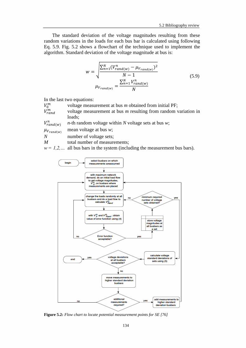
5.2 Bibliography review
134
The standard deviation of the voltage magnitudes resulting from these
random variations in the loads for each bus bar is calculated using following
Eq. 5.9. Fig. 5.2 shows a flowchart of the technique used to implement the
algorithm. Standard deviation of the voltage magnitude at bus is:
𝑤 = √
∑ (𝑉𝑟𝑎𝑛𝑑(𝑤)𝑛 − 𝜇𝑉𝑟𝑎𝑛𝑑(𝑤))
2𝑁𝑛=1
𝑁 − 1
𝜇𝑉𝑟𝑎𝑛𝑑(𝑤) =∑ 𝑉𝑟𝑎𝑛𝑑(𝑤)
𝑛𝑁𝑛=1
𝑁
(5.9)
In the last two equations:
𝑉0𝑚 voltage measurement at bus m obtained from initial PF;
𝑉𝑟𝑎𝑛𝑑𝑚 voltage measurement at bus m resulting from random variation in
loads;
𝑉𝑟𝑎𝑛𝑑(𝑤)𝑛 n-th random voltage within N voltage sets at bus w;
𝜇𝑉𝑟𝑎𝑛𝑑(𝑤) mean voltage at bus w;
N number of voltage sets;
M total number of measurements;
w = 1,2,… all bus bars in the system (including the measurement bus bars).
Figure 5.2: Flow chart to locate potential measurement points for SE [76]

5. Optimization of Measurement Equipment Placement
135
The results of the study have shown that the topology of the network is
important in placing the measurements. Measurement placement techniques
for TSSE cannot be directly applied to DNs for the purpose of DSSE. This is
both due to non-redundancy of measurements on these networks and the
unobservable nature of the estimation process with the addition of few
pseudo-measurements.
The authors conclude also that the technique does not obtain the global
optimal measurement system for the network as is done in TSs and neither
does it allocate measurements to overcome observability problems but
identifies those points on the network with the higher voltage variations. The
process provides a methodical approach to placing measurements on DSs for
SE rather than relying only on engineering judgment.
The research developed in [77] is also concerned with improvement of the
quality of voltage and angle estimates across a network, similar to the
previous reference. The proposed technique is based on the sequential
improvement of a bivariate probability index governing relative errors in
voltage and angle at each bus. The meter placement problem is simplified by
transforming it into a probability bound reduction problem [128], with the
help of the two sided-Chebyshev inequality. A straightforward solution
technique is proposed for the latter problem, based on the consideration of 2-𝜎
error ellipses.
In this research, three types of measurements were considered. The
voltage and flow measurements at the main substation and the substations
with DGs were taken as real measurements. Zero injections, with a very low
variance 10-8
, were modeled as virtual measurements. The error in the pseudo-
measurements was chosen on the basis of the uncertainty in the load estimates
of various classes of customers, like industrial, domestic and commercial. The
loads of the industrial customer can be estimated fairly accurately. The load of
the domestic customers is very difficult to estimate and will give rise to a
large estimation error. The uncertainty in the commercial load estimates lies
between the two. For a Gaussian distribution, a ±3𝜎 deviation about the mean
accounts for more than 99.73% of the area under the Gaussian curve. For a
given % of maximum error about the mean 𝜇𝑧𝑖, the standard deviation of the
error was computed as follows:
𝜎𝑧𝑖 =𝜇𝑧𝑖 ×%𝑒𝑟𝑟𝑜𝑟
3 × 100 (5.10)
Observing the relative voltage and angle errors at different buses, authors
concluded that when the measurement errors are small, the relative estimation
errors in the voltages and angles, in more than 95% of simulation cases, are
below their respective thresholds (i.e., 1% for voltage error and 5% for angle
error). With the increase in errors in the pseudo-measurements from 20% to
50%, the voltage estimate errors do not violate their threshold in all the
simulations, while the angle estimate errors violate their threshold in
significant number of simulation cases. With increase in the errors in the real
measurements from 1% to 3% both the errors in the voltage and the angle
estimates violate the threshold limits. This violation is significantly more for

5.2 Bibliography review
136
the voltage estimate errors than it is for the angle estimate errors. It can be
understood that the errors in the voltage estimates are highly influenced by the
errors in the real measurements and less influenced by the errors in the
pseudo-measurements (loads). On the other hand, the errors in angle estimates
are influenced by both. In the case when the errors in both real and pseudo-
measurements are high, the errors in voltage and angle estimates significantly
violate the limits. An efficient way to overcome this problem is to increase the
number of real measurements, although it may not be economical to place
large number of meters. Hence, a cost effective strategy for meter placement
should take account of the following factors:
location of meters;
type of measurements;
number of measurements;
The problem of meter placement is to identify the effective locations and
the number of real measurements, so that the following probability indices:
𝑝𝑖 = 𝑃𝑟 |𝑉𝑖−𝑉𝑡
𝑖
𝑉𝑡𝑖 | ≤ 휀1, |
𝑖−𝑡𝑖
𝑡𝑖 | ≤ 휀2, for i = 2,…,n (5.11)
In the previous equation:
𝑡𝑖, 𝛿𝑡
𝑖 true value of voltage and angle at the i-th bus, respectively;
𝑖, 𝛿𝑖 estimated value of voltage and angle at the i-th bus, respectively;
휀1 , 휀2 voltage and angle prespecified thresholds, respectively;
𝑛 number of the buses of DN.
Measurement Placement – The voltage measurements can efficiently bring
down the relative errors in the voltage estimates below threshold, but in some
cases the same may not be achieved for the angle estimates even with the help
of a large number of voltage meters. The reasons for this are evident from Fig.
5.3(a) and (b). As shown in Figure 5.3(a), at a given bus, the two axes of the
error ellipse are not aligned in the direction of coordinate axes. This implies
that the errors in voltage and angle estimates are correlated. In this case the
error reduction in the voltage estimate consequently reduces the error in angle
estimate and vice versa. The reduction of the error estimate in one variable
with respect to the other depends upon the degree of correlation between the
two. A stronger correlation implies that the error reduction in one variable
significantly reduces the error in the other.
Figure 5.3: Voltage and angle error ellipse: errors are (a) correlated, (b) uncorrelated [77]

5. Optimization of Measurement Equipment Placement
137
In Figure 5.3(b), the ellipse axes are in the direction of coordinate axes.
This means the errors in voltage and angle estimates are uncorrelated and
hence the reduction of one does not influence the other.
The process for the location and number of these measurements is as
follows:
Step 1. Run WLS over a set of Monte Carlo simulations and observe the
relative errors in voltages and angles in each simulation at all the
buses.
Step 2. If in more than 95% of the cases the relative errors in the voltages
and angles are below their specified thresholds, respectively (i.e., 1%
for voltage (휀1) and 5% for angle (휀2)), stop; else go to Step 3.
Step 3. If only the relative errors in voltage estimates satisfy the criterion in
Step 2, go to Step 6; else Step 4.
Step 4. Take the mean of the state error covariance matrix over all the Monte
Carlo simulations and extract the sub-matrices corresponding to the
voltage and angle at each bus.
Step 5. At every bus compute the area of the error ellipse from the
determinant of sub-matrix and identify the bus with the largest area
and place the voltage measurement at this bus. If measurement is
already present choose the bus with the next largest area. Go to Step
1.
Step 6. Compute the mean of error covariance matrix corresponding to the
real and reactive power flow, in each line.
Step 7. For each line compute the area of the line flow error ellipse and place
the flow measurement in the line with the largest area. If the
measurement is already present choose the line with the next largest
area. Go to Step 1.
The procedure is sequential and stops when the desired level of accuracy
in estimates is achieved. The advantage of the method is that it reduces the
errors in both voltage and angles by exploiting the error correlations under a
wide range of uncertainty in the pseudo-measurements. However, authors
notice that it produces feasible but not necessarily optimal solution. The
performance of the technique needs further investigation in view of the
possible presence of the leverage points in the network.
Finally, multi-objective optimization by implementing genetic algorithms
was used in research conducted by B. Milosevic and M. Begovic [78]. This
research considers PMU placement problem requiring simultaneous
optimization of two conflicting objectives, such as minimization of the
number of PMUs and maximization of the measurement redundancy.
The problem considered is the placement of a minimum set of PMUs, so
that the system is topologically observable (all of the bus voltage phasors can
be estimated) during its normal operation and following any single-line
contingency:
min𝑥∈𝑆
𝐾,−𝑅
Subject to: U = 0 (5.12)
where:

5.2 Bibliography review
138
S search space;
K total number of PMUs to be placed in the system;
R system single line-outage redundancy, expressed as a number of buses
that are observable following any single-line outage;
U total number of unobservable buses.
This is a typical multi-objective optimization problem requiring
simultaneous optimization of two objectives with different individual optima.
Objectives are such that none of these can be improved without degradation of
another. Therefore, instead of a unique optimal solution, there exists a set of
optimal trade-offs between the objectives, the so-called Pareto-optimal
solutions.
The concept of Pareto optimality may be explained in terms of a
dominance relation [79]. For a multi-objective problem having k objective
functions to be simultaneously minimized, a solution x is said to dominate the
other solution y if is better than y for at least one objective fi and is not worse
for any other fj, where j = 1,…,k and j ≠ i.
𝑓𝑖(𝑥) < 𝑓𝑖(𝑦) and 𝑓𝑗(𝑥) ≤ 𝑓𝑗(𝑦) then 𝑥 ≻ 𝑦 (5.13)
Here, the symbol ≻ denotes domination operator; 𝑥, 𝑦 ∈ 𝑃, where 𝑃 ⊆ 𝑆
and S denote the entire search space. The above concept is used to find a set
of non-dominated solutions in P. These solutions are equally optimal when all
objectives are considered, for none of them is dominated by any other solution
in P. The solutions that are non-dominated regarding the entire search space
are called Pareto-optimal solutions. The hypersurface connecting those
defines the Pareto-optimal front.
A minimum set of PMUs to ensure system topological observability 𝑚𝑖𝑛
is estimated by building a spanning measurement tree of full rank across the
system. Since the PMU provides measurements of voltages, as well as all
incident current phasors at the buses where it is located, a calculated current
phasor is assigned to any branch connecting two buses with known voltage
phasors, and to any branch whose current can be found by using Kirchoff’s
current law. A bus is considered observable (“covered”) if its voltage phasor
is either directly measured or calculated by using the available
measured/calculated voltage and current phasors.
The algorithm iterates two main steps until a set of unobservable buses is
exhausted: 1) bus ranking; and 2) selection of PMU locations among the
highest ranked buses by using a simple GA.
To reduce the number of PMU candidate locations, buses where PMUs
need and need not be placed are identified so that the system topological
observability is possible with minimum number of PMUs. These buses are
then removed from the initial set that comprises all system buses.
Buses are ranked in decreasing order of their coverage index C, where
C(i) is defined as the number of buses that become observable after a PMU
has been placed at bus i. Nodes with the highest coverage index are then
identified. If the total number of such buses, denoted as m, is equal to 1, a
PMU is placed at the corresponding bus, and the bus-ranking step is repeated.

5. Optimization of Measurement Equipment Placement
139
Otherwise, these m buses represent the candidate locations for PMU
placement and a simple GA is used to select the optimal ones among them.
The algorithm starts with a set of PMUs that ensures the system
topological observability. The additional PMUs are then added by iterating
the bus-ranking step and the GA step, until maximum measurement
redundancy Rmax has been achieved. In the bus-ranking step, the buses are
ranked based on the modified coverage index CR which is defined as the
number of buses that are observable following any single-line outage, after a
PMU has been placed at the corresponding bus. In the GA step, the
chromosomes are evaluated based on the objective function RR, given as a
total number of buses in the system “covered” by PMUs more than twice.
The population is classified into subsets (fronts) of individuals sharing the
same non-dominance properties, as shown in Fig. 5.4.
Figure 5.4: Population classification into fronts [78]
The infeasible solutions are repaired by removing the non-optimally
placed PMUs, and adding the additional ones, until the topological
observability is obtained. A PMU is considered non-optimally located if the
number of (un)observable buses remains the same when removed from the
system.
The algorithm terminates when the number of generations reaches the
predetermined maximum value Gmax. However, it could end in a number of
ways depending of decision maker’s satisfaction criteria.
The analysis of the computational complexity of the algorithm reveals
that most of the overhead is due to the solution repair (correction of infeasible
solutions). This imposes a limitation on the size of the problems that can
practically be handled using the proposed technique.
The important advantage of the algorithm and the justification for its
complexity are that it provides the entire Pareto-optimal front instead of a
single point solution, and could lend itself to application in an entire class of
problems where multi-objective optimization on a prohibitively large
enumerative search space is required.

5.2 Bibliography review
140
5.2.1 Critical review of the proposed bibliography
Approaches reported in [71] and [72] address the problem of OMEP or
similar approaches at transmission level. Unfortunately, as already stated,
mechanisms used in TS are not applicable in DS, firstly because of the
topological differences between them, further, because regarding
observability there are completely different. TN is in much better situation
then DN regarding observability with significantly larger number of
measurements present. TNs satisfy the conditions of redundancy, while DNs
no.
Approach and results provided in [73] bring an interesting perspective of
the problem but the limitations are reflected in the fact that the approach is
designed for simple test DNs that do not correspond to complex real systems
of today and advanced DSOs requirements. Also, approach proposes the
placement of too many measurement equipment from the point of economic
criteria.
Work elaborated in [74] is based on three-phase model for SE. This is not
applicable for real MV grids: the loads are generally balanced and the cables
parameters (especially mutual coupling) are not known.
Approach proposed by [75] is interesting because it includes DG in the
problem of OMEP in DSs. However, the major problem in this case as well as
in [77] is using of Monte Carlo simulations for the solution of the problem
and its practical inability to face the large scale problems such as DSSE and
DS OMEP. To elaborate on this, one should assume that the real and reactive
power flows in a line are measured together. The complete measurement set
Ω consists of n + 2l elements, where n is the number of voltage magnitudes,
and l is the number of line real and reactive power pairs (which coincides with
the number of line current magnitudes). The number of combinations of
deploying k meters is then:
𝑁 = (𝑛 + 2𝑙𝑘
) =(𝑛 + 2𝑙)!
𝑘! (𝑛 + 2𝑙 − 𝑘)! (5.14)
This is typically a very large number. Bearing in mind that Monte Carlo
evaluation of the cost is computationally expensive, one can see that
exhaustive search that is yield by implementing Monte Carlo simulations is
not a practical option [80].
For instance, if the DN has n = 95, l = 94 and k = 5 (and this is a small
DN compared to real size DNs), there are 1.45×10¹⁰
possible choices to be
examined. Although the number of choices can be reduced by exploiting the
structure of the problem, for example by excluding measurements on lines
which are connected to zero-injection buses, exhaustive search still may not
be a viable option for large-scale problems.
Work reported in [76] presents one of the first attempts in DN to solve the
problem of OMEP. However, authors themselves note that their solution does
not present the optimal solution of the problem nor it allocate measurements
to overcome observability problems but identifies those points on the network
with the higher voltage variations. Also, only voltage measurements are
considered.

5. Optimization of Measurement Equipment Placement
141
Approach reported in [77] brought a new view on the problem of OPM.
The problem of implementation with Monte Carlo simulations is already
addressed. To continue, authors assume a Gaussian distribution for the load
profile uncertainties. This is, however, inconsistent with real situation, due to
the fact that loads are estimated according to energy curves. So, although the
paper is very interesting from the point of view of the information it provides,
it does not correspond to real life situation. One more limitation is that the
research deals only with voltage measurements, which makes it very limited.
To conclude, authors themselves notice that the solution produces feasible but
not necessarily optimal solution and that further investigation is necessary.
Finally, work reported in [78] is quite a pioneering approach but its
practical usefulness is limited due to the fact that it uses PMUs to solve the
problem of OMEP. As it was already discussed in Chapter 4, the introduction
of PMUs in a realistic DN is very rare nowadays. The other problem of this
solution is that it covers only topological observability and not both
topological and numerical, nor it explores the state of the network by SE. This
is definitely a limiting factor.
In conclusion, the works presented here do not take into account some
important aspects of the present DNs:
the size and complexity of modern DNs;
requirements of DSOs;
available information of the realistic networks;
adequacy of the approaches for the realistic DNs;
economic burden of proposed solutions…
5.3 Optimization of Measurement Equipment Placement
Mathematical Model
The mathematical model of the OMEP problem can be formally defined
as a generalization of the advance state estimation model described by Eq.
(4.56) in subchapter 4.3.5, including the possibility to change and add or
eliminate various measurement equipment. For this, it is necessary to consider
all the possible measurement locations and types for the entire DN and
associate a new variable to each of them; this variable quantifies if a certain
quantity, located in a certain point in the network, is measured or not.
Moreover, the objective function needs to also take into account the quality of
DN observability. Therefore, the OMEP model can be defined as:
min∑ (𝛼𝑖
𝑥𝑖𝑚)
2
⋅ 𝑌𝑖 − 𝑓𝑜𝑏𝑠(𝑉𝑀, 𝑉𝐴, 𝐱𝐞𝐬𝐭, 𝛼)
𝑁𝑡𝑖=1 (5.15a)
𝑠. 𝑡. 𝑓𝑃(𝑉𝑀, 𝑉𝐴, 𝐱
𝐞𝐬𝐭) = 0
𝑓𝑄(𝑉𝑀, 𝑉𝐴, 𝐱𝐞𝐬𝐭) = 0
(5.15b)
Y𝑖(𝐱𝐦 − 𝐱𝐞𝐬𝐭 + 𝜶) = 0 (5.15c)
∑𝑌𝑖 ≤ 𝑁𝑝
𝑁𝑡
𝑖=1
(5.15d)
where:

5.3 Optimization of Measurement Equipment Placement Mathematical Model
142
𝑌𝑖 binary variable that models the existence of a measurement equipment
for the i-th measurable quantity, be it V, I, P, Q; when 𝑌𝑖 is 1, the i-th
quantity is measured, when it is 0, it is not;
𝑓𝑜𝑏𝑠 function quantifying the quality of DNs observability;
𝑁𝑡 total number of measurements that can be considered in the DN;
𝑁𝑝 maximum number of measurement equipment to install in the network;
The rest of the quantities have been already defined in subchapter 4.3.5.
As with the DSSE model (4.56), the first term in the objective function
(5.15, a) minimizes the estimation errors for the measured quantities, i.e. for
the quantities for which 𝑌𝑖 = 1. In details, for all the 𝑌𝑖 = 1 equations (5.15,
b) and (5.15, c) together with the first term of (5.15, a) constitute the
previously formulated DSSE model (4.56), and hence, the estimation of
networks state for a certain measurement configuration is thus assured.
Further, constraint (5.15, d) provides that a limited number of measurement
equipment is installed in the network; at limit this number can be strictly
imposed by converting this constraint into an equality constraint. Finally, in
order to guide the search of the optimal set of measurement locations, the
second term in the objective function (5.15, a), i.e. 𝑓𝑜𝑏𝑠(𝑉𝑀, 𝑉𝐴, 𝐱𝐞𝐬𝐭, 𝛼),
quantifies the quality of the observability of the DN in its whole. Since the
electric state of a bus is completely described by V, φ, P and Q, in its most
general form, this function should sum the estimation errors of V, φ, P and Q
in all the buses:
𝑓𝑜𝑏𝑠 = ∑ (|𝑉𝑖𝑎𝑐𝑡 − 𝑉𝑖
𝑒𝑠𝑡
𝑉𝑖𝑚 |
2
+ |𝜑𝑖𝑎𝑐𝑡 − 𝜑𝑖
𝑒𝑠𝑡
𝜑𝑖𝑚 |
2
+ |𝑃𝑖𝑎𝑐𝑡 − 𝑃𝑖
𝑒𝑠𝑡
𝑃𝑖𝑚 |
2
+ |𝑄𝑖𝑎𝑐𝑡 − 𝑄𝑖
𝑒𝑠𝑡
𝑄𝑖𝑚 |
2
)
𝑁𝑏𝑢𝑠
𝑖=1
(5.16)
where:
𝑉𝑖𝑎𝑐𝑡 actual value of the voltage magnitude of i-th bus;
𝑉𝑖𝑒𝑠𝑡 estimated value of the voltage magnitude of i-th bus computed by
DSSE;
𝜑𝑖𝑎𝑐𝑡 actual value of the phase angle of i-th bus;
𝜑𝑖𝑒𝑠𝑡 estimated value of the phase angle of i-th bus computed by DSSE;
𝑃𝑖𝑎𝑐𝑡 actual value of the real power of i-th bus;
𝑃𝑖𝑒𝑠𝑡 estimated value of the real power of i-th bus computed by DSSE;
𝑄𝑖𝑎𝑐𝑡 actual value of the reactive power of i-th bus;
𝑄𝑖𝑒𝑠𝑡 estimated value of the reactive power of i-th bus computed by DSSE.
This is a mix integer non-linear programming (MINLP) problem,
including strongly non-linear PF constraints, for which is not so simple to
write and solve a convex relaxation. . However, much harder to deal with with
when solving this model is the combinatorial dimension of the problem. For a
realistic DN the problem becomes very large in terms of possible feasible
discrete solutions. In particular, for a radial network consisting of N buses
(so, N-1 branches), as presented in Chapter 4, it is possible to install N voltage
measurements, N real and N reactive power measurements of the loads as well
as N real and N reactive power measurements of the generation in each bus of
the system, and N-1 real, N-1 reactive power flow and N-1 current flow

5. Optimization of Measurement Equipment Placement
143
measurements, resulting a total of 7N-3 possible measurements to install in all
the network. For a specified maximum number of measurement equipment Np
the total number of feasible combination is:
(7𝑁 − 3𝑁𝑝
) =(7𝑁 − 3)!
𝑁𝑝! (7𝑁 − 3 − 𝑁𝑝)
This means that for an average size DN of 500 buses with Np = 100
measurements, there are approximately 3500 discreet variables and the
number of possible feasible values of Y is given by the following number of
combinations:
(3500100
) = 6.56 ⋅ 10195
Therefore, it is hard to imagine that a combinatorial problem of this size
can be solved using traditional relaxation techniques such as Branch and
bound [147] or Lagrange relaxations [148].
At this point it is important to notice that this problem can be separated
into two distinctive sub-problems:
discreet problem i.e. finding the optimal measurement equipment
configuration – the optimal 𝑌𝑖 obtained by minimizing 𝑓𝑜𝑏𝑠; and
for each possible configuration - 𝑌𝑖 - there is a continuous sub-problem,
i.e. the SE.
Therefore, a more computationally simple alternative is to efficiently
explore a sub-space of the solution space by a heuristic search technique to
find a sub-optimal solution for the vector Y and solving, in the same time, the
already developed state estimation algorithm to correctly evaluate 𝑓𝑜𝑏𝑠 for
each possible Y.
Generally, finding the solution in this way can be made according to the
flow chart of Fig. 5.5. Firstly, one possible discrete solution, configuration
Ypossible is chosen. Ypossible refers to feasible solution i.e. the solution that
satisfies the constraints, but not necessarily optimal. Then ASE algorithm,
developed in Chapter 4, is run, function fobs is computed and the convergence
criterion is checked. It can be maximum number of iterations allowed,
maximum computation time or some other criteria. If the solution satisfies the
criteria, the optimization is finished, otherwise, another feasible configuration
is found according to the considered heuristic search algorithm and the
process is repeated until convergence.

5.4 Evolutionary Algorithms for Large-Scale Problems
144
Start
Ypossible
Run ASE
Evaluate fobs
Convergence
criteria
End
Change Y
Figure 5.5: Flow chart of the problem solution
In this dissertation, the use of evolutionary techniques, in particular
genetic algorithms, was selected for the heuristic search part. This
optimization approach uses the good properties of the possible solutions and
combines them together to produce better offspring. In the following
subchapters, these techniques will be explained in detail. Moreover, the
particular form of the OMEP problem (5.15) adapted for the use of
evolutionary techniques will be detailed. Lastly, various considerations will
be made concerning the reduction of the search space.
5.4 Evolutionary Algorithms for Large-Scale Problems
5.4.1 Evolutionary Algorithms vs. Classical Techniques
This part of the dissertation is dedicated to the solution of OMEP
problem. As the title already states, the aim is to optimize a large-scale
problem as the planning of DN definitely is. Solving the real-life large
problems of efficiently allocating limited resources, as well as developing and
managing complicated systems, and designing strategies for decision makers
to cope with different conflicting situations have always been demanding for
individuals and organizations [81]. To cope with these kinds of hard
problems, optimization is the key discipline that can facilitate the operators
with quantitative decision-making and decision analysis by applying scientific
methods and technologies. Optimization is the sub-discipline of applied
mathematics, where the aim is either to minimize or maximize the output of a
function over a set of input variables subject to a set of constraints.
Many of the optimization problems are combinatorial optimization [82],
where the desired optimal solutions are certain combinations of variable
settings (possibilities) from a finite pool [83]. Though some combinatorial

5. Optimization of Measurement Equipment Placement
145
optimization problems have well-known polynomial time algorithms, there is
a family of combinatorial optimization problems which is NP-hard. The NP-
hard [84] problems are very complex with huge search spaces and no exact
algorithm is known to solve them in polynomial time.
Many of the real-life NP-hard optimization problems are planning
problems. Planning problems can be defined in different ways depending on
the related field. The research covered by this chapter of the dissertation is on
planning the future distribution grid or extending the existing one with the
installation of the measurement equipment. As already said, this problem is to
be one of the central points of Smart Grid managing already today and even
more in a near future [129].
When a choice is made regarding the optimization tool for the solution of
the problem, one has to realize that in the large-scale realistic problems, it is
rarely possible to find the optimal solution which is offered by
implementation of the exhaustive search. This is because this type of search
needs to cover the entire search space at a time. Also, in order to model the
data, some techniques like Monte Carlo simulations need to be utilized.
OMEP for realistic DNs cannot be solved in this manner.
Classical optimization techniques, like exhaustive search, are incapable of
solving multi-objective problems. This group of problems is computationally
highly demanding and even if the computational time is not considered as an
obstacle, which obviously is, classical techniques show significant
convergence problems.
On the other side, Evolutionary Algorithms (EAs) are powerful and
sophisticated tools for optimization of the large-scale problems like this one.
The advantage of this method over many others is that it looks for the solution
over the group of possible solutions rather than whole search space at the time
and it combines the good properties of the individuals to produce better
offspring. Other multiple advantages of EAs over other methods are:
conceptual simplicity, proven broad applicability, outperformance of the
classical methods on real problems, potential to use knowledge and hybridize
with other methods, parallelism, robustness to dynamic changes, capability for
self-optimization, ability to solve problems that have no known solutions etc.
Another important characteristic of EA is that it is possible to apply EA
even if the gradient and the Hessian of the OF and constraints do not exist
(due to the presence of binary/integer variables).
5.4.2 Introduction to Evolutionary Algorithms
An EA is a stochastic iterative procedure for generating tentative
solutions for a certain problem. The algorithm manipulates a collection P of
individuals (the population), each of which comprises one or more
chromosomes. These chromosomes represent a potential solution for the
problem under consideration. An encoding/decoding process is responsible
for performing this mapping between chromosomes and solutions.
Chromosomes are divided into smaller units termed genes. The different
values a certain gene can take are called the alleles for that gene [130].
Initially, the population is generated at random or by means of some
heuristic seeding procedure. Each individual in P receives a fitness value: a

5.4 Evolutionary Algorithms for Large-Scale Problems
146
measure of how good the solution is for the problem being considered.
Subsequently, this value is used within the algorithm for guiding the search.
The whole process is sketched in Figure 5.6.
F
g
G
P’
P’’
Pt
σψ
ωx
ωm
Figure 5.6: Illustration of the evolutionary approach to optimization [130]
As it can be seen, it is assumed the existence of a set F (also known as
phenotype space) comprising the solutions for the problem at hand.
Associated with F, there also exists a set G (known as genotype space). These
sets G and F respectively constitute the domain and codomain of a function g
known as the growth (or expression) function. It could be the case that F and
G were actually equivalent, being g a trivial identity function. However, this
is not the general situation. As a matter of fact, the only requirement posed on
g is surjectivity. Furthermore, g could be undefined for some elements in G.
After having defined these two sets G and F, one should notice the
existence of a function t selecting some elements from G. This function is
called the initialization function, and these selected solutions (also known as
individuals) constitute the so-called initial population. This initial population
is in fact a pool of solutions onto which the EA will subsequently work,
iteratively applying evolutionary operators to modify its contents. More
precisely, the process comprises three major stages: selection (promising
solutions are picked from the population by using a selection function 𝜎),
reproduction (new solutions are created by modifying selected solutions using
some reproductive operators 𝜔𝑖), and replacement (the population is updated
by replacing some existing solutions by the newly created ones, using a
replacement function 𝜓). This process is repeated until a certain termination
criterion (usually reaching a maximum number of iterations) is satisfied. Each
iteration of this process is commonly termed a generation.
5.4.3 Diversification of Evolutionary Algorithms
EAs, as we know them now, began their existence during the late 1960s
and early 1970s (some earlier references to the topic exist [85]). In these
years, and almost simultaneously, scientists from different places in the world
began the task of putting nature at work in algorithmics, and more precisely in
search or problem solving duties. The existence of these different primordial
sources originated the rise of three different EA models. These classical
families are:

5. Optimization of Measurement Equipment Placement
147
Evolutionary Programming (EP): this EA family originated in the work
of Fogel et al. [86]. EP focuses in the adaption of individuals rather than
in the evolution of their genetic information. This implies a much more
abstract view of the evolutionary process, in which the behavior of
individuals is directly modified (as opposed to manipulating its genes).
This behavior is typically modeled by using complex data structures such
as finite automata or as graphs (see Figure 5.7-left). Traditionally, EP
uses asexual reproduction, also known as mutation, i.e. introducing slight
changes in an existing solution and selection techniques based on direct
competition among individuals.
Figure 5.7: Two examples of complex representations - (Left) A graph representing a neural
network. (Right) A tree representing a fuzzy rule. [130]
Evolution Strategies (ES): these techniques were initially developed in
Germany by Rechenberg and Schwefel [88],[89]. Their original goal was
serving as a tool for solving engineering problems. With this goal in
mind, these techniques are characterized by manipulating arrays of
floating-point numbers (there exist versions of ES for discrete problems,
but they are much more popular for continuous optimization). As EP,
mutation is sometimes the unique reproductive operator used in ES; it is
not rare to also consider Crossover (i.e. the construction of new solutions
by combining portions of some individuals) though. A very important
feature of ES is the utilization of self-adaptive mechanisms for
controlling the application of mutation. These mechanisms are aimed at
optimizing the progress of the search by evolving not only the solutions
for the problem being considered, but also some parameters for mutating
these solutions (in a typical situation, an ES individual is a pair (, ),
where is a vector of standard deviations used to control the Gaussian
mutation exerted on the actual solution ).
Genetic Algorithms (GA): GAs are possibly the most widespread variant
of EAs. They were conceived by Holland [90]. His work has had a great
influence in the development of the field, to the point that some portions,
arguably extrapolated, of it were taken almost like dogmas (i.e. the
ubiquitous use of binary strings as chromosomes). The main feature of
GAs is the use of a recombination (or crossover) operator as the primary
search tool. The rationale is the assumption that different parts of the
optimal solution can be independently discovered, and be later combined
to create better solutions. Additionally, mutation is also used, but it was
usually considered a secondary background operator whose purpose is
merely “keeping the pot boiling” by introducing new information in the

5.4 Evolutionary Algorithms for Large-Scale Problems
148
population (this classical interpretation is no longer considered valid
though).
These families have not grown in complete isolation from each other. On
the contrary, numerous researchers built bridges among them. As a result of
this interaction, the borders of these classical families tend to be fuzzy, and
new variants have emerged. The following can be cited:
Evolution Programs: this term is due to Michalewicz [91], and comprises
those techniques that, while using the principles of functioning of GAs,
evolve complex data structures, as in EP. Nowadays, it is customary to
use the acronym GA, or more generally EA, to refer to such an algorithm,
leaving the term “traditional GA” to denote classical bit-string based
GAs.
Genetic Programming (GP): the roots of GP can be traced back to the
work of Cramer [92], but it is undisputable that it has been Koza [93] the
researcher who promoted GP to its current status. Essentially, GP could
be viewed as an evolution program in which the structures evolved
represent computer programs. Such programs are typically encoded by
trees (see Figure 5.7-right). The final goal of GP is the automatic design
of a program for solving a certain task, formulated as a collection of
(input, output) examples.
Memetic Algorithms (MA): these techniques owe their name to Moscato
[94]. Some widespread misconception equates MAs to EAs augmented
with local search; although such an augmented EA could be indeed
considered a MA, other possibilities exist for defining MAs. In general, a
MA is problem-aware EA [95]. This problem awareness is typically
acquired by combining the EA with existing algorithms such as hill
climbing, branch and bound, etc.
5.4.4 Detailed Structure of Evolutionary Algorithm
Once the general structure of an EA has been presented, more detail on
the different components of the algorithm will be provided.
5.4.4.1 Fitness Function
This is an essential component of the EA, to the point that some early
(and nowadays discredited) views of EAs considered it as the unique point of
interaction with the problem that is intended to be solved. This way, the
fitness function measured how good a certain tentative solution is for the
problem of interest. This interpretation has given rise to several
misconceptions, the most important being the equation “fitness = quality of a
solution”. There are many examples in which this is simply not true [87], e.g.,
tackling the satisfability problem with EAs (that is, finding the truth
assignment that makes a logic formula in conjunctive normal form be
satisfied). If quality is used as fitness function, then the search space is
divided into solutions with fitness 1 (those satisfying the target formula), and
solutions with fitness 0 (those that do not satisfy it). Hence, the EA would be
essentially looking for a needle in a haystack (actually, there may be more

5. Optimization of Measurement Equipment Placement
149
than one needle in that haystack, but that does not change the situation). A
much more reasonable choice is making fitness be the number of satisfied
clauses in the formula by a certain solution. This introduces a gradation that
allows the EA “climbing” in search of near-optimal solutions.
The existence of this gradation is thus a central feature of the fitness
function, and its actual implementation is not that important as long this goal
is achieved. Of course, implementation issues are important from a
computational point of view, since the cost of the EA is typically assumed to
be that of evaluating solutions. In this sense, it must be taken into account that
fitness can be measured by means of a simple mathematical expression, or
may involve performing a complex simulation of a physical system.
Furthermore, this fitness function may incorporate some level of noise, or
even vary dynamically. The remaining components of the EA must be defined
accordingly so as to deal with these features of the fitness function, e.g., using
a non-haploid representation [96] (i.e., having more than one chromosome) so
as to have a genetic reservoir of worthwhile information in the past, and thus
be capable of tackling dynamic changes in the fitness function.
It should be noticed that there may even exist more than one criterion for
guiding the search (e.g., we would like to evolve the shape of a set of pillars,
so that their strength is maximal, but so that their cost is also minimal). These
criteria will be typically partially conflicting. In this case, a multi-objective
problem is being faced. This can be tackled in different ways, such as
performing an aggregation of these multiple criteria into a single value, or
using the notion of Pareto dominance (i.e., solution x dominates solution y if,
and only if, fi(x) yields a better or equal value than fi(y) for all i, where the fi's
represent the multiple criteria being optimized).
5.4.4.2 Initialization
In order to have the EA started, it is necessary to create the initial
population of solutions. This is typically addressed by randomly generating
the desired number of solutions. When the alphabet used for representing
solutions has low cardinality, this random initialization provides a more or
less uniform sample of the solution space. The EA can subsequently start
exploring the wide area covered by the initial population, in search of the
most promising regions.
In some cases, there exists the risk of not having the initial population
adequately scattered all over the search space (e.g., when using small
populations and/or large alphabets for representing solutions.) It is then
necessary to resort to systematic initialization procedures [99], so as to ensure
that all symbols are uniformly present in the initial population.
This random initialization can be complemented with the inclusion of
heuristic solutions in the initial population. Thus, the EA can benefit from the
existence of other algorithms, using the solutions they provide. This is termed
seeding, and it is known to be very beneficial in terms of convergence speed,
and quality of the solutions achieved [97],[98]. The potential drawback of this
technique is having the injected solutions taking over the whole population in
a few iterations, provoking the stagnation of the algorithm. This problem can
be remedied by tuning the selection intensity by some means (e.g., by making
an adequate choice of the selection operator).
5.4 Evolutionary Algorithms for Large-Scale Problems
150
5.4.4.3 Selection
In combination with replacement, selection is responsible for the
competition aspects of individuals in the population. In fact, replacement can
be intuitively regarded as the complementary application of the selection
operation.
Using the information provided by the fitness function, a sample of
individuals from the population is selected for breeding. This sample is
obviously biased towards better individuals, i.e., good, according to the fitness
function, solutions should be more likely in the sample than bad solutions and
this is the function of the selection.
The most popular techniques are fitness-proportionate methods. In these
methods, the probability of selecting an individual for breeding is proportional
to its fitness, i.e.:
𝑝𝑖 =𝑓𝑖
∑ 𝑓𝑗𝑗∈𝑃 (5.17)
where fi is the fitness of individual i, and pi is the probability of i getting into
the reproduction stage. This proportional selection can be implemented in a
number of ways. For example, roulette-wheel selection rolls a dice with |P|
sides, such that the i-th side has probability pi. This is repeated as many times
as individuals are required in the sample. A drawback of this procedure is that
the actual number of instances of individual i in the sample can largely
deviate from the expected |P|⋅pi. Stochastic Universal Sampling [100] (SUS)
does not have this problem, and produces a sample with minimal deviation
from expected values.
Fitness-proportionate selection faces problems when the fitness values of
individuals are very similar among them. In this case, pi would be
approximately |P|-1
for all i ∈ P, and hence selection would be essentially
random. This can be remedied by using fitness scaling. Typical options are
[90]:
Linear scaling: 𝑓𝑖′ = 𝑎 ⋅ 𝑓𝑖 + 𝑏 for some real numbers a, b;
Exponential scaling: 𝑓𝑖′ = (𝑓𝑖)
𝑘, for some real number k;
Sigma truncation: 𝑓𝑖′ = max(0, 𝑓𝑖 − (𝑓 − 𝑐 ⋅ 𝜎)), where 𝑓 is the mean
fitness of the individuals, 𝜎 is the fitness standard deviation and 𝑐 is a real
number.
Another problem is the appearance of an individual whose fitness is much
better than the remaining individuals. Such super-individuals can quickly take
over the population. To avoid this, the best option is to use non-fitness-
proportionate mechanism. A first possibility is ranking selection [101]:
individuals are ranked according to fitness (best first, worst last), and later
selected, e.g. by means of SUS, using the following probabilities:
𝑝𝑖 =1
|𝑃|[𝜂− + (𝜂+ − 𝜂−)
𝑖 − 1
|𝑃| − 1] (5.18)

5. Optimization of Measurement Equipment Placement
151
where pi is the possibility of selecting the i-th best individual, and 𝜂+ + 𝜂− = 2
Another possibility is using tournament selection [102]. A direct
competition is performed whenever an individual needs be selected. To be
precise, α individuals are sampled at random, and the best of them is selected
for reproduction. This is repeated as many times as needed. The parameter α
is termed the tournament size; the higher this value, the stronger the selective
pressure. These non-proportionate selection methods have the advantage of
being insensitive to fitness scaling problems and to the sense of optimization
(maximization or minimization). For a theoretical analysis of the properties of
different selection operators more can be found in [101],[102].
Regardless of the selection operator used, it was implicitly assumed in the
previous discussion that any two individuals in the population can mate, i.e.,
all individuals belong to an unstructured centralized population. However, this
is not necessarily the case. There exists a long tradition in using structured
populations in evolutionary algorithms, especially associated to parallel
implementations. Among the most widely known types of structured EAs,
distributed (dEA) and cellular (cEA) algorithms are very popular
optimization procedures [103].
Decentralizing a single population can be achieved by partitioning it into
several subpopulations, where component EAs are run performing sparse
exchanges of individuals (distributed EAs), or in the form of neighborhoods
(cellular EAs). The main difference is that a distributed EA has a large
subpopulation, usually much larger than the single individual and cEA has
typically small size subpopulations. In a dEA, the subpopulations are loosely
coupled, while for a cEA they are tightly coupled. Additionally, in a dEA,
there exist only a few subpopulations, while in a cEA there is a large number
of them [114].
The use of decentralized populations has a great influence in the selection
intensity, since not all individuals have to compete among them. As a
consequence, diversity is often better preserved.
5.4.4.4 Crossover
Crossover is a process that models information exchange among several
individuals (typically two of them, but a higher number is possible [103]).
This is done by constructing new solutions using the information contained in
a number of selected parents. If it is the case that the resulting individuals (the
offsprings) are entirely composed of information taken from the parents, then
the crossover is said to be transmitting [104],[105]. This is the case of
classical crossover operators for bit-strings such as single-point crossover, or
uniform crossover [108], among others. Figure 5.8 shows an example of the
application of these operators.

5.4 Evolutionary Algorithms for Large-Scale Problems
152
Figure 5.8: Two examples of crossover on bit-strings: single-point crossover (left) and
uniform crossover (right)
This property captures the a priori role of crossover: combining good
parts of solutions that have been independently discovered. It can be difficult
to achieve for certain problem domains though (the Traveling Salesman
Problem (TSP) is a typical example). In those situations, it is possible to
consider other properties of interest such as respect or assortment. The former
refers to the fact that the crossover operator generates descendants carrying all
features common to all parents; thus, this property can be seen as a part of the
exploitative side of the search. On the other hand, assortment represents the
exploratory side of crossover. A crossover operator is said to be properly
assorting if, and only if, it can generate descendants carrying any combination
of compatible features taken from the parents. The assortment is said to be
weak if it is necessary to perform several crossovers within the offspring to
achieve this effect.
5.4.4.5 Mutation
From a classical point of view (at least in the GA [79]), this was a
secondary operator whose mission is to keep the pot boiling, continuously
injecting new material in the population, but at a low rate (otherwise the
search would degrade to a random walk in the solution space). Evolutionary-
programming practitioners [87] would disagree with this characterization,
claiming a central role for mutation. Actually, it is considered the crucial part
of the search engine in this context. This later vision has nowadays
propagated to most EC researchers (at least in the sense of considering
mutation as important as crossover).
As it was the case for crossover, the choice of a mutation operator
depends on the representation used. In bit-strings (and in general, in linear
strings spanning Ʃn, where Ʃ is arbitrary alphabet) mutation is done by
randomly substituting the symbol contained at a certain position by a different
symbol. If a permutation representation is used, such a procedure cannot be
used for it would not produce a valid permutation. Typical strategies in this
case are swapping two randomly chosen positions, or inverting a segment of
the permutation.
5.4.4.6 Replacement
The role of replacement is keeping the population size constant. To do so,
some individuals from the population have to be substituted by some of the
individuals created during reproduction. This can be done in several ways:

5. Optimization of Measurement Equipment Placement
153
Replacement-of-the-worst: the population is sorted according to fitness,
and the new individuals replace the worst ones from the population;
Random replacement: the individuals to be replaced are selected at
random;
Tournament replacement: a subset of α individuals is selected at random,
and the worst one is selected for replacement. Notice that if α = 1 we
have random replacement;
Direct replacement: the offspring replace their parents.
Some variants of these strategies are possible. For example, it is possible
to consider the elitist versions of these, and only perform replacement if the
new individual is better than the individual it has to replace. The described
approach was adopted in this dissertation.
Two replacement strategies (comma and plus) are also typically
considered in the context of ES and EP. Comma replacement is analogous to
replacement of the worst, with the addition that the number of new individuals
|𝑃′′| (also denoted by 𝜆) can be larger than the population size |P| (also
denoted by 𝜇). In this case, the population is constructed using the best 𝜇 out
of the 𝜆 new individuals. As for the plus strategy, it would be the elitist
counterpart of the former, i.e., pick the best new 𝜇 individuals out of the 𝜇 old
individuals plus the 𝜆 new ones. The notation (𝜇, 𝜆) – EA and (𝜇 + 𝜆) – EA is
used to denote these two strategies [113].
It must be noted that the term elitism is often used as well to denote
replacement-of-the-worst strategies in which |𝑃′′| < |P|. This strategy is very
commonly used, and ensures that the best individual found so far is never lost.
An extreme situation takes place when |𝑃′′| = 1, i.e. just a single
individual is generated in each iteration of the algorithm. This is known as
steady-state reproduction, and it is usually associated with faster convergence
of the algorithm. The term generational is used to designate the classical
situation in which |𝑃′′| = |P|.
5.4.5 Genetic Algorithms as Optimization Tool
GA principles are different from classical optimization methodologies in
the following main ways [79]:
GA procedure does not usually use gradient information in its search
process. Thus, GA methodologies are direct search procedures, allowing
them to be applied to a wide variety of optimization problems.
GA procedure uses more than one solution (a population approach) in an
iteration, unlike in most classical optimization algorithms which updates
one solution at each iteration (a point approach). The use of a population
has a number of advantages: (i) it provides the GA with a parallel
processing power achieving a computationally quick overall search; (ii) it
allows the GA to find multiple optimal solutions, thereby facilitating the
solution of multi-modal and multi-objective optimization problems, and
(iii) it provides the GA with the ability to normalize decision variables (as
well as objective and constraint functions) within an evolving population
using the population-best minimum and maximum values.

5.4 Evolutionary Algorithms for Large-Scale Problems
154
GA procedure uses stochastic operators, unlike deterministic operators
used in most classical optimization methods. The operators tend to
achieve a desired effect by using higher probabilities towards desirable
outcomes, as opposed to using predetermined and fixed transition rules.
This allows the GA algorithm to negotiate multiple optima and other
complexities better and provide them with a global perspective in their
search.
The initialization procedure usually involves a random creation of
solutions. If in a problem the knowledge of some good solutions is available,
it is better to use such information in creating the initial population. Elsewhere
[106], it is highlighted that for solving complex real-world optimization
problems, such a customized initialization is useful and also helpful in
achieving a faster search. After the population members are evaluated, the
selection operator chooses above-average (in other words, better) solutions
with a larger probability to fill an intermediate mating pool. For this purpose,
several stochastic selection operators exist in the GA literature. In its simplest
form, two solutions can be picked at random from the evaluated population
and the better of the two (in terms of its evaluated order) can be picked. This
is called tournament selection [107].
The “variation” operator is a collection of a number of operators (such as
crossover, mutation etc.) which are used to generate a modified population.
The purpose of the crossover operator is to pick two or more solutions
(parents) randomly from the mating pool and create one or more solutions by
exchanging information among the parent solutions. The crossover operator is
applied with a crossover probability (𝑝𝑐 ∈ [0,1]), indicating the proportion of
population members participating in the crossover operation. The remaining
(1 − 𝑝𝑐) proportion of the population is simply copied to the modified (child)
population.
Each child solution, created by the crossover operator, is then perturbed in
its vicinity by a mutation operator [79]. Every variable is mutated with a
mutation probability 𝑝𝑚, usually set as 1/n (n is the number of variables), so
that on an average one variable gets mutated per solution.
The elitism operator combines the old population with the newly created
population and chooses to keep better solutions from the combined
population. Such an operation makes sure that an algorithm has a
monotonically non-degrading performance. Reference [107] proved an
asymptotic convergence of a specific GA but having elitism and mutation as
two essential operators.
On one hand, the GA procedure is flexible, thereby allowing a user to
choose suitable operators and problem-specific information to suit a specific
problem. On the other hand, the flexibility comes with a burden on the part of
a user to choose appropriate and tangible operators so as to create an efficient
and consistent search [110]. However, the benefits of having a flexible
optimization procedure, over their more rigid and deterministic optimization
algorithms, provide hope in solving difficult real-world optimization problems
involving non-differentiable objectives and constraints, non-linearities,
discreteness, multiple optima, large problem sizes, uncertainties in

5. Optimization of Measurement Equipment Placement
155
computation of objectives and constraints, uncertainties in decision variables,
mixed type of variables, and others.
A wiser approach to solving optimization problems of the real world
would be to first understand the niche of both GA and classical methodologies
and then adopt hybrid procedures employing the better of both worlds as the
search progresses over varying degrees of search-space complexity from start
to finish. There are two phases in the search of a GA. First, the GA exhibits a
more global search by maintaining a diverse population, thereby discovering
potentially good regions of interest. Second, a more local search takes place
by bringing the population members closer together.
5.5 Optimization of Measurement Equipment Placement
Method
Considering what was already discussed in subchapter 5.2.1, the proposed
OMEP algorithm is now defined and discussed. The algorithm uses the DSSE
algorithm described and tested in detail in Chapter 4. The problems related to
DNs are already mitigated.
First part of the OMEP problem is dedicated to the solution with the
single-objective technical fitness function – minimization of the sum of the
square differences between measured and estimated values of DN’s bus
voltage magnitudes, voltage angles and injected real and reactive powers. The
core of this part of the dissertation is devoted to the development of the
different single-objective GAs and comparing them in order to find the best
one to solve OMEP problem. In the following subchapters, the mechanism of
GAs for single-objective problems, coding techniques and different genetic
operators will be described in detail.
5.5.1 Structure of the OMEP algorithm
5.5.1.1 Candidate Bus and Measurement Configuration
A first step in designing the OMEP algorithm consists in defining the
fundamental element of measurement equipment location: it is possible to
consider each particular measurement apparatus (voltage, current etc.) for
each network element (bus, branch etc.) or group the measurements into
larger elements and consider these measurements as possible locations. Since
the major investment into the measurement equipment is given by the
acquisition unit, the second option was adopted: the fundamental unit for
measurement location that was considered is the electric substation (bus).
Therefore, if bus i is selected as a candidate (see Fig. 5.9), it means that
measurement equipment is installed for all the network elements connected to
bus i: the busbar voltage (Vi) branch powers (Pji and Qji, Pik and Qik, Pil and
Qil) that are joined to neighboring buses j, k and l respectively, generator
injections (PGi and QGi) and load (PLi and QLi).

5.5 Optimization of Measurement Equipment Placement Method
156
Figure 5.9: Bus candidate
The measurement configuration is a set of bus candidates with predefined
length. This length is set by the user’s needs. Each individual of the
population that is processed by GA is actually one measurement
configuration. Initial population can be formed in a randomized way or with a
priori seeding. Both cases were considered in this study. To quantify the
differences between individuals, to each of them, in the initialization step of
the algorithm, fitness is joined. The fitness is quantitatively different, of
course, because each configuration is composed of different bus candidates.
Fitness is the measure of how close to the optimal solution is the certain
solution and it is obtained as the result of running DSSE [69], which was
explained in details in Chapter 4.
5.5.1.2 Coding Approaches
The most important part of any genetic process is the design strategy of
the population. The first step is the selection of the possible bus candidates for
the placement of new measurement equipment. Some buses are not the
appropriate bus candidates:
They already contain measurement equipment;
They are buses with no load – “empty buses”;
They are buried welded junctions between various cables.
These buses have to be discarded from the set of available measurement
locations and the rest of the buses are defined as search space. From it,
algorithm randomly chooses the predefined number of the bus candidates. To
incorporate this information into the algorithm and, at the same time, update
the network structure accordingly, three coding techniques have been
evaluated.
5.5.1.2.1 Integer Coding Technique
The integer coding technique was introduced as the most straight-forward
approach. Information about each individual of the population regarding
measurement locations needs to be propagated to the physical buses of the
search space. The procedure of information propagation is depicted in Figure
5.10.
Pij, Q
ij
PGi
, QGi
Pik
, Qik
Pil, Q
il
PLi
, QLi
i

5. Optimization of Measurement Equipment Placement
157
i1 i2 ik in... ...
c1 c2 ci cj cn... ... ...c3
Chromosome
(individual)
Set of candidates
Figure 5.10: Integer coding GA
Figure shows one individual of the population (gen) during initialization
or inside generation process before obtaining fitness. Values i1, i2,…,im are
integer numbers that can have values from 1 to S where S is the length of the
search space and m is the length of chromosome i.e. predefined number of
measurement locations. Values i1 ≠ i2 ≠…≠ ik ≠…≠ im which is important as
repeating buses are not desired in the generation process because these
individuals would automatically have worse fitness values.
Set of candidates is denoted by c1, c2,…,cn and these values are also
integer numbers but this time they represent physical buses of the DN, not
necessarily starting with bus 1 (e.g. bus 1 might not be appropriate candidate).
Upper bound (UB) for values of this vector is the index of the last bus in the
DN. Length of the vector is not the same as the length of chromosome.
5.5.1.2.2 Binary Coding Technique
Binary coding technique has been implemented in order to try to broaden
the abilities of genetic operators compared to integer ones. In this approach
number of bits (alleles) of the gen is dependable on the search space size. If
the size of search space is S, then a vector A is defined as follows:
𝐴 = [21⏟1
22⏟2
… 2𝑘⏟𝑘
… 2𝑆⏟𝑆] (5.19)
In binary coding strategy, number of bits necessary to map one
measurement location in a binary chromosome is equal to the first index in
vector A such that the value given by that index is bigger than the size of the
search space S. In details, the number of the bits necessary to code one
possible measurement location is k if 2k ≥ S and 2
k-1 < S. Using the stated
rules, information propagation is shown on following Fig. 5.11.
... ... ... ...
c1 c2 ci cj cn... ... ...c3
Chromosome
(individual)
Set of candidates
Figure 5.11: Binary coding GA
Subvectors [𝑏1𝑖 𝑏2
𝑖 … 𝑏𝑘𝑖 ] in binary notation represent one
measurement location with respect to previously stated strategy. The
information they carry corresponds to certain bus of network’s search space.

5.5 Optimization of Measurement Equipment Placement Method
158
The length of the gen is k × m. In what regards the set of candidates, same
conclusions are valid as for integer notation.
Decoding process is necessary before the end of each generation cycle
because fitness values of the child population must be obtained using physical
buses as in initialization process. However, it is possible that after decoding,
locations that are not feasible occur in certain individuals of the child
population [c1 c2 … ci … cn] (where ci < LB or ci > UB, LB stands for 1 and
UB stands for the size of search space) or that one individual has repeating
locations [c1 c2 c2 … cn]. This is the result of using binary crossover and
mutation operators. The repeating measurement locations in the individual do
not pose the problem for the algorithm as such individuals will be probably
discarded from the population in the next cycle after the fitness evaluation
since the repeating locations are treated as a single physical location and the
fitness of these individuals would be worse (i.e. configurations are treated as
having fewer than desired physical measurement locations). “Out of bound”
locations are first altered to UB (or LB depending on the case) locations so
they do not pose the problem to the algorithm and after that these individuals
are treated the same as the other individuals. This is the trade-off of using the
binary coding GA.
5.5.1.2.3 Binary Coding Technique with Whole Search Space Approach
Binary coding GA with whole search space approach has been
implemented in order to try to exploit the search space as best as possible (i.e.
to avoid creating situations with repeating locations or locations out of
bounds). Each individual of the population is represented as a binary vector of
ones and zeros and has a size of the search space - S. In the initialization
process, random individuals are created which means that most of them will
have more or less then the predefined number of measurement location. As
the consequence, this type of coding requires the use of penalty factor in order
to force the convergence to a feasible solution where the number of
measurements is equal to the predefined desired number. In what regards the
set of candidates, same conclusions are valid as for integer notation. The
information propagation is shown on the Fig. 5.12.
b1 b2 bk bS... ...
c1 c2 ci cj cS... ... ...c3
Chromosome
(individual)
Set of candidates
Figure 5.12: Binary coding GA with whole search space approach
Neither special coding nor decoding procedure is necessary in this case as
the algorithm simply maps the locations with ones in chromosome structure to
physical buses of the network.
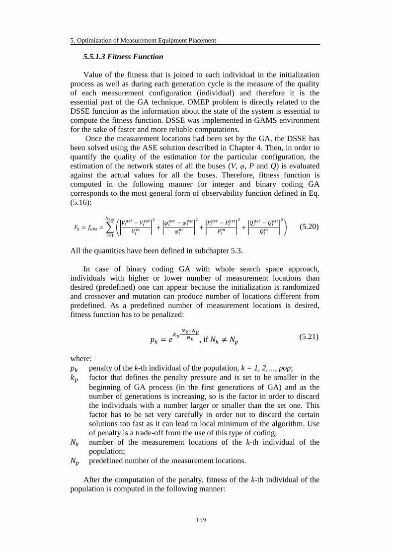
5. Optimization of Measurement Equipment Placement
159
5.5.1.3 Fitness Function
Value of the fitness that is joined to each individual in the initialization
process as well as during each generation cycle is the measure of the quality
of each measurement configuration (individual) and therefore it is the
essential part of the GA technique. OMEP problem is directly related to the
DSSE function as the information about the state of the system is essential to
compute the fitness function. DSSE was implemented in GAMS environment
for the sake of faster and more reliable computations.
Once the measurement locations had been set by the GA, the DSSE has
been solved using the ASE solution described in Chapter 4. Then, in order to
quantify the quality of the estimation for the particular configuration, the
estimation of the network states of all the buses (V, φ, P and Q) is evaluated
against the actual values for all the buses. Therefore, fitness function is
computed in the following manner for integer and binary coding GA
corresponds to the most general form of observability function defined in Eq.
(5.16):
𝐹𝑘 = 𝑓𝑜𝑏𝑠 = ∑ (|𝑉𝑖𝑎𝑐𝑡 − 𝑉𝑖
𝑒𝑠𝑡
𝑉𝑖𝑚 |
2
+ |𝜑𝑖𝑎𝑐𝑡 −𝜑𝑖
𝑒𝑠𝑡
𝜑𝑖𝑚 |
2
+ |𝑃𝑖𝑎𝑐𝑡 − 𝑃𝑖
𝑒𝑠𝑡
𝑃𝑖𝑚 |
2
+ |𝑄𝑖𝑎𝑐𝑡 −𝑄𝑖
𝑒𝑠𝑡
𝑄𝑖𝑚 |
2
)
𝑁𝑏𝑢𝑠
𝑖=1
(5.20)
All the quantities have been defined in subchapter 5.3.
In case of binary coding GA with whole search space approach,
individuals with higher or lower number of measurement locations than
desired (predefined) one can appear because the initialization is randomized
and crossover and mutation can produce number of locations different from
predefined. As a predefined number of measurement locations is desired,
fitness function has to be penalized:
𝑝𝑘 = 𝑒𝑘𝑝⋅
𝑁𝑘−𝑁𝑝
𝑁𝑝 , if 𝑁𝑘 ≠ 𝑁𝑝 (5.21)
where:
𝑝𝑘 penalty of the k-th individual of the population, k = 1, 2,…, pop;
𝑘𝑝 factor that defines the penalty pressure and is set to be smaller in the
beginning of GA process (in the first generations of GA) and as the
number of generations is increasing, so is the factor in order to discard
the individuals with a number larger or smaller than the set one. This
factor has to be set very carefully in order not to discard the certain
solutions too fast as it can lead to local minimum of the algorithm. Use
of penalty is a trade-off from the use of this type of coding;
𝑁𝑘 number of the measurement locations of the k-th individual of the
population;
𝑁𝑝 predefined number of the measurement locations.
After the computation of the penalty, fitness of the k-th individual of the
population is computed in the following manner:

5.5 Optimization of Measurement Equipment Placement Method
160
𝐹𝑘 = ∑ (|𝑉𝑖𝑎𝑐𝑡 − 𝑉𝑖
𝑒𝑠𝑡
𝑉𝑖𝑚 |
2
+ |𝜑𝑖𝑎𝑐𝑡 − 𝜑𝑖
𝑒𝑠𝑡
𝜑𝑖𝑚 |
2
+ |𝑃𝑖𝑎𝑐𝑡 − 𝑃𝑖
𝑒𝑠𝑡
𝑃𝑖𝑚 |
2
+ |𝑄𝑖𝑎𝑐𝑡 − 𝑄𝑖
𝑒𝑠𝑡
𝑄𝑖𝑚 |
2
) + 𝑝𝑘
𝑁𝑏𝑢𝑠
𝑖=1
(5.22)
5.5.1.4 Sorting Procedure
After the initialization procedure, in which initial population is created,
equipped with fitness value and coded in one of the stated ways, population is
sorted. Sorting is based on a non-dominance property of the individuals. An
individual is said to dominate another if the objective functions of it is no
worse than the other and at least in one of its objective functions it is better
than the other. The fast sort algorithm is described as:
for each individual p in main population P do the following:
- initialize Sp = . This set would contain all the individuals that is
being dominated by p;
- initialize np = 0. This would be the number of individuals that
dominate p;
- for each individual q in P:
if p dominated q then:
add q to the set Sp i.e. Sp = Sp ⋃ q;
else, if q dominates p then:
increment the domination counter for p i.e. np = np + 1;
- if np = 0 i.e. no individuals dominate p, then p belongs to the first
front; Set rank of individual p to one i.e. prank = 1. Update the first
front set by adding p to front one i.e. F1 = F1 ⋃ p;
this is carried out for all the individuals in main population P;
initialize the front counter to one: i = 1;
following is carried out while the ith
front is nonempty i.e. Fi ≠ :
- Q = . The set for storing the individuals for (i + 1)th
front;
- for each individual p in front Fi:
for each individual q in Sp (Sp is the set of individuals dominated
by p):
nq = nq – 1, decrement the domination count for individual
q;
if nq = 0 then none of the individuals in the subsequent
fronts would dominate q. Hence set qrank = i + 1. Update the
set Q with individual q i.e. Q = Q ⋃ q;
- increment the front counter by one;
- now the set Q is the next front and hence Fi = Q.
This algorithm utilizes the information about the set that an individual
dominate (Sp) and number of individuals that dominate the individual (np).
5.5.1.5 Crowding Distance
Although in this part of the dissertation the attention is on single-objective
optimization and crowding distance is the property of the multi-objective
optimization, it will be described in detail in this place as it is the part of the
sorting procedure and also because later attention will be on the multi-
objective problems.

5. Optimization of Measurement Equipment Placement
161
Once the non-dominated sort is complete the crowding distance is
assigned. Since the individuals are selected based on rank and crowding
distance all the individuals in the population are assigned a crowding distance
value. Crowding distance is assigned front wise and comparing the crowding
distance between two individuals in different front is meaningless. The
crowing distance is calculated as follows:
for each front Fi, n is the number of individuals:
- initialize the distance to be zero for all the individuals i.e. Fi(dj) = 0,
where j corresponds to the jth
individual in front Fi.
- for each objective function m:
sort the individuals in front Fi based on objective m i.e.
I = sort(Fi, m);
Assign infinite distance to boundary values for each individual
in Fi i.e. I(d1) = ∞ and I(dn) = ∞
𝐼(𝑑𝑘) = 𝐼(𝑑𝑘) +𝐼(𝑘+1).𝑚−𝐼(𝑘−1).𝑚
𝑓𝑚𝑚𝑎𝑥−𝑓𝑚
𝑚𝑖𝑛 ;
I(k).m is the value of the mth
objective function of the kth
individual in I.
The basic idea behind the crowing distance is finding the Euclidian
distance between each individual in a front based on their m objectives in the
m dimensional hyper space. The individuals in the boundary are always
selected since they have infinite distance assignment.
5.5.1.6 Selection
In this dissertation, a number of selection approaches were adopted: fixed
size tournament, fitness scaling – based roulette wheel, fine grained
tournament selection and stochastic universal sampling.
5.5.1.6.1 Tournament Selection
Tournament selection is probably the most popular selection method in
GA due to its efficiency and simple implementation [103]. In tournament
selection, n individuals out of N (the size of the population) are selected
randomly and placed in a mating pool from the larger population, and the
selected individuals compete against each other. Based on the replacement
strategy, in this dissertation, size of the pool was half of the population, if the
replacement is implicit, and whole population if the replacement is explicit
which will be further explained in the subsequent chapters.
The individual with the best fitness or the best ranking wins and will be
included as one of the next generation population. The number of individuals
competing in each tournament is referred to as tournament size, commonly set
to 2 (also called binary tournament). For testing purposes, in this dissertation,
tournament size was set to different values and it was proven that the best
results are obtained with the size 4.
Tournament selection also gives a chance to all individuals to be selected
and thus it preserves diversity, although keeping diversity may degrade the
convergence speed. Fig. 5.13 illustrates the mechanism of tournament
selection.

5.5 Optimization of Measurement Equipment Placement Method
162
The tournament selection has several advantages which include efficient
time complexity, especially if implemented in parallel, low susceptibility to
takeover by dominant individuals, and no requirement for fitness scaling or
sorting [103], [111].
Figure 5.13: Selection strategy with tournament mechanism [103]
In the above example, the tournament size, Ts, is set to three, which means
that three individuals compete against each other. Only the best chromosome
among them is selected to reproduce. In tournament selection, larger values of
tournament size lead to higher expected loss of diversity [111],[112]. The
larger tournament size means that a smaller portion of the population actually
contributes to genetic diversity, making the search increasingly greedy in
nature. There might be two factors that lead to the loss of diversity in regular
tournament selection; some individuals might not get sampled to participate in
a tournament at all while other individuals might not be selected for the
intermediate population because they lost a tournament.
5.5.1.6.2 Fitness scaling-based Roulette Wheel Selection
Fitness scaling-based roulette wheel selection is the selection strategy
where the probability of an individual being selected is based on its fitness
relative to the entire population. Fitness scaling -based selection schemes first
sort individuals in the population according to their fitness and then computes
selection probabilities according to their fitness values. Hence fitness scaling -
based roulette wheel selection can maintain a constant pressure in the
evolutionary search where it introduces a uniform scaling across the
population and is not influenced by super-individuals or the spreading of
fitness values at all as in proportional selection. Fitness scaling - based
roulette wheel selection uses a function to map the indices of individuals in
the sorted list to their selection probabilities. Although this mapping function
can be linear (linear ranking) or non-linear (non-linear ranking), the idea of
fitness scaling - based roulette wheel selection remains unchanged. The
performance of the selection scheme depends greatly on this mapping
function.
In this dissertation, linear based ranking was used [115]. For linear fitness
scaling - based selection, the biasness could be controlled through the
selection pressure (SP), such that the expected sampling rate of the best
individual is SP and the expected sampling rate of the worst individual is 2-SP
and the selective pressure of all other population members can be interpreted
by linear interpolation of the selection pressure according to rank. Consider n
the number of individuals in the population and Pos the position of an
individual in the population (least fit individual has Pos = 1, the fittest

5. Optimization of Measurement Equipment Placement
163
individual Pos = n). Instead of using the fitness value of an individual, the
scaled fitness of individuals is used. The fitness for an individual may be
scaled linearly using the following formula:
𝑅𝑎𝑛𝑘(𝑃𝑜𝑠) = 2 − 𝑆𝑃 + 2 ⋅ ((𝑆𝑃 − 1) ⋅𝑃𝑜𝑠 − 1
𝑛 − 1) (5.23)
Fitness scaling - based selection schemes can avoid premature
convergence, but can be computationally expensive because of the need to
sort populations. Once selection probabilities have been assigned, sampling
method using roulette wheel is required to populate the mating pool. Fitness
scaling - based selection scheme helps prevent premature convergence due to
“super” individuals, since the best individual is always assigned the same
selection probability, regardless of its objective value. However, this method
can lead to slower convergence, because the best chromosomes do not differ
so much from other ones. The difference between roulette wheel selection
without and with fitness scaling - based fitness is depicted in Fig. 5.14-left
and Fig. 5.14-right respectively.
Figure 5.14: Roulette – wheel selection; without fitness scaling- left and with fitness scaling-
right
As it can be seen from the figures, implementation of the fitness scaling
provides fairer share of the roulette wheel compared to the case without
fitness scaling.
5.5.1.6.3 Fine Grained Tournament Selection
Fine-grained Tournament Selection (FGTS) is an attempt to improve the
tournament selection. FGTS is controlled by real value parameter Ftour (the
desired average tournament size) instead of the integer parameter Ts (the
tournament size). Similarly to the tournament selection, an individual is
chosen if it is the best individual on the tournament. However, unlike
tournament selection, size of the tournament is not unique in the whole
population, i.e., tournaments with different number of competitors can be held
within one step of the selection [116].
The parameter Ftour governs the selection procedure; therefore, average
tournament size in population should be as close to Ftour as possible.
Sizes of the tournaments are 𝐹𝑡𝑜𝑢𝑟− = [𝐹𝑡𝑜𝑢𝑟], 𝐹𝑡𝑜𝑢𝑟
+ = [𝐹𝑡𝑜𝑢𝑟] + 1 where
[·] denotes the rounding of the real to the integer value. The size of all of n
held tournaments is either 𝐹𝑡𝑜𝑢𝑟− or 𝐹𝑡𝑜𝑢𝑟
+ . The number of tournaments with
size 𝐹𝑡𝑜𝑢𝑟− (denoted as n
−) and the number of tournaments with size 𝐹𝑡𝑜𝑢𝑟
+
5.5 Optimization of Measurement Equipment Placement Method
164
(denoted as n+), have to fulfill two conditions: their sum should be n and
average tournament size should be as close to real value Ftour as possible:
𝑛+ + 𝑛− = 𝑛
𝑛+𝐹𝑡𝑜𝑢𝑟+ + 𝑛−𝐹𝑡𝑜𝑢𝑟
− = 𝑛𝐹𝑡𝑜𝑢𝑟 (5.24)
The explicit formulas for n+ and n
− are obtained by solving these equations.
5.5.1.6.4 Stochastic Universal Sampling Selection
Stochastic Universal Sampling (SUS) developed by Baker [117] is a
single-phase sampling algorithm with minimum spread and zero bias. Instead
of a single selection pointer employed in roulette wheel methods (repetition of
the procedure until there are enough selected individuals), SUS uses N equally
spaced pointers, where N is the number of selections required. The population
is shuffled randomly and a single random number pointer1 in the range [0,
1/N] is generated. The N individuals are then chosen by generating the N
pointers, starting with pointer1 and spaced by 1/N, and selecting the
individuals whose fitness spans the positions of the pointers. If et(i) is the
expected number of trials of individual i, ⌊𝑒𝑡(𝑖)⌋ is the floor of 𝑒𝑡(𝑖) and
⌈𝑒𝑡(𝑖)⌉ is the ceiling, an individual is thus guaranteed to be selected a
minimum of times ⌊𝑒𝑡(𝑖)⌋ and no more than ⌈𝑒𝑡(𝑖)⌉, thus achieving minimum
spread. In addition, as individuals are selected entirely on their positions in the
population, SUS has zero bias. For these reasons, SUS has become one of the
most widely used selection algorithms in current GAs.
Figure 5.14 demonstrates the SUS. The individuals are mapped to
contiguous segments of a line, such that each individual’s segment is equal in
size to its fitness exactly as in roulette wheel selection. Equally spaced
pointers are placed over the line as many as there are individuals to be
selected (N). For 6 individuals (N = 6) to be selected, the distance between the
pointers is 1/6 = 0.167. Figure 5.15 shows the selection for the sample of the
random number 0.1 in the range [0, 0.167].
Figure 5.15: Stochastic universal sampling
After selection, the mating population consists of the individuals 1, 2, 3,
4, 6 and 8. Stochastic universal sampling ensures a selection of offspring
which is closer to what is desired than roulette wheel selection.
5.5.1.7 Crossover
Choice of crossover operators used in this dissertation depends on the
type of coding. For integer coding GAs, partially matched crossover was used
while, for the remaining two types of coding, scattered crossover was utilized.

5. Optimization of Measurement Equipment Placement
165
In all the approaches, the crossover operator probability is 0.9, which is the
standard value found in the majority of bibliography. This value has also
backed up good convergence property of OMEP algorithm.
5.5.1.7.1 Partially Matched Crossover
Partially matched crossover (PMX) is one of the most popular and
effective crossovers for order-based GAs to deal with combinatorial
optimization problems. In view of the operation, PMX can be regarded as a
modification of two-point crossover but additionally uses a mapping
relationship to legalize offspring that have duplicate numbers.
Goldberg and Lingle [118] developed partially matched crossover (PMX)
that preserves absolute position using two cut points in parents. This operator
first randomly selects two cut points on both parents. In order to create an
offspring, the substring between the two cut points in the first parent replaces
the corresponding substring in the second parent. Then, the inverse
replacement is applied outside of the cut points, in order to eliminate
duplicates and recover all cities.
PMX is executed following the steps:
Substring selection: Cut two substrings of equal size on each parent at the
same positions;
Substring exchange: Exchange the two selected substrings to produce
proto-child;
Mapping list determination: Determine the mapping relationship based on
the selected substrings;
Offspring legalization: Legalize proto-child with the mapping
relationship.
For instance, two parent chromosomes P1 and P2 are considered:
P1 = [1 2 3 | 5 4 6 7 | 8 9]
P2 = [4 5 2 | 1 8 7 6 | 9 3]
The first step is to immediately create the part of children C1 and C2 between
the cut points:
C1 = [* * * | 5 4 6 7 | * *]
C2 = [* * * | 1 8 7 6 | * *]
The two initialized sections C1 and C2 of define a mapping:
5 → 1, 4 → 8, 6 → 7, 7 → 6
Next, the vacant places of C1 are filled (if possible) with vertices from P2 that
happen to be in the same positions. Following is obtained:
C1 = [* * 2 | 5 4 6 7 | 9 3]

5.5 Optimization of Measurement Equipment Placement Method
166
The two remaining positions should be filled with 4 and 5. But since 4 and 5
are already present in C1, they are being replaced according to the above
mapping with 8 and 1 respectively. Thus, the completed first child is:
C1 = [8 1 2 | 5 4 6 7 | 9 3]
The second child C2 is completed by an analogous procedure, and it looks as
follows:
C2 = [5 2 3 | 1 8 7 6 | 4 9]
K. Deep and H. Mebrahtu [119] offered the variation of PMX (VPMX)
algorithm cutting two substrings of equal size on each parent at randomly
chosen positions. In this dissertation, both approaches, PMX and VPMX,
were implemented and tested. It was proven, however, that VPMX for OMEP
problem does not bring any improvements regarding convergence rate
compared to PMX.
5.5.1.7.2 Scattered Crossover
Unlike many traditional crossover techniques that are position oriented,
which means positioning has a great deal of relevance in deciding the
crossover’s efficiency, scattered crossover is position independent. This
means that the position and the ordering of the bits do not carry any
importance [120].
In this technique, random vector of binary values (the mask) is created
first (Fig. 5.16).
Figure 5.16: Scattered crossover
The length of the vector is the length of individuals. Each element of
vector is either 0 or 1, which denotes the parent. If the vector contains 0 at any
position, the gen corresponding to this position is taken from the first parent,
and vice versa. Thus position has no relevance in this; and hence this solution
is position independent. This characteristic is important because of the highly
interconnected nature of the genes and the attributes in deciding the fitness.
It should also be noted that the scattered crossover cannot be used for
integer coding GA because it could produce identical genes in the offspring
due to the mapping according to the mask.
5.5.1.8 Mutation
As with the crossover, the choice of mutation operator also depends of the
type of coding used. For integer coding GA, Mutation Matrix approach was
developed and for the other two types of coding, uniform mutation was used.

5. Optimization of Measurement Equipment Placement
167
5.5.1.8.1 Mutation Matrix Approach
This type of mutation was specially designed for the OMEP problem.
First mutation matrix of the parent population size is created. This matrix is a
binary matrix, composed of either ones or zeros. Ones are in the positions
where random number created by program was higher than mutation
probability - 0.05 and zeros in remaining locations. In most of the sources
found in bibliography, the value of the mutation probability is given by
inverse value of the population size (which in the most of the simulations ran
in case of OMEP is 200). Therefore, this value is 0.005 for the binary coding
GA. The reason why the 10 times higher value was used in case of integer
coding GA is because the integer coding crossover might not produce
satisfactory results regarding the variety of the offsprings, so additional
probability of the mutation needed to be adopted.
Program sweeps through the rows (individuals) of the parent population
one by one and changes the alleles of the individuals that correspond to the
position of ones in mutation matrix. The mutation, however, is not completely
random in order to avoid creating integer duplicates within the same
individual and therefore deteriorate the individual.
5.5.1.8.2 Uniform Mutation
Similar to mutation matrix approach, this type of mutation creates the
Mutation Points matrix which is binary and composed of ones and zeros.
Ones are in the locations where the random value is higher than mutation
probability (0.1 for binary approaches) and zeros in remaining locations.
Program sweeps through the rows (individuals) of the parent population
one by one and changes the alleles of the individuals that correspond to the
position of ones in mutation matrix. This time it is simpler than in mutation
matrix approach, as simply ones become zeros in appropriate locations and
vice versa.
5.5.1.9 Replacement
In this dissertation, two types of replacements were considered. The
classical approach, Replacement-of-the-worst or explicit elitist approach is
designed in a way that the population is sorted according to fitness and m best
individuals of population are stored before each generation cycle. All the
individuals of the population are then subjected to genetic operators. At the
end of each cycle, m best individuals stored before replace m worst
individuals obtained after the generation cycle.
Implicit elitism functions differently. To start with, not the entire
population of size N is subjected to genetic operators. After the population is
sorted according to fitness, only a part of population (in this dissertation N/2)
is selected into matting pool and later crossovered and mutated.
Once selection, crossover, and mutation have occurred, the child
population (size N/2) is combined with the entire parent population (size N) to
create an intermediate population (size 3N/2). This combined population is
subject to another non-dominated sorting and N solutions are chosen for the

5.5 Optimization of Measurement Equipment Placement Method
168
next population using rank and crowding comparison operator to compare
solutions in the same front, in case of multi-objective optimization. Therefore,
the resulting population consists of the best solutions from the newly formed
population as well as best solutions from the previous population that may
have been lost through the selection, crossover, and mutation operations.
The newly formed population undergoes selection, crossover, and
mutation and then recombination and reevaluation in subsequent generations
to eventually arrive at the optimal solution of the problem.
The implicit elitism involves a reduced computation time but may affect
the diversity of the population with respect to the explicit elitism.
5.5.2 Single-objective OMEP Results
5.5.2.1 Test of the Algorithm Convergence Quality
A set of pre-tests was conducted in order to check the convergence quality
of diverse approaches regarding coding and genetic operator types. This
particular test checks if the OMEP algorithm finds the optimal solution. The
test was conducted on different DNs and with different starting conditions.
These include:
random initialization of the measurement configuration population;
a priori seeding of the initial population with at least one super-
individual. i.e. configuration with fitness close to the optimal one;
a priori seeding of the initial population with a number of individuals
with poor fitness and no super-individuals.
These tests made with the algorithm of following characteristics:
integer coding GA;
tournament selection;
PMX crossover;
mutation matrix approach;
explicit replacement;
population size 200 individuals;
number of generations 200.
Test DN is shown in Fig. 5.17. It is a simple system with 29 buses and 28
branches, with distribution generation plant in bus 10 and three “empty”
buses. The available information of the network is previously described in
subchapter 4.3.1 and it concerns primary TS. When these buses are discarded
from the possible measurement equipment set, 23 out of 29 buses comprise
search space.

5. Optimization of Measurement Equipment Placement
169
Figure 5.17: 29-bus test DN with optimal measurement configuration
First, the algorithm was completed, thus providing the optimal
configuration of the OMEP problem. The reported configuration is the
following (Fig 5.17): 8, 10, 14, 18 and 26 with the fitness (according to Eq.
5.20) 5,8866. This configuration and fitness value were checked by multiple
runs of the algorithm.
In order to check if this configuration is really optimal, series of tests
were made by changing the position measurement equipment from optimal
buses to their neighboring buses and precomputing the fitness of these new
configurations. Here will be presented just some of these (Fig 5.18):
(a) (b) (c)
Figure 5.18: Manipulations of the optimal configuration
The manipulations are the following:
a) Replace the measurement equipment from bus 8 to bus 7;
b) Replace the measurement equipment from bus 10 to bus 12;
c) Replace the measurement equipment from bus 8 to bus 7 and bus 10 to
bus 12.

5.5 Optimization of Measurement Equipment Placement Method
170
New obtained configurations and appropriate fitness values are reported in
Table 5.1:
Table 5.1: Test of the Algorithm Convergence Quality
Manipulation Configuration Fitness
a) 7 10 14 18 26 6.3266
b) 8 12 14 18 26 7.1012
c) 7 12 14 18 26 8.2241
As it can be seen, all of the stated configurations in Table 5.1 are worse
than optimal configuration obtained by the OMEP algorithm which can be
clearly seen from the values of fitness that were obtained. This test proves the
convergence quality of the developed OMEP algorithm.
5.5.2.2 Test of the Algorithm Properties
The following test was made in order to distinguish how the algorithm
corresponds to different degrees of freedom set by the problem. Same
algorithm and network properties were used as in the first test. The test was
firstly run with 5 optimal measurement locations obtained in the previous test
and 5 new ones that algorithm should place in optimal places. Then the
algorithm was used to optimally place 10 new acquisition units in the same
DN. The situation is depicted in Fig. 5.19.
(a) (b)
Figure 5.19: DN with (a) 5 old and 5 new optimally placed units and (b) 10 new units
Fig. 5.19 (a) shows the previous 5 optimal locations set by the algorithm
in the first step (red dots) and 5 new optimally chosen locations (green dots).
Fig. 5.19 (b) shows completely new optimally located measurement
equipment (light blue dots). It is obvious that the configurations are
topologically different. Table 5.2 shows these configurations and their fitness
values.

5. Optimization of Measurement Equipment Placement
171
Table 5.2: Test of the Algorithm Properties
Type Configuration Fitness
(a) 8 9 10 14 17 18 24 25 26 28 1.7415
(b) 6 8 11 14 16 12 18 22 24 26 0.2060
Results show that the algorithm provides far better results if it can
optimize 10 locations at the time than if it optimizes 5 and then additional 5
locations. This is because the first option provides more degrees of freedom to
the algorithm and it can arrange the units more optimally.
However, this test also demonstrated the possibilities of the algorithm to
be used to planning new network but also improvement of the existing ones
thus showing its flexibility as the part of some future DMS software solution
apart from its main function – optimization of the measurement equipment
placement.
5.5.2.3 Comparison of Integer and Binary Approaches
While the previously described pre-tests are important to prove the
convergence capabilities of the different OMEP algorithms that were
developed, the core of this part of dissertation is to find the type of OMEP
algorithm with the best convergence characteristics with the variety of input
data regarding DN types, nature and parameters.
The ultimate goal was to design the algorithm that can provide
(sub)optimal solution for the realistic large-scale DNs in computationally
acceptable time frame. As many different approaches were developed, to
decide the best one, they were compared in different environments – smaller
to larger DNs, randomized or a priori initialization, different population sizes
and generation cycle number etc.
5.5.2.3.1 29-bus DN Tests
First group of tests was conducted on small size 29-bus test DN (Fig.
5.20) that was previously described. The aim was to prove the convergence of
the various GA approaches but also to make first conclusions about the speed
of convergence. Following algorithms were tested:
1. Integer coding GA with tournament selection, PMX crossover, mutation
matrix approach and implicit elitist replacement;
2. Integer coding GA with tournament selection, PMX crossover, mutation
matrix approach and explicit elitist replacement;
3. Integer coding GA with fitness scaling-based roulette wheel selection,
PMX crossover, mutation matrix approach and explicit elitist
replacement;
4. Integer coding GA with fine grained tournament selection, PMX
crossover, mutation matrix approach and explicit elitist replacement;
5. Binary coding GA with tournament selection, scattered crossover,
uniform mutation and explicit elitist replacement;
6. Binary coding GA with stochastic universal sampling selection, scattered
crossover, uniform mutation and explicit elitist replacement;
7. Binary coding GA with fine grained tournament selection, scattered
crossover, uniform mutation and explicit elitist replacement;

5.5 Optimization of Measurement Equipment Placement Method
172
8. Binary coding GA with whole search space approach, fine grained
tournament selection, scattered crossover, uniform mutation and explicit
elitist replacement.
These diverse algorithms are summarized in the following Table 5.3:
Table 5.3: Types of the approaches used for tests – 29-bus DN
Algorithm type 1. 2. 3. 4. 5. 6. 7. 8.
Coding
type
Integer
Binary
Binary with
whole SS
Selection
type
Tournament
Roulette
wheel
FGTS
SUS
Crossover
type
PMX
Scattered
Mutation
type
Mutation
matrix
Uniform
Elitism
type
Implicit
Explicit
In order to obtain the average behavior, each of the stated approaches was
run 5 times and results are reported for averaged fitness in each generation per
approach. Algorithm settings are the following:
Population size 200 individuals;
Number of generation cycles 200;
A priori initialization with super-individual(s) and poor-individuals
independently. This was done in order to have the same starting points for
all the runs of the algorithms. Also, it is important to observe if and how
much quantitatively starting point interferes with the convergence rate of
the algorithm.
Although the algorithm was run each time for 200 generations, it
converged much faster, so only the first 20 generations will be reported on the
following Figures 5.20 and 5.21. This is done in order to have the clearer
picture of the convergence rate of approaches.

5. Optimization of Measurement Equipment Placement
173
Figure 5.20: Comparison of algorithms – good initial fitness of the population
Figure 5.21: Comparison of algorithms – bad initial fitness of the population
Graphs show the obvious superiority of integer coding GAs compared to
binary ones. This conclusion is the same for both types of initial populations.
When comparing particular integer approaches, it can be concluded that all of
them converge quite fast (from 7th
to 15th
generation for good starting point or
9th
to 20th
generation for bad starting point) and that they converge in almost
same time. The algorithm with the best properties for the small network is
Integer coding GA with fine grained tournament selection, PMX crossover,
mutation matrix approach and explicit elitist replacement.
Another important conclusion that can be drawn from this test is that a
priori seeding of the initial population didn’t interfere in a great manner with
the rate of convergence of the algorithm. For example, the algorithm with the
best properties converged in 7 generations with the good starting fitness of the
population, while it took 9 generations to reach the optimal solution with the
bad starting fitness of the initial population.
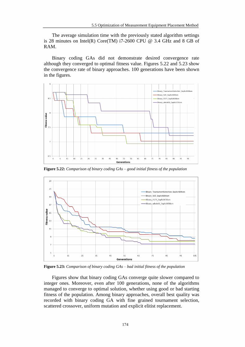
5.5 Optimization of Measurement Equipment Placement Method
174
The average simulation time with the previously stated algorithm settings
is 28 minutes on Intel(R) Core(TM) i7-2600 CPU @ 3.4 GHz and 8 GB of
RAM.
Binary coding GAs did not demonstrate desired convergence rate
although they converged to optimal fitness value. Figures 5.22 and 5.23 show
the convergence rate of binary approaches. 100 generations have been shown
in the figures.
Figure 5.22: Comparison of binary coding GAs – good initial fitness of the population
Figure 5.23: Comparison of binary coding GAs – bad initial fitness of the population
Figures show that binary coding GAs converge quite slower compared to
integer ones. Moreover, even after 100 generations, none of the algorithms
managed to converge to optimal solution, whether using good or bad starting
fitness of the population. Among binary approaches, overall best quality was
recorded with binary coding GA with fine grained tournament selection,
scattered crossover, uniform mutation and explicit elitist replacement.

5. Optimization of Measurement Equipment Placement
175
5.5.2.3.2 69-bus DN Tests
Last results have proven the superiority of integer coding GAs for solving
of the OMEP problem over the binary coding ones. This is why only the
results with the following types of integer coding GA will be published:
1. Integer coding GA with tournament selection, PMX crossover, mutation
matrix approach and implicit elitist replacement;
2. Integer coding GA with tournament selection, PMX crossover, mutation
matrix approach and explicit elitist replacement;
3. Integer coding GA with fitness scaling-based roulette wheel selection,
PMX crossover, mutation matrix approach and explicit elitist
replacement;
4. Integer coding GA with fine grained tournament selection, PMX
crossover, mutation matrix approach and explicit elitist replacement.
This diverse algorithms are summarized in the following Table 5.4:
Table 5.4: Types of the approaches used for tests – 69-bus DN
Algorithm type 1. 2. 3. 4.
Coding
type
Integer
Binary
Binary with
whole SS
Selection
type
Tournament
Roulette
wheel
FGTS
SUS
Crossover
type
PMX
Scattered
Mutation
type
Mutation
matrix
Uniform
Elitism
type
Implicit
Explicit
Test network is the medium sized realistic DN (Fig. 5.24) which is quite
active with DG in buses 9, 17, 20, 30, 41, 43, 57, 59 and 62. As with the 29-
bus network, this one is also measured only in primary TS. After removal of
the empty buses, size of the search space is 65.

5.5 Optimization of Measurement Equipment Placement Method
176
Figure 5.24: 69-bus distribution network
In order to obtain the average behavior, each of the stated approaches was
run 5 times and results are reported for averaged fitness in each generation per
approach. Algorithm settings are the following:
Population size 250 individuals;
Number of generation cycles 200;
Random initialization of the population;
Three measurement configurations: 15, 22 and 30 measurement
locations.
Figure 5.25 depicts the DN with the optimally located measurement
equipment for 15, 22 and 30 measurement configurations respectfully.
(a) (b) (c)
Figure 5.25: Optimal locations for (a) 15, (b) 22 and (c) 30 measurement equipment

5. Optimization of Measurement Equipment Placement
177
The average simulation time with the previously stated algorithm settings
is 2 h 38 min on Intel(R) Core(TM) i7-2600 CPU @ 3.4 GHz and 8 GB of
RAM.
Figures 5.26, 5.27 and 5.28 show the convergence rate of integer
approaches during 200 generations for 15, 22 and 30 measurements
configuration respectively in 69-bus DN.
Figure 5.26: Comparison of integer coding GAs – 15 measurements configuration
Figure 5.27: Comparison of integer coding GAs – 22 measurements configuration

5.5 Optimization of Measurement Equipment Placement Method
178
Figure 5.28: Comparison of integer coding GAs – 30 measurements configuration
Graphs demonstrate that all the approaches except integer coding GA
with fine grained tournament selection, PMX crossover, mutation matrix
approach and explicit elitist replacement converge to near-optimal region of
solution in a limited number of generations (in all the cases around 70th
generation. Near-optimal region of solutions is the solution region of the
problem whose fitness values are significantly less than the starting fitness
and without significant numerical improvements over many generations. In
order to explore furtherly in how many cases out of 5 runs algorithms reach
(sub)optimal solution and their pace of convergence, the results of the
simulations are shown in the following Tables 5.5, 5.6 and 5.7.
Table 5.5: Convergence quality of the algorithms – 15 measurements configuration
Type of the
algorithm
Number of generations to
reach sub(optimal) solution
Number of attempts to reach
(sub)optima solution /out of 5
1. 53 3
2. 39 2
3. 76 2
4. More than 200 0
Table 5.6: Convergence quality of the algorithms – 22 measurements configuration
Type of the
algorithm
Number of generations to
reach sub(optimal) solution
Number of attempts to reach
(sub)optima solution /out of 5
1. 77 3
2. 197 3
3. More than 200 0
4. More than 200 0

5. Optimization of Measurement Equipment Placement
179
Table 5.7: Convergence quality of the algorithms – 30 measurements configuration
Type of the
algorithm
Number of generations to
reach sub(optimal) solution
Number of attempts to reach
(sub)optima solution /out of 5
1. 86 4
2. 84 4
3. 125 2
4. More than 200 0
As it can be seen from the previous tables, further examination of the
approaches on 69-bus network has shown that Integer coding GA with
tournament selection, PMX crossover, mutation matrix approach and implicit
elitist replacement and Integer coding GA with tournament selection, PMX
crossover, mutation matrix approach and explicit elitist replacement give the
best results. Both approaches are well designed for OMEP problem in
different problem environments.
As the last step in deciding which approach is the best, two of the best
candidate algorithms were tested on 272-bus real DN and the results of this
study can be summed in the following subchapter.
5.5.2.3.3 272-bus DN Tests
This is a larger size realistic DN with three voltage levels. It is highly
active with 44 buses that contain DG. The only measured data correspond
from the equipment installed on primary TS and DN transformers. Search
space that was defined according to the rules from the subchapter 5.4.2.2 is of
size 187.
As all the binary approaches did not demonstrate promising convergence
quality and also, in last subchapter, two more approaches were discarded, the
following tests were run only with the two best integer coding GAs:
1. Integer coding GA with tournament selection, PMX crossover, mutation
matrix approach and implicit elitist replacement;
2. Integer coding GA with tournament selection, PMX crossover, mutation
matrix approach and explicit elitist replacement.
In order to obtain the average behavior, the approaches were run 5 times
and results are reported for averaged fitness in each generation per approach.
Algorithm settings are the following:
Population size 300 individuals;
Number of generation cycles 200;
Random initialization of the population;
25 measurement locations.
Figure 5.29 shows the comparison of convergence rate of the two best GA
approaches. Figure 5.30 show the same comparison but on the scale of last
200 generations to distinguish better the difference between convergence
curves.
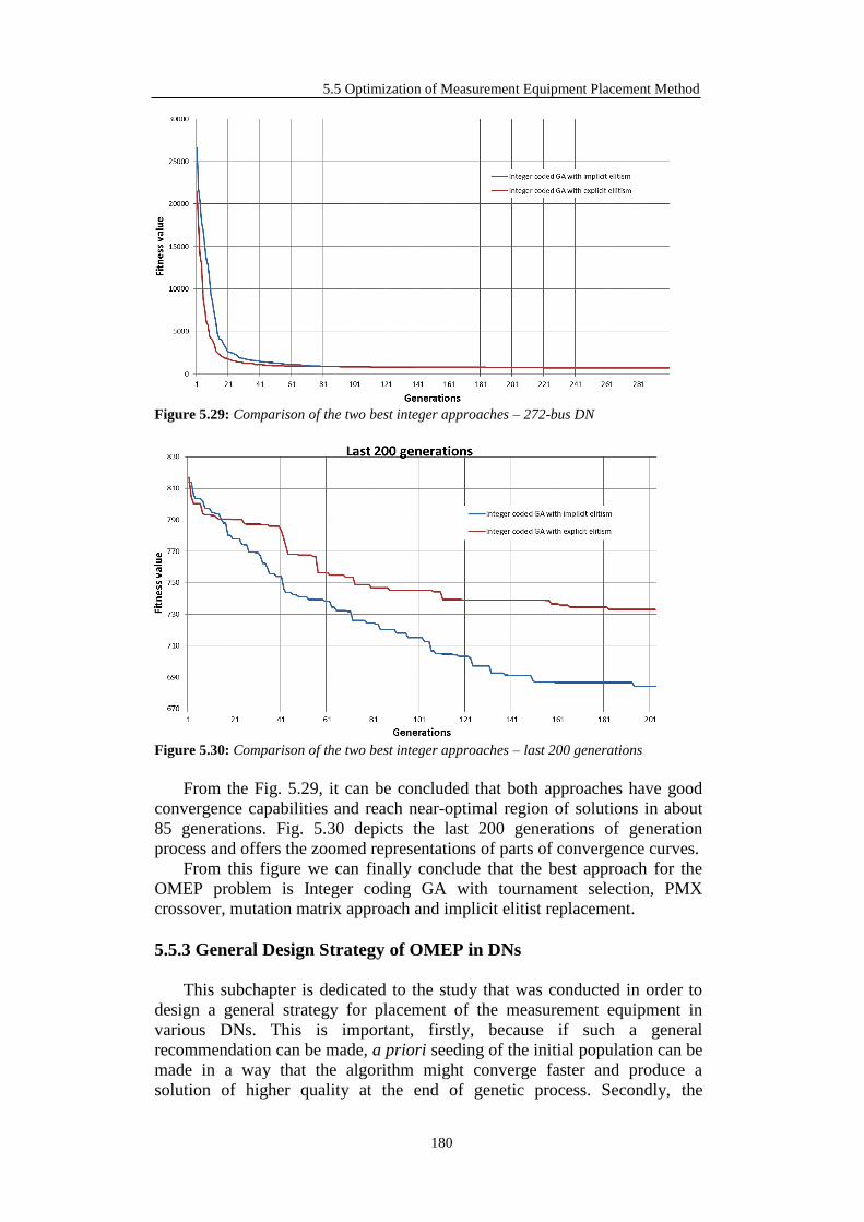
5.5 Optimization of Measurement Equipment Placement Method
180
Figure 5.29: Comparison of the two best integer approaches – 272-bus DN
Figure 5.30: Comparison of the two best integer approaches – last 200 generations
From the Fig. 5.29, it can be concluded that both approaches have good
convergence capabilities and reach near-optimal region of solutions in about
85 generations. Fig. 5.30 depicts the last 200 generations of generation
process and offers the zoomed representations of parts of convergence curves.
From this figure we can finally conclude that the best approach for the
OMEP problem is Integer coding GA with tournament selection, PMX
crossover, mutation matrix approach and implicit elitist replacement.
5.5.3 General Design Strategy of OMEP in DNs
This subchapter is dedicated to the study that was conducted in order to
design a general strategy for placement of the measurement equipment in
various DNs. This is important, firstly, because if such a general
recommendation can be made, a priori seeding of the initial population can be
made in a way that the algorithm might converge faster and produce a
solution of higher quality at the end of genetic process. Secondly, the

5. Optimization of Measurement Equipment Placement
181
conclusions made in this way could offer DSOs or owners of the DN general
guidelines about planning of new or improving of the existing DNs.
Hundred randomly generated measurement scenarios were created per test
by altering load following a standard uniform distribution (± 60%). After that,
GA was run as previously described. For the sake of this study, two DNs were
created. First test DN is shown in Fig. 5.31. It is 48-bus DN with 5
distribution feeders.
Figure 5.31: 48-bus test DN with equal loads
All the primary substations have the same electrical characteristics.
Branches do not have the same characteristics i.e. electrical distance between
buses is different. First feeder is without branching, i.e. without secondary
feeders. All the base values of the bus loads without branching are the same as
noted by white-blue squares on the Fig. 5.31. The rest of the feeders contain
the branching – second feeder at its beginning, third feeder at the middle,
fourth feeder close to the end and last one contains all three previously
described branching. Base bus loads at primary feeder with branching as well
as base loads of the buses of the secondary feeders are the same and
quantitatively less than the ones without branching (noted by white-green
squares at the previous figure).
For each bus and each scenario, following sets have been defined:
𝑉𝑟𝑒𝑎𝑙 set of real scenario voltage magnitudes;
𝑉𝑒𝑠𝑡 set of voltage magnitudes after the completion of SE;
𝑉𝑒𝑟𝑟𝑜𝑟 set of voltage magnitude errors;
𝜑𝑟𝑒𝑎𝑙 set of real scenario voltage angles;
𝜑𝑒𝑠𝑡 set of voltage angles after the completion of SE;
𝜑𝑒𝑟𝑟𝑜𝑟 set of phase angle errors.
Previously mentioned 𝑉𝑒𝑟𝑟𝑜𝑟 and 𝜑𝑒𝑟𝑟𝑜𝑟 are computed in the following way:
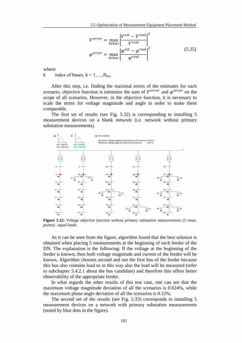
5.5 Optimization of Measurement Equipment Placement Method
182
𝑉𝑒𝑟𝑟𝑜𝑟 = max𝑘𝜖𝑏𝑢𝑠
|𝑉𝑒𝑠𝑡 − 𝑉𝑟𝑒𝑎𝑙
𝑉𝑟𝑒𝑎𝑙|
2
𝜑𝑒𝑟𝑟𝑜𝑟 = max𝑘𝜖𝑏𝑢𝑠
|𝜑𝑒𝑠𝑡 −𝜑𝑟𝑒𝑎𝑙
𝜑𝑟𝑒𝑎𝑙|
2
(5.25)
where:
k index of buses, k = 1,…,Nbus
After this step, i.e. finding the maximal errors of the estimates for each
scenario, objective function is minimize the sum of 𝑉𝑒𝑟𝑟𝑜𝑟 and 𝜑𝑒𝑟𝑟𝑜𝑟 on the
scope of all scenarios. However, in the objective function, it is necessary to
scale the terms for voltage magnitude and angle in order to make them
comparable.
The first set of results (see Fig. 5.32) is corresponding to installing 5
measurement devices on a blank network (i.e. network without primary
substation measurements).
Figure 5.32: Voltage objective function without primary substation measurements (5 meas.
points)– equal loads
As it can be seen from the figure, algorithm found that the best solution is
obtained when placing 5 measurements at the beginning of each feeder of the
DN. The explanation is the following: If the voltage at the beginning of the
feeder is known, then both voltage magnitude and current of the feeder will be
known. Algorithm chooses second and not the first bus of the feeder because
this bus also contains load so in this way also the load will be measured (refer
to subchapter 5.4.2.1 about the bus candidate) and therefore this offers better
observability of the appropriate feeder.
In what regards the other results of this test case, one can see that the
maximum voltage magnitude deviation of all the scenarios is 0.024%, while
the maximum phase angle deviation of all the scenarios is 0.52%.
The second set of the results (see Fig. 5.33) corresponds to installing 5
measurement devices on a network with primary substation measurements
(noted by blue dots in the figure).
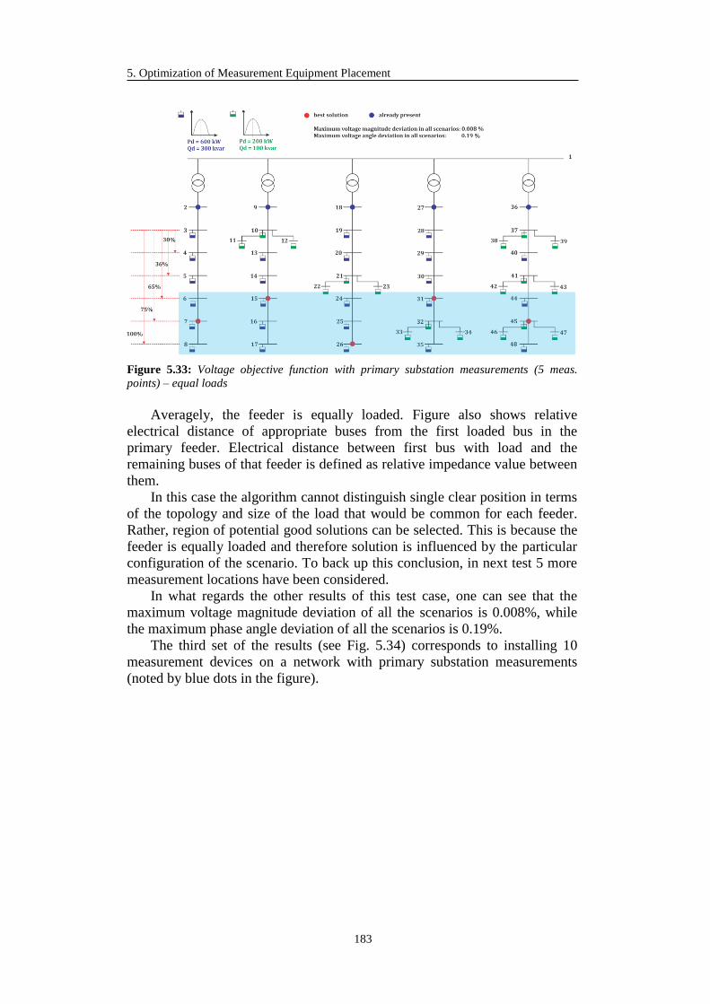
5. Optimization of Measurement Equipment Placement
183
Figure 5.33: Voltage objective function with primary substation measurements (5 meas.
points) – equal loads
Averagely, the feeder is equally loaded. Figure also shows relative
electrical distance of appropriate buses from the first loaded bus in the
primary feeder. Electrical distance between first bus with load and the
remaining buses of that feeder is defined as relative impedance value between
them.
In this case the algorithm cannot distinguish single clear position in terms
of the topology and size of the load that would be common for each feeder.
Rather, region of potential good solutions can be selected. This is because the
feeder is equally loaded and therefore solution is influenced by the particular
configuration of the scenario. To back up this conclusion, in next test 5 more
measurement locations have been considered.
In what regards the other results of this test case, one can see that the
maximum voltage magnitude deviation of all the scenarios is 0.008%, while
the maximum phase angle deviation of all the scenarios is 0.19%.
The third set of the results (see Fig. 5.34) corresponds to installing 10
measurement devices on a network with primary substation measurements
(noted by blue dots in the figure).

5.5 Optimization of Measurement Equipment Placement Method
184
Figure 5.34: Voltage objective function with primary substation measurements (10 meas.
points) – equal loads
As it can be seen, also in this case, solution is influenced by the particular
configuration of the scenario. The algorithm does not find one clear location
but rather two regions of possibly good solution. It is interesting, however,
that the difference in fitness value given by solutions within the same region,
e.g. bus 7 and 8 of the first feeder, are similar so deciding to place the
equipment in bus 7 instead of bus 8 does not deteriorate the solution a lot.
In what regards the other results of this test case, one can see that the
maximum voltage magnitude deviation of all the scenarios is 0.007%, while
the maximum phase angle deviation of all the scenarios is 0.11%.
The second test DN is shown in Fig. 5.35. As the first one, this is also 48-
bus DN with 5 distribution feeders. However, the feeders of this network are
not equally loaded.
Figure 5.35: 48-bus test DN with unequal loads

5. Optimization of Measurement Equipment Placement
185
The primary substations have the same electrical characteristics and
electrical distances between buses are different. The configuration of the
feeders regarding branching is the same as in first DN as well. In this case,
however, feeders are not equally loaded. It can be observed that each feeder
contains more and less loaded buses. Heavily loaded buses are depicted with
white-blue and white-green (in case of branching) squares while less loaded
buses are depicted by white-red and white-black (in case of branching)
squares in previous figure.
The first set of results (see Fig. 5.36) is corresponding to installing 5
measurement devices on a blank network (i.e. network without primary
substation measurements).
Figure 5.36: Voltage objective function without primary substation measurements (5 meas.
points) – unequal loads
The first set of results corresponds to the ones already stated for the first
DN, i.e. the best solution is obtained when placing 5 measurements at the
beginning of each feeder of the DN.
In what regards the other results of this test case, one can see that the
maximum voltage magnitude deviation of all the scenarios is 0.007%, while
the maximum phase angle deviation of all the scenarios is 0.29%.
The second set of the results (see Fig. 5.37) corresponds to installing 5
measurement devices on a network with primary substation measurements
(noted by blue dots in the figure).

5.5 Optimization of Measurement Equipment Placement Method
186
Figure 5.37: Voltage objective function with primary substation measurements (5 meas.
points) – unequal loads
Unlike the case of the first DN, algorithm was capable to propose the
same unique position for measurement placement in each feeder (red dots)
and the solution is no more influenced by the particular configuration of the
scenario. This position is close to highly loaded buses. The question of why is
optimal location on penultimate and not ultimate bus of the feeder can arise.
The answer is that measurement on penultimate bus (e.g. bus 7) ensures that
the power flows between this bus and buses 6 and 8 are known. As the bus 8
is the ultimate bus, all the flow from bus 7 is going to load of bus 8. In return,
very quality estimation of this load can be made. On the other side, buses 4, 5
and 6 are “less important” regarding estimator as the values of the load are
much less but the estimates of these loads and the larger load in bus 3 can still
be made with a fair quality thanks to measurements in buses 2 and 7.
In what regards the other results of this test case, one can see that the
maximum voltage magnitude deviation of all the scenarios is 0.007%, while
the maximum phase angle deviation of all the scenarios is 0.29%.
The last set of the results (see Fig. 5.37) corresponds to installing 10
measurement devices on a network with primary substation measurements
(noted by blue dots in the figure).

5. Optimization of Measurement Equipment Placement
187
Figure 5.38: Voltage objective function with primary substation measurements (10 meas.
points) – unequal loads
Also in this case algorithm was capable to propose the same unique
position for measurement equipment in each feeder (red dots). Observing the
optimal locations, following can be concluded: one optimal measurement
location is proposed at the second bus with load and the other at penultimate
bus of the feeder (observing from the top of the feeder). The conclusion about
choice of the penultimate bus is the same as in previous case. Similar is with
second bus with load of the feeder, e.g. bus 4. Although the size of the load
corresponding to this bus is much less than the neighboring bus 3, algorithm
proposes the placement of the equipment in bus 4. This ensures the
knowledge of the power flow of line 3 – 4 and, as there is measurement
equipment at primary substation, consecutively, the knowledge of the power
flow of line 2 – 3. Therefore, also the load of the bus 3 is well estimated. It
can be further concluded that with 3 measurement equipment, state of the 7
out of 5 buses can be very well estimated. Among these 7 buses, all heavily
loaded buses can be well estimated.
5.6 Advanced Optimization of Measurement Equipment
Placement Method
The core of this part of the dissertation is on the development of the
multi-objective GA that could be used to optimize vast family of OMEP
related realistic problems. This study can have a great importance for DSOs as
it can be used to take into account different limitations or requests that are
posed by DSOs when planning new network or improving the existing one.
As developed OMEP software solution is highly modular, it can also be used
to solve wider group of planning problems.
In the following subchapters, the mechanism of Genetic Multi-Objective
Optimization (GMOO), specific GA for multi-objective optimization, NSGA-
II, and a study regarding DN voltage observability will be explained.

5.6 Advanced Optimization of Measurement Equipment Placement Method
188
5.6.1 Genetic Multi-Objective Optimization (GMOO)
A multi-objective optimization problem involves a number of objective
functions which are to be either minimized or maximized. As in a single-
objective optimization problem, the multi-objective optimization problem
may contain a number of constraints which any feasible solution (including all
optimal solutions) must satisfy. Since objectives can be either minimized or
maximized, we state the multi-objective optimization problem in its general
form [146]:
min[𝒇1(𝐱), 𝒇𝟐(𝐱),… , 𝒇𝑗(𝐱),… , 𝒇𝑝(𝐱)]
subject to: 𝒈(𝐱) ≤ 0
𝐱 ∈ X
(5.26)
where: 𝒇𝑗(𝐱) j-th OF considered (to be minimized);
𝒈(𝐱) the constraint vector (m elements);
𝐱 the control variable vector (n elements) and X is the feasibility region.
One of the striking differences between single-objective and multi-
objective optimization is that in multi-objective optimization the objective
functions constitute a multi-dimensional space, in addition to the usual
decision variable space. This additional P-dimensional space is called the
objective space. To make the descriptions clear, we refer a “solution” as a
variable vector and a “point” as the corresponding objective vector.
The optimal solutions in multi-objective optimization can be defined from
a mathematical concept of partial ordering. In the parlance of multi-objective
optimization, the term domination is used for this purpose. In this subchapter,
the stress is on the unconstrained (without any equality, inequality or bound
constraints) optimization problems. The domination between two solutions is
defined as follows [84],[119]:
Definition 5.1 A solution x(1)
is said to dominate the other solution x(2)
, if both
the following conditions are true:
1. The solution x(1)
is no worse than x(2)
in all objectives. Thus, the solutions
are compared based on their objective function values (or location of the
corresponding points (z(1)
and z(2)
) on the objective space).
2. The solution is x(1)
strictly better than x(2)
in at least one objective.
For a given set of solutions (or corresponding points on the objective
space, for example, those shown in Fig. 5.39(a)), a pair-wise comparison can
be made using the above definition and whether one point dominates the other
can be established. All points which are not dominated by any other member
of the set are called the non-dominated points of class one, or simply the non-
dominated points. For the set of six solutions shown in the figure, they are
points 3, 5, and 6. One property of any two such points is that a gain in an
objective from one point to the other happens only due to a sacrifice in at least
one other objective. This trade-off property between the non-dominated points

5. Optimization of Measurement Equipment Placement
189
makes the practitioners interested in finding a wide variety of them before
making a final choice. These points make up a front when viewed them
together on the objective space; hence the non-dominated points are often
visualized to represent a non-domination front [121].
(a) (b)
Figure 5.39: A set of points and the first non-dominated front
With the above concept, now it is easier to define the Pareto-optimal
solutions in a multi-objective optimization problem. If the given set of points
for the above task contain all points in the search space (assuming a countable
number), the points lying on the non-domination front, by definition, do not
get dominated by any other point in the objective space, hence are Pareto-
optimal points (together they constitute the Pareto-optimal front) and the
corresponding pre-images (decision variable vectors) are called Pareto-
optimal solutions. However, more mathematically elegant definitions of
Pareto-optimality (including the ones for continuous search space problems)
exist in the multi-objective optimization literature [122],[123].
5.6.1.1 Principle of GMOO’s Search
In the context of multi-objective optimization, the extremist principle of
finding the optimum solution cannot be applied to one objective alone, when
the rest of the objectives are also important. Different solutions may produce
trade-offs (conflicting outcomes among objectives) among different
objectives. A solution that is extreme (in a better sense) with respect to one
objective requires a compromise in other objectives. This prohibits one to
choose a solution which is optimal with respect to only one objective. This
clearly suggests two ideal goals of multi-objective optimization:
1. Find a set of solutions which lie on the Pareto-optimal front, and
2. Find a set of solutions which are diverse enough to represent the entire
range of the Pareto-optimal front.
Although one fundamental difference between single and multiple
objective optimizations lies in the cardinality in the optimal set, from a
practical standpoint a user needs only one solution, no matter whether the
associated optimization problem is single or multi-objective. The user is now
in a dilemma. Since a number of solutions are optimal, the obvious question
arises: Which of these optimal solutions must one choose? This is not an easy
question to answer. It involves higher-level information which is often non-

5.6 Advanced Optimization of Measurement Equipment Placement Method
190
technical, qualitative and experience-driven. However, if a set of many trade-
off solutions are already worked out or available, one can evaluate the pros
and cons of each of these solutions based on all such non-technical and
qualitative, yet still important, considerations and compare them to make a
choice.
Thus, in a multi-objective optimization, ideally the effort must be made in
finding the set of trade-off optimal solutions by considering all objectives to
be important. After a set of such trade-off solutions are found, a user can then
use higher-level qualitative considerations to make a choice. Since the GMOO
procedure deals with a population of solutions in every iteration, it makes
them intuitive to be applied in multi-objective optimization to find a set of
non-dominated solutions. The GMOO based procedure works with the
following principle in handling multi-objective optimization problems:
Step 1. Find multiple non-dominated points as close to the Pareto-optimal
front as possible, with a wide trade-off among objectives;
Step 2. Choose one of the obtained points using higher-level information.
Since GMOO procedures are heuristic based, they may not guarantee in
finding Pareto-optimal points, as a theoretically provable optimization method
would do for tractable (for example, linear or convex) problems. But GMOO
procedures have essential operators to constantly improve the evolving non-
dominated points (from the point of view of convergence and diversity
discussed above) similar to the way most natural and artificial evolving
systems continuously improve their solutions.
In the first step of the GMOO-based multi-objective optimization,
multiple trade-off, non-dominated points are found. Thereafter, in the second
step, higher-level information is used to choose one of the obtained trade-off
points. This dual task allows an interesting feature, if applied for solving
single-objective optimization problems. It is easy to realize that a single-
objective optimization is a degenerate case of multi-objective optimization
[124]. In the case of single-objective optimization, having only one globally
optimal solution, the first step will ideally find only one solution, thereby not
requiring us to proceed to the second step. However, in the case of single-
objective optimization having multiple global optima, both steps are necessary
to first find all or multiple global optima, and then to choose one solution
from them by using a higher-level information about the problem. Thus,
although seems ideal for multi-objective optimization, the proposed
framework can be ideally thought as a generic principle for both single and
multiple objective optimization.
5.6.1.2 Generating Classical Methods and GMOO
In the generating Multi-Criteria Decision Making (MCDM) approach, the
task of finding multiple Pareto-optimal solutions is achieved by executing
many independent single-objective optimizations, each time finding a single
Pareto-optimal solution. A parametric scalarizing approach (such as the
weighted-sum approach, 𝜖-constraint approach, and others) can be used to
convert multiple objectives into a parametric single-objective function [125].
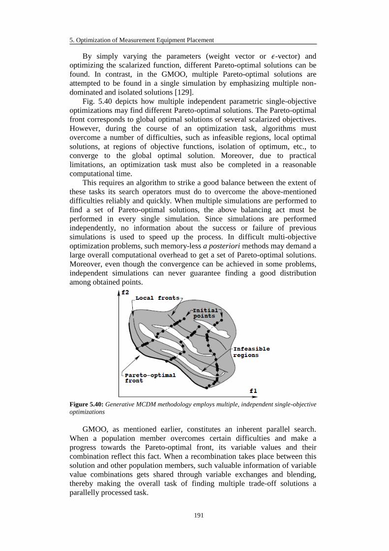
5. Optimization of Measurement Equipment Placement
191
By simply varying the parameters (weight vector or 𝜖-vector) and
optimizing the scalarized function, different Pareto-optimal solutions can be
found. In contrast, in the GMOO, multiple Pareto-optimal solutions are
attempted to be found in a single simulation by emphasizing multiple non-
dominated and isolated solutions [129].
Fig. 5.40 depicts how multiple independent parametric single-objective
optimizations may find different Pareto-optimal solutions. The Pareto-optimal
front corresponds to global optimal solutions of several scalarized objectives.
However, during the course of an optimization task, algorithms must
overcome a number of difficulties, such as infeasible regions, local optimal
solutions, at regions of objective functions, isolation of optimum, etc., to
converge to the global optimal solution. Moreover, due to practical
limitations, an optimization task must also be completed in a reasonable
computational time.
This requires an algorithm to strike a good balance between the extent of
these tasks its search operators must do to overcome the above-mentioned
difficulties reliably and quickly. When multiple simulations are performed to
find a set of Pareto-optimal solutions, the above balancing act must be
performed in every single simulation. Since simulations are performed
independently, no information about the success or failure of previous
simulations is used to speed up the process. In difficult multi-objective
optimization problems, such memory-less a posteriori methods may demand a
large overall computational overhead to get a set of Pareto-optimal solutions.
Moreover, even though the convergence can be achieved in some problems,
independent simulations can never guarantee finding a good distribution
among obtained points.
Figure 5.40: Generative MCDM methodology employs multiple, independent single-objective
optimizations
GMOO, as mentioned earlier, constitutes an inherent parallel search.
When a population member overcomes certain difficulties and make a
progress towards the Pareto-optimal front, its variable values and their
combination reflect this fact. When a recombination takes place between this
solution and other population members, such valuable information of variable
value combinations gets shared through variable exchanges and blending,
thereby making the overall task of finding multiple trade-off solutions a
parallelly processed task.

5.6 Advanced Optimization of Measurement Equipment Placement Method
192
5.6.2 Elitist Non-dominated Sorting GA or NSGA-II
The NSGA-II procedure [125] is one of the popularly used GMOO
procedures which attempt to find multiple Pareto-optimal solutions in a multi-
objective optimization problem and has the following three features:
1. it uses an implicit elitist principle;
2. it uses an explicit diversity preserving mechanism;
3. it emphasizes non-dominated solutions.
Initially, a random parent population P0 is created. The population is
sorted based on the non-domination. Each solution is assigned a fitness (or
rank) equal to its non-domination level (1 is the best level, 2 is the next-best
level, and so on). Thus, minimization of fitness is assumed. At first, the
tournament selection, crossover, and mutation operators are used to create an
offspring population Q0 of size N. Since elitism is introduced by comparing
current population with previously found best nondominated solutions, the
procedure is different after the initial generation. The t-th generation of the
proposed algorithm is considered below.
The step-by-step procedure shows that NSGA-II algorithm is simple and
straightforward. First, a combined population 𝑅𝑡 = 𝑃𝑡 ∪ 𝑄𝑡 is formed. The
population Rt is of size 2N. Then, the population Rt is sorted according to non-
domination. Since all previous and current population members are included
in Rt, elitism is ensured. Now, solutions belonging to the best nondominated
set F1 are of best solutions in the combined population and must be
emphasized more than any other solution in the combined population. If the
size of F1 is smaller than N, all members of the set F1 for the new population
Pt+1 are chosen. The remaining members of the population Pt+1 are chosen
from subsequent nondominated fronts in the order of their ranking. Thus,
solutions from the set F2 are chosen next, followed by solutions from the set
F3, and so on. This procedure is continued until no more sets can be
accommodated. Say that the set Fl is the last nondominated set beyond which
no other set can be accommodated. In general, the count of solutions in all
sets from F1 to Fl would be larger than the population size. To choose exactly
N population members, we sort the solutions of the last front Fl using the
crowded-comparison operator ≺𝑛 in descending order and choose the best
solutions needed to fill all population slots. The NSGA-II procedure is also
shown in Fig. 5.41. The new population Pt+1 of size N is now used for
selection, crossover, and mutation to create a new population Qt+1 of size N. It
is important to note that we use a tournament selection operator but the
selection criterion is now based on the crowded-comparison operator ≺𝑛.
Since this operator requires both the rank and crowded distance of each
solution in the population, we calculate these quantities while forming the
population Pt+1.
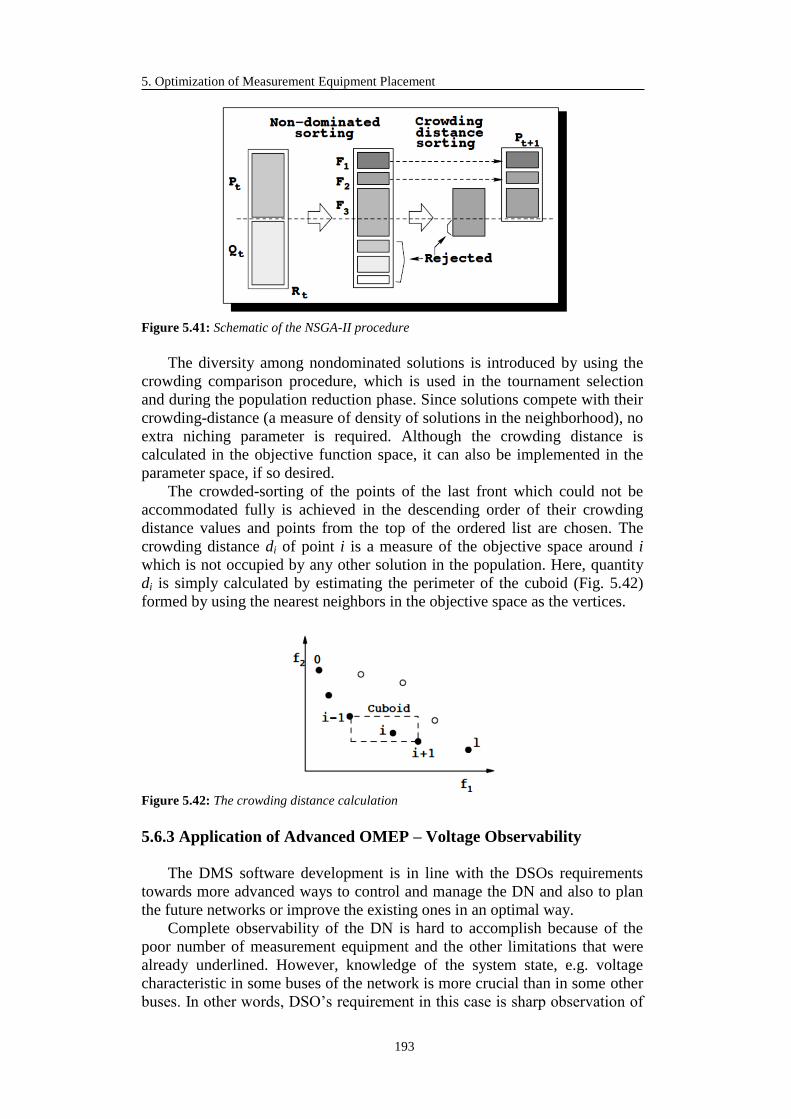
5. Optimization of Measurement Equipment Placement
193
Figure 5.41: Schematic of the NSGA-II procedure
The diversity among nondominated solutions is introduced by using the
crowding comparison procedure, which is used in the tournament selection
and during the population reduction phase. Since solutions compete with their
crowding-distance (a measure of density of solutions in the neighborhood), no
extra niching parameter is required. Although the crowding distance is
calculated in the objective function space, it can also be implemented in the
parameter space, if so desired.
The crowded-sorting of the points of the last front which could not be
accommodated fully is achieved in the descending order of their crowding
distance values and points from the top of the ordered list are chosen. The
crowding distance di of point i is a measure of the objective space around i
which is not occupied by any other solution in the population. Here, quantity
di is simply calculated by estimating the perimeter of the cuboid (Fig. 5.42)
formed by using the nearest neighbors in the objective space as the vertices.
Figure 5.42: The crowding distance calculation
5.6.3 Application of Advanced OMEP – Voltage Observability
The DMS software development is in line with the DSOs requirements
towards more advanced ways to control and manage the DN and also to plan
the future networks or improve the existing ones in an optimal way.
Complete observability of the DN is hard to accomplish because of the
poor number of measurement equipment and the other limitations that were
already underlined. However, knowledge of the system state, e.g. voltage
characteristic in some buses of the network is more crucial than in some other
buses. In other words, DSO’s requirement in this case is sharp observation of

5.6 Advanced Optimization of Measurement Equipment Placement Method
194
voltages in some buses and a good (permissible) observation of the remaining
ones.
The voltage observability requirement can be further explained observing
the Fig. 5.43. It is obvious that the best observability is obtained by
introducing the measurement equipment in all the buses of the network. For
the DSO, knowledge of the voltage might be more important in buses 1 and 3
because bus 1 is the source of DN i.e. first bus of the distribution feeder and
bus 3 contains generation unit. But what happens if we cannot install the
equipment in both buses 1 and 3? We need to use OMEP algorithm. In this
case, however, there are two sets of buses – buses 1 and 3 where the objective
is Δ𝑉1,3 → 0 (Δ𝑉𝑖 =𝑉𝑖𝑚−𝑉𝑖
𝑒𝑠𝑡
𝑉𝑖𝑚 ) while Δ𝑉2,4 should be reduced as much as
possible.
Figure 5.43: Voltage observability in DN
It is obvious that this is multi-objective problem. It can be solved by
adapting it into single-objective problem or using the developed NSGA-II
algorithm that gives the Pareto-optimal front in a single run.
In this study, one classical approach – weighted single objective GA and
NSGA-II have been compared. Weighted single objective function was
constructed in a following manner:
𝐹𝑘 = 𝑤1 Δ𝑉𝑖 + 𝑤2 Δ𝑉𝑗 (5.27)
where:
𝐹𝑘 fitness of the k-th individual of the population;
𝑤1, 𝑤2 weights of the objectives;
Δ𝑉𝑖 relative error (voltage objective) of the i-th measurement
configuration;
Δ𝑉𝑗 relative error (voltage objective) of the j-th measurement
configuration;
𝑖 index of the set of buses where exact observability is required;
𝑗 index of the set of buses where permissible observability is required.
There are two objectives of this study:
1. To find the optimal locations taking into account both objectives or more
precisely in this case – sets of data
2. To compare the quality of NSGA-II solution with the classical GA.
5.6.3.1 Voltage Observability: 29-bus DN Test
First test case is the small test DN (depicted in Fig. 5.17) which was
modified by adding 2 more generation plants – in buses 15 and 22. First set of
buses includes the terminal buses of all the feeders (5, 16, 21, 28, and 29) and

5. Optimization of Measurement Equipment Placement
195
buses with the generation plants (10, 15 and 22). The rest of the buses
(excluding the buses with measurements previously installed – primary TS
buses) are the members of the second set.
Algorithms settings are the following:
Number of generation cycles is 200;
Size of the population is 200;
5 measurement units;
Successive changes of w1 and w2 by 0.1 steps (i.e. running classical GA
eleven times starting from w1 = 1 and w2 = 0 until w1 = 0 and w2 = 1) to
obtain the complete Pareto-optimal front as explained in the previous
subchapter.
Resulting Pareto – optimal front using both weighted GA approach and
NSGA-II approach are shown in Fig. 5.44.
Figure 5.44(a): Comparison of weighted and NSGA-II approach for voltage observability
(29-bus DN)
Figure 5.44(b): Comparison of weighted and NSGA-II approach for voltage observability
(29-bus DN)
NSGA – II
Weight method
NSGA – II
Weight method

5.6 Advanced Optimization of Measurement Equipment Placement Method
196
It can be seen from the Fig. 5.44(a) that using NSGA-II algorithm ensured
high-quality solution compared to classical GA. Pareto-optimal front obtained
in this way corresponds to the solution given by 11 successive runs of
classical GA. Two best individuals (i.e. rank 1 individuals with infinite
crowding distance) are exactly the same whether obtained running NSGA-II
algorithm once or with critical values of weighted classical GA i.e. first and
eleventh run (w1 = 1, w2 = 0 and w2 = 0, w1 = 1)
Fig. 5.44(b) offers the zoomed view of the Fig. 5.44(a) in order to further
exam and conclude that the Pareto-optimal fronts really correspond one to
another.
This is a very important conclusion as it offers the possibility to use
NSGA-II algorithm for Advanced OMEP family of problems. It is ensured
that the quality of the results obtained this way will be preserved. This is also
important from the computational point of view. One simulation with the
NSGA-II algorithm takes approximately the same amount of time as one
simulation with the weighted method [125] so the solution is obtained 11
times faster. This is especially important for large-scale realistic DNs.
To sum up, the average simulation time with the weighted approach is 28
minutes per run, which summed up means 11∙28 min = 308 min, while for the
completion of NSGA-II simulation, only 28.2 min is required, on Intel(R)
Core(TM) i7-2600 CPU @ 3.4 GHz and 8 GB of RAM per run.
5.6.3.2 Voltage Observability: 69-bus DN Test
Second test is used as the confirmation test for the conclusions made on
small network. Therefore, the cause of the test is the same. It is necessary to
conduct voltage observability study with two sets and compare the results
obtained with classical weighted GA and special multi-objective NSGA-II
algorithm.
Test network is depicted in Fig. 5.24 and its properties were previously
described. First set of buses includes the terminal buses of all the feeders (27,
35, 46, 50, 52, 65, 67 and 69) and buses with the generation plants (9, 17, 20,
30, 41, 43, 57, 59 and 62). The rest of the buses (excluding the buses with
measurements previously installed – primary TS buses) are the members of
the second set.
Algorithms settings are the following:
Number of generation cycles is 260;
Size of the population is 200;
10 measurement units;
Successive changes of w1 and w2 by 0.1 steps (i.e. running classical GA
eleven times starting from w1 = 1 and w2 = 0 until w1 = 0 and w2 = 1) to
obtain the complete Pareto-optimal front.
Resulting Pareto – optimal front using both weighted GA approach and
NSGA-II approach are shown in Fig. 5.45.

5. Optimization of Measurement Equipment Placement
197
Figure 5.45: Comparison of weighted and NSGA-II approach for voltage observability (69-
bus DN)
It can be seen from the Fig. 5.44 that the conclusions of the previous tests
were confirmed also with the bigger DN.
To sum up, the average simulation time with the weighted approach is 2 h
38 min per run, which summed up means 11∙2 h 38 min ≈ 29 h, while for the
completion of NSGA-II simulation, only 2h 40 min is required, on Intel(R)
Core(TM) i7-2600 CPU @ 3.4 GHz and 8 GB of RAM per run.

198
CHAPTER 6
6. Conclusion and Future Work
6.1 Conclusion
Power systems of today are the subject of one of the biggest structural,
functional but also ethical change since the massive electrification started.
From vertically oriented, they are changing to Smart Grids. From big
concentrated generation plants, the global movement is towards dispersed
generation plants that are mostly connected to MV and LV networks. This,
indeed, changes the entire idea of not only the structure of power network but
also its management. Many new technologies are introduced in power
systems; they are interconnected with information technology now more than
ever because the stakes are higher – information about the status of the
network needs to be propagated in the optimal way and new management
strategies need to be developed and used. Power systems are also going
through ethical changes because of the rise of the consciousness about the
planet and depletion of conventional energy sources.
In this massive movement, distribution systems are probably
revolutionized the most as the major part of changes takes place here.
Motivated by the need to improve distribution system management, operation
and planning, this dissertation offers detailed mathematical models and
applications of distribution system state estimation and optimization of
measurement equipment placement. As discussed in the introduction, fields
covered by this dissertation already are and will increasingly continue to be in
the center of DMS software solutions as they are crucial for smart grid
environment.
The main empirical findings of this dissertation are concentrated in
Chapter 4 – Distribution System State Estimation and Chapter 5 –
Optimization of Measurement Equipment Placement.
The first motivation to develop the DSSE was triggered by limited
success in applying transmission system state estimation approach to

6. Conclusion and Future Work
199
distribution environment; and additionally, specific approaches that have been
developed for distribution systems experienced problems related to limitations
of the distribution grids.
The second motivation is due to the fact that the increased penetration of
dispersed generation is one of the main contributors to the new management
mechanisms that are being developed. To improve the hosting capacity of the
DN and to reduce the impact of DG on the regulation requirements of the bulk
power system, the DG has to provide ancillary services (to solve local and
global issues – frequency, reserve, voltage regulation, congestion
management). Therefore the distribution system will assume the role of DSO.
Premise of this is the knowledge of the network. For this reason, SE applied to
DN is a main tool to improve the effects of DG penetration.
The aim was to develop computationally fast, robust and adaptable DSSE
solution. For this reason, two SE modules have been developed and tested on
vast number of test DNs and on different scenarios. While the Simplified SE
can be used in most of the DN of today and provide satisfactory results with
impressive computational speed, Advanced SE is aimed for DNs with more
measurement points and it incorporates the power flow equations as
constraints. It has lower speed than the simplified module, but it provides
more accurate results in cases with high penetration of DG.
Both modules significantly improve the observability of the DN with a
little information currently present and are suitable for real-time operational
applications, which is a huge leap forward in DMS technology and reliable
base for numerous functionalities that rely on SE. Practicability and reliability
of the proposed SE is proven by the fact that it is operational in a number of
nationwide DNs: Smart Grid ACEA, ASM – Terni, Grid4EU – ENEL (co-
founded by the EU under the 7th
Framework Program), HERA – Modena (in
operation from June 2014), and A2A – Milan (finalizing stage) [149].
On the other side, planning of the DNs has to be conducted much more
carefully than in the past and therefore optimization procedures have to be
enforced in the early stages of development of new networks. Chapter 5 of
this dissertation is concerned with a very important planning functionality –
optimization of the measurement equipment placement. Having elaborated on
the fact that the knowledge of the network state is crucial for its operation, it
is not hard to understand why the installation of the new measurement
equipment has a central part in planning of the new or improvement of the
existing DNs.
The proposed solution strongly reckons on genetic algorithms that have
proven to possess good properties with large-scale problems like this one.
Many different implementation approaches have been developed, tested and
compared on large number of realistic test DNs for this dissertation and the
best approach is recorded. Apart from the fact that the OMEP algorithm
provides (sub)optimal solutions for all the tested systems, it is also robust,
highly modular and easily implementable in DMS solutions.
One another empirical finding of this dissertation is the general design
strategy of measurement equipment placement in DNs. Important guidelines
for the planners of the DNs regarding the good practices of measurement
placement are provided and backed up by a large number of tests.
Lastly, multi-objective genetic algorithm has been developed and tested
with the specific DSO requirements in order to show the broad applicability of

6.2 Future Work
200
the proposed OMEP solution. There are many more specific DSO
requirements regarding planning of future networks that can be exploited with
the proposed algorithm.
6.2 Future Work
This work opens several avenues for further investigation. The first
involves the improvements of the developed DSSE software solution. As this
solution is already used in a number of distribution control centers, the
particularities of specific networks bring out the possible points of
improvement of the solution itself as it needs to be globally operational, i.e.
on a vast number of different realistic DNs. The developers of this
functionality are already improving the algorithm in order to offer better
estimate of the network state and enable even better observability which is, as
many times underlined, crucial for other automated actions necessary in DNs.
Larger number of modern measurement equipment will also offer better
utilization of DSSE software solution. This is where the second functionality
described in this dissertation will find its place. SE techniques enable just the
limited performance if the number of the measurement equipment is poor. The
future field of study would be further implementation of the Advanced OMEP
problem to different DSOs requirements.
One of the avenues is also further utilization of Advanced OMEP
algorithm to similar families of problems. Exploitation of the algorithm can
offer multiple breakthroughs in similar fields.
Of course, work can be done in continuous improvement of the algorithm
itself, proposing other types of genetic operators and further interpretation of
the results in order to make a generalized pattern for measurement equipment
placement in distribution systems. These a priori solutions could also fasten
the generation process by diminishing the number of generations necessary
for the solution of the problem.

Bibliography
201
Bibliography
[1] National Academy of Engineering, "Greatest Engineering Achievements of the 20th
Century", 2014. [Online]. Available: http://www.greatachievements.org/.
[2] Council of European Energy Regulators ASBL, "Guidelines of Good Practice on
Estimation of Costs due to Electricity Interruptions and Voltage Disturbances",
Brussels, 2010. [Online]. Available:
http://www.ceer.eu/portal/page/portal/EER_HOME/EER_PUBLICATIONS/
[3] P. Donalek, R. Farmer, N. Hatziargyriou, I. Kamwa, P. Kundur, N. Martins, J.
Paserba, P. Pourbeik, J. Sanchez-Gasca, R. Schulz, A. Stankovic, C. Taylor, V.
Vittal, G. Andersson, "Causes of the 2003 major grid blackouts in North America
and Europe and recommended means to improve system dynamic performance",
IEEE TRANSACTIONS ON POWER SYSTEMS, vol. 20, no. 4, pp. 1922-1928,
2005.
[4] The Board of Directors of Enel SpA, "Preliminary Consolidated Results for 2013",
ENEL, Rome, 2014. [Online]. Available:
https://www.enel.com/en-gb/media/press_releases/
[5] V. P. Morano, "Aggregated Management of Distributed Energy Resources: Impact
on the Electrical System", 2014. [Online]. Available:
http://www.iit.upcomillas.es/pfc/resumenes/538a238fbf55a.pdf
[6] Eurelectric, "Active Distribution System Management", Eurelectric, 2013. [Online].
Available: http://www.eurelectric.org
[7] M. R. Mozayyani, Z. Modarres, H. S. Farmad, "Challenges Of Implementing Active
Distribution System Management", in CIRED Workshop, Rome, 11-12 June 2014.
[8] The European Parliament and the council of the European Union, "Directive
2009/28/EC on the promotion of the use of energy from renewable sources",
Official Journal of the European Union, pp. 1-47, 2009.
[9] The European Parliament and the Council of the European Union, "Directive
2012/27/EU on energy efficiency", Official Journal of the European Union, pp. 1-
56, 2012.
[10] The European Parliament and the Council of the European Union, "Directive
2009/72/EC concerning common rules for the internal market in electricity",
Official Journal of the European Union, pp. 1-39, 2009.
[11] R. van Gerwent, Distributed Generation and Renewables, Copper Development
Association, Brussels, 2006.
[12] P. Birkner, Smart Grid in Practice, Mainova, Frankfurt, 2012. [Online]. Available:
http://phoenix-forums.com/
[13] European Distribution Systems Operators for Smart Grids, "Flexibility: The role of
DSOs in tomorrows' electricity market", European Distribution Systems Operators
for Smart Grids, Brussels, 2014. [Online]. Available:
http://www.edsoforsmartgrids.eu/
[14] E. Binda Zane, R. Bruckmann, D. Bauknecht, F. Jirous, R. Piria, N. Trennepohl, J.
Bracker, R. Frank, J. Herling, "Integration of Electricity from Renewables to the
Electricity Grid and to the Electricity Market", Ecleron, Berlin, 2012. [Online].
Available: http://www.oeko.de
[15] Eurelectric, "RES Integration and Market Design", Eurelectric, Brussels, 2011.
[Online]. Available: http://www.eurelectric.org
[16] Autorita per l'energia elettrica e il gas, "Consultazioni", 1 August 2013. [Online].
Available: http://www.autorita.energia.it/it/index.htm.

Bibliography
202
[17] Expert Group for Regulatory Recommendations for Smart Grid Deployment,
"Options on Handling Smart Grids Data", Expert Group for Regulatory
Recommendations for Smart Grid Deployment, Brussels, 2013. [Online]. Available:
http://ec.europa.eu/energy/
[18] Union Fenosa Distribucion & other entities, "Development of technological
solutions for the Spanish Electricity Network of 2025", Union Fenosa Distribucion
& other entities, Madrid, 1012. [Online]. Available:
http://www.gasnaturalfenosa.com/es/1285338501612/inicio.html
[19] A. Becker, J. Schmiesing, E. Wehrmann, B. Werther, "Voltage control in low
voltage systems with controlled low voltage Transformer (CLVT)", in CIRED
Workshop, Lisbon, 29-30 May 2012.
[20] M. Zdrallek, J. Schmiesing, M. Schneider, H. H. Thies, "Future Structure of Rural
Medium-voltage Grids for Sustainable Energy Supply", in CIRED Workshop,
Lisbon, 29-30 May 2012.
[21] F. Gangale, G. Fulli, M. S. Jimenez, I. Onyeji, A. Colta, I. Papaioannou, A.
Mengolini, C. Alecu, T. Ojala, I. Maschio, V. Giordano, "Smart Grid Projects in
Europe: Lessons learned and current developments", Publications Office of the
European Union, Luxembourg, 2013. [Online]. Available: http://ses.jrc.ec.europa.eu
[22] F. C. Schweppe, J. Wildes, "Power System Static-State Estimation, Part I: Exact
Model", IEEE Transactions on Power Apparatus and Systems, vol. 89, no. 1, pp.
120-125, 1970.
[23] F. C. Schweppe, D. B. Rom, "Power System Static-State Estimation, Part II:
Approximate Model", IEEE Transactions on Power Apparatus and Systems, vol.
89, no. 1, pp. 125-130, 1970.
[24] F. C. Schweppe, "Power System Static-State Estimation, Part III: Implementation",
IEEE Transactions on Power Apparatus and Systems, vol. 89, no. 1, pp. 130-135,
1970.
[25] A. Abur, A. G. Exposito, Power System State Estimation - Theory and
Implementation, New York: Marcel Dekker, Inc, 2004.
[26] A. J. A. S. Costa, Power System State Estimation: Orthogonal Methods for
Estimation, Bad Data Processing and Techniques for Topological Observability,
Waterloo: University of Waterloo, 1981. [Online]. Available: https://www.wpi.edu
[27] D. Denzel, G. Schellstedem, F. Aschmoneit, "Optimal Power System Static State
Estimation" in Proceedings of the 5th Power Systems Computation Conference,
Cambridge, 1-5 September 1975.
[28] A. Monticelli, P. Abreu, A. Garcia, "Fast Decoupled State Estimator and Bad Data
Processing" IEEE Trans. on Power Apparatus and Systems, vol. 98, no. 5, pp.
1645-1652. 2007.
[29] K. L. Lo, P. S. Ong, R. D. McColl, A. M. Moffatt, J. L. Sulley, "Development of a
Static State Estimation Part I: Estimation and Bad data Suppression", IEEE
Transactions on Power Apparatus and Systems, vol. 7, no. 3, pp. 1378-1385, 1983.
[30] A. Garcia, A. Monticelli, "Reliable bad data processing for real-Time state
Estimation", IEEE Transactions on Power Apparatus and Systems, vol. 102, no. 5,
pp. 1126-1139, 1983.
[31] F. C. Schweppe, J. Kohlas, A. Fiechter, E. Handschin, "Bad data analysis for power
system state estimation," IEEE Transactions on Power Apparatus and Systems, vol.
94, no. 2, pp. 329-337, 1975.
[32] S. Wang, E. Yu, N. Xiang, "A New Approach for Detection and Identification of
Multiple Bad Data in Power System State Estimation", IEEE Transactions on
Power System State Estimation, vol. 101, no. 2, pp. 454-462, 1982.
[33] T. Van Cutsem, L. Mili, M. Ribbens-Pavella, "Hypothesis testing identification: a
new method for bad data analysis in power system state estimation", IEEE
Transactions on Power Apparatus and Systems, vol. 101, no. 2, pp. 3239-3252,
1984.
[34] K. A. Clements, P. W. Davis, G. R. Krumpholz, "Power system observability: a

Bibliography
203
practical algorithm using network observability", IEEE Transactions on Power
Apparatus and Systems, vol. 99, no. 4, pp. 1534-1542, 1980.
[35] A. Monticelli, F. F. Wu, "Network observability: identification of observable
islands and measurement placement - parts 1 and 2", IEEE Transactions on Power
Apparatus and Systems, vol. 103, no. 5, pp. 1035-1048, 1985.
[36] G. Golub, V. Klema, G. W. Stewart, "Rank degeneracy and least squares
problems", Stanford University, Stanford, 1976. [Online]. Available:
http://www.nber.org/papers/w165
[37] K. A. Clements, B. F. Wollenberg, "An Algorithm for Observability Determination
in Power System State Estimation", in IEEE Summer Power Meeting, San
Francisco, 20-25 July 1975.
[38] T. V. Cutsem, P. J. Gailly, "A simple algorithm for power system observability
analysis and related functions", in IFAC Symposium on Control Applications to
Power System Security, Florence, 5-8 Septmeber 1983.
[39] G. R. Krumpholz, P. W. Davis, K. A. Clements, "Power system state estimation
with measurement deficiency - an algorithm that determines the maximal
observable subnetwork", IEEE Transactions on Power Apparatus and Systems, vol.
101, no. 9, pp. 3044-3052, 1982.
[40] A. Simoes-Costa, A. Mandel, V. H. Quintana, "Power system topological
observability using a direct graph - theoretic approach", IEEE Transactions on
Power Apparatus and Systems, vol. 101, no. 3, pp. 617-626, 1982.
[41] A. Shaifu, V. Thornley, N. Jenkins, G. Strbac, A. Maloyd, "Control of Active
Networks", in 18th International Conference on Electricity Distribution, Turin, 6-9
June 2005.
[42] K. A. Clements, G. R. Krumpholz, P. W. Davis, J. W. Gu, "The solution of ill-
conditioned power system state estimation problems", IEEE Transactions on Power
Apparatus and Systems, vol. 102, no. 10, pp. 3473-3480, 1983.
[43] C. A. F. Murari, F. F. Wu, A. Monticelli, "A hybrid state estimator: solving normal
equations by orthogonal transformations", IEEE Transactions on Power Apparatus
and Systems, vol. 104, no. 12, pp. 3460-3468, 1985.
[44] N. Peterson, E. Adrian, F. Aschmoneit, "State estimation with equality constraints",
in Power Industry Computer Applications Conference, Toronto, 24-27 May 1977.
[45] D. S. Watkins, Fundamentals of Matrix Computations, 2nd edition, New York:
Wiley, 2002.
[46] R. Hoffman, "Practical State Estimation for Electric Distribution Networks", in
Power Systems Conference and Exposition, Atlanta, 15-20 March 2006.
[47] P. P. Barker, R. W. De Mello, "Determining the impact of distributed generation on
power systems: Part I - Radial Distribution Systems", in IEEE Power Engineering
Society Summer Meeting, Seattle, 16-20 July 2000.
[48] F. C. Schweppe, J. Wildes, "Power system static state estimation - Part I, II & III",
IEEE Transaction on Power Apparatus and Systems, vol. 89, no. 1, pp. 120-135,
1970.
[49] R. Critchley, E. Catz, M. Bazargan, P. Favre-Perrod, "New participants in
smartgrids and associated challenges in the transition towards the grid of the
future", in IEEE Powertech, Bucharest, 28 June - 2 July 2009.
[50] M. E. Baran, A. W. Kelley, "State estimation for real-time monitoring of
distribution systems", IEEE Transactions on Power Systems, vol. 9, no. 3, pp. 1601-
1609, 1994.
[51] S. Civanlar, J. J. Grainger, "Forecasting distribution feeder loads: modeling and
application to volt/VAr control", IEEE Transactions on Power Delivery, vol. 3, no.
1, pp. 255 - 264 , 1988.
[52] A. J. Wood, B. F. Wollenberg, Power Generation, Operation and Control, New
York: John Wiley & Sons, 1978.
[53] M. E. Baran, A. W. Kelley, "A branch-current-based state estimation method for

Bibliography
204
distribution systems", IEEE Transactions on Power Systems, vol. 10, no. 1, pp. 483-
491, 1995.
[54] J. H. Teng, W. H. E. Liu, C. N. Lu, "Distribution System State Estimation", IEEE
Transactions on Power Systems, vol. 10, no. 1, pp. 229-240, 1995.
[55] D. I. H. Sun, Distribution System Loss Analysis and Optimal Planning - PhD
Dissertation, Arlington: University of Texas, 1980. [Online]. Available:
www.uta.edu
[56] K. Li, "State estimation for power distribution system and measurement impact",
IEEE Transactions on Power Systems, vol. 11, no. 2, pp. 911-916, 1996.
[57] A. P. Sakis Meliopoulos, F. Zhang, "Multiphase Power Flow and State Estimation
for Power Distribution Systems", IEEE Transactions on Power Systems, vol. 11, no.
2, pp. 939-946, 1996.
[58] S. Lee, K. Vu, C.C. Liu, "Loss Minimization of Distribution Feeders: Optimality
and Algorithms", IEEE Transactions on Power Delivery, vol. 4, no. 2, pp. 1281-
1289, 1989.
[59] J. Jerome, "Network observability and bad data processing algorithm for
distribution networks", in Power Engineering Society Summer Meeting, Vancouver,
15-19 July 2001.
[60] B. C. Pal, R. A. Jabr, R. Singh, "Choice of estimator for distribution system state
estimation", IET Generation, Transmission and Distribution, vol. 3, no. 7, pp. 666-
678, 2008.
[61] S. S. Blackman, Multiple target tracking with radar applications, Dedham: Artech
House, Inc., 1986.
[62] H. Singh, F. L. Alvarado, "Weighted Least Absolute Value state estimation using
interior point methods", IEEE Transactions on Power Systems, vol. 9, no. 3, pp.
1478-1484, 1994.
[63] P. J. Huber, Robust Statistics, New York: John Wiley & Sons, 1981.
[64] T. Kozubowski, K. Podgorski, S. Kotz, The Laplace Distribution and
Generalizations, Basel: Birkhäuser, 2001.
[65] S. K. Salman, S. F. Tan, "Investigation into Protection of Active Distribution
Network with High Penetration of Embedded Generation Using Radial and Ring
Operation Mode", Proceedings of the 41st International Universities Power
Engineering Conference UPEC '06, vol. 3, pp. 841-845, Newcastle-upon-Tyne, 6-8
September 2006.
[66] M. Bigoloni, I. Rochira, M. Rodolfi, F. Zanellini, C. Bovo, V. Ilea, M. M. Subasic,
Merlo, G. Monfredini, R. Bonera, M. Arigoni, "The InGrid project and the
evolution of supervision & control systems for Smart Distribution System
management", in Convegno Nazionale AEIT, Mondello, 3-5 October 2013.
[67] I. Rochira, M. Bignoli, M. Rodolfi, F. Zanellini, C. Bovo, M. Merlo, V. Ilea, G.
Monfredini, M. Subasic, R. Bonera, "Smart distribution system the ingrid project
and the evolution of supervision & control systems for smart distribution system
management", in AEIT Annual Conference, Mondello, 3-5 October 2013.
[68] A .Berizzi, C. Bovo, V. Ilea, M. Merlo, G. Monfredini, M. Subasic, C. Arrigoni, F.
Zanellini, F. Corti, I. Rochira, "Advanced Functions for DSOs Control Center", in
IEEE Powertech, Grenoble, 16-20 June 2013.
[69] C. Bovo, V. Ilea, M. Subasic, F. Zanellini, C. Arrigoni, R. Bonera, "Improvement of
Observability in Poorly Measured Distribution Networks", PSCC 2014, Wroclaw,
17-23 August 2014.
[70] D. L. Lubkeman, M. J. Downey, R. H. Jones, A. K. Ghosh, "Distribution circuit
state estimation using a probabilistic approach", IEEE Transactions on Power
Systems, vol. 12, no. 1, pp. 45-51, 1997.
[71] A. Abur, B. Gou, "An Improved Measurement Placement Algorithm for Network
Observability", IEEE Transactions on Power Systems, vol. 16, no. 4, pp. 819-824,
2001.

Bibliography
205
[72] S. Premrudeepreechacharn, C. Rakpenthai, "An Optimal PMU Placement Method
Against Measurement Loss and Branch Outage", IEEE Transactions on Power
Delivery, vol. 22, no. 1, pp. 101-107, 2007
[73] J. Z. A. W. K. M. E. Baran, "Meter Placement for Real-Time Monitoring of
Distribution Feeders", IEEE Transactions on Power Systems, vol. 11, no. 1, pp.
332-337, 1996.
[74] N. Schulz, H. Wang, "A Revised Branch Current-Based Distribution System State
Estimation Algorithm and Meter Placement Impact", IEEE Transactions on Power
Systems, vol. 19, no. 1, pp. 207-213, 2004.
[75] F. Pilo, G. Pisano, S. Sulis, C. Muscas, "Optimal Placement of Measurement
Devices in Electric Distribution Systems", in Instrumentatiton and Measurement
Technology Conference IMTC 2006, Sorrento, 24-27 April 2006.
[76] N. Jenkins, G. Strbac, A. Shafiu, "Measurement location for state estimation of
distribution networks with generation", IEEE Proceedings on Generation,
Transmission and Distribution, vol. 152, no. 2, pp. 240-246, 2005.
[77] B. Pal, R. Vinter, R. Singh, "Measurement Placement in Distribution System State
Estimation", IEEE Transactions on Power Systems, vol. 24, no. 2, pp. 668-675,
2009.
[78] M. Begovic, B. Milosevic, "Nondominated Sorting Genetic Algorithm for Optimal
Phasor Measurement Placement", IEEE Transactions on Power Systems, vol. 18,
no. 1, pp. 69-75, 2003.
[79] D. E. Goldberg, Genetic Algorithms in Search, Optimization, and Machine
Learning, Reading: Addison-Wesley, 1989.
[80] B. C. Pal, R. A. Jabr, R. B. Vinter, R. Singh, "Meter Placement for Distribution
System State Estimation: An Ordinal Optimization Approach", IEEE Transactions
on Power Systems, vol. 26, no. 4, pp. 2328-2335, 2011.
[81] U. Derigs, Optimization and Operations Research, Cologne: Eolss Publishers
Company Limited, 2009.
[82] P. M. Pardalos, D.Z. Du, R. L. Graham, "Combinatorial optimization", in
Handbook of Combinatorics, Cambridge, MA, MIT Press, 1995, pp. 1541-1597.
[83] A. Schrijver, "A course in combinatorial optimization," TU Delft, Delft, 2000.
[84] D. S. Johnson, M. R. Garey, Computers and Intractability; A Guide to the Theory of
NP-Completeness, New York: W. H. Freeman & Co., 1990.
[85] K. Deb, "Multi-objective optimization using evolutionary algorithms", in Multi-
objective optimization, New York, John Wiley & Sons, 2001, pp. 13-46.
[86] D. B. Fogel, Evolutionary Computation: The Fossil Record, Piscataway, NJ: Wiley-
IEEE Press, 1998.
[87] A. Owens, M. Walsh, L.J. Fogel, Artificial Intelligence Through Simulated
Evolution, New York: Wiley and Sons, 1966.
[88] I. Rechenberg, Evolutionsstrategie: Optimierung technischer Systeme nach
Prinzipien der biologischen Evolution, Stuttgart: Frommann-Holzboog Verlag,
1973.
[89] H. Schwefel, Numerische Optimierung von Computer - Modellen mittels der
Evolutionsstrategie, Basel: Birkhauser, 1977.
[90] J. Holland, Adaptation in Natural and Artificial Systems, Ann Harbor: University of
Michigan Press, 1975.
[91] Z. Michalewicz, Genetic Algorithms + Data Structures = Evolution Programs,
Berlin: Springer-Verlag, 1992.
[92] M. L. Cramer, "A representation for the adaptive generation of simple seqential
programs", in Proceedings of the First International Conference on Genetic
Algorithms, Hillsdale, NJ, 1-6 August 1985.
[93] J. R. Koza, Genetic Programming, Cambridge, MA: MIT Press, 1992.

Bibliography
206
[94] P. Moscato, "On Evolution, Search, Optimization, Genetic Algorithms and Martial
Arts: Towards Memetic Algorithms", California Institute of Technology, Pasadena,
CA, 1989.
[95] C. Cotta, P. Moscato, "A gentle introduction to memetic algorithms", Handbook of
Metaheuristics, Boston, MA, Kluwer Academic Publishers, 2003, pp. 105-144.
[96] R. E. Smith, "Diploid genetic algorithms for search in time varying environments",
in Annual Southeast Regional Conference of the ACM, New York, NY, 10-19 April
1987.
[97] C. R. Reeves, "Using genetic algorithms with small populations", in Proceedings of
the Fifth International Conference on Genetic Algorithms, San Mateo, CA, 1993.
[98] C. Cotta, "On the evolutionary inference of temporal boolean networks", in
Computational Methods in Neural Modeling, Berlin, Springer-Verlag, 2003, pp.
494-501.
[99] J. Grefenstette, C. Ramsey, "Case-based initialization of genetic algorithms", in
Proceedings of the Fifth International Conference on Genetic Algorithms, San
Mateo, CA, 1993.
[100] J. E. Baker, "Reducing bias and inefficiency in the selection algorithm", in
Proceedings of Second International Conference on Genetic Algorithms, Hillsdale,
NJ, 1987.
[101] D. L. Whitley, "Using reproductive evaluation to improve genetic search and
heuristic discovery", in Proceedings of Second International Conference on Genetic
Algorithms, Hillsdale, NJ, 1987.
[102] L. Thiele, T. Bickle, "A mathematical analysis of tournament selection", in
Proceedings of Sixth International Conference on Genetic Algorithms, San
Francisco, CA, 1995.
[103] D. Goldberg, K. Deb, "A comparative analysis of selection schemes used in genetic
algorithms", in Foundations of Genetic Algorithms, San Mateo, CA, Morgan
Kaufman Publishers, Inc., 1991, pp. 69-93.
[104] E. Cantu-Paz, "Order statistics and selection methods of evolutionary algorithms",
Information Processing Letters, vol. 82, no. 1, pp. 15-22, 2002.
[105] P. E. Raue, Z. Ruttkay, A.E. Eiben, "Genetic algorithms with multi-parent
recombination", in Lecture Notes in Computer Science, Berlin, Springer-Verlag,
1994, pp. 78-87.
[106] J. Troya, C. Cotta, "Information processing in transmitting recombination", Applied
Mathematics Letters, vol. 16, no. 6, pp. 945-948, 2003.
[107] N. J. Radcliffe, "The algebra of genetic algorithms", Annalss of Mathematics and
Artificial Intelligence, vol. 10, no. 4, pp. 339-384, 1994.
[108] G. Syswerda, "Uniform crossover in genetic algorithms", in Third International
Conference on Genetic Algorithms, San Mateo, CA, 1989.
[109] A. R. Reddy, G. Singh, K. Deb, "Optimal scheduling of casting sequence using
genetic algorithms", Journal of Materials and Manufacturing Processes, vol. 18,
no. 3, pp. 409-432, 2003.
[110] K. Deb, "An introduction to genetic algorithms", Sadhana, vol. 24, no. 4, pp. 293-
315, 1999.
[111] G. Rudolph, "Convergence analysis of canonical genetic algorithms", IEEE
Transactions on Neural Networks, vol. 5, no. 1, pp. 96-101, 1994.
[112] I. Wegener, T. Jensen, "On the utility of populations", in Proceedings of Genetic
and Evolutionary Computation Conference, San Mateo, CA, 2001.
[113] N. J. Radcliffe, "Forma analysis and random respectful recombination", in
Proceedings of Fourth International Conference on Genetic Algorithms, San Diego,
CA, 1991.
[114] L. Thiele, T. Blickle, "A Comparison of Selection Schemes used in Genetic
Algorithms", TIK-Zurich, Zurich, 1995, [Online]. Available: www.tik.ee.ethz.ch

Bibliography
207
[115] D. Whitley, "The genitor algorithm and selection pressure: Why rank-based
allocation of reproductive trials is the best", in Proceedings of 3rd International
Conference on Genetic Algorithms, Fairfax, 1989.
[116] V. Filipovic, "Fine-grained Tournament Selection Operator in Genetic Algorithms",
Computing and Informatics, vol. 22, no. 3, pp. 143-161, 2003.
[117] J. Baker, "Reducing Bias and Inefficiency in the Selection Algorithm", Proceedings
of the Second International Conference on Genetic Algorithms and their
Application, Hillsdale, NJ, 1987.
[118] R. Lingle, D. E. Goldberg, "Alleles, Loci and the Traveling Salesman Problem", in
Proceedings of the First International Conference on Genetic Algorithms, Pittsburg,
1985.
[119] K. Deep, H. Mebrahtu, "Novel GA for metropolitan stations of Indian railways
when modelled as a TSP", in International Journal of Combinatorial Optimization
Problems and Informatics, vol. 3, no. 1, pp. 47-69, 2012.
[120] R. Tiwari, R. Kala, A. Shukla, Real Life Applications of Soft Computing, Boca
Raton, FL: Taylor & Francis Group, 2002.
[121] K. Miettinen, Nonlinear Multiobjective Optimization, Boston: Kluwer, 1999.
[122] F. Luccio, F. P. Preparata, H. T. Kung, "On finding the maxima of a set of vectors",
Journal of the Association for Computing Machinery, vol. 22, no. 4, pp. 469-476,
1975.
[123] M. Ehrgott, Multicriteria Optimization, Berlin: Springer, 2000.
[124] S. Tiwari, K. Deb, "Omni-optimizer: A generic evolutionary algorithm for global
optimization", European Journal of Operations Research, vol. 185, no. 3, pp. 1062-
1087, 2008.
[125] K. Deb, A. Pratap, S. Agarwal, T. Meyarivan, "A fast and Elitist multi-objective
Genetic Algorithm: NSGA-II", IEEE Transactions on Evolutionary Computation,
vol. 6, no. 2, pp. 182-197, 2002.
[126] Eurelectric, "Power Distribution in Europe - Facts and Figures", Eurelectric, 2013.
[Online]. Available: http://www.eurelectric.org
[127] J. W. Chinneck, Practical Optimization: A Gentle Introduction, Ottawa, Carleton
University, 2004. [Online]. Available: http://www.sce.carleton.ca
[128] D. Bertsimas, I. Popescu, "Optimal Inequalities in Probability Theory: A Convex
Optimization Approach", Society for Industrial and Applied Methematics, vol. 15,
no. 3, pp 780-804, 2005
[129] K. Deb, "Multi-Objective Optimization Using Evolutionary Algorithms: An
Introduction", KanGAL Report, Kanpur, 2011. [Online]. Available:
http://www.iitk.ac.in
[130] E. Alba, C. Cotta, "Evolutionary Algorithms", Universidad de Malaga, Malaga,
2004. [Online]. Available: www.lcc.uma.es
[131] Terna, "Piano di sviluppo 2014 (in Italian)," Rome, 2013. [Online]. Available:
www.terna.it
[132] EirGrid, "Winter Outlook 2013-2014," Belfast, 2013. [Online]. Available:
www.eirgrid.com
[133] F. Coffele, M. Dolan, C. Booth, G. Ault, G. Burt, "Coordination of protection and
active network management for smart distribution networks", in CIRED Workshop,
Lisbon, 29-30 May 2012.
[134] Eurelectric, "Active Distribution System Management - A key tool for the smooth
integration of distributed generation", Eurelectric, 2013. [Online]. Available:
http://www.eurelectric.org
[135] D. Pudjianto, M. Castro, G. Strbac, E. Gaxiola, "Transmission infrastructure
investment requirements in the future European low carbon electricity sytem",
International Conference on the European Energy Market, Stockholm, 27-31 May
2013

Bibliography
208
[136] F. C. Schweppe, D. B. Rom, "Power system static state estimation, part 2:
approximate model", IEEE Transactions on Power Apparatus and Systems, vol. 89,
no. 1, pp. 125-130, 1970.
[137] International Electrotechnical Comission, "International Standard IEC60909", IEC,
Geneva, 2001.
[138] The Department of Mathematical Sciences at The University of Alabama in
Huntsville, "The Chi-Square Distribution", [Online]. Available:
http://www.math.uah.edu/stat/special/ChiSquare.html
[139] U. N. Khan, "Impact of Distributed Generation on Distributed Network", University
of Technology, Wroclaw, 2008 [Online]. Available: http://www.dwm.pwr.wroc.pl
[140] R. D. Zimmerman, C. E. Murillo-Sánchez & D. Gan, "MATPOWER - A MATLAB
Power System Simulation Package", Power Systems Engineering Research Center -
Arizona State University, [Online].
Available: http://www.pserc.cornell.edu//matpower/#docs.
[141] M. Merlo, N. Scordino, F. Zanellini, "Optimal Power Flow approach to manage
Dispersed Generation rise and passive load energy needs over distribution grid",
International Review of Electrical Engineering, vol. 8, no. 5, pp. 1482-1493, 2013.
[142] CEI EN 50160 Voltage Characteristics of Electricity Supplied by Public
Distribution Networks, May 2011
[143] G. Beaulineu, M. Bollen, S. Malgarotti, R. Ball, "Power Quality Indices and
Objectives", International Conference and Exhibition on Electricity Distribution -
CIRED, Turin, 6-9 June 2005.
[144] C. Bovo, M. Baioni, A. Berizzi, "Power quality impact of cogeneration modules in
urban networks", International Conference on Harmonics and Quality of Power,
Bergamo, 26-29 September 2010.
[145] L. Kumpulainen, K. Kauhaniemi, "Analysis of the impact od distributed generation
on automatic reclosing", IEEE Power System Conference and Exposition, Hong
Kong,10-13 October 2004.
[146] A. Berizzi, C. Bovo, M. Innorta, P. Marannino, "Multiobjective optimization
techniques applied to modern power systems", IEEE Power Engineering Society
Winter Meeting, vol. 3, Columbus, 28. January - 1. February 2004.
[147] A. H. Land, A. G. Doig, " An Automatic Method of Solving Discrete Programming
Problems", Econometrica, vol. 28, no. 3, pp. 497-520, 1960.
[148] R. K. Ahuja, T. L. Magnanti, J. B. Orlin, Network Flows: Theory, Algorithms, and
Applications, Prentice Hall, Upper Saddle River, 1993.
[149] A. Berizzi, C. Bovo, V. Ilea, M. Merlo, G. Monfredini, M. Subasic, M. Bigoloni, I.
Rochira, R. Bonera, "Architecture and functionalities of a smart Distribution
Management System", IEEE International Conference on Harmonics and Quality
of Power (ICHQP), Bucharest, 25-28 May, 2014.