ADVANCED REMOTE SENSING - uni-halle.deparadigmaps.geo.uni-halle.de/dynac/sites/default/files/yan-etal2012f… · An increasing number of researchers from a diverse set of academic

ADVANCEDREMOTESENSING

Terrestrial Information Extraction and Applications

Edited by

SHUNLIN LIANG

XIAOWEN LI

JINDI WANG

AMSTERDAM • BOSTON • HEIDELBERG • LONDONNEW YORK • OXFORD • PARIS • SAN DIEGO

SAN FRANCISCO • SYDNEY • TOKYO

Academic Press is an imprint of Elsevier

Academic Press is an imprint of ElsevierThe Boulevard, Langford Lane, Kidlington, Oxford OX5 1GB, UKRadarweg 29, PO Box 211, 1000 AE Amsterdam, The Netherlands225 Wyman Street, Waltham, MA 02451, USA525 B Street, Suite 1900, San Diego, CA 92101-4495, USA

First edition 2012

Copyright � 2012 Elsevier Inc. All rights reserved

No part of this publication may be reproduced, stored in a retrieval system or transmitted in any form or byany means electronic, mechanical, photocopying, recording or otherwise without the prior written permissionof the publisher. Permissions may be sought directly from Elsevier's Science & Technology Rights Departmentin Oxford, UK: phone (+44) (0) 1865 843830; fax (+44) (0) 1865 853333; email: [email protected] you can submit your request online by visiting the Elsevier web site at http://elsevier.com/locate/permissions, and selecting Obtaining permission to use Elsevier material

NoticeNo responsibility is assumed by the publisher for any injury and/or damage to persons or property as a matterof products liability, negligence or otherwise, or from any use or operation of any methods, products,instructions or ideas contained in the material herein. Because of rapid advances in the medical sciences, inparticular, independent verification of diagnoses and drug dosages should be made

Library of Congress Cataloging-in-Publication DataApplication submitted

British Library Cataloguing in Publication DataA catalogue record for this book is available from the British Library

For information on all Academic Press publicationsvisit our web site at store.elsevier.com

Printed and bound in USA

12 13 14 15 16 10 9 8 7 6 5 4 3 2 1

ISBN: 978-0-12-385954-9

Preface

Chapters Titles Authors

1 A Systematic View ofRemote Sensing

S. Liang, J. Wang,B. Jiang

PART 1 Data Processing Methods and Techniques

2 Geometric Processingand PositioningTechniques

X. Yuan, S. Ji, J. Cao,X. Yu

3 Compositing,Smoothing, and Gap-Filling Techniques

Z. Xiao

4 Data Fusion J. Zhang, J. Yang

5 Atmospheric Correctionof Optical Imagery

X. Zhao, X. Zhang,S. Liang

PART 2 Estimation of Surface Radiation Budget Components

6 Incident Solar Radiation X. Zhang, S. Liang

7 Broadband Albedo Q. Liu, J. Wen, Y. Qu,T. He, X. Zhang

(Continued)

As the technology of remote sensing hasadvanced over the last two decades, the scientificpotential of the data that it produces has greatlyimproved. To better serve society’s needs, theimmense amounts of aggregated satellite dataneed to be transferred into high-level productsin order to improve the predictive capabilitiesof global and regional models at different scalesand to aid in decision making through variousdecision support systems. A general trend isthat the data centers are distributing morehigh-level products rather than simply the rawsatellite imagery.

An increasing number of researchers froma diverse set of academic and scientific disci-plines are now routinely using remotely senseddata products, and the mathematical and phys-ical sophistication of the techniques used toprocess and analyze these data have increasedconsiderably. As a result, there is an urgentneed for a reference book on the advancedmethods and algorithms that are now availablefor extracting information from the hugevolume of remotely sensed data, which areoften buried in various journals and other sour-ces. Such a book should be highly quantitativeand rigorously technical; at the same time, itshould be accessible to students at the upperundergraduate and first-year graduate studentlevel.

To meet this critical demand, we have identi-fied and organized a group of active researchscientists to contribute chapters and sectionsdrawn from their research expertise. Althoughthis is an edited volume with multiple authors,

xi

it is well designed and integrated. The editorsand authors have made great efforts to ensurethe consistency and integrity of the text.

In addition to the introductory chapter, thisbook consists of five parts: (1) data processingmethods and techniques; (2) estimation of land-surface radiation budget components; (3) estima-tion of biophysical and biochemical variables;(4) estimation of water cycle components; and(5) high-level product generation and applica-tion demonstrations. The titles and authors ofthe individual chapters are as follows:


8 Land-SurfaceTemperature andThermal InfraredEmissivity

J. Cheng, H. Ren

9 Surface LongwaveRadiation Budget

W. Wang

PART 3 Estimation of Biophysical and BiochemicalVariables

10 Canopy BiochemicalCharacteristics

Z. Niu, C. Yan

11 Leaf Area Index H. Fang, Z. Xiao,Y. Qu, J. Song

12 Fraction of AbsorbedPhotosyntheticallyActive Radiation byGreen Vegetation

W. Fan, X. Tao

13 Fractional VegetationCover

G. Yan, X. Mu,Y. Liu

14 Vegetation Height andVertical Structure

G. Sun, Y. Pang,W. Ni, W. Huang,Z. Li

15 Above-GroundBiomass

G. Sun, W. Sun,S. Liang, Z. Zhang,E. Chen

16 Vegetation Productionin TerrestrialEcosystems

W. Yuan, Z. Chen

PART 4 Estimation of Water Balance Components

17 Precipitation Y. Liu, Q. Fu,X. Zhao, C. Dou

18 TerrestrialEvapotranspiration

K. Wang. R.Dickinson, Q. Ma

19 Soil Moisture Contents S. Liang, B. Jiang,T. He, X. Zhu

20 Snow WaterEquivalence

L. Jiang, J. Du,L. Zhang, J. Shi,J. Pan, C. Xiong

21 Water Storage Y. Liu, P. Song


PART 5 Production Generation and ApplicationDemonstrations

22 High-Level LandProduct Integration

D. Wang

23 Production and DataManagement Systems

S. Liu, X. Zhao

24 Land-Cover and Land-Use Changes

X. Zhu, S. Liang,B. Jiang

PREFACExii

Chapter 1 presents introductory material andprovides an overview of the book. From thesystem perspective, it briefly describes the essen-tial components of the remote-sensing system,ranging from platforms and sensors, modelingapproaches, and information extraction methodsto applications.

Part 1 includes four chapters on data process-ing. Chapter 2 is the only chapter that presentsthe methods and techniques for handlinggeometric properties of remotely sensed data.These include the calibration of systematicerrors, geometric correction, geometric registra-tion, digital terrain model generation, and digitalortho-image generation.

Chapter 3 seeks to reconstruct spatial andtemporal continuous high-quality imagery. Asthe temporal resolution of satellite observationsgreatly increases, images are more often contam-inated by clouds and aerosols that partially orcompletely block the surface information. Twogroups of techniques are presented. The firstgroup deals with composite methods for aggre-gating the fine temporal resolution (say, daily)to the coarse resolution (say, weekly or monthly),and the second discusses smoothing and gap-filling methods to eliminate the impacts of cloudsand aerosols at the same temporal resolution.

Chapter 4 introduces the basic principles andmethods of data fusion for integrating multipledata sources on the pixel basis, which have

PREFACE xiii

different spatial resolutions, and are acquiredfrom different spectra (optical, thermal,microwave). This chapter focuses mainly onlow-level data products. (The methods for inte-grating high-level products are introduced inChapter 22.)

Chapter 5 introduces methods for correctingthe atmospheric effects of aerosols and watervapor on the optical imagery. Other atmosphericcorrection methods are discussed in Chapter 8for thermal-IR data and in Part 4 for microwavedata.

Part 2 focuses on estimation of surface radia-tion budget components. The surface radiationbudget is characterized by all-wave net radiation(Rn) that is the sum of shortwave (Sn) and long-wave (Ln) net radiation

Rn ¼ Sn þ Ln ¼ ðsY� s[Þ þ ðLY� L[Þ¼ ð1� aÞSYþ ðLY� L[Þ

where SY is the downward shortwave radiation(discussed in Chapter 6), S[ is the upward short-wave radiation, a is the surface shortwavealbedo (discussed in Chapter 7), LY is the down-ward longwave radiation, and L[ is the upwardlongwave radiation. Longwave net radiation (Ln)can be also calculated by

Ln ¼ εLY� εsT4s

where s is the Stefan-Boltzmann constant, ε issurface thermal broadband emissivity, and Ts issurface skin temperature. Estimation of ε andTs is discussed in Chapter 8, and LY and Ln arecovered in Chapter 9.

Part 3 focuses on the estimation of biochem-ical and biophysical variables of plant canopy.Chapter 10 introduces the various methods forestimating plant biochemical variables, such aschlorophyll, water, protein, lignin and cellulose.The biophysical variables discussed in this bookinclude leaf area index (LAI) in Chapter 11, thefraction of absorbed photosynthetically activeradiation by green vegetation (FPAR) in Chapter12, fractional vegetation cover in Chapter 13,

vegetation height and vertical structure inChapter 14, above-ground biomass in Chapter15, and vegetation production in terms of grossprimary production (GPP) and net primaryproduction (NPP) in Chapter 16. Various inver-sion methods are introduced in this part,including optimization methods (Section11.3.2), neural networks (Sections 11.3.3, 13.3.3and 15.3.4), genetic algorithms (Section 11.3.4),Bayesian networks (Section 11.3.5), regressiontree methods (Section 13.3.3), data assimilationmethods (Section 11.4) and look-up tablemethods (Section 11.3.6). Part 3 also discussesmultiple data sources besides optical imagery,such as Synthetic Aperture Radar (SAR) andLight Detection and Ranging (Lidar), and polar-imetric InSAR data.

Part 4 is on estimation of water balancecomponents. A general water balance equationis expressed by:

P ¼ Qþ Eþ DS

where P is precipitation (discussed in Chapter17), Q is runoff that is currently difficult to esti-mate from remote sensing, E is evapotranspira-tion (discussed in Chapter 18), and DS is thechange in storage to which three chapters arerelated: soil moisture in Chapter 19, snow waterequivalence in Chapter 20, and surface waterstorage in Chapter 21. In addition to opticaland thermal data, microwave data are dealtwith extensively in all chapters except in Chapter18. The gravity data with the GRACE data arealso briefly introduced in Chapter 21.

Part 5 deals with high-level product genera-tion, integration, and application. Chapter 22presents different methods for integrating high-level products of the same variable (e.g., LAI)that may be generated from different satellitedata or different inversion algorithms. The datafusion methods for integrating low-level prod-ucts are discussed in Chapter 4. Chapter 23describes the typical procedures for producinghigh-level products from low-level satellitedata and for developing a data management

PREFACExiv

system that is used for effectively handlinga large volume of satellite data. The last chapterdemonstrates how remote-sensing data productscan be used for land-cover and land-use changestudies, particularly on mapping the extent ofthree major land-use types (urban, forest, andagriculture), detecting changes in these land-use types, and evaluating the environmentalimpacts of these land-use changes.

One important feature of this book is its focuson extracting land-surface information fromsatellite observations. All relevant chaptersfollow the same template: introduction to basicconcepts and fundamental principles, review ofpractical algorithms with a comprehensive listof references, detailed descriptions of representa-tive algorithms and case studies, surveys ofcurrent products, spatiotemporal variations of

the variable, and identification of future researchdirections. The book includes almost 500 figuresand tables, as well as 1700 references.

This book can serve as a text for upper-levelundergraduate and graduate students in a varietyof disciplines related to Earth observation. Theentire bookmay be too lengthy for a one-semesteror one quarter class, but most chapters in Parts2e5 are relatively independent, and usinga subset of them will be useful in such classes.

The text can also serve as a valuable referencebook for anyone interested in the use and appli-cations of remote-sensing data. Ideally, thoseusing this book will have taken an introductoryremote-sensing course, but we have written it atsuch a level that even those who have had littleor no prior training in remote sensing can easilyunderstand the overall development of this field.

List of Contributors

Jinshan Cao School of Remote Sensing andInformation Engineering, Wuhan University, 129Luoyu Road, Wuhan 430079, China

Erxue Chen Institute of Forest ResourcesInformation Technology, Chinese Academy ofForestry, 1 Dongxiaofu, Beijing 100091, China

Zhuoqi Chen State Key Laboratory of RemoteSensing Science, Jointly Sponsored by BeijingNormal University and the Institute of RemoteSensing Applications of Chinese Academy ofSciences, 19 Xinjiekouwai Street, Beijing 100875,China and College of Global Change and EarthSystem Science, Beijing Normal University, 19Xinjiekouwai Street, Beijing 100875, China

Jie Cheng State Key Laboratory of Remote SensingScience, Jointly Sponsored by Beijing NormalUniversity and the Institute of Remote SensingApplications of Chinese Academy of Sciences,19 Xinjiekouwai Street, Beijing 100875, China andCollege of Global Change and Earth SystemScience, Beijing Normal University, 19Xinjiekouwai Street, Beijing 100875, China

Cuicui Dou Nanjing Institute of Geography andLimnology, Chinese Academy of Sciences, 73East Beijing Road, Nanjing 210008, China andSchool of Earth Sciences and Engineering,Hohai University, 1 Xikang Road, Nanjing210098, China

Jinyang Du State Key Laboratory of RemoteSensing Science, Jointly Sponsored by theInstitute of Remote Sensing Applications ofChinese Academy of Sciences and Beijing NormalUniversity, 20 Datun Road, Beijing 100101, China

Robert E. Dickinson Department of GeologicalSciences, University of Texas, Austin, TX 78712,USA

Wenjie Fan Institute of RS and GIS, PekingUniversity, 5 Yiheyuan Road, Beijing 100871, China

xvi

Hongliang Fang Institute of Geographic Sciencesand Natural Resources Research, ChineseAcademy of Sciences, 11A Datun Road, Beijing100101, China

Qiaoni Fu Nanjing Institute of Geography andLimnology, Chinese Academy of Sciences, 73 EastBeijing Road, Nanjing 210008, China andSchool of Earth Sciences and Engineering, HohaiUniversity, 1 Xikang Road, Nanjing 210098,China

Tao He Department of Geographical Sciences,University of Maryland, 2181 LeFrak Hall,College Park, MD 20742, USA

Wenli Huang Department of GeographicalSciences, University of Maryland, 2181 LeFrakHall, College Park, MD 20742, USA

Shunping Ji School of Remote Sensing andInformation Engineering, Wuhan University, 129Luoyu Road, Wuhan 430079, China

Bo Jiang State Key Laboratory of Remote SensingScience, Jointly Sponsored by Beijing NormalUniversity and the Institute of Remote SensingApplications of Chinese Academy of Sciences, 19Xinjiekouwai Street, Beijing 100875, China;School of Geography, Beijing NormalUniversity, 19 Xinjiekouwai Street, Beijing 100875,China and Department of GeographicalSciences, University of Maryland, 2181 LeFrakHall, College Park, MD 20742, USA

Lingmei Jiang State Key Laboratory of RemoteSensing Science, Jointly Sponsored by BeijingNormal University and the Institute of RemoteSensing Applications of Chinese Academy ofSciences, 19 Xinjiekouwai Street, Beijing 100875,China; Beijing Key Laboratory for RemoteSensing of Environment and Digital Cities, BeijingNormal University, 19 Xinjiekouwai Street,Beijing 100875, China and School of Geography,

i

LIST OF CONTRIBUTORSxviii

Beijing Normal University, 19 Xinjiekouwai Street,Beijing 100875, China

Zengyuan Li Institute of Forest ResourcesInformation Technology, Chinese Academy ofForestry, 1 Dongxiaofu, Beijing 100091, China

Shunlin Liang State Key Laboratory of RemoteSensing Science, Jointly Sponsored by BeijingNormal University and the Institute of RemoteSensing Applications of Chinese Academy ofSciences, 19 Xinjiekouwai Street, Beijing 100875,China; College of Global Change and EarthSystem Science, Beijing Normal University, 19Xinjiekouwai Street, Beijing 100875, China andDepartment of Geographical Sciences, Universityof Maryland, 2181 LeFrak Hall, College Park, MD20742, USA

Qiang Liu State Key Laboratory of Remote SensingScience, Jointly Sponsored by Beijing NormalUniversity and the Institute of Remote SensingApplications of Chinese Academy of Sciences,19 Xinjiekouwai Street, Beijing 100875, Chinaand College of Global Change and EarthSystem Science, Beijing Normal University, 19Xinjiekouwai Street, Beijing 100875, China

Suhong Liu State Key Laboratory of RemoteSensing Science, Jointly Sponsored by BeijingNormal University and the Institute of RemoteSensing Applications of Chinese Academy ofSciences, 19 Xinjiekouwai Street, Beijing 100875,China and School of Geography, BeijingNormal University, 19 Xinjiekouwai Street,Beijing 100875, China

Yaokai Liu State Key Laboratory of Remote SensingScience, Jointly Sponsored by Beijing NormalUniversity and the Institute of Remote SensingApplications of Chinese Academy of Sciences, 19Xinjiekouwai Street, Beijing 100875, China

Yuanbo Liu Nanjing Institute of Geography andLimnology, Chinese Academy of Sciences, 73 EastBeijing Road, Nanjing 210008, China

Qian Ma College of Global Change and EarthSystem Science, Beijing Normal University, 19Xinjiekouwai Street, Beijing 100875, China

Xihan Mu State Key Laboratory of Remote SensingScience, Jointly Sponsored by Beijing NormalUniversity and the Institute of Remote Sensing

Applications of Chinese Academy of Sciences, 19Xinjiekouwai Street, Beijing 100875, China;Beijing Key Laboratory for Remote Sensing ofEnvironment and Digital Cities, Beijing NormalUniversity, 19 Xinjiekouwai Street, Beijing 100875,China and School of Geography, Beijing NormalUniversity, 19 Xinjiekouwai Street, Beijing 100875,China

Wenjian Ni State Key Laboratory of RemoteSensing Science, Jointly Sponsored by theInstitute of Remote Sensing Applications ofChinese Academy of Sciences and Beijing NormalUniversity, 20 Datun Road, Beijing 100101, China

Zheng Niu State Key Laboratory of Remote SensingScience, Jointly Sponsored by the Institute ofRemote Sensing Applications of ChineseAcademy of Sciences and Beijing NormalUniversity, 20 Datun Road, Beijing 100101, China

Jinmei Pan State Key Laboratory of Remote SensingScience, Jointly Sponsored by Beijing NormalUniversity and the Institute of Remote SensingApplications of Chinese Academy of Sciences,19 Xinjiekouwai Street, Beijing 100875, China;Beijing Key Laboratory for Remote Sensing ofEnvironment and Digital Cities, Beijing NormalUniversity, 19 Xinjiekouwai Street, Beijing 100875,China and School of Geography, Beijing NormalUniversity, 19 Xinjiekouwai Street, Beijing 100875,China

Yong Pang Institute of Forest Resources InformationTechnology, Chinese Academy of Forestry, 1Dongxiaofu, Beijing 100091, China

Ying Qu State Key Laboratory of Remote SensingScience, Jointly Sponsored by Beijing NormalUniversity and the Institute of Remote SensingApplications of Chinese Academy of Sciences,19 Xinjiekouwai Street, Beijing 100875, Chinaand School of Geography, Beijing NormalUniversity, 19 Xinjiekouwai Street, Beijing 100875,China

Yonghua Qu State Key Laboratory of RemoteSensing Science, Jointly Sponsored by BeijingNormal University and the Institute of RemoteSensing Applications of Chinese Academy ofScience, 19 Xinjiekouwai Street, Beijing 100875,China, Beijing Key Laboratory for RemoteSensing of Environment and Digital Cities,

LIST OF CONTRIBUTORS xix

Beijing Normal University, 19 XinjiekouwaiStreet, Beijing 100875, China and School ofGeography, Beijing Normal University, 19Xinjiekouwai Street, Beijing 100875, China

Huazhong Ren State Key Laboratory of RemoteSensing Science, Jointly Sponsored by BeijingNormal University and the Institute of RemoteSensing Applications of Chinese Academy ofSciences, 19 Xinjiekouwai Street, Beijing 100875,China; Beijing Key Laboratory for RemoteSensing of Environment and Digital Cities,Beijing Normal University, 19 XinjiekouwaiStreet, Beijing 100875, China and School ofGeography, Beijing Normal University, 19Xinjiekouwai Street, Beijing 100875, China

Jiancheng Shi State Key Laboratory of RemoteSensing Science, Jointly Sponsored by theInstitute of Remote Sensing Applications ofChinese Academy of Sciences and Beijing NormalUniversity, 20 Datun Road, Beijing 100101, China

Jinling Song State Key Laboratory of RemoteSensing Science, Jointly Sponsored by BeijingNormal University and the Institute of RemoteSensing Applications of Chinese Academy ofSciences, 19 Xinjiekouwai Street, Beijing 100875,China; Beijing Key Laboratory for RemoteSensing of Environment and Digital Cities, BeijingNormal University, 19 Xinjiekouwai Street,Beijing 100875, China and School of Geography,Beijing Normal University, 19 XinjiekouwaiStreet, Beijing 100875, China

Ping Song Nanjing Institute of Geography andLimnology, Chinese Academy of Sciences, 73 EastBeijing Road, Nanjing 210008, China andGraduate University of Chinese Academy ofSciences, 19A Yuquan Road, Beijing 100049, China

Guoqing Sun State Key Laboratory of RemoteSensing Science, Jointly Sponsored by theInstitute of Remote Sensing Applications ofChinese Academy of Sciences and Beijing NormalUniversity, 20 Datun Road, Beijing 100101, Chinaand Department of Geographical Sciences,University of Maryland, 2181 LeFrak Hall,College Park, MD 20742, USA

Wanxiao Sun Department of Geography andPlanning, Grand Valley State University, 1Campus Drive, Allendale, MI 49401-9403, USA

Xin Tao Department of Geographical Sciences,University of Maryland, 2181 LeFrak Hall,College Park, MD 20742, USA

Dongdong Wang Department of GeographicalSciences, University of Maryland, 2181 LeFrakHall, College Park, MD 20742, USA

Jindi Wang State Key Laboratory of RemoteSensing Science, Jointly Sponsored by BeijingNormal University and the Institute of RemoteSensing Applications of Chinese Academy ofSciences, 19 Xinjiekouwai Street, Beijing 100875,China; Beijing Key Laboratory for RemoteSensing of Environment and Digital Cities, BeijingNormal University, 19 Xinjiekouwai Street,Beijing 100875, China and School of Geography,Beijing Normal University, 19 XinjiekouwaiStreet, Beijing 100875, China

Kaicun Wang College of Global Change and EarthSystem Science, Beijing Normal University, 19Xinjiekouwai Street, Beijing 100875, China andState Key Laboratory of Earth Surface Processesand Resource Ecology, Beijing Normal University,19 Xinjiekouwai Street, Beijing 100875, China

Wenhui Wang I.M. Systems Group at NOAA/NESDIS/STAR, 5200 Auth Road, Camp Springs,MD 20746, USA

Jianguang Wen State Key Laboratory of RemoteSensing Science, Jointly Sponsored by theInstitute of Remote Sensing Applications ofChinese Academy of Sciences and Beijing NormalUniversity, 20 Datun Road, Beijing 100101, China

Zhiqiang Xiao State Key Laboratory of RemoteSensing Science, Jointly Sponsored by BeijingNormal University and the Institute of RemoteSensing Applications of Chinese Academy ofSciences, 19 Xinjiekouwai Street, Beijing 100875,China; Beijing Key Laboratory for RemoteSensing of Environment and Digital Cities, BeijingNormal University, 19 Xinjiekouwai Street,Beijing 100875, China and School of Geography,Beijing Normal University, 19 XinjiekouwaiStreet, Beijing 100875, China

Chuan Xiong State Key Laboratory of RemoteSensing Science, Jointly Sponsored by theInstitute of Remote Sensing Applications ofChinese Academy of Sciences and Beijing NormalUniversity, 20 Datun Road, Beijing 100101, China

LIST OF CONTRIBUTORSxx

Chunyan Yan School of Earth Sciences andResources, China University of Geosciences,Beijing, 29 Xueyuan Road, Beijing 100083, China

Guangjian Yan State Key Laboratory of RemoteSensing Science, Jointly Sponsored by BeijingNormal University and the Institute of RemoteSensing Applications of Chinese Academy ofSciences, 19 Xinjiekouwai Street, Beijing 100875,China; Beijing Key Laboratory for RemoteSensing of Environment and Digital Cities,Beijing Normal University, 19 XinjiekouwaiStreet, Beijing 100875, China and School ofGeography, Beijing Normal University, 19Xinjiekouwai Street, Beijing 100875, China

Jinghui Yang Chinese Academy of Surveying andMapping, 28 Lianhuachi West Road, Beijing100830, China

Xiang Yu School of Remote Sensing andInformation Engineering, Wuhan University, 129Luoyu Road, Wuhan 430079, China

Wenping Yuan State Key Laboratory of RemoteSensing Science, Jointly Sponsored by BeijingNormal University and the Institute of RemoteSensing Applications of Chinese Academy ofSciences, 19 Xinjiekouwai Street, Beijing 100875,China and College of Global Change and EarthSystem Science, Beijing Normal University, 19Xinjiekouwai Street, Beijing 100875, China

Xiuxiao Yuan School of Remote Sensing andInformation Engineering, Wuhan University, 129Luoyu Road, Wuhan 430079, China

Jixian Zhang Chinese Academy of Surveying andMapping, 28 Lianhuachi West Road, Beijing100830, China

Lixin Zhang State Key Laboratory of RemoteSensing Science, Jointly Sponsored by BeijingNormal University and the Institute of RemoteSensing Applications of Chinese Academy ofSciences, 19 Xinjiekouwai Street, Beijing 100875,China; Beijing Key Laboratory for Remote

Sensing of Environment and Digital Cities, BeijingNormal University, 19 Xinjiekouwai Street,Beijing 100875, China and School of Geography,Beijing Normal University, 19 XinjiekouwaiStreet, Beijing 100875, China

Xiaotong Zhang State Key Laboratory of RemoteSensing Science, Jointly Sponsored by BeijingNormal University and the Institute of RemoteSensing Applications of Chinese Academy ofSciences, 19 Xinjiekouwai Street, Beijing 100875,China and College of Global Change and EarthSystem Science, Beijing Normal University, 19Xinjiekouwai Street, Beijing 100875, China

Xin Zhang State Key Laboratory of RemoteSensing Science, Jointly Sponsored by BeijingNormal University and the Institute of RemoteSensing Applications of Chinese Academy ofSciences, 19 Xinjiekouwai Street, Beijing 100875,China and School of Geography, Beijing NormalUniversity, 19 Xinjiekouwai Street, Beijing100875, China

Zhiyu Zhang State Key Laboratory of RemoteSensing Science, Jointly Sponsored by theInstitute of Remote Sensing Applications ofChinese Academy of Sciences and Beijing NormalUniversity, 20 Datun Road, Beijing 100101, China

Xiang Zhao State Key Laboratory of RemoteSensing Science, Jointly Sponsored by BeijingNormal University and the Institute of RemoteSensing Applications of Chinese Academy ofSciences, 19 Xinjiekouwai Street, Beijing 100875,China and College of Global Change and EarthSystem Science, Beijing Normal University, 19Xinjiekouwai Street, Beijing 100875, China

Xiaosong Zhao Nanjing Institute of Geography andLimnology, Chinese Academy of Sciences, 73 EastBeijing Road, Nanjing 210008, China

Xiufang Zhu Department of Geographical Sciences,University of Maryland, 2181 LeFrak Hall, CollegePark, MD 20742, USA

C H A
P T E R
13

Fractional Vegetation Cover

A

O U T L I N E

13.1. Introduction 41
6
13.2. Field Measurements of FVC 416
13.2.1. Visual Estimation 417
13.2.1.1. The TraditionalMethod
417
13.2.1.2. The Digital ImageMethod
417
13.2.1.3. The Grid Method
417 13.2.2. The Sampling Method 417
13.2.2.1. The QuadratSampling Method
418
13.2.2.2. The Belt-TransectSampling Method
418
13.2.2.3. The Point CountSampling Method
418
13.2.2.4. The ShadowSampling Method
418
13.2.3. Optical Measuring Instruments
418 13.2.3.1. Spatial Quantum
Sensor (SQS) andTraversing QuantumSell (TQS)
418
13.2.3.2. Digital Photography
418 13.2.3.3. LAI-2000 Indirect
Measurement
419
dvanced Remote Sensing DOI: 10.1016/B978-0-12-385954-9.00013-7 415

13.2.4. Examples of Field Measurement
419 13.2.4.1. Examples of
NoninstrumentalMeasurements
419
13.2.4.2. Examples of DigitalPhotographyMeasurement
421
13.3. The Remote-Sensing Retrieval 422
13.3.1. Regression Models 423
13.3.1.1. The LinearRregressionModel Method
424
13.3.1.2. The NonlinearRegressionModel Method
425
13.3.2. The Linear Unmixing Model
426 13.3.3. Machine Learning Methods 430
13.3.3.1. The Neural NetworkMethod
430
13.3.3.2. The Decision TreeMethod
431
13.4. Current Remote-Sensing Products 433

13.5. Challenges and Prospects for FVCEstimation 435

Copyright � 2012 Elsevier Inc. All rights reserved.

13. FRACTIONAL VEGETATION COVER416

AbstractFractional vegetation cover (FVC) is an importantbiophysical parameter describing the Earth’s surfacesystem. This chapter summarizes various methodsused for the field measurement and remote-sensingretrieval of FVC, including visual estimation,sampling and the use of optical measuring instru-ments, regression modeling, mixed pixel decomposi-tion, and computer learning methods. Somefrequently used methods are described in detail, andactual examples and discussions are given in thesection describing field measurement. Finally, theprincipal remote-sensing products and algorithms arebriefly introduced, and possible further improvementsof FVC estimation are presented.

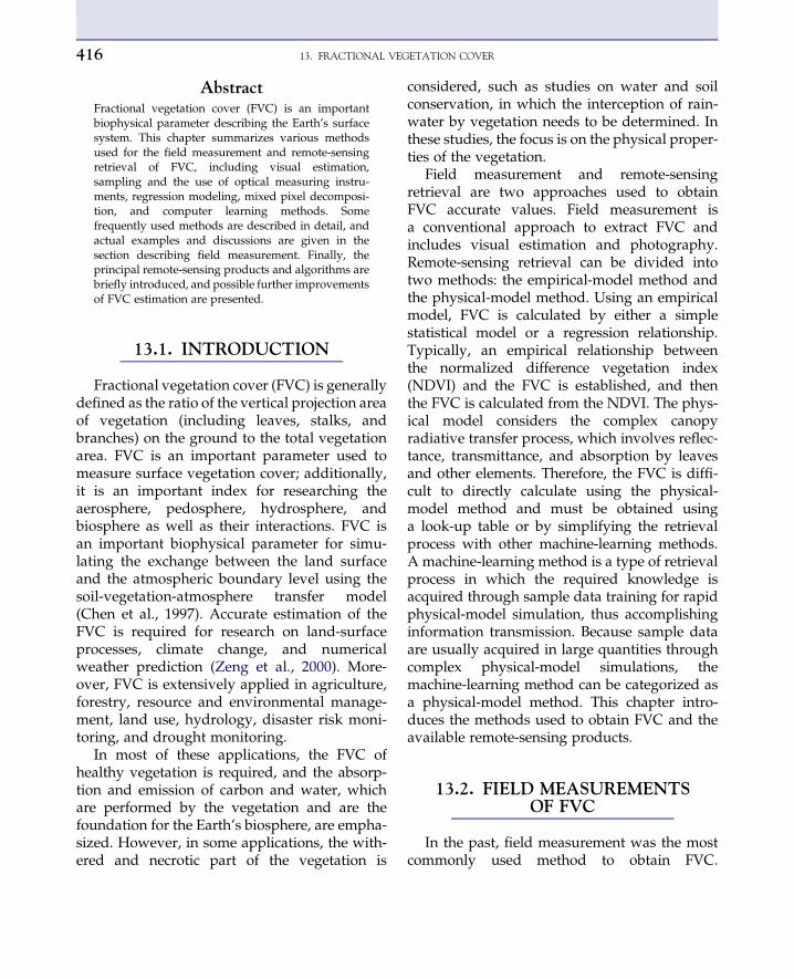
13.1. INTRODUCTION

Fractional vegetation cover (FVC) is generallydefined as the ratio of the vertical projection areaof vegetation (including leaves, stalks, andbranches) on the ground to the total vegetationarea. FVC is an important parameter used tomeasure surface vegetation cover; additionally,it is an important index for researching theaerosphere, pedosphere, hydrosphere, andbiosphere as well as their interactions. FVC isan important biophysical parameter for simu-lating the exchange between the land surfaceand the atmospheric boundary level using thesoil-vegetation-atmosphere transfer model(Chen et al., 1997). Accurate estimation of theFVC is required for research on land-surfaceprocesses, climate change, and numericalweather prediction (Zeng et al., 2000). More-over, FVC is extensively applied in agriculture,forestry, resource and environmental manage-ment, land use, hydrology, disaster risk moni-toring, and drought monitoring.

In most of these applications, the FVC ofhealthy vegetation is required, and the absorp-tion and emission of carbon and water, whichare performed by the vegetation and are thefoundation for the Earth’s biosphere, are empha-sized. However, in some applications, the with-ered and necrotic part of the vegetation is

considered, such as studies on water and soilconservation, in which the interception of rain-water by vegetation needs to be determined. Inthese studies, the focus is on the physical proper-ties of the vegetation.

Field measurement and remote-sensingretrieval are two approaches used to obtainFVC accurate values. Field measurement isa conventional approach to extract FVC andincludes visual estimation and photography.Remote-sensing retrieval can be divided intotwo methods: the empirical-model method andthe physical-model method. Using an empiricalmodel, FVC is calculated by either a simplestatistical model or a regression relationship.Typically, an empirical relationship betweenthe normalized difference vegetation index(NDVI) and the FVC is established, and thenthe FVC is calculated from the NDVI. The phys-ical model considers the complex canopyradiative transfer process, which involves reflec-tance, transmittance, and absorption by leavesand other elements. Therefore, the FVC is diffi-cult to directly calculate using the physical-model method and must be obtained usinga look-up table or by simplifying the retrievalprocess with other machine-learning methods.A machine-learning method is a type of retrievalprocess in which the required knowledge isacquired through sample data training for rapidphysical-model simulation, thus accomplishinginformation transmission. Because sample dataare usually acquired in large quantities throughcomplex physical-model simulations, themachine-learning method can be categorized asa physical-model method. This chapter intro-duces the methods used to obtain FVC and theavailable remote-sensing products.

13.2. FIELD MEASUREMENTSOF FVC

In the past, field measurement was the mostcommonly used method to obtain FVC.

13.2. FIELD MEASUREMENTS OF FVC 417

However, with the extensive application ofremote-sensing techniques for monitoring vege-tation, field measurement is losing its domi-nance. Regardless, field measurement continuesto play a nonnegligible role by providing basicdata for the remote-sensing estimation of FVC.Zhou believes that an ideal field measurementof FVC should have the following features: (a)instruments with operational ease and econom-ical utilization, (b) available, accurate, and objec-tive land-surface observation records, (c) a shortmeasurement duration, and (d) negligibleimpact from human factors. Most field measure-ment methods are unable to meet all fourrequirements, although digital photography iswidely applied in the field measurement ofFVC because it can satisfy all four requirements(Zhou et al., 2001).

13.2.1. Visual Estimation

In visual estimation, FVC is estimated basedon the estimator’s experience. This method ischaracterized by its simplicity and operationalease; however, it is highly subjective andrandom because the estimation precision isclosely associated with the estimator’s experi-ence. The following methods are included:

13.2.1.1. The Traditional Method

Several sample plots covering a given area areselected based on specific statistical require-ments. The FVC of the sample plots is directlyestimated based on experience.

13.2.1.2. The Digital Image Method

First, the vegetation within the sample plotsis vertically photographed; then, the photos arevisually estimated. To improve the estimationprecision, reference images are interpreted bypersonnel in accordance with certain stan-dards, and the average value is taken. In thismethod, a FVC standard image series mustbe generated, and the training of survey

personnel is required. Images that containa fractional amount (from 5 up to 95%) of vege-tation cover are printed and subsequentlycoded by survey personnel. Special measure-ment and calculation software is employed toestimate the FVC. Several colored images arerandomly selected each time for the visual esti-mation of the FVC by trained staff based onstandard images. Finally, the results of thevisual estimation and those provided by thesoftware are compared to determine the errorin visual estimation. Generally, training objec-tives require that the visual estimation erroris less than 10%.

13.2.1.3. The Grid Method

The grid method is an improvement on tradi-tional visual estimation. In this method, thesample plot is divided into several subquadratsof equal area based on vegetation type. Then,the FVC of each subquadrat is estimated usingthe traditional method of visual estimation. Themean value of the FVC is taken as the FVC ofthe sample plot. Research indicates that thegrid method is easier to perform and has a higherprecision than the traditional method. The gridmethod for visual estimation is essentiallya spatial sampling method that uses equalspacing.

13.2.2. The Sampling Method

The sampling method is also known as theprobability calculation method. In this method,the occurrence probability of vegetation in thesample plot is calculated using measurementmethods based on statistical principles. Thecalculated probability is taken as the FVC ofthe sample plot. This method has the disadvan-tages of operational complexity, long measure-ment duration, a large number of limitations,and low efficiency; however, the methodprovides high precision. Some samplingmethods are listed below.


13.2.2.1. The Quadrat Sampling Method

A square sample plot is marked off in theresearch area as the quadrat. The FVC ismeasured on two diagonals of the quadrat(measured only once for the overlapped section).The arithmetic mean is determined as the FVC ofthe quadrat.

13.2.2.2. The Belt-Transect SamplingMethod

Two perpendicularly crossed rectangular-belttransects are selected. The FVC of the sampleplot is defined as the ratio of the plant lengththat is in contact with the belt transect to the totallength of the belt transect. For example, tomeasure the forest canopy closure, the treeslocated on the two diagonals of the quadrat arethe objects of investigation. The forest canopyclosure is defined as the ratio of the number oftimes that a canopy is visible overhead to thetotal number of times that the head is raised.

13.2.2.3. The Point Count Sampling Method

Needles are vertically placed in the vegeta-tion, and the FVC is defined as the ratio of thenumber of needles in contact with leaves to thetotal number of needles.

13.2.2.4. The Shadow Sampling Method

The shadow sampling method is also termedthe meter-stick method. A meter stick is placedon the land surface parallel to the crop rows.The stick is moved forward a set distance, andthe length of shadow on the stick is read; theratio of shadow length on the stick to the totallength of the stick is recorded as the FVC. Thismethod is generally used for row crops, andhigh noon is considered the optimal time formeasurement.

13.2.3. Optical Measuring Instruments

As science and technology have developed,new measuring instruments are now being

applied to FVC measurement. For example, elec-tronic equipment is used to record the flux ofintercepted sunlight, which is then comparedto the level of direct sunlight at that location.From these data, the vegetation gap fraction isobtained. For these measurements, the FVC iscalculated as (1dthe vertical vegetation gapfraction). Other methods include direct imaging,such as digital photography, which is the mostextensively applied method. The proportions ofvarious vegetation types that are present arecalculated using image classification. Commonmeasurement techniques include the following:

13.2.3.1. Spatial Quantum Sensor (SQS)and Traversing Quantum Sell (TQS)

SQS and TQS are used to calculate FVC basedon the amount of sunlight that is intercepted byvegetation as measured by a sensor. However,these methods have not been extensively appliedin practice because specialized sensors areusually needed, resulting in field operationdifficulties.

13.2.3.2. Digital Photography

Digital photography is performed in a verticaland downward manner. FVC is the ratio ofthe number of vegetation pixels to the totalnumber of pixels in the digital images. Digitalphotography is used extensively in the fieldmeasurement of FVC because it is free of thesubjectivity of other measurements, has highprecision and good stability, and is easy to use.

In recent years, some progress has been madein estimating FVC using digital photography.Zhou et al. (1998) acquired FVC digital imagesusing a digital camera to test the consistency ofthis method. Gitelson et al. estimated the FVCof wheat in Nebraska, in the United States, usingdigital photography (Gitelson et al., 2002).Michael et al. conducted long-term monitoringof the FVC of an arid ecosystem in the UnitedStates using an agricultural digital camera,with accurate and effective results (Michaelet al., 2000). Based on a comparison of the


various techniques used to obtain field measure-ments of FVC, White et al. (2000) claimed thatdigital photography was the easiest and mostreliable technique to test and verify the extrac-tion of remote-sensing information. Hu et al.acquired photographs of sample plots ina research area and extracted FVC informationfrom digital images of the area through classifi-cation. The information extracted was laterused to verify the FVC of the entire researcharea obtained using remote-sensing estimation(Hu et al., 2007).

Despite the extensive application of digitalphotography, which is due to its easy operationand high efficiency, certain problems areencountered in obtaining FVC. Two major issuesaffect FVC extraction precision, and these factorsrequire certain skills to deal with them. The firstissue arises from the methods used for measure-ment and photography and includes theproblem of image edge distortion. The mostfrequently used solution is to cut the imageedge to remove this influence. The other issue,which is more striking and deserves more atten-tion, is the method used to extract FVC informa-tion from digital images. Supervised andunsupervised classifications are adopted to solvethis problem, and FVC is calculated as theproportion of classified vegetation. All the tradi-tional methods are unable to extract the FVCfrom digital images rapidly and automatically,thus lowering the practicability of digitalphotography. However, some researchers haveproposed methods that are more convenient toextract the FVC from digital images (Liu andPattey, 2010; Liu et al., 2011).

13.2.3.3. LAI-2000 Indirect Measurement

LAI-2000 is a more delicately designedmeasuring instrument and is mainly intendedto measure the leaf area index (LAI) (see Section11.1.2 in Chapter 11). Moreover, LAI-2000 cancalculate FVC based on the measured vegetationgap fraction.

LAI-2000 uses a camera with a fish-eye lens forobservation and imaging, and the image isdivided into several rings with variable radii byviewing the zenith angles of 7�, 23�, 38�, 53�, and68�. During FVC measurements, the observedarea in the ring with the minimum zenith angle(7�) is approximated as the zenith observation,and the FVC is calculated as (1dthe gap fractionfor the ring with the minimum zenith angle (7�))(Rautiainen et al., 2005). This measurement sharessimilar principles with digital photography. Inaddition, White et al. (2000), when measuringFVC using LAI-2000, first measured the plantarea index and then obtained the FVC throughconversion. Compared with the method whereonly the ring with the minimum zenith angle isinvolved, this method has the advantage ofexpanding the spatial range for measurement byutilizing a greater number of multiangle observa-tions in a wide field of view using a fish-eye lens.However, this method also has the disadvantageof incorporating a greater number of uncertainfactors.

As with the application of digital photographyfor FVCmeasurement, earlymorningandeveningare the optimal measuring times; the measure-ment should not be conducted in direct sunlight.Generally, the use of LAI-2000 is not as convenientas digital photography for measuring FVC.

13.2.4. Examples of Field Measurement

13.2.4.1. Examples of NoninstrumentalMeasurements

Some examples of field measurements of FVCare given below. Depending on the types andfeatures of the vegetation studied, the pointsampling, shadow sampling method and canopyprojection method are used.

1) Grassland

The point count sampling method is usedto measure grassland FVC. In the research plot,


1 m � 1 m subquadrats are selected. Needles areused as markers every 10 cm (4 ¼ 2 mm), that is,the needles are successively and verticallyinserted in the subquadrat above the grasslandat 10-cm intervals. The points where the needlescome into contact with grass are counted, andthe points where there are no contacts are notcounted. The FVC is the ratio of the number ofcontact points to the total number of points, asshown in Figure 13.1. The mean value of themeasured FVC for three subquadrats at threedifferent positions is recorded as the FVC ofthe quadrat.

2) Forested land

For tall vegetation, such as trees in forestedland, the forest canopy closure is generallyused to indicate the cover as expressed in Equa-tion (13.1):

D ¼ fdfe� 100% (13.1)

Here, D is the forest canopy closure (or theFVC of shrub land) expressed as a percentage;fe is the area of quadrat (units, m2), and fd is

FIGURE 13.1 Schematic diagram for measurement ofgrassland FVC (FVC ¼ 50%). The round circle at a crossmeans that a needle come into contact with grass.

the vertical projection area of the tree canopy(or grass canopy) in the quadrat (units, m2).

Forest canopy closure can also be measuredusing the tree canopy projection method,which is only applicable to forested land. Thismethod is similar to the grid method for visualestimation; therefore, it is not specifically intro-duced here. A 20 m � 20 m sample plot is typi-cally selected and divided into 5 m � 5 m gridswith a measuring tape. The position of eachtree in the grid is measured, and the projectionlength of the canopy of each tree is measured inthe northesouth and eastewest directionsusing the measuring tape and a compass. Thecanopy projection is plotted on grid paper onan appropriate scale. The areas of canopyprojection and the sample plot are calculatedbased on the grid; from these data, the forestcanopy closure can be derived as shown inFigure 13.2.

3) Shrubbery

The shadow sampling method is usuallyadopted for measuring the FVC of shrubbery.A rope or measuring tape is extended over thequadrat of shrubbery, and the length of that

FIGURE 13.2 Schematic diagram for measuring theforest canopy closure.

FIGURE 13.4 Observation platform for FVCmeasurement.


shadow that is cast on the measuring rope ismeasured. The FVC of the shrubbery is the ratioof the length of shadow cast by the shrub to thetotal length of the rope or the quadrat. Thisprocedure is repeated three times at threedifferent positions on the quadrat, and themean value is the FVC of shrubbery in thequadrat. The area of quadrat can be as small as10 m � 10 m.

13.2.4.2. Examples of Digital PhotographyMeasurement

1) Selecting the photography environment

First, illumination conditions must beselected. The vegetation should be photo-graphed on a cloudy day or in the morningor evening when the effect of shadows isminimal. However, because morning dewmight also affect the photography, themorning is not recommended. Artificiallighting equipment can be used in the darkduring the evening. In short, the spectraldifference between the vegetation and thesoil background should be as strong aspossible, and interference from shadowsshould be prevented. Figure 13.3 showsimages taken with a digital camera in variousenvironments; in (a), a flashlight was usedduring the night; in (b), the image was takenin direct sunlight; and in (c), the image wastaken during a cloudy day.

(a) (b)

FIGURE 13.3 Images of maize seedlings

In field measurements, a long stick with thecamera mounted on one end is beneficial toconveniently measure various species of vegeta-tion, enabling a larger area to be photographedwith a smaller field of view. The stick can beused to change the camera height; a fixed-focuscamera can be placed at the end of the instru-ment platform at the front end of the supportbar, and the camera can be operated by remotecontrol. Figure 13.4 shows a simple observationplatform designed by one of the authors duringthe field measurement of FVC.

The photographic method used depends onthe species of vegetation and planting pattern:

Low crops (<2 m) not in rows

(c)

taken under various lighting conditions.


The observation platform is used directlywhere the height of the installed camera abovethe canopy of vegetation far exceeds the crowndiameter of the vegetation. Sampling is con-ducted along the diagonals of the quadrat;finally, the arithmetic average is taken. Thismethod is similar to the quadrat samplingmethod.

Low crops (<2 m) in rows

In a situation with a small field of view (<30�),rows of more than two cycles should be includedin the field of view, and the side length of theimage should be parallel to the row. If thereare no more than two complete cycles, theninformation regarding row spacing and plantspacing are required. The FVC of the entire cycle,that is, the FVC of the quadrat, can be obtainedfrom the number of rows included in the fieldof view.

High crops (>2 m) not in rows

Sampling along the diagonals, as in thequadrat sampling method, can also be con-ducted. During the photography session, ifthe sampling points fall on the low vegetationbetween plants, then the observation platformis used; if the sampling points fall on the treecrown and the observation platform can bemaintained above the crown of the vegetationas high as possible, then the observation plat-form can also be used to obtain photographs.However, if the height is excessively great,then the images should be taken in a bottom-up manner from beneath the crown. Mean-while, the low vegetation is photographed ina top-down manner beneath the crown toobtain the total FVC of the region near the tree.

High vegetation in rows (>2 m)

Through the top-down photography of thelow vegetation underneath the crown and thebottom-up photography beneath the tree crown,the FVC within the crown projection area can beobtained by weighting the FVC obtained from

the two images. Next, the low vegetationbetween the trees is photographed, and theFVC that does not lie within the crown projec-tion area is calculated. Finally, the averagearea of the tree crown is obtained using thetree crown projection method. The ratio ofthe crown projection area to the area outsidethe projection is calculated based on rowspacing, and the FVC of the quadrat is obtainedby weighting.

2) FVC extraction from the classification ofdigital images

Many methods are available to extract theFVC from digital images, and the degree of auto-mation and the precision of identification areimportant factors that affect the efficiency of fieldmeasurements. For example, supervised classifi-cation has high precision but low efficiency,whereas unsupervised classification has highefficiency but low precision due to errors ofcommission and omission. Thus, the defects inthese methods restrict their application toa certain extent.

Figure 13.5 illustrates the results of the auto-matic and rapid extraction of FVC from digitalimages. This method, which is proposed by Liuet al. (2011), has the advantages of a simple algo-rithm, a high degree of automation and highprecision, as well as ease of operation. Morerapid classification methods with a higherdegree of automation and greater accuracy arerequired to maximize the superiority of digitalphotography.

13.3. THE REMOTE-SENSINGRETRIEVAL

The development of remote-sensing tech-nology facilitates the acquisition of multitem-poral and multiscale data to continuallymonitor FVC on a large or global scale. Accord-ingly, many FVC estimation methods are also

FIGURE 13.5 Comparison of the classification results and FVC using different classification methods.

13.3. THE REMOTE-SENSING RETRIEVAL 423

being developed. The most extensively appli-cable method involves establishing the relation-ship between FVC and vegetation index (suchas NDVI) to retrieve FVC. The commonlyused remote-sensing methods of FVC retrievalare mainly divided into two categories: empir-ical model methods and pixel decomposi-tion model methods. Additionally, manyresearchers have adoped machine-learningmethods, such as those that employ neuralnetworks, to estimate FVC.

13.3.1. Regression Models

Regression models are also called empiricalmodels and are constructed through the regres-sion of remote-sensing data collected usinga specific wave band, several wave bands, ora remotely sensed vegetation index (VI) tomeasure FVC. This model can be extended toFVC estimations on a larger scale.

The VI method is most frequently applied.Based on an analysis of the spectral features ofvegetation, this method selects the VI that

FIGURE 13.6 The linear regression relationship betweensoil-adjusted VI and FVC. (Choudhury et al., 1994, Fig. 12(a))


correlates well with FVC and then establishesthe conversion relationship between VI and FVCfor FVC estimation. Generally, the VI variesdepending on area and vegetation species. Themost extensively applied NDVI is expressedusing Formula (13.2).

NDVI ¼ rnir � rred

rnir þ rred(13.2)

where rnir is the reflectance of vegetation in thenear-infrared band and rred is the reflectance ofvegetation in the red band. The extensive appli-cation of NDVI, which can be used to indicatethe growth status of vegetation, stems from theconsiderable difference in the reflectance ofnormal vegetation in the red band and thenear-infrared band.

Previous research suggests that FVC is closelycorrelated with the VI and that the correlationbetween the two can be either linear ornonlinear. Therefore, the regression model canalso be linear or nonlinear, and the regressionmodel method can be subdivided into the linearand nonlinear regression model methods.

13.3.1.1. The Linear RregressionModel Method

In the linear regression model method, thelinear regression of the actual FVC and remotelysensed VI are determined to establish the estima-tion model for FVC in the research area. Thelinear regression model of NDVI and FVCprovides a simple method to estimate FVC;thus, it has achieved widespread application(Hurcom et al., 1998). For instance, Xiao andMoody, through the linear regression of 60points selected from a Landsat ETM þ NDVIimage and FVC (considered as the actual surfaceFVC), extracted a high-resolution (0.3 m) truecolor ortho-image and found a strong linear rela-tionship between NDVI and FVC (R2 ¼ 0.89).They then applied this formula to estimate theFVC of all of the pixels in the Landsat ETM þimage (Xiao & Moody, 2005).

For both dense and sparse vegetation, theFVC of a remote-sensing pixel can be definedas having a linear relationship with the VI ifthe influence of multiple scattering is omitted:

FVC ¼ a$VIþ b (13.3)

where FVC is the FVC of the mixed pixel, VI isthe VI of the mixed pixel and a and b are theregression coefficients of FVC and VI, respec-tively. Figure 13.6 shows the expression for thelinear regression of soil-adjusted VI and FVCestablished by Choudhury et al. (1994).

Some attempts have been made to grade thevalue of NDVI such that different grades indi-cate different FVCs. For instance, Mohammadet al. categorized NDVI after some conversion(NDVI ¼ (NDVI þ 0.5)*255) into six grades,namely, 5, 5e50, 50e100, 100e150, 150e200and 200e250, which represented the FVC of sixsituations, namely, 0%, 20%, 40%, 60%, 80%,and 100%, respectively (Mohammad et al.,2002). However, this method of segmentationwith discretization of NDVI still utilizes a linearor nonlinear relationship between VI and FVC.


13.3.1.2. The Nonlinear RegressionModel Method

By fitting NDVI and FVC, the nonlinearregression model can be established and appliedto calculate the FVC of an entire research area.Research by Carlson and Ripley indicates thatfor some values of FVC where LAI was 1e3,a higher clumping index of vegetation wouldresult in a better nonlinear correlation betweenthe VI and FVC (Carlson et al., 1997).

Choudhury et al. (1994) found that FVC wasrelated to scaled NDVI in a quadratic manner.Based on this finding, the authors estimated theFVC of a coniferous forest in the U.S. PacificNorthwest. The results indicated that althoughNDVI is the most commonly applied method,it did not have the strongest correlation withthe FVC of trees. Meanwhile, based on remote-sensing data from NOAA AVHRR, Choudhuryand coworkers estimated the FVC of a coniferousforest using the NDVI and scaled NDVI. Theyfound that the correlation coefficient was 0.55at a confidence interval of 99% (Choudhuryet al., 1994). Gillies & Carlson et al. obtaineda quadratic relationship between the FVC and

FIGURE 13.7 The expression for the regression relations

scaled NDVI using various methods and data-sets (Gillies et al., 1997; Carlson et al., 1997).

Some researchers have studied the VI methodusing both the linear and the nonlinear regres-sion method. For instance, Gitelson et al. con-ducted a regression of three types of VIs,namely, the NDVI, the Green NDVI, and thevisible atmospherically resistant index (VARI)with the FVC of wheat (Figure 13.7). Nonlinearregression was used for the NDVI and GreenNDVI, and linear regression was used for theVARI. A comparative analysis indicated thatthe VARI was very sensitive to FVC within therange of 0-10% and that it could minimize thesensitivity to atmospheric influence. It was sug-gested that the VARI should be utilized inthe linear regression model to estimate FVC(Gitelson et al., 2002). Either a strong linear rela-tionship (Ormsby et al., 1987) or a nonlinear rela-tionship (Li et al., 2005) was found between theVI and FVC, depending on the specific land-scape type. Both the linear and nonlinear modelshave difficulties with mixed vegetation. Evenwhen the FVC is 100%, the VI depends on thevegetation species that are present due to the

hip between VI and FVC. (Gitelson et al., 2002, Fig. 7 (B))


differences in their chlorophyll content andcanopy structure. It has been reported thateven when the actual FVC of different vegetationspecies is basically the same in a research area,the values of FVC directly calculated from theNDVI can deviate from each other by as muchas 40% as a result of the difference in chlorophyllcontent between natural and artificial vegetation(Glenn et al., 2008).

The estimation precision of FVC can beimproved if the features and species of the vege-tation are determined by field measurement.Previous researchers have used the average leafinclination angle corresponding to differentvegetation species under various land-surfaceconditions to predict the FVC from the VI(Anderson, 1997).

Non-VI forms can also be used to establish anempirical regression relationship with FVC.Graetz et al. conducted a linear regression anal-ysis on measured FVC data from the fifthchannel of Landsat MSS. The regression modelobtained was later applied to estimate the FVCof sparse grassland (Graetz et al., 1988). Peterused ATSR-2 remote-sensing data in four chan-nels (555, 670, 870, and 1,630 nm) to study thelinear regression of FVC with reflectance. Theresults indicated that applying the linear regres-sion model based on the data from four channelswas superior to application of VI alone for esti-mating FVC (Peter, 2002).

Due to its simplicity, the regression modelmethod has been widely applied in FVC estima-tions on a regional level with high precision.Nevertheless, it has been demonstrated that theempirical regression model has its own limita-tions, as it is only applicable to the FVC estima-tion of specific vegetation species in specificregions. For instance, Graetz’s linear regressionmodel is only applicable to sparse grassland,and his nonlinear regressionmodel was proposedspecifically for the study of degraded grassland(Graetz et al., 1986). In addition, due to itsregional limitations, the regression model is notsuitable for extensive applications, and the

empirical model (on the regional level) might beinvalid if it is used to estimate FVC on a largescale.

13.3.2. The Linear Unmixing Model

The linear unmixing model is based on theprinciple that each pixel in an image iscomposed of several components, and eachpixel contributes separately to the informationobserved by remote sensors. Through decom-position of the remote-sensing information(channel information or VI), the pixel decompo-sition model can be used to estimate FVC. Thismodel can be either linear or nonlinear;however, thus far, most of the studies on themixed pixel decomposition model focus on thelinear unmixing model. This section, therefore,mainly concentrates on application of the linearunmixing model to the remote-sensing calcula-tion of FVC.

The linear unmixing model is the most exten-sively applied model among the mixed pixeldecomposition models. In this model, pixelinformation is assumed to result from the linearsynthesis of the information of each component.The linear unmixing model involves the assump-tions that the photon reaching the sensor actsupon only one component and that the compo-nents are mutually independent and do notinteract. If the photon acts upon several compo-nents, then nonlinear mixing occurs. In fact, thelinear and nonlinear mixing methods are basedon a single concept; that is, linear mixing occursas an exception from nonlinear mixing whenmultiple reflections are ignored. To obtaina convenient solution, the number of regionalland feature types, and the major land featuretypes in particular, should not exceed thenumber of remote-sensing channels; otherwise,n þ 1 unknown variables would have to besolved using n equations; this constitutes thelargest limitation of the linear unmixing model.The linear unmixing model is able to calculateand extract the FVC for each pixel in the image.


Suppose that each component contained ina pixel contributes to the pixel informationreceived by the satellite sensors and that thevalue of the spectral characteristics of the vegeta-tion in each component is taken as a factor. Then,the linear mixing model is established using thearea of this specific component as the weight ofthis factor, which can be mathematicallyexpressed as:

Rb ¼Xn

i¼ 1

fi;bri;b þ eb (13.4)

where Rb is the reflectance of the pixel in channelb, fi is the proportion of the number of subpixel ito that of the mixed pixel, ri,b is the reflectance ofsubpixel i in channel b, n is the number of subpix-els, and eb is the fitting error of channel b (Vander Meer, 1999).

The proportion of each component in a mixedpixel can be solved using the least-squaresmethod. The FVC is then calculated based onthe proportion of each vegetation componentpresent. The precision of this solution dependsmainly on the selection of each pure component(Lu and Weng, 2004).

Among the various linear unmixing models,the simplest assumes that each pixel is composedof only two components, that is, vegetation andnonvegetation, and that the spectral informationresults from linear mixing of the two compo-nents. The proportional area of each componentin the pixel is the weight of each component. Theproportional area of vegetation is the FVC ofthe pixel, as mathematically expressed usingFormulas (13.5) and (13.6):

NDVI ¼ f �NDVIv þ ð1� f Þ �NDVIs (13.5)

and then; f ¼ NDVI�NDVIsNDVIv �NDVIs

(13.6)

where f is the proportion of vegetation area inthe mixed pixel (i.e., FVC), NDVI is the NDVIof the mixed pixel, NDVIv is the NDVI of thevegetation and NDVIs is the NDVI of bare soil.

It is clear from this equation that this dimidiatepixel model is a linear regression model for VI.To obtain the FVC of mixed pixels, the NDVIsof vegetation and of bare soil should be deter-mined. However, the determination of NDVIvand NDVIs is affected by many factors, such assoil, vegetation type, and chlorophyll content.Nevertheless, these parameters can be deter-mined through statistical analysis of spatialand temporal NDVI data. Time-series NDVIdata are analyzed statistically, and themaximum time-series NDVI is used as theNDVI of vegetation, whereas the minimumtime-series NDVI is used as the NDVI of baresoil (Gutman et al., 1998; Zeng et al., 2000).Some researchers directly select the maximumand minimum NDVIs of the research area asthe NDVI values for vegetation and bare soil,respectively (Xiao & Moody, 2005).

The dimidiate pixel model is extensivelyapplied because of its simple form. Figure 13.8illustrates the global seasonal FVC estimatedby Gutman and coworkers based on the dimidi-ate model of FVC and NDVI. Using clusteranalysis, the optimal maximum and minimumvalues of NDVI were selected from themaximum and minimum values of NDVI foreach season. Gutman et al. proposed that theFVC estimated using this model has a maximumerror of 0.35, which might be derived from esti-mation of the maximum and minimum valuesof NDVI (Gutman et al., 1998). Qi et al. usedthe dimidiate model in their study of the spatialand temporal variation of vegetation in the SanPedro Basin in the U.S. Southwest based onNDVI data. Landsat TM, SPOT4 VEGETATION,and aerial photography data were also used tostudy this method. The results indicated thatthe model was able to estimate the dynamic vari-ation of vegetation reliably, even without atmo-spheric correction (Qi et al., 2000). Leprieuret al. used SPOT data after atmospheric correc-tion to calculate NDVI and applied this modelto estimate the FVC in the Sahel (Leprieuret al., 1994).

FIGURE 13.8 Seasonal FVC. Details of snow masks can be found in the report by Gutman et al. (1995). (Gutman et al., 1998;Figure 5)


As the model requires pixels representingpure vegetation and bare soil, low-resolutionremote-sensing data are not applicable. Formany regions, pixels representing pure vegeta-tion are difficult to obtain in low-resolution data.

Gutman et al. obtaining FVC using the pixeldecompositionmodel based on the dimidiate pixelmodel (Gutman et al., 1998). Depending on thevegetation distribution features located in amixedpixel, the pixels were divided into uniform andmosaic pixels, and the latterwere further classifiedinto dense, nondense and variable-density vegeta-tion pixels. Different FVC models were con-structed for different subpixel structures.

In a sense, an essential part of the mixed pixeldecomposition model is extracting pure pixels torealize the conversion of remotely sensed spec-tral signals to physical vegetation parameters.

Xiao and Moody estimated the FVC within anarea of approximately 4000 km2 in New Mexico(Xiao & Moody, 2005) using various methods. Intheir report, they presented a comparative anal-ysis on the estimation of FVC by two methods:the mixed pixel decomposition model based on

spectral data (SMA3, SMA4, SMA5, and NDVI-SMA) and the linear regression model based onNDVI. The analyses of SMA3, SMA4, andSMA5 included a discussion on whether thesum of the proportions of each component ineach mixed pixel should be constrained to 1.Figure 13.9 shows the relationship between theFVC values that were estimated using variousmethods and the actual FVC. Figure 13.10 pres-ents the FVC values of a research area that wasestimated using various methods.

Xiao and Moody reported that the NDVI-based method of estimating the FVC of arid andsemiarid areas was appropriate and relativelyeasy. They also noted that the NDVI-based esti-mation of FVC was particularly sensitive to soilreflectance. Therefore, overestimating the NDVIof an area of sparse vegetation would lead tooverestimating FVC. The selection of the numberof components in mixed pixels and the selectionof each end member, which depends on the vege-tation structure and the distribution of vegetationin the research area, are themajor factors affectingFVC estimation in the mixed pixel decomposition

(a)

(c)

(e)

(g)

(b)

(d)

(f)

(h)

FIGURE 13.9 The relationship between the FVC that estimated using various methods and the actual FVC: (a) SMA3without constraint; (b) SMA3 with constraint; (c) SMA4 without constraint; (d) SMA with constraint; (e) a situation based onthe expression for regression with NDVI; (f) NDVIeSMA; (g) SMA5 without constraint; (h) SMA5 with constraint; the solidline is 1:1. (Xiao & Moody, 2005, Fig. 4)


(a) (b) (c) (d)

(h)(g)(f)(e)

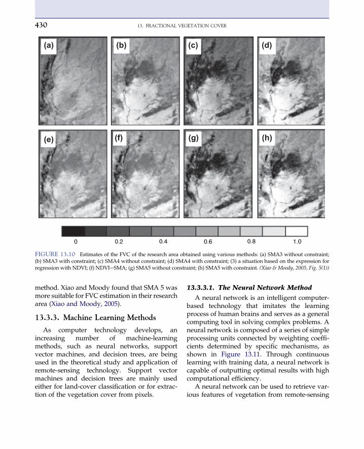
FIGURE 13.10 Estimates of the FVC of the research area obtained using various methods: (a) SMA3 without constraint;(b) SMA3 with constraint; (c) SMA4 without constraint; (d) SMA4 with constraint; (3) a situation based on the expression forregression with NDVI; (f) NDVIeSMA; (g) SMA5 without constraint; (h) SMA5 with constraint. (Xiao & Moody, 2005, Fig. 5(1))


method. Xiao and Moody found that SMA 5 wasmore suitable for FVC estimation in their researcharea (Xiao and Moody, 2005).

13.3.3. Machine Learning Methods

As computer technology develops, anincreasing number of machine-learningmethods, such as neural networks, supportvector machines, and decision trees, are beingused in the theoretical study and application ofremote-sensing technology. Support vectormachines and decision trees are mainly usedeither for land-cover classification or for extrac-tion of the vegetation cover from pixels.

13.3.3.1. The Neural Network Method

A neural network is an intelligent computer-based technology that imitates the learningprocess of human brains and serves as a generalcomputing tool in solving complex problems. Aneural network is composed of a series of simpleprocessing units connected by weighting coeffi-cients determined by specific mechanisms, asshown in Figure 13.11. Through continuouslearning with training data, a neural network iscapable of outputting optimal results with highcomputational efficiency.

A neural network can be used to retrieve var-ious features of vegetation from remote-sensing

FIGURE 13.11 A schematicdiagram for the neural networkretrieval of FVC.


data (Baret, 1995; Jensen et al., 1999; Foody et al.,2001). However, these studies usually employordinary neural networks or multi-layer percep-trons. Other types of neural networks mightpossess greater potential. However, many issuesneed to be considered if neural networks are tobe applied, as themiddle layer of neural networksis a black box. Consequently, it is difficult tocontrol the retrieval of the parameters.

Based on a comparison of multivariableregression analysis, the VI method, and theneural network method, Boyd et al. found thata neural network was the most applicable tothe FVC estimation of a forest in the U.S. PacificNorthwest. Three types of neural networkmethodsd namely, the multilayer perceptron,the radial basis function, and the gen-eralized regression neural networkdwere alsocompared. The multilayer perceptron wasfinally selected to determine the FVC of theresearch area. Using this method, 40 iterationswere performed on six black boxes using a back-propagation algorithm. Within a 99% confi-dence interval, the results demonstrated thatthis method estimated the FVC of the forestwith higher precision than the multi-elementregression analysis or the VI method; the coeffi-cient of determination with respect to the actualFVC of the forest was 0.57 (Boyd et al., 2002).Voorde et al. proposed using a multilayer

perceptron to randomly select 3037 pixels froman ETM þ image for training, followed bymixed pixel decomposition, to estimate theFVC of subpixels. Moreover, to compare theresults with those estimated using a neuralnetwork, regression analysis and the linearunmixing model were also used to estimatethe FVC of the research area. Figure 13.12 showsthe estimates of the FVC of the research areaobtained using various methods, whereasFigure 13.13 shows the error in the FVC estima-tion using various methods (Voorde et al., 2008).

13.3.3.2. The Decision Tree Method

Natural land features are diverse andconstantly change; this change is becomingmore complex due to human and natural factors.Therefore, it is a common phenomenon that oneland feature generates different spectra ordifferent land features share the same spectrumin remote sensing. This creates difficulties foridentifying and classifying remote-sensingimages. Therefore, it is necessary to study theinherent rules and associations of apparentlydisordered and intricate land features; then,based on the rules and associations discovered,a tree structure, or a decision tree, is established.This decision tree functions as the basis for iden-tifying and classifying land features. To ensurethe accuracy and objectivity of the classification,

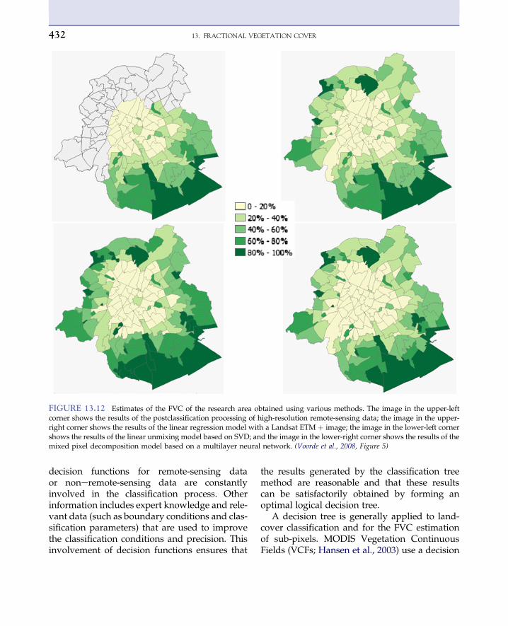
FIGURE 13.12 Estimates of the FVC of the research area obtained using various methods. The image in the upper-leftcorner shows the results of the postclassification processing of high-resolution remote-sensing data; the image in the upper-right corner shows the results of the linear regression model with a Landsat ETM þ image; the image in the lower-left cornershows the results of the linear unmixing model based on SVD; and the image in the lower-right corner shows the results of themixed pixel decomposition model based on a multilayer neural network. (Voorde et al., 2008, Figure 5)


decision functions for remote-sensing dataor noneremote-sensing data are constantlyinvolved in the classification process. Otherinformation includes expert knowledge and rele-vant data (such as boundary conditions and clas-sification parameters) that are used to improvethe classification conditions and precision. Thisinvolvement of decision functions ensures that

the results generated by the classification treemethod are reasonable and that these resultscan be satisfactorily obtained by forming anoptimal logical decision tree.

A decision tree is generally applied to land-cover classification and for the FVC estimationof sub-pixels. MODIS Vegetation ContinuousFields (VCFs; Hansen et al., 2003) use a decision

FIGURE 13.13 The error in the estimation of FVC using various methods. The image on the left shows the result of thelinear regression model; the image in the middle shows the result of the linear unmixing model based on SVD; and the imageon the right shows the result of the multilayer perceptron neural network model. (Voorde et al., 2008, Figure 4)

13.4. CURRENT REMOTE-SENSING PRODUCTS 433

tree to estimate the FVC of trees and grass on theglobal scale. Other studies (e.g., Hansen et al.,2002; Huang et al., 2003; Yang et al., 2003; Xuet al., 2005; Gessner et al., 2009) have also useda decision tree to solve problems related toremote-sensing subpixels. A decision tree isa parameter-free classification method.

The advantages of the decision tree method,which include the lack of parameterization andthe absence of a need to assume the normaldistribution or homogeneity of input data, facil-itate its extensive application in various fields.Rogan et al. adopted a decision tree that wasdesigned to identify and classify the input data.First, multitemporal spectral mixture analysis(MSMA) was performed to extract four typesof endmembers of green vegetation (GV), non-photosynthetic vegetation (NPV), shade, andsoil. Next, using the designed decision data, thefour types of endmembers were identified step-wise and classified.When the intercategory devi-ation was the greatest, a classification thresholdwas required to separate the two categories ateach step. Based on the classification results,four categories of endmembers were calculated,

and the user precision of the FVC of each end-member was determined to be approximately76% (Rogan et al., 2002).

13.4. CURRENT REMOTE-SENSINGPRODUCTS

A validation report of FVC products for theMSG/SEVIRI sensor summarizes currentlyavailable remote-sensing land-surface analysisvegetation products (Validation Report of LandSurface Analysis Vegetation products, 2008,URL: http://landsaf.meteo.pt/GetDocument.do?id¼301) as shown in Table 13.1. Satellitedata used in current products mainly comefrom SPOT/VEGETATION, ENVISAT/MERIS,and ADEOS/POLDER, which are polar-orbitingsatellite sensors, and MSG/SEVIRI.

FVC and LAI products for POLDER use theneural network method, and the radiative trans-fer model by Kuusk (Lacaze et al., 2003) has beenadopted as the training model. LAI products aredirectly outputted through the neural networkmethod. The FVC products are derived from

TABLE 13.1 Current Remote-Sensing FVC Products (Regional Scope of Complementary Products)

Literature Source/Project name Sensor Available time Spatial range Website

Roujean and Lacaze,2002

CNES/POLDER POLDER 1996-1997 2003 Global http://polder.cnes.fr/

Baret et al., 2007 FP5/CYCLOPES VGT 1998-2007 Global http://postel.mediasfrance.org/

Baret et al., 2006 ESA/MERIS MERIS 2002enow Global http://www.brockmann-consult.de/beam/plugins.html

Gutman and Ignatov,1998Bartolomé et al., 2002

GEOSUCCESS VGT 2001- now Global http://www.geosuccess.net/geosuccess/

García-Haro et al., 2005 EUMETSAT/LSA SAF

SEVIRI 2005-now Europe, Africa,South America

http://landsaf.meteo.pt


the LAI products based on the exponential rela-tionship between the two using the followingformula: FVC ¼ 1- exp (- 0.5 * LAI).

A MERIS sensor on the ENVISAT platform,which is also based on a neural network, isable to capture multiangular and multispectraldata. Unlike POLDER, FVC products are notdirectly obtained from LAI products. In addi-tion, FVC products, LAI products, and thefraction of absorbed photosynthetic activeradiation (FAPAR) products are generated byinputting observations from 13 channels simul-taneously. The training of the neural networkuses the PROSPECT þ SAIL model (Baretet al., 2006), and Bacour et al. (2006) have vali-dated the products.

CYCLOPES products, which use SPOT/VEGETATION (VGT) data to generate FVC,also have adopted the neural network method.

Other algorithms that generate FVC valuesusing multiangular and multispectral remote-sensing data, such as SEVIRI, have adoptedother methods, depending on the specific dataused. The SEVIRI sensor is supported by Meteo-sat Second Generation (MSG) and acquiresdata at a fixed observation angle with respectto specific observation sites. The sunlight

illumination angle varies with time. MSG hasa high temporal frequency for data acquisition;therefore, a coefficient of the kernel-driven bidi-rectional model k0 is used as input data (Baretet al., 2007). The physical meaning of k0 is thereflectance observed by the satellite in a verticalobservation at vertical solar illumination. Theadvantage of using k0 is that it reduces theangular effect between the sun and the satellite.The mixed pixel decomposition model is usedto determine the FVC.

In terms of validation results, the FVC prod-ucts of SEVIRI and MERIS sensors have goodspatial consistency. However, the FVC productsof the MERIS sensor systematically underesti-mate the FVC values (approximately 0.10e0.2)(García-Haro et al., 2008). The same problemalso exists for the FVC products of the SEVIRIand VGT sensors (Validation Report of LandSurface Analysis Vegetation products, 2008,URL: http://landsaf.meteo.pt/GetDocument.do?id¼301). The FVC products of VGT arehigher than those of SEVIRI (by approximately0.15); therefore, the value of the FVC productsof the SEVIRI sensor lies between those of theMERIS and VGT sensors. In their validationreport, Fillol et al. (2006) noted that the product

13.5. CHALLENGES AND PROSPECTS FOR FVC ESTIMATION 435

value of VGT data was lower than that of high-resolution SPOT data, even after spatial aggrega-tion. Thus, we can infer that the FVC products ofthe SEVIRI, VGT, and MERIS sensors all under-estimate FVC.

13.5. CHALLENGES ANDPROSPECTS FOR FVC ESTIMATION

The Earth is a planet brimming with life,where vegetation constitutes the fundamentalpart of the ecosystem and provides support forthe survival of animal life. As a group of livingorganisms, vegetation has evolved over severalbillion years, which has given it diversifiedfeatures. However, these variable featuresmake it difficult to estimate FVC using remote-sensing technology. Data extraction would befar less complicated if all vegetation were thesame. Currently, no remote-sensing methodcan simultaneously estimate the FVC of all vege-tative species, and all remote-sensing estimationmethods are limited by vegetative species, terri-tory, solar illumination, and soil. In essence, allremote-sensing signals are radiation, and FVCis a physical parameter of a specific species ofvegetation. Thus, converting between the twois crucial for estimating FVC.

Both the empirical and physical methods usedin remote sensing have conversion mechanismsfor estimating FVC that have advantages anddisadvantages. With the empirical method,several empirical coefficients need to be deter-mined regardless of the VI and empirical rela-tionship used. The acquisition of theseparameters is related to and restricted by land-surface conditions, vegetation types, lightingconditions, and the use of specific sensors. Appli-cation of the empirical method is usually limitedby changes in these conditions. Using the radia-tive transfer model, physical method establishesan algorithm framework that considers morefactors, thus elucidating the relationshipbetween the optical signals and the physical

vegetation parameters. The physical method ismore widely applicable, at least in a theoreticalsense. Because a large dataset is required andmany factors such as time, space, angle, andspectral response need to be considered in theapplication of satellite observation data, use ofthe physical method may be restricted due toa lack of data. Moreover, a dilemma existsregarding model selection: if too many parame-ters need to be estimated in a complex model,then calculations would be difficult; if the modelis simplified, then errors would inevitablyoccur. Thus, two problemsddata and modelselectiondimpair the applicability of the phys-ical method.

FVC is estimated more precisely using fieldmeasurement than using the remote-sensingmethod on a small scale. However, due to itslimitations, field measurement mainly serves asa supplementary validation method for theremote-sensing method in most applications.

FVC describes the two-dimensional distribu-tion of vegetation, whereas LAI is a physicalquantity describing the vertical distribution ofvegetation. Both play an important role in quan-titative land-surface analysis. With the increasein the quantity and type of remote-sensing dataand the relevant field data on the global andregional scale, FVC estimation models willbecome more complex and comprehensive. Atthe same time, NDVI and other vegetationindices will continue to be applied due to theireasy accessibility and will undergo constantdevelopment in the foreseeable future.

Some problems are associated with remote-sensing-based FVC estimation. For example,remote-sensing pixels have a specific spatialscale; when using remote-sensing data ona different scale to obtain FVC, the heterogeneityof pixels might bring about mismatches amongthe results obtained from data of different reso-lutions. That is, the FVC obtained from high-resolution data differs from that obtained fromlow-resolution data, thus causing a scale effect.In addition, current FVC estimation is based on


the response to chlorophyll content and leafwater content, which results in an FVC valuerepresenting green vegetation. Use of the NDVIof vegetation during flowering and fruitingperiods would considerably affect FVC determi-nation. Other situations, such as leaf yellowing,water content decline, and discoloration, allhave some effect on remote-sensing spectralsignals, thus resulting in deviations in FVC esti-mations. Finally, the FVC of different vegetationspecies in the ecosystem requires further identifi-cation and calculation, making this issue evenmore complex. Therefore, researchers shoulddevote their efforts to improving remote-sensingtechniques to meet the application requirementsof FVC.

FVC is not the most difficult parameter to beestimated by remote-sensing techniques. Atpresent, the precision of results obtained fromremote-sensing data is approximately 80% oreven higher. Progress in developing softwareand hardware will increase the precision andefficiency of FVC estimation even further. Forfield measurement, the digital photography-based extraction method is used most widely.In addition, more and newer types of platformssuch as engineering vans and unmanned aircraftwill become available to carry digital camerasand to ensure high-precision FVC estimationwithin a larger scope. VI regression, mixed pixeldecomposition, and neural network methods arefrequently mentioned in the literature. Theneural network method has been widely appliedin the algorithms used to generate productsbecause of its capacity to integrate with the phys-ical model, extendibility, and rapidity ofcalculation.

ReferencesAnderson, M. C., Norman, J. M., Diak, G. R., Kustas, W. P.,

& Mecikalski, J. R. (1997). A two-source time-integratedmodel for estimating surface fluxes using thermalinfrared remote sensing. Remote Sensing of Environment,60(2), 195e216.

Baret, F., Clevers, J. G. P. W., & Steven, M. D. (1995). Therobustness of canopy gap fraction estimations from redand near-infrared reflectances: A comparison ofapproaches. Remote Sensing of Environment, 54(2),141e151.

Baret, F., Pavageau, K., Béal, D., Weiss, M., Barthelot, B.,& Regner, P. (2006). Algorithm Theoretical BasisDocument for MERIS Top of Atmosphere LandProducts (TOAVEG). Report of ESA contract AO/1e4233/02/I-LG.

Baret, F., Hagolle, O., Geiger, B., Bicheron, P., Miras, B.,Huc, M., Berthelot, B., Nino, F., Weiss, M., Samain, O.,Roujean, J. L., & Leroy, M. (2007). LAI, FAPAR, andFCover CYCLOPES global products derived from Vege-tation. Part 1: principles of the algorithm. Remote Sensingof Environment, 110, 305e316, 2007.

Bartholomé, E., Bogaert, P., Cherlet, M., Defourny, P.,Mathoux, P., & Vogt, P. (2002). Rescaling NDVI from theVEGETATION instrument into apparent fraction coverfor dryland studies. GLC-2000. First Results Workshop.JRC-Ispra. March 18e22, 2002.

Boyd, D. S., Foody, G. M., & Ripple, W. J. (2002). Evaluationof approaches for forest cover estimation in the PacificNorthwest, USA, using remote sensing. Applied Geog-raphy, 22, 375e392.

Brown, M., et al. (1999). Support vector machines for optimalclassification and spectral unmixing. Ecological Modeling,120, 167e179.

Fillol, E., Baret, F., Weiss, M., Dedieu, G., Demarez, V.,Gouaux, P., & Ducrot, D. (2006). Cover fraction estima-tion from high resolution SPOT HRV&HRG and mediumresolution SPOT-VEGETATION sensors. Validation andcomparison over South-West France. Proceedings ofSecond Recent Advances in Quantitative Remote SensingSymposium, 659e663.

Foody, G. M., McCulloch, M. B., & Yates, W. B. (1995).Classification of remotely sensed data by an artificialneural network: Issues related to training data charac-teristics. Photogrammetric Engineering and Remote Sensing,61, 391e401.

GETATION imagery. Journal of Arid Environments, 67,308e327.

Hansen, M. C., DeFries, R. S., Townshend, J. R. G.,Sohlberg, R., Dimiceli, C., & Carroll, M. (2002).Towards an operational MODIS continuous field ofpercent tree cover algorithm: Examples using AVHRRand MODIS data. Remote Sensing of Environment, 83,303e319.

Hansen, M., DeFries, R. S., Townshend, J., Carroll, M.,Dimiceli, C., & Sohlberg, R. (2003). Global percent treecover at a spatial resolution of 500 meters: First results ofthe MODIS vegetation continuous fields algorithm. EarthInteractions, 7, 1e15.

REFERENCES 437

Hu, Z., He, F., Yin, J., Lu, X., Tang, S., Wang, L., & Li, X. (2007).Estimation of fractional vegetation cover based on digitalcamera survey data and a remote sensing model. Journalof China University of Mining & Technology, 17(1), 116e120.

Huang, C., & Townshend, J. R. G. (2003). A stepwiseregression tree for nonlinear approximation: applicationsto estimating subpixel land cover. International Journal ofRemote Sensing, 24, 75e90.

Hurcom, S. J., & Harrison, A. R. (1998). The NDVI andspectral decomposition for semi-arid vegetation abun-dance estimation. International Journal of Remote Sensing,19, 3109e3125.

García-Haro, F. J., Camacho-de Coca B.. Meliá, J., & Martínez,B. (2005). Operational derivation of vegetation productsin the framework of the LSA SAF project. EUMETSATMeteorological Satellite Conference. Dubrovnik (Croatia).September 19e23 (Eumetsat Publ.: Darmstad), ISBN92-9110-073-0, ISSN 1011-3932, pp. 247e254.

García-Haro, F. J., Camacho-de Coca, F., & Meliá, J. (2008).Inter-comparison of SEVIRI/MSG and MERIS/ENVISATbiophysical products over Europe and Africa, Proc. of the’2nd MERIS / (A)ATSR User Workshop’. Frascati, Italy.September 22e26, 2008 (ESA SP-666).

Gessner, U., Klein, D., Conrad, C., Schmidt, M., & Dech, S.(2009). Towards an automated estimation of vegetationcover fractions on multiple scales: Examples of Easternand Southern Africa. In Proceedings of the 33rd Interna-tional Symposium of Remote Sensing of the Environment.Italy: Stresa. May 4e8.

Graetz, R. D., Pech, R. P., Gentle, M. R., &O’Callaghan, J. F. (1986). The application of Landsatimage data to rangeland assessment and monitoring:The development and demonstration of a land basedresource information system (LIBRIS). Journal of AridEnvironments, 10, 53e80.

Gutman, G., Tarpley, D., Ignatov, A., & Olson, S. (1995). Theenhanced NOAA global land data set from the AdvancedVery High Resolution Radiometer. Bulletin of the Amer-ican Meteorological Society, 76, 1141e1156.

Gutman, G., & Ignatov, A. (1998). The derivation of thegreen vegetation fraction from NOAA/AVHRR data foruse in numerical weather prediction models. InternationalJournal of Remote Sensing, 19(8), 1533e1543.

Jensen, J. R., Qiu, F., & Ji, M. (1999). Predictive modelling ofconiferous forest age using statistical and artificial neuralnetwork approaches applied to remote sensor data.International Journal of Remote Sensing, 20, 2805e2822.

Lacaze, R, P., Richaume, O., Hautecoeur, T., Lalanne, A.,Quesney, F., Maignan, P., et al. (2003). Advanced algo-rithms of the ADEOS2/POLDER2 land surface process-ing line: Application to the ADEOS1/POLDER1 data.Proceedings of the XXIIIth IGARSS Symposium,Toulouse, France, July.

Leprieur, C., Verstraete, M. M., & Pinty, B. (1994). Evaluationof the performance of various vegetation indices toretrieve vegetation cover from AVHRR data. RemoteSensing Reviews, 10, 265e284.

Li, F., Kustas, W., Preuger, J., Neale, C., & Jackson, T. (2005).Utility of remote sensing-based two-source balancemodel under low- and high-vegetation cover conditions.Journal of Hydrometeorology, 6, 878e891.

Liu, J. G., & Pattey, E. (2010). Retrieval of leaf area indexfrom top-of-canopy digital photography over agricul-tural crops. Agricultural and Forest Meteorology, 150,1485e1490.

Liu, Y., Mu, X., Wang, H., & Yan, G. (2011). A novel methodfor extracting green fractional vegetation cover fromdigital images. Journal of Vegetation Science. Doi: 10.1111/j.1654-1103.2011.01373.x. (http://onlinelibrary.wiley.com/doi/10.1111/j.1654-1103.2011.01373.x/abstract).

Lu, D., & Weng, Q. (2004). Spectral mixture analysis of theurban landscape in Indianapolis with Landsat ETMþimagery. Photogrammetric Engineering and Remote Sensing,70, 1053e1062.

Michael, A., White, G. P. A., Ramakrishna, R., Nemani, Jeff L.,& Privette, StevenW. R. (2000). Measuring fractional coverand leaf area index in arid ecosystems: digital camera,radiation transmittance, and laser altimetry methods.Remote Sensing of Environment, 74, 45e57.

Mohammad, A. A., Shi, Z., Ahmad, Y., & Wang, R. (2002).Application of GIS and remote sensing in soil degrada-tion assessments in the Syrian coast. Journal of ZhejiangUniversity (Agric. & Life sci.), 26(2), 191e196.

North, P. R. J. (2002). Estimation of fAPAR, LAI, and vege-tation fractional cover from ATSR-2 imagery. RemoteSensing of Environment, 80, 114e121.

Ormsby, J., Choudry, B., & Owe, M. (1987). Vegetationspatial variability and its effect on vegetation indexes.International Journal of Remote Sensing, 8, 1301e1306.

Qi, J., Marsett, R. C., Moran, M. S., Goodrich, D. C.,Heilman, D. C., Heilman, P., Kerr, Y. H., & Zhang, X. X.(2000). Spatial and temporal dynamics of vegetation inthe San Pedro River basin area. Agricultural and ForestMeteorology, 105, 55e68.

Qin, W., Zhu, Q., Zhang, X., Li, W., & Fang, B. (2006).Review of vegetation covering and its measuring andcalculating method. Journal of Northwest Sci-Tech Univer-sity of Agriculture and Forestry (Natural Science Edition),34(9).

Rautiainen, M., Stenberg, P., & Nilson, T. (2005). Estimatingcanopy cover in Scots pine stands. Silva Fennica, 39,137e142.

Rogan, J., Franlin, J., & Roberts, D. A. (2002). A comparisonof methods for monitoring multitemporal vegetationchange using Thematic Mapper imagery. Remote Sensingof Environment, 80, 143e156.


Roujean, J. L., & Lacaze, R. (2002). Global mapping ofvegetation parameters from POLDER multiangularmeasurements for studies of surface-atmosphere inter-actions: A pragmatic method and its validation. Journal ofGeophysical Research, 107D, 10129e10145.

Su, L. (2009). Optimizing support vector machine learningfor semi-arid vegetation mapping by using clusteringanalysis. Journal of Photogrammetry and Remote Sensing, 64,407e413.

Su, L., Choppying, M. J., Rango, A., Martonchik, J. V., &Peters, D. P. (2007). Support vector machines for recog-nition of semi-arid vegetation types using MISR multi-angle imagery. Remote Sensing of Environment, 107,299e311.

Van der Meer, F. (1999). Image classification through spec-tral unmixing. In Spatial Statistics for Remote Sensing; Stein(pp. 185e193). Dordrecht, The Netherlands: KluwerAcademic Publishers.

Vapnik, V. (1995). The Nature of Statistical Learning Theory.New York: Springer-Verlag. p, 188.

Voorde, T. V. D., Vlaeminck, J., & Canters, F. (2008).Comparing different approaches for mapping urbanvegetation cover from Landsat ETM þ Data: A CaseStudy on Brussels. Sensors, 8, 3880e3902.

Walthall, C., Dulaney, W., Anderson, M., Norman, J.,Fang, H., & Liang, S. (2004). A comparison of empiricaland neural network approaches for estimating corn andsoybean leaf area index from Landsat ETMþ imagery.Remote Sensing of Environment, 92, 465e474.

White, M. A., Asner, G. P., Nemani, R. R., Privette, J. L., &Running, S. W. (2000). Measuring fractional cover andleaf area index in arid ecosystems: Digital camera, radi-ation transmittance, and laser altimetry methods. RemoteSensing of Environment, 74, 45e57.

Xiao, J. F., & Moody, A. (2005). A comparison of methods forestimating fractional green vegetation cover within adesert-to-upland transition zone in central New Mexico,USA. Remote Sensing of Environment, 98, 237e250.

Xu, M., Watanachaturaporn, P., Varshney, P. K., &Arora, M. K. (2005). Decision tree regression for softclassification of remote sensing data. Remote Sensing ofEnvironment, 97, 322e336.

Yang, L., Huang, C., Homer, C. G., Wylie, B. K., &Coan, M. J. (2003). An approach for mapping large-areaimpervious surfaces: synergistic use of Landsat-7 ETMþand high spatial resolution imagery. Canadian Journal ofRemote Sensing, 29, 230e240.

Zeng, X. B., Dickinson, R. E., Walker, A., Shaikh, M.,DeFries, R. S., &Qi, J. G. (2000). Derivation and evaluationof global 1-km fractional vegetation cover data for landmodeling. Journal of Applied Meteorology, 39, 826e839.

Zhou, Q., Roberson, M., & Pilesjo, R. (1998). On the groundestimation of vegetation cover in Australian rangelands.International Journal of Remote Sensing, 19(9), 1815e1820.

Zhou, Q., & Robson, M. (2001). Automated rangelandvegetation cover and density estimation using grounddigital images and a spectral-contextual classifier. Inter-national Journal of Remote Sensing, 22(17), 3457e3470.

Documents

ADVANCED REMOTE SENSING - uni-halle.deparadigmaps.geo.uni-halle.de/dynac/sites/default/files/yan-etal2012f… · An increasing number of researchers from a diverse set of academic