Embed Size (px)
Citation preview
refLoopa refLoopb
Doctorate Thesis
Advanced Modelling of Elastohydrodynamic
Lubrication
Petra Brajdic-Mitidieri
Tribology Section and Thermofluids Section
Department of Mechanical Engineering
Imperial College London
November, 2005
Abstract
The work presented in this thesis concerns computational modelling of lubrication
processes in various types of bearings using Computational Fluid Dynamics.
To describe the flow of a lubricant in a bearing, the Reynolds Equation is widely
used. This equation is deduced from the Navier-Stokes equations under certain as-
sumptions. In most cases, it can accurately predict the characteristics of the flow in
the lubricant film. However, if one wants to look at the region further away from the
narrow gap or if the surface roughnesses are of order of magnitude of the film thickness,
the Reynolds Equation may no longer be appropriate, and the need for using the full
set of Navier-Stokes equations becomes apparent.
In this work, order of magnitude analysis is conducted on the governing equations of
flow of lubricant in the two regions of the bearing; the contact region and the region far
from the contact. It is concluded that in order to accurately model the entire domain,
one needs to use the full Navier-Stokes equations.
The Finite Volume Method is introduced as it will be the discretisation method
employed in this work.
The Computational Fluid Dynamics is validated as a suitable means to compu-
tationally model the flow of a lubricant in simple converging bearings, for which the
analytical solution of the Reynolds Equation exists. By doing that, it is determined
that the CFD can accurately model lubrication problems.
In order to computationally model the geometry of a roller bearing, cavitation must
be addressed. A computational model for cavitation is introduced and tested.
Finally, the cavitation model is applied to the complex geometry of a pocketed pad
bearing, and a reduction in the friction coefficient is noted due to the pocket.
2
3
Acknowledgements
I would like to express my gratitude to my supervisors, Prof. H.A. Spikes, Prof. A.D.
Gosman and Prof. E. Ioannides for their continuous guidance and support during this
study.
I would also like to thank the past and present members of the Tribology and
Thermofluids Sections for their cooperation and support and for creating a pleasant
atmoshpere for work.
The text of this Thesis has benefited from valuable comments from Dr. H. Jasak
whose help is greatly appreciated.
I would also like to thank Mrs. Chrissy Stevens for the help with many adminis-
trative matters and for being a great friend.
My special thanks go to my family, especially to my husband Dario, my daugh-
ter Mara and my parents, Krunoslava and Mladen, for their enormous patience and
support.
The financial bursary provided by SKF, Netherlands is gratefully acknowledged.
Contents
1 Introduction 17
1.1 Background . . . . . . . . . . . . . . . . . . . . . . . . . . . . . . . . . 17
1.1.1 Fluid Film Lubrication . . . . . . . . . . . . . . . . . . . . . . . 17
1.2 Previous and Related Studies . . . . . . . . . . . . . . . . . . . . . . . 19
1.2.1 Numerical Work in Hydrodynamic and Elastohydrodynamic Lu-
brication . . . . . . . . . . . . . . . . . . . . . . . . . . . . . . . 19
1.2.2 Use of CFD in Fluid Film Lubrication . . . . . . . . . . . . . . 21
1.3 Thesis Outline . . . . . . . . . . . . . . . . . . . . . . . . . . . . . . . . 24
2 Governing Equations of Fluid Flow 26
2.1 Introduction . . . . . . . . . . . . . . . . . . . . . . . . . . . . . . . . . 26
2.2 Governing Equations of Continuum Mechanics . . . . . . . . . . . . . . 27
2.2.1 Mass and Momentum Conservation . . . . . . . . . . . . . . . . 27
2.2.2 Constitutive Relations for Newtonian Fluids . . . . . . . . . . . 28
2.2.3 Navier-Stokes Equations . . . . . . . . . . . . . . . . . . . . . . 29
2.3 Order of Magnitude Analysis . . . . . . . . . . . . . . . . . . . . . . . . 31
2.3.1 Non–Dimensional Variables . . . . . . . . . . . . . . . . . . . . 31
2.3.2 Characteristic Values . . . . . . . . . . . . . . . . . . . . . . . . 31
2.4 Non–Dimensional Equations . . . . . . . . . . . . . . . . . . . . . . . . 33
2.5 Non–dimensional Equations with Characteristic Values . . . . . . . . . 35
2.5.1 Outside the Contact . . . . . . . . . . . . . . . . . . . . . . . . 35
2.5.2 Dominant Terms Outside the Contact . . . . . . . . . . . . . . . 36
4
Contents 5
2.5.3 Inside the Contact . . . . . . . . . . . . . . . . . . . . . . . . . 37
2.5.4 Dominant Terms Inside the Contact . . . . . . . . . . . . . . . . 39
2.6 Closure . . . . . . . . . . . . . . . . . . . . . . . . . . . . . . . . . . . . 39
3 Finite Volume Discretisation 41
3.1 Introduction . . . . . . . . . . . . . . . . . . . . . . . . . . . . . . . . . 41
3.1.1 Components of a Numerical Solution Method . . . . . . . . . . 41
3.1.2 Properties of The Numerical Solution Method . . . . . . . . . . 43
3.2 Spatial Discretisation . . . . . . . . . . . . . . . . . . . . . . . . . . . . 45
3.3 Discretisation of the Governing Equations . . . . . . . . . . . . . . . . 46
3.3.1 Convection Term . . . . . . . . . . . . . . . . . . . . . . . . . . 49
3.3.2 Diffusion Term . . . . . . . . . . . . . . . . . . . . . . . . . . . 51
3.3.3 Source Term . . . . . . . . . . . . . . . . . . . . . . . . . . . . . 53
3.3.4 Temporal Discretisation . . . . . . . . . . . . . . . . . . . . . . 53
3.3.5 Implementation of Boundary Conditions . . . . . . . . . . . . . 55
3.4 System of Linear Algebraic Equations . . . . . . . . . . . . . . . . . . . 58
3.5 Discretisation of Navier-Stokes Equations . . . . . . . . . . . . . . . . . 61
3.5.1 Derivation of the Pressure Equation . . . . . . . . . . . . . . . . 62
3.5.2 Pressure-Velocity Coupling . . . . . . . . . . . . . . . . . . . . . 63
3.5.3 The PISO Algorithm . . . . . . . . . . . . . . . . . . . . . . . . 63
3.5.4 The SIMPLE Algorithm . . . . . . . . . . . . . . . . . . . . . . 64
3.6 Error Analysis . . . . . . . . . . . . . . . . . . . . . . . . . . . . . . . . 66
3.6.1 Richardson Extrapolation . . . . . . . . . . . . . . . . . . . . . 66
3.7 Closure . . . . . . . . . . . . . . . . . . . . . . . . . . . . . . . . . . . . 68
4 Validation of CFD Approach Using Simple Converging Bearings 69
4.1 Introduction . . . . . . . . . . . . . . . . . . . . . . . . . . . . . . . . . 69
4.2 Theoretical Considerations in Isoviscous-Rigid Hydrodynamic Lubrication 70
Contents 6
4.2.1 Simplifications Leading to Reynolds Equation . . . . . . . . . . 70
4.2.2 Boundary Conditions . . . . . . . . . . . . . . . . . . . . . . . . 72
4.2.3 Reynolds Equation . . . . . . . . . . . . . . . . . . . . . . . . . 72
4.2.4 Infinitely Long Bearings . . . . . . . . . . . . . . . . . . . . . . 73
4.3 Analysis of an Infinitely Long Linear Wedge . . . . . . . . . . . . . . . 74
4.3.1 Reynolds Solution . . . . . . . . . . . . . . . . . . . . . . . . . 74
4.3.2 Numerical Results and Mesh Selection . . . . . . . . . . . . . . 75
4.4 Analysis of the Step Bearing . . . . . . . . . . . . . . . . . . . . . . . . 79
4.4.1 Reynolds Solution . . . . . . . . . . . . . . . . . . . . . . . . . . 80
4.4.2 Mesh Selection and Numerical Results . . . . . . . . . . . . . . 82
4.5 Closure . . . . . . . . . . . . . . . . . . . . . . . . . . . . . . . . . . . . 84
5 Computational Modelling of Cavitation 87
5.1 Introduction . . . . . . . . . . . . . . . . . . . . . . . . . . . . . . . . . 87
5.2 Previous Work in Cavitation . . . . . . . . . . . . . . . . . . . . . . . . 88
5.3 Physical Modelling . . . . . . . . . . . . . . . . . . . . . . . . . . . . . 89
5.4 Fluid Properties . . . . . . . . . . . . . . . . . . . . . . . . . . . . . . . 91
5.5 Cylinder on a Flat Surface . . . . . . . . . . . . . . . . . . . . . . . . . 93
5.5.1 Reynolds Solution for Full Sommerfeld Condition . . . . . . . . 95
5.5.2 Numerical Results . . . . . . . . . . . . . . . . . . . . . . . . . 96
5.5.3 Mesh Selection . . . . . . . . . . . . . . . . . . . . . . . . . . . 101
5.6 Closure . . . . . . . . . . . . . . . . . . . . . . . . . . . . . . . . . . . . 104
6 Low Friction Pocketed Pad Bearing 105
6.1 Introduction . . . . . . . . . . . . . . . . . . . . . . . . . . . . . . . . . 105
6.2 Linear Bearings with Pockets . . . . . . . . . . . . . . . . . . . . . . . 107
6.2.1 Boundary Conditions . . . . . . . . . . . . . . . . . . . . . . . . 107
6.2.2 Load and Friction . . . . . . . . . . . . . . . . . . . . . . . . . . 107
Contents 7
6.2.3 Mesh Study and Selection . . . . . . . . . . . . . . . . . . . . . 108
6.3 2D Bearing with the Single Pocket . . . . . . . . . . . . . . . . . . . . 109
6.3.1 Varying Pocket Height . . . . . . . . . . . . . . . . . . . . . . . 110
6.3.2 Varying Location of the Pocket . . . . . . . . . . . . . . . . . . 111
6.3.3 Varying Convergence Ratio . . . . . . . . . . . . . . . . . . . . 116
6.3.4 Varying Size of the Pocket . . . . . . . . . . . . . . . . . . . . . 121
6.4 2D Bearing with Multiple Pockets . . . . . . . . . . . . . . . . . . . . . 121
6.4.1 Four Pockets Covering 25% of Total Area . . . . . . . . . . . . . 122
6.4.2 Eight Pockets Covering 50% of Total Area . . . . . . . . . . . . 122
6.5 3D Linear Wedge . . . . . . . . . . . . . . . . . . . . . . . . . . . . . . 124
6.5.1 3D Linear Wedge with One Pocket Covering 25% of Total Area 124
6.5.2 3D Linear Wedge with Two Pockets Covering 25% of Total Area 127
6.6 Conclusions . . . . . . . . . . . . . . . . . . . . . . . . . . . . . . . . . 127
6.7 Closure . . . . . . . . . . . . . . . . . . . . . . . . . . . . . . . . . . . . 130
7 Summary and Conclusions 132
7.1 Governing Equations of the Flow of Lubricant . . . . . . . . . . . . . . 133
7.2 Discretisation . . . . . . . . . . . . . . . . . . . . . . . . . . . . . . . . 133
7.3 Validation of CFD Solver On Simple Hydrodynamic Bearings . . . . . . 134
7.4 Modelling of Cavitation . . . . . . . . . . . . . . . . . . . . . . . . . . 135
7.5 Low Friction Pocketed Pad Bearing . . . . . . . . . . . . . . . . . . . . 136
7.6 Suggested Future Work . . . . . . . . . . . . . . . . . . . . . . . . . . . 137
List of Figures
2.1 A schematic picture of a contact in fluid film lubrication. . . . . . . . 32
3.1 Control volume . . . . . . . . . . . . . . . . . . . . . . . . . . . . . . . 46
3.2 Face Interpolation . . . . . . . . . . . . . . . . . . . . . . . . . . . . . . 50
3.3 Two neighbouring nodes, P and N in a non-orthogonal mesh . . . . . . 51
3.4 Over-relaxed approach in non-orthogonality treatment. . . . . . . . . . 53
3.5 Parameters at the face boundary . . . . . . . . . . . . . . . . . . . . . 56
4.1 Two generalised surfaces in relative motion . . . . . . . . . . . . . . . . 70
4.2 Linear wedge. . . . . . . . . . . . . . . . . . . . . . . . . . . . . . . . . 74
4.3 Mesh structure in the computational domain of the linear wedge. . . . 76
4.4 Variation of maximum pressure and total load with the mesh refinement
in (a) the x and z directions, (b) x direction, (c) z direction. . . . . . 77
4.5 Pressure distribution along the bottom wall of the linear wedge. . . . . 78
4.6 The x - component of the velocity vector at three different locations in
the linear wedge. . . . . . . . . . . . . . . . . . . . . . . . . . . . . . . 79
4.7 Velocity profiles on three different locations along the linear wedge. . . 79
4.8 The Rayleigh step bearing. . . . . . . . . . . . . . . . . . . . . . . . . 80
4.9 Mesh and block structure in the computational domain of the step bear-
ing. . . . . . . . . . . . . . . . . . . . . . . . . . . . . . . . . . . . . . 82
4.10 Pressure distribution along the bottom wall of the step bearing. . . . . 83
4.11 The x - component of the velocity vector at the inlet and the outlet of
the step bearing . . . . . . . . . . . . . . . . . . . . . . . . . . . . . . . 85
8
List of Figures 9
4.12 Velocity profile at the three positions in the step bearing. . . . . . . . . 85
5.1 Pressure-density relationship with different values for ag. . . . . . . . . 93
5.2 Bearing geometries used in cavitation model. . . . . . . . . . . . . . . . 94
5.3 Pressure distribution along the bottom wall of the roller bearing; . . . . 95
5.4 Density and pressure distributions along the bottom wall and bottom
half of the cylinder; (a) and (b) for rolling case, (c) and (d) for sliding
case . . . . . . . . . . . . . . . . . . . . . . . . . . . . . . . . . . . . . 97
5.5 Density distribution and isolines in exit region. . . . . . . . . . . . . . . 98
5.6 Pressure–density dependence for the half-cylinder case . . . . . . . . . 99
5.7 Streamlines in cavitation cases. . . . . . . . . . . . . . . . . . . . . . . 100
5.8 Velocity profiles for the half-cylinder case in the converging region lead-
ing to the contact at x = 0 m. . . . . . . . . . . . . . . . . . . . . . . . 101
5.9 Velocity profiles for the full cylinder case in the converging region leading
to the contact at x = 0 m. . . . . . . . . . . . . . . . . . . . . . . . . . 101
5.10 Density distribution and the velocity profile at the reformation point at
x = 40e-5 m. . . . . . . . . . . . . . . . . . . . . . . . . . . . . . . . . 102
5.11 Mesh structure in the computational domain of the cylinder on the flat
geometry. . . . . . . . . . . . . . . . . . . . . . . . . . . . . . . . . . . 103
6.1 Linear wedge with the pocket. . . . . . . . . . . . . . . . . . . . . . . . 108
6.2 Block structure used in pocketed bearing analysis. . . . . . . . . . . . . 109
6.3 Pressure and shear stress distribution along the bottom wall of the bear-
ing for various heights of the pocket. . . . . . . . . . . . . . . . . . . . 112
6.4 Dependence of friction coefficients on the height of the pocket. . . . . . 113
6.5 Velocity distribution at the beginning, middle and the end of the pocket. 113
6.6 Pressure and velocity distributions at: (a) the inlet of the pocket, (b)
the exit of the pocket. . . . . . . . . . . . . . . . . . . . . . . . . . . . 114
List of Figures 10
6.7 Pressure distribution along the bottom wall for bearings with varying
location of a pocket. . . . . . . . . . . . . . . . . . . . . . . . . . . . . 115
6.8 Friction coefficient ratio µh3/µ0 for different positions of the pocket. . . 115
6.9 Pressure distribution at the bottom wall of the bearing for varying con-
vergence ratio, K. . . . . . . . . . . . . . . . . . . . . . . . . . . . . . 117
6.10 Density distribution at the beginning of the pocket for K = 0.001. . . 119
6.11 Rate of convergence of solution for density in the pocket inlet region. . 120
6.12 Pressure distribution at the beginning and the end of the pocket for
K = 0.001. . . . . . . . . . . . . . . . . . . . . . . . . . . . . . . . . . 120
6.13 Linear wedge with multiple pockets. . . . . . . . . . . . . . . . . . . . . 122
6.14 Pressure distribution for the cases with four pockets covering 25% of
total area. . . . . . . . . . . . . . . . . . . . . . . . . . . . . . . . . . 123
6.15 Top view of a 3D linear wedge with the pocket. . . . . . . . . . . . . . 125
6.16 Pressure distribution across the bottom wall for the case with B1 = 5 mm.
126
6.17 Pressure distribution along the bottom wall for y = 0 m. . . . . . . . . 126
6.18 Top view of a 3D linear wedge with two pockets. . . . . . . . . . . . . . 127
6.19 Pressure distribution across the bottom wall for the case with two pock-
ets and B1 = 7 mm. . . . . . . . . . . . . . . . . . . . . . . . . . . . . 128
6.20 Pressure distribution along the bottom wall for y = 0 m. . . . . . . . . 129
List of Tables
1.1 Overview of numerical work using CFD in fluid film lubrication. . . . 24
2.1 Characteristic values inside and outside the contact in a bearing. . . . . 32
4.1 Mesh refinement in x- and z- directions. . . . . . . . . . . . . . . . . . . 76
4.2 Mesh refinement in both x- and z- directions. . . . . . . . . . . . . . . . 83
5.1 Values of the fluid properties used in the cavitation model. . . . . . . . 93
5.2 Number of points in the x− and the z− direction for each block. . . . . 103
6.1 Mesh study for 2D pocketed bearing. . . . . . . . . . . . . . . . . . . . 109
6.2 Influence of pocket height on bearing performance. . . . . . . . . . . . 111
6.3 Influence of pocket position on bearing performance. . . . . . . . . . . 116
6.4 Influence of the convergence ratio on bearing performance. . . . . . . . 118
6.5 Influence of the pocket size on bearing performance. . . . . . . . . . . . 121
6.6 Cases of linear wedge with four pockets covering 25% of total area. . . 123
6.7 Cases of linear wedge with eight pockets covering 50% of total area. . . 124
6.8 Effect of pocket position for 3D single pocket. . . . . . . . . . . . . . . 125
6.9 Cases of 3D linear wedge with two pockets covering 25% of total area. . 128
11
Nomenclature
Latin Characters
a – general vector property
aN – matrix coefficient corresponding to the neighbour N
aP – central coefficient
B – bearing width
Co – Courant number
d – vector between P and N
E – exact error
et – Taylor Series Error estimate
F – mass flux through the face, friction of the bearing
f – face, point in the centre of the face
fi – point of interpolation of the face
g – body force
h – mesh size, height of the bearing
I – unit tensor
K – convergence ratio
12
Nomenclature 13
k – non-orthogonal part of the face area vector
L – bearing length
N – point in the centre of the neighbouring control volume
n – outward pointing face area vector
p – pressure
P – point in the centre of the control volume
RP – right-hand-side of the algebraic equation
Re – Reynolds number
Sφ – source term
SMi – component of the source term in the Cartesian coordinates
SP – linear part of the source term
Su – constant part of the source term
t – time
U – velocity vector
u – component of the velocity vector U in x-direction in the Cartesian coordinates
V – volume
v – component of the velocity vector U in y-direction in the Cartesian coordinates
VP – volume of the cell
W – load support of the bearing
w – component of the velocity vector U in z-direction in the Cartesian coordinates

Nomenclature 14
x – position vector
x – component of x in the Cartesian coordinates
y – component of x in the Cartesian coordinates
z – component of x in the Cartesian coordinates
Greek Characters
α – pressure viscosity coefficient, under-relaxation factor, void fraction
∆ – orthogonal part of the face area vector
Γφ – diffusivity
η – dynamic viscosity
ν – kinematic viscosity
µ – friction coefficient
ρ – density
σ – stress tensor
τ – shear stress
Φ – exact solution
φ – general scalar property
Superscripts
q – mean

Nomenclature 15
Subscripts
q0 – characteristic value
q∗ – dimensionless value
Abbreviations
Bi-CG – Bi-Conjugate Gradient
CFD – Computational Fluid Dynamics
CG – Conjugate Gradient
CV – Control Volume
EHL – Elasto-Hydrodynamic Lubrication
FD – Finite Differencing
FV – Finite Volume
FVM – Finite Volume Method
HL – Hydrodynamic Lubrication
ICCG – Incomplete Cholesky Conjugate Gradient
NS – Navier-Stokes
PISO – Pressure-Implicit with Splitting of Operators
RE – Reynolds Equation
SIMPLE – Semi-Implicit Method for Pressure-Linked Equations
UD – Upwind Differencing
16
Chapter 1
Introduction
1.1 Background
The overall objective of this study is to develop and apply an efficient, CFD–based
simulation of hydrodynamic lubricated contact and apply this to study the performance
of pocketed bearings. Once developed, the numerical model will also be highly suited to
investigate the flow of lubricant in complex geometries of hydrodynamic bearings and
will give a good starting point for further numerical modelling of elastohydrodynamic
contacts.
1.1.1 Fluid Film Lubrication
Whenever there are two surfaces in rubbing contact, there is a friction between them.
This friction is associated with energy dissipation and often mechanical damage to the
rubbing surfaces so it is generally desirable to reduce it as much as possible. One way
of reducing friction is to separate two surfaces with a liquid lubricant. The lubricant
film should satisfy two requirements. Firstly, it should have a low shear strength to
obtain a low friction. Secondly, it should be strong enough to carry the entire load in
the direction perpendicular to the surfaces, to prevent direct contact between surfaces.
There are two main types of fluid film lubrication: hydrodynamic lubrication (HL)
and elastohydrodynamic lubrication (EHL). In hydrodynamic lubrication, the surfaces
form a shallow, converging wedge, so that, as their relative motion causes lubricant
entrainment into the contact, the lubricant becomes pressurised and so able to sup-
17
Chapter 1. Introduction 18
port load. The film thickness depends on the surface shapes, their relative speeds, and
the properties of the lubricant. Generally, film thickness is of the order of microme-
ters, supporting applied pressure of the order of Mega Pascals. This pressure is not
high enough to significantly deform the rubbing surfaces nor to increase the lubricant
viscosity.
The existence of a pressurised lubricant film was first noted by Tower [64]. In re-
sponse to his work, Reynolds [55], in 1886, developed a theory to explain fluid film
formation. He simplified the Navier-Stokes (NS) equations, assuming small film thick-
ness relative to the contact length, non-varying pressure across the film thickness, and
the dominance of certain viscous terms. The equation obtained relates fluid pressure
to the rate of gap convergence, surface velocities and lubricant viscosity. It is referred
to as the Reynolds Equation.
There were two other important fundamental equations derived around that time.
In 1881, Hertz [37] published his study of the contact between two spherical bodies, to
show how the surfaces deform due to high, local pressure. In 1892, Barus [7] determined
how the viscosity of oils increases as a function of pressure.
A detailed overview of the history of lubrication can be found in the History of
Tribology by Dowson [18].
Reynolds equation rapidly became a useful tool in bearing analysis and design.
However, when in 1916, Martin [50] and Grumbel [32] tried to apply Reynolds equation
to the lubrication of gear teeth, the film thickness they predicted was far too small, in
comparison to the surface roughness, to explain the long term successful operation of
gears. The difference between this problem and the previous ones, was that, in gears,
there is a non-conformal (concentrated) contact.
When the contact between the surfaces is a line or a point (non conformal contact),
the load is concentrated over a small contact area, and thus generates much higher
pressure of the order of Giga Pascals. Such a high pressure has two beneficial effects
Chapter 1. Introduction 19
not taken account of in hydrodynamic lubrication: it elastically flattens the surfaces,
creating a locally conforming contact, and it greatly increases the viscosity of the
lubricant in contact.
It took another 30 years until the work of Ertel [21] and Grubin and Vinogradova
[31] combined Reynolds equation with the two effects that Hertz and Barus determined;
the elastic deformation and viscosity increase due to the high pressure, to provide an
elegant semi–analytical solution to this problem.
Since EHL comprised of three key equations: Reynolds equation, elastic deforma-
tion, and viscosity dependence on pressure, the problem became much more compli-
cated to solve than HL problem, and the role of a digital computer and numerical
solutions in its analysis was far larger.
1.2 Previous and Related Studies
1.2.1 Numerical Work in Hydrodynamic and
Elastohydrodynamic Lubrication
Reynolds equation is a second order differential equation and thus not amenable to
analytical solution. This means that, from the time of Reynolds through to the 1940s,
almost all solutions of HL were based on the analytical solution of simplified forms of
RE, notably approximations in which pressure variation in one direction was assumed
to be zero.
In 1949, Cameron and Wood [11], and Sassenfeld and Walther [60], produced the
first computer–based numerical solutions in HL. No thermal or non-Newtonian effects
were included. For a historical review of various contributions in HL numerical work
the reader is referred to Cameron [12] and to Dowson [18].
In recent times, most numerical work in HL has involved the use of Reynolds equa-
tion and the finite difference method, although recently, as discussed in the next section,
some work has been carried out using CFD approach.
Chapter 1. Introduction 20
The first numerical solution of EHL was obtained in 1951 by Petrusevich [54], and
predicted a strange singularity in the pressure distribution: the ’pressure spike’. In the
1960s, the foundation of modern numerical solutions of the EHL problem was laid by
Dowson and Higginson [19], who solved the line contact problem for a variety of oper-
ating conditions, and providing a film thickness equation based on these calculations.
In 1976, advances in computer technology allowed Hamrock and Dowson [35] to solve
the circular contact problem. The numerical method was a direct approach based upon
the simple point Gauss–Seidel scheme, and even though it had a slow convergence, pre-
dictions of central and minimum film thicknesses were obtained for a comprehensive
set of conditions The method was, however, inadequate for pressures higher than about
0.5 GPa. In 1981, Evans and Snidle [24] [25], successfully extended the inverse method
to the point contact problem and solutions up to a maximum Hertzian pressure of 1.5
GPa were obtained.
Extensive research continued to improve numerical methods, but convergence was
still very slow and also computation of the elastic deformations was a very time-
consuming process. In 1977, Brandt [9] introduced the multigrid technique as a way to
accelerate drastically the convergence of non–linear elliptical equations. Lubrecht et al.
[48] [49] were the first to develop line and point contact solutions using this technique.
Highly loaded simulations were still limited by numerical instabilities.
Great progress has been made in recent years to understand the numerical problems.
Venner [68] has been a main contributor to these developments. He indicated the two
major difficulties that needed to be overcome if a good convergence at high pressure
was to be achieved. Numerical problems are all dependent on the changes in the nature
of Reynolds equation throughout the computational domain and on the manner used to
treat the Reynolds and elasticity equations with a high number of discretization points.
In the high–pressure region the problem behaves as an integral problem and the elastic
deformation integral is dominant. As a result, pressure changes tend to accumulate
Chapter 1. Introduction 21
when relaxing Reynolds equation for pressure. Venner showed that this effect can be
controlled by using a distributive relaxation scheme. The second problem, present
only in point contact, comes from the loss of coupling of the Reynolds equation in the
direction transverse to the flow in the high–pressure region. This problem requires the
use of line relaxation. However, to address both the problem of the accumulation of
change and the loss of coupling, the development of a distributive line relaxation is
required.
By integrating these numerical schemes into a multigrid technique, and by using
multilevel multi–integration technique developed by Brandt and Lubrecht [10], Venner
laid the foundations for fast EHL solvers.
The other method of handling the elastic deformation numerically is differential
deflection, given by Evans and Hughes [26]. The effect of the pressure distribution in
this method is shown to be extremely localised in comparison with direct evaluation
of the deflection. This reduces computing time significantly.
Even though major progress has been made in recent decades in numerical methods
in lubrication, the majority of work is still based on Reynolds equation and the finite
difference method.
1.2.2 Use of CFD in Fluid Film Lubrication
In this Section an overview of published CFD work in fluid film lubrication is presented
in chronological order, excluding the work relating to the cavitation and to the recessed
hydrodynamic bearings. In Chapter 5, previous studies related to cavitation will be
discussed, whilst in Chapter 6 an overview of the work on recessed hydrodynamic
bearings will be given.
Solution using CFD differs from finite difference work in the discretization method.
In the finite difference method, discrete approximations for the differential operators of
the governing differential equation are used. For the HL and EHL problem, this results
Chapter 1. Introduction 22
in a discrete representation of the Reynolds equation or its equivalent. However, ap-
plication of this discrete equation to a discretized solution domain does not necessarily
ensure that mass conservation exists. This has been exhibited in solutions by Hamrock
and Jacobsen [36].
CFD work started in the late 1970s with the application of the control volume
method as the discretisation tool. This technique was described by Patankar [52] in
1980. The major advantage that is offered by this technique is that the fundamental
conservation from which the governing differential equations are derived is maintained
in the discrete solution, regardless of the level of solution domain discretisation. This
provides the capability of more accurately modelling the phenomena being examined.
In 1985, Blahey [8] used the control volume method to examine thermal effects
in elliptical EHL contact and presented a method for the numerical solution of this
problem. He solved the set of simplified NS equations, using his own code. The
solution including thermal effects significantly lowered the height of the pressure spike
compared to the isothermal case. Thermal effects also reduced the fluid film thickness
considerably (25% less film thickness).
In 1992, Chang [14] analyzed the elliptical thermal EHL contact by using a control
volume method similar to Blahey’s. A novelty in his work is that he included a study
of the effects of non-Newtonian behaviour.
In 1997, Zhang and Rodkiewicz [74] used a CFD technique to examine the effects of
changing the height and the length of the fore-region (the groove) in hydrodynamically–
lubricated thrust bearings. They found that fluid inertia needs to be taken into consid-
eration when modelling the fluid behaviour in the fore-region. However, by setting the
groove depth equal to zero, the results showed negligible fluid inertia (as assumed by
Reynolds equation). It was also found that the depth of the groove had little influence
on the bearing performance, but the length of this region had a profound influence.
In 1998, Chen and Hahn [15] studied the suitability of computational fluid dynamics
Chapter 1. Introduction 23
for solving steady state hydrodynamic lubrication problems. The geometries studied
were slider bearings, step pad bearings, journal bearings and squeeze-film dampers.
The relevance of inertia and viscous terms neglected in the derivation of the Reynolds
number were investigated, and it was shown that the generally neglected viscous terms
have negligible effect.
In 2000, Schafer et al. [61] used CFD to show that the application of Reynolds
equation is permissible for the case of pure rolling in EHL line contact, but not when
considering partial or pure sliding. However, they used a Newtonian fluid model and
assumed isothermal conditions, which resulted in unrealistically high shear stresses in
the lubricant film.
In 2000, Almqvist [2] developed a thermo-hydrodynamic (THD) model for a lu-
bricated, pivoted thrust bearing based on CFD. The bearing could tilt both radially
and circumferentially, allowing for three–dimensional temperature distribution in the
oil film and in the pad, as well as two–dimensional temperature variation in the run-
ner. Viscosity and density were treated as functions of both temperature and pressure.
Fairly good agreement between theoretical and experimental investigations was found.
In 2001, Almqvist and Larsson [1] investigated the use of the NS equations in the
solution of thermal, smooth line contact EHL problems. Cavitation was simulated by
modifying the density, using the Dowson-Higginson expression, see Hamrock [34], when
the pressure is above a specified cavitation pressure pcav. When the pressure fell below
pcav, a second order polynomial was used to interpolate the density down to zero. They
also investigated the presence of the singularity in the pressure gradient.
In 2003, van Odyck and Venner [67] used the Stokes equation (NS equation minus
inertia terms) to solve the EHL problem. In order to handle non-rectangular boundaries
they transformed the independent variables from Cartesian to curvilinear coordinates.
They also discussed the difference between the two-phase (TP) cavitation model and
the Reynolds (RR) cavitation model. With the TP model it is possible to simulate a
Chapter 1. Introduction 24
cavitated region inside the contact, which is not possible with the RR model. In the
numerical solver, multigrid method [69] was implemented.
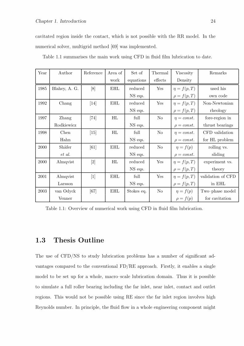
Table 1.1 summarises the main work using CFD in fluid film lubrication to date.
Year Author Reference Area of Set of Thermal Viscosity Remarks
work equations effects Density
1985 Blahey, A. G. [8] EHL reduced Yes η = f(p, T ) used his
NS eqs. ρ = f(p, T ) own code
1992 Chang [14] EHL reduced Yes η = f(p, T ) Non-Newtonian
NS eqs. ρ = f(p, T ) rheology
1997 Zhang [74] HL full No η = const. fore-region in
Rodkiewicz NS eqs. ρ = const. thrust bearings
1998 Chen [15] HL full No η = const. CFD validation
Hahn NS eqs. ρ = const. for HL problem
2000 Shafer [61] EHL reduced No η = f(p) rolling vs.
et al. NS eqs. ρ = const. sliding
2000 Almqvist [2] HL reduced Yes η = f(p, T ) experiment vs.
NS eqs. ρ = f(p, T ) theory
2001 Almqvist [1] EHL full Yes η = f(p, T ) validation of CFD
Larsson NS eqs. ρ = f(p, T ) in EHL
2003 van Odyck [67] EHL Stokes eq. No η = f(p) Two–phase model
Venner ρ = f(p) for cavitation
Table 1.1: Overview of numerical work using CFD in fluid film lubrication.
1.3 Thesis Outline
The use of CFD/NS to study lubrication problems has a number of significant ad-
vantages compared to the conventional FD/RE approach. Firstly, it enables a single
model to be set up for a whole, macro–scale lubrication domain. Thus it is possible
to simulate a full roller bearing including the far inlet, near inlet, contact and outlet
regions. This would not be possible using RE since the far inlet region involves high
Reynolds number. In principle, the fluid flow in a whole engineering component might
Chapter 1. Introduction 25
be simulated.
Another potential advantage is in rough surface lubricated contact, where the lu-
bricant film thickness is comparable to the scale of the roughness. In such conditions,
some of the assumptions which lead to RE may no longer hold, e.g. neglect of inertia.
There are also some bearing geometries to which RE cannot be applied, e.g. rapidly
diverging regions within a pad bearing, where recirculation may take place. Other
systems which CFD can model relevant to film fluid lubricant include two phase flow
such as cavitation, or lubrication by emulsions or solid dispersions.
The overall objective of this research is to develop and validate a CFD–based solu-
tion to the HL and EHL problems. The specific aims are as follows:
• To develop a CFD methodology for complex geometries in the HL research;
• To expand the computational domain well outside the contact zone;
• To include the two-phase flow (i.e. cavitation) in the analysis;
• To develop a CFD methodology for smooth and rough surface EHL simulation
based on finite volume and multigrid techniques;
• To use this to test the validity of the assumption of constant pressure across the
thickness of the film.
Chapter 2
Governing Equations of Fluid Flow
2.1 Introduction
In this Chapter the governing equations of continuum mechanics will be introduced.
Since the analysis of the fluid flow will be done at macroscopic length scales (> 10−9 m),
the molecular structure of matter and individual molecular motions will be ignored.
The behaviour of the fluid will be described in terms of macroscopic properties, e.g.
velocity, pressure and density, and their space and time derivatives. All the cases in
this study will be regarded as isothermal and therefore the energy equation will not be
included.
Order of magnitude analysis will be carried out on the governing equations with
the characteristic values for lubrication. To analyse the equations, non–dimensional
variables are introduced. By doing this, it will be possible to assess the relative sig-
nificance of the various terms in each equation for different regions in the domain and
geometries of interest.
In the contact region, where the aspect ratio (ratio between characteristic length and
characteristic height) is large (≈ 103), the Reynolds number is very small (Re ≈ 10−3)
and certain terms from the NS equation may be neglected. The full set of governing
equations then reduces to the Reynolds Equation. However, this is valid only in the
contact region and assuming there is no steep surface roughness present.
If one wants to expand the domain further outwards into the inlet and outlet regions,
26
Chapter 2. Governing Equations of Fluid Flow 27
the convective terms in NS equations cease being negligible. In this Chapter, order of
magnitude analysis is conducted both for the contact and far regions, demonstrating
the need to use the full NS equations in the latter.
2.2 Governing Equations of Continuum Mechanics
All the equations in this Chapter will be presented both in vector notation and in the
expanded form in the Cartesian (x, y and z) coordinates. The vector notation will
be used in Chapter 3 as a suitable form in which we will describe the Finite Volume
Method. The expanded form of the equations in the Cartesian coordinates will be used
in this Chapter to perform the order of magnitude analysis.
2.2.1 Mass and Momentum Conservation
The governing equations of fluid flow represent mathematical statements of the con-
servation laws of physics (Versteeg, [70]):
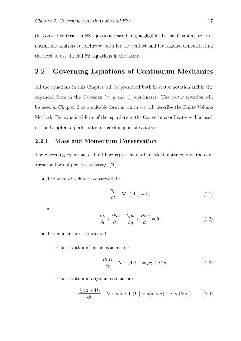
• The mass of a fluid is conserved, i.e.
∂ρ
∂t+ ∇ · (ρU) = 0, (2.1)
or,
∂ρ
∂t+
∂ρu
∂x+
∂ρv
∂y+
∂ρw
∂z= 0. (2.2)
• The momentum is conserved:
– Conservation of linear momentum:
∂ρU
∂t+ ∇ · (ρUU) = ρg + ∇·σ, (2.3)
– Conservation of angular momentum:
∂ρ(x × U)
∂t+ ∇ · [ρ(x × U)U] = ρ(x × g) + x × (∇·σ). (2.4)
Chapter 2. Governing Equations of Fluid Flow 28
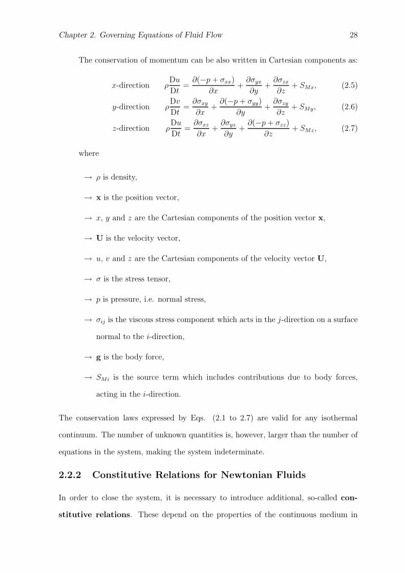
The conservation of momentum can be also written in Cartesian components as:
x-direction ρDu
Dt=
∂(−p + σxx)
∂x+
∂σyx
∂y+
∂σzx
∂z+ SMx, (2.5)
y-direction ρDv
Dt=
∂σxy
∂x+
∂(−p + σyy)
∂y+
∂σzy
∂z+ SMy, (2.6)
z-direction ρDu
Dt=
∂σxz
∂x+
∂σyz
∂y+
∂(−p + σzz)
∂z+ SMz, (2.7)
where
→ ρ is density,
→ x is the position vector,
→ x, y and z are the Cartesian components of the position vector x,
→ U is the velocity vector,
→ u, v and z are the Cartesian components of the velocity vector U,
→ σ is the stress tensor,
→ p is pressure, i.e. normal stress,
→ σij is the viscous stress component which acts in the j-direction on a surface
normal to the i-direction,
→ g is the body force,
→ SMi is the source term which includes contributions due to body forces,
acting in the i-direction.
The conservation laws expressed by Eqs. (2.1 to 2.7) are valid for any isothermal
continuum. The number of unknown quantities is, however, larger than the number of
equations in the system, making the system indeterminate.
2.2.2 Constitutive Relations for Newtonian Fluids
In order to close the system, it is necessary to introduce additional, so-called con-
stitutive relations. These depend on the properties of the continuous medium in
Chapter 2. Governing Equations of Fluid Flow 29
question. In the case of Newtonian fluids under isothermal conditions, the following
set of constitutive relations can be used:
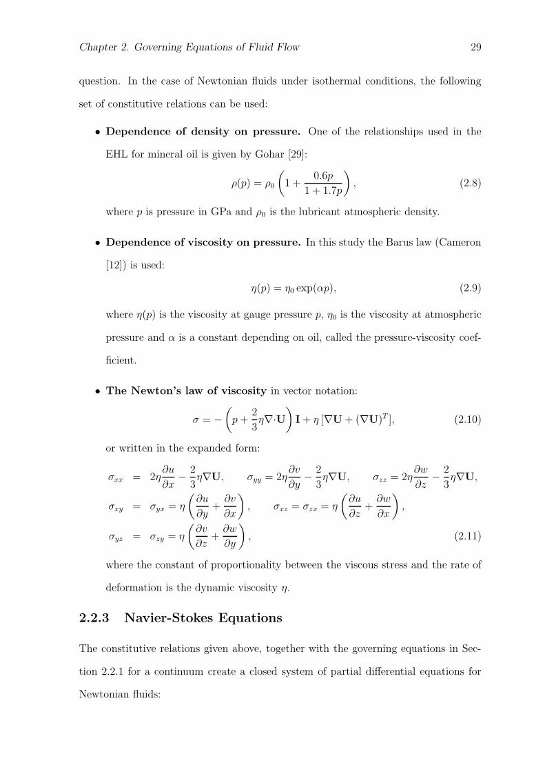
• Dependence of density on pressure. One of the relationships used in the
EHL for mineral oil is given by Gohar [29]:
ρ(p) = ρ0
(
1 +0.6p
1 + 1.7p
)
, (2.8)
where p is pressure in GPa and ρ0 is the lubricant atmospheric density.
• Dependence of viscosity on pressure. In this study the Barus law (Cameron
[12]) is used:
η(p) = η0 exp(αp), (2.9)
where η(p) is the viscosity at gauge pressure p, η0 is the viscosity at atmospheric
pressure and α is a constant depending on oil, called the pressure-viscosity coef-
ficient.
• The Newton’s law of viscosity in vector notation:
σ = −
(
p +2
3η∇·U
)
I + η [∇U + (∇U)T ], (2.10)
or written in the expanded form:
σxx = 2η∂u
∂x−
2
3η∇U, σyy = 2η
∂v
∂y−
2
3η∇U, σzz = 2η
∂w
∂z−
2
3η∇U,
σxy = σyx = η
(∂u
∂y+
∂v
∂x
)
, σxz = σzx = η
(∂u
∂z+
∂w
∂x
)
,
σyz = σzy = η
(∂v
∂z+
∂w
∂y
)
, (2.11)
where the constant of proportionality between the viscous stress and the rate of
deformation is the dynamic viscosity η.
2.2.3 Navier-Stokes Equations
The constitutive relations given above, together with the governing equations in Sec-
tion 2.2.1 for a continuum create a closed system of partial differential equations for
Newtonian fluids:
Chapter 2. Governing Equations of Fluid Flow 30
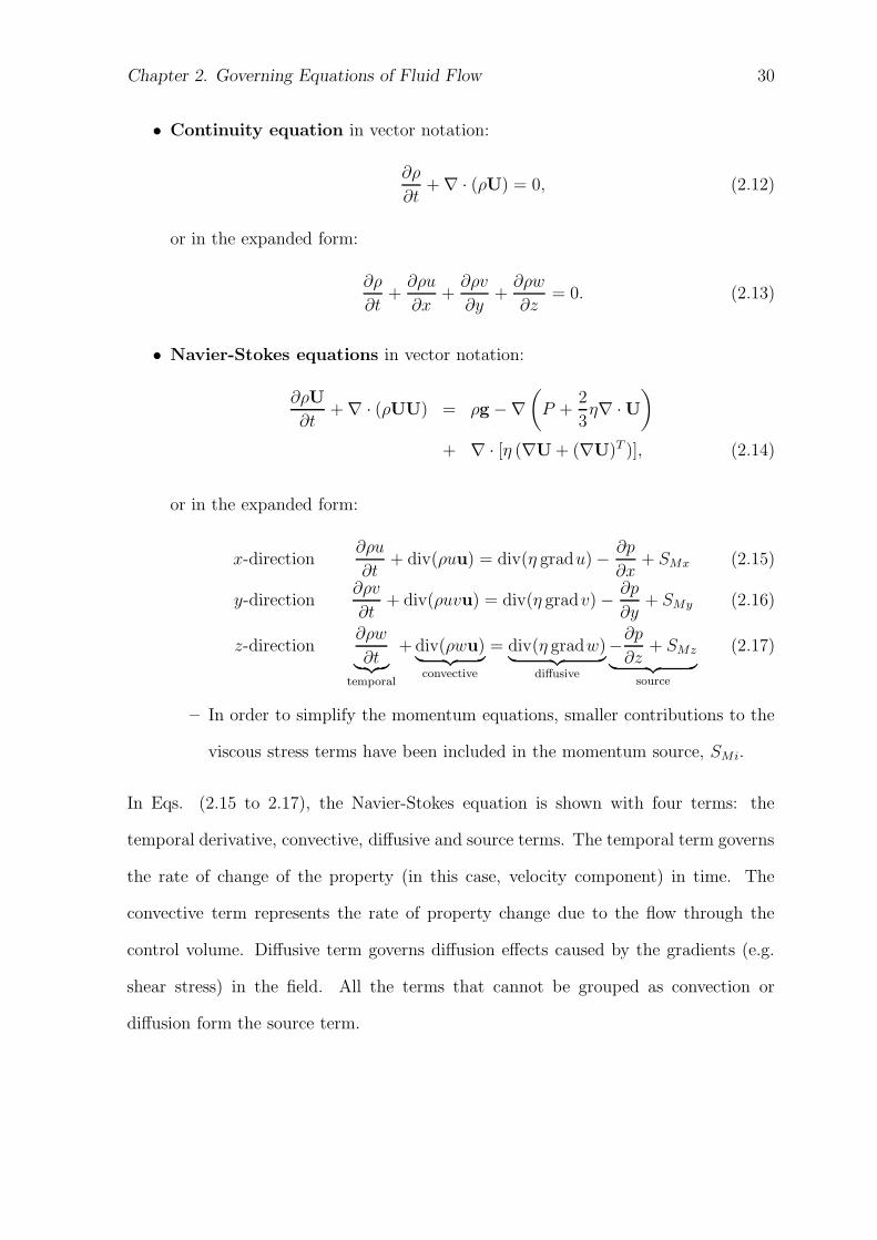
• Continuity equation in vector notation:
∂ρ
∂t+ ∇ · (ρU) = 0, (2.12)
or in the expanded form:
∂ρ
∂t+
∂ρu
∂x+
∂ρv
∂y+
∂ρw
∂z= 0. (2.13)
• Navier-Stokes equations in vector notation:
∂ρU
∂t+ ∇ · (ρUU) = ρg −∇
(
P +2
3η∇ ·U
)
+ ∇ · [η (∇U + (∇U)T )], (2.14)
or in the expanded form:
x-direction∂ρu
∂t+ div(ρuu) = div(η gradu) −
∂p
∂x+ SMx (2.15)
y-direction∂ρv
∂t+ div(ρuvu) = div(η gradv) −
∂p
∂y+ SMy (2.16)
z-direction∂ρw
∂t︸︷︷︸
temporal
+ div(ρwu)︸ ︷︷ ︸
convective
= div(η gradw)︸ ︷︷ ︸
diffusive
−∂p
∂z+ SMz
︸ ︷︷ ︸
source
(2.17)
– In order to simplify the momentum equations, smaller contributions to the
viscous stress terms have been included in the momentum source, SMi.
In Eqs. (2.15 to 2.17), the Navier-Stokes equation is shown with four terms: the
temporal derivative, convective, diffusive and source terms. The temporal term governs
the rate of change of the property (in this case, velocity component) in time. The
convective term represents the rate of property change due to the flow through the
control volume. Diffusive term governs diffusion effects caused by the gradients (e.g.
shear stress) in the field. All the terms that cannot be grouped as convection or
diffusion form the source term.
Chapter 2. Governing Equations of Fluid Flow 31
2.3 Order of Magnitude Analysis
2.3.1 Non–Dimensional Variables
In order to perform an order of magnitude analysis on equations from Section 2.2,
non–dimensional variables are introduced. Non-dimensional variables are generally
used in numerical analysis. Their advantage is that the results have generality and the
problems of different systems of units are removed.
Assuming the characteristic values, the non–dimensional variables, denoted by sub-
script ∗, are shown as a ratio between the dimensional variable and their characteristic
value, denoted by subscript o:
Pressure p∗ =p
p0,
Density ρ∗ =ρ
ρ0
,
x - Cartesian coordinate x∗ =x
x0,
y - Cartesian coordinate y∗ =y
y0
,
z - Cartesian coordinate z∗ =z
z0,
velocity component in x-direction u∗ =u
u0
, (2.18)
velocity component in y-direction v∗ =v
v0,
velocity component in z-direction u∗ =w
w0
,
Dynamic viscosity η∗ =η
η0,
Pressure - viscosity coefficient α∗ =α
α0.
2.3.2 Characteristic Values
In both hydrodynamic and elastohydrodynamimc lubrication, we encounter geometries
where the aspect ratio (i.e. ratio between the length and the height) in contact zones
is of order of magnitude 103. Figure 2.1 shows a schematic picture of a contact divided
into two regions:
Chapter 2. Governing Equations of Fluid Flow 32
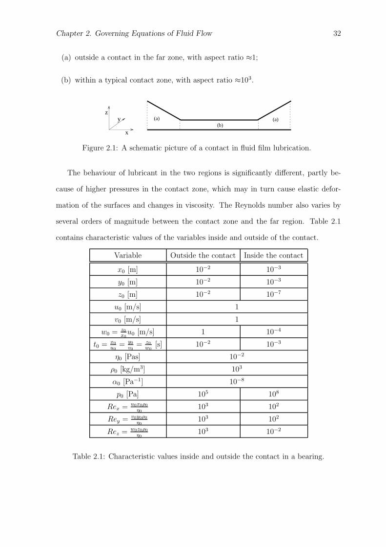
(a) outside a contact in the far zone, with aspect ratio ≈1;
(b) within a typical contact zone, with aspect ratio ≈103.
(a)(b)
(a)z
y
x
Figure 2.1: A schematic picture of a contact in fluid film lubrication.
The behaviour of lubricant in the two regions is significantly different, partly be-
cause of higher pressures in the contact zone, which may in turn cause elastic defor-
mation of the surfaces and changes in viscosity. The Reynolds number also varies by
several orders of magnitude between the contact zone and the far region. Table 2.1
contains characteristic values of the variables inside and outside of the contact.
Variable Outside the contact Inside the contact
x0 [m] 10−2 10−3
y0 [m] 10−2 10−3
z0 [m] 10−2 10−7
u0 [m/s] 1
v0 [m/s] 1
w0 = z0
x0
u0 [m/s] 1 10−4
t0 = x0
u0
= y0
v0
= z0
w0
[s] 10−2 10−3
η0 [Pas] 10−2
ρ0 [kg/m3] 103
α0 [Pa−1] 10−8
p0 [Pa] 105 108
Rex = u0x0ρ0
η0
103 102
Rey = v0y0ρ0
η0
103 102
Rez = w0z0ρ0
η0
103 10−2
Table 2.1: Characteristic values inside and outside the contact in a bearing.
Chapter 2. Governing Equations of Fluid Flow 33
2.4 Non–Dimensional Equations
In order to determine which terms in the equations are dominant, dimensional variables
in the governing equations will be replaced by the product of their non-dimensional
variable (see Eqn. 2.18) and the characteristic value. Different regions of the bearing
will be studied with their respective characteristic values. An exponential, Barus-type
viscosity-pressure relationship, Eqn. (2.9), is assumed.
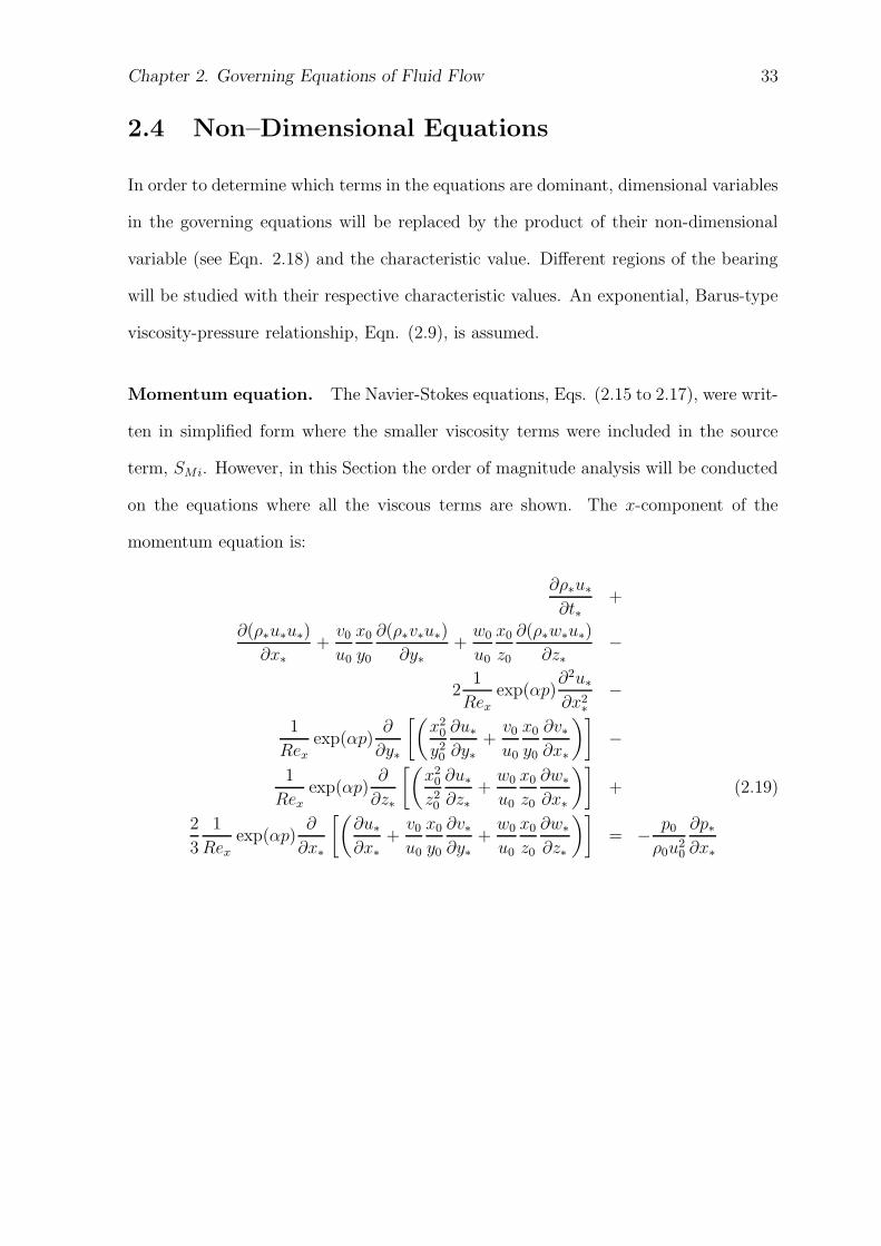
Momentum equation. The Navier-Stokes equations, Eqs. (2.15 to 2.17), were writ-
ten in simplified form where the smaller viscosity terms were included in the source
term, SMi. However, in this Section the order of magnitude analysis will be conducted
on the equations where all the viscous terms are shown. The x-component of the
momentum equation is:
∂ρ∗u∗
∂t∗+
∂(ρ∗u∗u∗)
∂x∗
+v0
u0
x0
y0
∂(ρ∗v∗u∗)
∂y∗+
w0
u0
x0
z0
∂(ρ∗w∗u∗)
∂z∗−
21
Rex
exp(αp)∂2u∗
∂x2∗
−
1
Rexexp(αp)
∂
∂y∗
[(x2
0
y20
∂u∗
∂y∗+
v0
u0
x0
y0
∂v∗∂x∗
)]
−
1
Rexexp(αp)
∂
∂z∗
[(x2
0
z20
∂u∗
∂z∗+
w0
u0
x0
z0
∂w∗
∂x∗
)]
+ (2.19)
2
3
1
Rex
exp(αp)∂
∂x∗
[(∂u∗
∂x∗
+v0
u0
x0
y0
∂v∗∂y∗
+w0
u0
x0
z0
∂w∗
∂z∗
)]
= −p0
ρ0u20
∂p∗∂x∗
Chapter 2. Governing Equations of Fluid Flow 34
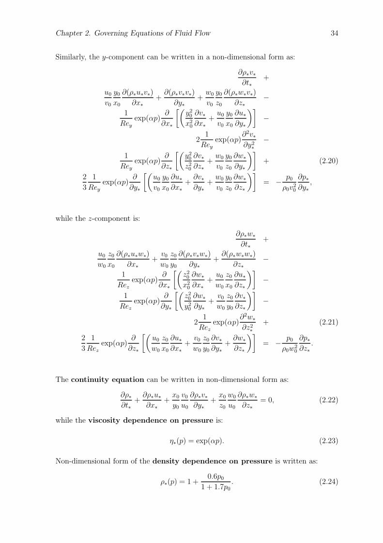
Similarly, the y-component can be written in a non-dimensional form as:
∂ρ∗v∗∂t∗
+
u0
v0
y0
x0
∂(ρ∗u∗v∗)
∂x∗
+∂(ρ∗v∗v∗)
∂y∗+
w0
v0
y0
z0
∂(ρ∗w∗v∗)
∂z∗−
1
Reyexp(αp)
∂
∂x∗
[(y2
0
x20
∂v∗∂x∗
+u0
v0
y0
x0
∂u∗
∂y∗
)]
−
21
Reyexp(αp)
∂2v∗∂y2
∗
−
1
Rey
exp(αp)∂
∂z∗
[(y2
0
z20
∂v∗∂z∗
+w0
v0
y0
z0
∂w∗
∂y∗
)]
+ (2.20)
2
3
1
Rey
exp(αp)∂
∂y∗
[(u0
v0
y0
x0
∂u∗
∂x∗
+∂v∗∂y∗
+w0
v0
y0
z0
∂w∗
∂z∗
)]
= −p0
ρ0v20
∂p∗∂y∗
,
while the z-component is:
∂ρ∗w∗
∂t∗+
u0
w0
z0
x0
∂(ρ∗u∗w∗)
∂x∗
+v0
w0
z0
y0
∂(ρ∗v∗w∗)
∂y∗+
∂(ρ∗w∗w∗)
∂z∗−
1
Rezexp(αp)
∂
∂x∗
[(z20
x20
∂w∗
∂x∗
+u0
w0
z0
x0
∂u∗
∂z∗
)]
−
1
Rezexp(αp)
∂
∂y∗
[(z20
y20
∂w∗
∂y∗+
v0
w0
z0
y0
∂v∗∂z∗
)]
−
21
Rezexp(αp)
∂2w∗
∂z2∗
+ (2.21)
2
3
1
Rezexp(αp)
∂
∂z∗
[(u0
w0
z0
x0
∂u∗
∂x∗
+v0
w0
z0
y0
∂v∗∂y∗
+∂w∗
∂z∗
)]
= −p0
ρ0w20
∂p∗∂z∗
.
The continuity equation can be written in non-dimensional form as:
∂ρ∗
∂t∗+
∂ρ∗u∗
∂x∗
+x0
y0
v0
u0
∂ρ∗v∗∂y∗
+x0
z0
w0
u0
∂ρ∗w∗
∂z∗= 0, (2.22)
while the viscosity dependence on pressure is:
η∗(p) = exp(αp). (2.23)
Non-dimensional form of the density dependence on pressure is written as:
ρ∗(p) = 1 +0.6p0
1 + 1.7p0. (2.24)
Chapter 2. Governing Equations of Fluid Flow 35
2.5 Non–dimensional Equations with
Characteristic Values
Characteristic values for the region of interest are now substituted in Eqs. (2.19 to
2.24), to identify the dominant terms for each equation. Printed in bold are the relative
magnitudes of each term.
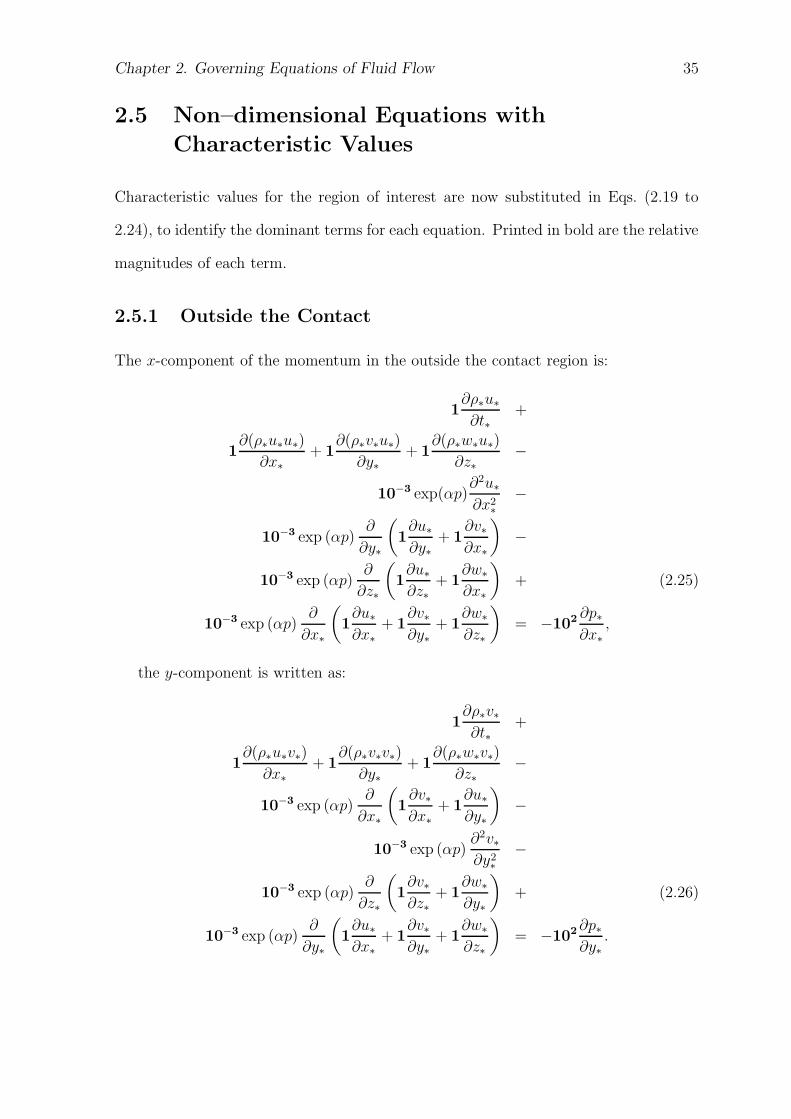
2.5.1 Outside the Contact
The x-component of the momentum in the outside the contact region is:
1∂ρ∗u∗
∂t∗+
1∂(ρ∗u∗u∗)
∂x∗
+ 1∂(ρ∗v∗u∗)
∂y∗+ 1
∂(ρ∗w∗u∗)
∂z∗−
10−3 exp(αp)∂2u∗
∂x2∗
−
10−3 exp (αp)∂
∂y∗
(
1∂u∗
∂y∗+ 1
∂v∗∂x∗
)
−
10−3 exp (αp)∂
∂z∗
(
1∂u∗
∂z∗+ 1
∂w∗
∂x∗
)
+ (2.25)
10−3 exp (αp)∂
∂x∗
(
1∂u∗
∂x∗
+ 1∂v∗∂y∗
+ 1∂w∗
∂z∗
)
= −102∂p∗∂x∗
,
the y-component is written as:
1∂ρ∗v∗∂t∗
+
1∂(ρ∗u∗v∗)
∂x∗
+ 1∂(ρ∗v∗v∗)
∂y∗+ 1
∂(ρ∗w∗v∗)
∂z∗−
10−3 exp (αp)∂
∂x∗
(
1∂v∗∂x∗
+ 1∂u∗
∂y∗
)
−
10−3 exp (αp)∂2v∗∂y2
∗
−
10−3 exp (αp)∂
∂z∗
(
1∂v∗∂z∗
+ 1∂w∗
∂y∗
)
+ (2.26)
10−3 exp (αp)∂
∂y∗
(
1∂u∗
∂x∗
+ 1∂v∗∂y∗
+ 1∂w∗
∂z∗
)
= −102∂p∗∂y∗
.
Chapter 2. Governing Equations of Fluid Flow 36
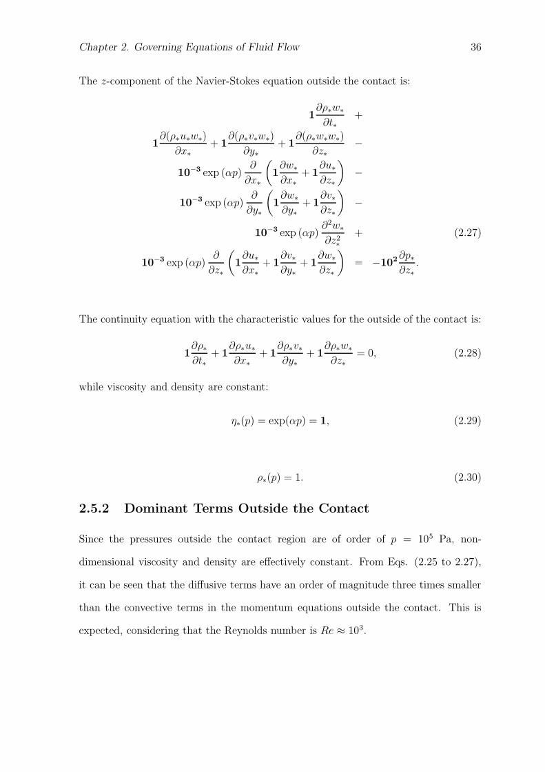
The z-component of the Navier-Stokes equation outside the contact is:
1∂ρ∗w∗
∂t∗+
1∂(ρ∗u∗w∗)
∂x∗
+ 1∂(ρ∗v∗w∗)
∂y∗+ 1
∂(ρ∗w∗w∗)
∂z∗−
10−3 exp (αp)∂
∂x∗
(
1∂w∗
∂x∗
+ 1∂u∗
∂z∗
)
−
10−3 exp (αp)∂
∂y∗
(
1∂w∗
∂y∗+ 1
∂v∗∂z∗
)
−
10−3 exp (αp)∂2w∗
∂z2∗
+ (2.27)
10−3 exp (αp)∂
∂z∗
(
1∂u∗
∂x∗
+ 1∂v∗∂y∗
+ 1∂w∗
∂z∗
)
= −102∂p∗∂z∗
.
The continuity equation with the characteristic values for the outside of the contact is:
1∂ρ∗
∂t∗+ 1
∂ρ∗u∗
∂x∗
+ 1∂ρ∗v∗∂y∗
+ 1∂ρ∗w∗
∂z∗= 0, (2.28)
while viscosity and density are constant:
η∗(p) = exp(αp) = 1, (2.29)
ρ∗(p) = 1. (2.30)
2.5.2 Dominant Terms Outside the Contact
Since the pressures outside the contact region are of order of p = 105 Pa, non-
dimensional viscosity and density are effectively constant. From Eqs. (2.25 to 2.27),
it can be seen that the diffusive terms have an order of magnitude three times smaller
than the convective terms in the momentum equations outside the contact. This is
expected, considering that the Reynolds number is Re ≈ 103.
Chapter 2. Governing Equations of Fluid Flow 37
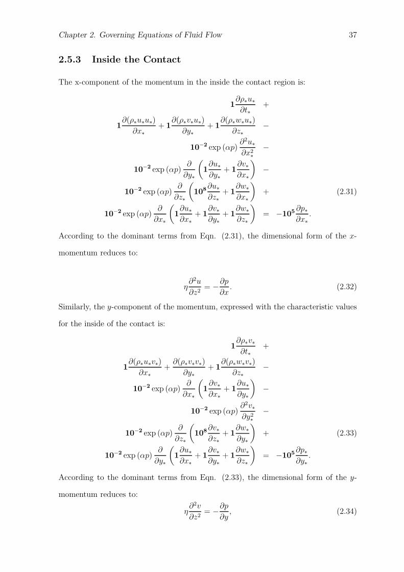
2.5.3 Inside the Contact
The x-component of the momentum in the inside the contact region is:
1∂ρ∗u∗
∂t∗+
1∂(ρ∗u∗u∗)
∂x∗
+ 1∂(ρ∗v∗u∗)
∂y∗+ 1
∂(ρ∗w∗u∗)
∂z∗−
10−2 exp (αp)∂2u∗
∂x2∗
−
10−2 exp (αp)∂
∂y∗
(
1∂u∗
∂y∗+ 1
∂v∗∂x∗
)
−
10−2 exp (αp)∂
∂z∗
(
108∂u∗
∂z∗+ 1
∂w∗
∂x∗
)
+ (2.31)
10−2 exp (αp)∂
∂x∗
(
1∂u∗
∂x∗
+ 1∂v∗∂y∗
+ 1∂w∗
∂z∗
)
= −105∂p∗∂x∗
.
According to the dominant terms from Eqn. (2.31), the dimensional form of the x-
momentum reduces to:
η∂2u
∂z2= −
∂p
∂x. (2.32)
Similarly, the y-component of the momentum, expressed with the characteristic values
for the inside of the contact is:
1∂ρ∗v∗∂t∗
+
1∂(ρ∗u∗v∗)
∂x∗
+∂(ρ∗v∗v∗)
∂y∗+ 1
∂(ρ∗w∗v∗)
∂z∗−
10−2 exp (αp)∂
∂x∗
(
1∂v∗∂x∗
+ 1∂u∗
∂y∗
)
−
10−2 exp (αp)∂2v∗∂y2
∗
−
10−2 exp (αp)∂
∂z∗
(
108∂v∗∂z∗
+ 1∂w∗
∂y∗
)
+ (2.33)
10−2 exp (αp)∂
∂y∗
(
1∂u∗
∂x∗
+ 1∂v∗∂y∗
+ 1∂w∗
∂z∗
)
= −105∂p∗∂y∗
.
According to the dominant terms from Eqn. (2.33), the dimensional form of the y-
momentum reduces to:
η∂2v
∂z2= −
∂p
∂y, (2.34)
Chapter 2. Governing Equations of Fluid Flow 38
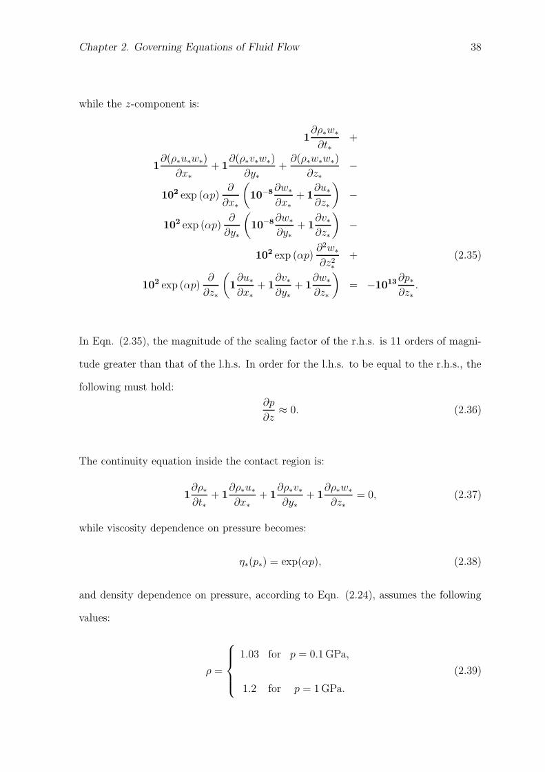
while the z-component is:
1∂ρ∗w∗
∂t∗+
1∂(ρ∗u∗w∗)
∂x∗
+ 1∂(ρ∗v∗w∗)
∂y∗+
∂(ρ∗w∗w∗)
∂z∗−
102 exp (αp)∂
∂x∗
(
10−8∂w∗
∂x∗
+ 1∂u∗
∂z∗
)
−
102 exp (αp)∂
∂y∗
(
10−8∂w∗
∂y∗+ 1
∂v∗∂z∗
)
−
102 exp (αp)∂2w∗
∂z2∗
+ (2.35)
102 exp (αp)∂
∂z∗
(
1∂u∗
∂x∗
+ 1∂v∗∂y∗
+ 1∂w∗
∂z∗
)
= −1013∂p∗∂z∗
.
In Eqn. (2.35), the magnitude of the scaling factor of the r.h.s. is 11 orders of magni-
tude greater than that of the l.h.s. In order for the l.h.s. to be equal to the r.h.s., the
following must hold:
∂p
∂z≈ 0. (2.36)
The continuity equation inside the contact region is:
1∂ρ∗
∂t∗+ 1
∂ρ∗u∗
∂x∗
+ 1∂ρ∗v∗∂y∗
+ 1∂ρ∗w∗
∂z∗= 0, (2.37)
while viscosity dependence on pressure becomes:
η∗(p∗) = exp(αp), (2.38)
and density dependence on pressure, according to Eqn. (2.24), assumes the following
values:
ρ =
1.03 for p = 0.1 GPa,
1.2 for p = 1 GPa.
(2.39)
Chapter 2. Governing Equations of Fluid Flow 39
2.5.4 Dominant Terms Inside the Contact
In the contact, the pressure can rise from the order of magnitude of 107 Pa to 109 Pa.
That implies that the non-dimensional viscosity, Eqn. (2.38), can assume values from
1 to 104. One has to bear in mind that the Barus law for viscosity dependence on
pressure, Eqn. (2.9), generally becomes inaccurate above 0.5 GPa and even more so if
the ambient temperature is high.
From Eqs. (2.31 to 2.35), it can be seen that inside the contact, the diffusive terms
dominate in the momentum equations. This is expected, considering that the Reynolds
number is Re ≈ 10−2. Due to the very high local pressure in the contact, fluid viscosity
(2.38) and density (2.39) are no longer constant, but dependent on pressure.
2.6 Closure
In this Chapter the governing equations for the flow of a lubricant in a bearing were
given. These equations were then non-dimensionalised and order of magnitude analysis
was carried out for the two regions of the bearing: the contact region and the region
outside the contact.
The order of magnitude analysis has shown that the Reynolds number based on film
height varies over the full computational domain from 10−2 to 103. Because of such a
big variation, different terms dominate the governing equations for the fluid flow in the
two regions. In the region outside the contact, convective terms are dominant, whereas
in the contact region diffusive terms are greater. This is one of the reasons why it is
necessary to use the full set of Navier-Stokes equations when solving the fluid flow over
the entire bearing and not only in the contact region.
In the high-pressure, contact region, the aspect ratio between film thickness, z0,
and the characteristic length, x0 is of the order of 10−4. In that region, if the surfaces
are so smooth that the minimum film thickness in the problem is large compared
to the surface roughness, Navier-Stokes equations simplify to Eqs. (2.32, 2.34 and
Chapter 2. Governing Equations of Fluid Flow 40
2.36), from which the Reynolds equation is obtained (see Chapter 4). However, if the
characteristic length of the surface roughness (x-dimension) is comparable to the local
film thickness, the local aspect ratio becomes much higher and certain viscous terms
in Navier-Stokes equations cannot be neglected (van Odyck [66]). Reynolds number is
still Rez � 1 which means that the convective terms remain negligible. The Reynolds
equation, therefore, cannot be used for calculation of the flow parameters in the contact
region with surface roughnesses, but Navier-Stokes equations can be reduced to Stokes
equations (i.e., the convective terms may be omitted).
Chapter 3
Finite Volume Discretisation
3.1 Introduction
In Chapter 2, fluid flow for situations relevant for lubrication, was described by a set
of partial differential equations which cannot be solved analytically. To obtain approx-
imate solutions numerically, we must use a discretisation method which approximates
the differential equations by a system of algebraic equations. The solution of this
system produces values at discrete locations in space and time.
One has to bear in mind that the numerical results are always approximate. The ac-
curacy of numerical solution depends on the quality of discretisations used. The errors
arise from the fact that differential equations describing the flow may contain approx-
imations and idealisations; from the approximations in the discretisation method, and
from convergence criteria, which may stop the iterations before the exact solution of
discretised equations is found.
3.1.1 Components of a Numerical Solution Method
The steps towards the numerical solution method are as follows:
Mathematical Model. It is the set of equations and boundary conditions that de-
scribe a particular problem. As mentioned before, this model may include simplifica-
tions and idealisations of the exact conservation laws. The solution method is usually
designed for a particular set of equations.
41
Chapter 3. Finite Volume Discretisation 42
Coordinate System. Different coordinate systems (e.g. Cartesian, cylindrical, spher-
ical, etc.) may be used depending on the form of the governing equations and on the
geometry of the problem. In this work, the coordinate system employed will be Carte-
sian.
Discretisation Method. One has to select an appropriate discretisation method
for the mathematical model chosen. The Finite Volume Method (FVM) will be used
in this work, which consists of the discretisation of the solution domain and equation
discretisation (Muzaferija [51]). The FVM consists of the following steps:
• Spatial Discretisation. Since the Finite Volume Method is used in the work,
the solution domain has to be divided into a finite number of subdomains, called
control volumes (CV). Each control volume can be of any polyhedral shape with
variable number of neighbours, but not overlapping with them. The grid used in
this study will be a block-structured grid, with a two level subdivision of solution
domain. The domain is divided coarsely into large segments, or blocks, which are
then subdivided into control volumes. By doing that, one can easily introduce a
much finer grid in areas where a high resolution is required.
• Finite Approximations. According to the grid type and discretisation method,
approximations used in the discretisation process must be selected. In the FVM,
one must select the methods of approximating surface and volume integrals. Some
of them will be briefly mentioned in the following Sections. The choice of ap-
proximation greatly influences the accuracy of the numerical solution. The more
accurate an approximation it is, the more computational work it requires. In this
study, the second-order approximation method will be used.
• Convergence Criteria. The convergence criteria must be set for the iterative
method. In the solution algorithms that will be used in this work, there are
two levels of iteration: inner iterations, within which the linear equations are
Chapter 3. Finite Volume Discretisation 43
solved, and outer iterations, that deal with the non-linearity and coupling of the
equations. It is important to consider both the accuracy and efficiency when
deciding to stop the iterative process on each level.
Solution Method Methods of solving the system of algebraic equations can be di-
vided into two categories:
1. Solution of the linear system;
2. Solution methods for handling multiple coupled equations (not in a single linear
system).
The problems which are encountered in CFD work use the latter methods. The two of
such methods, which will be used in this work are:
• SIMPLE algorithm, for steady-state, laminar, non-cavitating flows,
• PISO algorithm, for transient flows and flows with cavitation.
3.1.2 Properties of The Numerical Solution Method
In order for the solution method (in this work, FVM) to be acceptable, it must possess
certain properties. They are listed below:
Consistency. For a method to be consistent, the truncation error, i.e. the difference
between the discretised equation and the exact one, must become zero when the mesh
spacing tends to zero. Truncation error is usually proportional to a power of the grid
spacing ∆x and/or the time step ∆t. The method is called an n-th order approximation
if the leading term in the truncation error is proportional to (∆x)n. In this work, we
are going to use second order approximation throughout.
One has to bear in mind that even if the approximations are consistent, it does not
necessarily mean that the solution will become exact as ∆x → 0. For this to happen,
the solution must also be stable, as defined below.
Chapter 3. Finite Volume Discretisation 44
Stability. A numerical solution method is stable if it does not increase the errors
that appear in the numerical solution process. For temporal problems, the stable
method will produce a bounded solution whenever the solution of the exact equation is
bounded. For iterative methods, a stable method is one that does not diverge. Stability
can often be difficult to investigate. However, it is known that many solution schemes
require the time step to be smaller than a certain limit or that under-relaxation must
be used.
Convergence. A numerical method is convergent if the solution of the discretised
equations tends to the exact solution of the differential equation as the grid spacing
tends to zero. Convergence is usually checked using numerical experiments, i.e. re-
peating the calculation on a series of successively refined grids. If the method is stable
and if all approximations used in the discretisation process are consistent, the solution
usually converges to a grid-independent solution.
Conservation. The numerical method, both on a local and a global basis, should
respect the conservation laws that differential equations represent. The finite volume
method used in this work is conservative both for each individual control volume and
for the solution domain as a whole.
Boundedness. Numerical solutions should lie within proper bounds. That means
that physically non-negative quantities (e.g. density) must always be positive; other
quantities, e.g. concentration must lie between 0% and 100%.
Realisability. In this work, we will have to solve the system in which cavitation
occurs. That problem is too complex to be treated directly, and the method designed
must instead guarantee physically realistic solution. This, itself, is not a numerical
issue but models that are not realisable may result in unphysical solutions or cause
numerical methods to diverge.
Chapter 3. Finite Volume Discretisation 45
Accuracy. Numerical solutions of fluid flow are only approximate solutions. They
always include three kinds of systematic errors (Ferziger and Peric [28]):
• Modeling errors, i.e. the difference between the actual flow and the exact solution
of the mathematical model;
• Discretisation errors, i.e. the difference between the exact solution of the con-
servation equations and the exact solution of the algebraic system of discretised
equations;
• Iteration errors, i.e. the difference between the iterative and exact solutions of
the algebraic equations systems.
It is important to be aware of these errors and to try to distinguish one from another.
For example, modeling errors are negligible in case of laminar flows, since the
Navier-Stokes equations represent an accurate model of the flow. However, in cavi-
tating flows, the modeling error may be very large, making the exact solution of the
numerical model qualitatively wrong. This type of error is also introduced by simplify-
ing the geometry of the solution domain, simplifying boundary conditions, etc. These
errors are not known a priori; they can only be evaluated by comparing numerical so-
lutions in which the discretisation and convergence errors are negligible with accurate
experimental results.
3.2 Spatial Discretisation
In the Finite Volume Method, discretisation of the solution domain produces a number
of discrete points on which the governing equations are solved. It is done by dividing
the domain into a finite number of control volumes (CV), and the conservation equa-
tions are applied to each CV. Control volumes do not overlap and completely fill the
computational domain.
Chapter 3. Finite Volume Discretisation 46
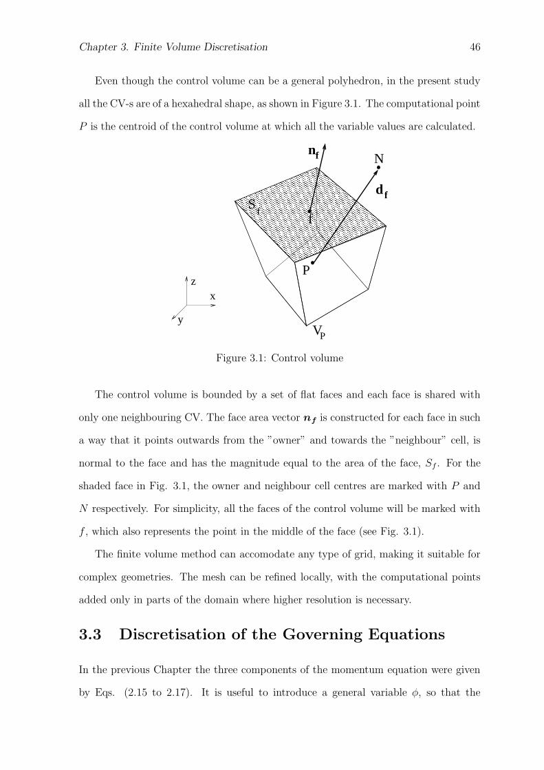
Even though the control volume can be a general polyhedron, in the present study
all the CV-s are of a hexahedral shape, as shown in Figure 3.1. The computational point
P is the centroid of the control volume at which all the variable values are calculated.
���������������������������������������������������������������������������������������������������������������������������������������������������������������������������������������������������������������������������������������������������������������������������������������������������������������������������������������������������������������������������������������������������������������������������������������������������������������������������������������������������������������������������������������������������������������������������������������������������������������������������������������������������������������������������������������������������������������������������������������������������������������������������������������������������������������������������������������������������������������������������������������������������������������������������������������������������������������������������������������������������������������
���������������������������������������������������������������������������������������������������������������������������������������������������������������������������������������������������������������������������������������������������������������������������������������������������������������������������������������������������������������������������������������������������������������������������������������������������������������������������������������������������������������������������������������������������������������������������������������������������������������������������������������������������������������������������������������������������������������������������������������������������������������������������������������������������������������������������������������������������������������������������������������������������������������������������������������������������������������������������������������������������������������
z
y
x
f
n
P
Nf
fdS
f
VP
Figure 3.1: Control volume
The control volume is bounded by a set of flat faces and each face is shared with
only one neighbouring CV. The face area vector nf is constructed for each face in such
a way that it points outwards from the ”owner” and towards the ”neighbour” cell, is
normal to the face and has the magnitude equal to the area of the face, Sf . For the
shaded face in Fig. 3.1, the owner and neighbour cell centres are marked with P and
N respectively. For simplicity, all the faces of the control volume will be marked with
f , which also represents the point in the middle of the face (see Fig. 3.1).
The finite volume method can accomodate any type of grid, making it suitable for
complex geometries. The mesh can be refined locally, with the computational points
added only in parts of the domain where higher resolution is necessary.
3.3 Discretisation of the Governing Equations
In the previous Chapter the three components of the momentum equation were given
by Eqs. (2.15 to 2.17). It is useful to introduce a general variable φ, so that the
Chapter 3. Finite Volume Discretisation 47
conservative form of all fluid flow equations (including also energy equation, etc.) can
be written as follows:
∂ρφ
∂t︸︷︷︸
temporal
+∇ · (ρUφ)︸ ︷︷ ︸
convection
−∇ · (ρΓφ∇φ)︸ ︷︷ ︸
diffusion
= Sφ(φ)︸ ︷︷ ︸
source
. (3.1)
In words
Rate of change Net rate of flow Rate of change Rate of change
of φ in fluid + of φ in or out of - of φ due to = of φ due to
element fluid element diffusion sources or sinks
Eqn. (3.1) is called a transport equation for property φ. It is used as the starting
point for computational procedures in the FVM. By setting φ equal to 1, u, v and w (if
thermal effects are included, also T ) and selecting appropriate values for the diffusion
coefficient Γ and source terms, Eqs. (2.13 to 2.17) are obtained.
The FVM uses the integral form of Eqn. (3.1) as the starting point:
∂
∂t
∫
VP
ρφ dV +
∫
VP
∇ · (ρUφ)dV −
∫
VP
∇ · (ρΓφ∇φ)dV
=
∫
VP
Sφ(φ)dV (3.2)
Volume integrals in the convective and diffusive terms are re-written as integrals
over the bounding surface of the CV by using the Gauss’ divergence theorem:
∫
CV
∇·a dV =
∮
∂V
dn · a, (3.3)∫
CV
∇φ dV =
∮
∂V
dnφ, (3.4)∫
CV
∇ a dV =
∮
∂V
dna, (3.5)
where ∂V is the closed surface bounding the volume V and dn represents an infinites-
imal surface element with associated outward pointing normal on ∂V .
Chapter 3. Finite Volume Discretisation 48
Since the diffusion term includes the second derivative of φ in space, this is a second-
order equation. To ensure consistency, the order of the discretisation must be of equal
or higher order than the order of the equation that is being discretised.
If we assume that φ = φ(x, t) varies linearly in space and time around the point P ,
it can be written:
φ(x) = φP + (x − xP ) · (∇φ)P , (3.6)
φ(t + ∆t) = φt + ∆t
(∂φ
∂t
)t
, (3.7)
where
φP = φ(xP ), (3.8)
φt = φ(t). (3.9)
The discretisation in this study is therefore second-order accurate in space and time,
since the most dominant term of the truncation error in Taylor series is proportional
to (x− xP )2, which for a 1-D situation is equal to the square of the size of the control
volume:
φ(x) = φP + (x − xP ) · (∇φ)P +1
2(x − xP )2 · (∇∇φ)P + ...
︸ ︷︷ ︸
truncation error
, (3.10)
The equivalent analysis shows that the truncation error in Eqn. (3.7) is proportional
to ∆t2, resulting in the second-order temporal accuracy.
From Eqn. (3.6), it follows that:∫
VP
φ(x) dV =
∫
VP
[φP + (x − xP ) · (∇φ)P ] dV
= φP
∫
VP
dV +
[∫
VP
(x − xP )dV
]
· (∆φ)P
= φPVP , (3.11)
where VP is the volume of the cell, since the point P is the centroid of the control
volume:∫
VP
(x − xP ) dV = 0. (3.12)
Chapter 3. Finite Volume Discretisation 49
In order to obtain a discretised form of the Gauss’ theorem, Eqn. (3.3) can be
transformed into a sum of integrals over all faces:
∫
CV
∇·a dV =
∮
∂V
dn · a,
=∑
f
(∫
f
dn · a
)
. (3.13)
If we assume that |a| varies linearly in space, the face integral in Eqn. (3.13) can be
written as:
∫
f
dn · a =
(∫
f
dn
)
· af +
[∫
f
dn(x − xf)
]
· (∇a)f
= n · af (3.14)
By combining Eqs. (3.11, 3.13 and 3.14), the following is obtained:
(∇·a)VP =∑
f
n · af , (3.15)
where af is the value of the variable a in the middle of the face f and n is the outward-
pointing face area vector.
3.3.1 Convection Term
The discretisation of the convection term is obtained using Eqn. (3.15):
∫
VP
∇·(ρUφ)dV =∑
f
n·(ρUφ)f
=∑
f
n·(ρU)fφf
=∑
f
Fφf , (3.16)
where F is the mass flux through the face:
F = n·(ρU)f (3.17)
Convection Differencing Scheme
From Eqn. (3.16), it is clear that the approximation to the integral form of the con-
vection term requires the values of variables at locations other than computational
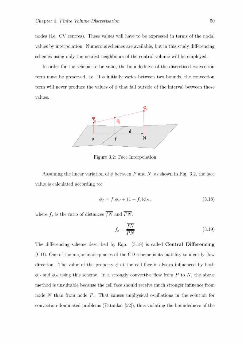
Chapter 3. Finite Volume Discretisation 50
nodes (i.e. CV centres). These values will have to be expressed in terms of the nodal
values by interpolation. Numerous schemes are available, but in this study differencing
schemes using only the nearest neighbours of the control volume will be employed.
In order for the scheme to be valid, the boundedness of the discretised convection
term must be preserved, i.e. if φ initially varies between two bounds, the convection
term will never produce the values of φ that fall outside of the interval between those
values.
φP
φN
f
dNP
φf
Figure 3.2: Face Interpolation
Assuming the linear variation of φ between P and N , as shown in Fig. 3.2, the face
value is calculated according to:
φf = fxφP + (1 − fx)φN , (3.18)
where fx is the ratio of distances fN and PN :
fx =fN
PN(3.19)
The differencing scheme described by Eqn. (3.18) is called Central Differencing
(CD). One of the major inadequacies of the CD scheme is its inability to identify flow
direction. The value of the property φ at the cell face is always influenced by both
φP and φN using this scheme. In a strongly convective flow from P to N , the above
method is unsuitable because the cell face should receive much stronger influence from
node N than from node P . That causes unphysical oscillations in the solution for
convection-dominated problems (Patankar [52]), thus violating the boundedness of the
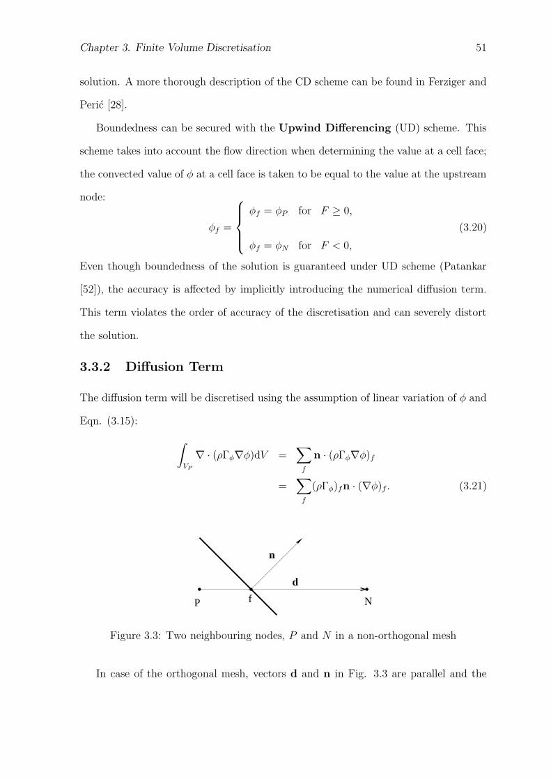
Chapter 3. Finite Volume Discretisation 51
solution. A more thorough description of the CD scheme can be found in Ferziger and
Peric [28].
Boundedness can be secured with the Upwind Differencing (UD) scheme. This
scheme takes into account the flow direction when determining the value at a cell face;
the convected value of φ at a cell face is taken to be equal to the value at the upstream
node:
φf =
φf = φP for F ≥ 0,
φf = φN for F < 0,
(3.20)
Even though boundedness of the solution is guaranteed under UD scheme (Patankar
[52]), the accuracy is affected by implicitly introducing the numerical diffusion term.
This term violates the order of accuracy of the discretisation and can severely distort
the solution.
3.3.2 Diffusion Term
The diffusion term will be discretised using the assumption of linear variation of φ and
Eqn. (3.15):
∫
VP
∇ · (ρΓφ∇φ)dV =∑
f
n · (ρΓφ∇φ)f
=∑
f
(ρΓφ)fn · (∇φ)f . (3.21)
P N
n
f
d
Figure 3.3: Two neighbouring nodes, P and N in a non-orthogonal mesh
In case of the orthogonal mesh, vectors d and n in Fig. 3.3 are parallel and the
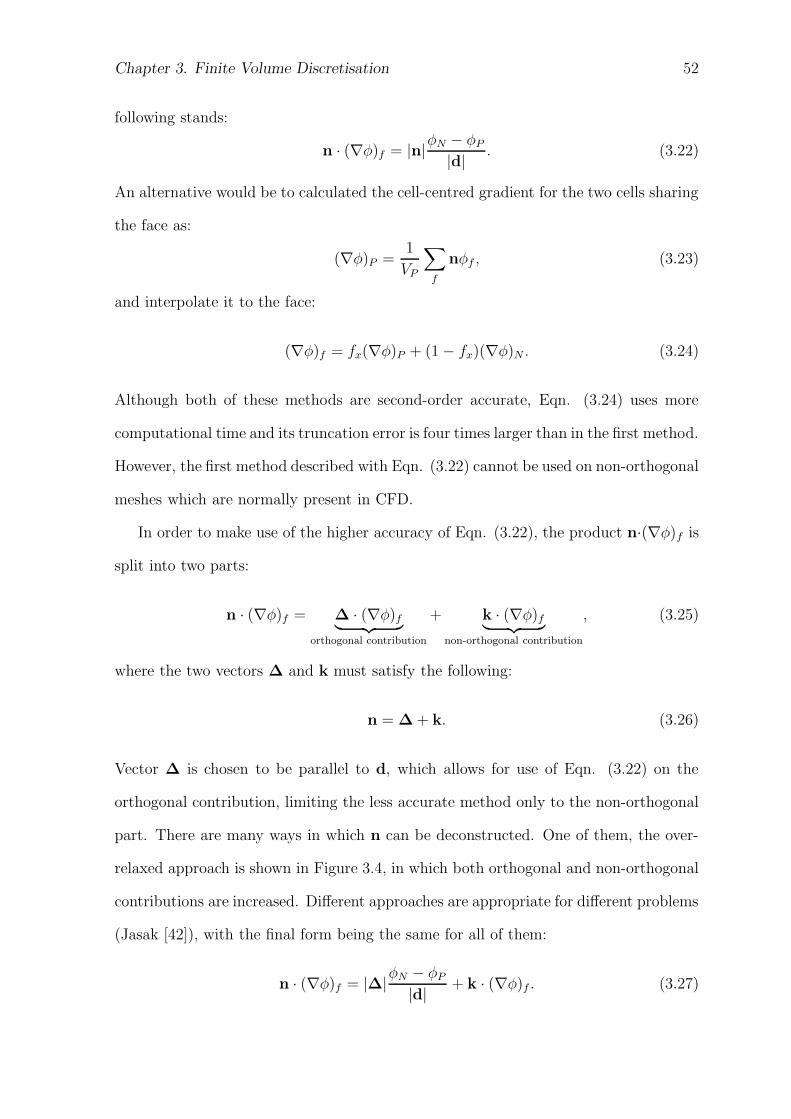
Chapter 3. Finite Volume Discretisation 52
following stands:
n · (∇φ)f = |n|φN − φP
|d|. (3.22)
An alternative would be to calculated the cell-centred gradient for the two cells sharing
the face as:
(∇φ)P =1
VP
∑
f
nφf , (3.23)
and interpolate it to the face:
(∇φ)f = fx(∇φ)P + (1 − fx)(∇φ)N . (3.24)
Although both of these methods are second-order accurate, Eqn. (3.24) uses more
computational time and its truncation error is four times larger than in the first method.
However, the first method described with Eqn. (3.22) cannot be used on non-orthogonal
meshes which are normally present in CFD.
In order to make use of the higher accuracy of Eqn. (3.22), the product n·(∇φ)f is
split into two parts:
n · (∇φ)f = ∆ · (∇φ)f︸ ︷︷ ︸
orthogonal contribution
+ k · (∇φ)f︸ ︷︷ ︸
non-orthogonal contribution
, (3.25)
where the two vectors ∆ and k must satisfy the following:
n = ∆ + k. (3.26)
Vector ∆ is chosen to be parallel to d, which allows for use of Eqn. (3.22) on the
orthogonal contribution, limiting the less accurate method only to the non-orthogonal
part. There are many ways in which n can be deconstructed. One of them, the over-
relaxed approach is shown in Figure 3.4, in which both orthogonal and non-orthogonal
contributions are increased. Different approaches are appropriate for different problems
(Jasak [42]), with the final form being the same for all of them:
n · (∇φ)f = |∆|φN − φP
|d|+ k · (∇φ)f . (3.27)
Chapter 3. Finite Volume Discretisation 53
NP
n
df ∆
k
Figure 3.4: Over-relaxed approach in non-orthogonality treatment.
3.3.3 Source Term
All terms in the transport equation, except diffusion, convection and temporal terms,
are included in the source term, Sφ(φ). Before discretising it, the FVM approximates
the source term by means of a linear form:
Sφ(φ) = Su + SP φ, (3.28)
where Su and SP can depend on φ. The volume integral of Eqn. (3.28) is written as:
∫
VP
Sφ(φ)dV = SuVP + SP VP φP . (3.29)
3.3.4 Temporal Discretisation
So far, in this Section, convection, diffusion and source terms have been discretised.
Using Eqs. (3.17, 3.27 and 3.29), and assuming that the control volumes do not change
in time, the integral form of transport equation, Eqn. (3.2) can be written as:
∂
∂t(ρP φP VP ) = −
∑
f
Fφf +∑
f
(ρΓφ)f n · (∇φ)f
+ SuVP + SP VP φP (3.30)
For simplicity, the r.h.s. of the Eqn. (3.30) will be denoted by M(t):
∂
∂t(ρP φP VP ) = M(t). (3.31)
Temporal discretisation of Eqn. (3.31) can be conducted in various ways, some of which
are presented below:
Chapter 3. Finite Volume Discretisation 54
Euler Explicit Method In this method the face values of φ and ∆φ are determined
from the old-time field (superscript o). The linear part of the source term is also
evaluated using the old-time value. That is why the r.h.s. is denoted with M(to):
ρnP φn
P − ρoP φo
P
∆tVP = M(to). (3.32)
The new value of φP can be calculated directly - it is not necessary to solve the system
of linear equations. The disadvantage of this method is the Courant number limit. The
Courant number is defined as:
Co =Uf · d
∆t, (3.33)
where Uf is the velocity interpolated on the face f . If the Courant number is larger
than unity, the explicit system becomes unstable. This puts a severe limitation in
choice of the size of the time step, ∆t.
Euler Implicit Method In this method, the temporal discretisation is the same as
in the previous one, but the face-values are expressed in terms of the new time-level
cell values, hence the r.h.s. is denoted by M(to):
ρnP φn
P − ρoP φo
P
∆tVP = M(tn). (3.34)
This is still a first-order accurate method, but unlike the explicit, this method creates
a system of equations which have this form:
aP φnP +
∑
N
aNφnN = RP . (3.35)
The coupling of the system is much stronger than in the explicit approach, and the
system is stable even if the Courant number limit is violated. Unlike the explicit
method, this form of temporal discretisation guarantees boundedness.
Crank-Nicholson Method The temporal discretisation is the same as in the pre-
vious two methods, and the face-values are expressed as an average between new- and
Chapter 3. Finite Volume Discretisation 55
old-time values:
ρnP φn
P − ρoP φo
P
∆tVP =
1
2[M(to) + M(tn)]. (3.36)
This method is second-order accurate in time and stable, but the boundedness of the
solution is not guaranteed.
If M(t) in Eqn. (3.36) is substituted by the r.h.s. from Eqn. (3.30), the following
expression is obtained:
ρnP φn
P − ρoP φo
P
∆tVP +
∑
f
Fφnf
∑
f
(ρΓφ)f n · (∇φ)nf
+∑
f
Fφof
∑
f
(ρΓφ)f n · (∇φ)of
= SuVP + SP VP φnP + SPVP φo
P (3.37)
3.3.5 Implementation of Boundary Conditions
In order to solve a discretised form of transport equation, we must determine φf and
nf ·(∇φ)f , i.e. the value of the variable φ and its normal gradient on face f .
Previously in this Section, it was shown how to find those values for the internal
mesh faces. However, for the faces located on the boundary of the domain, those values
are calculated from the boundary conditions.
There are two basic types of boundary conditions; a Dirichlet boundary condition
sets the value of the variable at the boundary, while a Neumann boundary condition
sets the value of its normal gradient at the boundary. A control volume with face
b located at the boundary of spatial domain is shown in Fig. 3.5. Vector db = Pb
connects the centroid P with the centre of the face b, while vector dn is parallel to
normal vector nb and defined as follows:
dn = (nb · db)nb. (3.38)
It is further assumed that the value which is set at the boundary face is constant over
that entire face. The boundary conditions are implemented into discretised equations
in the following way:
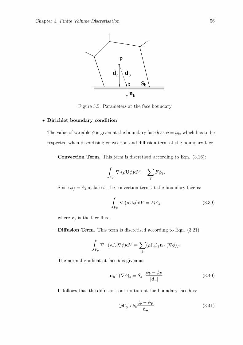
Chapter 3. Finite Volume Discretisation 56
P
b
bb
n
S
n
d d
b
Figure 3.5: Parameters at the face boundary
• Dirichlet boundary condition
The value of variable φ is given at the boundary face b as φ = φb, which has to be
respected when discretising convection and diffusion term at the boundary face.
– Convection Term. This term is discretised according to Eqn. (3.16):
∫
VP
∇·(ρUφ)dV =∑
f
Fφf .
Since φf = φb at face b, the convection term at the boundary face is:
∫
VP
∇·(ρUφ)dV = Fbφb, (3.39)
where Fb is the face flux.
– Diffusion Term. This term is discretised according to Eqn. (3.21):
∫
VP
∇ · (ρΓφ∇φ)dV =∑
f
(ρΓφ)fn · (∇φ)f .
The normal gradient at face b is given as:
nb · (∇φ)b = Sb ·φb − φP
|dn|(3.40)
It follows that the diffusion contribution at the boundary face b is:
(ρΓφ)b Sbφb − φP
|dn|(3.41)
Chapter 3. Finite Volume Discretisation 57
• Von Neumann boundary condition The normal gradient of the variable φ is
prescribed at the boundary face as:
nb·(∇φ)b = gb. (3.42)
Depending on which term this conditions is applied, that is done in the following
way:
– Convection term. In order to obtain the discretised value of the convection
term, it is necessary to find the value of φ at the boundary face:
φb = φP + |dn| gb, (3.43)
which means that the convection contribution at the boundary face will be
the following:
Fb (φP + |dn| gb). (3.44)
– Diffusion term. From Eqn. (3.42), it follows that the diffusion term at
the boundary face is:
(ρΓφ)b Sb gb. (3.45)
Physical Boundary Conditions
For incompressible flow, physical boundary conditions used in this study, are as follow-
ing:
• Inlet boundary. At the inlet boundary the velocity field has a fixed value, while
the pressure has the fixed zero gradient boundary condition.
• Outlet boundary. Mass conservation has to be satisfied when considering the
outlet boundary. There are two possibilities:
– The velocity distribution at the boundary is the same as in the row of cells
adjacent to the boundary. The pressure has again zero gradient condition.
Chapter 3. Finite Volume Discretisation 58
This approach can become unstable if there is an inflow through the face
specified as the outlet. This can be handled with additional modifications.
– The pressure distribution is specified and there is zero gradient boundary
condition on velocity. The mass conservation is guaranteed by the solution
of pressure equation.
• Symmetry plane boundary. The component of the gradient normal to the
boundary should be fixed to zero. The components parallel to the boundary are
projected to the boundary face from the inside of the domain, i.e. it is treated
by considering a mirror image cell beyond the boundary face.
• No-slip at the walls. The velocity of the fluid on the wall is equal to the
velocity of the wall itself. Since the flux through the solid wall is zero, the
pressure gradient condition is zero gradient.
3.4 System of Linear Algebraic Equations
In Eqn. (3.37), φnf and nn
f·(∇φ)n
f are dependent on the values of variable φ in the
neighbouring control volumes at the time tn. This relationship can be written as a
linear algebraic equation:
aP φnP +
∑
N
aNφnN = RP , (3.46)
where aP is a diagonal coefficient, aN a neighbouring coefficient, and RP on r.h.s.
contains all the other components of the transport equations which are not treated
explicitly. For each control volume there is one linear equation of the form of Eqn.
(3.46). Thus assembling the system of linear algebraic equations:
[A ] {φ} = {R }. (3.47)
The matrix [A ] contains coefficients aP on its diagonal, while above and below are
coefficents aN . Vector {φ} contains the values of φ for all the control volumes in the
Chapter 3. Finite Volume Discretisation 59
mesh, while vector R represents the source term. The matrix [A ] is a sparse matrix in
which most of the matrix coefficients are equal to zero.
This system of equations can be solved in many different ways which fall into two
categories: direct and iterative methods. Direct methods are suitable for small systems,
since the number of operations necessary to reach a solution is, at best, equal to the
number of the equations squared, thus making it too expensive for large systems.
In this study, iterative methods are used, which start with an initial guess and
improve it until solution tolerance criteria are met. Iterative methods are more eco-
nomical than direct ones. However, they require diagonal dominance of the matrix [A ]
to guarantee convergence. A matrix is diagonally equal if, in each row, the magnitude
of the diagonal coefficient is equal to the sum of magnitudes of off-diagonal coefficients:
|aP | =∑
N
|aN |. (3.48)
In order to be diagonally dominant, the following must stand for at least one row of
the matrix:
|aP | >∑
N
|aN |. (3.49)
The solver convergence is improved with the increase of diagonal dominance of the
system. Each component of the transport equation has the following influence on the
diagonal dominance of the system:
• Temporal term. Discretisation of the temporal term contributes only to the
diagonal coefficient and the source term of the system, and therefore increases
diagonal dominance. From Eqn. (3.37), it follows that the discretisation of the
temporal term contributes withρnV n
P
∆tto the diagonal coefficient. Therefore, with
the decrease of the time step ∆t, diagonal dominance of the system is increased.
• Convection term. The convection term creates a diagonally equal matrix only
for the Upwind Differencing (UD) scheme. In case of the Central Differencing
scheme, the matrix does not guarantee boundedness. There are various methods
Chapter 3. Finite Volume Discretisation 60
to improve the quality of the matrix for higher-order differencing schemes. One
of them is a deferred correction implementation (Khosla and Rubin [45]) in which
any differencing scheme is treated as an upgrade of UD. Here, the part of the
convection term corresponding to UD is built into the matrix, while the other part
is added into the source term. This, however, does not guarantee boundedness
even though the matrix is now diagonally equal.
• Diffusion term. Discretisation of the diffusion term on an orthogonal mesh
produces a diagonally equal matrix which guarantees boundedness. In case of
a non-orthogonal mesh, the matrix remains diagonally equal, but, since non-
orthogonal correction contributes to the source term of the system, diagonal
equality is not sufficient for the boundedness of the solution.
• Source term. If SP < 0, in Eqn. (3.28), the diagonal dominance is increased
and the term SP VP is part of the diagonal coefficient. If SP > 0, the entire source
term is part of the r.h.s. of the system.
From the above discussion it is seen that the only terms that enhance the diagonal
dominance are the linear part of the source and the temporal derivative. In steady-
state calculations, the influence of the temporal derivative does not exist, and the
diagonal dominance is enhanced through under-relaxation. If we again consider the
original system of equations, Eqn. (3.46):
aP φnP +
∑
N
aNφnN = RP ,
the diagonal dominance is increased by addition of the artificial term to both left and
right-hand side of Eqn. (3.46):
aP φnP +
1 − α
αaP φn
P +∑
N
aNφnN = RP +
1 − α
αaP φo
P , (3.50)
i.e.,
aP
αφn
P +∑
N
aNφnN = RP +
1 − α
αaP φo
P , (3.51)
Chapter 3. Finite Volume Discretisation 61
where φoP is the value from the previous iteration and α is the under-relaxation factor
(0 < α ≤ 1). When steady-state is reached, the value of φ stays the same in the
consecutive iterations (φoP = φn
P ) and the additional terms cancel out.
In this study, the Conjugate Gradient (CG) method, proposed by Hestens and
Steifel [38] is used. This method guarantees the the number of iterations needed to
obtain the solution is less or equal to the number of equations in the system. For
symmetric matrices, the ICCG solver (Jacobs [41]) is used, while asymmetric matrices
will be solved with Bi-CGSTAB method by van der Vorst [65].
3.5 Discretisation of Navier-Stokes Equations
A closed system of partial differential equations for Newtonian fluid flow was presented
in Chapter 2, by Eqs. (2.13 to 2.17). The incompressible form of this system can also
be written as:
∇ · U = 0, (3.52)
∂U
∂t+ ∇·(UU) −∇·(ν∇U) = −∇p. (3.53)
When solving this system, one has to pay attention to non-linear term in the momentum
equation, i.e. ∇ · (UU), and to the pressure-velocity coupling.
There are two ways of treating the non-linear term in the momentum equation
(Jasak [42]) - either by using a solver for non-linear systems, or by linearising the con-
vection term. The linearisation of this term is appropriate for steady-state calculations,
where, when the solution has converged, the fact that a part of the non-linear term
has been lagged is not significant. In transient problem, one can either iterate over
non-linear terms or neglect the non-linearity effects. If the time-step is large, itera-
tion greatly increases computational costs. However, in order to resolve the transient
problem well, one needs to use a small time-step, which keeps the iteration costs low
and insures that the non-linear system is fully resolved for each time-step. This holds
because the effect of lagged non-linearity is insignificant.
Chapter 3. Finite Volume Discretisation 62
3.5.1 Derivation of the Pressure Equation
Assuming that all the source terms, except the pressure gradient, are contained in the
H(U), the momentum equation can be written in a semi-discretised form:
aPUP = H(U) −∇p. (3.54)
Eqn. (3.54) has been obtained from the integral form of momentum equation and
divided by the volume in order to enable face interpolation of the coefficients.
The H(U) term contains the matrix coefficients multiplied by corresponding veloc-
ities and the source part apart from the pressure gradient. In this case there are no
additional source terms except the transient term:
H(U) =∑
N
aN(U)N +U0
∆t. (3.55)
From Eqn. (3.54), it follows:
UP =H(U)
aP
−∇p
aP
, (3.56)
and the expression for the velocities on the cell face, Uf , can be obtained by interpo-
lation:
Uf =
(H(U)
aP
)
f
−
(1
aP
)
f
(∇p)f , (3.57)
The discretised form of the continuity equation is obtained from Eqn. (3.15):
∇ · U =∑
f
n · Uf = 0. (3.58)
When Eqn. (3.57) is substituted into Eqn. (3.58) the following form of the pressure
equation is obtained:
∇ ·
(H(U)
aP
)
= ∇ ·
(1
aP∇p
)
. (3.59)
By using Eqn. (3.15), the Laplacian terms in Eqs. (3.54 and 3.59) are discretised,
leading to the following form of Eqs. (3.52 and 3.53):
aPUP = H(U) −∑
f
n · (p)f , (3.60)
∑
f
n ·
(H(U)
aP
)
f
=∑
f
n ·
[(1
aP
)
f
(∇p)f
]
. (3.61)
Chapter 3. Finite Volume Discretisation 63
Fluxes are obtained using Eqn. (3.57):
F = n · Uf = n·
[(H(U)
aP
)
f
−
(1
aP
)
f
(∇p)f
]
, (3.62)
which are guaranteed to be conservative if Eqn. (3.61) is satisfied.
3.5.2 Pressure-Velocity Coupling
There are two ways of treating linear dependence of velocity on pressure and vice-versa
shown in the discretised form of the Navier-Stokes system, Eqs. (3.60 and 3.61):
• Simultaneous algorithms, in which the complete system of equations is solved
simultaneously over the entire domain. This procedure does not handle non-
linearity and is comparatively costly, since the resulting matrix is several times
larger than the number of computational points.
• Segregated approach, in which the equations are solved in sequence. PISO
(Issa [40]) and SIMPLE (Patankar [52]) and their derivatives are the most popular
methods of solving inter-equation coupling in the pressure-velocity system. Their
iterative nature allows the non-linearity in the velocity equation to be handled
in the same framework, which means that they have lower storage requirements.
They are the methods used in this study.
3.5.3 The PISO Algorithm
The PISO algorithm has been developed by Issa [40] for solving transient flow calcu-
lations described by the discretised Navier-Stokes system for incompressible flow, Eqs.
(3.60 and 3.61). It can be described in the following steps:
1. Momentum Predictor. The momentum equation is solved first, using the pres-
sure field from the previous time-step. The solution of the momentum equation,
Eqn. (3.60), gives an approximation of the new velocity field.
Chapter 3. Finite Volume Discretisation 64
2. Pressure Solution. Using the predicted velocities, operator H(U) is assembled
and the pressure equation can be formed. The solution of the pressure equation
gives the first estimate of the new pressure field.
3. Explicit Velocity Correction. With the new pressure field, a set of conser-
vative fluxes is found. The velocity field is also corrected as a consequence of
the new pressure distribution. Velocity correction is done explicitly using Eqn.
(3.56).
4. Update of H(U) term. Since Eqn. (3.56) consists of two parts, there are
also two parts of the velocity correction - a correction due to the change in
the pressure gradient ( 1aP∇p) and the transported influence of corrections of
neighbouring velocities (H(U)aP
). Since the velocity correction is explicit, the latter
part is neglected - it is assumed that the entire velocity error comes from the error
in the pressure term. This is not true and it is therefore necessary to correct the
H(U) term, formulate the new pressure equation and repeat the procedure.
In other words, the PISO loop consists of an implicit momentum predictor followed
by a series of pressure solutions and explicit velocity corrections. The loop is repeated
until a pre-set tolerance is reached.
The dependence of H(U) on the flux field is, on the other hand, not taken into
consideration. It means that even though after each pressure solution, with a new set
of conservative fluxes is available, the term H(U) is not recalculated. It is assumed
that the non-linear coupling is less important than the pressure-velocity coupling and
the coefficients in H(U) are kept constant through the entire correction sequence and
will be changed only in the next momentum predictor.
3.5.4 The SIMPLE Algorithm
When solving a steady-state problem iteratively, non-linearity of the system becomes
more important since the effective time-step is much larger.
Chapter 3. Finite Volume Discretisation 65
The SIMPLE algorithm, developed by Patankar [52] has the following steps:
1. To initiate the SIMPLE calculation a pressure field is guessed. From the momen-
tum equation, using the guessed pressure field, the velocity field is solved. The
equation is under-relaxed using Eqn. (3.50), with the velocity under-relaxation
factor αU .
2. The pressure equation is solved to obtain the new pressure distribution.
3. A new set of fluxes is calculated using Eqn. (3.62). The new pressure field includes
both the pressure error and convection-diffusion error. In order to obtain a better
approximation of the pressure field, the coefficients of H(U) are recalculated with
the new set of conservative fluxes.
4. The pressure solution is under-relaxed in order to include the velocity part of the
error:
pn = po + αp(pp − po), (3.63)
where
• pn is the approximation of the pressure field which will be used in the next
momentum predictor,
• po is the pressure field used in the momentum predictor,
• pp is the solution of the pressure equation,
• αp is the pressure under-relaxation factor.
The recommended values of under-relaxation factors are (Peric [53]):
• αp = 0.2 for the pressure,
• αp = 0.8 for the velocity.
Chapter 3. Finite Volume Discretisation 66
3.6 Error Analysis
As already mentioned in Subsection 3.1.2, numerical solutions of fluid flow problems
are only approximate solutions, with systematic errors which fit into three categories:
modeling errors, discretisation errors and iteration errors. A more detailed description
of error analysis is given by Jasak [42].
The major source of numerical errors is the discretisation of the governing equations.
In this study, discretisation is second-order accurate in space and time, i.e. it is assumed
that the variation of the function over each control volume is linear. If a better solution
is needed, control volumes should be chosen in such a way that the assumption about
the linear variation becomes acceptable. In this study, the method chosen to examine
the discretisation error will be Richardson extrapolation.
3.6.1 Richardson Extrapolation
The error in the numerical solution is defined as the difference between the exact
solution of the governing equation Φ(x, t), and the numerical solution of the discrete
system φ:
E = Φ − φ. (3.64)
Richardson extrapolation is the most popular form of error estimation based on the
Taylor series truncation error analysis. The basic idea of Richardson extrapolation is
to obtain an approximation of the leading term in the truncation error from suitably
weighted solutions on two meshes with different cell size (Muzaferija [51]). The spatial
variation of the exact solution on two meshes with spacing h1 and h2 can be symbolically
written as (Muzaferija [51]):
Φ(x) = φ(x, h1) + hp1C(x) + O(x, hq
1), (3.65)
Φ(x) = φ(x, h2) + hp2C(x) + O(x, hq
2), (3.66)
where
Chapter 3. Finite Volume Discretisation 67
• φ(x, hi) is the approximate solution on the mesh with spacing hi,
• hpi C(x) is the leading term of the truncation error,
• h = h(x) is the local mesh size calculated as the ratio of cell volume and surface
area:
h =VP
∑
f |S|, (3.67)
• p is the order of accuracy of the discretisation method,
• O(x, hqi ) is the rest of the truncation error.
From Eqs. (3.65 and 3.66), C(x) can be approximated as:
C(x) =φ(x, h2) − φ(x, h1)
hp1 − hp
2
. (3.68)
The estimate of C(x), Eqn.(3.68), can be used to improve the fine mesh solution
φ(x, h2). The improved (qth order accurate) solution is:
φ(x, 0) = φ(x, h2)
(h1
h2
)p
(h1
h2
)p
− 1− φ(x, h1)
1(
h1
h2
)p
− 1. (3.69)
This improved solution can be used to estimate the error in φ(x, h2).
The Richardson extrapolation error estimate is calculated from the difference be-
tween the improved solution and the solution from the fine mesh:
et(φ) = |φ(x, 0) − φ(x, h2)| =|φ(x, h2) − φ(x, h1)|
(h1
h2
)p
− 1. (3.70)
For second-order accurate discretisation, this yields:
et(φ) =|φ(x, h2) − φ(x, h1)|
(h1
h2
)2
− 1. (3.71)
Chapter 3. Finite Volume Discretisation 68
3.7 Closure
In this Chapter, the Finite Volume Method of discretisation has been described. The
spatial discretisation, explained in Section 3.2, allows for the use of the arbitrary control
volumes, making it appropriate for complex geometries. In Section 3.3, discretisation of
each term of the governing equations has been described. Implementation of boundary
conditions has been briefly discussed.
In Section 3.4, a system of linear algebraic equations, obtained from the discreti-
sation of governing equations has been analysed. The influence of each term in the
transport equation on the system matrix has been studied.
The discretisation procedure for the Navier-Stokes systems has been presented in
Section 3.5. The pressure equation has been derived and two methods of solving the
pressure-velocity system have been described: the PISO algorithm for the transient
calculations and the SIMPLE method for steady-state flows.
Finally, in Section 3.6, Richardson Extrapolation, one of the methods of finding
numerical error was presented. This method will be used throughout this study.
Chapter 4
Validation of CFD Approach UsingSimple Converging Bearings
4.1 Introduction
In Chapter 3 we have briefly described the Finite Volume discretisation. By discretising
the governing equations for a particular problem, we obtain a system of algebraic
equations. When that system is solved, it produces an approximate solution at a
number of points in the domain. The quality of the numerical solution depends on the
chosen mesh as well as the applied discretisation practice.
This Chapter investigates the applicability of CFD as a suitable tool for solving lam-
inar hydrodynamic lubrication problems. Such applicability needs to be established for
lubrication problems because the fluid film thickness is several orders of magnitude less
than its longitudinal or transverse dimension, whereas the CFD method was developed
and has been shown to be an accurate numerical process only for relatively much thicker
films.
In this Chapter, two geometries (infinitely long linear wedge and infinitely long step
bearing) for which analytical solutions of the Reynolds Equation exist, are analysed.
The Reynolds Equation, itself, is an approximation which holds well in certain hy-
drodynamic conditions. Since both are hydrodynamic problems with smooth surfaces,
the Reynolds Equation should be applicable, so computational results using full NS
equation should, in principle, compare closely the analytical solution.
69
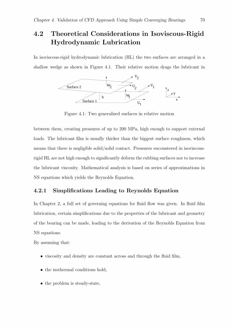
Chapter 4. Validation of CFD Approach Using Simple Converging Bearings 70
4.2 Theoretical Considerations in Isoviscous-Rigid
Hydrodynamic Lubrication
In isoviscous-rigid hydrodynamic lubrication (HL) the two surfaces are arranged in a
shallow wedge as shown in Figure 4.1. Their relative motion drags the lubricant in
U1
V1
W1
V2
W2 U2
hx
zy
Surface 2
Surface 1
Figure 4.1: Two generalised surfaces in relative motion
between them, creating pressures of up to 200 MPa, high enough to support external
loads. The lubricant film is usually thicker than the biggest surface roughness, which
means that there is negligible solid/solid contact. Pressures encountered in isoviscous-
rigid HL are not high enough to significantly deform the rubbing surfaces nor to increase
the lubricant viscosity. Mathematical analysis is based on series of approximations in
NS equations which yields the Reynolds Equation.
4.2.1 Simplifications Leading to Reynolds Equation
In Chapter 2, a full set of governing equations for fluid flow was given. In fluid film
lubrication, certain simplifications due to the properties of the lubricant and geometry
of the bearing can be made, leading to the derivation of the Reynolds Equation from
NS equations.
By assuming that:
• viscosity and density are constant across and through the fluid film,
• the isothermal conditions hold,
• the problem is steady-state,
Chapter 4. Validation of CFD Approach Using Simple Converging Bearings 71
the governing equations for any fluid flow, Eqs. (2.13 to 2.17) reduce to:
1
ρ
∂p
∂x= ν
(∂2u
∂x2+
∂2u
∂y2+
∂2u
∂z2
)
−
(∂u
∂t+ u
∂u
∂x+ v
∂u
∂y+ w
∂u
∂z
)
(4.1)
1
ρ
∂p
∂y= ν
(∂2v
∂x2+
∂2v
∂y2+
∂2v
∂z2
)
−
(∂v
∂t+ u
∂v
∂x+ v
∂v
∂y+ w
∂v
∂z
)
(4.2)
1
ρ
∂p
∂z= ν
(∂2w
∂x2+
∂2w
∂y2+
∂2w
∂z2
)
−
(∂w
∂t+ u
∂w
∂x+ v
∂w
∂y+ w
∂w
∂z
)
(4.3)
∂ρ
∂t+
∂ρu
∂x+
∂ρv
∂y+
∂ρw
∂z= 0 (4.4)
To obtain the Reynolds Equation, it is further assumed that:
• the pressure does not vary across the film, i.e.∂p
∂z= 0;
• inertial forces are negligible compared with viscous forces;
• the only relevant viscous terms are ν∂2u
∂z2and ν
∂2v
∂z2.
By taking into account these assumptions and since ν = ηρ, where ν is kinematic
viscosity, Eqs. (4.1 to 4.3) simplify to:
∂p
∂x= η
∂2u
∂z2, (4.5)
∂p
∂y= η
∂2v
∂z2, (4.6)
Chapter 4. Validation of CFD Approach Using Simple Converging Bearings 72
∂p
∂z= 0. (4.7)
The Eqs. (4.5 to 4.7) were also obtained through order of magnitude analysis for the
region inside the contact of the bearing in Chapter 2.
4.2.2 Boundary Conditions
For both cases studied in this Chapter, pressure at the inlet and outlet boundaries of
the bearing is set to zero and zero velocity gradient in the direction normal to sliding
is assumed. The entire domain is fully flooded.
At the solid walls, the ’no-slip’ boundary condition is assumed for the flow equations,
i.e. the velocity field has a fixed value, while the pressure field has a zero gradient
boundary condition.
4.2.3 Reynolds Equation
If we integrate Eqn. (4.5) over the boundary conditions at solid walls, z1 = 0 u1 = U1,
z2 = h u2 = U2, the x-component of the velocity profile in across the film is obtained:
u =1
2η
∂p
∂x· (z2 − zh) + (U2 − U1)
z
h+ U1. (4.8)
The velocity consists of three terms; the first term on r.h.s. in Eqn. (4.8) describes the
flow due to the pressure gradient, the second term describes the flow due to the mean
surface velocity and the third term is the velocity of the bottom surface. Similarly, the
y-component of the velocity profile is obtained from Eqn. (4.6).
By calculating the flow in each direction and applying the law of continuity of
volume flow (equivalent to the law of the continuity of mass, because of the constant
density), the Reynolds Equation for 2D -geometry is obtained:
∂
∂x
(h3
η
∂p
∂x
)
+∂
∂y
(h3
η
∂p
∂y
)
= 12
{(U1 + U2
2
)∂h
∂x+
(V1 + V2
2
)∂h
∂y+ (W2 − W1)
}
.
(4.9)
Chapter 4. Validation of CFD Approach Using Simple Converging Bearings 73
4.2.4 Infinitely Long Bearings
Let us assume that the bearing surfaces do not move in the transverse direction (i.e.
W1 = W2 = 0). If the flow in the transverse direction can be neglected, strictly
speaking valid only for infinitely long bearings, although it is often assumed to be true
even for bearings with aspect ratios (width-length ratios) as low as 5 (Chen and Hahn
[15]), the pressure is a function of x only and Eqn. (4.9) simplifies to:
∂
∂x
(h3
η
∂p
∂x
)
= 6U1∂h
∂x, (4.10)
which has an analytical solution for both geometries studied in this Chapter. The
pressure distribution is obtained by the integration over x.
Load
Load per unit length, W/L, is obtained by further integration of pressure equation:
W
L=
∫ B
0
pdx. (4.11)
Friction
Total friction is given by:
F =
∫ L
0
∫ B
0
τdydx, (4.12)
with shear stress τ at the bottom wall being:
τ =
(
η∂u
∂z
)
z=0
. (4.13)
Friction Coefficient
The friction coefficient is defined as the ratio between the total friction and the total
load on the bearing:
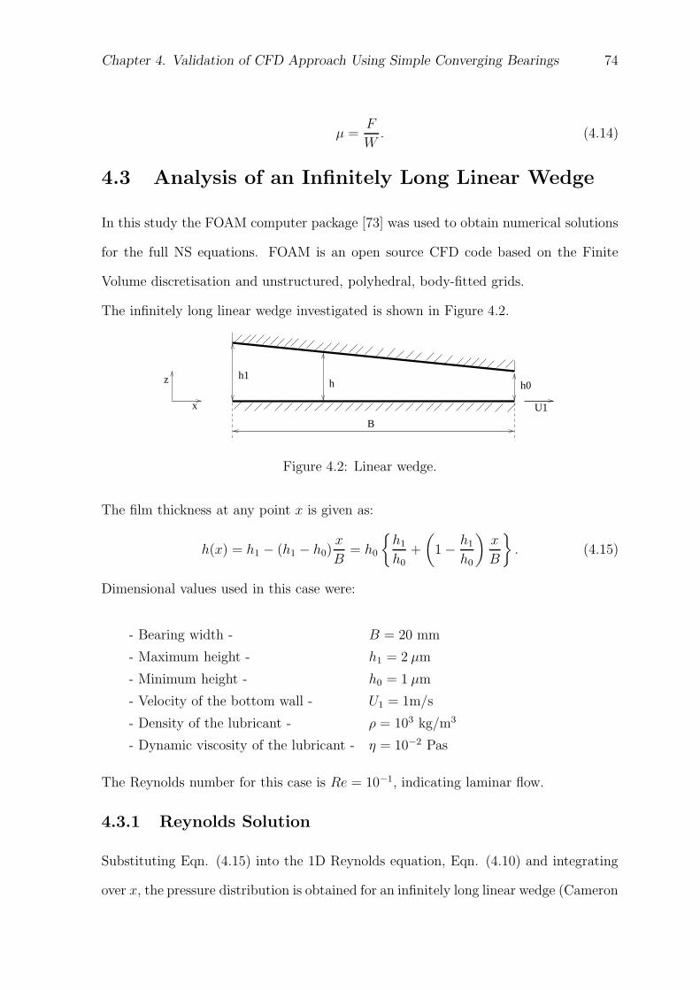
Chapter 4. Validation of CFD Approach Using Simple Converging Bearings 74
µ =F
W. (4.14)
4.3 Analysis of an Infinitely Long Linear Wedge
In this study the FOAM computer package [73] was used to obtain numerical solutions
for the full NS equations. FOAM is an open source CFD code based on the Finite
Volume discretisation and unstructured, polyhedral, body-fitted grids.
The infinitely long linear wedge investigated is shown in Figure 4.2.
h0h
B
z
x
h1
U1
Figure 4.2: Linear wedge.
The film thickness at any point x is given as:
h(x) = h1 − (h1 − h0)x
B= h0
{h1
h0+
(
1 −h1
h0
)x
B
}
. (4.15)
Dimensional values used in this case were:
- Bearing width - B = 20 mm
- Maximum height - h1 = 2 µm
- Minimum height - h0 = 1 µm
- Velocity of the bottom wall - U1 = 1m/s
- Density of the lubricant - ρ = 103 kg/m3
- Dynamic viscosity of the lubricant - η = 10−2 Pas
The Reynolds number for this case is Re = 10−1, indicating laminar flow.
4.3.1 Reynolds Solution
Substituting Eqn. (4.15) into the 1D Reynolds equation, Eqn. (4.10) and integrating
over x, the pressure distribution is obtained for an infinitely long linear wedge (Cameron
Chapter 4. Validation of CFD Approach Using Simple Converging Bearings 75
[12]):
p =6UηB
h20
K xB
(1 − x
B
)
(2 + K)(1 + K − K x
B
)2 , (4.16)
where
K =h1 − h0
h0
. (4.17)
Velocity is obtained from Eqn. (4.8):
u =3UK
h20 (2 + K)
1 + K − xB
(2 + K)(1 + K − Kx
B
)3 · (z2 − zh) − U1z
h+ U1, (4.18)
where h is given by Eqn. (4.15).
Substituting Eqn. (4.16) into Eqn. (4.11), the load per unit length is obtained:
W
L=
6UηB2
h20
1
K
(ln(1 + K)
K−
2
2 + K
)
. (4.19)
Total friction per unit length is
F
L=
BηU
h0
(4ln(1 + K)
K−
6
(2 + K)
)
. (4.20)
4.3.2 Numerical Results and Mesh Selection
In case of infinitely long linear wedge, the mesh consisted of one block with a uniform
grid as shown in Figure 4.3. The number of grid points in the longitudinal (Nx) and
transverse (Nz) direction was varied, and the resultant variations of maximum pressure
and total load were observed. Table 4.1 shows the results for the mesh refinement.
The mesh study was done in three ways. Firstly, the initial grid size 100 x 10 cells
was refined four times by factor 2 in both directions. The error in the numerical solution
for the maximum pressure along the bottom wall, et(pmax), was found using Richardson
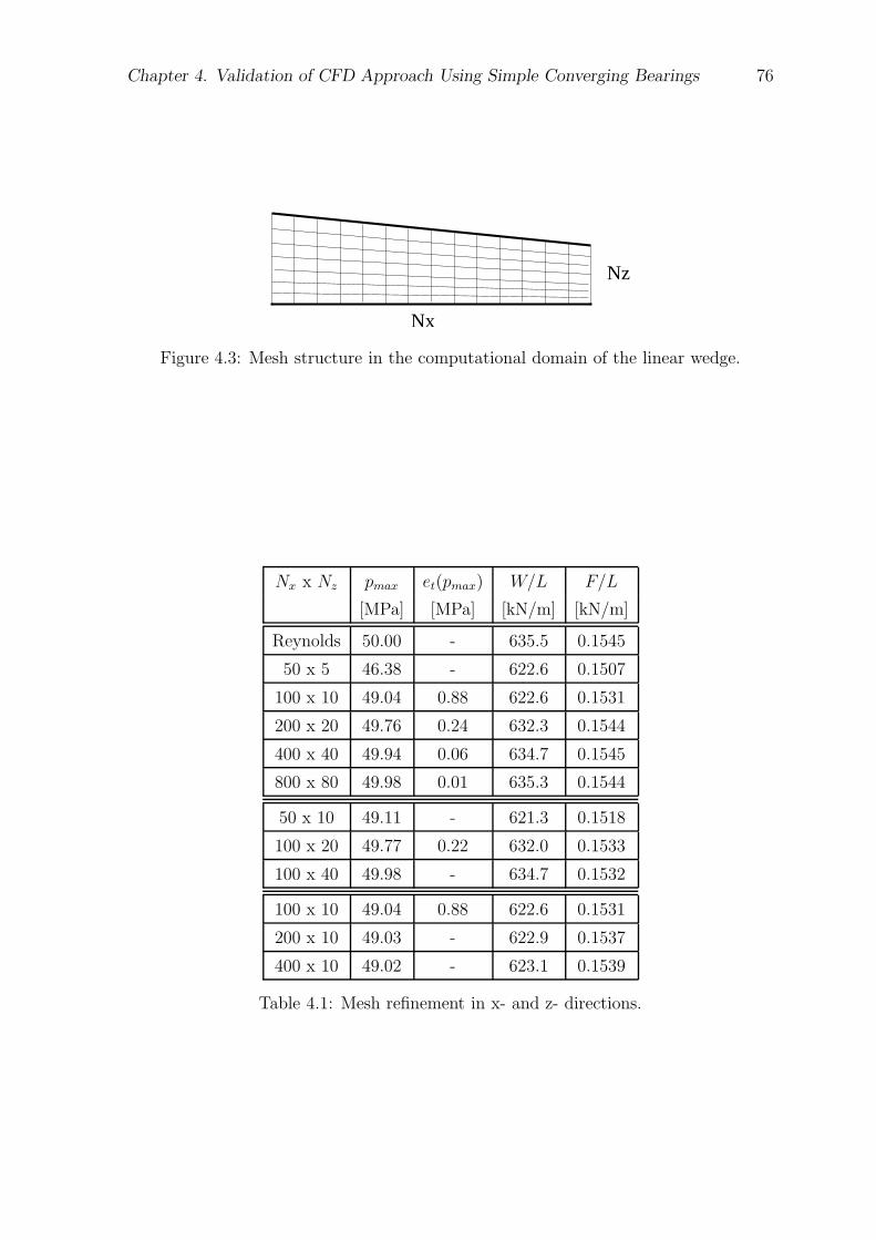
Chapter 4. Validation of CFD Approach Using Simple Converging Bearings 76
Nx
Nz
Figure 4.3: Mesh structure in the computational domain of the linear wedge.
Nx x Nz pmax et(pmax) W/L F/L
[MPa] [MPa] [kN/m] [kN/m]
Reynolds 50.00 - 635.5 0.1545
50 x 5 46.38 - 622.6 0.1507
100 x 10 49.04 0.88 622.6 0.1531
200 x 20 49.76 0.24 632.3 0.1544
400 x 40 49.94 0.06 634.7 0.1545
800 x 80 49.98 0.01 635.3 0.1544
50 x 10 49.11 - 621.3 0.1518
100 x 20 49.77 0.22 632.0 0.1533
100 x 40 49.98 - 634.7 0.1532
100 x 10 49.04 0.88 622.6 0.1531
200 x 10 49.03 - 622.9 0.1537
400 x 10 49.02 - 623.1 0.1539
Table 4.1: Mesh refinement in x- and z- directions.
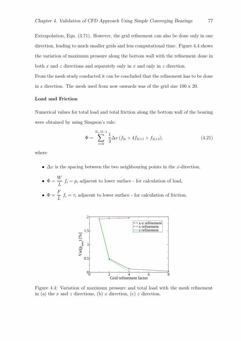
Chapter 4. Validation of CFD Approach Using Simple Converging Bearings 77
Extrapolation, Eqn. (3.71). However, the grid refinement can also be done only in one
direction, leading to much smaller grids and less computational time. Figure 4.4 shows
the variation of maximum pressure along the bottom wall with the refinement done in
both x and z directions and separately only in x and only in z direction.
From the mesh study conducted it can be concluded that the refinement has to be done
in z direction. The mesh used from now onwards was of the grid size 100 x 20.
Load and Friction
Numerical values for total load and total friction along the bottom wall of the bearing
were obtained by using Simpson’s rule:
Φ =
Nx/2−1∑
i=0
1
3∆x (f2i + 4f2i+1 + f2i+2), (4.21)
where
• ∆x is the spacing between the two neighbouring points in the x-direction,
• Φ =W
Lfi = pi adjacent to lower surface - for calculation of load,
• Φ =F
Lfi = τi adjacent to lower surface - for calculation of friction.
0 2 4 6 8Grid refinement factor
0
0.5
1
1.5
2
Var
(pm
ax)
[%]
x-z refinementx refinementz refinement
Figure 4.4: Variation of maximum pressure and total load with the mesh refinementin (a) the x and z directions, (b) x direction, (c) z direction.
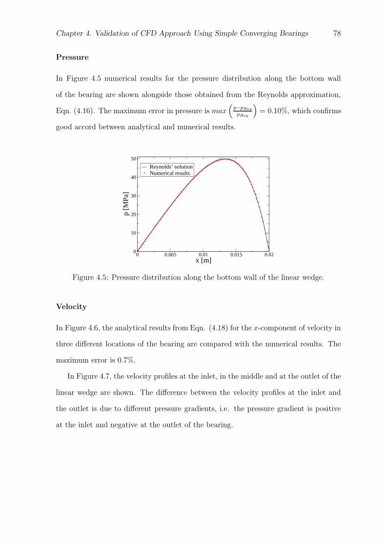
Chapter 4. Validation of CFD Approach Using Simple Converging Bearings 78
Pressure
In Figure 4.5 numerical results for the pressure distribution along the bottom wall
of the bearing are shown alongside those obtained from the Reynolds approximation,
Eqn. (4.16). The maximum error in pressure is max(
p−pRey
pRey
)
= 0.10%, which confirms
good accord between analytical and numerical results.
0 0.005 0.01 0.015 0.02x [m]
0
10
20
30
40
50
p [M
Pa]
Reynolds’ solutionNumerical results
Figure 4.5: Pressure distribution along the bottom wall of the linear wedge.
Velocity
In Figure 4.6, the analytical results from Eqn. (4.18) for the x-component of velocity in
three different locations of the bearing are compared with the numerical results. The
maximum error is 0.7%.
In Figure 4.7, the velocity profiles at the inlet, in the middle and at the outlet of the
linear wedge are shown. The difference between the velocity profiles at the inlet and
the outlet is due to different pressure gradients, i.e. the pressure gradient is positive
at the inlet and negative at the outlet of the bearing.
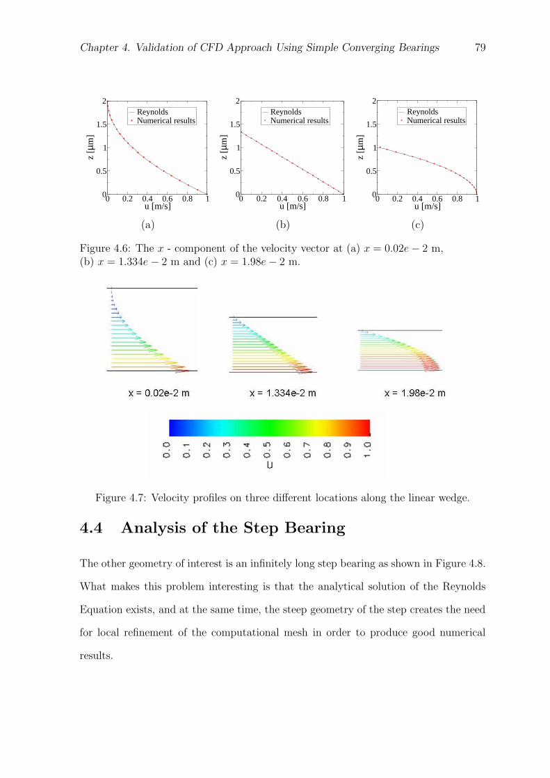
Chapter 4. Validation of CFD Approach Using Simple Converging Bearings 79
0 0.2 0.4 0.6 0.8 1u [m/s]
0
0.5
1
1.5
2z
[µm
]
ReynoldsNumerical results
0 0.2 0.4 0.6 0.8 1u [m/s]
0
0.5
1
1.5
2
z [µ
m]
ReynoldsNumerical results
0 0.2 0.4 0.6 0.8 1u [m/s]
0
0.5
1
1.5
2
z [µ
m]
ReynoldsNumerical results
(a) (b) (c)
Figure 4.6: The x - component of the velocity vector at (a) x = 0.02e − 2 m,(b) x = 1.334e − 2 m and (c) x = 1.98e − 2 m.
Figure 4.7: Velocity profiles on three different locations along the linear wedge.
4.4 Analysis of the Step Bearing
The other geometry of interest is an infinitely long step bearing as shown in Figure 4.8.
What makes this problem interesting is that the analytical solution of the Reynolds
Equation exists, and at the same time, the steep geometry of the step creates the need
for local refinement of the computational mesh in order to produce good numerical
results.
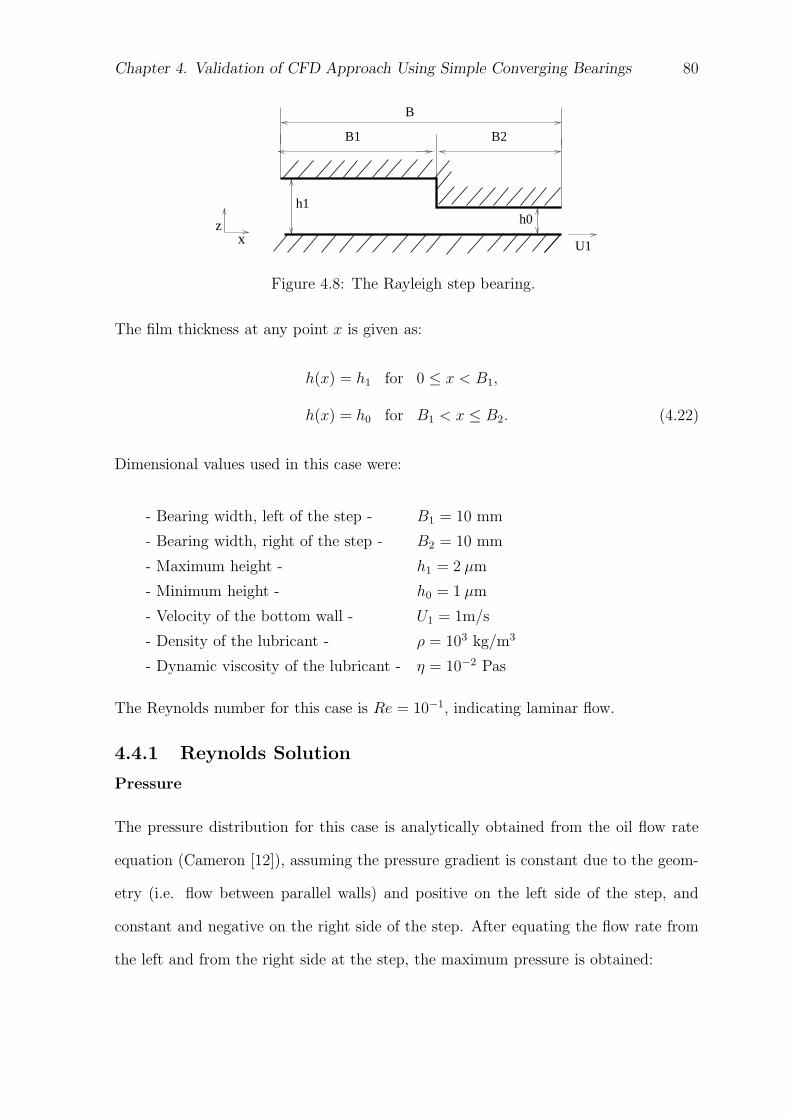
Chapter 4. Validation of CFD Approach Using Simple Converging Bearings 80
B1 B2
B
h1h0z
x U1
Figure 4.8: The Rayleigh step bearing.
The film thickness at any point x is given as:
h(x) = h1 for 0 ≤ x < B1,
h(x) = h0 for B1 < x ≤ B2. (4.22)
Dimensional values used in this case were:
- Bearing width, left of the step - B1 = 10 mm
- Bearing width, right of the step - B2 = 10 mm
- Maximum height - h1 = 2 µm
- Minimum height - h0 = 1 µm
- Velocity of the bottom wall - U1 = 1m/s
- Density of the lubricant - ρ = 103 kg/m3
- Dynamic viscosity of the lubricant - η = 10−2 Pas
The Reynolds number for this case is Re = 10−1, indicating laminar flow.
4.4.1 Reynolds Solution
Pressure
The pressure distribution for this case is analytically obtained from the oil flow rate
equation (Cameron [12]), assuming the pressure gradient is constant due to the geom-
etry (i.e. flow between parallel walls) and positive on the left side of the step, and
constant and negative on the right side of the step. After equating the flow rate from
the left and from the right side at the step, the maximum pressure is obtained:
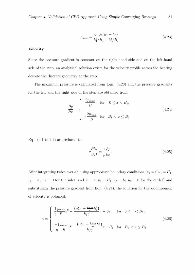
Chapter 4. Validation of CFD Approach Using Simple Converging Bearings 81
pmax =6ηU1(h1 − h0)
h31/B1 + h3
0/B2. (4.23)
Velocity
Since the pressure gradient is constant on the right hand side and on the left hand
side of the step, an analytical solution exists for the velocity profile across the bearing
despite the discrete geometry at the step.
The maximum pressure is calculated from Eqn. (4.23) and the pressure gradients
for the left and the right side of the step are obtained from:
∂p
∂x=
2pmax
Bfor 0 ≤ x < B1,
−2pmax
Bfor B1 < x ≤ B2.
(4.24)
Eqs. (4.1 to 4.4) are reduced to:
ν∂2u
∂z2=
1
ρ
∂p
∂x. (4.25)
After integrating twice over dz, using appropriate boundary conditions (z1 = 0 u1 = U1,
z2 = h1 u2 = 0 for the inlet, and z1 = 0 u1 = U1, z2 = h0 u2 = 0 for the outlet) and
substituting the pressure gradient from Eqn. (4.24), the equation for the x-component
of velocity is obtained:
u =
1
η
pmax
Bz2 −
(ηU1 + pmax
Bh2
1
)
h1ηz + U1 for 0 ≤ x < B1,
−1
η
pmax
Bz2 −
(ηU1 + pmax
Bh2
0
)
h0ηz + U1 for B1 < x ≤ B2.
(4.26)
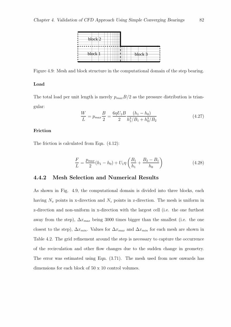
Chapter 4. Validation of CFD Approach Using Simple Converging Bearings 82
block 1
block 2
block 3
Figure 4.9: Mesh and block structure in the computational domain of the step bearing.
Load
The total load per unit length is merely pmaxB/2 as the pressure distribution is trian-
gular:
W
L= pmax
B
2=
6ηU1B
2
(h1 − h0)
h31/B1 + h3
0/B2(4.27)
Friction
The friction is calculated from Eqn. (4.12):
F
L=
pmax
2(h1 − h0) + U1η
(B1
h1+
B2 − B1
h0
)
(4.28)
4.4.2 Mesh Selection and Numerical Results
As shown in Fig. 4.9, the computational domain is divided into three blocks, each
having Nx points in x-direction and Nz points in z-direction. The mesh is uniform in
z-direction and non-uniform in x-direction with the largest cell (i.e. the one furthest
away from the step), ∆xmax being 3000 times bigger than the smallest (i.e. the one
closest to the step), ∆xmin. Values for ∆xmax and ∆xmin for each mesh are shown in
Table 4.2. The grid refinement around the step is necessary to capture the occurrence
of the recirculation and other flow changes due to the sudden change in geometry.
The error was estimated using Eqn. (3.71). The mesh used from now onwards has
dimensions for each block of 50 x 10 control volumes.
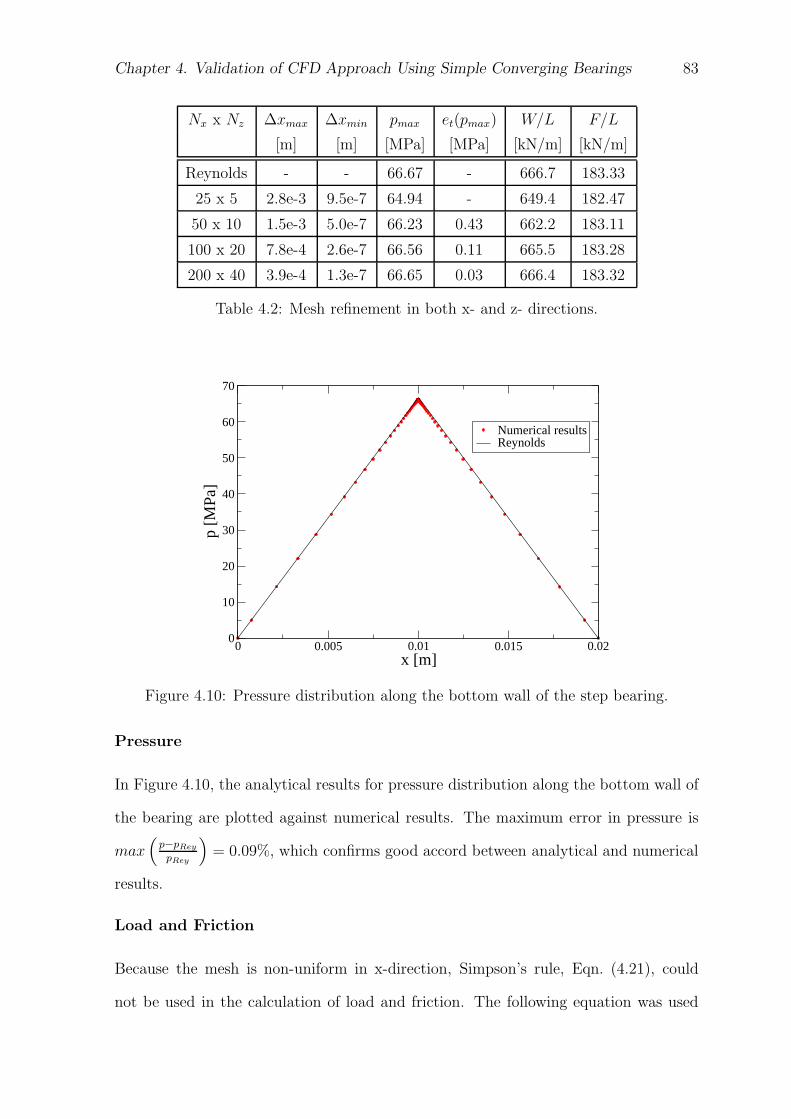
Chapter 4. Validation of CFD Approach Using Simple Converging Bearings 83
Nx x Nz ∆xmax ∆xmin pmax et(pmax) W/L F/L
[m] [m] [MPa] [MPa] [kN/m] [kN/m]
Reynolds - - 66.67 - 666.7 183.33
25 x 5 2.8e-3 9.5e-7 64.94 - 649.4 182.47
50 x 10 1.5e-3 5.0e-7 66.23 0.43 662.2 183.11
100 x 20 7.8e-4 2.6e-7 66.56 0.11 665.5 183.28
200 x 40 3.9e-4 1.3e-7 66.65 0.03 666.4 183.32
Table 4.2: Mesh refinement in both x- and z- directions.
0 0.005 0.01 0.015 0.02x [m]
0
10
20
30
40
50
60
70
p [M
Pa]
Numerical resultsReynolds
Figure 4.10: Pressure distribution along the bottom wall of the step bearing.
Pressure
In Figure 4.10, the analytical results for pressure distribution along the bottom wall of
the bearing are plotted against numerical results. The maximum error in pressure is
max(
p−pRey
pRey
)
= 0.09%, which confirms good accord between analytical and numerical
results.
Load and Friction
Because the mesh is non-uniform in x-direction, Simpson’s rule, Eqn. (4.21), could
not be used in the calculation of load and friction. The following equation was used
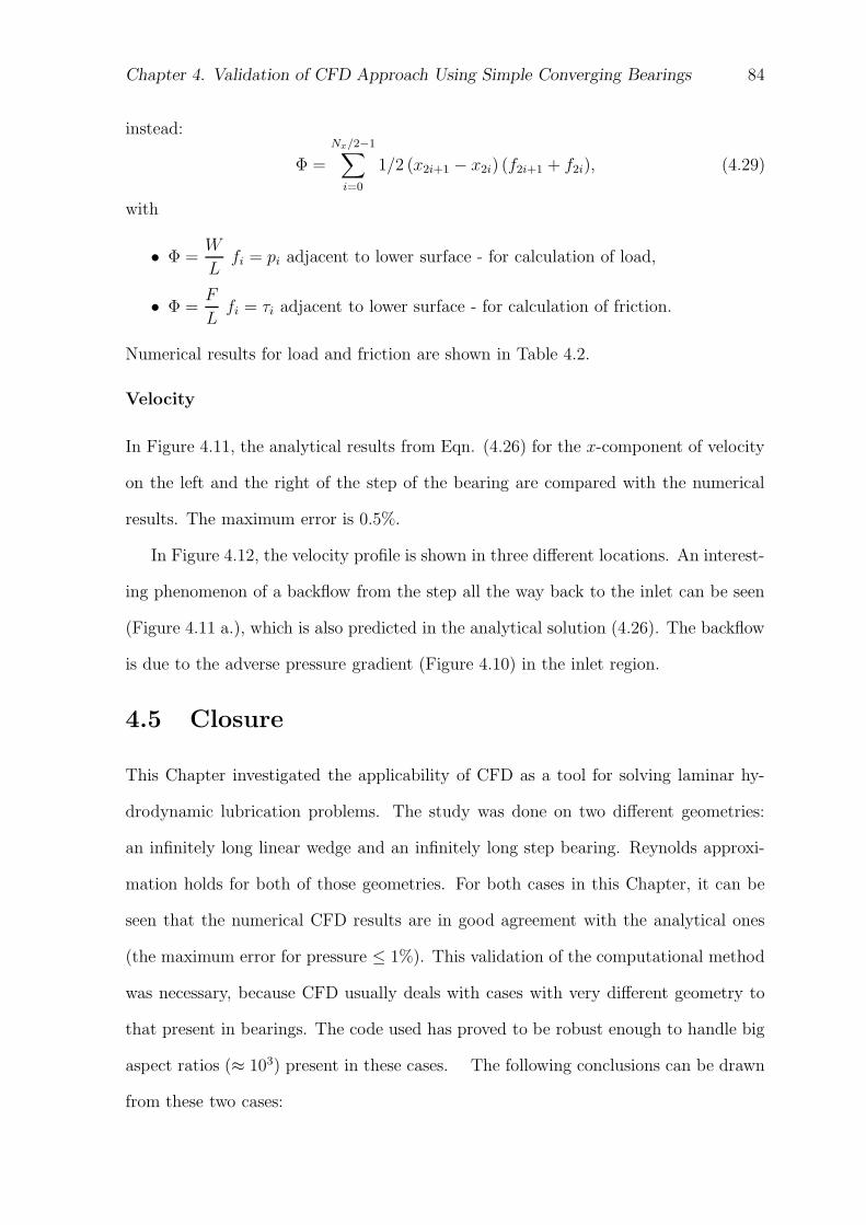
Chapter 4. Validation of CFD Approach Using Simple Converging Bearings 84
instead:
Φ =
Nx/2−1∑
i=0
1/2 (x2i+1 − x2i) (f2i+1 + f2i), (4.29)
with
• Φ =W
Lfi = pi adjacent to lower surface - for calculation of load,
• Φ =F
Lfi = τi adjacent to lower surface - for calculation of friction.
Numerical results for load and friction are shown in Table 4.2.
Velocity
In Figure 4.11, the analytical results from Eqn. (4.26) for the x-component of velocity
on the left and the right of the step of the bearing are compared with the numerical
results. The maximum error is 0.5%.
In Figure 4.12, the velocity profile is shown in three different locations. An interest-
ing phenomenon of a backflow from the step all the way back to the inlet can be seen
(Figure 4.11 a.), which is also predicted in the analytical solution (4.26). The backflow
is due to the adverse pressure gradient (Figure 4.10) in the inlet region.
4.5 Closure
This Chapter investigated the applicability of CFD as a tool for solving laminar hy-
drodynamic lubrication problems. The study was done on two different geometries:
an infinitely long linear wedge and an infinitely long step bearing. Reynolds approxi-
mation holds for both of those geometries. For both cases in this Chapter, it can be
seen that the numerical CFD results are in good agreement with the analytical ones
(the maximum error for pressure ≤ 1%). This validation of the computational method
was necessary, because CFD usually deals with cases with very different geometry to
that present in bearings. The code used has proved to be robust enough to handle big
aspect ratios (≈ 103) present in these cases. The following conclusions can be drawn
from these two cases:
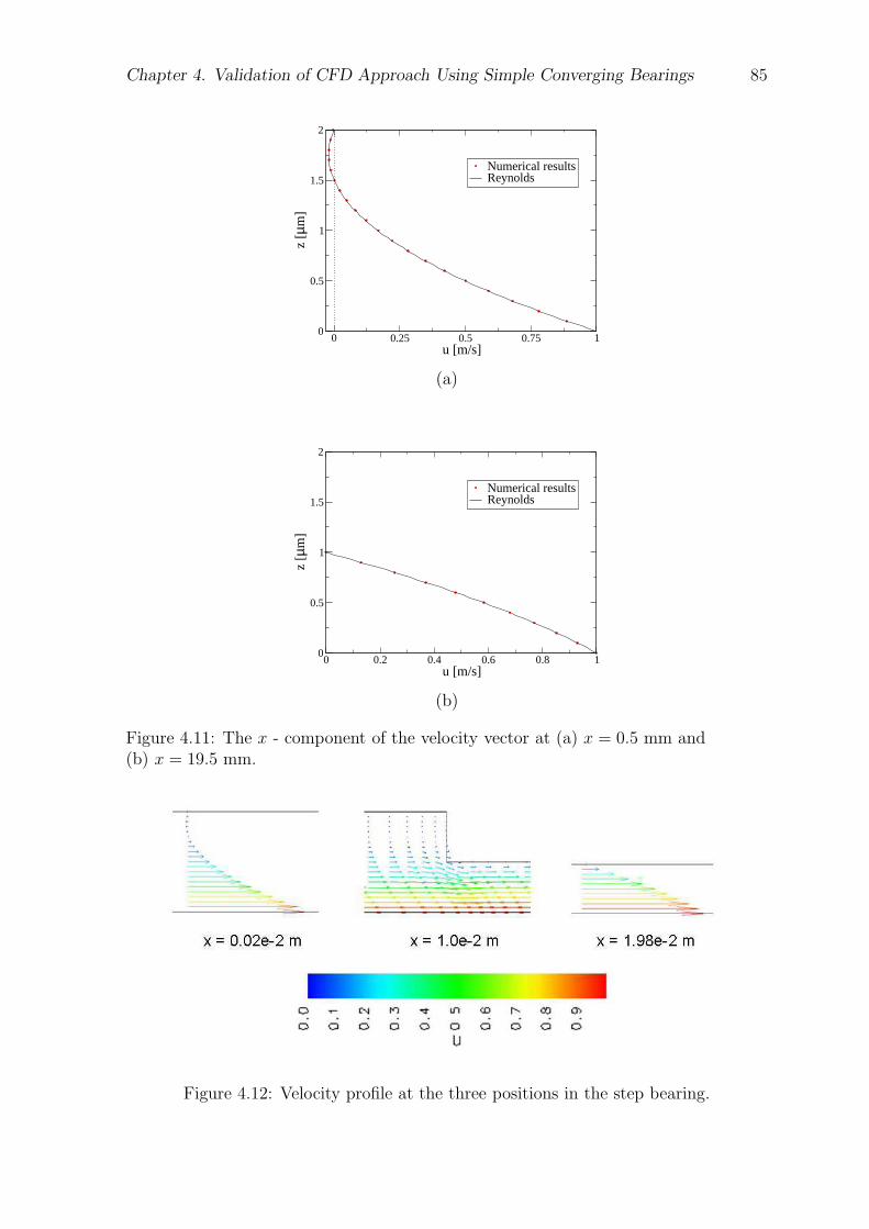
Chapter 4. Validation of CFD Approach Using Simple Converging Bearings 85
0 0.25 0.5 0.75 1u [m/s]
0
0.5
1
1.5
2
z [µ
m]
Numerical resultsReynolds
(a)
0 0.2 0.4 0.6 0.8 1u [m/s]
0
0.5
1
1.5
2
z [µ
m]
Numerical resultsReynolds
(b)
Figure 4.11: The x - component of the velocity vector at (a) x = 0.5 mm and(b) x = 19.5 mm.
Figure 4.12: Velocity profile at the three positions in the step bearing.

Chapter 4. Validation of CFD Approach Using Simple Converging Bearings 86
1. The CFD software has been shown to be capable of accurately handling steady
state hydrodynamic lubrication problems.
2. CFD results have confirmed the assumption of constant pressure across the film
(apart for the rapidly converging step in step bearing).
3. CFD results have confirmed that the neglect of inertia and certain viscous terms
in Reynolds equation is justified in the bearings analysed.
Based on this, we can safely use CFD in hydrodynamic lubrication.
Chapter 5
Computational Modelling ofCavitation
5.1 Introduction
In Chapter 4 the applicability of the CFD to solving HL problems was examined
using two hydrodynamic problems for which the Reynolds Equation has an analytical
solution. From the two geometries studied, it was shown that, for simple, converging
geometries, the CFD is a suitable tool for solving HL problems.
In the case of a roller bearing, however, the pressure drops below the atmospheric
pressure in the diverging region, so cavitation occurs. The physical situation in the case
of cavitation is extreme in several respects. The density ratio between two phases is very
large, roughly 10,000:1. The aspect ratio of the computational cells in the cavitating
region is of the order of 1000:1, which means that individual cavitation bubbles could
span several computational cells. These extremes make this a challenging problem to
model. Special steps are required to ensure stability when modelling a large change in
density over the space of a few computational cells.
In this Chapter, a cavitation model will be tested on a case of an infinitely long
roller bearing. It will be assumed that there is no elastic deformation, no piezo-viscous
effects and that the problem is iso-thermal.
87
Chapter 5. Computational Modelling of Cavitation 88
5.2 Previous Work in Cavitation
In CFD, cavitation has been modelled numerically by two main methods, interface
tracking and continuum methods. Interface tracking is a numerical technique for two-
phase flows. In this case each phase is treated separately and there is only one phase
present at any location in the solution domain. Normally, there are separate equations
for conservation of mass and momentum of each phase, which makes the computational
cost of modelling at least six times the cost of continuum methods, as shown by Rider
and Kothe [57]. The authors also noted that the maximum density ratio between the
liquid and vapour phase, with this method can be 1,000:1.
In a continuum method model, both phases are considered to be the same fluid,
where the density reflects the liquid and vapour content of the cell. The computational
cost of this model is lower than of the interface tracking because continuum method
requires no more equations than single-phase flow. The works of Kubota et al. [47],
Delannoy and Kueny [17], Chen and Heister [16], and Avva et al. [5] are all examples
of continuum methods.
Kubota et al. [47] developed one of the first continuum models of cavitating flow.
Their model was based on the assumption that the fluid was a uniform mixture of
liquid and very small, spherical bubbles. They used relations for bubble radius, average
cell density, and pressure to close the set of equations. Because of the extreme density
ratio between the liquid and vapour, they chose to neglect the mass of the vapour. The
authors were limited to moderate void fractions because of severe stability problems.
Delannoy and Kueny [17] used a simpler method for closure of the hydrodynamic
equations. They assumed a barotropic equation of state in which density was a function
of pressure. The two constant densities for liquid and vapour were joined by a sine
function whose maximum slope was chosen to represent roughly the speed of sound
of a two-phase mixture. Their scheme was based on the SIMPLE algorithm, which
models incompressible flows. One of the limitations of their model is that they used
Chapter 5. Computational Modelling of Cavitation 89
the vapour-to-liquid density ratio of 1:100, rather than a realistic ratio of 1:105. Their
model was later employed to model the cavitation in HL contacts by van Odyck [66]
but he was limited to use the unrealistically high vapour density.
Chen and Heister [16] rejected the idea of a simple one-to-one mapping of pressure
and density. They argued that the pressure field should be related to the density
history. However, they assumed that the bubble number per unit mass was constant
and that each cell was uniformly filled with small, spherical bubbles. This technique
worked well for large-scale flows, but was not appropriate for small-scale geometry, like
a roller bearing.
Avva et al. [5] used an energy equation for closure. They started with an energy
equation for a two-phase mixture and assumed homogeneous flow, no slip, and ther-
modynamic equilibrium. With these assumptions, the energy equation was simplified
to a single fluid energy equation based on a mean cell density. The model was limited
to the density ratio of 3,000:1. Avva’s model forms the basis of the one used in the
current study.
5.3 Physical Modelling
An important limitation of all the studies already mentioned is that the pure phases
are considered to be incompressible. The model which is used in the current study,
considers the compressibility of both pure phases. Thermal non-equilibrium effects will
be neglected, as will hydrodynamic non-equilibrium.
Suitable average properties (density, viscosity) are determined and the mixture
is treated as a pseudofluid that obeys the usual equations of single-component flow.
Differences in velocity, temperature, and chemical potential between the phases will
promote mutual momentum, heat and mass transfer. Often these processes proceed
very rapidly, particularly when one phase is finely dispersed in the other, and it can
be assumed that equilibrium is reached. In this case the average values of velocity,
Chapter 5. Computational Modelling of Cavitation 90
temperature, and chemical potential are the same as the values for each component
and the flow is homogeneous equilibrium flow . This method is a convenient way of
modeling the flow because it requires no more equations than the single-phase flow.
In this study, cavitation was addressed by considering the lubricant to be a two-
phase fluid, transforming from entirely liquid at high pressure, through a mixed liq-
uid/vapour phase at intermediate pressure, to entirely vapour phase at low pressure.
This enables a suitable fluid density-pressure relationship to be derived which spans
the liquid and vapour states and thus permits cavitation based on vapour formation
to occur as the pressure falls in a divergent region (Dellanoy and Kueny [17]). In the
current study, the isentropic phase transformation approach was employed (Avva [5]).
The conservation of energy equation, assuming homogeneous equilibrium of the two
phases and including the viscous dissipation term, Φ is written as:
ρDh
Dt=
DP
Dt+ ∇k∇T + Φ. (5.1)
Assuming that the rapid change between liquid and vapour phases during cavitation
is isentropic and that enthalpy and pressure work terms dominate (i.e. they are at least
five orders of magnitude greater than the conduction and viscous terms), the energy
equation reduces to:
ρDh
Dt=
DP
Dt. (5.2)
The remaining terms describe reversible work and Eqn. (5.2) can be written as an
isentropic model equation:
a2 Dρ
Dt=
DP
Dt. (5.3)
Eqn. (5.3) is considered an isentropic model of the phase change, where the speed
of sound of the mixture, a, is given by the homogeneous equilibrium model (HEM)
(Wallis [71]):
1
a2= ρ ·
(α
ρga2g
+1 − α
ρla2l
)
, (5.4)
Chapter 5. Computational Modelling of Cavitation 91
where ρg, ag, ρl, al are the density and speed of sound of the vapour and liquid phases
respectively, ρ is the density of the phase mixture and α is the volume fraction of
vapour or ”void fraction” defined by:
α =ρ − ρl
ρg − ρl. (5.5)
The densities of both the superheated vapour and the subcooled liquid were set to vary
linearly with pressure according to:
(i) Liquid phase; ρl = ρlSat+
p − psat
a2l
(ii) Vapour phase; ρg = max
(p
a2g
, ρgsat
)
, (5.6)
where ρlSat and ρgSat are the densities of the liquid and vapour at the saturation
pressure, pSat. (The second term in Eqn. (5.6 ii) prevents the density becoming
negative at negative pressures).
The density of the phase mixture is calculated using the continuity equation, Eqn.
(2.2), and the local vapour fraction can then be obtained via Eqn. (5.5).
The dynamic viscosity, η of the phase mixture is assumed to be linearly proportional
to the density, i.e.;
η = ρ · (ανg + (1 − α) νl) . (5.7)
5.4 Fluid Properties
From the equation of state for the ideal gas, the dependence of ρgsaton psat is derived:
ρgSat=
psat · M
R · T, (5.8)
where M is the molar mass, T temperature, and R is the Boltzmann constant.
In Faber [27], the speed of sound in vapour for an ideal gas is expressed by:
a2g =
γp
ρ=
γRT
M, (5.9)
where γ is the specific heat ratio cp/cv.
For a lubricant (in this case, values taken are for n-hexadecane), typical values are:
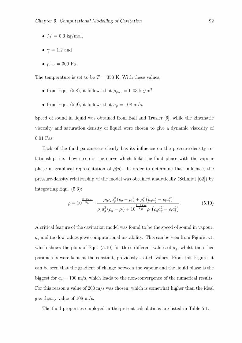
Chapter 5. Computational Modelling of Cavitation 92
• M = 0.3 kg/mol,
• γ = 1.2 and
• pSat = 300 Pa.
The temperature is set to be T = 353 K. With these values:
• from Eqn. (5.8), it follows that ρgsat= 0.03 kg/m3,
• from Eqn. (5.9), it follows that ag = 108 m/s.
Speed of sound in liquid was obtained from Ball and Trusler [6], while the kinematic
viscosity and saturation density of liquid were chosen to give a dynamic viscosity of
0.01 Pas.
Each of the fluid parameters clearly has its influence on the pressure-density re-
lationship, i.e. how steep is the curve which links the fluid phase with the vapour
phase in graphical representation of ρ(p). In order to determine that influence, the
pressure-density relationship of the model was obtained analytically (Schmidt [62]) by
integrating Eqn. (5.3):
ρ = 10p−pSat
pgl ·ρlρga
2g (ρg − ρl) + ρ2
l
(ρga
2g − ρla
2l
)
ρga2g (ρg − ρl) + 10
p−pSatpgl ρl
(ρga
2g − ρla
2l
). (5.10)
A critical feature of the cavitation model was found to be the speed of sound in vapour,
ag and too low values gave computational instability. This can be seen from Figure 5.1,
which shows the plots of Eqn. (5.10) for three different values of ag, whilst the other
parameters were kept at the constant, previously stated, values. From this Figure, it
can be seen that the gradient of change between the vapour and the liquid phase is the
biggest for ag = 100 m/s, which leads to the non-convergence of the numerical results.
For this reason a value of 200 m/s was chosen, which is somewhat higher than the ideal
gas theory value of 108 m/s.
The fluid properties employed in the present calculations are listed in Table 5.1.
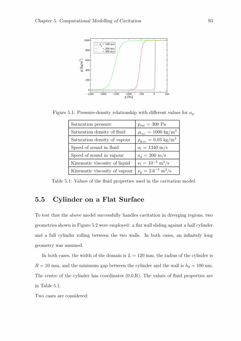
Chapter 5. Computational Modelling of Cavitation 93
-2500 -2000 -1500 -1000 -500 0 500p [Pa]
0
200
400
600
800
1000
ρ [k
g/m
3 ]
ag = 100 m/s
= 200 m/s = 300 m/s
Figure 5.1: Pressure-density relationship with different values for ag.
Saturation pressure psat = 300 Pa
Saturation density of fluid ρlsat= 1000 kg/m3
Saturation density of vapour ρgsat= 0.03 kg/m3
Speed of sound in fluid al = 1340 m/s
Speed of sound in vapour ag = 200 m/s
Kinematic viscosity of liquid νl = 10−5 m2/s
Kinematic viscosity of vapour νg = 2.6−5 m2/s
Table 5.1: Values of the fluid properties used in the cavitation model.
5.5 Cylinder on a Flat Surface
To test that the above model successfully handles cavitation in diverging regions, two
geometries shown in Figure 5.2 were employed: a flat wall sliding against a half cylinder
and a full cylinder rolling between the two walls. In both cases, an infinitely long
geometry was assumed.
In both cases, the width of the domain is L = 120 mm, the radius of the cylinder is
R = 10 mm, and the minimum gap between the cylinder and the wall is h0 = 100 nm.
The centre of the cylinder has coordinates (0,0,R). The values of fluid properties are
in Table 5.1.
Two cases are considered:
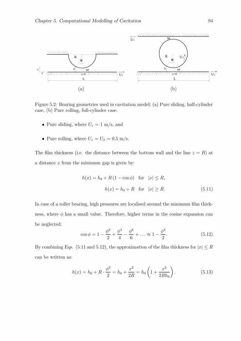
Chapter 5. Computational Modelling of Cavitation 94
z
L
h0
x=0x
h
R
U1
φ
L
h0
x=0
h
R
U1
U1
U2
h0
φ
(a) (b)
Figure 5.2: Bearing geometries used in cavitation model; (a) Pure sliding, half-cylindercase, (b) Pure rolling, full-cylinder case.
• Pure sliding, where U1 = 1 m/s, and
• Pure rolling, where U1 = U2 = 0.5 m/s.
The film thickness (i.e. the distance between the bottom wall and the line z = R) at
a distance x from the minimum gap is given by:
h(x) = h0 + R (1 − cos φ) for |x| ≤ R,
h(x) = h0 + R for |x| ≥ R. (5.11)
In case of a roller bearing, high pressures are localised around the minimum film thick-
ness, where φ has a small value. Therefore, higher terms in the cosine expansion can
be neglected:
cos φ = 1 −φ2
2+
φ4
4−
φ6
6+ . . . ≈ 1 −
φ2
2. (5.12)
By combining Eqs. (5.11 and 5.12), the approximation of the film thickness for |x| ≤ R
can be written as:
h(x) = h0 + R ·φ2
2= h0 +
x2
2R= h0
(
1 +x2
2Rh0
)
. (5.13)
Chapter 5. Computational Modelling of Cavitation 95
-0.0003 -0.0002 -0.0001 0 0.0001 0.0002 0.0003x [m]
-40
-30
-20
-10
0
10
20
30
40p
[MPa
]
Reynolds SolutionCFD - no cavitation
-0.0003 -0.0002 -0.0001 0 0.0001 0.0002 0.0003x [m]
-40
-30
-20
-10
0
10
20
30
40
p [M
Pa]
CFD - cavitationCFD - no cavitation
(a) Full Sommerfeld (b) Full Sommerfeld vs. Cavitation
Figure 5.3: Pressure distribution along the bottom wall of the roller bearing; (a) fora full Sommerfeld solution near the centre of the roller bearing; (b) numerical resultsobtained with and without the cavitation model
5.5.1 Reynolds Solution for Full Sommerfeld Condition
By substituting Eqn. (5.13) into the Reynolds Equation, Eqn. (4.10), and integrating
over the boundary conditions p = 105 Pa for x = ±∞, we obtain (Cameron [12]):
p(x) = −2U1ηx
h20
(
1 +x2
2Rh0
)2 + 105 for |x| ≤ R
p(x) = −2U1ηx
(h0 + R)2 + 105 for |x| ≥ R (5.14)
This pressure distribution, also known as Full Sommerfeld Condition, is anti- sym-
metrical, producing, therefore, unrealistic negative pressures and zero load support. In
order to obtain a realistic result, cavitation must be included in the numerical model.
Figure 5.3 (a) shows the pressure distribution obtained from Eqn. (5.14) alongside the
numerical results using the SIMPLE algorithm. In Figure 5.3 (b), numerical results
for pressure distribution with and without cavitation model are plotted alongside each
other for comparison.
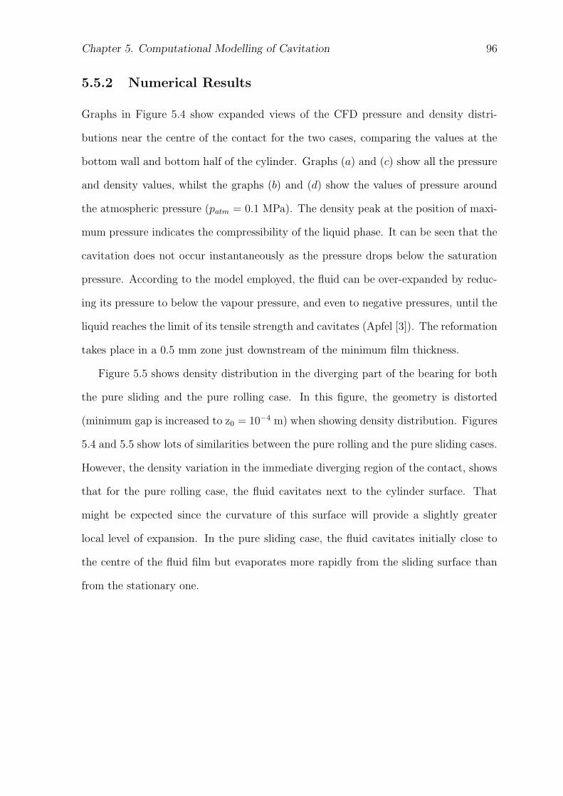
Chapter 5. Computational Modelling of Cavitation 96
5.5.2 Numerical Results
Graphs in Figure 5.4 show expanded views of the CFD pressure and density distri-
butions near the centre of the contact for the two cases, comparing the values at the
bottom wall and bottom half of the cylinder. Graphs (a) and (c) show all the pressure
and density values, whilst the graphs (b) and (d) show the values of pressure around
the atmospheric pressure (patm = 0.1 MPa). The density peak at the position of maxi-
mum pressure indicates the compressibility of the liquid phase. It can be seen that the
cavitation does not occur instantaneously as the pressure drops below the saturation
pressure. According to the model employed, the fluid can be over-expanded by reduc-
ing its pressure to below the vapour pressure, and even to negative pressures, until the
liquid reaches the limit of its tensile strength and cavitates (Apfel [3]). The reformation
takes place in a 0.5 mm zone just downstream of the minimum film thickness.
Figure 5.5 shows density distribution in the diverging part of the bearing for both
the pure sliding and the pure rolling case. In this figure, the geometry is distorted
(minimum gap is increased to z0 = 10−4 m) when showing density distribution. Figures
5.4 and 5.5 show lots of similarities between the pure rolling and the pure sliding cases.
However, the density variation in the immediate diverging region of the contact, shows
that for the pure rolling case, the fluid cavitates next to the cylinder surface. That
might be expected since the curvature of this surface will provide a slightly greater
local level of expansion. In the pure sliding case, the fluid cavitates initially close to
the centre of the fluid film but evaporates more rapidly from the sliding surface than
from the stationary one.
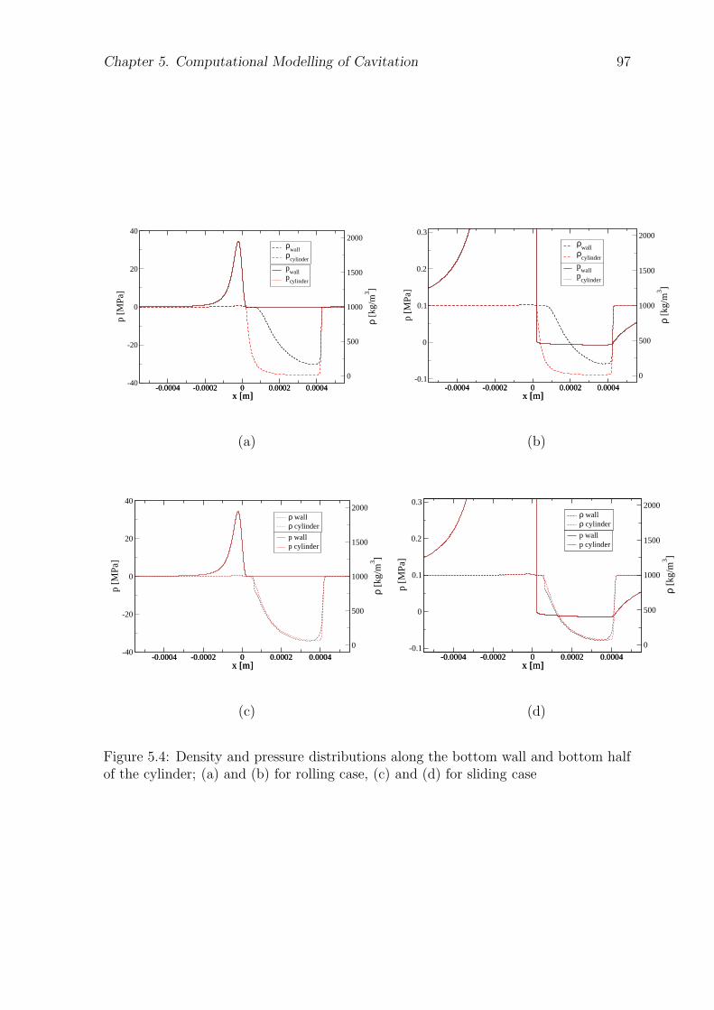
Chapter 5. Computational Modelling of Cavitation 97
-0.0004 -0.0002 0 0.0002 0.0004x [m]
-40
-20
0
20
40
p [M
Pa]
pwall
pcylinder
-0.0004 -0.0002 0 0.0002 0.0004x [m]
0
500
1000
1500
2000
ρ [k
g/m
3 ]
ρwall
ρcylinder
-0.0004 -0.0002 0 0.0002 0.0004x [m]
-0.1
0
0.1
0.2
0.3
p [M
Pa]
pwall
pcylinder
-0.0004 -0.0002 0 0.0002 0.0004x [m]
0
500
1000
1500
2000
ρ [k
g/m
3 ]
ρwall
ρcylinder
(a) (b)
-0.0004 -0.0002 0 0.0002 0.0004x [m]
0
500
1000
1500
2000
ρ [k
g/m
3 ]
ρ wallρ cylinder
-0.0004 -0.0002 0 0.0002 0.0004x [m]
-40
-20
0
20
40
p [M
Pa]
p wallp cylinder
-0.0004 -0.0002 0 0.0002 0.0004x [m]
0
500
1000
1500
2000
ρ [k
g/m
3 ]
ρ wallρ cylinder
-0.0004 -0.0002 0 0.0002 0.0004x [m]
-0.1
0
0.1
0.2
0.3
p [M
Pa]
p wallp cylinder
(c) (d)
Figure 5.4: Density and pressure distributions along the bottom wall and bottom halfof the cylinder; (a) and (b) for rolling case, (c) and (d) for sliding case
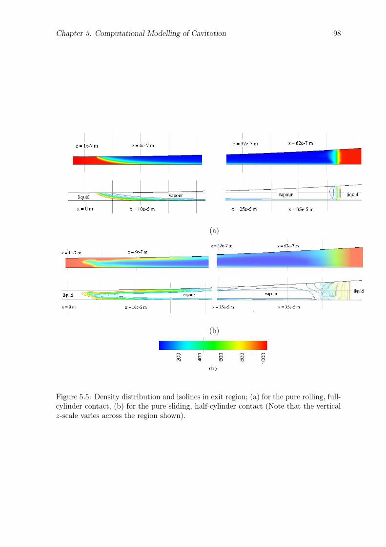
Chapter 5. Computational Modelling of Cavitation 98
(a)
(b)
Figure 5.5: Density distribution and isolines in exit region; (a) for the pure rolling, full-cylinder contact, (b) for the pure sliding, half-cylinder contact (Note that the verticalz-scale varies across the region shown).
Chapter 5. Computational Modelling of Cavitation 99
In Figure 5.6, the pressure-density dependence obtained from numerical results is
compared to the one obtained from Eqn. (5.10). There is a distinction between the
formation of cavitation and the subsequent re-formation of the fluid. The numerical
results do not correspond exactly to the analytical solution because according to the
barotropic relation pressure and density are not assumed to be in equilibrium.
-5000 0 5000 10000p [Pa]
0
200
400
600
800
1000
ρ [g
/m3 ]
Cavitation forms - cylinderLiquid reforms - cylinderCavitation forms - wallLiquid reforms - wallTheory - a
g = 200 m/s
Figure 5.6: Pressure–density dependence for the half-cylinder case (magnified aroundcavitation values).
Figures 5.7 (a) and 5.7 (b) show streamlines for the cavitation cases. The geometry
is distorted by increasing the apparent minimum gap to 10−3 m. Backflow can be
noticed both in the converging and diverging regions.
In Figure 5.8 it is shown that the backflow starts at x = -5e-5 m in the converging
region of the half-cylinder case and it goes all the way back to the inlet.
Figure 5.9 shows that, for the full cylinder case, the backflow in the converging
region starts at x = -15e-5 m at the bottom wall and at x = 15e-5 m at the top wall.
In the full cylinder, as expected, the flow is antisymmetrical with respect to x = R.
The backflow in the inlet region occurs because not all of the fluid can go through the
small gap, only a small amount gets dragged into the diverging region. Figure 5.10
shows the density isolines and the velocity profile for the half-cylinder and the full-
cylinder cases in the diverging region. It can be noticed that the backflow starts at
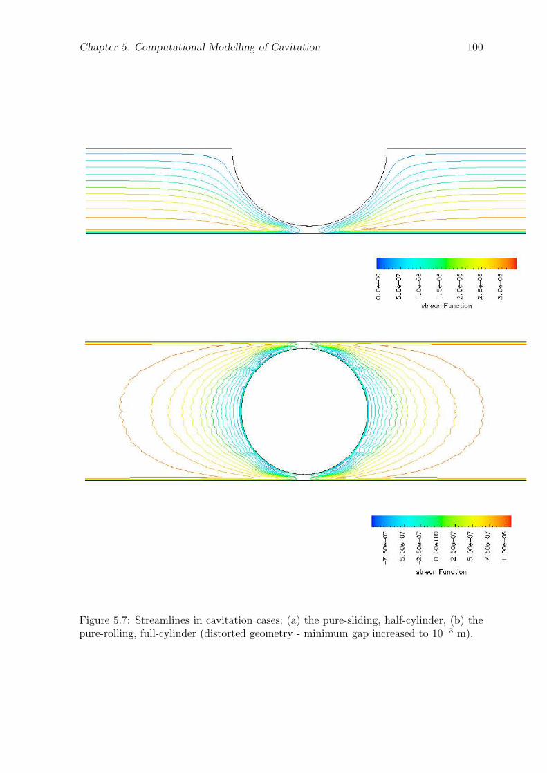
Chapter 5. Computational Modelling of Cavitation 100
Figure 5.7: Streamlines in cavitation cases; (a) the pure-sliding, half-cylinder, (b) thepure-rolling, full-cylinder (distorted geometry - minimum gap increased to 10−3 m).
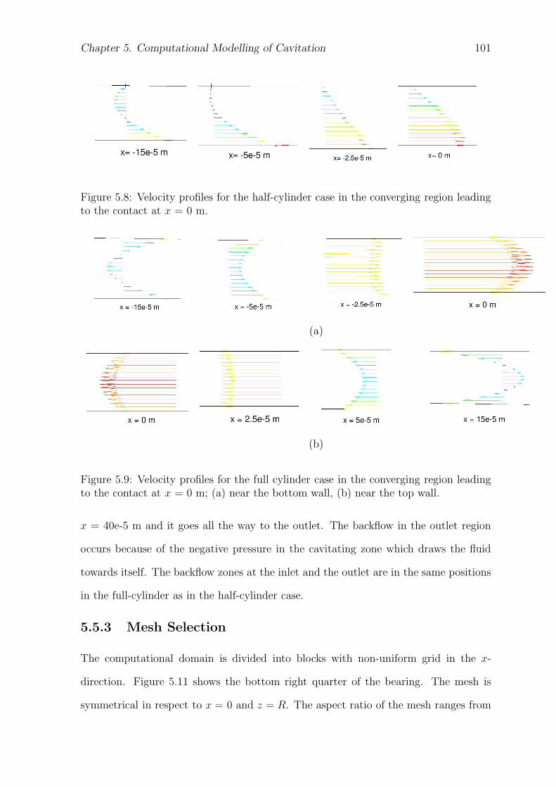
Chapter 5. Computational Modelling of Cavitation 101
Figure 5.8: Velocity profiles for the half-cylinder case in the converging region leadingto the contact at x = 0 m.
(a)
(b)
Figure 5.9: Velocity profiles for the full cylinder case in the converging region leadingto the contact at x = 0 m; (a) near the bottom wall, (b) near the top wall.
x = 40e-5 m and it goes all the way to the outlet. The backflow in the outlet region
occurs because of the negative pressure in the cavitating zone which draws the fluid
towards itself. The backflow zones at the inlet and the outlet are in the same positions
in the full-cylinder as in the half-cylinder case.
5.5.3 Mesh Selection
The computational domain is divided into blocks with non-uniform grid in the x-
direction. Figure 5.11 shows the bottom right quarter of the bearing. The mesh is
symmetrical in respect to x = 0 and z = R. The aspect ratio of the mesh ranges from
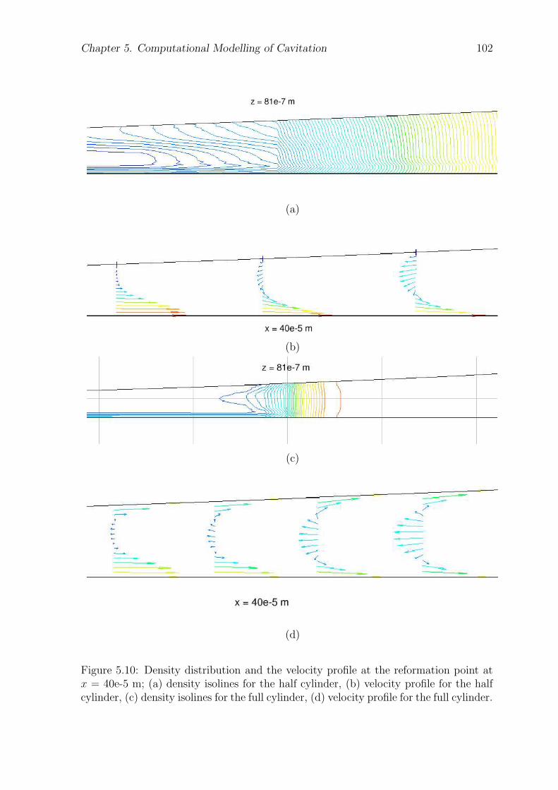
Chapter 5. Computational Modelling of Cavitation 102
(a)
(b)
(c)
(d)
Figure 5.10: Density distribution and the velocity profile at the reformation point atx = 40e-5 m; (a) density isolines for the half cylinder, (b) velocity profile for the halfcylinder, (c) density isolines for the full cylinder, (d) velocity profile for the full cylinder.
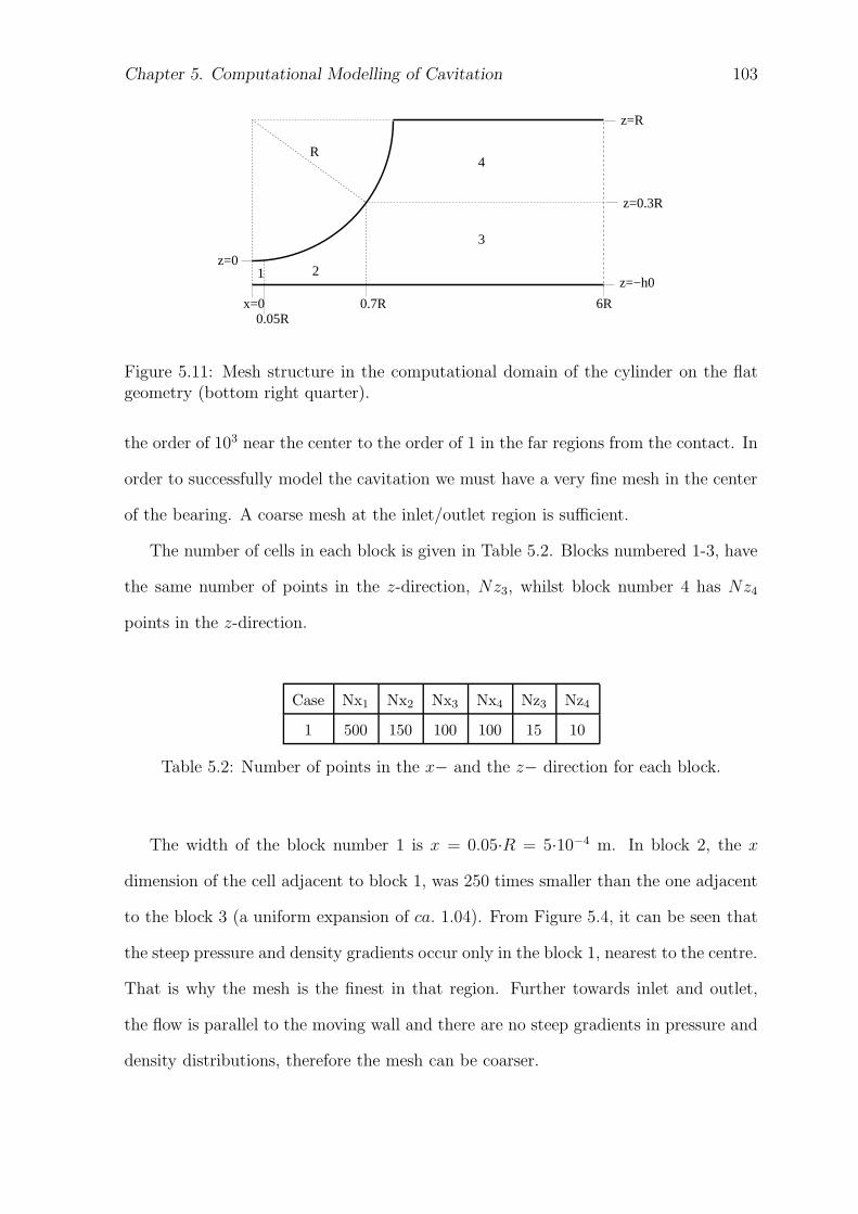
Chapter 5. Computational Modelling of Cavitation 103
0.7Rx=0
1
0.05R6R
z=R
z=0.3R
z=−h0
z=0
R
2
4
3
Figure 5.11: Mesh structure in the computational domain of the cylinder on the flatgeometry (bottom right quarter).
the order of 103 near the center to the order of 1 in the far regions from the contact. In
order to successfully model the cavitation we must have a very fine mesh in the center
of the bearing. A coarse mesh at the inlet/outlet region is sufficient.
The number of cells in each block is given in Table 5.2. Blocks numbered 1-3, have
the same number of points in the z-direction, Nz3, whilst block number 4 has Nz4
points in the z-direction.
Case Nx1 Nx2 Nx3 Nx4 Nz3 Nz4
1 500 150 100 100 15 10
Table 5.2: Number of points in the x− and the z− direction for each block.
The width of the block number 1 is x = 0.05·R = 5·10−4 m. In block 2, the x
dimension of the cell adjacent to block 1, was 250 times smaller than the one adjacent
to the block 3 (a uniform expansion of ca. 1.04). From Figure 5.4, it can be seen that
the steep pressure and density gradients occur only in the block 1, nearest to the centre.
That is why the mesh is the finest in that region. Further towards inlet and outlet,
the flow is parallel to the moving wall and there are no steep gradients in pressure and
density distributions, therefore the mesh can be coarser.
Chapter 5. Computational Modelling of Cavitation 104
5.6 Closure
In this Chapter two cases were studied: the pure rolling, full cylinder and the pure
sliding, half cylinder. In both cases the cavitation occurs in the divergent region of
the bearing, which requires a suitable computational model. The computational model
used in this work is a continuum method model with both the vapour and the liquid
phases considered to be the same fluid. The density of the fluid determines wheather
the fluid is a vapour, liquid or a mixture of the two.
Numerical results have shown many similarities between the pure sliding and the
pure rolling case. In both cases, there was occurrence of the backflow in the converging
and diverging region. The difference between them was that the fluid cavitated next
to the cylinder surface in the pure rolling case, whereas in the pure sliding case, it
started cavitating in the centre of the fluid film but evaporated more rapidly close to
the sliding surface.
It should be noted that the cavitation model used in this work should not be
taken to be quantitatively accurate. Firstly, it is unlikely that the assumed liquid
to vapour transition is the only process of cavitation in bearings; it is equally likely
that cavitation occurs via the escape of dissolved gases in low pressure liquid regions.
Also, the isentropic evaporation cavitation model adopted is one developed primarily
for behaviour in higher Reynolds number flows and may not be fully appropriate to
expansion in the pocket entry. However, the predictions made from it are likely to be
at least qualitatively correct.
Chapter 6
Low Friction Pocketed Pad Bearing
6.1 Introduction
Chapter 4 confirmed the applicability of CFD in treating HL problems on two geome-
tries: an infinitely long linear wedge and an infinitely long step bearing. It was seen
how the CFD solver can handle the steep geometry of the step bearing and how results
coincided with those obtained with Reynolds equation.
In Chapter 5, the geometry of a roller bearing was modelled, introducing the need
for cavitation modelling in the diverging region of the bearing. The results, even though
obtained by a simplified model, gave a realistic distribution of pressure and density.
This Chapter addresses the behaviour of lubricant in closed pockets or recesses in
bearings. Although pockets have been widely used for many years in hybrid hydrody-
namic/hydrostatic bearings, there are normally placed at the bearing inlet to promote
fluid entrainment (entry pockets) or are connected to an oil supply port or channel.
The use of isolated pockets in the bearing surface has, until recently, received little
attention.
In the last few years, however, it has been found that the friction coefficient of
very low or zero convergence ratio bearings (whose surfaces are almost parallel), such
as those present at piston skirts and face seals, may be very significantly reduced if
one of the bearing surfaces is indented with many tiny, closed pockets (Ronen et al.
[58], Ryk [59], Etsion [23], Goloch [30]). Theoretical analysis of such textured surface
105
Chapter 6. Low Friction Pocketed Pad Bearing 106
systems has been carried out using Reynolds equation, which suggests that cavitation
may occur at the divergent entrance to the pockets, followed by a local increase in
hydrodynamic pressure (Hamilton [33], Etsion [22]). Typical suggested dimple sizes
are 50 to 100 µm diameter, 5 to 10 µm depth, with a pocket density such as to cover
about 10 to 25% of the total bearing area.
More recently, experimental work has indicated that the main role of these pockets
may be to promote fluid entrainment at low speeds and thus cause the bearing to enter
the full-film hydrodynamic regime (with concomitantly reduced friction) at a lower
sliding speed than for smooth surfaces (Wang [72]), (Kovalchenko [46]). This may
imply that the dimples may be acting in the inlet as entry-pockets, as suggested by
Tonder [63]. Very recently, CFD has been employed to show that roughness, where
the depth and width scales of the roughness features are of similar order, can produce
additional lift due to convective inertia (Arghir et al. [4]).
In this study, a simple linear pad bearing was analysed in which the stator had one
or more shallow, macroscale pockets. A wide range of convergence ratios, from values
of unity, typical of plain thrust bearings, to very small values more representative of
piston skirt/liner contacts are considered.
In 6.2 general information about the fluid properties, boundary conditions and the
mesh study will be presented.
In Section 6.3, a 2D bearing with a single pocket will be studied. In this study, 2D
is used to mean a bearing which is infinitely long transverse to the direction of surface
motion, while a 3D one is a bearing of finite length transverse to the sliding/rolling
direction. The effect of varying the pocket height, position, size and convergence ratio
on total load support and total friction will be examined. The case with very low
convergence ratio will be briefly discussed because of the possible cavitation effects.
In Section 6.4, similar analysis will be conducted for a 2D bearing with more than
one pocket. Section 6.5 will conclude the Chapter with the study of a 3D bearing with
Chapter 6. Low Friction Pocketed Pad Bearing 107
pockets.
6.2 Linear Bearings with Pockets
Throughout this Chapter, density of liquid is set to ρ = 103 kg/m3, dynamic viscosity
to η = 10−2 Pas and the speed of the bottom wall of the bearing is U1 = 1 m/s. The
bearing width is B = 20 mm (see Figure 6.1).
The convergence ratio K, of the bearing is given by:
K =h1 − h0
h0
. (6.1)
In most work in this Chapter, the convergence ratio, K, was kept at a typical engineer-
ing value for pad bearings of K = 1. This convergence ratio gives almost optimally
high pressures in a linear bearing and in no case at K = 1 was any cavitation observed
to take place in the bearing pocket.
6.2.1 Boundary Conditions
The pressure at the inlet and outlet boundaries was set to atmospheric (105 Pa) and
zero velocity gradient in the normal direction was assumed for the velocity field. This
defines a fully developed flow approximation through these boundaries. It is important
to set the boundaries relatively far from the region of interest, so that they do not
overly influence the numerical solution. The domain was fully flooded.
At the solid walls, the ’no-slip’ boundary condition was assumed for the momentum
equations. In practice this involved setting the velocity of the face of each fluid cell
adjacent to the wall to have the same velocity as that of the wall itself.
6.2.2 Load and Friction
Total load and friction were obtained using Eqn. (4.29):
Φ =
Nx/2−1∑
i=0
1/2 (x2i+1 − x2i) (f2i+1 + f2i),
with
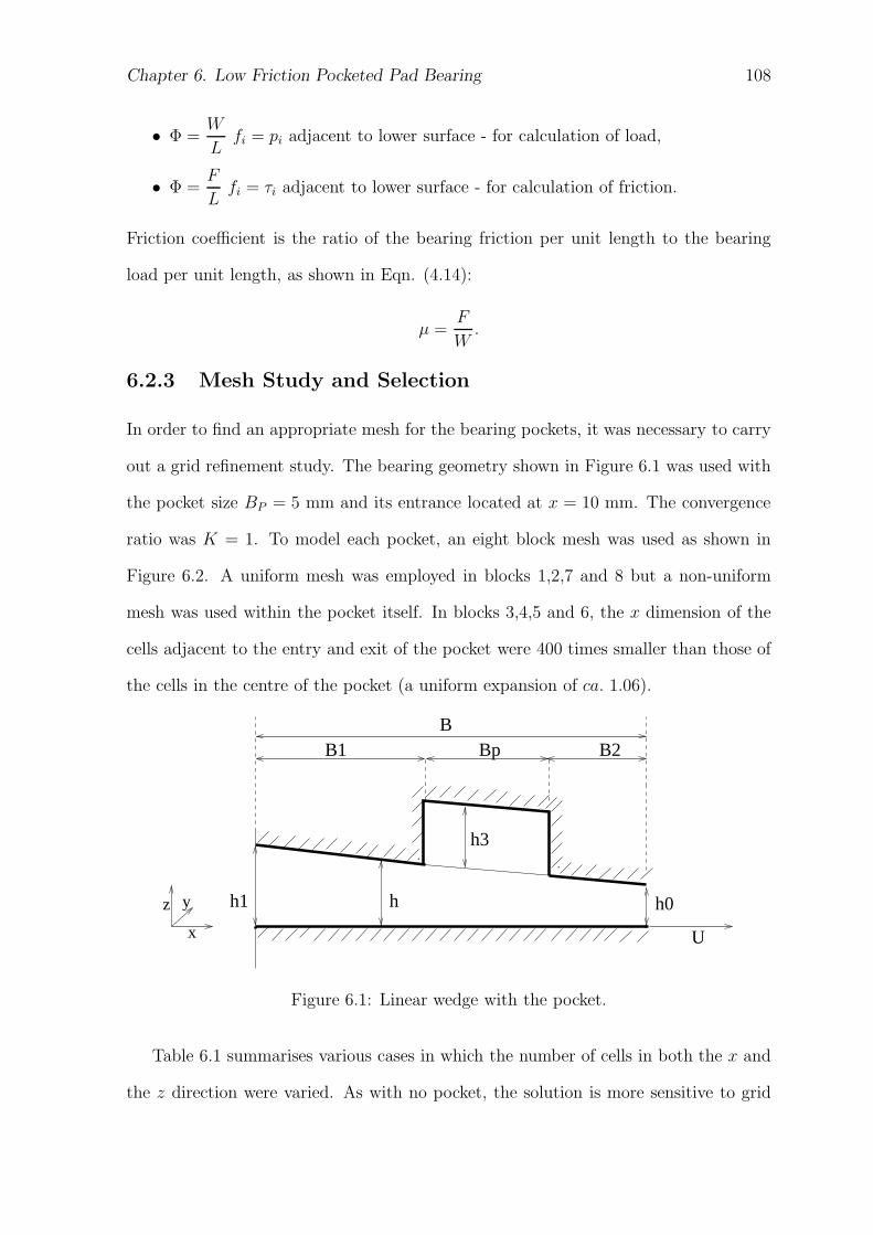
Chapter 6. Low Friction Pocketed Pad Bearing 108
• Φ =W
Lfi = pi adjacent to lower surface - for calculation of load,
• Φ =F
Lfi = τi adjacent to lower surface - for calculation of friction.
Friction coefficient is the ratio of the bearing friction per unit length to the bearing
load per unit length, as shown in Eqn. (4.14):
µ =F
W.
6.2.3 Mesh Study and Selection
In order to find an appropriate mesh for the bearing pockets, it was necessary to carry
out a grid refinement study. The bearing geometry shown in Figure 6.1 was used with
the pocket size BP = 5 mm and its entrance located at x = 10 mm. The convergence
ratio was K = 1. To model each pocket, an eight block mesh was used as shown in
Figure 6.2. A uniform mesh was employed in blocks 1,2,7 and 8 but a non-uniform
mesh was used within the pocket itself. In blocks 3,4,5 and 6, the x dimension of the
cells adjacent to the entry and exit of the pocket were 400 times smaller than those of
the cells in the centre of the pocket (a uniform expansion of ca. 1.06).
h1 h
..
B2BpB1B
h3
x
z y
U
h0
Figure 6.1: Linear wedge with the pocket.
Table 6.1 summarises various cases in which the number of cells in both the x and
the z direction were varied. As with no pocket, the solution is more sensitive to grid
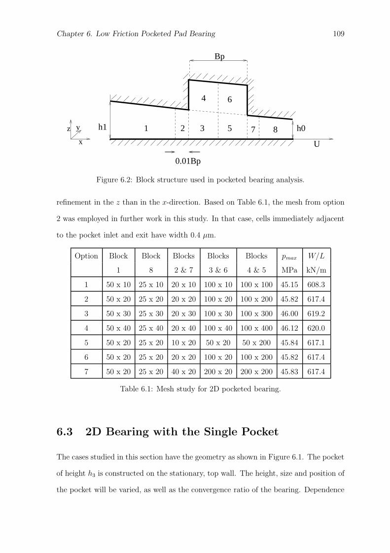
Chapter 6. Low Friction Pocketed Pad Bearing 109
h1
..
Bp
x
z y
U
h0
4 6
81 2 3 5 7
0.01Bp
Figure 6.2: Block structure used in pocketed bearing analysis.
refinement in the z than in the x-direction. Based on Table 6.1, the mesh from option
2 was employed in further work in this study. In that case, cells immediately adjacent
to the pocket inlet and exit have width 0.4 µm.
Option Block Block Blocks Blocks Blocks pmax W/L
1 8 2 & 7 3 & 6 4 & 5 MPa kN/m
1 50 x 10 25 x 10 20 x 10 100 x 10 100 x 100 45.15 608.3
2 50 x 20 25 x 20 20 x 20 100 x 20 100 x 200 45.82 617.4
3 50 x 30 25 x 30 20 x 30 100 x 30 100 x 300 46.00 619.2
4 50 x 40 25 x 40 20 x 40 100 x 40 100 x 400 46.12 620.0
5 50 x 20 25 x 20 10 x 20 50 x 20 50 x 200 45.84 617.1
6 50 x 20 25 x 20 20 x 20 100 x 20 100 x 200 45.82 617.4
7 50 x 20 25 x 20 40 x 20 200 x 20 200 x 200 45.83 617.4
Table 6.1: Mesh study for 2D pocketed bearing.
6.3 2D Bearing with the Single Pocket
The cases studied in this section have the geometry as shown in Figure 6.1. The pocket
of height h3 is constructed on the stationary, top wall. The height, size and position of
the pocket will be varied, as well as the convergence ratio of the bearing. Dependence
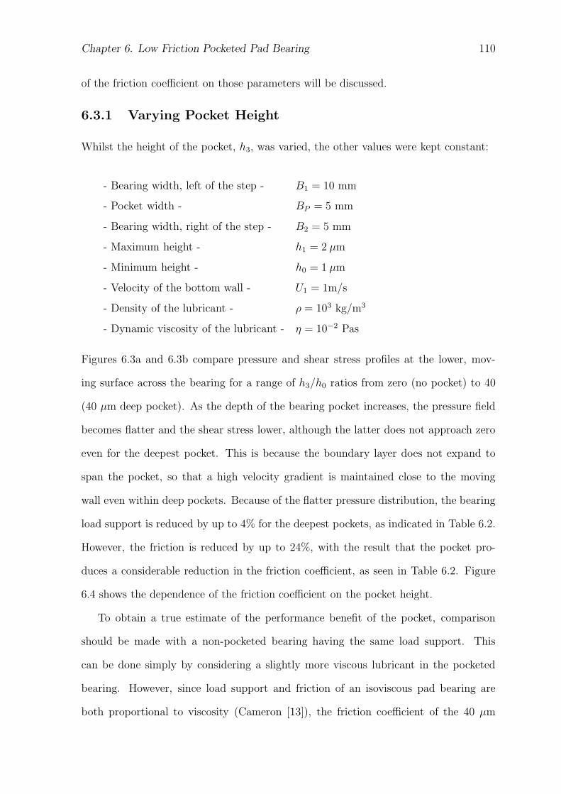
Chapter 6. Low Friction Pocketed Pad Bearing 110
of the friction coefficient on those parameters will be discussed.
6.3.1 Varying Pocket Height
Whilst the height of the pocket, h3, was varied, the other values were kept constant:
- Bearing width, left of the step - B1 = 10 mm
- Pocket width - BP = 5 mm
- Bearing width, right of the step - B2 = 5 mm
- Maximum height - h1 = 2 µm
- Minimum height - h0 = 1 µm
- Velocity of the bottom wall - U1 = 1m/s
- Density of the lubricant - ρ = 103 kg/m3
- Dynamic viscosity of the lubricant - η = 10−2 Pas
Figures 6.3a and 6.3b compare pressure and shear stress profiles at the lower, mov-
ing surface across the bearing for a range of h3/h0 ratios from zero (no pocket) to 40
(40 µm deep pocket). As the depth of the bearing pocket increases, the pressure field
becomes flatter and the shear stress lower, although the latter does not approach zero
even for the deepest pocket. This is because the boundary layer does not expand to
span the pocket, so that a high velocity gradient is maintained close to the moving
wall even within deep pockets. Because of the flatter pressure distribution, the bearing
load support is reduced by up to 4% for the deepest pockets, as indicated in Table 6.2.
However, the friction is reduced by up to 24%, with the result that the pocket pro-
duces a considerable reduction in the friction coefficient, as seen in Table 6.2. Figure
6.4 shows the dependence of the friction coefficient on the pocket height.
To obtain a true estimate of the performance benefit of the pocket, comparison
should be made with a non-pocketed bearing having the same load support. This
can be done simply by considering a slightly more viscous lubricant in the pocketed
bearing. However, since load support and friction of an isoviscous pad bearing are
both proportional to viscosity (Cameron [13]), the friction coefficient of the 40 µm
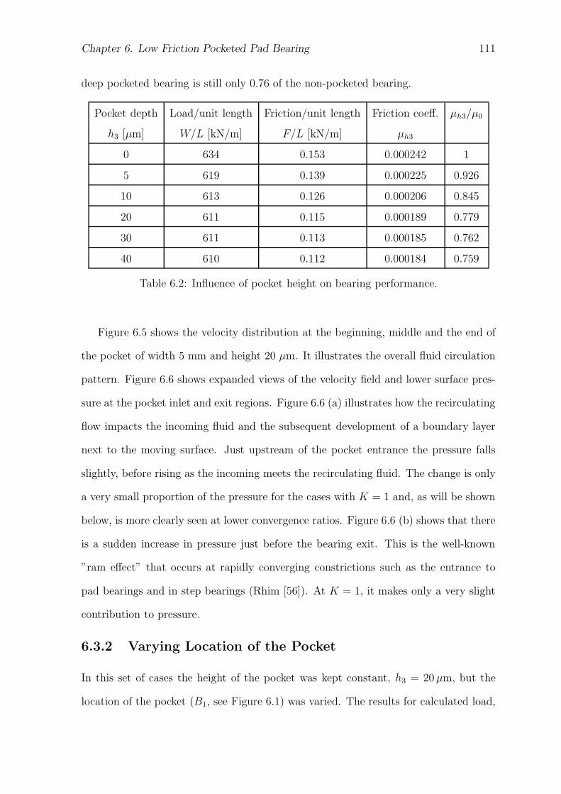
Chapter 6. Low Friction Pocketed Pad Bearing 111
deep pocketed bearing is still only 0.76 of the non-pocketed bearing.
Pocket depth Load/unit length Friction/unit length Friction coeff. µh3/µ0
h3 [µm] W/L [kN/m] F/L [kN/m] µh3
0 634 0.153 0.000242 1
5 619 0.139 0.000225 0.926
10 613 0.126 0.000206 0.845
20 611 0.115 0.000189 0.779
30 611 0.113 0.000185 0.762
40 610 0.112 0.000184 0.759
Table 6.2: Influence of pocket height on bearing performance.
Figure 6.5 shows the velocity distribution at the beginning, middle and the end of
the pocket of width 5 mm and height 20 µm. It illustrates the overall fluid circulation
pattern. Figure 6.6 shows expanded views of the velocity field and lower surface pres-
sure at the pocket inlet and exit regions. Figure 6.6 (a) illustrates how the recirculating
flow impacts the incoming fluid and the subsequent development of a boundary layer
next to the moving surface. Just upstream of the pocket entrance the pressure falls
slightly, before rising as the incoming meets the recirculating fluid. The change is only
a very small proportion of the pressure for the cases with K = 1 and, as will be shown
below, is more clearly seen at lower convergence ratios. Figure 6.6 (b) shows that there
is a sudden increase in pressure just before the bearing exit. This is the well-known
”ram effect” that occurs at rapidly converging constrictions such as the entrance to
pad bearings and in step bearings (Rhim [56]). At K = 1, it makes only a very slight
contribution to pressure.
6.3.2 Varying Location of the Pocket
In this set of cases the height of the pocket was kept constant, h3 = 20 µm, but the
location of the pocket (B1, see Figure 6.1) was varied. The results for calculated load,
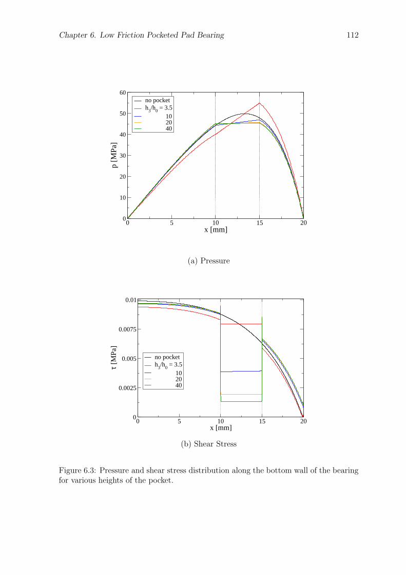
Chapter 6. Low Friction Pocketed Pad Bearing 112
0 5 10 15 20x [mm]
0
10
20
30
40
50
60
p [M
Pa]
no pocketh
3/h
0 = 3.5
10 20 40
(a) Pressure
0 5 10 15 20x [mm]
0
0.0025
0.005
0.0075
0.01
τ [M
Pa]
no pocketh
3/h
0 = 3.5
10 20 40
(b) Shear Stress
Figure 6.3: Pressure and shear stress distribution along the bottom wall of the bearingfor various heights of the pocket.
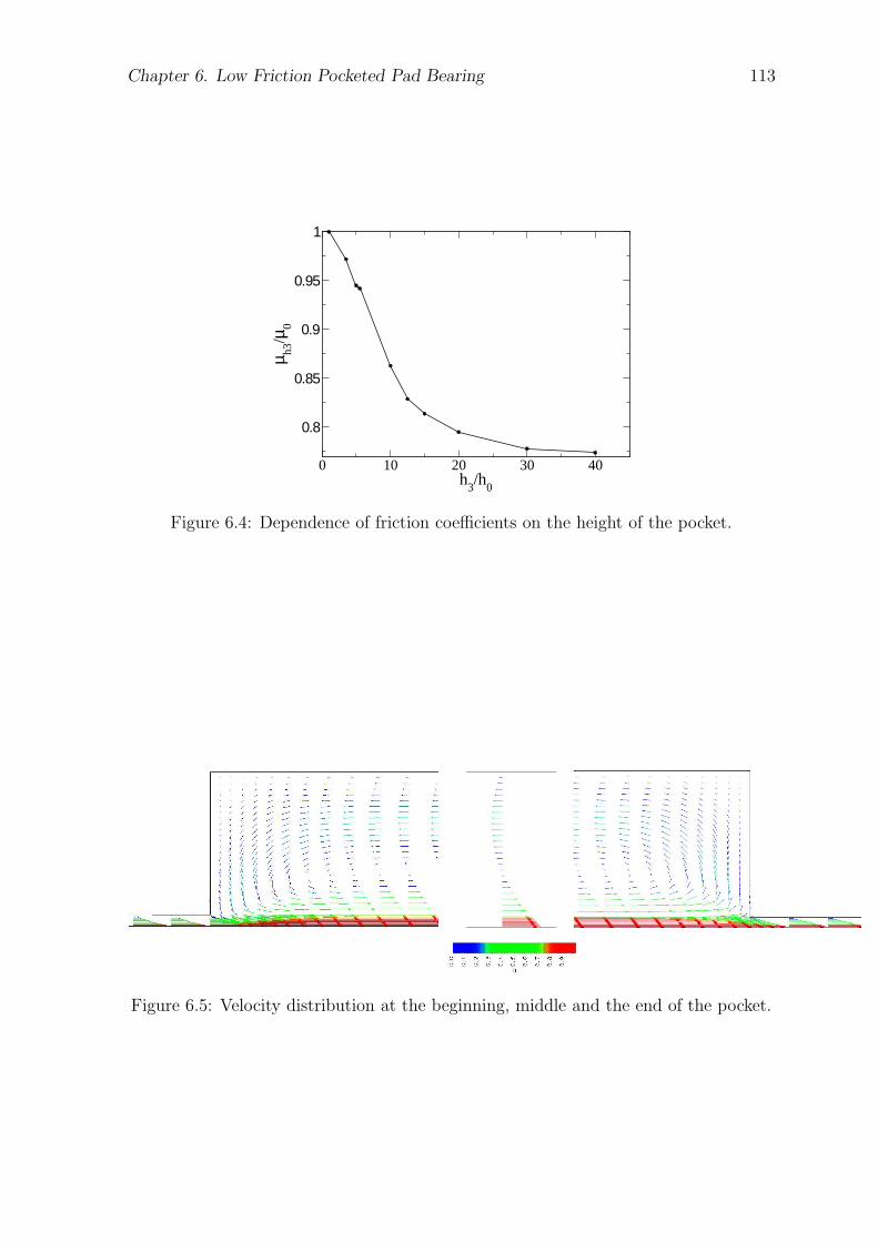
Chapter 6. Low Friction Pocketed Pad Bearing 113
0 10 20 30 40h
3/h
0
0.8
0.85
0.9
0.95
1
µ h3/µ
0
Figure 6.4: Dependence of friction coefficients on the height of the pocket.
Figure 6.5: Velocity distribution at the beginning, middle and the end of the pocket.
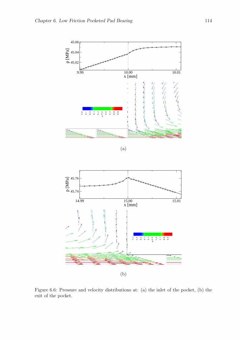
Chapter 6. Low Friction Pocketed Pad Bearing 114
9.99 10.00 10.01x [mm]
45.02
45.04
45.06
p [M
Pa]
(a)
14.99 15.00 15.01x [mm]
45.74
45.76
p [M
Pa]
(b)
Figure 6.6: Pressure and velocity distributions at: (a) the inlet of the pocket, (b) theexit of the pocket.
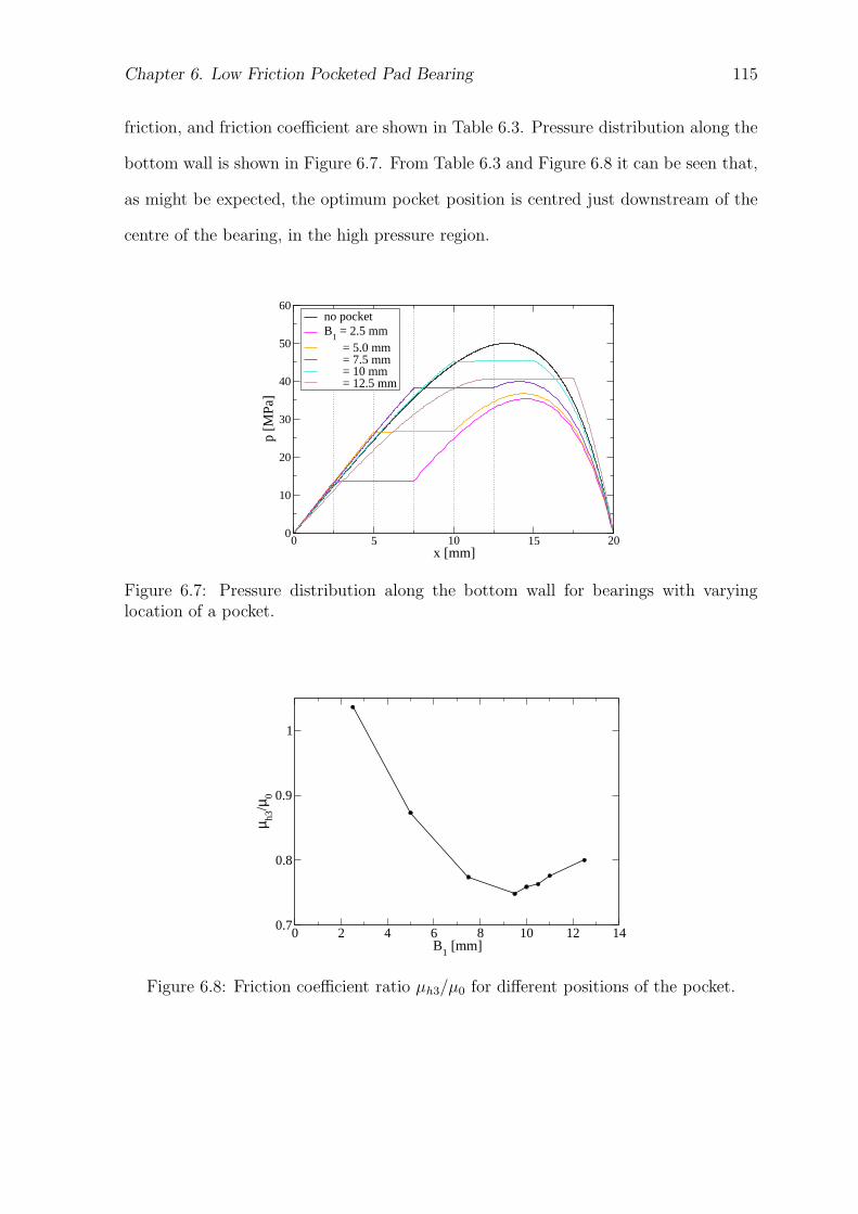
Chapter 6. Low Friction Pocketed Pad Bearing 115
friction, and friction coefficient are shown in Table 6.3. Pressure distribution along the
bottom wall is shown in Figure 6.7. From Table 6.3 and Figure 6.8 it can be seen that,
as might be expected, the optimum pocket position is centred just downstream of the
centre of the bearing, in the high pressure region.
0 5 10 15 20x [mm]
0
10
20
30
40
50
60
p [M
Pa]
no pocketB
1 = 2.5 mm
= 5.0 mm = 7.5 mm = 10 mm = 12.5 mm
Figure 6.7: Pressure distribution along the bottom wall for bearings with varyinglocation of a pocket.
0 2 4 6 8 10 12 14B
1 [mm]
0.7
0.8
0.9
1
µ h3/µ
0
Figure 6.8: Friction coefficient ratio µh3/µ0 for different positions of the pocket.
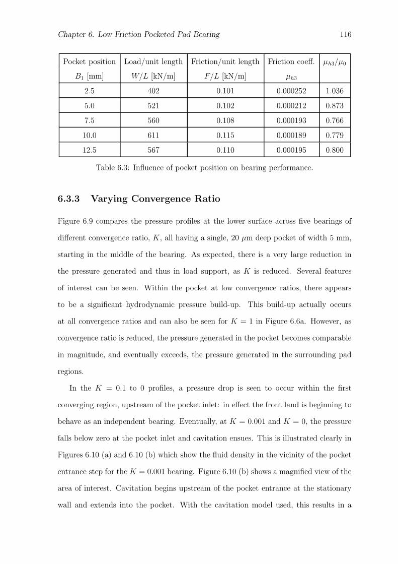
Chapter 6. Low Friction Pocketed Pad Bearing 116
Pocket position Load/unit length Friction/unit length Friction coeff. µh3/µ0
B1 [mm] W/L [kN/m] F/L [kN/m] µh3
2.5 402 0.101 0.000252 1.036
5.0 521 0.102 0.000212 0.873
7.5 560 0.108 0.000193 0.766
10.0 611 0.115 0.000189 0.779
12.5 567 0.110 0.000195 0.800
Table 6.3: Influence of pocket position on bearing performance.
6.3.3 Varying Convergence Ratio
Figure 6.9 compares the pressure profiles at the lower surface across five bearings of
different convergence ratio, K, all having a single, 20 µm deep pocket of width 5 mm,
starting in the middle of the bearing. As expected, there is a very large reduction in
the pressure generated and thus in load support, as K is reduced. Several features
of interest can be seen. Within the pocket at low convergence ratios, there appears
to be a significant hydrodynamic pressure build-up. This build-up actually occurs
at all convergence ratios and can also be seen for K = 1 in Figure 6.6a. However, as
convergence ratio is reduced, the pressure generated in the pocket becomes comparable
in magnitude, and eventually exceeds, the pressure generated in the surrounding pad
regions.
In the K = 0.1 to 0 profiles, a pressure drop is seen to occur within the first
converging region, upstream of the pocket inlet: in effect the front land is beginning to
behave as an independent bearing. Eventually, at K = 0.001 and K = 0, the pressure
falls below zero at the pocket inlet and cavitation ensues. This is illustrated clearly in
Figures 6.10 (a) and 6.10 (b) which show the fluid density in the vicinity of the pocket
entrance step for the K = 0.001 bearing. Figure 6.10 (b) shows a magnified view of the
area of interest. Cavitation begins upstream of the pocket entrance at the stationary
wall and extends into the pocket. With the cavitation model used, this results in a
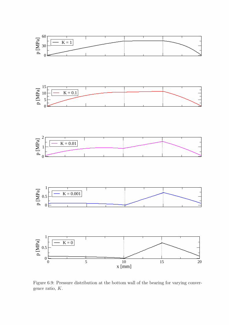
Chapter 6. Low Friction Pocketed Pad Bearing 117
0
30
60p
[MPa
]K = 1
0
5
10
15
p [M
Pa]
K = 0.1
0
1
2
p [M
Pa]
K = 0.01
0
0.5
1
p [M
Pa]
K = 0.001
0 5 10 15 20x [mm]
0
0.5
1
p [M
Pa]
K = 0
Figure 6.9: Pressure distribution at the bottom wall of the bearing for varying conver-gence ratio, K.
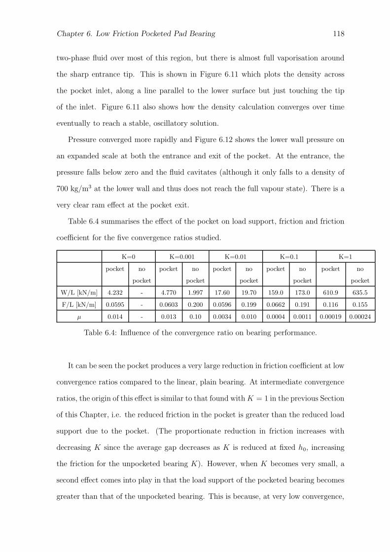
Chapter 6. Low Friction Pocketed Pad Bearing 118
two-phase fluid over most of this region, but there is almost full vaporisation around
the sharp entrance tip. This is shown in Figure 6.11 which plots the density across
the pocket inlet, along a line parallel to the lower surface but just touching the tip
of the inlet. Figure 6.11 also shows how the density calculation converges over time
eventually to reach a stable, oscillatory solution.
Pressure converged more rapidly and Figure 6.12 shows the lower wall pressure on
an expanded scale at both the entrance and exit of the pocket. At the entrance, the
pressure falls below zero and the fluid cavitates (although it only falls to a density of
700 kg/m3 at the lower wall and thus does not reach the full vapour state). There is a
very clear ram effect at the pocket exit.
Table 6.4 summarises the effect of the pocket on load support, friction and friction
coefficient for the five convergence ratios studied.
K=0 K=0.001 K=0.01 K=0.1 K=1
pocket no pocket no pocket no pocket no pocket no
pocket pocket pocket pocket pocket
W/L [kN/m] 4.232 - 4.770 1.997 17.60 19.70 159.0 173.0 610.9 635.5
F/L [kN/m] 0.0595 - 0.0603 0.200 0.0596 0.199 0.0662 0.191 0.116 0.155
µ 0.014 - 0.013 0.10 0.0034 0.010 0.0004 0.0011 0.00019 0.00024
Table 6.4: Influence of the convergence ratio on bearing performance.
It can be seen the pocket produces a very large reduction in friction coefficient at low
convergence ratios compared to the linear, plain bearing. At intermediate convergence
ratios, the origin of this effect is similar to that found with K = 1 in the previous Section
of this Chapter, i.e. the reduced friction in the pocket is greater than the reduced load
support due to the pocket. (The proportionate reduction in friction increases with
decreasing K since the average gap decreases as K is reduced at fixed h0, increasing
the friction for the unpocketed bearing K). However, when K becomes very small, a
second effect comes into play in that the load support of the pocketed bearing becomes
greater than that of the unpocketed bearing. This is because, at very low convergence,
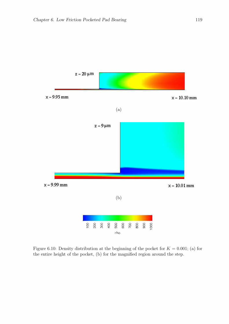
Chapter 6. Low Friction Pocketed Pad Bearing 119
(a)
(b)
Figure 6.10: Density distribution at the beginning of the pocket for K = 0.001; (a) forthe entire height of the pocket, (b) for the magnified region around the step.
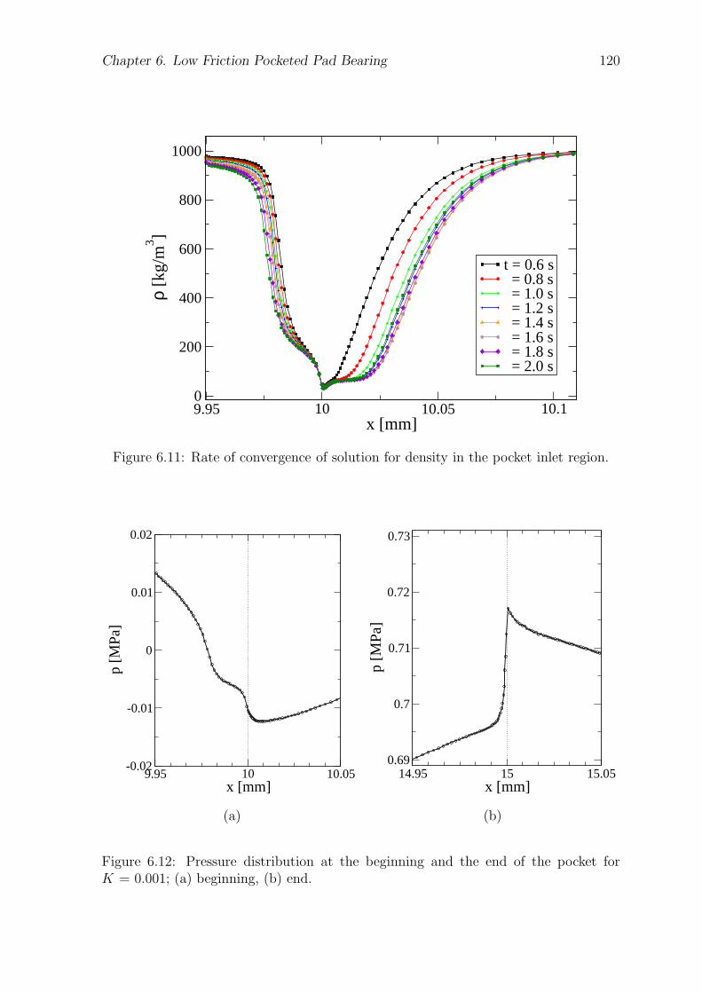
Chapter 6. Low Friction Pocketed Pad Bearing 120
9.95 10 10.05 10.1x [mm]
0
200
400
600
800
1000ρ
[kg/
m3 ]
t = 0.6 s = 0.8 s = 1.0 s = 1.2 s = 1.4 s = 1.6 s = 1.8 s = 2.0 s
Figure 6.11: Rate of convergence of solution for density in the pocket inlet region.
9.95 10 10.05x [mm]
-0.02
-0.01
0
0.01
0.02
p [M
Pa]
14.95 15 15.05x [mm]
0.69
0.7
0.71
0.72
0.73
p [M
Pa]
(a) (b)
Figure 6.12: Pressure distribution at the beginning and the end of the pocket forK = 0.001; (a) beginning, (b) end.
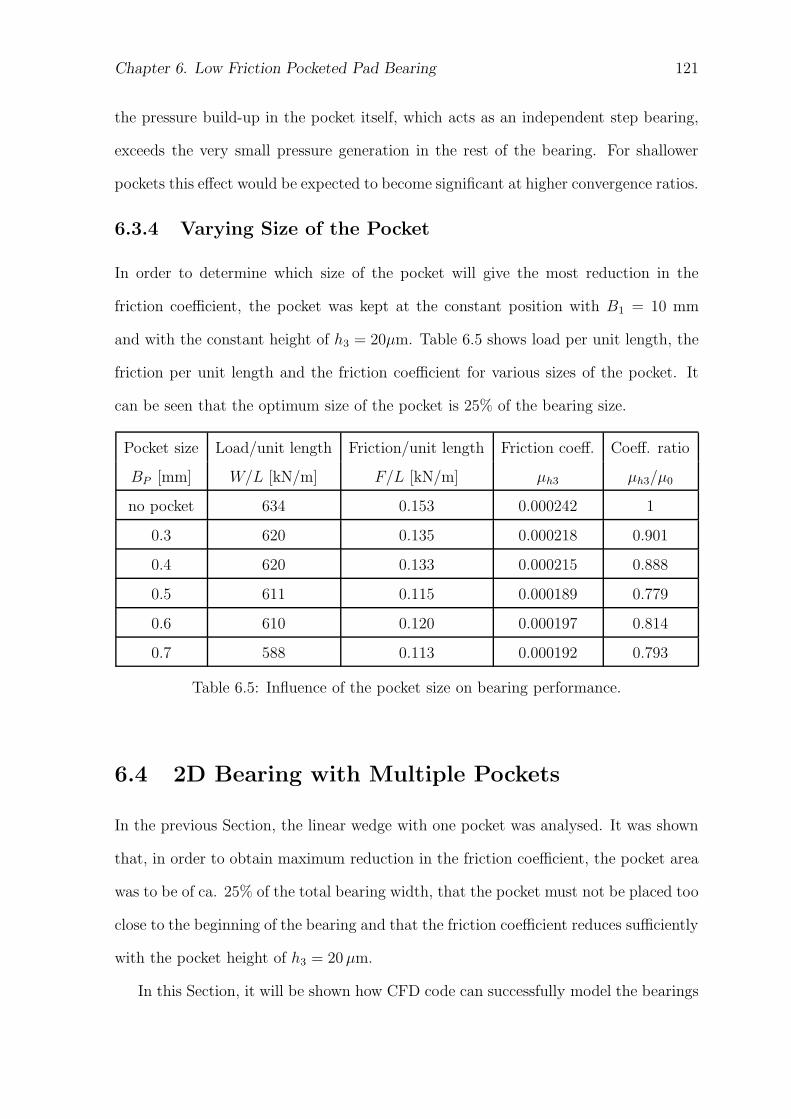
Chapter 6. Low Friction Pocketed Pad Bearing 121
the pressure build-up in the pocket itself, which acts as an independent step bearing,
exceeds the very small pressure generation in the rest of the bearing. For shallower
pockets this effect would be expected to become significant at higher convergence ratios.
6.3.4 Varying Size of the Pocket
In order to determine which size of the pocket will give the most reduction in the
friction coefficient, the pocket was kept at the constant position with B1 = 10 mm
and with the constant height of h3 = 20µm. Table 6.5 shows load per unit length, the
friction per unit length and the friction coefficient for various sizes of the pocket. It
can be seen that the optimum size of the pocket is 25% of the bearing size.
Pocket size Load/unit length Friction/unit length Friction coeff. Coeff. ratio
BP [mm] W/L [kN/m] F/L [kN/m] µh3 µh3/µ0
no pocket 634 0.153 0.000242 1
0.3 620 0.135 0.000218 0.901
0.4 620 0.133 0.000215 0.888
0.5 611 0.115 0.000189 0.779
0.6 610 0.120 0.000197 0.814
0.7 588 0.113 0.000192 0.793
Table 6.5: Influence of the pocket size on bearing performance.
6.4 2D Bearing with Multiple Pockets
In the previous Section, the linear wedge with one pocket was analysed. It was shown
that, in order to obtain maximum reduction in the friction coefficient, the pocket area
was to be of ca. 25% of the total bearing width, that the pocket must not be placed too
close to the beginning of the bearing and that the friction coefficient reduces sufficiently
with the pocket height of h3 = 20 µm.
In this Section, it will be shown how CFD code can successfully model the bearings
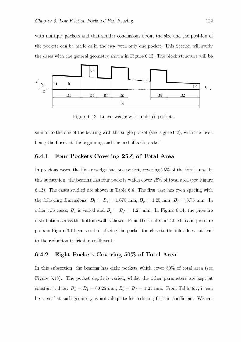
Chapter 6. Low Friction Pocketed Pad Bearing 122
with multiple pockets and that similar conclusions about the size and the position of
the pockets can be made as in the case with only one pocket. This Section will study
the cases with the general geometry shown in Figure 6.13. The block structure will be
B
B1 Bp Bf Bp B2Bp
U
h3
hh1
x
yzh0
Figure 6.13: Linear wedge with multiple pockets.
similar to the one of the bearing with the single pocket (see Figure 6.2), with the mesh
being the finest at the beginning and the end of each pocket.
6.4.1 Four Pockets Covering 25% of Total Area
In previous cases, the linear wedge had one pocket, covering 25% of the total area. In
this subsection, the bearing has four pockets which cover 25% of total area (see Figure
6.13). The cases studied are shown in Table 6.6. The first case has even spacing with
the following dimensions: B1 = B2 = 1.875 mm, Bp = 1.25 mm, Bf = 3.75 mm. In
other two cases, B1 is varied and Bp = Bf = 1.25 mm. In Figure 6.14, the pressure
distribution across the bottom wall is shown. From the results in Table 6.6 and pressure
plots in Figure 6.14, we see that placing the pocket too close to the inlet does not lead
to the reduction in friction coefficient.
6.4.2 Eight Pockets Covering 50% of Total Area
In this subsection, the bearing has eight pockets which cover 50% of total area (see
Figure 6.13). The pocket depth is varied, whilst the other parameters are kept at
constant values: B1 = B2 = 0.625 mm, Bp = Bf = 1.25 mm. From Table 6.7, it can
be seen that such geometry is not adequate for reducing friction coefficient. We can
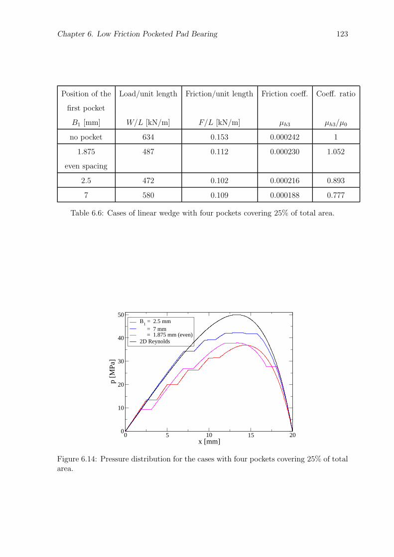
Chapter 6. Low Friction Pocketed Pad Bearing 123
Position of the Load/unit length Friction/unit length Friction coeff. Coeff. ratio
first pocket
B1 [mm] W/L [kN/m] F/L [kN/m] µh3 µh3/µ0
no pocket 634 0.153 0.000242 1
1.875 487 0.112 0.000230 1.052
even spacing
2.5 472 0.102 0.000216 0.893
7 580 0.109 0.000188 0.777
Table 6.6: Cases of linear wedge with four pockets covering 25% of total area.
0 5 10 15 20x [mm]
0
10
20
30
40
50
p [M
Pa]
B1 = 2.5 mm
= 7 mm = 1.875 mm (even)2D Reynolds
Figure 6.14: Pressure distribution for the cases with four pockets covering 25% of totalarea.
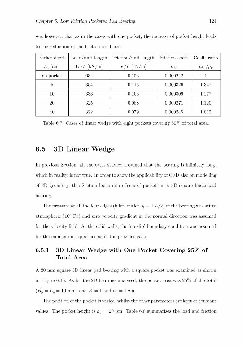
Chapter 6. Low Friction Pocketed Pad Bearing 124
see, however, that as in the cases with one pocket, the increase of pocket height leads
to the reduction of the friction coefficient.
Pocket depth Load/unit length Friction/unit length Friction coeff. Coeff. ratio
h3 [µm] W/L [kN/m] F/L [kN/m] µh3 µh3/µ0
no pocket 634 0.153 0.000242 1
5 354 0.115 0.000326 1.347
10 333 0.103 0.000309 1.277
20 325 0.088 0.000271 1.120
40 322 0.079 0.000245 1.012
Table 6.7: Cases of linear wedge with eight pockets covering 50% of total area.
6.5 3D Linear Wedge
In previous Section, all the cases studied assumed that the bearing is infinitely long,
which in reality, is not true. In order to show the applicability of CFD also on modelling
of 3D geometry, this Section looks into effects of pockets in a 3D square linear pad
bearing.
The pressure at all the four edges (inlet, outlet, y = ±L/2) of the bearing was set to
atmospheric (105 Pa) and zero velocity gradient in the normal direction was assumed
for the velocity field. At the solid walls, the ’no-slip’ boundary condition was assumed
for the momentum equations as in the previous cases.
6.5.1 3D Linear Wedge with One Pocket Covering 25% of
Total Area
A 20 mm square 3D linear pad bearing with a square pocket was examined as shown
in Figure 6.15. As for the 2D bearings analysed, the pocket area was 25% of the total
(Bp = Lp = 10 mm) and K = 1 and h0 = 1 µm.
The position of the pocket is varied, whilst the other parameters are kept at constant
values. The pocket height is h3 = 20 µm. Table 6.8 summarises the load and friction
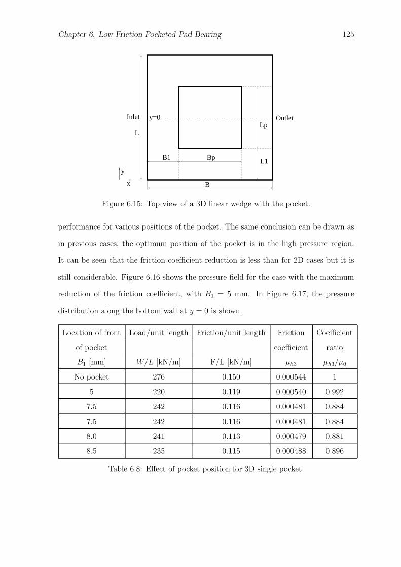
Chapter 6. Low Friction Pocketed Pad Bearing 125
Outlet
B1 Bp
B
L1
L
x
y
y=0Lp
Inlet
Figure 6.15: Top view of a 3D linear wedge with the pocket.
performance for various positions of the pocket. The same conclusion can be drawn as
in previous cases; the optimum position of the pocket is in the high pressure region.
It can be seen that the friction coefficient reduction is less than for 2D cases but it is
still considerable. Figure 6.16 shows the pressure field for the case with the maximum
reduction of the friction coefficient, with B1 = 5 mm. In Figure 6.17, the pressure
distribution along the bottom wall at y = 0 is shown.
Location of front Load/unit length Friction/unit length Friction Coefficient
of pocket coefficient ratio
B1 [mm] W/L [kN/m] F/L [kN/m] µh3 µh3/µ0
No pocket 276 0.150 0.000544 1
5 220 0.119 0.000540 0.992
7.5 242 0.116 0.000481 0.884
7.5 242 0.116 0.000481 0.884
8.0 241 0.113 0.000479 0.881
8.5 235 0.115 0.000488 0.896
Table 6.8: Effect of pocket position for 3D single pocket.
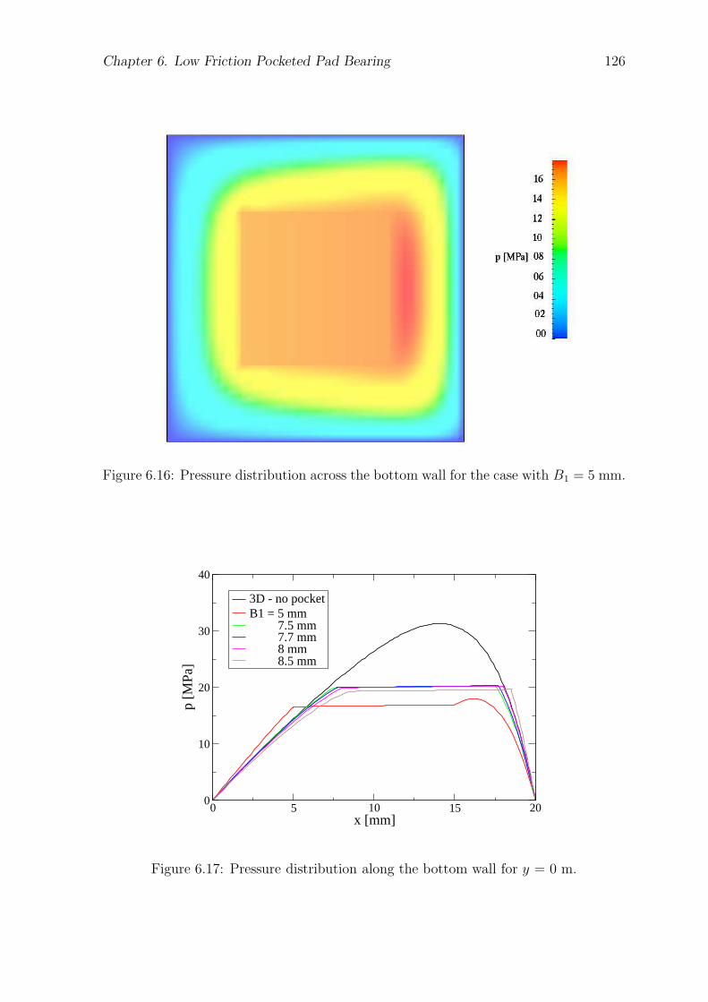
Chapter 6. Low Friction Pocketed Pad Bearing 126
Figure 6.16: Pressure distribution across the bottom wall for the case with B1 = 5 mm.
0 5 10 15 20x [mm]
0
10
20
30
40
p [M
Pa]
3D - no pocketB1 = 5 mm 7.5 mm 7.7 mm 8 mm 8.5 mm
Figure 6.17: Pressure distribution along the bottom wall for y = 0 m.
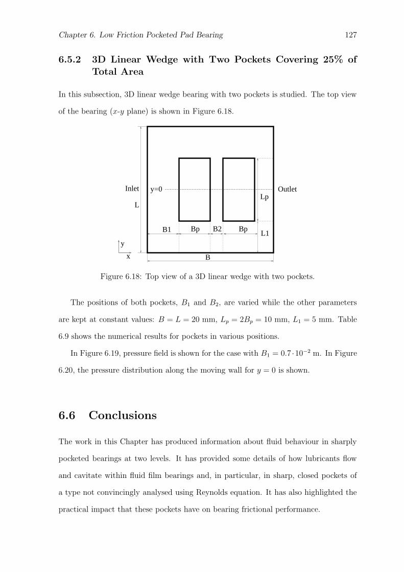
Chapter 6. Low Friction Pocketed Pad Bearing 127
6.5.2 3D Linear Wedge with Two Pockets Covering 25% ofTotal Area
In this subsection, 3D linear wedge bearing with two pockets is studied. The top view
of the bearing (x-y plane) is shown in Figure 6.18.
B1
B
L1
L
x
y
Lp
Bp Bp
Inlet Outlet
B2
y=0
Figure 6.18: Top view of a 3D linear wedge with two pockets.
The positions of both pockets, B1 and B2, are varied while the other parameters
are kept at constant values: B = L = 20 mm, Lp = 2Bp = 10 mm, L1 = 5 mm. Table
6.9 shows the numerical results for pockets in various positions.
In Figure 6.19, pressure field is shown for the case with B1 = 0.7 ·10−2 m. In Figure
6.20, the pressure distribution along the moving wall for y = 0 is shown.
6.6 Conclusions
The work in this Chapter has produced information about fluid behaviour in sharply
pocketed bearings at two levels. It has provided some details of how lubricants flow
and cavitate within fluid film bearings and, in particular, in sharp, closed pockets of
a type not convincingly analysed using Reynolds equation. It has also highlighted the
practical impact that these pockets have on bearing frictional performance.
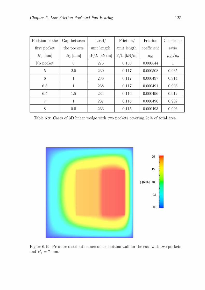
Chapter 6. Low Friction Pocketed Pad Bearing 128
Position of the Gap between Load/ Friction/ Friction Coefficient
first pocket the pockets unit length unit length coefficient ratio
B1 [mm] B2 [mm] W/L [kN/m] F/L [kN/m] µh3 µh3/µ0
No pocket 0 276 0.150 0.000544 1
5 2.5 230 0.117 0.000508 0.935
6 1 236 0.117 0.000497 0.914
6.5 1 238 0.117 0.000491 0.903
6.5 1.5 234 0.116 0.000496 0.912
7 1 237 0.116 0.000490 0.902
8 0.5 233 0.115 0.000493 0.906
Table 6.9: Cases of 3D linear wedge with two pockets covering 25% of total area.
Figure 6.19: Pressure distribution across the bottom wall for the case with two pocketsand B1 = 7 mm.
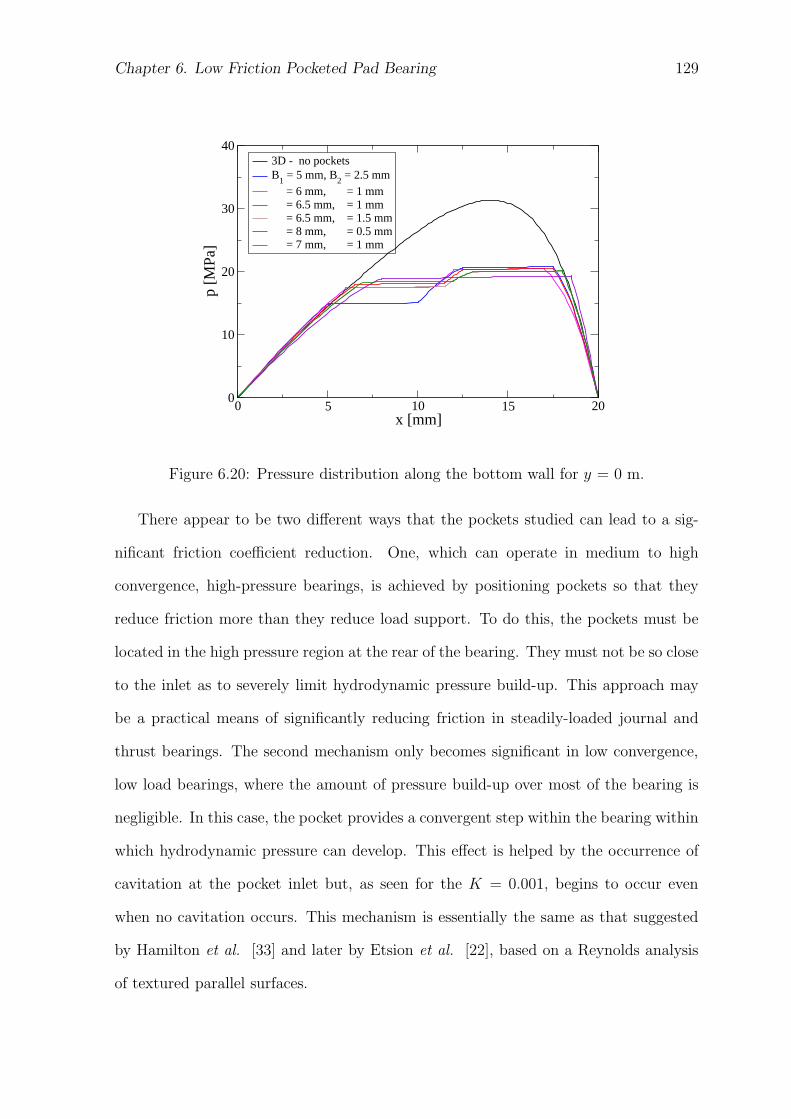
Chapter 6. Low Friction Pocketed Pad Bearing 129
0 5 10 15 20x [mm]
0
10
20
30
40
p [M
Pa]
3D - no pocketsB
1 = 5 mm, B
2 = 2.5 mm
= 6 mm, = 1 mm = 6.5 mm, = 1 mm = 6.5 mm, = 1.5 mm = 8 mm, = 0.5 mm = 7 mm, = 1 mm
Figure 6.20: Pressure distribution along the bottom wall for y = 0 m.
There appear to be two different ways that the pockets studied can lead to a sig-
nificant friction coefficient reduction. One, which can operate in medium to high
convergence, high-pressure bearings, is achieved by positioning pockets so that they
reduce friction more than they reduce load support. To do this, the pockets must be
located in the high pressure region at the rear of the bearing. They must not be so close
to the inlet as to severely limit hydrodynamic pressure build-up. This approach may
be a practical means of significantly reducing friction in steadily-loaded journal and
thrust bearings. The second mechanism only becomes significant in low convergence,
low load bearings, where the amount of pressure build-up over most of the bearing is
negligible. In this case, the pocket provides a convergent step within the bearing within
which hydrodynamic pressure can develop. This effect is helped by the occurrence of
cavitation at the pocket inlet but, as seen for the K = 0.001, begins to occur even
when no cavitation occurs. This mechanism is essentially the same as that suggested
by Hamilton et al. [33] and later by Etsion et al. [22], based on a Reynolds analysis
of textured parallel surfaces.

Chapter 6. Low Friction Pocketed Pad Bearing 130
This work does not rule out the possible contribution of inertial effects to load
support recently reported by Arghir et al. [4] in bearings with a high density of small
surface roughness features. These effects were, however, evident when the amplitude
and wavelength of roughness were of the same order of magnitude while the current
analysis, the ratio of pocket depth to width was typically only 0.005.
This work is clearly only the first step in the study of textured and pocketed hydro-
dynamic bearings. The pockets studied were always stationary, but there is interest
in the effect of pockets entering and then passing through a contact. The pockets in
this work have very simple, vertical edges, which, as seen in Figure 6.10, are especially
likely to promote cavitation, but which may be difficult to achieve in practical bear-
ings. Despite the limited scope, the work has shown the power of applying a modern
CFD package to explore the behaviour of lubricants in non-conventional hydrodynamic
bearing geometries.
6.7 Closure
A CFD model with cavitation has been applied to analyse the flow behaviour, load
support and friction of linear, convergent pad bearings having a closed pocket. This has
shown the development of a boundary layer and fluid recirculation behaviour within
the pocket, and a ram effect at the pocket exit.
It has been found that cavitation occurs only at very low bearing convergence ratios
and it takes place at the immediate pocket entrance, centred on the sharp recess edge.
A closed pocket of the type studied can produce a reduction in friction coefficient by
two different mechanisms. At high to medium convergence ratios, a suitably positioned
pocket in the high pressure region of the bearing reduces shear stress within the pocket
more than its pressure build-up. The result is lower friction and thus a reduced friction
coefficient. This effect increases with pocket height but levels out for a pocket to film
thickness ratio greater than ≈ 20. As the convergence ratio is reduced, an additional
Chapter 6. Low Friction Pocketed Pad Bearing 131
mechanism for friction coefficient comes into play in which the pocketed bearing has
higher load support (and thus lower friction coefficient) than the non-pocketed case.
This is because there is so little hydrodynamic pressure rise in the non-recessed
regions of the bearing that the pressure rise generated within the pocket due to its
convergent step shape makes a significant, and eventually an overwhelming contribution
to the overall load support of the bearing.
Chapter 7
Summary and Conclusions
The main concern of this study is finding a suitable computational model to describe the
flow of lubricant in hydrodynamic bearings. Although Computational Fluid Dynamics
has been an area of intensive study for the last three decades, it is only recently that
it has started to be applied in the field of lubrication.
The Reynolds equation has been widely used in lubrication for calculating the
pressure, film thickness, load support and other flow parameters in the high pressure
areas of the bearing. However, its restrictions become evident in the regions far from
the contact zone and if surface roughnesses of the size comparable to the film thickness,
are present. In those cases, the full set of Navier-Stokes equations needs to be solved.
The geometries found in lubrication problems vary significantly from those usually
modelled with the CFD; the aspect ratios found in lubrication can be of order of 103,
while the aspect ratios encountered in typical CFD problems are of order of 1. This
meant that the CFD solver had to be validated before applying it to complex geometries
for which there is no analytical solution of the Reynolds equation.
The next step was to create the computational model for the cavitation which occurs
in the divergent region of the bearing, where the pressure drops below the saturation
pressure.
Finally, the suitable solver was employed to computationally model pad bearings
with one or more pockets, the geometry which could not be examined with the Reynolds
equation.
132
Chapter 7. Summary and Conclusions 133
In the following Sections, the summary and conclusions of each Chapter will be
given.
7.1 Governing Equations of the Flow of Lubricant
The governing equations of the flow for a Newtonian fluid under isothermal conditions
consist of the conservation of mass and the conservation of momentum. The conser-
vation of momentum, or Navier-Stokes equation has four terms: transient, convective,
diffusive and source term. Depending on the type of the flow, different terms are dom-
inant. If the Reynolds number is low (Rez < 0.1), the diffusive terms are significantly
higher than the convective ones, and vice versa for higher Reynolds numbers.
Due to the high pressures, the viscosity and density stop being constant. The
dependence of density on pressure is relatively weak, but the viscosity can increase by
several orders of magnitude as the pressure gets into the EHL range (> 108 Pa).
In the high pressure region, convective terms and certain viscous terms drop out
from Navier-Stokes equations and the pressure is assumed to be constant across the film
thickness. That leads to the Reynolds equation, which is a suitable tool for solving cases
with smooth geometry in the area near the contact. However, if the surface roughnesses
with the characteristic length comparable to the film thickness are present, the local
aspect ratio becomes much higher and the viscous terms cannot be neglected from
Navier-Stokes equations.
According to order of magnitude analysis, Reynolds equation is not adequate for
solving the fluid flow in the areas far from the contact region or if the surface rough-
nesses are present.
7.2 Discretisation
The Finite Volume method is a well-established numerical procedure, suitable for fluid
flow simulations because of its conservative properties. It is based on a discretisation
Chapter 7. Summary and Conclusions 134
method which splits the computational domain into polyhedral control volumes with
a variable number of faces. The governing equations of continuum mechanics are con-
sequently discretised in the integral form over each control volume. The discretisation
is performed in real space, using a fixed Cartesian coordinate system on meshes that
do not change in time. The discretisation uses a colocated variable arrangement, with
all fields sharing the same control volumes.
The Finite Volume discretisation described above has been applied to fluid flow
problems. The solution algorithm for the Navier-Stokes system is summarised. The
pressure-velocity coupling is treated by the SIMPLE algorithm for steady-state calcu-
lations. For transient problems, the PISO algorithm has been used.
The Finite Volume method is an approximation of the full solution of the governing
equations. Therefore, there exists an error in the numerical simulations obtained using
this method. The error which arises from the discretisation procedure is estimated by
Richardson Extrapolation. The discretisation error is calculated from the leading term
of the truncation error from the Taylor series.
7.3 Validation of CFD Solver On Simple
Hydrodynamic Bearings
In hydrodynamic lubrication, there are geometries for which the Reynolds equation has
an analytical solution. Two of them are an infinitely long linear wedge and an infinitely
long step bearing. The analytical solution is useful to validate the numerical results
obtained with the CFD solver. The pressure field and the x-component of the velocity
vector obtained using CFD and the Reynolds equation, have been compared directly,
with the maximum difference being < 1%. The error in the numerical solution for the
maximum pressure is found using Richardson Extrapolation, and it shows a decrease
as the mesh gets finer in both x and z directions. However, the error decreases more
with grid refinement in the z direction only. Total load and friction per unit length are
calculated from the analytical solution and from the numerical results and again, they
Chapter 7. Summary and Conclusions 135
are in good agreement (the maximum difference is < 0.1% for the finest mesh).
For the linear wedge the mesh consists of one block and it is uniform in both
directions. The geometry is smooth, i.e. it does not have any steep gradients. However,
in the case of step bearing there is a steep geometry of the step, which creates the need
for local refinement of the computational mesh around the step.
The conclusions to be drawn from the study of these two geometries were that the
CFD software was capable of accurately handling steady state hydrodynamic lubrica-
tion problems. The work also confirmed the assumption of constant pressure across the
film thickness and that the neglect of inertia and certain viscous terms in the Reynolds
equation is justified.
7.4 Modelling of Cavitation
In the case of a roller bearing, the cavitation occurs in the diverging region when the
pressure of the fluid drops below the saturation pressure. As the fluid evaporates, the
density ratio between liquid and vapour phases is of the order of 105. The sudden
change in density makes this a challenging problem to model.
The numerical cavitation method used in this work is a continuum method, where
both phases are considered to be of the same fluid and only one set of governing
equations needs to be solved. This lowers the computational cost considerably. The
conservation of energy equation is used for closure, and the speed of sound of the
mixture is given by the homogeneous equilibrium model. Both liquid and vapour
phase are treated as compressible.
By integrating the energy equation, one obtains the equation for density dependence
on pressure. The critical feature in determining the gradient of the slope which links
the liquid and vapour phase is the speed of sound in vapour. In order for the model to
be numerically stable, the value of the speed of sound in vapour had to be somewhat
higher than the realistic one.
Chapter 7. Summary and Conclusions 136
The two cases studied are the pure rolling, full-cylinder and the pure sliding, half-
cylinder. When modelled without the cavitation, the numerical results were in agree-
ment with the Full Sommerfeld solution, as expected. With the cavitation model in-
cluded, the results for the two cases show many similarities. In both cases the pressure
drops below zero in the diverging region and the cavitation does not occur instanta-
neously but gradually over the space of ≈ 0.02R. The difference between the two cases
is that for the pure rolling case, the fluid begins to cavitate closer to the cylinder, while
for the pure sliding case, the fluid starts cavitating in the middle of the film thickness
but evaporates more rapidly from the moving wall. Backflow is present in both cases
in the converging and the diverging region.
The cavitation model used in this work produced results which are qualitatively
likely to be accurate. However, the results should not be considered to be quantitatively
correct. That is mainly because of the assumption that the liquid to vapour transition
is the only process of cavitation, because the speed of sound in vapour has unrealistic
value and because the possibility of dissolved gasses in the liquid phase is neglected.
7.5 Low Friction Pocketed Pad Bearing
The use of CFD enables us to examine more complex geometries, which could not be
solved with the Reynolds equation. In this study one or more pockets are placed on
the top wall of the simple pad bearing. Their height, size and position are varied, as
well as the convergence ratio of the bearing. The effect of the pockets on the reduction
of the friction coefficient is examined and the following conclusions are made:
• As the height of the pocket increases, both load support and friction decrease.
However, the reduction in load support is much smaller than the reduction in
friction, thus reducing the friction coefficient.
• The optimum location for the beginning of the pocket is in the middle of the
bearing. If the pocket is too close to the inlet, the pressure build-up is reduced,
Chapter 7. Summary and Conclusions 137
making the load support smaller which has negative effects on the reduction of
the friction coefficient.
• The size of the pocket which gives the biggest reduction in the friction coefficient
is 25% of the total area of the bearing.
• The presence of the pocket with the optimum height, position and size, reduces
the friction coefficient for the pad bearing with all the convergence ratios stud-
ied in this work. However, the pad bearing with smaller convergence ratio can
support smaller load. For the convergence ratio K = 0.001, the fluid cavitates at
the beginning of the pocket. For that case, the pocket acts as a separate bearing
producing a pressure build up which is significant in comparison to the pressure
in the inlet region of the bearing.
We can conclude that there are two ways that a closed pocket in pad bearing can reduce
the friction coefficient. In bearings with high convergence ratios, a suitably-positioned
and sized pocket reduces friction more than the load support, and in bearings with
low convergence ratios the pocketed bearing has higher load support than in the non-
pocketed case, leading again to the reduction in friction coefficient.
7.6 Suggested Future Work
The results in this study are obtained using several simplifications which are not real-
istic:
• Isothermal conditions were assumed throughout;
• The bearings were assumed to have smooth surfaces;
• In the cavitation model, the isentropic phase transformation approach was em-
ployed, and it was assumed that the fluid to vapour transition is the only process
of cavitation;
Chapter 7. Summary and Conclusions 138
• The surfaces of the roller bearing were assumed to be infinitely rigid, not allowing
for the elastic deformations due to the high pressures;
• The lubricant was assumed to be isoviscous.
In future work these simplifications need to be eliminated. One of possible directions in
which to continue this work is to improve the present cavitation model. As discussed
in Chapter 5, there are various types of cavitation models used in CFD. The most
elaborate are full multiphase models, which, given the initial sizes and distribution of
cavitation nucleii within the fluid, can calculate the evolution of vapour field, including
growth/collapse, transport by the fluid motion, etc. Employing a model of that type
would, most likely, improve the quantitative aspect of the result.
The next step towards the EHL solution could be the inclusion of elastic deforma-
tion of the surfaces due to the high pressures. There are two main ways of including
elastic deformation in numerical simulations of the EHL problem: multigrid methods
(Venner and Lubrecht [69]) and differential deflection (Evans and Hughes [26]). Both
of these methods reduce computational time needed to calculate the flow parameters
and the elastic deformation. In multigrid method, one uses several grids of different
sizes to smooth the iterative errors. The central point is that error components with
wavelengths which are comparable to the grid size are reduced efficiently, and those
with large wavelengths compared to the mesh size converge slowly. The basis of multi-
grid solutions method is to use coarser grids to solve the smooth error components,
which reduces computational time significantly. In differential deflection, the explicit
deflection equation is replaced by a second-order differential equation. In numerical cal-
culations the deflection can be reduced to a sum of coefficients multiplied by pressures
in each point of the domain. In the same way, the second-order differential equation
of the deflection can be constructed as a sum of coefficients multiplied by the corre-
sponding pressures. The coefficients in second-order differential deflection are shown
to decay at a much higher rate as the modulus of the index increases from zero than
Chapter 7. Summary and Conclusions 139
do the coefficients of the explicit deflection equation.
The inclusion of piezo-viscous effects could be the next step, followed by the intro-
duction of thermal effects. This would mean that the algorithm for the EHL problem
with piezo-viscous and thermal effects is developed. This CFD-solver could then be
applied to various geometries with surface roughnesses.
140
Bibliography
[1] Almqvist, T. and Larsson, R.: “The Navier-Stokes Approach for Thermal EHL
Line Contact Solutions”, Tribology International, 35, pp. 163-170, 2002.
[2] Almqvist, T.; Glavatskikh, S. B.; Larsson, R.: “THD Analysis of Tilting Pad
Thrust Bearings - Comparison Between Theory and Experiments”, Journal of
Tribology, Transactions of the ASME, 122 (2), pp. 412-417, 2000.
[3] Apfel, R. E.: “The Tensile Strength of Liquids”, Scientific American, 227, pp.
58-71, 1972.
[4] Arghir, M., Rouscou, N., Helene, M. and Frene, J.: “Theoretical Analysis of the
Incompressible Laminar Flow in a Macro-Roughness Cell”, Trans. ASME J. of
Tribology, 125, pp. 309-318, 2003.
[5] Avva, R. K.; Singhal, A.; Gibson, D. H.: “An Enthalpy Based Model of Cavita-
tion”, ASME FED, 226, pp. 63-70, 1995.
[6] Ball, S. J.; Trusler, J. P. M.: “Speed of Sound of n-Hexane and n-Hexadecane at
Temperatures Between 298 and 373 K and Pressures up to 100 MPa”, Interna-
tional Journal of Thermophysics, 22(2), pp. 427-443, 2001.
[7] Barus, C.,: “Isothermals, Isopiestics and Isometrics Relative to Viscosity”, Am.
J. of Science, 45, pp. 87-96, 1893.
[8] Blahey, A. G.: “The Elastohydrodynamic Lubrication of Elliptical Contacts with
Thermal Effects”, PhD thesis, University of Waterloo, Waterloo, Ontario, 1985.
141
[9] Brandt, A.: “Multi–Level Adaptive Solutions to Boundary–Value Problems”,
Mathematics of Computation, 31(138), pp. 333-389, 1977.
[10] Brandt, A. and Lubrecht, A. A.: “Multilevel Matrix Multiplication and Fast
Solution of Integral Equations”, J. Comp. Phys., 2, pp. 348-370, 1990.
[11] Cameron, A. and Wood, W. L.: “The Full Journal Bearing”, IProc. IMechE, 26,
pp. 59-64, 1949.
[12] Cameron, A.: “The Principles of Lubrication”, Longman Green and co,ltd, Lon-
don, 1966.
[13] Cameron, A. and Ettles, C. M. Mc.: “Basic Lubrication Theory”, 3rd Edition,
Chapter 5, pp. 70, 74. publ. Ellis Horwood, Chichester, UK, 1981
[14] Chang, H.: Infrared Temperature Measurement and Traction in Elastohydrody-
namic Lubrication, PhD thesis, Imperial College, University of London, 1992.
[15] Chen, P. Y. P. and Hahn, E. J.: “Use of Computational Fluid Dynamics in Hydro-
dynamic Lubrication”, Proc. Instn. Mech. Engrs, Part J,Journal of Engineering
Tribology, 212(J6), pp. 427-436, 1998.
[16] Chen, Y.; Heister, S. D.: “A Numerical Treatment for Attached Cavitation”, J.
Fluids Eng., 116(3), pp. 613-618, 1994.
[17] Delannoy, Y.; Kueny, J. L.: “Two Phase Flow Approach in Unsteady Cavitation
Modeling”, Cavitation and Multiphase Flow Forum, ASME FED , 98, pp. 153-158,
1990.
[18] Dowson, D.: “History of Tribology”, Longman Group Limited, London, 1979.
[19] Dowson, D. and Higginson, G. R.: “Elastohydrodynamic Lubrication, The Fun-
damentals of Roller and Gear Lubrication”, Pergamon Press, Oxford, 1966.
142
[20] Elcoate, C.D., Evans, H.P., Hughes, T. G.: “On the Coupling of the Elastohy-
drodynamic Problem,”, Proc. Instn. Mech. Engrs, Part C, 212(C), pp. 307-318,
1998.
[21] Ertel, A. M.: “Hydrodynamic Lubrication Based on New Principles”,Akad. Nauk
SSSR Prikadnaya Mathematica I Mekhanika, 3(2), pp. 41-52, 1939.
[22] Etsion, I., Kligerman, Y. and Halperin, G.: “Analytical and Experimental In-
vestigation of Laser-Textured Mechanical Seal Faces”, Tribology Transactions, 42,
pp. 511-516, 1999.
[23] Etsion, I.: “Laser Surface Texturing - Measure to Reduce Friction”, Proc. 14th
Intern. Colloq. Tribology, publ. Tech. Acad. Esslingen ed. W. J. Bartz, Jan. 2004
[24] Evans, H. P. and Snidle, R. W.: “Inverse Solution of Reynolds Equation of
Lubrication Under Point Contact Elastohydrodynamic Conditions”, Trans. ASME
F, J. of Lub. Tech., 103(4), pp. 539-546, 1981.
[25] Evans, H. P. and Snidle, R. W.: “The Elastohydrodynamic Lubrication of Point
Contacts at Heavy Loads”, Proc. R. Soc., A382, pp. 183-199, 1982.
[26] Evans, H.P., Hughes, T. G.: “Evaluation of Deflection in Semi-Infinite Bodies by
a Differential Method,”, Proc. Instn. Mech. Engrs, Part C, 214(C), pp. 563-584,
2000.
[27] Faber, T. E.: Fluid Dynamics for Physicists: Cambridge University Press, 1995
[28] Ferziger, J.H. and Peric, M.: Computational Methods for Fluid Dynamics:
Springer Verlag, Berlin-New York, 1995.
[29] Gohar, R.: Elastohydrodynamics: Ellis Horwood Limited, Chichester, UK, 1988.
143
[30] Goloch, R., Merker, G.P., Kesses, U. and Brinkmann, S.: “Benefits of Laser-
Structured Cylinder Liners for Internal Combustion Engines”, Proc. 14th Intern.
Colloq. Tribology, Esslingen, 1, pp. 321-328, ed. W. J. Bartz, Jan. 2004
[31] Grubin, A. N., and Vinogradova, I. E.: “Investigation of the Contact of Machine
Components”, F.Ketova(ed.) Central Scientific Research Institute for Technology
and Mechanical Engineering (Moscow), Book No.30, (DSIR translation No.337),
1949.
[32] Grumbel, L.: “Uber Geschmierte Arbeitsrader”: Z. ges. Turbinenwesen, 13 pp.
357, 1916.
[33] Hamilton, D. B., Walowit, J. A. and Allen, C. M.: “A Theory of Lubrication by
Micro-Irregularities”: ASME J. of Basic Eng. , 88, pp. 177-185, 1966.
[34] Hamrock, B. J.: “Fundamentals of Fluid Film Lubrication”, Singapore: McGraw-
Hill, 1994.
[35] Hamrock, B. J. and Dowson, D.: “Isothermal Elastohydrodynamic Lubrication
of Point Contacts, part 1, Theoretical Formulation”, ASME J. of Lub. Tech., 98,
pp. 223-229, 1976.
[36] Hamrock, B. J. and Jacobsen, B. O.: “Elastohydrodynamic Lubrication of Line
Contacts”, A.S.L.E. Trans., 27(4), 1984.
[37] Hertz, H.: “Uber die Beruhrung Fester Elastischer Korper,”J. reine und angew.
Math. 92, pp. 156-171, 1881.
[38] Hestens, M. R. and Steifel, E. L.: “Method of Conjugate Gradients for Solving
Linear Systems”, Journal of Research, 29, pp. 409-436, 1952.
[39] Hughes, T. G., Evans, H.P.: “Coupled Solution of the Elastohydrodynamic Line
144
Contact Problem Using a Differential Deflection Method,”, Proc. Instn. Mech.
Engrs, Part C, 214(C), pp. 585-598, 2000.
[40] Issa, R. I.: “Solution of the Implicitly Discretized Fluid Flow Equations by
Operator-Splitting”, J. Comp. Physics, 62, pp. 40-65, 1986.
[41] Jacobs, D. A. H.: “Preconditioned Conjugate Gradient Methods for Solving Sys-
tems of Algebraic Equations”: Central Electricity Research Laboratories Report,
RD/L/N193/80, 1980.
[42] Jasak, H.: Error Analysis and Estimation for the Finite Volume Method with
Applications to Fluid Flows, PhD thesis, Imperial College, University of London,
1996.
[43] Johnson, K. L.: Contact Mechanics: Cambridge University Press, 1999.
[44] Jolkin, A.: “EHL Investigations Using A Hybrid Technique - An Experimental
and Numerical Approach”, PhD thesis, Lulea University of Technology, Lulea,
Sweden, 1999.
[45] Khosla, P. K. and Rubin, S. G.: “A Diagonally Dominant Second-Order Accurate
Implicit Scheme”, Computers and Fluids, 2, pp. 207-209, 1974.
[46] Kovalchenko, A., Ajayi, O., Erdemir, A., Fenske, G. and Etsion, I. “The Effect of
Laser Texturing of Steel Surfaces and Speed-Load Parameters on the Transition
of Lubrication Regime from Boundary to Hydrodynamic”, Proc. STLE/ASME
Conf., Florida, 2003-TRIB-024, Oct. 2003
[47] Kubota, A.; Kato, H.; Yamaguchi, H.: “Finite Difference Analysis of Unsteady
Cavitation on a Two-Dimensional Hydrofoil”, Proc. 5th Int. Conf. on Numerical
Ship Hydrodynamics, Hiroshima, Japan, September 1989, pp. 667-683
145
[48] Lubrecht,A. A., ten Napel, W. E. and Bosma, R.: “Multigrid, and Alternative
Method of Solution for Two-Dimension Elastohydrodynamically Lubricated Point
Contact Calculations”, Trans. ASME F, J. Tribology, 108(3), pp. 551-556, 1986.
[49] Lubrecht, A. A.: “Numerical solution of the EHL Line and Point Contact Problem
Using Multigrid Techniques”, PhD thesis, Twente University, The Netherlands,
1987.
[50] Martin, H. M.: “Lubrication of Gear Teeth”, Engineering, 102, pp. 119-121, 1916.
[51] Muzaferija, S.: Adaptive Finite Volume Method for Flow Prediction Using Un-
structured Meshes and Multigrid Approach, PhD thesis, Imperial College, Univer-
sity of London, 1994.
[52] Patankar, S.V.: Numerical Heat Transfer and Fluid Flow, Hemisphere Publishing
Corporation, 1981.
[53] Peric, M.: A Finite Volume Method for the Prediction of Three-Dimensional Fluid
Flow in Complex Ducts, PhD thesis, Imperial College, University of London, 1985.
[54] Petrusevich, A. I.: “Fundamental Conclusions from the Contact Hydrodynamic
Theory of Lubrication”, Izv. Akad.Nauk SSR (OTN), 3, pp. 209-223, 1951.
[55] Reynolds, O.: “On the Theory of Lubrication and its Application to Mr.
Beauchamps Tower’s Experiments, Including and Experimental Determination of
the Viscosity of Olive Oil”, Phil. Trans, 177, pp. 157-234, 1886.
[56] Rhim, Y. and Tichy, J. A.: “Entry Flow into a Slider Bearing - Analysis and
Experiment”, Tribology Transactions, 31, pp. 350-358, 1988.
[57] Rider, W. J.; Kothe, D. B.: “Stretching and Tearing Interface Tracking Methods”,
Los Alamos Natl. Lab. Rep. LA-UR-95-1145, 1995, pp. 1-11.
146
[58] Ronen, A., Etsion, I. and Kligerman, Y.: “Friction Reducing Surface Texturing in
Reciprocating Automotive Components”, Tribology Transactions, 44, pp. 359-366,
2001.
[59] Ryk, G., Kligerman, Y. and Etsion, I.: “Experimental Investigation of Laser
Surface Texturing for Reciprocating Automotive Components”, Tribology Trans-
actions, 45, pp. 444-449, 2002.
[60] Sassenfeld, H. and Walther, A.: “Gleitlagerberechnungen”, VDI–Forschungsheft
441, Deutscher Ingineur–Verlag GMBH, Dusseldorf Germany, 1954.
[61] Schafer, C. T., Giese, P., Rowe, W. B. and Woolley, N. H.: “ Elastohydrodynam-
ically Lubricated Line Contact Based on the Navier-Stokes Equations” Thinning
Films and Tribological Interfaces D.Dowson et al. (Editors), Elsevier Science B.V.,
2000.
[62] Schmidt, D. P.; Rutland, C. J.; Corradini, M. L.: “A Fully Compressible, Two-
Dimensional Model of Small, High Speed, Cavitating Nozzles”, Atomization and
Sprays, 9, pp. 255-276, 1999.
[63] Tonder, K.: “Hydrodynamic Effect of Tailored Inlet Roughnesses: Extended
Theory”, Tribology International, 37, pp. 137-142, 2004.
[64] Tower, B.: “First Report on Friction Experiments (Friction of Lubricated Bear-
ings”, Proc. Instn. Mech.Engrs, pp. 632-659, Nov. 1883.
[65] Van Der Vorst, H. A.: “Bi-CGSTAB: A Fast and Smoothly Converging Variant
of Bi-CG for the Solution of Nonsymmetric Linear Systems”,SIAM J. Scientific
Computing, 13(2), pp. 631-644, 1992.
[66] van Odyck, D. E. A.: “Stokes Flow in Thin Films”, PhD thesis, University of
Twente, Enschede, The Netherlands, 2001.
147
[67] van Odyck, D. E. A., Venner C. H.: “Compressible Stokes Flow in Thin Films”,
Journal of Tribology, 125, pp. 543-551, 2003.
[68] Venner, C. H.: “Multilevel Solution of the EHL Line and Point Contact Problems”,
PhD thesis, University of Twente, The Netherlands, 1991.
[69] Venner, C. H. and Lubrecht, A. A.: “ Multilevel Methods in Lubrication,” Tri-
bology Series, 37, Elsevier, 1st edition, 2000.
[70] Versteeg, H. K. and Malalasekera, W.: An introduction to Computational Fluid
Dynamics, The Finite Volume Method, Longman, 1st edition, 1995.
[71] Wallis, G. B.: One-dimensional Tho-Phase Flow, McGraw-Hill, 1969.
[72] Wang, X., Kato, K., Adachi, K. and Aizawa, K.: “The Effect of Laser Texturing
of SiC Surface on the Critical Load for the Transition of Water Lubrication Mode
from Hydrodynamic to Mixed”, Tribology International, 34, pp. 703-711, 2001.
[73] Weller, H., Tabor, G., Jasak, H. and Fureby, C.: “A Tensorial Approach to Com-
putational Continuum Mechanics Using Object Orientated Techniques”, Com-
puter in Physics, 12, pp. 620-631, 1998.
[74] Zhang, J. X. and Rodkiewicz, C. M.: “On the Design of Thrust Bearings Using a
CFD Technique”, Tribology Transactions, 40(3), pp. 403-412, 1997.

148
List of Publications
Brajdic-Mitidieri, P., Gosman A. D., Ioannides, E., Spikes, H.A.: “CFD Analysis of a
Low Friction Pocketed Pad Bearing”, Journal of Tribology, Transactions of the ASME,
127, pp. 803-812, 2005.