Embed Size (px)
Citation preview
Advanced Mathematics for SecondaryTeachers:
A Capstone Experience
Curtis BennettDavid Meel
c© 2000
January 3, 2001

2
Contents
1 Introduction 51.1 A Description of the Course . . . . . . . . . . . . . . . . . . . 51.2 What is Mathematics? . . . . . . . . . . . . . . . . . . . . . . 61.3 Background . . . . . . . . . . . . . . . . . . . . . . . . . . . . 9
1.3.1 GCDs and the Fundamental Theorem of Arithmetic . . 101.3.2 Abstract Algebra and polynomials . . . . . . . . . . . . 11
1.4 Problems . . . . . . . . . . . . . . . . . . . . . . . . . . . . . . 14
2 Rational and Irrational Numbers 152.1 Decimal Representations . . . . . . . . . . . . . . . . . . . . . 182.2 Irrationality Proofs . . . . . . . . . . . . . . . . . . . . . . . . 232.3 Irrationality of e and π . . . . . . . . . . . . . . . . . . . . . . 262.4 Problems . . . . . . . . . . . . . . . . . . . . . . . . . . . . . . 30
3 Constructible Numbers 353.1 The Number Line . . . . . . . . . . . . . . . . . . . . . . . . . 373.2 Construction of Products and Sums . . . . . . . . . . . . . . . 393.3 Number Fields and Vector Spaces . . . . . . . . . . . . . . . . 443.4 Impossibility Theorems . . . . . . . . . . . . . . . . . . . . . . 543.5 Regular n-gons . . . . . . . . . . . . . . . . . . . . . . . . . . 583.6 Problems . . . . . . . . . . . . . . . . . . . . . . . . . . . . . . 60
4 Solving Equations by Radicals 634.1 Solving Simple Cubic Equations . . . . . . . . . . . . . . . . . 664.2 The General Cubic Equation . . . . . . . . . . . . . . . . . . . 724.3 The Complex Plane . . . . . . . . . . . . . . . . . . . . . . . . 744.4 Algebraic Numbers . . . . . . . . . . . . . . . . . . . . . . . . 784.5 Transcendental Numbers . . . . . . . . . . . . . . . . . . . . . 80
3
4 CONTENTS
5 Dedekind Cuts 875.1 Axioms for the Real Numbers . . . . . . . . . . . . . . . . . . 875.2 Dedekind Cuts . . . . . . . . . . . . . . . . . . . . . . . . . . 91
6 Classical Numbers 1056.1 The Logarithmic Function . . . . . . . . . . . . . . . . . . . . 105
7 Cardinality Questions 109
8 Finite Difference Methods 111
Chapter 1
Introduction
1.1 A Description of the Course
This course is intended as a capstone experience for mathematics studentsplanning on becoming high school teachers. This is not to say that this isa course in material from the high school curriculum. Nor is this a courseon how to teach topics from the high school curriculum. Rather, this isa course informed by the high school curriculum, by which we mean thatthe topics in this course are issues raised in the high school curriculum (butrarely dealt with there). Thus students should not expect the course to dealdirectly with the high school curriculum, although we hope that during thecourse, students will ask questions that they have concerning that material,including how what we do in the course relates to the curriculum. At theend of many of the sections, we try to include some brief words about howthe material from the section might be put to use by a high school teacher,but in truth, mostly this material is here to provide a good background forthe teacher, since what is being taught in schools today will probably not bewhat is taught in 10 years, and almost certainly is not what will be taughtin 20 years. Consider that in the 1960s, “New Math” was in vogue withset theory taught at all levels of the curriculum (from first through twelfthgrade), clock (or modular) arithmetic taught in elementary school, as wellas arithmetic in other bases, while in 1980, the “back to basics” movementtook over. The new math was replaced by emphasis on rote skills. Then in1989, the NCTM standards were introduced, causing changes, such as theelimination of proofs from some high school geometry texts (not what the
5

6 CHAPTER 1. INTRODUCTION
NCTM standards called for, but what the textbook writers decided), andnow we have the 2000 NCTM standards and their move to include more ofthe fundamental mathematics, but still with an emphasis on problem solving.Consequently, the goal of the collegiate mathematics education degree is notjust to prepare students for teaching now, but to give them the tools to beprepared for teaching twenty years from now.
In a nutshell, this course could be titled “Why do we need all these num-bers?” We follow a (mostly) historical development of the real (and Complex)number system, from the Greek Mathematicians through to modern analysisand Dedekind cuts. We begin with a discussion of fractions and rationalnumbers, and prove that many numbers are irrational. In particular, at theend of chapter 2, we prove that e and π are irrational. Knowing that irra-tional numbers exist, we then discuss what numbers can be represented asexact lengths using the tools of straightedge and compass. This naturallyleads us to prove the classical Greek impossibility theorems on doubling thecube and trisecting the general angle. Given that lengths are not enough, wenext move on to whether we can represent all real numbers using radical signsand the standard operations. We show that while we can solve cubic equa-tions this way, these numbers can be deceptive. At the end of that chapter,we give a brief discussion of the impossibility of solving the general quinticequation by radicals, but necessarily, we do not give a proof of this. Finally,having exhausted other methods of defining the real numbers, in the nextchapter, we discuss how one defines the real numbers today using Dedekindcuts, and why one is forced to do this. The subsequent chapters are reallyextras, which we are happy if we get to, but are not necessary to cover in thecourse if time does not permit.
1.2 What is Mathematics?
The question at the title of this section is extremely difficult. Mathematiciansthemselves disagree on this question, with some taking a purist view like G.H.Hardy, others taking a more applied approach, and still others giving an “Iknow it when I see it definition.” In this book, we shall suggest that a briefanswer to this question might be that there are four “Ps” to mathematics,pattern, precision, proof, and problem solving.
Mathematics is the science of patterns. The first obvious pattern is thatof number. Three people, three hats, and three camels all have something in
1.2. WHAT IS MATHEMATICS? 7
common. This is the recognition of a pattern. Seeing how numbers relate toeach other usually requires looking for patterns. Of course, patterns becomemore and more difficult to track down so we come up with more and morecomplicated techniques to look for them. One of the standard threads of theNCTM standards that fits in here is that of different representations of thesame thing. These different representations are often the recognition of thesame pattern showing up in two very different items. You have seen this inyour mathematics background when you discussed the idea of isomorphismin abstract algebra, congruence in geometry, or even modular equivalence ofintegers in discrete mathematics. Even elementary school students see thiswhen they first learn that different fractions can stand for the same quantity.One of the greatest discoveries of mathematics is the fundamental theoremof calculus. It is really the recognition that the area under curves and theslopes of curves fit together into a pattern. The idea of calculus is findingthe patterns relating these two curves.
To study patterns, you must be precise in your thinking. Thus mathe-matics is about precision, such as carefully defining what is meant by a term.The English language is fuzzy. By their very nature, words are not precise.As a result, mathematics emphasizes definitions throughout. One often talksabout the idea underlying a topic being important, and it is. However, be-ing able to work with this idea is also important, and it is difficult to do sowithout carefully defined terms.
To verify that the patterns we see actually occur, we turn to proof. Thereare numerous examples of where people see patterns when they don’t reallyexist. Proof keeps us from treating these patterns as real. For any trianglein the plane, the sum of its angles is 180 degrees. What about on a sphere?If you have studied spherical geometry you know that the sum of the anglesof a spherical triangle is greater than 180 degrees, but if you were livingon a very large sphere and could only draw relatively small triangles, youmight not believe that triangles have angle sum larger than 180 degrees.Why? Because all of the triangles you could easily draw would have anglesum extremely close to 180 degrees, and your measuring tool would not besufficiently accurate to tell you this. On a more complicated side, every oddnumber is of the form 4k + 1 or 4k + 3 where k is an integer. Here is aninteresting question: Is it the case that for any positive integer n the set ofprimes less than n of the form 4k + 3 has as many or more members thanthe set of primes less than n of the form 4k + 1? If we try and solve thisquestion by example, then we would list the primes of each form and come
8 CHAPTER 1. INTRODUCTION
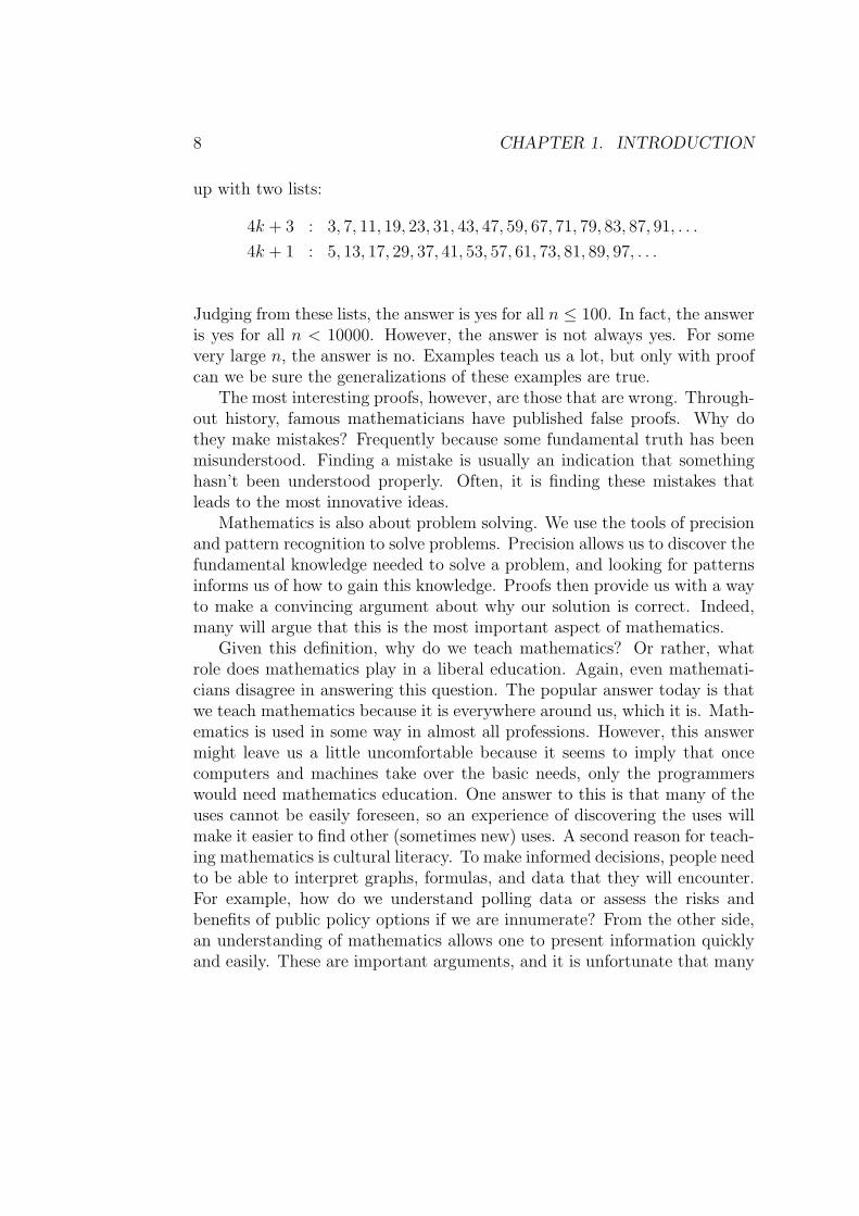
up with two lists:
4k + 3 : 3, 7, 11, 19, 23, 31, 43, 47, 59, 67, 71, 79, 83, 87, 91, . . .
4k + 1 : 5, 13, 17, 29, 37, 41, 53, 57, 61, 73, 81, 89, 97, . . .
Judging from these lists, the answer is yes for all n ≤ 100. In fact, the answeris yes for all n < 10000. However, the answer is not always yes. For somevery large n, the answer is no. Examples teach us a lot, but only with proofcan we be sure the generalizations of these examples are true.
The most interesting proofs, however, are those that are wrong. Through-out history, famous mathematicians have published false proofs. Why dothey make mistakes? Frequently because some fundamental truth has beenmisunderstood. Finding a mistake is usually an indication that somethinghasn’t been understood properly. Often, it is finding these mistakes thatleads to the most innovative ideas.
Mathematics is also about problem solving. We use the tools of precisionand pattern recognition to solve problems. Precision allows us to discover thefundamental knowledge needed to solve a problem, and looking for patternsinforms us of how to gain this knowledge. Proofs then provide us with a wayto make a convincing argument about why our solution is correct. Indeed,many will argue that this is the most important aspect of mathematics.
Given this definition, why do we teach mathematics? Or rather, whatrole does mathematics play in a liberal education. Again, even mathemati-cians disagree in answering this question. The popular answer today is thatwe teach mathematics because it is everywhere around us, which it is. Math-ematics is used in some way in almost all professions. However, this answermight leave us a little uncomfortable because it seems to imply that oncecomputers and machines take over the basic needs, only the programmerswould need mathematics education. One answer to this is that many of theuses cannot be easily foreseen, so an experience of discovering the uses willmake it easier to find other (sometimes new) uses. A second reason for teach-ing mathematics is cultural literacy. To make informed decisions, people needto be able to interpret graphs, formulas, and data that they will encounter.For example, how do we understand polling data or assess the risks andbenefits of public policy options if we are innumerate? From the other side,an understanding of mathematics allows one to present information quicklyand easily. These are important arguments, and it is unfortunate that many
1.3. BACKGROUND 9
people lack the level of mathematical knowledge to understand informationtoday, even though much of this understanding can be gained with a verybasic level of mathematical understanding. Another important reason tostudy mathematics is that it improves critical thinking skills. It encouragesone to think critically in a mathematical way, geometrically, arithmetically,algebraically, and logically. Moreover, proof teaches absolute argumentationso that the validity of other arguments can be weighed against mathematicalarguments. G. Polya says it best,
If the (mathematics) student failed to get acquainted with this orthat particular geometric fact, he did not miss so much; he mayhave little use for such facts later in life. But if he failed to getacquainted with geometric proofs, he missed the best and simplestexamples of true evidence and he missed the best opportunity toacquire the idea of strict reasoning. Without this idea, he lacks atrue standard with which to compare alleged evidence of all sortsaimed at him in modern life.
In short, if general education intends to bestow on the student theideas of intuitive evidence and logical reasoning, it must reservea place for geometric proofs. [8]
This view argues that it is not the individual facts of mathematics that mat-ter, but rather the ways of thinking it encourages. The study of mathematicsallows us to learn, practice, and master abstract, logical, numerical, and ge-ometric ways of thinking, and to use them to solve problems.
1.3 Background
In this course, we will assume students have familiarity with the conceptsfrom a first course in Abstract Algebra, Linear Algebra, Discrete Mathemat-ics (in particular induction and some basic counting identities), and a fullsequence in Calculus. Students may also find it helpful to have had someexperience with basic probability.
During the term we will briefly review some concepts from these areas,but students are strongly encouraged to have their textbooks from theseclasses available while reading this text and studying for this class. Moreover,students are responsible to review these areas on their own as necessary.

10 CHAPTER 1. INTRODUCTION
1.3.1 GCDs and the Fundamental Theorem of Arith-metic
Given integers a and b, we say that a divides b if there exists an integer nsuch that b = an, this is written a|b. Given the integers a and b, the greatestcommon divisor or gcd of a and b is the largest integer d such that d|a andd|b. We now state a very important theorem, which is proven in any discretemathematics or abstract algebra class.
Theorem 1.1 (GCD is a linear combination theorem) Let a and b betwo non-zero integers. Then there exist integers s and t such that gcd(a, b) =as+ bt.
Recall that an integer p ≥ 2 is prime if it has exactly two positive factors,namely 1 and p itself. Of course, if a is any integer and p is a prime, it followsthat gcd(a, p) is either 1 or p. We can now prove
Theorem 1.2 (Euclid’s Lemma) Let p be a prime and a, b be two inte-gers. If p|ab, then p|a or p|b.
Proof: Suppose ab = pn where a, b, and p are as above and n is an integer.Suppose p 6 |a. Then gcd(a, b) = 1 and there exists integers s and t such that1 = as+ pt. Multiplying by b yields b = abs+ ptb = pns+ ptb and p|b by thedistributive law. Thus either p|a or p|b.Q.E.D.
From Euclid’s Theorem and induction we obtain the following (which wewill not prove):
Theorem 1.3 (Fundamental Theorem of Arithmetic) Every positive in-teger greater than 1 has a unique prime factorization. That is, given aninteger n > 1, then n can be written uniquely as
pm11 pm2
2 . . . pmkk
where p1 < p2 < . . . < pk are primes and mi is a positive integer for i =1, . . . , k.
1.3. BACKGROUND 11
1.3.2 Abstract Algebra and polynomials
In this section we will talk about polynomials, roots, extension rings, andfields. In this section, typically we state theorems without proof. Studentswho wish to look up proofs are encouraged to do so. In general we restrict ourattention to polynomial rings and subrings of the complex numbers (and oftenthe real numbers), because these are the cases which will be used throughoutthe text rather than the more general context discussed in most algebra texts.
A number field F is a subset of the complex numbers that is closed underaddition, subtraction, multiplication, and (non-zero) division. The finiteseries
p(x) = a0 + a1x+ . . .+ anxn, ai ∈ F
is said to be a polynomial over F . If an 6= 0, we say that p(x) has degree n.The set of all polynomials over F is denoted by F [x]. We have the naturalmultiplication and addition of polynomials, and F [x] is an integral domainunder these operations.
A root of the polynomial f(x) is an element a ∈ F such that f(a) = 0.
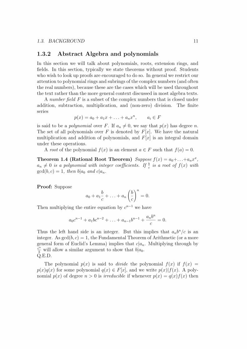
Theorem 1.4 (Rational Root Theorem) Suppose f(x) = a0+. . .+anxx,
an 6= 0 is a polynomial with integer coefficients. If bc
is a root of f(x) withgcd(b, c) = 1, then b|a0 and c|an.
Proof: Suppose
a0 + a1b
c+ . . .+ an
(b
c
)n= 0.
Then multiplying the entire equation by cn−1 we have
a0cn−1 + a1bc
n−2 + . . .+ an−1bn−1 +
anbn
c= 0.
Thus the left hand side is an integer. But this implies that anbn/c is an
integer. As gcd(b, c) = 1, the Fundamental Theorem of Arithmetic (or a moregeneral form of Euclid’s Lemma) implies that c|an. Multiplying through bycn
bwill allow a similar argument to show that b|a0.
Q.E.D.
The polynomial p(x) is said to divide the polynomial f(x) if f(x) =p(x)q(x) for some polynomial q(x) ∈ F [x], and we write p(x)|f(x). A poly-nomial p(x) of degree n > 0 is irreducible if whenever p(x) = q(x)f(x) then
12 CHAPTER 1. INTRODUCTION
either deg(q(x)) = 0 or deg(f(x)) = 0. Given two polynomials f(x) andg(x), a polynomial h(x) is a common divisor of f(x) and g(x) if h(x)|f(x)and h(x)|g(x). The polynomial h(x) is the greatest common divisor of f(x)and g(x) if whenever d(x) is also a common divisor of f(x) and g(x) thendeg(d(x)) ≤ deg(h(x)). Note that the greatest common divisor of two poly-nomials is only unique up to multiplication by a constant (when F is a field).
Theorem 1.5 (Division Algorithm for Polynomials) Let f(x) and g(x)be two non-zero polynomials over some field F . Then there exist unique poly-nomials q(x) and r(x)in F [x] such that
f(x) = g(x)q(x) + r(x)
where either r(x) = 0 or deg(r(x)) < deg(g(x)).
We can now easily see that a is a root of the polynomial f(x) if and only iff(a) = 0 by applying the Division Algorithm with g(x) = x−a and pluggingin a.
Theorem 1.6 (GCD is a Linear Combination) Let f(x) and g(x) be inF [x] (where F is a field). Suppose d(x) is the greatest common divisor of f(x)and g(x). Then there exist polynomials a(x) and b(x) in F [x] such that
d(x) = a(x)f(x) + b(x)g(x).
This last theorem is used to prove a version of Euclid’s Lemma for poly-nomials, but we state it here in particular because of what it means in thespecial case where the common divisor is 1.
In particular, if p(x) is an irreducible polynomial of degree n, then theset of residues of polynomials upon division by p(x)
Rp(x) = {a0 + a1x+ . . .+ an−1xn−1|ai ∈ F}
is a field under the addition and multiplication operations defined below.Given f(x) and g(x) in Rp(x), we define
f(x)g(x) = r(x)
where r(x) is the remainder of f(x)g(x) divided by p(x). Under this opera-tion, Rp(x) is a field which contains the field F as a subfield. The field Rp(x)
1.3. BACKGROUND 13
is naturally isomorphic with the quotient field F [x]/(p(x)), and Rp(x) can bethought of as a set of representatives of the cosets of the ideal (p(x)).
A better way of seeing the multiplication in Rp(x) is to look specifically atp(x). If p(x) = b0 + . . .+ bnx
n, then in Rp(x) we are simply demanding that
xn = − 1
bn(b0 + . . . bn−1x
n−1).
Note that this makes x a “root” of p(x) in the field Rp(x).For example, suppose F = Q is the field of rational numbers and p(x) =
x2− 2. If p(x) is reducible, then p(x) must have a linear factor. But a linearfactor would imply that p(x) has a rational root a/b. Using the rational roottest, however, we can see that the only possible roots are ±1 and ±2, whichclearly are not roots. Hence p(x) is irreducible. Thus, Rx2−2 = {a+ bx|a, b ∈Q} is a field. As
(ax+ b)(cx+ d) = acx2 + (ad+ bc)x+ bd,
in Q[x], and the division algorithm yields
acx2 + (ad+ bc)x+ bd = (ac)(x2 − 2) + [(ad+ bc)x+ bd+ 2ac],
we have that multiplication in Rx2−2 is
(ax+ b)(cx+ d) = (ad+ bc)x+ bd+ 2ac.
Next consider the subfield
Q[√
2] = {a√
2 + b|a, b ∈ Q}of the real numbers. In this field, multiplication is defined by
(a√
2 + b)(c√
2 + d) = 2ac+ bd+ (ad+ bc)√
2.
Comparing this to the multiplication for Rx2−2 we see that the two definitionsare identical except that we use
√2 in place of x in Q[
√2]. In this way, we
produce “extension” fields in a natural way.We point out that Rp(x) can be defined for any polynomial p(x), but that
it is a field only when p(x) ∈ F [x] is irreducible over the field F . This isbecause to get inverses of elements, you need for p(x) to be irreducible overF as you use the GCD is a Linear Combination Theorem.
We also note that if we replace Q with Z (the integers) in the aboveexample, the closure laws still hold. That is the set
Z[√
2] = {a+ b√
2|a, b ∈ Z}is closed under multiplication and addition. This is an easy exercise.
14 CHAPTER 1. INTRODUCTION
1.4 Problems
1. Show Z[√
2] is a subring of Q[√
2], by showing that multiplication anddivision are closed operations over Z[
√2].
2. Recall that Q[√
3] = {a + b√
3 | a, b ∈ Q}. Define addition and mul-tiplication in Q[
√3] and show how this multiplication is similar to
multiplication for Rx2−3, the residue field for x2 − 3 over Q[x].
3. Continuing the previous problem, define a correspondence betweenQ[√
3] and {(a 3bb a
)| a, b ∈ Q
}.
Chapter 2
Rational and IrrationalNumbers
In this chapter we shall be concerned with understanding the definition ofthe rational numbers, how this definition can be used to define the mathe-matical operations, how it corresponds to decimal representations of thesenumbers, and why we must expand our definition of number beyond therational numbers. To get us started, take a few minutes and consider thefollowing question.
What do we mean by the number one third?
In thinking about this question, think about the following:
• What role does this number play in different contexts?
• How does our meaning work with the mathematical operations (addi-tion, multiplication, etc.)?
• What makes the concept of fractions difficult for students to under-stand?
In answering the first of these three questions, you probably discovered thatwe have many different contexts in which we use fractions. For example, wecan think of one-third of thirty objects as being ten, or we can think of onethird of a stick, or we simply have a point on the number line. Other answers
15
16 CHAPTER 2. RATIONAL AND IRRATIONAL NUMBERS
might be 13
or 26. The affect of these multiple representations shows up in
both the understanding and the proper definition of a rational number.To effectively carry out the operations using fractions, one third should
denote an equivalence class, so that when we add fractions, we choose themost useful element of that class for the problem at hand. When you thinkabout the difficulties many mathematics majors have operating with equiv-alence classes, it suddenly becomes easier to understand why students whodo not like math often have so much trouble adding fractions.
To carefully define the rational numbers, one must use the language ofequivalence classes. As usual, we use Z to denote the integers (both positiveand negative). Let
F = {ab| a, b ∈ Z, b 6= 0}.
Let ∼ denote the equivalence relation on F given by ab∼ c
dif and only if
ad = bc. For the remainder of this section, when we use the word fraction,we shall mean an element of F .
We define the operations of addition and multiplication on F by
a
b+c
d=
ad+ bc
bd, and
a
b· cd
=ac
bd.
There is no guarantee that the definitions yield fractions in lowest terms. Infact, under our definition, 1
2+ 1
2= 4
4, which is then equivalent to 1
1. This
example illustrates how the formula differs from what you “know” is thecorrect definition for adding fractions with the same denominator, namelyac
+ bc
= a+bc
. Our definition does give an equivalent answer ac+bcc2
, since
c(ac+ bc) = ac2 + bc2.
Definition. The set Q of rational numbers is the set of equivalence classesof F under the operations (using
[ab
]to denote the equivalence class of a
b)[
ab
]+[cd
]=[ad+bcbd
]and
[ab
]·[cd
]=[acbd
].
These definitions of addition and multiplication for rationals are forcedupon us so that when equivalent fractions are added, we get as our answersequivalent fractions. For example:
2
3+
4
5=
22
154
6+
12
15=
132
90,
17
and 132 · 15 = 1980 = 22 · 90. Let’s prove this in general for addition.
Proof: Suppose ab∼ a′
b′and c
d∼ c′
d′. Adding, a
band c
dwe get ad+bc
bd. Similarly,
adding, a′
b′and c′
d′we get a′d′+b′c′
b′d′. We now simply need to check that the two
answers are equivalent. Multiplying out we get
(ad+ bc)(b′d′) = (ab′)dd′ + bb′(cd′)
= a′bdd′ + bb′c′d since ab∼ a′
b′and c
d∼ c′
d′
= (a′d′ + b′c′)(bd).
But this implies the answers are equivalent. Q.E.D.
Aside:Of course, when you learned to add fractions, you didn’t think in terms ofequivalence classes, but you did spend a long time getting used to the ideathat 1/3 = 2/6 = . . .. So why go through this proof at all? A commonproblem for precalculus students is how to add rational functions, thatis fractions of polynomials. Addition in this case appears strange until yousee that it only mimics the rational case. What’s more, the beautiful thingabout this definition for addition is that you avoid the difficulty of findinga least common denominator (l.c.d.). All you really need to do is follow theroutine which allows you to get away with any common denominator. Thisdoesn’t mean you should teach students not to find an l.c.d., but rather youshould point out that there are other ways to add fractions. Of course withlarge numbers and polynomials, least common denominators do make thecomputations easier which is the reason we teach them in the first place.
Now let us think a little about the proof of why this works. It turns outthat the proof really depends on two steps that are hidden by the algebra.Thus while the algebra is rather easy to do, the actual “reason” behind doingit is harder to find. This reason, however, is crucial to understanding theprocess and making it less magical. Most students in this class understandthe reason without making it public, but as a teacher, one cannot afford to dothis, and having multiple ways of explaining ideas helps enormously. Thus,as silly as it may seem to give two proofs of the same fact that we alreadyagree is correct, let us look at a second proof where we build the propositionup one step at a time.
18 CHAPTER 2. RATIONAL AND IRRATIONAL NUMBERS
Proof: First note that for any fraction ef
and non-zero integer x, ef
= exfx
.
Hence, if ab∼ a′
b′and c
d∼ c′
d′, then
a
b+c
d=
ad+ bc
bd
=(ad+ bc)b′d′
bdb′d′
=(ab′)dd′ + (cd′)bb′
bdb′d′
=(a′b)dd′ + (c′d)bb′
bdb′d′
=(a′d′)bd+ (b′c′)bd
bdb′d′
=a′d′ + b′c′
b′d′
=a′
b′+c′
d′.
Q.E.D.
This second proof is longer and has a few more steps in it. Thus, at theoutset it looks more difficult. However, the key step is more obvious. In thiscase it is the idea of cancellation of a common term in the numerator anddenominator, which then allows a simple algebraic calculation and hides theequivalence class idea altogether.
2.1 Decimal Representations
Rather than beginning this section with a question, we begin with a project.
Program your calculator or a spreadsheet to give an arbitrarynumber of digits for a fraction a
b .
That is, write a program so that given a and b, you can find as many digitsof the decimal expansion of a
b. In trying to do this, you will want to consider
several things
• What does it mean to “bring down a zero” when doing long division?
2.1. DECIMAL REPRESENTATIONS 19
• What portions of the algorithm repeat themselves?
Such a program will prove useful in many different contexts. It also leadsus into the question :
What do we mean by the infinite decimal α = .2345?
When thinking about this question, think about:
• What number does each digit of the decimal correspond to?
• What rational numbers do you know that α lies between?
• What makes infinite decimals hard to understand?
Decimals are really just an extension of place-value arithmetic in base
10. Thus if the kth digit to the right of the decimal is ak, then this digitcorresponds to the value ak · 10−k. Thus the finite decimal .2345 is equal to
2
10+
3
102+
4
103+
5
104=
2345
10000.
If we have k repetitions of this, we have
.23452345 . . . 2345 =k∑l=1
2345 · 10−4l,
where there are 4k digits in the decimal. Of course, if the decimal is infinite,we will have to resort to an infinite sum leading to limits, which we are notquite ready to do. Consequently, we shall settle for a more finite but lessenticing definition, namely that .2345 is a number α such that
k∑l=1
2345 · 10−4l ≤ α ≤k∑l=1
2345 · 10−4l + 10−4k
for all integers k. Ever since we were in elementary school, we have been toldthat such a number exists, however, the existence is not at all obvious.
At this point, we shall give a partial definition of an infinite decimal. Thisdefinition will be sufficient for finding the correspondence between rationalnumbers and decimals. If we desire to move beyond rational numbers in aconstructive way, however, we shall have more work to do.
20 CHAPTER 2. RATIONAL AND IRRATIONAL NUMBERS
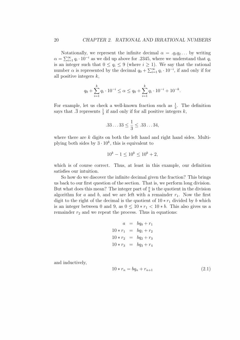
Notationally, we represent the infinite decimal α = .q1q2 . . . by writingα =
∑∞i=1 qi · 10−i as we did up above for .2345, where we understand that qi
is an integer such that 0 ≤ qi ≤ 9 (where i ≥ 1). We say that the rationalnumber α is represented by the decimal q0 +
∑∞i=1 qi · 10−i, if and only if for
all positive integers k,
q0 +k∑i=1
qi · 10−i ≤ α ≤ q0 +k∑i=1
qi · 10−i + 10−k.
For example, let us check a well-known fraction such as 13. The definition
says that .3 represents 13
if and only if for all positive integers k,
.33 . . . 33 ≤ 1
3≤ .33 . . . 34,
where there are k digits on both the left hand and right hand sides. Multi-plying both sides by 3 · 10k, this is equivalent to
10k − 1 ≤ 10k ≤ 10k + 2,
which is of course correct. Thus, at least in this example, our definitionsatisfies our intuition.
So how do we discover the infinite decimal given the fraction? This bringsus back to our first question of the section. That is, we perform long division.But what does this mean? The integer part of a
bis the quotient in the division
algorithm for a and b, and we are left with a remainder r1. Now the firstdigit to the right of the decimal is the quotient of 10 ∗ r1 divided by b whichis an integer between 0 and 9, as 0 ≤ 10 ∗ r1 < 10 ∗ b. This also gives us aremainder r2 and we repeat the process. Thus in equations:
a = bq0 + r1
10 ∗ r1 = bq1 + r2
10 ∗ r2 = bq2 + r3
10 ∗ r3 = bq3 + r4
and inductively,
10 ∗ rn = bqn + rn+1 (2.1)
2.1. DECIMAL REPRESENTATIONS 21
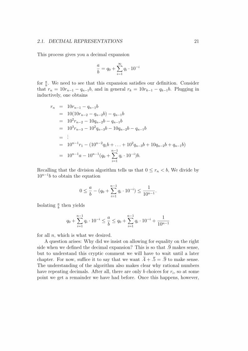
This process gives you a decimal expansion
a
b= q0 +
∞∑i=1
qi · 10−i
for ab. We need to see that this expansion satisfies our definition. Consider
that rn = 10rn−1 − qn−1b, and in general rk = 10rk−1 − qk−1b. Plugging ininductively, one obtains
rn = 10rn−1 − qn−1b
= 10(10rn−2 − qn−2b)− qn−1b
= 102rn−2 − 10qn−2b− qn−1b
= 103rn−3 − 102qn−3b− 10qn−2b− qn−1b
=...
= 10n−1r1 − (10n−2q1b+ . . .+ 102qn−3b+ 10qn−2b+ qn−1b)
= 10n−1a− 10n−1(q0 +n−1∑i=1
qi · 10−i)b.
Recalling that the division algorithm tells us that 0 ≤ rn < b, We divide by10n−1b to obtain the equation
0 ≤ a
b− (q0 +
n−1∑i=1
qi · 10−i) ≤ 1
10n−1.
Isolating ab
then yields
q0 +n−1∑i=1
qi · 10−i ≤ a
b≤ q0 +
n−1∑i=1
qi · 10−i +1
10n−1
for all n, which is what we desired.A question arises: Why did we insist on allowing for equality on the right
side when we defined the decimal expansion? This is so that .9 makes sense,but to understand this cryptic comment we will have to wait until a laterchapter. For now, suffice it to say that we want .4 + .5 = .9 to make sense.The understanding of the algorithm also makes clear why rational numbershave repeating decimals. After all, there are only b choices for ri, so at somepoint we get a remainder we have had before. Once this happens, however,
22 CHAPTER 2. RATIONAL AND IRRATIONAL NUMBERS
it must be the case that we have repetition as you will show in a homeworkexercise.
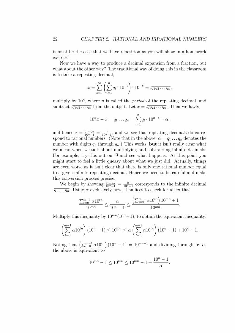
Now we have a way to produce a decimal expansion from a fraction, butwhat about the other way? The traditional way of doing this in the classroomis to take a repeating decimal,
x =∞∑k=0
(n∑i=1
qi · 10−i)· 10−k = .q1q2 . . . qn,
multiply by 10n, where n is called the period of the repeating decimal, andsubtract .q1q2 . . . qn from the output. Let x = .q1q2 . . . qn. Then we have:
10nx− x = q1 . . . qn =n∑i=1
qi · 10n−i = α,
and hence x = q1...qn10n−1
= α10n−1
, and we see that repeating decimals do corre-spond to rational numbers. (Note that in the above, α = q1 . . . qn denotes thenumber with digits q1 through qn.) This works, but it isn’t really clear whatwe mean when we talk about multiplying and subtracting infinite decimals.For example, try this out on .9 and see what happens. At this point youmight start to feel a little queasy about what we just did. Actually, thingsare even worse as it isn’t clear that there is only one rational number equalto a given infinite repeating decimal. Hence we need to be careful and makethis conversion process precise.
We begin by showing q1...qn10n−1
= α10n−1
corresponds to the infinite decimal.q1 . . . qn. Using α exclusively now, it suffices to check for all m that
∑m−1t=0 α10tn
10mn≤ α
10n − 1≤
(∑m−1t=0 α10tn
)10mn + 1
10mn.
Multiply this inequality by 10mn(10n−1), to obtain the equivalent inequality:(m−1∑t=0
α10tn)
(10n − 1) ≤ 10mn ≤ α
(m−1∑t=0
α10tn)
(10n − 1) + 10n − 1.
Noting that(∑m−1
t=0 α10tn)
(10n − 1) = 10mn−1 and dividing through by α,the above is equivalent to
10mn − 1 ≤ 10mn ≤ 10mn − 1 +10n − 1
α.
2.2. IRRATIONALITY PROOFS 23
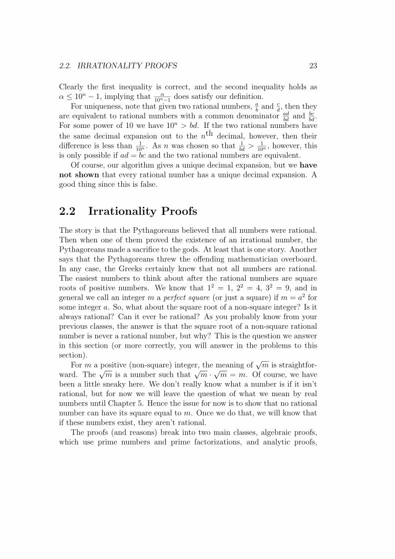
Clearly the first inequality is correct, and the second inequality holds asα ≤ 10n − 1, implying that α
10n−1does satisfy our definition.
For uniqueness, note that given two rational numbers, ab
and cd, then they
are equivalent to rational numbers with a common denominator adbd
and bcbd
.For some power of 10 we have 10n > bd. If the two rational numbers have
the same decimal expansion out to the nth decimal, however, then theirdifference is less than 1
10n. As n was chosen so that 1
bd> 1
10n, however, this
is only possible if ad = bc and the two rational numbers are equivalent.Of course, our algorithm gives a unique decimal expansion, but we have
not shown that every rational number has a unique decimal expansion. Agood thing since this is false.
2.2 Irrationality Proofs
The story is that the Pythagoreans believed that all numbers were rational.Then when one of them proved the existence of an irrational number, thePythagoreans made a sacrifice to the gods. At least that is one story. Anothersays that the Pythagoreans threw the offending mathematician overboard.In any case, the Greeks certainly knew that not all numbers are rational.The easiest numbers to think about after the rational numbers are squareroots of positive numbers. We know that 12 = 1, 22 = 4, 32 = 9, and ingeneral we call an integer m a perfect square (or just a square) if m = a2 forsome integer a. So, what about the square root of a non-square integer? Is italways rational? Can it ever be rational? As you probably know from yourprevious classes, the answer is that the square root of a non-square rationalnumber is never a rational number, but why? This is the question we answerin this section (or more correctly, you will answer in the problems to thissection).
For m a positive (non-square) integer, the meaning of√m is straightfor-
ward. The√m is a number such that
√m ·√m = m. Of course, we have
been a little sneaky here. We don’t really know what a number is if it isn’trational, but for now we will leave the question of what we mean by realnumbers until Chapter 5. Hence the issue for now is to show that no rationalnumber can have its square equal to m. Once we do that, we will know thatif these numbers exist, they aren’t rational.
The proofs (and reasons) break into two main classes, algebraic proofs,which use prime numbers and prime factorizations, and analytic proofs,
24 CHAPTER 2. RATIONAL AND IRRATIONAL NUMBERS
which use arguments based on inequalities. Here we will prove that√
2is irrational in 3 different ways. In the homework you will be asked to doother numbers.
We will begin with the algebraic versions:Proof 1: This is the traditional even-odd proof. If
√2 = m/n is rational, we
can choose integers m and n so that at least one is odd (not divisible by 2).But then we have n
√2 = m, and squaring both sides gives that m2 = 2n2 and
hence m is even (by Euclid’s Lemma). Writing m = 2k we have (2k)2 = 2n2,so that n2 = 2k2 and hence n is even. But this contradicts our choice of mand n. Hence
√2 is not rational.
Q.E.D.
One can also prove this by using the prime factorization of 2 or alterna-tively by using the rational root theorem on the polynomial x2 − 2. Both ofthese proofs, however, rest on Euclid’s Lemma (if p is a prime number, thenp|ab implies p|a or p|b), so for our purposes, they are really just more com-plicated versions of the same proof. Of course, when teaching high school,you might want to use one of these other proofs.
The next two proofs are analytic in nature. By this we mean that theyhave to do with inequalities, and in the case of the third proof, the idea oflimits.Proof 2: If
√2 is rational, there exists some smallest positive integer q such
that q√
2 = p is an integer. Then
(p− q)√
2 = p√
2−√
2q
= 2q − p
is also an integer. As 1 <√
2 < 2, we have q < p < 2q. Hence 0 < p− q < qand p − q is positive and smaller than q. But this contradicts the choiceof q as the smallest positive integer such that q
√2 is an integer. Hence a
contradiction has been reached and√
2 is not rational.Q.E.D.
Proof 3: Suppose√
2 = p/q with p and q integers. Note that√
2− 1 < 1/2since 2 < 9/4 implies
√2 < 3/2. Hence by choosing n large, we can make
(√
2−1)n > 0 as small as we want. However, (√
2−1)n = A√
2+B for somepair of integers A and B as Z[
√2] is a ring (see section 1.3.2), and hence is
closed under multiplication and addition. But then writing
(√
2− 1)n = A√
2 +B
2.2. IRRATIONALITY PROOFS 25
= Ap
q+B
=Ap+Bq
q,
we have that if it is positive it must be at least 1q. This contradicts that
(√
2− 1)n can get smaller than 1q. Hence
√2 is not rational.
Q.E.D.
Again, one might ask why we need three proofs that√
2 is irrational.Each illustrates a different property of rational numbers. The first we havealready discussed, the second proof ties into the existence of least termsfor a fraction again, but this time based on inequality rather than factors,and the third proof shows the fundamental property of the rational numbersconcerning how close you can get to zero using just two rational numbers(1 and p
q). This last idea turns out to be extremely useful in many number
theory proofs. Later, we shall use this idea in the proof of the irrationalityof π.
Teaching Aside: At this point, let’s think about when we might use theseother proofs in teaching high school? The answer to this question depends ona different question. Namely, why do we teach that
√2 is irrational? There
are several different answers to this latter question. One might argue thatstudents need to understand that not every number can be written exactlyas a fraction. However, this argument suggests that we need merely tell themthat and be done with it rather than give a proof that a specific number isnot rational. A better reasoning might be that understanding the proofs ofthe irrationality of
√2 helps one to better understand what the properties
of fractions and rational numbers are. Using this idea that we prove theirrationality to teach us about properties of numbers, we can then answerthe first question as follows: The first proof could be effectively presentedwhen discussing the fundamental theorem of arithmetic to students on primedecomposition, and its derivatives could be presented as applications to theroot theorem for polynomials. The second proof is a good way to intro-duce induction proofs into the high school (something the NCTM standardsrecommends), and it can help students learn how to multiply equations con-taining roots, something which is often covered in high school texts whendiscussing quadratic equations. Finally the third proof would be useful topresent in a precalculus class when discussing limits and the completeness
26 CHAPTER 2. RATIONAL AND IRRATIONAL NUMBERS
properties of the real numbers.End of Aside
What we have done here, is to show that if√
2 is a number, then it is notrational. Of course, we only have that it is a number because we know fromour background that it is a real number. While this statement seems obviousto us, the existence of a number like
√2 might not be clear. For example,
what about√−1. This is not a real number, so why do we get away with
saying that√
2 is a real number? We will deal more generally with this topiclater when we talk about what the real numbers are.
2.3 Irrationality of e and π
We end this chapter by proving that e and π are both irrational. Even morethan the previous section, we are going to use our previous knowledge aboutthese two numbers (and calculus too) to show their irrationality. That e wasirrational was known and proved by Euler using much the same techniqueas we use in Theorem ??. The irrationality of π, on the other hand, wasfirst proved by Lambert in 1761 by the use of continued fractions [?]. Wewill take a different approach using calculus. Rather than using the morestandard calculus proof as in [7], we shall follow the approach that Niventakes in [6]. All of these proofs are based on the same ideas as the secondand third proofs of the irrationality of
√2 above. That is, we desire to
show that if the number were rational, some sequence must get arbitrarilysmall and at the same time must be greater than some fixed positive numberestablishing a contradiction. For the
√2, we could do this without resorting
to the use of calculus. While one can use basic techniques for e (as we do inTheorem 2.1), proving π irrational requires significantly more work, and thecalculus approach seems clearest.
Theorem 2.1 The number e is irrational.
Proof: We begin by recalling from calculus that
e =∞∑n=0
1
n!.
2.3. IRRATIONALITY OF E AND π 27
By way of contradiction, suppose e = ab
with a and b positive integers. Then(b!)e is an integer. Using the above expression for e, we have
b!e =b∑
n=0
b!
n!+
∞∑n=b+1
b!
n!.
The first term on the right is an integer since the kth term of the sum,b(b− 1) . . . (k) is an integer. Consequently, the second sum is the differenceof two integers, and is therefore itself an integer. Moreover, it is clearlypositive, so that we have
1 ≤∞∑
n=b+1
b!
n!. (2.2)
At this point we analyze each term of this sum. If n ≥ b + 1 is an integer,then
n! = n(n− 1) . . . (b+ 1)b! ≥ (b+ 1)n−b · b!.Thus
b!
n!≤ (b+ 1)b−n,
whenever n > b is an integer. Moreover, the inequality is strict if n > b+ 1.Hence equation 2.2 yields
1 ≤∞∑
n=b+1
b!
n!
<∞∑
n=b+1
(b+ 1)b−n
=∞∑n=1
(b+ 1)−n.
This last is a geometric series. Again, from calculus (or some other previousclass), the sum of this series is
1
b+ 1· 1
1− (b+ 1)−1=
1
b.
Putting this all together, we obtain that 1 < 1b, a contradiction.
Q.E.D.
The proof for π is more complicated. In order to help the reader gainsome familiarity with the type of argument we use for π, we give a secondproof that e is irrational. This proof is given in [13].
28 CHAPTER 2. RATIONAL AND IRRATIONAL NUMBERS
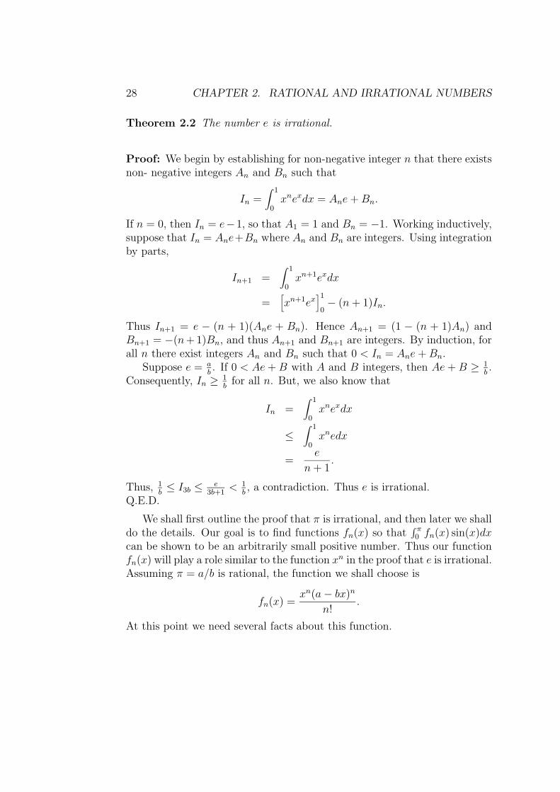
Theorem 2.2 The number e is irrational.
Proof: We begin by establishing for non-negative integer n that there existsnon- negative integers An and Bn such that
In =∫ 1
0xnexdx = Ane+Bn.
If n = 0, then In = e−1, so that A1 = 1 and Bn = −1. Working inductively,suppose that In = Ane+Bn where An and Bn are integers. Using integrationby parts,
In+1 =∫ 1
0xn+1exdx
=[xn+1ex
]10− (n+ 1)In.
Thus In+1 = e − (n + 1)(Ane + Bn). Hence An+1 = (1 − (n + 1)An) andBn+1 = −(n+ 1)Bn, and thus An+1 and Bn+1 are integers. By induction, forall n there exist integers An and Bn such that 0 < In = Ane+Bn.
Suppose e = ab. If 0 < Ae+B with A and B integers, then Ae+B ≥ 1
b.
Consequently, In ≥ 1b
for all n. But, we also know that
In =∫ 1
0xnexdx
≤∫ 1
0xnedx
=e
n+ 1.
Thus, 1b≤ I3b ≤ e
3b+1< 1
b, a contradiction. Thus e is irrational.
Q.E.D.
We shall first outline the proof that π is irrational, and then later we shalldo the details. Our goal is to find functions fn(x) so that
∫ π0 fn(x) sin(x)dx
can be shown to be an arbitrarily small positive number. Thus our functionfn(x) will play a role similar to the function xn in the proof that e is irrational.Assuming π = a/b is rational, the function we shall choose is
fn(x) =xn(a− bx)n
n!.
At this point we need several facts about this function.

2.3. IRRATIONALITY OF E AND π 29
Lemma 2.3 Suppose π = a/b. For any non-negative integer k, f (k)n (0) and
f (k)n (π) are both integers, (where f (k)
n denotes the kth derivative of fn).
Proof: Let k be given, and note by the product rule that f (k)n (x) is a sum of
terms of the form Am,lxn−m(a− bx)n−l where Am,l is an integer multiple of
n(n− 1) . . . (n−m+ 1) · n(n− 1) . . . (n− l + 1)
n!
(you should check this!). Thus if a term in the sum for f (k)n (0) is not 0, it
is an integer as in this case m = n (and l ≤ n). Similarly if a term in thesum for f (k)
n (π) is not 0 it is an integer. Consequently, f (k)n (0) and f (k)
n (π)are both integers.Q.E.D.
The next step in the proof concerns integrating∫ π
0 fn(x) sin(x)dx. As youmay recall from calculus, to do this requires integration by parts many times.The reader should do this for n = 1, n = 2, and n = 3 with the functionabove to get a feel for what is going to happen. Once done, read on.
At this point we set
Fn(x) = fn(x)− f (2)n (x) + f (4)
n (x) + . . .+ (−1)nf (2n)n (x).
By the above Lemma, note that Fn(0) and Fn(π) are integers. We compute
d
dx(F ′n(x) sin x− Fn(x) cos x) = F ′′n (x) sin x+ F (x) sin x
= f(x) sin x,
where the last follows as f (2n+1)n (x) = 0 as fn(x) is a polynomial of degree
2n. Consequently, by the Fundamental Theorem of Calculus,∫ π
0fn(x) sin xdx = [F ′n(x) sin x− Fn(x) cos x]
π0 = Fn(π) + Fn(0). (2.3)
Thus by the above, this integral is an integer. At this point we state ourtheorem.
Theorem 2.4 The number π is irrational.
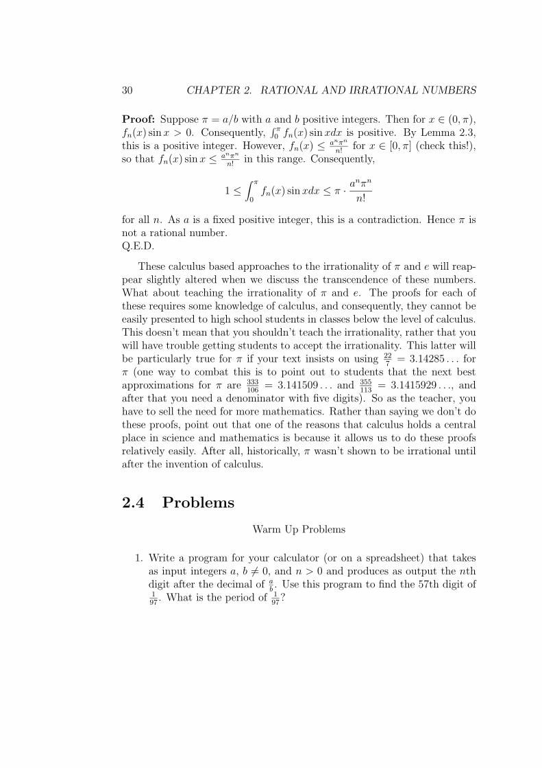
30 CHAPTER 2. RATIONAL AND IRRATIONAL NUMBERS
Proof: Suppose π = a/b with a and b positive integers. Then for x ∈ (0, π),fn(x) sin x > 0. Consequently,
∫ π0 fn(x) sin xdx is positive. By Lemma 2.3,
this is a positive integer. However, fn(x) ≤ anπn
n!for x ∈ [0, π] (check this!),
so that fn(x) sin x ≤ anπn
n!in this range. Consequently,
1 ≤∫ π
0fn(x) sin xdx ≤ π · a
nπn
n!
for all n. As a is a fixed positive integer, this is a contradiction. Hence π isnot a rational number.Q.E.D.
These calculus based approaches to the irrationality of π and e will reap-pear slightly altered when we discuss the transcendence of these numbers.What about teaching the irrationality of π and e. The proofs for each ofthese requires some knowledge of calculus, and consequently, they cannot beeasily presented to high school students in classes below the level of calculus.This doesn’t mean that you shouldn’t teach the irrationality, rather that youwill have trouble getting students to accept the irrationality. This latter willbe particularly true for π if your text insists on using 22
7= 3.14285 . . . for
π (one way to combat this is to point out to students that the next bestapproximations for π are 333
106= 3.141509 . . . and 355
113= 3.1415929 . . ., and
after that you need a denominator with five digits). So as the teacher, youhave to sell the need for more mathematics. Rather than saying we don’t dothese proofs, point out that one of the reasons that calculus holds a centralplace in science and mathematics is because it allows us to do these proofsrelatively easily. After all, historically, π wasn’t shown to be irrational untilafter the invention of calculus.
2.4 Problems
Warm Up Problems
1. Write a program for your calculator (or on a spreadsheet) that takesas input integers a, b 6= 0, and n > 0 and produces as output the nthdigit after the decimal of a
b. Use this program to find the 57th digit of
197
. What is the period of 197
?
2.4. PROBLEMS 31
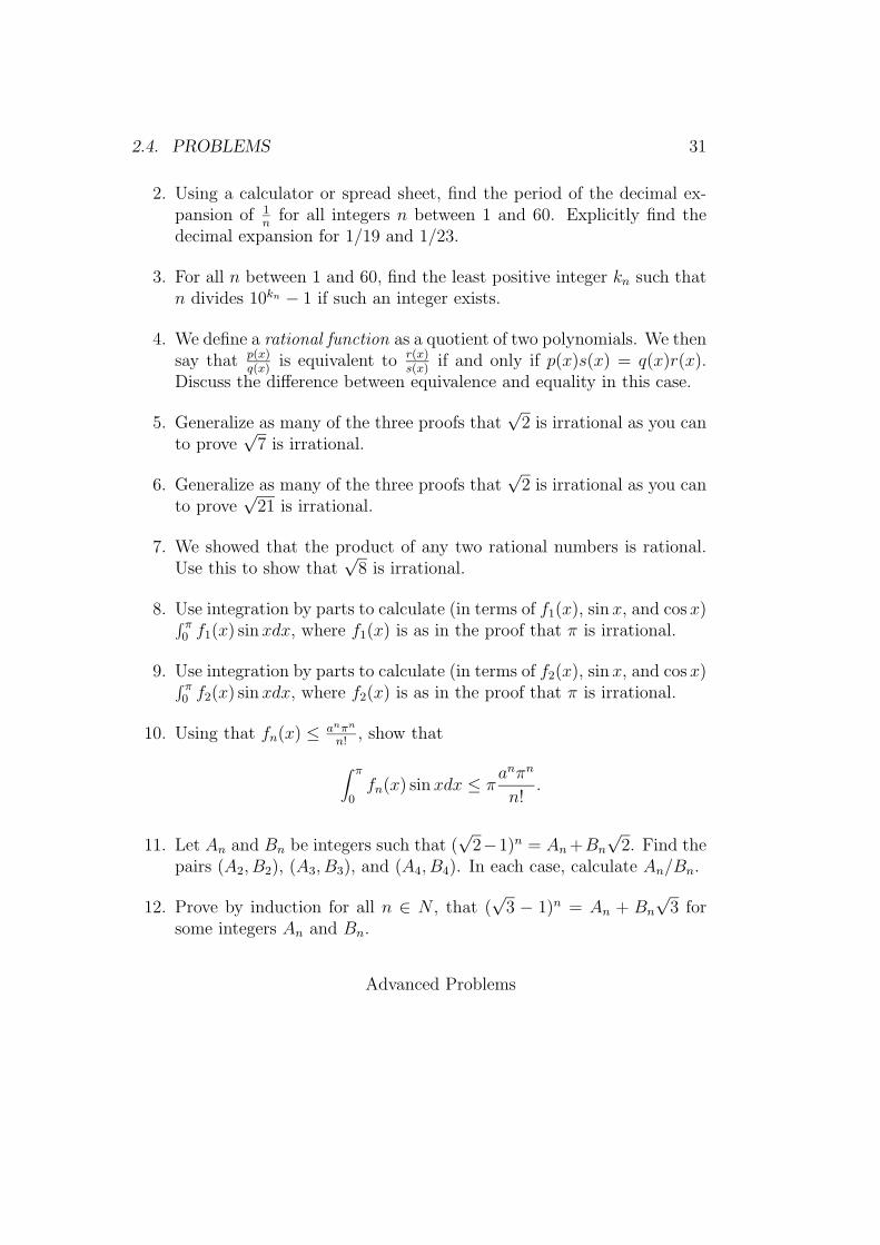
2. Using a calculator or spread sheet, find the period of the decimal ex-pansion of 1
nfor all integers n between 1 and 60. Explicitly find the
decimal expansion for 1/19 and 1/23.
3. For all n between 1 and 60, find the least positive integer kn such thatn divides 10kn − 1 if such an integer exists.
4. We define a rational function as a quotient of two polynomials. We thensay that p(x)
q(x)is equivalent to r(x)
s(x)if and only if p(x)s(x) = q(x)r(x).
Discuss the difference between equivalence and equality in this case.
5. Generalize as many of the three proofs that√
2 is irrational as you canto prove
√7 is irrational.
6. Generalize as many of the three proofs that√
2 is irrational as you canto prove
√21 is irrational.
7. We showed that the product of any two rational numbers is rational.Use this to show that
√8 is irrational.
8. Use integration by parts to calculate (in terms of f1(x), sinx, and cosx)∫ π0 f1(x) sin xdx, where f1(x) is as in the proof that π is irrational.
9. Use integration by parts to calculate (in terms of f2(x), sinx, and cosx)∫ π0 f2(x) sin xdx, where f2(x) is as in the proof that π is irrational.
10. Using that fn(x) ≤ anπn
n!, show that
∫ π
0fn(x) sin xdx ≤ π
anπn
n!.
11. Let An and Bn be integers such that (√
2−1)n = An+Bn
√2. Find the
pairs (A2, B2), (A3, B3), and (A4, B4). In each case, calculate An/Bn.
12. Prove by induction for all n ∈ N , that (√
3 − 1)n = An + Bn
√3 for
some integers An and Bn.
Advanced Problems
32 CHAPTER 2. RATIONAL AND IRRATIONAL NUMBERS
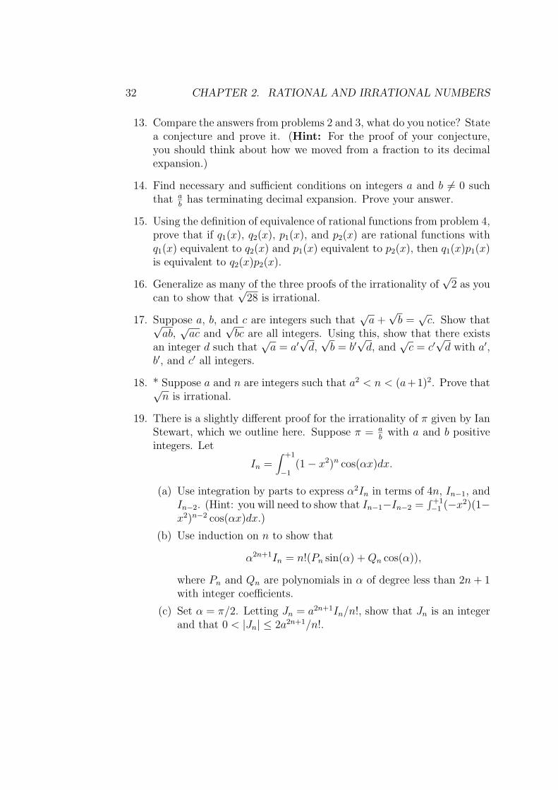
13. Compare the answers from problems 2 and 3, what do you notice? Statea conjecture and prove it. (Hint: For the proof of your conjecture,you should think about how we moved from a fraction to its decimalexpansion.)
14. Find necessary and sufficient conditions on integers a and b 6= 0 suchthat a
bhas terminating decimal expansion. Prove your answer.
15. Using the definition of equivalence of rational functions from problem 4,prove that if q1(x), q2(x), p1(x), and p2(x) are rational functions withq1(x) equivalent to q2(x) and p1(x) equivalent to p2(x), then q1(x)p1(x)is equivalent to q2(x)p2(x).
16. Generalize as many of the three proofs of the irrationality of√
2 as youcan to show that
√28 is irrational.
17. Suppose a, b, and c are integers such that√a +√b =√c. Show that√
ab,√ac and
√bc are all integers. Using this, show that there exists
an integer d such that√a = a′
√d,√b = b′
√d, and
√c = c′
√d with a′,
b′, and c′ all integers.
18. * Suppose a and n are integers such that a2 < n < (a+1)2. Prove that√n is irrational.
19. There is a slightly different proof for the irrationality of π given by IanStewart, which we outline here. Suppose π = a
bwith a and b positive
integers. Let
In =∫ +1
−1(1− x2)n cos(αx)dx.
(a) Use integration by parts to express α2In in terms of 4n, In−1, andIn−2. (Hint: you will need to show that In−1−In−2 =
∫+1−1 (−x2)(1−
x2)n−2 cos(αx)dx.)
(b) Use induction on n to show that
α2n+1In = n!(Pn sin(α) +Qn cos(α)),
where Pn and Qn are polynomials in α of degree less than 2n+ 1with integer coefficients.
(c) Set α = π/2. Letting Jn = a2n+1In/n!, show that Jn is an integerand that 0 < |Jn| ≤ 2a2n+1/n!.
2.4. PROBLEMS 33
(d) Use the above step to establish a contradiction, so that π must beirrational.

34 CHAPTER 2. RATIONAL AND IRRATIONAL NUMBERS
Chapter 3
Constructible Numbers
We have now worked through the definition of the rational numbers, thedefinition of operations on rational numbers, and examples of numbers thatwe want to exist, that cannot be rational. Let us begin to examine thesenumbers. First, consider the following question:
What do we mean by√
2 and how do we know it exists? What about√
3?
While thinking about this question, you might want to consider a few thoughts.
• Our calculator gives us a decimal, but can it give us a way of knowingall of the digits?
• Is there some other way to describe√
2?
• How do we know exactly where to place√
2 on the number line?
You probably came up with one of two usual answers to the questionof how do we know
√2 exists. The first answer might involve looking at a
graph of f(x) = x2 and noting that f(0) is less than 2 while f(2) is greaterthan 2. Since the graph is unbroken, this implies that at some value of xbetween 0 and 2, we must have f(x) = 2. This argument is correct, butto make it precise, we need the intermediate value theorem which requiresa significantly deeper understanding of what a real number is in terms ofdecimals. We will get into this answer in chapter 5.
The other answer involves noting that given a square with side lengthequal to one unit, the diagonal has side length equal to two units by thePythagorean Theorem. This works for
√2, but what about
√3? Once we
35
36 CHAPTER 3. CONSTRUCTIBLE NUMBERS
have the√
2, we know that√
3 units is the length of the hypotenuse of aright triangle having legs measuring 1 unit and
√2 units. Continuing in
this manner, we can then get all the square roots of integers as recognizablelengths.
One of the primary ways of thinking of numbers is that they measurelengths. As seen above, the advantage of this view of numbers is that itallows us to naturally consider at least some irrational numbers. Of course,if it can’t let us view rational numbers at the same time, it wouldn’t be veryhelpful. But at least the numbers 1
ncan be viewed as lengths breaking a unit
length into n equal parts, so that 12
can be viewed as the measure of half aunit stick.
The philosopher/mathematician Zeno came up with several paradoxesrelated to this. Suppose Achilles and a tortoise are having a race, and tomake the race fair, Achilles has given the tortoise a head start. When Achillesreaches the point that the tortoise started at, the tortoise will have movedjust a little to some new point p1. When he reaches the point that thetortoise is a point, however, the tortoise will have moved just a bit fartheron from where he was. When Achilles reaches the point p1, the tortoise willno longer be there, but will be at some new point p2, and so on and so on.Thus Achilles will never reach the tortoise.
Another of Zeno’s paradoxes is specific to motion: Suppose you shoot anarrow at a target. Before the arrow can get to the target, it must first gethalfway. Now before the arrow can get to the target, it must first go half thedistance from where it is to the target. Once the arrow has gone 3/4 of thedistance, it must go halfway again, ad infinitum. Thus motion is impossible.
These logical paradoxes are very hard to deal with. We know that theycannot be correct, but on the other hand, where is the flaw in the logic. Oneanswer is that length (or time, or whatever) is not infinitely decomposable.Quantum physics offers up the solution that the location of a particle is notprecise so that it is meaningless to say that something is exactly halfway tosomewhere else. Others will simply point out that motion happens and willthen call it a day.
For us these paradoxes actually get at the heart of the question of whatwe really mean by number and length. Of course, it is fine to define abstractnumbers as infinitely decomposable because we don’t actually ask for dis-tances. On the other hand, if we do this, what happens to our applicationsof numbers. Zeno’s paradoxes made a great impact upon Greek mathemat-ics. While the Greeks essentially had the idea of limits, they used the process
3.1. THE NUMBER LINE 37
of exhaustion in many proofs, they also separated the concepts of magnitudeand number. Today, however, we tend to use these concepts interchangeably.In fact, one of the strengths of mathematics, is that it often allows us to lookat similar concepts as being essentially the same. We saw this in the lastchapter when we had two different ways to look at rational numbers, as ra-tios and repeating decimals, and we see it again here when we obtain a newnotion, that of distance measurement.
3.1 The Number Line
We begin by noting that one can make sense of rational numbers as lengthin an elegant way. Suppose we have a unit length called 1. The positiveintegers are then simply the lengths you can obtain by appending copies ofyour unit length. This is seen naturally in the number line, where we assignto each point on the number line its distance from 0, where if 0 is to the rightof the point, the distance is thought of as negative. With this definition, thepoint at unit distance to the right of 0 is assigned the number 1, the pointtwo units to the right of 0 is assigned 2, and so on.
Given two lengths d1 and d2, we say that they are commensurable if thereexists a length m with which you can make lengths d1 and d2 by repeatedcopies. In algebraic notation, this means there exists natural numbers n1
and n2 such that
d1 = m · n1, and
d2 = m · n2.
We can now see that if d1 and d2 are commensurable then d2 is a rationalmultiple of d1 (as a number), as d2 = n2
n1d1. Hence, we can define the positive
rational numbers as the lengths that are commensurable with our given unitlength 1. We will refer to a length with which you can make the lengthsd1 and d2 as a common yardstick. Of course, any rational length a
bhas a
common yardstick with the unit length, namely the length 1b.
This understanding of number as lengths also gives us a geometric picturefor both the division algorithm and the Euclidean algorithm. In particular,when dividing the number a by b, we are just seeing how many b lengthyardsticks it takes to make up an a length yardstick. As a result this givesthe quotient as the number of complete b length yardsticks we can line upinside of an a length, and the remainder is the bit left over.
38 CHAPTER 3. CONSTRUCTIBLE NUMBERS
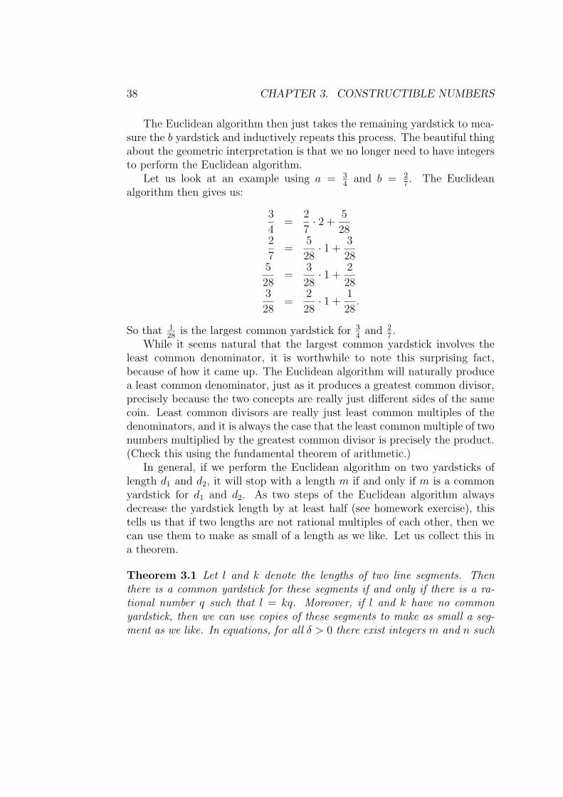
The Euclidean algorithm then just takes the remaining yardstick to mea-sure the b yardstick and inductively repeats this process. The beautiful thingabout the geometric interpretation is that we no longer need to have integersto perform the Euclidean algorithm.
Let us look at an example using a = 34
and b = 27. The Euclidean
algorithm then gives us:
3
4=
2
7· 2 +
5
282
7=
5
28· 1 +
3
285
28=
3
28· 1 +
2
283
28=
2
28· 1 +
1
28.
So that 128
is the largest common yardstick for 34
and 27.
While it seems natural that the largest common yardstick involves theleast common denominator, it is worthwhile to note this surprising fact,because of how it came up. The Euclidean algorithm will naturally producea least common denominator, just as it produces a greatest common divisor,precisely because the two concepts are really just different sides of the samecoin. Least common divisors are really just least common multiples of thedenominators, and it is always the case that the least common multiple of twonumbers multiplied by the greatest common divisor is precisely the product.(Check this using the fundamental theorem of arithmetic.)
In general, if we perform the Euclidean algorithm on two yardsticks oflength d1 and d2, it will stop with a length m if and only if m is a commonyardstick for d1 and d2. As two steps of the Euclidean algorithm alwaysdecrease the yardstick length by at least half (see homework exercise), thistells us that if two lengths are not rational multiples of each other, then wecan use them to make as small of a length as we like. Let us collect this ina theorem.
Theorem 3.1 Let l and k denote the lengths of two line segments. Thenthere is a common yardstick for these segments if and only if there is a ra-tional number q such that l = kq. Moreover, if l and k have no commonyardstick, then we can use copies of these segments to make as small a seg-ment as we like. In equations, for all δ > 0 there exist integers m and n such
3.2. CONSTRUCTION OF PRODUCTS AND SUMS 39
that
δ > ml + nk.
As a quick example, in the above case, with l = 34
and k = 27, we get q = 21
8.
We have now exhausted what we can do with lengths in one dimension. Canwe improve on this using two dimensions?
3.2 Construction of Products and Sums
Let us get back to our basic question. What do we mean by√
2? Alge-braically, we mean a number x that satisfies the equation x2 = 2. But howdo we know such a number exists. In fact, how do we know where to put iton the number line? Of course, we can only put it down approximately onthe number line, but in theory we can place the square root of two exactly.All we need to do is construct an isosceles right triangle with legs of length1 unit, and then the Pythagorean theorem tells us that the hypotenuse haslength
√2. This leads us to the idea of constructible numbers. For our pur-
poses we shall follow the rules that the ancient Greeks followed. Given aunit length, we say that the positive number a is constructible, if we canconstruct a segment of length a using just a straightedge (a ruler with nomarks) and compass. (We will give a slightly more precise definition muchlater in the chapter, but for now we shall use this definition.) These rules arearbitrary, and other sets of rules can be developed that also lead to interestingwork. For this text, our starting assumptions will be that you know how tocopy angles, copy lengths, construct perpendiculars, and bisect lengths andangles using a straightedge and compass. Moreover, we shall assume thatthe laws of side-side-side (SSS), side-angle-side (SAS), and angle-side-angle(ASA) congruence are all known (and have ideally been thoroughly discussedin a previous course).
Consider the following question:
Given a unit length segment and segments of length a units and b units,can you construct using only a straightedge and compass a segment of
length a · b units? What about a segment of length ab
units?
While thinking about this question, consider the following
• What theorems about triangles involve products or quotients?
40 CHAPTER 3. CONSTRUCTIBLE NUMBERS
• How can you construct triangles that satisfy these laws?
• How is division really defined?
If you are still having trouble coming up with a way to do this, think aboutdifferent methods for measuring the height of a flag pole. The traditionalmathematical method is to use similar triangles. Using a meter stick, youmeasure the shadow of the meter stick and the shadow of the flag pole.Then using similar triangles, you know that the height of the flag pole (inmeters) is the length of the shadow of the flag pole divided by the lengthof the meter stick. What we have just done is discovered how to divide twonumbers via similar triangles. At this point, you should figure out how todo multiplication by yourself. (This idea of performing multiplication anddivision of two lengths and getting a length out, seems to have first beendone by Rene Descartes in his book Geometrie [12]/)
Since we just used similar triangles, let us go back and review them. Re-call that two geometric figures are defined to be similar if their correspondingangles are congruent and their corresponding sides are in a common ratio.Conveniently, for triangles it suffices to check that the corresponding anglesare congruent. Since all rectangles have four right angles, and yet there arecertainly two rectangles that aren’t similar, a theorem like the Angle-Angle-Angle (AAA) theorem for similarity is false for polygons with more sides.Why is this theorem true?
Theorem 3.2 (AAA Theorem) Given triangles ABC and DEF , suchthat the corresponding angles are congruent, then the triangles are similar.
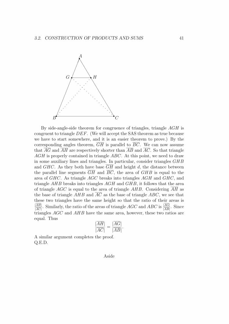
Proof: Let triangle ABC be given, r1 be the ray with end point A throughB, and r2 be the ray with end point A through C. Let G and H be thepoints on r1 and r2 respectively so that DE ≡ AG and DF ≡ AH.
3.2. CONSTRUCTION OF PRODUCTS AND SUMS 41
r
r
r
r r
����������������TTTTTTTTTTTTTTT
B
A
C
G H
p p p p pp p p p pp p p p pp p p p pp p p p p p p p p p p p p p p p p p p p
By side-angle-side theorem for congruence of triangles, triangle AGH iscongruent to triangle DEF . (We will accept the SAS theorem as true becausewe have to start somewhere, and it is an easier theorem to prove.) By thecorresponding angles theorem, GH is parallel to BC. We can now assumethat AG and AH are respectively shorter than AB and AC. So that triangleAGH is properly contained in triangle ABC. At this point, we need to drawin some auxiliary lines and triangles. In particular, consider triangles GHBand GHC. As they both have base GH and height d, the distance betweenthe parallel line segments GH and BC, the area of GHB is equal to thearea of GHC. As triangle AGC breaks into triangles AGH and GHC, andtriangle AHB breaks into triangles AGH and GHB, it follows that the areaof triangle AGC is equal to the area of triangle AHB. Considering AH asthe base of triangle AHB and AC as the base of triangle ABC, we see thatthese two triangles have the same height so that the ratio of their areas is|AH||AC| . Similarly, the ratio of the areas of triangle AGC and ABC is |AG||AB| . Since
triangles AGC and AHB have the same area, however, these two ratios areequal. Thus
|AH||AC|
=|AG||AB|
.
A similar argument completes the proof.Q.E.D.
Aside
42 CHAPTER 3. CONSTRUCTIBLE NUMBERS
Why did we put this proof in the book. First of all, why bother with theproof. Probably, we all remember this theorem from an earlier class. Let’sthink about the following, if you teach this theorem in a high school geometryclass. Why do you want students to learn it, why might you want them tosee a proof, and why might you need to know a proof? Most students thattake high school geometry will not remember this theorem when they are25, so it is unlikely that most students will need to know this fact whenthey finish their schooling. Of course, it is probably good for them to haveseen this, so if they do need it later, they can relearn it quicker. Maybe thisanswers the first question. But then, why might you want them to see theproof? Proofs in general are a useful way of thinking. Recall the words ofG. Polya, “But if he (the student) failed to get acquainted with geometricproofs, he missed the best and simplest examples of true evidence and hemissed the best opportunity to acquire the idea of strict reasoning. Withoutthis idea, he lacks a true standard with which to compare alleged evidenceof all sorts aimed at him in modern life. (paragraph) In short, if generaleducation intends to bestow on the student the ideas of intuitive evidenceand logical reasoning, it must reserve a place for geometric proofs.” Polya’sargument is that students don’t need to know all geometric facts, but theyneed to be acquainted with the proof.
Another reason for looking at this particular proof, is that in discussingit, we can illustrate two useful techniques hidden inside of the proof. Themain idea of the proof is to use area to talk about length, even though thereis no obvious area to consider at the outset. Thus the proof illustrates thepossible benefit of changing the problem at hand so that we can apply otherideas to it. This method of problem solving is useful not only in mathematics,but also in solving any difficult problem. The second technique is to considerauxiliary triangles, that is we drew a line that did not appear in the originalproblem. This technique is extremely helpful in solving geometric problems.
Let’s think about algebra now. The whole idea behind the use of variablesin algebra is that it allows us to solve many equations at the same time.Hence, a common trick is to solve a problem with simple numbers, and thenchange some of the numbers to variables. Here we are eliminating informationto solve many problems. However, often what one does is to assign variablesspecific values, solve the specific problems, and then attempt to put thevariables back in step by step. In this case, we add in extra information thatmakes the problem easier to solve.
Leaving the mathematical domain, think about what we do when giving
3.2. CONSTRUCTION OF PRODUCTS AND SUMS 43
directions to people. We often add in extra information to make it easier forthem to follow the directions. Of course, we call these landmarks.
None of these ideas can come out however, if you don’t discuss the proof,either while doing it, or after you have completed the proof. Thus, whenteaching something like the AAA proof, it is worthwhile to point out whattechniques make the proof possible. In particular, after concluding a prooflike this, it will help the students immensely if you go back and help themsee what in the proof is worth looking at for review.
End of the Aside
From the AAA-theorem, we can now construct similar triangles, one hav-ing sides of length 1 and a, and the other having corresponding sides of lengthb and x. The length of x must then be a · b giving our product. It is leftto the reader to find a technique for the quotient. Of course, constructingsums and products of constructible lengths is easy. So, what does this mean?Before finishing, let us define a negative number x to be constructible if |x| isconstructible. Now, we can construct products, sums, differences, and divideby non-zero numbers. Thus:
Theorem 3.3 The set of constructible numbers forms a field.
We already know that the set of constructible numbers is larger than theset of rational numbers. Does it cover all the real numbers? In the rationalcase, we discovered that there were rational numbers that didn’t have arational square root. Let our first goal be to show that every constructiblenumber has a constructible square root.
Theorem 3.4 If a is a constructible number, then so is√a.
Proof: We will outline the steps of the construction here and leave thedetails for the reader. Since we can construct a segment of length a, we canconstruct a segment of length 1 + a, which we will denote AB, letting Cbe the point on this segment such that |AC| = 1 and |CB| = a. Let O be
the midpoint of the segment |AB|, which we can construct by bisecting thesegment. At this point we can construct the circle centered at O through the
44 CHAPTER 3. CONSTRUCTIBLE NUMBERS
points A and B. Let ` be a line perpendicular to AB and let D be the pointof intersection of ` and the circle. By homework 11, angle 6 ADB is a rightangle. Then by homework problem 12 |DB| =
√a.
Q.E.D.
3.3 Number Fields and Vector Spaces
Our main goal in this section is to examine whether there are any limits onwhat numbers we can construct. This study has great historical significance.The ancient Greeks asked the questions of whether you could trisect a generalangle with straightedge and compass, whether you could double the cubewith straightedge and compass, and whether you could square the circlewith straightedge and compass. Let us take these one at a time and see whatthey mean.
To trisect the general angle means to give an algorithm using a straight-edge and compass that will given the input of an angle, produce an angleof measure one third the first angle. This problem seems least clearly asso-ciated to what numbers we can construct, but as we shall see later, usingangle sum identities for the cosine, we can turn this question into one aboutconstructing lengths.
The proper statement of the doubling the cube question is: Given asegment congruent to the side of a cube, use a straightedge and compassto construct a segment congruent to the side of a cube of twice the volumeof the original. Thus, if the first segment has length a, and thus the cubehas volume a3, we wish to construct a segment of length b so that b3 = 2a3.Thus, if a is chosen to be 1, b would need to be 3
√2. Hence, the question of
doubling a cube is equivalent to the question: Given a unit segment, can weconstruct a segment of length 3
√2?
Squaring the circle is shorthand for the problem of given the radius ofa circle, can you construct a line segment so that a square having sidescongruent to your segment would have the same area as the circle. Givena circle of radius 1, this is equivalent to constructing
√π. As π is a more
complicated number than 2, we would expect this to be a significantly harderproblem.
While the Greeks could not solve these problems, and indeed, the last ofthem was only solved in the late 19th century, that isn’t to say that theydidn’t know how to do them with other tools. Indeed, using conic sections
3.3. NUMBER FIELDS AND VECTOR SPACES 45
and other curves, they were able to solve these problems (see [?] for referencesto early proofs for example). They simply could not solve them using theconstraints of a straightedge and compass.
Tackling these problems requires a surprising amount of sophistication.The proofs are complicated enough that they are hard to explain to non-mathematicians. Ideally, however, prospective teachers should be able to atleast broach the subject with their students, particularly as many studentsfind the existence of impossibility proofs to be fascinating. So, let us beginby reviewing necessary material.
We say that a subset of the complex numbers is a number field if itis closed under addition, subtraction, multiplication, non-zero division, andcontains at least one non- zero element. Recall that a pair (V,+) is anadditive set if V is a non-empty set and + is a binary map from V × V toV . Given a number field F , an additive set (V,+) and a binary operation· : F × V → V , we say that V is a vector space over F if
1. For all u, v ∈ V , u+ v = v + u (+ is commutative);
2. For all u, v, w ∈ V , (u+ v) + w = u+ (v + w) (+ is associative);
3. The set V has a unique zero vector 0.
4. For all v ∈ V there is a unique element v′ ∈ V such that u+ v = 0.
5. For all a, b ∈ F and v ∈ V , a · (b · v) = (ab) · v;
6. For all a, b ∈ F and v ∈ V , (a+ b) · v = a · v + b · v;
7. For all a ∈ F and u, v ∈ V , a · (u+ v) = a · u+ a · v;
8. For all v ∈ V , 1 · v = v.
There are several other basic properties that we want. From this set ofaxioms, however, we can prove these conditions. For example, 0 · v = 0 forall v ∈ V . To see this, note that 0 · v = (0 + 0) · v = 0 · v + 0 · v by number6 above. Letting v′ be the additive inverse of v, by adding v′ to both sides,we obtain that 0 = 0 · v + 0 = 0 · v. Similarly, we can deduce that a · 0 = 0for all a ∈ F and (−1) · v = v′, that is that −1 · v is the additive inverse ofv. Consequently, we actually use −v rather than v′ in general.
For our purposes, we will often write 0 for the zero-vector unless it willlead to confusion.
46 CHAPTER 3. CONSTRUCTIBLE NUMBERS
Now suppose we are given two number fields E and F with F ⊆ E.Our main tool will be to turn E into a vector space over F . How do wedo this? Consider what we really need to make E a vector space over F ,an addition operation on E and a “multiplication” operation for elements ofF with elements of E. We already have these, namely the field addition ofE will be our addition, and the field multiplication of E certainly works asmultiplication of an element of F with an element of E.
Theorem 3.5 If F and E are number fields with F ⊆ E, then E is a vectorspace over F .
Mathematicians refer to what we are doing as applying a “forgetful” op-eration. Namely, we are forgetting some of the information given to us. Asone mathematician said, “Mathematics is the art of forgetting the right in-formation at the right time.” Why do we want to forget the information?Because vector spaces are a tool that mathematicians know a lot about. Inparticular, we have many tools with which to study vector spaces, as we shallsee.
If E is a vector space over F , a set of vectors {v1, . . . , vn} ⊂ E is linearindependent over F if
n∑i=1
aivi = 0
implies ai = 0 for all i. If a set is not linearly independent, we say that it islinearly dependent.
We say that a set {v1, . . . , vn} ⊂ E spans E over F if the set
{n∑i=1
aivi | ai ∈ F} = E.
The set B = {v1, . . . , vn} is then a basis for E over F if B is a linearlyindependent spanning set. One can extend these definitions to allow forinfinite bases and infinite spanning sets, although we will not do that here.An important theorem of linear algebra then states
Theorem 3.6 If V is a vector space over F , then there exists a basis for Vover F . Moreover, every such basis has the same cardinality.
We define the dimension of E over F to be the cardinality of any basis forE over F , feeling comfortable that this is well defined by the above theorem.
3.3. NUMBER FIELDS AND VECTOR SPACES 47
Other ways of defining the dimension that you may have learned in linearalgebra (at least in finite cases) is that the dimension is the size of a maximallylinearly independent set over F , or a minimal spanning set. The dimensionof a vector space is one of the important invariants we shall analyze.
At this point, let us consider an example. We will take the rationals Qfor our ground field, and let
E = Q[√
2] = {a+ b√
2 | a, b ∈ Q}.
To see that E is actually a field, we need to check that it is closed underaddition, subtraction, multiplication, and non-zero division. Except for di-vision these are all straightforward. For division, however, we just use theprocess of rationalizing the denominator (this being one of the few times acollege professor will have you rationalize a denominator). That is,
(a+ b√
2)/(c+ d√
2) =ac− 2bd
c2 − 2d2+bc− adc2 − 2d2
√2.
To be sure that this is actually an element of our field E, we need to knowthat c2 − 2d2 6= 0, but if it did, then we would have
√2 = c/d, a rational
number, contradicting the irrationality of√
2. Thus E is a field. What is abasis for E over Q. The obvious basis is the pair {1,
√2}. There are other
bases, though. For example {1 +√
2, 1−√
2} and {2 + 7√
2, 3 +√
2} are alsobases for E over Q. In this case, we have that E is 2-dimensional over Q.
When F ⊆ E are number fields, we say that E is a field extension of F ,and we define the degree of E over F to be the dimension of E as a vectorspace over F . We write these as
[E : F ] = dimF (E).
Let’s do a couple more examples. This time, let
E = Q[3√
2] := {a+ b3√
2 + c3√
4 | a, b, c ∈ Q}.
Again, it is fairly easy to check addition, subtraction, and multiplication.This time, it is a lot more complicated to check on how to divide. In par-ticular, what is 1/(3 + 3
√2− 5 3
√4)? In high school, you were never asked to
rationalize this denominator, yet you can. (Actually, there was one ratherannoying boy in my algebra II class who asked how to rationalize this de-nominator.) The annoying answer is that you just multiply top and bottom
48 CHAPTER 3. CONSTRUCTIBLE NUMBERS
by 19 + 47 3√
2 + 16 3√
4, and if we do this, we get −381 so that
1
3 + 3√
2− 5 3√
4=−19
381+−47
3813√
2 +−16
3813√
4.
That was of course “magic”, and the first time most high school studentssee it, rationalizing quadratic denominators also seem like magic. (As abrief aside, rationalizing denominators is one of the things that is thankfullyleaving the curriculum. It is rarely used and is generally taught as a purealgorithm. The reason why we might have wanted it on the other hand isthat it gives students practice on understanding the value of knowing thedifference of squares factorization.)
So how did we come up with this magic number above? There are twotypical ways to do it. The first you probably learned and promptly forgot inabstract algebra. It involved factor rings of Q[x] by the ideal (x3 − 2). Thesecond way involves matrix theory. We will do both.
Method 1 (The Euclidean Algorithm for Polynomials): In abstract al-gebra, you learned that if p(x) is an irreducible polynomial in Q[x] and (p(x))denotes the ideal of all multiples of p(x), then the factor ring Q[x]/(p(x)) isisomorphic to Q[a] where a is a root of p(x) (and Q[a] denotes the smallestring containing the rational numbers and a). The idea is that we define poly-nomials f(x) and g(x) to be equivalent if p(x)|(f(x)−g(x)) (just like we definemodular arithmetic). In particular, every polynomial f(x) is equivalent to itsremainder rf (x) upon division by p(x). Thus any polynomial is equivalent toa polynomial of the for a0 + a1x + . . . + an−1x
n−1, where deg(p(x)) = n.The main theorem you then proved was that if f(x) ≡ g(x)mod p andh(x) ≡ k(x)mod p, then f(x) +h(x) ≡ g(x) + k(x) and f(x)h(x) ≡ g(x)k(x)modulo p(x) (again, just like in modular arithmetic). Thus Q[x]/(p(x)) is awell-defined commutative ring.
The question that arises is when is this a field. Well, since p(x) isirreducible, if f(x) ∈ Q(x) is not equivalent to the 0 polynomial, thenp(x) 6 |f(x), so the greatest common divisor of p(x) and f(x) is 1. Finally,you had a theorem which said that if d(x) was the greatest common divi-sor of p(x) and f(x), then there existed polynomial r(x) and s(x) such thatp(x)r(x) + f(x)s(x) = d(x), and hence in this case, f(x)s(x) ≡ 1 modulop(x), so that s(x) is the “inverse” of f(x). We use the quotation here be-cause, neither f(x) nor s(x) is actually an element of Q[x]/(p(x)), but rather
3.3. NUMBER FIELDS AND VECTOR SPACES 49
they represent equivalence classes of elements (just like fractions representequivalence classes of elements of the rationals).
To find s(x), you then enact the Euclidean Algorithm as we are about todo. The difficulty here is that the denominators become truly terrible. Inour case above, p(x) = x3− 2, and the correspondence is that a+ b 3
√2 + c 3√
4corresponds to the polynomial a + bx + cx2, since x is a root of p(x) inQ[x]/(p(x)). Thus, our case has f(x) = 3 + x − 5x2. Since this case willgive very ugly fractions, let us see how everything should work with an easierelement. For example, suppose we want to invert 3 + 3
√2. This corresponds
to the function g1(x) = x+ 3, and the division algorithm gives:
x3 − 2 = (x2 − 3x+ 9)(x+ 3)− 29
Thus 29 = −(x3 − 2) + (x + 3)(x2 − 3x + 9), so that 1 = − 129
(x3 − 2) +
(x + 3)( 129x2 − 3
29x + 9
29), giving (3 + 3
√2)−1 as 9
29− 3
293√
2 + 129
3√
4. It turnsout that despite all appearances, this is a much simpler case than what westarted with. Using g(x) = −5x2 + x+ 3 now, the first step of the Euclideanalgorithm yields
x3 − 2 = (−1
5x− 1
25)(−5x2 + x+ 3) + (
16
25x+−47
25).
Of course, the fractions get worse in the next step, at which point we get
−5x2 + x+ 3 = (16
25x+−47
25) ∗ (−125
16x− 5475
256)− 9525
256.
Of course, now we plug back in to find out what s(x) and t(x) should be sothat we get the desired inverse. Clearly this is a job that should be done bya computer, not a human, and resorting to such, we have modulo x3−2 that
(−5x2 + x+ 3) = ((−125
16x− 5475
256)(
1
5x+
1
25)− 1) ∗ 256
25 · 381.
When the dust settles, this last is equal to
− 16
381x2 − 47
381x− 19
381.
Method 2 (Matrices): Fortunately, there is a way that let’s us use our TI-83 calculators, and lets us bypass a lot of the messy calculations. To do this

50 CHAPTER 3. CONSTRUCTIBLE NUMBERS
we us, another way of expressing this field Q[√
2] that uses linear algebra.Recall for a vector space V over a field F , a map f : V → V is lF -inear if
f(au+ bv) = af(u) + bf(v)
for all a, b ∈ F and u, v ∈ V . It is easy to check (do so!) that if E and F arenumber fields with F ⊆ E and α ∈ E, then multiplication by α (applying φα)is an F - linear map of the vectors space E over F . Namely, for all a, b ∈ Fand u, v ∈ E, the map φα(x) = α(x) has the property that
φα(au+ bv) = α(au+ bv) = a(αu) + b(αv).
Given an F -basis for E, any F -linear map uniquely corresponds to a matrix.If follows that if we choose a basis, φα can be represented by a unique matrixover F .
Let’s do another example. Suppose F is the set of real numbers, andthat E is the set of complex numbers. An R-basis for C is {1, i}. Let theα = 3− i. At this point take a few minutes and try and work out for yourselfwhat the corresponding matrix for α is.
There are two possible answers, depending on whether you like your ma-trices to multiply on the left or the right. The traditional way is to write thefunction on the left, so let us do that. Again, let us return to linear algebra.Given a basis {v1, . . . , vn}, and a linear map f , the corresponding matrixfor f is (aj,k), where f(vj) =
∑nk=1 aj,kvk. In the case above, v1 = 1, v2 = i,
f(v1) = f(1) = 3+(−1)i, and f(v2) = f(i) = 1+3i. Thus a1,1 = 3, a2,1 = −1,
a1,2 = 1, and a2,2 = 3. Thus the corresponding matrix is
(3 1−1 3
). You
should check that the corresponding matrix for the complex number a+ bi is(a −bb a
). Probably in your abstract algebra course, you proved that the
complex numbers were isomorphic to the set of real two by two matrices ofthe above form. This linear algebra reason is why this happens.
So how does this help us with our problem of finding an inverse? In ourcase, E = Q[ 3
√2] had a natural basis (we could choose another, but it would
just make matters more confusing) of {1, 3√
2, 3√
4}, and given an elementa+ b 3
√2 + c 3
√4, the corresponding matrix is a 2c 2b
b a 2cc b a
.
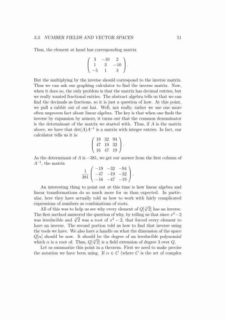
3.3. NUMBER FIELDS AND VECTOR SPACES 51
Thus, the element at hand has corresponding matrix 3 −10 21 3 −10−5 1 3
.But the multiplying by the inverse should correspond to the inverse matrix.Thus we can ask our graphing calculator to find the inverse matrix. Now,when it does so, the only problem is that the matrix has decimal entries, butwe really wanted fractional entries. The abstract algebra tells us that we canfind the decimals as fractions, so it is just a question of how. At this point,we pull a rabbit out of our hat. Well, not really, rather we use one moreoften unproven fact about linear algebra. The key is that when one finds theinverse by expansion by minors, it turns out that the common denominatoris the determinant of the matrix we started with. Thus, if A is the matrixabove, we have that det(A)A−1 is a matrix with integer entries. In fact, ourcalculator tells us it is: 19 32 94
47 19 3216 47 19
.As the determinant of A is −381, we get our answer from the first column ofA−1, the matrix
1
381
−19 −32 −94−47 −19 −32−16 −47 −19
.An interesting thing to point out at this time is how linear algebra and
linear transformations do so much more for us than expected. In partic-ular, here they have actually told us how to work with fairly complicatedexpressions of numbers as combinations of roots.
All of this was to help us see why every element of Q[ 3√
2] has an inverse.The first method answered the question of why, by telling us that since x3−2was irreducible and 3
√2 was a root of x3 − 2, that forced every element to
have an inverse. The second portion told us how to find that inverse usingthe tools we have. We also have a handle on what the dimension of the spaceQ[α] should be now. It should be the degree of an irreducible polynomialwhich α is a root of. Thus, Q[ 3
√2] is a field extension of degree 3 over Q.
Let us summarize this point in a theorem. First we need to make precisethe notation we have been using. If α ∈ C (where C is the set of complex
52 CHAPTER 3. CONSTRUCTIBLE NUMBERS
numbers) and K is subfield of C (note, just think that K = Q for now), thenby K[α] we mean the smallest subring of C containing K and α. Here wehave
K[α] = {k∑I=0
aiαI | ai ∈ K and k ∈ Z}
By K(α), we mean the smallest subfield of C containing K and α.
Theorem 3.7 If f(x) is an irreducible polynomial with coefficients in a num-ber field K, and α is a root of f(x) in C, then K(α) = K[α], and the degreeof the field extension K[α] over K is the degree of f(x).
Proof: From abstract algebra, we haveK[x]/(f(x)) ∼= K[α]. But every poly-nomial of K[x] is equivalent modulo f(x) to a polynomial of degree less thann by the division algorithm. Thus {1 + (f(x)), x+ (f(x)), . . . , xn−1 + (f(x))}spans K[x]/(f(x)) over K. Any non-zero polynomial g(x) =
∑n−1i=0 aix
i isnot divisible by f(x), so that g(x) + (f(x)) 6= 0 + (f(x)). Consequently,{1 + (f(x)), . . . , xn−1 + (f(x))} is linearly independent, and the dimension ofK[x]/(f(x)) over K is n.Q.E.D.
We are now ready to state our “big” theorem for this section. The di-mensions multiply theorem.
Theorem 3.8 If F and E are number fields with Q ⊆ F ⊆ E, then
dimQ(E) = dimQ(F ) · dimF (E).
Proof: Let {α1, . . . , αn} be a basis for F over Q, and let {β1, . . . , βm} be abasis for E over F . We will show that
B = {αiβj | i ∈ {1, . . . , n}, j ∈ {1, . . . ,m}}
is a basis for E over Q. We begin by showing that B is a linearly independentset. Suppose ∑
i,j
aijαiβj = 0,
3.3. NUMBER FIELDS AND VECTOR SPACES 53
where the aij’s are all rational numbers. Rearranging the terms in the sum-mation, we have that
0 =n∑i=1
m∑j=1
aijαiβj (3.1)
=m∑j=1
(n∑i=1
aijαi
)βj. (3.2)
Now, the set of βj is linearly independent over F , and since∑ni=1 aijαi is an
element of F as the αi’s are all in F , we have by the definition of linearlyindependence that
n∑i=1
aijαi = 0
for all j. Since the set of αi’s is linearly independent over the rationals, andthe aij’s are all rational, we then have that aij = 0 for all i and j. Hence theset B is linearly independent over Q.
We now must check that B is a spanning set for E over Q. Let x bean arbitrary element of E. Since the set of βj’s span E over F , there existelements bj ∈ F such that x =
∑mj=1 bjβj. Since the bj’s are in F and the
αi’s span F over Q, there exist aij ∈ Q such that bj =∑ni=1 aijαi for all j.
Unraveling the above equations, we have that
x =m∑j=1
bjβj (3.3)
=m∑j=1
(n∑i=1
aijαi
)βj (3.4)
=∑i,j
aijαiβj. (3.5)
Since x was an arbitrary element of E, we have that B spans E over Q. Aswe have shown that B is a linearly independent spanning set for E over Q,we have shown that B is a basis for E over Q. Since |B| = nm, we haveshown that dimQ(E) = dimQ(F ) · dimF (E).Q.E.D.
In fact, this theorem is more general than stated. We didn’t really needfor the smallest field to be the rational numbers. It could have been anysubfield of F .
54 CHAPTER 3. CONSTRUCTIBLE NUMBERS
Teaching Aside
At this point, you are probably wondering how any of this really ties into thehigh school curriculum. In a basic way, the division algorithm for polynomialsand elementary matrix theory are in the curriculum so that these points showa natural extension. On the other hand, we claim that there is more to itthan that.
In particular, one of the great question that many students ask when youdo long division of polynomials, is why should we do this? If you take a util-ity standpoint, the answer lies in the division algorithm and the Euclideanalgorithm (our first technique for inverting polynomials). Most of the error-correcting coding systems, use polynomial arithmetic extensively. In truth,this arithmetic is usually done over a finite field rather than Q, but these sys-tems require the division algorithm and the Euclidean algorithm. Similarly,most secret coding systems use the Euclidean algorithm for integers.
What about problem solving? Let’s think about how we solved the prob-lem of finding an inverse of 3 + 3
√2 − 5 3
√4. In both cases, we turned the
problem into a completely different problem that used ideas that we alreadyknew. This is an important problem solving strategy that needs to be taught.Moreover, matrices and linear algebra are one of the strongest tools to usein this way. That is, the applications of matrices are wide ranging and helpus solve many different problems.
The last issue that we would like to raise here is that the idea of multiplerepresentations is an important strand running through the NCTM stan-dards. What we have seen here is that there are three very different ways tothink about something as simple as the 3
√2, each with its own strengths and
weaknesses. Certainly, in a high school classroom, one can remember thesedifferent representations and answer the sort of questions that might requireusing one of them.End of Aside
3.4 Impossibility Theorems
The impossibility theorems for the constructibility of 3√
2 and trisecting thegeneral angle are very similar. The key to both is theorem 3.8 from theprevious section. We shall show that any time you construct a new pointon the plane using straightedge and compass, the numerical values for the
3.4. IMPOSSIBILITY THEOREMS 55
coordinates of this new point only involve the numerical values for the coor-dinates of points already known and the square roots of such values. In thelanguage above, the coordinates lie in a field of dimension 2 over the small-est field containing all previously constructed coordinates. Consequently, byTheorem 3.8, every field extension Eobtained via straightedge and compassconstruction has dimension 2n over Q. But suppose 3
√2 was constructible,
then Q[ 3√
2] would be a subfield of one of these fields E. But then Theo-rem 3.8 would imply that 3|2n, a contradiction. Thus we cannot construct3√
2. For the trisection, we do something similar. Namely, we show that ifyou can construct a 20 degree angle, then you would be able to constructa root of an irreducible cubic polynomial with rational coefficients. Again,this would imply that one of our fields E of dimension 2n would contain asubfield of dimension 3 over Q, a contradiction.
Now that we have outlined our attack, let’s fill in the gaps a little better.The first thing we need to do is to answer the following three questions:
1. Suppose you have four points A = (x1, y1), B = (x2, y2), C = (x3, y3),and D = (x4, y4), with all coordinates lying in a field E, and AB andCD intersect. What are the coordinates of the intersection point?
2. Suppose you have the same four points, and the line AB intersects thecircle with center C through point D. What are the coordinates of theintersection point?
3. Now suppose the circle with center at A through B intersects the circlewith center at C throughD, what are the coordinates of the intersectionpoint?
In all cases, you should have found out that the coordinates involve at mostthe square root of some number from the field E. (This is in-class groupwork and homework.)
Let us summarize what you just showed in a lemma.
Lemma 3.9 Let E be a subfield of the real numbers, and suppose
x1, x2, x3, x4, y1, y2, y3, y4 ∈ E.
If (x, y) is a point
1. at the intersection of the line joining (x1, y1) and (x2, y2) and the linejoining (x3, y3) and (x4, y4), then x, y ∈ E.
56 CHAPTER 3. CONSTRUCTIBLE NUMBERS
2. at the intersection of the line joining (x1, y1) and (x2, y2) and the circlewith center (x3, y3) and through (x4, y4), then there exists an elementd ∈ E such that x, y ∈ E[
√d].
3. at the intersection of the circle centered at (x1, y1) through (x2, y2) andthe circle centered at (x3, y3) through (x4, y4), then there exists d ∈ Esuch that x, y ∈ E[
√d].
At this point let us finish the proof of the impossibility theorems. Tobegin with, we now need to be precise about our terminology. We followStewart [13]. Assume that P0 is a set of points in the Euclidean plane R2,and consider operations of two kinds:
1. through any two points draw a straight line, and
2. Draw a circle centered at one point and through any other point.
A point (x, y) ∈ R2 is said to be constructible from P0, if there exist asequence of points
(x1, y1), (x2, y2), . . . , (xt, yt) = (x, y)
such that the point (xi, yi) can be obtained as the intersection point of twodistinct lines or a line and a circle or two distinct circles when drawn usingone of our two operations from the points P0∪{(x1, y1), . . . , (xi−1, yi−1)}. Wesay that (x, y) is constructible over the rationals if (x, y) is constructible overthe set P = {(a, b) | a, b ∈ Q}.
We will prove our result in a series of lemmas.
Lemma 3.10 Suppose (x, y) is constructible over the rationals via the se-quence (x1, y1), (x2, y2), . . . , (xt, yt) = (x, y). Define Ki = Q[x1, y1, . . . , xi, yi]to be the smallest field containing Q and the numbers x1, y1, x2, . . . , yi. ThenKi = Ki−1[
√a] for some a ∈ Ki−1.
Proof: This follows from Lemma 3.9.Q.E.D.
Lemma 3.11 Using the notation of the proceeding Lemma, we have dimKi−1Ki
is 1 or 2.
3.4. IMPOSSIBILITY THEOREMS 57
Proof: By the preceding lemma, Ki = Ki−1[√
(a)] for some a ∈ Ki−1. Thus,
x2 − a is either an irreducible polynomial over Ki−1 or√a ∈ Ki−1. By
Theorem 3.7, we have dimKi−1Ki is either 1 or 2.
Q.E.D.
We now define a real number α to be constructible if (α, 0) is constructibleover Q.
Theorem 3.12 Suppose x is a constructible number. Then [Q(x) : Q] is apower of 2.
Proof: As x is constructible, there exists a sequence of points
(x1, y1), (x2, y2), . . . , (xt, yt) = (x, 0)
as in the definition of a constructible point (x, 0). Let Ki be defined as before.Then x ∈ Kt. We now prove by induction on i that Ki has dimension a powerof 2 over Q. Since K0 = Q, it has dimension 1 = 20 over Q establishing thebasis step. Suppose i > 0 and that Ki−1 has dimension 2l over Q for some l.By Lemma 3.11, we have dimKi−1
Ki is 1 or 2. Consequently, by the degreesmultiply theorem, it follows that dimQ(Ki) is equal to 2l times one or two,and hence is again a power of two. By induction, dimQ(Kt) = 2l for some l.
As x ∈ Kt, it follows that Q(x) is a subfield of Kt. The degrees multiplytheorem then implies that dimQ(Kt) = dimQ(Q(x)) · dimQ(x)(Kt). ThusdimQ(Q(x)) divides dimQ(Kt) = 2l. Thus dimQ(Q(x)) = [Q(x) : Q] mustalso be a power of 2.Q.E.D.
Theorem 3.13 The 3√
2 is not constructible.
Proof: We have already seen that [Q( 3√
2) : Q] = 3. Thus Theorem 3.12implies 3
√2 is not constructible.
Q.E.D.
Question: Can you find an irreducible polynomial satisfied by cos(20◦)?Think about how one can use the angle sum formulas and the knowledgethat cos(60◦) = .5 to find an equation that cos(20) is a root of. (In classhomework assignment).
58 CHAPTER 3. CONSTRUCTIBLE NUMBERS
Based on your answer to the last problem, you should have discovered thatcos(20) is the root of an irreducible cubic polynomial with integer coefficients.This implies by our previous arguments that cos(20) cannot be constructed.
Theorem 3.14 There does not exist an algorithm which can trisect a 60◦
angle with straightedge and compass.
Proof: Suppose there did exist such an algorithm. As an equilateral trianglecan be constructed, we can construct a 60◦ angle. Consequently, we couldconstruct a 20◦ angle. From this it follows that we can construct a linemaking a 20◦ angle with the x-axis of length 1 from the origin. Thus, asin the picture below, by dropping a perpendicular, we can construct the
point (cos(20), 0), implying that cos(20) is constructible. Having achieved acontradiction, we see that we cannot trisect a 60◦ angle.Q.E.D.
3.5 Regular n-gons
One of the great feats of Gauss was to discover with proof, which of theregular n-gons can be constructed with straightedge and compass. Unfortu-nately, the proof of Gauss’s result goes beyond the scope of this book, butlet us,but let us at least state the result.
Theorem 3.15 A regular n-gon can be constructed with straightedge andcompass if and only if n = 2k1p1p2 . . . pt, where k1 is a non-negative integer,and the pis are distinct Fermat primes.
A Fermat prime is a prime number of the form 22s + 1, so that 3, 5, 17, 257,and 65537 are the first four Fermat primes. Thus, a regular 17-gon can beconstructed, but a regular 9-gon cannot. Briefly, the proof of this theoremseems to require Galois theory or mathematics at roughly the same level,and the interested reader is encouraged to look at [13].
It turns out that we have already handled the question of the regular 9-gon since constructing such a figure would require constructing a 40◦ exteriorangle which could then be bisected to produce a 20◦ angle, a contradiction.
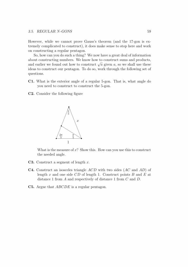
3.5. REGULAR N -GONS 59
However, while we cannot prove Gauss’s theorem (and the 17-gon is ex-tremely complicated to construct), it does make sense to stop here and workon constructing a regular pentagon.
So, how can you do such a thing? We now have a great deal of informationabout constructing numbers. We know how to construct sums and products,and earlier we found out how to construct
√a given a, so we shall use these
ideas to construct our pentagon. To do so, work through the following set ofquestions.
C1. What is the exterior angle of a regular 5-gon. That is, what angle doyou need to construct to construct the 5-gon.
C2. Consider the following figure
r r
r
�����������
LLLLLLLLLLL
rp p p p p p p p p p p p p p p p p p p p p p p p p p p p p p p p p p p p p p p p
π5
2π5
π5
1
x
What is the measure of x? Show this. How can you use this to constructthe needed angle.
C3. Construct a segment of length x.
C4. Construct an isosceles triangle ACD with two sides (AC and AD) oflength x and one side CD of length 1. Construct points B and E atdistance 1 from A and respectively of distance 1 from C and D.
C5. Argue that ABCDE is a regular pentagon.
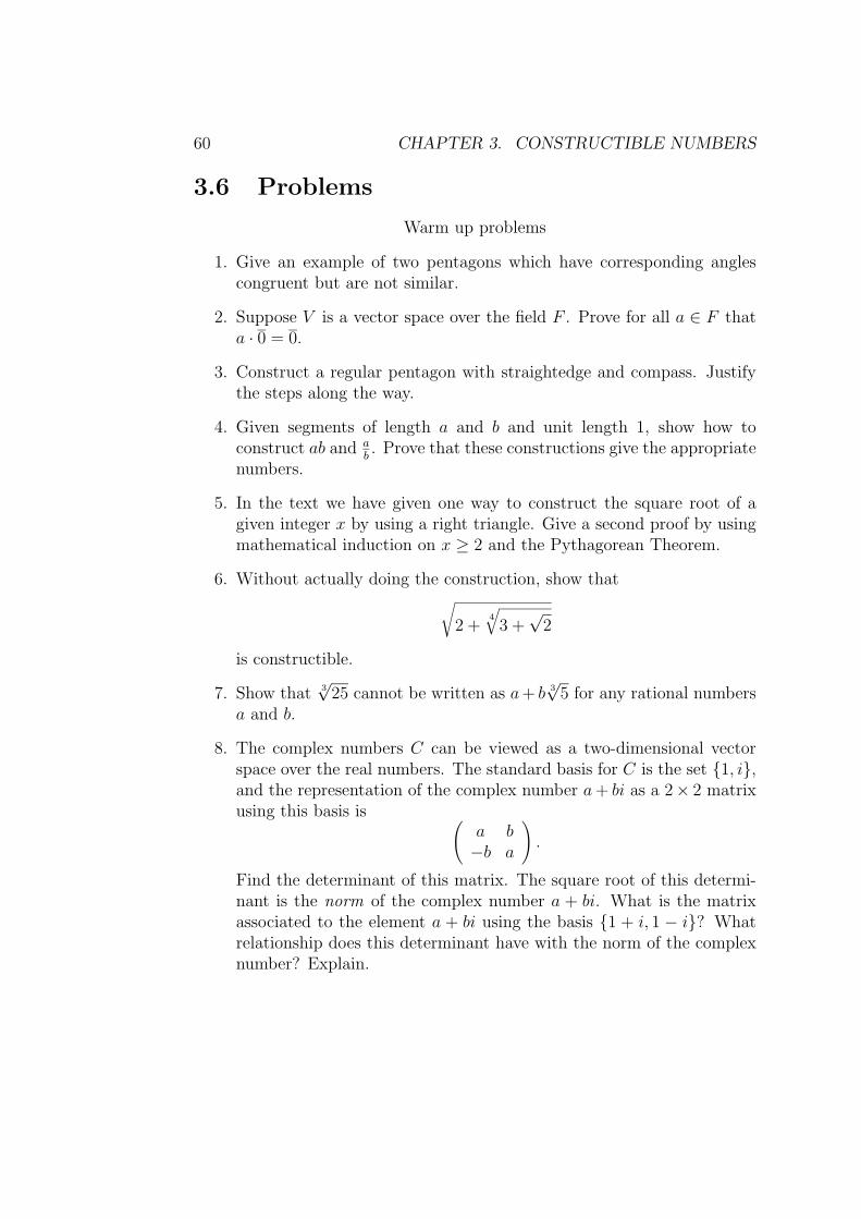
60 CHAPTER 3. CONSTRUCTIBLE NUMBERS
3.6 Problems
Warm up problems
1. Give an example of two pentagons which have corresponding anglescongruent but are not similar.
2. Suppose V is a vector space over the field F . Prove for all a ∈ F thata · 0 = 0.
3. Construct a regular pentagon with straightedge and compass. Justifythe steps along the way.
4. Given segments of length a and b and unit length 1, show how toconstruct ab and a
b. Prove that these constructions give the appropriate
numbers.
5. In the text we have given one way to construct the square root of agiven integer x by using a right triangle. Give a second proof by usingmathematical induction on x ≥ 2 and the Pythagorean Theorem.
6. Without actually doing the construction, show that√2 +
4√
3 +√
2
is constructible.
7. Show that 3√
25 cannot be written as a+ b 3√
5 for any rational numbersa and b.
8. The complex numbers C can be viewed as a two-dimensional vectorspace over the real numbers. The standard basis for C is the set {1, i},and the representation of the complex number a+ bi as a 2× 2 matrixusing this basis is (
a b−b a
).
Find the determinant of this matrix. The square root of this determi-nant is the norm of the complex number a + bi. What is the matrixassociated to the element a + bi using the basis {1 + i, 1 − i}? Whatrelationship does this determinant have with the norm of the complexnumber? Explain.
3.6. PROBLEMS 61
9. Is 5√
45 constructible.
10. Given a triangle provide the constructions for inscribing a circle withinthe triangle and circumscribing a circle about the triangle.
Advanced Problems
11. In the next problem, we show how to construct√a given a unit length
and a length a. To do this we will use the theorem from Euclideangeometry which states: if an angle A is inscribed in a circle, then thearc cut off by A has measurement 2|A| where |A| denotes the radianmeasure of A. Prove this.
12. Given the following picture, prove that |DB| =√|CB|, given that the
circle centered at O through A, also runs through C and D.
rr r rr
�����HHHH
HHHHHH
OA C
B
D
1
13. Without actually doing the construction show that(4√
3 +√
7 +√
5)(
8√√
3 +√
5 + 2)
is constructible.
14. Suppose a line defined by two points with coordinates in a field F isintersected with a circle having center with coordinates in F and radiusin F . Prove that the points of intersection have coordinates in a fieldF ′ which is two dimensional over F .
15. Prove without working too hard that Q[√
2, 3√
2] is a field of dimension6 over the rational numbers.
62 CHAPTER 3. CONSTRUCTIBLE NUMBERS
16. Find the multiplicative inverse of the number x = 1 + 2 3√
3 + 2 3√
9, andprove that your answer is correct.Hint: To do this, you simply need to come up with a candidate for theinverse and multiply the two numbers together and see that you get 1.To find a candidate you should follow the steps given:
(a) Using the basis {1, 3√
3, 3√
9} for the field Q[ 3√
3] over the field Q,write the 3 × 3 matrix M corresponding x viewed as a lineartransformation from Q3 to Q3.
(b) Use Gaussian elimination to find the inverse of the matrix M .
(c) Find the element y of Q[ 3√
3] corresponding to M . Now multiplyx and y to check that xy = 1.
17. If we take the basis of {1,√
3,√
5,√
15} for the field Q[√
3,√
5] over Q,then what is the matrix associated to the element 2 +
√3−√
15 of thisring? What is the inverse of this element?
18. Let n be an integer. Find necessary and sufficient conditions that anangle of n degrees can be constructed with straightedge and compass.(Hint, show that a 3◦ angle can be constructed and that a 2◦ anglecannot be constructed with straightedge and compass.)
Chapter 4
Solving Equations by Radicals
In the last chapter we proved that 3√
2 is not a constructible number. Obvi-ously, we might do somewhat better if we used different tools of construction.In fact, the ancient Greeks knew how to trisect the general angle if they wereallowed to use extra tools. Similarly, they could construct cube roots usingother tools. Today, one of the methods used to do constructive type geome-try in the schools is by allowing the construction tools that you have whenpaper folding. It has been shown that using paper folding, it is possible toconstruct 3
√2. Nevertheless, for each of these expanded definitions of con-
struction tools, a proof similar to the one given in the last chapter will showthat there exists some numbers that cannot be constructed. In fact, in all ofthese cases, the proof shows that there is some nth root of 2 that cannot beconstructed.
On the other hand, we have an algebraic definition for the number n√
2.Thus, we can ask, can we get all real numbers via combinations of radicals.By this, we mean is it the case that any real number can be written using justthe operations of addition, subtraction, multiplication, division, and takingan nth root, together with the rational numbers? It is certainly true that wecan get a lot of numbers this way that we couldn’t get via constructions. Forexample,
7
√2
3− 9√
5 +3√
2
is one such number. Can this be everything? As a simpler question, wemight ask simply, can we solve every algebraic equation that has real rootsthis way? (We could even go so far as to ask the question for complex
63
64 CHAPTER 4. SOLVING EQUATIONS BY RADICALS
roots since after all, i =√−1). While on the face of it, this question might
look straightforward, many great mathematicians had difficulty with thisquestion. For example, Euler wrote at least one article in which he suggestedthat this should be the case, but there was a mistake found in his work.
Since we know that every linear equation with rational coefficients canbe solved over the rational numbers, the first interesting case for us will bethe quadratic equation. You should start by working through the followingproblem:Derive the quadratic formula.
Chances are that your derivation looks something like the following:
Derivation of the Quadratic Formula: Suppose ax2 + bx+ c = 0 wherea, b, and c are real numbers with a 6= 0. Subtracting c from both sides, thisis equivalent to
ax2 + bx = −c.Dividing both sides of the equation by a, our original equation is then equiv-alent to
x2 +b
ax =−ca.
At this point, we add ( b2a
)2 to both sides so that the left hand side of theequation is a perfect square. Thus x solves our original equation if and onlyif x solves
x2 +b
ax+ (
b
2a)2 =
−ca
+ (b
2a)2.
The right hand side of this equation is then (x+ b2a
)2, so that
x+b
2a= ±
√−ca
+ (b
2a)2.
Thus x is a root of our original equation if and only if
x =−b2a±√−ca
+ (b
2a)2
=−b2a±
√√√√−4ac
(2a)2+
b2
(2a)2
=−b2a± 1
2a
√−4ac+ b2
=−b±
√b2 − 4ac
2a.
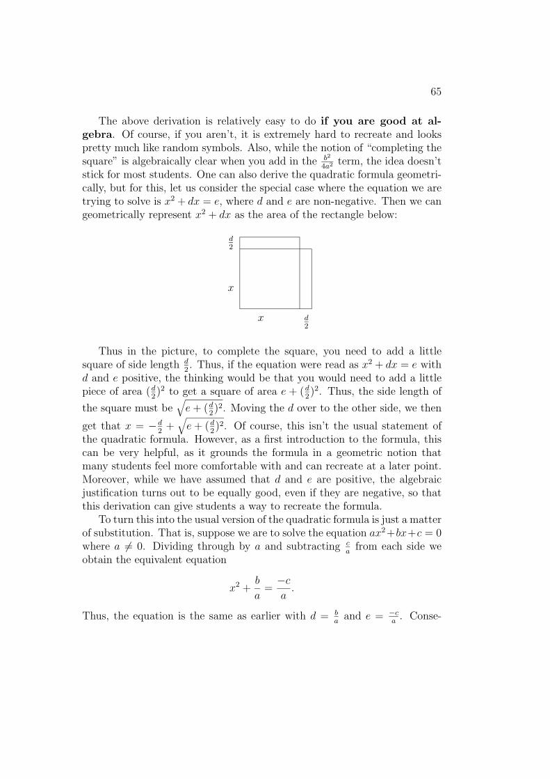
65
The above derivation is relatively easy to do if you are good at al-gebra. Of course, if you aren’t, it is extremely hard to recreate and lookspretty much like random symbols. Also, while the notion of “completing thesquare” is algebraically clear when you add in the b2
4a2 term, the idea doesn’tstick for most students. One can also derive the quadratic formula geometri-cally, but for this, let us consider the special case where the equation we aretrying to solve is x2 + dx = e, where d and e are non-negative. Then we cangeometrically represent x2 + dx as the area of the rectangle below:
x
x
d2
d2
Thus in the picture, to complete the square, you need to add a littlesquare of side length d
2. Thus, if the equation were read as x2 + dx = e with
d and e positive, the thinking would be that you would need to add a littlepiece of area (d
2)2 to get a square of area e + (d
2)2. Thus, the side length of
the square must be√e+ (d
2)2. Moving the d over to the other side, we then
get that x = −d2
+√e+ (d
2)2. Of course, this isn’t the usual statement of
the quadratic formula. However, as a first introduction to the formula, thiscan be very helpful, as it grounds the formula in a geometric notion thatmany students feel more comfortable with and can recreate at a later point.Moreover, while we have assumed that d and e are positive, the algebraicjustification turns out to be equally good, even if they are negative, so thatthis derivation can give students a way to recreate the formula.
To turn this into the usual version of the quadratic formula is just a matterof substitution. That is, suppose we are to solve the equation ax2 +bx+c = 0where a 6= 0. Dividing through by a and subtracting c
afrom each side we
obtain the equivalent equation
x2 +b
a=−ca.
Thus, the equation is the same as earlier with d = ba
and e = −ca
. Conse-
66 CHAPTER 4. SOLVING EQUATIONS BY RADICALS
quently, our earlier solution tells us that
x = −d2±√e+ (
d
2)2
= − b
2a±√−ca
+ (b
2a)2
= − b
2a±√−ca
+ (b2
4a2)
= − b
2a±√b2 − 4ac
4a2
= − b
2a±√b2 − 4ac
2a
as desired.Of course, when solving a quadratic equation with this approach, it might
make more sense (at least initially) to solve it step by step rather than applythe formula. For example, given the equation 2x2 + 5x− 8 = 0, the first stepis to divide the equation through by 2, yielding x2 + 5
2x−4 = 0. At this point
we can apply our reduced quadratic formula with d = 52
and e = 4, yielding
x = −5
4±√
4 +(
5
4
)2
= −5
4±√
4 +25
16
= −5
4±√
89/16
=−5±
√89
4.
In truth, one can skip the last three lines here as the first statement is correct,it just isn’t simplified in the standard way. Of course, depending on whatyou want the answer for, it doesn’t need to be simplified.
4.1 Solving Simple Cubic Equations
Now, let us think about these geometric methods and what they might meanin three dimensions. Consider a cube of side length u, with a little cube cut
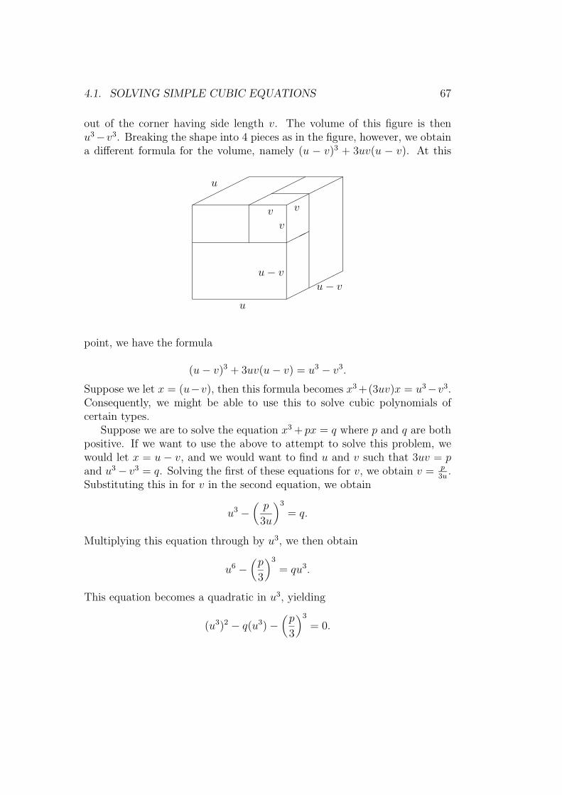
4.1. SOLVING SIMPLE CUBIC EQUATIONS 67
out of the corner having side length v. The volume of this figure is thenu3−v3. Breaking the shape into 4 pieces as in the figure, however, we obtaina different formula for the volume, namely (u − v)3 + 3uv(u − v). At this
point, we have the formula
������
������
������
������
���
u
vv
v
u− vu− v
u
(u− v)3 + 3uv(u− v) = u3 − v3.
Suppose we let x = (u−v), then this formula becomes x3 +(3uv)x = u3−v3.Consequently, we might be able to use this to solve cubic polynomials ofcertain types.
Suppose we are to solve the equation x3 + px = q where p and q are bothpositive. If we want to use the above to attempt to solve this problem, wewould let x = u − v, and we would want to find u and v such that 3uv = pand u3− v3 = q. Solving the first of these equations for v, we obtain v = p
3u.
Substituting this in for v in the second equation, we obtain
u3 −(p
3u
)3
= q.
Multiplying this equation through by u3, we then obtain
u6 −(p
3
)3
= qu3.
This equation becomes a quadratic in u3, yielding
(u3)2 − q(u3)−(p
3
)3
= 0.
68 CHAPTER 4. SOLVING EQUATIONS BY RADICALS
We can now use the quadratic formula to obtain a value for u3. Namely,
u3 =q
2±√(
q
2
)2
+(p
3
)3
.
Hence
u =3
√√√√q
2±√(
q
2
)2
+(p
3
)3
.
We can now plug the value for u3 into the equation u3 − v3 = q to obtainthat
v3 =q
2±√(
q
2
)2
+(p
3
)3
− q
= −q2±√(
q
2
)2
+(p
3
)3
.
Thus, taking the cube root, we obtain that
v =3
√√√√−q2±√(
q
2
)2
+(p
3
)3
.
As the quantity under the square root sign is necessarily positive, once wechoose which of the square roots we use for u, we get a unique real solution.Suppose for the time being that for u we take the positive square root. Asx = u− v, we end up with the solution:
x =3
√√√√q
2+
√(q
2
)2
+(p
3
)3
− 3
√√√√−q2
+
√(q
2
)2
+(p
3
)3
.
Curiously, as you will show in homework ??, choosing the other sign for uyields the same answer for x. This technique gives us at least one solutionto the equation in the case where p and q are both non-negative.
Example 1: Consider the equation x3 + 2x = 8. In this case, p = 2 andq = 8. Using our formula, we have
x =3
√√√√4 +
√42 + (
2
3)3 − 3
√√√√−4 +
√42 + (
2
3)3
4.1. SOLVING SIMPLE CUBIC EQUATIONS 69
=3
√√√√4 +
√16 +
8
27− 3
√√√√−4 +
√16 +
8
27
=3
√√√√4 + 2
√4 +
2
27− 3
√√√√−4 + 2
√4 +
2
27.
Example 2: Consider the equation x3 + 3x = 14. In this case, p = 3 andq = 14. For the given solution above, we have p
3= 1 and q
2= 7. Thus a real
solution is given by
x =3√
7 +√
72 + 13 −√−7 +
√72 + 13.
Simplifying this expression, we see that
x =3√
7 + 5√
2− 3√−7 + 5
√2.
Before going on and trying to pull out a factor from our equation above sothat we can use the quadratic formula, let us take a minute and see if we cansimplify this term at all. If we plug this into our calculator, we find that itis so close to 2 that our calculator thinks it is 2. So, we have to ask, is it 2?
We have actually discussed a question like this before. If it is 2, then we
would know that {1, 3√
7 +√
72 + 13,√−7 +
√72 + 13} is a linearly depen-
dent set over Q. (Of course, if it isn’t 2, that does not establish that the setis independent.) Now that we know we have seen the question before, doesthat help us solve it? Well, not really. The difficulty is that we need to findout whether there is an easier way of writing the cube root of 7 + 5
√2. We
might guess that the cube root should have the form a+b√
2 for two rationalnumbers a and b. If so, then we would know that (a + b
√2)3 = 7 + 5
√2.
On the bright side, we can actually cube the left hand side. Doing this, weobtain
7 + 5√
2 = a3 + 3a2b√
2 + 3a(b√
2)2 + (b√
2)3
= a3 + 3a2b√
2 + 3ab2 · 2 + 2b3√
2
= a3 + 6ab2 + (3ab2 + 2b3)√
2.
Since we know that {1,√
2} is linearly independent over the rational numbers,the only way we can have 7 + 5
√2 = a3 + 6ab2 + (3ab2 + 2b3)
√2 is if
a3 + 6ab2 = 7 and
3a2b+ 2b3 = 5.
70 CHAPTER 4. SOLVING EQUATIONS BY RADICALS
If we are really lucky, we can solve this by inspection, and in this case we arequite fortunate in that a = 1 and b = 1 is indeed a solution. Thus
3√
7 + 5√
2 = 1 +√
2.
A similar check shows that
3√−7 + 5
√2 = −1 +
√2,
so that
x =3√
7 + 5√
2− 3√−7 + 5
√2
= (1 +√
2)− (−1 +√
2)
= 2,
as we suspected.This example has shown us that writing numbers with radicals is fraught
with dangers. Numbers that don’t even look like rational numbers mightturn out to be rational numbers. We could have seen this just using square
roots since√
3 + 2√
2 = 1 +√
2, but the example above actually arises quitenaturally from our solution to the cubic equation. In fact, if you look at theoriginal equation, you can immediately see that x = 2 is a solution.
While we initially assumed p and q are both positive, we only needed todo this because we were talking about lengths and volumes. However, thealgebraic statement u3 − v3 = 3uv(u − v) + (u − v)3 is true independentof the volume argument. Consequently, we need not assume that both uand v are positive for the argument to make sense. Consequently, we cantry and do everything the same way, even when p and q are not necessarilypositive. So what might go wrong in this case? A difficulty might arisebecause the quantity under the square root sign might be negative, leadingto an imaginary square root, which we don’t know how to take the cube rootof. For example, consider the equation
x3 − 15x = 4
For our solution, we have p = −15 and q = 4. Thus p3
= −5 and q2
= 2.Plugging these values into the equation, we obtain:
x =3√
2 +√
22 − 53 − 3√−2 +
√22 − 53
=3√
2 +√−121− 3
√−2 +
√−121.
4.1. SOLVING SIMPLE CUBIC EQUATIONS 71
In this case, it is not at all clear what to do. However, if we look at theoriginal equation, x = 4 is a solution! This was, in fact, one of the equationsthat had the Italian mathematicians stymied.
The Italian mathematician Bombelli had a “wild” idea. He thought totreat
√−1 as just another algebraic symbol. Working as we did above on
taking the cube root of 7 + 5√
2, he attempted to find numbers a and b sothat
(a+ b√−1)3 = 2 +
√−121.
Setting√−121 = 11
√−1, Bombelli cubed the left hand side to get
a3 − 3ab2 + (3a2b− b3)√−1 = 2 +
√−121.
Thus, he needed to find values for a and b such that
a3 − 3ab2 = 2 and
3a2b− b3 = 11.
One solution is given by a = 2 and b = 1. Thus 3√
2 +√−121 = 2 +
√−1.
The cube root of −2+√−121 turns out to be −2+
√−1, so that the Cardano
method of solving the cubic yields
x = 2 +√−1− (−2 +
√−1) = 4
as we expected.
Teaching and Historical Aside:Many textbooks assert that the complex numbers arose in mathematics to
solve the equation x2+1 = 0, which is simply not true. In fact, they originallyarose as in the above example. The complex numbers were certainly notaccepted as anything more than a useful tool for centuries. A century ago,the great mathematician Felix Klein gave the following description of thehistory of the complex numbers [4]
...imaginary numbers made their own way into arithmetic cal-culation without the approval, and even against the desires ofindividual mathematicians, and obtained wider circulation onlygradually and to the extent to which they showed themselves use-ful. Meanwhile the mathematicians were not altogether happyabout it. Imaginary numbers long retained a somewhat mystic
72 CHAPTER 4. SOLVING EQUATIONS BY RADICALS
coloring, just as they have today for every pupil who hears forthe first time about that remarkable i = sqrt−1. As evidence, Imention a very significant utterance by Leibniz in the year 1702,“Imaginary numbers are a fine and wonderful refuge of the di-vine spirit, almost an amphibian between being and non-being.”In the eighteenth century, the notion was indeed by no meanscleared up, although Euler, above all, recognized their fundamen-tal significance for the theory of functions. In 1748 Euler set upthat remarkable relation:
eix = cos x+ i sin x
by means of which one recognizes the fundamental relationshipamong the kinds of functions which appear in elementary analysis.The nineteenth century finally brought the clear understanding ofthe nature of the complex numbers.
What Klein doesn’t mention is the difficulty that many great mathematicianshad dealing with the complex numbers. In one paper, Leibniz argued that
√i
was not a complex number, apparently not recognizing that ( 1√2
+ i 1√2)2 = i.
This difficulty was a reflection of the difficulty mathematicians had earlierwith the concept of negative numbers.
Today, the complex numbers show up in physics problems, and do have ageometric meaning as we shall explore below, in an attempt to find all of thesolutions to our cubic. Thus, when teaching about the complex numbers, itis important to remember that we work with them because they are useful,and that they are a natural extension of the idea of number.
End of Aside
At this point, we have a way to find real roots for some equations. Beforeturning to the question of finding all roots, which will require investigatingthe complex plane, let us first show how to use the special case solution tosolve the more general cubic.
4.2 The General Cubic Equation
Suppose we are given the equation
x3 + bx2 + cx+ d = 0.
4.2. THE GENERAL CUBIC EQUATION 73
We would like to use our previous work to solve this problem, but the diffi-culty is that this time we have a quadratic term (if b 6= 0). Consequently, wewould like to find a way to eliminate this term. At this point, let us returnto the quadratic equation and examine it again to see if we can find anotherway to approach the general cubic.
Consider the function f(x) = x2 + bx+ c. Solving a quadratic equation isequivalent to finding the roots of the function f(x). Rather than transformingthe problem its equation form, however, let us examine the function formmore. Certainly, the roots of the function g(x) = x2 + c can be easily foundto be x = ±
√−c. Thus, it might be helpful to find a way to transform
the function f(x) into a function of the form g(x). How might we do this?To come up with an answer, requires that we look at the properties of thegraph of g(x). The key element here is that the graph of g(x) is symmetricabout the y-axis. Thus, we would like to transform f(x) into a function thatis symmetric about the y-axis. The graph of f(x) is a parabola, and anyparabola is symmetric about a line through its vertex. Consequently, if wetranslate the graph of f(x) sufficiently, we should be able to arrive at a casewhere it too is symmetric about the y-axis. But what should be translatethe function by. There are several options here. One is to calculate f(x− d)and discover what value of d eliminates the linear term, another would beto guess and check, and a third would be to use calculus to find the x-valueof the vertex (where f ′(x) = 0). Working through any one of these ideas,we see that the appropriate value is to translate f(x) b
2units to the right.
Calculating
f(x− b
2) = (x− b
2)2 + b(x− b
2) + c
= x2 − bx+b2
4+ bx− b b
2+ c
= x2 + (−b2
4+ c).
Consequently, the roots of f(x− b2) are ±
√b2
4− c. Using our translation, the
roots of f(x) are then
− b2±√b2
4− c
as desired.
74 CHAPTER 4. SOLVING EQUATIONS BY RADICALS
How do we apply this to the cubic equation? We need to figure out howmuch to translate the function to get the type of graph we want. If wetranslate the function f(x) = x3 + bx2 + cx+ d by δ, we obtain the equation
f(x− δ) = (x− δ)3 + b(x− δ)2 + c(x− δ) + d
= x3 − 3δx2 + 3δ2x− δ3 + b(x2 − 2δx+ δ2) + cx− cδ + d
= x3 + (b− 3δ)x2 + (c+ 3δ2 − 2bδ)x+ (d− δ3 + bδ2 − cδ).
To eliminate the x2 term, we then must let δ = b3. Plugging this in above,
we have
f(x− b
3) = x3 + (c+ 3
(b
3
)2
− 2bb
3)x+ (d−
(b
3
)3
+ b
(b
3
)2
− c b3
).
Simplifying this equation we obtain:
f(x− b
3) = x3 + (c− b2/3)x+ (d+ 2b3/27− bc/3).
We can now find the roots of f(x − b3) by setting p = (c − b2/3) and q =
bc/3−2b3/27−d to obtain a value X which when plugged in for x in f(x− b3)
will yield 0. Once you have this value X, then X − b3
will be a root of thefunction f(x).
4.3 The Complex Plane
To see how to get all of the roots of a cubic, we need to analyze cube rootsmore and see what happens with the case of having a negative value inside ofthe square root. After all, we have found one root of a cubic polynomial, butwe know in general that there should be three such roots. Where does oursolution allow for this? It shows up in our solution when we move from u3 tou. That is, we take a cube root, but there are really three different choicesfor the cube root of a number when we work in the complex numbers.
Before going into too much detail here, we need to examine the complexnumbers more deeply, and we would like to attach some geometric meaningto them. In the last chapter, we noted that we could treat extension fieldsas vector spaces. In particular, thinking of the Complex numbers as a twodimensional vector space over the real numbers and taking {1, i} as a basisfor this vector space, the complex number a + bi corresponds to the matrix
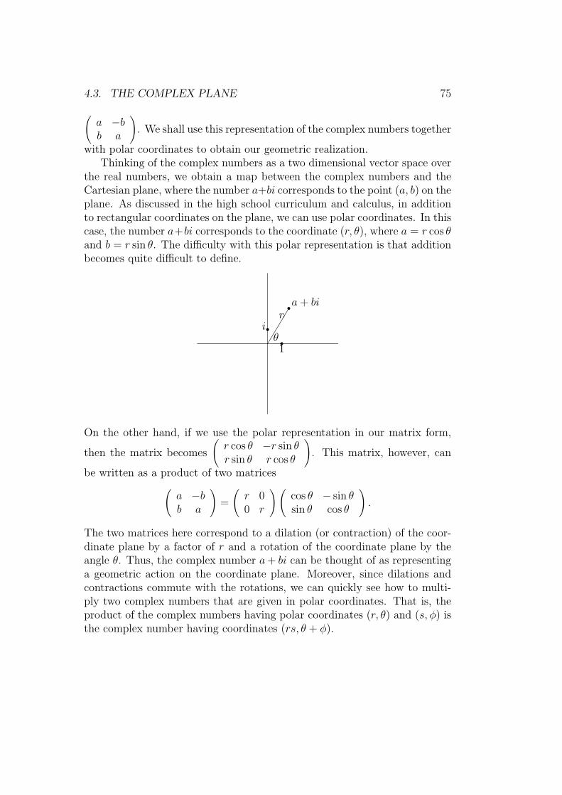
4.3. THE COMPLEX PLANE 75
(a −bb a
). We shall use this representation of the complex numbers together
with polar coordinates to obtain our geometric realization.Thinking of the complex numbers as a two dimensional vector space over
the real numbers, we obtain a map between the complex numbers and theCartesian plane, where the number a+bi corresponds to the point (a, b) on theplane. As discussed in the high school curriculum and calculus, in additionto rectangular coordinates on the plane, we can use polar coordinates. In thiscase, the number a+bi corresponds to the coordinate (r, θ), where a = r cos θand b = r sin θ. The difficulty with this polar representation is that additionbecomes quite difficult to define.
ri r1
ra+ bi
����r
θ
On the other hand, if we use the polar representation in our matrix form,
then the matrix becomes
(r cos θ −r sin θr sin θ r cos θ
). This matrix, however, can
be written as a product of two matrices(a −bb a
)=
(r 00 r
)(cos θ − sin θsin θ cos θ
).
The two matrices here correspond to a dilation (or contraction) of the coor-dinate plane by a factor of r and a rotation of the coordinate plane by theangle θ. Thus, the complex number a+ bi can be thought of as representinga geometric action on the coordinate plane. Moreover, since dilations andcontractions commute with the rotations, we can quickly see how to multi-ply two complex numbers that are given in polar coordinates. That is, theproduct of the complex numbers having polar coordinates (r, θ) and (s, φ) isthe complex number having coordinates (rs, θ + φ).
76 CHAPTER 4. SOLVING EQUATIONS BY RADICALS
The piece of the puzzle of complex numbers comes from the work ofEuler. In working with the exponential function and its Taylor series, Eulerexamined what happens when evaluating eix. Of course, the meaning ofraising a number to a non-rational power is not easily described. When wefirst discuss raising a number to a positive integer power, we describe it asrepresenting a repeated multiplication. We extend exponentiation to therational numbers by taking roots. The next extension to irrational powers,on the other hand, must be done using limits in one way or another. Ofcourse, in the high school curriculum, we frequently gloss over this fact, butwe should remember that limits are there in the background. Even withlimits, however, it is unclear what we should mean when raising a numberto a complex power. The exponential function ex being somewhat easier todeal with than other such functions as it has a nice Taylor’s series for thefunction,
ex = 1 +x
1!+x2
2!+x3
3!+x4
4!+x5
5!+ . . . .
allows us a method to attack this question. Euler’s solution was to simplyuse ix in place of x in the above equation, yielding:
eix = 1 +ix
1!+
(ix)2
2!+
(ix)3
3!+
(ix)4
4!+
(ix)5
5!+ . . . .
Using that i2 = −1, and bringing the terms together that involve i, we obtain
eix =
(1− x2
2!+x4
4!− x6
6!+ . . .
)+ i
(x
1!− x3
3!+x5
5!+ . . .
).
Examining these two terms more closely, however, we see that they corre-spond to the Taylor series for cosx and sin x respectively, giving Euler’s greatformula
eix = cos x+ i sin x.
Thus, using the complex number r cos θ+ ir sin θ can be written as reiθ, andin this form, the multiplication rule reiθ · seiφ = rsei(θ+φ) becomes easy toremember. Moreover, using this, taking roots becomes simplified. Namely,if you want the nth root of reiθ, you can simply raise this number to the 1
n
power, yielding (reiθ)
) 1n = r
1n ei
θn .
4.3. THE COMPLEX PLANE 77
The above is only one root among n, however. To get the other roots, weuse the identity
eiθ = ei(θ+2kπ),
where k is an arbitrary integer to arrive a the general solution
(reiθ)
) 1n = r
1n ei
θ+2kπn .
This gives us n different solutions for k = 0, 1, . . . , n − 1. At this point, wecan now finish the solution of the cubic.
Given an arbitrary cubic equation rx3 + sx2 + tx+u = 0 with r, s, t, andu all real numbers and r 6= 0, we begin by dividing the equation through byr, to obtain an equation of the form x3 + bx2 + cx + d = 0 where b = s/r,c = t/r and d = u/r. At this point, we let x = x′−b/3 to obtain the equation(x′)3 + px = q, where p = (c − b2/3) and q = bc/3 − 2b3/27 − d as we sawearlier. At this point, we can solve for x′ to obtain that x′ = u− v, where
u =3
√√√√q
2+
√(q
2
)2
+(p
3
)3
and
v =3
√√√√−q2
+
√(q
2
)2
+(p
3
)3
.
While we have three choices for both u and v, we have one further constraintin that 3uv = p. Thus, we choose our cube roots so that we have thisrequirement, which can be done simply by checking that the angles add upto either π or 0 depending on whether p is negative or positive. Then wehave three choices for x′ = u− v, and x = x′ − b/3.
Aside
At this point, we have looked at number as ratio, as magnitude, andas being built up from roots. None of these really account for how we canthink of negative numbers. In fact, in the history of European mathematics,negative numbers came after all of these understandings. Descartes, amongothers, considered negative numbers as fanciful constructs. Even today, oneof the most difficult tasks of the middle school teacher is getting students
78 CHAPTER 4. SOLVING EQUATIONS BY RADICALS
to understand why the product of two negative numbers should be a posi-tive number. Sfard argues that one cannot make this argument successfullywithout using our desire for the number system to satisfy the distributivelaw [11], or giving a new understanding of number. Complex numbers havea similar difficulty associated to them. What we have seen in this section,however, is that we can give these numbers a geometric meaning, if we con-sider them not as quantities that measure something, but rather as functionson the Euclidean plane (like matrices).
This understanding of number, opens up a whole new realm of mathe-matics. Numbers need no longer have a specific meaning. Instead, numbersare classified by the properties they have. This allows for one to considermore and more general sorts of “numbers,” and even to analyze what theproperties themselves imply. This analysis of the properties devoid of theactual entities becomes the basis of abstract algebra, the study of groups,rings, fields, and integral domains. Indeed, in modern mathematics, the realnumber system is one of many different systems that extends the rationalnumbers.
End of Aside
4.4 Algebraic Numbers
We have seen that we can solve a cubic equation by using radical signs, andthe operations of addition, subtraction, multiplication, and division on thecoefficients. After the general cubic was solved, the next step in the mathe-matics of solving equations was to solve the general quartic or fourth degreeequation by radicals. In current times, this is done most easily by first solvinga cubic that arises from the original equation (much like we used a quadraticequation for our cubic solution) and then use this cubic solution to allowus to change the problem to an easier quartic equation that we could solve.The next step was to solve the quintic equation by radicals. Unfortunately,try as hard as they might, no one could find a solution by radicals for manyyears. Finally, it began to dawn on mathematicians that perhaps no solutioncould be found. This result was then first proved by Niels Abel in the 1800s,and then later Evariste Galois was able to create a theory, which allowedmathematicians to determine precisely when a polynomial could be solvedby radicals. While Galois theory is beautiful and wonderful to study, it isbeyond the scope of this class, as is Abel’s proof of the impossibility of solv-
4.4. ALGEBRAIC NUMBERS 79
ing the general quintic by radicals. (A great summary of this history can befound in [13].)
If we cannot solve every quintic by radicals, this means that there mustbe real numbers which cannot be found using the operations of addition,subtraction, multiplication, division, and taking nth roots on the rationalnumbers. Thus, yet again, we need to extend our definition of what a numbershould be. Our study of the complex numbers, however, has also given usa certain amount of freedom, as we might now realize that we can allow fornumbers to be defined less concretely.
We say the real number α is algebraic if α is the root of some polynomialwith rational coefficients. For example, 3
√3 is algebraic since it is the root of
the polynomial x3 − 3. If a number is not algebraic, then we say that it istranscentdental. It is unclear whether any number can be transcendental atfirst glance. Certainly, most numbers that we might write down are algebraic.It turns out that both e and π are transcendental, although this is quitedifficult to show. Our goal in this section will be to show that the algebraicnumbers form a subfield of the real numbers, and then to show that onespecific number is transcendental via a technique due to Liouville.
As we saw earlier, if α is a root of the polynomial p(x), and p(x) isirreducible over the rational numbers, then Q[α] is finite dimensional over Q.Now, suppose β is also the root of an irreducible polynomial with rationalcoefficients. Let q(x) be a polynomial of minimal degree having β as a root.Again, we have that [Q[β] : Q] is finite. Unfortunately, we do not yet have thematter in hand to show that Q[α, β] is finite dimensional over Q. However,we know that g(x) is a polynomial over Q[α] since all of its coefficients liein Q ⊆ Q[α]. Thus, a polynomial of Q[α] of minimal degree having β asa root, must have degree smaller than the degree of g(x). Consequently,[Q[α, β], Q[α]] ≤ [Q[β], Q], and Q[α, β] is finite dimensional over Q since itis the product of dimQ[α](Q[α, β]) and dimQ(Q[α]), both of which are finite.
At this point, let us set E = Q[α, β]. As E is a field, α + β, α − β, αβ,and α/β are all elements of E. Thus, if we can show that any element ofE must be a root of some polynomial with rational coefficients, we wouldhave that this is true for αβ, α + β, α − β, αβ, and α/β. But this last isprecisely what we need to see that the algebraic numbers form a field! Thus,we have reduced that problem of showing the algebraic numbers are a field,to showing that any element of E must be the root of a (non-zero) polynomialwith rational coefficients.
Let γ ∈ E, suppose dimQ(E) = k, and consider the set {1, γ, γ2, γ3, . . . , γk}.
80 CHAPTER 4. SOLVING EQUATIONS BY RADICALS
Since this set has k+ 1 elements, it follows that it is linearly dependent overQ. That is, there exist elements a0, a1, . . . , ak ∈ Q not all equal to 0, suchthat
k∑i=0
aiγi = 0.
This, however, implies that γ is a root of the polynomial
k∑i=0
aixi.
Thus, we have shown:
Theorem 4.1 The algebraic numbers form a field.
4.5 Transcendental Numbers
The question now becomes: Is every real number algebraic? Euler gave thefirst definition of transcendental numbers, numbers that are not the root ofany nonzero polynomial with rational coefficients. Euler, however, was un-able to prove that any number was transcendental, although there is goodevidence that he believed that both e and π were transcendental. The proof,however, of the existence of a transcendental number had to wait about50 years, until 1844 when Liouville proved that
∑∞n=1 10−n! was transcenden-
tal (along with many other similar numbers). While this result proved theexistence of transcendental numbers, it did not show that any particularlyinteresting number (at the time) was transcendental. In 1873, however, Her-mite proved that e was transcendental. In 1874, Cantor produced a startlingresult showing that transcendental numbers existed, although it did not pro-duce any. More curious, Cantor showed that most real numbers are in facttranscendental, even though at the time, only few numbers could be writtendown and proved to be transcendental. By 1883, Lindemann showed thatπ was transcendental. Lindemann’s work, while settling the question of thesquaring of the circle, however, is not considered quite as grand as Hermite’s,since Lindemann essentially used the same techniques as Hermite in a littlebit more generality. In 1900, Hilbert presented a list of 23 problems formathematics to answer in the new century. The seventh problem of Hilbertwas to determine whether or not 2
√2 was transcendental. The problem was
4.5. TRANSCENDENTAL NUMBERS 81
answered in 1934 when A.O. Gelfond proved the result (also done indepen-dently in 1935 by T. Schneider) that if α and β are algebraic numbers withα 6= 0, α 6= 1, and β not a real rational number, then any value of αβ istranscendental. (See [6] pp.134-150 for a historical treatment and proof ofthis remarkable result, while the original works by Gelfond and Schneider canbe found in [?] and [9], although more readable expositions of these resultscan be found in [3].)
How can one show that a number α is transcendental? To do so, requiresproving somehow that no non-zero polynomial with rational coefficients canhave α as a root. We can make things a little easier by reducing this problemto the case where the polynomials are only allowed to have integer coefficients,since we can multiply through by a common denominator of the coefficients.As with the proofs of irrationality, we need to use proof by contradiction inthis case. That is, we will need to assume that our candidate α is the rootof a polynomial with integer coefficients, and then obtain a contradiction.Liouville was able to use this method and calculus to show that the number∑∞n=1 10−n! was transcendental. We now prove this.
Theorem 4.2 The real number α =∑∞n=1 10−n! is transcendental.
Proof: Suppose that p(x) is a polynomial with integer coefficients such thatp(α) = 0. We shall aim for a contradiction by showing that if α is the root ofthis polynomial, then there are only finitely many rational numbers a
bsuch
that |α− ab| < b−n−1 where n is the degree of p(x). Using this together with
|α−∑kn=1 | < 10−(k+1)!, will give us the desired contradiction since
∑kn=1 = a
b
where b = 10−k!.
Now, suppose that a, b ∈ Z are such that p(ab) 6= 0 (note that there are
only finitely many rational numbers that do not satisfy this property). Sincethe coefficients of p(x) are all integers, it must be the case that that p(a
b) = A
bn
for some integer A 6= 0, where n = deg(p(x)) (show this!).
The second step in the proof is to get some control on the values thatp(x) can take on nearby α. Since [α−1, α+1] is a closed interval and p(x) isa polynomial, it follows that |p′(x)| ≤ m for some integer m on the interval[α− 1, α + 1].
At this point, we suppose ab6= α is a rational number in the interval
[α − 1, α + 1]. For the time being, we shall assume that ab< α and that
p(ab) < 0, and is therefore less than or equal to 1
bn. As p′(x) < m on [c, d], if
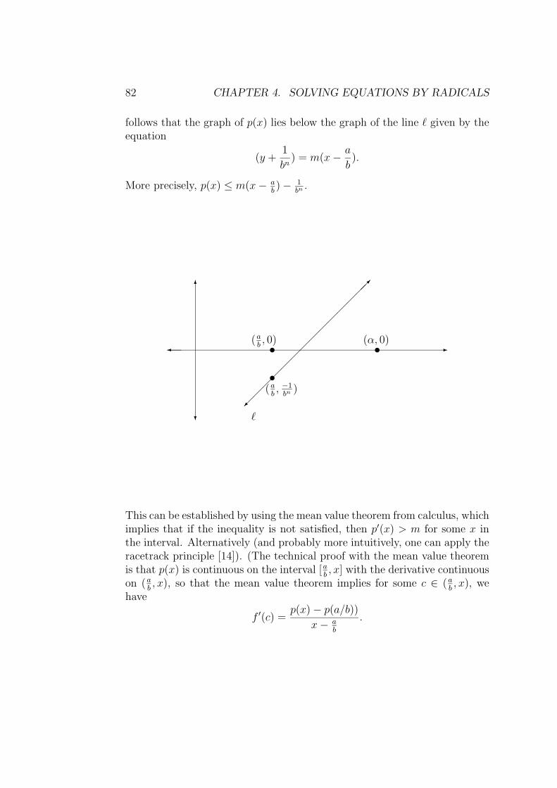
82 CHAPTER 4. SOLVING EQUATIONS BY RADICALS
follows that the graph of p(x) lies below the graph of the line ` given by theequation
(y +1
bn) = m(x− a
b).
More precisely, p(x) ≤ m(x− ab)− 1
bn.
-�
6
?
t tt���
���������
��
�
(ab, 0) (α, 0)
`
(ab, −1bn
)
This can be established by using the mean value theorem from calculus, whichimplies that if the inequality is not satisfied, then p′(x) > m for some x inthe interval. Alternatively (and probably more intuitively, one can apply theracetrack principle [14]). (The technical proof with the mean value theoremis that p(x) is continuous on the interval [a
b, x] with the derivative continuous
on (ab, x), so that the mean value theorem implies for some c ∈ (a
b, x), we
have
f ′(c) =p(x)− p(a/b))
x− ab
.
4.5. TRANSCENDENTAL NUMBERS 83
Since f ′(c) ≤ m, it follows that
p(x) ≤ mx−ma
b+ p(a/b) ≤ mx−ma
b− 1
bn,
where the last term follows because we have assumed that p(a/b) < 0 so thatp(a/b) < 1
bnfrom above.)
Thus, the value of α is greater than the x-coordinate of the intersectionpoint of ` and the x-axis. We can calculate this coordinate, however, and itis δ = a
b+ 1
mbn. Consequently,
|α− a
b| ≥ 1
mbn.
If b > 2m, however, we then have
|α− a
b| ≥ 2
bn+1.
Choosing t > 2m sufficiently large, it follows that for any b > t, if |α− ab| ≤
2bn+1 it must be the case that a
b∈ [c, d]. However, we also just showed that
if ab6= α then |α− a
b| > 2
bn+1 . Consequently, there can only be finitely manyrational numbers a
bhaving the property
|α− a
b| < 2
bn+1.
(Note that if we had assumed that p(a/b) > 0 and/or a/b > α, we wouldmerely have changed which line we were looking at, and we still would obtainthe same final result.) At this point, we are nearly done with the proof thatα =
∑∞n=1 10−n! is transcendental. Let qk =
∑kn=1 10−k!. Then
|α− qk| =∞∑
n=k+1
10−n! ≤ 2
10(k+1)!.
However, qk = akbk
= ak10k! for some integer ak, and bk = (10k!)n+1 = 10(n+1)(k!).
If k > n, however, we then have the difference
|α− qk| <2
10(k+1)!
=2
10(k+1)(k!)
<2
10(n+1)(k!)
=2
bn+1k
.

84 CHAPTER 4. SOLVING EQUATIONS BY RADICALS
Since qk has the property for all k > n that |α− qk| < bn+1k , it follows that α
cannot be algebraic.Q.E.D.
Most analytic number theory texts prove the general statement of Liou-ville’s theorem, which can be read out of our proof. Namely that
Theorem 4.3 If α is a real algebraic number, then there exists only finitelymany rational numbers q = a
b(where a and b are integers with b > 0) such
that |α− q| < 2bn+1 .
The choice for this presentation was to concentrate on one specific number.
Aside
Why go through this proof at all? I have two reasons. The first is thatwe frequently tell our students that e and π are transcendental numbers,without truly understanding what this means. Unfortunately, the proofs forthe transcendence of e and π are both substantially more difficult than theproof that we gave in Chapter 2 that π was irrational, and consequently, itis really beyond the high school curriculum. On the other hand, the onlymaterial really needed for the proof of Liouville’s theorem are the conceptof slope or rate of change and the understanding of what value polynomialswith integer coefficients can take on rational numbers. While some might takeissue, pointing out that we used derivatives and continuity in our proof, bothof these concepts can be understood at a lower level by drawing graphicalrepresentations of polynomials, while leaving the capital P Proof for latercourses. Moreover, one can turn the Mean Value Theorem with the racetrack lemma (as put in [14]), that can be put simply as: if two race tracksare going around a track, and the first car is always going faster than thesecond car, then the first car is always ahead of the second car. This readilybelieved lemma on race cars works with our polynomials to establish thatthe polynomial must lie between the two lines.
Thus, from this one can get a better understanding of some of the proper-ties distinguishing algebraic numbers from transcendental numbers from thisproof. In particular, the idea that there is a limit to how well one can ap-proximate algebraic numbers, whereas at least some transcendental numberscan be approximated remarkably well. You should note in fact, the similarity
4.5. TRANSCENDENTAL NUMBERS 85
that this argument has with several of our proofs of irrationality. The onedifference is that the level of approximation required is much tighter in thetranscendence proof than it was in the irrationality proof.
At this point, it makes sense to emphasize the role of proof in mathemat-ics. The standard argument is that proof allows us to know something with acertainty. While this certainty is important in many cases, what is probablymore important is the role of proof in mathematical problem solving. Whensolving a problem in mathematics, proof can play a very important part.Schoenfeld says [10]
For the mathematician, dependence on argumentation as a formof discovery is learned behavior, a function of experience. Thisperspective is not “natural”; few B.A.s in mathematics possess it.Those who become mathematicians generally develop this per-spective in graduate school, during their apprenticeship to thediscipline. At first, “proof” is mandatory, an accepted standard.As one becomes acculturated to mathematics, it becomes nat-ural to work in such terms. “Prove it to me” comes to mean“explain to me why it is true,” and argumentation becomes aform of explanation, a means of conveying understanding. Asthe mathematician begins to work on new problems (perhaps ona dissertation), this progression continues. Mathematical argu-ment becomes a way of convincing oneself that something oughtto be true. Even unsuccessful attempts turn out to be valuable,because consistent failures point to weak spots in one’s under-standing. After numerous attempts to demonstrate a particularresult, one can see a pattern in the failures and decide the resultmay not be true. To see if it is false, one may try to constructsome examples that exploit the weak spots. If none of the exam-ples one tries demonstrate that the result is false, one may againbegin to believe the result is true - and a pattern in the failedexamples may suggest the information that was missing from theoriginal attempts. Thus mathematical argument becomes a toolin the dialectic between what the mathematician suspects to betrue and what the mathematician knows to be true. In short,deduction becomes a tool of discovery. (pp.172-173)
An important point here is the idea of mathematical argument as a tool forunderstanding and learning. For example, the proof that the product of two
86 CHAPTER 4. SOLVING EQUATIONS BY RADICALS
odd integers is odd, can be used several different ways in a classroom. If theteacher presents it, then it becomes an exercise in writing a proof. In thisfashion, however, students will disengage from the process, or learn it by rotewithout understanding. A second method can be for the students to completethe proof themselves, may well feel like busy work to the students. A thirdmethod is to have the students analyze the proof and see what they can sayif odd is replaced by divisible by three. The natural proof (before Euclid’sLemma is introduced to students) for the odd multiples is to write down twoarbitrary odd numbers as 2k+ 1 and 2l+ 1 and to multiply them out. Whentrying to see how this works for the case of 3, the students can discover howto break the problem into separate cases, to arrive at arithmetic modulo 3.Similarly, when discussing geometric constructions, it is the knowledge ofwhat theorems are true and how to apply them that is crucial in developinggeometrical constructions.
For the above reasons, one of the important tools to learn in any math-ematics class is the role of proof in discovery. Reasoning plays a major rolein the NCTM standards. One major understanding is the varying levels ofproof (from heuristic and intuitive argumentation to formal) and their rolein problem solving. One possible interpretation (mine) for how teachers canhelp students develop mathematical reasoning and problem solving skills isby varying the levels as one moves through the curriculum.
End of Aside
Chapter 5
Dedekind Cuts
5.1 Axioms for the Real Numbers
We are about to embark on the explicit construction of the real numbers fromthe rational numbers. Before doing so, however, you should work throughthe following questions. The purpose of these questions are to encourage youto think about what properties we would like the real numbers to satisfy andto work from a minimum set of axioms to define the real numbers.
To begin with, consider the following:The guiding principle in defining the real numbers is the number line. Whatare all the properties that the set of real numbers should have? You shouldcome up with at least twelve properties that are expected of the set (Hint:Think about the entire field).
87
88 CHAPTER 5. DEDEKIND CUTS
Below we list the actual defining axioms for the real numbers. You maywell not have gotten all of them. In fact, it is fairly typical that students willmiss out on all of the axioms involving the order relationship <. One of thereasons for this is that we tend to take the idea of order on the number linefor granted. Thus we tend to take it as a given that the order relation exists.Moreover, we also often take it for granted that this relationship
The real numbers R are a set together with the two binary operations+ : R × R → R, · : R × R → R, and the binary relation < on R under thefollowing thirteen axioms:
1. The operations + and · are associative.
2. The operations + and · are commutative.
3. The operation · is distributive over +. That is, for all a, b, c ∈ R,a · (b+ c) = a · b+ a · c.
4. There exist at least two distinct elements in R.
5. There exists an element 0 ∈ R such that for all a ∈ R, a+ 0 = a.
6. For each element a ∈ R, there exists an element b ∈ R such thata+ b = 0. We call this element −a.
7. There exists an element 1 ∈ R such that for all a ∈ R, a · 1 = a.
8. For each element a ∈ R, with a 6= 0 there exists an element b ∈ R suchthat a · b = 1. We call this element a−1 or 1
a.
9. The relation < is transitive on R.
10. (The Trichotomy Law). For every a, b ∈ R, exactly one of a < b, a = b,and a > b is true.
11. For all a, b, c ∈ R, if a < b then a+ c < b+ c.
12. For all a, b, c ∈ R, if a < b and c > 0, then a · c < b · c.
13. (The Greatest Lower Bound Axiom) If S ⊂ R is a non-empty subset,and there exists a lower bound b ∈ R such that for all a ∈ S we haveb ≤ a, then there exists a greatest lower bound c for S. That is, thereexists c ∈ R such that c < a for all a ∈ S and moreover, if b ∈ R alsosatisfies the condition b < a for all a ∈ S, then c ≤ b.
5.1. AXIOMS FOR THE REAL NUMBERS 89
Using the axioms above, let us move on to prove some things that weexpect about the real numbers.
1. If x < y, then −y < −x. Hint: Assume x < y and add the same thingto both sides of the inequality in order to establish that −y < −x.
2. 0 < 1. Although this statement seems obvious, you need to establishthis result using the pink sheets axioms. What are the three possibleways of relating 0 and 1? Use the axioms to establish that what youknow is impossible is truly impossible.
3. If 0 < x < y, then 0 < 1x< 1
y.
(a) Assume 0 < x < y. What are the possibilities for the relationshipbetween 0 and 1
x?
(b) Argue why, from the set of axioms, two of these possibilities cannotbe true.
(c) What does this mean about 1y?
(d) Using 0 < x < y, multiply each element of the compound inequal-ity by the same factor in order to establish 0 < 1
y< 1
x. Explain
why this is legal.
4. If x < y and z < 0, then yz < xz. Hint: Assume x < y and z < 0. Useaxiom 11 and a previous result to establish yz < xz.
5. Prove the Theorem:
Theorem 5.1 If S is a non-empty set of real numbers that is boundedfrom above, then S has a least upper bound.
(a) Argue why if M is an upper bound for S, then M ≥ s for alls ∈ S.
(b) Let T = {t | t = −s, for some s ∈ S}. Argue why −M is a lowerbound for T .
(c) Explain why if K is a lower bound for T , then −K is an upperbound for S.
(d) Argue why T must have a greatest lower bound, call it B.
90 CHAPTER 5. DEDEKIND CUTS
(e) Argue why −B must be an upper bound for S.
(f) If C is an upper bound for S, then what is the relationship between−C and B as well as −C with the set T?
(g) What is the relationship between C and −B? How does this imply−B is the least upper bound for S?
6. Prove the following theorem:
Theorem 5.2 Let x be any real number. Then there is an integern ≤ x < n+ 1.
In order to accomplish this, we need to define the setA = {n | n ∈ Z and n ≤ x}.
(a) If A is non-empty, argue why A is bounded from above and has aleast upper bound (call it n0).
(b) Explain why if you subtract 1 from n0, the resultant value will notbe an upper bound of A.
(c) Discuss why there exists an m ∈ A such that n0 − 1 < m ≤ n0.
(d) Explain why m+ 1 /∈ A and x < m+ 1.
(e) How does this establish, for the case that A is non-empty, theresult that we can find an integer n such that n ≤ x < n+ 1.
(f) To show thatA is not empty, consider the setB = {b | b > x and b ∈ Z},and show that it must have a least upper bound called b0. Arguethat there exists a m ∈ B such that b0 ≤ m < b0 + 1 so thatm− 1 ∈ A.
7. Prove the following theorem
Theorem 5.3 Between any two real numbers is both a rational numberand an irrational number.
(a) Let x and y be real numbers with x < y. Why is there an integerN such that 0 < 2
y−x < N?
(b) Argue why there exists an integer n ≤ Nx < n+ 1.
(c) Argue why n+ 2 < Ny.
(d) Explain why n+1N
and n+2N
are rational numbers between x and y.
(e) Explain why n+√
2N
is an irrational number between x and y.
5.2. DEDEKIND CUTS 91
5.2 Dedekind Cuts
Descartes’ Geometry is an important advance in mathematics, because itgives the first instance of a mathematician writing equations for geometricfigures (although, the equation of a line occurs only once within the text[12]) and it gives the first idea of calculating the normal to a curve. Movingforward in time, Leibniz and Newton develop calculus using the idea of thecoordinate axes and rates of change, and as we have seen earlier, questionsabout algebraic and transcendental numbers begin to be raised by Euler inthe 1700s. Cauchy defines and “proves” that Cauchy sequences converge inthe early 1800s, but curiously, it is not until the 1890s that mathematiciansrealized that they did not have a proper definition of the real numbers. Insome ways, this isn’t so surprising. The move to axiomatize all mathematicalsystems is a product of the late 1800s and the discovery of non-Euclideangeometries, and the real numbers seen as points on the number line arewell defined by intuitive standards. Moreover, calculus and analysis wereextremely successful without worrying about foundational issues. On theother hand, as we shall see later, even such great mathematicians as Cantor,were prone to make subtle errors when dealing with the real numbers.
In the 1890s, Richard Dedekind taught a calculus course in Germany. Hedecided that he wanted to start from the basic definitions and put calculuson a firm foundation. As he began to design the course, he ran into troubleproving the intermediate value theorem, one of the important foundationaltheorems of the calculus. After struggling with this, he realized that theproblem was that he had no strict definition of the real numbers to workfrom.
Theorem 5.4 (The Intermediate Value Theorem) If f(x) is a continuousfunction on the closed interval [a, b] with f(a) < 0 and f(b) > 0, then thereexists c ∈ (a, b) such that f(c) = 0.
The proof of this theorem uses the greatest lower bound axiom. Namely thatevery non-empty set of real numbers that has a lower bound has a greatestlower bound. To prove the theorem, one considers the set C = {x ∈ [a, b] |f(x) ≥ 0}. The set C is non-empty since b ∈ C, and the set has a lowerbound since a < x for all x ∈ C. Thus C has a greatest lower bound, whichwe shall call c. At this point, all that remains is to prove that f(c) = 0. Tosee this, we use the continuity of f . By continuity and the knowledge thatf(b) > 0 and f(a) < 0, it follows that c ∈ (a, b). Now, since for all d /∈ C,
92 CHAPTER 5. DEDEKIND CUTS
we know that f(d) ≤ 0, we have that f(c) ≤ 0 as f(x) is continuous. Onthe other hand, for all δ > 0, there exist a y ∈ C such that y < c+ δ since cis a greatest lower bound. However, then f(y) ≥ 0. Thus, continuity againimplies that f(c) ≥ 0, leaving us with f(c) = 0.
This is the modern proof of the theorem, where we take one of the com-pleteness axioms as part of the axiomatic definition of the real numbers.Consider Dedekind’s problem, however. The real numbers are not axiomat-ically defined, but rather they are intuitively defined by the number line.The greatest lower bound axiom is only true intuitively in this situation, andcan hardly be called on in a late 19th century perspective. Thus, Dedekindneeded to construct the real numbers in some way. His insight was to usethe intuition of the number line in his construction. That is, he reasonedthat every point on the number line breaks the real line into two separatepieces, and he wanted to use the pieces to identify the numbers. The downside of this attempt is that the pieces consist intuitively of real numbers,and you cannot use the real numbers in defining what the real numbers are!On the other hand, the rational numbers were well-defined at this time, soDedekind reasoned that to determine the two pieces of the number line, itwas sufficient to consider only the rational numbers in each piece. From thisintuition, Dedekind gave the following definition:Definition: A Dedekind cut is a pair (A,B) of non-empty sets such that
1. A ∪B = Q,
2. A ∩B = ∅, and
3. If a ∈ A and b ∈ B, then a < b.
Dedekind’s goal was to define the real numbers as the set of Dedekindcuts. However, one needs to be careful about this. If the intuition is tothink about how the line breaks into pieces, the point at which you breakthe line needs to end up on one side or the other. If the point that youbreak the number line at is not rational, this isn’t a problem since the piecesnow consist only of the rational numbers. However, if you break the line ata rational point, then you do have a problem, and a choice has to be madeabout which one of the two sets to put it in. We will take Dedekind’s point ofview, which is different from most modern authors, in that we will considereach of these to be a Dedekind cut. That is, given a rational number q, there
5.2. DEDEKIND CUTS 93
are two cuts associated to q, namely the cut (Aq, Bq) given by
Aq = {a ∈ Q | a ≤ q}Bq = {b ∈ Q | b > q},
and the cut (Aq, Bq) given by
Aq = {a ∈ Q | a < q}Bq = {b ∈ Q | b ≥ q}.
In the modern treatment, a Dedekind is defined slightly differently. In par-ticular, a cut is usually a single set corresponding to only one of our twosets.
We define an equivalence relation on Dedekind cuts so as to ensure thatthe two cuts associated to the same rational number are equivalent. To thisend, we say that the cuts (A,B) and (C,D) are equivalent if (A∪C)\(A∩C)is a set consisting of at most one element. That is, the sets A and B differby at most one element.
We now define the real numbers as the set of equivalence classes ofDedekind cuts. At this point, we need to define the operations and orderrelation. One can make most of these definitions easier by assuming that if(A,B) is a rational cut, then the corresponding rational number is an elementof B. While we will not do this in general, we will state these definitions inparentheses after our definitions. The reason for this change is that we wantto be able to work with either element of the equivalence class. Basically,you either have to work with a particular element of each equivalence classor worry about proving that the operations we shall define are well defined.
We define the order relation < on R as follows: Given two non-equivalentDedekind cuts (A,B) and (C,D), we say that (A,B) < (C,D) if and only ifA ⊂ C. (The condition is not simplified by the assumption that if the cutis rational then the rational point lies on the left hand side.) This conditionimplies in our intuitive understanding of Dedekind cuts that the breakingpoint of the number line determined by (A,B) lies to the left of the breakingpoint of the number line determined by (C,D). We need to check that thisdefinition is well defined. Namely, that if we choose cuts equivalent to (A,B)and (C,D), that we will not change the definition of the relation <.
Suppose now that (A,B) < (C,D) and (A′, B′) ∼ (A,B) and (C ′, D′) ∼(C,D). By our assumptions, there exists c ∈ C such that c /∈ A. Since
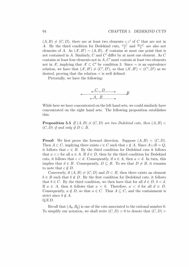
94 CHAPTER 5. DEDEKIND CUTS
(A,B) 6∼ (C,D), there are at least two elements c, c′ of C that are not inA. By the third condition for Dedekind cuts, c+c′
2and 2c+c′
3are also not
elements of A. As (A′, B′) ∼ (A,B), A′ contains at most one point that isnot contained in A. Similarly, C and C ′ differ by at most one element. As Ccontains at least four elements not in A, C ′ must contain at least two elementsnot in A′, implying that A′ ⊂ C ′ by condition 3. Since ∼ is an equivalencerelation, we have that (A′, B′) 6∼ (C ′, D′), so that (A′, B′) < (C ′, D′) as wedesired, proving that the relation < is well defined.
Pictorially, we have the following:
� -R� a -A B
� -aC D
While here we have concentrated on the left hand sets, we could similarly haveconcentrated on the right hand sets. The following proposition establishesthis:
Proposition 5.5 If (A,B) 6∼ (C,D) are two Dedekind cuts, then (A,B) <(C,D) if and only if D ⊂ B.
Proof: We first prove the forward direction. Suppose (A,B) < (C,D).Then A ⊂ C, implying there exists c ∈ C such that c /∈ A. Since A∪B = Q,it follows that c ∈ B. By the third condition for Dedekind cuts it followsthat a < c for all a ∈ A. If d ∈ D, then by the third condition for Dedekindcuts, it follows that c < d. Consequently, if a ∈ A, then a < d. In turn, thisimplies that d ∈ B. Consequently, D ⊆ B. To see that D 6= B, it remainsto note that c /∈ D.
Conversely, if (A,B) 6∼ (C,D) and D ⊂ B, then there exists an elementb ∈ B such that b /∈ D. By the first condition for Dedekind cuts, it followsthat b ∈ C. By the third condition, we then have that for all d ∈ D, b < d.If a ∈ A, then it follows that a < b. Therefore, a < d for all d ∈ D.Consequently, a /∈ D, so that a ∈ C. Thus A ⊆ C, and the containment isstrict since b /∈ A.Q.E.D.
Recall that (A0, B0) is one of the cuts associated to the rational number 0.To simplify our notation, we shall write (C,D) > 0 to denote that (C,D) >
5.2. DEDEKIND CUTS 95
(A0, B0). In a similar way, we will write (C,D) > q to denote that (C,D) isgreater than either cut associated to q.
At this point, we need to define the binary operation of addition.Definition: For Dedekind cuts (A,B) and (C,D) we define (A,B) + (C,D)to be the cut (E,F ) where
F = {b+ d | b ∈ B, d ∈ D}
and E = Q \F . (If we insist that rational cuts contain the rational point onthe right, then we can write E = {a + c | a ∈ A, c ∈ C}. Again, we shouldcheck that this definition is well defined, but this is left to the reader.
Given that this definition is well defined, it is a straightforward check tosee that addition is commutative and associative, and thus we have that thefirst two axioms are satisfied for addition.
To define multiplication of Dedekind cuts is unfortunately harder. Inparticular, the difficulty of multiplying negative numbers comes back to hauntus.Definition: Given two Dedekind cuts (A,B) > 0 and (C,D) > 0, theproduct of these cuts is defined to be the cut (E,F ) where
F = {bd | b ∈ B, d ∈ D}
and E = Q \ F .Before moving on to define the product of negative cuts, let us first show
that this definition is well defined. Suppose that (A′, B′) ∼ (A,B) and(C ′, D′) ∼ (C,D), and let F ′ = {bd | b ∈ B′, d ∈ D′}. Without loss ofgenerality, assume that D ⊂ D′, and the containment is proper. Then itfollows that D′ = D ∪ {q} where q is a minimal element of D′. We claimthat F ′ 6= F if and only if B is a proper subset of B′, and in this case F ′
and F differ by at most one element. Suppose first that B′ does not containa minimal element. Then if x = b′d′ for some b′ ∈ B′ and some d′ ∈ D′,as B′ does not contain a minimal element (implying that B′ ⊆ B, thereexists a rational number b ∈ B′ such that b < b′. Consequently x
b> d′, and
xb
is therefore an element of D′ and also of D. This implies however that
x = bd ∈ F , so that F ′ ⊆ F . Next, suppose B′ contains a least element r.Let x ∈ F ′. By the previous argument, x ∈ F if x = bq for some b ∈ B′ withb 6= r. Similarly, the argument above would imply x ∈ F if x = rd for somed ∈ D with d 6= q. Consequently, x ∈ F but x /∈ F ′ implies x = rq, and F ′
contains at most one element more than F , and only in the case where B′ and
96 CHAPTER 5. DEDEKIND CUTS
D′ both contain a minimal element but one of B or D does not. Reversing theroles of F and F ′ above yields that F and F ′ differ by at most one element,and thus (E,F ) ∼ (E ′, F ′). This argument is tedious; it does however bringlight to why the modern treatment simply insists on defining cuts in onlyone direction. Namely, by doing so, we can avoid both equivalence classesand the trivialities of proving the operations are well defined.
Actually, we still need to check that the product of two positive cuts is,in fact, a cut.
Proposition 5.6 Let (A,B) > 0 and (C,D) > 0 be two Dedekind cuts, andlet (E,F ) be their product. Then (E,F ) is also a Dedekind cut.
Proof: Since B and D are both non-empty (as (A,B) and (C,D) are cuts,it follows that there exists b ∈ B and d ∈ D so that bd ∈ F , and hence Fis non-empty. Since B and D consist only of positive numbers, so does F ,so that 0 ∈ E and hence E is non-empty. The first two conditions for cutsare satisfied since F ⊂ Q follows from the closure of the rational numbersunder multiplication, and then defining E = Q \ F forces E ∪ F = Q andE ∩ F = ∅. Consequently, it remains to show the third condition. To seethis, we shall first show that x ∈ F and y ∈ Q with y > x implies y ∈ F .As x ∈ F , x = bd for some b ∈ B and d ∈ D. Since y > x and b > 0,y/b > x/b = d. Consequently, y/b is a rational number, and by condition 3for the Dedekind cut (C,D) implies that y/b ∈ D. Thus y = b · (y/b) is anelement of F . Now suppose e ∈ E and f ∈ F . If e ≥ f , the above wouldimply that e ∈ F , contradicting that E ∩F = ∅. Thus e < f as desired, and(E,F ) is a Dedekind cut.Q.E.D.
Before giving the general definition of multiplication, we next need todefine the negative of a cut (A,B). Given a cut (A,B), let −(A,B) denotethe cut (−B,−A) where
−A = {−a | a ∈ A}−B = {−b | b ∈ B}
To see that (−B,−A) is a cut is straightforward as all but condition 3 fol-low immediately from the same conditions for (A,B). The third conditionrequires a little more work. Suppose x ∈ −B and y ∈ −A. Then x = −a for
5.2. DEDEKIND CUTS 97
some a ∈ A and y = −b for some b ∈ B. By condition 3 for (A,B), we havethat a < b. Thus, using the rules of inequality for the rational numbers, wehave −b < −a, and hence x < y as desired. Therefore −(A,B) is a Dedekindcut. To check that this is well-defined, suppose that (A,B) ∼ (C,D). ThenA and C differ by at most one element. From this it follows that −A and−C differ by at most one element, implying that (−B,−A) ∼ (−D,−C).
Proposition 5.7 If (A,B) is a Dedekind cut with (A,B) < 0, then −(A,B) >0.
Proof: From the above, we know that −(A,B) is a Dedekind cut. Thus,it suffices to show that −(A,B) > 0. By the definitions, this requires us toshow that A0 ⊂ −B, and −(A,B) 6∼ (A0, B0). Recall that this means thatwe need to show that if x < 0 then x ∈ −B, and that there exists some y > 0such that y ∈ −B, as this would mean that −B contains at least two pointsnot in A0. But, x < 0 implies that −x > 0. As (A,B) < 0, we know thatB0 ⊂ B by proposition 5.5, so that −x ∈ B0 implies −x ∈ B. Thus x ∈ −Bas desired. Moreover, (A,B) > (A0, B0) also implies that B contains at leasttwo elements not in B0. I.e., B contains some negative rational number −y.Thus y ∈ −B, and y > 0. Consequently −(A,B) > 0.Q.E.D.
We are now ready to define multiplication of two arbitrary Dedekind cuts.Let (A,B) and (C,D) be two cuts. Then
(A,B) · (C,D) =
(A,B) · (C,D) if (A,B) > 0 and (C,D) > 0−( −(A,B) · (C,D) ) if (A,B) < 0 and (C,D) > 0−( (A,B) · −(C,D) ) if (A,B) > 0 and (C,D) < 0−(A,B) · −(C,D) if (A,B) < 0 and (C,D) < 0.
That this is a well-defined definition follows as multiplications of positivecuts is well-defined, as is the definition of −(A,B).
At this point, we can prove the associative, commutative, and distributivelaws for multiplication and addition. The proofs, however, are tedious andnot terribly informative. We shall prove the commutative law for addition,and leave it to the reader to check the others.
Proposition 5.8 If (A,B) and (C,D) are any two Dedekind cuts, then(A,B) + (C,D) = (C,D) + (A,B).
98 CHAPTER 5. DEDEKIND CUTS
Proof: Let (A,B) + (C,D) = (E,F ) and (C,D) + (A,B) = (G,H). Then
F = {b+ d | b ∈ B, d ∈ D} (5.1)
= {d+ b | b ∈ B, d ∈ D} by the commutative law for addition of rational numbers(5.2)
= H. (5.3)
Thus (E,F ) = (G,H).Q.E.D.This proof is similar to all of the proofs, in that they use the same
property for the rational numbers to establish it for the real numbers (asDedekind cuts). Note that this is similar to how we learn about the numbersystems. We first learn the rules for the natural numbers, and having themfor the natural numbers, we extend the rule to the integers, having the rule forthe integers, we extend it to the rational numbers. Thus, extending the rulesto the real numbers from the rule for the rational numbers is quite natural.This extension is also reflected in the NCTM standards, since students areto learn the properties of addition and multiplication in elementary school,and then that these properties hold true for the real numbers is a naturalextension.
There are several items we haven’t checked yet from our axiom systemfor the real numbers. Namely, we need to check the following proposition:
Proposition 5.9 If (A,B) is a Dedekind cut, then (A,B) + (−(A,B)) = 0(by which we again mean for 0 to represent the equivalent cuts correspondingto 0).
Proof: Let this sum be the cut (C,D). Then D = {b+(−a) | b ∈ B, a ∈ A}.Since (A,B) a cut implies that a < b for all a ∈ A and b ∈ B, it follows thatb+(−a) > 0 for all a ∈ A and all b ∈ B. We need to show next, that if x > 0and x is rational, then x ∈ D, as this would tell us that D = {x | x > 0}.Suppose x > 0 is a fixed rational number. Write this in lowest terms asef. Since (A,B) is a cut, there exists b ∈ B. Moreover, b is a rational
number, and can thus be written as gh
for some positive integers g and h.Since he and fg are positive integers, there exists a natural number n suchthat n(he) > fg. Consequently nx > b. Choose n to be the least positiveinteger such that nx ∈ B (which exists by the Well Ordering Principle forthe natural numbers). Then, (n − 1)x ∈ A since A ∪ B = Q. Moreovernx + (−((n − 1)x)) = x is an element of D. Thus D consists of all positive
5.2. DEDEKIND CUTS 99
rational numbers, and the cut (C,D) = 0 as desired.Q.E.D.To establish this result, we again used fundamental properties of the
integers.To finish up our axioms, we need to show that the cut associated to 1 is a
multiplicative identity, to define the multiplicative inverse of a non-zero cut,and to establish our completeness axiom that a non-empty set of cuts witha lower bound has a greatest lower bound.
For the first of these, note that if we look at the cut for 1 with 1 inthe set B1, then establishing that (A1, B1) is a multiplicative identity isstraightforward as given a cut (C,D), then (A1, B1) · (C,D) is defined to bethe cut (E,F ) where
F = {bd | b ∈ B1, d ∈ D}.
But b ∈ B1 implies that b ≥ 1. Thus bd ≥ d no matter what d is. Thus, ifd ∈ D, by the definition of a cut, bd ∈ D. Therefore, F ⊆ D. On the otherhand, d = 1d ∈ F for all d ∈ D since 1 ∈ B. Thus D ⊆ F , and it followsthat D = F , so that (C,D) = (E,F ) and we have the required result. (Notethat we should have proven (A0, B0) really was an additive identity, but theproof of that is almost identical to the above proof.)
Thus, we need to define the multiplicative inverse. Again, we shall restrictto the case where (A,B) > 0. In this case, we define the multiplicative inverseof (A,B) by (A,B)−1 = (C,D), where D is given by
D = {1
a| a ∈ A, a > 0},
and C = Q \D. Note that we had to be a little careful in our definition ofD as we could not simply choose for D the set of all inverses of elements ofA, since that would have given us all negative numbers, and consequently,we would not have had a cut when we were done.
Proposition 5.10 If (A,B) > 0 is a Dedekind cut, then (A,B)−1 is aDedekind cut, and (A,B) · (A,B)−1 ∼ (A1, B1).
Proof: We begin by showing the (A,B)−1 is a cut. Let (C,D) be as above.First, as (A,B) > 0, we have that there exists a positive rational numberq ∈ A. Thus 1/q ∈ D, so that D 6= ∅. Since 0 /∈ D, it follows that 0 ∈ C.
100 CHAPTER 5. DEDEKIND CUTS
Hence both C and D are not empty. Note that if q is a rational number,then so is 1/q. Consequently, since A ⊂ Q, it is also the case that D ⊂ Q.Now it is immediate that Q = C ∪ D and C ∩ D = ∅ by the definition ofC. Finally, suppose d ∈ D and c is a rational number greater than d. Sinced ∈ D, there exists a positive element a ∈ A such that d = 1
a. As c > d > 0,
we have 0 < 1c< 1
d= a. Since (A,B) is a Dedekind cut and hence satisfies
condition 3 for cuts, 1c< a implies 1
c∈ A (since it is rational). Moreover,
as 1c> 0, it must be the case that c = 1
1c
∈ D. Thus, if c > d is a rational
number, then c ∈ D. By the contrapositive of this, we have that if c ∈ C andd ∈ D then c < d, establishing the third condition and showing that (C,D)is a cut.
It remains to show that (A,B) · (C,D) ∼ (A1, B1). We will let (E,F )be the product of the cuts (A,B) and (C,D). We will prove that (E,F ) ∼(A1, B1) by showing that if x is a rational number greater than 1 then x ∈ Fand if x ∈ F then x > 1. Let q ∈ F . Then q = bd for some b ∈ B and somed ∈ D. As d ∈ D, we have d = 1
afor some positive a ∈ A. By condition 3 for
the cut (A,B), a < b so that b · 1a> 1. Thus q ∈ F implies q > 1. Conversely,
suppose q > 1 is a given rational number. Since (A,B) > 0, there existsa ∈ A such that a > 0. Our goal is to use this a to find some a′ ∈ A andb ∈ B such that b
a′= q, as this would force q to be an element of F . How do
we find such an a′ and b? Noting that ba′< q is true if and only if b = qa′, it
makes sense to look at the sequence
a, qa, q2a, q3a, . . . .
At this point, we claim that for some n ∈ N , aqn ∈ A but aqn+1 ∈ B. Tosee this, note that by writing q = 1 + δ, we have that qm > 1 + mδ for anym ∈ N . Thus aqm > a + maδ. Since aδ > 0, by the Archimedean principlefor the rational numbers (which follows from the well-ordering principle), wehave for any b ∈ Q there exists an m ∈ N that aqm > b. Choosing b ∈ B,we have for some m ∈ N that aqm ∈ B. Consequently, there is a leastn ∈ N such that aqn ∈ B. Thus aqn−1 /∈ B, so that aqn−1 ∈ A. Therefore,q = aqn · 1
aqn−1 ∈ F . Since q > 1 was arbitrary, we have shown that F contains
every rational number greater than 1, and consequently (E,F ) ∼ (A1, B1)as desired.Q.E.D.
The next of our axioms with a proof that requires more than definitionchasing is the completeness axiom. We deal with this now. Recall that the
5.2. DEDEKIND CUTS 101
version of the completeness axiom we chose to deal with was the greatestlower bound law. (The other versions are the least upper bound principleand the requirement that Cauchy sequences converge.)
Theorem 5.11 The set of Dedekind cuts satisfies the greatest lower boundprinciple.
Proof: Let S be a non-empty set of Dedekind cuts that is bounded below.Since S is bounded below, there exists a cut (A,B) such that (A,B) ≤ (C,D)for all cuts (C,D) ∈ S. At this point, we are prepared to define our leastupper bound. Let (U, V ) be the pair of sets defined by
V = ∪(C,D)∈SD,
and U = Q \ V . Our first goal is to show that (U, V ) is a cut. Since S isnonempty, there exists some (C,D) ∈ S. As (C,D) is a cut, D 6= ∅, butD ⊂ V , so that V 6= ∅. On the other hand, let a ∈ A be a rational number,and let a′ < a be another rational number. Since (A,B) is a cut, a′ ∈ A.Let v ∈ V . By definition, this implies that v ∈ D for some cut (C,D) ∈ S.If (A,B) < (C,D) then a′ < v. If (A,B) ∼ (C,D) on the other hand, as Aand C differ by at most one element, that element must be greater than orequal to a. Consequently, a′ ∈ C again, and thus a′ < v. Thus a′ < v forall v ∈ V . Thus a′ ∈ U and U 6= ∅. A straightforward argument shows thatU ∪ V = Q and U ∩ V = ∅. For the last condition, suppose v ∈ V and x > vbe a rational number. By definition of V , it follows that v ∈ D for someD where (C,D) ∈ S. As (C,D) is a cut, the last condition for cuts impliess ∈ D. Thus x ∈ V also. Consequently, if u ∈ U and v ∈ V , the conditionthat U ∩ V = ∅ implies that u < v. Thus (U, V ) is a cut.
We now claim that (U, V ) is a greatest lower bound for S. First, notethat (C,D) ∈ S implies that D ⊆ V . Thus (U, V ) ≤ (C,D), and (U, V ) is alower bound for S. Suppose that (E,F ) is another lower bound for S. Letx ∈ E and v ∈ V be given. By definition v ∈ D for some cut (C,D) ∈ S. As(E,F ) is a lower bound for S, it follows that x ≤ v. This, however, impliesthat (E,F ) ≤ (U, V ) as desired. Thus (U, V ) is a greatest lower bound forS.Q.E.D.
Thus, the Dedekind cuts are a model for the real numbers. The value ofthis particular model, is that it arises naturally from the number line, which
102 CHAPTER 5. DEDEKIND CUTS
is the geometric motivation of the real numbers and many of our theoremsabout them. We note here that the more modern treatment of Dedekindcuts only considers one half of the cut. If you look back at our definitions ofmultiplication, addition, inverses, etc. you will notice that in every case wedefined the lower half of the cut as the complement of the upper half of thecut. Consequently, we might have saved ourselves some trouble by simplydefining cuts by their upper halves. This also allows for us to avoid thedifficulty of having two equivalent cuts. The down side is that this one-sideddefinition is more complicated than the two sided definition, although thisdefinition is hidden in our proofs for the most part.
At this point, we are finally ready to define the number represented byan arbitrary infinite decimal
∞∑n=−k
an10−n,
where ai ∈ {0, 1, . . . , 9}. There are two ways to approach this right now.The standard technique, which works independent of whether we have usedDedekind cuts to define the real numbers or not, is to let
S = {l∑
n=−kan10−n | l = 1, 2 . . .},
and to define the infinite decimal expansion as the least upper bound of theset S. Since we know that any non-empty set has a least upper bound byTheorem 5.1, every infinite decimal corresponds to a unique real number.That 1 = .9 then simply states that two slightly different sets have thesame least upper bound, which seems reasonable since two ratios might alsorepresent the same real number. On the other hand, we can explicitly useDedekind cuts to define infinite decimals. That is, we define the real numberassociated to ∞∑
n=−kan10−n
to be the Dedekind cut (A,B), where
A = {x ∈ Q | x ≤l∑
n=−kfor some l = 1, 2, . . .},
and B = Q \ A. Let us look at what happens in this case when we look atthe cuts for 1 and for .9. Writing (A,B) for the cut associated to 1 = 1.0,
5.2. DEDEKIND CUTS 103
we see that A = {x ≤ 1 | x ∈ Q}, while B = {x > 1 | x ∈ Q}. Writing(C,D) for the cut associated to .9, we see that C = {x < 1 | x ∈ Q}, whileD = {x ≥ 1 | x ∈ Q}. While these two cuts are not the same, they areequivalent! That is, the two decimals represent different but equivalentcuts. In this case, one can then see the different decimal representationsof the number 1 as naturally corresponding to distinct but equivalent cuts.Thus, these two decimals correspond naturally to deciding which part of theline one wants to include the number 1 when creating the cut.
The preceding is a little disingenuous in that we might expect to seemultiple decimal representations for all rational numbers, which we do not.However, we do have multiple representations for all a
b6= 0 in base b (where
a and b are integers with b > 0). Thus, the multiple representations hassomething to do with the base of the representation also.
104 CHAPTER 5. DEDEKIND CUTS
Chapter 6
Classical Numbers
In this chapter, we shall discuss the important numbers e and π and thefunctions associated with them. While π is more commonly dealt with in theschools, the treatment here will begin with the number e. We have alreadybriefly dealt with e on several occasions. In particular, in chapter 2, we gaveseveral proofs that e is irrational. We also mentioned in chapter 4 that e istranscendental, and briefly discussed the complex plane. Similarly, we havealready spent some time on π in the text, proving its irrationality and stat-ing that it too is transcendental. Our goal in this chapter is to discuss thehistorical development of the logarithmic function and the function ex. Afterdiscussing e, our next goal will be to discuss the number π, spending a littletime on how one finds the billions of digits of π that we know today. After-wards, we shall spend some time discussing the trigonometric functions andhow one might define them in a more natural way in the high school class-room. As always, Klein’s book Elementary Mathematics from an AdvancedStandpoint is a major basis for our discussion.
6.1 The Logarithmic Function
In the schools, the logarithmic functions are naturally introduced as theinverse function of the exponential function y = bx where b is a fixed positivenumber, and we write x = logb(y). To do so, we begin by restricting x tothe positive integers, and then slowly building up values for bx when x is anegative number, and then a rational number. At each step, we do so byappealing to the multiplicative formula ba+c = babc. As we get to rational
105
106 CHAPTER 6. CLASSICAL NUMBERS
values for x, we recognize that for all rational values to make sense, we mustrestrict b to a positive number. At this point, we extend the function y = bx
to irrational numbers as necessary using the density of the rational numbers.Of course, these texts never mention the idea that one could have allowedb to be a negative number and simply restricted the rational numbers toquotients of two odd integers, at which point, we could have appealed to thedensity of these numbers to define the logarithm for all numbers. They avoidthis because to do so calls into play complex analysis, a topic well beyondthe secondary student. Rather, we simply inform students that b must bepositive for the logarithm to make sense.
The natural logarithmic function is often introduced as the inverse func-tion of the exponential function ex where e is the natural base of the logarith-mic function, the number 2.718281828459045 . . .. To do this, the standardtext uses the idea of compound interest. The idea being that if one investsP dollars in the bank and it compounds monthly at 100% interest (12 timesa year), then at the end of one year, you have P (1 + 1
12)12 dollars. Alterna-
tively, if you compound the interest daily (banks use 360 days a year) youhave P (1 + 1
360)360 dollars. Continuing in this fashion, if you compound it
instantaneously , then at the end of one year you have
P · limn→∞
(1 +1
n)n
dollars. At this point, we define the number e to be the limit. One can thendefine ex similarly as
ex = limn→∞
(1 +x
n)n.
Unfortunately, this definition does not do much for students attemptingto gain an understanding of the number e and why it should arise mathe-matically. Let us turn to the historical development of the number e and thelogarithmic function so that we can gain a better understanding.
The first logarithmic tables were published by the Scottish mathematicianJohn Napier (1550-1617) in 1614. His methods for calculating these tablesappeared after his death in 1619. For the basis of his logarithmic function,Napier chose the number .999999999, as he was interested in applying loga-rithms to trigonometric functions, where one deals primarily with numbersless than 1 (and Napier’s choice made the logarithms of such numbers posi-tive). The Swiss mathematician Jobst Burgi published his set of log tablesin 1620 independently of Napier using the base b = 1.0001.

6.1. THE LOGARITHMIC FUNCTION 107
Both Napier and Burgi calculated their logarithms by trying to solve theequation x = by for integer values of y, and try to find an arrangement wherethe known values of these numbers are as close together as possible. In themodern treatment, we allow for y to be a rational number, thus squeezingtogether the values of by. Napier and Burgi, however, both hit upon theuseful idea of taking b very close to 1, so that for integer values of y, thenumbers x are close together. Even so, calculations would appear to be verycomplicated. (Try raising 1.0001 to the 5000th power by hand.) However,using the idea of difference methods, if we take Burgi’s base, we can workinductively. That is, if we know that x = (1 + 10−4)y, then letting
x+ ∆x = (1 + 10−4)y+1 = x(1 + 10−4),
we obtain that ∆x = fracx104. Letting ∆y = 1 (the difference in they values in this case, we obtain the difference equation (or essentially anapproximation of the derivative)
∆y
∆x=
104
x.
Thus, if we know the logb(x), then
logb(x+ δ) = logb(x) + δ104
x.
In fact, this is essentially how Burgi did his calculations. In a similar way,Napier’s logarithms satisfy a difference equation of
∆y
∆x= −107
x.
At this point it is worthwhile to notice that if we take as our base (1.0001)10000,we only change the decimal in the logarithm. Moreover, the new base in thiscase is 2.718146, which is extremely close to e!
At this point, we should take a geometric look at what we have. Inparticular, taking the function y = 1
x, and starting at x = 1, we arrive at a
sum, z =∑ ∆x
x, where z is the value of the logarithm, and x and ∆x change
throughout the sum so that the rectangle having height 1x
(the y value onthe curve at x) and width ∆x. At this point the picture should remind usof the approximations of the integral, and in fact, one can define the naturallogarithm by
ln(a) =∫ a
1
1
xdx.
108 CHAPTER 6. CLASSICAL NUMBERS
This is the historical treatment and the main step was taken in 1650, whenthe infinitesimal calculus was attacking the problems of the area under (orthe quadature of) various curves. Nicolas Mercator (1620-1687) was in theforefront of making this definition and is responsible for the name “naturallogarithm.”
Before examining this definition more carefully, we should note that theEnglish mathematician Henry Briggs (1566-1630) recognized the calcula-tional value of having logarithms base 10, and it was he who first introducedthem in 1617.
Chapter 7
Cardinality Questions
109
110 CHAPTER 7. CARDINALITY QUESTIONS
Chapter 8
Finite Difference Methods
111
112 CHAPTER 8. FINITE DIFFERENCE METHODS
Bibliography
[1] Chrystal, G., Algebra, Adam and Charles Black, London, 2nd edition,1900.
[2] Gelfond, A.O., Doklady Akad. Nauk S.S.S.R., 2, 1934, pp. 1-6.
[3] Hille, E., American Mathematical Monthly, 49, 1942, pp. 654-661.
[4] Klein, F., Elementary Mathematics from an Advanced Viewpoint,Dover, New York (translated into English by E.R. Hedrick and C.A.Noble).
[5] Klein, F., et al, Famous Problems and Other Monographs, Chelsea,New York, 1962.
[6] Niven, I., A simple proof that π is irrational, American MathematicalMonthly, 1947, p. 509.
[7] Niven, I., Irrational Numbers, The Carus Mathematical Monographs,No. 11, John Wiley and Sons, New Jersey, 1956.
[8] Polya, G., How To Solve It, second edition, Doubleday, New York,1957.
[9] Schneider, T., J. Reine Angew. Math., 172, 1935, pp. 65-69.
[10] Schoenfeld, A., Mathematical Problem Solving, Academic Press, Or-lando, 1985.
[11] Sfard, A., On reform movements and the limits of mathematical dis-course, Mathematical Thinking and Learning, Vol. 2 3, 2000, pp. 157-190.
113
114 BIBLIOGRAPHY
[12] Smith, D., Latham, M., The Geometry of Rene Descartes: translatedform the French and Latin, Open Court Publishing Company, Chicago,1925.
[13] Stewart, I., Galois Theory.
[14] Uhl, J.