Advanced Finance 2007-2008 Introduction Professor André Farber Solvay Business School Université Libre de Bruxelles

Advanced Finance2007-2008Introduction

Professor André Farber

Solvay Business School

Université Libre de Bruxelles

Advanced Finance 2008 01 Introduction |204/18/23

Recently in the press

• High demand for Fiat paper Financial Times February 7 2006

• Fiat, the Italian carmaker, will today sell as much as €1bn of high-yield bonds, providing further evidence that investors are willing to buy new deals in a choppy secondary market.

• Investors had placed orders worth more than €2.5bn when the books closed yesterday and the issue would not exceed €1bn, said sources close to the deal. The 2013 bonds were offered to yield between 6.625 and 6.75 per cent, and the strong demand could lead the issuer to push down the borrowing cost towards the low end of the range.

• A yield of 6.625 per cent would equate to about 330 basis points more than mid-swap rates for seven-year money. That would still leave a new issue premium over five-year credit default swaps, which have dropped to about 280bp from more than 350bp in December.

• Fiat has reduced debt and improved its operating performance since it lost its investment grade rating in 2002. The company's efforts were rewarded last month, when Moody's Investors Service and Fitch Ratings changed their outlook for Fiat to "stable" from "negative". Moody's rates Fiat Ba3, three notches below investment grade, and Standard & Poor's and Fitch have assigned equivalent BB- ratings.

• Barclays Capital, BNP Paribas, Citigroup and UBM are lead-managing the sale.


How to finance a company?

• Should a firm pay its earnings as a dividends?

• When should it repurchase some of its shares?

• If money is needed, should a firm issue stock or borrow?

• Should it borrow short-term or long-term?

• When should it issue convertible bonds?


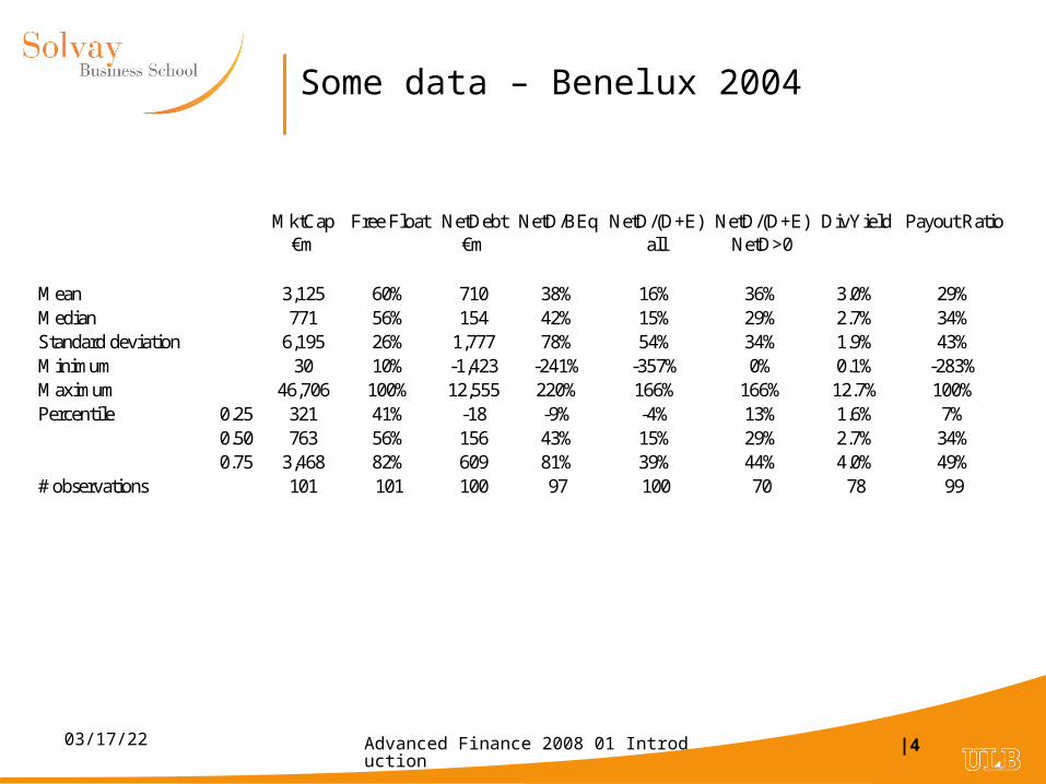
Some data – Benelux 2004

MktCap€m

Free Float NetDebt€m

NetD/BEq NetD/(D+E)all

NetD/(D+E)NetD>0

DivYield Payout Ratio

Mean 3,125 60% 710 38% 16% 36% 3.0% 29%Median 771 56% 154 42% 15% 29% 2.7% 34%Standard deviation 6,195 26% 1,777 78% 54% 34% 1.9% 43%Minimum 30 10% -1,423 -241% -357% 0% 0.1% -283%Maximum 46,706 100% 12,555 220% 166% 166% 12.7% 100%Percentile 0.25 321 41% -18 -9% -4% 13% 1.6% 7%

0.50 763 56% 156 43% 15% 29% 2.7% 34%0.75 3,468 82% 609 81% 39% 44% 4.0% 49%

# observations 101 101 100 97 100 70 78 99


Divide and conquer: the separation principle

• Assumes that capital budgeting and financing decision are independent.

• Calculate present values assuming all-equity financing

• Rational: in perfect capital markets, NPV(Financing) = 0

• 2 key irrelevance results:

– Modigliani-Miller 1958 (MM 58) on capital structure

The value of a firm is independent of its financing

The cost of capital of a firm is independent of its financing

– Miller-Modigliani 1961 (MM 61) on dividend policy

The value of a firm is determined by its free cash flows

Dividend policy doesn’t matter.

• Hotly debated: the efficient market hypothesis


Market imperfections

• Issuing securities is costly

• Taxes might have an impact on the financial policy of a company

• Tax rates on dividends are higher than on capital gains

• Interest expenses are tax deductible

• Agency problems

• Conflicts of interest between

– Managers and stockholders

– Stockholders and bondholders

• Information asymmetries


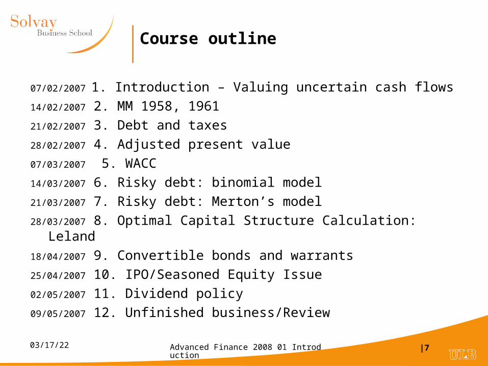
Course outline

07/02/2007 1. Introduction – Valuing uncertain cash flows

14/02/2007 2. MM 1958, 1961

21/02/2007 3. Debt and taxes

28/02/2007 4. Adjusted present value

07/03/2007 5. WACC

14/03/2007 6. Risky debt: binomial model

21/03/2007 7. Risky debt: Merton’s model

28/03/2007 8. Optimal Capital Structure Calculation: Leland

18/04/2007 9. Convertible bonds and warrants

25/04/2007 10. IPO/Seasoned Equity Issue

02/05/2007 11. Dividend policy

09/05/2007 12. Unfinished business/Review


Practice of corporate finance: evidence from the field

• Graham & Harvey (2001) : survey of 392 CFOs about cost of capital, capital budgeting, capital structure.

• « ..executives use the mainline techniques that business schools have taught for years, NPV and CAPM to value projects and to estimate the cost of equity. Interestingly, financial executives are much less likely to follows the academically proscribed factor and theories when determining capital structure »

• Are theories valid? Are CFOs ignorant?

• Are business schools better at teaching capital budgeting and the cost of capital than at teaching capital structure?

• Graham and Harvey Journal of Financial Economics 60 (2001) 187-243


Finance 101 – A review

• Objective: Value creation – increase market value of company

• Net Present Value (NPV): a measure of the change in the market value of the company

NPV = V

• Market Value of Company = present value of future free cash flows

• Free Cash Flow = CF from operation + CF from investment

• CFop = Net Income + Depreciation - Working Capital Requirement


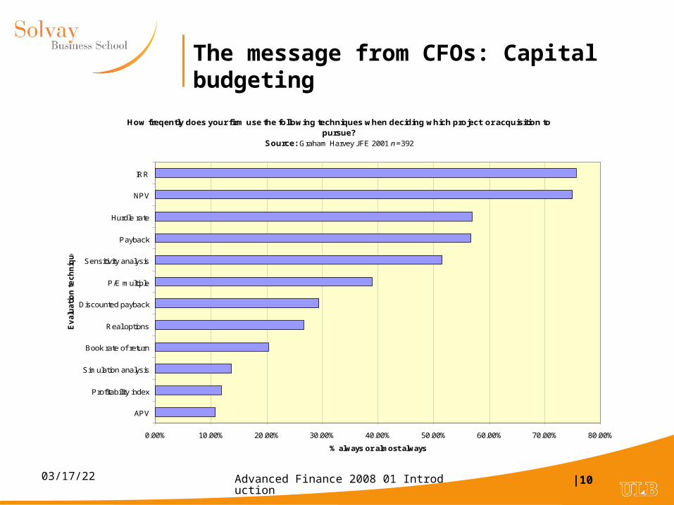
The message from CFOs: Capital budgeting

How freqently does your firm use the following techniques when deciding which project or acquisition to pursue?

Source: Graham Harvey JFE 2001 n=392

0.00% 10.00% 20.00% 30.00% 40.00% 50.00% 60.00% 70.00% 80.00%

APV

Profitability index

Simulation analysis

Book rate of return

Real options

Discounted payback

P/E multiple

Sensitivity analysis

Payback

Hurdle rate

NPV

IRR

Ev

alu

ati

on

te

ch

niq

ue

% always or almost always


Valuation models

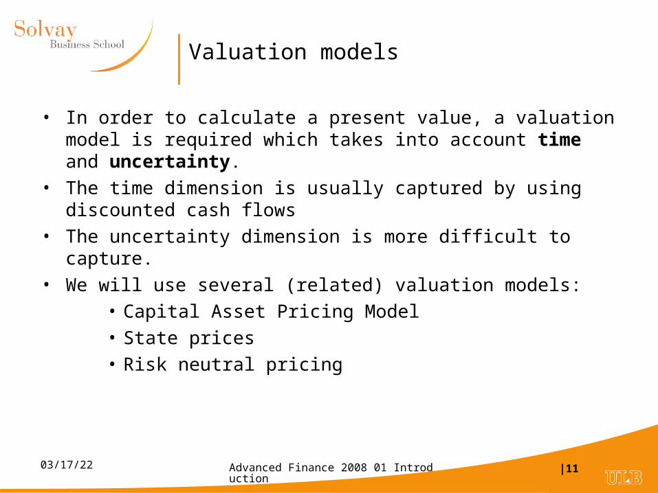
• In order to calculate a present value, a valuation model is required which takes into account time and uncertainty.

• The time dimension is usually captured by using discounted cash flows

• The uncertainty dimension is more difficult to capture.

• We will use several (related) valuation models:

• Capital Asset Pricing Model

• State prices

• Risk neutral pricing


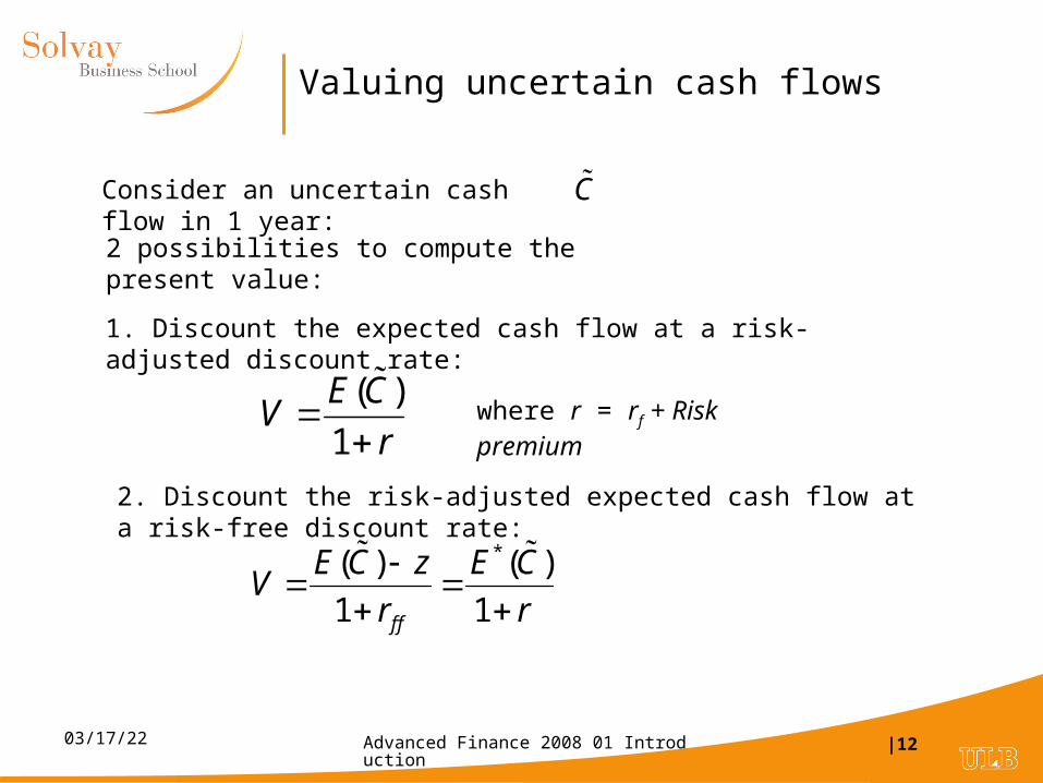
Valuing uncertain cash flows

Consider an uncertain cash flow in 1 year: C

2 possibilities to compute the present value:

1. Discount the expected cash flow at a risk-adjusted discount rate:

( )

1

E CV

r

where r = rf + Risk premium

2. Discount the risk-adjusted expected cash flow at a risk-free discount rate:

*( ) ( )

1 1f f

E C z E CV

r r


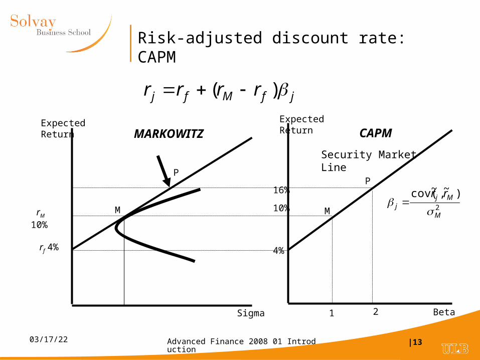
Risk-adjusted discount rate: CAPM

jfMfj rrrr )(

rf 4%

rM 10%

1 2 Beta

M

P

4%

10%

16%

Sigma

Expected ReturnExpected Return

M

P

2

)~,~cov(

M

Mjj

rr

Security Market Line

MARKOWITZ CAPM


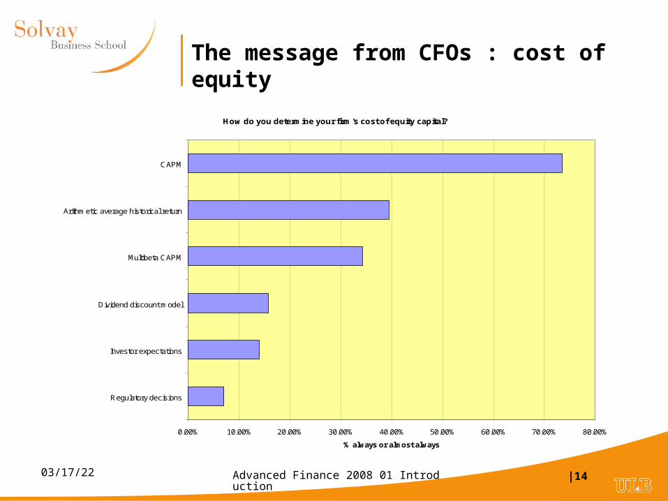
The message from CFOs : cost of equity

How do you determine your firm's cost of equity capital?

0.00% 10.00% 20.00% 30.00% 40.00% 50.00% 60.00% 70.00% 80.00%

Regulatory decisions

Investor expectations

Dividend discount model

Multibeta CAPM

Arithmetic average historical return

CAPM

% always or almost always


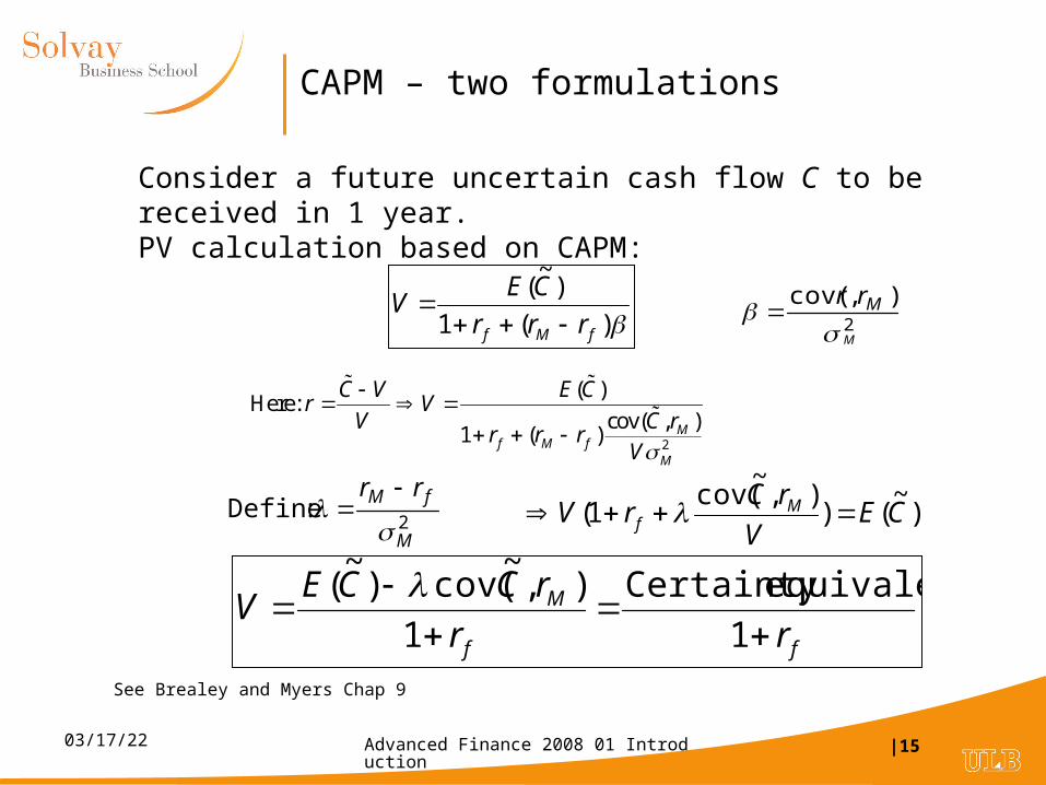
CAPM – two formulations

)(1

)~

(

fMf rrr

CEV

2

),cov(

M

Mrr

2

( )Here:

cov( , )1 ( ) M

f M fM

C V E Cr V

V C rr r r

V

Consider a future uncertain cash flow C to be received in 1 year.PV calculation based on CAPM:

)~

()),

~cov(

1( CEV

rCrV M

f 2 :Define

M

fM rr

ff

M

rr

rCCEV

1

equivalentCertainty

1

),~

cov()~

(

See Brealey and Myers Chap 9


Risk-adjusted expected cash flow

Using risk-adjusted discount rates is OK if you know beta.

The adjusted risk-adjusted discount rate does not work for OPTIONS or projects with unknown betas.

To understand how to proceed in that case, we need to go deeper into valuation theory.


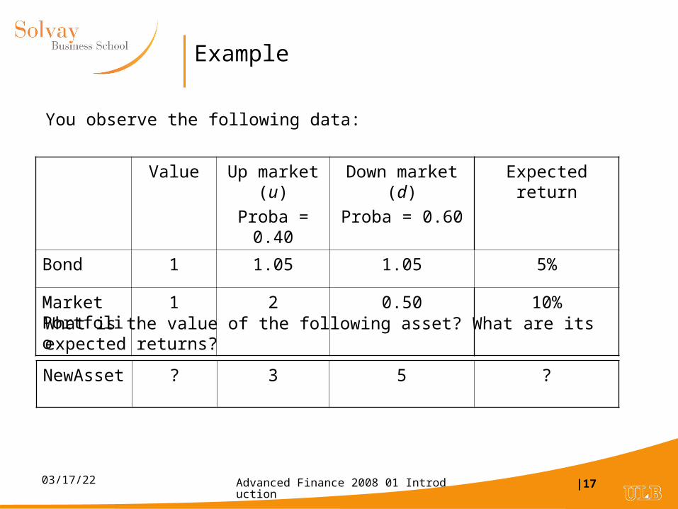
Example

Value Up market (u)

Proba = 0.40

Down market (d)

Proba = 0.60

Expected return

Bond 1 1.05 1.05 5%

Market Portfolio

1 2 0.50 10%

NewAsset ? 3 5 ?

What is the value of the following asset? What are its expected returns?

You observe the following data:


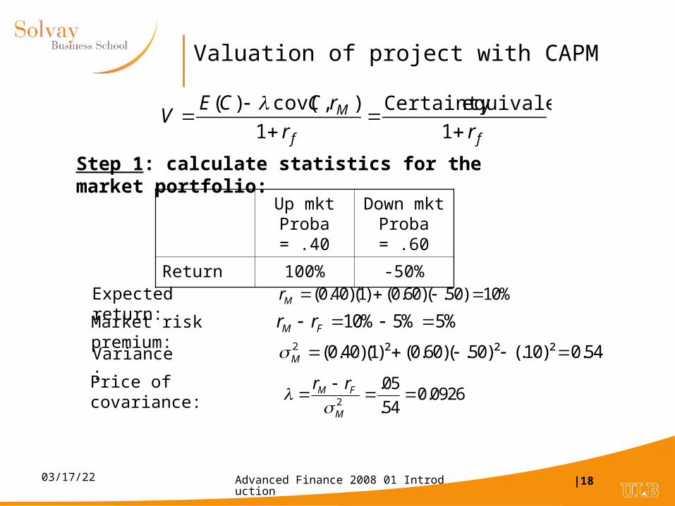
Valuation of project with CAPM

ff

M

rr

rCCEV

1

equivalentCertainty

1

),cov()(

Step 1: calculate statistics for the market portfolio:

Up mkt Proba = .40

Down mkt Proba = .60

Return 100% -50%

Expected return: (0.40)(1) (0.60)( .50) 10%Mr

Variance:2 (0.40)(1)² (0.60)( .50)² (.10)² 0.54M

Market risk premium: 10% 5% 5%M Fr r

Price of covariance:2

.050.0926

.54M F

M

r r


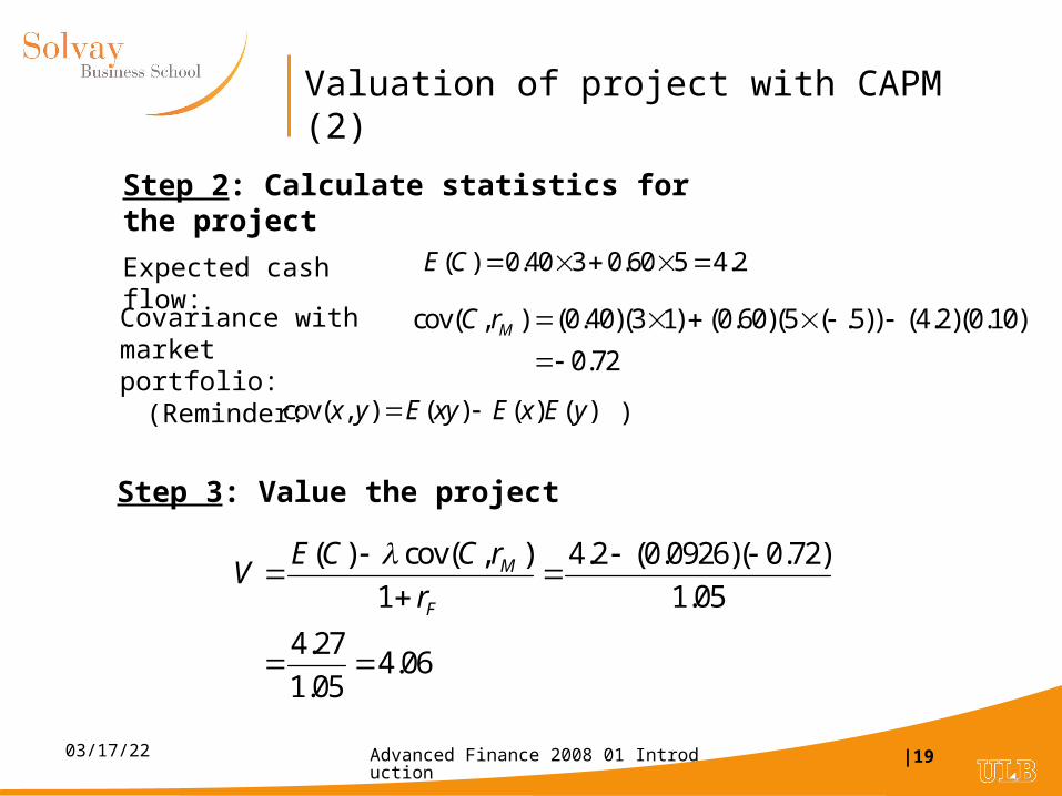
Valuation of project with CAPM (2)

Step 2: Calculate statistics for the project

Expected cash flow: ( ) 0.40 3 0.60 5 4.2E C

Covariance with market portfolio:

cov( , ) ( ) ( ) ( )x y E xy E x E y

cov( , ) (0.40)(3 1) (0.60)(5 ( .5)) (4.2)(0.10)

0.72MC r

(Reminder: )

Step 3: Value the project

( ) cov( , ) 4.2 (0.0926)( 0.72)

1 1.05

4.274.06

1.05

M

F

E C C rV

r


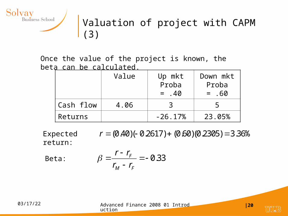
Valuation of project with CAPM (3)

Once the value of the project is known, the beta can be calculated.

Value Up mkt Proba = .40

Down mkt Proba = .60

Cash flow 4.06 3 5

Returns -26.17% 23.05%

Expected return: (0.40)( 0.2617) (0.60)(0.2305) 3.36%r

Beta: 0.33F

M F

r r

r r


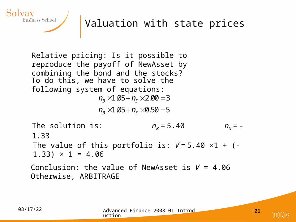
Valuation with state prices

Relative pricing: Is it possible to reproduce the payoff of NewAsset by combining the bond and the stocks?

To do this, we have to solve the following system of equations:

1.05 2.00 3

1.05 0.50 5B S

B S

n n

n n

The solution is: nB = 5.40 nS = - 1.33

The value of this portfolio is: V = 5.40 ×1 + (-1.33) × 1 = 4.06

Conclusion: the value of NewAsset is V = 4.06 Otherwise, ARBITRAGE


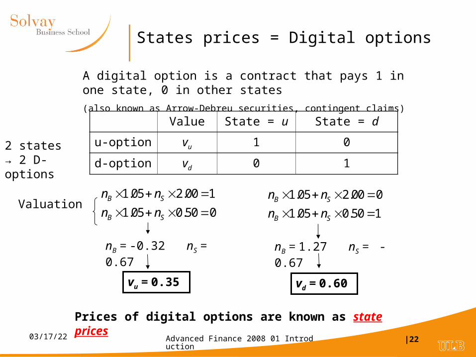
States prices = Digital options

Value State = u State = d

u-option vu 1 0

d-option vd 0 1

1.05 2.00 1

1.05 0.50 0B S

B S

n n

n n

1.05 2.00 0

1.05 0.50 1B S

B S

n n

n n

nB = -0.32 nS = 0.67 nB = 1.27 nS = -0.67

vu = 0.35 vd = 0.60

A digital option is a contract that pays 1 in one state, 0 in other states

(also known as Arrow-Debreu securities, contingent claims)

2 states→ 2 D-options

Valuation

Prices of digital options are known as state prices


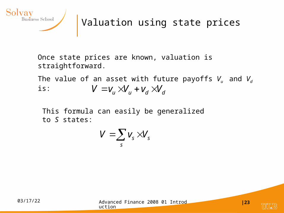
Valuation using state prices

Once state prices are known, valuation is straightforward.

The value of an asset with future payoffs Vu and Vd is:

u u d dV v V v V

This formula can easily be generalized to S states:

s ss

V v V


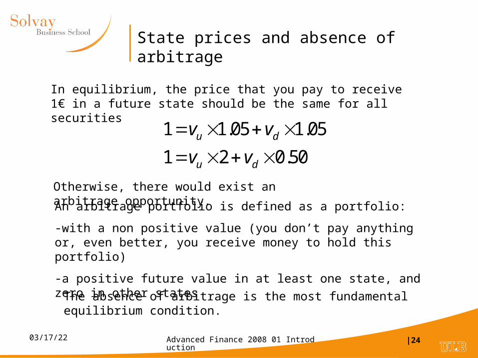
State prices and absence of arbitrage

In equilibrium, the price that you pay to receive 1€ in a future state should be the same for all securities

1 1.05 1.05

1 2 0.50u d

u d

v v

v v

Otherwise, there would exist an arbitrage opportunity.

An arbitrage portfolio is defined as a portfolio:

-with a non positive value (you don’t pay anything or, even better, you receive money to hold this portfolio)

-a positive future value in at least one state, and zero in other states

The absence of arbitrage is the most fundamental equilibrium condition.


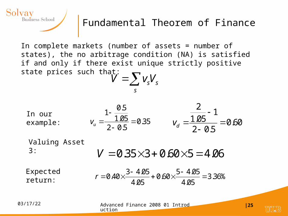
Fundamental Theorem of Finance

s ss

V v V

In our example:0.5

11.05 0.35

2 0.5uv

21

1.05 0.602 0.5dv

In complete markets (number of assets = number of states), the no arbitrage condition (NA) is satisfied if and only if there exist unique strictly positive state prices such that:

0.35 3 0.60 5 4.06V Valuing Asset 3:

Expected return: 3 4.05 5 4.050.40 0.60 3.36%

4.05 4.05r


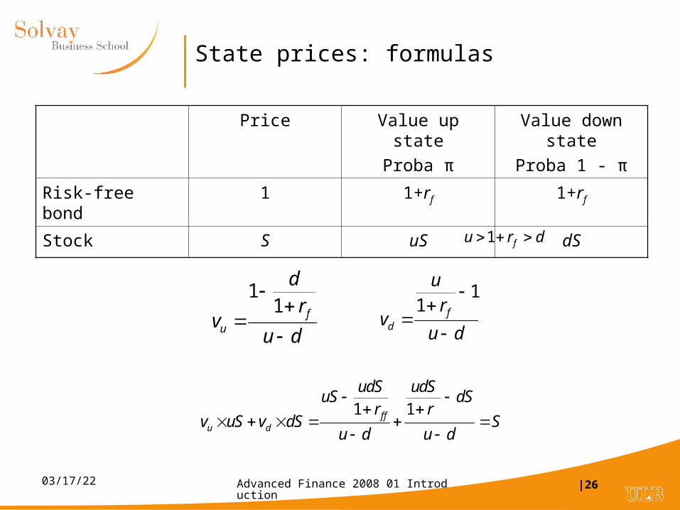
State prices: formulas

Price Value up state

Proba π

Value down state

Proba 1 - π

Risk-free bond 1 1+rf 1+rf

Stock S uS dS

11 f

u

dr

vu d

11 f

d

ur

vu d

1 1f fu d

udS udSuS dS

r rv uS v dS S

u d u d

1 fu r d


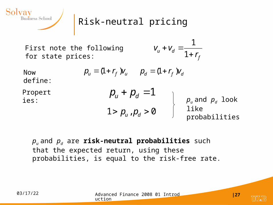
Risk-neutral pricing

(1 )d f dp r v

1

1u df

v vr

(1 )u f up r v Now define:

1u dp p

1 , 0u dp p pu and pd look like probabilities

Properties:

First note the following for state prices:

pu and pd are risk-neutral probabilities such that the expected return, using these probabilities, is equal to the risk-free rate.


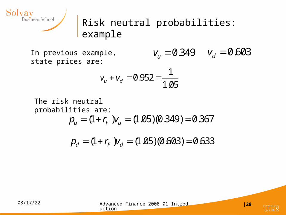
Risk neutral probabilities: example

In previous example, state prices are: 0.349uv 0.603dv

10.952

1.05u dv v

The risk neutral probabilities are:

(1 ) (1.05)(0.349) 0.367u F up r v

(1 ) (1.05)(0.603) 0.633d F dp r v


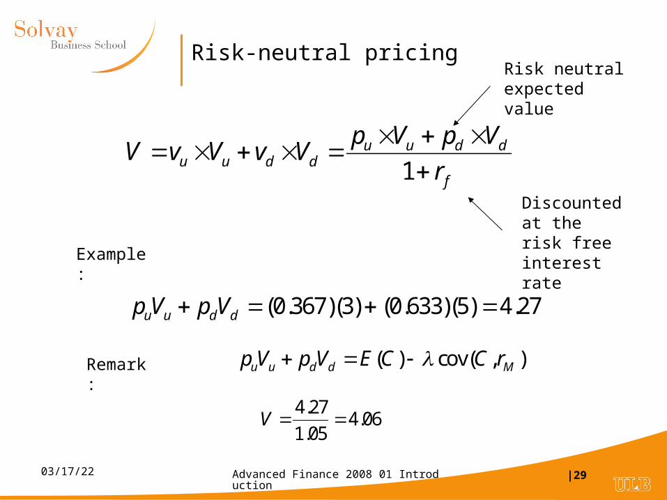
Risk-neutral pricing

1u u d d

u u d df

p V p VV v V v V

r

Risk neutral expected value

Discounted at the risk free interest rate

(0.367)(3) (0.633)(5) 4.27u u d dp V p V

( ) cov( , )u u d d Mp V p V E C C r

Example:

Remark:

4.274.06

1.05V

Documents

Advanced Finance 2007-2008 Introduction Professor André Farber Solvay Business School Université Libre de Bruxelles