Advanced ExcelCrash Course

By Lori Rayl

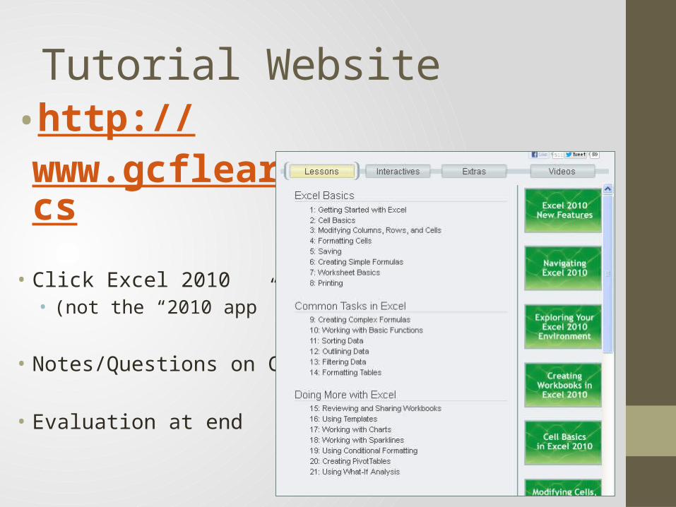
Tutorial Website•http://www.gcflearnfree.org/topics

• Click Excel 2010 • (not the “2010 app” option)

• Notes/Questions on Card

• Evaluation at end

Excel Basics (from Lessons 1-8)New to 2010 and FAQ

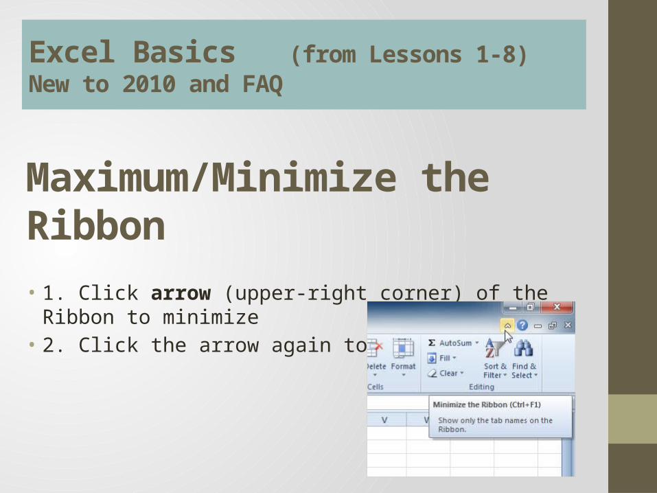
Maximum/Minimize the Ribbon

• 1. Click arrow (upper-right corner) of the Ribbon to minimize• 2. Click the arrow again to maximize

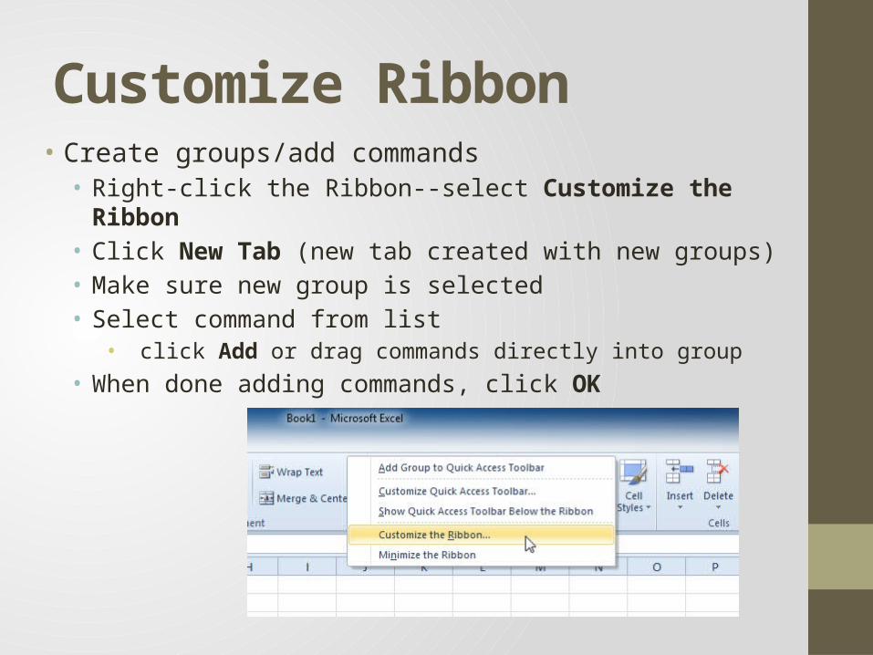
Customize Ribbon• Create groups/add commands• Right-click the Ribbon--select Customize the Ribbon• Click New Tab (new tab created with new groups)• Make sure new group is selected• Select command from list

• click Add or drag commands directly into group• When done adding commands, click OK

Customize Quick Access Toolbar

Add Commands to Quick Access Toolbar:• 1. Click drop-down arrow --right of the

Quick Access Toolbar.• 2. Select command to add

• Challenge: Lesson 1 Page 7 (customize ribbon, quick access toolbar)

Drag and Drop Cells• Select the cells that you wish to move. • mouse on outside edge of the selected cells (mouse changes

from white cross to black cross with 4 arrows) • Click and drag cells to new location• Release mouse

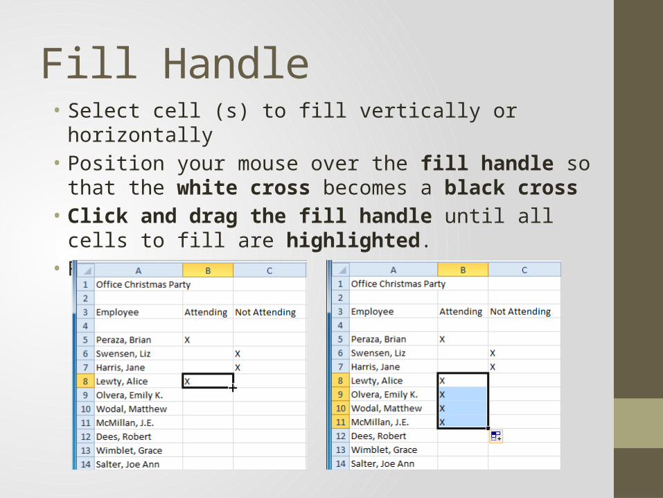
Fill Handle• Select cell (s) to fill vertically or horizontally• Position your mouse over the fill handle so that the white cross

becomes a black cross • Click and drag the fill handle until all cells to fill are highlighted.• Release the mouse

Auto Recover• To recover file if forget to save or Excel crashes• Click File, click Info.• Under Versions. Click on the file to open.• A yellow caution note appears on the ribbon• click Restore and then click OK.

• Excel autosaves every 10 minutes• If no previously saved versions, browse all autosaved files • click on the Manage Versions button• select Recover Unsaved Workbooks

(illustrated on next slide)

Saving• To save as Excel 97-2003 Workbook• Click File tab.• Select Save As• In Save as type drop-down menu, select Excel 97-2003

Workbook.

• To save as PDF File (if sharing but no Excel)• In the Save as type menu, select PDF• Note: only saves worksheet—for workbook, click Options, Entire

Workbook, OK.

• Challenge: Lesson 5 Page 4 (2003, pdf)

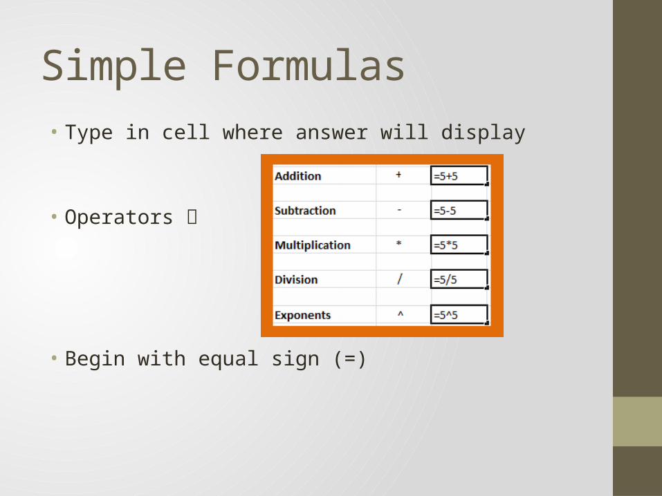
Simple Formulas• Type in cell where answer will display

• Operators

• Begin with equal sign (=)

Cell References in Formulas

• Type formula you want Excel to calculate• For example =75/250

• Or type cell references • For example =B2/B3 (now changed values auto recalculate)• Point and click method (B2 and B3)

• Challenge Lesson 6, Page 6 (simple formulas)

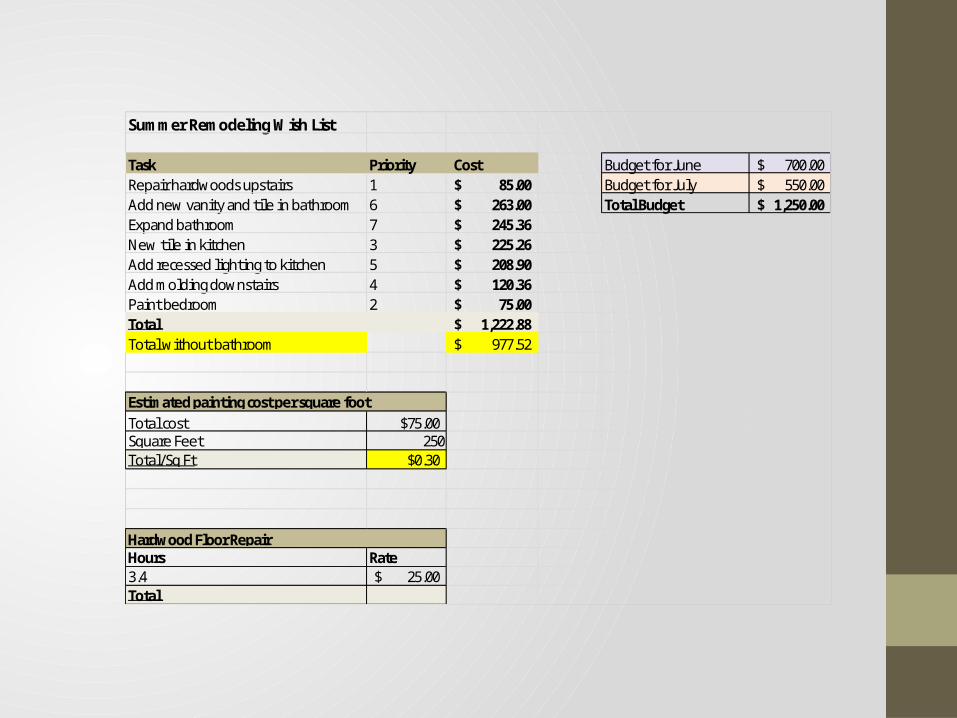
Summer Remodeling Wish List

Task Priority Cost Budget for June 700.00$ Repair hardwoods upstairs 1 85.00$ Budget for July 550.00$ Add new vanity and tile in bathroom 6 263.00$ Total Budget 1,250.00$ Expand bathroom 7 245.36$ New tile in kitchen 3 225.26$ Add recessed lighting to kitchen 5 208.90$ Add molding downstairs 4 120.36$ Paint bedroom 2 75.00$ Total 1,222.88$ Total without bathroom 977.52$

Total cost $75.00Square Feet 250Total/Sq Ft $0.30

Hours Rate3.4 25.00$ Total

Estimated painting cost per square foot

Hardwood Floor Repair

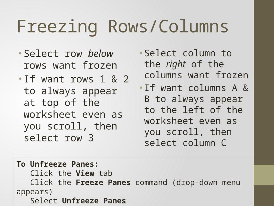
Freezing Rows/Columns• Select row below rows

want frozen• If want rows 1 & 2 to

always appear at top of the worksheet even as you scroll, then select row 3

• Select column to the right of the columns want frozen• If want columns A & B

to always appear to the left of the worksheet even as you scroll, then select column C

To Unfreeze Panes:Click the View tabClick the Freeze Panes command (drop-down menu appears)Select Unfreeze Panes

Print Specialties

• To Print a Selection, or Set the Print Area:• Printing a selection (to choose which cells to print—not entire

worksheet• Selected cells to print • Click the File tab.• Select Print to access the Print pane.• Select Print Selection from the print range drop-down menu.

Print Titles• For Titles to appear on each page• Click the Page Layout tab.• Select the Print Titles command• Page Setup dialog box appears • Click icon at end of Rows to repeat at top field.

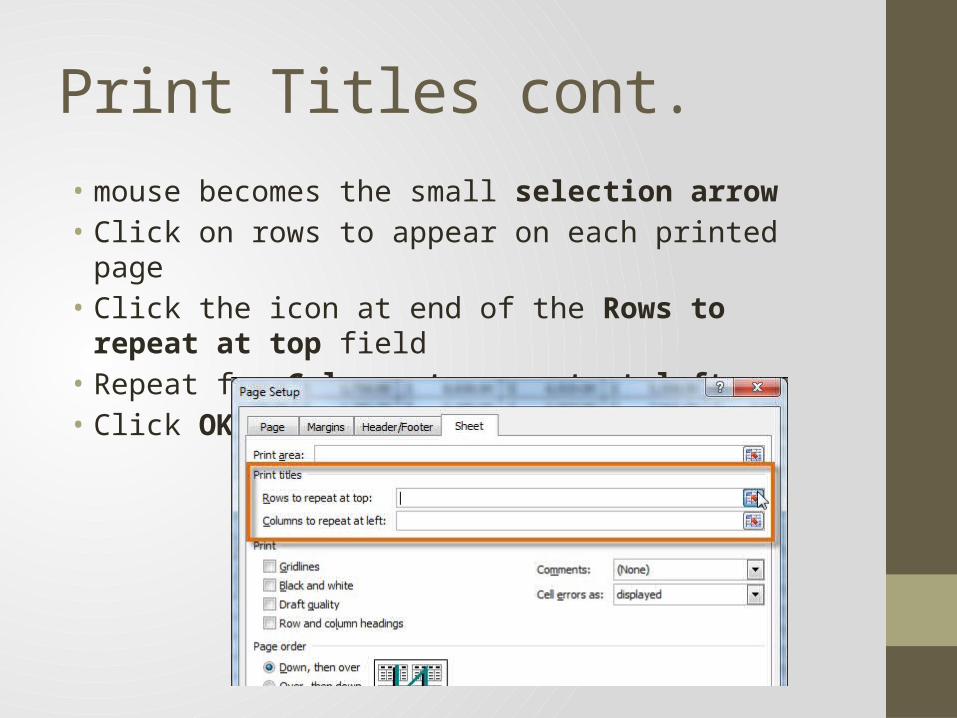
Print Titles cont.• mouse becomes the small selection arrow• Click on rows to appear on each printed page• Click the icon at end of the Rows to repeat at top field• Repeat for Columns to repeat at left• Click OK

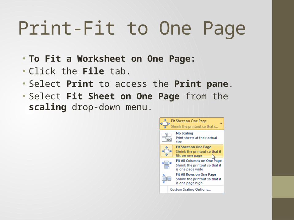
Print-Fit to One Page• To Fit a Worksheet on One Page:• Click the File tab.• Select Print to access the Print pane.• Select Fit Sheet on One Page from the scaling drop-down

menu.

Excel–Beyond the Basics• Hit highlights Lessons 9 thru 21• Challenges end of each Lesson• Notes on Card• Questions• Lessons interest you

Lesson 9: Complex Formulas• Order of Operations• Excel calculates formulas as follows:• Operations enclosed in parentheses• Exponential calculations (to the power of)• Multiplication and division, whichever comes first• Addition and subtraction, whichever comes first

• A mnemonic - Please Excuse My Dear Aunt Sally

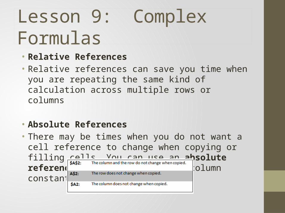
Lesson 9: Complex Formulas• Relative References• Relative references can save you time when you are repeating

the same kind of calculation across multiple rows or columns

• Absolute References• There may be times when you do not want a cell reference to

change when copying or filling cells. You can use an absolute reference to keep a row and/or column constant in the formula.

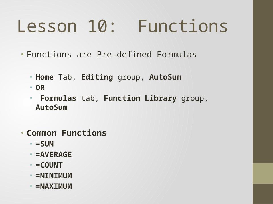
Lesson 10: Functions• Functions are Pre-defined Formulas

• Home Tab, Editing group, AutoSum• OR• Formulas tab, Function Library group, AutoSum

• Common Functions• =SUM• =AVERAGE• =COUNT• =MINIMUM• =MAXIMUM

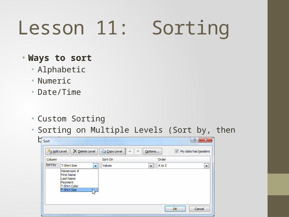
Lesson 11: Sorting• Ways to sort• Alphabetic• Numeric• Date/Time

• Custom Sorting• Sorting on Multiple Levels (Sort by, then by….)

Lesson 12: Outlining• organize your data into groups• show or hide them from view• summarize data using Subtotal command

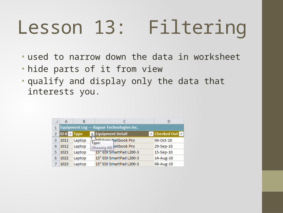
Lesson 13: Filtering• used to narrow down the data in worksheet• hide parts of it from view• qualify and display only the data that interests you.

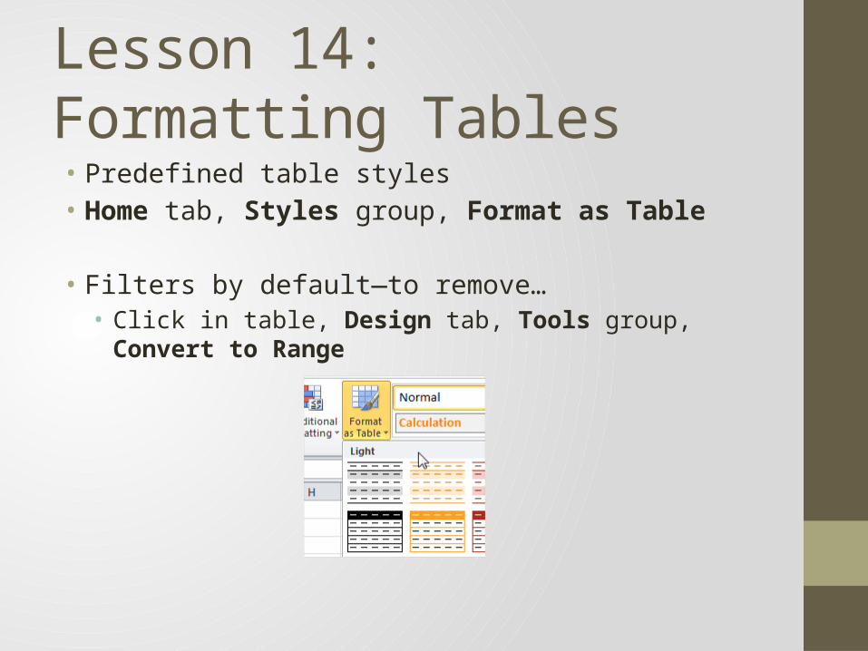
Lesson 14: Formatting Tables• Predefined table styles• Home tab, Styles group, Format as Table

• Filters by default—to remove…• Click in table, Design tab, Tools group, Convert to Range

Lesson 15: Reviewing/Sharing Workbooks

• Review

• Collaborate

Lesson 16: Templates

• File tab, New• Examples:• Agendas• Faxes• Expense Reports• Inventories

Templates are Pre-designed spreadsheets

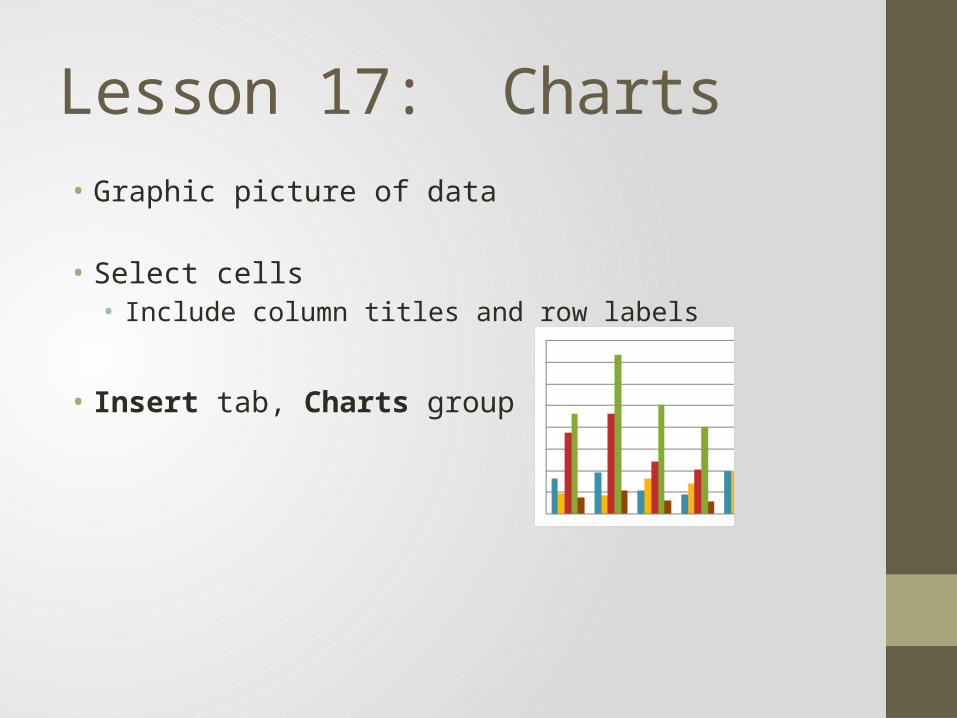
Lesson 17: Charts• Graphic picture of data

• Select cells• Include column titles and row labels

• Insert tab, Charts group

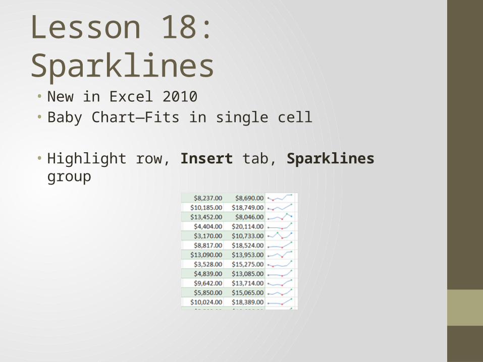
Lesson 18: Sparklines• New in Excel 2010• Baby Chart—Fits in single cell

• Highlight row, Insert tab, Sparklines group

Lesson 19: Conditional Formatting

• Visualize cell values using conditional rules• If cell value > 100 then cell green

• To set up:• Select cells, Home tab, Styles group, Conditional Formatting

• To clear:• Select cells, Home tab, Styles group, Conditional Formatting,

Clear Rules checkbox

Lesson 20: PivotTables• Summarize and manipulate data

• To create:• Select table or cells• Insert tab, Tables group, PivotTable

• PivotCharts to display PivotTable data

Lesson 21: What-If Analysis• What-If analysis --to see the effect that different values have in

formulas

• What interest rate do I need for car payment of $400?

• Goal Seek• Scenarios• Data tables

Evaluation• Website: