ADVANCED DIGITAL SYSTEMS(CS 401 Class Note)

Instructor: Dr. C. N. Zhang

Department of Computer ScienceUniversity of Regina

Regina, SaskatchewanCanada, S4S 0A2

Table of Contents

1. Introduction to Parallel Processing........................................................32. Reduced Instruction Set Computers ( RISCs ).....................................103. Analysis of Parallelism in Algorithms...................................................184. Parallelism for Loop Algorithms...........................................................275. Parallel Computer Architectures...........................................................486. Mapping Nested Loops into Systolic Arrays.........................................687. Associative Memory................................................................................848. Data Flow Computing.............................................................................87

9. Intel MMXTM

Technology...................................................................91

2

1. Introduction to Parallel Processing1. Parallel Processing: two or more tasks being performed (executed) simultaneously.1.1 Basic techniques for parallel processing

a. pipelineb. replicated unitsc. pipeline plus replicated units

1.2 Parallel processing can be implemented at the different levelsa. at processor level : multiple processorsb. at instruction execution level : instruction pipeline c. at arithmetic and logic operation level : multiple ALU, pipelined ALUd. at logic circuit level : fast adder, pipelined multiplier

1.3 Speed-up of the parallel processing:

where TS is the time by processing sequential (non-parallel) manner and TP is the processing time required by parallel processing technique.

1.4 Efficiency of the parallel processing

where n is the number of units used to perform the parallel processing.Note: 0 S n and 0 E 1

where aijs are integers. i=1, 2, … , n, j=1, 2, …, m. Assume that the time delay of the Adder is t. Sequential processing: Use one Adder. TS = ( n-1 ) m t

Parallel Processing:a. use two adders:

S = 2 E = 1b. use m adders: Tp = ( n-1 ) t S = m E = 1c. use n-1 adders ( n = 2k ) as pipelining (see figure 1.1 in the next page)

e.g. n = 8 Tp = ( logn + m-1 ) t

3

a11 a21 a31 a41 a51 a61 a71 a81

a12 a22 a32 a42 a52 a62 a72 a82

… … … … … … … … a1m a2m a3m a4m a5m a6m a7m a8m Figure 1.1

1.5 Pipeline Designa. The task is able to be divided into a number of subtasks in sequence, and

hopefully each subtask requires the same amount time.b. Design an independent hardware unit for each subtask.c. Connect all units in order.d. Arrange the input data and collect the output data.

Subtask1: S1 = a1j + a2j

Subtask2: S2 = S1 + a3j

Subtask3: Yj = S2 + a4j

b. unit for subtask1: S1

a1j a2j

4

+

+

+ +

++++

unit for subtask2: S2

S1 a3j

unit for subtask3: Yj

+++

S2 a3j

c. unit connections

S1 S2

a1j

a2j Yj

a3j a4j

d. input and output arrangement 0 0 a14 a13 a12 a11

0 0 a24 a23 a22 a21 Y4Y3Y2Y1

0 0 a31 0 a32 a41

a33 a42

a34 a43

0 a44 Figure 1.2

Tp = ( n + m - 2 ) t

Second pipeline design:

5

+

+

+ + +

+ + +

Subtask1: S1 = a1j + a2j and S2 = a3j + a4j

Subtask2: Yj = S1 + S2 S1 S2

b. unit for subtask1:

a1j a2j a3j a4j

unit for subtask2: Yj

S1 S2 c. unit connections Yj

S1 S2

a1j a2j a3j a4j

d. input and output arrangement Y1

Y2

Y3

Y4

a11 a21 a31 a41

a12 a22 a32 a42

a13

a23

a33

a43

6

+

+

+

++

+

++

+

a14 a24 a34 a44 Figure 1.3Tp = ( m -1 + logn ) t

2. Review of Computer Architecture

2.1 Basic Components of Computer System• CPU : includes ALU and Control Unit• Memory: cache memory, main memory, secondary memory• I/O : DMA, I/O interface, and I/O devices

• Bus : a set of communication pathways (data, address, and control signals)

connect two or more components2.2 Single Processor Configurations

• Multiple bus connected computer systems.

I/O Bus Memory Bus

or

I/O Bus Memory Bus

Figure 1.4

• Single bus connected systems

BBSY BR

7

CPU Memory

I/O

I/O

CPUMemory

I/O

I/O

CPU Memory I/O I/ODMAArbiter

BG

System Bus

Figure 1.5

Note: • At any time only one unit can control the bus, though two or more units require to use the bus at the same time.• The arbiter is used to select which unit is going to use the bus next time.• BR (bus request), BG (bus grant), SACK (Select acknowledgement), and BBSY (bus busy) are the most important control signals used by the arbiter.• The timing diagram of these control signals are:

BBSY

BR

BG

SACK

Figure 1.6

2.3 Central Processing Unit (CPU) • ALU : performs all logic and arithmetic operations and has a number of general purpose registers. . • Control Unit: produces all control signals required by ALU and bus. Control unit be implemented by logic circuits or microprogramming.

An instruction cycle includes several smaller function cycles, e.g.,1) instruction fetch cycle.2) indirect (operand fetch) cycle.3) execution cycle.4) interrupt cycle

2.4 Memory • Store instructions and data • Memory configuration: Hardware mapping

8

cache

Cache

Main Memory

DMA transfer

Figure 1.7 •) cache memory : a small fast memory which is placed between CPU and main memory •) why cache ? : there is a big speed gap between CPU and main memory •) hardware mapping: direct mapping, associative mapping, and set associative mapping2.5 Inputs and Outputs (I/O) • Programming I/O: CPU is idle While waiting • interrupt driven I/O: CPU is interrupted when I/O requires service

Bus

Figure 1.8

• DMA 1/0 : HD, CDROM······· for direct memory access

Bus

Figure 1.9

2.6. How To Improve Performance of Computer Systems?• by electronic technology, e.g., new VLSI development• by software development, e.g., better OS and compiler

9

Secondary Memory

I/O Device

I/O Device

I/O Interface

High speed I/O

DMA controller

• by architecture enhancements

2.7 Architecture Enhancements• pipeline• parallelism• memory hierarchy• multiple processor computer systems• hardware supports for OS and compiler• special purpose architectures

2. Reduced Instruction Set Computers ( RISCs )2. 1 The Instruction Execution Characteristics

Table 2.1

Weighted Relative Dynamic Frequency of HLL Operations

Machine- Memory- Dynamic Instruction Reference Occurrence Weighted Weighted Pascal C Pascal C Pascal C

ASSIGN 45 38 13 13 14 15

LOOP 5 3 42 32 33 26

CALL 15 12 31 33 44 45

IF 29 43 11 21 7 13

GOTO - 3 - - - -

OTHER 6 1 3 1 2 1

Procedure Arguments and Local Scalar Variables

Percentage of Executed Compiler, Interpreter Small NonnumericProcedure Calls with and Typesetter Programs

>3 arguments 0-7% 0-5%

>5 arguments 0-3% 0%

>8 words of arguments

and local scalars 1-20% 0-6%

>12 words of arguments

and local scalars 1-6% 0-3%

10

Conclusion:

a) Most frequent statements are simple assignment statements.b) Conditional statements (if, loop, conditional branch) are also important.c) Programs are organized in procedures. Procedure call and return are very frequent

and time consuming. d) Procedures usually have • a few input arguments from parent procedure • a few result arguments to parent procedure • a few local variables • a few global variables • the depth of nested procedures is small ( < 5 ) • most variables are scalars

2.2. RISC Architecture

• Register-oriented organization a) register is the fastest available storage device b) save memory access time for most data passing operations c) VLSI makes it possible to build large number of registers on a single chip

• Few instructions with fixed length: a) there are two groups of instructions: register to register, memory to register or register to memory b) complex instructions are done by software (macro program)c) make it easy for instruction decoding and pipeline

• Simple addressing models a) simplify memory address calculation b) makes it easy to pipeline

• Use register window technique a) optimizing compilers with fewer instructions b) based on large register file

• CPU on a single VLSI chip a) avoid long time delay of off-chip signals b) regular ALU and simple control unit

• Pipelined instruction execution a) two-, three-, or four-stage pipelines b) delayed-branch and data forward

2.3. RISC Register Windows Technique

• Time spent for each procedure call and return

11

1) T1 : save the contents of registers used by parent procedure 2) T7 : read in parameters assigned by the parent procedure 3) T3 : execution 4) T4 : pass the results to locations assigned by parent procedure 5) T5 : restore all contents of registers in step 1.

Figure 2.1 • Fixed size overlapping register windows

1) There are a number of windows which are organized as a circular buffer. One window for one procedure.

12

Pare

nt p

roce

dure

curr

ent p

roce

dure

Figure 2.22) At any time, only one window is visible for current procedure pointed by current

window pointer (CWP).3) Each window consists of three parts: parameter registers, local registers, and

temporary registers. Each of them has a fixed number of registers. The number of registers in parameter and temporary registers are the same. Temporary register of parent procedure is overlapped with parameter register of current procedure which permits the parameters to be passed without actual data movements.

Parameter Registers

LocalRegisters

Temporary Registers

Call return

Parameter Registers

LocalRegisters

Temporary Registers

Figure 2.3

• Parameter Registers (PR): hold parameters passed down from the parent procedure and pass the results back up to the parent procedure by the current (child) procedure.

• Local Registers (LR): are used for local variables assigned by compiler.

• Temporary Registers (TR): are used to exchange parameters and results with the procedure called by parent procedure. Before a procedure call, parent procedure writes the actual parameters into TR. After the call, current procedure has all parameters in PR of its own window. Before returning from current procedure to its parent procedure, it sends all results into PR. Therefore, After the return, parent procedure gets all results in its TR.

4) There are two pointer registers: current window pointer (CWP) and saved windows pointer (SWP). CWP: points to the window of the current active procedure. After each procedure call, CWP : = CWP + 1 mod n (suppose there are n windows numbered by 0,1, 2, ..., n-1. Initially, CWP : = n-1 ). After each return, CWP: =CWP-1, mod n. SWP : identifies the youngest window that has been saved in the stack. Initially, SWP : = n-l.

13

Level J

Level J+1

When window overflow occurs, SWP : = SWP + 1 mod n, and save the window pointed by SWP into memory stack. When window underflow occurs, POP back the registers from memory stack and send them to the window pointed by the SWP and SWP : = SWP - 1 mod n.

5) Condition of window overflow: CWP : = CWP + 1 mod n (after a procedure call) CWP : = SWP

6) Condition of window underflow:CWP : = CWP-1 mod n (after a procedure return)

SWP : = CWP

Example: n=6

Initially, CWP = 5 SWP = 5Call A CWP = 0 SWP = 5A calls B CWP = l SWP = 5B calls C CWP = 2 SWP = 5C calls D CWP = 3 SWP = 5D calls E CWP = 4 SWP = 5E calls F CWP = 5 SWP = 5 window overflow, SWP : = SWP + 1

mod 6 = 0, and save the window A to memory stack.F returns CWP = 4 SWP = 0E returns CWP = 3 SWP = 0D returns CWP = 2 SWP = 0C returns CWP = 1 SWP = 0B returns CWP = 0 SWP = 0 window underflow, read window A from stack, and SWP : =SWP-1 mod 6 = 5.

2.4. RISC Instruction Pipelining

• There are two types of instruction in RISCV. 1) Register-to-register, each of which can be done by the following two phases: I : Instruction fetch E: Instruction execution 2) Memory-to-register (load) and register-to-memory (store), each of which can be done by the following three phases: I: Instruction fetch E: Memory address calculation D: Memory operation

• Pipeline: a task or operation is divided into a number of subtasks; that need to be performed in sequence, each of which requires the same amount of time.

14

where Ts is the total time required for a job performed by non-pipeline.Tp is the time required by pipeline.

• Pipeline conflict: If two subtasks on the two pipeline units can not be computed simultaneously. One task must wastes until another task is completed. • To resolve the pipeline conflict in the instruction pipeline the following techniques are used a. inset a no operation stage ( N ) used by two-way pipeline. b. inset no operation instruction ( Noop ) used by three-way and four-way pipeline. • Two-way Pipeline : there is only one memory in the computer which stores both instructions and data. Phases of I and E can be overlapped. Example:

Load A M Sequential execution Load B M Add C A + B Store M C Branch X X: Add B C + A Halt

Load A M Two-way pipelining Load B M Add C A + B Store M C Branch X X: Add B C + A Halt

Figure 2.4

Speed-up = 17 / 11 = 1.54Where N represent the NO operation stage (waiting stage) inserted by OS.

• Three-way pipeline: there are two memory units, one stores instructions, another stores data. Phases of I, E, and D can be overlapped. The NOOP instruction ( two-stage ) is used when there is a pipeline conflict Example:

Load A M Three-way pipelining Load B M NOOP Add C A + B Store M C Branch X

15

I E D

I

I

I

I

I

I

E

E

E

E

E

E

D

D

I

I

N

I

I

I

I

E

E

E

E

E

E

E

D

D

D

NNN

NNN

IN

N N

NN

I E D

I

I

I

I

I

E

E

E

E

E

D

D

NOOP X: Add B C + A Halt

Figure 2.5

Speed-up = 17 / 10 = 1.7Where NOOP represent the NO operation stage (waiting stage) inserted by OS.

• Four-way pipeline: same as the three-way pipeline, but phase E is divided into two stages: E1: register file read E2: ALU operation and register write Phases of I, D, E1, and E2 can be overlapped. Example:

Load A M Four-way pipelining Load B M NOOP NOOP Add C A + B Store M C Branch X NOOP NOOP X: Add B C + A Halt

Figure 2.6

Speed-up = 24 / 13 = 1.85

• Delayed Branch. The goal is to reduce the number of noop instructions by exchanging the order of the instruction prior the branch instruction and the branch instruction Example: (three-way pipeline)

100 Load A M Inserted NOOP

101 Add B B + 1

102 Branch 106

103 NOOP

106 Store M B

16

I E

E

E

I

I

I E1 DE2

D

D

I

I

I

I

I

I

I

I

I

I

E1

E1

E1

E1

E1

E1

E1

E1

E1

E1

E2

E2

E2

E2

E2

E2

E2

E2

E2

E2

I

I

I

I

I

E

E

E

E

E

D

D

100 Load A M Reversed Instructions

101 Branch 106

102 Add B B + 1

106 Store M B

Use of the delayed branch

Figure 2.7

17

I

I

I

I

E

E

E

E

D

D

3. Analysis of Parallelism in Algorithms3. 1. Parallel Computations

• Parallelism is a general term used to characterize a variety of simultaneities; occurring in modem computers.

• Models of Parallel Computations:

a) Pipeliningb) Vector processorsc) Array processorsd) Computer networkse) Dataflow computer

• Performance Indices of Parallel Computation:

a) Execution rate: number of execution per time unit, e.g., Mips : millions of instructions per second Mflops : millions of floating point operations per second

T1 : time taken on one processor for one problem. Tp : time taken on p processors for the same problem.

O1 : total number of instructions (operations) required to compute a problem with one processor. Op : total number of instructions (operations) required to compute the same problem with p processors.

3.2 Analysis of Parallelism with non-loops

18

• > Data dependence of two computations: one computation can not start until the other one is completed. • > Parallelism detection: find out sets of computations that can be performed simultaneously (no data dependencies exist in the set of computations). • > Types of data dependencies on non-loop algorithms or programs: Suppose that Si and Sj are two computations (statements or instructions in a non-loop algorithm or program). Ii , Ij and Oi , Oj are the inputs and outputs of Si and Sj , respectively.

a) Type-1: data flow dependence ( read after write, denoted by RAW )

•) condition (1) j > i(2) Ij Oi

example-1 : : 100 R1 R2 R3

: 105 R5 Rl + R4 example-2: : :

Si : A : = B + C Sj : D : = A E + 2

•) notation: ( computation Sj defends on computation Si )

b) Type-2: data antidependence ( write after read, denoted by WAR ) •) condition: (1) j > i

(2) Oj Ii example-1 : : 200 R1 R2 R3

: 205 R5 R2 + R5 example-2: : :

19

Si

Sj

Si : A : = B C Sj : B : = D + 5

•) notation: ( computation Sj defends on computation Si )

a) Type-3: data-output dependence ( write after read , denoted by WAW )

•) condition (1) j > i(2) Oi Oj

example: : :

Si : A : = B + C :

Sj : A : = D E

•) notation: ( computation Sj defends on computation Si )

•> Data dependence graph ( DDG ): represents all data dependencies among statements (instructions). Example: find DDG for the following program.

100 R1 R3 div R2

101 R4 R4 R5

102 R6 R1 + R3

103 R4 R2 + R3

104 R2 R4 + R2

Solution: Si, Sj Dependency di

100, 101 no100, 102 type-1 1100, 103 no 100, 104 type-2 2

20

Si

Sj

Si

Sj

Si

Ai

Sj

Aj

101, 102 no101, 103 type-3 and type-2 4 and 5101, 104 type-1 6

102, 103 no102, 104 no

103, 104 type-1 and type-2 7 and 8

DDG: d2

d8

d7

d5 d4

d1 O d6

Suppose each statement requires the same amount of time for execution (t), and there are two identical processors (P1 and P2). One of statement – processor assignment can be as follows which

is called space/time diagram or Gantt Chart.

In general data dependent graph (DDG) is a directed acyclic graph DDS = (S, E) where S is set of tasks: S = {S1, S2, … Sn},

Dij

Represents that task Sj depends on Si, and Dij represents the communication cost between Si and Sj. Each note (task) Si is associated with a computation cost Ai.

Suppose that there are three identical processors and there is no cost (Dij = 0) for communications. An example of DDG and corresponding Gantt Chart is shown in Figure 3.1.

1 2 3P1 100 102P2 101 103 104

21

100

101

102

103

104

Figure 3.1. (a) example of DDG; (b) a possible Gantt Chart

3.3. Analysis of Parallelism in loops

Consider the case of single loop in the form:

For l = l1 to ln Do l = l1, ln Begin S1 S1 S2 or S2 : : SN SN End Enddo

A loop can be viewed as a sequence of statements in which the statements (the body of an algorithm) are repeated n times.

e.g., ( n = 3, N = 2 ) S1 ( l = l1 )

S2 ( l = l1 ) S1 ( l = l2 ) S2 ( l = l2 ) S1 ( l = l3 ) S2 ( l = l3 )

22

There are still three types of data dependencies. However, the conditions should be modified. Suppose that Si(li) and Sj(lj) are two statements in the loop, Where li and 1j are the indices of the variable shared by Si and Sj respectively

a) Type-1: (RAW) •) condition: (1) li - 1j > 0 or li = 1j and j > i

(2) Oi Ij •) notation: distance, d = li - 1j 0

d

•) example: for l : = 1 to 5 begin

S1 : B( l + 1 ) : = A(l) C( l + 1 ) S2 : C( l + 4 ) : = B(l) A( l + 1 )

end

Si Sj shared variable li - 1j = d S1 S2 B ( l + 1 ) – l = 1 S2 S1 C ( l + 4 ) – ( l + 1 ) = 3

d = 1 d = 3

b) Type-2: (WAR) •) condition: (1) li - 1j > 0 or li = 1j and j > i

(2) Oj Ii •) notation: distance, d = li - 1j 0

d

c) Type-3: (WAW) ( i j ) •) condition: (1) li - 1j > 0 or li = 1j and j > i

(2) Oi Oj •) notation: distance, d = li - 1j 0

d

23

Si

Sj

Si

Sj

Si

Sj

Si

Sj

•) example: DO l = 1, 4

S1 : A(l) : = B(l) + C(l) S2 : D(l) : = A( l - 1 ) + C(l) S3 : E(l) : = A( l - 1 ) + C( l – 2 ) ENDDO

Si Sj shared variable li - 1j = d Type di S1 S1 no S1 S2 A l - ( l - 1 ) = 1 1 d1

S1 S3 A l - ( l - 1 ) = 1 1 d2

S2 S1 A ( l – 1) - l = -1 no S2 S2 no S2 S3 D l - ( l - 2 ) = 2 1 d3

S3 S1 A ( l - 1 ) - l = -1 no S3 S2 D l - 2 - l = -2 no S3 S3 no

DDG: l = 1 l = 2 l = 3 l = 4

d1 d1 d1

d2 d2 d2

d3 d3

3.4. Techniques for removing some Data Dependencies

• Variable renaming.

24

S1

S2

S3

S1

S1

S1

S2

S2

S2

S3

S3

S3

S1 : A : = B C S1 : A : = B C S2 : D : = A + 1 ======> S2 : D : = A + 1 S3 : A : = A D S3 : AA : = A D

Data dependencies:

======>

• Node splitting (introducing new variable).

DO l = 1, N DO l = 1, N S0 : AA(l) : = A( l + 1) S1 : A(l) : = B(l) + C(l) S1 : A(l) : = B(l) + C(l) S2 : D(l) : = A(l) + 2 ======> S2 : D(l) : = A(l) + 2 S3 : F(l) : = D(l) + A(l) S3 : F(l) : = D(l) + AA(l) ENDDO ENDDO Data dependencies:

======>

25

S1

S1

S3

S3

S2

S2

S1

S1

S3

S3

S2

S2

S0

• Variable substitution.

S1 : X : = A + B S1 : X : = A + B S2 : Y : = C D ======> S2 : Y : = C D S3 : Z : = EX + FY S3 : Z : = E( A + B ) + F( C D )

Data dependencies:

======>

3.5. Remove non-index variables in the loop

• If a variable does not change its value in the loop, then this variable can be viewed as a constant.

DO l = 1, N DO l = 1, N S1 : A(l) : = B( l – 1 ) + C(l) S1 : A(l) : = B( l – 1 ) + C(l) S2 : B(l) : = A( l - 2 ) D ======> S2 : B(l) : = A( l - 2 ) d ENDDO ENDDO ( suppose D = d before loop )

• If a variable changes its value in the loop, then replace the variable by a new variable with index.

DO l = 1, N DO l = 1, N S1 : A(l) : = B + C( l – 1 ) S1 : A(l) : = B + C( l – 1 ) S2 : B : = D(l) + C( l - 1 ) ======> S2 : B(l) : = D(l) + C( l - 1 ) ENDDO ENDDO

26

S1

S1

S3

S3

S2

S2

4. Parallelism for Loop Algorithms

4.1. FORALL (DOALL) and FORALL GROUPING Statements

• FORALL (DOALL) is the parallel form of FOR (DO) statement for loops.

• Condition of using FORALL (DOALL): there are no data dependences in the loop or distance of all data dependences is zero.

• Assumption : there are n+1 processors when n is the number of iterations in the loop.

• Consider a loop using FORALL (DOALL): forall l : = l1 to ln DOALL l1 , ln begin S1

S1 S2

S2 : : Sm

Sm ENDDO end For example, consider following sequential program taking square roots of array elements:

PPRGRAM Squareroot;VAR A: ARRAY [1..100] OF REAL; i : INTEGER;BEGIN

. . .

FOR i:=1 TO 100 DO A[i]:=SQRT(A[i]); . . .

END.

It can be modified to parallel form that operates on all the 100 array elements in parallel with 100 parallel processes:

PPRGRAM ParallelSquareroot;VAR A: ARRAY [1..100] OF REAL; i : INTEGER;BEGIN

. . .

27

FORALL i:=1 TO 100 DO A[i]:=SQRT(A[i]); . . .

END.

It requires the following two steps:1. a processor creates n processes by assign one iteration to one processor.2. n processors execute n iterations at the same time.

Where t1 is the processing time for one iteration, t2 is the time to create one process. Example: For i : = 1 to 100 begin A(i) : = SQRT(A(i)); ( S1 ) B(i) : = A(i) B(i); ( S2 ) end

Data dependence graph:

d1 = 0

applying FORALL : FORALL i : = 1 to 100 DO begin A(i) : = SQRT(A(i)) ; B(i) : = A(i) B(i) ; end

Assuming the process creation time is 10 time units (10t), and the execution time for each iteration is 100t.

It requires 100 + 1 = 101 processors.

28

S1

S2

As illustrated in figure 4.1. The main program running on Processor 0 is the "parent" process, and it creates 100 "child" processes for the 100 processors. The array A is stored in the shared memory, and each processor will work on a separate element of the array, all in parallel.

Figure 4.1 Creating processes with FORALL.

Process Granularity

Granularity of the process refers to the duration or execution time of each process.To justify the overhead, the duration of the process must be much larger than the process creation time.

Creating a new process requires some computational activity.The creation of a new process usually involves adding some new entries to the operating system tables, possibly changing some pointers, and the like. Typically, the activity of creating a process may require the execution of 30 to 50 machine level instructions, or perhaps much more in some computer systems.

As for the above example, following computing activity will take place in Processor 0:Create child process and give Processor 1;Create child process and give Processor 2;Create child process and give Processor 3;...Create child process and give Processor 100;

Assume that the process creation time is 10 time units, then the FORALL statement requires 100*10 =1000 time units on Processor 0 to create all of the processes. Suppose the assignment statement forming the body of each child process also requires 10 time units, the whole FOR loop requires 100*10=1000 time units. Thus, we have used 100 processors to do a task in 1010 time units, but on one processor we could have done it in 1000 time units

Now suppose the FORALL statement has a large granularity of 10,000 time units. The total process creation time on Process 0 is the same as before: 1000 time units. However, each child process now run much longer, which consumes 10,000 time units. Therefore, the total execution time for the FORALL is 11,000 time units. A sequential FOR loop will require 10,000 time units,

29

resulting in a total execution FORALL statement over the sequential FOR loop is 1,000,000/11,000 =91.

Parallel programming has a feature to help overcome the granularity problem by allowing index values to be grouped together in the same process. The keyword GROUPING may be used to group together a certain number of index values in each process as follows:

PPRGRAM ParallelSquareroot;VAR A: ARRAY [1..100] OF REAL; i : INTEGER;BEGIN . . .

FORALL i:=1 TO 100 GROUPING 10 DO A[i]:=SQRT(A[i]); . . .

It creates 10 processes that each iterates through 10 values of the index variable i. In this way, there are 10 large-grain processes rather than 100 small-grain processes.

The general syntax of the FORALL statement is as follows:FORALL <index-variable> := <initial> TO <final> {GROUPING <size> } DO <statement>;

Optimal Group Size

Following figure shows a graph of overall execution time of the following FORALL statement as the group size G is increased from 1 to 25:FORALL i:= 1 TO 100 GROUPING G DOA[i] := SQRT( A[i]);

Figure 4.2 Effect of group size on FORALL execution time.

In Figure 4.2 that the optimal group size seems to be approximately G=10.To derive a general algebraic expression for the optimal group size in an arbitrary FORALL statement, consider the following definitions:

30

n--- Total number of index values in FORALLG-- Group sizec--- Time to create each processT-- Execution time of the statement inside the FORALL

Then the total execution time for the FORALL is as follows: Cn/G + GTOptimal group is :

In FORALL statements with very short bodies, a good general rule of thumb is to set group size equal to the square root of the total number of index values. For long bodies, the grouping may not be necessary.

Using the GROUPING will also be beneficial when the number of parallel processes greatly exceeds the total number of available physical processors. The reason is that the physical processors do not have to waster any time in switching between processes.

Example: Parallel Sorting

As shown below, Rank Sort can be done with two nested loops: the outer loop ranges over all the elements of the list to select the test element e, and the inner loop again ranges over all the elements in the list to compare them with e and keep a running total of the rank of e:

RANK SORT: For each element e in the list. Begin Rank := 1; For each element t in the list, if e>=t then rank := rank+1; Place e in position "rank" of final sorted list; End;

The outer loop in this sequential algorithm can be easily parallelized as below:

FORALL i := 1 TO n DO Begin same as above, using e := values[ i ] ; End;

The inside part of this FORALL statement can be encapsulated into a Procedure called "PutinPlace." which is shown in following figure.

1 PROGRAM RankSort

31

2 CONST n = 100;3 VAR values, final : ARRAY [1.. n] OF INTEGER;4 i : INTEGER;5 PROCEDURE PutinPlace ( src : INTEGER) ;6 VAR testval, j, rank: INTEGER;7 BEGIN8 testval := values [ src ];9 j:= src ; (* j will move sequentially through the whole array*)10 rank := 0;11 REPEAT12 j:= j+1 MOD n+1;13 IF testval >= values [j] THEN rank := rank +1;14 UNTIL j=src;15 final [rank] := testval ; (*put value into its sorted position*)16 END;

17 BEGIN18 FOR i:=1 TO n DO19 Readln ( values [ i ]) ; (*initialize values to be sorted*)20 FORALL i:=1 TO n DO21 PutinPlace( i ); (*find rank of values[i] and put in position *)22 END.

The index values are assigned to each of the 100 physical processors, as shown in Figure 4.3.For Procedure PutinPlace, there are three local variables: testval, j, rank. Each call to any procedure will create a new copy of all the local variables.

Figure 4.3 Execution of Parallel Rank Sort

GROUPING option can be used in line 20 if there are less than 100 physical processors on target multiprocessor architecture. For example, following code will create only 25 child processes.

FORALL i:= TO 100 GROUPING 4 DO PutinPlace (i) ;

32

For sequential Rank Sort program, the execution time is O(n2) because it has two nested loops, each being executed n times.For parallel program, the execution is O(n), since each call to PutinPlace takes time of O(n), and they are all executed in parallel.If the number of array elements is larger than the number of physical processors, then GROUPING option can be used, which results the total execution time of O(n2/p).

Nested Loops

FORALL statements may be nested to produce greater concurrency. For example:

PROGRAM SumArrays1;VAR i, j: integer; A, B, C: ARRAY [1..20, 1..30] OF REAL;BEGIN. . .FORALL i:=1 TO 20 DO FORALL j:= 1 TO 30 DO C[I, j] := A[i, j] + B[i, j] ;. . .

END. 600 processes are created: one for each element of the two -dimensional array.

Two generations of child processes are created by the nested FORALL statements. For the parnet process, there are 20 children and 600 grandchildren. If there are 20 processors, and the time to create a single process is C, then to create nm processes requires C(n+m). If there is only one parent process, the total time will be much larger as Cnm.

Considering the large number of short processes in this example, we use GROUPING option to avoid the granularity problem. It shows as follows:

PROGRAM SumArrays2;VAR i, j: integer; A, B, C: ARRAY [1..20, 1..30] OF REAL;BEGIN. . . FORALL i:= 1 TO 20 DO FORALL j:= 1 TO 30 GROUPING 6 DO C[i, j] := A[i, j] +B[i, j};. . .

END.

Example: Matrix Multiplication

33

Multiplying two matrices involves a complex pattern of multiplying and adding numbers from the two matrices, which is shown in Figure 4.3. This multiplication can best be understood by first considering the multiplication of two vectors.The vector product is a single number defined as follows: X[1]*Y[1] + X[2]*Y[2] + … + X[n]*Y[n]

This vector product can be computed by the following code:

Sum := 0;FOR k:= 1 TO n DO sum := sum + X[k]* Y[k];

Figure 4.4 Matrix multiplication.

For sequential multiplication of two matrices A and B, the FORALL loop will be as follows:

Matrix Multiplication C=A*B:

FOR i :=1 TO n DO FOR j:= 1 TO n DO compute C[ i , j] as the vector product of row i of A with column j of B;

Below is the complete code:

PROGRAM MatrixMultiply ;CONST n=10;VAR A, B, C: ARRAY [1..n, 1..n] OF REAL; i , j, k : INTEGER; sum: REAL;BEGIN. . .

FOR i := 1 TO n DO FOR j :=1 TO n DO BEGIN sum := 0; FOR k:=1 TO n DO

34

sum := sum + A[i , k] * B[k, j]; C[i , j] := sum; END;. . .

END.

The total execution time of this sequential matrix multiplication algorithm is O(n3).By making the outer i loop a FORALL, we can parallelize this algorithm. Here the inner FOR loop that comutes the vector product is pulled up into a Procedure called "VectorProduct".The program is shown below:

PROGRAM ParallelMatrixMultiply ;CONST n=10;VAR A, B, C: ARRAY [1..n, 1..n] OF REAL; i , j : integer; PROCEDURE VectorProduct(i , j : INTEGER);VAR sum: REAL; k: INTEGER; BEGIN sum:=0; FOR k:=1 TO n DO sum:=sum+A[i , k]* B[k, j]; C[i , j] := sum;END;

BEGIN (*Body of Main Program*) . . .

FORALL i := 1 TO n DO FORALL j :=1 TO n DO VectorProduct(i , j) ; (* compute row i of A times column j of B*)

. . .

END.

n2 processors are used in this program, and the total execution time is O(n) since all of the required n2 vector products are computed in parallel by different physical processors.

If there are n3 processors available, then the parallel program execution time can be reduced to O(log n).

Here please note in the above parallel program that this parallel computation of the vector product cannot simply be achieved by changing the inner FOR loop (index k) to a FORALL statement.

4.2. THE FORK and JOIN Statement

35

The FORK operator can be used to turn an individual statement into a child process, The general syntax of FORK is as follows:

FORK <statement> ;

This <statement> will become a child process that it executed on a different processor. The parent process will continue execution immediately without waiting for the child process. The FORK operator may precede any statement causing that whole statement to be executed as a parallel process. The execution time of the FORK statement is the child process creation time.

Process Termination

A process terminates when it reaches the end of its code. For the parent process containing the FORALL, it will wait for all child processes to terminate. For the FORK statement, the parent continues execution immediately without waiting for the child to terminate.However, if the parent reaches the end its program code while one or more of its child processes is still running, the execution of the parent will be suspended until all the children terminate, and then the parent will also terminate.

The JOIN Statement

The JOIN statement let parent process wait at some point for the termination of one or all of its FORK children. If a parent process has multiple FORK children, then the termination of any of these children will satisfy any JOIN in the parent. It may execute multiple JOIN statements to wait for all FORK children to terminate as in following example:

FOR i := 1 TO 10 DO FORK Compute (A[i ]) ;FOR i := 1 TO 10 DO JOIN ;

The parent would not terminate until all children had terminated.

Parallel List Processing

For functional parallelism, many different computational activities are performed in parallel. For data parallelism, the same computation is applied in parallel to different data items.

FORK statement can be used to execute different procedures in parallel as following example: FORK ProcedureA;FORK ProcedureB;FORK ProcedureC;FORK ProcedureD;

FORK statement can also be used for parallel processing of data structures formed with pointers. For example:

PROGRAM ParallelListApply;TYPE pnttype = ^ elementtype ;

36

Elementtype = RECORD Data : REAL; Next: pnntype; END;VAR pnt, listhead: pnttype;

PROCEDURE Compute(value: REAL) ; BEGIN . . .

END;

BEGIN (*Main*) . . .pnt := listhead;WHILE pnt <> nil DO BEGIN FORK Compute(pnt^.data) ; (*Create child process*) pnt := pnt^.next ; (*Move to next list element*) END; . . .

END.

In this case, the parent sequentially traverses the list structure by following pointers, and creates a child process for each data item in the list.

4.3. DOACROSS Transformation for loops

a) Assumptions: •> There are N processors. Each processor will execute one iteration of the loop. •> Each - processor can communicate with others. •> Simple loop algorithm has analyzed and some data dependencies have been removed. The algorithm will have the following form, and there is (are) data dependence(s) among the statements, and at least one data dependence is of no-zero distance .

DO l = 1, N S1

S2

: Sn

ENDDO

b) DOACROSS is a parallel language construct to transform sequential loops into

37

parallel forms. DOACROSS is used when there are data dependencies between iterations.

•> Each processor performs all computations that belong to the sad6 iteration, e.g., all computations belong to the first iteration are performed by processor_1 and processor_n will perform all computations belong to the nth iteration.

•> If there is a data dependency, dk , between Si and Sj and dk 0, then a special statement, synchronization dk , must be inserted before the statement Sj. This means that statement Sj can not be executed until statement Si is completed.

•> A special table, called space-time diagram, can be used to calculate the speed-up and other performance indices.

Example-1:

DO l = 1, 4 S1 : A(l) : = B(l) + C(l) S2 : D(l) : = B( l - 1 ) + C(l) S3 : E(l) : = A( l - 1 ) + D( l - 2 ) ENDDO Data dependencies:

d1 = 1

d2 = 2

DDG:

38

S1

S3

S2

l = 1 l = 2 l = 3 l = 4

DOACROSS Transformation:

DOACROSS l = 1, 4 S1 : A(l) : = B(l) + C(l) S2 : D(l) : = B( l - 1 ) + C(l) Synchronization d1

Synchronization d2

S3 : E(l) : = A( l - 1 ) + D( l - 2 ) ENDDOACROSS

Space-time Diagram: (assuming no time is required for Synchronization)

39

S1

S2

S3

S1

S1

S1

S2

S2

S2

S3

S3

S3

time

1 2 3 4 5

1

2

3

4

Example-2:

DO l = 1, 4 S1 : B(l) : = A( l - 2 ) + 2 S2 : A(l) : = D(l) + C(l) S3 : C(l) : = A( l - 1 ) + 3 ENDDO Data dependencies:

d1 = 2

d2 = 1

DDG:

40

proc

esso

r

S1

S3

S2

l = 1 l = 2 l = 3 l = 4

DOACROSS Transformation:

DOACROSS l = 1, 4 Synchronization d1

S1 : B(l) : = A( l - 2 ) + 2 S2 : A(l) : = D(l ) + C(l)

Synchronization d2

S3 : C(l) : = A( l - 1 ) + 3 ENDDOACROSS

Space-time Diagram: ( assuming no time is required for Synchronization )

time

1 2 3 4 5

1

2

3

4

Note:

41

S1

S2

S3

S1

S1

S1

S2

S2

S2

S3

S3

S3

proc

esso

r

If the order of statement S1, and S2 is changed (the algorithm remains equivalent to the original one ), then the speed-up equals 4.

4.4. Pipelining Transformation

a) Assumptions: •> It Sj depends on Si then j >= i. •> There are n processors and n statements in each iteration. Each processor computes one statement in the loop. •> The n processors form a pipeline.

Output

Example:

DO l = 1, 4 S1 : A(l) : = A( l - 1 ) + C(l) S2 : B(l) : = C(l) + B( l - 1 ) S3 : C(l) : = A( l - 2 ) + C( l - 1 ) ENDDO Data dependencies: d1 = 1

d3 = 2 d2 = 1

DDG:

42

P1 P2 Pn

S1

S3

S2

l = 1 l = 2 l = 3 l = 4

Space-time Diagram: (by pipelining transformation)

time

1 2 3 4 5

1

2

3

Pipeline: A A.B A. B. D

Compare with the space-time diagram by DOACROSS Transformation:

43

S1

S2

S3

S1

S1

S1

S2

S2

S2

S3

S3

S3

proc

esso

r

P1 P2 P3

time

1 2 3 4 5 6

1

2

3

4

b) Parallel Sorting: •> Problem: given a set of n numbers. •> Compute: reorder those n numbers in ascending or descending order. •> Time complexity of sorting: i) by sequential machine:

1) O(n2) ordinary sorting algorithm 2) O(n log n) fast sorting algorithm

ii) by parallel processing: O(log2n) odd-even sorting A MIN(A,B) Total number of processors used: O(n log2n) Each processor compares two numbers. B MAX(A,B)

7 5 2 1 1

3 2 2 5 7 5 2 5 5 3 3 2 3 5 4 2 3 7 6 5 4 1 1 3

1 4 6 4 4 4 6 6 7 7 8 6 4 7

6 8 8 8 8

Note:

44

proc

esso

r

This design can be modified into a pipeline design by adding some buffers in the network. (leave as an exercise).

Design problem: connections are not local, nor regular.

4.5. Loop Vectorization

a) Vector processors (supercomputers):

Input Register

Output Register

•> Special computer for vector computations.

•> There are a number of ALUs each of which can perform computation independently.

•> Two kinds of instructions: a) ordinary instructions b) vector instructions Vector instructions perform vector operations between two vector registers. Example of vector instructions are:

•) Vector load : Load data from memory to a vector register •) Vector store : Store data from a vector register to memory •) Vector Addition : VRi + VRj VRk, where VRi , VRj and VRk are vector registers. •) Vector Multiplication : VRi * VRj --> VRk

Example of vector processor program:

45

ALU

ALU

ALUMemory

A + B = C, where A, B, and C are n-element vectors.

Vector load VR1 ; A VR1 Vector load VR2 ; B VR2 Vector load VR1 VR2 VR3 ; VR1 + VR2 VR3 Vector load VR3 ; VR3 C

b) Loop vectorization: If there are no data dependence cycles in the body of a loop, then the vector computer can assign one iteration to an ALU such that all iteration can be executed simultaneously.

Note: In a high level language, vector operation for C = A + B is represented by

C(1:n) = A(1:n) + B(1:n)

If there is a data dependence cycle, then only statements outside the cycle can be vectorized.

Example: DO l = 1, N

S1 : D(l) : = A(1+1) + 3 S2 : A(l) : = B(1-1) + C(l) S3 : B(l) : = A(l) - 5

ENDDO

Data dependencies:

There is a cycle between S2 and S3. Only S1 can be vectorized.

S1 : D( 1 : N ) : = A( 2 : N + 1 ) + 3 DO l = 1, N

S2 : A(l) : = B(1-1) + C(l) S3 : B(l) : = A(l) - 5

46

S1

S3

S2

ENDDO

Speed-up: Tp = ( 1 + N 2 ) t T1 = 3 N t

5. Parallel Computer Architectures According to Flynn's classification all normal stored program computers (von Neumann computers) can be classified into: • Single-instruction single-data computers (SISD) • Single-instruction multiple-data computers (SDID)

47

• Multi ple-instruction multiple-data computers (MIMD) • Multiple-instruction single-data computers (MISD)

Processors Processors Control (ALU and Control (ALU and Units registers) units registers)

SISD MISD Instructions Instruction Data Data

SIMD Data MIMD Instructions Data Instruction

Figure 5.1

5.1. SIMD Computers

• SIMD computer: a single instruction stream is generated by a single control unit and the instructions are broadcast to more than one processors. Each processor executes the same instruction on different data.

There are two kinds of SIMD computers.

5.1.1 Shared memory SIMD computers

48

HOST

CU memory

Figure 5.2

(i) Memories are separated from PEs (ii) There are several architectures for shared memory access:

(1) Single bus

Processors/memories

Only one processor can access the memory at a time(bus cycle) There is a bus arbiter to determine which processor can access the

memory

(2) Multiple buses

Processors/memories

49

PE1

M1

PEnPE2

M2 Mm

CU

Interconnection Network ( IN )

There are b buses, m memories (m > b) Up to b processors can access b different memories at a time Two-stage arbitration is required

Stage1: Each memory has an arbiter to determine which processor can be grated next time. Up to b such granted processor – memory pairs will be generated.Stage 2: There is a bus arbiter to determine up to b pairs of processor – memory for the total b buses.

(3) Cross-bar switch

Memories

A cross-bar is a bus switch (on or off) which is an expensive circuit. For a n processors and M memories computer, total (n х m) cross-bar

switches are required. There is a cross-bar controller or a master processor to control all

cross-bar switches. (4) Multistage interconnection networks

Switching Network

5.1.2 Local memory SIMD computers

I/O

50

Proc

esso

rsPr

oces

sors

Mem

orie

s

HOST

Data bus

IN control

Control bus

Figure 5.3

(i) Each PE has its own memory (ii) The interconnection network (IN) is used to make the connections between processors(iii) IN can be 1-D or 2-D (see below), and can static (fixed) or dynamic (programmable)

Suppose there are total n processors. The following critical factors are used to evaluate the different INs.

1. Total number of links between two nodes (processors) denoted by link-total2. Number of links emanating from each node denoted by link-node3. Longest distance is the largest number of links between any pair of nodes denoted by dmax

4. Routing algorithm is the algorithm to find shortest path from one node to another node.

(1) Line

(2) Ring

51

PE1

M1

PEnPE2

M2 Mn

CU memory

CU

Interconnection Network ( IN )

(3) Mesh

(4) Nodes with eight links

(5) Hypercube

52

(6) Exhaustive

(7) Tree

(iv) There are two kinds of instructions: - vector instructions- non vector instructions

(v) All control instructions and scalar instructions (non vector) are executed by host.

(vi) If it is a vector instruction, the CU broadcasts: - instruction to all PEs - constant to all PEs (if it is needed)

- address to all PEs (if the instruction requires PEs to access data from their memories.

Note: Each PE has its own address index register

read address = address sent by CU + index register

53

Suppose n = 4 and each PE has three address index registers: RA, RB, and RC. The data stored in the four PEs are as follow:

k j j

i k i =

Program:

for i = 1 to n in parallel for all j, 1 j n

RC(j) = 0 /* processors clear RC registers */ for k= 1 to n

fetch a( i, k ) /* by control unit */ broadcast a( i, k ) /* by control unit */ RA(j) = a( i, k ) /* processors store broadcast data */

54

a11

a21

a31

a41

b11

b21

b31

b41

c11

c21

c31

c41

a12

a22

a32

a42

b12

b22

b32

b42

c12

c22

c32

c42

a13

a23

a33

a43

b13

b23

b33

b43

c13

c23

c33

c43

a14

a24

a34

a44

b14

b24

b34

b44

c14

c24

c34

c44

RB(j) = b( k, j ) /* processors fetch local operands */ RA(j) = A(j) * RB(j) /* processor multiply */ RC(j) = RA(j) + RC(j) /* processors update RC registers */

end loop k c( i, j ) = RC(j) /* processors store RC registers */

end loop i

5.2. MIMD Computers

There are two types of MIMD computer systems: Shared memory MIMD computers (multiprocessors). Message-passing MIMD computers (multiple computers).

5.2.1 Shared memory MIMD computers (multi-processor computers)As shown in Figure 5.4:

Figure 5.4 Multiprocessor computers organization with common bus

One problem for shared memory computers: Memory contention.It happens when the shared memory is dealing with many processor requests within a very short time period. Some of the processors must wait for other processors to be served. It increases as the number of processors increases. Some techniques helping reduce the memory: Local cache, shared memory with multiple modules

For local cache:Each processor has its own local cache, accessing memory values with no possibility of contention.Problem: cache coherence.Solution: Snooping cache monitoring common bus, and refreshing values immediately after update.

For shared memory with multiple modules: (as Figure 5.5 shows)

55

Figure 5.5 Shared memory with multiple modules

Processors access the memory modules through processor-memory connection network. All memory modules form a single shared memory. The activity of Connection network is handled in hardware and is not visible to programmer.The cost and performance depends on the internal design of the connection networks which are same as the connection networks of share memory SIMD computers including single bus, multiple bus, crossbar and multiple stage networks.

5.2.2. Message passing MIMD computers (multi-computer systems)

As figure 5.6 shows:

Figure 5. 6 Message passing MIMD computer Each processor has its own local memory. There is a communication network for processor interaction via message passing. The goal of communication network topologies:

Reducing the cost and complexity of the network, while ensure the rapid communication between processors.

56

To provide a connection between every pair of processors requires n2 communication paths. (Generally impossible)

To maintain a reasonable cost and allow the system to be easily scaled up to large numbers of processors, the number of paths coming into each processor must be constant or grow logarithmically with the number of processors.

Common multiple computer topologies: Hypercube, mesh, torus, and ring.

5.2.3 Topologies of Communication Networks

When designing communication network in a multiple computer, the cost-performance tradeoff must be considered. Suppose that there are total n processors.One important parameter is the connectivity of the topology, which is an important factor in determining the cost of the network. It is defined as the umber of incident links on each interface denoted by Cn.Another parameter is the diameter of the topology, which is an important factor in network performance. It is defined as the maximum number of links required to transmit message between the most distant processors denoted by dmax. The total number of links denoted by l is the cost of the toplogy.

Line and Ring Topology

Generally in the line topology with n processors, the connectivity is 2, the diameter is n-1, and the total number of links is n-1.

As in above figure, the diameter is 7 since there are 8 processors..

Ring topology has a better performance than Line topology. For a n processor Ring topology, the diameter is n/2, as following figure shows:

Mesh Topology

57

A two-dimensional Mesh increases the number of communication links, and therefore reduces the diameter and the network and average communication delay. As shown below, the processors are numbered sequentially by rows.The diameter of the Mesh topology with n processors is always 2(n-1).

To improve the Mesh topology just the Ring topology improves the Line topology, the Torus topology adds the end-around connection to each row and column. It is shown in figure

The connectivity of Torus topology is always 4. For the n by n Torus topology, the diameter is n.

To extend to 3 dimensions, we get the following three-dimension mesh topology. The connectivity of it is 4, and the diameter for a 3-D Mesh with n3 processors is 3(n-1)

58

Hypercube Topology

In a Hypercube interconnection topology, the number of processors is always an exact power of 2. Here , the d is defined the dimension of the hypercube with 2d processors.The processors can be numbered as binary digital numbers as 000, 001, 010, ..... .The following figure shows the hypercube with dimension of 3, it is similar to the 3-D Mesh topology.

Following is the hypercube topology with 16 processors and of dimension 4.

The distance between processors in Hypercube topology is equal to the number of bit positions in which their processor numbers differ.The connectivity for a n dimension Hypercube is n, and the diameter is also n.

A Hypercube can be constructed by following recursive procedure:

1. Create an exact duplicate of the Hypercube with dimension d, including processor numbers.

2. Create a direct connection between processors with the same number in the original and duplicate.

59

3. Append a binary 1 to the left of each processor number in the duplicate, and a binary 0 to left of each processor number in the original.

The following figure shows the construction for hypercube of dimension 1-3:

The following chart summarizes the characteristics of each of topologies. The topologies are listed in order of increasing cost and improving performance.

Topology Connectivity DiameterLine 2 n-1Ring 2 n/22D-Mesh 2-4 2(n1/2 -1)Torus 4 n1/2

3D-Mesh 3-6 3(n1/3-1)Hypercube Log n Log n

Hypercube Embedding

If the logical communication structure matchs the physical communication structure of the multiple computer topology, then performance of the program will be enhanced. For example, the logical pipeline process structure is mapped onto a physical Line multiple computer topology.The Ring topology is also equally suitable for executing pipeline algorithms.

60

A topology X can be embedded in a topology Y if there is some specific mapping of processors in X to processors in Y, such that every communication link in topology X has a corresponding communication link in Y.Therefore, we can use the snake-like ordering to embed the pipeline in the 2-D Mesh as follows:

Any of the topologies discussed here can be embedded in a Hypercube, provided that the number of processors is an exact power of two.Gray Code can be used for embedding a Line topology into a Hypercube.Gray Code is defined as a sequence of numbers such that each successive number differs from the previous one in only one binary digit. Here is an example of Gray Code form 0-7:000 001 011 010 110 111 101 100In general, the k-bit Gray Code Gk is defined recursively as follows:

G1 is the sequence : 0 1

For all k>1, Gk is the sequence constructed by the following rules:1. Construct a new sequence by appending a 0 to the left of all members of Gk-1.

2. Construct a new sequence by reversing Gk-1 and then appending a 1 to the left of all members of the sequence.

3. Gk is the concatenation of the sequences defined in step 1 and 2.

For an m by m Mesh, the number of processors is m2, and therefore the dimension of required Hypercube is 2 log m. Figure 3.14 shows the 4 by 4 mesh in a Hypercube.

61

A Gray Code sequence p1, p2, ... , pn will define the next Gray Code sequence with twice the length as follows:

0p1, 0p2, ... , 0pn, 1pn-1, ... , 1p1

If this sequence is folded over on itself with an snake-like pattern, the following is the result:

0p1 ---- 0p2 ---- 0p3 ---- . . . ----0pn |

1p1 ---- 1p2 ---- 1p3 ---- . . . ----1pn

This snake-like Gray Code ordering can also be used to embed any 3-D Mesh into a Hypercube with the same number of processors. Following is an example:

Line, Ring, 2-D Mesh, Torus, and 3-D Mesh topology can all be embedded in the Hypercube topology. The disadvantage of the Hypercube is that the cost of the communication network grows as the logarithm of the number of processors, whereas in all the other topologies, the cost grows linearly with the number of processors.

5.2.4 Communication Ports

For multiple computer, a processor can only access the remote data by asking remote processor to read the data from the local memory and send it through the network.

62

Channel is the mechanism that allows processes to interact while they are executing.

Communication Channels

Similar as the "process" is the software abstraction of the physical processor, the channel is the software abstraction of the physical communication links.To allow channel variables to more closely reflect the properties of communication links, the "receiving" end of each channel variable is directly connected to a specific process.As shown in figure 5.7, Channel variable Com[i ] is connected to Process i at the receiving endEach of the Processes has its own input channel variable for receiving return messages

from Process i.Figure 5.7 Communication channels .

When Processes X, Y, Z write a message into channel variable Com[i ], it is automatically routed through the communication network to its destination at Process i .

5.2.4 Language support for Message-Passing

The PORT Declaration

In order to let the process receive message from other processes through the channel, a PORT declaration is used to assign a channel variable to a specific process.

The general syntax of the PORT declaration is as follows:( PORT < channel-list> ) <statement> ;

There are two categories for a channel reference: a channel variable and an array of channels.

63

For example, if following channel declarations appearing at the beginning of the main program:VAR C: CHANNEL OF CHAR; archan: ARRAY[1..10] OF CHANNEL OF INTEGER:

Then following are valid PORT declaration:( PORT C)( PORT archan[2] )( PORT archan )

The subscript expressions are evaluated dynamically at runtime to select the specific array elements. Therefore, the declaration as: ( PORT A[k, j+2*k] ) is valid.The channels declared at the beginning of the main program, but are not included in any PORT declaration are assigned by default to be communication ports for the main process.

As each process is completed, it needs to return the final result to the main program. VAR parameter is a language mechanism for doing this. VAR passed the address of the argument.

Remote-VAR parameters are the VAR parameters appearing in the process definition procedure. They are write only within the created process. Therefore, it cannot be on the right side of an assignment statement or in any expression that is evaluated by the process.

Generally in multiple computer topologies, the communication delay depends on the relative location of the processors. To minimize the communication delays in a parallel program, it is important to place communicating processes in nearby processors.

Communication Delay and Model

The purpose of this section is to explain the communication model.

There are four types of events in the execution of a program with will cause a message to be sent through the communication network:Writing to a communication portCreating a new processWriting to a remote-var parameterProcess termination

For the basic communication model, One important parameter that determines the speed of communications in a multiple computer is the time T to transmit a packet through a single physical communication link. Another important parameter is the processing time P for each packet in the communication interface. If the processing time is negligible, for the communication time of a message with k packets along a path with m communication links, the formula is:

64

Communication Delay: (m+k-1)T

If the processing time P is not negligible, assuming that processing in each communication interface can be fully overlapped with transmission on connecting communication, the formula is:Communication Delay: m(T+P)+(k+1)max(T, P)

Further assume T=P=D/2, the formula simplifies to following:Communication Delay: (M+ (k-1)/2)D

Therefore, if k=3, m=3, the communication time will be 4D, which is illustrated in figure 5.9:

Figure 5.9 Transmission of multipacket message.

It is the snapshot of the situation after every D/2 time units. The above formula is enough for low message traffic. There is a "congestion" option to simulate the execution of programs with frequent communication.

Multiple PORT communications

Multiple Aggregation

An efficient aggregation algorithm useful for convergence testing during the execution of many iterative numerical programs. For a Hypercube topology, the Tournament technique described before is especially useful because all direct communication occurs between processes whose binary number differs in only one bit.

65

In the Tournament algorithm, for a Hypercube with n processors and basic communication delay D, the amount of communication time overhead required is 2D log n. To traverse the tree only once and thus reduce the communication overhead by a factor of two, a new algorithm called Multiple Aggregation is presented below. Following is a high level description of it for each processor.

FOR i:=1 TO d DO BEGIN Compute "partner" by reversing ith bit of my number; Send "myboolean" to partner; Receive "his boolean" from partner; myboolean:=myboolean AND hisboolean; END;final result is in "myboolean";

Figure 5.10 shows the overall structure of this Multiple Aggregation algorithm for a Hypercube with dimension 3:

Figure 5.10 Hypercube aggregation.

Notice that every processor lies at the root of its own binary tree, with all the processors at the leaves of that tree. This is explicitly shown for processor 010 in figure 5.11:

66

Figure 5.11 Binary tree in butterfly pattern.

Processor 010 will receive the combined logical AND of all the initial Boolean values of all the processors.Provided that each physical communication link can transmit messages in both directions simultaneously, this Multiple Aggregation algorithm has a communication overhead D log n.

67

6. Mapping Nested Loops into Systolic Arrays6.1. Systolic Array Processors • It consists of : (i) Host computer : controls whole processing (ii) Colltrol unit : provides system clock, control signals input data to systolic array, and collects results from systolic array. Only boundary PEs are connected to control unit. (iii) Systolic array : is a multiple processors network plus pipelining.

Possible types of systolic arrays: (a) Linear array:

Figure 6.1

(b) Mesh connected 2-D array:

Figure 6.2

(c) 2-D hexagonal array

Figure 6.3

68

(c) Binary tree

Figure 6.4

(c) Triangular array

Figure 6.5

• Features of systolic arrays:

(i) PEs are simple, usually contain a few registers and simple ALU circuits (ii) There are a few types of PEs (iii) Interconnections are local and regular (iv) All PEs are acting rythmically controlled by a common clock

(v) The input data are used repeatedly when they pass the PEs

Conclusion: - systolic arrays are very suitable for VLSI design- systolic arrays are recommended for computation-intensive algorithms

Example-1: matrix-vector multiplication: Y = A X ,where A is an (n n) matrix and Y and X are (n 1) matrices.

69

t6 a44

t5 a43 a34

t4 a42 a33 a24 t3 a41 a32 a23 a14

t2 a31 a22 a13

t1 a21 a12

t0 a11

x1 x2 x3 x4

Figure 6.6

where A, B, and C are (n n) matrices.

j k j

i i k =

a31 a32 a33

70

a21 a22 a23

a11 a12 a13

time fronts

b11

b12 b21

b13 b22 b31

b23 b32

b33

c33 c32 c31

c23

c13 c22 c21

c12

c11

A two-dimensional systolic array for matrix multiplication.

Figure 6.7

6.2. Mapping Nested Loop Algorithms onto Systolic Arrays

• Some design objective parameters: (i) Number of PEs ( np ): total number of PEs required. (ii) Computation time ( nc ): total number of clocks required for systolic array to

complete a computation. (iii) Pipeline period (p): time period of pipelining.

71

(iv) Space time2 ( np tc2 ): is used to measure cost and performance, suppose

speed is more* important than cost.

• In general, a mapping procedure involves the following steps:

Step 1: algorithm normalization (all variables should be with all indices)

Step 2: find the data dependence matrix of the algorithm called D

Step 3: pick up a valid l l transformation T (suppose the algorithm is a l-nested loops)

Step 4: PE design and systolic array design

Step 5: systolic array I/O scheduling

• Algorithm normalization Some variables of a given nested algorithms may not have all indices which are called broadcasting variables. In order to find out the data dependence matrix of the algorithm, it is necessary to eliminate all broadcasting variables by renaming or adding more variables.

which can be described by the following nested algorithm:

for i : = 1 to n for j : = 1 to n for k : = 1 to n C( i, j ) : = C( i, j ) + A( i, k ) * B( k, j );

(suppose all C( i, j ) = 0 before the computation)

algorithm normalization:

for i : = 1 to n for j : = 1 to n for k : = 1 to n begin A( i, j, k ) : = A( i, j-1, k ); B( i, j, k ) : = B( i-1, j, k ); C( i, j, k ) : = C( i, j, k-1 ) + A( i, j, k ) * B( i, k, j );

End

where A( i, 0, k ) = aik , B( 0, j, k ) = bkj, C( i, j, 0 ) = 0, and C( i, j, n ) = cij

72

• Data dependence matrix (i) generated variables: those variables appearing on the left side of the assignment statements (ii) used variables: those variables appearing on the right side of the assignment statements (iii) data dependence vector:

given algorithm: for i1 : = l1

1 to ln1

for i2 : = l22 to ln

2

: : for il : = ll

1 to ln1

begin S1

S2 : : Sm

end

Let A( i11 , i2

1 , …, in1 ) and A( i1

2 , i22 , …, il

2 ) be a pair of generated variable, both of them have the same name (A).

Vector is called a data dependence denoted by dj vector with respect to

pair of A( i1

1 , i21 , …, in

1 ) and A( i12 , i2

2 , …, il2 )

(iv) The data dependence matrix consists of all possible data dependence vectors of an algorithm.

Example: In the above example ( matrix-matrix multiplication ), we have

• Valid linear transformation matrix T: Suppose l = 3 ( i1 = i, i2 = j, i3 = k )

Where is a ( 1 3), matrix, S is a ( 2 3) matrix

T is a valid transformation if it meets the following conditions

73

(a) det (T) 0 (b) di > 0 for all i

In fact, T can be viewed as a linear mapping which maps an index space into

is called the time transformation, S is called the space transformation.

Det (T) 0 implies that it is a one to one mapping. A computation originally is performed at ( i, j, k ) is now computed at a PE located at ( x, y ) at time t, where t and ( x, y ) are determined as shown above.

Note that for a given algorithm there may be a large number of valid transformations exist. An important goal of mapping is to choose an "optimal" one which is defined by user. For example, it can reach the minimum value of tc

2 np .

• PE design including:

(a) arithmetic unit design according to the computations required in the body of the loop

(b) inputs and outputs and their directions. The number of inputs and outputs are always the same which equals to the

number of vectors in the matrix D. The direction of each pair of (input, output) is determined by the new vector obtained by:

y

1

-1 x

• Systolic array design include:

(a) Locations of all PEs which are obtained by the equation,

be all possible index points in the given algorithm. For

74

instance in the above example, suppose n = 3, then the set of all possible index points are J = ({ 1, 1, 1 ), ( 1, 1, 2 ), ... , ( 3, 3, 3 )}. All possible different values of pair ( x, y ) form all locations of PEs.

(b) After having located all PEs in the X-Y plane, interconnections between PES are obtained according to the data path of each pair of input and output determined in the PE design stage.

Example:

Consider the matrix-matrix multiplication again. We have:

• PE design: According to the body of the algorithm, it requires one adder and one multiplier. Since

there are three pairs of inputs and outputs: ( ain, aout ), ( bin, bout ), and ( cin, cout ).

Y

aout

75

c aout : = ain bout : = bin c : = c + ain * bin bout bin

ain

XFigure 6.8

The mapped vector indicates that variable will stay in the register.

• More detail design of the PE:

aout

bout bin

ain

Figure 6.9

• Array design (n = 3)

According to we have the following PE location table, where

1 i 3, 1 j 3, and 1 k 3.

76

PE

+

C *

1 1 11 1 21 1 31 2 11 2 21 2 31 3 11 3 21 3 3

2 1 12 1 22 1 32 2 12 2 22 2 32 3 12 3 22 3 3

3 1 13 1 23 1 33 2 13 2 23 2 33 3 13 3 23 3 3

-1 1 -1 1 -1 1 -1 2 -1 2 -1 2 -1 3 -1 3 -1 3

-3 1 -3 1 -3 1 -3 2 -3 2 -3 2 -3 3 -3 3 -3 3

-2 1 -2 1 -2 1 -2 2 -2 2 -2 2 -2 3 -2 3 -2 3

x y x y x y i j k i j k i j k

Table 6.10

All possible PE locations are (-1, 1), (-1, 2), (-1, 3), (-2, 1), (-2, 2), (-2, 3), (-3, 1), (-3, 2), and (-3, 3). Place all PEs on the X-Y plane according to those locations and connect them according to the data paths determined in the PE design. Thus, we have the following array ( np = 9 ):

Y

X

Figure 6.11

• I/O Scheduling: determine locations of all input and output data.

Computation time: tc = tmax - tmin + 1

77

In the above example, we have tmax = 9, tmin = 3, tc = 9 – 3 + 1 =7.

Reference time tref = tmin – 1 = 2. Input data are: a11 a12 a13 a21 a22 a23 a31 a32 a33

b11 b12 b13 b21 b22 b23 b31 b32 b33

c11 c12 c13 c21 c22 c23 c31 c32 c33

Output data are: c11 c12 c13 c21 c22 c23 c31 c32 c33

Location of all: according to the assumption of the normalized algorithm all = a(1,0,1).

Since t = tref = 2, all should be placed

at x = -1 and y =0.

Location of a12 :

Since t = 3 > reference time (tref = 2 ), therefore, a12 will be placed at x = -1 and y = -1 (shift back the difference along the direction of "a" data path).

Location of c11 : c11 = c( 1, 1, 0 ),

Therefore, c11 is located in PE at x = -1 and y = 1.

Continue this process. Finally, we have the following 1/0 scheduled systolic design:

0 0 b13 b23 b33

78

C2

3

C1

3

C3

3

0 b12 b22 b32

b11 b21 b31

0 0 a11 0 a21 a12 a31 a22 a13 a32 a23 a33

Figure 6.12

6.3. Approaches To Find Valid Transformations

For a given algorithm, there may be a large number of valid transformations exist. An important task in the mapping problem is to find an efficient systematic approach to search for all possible solutions and find an optimal one. In general, we hope to find a valid transformation such that: (i) computation time is minimized

(ii) total number of PEs is minimized (iii) pipeline period is 1

As shown in the above example, all these parameters ( tc, np, p ) can be calculated after the whole design steps are completed. In the following, we give simple formulae for those design parameters without proof.

Suppose the normalized algorithm has the form: for i : = 1 to n for j : = 1 to n for k : = 1 to n

begin S1

S2 : : Sm

79

C3

2

C3

1

C1

1

C2

1

C2

2

C1

2

end

The valid transformation is

• Computation time ( tc ): tc = ( l1 - 1 ) | t11 | + ( l2 - 1 ) | t12 | +( l3 - 1 ) | t13 |

• Number of PEs ( np ):

Tij is the ( i, j )-cofactor of matrix T.

• Pipeline period ( p ):

• Approach-1:

Three basic row operations: (1) rowi < --- > rowj

(2) rowi : = rowi + K rowj , i j, K is an integer (3) rowI : = rowi (-1)

Each row operation can be done by multiplying an elemental matrix to the given matrix, for example:

80

Suppose for a given matrix D, after applying those basic row operations ( R1, R2, Rn ), we have matrix as the result, such that all elements of the first row become positive integers. We conclude that matrix T = Rn ... R2 R1 , is a valid transformation.

In fact, it is easy to verify: (i) T = Rn ... R2 R1 , det(T) = det(Rn) .... det(R1)

Since det(Ri) = 1, therefore, det(T) = 1 (ii) Since all elements of the first row of T D > 0, it means di > 0 for all i.

Besides, according to the formula , we have p = 1.

Example: we use the same example again.

• Approach-2 (Search approach)

Given D = [d1, d2 ... dm] Find an optional transformation matrix

81

Initially let np = max, tc = max

Repeat the following steps until all possible and S have been checked. Step 1. Select a such that di > 0 for all 1 and

Step 2. Select a S such that det

Step 3. Compute current np and current tc according to current T.Step 4. If then replace the T by the crrent T and let tc = current tc and np = current np.

6.4. Mapping Nested Loop Algorithms onto SIMD Computers

. SUMD Computers: • there are n n processors • each processor is connected to its four neighbour processors • all processors in the same row can broadcast data to each other directly • all processors in the same column can broadcast data to each other directly

. Valid Transformation:

• det (T) 0 • Pdi 0 for all i ( due to capability of data broadcasting )

. Mapping Procedure: same as the case of mapping onto systolic array . Design Parameters: • total number of processors needed: np • computation time: tc • total communication time: tr

Communication time tr:

(i) Let Ri represent the number of communication steps required for variable Vi for each computation step.

(ii) Let RT represent the maximum communication steps required for all variables: • RT = max1 i m Ri

82

(iii) Total communication time: tr = ( tmax - tmin ) RT

= ( tc - 1) RT

7. Associative Memory• Associative Memory (AM): is a special memory. A word of AM is addressed on the basis of its content rather than on the basis of its memory address. It is also called Content Addressable Memory (CAM).

• Structure of Associative Processor:

83

1 m

Control

Comparand

Mask

1

n words

wi

n m bits Tags Data gathering

Figure 7.1

(i) Host computer: an associative memory is controlled by a host computer which sends data and control signals to AM, collects results from AM, and executes instructions that are not executable by AM. (ii) Control unit: accepts control signal from host computer and controls associative processing. (iii) Comparand register (C): stores data (pattern) which is used for searching in AM. (iv) Mask register (M): it has the same number of bits as C. All bits in C whose corresponding bits in M is “1” will participate in searching. (v) AM: is composed of n words, each word has m bits ( wi = ( bil b2l … bim )).

84

Host Computer

bij

Each bit, bij, can be read and written and is compared with Cj if Mj = 1. (vi) Tag register (T): is used to indicate the result of a search or the operands in AM which will be operated. T = ( t1 t2 ... tn ). (vii) Data gathering registers (D): One or more registers ( D = (d1, d2 ... dn )) are used to store the results from T. T and D can perform some simple logic operations. (viii) Flag some/none: it will be set to one if there is at least one word in AM matches C (masked by M), otherwise it is set to zero.

• Basic Operations:

(1) Set and Reset: to set/reset registers T, D, C, M. (2) Load: to load registers C and M. (3) Search: before searching, C and M should be loaded and T should be set to one. The search will perform the following steps:

(a) for j = 1 to m parallel for all i do if bij Cj ( Mj = 1 ) then set dismatchi

j = 1 end parallel do (b) set dismatchi = dismatchi

1 + dismatchi2 + ... + dismatchim

(c) set ti = 0 if dismatchi = 1. The words whose tag bits remain one match C.

(4) Conditional branch: depends on the value of flag some/none. (5) Move: to move T to D. (6) Read: read out words, whose tag bits are one, one by one to host computer.

(7) Write: write content of C to all words, whose tag bits are one, in parallel.

Examples of AM program: (i) Search for a pattern (101010…10)

1. Set T2. Load C = 101010…103. Load M = 111111…114. Search5. If some/none = 1 then

else done (ii) Find maximum number in AM

1. Set D and T2. Load C = 111…13. For j = m to do

Begin Load M = 2j

Search if some/none = 1 then D = DT and T = D end

85

4. Move D to T5. If some/none = 1 then Read then

else done

8. Data Flow Computing• Idea of data flow computing: computations will take place when all operands are available. • Comparison between ordinary computer (von Neumann machines) and data flow computers: . von Neumann computers: (i) program and data are stored in memory (ii) sequence of instruction executions is controlled by program counter (PC) (iii) operands may be given as values or addresses

86

. Data flow computers: (i) a data-flow operation is executed when all its operands become available (ii) all operands must be given as values (iii) data-flow programs are described in terms of directed graphs called data flow graphs

Example of data flow graph: Compute:

B

A C

Dataflow graph of Result computation A / B + B C

Figure 8.1

• Token: is placed on the input of computation node to indicate the operand is available. After the execution (called firing), the token will move from the output of the computation node.

Examples of token movement:

B B

A C A C B B

87

copy

/

+

x

copy

/ x

copy

/ x

Result Result

After inputs applied After copy instruction executed

B B

A C A C

A / B B C

A / B + B C Result Result After divide and multiply After addition instructions executed instruction executed

Figure 8.2

• Initially, tokens are placed on all inputs of a program. The program is complete when token appears on the output of the program. Example of data flow program represented by data flow graph:

input ( x, y ) while x < y do z = 0 if z < 10 then z = z + 1 else z = z - 5 x = x +1 end output (z)

88

+ +

copy

/

+

x

copy

/

+

x

x y 0 10

z

Figure 8.3

89

T

<

<F

T F

F T

T F

+1

T

T F

+1 -5

T

9. Intel MMXTM Technology 9.1. Introduction to MMX multimedia extension technology

Features of the MMX Technology

- MMX technology: to accelerate multimedia and communication by adding new instructions and defining new 64-bit data types.

- MMX technology introduces new general-purpose instructions. These instructions operate in

parallel on multiple data elements packed into 64-bit quantities. These instructions accelerate the performance of applications with compute-intensive algorithms that perform localized, recurring operations on small native data. These applications include motion video, combined graphics with video, image processing, audio, synthesis, speech synthesis and compression, telephony, video conferencing, 2D graphics, and 3d graphics.

- Single Instruction, Multiple Data (SIMD) technique. The MMX technology uses SIMD technique to speed up software performance by processing multiple data elements in parallel, using a single instruction. The MMX technology supports parallel operations on byte, word, and doubleword data elements, and the new quadword (64-bit) integer data type.

- 57 new instructions

- Eight 64-bit wide MMX registers (MM0~MM7)

9.2. MMX New Data Types & MMX Registers 9.2.1 MMX New Data Types

(4) Quadword : one 64-bit quantity

The principal data type of the MMX technology is the packed fixed-point integer. The decimal point of the fixed-point values is implicit and is left for the user to control for maximum flexibility.

The MMX technology defines the following four new 64-bit quantity:

(1) Packed byte: Eight bytes packed into one 64-bit quantity (2) Packed word: Four words packed into one 64-bit quantity (3) Packed doubleword: Two double words packed into one 64-bit quantity

9.2.2 MMX Registers The Intel MMX technology provides eight 64-bit, general-purpose registers. The registers are aliased on the floating-point registers. The operating system handles the MMX technology as it would handle floating-point.

The MMX registers can hold packed 64-bit data types. The MMX instructions access the MMX registers directly using the register names MM0 to MM7. The MMX registers can be used to perform calculations on data. They cannot be used to address memory; addressing is accomplished by using the integer registers and standard addressing modes.

9.3. MMX Instructions (Total 57) Overview 9.3.1 Types of Instructions

• Arithmetic: add, subtract, multiply, arithmetic shift and multiply add. • Comparison: • Logic: AND, AND NOT, OR, and XOR • Shift: • Conversion: • Data transfer: • EMMS: empty MMX state 9.3.2 MMX Instructions: Syntax

90

• Typical MMX instruction: -- Prefix: P for Packed -- Instruction operation: for example, ADD, CMP, XOR -- Suffix: US for Unsigned Saturation S for Signed saturation B, W, D, Q for the data type: Example: PADDUSW Packed Add Unsigned with Saturation for word 9.3.3 MMX Instructions: Format

• For data transfer instruction: -- destination and source operands can reside in memory, integer registers, or MMX registers • For all other MMX instructions: -- destination operand: MMX register -- source operand: MMX register, memory, or immediate operands

91

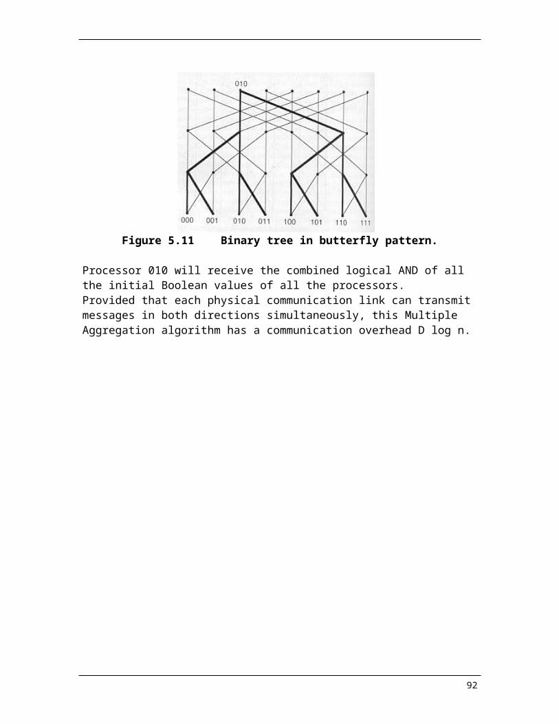
9.3.4 MMX Instructions: Conventions

• source operand: at right place destination operand: at left place e.g. PSLLW mm, mm/m64 • memory address: as the address of the least significant byte of the data

9.3.5 MMX Instructions: Conventions

• Wrap Around: if overflow or underflow , a data is truncated , only the lower (least significant) bits are returned. Carry is ignored. • Saturation: if overflow or underflow , a data is clipped (saturated) to a data-range limit for the data type. Lower limit upper limit signed byte 80H 7FH signed word 8000H 7FFFH unsigned byte 00H FFH unsigned word 0000H FFFFH • e.g for unsigned byte, e5H+62H= ffH (saturation) e5H+62H= 47H (wrap around)

92

9.3.6 How MMX works

To understand Intel's MMX instructions, consider a register file with a number of 64-bit registers. MMX actually uses 8 64-bit floating-point registers as the MMX integer register file, but this is just a cost-saving design choice. More registers would have increased the performance impact of MMX. A 64-bit MMX register can be viewed as holding a single 64-bit integer or a vector of 2, 4, or 8 progressively narrower integer operands. Various arithmetic, logic, comparison, and rearrangement instructions are provided for each of these vector lengths. Table 1 lists the instruction classes and their effects. The column labeled "Vector" indicates the number of independent vector elements that can be specified in the 64-bit operand.

TABLE 1. Intel MMX instructions.

Class Instruction Vector Op type Function or results

Register copy 32 bits Integer register (+ MMX registerCopy Parallel pack 4,2 Saturate Convert to narrower elements

Parallel unpack low 8,4,2 Merge lower halves of 2 vectorsParallel unpack high 8,4,2 Merge upper halves of 2 vectorsParallel add 8,4,2 Wrap/Saturatel Add; inhibit carry at boundariesParallel subtract 8,4,2 Wrap/Saturate' Subtract with carry inhibitionParallel multiply low 4 Multiply, keep the 4 low halves

Arithmetic Parallel multiply high 4 Multiply, keep the 4 high halvesParallel multiply-add 4 Multiply, add adjacent products 2Parallel compare equal 8,4,2 All Is where equal, else all OsParallel compare greater 8,4,2 All Is where greater, else all OsParallel left shift logical 4,2,1 Shift left, respect boundaries

Shift Parallel fight shift logical4,2,1 Shift right, respect boundariesParallel right shift arith 4,2 Arith shift within each (half)wordParallel AND I Bitwise dest (srel) A (src2)

Logic Parallel ANDNOT I Bitwise dest (sre I) A (src2)'Parallel OR I Bitwise dest (srel) V (src2)Parallel XOR I Bitwise dest (sre 1) G (src2)

Memory access Parallel load MMX reg 32 or 64 bits Address given in integer registerParallel store MMX reg 32 or 64 bit Address given in integer register

Control Empty FP tag bits Required for compatibility3

'Wrap simply means dropping the carry-out; saturation may be unsigned or signed.

2Four 16-bit multiplications, four 32-bit intermediate results, two 32-bit final results.

3 Floating-point tag bits help with faster context switching, among other functions.

93

The parallel pack and unpack instructions are quite interesting and useful. Unpacking allows vector elements to be extended to the next larger width (byte to word, word to doubleword, doubleword to quadword) to allow computation of intermediate results with greater precision. The unpacking operations can be specified thus,

8-vectors, low: xxxxabcd, xxxxefgh --> aebfcgdh8-vectors, high: abcdxxxx, efghxxxx --> aebfcgdh4-vectors, low: xxab, xxcd --> acbd4-vectors, high: abxx, cdxx --> acbd2-vectors, low: xa, xb --> ab2-vectors, high: ax, bx --> ab

where i-vector means a vector of length i and letters stand for vector elements in the operands (on the left of the arrow) and results (on the right). As an example, when the first vector is all Os, this operation effectively doubles the width of the lower or upper elements of the second operand through O-extension (e.g., 0000, xxcd --> 0c0d). Packing performs the reverse conversion in that it allows returning the results to the original width:

4-vector: a1a0b1b0c1c0d1d0 --> 0000abcd

2-vector: a1a0b1b0 --> 00ab

In filtering, for example, pixel values may have to be multiplied by the corresponding filter coefficients; this usually leads to overflow if elements are not first unpacked.

A key feature of MMX is the capability for saturating arithmetic. With ordinary unsigned arithmetic, overflow causes the apparent result (after dropping the carry-out bit) to become smaller then either operand. This is known as wrapped arithmetic. When applied to arithmetic on pixel attributes, this type of wraparound may lead to anomalies such as bright pixels within regions that are supposed to be fairly dark. With saturating arithmetic, results that exceed the maximum representable value are forced to that maximum value. A saturating unsigned adder, for example, can be built from an ordinary adder and a multiplexer at the output that chooses between the adder result and a constant, depending on the carry-out bit. For signed results. saturating arithmetic can be defined in an analogous way, with the most positive or negative value used depending on the direction of overflow. For example.the results of the wrapped and the saturating unsigned addtion of A9 and F3 are IC and FF respectively.

Arithmetic with subword parallelism requires modifying the ALU to treat 64-bit words in a variety of ways, depending on the vector length. For wrapped addition, this capability is easy to provide and essentially comes for free. Saturating addition requires detection of overflow within subwords and choosing either the adder output or a constant as the operation result within that subword. Multiplication is slightly harder, but still quite cost-effective in terms of circuit implementation (supplying the details is left as an exercise). The effects of parallel multiplication and parallel multiply-add MMX

94

instructions are depicted in Figure 9.1. Parallel comparison instructions are illustrated in Figure 9.2.

Note that MMX deals exclusively with integer values. A similar capability was added in a subsequent extension to the Intel processors to provide similar speedups with 32- or 64-bit floating-point operands, packed within 128-bit quadwords in registers. The latter capability is known as the streaming SIMD extension (SSE).

Figure 9.1. Parallel multiplication and multiply-add in MMX

Figure 9.2. Parallel comparisons in MMX

95

9.4. MMX Instructions Arithmetic (PADD, Wrap around)

96

• PADDB mm, mm/m64, Operation as: mm(7…0) ← mm(7…0) + mm/m64(7...0) mm(15…8) ← mm(15…8) + mm/m64(15…8) ……………………………. mm(63…56) ← mm(63…56) +mm/m64(63…56)

• PADDW mm, mm/m64, Operation as: mm(15…0) ← mm(15…0) + mm/m64(15...0) mm(31…16) ← mm(31…16) + mm/m64(31…16) ……………………………. mm(63…48) ← mm(63…48) + mm/m64(63…48)

• PADDD mm, mm/m64, Operation as: mm(31…0) ← mm(31…0) + mm/m64(31...0) mm(63…32) ← mm(63…32) + mm/m64(63…32)

Arithmetic (PADD, saturation)

97

• PADDSB mm, mm/m64, Operation as: mm(7…0) ←SaturateToSignedByte( mm(7…0) + mm/m64(7...0)) mm(15…8) ← SaturateToSignedByte( mm(15…8) + mm/m64(15…8)) ……………………………. mm(63…56) ← SaturateToSignedByte( mm(63…56) +mm/m64(63…56))

• PADDSW mm, mm/m64, Operation as: mm(15…0) ← SaturateToSignedWord( mm(15…0) + mm/m64(15...0)) mm(31…16) ← SaturateToSignedWord( mm(31…16) + mm/m64(31…16)) ……………………………. mm(63…48) ← SaturateToSignedWord( mm(63…48) + mm/m64(63…48))

• Packed Add Unsigned with Saturation --- PADDUSB mm, mm/m64 --- PADDUSW mm, mm/m64 • Subtraction: --- PSUB[B,W,D] mm, mm/m64 (Wrap Around) --- PSUBS[B,W] mm, mm/m64 (Saturation) --- PSUBUS[B,W] mm, mm/m64 (Saturation)

Arithmetic (PMADD)

98

--- PMADDWD mm, mm/m64, • Packed Multiply and Add

Multiply the packed word by the packed word in MMX reg/memory. Add the 32-bit results pairwise and store in MMX register as doubleword.

• Packed Multiply High --- PMULHW mm, mm/m64, Multiply the signed packed word in MMX register with the signed packed word in MMX reg/memory, then store the high-order 16 bits of the result in MMX register. mm(15…0) ← (mm(15…0) * mm/m64(15...0)) mm(31…16) ← (mm(31…16) * mm/m64(31…16)) mm(47…32) ← (mm(47…32) * mm/m64(47…32)) mm(63…48) ← (mm(63…48) * mm/m64(63…48))

• Packed Multiply Low --- PMULHL mm, mm/m64, Multiply the signed packed word in MMX register with the signed packed word in MMX reg/memory, then store the low-order 16 bits of the result in MMX register. mm(15…0) ← (mm(15…0) * mm/m64(15...0))

mm(31…16) ← (mm(31…16) * mm/m64(31…16)) mm(47…32) ← (mm(47…32) * mm/m64(47…32)) mm(63…48) ← (mm(63…48) * mm/m64(63…48)) Comparison

99

• Packed Compare for Equality [byte, word, doubleword] --- PCMPEQB mm, mm/m64, Return (0xff, or 0) --- PCMPEQW mm, mm/m64, Return (0xffff, or 0) --- PCMPEQD mm, mm/m64, Return (0xffffffff, or 0) • Packed Compare for Greater than --- PCMPGT[B, W,Q];

Logic

• Bit-wise Logical Exclusive OR

--- PXOR mm, mm/m64,

mm← mm XOR mm/m64 • Bit-wise Logical AND

--- PAND mm, mm/m64,

mm← mm AND mm/m64 • Bit-wise Logical AND NOT

--- PANDN mm, mm/m64,

mm←(NOT mm) AND mm/m64 • Bit-wise Logical OR

--- POR mm, mm/m64,

mm← mm OR mm/m64

Shift

• Packed shift left logical (Shifting in zero)

--- PSLL[W, D, Q] mm, mm/m64, • Packed shift Right logical (Shifting in zero)

--- PSRL[W, D,Q] mm, mm/m64, • Packed shift right arithmetic (Shifting in sign bits)

--- PSRA[W, D] mm, mm/m64,

100

Conversion

mm(15…8) ← SaturateSignedWordToUnsignedByte mm(31…16);

• Pack with unsigned saturation --- PACKUSWB mm, mm/m64, Pack and saturate signed words from MMX register and MMX register /memory into unsigned bytes in MMX register.

mm(7…0) ← SaturateSignedWord of mm(15...0)

mm(23…16)← SaturateSignedWord of mm(47…32) mm(31…24) ← SaturateSignedWord of mm(63…48) mm(39…32) ← SaturateSignedWord of m/m64(15...0) mm(47…40)← SaturateSignedWord of mm/m64(31…16) mm(55…48)← SaturateSignedWord of mm/m64(47…32) mm(63…56)← aturateSignedWord of mm/m64(63…48)

• Pack with signed saturation --- PACKSSWB mm, mm/m64, Pack and saturate signed words from MMX register and MMX register /memory into signed bytes in MMX register.

mm(7…0) ← SaturateSignedWord of mm(15...0) mm(15…8) ← SaturateSignedWord of mm(31…16) mm(23…16) ← SaturateSignedWord of mm(47…32) mm(31…24) ← SaturateSignedWord of mm(63…48) mm(39…32) ← SaturateSignedWord of mm/m64(15...0) mm(47…40) ← SaturateSignedWord of mm/m64(31…16)

mm(63…56) ← SaturateSignedWord of mm/m64(63…48) • Pack with signed saturation --- PACKSSDW mm, mm/m64, Pack and saturate signed dwords from MMX register and MMX register /memory into signed words in MMX register.

mm(15…0) ← SaturateSignedDwordToSigignedWord mm(31...0) mm(31…16) ← SaturateSignedDwordToSignedWord mm(63…32) mm(47…32) ← SaturateSignedDwordToSignedWord mm/m64(31...0) mm(63…48) ← SaturateSignedDwordToSignedWord mm/m64(63…32) • Unpack High Packed Data --- PUNPCKH[BW, WD, DQ]SSDW mm, mm/m64, Unpack and interleave the high-order data elements of the destination and source operands into the destination operand. The low order elements are ignored.

E.g. PUNPCKHWD mm(63…48) ← mm/m64(63…48) mm(47…32) ← mm (63…48) mm(31…16) ← mm/m64(47…32) mm(15…0) ← mm (47…32) • Unpack Low Packed Data --- PUNPCKL[BW, WD, DQ]SSDW mm, mm/m64, Unpack and interleave the low-order data elements of the destination and source operands into the destination operand. The high order elements are ignored. E.g. PUNPCKLWD mm(63…48) ← mm/m64(31…16) mm(47…32) ← mm (31…16) mm(31…16) ← mm/m64(15…0) mm(15…0) ← mm (15…0)

101

Data Transfer

• Move 32 bits --- MOVD mm, r/m32 move 32 bits from integer register/memory to MMX register mm(63…0) ← ZeroExtend(r/m32);

• Move 32 bits --- MOVD r/m32 , mm move 32 bits from MMX register to integer register/memory r/m32 ← mm(31…0).

• Move 64 bits --- MOVQ mm, mm/m64 move 64 bits from MMX register/memory to MMX register mm← mm/m64; --- MOVQ mm/64, mm move 64 bits from MMX register to MMX register/memory mm/m64← mm;

Instruction Samples

102

e.g. MOVD MM0, EAX;

PSLLQ MM0, 32;

MOVD MM1, EBX; POR MM0, MM1;

MOVQ MM2, MM3;

PSLLQ MM3, 1;

PXOR MM3, MM2;

9.5. MMX Code Optimization 9.5.1 Code Optimization Guidelines

• use the current compiler • do not intermix MMX instructions and FP instructions • use the opcode reg, mem instruction format whenever possible • Put an EMMS instruction at the end of all MMX code sections that will transition to FP code • Optimize data cache bandwidth to MMX register

9.5.2 Accessing Memory

• change MOVQ reg, reg and opcode reg, mem to

• Recommend: merging loads whenever the same address is used more than twice. (not memory-bound)

103

• Pentium II and III, -- opcode reg, mem (2 micro-ops) -- opcode reg, reg (1 micro-op) • Recommend: merging loads whenever the same address is used more than once. (memory-bound)

MOVQ reg, mem and opcode reg, reg to save one micro-op.

104

9.6. Programming Tools and Examples

9.6.1 Programming Tools

• MASM 6.11 or above. With 6.14 Patch ( install the ML614.exe)

• VC++ 6.0 can compile MMX instructions key functions written with assembly language including MMX instructions.

• Some CIC++ compilers also including the MASM tool

9.6.2 Programming Examples

// Name: cpu,_test.C// Purpose: to test some MMX instructions

#include <stdio.h>

// to test if the CPU is MMX compatible int cpu_test( );

// to left shift 16 bit for X and append the low 8 bit of y return x; unsigned int MMX-test(unsigned int x, unsigned int y);

// Main function for the program void main( void){I

int found-MMX=cpu - testo;if (found-MMX==l)

printf("This CPU support MMX technology\n");

elseprintf("This CPU doen NOT support MMX technology\n");

// test the MMX instruction unsigned int x= OxI2345678; unsigned int y= Ox99999999; printf("The original value of x is Ox%x\n", x); printf("The original value of y is Ox%x\n", y); x=MMX-test(x, y); printf("After left shifting 16 bit of x and append the \n"); printfi("low 8 bit of y , value of y is Ox%x\n", x);

}// Function Name: cpu _test//Return: If the CPU supports MMX, returns value 1, otherwise returns value 2int cpu_testo{ _asm{

105

// test if the cpu support MMXmov eax, 1;cpuid;test edx, 00800000h;jnz found;mov eax, 2;jmp end;

found: mov eax, 1;end: EMMS;} /* Return with result in EAX

}

//Function Name: MMX_test //Parameters: Two unsigned integers x, and y //Purpose: to test some MMX instructions //Return: to left shift 16 bit for X and append it with the low 8 bit of Y, return X; unsigned int MMX-test(unsigned int x, unsigned int y) { _asm{

mov eax, x; mov ebx, y;

movd mmO, eax;mov eax, Oxff; movd mm2, eax psllq mmO, 16; movd mm I, ebx; pand mm 1, mm2;por mmO, mm I; movd eax, mmO;

}}

Results: This CPU support MMX technology The original value of x is OxI2345678 The original value of y is Ox99999999 After left shifting 16 bit of x and appending the low 8 bit of y , value of y is Ox56780099

106

Reference

1. MMX Technology Programmer's Reference Manual2. MMX Technology Technical Overview3. Intel Architecture Optimization Reference Manual4. Intel Architecture Software Developer manual 15. Intel Architecture Software Developer manual 26. Intel Architecture Software Developer manual 37. Http://www.intel.com/

107