Embed Size (px)
Citation preview

Advanced Digital Communications
Suhas Diggavi
Ecole Polytechnique Federale de Lausanne (EPFL)School of Computer and Communication Sciences
Laboratory of Information and Communication Systems (LICOS)
23rd October 2005

2

Contents
I Review of Signal Processing and Detection 7
1 Overview 91.1 Digital data transmission . . . . . . . . . . . . . . . . . . . . . . . . . . . . . . . . . . . . 91.2 Communication system blocks . . . . . . . . . . . . . . . . . . . . . . . . . . . . . . . . . . 91.3 Goals of this class . . . . . . . . . . . . . . . . . . . . . . . . . . . . . . . . . . . . . . . . 121.4 Class organization . . . . . . . . . . . . . . . . . . . . . . . . . . . . . . . . . . . . . . . . 131.5 Lessons from class . . . . . . . . . . . . . . . . . . . . . . . . . . . . . . . . . . . . . . . . 13
2 Signals and Detection 152.1 Data Modulation and Demodulation . . . . . . . . . . . . . . . . . . . . . . . . . . . . . . 15
2.1.1 Mapping of vectors to waveforms . . . . . . . . . . . . . . . . . . . . . . . . . . . . 162.1.2 Demodulation . . . . . . . . . . . . . . . . . . . . . . . . . . . . . . . . . . . . . . . 18
2.2 Data detection . . . . . . . . . . . . . . . . . . . . . . . . . . . . . . . . . . . . . . . . . . 192.2.1 Criteria for detection . . . . . . . . . . . . . . . . . . . . . . . . . . . . . . . . . . . 202.2.2 Minmax decoding rule . . . . . . . . . . . . . . . . . . . . . . . . . . . . . . . . . . 232.2.3 Decision regions . . . . . . . . . . . . . . . . . . . . . . . . . . . . . . . . . . . . . 262.2.4 Bayes rule for minimizing risk . . . . . . . . . . . . . . . . . . . . . . . . . . . . . . 272.2.5 Irrelevance and reversibility . . . . . . . . . . . . . . . . . . . . . . . . . . . . . . . 282.2.6 Complex Gaussian Noise . . . . . . . . . . . . . . . . . . . . . . . . . . . . . . . . . 302.2.7 Continuous additive white Gaussian noise channel . . . . . . . . . . . . . . . . . . 302.2.8 Binary constellation error probability . . . . . . . . . . . . . . . . . . . . . . . . . 32
2.3 Error Probability for AWGN Channels . . . . . . . . . . . . . . . . . . . . . . . . . . . . . 322.3.1 Discrete detection rules for AWGN . . . . . . . . . . . . . . . . . . . . . . . . . . . 322.3.2 Rotational and transitional invariance . . . . . . . . . . . . . . . . . . . . . . . . . 332.3.3 Bounds for M > 2 . . . . . . . . . . . . . . . . . . . . . . . . . . . . . . . . . . . . 33
2.4 Signal sets and measures . . . . . . . . . . . . . . . . . . . . . . . . . . . . . . . . . . . . . 362.4.1 Basic terminology . . . . . . . . . . . . . . . . . . . . . . . . . . . . . . . . . . . . 362.4.2 Signal constellations . . . . . . . . . . . . . . . . . . . . . . . . . . . . . . . . . . . 372.4.3 Lattice-based constellation: . . . . . . . . . . . . . . . . . . . . . . . . . . . . . . . 38
2.5 Problems . . . . . . . . . . . . . . . . . . . . . . . . . . . . . . . . . . . . . . . . . . . . . 39
3 Passband Systems 473.1 Equivalent representations . . . . . . . . . . . . . . . . . . . . . . . . . . . . . . . . . . . . 473.2 Frequency analysis . . . . . . . . . . . . . . . . . . . . . . . . . . . . . . . . . . . . . . . . 483.3 Channel Input-Output Relationships . . . . . . . . . . . . . . . . . . . . . . . . . . . . . . 503.4 Baseband equivalent Gaussian noise . . . . . . . . . . . . . . . . . . . . . . . . . . . . . . 513.5 Circularly symmetric complex Gaussian processes . . . . . . . . . . . . . . . . . . . . . . . 54
3.5.1 Gaussian hypothesis testing - complex case . . . . . . . . . . . . . . . . . . . . . . 55
3

4 CONTENTS
3.6 Problems . . . . . . . . . . . . . . . . . . . . . . . . . . . . . . . . . . . . . . . . . . . . . 56
II Transmission over Linear Time-Invariant channels 59
4 Inter-symbol Interference and optimal detection 614.1 Successive transmission over an AWGN channel . . . . . . . . . . . . . . . . . . . . . . . . 614.2 Inter-symbol Interference channel . . . . . . . . . . . . . . . . . . . . . . . . . . . . . . . . 62
4.2.1 Matched filter . . . . . . . . . . . . . . . . . . . . . . . . . . . . . . . . . . . . . . . 634.2.2 Noise whitening . . . . . . . . . . . . . . . . . . . . . . . . . . . . . . . . . . . . . . 64
4.3 Maximum Likelihood Sequence Estimation (MLSE) . . . . . . . . . . . . . . . . . . . . . 674.3.1 Viterbi Algorithm . . . . . . . . . . . . . . . . . . . . . . . . . . . . . . . . . . . . 684.3.2 Error Analysis . . . . . . . . . . . . . . . . . . . . . . . . . . . . . . . . . . . . . . 69
4.4 Maximum a-posteriori symbol detection . . . . . . . . . . . . . . . . . . . . . . . . . . . . 714.4.1 BCJR Algorithm . . . . . . . . . . . . . . . . . . . . . . . . . . . . . . . . . . . . . 71
4.5 Problems . . . . . . . . . . . . . . . . . . . . . . . . . . . . . . . . . . . . . . . . . . . . . 73
5 Equalization: Low complexity suboptimal receivers 775.1 Linear estimation . . . . . . . . . . . . . . . . . . . . . . . . . . . . . . . . . . . . . . . . . 77
5.1.1 Orthogonality principle . . . . . . . . . . . . . . . . . . . . . . . . . . . . . . . . . 775.1.2 Wiener smoothing . . . . . . . . . . . . . . . . . . . . . . . . . . . . . . . . . . . . 805.1.3 Linear prediction . . . . . . . . . . . . . . . . . . . . . . . . . . . . . . . . . . . . . 825.1.4 Geometry of random processes . . . . . . . . . . . . . . . . . . . . . . . . . . . . . 84
5.2 Suboptimal detection: Equalization . . . . . . . . . . . . . . . . . . . . . . . . . . . . . . . 855.3 Zero-forcing equalizer (ZFE) . . . . . . . . . . . . . . . . . . . . . . . . . . . . . . . . . . . 86
5.3.1 Performance analysis of the ZFE . . . . . . . . . . . . . . . . . . . . . . . . . . . . 875.4 Minimum mean squared error linear equalization (MMSE-LE) . . . . . . . . . . . . . . . . 88
5.4.1 Performance of the MMSE-LE . . . . . . . . . . . . . . . . . . . . . . . . . . . . . 895.5 Decision-feedback equalizer . . . . . . . . . . . . . . . . . . . . . . . . . . . . . . . . . . . 92
5.5.1 Performance analysis of the MMSE-DFE . . . . . . . . . . . . . . . . . . . . . . . 955.5.2 Zero forcing DFE . . . . . . . . . . . . . . . . . . . . . . . . . . . . . . . . . . . . . 98
5.6 Fractionally spaced equalization . . . . . . . . . . . . . . . . . . . . . . . . . . . . . . . . . 995.6.1 Zero-forcing equalizer . . . . . . . . . . . . . . . . . . . . . . . . . . . . . . . . . . 101
5.7 Finite-length equalizers . . . . . . . . . . . . . . . . . . . . . . . . . . . . . . . . . . . . . 1015.7.1 FIR MMSE-LE . . . . . . . . . . . . . . . . . . . . . . . . . . . . . . . . . . . . . . 1025.7.2 FIR MMSE-DFE . . . . . . . . . . . . . . . . . . . . . . . . . . . . . . . . . . . . . 104
5.8 Problems . . . . . . . . . . . . . . . . . . . . . . . . . . . . . . . . . . . . . . . . . . . . . 109
6 Transmission structures 1196.1 Pre-coding . . . . . . . . . . . . . . . . . . . . . . . . . . . . . . . . . . . . . . . . . . . . . 119
6.1.1 Tomlinson-Harashima precoding . . . . . . . . . . . . . . . . . . . . . . . . . . . . 1196.2 Multicarrier Transmission (OFDM) . . . . . . . . . . . . . . . . . . . . . . . . . . . . . . . 123
6.2.1 Fourier eigenbasis of LTI channels . . . . . . . . . . . . . . . . . . . . . . . . . . . 1236.2.2 Orthogonal Frequency Division Multiplexing (OFDM) . . . . . . . . . . . . . . . . 1236.2.3 Frequency Domain Equalizer (FEQ) . . . . . . . . . . . . . . . . . . . . . . . . . . 1286.2.4 Alternate derivation of OFDM . . . . . . . . . . . . . . . . . . . . . . . . . . . . . 1286.2.5 Successive Block Transmission . . . . . . . . . . . . . . . . . . . . . . . . . . . . . 130
6.3 Channel Estimation . . . . . . . . . . . . . . . . . . . . . . . . . . . . . . . . . . . . . . . 1316.3.1 Training sequence design . . . . . . . . . . . . . . . . . . . . . . . . . . . . . . . . 1346.3.2 Relationship between stochastic and deterministic least squares . . . . . . . . . . . 137
6.4 Problems . . . . . . . . . . . . . . . . . . . . . . . . . . . . . . . . . . . . . . . . . . . . . 139

CONTENTS 5
III Wireless Communications 147
7 Wireless channel models 1497.1 Radio wave propagation . . . . . . . . . . . . . . . . . . . . . . . . . . . . . . . . . . . . . 151
7.1.1 Free space propagation . . . . . . . . . . . . . . . . . . . . . . . . . . . . . . . . . . 1517.1.2 Ground Reflection . . . . . . . . . . . . . . . . . . . . . . . . . . . . . . . . . . . . 1527.1.3 Log-normal Shadowing . . . . . . . . . . . . . . . . . . . . . . . . . . . . . . . . . . 1557.1.4 Mobility and multipath fading . . . . . . . . . . . . . . . . . . . . . . . . . . . . . 1557.1.5 Summary of radio propagation effects . . . . . . . . . . . . . . . . . . . . . . . . . 158
7.2 Wireless communication channel . . . . . . . . . . . . . . . . . . . . . . . . . . . . . . . . 1587.2.1 Linear time-varying channel . . . . . . . . . . . . . . . . . . . . . . . . . . . . . . . 1597.2.2 Statistical Models . . . . . . . . . . . . . . . . . . . . . . . . . . . . . . . . . . . . 1607.2.3 Time and frequency variation . . . . . . . . . . . . . . . . . . . . . . . . . . . . . . 1627.2.4 Overall communication model . . . . . . . . . . . . . . . . . . . . . . . . . . . . . . 162
7.3 Problems . . . . . . . . . . . . . . . . . . . . . . . . . . . . . . . . . . . . . . . . . . . . . 163
8 Single-user communication 1658.1 Detection for wireless channels . . . . . . . . . . . . . . . . . . . . . . . . . . . . . . . . . 166
8.1.1 Coherent Detection . . . . . . . . . . . . . . . . . . . . . . . . . . . . . . . . . . . . 1668.1.2 Non-coherent Detection . . . . . . . . . . . . . . . . . . . . . . . . . . . . . . . . . 1688.1.3 Error probability behavior . . . . . . . . . . . . . . . . . . . . . . . . . . . . . . . . 1708.1.4 Diversity . . . . . . . . . . . . . . . . . . . . . . . . . . . . . . . . . . . . . . . . . 170
8.2 Time Diversity . . . . . . . . . . . . . . . . . . . . . . . . . . . . . . . . . . . . . . . . . . 1718.2.1 Repetition Coding . . . . . . . . . . . . . . . . . . . . . . . . . . . . . . . . . . . . 1718.2.2 Time diversity codes . . . . . . . . . . . . . . . . . . . . . . . . . . . . . . . . . . . 173
8.3 Frequency Diversity . . . . . . . . . . . . . . . . . . . . . . . . . . . . . . . . . . . . . . . 1748.3.1 OFDM frequency diversity . . . . . . . . . . . . . . . . . . . . . . . . . . . . . . . 1768.3.2 Frequency diversity through equalization . . . . . . . . . . . . . . . . . . . . . . . 177
8.4 Spatial Diversity . . . . . . . . . . . . . . . . . . . . . . . . . . . . . . . . . . . . . . . . . 1788.4.1 Receive Diversity . . . . . . . . . . . . . . . . . . . . . . . . . . . . . . . . . . . . . 1798.4.2 Transmit Diversity . . . . . . . . . . . . . . . . . . . . . . . . . . . . . . . . . . . . 179
8.5 Tools for reliable wireless communication . . . . . . . . . . . . . . . . . . . . . . . . . . . 1828.6 Problems . . . . . . . . . . . . . . . . . . . . . . . . . . . . . . . . . . . . . . . . . . . . . 1828.A Exact Calculations of Coherent Error Probability . . . . . . . . . . . . . . . . . . . . . . . 1868.B Non-coherent detection: fast time variation . . . . . . . . . . . . . . . . . . . . . . . . . . 1878.C Error probability for non-coherent detector . . . . . . . . . . . . . . . . . . . . . . . . . . 189
9 Multi-user communication 1939.1 Communication topologies . . . . . . . . . . . . . . . . . . . . . . . . . . . . . . . . . . . . 193
9.1.1 Hierarchical networks . . . . . . . . . . . . . . . . . . . . . . . . . . . . . . . . . . 1939.1.2 Ad hoc wireless networks . . . . . . . . . . . . . . . . . . . . . . . . . . . . . . . . 194
9.2 Access techniques . . . . . . . . . . . . . . . . . . . . . . . . . . . . . . . . . . . . . . . . . 1959.2.1 Time Division Multiple Access (TDMA) . . . . . . . . . . . . . . . . . . . . . . . . 1959.2.2 Frequency Division Multiple Access (FDMA) . . . . . . . . . . . . . . . . . . . . . 1969.2.3 Code Division Multiple Access (CDMA) . . . . . . . . . . . . . . . . . . . . . . . . 196
9.3 Direct-sequence CDMA multiple access channels . . . . . . . . . . . . . . . . . . . . . . . 1989.3.1 DS-CDMA model . . . . . . . . . . . . . . . . . . . . . . . . . . . . . . . . . . . . 1989.3.2 Multiuser matched filter . . . . . . . . . . . . . . . . . . . . . . . . . . . . . . . . . 199
9.4 Linear Multiuser Detection . . . . . . . . . . . . . . . . . . . . . . . . . . . . . . . . . . . 2019.4.1 Decorrelating receiver . . . . . . . . . . . . . . . . . . . . . . . . . . . . . . . . . . 202

6 CONTENTS
9.4.2 MMSE linear multiuser detector . . . . . . . . . . . . . . . . . . . . . . . . . . . . 2029.5 Epilogue for multiuser wireless communications . . . . . . . . . . . . . . . . . . . . . . . . 2049.6 Problems . . . . . . . . . . . . . . . . . . . . . . . . . . . . . . . . . . . . . . . . . . . . . 204
IV Connections to Information Theory 211
10 Reliable transmission for ISI channels 21310.1 Capacity of ISI channels . . . . . . . . . . . . . . . . . . . . . . . . . . . . . . . . . . . . . 21310.2 Coded OFDM . . . . . . . . . . . . . . . . . . . . . . . . . . . . . . . . . . . . . . . . . . . 217
10.2.1 Achievable rate for coded OFDM . . . . . . . . . . . . . . . . . . . . . . . . . . . . 21910.2.2 Waterfilling algorithm . . . . . . . . . . . . . . . . . . . . . . . . . . . . . . . . . . 22010.2.3 Algorithm Analysis . . . . . . . . . . . . . . . . . . . . . . . . . . . . . . . . . . . . 223
10.3 An information-theoretic approach to MMSE-DFE . . . . . . . . . . . . . . . . . . . . . . 22310.3.1 Relationship of mutual information to MMSE-DFE . . . . . . . . . . . . . . . . . . 22510.3.2 Consequences of CDEF result . . . . . . . . . . . . . . . . . . . . . . . . . . . . . . 225
10.4 Problems . . . . . . . . . . . . . . . . . . . . . . . . . . . . . . . . . . . . . . . . . . . . . 228
V Appendix 231
A Mathematical Preliminaries 233A.1 The Q function . . . . . . . . . . . . . . . . . . . . . . . . . . . . . . . . . . . . . . . . . . 233A.2 Fourier Transform . . . . . . . . . . . . . . . . . . . . . . . . . . . . . . . . . . . . . . . . 234
A.2.1 Definition . . . . . . . . . . . . . . . . . . . . . . . . . . . . . . . . . . . . . . . . . 234A.2.2 Properties of the Fourier Transform . . . . . . . . . . . . . . . . . . . . . . . . . . 234A.2.3 Basic Properties of the sinc Function . . . . . . . . . . . . . . . . . . . . . . . . . . 234
A.3 Z-Transform . . . . . . . . . . . . . . . . . . . . . . . . . . . . . . . . . . . . . . . . . . . . 235A.3.1 Definition . . . . . . . . . . . . . . . . . . . . . . . . . . . . . . . . . . . . . . . . . 235A.3.2 Basic Properties . . . . . . . . . . . . . . . . . . . . . . . . . . . . . . . . . . . . . 235
A.4 Energy and power constraints . . . . . . . . . . . . . . . . . . . . . . . . . . . . . . . . . . 235A.5 Random Processes . . . . . . . . . . . . . . . . . . . . . . . . . . . . . . . . . . . . . . . . 236A.6 Wide sense stationary processes . . . . . . . . . . . . . . . . . . . . . . . . . . . . . . . . . 237A.7 Gram-Schmidt orthonormalisation . . . . . . . . . . . . . . . . . . . . . . . . . . . . . . . 237A.8 The Sampling Theorem . . . . . . . . . . . . . . . . . . . . . . . . . . . . . . . . . . . . . 238A.9 Nyquist Criterion . . . . . . . . . . . . . . . . . . . . . . . . . . . . . . . . . . . . . . . . . 238A.10 Choleski Decomposition . . . . . . . . . . . . . . . . . . . . . . . . . . . . . . . . . . . . . 239A.11 Problems . . . . . . . . . . . . . . . . . . . . . . . . . . . . . . . . . . . . . . . . . . . . . 239

Part I
Review of Signal Processing andDetection
7


Chapter 1
Overview
1.1 Digital data transmission
Most of us have used communication devices, either by talking on a telephone, or browsing the interneton a computer. This course is about the mechanisms that allows such communications to occur. Thefocus of this class is on how “bits” are transmitted through a “communication” channel. The overallcommunication system is illustrated in Figure 1.1
Figure 1.1: Communication block diagram.
1.2 Communication system blocks
Communication Channel: A communication channel provides a way to communicate at large dis-tances. But there are external signals or “noise” that effects transmission. Also ‘channel’ might behavedifferently to different input signals. A main focus of the course is to understand signal processing tech-niques to enable digital transmission over such channels. Examples of such communication channelsinclude: telephone lines, cable TV lines, cell-phones, satellite networks, etc. In order to study theseproblems precisely, communication channels are often modelled mathematically as illustrated in Figure1.2.
Source, Source Coder, Applications: The main reason to communicate is to be able to talk, listento music, watch a video, look at content over the internet, etc. For each of these cases the “signal”
9

10 CHAPTER 1. OVERVIEW
Figure 1.2: Models for communication channels.
respectively voice, music, video, graphics has to be converted into a stream of bits. Such a device is calleda quantizer and a simple scalar quantizer is illustrated in Figure 1.3. There exists many quantizationmethods which convert and compress the original signal into bits. You might have come across methodslike PCM, vector quantization, etc.
Channel coder: A channel coding scheme adds redundancy to protect against errors introduced bythe noisy channel. For example a binary symmetric channel (illustrated in Figure 1.4) flips bits randomlyand an error correcting code attempts to communicate reliably despite them.
256 LEVELS ≡ 8 bits
LEVELS
SOURCE
0
1
2
3
4
Figure 1.3: Source coder or quantizer.
Signal transmission: Converts “bits” into signals suitable for communication channel which is typi-cally analog. Thus message sets are converted into waveforms to be sent over the communication channel.

1.2. COMMUNICATION SYSTEM BLOCKS 11
BSC
0 0
1 1
Pe
Pe
1 − Pe
1 − Pe
Figure 1.4: Binary symmetric channel.
This is called modulation or signal transmission. One of the main focuses of the class.
Signal detection: Based on noisy received signal, receiver decides which message was sent. This proce-dure called “signal detection” depends on the signal transmission methods as well as the communicationchannel. Optimum detector minimizes the probability of an erroneous receiver decision. Many signaldetection techniques are discussed as a part of the main theme of the class.
Local to Base
Base Station
Local To Base
Remote
Remote
Local To MobileCo-channel mobile
Figure 1.5: Multiuser wireless environment.
Multiuser networks: Multiuser networks arise when many users share the same communication chan-nel. This naturally occurs in wireless networks as shown in Figure 1.5. There are many different formsof multiuser networks as shown in Figures 1.6, 1.7 and 1.8.

12 CHAPTER 1. OVERVIEW
Figure 1.6: Multiple Access Channel (MAC).
Figure 1.7: Broadcast Channel (BC).
1.3 Goals of this class
• Understand basic techniques of signal transmission and detection.
• Communication over frequency selective or inter-symbol interference (ISI) channels.
• Reduced complexity (sub-optimal) detection for ISI channels and their performances.
• Multiuser networks.
• Wireless communication - rudimentary exposition.
• Connection to information theory.
Complementary classes
• Source coding/quantization (ref.: Gersho & Gray, Jayant & Noll)
• Channel coding (Modern Coding theory, Urbanke & Richardson, Error correcting codes, Blahut)
• Information theory (Cover & Thomas)
Figure 1.8: Adhoc network.

1.4. CLASS ORGANIZATION 13
1.4 Class organization
These are the topics covered in the class.
• Digital communication & transmission
• Signal transmission and modulation
• Hypothesis testing & signal detection
• Inter-symbol interference channel - transmission & detection
• Wireless channel models: fading channel
• Detection for fading channels and the tool of diversity
• Multiuser communication - TDMA, CDMA
• Multiuser detection
• Connection to information theory
1.5 Lessons from class
These are the skills that you should know at the end of the class.
• Basic understanding of optimal detection
• Ability to design transmission & detection schemes in inter-symbol interference channels
• Rudimentary understanding of wireless channels
• Understanding wireless receivers and notion of diversity
• Ability to design multiuser detectors
• Connect the communication blocks together with information theory

14 CHAPTER 1. OVERVIEW

Chapter 2
Signals and Detection
2.1 Data Modulation and Demodulation
MESSAGE
SOURCE ENCODER
VECTORMODULATOR
MESSAGE
SINK
VECTOR
CHANNEL
DETECTORDEMODULATOR
m x
m ^
i
i i
Figure 2.1: Block model for the modulation and demodulation procedures.
In data modulation we convert information bits into waveforms or signals that are suitable for trans-mission over a communication channel. The detection problem is reversing the modulation, i.e., findingwhich bits were transmitted over the noisy channel.
Example 2.1.1. (see Figure 2.2) Binary phase shift keying. Since DC does not go through channel, thisimplies that 0V, and 1V, mapping for binary bits will not work. Use:
x0(t) = cos(2π150t), x1(t) = − cos(2π150t).
Detection: Detect +1 or -1 at the output.Caveat: This is for single transmission. For successive transmissions, stay tuned!
15

16 CHAPTER 2. SIGNALS AND DETECTION
100 200Frequency
Figure 2.2: The channel in example 1.
2.1.1 Mapping of vectors to waveforms
Consider set of real-valued functions f(t), t ∈ [0, T ] such that
∫ T
0
f2(t)dt <∞
This is called a Hilbert space of continuous functions, i.e., L2[0, T ].
Inner product
< f, g >=
∫ T
0
f(t)g(t)dt.
Basis functions: A class of functions can be expressed in terms of basis functions φn(t) as
x(t) =
N∑
n=1
xnφn(t), (2.1)
where < φn, φm >= δn−m. The waveform carries the information through the communication channel.
Relationship in (2.1) implies a mapping x =
x1
...xN
to x(t).
Definition 2.1.1. Signal Constellation The set of M vectors xi, i = 0, . . . ,M−1 is called the signalconstellation.
01 00
01
11
10
Binary Antipodal Quadrature Phase−Shift Keying
Figure 2.3: Example of signal constellations.
The mapping in (2.1) enables mapping of points in L2[0, T ] with properties in RI N . If x1(t) and x2(t)are waveforms and their corresponding basis representation are x1 and x2 respectively, then,
< x1, x2 >=< x1,x2 >

2.1. DATA MODULATION AND DEMODULATION 17
where the left side of the equation is < x1, x2 >=∫ T
0 x1(t)x2(t)dt and the right side is < x1,x2 >=∑Ni=1 x1(i)x2(i).
Examples of signal constellations: Binary antipodal, QPSK (Quadrature Phase Shift Keying).
Vector Mapper: Mapping of binary vector into one of the signal points. Mapping is not arbitrary,clever choices lead to better performance over noisy channels.In some channels it is suitable to label points that are “close” in Euclidean distance to map to being“close” in Hamming distance. Examples of two alternate labelling schemes are illustrated in Figure 2.4.
00
01
00
01
11
1011
10
Figure 2.4: A vector mapper.
Modulator: Implements the basis expansion of (2.1).
x(t)
φ1(t)
x1
xN
φN (t)
Figure 2.5: Modulator implementing the basis expansion.
Signal Set: Set of modulated waveforms xi(t), i = 0, . . . ,M − 1 corresponding to the signal constel-
lation xi =
xi,1
...xi,N
∈ RN .
Definition 2.1.2. Average Energy:
Ex = E[||x||2] =
M−1∑
i=0
||xi||2px(i)
where px(i) is the probability of choosing xi.

18 CHAPTER 2. SIGNALS AND DETECTION
The probability px(i) depends on,
• Underlying probability distribution of bits in message source.
• The vector mapper.
Definition 2.1.3. Average power: Px = Ex
T (energy per unit time)
Example 2.1.2. Consider a 16 QAM constellation with basis functions:
Figure 2.6: 16 QAM constellation.
φ1(t) =
√2
Tcos
πt
T, φ2(t) =
√2
Tsin
πt
T
For 1T = 2400Hz, we get a rate of log(16) × 2400 = 9.6kb/s.
Gram-Schmidt procedure allows choice of minimal basis to represent xi(t) signal sets. More on thisduring the review/exercise sessions.
2.1.2 Demodulation
The demodulation takes the continuous time waveforms and extracts the discrete version. Given thebasis expansion of (2.1), the demodulation extracts the coefficients of the expansion by projecting thesignal onto its basis as shown below.
x(t) =
N∑
k=1
xkφk(t) (2.2)
=⇒∫ T
0
x(t)φn(t)dt =
∫ T
0
N∑
k=1
xkφk(t)φn(t)dt
=
N∑
k=1
xk
∫ T
0
φk(t)φn(t)dt =
N∑
k=1
xkδk−n = xn
Therefore in the noiseless case, demodulation is just recovering the coefficients of the basis functions.
Definition 2.1.4. Matched Filter: The matched filter operation is equivalent to the recovery of the
coefficients of the basis expansion since we can write as an equation:∫ T
0x(t)φn(t)dt == x(t) ∗ φn(T −
t)|t=T = x(t) ∗ φn(−t)|t=0.
Therefore, the basis coefficients recovery can be interpreted as a filtering operation.

2.2. DATA DETECTION 19
y(t)
ϕ1(T − t)
ϕN (T − t)
x1
xN
Figure 2.7: Matched filter demodulator.
∑xnϕn(t)
b0, b1, ..., b2RT
x
MessageModulator Channel
xVector Map
Demodulator
Figure 2.8: Modulation and demodulation set-up as discussed up to know.
2.2 Data detection
We assume that the demodulator captures the “essential” information about x from y(t). This notion of“essential” information will be explored in more depth later.In discrete domain:
PY (y) =M−1∑
i=0
pY |X(y|i)pX(i)
This is illustrated in Figure 2.9 showing the equivalent discrete channel.
Example 2.2.1. Consider the Additive White Gaussian Noise Channel (AWGN). Here y = x + z, and
MAPPER
VECTORCHANNEL
m x
PY|X
y
Figure 2.9: Equivalent discrete channel.

20 CHAPTER 2. SIGNALS AND DETECTION
hence pY |X(y|x) = pZ(y − x) = 1√2πσ
e−(y−x)2
2σ2 .
2.2.1 Criteria for detection
Detection is guessing input x given the noisy output y. This is expressed as a function m = H(y).If M = m was the message sent, then
Probability of error = Pedef= Prob(m 6= m).
Definition 2.2.1. Optimum detector: Minimizes error probability over all detectors. The probabilityof observing Y=y if the message mi was sent is,
p(Y = y | M = mi) = pY|X(y | i)Decision Rule: H : Y → M is a function which takes input y and outputs a guess on the transmittedmessage. Now,
P(H(Y) is correct) =
∫
y
P[H(y) is correct | Y = y]pY(y)dy (2.3)
Now H(y) is a deterministic function of y. Suppose m was transmitted. For the given y, H(•) chooses aparticular hypothesis, say mi, deterministically. Now, what is the probability that i was the transmittedmessage? This is the probability that y resulted through mi being transmitted. Therefore we can write
P[H(Y) is correct | Y = y] = P[m = H(y) = mi | Y = y]
= P[x = x(mi) = xi | Y = y]
= PX|Y[x = xi | y]
Inserting this into (2.3), we get
P(H(Y) is correct) =
∫
y
PX|Y[X = xi | y]pY(y)dy
≤∫
y
maxi
PX|Y[X = xi | y]pY(y)dy
= P(HMAP (Y) is correct)
Implication: The decision rule
HMAP (y) = argmaxi
PX|Y[X = xi | y]
maximizes probability of being correct, i.e., minimizes error probability. Therefore, this is the optimaldecision rule. This is called the Maximum-a-posteriori (MAP) decision rule.
Notes:
• MAP detector needs knowledge of the priors pX(x).
• It can be simplified as follows:
pX|Y(xi | y) =pY|X[y | xi]pX(xi)
pY(y)≡ pY|X[y | xi]pX(xi)
since pY(y) is common to all hypotheses. Therefore the MAP decision rule is equivalently writtenas:
HMAP (y) = arg maxi
pY|X[y | xi]pX(xi)

2.2. DATA DETECTION 21
An alternate proof for MAP decoding rule (binary hypothesis)
Let Γ0 be the region such that ∀ y ∈ Γ0, H(y) = x0 and similarly Γ1 is the region associated to x1.
For π0 = PX(x0) and π1 = PX(x1)
P[error] = P[H(y)is wrong] = π0P[y ∈ Γ1 | H0] + π1P[y ∈ Γ0 | H1] (2.4)
= π0
∫
Γ1
PY|X(y | x0)dy + π1
∫
Γ0
PY|X(y | x1)dy
= π0
∫
Γ1
PY|X(y | x0)dy + π1
[1 −
∫
Γ1
PY|X(y | x1)dy
]
= π1 +
∫
Γ1
[π0PY|X(y | x0) − π1PY|X(y | x1)
]dy
= π1 +
∫
RN
11y∈Γ1[π0PY|X(y | x0) − π1PY|X(y | x1)
]dy
︸ ︷︷ ︸to make this term the smallest, collect all the negative area
Therefore, in order to make the error probability smallest, we choose on y ∈ Γ1 if
π0PY|X(y | x0) − π1PY|X(y | x1)
y →
Figure 2.10: Functional dependence of integrand in (2.4).
π0PY|X(y | x0) < π1PY|X(y | x1)
That is, Γ1 is defined as,
PX(x0)PY|X(y | x0)
PY(y)<
PX(x1)PY|X(y | x1)
PY(y)
or y ∈ Γ1, if,
PX|Y(x0 | y) < PX|Y(x1 | y)
i.e., the MAP rule!
Maximum Likelihood detector: If the priors are assumed uniform, i.e., pX(xi) = 1M then the MAP
rule becomes,HML(y) = arg max
ipY|X[y | xi]

22 CHAPTER 2. SIGNALS AND DETECTION
which is called the Maximum-Likelihood rule. This because it chooses the message that most likelycaused the observation (ignoring how likely the message itself was). This decision rule is clearly inferiorto MAP for non-uniform priors.Question: Suppose the prior probabilities were unknown, is there a “robust” detection scheme?One can think of this as a “game” where nature chooses the prior distribution and the detection rule isunder our control.
Theorem 2.2.1. The ML detector minimizes the maximum possible average error probability when theinput distribution is unknown and if the conditional probability of error p[HML(y) is incorrect | M = mi]is independent of i.
Proof: Assume that Pe,ML|m=miis independent of i.
Let
Pe,ML|m=mi= PML
e (i)def= P
ML
Hence
Pe,ML(Px) =
M−1∑
i=0
PX(i)Pe,ML|m=mi= P
ML (2.5)
Therefore
maxPX
Pe,ML = maxPX
M−1∑
i=0
PX(i)Pe,ML|m=mi= P
ML
For any hypothesis test H,
maxPX
Pe,H = maxPX
M−1∑
i=0
PX(i)Pe,H|m=mi
(a)
≥M−1∑
i=0
1
MPe,H|m=mi
(b)
≥M−1∑
i=0
1
MPe,ML|m=mi
= Pe,ML
where (a) is because a particular choice of PX can only be smaller than the maximum. And (b) is becausethe ML decoder is optimal for the uniform prior.Thus,
maxPX
Pe,H ≥ Pe,ML = PML,
since due to (2.5)
Pe,ML = PML, ∀Px.
Interpretation: ML decoding is not just a simplification of the MAP rule, but also has some canonical“robustness” properties for detection under uncertainty of priors, if the regularity condition of theorem2.2.1 is satisfied. We will explore this further in Section 2.2.2.
Example 2.2.2. The AWGN channel:Let us assume the following,
y = xi + z ,

2.2. DATA DETECTION 23
wherez ∼ N (0, σ2I), x,y, z ∈ R
N
Hence
pZ(z) =1
(2πσ2)N2
e−||z||22σ2
givingpY|X(y | x) = pZ(y− x)
MAP decision rule for AWGN channel
pY|X[y | xi] = 1
(2πσ2)N2e
−||y−xi||2
2σ2
pX|Y[X = xi | y] =pY|X[y|xi]pX(xi)
pY(y)
Therefore the MAP decision rule is:
HMAP (y) = arg maxi
pX|Y[X = xi | y]
= arg max
i
pY|X[y | xi]pX(xi)
= arg maxi
pX(xi)
1
(2πσ2)N2
e−||y−xi||2
2σ2
= arg maxi
log[pX(xi)] −
||y− xi||22σ2
= arg mini
||y − xi||22σ2
− log[pX(xi)]
ML decision rule for AWGN channels
HML(y) = arg maxi
pY|X[y | X = xi]
= arg maxi
1
(2πσ2)N2
e−||y−xi||2
2σ2
= arg maxi
−||y− xi||2
2σ2
= arg mini
||y − xi||22σ2
Interpretation: The maximum likelihood decision rule selects the message that is closest in Euclideandistance to received signal.
Observation: In both MAP and ML decision rules, one does not need y, but just the functions,‖ y−xi ‖2, i ∈ 0, ...,M−1 in order to evaluate the decision rule. Therefore, there is no loss of informationif we retain scalars, ‖ y− xi ‖2 instead of y. In this case, it is moot, but in continuous detection, thisreduction is important. Such a function that retains the “essential” information about the parameter ofinterest is called a sufficient statistic.
2.2.2 Minmax decoding rule
The MAP decoding rule needs the knowledge of the prior distribution PX(x = xi). If the prior isunknown we develop a criterion which is “robust” to the prior distribution. Consider the criterion
maxPX
minHPe,H (px)

24 CHAPTER 2. SIGNALS AND DETECTION
where Pe,H(px) is the error probability of decision rule H, i.e.,
P[H(y) is incorrect] explicitly depends on PX(x)
‖Pe,H(pX)
For the binary case,
Pe,H(pX ) = π0 P[y ∈ Γ1 | x0]︸ ︷︷ ︸does not depend on π1,π0
+π1 P[y ∈ Γ0 | x1]︸ ︷︷ ︸does not depend on π1,π0
= π0
∫
Γ1
PY|X(y | x0)dy + (1 − π0)
∫
Γ0
PY|X(y | x1)dy
Thus for a given decision rule H which does not depend on px, Pe,H (pX) is a linear function of PX(x).
π01
Pe,H(π0) = π0P[y ∈ Γ1 | H0] + (1 − π0)P[y ∈ Γ0 | H1]
Pe,H(π0)
P[y ∈ Γo | H1]
P[y ∈ Γ1 | H0]
Figure 2.11: Pe,ML(π0) as a function of the prior π0.
A “robust” detection criterion is when we want to
minH
maxπ0
Pe,H (π0).
Clearly for a given decision rule H,
maxπ0
Pe,H (π0) = maxP[y ∈ Γ1 | H0], P[y ∈ Γ0 | H1]
Now let us look at the MAP rule for every choice of π0.Let V (π0) = PMAP
e (π0) i.e., the error probability of the MAP decoding rule as a function of PX(x) (orπ0).Since the MAP decoding rule does depend on PX(x), the error probability is no longer a linear functionand is actually concave (see Figure 2.12, and HW problem). Such a concave function has a uniquemaximum value and if it is strictly concave has a unique maximizer π∗
0 . This value V (π∗0) is the largest
average error probability for the MAP detector and π∗0 is the worst prior for the MAP detector.
Now, for any decision rule that does not depend on PX(x), Pe,H (px) is a linear function of π0 (for thebinary case) and this is illustrated in Figure 2.11. Since Pe,H (px) ≥ Pe,MAP (px) for each px. The line

2.2. DATA DETECTION 25
1π∗0
π00
π∗0 ≡ worst prior
Pe,MAP (π0)
Figure 2.12: The average error probability Pe,ML(π0) of the MAP rule as a function of the prior π0.
1π∗0
π0
Minmax rulePe,H(π0)
π0
Figure 2.13: Pe.H (π0) and Pe,MAP (π0) as a function of prior π0.
always lies above the curve V (π0). The best we could do is to make it tangential to V (π0) for some π0,as shown in Figure 2.13. This means that such a decision rule is the MAP decoding rule designed forprior π0. If we want the max
PX
Pe,H(px) to be the smallest it is clear that we want π0 = π∗0 , i.e., design
the robust detection rule as the MAP rule for π∗0 . Since π∗
0 is the worst prior for the MAP rule, this isthe best one could hope for. Since the tangent to V (π0) at π∗
0 has slope 0, such a detection rule has theproperty that Pe,H(π0) is independent of π0.Therefore, for the minmax rule H∗, we would have
PH∗ [y ∈ Γ1 | H0] = PH∗ [y ∈ Γ0 | H1]
Therefore for the minmax rule,
Pe,H∗(π0) = π0PH∗ [y ∈ Γ1 | H0] + (1 − π0)PH∗ [y ∈ Γ0 | H1]
= PH∗ [y ∈ Γ1 | H0] = PH∗ [y ∈ Γ0 | H1]
is independent of π0.Hence Pe,H|x=x0
= Pe,H|x=x1, i.e., the error probability conditioned on the message are the same. Note
that this was the regularity condition we used in Theorem 2.2.1. Hence regardless of the choice of π0, theerror probability (average) is the same! If π∗
0 = 12 (i.e., px is uniform), then the maximum likelihood rule

26 CHAPTER 2. SIGNALS AND DETECTION
is the robust detection rule as stated in Theorem 2.2.1. Note that this is not so if π∗0 6= 1
2 , then the MAPrule for π∗
0 becomes the robust detection rule. Also note that the minmax rule makes the performance ofall priors as bad as the worst prior.Note: If π∗
0 = 12 , or P ∗
X(x) is uniform then minmax is the same as ML, and this occurs in several cases.
Prob. of error
π0
V (π0) = Error prob. of Bayes rule
Figure 2.14: Pe,H (π0) Minmax detection rule.
Since minmax rule becomes Bayes rule for the worst prior, if the worst prior is uniform then clearly theminmax rule is the ML rule. Clearly if ML satisfies PML[error | Hj ] independent of j then the ML ruleis the robust detection rule.
2.2.3 Decision regions
Given the MAP and ML decision rules, we can divide RN into regions which correspond to differentdecisions.For example, in the AWGN case, the ML decoding rule will always decide to choose mi if
‖ y − xi ‖2<‖ y− xj ‖2, ∀j 6= i
Therefore, we can think of the region Γi as the decision region for mi where,
ΓMLi = y ∈ R
N : ‖ y− xi ‖2<‖ y − xj ‖2, ∀j 6= iThe MAP rule for the AWGN channel is a shifted region:
ΓMAPi = y ∈ R
N :‖ y − xi ‖2
2σ2− log[pX(xi)] <
‖ y − xj ‖2
2σ2− log[pX(xj)], ∀j 6= i
The ML decision regions have a nice geometric interpretation. They are the Voronoi regions of the setof points xi. That is, the decision region associated with mi is the set of all points in RN which arecloser to xi than all the rest.Moreover, since they are defined by Euclidean norms ‖ y − xi ‖2, the regions are separated by hyperplanes. To see this observe the decision regions are:
‖ y − xi ‖2 ≤ ‖ y − xj ‖2, ∀j 6= i
⇒ −2 < y,xi > + ‖ xi ‖2 ≤ −2 < y,xj > + ‖ xj ‖2
⇒< y,xj − xi > ≤ 1
2(‖ xj ‖2 − ‖ xi ‖2)
⇒< y − 1
2(xj + xi),xi − xj > ≥ 0 ∀j 6= i
Hence the decision regions are bounded by hyperplanes since they are determined by a set of linearinequalities. The MAP decoding rule still produces decision regions that are hyper planes.

2.2. DATA DETECTION 27
Figure 2.15: Voronoi regions for xi, for uniform prior. Hence here the ML and MAP decision regionscoincide.
2.2.4 Bayes rule for minimizing risk
Error probability is just one possible criterion for choosing a detector. More generally the detectorsminimize other cost functions. For example, let Ci,j denote the cost of choosing hypothesis i whenactually hypothesis j was true. Then the expected cost incurred by some decision rule H(y) is:
Rj(H) =∑
i
Ci,jP[H(Y) = mi | M = mj ]
Therefore the overall average cost after taking prior probabilities into account is:
R(H) =∑
j
PX(j)Rj(H)
Armed with this criterion we can ask the same question:
Question: What is the optimal decision rule to minimize the above equation?
Note: The error probability criterion corresponds to a cost assignment:
Ci,j = 1, i 6= j, Ci,j = 0, i = j.
Consider case M=2, i.e., distinguishing between 2 hypotheses. Rewriting the equation for this case:
R(H) = Px(0)R0(H) + PX(1)R1(H)
where,
Rj(H) = C0,jP[H(Y) = m0 | M = mj ] + C1,jP[H(Y) = m1 | M = mj ], j = 0, 1
= C0,j1− P[H(Y) = m1 | M = mj ] + C1,jP[H(Y) = m1 | M = mj ], j = 0, 1
Let PX(0) = π0, PX(1) = 1 − π0

28 CHAPTER 2. SIGNALS AND DETECTION
R(H) = π0C0,0P[y ∈ Γ0 | x = x0] + π0C1,0P[y ∈ Γ1 | x = x0]
+ π1C0,1P[y ∈ Γ0 | x = x1] + π1C1,1P[y ∈ Γ1 | x = x1]
= π0C0,0 − π0C0,0P[y ∈ Γ1 | x = x0] + π0C1,0P[y ∈ Γ1 | x = x0]
+ π1C0,1 − π1C0,1P[y ∈ Γ1 | x = x1] + π1C1,1P[y ∈ Γ1 | x = x1]
= π0C0,0 + π1C0,1 + π0(C1,0 − C0,0)
∫
y∈Γ1
PY|X(y | x = x0)dy
+ π1(C1,1 − C0,1)
∫
y∈Γ1
PY|X(y | x = x1)dy
=
1∑
j=0
πjC0,j +
∫
y∈Γ1
1∑
j=0
πj(C1,j − C0,j)PY|X(y | x = xj)
dy
Now, just like in the alternate proof for the MAP decoding rule, (see (2.4)) we want to minimize the last
term. As seen in Figure 2.10 this is done by collecting the negative area in the function∑1
j=0 πj(C1,j −C0,j)PY|X(y | x = xj) as a function of y. Therefore we get the decision rule,
Γ1 = y ∈ RN :
1∑
j=0
PX(j)(C1,j − C0,j)PY|X(y | xj) < 0
Likelihood ratio: Surprisingly, in all the detection criteria we have seen the likelihood ratio defined as,
PY|X(y | x0)
PY|X(y | x1)
seems to appear as a part of the decision rule.For example, if C1,1 < C0,1, then we have,
Γ1 = y ∈ RN : PY|X(y | x1) > τPY|X(y | x0)
where τ =PX(0)(C1,0−C0,0)
PX(1)(C0,1−C1,1)
For C0,0 = C1,1 = 0 and C0,1 = C1,0 = 1, we get the MAP rule, i.e., τ = PX(0)
PX(1)which minimizes average
error probability.
2.2.5 Irrelevance and reversibility
An output may contain parts that do not help to determine the message. These irrelevant componentscan be discarded without loss of performance. This is illustrated in the following example.
Example 2.2.3. As shown Figure 2.16 if z1 and z2 are independent then clearly y2 is irrelevant.
Theorem 2.2.2. If y =
[y1
y2
], and we have either of the following equivalent conditions:
• PX|Y1,Y2= PX|Y1
• PY2|Y1,X = PY2|Y1
then y2 is irrelevant for the detection of X.

2.2. DATA DETECTION 29
Z1 Z2
Y2
Y1
+X +
Figure 2.16: Example 2.2.3.
Proof: If PX|Y1,Y2= PX|Y1
, then clearly the MAP decoding rule ignores Y2, and therefore it
is irrelevant almost by definition. The question is whether the second statement is equivalent. LetPY2|Y1,X = PY2|Y1
PY2|Y1=
PY1,Y2
PY1
(2.6)
PY2|Y1,X =PY1,Y2|X
PY1|X(2.7)
Hence,
PY2|Y1,X = PY2|Y1⇔
PY1,Y2
PY1
=PY1,Y2|X
PY1|X
⇔PY1,Y2|XPY1,Y2
=PY1|XPY1
(2.8)
⇔PY1,Y2|XPX
PY1,Y2
=PY1|XPX
PY1
⇔ PX|Y1,Y2= PX|Y1
Note: The irrelevance theorem is summarized by a Markov chain relationship
X ↔ Y1 ↔ Y2
which means that conditioned on Y1, Y2 is independent of X .
Application of Irrelevance theorem
Theorem 2.2.3. (Reversibility theorem) The application of an invertible mapping on the channeloutput vector y, does not affect the performance of the MAP detector.
Proof: Let y2 be the channel output, and y1 = G(y2), where G(·) is an invertible map. Theny2 = G−1(y1). Clearly [
y1
y2
]=
[y1
G−1(y1)
]
30 CHAPTER 2. SIGNALS AND DETECTION
and therefore,PX|Y1,Y2
= PX|Y1
and hence by applying the irrelevance theorem, we can drop y2.
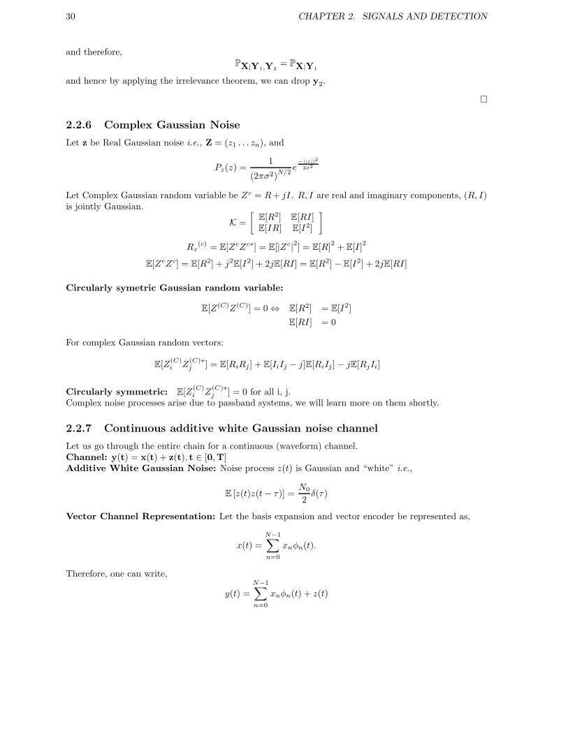
2.2.6 Complex Gaussian Noise
Let z be Real Gaussian noise i.e., Z = (z1 . . . zn), and
Pz(z) =1
(2πσ2)N/2
e−||z||2
2σ2
Let Complex Gaussian random variable be Zc = R+ jI . R, I are real and imaginary components, (R, I)is jointly Gaussian.
K =
[E[R2] E[RI ]E[IR] E[I2]
]
Rz(c) = E[ZcZc∗] = E[|Zc|2] = E[R]
2+ E[I ]
2
E[ZcZc] = E[R2] + j2E[I2] + 2jE[RI ] = E[R2] − E[I2] + 2jE[RI ]
Circularly symetric Gaussian random variable:
E[Z(C)Z(C)] = 0 ⇔ E[R2] = E[I2]
E[RI ] = 0
For complex Gaussian random vectors:
E[Z(C)i Z
(C)∗j ] = E[RiRj ] + E[IiIj − j]E[RiIj ] − jE[RjIi]
Circularly symmetric: E[Z(C)i Z
(C)∗j ] = 0 for all i, j.
Complex noise processes arise due to passband systems, we will learn more on them shortly.
2.2.7 Continuous additive white Gaussian noise channel
Let us go through the entire chain for a continuous (waveform) channel.Channel: y(t) = x(t) + z(t), t ∈ [0,T]Additive White Gaussian Noise: Noise process z(t) is Gaussian and “white” i.e.,
E [z(t)z(t− τ)] =N0
2δ(τ)
Vector Channel Representation: Let the basis expansion and vector encoder be represented as,
x(t) =
N−1∑
n=0
xnφn(t).
Therefore, one can write,
y(t) =
N−1∑
n=0
xnφn(t) + z(t)

2.2. DATA DETECTION 31
Let
yn =< y(t), φn(t) >, zn =< z(t), φn(t) >, n = 0, . . . , N − 1
Consider vector model,
y =
y0...
yN−1
= x + z
Note:
z(t)def=
N−1∑
n=0
znφn(t) 6= z(t) =⇒ y(t)def=
N−1∑
n=0
ynφn(t) 6= y(t)
Lemma 2.2.1. (Uncorrelated noise samples) Given any orthonormal basis functions φn(t), andwhite Gaussian noise z(t). The coefficients zn =< z, φn > of the basis expansion are Gaussian andindependent and identically distributed, with variance N0
2 , i.e. E[znzk] = N0
2 δn−k.
Therefore, if we extend the orthonormal basis φn(t)N−1n=0 to span z(t), the coefficients of the expansion
znN−1n=0 would be independent of the rest of the coefficients.
Let us examine,
y(t) = y(t) + y(t) =N−1∑
n=0
(xn + zn)φn(t)
︸ ︷︷ ︸y(t)
+ z(t) − z(t)︸ ︷︷ ︸y(t)
Therefore, in vector expansion, y is the vector containing basis coefficients from φn(t), n = N, . . ..These coefficients can be shown to be irrelevant to the detection of x, and can therefore be dropped.Hence for the detection process the following vector model is sufficient.
y = x + z
Now we are back in “familiar” territory. We can write the MAP and ML decoding rules as before.Therefore the MAP decision rule is:
HMAP(y) = arg mini
[ ||y − xi||22σ2
− log[PX(xi)]
]
And the ML decision rule is:
HML(y) = argmini
[ ||y − xi||22σ2
]
Let px(xi) = 1M i.e. uniform prior.
Here ML ≡MAP ≡ optimal detector.
Pe =
M−1∑
i=0
Pe|x=xiPx(xi) = 1 −
M−1∑
i=0
Pc|x=xiPx(xi)
Puniform priore,ML =
1
M
M−1∑
i=0
Pe,ML|x=xi= 1 − 1
M
M−1∑
i=0
Pc|x=xi
The error probabilities depend on chosen signal constellation. More soon...

32 CHAPTER 2. SIGNALS AND DETECTION
2.2.8 Binary constellation error probability
Y = Xi + Z, i = 0, 1, Z ∼ N (0, σ2IN )
Hence, conditional error probability is:
Pe,ML|x=x0= P[||y − x0|| ≥ ||y − x1||], since y = x0 + z, (2.9)
⇒ Pe,ML|x=x0= P[||z|| ≥ ||(x0 − x1) + z||]= P[||z||2 ≥ ||(x1 − x0) − z||2]= P[||z||2 ≥ ||x1 − x0||2 + ||z||2 − 2 < (x1 − x0), z >] (2.10)
= P[< (x1 − x0), z >
||x1 − x0||≥ ||x1 − x0||
2]
But < (x1 − x0), z > is a Gaussian i.e. U = (x1−x0)t
||x1−x0||Z is Gaussian, with E[U ] = 0, E[|U |2] = σ2
⇒ Pe,ML|x=x0=
∫ ∞
||x1−x0||2
1
(2πσ2)12
e−1
2σ2 ||U ||2dU (2.11)
=
∫ ∞
||x1−x0||2σ
1
(2π)12
e−|| eU||2
2 dU (2.12)
def= Q
( ||x1 − x0||2σ
)(2.13)
⇒ Pe,ML = Pxx0Pe,ML|x = x0 + Pxx1Pe,ML|x = x1 = Q
( ||x1 − x0||2σ
)
2.3 Error Probability for AWGN Channels
2.3.1 Discrete detection rules for AWGN
AWGN Channel: Y = X + Z, Y ∈ CN , x ∈ CN , Z ∼ C .
X Y+
Z
Let px(xi) = 1M i.e. uniform prior, hence the ML is equivalent to MAP detector.
Detection Rule:
Γi = y ∈ CN : ||y − xi||2 ≤ ||y − xj ||2, j 6= i
Pe =M−1∑
i=0
Pe|x=xiPx(xi) = 1 −
M−1∑
i=0
Pc|x=xiPx(xi)
P uniform priore,ML =
1
M
M−1∑
i=0
Pe,ML|x=xi= 1 − 1
M
M−1∑
i=0
Pe|x=xi
Hence, for M > 2, the error probability calculation could be difficult. We will develop properties andbounds that might help in this problem.
2.3. ERROR PROBABILITY FOR AWGN CHANNELS 33
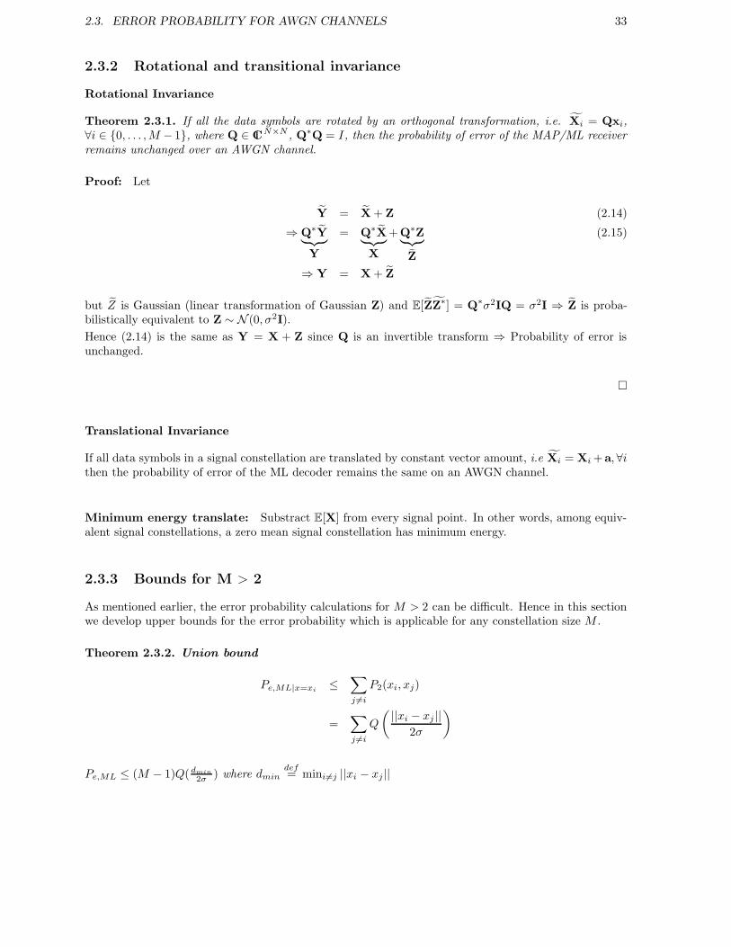
2.3.2 Rotational and transitional invariance
Rotational Invariance
Theorem 2.3.1. If all the data symbols are rotated by an orthogonal transformation, i.e. Xi = Qxi,∀i ∈ 0, . . . ,M − 1, where Q ∈ CN×N , Q∗Q = I, then the probability of error of the MAP/ML receiverremains unchanged over an AWGN channel.
Proof: Let
Y = X + Z (2.14)
⇒ Q∗Y︸ ︷︷ ︸Y
= Q∗X︸ ︷︷ ︸X
+Q∗Z︸︷︷︸eZ
(2.15)
⇒ Y = X + Z
but Z is Gaussian (linear transformation of Gaussian Z) and E[ZZ∗] = Q∗σ2IQ = σ2I ⇒ Z is proba-bilistically equivalent to Z ∼ N (0, σ2I).
Hence (2.14) is the same as Y = X + Z since Q is an invertible transform ⇒ Probability of error isunchanged.
Translational Invariance
If all data symbols in a signal constellation are translated by constant vector amount, i.e Xi = Xi +a, ∀ithen the probability of error of the ML decoder remains the same on an AWGN channel.
Minimum energy translate: Substract E[X] from every signal point. In other words, among equiv-alent signal constellations, a zero mean signal constellation has minimum energy.
2.3.3 Bounds for M > 2
As mentioned earlier, the error probability calculations for M > 2 can be difficult. Hence in this sectionwe develop upper bounds for the error probability which is applicable for any constellation size M .
Theorem 2.3.2. Union bound
Pe,ML|x=xi≤
∑
j 6=i
P2(xi, xj)
=∑
j 6=i
Q
( ||xi − xj ||2σ
)
Pe,ML ≤ (M − 1)Q(dmin
2σ ) where dmindef= mini6=j ||xi − xj ||

34 CHAPTER 2. SIGNALS AND DETECTION
Proof: For x = xi, i.e. y = xi + z
Pe,ML|x=xi= P
⋃
j 6=i
||y − xi|| > ||y − xj ||
≤UB∑
i6=j
P [||y − xi|| > ||y − xj ||] =∑
i6=j
P2(xi, xj)
≤∑
i6=j
Q
( ||xi − xj ||2σ
)
≤ (M − 1)Q
(dmin
2σ
)
since Q(.) is a monotonously decreasing function. Therefore
Pe,ML =
M−1∑
i=0
Px(xi)P (e,ML|x = xi)
≤M−1∑
i=0
Px(xi)(M − 1)Q
(dmin
2σ
)
= (M − 1)Q
(dmin
2σ
)
Tighter Bound (Nearest Neighbor Union Bound)Let Ni be the number of points sharing a decision boundary Di with xi. Suppose xk does not share a
If y /∈ Γi, an error occurs
Γi
Pr[⋃
j 6=i||y − xj || < ||y − xi||] = Pr[y /∈ Γi]
Figure 2.17: Decision regions for AWGN channel and error probability.
decision boundary with xi, but ||y − xi|| > ||y− xk || then ∃xj ∈ Di s.t. ||y − xi|| > ||y− xj || where Di isa set of points sharing the same decision boundary. Hence

2.3. ERROR PROBABILITY FOR AWGN CHANNELS 35
xi
y ∈ Γk
xk
D
Dxj
Figure 2.18: Figure illustrating geometry when xk ∈ Di, then there is a xj ∈ Di such that y is closer toxi.
||y − xk|| < ||y − xi|| ⇒ ∃j ∈ Di such that ||y − xj || < ||y − xi||
⇒ P[⋃
j 6=i
||y − xj || < ||y − xi||]
= P[⋃
j∈Di
||y − xj || < ||y − xi||]
≤ NiQ
(dmin
2σ
)
Pe,ML =
M−1∑
i=0
Px(xi)P (e,ML|x = xi)
≤M−1∑
i=0
Px(xi)Q
(dmin
2σ
)Ni
⇒ Pe,ML ≤ NeQ
(dmin
2σ
)where Ne =
∑
i
NiPx(xi)
Hence we have proved the following result,
Theorem 2.3.3. Nearest Neighbor Union bound (NNUB)
Pe,ML ≤ NeQ(dmin
2σ)
where
Ne =∑
NiPx(xi)
and Ni is the number of constellation points sharing a decision boundary with xi.

36 CHAPTER 2. SIGNALS AND DETECTION
2.4 Signal sets and measures
2.4.1 Basic terminology
In this section we discuss the terminology used i.e., the rate, number of dimensions etc. and discuss whatwould be fair comparisons between constellations.
If signal bandwidth is approximately W and is approximately time-limited to T, then a deep theoremfrom signal analysis states that the space has dimension N which is
N = 2WT
If b bits are in a constellation in dimension N .
⇒ b =b
N= # of bits/dimension
R = rate =b
T= # bits/unit time
R
W= 2b = # bits/sec/Hz
Ex = Average energy per dimension =Ex
N
Px = Average power =Ex
T
Ex useful in compound signal sets with different # of dimension.Signal to noise ratio (SNR)
SNR =Ex
σ2=
Energy/dim
Noise energy/dim
Constellation figure of merit (CFM)
ζxdef=
(dmin/2)2
Ex
As ζx increases we get better performance (for same # of bits per dimension only).Fair comparison: In order to make a fair comparison between constellations, we need to make a multi-parameter comparison across the following measures.
Data rate (R) bits/dim (b)Power (Px) Energy/dim (Ex)Total BW (W ) OR Normalized probability of error (Pe)Symbol period (T )Error probability (Pe)

2.4. SIGNAL SETS AND MEASURES 37
2.4.2 Signal constellations
Cubic constellations
x =
N−1∑
i=0
Uiei
where N is the number of dimensions, and ei ∈ RN is,
ei(k) =
1 if k = i0 else
where Ui ∈ 0, 1 depending on “bit sequence”. Hence the number of constellation points is, M = 2N .
Orthogonal constellations
M = αN . Example: Bi-orthogonal signal set →M = 2N and xi = ±ei ⇒ 2N signal points.
Circular constellations
M th root of unity
8 PSK
Example 2.4.1. Quadrature Phase-Shift Keying (QPSK):
φ1(t) =
√2
Tcos(
2πt
T) 0 ≤ t ≤ T,
φ2(t) =
√2
Tsin(
2πt
T) 0 ≤ t ≤ T

38 CHAPTER 2. SIGNALS AND DETECTION
The constellation consists of x =
(x1
x2
), where xi ∈ −
√Ex
2 ,√
Ex
2
⇒ d2min = 2Ex, ζx =
[√
2εx
2 ]2
εx
2
= 1.
Note that, d2min = 4Ex for BPSK.
Error Probability:
Pcorrect =
3∑
i=0
Pcorrect|iPx(i) = Pcorrect|0
= [1 −Q(dmin
2σ)]2
⇒ Perror = 2Q(dmin
2σ) − [Q(
dmin
2σ)]2 < 2Q(
dmin
2σ) → NNUB
Where 2Q(dmin
2σ ) is the NNUB. Hence for dmin reasonably large the NNUB is tight.
Example 2.4.2. M-ary Phase-Shift Keying (MPSK)
dmin2π/M
π/M
Figure 2.19: Figure for M-ary Phase-Shift keying.
dmin = 2√Ex sin(
π
M), ζx =
[√Ex sin( π
M )]2
εx
2
= 2 sin2 π
M
Error Probability: Pe < 2Q(√Ex sin( π
M )
σ )
2.4.3 Lattice-based constellation:
A lattice is a “regular” arrangement of points in an N-dimensional space.
x = Ga, ai in Z
where G ∈ RN×N is called the generator matrix.

2.5. PROBLEMS 39
Example 2.4.3. Integer lattice: G=I ⇒ x ∈ ZN
If N=1 we get the “Pulse Amplitude Modulation” (PAM) constellation.
For this, Ex = d2
12 (M2 − 1). Thus,
d2min =
12Ex
M2 − 1, ζx =
3Ex
M2 − 1
−3d/2 −d/2 0 d/2 3d/2
Figure 2.20: PAM constellation.
Error Probability:
Pcorrect =M − 2
M[1 − 2Q(
dmin
2σ)] +
1
M[1 −Q(
dmin
2σ)]
⇒ Pe = 2(1 − 1
M)Q(
dmin
2σ)
Number of nearest neighbors: Nj = 2 for interior points, and Nj = 1 for end points.
Ne =M − 2
M2 +
2
M= 2(1 − 1
M)
Note: Hence NNUB is exact.
Curious fact: For a given minimum distance d,
M2 = 1 +12Ex
d2
⇒ b = logM =1
2log(1 +
12Ex
d2)
Is this familiar? If so, is this a coincidence? More about this later...
Other lattice based constellations
Quadrature Amplitude Modulation (QAM): “Cookie-slice” of 2-dimensional integer lattice. Otherconstellations are carved out of other lattices (e.g. hexagonal lattice).
Other performance measures of interest
• Coding gain: γ = ζ1
ζ2
• Shaping gain of lattice.
• Peak-to-average ratio.
2.5 Problems
Problem 2.1
Consider a Gaussian hypothesis testing problem with m = 2. Under hypothesis H = 0 the transmittedpoint is equally likely to be a00 = (1, 1) or a01 = (−1,−1), whereas under hypothesis H = 1 thetransmitted point is equally likely to be a10 = (−1, 1) or a11 = (1,−1). Under the assumption of uniformpriors, write down the formula for the MAP decision rule and determine geometrically the decisionregions.

40 CHAPTER 2. SIGNALS AND DETECTION
Problem 2.2
[ Minimax ] Consider a scalar channel
Y = X + Z (2.16)
where X = ±1 (i.e. X ∈ −1, 1) and Z ∼ N (0, 1) (and Z is a real Gaussian random variable).
1. Let P[X = −1] = 12 = P[X = 1], find the MAP decoding rule. Note that this is also the ML
decoding rule. Now, let P[X = −1] = Π0 and P[X = 1] = 1 − Π0. Now, compute the errorprobability associated with the ML decoding rule as a function of Π0. Given this calculationcan you guess the worst prior for the MAP decoding rule? (Hint: You do not need to calculatePe,MAP (Π0) for this)
2. Now, consider another receiver DR, which implements the following decoding rule (for the samechannel as in (2.16)).
DR,1 = [ 12 ,∞) , DR,−1 = (−∞, 12 )
That is, the receiver decides that 1 was transmitted if it receives Y ∈ [ 12 ,∞) and decides that -1
was transmitted if Y ∈ (−∞, 12 ).
Find Pe,R(Π0), the error probability of this receiver as a function of Π0 = P[X = −1]. Plot Pe,R(Π0)as a function of Π0. Does it behave as you might have expected?
3. Find maxΠ0 Pe,R(Π0), i.e. what is the worst prior for this receiver?
4. Find out the value Π0 for which the receiver DR specified in parts (2) and (3) corresponds to theMAP decision rule. In other words, find for which value of Π0, DR is optimal in terms of errorprobability.
Problem 2.3
Consider the binary hypothesis testing problem with MAP decoding. Assume that priors are given by(π0, 1 − π0).
1. Let V (π0) be average probability of error. Write the expression for V (π0).
2. Show that V (π0) is a concave function of π0 i.e.
V (λπ0 + (1 − λ)π′0) ≥ λV (π0) + (1 − λ)V (π′
0),
for priors (π0, 1 − π0) and (π′0, 1 − π′
0).
3. What is the implication of concavity in terms of maximum of V (π0) for π0 ∈ [0, 1]?
Problem 2.4
Consider the Gaussian hypothesis testing case with non uniform priors. Prove that in this case, if y1
and y2 are elements of the decision region associated to hypothesis i then so is αy1 + (1 − α)y2, whereα ∈ [0, 1].
2.5. PROBLEMS 41
Problem 2.5
Suppose Y is a random variable that under hypothesis Hj has density
pj(y) =j + 1
2e−(j+1)|y|, y ∈ R, j = 0, 1.
Assume that costs are given by
Cij =
0 if i = j,1 if i = 1 and j = 0,3/4 if i = 0 and j = 1.
1. Find the MAP decision region assuming equal priors.
2. Recall that average risk function is given by:
RH(π0) =1∑
j=0
πjC0,j +1∑
j=0
πj(C1,j − C0,j)P [H(Y) = m1|M = mj ].
Assume that costs are given as above. Show that RMAP(π0) is a concave function of π0. Find theminimum, maximum value of RMAP(π0) and the corresponding priors.
Problem 2.6
Consider the simple hypothesis testing problem for the real-valued observation Y :
H0 : p0(y) = exp(−y2/2)/√
2π, y ∈ R
H1 : p1(y) = exp(−(y − 1)2/2)/√
2π, y ∈ R
Suppose the cost assignment is given by C00 = C11 = 0, C10 = 1, and C01 = N . Find the minmax ruleand risk. Investigate the behavior when N is very large.
Problem 2.7
Suppose we have a real observation Y and binary hypotheses described by the following pair of PDFs:
p0(y) =
(1 − |y|), if |y| ≤ 10, if |y| > 1
and
p1(y) =
14 (2 − |y|), if |y| ≤ 20, if |y| > 2
Assume that the costs are given by
C01 = 2C10 > 0C00 = C11 = 0.
Find the minimax test of H0 versus H1 and the corresponding minimax risk.
42 CHAPTER 2. SIGNALS AND DETECTION
Problem 2.8
In the following a complex-valued random vector is defined as:
U = UR + jUI
and we define the covariance matrix of a zero mean complex-valued random vector as :
KU = E[UU†]
We recall that a complex random vector is proper iff KUR = KUI and KUIUR = −KTUIUR
. We want toprove that if U is a proper complex n-dimensional Gaussian zero mean random vector with covarianceΛ = E[UU†]], then the pdf of U is given by:
pU(u) =1
πn det(Λ)exp−u†Λ−1u
1. Compute Φ =Cov[[UR
UI
],
[UR
UI
] ]
2. A complex Gaussian random vector is defined as a vector with jointly Gaussian real and imaginaryparts. Write pURUI
(uR,uI).
3. Show the following lemma: Define the Hermitian n × n matrix M = MR + MI + j(MIR −MTIR)
and the symmetric 2n× 2n matrix Ψ = 2
[MR MRI
MIR MI
], then the quadratic forms E = u†Mu and
E ′ =[uT
R uTI
]Ψ
[uR
uI
]are equal for all u = uR + juI iff MI = MR and MIR = −MT
IR
4. Suppose that Λ−1 = 12∆−1(I − jΛIRΛ−1
R ) where ∆ = ΛR + ΛIRΛ−1R ΛIR. Apply the lemma given
above to Ψ = 12Φ−1 and M = 1
2∆−1(I− jΛIRΛ−1R ) in order to show that pU(u) and pURUI
(uR,uI)have the same exponents. Use the matrix inversion formulae.
5. Show that det
[A BC D
]= det(AD −BD−1CD).
6. Using the result above show that 2n√
det Φ = det Λ
Problem 2.9
Consider the following signals:
x0(t) =
2√T
cos(
2πtT + π
6
)if t ∈ [0, T ]
0 otherwise
x1(t) =
2√T
cos(
2πtT + 5π
6
)if t ∈ [0, T ]
0 otherwise
x2(t) =
2√T
cos(
2πtT + 3π
2
)if t ∈ [0, T ]
0 otherwise
(a) Find a set of orthonormal basis functions for this signal set. Show that they are orthonormal.Hint : Use the identity for cos(a+ b) = cos(a) cos(b) − sin(a) sin(b).

2.5. PROBLEMS 43
(b) Find the data symbols corresponding to the signals above using the basis functions you found in(a).
(c) Find the following inner products:
(i) < x0(t), x0(t) >
(ii) < x0(t), x1(t) >
(iii) < x0(t), x2(t) >
Problem 2.10
Consider an additive-noise channel y = x+ n, where x takes on the values ±3 with P (x = 3) = 1/3 andwhere n is a Cauchy random variable with PDF:
pn(z) =1
π(1 + z2).
Determine the decision regions of the MAP detector. Compare the decision regions found with those ofthe MAP detector for n ∼ N (0, 1). Compute the error probability in the two cases (Cauchy and Gaussiannoise).
Problem 2.11
Consider the following constellation to be used on an AWGN channel with variance σ2:
x0 = (−1,−1)
x1 = (1,−1)
x2 = (−1, 1)
x3 = (1, 1)
x4 = (0, 3)
1. Find the decision region for the ML detector.
2. Find the union bound and nearest neighbor union bound on Pe for the ML detector on this signalconstellation.
Problem 2.12
A set of 4 orthogonal basis functions φ1(t), φ2(t), φ3(t), φ4(t) is used in the following constellation.In both the first 2 dimensions and again in the second two dimensions: The constellation points arerestricted such that a point E can only follow a point E and a point O can only follow a point O. Thepoints 1, 1, −1,−1 are labeled as E and 1,−1, −1, 1 are labeled as O points. For instance, the4- dimensional point [1, 1,−1,−1] is permitted to occur, but the point [1, 1,−1, 1] can not occur.
1. Enumerate all M points as ordered-4-tuples.
2. Find b, b.
3. Find Ex and Ex (energy per dimension) for this constellation.
4. Find dmin for this constellation.
5. Find Pe and P e for this constellation using the NNUB if used on an AWGN with σ2 = 0.1.

44 CHAPTER 2. SIGNALS AND DETECTION
Problem 2.13
Consider an additive-noise channel y = x+n, where x takes on the values ±A with equalprobability andwhere n is a Laplace random variable with PDF:
pn(z) =1√2σe−|z|
√2/σ
Determine the decision regions of the MAP detector. Compare the decision regions found with thoseof the MAP detector for n ∼ N (0, σ2). Compute the error probability in the two cases (Laplace andGaussian noise) and compare the resulting error probabilities for the same SNR (SNR is defined as
SNR = E[|x|2]E[|n|2] ). What is the worst-case noise in the high SNR ?
Problem 2.14
Consider the general case of the 3-D Ternary Amplitude Modulation (TAM) constellation for which thedata symbols are,
(xl, xm, xn) =
(d
2(2l − 1 −M
13 ),
d
2(2m− 1 −M
13 ),
d
2(2n− 1 −M
13 )
)
with l = 1, 2, . . . ,M13 , m = 1, 2, . . . ,M
13 , n = 1, 2, . . . ,M
13 . Assume that M
13 is an even integer.
1. Show that the energy of this constellation is
Ex =1
M
3M
23
M13∑
l=1
x2l
.
2. Now show that
Ex =d2
4(M
23 − 1).
3. Find b and b.
4. Find Ex and the energy per bit Eb.
5. For an equal number of bits per dimension b = bN , find the figure of merit for PAM, QAM and
TAM constellations with appropriate sizes of M . Compare your results.
Problem 2.15
[ Binary Communication Channel]Let X ∈ 0, 1 and Zi ∈ 0, 1,
Yi = X ⊕ Zi, i = 1, . . . , n,
where ⊕ indicates a modulo-2 addition operation, i.e.,
0 ⊕ 0 = 0, 0 ⊕ 1 = 1, 1⊕ 0 = 1, 1 ⊕ 1 = 0.
Let X and Zi be independent and for ε < 0.5
X =
0 w.p. π0
1 w.p. π1(2.17)
Zi =
0 w.p. 1 − ε1 w.p. ε
(2.18)

2.5. PROBLEMS 45
Zini=1 is an independent and identically distributed binary process, i.e.,
Pz(Z1, . . . , Zn) =
n∏
i=1
Pz(Zi)
where Pz(Zi) is specified in (2.18).
1. Given observations Y1, . . . , Yn find the MAP rule for detecting X . Note here that X is a scalar,i.e., a binary symbol transmitted n consecutive times over the channel. Hint: You can state thedecision rule in terms of the number of ones in Yi, i.e. in terms of
∑ni=1 Yi.
2. Find the error probability of detecting X as a function of the prior π0.
3. What is the minmax rule for detecting X when the prior is unknown?
4. Assume now that π0 = π1 = 12 . Let
Y =
Y1
...Yn
︸ ︷︷ ︸Y
=
X1
...Xn
︸ ︷︷ ︸X
⊕
Z1
...Zn
︸ ︷︷ ︸Z
where ⊕ is again the modulo-2 addition aperator and the addition is done component-wise.
Here X is a vector and has the following two possible hypotheses
X =
0 w.p. 1
2 −→ Hypothesis H0
S w.p. 12 −→ Hypothesis H1
where 0 = [0, . . . , 0] and S = [S1, . . . , Sn] is an i.i.d. process with
PS(Si) =
12 Si = 012 Si = 1
.
Given n observations Y1, . . . , Yn, we want to decide between the two hypotheses. Find the maximumlikelihood rule to decide if X = 0 or X = S, i.e. hypothesis H0 or H1. Again, you can state thedecision rule in terms of the number of ones in Yi.
Problem 2.16
[ Repeater channel]We want to lay down a communication line from Lausanne to Geneva. Unfortunately due to the distance,
TransmitterLausanne Channel 1 Aubonne
RepeaterChannel 2
Decoder Geneva
Figure 2.21: Block diagram for repeater channel
we need a repeater in Aubonne. Luckily we get to design the repeater in Aubanne and use this to transmitthe signal X1(t). In Geneva we are left with the task of detecting the transmitted bits. Let
Y1(t) = X(t) + Z1(t),
Y2(t) = X1(t) + Z2(t).

46 CHAPTER 2. SIGNALS AND DETECTION
We assume that Z1(t) and Z2(t) are independent and identically distributed real zero-mean Gaussiannoise processes with E
[Z1(t)
2]
= E[Z2(t)
2]
= σ2. Let
X(t) = bφ(t).
where φ(t) is a normalized function, i.e.,∫|φ(t)|2dt = 1 and
b =
√Ex w.p. 12
−√Ex w.p. 12
1. Let the receiver is Aubonne attempt to detect the bit using a ML detector and then sends the signal
X1(t) = b1φ(t), (2.19)
on wards to Geneva. Let it use a decoder such that
p1 = P
[b1 =
√Ex|b = −
√Ex
]
p0 = P
[b1 = −
√Ex|b =
√Ex
]
where 0 < p0, p1 <12 . Find the decoder in Geneva that minimizes
P(error) = P
[b 6= b
]
and find an expression for the minimum P(error) in terms of p0 and p1.
2. Show that to minimize P(error) the decoder in Aubonne must be chosen to minimize P
(b1 6= b
).
Specify the optimal decoder in Aubonne and the overall error probability in Geneva, i.e.,
P
(b 6= b
),
given this decoder in Aubonne.

Chapter 3
Passband Systems
In most communication systems the transmission occurs at a frequency band which is not at base band,but centered at a higher frequency. An example is that of wireless transmission, where the signal iscentered around 1GHz or more. Other examples include TV broadcast, cordless phones, satellite com-munication, etc. In order to understand transmission over such channels we study representations ofpassband systems.
3.1 Equivalent representations
|X(f)|
fc−fc
Figure 3.1: Passband transmission centered at frequency fc.
Let carrier modulated signal x(t) be given by,
x(t) = a(t) cos[ωct+ θ(t)]
the quadrature decomposition is
x(t) = xI (t) cos(ωct)︸ ︷︷ ︸in−phase
− xQ(t) sin(ωct)︸ ︷︷ ︸quadrature−phase
Thus, a(t) =√x2
I (t) + x2Q(t) , θ(t) = tan−1
[xQ(t)xI(t)
].
The baseband-equivalent signal is
xbb(t)def= xI(t) + jxQ(t) (3.1)
47

48 CHAPTER 3. PASSBAND SYSTEMS
Note that in (3.1) there is no reference to ωc.The analytic equivalent signal is,
xA(t) = xbb(t)ejωct
Hence,
x(t) = Re[xA(t)]
Let
x(t) = Im[xA(t)]
Then
xbb(t) = xA(t)e−jωct = [x(t) + jx(t)]e−jωct
Hence
xbb(t) = [x(t) cos(ωct) + x(t) sin(ωct)]︸ ︷︷ ︸xI(t)
+j [x(t) cos(ωct) − x(t) sin(ωct)]︸ ︷︷ ︸xQ(t)
Representation of passband signals Equivalent representations for x(t) = a(t) cos[ωx(t) + θ(t)] are,
1. Magnitude and phase: a(t), θ(t)
2. In-phase and quadrature phase: xI(t), xQ(t)
3. Complex baseband equivalent: xbb(t)
4. Analytic signal: xA(t)
3.2 Frequency analysis
We assume that the signal bandwidth is such that
XQ(ω) = 0XI(ω) = 0
|ω| > ωc
xA(t) = xbb(t)ejωct = x(t) + jx(t)
Now
F [x(t)] = F [xI(t) cosωct− xQ(t) sinωct]
Where F(·) is the Fourier transform.Hence
X(ω) =1
2[ XI(ω − ωc)︸ ︷︷ ︸6=0 only forω>0
+ XI(ω + ωc)︸ ︷︷ ︸6=0 only for ω<0
] − 1
2j[ XQ(ω − ωc)︸ ︷︷ ︸6=0 only for ω>0
− XQ(ω + ωc)︸ ︷︷ ︸6=0 only for ω<0
]
Let sgn(x) be the function as defined in Figure 3.2.

3.2. FREQUENCY ANALYSIS 49
−1
+1
sgn(x)
sgn(x) =
1, x > 00, x = 0−1, x < 0
Figure 3.2: The sgn(·) function.
Now consider
−jsgn(ω)X(ω) =−j2
[XI(ω − ωc) −XI(ω + ωc)] +j
2j[XQ(ω − ωc) +XQ(ω + ωc)]
=1
2j[XI(ω − ωc) −XI(ω + ωc)] +
1
2[XQ(ω − ωc) +XQ(ω + ωc)]
Therefore
F−1−jsgn(ω)X(ω) = xI (t) sinωct+ xQ(t) cosωct = Im[xA(t)]
⇒ FIm[xA(t)] = F [x(t)] = X(ω) = −jsgn(ω)X(ω)
Hence we have
XA(ω) = X(ω) + j(−jsgn(ω))X(ω) = [1 + sgn(ω)]X(ω)
Fourier relationships:
x(t) = xI cosωct− xQ(t) sinωct
x(t)F⇐⇒ X(ω)
xbb(t) = xI(t) + jxQ(t)F⇔ Xbb(ω)
xA(t) = xbb(t)ejωct F⇔ Xbb(ω − ωc) = XA(ω) = [1 + sgn(ω)]X(ω)
⇒ Xbb(ω − ωc) = [1 + sgn(ω)]X(ω)
or Xbb(ω) = [1 + sgn(ω + ωc)]X(ω + ωc) = XA(ω + ωc)

50 CHAPTER 3. PASSBAND SYSTEMS
Xbb(w)
2⇒
wc + B
1
X(w)
0 B−B−wc + B wc − B−wc − B −wc wc
Figure 3.3: Passband and baseband signal representation.
3.3 Channel Input-Output Relationships
Given a passband channel H(ω), we can rewrite the channel output as,
Y (ω) = H(ω)X(ω)
⇒ Y (ω)[1 + sgn(ω)] = H(ω)[1 + sgn(ω)]X(ω)
YA(ω)(a)= H(ω)XA(ω)
YA(ω)(b)=
1
2[1 + sgn(ω)]H(ω)XA(ω)
⇒ YA(ω) =1
2HA(ω)XA(ω)
Where (a) follows from derivation of XA(ω), (b) is because XA(ω) is non-zero only for ω ≥ 0 and hence12 [1 + sgn(ω)] = 1 for these frequencies. Now,
Ybb(ω) = YA(ω + ωc) =1
2HA(ω + ωc)XA(ω + ωc)
Ybb(ω) =1
2Hbb(ω)Xbb(ω)
Also,Ybb(ω) = H(ω + ωc)Xbb(ω) for ω > −ωc
y(t)x(t) h(t)
X(ω)
−ωc ωc
Y (ω)
ωc−ωc
H(ω)
−ωc ωc
Figure 3.4: Representation for passband channels.

3.4. BASEBAND EQUIVALENT GAUSSIAN NOISE 51
21
2
Xbb(ω) Hbb(ω)
Ybb(ω)
Figure 3.5: Representation with baseband signals.
SUMMARY of signal representations.
Passband y(t) = x(t) ∗ h(t)Y (ω) = X(ω)H(ω)
Analytic equivalent yA(t) = xA(t) ∗ 12hA(t)
YA(ω) = XA(ω)H(ω) = XA(ω) 12HA(ω)
Baseband ybb(t) = xbb(t) ∗ 12hbb(t)
Ybb(ω) = Xbb(ω)H(ω + ωc)
3.4 Baseband equivalent Gaussian noise
Let the noise process be z(t).
Sz(ω) = E[|Z(ω)|]2 =
N0
2 ωc −W < |ω| < ωc +W0 elsewhere
Sz(ω)
N0/2 N0/2
ωc−ωc +W−ωc
Figure 3.6: Bandlimited noise spectral density.
We can write,zA(t) = z(t) + jz(t).
The correlation function is,E[z(t)z(t− τ)] = rz(τ)

52 CHAPTER 3. PASSBAND SYSTEMS
Hence the power spectral density Sz(ω) is given by,
Sz(ω) = Frz(τ)
Note that formally Sz(ω) = E[| Z(ω) |2], though these are technicalities which make this a formal ratherthan a precise relationship.Therefore,
E[|Z(ω)|2] = E[|Z(ω)|2] = Sz(ω)
Sz(ω) = Sz(ω)
Hence we get the fact thatrz(τ) = rz(τ) (3.2)
almost everywhere (i.e., except over a set of measure zero). Now let the Hilbert transform ~(t) be,
H(w) = jsgn(w)
m F−1
~(t) =
1πt t 6= 00 t = 0
Hence we have,
z(t) = ~(t) ∗ z(t)Now,
rzz = E[z(t)z(t− τ)] = −~(τ) ∗ rz(τ) = −rz(τ)rzz = E[z(t)z(t− τ)] = ~(τ) ∗ rz(τ) = rz(τ)
Hence for,
zA(t) = z(t) + jz(t)
We have 1,
rzA(τ) = E[zA(t)z∗A(t− τ)]
= E[z(t)z∗(t− τ)] − jE[z(t)z∗(t− τ)] + E[z(t)z∗(t− τ)] − j2E[z(t)z(t− τ)]
= rz(τ) − j(−rz(τ)) + jrz(τ) + rz(τ)
Therefore we get,
rzA(τ) = 2[rz(τ) + jrz(τ)]
which implies
F [rzA(τ)] = SzA(ω)
= 2[1 + sgn(ω))]Sz(ω)
=
4Sz(ω) ω > 00 elsewhere
1We denote the complex conjugate by Z∗.
3.4. BASEBAND EQUIVALENT GAUSSIAN NOISE 53
This gives us
SzA(ω) = 4Sz(ω) for ω > 0
that is,
SzA(ω) =
2N0 ωc −W ≤ ω ≤ ωc +W0 elsewhere
Since zA(t) = zbb(t)ejωct, this implies that rza(τ) = rzbb
(τ)ejωcτ , and we get (3.3),
Szbb(ω) = SzA(ω + ωc)
⇒ Szbb(ω) =
2N0 |ω| < W0 elsewhere
(3.3)
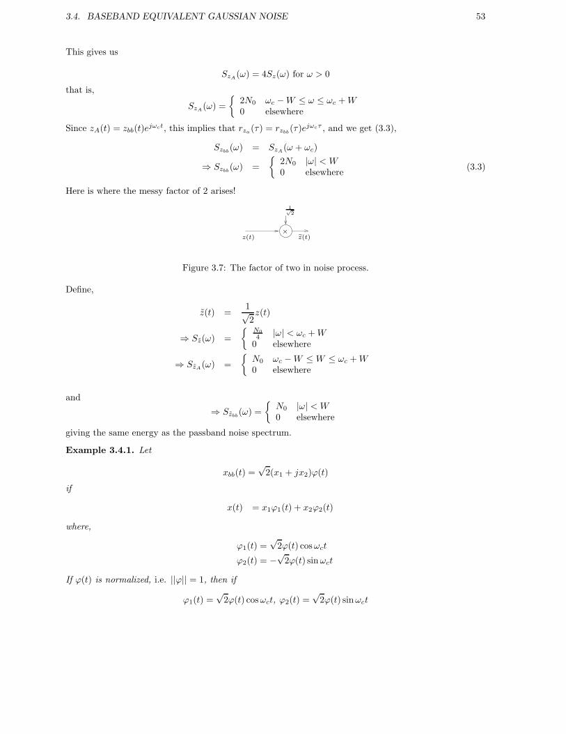
Here is where the messy factor of 2 arises!
1√2
ez(t)z(t)×
Figure 3.7: The factor of two in noise process.
Define,
z(t) =1√2z(t)
⇒ Sz(ω) =
N0
4 |ω| < ωc +W0 elsewhere
⇒ SzA(ω) =
N0 ωc −W ≤W ≤ ωc +W0 elsewhere
and
⇒ Szbb(ω) =
N0 |ω| < W0 elsewhere
giving the same energy as the passband noise spectrum.
Example 3.4.1. Let
xbb(t) =√
2(x1 + jx2)ϕ(t)
if
x(t) = x1ϕ1(t) + x2ϕ2(t)
where,
ϕ1(t) =√
2ϕ(t) cosωct
ϕ2(t) = −√
2ϕ(t) sinωct
If ϕ(t) is normalized, i.e. ||ϕ|| = 1, then if
ϕ1(t) =√
2ϕ(t) cosωct, ϕ2(t) =√
2ϕ(t) sinωct

54 CHAPTER 3. PASSBAND SYSTEMS
x
+
+
H(w + wc)
H(w + wc)
1√2
y(t)
ybb(t)
ybb(t)
ybb(t)
xbb(t)√2
Sn(f) = N0/2
(x1 + jx2)ϕ
1√2nbb(t)
Phase splitter
Figure 3.8: Representation of additive noise channel.
⇒ ||ϕ1|| = ||ϕ2|| = 1
So under modulation√
2 factor is needed.Verification: Let us verify that indeed ϕ1 and ϕ2 are normalized.
Φ1(ω) =√
2[1
2Φ(ω − ωc) +
1
2Φ(ω + ωc)] =
1√2[Φ(ω − ωc) + Φ(ω + ωc)],
where Φi(ω) = F(ϕi), i = 1, 2. Hence, it is normalized, i.e.,
||Φ1|| =1
2[||Φ|| + ||Φ||] = 1
Note: Scaling is really for analytical convenience, since scaling does not change SNR since it is afterreceived signal.Therefore to be precise when XA(w) = [1 + sgn(w)]X(w)
⇒ XA(ω) =
2X(ω) ω > 0X(ω) ω = 00 ω < 0
3.5 Circularly symmetric complex Gaussian processes
Let Z = R+ jI where I and R denote real and imaginary components respectively.
Z complex Gaussian ⇒ R, I are jointly Gaussian
Now if we think of
(RI
)as a vector then
E
[(RI
)(R I
)]=
(E[R2]
E [RI ]E [IR] E
[I2])

3.5. CIRCULARLY SYMMETRIC COMPLEX GAUSSIAN PROCESSES 55
Note that since E [IR] = E [RI ], there are three degrees of freedom.Let
Rz = E [ZZ∗] = E[R2]+ E
[I2]
Clearly this has only one degree of freedom. Hence, this is not sufficient to specify the Gaussian randomvariable Z.Define
Rz = E [ZZ] = E[R2]− E
[I2]+ 2jE [RI ]
Thus we have 2 degrees of freedom here.
Definition 3.5.1. Circularly symmetric complex Gaussian variables. A random variable Z is
circularly symmetric iff ⇒ Rz = 0, i.e.
E[R2]
= E[I2]
E [RI ] = 0
This can be generalized to vectors,
Z =
z1...zN
∈ CN
is a complex Gaussian circularly symmetric random variable, iff,
E[ZZt
]= 0
This implies,
E [zizj ] = 0 ∀i, j
Therefore the complex covariance matrix Rz for zero mean random variables is,
Rz = E [zz∗]
Complex Gaussian vectors The probability density function (pdf) is,
Pz(z) =1
|πRz|e−(z−µ)∗Rz
−1(z−µ)
where E [z] = µ, and Rz = E[(z − µ)(z − µ)∗
].
3.5.1 Gaussian hypothesis testing - complex case
y = x + z
where x,y,z ∈ CN and z is a circularly symmetric complex Gaussian random vector with Rz = σ2I ,

56 CHAPTER 3. PASSBAND SYSTEMS
µ = 0.
HMAP (y) = argmaxi
Px|y(xi|y)
= argmaxi
Px(xi)Py|x(y|xi)
= argmaxi
Px(xi)Pz(y − xi)
= argmaxi
Px(xi)1
(πσ2)Ne−
||y−xi||2
σ2
= argmaxi
[ln Px(xi) −
||y − xi||2σ2
]
= argmaxi
[ln Px(xi) −
||y||2σ2
− ||xi||2σ2
+2< < y, xi >
σ2
]
⇒ HMAP (y) = argmaxi
[ln Px(xi) +
2< < y, xi >
σ2− ||xi||2
σ2
]
where < y, x >= y∗xSimilarly
HML(y) = arg maxi
[−||y − xi||2]
= arg maxi
[2< < y, xi > −||xi||2]
= arg mini
[||y − xi||2]
3.6 Problems
Problem 3.1
Let the transmitted bandpass signal be given by
x(t) = a cos(2π(fc + 1
T )t)
+ b cos(2π(fc + 2
T )t)
t ∈ [0, T ]
and a ∈ 0, A, b ∈ 0, A.1. Find the baseband equivalent signal xbb(t) for the transmitted signal.
2. Find the vector representation of the baseband signal and draw the corresponding signal constella-tion.
3. If a =
0 w.p. 1
2A w.p. 1
2
and b =
0 w.p. 1
2A w.p. 1
2find the average energy of the baseband signal. Is this a minimum energy configuration? If not howwill you modify the constellation so that it is of minimum energy?
Problem 3.2
Consider the following passband waveform:
x(t) = sinc(t)(1 +A sin(4πt)) cos(ωct+
π
4
),
where ωc >> 4π.

3.6. PROBLEMS 57
1. Find xbb(t) and xA(t), the baseband and analytical equivalents of x(t).
2. Let x(t) is passed through a channel with impulse response h(t) = δ(t) − δ(t− 1). Let the outputbe y(t). Find ybb(t) and yA(t).
Problem 3.3
[Passband Systems] Let the transmitted bandpass signal be given by
x(t) = a cos(2π(fc + 1
T )t)
+ b cos(2π(fc + 2
T )t)
t ∈ [0, T ]
and a ∈ 0, A, b ∈ 0, A.
1. Find the baseband equivalent signal xbb(t) for the transmitted signal.
2. Find the vector representation of the baseband signal and draw the corresponding signal constella-tion.
3. If a =
0 w.p. 1
2A w.p. 1
2
and b =
0 w.p. 1
2A w.p. 1
2find the average energy of the baseband signal. Is this a minimum energy configuration? If not howwill you modify the constellation so that is is minimum energy?
Problem 3.4
A baseband-equivalent waveform (wc > 2π)
xbb(t) = (x1 + jx2)sinc(t)
is convolved with the complex filterw1(t) = δ(t) − jδ(t− 1)
1. Findy(t) = w1(t) ∗ xbb(t).
2. Suppose y(t) is convolved with the imaginary filter
w2(t) = 2jsinc(t)
to get
z(t) = w2(t) ∗ y(t)= w2(t) ∗ w1(t) ∗ xbb(t)
= w(t) ∗ xbb(t).
Find z(t). Note that sinc(t) ∗ sinc(t− k) = sinc(t− k), k an integer.
3. Letz(t) = <z(t)ejwct = w(t) ∗ x(t)
where x(t) = <xbb(t)ejwct. Show that
w(t) = 4 sinc(t− 1) cos(wct) − 4 sinc(t) sin(wct)
when convolved with the passband x(t) will produce z(t). Hint: use baseband calculations.

58 CHAPTER 3. PASSBAND SYSTEMS
Problem 3.5
For the AWGN channel with transfer function,
H(f) =
1 75MHz ≤ |f | ≤ 175MHz0 otherwise
a transmitted signal cannot exceed 1 mW and the power spectral density is also limited according toSx(f) ≤ −83 dBm/Hz (two sided psd). The two-sided noise power spectral density is σ2 = −98 dBm/Hz.The carrier frequency is fc = 100 MHz for QAM transmission. The probability of error is Pe = 10−6.(P dBm = 10P/10 mW.)
1. Find the base band channel model Hbb(f)2 (after the scaling).
2. Find the largest symbol rate that can be used with the 100 MHz carrier frequency.
3. What is the maximum signal power at the channel output with QAM?
4. What QAM data rate can be achieved with the symbol rate of part 2?
Problem 3.6
[ Whitening passband random processes]Let us consider a real valued passband random process
X(t) = XI(t) cos(ωct) −XQ(t) sin(ωct), (3.4)
at a carrier frequency of ωc. The processes XI(t) and XQ(t) are independent stationary zero-meanGaussian random processes with,
E [XI(t)XI(t− τ)] = rI (τ)
and E [XQ(t)XQ(t− τ)] = rQ(τ).
We assume that
rI (τ) = rQ(τ) = e−2|τ |
and E [XI(t)XQ(t− τ)] = 0 ∀τ.
1. Find rx(τ) = E [X(t)X(t− τ)] in terms of rI (τ) = rQ(τ) as a function of ωc.
2. Find the correlation function for the baseband equivalent of X(t) in equation (3.4), i.e., find
E [Xbb(t)X∗bb(t− τ)] = rbb(τ).
Also find the correlation function of the analytic equivalent signal E [XA(t)X∗A(t− τ)].
3. We sample Xbb(t) at times t = k, i.e., at integer times,
Y (k) = Xbb(k).
HenceE [Y (k)Y ∗(k − l)] = E [Xbb(k)X
∗bb(k − l)] = rbb(l).
We want to find a baseband filter to whiten this Y (k) process. Compute such a causal whiteningfilter.

Part II
Transmission over LinearTime-Invariant channels
59


Chapter 4
Inter-symbol Interference andoptimal detection
The main focus till now was one “one-shot” transmission, i.e., transmission of one of M messages using aN dimensional symbol. Typically, a transmission system sends a sequence of messages. If the channel ismemoryless, i.e., successive transmissions do not interfere with each other, then the analysis up to nowis sufficient. More formally, a channel is memoryless if
P(y1, y2, . . . , yt|x1, x2, . . . , xt) =t∏
k=1
P(yk|xk)
where yktk=1 are symbols received over t successive time periods. In practice, symbols do interfere with
each other causing Inter-Symbol-Interference (ISI).
4.1 Successive transmission over an AWGN channel
First, let us examine successive transmission over a memoryless AWGN channel. If we reuse the channelwe send one out of M messages every T seconds. If T is the symbol period then 1
T is the symbol rate.Then the data rate R is defined as
Rdef=
log2M
Tbits/second.
In order to transmit k successive messages, we send
x(t) =
K−1∑
k=0
xk(t− kT ) (4.1)
where k indicates time index (i.e., message transmitted at kth time instant). We also define
xk(t) =N−1∑
n=0
xk,nφn(t)
Therefore, now the basis expansion has two indices, one indicating the symbol time and other for thebasis coefficient, for the symbol time. One can form the optimal receiver by thinking of (4.1) as a one-shotproblem with Mk possible messages and therefore decode optimally. If the channel is memoryless, the
61

62 CHAPTER 4. INTER-SYMBOL INTERFERENCE AND OPTIMAL DETECTION
problem decouples and instead of Mk, we get k, M -dimensional independently solvable problems and thedimensionality of the problem does not go up exponentially i.e., the complexity does not grow as M k.
Notes:
1. Even though < ϕn, ϕk >= δn−k, < ϕn(t− kT ), ϕk(t− lT ) > need not be δn−k for k 6= l.
However, if < ϕn(t−kT ), ϕk(t− lT ) >= δn−k again the problem decouples and we can do “symbol-by-symbol” detection.
2. The inherent assumption is that the successive messages are independent. However, if there is de-pendance, then clearly “symbol-by-symbol” detection is not optimal even for memoryless channels.
4.2 Inter-symbol Interference channel
The inter-symbol interference channel we will focus on is illustrated in Figure 4.1.
h(t)x(t)
+ y(t)x(t)
z(t)
Figure 4.1: The inter symbol interference channel.
The transmitted waveform is,
x(t) =
K−1∑
k=0
N−1∑
n=0
xk,n [ϕn(t− kT ) ∗ h(t)]︸ ︷︷ ︸pn(t−kT )
,
and the received waveform is with Gaussian noise,
y(t) = x(t) + z(t) =
K−1∑
k=0
N−1∑
n=0
xk,n [ϕn(t− kT ) ∗ h(t)]︸ ︷︷ ︸pn(t−kT )
+z(t), (4.2)
where z(t) is additive Gaussian noise.
Therefore the nth pulse response is,
pn(t) = ϕn(t) ∗ h(t)
Definition 4.2.1. We define the normalized pulse response ϕn(t) as,
ϕn(t) =pn(t)
||pn||
where ||pn|| = < pn, pn >1/2.

4.2. INTER-SYMBOL INTERFERENCE CHANNEL 63
Hence, we can rewrite the transmitted waveform as,
x(t) =
K−1∑
k=0
N−1∑
n=0
xk,n||p||︸ ︷︷ ︸scaled version of symbol
ϕn(t− kT )
Now consider an isolated symbol transmitted over the channel, i.e., not successive transmission. Thismeans that xk = x0δ(k), and the waveform y(t) is observed in order to detect x0. Therefore, this“one-shot” transmission specifies a lower bound to the error probability of i.i.d. symbols. Therefore theSNR of this channel is an upper bound to the SNR of successive data transmission over the ISI channel.Therefore, this is called the matched filter bound.
Definition 4.2.2. The SNRMFB is the SNR of a single shot transmission over the channel given in(4.2) and is given by,
SNRMFB =Ex||p||2N0
, (4.3)
where Ex = E[||xk||2] and N0 = E[|z(t)|2].The main question we first address is, what should the optimum receiver structure be for successivetransmission over the channel given in Figure 4.1. In the sequel, we consider N = 1 for simplicity. Hencewe will drop the subscript from ϕn(t) and use it as ϕ(t). Clearly all the discussion can be extended tothe case when N > 1 complex dimensions.
4.2.1 Matched filter
In this section we derive a set of sufficient statistics for the ISI channel.
Theorem 4.2.1. The set of discrete-time samples y(kT )k∈(−∞,∞) where y(kT ) = y(t) ∗ ϕ∗(−t)|t=kT
are a set of sufficient statistics for the detection of xk over a continuous-time ISI channel whose outputis y(t), i.e.,
y(t) = h(t) ∗∑
n
xkϕ(t− nT ) + z(t)︸︷︷︸AWGN
and ϕ(t)def= h(t)∗ϕ(t)
||h∗ϕ||
Notes:
1. Here we have assumed N = 1, and hence the subscript of ϕ has been dropped for convenience.
2. The result indicates that the following detector structure incurs no loss of optimality.
Detector
h(t)
z(t)
ϕ(t)
kTy(kT )
xk
xk
ϕ∗(−t)
+
64 CHAPTER 4. INTER-SYMBOL INTERFERENCE AND OPTIMAL DETECTION
Proof: Consider the following problem
y(t) =∑
k
xk ||p||ϕ(t− kT ) + z(t), t ∈ (−∞,∞)
This is like transmitting symbols xk, where xk = xk||p|| using modulating functions ϕk(t) where
ϕk(t) = ϕ(t− kT ) (4.4)
We can use a Gram-Schmidt orthogonalization process, for example, to create an orthonormal basis forthe space spanned by ϕk. We can call this orthonormal basis ψk which can be obtained by aninvertible transformation Γ. That is
ψk = Γ(ϕk)ϕk = Γ−1(ψk)
Therefore one can writey(t) =
∑
k
ukψk(t) + z(t) (4.5)
where uk is the coefficients of∑
k xkϕk(t) in the new basis. From “single shot” transmission, we knowthat for white Gaussian noise, the optimal receiver projects onto the orthonormal basis directions, i.e.,< y, ψk > form a set of sufficient statistics for detecting uk.Now if we apply an invertible transform Γ−1 to recover uk expressed in their orthogonal basis ϕk(which may not be orthonormal), then we obtain < y, ϕk > as the set of outputs we process. In otherwords, uk expresses x(t) in terms of the basis ϕk (see (4.5) above), and we can do a change of basisto express x(t) in terms of ϕk which yields the basis coefficients < y, ϕk >. Since, the transform isinvertible, by the reversibility theorem we are done.
Alternate (more explicit) proof:Let us consider a finite number of transmissions, i.e., k = 0, . . . ,K − 1.
y(t) =K−1∑
k=0
xk||p||ϕ(t− kT ) + z(t), t ∈ (−∞,∞)
Optimal receiver projects onto subspace spanned by signal when noise is white. That is, let yE = P(y),where P projects onto the signal space. Therefore the projections are,
< y,∑
xk||p||ϕk >=∑
< y, ϕk > (xk||p||)
Hence,
yk =< y, ϕk >= y(t) ∗ ϕk(−t)|t=kT
form a set of sufficient statistics.
4.2.2 Noise whitening
As a result of the matched filtering operation illustrated in Figure 4.2, the noise observed after samplingneed not be white. Consider the output of the matched filter which projects the signal onto the basis,i.e.,
y(kT ) =< y, ϕk >

4.2. INTER-SYMBOL INTERFERENCE CHANNEL 65
ϕ(t)
sample at times kT
z(t)
ϕ∗(−t)+
xk = ||p||xk
Figure 4.2: Colored noise at the output of the matched filter.
Let us define,
y(kT )def= yk =
∑
n
xn||p|| < ϕn, ϕk > + < z, ϕk > (4.6)
Now,
< ϕn, ϕk > =
∫ϕ(t− nT )ϕ∗(t− kT )dt
=
∫ϕ(t)ϕ∗(t− (k − n)T )dt
Hence
< ϕn, ϕk > = < ϕ0, ϕk−n >
Letql =< ϕ0, ϕl >
Clearly q∗l = q−l and hence ql has conjugate symmetry.From (4.6),
yk =∑
n
xnqk−n+ < z, ϕk >
=∑
n
xn−kqk+ < z, ϕk >
Consider the noise process
zndef= < z, ϕn >
The spectrum of this noise is,
E[zn, z∗n−k] = E
[∫ ∫z(t)ϕ∗(t− nT )dtz∗(t)ϕ(τ − (n− k)T )dτ
]
=
∫
t
∫
τ
ϕ∗(t− nT )ϕ(τ − (n− k)T )E[z(t)z∗(τ)]dtdτ
=
∫
t
∫
τ
ϕ∗(t− nT )ϕ(τ − (n− k)T )N0δ(t− τ)dtdτ
= N0
∫
t
ϕ∗(t− nT )ϕ(t− (n− k)T )dt
= N0 < ϕn−k, ϕn >= qkN0

66 CHAPTER 4. INTER-SYMBOL INTERFERENCE AND OPTIMAL DETECTION
zn wng(n)
Figure 4.3: The noise whitening filter.
Hence zk is not in general white. Therefore, after filtering, we have a colored noise process. Ideally, wewould like to work with white noise, and hence we would like to “whiten” it as illustrated in Figure 4.3.To avoid confusion of lots of z’s floating around, the D-transform is the Z-transform with D = z−1
Definition 4.2.3. (The D-transform)If H(z) is the z-transform of the sequence hn, i.e.,
H(z) =∑
n
hnz−n,
then the D-transform of hn is
H(D) =∑
n
hnDn
and we denote the transform pair by
hn D⇔ H(D)
Now, given the review class, we know that the power spectral density of a random (stationary) process is
Sz(D) = DE[zkz∗k−n]
And passing a random process (stationary) through a linear filter gn (i.e., with D-transform G(D))results in
Sw(D) = G(D)G∗(1
D∗ )Sz(D)
Now we use the spectral factorization theorem.
Theorem 4.2.2. (Spectral factorization theorem) A power spectrum S(D), can be factorized into S(D) =F (D)F ∗( 1
D∗ ) iff the Paley-Wiener condition holds, i.e.,
1
2π
∫ π
−π
ln[S(ejω)]dω <∞
We assume, that this holds for the process that we deal with. Now, armed with this we can write
Sz(D) = N0Q(D) = F (D)F ∗(1
D∗ )
And therefore the filtering zk through G(D) gives,
Sw(D) = G(D)G∗(1
D∗ )F (D)F ∗(1
D∗ )
By choosing G(D) =√
N0
F∗( 1D∗ )
, we see that Sw(D) = N0, i.e., white noise! Now,what happens to our
receiver? Note that Sz(D) = N0Dqn, hence we have in D-transform notation
Y (D) = Q(D) ‖ p ‖ X(D) + Z(D)
=1
N0Sz(D) ‖ p ‖ X(D) + Z(D)

4.3. MAXIMUM LIKELIHOOD SEQUENCE ESTIMATION (MLSE) 67
Therefore,
G(D)Y (D) =
√N0
F ∗( 1D∗ )
F (D)F ∗( 1D∗ )
N0‖ p ‖ X(D) +W (D)
=1√N0
F (D) ‖ p ‖ X(D) +W (D)
So, it is like converting the channel into F (D)√N0
. A natural question to ask is whether this procedure gives
any advantage.The spectral factorization can be arranged such that Sz(D) = F (D)F ∗( 1
D∗ ) has a causal factor F (D).Hence we have not only whitened the noise but have converted our channel into a causal sequence. Thiscombination of ϕ∗(−t) and G(D) together is called the whitened matched filter .
Now we have the following problem at hand. Detect sequence xk when we observe
Y (D) =1√N0
F (D) ‖ p ‖ X(D) +W (D) (4.7)
Or in time domain,
yk =∑
n≥0
xk−n fn︸︷︷︸D−1( ‖p‖F(D)√
N0)
+wk
when wk is now white Gaussian noise and fn is a causal sequence. Given the problem stated in (4.7),we would now like to derive efficient detection algorithms while retaining optimality. A naive detectionscheme would incur a complexity of MK where M is the constellation size and K the time window ofdetection. Clearly we would need better methods than exponential and the next two sections give efficientML and MAP decoders for this problem.
4.3 Maximum Likelihood Sequence Estimation (MLSE)
Consider again1,Y (D) = F (D)X(D) + Z(D) (4.8)
where F (D) = f0 + f1D+. . .+fνDν i.e. a finite length response.
Let
Sz(D) =N0
2
def= σ2
Note that the signal to noise ratio (SNR) is given by,
E
[|y(k) − z(k)|2
]
E
[|z(k)|2
] =||f ||2E
[|x(k)|2
]
σ2=
Ex
σ2||f ||2
We make the following assumptions,
• Uniform priors
• ν <∞ ⇒ finite impulse response
Implication: y(k) is the output of a finite state machine operating over C (see Figure 4.4), withadditive i.i.d. noise process w(k).
1We revert back to using z(k) as the notation for noise. In the previous notation this was w(k) and we use z(k) as whitenoise.
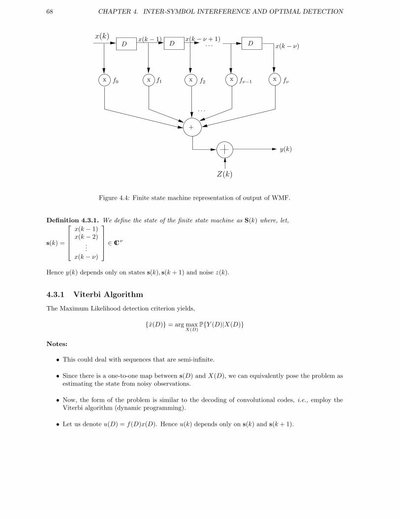
68 CHAPTER 4. INTER-SYMBOL INTERFERENCE AND OPTIMAL DETECTION
. . .
x x x x x
D D D
f0 f1 f2 fν−1 fν
+
x(k − 1) x(k − ν + 1). . . x(k − ν)
y(k)
Z(k)
x(k)
Figure 4.4: Finite state machine representation of output of WMF.
Definition 4.3.1. We define the state of the finite state machine as S(k) where, let,
s(k) =
x(k − 1)x(k − 2)
...x(k − ν)
∈ Cν
Hence y(k) depends only on states s(k), s(k + 1) and noise z(k).
4.3.1 Viterbi Algorithm
The Maximum Likelihood detection criterion yields,
x(D) = arg maxX(D)
PY (D)|X(D)
Notes:
• This could deal with sequences that are semi-infinite.
• Since there is a one-to-one map between s(D) and X(D), we can equivalently pose the problem asestimating the state from noisy observations.
• Now, the form of the problem is similar to the decoding of convolutional codes, i.e., employ theViterbi algorithm (dynamic programming).
• Let us denote u(D) = f(D)x(D). Hence u(k) depends only on s(k) and s(k + 1).

4.3. MAXIMUM LIKELIHOOD SEQUENCE ESTIMATION (MLSE) 69
Since z(k) is i.i.d. Gaussian, the log-likelihood splits up as
log Py(D)|s(D) =∑
k
log Pzy(k) − u(k)
=∑
k
[log(2πσ2) − |y(k) − u(k)|2
]
Let us denote
Γ[s(D)]k2
k1
def=
k2−1∑
k=k1
log Pz [y(k) − u(s(k), s(k + 1))]
u(s(k), s(k + 1)) shows explicit dependence of u(k) on s(k), s(k + 1).
Dynamic programming principle: Suppose, for the moment, we knew that the state s(k) at timek was Sj (one particular choice out of M ν choices). Then, for any allowable state sequence s(D), thatstarts with s(0) = 0 and passes through state Sj at time k, the log likelihood would break up into twoindependent parts,
Γ[s(D)]K0 = Γ[s(D)]
k0 + Γ[s(D)]
Kk
If sj(D) be any allowable state sequence from time 0 to k, that has maximum log-likelihood Γ[s(D)]k0
among all the allowable state sequences starting from s(0) = 0 and ending at s(K) = S j . We call sj(D),the survivor at time k corresponding to state Sj .Therefore, sj(D) must be the initial segment of the maximum likelihood state sequence, if indeed the truestate sequence was Sj at time k. We do not know the state sequence s(k) but clearly it has to be one ofa finite set of sizeMν . Consequently, we store survivor sequences for each state and their correspondinglog-likelihoods Γ[sj(D)]
k0 for j ∈ 1,. . . ,Mν.
Thus we store Mν sequences sj(D) and their log-likelihoods Γ[sj(D)]k0 and update them as follows:
1. For each of the M allowable extensions of sj(D) to time k+1, compute for each of the M ν survivors:
Γ[sj(D)]k+10 = Γ[sl(D)]k0 + ln Pz[y(k) − u(S l,Sj)] ∀j ∈ 1, . . . ,Mν
where l ∈ 1,. . . ,Mν. This needs MνM = Mν+1 additions.
2. For each state j, compare the log likelihoods Γ[sj(D)]k+10 of the M extensions that end in state Sj ,
and select the largest as the corresponding survivor. This needs M ν , M -ary comparisons.
This summarizes the Viterbi algorithm, which in principle terminates only at k → ∞. However, we canmake a decision on a particular state (dynamic programming for ISI channel), if all the survivors agree onthat state. Moreover in practice, typically good decisions can be made with a finite time horizon. Notethat such a sequence estimation can also work if x(D), itself was the result of the finite state machine(e.g., convolutional code). In this case the state machine can be augmented and one can obtain anoptimal joint equalization and decoding of the channel code.
4.3.2 Error Analysis
A correct state sequence and an erroneous one are illustrated in Figure 4.5.Error event: An error event extends from time k1 to k2 if the estimated state sequence s(D) is equal tothe correct state sequence s(D) at times k1 and k2 but nowhere in between. Hence s(k1) = s(k1), s(k2) =

70 CHAPTER 4. INTER-SYMBOL INTERFERENCE AND OPTIMAL DETECTION
correct state sequence
incorrect state sequence
Figure 4.5:
s(k2), s(k) 6= s(k), k1 < k < k2. The Length of error event is n = k2 − k1 − 1 ≥ ν.Clearly for such an error event:
x(k) = x(k), k1 − ν ≤ k ≤ k1 − 1 and k2 − ν ≤ k ≤ k2 − 1
from the definition of s(k).However, x(k1) 6= x(k1) and x(k2−ν−1) 6= x(k2−ν−1) since, s(k1+1) 6= s(k1+1), and s(k2−1) 6= s(k2−1),we can define,
εx(D)def= [x(k1) − x(k1)] + [x(k1 + 1) − x(k1 + 1)]D + . . .+ [x(k2 − ν − 1) − x(k2 − ν − 1)]Dn−ν
εu(D)def= [u(k1) − u(k1)] + [u(k1 + 1) − u(k1 + 1)]D + . . .+ [u(k2 − 1) − u(k2 − 1)]Dn
Since u(D) = f(D)x(D), clearly we have εu(D) = f(D)εx(D)
Probability of a particular error event:
u(D)
y(D)
u(D)
||y(D) − u(D)|| < ||y(D) − u(D)||
Think of u(D) being “symbols” in sequence space. Hence, the same way as we did earlier, we can writethe NNUB as
Pe,MLSE ≤ NeQ
(dmin
2σ
)
where dmin is the minimum distance between sequences u(D), i.e.
dmin = minu6=u
||u(D) − u(D)||
Ne is again Ne =∑
x Px(εx + x)Nu that is, the average # of nearest neighbors. Note that this is done insequence space and we calculate over the allowable sequences, i.e., εx + x must be an allowable sequence.The main question is to be able to calculate dmin for different channels.

4.4. MAXIMUM A-POSTERIORI SYMBOL DETECTION 71
4.4 Maximum a-posteriori symbol detection
In section (4.3), we explored the maximum likelihood detector. But if the priors are not uniform theMAP detector is the optimal scheme and this is the focus of the following section.
4.4.1 BCJR Algorithm
For minimizing symbol error probability we use
x(n) = arg maxx(n)
P[x(n)|y(0), . . . y(N − 1)]
The BCJR algorithm efficiently does this computation simultaneously for all x(n).
x(n) = arg maxx(n)
P[x(n)|yN−10 ] = arg max
x(n)P[x(n),yN−1
0 ]
where yk2
k1= y(k1), . . . , y(k2)
P[x(n),yN−10 ] =
∑
i,j
P(x(n),yn−10 , y(n),yN−1
n+1 , s(n) = Si, s(n+ 1) = Sj)
=∑
i,j
P[yn−10 , s(n) = S i]P[x(n), y(n),yN−1
n+1 , s(n+ 1) = Sj |yn−10 , s(n) = S i]
=∑
i,j
P[yn−10 , s(n) = S i]P[x(n), y(n), s(n+ 1) = Sj |yn−1
0 , s(n) = Si]
P[yN−1n+1 |x(n),yn−1
0 , y(n), s(n) = S i, s(n+ 1) = Sj ]
(a)=
∑
i,j
P[yn−10 , s(n) = S i]︸ ︷︷ ︸
αn(i)
P[x(n), y(n), s(n+ 1) = Sj |s(n) = Si]︸ ︷︷ ︸γn(i,j)
P[yN−1n+1 |s(n+ 1) = Sj ]︸ ︷︷ ︸
βn+1(j)
where (a) is due to the Markov property of the finite state machine. Therefore we obtain the relationship,
P[x(n),yN−10 ] =
∑
i,j
αn(i)γn(i, j)βn+1(j)
The BCJR algorithm essentially computes αn(i), and βn+1(j) efficiently through the forward-backwardrecursion.
γn(i, j) = P[y(n), x(n), s(n+ 1)) = Sj |s(n) = S i]
This can be computed for each n, as,
γn(i, j) = P[y(n), x(n)|s(n) = S i]P[s(n+ 1) = Sj |s(n) = S i, x(n), y(n)]
= p(x(n))p (y(n) | x(n), s(n) = Si) P[s(n+ 1) = Sj |s(n) = Si, x(n), y(n)]
If the transition from Si to Sj occurs due to symbol x(n), then
P[s(n+ 1) = Sj |s(n) = S i, x(n), y(n)]
is either 1 if x(n) = x(n), and 0 otherwise. Now we need to compute αn(i) and βn(j).

72 CHAPTER 4. INTER-SYMBOL INTERFERENCE AND OPTIMAL DETECTION
Forward recursion
Computation of αn(i)
αn(i) = P[yn−10 , s(n) = S i]
=∑
k
P[yn−10 , s(n) = Si, s(n− 1) = Sk]
=∑
k
P[yn−20 , y(n− 1), s(n) = Si, s(n− 1) = Sk]
=∑
k
P[yn−20 , s(n− 1) = Sk]P[y(n− 1), s(n) = Si|yn−2
0 , s(n− 1) = Sk]
=∑
k
αn−1(k)γn−1(k, i)
Therefore we get the following forward recursion,
αn(i) =∑
k
αn−1(k)γn−1(k, i). (4.9)
Backward recursion
Computation of βn(j)
βn+1(j) = P[yN−1n+1 |s(n+ 1) = Sj ]
=∑
k
P[yN−1n+1 , s(n+ 2) = Sk|s(n+ 1) = Sj ]
=∑
k
P[yN−1n+2 , y(n+ 1), s(n+ 2) = Sk|s(n+ 1) = Sj ]
=∑
k
P[y(n+ 1), s(n+ 2) = Sk|s(n+ 1) = Sj ]
P[yN−1n+2 |y(n+ 1), s(n+ 2) = Sk, s(n+ 1) = Sj ]
=∑
k
γn+1(j, k)βn+2(k)
Hence we get the following backward recursion,
βn+1(j) =∑
k
γn+1(j, k)βn+2(k) (4.10)
Using the forward-backward recursions, one can then compute the max-a-posteriori symbols x(n)N−1n=0 .
Notes:
1. The BCJR algorithm computes x(n) according to minimum symbol-by-symbol error probability:This could be different from the sequence of error probability
2. BCJR also gives us “soft-information” on the reliability of the symbols detected.
3. The BCJR algorithm and the Viterbi algorithm (MLSE) applied to same observations (and uniformpriors) may give different candidate sequences, since they optimize different criteria. The choice ofwhich criteria is important depends on the application.

4.5. PROBLEMS 73
4.5 Problems
Problem 4.1
Let the transmission over an ISI channel yield after matched filtering the following model,
Y (D) = ||p||X(D)Q(D) + Z(D)
where ql = e−2|l| and Sz(D) = N0Q(D) and Q(D) is the D-Transform of ql.Find the whitening filter W (D) to whiten the noise. Choose the whitening filter such that the resultingcommunication channel after the whitening filter is causal. That is, Q(D)W (D) is causal.
Problem 4.2
Suppose we are given qk, (the autocorrelation function of the normalized pulse function) by : q0 = 5/4,q1 = q−1 = −1/2, and where the equivalent channel in D-transform resulting out of matching filter isgiven by :
Y (D) =1
N0Sz(D)||p||X(D) + Z(D)
Find Sz(D), F (D) and the resulting channel ( write in the temporal domain G(D)Y (D)).
Problem 4.3
[Whitening and coloring]
1. Let the transmission over an ISI channel yield after matched filtering the following model,
Y (D) = ||p||X(D)Q(D) + Z(D)
where ql = e−2|l| and Sz(D) = N0Q(D) and Q(D) is the D-Transform of ql.Find the whitening filter W (D) to whiten the noise. Choose the whitening filter such that theresulting communication channel after the whitening filter is causal. That is,
Y (D)W (D) = ||p||X(D) Q(D)W (D)︸ ︷︷ ︸causal channel
+Z(D)W (D)
2. Let Zn be a wide-sense stationary random process with EZn = 0,
EZnZn−l =
1.81 l = 00.9 |l| = 1
0 else
and let Zn be a real process. Now let Un be a white, wide-sense stationary real random process,
i.e EUn = 0, and EUnUn−l =
1 l = 00 else
Find a coloring filter Cn such that Zn = Cn ∗ Un
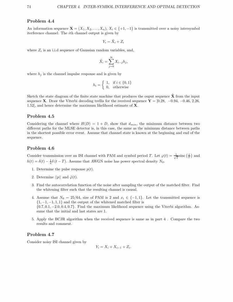
74 CHAPTER 4. INTER-SYMBOL INTERFERENCE AND OPTIMAL DETECTION
Problem 4.4
An information sequence X = (X1, X2, . . . , Xn), Xi ∈ +1,−1 is transmitted over a noisy intersymboliterference channel. The ith channel output is given by
Yi = Xi + Zi
where Zi is an i.i.d sequence of Gaussian random variables, and,
Xi =
∞∑
j=0
Xi−jhj ,
where hj is the channel impulse response and is given by
hi =
1, if i ∈ 0, 10, otherwise
Sketch the state diagram of the finite state machine that produces the ouput sequence X from the inputsequence X. Draw the Viterbi decoding trellis for the received sequence Y = [0.28, −0.94, −0.46, 2.26,1.52], and hence determine the maximum likelihood estimate of X.
Problem 4.5
Considering the channel where H(D) = 1 + D, show that dmin, the minimum distance between twodifferent paths for the MLSE detector is, in this case, the same as the minimum distance between pathsin the shortest possible error event. Assume that channel state is known at the beginning and end of thesequence.
Problem 4.6
Consider transmission over an ISI channel with PAM and symbol period T . Let ϕ(t) = 1√T
sinc(
tT
)and
h(t) = δ(t) − 12δ (t− T ). Assume that AWGN noise has power spectral density N0.
1. Determine the pulse response p(t).
2. Determine ||p|| and ϕ(t).
3. Find the autocorrelation function of the noise after sampling the output of the matched filter. Findthe whitening filter such that the resulting channel is causal.
4. Assume that N0 = 25/64, size of PAM is 2 and xi ∈ −1, 1. Let the transmitted sequence is1,−1,−1, 1, 1 and the output of the whitened matched filter is0.7, 0.1,−2.0, 0.4, 0.7. Find the maximum likelihood sequence using the Viterbi algorithm. As-sume that the initial and last states are 1.
5. Apply the BCJR algorithm when the received sequence is same as in part 4 . Compare the tworesults and comment.
Problem 4.7
Consider noisy ISI channel given by
Yi = Xi +Xi−1 + Zi.

4.5. PROBLEMS 75
where Xi and Yi are the channel input and output, respectively, at time index i, Z is a sequence ofi.i.d. Gaussian random variables, with zero mean and unit variance and xi ∈ −1, 1. Calculate thesymbol-wise MAP esitmate of X, using the BCJR algorithm, if the received sequence Y = [0.28, −0.54,−0.46, 2.26, 1.52]. You may assume that the channel is in state +1 at the begining and the end of thesequence. Compare this to the decoding estimate from the MLSE decoder.

76 CHAPTER 4. INTER-SYMBOL INTERFERENCE AND OPTIMAL DETECTION

Chapter 5
Equalization: Low complexitysuboptimal receivers
In many applications even the efficient implementation of optimal receivers may be too computationallyintensive for practical use. In such cases further reductions in complexity are sought at the cost ofoptimality. This chapter explores several such structures for detection in ISI channels. The chapterstarts with a discussion of linear estimation which forms the principles behind all the structures studiedin this chapter. We then proceed to derive and analyze several suboptimal schemes for ISI channels usinglinear estimation as a tool.
5.1 Linear estimation
5.1.1 Orthogonality principle
Suppose
y(k) = Ax(k) + z(k)
and given observations y(k) one wants to estimate x(k). Here z(k) is assumed to be Gaussian i.i.d.noise.Estimation criterion
min E
[||x(k) − x(k)||2
]
This is called the minimum mean squared error (MMSE) criterion. Our interest is restricted to a classof linear estimators, i.e.,
x(k) = Wy(k)
where W is the linear estimator matrix.Hence
e(k)def= x(k) − x(k) = x(k) −Wy(k)
and the problem becomes to find W such that
Wopt = argminW
E
[||x(k) −Wy(k)||2
]
and the MMSE is defined as
σ2MMSE = E
[||x(k) − Wopty(k)||2
]
77
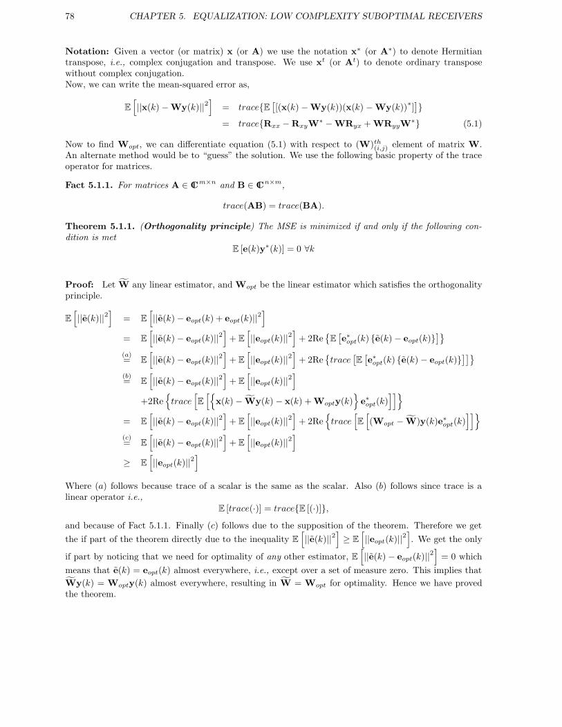
78 CHAPTER 5. EQUALIZATION: LOW COMPLEXITY SUBOPTIMAL RECEIVERS
Notation: Given a vector (or matrix) x (or A) we use the notation x∗ (or A∗) to denote Hermitiantranspose, i.e., complex conjugation and transpose. We use xt (or At) to denote ordinary transposewithout complex conjugation.Now, we can write the mean-squared error as,
E
[||x(k) −Wy(k)||2
]= traceE
[[(x(k) −Wy(k))(x(k) −Wy(k))
∗]]
= traceRxx −RxyW∗ −WRyx + WRyyW
∗ (5.1)
Now to find Wopt, we can differentiate equation (5.1) with respect to (W)th(i,j) element of matrix W.
An alternate method would be to “guess” the solution. We use the following basic property of the traceoperator for matrices.
Fact 5.1.1. For matrices A ∈ Cm×n and B ∈ Cn×m,
trace(AB) = trace(BA).
Theorem 5.1.1. (Orthogonality principle) The MSE is minimized if and only if the following con-dition is met
E [e(k)y∗(k)] = 0 ∀k
Proof: Let W any linear estimator, and Wopt be the linear estimator which satisfies the orthogonalityprinciple.
E
[||e(k)||2
]= E
[||e(k) − eopt(k) + eopt(k)||2
]
= E
[||e(k) − eopt(k)||2
]+ E
[||eopt(k)||2
]+ 2Re
E[e∗opt(k) e(k) − eopt(k)
]
(a)= E
[||e(k) − eopt(k)||2
]+ E
[||eopt(k)||2
]+ 2Re
trace
[E[e∗opt(k) e(k) − eopt(k)
]]
(b)= E
[||e(k) − eopt(k)||2
]+ E
[||eopt(k)||2
]
+2Retrace
[E
[x(k) − Wy(k) − x(k) + Wopty(k)
e∗opt(k)
]]
= E
[||e(k) − eopt(k)||2
]+ E
[||eopt(k)||2
]+ 2Re
trace
[E
[(Wopt − W)y(k)e∗opt(k)
]]
(c)= E
[||e(k) − eopt(k)||2
]+ E
[||eopt(k)||2
]
≥ E
[||eopt(k)||2
]
Where (a) follows because trace of a scalar is the same as the scalar. Also (b) follows since trace is alinear operator i.e.,
E [trace(·)] = traceE [(·)],and because of Fact 5.1.1. Finally (c) follows due to the supposition of the theorem. Therefore we get
the if part of the theorem directly due to the inequality E
[||e(k)||2
]≥ E
[||eopt(k)||2
]. We get the only
if part by noticing that we need for optimality of any other estimator, E
[||e(k) − eopt(k)||2
]= 0 which
means that e(k) = eopt(k) almost everywhere, i.e., except over a set of measure zero. This implies that
Wy(k) = Wopty(k) almost everywhere, resulting in W = Wopt for optimality. Hence we have provedthe theorem.

5.1. LINEAR ESTIMATION 79
Therefore, using the orthogonality principle, we have
E [(x(k) −Wopty(k))y∗(k)] = 0
or
WoptRyy = Rxy
where Ryy = E [y(k)y∗(k)], Rxy = E [x(k)y∗(k)] and hence
Wopt = RxyR−1yy (5.2)
Now, let us calculate the minimum mean-squared error (MMSE) of the optimal estimator.
σ2MMSE = E
[||x(k) −Wopty(k)||2
]
= E [(x(k) −Wopty(k))∗eopt]
= E [x∗(k)eopt] − trace E [Wopty(k)eopt](a)= E [x∗(k)(x(k) −Wopty(k))]
= E
[||x(k)||2
]− traceE [Wopty(k)x∗(k)]
= trace [E [xx∗] −WoptE [yx∗]]
= trace [Rxx −WoptRyx]
Where (a) follows due to Theorem 5.1.1.
Optimum (non-linear) MMSE estimation
A natural question to ask is what the optimal estimator is, without the restriction to a linear estimator.We next show that the optimal estimator is given by
x = E [x | Y = y] .
Notes:
1. In general, depending on the distributions x = E [x|Y = y] could be a non-linear function of y. Forbrevity we will denote E [x|Y = y] by E [x|y].
2. If x,y are jointly Gaussian , then x = E [x|y] is linear and hence linear estimators are optimal forestimating Gaussian random processes from another (correlated) Gaussian random process.
3. Here as well we will show (see Theorem 5.1.2), that the orthogonality principle holds, i.e.,
(x − E[x | y]) ⊥ (g(y))
for any (measurable) function g(y). Hence
E[eopty∗] = 0.
Theorem 5.1.2. xopt = E[X | Y = y] and x − xopt ⊥ g(y) for any (measurable) function g.

80 CHAPTER 5. EQUALIZATION: LOW COMPLEXITY SUBOPTIMAL RECEIVERS
Proof: First, it is easy to see that the tower property holds, i.e.,
Ex[X] = Ey
[Ex|y[X]
].
Hence
E[Xg∗(y)] = Ey
[Ex|y[Xg∗(y)]
]= Ey
[(Ex|y[X]
)g∗(y)
]
= Ey
[(Ex|y[X | Y]
)g∗(y)
]
⇒ E[(
X − Ex|y[X])g∗(y)
]= 0.
Therefore, if we denote xopt = Ex|y[X | Y], then x− xopt ⊥ g(y).Now, let x be any other estimator
⇒ E[‖ x − x ‖2] = E[‖ x − x + xopt − xopt ‖2]
= E[‖ (xopt − x) + eopt ‖2]
= E[‖ (xopt − x) ‖2] + E[‖ eopt ‖2] + 2Re
E[eopt (xopt − x)∗︸ ︷︷ ︸g(y)
]
⇒ E[‖ x − x ‖2] = E[‖ (xopt − x) ‖2] + E[‖ eopt ‖2]
⇒ x = xopt, a.e.
Where the notation a.e. means “almost everywhere”, i.e., everything except over a set of zero measures.
The estimation principles can be applied to a variety of situations. In particular we are interested inapplying it to scenarios where we observe a random process y(k) which is a noisy observation of theprocess x(k) which we want to estimate. Note that in general the processes x(k), y(k) need notbe white, i.e., there could be dependencies over time which we can exploit. In this context in the nextsections we consider the following cases.
Smoothing: Here we are allowed to use the entire observation y(n), n ∈ (−∞,∞) in order to estimatex(k). Therefore we can use “future” observations in the estimate of x(k).
Prediction: In this case we are only allowed to process the observations strictly causally. Therefore,in estimating x(k), we can only use observations y(n), n ∈ (−∞, k − 1). In this problem, we canalso formulate a pure prediction problem where the observations x(n), n ∈ (−∞, k − 1) are usedto predict the value of x(k).
Filtering: In this case we are only allowed to process the observations causally. Therefore, in estimatingx(k), we can only use observations y(n), n ∈ (−∞, k). Therefore the difference between predictionand filtering is that one can use the “current” observation as well for the estimate of x(k). However,this means that the filtering problem is degenerate if the observations are x(k) itself.
5.1.2 Wiener smoothing
Recall, for a random process x(k), (scalar and wide-sense stationary).Autocorrelation:
rxx(l) = E [x(k)x∗(k − l)]
rxx(l) = r∗xx(−l)

5.1. LINEAR ESTIMATION 81
i.e., rxx(l) exhibits conjugate symmetry.Power Spectrum: We define the power spectrum and cross spectrum as,
Rxx(D) = DE[xkx∗k−n], Rxy(D) = DE[xky
∗k−n], (5.3)
where D(·) denotes the D-transform. Note that there is conjugate symmetry in the power spectrum, i.e.,Rxx(D) = R∗
xx(D−∗).Notation (mneumonic): Very often in the class we denote the power spectrum and cross spectrumloosely as
Rxx(D) = E[X(D)X∗(D−∗)], Rxy(D) = E[X(D)Y ∗(D−∗)],
but this is an imprecise statement. What we really mean is the relationship in (5.3). This notation isreally used as a mneumonic to easily write out relationships.Suppose we observe y(k) and we want to estimate x(k) where unlike our previous set-up, there wouldbe correlation between y(l) and x(k), k 6= l. Here we would need to “filter” y(k) to estimate x(k).We restrict our attention to linear filters, i.e.,
x(k) =∑
n
w(n)y(k − n)
Hence,
X(D) = W (D)Y (D)
E(D) = X(D) −W (D)Y (D)︸ ︷︷ ︸X(D)
We use the criterion,
minW (D)
E
[|e(k)|2
]
Claim 5.1.1. The optimal estimator Wopt(D) is such that
E [eopt(k)y∗(k − n)] = 0, ∀n
where eopt(k) = x(k) − xopt(k), where Xopt(D) = Wopt(D)Y (D).
Using this orthogonality principle we have,
E [eopt(k)y∗(k − n)] = 0, ∀n (5.4)
Hence,
E
[[x(k) −
∑
l
wopt(l)y(k − l)
]y∗(k − n)
]= 0
⇒ E [x(k)y∗(k − n)] −∑
l
wopt(l)E [y(k − l)y∗(k − n)] = 0
⇒ rxy(n) =∑
l
wopt(l)ryy(n− l)
⇒ Rxy(D) = Wopt(D)Ryy(D) (5.5)
where we have denoted rxy(n) = E [x(k)y∗(k − n)] and ryy(n− l) = E [y(k − l)y∗(k − n)].
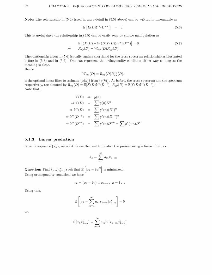
82 CHAPTER 5. EQUALIZATION: LOW COMPLEXITY SUBOPTIMAL RECEIVERS
Note: The relationship in (5.4) (seen in more detail in (5.5) above) can be written in mneumonic as
E[E(D)Y ∗(D−∗)
]= 0. (5.6)
This is useful since the relationship in (5.5) can be easily seen by simple manipulation as
E[X(D) −W (D)Y (D)Y ∗(D−∗)
]= 0 (5.7)
⇒ Rxy(D) = Wopt(D)Ryy(D).
The relationship given in (5.6) is really again a shorthand for the cross-spectrum relationship as illustratedbefore in (5.3) and in (5.5). One can represent the orthogonality condition either way as long as themeaning is clear.
Hence
Wopt(D) = Rxy(D)R−1yy (D).
is the optimal linear filter to estimate x(k) from y(k). As before, the cross-spectrum and the spectrumrespectively, are denoted by Rxy(D) = E[X(D)Y ∗(D−∗)], Ryy(D) = E[Y (D)Y ∗(D−∗)].Note that,
Y (D) ⇔ y(n)
⇒ Y (D) =∑
y(n)Dn
⇒ Y ∗(D) =∑
y∗(n)(D∗)n
⇒ Y ∗(D−1) =∑
y∗(n)(D−∗)n
⇒ Y ∗(D−∗) =∑
y∗(n)D−n =∑
y∗(−n)Dn
5.1.3 Linear prediction
Given a sequence xk, we want to use the past to predict the present using a linear filter, i.e.,
xk =
∞∑
m=1
amxk−m
Question: Find am∞m=1 such that E
[|xk − xk|2
]is minimized.
Using orthogonality condition, we have
ek = (xk − xk) ⊥ xk−n, n = 1 . . .
Using this,
E
[[xk −
∞∑
m=1
amxk−m]x∗k−n
]= 0
or,
E[xkx
∗k−n
]=
∞∑
m=1
amE[xk−mx
∗k−n
]

5.1. LINEAR ESTIMATION 83
giving,
rx(n) =
∞∑
m=1
amrx(n−m), n = 1, . . . (5.8)
Let,
gn = rx(n) −∞∑
m=1
amrx(n−m) =
∞∑
m=0
a′mrx(n−m) (5.9)
with,
a′0 = 1, a′m = −am,m ≥ 1
Clearly, due to (5.8) gn is a anti-causal sequence. Now, suppose the Paley-Wiener condition holds andwe can write the power spectral density (PSD) of x(k) as,
Sx(D) = L(D)L∗(D−∗)Γx
where L(D) is minimum phase (i.e., zeros and poles of L(Z) are strictly inside the unit circle). Now,taking the D-transform on both sides of (5.9) we get
G(D) = A′(D)Sx(D) = A′(D)L(D)L∗(D−∗)Γx
where A′(D) is causal and monic and G(D) is anti-causal. Hence,
G(D)
ΓxL∗(D−∗)= A′(D)L(D) (5.10)
Now, since L(D) is minimum phase, L−1(D) is causal and stable, and 1/L∗(D−n) is anti-causal 1.Hence we have LHS of (5.10) which is anti-causal, equal to the RHS which is causal. Also, sinceA′(D), L(D) are monic and causal, A′(D)L(D) is also monic. Hence for (5.10) to be true, we need
A′(D) =1
L(D)
Since L(D) is a minimum phase, A′(D) is therefore causal and stable.Also for l > 1
E[eke
∗k−l
]= E
[ekxk−l −
∞∑
m=1
amxk−m−l∗]
= E[ekx
∗k−l
]−
∞∑
m=1
a∗mE[ekx
∗k−m−l
]
Since due to orthogonality principle, E[ekx∗k−l] = 0, ∀l > 1, we get,
E[eke
∗k−l
]= 0, l 6= 0
i.e., ek is a white sequence and the prediction filter is also a whitening filter for the error sequence.The prediction error sequence is called the innovation sequence as it conveys the unpredictability or the“new” information in each step of the process.
1L−1(D) = l0 +P∞
n=1 lnDn ⇒ L−∗(D−∗) = l∗0 +P∞
n=1 l∗nD−n is anti-causal.

84 CHAPTER 5. EQUALIZATION: LOW COMPLEXITY SUBOPTIMAL RECEIVERS
5.1.4 Geometry of random processes
A random variable/vector/process is a mapping from a probability space Ω, to Cn. i.e., if x ∈ Cn,x = x(ω), X : Ω → Cn.
Example 5.1.1. Think of ω ∈ Ω as an outcome of a single trial, and X(ω) is just a mapping from theoutcome of the trial to a complex vector.
x = Wy
e = x− x
x
Linear space of y
L(y)
Figure 5.1: Geometry of random processes.
Just as in elementary geometry there is a Pythagorean relationship between x, xopt and x.
Theorem 5.1.3. Pythagorean theorem:
E[‖ x − xopt ‖2] + E[‖ x ‖2] = E[‖ x ‖2]
Inner products: The following properties define an inner product.
1. Linearity: < α1x1 + α2x2,y >= α1 < x1,y > +α2 < x2,y >for α1, α2 ∈ C.
2. Reflexivity: < x,y >=< y,x >∗
3. Non degenerative: ‖ x ‖2∆=< x,x >= 0 ⇔ x = 0
Definition 5.1.1. (Linear Vector Spaces) A linear space V whose elements are vectors, and a ring ofscalars S through which the operation αx ∈ V, for α ∈ S, x ∈ V is well defined. Moreover the additionoperator x + y ∈ V for any x,y ∈ V is also defined.V is a linear space if given x,y, z ∈ V, α, β ∈ S the following are satisfied,
(i) x + y = y + x
(ii) (x + y) + z = x + (y + z)
(iii) α(x + y) = αx + αy

5.2. SUBOPTIMAL DETECTION: EQUALIZATION 85
(iv) (α+ β)x = αx + βx
(v) (αβ)x = α(βx)
(vi) 0 · x = 0, 1 · x = x
Usually S = C in our application. Also, of importance is S = set of square n × n matrices i.e.,S = Cn×n.For vector valued random variables y, z ∈ Cn
< y(ω), z(ω) >= E[y(ω)z∗(ω)] ∈ Cn×n
If S = Cn×n (i.e., square matrices), then V is a linear space over S, and is an inner product space since,
E[zy∗] = (E[yz∗])∗
and hence< z,y >=< y, z >∗
also‖ y ‖2= E[yy∗] = 0 ⇔ y = 0 a.e. (almost everywhere)
Hence as< α1x1 + α2x2,y >= α < x1,y > +α2 < x2,y >
for α1, α2 ∈ S, clearly the space of vector valued random variables is a linear inner product space. Henceour geometric intuition of orthogonality is precise in this setting.
5.2 Suboptimal detection: Equalization
Let us consider the ISI channel setup introduced in Chapter 4, and illustrated in Figure 5.2. Let us startwith just the matched filter output,
yk =∑
n
xn||p||< ϕn, ϕk >︸ ︷︷ ︸qk−n
+< z, ϕk >︸ ︷︷ ︸zk
,
which is written compactly as,
yk =∑
n
xn||p||qk−n + zk
or,
yk = ||p||[xk ∗ qk] + zk (5.11)
In the “suboptimal” receivers, we are only interested in minimizing marginal measures, i.e. E
[|ek|2
].
Thus, having colored noise does not change the principles. We could equivalently have worked with theoutput of the whitened filter (WMF) and done exactly what we will do next. Just for consistency withother notes, we will do it at the output of the matched filter rather than at the WMF.All these results can be translated to the latter case and we leave this as an exercise for the students.Basic idea: The output rk is to make the equivalent channel as “close” to the AWGN channel aspossible. The equalizer is composed of linear filtering blocks and the detection at the output rx is done“symbol-by-symbol”. The complexity of decoding therefore does not grow exponentially with the channellength as in optimal decoding (MLSE, MAPSD). However, the price is paid in terms of performance. Wewill consider four kinds of structures:
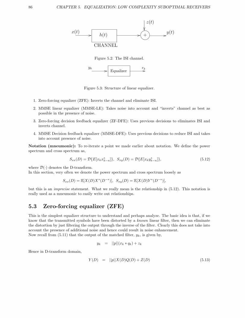
86 CHAPTER 5. EQUALIZATION: LOW COMPLEXITY SUBOPTIMAL RECEIVERS
x(t)
z(t)
+y(t)
h(t)
CHANNEL
Figure 5.2: The ISI channel.
yk rkEqualizer
Figure 5.3: Structure of linear equalizer.
1. Zero-forcing equalizer (ZFE): Inverts the channel and eliminate ISI.
2. MMSE linear equalizer (MMSE-LE): Takes noise into account and “inverts” channel as best aspossible in the presence of noise.
3. Zero-forcing decision feedback equalizer (ZF-DFE): Uses previous decisions to eliminates ISI andinverts channel.
4. MMSE Decision feedback equalizer (MMSE-DFE): Uses previous decisions to reduce ISI and takesinto account presence of noise.
Notation (mneumonic): To re-iterate a point we made earlier about notation. We define the powerspectrum and cross spectrum as,
Sxx(D) = DE[xkx∗k−n], Sxy(D) = DE[xky
∗k−n], (5.12)
where D(·) denotes the D-transform.In this section, very often we denote the power spectrum and cross spectrum loosely as
Sxx(D) = E[X(D)X∗(D−∗)], Sxy(D) = E[X(D)Y ∗(D−∗)],
but this is an imprecise statement. What we really mean is the relationship in (5.12). This notation isreally used as a mneumonic to easily write out relationships.
5.3 Zero-forcing equalizer (ZFE)
This is the simplest equalizer structure to understand and perhaps analyze. The basic idea is that, if weknow that the transmitted symbols have been distorted by a known linear filter, then we can eliminatethe distortion by just filtering the output through the inverse of the filter. Clearly this does not take intoaccount the presence of additional noise and hence could result in noise enhancement.Now recall from (5.11) that the output of the matched filter, yk, is given by,
yk = ||p||(xk ∗ qk) + zk
Hence in D-transform domain,
Y (D) = ||p||X(D)Q(D) + Z(D) (5.13)

5.3. ZERO-FORCING EQUALIZER (ZFE) 87
||p||Q(D) X(D) + Z(D)||p||Q(D)
WZFE(D)
1||p||Q(D)
X(D)
Z(D)
Y (D)
+
Figure 5.4: Zero-forcing equalizer.
This relationship (5.13) forms the starting point of all the equalization schemes. Now, if we invert thechannel using WZFE(D) given by
WZFE(D) =1
‖ p ‖ Q(D)
we get,
R(D) = WZFE(D)Y (D) =1
||p||Q(D)︸ ︷︷ ︸ZFE
[||p||X(D) + Z(D)]
Hence we see that,
R(D) = X(D) +Z(D)
||p||Q(D)
Clearly, the ZFE, WZFE(D), has eliminated the ISI, but it could have severely enhanced the noise, in that1
Q(D) could actually be very large, and in the absence of noise this would not have mattered. However in
the presence of noise, this could severely degrade the SNR.
5.3.1 Performance analysis of the ZFE
We have seen that the noise at the output of the matched filter has a PSD given by,
Sz(D) = N0Q(D).
Normalized per real dimension this is
Sz(D) =N0
2Q(D).
Now, after the ZFE,rk = xk + zZFE
k
where,
zZFEk = D−1
[Z(D)
||p||Q(D)
].
Hence, per dimension, the PSD of the noise zZFEk is,
SzZF E (D) =N0
2Q(D)
1
||p||Q(D)
1
||p||Q∗(D−∗).
ButQ(D) = Q∗(D−∗)

88 CHAPTER 5. EQUALIZATION: LOW COMPLEXITY SUBOPTIMAL RECEIVERS
due to conjugate symmetry of ql.Therefore,
SzZF E (D) =N0
2
1
||p||21
Q(D)=N0
2
WZFE(D)
||p|| .
Now,
σ2ZFE =
T
2π
∫ πT
−πT
SzZF E (e−jωT )dω
=T
2π
∫ πT
−πT
N0
2
WZFE(e−jωT )
||p|| dω
=N0
2
1
||p||
[T
2π
∫ πT
−πT
WZFE(e−jωT )dω
]
︸ ︷︷ ︸wZF E(0)
Thus we have
SNRZFE =Ex
σ2ZFE
=Ex
N0
21
||p||wZFE(0)
=
(Ex||p||
N0
2
)1
wZFE(0)
Noise enhancement: The basic problem occurs when Q(D) has zeroes close to the unit circle as seenin Figure 5.3.1. Hence, inverting Q(D) results in a “gain” that becomes large and hence enhances the
π/T π/T
Q(e−jwT ) W (e−jwT )
Figure 5.5: The noise enhancement in ZFE.
noise power that was ignored.
5.4 Minimum mean squared error linear equalization (MMSE-LE)
In order to deal with the noise enhancement of the ZFE, we need to take into account the presence ofnoise. The first method is to modify the ZFE to take the noise into account, by finding a linear filter

5.4. MINIMUM MEAN SQUARED ERROR LINEAR EQUALIZATION (MMSE-LE) 89
that minimizes the output noise variance.
ek = xk − wk ∗ yk (5.14)
The MMSE-LE, attempts to find the linear filter according to the MMSE criterion applied to (5.14) as,
WMMSE−LE(D) = arg minW (D)
E
[|ek|2
]
Now, we use the MMSE machinery we have developed in Section 5.1. We want to find WMMSE−LE(D)such that MMSE of output is minimized. By using the orthogonality principle2 as in (5.5), we have,
E[E(D)Y ∗(D−∗)
]= 0
Hence we get,
E[(X(D) −WMMSE−LE(D)Y (D))(Y ∗(D−∗))
]= 0
This gives us,
Sxy(D) = WMMSE−LE(D)Syy(D),
or
WMMSE−LE(D) =Sxy(D)
Syy(D)=
||p||Q(D)Ex
||p||2Q2(D)Ex +N0Q(D),
giving us
WMMSE−LE(D) =||p||Ex
||p||2Q(D)Ex +N0
=1
||p||Q(D) +(
N0
||p||Ex
) (5.15)
Note that the difference between WMMSE−LE(D) and WZFE(D) is the additive term in the denominatorof (5.15). Even if Q(e−jωT ) = 0 for some ω, the gain of the WMMSE−LE(D) does not blow up at thesefrequencies, as would WZFE(D). Note that as N0
Ex→ 0 or SNR → ∞ , the MMSE-LE tends towards the
ZFE as one would expect.
5.4.1 Performance of the MMSE-LE
At the output of the MMSE-LE, the D-transform is,
R(D) = WMMSE−LE(D)Y (D)
=1
||p||(Q(D) + 1
SNRMF B
)X(D)Q(D)||p|| + Z(D)
||p||(Q(D) + 1
SNRMF B
)
where, as defined in definition 4.2.2,
SNRMFB =Ex||p||2N0
=Ex||p||2N0/2
(5.16)
2Again recall that the precise relationship is given in (5.5), but we use the mneumonic given in (5.6) for convenience ofmanupulation.

90 CHAPTER 5. EQUALIZATION: LOW COMPLEXITY SUBOPTIMAL RECEIVERS
Therefore
R(D) =
[Q(D)
Q(D) + 1/SNRMFB
]X(D) +
[1
||p|| (Q(D) + 1/SNRMFB)
]Z(D)
︸ ︷︷ ︸Z′(D)
=
1 − 1/SNRMFB
Q(D) + 1/SNRMFB
︸ ︷︷ ︸1−V (D)
X(D) + Z ′(D)
Where we have defined,
V (D) =||p||
SNRMFBWMMSE−LE(D) =
1
SNRMFB
[Q(D) + 1
SNRMF B
] (5.17)
Writing it in time domain, we getrk = xk − vk ∗ xk + z′k
Let us examine, the contribution of xk in (vk ∗ xk),
vk ∗ xk =∑
n
vnxk−n = v0xk +∑
n6=0
vnxk−n
where the second term does not depend on xk.Hence we have
rk = xk − v0xk −∑
n6=0
vnxk−n + z′k
︸ ︷︷ ︸e′
k
yielding,rk = (1 − v0)xk + e′k (5.18)
Hence one would naturally have defined the detection SNR as,
SNRMMSE−LE,U =Ex(1 − v0)
2
E [|e′k|2](5.19)
However, in the MMSE minimization, one computes E[|ek|2
], where
ek = xk − wMMSE−LE(k) ∗ yk = xk − rk
Using this in (5.18),
ek = v0xk − e′k
Hence Ex
E[|ek|2]is not the same as what a detector encounters in (5.18). Therefore, the discrepancy needs
to be taken into account in the analysis of the MMSE-LE. Let us first calculate,
σ2MMSE−LE = E
[|ek|2
]
Similar to the ZFE analysis,
SEE(D) = DE[ele
∗l−k
]
= Ex −W ∗MMSE−LE(D−∗)SXY (D) −WMMSE−LE(D)S∗
XY (D−∗)
+WMMSE−LE(D)SY Y (D)W ∗MMSE−LE(D−∗)
= Ex −WMMSE−LE(D)SY Y (D)W ∗MMSE−LE(D−∗) (5.20)

5.4. MINIMUM MEAN SQUARED ERROR LINEAR EQUALIZATION (MMSE-LE) 91
Now,
WMMSE−LE(D) =||p||Q(D)Ex
||p||2Q2(D) +N0Q(D)=
1
||p|| [Q(D) + 1/SNRMFB](5.21)
and
SY Y (D) = ||p||2Q2(D)Ex +N0Q(D) = Ex||p||2Q(D)
[Q(D) +
1
SNRMFB
](5.22)
Inserting (5.21) and (5.22) into (5.20) we obtain
SEE(D) = Ex − ExQ(D)(Q(D) + 1
SNRMF B
)
=Ex/SNRMFB
Q(D) + 1SNRMFB
=
N0
||p||
||p||[Q(D) + 1
SNRMF B
] (5.23)
Now using (5.16) and (5.17) in (5.23), we get
SEE(D) = ExV (D) =N0
||p||WMMSE−LE(D)
Hence
E[|ek|2
]= σ2
MMSE−LE = Exv0 =N0
||p||wMMSE−LE(0). (5.24)
But the performance really depends upon E[|e′k|2
](see (5.18)). Now we relate them as,
E[|ek|2
]= v2
0Ex + E[|e′k|2
]
Therefore,
E[|e′k|2
]= E
[|ek|2
]− v2
0Ex = Exv0 − v20Ex (5.25)
Thus σ2MMSE−LE,U = E[| e′k |2] is,
σ2MMSE−LE,U = Exv0[1 − v0] (5.26)
Inserting (5.26) in (5.19) we get,
SNRMMSE−LE =Ex
σ2MMSE−LE
=Ex
Exv0=
1
v0
SNRMMSE−LE,U =Ex(1 − v0)
2
Exv0(1 − v0)=
1 − v0v0
=1
v0− 1
Hence,SNRMMSE−LE = 1 + SNRMMSE−LE,U (5.27)

92 CHAPTER 5. EQUALIZATION: LOW COMPLEXITY SUBOPTIMAL RECEIVERS
Whitened matchedfilter
Decision−feedbackequalizer
p(t)xk
z(t)
W (D)kT
ϕ∗(−t)
xk
r′ky(t)
1 − B(D)
rk
Figure 5.6: The decision feedback equalizer.
The “biased” SNR i.e., SNRMMSE−LE arises directly out of the calculation deriving that MMSE-LE.However, by looking at (5.18), one realizes that the detector actually works with a different SNR, i.e.,SNRMMSE−LE,U and hence we need to be careful in finding the performance of the MMSE-LE to usethe correct “noise” variance.
Till now we have considered two flavors of the equalizer structure. Both the ZFE and the MMSE-LE attempts to filter the received sequence through a linear filter (WZFE(D) and WMMSE−LE(D)respectively) in order to convert the ISI problem to be “close” to an AWGN problem. The ZFE didthat by inverting the channel, but could cause noise enhancement. The MMSE-LE took the noise intoaccount, but it now has transmitted symbols as part of the “noise”. Can we take advantage of the factthat the noise contains some past/future transmitted symbols? This idea forms the basis of the decisionfeedback equalizer, which we study next.
5.5 Decision-feedback equalizer
The basic idea of decision feedback equalization comes from the realization that one could potentiallyuse previous decisions while attempting to estimate the current symbol.The derivation and analysis of DFE requires us to make a strong assumption, that the decisions are indeedcorrect! Without this, the analysis of the DFE is still an open question. We will make this assumptionand proceed with the DFE.Criterion for the MMSE-DFE: The basic optimization problem is,
minW (D),B(D),b0=1
E[|xk − r′k|2
]
Notes:
1. In order to utilize past decisions, one should ensure that rk depends only on the past symbols.
2. The feedforward filter W (D) shapes the sequenceyk in order to have only “trailing” ISI terms.
3. We have seen one structure that caused the equivalent channel to be causal i.e., the whitenedmatched filter.

5.5. DECISION-FEEDBACK EQUALIZER 93
4. We need B(D) such that, B(D) is causal and monic, i.e.,
B(D) = 1 + b1D + b2D2 + . . .
which implies that
1 −B(D) = −∞∑
n=1
bnDn
and hence X(D)[1 −B(D)] depends only on past decisions as shown in Figure 5.6.
Main steps in deriving the MMSE-DFE:
Step 1 Fix feedback filterB(D) and find feedforward filterW (D), in terms of B(D), such that E[|(xk − r′k)|2
]
is minimized.
Step 2 Express result of operating W (D) on Y (D), i.e., express W (D) in terms of B(D) and set uplinear prediction problem.
Step 3 Solve linear prediction problem to find the causal, B(D) that minimizes E[|(xk − r′k)|2
]. And
hence find the MMSE-DFE, i.e., W (D), B(D).
Step 4 (Analysis) As in the MMSE-LE, remove the bias term to find the equivalent SNRMMSE−DFE,U .
We will first focus on step 1-3 to obtain the MMSE-DFE and then analyze its performance through step4.Step # 1:Let us fix B(D), and then find W (D) that minimizes MMSE criterion. We can write the error E(D) as,
E(D) = X(D) − W (D)Y (D) + (1 −B(D))X(D)︸ ︷︷ ︸R′(D)
Hence,
E(D) = B(D)X(D) −W (D)Y (D) (5.28)
Now, to find W (D) that minimizes E[|ek|2
], we use the orthogonality principle3 (see (5.5)) as,
E[E(D)Y ∗(D−∗)
]= E
[[B(D)X(D) −W (D)Y (D)]Y ∗(D−∗)
]= 0
= B(D)SXY (D) −W (D)SY Y (D) = 0
Hence,
W (D) = B(D)SXY (D)
SY Y (D)= B(D)WMMSE−LE(D) =
B(D)
||p||(Q(D) + 1
SNRMF B
) (5.29)
Step # 2: Now, we express the resulting error in terms of B(D) by substituting (5.29) in (5.28) as,
E(D) = B(D)X(D) −B(D)WMMSE−LE(D)Y (D)
= B(D) [X(D) −WMMSE−LE(D)Y (D)]︸ ︷︷ ︸U(D)
= (1 +B(D) − 1)U(D) = U(D) − [1 − B(D)]U(D)
3Again recall that the precise relationship is given in (5.5), but we use the mneumonic given in (5.6) for convenience ofmanupulation.

94 CHAPTER 5. EQUALIZATION: LOW COMPLEXITY SUBOPTIMAL RECEIVERS
where 1−B(D) is a strictly causal sequence. Now, this is exactly like the linear prediction problem thatwe studied in Section 5.1.3, where we want to predict the sequence uk = D−1(U(D)).
Step # 3: In Section 5.1.3, we studied the linear prediction problem and we found the optimal linearpredictor as,
Bopt(D) =1
L(D)
where
SU (D) = ΓUL(D)L∗(D−∗)
through spectral factorization. Now let us find SU (D).
SU (D) = E[[X(D) −WMMSE−LE(D)Y (D)][X∗(D−∗) −W ∗
MMSE−LE(D−∗)Y ∗(D−∗)]]
(a)= SXX(D) −W ∗
MMSE−LE(D−∗)SY Y (D)WMMSE−LE(D)
where (a) follows because WMMSE−LE(D) = SXY (D)SY Y (D) .
Hence,
SU (D) = Ex − ExQ(D)
Q(D) + 1SNRMFB
=N0/||p||2
Q(D) + 1SNRMFB
(b)= ΓUL(D)L∗(D−∗)
where (b) is the spectral factorization, with L(D) being causal, monic and minimum phase.Then we get
Bopt(D) =1
L(D)
which is still causal, monic and stable. Hence
SE(D) = B(D)SU (D)B∗(D−∗)
=1
L(D)ΓUL(D)L∗(D−∗)
1
L∗(D−∗)
= ΓU
Alternatively, if
Q(D) +1
SNRMFB= γ0G(D)G∗(D−∗) (5.30)
then
SU (D) =N0/||p||2
Q(D) + 1SNRMF B
=N0/||p||2
γ0G(D)G∗(D−∗)
Thus in this notation, ΓU = N0
||p||2γ0, L(D) = 1
G(D) then
Bopt(D) = G(D). (5.31)

5.5. DECISION-FEEDBACK EQUALIZER 95
Now, let us substitute this in (5.29) to get,
Wopt(D) = Bopt(D)WMMSE−LE(D) (5.32)
= G(D)1
||p||(Q(D) + 1
SNRMF B
)
= G(D)1
||p||γ0G(D)G∗(D−∗)
=1
||p||γ0
1
G∗(D−∗)
So, the main computation is to figure out the spectral factorization of[Q(D) + 1
SNRMF B
]. For the choice
of Bopt(D) and Wopt(D), the error spectrum is:
SEE(D) = Bopt(D)SU (D)B∗(D−∗)
= ΓU =N0
γ0||p||2(5.33)
5.5.1 Performance analysis of the MMSE-DFE
First the PSD of the error sequence is,
SEE(D) =N0
γ0||p||2,
hence the per-dimension PSD is
SEE(D) =N0/2
γ0||p||2
Thus, the error sequence of the MMSE-DFE (with no decision error propagation) is white, when it isminimized.Now, to compute γ0 we illustrate this with the following. Let us assume that we have a rational spectrumS(D), i.e.,
S(D) = γ0
∏Mk=1(1 − ckD)(1 − c∗kD
−1)∏N
k=1(1 − dkD)(1 − d∗kD−1)
(5.34)
Claim 5.5.1. For S(D) of the form given in (5.34)
T
2π
∫ π/T
−π/T
lnS(e−jωT )dω = ln γ0
if the finite energy constraint is satisfied, i.e.,
R(0) =T
2π
∫ π/T
−π/T
S(e−jωT )dω <∞
Notes:
1. This result actually holds in more generality than just rational spectrum, but we do the proof underthis restrictive assumption.
2. The finite energy constraint for rational spectra is equivalent to saying that there are no poles ofS(D) on the unit circle.

96 CHAPTER 5. EQUALIZATION: LOW COMPLEXITY SUBOPTIMAL RECEIVERS
Proof:
T
2π
∫ π/T
−π/T
lnS(ejωT )dω = ln γ0 +M∑
k=1
T
2π
∫ π/T
−π/T
ln(1 − cke−jωT )dω
+
M∑
k=1
T
2π
∫ π/T
−π/T
ln(1 − c∗kejωT )dω
−N∑
k=1
T
2π
∫ π/T
−π/T
ln(1 − dke−jωT )dω
−N∑
k=1
T
2π
∫ π/T
−π/T
ln(1 − d∗kejωT )dω (5.35)
Now, if a ∈ C , |a| ≤ 1, a = |a|ejφa
T
2π
∫ π/T
−π/T
ln[1 − ae−jωT ][1 − a∗ejωT ]dω =T
2π
∫ π/T
−π/T
ln[1 + |a|2 − 2|a| cos(ωT − φa)]dω
(a)= 0
where (a) follows from standard integral tables.Inserting this in (5.35) we get
T
2π
∫ π/T
−π/T
lnS(ejwT )dw = ln γ0
This formula is called the Szego formula.
Using the Szego formula for the MMSE-DFE, i.e., using it in (5.33) we obtain
σ2MMSE−DFE =
N0/2
||p||2 exp[− T
2π
∫ π/T
−π/T
ln
(Q(e−jωT ) +
1
SNRMFB
)dω]
This is called Salz formula as it was derived by Salz in 1973. Hence we get,
SNRMMSE−DFE =Ex
σ2MMSE−DFE
= SNRMFB exp[T
2π
∫ π/T
−π/T
ln
(Q(e−jωT ) +
1
SNRMFB
)dω]
= γ0SNRMFB =γ0||p||2Ex
N0
Now, we have issue of “bias”, i.e., to check whether this SNRMMSE−DFE is the right quantity toexamine4. Let us first find out if we have a biased receiver.
R′(D) = R(D) + [1 −B(D)]X(D)
= W (D)Y (D) +X(D) −B(D)X(D)
= X(D) − [B(D)X(D) −W (D)Y (D)]
= X(D) −E(D)
4This was the same issue investigated in the MMSE-LE.

5.5. DECISION-FEEDBACK EQUALIZER 97
The receiver makes decisions on xk, based on r′k
R′(D) = X(D) −[G(D)X(D) − 1
||p||γ0
Y (D)
G∗(D−∗)
]
= X(D) −[G(D)X(D) − 1
||p||γ0
||p||Q(D)
G∗(D−∗)X(D) − 1
||p||γ0
Z(D)
G∗(D−∗)
]
=
1 −G(D) +
Q(D)
γ0G∗(D−∗)
X(D) +
1
||p||γ0
1
G∗(D−∗)Z(D)
=
1 − −Q(D) + γ0G(D)G∗(D−∗)
γ0G∗(D−∗)
X(D) +
1
||p||γ0
1
G∗(D−∗)Z(D)
(a)=
1 −
1SNRMFB
γ0G∗(D−∗)
︸ ︷︷ ︸1−V (D)
X(D) +1
||p||γ0G∗(D−∗)Z(D)
︸ ︷︷ ︸Z′(D)
Where (a) follows due to (5.30) and we have defined
V (D) =1
SNRMF B
γ0G∗(D−∗)(5.36)
Note that V (D) =1
SNRMFB
γ0G∗(D−∗) is a purely anti-causal filter. Therefore, in a manner identical to what we
did for the MMSE-LE,
r′k = (1 − v0)xk −∑
n6=0
vnxk−n + z′k
︸ ︷︷ ︸e′
k
Hence,r′k = (1 − v0)xk + e′k
Hence, we again have a biased receiver, and the SNR measure that reflects error probability needs to takethis into account. Note that since
E(D) = X(D) −R′(D)
In time domain,ek = v0xk − e′k
And therefore for the same reason as in the MMSE-LE, the SNRMMSE−DFE is not the right measureto use for detecting SNR. Hence we need to find E[| e′k |2] and to do that first we find E[| ek |2] as,
E[|ek|2
]= σ2
MMSE−DFE = v20Ex + E
[|e′k|2
]
= v20Ex + σ2
MMSE−DFE,U
Hence,
σ2MMSE−DFE,U = σ2
MMSE−DFE − v20Ex =
N0
||p||2γ0− v2
0Ex (5.37)
Since from (5.36)
V (D) =1
SNRMFB
1
γ0
1
G∗(D−∗)

98 CHAPTER 5. EQUALIZATION: LOW COMPLEXITY SUBOPTIMAL RECEIVERS
and G∗(D−∗) is monic and anti-causal, therefore so is 1G∗(D−∗) ,
v0 =1
SNRMFB
1
γ0=
N0
||p||2Ex
1
γ0
Therefore
1
γ0=
||p||2Ex
N0v0
Using this in (5.33) we see that
σ2MMSE−DFE = v0Ex
Inserting this in (5.37), we get
σ2MMSE−DFE,U = Exv0 − v2
0Ex = v0Ex(1 − v0)
And hence we get the more informative SNR,
SNRMMSE−DFE,U =(1 − v0)
2Ex
v0(1 − v0)Ex=
1
v0− 1 = SNRMMSE−DFE − 1
Therefore we have
SNRMMSE−DFE = SNRMMSE−DFE,U + 1 (5.38)
Notice the similarity in the relationship in (5.38) and (5.27). In both cases the unbiased SNR and thebiased SNR differ by 1. This turns out to be a fundamental relationship between the SNR of biased andunbiased detectors.Note that the error sequence e′k is not in general white, even with the correct past decisions assump-tion. Again, the main calculating in finding SNRMMSE−DFE,U is to find the spectral factorization of[Q(D) + 1
SNRMF B
]and by using γ0 found from it we can obtain v0 and hence SNRMMSE−DFE,U .
5.5.2 Zero forcing DFE
We can find the ZF-DFE forward and feedback filters by simply setting SNRMFB → ∞ in the expressionsderived in the MMSE-DFE. Therefore we do a spectral factorization of
Q(D) = η0Pc(D)P ∗c (D−∗)
and set the feed forward and feedback filters of the ZF-DFE as,
W (D) =1
η0||p||P ∗c (D−∗)
, B(D) = Pc(D) (5.39)
It is not immediately clear what criterion the zero-forcing DFE is operating on. The zero-forcing DFE isthe direct extension of the algebraic argument that led to the ZFE. In the ZFE, we observed that in theabsence of noise,
Y (D) = ||p||Q(D)X(D) (5.40)
and hence we can solve this algebraic equation for xk by “inverting” the channel, i.e., WZFE(D) =1
‖p‖Q(D) . The zero-forcing DFE also solves an algebraic equation, where we further assume that previous
symbols, xk−1, . . . are known. The result of solving (5.40) for xk, given previous symbols is exactly what

5.6. FRACTIONALLY SPACED EQUALIZATION 99
the ZF-DFE is doing. In order to observe this, let us use (5.39) and examine its effect on rk and r′
k. Sincethe structure of the ZF-DFE is the same as Figure 5.6, at the output of the feedforward filter we have,
R(D) = W (D)Y (D) =1
η0||p||P ∗c (D−∗)
‖ p ‖ Q(D)X(D) +1
η0||p||P ∗c (D−∗)
Z(D) (5.41)
(a)= Pc(D)X(D) + Z
′(D) = B(D)X(D) + Z
′(D),
where (a) follows from (5.39). Now, notice that since R′(D) = R(D) + [1 −B(D)]X(D),
r′
k = xk + z′
k, (5.42)
which has eliminated the inter-symbol interference. Therefore, in the absence of noise, we would havesolved the algebraic equation (5.40) for xk . Notice that the power spectral density Sz′ (D) of the modified
noise process Z′(D) in (5.42) is,
Sz′ (D) =1
η20 ||p||2Pc(D)P ∗
c (D−∗)Sz(D) =
N0Q(D)
η0||p||2Q(D)=
N0
η0||p||2, (5.43)
i.e., it is white! Therefore we have converted the problem into (5.42) which is like the AWGN channel westudied in Chapter 2. However, the caveat is ofcourse that we have assumed perfect decision feedback.We will study how to remove that assumption using a technique described in Section 6.1.
5.6 Fractionally spaced equalization
We have till now assumed perfect synchronization, i.e., we know exactly when the sampling at the outputof the WMF occurs. Suppose we think that sampling occurs at kT , but it occurs at kT + t0. Then theequivalent channel is
y(kT + t0) =∑
m
xm||p||q(kT −mT + t0) + z(kT + t0)
Therefore we are sampling q(t+ t0) at kT , and we design equalizers assuming that it was q(t), hence theequivalent channel is Q(ω)e−jωt0 which could cause loss in performance. One solution is to work withNyquist sampling and collecting sufficient statistics by this method.There are several motivations to collect sufficient statistics through Nyquist sampling. One, is as explainedabove, is due to robustness to timing errors. Another more subtle reason is that in practice, the channelis unknown to the receiver and one needs to estimate the channel. We will learn channel estimationmethods in Section 6.3. Therefore, we may not be able to form the matched filter to collect sufficientstatistics. Given this, we need a channel independent method to do so, and Nyquist sampling gives ussuch a tool. By sampling at Nyquist rate, we actually sample at higher than the symbol rate T , andtherefore sometimes the terminology “oversampling” is used for this.Let,
yi(k) = y
(kT − iT
L
), i = 0, . . . , L− 1 (5.44)
Hence, in transform domain,
Yi(D) = Pi(D)X(D) + Zi(D), i = 0, . . . , L− 1
Where,
Pi(D) = D[pi(k)]

100 CHAPTER 5. EQUALIZATION: LOW COMPLEXITY SUBOPTIMAL RECEIVERS
p(t)
Anti aliasing filter
kT/L
Fractionallyspaced equalizer
Z(t)
xk+ xk
Figure 5.7: Fractionally spaced equalizer.
and
pi(k) = [h(t) ∗ ϕ(t)]t=kT− iTL
and
zi(k) = z
(kT − iT
L
)
Stacking up all the “oversampled” or fractionally sampled versions, one obtains
Y(D) =
Y0(D)...
YL−1(D)
=
P0(D)...
PL−1(D)
︸ ︷︷ ︸P(D)
X(D) +
Z0(D)...
ZL−1(D)
︸ ︷︷ ︸Z(D)
Which in more compact notation is,
Y(D) = P(D)X(D) + Z(D)
The equalizer structure can now be a row vector
W(D) = [W0(D), . . . ,WL−1(D)]
and the output of the equalizer is
R(D) = W(D)Y(D) = W(D)P(D)X(D) + W(D)Z(D)
Again, from basic linear estimation principles, the fractionally spaced MMSE-LE can be found by or-thogonality principle,
E[E(D)Y∗(D−∗)
]= 0
This gives,
E[X(D) −WMMSE−LE(D)Y(D)]Y∗(D−∗)
]= 0
Yielding,
WMMSE−LE(D) = E[X(D)Y∗(D−∗)
]E[Y(D)Y∗(D−∗)
]−1
= ExP∗(D−∗)
[ExP(D)P∗(D−∗) + LN0I
]−1
Note that the equalization is done and then the output is downsampled, and this alleviates some of theproblems of timing offset.

5.7. FINITE-LENGTH EQUALIZERS 101
5.6.1 Zero-forcing equalizer
An interesting feature of the fractionally-spaced case is the special case of the zero-forcing equalizer. Herewe need
WZF (D)P(D) = 1 =
L−1∑
i=0
Wi,ZF (D)Pi(D) (5.45)
Now the interesting aspect of this is that one can have Wi(D) which are finite length polynomials andstill be able to satisfy (5.45). This implies that for this case one is able to “convert” the channel withoutinfinite length “inverses”! This is really because we only need the downsampled version of the equalizeroutput to behave like a discrete-time delta function.
Theorem 5.6.1 (Bezout identity). If Pi(D)L−1i=0 do not share common zeros, then there exists a
vector polynomial (of finite degree)
W(D) = [W0(D), . . . ,WL−1(D)]
such that
W(D)P(D) = 1
Remarks:
1. In fact this condition is a necessary and sufficient condition, i.e., Pi(D)L−1i=0 do not share common
zeros (are co-primes) iff there exists a polynomial vector W(D) such that WZF (D)P(D) = 1.
2. This result was shown first by Sylvester (1840) as a test for co-primeness.
3. This shows that there exists a finite-impulse response inverse to the vector channel if the vectorchannel satisfies the regularity condition of Theorem 5.6.1. Again this inverse is only after “down-sampling”.
4. One can also have fractionally spaced decision-feedback equalizer, where the feedforward sectionoperates in fractional spacing and the feedback section is symbol spaced. We will learn more aboutsuch structures in the context of finite length equalizers in Section 5.7.
5.7 Finite-length equalizers
In practice one can only implement finite length filters using digital signal processors. One way is to“truncate” the infinite length filters we have derived till now and implement them. However, a moreprincipled approach is to start with the requirement of finite length filtering and derive the optimal finitelength filters for equalization. Again, we use oversampled version of the receiver, as done in (5.44).
y
(kT − iT
L
)=∑
m
xmp(kT − iT
L−mT ) + z
(kT − iT
L
), i = 0, . . . , L− 1
We define,
yk =
y(kT )...y(kT − L−1
L T)
=
∑
m
xm
p(kT −mT )...p(kT − L−1
L T −mT)
︸ ︷︷ ︸pk−m
+
z(kT )...z(kT − L−1
L T)
︸ ︷︷ ︸zk
(5.46)

102 CHAPTER 5. EQUALIZATION: LOW COMPLEXITY SUBOPTIMAL RECEIVERS
Hence in more compact notation,
yk =∑
n
pnxk−n + zk
Assumption: We impose the condition that the pulse response is of finite duration i.e.,
p(t) = 0 for t /∈ [0, νT ]
which implies that
pk = 0 for k < 0 and k > ν.
Note that in practice this is a reasonable assumption since most “real-world” channels are approximatelytime-limited.Thus using this assumption (5.46) becomes
yk = [p0,p1, . . . ,pν ]
xk
...xk−ν
+ zk.
Now, we collect Nf samples of yk, i.e., a frame of Nf + ν transmitted symbols as,
Yk =
yk
yk−1...yk−Nf+1
=
p0 p1 . . . pν 0 0 . . . 00 p0 p1 . . . pν 0 . . . 0...
.... . .
. . .. . .
. . .... 0
0 . . . 0 0 p0 p1 . . . pν
︸ ︷︷ ︸P
xk
xk−1
...xk−Nf−ν+1
︸ ︷︷ ︸Xk
+
zk
zk−1
...zk−Nf−ν+1
︸ ︷︷ ︸Zk
(5.47)This is the basic model that will be used for finite length equalization. This model is like the basicrelationship (5.11) seen in Section 5.2.
5.7.1 FIR MMSE-LE
In this section we derive a finite length MMSE linear equalizer, i.e., the equalizer is restricted to operateon Nf symbol times, or NfL samples of received sequence. Therefore, the equalizer is a NfL dimensionalrow vector applied to the received (sampled) vector Yk.
rk = wYk
where w ∈ C1×Nf L.Since one cannot implement a non-causal filter, the system has to be designed for a given delay, i.e.,the equalized output rk, is close to xk−∆, where ∆ is the delay. Note that for infinite filters we did notconsider this issue, though a delay was implicitly assumed since we can only implement causal systems.Hence the equalizer works by minimizing the following error:
ek = xk−∆ − rk.
For the FIR MMSE-LE, the criterion is
w(∆) = argminw
E[|ek|2
]
Using the orthogonality principle,E [ekY
∗k] = 0

5.7. FINITE-LENGTH EQUALIZERS 103
To find w, we use this orthogonality principle as,
E [xk−∆Y∗k] = wopt(∆)E [YkY
∗k]
where
RY Y = E [YkY∗k]
is the auto-correlation matrix.
RY X(∆) = E[YkX
∗k−∆
]
is the cross-correlation matrix, and hence,
wopt(∆) = RXY (∆)R−1Y Y
In more detail,
RXY (∆) = E [xk−∆(X∗kP
∗ + Z∗k)]
= [0 . . . 0 Ex︸︷︷︸(∆+1)thposition
0 . . . 0]P∗
= Ex[0 . . . 0 p∗ν︸︷︷︸
(∆+1)thposition
. . .p∗0, 0 . . . 0]
Let
11∆ = [0, . . . , 0, 1, 0, . . . , 0]∗ ∈ CNf+ν ,
where the 1 occurs in the (∆ + 1)th position. Hence,
RXY (∆) = Ex11∗∆P∗
Also,
RY Y = E [PXkX∗kP
∗] + E [ZkZ∗k]
= ExPP∗ + LN0INf L.
One finds ∆ by choosing the setting that minimized σ2FIR−MMSE−LE , the MMSE for the FIR equalizer.
Now, to compute the MMSE of the finite length equalizer we can write
σ2MMSE−LE = E[‖ xk−∆ −w(∆)Yk ‖2]
= Ex −RXY (∆)R−1Y Y R∗
XY (∆)
= Ex −wopt(∆)R∗XY (∆)
= Ex − Ex11∗∆P∗ [ExPP∗ + LN0INf L
]−1P11∆Ex
(a)= 11
∗∆
ExINf+ν − ExP
∗ [ExPP∗ + LN0INf L
]−1PEx
11∆ (5.48)
where (a) follows because
11∗∆11∆ = 1.
Now the matrix inversion lemma (Woodbury’s identity) gives

104 CHAPTER 5. EQUALIZATION: LOW COMPLEXITY SUBOPTIMAL RECEIVERS
Lemma 5.7.1. (Matrix inversion lemma) Given matrices A,B,C,
[A + BCB∗]−1 = A−1 −A−1B[C−1 + B∗A−1B]−1B∗A−1
By identifying,
A−1 = ExINf+ν , B = P∗, C−1 = LN0INf L
in Lemma 5.7.1 and using this in (5.48), we get,
σ2MMSE−LE = 11
∗∆
E−1
x INf+ν + P∗P1
N0L
−1
11∆
= N0L11∗∆
P∗P +
N0L
ExINf+ν
−1
︸ ︷︷ ︸Q(∆)
11∆
= N0L11∗∆Q(∆)11∆ (5.49)
Therefore the smallest σ2MMSE−LE occurs by choosing the ∆ corresponding to the smallest diagonal
element of Q(∆). Therefore the optimal delay can be easily identified by just one matrix inversion.
5.7.2 FIR MMSE-DFE
The FIR MMSE-DFE (see Figure 5.8), is similar to the FIR MMSE-LE except that there is now a symbolspaced feedback filter which is also of finite lengthNb, which filter the past decisions xk−∆−1, . . . , xk−∆−Nb
,
ek = xk−∆ −
[b1, . . . , bNb]
xk−∆−1
...xk−∆−Nb
+ wYk
p(t)xk +
z(t)
Anti-aliasingfilter +
xk−∆
length Nb
length NfL
kT/L
b
w
Figure 5.8: Structure of the FIR MMSE-DFE.
As in the earlier MMSE-DFE setting, we derive the DFE assuming correct past decisions.Let
b = [1,−b1,−b2, . . . ,−bNb]
and
Xk−∆k−∆−Nb
=
xk−∆
xk−∆−1
...xk−∆−Nb

5.7. FINITE-LENGTH EQUALIZERS 105
Therefore we can write,
ek = xk−∆ −
[b1, . . . , bNb]
xk−∆−1
...xk−∆−Nb
+ wYk
= [1,−b1, . . . ,−bNb]
xk−∆
xk−∆−1
...xk−∆−Nb
−wYk
(a)= bXk−∆
k−∆−Nb−wYk
where (a) follows due to perfect decision feedback assumption.FIR MMSE-DFE criterion:
bopt,wopt = argb,w min E[|ek|2
]
= arg
minb
minw
E[|ek|2
]
That is, we do the minimization in a nested manner just like in the infinite length case. First let us fixb and find w in terms of b. To do that, apply orthogonality principle
E [ekY∗
k] = 0
which gives,
E[
bXk−∆k−∆−Nb
−wYk
Y∗
k
]= 0
or
wE [YkY∗k] = bE
[Xk−∆
k−∆−NbY∗
k
](5.50)
Now, let us find the terms in (5.50)
E[Xk−∆
k−∆−NbY∗
k
]= E
xk−∆
...xk−∆−Nb
P
xk
...xk−Nf −ν+1
+ Zk
∗
= E
xk−∆
...xk−∆−Nb
︸ ︷︷ ︸(Nb+1)×1
[x∗k . . . x
∗k−Nf−ν+1
]
︸ ︷︷ ︸1×(Nf+ν)
P∗︸︷︷︸
(Nf+ν)×Nf L
∆= ExJ∆P∗
Now, let us write J∆ in more detail. First let us assume that xk−∆ occurs in the information window,i.e.,
∆ ≤ Nf + ν − 1
then J∆ 6= 0 for i.i.d. symbols xk. Now the question is whether xk−∆−Nboccurs before or after
xk−Nf +1−ν

106 CHAPTER 5. EQUALIZATION: LOW COMPLEXITY SUBOPTIMAL RECEIVERS
Case I: ∆ +Nb ≤ Nf + ν − 1Then xk−∆−Nb
occurs in the information window xk, . . . , xk−Nf−ν+1 and this is the “easy” case.
J∆ =1
ExE
xk−∆
...xk−∆−Nb
[x∗k, . . . , x
∗k−∆, . . . , x
∗k−∆−Nb
, . . . , x∗k−Nf−ν+1
](5.51)
=[
0(Nb+1)×∆, I(Nb+1)×(Nb+1), 0(Nb+1)×(Nf+ν−1−∆−Nb)
]
Case II: ∆ +Nb > Nf + ν − 1Then xk−∆−Nb
does not appear in the observation window of information and therefore we have atruncation at the end. Hence the observation looks like,
xk, . . . , xk−∆, . . . , xk−Nf−ν+1︸ ︷︷ ︸observation window Xk
, . . . , xk−∆−Nb
And we have
Xk−∆k−∆−Nb
=
xk−∆
...xk−Nf−ν+1
...xk−∆−Nb
Therefore, the b that needs to be used is also truncated since, xk−Nf−ν , . . . , xk−∆−Nb are not part
of the observation window. This is really the edge effect that we need to be aware of. One can easilycalculate the correct b for this case by now choosing a shorter decision feedback window size, i.e.,
xk−∆
...xk−Nf−ν+1
of length (Nf + ν − ∆), and setting the rest of the taps to zero. For completeness
J∆ =1
ExE
xk−∆
...xk−Nf−ν+1
...xk−∆−Nb
[x∗k , . . . , x∗k−∆, . . . , x
∗k−Nf−ν+1]
=
[0(Nf+ν−∆)×∆ I(Nf+ν−∆)×(Nf+ν−∆)
0(∆+Nb−Nf−ν+1)×∆ 0(∆+Nb−Nf−ν+1)×(Nf+ν−∆)
]
For b = [1,−b1, . . . ,−bNb],
bJ∆J∗∆b∗ = E2
xbb∗
Note: The Case II is really an edge effect that we will not consider in detail, but we enunciated it morefor completeness. We will focus our attention on Case I.Now, expressing w in term of b we obtain, for Case I,
σ2e(∆) = E
[∣∣bXk−∆k−∆−Nb
− ExbJ∆P∗R−1Y Y Yk
∣∣2]
(5.52)
= bExI(Nb+1) − ExJ∆P∗R−1
Y Y PJ∗∆Ex
b∗

5.7. FINITE-LENGTH EQUALIZERS 107
where,
RY Y =[ExPP∗ + LN0INf L
]
We now use this in (5.52),
σ2e (∆) = Exb
INb+1 − J∆P∗
[PP∗ +
LN0
ExINf L
]−1
PJ∗∆
b∗ (5.53)
Now, for case I using (5.51) we have,
J∆J∗∆ = INb+1.
Using this in (5.53) we get,
σ2e(∆) = ExbJ∆
INf +ν −P∗
[PP∗ +
LN0
ExINf L
]−1
P
J∗
∆b∗ (5.54)
Now we use the matrix inversion lemma (Lemma 5.7.1) in (5.54) after identifying,
A = INf+ν , B = P∗, C−1 =LN0
ExINf L.
Hence using this in (5.54) we get
σ2e(∆) = ExbJ∆
INf+ν −P∗
[PP∗ +
LN0
ExINf L
]−1
P
J∗
∆b∗ (5.55)
= Exb
[J∆
INf+ν +
Ex
LN0P∗P
−1
J∗∆
]b∗
= LN0b
[J∆
L
SNRI + P∗P
−1
J∗∆
]
︸ ︷︷ ︸Q−1(∆)
b∗
∆= LN0bQ−1(∆)b∗ (5.56)
Let us define the Choleski decomposition,
Q(∆) = G∗∆S−1
∆ G∆
Q−1(∆) = G−1∆ S∆G−∗
∆
where G∆ is an upper triangular matrix, and hence G∗∆ is a lower triangular matrix.
Fact 5.7.1. If G∆ is an upper triangular matrix, so is G−1∆ .
Hence, the same fact follows for lower triangular matrices. Therefore, G−1∆ is upper triangular and G−∗
∆
is lower triangular. Now, suppose we have
S∆ =
s0(∆) 0
. . .
0 sNb(∆)
(5.57)

108 CHAPTER 5. EQUALIZATION: LOW COMPLEXITY SUBOPTIMAL RECEIVERS
as the diagonal matrix S∆, with the ordering property,
s0(∆) ≤ s1(∆) ≤ . . . ≤ sNb(∆)
This property is assured due to the Choleski factorization. Hence,
σ2e (∆) = LN0b
[G−1
∆ S∆G−∗∆
]b
= LN0(bG−1∆ )S∆(bG−1
∆ )∗ (5.58)
To minimize this we want to pick off s0(∆), i.e., the top-left corner element of S∆, for which we want
bG−1∆ = [1, 0, . . . , 0]
This means that we want b to be the first row of G∆. This can be seen by noticing that,
G∆G−1∆ = I
If
G∆ =
g∆(0)...g∆(Nb)
,
then clearlyg∆(0)G−1
∆ = [1, 0, . . . , 0]
If g∆(0) is the top row of upper triangular matrix G∆
bopt = g∆(0) (5.59)
and
wopt = boptRXY (∆)R−1Y Y
(b)= g∆(0)J∆(P∗P +
L
SNRI)−1
︸ ︷︷ ︸feed forward filter
P∗︸︷︷︸
matched filter
where (b) follows because,
P∗PP∗ + P∗ L
SNR= P∗PP∗ +
L
SNRP∗
P∗(PP∗ +
L
SNRI
)=
(P∗P +
L
SNRI
)P∗
⇒(P∗P +
L
SNRI
)−1
P∗ = P∗(PP∗ +
L
SNRI
)−1
Hence, we basically have the same interpretation of the FIR MMSE-DFE as in the infinite length case asa matched filter cascaded with a feed forward filter.Now, for the performance of the FIR MMSE-DFE, from (5.58) and (5.59), we see that
σ2e (∆) = LN0s0(∆)
where s0(∆) is defined in (5.57). Hence, both the settings of the FIR MMSE-DFE and the analysisinvolves the Choleski decomposition of Q(∆) defined in (5.56). This is similar to the analysis of the FIRMMSE-LE. However, the optimization with respect to the decision delay, ∆, needs to be carried outseparately unlike the FIR MMSE-LE. Therefore for different values of ∆, the σ2
e (∆) is evaluated and thedelay corresponding to the minimum is chosen.

5.8. PROBLEMS 109
5.8 Problems
Problem 5.1
Assume that Y(k),X(k),Z(k) ∈ R2. Given the model Y(k) = HX(k) + Z(k), where X(k),Z(k) are
independent zero mean Gaussian random vectors with covariance matrices K =
[1 −1−1 1
]and I respec-
tively. Let H =
[1 1−1 1
]. Find the optimal (MMSE criterion) W such that X(k) = WY(k). Find
σ2MMSE.
Problem 5.2
Assume that Y(k) ∈ CN be a noisy observation of X(k) ∈ CN . We allow dependency between Y(k),X(l)where k 6= l. We observe the complete sequence Y(k) and would like to estimate X(k) by passing itthrough a filter W(k) ∈ CN×N i.e.
X(k) =∑
n
W(n)Y(k − n).
Let SXY(D) = E[X(D)Y∗( 1D∗ )], SXY(D),SYY(D) ∈ CN×N . Find the optimum filter W(D) (in the
MMSE sense) in terms of SXY(D) and SYY(D).
Note that X(k) is obtained by using the complete noisy sequence Y(k)∞k=−∞. This operation is calledas smoothing.Hint: For the D-transform of vectors or matrices, we take D-transform of individual components.
Problem 5.3
1. Let the autocorrelation function of x(k) is given by φx(l) = e−2|l|. Find the optimal (MMSE) linearprediction filter for x(k), i.e.
x(k) =
∞∑
i=1
aix(k − i).
2. We know that in the prediction problem the estimate x(k) =∑∞
i=1 aixk−i depends on the past. Inthis problem which is an instance of a filtering problem, we would like to estimate x(k) based onthe noisy observations y(k) of the past and present by filtering i.e.
x(k) =
∞∑
i=0
aiyk−i.
Let the autocorrelation function of x(k) be φx(l) = e−2|l|. Also
y(k) = x(k) + z(k),
where z(k) is zero-mean unit-variance white Gaussian noise. Find the optimum ai∞i=0 (in theMMSE sense).
Note: In the filtering problem we only use the noisy observation of the past and present, while inthe smoothing problem (problem 2) we also use the future noisy observations.
Hint: Use orthogonality principle.

110 CHAPTER 5. EQUALIZATION: LOW COMPLEXITY SUBOPTIMAL RECEIVERS
Problem 5.4
Suppose we are given Sx(z) = 1 − b?D−1 − bD + |b|2. Suppose the Paley-Wiener condition holds. Writethe spectral factorization of Sx(D). Depending on b, find the the linear filter used to do a linear predictionfrom the sequence xk.
Problem 5.5
Given some realizations yn, we want to estimate x by using a linear filter. Derive the orthogonalityprinciple E[eopt(k)y
?(k)] = 0, and determine the coefficients of the filter hk,n from the MMSE estimationproblem.
Problem 5.6
Given the following model y(k) = Hx(k) + z(k) where z(k) is a white Gaussian noise vector. Find theoptimal W such that x(k) = Wy(k).
Problem 5.7
Given two WSS random sequences xk and yk , we want to use ylkl=−∞ to predict xk by using a
linear filter, i.e xk =∑∞
l=0 alyk−l. Find al.
Problem 5.8
[Linear Estimation] Consider the additive noise model given in Fig. 5.9. Let X , Y1, Y2, Z1, Z2 ∈ C,
Y1
Y2
Z2
Z1
X
Figure 5.9: Additive Noise Channel
i.e complex random variables. Moreover, let EX = 0 = EZ1 = EZ2, and Z1 and Z2 are independent ofX .
1. Given Y1, Y2 find the best minimum mean squared error linear estimator X, where the optimizationcriterion is E|X − X |2.Assume the following: E|X |2 = Ex, E|Z1|2 = E|Z2|2 = 1, EZ1Z
∗2 = 1√
2

5.8. PROBLEMS 111
2. If EZ1Z∗2 = 1 = EZ2Z
∗1 , what is the best MMSE linear estimator of X ?
Problem 5.9
[ Combining linear estimators] Let Ya and Yb be two separate observations of a zero mean randomvariable X such that
Ya = HaX + Va
and Yb = HbX + Vb,
where Va, Vb, X are mutually independent and zero-mean random variables, and Va, Vb, X, Ya, Yb ∈ C.
1. Let Xa and Xb denote the linear MMSE estimators for X given Ya and Yb respectively. That is
Wa = argminWaE[||X −WaYa||2
],
Wb = argminWbE[||X −WbYb||2
]
andXa = WaYa and Xb = WbYb.
Find Xa and Xb given that
E [XX∗] = σ2x,E [VaV
∗a ] = σ2
a,E [VbV∗b ] = σ2
b .
Also, find the error variances,
Pa = E
[(X − Xa)(X − Xa)∗
]
Pb = E
[(X − Xb)(X − Xb)
∗]
2. We, have the following identities,
rxh∗ [hrxh
∗ + rv]−1
=[r−1
x + h∗r−1v h
]−1h∗r−1
v (5.60)
rx − rxh∗ [hrxh
∗ + rv]−1
hrx =[r−1
x + h∗r−1v h
]−1(5.61)
Prove that
P−1a Xa =
H∗a
σ2a
Ya, P−1b Xb =
H∗b
σ2b
Yb. (5.62)
and
P−1a =
1
σ2x
+HaH
∗a
σ2a
, P−1b =
1
σ2x
+HbH
∗b
σ2b
. (5.63)
Hint: Use identities (5.60), (5.61).
3. Now we find the estimator X, given both observations Ya and Yb, i.e.,(Ya
Yb
)=
(Ha
Hb
)X +
(Va
Vb
).
We want to find the linear MMSE estimate
X =(Ua Ub
)( Ya
Yb
),
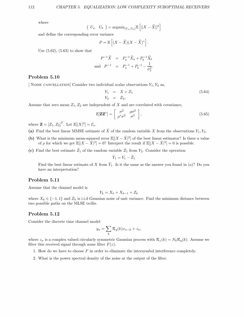
112 CHAPTER 5. EQUALIZATION: LOW COMPLEXITY SUBOPTIMAL RECEIVERS
where (Ua Ub
)= argmin(Ua,Ub)
E
[||X − X||2
]
and define the corresponding error variance
P = E
[(X − X)(X − X)∗
].
Use (5.62), (5.63) to show that
P−1X = P−1a Xa + P−1
b Xb
and P−1 = P−1a + P−1
b − 1
σ2x
.
Problem 5.10
[ Noise cancellation] Consider two individual scalar observations Y1, Y2 as,
Y1 = X + Z1 (5.64)
Y2 = Z2,
Assume that zero mean Z1, Z2 are independent of X and are correlated with covariance,
E[ZZ∗] =
[σ2 ρσ2
ρ∗σ2 σ2
], (5.65)
where Z = [Z1, Z2]T . Let E[|X |2] = Ex.
(a) Find the best linear MMSE estimate of X of the random variable X from the observations Y1, Y2.
(b) What is the minimum mean-squared error E[|X − X|2] of the best linear estimator? Is there a valueof ρ for which we get E[|X − X|2] = 0? Interpret the result if E[|X − X |2] = 0 is possible.
(c) Find the best estimate Z1 of the random variable Z1 from Y2. Consider the operation
Y1 = Y1 − Z1
Find the best linear estimate of X from Y1. Is it the same as the answer you found in (a)? Do youhave an interpretation?
Problem 5.11
Assume that the channel model isYk = Xk +Xk−1 + Zk
where Xk ∈ −1, 1 and Zk is i.i.d Gaussian noise of unit variance. Find the minimum distance betweentwo possible paths on the MLSE trellis.
Problem 5.12
Consider the discrete time channel model
yn =∑
k
Rg(k)xn−k + zn,
where zn is a complex valued circularly symmetric Gaussian process with Rz(k) = N0Rg(k). Assume wefilter this received signal through some filter F (z).
1. How do we have to choose F in order to eliminate the intersymbol interference completely.
2. What is the power spectral density of the noise at the output of the filter.
5.8. PROBLEMS 113
Problem 5.13
Consider the channel Y (D) = ||p||Q(D)X(D) + Z(D) with
||p||2 = 1 + aa∗
Q(D) =a∗D−1 + ||p||2 + aD
||p||2
0 ≤ |a| < 1.
• Find the zero forcing and minimum mean square error equalizers WZFE(D) and WMMSE-LE(D).
Use the variable b = ||p||2(1 + 1
SNRMF B
)in your expression for WMMSE-LE(D).
• Find the roots r1, r2 of the polynomial
aD2 + bD + a∗.
Show that b2 − 4aa∗ is always a real positive rumber (for |a| 6= 1). Hint: Consider the case where1
SNRMF B= 0. Let r2 be the root for which |r2| < |r1|. Show that r1r
∗2 = 1.
• Use the previous results to show that for the MMSE-LE
W (D) =||p||a
D
(D − r1)(D − r2)=
||p||a(r1 − r2)
(r1
D − r1− r2D − r2
).
• Find w(0).
• Show that the canonical factorization is
Q(D) +1
SNRMFB= γ0(1 − r2D
−1)(1 − r∗2D).
What is γ0 in terms of a and b?
• Find B(D) and W (D) for the MMSE-DFE.
• Find expressions for SNRZFE , SNRMMSE−LE−U , SNRMMSE−LE , SNRMMSE−DFE−U andSNRMMSE−DFE .
Problem 5.14
Consider the following system where σ2n = 0.1, Ex = 1, l = 1:
φ(t) =1√T
sinc(t
T)
h(t) = δ(t) − 0.5δ(t− T )
1. We assume perfect anti-aliasing filtering wih gain√T . Find p(t) corresponding to the discrete
time-channel:yk = xk − 0.5xk−1 + nk
Also find the matrix P .
2. Find a 3 tap FIR MMSE-LE for ∆ = 2.
3. Find the σ2MMSE−LE for the equalizer of the previous part.
4. Design an MMSE-DFE which has 2 feedforward taps and 1 feedback tap. Assume that ∆ = 1.
5. Find the σ2MMSE−DFE for the equalizer of the previous part.

114 CHAPTER 5. EQUALIZATION: LOW COMPLEXITY SUBOPTIMAL RECEIVERS
Problem 5.15
Consider transmission over an ISI channel with 2-PAM constellation of unit energy and symbol periodT . Let ϕ(t) = 1√
Tsinc
(tT
)and h(t) = δ(t) − 1
2δ (t− T ). Assume that AWGN noise has power spectral
density N0/2 = 0.01 (this is the problem-2 of homework-4, you can use necessary results). Recall thatafter matched filtering the model is Y (D) = ||p||Q(D)X(D) + Z(D). Find the ZFE, MMSE-LE andMMSE-DFE equalizers for this model. Find SNRZFE, SNRMMSE-LE and SNRMMSE-DFE.
Problem 5.16
Consider the channel model discussed in class Y (D) = ||p||Q(D)X(D) + Z(D) with
Ex = 1
N0 = 0.01
||p||2 = 1.25
Q(D) =2
5D−1 + 1 +
2
5D
1. Find B(D) and W (D) for the ZF-DFE.
2. Find SNRZF−DFE .
Problem 5.17
Consider the channel Y (D) = ||p||Q(D)X(D) + Z(D) with
Ex = 1
N0 = 0.01
||p||2 = 1 + aa∗
Q(D) =a∗D−1 + ||p||2 + aD
||p||2
0 ≤ |a| < 1.
1. Find η0 and Pc(D) such that Q(D) = η0Pc(D)P ∗c (D−∗)
2. Find B(D) and W (D) for the ZF-DFE.
3. Find SNRZF−DFE .
Problem 5.18
[ Equalization] Given a channel with transfer function H(Z) = 1 + cz−1 with |c| < 1, additive whiteGaussian noise of variance σ2
z and channel input xk with E|xk|2 = 1.
1. Find the zero forcing linear equalizer WZFE(D). Find the expression of SNRZFE .
2. Find the MMSE linear equalizer WMMSE−LE(D). Find the expression of SNRMMSE−LE .
3. Find the MMSE-DFE equalizer, i.e. BMMSE−DFE(D) and WMMSE−DFE(D). Also find an expres-sion for SNRMMSE−DFE .
Hint : the integral relations in the Instructions may be of use here.

5.8. PROBLEMS 115
+
++
−
Figure 5.10: Block diagram for noise prediction DFE
Problem 5.19
[ Noise prediction DFE] Consider the discrete time model studied in class
Y (D) = ||p||Q(D)X(D) + Z(D),
where Sx(D) = Ex, Sz(D) = N0Q(D) with Q(D) = Q∗(D−∗). In class we derived the MMSE-DFE, butin this problem we consider a slightly different structure shown in Figure 5.10. As in class we considerperfect decision feedback, i.e., all past decisions are correct. Let
R(D) = H(D)Y (D),
R′(D) = R(D) + (1 −B(D))(X(D) −R(D)).
We restrict B(D) to be causal and monic, i.e.,
B(D) = 1 +
∞∑
l=1
blDl.
We choose H(D) and B(D) to minimizeE[|xk − r′k|2
]
as we did in class.
1. Find H(D) in terms of B(D) by using orthogonality principle.
2. Set-up the prediction problem by proving that the error
E(D) = X(D) −R′(D) = B(D)X(D) −B(D)H(D)Y (D).
Use the solution of H(D) in terms of B(D) found in part (1) to show that
E(D) = B(D)U(D)

116 CHAPTER 5. EQUALIZATION: LOW COMPLEXITY SUBOPTIMAL RECEIVERS
and find the expression for U(D).It can be shown (you don’t have to do this) that
SU (D) =N0/||p||2
Q(D) + 1/SNRMFB.
Given this can you comment on the values of H(D) and B(D) with respect to the quantities derivedin class. In particular, is the noise-prediction DFE the same as the MMSE-DFE derived in the class?
3. If B(D) = 1, what does the structure in Figure 5.10 become?
Problem 5.20
[The Oversampled ZF equalizer ] Let
[Y1(D)Y2(D)
]=
[1 + 0.9D1 + 0.8D
]X(D) +
[Z1(D)Z2(D)
]
i.e. no common zeros among the oversampled responses. Find the ZFE for this case. This should turnout to be a FIR channel since the Pi(D) do not share a common zero.
Problem 5.21
Consider the following system where σ2n = 0.1, Ex = 1, the oversampling factor L = 2:
φ(t) =1√T
sinc(t
T)
h(t) = δ(t) − 0.5δ(t− T )
1. We assume perfect anti-aliasing filtering wih gain√T . Find p(t) at the output of the anti-aliasing
filter. Find p(t) corresponding to the discrete time-channel:
yk = p0xk + p1xk−1 + zk
Also find [p0,p1].
2. We want to design a 4 tap FIR MMSE-LE equalizer. Find the ∆ which minimizes σ2MMSE−LE and
for that ∆ find the corresponding equalizer. Also find σ2MMSE−LE .
3. Design an FIR MMSE-DFE which has 4 feedforward taps and 1 feedback tap. Assume that ∆ = 1.Also find σ2
MMSE−DFE .
Problem 5.22
Consider the following signal model:Yk = PYk + Zk
where Zk,Yk ∈ CNfL, P ∈ C(NfL)×(Nf+ν), X ∈ CNf+ν
1. Using the orthogonality principle, derive the FIR MMSE-LE equalizer.
2. Find the expression of σ2MMSE−LE .
3. How can we choose the value of ∆?

5.8. PROBLEMS 117
Problem 5.23
[Target Channels] Suppose we have a linear time-invariant channel i.e
yk =
ν∑
n=0
pnxk−n + zk
where yk ,pn, zk ∈ CL and xk ∈ C . In class we developed the following block model for Nf samples ofyk:
Yk = PXk + Zk
where Yk, Zk ∈ CNf L, Xk ∈ CNf , P ∈ CNf L×(N+ν). Suppose we want the following receiver structureand we want rk ≈ ∑η
n=0 hnxk−∆−n, where η ν. That is we want the output of the equalizer to be
W
yk rk
close to a given target channel hn. Therefore we find W ∈ C1×Nf L :
Wopt = arg minW
E||WYk −HXk||2 (5.66)
where H = [ 0 · · · 0︸ ︷︷ ︸∆ times
h0 h1 · · · hη 0 · · · 0︸ ︷︷ ︸Nf+ν−η−1
] i.e H ∈ C1×(Nf+ν) You may assume that Exkxk−` =
Exδ`, E|zk|2 = σ2 and zk is AWGN.
1. (Complete equalization) In class we derived the finite length equalizer when
hn =
1 n = 00 otherwise
(5.67)
Re-derive the optimal MMSE finite length equalizer W, for this case, i.e. for hn given in (5.67)and the criterion in (5.66) (i.e. same as done in class).
2. Now if we want a particular target channel hnηn=0, and the criterion is given in (5.66), derive the
optimal filter Wopt for the given target channel.
3. For a given target channel hnηn=0, compute the σ2
FIR-MMSE-LE, i.e.
E||WoptYk −HXk||2
Problem 5.24
[ Target channels] Suppose we have a linear time invariant channel done in class, i.e.,
Y (D) = ||p||Q(D)X(D) + Z(D),
with Q(D) = Q∗(D−∗). Also there is another process U(D) = H(D)X(D), which we want to estimate.
1. Given observations yk, find the linear estimator
U(D) = W (D)Y (D)
which minimizes the mean-squared error, i.e.,

118 CHAPTER 5. EQUALIZATION: LOW COMPLEXITY SUBOPTIMAL RECEIVERS
Figure 5.11: MMSE estimation
W (D) = argminW (D)E[||uk − uk||2
].
You can assume that Xk and Zk are independent and that
Sx(D) = Ex, Sz(D) = N0Q(D).
2. Given the optimum linear MMSE estimator given in part (1) we define the error as
ek = uk − uk.
Find the power spectral density of ek, SE(D).
3. If H(D) = 1, can you comment on the operation performed in part (1)?Hint: Is it related to any structure studied in class?

Chapter 6
Transmission structures
In Chapter 4 and 5, we learnt detection for ISI channels. However, the transmission structure remainedthe same as an AWGN channel. This chapter examines techniques at the transmitter that are suitablefor ISI channels. We study precoding in Section 6.1 which also mitigates error-propagation effects of theDFE. Section 6.2 demonstrates a canonical transmission and reception structure which is suitable for ISIchannels. Finally, Section 6.3 is devoted to training sequence optimization for channel estimation.
6.1 Pre-coding
In order to counter error-propagation in DFE’s, one method is to do “precoding”. The first idea is tomove the feedback section of the DFE to the transmitter. Note that this requires the knowledge of thechannel at the transmitter. We will also study another transmit strategy in this chapter which usesalternate way of simplifying the equalization problem (multi carrier transmission).
6.1.1 Tomlinson-Harashima precoding
For simplicity we will first illustrate this with real (i.e., one-dimensional) baseband signals.
xk ψk
vk
1 −B(D)
ΓM (x)xk
M-ary input+
Figure 6.1: The Tomlinson-Harashima precoder for real baseband signals.
The basic idea is understood by examining the ZF-DFE. In the ZF-DFE as seen in Section 5.7.2, we have,
W (D) =1
γ0||p||P ∗c (D−∗)
, B(D) = Pc(D) (6.1)
where,Q(D) = γ0Pc(D)P ∗
c (D−∗),
119

120 CHAPTER 6. TRANSMISSION STRUCTURES
and B(D) is monic, i.e., b0 = 1. Now, suppose we remove the ΓM (·) block from Figure 6.1, then we get,
ψk = xk −∞∑
l=1
blψk−l (6.2)
Therefore we get,
∞∑
l=0
blψk−l = xk . (6.3)
Using this we get for Ψ(D) = D(ψk),
Ψ(D) =X(D)
B(D)
(a)=
X(D)
Pc(D),
where (a) follows due to the fact that we are using the settings of the ZF-DFE given in (6.1). Now,suppose instead of xk, we transmit ψk. Then, after matched filtering,
Y (D) = ||p||Q(D)Ψ(D) + Z(D).
Now, suppose we go through the feed-forward filter W (D), then we get,
Y (D)W (D) = ||p||W (D)Q(D)Ψ(D) + Z(D)W (D)
=||p||γ0Pc(D)P ∗
c (D−∗)
γ0||p||P ∗c (D−∗)
X(D)
Pc(D)+
Z(D)
γ0||p||P ∗c (D−∗)
= X(D) + Z(D)
where the noise PSD is,
SZ(D) =N0Q(D)
γ20 ||p||2Pc(D)P ∗
c (D−∗)=
N0
γ0||p||2
Hence, we have removed ISI, and the noise is white! The basic problem with this first attempt is thatthe transmit power is boosted. To see this, if Sx(D) = Ex is white, then,
SΨ(D) =Ex
Pc(D)P ∗c (D−∗)
=Exγ0
Q(D)
The transmit power is then
T
2π
∫ π/T
−π/T
SΨ(e−jωT )dω
which could be larger than Ex. Moreover, Ψ(D) is no longer a white process, i.e., there is memory intransmitted symbols. A simple trick eliminates the power problem almost completely.Modulo operator: ΓM (x) is a non-linear function defined on a M -ary PAM input constellation withuniform spacing of d such that
ΓM (x) = x−Mdbx+ Md2
Mdc
where byc means the largest integer that is less than or equal to y (lower ceil operation). The modulooperator is illustrated in Figure 6.2. Therefore the modulo operator ΓM (·) maps all points x ∈ RI backto the interval [−Md
2 , Md2 ]. This is done by first tiling the real line with intervals of size M . Then the
intuitive explanation of the operator is as follows. We map any point x ∈ RI by observing its relative

6.1. PRE-CODING 121
−Md/2 Md/2 3Md/2−3Md/2
Figure 6.2: Illustration if the one-dimensional modulo operator.
ΓM (x)
Md2
Md2
3Md2−Md
2− 3Md2
x
Figure 6.3: The modulo function.
position in the corresponding interval and mapping it back to the corresponding position in the interval[−Md
2 , Md2 ] as shown in Figure 6.2.
Properties of modulo operator:
ΓM (x+ y) = ΓM (x) ⊕M ΓM (y)
ΓM (x− y) = ΓM (x) M ΓM (y)
where
a⊕M b = ΓM (a+ b)
aM b = ΓM (a− b)
We denote ⊕M and M operators to mean addition and substraction modulo M . So, now, let us takeour first idea and pass the output through a modulo operator in order to ensure the transmit power iscontrolled. From Figure 6.1, we see that,
Ψ(D) = X(D) + (1 −B(D))X(D)
where B(D) is defined in (6.1). Therefore in time domain,
ψk = xk −∞∑
i=1
bixk−i

122 CHAPTER 6. TRANSMISSION STRUCTURES
where from Figure 6.1 we see that,
xk = ΓM (ψk) = ΓM
[xk −
∞∑
i=1
bixk−i
]
Now, going back to our earlier calculation, with W (D) = 1γ0||p||P∗
c (D−∗) and B(D) = Pc(D), we get
Y (D) = ||p||Q(D)X(D) + Z(D)
Hence after the feed forward filter,
R(D) = Y (D)W (D) =||p||Q(D)
γ0||p||P ∗c (D−∗)
X(D) +Z(D)
γ0||p||P ∗c (D−∗)
= Pc(D)X(D) + Z(D)
Therefore, in time domain,
rk = xk +
∞∑
i=1
bixk−i + zk
where the noise zk is white.Now, suppose we do a modulo operation at the output, i.e.,
ΓM (rk) = ΓM
[xk +
∞∑
i=1
bixk−i + zk
]
= ΓM
[ΓM (ψk) +
∞∑
i=1
bixk−i + zk
]
= ΓM
[ΓM
(xk −
∞∑
i=1
bixk−i
)+
∞∑
i=1
bixk−i + zk
]
(a)= ΓM
[xk −
∞∑
i=1
bixk−i +
∞∑
i=1
bixk−i + zk
]
= ΓM [xk + zk] = xk ⊕M ΓM (zk)
Here (a) follows because
ΓM (ΓM (a) + b) = ΓM (ΓM (a)) ⊕M ΓM (b)
= ΓM (a) ⊕M ΓM (b)
= ΓM (a+ b)
The Tomlinson-Harashima precoder can be also adapted to the MMSE-DFE case, but we will not go intodetails here. Also, for complex symbols and multidimensional signals, the only change needed is in thedefinition of ΓM (x), the modulo-operator. All the arguments in the above stated case go through in suchcase as well with an appropriately defined modulo operator. Next, we address the transmit power of theprecoder.The original PAM constellation had an average energy of
Ex =M2 − 1
12d2
For xk uniformly distributed in [−Md/2,Md/2] the power is approximately M2d2
12 , which results in a
power increase of M2
M2−1 in the transmission which implies a small increase in power that vanishes forlarge M . Note that this is an approximate calculation and not a formal result for finite M . A morecomplete calculation is beyond the scope of this class.

6.2. MULTICARRIER TRANSMISSION (OFDM) 123
6.2 Multicarrier Transmission (OFDM)
Now, we have studied various methods of dealing with inter-symbol-interference. The main techniqueswere receiver driver, i.e., the transmission was as if we had an AWGN channel, but the receiver tookthe ISI into account. One exception was the Tomlinson-Harashima precoder, which did change thetransmission scheme. However it required knowledge of the channel of the transmitter. Next we aregoing to study a transmission and reception scheme that utilizes a characteristic of the channel (being aLTI channel) rather than the specifics of the channel response.
6.2.1 Fourier eigenbasis of LTI channels
pnxk
zk
yk+
Figure 6.4: Transmission over LTI channel.
The basic idea is that the Fourier basis is the eigenbasis for LTI channels. In Figure 6.4, let X(ω) =δ(ω − ω0), then
X(ω)P (ω) = P (ω)δ(ω − ω0) = P (ω0)δ(ω − ω0)
i.e.,
x(k) = e−jω0k ⇒ x(k) ∗ p(k) = P (ω0)e−jω0k (6.4)
Thus the output is just a scaled version of the input, in other words the Fourier basis is the eigenbasisfor LTI channels. This property only utilizes the LTI nature of the channel and not any specific form ofchannel impulse response. This canonical orthogonal decomposition property is the central idea behindthe transmission strategies discussed in this section.
6.2.2 Orthogonal Frequency Division Multiplexing (OFDM)
The idea in OFDM (Orthogonal Frequency Division Multiplexing) is to utilize this eigen-property of LTIchannels. Let us use the modulation studied in Chapter 2, and therefore the cascade of the channel alongwith the basis function is defined as in Section 4.2. We use the same notation from there to denote theequivalent discrete time ISI channel as pn. Therefore if we transmit (see Figure 6.5)
xk =
N−1∑
n=0
X(n)e−jωnk,
using the eigenproperty shown in (6.4), we see that the output yk is
yk =
N−1∑
n=0
X(n)P (ωn)e−jωnk + zk
Now, we convolve the output using filters tuned to specific frequencies, ω0, ..., ωN−1.Then we could just pick out the different frequency components of yk and observe the noisy versions ofwhat was transmitted, i.e.,
Y (n) = P (ωn)X(n) + Z(n), n = 0, . . . , N − 1,

124 CHAPTER 6. TRANSMISSION STRUCTURES
xk pn
zk
yk+
X(0)e−jkω0
X(1)e−jkω1
X(N − 1)e−jkωN−1
.
..
+
Y (N − 1)
Y (0)
δ(ω − ωN−1)
δ(ω − ω0)
Figure 6.5: Decomposition of LTI channels using sinusoids.
where Y (n) is the received signal at frequency ωn, and Z(n) is the corresponding noise at ωn.Therefore we get a set of parallel channels, each of which is memoryless. Hence we have decomposed anISI channel into a set of memoryless channels which are much easier to work with. However, in doingthis we needed infinite length blocks. In reality we only have finite transmission blocks, and thereforea natural question to ask is whether this creates a roadblock to this approach. This is the topic westudy next. Note that since we send information using multiple sinusoid “carriers” this idea is also calledmulticarrier transmission. Since we are using discrete spacing of the carriers the terminology commonlyused is Discrete Multi-Tone or DMT for short.
Cyclic prefix
We now use an additional assumption on the channel response, i.e., that it is a finite impulse response.A similar assumption was used in Section 5.7 while considering finite length equalizers. In fact we usethe same setup as shown in Figure 6.6 for an oversampled receiver.Consider the model given in (5.47)
yk...yk−N+1
=
p0 p1 . . . pν 0 0 . . . 00 p0 p1 . . . pν 0 . . . 0...
.... . .
. . .. . .
. . .... 0
0 . . . 0 0 p0 p1 . . . pν
xk
xk−1
...xk−N−ν+1
+
zk
zk−1
...zk−N+1
(6.5)
Here, the output
yk =
yk(0)...yk(L− 1)
is the output of the “oversampler” and anti-aliasing filter, as shown in Figure 6.6. Also the pulse responseis assumed finite, i.e., of length νT . Now the idea is that for a block of N (vector) received samples1, itis actually affected by N + ν input symbols, xk, . . . , xk−N−ν+1 (see Figure 6.7).Clearly the receiver symbols yk−N , . . . , yk−N−ν+1 depend on xk−N , ..., xk−N−ν+1 which also affect theobservation frame shown in (6.5). Therefore, in a way we are “discarding” those observations. Now, let uscreate a dependency between xk−N , . . . , xk−N−ν+1 and xk, . . . , xk−N+1 (see Figure 6.8). Thereforewe are only sending N information symbols in a block of N + ν symbols.Let us create a prefix xk−N−ν+1, ..., xk−N+1
xk−N−i = xk−i, i = 0, . . . , ν − 1 (6.6)
1For simplicity of notation we will sometimes use L = 1, but the principle is identical in the more general (and correct)case.
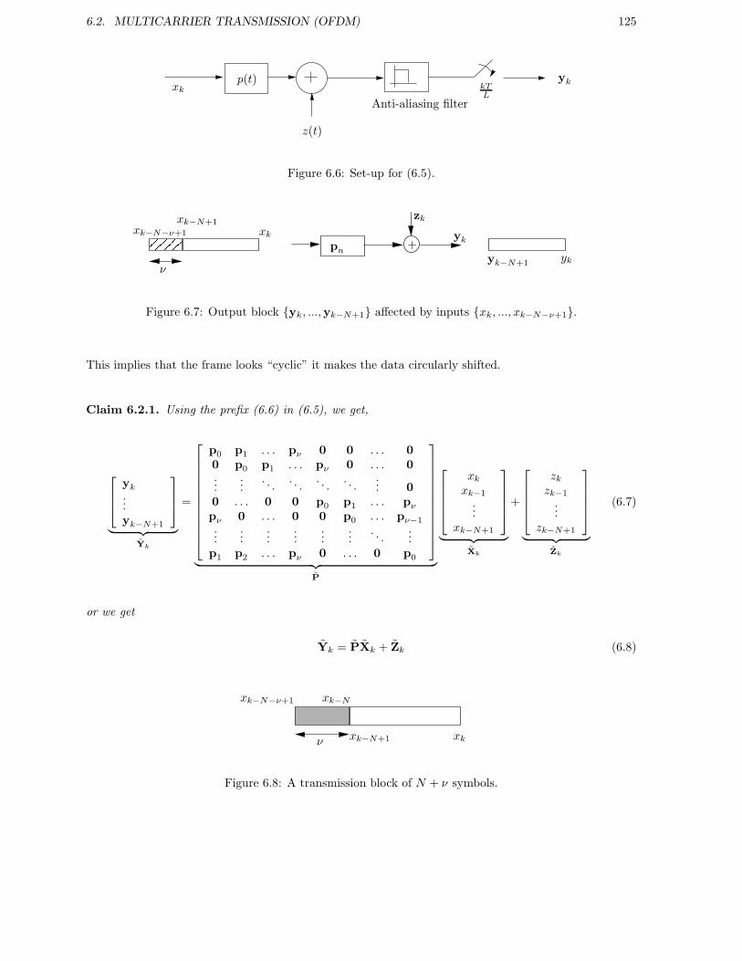
6.2. MULTICARRIER TRANSMISSION (OFDM) 125
xk
z(t)
Anti-aliasing filter
ykp(t)kTL
Figure 6.6: Set-up for (6.5).
pn
+
zk
yk
yk−N+1 ykν
xkxk−N−ν+1
xk−N+1
Figure 6.7: Output block yk, ...,yk−N+1 affected by inputs xk, ..., xk−N−ν+1.
This implies that the frame looks “cyclic” it makes the data circularly shifted.
Claim 6.2.1. Using the prefix (6.6) in (6.5), we get,
yk...yk−N+1
︸ ︷︷ ︸Yk
=
p0 p1 . . . pν 0 0 . . . 00 p0 p1 . . . pν 0 . . . 0...
.... . .
. . .. . .
. . .... 0
0 . . . 0 0 p0 p1 . . . pν
pν 0 . . . 0 0 p0 . . . pν−1...
......
......
.... . .
...p1 p2 . . . pν 0 . . . 0 p0
︸ ︷︷ ︸P
xk
xk−1
...xk−N+1
︸ ︷︷ ︸Xk
+
zk
zk−1
...zk−N+1
︸ ︷︷ ︸Zk
(6.7)
or we get
Yk = PXk + Zk (6.8)
xk−N+1 xk
xk−N−ν+1 xk−N
ν
Figure 6.8: A transmission block of N + ν symbols.
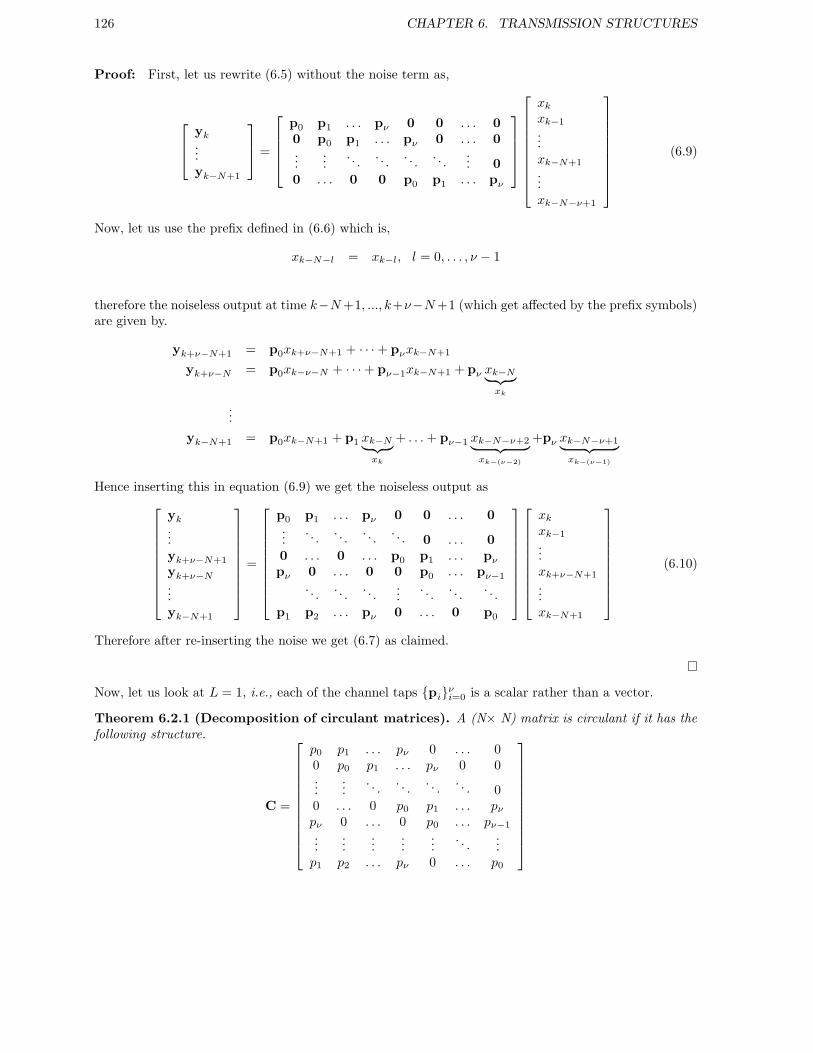
126 CHAPTER 6. TRANSMISSION STRUCTURES
Proof: First, let us rewrite (6.5) without the noise term as,
yk...yk−N+1
=
p0 p1 . . . pν 0 0 . . . 00 p0 p1 . . . pν 0 . . . 0...
.... . .
. . .. . .
. . .... 0
0 . . . 0 0 p0 p1 . . . pν
xk
xk−1
...xk−N+1
...xk−N−ν+1
(6.9)
Now, let us use the prefix defined in (6.6) which is,
xk−N−l = xk−l, l = 0, . . . , ν − 1
therefore the noiseless output at time k−N+1, ..., k+ν−N+1 (which get affected by the prefix symbols)are given by.
yk+ν−N+1 = p0xk+ν−N+1 + · · · + pνxk−N+1
yk+ν−N = p0xk−ν−N + · · · + pν−1xk−N+1 + pν xk−N︸ ︷︷ ︸xk
...
yk−N+1 = p0xk−N+1 + p1 xk−N︸ ︷︷ ︸xk
+ . . .+ pν−1 xk−N−ν+2︸ ︷︷ ︸xk−(ν−2)
+pν xk−N−ν+1︸ ︷︷ ︸xk−(ν−1)
Hence inserting this in equation (6.9) we get the noiseless output as
yk...yk+ν−N+1
yk+ν−N...yk−N+1
=
p0 p1 . . . pν 0 0 . . . 0...
. . .. . .
. . .. . . 0 . . . 0
0 . . . 0 . . . p0 p1 . . . pν
pν 0 . . . 0 0 p0 . . . pν−1
. . .. . .
. . ....
. . .. . .
. . .
p1 p2 . . . pν 0 . . . 0 p0
xk
xk−1
...xk+ν−N+1
...xk−N+1
(6.10)
Therefore after re-inserting the noise we get (6.7) as claimed.
Now, let us look at L = 1, i.e., each of the channel taps piνi=0 is a scalar rather than a vector.
Theorem 6.2.1 (Decomposition of circulant matrices). A (N× N) matrix is circulant if it has thefollowing structure.
C =
p0 p1 . . . pν 0 . . . 00 p0 p1 . . . pν 0 0...
.... . .
. . .. . .
. . . 00 . . . 0 p0 p1 . . . pν
pν 0 . . . 0 p0 . . . pν−1
......
......
.... . .
...p1 p2 . . . pν 0 . . . p0

6.2. MULTICARRIER TRANSMISSION (OFDM) 127
A circulant matrix has an eigen-decomposition
C = F∗ΛF
where
(F)p,q =1√N
exp
−j 2π
N(p− 1)(q − 1)
and Λ = diag(dl) where dl is
dl =
ν∑
m=0
pme−j 2π
N ml
That is,
Λ =
d0 0
...0 dN−1
Note: The matrix F as one would recognize is the DFT matrix and Λ contains on its diagonal theFourier transform of the channel taps.
Now, let us use Theorem 6.2.1 in the basic OFDM equation (6.8) which is,
Yk = PXk + Zk
Now, let us define
Xk = FXk
Yk = FYk
Zk = FZk
Then using Theorem 6.2.1 we have,
Yk = ΛXk + Zk
since the DFT matrix is unitary i.e.,
F∗F = I
Hence
Yk(l) = dlXk(l) + Zk(l), l = 0, . . . , N − 1 (6.11)
Therefore we have created ISI-free channel! Basically to do this, we have used the eigen property of LTIchannels as well as the finite impulse response property of the channel. Note that for arbitrary L, (6.11)just becomes a vector relationship in the following way.
Yk(l) = DlXk(l) + Zk(l), l = 0, . . . , N − 1
Here
Dl =
∑νm=0 p0(m)e−j 2π
N ml
...∑νm=0 pL−1(m)e−j 2π
N ml
=
ν∑
m=0
p(m)e−j 2πN ml.

128 CHAPTER 6. TRANSMISSION STRUCTURES
6.2.3 Frequency Domain Equalizer (FEQ)
Now, the relationship given in (6.11) for L = 1, forms the basis of the receiver in a manner similar to(5.45) for finite length equalizers. Given that we have no interference between the symbols Xn(l) theMMSE receiver is quite simple. Since we have transmitted symbols in additive (white) noise, the MMSEestimator is just.
Xl(k) =d∗l
|dl|2 + σ2/Ex
Yk(l)
where Ex is the energy on every symbol. Since we are doing N successive transmissions, and F is a unitarytransform, typically Ex = Ex, the energy of originally intended symbol. The above FEQ is equivalent tothe MMSE-LE applied in the frequency domain.
6.2.4 Alternate derivation of OFDM
Consider a periodic sequence xn of period N, given by
xk−rN = xk , r ∈ ZZ , k ∈ 0, . . . , N − 1
Therefore the Fourier transform of xk is (basically Fourier series coefficients) is given by
X(ω) =
N−1∑
n=0
Xnδ(ω − 2π
Nn)
Now, let us pass this periodic sequence through a LTI channel as shown in Figure 6.9.The output Y (ω) is,
Y (ω) = P (ω)X(ω) = P (ω)N−1∑
n=0
Xnδ(ω − 2π
Nn) =
N−1∑
n=0
XnP (2π
Nn)δ(ω − 2π
Nn) (6.12)
. . .
X(w)
. . .
P (0)X0
P (w)
P(
2πN (N − 1)
)XN−1
Figure 6.9: Transmission of periodic sequence through LTI channel.
Therefore, yk is also periodic with period N , i.e.,
yk+rN = yk , r ∈ ZZ , k ∈ 0, . . . , N − 1
Hence, just N samples of ykN−1k=0 are enough to reconstruct the sequence.
Therefore, the Fourier coefficients of Y (ω) are
Y (ω) =
N−1∑
n=0
Ynδ(ω − 2π
Nn) (6.13)
From equations (6.12) and (6.13), we obtain,
Yn = P
(2πn
N
)Xn, n = 0, . . . , N − 1. (6.14)
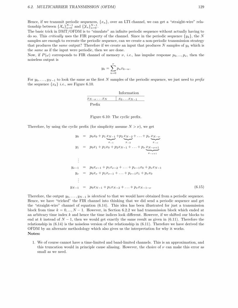
6.2. MULTICARRIER TRANSMISSION (OFDM) 129
Hence, if we transmit periodic sequences, xn, over an LTI channel, we can get a “straight-wire” rela-tionship between XnN−1
n=0 and YnN−1n=0 .
The basic trick in DMT/OFDM is to “simulate” an infinite periodic sequence without actually having todo so. This critically uses the FIR property of the channel. Since in the periodic sequence yk, the Nsamples are enough to recreate the periodic sequence, can we create a non-periodic transmission strategythat produces the same output? Therefore if we create an input that produces N samples of yk which isthe same as if the input were periodic, then we are done.
Now, if P (ω) corresponds to FIR channel of memory ν, i.e., has impulse response p0, ..., pν , then thenoiseless output is
yk =
ν∑
n=0
pnxk−n.
For y0, . . . , yN−1 to look the same as the first N samples of the periodic sequence, we just need to prefixthe sequence xk i.e., see Figure 6.10.
Prefix
Information
x0 . . . xN−1xN−ν . . . xN
Figure 6.10: The cyclic prefix.
Therefore, by using the cyclic prefix (for simplicity assume N > ν), we get
y0 = p0x0 + p1 xN−1︸ ︷︷ ︸x−1
+p2 xN−2︸ ︷︷ ︸x−2
+ . . .+ pν xN−ν︸ ︷︷ ︸x−ν
y1 = p0x1 + p1x0 + p2xN−1 + . . .+ pν xN−ν+1︸ ︷︷ ︸x−ν+1
...
yν−1 = p0xν−1 + p1xν−2 + . . .+ pν−1x0 + pνxN−1
yν = p0xν + p1xν−1 + . . .+ pν−1x1 + pνx0
...
yN−1 = p0xN−1 + p1xN−2 + . . .+ pνxN−1−ν (6.15)
Therefore, the output y0, . . . , yN−1 is identical to that we would have obtained from a periodic sequence.Hence, we have “tricked” the FIR channel into thinking that we did send a periodic sequence and getthe “straight-wire” channel of equation (6.14). This idea has been illustrated for just a transmissionblock from time k = 0, ..., N − 1. However, in Section 6.2.2 we had transmission block which ended atan arbitrary time index k and hence the time indices look different. However, if we shifted our blocks toend at k instead of N − 1, then we would get exactly the same result as given in (6.11). Therefore therelationship in (6.14) is the noiseless version of the relationship in (6.11). Therefore we have derived theOFDM by an alternate methodology which also gives us the interpretation for why it works.
Notes:
1. We of course cannot have a time-limited and band-limited channels. This is an approximation, andthis truncation would in principle cause aliasing. However, the choice of ν can make this error assmall as we need.

130 CHAPTER 6. TRANSMISSION STRUCTURES
2. By the trick shown, we essentially “sample” the channel in the frequency domain,i.e.,P(
2πN n)N−1
n=0.
This is correct for periodic sequences, but with a-periodic sequences, such a sampling could incura loss, which is the same as the “aliasing” error in 1) above.
3. The decomposition of the channel into parallel channels through the cyclic prefix trick did not needthe transmitter to know the channel impulse response. All that was used was
• The channel was LTI
• It had a finite response of length ν + 1
This property makes the decomposition canonical for FIR LTI channels.
The interpretation through periodic sequences leads us to the use of circular convolution. For a given N ,the circular convolution between two sequences u0, ..., uN−1 and v0, ..., vN−1 is defined as
uk ⊗N vk =
N−1∑
n=0
unv(k−n)N, k = 0, ..., N − 1 (6.16)
where (k − n)N is the modulo operator i.e., (k − n)N = r if k − n = qN + r, for some q ∈ Z.Therefore in our case if (k − n) < 0 then
(k − n)N = N − (k − n).
Hence we can interpret the relationship in (6.15) by a circular convolution, i.e.,
yk = pk ⊗N xk .
This is also true in the relationship in (6.10) where
yk = pk ⊗N xk
Thus the operations in DMT/OFDM can also be interpreted in terms of circular convolutions. Thisinterpretation is explicit in our derivation using periodic sequences. Note that circular convolution likeperiodic convolution is a commutative operation.
6.2.5 Successive Block Transmission
Note that the development till now has been on a single block of transmission. What happens forcontinuous transmissions? This is illustrated in Figure 6.13. For continuous transmission, the idea goesthrough again in the following manner.
Prefix for
block k
xk(N − ν), . . . , xk(N − 1) xk(0), . . . , xk(N − 1)
Block k
xk+1(N − ν), . . . , xk+1(N − 1) xk+1(0), . . . , . . . , xk+1(N − 1)
Block k+1
block k+1
Prefix for
Figure 6.11: Transmitted sequence for OFDM blocks.
We define the following quantities (see Figures 6.11 and 6.12) in relation to the single frame trans-mission notation given in (6.7). We denote the frame of N + ν symbols transmitted in block k as

6.3. CHANNEL ESTIMATION 131
Block k
yk(−ν), . . . , yk(−1) yk(0), . . . , yk(N − 1) yk+1(−ν), . . . , yk+1(−1) yk+1(0), . . . , yk+1(N − 1)
Block k+1
Figure 6.12: Received sequence for OFDM blocks.
... ...
νννN symbols
(k + 1)st blockN + ν kth block
Figure 6.13: Continuous transmission blocks.
xk(−ν), ..., xk(−1), xk(0)..., xk(N − 1) which along with the cyclic prefix relationship in (6.6) we seethat the transmitted frame is xk(N − ν), ..., xk(N − 1), xk(0), ..., xk(N − 1).The received frame of N + ν symbols for block k is denoted by, yk(−ν), ..., yk(−1), yk(0), ..., yk(n− 1).Now for each block of transmission, it is clear that yk(−ν), ..., yk(−1) are influenced by symbols trans-mitted in the previous frame (i.e., xk−1(l), l = 0, ..., N −1). Therefore, we discard yk(−ν), ..., yk(−1) andonly use yk(0), ..., yk(N − 1). Hence,
yk+1(0) = p0xk+1(0) + p1 xk+1(N − 1)︸ ︷︷ ︸xk+1(−1)
+...+ pν xk+1(N − ν)︸ ︷︷ ︸xk+1(−ν)
where due to the cyclic prefix the interference from the previous transmitted block (block k) has beeneliminated. Therefore the prefix has eliminated the interblock interference at the cost of added redundancyof ν symbols per block. Hence the redundancy rate is ν
N+ν per transmitted symbol.Note that if we examined yk+1(−1), we would have dependencies from the previous transmitted block(block k) and this is the reason for discarding it. Therefore the prefix given in (6.6) serves anotherpurpose, i.e., it prevents successive blocks from interfering with each other. This function causes it to bealso called the “guard” interval.The overall block diagram implementation of DMT is shown in Figure 6.14.
Disadvantages of OFDM
The OFDM technique seems like a panacea and solves our ISI channel problem. However, it does havesome disadvantage like longer transmit symbols, larger peak-to-average ratio, sensitivity to mismatch andsynchronization errors. So, in practice, it depends on the real gain in system performance to make theappropriate choice between time-domain equalization and OFDM. Sometimes a combination of the twomight be appropriate.
6.3 Channel Estimation
Up to now, the main assumption is that the transmission channel is known at the receiver. All thealgorithms and techniques we have seen critically utilize this fact. A natural question is how we havesuch knowledge. The basic idea in channel estimation is to send known information symbols and estimatethe channel. The technique is a dual of estimating information symbols while sending it through a knownchannel. Let us re-examine the discrete-time model given in (5.46) and for simplicity consider L = 1.

132 CHAPTER 6. TRANSMISSION STRUCTURES
INPUT
BITS
SYMBOL
BIT
MAPPER
I
F
F
T
Re(Xi)
Im(Xi)
C
TRANSMIT
FILTER
CARRIER
z(t)s(t)
CHANNELCARRIER
D
AXi
CYCLIC PREFIX
V-POINT
MODULATION
+DEMODULATION
C
D
A
PROCESSING
CYCLIC PREFIX
F
F
T
DECODING
T′
T′
Yi
Xi
Figure 6.14: Block diagram for OFDM.
Therefore, we can re-write it as
yk =
ν∑
m=0
pmxk−m + zk,
and in vector form it is,
yk
...yk−NT +1
︸ ︷︷ ︸Y
=
xk xk−1 . . . xk−ν
xk−1 xk−2 . . . xk−ν−1
......
......
xk−N+1 xk−NT . . . xk−NT +1−ν
︸ ︷︷ ︸X
p0
p1
...pν
︸ ︷︷ ︸p
+
zk
...
...zk−NT +1
︸ ︷︷ ︸z
(6.17)
where NT = length of training. The problem is now of estimating p from Y when xk, . . . , xk−NT +1−νare known symbols. Thus in compact form, (6.17) is written as
Y = Xp + z (6.18)
A criterion to estimate p from Y is
popt = arg minp
||Y − Xp||2 (6.19)
This can be written in more detail as,
arg minp
NT−1∑
t=0
∣∣∣∣∣yk−t −ν∑
m=0
pmxk−t−m
∣∣∣∣∣
2
= popt
Note that this criterion does not involve any expectation (E[·]) operation. This is because we are assumingthe channel to be an unknown constant and not a stochastic quantity. The criterion given in (6.19) is calledthe deterministic least squares criterion. As we shall see below, several of the geometric interpretations

6.3. CHANNEL ESTIMATION 133
we had for the MMSE criterion (stochastic least squares) in Section 5.1 also carries through here as well.We will examine a relationship between deterministic and stochastic least squares in Section 6.3.2.We now know derive the orthogonality principle appropriate for the deterministic least squares problem(see also Figure 6.15). Let us write the cost function given in (6.19) as,
J (p) = ||Y − Xp||2= Y∗Y + p∗X ∗Xp − Y∗Xp − p∗X ∗Y
By differentiation one gets
X ∗X popt = X ∗Y (6.20)
which in the terminology of least squares is the normal equation. If X ∗X is invertible then
popt = (X ∗X )−1X ∗Y (6.21)
Note that the normal equation (6.20) implies the orthogonality principle, i.e.,
eopt = Y − X popt
= Y − X (X ∗X )−1X ∗Y⇒ X ∗eopt = X ∗Y − (X ∗X )(XX ∗)−1X ∗Y
= 0 (6.22)
R(X )
eopt
Y
Xpopt
(Y − Y) ⊥ R(X )
Figure 6.15: Geometry of the deterministic least squares problem.
Hence eopt⊥X , is the orthogonality principle in this context (see also Figure 6.15).Now, let us use this result in the model of interest, i.e., (6.18). Therefore, we get
popt = (X ∗X )−1X ∗[Xp + z] = p + (X ∗X )−1X ∗z (6.23)
The estimation error for criterion (6.19) is therefore
eopt = Y − X (X ∗X )−1X ∗Y =[I−X (X ∗X )−1X ∗]Y
Now, we can find the least squares error norm as
‖ eopt ‖2 = ‖ Y − X popt ‖2= Y∗eopt − poptX ∗eopt
(a)= Y∗eopt = Y∗Y − Y∗X popt
= Y∗Y − (X ∗Y)∗popt
(b)= Y∗Y − (X ∗X popt)
∗popt
= Y∗Y− ‖ X popt ‖2
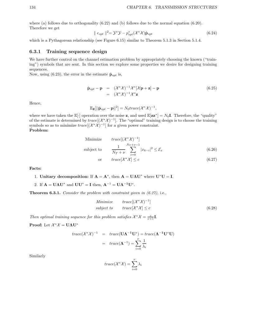
134 CHAPTER 6. TRANSMISSION STRUCTURES
where (a) follows due to orthogonality (6.22) and (b) follows due to the normal equation (6.20).Therefore we get
‖ eopt ‖2= Y∗Y − p∗opt(X ∗X )popt (6.24)
which is a Pythagorean relationship (see Figure 6.15) similar to Theorem 5.1.3 in Section 5.1.4.
6.3.1 Training sequence design
We have further control on the channel estimation problem by appropriately choosing the known (“train-ing”) symbols that are sent. In this section we explore some properties we desire for designing trainingsequences.Now, using (6.23), the error in the estimate popt is,
popt − p = (X ∗X )−1X ∗[Xp + z] − p (6.25)
= (X ∗X )−1X ∗z
Hence,Ez[||popt − p||2] = N0trace(X ∗X )−1,
where we have taken the E[·] operation over the noise z, and used E[zz∗] = N0I. Therefore, the “quality”of the estimate is determined by trace[(X ∗X )−1]. The “optimal” training design is to choose the trainingsymbols so as to minimize trace[(X ∗X )−1] for a given power constraint.Problem:
Minimize trace[(X ∗X )−1]
subject to1
NT + ν
NT +ν−1∑
i=0
|xk−i|2 ≤ Ex (6.26)
or trace[X ∗X ] ≤ c (6.27)
Facts:
1. Unitary decomposition: If A = A∗, then A = UΛU∗ where U∗U = I.
2. If A = UΛU∗ and UU∗ = I then, A−1 = UΛ−1U∗.
Theorem 6.3.1. Consider the problem with constraint given in (6.27), i.e.,
Minimize trace[(X ∗X )−1]
subject to trace[X ∗X ] ≤ c (6.28)
Then optimal training sequence for this problem satisfies X ∗X = cν+1 I.
Proof: Let X ∗X = UΛU∗
trace(X ∗X )−1 = trace(UΛ−1U∗) = trace(Λ−1U∗U)
= trace(Λ−1) =ν∑
i=0
1
λi
Similarly
trace(X ∗X ) =
ν∑
i=0
λi

6.3. CHANNEL ESTIMATION 135
The problem with the constraint in (6.27) is then,
Minimize∑ 1
λi
s.t∑
λi ≤ c
Let us write the Lagrangian form for constrained optimization,
J (λ) =∑ 1
λi− γ
∑λi
∂J∂λi
= − 1
λ2i
− γ = 0
Therefore we see that λ2i = − 1
γ is a constant independent of index i. Therefore
Λ = − 1√γI,
giving us
X ∗X = − 1√γI.
Using this in (6.27) with equality we get
X ∗X =c
ν + 1I
This was a toy problem in that we did not take the exact constraints into account (there are edge effectsthat mean that problem (6.26) and (6.27) are not equivalent). Also, typically we want xk to comefrom a particular constellation. That makes the training sequence optimization problem a discrete one,i.e., a discrete optimization problem. However, this gives one an idea of what kind of training sequenceswe should attempt to design. Another way of interpreting this is that we want the training sequencesto have low cross-correlation with shifted versions. This requirement on sequences also arises in CDMAwireless multiple access communications.
Now, let us compare the true constraint given in (6.26)
1
NT + ν
NT +ν−1∑
l=0
|xk−l|2 ≤ Ex
and the formal constraint (6.27) that we solved, i.e.,
tr [X ∗X ] ≤ c.
In order to do this we can write,
X ∗X =
xk . . . xk−ν
......
xk−NT +1 . . . xk−ν−NT +1
∗ xk . . . xk−ν
......
xk−NT +1 . . . xk−ν−NT +1

136 CHAPTER 6. TRANSMISSION STRUCTURES
Hence we get,
trace (X ∗X ) =
ν∑
l=0
NT −1∑
t=0
|xk−l−t|2 (6.29)
= (ν + 1)
[NT −1∑
l=ν
|xk−l|2]
+ |xk|2 + 2|xk−1|2 + . . .+ ν|xk−ν+1|2 + ν|xk−NT |2
+ . . .+ 2|xk−ν−NT +2|2 + |xk−ν−NT +1|2
Therefore we get,
trace (X ∗X ) = (ν + 1)
[NT +ν−1∑
l=0
|xk−l|2]−ν|xk |2 + . . .+ |xk−ν+1|2
−|xk−NT |2 + . . .+ ν|xk−NT −ν+1|2
≤ (ν + 1)(NT + ν)Ex −ν|xk |2 + . . .+ |xk−ν+1|2
−|xk−NT |2 + . . .+ ν|xk−NT −ν+1|2
≈ (ν + 1)(NT + ν)Ex (6.30)
Therefore c ≈ (ν + 1)(NT + ν)Ex if we ignore the edge effects.Now if we use the “optimal” training sequence sa specified in Theorem 6.3.1, we get
(X ∗X ) =c
ν + 1I = (NT + ν)ExI
and applying this using (6.25) we have
E(p − popt)(p − popt)∗ = (X ∗X )
−1N0.
These together give us,
E(p− popt)(p − popt)∗ =
N0
(NT + ν)ExI
Therefore, for the optimal training sequences,
E[‖ p− popt ‖2] =N0ν
(NT + ν)Ex=
[1
SNR
1 + NT
ν
].
Given this, the error in the estimate is made small by choosing NT >> ν, i.e., the training length shouldbe much larger then the number of parameters being estimated. If such a large NT is chosen, then theassumption of “perfect” channel state information becomes quite reasonable.
Channel mismatch
Since the channel estimation error is non-zero, the use of channel estimate instead of true channel incursa penality. Therefore we think that the output behaves as,
Yk =
ν∑
m=0
popt,mxk−m +∑
(pm − popt,m)xk−m + zk︸ ︷︷ ︸
Z′k
If xk are assumed i.i.d then
E[||Z′
k||2]
= ExE
[||Popt −P||2
]+N0L

6.3. CHANNEL ESTIMATION 137
Hence, if the estimation error is small, then the use of the estimated channel does not greatly affectperformance. However, if either the training sequence length NT , is small of the sequence was chosenpoorly, the mismatch in the channel could adversely affect performance. For good system design, onetries to ensure that the channel mismatch is small. If NT becomes large, it is clear that the mismatchasymptotically vanishes. In wireless channels (which we will encounter soon), there may be constraintson NT causing non-negligible channel mismatch.
6.3.2 Relationship between stochastic and deterministic least squares
In this section we explore the relationship between deterministic and stochastic least squares. We do thisusing the model given in (6.18)
Y = Xp + z
and make the assumption that p is a stochastic variable with
Epp∗ = αI,
As before we assume that
Ezz∗ = N0I.
Now we use a linear estimator
ps = MY (6.31)
and we use the criterion
ps = argminp
E[‖ p− p ‖2] (6.32)
Using orthogonality principle (seen in Section 5.1) we have
p − ps ⊥ Y
Hence we have,
E [(p−MY)Y∗] = 0
giving us
M = E(pY∗) E [YY∗]−1
Now we can write this explicitly using our assumptions as,
EpY∗ = (αI)X ∗,
EYY∗ = (αXX ∗ +N0I)
Hence we see that the linear estimator using the stochastic criterion (6.32) is given by
M = αX ∗ [αXX ∗ +N0INT ]−1
(6.33)
Claim 6.3.1.
M =
[N0
αIν+1 + X ∗X
]−1
X ∗
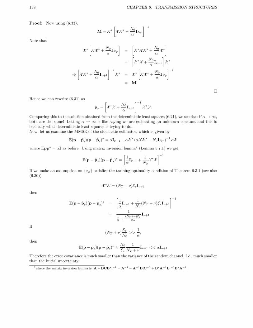
138 CHAPTER 6. TRANSMISSION STRUCTURES
Proof: Now using (6.33),
M = X ∗[XX ∗ +
N0
αINT
]−1
Note that
X ∗[XX ∗ +
N0
αINT
]=
[X ∗XX ∗ +
N0
αX ∗]
=
[X ∗X +
N0
αIν+1
]X ∗
⇒[XX ∗ +
N0
αIν+1
]−1
X ∗ = X ∗[XX ∗ +
N0
αINT
]−1
= M
Hence we can rewrite (6.31) as
ps =
[X ∗X +
N0
αIν+1
]−1
X ∗Y .
Comparing this to the solution obtained from the deterministic least squares (6.21), we see that if α → ∞,both are the same! Letting α → ∞ is like saying we are estimating an unknown constant and this isbasically what deterministic least squares is trying to do.Now, let us examine the MMSE of the stochastic estimator, which is given by
E(p − ps)(p − ps)∗ = αIν+1 − αX ∗ (αXX ∗ +N0INT )
−1αX
where Epp∗ = αI as before. Using matrix inversion lemma2 (Lemma 5.7.1) we get,
E(p − ps)(p − ps)∗ =
[1
αIν+1 +
1
N0X ∗X
]−1
If we make an assumption on xk satisfies the training optimality condition of Theorem 6.3.1 (see also(6.30)),
X ∗X = (NT + ν)ExIν+1
then
E(p − ps)(p − ps)∗ =
[1
αIν+1 +
1
N0(NT + ν)ExIν+1
]−1
=1
1α + (NT +ν)Ex
N0
Iν+1
If
(NT + ν)Ex
N0>>
1
α,
then
E(p − ps)(p − ps)∗ ≈ N0
Ex
1
NT + νIν+1 << αIν+1
Therefore the error covariance is much smaller than the variance of the random channel, i.e., much smallerthan the initial uncertainty.
2where the matrix inversion lemma is [A + BCB∗]−1 = A−1 − A−1B[C−1 + B∗A−1B]−1B∗A−1.

6.4. PROBLEMS 139
6.4 Problems
Problem 6.1
For a channel with
Q(D) =1
||p||2[0.9D+ 1.81 + 0.9D−1
]
Assume that the noise variance is σ2n = 0.1, and Ex = 1.
1. Find G(D) and W(D)for the ZF-DFE.
2. Find SNRZF−DFE .
3. Design (draw) a Tomlinson precoder.
4. Let M = 4 (PAM constellation) for your precoder, Find Pe. Recall that the Tomlinson Precoderoutput is approximately i.i.d when the input is an i.i.d sequence, and furthermore the outputsequence is approximately uniform in distribution over the inteval [−Md/2,Md/2].
Problem 6.2
Consider the channel model in Problem 5.6:
1. Design (draw) a Tomlinson precoder for this channel model and ZF-DFE.
2. Let M be a large value (PAM constellation) for your precoder, Find Pe. Recall that the TomlinsonPrecoder output is approximately i.i.d when the input is an i.i.d sequence, and furthermore theoutput sequence is approximately uniform in distribution over the inteval [−Md/2,Md/2].
Problem 6.3
Consider the H(D) = 1 +D channel. The differential precoder for this channel has the form
mk = mk mk−1
where represents subtraction modulo-M , mk and mk are the precoder input and output, respectively,and take values in 0, . . . ,M − 1.
1. Derive the mapping from the precoder output to xk, the channel input, assuming PAM modulationwith symbols separated by distance d.
2. Find the noiseless equivalent channel output. Also determine the input mk from this output. Hint :Apply the inverse of the mapping you found in part (a). You may use the (·)M operator to show aquantity calculated in M-level arithmetic.
3. Assuming the presence of additive noise, what is the estimate of the input mk if you apply the samemethod as in part-2 to determine mk?
Problem 6.4
[Tomlinson-Harashima Precoder for the MMSE-DFE ]
1. Derive the expression for R(D), the output of the feedforward filter in the MMSE-DFE.
2. Write an expression for GU (D), the equvialent unbiased filter for the MMSE-DFE.

140 CHAPTER 6. TRANSMISSION STRUCTURES
3. Using the fact that the SNRMMSE−DF E
SNRMMSE−DF E,Uscaled value of rk, the output of the MMSE WMF, is an
unbiased MMSE approximation of X(D)GU (D), find the feedback filter, B(D) for the Tomlison-Harashima precoder for the MMSE-DFE. Hence find rU,k, the scaled output of the feedforwardfilter.
4. Determine the output of the precoder after the modulo operation, Γ(rU,k).
Problem 6.5
1. Suppose we are given a periodic channel h(t) = h(t+ T ). Show that ϕn(t) = ej 2πT nt are eigenfunc-
tions of the channel. (Hint: express h(t) in a Fourier series). By eigenfunctions, we mean that ifφ(t), t ∈ [0, T ) is used for a periodic channel h(t), the output y(t), t ∈ [0, T ), will be a scaled versionof φ(t). Note here, that both the input and the output signals are restricted to the interval [0, T ).
2. What are the associated eigenvalues ?
3. If the channel is not periodic, but had finite length ν, how could the designer create a new set offunctions ϕn(t) from ϕ(t) such that the output looks as if it was created by a periodic channel.
4. If the receiver only looks at the periodic part of the output signal, what would the associatedeigenvalues be ?
5. If a transmission uses the channel eigenfunctions developed here, how much faster does the samplingrate hav to be ? ( or how much more bandwith does the design have to use ?)
Problem 6.6
Assume an OFDM system with N subcarriers, of symbol length T , of which ν is the length of the cyclicprefix
φk(t) =
1√
T−νej2π W
N k(t−ν) , if t ∈ [0, T ]
0 , otherwise
On a particular symbol, we have the transmitted signal given by:
sl(t) =
N−1∑
k=0
xk,lφk(t− lT )
Then the output from a transmitter is:
s(t) =
∞∑
l=0
sl(t)
Moreover we assume that the impulse response g(t) of the channel is of length ν.
1. Compute the received signal r(t). (consider an AWGN channel noise n(t))
2. The OFDM receiver consists of a filter bank, matched to the last part [ν, T ] of the transmitterwaveforms φk(t) :
ψk(t) =
φ∗k(T − t) , if t ∈ [0, T − ν]
0 , otherwise
Compute the sampled output from the receiver filter banks yk = (r ∗ψk)(t) |t=T and show that it isof the form yk = hkxk + nk. (Remember that since the cyclic prefix contains all ISI from previoussymbol, we can ignore the time index l)

6.4. PROBLEMS 141
Problem 6.7
Given an OFDM system with N subcarriers , compute the channel estimation in the frequency domain.Do we need N pilot symbols?
Problem 6.8
Given an OFDM system with N = 4 sub-carriers, cyclic prefix and a given channel P (D) = 1 + 1.81D+0.81D2:
1. Find the matrix P and compute its eigen decomposition.
2. After applying FEQ, compute the SNR on each sub carrier.
Assume that Ex = 0.1 and σ2 = 0.01.
Problem 6.9
Consider a finite impulse response channel
yk =
ν∑
n=0
pnxk−n + zk
where yk, zk ∈ C2 and pn ∈ C2, i.e they are 2-dimensional vectors. This could arise, for example,through Nyquist sampling like the model considered in class (L = 2).
1. Suppose one observes a block of N samples of yk, Yk =
yk
...yk−N+1
. Write down the relationship
between Yk and Xk =
xk
...xk−N+1
...xk−N+1−ν
in the form
Yk = PXk + Zk
where Yk , Zk ∈ C2N , Xk ∈ CN+ν , P ∈ C2N×(N+ν) by specifying the form of P.
2. Suppose we use a cyclic prefix, i.e
xk−N−l = xk−l, l = 0, · · · , ν − 1
Develop the equivalent model:
Yk = PXk + Zk (6.34)
where Xk =
xk
...xk−N+1
∈ CN and P ∈ C2N×N . Find P.

142 CHAPTER 6. TRANSMISSION STRUCTURES
k−N+1−ν k−N+1 k
cyclic prefix
ν
Figure 6.16: Cyclic Prefix
3. Let Y(`) = 1√N
∑N−1k=0 yke
−j 2πN k`, Z(`) = 1√
N
∑N−1k=0 zke
−j 2πN k`,
P(`) =∑ν
n=0 pne−j 2π
N n`, X(`) = 1√N
∑N−1k=0 xke
−j 2πN k`.
Develop the vector OFDM form for (6.34), i.e, show that
Y(`) = P(`)X(`) + Z(`), ` = 0, · · · , N − 1 (6.35)
This can be done by either arguing about equivalent periodic sequences or any other proof technique.Here we would like to see a derivation, just stating the result is not enough.
4. In the form given in (6.35), we get N parallel vector channels. If we want to detect each componentX(`) separately what would be the best linear estimator of X(`) from Y(`), i.e the appropriate“frequency-domain” MMSE linear equalizer (FEQ).
Problem 6.10
Find the MMSE-LE filter that normalizes the following channel
P (D) = 0.7 + 1.5D + 0.8D2
to a target channel of H(D) = 1 +D. In this case our predicition error becomes
E(D) = X(D)H(D) −W (D)Y (D).
You may assume that Rxx = Ex and that there is additive white Gaussian noise of power N0.The goal of this exercise to show the links between equalization, and the other methods of dealing withISI that we looked at such as OFDM and sequence detection. In pratical systems a channel is rarelyfully equalized to a delta function (H(D) = 1). Instead the channel is equalized to something relativelybenign (such as 1 +D), and then OFDM or sequence detection is applied to this equivalent channel.We see that the techniques we have learned for dealing with ISI channels do not have to be used indepen-dently, and indeed in practical systems equalization is often combined with another method for copingwith ISI.
Problem 6.11
Given an OFDM system with N = 8 subcarriers, and a given channel P (D) = 1 + 0.9D:
1. Find the matrix P and compute its eigen decomposition.
2. After applying FEQ, compute the SNR on each subcarrier.
3. Calculate the error rate for QPSK modulation.
4. What is the worst error rate?

6.4. PROBLEMS 143
Problem 6.12
[Sensitivity of OFDM to frequency offset ]To the P (D) = 1 + D channel, add a small frequency offset, δω. This will make the P matrix notexactly circulant anymore. Calculate the inter-carrier interference and quantify for what frequency offsetit becomes significant. Let N = 4. δω = ωoT , where ωo is the frequency offset and T is the symbolperiod. p(n) is replace to include the frequency offset such that
y(k) =
ν∑
n=0
ejδωkp(n)x(k − n) + z(k)
Hint: Calculate the new P matrix, then calculate the Λ matrix.
Problem 6.13
[Inter-carrier Interference in OFDM]Consider the scalar discrete-time inter symbol interference channel considered in the class,
yk =ν∑
n=0
pnxk−n + zk, k = 0, . . . , N − 1, (6.36)
where zk ∼ CN (0, σ2z) and is i.i.d., independent of xk. Let us employ a cyclic prefix as done in OFDM,
i.e.,x−l = xN−1−l, l = 0, . . . , ν.
As done in class given the cyclic prefix,
y =
yN−1
...y0
=
p0 . . . . . . pν 0 . . . 0 00 p0 . . . pν−1 pν 0 . . . 0
. . .. . .
. . .. . .
. . .. . .
0 . . . . . . 0 p0 . . . . . . pν
pν 0 . . . 0 0 p0 . . . pν−1
. . .. . .
. . .. . .
. . .
p1 . . . pν 0 . . . 0 0 p0
︸ ︷︷ ︸P
xN−1
...x0
︸ ︷︷ ︸x
+
zN−1
...z0
︸ ︷︷ ︸z
. (6.37)
In the derivation of OFDM we used the property that
P = F∗DF, (6.38)
where
Fp,q =1√N
exp
(−j 2π
N(p− 1)(q − 1)
)
and D is the diagonal matrix with
Dl,l = dl =
ν∑
n=0
pne−j 2π
N nl.
Using this we obtainedY = Fy = DX + Z,

144 CHAPTER 6. TRANSMISSION STRUCTURES
where X = Fx, Z = Fz. This yields the parallel channel result
Yl = dlXl + Zl. (6.39)
If the carrier synchronization is not accurate, then (6.36) gets modified as
y(k) =
ν∑
n=0
ej2πf0kpnxk−n + zk, k = 0, . . . , N − 1 (6.40)
where f0 is the carrier frequency offset. If we still use the cyclic prefix for transmission, then (6.37) getsmodified as
y(N − 1)..
y(0)
︸ ︷︷ ︸y
=
p0ej2πf0(N−1) . . . pνe
j2πf0(N−1) 0 . . . 0 0. . .
. . .. . .
. . .. . .
0. . .
. . .. . . ej2πf0νp0 . . . ej2πf0νpν
. . .. . .
. . .. . .
. . .
ej2πf00p1 . . . ej2πf00pν 0 . . . 0 ej2πf00p0
︸ ︷︷ ︸H
xN−1
...x0
︸ ︷︷ ︸x
+
zN−1
...z0
︸ ︷︷ ︸z
.
(6.41)i.e.,
y = Hx + z
Note thatH = SP,
where S is a diagonal matrix with Sl,l = ej2πf0(N−l) and P is defined as in (6.37).
(a) Show that for Y = Fy, X = Fx,Y = GX + Z (6.42)
and prove thatG = FSF∗D.
(b) If f0 6= 0, we see from part (a) that G is no longer a diagonal matrix and therefore we do not obtainthe parallel channel result of (6.39). We get inter-carrier interference (ICI), i.e., we have
Yl = Gl,lXl +∑
q 6=l
G(l, q)Xq + Zl
︸ ︷︷ ︸ICI + noise
, l = 0, . . . , N − 1,
which shows that the other carriers interfere with Xl. Compute the SINR (signal-to-interferenceplus noise ratio). Assume Xl are i.i.d, with E|Xl|2 = Ex. You can compute the SINR for theparticular l and leave the expression in terms of G(l, q).
(c) Find the filter Wl, such that the MMSE criterion is fulfilled,
minWlE|W∗
l Y −Xl|2.
You can again assume that Xl are i.i.d with E|Xl|2 = Ex and that the receiver knows G. Youcan now state the answer in terms of G.
(d) Find an expression for Gl,q in terms of f0, N, dl. Given this and (b), what can you conclude aboutthe value of f0. For what values of f0 do you think that the inter-carrier interference problem isimportant? Hint: Use the summation of the geometric series hint given in first page.

6.4. PROBLEMS 145
Problem 6.14
Consider the channel estimation problem based on the deterministic criterion. Let the channel be:
Y = Xp + z,
where channel memory length ν = 1 and length of the training sequence NT = 2. The deterministiccriterion to estimate p is given by:
popt = argminp||Y − Xp||.
1. Assume that all the signal are real, prove directly by differentiating that the optimum p satisfies
popt = (X ∗X )−1X ∗Y . (6.43)
Prove eqn(6.43) when the signals can be complex.
2. Let Ex = 0.1, σ2 = 0.01. Find the expected error in the estimation assuming that the trainingsequence is the optimal sequence obtained under the constraint Tr(X ∗X ) ≤ (ν + 1)(NT + ν)Ex.

146 CHAPTER 6. TRANSMISSION STRUCTURES

Part III
Wireless Communications
147


Chapter 7
Wireless channel models
Wireless communication refers to communication using electromagnetic waves propagated in “air” to carryinformation. This is different from the telephone line channel or the cable channel that required a wire tocarry information across from point to point. Today wireless networks have significantly penetrated ourlives through cellular phones, satellite TV and even cordless phones which combine with the traditionalPSTN wired telephone line network.Wireless communication has a long history, dating back to 1897 when Marconi successfully demonstratedwireless telegraphy. The early 20th century witnessed the birth of radio transmission with speech andaudio carried across the ocean. Soon, television transmission started in the 1930s and the launching ofsatellites in the 1950s started long-haul wireless networks. Today microwave networks for line-of-sighttransmission, cellular networks for wireless telephony and wireless LANs for data access seem ubiquitous.In this part of the class we introduce the transmission medium in cellular wireless communication andsome of the signal processing issues dealing with reception of multiple user wireless transmissions.There are two main distinguishing features of wireless communications in comparison to wired channels.The first is the channel could be time-varying causing the received signal strength to wax and wane. Thisphenomenon is called channel fading, and occurs due to radio wave propagation effects. The second is thatthe wireless channel is an inherently shared medium and hence multiple user interact and interfere witheach other. Therefore we need to devise techniques to handle multiuser interference making it distinctfrom the point-to-point (single-user) detectors we studied in Chapter 2. In general we also encounterinter-symbol interference in wireless channels, but this is something we have already encountered inChapter 4-6.A cellular network consists of users spread over a geographical area served by a “base station”. Thearea of a single base station is often called a “cell” and hence the name cellular communication. Severalbase-stations combine to cover large geographical areas. For example New York city has base-stationsevery couple of blocks and therefore the cells could be quite small. On the other hand in sub-urban andrural areas the cells could be quite large, of the order several square kilometers.
The base-stations connect to the wired telephone network enabling calls to and from the telephone linenetwork to the wireless cellular network. Given this background, we study the following aspects of wirelessnetworks.
• Radio wave propagation in scattering environments.
• Physical and statistical models for wireless channels.
• Detection in wireless point-to-point (single users) channels.
• Concept of diversity in various forms.
149

150 CHAPTER 7. WIRELESS CHANNEL MODELS
Base station
Figure 7.1: A cartoon of a cellular base station.
Base station
Cell
base station
Figure 7.2: An oversimplified view of cells in geographical area.

7.1. RADIO WAVE PROPAGATION 151
• Wireless multi-users channels, in particular focus on the multiple access channel.
• Multiuser detection for multiple access channels.
In this chapter we study wireless channel models after understanding the effects of radio wave propagation.In Chapter 8, we study detection in point-to-point (single user) wireless channels. In Chapter 9, we studymultiuser wireless channels and focus on multiple access channels.
7.1 Radio wave propagation
Wireless transmission occurs by modulating electromagnetic waves which are then transmitted throughan antenna. The receiver processes the impinging electromagnetic wave and detects the transmittedinformation. The typical carrier frequencies are 0.9 GHz, 1.8 GHz, 2.4 GHz, etc. for cellular wirelessnetworks. The main effects on the information transmission arises due to the propagation effects on theelectromagnetic waves due to reflection, absorption and constructive and destructive combining of theseelectromagnetic waves. Therefore we first study these effects and their impact on communication.
7.1.1 Free space propagation
Receivingantenna
transmittingantenna
(0, 0, 0)
(r, θ, ψ)
Figure 7.3: Free space radio propagation.
Free space propagation occurs when the transmitter and the receiver have an unobstructed line-of-sightpath between them. For a fixed transmitting and fixed receiving antenna, and for a pure sinusoid cos 2πfttransmitted, the observed electric field (far field) at time t and position (r, θ, ψ) is
E[f, t, (r, θ, ψ)] =1
rRe[αs(θ, ψ, f)ej2πf(t−r/c)] (7.1)
where αs(θ, ψ, f) is the radiation pattern of transmitting antenna, c = 3 × 10⁸ (velocity of light). Notethat phase variation of fr/c is just due to the delay caused by radiation travelling at the speed of light.The receiving antenna could have a radiation (reception) pattern of its own and this could modify the ob-served electric field. This just means α(θ, ψ, f) replaces αs(θ, ψ, f) where α(θ, ψ, f) = αs(θ, ψ, f)αr(θ, ψ, f).Therefore the received electric field at the antenna is
E[f, t, (r, θ, ψ)] =1
rRe[α(θ, ψ, f)ej2πf(t− r
c )]. (7.2)
Notes:
1. Notice that in (7.2) the electric field decays as 1r as a function of distance between transmitting
and receiving antennas. Thus the power behaves as,
Pr =| α(θ, ψ, f) |2
r2(7.3)

152 CHAPTER 7. WIRELESS CHANNEL MODELS
and hence decays as 1r2 , as a function of the distance. This is often called the squared law loss
and determines how far we can have the transmitter and receiver, implying the coverage area of abase-station for example.
2. The relationship in (7.2) holds only for free space propagation, i.e. no absorption, no reflections orscattering.
3. The radiation pattern of the transmitting antenna could be directional and also cause phase varia-tions.
4. It is clear that (7.2) does not hold for r = 0, i.e., this is a far field model when the transmitter andthe receiver are far apart.
5. Linearity: The observed electric field is linear in the input, i.e. if we transmit a sum (superposition)of two sinusoids, the output will be the sum of the outputs one would have observed if each of themwere transmitted alone. This is an important feature of the propagation behavior that will be usedin the channel models later.
7.1.2 Ground Reflection
In typical scenarios, an unobstructed line-of-sight path between the transmitter and the receiver is rare.We will now look at our first modification of the free space model developed in Section 7.1.1.A two-ray ground reflection model is a usual first step in demonstrating the kind of impairments wewould see in a real propagation environment. Even though such a model (shown in Figure 7.4) does notcapture all the complexities of a real-world channel, it gives us a taste of what to expect.In Figure 7.4, we consider a typical scenario where one antenna (say the transmitter) is much higher (at aheight ht) than the receiver (at height hr). This might represent a base-station transmitting to a mobileunit. We consider a perfect omnidirectional transmitter and receiver, i.e., α(θ, ψ, f) = 1.
r0
hr
ht
Erefl
Edirect
rdirect
Figure 7.4: A two-ray ground reflection model.
We assume that receiver observes two versions of the transmitted wave, one which reaches it directlyand we call this Edirect and the other which reflects off the ground and reaches it after travelling a totaldistance of rb. Due to linearity, the total electric field is the sum of these two components given by,
E(f, t) = Edirect(f, t) + Erefl(f, t) (7.4)
Let E0 be the observed electric field at a reference distance d0 from the transmitter. If the ground is aperfect reflector, then
Edirect =E0d0
rdcos(2πf
(t− rd
c
))
Erefl =−E0d0
rbcos(2πf
(t− rb
c
))

7.1. RADIO WAVE PROPAGATION 153
where rd is the distance travelled by the direct wave, i.e., rd is the distance from transmitter to receiverand rb is the total distance travelled by reflected wave.
Now, let us define the path difference ∆ as,
∆ = rb − rd(a)=√
(ht + hr)2 + r20 −√
(ht − hr)2 + r20
= r0
[1 +
(ht + hr
r0
)2]1/2
− r0
[1 +
(ht − hr
r0
)2]1/2
(b)≈ r0
[1 +
1
2
(ht + hr
r0
)2
− 1 − 1
2
(ht − hr
r0
)2]
=1
2r0
[(ht + hr)
2 − (ht − hr)2]
=1
2r0(4hthr) =
2
r0hthr
where (a) occurs due to geometry in Figure 7.5 i.e.,
r2b = (ht + hr)2 + r20
r2d = (ht − hr)2 + r20 (7.5)
and the approximation (b) is for r0 >> (ht + hr). This means that the distance between the transmitterand the receiver are much larger than the antenna heights. Hence we get
∆ = rb − rd ≈ 2
r0hthr (7.6)
Therefore using this in (7.4) we get
E(f, t) =E0d0
rdcos[2πf
(t− rd
c
)]− E0d0
rbcos[2π(ft− f
rbc
)]
≈ E0d0
r0cos[2πf
(t− rd
c
)]− E0d0
r0cos[2πf(t− rb
c)]
where the approximation is because rb =√
(ht + hr)2 + r20 ≈ r0 and rd =√
(ht + hr)2 + r20 ≈ r0 in thefirst order.
hr
ht
rb
rd
hr
hr
ht
rb
r0
Figure 7.5: Trigonometry to find path differences.
Now, let us consider the complex representation of the electric field. One can get to the previous repre-
154 CHAPTER 7. WIRELESS CHANNEL MODELS
sentation by taking the real part.
E(f, t) =E0d0
rdejω(t− rd
c ) − E0d0
rbejω(t− rb
c )
≈ E0d0
r0
[ejω(t− rd
c ) − ejω(t− rbc )]
where as before the approximation is that 1rd
≈ 1rb
≈ 1r0
in the far field. Moreover we have used thenotation ω = 2πf , for brevity.Using this we get
E(f, t) ≈ E0d0
r0ejωt
[e−jω
rdc − e−jω
rbc
]
=
[E0d0
r0
]ejωte−jω
rbc
[e
jω“
rb−rdc
”
− 1
].
Now to find the power we need the total magnitude of the electric field, i.e.,
|E(f, t)| =
∣∣∣∣E0d0
r0
∣∣∣∣∣∣∣∣e
jω“
rb−rdc
”
− 1
∣∣∣∣
Consider the second term above,∣∣∣∣e
jω“
rb−rdc
”
− 1
∣∣∣∣2
=
cos
[ω
(rb − rdc
)]− 1
2
+ sin2
[ω
(rb − rdc
)]
= 1 + 1 − 2 cos
[ω
(rb − rdc
)]
= 2
1 − cos
[ω
(rb − rdc
)]
= 2
2 sin2
[ω
(rb − rd
2c
)]
Therefore now we use the approximation developed in (7.6) as,
|E(f, t)| ≈∣∣∣∣E0d0
r0
∣∣∣∣ 2 sin
[ω
(rb − rd
2c
)]
(a)≈∣∣∣∣E0d0
r0
∣∣∣∣ 2 sin
(ω
2hthr
r02c
)
(b)≈∣∣∣∣E0d0
r0
∣∣∣∣2ω
c
hthr
r0
=1
r20
[2E0d0hthr
c
]
where (a) occurs due to the approximations in (7.6) and (b) occurs because sin θ ≈ θ for small θ.Hence the power received is | E(f, t) |2 is Pr ≈ 1
r40
[4E0d0hthr
c
].
Hence, the received power decays as 1r40
instead of 1r20
as was seen in the free space propagation model.
This drastically different behavior in the power decay shows that complex reflections can alter the decaybehavior with distance.The main ideas from radio wave propagation considered in Section 7.1.1 and 7.1.2 can be summarized asfollows.

7.1. RADIO WAVE PROPAGATION 155
1. The free space transmission resulted in a linear time-invariant system with a power decay of 1r20,
where r0 was the distance between sender and receiver.
2. For a ground reflection, which occurs frequently in rural and suburban environments, the powerloss become 1/r40 i.e., it decays much faster than in free space. Therefore in general the radio wavepropagation causes a decay of power as
Pr ∝ 1
rβ(7.7)
where β ≥ 2. Typically β ∈ [2, 6].
7.1.3 Log-normal Shadowing
The model given in (7.7) may not completely capture the power loss behavior. Unfortunately the radiopropagation environment is much more complicated than just a reflection model. Typically radio wavesget reflected, absorbed, scattered and diffracted. All these depend very highly on the particular propa-gation environment. For example, the presence of a large building causing absorption, or a rough surfacecausing scattering means that one cannot easily predict the radio wave propagation behavior. Here iswhere we first encounter a stochastic model for the propagation, where the randomness corresponds tothe unknown or uncertain propagation environment.Given that just the “distance loss” behavior of (7.7) does not account for the complete effects of radiopropagation, we introduce the notion of shadowing to account for the randomness in the propagationenvironment. It has been empirically observed that the received signal power Pr(r0) as a function ofdistance r0 between transmitter and receiver behaves as,
Pr(r0) ∝S
(r0)β(7.8)
where S is a random variable (shadowing) accounting for some of the uncertainties in the propagationenvironment. Through empirical studies it has been observed that the random variable S behaves asa log-normal distribution, i.e., logS is a zero-mean Gaussian distributed random variable with a givenvariance. This model attempts to account for the variability in the empirical signal seen, even for thesame distance separation between the transmitter and the receiver. Therefore the model in (7.8) showsthat the received signal levels at a particular transmitter-receiver separation of r0 is a random variable.In terms of signal power measured in dB,
10 logPr(r0) = K + 10 logS − 10β log r0,
where K is the proportionality constant. Since log S is modelled as zero-mean, the mean received powerin dB is that given by the distance loss and the shadowing adds on to this with a normal distribution.In summary the shadowing represents the absorption and clutter loss which depends on the unknown(and uncertain) propagation environment. This is our first encounter with such randomness in themodelling. We will encounter it again in the next section where we consider mobility. Note, howeverthat the shadowing loss is modelled only for fixed environments. The modelling of shadowing for mobileenvironments is quite difficult.
7.1.4 Mobility and multipath fading
Up to now the propagation effects have been perhaps random but time-invariant. In this section weintroduce one of the distinguishing features of wireless channels, i.e., time-variation. These rapid fluctu-ations in signal strength are called fading and are caused by constructive and destructive interference of

156 CHAPTER 7. WIRELESS CHANNEL MODELS
reflected waves. We have already seen the effect of such superposition in Section 7.1.2 where we saw thecombination of a direct and a ground reflected wave. The essential difference here is that the receiverand/or the transmitter is mobile and hence these superpositions change over time causing the rapid sig-nal strength fluctuations. These are small-scale effects in that the distance travelled is of the order ofseveral wavelengths of the carrier wave in order to observe these variations. Therefore the signal strengthvariations do not occur due to changes in the propagation environment (i.e., reflectors, etc.) but due tophase changes in the “multipath” superposed reflections themselves.
Doppler Shift: Consider a mobile moving at a constant velocity v, along a path AB as illustrated inFigure 7.6. Suppose, as shown in Figure 7.6 there is a remote fixed transmitter T .
v
d
BA
θ
∆p
T
≈ θ
Figure 7.6: Doppler shift.
The difference in path length travelled by a wave from T to the mobile at A and B is ∆p = d cos θ =v∆t cos θ where ∆t is the time needed for the car to go from A to B and θ is the angle between AB andAT . Here we have assumed that T is far enough that the angles from A and B are the same, i.e., θ.Therefore due to the path length difference the phase difference of the radio wave is
∆φ =2π∆p
λ=
2πv∆t
λcos θ
where λ is the wavelength of the carrier. Therefore the apparent change in frequency is given by
fd =1
2π
∆φ
∆t=v
λcos θ. (7.9)
The relationship given in (7.9) relates the mobile speed to the change in frequency, which is called theDoppler shift. This is a phenomenon one might have encountered often when a police siren seems toincrease in frequency while approaching while decreasing when it is receding. Though the siren is alwaystransmitting at the same frequency a fixed listener observes a variation in the frequency and this effect iscalled the Doppler effect after its discoverer. Clearly, in (7.9) we see that if the mobile is moving towardsT , i.e., θ > 0, then the frequency shift is positive (i.e., apparent frequency is higher) and the shift isnegative when it is receding from T (i.e., θ < 0).
Now, this Doppler shift is the cause for the time-variation seen in wireless channels. The situationbecomes more complex when the mobile receives not one copy but several reflected copies of the signaltransmitted by T . This can be modelled as having several virtual sources Tl transmitted to the mobile.

7.1. RADIO WAVE PROPAGATION 157
Tl
T1
TL
Treflected paths
v
Figure 7.7: Multipath reflections and Doppler shifts.
Now, consider the effect of (7.9) on the received electric field, given in (7.1). The change in frequencycauses the received field at point B to be
E(f, t) ≈ 1
r0Re[α(θ, ψ, f)ej2π(f+fd)t]
For an ideal omni-directional transmitter and receiver, the complex electric field is given by
E(f, t) =
[1
r0ej2πft
]ej2πfdt
Therefore in the baseband and after compensation of distance loss we get
Eb(t) = ej2πfdt
Now, this is for a single path and for reflections we get several virtual sources, i.e., the received basebandsignal is
y(t) =
L∑
l=1
clej2π[ v
λ cos θl]t (7.10)
where θl are the angles to the different reflectors and cl are the (complex) reflection coefficients ofeach of the reflectors. This is because each of the reflectors could cause phase shift as well as absorb toreduce the amplitude. This is illustrated in Figure 7.7.In general, the reflectors could be such that one also gets delayed versions of the signal, but this is aneffect we will study in Section 7.2.The model given in (7.10) was for a single sinusoid sent at a carrier frequency and it showed the basebandequivalent signal. Now, if a narrowband signal x(t) was sent instead of a pure sinusoid, then the receivedsignal would be,
y(t) =
[L∑
l=1
clej2π v
λ cos θlt
]x(t)
∆= f(t)x(t) (7.11)
The relationship in (7.11) illustrates two things. One, that the equivalent channel is multiplicative, i.e.,the channel f(t) is time-varying and causes the received signal strength fluctuations. Second, the overallsystem behavior is that of a linear time-varying system.

158 CHAPTER 7. WIRELESS CHANNEL MODELS
7.1.5 Summary of radio propagation effects
There were three main effects that we studied in Sections 7.1.1-7.1.4, i.e., distance loss effect, shadowingand multipath fading. Overall, for a baseband signal if a narrowband signal x(t) is transmitted, then thereceived signal is
y(t) =S
(r0)β2
f(t)x(t),
where S represents the random log-normal shadowing described in Section 7.1.3, (r0)−β2 loss describes
the distance loss and f(t) describes the small-scale fast fading alternation. In most baseband systems,the relatively constant qualities of the shadowing and distance loss one compensated by automatic gaincontrol. Therefore the multipath fading becomes the dominant effect for a communication system designand analysis. Clearly the overall model depends on unknown propagation environment that changes overtime. Thus leads to modelling the channel as a random variable with given probability laws which arecharacterized empirically.
7.2 Wireless communication channel
Transmitter
Receiver
y(t)
x(t)
Figure 7.8: Delayed reflections of radio waves.
As can be seen from the discussion in Sections 7.1.3-7.1.5, the propagation models for the wireless channelcan quickly become quite complicated. As mentioned in Section 7.1.4, there can also be delays τdbetween different reflected waves (see also Figure 7.8) and hence we can get the received baseband signalto be,
y(t) =D∑
d=1
Sd
(rd)β2
f′
d(t)
︸ ︷︷ ︸fd(t)
x(t− τd) =D∑
d=1
fd(t)x(t − τd) (7.12)
where D are the number of delayed paths with Sd and rd respectively the shadowing and distance lossesof the delayed paths. There could be several reflectors at approximately the same delay τd, and henceas in Section 7.1.4, (7.11), we have
f′
d(t) =
Ld∑
l=1
cl(d)ej 2π
x v cos θl(d)t, d = 1, ...,D. (7.13)
Adding is the usual receiver noise into (7.12), we get the received signal to be
y(t) =
D∑
d=1
fd(t)x(t− τd) + z(t) (7.14)

7.2. WIRELESS COMMUNICATION CHANNEL 159
where z(t) is typically additive Gaussian noise and we have defined fd(t) = Sd
(rd)β2
f′
d. As can be seen,
the description of the model depends crucially on the multipath fading fd(t) as well as the delays τdaside from the coarser quantities of distance loss and shadowing. The power of each delayed path dependson the coarser quantities which leads to the power-delay profile in (7.14) which is the main model forcommunication.
7.2.1 Linear time-varying channel
The model given is (7.14) can be represented as a linear time-varying channel as follows. We can rewrite(7.14) as,
y(t) =
∫
τ
hp(t; τ)x(t − τ)dτ + z(t)
where
hp(t; τ) =
D∑
d=1
fd(t)δ(τ − τd).
This compactly represents the linear time-varying channel imposed by the electromagnetic wave propaga-tion. Now, we can go to the discrete time model by sampling at Nyquist rate. Note that for a time-varyingsystem this means sampling at a rate higher than 2(WI +Ws) where WI is the input bandwidth and Ws
is the bandwidth of the channel time-variation. Now if we sample at times Ts <1
2(WI+Ws) , then
y(kTs) =
∫
τ
hp(kTs; τ)x(kTs − τ)dτ + z(kTs).
Now, if the transmitted signal was modulated as in Chapter 4, then
x(t) =∑
n
xnϕ(t− nT )
Where T is the symbol period and as in Chapter 4, we have assumed N = 1 complex dimensions for themodulation. Therefore if we assume that Ts = T
L , where L as in Chapter 5 is the “over sampling” factor,then,
yi(k)∆= y(kT − iT
L) =
D∑
d=1
fd(kT − iT
L)∑
n
xnϕ(kT − iT
L− τd − nT ) + z(kT − iT
L)
︸ ︷︷ ︸zi(k)
=∑
n
xn
D∑
d=1
fd(kT − iT
L)ϕ
[(k − n)T − iT
L− τd
]+ zi(k)
=∑
m
xk−m
D∑
d=1
fd(kT − iT
L)ϕ(mT − iT
L− τd)
+ zi(k)
∆=
∑
m
xk−mhi(k;m) + zi(k)
where
hi(k;m) =
D∑
d=1
fd(kT − iT
L)ϕ(mT − iT
L− τd)

160 CHAPTER 7. WIRELESS CHANNEL MODELS
Therefore a vector linear time-varying channel model is,
y(k) =
y0(k)...
yL−1(k)
=∑
m
h(k;m)xk−m + z(k) (7.15)
where
h(k;m) =
h0(k;m)...
hL−1(k;m)
, z(k) =
z0(k)...
zL−1(k)
(7.16)
The model given in (7.15) is the linear time-varying model that summarizes the effects of the radio wavepropagation on the communication channel.Notes:
1. This model looks very similar to the one we have been studying till now in this class. The maindifference is that the linear time-invariant channel has been replaced by the linear time-varyingchannel.
2. The impulse response h(k, l) is composed of several components, due to reflection, absorption,path loss, an multipath combining. Instead of a detailed model for this, it is more fruitful to describeit statistically, as we will do in Section 7.2.2.
3. The processes fd(t) vary in time and their correlation depends on the relative velocity betweensender and receiver. The bandwidths of these variations depend on the Doppler shifts of thereflected paths. Thus the random process fd(t) has a spectral bandwidth which is roughly pro-portional to fc
vc . For example at fc = 1 GHz, v = 30m/s(≈ 60mph), the bandwidth of variation is
approximately 100 Hz.
4. The time-scales become important. During a transmission burst which might last a few secondsat most, the path loss, shadowing (absorption) and the reflectors remain approximately constant.The main variation comes from Doppler spread i.e., mobility. Hence, the variation in fd(t) arisesmainly from this effect.
7.2.2 Statistical Models
WirelessChannel
x(t)
z(t)
y(t)+
In the model given in (7.15), one can describe in fine detail each of the quantities influencing h(k;m) interms of the reflector geometries and the delays. However, as one can imagine, such a description canquickly become difficult in most realistic environments. Therefore we revert to a statistical (random)channel description that captures the spirit rather than each of the fine details.The first question is about the behavior of f ′
d(t) given in (7.13), which greatly infuences the lineartime-varying response h(k;m). Given that it corresponds to the addition of several random quantities,

7.2. WIRELESS COMMUNICATION CHANNEL 161
one can surmise that it can be well modelled by a Gaussian stochastic process. In fact this has also beenwell justified by empirical studies. It has been shown that it can be well modelled as a complex Gaussianprocess which has a power spectral density which is relatively flat over a bandwidth of ( v
λ ) Hz, where λis the carrier wavelength. Therefore we have the model that fd(t) is Gaussian with
Sf′d(ω) =
1
2Ws, | ω |< 2π v
λ
0 else(7.17)
where Ws = vλ . It is also a good model that the reflectors at different delays have independent fading,
i.e., f ′
d(t) are i.i.d. over d = 1, ...,D. Therefore we have statistical description of the fading processes
f ′
d(t).The delays τd are difficult to characterize empirically. Depending on the propagation environment(urban, sub-urban or rural) the maximal delay τD can be characterized. For example in urban environ-ments, | τD |< 5 µsec. Where as in rural environments one could have larger delays of the order of tensof µsecs. This corresponds to reflectors being further away like mountains etc. Note that a 1 µsec delayimplies a distance of 300 m (3 × 108 × 10−6 = 300). As mentioned earlier, there is a power-delay profileassociated with f ′
d(t).Usually the larger delay reflections have lower power since they have travelleda larger distance. However the effects of shadowing means that there is randomness in the power-delayprofile as well. Therefore there are the models for the delays depending on the environment and typicallythe models are given for urban, sub-urban or rural propagation scenarios.
Special Cases
1. Linear time invariant model: if v = 0, i.e., the mobile is stationary, then fd(t) is independent oft, (see (7.14)), and we recover a linear time invariant model since (h(k;m) = h(0;m), and hence(7.15) becomes
y(k) =∑
m
h(0;m)xk−m + z(k)
2. Flat fading model: If the delay spread i.e., maxd τd = τD, is small, i.e, τD ≈ 0, then we get
hi(k;m) =
[ D∑
d=1
fd(kT − iT
L)
]ϕ(mT − iT
L)
Hence
h0(k;m) =
[ D∑
d=1
fd(kT )
]ϕ(mT ).
Therefore, for this case with L = 1, we get for pulse shapes like the sinc pulse which have
ϕ(mT ) = 0, m 6= 0
the flat fading model where there is no inter-symbol interference, i.e.,
y0(k) = h0(k; 0)xk + z0(k).
This gives a frequency “non-selective” (i.e., no ISI) but time varying channel.

162 CHAPTER 7. WIRELESS CHANNEL MODELS
7.2.3 Time and frequency variation
In Chapter 4-6, we encountered ISI channels where the model was a linear time invariant channel. Inthis chapter the model of the wireless channel is one of linear time-varying channel.Now, the variation in time depends or the Doppler shifts as seen in (7.10), and therefore across all thereflected paths one can define the largest Doppler variations. Clearly this is upper bounded by 2v
λ andthis is the maximal Doppler spread fmax of the time variation. This was the bandwidth of time variationused in (7.17) for the statistical model. This Doppler spread corresponds to how fast the channel variesover time. Hence we define the coherence time Tc as,
Tc∆=
1
fmax
which corresponds approximately the time period over which the channel is expected to remain roughly thesame. In a similar manner we can find the maximal delay spread of the channel response as Td = maxd τd.This relates to the longest delay seen and characterizes the frequency variation of the random frequencyresponse of the wireless channel. We define the coherence bandwidth Wc as
Wc∆=
1
2Td
which corresponds approximately to the frequency range over which we expect the response to be roughlythe same.Therefore we obtain characterization of the order-of-magnitude behavior in time and frequency of therandom time-varying channel through the coherence time and coherence bandwidths. For example, if weare transmitting at 1 GHz, and a mobile is moving at 60 miles per hour (approximately 30 m
s ) then wehave fmax = 2v
λ = 200 Hz and Tc = 5 msec. Therefore approximately every 5 msec the channel becomesindependent and this gives us an engineering insight into block lengths we could use and other designconsiderations. Similarly if we have a maximum delay spread of 20 µsec, then Wc = 2.5× 10⁴. Thereforefor signal bandwidth of less than Wc, we would expect the variation of the channel in frequency to besmall.
7.2.4 Overall communication model
The wireless model given in (7.15) forms the basis of all the discussion in Chapter 8. The model comprisesof time-variation which is roughly characterized by the coherence time Tc, and frequency variation (ap-proximately characterized by Wc, the coherence bandwidth). The frequency variation causes intersymbolinterference and we have studied such impairments in Chapter 4-6. However due to time-variation onemight encounter several realizations of the channel over a transmission burst and this is exactly the newfeature in wireless communication. We will need to understand the impact of this on the communicationsystem. Therefore we have a linear time-varying communication model that is modelled as a stochasticprocess as described in Section 7.2.2.Block time-invariant models: In many situations it is useful to consider the channel as remainingconstant over a small number of transmissions and then change to another value after that. For exampleif we transmit a block over a duration which is much smaller than the coherence time Tc of the channel,then for all practical purpose the channel encountered over the transmission block is constant. Thenif the next transmission occurs at a time which is longer than Tc after the previous transmission, thenthe channel encountered can be well modelled as being independent of the previous transmission. Thisargument leads us to an intermediate model between a continuously varying channel and a time-invariantchannel, i.e., a block time-invariant channel.Consider a transmission of K symbols with symbol period T . If kT Tc, then h(k;n) are approx-imately the same for each of the symbols. If we call the transmission block b, then we can index the“constant” channel realization by h(b).

7.3. PROBLEMS 163
TI
BLOCK b
K symbols
BLOCK b+ 1
Figure 7.9: Block time-invariant model.
Now, if the next transmission occurs after TI time where TI Tc, then the channel realization h(b+1) iswell modelled as being independent of h(b) and identically distributed. Thus behavior is called a blocktime-invariant channel model.Multiuser channels: In a multiuser setting of Chapter 9, we could have several users which haveindependent channels transmitting simultaneously to a single receiver. This model would a multiusergeneralization to the point-to-point model given in (7.15). Such a generalization is the second distin-guishing element of wireless channels and we will study the impact of multiuser interference in moredetail in Chapter 9.
7.3 Problems
Problem 7.1
Suppose g(t, τ) represents the response of a linear filter at time t to an impulse τ time units earlier, i.e.,if the signal x is the input to the filter its output y is given by y(t) =
∫x(t − τ)g(t, τ)dτ . How can we
tell if the filter described by g is time-invariant?A linear time invariant filter can be characterized by its impulse response h(t), which is the response attime t to an impulse at time 0. We can view this linear time invariant filter as just a linear filter withresponse g(t, τ). What is the relationship between g(τ, t) and h(t) (i.e., what is g in terms of h)?
Problem 7.2
r1
r2hs
hr
r
1. Let r1 be the length of the direct path and r2 the length of the reflected path ( from the transmitterto the ground and from the ground to the receiver). Show that r2 − r1 is asymptotically equal toa/r. Find a.

164 CHAPTER 7. WIRELESS CHANNEL MODELS
2. Assume that the received waveform at the receiving antenna is given by
Er(f, t) =<[α exp j2π[ft− fr1/c]]
r1− <[α exp j2π[ft− fr2/c]]
r2
Approximate the denominator r2 by r1 and show that Er ≈ γr2 for 1/r c/f . Find γ.
3. Explain why the asymptotic expression remains valid without first approximating the denominatorr2 by r1.
Problem 7.3
Y
X
φ
v
Figure 7.10: Moving mobile receiver
Consider a mobile receiver moving along the X-axis with velocity v as shown in Figure 7.10. The receivedsignal arrives at an angle φ. What is the amount of associated Doppler shift?

Chapter 8
Single-user communication
In wireless channels the detection problem is different from that considered for linear time-invariantchannels (studied in Chapter 4-5) in two important ways.First as seen in Chapter 7, the wireless channel can vary quite rapidly (within a few milliseconds) andtherefore one might not be able to have an accurate estimate of the channel. This is because the channelestimation schemes (such as those studied in Section 6.3) might not have enough training symbols toaccurately estimate the rapidly varying channel. Therefore, we might have to design detectors that donot utilize the actual realization of the channel but only the know statistics of the channel. Such detectorsare called non-coherent detectors as opposed to coherent detectors which use channel knowledge (orestimates) for detection. We will study non-coherent detectors in Section 8.1.2.The second difference is in the error probability behavior. In the linear time invariant channels studiedin Chapter 4-5, the error probability was averaged over the noise statistics alone. This was becausethe linear time-invariant channel was the same over the entire duration of the transmission. However,in wireless communication the channel need not be a constant over the duration of the transmission.Consider the block time-invariant model introduced in Section 7.2.4.Given any transmission strategy and a detection strategy, clearly the error probability averaged over thenoise statistics depends on the channel realization h(k;n), i.e.,
Pe,b(xb 6= xb) = g(h(b);SNR)
where g(·, ·) is a function of h(b), the channel realization for transmission block b, (h(b)) as well as theSNR. Now if we transmit over B such blocks, the average error block error probability is
Pe(x 6= x) =1
B
B∑
b=1
Pe,b(xb 6= xb).
If the channel realization process h(b) is assumed to be i.i.d. over transmission blocks (or more generallystationary and ergodic), then over a large number of blocks (i.e., B → ∞), the average block errorprobability would go to
Pe = Ehb[Pe,b(xb 6= xb)].
Therefore there is a second averaging we need to perform for wireless channels which are over the channelstatistics and this is a new feature we will encounter. As we will see in Section 8.1, this will considerablyalter the behavior of the error probability with SNR.In Section 8.1 we will study coherent and non-coherent detectors for the channel given in (8.1) and alsofind the behavior of the error probability with SNR. In Section 8.2 we will study the tool of diversitywhich is an important method to deal with the fading wireless channel.
165
166 CHAPTER 8. SINGLE-USER COMMUNICATION
8.1 Detection for wireless channels
In this section we will derive and analyse the average block error probability of detection for wirelesschannels. In Section 8.1.1, we analyse the coherent detector, where the channel varies slowly enough forus to “perfectly” estimate the channel and use the realization for detection. This is similar in flavor todetection schemes studied earlier in Chapters 2 and 4. However, when we have fast time-varying channelswe may not have knowledge of the channel realization but only its statistical behavior. In such cases wehave a non-coherent detection scheme as described in Section 8.1.2.In the following we will for simplicity assume a flat fading model (see Section 7.2.2) where the basebandreceived signal in transmission block b, is well modeled as,
y(k) = h(b)x(k) + z(k), , k ∈ T (b) (8.1)
with h(b) being a complex Gaussian process which is i.i.d. over transmission blocks b. For notationalreasons we will denote the time span of the bth block by T (b).
8.1.1 Coherent Detection
Suppose we estimate the channel and use this to detect the transmitted symbols. This is suitable if thechannel was block time-invariant (as given in (8.1), also see Section 7.2.4). Therefore one could inserttraining symbols to estimate the particular channel realization for the block. If the channel varies slowly,we can get a very accurate estimate of it. Therefore we assume that the channel is known perfectly atthe decoder. That is, for the maximum-likelihood decoding, for block b
y(k) = h(b)x(k) + z(k), k ∈ T (b)
we getxb = arg max
xPY|X,h(y|x, h(b))
where xb = x(k) for the bth block. Therefore the decision rule is
xb = argminx
∑
k∈T (b)
∣∣∣y(k) − h(b)x(k)∣∣∣2
since z(k) is AWGN.As mentioned earlier, the probability of error is calculated by averaging the error probability over manytransmission blocks. For a given transmission block b, the error probability for binary transmission is
Pe(h(b)) = Q
(dmin|h(b)|
2σz
), (8.2)
as was derived in Chapter 2 where we notice that the error depends on minimum distance of the alteredconstellation h(b)x(k).It is well known that the Q(·) function decays exponentially, i.e.,
1
2√
2πx
[1 − 1
x2
]e−
x2
2 ≤ Q(x) ≤ e−x2
2 , x > 1
Therefore we have
Pe(h(b)) = Q
(dmin|h(b)|
2σz
)≤ e
−d2min|h(b) |2
8σ2z . (8.3)

8.1. DETECTION FOR WIRELESS CHANNELS 167
Note that Pe(h(b)) is a random variable depending on the random channel realization h(b). In order to
find the error probability we need to calculate
Pe = EhQ
(dmin|h(b)|
2σz
)≤ Ehe
−d2min|h(b) |2
8σ2z (8.4)
Lemma 8.1.1. If U ∼ CN (0,KU ), (K−1U + bA) > 0, and A = A∗, for some b ∈ C then
EU
[e−bU∗AU
]=
1
|I + bKUA| (8.5)
Proof:
EU
[e−bU∗AU
]=
1
π
∫
U
1
| KU |e−U∗K−1
U Ue−bU∗AUdU
=1
π
1
| KU |
∫
U
e−U∗(K−1U +Ab)UdU
Let KU = (K−1U + bA)−1, then
EU
[e−bU∗AU
]=
1
π
1
|KU |
∫
U
e−U∗(K−1U +Ab)UdU
=|KU ||KU |
1
π
1
|KU |
∫
U
e−u∗K−1U UdU
=|KU ||KU |
=1∣∣KU (K−1
U + bA)∣∣
=1
|I + bKUA|
Now, we use this result in (8.4) to get an upper bound to the average error probability. By identifying
u = h(b), A =d2
min
8σ2z
, b = 1 and KU = 1 = E[|h(b)|2], we get
Pe ≤ Eh
e− d2
min|h|2
8σ2z
=
1
1 +d2
min
8σ2z
(8.6)
Therefore in BPSK transmission, with average energy Ex, we have dmin = 2√Ex and hence we have,
Pe ≤ 1
1 + SNR≤ 1
SNR(8.7)
and hence the behavior of the error probability at high SNR is like 1SNR . This can be seen more explicitly
by carrying out the calculation in (8.4) exactly.This calculation is done in Appendix 8.A and the result from (8.30) is that,
Pe =1
2
1 − 1√
1 + 8σ2
d2min
.
Now, if we have BPSK, where ±√Ex are the symbols, this gives dmin = 2√Ex and hence
d2min
σ2z8 = Ex
2N02
=
Ex
N0= SNR.

168 CHAPTER 8. SINGLE-USER COMMUNICATION
Hence we have
Pe =1
2
1 − 1√
1 + 1SNR
(8.8)
Now, at high SNR, i.e., SNR→ ∞, we have
Pe =1
2
[1 − (1 + SNR−1)−
12
]≈ 1
2
[1 − (1 − 1
2
1
SNR)
]
This gives at high SNR
Pe ≈ 1
4SNR,
which is the same behavior as was observed in (8.6), where we just did the upper bound.From this calculation we learn two important lessons. One is that at high SNR, the average errorprobability decays inversely with SNR instead of exponentially as in an AWGN channel. The secondlesson is that the upper bound technique developed in Lemma 8.1.1 is actually tight at high SNR.The first observation is quite striking since it means that to obtain the same error rates, one needs to goto much higher SNR in a fading channel as compared to that in a time invariant channel. The surprise isthat this behavior occurs even with a coherent receiver which uses perfect channel information. A roughintuitive argument for this can be seen as follows. From (8.2) we see that for a single frame the errorprobability is given by
Pe(h(b)) = Q
(dmin
2σz|h(b)|
)= Q
(√2SNR |h(b)|
)
and hence if |h(b)|√
2SNR 1, then Pe(h(b)) ≈ 0 and if |h(b)|
√2SNR 1, then Pe(h
(b)) ≈ 12 . Therefore
a frame is in error with high probability when the channel gain |h(b)|2 1SNR , i.e., when the channel is
in a “deep fade”. Therefore the average error probability is well approximated by the probability that|h(b)|2 1
SNR , and for high SNR we can show that
P
|h|2 < 1
SNR
≈ 1
SNR
and this explains the behavior of the average error probability. Although this is a crude analysis, it bringsout the most important difference between the AWGN and the fading channel. The typical way in whichan error occurs in a fading channel is due to channel failure, i.e., when the channel gain |h| is very small,less than 1
SNR . On the other hand in an AWGN channel errors occur when the noise is large and sincethe noise is Gaussian, it has an exponential tail causing this to be very unlikely at high SNR.
8.1.2 Non-coherent Detection
As mentioned before, due to the fast time variation, one could have very imperfect knowledge of thechannel state h(b) in a particular block b. This could occur if the block is too short and/or if the channelvaries too fast. In such a case we can take an extremal view where we have no knowledge of the channelat the receiver, but only know its statistical behavior (i.e., that h(b) ∼ CN (0, 1) and that it is i.i.d.from block to block). In such a case the detector structure becomes different from the coherent detectorstudied in Section 8.1.1.Let us consider a block time invariant model where
y(k) = h(b)x(k) + z(k), k ∈ T (b)
8.1. DETECTION FOR WIRELESS CHANNELS 169
Let h(b) ∼ CN (0, 1) and let us makeK observations, i.e., a transmission block ofK symbols (|T (b)| = K).If we collect these K samples in a vector form it gives us
y =
y(K − 1)...
y(0)
= h
x(K − 1)...
x(0)
︸ ︷︷ ︸x
+
z(K − 1)...
z(0)
︸ ︷︷ ︸z
Hence we get for the likelihood function
PY|X(y | x) ∼ CN (0,E[|h|2]xx∗ + σ2zIK).
Hence for E[|h|2] = 1, the log-likelihood function is
logPY|X(y | x) = − logπ − log |xx∗ + σ2zIK | − y∗(xx∗ + σ2
zIK)−1y (8.9)
Now,
|xx∗ + σ2zIK | = (σ2
z)K | xx∗
σ2z
+ IK |(a)=
(x∗x
σ2z
+ 1
)(σ2
z)K
where (a) follows because | I + AB |=| I + BA |.Assumption: Now if we use a constant modulus transmission, i.e., |x(i)|2 = Ex, which occurs forexample with PSK constellations, we get
|xx∗ + σ2zIK | = (σ2
z)K
[1 +
KEx
σ2z
]
which is independent of x. Therefore for the constant modulus constellation the maximum likelihoodcriterion from (8.9) gives us
x = argmaxx
−y∗(xx∗ + σ2
zIK)−1y
(8.10)
Now, if we use the matrix inversion lemma, Lemma 5.7.1, we have
[xx∗ + σ2
zIK
]−1=
1
σ2z
IK − 1
σ2z
x
[1 +
x∗x
σ2z
]−11
σ2z
x∗
=1
σ2z
IK − 1
σ2z
xx∗
1 + x∗xσ2
z
(b)=
1
σ2z
IK − 1
σ2z
xx∗
1 + KEx
σ2z
(8.11)
where (b) follows due to the constant modulus assumption i.e., |x(i)|2 = Ex, ∀i. Using (8.11) in (8.10)the detection criterion becomes,
x = argmaxx
y∗xx∗y = argmaxx
|y∗x|2 (8.12)
Therefore we choose the input x which has the largest projection (inner product) to the observationy. This is a useful interpretation that generalizes to several other non-coherent detection schemes. Anillustration of a fast time-varying case for the non-coherent detector is given in Appendix 8.B.

170 CHAPTER 8. SINGLE-USER COMMUNICATION
Now, in Appendix 8.C we derive the error probability behavior of the detector given in (8.12).As seen in Appendix 8.C, even for the non-coherent case we get an error probability that decays as 1
SNRat high SNR. Hence at high SNR, the main cause of error is a “bad” channel realization h. This is themain cause of the striking difference between fading channels and AWGN channels. A natural questionto ask is weather there is a mechanism by which we can improve the performance of transmission overfading channels? This is what we study in Sections 8.2-8.4.
8.1.3 Error probability behavior
As has been seen in Section 8.1.1-8.1.2, and the detailed calculations in Appendices 8.A and 8.C, we seethat the error probability for both the coherent and the non-coherent detectors behave inversely withSNR, at high SNR.As mentioned earlier, this is in contrast to the AWGN channel where the error probability decreasesexponentially with SNR. To get a feel for the difference, consider an AWGN channel with a dmin
2σ = 13.5dB, then the error probability is
Pe = Q(101· 352 ) ≈ 10−6
where as for a coherent detector we see from (8.8) that
Pe =1
2
1 − 1√
1 + 10−1· 35√
2
≈ 0.01
Therefore the error probability is orders of magnitude larger. In fact to get to an error rate of 10−6, forthe fading channel one would need an SNR of over 60 dB! This shows that for reliable communicationone fading channels one would require other tools. These tools are called diversity which we study inSection 8.1.4.Diversity order: In both the coherent and non-coherent cases we were interested in the error probabilitybehavior in the high SNR regime. In order to compare the behavior of different systems in this regime,we use the notion of diversity order which is defined below.
Definition 8.1.1. A coding scheme which has an average error probability Pe(SNR) as a function ofSNR that behaves as
limSNR→∞
log Pe(SNR)
log(SNR)= −d
is said to have a diversity order of d.
In words, a scheme with diversity order d has an average error probability of the order 1SNRd at high
SNR. We would also use the notation
Pe(SNR)·= SNR−d
to indicate such a relationship where we do not explicitly specify the constants involved.
8.1.4 Diversity
Fading channels imply that there could be a high probability of “link” failure. Therefore a naturalapproach is to send over several links each of which fail independent of one another. This is the basicidea of diversity, where we send information over links such that the probability of failure of all linksis exponentially smaller than the fading of a single one. The main question is how such a mechanismchanges performance and can we build transmission and reception schemes that utilize the presence ofmultiple conduits of information transmission.

8.2. TIME DIVERSITY 171
There are several ways in which we can obtain diversity. One is over time, so that the channel faderealization varies independently. For example by transmitting symbols separated by the coherence timeof the channel, the symbols experience independent fades.A second mechanism is through frequency. In a frequency-selective channel (i.e. ISI channel) the pathgains (fades) of the delayed paths could be (roughly) independent. Therefore this translates for the prop-erty that the frequency response of the channel is independent, if separated further than the “coherencebandwidth” of the channel.A third mechanism is through space, i.e., when the signal is transmitted (and/or received) through mul-tiple antennas. Since we saw that the response of the electromagnetic propagation depends on the spatiallocation, the spatial diversity samples this response at multiple locations by using multiple antennas.If the antennas are separated by distance larger than the “spatial coherence distance” then one wouldexpect (almost) independent fading at the different antennas.
8.2 Time Diversity
Here we transmit information spread over a time period larger than the coherence time of the channel.Typically, we “interleave” the transmitted symbols so that they experience independent fading. Aninterleaver just permutes the transmitted symbols.
u(0), u(1), ..., u(N − 1)
u(k)Π
u(3), u(15), ...
x(k)
Figure 8.1: Interleaving operation.
For example for a given block sizeN , the interleaver chooses a particular one ofN ! choices of permutation,and therefore the operation can be represented as x(k) = u(π(k)). The goal is to “uniformly” interspersethe symbols in the block. If the interleaver is effective, the consecutive information symbols would bedispersed far enough to experience independent fading. If this occurs, then we get
y(k) = h(k)x(k) + z(k), k = 0, . . . ,D − 1 (8.13)
and h(k) are i.i.d., i.e., we have independent fading over D symbols. Hence we are transmitting over Dindependent instantiations of the fading and have created time diversity. The question we address nextis how to utilize the time diversity we have created.
8.2.1 Repetition Coding
The simplest way one can utilize the diversity if by repeating the same symbol over all the diversitypaths. For example, in (8.13), we could send the same symbol x(0) for all times k = 1, . . . ,D − 1. Then
y(k) = h(k)x(0) + z(k), k = 0, . . . ,D − 1
This yields,
y(D − 1)
...y(0)
︸ ︷︷ ︸y
=
h(D − 1)
...h(0)
︸ ︷︷ ︸h
x(0) +
z(D − 1)
...z(0)
︸ ︷︷ ︸z
. (8.14)
172 CHAPTER 8. SINGLE-USER COMMUNICATION
Let us examine the probability that x′(0) 6= x(0) is chosen by a coherent detector for (8.14), for a givenchannel realization h. If we denote this by P(x(0) → x′(0)|h), we then have
P(x(0) → x′(0)|h) = P[||y − hx′(0)||2 < ||y − hx(0)||2h
]
= Q
( ||h||dmin
2σ
)(8.15)
where dmin is the minimum distance of the constellation. Now, ||h||2 =∑L−1
l=0 |h(l)|2, and if h(l) arei.i.d. complex Gaussian, i.e.,
h(l) ∼ CN (0, 1)
then ||h||2 distribution can be found to be,
f||h||2(α) =1
(D − 1)!αD−1e−α, α ≥ 0
Therefore to find the error probability for repetition coding, we would average (8.15) over the distributionof ||h||2:
P(x(0) → x′(0)) = E[||h||2] [P(x(0) → x′(0)|h)]
= E[||h||2]Q
(||h||dmin
2σ
)
≤ E[||h||2]e−||h||2d2
min/8σ2
=
∫
α
1
(D − 1)!αD−1e−αe−α
d2min8σ2 dα
=1
(D − 1)!
∫
α
αD−1e−α
„1+
d2min8σ2
«
dα
=1
(1 +
d2min
8σ2
)D
Note that we could have explicitly evaluated the error probability as we did in Appendix 8.A. However,since we are interested in high SNR behavior we use the Chernoff upper bound as done in (8.7). At highSNR this upper bound accurately depicts the error probability behavior.
Ifd2
min
8σ2 = SNR
(d′2min
4
)then,
P(x(0) → x′(0)) ≤ 1(1 + SNR
d′2min
4
)D
≤ 4D
SNRD(d′2min)D
·= SNR−D
Hence, by using D diversity paths and sample repetition coding one changes the error probability behavior(at high SNR) from 1
SNR to 1SNRD . This is really the value of using diversity paths and this is one of the
best tools available to combat fading in wireless communications.

8.2. TIME DIVERSITY 173
8.2.2 Time diversity codes
Suppose we do not restrict ourselves to repetition coding, then we would return to (8.13) to rewrite it as
y(k) = h(k)x(k) + z(k), k = 0, . . . ,D − 1
Now, we wish to find the criteria for choosing x(k) to maximize performance (lower error probability).y(D − 1)
...y(0)
︸ ︷︷ ︸y
=
x(D − 1) 0
. . .
0 x(0)
︸ ︷︷ ︸X
h(D − 1)
...h(0)
︸ ︷︷ ︸h
+
z(D − 1)
...z(0)
︸ ︷︷ ︸z
(8.16)
which can be written as
y = Xh + z (8.17)
Therefore for a block of transmissions, we can write the probability of a coherent detector erroneously x′
instead of x for a given realization of the channel h (see also (8.15) for a similar argument) is given by,
P(X → X′|h) = Q
[(h∗(X −X′)∗(X −X′)h
4σ2
)1/2]
If h ∼ CN (0, 1) then again we can write the average pairwise error probability as,
P(X → X′) = Eh
[P(X → X′|h)
]
= EhQ
[(h∗(X −X′)∗(X −X′)h
4σ2
)1/2]
(a)
≤ Ehe−[h∗(X−X′
)∗(X−X′)h]/8σ2
(b)=
1∣∣∣I + (X−X′)∗(X−X′
)4σ2
∣∣∣
=1
∏D−1l=0
(1 + |x(l)−x′(l)|2
4σ2
)
≤ 1∏D−1
l=0|x(l)−x′(l)|2
4σ2
where (a) follows because of (8.3) and (b) follows by use of Lemma 8.1.1.Now if, l : x(l) 6= x′(l) = B, then
P(X → X′) ≤ 1∏
l∈B
(1 + |x(l)−x′(l)|2
4σ2
) .=
C
(SNR)|B|
Therefore the error probability behavior is dictated by B, which is the set over which the constellationsymbols differ over the diversity paths. In order to get maximal decay rate of error probability, wewant |B| = D, i.e., the transmitted symbols must be coded such that the distinct codewords differ on alldiversity paths. Clearly the repetition code is a simple instance of this where distinct transmitted symbolswould obviously differ on all diversity paths. However, the repetition code does so by sacrificing rate oftransmission. Therefore the question is whether one can design codes which have higher transmissionrate but obtain same error performance (at least the decay rate of error probability with SNR) as therepetition code. We will see that later by using spatial diversity.

174 CHAPTER 8. SINGLE-USER COMMUNICATION
8.3 Frequency Diversity
This is useful in a scenario where the transmission bandwidth is larger than the “coherence bandwidth”of the channel. This form of diversity is the dual of time diversity in that it utilizes the frequencyvariation of the channel (instead of time variations). The frequency variation arises because the multiplepaths of the electromagnetic scattering (propagation) environment could be received at different delays.Therefore, if the fading on the different delayed paths are independent, one can obtain diversity bycombining the (independent) delayed paths. Therefore in principle, they are identical to the time andspatial diversity methods. The reason why the delayed paths could experience independent fading isbecause, they encounter different scatterers (reflections) and hence the statistical variations (fading)would most likely be independent for different scatterers.Hence, if there exists a “delay spread” it leads to an intersymbol interference (ISI) channel which we havestudied in great depth in the earlier part of this class.There are primarily three ways of exploiting frequency diversity:
1. Time-domain equalization: Here optimal receivers that we have studied for ISI channels aswell as sub-optimal equalizers can be shown to take advantage of frequency diversity.
2. Multicarrier techniques (DMT/OFDM): In wireless channels, if the transmission block issmall enough, then the channel is (approximately) constant over one transmission block. Therefore,in this block time-invariant model (studied in Section 7.2.4), the DMT/OFDM technique is able tocreate parallel channels in the frequency domain. If the (fading) coherence bandwidth is smallerthan the overall transmission bandwidth, i.e., the channel (frequency) coefficients are independentif separated by a “large-enough” frequencies, (i.e., separated by the coherence bandwidth) we getfrequency diversity.
3. Spread spectrum technique: Here the information is spread across a larger transmission band-width by using an operation involving pseudo-random noise sequences. Here parts of the channelspectrum which have high gain could be used to decode transmitted information. We will go intothis in more detail in Chapter 9 in the context of multiple access channels.
Illustration of frequency diversity
The channel frequency selectivity is determined by the multipath delay spread, Td introduced in Section7.2.3. It is the bandwidth beyond which the channel response (in the frequency domain) are approximatelyindependent. A measure of this is the coherence bandwidth, i.e.,
Wc =1
2Td
It can also be related to the correlation between channel responses at two different frequencies, i.e. if
Ψ(∆f) = E[H(f)H∗(f + ∆f)]
the bandwidth of Ψ(·) is the coherence bandwidth of the channel.Now, consider an OFDM scenario for the block time invariant channel, with N carriers,
Y (l) = H
(2π
Nl
)X(l) + Z(l), l = 0, . . . , N − 1
Now, if we have a coherence bandwidth of Wc, then the frequency responsesH(
2πN l)
which are sepa-rated by larger than this bandwidth are approximately independent. If total transmission bandwidth is
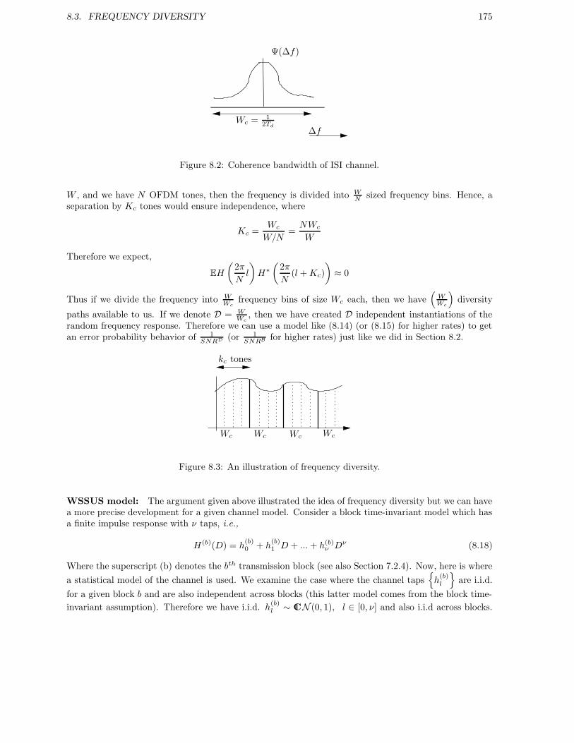
8.3. FREQUENCY DIVERSITY 175
Ψ(∆f)
Wc = 12Td
∆f
Figure 8.2: Coherence bandwidth of ISI channel.
W , and we have N OFDM tones, then the frequency is divided into WN sized frequency bins. Hence, a
separation by Kc tones would ensure independence, where
Kc =Wc
W/N=NWc
W
Therefore we expect,
EH
(2π
Nl
)H∗(
2π
N(l +Kc)
)≈ 0
Thus if we divide the frequency into WWc
frequency bins of size Wc each, then we have(
WWc
)diversity
paths available to us. If we denote D = WWc
, then we have created D independent instantiations of therandom frequency response. Therefore we can use a model like (8.14) (or (8.15) for higher rates) to getan error probability behavior of 1
SNRD (or 1SNRB for higher rates) just like we did in Section 8.2.
Wc Wc Wc Wc
kc tones
Figure 8.3: An illustration of frequency diversity.
WSSUS model: The argument given above illustrated the idea of frequency diversity but we can havea more precise development for a given channel model. Consider a block time-invariant model which hasa finite impulse response with ν taps, i.e.,
H(b)(D) = h(b)0 + h
(b)1 D + ...+ h(b)
ν Dν (8.18)
Where the superscript (b) denotes the bth transmission block (see also Section 7.2.4). Now, here is where
a statistical model of the channel is used. We examine the case where the channel tapsh
(b)l
are i.i.d.
for a given block b and are also independent across blocks (this latter model comes from the block time-
invariant assumption). Therefore we have i.i.d. h(b)l ∼ CN (0, 1), l ∈ [0, ν] and also i.i.d across blocks.

176 CHAPTER 8. SINGLE-USER COMMUNICATION
This model is widely known as the wide-sense stationary uncorrelated scattering model (WSSUS) for afading ISI Channel. We will use this model to examine the impact of frequency diversity. Note that
E [H(ω)H∗(ω +WS)] = E|h0|2 + E|h1|2ejWS + ...+ E|hν |2ejWSν
=
ν∑
n=0
ejnWS =1 − ej(ν+1)WS
1 − ejWS
Therefore for Ws = 2πν+1 , we have independence between the frequency responses for the WSSUS model.
Therefore the coherence bandwidth Wc = Wν+1 , where W is the signal bandwidth. Thus the larger ν
implies a larger frequency diversity for a given transmission bandwidth in the WSSUS model.
8.3.1 OFDM frequency diversity
Now, let us consider using OFDM for the block time-invariant (WSSUS) model given in (8.18). Thereforeif we use N carriers for each block we get, ( see Section 6.2),
Y (n) = H(2π
Nn)X(n) + Z(n), n = 0, ..., N − 1.
First, let us consider repetition coding as was done in Section 8.2.1. Here we do the repetition in frequency,i.e., X(n) = X(0), ∀n, yielding
Y (N − 1)...
Y (0)
︸ ︷︷ ︸Y
=
H(
2πN (N − 1)
)
.
.
.H(0)
︸ ︷︷ ︸H
X(0) +
Z(N − 1)...
Z(0)
︸ ︷︷ ︸Z
Y = HX(0) + Z (8.19)
Notice that (8.19) looks quite similar in form to (8.14).However we can see from (8.18) that
H =
1 ej 2πN (N−1) . . . ej 2π
N ν(N−1)
. . .
. . .
. . .1 1 . . . 1
︸ ︷︷ ︸F
h0
.
.
.hν
︸ ︷︷ ︸h
(8.20)
Note that F is truncated DFT matrix and is full rank. Using (8.20) in (8.19), we get
Y = FhX(0) + Z
A coherent detector for this will erroneously declare X′(0) to be the transmitted symbol instead of X(0)
for a given realization h with a probability of
P
(X(0) → X
′(0) | h
)= Q(
√[x′(0) − x(0)]2h∗F∗Fh
2σ2z
) (8.21)
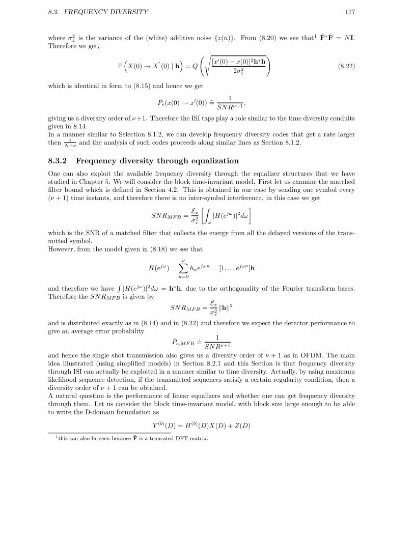
8.3. FREQUENCY DIVERSITY 177
where σ2z is the variance of the (white) additive noise z(n). From (8.20) we see that1 F∗F = NI.
Therefore we get,
P
(X(0) → X
′(0) | h
)= Q
(√[x′(0) − x(0)]2h∗h
2σ2z
)(8.22)
which is identical in form to (8.15) and hence we get
Pe(x(0) → x′(0)).=
1
SNRν+1,
giving us a diversity order of ν+1. Therefore the ISI taps play a role similar to the time diversity conduitsgiven in 8.14.In a manner similar to Selection 8.1.2, we can develop frequency diversity codes that get a rate largerthen 1
N+ν and the analysis of such codes proceeds along similar lines as Section 8.1.2.
8.3.2 Frequency diversity through equalization
One can also exploit the available frequency diversity through the equalizer structures that we havestudied in Chapter 5. We will consider the block time-invariant model. First let us examine the matchedfilter bound which is defined in Section 4.2. This is obtained in our case by sending one symbol every(ν + 1) time instants, and therefore there is no inter-symbol interference. in this case we get
SNRMFB =Ex
σ2z
[∫
ω
|H(ejω)|2dω]
which is the SNR of a matched filter that collects the energy from all the delayed versions of the trans-mitted symbol.However, from the model given in (8.18) we see that
H(ejω) =ν∑
n=0
hnejωn = [1, ..., ejων ]h
and therefore we have∫|H(ejω)|2dω = h∗h, due to the orthogonality of the Fourier transform bases.
Therefore the SNRMFB is given by
SNRMFB =Ex
σ2z
||h||2
and is distributed exactly as in (8.14) and in (8.22) and therefore we expect the detector performance togive an average error probability
Pe,MFB.=
1
SNRν+1
and hence the single shot transmission also gives us a diversity order of ν + 1 as in OFDM. The mainidea illustrated (using simplified models) in Section 8.2.1 and this Section is that frequency diversitythrough ISI can actually be exploited in a manner similar to time diversity. Actually, by using maximumlikelihood sequence detection, if the transmitted sequences satisfy a certain regularity condition, then adiversity order of ν + 1 can be obtained.A natural question is the performance of linear equalizers and whether one can get frequency diversitythrough them. Let us consider the block time-invariant model, with block size large enough to be ableto write the D-domain formulation as
Y (b)(D) = H(b)(D)X(D) + Z(D)
1this can also be seen because F is a truncated DFT matrix.

178 CHAPTER 8. SINGLE-USER COMMUNICATION
where Sz(D) = σ2z . Using the results from Section 5.4 for the MMSE-LE, we have
WMMSE−LE(D) =H∗(D−∗)Ex
H(D)H∗(D−∗)Ex + σ2z
and
SEE(D) = Ex − H(D)H∗(D−∗)E2x
H(D)H∗(D−∗)Ex + σ2z
=σ2
zEx
H(D)H∗(D−∗)Ex + σ2z
=σ2
z
H(D)H∗(D−∗) +σ2
z
Ex
Therefore we have
SNRMMSE−LE =Ex
σ2z
∫
ω
[|H(ejω)|2 +
σ2z
Ex
]−1
dω
−1
,
which depends on the random variable∫
ω
[|H(ejω)|2 +
σ2z
Ex
]−1
dω.
This computation in general is difficult, however for large SNR one can show that under suitable regularityconditions,
SNRMMSE−LE ≥ c||h||2
where c is a constant independent of h. Therefore we obtain
Pe,MMSE−LE·=
1
SNRν+1.
We did not go through the details of this argument, but one can make this more precise. Therefore, wesee that we can obtain frequency diversity through linear equalization as well.
8.4 Spatial Diversity
In this case one obtains diversity by placing multiple antennas at the transmitter and/or receiver. If theplacement is such that the sample “independent” fading in space, one obtains a similar model for diversityas in time diversity. The crucial difference is that the spatial diversity is obtained by simultaneouslytransmitting and receiving symbols and therefore one can potentially increase transmission rate.
Multiple antennas at base station
Multiple antennas at mobile
Figure 8.4: Spatial diversity: Multiple transmit and receive antennas.

8.4. SPATIAL DIVERSITY 179
8.4.1 Receive Diversity
In this case the transmitter is as before, but the reception is done through multiple antennas, i.e.,
yl(k) = hlx(k) + zl(k), l = 1, . . . ,D
where yl(k) is the signal received on lth receive antenna at time instant k, hl is the fading variable/attenuationon the lth receive antenna, zl(k) is the additive noise on lth receive antenna and x(k) is the symbol trans-mitted at time instant k. Let us focus on a particular time instant k.
y(k) =
y1(k)
...yD(k)
=
h1
...hD
︸ ︷︷ ︸h
x(k) +
z1(k)
...zD(k)
︸ ︷︷ ︸z(k)
Therefore we get
y(k) = hx(k) + z(k) (8.23)
This model seems identical to equation (8.14) and if the model for fading channel attenuation h(l) arethe same, we would get the same performance. Hence, one gets for i.i.d. spatial fading
Pe(x(k) → x′(k)).=
1
(SNR)D
Note that we get same performance as repetition coding but without the rate loss. Another way toobserve the performance of receive diversity is as follows. It can easily be shown that a sufficient statisticfor (8.23) is
y(k) = h∗y(k) =
L∑
l=1
h∗l yl(k) = ||h||2x(k) + h∗z(k)
Hence the receiver combines the signals from each antenna by weighting them according to the channelattenuation, and this is called a maximal ratio combiner. This also shows that the SNR at the receiveris ‖ h ‖2 SNR which has a form identical to (8.14) and therefore we get the same average error probabilitybehavior.Note that multiple antennas imply multiple radio frequency (RF) circuitry associated with each antennaand hence increased cost. Typically multiple antennas are available at the base station and hence one couldenvisage using them in the above manner to increase performance on “uplink”, i.e. mobile transmittingto base-station.
8.4.2 Transmit Diversity
If one has multiple antennas at the base-station, a natural question to ask is whether we can utilizethem for transmission to a mobile (i.e. “downlink” transmission). This has been an active researcharea for the past decade or so and numerous interesting results have been obtained both for coding andsignal processing schemes as well as bounds for fundamental limits of transmission (information theoreticbounds). We will illustrate some of the ideas of the topic through a simple example.
Alamouti code: Consider the scenario with 2 transmit antennas and 1 receive antenna.
y(k) = h1(k)x1(k) + h2(k)x2(k) + z(k)
y(k) = [h1(k) h2(k)]
[x1(k)x2(k)
]+ z(k) (8.24)

180 CHAPTER 8. SINGLE-USER COMMUNICATION
Now let us examine a code over 2 consecutive instants of time where we assume that the channel is blocktime-invariant, i.e.,
h1(k) = h1(k + 1) = h1, h2(k) = h2(k + 1) = h2
Moreover, let
x1(k) = x1, x1(k + 1) = x2
x2(k) = −x∗2, x2(k + 1) = x∗1
Then over two consecutive instants of time of (8.24) we get,
[y(k), y(k + 1)]︸ ︷︷ ︸y
= [h1 h2]
[x1 x2
−x∗2 x∗1
]+ [z(k), z(k + 1)]︸ ︷︷ ︸
z
(8.25)
Note that,
y(k) = h1x1 − h2x∗2 + z(k)
y(k + 1) = h1x2 + h2x∗1 + z(k + 1).
Therefore we get,
y∗(k + 1) = (h∗1x∗2 + h∗2x1) + z∗(k + 1)
Putting these together we have
[y(k), y∗(k + 1)] = [x1 x∗2]
[h1 h∗2−h2 h∗1
]+ [z(k), z∗(k + 1)]. (8.26)
Therefore, using (8.26) we get,
[y(k), y∗(k + 1)] = [x1 x∗2]︸ ︷︷ ︸
x
[h1 h∗2−h2 h∗1
]+ [z(k), z∗(k + 1)]︸ ︷︷ ︸
z
(8.27)
Claim 8.4.1. The matrix
[h1 h∗2−h2 h∗1
]is unitary.
Proof:[h1 h∗2−h2 h∗1
][h1 h∗2−h2 h∗1
]∗=
[h1 h∗2−h2 h∗1
][h∗1 −h∗2h2 h1
]
=
[|h1|2 + |h2|2 h1(−h∗2) + (h∗2)(h1)(−h2)h
∗1 + (h∗1)(h2) |h1|2 + |h2|2
]
=
[|h1|2 + |h2|2 00 |h1|2 + |h2|2
]
= (|h1|2 + |h2|2)I
Notes:
1. The form of the matrix
[h1 h∗2−h2 h∗1
]is unitary and this matrix is the linear algebraic representation
of the quaternionic group. It is a non-commutative multiplicative group.

8.4. SPATIAL DIVERSITY 181
2. There are several other forms of the 2 × 2 matrices of similar natures, e.g.,
[h1 h2
h∗2 −h∗1
],
[−h1 h2
H∗2 h∗1
],
[h1 h2
−h∗2 h∗1
]etc. . .
Some of these form multiplicative groups, and others do not.
Now, let us use this property in (8.27)
[y(k), y(k + 1)] =1
(|h1|2 + |h2|2)1/2[y(k), y∗(k + 1)]
[h∗1 −h∗2h2 h1
]
(a)=
(|h1|2 + |h2|2
)1/2[x1 x
∗2] +
1
(|h1|2 + |h2|2)1/2[z(k), z∗(k + 1)]
[h∗1 −h∗2h2 h1
]
where (a) follows due to Claim 8.4.1.
Now, since
[h∗1 −h∗2h2 h1
]is orthogonal, the noise after this transformation remains white, and because
of the factor 1(|h1|2+|h2|2)1/2 , the transformation is unitary. Therefore the noise is statistically identical to
the one before transformation. Hence we get
[y(k), y(k + 1)] = (|h1|2 + |h2|2)1/2[x1 x∗2] + [z(k) z(k + 1)]
which gives,
y(k) = (|h1|2 + |h2|2)1/2x1 + z(k)
y(k + 1) = (|h1|2 + |h2|2)1/2x∗2 + z(k + 1)
Hence, we can detect x1 and x2 independently and we get error probability behavior as
P(x1 → x′1|h) = Q
( ||h||dmin
2σ
)
P(x2 → x′2|h) = Q
( ||h||dmin
2σ
)
Therefore we get the average error probability at high SNR as,
Pe(x1 → x′1) = Eh [P(x1 → x′1|h)].=
1
SNR2
Pe(x2 → x′2).=
1
SNR2
Therefore, by using this coding scheme at the transmitter, one has utilized maximally two diversity pathswhich was available.Notes:
1. The coding scheme achieved similar performance as receive diversity i.e. getting error behavior athigh SNR as Pe
.= 1
SNR2 , yielding a diversity order of 2.
2. The decoding scheme shown is actually a maximal likelihood decoder and therefore obtains optimalperformance.
182 CHAPTER 8. SINGLE-USER COMMUNICATION
3. The decoupling of two simultaneously transmitted streams is attained in a simple manner because
of the orthogonality of the matrix
[h1 h∗2−h2 h∗1
].
4. In general if x1 and x2 each had a constellation size of |S|, the search space for a maximum likelihooddecoder would have been |S|2. Due to the coding scheme one is able to decouple the problem into2 problems of size |S| each, i.e. linear decoding complexity of O(|S|).
5. The transmission rate is still log |S|, since we transmit |S|2 information symbols in 2 time instant,i.e.,
R =1
2log |S|2 = log |S|.
6. This particularly elegant coding scheme has now become part of next generation wireless networkproposals.
7. There are several general principles that can be gleaned from this example. The idea of coding in-formation across multiple transmit antennas (i.e. “space”) and over multiple transmission instanceis called “space-time” coding. There is a deeper theory and a set of design criteria that can bederived for these class of codes which is outside the scope of this chapter.
8.5 Tools for reliable wireless communication
The main idea we learnt in this chapter was that the error probability behavior of fading channelsdiffer significantly from that of time-invariant channels. This is due to the random fluctuations of thechannel gain and this led to Pe
.= 1
SNR . In order to combat this, we needed to use multiple independentinstantiations of the channel and code acrosse them. These diversity techniques form the basis tools forincreasing reliability over wireless channels. In all the techniques we examined, we obtained an errorprobability behavior of Pe
.= 1
SNRD , by using D instantiations of randomness. This gives a significantimprovement in error probability.We saw three main diversity mechanisms.
Time diversity: Here we code over time periods longer than the coherence time of the channel andobtained the D independent channels by this mechanism. Using a single repetition code we couldget a diversity order of D. However, we can improve the transmission rate at the cost of diversityorder.
Frequency diversity: Here we exploited the “independent” variations in the random frequency responseof the ISI channel. Both equalization and multicarrier techniques yielded the maximal diversityorder of (ν + 1), where ν was the order of the WSSUS channel.
Spatial Diversity: We code across multiple transmit antennas and/or receive with multiple antennas.We saw a simple example of coded transmit diversity a.k.a. space time codes.
Using diversity is the primary tool for combating channel fading. Many modern techniques combine allthree diversity mechanisms for robust performance.
8.6 Problems
Problem 8.1
Assume the channel modely(k) = α(k)x(k) + z(k)
8.6. PROBLEMS 183
Where y(k) is the channel output, α(k) is the flat fading process, x(k) is the channel input and z(k) isthe additive white Gaussian noise of zero mean of power σ2.
1. What is the probability of error for a known value of α?
2. Calculate exactly the average probability of error.
Problem 8.2
Let y ∼ CN (0,M), Q = Q∗ (Q need not be positive definite), where M,Q ∈ CK×K . Prove that thecharacteristic function Φ(ω) of y∗Qy is given by
Φ(ω) = E[exp(jωy∗Qy)] =
K∏
n=1
1
1 − jωγn,
where γn are eigen values of the matrix MQ.
Problem 8.3
Consider the transmission of BPSK signal x = ±a. Let W has distribution CN (0, N0) and H hasdistribution CN (0, 1). Let us assume that we transmit over a flat fading channel with coherent detection
Y = HX +W.
1. Argue that r := Re(
H∗
|H|Y)
is a sufficient statistics for detection of X . Find the distribution of the
additive noise in r.
2. Find the exact expression for average (over H) probability of error for part(1) in terms of theSNR = a2/N0.
3. Assume we transmit over the AWGN channel
Y = X +W.
Find the exact expression for the probability of error in terms of SNR.
4. Compare the average error probability for the flat fading and AWGN channel for SNR = 1, 10, 102, 104, 108.
Problem 8.4
Let the channel be given byy(D − 1)
...y(0)
︸ ︷︷ ︸Y
=
h(D − 1)
...h(0)
︸ ︷︷ ︸h
x(0) +
z(D − 1)
...z(0)
︸ ︷︷ ︸z
Assume that h(l) is perfectly known at the receiver and therefore we can form a coherent detector. Ifx(0) was the transmitted symbol, then the probability that x(0) is mistaken for x′(0) is
Px(0) → x′(0)|h = P||y − hx′(0)||2 < ||y − hx(0)||2|h
= Q
( ||h||dmin
2σ
),

184 CHAPTER 8. SINGLE-USER COMMUNICATION
where ||h||2 =∑L−1
l=0 |h(l)|2.Suppose that h ∼ Cη(0,Kh), where Kh is not necessarily diagonal.
1. Find the bound on average probability of error assuming high SNR.
2. Assume that the matrix Kh is positive definite. Find the diversity order.
Problem 8.5
Suppose there is a transmitter which is sending signals to be received by two receive antennas. Howeverdue to a strange and unfortunate coincidence there is a flag fluttering in the wind quite close to one ofthe receive antennas and sometimes completely blocks the received signal.In the absence of the flag, the received signal is given by a flat fading model, (discrete time model asdone in class).
Yk =
[y1(k)y2(k)
]=
[h1(k)h2(k)
]x(k) +
[z1(k)z2(k)
](8.28)
where y1(k), y2(k) are the received signals on first and second receive antennas respectively, x(k) is thetransmitted signal and h1(k), h2(k) are respectively the fading attenuation from the transmitter to thefirst and second receive antennas. Assume that x(k) is binary, i.e. x(k) ∈ −√Ex,
√Ex. The additivenoise z1(k), z2(k) are assumed to be independent circularly symmetric complex Gaussian with variance(each) of σ2. Assume that h1(k), h2(k) are i.i.d complex Gaussian Cη(0, 1).
1. Over several transmission blocks, compute the upper bound to the error probability and commentabout the behavior of the error probability with respect to SNR for high SNR. Hint : Use the factthat Q(x) ≤ e−x2/2.
2. Now let us consider the presence of fluttering flag which could potentially block only the secondreceive antenna. The model given in (8.28) now changes to:
Yk =
[y1(k)y2(k)
]=
[h1(k)
Fkh2(k)
]x(k) +
[z1(k)z2(k)
]
where:
Fk =
1 if there is no obstruction from the flag0 if flag obstructs
Suppose due to the random fluttering, the flag blocks a fraction q of the transmissions, i.e for afraction q of the transmission, one receives only the signal from the first antenna.
Conditioned on F , write down the error probabilities, i.e find and expression for Pe(x → x′|F) andcompute its upper bound (see hint in (1)).

8.6. PROBLEMS 185
3. Find the overall error probability in the presence of the fluttering. How does the error probabilitybehave at high SNR, i.e what diversity order does one obtain.
Hint : If the error probability behaves as 1SNRD at high SNR, the diversity order is D.
Problem 8.6
We have studied time diversity with repetition coding for coherent detection. Let number of diversitypaths D = 2. A repetition coding repeats the BPSK symbol u = ±a over both the diversity paths. Inthis problem we study another coding scheme by which we need not sacrifice the rate like in the repetitioncoding. Consider instead a coding scheme
x = R
[u1
u2
].
where u1, u2 ∈ ±a and the matrix R is given by
[cos(θ) − sin(θ)sin(θ) cos(θ)
].
R is a rotation matrix (for some θ ∈ (0, 2π)). Now the received signal is given by:
yl = hlxl + zl, l = 1, 2.
where hl are i.i.d and has the distribution CN(0, 1).
1. Suppose that we transmit xA = R
[aa
]and use Re
(h∗
l yl
|hl|
)as the sufficient statistics. Use the union
bound to upper bound the probability of error.
2. What should be the condition on θ so that we obtain a diversity order of 2?
Problem 8.7
We have studied the performance of the Alamouti scheme in a system with two transmit and one receiveantenna. Suppose now we have an additional receive antenna. Assume that the channel is block timeinvariant for 2-consecutive transmissions. Let the input be BPSK i.e. xi ∈ ±a and we assume coherentdetection.
1. Denote the received vector (with appropriate conjugation of the components as required in theAlamouti scheme) at the two receiving antennas over two consecutive transmissions by y ∈ C4. Let
the channel model be y = H
[x1
x2
]+ z, where z ∈ C4 and has the distribution CN(0, N0I4). Write
down explicitly y,H.
2. Show that the columns of H are orthogonal. Using this show that projection of y on the normalized
column vectors of H gives sufficient statistics for
[x1
x2
].
3. Write down the ML decision rule and find the upper bound on average probability of error. Findthe diversity gain for this scheme.

186 CHAPTER 8. SINGLE-USER COMMUNICATION
Problem 8.8
1. Show that 1x−x0≥0 ≤ eγ(x−x0). Using this, prove Pr(x ≥ x0) ≤ E[eγ(x−x0)] for any γ > 0.
2. Use this to prove an upper bound for Pr(||y − hx|| ≥ ||y − hx′|| |h, x) where y = hx+ z. (here youwould get the exponential bound). Optimize w.r.t γ to get the e−h∗(x−x′)(x−x′)∗h/4σ2 bound.
3. From here, use the distribution of h to get the 1/SNR type of behaviour.
Problem 8.9
Show that the quaternionic group is a non-commutative multiplicative group.
Appendices for Chapter 8
8.A Exact Calculations of Coherent Error Probability
First let us examine the probability distribution of |h|.Since,
|h|2 = [Re(h)]2+ [Im(h)]
2
where Re(h) ∼ N (0, 12 ) and Im(h) ∼ N (0, 1
2 ) as h is a circular symmetric Complex Gaussian randomvariable. It can be therefore seen2 that if u = |h|2,
fV (u) = e−u (8.29)
Now, using (8.29) in (8.4) we get
Pe =
∫ ∞
u=0
e−uQ(a√u)du
where we have defined a = dmin
2σz. Therefore we can write
Pe =
∫ ∞
u=0
e−u
[∫ ∞
√2a
√u
1√2πe−
v2
2 dv
]du =
∫ ∞
v=0
1√2πe−
v2
2
[∫ v2
a2
0
e−udu
]dv
=
∫ ∞
v=0
1√2πe−
v2
2 (1 − e−v2
a2 )dv =1
2−∫ ∞
v=0
1√2πe−v2[ 1
2+ 1a2 ]dv
=1
2− γ
∫ ∞
v=0
1√2πγ
e− v2
2γ2 dv =1
2[1 − γ]
where γ2 = 11+ 2
a2.
Hence
Pe =1
2
1 − 1√
1 + ( 2a2 )
=
1
2
1 − 1√
1 +8σ2
z
d2min
. (8.30)
2Since Re(h) and Im(h) are i.i.d. real Gaussian random variables, [Re(h)]2 and [Im(h)]2 are also i.i.d. with density
function PV (v) = 1√2πv
e− v
2σ2 , where v = Re(h) or v = Im(h), and σ2 = E[Re(h)]2 = E[Im(h)]2 = 12. Hence the
characteristic function of [Re(h)]2 is E[ejω[Re(h)]2 ] = 1
(1−j2ωσ2)12
. This allows us to write the characteristic function of
[Re(h)]2 + [Im(h)]2 as 11−j2ωσ2 , and hence the inverse Fourier transform of this yields (8.29).

8.B. NON-COHERENT DETECTION: FAST TIME VARIATION 187
8.B Non-coherent detection: fast time variation
In order to illustrate rapid time variation we consider extremely small block sizes, i.e., blocks of size one,which yields
y(k) = h(k)x(k) + z(k)
where h(k) are Gaussian with a given covariance. If we want to do maximum-likelihood detection, weform, PY |X(y|x). Note that here h(k) is also a source of randomness and hence for each k we have,
PY |X(y|x) ∼ CN(0,E[|h|2]
|x|2 + σ2
z
)(8.31)
Therefore as one would expect from this relationship the maximum likelihood criterion takes a form thatis substantially different from what we were used to in Section 8.1.1.Let us form the detector for a sequence of transmitted symbols. Furthermore, let us assume that for theshort interval of the transmission the channel has a given statistical variation. With no loss in generalitylet us assume that we transmit a block of K symbols from time 0 to K − 1
y =
y(K − 1)
...y(0)
=
h(K − 1) 0
. . .
0 h(0)
︸ ︷︷ ︸H
x(K − 1)
...x(0)
︸ ︷︷ ︸X
+
z(K − 1)
...z(0)
︸ ︷︷ ︸Z
=
x(K − 1)
. . .
x(0)
︸ ︷︷ ︸X
h(K − 1)
...h(0)
︸ ︷︷ ︸h
+z (8.32)
For a given X , using the same idea as in (8.31), we get for (8.32)
y ∼ CN (0,XE [hh∗]X ∗ + σ2zIK)
where Rh = E [hh∗] depends on the time-correlation of the (fading) channel random process. For themaximum likelihood rule, we have
PY|X(y|x) =1
π|XRhX ∗ + σ2zIK | exp
(−y∗[XRhX ∗ + σ2
zIK ]−1y)
Therefore the log-likelihood is,
log PY|X(y|x) = − logπ − log |XRhX ∗ + σ2zIK | − y∗[XRhX ∗ + σ2
zIK ]−1y
Consider the important special case when |x(i)|2 = Ex, i.e. we have a constant modulus constellation(e.g., PSK).Hence if |x(i)|2 = Ex then XX ∗ = ExIK , hence
|XRhX ∗ + σ2zIK | = |XRhX ∗ +
σ2z
ExXX ∗|
= |X (Rh +σ2
z
ExIK)X ∗|
(a)=
∣∣∣∣[Rh +
σ2z
ExIK
]Ex
∣∣∣∣

188 CHAPTER 8. SINGLE-USER COMMUNICATION
where (a) follows because |x(i)|2 = Ex ∀i.Hence we get the maximum likelihood rule as,
x = argmaxx
−y∗ [σ2
zIK + XRhX ∗]−1y
(8.33)
Now by the matrix inversion lemma, Lemma 5.7.1 we have
[σ2
zIK + XRhX ∗]−1=
1
σ2z
IK − 1
σ2z
X(R−1
h +XX ∗
σ2z
)−11
σ2z
X ∗
Therefore using this in (8.33) we get
x = argmaxx
y∗X
[R−1
h +XX ∗
σ2z
]−1
X ∗y
= argmaxx
y∗X
[R−1
h +Ex
σ2z
IK
]−1
X ∗y
(8.34)
This projects the received signal onto the space spanned by the codeword and a weighted norm is taken.This idea of projecting the received signal onto the space spanned by the codewords is actually a usefuland important idea for non-coherent detection.We can recover from this the result in Section 8.1.2. For the block time-invariant model considered therewe have,
Rh = 11t
where 1t = [1, . . . , 1]. Then, the detection criterion given in (8.33) becomes,
x = arg maxx
−y∗ [σ2
zIK + X11tX ∗]−1y
(8.35)
Now,
X1 =
x(N − 1)
...x(0)
= x.
Therefore using this in (8.35) we have
[σ2
zIK + xx∗]−1=
1
σ2z
IK − 1
σ2z
x
(1 +
x∗x
σ2z
)−11
σ2z
x∗.
Hence the criterion becomes,
x = arg maxx
y∗xx∗y(1 + ExK
σ2z
)(σ2
z)2
.
If |x(i)|2 = Ex we get x∗x = NEx, therefore we have
x = argmaxx
|x∗y|2 1
(σ2z)2(1 + ExK
σ2z
)
= arg max
x|x∗y|2 ,
which is the same criterion derived in Section 8.1.2.

8.C. ERROR PROBABILITY FOR NON-COHERENT DETECTOR 189
8.C Error probability for non-coherent detector
Let us consider the error probability for the non-coherent detector given in 8.1.2. For such a detector, ifx was sent we detect it to be x 6= x if
P x → x = P
1
(σ2z)2
|x∗y|2 < 1
(σ2z)2
|x∗y|2
= P
1
(σ2z)2
y∗ [xx∗ − xx∗]y > 0
(8.36)
Let us define
Q =1
(σ2z)2
xx∗ − xx∗
and notice that since x was transmitted
y ∼ CN (0,xx∗ + σ2zIK).
So we have the error probability of a Gaussian quadratic form where
Px → x = Py∗Qy > 0.
and Q = Q∗, but need not be positive-semidefinite, i.e., could have negative eigenvalues.
Lemma 8.C.1. If y ∼ CN (0,M) and Q = Q∗, then
P y∗Qy > 0 =∑
γi<0
K∏
n=1
(1
1 − γn
γi
)
where M ∈ CK×K and γn are the eigenvalues of MQ.
Proof: The characteristic function of y∗Qy is given by
Φ(ω) = E exp (jωy∗Qy) =
K∏
n=1
1
1 − jωγn
where γn are the eigenvalues of the matrix MQ.Therefore, the error probability is
P x → x = P y∗Qy > 0 (8.37)
=
∫ ∞
0
[1
2π
∫ ∞
−∞Φ(ω)e−jωudω
]du
=1
2π
∫ ∞
−∞Φ(ω)
[∫ ∞
0
e−jωudu
]dω
=1
2π
∫ ∞
−∞Φ(ω)
[πδ(ω) − 1
jω
]dω
=1
2
∫ ∞
−∞Φ(ω)δ(ω)dω − 1
2π
∫ ∞
−∞
1
jω
K∏
n=1
1
(1 − jωγn)dω
=1
2− 1
2π
∫ ∞
−∞
1
jω
K∏
n=1
(1
1 − jωγn
)dω
In order to evaluate this integral we use the residue theorem which is stated for convenience below.

190 CHAPTER 8. SINGLE-USER COMMUNICATION
Theorem 8.C.1. (Residue theorem) Let f(z) be a function which is analytic inside a simple closedpath C and on C, except for a finitely many singular points a1, . . . , am inside C. Then
∫
Cf(z)dz = 2πj
m∑
i=1
Resf(z)z=ai
where for a simple pole ai of f(z), Resf(z)z=ai= (z − ai)f(z)|z=ai .
In order to use this result we use the integral path on the upper half of the C plane in (8.38). Noticethat,
1
1 − jωγn=
jγ−1n
jγ−1n + ω
Therefore using this and the residue theorem 8.C.1 we get,
1
2− 1
2π
∫ ∞
−∞
1
jω
K∏
n=1
(1
1 − jωγn
)dω =
1
2−
1
2−∑
γi<0
K∏
n=1,n6=i
(1
1 − γn
γi
)
Therefore, we get the stated result,
P x → x =∑
γi<0
K∏
n=1
(1
1 − γn
γi
).
Let u1 = 1σ2
zx∗y, u2 = 1
σ2zx∗y. Clearly, u1 and u2 are scalar complex Gaussian random variables.
E|u1|2 =1
(σ2z)2
x∗[σ2zI + xx∗]x = Kρ+
1
(σ2z)2
|x∗x|2 = Kρ+ |ρKβ|2
E|u2|2 =1
(σ2z)2
KExσ
2z + (KEx)2
= Kρ[1 +Kρ]
Eu1u∗2 =
1
(σ2z)2
x∗[σ2zI + xx∗]x = Kρβ +KρβKρ = (Kρβ)[1 + ρK]
where we have defined x∗x = ExKβ and ρ = Ex
σ2z. Using this in (8.36) we get,
Px → x = P|u1|2 − |u2|2 > 0
= P
[u∗1, u
∗2]
[1 00 −1
][u1
u2
]> 0
.
Now let us use this in Lemma 8.C.1, we get
M =
[Kρ(1 +Kρ|β|2), (Kρβ)[1 + ρK](Kρβ∗)[1 + ρK], Kρ[1 +Kρ]
]
Also we have
Q =
[1 00 −1
].

8.C. ERROR PROBABILITY FOR NON-COHERENT DETECTOR 191
Clearly, the conditions of of Lemma 8.C.1 are satisfied and so we need the eigenvalues of MQ. Now wehave,
MQ =
[Kρ(1 +Kρ|β|2), −(Kρβ)[1 + ρK](Kρβ∗)[1 + ρK], −Kρ[1 +Kρ]
]
= Kρ[1 + ρK]
[1+Kρ|β|2[1+ρK] , −ββ∗, −1
]
Therefore the eigenvalues of MQ are,
γ1 = Kρ[1 + ρK]λ1
γ2 = Kρ[1 + ρK]λ2
where λ1, λ2 are the eigenvalues of [1+Kρ|β|2[1+ρK] , −ββ∗, −1
]
and hence for Γ = 1+Kρ|β|21+Kρ , we have
λ1 =1
2
(Γ − 1) −
√(Γ − 1)2 + 4(Γ − |β|2)
λ2 =1
2
(Γ − 1) +
√(Γ − 1)2 + 4(Γ − |β|2)
and observing that 1 − Γ = Kρ(1−|β|2)1+Kρ and Γ − |β|2 = 1−|β|2
1+Kρ , we get,
λ1 =1
2(1 +Kρ)
−Kρ(1− |β|2) −
√Kρ(1 − |β|2)2
+ 4(1 − |β|2)(1 +Kρ)
< 0
λ2 =1
2(1 +Kρ)
−Kρ(1− |β|2) +
√Kρ(1 − |β|2)2
+ 4(1 − |β|2)(1 +Kρ)
> 0
Hence we have,
γ1 =(Kρ)2(1 − |β|2)
2
−1−
√1 +
4(1 +Kρ)
(Kρ)2(1 − |β|2)
< 0
γ2 =(Kρ)2(1 − |β|2)
2
−1 +
√1 +
4(1 +Kρ)
(Kρ)2(1 − |β|2)
> 0
Using Lemma 8.C.1, we get
Px → x =1
1 − γ2
γ1
=−γ1
γ2 − γ1
Hence we get at high SNR,
Px → x ·=
1
SNR.
Therefore the high SNR behavior of the error probability is like 1SNR , which is like the coherent case.

192 CHAPTER 8. SINGLE-USER COMMUNICATION

Chapter 9
Multi-user communication
The wireless propagation medium is (almost by definition!) shared by many simultaneously transmittingusers. For example one has seen that several people use their mobile phones simultaneously in a smallgeographical area. Therefore, these users’ signals would overlap and interfere with one another. Inthis chapter we study basic communication topologies which arise in wireless networks. We study howmultiple users can share and access common resources. After studying these in Section 9.1, we focus ourattention on multiple access channels in Section 9.3 and 9.4. In Section 9.2 we will study different accesstechniques for multiuser channels. In Section 9.3, we set up the model and sufficient statistics for themultiple access problem. In Section 9.4 we study multi-user detectors that naturally generalize some ofthe ideas from Chapter 4 and 5.
9.1 Communication topologies
In order to build a multiuser wireless network the first question is how to share the common “channel”resources among the different users.
To address this question let us first examine the various configurations that can arise in multiuser net-works. There are two categories of configurations. One is hierarchical where there is a central accesspoint and users communicate to the access point. The other configuration could be where the users areallowed to communicate directly to one another perhaps using other users as relays. Such configurationsare called ad hoc networks and we briefly talk about them in Section 9.1.2.
9.1.1 Hierarchical networks
In most current wireless systems there are two main hierarchical configurations that are used.
Broadcast Base-station to user (one-to-many) broadcast or downlink communication.
Multiple access Users to base-station (many-to-one) multiple access or uplink communication.
These configuration are shown in figures 9.1 and 9.2. In the “downlink” broadcast communication, the(server) base-station communicates to the users. This can be the case where the base-station sendsinformation like web-downloads or voice information to the mobile user.
The “uplink” multiple access communication is exactly the reverse of this, i.e., many users send informa-tion (to be transferred) to the base-station (server). This could occur when the users send a request, orupload data or are sending a voice message/conversation to the base-station intending it to be forwardedto its final destination.
193

194 CHAPTER 9. MULTI-USER COMMUNICATION
Mobileuser
Mobileuser
WirelessLaptopuser
Base-station
Figure 9.1: Base-station to user (one-to-many) broadcast/downlink communication.
Mobileuser
WirelessLaptopuser
Mobileuser Base-station
Figure 9.2: Users to base-station (many-to-one) multiple access/uplink communication.
In both cases, the users receive/transmit signals “simultaneously”. Therefore, in order to help distinguishthe signals from the different users, typically the channel resources (time, frequency) are divided amongthe users. This idea leads to the main “channel access” techniques used in current systems. Theseaccess schemes are called Time-Division Multiple Access (TDMA), Frequency-Division Multiple Access(FDMA) and Code-division Multiple Access (CDMA).
9.1.2 Ad hoc wireless networks
In contrast to hierarchical networks where we have a base-station serving a cluster of mobiles (see Figures9.1 and 9.2) another configuration is where there is no central infrastructure. These networks variouslycalled ad hoc networks, self organized networks, mesh networks etc. They are primarily used in militaryapplications where there was a need to have an architecture without clear vulnerabilities. In an ad hocnetwork, the mobiles can form any configuration depending on the communication conditions and needs.The most distinct feature of such network is the use of relays to transmit information from one node toanother. This is illustrated in figure 9.3.
For example, if source node S wants to transmit to destination T it can transmit through several al-ternate routes depending on the transmission conditions. For example in Figure 9.3, route 1, relays theinformation through relay node A, and route 2 sends it through nodes B and C.
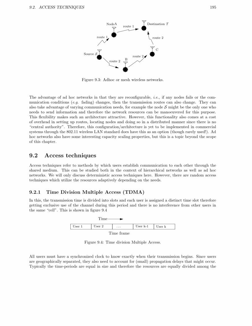
9.2. ACCESS TECHNIQUES 195
C
route 2
Source S
NodeA Destination T
B
route 1
route 2
route 2route 1
Figure 9.3: Adhoc or mesh wireless networks.
The advantage of ad hoc networks in that they are reconfigurable, i.e., if any nodes fails or the com-munication conditions (e.g. fading) changes, then the transmission routes can also change. They canalso take advantage of varying communication needs, for example the node S might be the only one whoneeds to send information and therefore the network resources can be manoeuvered for this purpose.This flexibility makes such an architecture attractive. However, this functionality also comes at a costof overhead in setting up routes, locating nodes and doing so in a distributed manner since there is no“central authority”. Therefore, this configuration/architecture is yet to be implemented in commercialsystems through the 802.11 wireless LAN standard does have this as an option (though rarely used!). Adhoc networks also have some interesting capacity scaling properties, but this is a topic beyond the scopeof this chapter.
9.2 Access techniques
Access techniques refer to methods by which users establish communication to each other through theshared medium. This can be studied both in the context of hierarchical networks as well as ad hocnetworks. We will only discuss deterministic access techniques here. However, there are random accesstechniques which utilize the resources adaptively depending on the needs.
9.2.1 Time Division Multiple Access (TDMA)
In this, the transmission time is divided into slots and each user is assigned a distinct time slot thereforegetting exclusive use of the channel during this period and there is no interference from other users inthe same “cell”. This is shown in figure 9.4
User 1 User 2 . . . User k-1 User k
Time frame
Time
Figure 9.4: Time division Multiple Access.
All users must have a synchronized clock to know exactly when their transmission begins. Since usersare geographically separated, they also need to account for (small) propagation delays that might occur.Typically the time-periods are equal in size and therefore the resources are equally divided among the

196 CHAPTER 9. MULTI-USER COMMUNICATION
users. Some recent proposals use unequals slots or assign more than one slot to a user in order to givedifferentiated services to the users. TDMA is implemented in several current wireless systems, both inthe USA, Europe and in Japan. These systems are used for mobile telephony are called IS-136, GSM etc.
9.2.2 Frequency Division Multiple Access (FDMA)
This is the frequency dual of TDMA, where instead of time, frequency is broken up into slots and usersare assigned exclusive use of the small piece of the frequency spectrum. Again, this is used for bothuplink and downlink. Most commercial systems use both TDMA and FDMA to divide the resources.The frequency is divided and then each part could be further divided using TDMA. A more modernmethod for FDMA involves use of OFDM which we have seen in Section 6.2. In this, the users transmiton a wide bandwidth and they are assigned “carriers” or “tones” of the OFDM scheme. They transmit(or listen) only on those tones and these tones can also be dynamically allocated. The advantage ofOFDM is the flexibility in assignment and the ability to dynamically change it as well as data rates onthe tones depending on the channel condition of the different users.
9.2.3 Code Division Multiple Access (CDMA)
CDMA is philosophically slightly different from TDMA and FDMA in that the users do interfere withone another since they are allowed to transmit simultaneously. The idea is to assign a “spreading code”to each user so as to minimize the interference. There are two flavors of CDMA - frequency hoppedCDMA and direct-sequence CDMA. Both arise from “spread-spectrum” techniques which transmit overa wide bandwidth and only transmit at a rate much smaller than the transmission bandwidth could haveallowed.
• Frequency-hopped spread spectrum: Here we can imagine a combination of FDMA andTDMA, where a random assignment of frequency and time slots is given to each user. This isillustrated in Figure 9.5 in a time frequency grid.
!! ""
frequencybins
User 1
User 2
User k
time slots
Figure 9.5: Frequency hopped spread Spectrum.
The users’ “hopping pattern” are basically the frequency bin they transmit in at a certain time.Therefore, if they are assigned random hopping patterns, they could in principle “collide” i.e. getassigned same transmission slot. Also note that they transmit over much larger bandwidth overall,than their data rate requires, i.e., they use many more degrees of freedom than their transmissionneeds. This gives it the name spread-spectrum, since the signals spread over a large bandwidth.This spreading over a wide bandwidth is in order to accommodate other simultaneously transmittingusers. This form of frequency-hopping is also used in some modern TDMA/FDMA systems in order
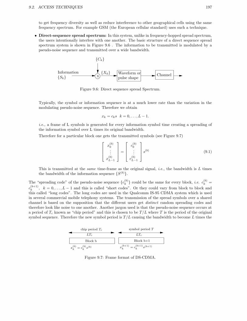
9.2. ACCESS TECHNIQUES 197
to get frequency diversity as well as reduce interference to other geographical cells using the samefrequency spectrum. For example GSM (the European cellular standard) uses such a technique.
• Direct-sequence spread spectrum: In this system, unlike in frequency-hopped spread spectrum,the users intentionally interfere with one another. The basic structure of a direct sequence spreadspectrum system is shown in Figure 9.6 . The information to be transmitted is modulated by apseudo-noise sequence and transmitted over a wide bandwidth.
Waveform orpulse shape
Ck
XkSkInformation
Channelx
Figure 9.6: Direct sequence spread Spectrum.
Typically, the symbol or information sequence is at a much lower rate than the variation in themodulating pseudo-noise sequence. Therefore we obtain
xk = cks k = 0, . . . , L− 1.
i.e., a frame of L symbols is generated for every information symbol time creating a spreading ofthe information symbol over L times its original bandwidth.
Therefore for a particular block one gets the transmitted symbols (see Figure 9.7)
x(b)0...
x(b)L−1
=
c(b)0...
c(b)L−1
s
(b) (9.1)
This is transmitted at the same time-frame as the original signal, i.e., the bandwidth is L timesthe bandwidth of the information sequence S(b).
The “spreading code” of the pseudo-noise sequence c(b)k could be the same for every block, i.e. c(b)k =
c(b+1)k , k = 0, . . . , L − 1 and this is called “short codes”. Or they could vary from block to block and
this called “long codes”. The long codes are used in the Qualcomm IS-95 CDMA system which is usedin several commercial mobile telephony systems. The transmission of the spread symbols over a sharedchannel is based on the supposition that the different users get distinct random spreading codes andtherefore look like noise to one another. Another jargon used is that the pseudo-noise sequence occurs ata period of Tc known as “chip period” and this is chosen to be T/L where T is the period of the originalsymbol sequence. Therefore the new symbol period is T/L causing the bandwidth to become L times the
Block b Block b+1
x(b)k
= c(b)k
s(b) x(b+1)k
= c(b+1)k
s(b+1)
LTc
chip period Tc symbol period T
LTc
Figure 9.7: Frame format of DS-CDMA.

198 CHAPTER 9. MULTI-USER COMMUNICATION
original bandwidth. The power per symbol transmitted is reduced by a factor of L and therefore reducethe interference to the other users. In a multiple access area broadcast configuration, by considering theother users as undesired noise-like interference, one can see that a simple single user receiver can be built.We will study more sophisticated receivers that take into account presence of multiple users. Note that,“spreading gain” refers to the length L of the spreading code.
9.3 Direct-sequence CDMA multiple access channels
We will focus on one hierarchical configuration - the many-to-one communication of the wireless “uplink”(see Figure 9.2). In the TDMA and FDMA access techniques, the users do not interfere with oneanother and therefore the detection techniques discussed in the first part of the class (for single-usercommunication) apply directly and there is no need for further discussion. The problem becomes moreinteresting for direct sequence CDMA (or spread spectrum) where the users continuously interfere withone another.
9.3.1 DS-CDMA model
Recall from (9.1) that in Direct-sequence CDMA (DS-CDMA) each user u is assigned a distinct spreadingcode for each information block b, i.e., a code sequence
c(b)u (0), . . . , c(b)u (L− 1)
,
for user u, in block b, of length L. Therefore each user modulates its information sequence s(b)u through
its spreading sequence to produce
x(b)u (l) = c(b)u (l)s(b)u , l = 0, . . . , L− 1
x(b)u =
x(b)u (0)
...
x(b)u (L− 1)
=
c(b)u (0)
...
c(b)u (L− 1)
s
(b)u (9.2)
Given the multiple access configuration (see figure 9.2), each user u transmits to the (central) base-station.
User 1
User 2
Base-station
X(b)1
X(b)2
User U X(b)U
Figure 9.8: DS-CDMA multiple access channel
Each user experiences its own fading channel h(b)u (l), l = 0, . . . , L−1. For simplicity we make the following
assumptions.

9.3. DIRECT-SEQUENCE CDMA MULTIPLE ACCESS CHANNELS 199
Assumption # 1: All users are synchronized both at block and at chip level, i.e. their transmission framescoincide exactly.Assumption # 2: The power of each user is adjusted such that the channel fading (or attenuation) isexactly compensated.
This assumption implies that we can consider a unit gain channel for each user. This can be accom-plished by user “power control” where the users change their transmit power according to feedback givenby the base-station. Such a mechanism is commonly used in commercial DS-CDMA systems to reducethe received power disparity among the users.Assumption # 3: The delay spread in the channel is small in comparison to the symbol period T andtherefore the channel does not give rise to intersymbol interference. This assumption is mainly for simplic-ity and can be easily taken care of with more sophisticated receivers. In order to illustrate the conceptswe will not deal with this issue right now.
Under these assumptions we can write the received signal at the base-station as (see figure 9.2 and 9.8)
y(b)(t) =
U∑
u=1
s(b)u ϕu(t) + z(b)(t), t ∈ ((b− 1)T, bT )
ϕ(b)u (t) =
L−1∑
l=0
c(b)u (l)ψ(t− lTc), t ∈ ((b− 1)T, bT ) (9.3)
where z(b)(t) is additive (Gaussian) receiver noise.
The basis expansion ϕu(t) for each user is in terms of a waveform at the “chip” level, i.e, ψ(t) shifted at“chip” period Tc. The symbol period is T = LTc, where L is the spreading gain. The waveform ϕu(t)serves as a signature waveform for user u.
9.3.2 Multiuser matched filter
The continuous time waveform equation (9.3) is the same type of relationship as we encountered in thesingle-user case. Therefore, the optimal detector for this can be found by considering this as a larger
dimensional single-user problem, i.e. s(b) = [s(b)1 , . . . , s
(b)U ] as the input symbol expressed in the basis
function ϕ(b)(t) = [ϕ(b)1 (t), . . . , ϕ
(b)U (t)]. Then as shown in Section 4.2.1 we have seen that the optimum
receiver is a bank of matched filters as shown in Figure 9.9.
Therefore we can write the output of the matched as,
y(b)1 =
∫ bT
(b−1)T
y(b)(t)ϕ(b)∗1 (t)dt =
U∑
u=1
s(b)u < ϕ(b)u , ϕ
(b)1 > +< z(b), ϕ
(b)1 >︸ ︷︷ ︸
Z(b)1
...
y(b)U =
∫ bT
(b−1)T
y(b)(t)ϕ(b)∗U (t)dt =
U∑
u=1
s(b)u < ϕ(b)u , ϕ
(b)U > +< z(b), ϕ
(b)U >︸ ︷︷ ︸
z(b)U
Hence, we see that
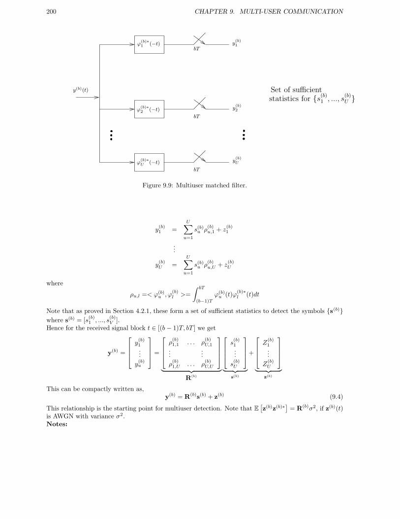
200 CHAPTER 9. MULTI-USER COMMUNICATION
bT
bT
bT
y(b)(t)
ϕ(b)∗1 (−t)
ϕ(b)∗2 (−t)
ϕ(b)∗U
(−t)
y(b)2
y(b)U
y(b)1
Set of sufficientstatistics for s(b)
1 , ..., s(b)U
Figure 9.9: Multiuser matched filter.
y(b)1 =
U∑
u=1
s(b)u ρ(b)u,1 + z
(b)1
...
y(b)U =
U∑
u=1
s(b)u ρ(b)u,U + z
(b)U
where
ρu,l =< ϕ(b)u , ϕ
(b)l >=
∫ bT
(b−1)T
ϕ(b)u (t)ϕ
(b)∗l (t)dt
Note that as proved in Section 4.2.1, these form a set of sufficient statistics to detect the symbols s(b)where s(b) = [s
(b)1 , ..., s
(b)V ].
Hence for the received signal block t ∈ [(b− 1)T, bT ] we get
y(b) =
y(b)1...
y(b)u
=
ρ(b)1,1 . . . ρ
(b)U,1
......
ρ(b)1,U . . . ρ
(b)U,U
︸ ︷︷ ︸R(b)
s(b)1...
s(b)U
︸ ︷︷ ︸s(b)
+
Z(b)1...
Z(b)U
︸ ︷︷ ︸z(b)
This can be compactly written as,y(b) = R(b)s(b) + z(b) (9.4)
This relationship is the starting point for multiuser detection. Note that E[z(b)z(b)∗] = R(b)σ2, if z(b)(t)
is AWGN with variance σ2.Notes:

9.4. LINEAR MULTIUSER DETECTION 201
1. The form and structure of the receiver is very similar to the single user case. The difference isthat there are U information sequences to be recovered (one for every user). The conversion of thewaveform to discrete-time through collecting sufficient statistics is identical to the simple-user caseand we do not dwell on this issue further.
This is an important point that should not be neglected. As in the single-user presentation we startfrom the discrete-time version here as well.
2. In the relationship (9.4), we can add more details such as the channel attenuations h(b)u (l), de-
layed symbols causing inter-symbol interference as well as asynchronism between users. However,conceptually all these are handled in a similar manner and therefore for simplicity of exposition,these are ignored.
3. If short codes are employed, c(b) would be independent of the block index b. However for longcodes, this dependence exists and therefore the model in (9.4) applies to both cases.
4. The linear relationship in (9.4) is reminiscent of the single-user ISI channel relationship. Thereforeone would expect schemes to detect s(b) would also be similar. In fact all multiuser detections
have an analogous ISI detector structure. Here we consider [s(b)1 , . . . , s
(b)U ] as a “sequence” of vector
information symbols.
5. In the absence of ISI or asynchronism, we can do symbol-by-symbol detection, i.e., we detect
s(b) = [s(b)1 , . . . , s
(b)U ] by considering only y(b) and therefore for brevity of notation we will drop the
index b.
6. The optimal detector would have complexity O(|S|U ) where S is the size of the constellation (com-mon for each user for simplicity). All the principles of optimal detection we developed for the single
user case apply here by considering the symbol to be detected as
s(b)1...
s(b)U
and therefore we will
not repeat it here (e.g. MAP, ML, etc.).
7. Where there is a large number of users U , the complexity grows exponentially in U and therefore weexamine sub-optimal detectors. The reason is almost identical to the cause for looking at suboptimalequalizers of lower complexity for ISI channels. In fact the mathematical model given in (9.4) isidentical in form to that in the ISI model we had developed for the finite block case.
9.4 Linear Multiuser Detection
Motivated by the last comment in Section 9.2.2, we examine sub-optimal linear detectors for the DS-CDMA multiple access channel. We assume that the symbols are i.i.d. and therefore we can do symbol-by-symbol detection rather than sequences detection.Let us rewrite (9.4) here without the cumbersome additional block index b. This is because we knowthat ”symbol-by-symbol” detection is optimal for this case and we develop linear ”symbol-by-symbol”detections.
y = Rs + z (9.5)
The model is similar to the finite block ISI model and we considered two types of linear detections of lowercomplexity, i.e., the zero-forcing and the MMSE receivers. In the multiuser case as well, the analogousdetectors are called the “decorrelating receivers” and the “MMSE linear detector”.

202 CHAPTER 9. MULTI-USER COMMUNICATION
9.4.1 Decorrelating receiver
In analogy with the ISI case, we want to recover a particular symbol su from the interfering symbols in(9.5). Therefore in the zero-forcing case we invert the ”channel”. In this case the role of the channel istaken by the cross-correlation matrix R.
R−1y = s + R−1z
and then we can find the symbol for each user u as,
su = D[(R−1y)u]
where D is a single-user detector for the given Gaussian noise (see also Figure 9.10).
R−1
D
D(R−1y)1
(R−1y)U
s1
sU
y
Figure 9.10: Decorrelating multiuser detector
This receiver has the same attributes as the zero forcing detector equalizer, i.e., it is conceptually simpleand ignores the background noise. Therefore it could cause noise enhancement especially if R is close tobeing singular. Therefore, we can take the next step of accounting for the presence of noise and developthe MMSE linear multiuser detector.
9.4.2 MMSE linear multiuser detector
We want to find a linear transformation M such that output is “close” to the information symbols, i.e.,My is close to s.The meaning of “close” is make precise by considering the MMSE metric and therefore we pose theproblem as
minM∈C
U×UE[||s−My||2
]
Now, by using orthogonality principle, we get
E [(s−My)y∗] = 0,
This yields
E [sy∗] = ME [yy∗]
M = E [sy∗] [E [yy∗]]−1 (9.6)
Now
E [sy∗] = E [ss∗]R∗ = EsIR∗
E [yy∗] = RE [ss∗]R∗ + E [zz∗]
= EsRR∗ + σ2R (9.7)

9.4. LINEAR MULTIUSER DETECTION 203
where we have assumed equal power Es for each user and independent symbols, i.e. E [ss∗] = EsI.Moreover since the noise z is the output of the matched filter (see Figure 9.11) and equation (9.4), thenoise has covariance σ2R = E [zz∗].Using (9.7) in (9.6) we get,
M = EsR∗(EsRR∗ + σ2R)−1
Since R is a cross-correlation matrix of the signature waveforms, (9.4), it is symmetric, i.e., R∗ = R andtherefore
M =
(R +
σ2
EsI
)−1
in the MMSE-optimal linear multiuser detector. The MMSE-linear multiuser detector is depicted inFigure 9.11.
y(t)
ϕ∗1(−t)
ϕ∗U
(−t)
bT
bT
y(b)1
y(b)U
“
R + σ2
ESR
”−1
s(b)1
s(b)U
Figure 9.11: Receiver for linear multiuser detection.
Therefore even if R is singular, M is well defined and does not cause noise enhancement. Moreover justas in the linear equalizers if we let σ2/Es → 0 the MMSE linear detector reduces to the decorrelatingreceiver.Notes:
1. The main utility of multiuser detection is the resistance to the “near-far” problem. Here the userscould have very disparate received power and the strong user could ”drown” out the weak user.All the forms of multiuser detections do exhibit resistance to this problem. We have not explicitlyexhibited them since we assumed equal received power for all users. However a simple modification
to (9.4) would take care of this. If each user u has received power A(b)u , then
y(b) =
ρ(b)1,1 . . . ρ
(b)U,1
......
ρ(b)1,U . . . ρ
(b)U,U
︸ ︷︷ ︸R(b)
A1 0
. . .
0 AU
︸ ︷︷ ︸A(b)
s(b)1...
s(b)U
︸ ︷︷ ︸s(b)
+
z(b)1...
z(b)U
︸ ︷︷ ︸z(b)
.
In more compact form,y(b) = R(b)A(b)s(b) + z(b)
Then the (zero-forcing) decorrelating receiver remains
A(b)s(b) = R−1y(b) = A(b)s(b) + R−1z(b)
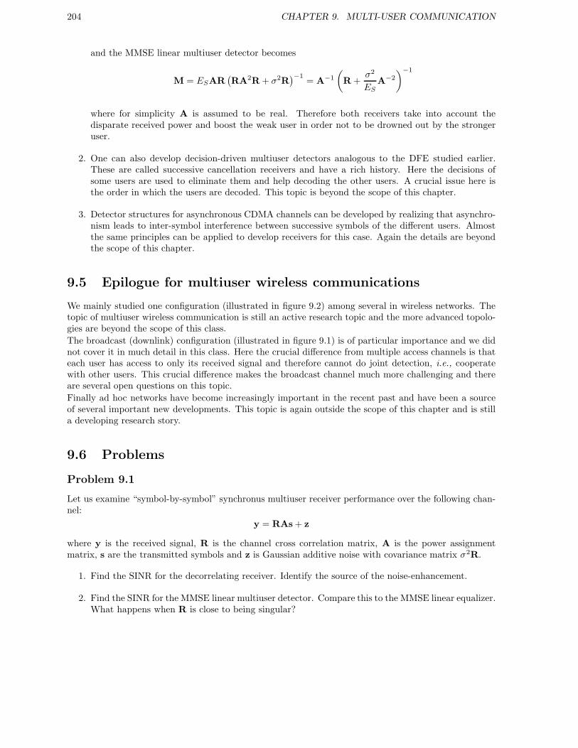
204 CHAPTER 9. MULTI-USER COMMUNICATION
and the MMSE linear multiuser detector becomes
M = ESAR(RA2R + σ2R
)−1= A−1
(R +
σ2
ESA−2
)−1
where for simplicity A is assumed to be real. Therefore both receivers take into account thedisparate received power and boost the weak user in order not to be drowned out by the strongeruser.
2. One can also develop decision-driven multiuser detectors analogous to the DFE studied earlier.These are called successive cancellation receivers and have a rich history. Here the decisions ofsome users are used to eliminate them and help decoding the other users. A crucial issue here isthe order in which the users are decoded. This topic is beyond the scope of this chapter.
3. Detector structures for asynchronous CDMA channels can be developed by realizing that asynchro-nism leads to inter-symbol interference between successive symbols of the different users. Almostthe same principles can be applied to develop receivers for this case. Again the details are beyondthe scope of this chapter.
9.5 Epilogue for multiuser wireless communications
We mainly studied one configuration (illustrated in figure 9.2) among several in wireless networks. Thetopic of multiuser wireless communication is still an active research topic and the more advanced topolo-gies are beyond the scope of this class.
The broadcast (downlink) configuration (illustrated in figure 9.1) is of particular importance and we didnot cover it in much detail in this class. Here the crucial difference from multiple access channels is thateach user has access to only its received signal and therefore cannot do joint detection, i.e., cooperatewith other users. This crucial difference makes the broadcast channel much more challenging and thereare several open questions on this topic.
Finally ad hoc networks have become increasingly important in the recent past and have been a sourceof several important new developments. This topic is again outside the scope of this chapter and is stilla developing research story.
9.6 Problems
Problem 9.1
Let us examine “symbol-by-symbol” synchronus multiuser receiver performance over the following chan-nel:
y = RAs + z
where y is the received signal, R is the channel cross correlation matrix, A is the power assignmentmatrix, s are the transmitted symbols and z is Gaussian additive noise with covariance matrix σ2R.
1. Find the SINR for the decorrelating receiver. Identify the source of the noise-enhancement.
2. Find the SINR for the MMSE linear multiuser detector. Compare this to the MMSE linear equalizer.What happens when R is close to being singular?

9.6. PROBLEMS 205
Problem 9.2
Consider transmission using Direct-sequence CDMA (DS-CDMA) using block invariant code sequencesfor each user. Then the output during a block period is given by
y(t) =
U∑
u=1
suφu(t) + z(t), t ∈ ((b− 1)T, bT ),
φu(t) =L−1∑
l=0
cu(l)ψ (t− lTc) , t ∈ ((b− 1)T, bT ).
Assume that shifted versions of ψ(t) by some integral multiple of Tc are orthogonal to each other, i.e.,
〈ψ (t−mTc) , ψ (t− nTc)〉 =
1 m = n,0 otherwise.
Show that the entries of correlation matrix R are given by the dot product of the code-sequences i.e.,
Rij =L−1∑
l=0
ci(l)c∗j (l).
Problem 9.3
In this problem we study the near-far problem: users 1 and 2 are transmitting and we want to detectuser 1 using conventional detection (single user detection). If the user 2 is sufficiently powerful then itcan cause arbitrary performance degradation in the detection of user 1. To this end, consider a two-user,synchronous DS-CDMA system with signature sequences given by
s1(t) =
1 0 ≤ t ≤ 1,0 otherwise.
s2(t) =
A 0 ≤ t ≤ 0.5,−AB 0.5 < t ≤ 1,0 otherwise.
The parameters take values A ≥ 0 and 0 ≤ B ≤ 1. The received waveform at time t can be written as
r(t) =
2∑
k=1
∞∑
i=−∞
√Ekbk(i)sk(t− i) + n(t)
where n(t) is the white Gaussian noise with power spectral density σ2, and bk(i) = ±1 with equalprobability. A conventional detector is used, which detects the bk(0) bit as
bk(0) = sgn(rk), where rk =
∫ 1
0
r(t)sk(t)dt.
1. Determine expressions for the probability of bit error for user 1 and 2 respectively.
2. For user 1, what is the form of the bit error expression for A→ 0, B < 1.
3. For user 1, what is the form of the bit error expression for A → ∞, B < 1. What does this sayabout the conventional detection?
4. For user 1, what is the form of the bit error expression for B = 1. Compare with the result inpart(3) and explain.

206 CHAPTER 9. MULTI-USER COMMUNICATION
Problem 9.4
Suppose we have two users u = 1, 2, transmitting information x1(k) and x2(k). Consider a simplemultiple access channel where the received signal (discrete time) is
y(k) = x1(k) + x2(k) + z(k)
where z(k) is additive white complex Gaussian noise with variance σ2, is i.i.d. and independent ofx1(k) and x2(k). You may assume that x1 and x2 are independent with identical variance Ex.
1. Suppose we use blocks of length two for transmission and the users use the following transmissionstrategy,
x1(k) = s1 , x1(k + 1) = s1x2(k) = −s2 , x2(k + 1) = s2
(9.8)
Express the received signal, [y(k), y(k + 1)] in terms of the transmitted symbols, i.e. specialize
y(k) = x1(k) + x2(k) + z(k)
y(k + 1) = x1(k + 1) + x2(k + 1) + z(k + 1)
to the transmission strategy in (9.8), prove that
y = Rs + z.
and find the form of R.
2. Find
y = R∗y
and comment about its implications to detecting s1 and s2. Is this equivalent to the decorrelatingdetector?
3. Find the MMSE multiuser detector M such that
E||My − s||2 is minimized.
Explicitly calculate M and comment about its relationship to the receiver in (2).
4. What is the error performance of the receivers in (2) and (3) in the presence of i.i.d. noise Cη(0, σ2)?
5. What is the transmission rate for each of the users in the model given in (9.8)?
6. More generally if we develop a transmission strategy for U users, such that
y = Rs + z
where y, z ∈ CU×U , s =
s1...sU
∈ CU and R∗R = UI. Develop the decorrelating and the MMSE
linear multiuser detector for this case. You may assume E[ss∗] = EsI, E[zz∗] = σ2I and that sand z are independent. Can you comment about the relationship of this strategy with respect toTDMA or FDMA?

9.6. PROBLEMS 207
Problem 9.5
Consider a three-user synchronous CDMA channel with equal power users A1 = A2 = A3 = 1.
1. Find a crosscorrelation matrix R such that:
|([R + σ2I]−1R)13|([R + σ2I]−1R)11
> |ρ13|
Without loss of generality, one can consider that detR = 0, ρ13 = 0, ρ12 = ρ23 and ρ11 = 1. Whatcan one conclude?
2. For the crosscorrelation matrix you selected above, verify that:
([R + σ2I]−1R)212([R + σ2I]−1R)211
+([R + σ2I]−1R)213([R + σ2I]−1R)211
< ρ212 + ρ2
13
What can one conclude?
Problem 9.6
[ Multiple Access Channel and Transmit Code] Consider a two user multiple access channelwhere each user has two transmit antennas and the receiver has two antennas (see Figure 9.6). Let
Figure 9.12: Multiple access channel for problem 4.
u(k) =
[u1(k)u2(k)
], v(k) =
[v1(k)v2(k)
]be the transmit signal from each user. The receiver gets a linear
combination of the transmit signals,
y1(k) = e1u1(k) + e2u2(k) + f1v1(k) + f2v2(k) + z1(k),
y2(k) = h1u1(k) + h2u2(k) + g1v1(k) + g2v2(k) + z2(k),
where zi(k) ∼ Cη(0, σ2z) and zi(k) is i.i.d circularly symmetric Gaussian random variables. Now,
suppose the users use an Alamouti code, i.e., for user 1 the transmit signal is
u1(k) = a1, u2(k) = a2,
u1(k + 1) = −a∗2, u2(k + 1) = a∗1,

208 CHAPTER 9. MULTI-USER COMMUNICATION
and for user 2, it isv1(k) = b1, v2(k) = b2,
v1(k + 1) = −b∗2, v2(k + 1) = b∗1.
Therefore we get
[y1(k) y1(k + 1)
]=
[e1 e2
] [a1 −a∗2a2 a∗1
]+[f1 f2
] [b1 −b∗2b2 b∗1
]+[z1(k) z1(k + 1)
](9.9)
[y2(k) y2(k + 1)
]=
[h1 h2
] [a1 −a∗2a2 a∗1
]+[g1 g2
] [b1 −b∗2b2 b∗1
]+[z2(k) z2(k + 1)
]. (9.10)
(a) Prove that (9.9) can be equivalently rewritten as
Y1 =[y1(k) y1(k + 1)
]=[a1 a2
] [e1 −e∗2e2 e∗1
]+[b1 b2
] [f1 −f∗2
f2 f∗1
]+[z1(k) z1(k + 1)
]
and (9.10) can be rewritten as
Y2 =[y2(k) y2(k + 1)
]=[a1 a2
] [h1 −h∗2h2 h∗1
]+[b1 b2
] [g1 −g∗2g2 g∗1
]+[z2(k) z2(k + 1)
],
where z1(k), z1(k+1), z2(k), z2(k+1) are i.i.d circularly symmetric complex Gaussian random vari-ables with distribution Cη(0, σ2
z). Explicitly write out how[y1(k) y1(k + 1)
],[y2(k) y2(k + 1)
]
are related to[y1(k) y1(k + 1)
],[y2(k) y2(k + 1)
]respectively.
(b) Let
E =
[e1 −e∗2e2 e∗1
], F =
[f1 −f∗
2
f2 f∗1
], G =
[g1 −g∗2g2 g∗1
], H =
[h1 −h∗2h2 h∗1
],
a =[a1 a2
], b =
[b1 b2
], Z1 =
[z1(k) z1(k + 1)
], Z2 =
[z2(k) z2(k + 1)
].
Then the equations (9.9,9.10) can be written as
[Y1 Y2
]=[a b
] [E HF G
]+[Z1 Z2
].
Prove that
W =
[I2 −E−1H
−G−1F I2
]
decouples the signals from user 1 and 2, i.e.,
[Y1 Y2
]=[Y1 Y2
]W =
[a b
] [H 0
0 G
]+[Z1 Z2
], (9.11)
where Z1, Z2 are still Gaussian.
(c) Prove that H and G are of the form
H =
[h1 −h∗2h2 h∗1
], G =
[g1 −g∗2g2 g∗1
].
Hint: You do not need to explicitly write out the expressions for h1, h2, g1, g2.

9.6. PROBLEMS 209
(d) In (9.11) it is seen thatY1 = aH + Z1,
Y2 = bG + Z2.
Show thatY1H
∗ = ||h||2[a1 a2
]+ Z1H
∗,
Y2G∗ = ||g||2
[b1 b2
]+ Z2G
∗,
where h =[h1 h2
], g =
[g1 g2
]. This completes the decoupling of the individual streams of the
multiple access channel.
(e) If h1, h2, g1, g2, e1, e2, f1, f2 are i.i.d and have distribution Cη(0, 1), can you guess the diversity orderfor detecting a1, a2, b1, b2?
Problem 9.7
[Relay Diversity] In a wireless network let us assume that there are three nodes, where the source
!"#%$&
Figure 9.13: Communication using relay.
(S) wants to transmit information to the destination (T ) and can obtain help from a relay (R). Assumethat the channels are block time-invariant over a transmission block of size T . We use the followingtransmission protocol over a block of time of length T . Let s(k) ∈ a,−a be a binary information
')(+* ',(-*
.0/214365 *.0/214365-7
8:9<; 14=>3?:@ 9 3 A 9<; 14=>3?B@ 9 3
Figure 9.14: Transmission protocol.
sequence that source S wants to convey to the destination T . Then, for the first phase the relay receives
yR(k) and the destination receives y(1)T (k), with
yR(k) = fs(k) + zR(k), (9.12)
y(1)T (k) = hs(k) + zT (k), (9.13)

210 CHAPTER 9. MULTI-USER COMMUNICATION
where zR(k), zT (k) ∼ Cη(0, σ2) are i.i.d, circularly symmetric complex Gaussian noise. We also assumea fading channel, f, g, h ∼ Cη(0, 1) and are independent of each other. Assume that g, h are known atT , f is known at R, but they are unknown at S (except for part (c))In the second phase for parts (a), (b),
y(2)T (k) = gu(k) + zT (k)
where u(k) is the signal transmitted by the relay and g ∼ Cη(0, 1).
(a) Suppose the relay was absent, i.e., u(k) = 0, then give an expression (or bound) on the average errorprobability of s(k) averaged over the channel realizations h. What is the diversity order, i.e.,
limSNR→∞
− log(Pe(SNR))
log(SNR)
for the detection of s(k).(b) Suppose that the relay R attempts to decode s(k) in phase 1 and transmits u(k) = sR(k) in phase
2. That is, it sends the decoded sequence to T . Assume now that there is an oracle which tellsthe destination T if relay R has decoded correctly or not. Note that the oracle just lets T knowif sR(k) = s(k) but not its value. Now, T can use the received sequence from both phase 1 andphase 2 in order to decode s(k). Find expressions (or bounds) for the error probability for thisdecoder averaged over the channel realizations which achieve the best diversity order at T . Whatis the best diversity order that can be achieved at T for detecting s(k)? Hint: Develop a receiverstrategy that uses the information given by the oracle. You do not need very detailed calculationsfor obtaining error probability bounds.
(c) Suppose now that we have a new protocol. Phase 1 is as before, where S transmits and both R andT receive the signal as in (9.12) and (9.13) respectively. At the end of phase 1, there is a feedbackchannel from R to S which informs S about the realization of channel f . Now the protocol S and Rfollow is given by: if |f |2 ≤ c(SNR) (where c(SNR) is a function of SNR), then in phase 2, S repeatsthe same information it transmitted in phase 1 and the relay R remains silent, i.e., s(k) fromphase 1 is repeated and u(k) = 0 in phase 2. If |f |2 > c(SNR), then the protocol is as in part (b),i.e., S remains silent and R sends the decoded information u(k) = sR(k). Let c(SNR) = 1
SNR1−ε
for an arbitrarily small ε > 0, Assume that an oracle informs the receiver T whether in phase 2, Sor R is transmitting. If in phase 2, S is transmitting, the receiver T forms the decision variable,
yT =[h∗ h∗
][y(1)Ty(2)T
]
where y(1)T , y
(2)T are the received signals in phase 1 and phase 2 respectively. On the other hand if
in phase 2, the relay R is transmitting, receiver T forms the decision variable
yT =[h∗ g∗
][y(1)Ty(2)T
]
where again y(1)T , y
(2)T are the received signals in phase 1 and phase 2 respectively. The decision
rule in both situations is that T chooses sT = +a if <(yT ) ≥ 0 and sT = −a otherwise. Analyzethe performance of this receive strategy i.e., find the diversity order that can be achieved by T fors(k). Note that we are looking for diversity order and so we do not necessarily need a detailedanalysis to find the diversity order. Hint: Condition on appropriate error events at the relay anduse error probability bounds. You can also use properties given in the hints in the first page.
Part IV
Connections to Information Theory
211


Chapter 10
Reliable transmission for ISIchannels
A focus of this class has been transmission and reception over LTI channels. Even in the wireless trans-mission, the channels were considered to be block-time-invariant. Therefore, we examine the fundamentallimits of transmission over such channels and compare the structures we studied to that which informa-tion theory predicts. In order to do that, we first study the capacity of ISI channels in Section 10.1. Thenin Section 10.2 and 10.3 we study canonical properties of OFDM and the MMSE-DFE as informationtheoretic structures.
10.1 Capacity of ISI channels
The complete and rigorous derivation of the capacity of a (bandlimited) frequency selective (time-invariant) channel is beyond the scope and goal of this class. Here we give a heuristic developmentof the capacity expression with the intention to connect it to the transmission and receiver structuresthat we have studied in this class.
t ∈ (−T/2, T/2)
y(t)
t ∈ (−T/2, T/2)h(t)
x(t)
z(t) AWGN
LTI channel
+
Figure 10.1: Model for frequency selective channels.
We represent the input x(t) in terms of a Fourier series (where x(t) is time-limited to (−T/2, T/2)interval).
x(t) =
+∞∑
i=−∞xiφi(t)
where φi are the Fourier series basis functions.
x(t) ∗ h(t) =
∫ ∑
i
xiφi(τ)h(t − τ)dτ =∑
i
xi
∫φi(τ)h(t − τ)dτ
213

214 CHAPTER 10. RELIABLE TRANSMISSION FOR ISI CHANNELS
Let
θi(t) =
∫φi(τ)h(t − τ)dτ
Thenx(t) ∗ h(t) =
∑
i
xiθi(t)
y(t) = x(t) ∗ h(t) + z(t) =∑
i
xiθi(t) + z(t)
When T becomes large, the Fourier series basis φi tend towards the Fourier basis, which are theeigenbasis for linear time-invariant channels. Therefore we can write
θi(t) ≈ H
(2π
Ti
)gT (t)
where gT (t) becomes the Dirac delta function when T → ∞. Similarly, we can expand the noise in thefrequency domain and by doing so we obtain:
yi ≈ xiH
(2π
Ti
)+ zi (10.1)
where yi is the Fourier series coefficients of y(t) and zi that of z(t). This is a very imprecise andheuristic development and a precise development is clearly out of the scope of this class. Since therelationship in (10.1) is output of parallel additive Gaussian noise channels, mutual information is,
I(yi; xi) =1
2log
|HRxHt + Rz|
|Rz|≤ 1
2
∑
i
log
(∣∣∣∣H(
2π
Ti
)∣∣∣∣2
E[|xi|2
]
E [|zi|2]+ 1
)(10.2)
where |.| denotes the determinant and we have assumed that E [zizj ] = E[|zi|2
]δi−j , i.e. white Gaussian
noise. Now, if we impose the input power constraint,
1
T
∫ T/2
−T/2
|x(t)|2dt ≤ P
this translates (due to orthonormal expansion) to
∑
i
x2i ≤ PT
Now, the capacity therefore is maximization of the mutual information.
CT = maxPx:
Px2
i≤PT
1
T
∑
i
1
2log
(∣∣∣∣H(
2π
Ti
)∣∣∣∣2
E[|xi|2
]
E [|zi|2]+ 1
)
Since we can choose independent xi, we can make the inequality in (10.2) into equality as we havedone.
Now as T → ∞, 1T E[|xi|2
]= ST
(2πT i)→ S(f) the power spectral density of the input, and
E[|z2i |]
T → σ2.Also 1
T
∑x2
i →∫S(f)df and hence we get
limT→∞
CT = maxS(f):
RS(f)df≤P
1
2
∫log
(1 + |H(f)|2S(f)
σ2
)df

10.1. CAPACITY OF ISI CHANNELS 215
This is the expression for capacity that we will work with. Next the goal is to find the optimal inputpower spectrum.
C = maxS(f):
RS(f)df≤P
1
2
∫log
(1 +
|H(f)|2σ2
S(f)
)df (10.3)
Now, to find the maximizing input spectrum S(f), we can do so by calculus of variations. However wecan also do so by taking formal derivatives.
max1
2
∫log
(1 +
|H(f)|2σ2
S(f)
)df
such that ∫S(f)df ≤ P
Since C increases with S(f), the last inequality can be replaced with equality. Let,
I =1
2
∫log
(1 +
|H(f)|2σ2
S(f)
)df − λ
∫S(f)df
∂I∂S(f)
=1/2
1 + |H(f)|2σ2 S(f)
|H(f)|2σ2
− λ
The Kuhn-Tucker conditions imply that
∂I∂S(f)
= 0 if S(f) > 0
∂I∂S(f)
< 0 if S(f) = 0
Hence for f : S(f) > 0 we have1/2|H(f)|2/σ2
1 + |H(f)|2σ2 S(f)
= λ
or1
2λ=
σ2
|H(f)|2 + S(f), f ∈ f : S(f) > 0
Let 12λ = ν, thus we get the optimal input spectrum S∗(f) as
S∗(f) = ν − σ2
|H(f)|2 f ∈ f : S(f) > 0
Using the Kuhn-Tucker conditions, we can write
S∗(f) =
(ν − σ2
|H(f)|2)+
∀f (10.4)
where (x)+ =
x ifx ≥ 00 else
We can find ν by satisfying the constraint
∫S∗(f)df = P, i.e.
∫ (ν − σ2
|H(f)|2)+
df = P
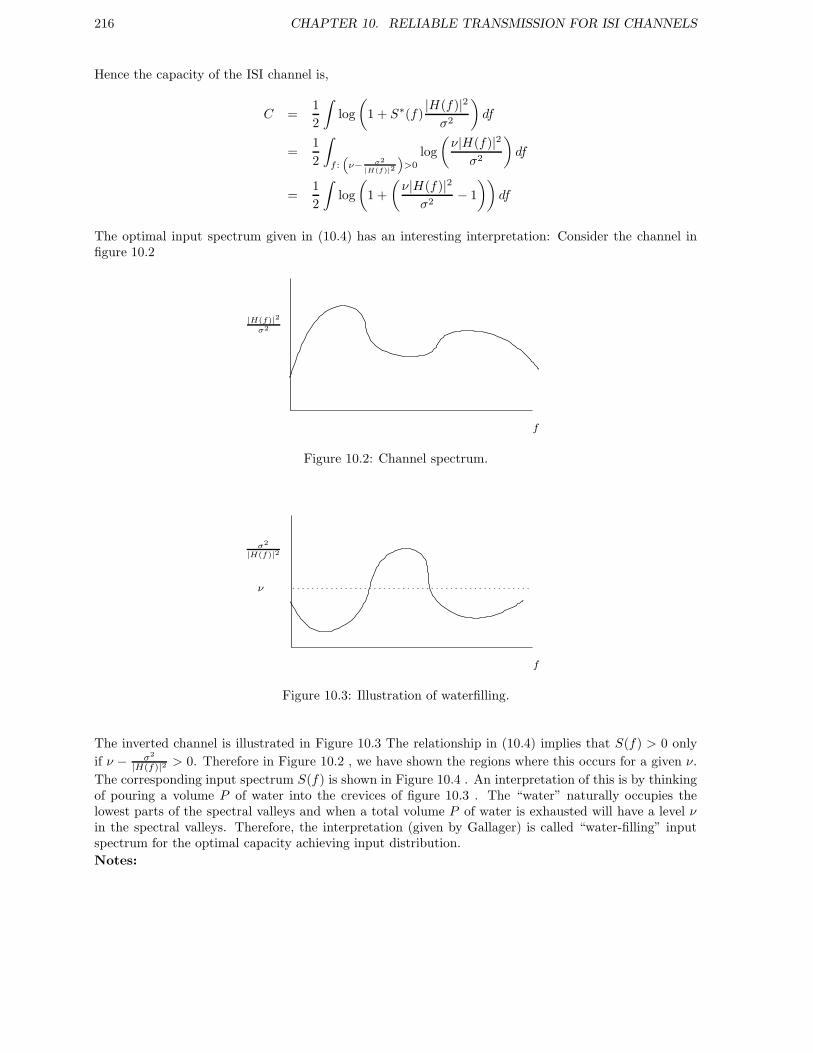
216 CHAPTER 10. RELIABLE TRANSMISSION FOR ISI CHANNELS
Hence the capacity of the ISI channel is,
C =1
2
∫log
(1 + S∗(f)
|H(f)|2σ2
)df
=1
2
∫
f :“
ν− σ2
|H(f)|2
”>0
log
(ν|H(f)|2
σ2
)df
=1
2
∫log
(1 +
(ν|H(f)|2
σ2− 1
))df
The optimal input spectrum given in (10.4) has an interesting interpretation: Consider the channel infigure 10.2
f
|H(f)|2σ2
Figure 10.2: Channel spectrum.
f
ν
σ2
|H(f)|2
Figure 10.3: Illustration of waterfilling.
The inverted channel is illustrated in Figure 10.3 The relationship in (10.4) implies that S(f) > 0 only
if ν − σ2
|H(f)|2 > 0. Therefore in Figure 10.2 , we have shown the regions where this occurs for a given ν.
The corresponding input spectrum S(f) is shown in Figure 10.4 . An interpretation of this is by thinkingof pouring a volume P of water into the crevices of figure 10.3 . The “water” naturally occupies thelowest parts of the spectral valleys and when a total volume P of water is exhausted will have a level νin the spectral valleys. Therefore, the interpretation (given by Gallager) is called “water-filling” inputspectrum for the optimal capacity achieving input distribution.
Notes:

10.2. CODED OFDM 217
f
S(f)
Figure 10.4: Transmit spectrum.
1. The main insight to drawn from the result is that the transmission scheme should focus its power onthe “sweet spots” of the channel where gains are the largest. The concavity of the log function (giv-ing diminishing “returns”) implies that the power is transmitted only in the best channel responsefrequency, but descends down by spreading the input power to lower channel gains |H(f)|2.
2. Most of the transmission schemes that we discussed in ISI channels had a “flat” input spectrum,i.e. SX(f) = P/W , where W was the transmission bandwidth. Clearly this is not optimal andwe will examine the performance of the ISI transmission an receiver structures if we take this intoaccount.
3. A canonical decomposition was through the Fourier basis, creating parallel channels. This decom-position was used in one transmission/reception structure we studied, i.e. OFDM. There we didnot consider changing the input spectrum, but given this insight we will re-examine that problem
4. The ISI channel capacity pre-suppose that the channel response is known at the transmitter. Forwire line channels this is realistic since the channel remains constant for a long period and thereforethe response can be fed back to the transmitter. However, for wireless channels, such an assumptionmight be unrealistic. This is a topic outside the scope of this class.
5. The “single carrier” (equalization receiver) structure extensively discussed in the class can alsobe modified to have a non-uniform input power spectrum. In fact such a structure has beenimplemented in the V-34 modem for telephone lines.
Next, we compare some of the transmission and reception structures discussed in Chapter 5 and 6 to thecapacity of the ISI channel.
10.2 Coded OFDM
Recall from Section 6.2 that in OFDM the cyclic prefix allowed us to relate the input (in the frequencydomain) to the output (again in the frequency domain) as
Y (l) = P (l)X(l) + Z(l), , l = 0, . . . , N − 1
where P (l) was the frequency domain pulse response
P (l) =
ν∑
n=0
pne−j 2π
N ln, l = 0, . . . , N − 1

218 CHAPTER 10. RELIABLE TRANSMISSION FOR ISI CHANNELS
×X(0)
X(N − 1) Y (N − 1)
Y (0)
Z(N − 1)
Z(0)P (0)
P (N − 1)
× +
+
Figure 10.5: Parallel channels in OFDM.
and Z(l) was the noise (in the frequency domain) and X(l) was the input in the frequency domain.This relationship can be illustrated as shown in Figure 10.5.
Now, one can concatenate an outer code along with the frequency domain input and code over a sequenceof transmission blocks. That is, one can have codes Cl for each of the N parallel channels and codesuch that the inputs come from the corresponding symbols from each block. This is illustrated in figure10.6 which shows the transformation from a uncoded OFDM system to a coded system.
Block 1 Block 2 Block Nc
M0 MN−1
Message set Message set
. . .
. . .
. . .
X(1)(0) . . . X
(1)(N−1)
. . . . . .X(2)(0)
X(2)(N−1)
X(Nc)(0) X
(Nc)(N−1)
C0 CN−1
Figure 10.6: A coded OFDM transmissions scheme.
If |Ml| = 2NcRl , where the rate on subchannel l is Rl, the code Cl sends out Nc consecutive symbolswhich have been coded from the message from set Ml. The symbols from each code form a sequenceX(k)(l)Nc−1
k=0 of length Nc which is the length of the code. Each symbol is placed in the appropriatefrequency sub-carrier of the OFDM. By doing this, for a large enough Nc information theory tells us thatthe Rl achievable is

10.2. CODED OFDM 219
Rl =1
2log
(1 +Ql
|P (l)|2σ2
)
where P (l) is the frequency response of the channel and
Ql = limNC→∞
1
Nc
Nc−1∑
k=0
|X(k)(l)|2, l = 0, . . . , N − 1
is the power assigned to subcarrier l.Therefore the overall rate achievable for OFDM is
R =
N−1∑
l=0
Rl =1
2
N−1∑
l=0
log
(1 +Ql
|P (l)|2σ2
)(10.5)
with the constraint that∑N−1
l=0 Ql ≤ Ptot where Ptot is the transmit power. Note that as N → ∞, we get
R∗ = limN→∞
R =1
2
∫log
(1 +Q(f)
|P (f)|2σ2
)df
with∫Q(f)df ≤ Ptot.
This looks strikingly similar to the ISI channel capacity expression discussed in (10.3). In fact with theappropriate power allocation we can make the two identical. This gives a hint that OFDM structure iscanonical in terms of information theory.
10.2.1 Achievable rate for coded OFDM
Now, let us return to the realm of finite number of subcarriersN . From equation (10.5) the achievable rateof OFDM depends on the power allocated to the various subcarriers, i.e. QlN−1
l=0 . We now can maximize
the rate by choosing an appropriate power allocation subject to the constraint that∑N−1
l=0 Ql ≤ Ptot.
maximize1
2
N−1∑
l=0
log
(1 +Ql
|P (l)|2σ2
)
such that
N−1∑
l=0
Ql ≤ Ptot
Clearly this is a problem we have seen (and solved!) before, which led us to the water filling inputspectrum. We now solve the discrete version of this problem and give an explicit algorithm that calculatesthe optimal power distribution Q. As before, let us solve the problem using Kuhn-Tucker conditions.Define the Lagrangian,
J =1
2
N−1∑
l=0
log
(1 +Ql
|P (l)|2σ2
)− λ
N−1∑
l=0
Ql.
This yields,∂J∂Ql
=1/2
1 +Ql|P (l)|2
σ2
|P (l)|2σ2
− λ.
Using the Kuhn-Tucker conditions, we have for optimality
∂J∂Ql
= 0 if Ql > 0
∂J∂Ql
< 0 if Ql = 0
220 CHAPTER 10. RELIABLE TRANSMISSION FOR ISI CHANNELS
Thus, for l : Ql > 0 we get,
1/2σ2
|P (l)|2 +Ql
= λ
and hence
Ql = ν − σ2
|P (l)|2 l ∈ l : Ql > 0
where ν = 1/2λ. Now using Kuhn-Tucker conditions we can easily verify that the optimal power distri-bution Q∗
l can be written as
Q∗l =
(ν − σ2
|P (l)|2)+
∀l ∈ 0, . . . , N − 1 (10.6)
where (x)+ =
x ifx ≥ 00 else
and ν is chosen such that∑N−1
l=0
(ν − σ2
|P (l)|2)+
≤ Ptot.
The “waterfilling” algorithm computes ν and therefore gives us a method to calculate the optimal powerdistribution. The algorithm is derived in Section 9.2.2.
10.2.2 Waterfilling algorithm
Step 1
If Ql > 0 ∀l, then finding ν becomes easy
N−1∑
l=0
[ν − σ2
|P (l)|2]
= Ptot
This yields,
Nν = Ptot +
N−1∑
l=0
σ2
|P (l)|2
or ν =1
N
[Ptot +
1
N
N−1∑
l=0
σ2
|P (l)|2
](10.7)
However, for such a choice of ν, we have
Ql = ν − σ2
|P (l)|2
=1
NPtot +
1
N
N−1∑
l=0
σ2
|P (l)|2 − σ2
|P (l)|2 (10.8)
There is no guarantee that the Ql that arises from a choice of ν given in equation (10.7) would benon-negative in (10.8) in general.

10.2. CODED OFDM 221
Step 2
If we know the set of “active” subchannels A = l : Ql > 0, then again finding ν becomes easy.
∑
l∈A
(ν − σ2
|P (l)|2)
= Ptot
This yields,
ν =1
|A|Ptot +1
|A|∑
l∈A
σ2
|P (l)|2
and Ql =
1
|A|Ptot + 1|A|∑
k∈Aσ2
|P (k)|2 − σ2
|P (l)2| l ∈ A0 otherwise
However, one does not know the active set A.
Step 3
In order to find the correct active set we can start by assuming A = 0, . . . , N − 1, i.e. the entire setof subcarriers. Then from (10.7) we can find the appropriate ν. But (10.8) would tell us which Ql arenegative. If there is Ql < 0, then we drop the “worst” channel from the active list i.e.,
l1 = argmaxl
σ2
|P (l)|2
and consider the active list as A = 0, . . . , N − 1 \ l1, where the notation means the set difference.Given this order preference in the choice of active subchannels we reduce the number of candidate active
sets from N ! to N by ordering
σ2
|P (l)|2
in increasing order. We can index the candidate active sets by
choice (in increasing order) of the values
σ2
|P (l)|2. By doing this one can find the optimal active set.
The main step in this is the observation that if a particular subchannel l′ is active, then all subchannelssuch that
σ2
|P (l)|2 ≤ σ2
|P (l′)|2
are also active. This can be seen from the relationship in (10.6) and we next give a formal statement andproof of this claim.
Claim 10.2.1. If the optimal active set A∗ contains subchannel l′, then it must also contain elements lwhen
σ2
|P (l)|2<
σ2
|P (l′)|2 (10.9)
Proof: Suppose, A∗ is the optimal active set and it contains element l′ and does not contain an elementl which is such that
σ2
|P (l)|2<
σ2
|P (l′)|2
Now, we prove the assertion by contradiction. Since l′ ∈ A∗ and l /∈ A∗ ⇒ Ql′ > 0 , Ql = 0. And theoptimal rate is
R∗ =1
2
∑
l∈A∗
log
(1 +Ql
|P (l)|2σ2
)(10.10)
222 CHAPTER 10. RELIABLE TRANSMISSION FOR ISI CHANNELS
Now consider a different power allocation Ql where all the allocation is the same except we choose forsmall enough ε > 0,
Ql′ = Ql′ − ε and Ql = ε > 0
For this allocation
R =1
2
∑
l∈A∗\l′
log
(1 +Ql
|P (l)|2σ2
)
+1
2log
(1 + (Ql′ − ε)
|P (l′)|2σ2
)
+1
2log
(1 + ε
|P (l)|2σ2
)(10.11)
Using (10.10) and (10.11) we get
R∗ − R =1
2log
(1 +Ql′
|P (l′)|2σ2
)
−1
2log
(1 + (Ql′ − ε)
|P (l′)|2σ2
)
−1
2log
(1 + ε
|P (l)|2σ2
)
(a)
≤ 1
2log
(1 +Ql′
|P (l)|2σ2
)
−1
2log
(1 + (Ql′ − ε)
|P (l′)|2σ2
)
−1
2log
(1 + ε
|P (l′)|2σ2
)(10.12)
where (a) follows because log is an increasing function and |P (l)|2σ2 > |P (l′)|2
σ2 due to assumption (10.10).Continuing with (10.12) we get
R∗ − R ≤ 1
2log
(1 +Ql′
|P (l′)|2σ2
)
−1
2log
(1 + ε
|P (l′)|2σ2
)− 1
2log
(1 + (Ql′ − ε)
|P (l′)|2σ2
)
=1
2log
(σ2 +Ql′ |P (l′)|2σ2 + ε|P (l′)|2
)− 1
2log
(1 + (Ql′ − ε)
|P (l′)|2σ2
)
=1
2log
(1 +
(Ql′ − ε)|P (l′)|2σ2 + ε|P (l′)|2
)− 1
2log
(1 + (Ql′ − ε)
|P (l′)|2σ2
)
< 0
Hence R∗ < R and therefore A∗ cannot be the optimal active set assignment. Therefore we have acontradiction and hence the claim is proved.
Therefore, we need to consider only N candidate active sets instead of N ! and therefore giving a O(N)steps water filling algorithm.

10.3. AN INFORMATION-THEORETIC APPROACH TO MMSE-DFE 223
10.2.3 Algorithm Analysis
1. Sort
σ2
|P (l)|2
in ascending order, i.e.
σ2
|P (l1)|2≤ σ2
|P (l2)|2≤ . . . ≤ σ2
|P (lN )|2
2. Let A = l1, l2, . . . , lN, p = N
3. Compute
ν =1
|A|Ptot +1
|A|∑
k∈A
σ2
|P (k)|2
4. If ∃Qk < 0, then let A = A \ lp and p = p− 1. Goto step 3.Else optimal power allocation found.
Notes
1. This algorithm terminates in at most N steps.
2. The sorting takes O(N logN) complexity and the computation of ν takes O(N) complexity. Hencewe have O(N logN) algorithm for computing the optimal power allocation.
3. We devised this algorithm based on claim 10.2.1 where we showed that the ordering of
σ2
|P (l)|2
determined the active set. Therefore we choose the complete set as A first and then eliminate theworst channel, one-by-one till we get the correct A∗.
4. Ties in this algorithm can be resolved arbitrarily since the final rate does not get affected.
5. The algorithm does not take into account particular alphabets/constellations one might use for thetransmission. Other algorithms that utilize this have been found. They are outside the scope ofthis class.
10.3 An information-theoretic approach to MMSE-DFE
Fact 1 If (x,y) are jointly Gaussian then Px|y(x|y) is also Gaussian with mean E [x|y] and covariance
E[x − E [x|y] x− E [x|y]∗
]= R⊥
x|y which is the error covariance of a linear estimator of xfrom y .
Fact 2 For a Gaussian random vector x ∼ Cη(0,Rxx) the entropy is
Hx = log[(πe)N |Rxx|
]
where N is the dimension of x and |Rxx| is the determinant of Rxx
Fact 3 If (x,y) are jointly Gaussian, then the conditional entropy Hx|y is
Hx|y = log[(πe)N |R⊥
x|y|]
where R⊥x|y is the error covariance of linear estimator of x from y.

224 CHAPTER 10. RELIABLE TRANSMISSION FOR ISI CHANNELS
Now,
R⊥x|y = Rxx −RxyR
−1yy Ryx
where
Rxy = E [xy∗] , Ryx = E [yx∗] , Ryy = E [yy∗]
For a stationary Gaussian process, the chain rule of entropy allows computation of its entropy based onprediction. For a sequence x = xk, xk−1, . . . , x0 ,
Hx = Hxk|[xk−1,...,x0] +Hxk−1|[xk−2,...,x0] + . . .
+Hx1|x0+Hx0
=
k∑
n=0
Hxn|[xn−1,...,x0]
where we have defined Hx0|x−1
∆= Hx0 .
Definition 10.3.1. For a stationary process xk, the entropy rate Hx(D) is,
Hx(D) = limk→∞
1
k + 1H([xk, . . . , x0]) = lim
k→∞
1
k + 1
k∑
n=0
H(xn|[xn−1, . . . , x0])
For a stationary sequence this quantity converges to
Hx(D) = limk→∞
H(xk|xk−1, . . .)
This is related to the estimation error associated with predicting xk from its past, i.e.
Hx(D) = log[πeσ2
x|past
]
where σ2x|past is the MMSE error of predicting xk (the “present”) from the entire history of the sequence.
Given input xk and output yk
I(x(D); y(D)) = limk→∞
1
k + 1I(xk
0 ,yk0)
where xk0 = x0, . . . , xl, yk
0 = y0, . . . , yk and I(x;y) is the mutual information between x and y. Foran inter-symbol interference (ISI) channel, we have seen from before that
I(x(D); y(D)) =1
2π
∫ π
−π
log
[Sy(w)
Su(w)
]dw
where Sy(w) and Sz(w) are the power spectral densities of the processes yk and the noise zk respec-tively. Now
I(x(D); y(D)) = Hx(D) −Hx(D)|y(D)
= Hxk|xk−1... −Hxk|y∞−∞,xk−1,... (10.13)
Therefore the mutual information can be written as,
I(x(D); y(D)) = I(xk ; y∞−∞|xk−1−∞)

10.3. AN INFORMATION-THEORETIC APPROACH TO MMSE-DFE 225
10.3.1 Relationship of mutual information to MMSE-DFE
From 10.13 we see that
I(x(D); y(D)) = Hxk|xk−1−∞
−Hxk|y∞−∞,xk−1
−∞
= log(πe)σ2xk |xk−1
−∞− log(πe)σ2
xk|y∞−∞,xk−1
−∞(10.14)
But,
σ2xk|xk−1
−∞= γx = MMSE associated with predicting xk from its past
σ2xk|y∞
−∞,xk−1−∞
= σ2MMSE−DFE = The variance of error in perfect past decisions, DFE.
Inserting this into 10.14 we get,
I(x(D); y(D)) = logγx
σ2MMSE−DFE
= logSNRMMSE−DFE
= log [1 + SNRMMSE−DFE,U ]
This results in what is knows as the ”CDEF result” (after the result of Cioffi-Dudevoir-Eyuboglu-Forneydone in 1995).
Lemma 10.3.1 (CDEF result). The unbiaised SNR of a MMSE-DFE is related to the mutual infor-mation for a linear ISI channel with additive Gaussian noise in exactly the same formula as the SNR ofan ISI free channel is related to the mutual information of that channel. Assuming that the input andoutput are jointly (stationary) Gaussian and the MMSE-DFE exists.
10.3.2 Consequences of CDEF result
1. This result seems to show that with the perfect past decisions assumption, the MMSE-DFE is acanonical structure, i.e. it can achieve the capacity of the ISI channel.
2. In the development of the MMSE-DFE, we assumed i.i.d. inputs, which meant a ”flat” inputspectrum Sx(ω). The development we had on the capacity of the ISI channels indicates that thismight not be optimal. Hence the modification we need to make the MMSE-DFE canonical, is inputspectral shaping.
3. There are several other caveats and we will next do a more careful derivation of the result toilluminate these caveats.
Caveats of CDEF results
To do this we establish first a lemma.
Lemma 10.3.2. Let x = xk, y = yk be jointly Gaussian zero mean random processes, then
I(x;y) = I(x;πy(x))
where πy(x) is the orthogonal projection operator of y onto x, i.e., from Gaussian processes,
πy(x) = E [x|y]

226 CHAPTER 10. RELIABLE TRANSMISSION FOR ISI CHANNELS
Recall from linear prediction, of process xk, i.e., predicting xk from its infinite past,
xk =
∞∑
m=1
amxk−m ⇒ X(D) = A(D)X(D)
with A(D) being strictly causal. A(D) = 1 −A′(D) and we found that
A′(D) =1
L(D)where
Sx(D) = γxL(D)L∗(D−∗)
where L(D) is monic, minimum and stable.Now, using the chain rule of mutual information,
I(xk , y∞−∞, x
k−1−∞) = I(xk;xk−1
−∞) + I(xk ; y∞−∞|xk−1−∞)
Hence, using (10.14) we get
I(X(D);Y (D)) = I(xk; y∞−∞, xk−1−∞) − I(xk ;xk−1
−∞)
Therefore, unless we have a white input, i.e. I(xk ;xk−1−∞) = 0, the two quantities I(xk ; y∞−∞, x
k−1−∞) and
I(X(D);Y (D)) are distinct and in fact,
I(X(D);Y (D)) ≤ I(xk; y∞−∞, xk−1−∞)
with equality iff the input is white.However, as we have seen in the waterfilling solution to achieving ISI channel capacity, the optimalsequence xk need not to be white and therefore the above quantities are distinct. It can be shown that
I(xk; y∞−∞, xk−1−∞) = I(xk ; rk) + I(ek; ek−1
−∞)
= I(xk ; rk + ek) (10.15)
whererk = E
[xk|y∞−∞
], ek = xk − xk
Pictorially this is depicted in Figure 10.7.In Figure 10.7, we use, I(ek; ek−1
−∞) = I(ek; ek), where ek = E[ek|ek−1
−∞], by using the lemma. Moreover
forek = xk − rk,
it has a spectral factorizationSe(D) = γeLe(D)L∗
e(D−∗)
yielding a linear predictor filter,
A′e(D) =
1
Le(D)
E(D) = [1 −A′e(D)]E(D) = [1 −A′
e(D)][X(D) −R(D)]
= X(D) −R(D) −A′e(D)X(D) +A′
e(D)R(D)
⇒ R(D) + E(D) = X(D)[1 −A′e(D)] +A′(D)R(D)
Using this we can modify figure (10.7) as,
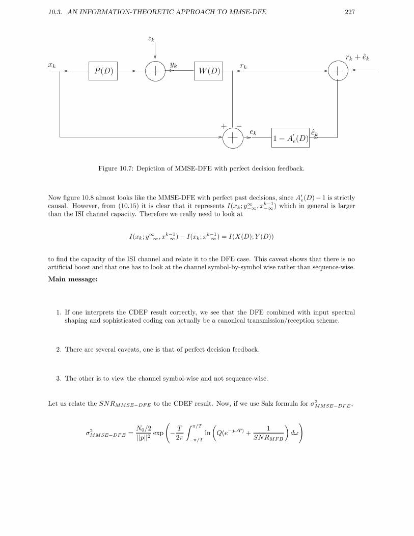
10.3. AN INFORMATION-THEORETIC APPROACH TO MMSE-DFE 227
xkP (D)
zk
ykW (D)
rk
rk + ek
ekek−+
1 − A′e(D)
Figure 10.7: Depiction of MMSE-DFE with perfect decision feedback.
Now figure 10.8 almost looks like the MMSE-DFE with perfect past decisions, since A′e(D)− 1 is strictly
causal. However, from (10.15) it is clear that it represents I(xk ; y∞−∞, xk−1−∞) which in general is larger
than the ISI channel capacity. Therefore we really need to look at
I(xk ; y∞−∞, xk−1−∞) − I(xk;xk−1
−∞) = I(X(D);Y (D))
to find the capacity of the ISI channel and relate it to the DFE case. This caveat shows that there is noartificial boost and that one has to look at the channel symbol-by-symbol wise rather than sequence-wise.
Main message:
1. If one interprets the CDEF result correctly, we see that the DFE combined with input spectralshaping and sophisticated coding can actually be a canonical transmission/reception scheme.
2. There are several caveats, one is that of perfect decision feedback.
3. The other is to view the channel symbol-wise and not sequence-wise.
Let us relate the SNRMMSE−DFE to the CDEF result. Now, if we use Salz formula for σ2MMSE−DFE ,
σ2MMSE−DFE =
N0/2
||p||2 exp
(− T
2π
∫ π/T
−π/T
ln
(Q(e−jωT ) +
1
SNRMFB
)dω
)

228 CHAPTER 10. RELIABLE TRANSMISSION FOR ISI CHANNELS
xkP (D)
zk
yk
rk + ek
+−
A′e(D)W (D)
A′e(D) − 1
Figure 10.8: Modified form of Figure 10.7.
Using the Salz formula in the CDEF result we get
I(X(D);Y (D)) = log
γx
N0/2||p||2
exp
(T
2π
∫ π/T
−π/T
log
Q(e−jωT ) +
1
SNRMFB
)dω
= log
( ||p||2γx
N0/2
)+
T
2π
∫ π/T
−π/T
log
[Q(e−jωT ) +
1
SNRMFB
]dω
= logSNRMFB +T
2π
∫ π/T
−π/T
log1
SNRMFBdω
+T
2π
∫ π/T
−π/T
log[Q(e−jωT )SNRMFB + 1
]dω
=T
2π
∫ π/T
−π/T
log[1 +Q(e−jωT )SNRMFB
]dω
This result for i.i.d. inputs and we can improve the rates by input spectral shaping. The V.34 modemdoes this with precoding to get close to the predicted channel capacity.
10.4 Problems
Problem 10.1
Consider a set of parallel independent AWGN channels:
1. Show that the mutual information for the set of channels is the sum of the mutual informationquantities for the set.
2. If the set of parallel channels has a total energy constraint that is equal to the sum of the energyconstraints, what energy En, n = 1 · · ·N should be allocated to each of the channels to maximize themutual information. You may presume the subchannel gains are given as gn (so that the individualSNRs would be then Engn).
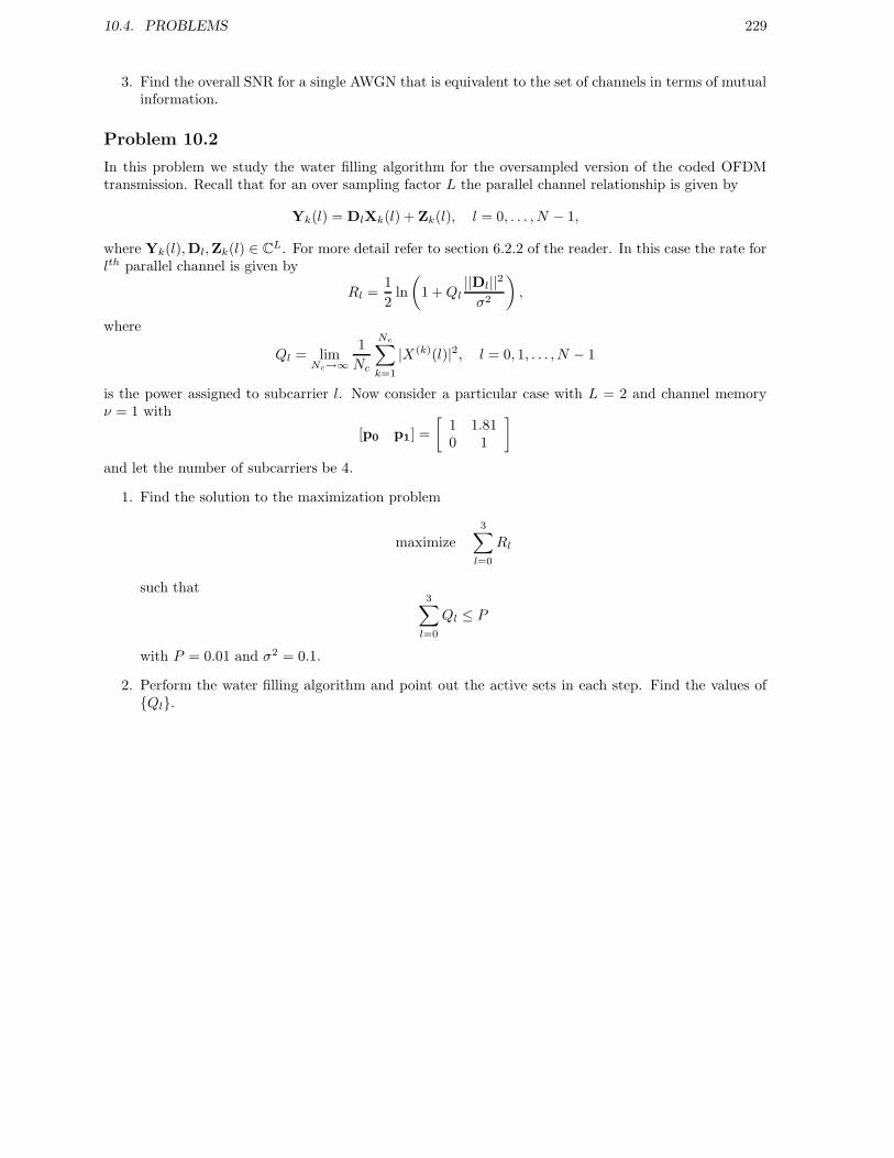
10.4. PROBLEMS 229
3. Find the overall SNR for a single AWGN that is equivalent to the set of channels in terms of mutualinformation.
Problem 10.2
In this problem we study the water filling algorithm for the oversampled version of the coded OFDMtransmission. Recall that for an over sampling factor L the parallel channel relationship is given by
Yk(l) = DlXk(l) + Zk(l), l = 0, . . . , N − 1,
where Yk(l),Dl,Zk(l) ∈ CL. For more detail refer to section 6.2.2 of the reader. In this case the rate forlth parallel channel is given by
Rl =1
2ln
(1 +Ql
||Dl||2σ2
),
where
Ql = limNc→∞
1
Nc
Nc∑
k=1
|X(k)(l)|2, l = 0, 1, . . . , N − 1
is the power assigned to subcarrier l. Now consider a particular case with L = 2 and channel memoryν = 1 with
[p0 p1] =
[1 1.810 1
]
and let the number of subcarriers be 4.
1. Find the solution to the maximization problem
maximize3∑
l=0
Rl
such that3∑
l=0
Ql ≤ P
with P = 0.01 and σ2 = 0.1.
2. Perform the water filling algorithm and point out the active sets in each step. Find the values ofQl.

230 CHAPTER 10. RELIABLE TRANSMISSION FOR ISI CHANNELS

Part V
Appendix
231


Appendix A
Mathematical Preliminaries
A.1 The Q function
The Q function is defined as:
Q(x)4=
1√2π
∫ ∞
x
e−ξ2
2 dξ.
Hence, if Z ∼ N (0, 1) (meaning that Z is a Normally distributed zero-mean random variable of unitvariance) then PrZ ≥ x = Q(x) .
If Z ∼ N (m,σ2) , then the probability PrZ ≥ x can be written using the Q function by noticing thatZ ≥ x is equivalent to Z−m
σ ≥ x−mσ . Hence PrZ ≥ x = Q(x−m
σ ) .
We now describe some of the key properties of Q(x) .
(a) If Z ∼ N (0, 1) , FZ(z) = PrZ ≤ z = 1 −Q(z) .
(b) Q(0) = 1/2 , Q(−∞) = 1 , Q(∞) = 0 .
(c) Q(−x) +Q(x) = 1 .
(d) 1√2πα
e−α2
2 (1 − 1α2 ) < Q(α) < 1√
2παe−
α2
2 , α > 0 .
(e) An alternative expression with fixed integration limits is Q(x) = 1π
∫ π2
0e−
x2
2 sin2 θ dθ . It holds forx ≥ 0 .
(f) Q(α) ≤ 12e
−α2
2 , α ≥ 0.
233
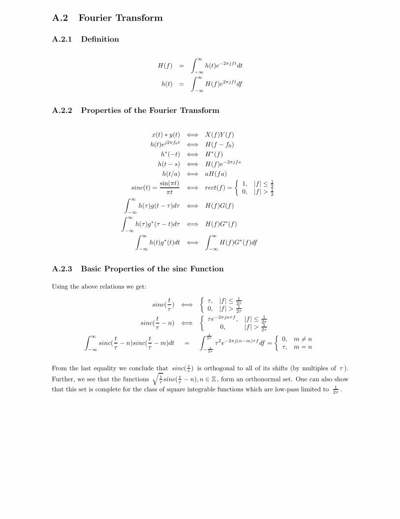
234 APPENDIX A. MATHEMATICAL PRELIMINARIES
A.2 Fourier Transform
A.2.1 Definition
H(f) =
∫ ∞
−∞h(t)e−2πjftdt
h(t) =
∫ ∞
−∞H(f)e2πjftdf
A.2.2 Properties of the Fourier Transform
x(t) ∗ y(t) ⇐⇒ X(f)Y (f)
h(t)ej2πf0t ⇐⇒ H(f − f0)
h∗(−t) ⇐⇒ H∗(f)
h(t− s) ⇐⇒ H(f)e−2πjfs
h(t/a) ⇐⇒ aH(fa)
sinc(t) =sin(πt)
πt⇐⇒ rect(f) =
1, |f | ≤ 1
20, |f | > 1
2∫ ∞
−∞h(τ)g(t− τ)dτ ⇐⇒ H(f)G(f)
∫ ∞
−∞h(τ)g∗(τ − t)dτ ⇐⇒ H(f)G∗(f)
∫ ∞
−∞h(t)g∗(t)dt ⇐⇒
∫ ∞
−∞H(f)G∗(f)df
A.2.3 Basic Properties of the sinc Function
Using the above relations we get:
sinc(t
τ) ⇐⇒
τ, |f | ≤ 1
2τ0, |f | > 1
2τ
sinc(t
τ− n) ⇐⇒
τe−2πjnτf , |f | ≤ 1
2τ0, |f | > 1
2τ∫ ∞
−∞sinc(
t
τ− n)sinc(
t
τ−m)dt =
∫ 12τ
− 12τ
τ2e−2πj(n−m)τfdf =
0, m 6= nτ, m = n
From the last equality we conclude that sinc( tτ ) is orthogonal to all of its shifts (by multiples of τ ).
Further, we see that the functions√
1τ sinc(
tτ − n), n ∈ Z , form an orthonormal set. One can also show
that this set is complete for the class of square integrable functions which are low-pass limited to 12τ .

A.3. Z-TRANSFORM 235
A.3 Z-Transform
A.3.1 Definition
Assume we have a discrete time (real or complex valued) signal xn , n ∈ Z . Its associated z-transform,call it X(z) (if it exists), is defined by
X(z) =
+∞∑
n=−∞x(n)z−n
The region of convergence, known as the ROC, is important to understand because it defines the regionwhere the z-transform exists. The ROC for a given x[n] is defined as the range of z for which the z-
transform converges. By the Cauchy criterion, a power series∑∞
k=0 u(k) converges if limk→∞ |u(k)| 1k <
1 . One can write+∞∑
n=−∞x(n)z−n =
+∞∑
n=1
x(−n)zn +
+∞∑
n=0
x(n)z−n
and it follows by the Cauchy criterion that the first series converges if |z| < limk→∞1
|x(−k)|1k
= Rx+ and
the second converges if |z| > limk→∞ |x(k)| 1k = Rx− Then the region of convergence is an annular region
such that Rx− < |z| < Rx+
A.3.2 Basic Properties
x∗−n ⇐⇒ X∗(1/z∗)
x∗n−m ⇐⇒ X(z)z−m
∑
k
xkyn−k ⇐⇒ X(z)Y (z)
∑
k
xky∗n−k ⇐⇒ X(z)Y ∗(1/z∗)
We say that a sequence xn is causal if xn = 0 for n < 0 and we say that it is anticausal if xn = 0 forn > 0 . For a causal sequence the ROC is of the form |z| > R whereas for an anticausal it is of the form|z| < R . We say that a sequence is stable if
∑n |xn| <∞ . The ROC of a stable sequence must contain
the unit circle. If X(z) , the z-transform of xn , is rational then it implies that for a stable and causalsystem all the poles of X(z) must be within the unit circle. Finally, we say that a sequence xn withrational z-transform X(z) is minimum phase, if all its poles and zeros are within the unit circle. Such a
sequence has the property that for all N ≥ 0 it maximizes the quantity∑N
n=0 |xn|2 over all sequenceswhich have the same |H(z)| .
A.4 Energy and power constraints
The signal x(t) is said to have finite energy if
Ex4=
∫|x(t)|2dt <∞
and it is said to have finite power if
Px4= lim
T→∞
1
T
∫ T2
−T2
|x(t)|2dt <∞
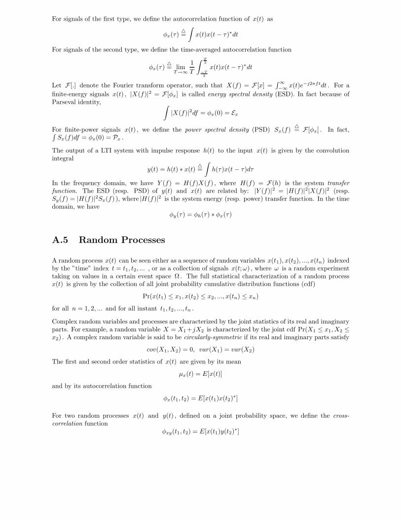
236 APPENDIX A. MATHEMATICAL PRELIMINARIES
For signals of the first type, we define the autocorrelation function of x(t) as
φx(τ)4=
∫x(t)x(t − τ)∗dt
For signals of the second type, we define the time-averaged autocorrelation function
φx(τ)4= lim
T→∞
1
T
∫ T2
−T2
x(t)x(t − τ)∗dt
Let F [.] denote the Fourier transform operator, such that X(f) = F [x] =∫∞−∞ x(t)e−j2πftdt . For a
finite-energy signals x(t) , |X(f)|2 = F [φx] is called energy spectral density (ESD). In fact because ofParseval identity, ∫
|X(f)|2df = φx(0) = Ex
For finite-power signals x(t) , we define the power spectral density (PSD) Sx(f)4= F [φx] . In fact,∫
Sx(f)df = φx(0) = Px .
The output of a LTI system with impulse response h(t) to the input x(t) is given by the convolutionintegral
y(t) = h(t) ∗ x(t) 4=
∫h(τ)x(t − τ)dτ
In the frequency domain, we have Y (f) = H(f)X(f) , where H(f) = F(h) is the system transferfunction. The ESD (resp. PSD) of y(t) and x(t) are related by: |Y (f)|2 = |H(f)|2|X(f)|2 (resp.Sy(f) = |H(f)|2Sx(f) ), where |H(f)|2 is the system energy (resp. power) transfer function. In the timedomain, we have
φy(τ) = φh(τ) ∗ φx(τ)
A.5 Random Processes
A random process x(t) can be seen either as a sequence of random variables x(t1), x(t2), ..., x(tn) indexedby the ”time” index t = t1, t2, ... , or as a collection of signals x(t;ω) , where ω is a random experimenttaking on values in a certain event space Ω . The full statistical characterization of a random processx(t) is given by the collection of all joint probability cumulative distribution functions (cdf)
Pr(x(t1) ≤ x1, x(t2) ≤ x2, ..., x(tn) ≤ xn)
for all n = 1, 2, ... and for all instant t1, t2, ..., tn .
Complex random variables and processes are characterized by the joint statistics of its real and imaginaryparts. For example, a random variable X = X1+jX2 is characterized by the joint cdf Pr(X1 ≤ x1, X2 ≤x2) . A complex random variable is said to be circularly-symmetric if its real and imaginary parts satisfy
cov(X1, X2) = 0, var(X1) = var(X2)
The first and second order statistics of x(t) are given by its mean
µx(t) = E[x(t)]
and by its autocorrelation function
φx(t1, t2) = E[x(t1)x(t2)∗]
For two random processes x(t) and y(t) , defined on a joint probability space, we define the cross-correlation function
φxy(t1, t2) = E[x(t1)y(t2)∗]

A.6. WIDE SENSE STATIONARY PROCESSES 237
A.6 Wide sense stationary processes
A random process x(t) is said to be wide-sense stationary (WSS) if
(a) µx(t) = µx is constant with t
(b) φx(t1, t2) depends only on the difference τ = t1 − t2 (we can use the notation φx(τ)4= φx(t+ τ, t) ).
Two random processes x(t) and y(t) are said to be jointly WSS if both x(t) and y(t) are individuallyWSS and if their cross-correlation function φxy(t1, t2) depends only on the difference t1 − t2 .
For WSS processes, we have
Sx(f) = F [φx] =
∫φx(t)e−j2πftdt
and for jointly WSS processes, the cross-spectrum is given by Sxy(f) = F [φxy(τ)] .
The output of a LTI system with impulse response h(t) to the WSS input x(t) is the WSS process givenby
y(t) = h(t) ∗ x(t) 4=
∫h(τ)x(t − τ)dτ
The two processes x(t) and y(t) are jointly WSS. The mean and autocorrelation of y(t) and the cross-correlation between x(t) and y(t) are given by
µy = µx
∫h(t)dt
φy(τ) = φh(τ) ∗ φx(τ)
φxy(τ) = h(−τ)∗ ∗ φx(τ)
In the frequency domain we haveµy = µxH(0)
Sy(f) = H(f)2Sx(f)
Sxy(f) = H(f)∗Sx(f)
Since φyx(τ) = φxy(−τ)∗ , we have Syx(f) = Sxy(f)∗ , that yields Syx(f) = H(f)Sx(f) , since Sx(f) isreal.
A.7 Gram-Schmidt orthonormalisation
Let V be an inner product space and let A = a1, ..., am be a set of elements of V . The followingGram-Schmidt procedure then allows us to find an orthonormal basis for A . Let this basis be ψ1, ..., ψn ,n ≤ m , so that
ai =
n∑
j=1
〈ai, ψj〉ψj , i ∈ [n]

238 APPENDIX A. MATHEMATICAL PRELIMINARIES
This basis is recursively defined by (ignoring cases of dependent vectors)
ψ1 =a1√
〈a1, a1〉
ψ2 =a2 − 〈a2, ψ1〉ψ1√⟨
(a2 − 〈a2, ψ1〉ψ1), (a2 − 〈a2, ψ1〉ψ1)⟩
... . . .
ψn =am −∑m−1
j=1 〈am, ψj〉ψj√⟨(am −∑m−1
j=1 〈am, ψj〉ψj), (am −∑m−1j=1 〈am, ψj〉ψj)
⟩
In general, the basis obtained by the above algorithm depends on the order in which the elements ai areconsidered. Different ordering yield different bases for the same vector space.
A.8 The Sampling Theorem
Let s(t) be a function in L2 that is lowpass limited to B . Then s(t) is specified by its values at asequence of points spaced at T = 1
2B intervals by the interpolation formula:
s(t) =
∞∑
n=−∞s(nT ) sinc(
t
T− n)
where sinc(t) = sin(πt)πt .
The sinc pulse does not have unit energy. Hence we define (its normalized version) ψ(t) = 1√T
sinc ( tT ) .
The set ψ(t− iT )∞i=−∞ forms an orthonormal set. Hence we can write:
s(t) =∞∑
i=−∞siψ(t− iT )
where si = s(nT )√T . This highlights the way the sampling theorem should be seen, namely as a
particular instance of an orthonormal expansion. In this expansion the basis is formed by time translatedsinc pulses. Implicit in the sampling theorem is the fact that the set ψ(t − iT )∞i=−∞ is a completeorthonormal basis for the set of waveforms that are lowpass limited to B = 1
2T .
A.9 Nyquist Criterion
We are looking for functions ψ(t − T ) (like the sinc function constructed above) with the property:∫∞−∞ ψ(t− nT )ψ∗(t)dt = δn
We now look for the condition under which a real-valued function ψ(t) ensures that ψ(t), ψ(t−T ), ψ(t−2T ), . . . forms an orthonormal sequence.
Define
g(f) =∑
k∈N
ψF (f +k
T)ψ∗
F (f +k
T).

A.10. CHOLESKI DECOMPOSITION 239
where ψF(f) = Fψ(t) Now
δn =
∫ ∞
−∞ψF (t− nT )ψ∗
F(t)dt
(Parseval)=
∫ ∞
−∞ψF (f)ψ∗
F (f)e−j2πnTfdf
=
∞∑
−∞
∫ (2m+1)/2T
(2m−1)/2T
ψF (f)ψ∗F (f)e−j2πnTfdf
=
∞∑
−∞
∫ 1/2T
−1/2T
ψF (f +m/T )ψ∗F(f +m/T )e−j2πnTfdf
=
∫ 12T
− 12T
g(f)e−j2πnTfdf.
The last expression is T times the n -th Fourier series coefficient of g(f) . Since only the coefficient withn = 0 is nonzero, the function g(f) must be constant. Specifically, g(f) ≡ T, f ∈ [− 1
2T ,1
2T ] .
Then, one can state :
A waveform ψ(t) is orthonormal to each shift ψ(t− nT ) if and only if
∞∑
k=−∞|ψF (f +
k
T)|2 = T for f ∈ [− 1
2T,
1
2T]
T
f1T
|ψF (f)|2 + |ψF (f − 1/T )|2 = T
A.10 Choleski Decomposition
Given a Hermitian positive definite matrix A , the Cholesky decomposition is a diagonal matrix D andan upper triangular matrix U with ones on the main diagonal such that
A = U∗DU .
A.11 Problems
Problem A.1
Prove the following bounds on Q -function for α > 0 :
1√2πα
e−α2
2 (1 − 1
α2) < Q(α) <
1√2πα
e−α2
2 .

240 APPENDIX A. MATHEMATICAL PRELIMINARIES
Hint: e−y2
2 = e−y2
2 y 1y and integrate by parts.
Problem A.2
Prove the following properties of fourier transform:
• frequency shift - h(t)ej2πf0t ⇐⇒ H(f − f0) .
• time shift - h(t− s) ⇐⇒ H(f)e−2πjfs .
• lateral inversion - h∗(−t) ⇐⇒ H∗(f) .
• time scaling - h(
ta
)⇐⇒ |a|H(fa) .
Problem A.3
Given 0 < a < b , find the temporal sequence x(n) of
X(z) =2 − (a+ b)z−1
(1 − az−1)(1 − bz−1),
when
(a) the ROC is |z| > b .
(b) the ROC is a < |z| < b .
Problem A.4
(a) A random process Z(t) is given by
Z(t) = sin(2πf0t+ Θ),
where Θ is uniformaly distributed on [−π, π] . Find its power spectral density.
(b) Let X(t) be a WSS process with autocorrelation function φX(τ) = e−|τ | . Find E
[(X(0) +X(2))
2].
(c) Let W (t) = Ybtc , where Yi∞−∞ are independent zero-mean, unit-variance Gaussian random vari-ables. Is W (t) a WSS process?
Problem A.5
A zero-mean WSS process x(t) with autocorrelation function φX(τ) = e−|τ | is passed through a LTIfilter with impulse response h(t) = e−t . Show that x(t) and y(t) are jointly WSS. Find φY (τ) andφXY (τ) .

A.11. PROBLEMS 241
Problem A.6
In this exercise we continue our review of what happens when stationary stochastic processes are filtered.Let X(t) and U(t) denote two stochastic processes and let Y (t) and V (t) be the result of passing X(t)respectively U(t) through linear time invariant filters with impulse response h(t) and g(t) , respectively.For any pair (X,U) of stochastic processes define the cross-correlation as
RXU (t1, t2) = E[X(t1)U∗(t2)],
We say that the pair (X,U) is jointly wide sense stationary if each of them is wide sense stationary andif RXU (t1, t2) is a function of the time difference only. In this case we define a cross-power spectrum asthe Fourier transform of the cross-correlation function.
Show that if (X,U) are jointly wide sense stationary then so are (Y, V ) and that
SY V (f) = SXU (f)H(f)G∗(f).
Problem A.7
Show that the cross-correlation function RXU (τ) has symmetry
RXU (τ) = R∗UX (−τ)
Problem A.8
(a) Let Xr and Xi be statistically independent zero-mean Gaussian random variables with identicalvariances. Show that a (rotational) transformation of the form
Yr + jYi = (Xr + jXi)ejφ
results in another pair (Yr, Yi) of Gaussian random variables that have the same joint PDF as thepair (Xr, Xi) .
(b) Note that [Yr
Yi
]= A
[Xr
Xi
]
where A is a 2 × 2 matrix. As a generalization of the transformation considered in (1), whatproperty must the linear transformation A satisfy if the PDFs for X and Y , where Y = AX , X =(X1, X2, · · · , Xn) and Y = (Y1, Y2, · · · , Yn) are identical? Here also we assume that (X1, · · · , Xn)are zero-mean statistically independent Gaussian random variables with same variance.
Problem A.9
[Transformation of Gaussian Random Variables] Let Z = (Z1, . . . , Zn) denote a jointly Gaussian vectorwith independent components with zero mean and each with variance σ2 , i.e., we have
fZ(z) =1
(2πσ2)n/2e−
‖z‖2
2σ2
Let ψ1, . . . , ψn be any basis for Rn , i.e., an orthonormal set and let W = (W1, . . . ,Wn) denote a
random vector whose components are the projections of Z onto this basis, i.e, Wi = 〈Z,ψi〉 . Show thatW has the same distribution as Z , i.e., W is a jointly Gaussian vector with independent componentswith zero mean and each with variance σ2 .

242 APPENDIX A. MATHEMATICAL PRELIMINARIES
Problem A.10
Let Z(t) be a real-valued Gaussian process with double-sided power spectral density equal to N0
2 . Letψ1(t) and ψ2(t) be two orthonormal functions and for k = 0, 1 define the random variables Zk =∫∞−∞ Z(t)ψk(t)dt . What is the distribution of (Z1, Z2) ?