Embed Size (px)
Citation preview

Advanced Controllers for Electromechanical
Motion Systems
Graduation committee:
Chairman: prof.dr.ir. A.J. Mouthaan University of Twente, EWI
Secretary: prof.dr.ir. A.J. Mouthaan University of Twente, EWI
Promotor: prof.dr.ir. J. van Amerongen University of Twente, EWI
Asst. promotor: dr.ir. T.J.A. de Vries University of Twente, EWI
Members: prof.dr.ir. P.H. Veltink University of Twente, EWI
dr. J.W. Polderman University of Twente, EWI
prof.dr.ir. P.P.J. van den Bosch University of Eindhoven
prof.dr.ir. G. van Straten University of Wageningen
The author has followed the educational program of the Dutch Institute of Systems
and Control (DISC).
This research was financially supported by the Vietnamese Government through
the 322 project and carried out at the Control Engineering group, University of
Twente, The Netherlands.
ISBN: 978-90-365-2654-8
The cover figure of this thesis gives an overview of the input reference and the
tracking errors for the different controllers that have been tested on the Tripod.
Copyright c© 2008 by Nguyen Duy Cuong
Printed at Wohrmann Print Service, Zutphen, The Netherlands.

ADVANCED CONTROLLERS
FOR
ELECTROMECHANICAL MOTION SYSTEMS
DISSERTATION
to obtain
the degree of doctor at the University of Twente,
on the authority of the rector magnificus,
prof.dr.W.H.M. Zijm,
on account of the decision of the graduation committee,
to be publicly defended
on Thursday, 10th of April 2008 at 13.15h
by
Nguyen Duy Cuong
born on 9th of May, 1962
in Laocai, Vietnam

This dissertation is approved by:
Prof.dr.ir. J. van Amerongen, promotor
Dr.ir. T.J.A. de Vries, assistant promotor

SUMMARY
The aim of this research is to develop advanced controllers for electromechan-
ical motion systems. In order to increase efficiency and reliability, these control
systems are required to achieve high performance and robustness in the face of
model uncertainty, measurement noise, and reproducible disturbances.
Proportional Integral Derivative (PID), Linear Quadratic Gaussian (LQG),
Model Reference Adaptive Systems (MRAS) are typical conventional approaches
where control designs involve compromises between conflicting goals. In general,
for the PID control design, a compromise has to be made between performance
and robust stability. In the LQG design the main issue is to trade-off attenuation
of the process disturbances and the fluctuations created by measurement noise
that is injected in the system due to the feedback. Direct MRAS offers a poten-
tial solution to reduce tracking errors when there are large changes in the process
parameters. However, this control algorithm may fail to be robust to measure-
ment noise. Indirect MRAS offers an effective solution to improve the control
performance in the presence of parametric uncertainty and measurement noise.
However, a small tracking error cannot always be obtained.
For motion control systems, Learning Feed-Forward Control (LFFC) may be
used as a framework for solving the problems of reproducible disturbances. The
solution is in the form of a two-degree-of-freedom controller, whose feedback and
feed-forward paths independently provide the appropriate signals for disturbance
rejection and model uncertainty. The use of LFFC can improve not only the dis-
turbance rejection, but also the stability robustness of the controlled systems. Two
main distinct methods, namely Neural Network (NN)-based LFFC and Model
Reference Adaptive Systems (MRAS)-based LFFC, are investigated. Although
both methods have been studied, little effort has been devoted to comparing or
combining them. In this thesis, designs of NN-based LFFC and of MRAS-based
LFFC have been developed for the high-performance robust motion control of a
linear motor and a comparison of the two approaches has been evaluated. It is our
first main contribution.
One of the main drawbacks of the NN-based LFFC is the requirement that
the training motions are chosen carefully, such that all possibly relevant input
combinations are covered. This requirement may be quite restrictive in practical
applications. MRAS-based LFFC can be used to overcome such problem. By im-
plementing both controllers on the Tripod setup, the performances of each method
are compared. The experimental results show that both control algorithms reach
almost the same tracking error after convergence and are superior to the PID con-
troller. However, after convergence the MRAS-based LFFC is able to generate a
much better feed-forward control and hence obtain about a 5 times smaller maxi-

vi
mum tracking error than the NN-based LFFC with an untrained reference motion.
The reason for this is that MRAS-based LFFC can quickly generate appropri-
ate actions for any coming input change. Moreover, compared to the NN-based
LFFC, the MRAS-based LFFC is simpler to implement. The resulting control
laws are simple and thus interesting for use in practical applications. Further-
more, an important difference is that the stability of the MRAS-based LFFC is
analyzed by the Lyapunov theory. In other words, the stability properties of the
MRAS-based LFFC are better understood.
We have shown that a combination of NN-based LFFC (to deal with non-
linearities, like cogging) and MRAS-based LFFC is superior to both systems
alone. The combination performs better with respect to tracking errors and speed
of learning and is simpler to realize. This is our second contribution. Both NN-
based LFFC and MRAS-based LFFC can achieve good disturbance rejection, but
the performance is limited by measurement noise.
In recent researches, variants of LQG have been used in combination with
other algorithms to achieve better performance. Our third main contribution is
the design of LQG combined with MRAS-based LFFC. This is a robust, high-
performance control scheme that combines the advantages and overcomes the
disadvantages of both types of techniques. In comparison to a PID controller,
the LQG combined with MRAS-based LFFC has the following benefits: (1) it
significantly reduces the tracking errors for any input reference signal; (2) it ef-
fectively improves the robustness with respect to changes in plant parameters and
respect to measurement noise; (3) it can obtain faster transient response.
vii
SAMENVATTING
Het doel van dit onderzoek is het ontwikkelen van geavanceerde regelaars voor
elektro-mechanische bewegingssystemen. Om de efficintie en betrouwbaarheid
te vergroten dienen deze regelaars een hoog prestatie- en robuustheidsniveau te
realiseren, ondanks de aanwezigheid van modelonzekerheid, meetruis en repro-
duceerbare verstoringen.
PID (proportioneel, integrerend, differentirend), LQG (lineair, kwadratisch,
Gaussisch), of MRAS (model-referentie adapterende systemen) zijn kenmerkende
conventionele benaderingen, waarbij het regelaar-ontwerp een compromis vormt
tussen onderling strijdige regeldoelen. Voor een PID-ontwerp is het in het al-
gemeen noodzakelijk om de haalbare prestatie te beperken ten gunste van een
robuuste stabiliteit. In het LQG-ontwerp ligt de nadruk op het uitruilen van de
onderdrukking van procesverstoringen tegen variaties die ontstaan door meetruis
die het systeem binnenkomt als gevolg van het aanbrengen van terugkoppeling.
Directe MRAS biedt een mogelijke oplossing voor het reduceren van volgfouten
wanneer er grote veranderingen optreden in de procesparameters. Echter, dit rege-
lalgoritme zal doorgaans geen robuustheid voor meetruis kunnen bieden. Indirecte
MRAS vormt een effectieve oplossing voor het verbeteren van de regelprestatie
bij aanwezigheid van parametrische onzekerheid en meetruis. Echter, een kleine
volgfout wordt niet altijd verkregen.
Bij regelaars voor bewegingssystemen kan Lerende Vooruitkoppeling (LFFC)
worden gebruikt als een raamwerk voor het oplossen van de problemen ten
gevolge van reproduceerbare verstoringen. De oplossing heeft de vorm van
een twee-graden-van-vrijheid regelaarstructuur, waarbij de terugkoppeling en de
vooruitkoppeling onafhankelijk van elkaar in de signalen voorzien die geschikt
zijn voor het tegengaan van verstoringen en voor modelonzekerheid. Het inzetten
van LFFC kan zorgen voor een betere storingsonderdrukking, en tegelijkertijd de
robuuste stabiliteit van het geregelde systeem vergroten. Twee verschillende vor-
men zijn onderzocht, namelijk op Neurale Netwerken (NN) gebaseerde LFFC en
op MRAS gebaseerde LFFC. Beide methoden zijn eerder bestudeerd, maar er is
nog weinig aandacht gegeven aan het vergelijken en het combineren ervan. In
dit proefschrift zijn NN-gebaseerde en MRAS-gebaseerde LFFC ontwerpen on-
twikkeld voor hoog-performante robuuste regeling van een lineaire aandrijving en
is een vergelijkende evaluatie van de twee benaderingen uitgevoerd. Dit is onze
eerste bijdrage.
Een van de belangrijkste nadelen van de NN-gebaseerde LFFC is de vereiste
dat de bewegingen voor het trainen zodanig zorgvuldig worden gekozen, dat alle
mogelijk relevante combinaties van ingangs-variabelen worden afgedekt. In prak-
tische situaties kan dit als restrictief worden ervaren. MRAS-gebaseerde LFFC

viii
kan worden ingezet om dergelijke moeilijkheden te overwinnen. Door beide rege-
laars te implementeren op de Tripod opstelling zijn de prestaties van elk van de
methodes vergeleken. De experimentele resultaten laten zien dat de beide rege-
lalgoritmen na convergentie ongeveer dezelfde volgfout bezitten en superieur zijn
aan de PID regelaar. Echter, na convergentie is de MRAS-gebaseerde LFFC in
staat om veel betere voorwaartse sturing en dus een omstreeks 5 keer kleinere
maximale volgfout te realiseren ten opzichte van de NN-gebaseerde LFFC voor
een niet-getrainde beweging. De reden hiervan is dat MRAS-gebaseerde LFFC
snel geschikte regelacties kan genereren voor elke verandering van de ingangsvari-
abelen. Bovendien is de MRAS-gebaseerde LFFC in vergelijking met de NN-
gebaseerde LFFC eenvoudiger te implementeren. De resulterende regelwetten zijn
eenvoudig en dus interessant voor gebruik in realistische toepassingen. Voorts is
een belangrijk verschil dat de stabiliteit van de MRAS-gebaseerde LFFC is ge-
analyseerd met behulp van de theorie van Lyapunov. Met andere woorden, de
stabiliteitseigenschappen van de MRAS-gebaseerde LFFC zijn beter begrepen.
We hebben laten zien dat een combinatie van NN-gebaseerde LFFC (nodig
voor niet-lineariteiten zoals krachtrimpel) en MRAS-gebaseerde LFFC superieur
is aan beide systemen individueel. De combinatie presteert beter met betrekking
tot volgfouten en snelheid van leren en is eenvoudiger te realiseren. Dit is onze
tweede bijdrage. Zowel NN-gebaseerde LFFC als MRAS-gebaseerde LFFC is in
staat om verstoringen te onderdrukken, maar de prestaties worden beperkt door
meetruis.
In recent onderzoek zijn varianten van LQG ingezet in combinatie met an-
dere algoritmes om te komen tot betere prestatie. Onze derde bijdrage is het on-
twerp van LQG gecombineerd met MRAS-gebaseerde LFFC. Dit vormt een robu-
ust, hoog-performant regelschema dat de voordelen samenbrengt en de nadelen
oplost van beide technieken. In vergelijking met een PID-regelaar heeft de LQG
gecombineerd met de MRAS-gebaseerde LFFC de volgende voordelen: (1) de
volgfouten voor willekeurige gewenste ingangssignalen zijn significant verkleind;
(2) de robuustheid voor veranderingen in procesparameters en voor meetruis zijn
op effectieve wijze verbeterd; (3) de responsie op overgangen is versneld.

To my parents,
my sister Canh-Ty, my brothers Hung-Tam and Cuong-Cham,
to my wife Linh, and to Thanh Van - Duy An


Contents
1 Introduction 1
1.1 Advanced Controllers for Motion Systems - Why? . . . . . . . . . 1
1.2 Disturbances in electromechanical motion systems . . . . . . . . 2
1.2.1 Plant reproducible disturbances . . . . . . . . . . . . . . 2
1.2.2 Measurement noise . . . . . . . . . . . . . . . . . . . . . 4
1.2.3 Model uncertainty . . . . . . . . . . . . . . . . . . . . . 5
1.3 Design of Control Systems . . . . . . . . . . . . . . . . . . . . . 5
1.4 Applications . . . . . . . . . . . . . . . . . . . . . . . . . . . . . 6
1.4.1 The MeDe5 . . . . . . . . . . . . . . . . . . . . . . . . . 6
1.4.2 The Tripod . . . . . . . . . . . . . . . . . . . . . . . . . 9
1.5 Aim and outline of the thesis . . . . . . . . . . . . . . . . . . . . 10
2 A review of Classical and Advanced Controllers 13
2.1 Introduction . . . . . . . . . . . . . . . . . . . . . . . . . . . . . 13
2.2 PID Controller . . . . . . . . . . . . . . . . . . . . . . . . . . . 14
2.3 Linear Quadratic Gaussian . . . . . . . . . . . . . . . . . . . . . 17
2.3.1 Linear Quadratic Regulator . . . . . . . . . . . . . . . . . 17
2.3.2 Linear Quadratic Estimator . . . . . . . . . . . . . . . . . 19
2.3.3 Linear Quadratic Gaussian . . . . . . . . . . . . . . . . . 20
2.3.4 Discrete LQG design . . . . . . . . . . . . . . . . . . . . 22
2.4 Model Reference Adaptive Systems . . . . . . . . . . . . . . . . 25
2.4.1 Direct MRAS . . . . . . . . . . . . . . . . . . . . . . . . 26
2.4.2 Indirect MRAS . . . . . . . . . . . . . . . . . . . . . . . 28
2.5 Discussion . . . . . . . . . . . . . . . . . . . . . . . . . . . . . . 33
3 Neural Network based Learning Feed-Forward Control 35
3.1 Introduction . . . . . . . . . . . . . . . . . . . . . . . . . . . . . 35
3.2 Learning Control . . . . . . . . . . . . . . . . . . . . . . . . . . 36
3.3 Feedback-error learning . . . . . . . . . . . . . . . . . . . . . . . 37
3.3.1 Control Structure . . . . . . . . . . . . . . . . . . . . . . 37
3.3.2 Plant disturbance compensation . . . . . . . . . . . . . . 38
xi
xii CONTENTS
3.3.3 Multi-Layer Perceptron (MLP) neural network . . . . . . 39
3.4 Learning feed-forward control using B-spline neural network . . . 40
3.4.1 Control structure . . . . . . . . . . . . . . . . . . . . . . 40
3.4.2 B-spline neural network . . . . . . . . . . . . . . . . . . 41
3.4.3 Design of LFFC using BSNs . . . . . . . . . . . . . . . . 42
3.5 Input selection of the LFFC . . . . . . . . . . . . . . . . . . . . . 44
3.6 B-spline distribution . . . . . . . . . . . . . . . . . . . . . . . . 45
3.7 Parsimonious LFFC . . . . . . . . . . . . . . . . . . . . . . . . . 46
3.8 Phase correction for LFFC . . . . . . . . . . . . . . . . . . . . . 47
3.8.1 Un-delayed learning . . . . . . . . . . . . . . . . . . . . 47
3.8.2 Delayed learning . . . . . . . . . . . . . . . . . . . . . . 48
3.8.3 Phase-corrected learning feed-forward control . . . . . . . 49
3.9 Design of a parsimonious LFFC . . . . . . . . . . . . . . . . . . 49
3.10 Conclusions . . . . . . . . . . . . . . . . . . . . . . . . . . . . . 59
4 LQG combined with MRAS-based LFFC 61
4.1 Introduction . . . . . . . . . . . . . . . . . . . . . . . . . . . . . 61
4.2 An MRAS-based Learning Feed-Forward Controller . . . . . . . 62
4.2.1 Theoretical Background . . . . . . . . . . . . . . . . . . 62
4.3 Design of the proposed controller . . . . . . . . . . . . . . . . . . 68
4.3.1 Design the MRAS-based LFFC . . . . . . . . . . . . . . 69
4.3.2 Discrete LQG design . . . . . . . . . . . . . . . . . . . . 74
4.3.3 Solution for friction compensation . . . . . . . . . . . . . 77
4.3.4 Solution for cogging compensation . . . . . . . . . . . . 80
4.4 comparison with the conventional PID controller . . . . . . . . . 82
4.5 Discussion . . . . . . . . . . . . . . . . . . . . . . . . . . . . . . 82
4.6 Conclusions . . . . . . . . . . . . . . . . . . . . . . . . . . . . . 83
5 Applications 85
5.1 Introduction . . . . . . . . . . . . . . . . . . . . . . . . . . . . . 85
5.2 Implementation for the MeDe5 . . . . . . . . . . . . . . . . . . . 86
5.3 Implementation for the Tripod . . . . . . . . . . . . . . . . . . . 90
5.3.1 Design of a parsimonious LFFC . . . . . . . . . . . . . . 91
5.3.2 Design of an MRAS-based LFFC . . . . . . . . . . . . . 93
5.3.3 Experimental results . . . . . . . . . . . . . . . . . . . . 94
6 Discussion 97
6.1 Review . . . . . . . . . . . . . . . . . . . . . . . . . . . . . . . 97
6.2 Conclusions . . . . . . . . . . . . . . . . . . . . . . . . . . . . . 100
6.3 Recommendations for future work . . . . . . . . . . . . . . . . . 101

Chapter 1
Introduction
1.1 Advanced Controllers for Electromechanical
Motion Systems - Why?
Motion control is concerned with manipulating power to control the movement
of a mechanical system, and is widely used in packaging, printing, textile, and
other industrial applications. A large amount of motion control is now performed
using electric motors, so that will be our main focus. Motion control systems can
be quite complicated because many different factors have to be considered in the
design. The following issues must typically be considered:
- Reduction of the influence of plant disturbances
- Attenuation of the effect of measurement noise
- Variations and uncertainties in plant behavior
It is difficult to find design methods that consider all these factors, especially
for the conventional control approaches where control designs involve compro-
mises between conflicting goals. In order to design control systems to get high
performance and robustness when controlling such complicated processes, ad-
vanced controllers have been introduced.
The advanced control approaches discussed in this thesis will typically focus
on a few of the issues to obtain suitable solutions. The control methods will be
developed gradually. We start with a simplest design approach and step by step
make it more and more realistic. In a high-quality design it is often necessary to
take into account all mentioned factors, such that high performance and robust
stability can be achieved simultaneously. Several good properties achieved via
the control structures presented in this thesis have the potential of being applied
to electromechanical motion systems where linear or other controllers are unable
to give the desired level of performance.
1

2 Chapter 1: Introduction
1.2 Reproducible disturbances, measurement noise,
and plant uncertainty in electromechanical mo-
tion systems
An electromechanical motion system (see Fig 1.1) is an electrically actuated me-
chanical plant that requires the control of the position of the end-effector [7]. A
path generator indicates a desired path for the end-effector. Electric motors used
can be AC or DC, rotary or linear. Mechanical components to transform the mo-
tion of the electric motor into the end-effector (may) include: shafts, gears, belts,
linkages, rotational bearings, and so on. The use of feedback in order to create
a stable closed-loop system requires the use of suitable sensors to provide the
necessary information on the process. These sensors are generally located at the
actuator and/or the end-effector. With this structure, drawbacks for designing a
Figure 1.1: Electromechanical Motion System.
control system such as plant reproducible disturbances, model uncertainty, and
measurement noise are inevitable. It is difficult to control this system with feed-
back alone to obtain high performance and robustness. The presence of these
challenges is one of the main reasons for using advanced controllers.
1.2.1 Plant reproducible disturbances
A large class of motion control using an electric motor can be represented by
a simple simulation model shown in Fig 1.2 [34]. The plant is always subject
to disturbances. In the permanent-magnet linear motor case, the cogging force is
considered as a position-dependent disturbance and the friction force is a velocity-
dependent disturbance. Thus, these disturbances can be viewed as a function of
the state of the plant and they can have a reproducible characteristic - this means
that reproducible disturbances reoccur in the same manner when a specific motion
is repeated.

Advanced Controllers for Electromechanical Motion Systems 3
The friction force is exerted in a direction that opposes movement, friction
usually does negative work. As explained in [17], friction can be modeled as a
velocity-dependent disturbance, which is natural to most of motion systems. Fric-
tion is highly non-linear and may cause steady-state errors, limit cycles, and poor
performance. The cogging forces [1] are due to the interaction between the perma-
nent magnets and the iron teeth of the primary section. They are especially promi-
nent at lower speeds. They are undesirable effects that prevent smooth movement
of the rotor or translator. In permanent-magnet direct drive linear motors, the cog-
ging forces are considered to be the main disturbances. It is important for the con-
trol engineer to understand friction, and cogging phenomena and to know how to
deal with them. By examining the effects of the cogging and friction disturbances
it is thus possible to detect the status of the process. These reproducible distur-
bances may be reduced at their source. Friction force in a servo can be reduced,
by using better bearings and cogging force can be minimized, by optimizing the
magnet pole arc or width [1]. In this thesis we will focus on reducing effects of
reproducible disturbances by means of control. In order to achieve high-precision
motion control, friction and cogging must be appropriately compensated.
Figure 1.2: Plant model and reproducible disturbances .
Traditionally, the standard Proportional-Integral-Derivative (PID) algorithm
is used in motion control to cope with the friction problem. Integral action is
included in the controller to eliminate the offset. The use of feedback is often
simple and effective because it is not necessary to have the detailed characteristics
of the process [5]. High tracking performance can be obtained when a high gain
is used in the loop. However, increasing the controller gains may make the loop
unstable [4, 3]. The friction force can also be compensated by feed-forward con-
trol but it is only suitable if the desired velocity trajectory is known in advance.
The idea is simple. The friction disturbance is measured, and a control signal that
attempts to counteract this disturbance is generated and applied to the process.

4 Chapter 1: Introduction
In fact, friction varies depending on many factors such as normal force, position,
temperature, and etc. A variation in one of these factors may change the friction
characteristics in complex ways. Since friction characteristics depend on so many
factors it leads to the requirement for automatic adaptation. Cogging disturbances
can be well reduced by feed-forward control. Neural networks are a suitable can-
didate for cogging compensation. The design of a feed-forward compensator is
in essence an approximation of the inverse of a dynamic system [5, 11]. In our
study the compensation of state-dependent effects (such as friction and cogging)
are realized by learning feed-forward control.
1.2.2 Measurement noise
In order to create a closed loop, it is necessary to measure the outputs of the
system. This is implemented by means of sensors in the system. However, these
sensors have noise associated with them, which means that the feedback signal
of the system is corrupted by noise (see Fig 1.3). Next, sensor noise will be
injected into the plant through the control law. Measurement noise then may be
considerably amplified by feedback gains and deteriorates performance. Sensor
noise in a motion control system limits the achievable bandwidth of the closed
loop system. The effect of measurement noise can be attenuated, by moving a
sensor to a position where there are smaller noises or by replacing a sensor with
another that has less noise. In this thesis we will focus on reducing effects of
Figure 1.3: Process disturbance and measurement noise.
measurement noise by means of filtering. Kalman filters and adaptive estimators
are typical examples. In fact, the control signal will often be contaminated by
unwanted signals, thus filtering is necessary in order to make the process response
close to the desired response. Frequently, in talking about filtering and related
problems, it is implicit that the systems under control are noisy. As stated in [2],
the best filter is that which, on the average, has its output closest to the correct or
useful signal. As can be seen in Fig 1.3, process disturbance acts at the process
input and measurement noise acts at the process output. Major issue in many
control designs is a compromise between reduction of process disturbances and
eliminating the fluctuations caused by the measurement noise [5].

Advanced Controllers for Electromechanical Motion Systems 5
1.2.3 Model uncertainty
In reality, motion control systems always operate with model uncertainty. Un-
certainty is the absence of information, which may be described and measured.
Model uncertainty may consist of parametric uncertainty and un-modeled dynam-
ics. As explained in [20], parametric uncertainty may be caused by variable pay-
load, poorly known masses and inertias, or by unknown and slowly time-varying
friction parameters, etc. Structural uncertainty due to un-modeled dynamics may
be caused by neglected friction in the drives, backlash in the gears, by neglected
flexibility in joints and links, etc. In control theory, model uncertainty is consid-
ered from the points of view of physical system modeling. Un-modeled dynamics
and parametric uncertainty have a negative effect on the tracking performance
and can even lead to instability. If the model structure is assumed to be correct,
but only accurate knowledge of plant parameters is not available, adaptive con-
trol can be applied [4, 40]. In adaptive control, one or more control parameters
and/or model parameters are adjusted on-line by an adaptation algorithm such
that the closed-loop dynamics match approximately the behavior of the desired
reference model despite of unknown or time varying plant parameters. Hence,
to achieve asymptotic trajectory tracking, parametric uncertainty should be taken
into account, under the condition that a stable closed-loop performance can be
guaranteed.
1.3 Design of Control Systems
Most control systems are inherently nonlinear in nature. It is common to approxi-
mate them as linear mathematical models with disturbance and model uncertainty,
which allows us to use the well-developed analytical design methods for linear
systems. The aim of control engineering design is to obtain the configuration,
specifications, and identification of the key parameters of a given system to meet
an actual need [33]. Specifications are an explicit set of requirements to be satis-
fied by the device or product. Generally, the performance specifications given to
the particular system suggest which control design method to use.
If the performance specifications are given in terms of frequency-domain per-
formance measures and/or transient-response characteristics, then a conventional
approach based on the frequency-response and/or root-locus methods may be
used. With the classical control methods, the system under control is described by
the input-output relationship, or transfer function. When using frequency response
methods, the control designer wishes to alter the system so that the frequency re-
sponse of the designed system will satisfy the specifications. When using root
locus methods, the designer wishes to alter and reshape the root locus so that the

6 Chapter 1: Introduction
roots of the obtained system will lie in the desired position in the s-plane. Con-
trol designs based on a conventional approach are in principle limited to linear
time-invariant systems [33, 15].
If the performance specifications are given as performance indices in terms of
state variables, then a modern control approach should be used. These specifi-
cations may include characteristics such as the energy dissipated by the system,
and the required control effort. For a physical system these indices are always
constrained. In modern control design, the system under control is described in
state space or input-output model and control methods are mainly developed in
the time domain. By using modern control approaches, the control designer is
able to start from a performance index, together with constraints imposed on the
system to create a stable system. The design via the context of modern control
theory uses mathematical formulations of the problem and applies mathematical
theory to the design problem in which the system can have multiple inputs and
multiple outputs and can be time varying [33]. It enables the designer to create a
designed system that is optimal with respect to the performance index.
Once performance specifications and an appropriate plant model are deter-
mined, the actual design of the control system can be established. There are many
control methods for control system design. However, the preferable method is
selected based on the performance specifications, the plant model, and the knowl-
edge and experience of the designer. After a system is designed, if we can achieve
the desired performance by adjusting the parameters, we will finalize the design
and proceed to document the results. If it does not, we will need to change the
system configuration and/or select an enhanced actuator and sensor then we will
repeat the design steps until we are able to meet the required specifications. The
educated trial-and-error-repetition technique is helpfully used in order to achieve
the desired parameter settings.
It is commonly expected that: (1) the designed system should exhibit as small
errors as possible in responding to the desired reference input, (2) the system
dynamics should be relatively insensitive to changes in system parameters, and
(3) the effects of the process disturbances should be attenuated and the influence
of measurement noise should be suppressed.
1.4 Applications
1.4.1 The MeDe5
For the purpose of testing the results of the controller designs for linear and non-
linear systems, The Control Engineering group of The Department of Electrical
Engineering in The Faculty of Electrical Engineering, Mathematics and Computer
Advanced Controllers for Electromechanical Motion Systems 7
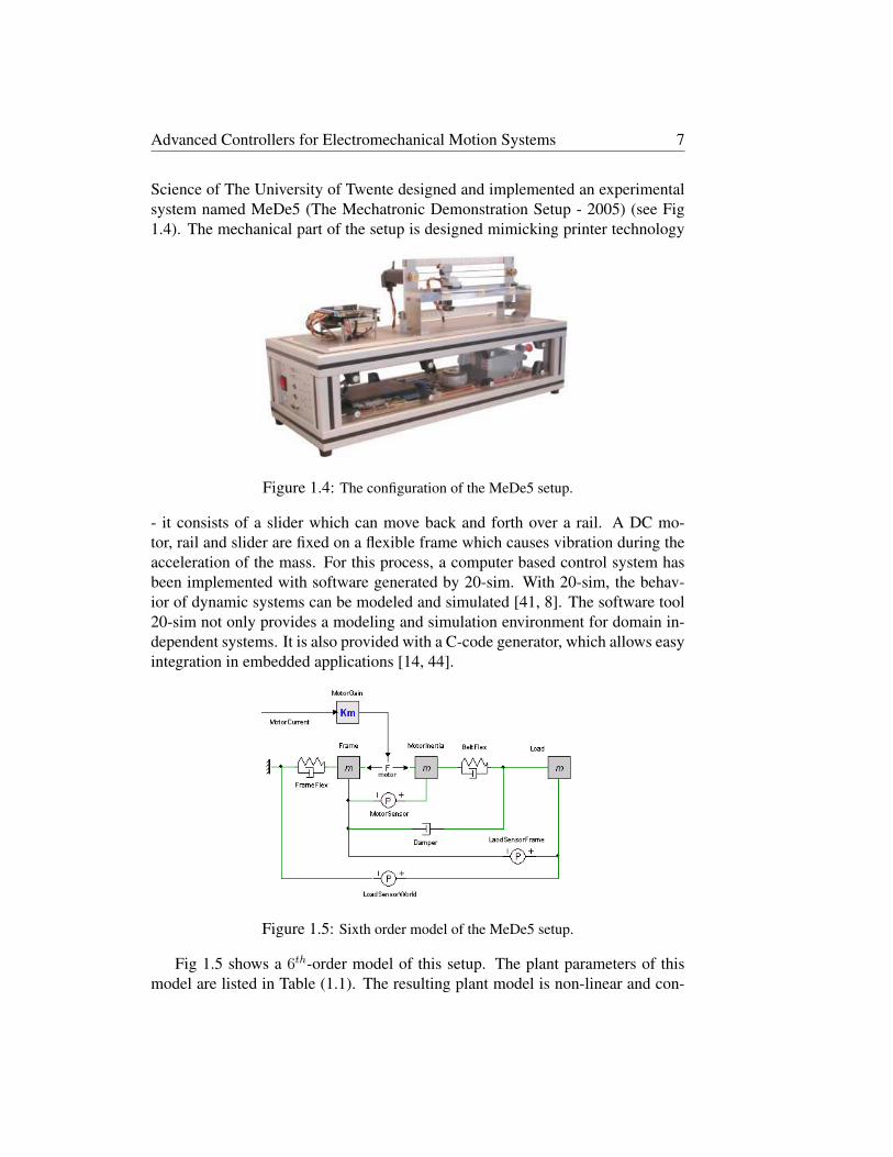
Science of The University of Twente designed and implemented an experimental
system named MeDe5 (The Mechatronic Demonstration Setup - 2005) (see Fig
1.4). The mechanical part of the setup is designed mimicking printer technology
Figure 1.4: The configuration of the MeDe5 setup.
- it consists of a slider which can move back and forth over a rail. A DC mo-
tor, rail and slider are fixed on a flexible frame which causes vibration during the
acceleration of the mass. For this process, a computer based control system has
been implemented with software generated by 20-sim. With 20-sim, the behav-
ior of dynamic systems can be modeled and simulated [41, 8]. The software tool
20-sim not only provides a modeling and simulation environment for domain in-
dependent systems. It is also provided with a C-code generator, which allows easy
integration in embedded applications [14, 44].
Figure 1.5: Sixth order model of the MeDe5 setup.
Fig 1.5 shows a 6th-order model of this setup. The plant parameters of this
model are listed in Table (1.1). The resulting plant model is non-linear and con-

8 Chapter 1: Introduction
tains high-order terms. In order to obtain a more simple plant model, linearization
should be first applied and then the resulting high-order linear model should be
reduced to an appropriate order. This allows us to use one or more of the well-
developed design methods for linear systems. The model as shown in Fig 1.5
Element Parameter Value
Motor-Gain Motor constant 5.7 N/A
Frame Mass of the frame 0.8 kg
Frame-Flex Spring constant 6 kN/m
Damping in frame 6 Ns/m
Motor-Inertia Inertia of the motor 1e-5 kg
Load Mass of the end effector (slider) 0.3 kg
Belt-Flex Spring constant 80 kN/m
Damping in belt 1 Ns/m
Damper Viscous friction 3 Ns/m
Coulomb friction 0.5 N
Table 1.1: Plant parameters of the MeDe5
also contains a non-linear part. The Damper component represents a viscous and
Coulomb friction. Coulomb friction always opposes relative motion and is simply
modeled as
Fc = dc · tanh (1000 · x) (1.1)
where dc is the Coulomb parameter of the Damper element, x is the velocity of
the load. Viscous friction is proportional to the velocity. It is normally described
as
Fv = d · x (1.2)
where d is the viscous parameter of the Damper element. The mathematical ex-
pression for the combination of viscous and Coulomb friction is
F = Fv + Fc = d · x + dc · tanh (1000 · x) (1.3)
If the non-linear Coulomb friction part is disregarded, the model only contains
linear components. In this case we get a linear process model. The dynamics
of the 6th-order model consist of a DC motor, a flexible frame, a flexible belt, a
damper, and a load. If we assume the flexible belt to be stiff and ignore the inertia
of the motor we get a linear 4th order approximation. In the same way, if we
continue to assume the flexible frame to be stiff, then we get a linear 2nd order
approximation of the process. The flexible frame causes an additional behavior,
which is useful for comparing 2nd and 4th order control configurations. The full

Advanced Controllers for Electromechanical Motion Systems 9
plant model is described in Appendix A. The MeDe5 is designed in such a way
that it is convenient to test different types of controllers [14, 44]. To predict the
behavior of the controlled system, simulations are performed with both the linear
reduced-order model and with the 6th-order model. Based on simulation results,
frequency responses, and other tools, the design of the controller is evaluated.
1.4.2 The Tripod
The Tripod is a pick-and-place machine, which is manufactured by the Imotec
company [16]. The Tripod is designed to test different types of advanced con-
trollers. A picture and a schematic view of this setup are depicted in Fig 1.6
[9]. This setup consists of three linear motors, which can move up and down
within their safe operating regions. A pair of rods is connected to each linear
motor, and the other side of these rods is connected to the platform. Due to the
constrained movement of the rods, the platform cannot rotate but only translate.
The constraints on the rods make the rods form a parallelogram. The position of
the platform is determined by the positions of the three linear motors. Only the
position of the three linear motors is measured [9].
Figure 1.6: The Tripod.
In linear motors the electromagnetic force is applied directly to the payload
without any mechanical transmission. This greatly reduces non-linearities and
disturbances caused by backlash and additional frictional forces. Thus, linear mo-
tors are popularly used for accurate speed and position control of linear motion
[1]. On the other hand, because of this direct drive construction, the cogging

10 Chapter 1: Introduction
Figure 1.7: Magnets on the stator of a linear motor.
forces are not reduced by a transmission and form the main disturbance. More-
over, the friction force is a dominant disturbance. If the cogging and the friction
of the linear motors are predicable, they can be compensated for by a learning
feed-forward controller. This will be dealt with in Chapter 3 and Chapter 4. A
plant model of a single axis of the Tripod indicated in Fig 1.2. The parameters of
this model are listed in Table 1.2 [9].
Cogging amplitude 30 [N]
Cogging period 24 [mm]
Coulomb friction 12 [N]
Mass 5.8 - 6.2 [kg]
Table 1.2: Characteristics of the linear motor
1.5 Aim and outline of the thesis
The aim of this research is to develop advanced controllers for electromechanical
motion systems. In order to provide the necessary insight and knowledge for se-
lecting a suitable control strategy that will be applied for a specific motion control
system, this thesis is structured as follows:
Chapter 2: A review of conventional and advanced controllers.
In this chapter, more general control problems are discussed. The process model
is assumed to be linear, but it may be time varying. Only brief reviews of the main
ideas and results are given. This chapter starts by considering a conventional PID

Advanced Controllers for Electromechanical Motion Systems 11
controlled system. For this type of controller, reduction of the effect of measure-
ment noise suggests low PID gains, but attenuation of process disturbances sug-
gests high PID gains. Both requirements cannot be achieved simultaneously. This
problem can be overcome by using more advanced controllers. Next, the com-
bination of the optimal Linear Quadratic Regulator (LQR) and Linear Quadratic
Estimator (LQE) resulting in the LQG controller is discussed. This control ap-
proach enables us to trade-off between regulation performance and control effort,
and to take into account process and measurement noise. However, in practice the
plants are subject to parametric uncertainty and un-modeled dynamics. These un-
certainties are not explicitly taken into account in the LQG design. The problem
of parametric uncertainty will then be considered. This problem will be overcome
by using adaptive techniques. Only two adaptive control methods, notably Model
Reference Adaptive Systems (MRAS), and the Self-Tuning Regulator (STR) are
considered. In the MRAS design the adaptive laws are based on the Liapunov
stability theory.
Chapter 3: Neural network based Leaning Feed-Forward Control
For motion control systems, in order to get high tracking performance, the tradi-
tional feedback control should be combined with a feed-forward controller in a
two Degree-of-Freedom control structure. When an accurate process model is not
available, a fixed conventional feed-forward controller can be replaced by a Learn-
ing Feed-Forward controller (LFFC) [11, 12]. In this chapter, LFFC is examined
in which the function approximator is implemented as a B-Spline Network (BSN).
Chapter 4: LQG combined with MRAS-based LFFC
In this chapter, the combination of LQG and MRAS-based LFFC are investigated.
The control architecture is geared towards attenuating of the effects of the re-
producible disturbances, measurement noise, and parameter variations and model
uncertainty. The design procedure of the LQG controller was presented in Chapter
2. Hence, we focus only on the design of the MRAS-based LFFC. The setpoint
generator is used as a reference model. In order to find the adaptive laws for the
feed-forward parameters, the well-known Liapunov stability approach is used.
Chapter 5: Applications
This chapter deals with experiments on the Tripod setup and the MeDe5 setup.
NN-based LFFC introduced in Chapter 3 and MRAS-based LFFC introduced in
Chapter 4 are tested on the Tripod and the LQG combined with MRAS-based
LFFC developed in Chapter 4 is tested on the MeDe5.
Chapter 6: Discussion
Firstly, we review the design procedures and experimental results of the previous
chapters. Finally, conclusions are drawn.

12 Chapter 2: A review of classical and advanced controllers

Chapter 2
A review of Classical and Advanced
Controllers
2.1 Introduction
This chapter presents and evaluates various designs of controllers for electrome-
chanical motion systems such as Proportional Integral Derivative (PID) con-
trollers, Linear Quadratic Gaussian (LQG) controllers, and Model Reference
Adaptive Systems (MRAS). The results of the design methods are simulated by
20-Sim-software and tested on the Mechatronic Demonstration Setup (MeDe5).
Mainly via simulation results, from a mechatronic point of view, the positive and
negative points of each method are shown and the performances are compared.
The study is to start with a conventional PID controller, which is the most com-
mon form of feedback [3]. For this type of controller, the simulation results show
two main negative points. Firstly, the control signal is corrupted by measurement
noise. Secondly, the tracking error depends on plant parameter variations. There-
fore, simple PID controllers are not suitable for all processes. To overcome these
problems, improved PID controllers or other advanced controllers have been ap-
plied. With the MeDe5 setup, the above control methods are tested. These meth-
ods are examined in both continuous and discrete time domains. The order of the
linear plant model is 6 [14, 44]. However, designs based on its approximation as
a second and fourth order model were also implemented.
By means of a good control algorithm, acceleration and deceleration of the
slider will be smooth during operation. As a result, the vibration of the flexible
frame will be reduced. The higher quality control methods should show better
performances. However, in fact, depending on the behavior of the plant to be
controlled and the qualitative control requirements that the system has to achieve,
the designer can choose the most suitable type of controllers. The best controller
13

14 Chapter 2: A review of classical and advanced controllers
is the simplest one that is powerful enough to fulfill the system requirements.
In order to show implementation of the controllers in the presence of mea-
surement noise and plant parameter variations, the following numerical values are
fixed for most simulations: an input reference (with stroke R = 0.1 [m], period
T = 2 [s]), measurement noise on the slider position (with amplitude A = 5.10−4
[m]), and a parameter variation in the load (with mass variation △m = 0.15 [kg]).Most of the experiments consist of three phases: t = 0 − 6 [s]: homing operation,
the system is controlled by a fixed PID controller; t = 6 − 15 [s]: normal param-
eters, the system is controlled by the proposed controller; and t = 15 − 22 [s]: at
t = 15 [s] a parameter variation is added to the load of the plant.
This chapter is organized as follows. In Sections 2.2 to 2.4 the results with
the MeDe5 model with control methods as PID, LQG, and MRAS are shown
with some comments. No detailed theoretical analyses are given in these sections.
Finally, Section 2.5 summarizes the conclusions of this chapter.
2.2 PID Controller
Figure 2.1: A parallel PID controlled system
A PID controller is used for most industrial control applications [4, 3]. The
PID algorithm can be implemented in several ways. The parallel form is the typ-
ical form where the P, I and D components are given in parallel (see Figure 2.1).
The output of the controller is given by:
u(t) = K
(
e(t) +1
Ti
∫ t
0
e(τ)d(τ) + Td
de(t)
dt
)
(2.1)
where, u is the control signal, e is the control error (e = r − y), y is the measured
process variable, r the reference variable, K is the proportional gain, Ti the in-
tegral time, and Td is the derivative time. Roughly, it can be stated that all these
actions have their own function [7]:

Advanced Controllers for Electromechanical Motion Systems 15
a - The proportional action primarily provides a desired bandwidth. Larger
gain results in a smaller error, and a more sensitive system. However, there will
usually be a steady state error with proportional control due to Coulomb friction.
b - The integral action provides extra gain at low frequencies that results in
suppressing low frequency disturbances. The strength of the integral action in-
creases with decreasing Ti. The steady state error decreases when the integral
action is used. Smaller Ti implies that steady state errors are eliminated quicker,
but it may make the transient response worse.
c - The derivative action mainly stabilizes loops since it adds phase lead.
Larger Td decreases overshoot, but may slow down the transient response.
Figure 2.2: The MeDe5 with discrete PID controller
In practice some applications may require only using one or two of the con-
troller actions. The PID structure can be simplified by setting one or two of the
gains to zero, which will result in for instance a PI, PD, P or I control algorithm.
In motion control, a PD algorithm can be considered as a state feedback controller
for a second order system. The MeDe5 will be a system controlled by a computer,
which requires a discrete control algorithm [14, 44]. This leads to the control con-
figuration of Fig 2.2. A more detailed procedure of the PID design can be found
in [7]. Figures 2.3a and 2.3b show the corresponding responses for the system
depicted in Fig 2.2. As can be seen in Fig 2.3b, the simulation of the model can be
divided in three phases (t = 0 − 6 [s]: homing operation; t = 0 − 15 [s]: normal
parameters; t = 15 − 22 [s]: a mass variation is added to the load). The simulation
results in Fig 2.3a confirm that the PID controller performs poorly for this process
in the presence of measurement noise. The control signal to the process (lowest
line) is corrupted by measurement noise on the slider position. Another negative
point of the PID controller is also shown in Fig 2.3b. When plant parameters
change, the increased tracking error obtained with this structure is clearly visible.
The position tracking error will increase rapidly with increasing values of the mass

16 Chapter 2: A review of classical and advanced controllers
Figure 2.3: (a) Control signal is corrupted by measurement noise. (b) Position tracking
error depends on plant parameter variations (t > 15 [s])
of the load (m = 0.3 [kg] at t = 0 [s] and m = 0.45 [kg] at t = 15 [s]). The simu-
Figure 2.4: (a) Simulation results with Kp = 250. (b)... with Kp = 500
lation results show that the PID controlled system will be relatively insensitive to
system disturbances or plant parameter variations if the proportional gain is high
(see Fig 2.4). However, when the proportional gain is increased, there is a risk
that the closed-loop system may become unstable due to un-modeled dynamics.
Furthermore, measurement noise is amplified even more. In order to reduce the
harmful effects of measurement noise to the control signal as seen in Fig 2.3a and
Fig 2.4, a block diagram of a parallel PID and a Low Pass Filter is introduced in
Fig 2.5. The low pass filter passes low frequencies and rejects frequencies higher

Advanced Controllers for Electromechanical Motion Systems 17
than the cutoff frequency from its input signal. As a result, the quality of the
Figure 2.5: A parallel PID controlled system with a low pass filter
control signal is improved significantly in the presence of measurement noise (see
Fig 2.6b). However, low pass filters have inherent disadvantages. On the one hand
they may reduce the noise level, but on the other hand they produce phase shifts.
They have to be tuned carefully.
Figure 2.6: (a) Without low pass filter. (b) When a low pass filter is added
2.3 Linear Quadratic Gaussian
2.3.1 Linear Quadratic Regulator
In the theory of optimal control, the Linear Quadratic Regulator (LQR) is a
method of designing state feedback control laws for linear systems that minimize
a given quadratic cost function [42]. In the so called Linear Quadratic Regulator,
the term ”Linear” refers to the system dynamics which are described by a set of
linear differential equations and the term ”Quadratic” refers to the performance
index which is described by a quadratic functional. The aim of the LQR algo-
rithm is finding an appropriate state-feedback controller. The design procedure
is implemented by choosing the appropriate positive semi-definite weighting ma-
trix QR and positive definite weighting matrix RR. The advantage of the control
algorithm is that it provides a robust system by guaranteeing stability margins.

18 Chapter 2: A review of classical and advanced controllers
Figure 2.7: Principle of state feedback
An LQR however requires access to system state variables. A state feedback
system is depicted in Fig 2.7 [42]. The internal states of the system are fed back to
the controller, which converts these signals into the control signal for the process.
In order to implement the deterministic LQR, it is necessary to measure all the
states of the system. This can be implemented by means of sensors in the system.
However, these sensors have noise associated with them, which means that the
measured states of the system are not clean. That is, controller designs based on
LQR theory fail to be robust to measurement noise. In addition, it may be difficult
or too expensive to measure all states.
Figure 2.8: Continuous-time 2nd order State Variable Filter
State Variable Filters (SVFs) can be used to make a complete state feedback.
When the noise spectrum is principally located outside the band pass of the filter,
measurement noise can be suppressed by properly choosing ω of the filter [22].
For example, in the MeD5, information about the position is measured with a
lot of noise at any time instant. The SVFs remove the effects of the noise and
produce a good estimate of the positions and velocities (see Fig 2.9). However,
SVFs cause phase lags (see Fig 2.10). The phase lags can be reduced by means

Advanced Controllers for Electromechanical Motion Systems 19
Figure 2.9: Clean state feedback of the process is obtained by using State Variable Filters
of increasing the omega of the SVF. In practice, the choice of the omega is a
compromise between the phase lag and the sensitivity for noise [22].
Figure 2.10: The phase lag between the input and output signal of an SVF with an omega
of 50 (rad/sec)
2.3.2 Linear Quadratic Estimator
Another way to estimate the internal state of the system is by using a Linear
Quadratic Estimator (LQE) (see Fig 2.11). In control theory, the LQE is most
commonly referred to as a Kalman filter or an Observer [42]. The Kalman filter
is a recursive estimator. This implies that to compute the estimate for the current
state, the estimated state from the previous time step and the current measurement
are required. The Kalman filter is implemented with two distinct phases:
i - The prediction phase, the estimate from the previous step is used to create
an estimate of the current state.

20 Chapter 2: A review of classical and advanced controllers
ii - The update phase uses measurement information from the current step to
refine this prediction to arrive at a new estimate.
A Kalman filter is based on a mathematical model of a process. It is driven by
the control signals to the process and the measured signals. When we use Kalman
filters or observers disturbances at the input of the process are mostly referred to
as ”system noise” as in Fig 2.11.
Figure 2.11: Principle of an observer
Its output is an estimate of the states of the system including the signals that
cannot be measured directly. The Kalman filter provides an optimal estimate of
the states of the system in the presence of measurement noise and system noise.
In order to obtain optimality the following conditions must be satisfied [42]:
i - Structure and parameters of process and model must be identical.
ii - Measurement and system noise have average zero and known variance.
The LQE design determines the optimal steady-state filter gain L based on
linear parameters of the process, the system noise covariance QE and the mea-
surement noise covariance RE . The states of the model will follow the states of
the plant, depending on the choice of QE and RE .
2.3.3 Linear Quadratic Gaussian
Linear Quadratic Gaussian (LQG) is simply the combination of a Linear Quadratic
Regulator (LQR) and a Linear Quadratic Estimator (LQE) [42]. This means that
LQG is a method of designing state feedback control laws for linear systems with
additive Gaussian noise that minimizes a given quadratic cost function. The con-
trol configuration is shown in Fig 2.12. The design of the LQR and LQE can be
carried out separately. LQG enables us to optimize the system performance and

Advanced Controllers for Electromechanical Motion Systems 21
Figure 2.12: LQG explanation
to reduce measurement noise. The LQE yields the estimated states of the process.
The LQR calculates the optimal gain vector and then calculates the control sig-
nal. However, in state feedback controller designs reduction of the tracking error
Figure 2.13: Addition of integrator to LQG
is not automatically realized. In motion control systems, Coulomb friction is the
major non-linearity, which causes a static error. This problem can be solved, by
introducing an additional integral action to the LQG control structure [42]. The
difference between process and model is integrated, instead of the error between
reference and process output (in the PID controller). Adding the integral term to
the LQG control structure leads to the system indicated in Figure 2.13.

22 Chapter 2: A review of classical and advanced controllers
2.3.4 Discrete LQG design
We consider the LQG design based on the 2nd order approximation of the 6th
order mathematical model. A more detailed exposition of the LQG design can be
found in [42]. The design procedure in here is also based on this book.
Discrete LQR
Figure 2.14: The MeDe5 with 2nd order discrete LQG controller
We consider a discrete-time linear plant described by
{
xk+1 = Axk + Buk
yk = Cxk + Duk.(2.2)
with a performance index defined as
J = Σ∞k=0(e
Tk QRek + uT
k RRuk) (2.3)
In equations (2.2) and (2.3) A, B, C and D are discrete state matrices of the
plant to be controlled, x denotes the state of the plant, e is the tracking error, uis the control signal, QR and RR are matrices in the optimization criterion (QR
is positive semi-definite weighting matrix and RR is positive definite weighting

Advanced Controllers for Electromechanical Motion Systems 23
matrix). The optimal state feedback controller will be achieved by choosing a
feedback vector
KLQR = (BT PB + RR)−1BT PA, (2.4)
in which P is the solution of the reduced matrix Riccati equation
AT PA − P − AT PB(BT PB + RR)−1BT PA + QR + P = 0, (2.5)
The output of the state feedback controller is
u = −KLQRxm, (2.6)
where
xm =[
xm2 xm1
]T, (2.7)
xm2 and xm1 are defined in Fig 2.14. The following parameters from the MeDe5
(see Appendix A) are used in the simulations:
A =
[a11 a12
a21 a22
]
=
[0.990 0.0000.001 1.000
]
, B =
[b1
b2
]
=
[0.0190.000
]
, (2.8)
QR =
[0.000 0.0000.000 1000
]
, RR = 0.0001. (2.9)
These values result in the following stationary feedback controller gains
KLQR =[
Kd Kp
]=
[18.10 2657.90
]. (2.10)
Discrete LQE
The feedback matrix L yielding optimal estimation of the process states is com-
puted as
L = PCT (CPCT + REI)−1, (2.11)
where P is the solution of the following matrix Riccati equation
next(P ) = A(I − LC)PAT + QE, (2.12)
in which A and C are discrete state matrices of the plant to be controlled, QE is
the system noise covariance, and RE the sensor noise covariance. The following
settings were used
A =
[0.990 0.0000.001 1.000
]
, C =[
0 1], (2.13)

24 Chapter 2: A review of classical and advanced controllers
Figure 2.15: Control signal is insensitive for measurement noise
QE =
[10 0.00.0 10
]
, RE = 1000. (2.14)
The settings result in the following stationary gains
LLQE =
[L1
L2
]
=
[0.00430.0951
]
. (2.15)
The results lead to the control structure shown in Fig 2.14. With the LQG reg-
ulator, noise on the measurements of the process has almost no influence on the
system. This is illustrated in Figure 2.15; the real position state (second line) and
the position state error (fourth line) are corrupted by measurement noise, whereas,
the estimated position state (third line) and the control signal (lowest line) are al-
most clean. The integral action is used to compensate the effect of the process
disturbances (see Figure 2.14). The gain of the integrator can be tuned manually,
or it can be included in the solution of the Riccati equation [22]. By comparing
two simulation results as indicated in Fig 2.16a and Fig 2.16b, it is observed that
when the integral action is used with KC = 2500 the tracking error is decreased.

Advanced Controllers for Electromechanical Motion Systems 25
Figure 2.16: (a) Without integral action. (b) With integral action
2.4 Model Reference Adaptive Systems
Model reference adaptive control systems (MRAS) are one of the main approaches
to adaptive control. The desired performance is expressed in terms of a reference
model (a model that describes the desired input-output properties of the closed
loop system). When the behavior of the controlled process differs from the ”ideal
Figure 2.17: Direct MRAS - Parameter adaptive system
behavior”, which is determined by the reference model, the process is modified,
either by adjusting the parameters of a controller (see Fig 2.17), or by generat-
ing an additional input signal for the process (see Fig 2.18) based on the error
between the reference model output and the system output [40, 3]. The aim is to
let parameters converge to ideal values that result in a plant response that tracks
the response of the reference model. As can be seen from Fig 2.17 and Fig 2.18,
there are two loops, namely an inner (primary) loop, which provides the ordinary
feedback control, and an outer (secondary) loop, which adjusts the parameters in
the inner loop. The inner loop is assumed to be faster than the outer loop [40].
Model reference adaptive control systems can be classified into two main
classes [40, 3, 22]: The first is indirect or explicit adaptive control, in which on-
line estimates of the plant parameters are used for control law adjustment. The
second is direct, or implicit adaptive control, in which no effort is made to iden-
tify the plant parameters, that is, the control law is directly adjusted to minimize

26 Chapter 2: A review of classical and advanced controllers
Figure 2.18: Direct MRAS - signal adaptive system
the errors between the reference outputs and the process outputs. A more detailed
procedure of the MRAS design can be found in [22, 40].
The control configuration of direct MRAS is illustrated in Figure 2.17 and
also in Figure 2.18. In this case the process must follow the response of the ref-
erence model. The structure depicted in Fig 2.17 can be used as an adaptive PID
controlled system. The controller parameters are adapted directly by the tracking
error between the plant output and the reference model output to form the control
signal.
2.4.1 Direct MRAS
Figure 2.19: Control configuration of the adaptive PID controlled 6th order process

Advanced Controllers for Electromechanical Motion Systems 27
For the system shown in Fig 2.19, a state variable filter is placed after the pro-
cess output in order to obtain filtered values of the measured position and velocity
of the load with respect to the fixed world. The states of the reference model are
compared with the filtered states of the process. The adaptive laws used in this
controller are based on the Liapunov stability theory [40]. In discrete time the
adjustable parameters of the controller are given by:
Kp = αp
∑
[(p21e1 + p22e2)(R − x1)] · Ts + Kp(0), (2.16)
Kd = αd
∑
[(p21e1 + p22e2)x2] · Ts + Kd(0), (2.17)
Ki = αi
∑
[(p21e1 + p22e2)] · Ts + Ki(0), (2.18)
where αp, αd and αi are the speed of adaptation, e1, e2, R, x1, and x2 are defined
in Fig 2.19, Ts is the sampling interval, p21 and p22 are elements of the P matrix,
obtained from the solution of the Liapunov equation:
next(P ) = (ATmP + PAm + Q) · Ts + P. (2.19)
In this equation Q is a positive definite matrix; matrix Am belongs to the desired
Figure 2.20: Simulation results (a load mass variation is added at t = 15 [s])

28 Chapter 2: A review of classical and advanced controllers
reference model. The following settings were used
Am =
[0.00 1.00−100 −20.0
]
, Q =
[100 00 100
]
, Ts = 0.001. (2.20)
The settings result in the steady state values
p21 = 0.3785, p22 = 0.8359. (2.21)
The following speeds of adaptation are chosen
αp = 5000, αd = 50, αi = 25 (2.22)
The control configuration as used for the adaptive controlled process given in Fig
2.19 is based on the structure indicated in Figure 2.17. As can be seen in Fig
2.20 Kp and Kd reach stationary values while Ki remains varying to maintain
a small position tracking error. In the beginning the maximum tracking error is
large. However, when the adaptive gains Kp and Kd reach stationary values, it
will decrease quickly to a small value.
By comparing two simulation results as indicated in Fig 2.3b and Fig (2.20 -
third line), it can be seen that in the direct MRAS case, after a load mass variation
at t = 15 [s], the position tracking error quickly converges to a small value. The
conventional PID controller cannot do that. In other words, with respect to repre-
sentative load variations, the direct MRAS algorithm is more robust than the PID
algorithm. However, negative point of the direct MRAS is shown in Fig 2.21. The
control signal is corrupted by measurement noise.
Figure 2.21: Control signal is corrupted by measurement noise
The adaptive gains, which determine the speed of adaptation, can in principle
be chosen freely [40]. However, un-modeled system dynamics limit these values
in practice.
2.4.2 Indirect MRAS
Fig 2.22 shows the block diagram of the indirect MRAS, which combines an adap-
tive observer and an adaptive Linear Quadratic Regulator (LQR). The function of

Advanced Controllers for Electromechanical Motion Systems 29
this adaptive observer and the function of the LQE block, which is indicated in
Fig 2.12, are almost the same. The control scheme consists of two phases at each
time step. The first phase consists of identifying the process dynamics by adjust-
ing the parameters of the model. In the second phase, the adaptive LQR design is
implemented, not from a fixed mathematical model of the process, but from the
identified model.
Figure 2.22: Adaptive LQG = Adaptive LQR + Adaptive Observer
Adaptive observer
The reference model, in this case referred to as the ’adjustable model’, will follow
the response of the process [40]. In the following discussions the terms ”adjustable
model” and ”adaptive observer” are used interchangeably. The goal in process
identification is to obtain a satisfactory model of a real process by observing the
process input-output behavior. Identification of a dynamic process contains four
basic steps [22]. The first step is structural identification, which allows us to char-
acterize the structure of the mathematical model of the process to be identified.
This can be done from the phenomenological analysis of the process. Next, we
determine the inputs and outputs. Third step is parameter identification. This step
allows us to determine the parameters of the mathematical model of the process.
Finally, the identified model is validated. When the parameters of the identified
model and the process are supposed to be ”identical”, the model states can be
considered as estimates of the process states. When the states of the process are
corrupted with noise, the structure of the adaptive observer can be used to get
filtered estimates of the process states. When the input signal itself is not very
noisy, the model states will also be almost free of noise (see Fig 2.24). It is im-
portant to notice that in this case the filtering is realized with minimum phase lag
[40], like the LQE. However, this observer is also able to deal with unknown or
time-varying parameters.

30 Chapter 2: A review of classical and advanced controllers
Figure 2.23: The Mede5 with the 2nd adaptive observer and the 2nd adaptive state feed-
back
The structure of the adjustable model depends on the chosen order, which is
used for the identification. Here, we consider an adjustable model of second order.
A state variable filter is used in order to obtain filtered values of the measured
position and velocity. In discrete time the adjustable parameters of the adaptive
observer are:
b1 = β1
∑
[(p21e1 + p22e2)u)] · Ts + b1(0) (2.23)
a11 = β11
∑
[(p11e1 + p12e2)xm2] · Ts + a11(0) (2.24)
a21 = β21
∑
[(p21e1 + p22e2)xm2] · Ts + a21(0) (2.25)
a22 = β22
∑
[(p21e1 + p22e2)xm1] · Ts + a22(0) (2.26)
in which β1, β11, β21, and β22 are the speeds of adaptation, e1, e2, u, xm1, and
xm2 are defined in Fig 2.23, Ts is the sampling interval, p11, p12, p21 and p22 are
elements of the P matrix, obtained from the solution of the Liapunov equation
indicated in (2.27).
next(P ) = (ATp P + PAp + Q) · Ts + P (2.27)

Advanced Controllers for Electromechanical Motion Systems 31
Figure 2.24: Simulation results of indirect MRAS controlled system (a load mass varia-
tion is added at t = 15 [s])
Because Ap is not exactly known and may vary in time, we approximate Ap by
its nominal value (see Appendix A)
Ap =
[−10 01 0
]
, Bp =
[190
]
. (2.28)
The following settings are used
Q =
[100 00 100
]
, Ts = 0.001. (2.29)
The settings result in the stationary values of P
p11 = 0.9146, p12 = 0.0043, p21 = 0.0043, p22 = 1.0000. (2.30)

32 Chapter 2: A review of classical and advanced controllers
Adaptive LQR
The non-adaptive LQR design was shown in Sections 2.2 and 2.3. The gains of
the controller are determined by minimizing a cost function, which reduces the
tracking error and the control signal. When the state matrices A and B of the
process are given accurately, the optimal feedback gain vector K can be obtained.
However, in practice an accurate state space description of the process is usually
not present. And, if there is an initial accurate state space description but the pro-
cess parameters change during operation, then the optimal feedback gain vector
cannot be achieved. Adaptive LQR can be used in order to overcome this prob-
lem. In the control design, the feedback gains will be determined based on the Am
and Bm matrices of the adjustable model which follows continuously the process
at different load conditions. The results of the combination of the adaptive LQR
and the adaptive observer are illustrated in Fig 2.22. The detailed control structure
based on the 2nd order approximation of the 6th-order model is shown in Fig 2.23.
Fig 2.24 shows the corresponding responses for the system of Fig 2.23. The
obtained responses show that the control structure was robust in the presence of
sudden load changes and the control signal was relatively insensitive for measure-
ment noise.
A Kalman filter has been shown to estimate the states and reject disturbances
for systems with known parameters and when the injection points of all distur-
bances are known, while, the adaptive observer allows for the estimation and re-
jection of disturbances when the plant parameters are unknown. By comparing
two simulation results as indicated in Fig 2.25left and Fig 2.25right, it can be seen
that in the adaptive observer case, when a mass variation is added to the load, after
a short time, the slider position state error yp − ym converges rapidly to a small
value. When the designer has limited knowledge of the plant parameters, it may
be desirable to utilize MRAS to adjust the control law on-line in order to reduce
the effects of the unknown parameters [40, 22].
Figure 2.25: A comparison

Advanced Controllers for Electromechanical Motion Systems 33
2.5 Discussion
A PID controller is an effective solution for most industrial control applications.
It is often the first choice for a new controller design. The development went from
mechanical devices to digital devices, but the control algorithm is almost the same
[4]. The PID controller is used to make decisions about changes to the control
signal that drives the plant. With the proportional action, the controller output can
be adjusted by multiplying the error by a constant proportional gain. This gain is
also frequently expressed as a percentage of the proportional band. The integral
action gives the controller a large gain at low frequencies which results in reducing
the static error. With the derivative action, the controller output is proportional to
the rate of change of the error. It can stabilize loops since it adds phase lead. And
it is often used to reduce overshoot.
The PID controlled system is sensitive to measurement noise. When the error
is corrupted by noise, the noise content will be amplified by PID gains. Another
problem with this controller is that the tracking error depends on plant parameter
variations. Because the selection of PID gains depends on the physical charac-
teristics of the system to be controlled, there is no set of constant values that is
suitable to every implementation when the dynamic characteristics are changing.
In fact, the control designer wants to reach a controlled system which is insensi-
tive for measurement noise and plant parameters variations. Insensitive for mea-
surement noise suggests low PID gains. While, insensitive for plant parameter
variations suggests high PID gains. Achieving both desired properties at the same
time may not be possible in every system. Negative points of the conventional
PID controller, can be solved by applying more advanced controllers.
For linear finite-dimensional systems, LQR theory plays a particular role be-
cause optimal gains can be easily calculated by solving algebraic Riccati equation
and the control signal stabilizes the closed-loop system. The LQR design is to
find a state-feedback law that minimizes a cost function, which involves the de-
sired performance specifications of the closed loop system. The cost function is a
quadratic performance criterion with user-specified weighting matrices. The opti-
mal state feedback requires full-state measurements of the plant to be controlled.
In practice, however, not all state variables are available for feedback. In addition,
the measured state variables may be corrupted by measurement noise at any time
instant. The Kalman filter is a common approach to overcome these problems.
The Kalman filter is an efficient recursive filter that supports estimation of past,
present, and even future states of a dynamic system when dealing with Gaussian
white noise. It minimizes the asymptotic covariance of the estimation error. In
optimal control theory, the Kalman filter is known as Linear Quadratic Estimation
(LQE). The choice of the process noise covariance QE and the sensor noise co-
variance RE has a great influence on the optimal state filter gain L. The solution

34 Chapter 2: A review of classical and advanced controllers
is a compromise between model and sensor uncertainty.
The combination of the optimal LQR and LQE results in the LQG controller,
which is optimal under the given quadratic cost function. The estimator and feed-
back controller may be designed independently. It enables us to compromise be-
tween regulation performance and control effort, and to take into account process
and measurement noise. However, it is not always obvious to find the relative
weights between state variables and control variables. Most real world control
problems involve nonlinear models while the LQG control theory is limited to
linear models. Even for linear plants, the mathematical models of the plants are
subject to uncertainties that may arise from un-modeled dynamics, and parameter
variations. These uncertainties are not explicitly taken into account in the LQG
design. These problems can be solved, by using adaptive control systems such as
Model Reference Adaptive Systems (MRAS) or Self Tuning Regulators (STR).
The basic philosophy behind Model Reference Adaptive Systems (MRAS) is
to create a closed loop controller with parameters that can be adjusted based on
the error between the output of the system and the desired response from a refer-
ence model. For implementing MRAS when only input and output measurements
are available, state variable filters (SVFs) can be used, allowing us to obtain fil-
tered derivatives. Moreover, the SVFs offer a beneficial solution to reduce the
influence of the measurement noise if the noise spectrum is principally located
outside the band pass of the SVFs. Direct MRAS offers a potential solution to
reduce the tracking errors. However, this control algorithm may fail to be robust
to measurement noise. In indirect MRAS, estimation of parameters in the model
leads indirectly to adaptation of parameters in the controller. In other worlds, for
indirect MRAS the adaptation mechanism modifies the system performance by
adjusting the parameters of the adjustable model, by adapting the parameters of
the controller. Indirect MRAS can have a beneficial effect on reducing the influ-
ence of measurement noise. On line MRAS is vital for control systems where the
model parameters are poorly known, due to modeling errors and changing envi-
ronment. However, the MRAS methods need a priori structural information of the
plant to be controlled.

Chapter 3
Neural Network based Learning
Feed-Forward Control
3.1 Introduction
In order to eliminate positional inaccuracy due to reproducible disturbances and
model uncertainty we consider a learning feed-forward controller structure that
consists of a feedback and a feed-forward controller. We assume that the state of
the process and the state of the reference model are identical and use the approx-
imated inverse dynamics of the process to compute the feed-forward signal. For
proper reference signals and when there are no disturbances, if the feed-forward
controller equals the inverse of the plant, the tracking error will be zero. The feed-
back controller is designed such that robust stability is guaranteed in the presence
of model uncertainty, while the feed-forward controller is used to compensate for
known reproducible disturbances.
The aim of this chapter is the design of the feed-forward controller. The prob-
lem that we are going to solve is to find a suitable feed-forward structure and
parameters that allow achieving an as small as possible tracking error with respect
to the reference input, i.e. the error between the output of the reference path gen-
erator and the end-effector (see Fig1.1). We would like to note the contributions
of De Vries et al [10, 9, 34, 11, 12, 13, 46, 45] as a motivation for the development
of learning feed-forward control. The design procedure in here is also based on
their published papers.
This chapter consists of ten main sections. In the next section a brief defi-
nition of learning control is given. Feedback error learning (FEL) is introduced
in Section 3.3. Section 3.4 presents a learning feed-forward controller (LFFC).
In Section 3.5 we discuss in detail how to select the inputs for the feed-forward
part. The B-spline distribution on each of the inputs of the feed-forward part is
35

36 Advanced Controllers for Electromechanical Motion Systems
introduced in Section 3.6. The concepts ”Curse of Dimensionality in LFFC” and
”Parsimonious LFFC” are discussed in Section 3.7. Phase correction for LFFC is
introduced in Section 3.8. Section 3.9 treats the design of a parsimonious LFFC.
The obtained knowledge is used to formulate a practical design procedure. The ef-
fectiveness of the proposed controller is illustrated through the simulation results.
At the end of the chapter a review is given.
3.2 Learning Control
Traditionally, the design of a controller is often based on an explicit plant de-
scription in terms of a mathematical model [15]. The mathematical model, which
describes the dynamical behavior of the plant, is firstly developed, and then con-
trol design techniques are applied to design appropriate controllers. The mathe-
matical model of the system must be ”simple enough” so that it can be analyzed
with available mathematical techniques, and ”accurate enough” to describe the
important aspects of the relevant dynamical behavior [33]. The controller is then
realized via hardware and/or software and it is used to control the physical system.
It is clear that, a more accurate mathematical model of the plant will result in a
controller with a better performance. However, in many practical cases the math-
ematical model of the plant to be controlled is generally unknown or ill defined.
Moreover, the system may be complex with non-linearity and parameter variation
problems. When accurate mathematical models are unavailable or too complex to
be established, learning control may be considered [12, 45].
Neural networks offer methodologies to perform learning functions. A learn-
ing controller comprises a function approximator of which the input-output map-
ping is adapted during control such that a desired behavior of the controlled sys-
tem can be obtained. A function approximator is an input-output mapping deter-
mined by a selected function F (., θ), of which the parameter vector θ is chosen
such that a function f(.) is ”best” approximated [32].
Neural network literature for function approximation is sufficiently wealthy
[24]. In its complete form, the problem involves both parametric and structural
learning. The properties of a neural network are determined by its structure and
the learning rule is used to adapt the weights. The network structure is defined
based on the basic processing units and the way in which they are interconnected.
The network allows any unit to be connected to any other unit in the network. The
principal importance of a neural network is not only the way a neuron is imple-
mented but also how interconnections are made. The learning rules, also known as
training algorithms, are procedures for modifying the weights on the connection
links in a neural network. Finding appropriate learning rules and finding an appro-
priate network structure are two different issues. Neural networks typically take a

Chapter 3. Learning Feed-Forward Control 37
vector of input values and produce a vector of output values. Inside, the weights
of neurons are trained to build a representation of a function that will approximate
the input to output mapping.
3.3 Feedback-error learning using multi-layer per-
ceptron neural network
3.3.1 Control Structure
Figure 3.1: Feedback-error learning control; A Multi-layer perceptron neural network is
used in the feed-forward part.
Fig 3.1 shows the block diagram of a feedback-error learning (FEL) controller
as introduced in [19], which combines a feed-forward controller and a linear feed-
back controller. The type of function approximation that Kawato used is a Multi
Layer Perceptron (MLP) neural network. Among various neural network learning
control schemes, feedback error learning has been known for the reason that it has
advantages over other schemes [26, 45]. This technique aims to acquire the in-
verse dynamics model of the plant and uses neural networks acting as an adaptive
controller to minimize the tracking error during training. Most control action for
disturbance rejection is finally performed by the feed-forward action. The FEL
can also be interpreted as a form of nonlinear adaptive control [26].
Commonly, a few simple types of feedback controller structures such as PD,
PID, or PID plus a low pass filter are applied. In general, the feedback controller is
used to provide the learning signal for the feed-forward controller, and to robustly
stabilize the system. Furthermore it determines minimum tracking performance
at the beginning of learning

38 Advanced Controllers for Electromechanical Motion Systems
3.3.2 Plant disturbance compensation
Motion control systems are usually designed to track given trajectories with small
tracking errors. The assumed model of a plant with state dependent effects is
illustrated in Fig 3.2. There are only integrators in the forward path. The state
dependent effects are assumed to be known and act on the input that generates
effects which are known as reproducible disturbances. Thus, reproducible distur-
bances can be viewed as a function of the state of the plant. These disturbances
may significantly affect the control performances during the object operations.
Figure 3.2: Plant and reproducible disturbances.
The reproducible disturbances would be difficult to be compensated by me-
chanical or electrical means. However, a fast and accurate servo response can be
achieved by using a state space reference model with feed-forward compensation
of these disturbances. If the disturbances are known then a control signal that at-
tempts to counteract the disturbances can be created and applied to the process.
For example: The inertia of a rotating mass can be computed or measured. If the
inertia and the desired acceleration rate are known, the torque required to acceler-
ate the mass to a desired speed can be computed and then used as a feed-forward
signal such that the rotational speed tracks the speed reference with a small er-
ror. This is known as inertia compensation. In order to achieve high-precision
motion control, friction must be appropriately compensated for. Coulomb friction
has a constant value with a sign, which is opposite to the sign of the velocity.
Viscous friction is proportional to the velocity. The total friction force can be
modeled as a velocity-dependent nonlinear disturbance. The friction force can
be predicted largely if the velocity is known and can thus be effectively compen-
sated. The cogging force is considered as a position-dependent disturbance. It is
generally modeled as a sinusoidal function of the displacement. Therefore, if the
feed-forward part has access to the desired position, the cogging disturbance can
be compensated.

Chapter 3. Learning Feed-Forward Control 39
3.3.3 Multi-Layer Perceptron (MLP) neural network
MLPs are the most common neural network structures used for a broad range of
applications [26, 31]. A multi-layer neural network is a neural network, which
has more than one layer of neurons. The first layer is called the input layer, with
a number of neurons equal to the number of input variables of the problem. The
last one is the output layer, where the perceptron response is made (a single-layer
neural network is called a perceptron), with a number of neurons equal to the
desired number of quantities computed from the inputs. In between there may
be one or more hidden layers. Neurons in the hidden layer compute a non-linear
function of their input (with no hidden layer, the perceptron can only perform
linear tasks). Every processing node in one particular layer is usually connected
to every node in the layer above and below.
Figure 3.3: Multi Layer Perceptron Network with one hidden layer (the weight of each
connection is not represented but must exist in the reality).
Training the MLP networks is performed, by adapting the weights of the con-
nections according to the back propagation mechanism [31]. The connections
carry weights, which encapsulate the behavior of the network. Beginning with
small random weights, the linear neurons are adjusted so that a slight non-linearity
is added after the linear summation. The training set is presented iteratively to the
network until a stable set of weights is achieved and the error between the network
output and the desired output is reduced to an acceptable level. The complexity of
the MLP network can be changed by varying the number of layers and the number
of units in each layer. In fact, it has been shown that, given enough hidden units
and enough data, MLPs can approximate almost any function to any desired accu-
racy [26]. This means that MLPs network are universal function approximators.
In the design of the feedback error learning the following advantages of MLP

40 Advanced Controllers for Electromechanical Motion Systems
networks can be shown [31, 24]: first, the MLP network exhibits a great degree of
robustness and fault tolerance because of built-in redundancy. Second, the MLP
network can form any unbounded decision region in the space spanned by the
inputs. Third, the MLP networks have a capability for function approximation.
However, the MLP network has the following disadvantages: first, it is often un-
clear which network topology is required for the solution of a given task. For a
given problem, the numbers of hidden units are tuned until satisfactory results are
obtained. Second, the network might become trapped in a local minimum of the
error function being minimized. This can be caused by an improper setting of
the initial weights. Third, there is no theory explaining the behavior and mapping
capabilities of the MLP network. There is also no rule to determine the optimal
number of hidden units required for the solution of a given task. Moreover, the
method to find a set of weights to approximate the given function is still unclear.
To overcome these problems, in Learning Feed-forward Control introduced later,
a B-spline network is chosen for the feed-forward part instead of an MLP.
3.4 Learning feed-forward control using B-spline
neural network
3.4.1 Control structure
Since the difficulties of FEL control are mainly caused by the MLP network, one
of the approaches to overcome the problems is the use of a B-spline network for
the feed-forward part instead of an MLP.
Figure 3.4: Learning Feed-Forward Control; A B-spline neural network is used in the
feed-forward controller.
This adopts direct inverse control of B-spline neural network. The neural net-

Chapter 3. Learning Feed-Forward Control 41
work inverse model of the plant is in series with the plant such that the transfer
function between the input of the system and the output of the plant is equal to
1. In order to obtain the input-output behavior of an inverse dynamics model over
time, the B-spline network should be trained. During training, the plant output is
compared with a desired reference output. The error between these two signals is
used to adjust the weights which are known as the free parameters of the function
approximator.
3.4.2 B-spline neural network
The B-spline neural network (BSN) has become popular, mainly due to its ability
to universally approximate any continuous nonlinear function [12, 24]. In a BSN
the input-output mapping is created using basis functions, known as B-splines. A
B-spline of order n consists of piece-wise polynomial functions of order n − 1.
The function evaluation of a B-spline is generally called the membership and is
denoted as µ ∈ [0, 1]. That part of the input space for which µ 6= 0 is known as
its support. The output of the BSN is a weighted sum of the B-spline evaluations.
We will only consider B-splines of order 2. In order to produce an input-output
mapping from r, r and r to y, the B-splines are placed on the domain of the BSN
input such that at each input value the sum of all memberships equals 1. The
output of the BSN is determined as
y(x) =N∑
i=1
wiµi(x), (3.1)
in which y(x) is the output of the BSN, µi(x) is the membership of the i − th basic
function at input x, wi the weight of the basis function, and N is the number of
B-splines. Training of the network can either be done after each sampling interval,
which is known as on-line learning, or after a motion has been completed, known
as off-line learning. In the on-line case, the cost function j that is minimized is
the squared approximation error between the desired output of the BSN yd and the
actual output y [24, 45]:
J =1
2(yd − y)2 (3.2)
Applying the back propagation rule, this yields:
∆ωi = −γ∂J
∂ωi
= γ(yd − y)∂y
∂ωi
(3.3)
Substituting (3.1) in (3.3) gives:
∆ωi = γ(yd − y)∂
∑N
j=1 µj(x)ωj
∂ωi
= γ(yd − y)µi(x). (3.4)

42 Advanced Controllers for Electromechanical Motion Systems
Figure 3.5: Top: I/O mapping. Bottom: 2nd order B-splines.
In this equation ∆ωi denotes the adaptation of the weight of the i − th B-spline,
and γ the learning rate, 0 < γ < 1. In the off-line case the cost function is given
by:
J =1
2
∑
j
(yd,j − yj)2, (3.5)
where yd,j is the desired output for input xi and yj the actual output of the BSN.
The adaptation of weights is then determined as:
∆ωi = γ∑
j
(yd,j − yj)µni (xj) (3.6)
In order to prevent large weight-adaptations, (3.6) is normalized by:
∆ωi = γ
∑
j(yd,j − yj)µni (xj)
∑
j µni (xj)
(3.7)
The off-line learning rule (3.7) implies that the weights are updated after a refer-
ence motion has been completed.
3.4.3 Design of LFFC using BSNs
In the detailed design of LFFC the following parameters of the feed-forward part
have to be considered based on stability analysis in the frequency domain [46]:

Chapter 3. Learning Feed-Forward Control 43
1. Selection of the inputs of the feed-forward part: The inputs of the BSN
depend on the nature of the plant and the reproducible disturbances that the
LFFC has to compensate. For random motions, the inputs should consist of
the reference position and its derivatives/integrals.
2. Selection of the B-spline distribution on each of the inputs of the BSN:
The BSN is able to accurately approximate a given signal by choosing a
suitable width of the B-splines. A large number of ”narrow” B-splines,
allows the BSN to precisely approximate a high frequency signal. While a
low frequency target signal requires a small number of ”wide” B-splines.
3. The learning mechanism: Adaptation of the network weights can either
be done after each sample, which is known as on-line learning, or after a
motion has been completed, known as off-line learning.
4. The learning rate: The learning rate γ determines how strong the weights
of the BSN are adjusted. A large learning rate implies that the weights
are adjusted quickly. When a small learning rate is used the weights are
adjusted slowly. However, a too high learning rate will cause unstability.
By using a BSN, we have the following advantages [45]:
1. Local learning: Due to the compact support of the B-splines, only a small
number of the weights contribute to the output. Only these weights need to
be updated during training. While, in the case of the MLP, during training
all network weights need to be updated. This means, the BSN converges
much faster than the MLP.
2. No local minima: The output of the BSN is a linear function of the weights.
This implies that, both for off-line and on-line learning the learning mecha-
nisms do not suffer from local minima. This means that the initial weights
of the BSN do not influence the final tracking accuracy.
3. Tune-able precision: The choice of the number of the B-splines and their
locations determines the smoothness of the input-output relation. Random
target signals can be accurately approximated, by choosing B-splines that
have a proper compact support.
The principal drawback of BSNs is that the number of network weights grows
exponentially with the dimension of the input space [12].

44 Advanced Controllers for Electromechanical Motion Systems
3.5 Input selection of the LFFC
Models of the plant dynamics and of the reproducible disturbances are needed to
create a structure for non-repetitive motions. We assume that the process can be
modeled by a linear state space model and additive non-linear dynamics, shown
in Fig 3.6. This yields for the linear process
Figure 3.6: A non-linear process consists of a linear process and a non-linearity h (.).
x = Ax + Bu (3.8)
The state vector is chosen such that it consists of positions (x2) and their corre-
sponding velocities (x1), (x2 = x1). This gives[
x1
x2
]
=
[A11 A12
I 0
] [x1
x2
]
+
[B1
0
]
u (3.9)
Now we consider additive non-linear dynamics. For example, the case that the
process has both a velocity and a position dependent non-linearity. This yields for
the non-linear process:[
x1
x2
]
=
[A11 A12
I 0
] [x1
x2
]
+
[h(x1) + h(x2)
0
]
+
[B1
0
]
u (3.10)
The desired feed-forward signal ud, that makes the actual position of the process
x2 track the desired states x2,d, is given by (if B−11 exists):
B−11 (x2,d − A11x2,d − A12x2,d − h(.)) = ud (3.11)
The specific inputs of a BSN can be determined on the basis of a (non-linear) state
space representation of the plant dynamics. To ensure the LFFC to accurately con-
trol the process for random motions, the states involved in (3.11) should be used as

Chapter 3. Learning Feed-Forward Control 45
inputs of the BSNs. In general, this will result in a BSN that has multiple inputs.
It is clear that when the disturbances depend on the velocity of the plant, the refer-
ence velocity must be used as input of the LFFC. In case the disturbances do not
only depend on the velocity of the plant, but also on the acceleration, both the ref-
erence velocity and acceleration must be used as inputs of the LFFC. Each of the
reference inputs of the LFFC will be used to compensate one specific disturbance.
3.6 B-spline distribution
The aim of the BSN is to create the control signal that would result in the smallest
possible tracking error. The width or support of the B-splines determines the
accuracy such that the BSN is able to approximate an input-output relation. In case
a one-dimensional BSN with second-order B-splines is used, the output consists of
first-order polynomials between the B-spline knots [45]. Therefore the smaller the
distance between the B-spline knots the more accurate the LFFC can be obtained.
When a small width is chosen the BSN is able to accurately approximate high
frequency signals. For smooth target signals, a large width of the B-splines is
required. The width of the B-splines should be chosen such that the BSN is able
to learn the desired feed-forward signal.
As stated the accuracy of the approximation can be improved if a large number
of the B-splines is applied. The designer would naturally prefer a distribution that
has a large number of the B-splines. In this case the BSN is able to accurately
learn any feed-forward signal. However, the following troubles may happen [45]:
firstly, the stability analysis shows that B-splines with a small width may result
in unstable behavior. Secondly, the rate of convergence of the LFFC decreases.
Finally, a large amount of computer memory is required to store the feed-forward
signal.
Prior knowledge of the process and the disturbances are needed to determine
the width of the B-splines. The minimum width of the B-splines, dmin , for which
the system remains stable, can be determined on the basis of a Bode plot of the
negative complementary sensitivity function, | − T (jω)|∞, of the closed loop.
The following steps are given [46]:
1. Determine | − T (jω)|∞ from a model of the closed loop system.
2. Use the Bode plot of the model to find out min{ω∈R|cos(ϕ)≤0}
| −T (jω) |
3. Search for the smallest value of ω1 at which ϕ1 = arg(−T (jω1) satisfies
ϕ1 = arccos
−0.0147 ·| −T (jω) |∞
min{ω∈R|cos(ϕ)≤0}
| −T (jω) |
(3.12)

46 Advanced Controllers for Electromechanical Motion Systems
4. The minimum value of the width of the B-splines, dmin, is given by
dmin =2π
ω1
[sec] (3.13)
Formula 3.13 can be used to derive e.g. speed limitation that should be
obeyed during training of position-dependent disturbances. Later, we show
how this can be done.
In order for the learning to converge, the learning rate should satisfy [45]
γ ≤2
| − T (jω)|∞(3.14)
When the minimum width of the B-splines has been determined, then the dis-
tribution of the B-splines can be chosen. The B-spline distribution should be
determined on the basis of the desired reference inputs which are supposed to be
known. Based on the knowledge of these inputs, an initial B-splines distribution
is chosen. However, the initial B-spline distribution may not result in a satisfac-
tory tracking performance. To optimize the tracking performance, the B-spline
distribution could be adjusted in an iterative way during the training phase. This
is implemented, by decreasing the width of the B-splines at those positions where
the tracking performance is poor [45]. Because −T (jω) depends on the feed-
back controller, it follows that if the obtained value dmin is too large, the feedback
controller should be redesigned.
3.7 Parsimonious LFFC
The BSN is trained on the basis of observed input-output data. When the inputs
of the LFFC are chosen in a straightforward way on basis of qualitative knowl-
edge of the plant model and the disturbances, this often leads to BSNs that have
multiple inputs. For a B-spline the number of the network weights depends on the
dimension of the input space in an exponential way. The growth of the number
of weights will result in large memories, poor training, and bad generalization.
This is known as the curse of dimensionality. To overcome this problem, a net-
work structure should be chosen that it consists of several low-dimensional BSNs
instead of one high-dimensional BSN, each compensating for one specific distur-
bance. This is known as a parsimonious network structure [11]. The parsimonious
LFFC generates a feed-forward signal by summing the BSNs output signals with
properly chosen weights.
To make the problem clear, we consider an example
y = f(x1, x2, x3) = f1,2(x1, x2) + f2(x2) + f1,3(x1, x3) (3.15)

Chapter 3. Learning Feed-Forward Control 47
This function can either be learnt by one three-dimensional network or by a parsi-
monious network structure consisting of three lower-dimensional BSNs, see Fig-
ure 3.7. If the above function would be learnt in one three-dimensional network,
Figure 3.7: Splitting up one multi-dimensional SBN (left) into several lower-dimensional
BSNs (right).
the total number of weights would be equal to
Nmulti = N1N2N3, (3.16)
where Ni is the number of weights of one-dimensional BSN defined on the input
domain. Assuming N1 = N2 = N3 = 10 this results in Nmulti = 1000. However,
if this function would be learnt in a network consisting of three lower-dimensional
networks, the total number of required weights would become
Nlower = N1N2 + N2 + N1N3 = 210. (3.17)
3.8 Phase correction for LFFC
3.8.1 Un-delayed learning
We first consider the ideal case. In Figure 3.8 (left) a block diagram is given of
the system which will be used as an example. We use a B-spline network with one
input to approximate a simple non-linear function from the reference model:
yp = sin(input) (3.18)
where the input = A sin(ωt), A = 1 [m], and ω = 20 [rad/s]. A network with
10 second-order splines is used. This B-spline network is trained by adapting the
weights. During training the network output is compared with a desired output.
The actual error e between these two signals is used to adapt the weights. The
output of the B-spline network is a combination of all ten B-Splines. The simula-
tion results when the actual error is being used to adapt the weights is illustrated
in Fig 3.9 (left). As can be seen, the error rapidly decreases and converges after a
few runs, due to the network learning.

48 Advanced Controllers for Electromechanical Motion Systems
Figure 3.8: Left: un-delayed learning. Right: delayed learning learning.
Figure 3.9: Simulation results: (left) un-delayed and (right) delayed learning.
3.8.2 Delayed learning
However, the model shown in Fig 3.8 (left) is an ideal case because in practice the
actual error e cannot be directly measured. We can only get information about edelayed by plant dynamics. This indicated in a simplified form in Fig 3.8. The
signal e1 is available instead of e. The simulation results due to the delayed error
being used to adapt the weights as illustrated in Figure 3.9 (right). In this simula-
tion a low pass filter is chosen as the delay component with the transfer function:
H(s) =ω2
n
s2 + 2ςωns + ω2n
(3.19)
The following numerical values are chosen:
ωn = 50, ς = 2. (3.20)
From the obtained simulation results, it is observed that the error rapidly increases
and diverges in the next runs.

Chapter 3. Learning Feed-Forward Control 49
3.8.3 Phase-corrected learning feed-forward control
Figure 3.10: Learning filter is used to generate the learning signal.
The phase shift results in growth of the tracking error. Adding T−1 (T denotes
the complementary sensitivity function) in series with the learning signal offers a
solution. Instead of using the output signal from the feedback controller, a filtered
signal is used to adapt the weights (see Fig 3.10). The learning filter F is designed
in such way that it corrects the phase shift of the closed loop transfer function. The
transfer function of T−1 is given by:
T−1(s) =
1 + C(s)P(s)
C(s)P(s)
(3.21)
However, this filter is not proper. Adding a low-pass filter Q offers a solution to
this. The transfer function of Q is given as:
Q(s) =ω2
n
s2 + 2ςωns + ω2n
(3.22)
The value of ωn will usually be somewhat large than the bandwidth of T. The
transfer function of the learning filter is determined by:
F (s) = T−1(s) Q(s) (3.23)
Note that application of this filter implies that a smaller dm is obtained (see 3.13).
3.9 Design of a parsimonious LFFC
In this section a parsimonious LFFC will be designed on the basis of the analyses
shown in the previous sections. The controlled process is the MeDe5 that has been

50 Advanced Controllers for Electromechanical Motion Systems
described in Chapter 1. An approximate model, used in the simulations, is shown
in Fig 3.11. As stated in Chapter 1, for the MeDe5, the cogging phenomenon is so
insignificant that can be ignored. However, in order to illustrate the effectiveness
of the control method, the cogging force is added in the plant model. The plant
state vector is chosen such that it consists of the position and its corresponding
velocity. The LFFC is to learn the steering signal u, which makes the actual po-
sition of the process y track the desired reference position r with a small tracking
error. The design procedure for a parsimonious LFFC is give below:
Figure 3.11: Approximate model of the MeDe5.
Step 1: Design the feedback controller
Feedback controllers are generally designed on the basis of a process model. As
stated in the previous sections, for the LFFC, the feed-forward part is used to
obtain good tracking performance. Therefore, the feedback controller should be
designed such that it mainly features a robust stability. It can be done on the basis
of a crude process model. The compensator that is used is of the PD-type:
C(s) = Kp + Kds. (3.24)
The following values of the parameters are used in the simulations:
Kp = 800, Kd = 4. (3.25)
These parameters have been determined using the root locus technique.
Step 2: Determine the inputs of the feed-forward part
In the MeDe5 the plant is subject to the following disturbances: unknown mass,
unknown friction force, and unknown cogging force. We illustrate Formula (3.11)

Chapter 3. Learning Feed-Forward Control 51
Figure 3.12: Selected inputs of the LFFC part.
for the experimental process. The state vector of the process consists of slider
position x2 and its corresponding velocity x1. The process states for which the
process output yp equals the desired reference input r are denoted as r and r,
giving:
x2 = yp = r, x1 = r,
x =
[x1
x2
]
=
[rr
]
, A =
[a11 01 0
]
=
[− d
m0
1 0
]
, B =
[km
m
0
]
, (3.26)
h(.) =
[h(x1) + h(x2)
0
]
=
[−dc
msign(r) − cg
msin(1256r)
0
]
.
The desired feed-forward signal is given by
ud =m
km
r +d
km
r +dc
km
sign(r) +cg
km
sin(1256r). (3.27)
That is, we should select [r, r, sign(r), r] as inputs of the feed-forward controller
(see Fig 3.12).
Step 3: Choose the structure of the feed-forward part
As analysed in Section 3.7, in a BSN the number of network weights that is nec-
essary to cover the input space grows exponentially with the dimension of the
inputs. Therefore, when high-dimensional BSNs are used, a large number of net-
work weights and poor learning may result. To overcome this, splitting the multi-
dimensional BSN into several low-dimensional BSNs that each compensate one
specific disturbance, gives a solution. For the MeDe5 design, the solution to pre-
vent the curse of dimensionality is given in Fig 3.13. The proposed network struc-
ture should consist of four BSNs that have the reference position r, velocity r, sign
of velocity, and acceleration r as inputs. The inertia is acceleration-dependent and
can be approximated by n1 splines. The BSN that has the reference velocity r as
input has to compensate for the viscous friction. To be able to do this accurately,

52 Advanced Controllers for Electromechanical Motion Systems
Figure 3.13: Parsimonious network structure.
we need n2 splines. The Coulomb-friction is sign-of-velocity-dependent and can
be approximated by n3 splines. The cogging is compensated by the BSN that has
the reference position r as input and n4 splines are needed. If these effects would
be learnt in one four-dimensional network, the total number of weights would be
equal to n1n2n3n4 . In case all effects would be learnt in four one-dimensional
BSNs, the total number of required weights would become n1 + n2 + n3 + n4.
The parsimonious LFFC designed for the MeDe5 is shown in Fig 3.14. Since
the learning filter is not contained in the primary closed loop system, it has only
limited influence on the robustness.
Step 4: Choose the B-spline distribution
Determine the minimum width of the support of the B-splines and the maximum
learning rate: In order to determine the minimum width of the B-splines for which
learning converges, a Bode plot of the negative complementary sensitivity func-
tion −T is required. The transfer function −T is determined by:
− T (s) =−19(Kds + Kp)
s2 + 10s + 19(Kds + Kp)=
−76s − 15700
s2 + 86s + 15700(3.28)
where Kd and Kd were given in (3.25). To obtain the minimum B-spline width,
we need to determine
ϕ = arccos
−0.0147 ·| −T (jω) |∞
min{ω∈R|cos(ϕ)≤0}
| −T (jω) |
(3.29)
From the Bode plot presented in Fig (3.15-right) it can be seen
| −T (jω) |∞= 1.71 [4.65 dB] (3.30)

Chapter 3. Learning Feed-Forward Control 53
Figure 3.14: Parsimonious network structure for the MeDe5.
min{ω∈R|cos(ϕ)≤0}
| −T (jω) |= 1 [0 dB] (3.31)
This means that (3.29) results in
ϕ = 78.3 [deg] (3.32)
The frequency at which the phase shift is equal to 78.3 [deg] is
ω = 316 [rad s−1] (3.33)
The minimum support of the B-splines is thus
dmin =2π
ω= 0.002[s] (3.34)
This (limit in time) will be translated to a measure in the appropriate unit later.
Next, the maximum learning rate can be determined according to (3.14)
γ ≤2
| −T (jω) |∞(3.35)
Using (3.30) this gives
γ ≤2
| −T (jω) |∞=
2
1.71= 1.16 (3.36)

54 Advanced Controllers for Electromechanical Motion Systems
Figure 3.15: Step response of -T (left); Bode plot of -T (right).
Figure 3.16: Reference inputs of the LFFC part.
- Cogging BSN: The cogging force is compensated by the BSN that has the
reference position as input. The cogging force has a magnitude of cg = 0.2 [N ]and has a period of 0.005 [m]. It was modeled as:
FC(x) = 0.2sin
(2π
0.005x
)
= 0.2sin(1256x)[N ]. (3.37)
To accurately compensate cogging, 25 B-splines are defined on one cogging pe-
riod. For a position range of 0.1 m, this gives 25(0.1/0.005) = 500 B-splines on
the input domain, (−0.05 [m], 0.05 [m]). The width of the B-splines is 0.0042 [m].A part of the B-spline distribution is shown in Fig 3.17. According to (3.34) the B-
splines are at least 0.002 [s] wide, this BSN must be trained at a reference velocity
that satisfies:
r(t) <0.0042 [m]
0.002 [s]= 2.1 [ms−1]. (3.38)

Chapter 3. Learning Feed-Forward Control 55
- Viscous friction BSN: The BSN that has the reference velocity as input has to
Figure 3.17: B-spline distribution of the cogging BSN.
Figure 3.18: B-spline distribution ....
compensate the viscous friction. This is also a linear phenomenon. In total three
B-splines have been defined on the velocity domain [−0.7 ms−1, 0.7 ms−1]. The
width of the B-spline is 1.4 [ms−1]. Therefore, this BSN must be trained at a
reference acceleration that satisfies the following condition:
r(t) <1.4 [ms−1]
0.002 [s]= 70 [ms−2]. (3.39)
- Coulomb friction BSN: The Coulomb friction is compensated by the BSN
that has the reference sign of velocity as input. In total three B-splines have been
defined on the input domain [−1, 1] (see Fig 3.18).
- Inertia BSN: The inertia is compensated by the BSN that has the refer-
ence acceleration as input. Since this is a linear phenomenon only few B-splines
are needed. Therefore three B-splines are defined on the acceleration domain
(−7 [ms−2], 7 [ms−2]) .
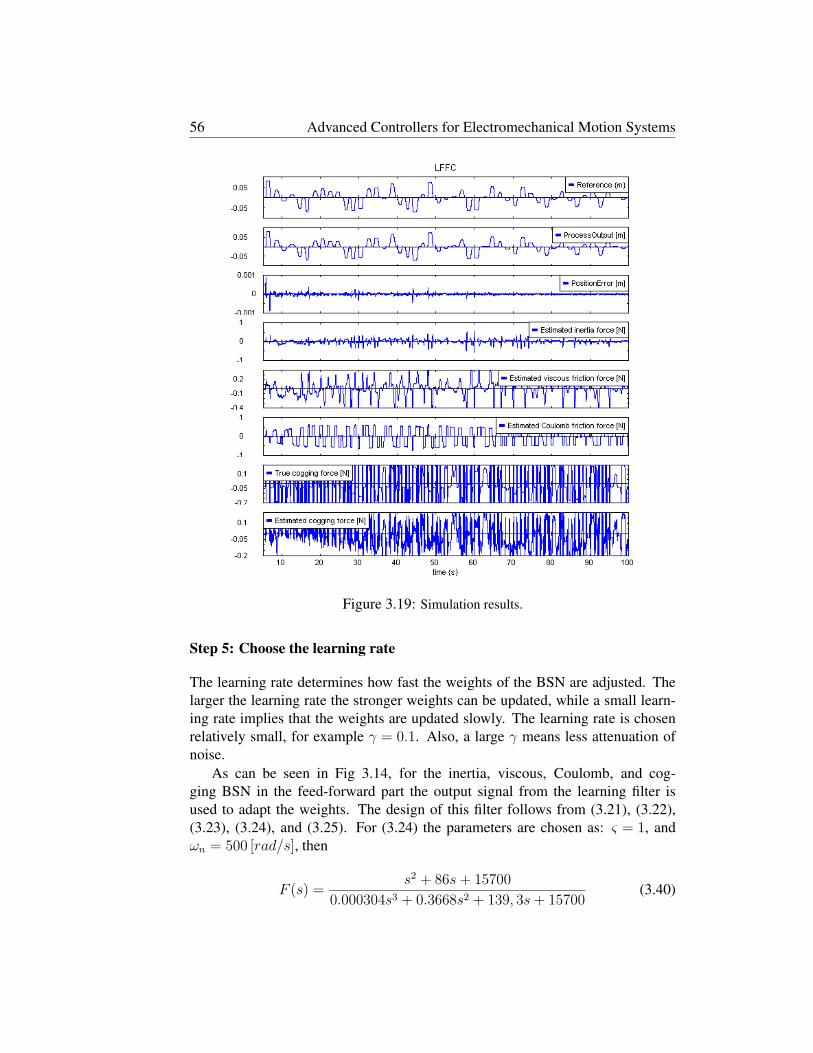
56 Advanced Controllers for Electromechanical Motion Systems
Figure 3.19: Simulation results.
Step 5: Choose the learning rate
The learning rate determines how fast the weights of the BSN are adjusted. The
larger the learning rate the stronger weights can be updated, while a small learn-
ing rate implies that the weights are updated slowly. The learning rate is chosen
relatively small, for example γ = 0.1. Also, a large γ means less attenuation of
noise.
As can be seen in Fig 3.14, for the inertia, viscous, Coulomb, and cog-
ging BSN in the feed-forward part the output signal from the learning filter is
used to adapt the weights. The design of this filter follows from (3.21), (3.22),
(3.23), (3.24), and (3.25). For (3.24) the parameters are chosen as: ς = 1, and
ωn = 500 [rad/s], then
F (s) =s2 + 86s + 15700
0.000304s3 + 0.3668s2 + 139, 3s + 15700(3.40)
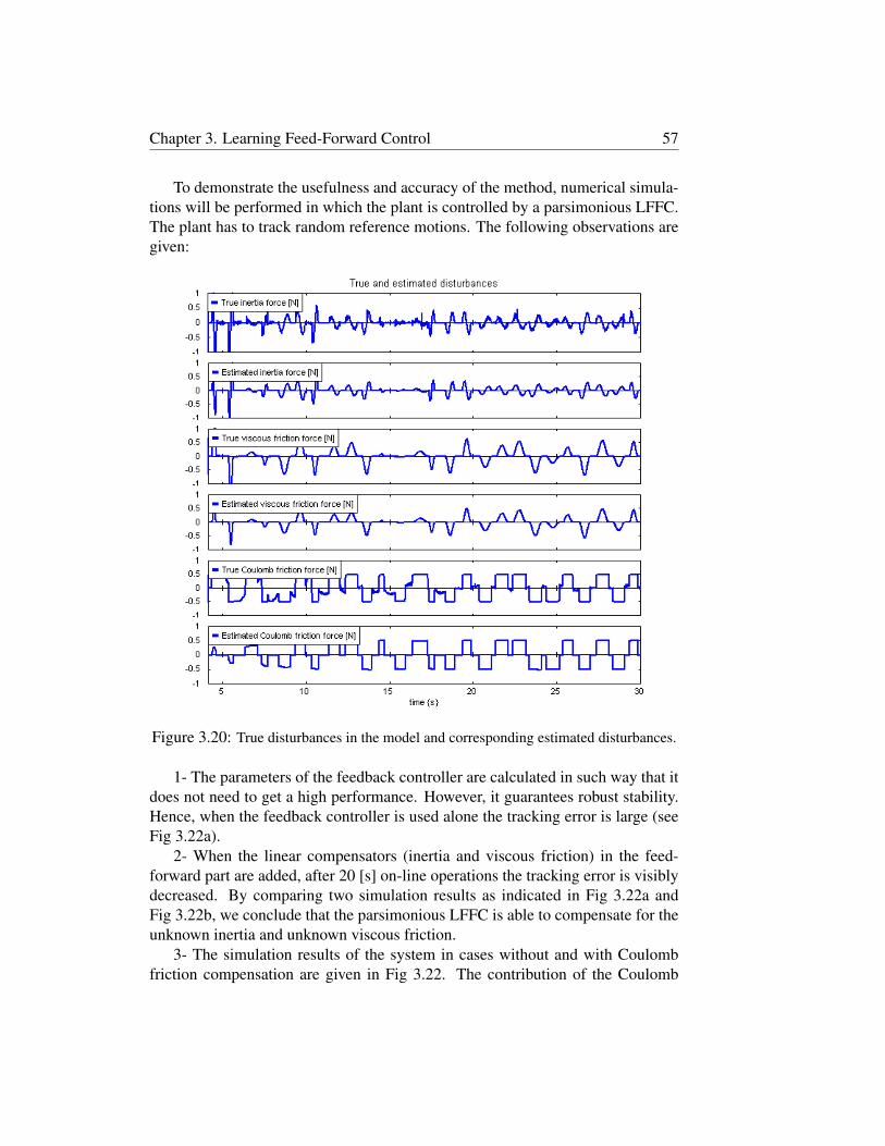
Chapter 3. Learning Feed-Forward Control 57
To demonstrate the usefulness and accuracy of the method, numerical simula-
tions will be performed in which the plant is controlled by a parsimonious LFFC.
The plant has to track random reference motions. The following observations are
given:
Figure 3.20: True disturbances in the model and corresponding estimated disturbances.
1- The parameters of the feedback controller are calculated in such way that it
does not need to get a high performance. However, it guarantees robust stability.
Hence, when the feedback controller is used alone the tracking error is large (see
Fig 3.22a).
2- When the linear compensators (inertia and viscous friction) in the feed-
forward part are added, after 20 [s] on-line operations the tracking error is visibly
decreased. By comparing two simulation results as indicated in Fig 3.22a and
Fig 3.22b, we conclude that the parsimonious LFFC is able to compensate for the
unknown inertia and unknown viscous friction.
3- The simulation results of the system in cases without and with Coulomb
friction compensation are given in Fig 3.22. The contribution of the Coulomb

58 Advanced Controllers for Electromechanical Motion Systems
friction compensator is clearly shown. In Fig 3.22c, without Coulomb friction
compensator, the effect of Coulomb friction will result in a large tracking error.
However, when the Coulomb friction BSN is added, this effect is considerably
compensated (see Fig 3.22d). After a few motions the tracking error will converge
to a smaller value. It is observed that the Coulomb friction force is significantly
compensated in the feed-forward part (also indicated in Fig 3.20).
Figure 3.21: True and estimated cogging force.
4- The role of the cogging compensator is clearly shown by comparing the
simulation results as indicated in Fig 3.22e and Fig 3.22f. When the cogging BSN
is used, the tracking error is considerably decreased. In other words, the unknown
cogging force is well compensated in the feed-forward controller (also indicated
in Fig 3.21).
Figure 3.22: Comparison of simulation results.

Chapter 3. Learning Feed-Forward Control 59
From the obtained observations we can conclude that the LFFC is suitable for
controlling motion systems that are subject to reproducible disturbances. LFFC
offers several potential advantages over conventional control algorithms. The ef-
fectiveness of the considered control strategy was verified through the simulation
results. The LFFC was well able to compensate for the known disturbances. A
fast rate of convergence and high robustness can be obtained. After a short train-
ing time, the parsimonious LFFC was able to obtain about a 7 times smaller peaks
in the tracking error than the feedback controller (compare 3.22a with 3.22f).
3.10 Conclusions
Since motion systems may have complicated nonlinear mathematical models, con-
trol algorithms that require accurate process models are difficult to implement.
To overcome this, several learning control methods have been proposed. These
controllers are not designed fully prior to operation but trained during control.
The characteristics of the Learning Control introduced here are that the controller
can be chosen as the inverse dynamical model of the plant and it is composed of
the feed-forward loop besides the feedback controller loop. This type of learn-
ing control is known as the learning feed-forward control scheme. The feedback
controller can be designed for robustness mainly, which does not require an accu-
rate process model. The feedback controller compensates unknown disturbances
and it does not have to know exactly how a system will respond to disturbances.
The feed-forward controller compensates the reproducible disturbances that de-
pend on the state of the process before they can affect the system. Normally, a
feed-forward controller is designed on the basis of an accurate process model of
the process. The obtained LFFC does not suffer from a trade-off between high
performance and robust stability.
In LFFC, a B-spline network is chosen for the feed-forward part. In order to
learn the input-output behavior of the inverse dynamical model of the controlled
object, a learning signal is required. The output of the feedback controller pro-
vides the training signal for the LFFC. The feed-forward design is formulated as a
linear program that optimizes the number and position of the knots of the splines.
Detailed design formulas were given for two parameters of B-spline network: the
B-spline support width and the learning gain are given based on stability analysis
in frequency domain [45]. There is a tradeoff between accuracy and computa-
tional complexity of training, since the number of inputs used affects the number
of weights in the neural network. An on-line B-spline neural network is used be-
cause of its local weight-updating characteristic, which has the advantages of fast
convergence speed and low computation complexity. This is very important for
real-time control applications.

60 Advanced Controllers for Electromechanical Motion Systems
The inputs of the feed-forward part depend on the plant and the reproducible
disturbances that the LFFC has to compensate. In case of random reference mo-
tions the reference signal and its derivatives/integrals, are used as inputs. A cor-
rect state space representation of the plant is used to determine the specific inputs.
Each of reference inputs of the LFFC will be used to compensate one specific
disturbance.
The width of the B-splines should be chosen such that the BSN is able to
learn the desired feed-forward signal. The smaller the support of the B-splines
the more accurate the LFFC can be obtained. However, a too small support may
result in unstable behavior. The frequency response of the closed loop system
can be used to determine the minimum width of the B-splines, for which learning
converges. The B-spline distribution is then chosen on the basis of qualitative
process knowledge.
When the inputs of the BSN are chosen straightforwardly on basis of the plant
model, a multidimensional BSN results. Large network sizes and poor general-
izing ability may result, known as the curse of dimensionality. A parsimonious
LFFC offers a solution by splitting up the multidimensional BSN into several
lower-dimensional BSNs. In this case the implementation requires a low number
of weights, which means that it is memory efficient and learn relatively fast, while
it is relatively insensitive to noise. The parsimonious network structure can be
designed on the basis of qualitative knowledge of the process and disturbances.
The effectiveness of the LFFC is illustrated through comparison with a PID
controller, obtained by observing the system dynamic performances. The simu-
lation results confirm that the LFFC is an attractive control strategy for motion
systems that are subject to reproducible disturbances.
Chapter 4
LQG combined with MRAS-based
LFFC
4.1 Introduction
In Chapter 3, a function approximator with ”standard” neural networks was used
which enabled to approximate complex non-linear functions [41, 45]. However,
they are not always suited for controller design applications because of too many
adjustable parameters. Moreover, using neural networks for simple tasks is unnec-
essary. To deal with this problem, a MRAS-based learning feed-forward controller
has been applied [43]. The idea of LFFC is applied but without using the com-
plex B-spline neural networks. Instead, we propose to use MRAS-based adaptive
components.
In this chapter we introduce a control structure, which consists of an LQG
controller and an MRAS-based learning feed-forward controller. Feed-forward
is used in addition to LQG, because LQG is still required to account for imper-
fections in the feed-forward system model. By adding a (learning) feed-forward
component to the LQG controller, an extra degree of freedom in the controller
design is created. A control scheme is derived which has good properties in com-
mon with both the LQG and LFFC controller. This control structure can capture
many aspects of the control problem as mentioned in Chapter 1. The responses to
setpoint changes and reproducible disturbances are mainly obtained by the LFFC.
The LQG is designed to obtain a stable closed-loop system that is insensitive to
measurement noise and variations and uncertainties in process behavior.
This chapter is organized as follows. In Section 4.2, the new LFFC is intro-
duced. It is called an MRAS-based Learning Feed-forward Control. The LFFC is
used to cancel the unwanted signal, disturbing the input of the plant. Theoretical
background of the MRAS-based LFFC is also given in this section. The design
61

62 Chapter 4. LQG combined with MRAS-based LFFC
of the proposed controller is introduced in Section 4.3. The controller structures
with Coulomb friction force and Cogging force compensation are given in Sec-
tions 4.3.3 and 4.3.4, respectively. At the end of this chapter, a review of the
chapter is given, including a comparison with previous methods.
4.2 An MRAS-based Learning Feed-Forward Con-
troller
This section will deal with the basic theory of an MRAS-based learning feed-
forward control as presented in the paper of Van Amerongen [43]. As was in-
troduced in Chapter 3, LFFC consists of a feedback and a feed-forward con-
troller. The feed-forward part is considered as a function approximator whose
input-output mapping can be adapted during control and is intended to become
the (stable part of the) inverse of the plant [13, 45]. It is clear that if an accurate
model of the process is available, and if its inverse exists, then process dynamics
can be canceled by the inverse model. As a result, the output of the process will
be equal to the desired output if no other disturbances are present. In order to
approximate the state dependent function, some kind of function approximator is
introduced. In this study, in order to obtain high stability and fast convergence
for the design of a linear process, the feed-forward part is proposed using adap-
tive components. The mechanism that adjusts the input-output mapping of the
adaptive components is based on the tracking error. The well-known Liapunov
approach is used to find stable adaptive laws for the feed-forward parameters in
such way that learning converges.
4.2.1 Theoretical Background
4.2.1.1 Introduction
As was introduced in Chapter 2, there are two main types of MRAS ([40, 4] and
[22]). 1. Direct MRAS : the idea is to create a closed loop controller with param-
eters that can be adjusted to change the response of the system. The output of the
process is compared to a desired response from a reference model. The controller
parameters are adjusted based on this error. Finally, the controller parameters con-
verge to suitable values, that is, the process response tracks the reference response
with a vanishing error. 2. Indirect MRAS: there are two tasks at each time step.
The first is the identification of relevant plant parameters. Then, the controller
parameters are computed based on the estimated plant parameters.
A setpoint generator, in mechatronic systems called a motion profile, can also
act and be used as a reference model. This leads to the basic structure of Fig

Advanced Controllers for Electromechanical Motion Systems 63
Figure 4.1: Learning Feed-Forward Controller
4.1. A typical controller for a high-precision motion system consists of a feed-
forward controller and a feedback controller. The inputs to the feed-forward part
are the states of the setpoint generator. The feed-forward controller generates a
feed-forward signal by summing the profile setpoint signals with properly chosen
weights. The feed-forward parameters are adjusted all the time. This implies that
they follow changes in the process. As a result, it can be expected that a proper
feed-forward controller signal is generated, effective for providing good tracking
control performance. Note that, addition of the proper feed-forward component
may improve performance, without affecting the stability, and robustness proper-
ties [5].
4.2.1.2 MRAS-based Feed-Forward Control
A state variable filter (SVF) can be used as the reference model to generate a set
of profile setpoint signals including position, velocity, and acceleration. For the
second-order case, such a filter is described by a second order transfer function.
Note that, denominator coefficients should always have positive values to guaran-
tee stabilization. By means of the feed-forward controller, the SVF output signals
can be used to generate an inverse model of the process. Let the feedback con-
trolled process be described by the transfer function Hp, and the reference model
by Href
Hp =1
aps2 + bps + cp
(4.1)
Href =ω2
n
s2 + 2ςωns + ω2n
(4.2)

64 Chapter 4. LQG combined with MRAS-based LFFC
Figure 4.2: Realization of an inverse model of the process
In Figure 4.2 the transfer from reference R to process output Y is:
Htot =ω2
n
s2 + 2ςωns + ω2n
ams2 + bms + cm
aps2 + bps + cp
(4.3)
If am, bm and cm are equal to respectively ap, bp and cp, Htot is equal to the desired
response, given by Href . The desired response from the setpoint generator is
compared to the process response. Based on this error, we should try to find a
learning mechanism that adjusts the parameters am, bm and cm, such that they
converge to ap, bp and cp, respectively. When there are disturbances present, the
first thing that might come to mind is using a feedback controller. However, when
we model these disturbances as a ’constant’ disturbance, this disturbance could
also be compensated in a feed-forward manner by adding a ’constant’ input dm to
be found by the learning mechanism. The resulting controller is given in Fig 4.3.
4.2.1.3 Adaptive laws
As can be seen in Fig 4.3, the setpoint generator can be used as the reference
model. The learning signal is determined by the difference between the output of
the reference model and the process. In order to find adaptive laws for the feed-
forward parameters am, bm, cm and dm , such that they converge to ideal values
that cause the process response matches the response of the reference model, the
Liapunov stability approach can be used. The design procedure will be illustrated
with the second-order example. We assume that the process parameters are un-
known and vary slowly. In general, the feedback controller is used to compensate
for random disturbances and possibly also to generate a learning signal for the
learning mechanism. We assume at this stage that the disturbance is zero. The de-
sign problem is thus: Find (stable) adjustment laws for the adjustable parameters
am, bm, and cm such that the error e between the reference model and the process
as well as the errors in the feed-forward parameters asymptotically go to zero.

Advanced Controllers for Electromechanical Motion Systems 65
Figure 4.3: MRAS-based Learning Feed-Forward Controller
Equations (4.1) and (4.2) are rewritten in state space form. This gives the
second-order reference model:
xm =
[0 1
−ω2n −2ςωn
]
xm +
[0ω2
n
]
R (4.4)
An extra state xm,3 is defined as
xm,3 = xm,2 = ω2nR − ω2
nxm,1 − 2ςωnxm,2 (4.5)
This gives the process equations
xp =
[
0 1
− cp
ap− bp
ap
]
xp +
[0 0cm
ap
bm
ap
]
xm +
[0
am
ap
]
xm,3. (4.6)
Because the parameters am, bm, and cm should converge to ap, bp and cp we define
the error in the parameters as
am − ap
ap
=am
ap
− 1 = a ⇒am
ap
= 1 + a
bm − bp
ap
= b′m − b′p = b (4.7)
cm − cp
ap
= c′m − c′p = c.

66 Chapter 4. LQG combined with MRAS-based LFFC
After substitution of equations (4.7) in equation (4.6), and using (4.5) the process
model is modified as
xp =
[0 1
−c′p −b′p
]
xp +
[0 0c′m b′m
]
xm + (4.8)
+
[0 0
−ω2n −2ςωn
]
xm +
[0ω2
n
]
R +
[0a
]
xm,3
We define the error e = (e1, e2)T = xm − xp. By subtracting equation (4.8) from
equation (4.4), it follows that
e =
[0 1
−ω2n −2ςωn
]
xm +
[0ω2
n
]
R −
[0 1
−ω2n −2ςωn
]
xm − (4.9)
−
[0ω2
n
]
R −
[0 1
−c′p b′p
]
xp −
[0 0c′m b′m
]
xm −
[0a
]
xm,3
This simplifies into:
e =
[0 1
−c′m −b′m
]
xm −
[0 1
−c′p −b′p
]
xp −
[0a
]
xm,3 (4.10)
and can be rewritten as
e = Amxm − Apxp −
[0a
]
xm,3 (4.11)
or
e = Amxm − Apxm + Apxm︸ ︷︷ ︸
=0
− Apxp −
[0a
]
xm,3
= Amxm − Apxm︸ ︷︷ ︸
A′xm
+ Apxm − Apxp︸ ︷︷ ︸
Ape
−
[0a
]
xm,3 (4.12)
= A′xm − Ape −
[0a
]
xm,3,
in which the matrix A′ contains the parameter errors b and c
A′ = Am − Ap =
[0 0−c −b
]
(4.13)
Combining the parameter errors a, b and c in the error vector ε and in the error
matrix A and redefining xm gives
ε =
−c−b−a
, A =
[0 0 0−c −b −a
]
, xm =
xm,1
xm,2
xm,3
, e = Axm + Ape.
(4.14)

Advanced Controllers for Electromechanical Motion Systems 67
In order to proof the asymptotic stability of e we define a positive definite Lia-
punov function:
V = eT Pe + εT αε, (4.15)
in which P a positive definite symmetrical matrix and α a diagonal matrix with
in principle arbitrary coefficients > 0 . For a stable adaptive system the time
derivative of V should be ≤ 0:
dV
dt= eT Pe + eT P e + εT αε + εT αε. (4.16)
Substituting e from (4.14) and rearranging the terms yields:
dV
dt= eT AT
p Pe + eT PApe + 2eT PAxm + 2εT αε. (4.17)
With the first two terms of (4.17) equal to:
eT (ATp P + PAp)e = −eT Qe (4.18)
It follows that:dV
dt= −eT Qe + 2eT PAxm + 2εT αε (4.19)
When Q is a positive definite symmetrical matrix the first term in equation (4.19)
is always negative or zero and when the other terms are made equal to zero,dVdt
≤ 0. When Ap is stable, we can find for any positive definite symmetrical
matrix Q a positive definite symmetrical matrix P by solving the Liapunov equa-
tion
ATp P + PAp = −Q. (4.20)
If the process matrix Ap is not stable, the process must be stabilized first by ap-
propriate feedback.
The adjustment rules for the feed-forward gains follow from the condition that
the remaining terms should be zero.
2eT PAxm + 2εT αε = 0 ⇔ εT αε = −eT PAxm. (4.21)
After simplification (taking into account that only the last row of A contains values
6= 0) this yields:dε
dt= −α−1(p21e + p22e)xm. (4.22)
If it is assumed that the adaptation is fast compared with the variations in the
process parameters it follows that:
dε
dt=
d
dt
−(cm + cp)/ap
−(bm + bp)/bp
−(am/ap − 1)
= −d
dt
cm/ap
bm/ap
am/ap
. (4.23)

68 Chapter 4. LQG combined with MRAS-based LFFC
When the unknown ”constant” parameter ap is part of the (’arbitrary’) adaptive
gains α−1, this yields the following adjustment rules:
am =1
α33
∫
[(p21e + p22e)xm,3]dt + am(0)
bm =1
α22
∫
[(p21e + p22e)xm,2]dt + bm(0) (4.24)
cm =1
α11
∫
[(p21e + p22e)xm,1]dt + cm(0)
Like in any MRAS-based system, adaptive disturbance compensation can be
added, by realizing that the parameter dm acts on an extra input signal 1, instead
of on one of the state variables:
dm =1
γ
∫
[(p21e + p22e)1]dt + dm(0) (4.25)
in which 1/α11, 1/α22, 1/α33, and 1/γ are called the adaptive gains. They de-
termine the speed of adaptation and they can, under the condition that they are
larger than zero, in principle, be arbitrarily chosen. Equations (4.24) can be gen-
eralized to an equation for higher-order systems. For an nth-order system we find
for parameter am,i:
dam,i
dt=
1
αii
(n∑
k=1
Pnkek
)
xm,i (4.26)
In the adjustment laws the derivative of the error is needed. This derivative
can be obtained by means of a second-order state variable filter. The bandwidth
of this filter has to be at least 10 times larger than the bandwidth of the reference
model in order not to endanger the stability of the system. On the other hand,
the combination of a state variable filter with not too large bandwidth and use of
the model states for the adaptation as well as for the control makes the system
relatively insensitive for noisy measurements and leads to a robust system.
4.3 Design of the proposed controller
The obtained knowledge in the previous sections is now used to formulate a prac-
tical design procedure. Fig 4.4 shows the block diagram of the proposed control
structure, which combines an MRAS-based LFFC and a separate LQG controller.
In the feed-forward control part, the parameter adaptation is driven by the tracking
error between reference output and measured process output, while in the LQG
part the observer is driven by the prediction errors between measured process
variables and corresponding estimated variables.

Advanced Controllers for Electromechanical Motion Systems 69
Figure 4.4: LQG combined with MRAS-based LFFC
For the MeDe5 setup, in order to take the flexible frame behavior into account,
in this study the LQG design is based on the 4th order approximation of the 6th-
order model. The performance of the proposed controller will be investigated
with the tracking error due to following a random trajectory. The ability to track
a trajectory in the presence of load changes will be evaluated. The ability to
attenuate the effect of measurement noise acting on the process output will also
be investigated. By separating the design objectives, decoupling the MRAS-based
LFFC, and the LQG controller, both objectives can be achieved.
There are two main design steps. In the first step, the design of an MRAS-
based LFFC is carried out and in the second step we address the design of an
LQG controller.
4.3.1 Design the MRAS-based LFFC
In practice, the MeDe5 is implemented based on computer control. Therefore, the
continuous-time feed-forward controller given in Section 4.3 has to be replaced
by a discrete-time feed-forward controller.
- Instead of using equation
dPc
dt= AT
mPc + PcAm + Qc (4.27)
where Am is the continuous time state matrix of the reference model, the Euler

70 Chapter 4. LQG combined with MRAS-based LFFC
approximation of this equation is given
next(P ) − P
Ts
= ATmP + PAm + Qd,
→ next(P ) = (ATmP + PAm + Qd)Ts + P, (4.28)
in which, Ts is the sampling interval.
- The continuous-time integrators in Equation (4.24) are replaced by, the
discrete-time integrators.
am =1
α33
∑
[(p21e + p22e)xm,3]Ts + am(0),
bm =1
α22
∑
[(p21e + p22e)xm,2]Ts + bm(0), (4.29)
cm =1
α11
∑
[(p21e + p22e)xm,1]Ts + cm(0).
- The continuous-time reference model and state variable filter in the learning
block solve the following differential equation
dx
dt= AF x + BF u (4.30)
In discrete time domain, this could be approximated with the Euler approximation
given by:
next(x) − x
Ts
= AF x + BF u
→ next(x) = (AF x + BF u)Ts + x. (4.31)
Feedback controller: As discussed in the previous sections, tracking perfor-
mance is obtained by the MRAS-based LFF. The feedback controller is designed
such that it features robust stability for closed loop when used alone. Initially, the
feedback controller is of the PD-type with the chosen parameters Kp = 100 and
Kd = 1.
Reference model: Explicit position, velocity, and acceleration profile setpoint
signals are created using the reference model, which is described by the transfer
function
Href =ω2
n
s2 + 2ςωns + ω2n
. (4.32)
The parameters of the reference model are chosen such that the higher order dy-
namics of the system will not be activated [22]. The following values are chosen:

Advanced Controllers for Electromechanical Motion Systems 71
Figure 4.5: MRAS-based LFFC controlled system
ωn = 10 [rad/s], and ς = 1, such that:
Am =
[0 1
−ω2n −2ςωn
]
=
[0 1
−100 −20
]
,
Bm =
[0ω2
n
]
=
[0
100
]
. (4.33)
State variable filter: As mentioned in Section 4.3, the derivative of the error
can be created using a state variable filter. The parameters of this state variable
filter are chosen in such a way that the parameters of the reference model can vary
without the need to change the parameters of the state variable filter every time
[42, 22]. The parameters are chosen as: ωn = 1000 [rad/s] and ς = 0.7, then
AF =
[0 1
−ω2n −2ςωn
]
=
[0 1
−106 −1.4 ∗ 103
]
,
BF =
[0ω2
n
]
=
[0
106
]
. (4.34)
The learning signal for the adaptive components is given
uLearning(k) = p21e(k) + p22e(k). (4.35)
- Qd is chosen positive definite matrix and P is solved from Equation (4.28).
The following numerical values are used:
Qd =
[100 00 100
]
, Ts = 0.001. (4.36)

72 Chapter 4. LQG combined with MRAS-based LFFC
Figure 4.6: Simulation results when the feedback controller is switched off
These settings lead to the following Liapunov gains:
p21 = 0.3785, p22 = 0.8359. (4.37)
- The adaptive gains determine the speed of adaptation and they can be arbi-
trary chosen. The following settings are chosen (1/α33) = 100, (1/α22) = 25000,
and (1/α11) = 20.
- The fixed feed-forward parameters are chosen initially, the learning
process then makes them effective for compensating the disturbances. In
this simulation, the initial values of the feed-forward gains are chosen
am(0) = bm(0) = cm(0) = 0.
Fig 4.6 shows the corresponding responses for the system of Fig 4.5. The
adaptive feed-forward controller automatically finds the right parameters (am, bm
and cm) to result in the stable system and properly generate the inversion of the
process model. There are two major advantages of the MRAS-based LFFC com-
pared with control based on feedback from the output. First of all, this structure
can eliminate the influence of measurement noise by switching off the feedback

Advanced Controllers for Electromechanical Motion Systems 73
Figure 4.7: Linear disturbances are well compensated
controller completely, or almost completely [43]. In the ideal case, the effects of
the measurement noise can then be totally eliminated. Furthermore, this controller
Figure 4.8: When the feedback controller is added, the control signal is corrupted by
measurement noise
can reduce the influence of some disturbances. Such a structure can consider-
ably improve the performance of the controlled system with respect to reference
changes and plant parameter variations. An MRAS-based LFFC deals much bet-
ter with noisy measurements than direct MRAS that has already been discussed in
Chapter 2. The simulation results indicated in Fig 4.7 show that the inertia force
and viscous friction force are well compensated by the feed-forward signals. This
structure is suitable for the control of linear systems, or systems that can be ap-
proximated as such. It is very robust [43]. Also note that this 2nd order LFFC is
able to compensate the dynamics of 6th order process.
However, it is clear that, when used alone a feed-forward controller cannot
effectively compensate every disturbance, and robust stability cannot be guaran-
teed. When a feedback controller is used, sensor noises may be amplified and
deteriorate performance. It is clearly observed in Fig 4.8 that the control signal is
corrupted by measurement noise.

74 Chapter 4. LQG combined with MRAS-based LFFC
4.3.2 Discrete LQG design
The design procedure for the discrete LQG controlled system based on the 2nd-
order linear process model was introduced in Chapter 2. In this section we carry
out the design with the 4th- order linear process model. The LQG controller
should be good enough to stabilize the process when used alone, but when com-
bined with a feed-forward controller it does not need to minimize the position
tracking error.
Discrete state matrices of the plant: The linear plant model to be controlled
is {
xk+1 = Axk + Buk
yk = Cxk + Duk,(4.38)
in which (see Appendix A)
A =
1.0000 0.0000 −0.0100 0.00000.0010 1.0000 0.0000 0.00000.0075 7.5000 0.9787 −7.50000.0000 0.0000 0.0010 1.0000
, B =
0.01900.00000.02610.0000
,
C =
[0 1 0 00 0 0 1
]
, D =
[00
]
. (4.39)
x =[
vL xL vF xF
]T. (4.40)
In formula (4.40) vL is the velocity of the load, xL denotes the position of the load,
vF is the velocity of the frame, and xF denotes the position of the frame.
Discrete optimal state feedback (LQR): The output of the state feedback
controller is
u = −Kx (4.41)
in which x represents the state of the system and K is the gain vector based on the
linear process model and optimization criterion
K = (BT PB + RR)−1BT PA, (4.42)
where P is the solution of the reduced matrix Riccati equation
AT PA − P − AT PB(BT PB + RR)−1BT PA + QR + P = 0. (4.43)
In this equation A and B are discrete state matrices of the plant to be controlled,
QR and RR are matrices in the optimization criterion (QR is positive semi-definite
weighting matrix and RR is positive definite weighting matrix). The following

Advanced Controllers for Electromechanical Motion Systems 75
Figure 4.9: Estimated states and control signal are insensitive for measurement noise
settings are used
QR =
0 0 0 00 100 0 00 0 0 00 0 0 100
, RR = 0.5.
These values result in the following stationary feedback controller gains:
KLQR =[
1.008 9.412 0.010 10.38].
Discrete Linear Quadratic Estimator (LQE) : The feedback matrix L yielding
optimal estimation of the process states is defined as
L = PCT (CPCT + REI)−1, (4.44)

76 Chapter 4. LQG combined with MRAS-based LFFC
where P is the solution of the following matrix Riccati equation
next(P ) = A(I − LC)PAT + QE, (4.45)
in which A and C are discrete state matrices of the plant to be controlled, QE is
the system noise covariance, and RE the sensor noise covariance. The following
settings were used
QE =
10 0 0 00 100 0 00 0 100 00 0 0 10
, RE = 1.
The settings result in the following stationary gains
LLQE =
0.3048 −0.00590.9167 0.00000.6294 −0.39150.0000 0.9160
.
The simulation results of the LQG controlled system are shown in Fig 4.9. As
can be seen, noise on the measurements of the process has almost no influence
on the system. The real position measurement (second line) and the position state
error (fourth line) are corrupted by measurement noise, whereas, the estimated
position state (third line) and the control signal (lowest line) are almost clean.
Figure 4.10: The proposed control structure with Coulomb friction compensation

Advanced Controllers for Electromechanical Motion Systems 77
4.3.3 LQG combined with MRAS-based LFFC with friction
compensation
With the MRAS-based learning feed-forward control as given in Section 4.2, only
compensation for the effect of the viscous friction is mentioned. In order to im-
prove tracking systems capabilities we have to take the effect of the Coulomb
friction into account. This is can be realized by adding an extra learning compo-
nent in the learning feed-forward part (See Fig 4.10). The Coulomb friction force
depends on the direction of the velocity, therefore, the adjustable gain has to be
dependent on the sign of the velocity. Thus the adjustment rule for the adjustable
parameter to compensate the Coulomb friction is
dm =1
θΣ[(p21e + p22e)sign(xm,2)]Ts + dm(0) (4.46)
Figure 4.11: Simulation results in the presence of measurement noise and mass variation
The adjustment of the parameter depends on the sign of xm,2, which is the
reference velocity. To illustrate the design method, the values of the simulation

78 Chapter 4. LQG combined with MRAS-based LFFC
parameters are used as given in the previous simulations and the value of the
adaptive gain of the Coulomb friction compensation is chosen as (1/θ) = 3000.
Figure 4.12: Position error without (left) and with (right) Coulomb friction compensation
To illustrate the performance of the controller in the presence of measure-
ment noise and plant parameter variations, the following numerical values are
used: an input reference (with stroke R = 0.1 [m], measurement noise on slider
position (with amplitude A = 0.0001 [m]), and a parameter variation in the load
(with mass variation ∆m = 0.1 [kg]. The experiments consist of three phases:
t = 0 − 5 [s]; homing operator, the system is controlled by a fixed PID controller;
t = 5 − 25 [s] ; normal parameter, the system is controlled by the proposed con-
troller; t = 25 − 50 [s]; at t = 25 [s] a parameter variation is added to the load of
the plant. The simulation results (see Fig 4.11) show that when a mass varia-
Figure 4.13: Feed-forward and LQG output signals
tion of the load is switched on, after a few motions, the feed forward controller
is able to give a good control signal for the process. The parameters am, bm, cm
and dm quickly search the new stationary values. The influence of measurement
noise is well eliminated. It is observed that the control signal is almost clean. By
combining LQG and MRAS-based LFFC, it is possible to improve both tracking
errors and the measurement noise rejection property. The compensation of the
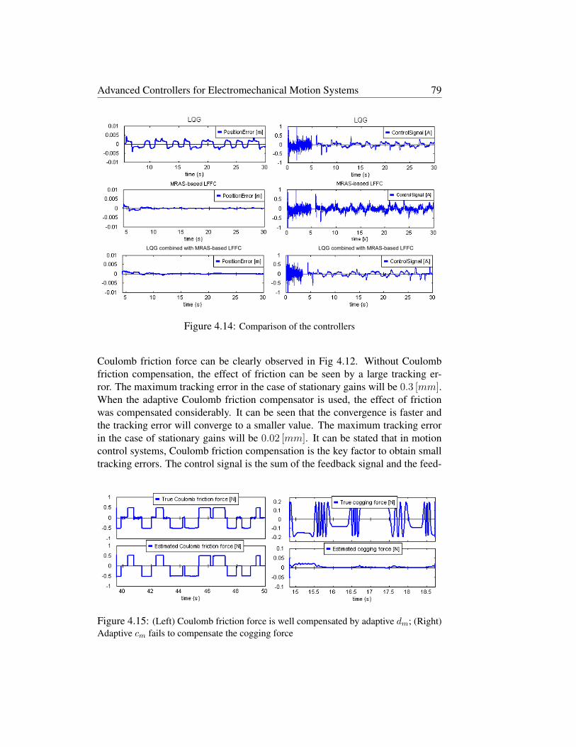
Advanced Controllers for Electromechanical Motion Systems 79
Figure 4.14: Comparison of the controllers
Coulomb friction force can be clearly observed in Fig 4.12. Without Coulomb
friction compensation, the effect of friction can be seen by a large tracking er-
ror. The maximum tracking error in the case of stationary gains will be 0.3 [mm].When the adaptive Coulomb friction compensator is used, the effect of friction
was compensated considerably. It can be seen that the convergence is faster and
the tracking error will converge to a smaller value. The maximum tracking error
in the case of stationary gains will be 0.02 [mm]. It can be stated that in motion
control systems, Coulomb friction compensation is the key factor to obtain small
tracking errors. The control signal is the sum of the feedback signal and the feed-
Figure 4.15: (Left) Coulomb friction force is well compensated by adaptive dm; (Right)
Adaptive cm fails to compensate the cogging force

80 Chapter 4. LQG combined with MRAS-based LFFC
forward signal. As can be seen in Fig 4.13, in the first run, the control signal is
determined by both the control signals, whereas, in the second run, it is deter-
mined almost completely by the feed forward controller. The combined controller
is superior to the two methods when used separately (see Fig 2). The advantages
of both methods are combined, whereas, the disadvantages are eliminated.
4.3.4 LQG combined with MRAS-based LFFC with cogging
compensation
As introduced in Chapter 3, for the MeDe5, the cogging phenomenon is insignifi-
cant such that can be ignored. However, in order to illustrate the effectiveness of
the proposed control structure, cogging force is added in the plant model. In this
simulation, we assume that the cogging force has a magnitude of 0.2 [N ], and a
period of 0.005 [m]. It was modeled as:
FC(x) = 0.2 sin
(2π
0.005x
)
= 0.2 sin(1256x) [N ] (4.47)
Figure 4.16: B-spline neural network is used to compensate the cogging force
The adaptive cm that has the reference position as input has to compensate
the cogging force. However, with the proposed control structure, the simulation

Advanced Controllers for Electromechanical Motion Systems 81
results show that the adaptation if cm is not fast enough such that the cogging force
could not be compensated (see Fig 4.15). To overcome this problem, the solution
is that the adaptive cm should be replaced by a B-spline neural network (BSN)
with a separate learning signal, as shown in Fig 4.16. The parameters of this BSN
are indicated in Chapter 3. In Fig 4.19, with an adaptive cogging compensator,
the effect of cogging force could not be compensated. It results in a large tracking
error. When the adaptive cogging compensator is replaced by the BSN, the effect
of cogging force was compensated significantly (see Fig 4.18 and Fig 4.19). After
a few motions, the feed forward controller is able to give an optimal control signal
for which the process output will track the desired reference with a small error.
Figure 4.17: Simulation results when the BSN is used

82 Chapter 4. LQG combined with MRAS-based LFFC
Figure 4.18: The BSN well compensates for the cogging force
Figure 4.19: Position error without (left) and with (right) cogging compensation
4.4 The LQG combined with MRAS-based LFFC
controller compared with the PID controller
The performances of the proposed controller and a conventional PID controller are
compared in the presence of measurement noise and plant parameter variations. A
measurement noise on the slider position with amplitude A = 0.0001 [m] is added
at t = 0 [s], and a mass variation is added to the load of the plant at t = 25 [s].The parameters of both controllers are given in previous sections. By comparing
two simulation results as indicated in Fig 4.20, the main advantages of the pro-
posed controller are clearly shown: (1) The proposed structure exhibits smaller
tracking errors; (2) The system dynamics are relatively insensitive to changes in
system parameters; (3) The control signal is relatively insensitive to measurement
noise. With an MRAS-based LFFC combined with LQG, it is thus possible to
obtain accurate control of a given plant, whereas with doing so is impossible in
conventional control structures.
4.5 Discussion
1. In Section 4.2, the design of an MRAS-based LFFC was carried out with
the second-order example, however the approach can be effectively applied
to higher order systems as well. This was demonstrated by using a second-

Advanced Controllers for Electromechanical Motion Systems 83
Figure 4.20: Comparison of the controllers
order controller structure for the control of a sixth-order process.
2. The advantages of the use of the profile setpoint signals is that they are
easily accessible and noise free.
3. The design is based on the assumption that the difference between the
reference state and the process state is small. If it would be large the inverse
model of the plant cannot be realized in the feed-forward controller.
4. The adjustable parameter component has an integral component inside.
This implies that even when the learning signal is corrupted by measurement
noise the output signal is almost clean. This allows us using a large learning
signal to shorten the setting time.
5. In case of an MRAS-based LFFC, when all disturbances can be effectively
compensated for by a feed-forward signal, this allows us to reduce the val-
ues of the feedback controller gains. In this case measurement noise has
almost no influence on the system.
6. The parameters of the LQG controller are given fixed values, correspond-
ing with the nominal values of the plant. With the parameter variations of
the plant considered here it appeared that the LQG was robust enough to
deal with these variations and to produce good enough results for the basic
feedback control system.
4.6 Conclusions
The plant is always subject to disturbances, model uncertainty, and measurement
noise. The nature of the disturbances affects the quality of performance in a con-
trolled system. Un-modeled dynamics and parametric uncertainty have a negative

84 Chapter 4. LQG combined with MRAS-based LFFC
effect on the tracking performance and can even lead to instability. Measure-
ment noise limits the achievable bandwidth of the closed-loop system. In order
to reduce the effects of unwanted factors as mentioned we have to take them into
account in the design procedure. The solution is in the form of a two-degrees-of-
freedom controller, which consists of an LQG controller and a separate MRAS-
based LFFC.
When LQG is used alone a compromise has to be made between performance
and robustness specifications. The feed-forward may help to overcome this dif-
ficulty. As expected, a combined LQG and MRAS-based LFFC exhibits small
tracking error, as well as good measurement noise rejection properties in the pres-
ence of plant parameter variations and measurement noise. The effectiveness of
the controller is also illustrated through the comparison, obtained by observing the
simulation results, when using PID controller. The control ability of the proposed
structure is greatly improved when the adaptive feed-forward cm is replaced by
the corresponding B-spline neural network element. The unknown cogging force
is well compensated in the feed-forward controller. From results obtained of this
study we can state that the combination between LQG and MRAS-based LFFC is
an attractive approach for controlling electromechanical motion systems that are
subject to reproducible disturbances, measurement noise, and model uncertainty.

Chapter 5
Applications
5.1 Introduction
In the previous chapters, several control algorithms for electromechanical motion
systems have been introduced. We have performed experiments to confirm the
effectiveness of the proposed control methods to put them to practical use. The
obtained knowledge and insight will be applied to the Tripod and the MeDe5
setup. However, all of the control algorithms introduced in Chapter 2 (PID, LQG,
Direct MRAS, Indirect MRAS, and STR) have already been tested on the MeDe5
[14, 44]. Thus, in this chapter we concentrate only on experimental tests for the
control algorithms introduced in Chapters 3 and 4.
In Section 5.2 the LQG combined with MRAS-based LFFC is tested on the
MeDe5. We address the problem relating to the precision control of the DC mo-
tor, which requires the needs of mechanical transmission from the rotary to linear
motion. Our main focuses are: (i) whether and how the compensation of state
dependent effects, e.g. friction, mass deviation, can be realized by the MRAS-
based LFFC; (ii) how the attenuation of measurement noise, and the reduction of
plant parameter variations, can be realized by LQG controller. Experimental tests
will be carried out to demonstrate the performance difference between the system
based on the LQG controller and that based on the addition of the MRAS-based
LFFC. In Section 5.3 the parsimonious LFFC introduced in Chapter 3 and the
MRAS-based LFFC introduced in Chapter 4 are tested on the Tripod. We address
the problem relating to the precision control of the linear motor to track desired
motion trajectories. Our main interest is whether and how the compensation of
state dependent effects, e.g. friction, cogging and mass deviation, can be realized
by LFFC. Thus, experimental tests will be carried out to demonstrate the perfor-
mance difference between the system based on the feedback controller only and
that based on the addition of the feed-forward controller.
85

86 Advanced Controllers for Electromechanical Motion Systems
5.2 Implementation for the MeDe5
This section describes the testing of LQG combined with the MRAS-based LFFC
control algorithm on the MeDe5. The total system for testing in practice is de-
picted in Fig 5.1. To demonstrate the usefulness and accuracy of the method,
Figure 5.1: The MeDe5 with LQG combined with MRAS-based LFFC.
several experiments with the LQG controller alone and the addition of the MRAS-
based LFFC are performed. These experiments will completely follow the control
designs introduced in Chapter 4. After generating and uploading the C-code of
this controller into the PC104-board of the MeDe5, the performance of the sys-
tem can be measured [14].
Figure 5.2: Experimental results when a repeating motion profile is used.
In the first experiment only the LQG controller is used. As can be seen in
Fig 5.2, the LQG controlled system does not reach its reference values of (-0.05m
and 0.05 m). A considerable static error remains in the system due to friction.

Chapter 5: Applications 87
The value of the maximum tracking error is 0.25 [mm]. We expect, the remaining
static error in the LQG system to be decreased by adding an MRAS-based LFFC
to the LQG control algorithm.
Comparing the results of the LQG controlled system in simulation (see Fig
5.3 top) and in experiment (see Fig 5.3 bottom) it is observed that the maximum
tracking error is significantly bigger in the simulation case. It can be explained
that the mathematical model does not correspond the real process.
Figure 5.3: A comparison between simulation result and experimental result.
Next, the experimental test is repeated with a random motion profile, the max-
imum tracking error in this case will be as large as 0.5 [mm] (see Fig 5.4). Both
in simulation and experimental results it is shown that the LQG controlled system
operates better on a repeating motion than with a random motion.
Figure 5.4: Experimental results when a random motion profile is used.
In the second experiment the MRAS-based LFFC is added to the LQG con-
troller. The role of the MRAS-based LFFC is clearly shown by comparing two

88 Advanced Controllers for Electromechanical Motion Systems
simulation results as indicated in Fig (5.5 top) and Fig (5.5 bottom). This addi-
tion significantly increases the performance of the controller: the large static error
with the LQG controller almost disappears. The maximal tracking error with a
repeating motion profile is about 0.035 [mm].
Figure 5.5: A comparison when a repeating motion profile is used.
The feed-forward parameters are shown in Fig 5.6 and the estimated distur-
bances in Fig 5.7. It is observed that the expected shapes of the estimated dis-
turbances are obtained. In other worlds, the reproducible disturbances are well
compensated by the feed-forward part.
Figure 5.6: Feed-forward parameters.
The stability of the combination of an LQG controller and the MRAS-based
LFFC was tested with a long time experiment. The system is stable and shows no
drift in the parameters. It is confirmed by comparing two experimental results as
indicated in Figures 5.6 and 5.8. The feed-forward parameters after 10 minutes

Chapter 5: Applications 89
and the corresponding feed-forward parameters after 60 minutes are almost the
same.
Figure 5.7: Estimated disturbances when a repeating motion profile is used.
Next, a random motion profile is used. The contribution of the MRAS-based
LFFC is clearly shown. In Fig (5.9 top), without MRAS-based LFFC, the effect
of reproducible disturbances will result in a large tracking error. However, when
the MRAS-based LFFC is added, this effect is greatly compensated (see Fig 5.9
bottom). Since this was the primary goal of the feed-forward controller, it can be
concluded that the benefit of the implementation of the MRAS-based LFFC has
been successful. The value of the maximum tracking error is about 0.1 [mm].
Figure 5.8: Long time experiment.
Discussion
1. When the LQG controller is used alone the tracking error is large.

90 Advanced Controllers for Electromechanical Motion Systems
Figure 5.9: A comparison when a random motion profile is used.
2. The friction compensation in the MRAS-based LFFC makes a large en-
hancement on the behavior of the system. A combination of both the con-
trollers will reduce the tracking error.
3. In order to obtain a faster rate of convergence the initial values of the
adjustable feed-forward parameters should be chosen as close as possible to
their corresponding final values.
4. The LQG combined with MRAS-based LFFC operates better on a repeti-
tive motion instead of a random motion. It is proved in both simulation and
experimental results.
5. Both simulation and experimental results are presented to verify the effec-
tiveness of the proposed controller. The LQG combined with the MRAS-
based LFFC is able to obtain a 5 times smaller tracking error than the LQG
controller alone. Moreover, the proposed controller also can obtain fast dy-
namic response and high stability. This is important for real-time control
applications.
5.3 Implementation for the Tripod
In this section, we will apply NN-based LFFC and MRAS-based LFFC to the Tri-
pod setup. The design of the parsimonious LFFC introduced in Chapter 3 and the
design of the MRAS-based LFFC in Chapter 4 are repeated in short in Paragraphs
5.3.1 and 5.3.2, respectively. No detailed theoretical analyses are discussed in
these paragraphs, however, main calculated results are given . The Tripod is a
system controlled by a computer, which requires a discrete control algorithm [9]

Chapter 5: Applications 91
(see Fig 5.10 and Fig 5.13). In Section 5.3.3 the designed controllers will be tested
on the real setup. The results are shown for different experiments to demonstrate
the effectiveness of the proposed control schemes.
5.3.1 Design of a parsimonious LFFC
Figure 5.10: NN-based LFFC controlled system for each motor of the Tripod.
Step 1: Design the feedback controller
The behavior of each motor is modeled as a moving mass:
P (s) =1
ms2, (5.1)
where m (= 6 [kg]) represents mass of the load. A PD-controller is chosen for the
control of each motor. The transfer function of the controller is given by [9]:
C(s) = Kp
sτd + 1
sβτd + 1(5.2)
where Kp = 809.104, τd = 8.43.10−3, and β = 0.1.
Step 2: Determine the inputs of the feed-forward part

92 Advanced Controllers for Electromechanical Motion Systems
In the Tripod the plant is subject to the following disturbances: unknown friction
force, and unknown cogging force. That is, we should select [r, r, sign(r), r] as
inputs of the feed-forward controller.
Step 3: Choose the structure of the feed-forward part
For the Tripod design, the solution to prevent the curse of dimensionality is given
in Fig 5.10. The proposed network structure should consist of four BSNs that have
the reference position r, velocity r, sign of velocity, and acceleration r as inputs.
Step 4: Choose the B-spline distribution
Figure 5.11: Step response of -T (left); Bode plot of -T (right).
Figure 5.12: Reference inputs of the LFFC part.
The transfer function of −T is determined by:
− T (s) =−640s − 80900
0.004215s3 + 5s2 + 640s + 80900. (5.3)

Chapter 5: Applications 93
The step response of −T and the Bode plot of −T are given in Fig 5.11. The
reference inputs of the LFFC part are shown in Fig 5.12. The minimum support
of the B-splines follows 3.12 and 3.13 is
dmin = 0.00185[s] (5.4)
The maximum learning rate is:
γ ≤ 0.95. (5.5)
For the cogging BSN, in total 500 B-splines have been defined on the position do-
main (0 [m], 0.1 [m]); We choose to define three B-splines on the velocity domain
(−0.2 [ms−1], 0.2 [ms−1]) for the viscous BSN; For the Coulomb friction BSN,
three B-splines have been defined on the input domain [−1, 1]; Three B-splines
are defined on the acceleration domain (−0.75 [ms−2], 0.75 [ms−2]) for the iner-
tia BSN.
Step 5: Choose the learning rate
The learning rate is chosen relatively small, for example γ = 0.1 .
5.3.2 Design of an MRAS-based LFFC
Fig 5.13 shows the total system for testing in practice. The proposed controller
consists of an MRAS-based LFFC and a separate feedback controller. The same
feedback controller and the same cogging BSN are used as in case of the parsi-
monious LFFC introduced in Section 5.3.1. The same setpoint generator and the
same state variable filter are used as in case of the MRAS-based LFFC introduced
in Section 4.3.1. The Liapunov gains following from (4.28), (4.33) and (4.36)
are: p21 = 0.3785, p22 = 0.8359. The adjustable parameters of the feed-forward
controller are given by:
am =1
αa
∑
[(p21e + p22e)r]Ts + am(0). (5.6)
bm =1
αb
∑
[(p21e + p22e)r]Ts + bm(0). (5.7)
dm =1
αd
∑
[(p21e + p22e)sign(r)]Ts + dm(0). (5.8)
In this design, the initial values of the feed-forward gains are chosen
am(0) = bm(0) = dm(0) = 0 and the adaptive gains are (1/αa = 7000), (1/αb =200000), and (1/αd = 30000). These values are the same as used in the simulation
experiments.

94 Advanced Controllers for Electromechanical Motion Systems
Figure 5.13: MRAS-based LFFC controlled system for each motor of the Tripod.
5.3.3 Experimental results
The experimental tests were carried out with only one motor moving. Fig 5.14
gives an overview of the input reference and the tracking errors for the different
controllers that have been tested on the Tripod. In order to evaluate implementa-
tion of the controllers, the shape of the motion profile is purposely generated (see
Fig 5.14 - top plot ). It consists of four phases; t = 0 − 20 [s] and t = 36 − 56 [s]:the repeating motion profiles are generated with stroke R = 0.1 [m] and period
T = 1 [s]; t = 20 − 36 [s] and t = 56 − 72 [s]: the random motion profiles are
generated.
In the first experiment only the PD controller is used. A large tracking error
remains in the system due to reproducible disturbances (see Fig 5.14 - second
plot). The maximum tracking error with a ”slow” reference motion is 0.2 [mm]
and with a ”fast” reference motion it is about 0.4 [mm]. We expect, that the large
tracking error with the PD controller will disappear by adding a LFFC.
In the second experiment the NN-based LFFC is added to the PD controller.
With a ”slow” reference motion, the reproducible disturbances are well compen-
sated by the feed-forward part. The maximum tracking error in this situation (after
10 motions) is 0.04 [mm]. Note that convergence is fast; in about 2 strokes, the
error is minimal. However, this value will be as large as 0.4 [mm] with a ”fast”
reference motion (see Fig 5.14 - third plot).
In the third experiment the MRAS-based LFFC is added to the PD controller.
The correction signal is added directly to the output of the PD controller. First,

Chapter 5: Applications 95
Figure 5.14: Experimental results.
with a ”slow” reference motion the maximum tracking error (after 25 motions)
is about 0.04 [mm]. It is observed that the influence of plant disturbances is sig-
nificantly reduced. After that a ”fast” motion profile is used, which results in a
maximum tracking error of 0.1 [mm] (see Fig 5.14 - lowest plot). In this situa-
tion the reproducible disturbance are also well compensated by the feed-forward
part. The feed-forward parameters are shown in Fig 5.15. The controlled system
is stable and shows convergence in the parameters.
Discussion
1. Both simulation and experimental results are presented to verify the ef-
fectiveness of the NN-based LFFC and of the MRAS-based LFFC. These
control algorithms ensure the precision and robustness of the controlled sys-
tems with respect to reproducible disturbances. They outperform the PID
controller.

96 Advanced Controllers for Electromechanical Motion Systems
Figure 5.15: MRAS-based LFFC; Experimental parameters of the feed-forward part.
2. With a ”slow” reference motion, both control algorithms show almost the
same tracking errors after convergence. However, with a ”fast” reference
motion the MRAS-based LFFC operates much better. These results confirm
an important point: when performing a ’straightforward’ training (i.e., no
particular sequence of carefully selected motions), the NN-based LFFC has
the risk of not learning the appropriate mapping for a non-trained reference
motion; with the MRAS-based LFFC, this risk is much smaller. Hence, the
simplicity and ’degree’ of control of the MRAS-based scheme is attractive
for this reason.
3. If we would do ”strategic training”, the results with the NN-based LFFC
would be good as well [9]. It is performed by carefully selecting a sequence
of training motions such that any possible combination of reference inputs
is covered. However, doing strategic training experiments is rather involved
and in practice not desirable.
Chapter 6
Discussion
6.1 Review
The aim of this research was to develop advanced controllers for electromechani-
cal motion systems. A new controller is proposed in this thesis to take into account
the inherent non-linear disturbances, measurement noise, and variations and un-
certainties in process behavior. It consists of a Linear Quadratic Gaussian (LQG)
controller and a separate supplementary MRAS-based Learning Feed-Forward
Controller (LFFC). In the LQG controller, the parameter estimation is driven by
the prediction error, while in the MRAS-based LFFC controller, the parameter
adaptation is driven by the tracking error.
A two-degree-of-freedom optimal control law is derived, which has proper-
ties in common with both the LFFC and the LQG control laws. The responses to
control problems are completely separated. In general, the LQG controller is de-
signed to robustly stabilize the system, compensate random disturbances, and to
attenuate the influence of measurement noise, whereas the adaptive feed-forward
controller is used to improve the tracking performance in the presence of repro-
ducible disturbances.
LQG is basically a combination of a Linear Quadratic Estimator (LQE) with a
Linear Quadratic Regulation (LQR). The Separation principle guarantees that if a
stable LQE and a stable LQR are designed for a linear time-invariant system, then
a combined LQE and LQR results in a stable LQG system. The LQG design is
based on a fixed mathematical model of the process. The estimator and feedback
controller may be designed independently. It enables us to compromise between
regulation performance and control effort, and to take into account process and
measurement noise. The selection of weighting matrices Q and R has a direct
effect on the system performance.
The MRAS-based LFFC aims to acquire the (stable part of the) inverse dy-
97

98 Advanced Controllers for Electromechanical Motion Systems
namics of the plant. A reference model is used to generate a desired set of states.
The feed-forward signal is obtained by summing the profile set-point signals mul-
tiplied by appropriate weights. On-line parameter adaptation is utilized to reduce
the effect of the disturbances such as mass deviation, friction force, and cogging
force resulting in a dynamic inverse of the process. With feed-forward control, the
state-dependent disturbances can be compensated, before they have time to affect
the system. The control action for disturbance rejection is obtained from the feed-
forward path output. Compared to the NN-based LFFC, the MRAS-based LFFC
is simpler to implement.
In order to find the adaptive laws for the feed-forward parameters, the well-
known Liapunov stability approach can be used. The A-matrix of the reference
model is used to calculate the solution P of the Liapunov equation. In the adjust-
ment laws the derivative of the error is needed. This derivative can be obtained by
means of a second-order state variable filter. The parameters of this state variable
filter are chosen in such a way that the parameters of the reference model can vary
without the need to change the parameters of the state variable filter every time.
Moreover, the SVF offers a beneficial solution to reduce the influence of the mea-
surement noise if the noise spectrum is principally located outside the band pass
of the SVFs. The adjustable parameter component has an integral component in-
side. This implies that even when the learning signal is corrupted by measurement
noise the parameter estimates are almost noise free. This allows us using a large
learning signal to shorten the setting time
With a linear approach only compensation for influence of the viscous friction
is realized. It is possible to take the effects of Coulomb friction force and cogging
force into account to improve the behavior of the system. This can be done by,
adding extra adaptive learning components in the learning feed-forward part. For
the Coulomb friction adaptive component the sign of the reference velocity is
used as the input. However, the learning feed-forward that uses merely MRAS-
based adaptive components is unable to compensate for cogging force. A hybrid
learning feed-forward part offers a solution. The cogging can be dealt with by a
B-spline neural network element.
The phase shift between the actual error and the measured error at low fre-
quencies can be ignored. However, in the high frequency range the measured
error exhibits phase lag that increases with frequency. A learning filter offers an
efficient solution to correct the phase lag. For the inertia adaptive component, the
viscous friction adaptive component, and the Coulomb friction adaptive compo-
nent in the feed-forward part the Liapunov error can be used to adapt the weights.
However, for the cogging BSN, the signal from a separate learning filter output is
used to adapt the weights.
The design of the LQG and the MRAS-based LFFC can be carried out sepa-
rately. For the MeDe5 designs, the LQG approach suffers from the disadvantage

Chapter 6: Discussion 99
in that it does not take into account the effects of reproducible disturbances, in
particular Coulomb friction. The MRAS-based LFFC may be of much lower
order than the process. It can respond quickly to known and predictable kinds
of disturbances, but cannot do much with random disturbances. It is clear that,
the combination of LQG and MRAS based LFFC control structure is shown to
be superior to the two control methods when used separately. This is a robust,
high-performance control scheme that combines the advantages and overcomes
the disadvantages of both types of techniques. The MRAS-based LFFC can be
applied to arbitrary motion profiles.
Simulation results demonstrate the potential benefits of the proposed method.
In comparison to a Proportional-Integral-Derivative (PID) controller, the LQG
combined with MRAS-based LFFC has the following benefits: (1) it significantly
reduced the tracking errors in responding to the input reference; (2) it effectively
improved the robustness to changes in plant parameters and to measurement noise;
(3) it can obtain fast transient response.
For the design of a control system for a linear process using an MRAS-based
LFFC it can be expected that a proper feed-forward controller signal is generated,
effective for providing good tracking control performance. This is also true for
some non-linearities such as Coulomb friction.
The LQG combined with MRAS-based LFFC was tested on the MeDe5. Both
simulation and experimental results were presented to verify the effectiveness of
the proposed control strategy. The simulation results confirm a promising tracking
control capability of the proposed controller in the presence of measurement noise
and plant parameter variations. From the experiment results, it is observed that
the convergence of the adaptive parameters is satisfying and its control precision
is better than that of the LQG controller. Moreover, the proposed controller also
can obtain fast dynamic response. Thus, the LQG combined with MRAS-based
LFFC is an efficient control algorithm of improving the tracking performance for
electromechanical motion systems.
NN-based LFFC has been widely regarded as one of the standard control
paradigms for motion systems. The use of NN-based LFFC can improve not only
the disturbance rejection, but also the stability robustness of the controlled sys-
tems. One of the main drawbacks of the NN-based LFFC is the requirement that
the training motions are chosen carefully, such that all possibly relevant input
combinations are covered. This requirement may be quite restrictive in practical
applications. To overcome such problem, the use of MRAS-based LFFC can be
applied. Compared to the NN-based LFFC, the MRAS-based LFFC is simpler to
implement. The resulting control laws are simple and thus interesting for use in
practical applications. By implementing both controllers on the Tripod setup, the
performances of each method are compared. The experimental results show that
both control algorithms reach almost the same tracking error after convergence

100 Advanced Controllers for Electromechanical Motion Systems
and are superior to the PID controller. However, after convergence the MRAS-
based LFFC is able to generate a much better feed-forward control and hence
obtain about a 5 times smaller maximum tracking error than the NN-based LFFC
with an untrained reference motion.
6.2 Conclusions
The conclusions that can be drawn from this research concerning advanced con-
troller for electromechanical motion systems are:
1. In the design of an electromechanical motion system, the following typical
factors have to be considered: (a) reduction of the effect of reproducible
disturbances; (b) attenuation of measurement noise; and (c) uncertainties
and variations in plant behavior. It is difficult to control such a system with
feedback alone to obtain high performance and robustness.
2. A PID controller has some limitations. In order to cope with the fact that the
parameters of the system being controlled are slowly time-varying and/or
uncertain, and the presence of reproducible disturbances, high PID gains
are required. However, having large gains can lead to system instability. In
general, for the PID control design, a compromise has to be made between
performance and robust stability.
3. In the LQG design the main issue is to trade-off attenuation of the process
disturbances and the fluctuations created by measurement noise that is in-
jected in the system due to the feedback. However, the LQG algorithm may
fail to ensure closed-loop stability if the variations or/and uncertainties are
large enough.
4. When the parameters of the system are unknown or time varying, an adap-
tive control algorithm could be used. The stability of the closed-loop system
can be guaranteed by the Lyapunov theory. Direct MRAS offers a potential
solution to reduce the tracking errors. However, this control algorithm may
fail to be robust to measurement noise. Indirect MRAS offers an effective
solution to improve the control performance in the presence of paramet-
ric uncertainty and measurement noise. However, a small tracking error
cannot always be obtained. In general, by using a single degree of free-
dom controller, small tracking errors and good measurement noise rejection
properties cannot be implemented simultaneously.
5. Since most practical motion control systems are subject to reproducible dis-
turbances, NN-based LFFC is used to address this problem. The NN-based

Chapter 6: Discussion 101
LFFC can be designed on the basis of qualitative knowledge of the plant
and the disturbances. If a set of the reproducible disturbances need to be
rejected, a corresponding set of feed-forward signals is created, with each
individual feed-forward signal designed to reject only one of the known re-
producible disturbances. When the feedback signal is used to learn the state-
dependent effects, learning filter can be used to correct the phase lag. Sim-
ulation and experimental results show that the NN-based LFFC can achieve
a low tracking error compared with conventional control methods. This ap-
proach can be effectively used for non-repetitive motions. NN-based LFFC
can achieve good disturbance, but the performance is limited by measure-
ment noise. Furthermore, it is not clear how the learning rule of LFFC is
obtained in the stability sense.
6. LQG combined with MRAS-based LFFC offers a potential solution to de-
liver more accurate and high overall performance in the presence of all
the preceding issues. In comparison to NN-based LFFC positive points of
MRAS-based LFFC are its simplicity, and its flexibility against variations in
the motion profile to be realized. Moreover, an important difference is that
the stability of the MRAS-based LFFC is analyzed by the Liapunov theory.
In other words, the stability properties of the MRAS-based LFFC are bet-
ter understood. The design of the LQG and the MRAS-based LFFC can
be carried out separately. We investigated the effect of the controller from
the simulation results and the experimental results. Compared to the case
with LQG controller only, the proposed controller, for instance, can do the
following: (1) Improve the transient behavior of the system; (2) Decrease
the sensitivity to plant parameter changes; (3) Eliminate steady-state errors;
and (4) Decrease the influence of load disturbances and measurement noise.
The simulation results show that the proposed method exhibits better perfor-
mances than linear or other controllers, especially when large plant parame-
ter variations and measurement noise occur. Strong properties achieved via
the proposed method confirm that LQG combined with MRAS-based LFFC
is an attractive approach for controlling electromechanical motion systems.
6.3 Recommendations for future work
1. In Chapter 4, as can be seen in Fig 4.11, after a short time the parameters am,
bm, and cm in the feed-forward part converse quickly to stationary values.
They denote the characteristic of the process model and could be used for
the LQG design. The optimal steady-state filter gain L in the LQE and the
feedback gain K in the LQR can be determined based on the parameters of

102 Advanced Controllers for Electromechanical Motion Systems
the feed-forward part, which follows continuously the process at different
load conditions. This will result in ”an adaptive LQG combined with the
MRAS-based LFFC” like in the control structure of Fig 2.22. In addition,
the derivative of the error could be obtained from the LQE instead of the
SVF.
2. In Chapter 5, the experiments were carried out with a single linear mo-
tor, which was not operated together with the other motors of the Tripod.
The LFFC only had to learn the characteristics of the single motor. In the
next design and experiments, all three motors have to move simultaneously.
Apart from the motor characteristics, the dynamic coupling from the other
motors has to be learned.

Advanced controllers for electromechanical motion systems 103
Appendix A: The MeDe5
As was introduced in Chapter 1, the MeDe5 has a slider, which is connected to the
motor inertia with an elastic belt. The Motor and slider are placed on an elastic
frame (see Fig 1). If all these springs and masses are taken into account, the
MeDe5 can be considered as a 6th order system [14].
Figure 1: Mechanical setup of the MeDe5
The 6th order linear plant model is described in state space form as given in
Formulas A.2 and A.3. The abbreviations used in these formulas are explained in
Table 1.{
x = Ax + Bu
y = Cx + Du.(A.1)
vL
xL
vF
xF
vM
xM
=
−(dB+d)m
0 dm
0 dB
mkB
m
1 0 0 0 0 0d
mF0 −(dF +d)
mF
kF
mF0 0
0 0 −1 0 0 0dB
mI0 0 0 −dB
mI
−kB
mI
−1 0 0 1 0 0
vL
xL
vF
xF
vM
xM
+
00
−km
mF
0km
mI
0
F
(A.2)
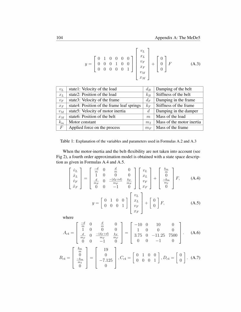
104 Appendix A: The MeDe5
y =
0 1 0 0 0 00 0 0 1 0 00 0 0 0 0 1
vL
xL
vF
xF
vM
xM
+
000
F (A.3)
vL state1: Velocity of the load dB Damping of the belt
xL state2: Position of the load kB Stiffness of the belt
vF state3: Velocity of the frame dF Damping in the frame
xF state4: Position of the frame leaf springs kF Stiffness of the frame
vM state5: Velocity of motor inertia d Damping in the damper
xM state6: Position of the belt m Mass of the load
km Motor constant mI Mass of the motor inertia
F Applied force on the process mF Mass of the frame
Table 1: Explanation of the variables and parameters used in Formulas A.2 and A.3
When the motor-inertia and the belt-flexibility are not taken into account (see
Fig 2), a fourth order approximation model is obtained with a state space descrip-
tion as given in Formulas A.4 and A.5.
vL
xL
vF
xF
=
−dm
0 dm
01 0 0 0d
mF0 −(dF +d)
mF
kF
mF
0 0 −1 0
vL
xL
vF
xF
+
km
m
0−km
mI
0
F, (A.4)
y =
[0 1 0 00 0 0 1
]
vL
xL
vF
xF
+
[00
]
F, (A.5)
where
Ac4 =
−dm
0 dm
01 0 0 0d
mF0 −(dF +d)
mF
kF
mF
0 0 −1 0
=
−10 0 10 01 0 0 0
3.75 0 −11.25 75000 0 −1 0
. (A.6)
Bc4 =
km
m
0−km
mI
0
=
190
−7.1250
, Cc4 =
[0 1 0 00 0 0 1
]
, Dc4 =
[00
]
. (A.7)
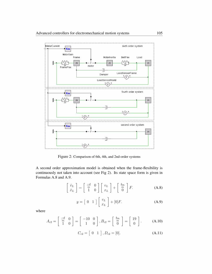
Advanced controllers for electromechanical motion systems 105
Figure 2: Comparison of 6th, 4th, and 2nd-order systems
A second order approximation model is obtained when the frame-flexibility is
continuously not taken into account (see Fig 2). Its state space form is given in
Formulas A.8 and A.9.
[vL
xL
]
=
[−dm
01 0
] [vL
xL
]
+
[km
m
0
]
F. (A.8)
y =[
0 1][
vL
xL
]
+ [0]F. (A.9)
where
Ac2 =
[−dm
01 0
]
=
[−10 01 0
]
, Bc2 =
[km
m
0
]
=
[190
]
. (A.10)
Cc2 =[
0 1], Dc2 = [0]. (A.11)

106 Appendix A: The MeDe5
When we mention the nonlinear friction term of the Damper element then:
[vL
xL
]
=
[− d
m0
1 0
] [vL
xL
]
+
[−dc
msign(vL)
0
]
+
[km
m
0
]
F (A.12)
where dc is the Coulomb parameter of the Damper element.
Since discrete controllers will be implemented in the MeDe5 setup, discretiza-
tion of these state matrices is required. This has been done by the C2DM-
command in Matlab, assuming a zero-order-hold discretization process and a sam-
ple frequency of 1 [KHz], the corresponding discrete state matrices are:
Ad4 =
1.0000 0.0000 −0.0100 0.00000.0010 1.0000 0.0000 0.00000.0075 7.5000 0.9787 −7.50000.0000 0.0000 0.0010 1.0000
, Bd4 =
0.01900.00000.02610.0000
. (A.13)
Cd4 =
[0 1 0 00 0 0 1
]
. (A.14)
Ad2 =
[0.990 0.0000.001 1.000
]
, Bd2 =
[0.0190.000
]
. (A.15)
Cd2 =[
0 1], Dd4 =
[00
]
, Dd2 = [0]. (A.16)

Bibliography
[1] Ahn, H. S., Chen, Y. Q., and Dou, H., 2005, State-Periodic Adaptive Com-
pensation of Cogging and Coulomb Friction in Permanent Magnet Linear
Motors, 2005 American Control Confrence, Portland, OR, USA.
[2] Anderson, Brian D. O., Moore, John B., 1979, Optimal Filtering, Informa-
tion and System Sciences Series, Thomas Kailath Editor, Prentice Hall Elec-
trical Engineering Series, ISBN 0-13-638122-7.
[3] Astrom, K. J., Hagglund, T., 1995, PID controllers: Theory, Design and
Tuning, Instrument Society of America, Research Triangle Park, NC, USA.
[4] Astrom, K. J., Wittenmark, B., 1989, Adaptive Control, Lund Institute of
Technology, Addison-Wesley Publishing Company, TJ217.A67 1989.
[5] Astrom, K. J., Wittenmark, B., 1997, Computer-Controlled Systems - Theory
and Design, Third Edition, Prentice Hall Information and System sciences
Series, Prentice Hall, Upper Saddle River, New Jersey 07458, ISNB 0-13-
314899-8.
[6] Berghuis, H., 1993, Model-Based Robot Control: from Theory to Practice,
PhD thesis, University of Twente, Enschede,The Netherlands.
[7] Coelingh, H. J., 2000, Design Support for Motion Control Systems: a mecha-
tronic approach, PhD thesis, University of Twente, Enschede, The Nether-
lands.
[8] Controllab Products B.V, 20-Sim-software version 3.6, 2006
(http://www.20sim.com).
[9] de Kruif, Bas J., 2004, Function Approximation for Learning Control: a key
sample based approach, PhD thesis, University of Twente, Enschede, The
Netherlands.
107

108 Bibliography
[10] de Kruif, Bas J., de Vries, Theo J. A., 2003, Phase Correction for Learning
Feed-Forward Control, Proceeding of the 2003 IEEE/ASME, International
Conference on Advanced Intelligent Mechatronics.
[11] de Vries, Theo J. A., Idema, L. J., and Velthuis, Wubbe J. R., 1998, Parsimo-
nious Learning Feed-Forward Control, Proceeding 6th European Symposium
on Artificial Neural Networks ESANN (Bruges, Belgium), M. Verleysen (ed-
itor), ISBN 2-9600049-8-1.
[12] de Vries, Theo J. A., Velthuis, Wubble J. R., and van Amerongen, J.,
2000, Learning Feed-Forward Control: A survey and Historical Note,
Proc. 1th IFAC Conf. on Mechatronic Systems (Darmstadt, Germany, 18-20
Sept.2000), R. Tsermann (ed.), VDI/VDE Gesellschaft Mess-und Automa-
tiserungstechnick GMA, Dusseldorf, Germany.
[13] de Vries, Theo J. A., Velthuis, Wubbe J. R., and Idema, L. J., 2001, Ap-
plication of Parsimonious Learning Feed-Forward Control to Mechatronic
Systems, IEE Pro. Control Theory Appl, Vol. 148, No. 4, July 2001.
[14] Dirne, H., Demonstrator of Advanced Controller, Master thesis, University
of Twente, The Netherlands, May 2005.
[15] Dorf, R. C., Bishop, R. H., 2005, Mordern Control Systems, Tenth Edi-
tion, Pearson Educational International, Pearson Prentice Hall, Upper Saddle
River, NJ 07458, ISBN: 0-13-127765-0.
[16] Eglence, M., Design and Realization of a Safe Control System for a Parallel
Manipulator, Master thesis, University of Twente, The Netherlands, June
2003.
[17] Ge, S. S., Lee, T. H., and Ren, S. X., 2001, Adaptive Friction Compensation
of Servo Mechanisms, International Journal of Systems Science, volume 32,
number 4, pages 523-532.
[18] Hesselink, R. O., MRAS-based Learning Feed-Forward Control, Master the-
sis, University of Twente, The Netherlands, November 2006.
[19] Kawato, M., 1990, Feedback-Error-Learning Neural Network for Super-
vised Motor Learning, 365-372, Advanced Neural Computers, Amsterdam,
The Netherlands, Elsevier Science Publishers B.V.
[20] Lammerts, Ivonne M. M., 1993, Adaptive Computed Reference Computed
Torque Control of Flexible Manipulators, PhD thesis, Eindhoven University
of Technology, Eindhoven, The Netherlands.
Advanced controllers for electromechanical motion systems 109
[21] Landau, I. D., Lozano, R., and Saad, M. M’., 1998, Adaptive Control,
Communications and Control Engineering, Springer-Verlag London Lim-
ited, printed in Great Britain, ISBN 354076187x.
[22] Landau, Y. D., 1979, Control and Systems Theory - Adaptive Control - The
Model Reference Approach, Marcel Dekker, INC, ISBN 0-8247-6548-6.
[23] Maciejowski, J. M., 2003, Predictive Control with Constrains, Prentice Hall,
ISBN 0 201 39823 0 PPR.
[24] Miller, W. T., Sutton, R. S., and Werbos, P. J., 1995, Neural Networks for
Control, The MIT Press Cambridge, Massachustts London, England, ISBN
0-262-13261-3 (HB), 0-262-63161-X (PB).
[25] Moore, K. L., 1993, Iterative learning control for deterministic systems, Ad-
vances in Industrial Control. Springer - Verlag.
[26] Ng, G. W., Application of Neural Networks to Adaptive Control of Nonlinear
Systems, 1997, Control Systems Center Series, Research Studies Press LTD,
Jonh Wiley and Sons INC, ISBN 0 86380 214.
[27] Nguyen, C. D., Dao, P. B., Phan, M. X., 2006, A Review of Classical and
Advanced Controllers, HUT conference of Automatic, Ha noi, 2006.
[28] Nguyen, C. D., Dao, P. B., Phan, M. X., MRAS-based Controllers, Viet-
namese conference of Mechatronics, Ha noi, 2006.
[29] Nguyen, C. D., Dao, P. B., de Vries, Theo J. A., van Amerongen, J., 2007,
Learning Feed-Forward Controller for Electromechanical Motion Systems,
Vietnamese conference of Mechanic, Ha noi, 2007.
[30] Nguyen, C. D., Dao, P. B., de Vries, Theo J. A., van Amerongen, J., An
Advanced Controller Applied to Electromechanical Motion Systems, Viet-
namese conference of Mechanic, Ha noi, 2007.
[31] Nguyen, H. T., Prasad, N. R., Walker, C. L., and Walker, E. A., 2003, A First
Course in Fuzzy and Neural Control, Chapman and Hall/CRC, A CRC Press
Company.
[32] Nogaard, M., Ravn, O., Poulsen, N. K., and Hansen, L. K., 2000, Neural Net-
work for Modeling and Control of Dynamic Systems, Advanced Textbooks
in Control and Signal Processing, ISBN 1- 85233-227-1 Springer Verlag
London.

110 Bibliography
[33] Ogata, K., 1997, Modern Control Engineering, Third Edition, Prentice Hall
International, Simon and Schuster/A Viacom Company, Upper Saddle River,
NJ 07458.
[34] Otten, G., de Vries, Theo J. A., van Amerongen, J., Rankers, A. M., and
Gaal, E. W., 1997, Linear Motor Motion Control Using a Learning Feed-
Forward Controller, IEEE/ASME Transactions on Mechatronics, Vol. 2, No.
3, 1997.
[35] Paraskevopoulos, P. N., 1996, Digital Control Systems, Prentice Hall, Math-
ematical Composition Setters Ltd, ISBN 0-13-341876-6.
[36] Stramigioli, S., Intelligent Control Course 2004, Sheets of the lecture on Self
Tuning Regulators, University of Twente, The Netherlands, 2004.
[37] Sunan, H., Kiong, T. K., and Heng, L. T., 2002, Applied Predictive Control,
Advanced in Industrial Control, Springer, ISBN 18523333383.
[38] Tomizuka, M., 1987, Zero Phase Error Tracking Algorithm for Digital
control, Journal of Dynamic Systems, Measurement, and Control, vol.109,
pp.65-68.
[39] van Amerongen, J., de Vries, Theo J. A., and Coelingh, E., Computer Sup-
port for Mechatronic Control Design, The invited session on ’Computer Sup-
port for Mechatronics System Design’ at the International Conference on
Advanced Mechatronics, Okayama, Japan, 3-5 August 1998.
[40] van Amerongen, J., Intelligent Control (part 1)-MRAS, Lecture notes, Uni-
versity of Twente, The Netherlands, March 2004.
[41] van Amerongen, J., 2004, 15 Years of Experience with Mechatronics Re-
search and Education, The 9th Mechatronics Forum International Confer-
ence, Ankara, Turkey.
[42] van Amerongen, J., de Vries, Theo J. A., Digital Control Engineering, Uni-
versity of Twente, The Netherlands, May 2005.
[43] van Amerongen, J., An MRAS-based learning feed-forward controller,
Mechatronics 2006 - 4th IFAC-Symposium on Mechatronic Systems Heidel-
berg, Germany, September 12th-14th, 2006, pp. 6, 2006.
[44] van Twillert, H., Demonstrator of Advanced Controllers, Adaptive control
configurations, Master thesis, University of Twente, The Netherlands, Au-
gust 2005.

Advanced controllers for electromechanical motion systems 111
[45] Velthuis, Wubbe J. R., 2000, Learning Feed-Forward Control: Theory, De-
sign, and Applications, PhD thesis, University of Twente, Enschede, The
Netherlands.
[46] Velthuis, Wubbe J. R., de Vries, Theo J. A., and van Amerongen, J., 2000,
Design procedure for a Learning Feed-Forward Controller, Proc. 1th IFAC
Conf. on Mechatronic Systems (Darmstadt, Germany, 18-20 Sept.2000), R.
Tsermann (ed.), VDI/VDE Gesellschaft Mess-und Automatiserungstechnick
GMA, Dusseldorf, Germany.
[47] Verwoerd, M., 2005, Iterative Learning Control - a critical review, PhD the-
sis, University of Twente, Enschede, The Netherlands.
[48] Wassink, M., Design of an Indirect Self Tuning Regulator simulation model
for 20-sim, Report nr. 045 CE 2005, University of Twente, The Netherlands,
2005.
[49] Yao, B., 1997, High performance adaptive robust control of nonlinear sys-
tems: a general framework and new schemes, Proceeding of the IEEE Con-
ference on Decision and Control, p.2489-94.
[50] Yao, B., Tomizuka, M., 1996, Smooth robust adaptive sliding mode control
of robot manipulators with guaranteed transient performance. Trans J Dyn
Syst, Meas, Control; 118(4):764-775.
[51] Yao, B., Xu, L., 2000, Adaptive robust motion control of linear motors
for precision manufacturing, Proceeding of the Mechatronics 2002, S0957-
4158.
[52] Zbikowski, R., Hunt, K. J., 1996, Neural Adaptive Control Technology,
World Scientific Series in Robotics and Intelligent Systems - Vol.15, ISBN
9810225571.

112 Bibliography

Acknowledgments
The research presented in this thesis will have never been accomplished without
the help and support from many people. I would like to express my thanks to all
of them.
First of all, I would like to express my gratitude to my promotor, Prof.dr.ir. Job
van Amerongen, who brought me to the Control Engineering group. At the be-
ginning, I had no background knowledge as many PhD students in the CE group.
I went to his room every Wednesday, asking questions, discussing ideas. He suf-
fered a lot from my English. He supported me all the time, giving me the necessary
encouragements after each small success, which I achieved. With his extensive
knowledge on Mechatronics, Intelligent Control, and Modeling and Simulation,
he helped me a lot in solving problems. His comments on my work were always
short but meaningful. I benefited a lot from his remarks. Thank you very much
Prof. Job, I cannot express my appreciation enough to you.
Next, I wish to thank my assistant-promotor, Dr.ir. T.J.A. de Vries, for his
guidance, discussions, and the Dutch translation of the summary. His criticisms
about our works were strict and helpful. Every paragraph in this thesis became
precise and clear after his corrections and comments.
I am thankful to the Vietnamese Government for financial support. Thanks
to all members of the 322- project from the MOET for their management and
service.
I would like to thank all the committee members for their careful reading and
constructive comments to my thesis.
I would like to thank all the members of the CE group for a pleasant working
atmosphere. I am very grateful to Carla for her useful helps with all documents
relating to the period of my studying in the Netherlands. My thanks are expressed
to Dr.ir. Peter, Dr.ir. Jan, Dr.ing. Raffaella, Dr. Maarten, Prof.dr.ir. Paul, Prof.dr.ir
Stefano, Frank, Peter, Paul, and Christian for their supports. I thank Gerben,
Marcel, and Alfred for their technical help. The other colleagues: Michel, Marcel,
Aditya , Gijs , Martijin, Wei, Martin, Edwin, and Oscar made the wonderful time
for me. I thank Tim for his working on the Tripod setup.
I would like to express my gratitude to all people of the Thainguyen University
113

of Technology for their supports. My acknowledgments are also sent to Prof.
dr. Vo Quang Lap - my supervisor for my bachelor and also master studies. I
wish to thank Prof.dr. Nguyen Dang Binh for his encouragements and supports.
My thanks and regards are expressed to Cao Thanh Long, Vu Ngoc Pi, Nguyen
Van Du, Nguyen Tien Hung, Le Quoc Phong, and Nguyen Duc Thang for their
cheerful friendship and help during the years.
My thanks are also sent to all members of the K15 I company for their useful
helps to my family.
To my Vietnamese friends in Twente, Delft, Groningen, Leiden, Hanoi, and
Thainguyen. I can only mention the names of some of them here: Nhon-Loi
(Hanoi), Giang-Linh (Thainguyen), Kim-Van Anh, Ha-Hanh, Hien-Nhu, Tu-An,
Trung-Thanh, Giang-Chi, Duy-Chi, Thang-Mai, Phuong-Ha, Ha-Huong, Hoa-
Huong, Nhung, Phong, Chau, Nhi, Minh, So, Hanh (ITC), Minh and Khuong
(Groningen), Hoan (Delft), Sam (Leiden). Thank all of you, my friends!
My most grateful worlds are expressed to my parents, my sister Canh-Ty and
brothers Hung-Tam and Cuong-Cham for their whole life support and love that
they have given me.
I thank my wife Linh for her patience love and sacrifices, which she has done
for me, my daughter Thanh Van and my son Duy An.
Enschede, 10th of March, 2008.
Nguyen Duy Cuong

About the Author
Nguyen Duy Cuong was born on May 9th, 1962 in Camduong - Laocai, a small
town in the north of Vietnam. After completing his secondary education in 1979,
he started his bachelor study in Electrical Engineering at the Thainguyen Uni-
versity of Technology in Vietnam. In 1984, he obtained his bachelor degree and
worked as a lecturer at the faculty of Electrical Engineering of the same university
in the field of Electronic Technique. In 2001, he obtained his M.Sc. degree with
a thesis on automatic control of an industrial furnace. In 2004, he was granted a
scholarship from the Vietnamese Government through the 322 project and started
his Ph.D. position at the Control Engineering group, University of Twente, The
Netherlands, under the supervision of Prof.dr.ir. Job van Amerongen and Dr.ir.
Theo.J.A. de Vries. He has successfully completed his PhD research on Advanced
Controllers for Electromechanical Motion Systems.
115