Advanced Calculus I (Math 4209) - web.mst.eduweb.mst.edu/~bohner/math4209-18/4209-notes.pdf · Spring 2018 Lecture Notes Martin Bohner Version from February 20, 2018 Author address:

Advanced Calculus I (Math 4209)

Spring 2018 Lecture Notes

Martin Bohner

Version from May 4, 2018

Author address:

Department of Mathematics and Statistics, Missouri University of

Science and Technology, Rolla, Missouri 65409-0020

E-mail address: [email protected]

URL: http://web.mst.edu/~bohner

Contents

Chapter 1. Preliminaries 1

1.1. Sets 1

1.2. Functions 2

1.3. Proofs 3

Chapter 2. The Real Number System 5

2.1. The Field Axioms 5

2.2. The Positivity Axioms 6

2.3. The Completeness Axiom 7

2.4. The Natural Numbers 8

2.5. Some Inequalities and Identities 9

Chapter 3. Sequences of Real Numbers 13

3.1. The Convergence of Sequences 13

3.2. Monotone Sequences 14

Chapter 4. Continuous Functions 17

Chapter 5. Differentiation 21

5.1. Differentiation Rules 21

5.2. The Mean Value Theorems 22

5.3. Applications of the Mean Value Theorems 23

Chapter 6. Integration 27

6.1. The Definition of the Integral 27

6.2. The Fundamental Theorem of Calculus 28

iii

iv CONTENTS

6.3. Applications 29

6.4. Improper Integrals 29

Chapter 7. Infinite Series of Functions 31

7.1. Uniform Convergence 31

7.2. Interchanging of Limit Processes 32

CHAPTER 1

Preliminaries

1.1. Sets

Definition 1.1 (Cantor). A set is a collection of certain distinct objects which are

called elements of the set.

Notation 1.2. The following notation will be used throughout this class:

• x ∈ A (or x 6∈ A): x is an element (or is not an element) of the set A;

• A ⊂ B: A is a subset of B, i.e., if x ∈ A, then x ∈ B (or: x ∈ A =⇒ x ∈ B);

• A = B ⇐⇒ A ⊂ B and B ⊂ A;

• ∅: empty set. We have ∅ ⊂ A for all sets A;

• A = {a, b, c}: A consists of the elements a, b, and c;

• A = {x : x has the property P}: A consists of all elements x that have the

property P ;

• A ∪B := {x : x ∈ A or x ∈ B}: union of A and B;

• A ∩B := {x : x ∈ A and x ∈ B}: intersection of A and B;

• A \B := {x : x ∈ A and x 6∈ B}: difference of A and B;

• A × B := {(a, b) : a ∈ A and b ∈ B}: Cartesian product of A and B (with

(a, b) = (c, d) ⇐⇒ a = c and b = d);

• Ac := {x : x 6∈ A}: complement of A (with respect to a given set X);

• P(A) := {B : B ⊂ A}: power set of A.

Notation 1.3 (Quantifiers). We use the following quantifiers throughout this class:

• universal quantifier: ∀ “for all”;

• existential quantifier: ∃ “there exists”.

• unique existential quantifier: ∃! “there exists exactly one”.

Lemma 1.4. The operations ∪ and ∩ satisfy the commutative, associative, and

distributive laws.

1

2 1. PRELIMINARIES

1.2. Functions

Definition 1.5. Let X and Y be nonempty sets. A function (or mapping) f from

X to Y is a correspondence that associates with each point x ∈ X in a unique way

a y ∈ Y ; we write y = f(x). X is called the domain of f while Y is called the range

of f . We write f : X → Y .

Remark 1.6. Two functions f : X → Y and g : U → V are called equal (we write

f = g) iff X = U and Y = V and f(x) = g(x) for all x ∈ X.

Notation 1.7. Let f : X → Y be a function. Then we call

(i) G(f) := {(x, f(x)) : x ∈ X} ⊂ X × Y the graph of f ;

(ii) f(A) := {f(x) : x ∈ A} ⊂ Y the image of a set A ⊂ X;

(iii) f−1(B) := {x ∈ X : f(x) ∈ B} ⊂ X the inverse image of a set B ⊂ Y .

Lemma 1.8. Let f : X → Y be a function and A ⊂ X, B ⊂ Y . Then we have

(i) y ∈ f(A) ⇐⇒ ∃x ∈ A : f(x) = y;

(ii) x ∈ A =⇒ f(x) ∈ f(A);

(iii) x ∈ f−1(B) ⇐⇒ f(x) ∈ B.

Definition 1.9. Let f : X → Y be a function. Then f is called

(i) one-to-one if x1, x2 ∈ X with x1 6= x2 always implies f(x1) 6= f(x2);

(ii) onto if f(X) = Y ;

(iii) invertible if f is both one-to-one and onto.

Remark 1.10. (i) f : X → Y is a function iff ∀x ∈ X ∃!y ∈ Y : f(x) = y;

(ii) f : X → Y is onto iff ∀y ∈ Y ∃x ∈ X : f(x) = y;

(iii) f : X → Y is invertible iff ∀y ∈ Y ∃!x ∈ X : f(x) = y.

Definition 1.11. Let f : X → Y and g : Y → Z be functions. Then the function

g ◦ f : X → Z with (g ◦ f)(x) = g(f(x)) for all x ∈ X is called the composite

function of f and g.

Proposition 1.12. A function f : X → Y is invertible iff there exists exactly one

function g : Y → X satisfying

(f ◦ g)(y) = y ∀y ∈ Y and (g ◦ f)(x) = x ∀x ∈ X.

1.3. PROOFS 3

Notation 1.13. Let f : X → Y . The unique function g : Y → X from Proposition

1.12 is called the inverse function of f and denoted by f−1.

1.3. Proofs

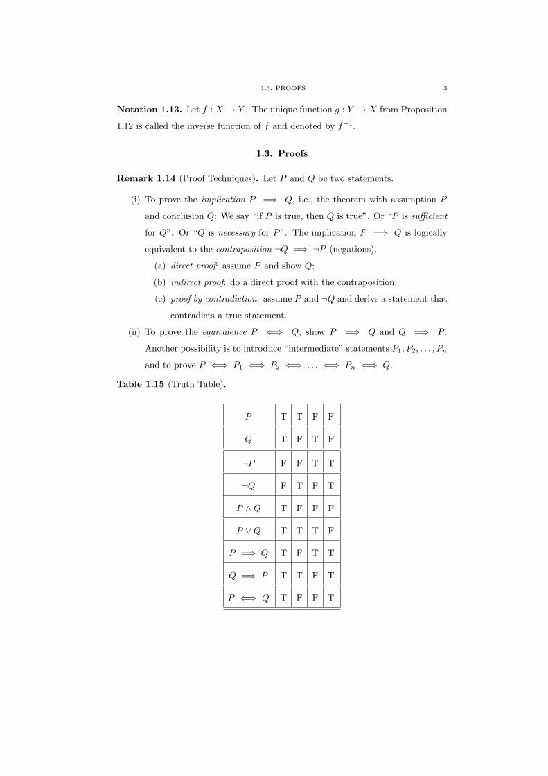
Remark 1.14 (Proof Techniques). Let P and Q be two statements.

(i) To prove the implication P =⇒ Q, i.e., the theorem with assumption P

and conclusion Q: We say “if P is true, then Q is true”. Or “P is sufficient

for Q”. Or “Q is necessary for P”. The implication P =⇒ Q is logically

equivalent to the contraposition ¬Q =⇒ ¬P (negations).

(a) direct proof: assume P and show Q;

(b) indirect proof: do a direct proof with the contraposition;

(c) proof by contradiction: assume P and ¬Q and derive a statement that

contradicts a true statement.

(ii) To prove the equivalence P ⇐⇒ Q, show P =⇒ Q and Q =⇒ P .

Another possibility is to introduce “intermediate” statements P1, P2, . . . , Pn

and to prove P ⇐⇒ P1 ⇐⇒ P2 ⇐⇒ . . . ⇐⇒ Pn ⇐⇒ Q.

Table 1.15 (Truth Table).

P T T F F

Q T F T F

¬P F F T T

¬Q F T F T

P ∧Q T F F F

P ∨Q T T T F

P =⇒ Q T F T T

Q =⇒ P T T F T

P ⇐⇒ Q T F F T

4 1. PRELIMINARIES

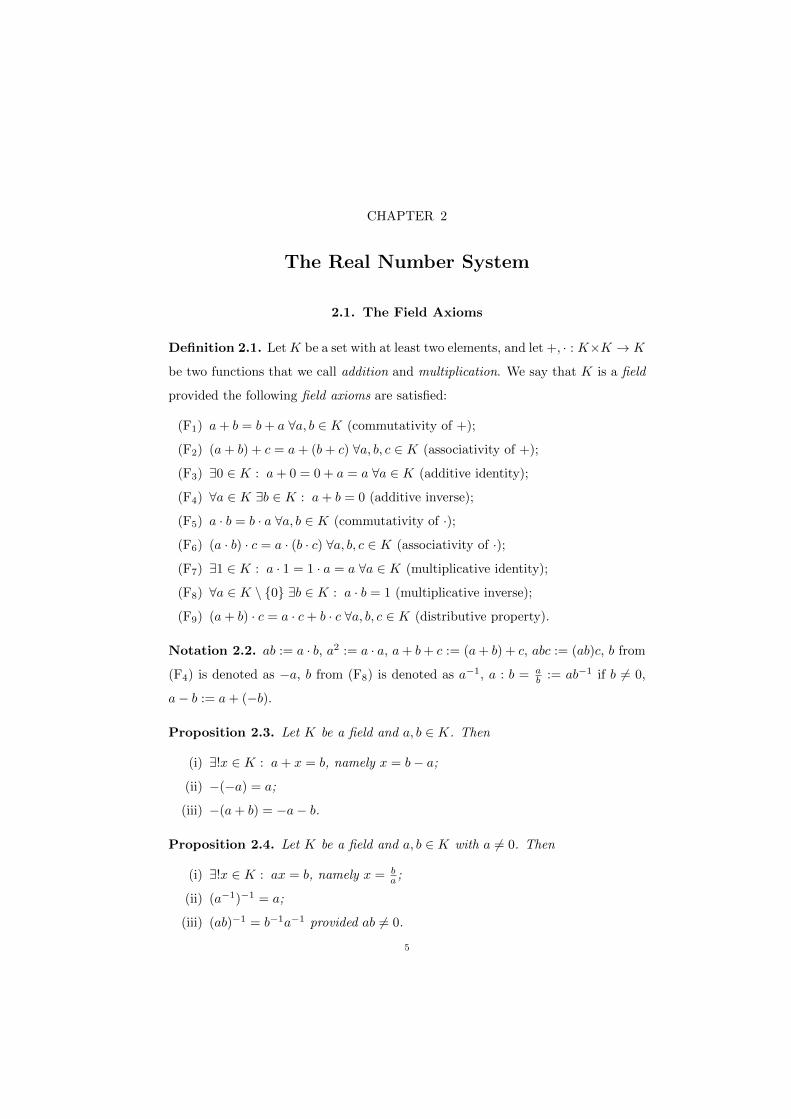
CHAPTER 2

The Real Number System

2.1. The Field Axioms

Definition 2.1. LetK be a set with at least two elements, and let +, · : K×K → K

be two functions that we call addition and multiplication. We say that K is a field

provided the following field axioms are satisfied:

(F1) a+ b = b+ a ∀a, b ∈ K (commutativity of +);

(F2) (a+ b) + c = a+ (b+ c) ∀a, b, c ∈ K (associativity of +);

(F3) ∃0 ∈ K : a+ 0 = 0 + a = a ∀a ∈ K (additive identity);

(F4) ∀a ∈ K ∃b ∈ K : a+ b = 0 (additive inverse);

(F5) a · b = b · a ∀a, b ∈ K (commutativity of ·);

(F6) (a · b) · c = a · (b · c) ∀a, b, c ∈ K (associativity of ·);

(F7) ∃1 ∈ K : a · 1 = 1 · a = a ∀a ∈ K (multiplicative identity);

(F8) ∀a ∈ K \ {0} ∃b ∈ K : a · b = 1 (multiplicative inverse);

(F9) (a+ b) · c = a · c+ b · c ∀a, b, c ∈ K (distributive property).

Notation 2.2. ab := a · b, a2 := a · a, a+ b+ c := (a+ b) + c, abc := (ab)c, b from

(F4) is denoted as −a, b from (F8) is denoted as a−1, a : b = ab := ab−1 if b 6= 0,

a− b := a+ (−b).

Proposition 2.3. Let K be a field and a, b ∈ K. Then

(i) ∃!x ∈ K : a+ x = b, namely x = b− a;

(ii) −(−a) = a;

(iii) −(a+ b) = −a− b.

Proposition 2.4. Let K be a field and a, b ∈ K with a 6= 0. Then

(i) ∃!x ∈ K : ax = b, namely x = ba ;

(ii) (a−1)−1 = a;

(iii) (ab)−1 = b−1a−1 provided ab 6= 0.

5

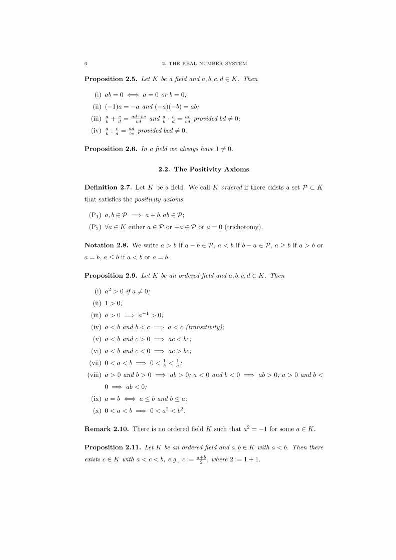
6 2. THE REAL NUMBER SYSTEM

Proposition 2.5. Let K be a field and a, b, c, d ∈ K. Then

(i) ab = 0 ⇐⇒ a = 0 or b = 0;

(ii) (−1)a = −a and (−a)(−b) = ab;

(iii) ab + c

d = ad+bcbd and a

b ·cd = ac

bd provided bd 6= 0;

(iv) ab : cd = ad

bc provided bcd 6= 0.

Proposition 2.6. In a field we always have 1 6= 0.

2.2. The Positivity Axioms

Definition 2.7. Let K be a field. We call K ordered if there exists a set P ⊂ K

that satisfies the positivity axioms:

(P1) a, b ∈ P =⇒ a+ b, ab ∈ P;

(P2) ∀a ∈ K either a ∈ P or −a ∈ P or a = 0 (trichotomy).

Notation 2.8. We write a > b if a − b ∈ P, a b or

a = b, a ≤ b if a 0 if a 6= 0;

(ii) 1 > 0;

(iii) a > 0 =⇒ a−1 > 0;

(iv) a 0 =⇒ ac < bc;

(vi) a bc;

(vii) 0 < a 0 and b > 0 =⇒ ab > 0; a < 0 and b < 0 =⇒ ab > 0; a > 0 and b <

0 =⇒ ab < 0;

(ix) a = b ⇐⇒ a ≤ b and b ≤ a;

(x) 0 < a < b =⇒ 0 < a2 < b2.

Remark 2.10. There is no ordered field K such that a2 = −1 for some a ∈ K.

Proposition 2.11. Let K be an ordered field and a, b ∈ K with a < b. Then there

exists c ∈ K with a < c < b, e.g., c := a+b2 , where 2 := 1 + 1.

2.3. THE COMPLETENESS AXIOM 7

Notation 2.12. If K is an ordered field and a, b ∈ K, then we put

(a, b) := {x ∈ K : a < x < b},

[a, b] := {x ∈ K : a ≤ x ≤ b},

(a, b] := {x ∈ K : a < x ≤ b},

and

[a, b) := {x ∈ K : a ≤ x < b}.

Definition 2.13. Let K be an ordered field and T ⊂ K with T 6= ∅. An m ∈ T is

called minimum (or maximum) of T provided m ≤ t (or m ≥ t) for all t ∈ T . We

write m = minT (or m = maxT ).

Proposition 2.14. Let K be an ordered field and T ⊂ K with T 6= ∅. If minT (or

maxT ) exists, then it is uniquely determined.

Example 2.15. For T = (0, 1] we have maxT = 1 and minT does not exist.

2.3. The Completeness Axiom

Definition 2.16. Let K be an ordered field and T ⊂ K. We call

(i) s ∈ K an upper (or lower) bound of T if t ≤ s (or t ≥ s) for all t ∈ T ;

(ii) T bounded above (or bounded below) if it has an upper (or lower) bound;

(iii) T bounded if it is bounded above and below;

(iv) s = supT the supremum of T (and the infimum inf T analogously) if

(a) s is an upper bound of T and

(b) s ≤ s for all upper bounds s of T .

Proposition 2.17. Let K be an ordered field and T ⊂ K. Then

m = maxT exists ⇐⇒ s = supT exists and s ∈ T,

and then s = m.

Theorem 2.18. Let K be an ordered field and T ⊂ K. Then

s = supT ⇐⇒

∀t ∈ T : s ≥ t and

∀ε > 0 ∃t ∈ T : t > s− ε.


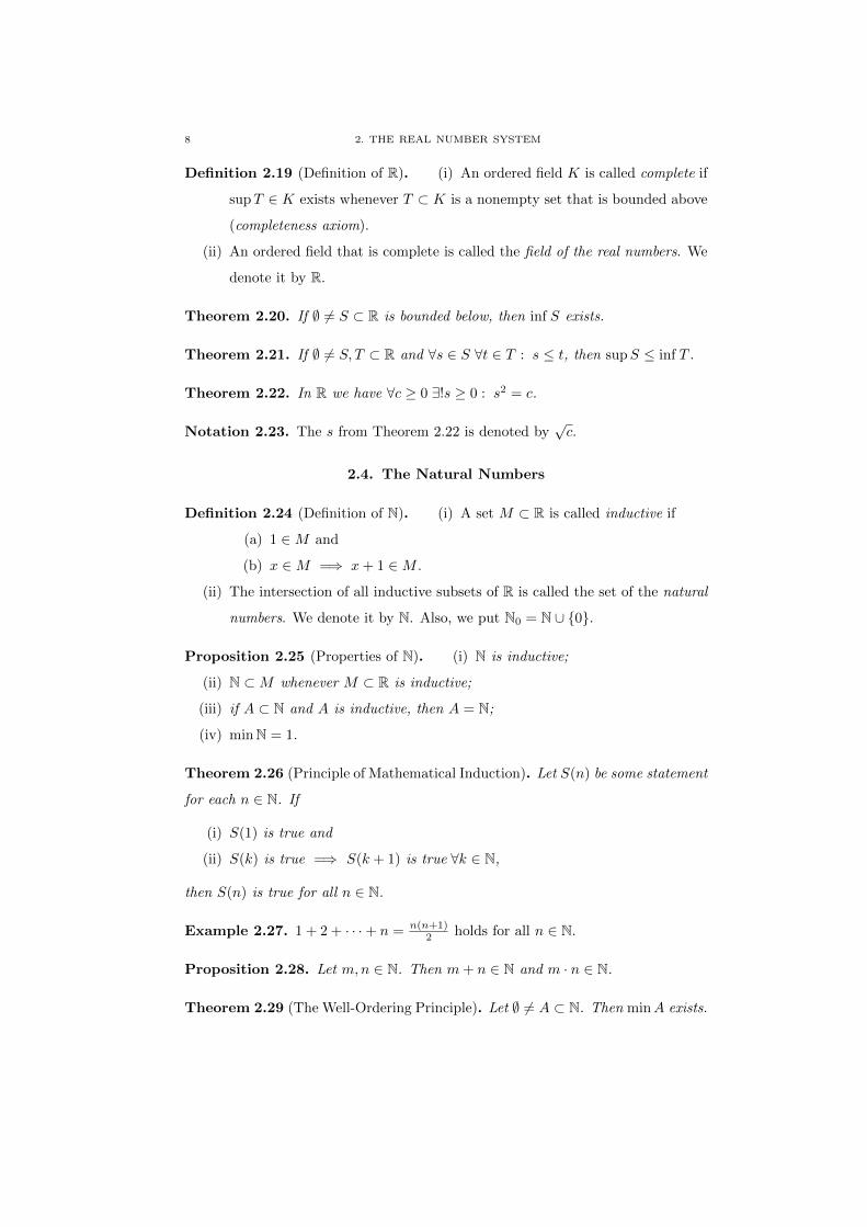
Definition 2.19 (Definition of R). (i) An ordered field K is called complete if

supT ∈ K exists whenever T ⊂ K is a nonempty set that is bounded above

(completeness axiom).

(ii) An ordered field that is complete is called the field of the real numbers. We

denote it by R.

Theorem 2.20. If ∅ 6= S ⊂ R is bounded below, then inf S exists.

Theorem 2.21. If ∅ 6= S, T ⊂ R and ∀s ∈ S ∀t ∈ T : s ≤ t, then supS ≤ inf T .

Theorem 2.22. In R we have ∀c ≥ 0 ∃!s ≥ 0 : s2 = c.

Notation 2.23. The s from Theorem 2.22 is denoted by√c.

2.4. The Natural Numbers

Definition 2.24 (Definition of N). (i) A set M ⊂ R is called inductive if

(a) 1 ∈M and

(b) x ∈M =⇒ x+ 1 ∈M .

(ii) The intersection of all inductive subsets of R is called the set of the natural

numbers. We denote it by N. Also, we put N0 = N ∪ {0}.

Proposition 2.25 (Properties of N). (i) N is inductive;

(ii) N ⊂M whenever M ⊂ R is inductive;

(iii) if A ⊂ N and A is inductive, then A = N;

(iv) minN = 1.

Theorem 2.26 (Principle of Mathematical Induction). Let S(n) be some statement

for each n ∈ N. If

(i) S(1) is true and

(ii) S(k) is true =⇒ S(k + 1) is true ∀k ∈ N,

then S(n) is true for all n ∈ N.

Example 2.27. 1 + 2 + · · ·+ n = n(n+1)2 holds for all n ∈ N.

Proposition 2.28. Let m,n ∈ N. Then m+ n ∈ N and m · n ∈ N.

Theorem 2.29 (The Well-Ordering Principle). Let ∅ 6= A ⊂ N. Then minA exists.

2.5. SOME INEQUALITIES AND IDENTITIES 9

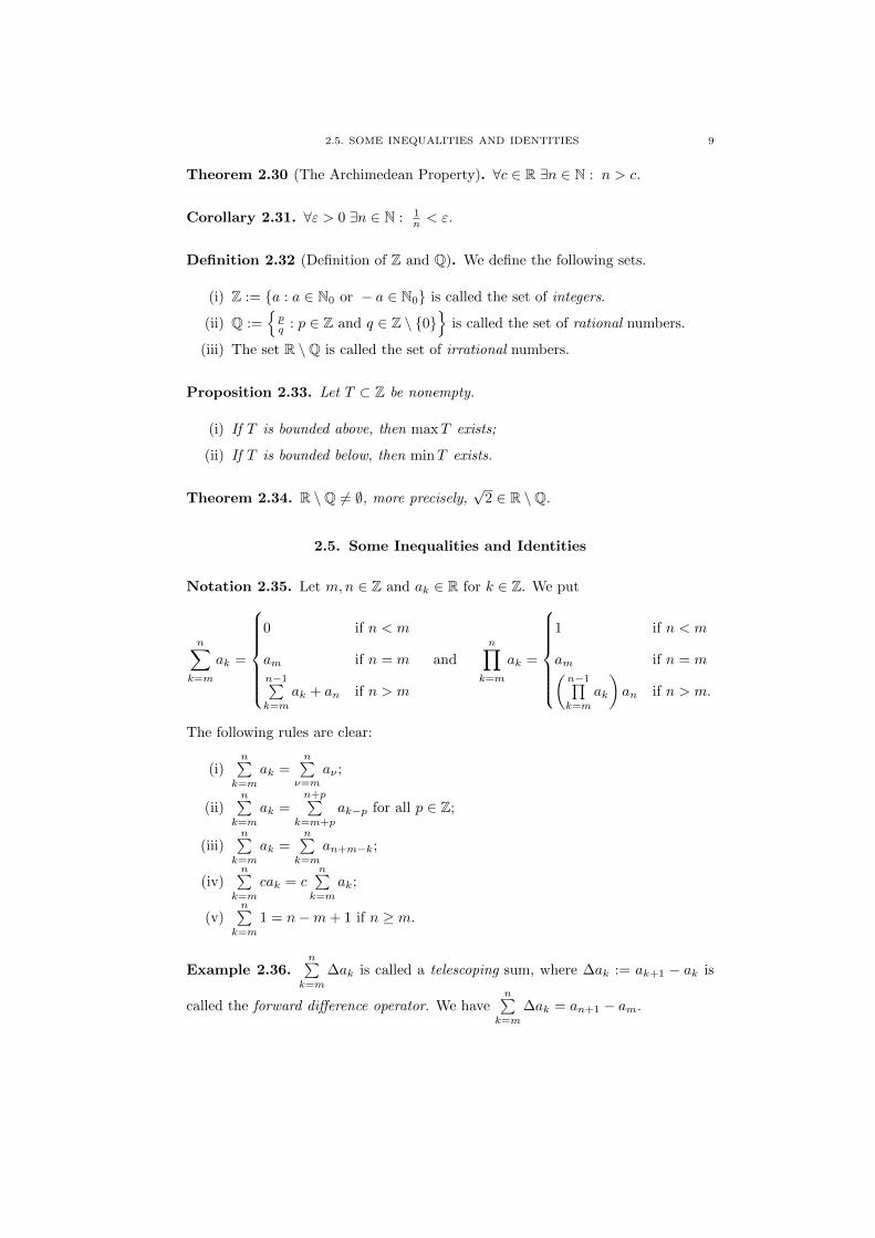
Theorem 2.30 (The Archimedean Property). ∀c ∈ R ∃n ∈ N : n > c.

Corollary 2.31. ∀ε > 0 ∃n ∈ N : 1n < ε.

Definition 2.32 (Definition of Z and Q). We define the following sets.

(i) Z := {a : a ∈ N0 or − a ∈ N0} is called the set of integers.

(ii) Q :={pq : p ∈ Z and q ∈ Z \ {0}

}is called the set of rational numbers.

(iii) The set R \Q is called the set of irrational numbers.

Proposition 2.33. Let T ⊂ Z be nonempty.

(i) If T is bounded above, then maxT exists;

(ii) If T is bounded below, then minT exists.

Theorem 2.34. R \Q 6= ∅, more precisely,√

2 ∈ R \Q.

2.5. Some Inequalities and Identities

Notation 2.35. Let m,n ∈ Z and ak ∈ R for k ∈ Z. We put

n∑k=m

ak =

0 if n < m

am if n = mn−1∑k=m

ak + an if n > m

and

n∏k=m

ak =

1 if n < m

am if n = m(n−1∏k=m

ak

)an if n > m.

The following rules are clear:

(i)n∑

k=m

ak =n∑

ν=maν ;

(ii)n∑

k=m

ak =n+p∑

k=m+p

ak−p for all p ∈ Z;

(iii)n∑

k=m

ak =n∑

k=m

an+m−k;

(iv)n∑

k=m

cak = cn∑

k=m

ak;

(v)n∑

k=m

1 = n−m+ 1 if n ≥ m.

Example 2.36.n∑

k=m

∆ak is called a telescoping sum, where ∆ak := ak+1 − ak is

called the forward difference operator. We haven∑

k=m

∆ak = an+1 − am.


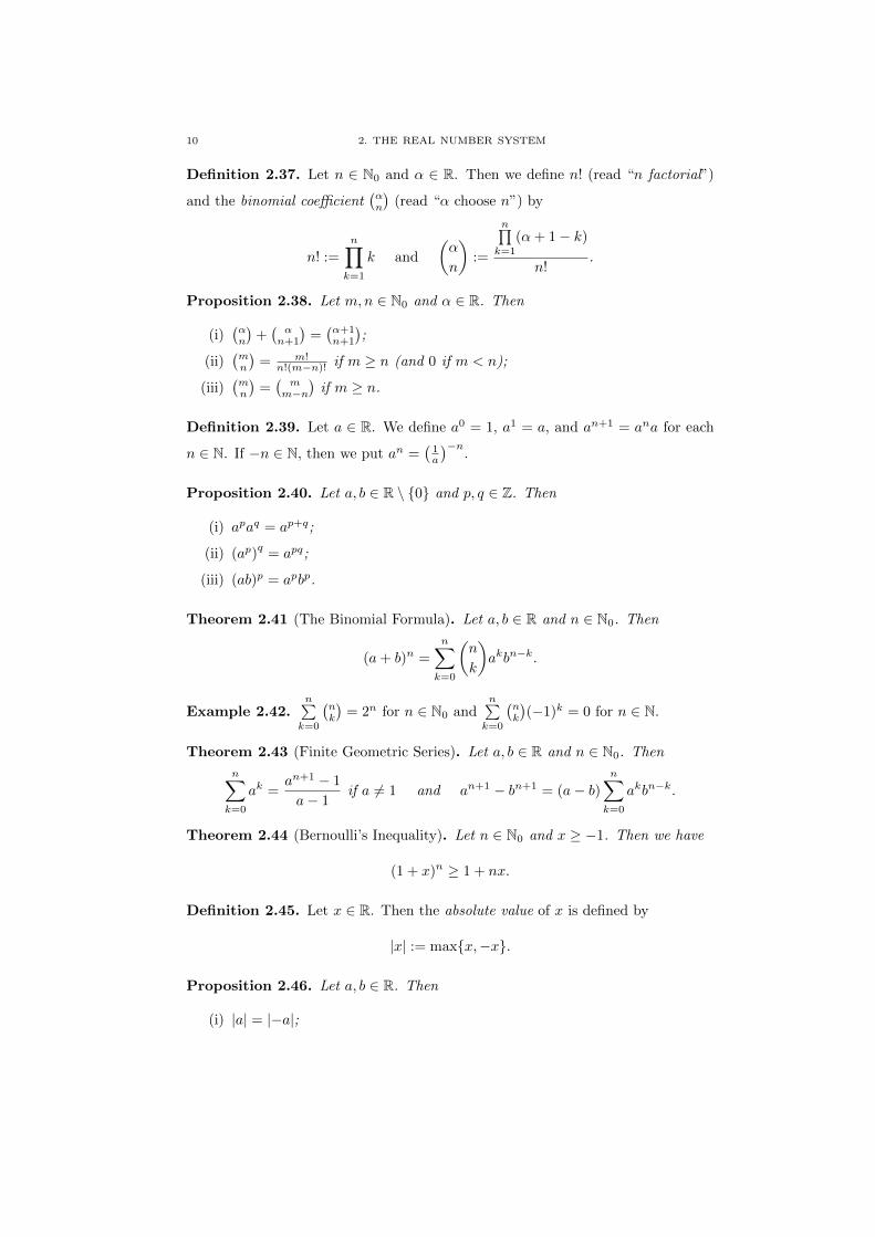
Definition 2.37. Let n ∈ N0 and α ∈ R. Then we define n! (read “n factorial”)

and the binomial coefficient(αn

)(read “α choose n”) by

n! :=

n∏k=1

k and

(α

n

):=

n∏k=1

(α+ 1− k)

n!.

Proposition 2.38. Let m,n ∈ N0 and α ∈ R. Then

(i)(αn

)+(αn+1

)=(α+1n+1

);

(ii)(mn

)= m!

n!(m−n)! if m ≥ n (and 0 if m < n);

(iii)(mn

)=(m

m−n)

if m ≥ n.

Definition 2.39. Let a ∈ R. We define a0 = 1, a1 = a, and an+1 = ana for each

n ∈ N. If −n ∈ N, then we put an =(1a

)−n.

Proposition 2.40. Let a, b ∈ R \ {0} and p, q ∈ Z. Then

(i) apaq = ap+q;

(ii) (ap)q

= apq;

(iii) (ab)p = apbp.

Theorem 2.41 (The Binomial Formula). Let a, b ∈ R and n ∈ N0. Then

(a+ b)n =

n∑k=0

(n

k

)akbn−k.

Example 2.42.n∑k=0

(nk

)= 2n for n ∈ N0 and

n∑k=0

(nk

)(−1)k = 0 for n ∈ N.

Theorem 2.43 (Finite Geometric Series). Let a, b ∈ R and n ∈ N0. Then

n∑k=0

ak =an+1 − 1

a− 1if a 6= 1 and an+1 − bn+1 = (a− b)

n∑k=0

akbn−k.

Theorem 2.44 (Bernoulli’s Inequality). Let n ∈ N0 and x ≥ −1. Then we have

(1 + x)n ≥ 1 + nx.

Definition 2.45. Let x ∈ R. Then the absolute value of x is defined by

|x| := max{x,−x}.

Proposition 2.46. Let a, b ∈ R. Then

(i) |a| = |−a|;

2.5. SOME INEQUALITIES AND IDENTITIES 11

(ii) |a| ≥ 0; and |a| = 0 ⇐⇒ a = 0;

(iii) |ab| = |a||b|;

(iv) a = 0 ⇐⇒ |a| < ε ∀ε > 0.

Theorem 2.47 (Triangle Inequalities). If a, b ∈ R, then

||a| − |b|| ≤ |a+ b| ≤ |a|+ |b|.

Remark 2.48. Define d(x, y) := |x− y| for x, y ∈ R. Then

(i) d(x, y) = d(y, x);

(ii) d(x, y) ≥ 0; and d(x, y) = 0 ⇐⇒ x = y;

(iii) d(x, z) ≤ d(x, y) + d(y, z).


CHAPTER 3

Sequences of Real Numbers

3.1. The Convergence of Sequences

Definition 3.1. If x : N → R is a function, then we call x a sequence (of real

numbers). Instead of x(n) we rather write xn, n ∈ N. The sequence s defined by

sn =∑nk=1 xk, n ∈ N, is also known as a series.

Example 3.2. (i) an = 1 + (−1)n;

(ii) an = max{k ∈ N : k ≤√n3};

(iii) x0 = 1 and xn+1 = 2xn for all n ∈ N0;

(iv) f0 = f1 = 1 and fn+2 = fn+1 + fn for all n ∈ N0;

(v) an =∑nk=1

1k .

Definition 3.3. A sequence a is said to be convergent if

∃α ∈ R ∀ε > 0 ∃N ∈ N ∀n ≥ N : |an − α| < ε.

We write α = limn→∞ an or an → α (as n→∞). A sequence is called divergent if

it is not convergent.

Example 3.4. (i) an = 2n4n+3 ;

(ii) an = (−1)n.

Proposition 3.5. Any sequence has at most one limit.

Proposition 3.6 (Some Limits). We have

(i) If an = α for all n ∈ N, then limn→∞ an = α;

(ii) limn→∞1n = 0;

(iii) if |x| < 1, then limn→∞ xn = 0;

(iv) if |x| < 1, then limn→∞∑nk=0 x

k = 11−x .

13

14 3. SEQUENCES OF REAL NUMBERS

Definition 3.7. A sequence a is called bounded (or bounded above, or bounded

below) if the set {an : n ∈ N} is bounded (or bounded above, or bounded below).

Proposition 3.8 (Necessary Conditions for Convergence). Let a be a convergent

sequence. Then

(i) a is bounded;

(ii) a satisfies the Cauchy Condition, i.e.,

∀ε > 0 ∃N ∈ N : ∀m,n ≥ N |an − am| < ε.

Remark 3.9. an → α implies an+1 − an → 0, a2n − an → 0.

Example 3.10. (i) an = (−1)n;

(ii) an =∑nk=1

1k (the harmonic series).

Theorem 3.11. Suppose an → α and bn → β as n→∞. Then

(i) |an| → |α|;

(ii) an + bn → α+ β;

(iii) ∀c ∈ R : can → cα;

(iv) an · bn → αβ;

(v) anbn→ α

β if β 6= 0.

Example 3.12. (i) an → α, m ∈ N =⇒ amn → αm;

(ii) n2−32n2+3n →

12 as n→∞.

Theorem 3.13. Suppose an → α, bn → β, cn ∈ R. Then

(i) ∃K ∈ R ∀n ∈ N : |an| ≤ K =⇒ |α| ≤ K;

(ii) ∀n ∈ N : an ≤ bn =⇒ α ≤ β;

(iii) α = β and ∀n ∈ N : an ≤ cn ≤ bn =⇒ limn→∞ cn = α.

3.2. Monotone Sequences

Definition 3.14. A sequence a is called monotonically increasing (or monotonically

decreasing, strictly increasing, strictly decreasing) provided an ≤ an+1 (an ≥ an+1,

an < an+1, an > an+1) holds for all n ∈ N. We write an ↗ (↘, ↑, ↓). The sequence

is called monotone if it is either one of the above.

3.2. MONOTONE SEQUENCES 15

Theorem 3.15 (The Monotone Convergence Theorem). A monotone sequence

converges iff it is bounded.

Example 3.16. (i) a1 = 2 and an+1 = an+62 for all n ∈ N;

(ii) sn =∑nk=1

1k ;

(iii) sn =∑nk=1

1k2k

;

(iv) an =(1 + 1

n

)n. We denote the limit of this sequence by e.

Definition 3.17. Let an be a sequence and let nk be a sequence of natural numbers

that is strictly increasing. Then the sequence bk defined by bk = ankfor k ∈ N is

called a subsequence of the sequence an.

Theorem 3.18. Every sequence has a monotone subsequence.

Theorem 3.19 (Bolzano–Weierstraß). Let a, b ∈ R with a < b. Every sequence in

[a, b] has a convergent subsequence that has its limit in [a, b].

Theorem 3.20 (Cauchy). A real sequence converges iff it is a Cauchy sequence.

Proposition 3.21. Let an be a convergent sequence with limn→∞ an = α. Then

every subsequence ankof an converges with limk→∞ ank

= α.

Example 3.22. (i) an → α =⇒ a2n → α, an+1 → α;

(ii)(1 + 1

2n

)2n,(1 + 1

n2

)n2

;

(iii) (−1)n(1 + 1

n

).

Theorem 3.23 (The Nested Interval Theorem). Let an, bn ∈ R with an < bn for

all n ∈ N, put In = [an, bn], and assume In+1 ⊂ In for all n ∈ N and bn − an → 0

as n → ∞. Then⋂n∈N In = {α} with α ∈ R and limn→∞ an = limn→∞ bn = α

exist.

16 3. SEQUENCES OF REAL NUMBERS

CHAPTER 4

Continuous Functions

Definition 4.1. A function f : D → R is said to be continuous at (or in) x0 ∈ D

provided

{xn : n ∈ N} ⊂ D, limn→∞

xn = x0 =⇒ limn→∞

f(xn) = f(x0).

Also, f is called continuous if it is continuous at each x0 ∈ D.

Example 4.2. (i) f(x) = x2 + 3x− 2, x ∈ R;

(ii) f(x) =√x, x ≥ 0;

(iii) f = χ[0,1];

(iv) f = χQ is called the Dirichlet function.

Notation 4.3. For two functions f, g : D → R we define the sum f + g : D → R

and the product f ·g : D → R by (f+g)(x) = f(x)+g(x) and (f ·g)(x) = f(x)g(x)

for x ∈ D. If g(x) 6= 0 for all x ∈ D, then fg : D → R is defined by

(fg

)(x) = f(x)

g(x)

for x ∈ D.

Theorem 4.4. Let f, g : D → R be continuous functions. Then f+g, f ·g : D → R

are continuous. If g(x) 6= 0 for all x ∈ D, then fg : D → R is continuous.

Corollary 4.5. Let m ∈ N, ck ∈ R (0 ≤ k ≤ m), and p : R → R be defined by

p(x) =∑mk=0 ckx

k, i.e., p is a polynomial with degree m if cm 6= 0. Then p is

continuous. Also, if p, q are both polynomials and D = {x ∈ R : q(x) 6= 0}, then

the rational function pq : D → R is continuous.

Theorem 4.6. If f : D → R, g : U → R are functions with f(D) ⊂ U such that f

is continuous at x0 ∈ D and g is continuous at f(x0) ∈ U , then g ◦ f : D → R is

continuous at x0 ∈ D.

Example 4.7.√

1− x2, x ∈ [−1, 1].

17

18 4. CONTINUOUS FUNCTIONS

Theorem 4.8. Let f : [a, b]→ R be continuous, where a, b ∈ R with a < b. Assume

f(a) < 0 and f(b) > 0. Then ∃α ∈ (a, b) : f(α) = 0.

Theorem 4.9 (The Intermediate Value Theorem). Let f : [a, b]→ R be continuous,

where a, b ∈ R with a < b. If f(a) < c < f(b) or f(b) < c < f(a), then ∃ α ∈ (a, b) :

f(α) = c.

Example 4.10. (i) h(x) = x5 + x+ 1, x ∈ R, has a zero in (−2, 0);

(ii) h(x) = 1√1+x2

− x2, x ∈ R, has a zero in (0, 1);

(iii) if I ⊂ R is an interval and f : I → R is continuous, then f(I) is an interval.

Theorem 4.11 (The Extreme Value Theorem). Let f : I = [a, b]→ R be continu-

ous, where a, b ∈ R with a < b. Then both max f(I) and min f(I) exist.

Definition 4.12. Let D ⊂ R. The function f : D → R is called strictly increasing

(or strictly decreasing, increasing, decreasing) if f(v) > f(u) (or f(v) < f(u),

f(v) ≥ f(u), f(v) ≤ f(u)) holds for all u, v ∈ D with u < v. We write f ↑

(↓,↗,↘). Also, f is called strictly monotone if it is either strictly increasing or

strictly decreasing.

Theorem 4.13. Let f : I → f(I) be strictly monotone, where I is an interval.

Then f is invertible and f−1 : f(I)→ I is continuous and strictly monotone.

Corollary 4.14. Suppose I is an interval and f : I → R is strictly monotone.

Then f is continuous iff f(I) is an interval.

Theorem 4.15. Let x0 ∈ D ⊂ R and f : D → R. Then f is continuous at x0 iff

∀ε > 0 ∃δ > 0 (∀x ∈ D : |x− x0| < δ) |f(x)− f(x0)| < ε.

Example 4.16. (i) f(x) =√x, f : [0,∞)→ [0,∞) is continuous at x0 = 4;

(ii) f(x) = x3, f : R→ R is continuous at x0 = 2;

(iii) f from (ii) is continuous on D = [0, 20];

(iv) f(x) = 1x , f : (0, 1)→ R.

Definition 4.17. LetD ⊂ R and f : D → R. Then f is called uniformly continuous

(on D) if

∀ε > 0 ∃δ > 0 : (∀u, v ∈ D : |u− v| < δ) |f(u)− f(v)| < ε.

4. CONTINUOUS FUNCTIONS 19

Theorem 4.18. Let f : [a, b]→ R be continuous, where a, b ∈ R with a < b. Then

f is uniformly continuous.

20 4. CONTINUOUS FUNCTIONS

CHAPTER 5

Differentiation

5.1. Differentiation Rules

Definition 5.1. (i) An x0 ∈ R is called a limit point of D if there exists {xn :

n ∈ N} ⊂ D \ {x0} with limn→∞ xn = x0.

(ii) We write limx→x0,x∈D f(x) = l provided x0 is a limit point of D and

limn→∞ f(xn) = l whenever {xn : n ∈ N} ⊂ D \{x0} with limn→∞ xn = x0.

Example 5.2. (i) limx→4(x2 − 2x+ 3) = 11;

(ii) limx→1x2−1x−1 = 2.

Remark 5.3. (i) Let x0 ∈ D be a limit point of D. Then f : D → R is

continuous at x0 iff limx→x0 f(x) = f(x0).

(ii) If x0 is a limit point of D and f, g : D → R with limx→x0 f(x) = α ∈ R and

limx→x0g(x) = β ∈ R, then (by Theorem 3.11)

limx→x0

((f + g)(x)) = α+ β, limx→x0

((fg)(x)) = αβ,

and (if β 6= 0)

limx→x0

((f/g)(x)) = α/β.

Definition 5.4. Let x0 ∈ (a, b) = I. A function f : I → R is called differentiable

at (or in) x0 provided

limx→x0

f(x)− f(x0)

x− x0exists, in which case we denote this limit by f ′(x0). Also, f is called differentiable

(on I) if f ′(x) exists for all x ∈ I. In this case, f ′ : I → R is called the derivative

of f .

Example 5.5. (i) f(x) = 4x− 5;

(ii) f(x) = mx+ b;

(iii) f(x) = x2;

21

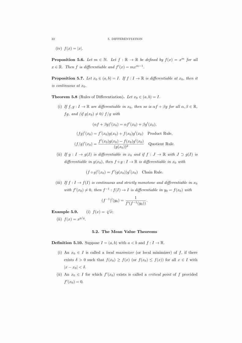
22 5. DIFFERENTIATION

(iv) f(x) = |x|.

Proposition 5.6. Let m ∈ N. Let f : R → R be defined by f(x) = xm for all

x ∈ R. Then f is differentiable and f ′(x) = mxm−1.

Proposition 5.7. Let x0 ∈ (a, b) = I. If f : I → R is differentiable at x0, then it

is continuous at x0.

Theorem 5.8 (Rules of Differentiation). Let x0 ∈ (a, b) = I.

(i) If f, g : I → R are differentiable in x0, then so is αf + βg for all α, β ∈ R,

fg, and (if g(x0) 6= 0) f/g with

(αf + βg)′(x0) = αf ′(x0) + βg′(x0),

(fg)′(x0) = f ′(x0)g(x0) + f(x0)g′(x0) Product Rule,

(f/g)′(x0) =f ′(x0)g(x0)− f(x0)g′(x0)

(g(x0))2Quotient Rule.

(ii) If g : I → g(I) is differentiable in x0 and if f : J → R with J ⊃ g(I) is

differentiable in g(x0), then f ◦ g : I → R is differentiable in x0 with

(f ◦ g)′(x0) = f ′(g(x0))g′(x0) Chain Rule.

(iii) If f : I → f(I) is continuous and strictly monotone and differentiable in x0

with f ′(x0) 6= 0, then f−1 : f(I)→ I is differentiable in y0 = f(x0) with

(f−1)′(y0) =1

f ′(f−1(y0)).

Example 5.9. (i) f(x) = n√x;

(ii) f(x) = xp/q.

5.2. The Mean Value Theorems

Definition 5.10. Suppose I = (a, b) with a 0 such that f(x0) ≥ f(x) (or f(x0) ≤ f(x)) for all x ∈ I with

|x− x0| < δ.

(ii) An x0 ∈ I for which f ′(x0) exists is called a critical point of f provided

f ′(x0) = 0.

5.3. APPLICATIONS OF THE MEAN VALUE THEOREMS 23

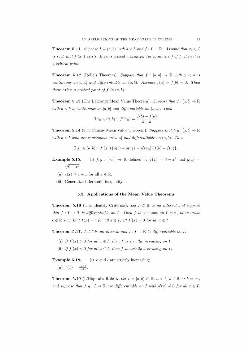
Theorem 5.11. Suppose I = (a, b) with a < b and f : I → R. Assume that x0 ∈ I

is such that f ′(x0) exists. If x0 is a local maximizer (or minimizer) of f , then it is

a critical point.

Theorem 5.12 (Rolle’s Theorem). Suppose that f : [a, b] → R with a < b is

continuous on [a, b] and differentiable on (a, b). Assume f(a) = f(b) = 0. Then

there exists a critical point of f in (a, b).

Theorem 5.13 (The Lagrange Mean Value Theorem). Suppose that f : [a, b]→ R

with a < b is continuous on [a, b] and differentiable on (a, b). Then

∃ x0 ∈ (a, b) : f ′(x0) =f(b)− f(a)

b− a.

Theorem 5.14 (The Cauchy Mean Value Theorem). Suppose that f, g : [a, b]→ R

with a < b both are continuous on [a, b] and differentiable on (a, b). Then

∃ x0 ∈ (a, b) : f ′(x0) {g(b)− g(a)} = g′(x0) {f(b)− f(a)} .

Example 5.15. (i) f, g : [0, 3] → R defined by f(x) = 3 − x2 and g(x) =√

9− x2;

(ii) e(x) ≥ 1 + x for all x ∈ R;

(iii) Generalized Bernoulli inequality.

5.3. Applications of the Mean Value Theorems

Theorem 5.16 (The Identity Criterion). Let I ⊂ R be an interval and suppose

that f : I → R is differentiable on I. Then f is constant on I (i.e., there exists

c ∈ R such that f(x) = c for all x ∈ I) iff f ′(x) = 0 for all x ∈ I.

Theorem 5.17. Let I be an interval and f : I → R be differentiable on I.

(i) If f ′(x) > 0 for all x ∈ I, then f is strictly increasing on I.

(ii) If f ′(x) < 0 for all x ∈ I, then f is strictly decreasing on I.

Example 5.18. (i) e and l are strictly increasing;

(ii) f(x) = ax+bcx+d .

Theorem 5.19 (L’Hopital’s Rules). Let I = [a, b) ⊂ R, a < b, b ∈ R or b = ∞,

and suppose that f, g : I → R are differentiable on I with g′(x) 6= 0 for all x ∈ I.


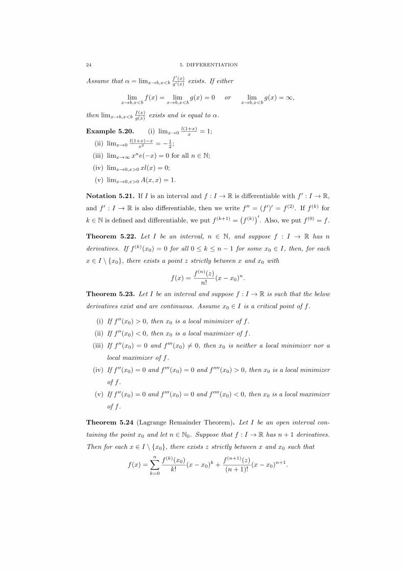
Assume that α = limx→b,x<bf ′(x)g′(x) exists. If either

limx→b,x<b

f(x) = limx→b,x<b

g(x) = 0 or limx→b,x0 xl(x) = 0;

(v) limx→0,x>0A(x, x) = 1.

Notation 5.21. If I is an interval and f : I → R is differentiable with f ′ : I → R,

and f ′ : I → R is also differentiable, then we write f ′′ = (f ′)′ = f (2). If f (k) for

k ∈ N is defined and differentiable, we put f (k+1) =(f (k)

)′. Also, we put f (0) = f .

Theorem 5.22. Let I be an interval, n ∈ N, and suppose f : I → R has n

derivatives. If f (k)(x0) = 0 for all 0 ≤ k ≤ n − 1 for some x0 ∈ I, then, for each

x ∈ I \ {x0}, there exists a point z strictly between x and x0 with

f(x) =f (n)(z)

n!(x− x0)n.

Theorem 5.23. Let I be an interval and suppose f : I → R is such that the below

derivatives exist and are continuous. Assume x0 ∈ I is a critical point of f .

(i) If f ′′(x0) > 0, then x0 is a local minimizer of f .

(ii) If f ′′(x0) < 0, then x0 is a local maximizer of f .

(iii) If f ′′(x0) = 0 and f ′′′(x0) 6= 0, then x0 is neither a local minimizer nor a

local maximizer of f .

(iv) If f ′′(x0) = 0 and f ′′′(x0) = 0 and f ′′′′(x0) > 0, then x0 is a local minimizer

of f .

(v) If f ′′(x0) = 0 and f ′′′(x0) = 0 and f ′′′′(x0) < 0, then x0 is a local maximizer

of f .

Theorem 5.24 (Lagrange Remainder Theorem). Let I be an open interval con-

taining the point x0 and let n ∈ N0. Suppose that f : I → R has n+ 1 derivatives.

Then for each x ∈ I \ {x0}, there exists z strictly between x and x0 such that

f(x) =

n∑k=0

f (k)(x0)

k!(x− x0)k +

f (n+1)(z)

(n+ 1)!(x− x0)n+1.

5.3. APPLICATIONS OF THE MEAN VALUE THEOREMS 25

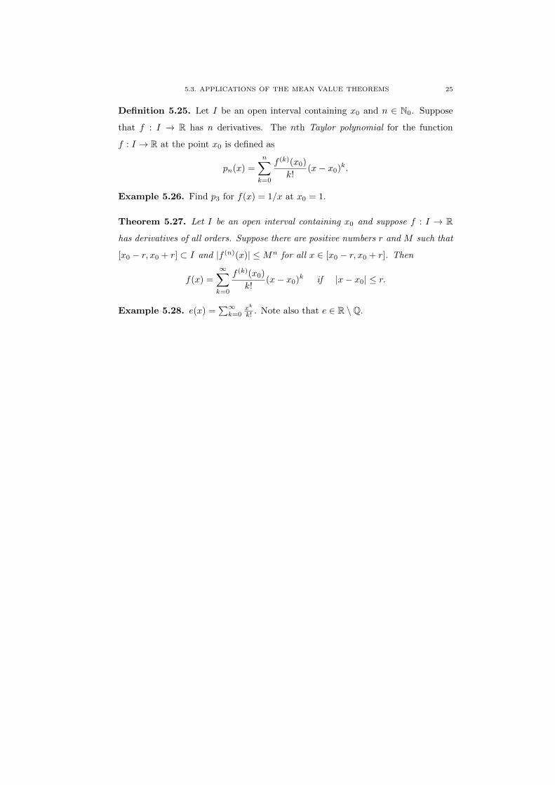
Definition 5.25. Let I be an open interval containing x0 and n ∈ N0. Suppose

that f : I → R has n derivatives. The nth Taylor polynomial for the function

f : I → R at the point x0 is defined as

pn(x) =

n∑k=0

f (k)(x0)

k!(x− x0)k.

Example 5.26. Find p3 for f(x) = 1/x at x0 = 1.

Theorem 5.27. Let I be an open interval containing x0 and suppose f : I → R

has derivatives of all orders. Suppose there are positive numbers r and M such that

[x0 − r, x0 + r] ⊂ I and |f (n)(x)| ≤Mn for all x ∈ [x0 − r, x0 + r]. Then

f(x) =

∞∑k=0

f (k)(x0)

k!(x− x0)k if |x− x0| ≤ r.

Example 5.28. e(x) =∑∞k=0

xk

k! . Note also that e ∈ R \Q.


CHAPTER 6

Integration

6.1. The Definition of the Integral

Definition 6.1. Let f : [a, b] → R with a < b be a function. If a = x0 < x1 <

x2 < · · · < xn = b, then Z = {x0, x1, · · · , xn} is called a partition of the interval

[a, b] with gap ‖Z‖ = max{xk − xk−1 : 1 ≤ k ≤ n}, and if ξk ∈ [xk−1, xk] for all

1 ≤ k ≤ n, then we call ξ = (ξ1, ξ2, · · · , ξn) intermediate points of the partition Z.

The sum

S(f,Z, ξ) =

n∑k=1

f(ξk)(xk − xk−1)

is called a Riemann sum. If ξ is such that f(ξk) = inf f([xk−1, xk]) for all 1 ≤ k ≤ n

(or f(ξk) = sup f([xk−1, xk]) for all 1 ≤ k ≤ n), then we call L(f,Z) = S(f,Z, ξ)

the lower Darboux sum (or U(f,Z) = S(f,Z, ξ) the upper Darboux sum).

Definition 6.2. A function f : [a, b] → R with a < b is said to be Riemann

integrable if limn→∞ S(f,Zn, ξn) exists for any sequence of partitions Zn with

limn→∞‖Zn‖ = 0 and with intermediate points ξn.

Remark 6.3. If f : [a, b] → R is Riemann integrable, then, no matter what

sequences Zn and ξn we take, the limit of S(f,Zn, ξn) as n → ∞ is always the

same. We then call this limit∫ baf(x)dx =

∫ baf .

Example 6.4. f(x) = x, I = [a, b].

Proposition 6.5. Let a < b and I = [a, b].

(i) If f, g : I → R are Riemann integrable, then so is αf + βg for all α, β ∈ R

with ∫ b

a

(αf + βg) = α

∫ b

a

f + β

∫ b

a

g.

(ii) If f(x) = c for all x ∈ I, then f is Riemann integrable with∫ baf = c(b− a).

27

28 6. INTEGRATION

(iii) If f, g : I → R are Riemann integrable and f(x) ≤ g(x) for all x ∈ I, then∫ baf ≤

∫ bag.

(iv) If f : I → R is Riemann integrable, then f is bounded on I and

inf f(I) ≤∫ baf

b− a≤ sup f(I).

(v) If f : I → R is Riemann integrable and if g(x) = f(x) for all x ∈ I but a

finite number of points x ∈ I, then g is Riemann integrable and∫ baf =

∫ bag.

(vi) If c ∈ (a, b) and f : I → R and f : [a, c] → R, f : [c, b] → R are Riemann

integrable, then ∫ b

a

f =

∫ c

a

f +

∫ b

c

f.

Theorem 6.6. If f : [a, b] → R with a b, then we put∫ baf = −

∫ abf . We also put

∫ aaf = 0.

6.2. The Fundamental Theorem of Calculus

Theorem 6.8 (Fundamental Theorem of Calculus, First Part). Suppose F :

[a, b] → R is differentiable on [a, b] and F ′ : [a, b] → R is Riemann integrable

on [a, b]. Then ∫ b

a

F ′ = F (b)− F (a).

Definition 6.9. A function F : I → R is called an antiderivative of f : I → R if F

is differentiable with F ′(x) = f(x) for all x ∈ I.

Remark 6.10. If f possesses an antiderivative F , then any other antiderivative of

f can differ from F only by a constant.

Example 6.11. (i)∫ 5

0x3dx = 54

4 ;

(ii)∫ 4

0e = e(4)− 1;

(iii)∫ p0s = 1;

(iv) 1n6

∑nk=1 k

5 → 16 as n→∞.

Theorem 6.12 (Fundamental Theorem of Calculus, Second Part). Let f : I → R

be continuous on the interval I ⊂ R and let a ∈ I. Then

F (x) :=

∫ x

a

f for each x ∈ I

6.4. IMPROPER INTEGRALS 29

is an antiderivative of f .

Remark 6.13. Continuous functions possess antiderivatives.

Proposition 6.14. If f is Riemann integrable on I, then F defined in the FTOC

(Part II) is continuous (even Lipschitz continuous) on I.

Example 6.15. (i)∫ x1

dtt ;

(ii)∫ x0

dt1+t2 .

6.3. Applications

Theorem 6.16. Suppose f, g : I → R are continuous, x0 ∈ I, y0 ∈ R. Then

there exists exactly one continuously differentiable function y with y(x0) = y0 and

y′(x) = f(x)y(x) + g(x) for all x ∈ I, namely

y(x) = e(F (x))

{y0 +

∫ x

x0

g(t)e(−F (t))dt

}with F (x) =

∫ x

x0

f(t)dt.

Example 6.17. xy′ + 2y = 4x2, y(1) = 2.

Theorem 6.18 (Integration by Parts). Let f, g : [a, b]→ R be continuously differ-

entiable. Then∫ b

a

f(x)g′(x)dx = f(b)g(b)− f(a)g(a)−∫ b

a

f ′(x)g(x)dx.

Example 6.19.∫ 1

0te(t)dt = 1.

Theorem 6.20 (Substitution). If g : [α, β] → R is continuously differentiable,

f : g([α, β])→ R continuous, then∫ b

a

f(g(t))g′(t)dt =

∫ g(b)

g(a)

f(x)dx.

Example 6.21.∫ 2

0e(√x)dx = 2(

√2− 1)e(

√2) + 2.

6.4. Improper Integrals

Definition 6.22. Let a < b and f : (a, b)→ R.

(i) f is said to be locally integrable on (a, b) if f is integrable on each closed

subinterval [c, d] ⊂ (a, b).

30 6. INTEGRATION

(ii) f is said to be improperly integrable on (a, b) if f is locally integrable on

(a, b) and if ∫ b

a

f(x)dx := limc→a+,d→b−

∫ d

c

f(x)dx

exists and is finite. This limit is called the improper Riemann integral of f

over (a, b).

Example 6.23. (i)∫ 1

01√x

dx = 2;

(ii)∫∞1

1x2 dx = 1.

Theorem 6.24. If f, g are improperly integrable on (a, b) and α, β ∈ R, then

αf + βg is improperly integrable on (a, b), and∫ b

a

(αf + βg)(x)dx = α

∫ b

a

f(x)dx+ β

∫ b

a

g(x)dx.

Theorem 6.25 (Comparison Theorem). Suppose f, g : (a, b) → R are locally in-

tegrable. If 0 ≤ f(x) ≤ g(x) for all x ∈ (a, b), and if g is improperly integrable on

(a, b), then f is improperly integrable on (a, b) with∫ b

a

f(x)dx ≤∫ b

a

g(x)dx.

Example 6.26. (i) |s(x)/√x3| is improperly integrable on (0, 1];

(ii) |l(x)/√x5| is improperly integrable on [1,∞).

Definition 6.27. Let a < b and f : (a, b)→ R.

(i) f is said to be absolutely integrable on (a, b) if |f | is improperly integrable

on (a, b).

(ii) f is said to be conditionally integrable on (a, b) if f is improperly integrable

but not absolutely integrable on (a, b).

Theorem 6.28. If f is locally and absolutely integrable on (a, b), then f is im-

properly integrable on (a, b), and∣∣∣∣∣∫ b

a

f(x)dx

∣∣∣∣∣ ≤∫ b

a

|f(x)|dx.

Example 6.29. s(x)/x is conditionally integrable on [1,∞).

CHAPTER 7

Infinite Series of Functions

7.1. Uniform Convergence

Example 7.1. (i) limx→x0limn→∞(1 + x/n)n = limn→∞ limx→x0

(1 + x/n)n;

(ii) ddx limn→∞(1 + x/n)n = limn→∞

ddx (1 + x/n)n;

(iii)∫ 1

0limn→∞(1 + x/n)ndx = limn→∞

∫ 1

0(1 + x/n)ndx;

(iv) fn(x) = nx/(1 + nx), n→∞, x→ 0;

(v) fn(x) = xn;

(vi) fn(x) = s(nx)n .

Definition 7.2. Let fn : I → R be functions for each n ∈ N and let f : I → R.

We say that the sequence fn converges

(i) pointwise to f if limn→∞ fn(x) = f(x) for all x ∈ I;

(ii) uniformly to f if

∀ε > 0 ∃N ∈ N : (∀n ≥ N ∀x ∈ I) |fn(x)− f(x)| < ε.

The pointwise or uniform convergence of the series∑∞k=0 gk is defined as above

with fn =∑nk=0 gk.

Example 7.3. Let fn(x) = xn on [0, 1].

(i) fn converges uniformly on [0, 1/2];

(ii) fn does not converge uniformly on [0, 1].

Example 7.4. fn(x) = 2n2x/(1 + n4x4) is not uniformly convergent on R.

Theorem 7.5 (Cauchy Criterion). A sequence of functions fn : I → R converges

uniformly on I iff

∀ε > 0 ∃N ∈ N : (∀m,n ≥ N ∀x ∈ I) |fn(x)− fm(x)| < ε.

31

32 7. INFINITE SERIES OF FUNCTIONS

Theorem 7.6 (Weierstraß M -Test). Suppose gk : I → R satisfies |gk(x)| ≤Mk for

all x ∈ I and for all k ∈ N such that∑∞k=1Mk is convergent. Then

∑∞k=1 gk(x) is

uniformly convergent.

Example 7.7.∑∞k=1

c(k2√x)

k3 is uniformly convergent on R.

7.2. Interchanging of Limit Processes

Theorem 7.8 (Continuity of the Limit Function). Let fn : I → R be continuous

on I for all n ∈ N and suppose that fn → f uniformly on I. Then f is continuous

on I, i.e.,

limx→x0

limn→∞

fn(x) = limn→∞

limx→x0

fn(x) for all x0 ∈ I.

Example 7.9. f(x) =∑∞k=1

s(kx)k2 is continuous on R.

Theorem 7.10 (Integration of the Limit Function). Let fn : I = [a, b] → R be

Riemann integrable on I for all n ∈ N and suppose that fn → f uniformly on I.

Then f is Riemann integrable on I with(∫ b

a

limn→∞

fn(x)dx =

)∫ b

a

f(x)dx = limn→∞

∫ b

a

fn(x)dx.

Corollary 7.11.∑∞k=1

∫ bafk(x)dx =

∫ ba

∑∞k=1 fk(x)dx if fk : [a, b] → R are Rie-

mann integrable for all k ∈ N and∑∞k=1 fk(x) is uniformly convergent on [a, b].

Theorem 7.12 (Differentiation of the Limit Function). Let fn : I = [a, b]→ R be

differentiable on I for all n ∈ N and suppose that f ′n → g uniformly on I. Also

suppose that limn→∞ fn(x0) exists for at least one x0 ∈ I. Then fn converges

uniformly on I, say to f , and f is differentiable on I with

f ′(x) = g(x), i.e., limn→∞

d

dxfn(x) =

d

dxlimn→∞

fn(x).

Corollary 7.13. ddx

∑∞k=1 fk(x) =

∑∞k=1

ddxfk(x) if fk : [a, b] → R are differen-

tiable for all k ∈ N,∑∞k=1 f

′k(x) is uniformly convergent on [a, b], and

∑∞k=1 fk(x0)

is convergent for at least one x0 ∈ [a, b].

Example 7.14. (i)∑∞k=0 ak(x− x0)k;

(ii)∑∞k=1

s(kx)k3 ;

(iii) fn(x) = s(n2x)n .

Documents

Advanced Calculus I (Math 4209) - web.mst.eduweb.mst.edu/~bohner/math4209-18/4209-notes.pdf · Spring 2018 Lecture Notes Martin Bohner Version from February 20, 2018 Author address: