Advanced Algorithms for Mobile Robot Motion Planning and

SERBIAN JOURNAL OF ELECTRICAL ENGINEERING Vol. 9, No. 1, February 2012, 9-28

9

Advanced Algorithms for Mobile Robot Motion Planning and Tracking in Structured Static

Environments Using Particle Swarm Optimization*

Aleksandar Ćosić1, Marko Šušić1, Duško Katić1

Abstract: An approach to intelligent robot motion planning and tracking in known and static environments is presented in this paper. This complex problem is divided into several simpler problems. The first is generation of a collision-free path from starting to destination point, which is solved using a particle swarm optimization (PSO) algorithm. The second is interpolation of the obtained collision-free path, which is solved using a radial basis function neural network (RBFNN), and trajectory generation, based on the interpolated path. The last is a trajectory tracking problem, which is solved using a proportional-integral (PI) controller. Due to uncertainties, obstacle avoidance is still not ensured, so an additional fuzzy controller is introduced, which corrects the control action of the PI controller. The proposed solution can be used even in dynamic environments, where obstacles change their position in time. Simulation studies were realized to validate and illustrate this approach.

Keywords: Mobile robots, Motion planning, Particle swarm optimization, Radial basis function neural networks.

1 Introduction Efficient navigation of mobile robot means generation of collision free path

and design of control law, which provides desired path following. Significant efforts have been made in order to solve robot motion planning (RMP) problems. Such a complex problem can be divided into several simpler problems. The first is generation of collision free path in space with obstacles. It is assumed that all obstacles are static and that their positions are known. Solution of the problem is given with NP–hard algorithm, given in [1]. There are two different approaches for mobile robot motion planning: classic and heuristic [2 – 4]. The current developed classic methods are variations of a few general approaches: Roadmap, Cell decomposition, Potential fields, and Mathematical programming. The mentioned classic approaches suffer from 1Mihajlo Pupin Institute, University of Belgrade, Volgina 15, 11000 Belgrade, Serbia; E-mails: [email protected], [email protected], [email protected]

*Award for the best paper presented in Section Robotics, at Conference ETRAN 2011, June 6 – 9, Banja Vrućica – Teslić, Bosnia and Herzegovina.

UDK: 007.52:004.032.26 DOI: 10.2298/SJEE1201009C

A. Ćosić, M. Šušić, D. Katić

10

many drawbacks, such as high time complexity in high dimensions and trapping in local minima, which makes them inefficient in practice. In order to improve the efficiency of classic methods, many heuristic and meta-heuristic algorithms are used in RMP [4]: Simulated Annealing (SA), Artificial Neural Networks (ANN), Genetic Algorithms (GA), Particle Swarm Optimization (PSO), Ant Colony (ACO), Stigmergy, Wavelet Theory, Fuzzy Logic (FL) and Tabu Search (TS). Heuristic algorithms do not guarantee to find a solution, but if they do, are likely to do so much faster than deterministic methods.

In this paper, PSO algorithm for mobile robot path generation is chosen [5 – 8]. PSO represents multi-agent search technique [9], which is based on simplified social behavior of large animal groups. It has been proven that in many cases PSO algorithm provides fast and efficient solution of optimization problems.

The second problem is path following. This problem can be solved using fuzzy controller, which is a good solution when it is difficult to obtain valid mathematical model. From the other hand, parameter adjustment is very time-consuming task, so the evolution techniques could be helpful for adjustment of large number of parameters [10 – 12]. This problem could also be solved using nonlinear backstepping procedure, given in [13 – 14]. In this paper, problem is decomposed on trajectory generation and trajectory tracking. Collision free path generated by PSO is not smooth and it is represented as an array of points in two-dimensional space. In order to make it smooth it has to be interpolated using RBFNN. The next step is trajectory generation, based on interpolated path, such that the velocity of the mobile robot is large on straight segments of the path, and small in sharp curves. Simple PI controller is proposed as a tracking controller. In order to prevent collisions with obstacles due to uncertainties and movement of obstacles, additional fuzzy controller is introduced, which corrects action of tracking controller. For demonstration of algorithm performance, kinematic model of mobile robot is used.

The rest of the paper is organized as follows: Section II provides short description of PSO algorithm and RBFNN, while Section III provides algorithms for generating collision free path using PSO, path interpolation using RBFNN, and trajectory generation. In Section IV, control algorithms for trajectory tracking and obstacle avoidance are shown. In Section V simulation results are presented, while conclusion is given in Section VI.

2 Basic Theoretical Concepts 2.1 Particle swarm optimization

PSO algorithm is multi-agent evolutionary search technique. The space of solution is searched with multiple particles, whereby every particle is directed on the basis of its own experience and the experience of the whole swarm. Basic

Advanced Algorithms for Mobile Robot Motion Planning and Tracking…

11

variables are position of particle, which represents the potential solution, velocity of the particle, which represents the change of position in current iteration and fitness function, which is the measure of success of the particle.

Let ( )ix k and ( )iv k denote the position and velocity of i-th particle in k-th iteration, respectively. Algorithm can be described by following steps:

1. Problem definition: Allowable position and velocity ranges [ ]min max,V V and [ ]min max,X X , respectively, swarm size N, measure of success for every particle – fitness function ( )iP k ; value of this function measures the success of the i-th particle;

2. Algorithm initialization: Positions and velocities of particles are initialized with uniform random numbers from [ ]min max,X X and [ ]min max,V V , respectively, i.e.,

( ) ( )( ) ( )

min 1 max min

min 2 max min

0

0 χi

i

x X X X

v V V V

= + χ −

= + − (1)

where 1χ and 2χ are uniform random numbers from [0,1]; 3. Fitness function evaluation:

For every particle in swarm, the following variables are evaluated: fitness function, self-best position ( )ip k and global-best position

( )gp k ; 4. Velocity correction:

( ) ( ) ( ) ( ) ( ) ( )1 1 2 2

effect of current effect of particle's effect of swarm'smotion experince experience

1 γi i i i g iv k wv k c p k x k c p k x k⎡ ⎤+ = + ⎡ − ⎤ + γ −⎣ ⎦ ⎣ ⎦ , (2)

where 1c and 2c denote self-confidence and swarm-confidence parameters, respectively, while w stands for inertia factor and 1γ , 2γ are random numbers from [0,1]. Inertia factor determines the effect of current motion on a future motion. Large values of this parameter leads to global search, while small values leads to fine, local search, which is suitable when algorithm converges. Thus, variable value of inertia is used, such that inertia starts from large value, and decreases as algorithm iterates. Also self-confidence and swarm-confidence factors should be variable. Self-experience should have dominant effect on particle motion at the beginning of the algorithm, while later, swarm-experience should prevail. Particles velocities must stay inside allowable interval [ ]min max,V V ;


12

5. Position correction: ( ) ( ) ( )1 1i i ix k x k v k+ = + + . (3)

Position must stay inside allowable interval [ ]min max,X X ; 6. Termination of algorithm:

Algorithm terminates when maximum number of iterations is reached, or good enough value of fitness function.

Performance of algorithm heavily depends on particles diversity. It is preferred that swarm consists of diverse particles at the beginning of algorithm. Later, as algorithm iterate, diversity should decrease, in order to finely converge to optimum. It is necessary to allow passing through detected optimum, in order to avoid stucking in it, because it can be local minima.

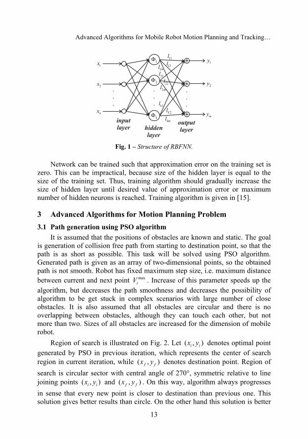
2.2 Radial basis function neural networks Radial basis function neural networks (RBFNN) are three-layer neural

networks. Their structure is shown on Fig. 1. These networks are widely used for nonlinear function approximation, as well as multilayer perceptrons (MLPs). Although they cannot achieve the accuracy of the MLP networks, their advantage over MLP is in much faster training. For achieving the same accuracy as MLP, RBFNN is usually more complex, i.e., it has more nodes in the hidden layer.

Let [ ]1T

nx x=x and [ ]1T

my y=y denote input and output vectors, respectively. Activation function of hidden neurons is:

( )2

22e , 1,..,i

i x i n−

−σΦ = =

x w

, (4)

where || ||⋅ denotes Euclidean norm. Activation function ( )i xΦ is centred in vector iw , while σ denotes spread of the function. Output layer is linear, so output of the network is linear combination of the hidden layer outputs:

1

( ), 1,..,k

j ij ii

y l x j m=

= Φ =∑ . (5)

It can be seen from (4) that activation of hidden layer neuron i is the strongest when i=x w , because ( ) 1i xΦ = . Activation decreases when input departs from vector iw . Basic idea is to divide input space onto k overlapping regions, while every hidden neuron will be active only in one region, i.e. some neighbourhood of iw . If region width σ is too small, network generalizes poorly, while for large values of this parameter, interpolation can be coarse.


13

Fig. 1 – Structure of RBFNN.

Network can be trained such that approximation error on the training set is

zero. This can be impractical, because size of the hidden layer is equal to the size of the training set. Thus, training algorithm should gradually increase the size of hidden layer until desired value of approximation error or maximum number of hidden neurons is reached. Training algorithm is given in [15].

3 Advanced Algorithms for Motion Planning Problem 3.1 Path generation using PSO algorithm

It is assumed that the positions of obstacles are known and static. The goal is generation of collision free path from starting to destination point, so that the path is as short as possible. This task will be solved using PSO algorithm. Generated path is given as an array of two-dimensional points, so the obtained path is not smooth. Robot has fixed maximum step size, i.e. maximum distance between current and next point max

rV . Increase of this parameter speeds up the algorithm, but decreases the path smoothness and decreases the possibility of algorithm to be get stuck in complex scenarios with large number of close obstacles. It is also assumed that all obstacles are circular and there is no overlapping between obstacles, although they can touch each other, but not more than two. Sizes of all obstacles are increased for the dimension of mobile robot.

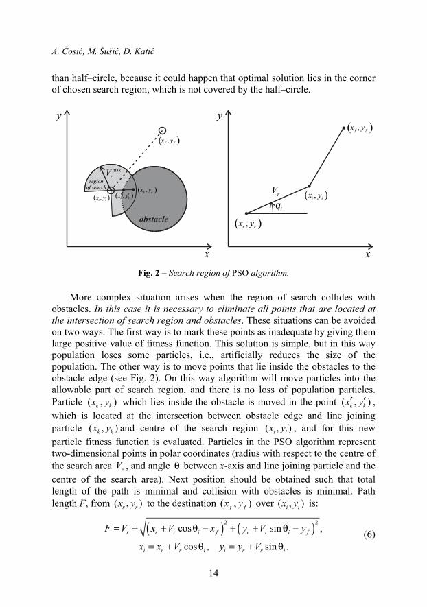
Region of search is illustrated on Fig. 2. Let ( , )i ix y denotes optimal point generated by PSO in previous iteration, which represents the center of search region in current iteration, while ( , )f fx y denotes destination point. Region of search is circular sector with central angle of 270°, symmetric relative to line joining points ( , )i ix y and ( , )f fx y . On this way, algorithm always progresses in sense that every new point is closer to destination than previous one. This solution gives better results than circle. On the other hand this solution is better


14

than half–circle, because it could happen that optimal solution lies in the corner of chosen search region, which is not covered by the half–circle.

Fig. 2 – Search region of PSO algorithm.

More complex situation arises when the region of search collides with

obstacles. In this case it is necessary to eliminate all points that are located at the intersection of search region and obstacles. These situations can be avoided on two ways. The first way is to mark these points as inadequate by giving them large positive value of fitness function. This solution is simple, but in this way population loses some particles, i.e., artificially reduces the size of the population. The other way is to move points that lie inside the obstacles to the obstacle edge (see Fig. 2). On this way algorithm will move particles into the allowable part of search region, and there is no loss of population particles. Particle ( , )k kx y which lies inside the obstacle is moved in the point ( , )k kx y′ ′ , which is located at the intersection between obstacle edge and line joining particle ( , )k kx y and centre of the search region ( , )i ix y , and for this new particle fitness function is evaluated. Particles in the PSO algorithm represent two-dimensional points in polar coordinates (radius with respect to the centre of the search area rV , and angle θ between x-axis and line joining particle and the centre of the search area). Next position should be obtained such that total length of the path is minimal and collision with obstacles is minimal. Path length F, from ( , )r rx y to the destination ( , )f fx y over ( , )i ix y is:

( ) ( )2 2cos sin ,

cos , sin .r r r i f r r i f

i r r i i r r i

F V x V x y V y

x x V y y V

= + + θ − + + θ −

= + θ = + θ (6)


15

Fitness function is weighted sum of path length F, given in (6) and additional term ( )P i , which represents penalties if path leads over the obstacles. This term has to be variable, taking into account size, position and orientation of the obstacles. Finally, fitness function ifit is given by:

( ) ( )

1 2 2 1 3 2

2 2

( ), ( ) ( ) ( ),

cos sin .

i i

i r r r i f r r i f

fit w F w P i P i w P i w P i

F V x V x y V y

= + = +

= + + θ − + + θ − (7)

Penalization factor ( )P i consists of two factors 1( )P i , which represents penalization due to the existence of intersection between obstacle and path generated from current particle to the destination point, and 2 ( )P i , which represents penalization due to the existence of intersection between obstacle and path generated from particle given in the previous algorithm iteration to the current particle.

Weights 1 2 3, ,w w w weight path length and path intersection with obstacles, respectively. Larger values of the 1w will give a shorter path, which leads mobile robot very close to the obstacles, while larger values of 2w and 3w means less chance for collision between mobile robot and obstacles at the expense of longer path. It is recommended to choose larger values of 2w and

3w in cases when algorithm works with larger values of the radius maxrV , in

order to ensure that generated path does not lead over the obstacles.

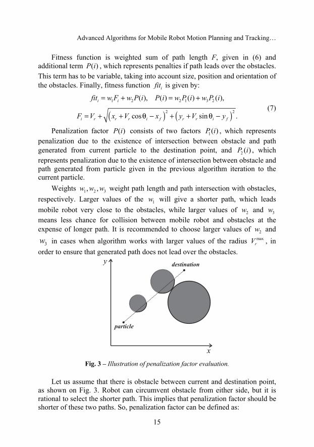
Fig. 3 – Illustration of penalization factor evaluation.

Let us assume that there is obstacle between current and destination point,

as shown on Fig. 3. Robot can circumvent obstacle from either side, but it is rational to select the shorter path. This implies that penalization factor should be shorter of these two paths. So, penalization factor can be defined as:


16

( ) ( ) { } { }1

min , 1,2 , 1,2S

k js

P i arc obim s j k=

⎧ ⎫= + ∈ ∈⎨ ⎬⎩ ⎭

∑ , (8)

where jarc denotes arc of the obstacle intersected by path, and ( )c s denotes circumference of adjacent obstacle. Algorithm has stochastic nature, so it will not give the same result if it proceeds from starting to destination point and in reverse direction. So algorithm must proceed in both directions, and choose shorter path.

3.2 Path interpolation using RBFNN Path smoothing is achieved by interpolation using RBFNN. For this

purpose, some other types of neural networks can be used (such as MLP networks), but in this case RBFNN gives very good results, accurate approximation and fast training. Neural networks are used for function approximation. This means that in general case they cannot be used here directly, because obtained path may not be a function. So, the idea is to parameterize x and y coordinate of the path, i.e., to associate time instant to every point of the path.

Path interpolation is performed using RBFNN with one input (time) and two outputs (x and y coordinate of path point). The first step is generation of training set. This means that time instant must be associated to every point of the path. The simplest way to generate time vector is to adopt uniform velocity of motion v along the path. Now, time vector can be evaluated recursively using (9), where iP and 1iP− denote two successive points of the path.

( ) ( )11 1 1 1, , , ,i i

i i i i i i i i

P Pt t P x y P x y

v−

− − − −

−= + = = . (9)

Region centers iw and output layer weights ijl in (4) and (5) are determined in training process, but region width σ and hidden layer size must be adjusted experimentally. Choice of these two parameters is critical. Simple networks cannot approximate path adequately, while too complex networks can learn features that do not exist in training set. It is important to note that after training it could happen that path generated by RBFNN is not collision free. So the accuracy of the approximation is not the only criteria that influences choice of the hidden layer size and σ, collision free property is a more important one.

3.3 Trajectory generation based on interpolated path Trajectory generation based on given path means introduction of time, i.e.

trajectory represents time-parameterized path. Trajectory obtained in the interpolation step assumed uniform motion along path, which is not a good solution. So, the goal is achievement of variable velocity of motion, such that


17

robot moves fast on straight segments of the path and slowly in curves, i.e. robot velocity should be inversely proportional to some measure of path curvature. At the beginning, robot should accelerate uniformly, until it reaches the desired velocity and slow down uniformly, at the end of the motion.

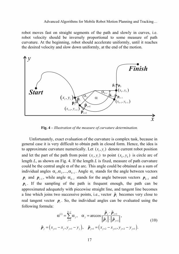
Fig. 4 – Illustration of the measure of curvature determination.

Unfortunately, exact evaluation of the curvature is complex task, because in general case it is very difficult to obtain path in closed form. Hence, the idea is to approximate curvature numerically. Let ( , )i ix y denote current robot position and let the part of the path from point ( , )i ix y to point ( , )k kx y is circle arc of length L, as shown on Fig. 4. If the length L is fixed, measure of path curvature could be the central angle α of the arc. This angle could be obtained as a sum of individual angles 1 2, ,..., k i−α α α . Angle 1α stands for the angle between vectors

ip and 1i−p , while angle k i−α stands for the angle between vectors 1k −p and

kp . If the sampling of the path is frequent enough, the path can be approximated adequately with piecewise straight line, and tangent line becomes a line which joins two successive points, i.e., vector ip becomes very close to real tangent vector ip . So, the individual angles can be evaluated using the following formula:

( )

( ) ( )

1

1 1

1 1 1 2 1 2 1

, arccos ,

, , , .

k ij ji

j jj j j

j j j j j j j j j jx x y y x x y y

−+

= +

+ + + + + + +

⋅α = α α =

⋅

= − − = − −

∑p pp p

p p (10)


18

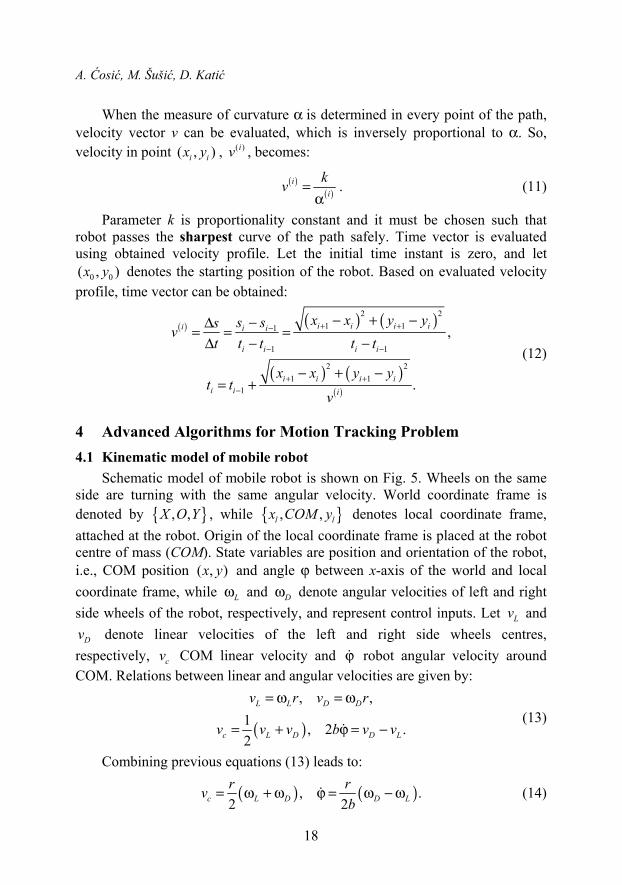
When the measure of curvature α is determined in every point of the path, velocity vector v can be evaluated, which is inversely proportional to α. So, velocity in point ( , )i ix y , ( )iv , becomes:

( )( )

ii

kv =α

. (11)

Parameter k is proportionality constant and it must be chosen such that robot passes the sharpest curve of the path safely. Time vector is evaluated using obtained velocity profile. Let the initial time instant is zero, and let

0 0( , )x y denotes the starting position of the robot. Based on evaluated velocity profile, time vector can be obtained:

( ) ( ) ( )

( ) ( )( )

2 21 11

1 1

2 21 1

1

,

.

i i i ii i i

i i i i

i i i ii i i

x x y ys ssvt t t t t

x x y yt t

v

+ +−

− −

+ +−

− + −−Δ= = =Δ − −

− + −= +

(12)

4 Advanced Algorithms for Motion Tracking Problem 4.1 Kinematic model of mobile robot

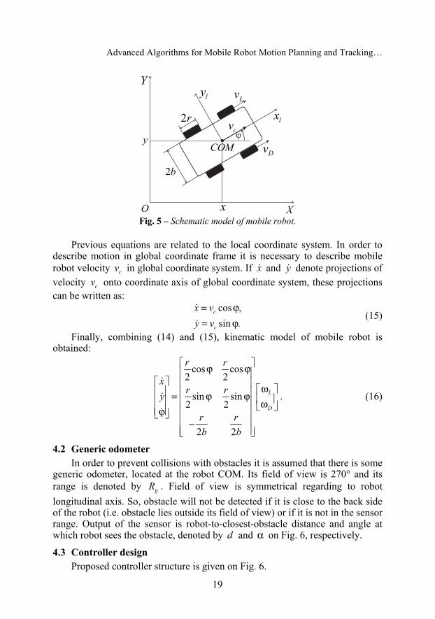
Schematic model of mobile robot is shown on Fig. 5. Wheels on the same side are turning with the same angular velocity. World coordinate frame is denoted by { }, ,X O Y , while { }, ,l lx COM y denotes local coordinate frame, attached at the robot. Origin of the local coordinate frame is placed at the robot centre of mass (COM). State variables are position and orientation of the robot, i.e., COM position ( , )x y and angle ϕ between x-axis of the world and local coordinate frame, while Lω and Dω denote angular velocities of left and right side wheels of the robot, respectively, and represent control inputs. Let Lv and

Dv denote linear velocities of the left and right side wheels centres, respectively, cv COM linear velocity and ϕ robot angular velocity around COM. Relations between linear and angular velocities are given by:

( )

, ,1 , 2 .2

L L D D

c L D D L

v r v r

v v v b v v

= ω = ω

= + ϕ = − (13)

Combining previous equations (13) leads to:

( ) ( ), .2 2c L D D Lr rv

b= ω + ω ϕ = ω − ω (14)


19

Fig. 5 – Schematic model of mobile robot.

Previous equations are related to the local coordinate system. In order to

describe motion in global coordinate frame it is necessary to describe mobile robot velocity cv in global coordinate system. If x and y denote projections of velocity cv onto coordinate axis of global coordinate system, these projections can be written as:

cos ,sin .

c

c

x vy v

= ϕ= ϕ

(15)

Finally, combining (14) and (15), kinematic model of mobile robot is obtained:

cos cos2 2

sin sin2 2

2 2

L

D

r r

xr ry

r rb b

⎡ ⎤ϕ ϕ⎢ ⎥⎡ ⎤ ⎢ ⎥ ω⎡ ⎤⎢ ⎥ ⎢ ⎥= ϕ ϕ ⎢ ⎥⎢ ⎥ ⎢ ⎥ ω⎣ ⎦⎢ ⎥ϕ ⎢ ⎥⎣ ⎦

⎢ ⎥−⎢ ⎥⎣ ⎦

. (16)

4.2 Generic odometer In order to prevent collisions with obstacles it is assumed that there is some

generic odometer, located at the robot COM. Its field of view is 270° and its range is denoted by gR . Field of view is symmetrical regarding to robot longitudinal axis. So, obstacle will not be detected if it is close to the back side of the robot (i.e. obstacle lies outside its field of view) or if it is not in the sensor range. Output of the sensor is robot-to-closest-obstacle distance and angle at which robot sees the obstacle, denoted by d and α on Fig. 6, respectively.

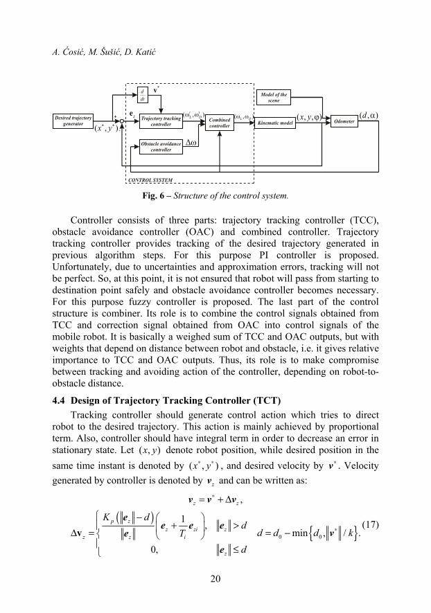
4.3 Controller design Proposed controller structure is given on Fig. 6.


20

Fig. 6 – Structure of the control system.

Controller consists of three parts: trajectory tracking controller (TCC),

obstacle avoidance controller (OAC) and combined controller. Trajectory tracking controller provides tracking of the desired trajectory generated in previous algorithm steps. For this purpose PI controller is proposed. Unfortunately, due to uncertainties and approximation errors, tracking will not be perfect. So, at this point, it is not ensured that robot will pass from starting to destination point safely and obstacle avoidance controller becomes necessary. For this purpose fuzzy controller is proposed. The last part of the control structure is combiner. Its role is to combine the control signals obtained from TCC and correction signal obtained from OAC into control signals of the mobile robot. It is basically a weighed sum of TCC and OAC outputs, but with weights that depend on distance between robot and obstacle, i.e. it gives relative importance to TCC and OAC outputs. Thus, its role is to make compromise between tracking and avoiding action of the controller, depending on robot-to-obstacle distance.

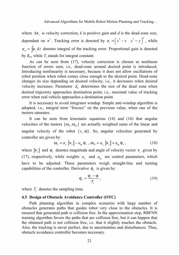
4.4 Design of Trajectory Tracking Controller (TCT) Tracking controller should generate control action which tries to direct

robot to the desired trajectory. This action is mainly achieved by proportional term. Also, controller should have integral term in order to decrease an error in stationary state. Let ( , )x y denote robot position, while desired position in the same time instant is denoted by ( , )x y∗ ∗ , and desired velocity by ∗v . Velocity generated by controller is denoted by zv and can be written as:

( ){ }0 0

,

1 ,min , / .

0,

z z

p zz zi z

z z i

z

K dd

d d d kTd

∗

∗

= + Δ

⎧ − ⎛ ⎞+ >⎪ ⎜ ⎟Δ = = −⎨ ⎝ ⎠

⎪ ≤⎩

v v v

ee e e

vee

v(17)


21

where zΔv is velocity correction, k is positive gain and d is the dead-zone size,

dependant on *v . Tracking error is denoted by * * T

z x x y y⎡ ⎤= − −⎣ ⎦e , while

dzi z t= ∫e e denotes integral of the tracking error. Proportional gain is denoted

by Kp, while Ti stands for integral constant. As can be seen from (17), velocity correction is chosen as nonlinear

function of errors sum, i.e., dead-zone around desired point is introduced. Introducing nonlinearity is necessary, because it does not allow oscillations of robot position when robot comes close enough to the desired point. Dead-zone changes its size depending on desired velocity, i.e., it decreases when desired velocity increases. Parameter 0d determines the size of the dead zone when desired trajectory approaches destination point, i.e., maximal value of tracking error when real vehicle approaches a destination point.

It is necessary to avoid integrator windup. Simple anti-windup algorithm is adopted, i.e., integral term “freezes” on the previous value, when one of the motors saturates.

It can be seen from kinematic equations (14) and (16) that angular velocities of the motors ( ),L Dω ω are actually weighted sums of the linear and angular velocity of the robot ( ),cv ϕ . So, angular velocities generated by controller are given by: ,

z z z zL v z z D v z za a a aϕ ϕω = − ϕ ω = + ϕv v , (18)

where zv and zϕ denotes magnitude and angle of velocity vector zv given by (17), respectively, while weights

zva and z

aϕ are control parameters, which have to be adjusted. These parameters weigh straight-line and turning capabilities of the controller. Derivative zϕ is given by:

zz

sTϕ − ϕϕ = , (19)

where sT denotes the sampling time.

4.5 Design of Obstacle Avoidance Controller (OTC) Path planning algorithm in complex scenarios with large number of

obstacles generates paths that guides robot very close to the obstacles. It is ensured that generated path is collision free. In the approximation step, RBFNN training algorithm favors the paths that are collision free, but it can happen that the obtained path is not collision free, i.e. that it slightly touches the obstacle. Also, the tracking is never perfect, due to uncertainties and disturbances. Thus, obstacle avoidance controller becomes necessary.


22

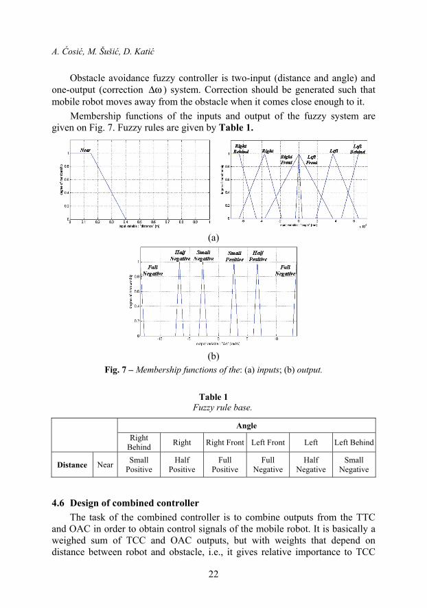
Obstacle avoidance fuzzy controller is two-input (distance and angle) and one-output (correction Δω ) system. Correction should be generated such that mobile robot moves away from the obstacle when it comes close enough to it.

Membership functions of the inputs and output of the fuzzy system are given on Fig. 7. Fuzzy rules are given by Table 1.

(a)

(b)

Fig. 7 – Membership functions of the: (a) inputs; (b) output.

Table 1 Fuzzy rule base.

Angle Right

Behind Right Right Front Left Front Left Left Behind

Distance Near Small Positive

Half Positive

Full Positive

Full Negative

Half Negative

Small Negative

4.6 Design of combined controller The task of the combined controller is to combine outputs from the TTC

and OAC in order to obtain control signals of the mobile robot. It is basically a weighed sum of TCC and OAC outputs, but with weights that depend on distance between robot and obstacle, i.e., it gives relative importance to TCC


23

and OAC outputs. When robot comes close to the obstacle, OAC output becomes dominant. When the robot is far away from the obstacle TCC output is dominant. Following the notes introduced on Fig. 6, the output signal of the combined controller, can be written as a weighted sum of its inputs: 1 2 1 2,t t

L L D DK K K Kω = ω − Δω ω = ω + Δω , (20)

where 1K and 2K denote the weights of the sum, tLω and t

Dω are the outputs of the tracking controller and Δω is the output of the obstacle avoidance controller. Weights must be dependable on distance between robot and obstacle, in order to change relative importance of “tracking” and “avoiding” control signal. When the robot approaches the obstacle, “avoiding” signal should be dominant. If there is no obstacles in the close neighborhood of the robot, “tracking” signal should be dominant.

5 Simulation Results Proposed algorithm for motion planning of mobile robot is implemented in

MATLAB package, using Virtual WRSN software for mobile robot navigation, given in [16] and [17].

The scenario with seven obstacles is adopted. In order to include robot dimensions, obstacles are enlarged with the dimension of mobile robot. It is assumed that robot width is 2 30b = cm and wheel radius is 6r = cm. Maximum angular velocities of the wheels are max max 15L Dω = ω = rad/s. It is assumed that the robot position and orientation measurements are corrupted with white Gaussian noise, which standard deviations are 1 cm and 1°, respectively. Odometer range is 1.5gR = m.

Starting point is (2,4.5) m, while the destination point is (4.5,0.5) m. PSO algorithm searches space with the 30 particles in the swarm. Particles velocities are bounded on interval [–1,+1]. Search area radius is max 0.25rV = m. Choice of this parameter is critical. Small values lead to fine search, which produces smooth path with large number of points, but there is possibility of stucking between obstacles in complex scenarios, because algorithm has to choose between particles with similar quality. Larger values of max

rV give the coarse path, but the possibility to be get stuck is very small. The algorithm terminates after 100 iterations. Values of weights in fitness function are 1 1w = ,

2 3 5w w= = . Larger values of 1w shortens the path length, but path passes very close to the obstacles, while larger values of 2w and 3w pushes the path away from the obstacles, but the path becomes longer. Parameters 1 2, ,c c w are iteration-variable, chosen according to following law:


24

( ) ( ) ( )2

81 20.4 0.8, 0.01 0.48, 0.05 0.89

k

c k e c k k w k k−−

= + = + = − + . (21)

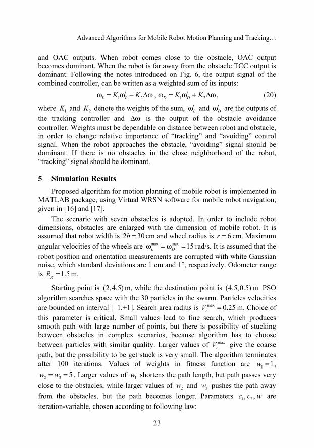
Because of the stochastic nature of the algorithm, paths generated from starting to destination point (blue line on Fig. 8a) and vice versa (red line on Fig. 8a) will not be the same. Length of the blue path is 5.20 m, while the length of the red path is 5.13 m. So, in this case, red path is better one. On Fig. 8a, points generated by algorithm are represented with stars, while real obstacles are represented with solid black line. Obstacles enlarged by robot dimension are represented with dashed black line.

The next step is path interpolation using RBFNN. Training set consists of input-output training pairs. Each training pair consists of point on the path and corresponding time instant, which is obtained assuming constant velocity of robot motion. It is assumed that this velocity is 0.2v = m/s. Hidden layer size should be chosen such that approximation of the path is adequate and collision free. Approximation performance heavily depends on hidden layer size and region width σ. These parameters have been determined experimentally. Hidden layer has 24 neurons, while 2.375σ = . Neural network response is shown on Fig. 8b.

When the interpolated path is generated, the next step is trajectory generation based on previously obtained path. Algorithm uses following values of parameters: length on which the path character is analyzed is 0.5L = m, maximal velocity of the robot is max 0.5v = m/s and proportionality constant in (11) is 0.25k = . Velocity profile, as well as x and y coordinate plots of the desired trajectory versus time are shown on Fig. 9.

(a) (b)

Fig. 8 – (a) Paths generated by PSO algorithm, (b) Interpolated path using RBFNN.


25

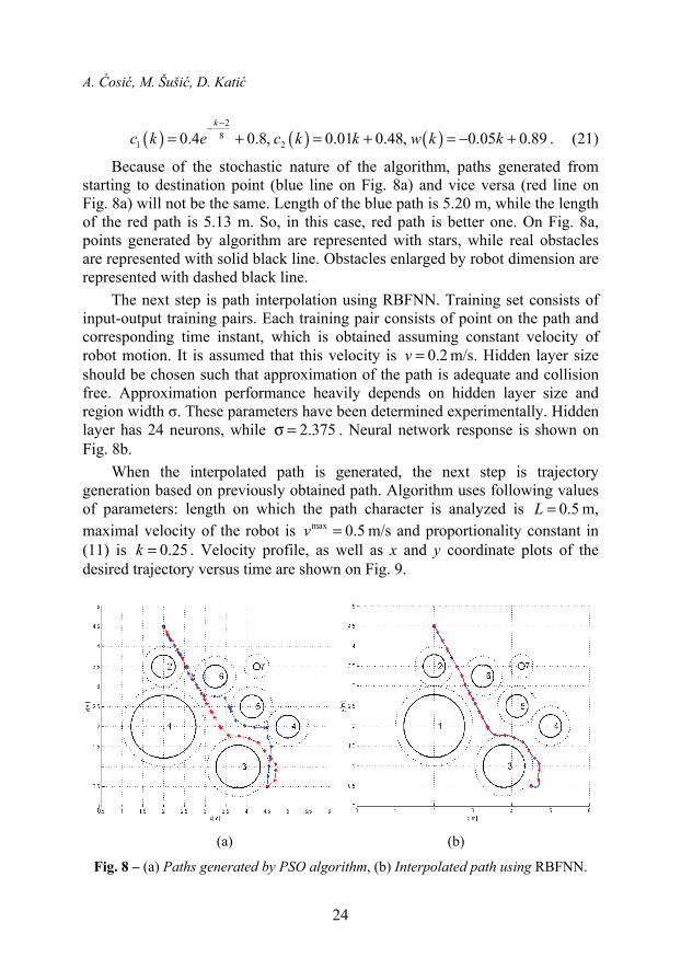
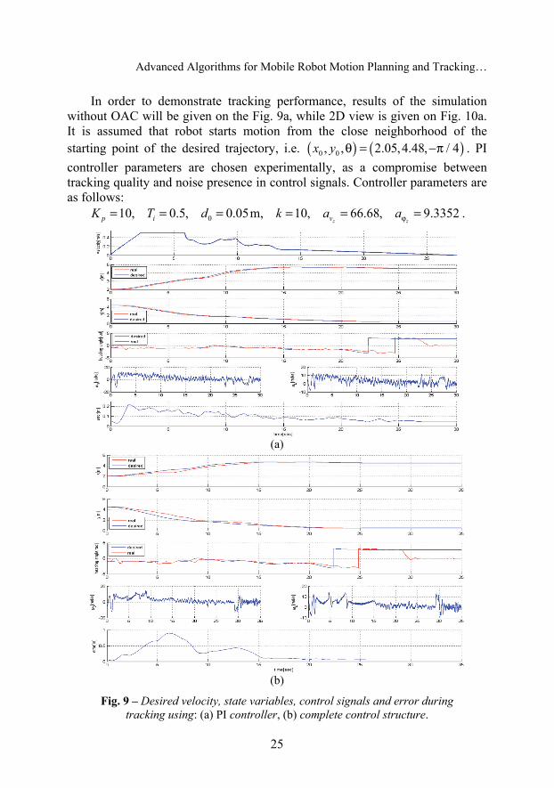
In order to demonstrate tracking performance, results of the simulation without OAC will be given on the Fig. 9a, while 2D view is given on Fig. 10a. It is assumed that robot starts motion from the close neighborhood of the starting point of the desired trajectory, i.e. ( ) ( )0 0, , 2.05,4.48, / 4x y θ = −π . PI controller parameters are chosen experimentally, as a compromise between tracking quality and noise presence in control signals. Controller parameters are as follows: 010, 0.5, 0.05m, 10, 66.68, 9.3352

z zp i vK T d k a aϕ= = = = = = .

(a)

(b)

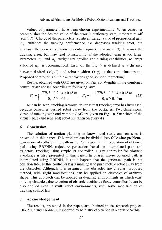
Fig. 9 – Desired velocity, state variables, control signals and error during tracking using: (a) PI controller, (b) complete control structure.


26

(a) (b)

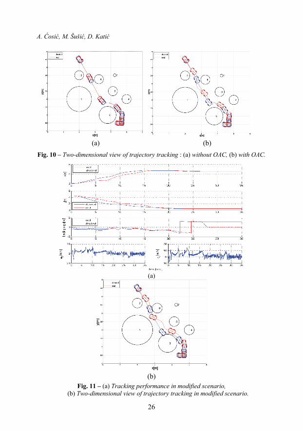
Fig. 10 – Two-dimensional view of trajectory tracking : (a) without OAC, (b) with OAC.

(a)

(b)

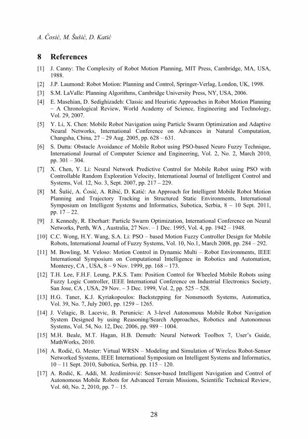
Fig. 11 – (a) Tracking performance in modified scenario, (b) Two-dimensional view of trajectory tracking in modified scenario.


27

Values of parameters have been chosen experimentally. When controller accomplishes the desired value of the error in stationary state, motors turn off (see (17)). Choice of the parameters is critical. Larger value of proportional gain

pK enhances the tracking performance, i.e. decreases tracking error, but increases the presence of noise in control signals. Increase of iT decreases the tracking error, but may lead to instability, if the adopted value is too large. Parameters

zva and z

aϕ weight straight-line and turning capabilities, so larger value of

zaϕ is recommended. Error on the Fig. 9 is defined as a distance

between desired ( , )x y∗ ∗ and robot position ( , )x y at the same time instant. Proposed controller is simple and provides good solution to tracking.

Results obtained with OAC are given on Fig. 9b. Weights in the combined controller are chosen according to following law:

1 2

1.778 0.2, 0.45m 1.778 0.8, 0.45m,

0, 0.45m 0, 0.45md d d d

K Kd d

+ < − + <⎧ ⎧= =⎨ ⎨≥ ≥⎩ ⎩

(22)

As can be seen, tracking is worse, in sense that tracking error has increased, because controller pushed robot away from the obstacles. Two-dimensional views of tracking with and without OAC are given on Fig. 10. Snapshots of the virtual (blue) and real (red) robot are taken on every 4 s.

6 Conclusion The solution of motion planning in known and static environments is

presented in this paper. This problem can be divided into following problems: generation of collision free path using PSO algorithm, interpolation of obtained path using RBFNN, trajectory generation based on interpolated path and trajectory tracking using simple PI controller. Fuzzy controller for obstacle avoidance is also presented in this paper. In phases where obtained path is interpolated using RBFNN, it could happen that the generated path is not collision free, so this controller has a main goal to push mobile robot away from the obstacles. Although it is assumed that obstacles are circular, proposed method, with slight modifications, can be applied on obstacles of arbitrary shape. This approach can be applied in dynamic environments in which exist moving obstacles, due to action of obstacle avoidance fuzzy controller. It can be also applied even in multi robot environments, with some modification of tracking control law.

7 Acknowledgement The results, presented in the paper, are obtained in the research projects

TR-35003 and TR-44008 supported by Ministry of Science of Republic Serbia.


28

8 References [1] J. Canny: The Complexity of Robot Motion Planning, MIT Press, Cambridge, MA, USA,

1988. [2] J.P. Laumond: Robot Motion: Planning and Control, Springer-Verlag, London, UK, 1998. [3] S.M. LaValle: Planning Algorithms, Cambridge University Press, NY, USA, 2006. [4] E. Masehian, D. Sedighizadeh: Classic and Heuristic Approaches in Robot Motion Planning

– A Chronological Review, World Academy of Science, Engineering and Technology, Vol. 29, 2007.

[5] Y. Li, X. Chen: Mobile Robot Navigation using Particle Swarm Optimization and Adaptive Neural Networks, International Conference on Advances in Natural Computation, Changsha, China, 27 – 29 Aug. 2005, pp. 628 – 631.

[6] S. Dutta: Obstacle Avoidance of Mobile Robot using PSO-based Neuro Fuzzy Technique, International Journal of Computer Science and Engineering, Vol. 2, No. 2, March 2010, pp. 301 – 304.

[7] X. Chen, Y. Li: Neural Network Predictive Control for Mobile Robot using PSO with Controllable Random Exploration Velocity, International Journal of Intelligent Control and Systems, Vol. 12, No. 3, Sept. 2007, pp. 217 – 229.

[8] M. Šušić, A. Ćosić, A. Ribić, D. Katić: An Approach for Intelligent Mobile Robot Motion Planning and Trajectory Tracking in Structured Static Environments, International Symposium on Intelligent Systems and Informatics, Subotica, Serbia, 8 – 10 Sept. 2011, pp. 17 – 22.

[9] J. Kennedy, R. Eberhart: Particle Swarm Optimization, International Conference on Neural Networks, Perth, WA , Australia, 27 Nov. – 1 Dec. 1995, Vol. 4, pp. 1942 – 1948.

[10] C.C. Wong, H.Y. Wang, S.A. Li: PSO – based Motion Fuzzy Controller Design for Mobile Robots, International Journal of Fuzzy Systems, Vol. 10, No.1, March 2008, pp. 284 – 292.

[11] M. Bowling, M. Veloso: Motion Control in Dynamic Multi – Robot Environments, IEEE International Symposium on Computational Intelligence in Robotics and Automation, Monterey, CA , USA, 8 – 9 Nov. 1999, pp. 168 – 173.

[12] T.H. Lee, F.H.F. Leung, P.K.S. Tam: Position Control for Wheeled Mobile Robots using Fuzzy Logic Controller, IEEE International Conference on Industrial Electronics Society, San Jose, CA , USA, 29 Nov. – 3 Dec. 1999, Vol. 2, pp. 525 – 528.

[13] H.G. Taner, K.J. Kyriakopoulos: Backstepping for Nonsmooth Systems, Automatica, Vol. 39, No. 7, July 2003, pp. 1259 – 1265.

[14] J. Velagic, B. Lacevic, B. Perunicic: A 3-level Autonomous Mobile Robot Navigation System Designed by using Reasoning/Search Approaches, Robotics and Autonomous Systems, Vol. 54, No. 12, Dec. 2006, pp. 989 – 1004.

[15] M.H. Beale, M.T. Hagan, H.B. Demuth: Neural Network Toolbox 7, User’s Guide, MathWorks, 2010.

[16] A. Rodić, G. Mester: Virtual WRSN – Modeling and Simulation of Wireless Robot-Sensor Networked Systems, IEEE International Symposium on Intelligent Systems and Informatics, 10 – 11 Sept. 2010, Subotica, Serbia, pp. 115 – 120.

[17] A. Rodić, K. Addi, M. Jezdimirović: Sensor-based Intelligent Navigation and Control of Autonomous Mobile Robots for Advanced Terrain Missions, Scientific Technical Review, Vol. 60, No. 2, 2010, pp. 7 – 15.

Documents

Advanced Algorithms for Mobile Robot Motion Planning and