Admissible Subspace TRajectory Optimizer (ASTRO)

for Autonomous Robot Operations on the Space

Station

Gregory E. Chamitoff,∗ Alvar Saenz-Otero,† Jacob G. Katz,‡ and Steve Ulrich§

Massachusetts Institute of Technology, Cambridge, Massachusetts, 02139

This paper presents the development of a real-time path-planning optimization approachto controlling the motion of space-based robots. The algorithm is capable of designing atrajectory for a robot to navigate within complex surroundings that include numerous ob-stacles (generalized shapes) and constraints (geometric and performance limitations). Themethodology employs a unique transformation that effectively changes a complex optimiza-tion problem into one with a positive definite cost function that enables high convergencerates for complex geometries, enabling its application to real-time operations. This strat-egy was implemented on the Synchronized Position Hold Engage Reorient ExperimentalSatellite (SPHERES) test-bed on the International Space Station (ISS), and iterative ex-perimental testing was conducted onboard the ISS during Expedition 17 by the first author.

I. Introduction

Real-time navigation for autonomous vehicles of all kinds is a challenging technical problem, but onethat holds great promise for enabling major leaps in future capability. The next generation of robotic

systems, self-guided aircraft, and autonomous spacecraft will need to have the capability to analyze andinterpret their own environment in order to design and conduct their mission.1 Computing power and sensortechnology have advanced to the stage that it has become possible for an autonomous machine to gatherdata and construct an internal model of its surroundings fast enough to use that information for real-timedecision making. Likewise, given a continuously evolving internal model, it is necessary to plan and re-planan optimal approach for conducting a mission or performing a task. This may also involve simultaneouscooperative planning with other autonomous vehicles.

To accomplish this, algorithms to solve complex multi-dimensional optimization problems in near real-time for spacecraft proximity operations have been studied extensively. Of special interest are trajectoryoptimization techniques with not only terminal constraints, such a position and velocity, but interior-pointconstraints for example. The complex constraints can be presented by several mathematical forms, such asequality constraints and second-order inequality constraints. For example, thrust limited maneuvers withpath constraints based on the primer-vector theory has been considered by Taur et al.,2 where the full adjointequations and corresponding optimality constraints are imposed for the rendezvous and intercept transfersof a spacecraft between two circular, coplanar orbits with a minimum periapsis constraint for the chaservehicle.

Trajectory optimization based on adaptive artificial potential functions (AAPF) was proposed by Munozand Fitz-Coy3 for rapid path-planning of spacecraft autonomous proximity operations. The AAPF methodpermits attractive potential with time dependent weights which are defined by an adaptive update law.Simulation results demonstrated that the developed methodology enables proximity operations with increasedperformance compared to the standard artificial potential function in an evolving environment.

∗Research Affiliate MIT, NASA Astronaut - ISS Expedition 17/18 Flight Engineer & Science Officer, Professor, Universityof Sydney and Texas A&M University. Associate Fellow AIAA.†Research Scientist, Department of Aeronautics and Astronautics, 77 Massachusetts Avenue. Senior Member AIAA.‡PhD Candidate, Department of Aeronautics and Astronautics, 77 Massachusetts Avenue; now GNC Engineer, Space

Exploration Technologies, Los Angeles, California.§Postdoctoral Associate, Department of Aeronautics and Astronautics, 77 Massachusetts Avenue; now Assistant Professor,

Department of Mechanical and Aerospace Engineering, Carleton University, Ottawa, Canada. Member AIAA.

1 of 17

American Institute of Aeronautics and Astronautics

Dow

nloa

ded

by S

teve

Ulr

ich

on F

ebru

ary

10, 2

016

| http

://ar

c.ai

aa.o

rg |

DO

I: 1

0.25

14/6

.201

4-12

90

AIAA Guidance, Navigation, and Control Conference

13-17 January 2014, National Harbor, Maryland

AIAA 2014-1290

Copyright © 2014 by G. E. Chamitoff, A. Saenz-Otero, J. G. Katz and S. Ulrich. Published by the American Institute of Aeronautics and Astronautics, Inc., with permission.

AIAA SciTech

Ulybyshev4 presented trajectory optimization methods for low-thrust spacecraft proximity maneuveringat near-circular orbits with interior-point constrains. The methods used discretization of the spacecrafttrajectory on segments and sets of pseudo-impulses for each segment. Then, a matrix inequality on the sumof the characteristic velocities for the pseudo-impulses is used to transform the problem into a large-scalelinear programming form, and terminal boundary conditions were presented as a linear matrix equation. InMassachusetts

Hadaegh et al.5 imposed a minimum relative distance constraint via an indirect optimization methodusing the relative motion equations while ignoring all orbital forces. While such indirect optimization meth-ods are known to provide mathematically elegant solutions and can handle path constraints, they sometimescan be cumbersome, especially as the constraints get more complicated in their algebraic expression. Typi-cally, the addition of each path constraint requires the detailed derivation of the associated Euler-Lagrange(adjoint) equations and a corresponding set of optimality conditions that are not trivial to derive or to im-plement. Similarly, Jezewski6 used interior path-constraints in an indirect formulation and also includes theeffect of J2 in the equations of motion and adjoint equations. Haufler et al.7 used parameter optimization tohandle a larger set of path constraints. In addition to the minimum periapsis constraint of Jezewski,6 a min-imum and maximum relative distance between the target and chaser constraint, and a maximum magnitudeof the impulses constraint are considered. Hadaegh and Singh8 also used a method performing parameteroptimization to enforce collision avoidance for deep space applications (i.e. no orbital mechanics effects) byrepresenting the trajectories as splines.

Richard et al.9 described a technique that used mixed-integer linear programming (MILP) in which theoptimization objective was to find a trajectory that satisfies the logical constraints and minimizes fuel use.10

The examples include the use of a microsatellite to inspect the International Space Station (ISS). Bregerand How11 also used mixed-integer linear programming (MILP) to enforce collision avoidance with a varietyof shapes, evaluating a series of active constraints (determined via binary variables) at grid points. Thekeep out zones were simplified to a set of planar faces roughly enclosing the volume to be avoided and thebinary variables are used to eliminate all the planar faces that are currently inactive as a path constraint.At most, all but one face was removed leaving a single, simple linear inequality constraint to be evaluatedat the corresponding grid point.

Luo et al.12,13 used multi-objective genetic algorithms to handle path-constrained proximity operations.Collision avoidance with a sphere of safety constraint and a line of approach cone are imposed. With theproposed approach, any trajectory that is considered as violating the imposed constraint was removed fromthe population after each generation. A fixed, equally-spaced grid is utilized to determine the satisfaction ofthe constraint over the trajectory after the trajectory is finished integrating.

Ranieri,14 solved the path-planning optimization problem by using the sparse optimal control software(SOCS), a direct collocation optimization package developed by Boeing that utilizes implicit integration ofthe equations of motion. This optimization software has the capability to handle path constraints throughthe use of a series of mesh refinements of the implicit integration grid that ensures that the path constraintis evaluated and satisfied throughout the integration. The grid is made progressively denser as any pathconstraint boundaries are approached to ensure that the path constraints are not violated between the gridpoints.

Another highly-efficient solution to address the autonomous path-planning optimization problem makesuse of second-order cone programming (SOCP) methodologies, which consist of convex optimization prob-lems with linear cost functions, equality constraints, and second-order conic inequality constraints.15,16 Tofind numerical solutions to SOCP problems, interior-point algorithms are often used. As explained by Luand Liu,17 such an algorithm has polynomial complexity and upper bounds on operations and the numberof iterations required to find the solution, all of which can be determined a priori, even though conver-gence is typically achieved much faster than those conservative bounds indicate (they guarantee convergenceto the global optimal solution if the inequality constraints have an interior point). See Nesterov and Ne-mirovsky18 for a detailed treatment on interior-point polynomial algorithms in convex programming. Thesefeatures make the SOCP methodology appealing for potential real-time applications. In particular, Wangand Boyd19 and Mattingley and Boyd20 considered a special class of convex optimization well suited forreal-time operations to which SOCP belongs. Lu and Liu17 developed an SOCP-based method to solve theproblem of autonomous trajectory planning for spacecraft rendezvous and proximity operations. In theirwork, the authors formulated the problem as a nonlinear optimal control problem, subject to various stateand control inequality constraints and equality constraints on interior points and terminal condition. A

2 of 17

American Institute of Aeronautics and Astronautics

Dow

nloa

ded

by S

teve

Ulr

ich

on F

ebru

ary

10, 2

016

| http

://ar

c.ai

aa.o

rg |

DO

I: 1

0.25

14/6

.201

4-12

90

relaxed problem was formed and then solved by a successive solution process, in which the solutions of asequence of constrained sub-problems with linear, time-varying dynamics are sought. After discretization,each of these problems becomes a second-order cone programming problem. Their solutions, if they exist, areguaranteed to be found by a primal-dual interior-point algorithm. The efficacy of the proposed methodologywas demonstrated by numerical simulations.

The methods described above include various techniques to address the challenges of real-time compu-tation and nonlinear constrained non-convex optimization problems. The approach presented in this paper,called the Admissible Subspace TRajectory Optimizer (ASTRO) algorithm, overcomes these challenges bytransforming the problem into a parameter space that is well behaved for real-time optimization. The AS-TRO algorithm is capable of designing a planned trajectory for a spacecraft robot to navigate within complexsurroundings that include numerous obstacles and constraints. Obstacles consist of generalized shapes andinclude a class of moving objects as well. Constraints include both geometric and performance-based limita-tions on the robot’s motion. Typically, the solution of a general nonlinear optimization problem like this isvery difficult and time-consuming to solve. Depending on the technique used, it can also get caught in localminima and may never find the globally optimal solution. It’s a significant challenge to design a system thatcan find reliable solutions in real-time. To cope with these difficulties, the original contribution of this workis the development of an algorithm that employs a unique transformation that effectively changes a complexoptimization problem into one with a positive definite cost function that enables very fast convergence toa solution. This is accomplished through mathematical definitions for how the constraints should be mod-eled, and by taking advantage of some unique properties of orthogonal polynomials. By expressing certainparameters with these polynomials, it becomes possible to transform a complex cost function into a simpleone in higher dimension. The result is that very high convergence rates can be obtained even for complexgeometric problems that would otherwise appear to be quite nonlinear.

In order to test the ASTRO algorithm on the ISS, a custom interface was designed to enable the crewto use MATLAB directly to program and execute the algorithm. Following standard ISS procedures andoperational rules it is never possible for the crew to change the software of the SPHERES satellites onboardthe ISS themselves. The development of ASTRO aboard ISS was itself a space first: the first ever use ofMATLAB aboard the ISS, and the first time that an astronaut conducted research on the ISS based ontheir own research on the ground. The advantage was that by integrating MATLAB with the SPHERES C-code interface (on a Space-Station Support Computer), it was possible to perform real-time commanding andtelemetry communications with the SPHERES satellites. A series of test cases were conducted to demonstratethe ability of ASTRO to incorporate increasingly complex constraints while producing admissible (feasible)trajectories for the SPHERES satellite to follow. All constraints were simulated virtually, but the satelliteactually flew physically inside the habitable volume of the US Laboratory on the ISS. In order to test theability to navigate around moving obstacles, a second SPHERES satellite was specifically programmed toattempt to get in the way. Specifics on the implementation and the experimental results are presented inthe paper.

The remainder of this paper is organized as follows. Section II presents the theoretical development ofthe ASTRO algorithm including conditions for guaranteed convergence. Section III demonstrates the effec-tiveness of ASTRO in simulation for a complex path planning problem. Section IV covers the experimentalsetup onboard the ISS and presents an analysis of results from several test cases. Finally, a conclusion isprovided in Section V.

II. ASTRO Algorithm

The ASTRO algorithm effectively solves a guidance problem, while an inner-loop controller handles thetask of trajectory tracking. In order to assure that the trajectory solution is feasible, maneuvering capabilitiesof the vehicle are incorporated as performance constraints within the trajectory optimization. In other words,the solution is not allowed to ask for maneuvers that the vehicle cannot achieve given its mass propertiesand the limitations of its actuators (thrusters). The optimization strategy is based on a two-stage approach.The first stage is designed to identify admissible trajectories as quickly as possible. These trajectories meetthe initial and final boundary conditions while avoiding all spatial (geometric) and performance constraints.The second stage uses any remaining computation time to refine the solution towards the optimal path.

The optimization itself is accomplished by using an augmented cost function that penalizes a combinationof path length and active constraint violations. The flight path is parameterized using Legendre polynomials.

3 of 17

American Institute of Aeronautics and Astronautics

Dow

nloa

ded

by S

teve

Ulr

ich

on F

ebru

ary

10, 2

016

| http

://ar

c.ai

aa.o

rg |

DO

I: 1

0.25

14/6

.201

4-12

90

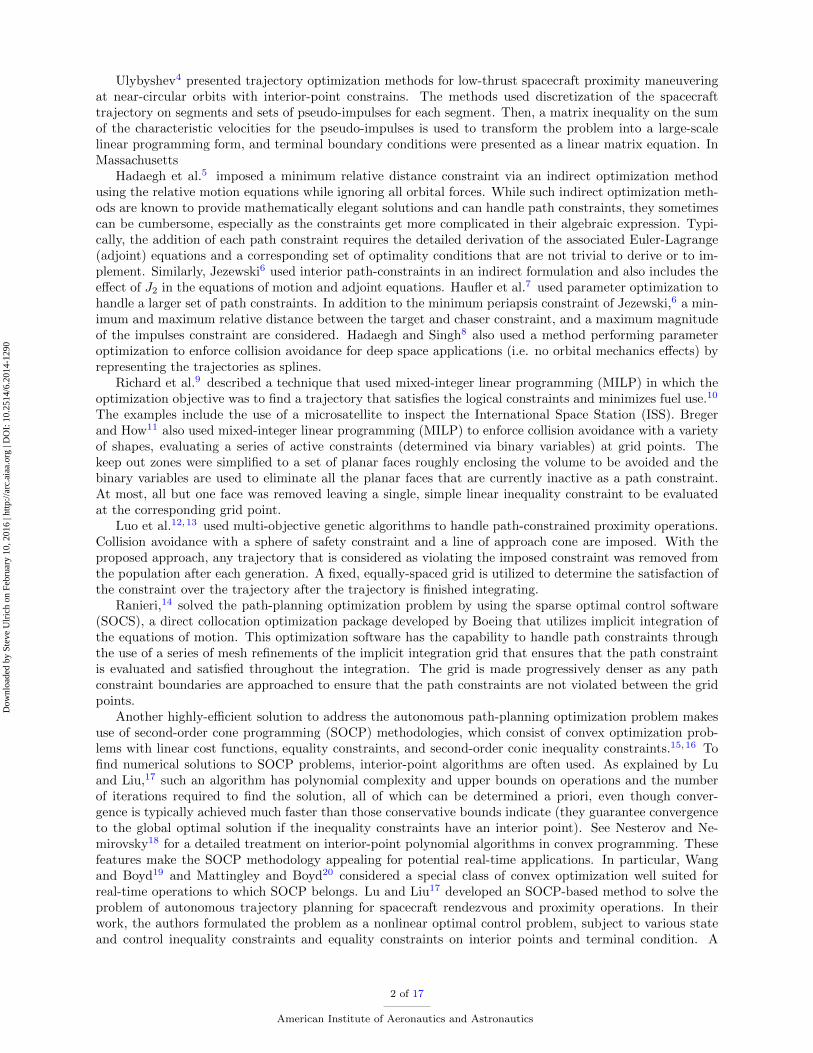
Figure 1. The ASTRO algorithm optimizes the path from x(t0) to x(tf ).

Initial parameter estimates are obtained by performing a low-order spline to meet the boundary conditionsof a relaxed problem (i.e. without constraints). A special feature of the ASTRO algorithm is its abilityto perform the parameter optimization by projecting numerical gradient information onto the sub-space ofparametric variations that enforce the boundary conditions. As such, each iteration meets the boundaryconditions perfectly, and subsequent iterations move closer to a solution that satisfies the constraints as well.Relative weights in the cost function are used to assure that constraint violation gradients dominate theparameter search while any constraints remain active. Finally, by taking advantage of certain propertiesof Legendre polynomials, the constraint and path-length penalty functions can be defined to meet certainconditions that ensure a positive definite cost function with respect to the higher dimensional space ofparameter errors. This property guarantees asymptotic convergence directly to an admissible solution, andthen to the optimal solution.

II.A. Problem Statement

The general guidance problem addressed by the ASTRO algorithm is that of generating an optimal flightpath for an autonomous space-based robot through its environment in order to accomplish some task. Itmust start with the robot’s current position and velocity and end up at some final desired state. Along theway it must avoid geometric constraints (physical objects), and it must maneuver within the performancelimitations of its actuators (thrusters etc). This problem is illustrated in Fig. 1.

The definition of optimality in this case is taken to mean the most direct, minimum length, path betweenthe initial position at the initial time x0(t0) to the final position at the final time xf (tf ). The initial andfinal velocity vectors are also specified as x0(t0) and xf (tf ). These boundary conditions can be expressed asfollows

fBC1= (x(t0), x(t0)) = 0 (1)

fBC2= (x(tf ), x(tf )) = 0

The cost function to be minimized is the path length expressed by

S =

∫ xf

x0

ds =

∫ tf

t0

√x(t)2 + y(t)2 + z(t)2dt (2)

and the functions x(t), y(t) and z(t), (i.e. the path specified by the vector x(t)) are to be determined bythe algorithm. This is complicated by the environmental obstacles, and these can be described by functionsof the same variables. As a simple example, the definition of a wall could be x < 5, meaning that if x = 5the robot has hit the wall. If the trajectory x(t) includes portions for which x ≥ 5, then that amounts to aconstraint violation. An admissible solution is one that meets the initial and final boundary conditions at

4 of 17

American Institute of Aeronautics and Astronautics

Dow

nloa

ded

by S

teve

Ulr

ich

on F

ebru

ary

10, 2

016

| http

://ar

c.ai

aa.o

rg |

DO

I: 1

0.25

14/6

.201

4-12

90

x(t0) and x(tf ) and does not violate any of the geometric constraints along the trajectory. In addition thereare performance constraints on the ability of the robot to maneuver, and these can be expressed as functionsof the higher derivatives of the trajectory. For another simple example, limiting the required accelerationalong one axis could be described by x(t) < 100, meaning that an achievable acceleration due to thrustermagnitude and mass properties is less than 100 units. As with the geometric constraints, an admissiblesolution for the trajectory and its higher derivatives must not violate these performance constraints. Ingeneral, the geometric and performance constraints can be described by

fci(x(t), x(t), x(t)) ≤ 0, ∀i ∈ [1, n] , ∀t ∈ [t0, tf ] (3)

where n is the number of constraint functions. Note that the ASTRO algorithm is designed to find anadmissible trajectory, that is a solution that satisfies Eqs. (1) and (3), very quickly, and then spends anyremaining computation time to optimize further by minimizing Eq. (2). This two-stage search is achievedby constructing an augmented cost function of the form

J = f2s (S) +

n∑j=1

Kjmaxt∈[t0,tf ]f2cj (4)

where f2s (S) is the path length cost function from Eq. (2). The coefficients Kj represent the relative weightsWj for each constraint function, and are given by

Kj =

{0, if fcj ≤ 0

Wj , if fcj > 0(5)

These values only need to be chosen to assure that the constraint violations dominate the cost function.Once a solution is found that drives the second term in Eq. (4) to zero, then the resulting trajectory isadmissible.

II.B. Legendre Polynomial Parametrization

In general, Eq. (4) represents a difficult and nonlinear optimization problem. The ASTRO algorithm trans-forms this into a simpler problem by parameterizing the trajectory by Legendre polynomials and normalizingthe time interval such that certain orthogonality properties of Legendre polynomials can be used to its ad-vantage. The parameterization is expressed as follows

xi(t′) =

N∑k=0

CikPk(t′) (6)

where

t′ = 2

[t− t0tf − t0

]− 1 (7)

The Cik are coefficients of the Legendre polynomials of order k that represent the trajectory xi(t). Time isnormalized such that t′ ∈ [−1, 1]. Over this interval, and taking advantage of the orthogonality of Legendrefunctions, the squared path-length component of the cost function in Eq. (4) can be reduced to the following

S2 =

3∑i=1

N∑k=0

{C2

ik

∫ 1

−1[P ′k(t′)]

2dt′}

(8)

In Eq. (8), S represents an upper bound to the path length, P ′k are derivatives of the standard Legendrepolynomial and therefore the integral can be evaluated off-line. The result is that the cost function is reducedto a sum of parameters weighted by fixed values. Due to the orthogonality of Legendre polynomials, all ofthe cross terms are zero, and this reduces the computation by a factor N , which is the minimum order ofthe polynomials required to find a solution.21

Since the flight path, velocity along that path, and all geometric and performance constraints can beexpressed as functions of x(t) and higher derivatives, referring to Eqs. (6) and (8), the full cost function inEq. (4) can be written as

5 of 17

American Institute of Aeronautics and Astronautics

Dow

nloa

ded

by S

teve

Ulr

ich

on F

ebru

ary

10, 2

016

| http

://ar

c.ai

aa.o

rg |

DO

I: 1

0.25

14/6

.201

4-12

90

J =

n+1∑j=1

[fj(C)]2

(9)

where the rows of C =

C11 · · · C1n

.... . .

...

C31 · · · C3n

correspond to coefficients of the Legendre polynomials that

parameterize the curves for xi(t), and the fj represent the maximum violation along a given trajectory foreach constraint function. The n+ 1 term represents the path length cost term fn+1(C) = fs(S

2).

II.C. Formulation as a Convex Search Space

The advantage of transforming the cost function from Eq. (4) into Eq. (9) is that it can be shown thatthe optimization can now be performed on a convex space using a simple gradient-descent procedure. InEq. (9), J is a convex (positive-definite) function of fj(C), but it is not, in general, convex with respect tothe parameters Cik or to the parameter errors (Cik−C∗ik), where C∗ik are the optimal values of the coefficientsfor the optimal trajectory.

If the cost function could be restricted, however, such that J is positive definite with respect to (Cik−C∗ik),then a gradient (∂J/∂Cik) based search algorithm could be made to converge to the optimal solution. Thiscan be seen as follows.

First, recall the definition of a positive-definite function: V (x) is positive definite if V (0) = 0, V (x) > 0for x 6= 0,and V (x) > g(|x|) where g(·) is a non-decreasing function.

Second, define ∆Cik = Cik − C∗ik, and note that (∂J/∂Cik) = (∂J/∆C∗ik) since (∂J/∂C∗ik) = 0. Nowassume that J(∆Cik) is a positive-definite function of ∆Cik, and the problem is to search over the spacedefined by Cik for the optimal parameters C∗ik. Since J = 0 only for ∆Cik = 0, and J > 0 for all othervalues of ∆Cik, there is a unique minimum for J . Likewise, ∂J/(∂|∆Cik|) ≥ 0 by the definition above, andtherefore ∂J/∂∆Cik = 0 only at ∆Cik = 0, or at other local inflection points in the parameter space. Localminima, however, would require that ∂J/(∂|∆Cik|) < 0 over some interval between that point and C∗ik,which violates the definition of positive definite. Therefore, if J(∆Cik) is positive-definite, ∆Cik = 0 is theonly extremal point, and any other point has a negative gradient −∂J/(∂Cik) pointing in the direction ofthe global minimum (except when −∂J/(∂Cik) = 0, which can be handled by a minimum step-size).

To make the cost function Eq. (9) positive definite in the parameter errors (Cik − C∗ik), consider therevised function

J ′ = J − J∗ =

n+1∑j=1

[fj(C)]2 −

n+1∑j=1

[fj(C∗)]

2(10)

J∗ is the cost for the optimal solution. Note that J’ is not a realizable cost function, since J∗ is unknown,but it simply differs from the original cost by a constant scalar. Now consider the positive-definite criteriafor J ′ with respect to (Cik − C∗ik). Since J ′ = 0 when Cik = C∗ik, and J ′ > 0 when Cik 6= C∗ik, we have thatJ ′ is positive definite in (Cik−C∗ik) if ∂J ′/∂|∆Cik| ≥ 0. This condition is equivalent to saying that ∂J ′/∂Cik

must be non-decreasing (i.e. monotonic). Therefore, in terms of Eq. (10), J ′ is positive definite with respectto (Cik − C∗ik) if one of the following conditions is satisfied:

∂J ′

∂Cik= 2

n+1∑j=1

fj(Cik)∂fj∂Cik

is monotonic (11)

∂2J ′

∂C2ik

= 2

n+1∑j=1

(∂fj∂Cik

)2

+ fj(Cik)∂2fj∂C2

ik

≥ 0

Assuming these conditions on fj(Cik) given by Eq. (11) are satisfied, then the following are true:

1. J ′ is a positive-definite function with respect to the parameter errors (Cik − C∗ik);

2. the point Cik = C∗ik is a unique minimum for J ′;

6 of 17

American Institute of Aeronautics and Astronautics

Dow

nloa

ded

by S

teve

Ulr

ich

on F

ebru

ary

10, 2

016

| http

://ar

c.ai

aa.o

rg |

DO

I: 1

0.25

14/6

.201

4-12

90

3. for any Cik 6= C∗ik, J ′ can be reduced by a discrete step in Cik, that is

[Cik]new = [Cik]old + δCik (12)

where

δCik = −α[∂J ′

∂Cik

]+ βik (13)

with α > 0 and βik 6= 0; and

4. the pseudo-gradient search algorithm above will converge to C∗ik.

Now, since J ′ and J only differ by a constant, a procedure which minimizes J ′ also minimizes J . Thus,provided the conditions on fj(Cik) are met, the optimization of J(Cik) can be accomplished by the samemethod.

Fortunately, the restrictions on the form of fj(Cik), which apply to the path length penalty fn+1(C) =fs(S

2) and to all constraint functions fcj (x(t), x(t), x(t)) are not too difficult to satisfy. In particular, thepath length in Eq. (8), can be simplified as follows. Define the path length function fs as

fs(S2) =

3∑i=1

N∑k=0

IkC2ik (14)

where

Ik =

∫ 1

−1[P ′k(t′)]

2dt′ (15)

and now apply the condition defined in Eq. (11). The result is

4

(3∑

i=1

N∑k=0

IkCik

)2

+

(3∑

i=1

N∑k=0

Ik

)(3∑

i=1

N∑k=0

IkC2ik

)≥ 0 (16)

which is clearly satisfied since all summation terms on the left are positive. For the constraint functions,most spacial or performance related constraints that would be of interest can be expressed generally by

g(X) ≤ q0 (17)

or

fc(X) =

{[g(X)− g0]

2, if g(X) > g0

0, if g(X) ≤ g0(18)

where xp, xp, and xp are constants and where X(t) is given by

X(t) =

x(t)− xp

x(t)− xp

x(t)− xp

(19)

For each constraint function fc(·), a sufficient condition for satisfying Eq. (11) is that(∂fc∂Cik

)2

+ fc(Cik)

(∂2fc∂C2

ik

)≥ 0 (20)

for each of the parameters Cik. Since (∂fc/∂Cik)2 is clearly non-negative, and fc ≥ 0 by definition, we arerestricted to a class of constraint functions for which (∂2fc/∂C

2ik) ≥ 0. Evaluating this derivative gives

1

2

∂2fc∂C2

ik

=

(∂g

∂X

∂X

∂Cik

)2

+ [g(X)− g0]

(∂2g

∂X2

)(∂X

∂Cik

)2

≥ 0 (21)

7 of 17

American Institute of Aeronautics and Astronautics

Dow

nloa

ded

by S

teve

Ulr

ich

on F

ebru

ary

10, 2

016

| http

://ar

c.ai

aa.o

rg |

DO

I: 1

0.25

14/6

.201

4-12

90

which is non-negative if ∂2g/∂X2 ≥ 0, since all other terms are non-negative, including [g(X)− g0] for anactive constraint violation. Therefore, any constraint g(X) that is a non-concave function of the states,derivatives, and/or acceleration defined by X(t) is allowable. In fact, if the matrix ∂2g/∂X2 is strictly

positive definite (i.e. zT[(∂2g/∂X2

]z > 0 for any vector z ∈ Rdim(X)), then (∂2J ′)/(∂C2

ik) will also bestrictly positive definite, and a gradient based search would encounter ∂J ′/∂Cik = 0 only at Cik = C∗ik.

To summarize, any constraint function of the form

g(X) ≤ g0 (22)

with ∂2g/∂X2 ≥ g0 will satisfy the conditions required by Eq. (8) for a successful gradient-based trajectoryoptimization. The requirements on the mathematical form of the constraints are not too restrictive. Someexample constraint functions that could easily be structured to satisfy this form include bounds on theconstrained volume (walls), ellipsoid or more complex convex shapes within the environment, cylinders,planes of any orientation, maximum speeds or accelerations, maximum path curvature, moving obstacles,etc.

II.D. Boundary Conditions and Projected Gradient Search

With the cost function defined by Eq. (9) and the constraints formulated to fit the conditions of Eq. (11),the negative gradient of J with respect to the parameters Cik, that is −∂J/∂Cik, is always directed towardsJmin and a descent gradient search will find the optimal trajectory. However, to assure that admissiblesub-optimal solutions are generated as quickly as possible, a gradient projection is used to assure thatthe boundary conditions at t0 and tf are always met. In fact, these equality constraints are very usefulin providing an initial guess for the trajectory parameters, and, more importantly, they can be used todramatically reduce the degrees of freedom in the search space.

From the trajectory parameterization xi(t′) =

∑Nk=0 CikPk(t′), the boundary conditions can be written

as follows

XBC = PBCC (23)

or x(t0) y(t0) z(t0)

x(t0) y(t0) z(t0)

x(tf ) y(tf ) z(tf )

x(tf ) y(tf ) z(tf )

=

P1(−1) P2(−1) · · · PN (−1)

P1(−1) P2(−1) · · · PN (−1)

P1(1) P2(1) · · · PN (1)

P1(1) P2(1) · · · PN (1)

C (24)

In this equation XBC is the matrix of boundary conditions, PBC is a directly computable function ofthe Legendre polynomials, and C represents the matrix of coefficients to be optimized for the trajectory.There are 12 equations and 3N unknowns (i.e., the elements of C). If the polynomials are limited to 4thorder, then the coefficients of C are uniquely determined. This represents (exactly) the cubic-spline curvebetween the initial and final positions and velocities, which is an ideal initial guess for the trajectory. SoCstart = P−1BCXBC for N = 4.

From this initial guess it is possible to assure that all future optimization steps maintain the boundaryconditions by projecting the gradient in such a way that it does not span the space of the 12 degrees offreedom already determined by the boundary conditions. For N > 4, there are (3N − 12) additional degreesof freedom over which to search in order to avoid constraints and minimize the cost function. This isaccomplished by the partitioning the C matrix as CN×3 = C⊥N×3

+ C|||N×3, such that

XBC = PBCCN×3 = PBC

{C⊥N×3

+ C|||N×3

}(25)

where

PBCC⊥N×3= 0 (26)

In other words, the columns of C||| are in the row-space of PBC , and the columns of C⊥ are in the null-spaceof PBC . Any variation of C⊥ that maintains PBCC⊥N×3

= 0 will assure that the boundary conditionsare not disturbed. Given an arbitrary gradient step in the matrix C, given by δC = δC||| + δC⊥, the

8 of 17

American Institute of Aeronautics and Astronautics

Dow

nloa

ded

by S

teve

Ulr

ich

on F

ebru

ary

10, 2

016

| http

://ar

c.ai

aa.o

rg |

DO

I: 1

0.25

14/6

.201

4-12

90

desired component of that step is δC⊥, since it won’t change the boundary conditions. Using the fact thatPBCδC = PBCδC⊥ + PBCδC||| = PBCδC|||, the projected gradient step is

δC⊥ =

[I−PT

BC

(PBCPT

BC

)−1PBC

]δC (27)

where

δC = −α [∂J/∂C] + β (28)

and the parameter adjustments are now limited to the 3N − 12 degrees of freedom remaining. δC is thegradient step from any generalized solver and δC⊥ amounts to a projection of the negative gradient of Jonto the sub-space of parametric variations that enforce the boundary conditions.

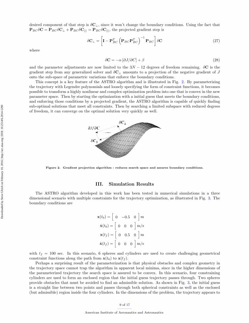
This concept is a key feature of the ASTRO algorithm and is illustrated in Fig. 2. By parameterizingthe trajectory with Legendre polynomials and loosely specifying the form of constraint functions, it becomespossible to transform a highly nonlinear and complex optimization problem into one that is convex in the newparameter space. Then by starting the optimization with a initial guess that meets the boundary conditions,and enforcing those conditions by a projected gradient, the ASTRO algorithm is capable of quickly findingsub-optimal solutions that meet all constraints. Then by searching a limited subspace with reduced degreesof freedom, it can converge on the optimal solution very quickly as well.

Figure 2. Gradient projection algorithm - reduces search space and assures boundary conditions.

III. Simulation Results

The ASTRO algorithm developed in this work has been tested in numerical simulations in a threedimensional scenario with multiple constraints for the trajectory optimization, as illustrated in Fig. 3. Theboundary conditions are

x(t0) =[

0 −0.5 0]

m

x(t0) =[

0 0 0]

m/s

x(tf ) =[

0 0.5 0]

m

x(tf ) =[

0 0 0]

m/s

with tf = 100 sec. In this scenario, 6 spheres and cylinders are used to create challenging geometricalconstraint functions along the path from x(t0) to x(tf ).

Perhaps a surprising result of the parameterization is that physical obstacles and complex geometry inthe trajectory space cannot trap the algorithm in apparent local minima, since in the higher dimensions ofthe parameterized trajectory the search space is assured to be convex. In this scenario, four constrainingcylinders are used to form an enclosed region that the initial guess trajectory passes through. Two spheresprovide obstacles that must be avoided to find an admissible solution. As shown in Fig. 3, the initial guessis a straight line between two points and passes through both spherical constraints as well as the enclosed(but admissible) region inside the four cylinders. In the dimensions of the problem, the trajectory appears to

9 of 17

American Institute of Aeronautics and Astronautics

Dow

nloa

ded

by S

teve

Ulr

ich

on F

ebru

ary

10, 2

016

| http

://ar

c.ai

aa.o

rg |

DO

I: 1

0.25

14/6

.201

4-12

90

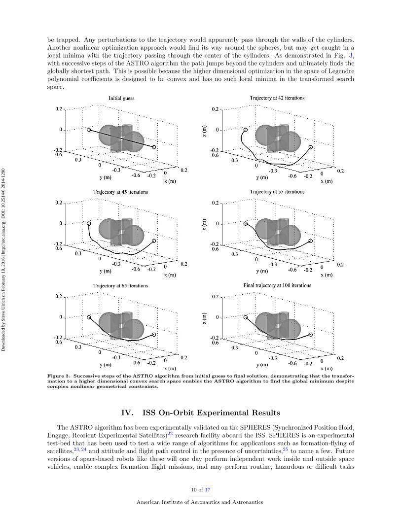
be trapped. Any perturbations to the trajectory would apparently pass through the walls of the cylinders.Another nonlinear optimization approach would find its way around the spheres, but may get caught in alocal minima with the trajectory passing through the center of the cylinders. As demonstrated in Fig. 3,with successive steps of the ASTRO algorithm the path jumps beyond the cylinders and ultimately finds theglobally shortest path. This is possible because the higher dimensional optimization in the space of Legendrepolynomial coefficients is designed to be convex and has no such local minima in the transformed searchspace.

Figure 3. Successive steps of the ASTRO algorithm from initial guess to final solution, demonstrating that the transfor-mation to a higher dimensional convex search space enables the ASTRO algorithm to find the global minimum despitecomplex nonlinear geometrical constraints.

IV. ISS On-Orbit Experimental Results

The ASTRO algorithm has been experimentally validated on the SPHERES (Synchronized Position Hold,Engage, Reorient Experimental Satellites)22 research facility aboard the ISS. SPHERES is an experimentaltest-bed that has been used to test a wide range of algorithms for applications such as formation-flying ofsatellites,23,24 and attitude and flight path control in the presence of uncertainties,25 to name a few. Futureversions of space-based robots like these will one day perform independent work inside and outside spacevehicles, enable complex formation flight missions, and may perform routine, hazardous or difficult tasks

10 of 17

American Institute of Aeronautics and Astronautics

Dow

nloa

ded

by S

teve

Ulr

ich

on F

ebru

ary

10, 2

016

| http

://ar

c.ai

aa.o

rg |

DO

I: 1

0.25

14/6

.201

4-12

90

that are not feasible or efficient for humans to perform. The SPHERES platform is ideal for investigatingthe technical approach for many future robotic applications in a 6 DOF microgravity environment.

IV.A. Experimental Setup

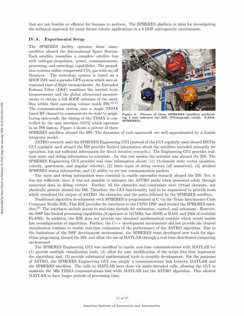
Figure 4. Picture of three SPHERES satellites perform-ing a test onboard the ISS. (Photograph credit: NASA-SPHERES).

The SPHERES facility operates three nano-satellites aboard the International Space Station.Each satellite resembles a complete satellite buswith cold-gas propulsion, power, communications,processing, and metrology capabilities. The propul-sion systems utilize compressed CO2 gas with on/offthrusters. The metrology system is based on a6DOF IMU and a pseudo-GPS system which uses ul-trasound time of flight measurements. An ExtendedKalman Filter (EKF) combines the inertial bodymeasurements and the global ultrasound measure-ments to obtain a full 6DOF estimate of the satel-lites within their operating volume inside ISS.26,27

The communication system uses a single TDMAbased RF channel to communicate its state to neigh-boring spacecraft; the timing of the TDMA is con-trolled by the user interface (GUI) which operatesin an ISS laptop. Figure 4 shows a picture of threeSPHERES satellites aboard the ISS. The dynamics of each spacecraft are well approximated by a doubleintegrator model.

ASTRO research used the SPHERES Engineering GUI (instead of the GUI regularly used aboard ISSTheGUI regularly used aboard the ISS provides limited information about the satellites intended primarily foroperation, but not sufficient information for direct iterative research.). The Engineering GUI provides real-time state and debug information to scientists - for this test session the scientist was aboard the ISS. TheSPHERES Engineering GUI provides real time information about: (1) 13-element state vector (position,velocity, quaternion, and angular velocity), (2) three types of debug vectors (all numerical), (3) detailedSPHERES status information, and (4) ability to see raw communication packets.

The state and debug information were essential to enable successful research aboard the ISS. Yet, itwas not sufficient, since it was not possible to interpret the ASTRO paths when presented solely throughnumerical data in debug vectors. Further, all the obstacles and constraints were virtual elements, notphysically present aboard the ISS. Therefore, the GUI functionality had to be augmented to provide toolswhich visualized the output of ASTRO, the obstacles, and the paths followed by the SPHERES satellites.

Traditional algorithm development with SPHERES is programmed in C via the Texas Instruments CodeComposer Studio IDE. This IDE provides the interfaces to the C6701 DSP used aboard the SPHERES satel-lites.28 The interfaces include access to real-time threads for estimation, control, and autonomy. However,the DSP has limited processing capabilities (it operates at 167MHz, has 16MB or RAM, and 256k of availableFLASH). In addition, the IDE does not provide any standard mathematical routines which would enablefast reconfiguration of algorithms. Further, the C++ development environment did not provide the desiredvisualization routines to enable real-time evaluation of the performance of the ASTRO algorithm. Due tothe limitations of the DSP development environment, the SPHERES team developed new tools for algo-rithm programing aboard the ISS, and allow the use of MATLAB through a real-time distributed-computingenvironment.

The SPHERES Engineering GUI was modified to enable real-time communications with MATLAB to:(1) provide multiple visualization tools, (2) allow for easy modification of the script files that implementthe algorithms and, (3) provide substantial mathematical tools to simplify development. For the purposesof ASTRO, the SPHERES Engineering GUI was simply a communications link between MATLAB andthe SPHERES satellites. The calls to MATLAB were done via multi-threaded calls, allowing the GUI tomaintain the 5Hz TDMA communications link while MATLAB ran the ASTRO algorithm. This allowedMATLAB to have longer periods of processing time.

11 of 17

American Institute of Aeronautics and Astronautics

Dow

nloa

ded

by S

teve

Ulr

ich

on F

ebru

ary

10, 2

016

| http

://ar

c.ai

aa.o

rg |

DO

I: 1

0.25

14/6

.201

4-12

90

IV.B. Real-time Traffic Control Model for Distributed Satellite Systems

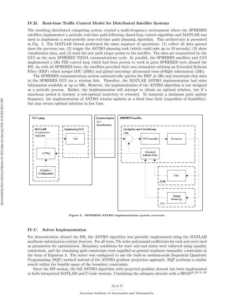
The resulting distributed computing system created a multi-frequency environment where the SPHERESsatellites implemented a periodic real-time path-following closed-loop control algorithm and MATLAB wasused to implement a semi-periodic near-real-time path planning algorithm. This architecture is presentedin Fig. 5. The MATLAB thread performed the same sequence of operations: (1) collect all data queuedsince the previous run, (2) trigger the ASTRO planning task (which could take up to 10 seconds), (3) showvisualization data, and (4) send the new path target points to the satellite. The data are transmitted by theGUI on the next SPHERES TDMA communications cycle. In parallel, the SPHERES satellites and GUIimplemented a 1Hz PID control loop which had been proven to work in prior SPHERES tests aboard theISS. As with all SPHERES tests, the satellites provided their own estimation utilizing an Extended KalmanFilter (EKF) which merges IMU (20Hz) and global metrology ultrasound time-of-flight information (5Hz).

The SPHERES communications system automatically queries the EKF at 5Hz and downloads that datato the SPHERES GUI via a wireless link. Therefore, the MATLAB ASTRO implementation had stateinformation available at up to 5Hz. However, the implementation of the ASTRO algorithm is not designedas a periodic process. Rather, the implementation will attempt to obtain an optimal solution, but if amaximum period is reached, a sub-optimal trajectory is returned. To maintain a minimum path updatefrequency, the implementation of ASTRO returns updates at a fixed time limit (regardless of feasibility),but may return optimal solutions in less time.

Figure 5. SPHERES ASTRO implementation system overview.

IV.C. Solver Implementation

For demonstration aboard the ISS, the ASTRO algorithm was partially implemented using the MATLABnonlinear optimization routine fmincon. For all tests, 7th order polynomial coefficients for each axis were usedas parameters for optimization. Boundary conditions for start and end states were enforced using equalityconstraints, and the remaining path constraints were supplied as general nonlinear inequality constraints inthe form of Equation 3. The solver was configured to use the built-in medium-scale Sequential QuadraticProgramming (SQP) method instead of the ASTRO gradient projection approach. SQP performs a similarsearch within the feasible space of the boundary constraints.

Since the ISS session, the full ASTRO algorithm with projected gradient descent has been implementedin both interpreted MATLAB and C-code versions. Combining the subspace descent with a BFGS29,30,31,32

12 of 17

American Institute of Aeronautics and Astronautics

Dow

nloa

ded

by S

teve

Ulr

ich

on F

ebru

ary

10, 2

016

| http

://ar

c.ai

aa.o

rg |

DO

I: 1

0.25

14/6

.201

4-12

90

quasi-Newton descent method results in a 10-20x speedup over fmincon for equivalent problems. Compilingthe algorithm produces as much as a 60x speedup.

IV.D. Test Scenarios

A sequence of tests was devised to validate incremental features of the algorithm, and test it under variousconditions. For all tests, combinations of the configurable parameters were available to the operating crewmember including:

• the total time for a test to be executed, tf ;

• the final target location, xf ;

• the time available for computation before the algorithm should be stopped and the path sent to thesatellite;

• the order of the Legendre polynomial series expansion; and

• a set of five constraints which could be activated or deactivated, each satisfying Eq. (22):

planes restricting the satellite motion to stay within the ISS test volume;

maximum velocity;

maximum acceleration;

three spherical obstacles (configurable center and radius); and

three ellipsoidal obstacles (configurable center and axis sizes).

The ISS test session’s objectives can be summarized as follows: (1) validate the distributed computationarchitecture, computing optimal paths on a central computer and sending target commands to the vehicles,(2) validate the capability of ASTRO to function as an on-line path planner starting from arbitrary initialconditions, and (3) determine the limitations of ASTRO, in number of constraints, complexity, and speed.

IV.E. Experimental Results

The first test verified the distributed control architecture with a simple scenario. A single 0.3 m sphericalobstacle was placed between the starting point and the end goal, and the satellite acceleration was con-strained to 0.05 m/s2. One complete optimization loop was executed over 17 seconds to produce an optimalfeasible trajectory. After convergence, the GUI sequentially transmitted targets to the satellite, indexing thetrajectory with total elapsed time. Figure 6 displays the trajectory as estimated by the SPHERES globalmetrology system in comparison to the reference path generated from the solver. The satellite successfullynavigates the edge of the obstacle with close tracking of the reference trajectory.

In all subsequent tests, the distributed planning and control architecture was configured to run ASTROas an online path planner as illustrated in Fig. 5. In this mode, the GUI repeatedly executed the ASTROoptimization routines using the initial condition of the satellite as one of the boundary conditions. After thesolver converged or a time limit expired, a single target was transmitted to the satellite, and the optimizationwas restarted. Figure 7 shows a repeat of the initial validation test with the online planning method enabled.In comparison to the first test, the satellite still navigates around the obstacle, but there is a gradual driftin the trajectory as the solver repeats the optimization. The most likely cause of this behavior is thetargeting of waypoints near to the satellite trajectory. In this case a small residual velocity perpendicularto the trajectory takes a long time to remove because the waypoint target is repeatedly moved closer tothe satellite as it drifts away. Without a large error, the PID controller takes much longer to integrate acommand above the minimum thruster firing time and correct the drift.

The next test introduced a more cluttered obstacle field with three ellipsoids between the initial positionand the final target. Figure 8 displays trajectories created by the ASTRO solver as the satellite moved todifferent positions in the work area. Each initial condition starting from a feasible location resulted in afeasible trajectory plan.

In many cases, the actual trajectory followed by the satellite varied significantly from the desired pathscreated by the solver due to an important implementation error. The single target transmitted at the end

13 of 17

American Institute of Aeronautics and Astronautics

Dow

nloa

ded

by S

teve

Ulr

ich

on F

ebru

ary

10, 2

016

| http

://ar

c.ai

aa.o

rg |

DO

I: 1

0.25

14/6

.201

4-12

90

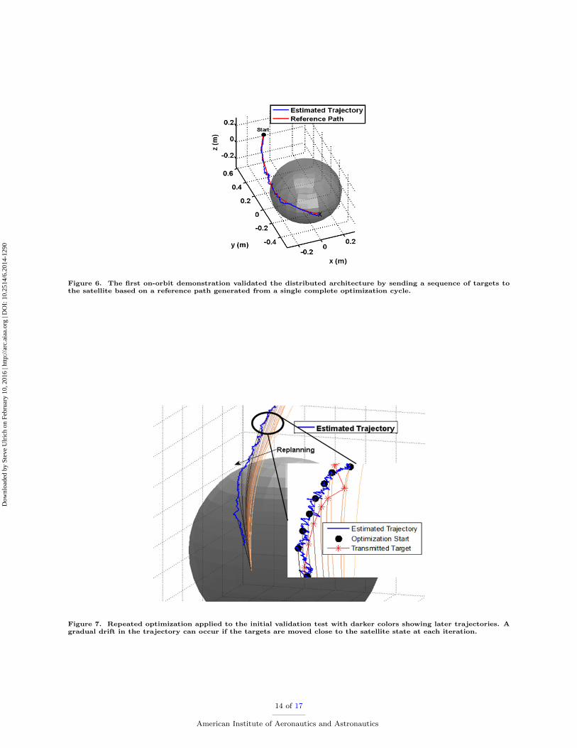
Figure 6. The first on-orbit demonstration validated the distributed architecture by sending a sequence of targets tothe satellite based on a reference path generated from a single complete optimization cycle.

Figure 7. Repeated optimization applied to the initial validation test with darker colors showing later trajectories. Agradual drift in the trajectory can occur if the targets are moved close to the satellite state at each iteration.

14 of 17

American Institute of Aeronautics and Astronautics

Dow

nloa

ded

by S

teve

Ulr

ich

on F

ebru

ary

10, 2

016

| http

://ar

c.ai

aa.o

rg |

DO

I: 1

0.25

14/6

.201

4-12

90

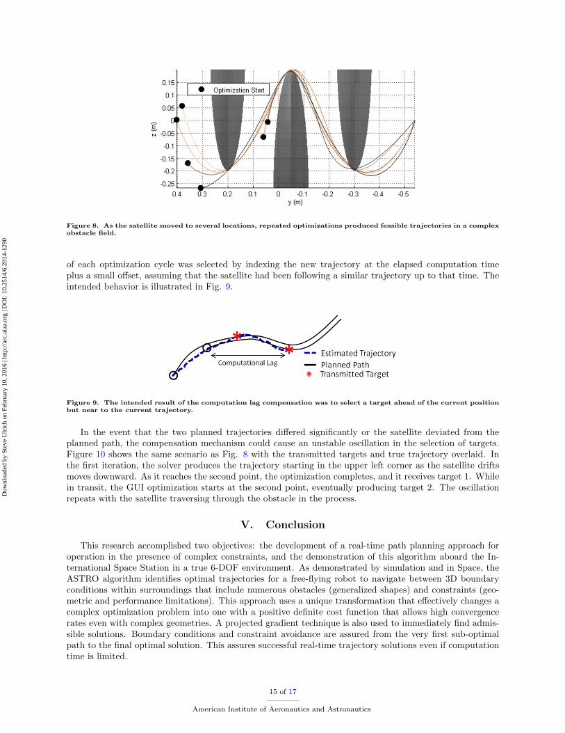
Figure 8. As the satellite moved to several locations, repeated optimizations produced feasible trajectories in a complexobstacle field.

of each optimization cycle was selected by indexing the new trajectory at the elapsed computation timeplus a small offset, assuming that the satellite had been following a similar trajectory up to that time. Theintended behavior is illustrated in Fig. 9.

Figure 9. The intended result of the computation lag compensation was to select a target ahead of the current positionbut near to the current trajectory.

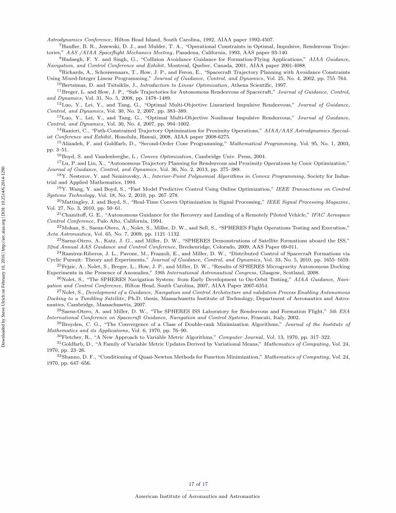
In the event that the two planned trajectories differed significantly or the satellite deviated from theplanned path, the compensation mechanism could cause an unstable oscillation in the selection of targets.Figure 10 shows the same scenario as Fig. 8 with the transmitted targets and true trajectory overlaid. Inthe first iteration, the solver produces the trajectory starting in the upper left corner as the satellite driftsmoves downward. As it reaches the second point, the optimization completes, and it receives target 1. Whilein transit, the GUI optimization starts at the second point, eventually producing target 2. The oscillationrepeats with the satellite traversing through the obstacle in the process.

V. Conclusion

This research accomplished two objectives: the development of a real-time path planning approach foroperation in the presence of complex constraints, and the demonstration of this algorithm aboard the In-ternational Space Station in a true 6-DOF environment. As demonstrated by simulation and in Space, theASTRO algorithm identifies optimal trajectories for a free-flying robot to navigate between 3D boundaryconditions within surroundings that include numerous obstacles (generalized shapes) and constraints (geo-metric and performance limitations). This approach uses a unique transformation that effectively changes acomplex optimization problem into one with a positive definite cost function that allows high convergencerates even with complex geometries. A projected gradient technique is also used to immediately find admis-sible solutions. Boundary conditions and constraint avoidance are assured from the very first sub-optimalpath to the final optimal solution. This assures successful real-time trajectory solutions even if computationtime is limited.

15 of 17

American Institute of Aeronautics and Astronautics

Dow

nloa

ded

by S

teve

Ulr

ich

on F

ebru

ary

10, 2

016

| http

://ar

c.ai

aa.o

rg |

DO

I: 1

0.25

14/6

.201

4-12

90

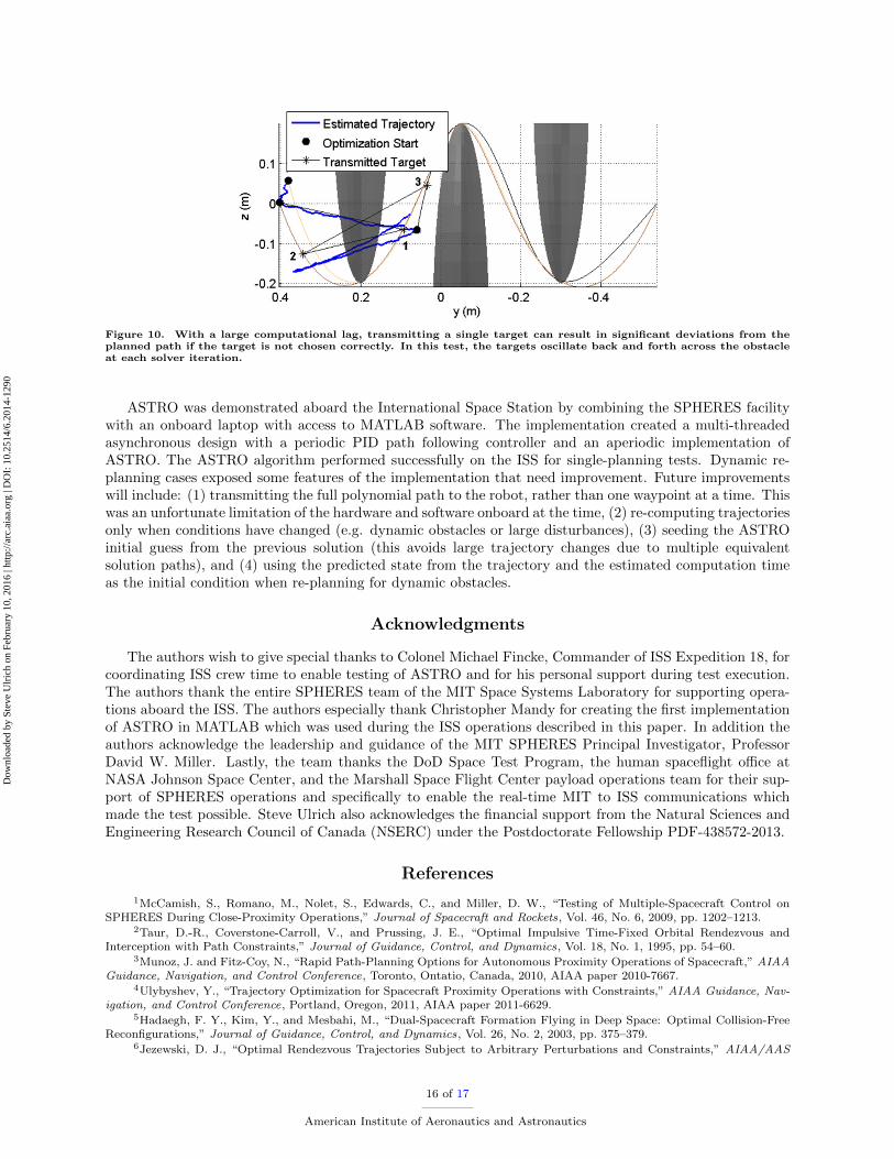
Figure 10. With a large computational lag, transmitting a single target can result in significant deviations from theplanned path if the target is not chosen correctly. In this test, the targets oscillate back and forth across the obstacleat each solver iteration.

ASTRO was demonstrated aboard the International Space Station by combining the SPHERES facilitywith an onboard laptop with access to MATLAB software. The implementation created a multi-threadedasynchronous design with a periodic PID path following controller and an aperiodic implementation ofASTRO. The ASTRO algorithm performed successfully on the ISS for single-planning tests. Dynamic re-planning cases exposed some features of the implementation that need improvement. Future improvementswill include: (1) transmitting the full polynomial path to the robot, rather than one waypoint at a time. Thiswas an unfortunate limitation of the hardware and software onboard at the time, (2) re-computing trajectoriesonly when conditions have changed (e.g. dynamic obstacles or large disturbances), (3) seeding the ASTROinitial guess from the previous solution (this avoids large trajectory changes due to multiple equivalentsolution paths), and (4) using the predicted state from the trajectory and the estimated computation timeas the initial condition when re-planning for dynamic obstacles.

Acknowledgments

The authors wish to give special thanks to Colonel Michael Fincke, Commander of ISS Expedition 18, forcoordinating ISS crew time to enable testing of ASTRO and for his personal support during test execution.The authors thank the entire SPHERES team of the MIT Space Systems Laboratory for supporting opera-tions aboard the ISS. The authors especially thank Christopher Mandy for creating the first implementationof ASTRO in MATLAB which was used during the ISS operations described in this paper. In addition theauthors acknowledge the leadership and guidance of the MIT SPHERES Principal Investigator, ProfessorDavid W. Miller. Lastly, the team thanks the DoD Space Test Program, the human spaceflight office atNASA Johnson Space Center, and the Marshall Space Flight Center payload operations team for their sup-port of SPHERES operations and specifically to enable the real-time MIT to ISS communications whichmade the test possible. Steve Ulrich also acknowledges the financial support from the Natural Sciences andEngineering Research Council of Canada (NSERC) under the Postdoctorate Fellowship PDF-438572-2013.

References

1McCamish, S., Romano, M., Nolet, S., Edwards, C., and Miller, D. W., “Testing of Multiple-Spacecraft Control onSPHERES During Close-Proximity Operations,” Journal of Spacecraft and Rockets, Vol. 46, No. 6, 2009, pp. 1202–1213.

2Taur, D.-R., Coverstone-Carroll, V., and Prussing, J. E., “Optimal Impulsive Time-Fixed Orbital Rendezvous andInterception with Path Constraints,” Journal of Guidance, Control, and Dynamics, Vol. 18, No. 1, 1995, pp. 54–60.

3Munoz, J. and Fitz-Coy, N., “Rapid Path-Planning Options for Autonomous Proximity Operations of Spacecraft,” AIAAGuidance, Navigation, and Control Conference, Toronto, Ontatio, Canada, 2010, AIAA paper 2010-7667.

4Ulybyshev, Y., “Trajectory Optimization for Spacecraft Proximity Operations with Constraints,” AIAA Guidance, Nav-igation, and Control Conference, Portland, Oregon, 2011, AIAA paper 2011-6629.

5Hadaegh, F. Y., Kim, Y., and Mesbahi, M., “Dual-Spacecraft Formation Flying in Deep Space: Optimal Collision-FreeReconfigurations,” Journal of Guidance, Control, and Dynamics, Vol. 26, No. 2, 2003, pp. 375–379.

6Jezewski, D. J., “Optimal Rendezvous Trajectories Subject to Arbitrary Perturbations and Constraints,” AIAA/AAS

16 of 17

American Institute of Aeronautics and Astronautics

Dow

nloa

ded

by S

teve

Ulr

ich

on F

ebru

ary

10, 2

016

| http

://ar

c.ai

aa.o

rg |

DO

I: 1

0.25

14/6

.201

4-12

90

Astrodynamics Conference, Hilton Head Island, South Carolina, 1992, AIAA paper 1992-4507.7Haufler, B. R., Jezewski, D. J., and Mulder, T. A., “Operational Constraints in Optimal, Impulsive, Rendezvous Trajec-

tories,” AAS /AIAA Spaceflight Mechanics Meeting, Pasadena, California, 1993, AAS paper 93-140.8Hadaegh, F. Y. and Singh, G., “Collision Avoidance Guidance for Formation-Flying Applications,” AIAA Guidance,

Navigation, and Control Conference and Exhibit , Montreal, Quebec, Canada, 2001, AIAA paper 2001-4088.9Richards, A., Schouwenaars, T., How, J. P., and Feron, E., “Spacecraft Trajectory Planning with Avoidance Constraints

Using Mixed-Integer Linear Programming,” Journal of Guidance, Control, and Dynamics, Vol. 25, No. 4, 2002, pp. 755–764.10Bertsimas, D. and Tsitsiklis, J., Introduction to Linear Optimization, Athena Scientific, 1997.11Breger, L. and How, J. P., “Safe Trajectories for Autonomous Rendezvous of Spacecraft,” Journal of Guidance, Control,

and Dynamics, Vol. 31, No. 5, 2008, pp. 1478–1489.12Luo, Y., Lei, Y., and Tang, G., “Optimal Multi-Objective Linearized Impulsive Rendezvous,” Journal of Guidance,

Control, and Dynamics, Vol. 30, No. 2, 2007, pp. 383–389.13Luo, Y., Lei, Y., and Tang, G., “Optimal Multi-Objective Nonlinear Impulsive Rendezvous,” Journal of Guidance,

Control, and Dynamics, Vol. 30, No. 4, 2007, pp. 994–1002.14Ranieri, C., “Path-Constrained Trajectory Optimization for Proximity Operations,” AIAA/AAS Astrodynamics Special-

ist Conference and Exhibit , Honolulu, Hawaii, 2008, AIAA paper 2008-6275.15Alizadeh, F. and Goldfarb, D., “Second-Order Cone Programming,” Mathematical Programming, Vol. 95, No. 1, 2003,

pp. 3–51.16Boyd, S. and Vandenberghe, L., Convex Optimization, Cambridge Univ. Press, 2004.17Lu, P. and Liu, X., “Autonomous Trajectory Planning for Rendezvous and Proximity Operations by Conic Optimization,”

Journal of Guidance, Control, and Dynamics, Vol. 36, No. 2, 2013, pp. 375–389.18Y. Nesterov, Y. and Nemirovsky, A., Interior-Point Polynomial Algorithms in Convex Programming, Society for Indus-

trial and Applied Mathematics, 1994.19Y. Wang, Y. and Boyd, S., “Fast Model Predictive Control Using Online Optimization,” IEEE Transactions on Control

Systems Technology, Vol. 18, No. 2, 2010, pp. 267–278.20Mattingley, J. and Boyd, S., “Real-Time Convex Optimization in Signal Processing,” IEEE Signal Processing Magazine,

Vol. 27, No. 3, 2010, pp. 50–61.21Chamitoff, G. E., “Autonomous Guidance for the Recovery and Landing of a Remotely Piloted Vehicle,” IFAC Aerospace

Control Conference, Palo Alto, California, 1994.22Mohan, S., Saenz-Otero, A., Nolet, S., Miller, D. W., and Sell, S., “SPHERES Flight Operations Testing and Execution,”

Acta Astronautica, Vol. 65, No. 7, 2009, pp. 1121–1132.23Saenz-Otero, A., Katz, J. G., and Miller, D. W., “SPHERES Demonstrations of Satellite Formations aboard the ISS,”

32nd Annual AAS Guidance and Control Conference, Breckenridge, Colorado, 2009, AAS Paper 09-011.24Ramirez-Riberos, J. L., Pavone, M., Frazzoli, E., and Miller, D. W., “Distributed Control of Spacecraft Formations via

Cyclic Pursuit: Theory and Experiments,” Journal of Guidance, Control, and Dynamics, Vol. 33, No. 5, 2010, pp. 1655–1659.25Fejzic, A., Nolet, S., Breger, L., How, J. P., and Miller, D. W., “Results of SPHERES Microgravity Autonomous Docking

Experiments in the Presence of Anomalies,” 59th International Astronautical Congress, Glasgow, Scotland, 2008.26Nolet, S., “The SPHERES Navigation System: from Early Development to On-Orbit Testing,” AIAA Guidance, Navi-

gation and Control Conference, Hilton Head, South Carolina, 2007, AIAA Paper 2007-6354.27Nolet, S., Development of a Guidance, Navigation and Control Architecture and validation Process Enabling Autonomous

Docking to a Tumbling Satellite, Ph.D. thesis, Massachusetts Institute of Technology, Department of Aeronautics and Astro-nautics, Cambridge, Massachusetts, 2007.

28Saenz-Otero, A. and Miller, D. W., “The SPHERES ISS Laboratory for Rendezvous and Formation Flight,” 5th ESAInternational Conference on Spacecraft Guidance, Navigation and Control Systems, Frascati, Italy, 2002.

29Broyden, C. G., “The Convergence of a Class of Double-rank Minimization Algorithms,” Journal of the Institute ofMathematics and its Applications, Vol. 6, 1970, pp. 76–90.

30Fletcher, R., “A New Approach to Variable Metric Algorithms,” Computer Journal , Vol. 13, 1970, pp. 317–322.31Goldfarb, D., “A Family of Variable Metric Updates Derived by Variational Means,” Mathematics of Computing, Vol. 24,

1970, pp. 23–26.32Shanno, D. F., “Conditioning of Quasi-Newton Methods for Function Minimization,” Mathematics of Computing, Vol. 24,

1970, pp. 647–656.

17 of 17

American Institute of Aeronautics and Astronautics

Dow

nloa

ded

by S

teve

Ulr

ich

on F

ebru

ary

10, 2

016

| http

://ar

c.ai

aa.o

rg |

DO

I: 1

0.25

14/6

.201

4-12

90