JAWAHARLAL

INSTITUTE OF TECHNOLOGY(Approved by AICTE & Affiliated to Anna University)

COIMBATORE – 641 105

NAME : ___________________________________________

REG.NO : ___________________________________________

SUBJECT : ___________________________________________

COURSE : ___________________________________________

JAWAHARLAL INSTITUTE OF TECHNOLOGY

COIMBATORE – 641 105

DEPARTMENT OF AERONAUTICAL ENGINEERING

Certified that this is the bonafide record work done by

……………….………………………………………………………… in the

AIRCRAFT DESIGN LAB – I of this institution as prescribed by the Anna

University, Coimbatore for the ………........semester during the year 2010 – 2011.

Staff In charge: Head of the Department

University Register No.: ……………………………………

Submitted for the Practical Examination of the Anna University conducted on

……………

INTERNAL EXAMINER EXTERNAL EXAMINER

ABSTRACT In this project we have designed a MILITARY TRAINER AIRCRAFT.

We have taken the sufficient steps to make sure that the aircraft what

we are designing is in an optimum range. The aircraft parameters like

cruise velocity, cruise altitude, wing loading etc and weight estimation,

airfoil selection, wing selection, landing gear selection have been made

with extreme care. The adequate details have been collected to make

our calculation easier and to make design more precision. The details

have been collected from various sources which are given in the

bibliography.

ABBREVIATIONA.R. - Aspect Ratio

b - Wing Span

Cswell - Chord of the Airfoil

Croot - Chord at Root

Ctip - Chord at Tip

C - Mean Aerodynamic Chord

CD - Drag Co-efficient

CD,0 - Zero Lift Drag Co-efficient

Cj - Specific fuel consumption

CL - Lift Co-efficient

D - Drag

E - Endurance

e - Oswald efficiency

g - Acceleration due to gravity

G - Factor due to ground effect

JA, JT - Symbols

h - Height from ground

hOB - Obstacle height

k1 - Proportionality constant

kuc- Factor depends on flap deflection

KA , KT - Symbols

L - Lift

( LD )loiter - Lift-to-drag ratio at loiter

( LD )cruise - Lift-to-drag ratio at cruise

M - Mach number of aircraft

mff - Mission segment fuel fraction

N - Time between initiation of rotation and actual

R - Range

Re - Reynolds Number

R/C - Rate of climb

S - Wing Area

Sa - Approach distance

Sab - Distance require to clear an obstacle after becoming airborne

Sf - Flare distance

Sg - Ground Roll

Sref. - Reference surface area

Swet.. - Wetted surface area

T - Thrust

P - Power

Pcruise - Thrust at cruise

Ptake-off - Thrust at take-off

( PW )loiter - Thrust-to-weight ratio at loiter

( PW )cruise - Thrust-to-weight ratio at cruise

( PW )takeoff - Thrust-to-weight ratio at take-off

Vcruise - Velocity at cruise

Vstall - Velocity at stall

VLO - Lift off Speed

VTD - Touch down speed

Wcrew - Crew weight

Wempty - Empty weight of aircraft

Wfuel - Weight of fuel

Wpayload - Payload of aircraft

W0 - Overall weight of aircraft

WS - Wing loading

ρ - Density of air

μ - Dynamic viscosity

μ r - Co-efficient of rolling friction

λ - Tapered ratio

θOB - Angle between flight path and take-off

β - Turning angle

φ - Gliding angle

R/C - Rate of climb

INTRODUCTIONPurpose and scope of airplane design

An airplane is designed to meet the functional, operational and safety requirements set by or acceptable to the ultimate user. The actual process of design is a complex and long drawn out engineering task involving:

Selection of airplane type and shape Determination of geometric parameters Selection of power plant Structural design and analysis of various components and Determination of airplane flight and operational characteristics.

Over the year of this century, aircraft have evolved in many directions and the design of any modern plane is a joint project for a large body of competent engineers and technicians, headed by a chief designer. Different groups in the project specialize in the design of different components of the airplane, such as the wing, fuselage etc.

A new experimental plane has to meet higher performance requirements than similar planes already in service. Hence design laboratories involved in experimental and research work are indispensable adjuncts to a design office. These laboratories as well as allied specialized design offices and research institutions are concerned in helping the designer to obtain the best possible solutions for all problems pertaining to airplane design and construction and in the development of suitable components and equipment.

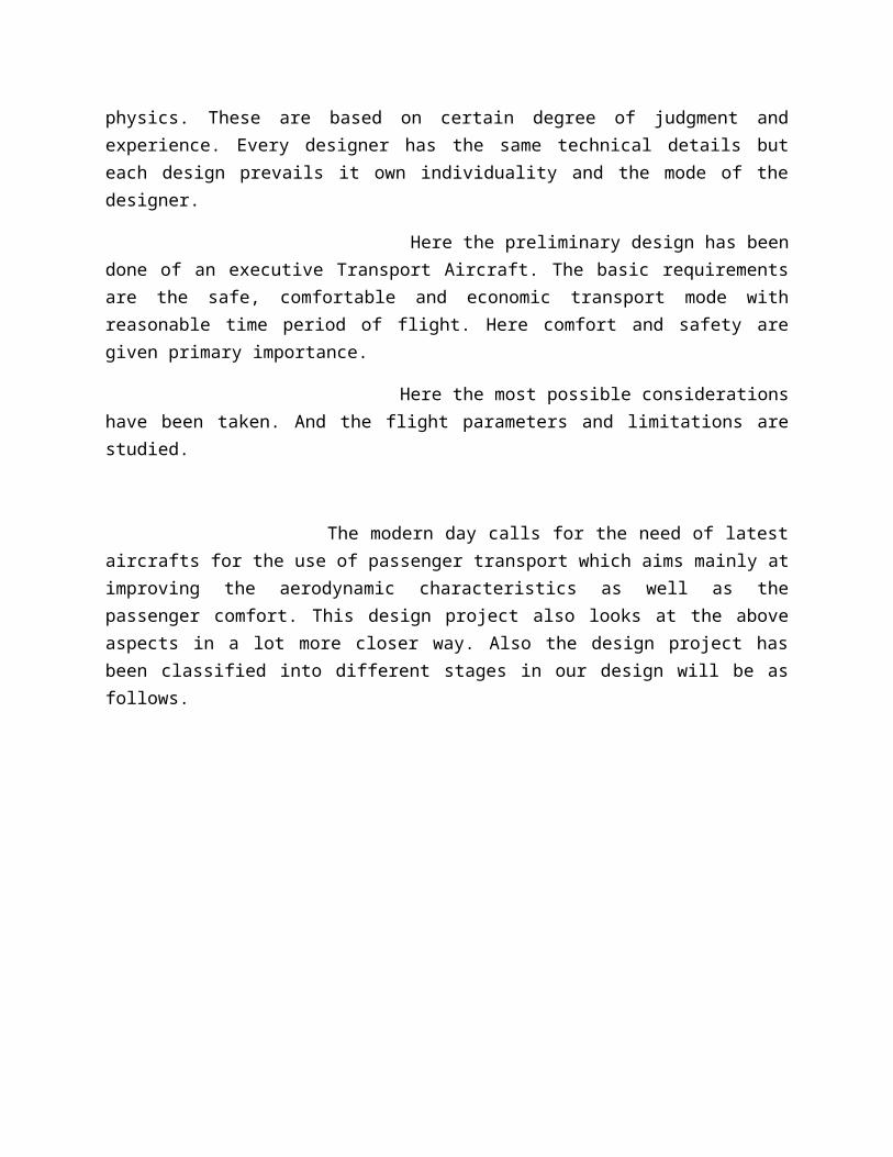
Airplane design procedure is basically a method of trial and error for the design of component units and their harmonization into a complete aircraft system. Thus each trial aims at a closer approach to the final goal and is based on a more profound study of the various problems involved. The three phases of aircraft design are

Conceptual design Preliminary design detail

Phase of aircraft design

Conceptual design

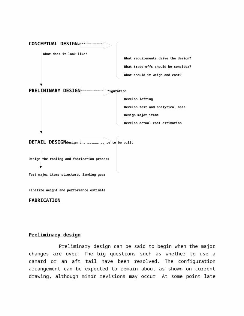
Aircraft design can be broken into three major phases, as depicted in figure. Conceptual design is the primary focus of this book. It is in conceptual design that the basic questions of configuration arrangement, size and weight, and performance are answered.

The first question is “can an affordable aircraft be built that meets the requirements?” if not, the customer may wish to relax the requirements.

Conceptual design is a very fluid process. New ideas and problems emerge as a design is investigated in increasing detail. Each time the latest design is analyzed and sized, it must be redrawn to reflect the new gross weight, fuel weight, wing size, and other changes. Early wind tunnel test often revel problems requiring some changes to the configuration.

REQUIREMENTS

CONCEPTUAL DESIGNwill it work?

What does it look like? What requirements drive the design?

What trade-offs should be consider?

What should it weigh and cost?

PRELIMINARY DESIGNfreeze the configuration

Develop lofting

Develop test and analytical base

Design major items

Develop actual cost estimation

DETAIL DESIGNdesign the actual piece to be built

Design the tooling and fabrication process

Test major items structure, landing gear

Finalize weight and performance estimate

FABRICATION

Preliminary design

Preliminary design can be said to begin when the major changes are over. The big questions such as whether to use a canard or an aft tail have been resolved. The configuration arrangement can be expected to remain about as shown on current drawing, although minor revisions may occur. At some point late in preliminary design, even minor changes are stopped when a decision is made to freeze the configuration.

During preliminary design the specialists in area such as structure landing gear and control systems will design and analyze their portion of the aircraft. Testing is initiated in areas such as aerodynamics, propulsion, structures, and control. A mockup may be constructed at this point.

A key activity during preliminary design is “lofting”. Lifting is the mathematical modeling of the outside skin of the aircraft with sufficient accuracy to insure proper fit between its different parts, even if they are designed by different designers and possibly fabricated in different location. Lofting originated in shipyards and was originally done with long flexible rulers called” splines”. This work was done in a loft over the shipyard; hence the name.

The ultimate objective during preliminary design is to ready the company for the detail design stage, also called full-scale development. Thus, the end of preliminary design usually involves a full scale development proposal. In today’s environment, this can result in a situation jokingly referred to as “you-bet-your-company”. The possible loss on an overrun contrast o from lack of sales can exceed the net worth of the company! Preliminary design must establish confidence that the airplane can be built in time and at the estimated cost.

Detailed design

Assuming a favorable decision for entering full scale development, the detail deign phase begins in which the actual pieces to be fabricated are designed. For example, during conceptual and preliminary design the wing box will be designed and analyzed as a whole. During detail design, that whole will be broken down in to individual ribs, spars and skins, each of which must be separately designed and analyzed.

Another important part of detailed is called production design. Specialist determine how the airplane will be fabricated, starting with the smallest and simplest subassemblies and

building up to the final assembly process. Production designers frequently wish to modify the design for ease of manufacture; that can have a major impact on performance or weight. Compromises are inevitable, but the design must still meet the original requirements.

It is interesting to note that in the Soviet Union, the production design is done by a completely different design bureau than the conceptual and preliminary design, resulting in superior producibility at some expense in performance and weight.

During detail design, the testing effort intensifies. Actual structure of the aircraft is fabricated and tested. Control laws for the flight control system arte tested on an “iron-bird” simulator, a detailed working model of the actuator and flight control surfaces. Flight simulator are developed and flown by both company and customer test pilot.

Detail design ends with fabrication of the aircraft. Frequently the fabrication Begins on part of the aircraft before the entire detail-design effort is completed. Hopefully, changes to already- fabricated pieces can be avoided. The further along a design progresses, the more people are involved. In fact, most of the engineers who go to work for a major aerospace company will work in preliminary on detail design.

Classification of airplanes design

Functional classification:

The airplane today is used for a multitude of activities in civil and military fields. Civil applications include cargo transport, passenger travel, mail distribution, and specialized uses like agricultural, ambulance and executive flying. The main types of military airplane at the present time are fighters and bombers. Each of these types may be further divided into various groups, such as strategic fighters, interceptors, escort fighters, tactical bombers and strategic bombers. There are also special aircraft, such as ground attack planes and photo-re-connaisance planes. Sometimes more than one function may be combines so that we have multi-purpose airplanes like fighter-bombers. In addition to these, we have airplanes for training and sport.

Classification by power plants:

Types of engines used for power plant:

Piston engines (krishak, Dakota, super constellation) Turbo-prop engines ( viscount,friendship,An-102) Turbo-fan engines (HJT – 16, Boeing series, MIG-21)

Ramjet engines Rockets (liquid and solid propellants) (X-15A)

Location of power plant:

Engine ( with propeller) located in fuselage nose (single engine) (HT-2,Yak-9,A-109)

Pusher engine located in the rear fuselage (Bede XBD-2) Jet engines submerged in the wing

1. At the root(DH Comet, Tu-104,Tu-16)2. Along the span (Canberra, U-2, YF-12A)

Jet engines in nacelles suspended under the wing (pod mountings) (Boeing 707,DC-8,Convair 880)

Jet engines located on the rear fuselage (Trident, VC – 10 ,i1-62) Jet engines located within the rear fuselage (Hf – 24, lighting,MIG-

19)Classification by configuration:

Airplanes are also classified in accordance with their shape and structural layout, which in turn contribute to their aerodynamic, tactical and operational characteristics. Classification by configuration is made according to:

Shape and position of the wing Type of fuselage Location of horizontal tail surfaces

Shape and position of the wing:

Braved biplane(D.H. Tiger moth) Braced sesquiplane (An-2) Semi-cantilever parasol monoplane (baby ace) Cantilever low wing monoplane (DC-3,HJT-16,I1-18,DH Comet)

Cantilever mid wing monoplane (Hunter, Canberra) Cantilever high wing monoplane (An-22,Brequet 941 Fokker

Friendship) Straight wing monoplane (F-104 A) Swept wing monoplane (HF-24, MIG-21, Lighting) Delta monoplane with small aspect ratio (Avro-707, B-58 Hustler,

AvroVulcan)Type of fuselage

Conventional single fuselage design ( HT-2,Boeing 707 Twin- fuselage design Pod and boom construction (Packet, Vampire)

Types of landing gear:

Retractable landing gear (DC-9,Tu-114,SAAB-35) Non- retractable landing gear (pushpak, An-14, Fuji KM-2) Tail wheel landing gear (HT-2,Dakota,Cessana J85 C) Nose wheel landing gear (Avro-748, Tu-134,F-5A) Bicycle landing gear (Yak-25,HS-P,112)

THE DESIGN

Design is a process of usage of creativity with the knowledge of science where we try to get the most of the best things available and to overcome the pitfalls the previous design has. It is an iterative process to idealism toward with everyone is marching still.

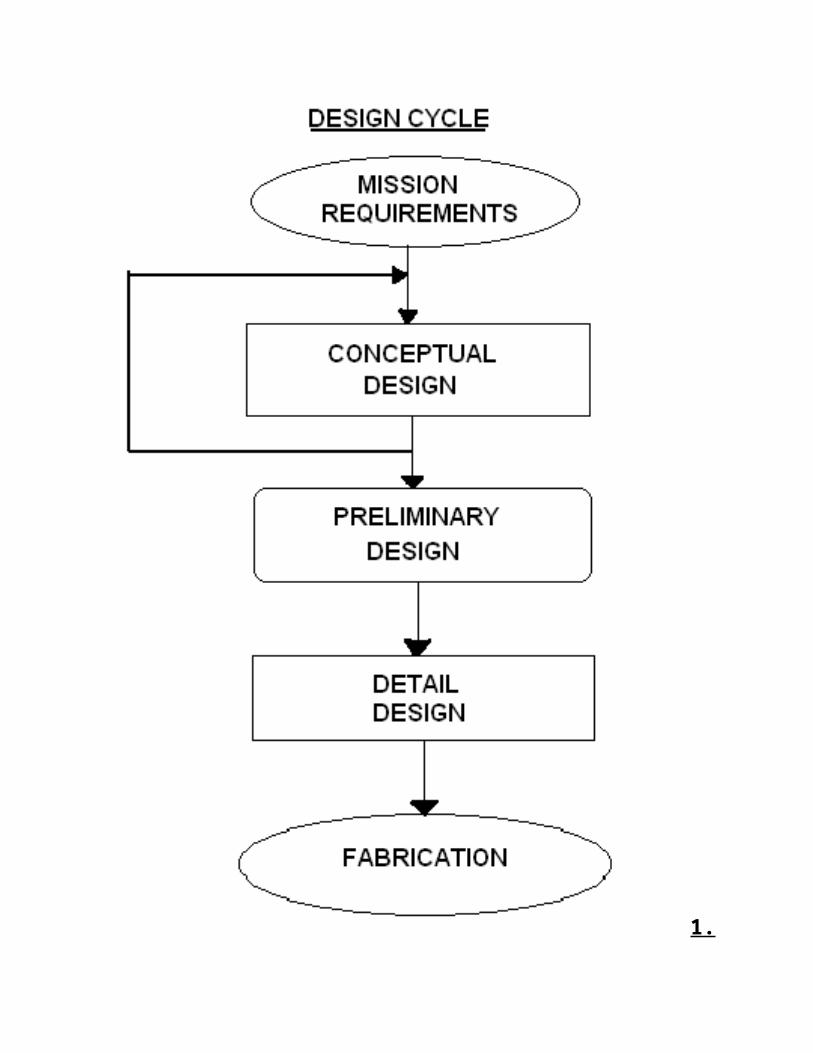
Design of any system is of successful application of fundamentals of physics. Thus the airplane design incorporates the fundamentals of aerodynamics, structures, performance and stability & control and basic physics. These are based on certain degree of judgment and experience. Every designer has the same technical details but each design prevails it own individuality and the mode of the designer.

Here the preliminary design has been done of an executive Transport Aircraft. The basic requirements are the safe, comfortable and economic transport mode with reasonable time period of flight. Here comfort and safety are given primary importance.

Here the most possible considerations have been taken. And the flight parameters and limitations are studied.

The modern day calls for the need of latest aircrafts for the use of passenger transport which aims mainly at improving the aerodynamic characteristics as well as the passenger comfort. This design project also looks at the above aspects in a lot more closer way. Also the design project has been classified into different stages in our design will be as follows.

1.V – n Diagram

Factor of safety – flight envelope:

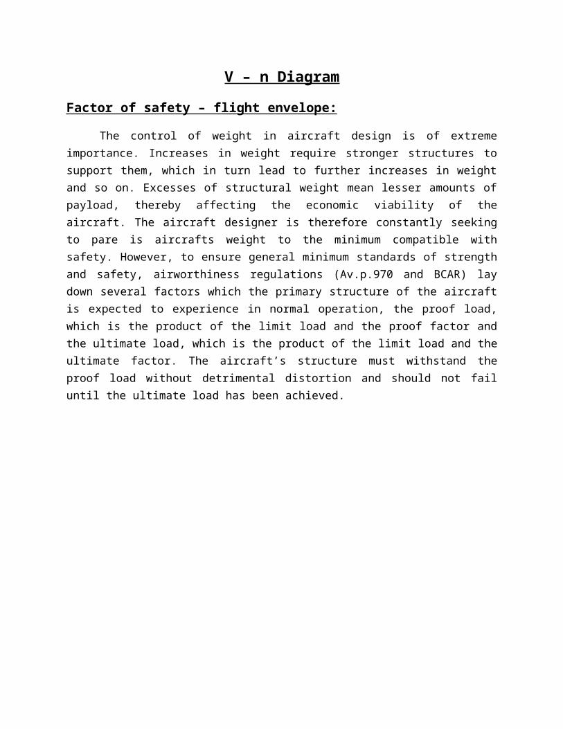
The control of weight in aircraft design is of extreme importance. Increases in weight require stronger structures to support them, which in turn lead to further increases in weight and so on. Excesses of structural weight mean lesser amounts of payload, thereby affecting the economic viability of the aircraft. The aircraft designer is therefore constantly seeking to pare is aircrafts weight to the minimum compatible with safety. However, to ensure general minimum standards of strength and safety, airworthiness regulations (Av.p.970 and BCAR) lay down several factors which the primary structure of the aircraft is expected to experience in normal operation, the proof load, which is the product of the limit load and the proof factor and the ultimate load, which is the product of the limit load and the ultimate factor. The aircraft’s structure must withstand the proof load without detrimental distortion and should not fail until the ultimate load has been achieved.

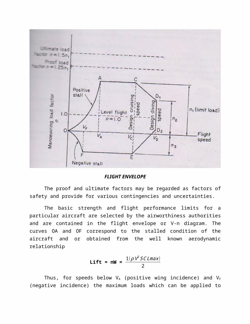
FLIGHT ENVELOPE

The proof and ultimate factors may be regarded as factors of safety and provide for various contingencies and uncertainties.

The basic strength and flight performance limits for a particular aircraft are selected by the airworthiness authorities and are contained in the flight envelope or V-n diagram. The curves OA and OF correspond to the stalled condition of the aircraft and or obtained from the well known aerodynamic relationship

Lift = nW = 1(ρV 2SC Lmax)2

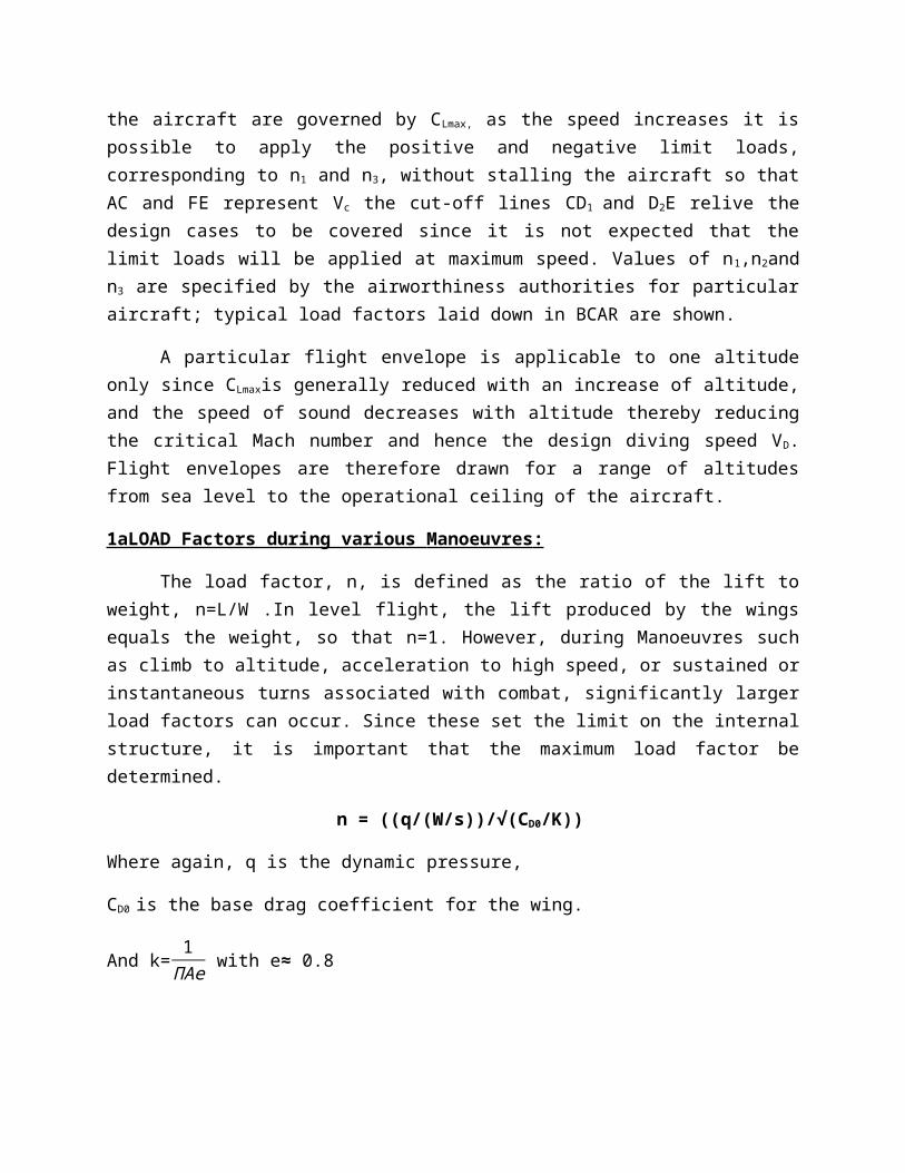
Thus, for speeds below VA (positive wing incidence) and VF (negative incidence) the maximum loads which can be applied to the aircraft are governed by CLmax, as the speed increases it is possible to apply the positive and negative limit loads, corresponding to n1 and n3, without stalling the aircraft so that AC and FE represent Vc the cut-off lines CD1 and D2E relive the design cases to be covered since it is not expected that the limit loads will be applied at maximum speed. Values of n1,n2and n3 are specified by the airworthiness authorities for particular aircraft; typical load factors laid down in BCAR are shown.

A particular flight envelope is applicable to one altitude only since CLmaxis generally reduced with an increase of altitude, and the speed of sound decreases with altitude thereby reducing the critical Mach number and hence the design diving speed VD. Flight envelopes are therefore drawn for a range of altitudes from sea level to the operational ceiling of the aircraft.

1aLOAD Factors during various Manoeuvres :

The load factor, n, is defined as the ratio of the lift to weight, n=L/W .In level flight, the lift produced by the wings equals the weight, so that n=1. However, during Manoeuvres such as climb to altitude, acceleration to high speed, or sustained or instantaneous turns associated with combat, significantly larger load factors can occur. Since these set the limit on the internal structure, it is important that the maximum load factor be determined.

n = ((q/(W/s))/√(CD0/K))

Where again, q is the dynamic pressure,

CD0 is the base drag coefficient for the wing.

And k=1ПAe with e≈ 0.8

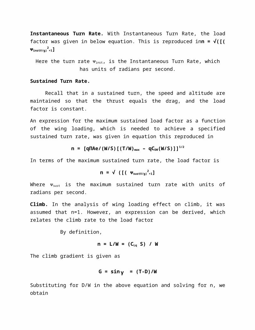
Instantaneous Turn Rate. With Instantaneous Turn Rate, the load factor was given in below equation. This is reproduced inn = √([( ᴪinstV/g)

2+1]

Here the turn rate ᴪinst, is the Instantaneous Turn Rate, which has units of radians per second.

Sustained Turn Rate.

Recall that in a sustained turn, the speed and altitude are maintained so that the thrust equals the drag, and the load factor is constant.

An expression for the maximum sustained load factor as a function of the wing loading, which is needed to achieve a specified sustained turn rate, was given in equation this reproduced in

n = [qПAe/(W/S)[(T/W)max – qCD0(W/S)]]1/2

In terms of the maximum sustained turn rate, the load factor is

n = √ ([( ᴪsustV/g)2+1]

Where ᴪsust is the maximum sustained turn rate with units of radians per second.

Climb. In the analysis of wing loading effect on climb, it was assumed that n=1. However, an expression can be derived, which relates the climb rate to the load factor

By definition,

n = L/W = (CLq S) / W

The climb gradient is given as

G = sinᵧ = (T-D)/W

Substituting for D/W in the above equation and solving for n, we obtain

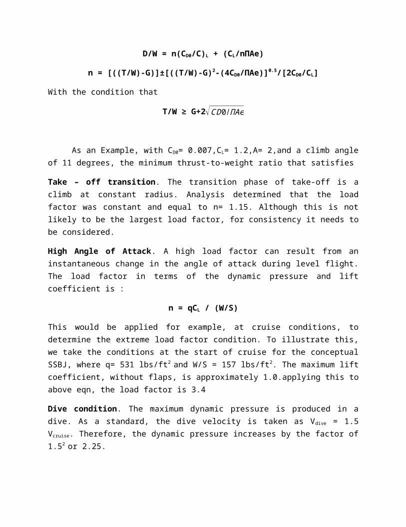
D/W = n(CD0/C)L + (CL/nПAe)

n = [((T/W)-G)]±[((T/W)-G)2-(4CD0/ПAe)]0.5/[2CD0/CL]

With the condition that

T/W ≥ G+2√C D 0/ПAe

As an Example, with CD0= 0.007,CL= 1.2,A= 2,and a climb angle of 11 degrees, the minimum thrust-to-weight ratio that satisfies

Take – off transition. The transition phase of take-off is a climb at constant radius. Analysis determined that the load factor was constant and equal to n= 1.15. Although this is not likely to be the largest load factor, for consistency it needs to be considered.

High Angle of Attack. A high load factor can result from an instantaneous change in the angle of attack during level flight. The load factor in terms of the dynamic pressure and lift coefficient is :

n = qCL / (W/S)

This would be applied for example, at cruise conditions, to determine the extreme load factor condition. To illustrate this, we take the conditions at the start of cruise for the conceptual SSBJ, where q= 531 lbs/ft2 and W/S = 157 lbs/ft2. The maximum lift coefficient, without flaps, is approximately 1.0.applying this to above eqn, the load factor is 3.4

Dive condition. The maximum dynamic pressure is produced in a dive. As a standard, the dive velocity is taken as Vdive = 1.5 Vcruise. Therefore, the dynamic pressure increases by the factor of 1.52 or 2.25.

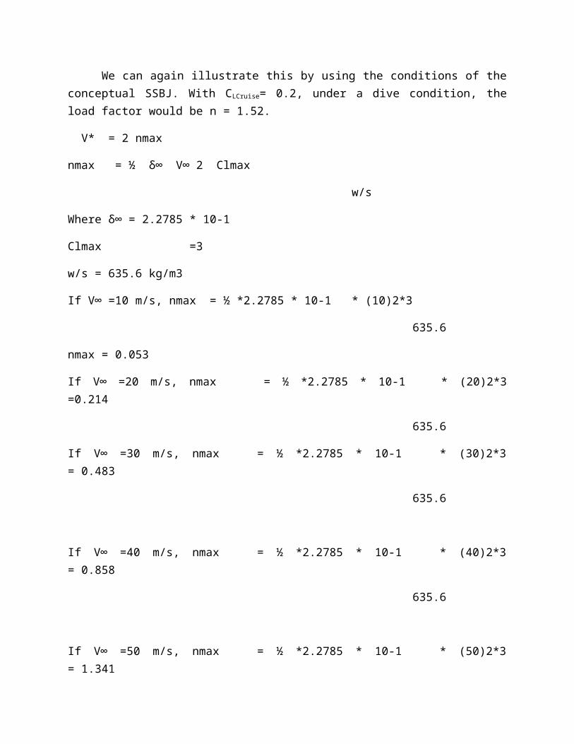
We can again illustrate this by using the conditions of the conceptual SSBJ. With CLCruise= 0.2, under a dive condition, the load factor would be n = 1.52.

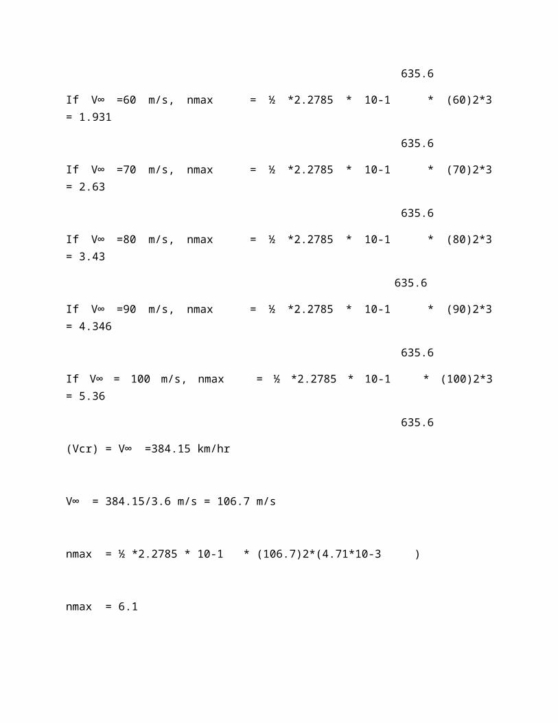
V* = 2 nmax

nmax = ½ δ∞ V∞ 2 Clmax

w/s

Where δ∞ = 2.2785 * 10-1

Clmax =3

w/s = 635.6 kg/m3

If V∞ =10 m/s, nmax = ½ *2.2785 * 10-1 * (10)2*3

635.6

nmax = 0.053

If V∞ =20 m/s, nmax = ½ *2.2785 * 10-1 * (20)2*3 =0.214

635.6

If V∞ =30 m/s, nmax = ½ *2.2785 * 10-1 * (30)2*3 = 0.483

635.6

If V∞ =40 m/s, nmax = ½ *2.2785 * 10-1 * (40)2*3 = 0.858

635.6

If V∞ =50 m/s, nmax = ½ *2.2785 * 10-1 * (50)2*3 = 1.341

635.6

If V∞ =60 m/s, nmax = ½ *2.2785 * 10-1 * (60)2*3 = 1.931

635.6

If V∞ =70 m/s, nmax = ½ *2.2785 * 10-1 * (70)2*3 = 2.63

635.6

If V∞ =80 m/s, nmax = ½ *2.2785 * 10-1 * (80)2*3 = 3.43

635.6

If V∞ =90 m/s, nmax = ½ *2.2785 * 10-1 * (90)2*3 = 4.346

635.6

If V∞ = 100 m/s, nmax = ½ *2.2785 * 10-1 * (100)2*3 = 5.36

635.6

(Vcr) = V∞ =384.15 km/hr

V∞ = 384.15/3.6 m/s = 106.7 m/s

nmax = ½ *2.2785 * 10-1 * (106.7)2*(4.71*10-3 )

nmax = 6.1

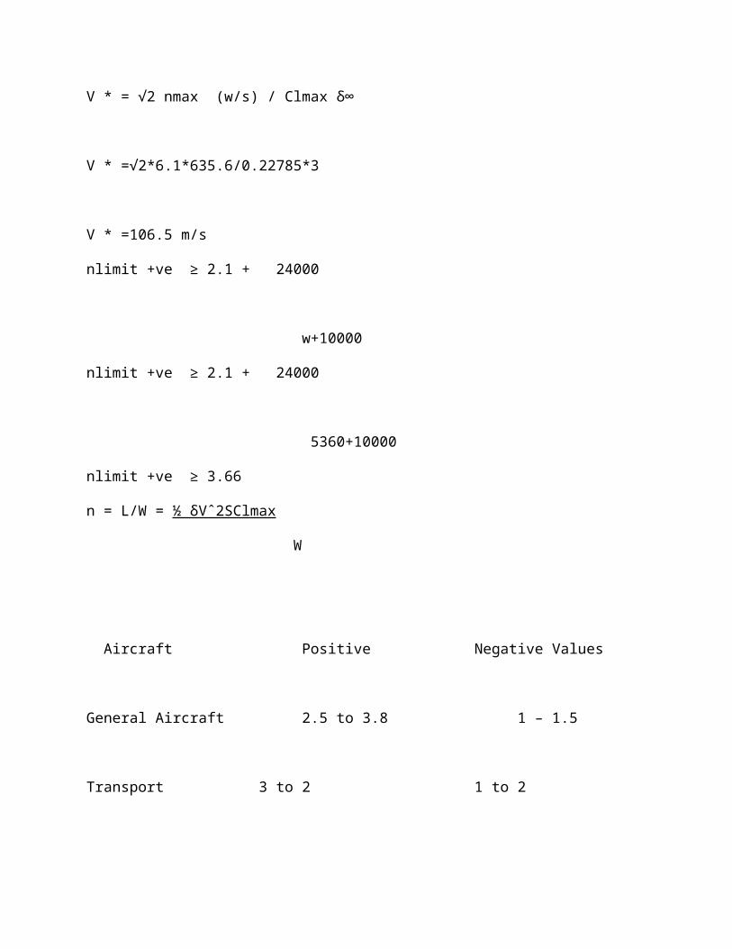
V * = √2 nmax (w/s) / Clmax δ∞

V * =√2*6.1*635.6/0.22785*3

V * =106.5 m/s

nlimit +ve ≥ 2.1 + 24000

w+10000

nlimit +ve ≥ 2.1 + 24000

5360+10000

nlimit +ve ≥ 3.66

n = L/W = ½ δVˆ2SClmax

W

Aircraft Positive Negative Values

General Aircraft 2.5 to 3.8 1 – 1.5

Transport 3 to 2 1 to 2

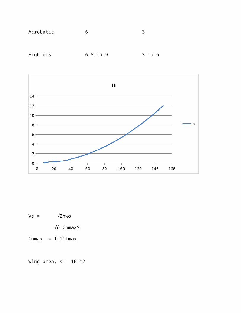
Acrobatic 6 3

Fighters 6.5 to 9 3 to 6

0 20 40 60 80 100 120 140 1600

2

4

6

8

10

12

14

n

n

Vs = √2nwo

√δ CnmaxS

Cnmax = 1.1Clmax

Wing area, s = 16 m2

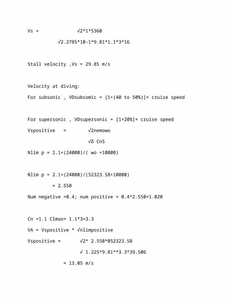
Vs = √2*1*5360

√2.2785*10-1*9.81*1.1*3*16

Stall velocity ,Vs = 29.85 m/s

Velocity at diving:

For subsonic , VDsubsomic = [1+(40 to 50%)]× cruise speed

For supersonic , VDsupersonic = [1+20%]× cruise speed

Vspositive = √2nemowo

√δ CnS

Nlim p = 2.1+(24000)/( wo +10000)

Nlim p = 2.1+(24000)/(52323.58+10000)

= 2.550

Num negative =0.4; num positive = 0.4*2.550=1.020

Cn =1.1 Clmax= 1.1*3=3.3

VA = Vspositive * √nlimpositive

Vspositive = √2* 2.550*052323.58

√ 1.225*9.81**3.3*39.506

= 13.05 m/s

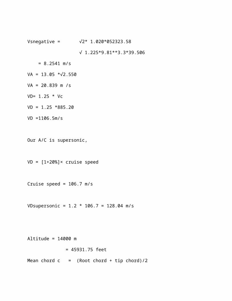
Vsnegative = √2* 1.020*052323.58

√ 1.225*9.81**3.3*39.506

= 8.2541 m/s

VA = 13.05 *√2.550

VA = 20.839 m /s

VD= 1.25 * Vc

VD = 1.25 *885.20

VD =1106.5m/s

Our A/C is supersonic,

VD = [1+20%]× cruise speed

Cruise speed = 106.7 m/s

VDsupersonic = 1.2 * 106.7 = 128.04 m/s

Altitude = 14000 m

= 45931.75 feet

Mean chord c = (Root chord + tip chord)/2

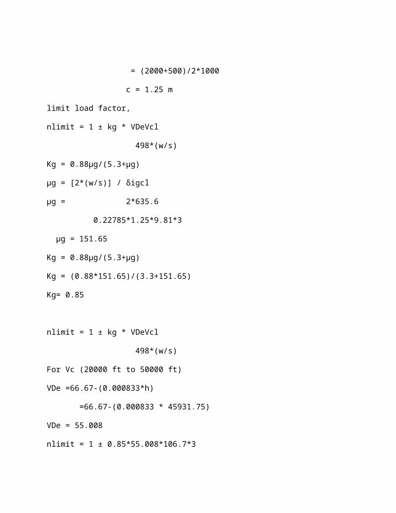
= (2000+500)/2*1000

c = 1.25 m

limit load factor,

nlimit = 1 ± kg * VDeVcl

498*(w/s)

Kg = 0.88µg/(5.3+µg)

µg = [2*(w/s)] / δigcl

µg = 2*635.6

0.22785*1.25*9.81*3

µg = 151.65

Kg = 0.88µg/(5.3+µg)

Kg = (0.88*151.65)/(3.3+151.65)

Kg= 0.85

nlimit = 1 ± kg * VDeVcl

498*(w/s)

For Vc (20000 ft to 50000 ft)

VDe =66.67-(0.000833*h)

=66.67-(0.000833 * 45931.75)

VDe = 55.008

nlimit = 1 ± 0.85*55.008*106.7*3

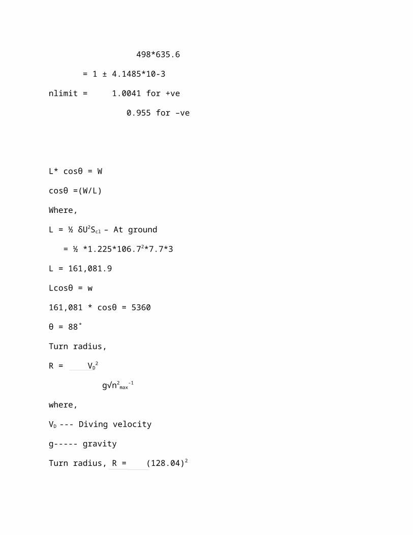
498*635.6

= 1 ± 4.1485*10-3

nlimit = 1.0041 for +ve

0.955 for –ve

L* cosθ = W

cosθ =(W/L)

Where,

L = ½ δU2Scl – At ground

= ½ *1.225*106.72*7.7*3

L = 161,081.9

Lcosθ = w

161,081 * cosθ = 5360

θ = 88˚

Turn radius,

R = VD2

g√n2max

-1

where,

VD --- Diving velocity

g----- gravity

Turn radius, R = (128.04)2

9.81√n2max

-1

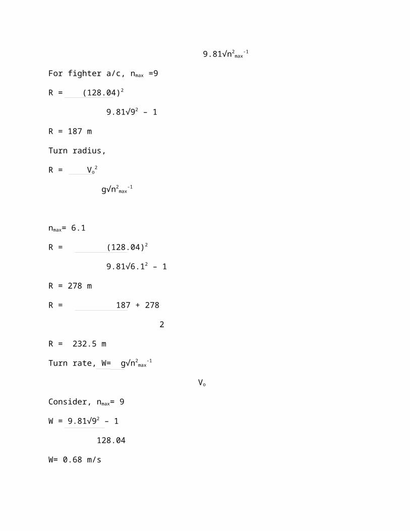
For fighter a/c, nmax =9

R = (128.04)2

9.81√92 – 1

R = 187 m

Turn radius,

R = Vo2

g√n2max

-1

nmax= 6.1

R = (128.04)2

9.81√6.12 – 1

R = 278 m

R = 187 + 278

2

R = 232.5 m

Turn rate, W= g√n2max

-1

Vo

Consider, nmax= 9

W = 9.81√92 – 1

128.04

W= 0.68 m/s

For , nmax= 6.1

W = 9.81√6.12 – 1

128.04

W= 0.46 m/s

0 10 20 30 40 50 60 70 80 90 100 110 120 130 140 150 160

-1.5-1

-0.50

0.51

1.52

2.53

3.54

4.55

5.56

6.57

7.58

8.59

9.510

10.511

11.512

12.513

-1-1-1-0.91

0 0.0530.2140.483

0.8581.341

1.931

2.63

3.43

4.346

5.36

6.49

7.72

9.06

10.4

12.07

Vn diagram

n

VELOCITY (V)

LOAD

FAC

TOR

(n)

positive limit load fac-tor

stall vel-cocity

Cruise velocity

Dive velocity

2. GUST LOAD ESTIMATION

2a Gust loads:

Gust loads are unsteady aerodynamic loads that are produced by atmospheric turbulence. They represent a load factor that is added to the aerodynamic loads, which were presented in the previous sections. The effect of a turbulent gust is to produce short-time change in the effective angle of attack. This change can be either positive or negative, thereby producing an increase or decrease in the wing lift and a change in the load factor, n= ±L/W.

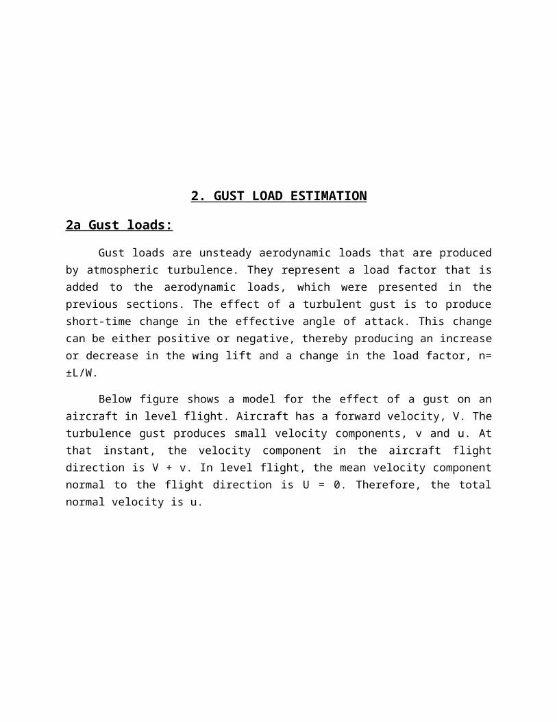
Below figure shows a model for the effect of a gust on an aircraft in level flight. Aircraft has a forward velocity, V. The turbulence gust produces small velocity components, v and u. At that instant, the velocity component in the aircraft flight direction is V + v. In level flight, the mean velocity component normal to the flight direction is U = 0. Therefore, the total normal velocity is u.

MODEL FOR GUST LOAD EFFECT ON A AIRCRAFT IN LEVEL FLIGHT

In most cases, u and v are much less than the flight speed, V.Therefore, V + v ≈V. Based on this assumption, the effective angle of attack is

∆α = tan-1 (u/V)

Because u is small compared to V

∆α ≈tan-1 (u/V)

The incremental lift produced by the small change in the angle of attack is

∆L = 1(ρV 2SC La∆α )2

Substituting the above equation gives

∆L = 1(ρV 2SC Lau)2

The incremental load factor is then

∆n = S/2W (ρuV C La¿

The peak load factor is then the sum of the mean load factor at cruise (n=1) and the fluctuation load factor, namely,

npeak= n + ∆n

The gusts that result from at atmospheric turbulence occur in a fairly large band of frequencies. Therefore their effect on an aircraft depends on factors that affect its frequency response. In particular, the frequency response is governed by an equivalent mass ratio,µ, defined as

µ = (2W/S) /(ρuV C La)

Where c is the mean chord of the mail wing and g is the gravitational constant. Note that µ is dimensionless, so that in British units, gc= 32.2f – (lbm/ lbf) – s2 is required in the numerator.

The mass ratio, µ is a parameter in a response coefficient, K, which is defined differently for subsonic and supersonic aircraft, namely,

K = 0.88 µ / (5.33 + µ) (Subsonic)

K = µ1.03 / (6.95 + µ1.03)(Supersonic)

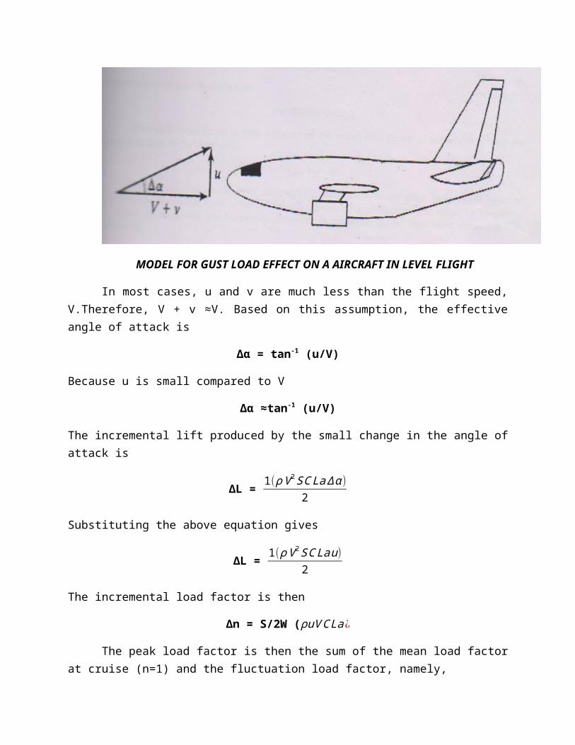
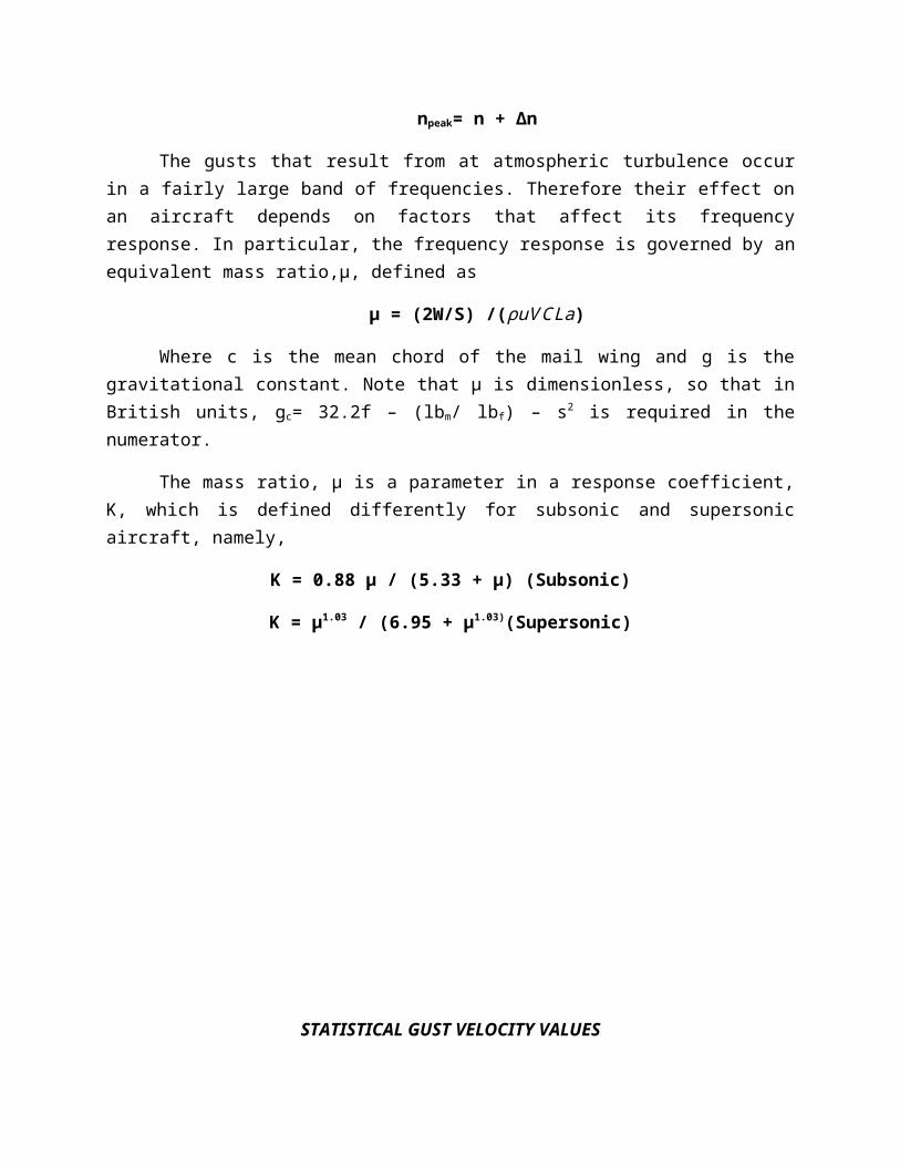
STATISTICAL GUST VELOCITY VALUES

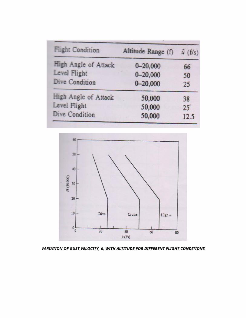
VARIATION OF GUST VELOCITY, ū, WITH ALTITUDE FOR DIFFERENT FLIGHT CONDITIONS

The normal component of the gust velocity, u, is the product of the statistical average of values taken from flight data, ū, and the response coefficient, or

u = K ū

The above table gives values of ū. The variation with altitude is presented in the figure.

Considering equation, we observe that turbulent gusts have a greater effect on aircraft with a lower wing loading. Therefore, a higher wing loading is better to produce a “smoother” flight, as well as in lowering the incremental structural loads.

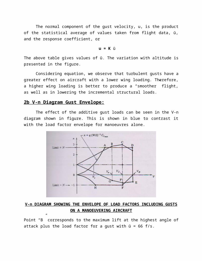
2b V-n Diagram Gust Envelope:

The effect of the additive gust loads can be seen in the V-n diagram shown in figure. This is shown in blue to contrast it with the load factor envelope for manoeuvres alone.

V-n DIAGRAM SHOWING THE ENVELOPE OF LOAD FACTORS INCLUDING GUSTS ON A MANOEUVERING AIRCRAFT

Point “B” corresponds to the maximum lift at the highest angle of attack plus the load factor for a gust with ū = 66 f/s.

Point “C” refers to the load factor at the design cruise velocity, Vc plus that for a gust with ū = 50 f/s.

Point “D” corresponds to the load factor at the dive velocity, VD plus that for a gust with ū = 25 f/s.

Points “E”, “F” and “G” correspond to the additional of loads from negative gusts at the velocities corresponding to dive, VD; cruise, VC; and maximum lift, Vα ,respectively.For gust velocity, Vb

Max value, Vb =10.34 m/s

Min value, Vb =5.30 m/s

For Vb = 10.34 m/s

nlimit = 1 ± kg * VDeVcl

498*(w/s)

V=10.34 m/s

VDe =84.67+(0.000933*h)

= 84.67+(0.000933*14000)

VDe = 97.732

nlimit = 1 ± 0.85*97.732*10.34*3

498*635.6

nlimit = 1.0086 for +ve

0.9999 for –ve

Vd = 128.04

nlimit = 1 ± 0.85*55.008*128.04*3

498*635.6

nlimit = 1.057for +ve

0.94 for –ve

For Vs= 29.85

nlimit = 1 ± 0.85*55.008*29.85*3

498*635.6

nlimit = 1.013for +ve

0.94 for –ve

Plots like figure which superpose the manoeuvre loads with the gust loads, are important for determine the conditions that produce the highest load factors. The largest values are the ones used in the structural design.

2c Design Load Factor:

The “limit load factor” denoted in the above figures is the highest of all the manoeuvring load factors plus the incremental load due to turbulent gusts.

nlimit = nmax + ∆n

In order to provide a margin of safety to the structural design, the limit load factor is multiplied by a “safety factor”, SF. The standard safety factor used in the aircraft industry is 1.5. This value was originally defined in 1930 because it corresponds to the ratio of the tensile ultimate load strength to yield strength of 24 STaluminium alloy, a material commonly used on aircraft. Over the years since it was first designated, this safety factor has proved to be reliable.

The “Design Load Factor” is then defined as the product of the limit load factor and the safety factor.

ndesign= 1.5 nlimit

This factor represents the ultimate load that the internal structure is designed to withstand. In the selection of materials used in the design of the structure, the material ultimate stress will be divided by the nlimit to guarantee that the material will not fail up to the design load limit.

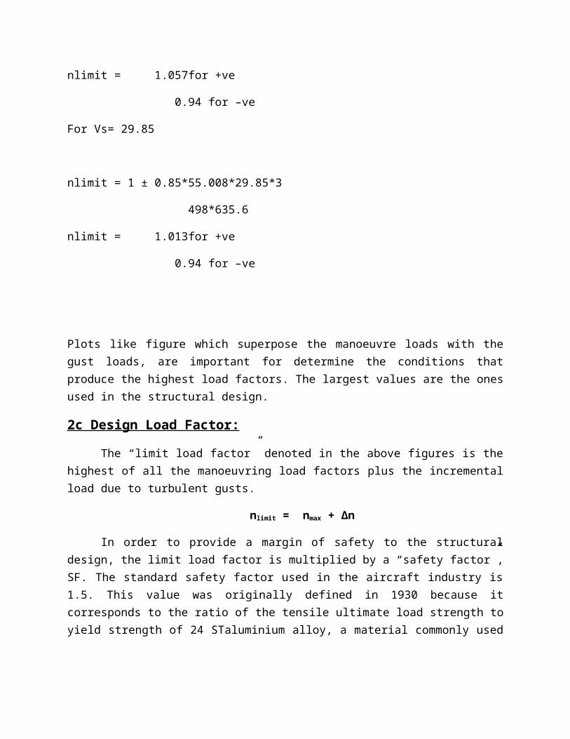
Bending moment Vs Span

BM = -LX3/6b

Where, L----ift ,

b---- span(one side)

X---- 0.5,1,………..3.85(sectional span)

L= ½ δV2Sl2

S= b2/AR

b-half span = 3.85

S = (3.85)2/4

S = 3.7

L = ½ * 2.2785*10-1*(106.7)2* 3.7 *3

L =14,396.96

BM = -LX3/6b

BM = -14,396.96*X3/6*3.85

0 0.5 1 1.5 2 2.5 3 3.5 4 4.5

-40000

-35000

-30000

-25000

-20000

-15000

-10000

-5000

0

bending moment

bending moment

X BM

0.5 -77.9

1.0 -623.2

1.5 -2103.3

2.0 -4985.6

2.5 -9737.5

3.0 -16,826.49

3.5 -26,719.8

3.85 -35,564.11

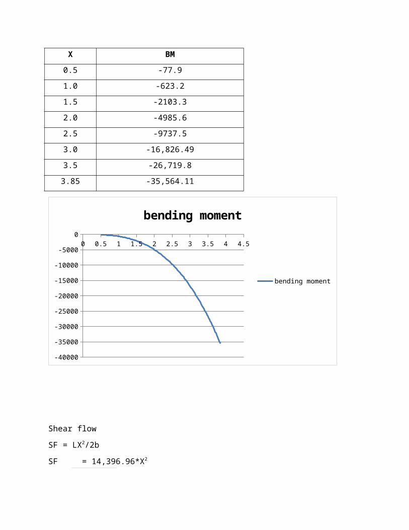
Shear flow

SF = LX2/2b

SF = 14,396.96*X2

2 * 3.85

X SF

0.5 467.43

1.0 1869.73

1.5 4206.9

2.0 7478.9

2.5 11,685.8

3.0 16,827.6

3.5 22,904.25

3.85 27,714.14

0 0.5 1 1.5 2 2.5 3 3.5 4 4.50

5000

10000

15000

20000

25000

30000

shear flow

shear flow

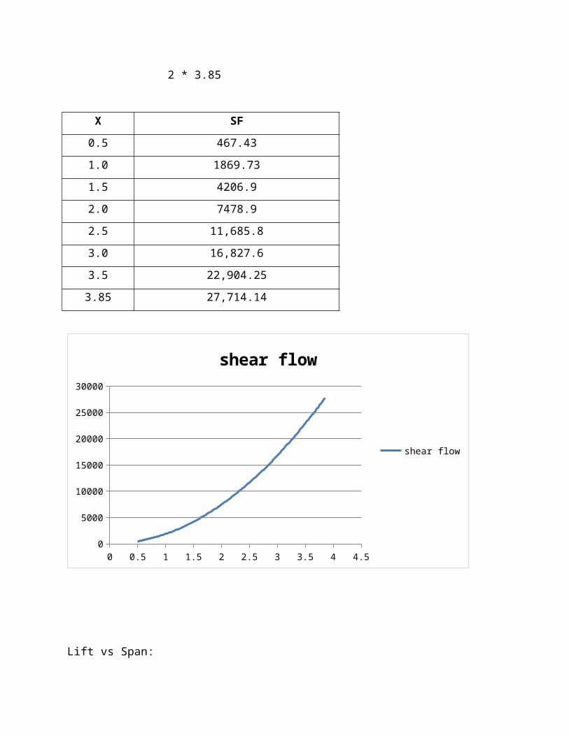
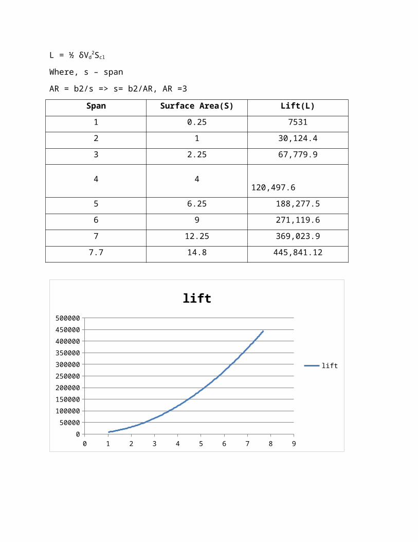
Lift vs Span:

L = ½ δVd2Scl

Where, s – span

AR = b2/s => s= b2/AR, AR =3

Span Surface Area(S) Lift(L)

1 0.25 7531

2 1 30,124.4

3 2.25 67,779.9

4 4 120,497.6

5 6.25 188,277.5

6 9 271,119.6

7 12.25 369,023.9

7.7 14.8 445,841.12

0 1 2 3 4 5 6 7 8 90

50000

100000

150000

200000

250000

300000

350000

400000

450000

500000

lift

lift

3. MANOEUVERING LOADS ESTIMATION

3a Symmetrical manoeuvers loads:

In symmetric manoeuvers we consider the motion of the aircraft initiated by movement of the control surfaces in the plane of symmetry. Examples of such maneuvers are loops, straight pull – outs and bunts, and tail plane loads at given flight speeds and altitudes. The effects of atmospheric turbulence and gusts are discussed.

3b Level flight:

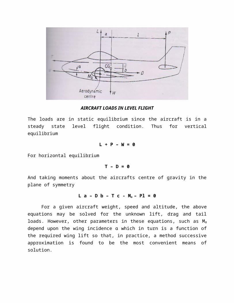
Although steady level flight is not a maneuver in the strict sense of the world, it is a usefulcondition to investigate initial since it establishes points of load application and gives some idea of the equilibrium of an aircraft in the longitudinal plane. The loads acting on an aircraft in steady flight are shown in figure, with the following notation.

L is the lift acting at the aerodynamic centre of the wing,

D is the aircraft drag,

M o is the aerodynamic pitching moment of the aircraft less its horizontal tail,

P is the horizontal tail load acting at the aerodynamic centre of the tail, usually taken to be at approximately one-third of the tail plane chord,

W is the aircraft weight acting at its centre of gravity,

T is the engine thrust, assumed here to act parallel to the direction of flight in order to simplify calculation.

AIRCRAFT LOADS IN LEVEL FLIGHT

The loads are in static equilibrium since the aircraft is in a steady state level flight condition. Thus for vertical equilibrium

L + P – W = 0

For horizontal equilibrium

T – D = 0

And taking moments about the aircrafts centre of gravity in the plane of symmetry

L a – D b – T c - Mo – Pl = 0

For a given aircraft weight, speed and altitude, the above equations may be solved for the unknown lift, drag and tail loads. However, other parameters in these equations, such as M0

depend upon the wing incidence α which in turn is a function of the required wing lift so that, in practice, a method successive approximation is found to be the most convenient means of solution.

As a first approximation we assume that tail load P is small compared with the wing lift L so that, from the above equation L ≈ W. From aerodynamic theory with the usual notation

L = 1(ρV 2SC L)2

Hence

1(ρV 2SC L)2

≈ W

The above equation gives the approximate lift coefficient CL and thus (from CL – α curves established by wind tunnel tests) the wing incidence α. The drag load D follows (knowing V and α) and hence we obtain the required engine thrust T from above equation also Mo, a, b, c & l may be calculated (again since V and α are known) and the equation can be solved for P.As a second approximation this value of P is substituted in above equation to obtain a more accurate value for L and the procedure is repeated. Usually three approximations are sufficient to produce reasonably accurate values.

In most cases P, D and T are small compared with the lift and aircraft weight. Therefore, from above equation L ≈ W and substitution in the above equation gives, neglecting D and T

P ≈W ((a/l)-Mo/l))

We see from above return equation that if a is large then P will most likely be positive. In other words the tail load acts upwards when the centre of gravity of the aircraft is far aft. When a is small or negative, that is, a forward centre of gravity, then P will probably be negative and act downwards.

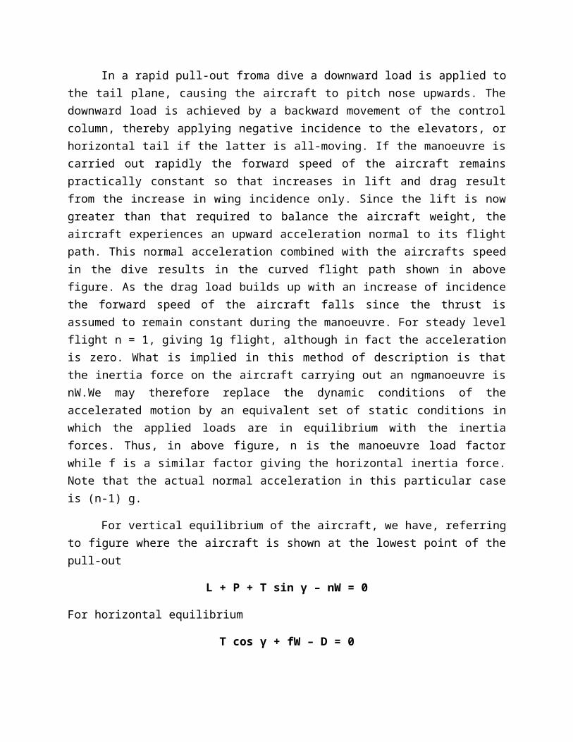
3c Pull out manoeuvres:

In a rapid pull-out froma dive a downward load is applied to the tail plane, causing the aircraft to pitch nose upwards. The downward load is achieved by a backward movement of the control column, thereby applying negative incidence to the elevators, or horizontal tail if the latter is all-moving. If the manoeuvre is carried out rapidly the forward speed of the aircraft remains practically constant so that increases in lift and drag result from the increase in wing incidence only. Since the lift is now greater than that required to balance the aircraft weight, the aircraft experiences an upward acceleration normal to its flight path. This normal acceleration combined with the aircrafts speed in the dive results in the curved flight path shown in above figure. As the drag load builds up with an increase of incidence the forward speed of the aircraft falls since the thrust is assumed to remain constant during the manoeuvre. For steady level flight n = 1, giving 1g flight, although in fact the acceleration is zero. What is implied in this method of description is that the inertia force on the aircraft carrying out an ngmanoeuvre is nW.We may therefore replace the dynamic conditions of the accelerated motion by an equivalent set of static conditions in which the applied loads are in equilibrium with the inertia forces. Thus, in above figure, n is the manoeuvre load factor while f is a similar factor giving the horizontal inertia force. Note that the actual normal acceleration in this particular case is (n-1) g.

For vertical equilibrium of the aircraft, we have, referring to figure where the aircraft is shown at the lowest point of the pull-out

L + P + T sin γ – nW = 0

For horizontal equilibrium

T cos γ + fW – D = 0

And for pitching moment equilibrium about the aircrafts centre of gravity

L a – D b – T c - Mo – Pl = 0

The above equation contains no terms representing the effect of pitching acceleration of the aircraft; this is assumed to be negligible at this stage. The engine thrust T is no longer directly related to the drag D as the latter changes during the manoeuvre. Generally the thrust is regarded as remaining constant and equal to the appropriate to conditions before the manoeurve began.

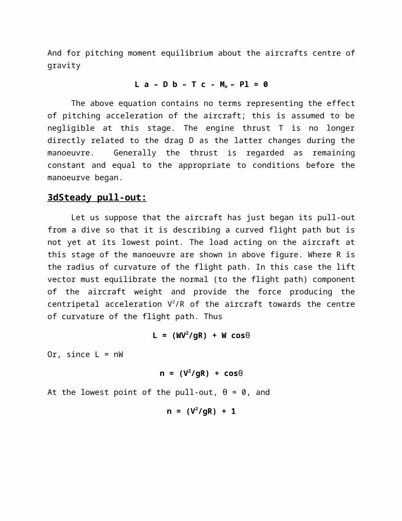
3dSteady pull-out:

Let us suppose that the aircraft has just began its pull-out from a dive so that it is describing a curved flight path but is not yet at its lowest point. The load acting on the aircraft at this stage of the manoeuvre are shown in above figure. Where R is the radius of curvature of the flight path. In this case the lift vector must equilibrate the normal (to the flight path) component

of the aircraft weight and provide the force producing the centripetal acceleration V2/R of the aircraft towards the centre of curvature of the flight path. Thus

L = (WV2/gR) + W cosθ

Or, since L = nW

n = (V2/gR) + cosθ

At the lowest point of the pull-out, θ = 0, and

n = (V2/gR) + 1

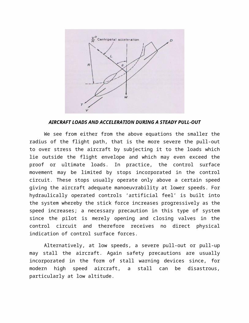
AIRCRAFT LOADS AND ACCELERATION DURING A STEADY PULL-OUT

We see from either from the above equations the smaller the radius of the flight path, that is the more severe the pull-out to over stress the aircraft by subjecting it to the loads which lie outside the flight envelope and which may even exceed the proof or ultimate loads. In practice, the control surface movement may be limited by stops incorporated in the control circuit. These stops usually operate only above a certain speed giving the aircraft adequate manoeuvrability at lower speeds. For hydraulically operated controls ‘artificial feel’ is built into the system whereby the stick force increases progressively as the speed increases; a necessary precaution in this type of system since the pilot is merely opening and closing valves in the control circuit and therefore receives no direct physical indication of control surface forces.

Alternatively, at low speeds, a severe pull-out or pull-up may stall the aircraft. Again safety precautions are usually incorporated in the form of stall warning devices since, for modern high speed aircraft, a stall can be disastrous, particularly at low altitude.

3eCorrectly banked turn:

In this manoeuvre the aircraft flies in a horizontal turn with no side slip at constant speed. If the radius of the turn is R and the angle of bank φ, then the forces acting on the aircraft are those shown in the figure.The horizontal component of the lift vector in this case provides the force necessary to produce the centripetal acceleration of the aircraft towards the center of the turn.Thus

Lsinɸ = WV2/gR

And for vertical equilibrium

Lcosɸ = W

Or

L = Wsecɸ

From the above equation we see that the load factor n in the turn is given by

n = secɸ

Also, dividing the equations

tanɸ = V2/gR

Examination of the above equation reveals that the tighter the turn the greater the angle of bank required to maintain horizontal flight. Furthermore, we see from (n = sec ɸ) Equation that an increase in bank angle results in an increased load factor. Aerodynamic theory shows that for a limiting value of n the minimum time taken to turn through a given angle at a given value of engine thrust occurs when the lift coefficient CL is a maximum; that is, when the aircraft on the point of stalling.

4. LOAD ESTIMATION OF WINGS

Wing Load Distribution:

The loads on the wing are made up of aerodynamic lift and drag forces; as well the concentrated or distributed weight of wing-mounted engines, stored fuel, weapons, structural elements, etc., this section will consider these as the first step in designing the internal stricture for the wing.

Span wise lift distribution. As a result of the finite aspect ratio of the wing, the lift distribution varies along the span, from a maximum lift at the root, to a minimum lift at the tip. The span wise lift distribution should be proportional to the shape of the wing planform.It can readily be calculated using a vortex panel method. However, if the wing planform is elliptic in shape, with a local chord distribution c(y) given as

c(y) = (4S/Пb)(√1−(2 yb )

2

)

An analytic span wise lift distribution exists. This is given as

LE(y) = (4L/Пb)(√1−(2 yb )

2

)

Where LE is the total lift generated by the wing with an elliptic planform. In both these expressions, y is the span wise coordinate of the wing, with y = 0 corresponding to the wing root, and y = ± b/2 corresponding to the wing tips. A schematic is shown in the figure.

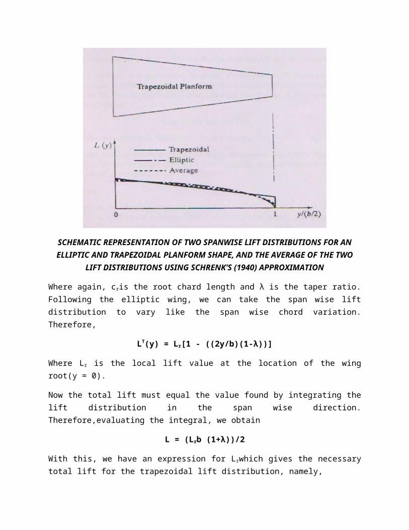
The analysis of the elliptic planform wing shows that it results in an elliptic lift distribution in the span wise direction. This is the basis for a semi-empirical method for estimating the span wise lift distribution on untwisted wings with general trapezoidal planform shapes. The method is attributed to Schrenk (1940) and assumes that the span wise lift distribution of a general untwisted wing has a shape that is the average between the actual planform chord distribution, c(y), and that of an elliptic wing. In this approach, the areas under the span wise lift distribution. For the elliptic or general planform, must equal the total required lift.

For the trapezoidal wing, the local chord length, c(y), varies along the span as

c(y) = cr[1 - ((2y/b)(1-λ))]

SCHEMATIC REPRESENTATION OF TWO SPANWISE LIFT DISTRIBUTIONS FOR AN ELLIPTIC AND TRAPEZOIDAL PLANFORM SHAPE, AND THE AVERAGE OF THE

TWO LIFT DISTRIBUTIONS USING SCHRENK’S (1940) APPROXIMATION

Where again, cris the root chard length and λ is the taper ratio. Following the elliptic wing, we can take the span wise lift distribution to vary like the span wise chord variation. Therefore,

LT(y) = Lr[1 - ((2y/b)(1-λ))]

Where Lr is the local lift value at the location of the wing root(y = 0).

Now the total lift must equal the value found by integrating the lift distribution in the span wise direction. Therefore,evaluating the integral, we obtain

L = (Lrb (1+λ))/2

With this, we have an expression for Lrwhich gives the necessary total lift for the trapezoidal lift distribution, namely,

Lr = (2L) / (b (1+λ))

And therefore,

LT(y) = 2L/ (b (1+λ)) [1 - (2y/b) (1-λ)]

As a check, for a planar wing (λ = 1), LT (y) = L/b, which is the correct lift per span.

To use Schrenk’s method, it is necessary to graph the span wise lift distribution given in the equation for the elliptic platform and the above equation for the trapezoidal planform. In each case, L is the required total lift. The approximated span wise lift distribution is then the local average of the two distributions,namely,

L(y) = ½[LT(y) + LE(y)]

An example of this corresponds to the dotted curve in figure.

It should be pointed out that Schrenk’s method does not provide a suitable estimate of the span wise lift distribution for highly swept wings. In that instance, a panel method approach or other computational method is necessary.

Added flap Loads:

Leading-edge and trailing-edge flaps enhance the lift over the span wise extent where they are placed. The lift force is assumed to be uniform in the region of the flaps and to add to the local span wise lift distribution that is derived for the unflapped wing.

The determination of the added lift force produced by the flaps requires specifying a velocity. For this, the velocity is taken to be twice the stall value, 2Vs, with flaps down.

Span wise Drag Distribution:

The drag force on the wing varies along the span, with a particular concentration occurring near the wing tips. An approximation that is suitable for the conceptual design is to assume that

1. The drag force is constant from the wing root to 80 percent of the wing span and equal to 95 percent of the total drag on the wing;

2. The drag on the outward 20 percent of the wing is constant and equal to 120 percent of the wing total drag.

In most cases, the wing structure is inherently strong (stiff) in the drag component direction because the relevant length for the bending moment of inertia is the wing chord, which is large compared to the wing thickness. Therefore, the principle bending of the wing occurs in the lift component direction. The design of the internal structure of the wing is then primarily driven by the need to counter the wing-thickness bending moments.

0 0.5 1 1.5 2 2.5 3 3.5 4 4.50

0.02

0.04

0.06

0.08

0.1

0.12

0.14

0.16

wing loading

wing loading

Concentrated and Distributed Wing Weights:

Other loads on the wing, besides the aerodynamic loads, are due to concentrated weights, such as wing-mounted engines, weapons, fuel tanks, etc., and due to distributed loads such as the wing structure.

Since the structure is being designed at this step, it is difficult to know precisely what the final weight will be. Therefore, historic weight trends for aircraft are used to make estimates at this stage of the design. A refined weight analysis will be done later as the initial step in determining the static stability coefficients for the aircraft.

The above table gives historic weights for the major components of a range of different aircraft. These include the main wing, horizontal and vertical tails, fuselage, installed engine and landing gear. The weights of these components are determined from the table as

W (lbf) = Multiplier * Factor

Where the “multiplier” is a number that corresponds to a general type and the “Factor” is a reference portion of the aircraft, such as the wing planform area, SW, or the fuselage wetted area, Sfuse-wetted.

Engines and landing gear mounted on the wing can be treated as concentrated loads. The wing structure will be considered as a distributed load. It is reasonable to consider that the weight of a span wise section of the wing would scale with the wing chord length, so that with a linear tapered wing, the distributed weight would decrease in proportion to the local chord from the root to the tip. Structural Parameters:

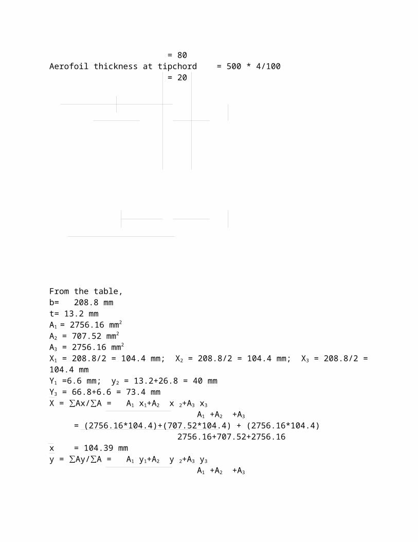
NACA 64A004Aerofoil thickness at rootchord = 2000 * 4/100

= 80Aerofoil thickness at tipchord = 500 * 4/100

= 20

From the table,b= 208.8 mmt= 13.2 mmA1 = 2756.16 mm2

A2 = 707.52 mm2

A3 = 2756.16 mm2

X1 = 208.8/2 = 104.4 mm; X2 = 208.8/2 = 104.4 mm; X3 = 208.8/2 = 104.4 mmY1 =6.6 mm; y2 = 13.2+26.8 = 40 mmY3 = 66.8+6.6 = 73.4 mmX = ∑Ax/∑A = A1 x1+A2 x 2+A3 x3

A1 +A2 +A3

= (2756.16*104.4)+(707.52*104.4) + (2756.16*104.4) 2756.16+707.52+2756.16x = 104.39 mmy = ∑Ay/∑A = A1 y1+A2 y 2+A3 y3

A1 +A2 +A3

= (2756.16*6.6)+(707.52*40) + (2756.16* 73.4) 2756.16+707.52+2756.16y = 39.99 mm

Ixx = Ix1 +A1y12 + Ix2 +A2y2

2 + Ix3 +A3y32

= b1d13/12 + A1y1

2+ b2d23/12 + A2y2

2 + b3d33/12 + A3y3

2

Where yi = y – yY1 = 6.6 mmY2 = 40 mmY3 =73.4 mmIxx= 208.8*13.23 + [2756.16 * (33.39)2] + 13.2*53.63 + [707.52 * (.01)2] + 208.8*13.23 + [2756.16 * 12 12 12(-33.41)2]

Ixx = 40019.44 + 3028225.32 + 169.38*103 + 0.070752+ 40019.44 +3.076*106

Ixx = 6354212.44mm4

Iyy = Iy1 +A1x12 + Iy2 +A2x2

2 + Iy3 +A3x32

= d1b13/12 + A1x1

2+ d2b23/12 + A2x2

2 + d3b33/12 + A3x3

2

Where xi = x – x

X1 = X2 = X3 = 104.4 mmIyy= 13.2*208.83 /12 + [2756.16 * (-.01)2] + 53.6*13.23 /12+ [707.52 * (.01)2] + 13.2*208.83 /12+ [2756.16 * (-.01)2]

Iyy = 19865043.82mm4

wf/ wg=0.6552wf=0.6552 * 5360wf=3511.872 kgMax.Bending moment:Wl2/6 = (l – wf)b2/6

= (161081.9– 34451.4) (3.85)2

6

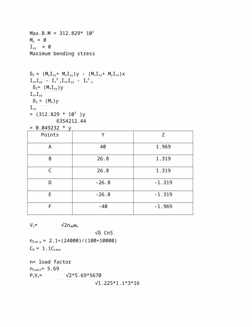
Max.B.M = 312.829* 103

My = 0Ixy = 0 Maximum bending stress

δ2 = (MyIxy+ MxIyy)y - (MxIxy+ MyIxx)xIxxIyy - Ix

2 yIxxIyy - Ix

2 y

δ2= (MxIyy)yIxxIyy

δ2 = (Mx)yIxx

= (312.829 * 103 )y 6354212.44= 0.049232 * y

Points Y Z

A 40 1.969

B 26.8 1.319

C 26.8 1.319

D -26.8 -1.319

E -26.8 -1.319

F -40 -1.969

Vs= √2ndmwe

√δ CnSnlim p = 2.1+(24000)/(100+10000)CN = 1.1CLmax

n= load factornlimit= 5.69PsVs= √2*5.69*5670 √1.225*1.1*3*16

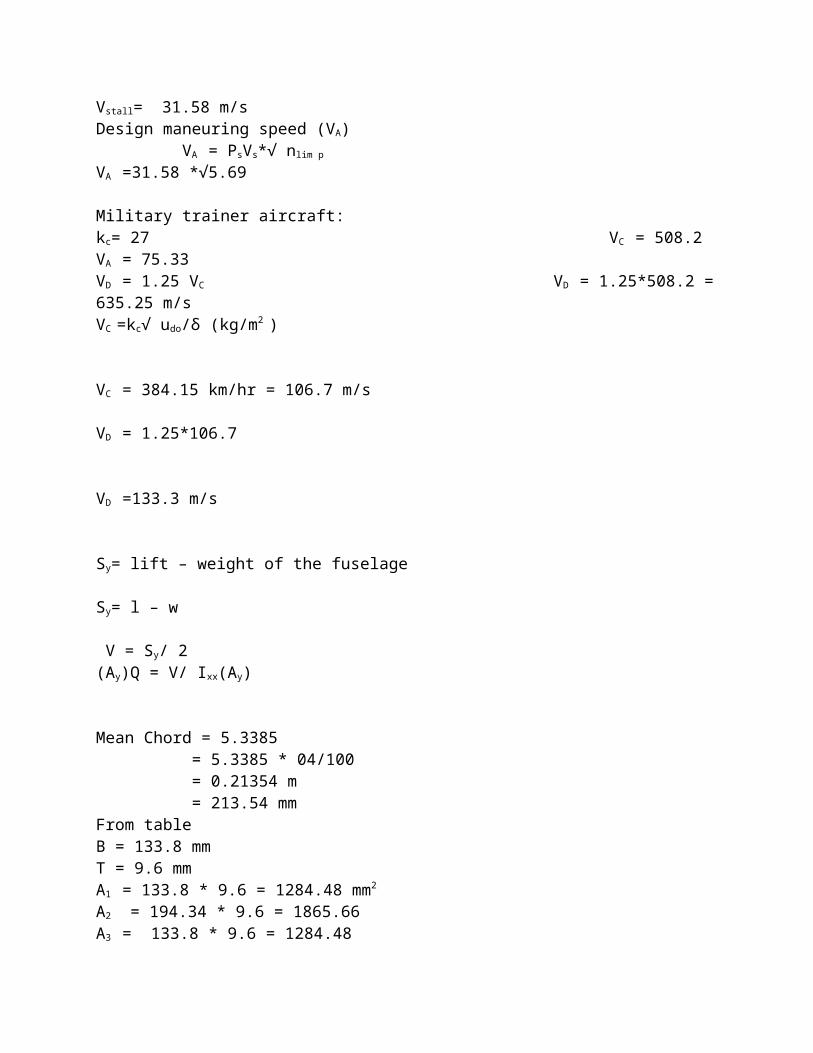
Vstall= 31.58 m/s Design maneuring speed (VA) VA = PsVs*√ nlim p

VA =31.58 *√5.69

Military trainer aircraft:kc= 27 VC = 508.2 VA = 75.33 VD = 1.25 VC VD = 1.25*508.2 = 635.25 m/sVC =kc√ udo/δ (kg/m2 )

VC = 384.15 km/hr = 106.7 m/s

VD = 1.25*106.7

VD =133.3 m/s

Sy= lift – weight of the fuselage

Sy= l – w

V = Sy/ 2(Ay)Q = V/ Ixx(Ay)

Mean Chord = 5.3385= 5.3385 * 04/100= 0.21354 m = 213.54 mm

From table B = 133.8 mmT = 9.6 mmA1 = 133.8 * 9.6 = 1284.48 mm2

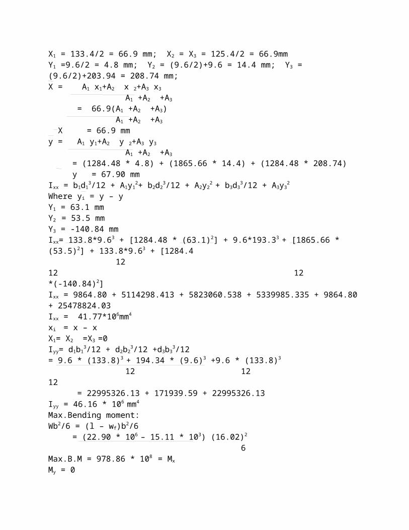
A2 = 194.34 * 9.6 = 1865.66 A3 = 133.8 * 9.6 = 1284.48 X1 = 133.4/2 = 66.9 mm; X2 = X3 = 125.4/2 = 66.9mmY1 =9.6/2 = 4.8 mm; Y2 = (9.6/2)+9.6 = 14.4 mm; Y3 = (9.6/2)+203.94 = 208.74 mm; X = A1 x1+A2 x 2+A3 x3

A1 +A2 +A3

= 66.9(A1 +A2 +A3) A1 +A2 +A3

X = 66.9 mmy = A1 y1+A2 y 2+A3 y3

A1 +A2 +A3

= (1284.48 * 4.8) + (1865.66 * 14.4) + (1284.48 * 208.74) y = 67.90 mmIxx = b1d1

3/12 + A1y12+ b2d2

3/12 + A2y22 + b3d3

3/12 + A3y32

Where yi = y – yY1 = 63.1 mmY2 = 53.5 mmY3 = -140.84 mmIxx= 133.8*9.63 + [1284.48 * (63.1)2] + 9.6*193.33 + [1865.66 * (53.5)2] + 133.8*9.63 + [1284.4 12 12 12*(-140.84)2]Ixx = 9864.80 + 5114298.413 + 5823060.538 + 5339985.335 + 9864.80 + 25478824.03Ixx = 41.77*106mm4

xi = x – xX1= X2 =X3 =0Iyy= d1b1

3/12 + d2b23/12 +d3b3

3/12 = 9.6 * (133.8)3 + 194.34 * (9.6)3 +9.6 * (133.8)3

12 12 12 = 22995326.13 + 171939.59 + 22995326.13

Iyy = 46.16 * 106 mm4

Max.Bending moment:Wb2/6 = (l – wf)b2/6

= (22.90 * 106 – 15.11 * 103) (16.02)2

6Max.B.M = 978.86 * 108 = Mx

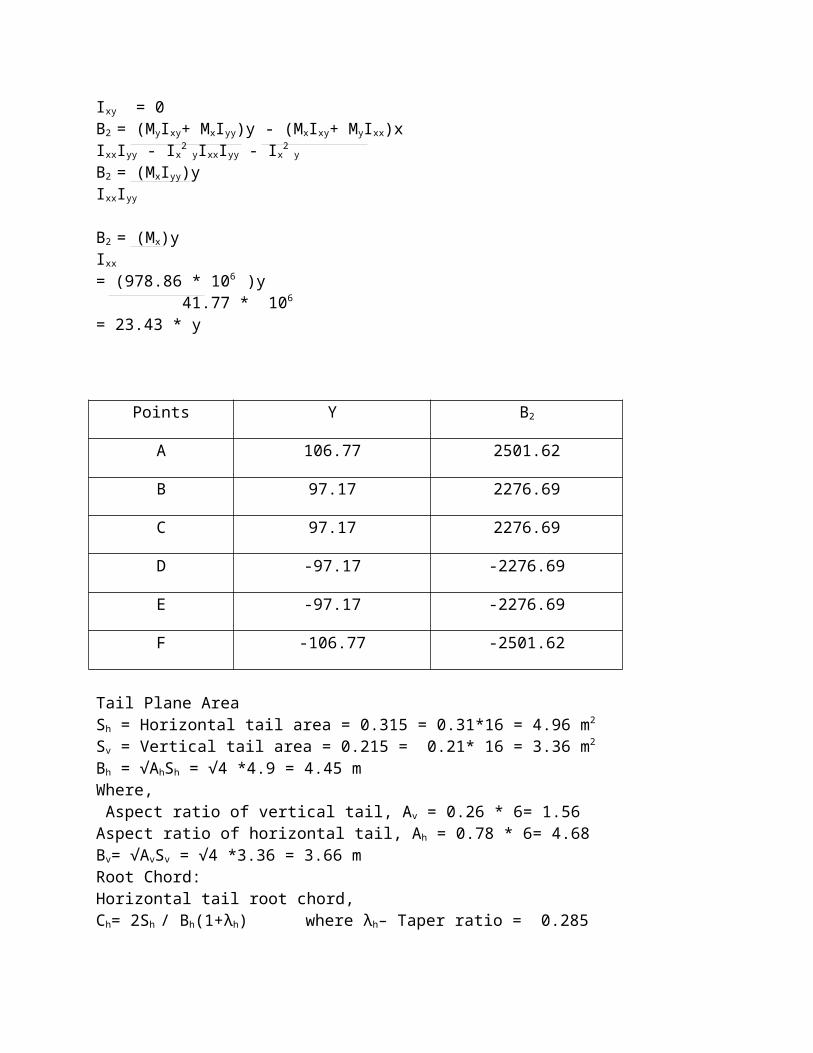
My = 0Ixy = 0 B2 = (MyIxy+ MxIyy)y - (MxIxy+ MyIxx)xIxxIyy - Ix

2 yIxxIyy - Ix

2 y

B2 = (MxIyy)yIxxIyy

B2 = (Mx)yIxx

= (978.86 * 106 )y 41.77 * 106

= 23.43 * y

Points Y B2

A 106.77 2501.62

B 97.17 2276.69

C 97.17 2276.69

D -97.17 -2276.69

E -97.17 -2276.69

F -106.77 -2501.62

Tail Plane AreaSh = Horizontal tail area = 0.315 = 0.31*16 = 4.96 m2

Sv = Vertical tail area = 0.215 = 0.21* 16 = 3.36 m2

Bh = √AhSh = √4 *4.9 = 4.45 mWhere, Aspect ratio of vertical tail, Av = 0.26 * 6= 1.56Aspect ratio of horizontal tail, Ah = 0.78 * 6= 4.68Bv= √AvSv = √4 *3.36 = 3.66 mRoot Chord:Horizontal tail root chord, Ch= 2Sh / Bh(1+λh) where λh– Taper ratio = 0.285

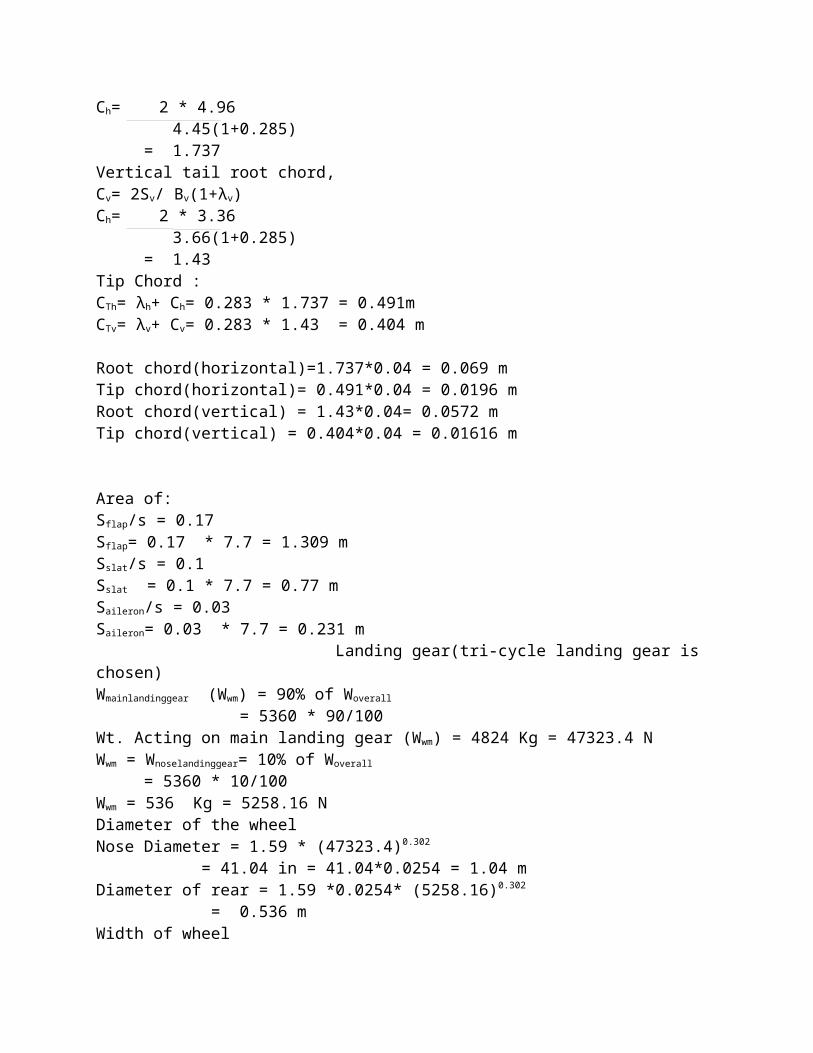
Ch= 2 * 4.96 4.45(1+0.285) = 1.737Vertical tail root chord, Cv= 2Sv/ Bv(1+λv) Ch= 2 * 3.36 3.66(1+0.285) = 1.43Tip Chord :CTh= λh+ Ch= 0.283 * 1.737 = 0.491mCTv= λv+ Cv= 0.283 * 1.43 = 0.404 m

Root chord(horizontal)=1.737*0.04 = 0.069 mTip chord(horizontal)= 0.491*0.04 = 0.0196 mRoot chord(vertical) = 1.43*0.04= 0.0572 mTip chord(vertical) = 0.404*0.04 = 0.01616 m

Area of:Sflap/s = 0.17Sflap= 0.17 * 7.7 = 1.309 mSslat/s = 0.1Sslat = 0.1 * 7.7 = 0.77 mSaileron/s = 0.03Saileron= 0.03 * 7.7 = 0.231 m Landing gear(tri-cycle landing gear is chosen)Wmainlandinggear (Wwm) = 90% of Woverall

= 5360 * 90/100Wt. Acting on main landing gear (Wwm) = 4824 Kg = 47323.4 NWwm = Wnoselandinggear= 10% of Woverall

= 5360 * 10/100Wwm = 536 Kg = 5258.16 NDiameter of the wheelNose Diameter = 1.59 * (47323.4)0.302

= 41.04 in = 41.04*0.0254 = 1.04 mDiameter of rear = 1.59 *0.0254* (5258.16)0.302

= 0.536 mWidth of wheel Nose width = AWnose

B

= 0.098 * (5232.358 * 9.81)0.467

= 15.52 m = 39.42 cm = 0.39 mRear width = 0.098 * (47091.22 * 9.81)0.467

= 43.31 m = 110.01 cm = 1.10 m

5. LOAD ESTIMATION OF FUSELAGE

Fuselage load distribution:

The fuselage can be considered to be supported at the location of the center of lift of the main wing. The loads on the fuselage structure are then due to shear force and bending moment about that point.

The loads come from a variety of components, forexample, the weights of payload, fuel, wing structure, engines, fuselagestructure, and tail control lift force. Figure illustrates a typical load distribution. Note that the coordinate along the fuselage is denoted as x and the length of the fuselage is L.

SCHEMATIC REPRESENTATION OF FORCES ACTING ON A GENERIC FUSELAGE

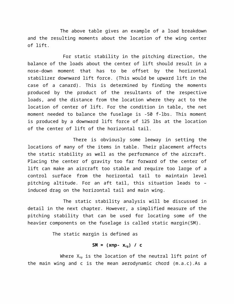
The above table gives an example of a load breakdown and the resulting moments about the location of the wing center of lift.

For static stability in the pitching direction, the balance of the loads about the center of lift should result in a nose-down moment that has to be offset by the horizontal stabilizer downward lift force. (This would be upward lift in the case of a canard). This is determined by finding the moments produced by the product of the resultants of the respective loads, and the distance from the location where they act to the location of center of lift. For the condition in table, the net moment needed to balance the fuselage is -50 f-lbs. This moment is produced by a downward lift force of 125 lbs at the location of the center of lift of the horizontal tail.

There is obviously some leeway in setting the locations of many of the items in table. Their placement affects the static stability as well as the performance of the aircraft. Placing the

center of gravity too far forward of the center of lift can make an aircraft too stable and require too large of a control surface from the horizontal tail to maintain level pitching altitude. For an aft tail, this situation leads to – induced drag on the horizontal tail and main wing.

The static stability analysis will be discussed in detail in the next chapter. However, a simplified measure of the pitching stability that can be used for locating some of the heavier components on the fuselage is called static margin(SM).

The static margin is defined as

SM = (xnp- xcg) / c

Where Xnp is the location of the neutral lift point of the main wing and c is the mean aerodynamic chord (m.a.c).As a first approximation, we can neglect the lift-induced moment of the main wing so that Xnp corresponds to the center of lift Xcl.

For static stability in the pitching direction the static margin is positive(SM>0). Normal values for the static margin for a large spectrum of aircraft give a range of 3≤SM≤10.

A consideration in the placement of the fuel is how the location of the center of the mass will shift as the fuel wait is reduced over a flight plan. In the case of a long-range aircraft, the static margin can change significantly from the start of cruise to the end of cruise. The placement of fuel should be such that the static margin always remains positive.

Fuselage structural analysisL = δτV∞

Τ = 2╥(-V0 + 2 V∞)Resultant load = L-WCirculation, τ = 2╥(-1033.6 +( 2* 3234.924)

τ = 34156.95L = δτV∞

= 2.2785 * 10-1 * 34156 * 32340934L = 25176317.04L = 2.51* 106

Wing volumeWing volume = area * thicknessVolume by taking tip thicknessTip:Volume = 39.506 * 0.08268

= 3266.35 m3

Root:Vol = 39.506 * 0.3444 = 13605.86 m3

Avg.Vol = (3.266 + 13.605)/2 = 8.43 C

Horizontal tail volume

ttail = 0.9 * 0.344 = 0.309Vhor.tail = t * A = 0.309 *12.24 = 3.78 m3

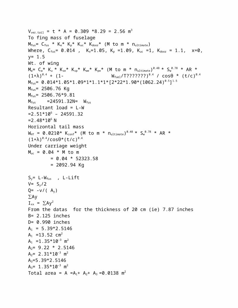
Vver.tail = t * A = 0.309 *8.29 = 2.56 m3

To fing mass of fuselageMfus= Cfus * Ke* Kp* Kuc* Kdoor* (M to m * nultimate)Where, Cfus= 0.014 , Ke=1.05, Kp =1.09, Kuc =1, Kdoor = 1.1, x=0, y= 1.5Wt. of wing Mw= Cw* Ku * Kse* Ksp* Kwe* Kpe* (M to m * nultimate)0.48 * Sw

0.78 * AR * (1+λ)0.4 + (1- Wfuel/T???????)0.4 / cosθ * (t/c)0.4

Mfus= 0.014*1.05*1.09*1*1.1*1*[2*22*1.90*(1062.24)0.5]1.5

Mfus= 2506.76 KgMfus= 2506.76*9.81Mfus =24591.32N= Wfus

Resultant load = L-W=2.51*106 – 24591.32=2.48*106 NHorizontal tail massWHT = 0.0210* Kconf* (M to m * nultimate)0.48 * Sw

0.78 * AR * (1+λ)0.4/cosθ*(t/c)0.4

Under carriage weightMuc = 0.04 * M to m = 0.04 * 52323.58 = 2092.94 Kg

Sy= L-Wfus , L-LiftV= Sy/2Q= -v/( Ay)∑AyIxx = ∑Ay2

From the datas for the thickness of 20 cm (ie) 7.87 inchesB= 2.125 inchesD= 0.990 inchesA1 = 5.39*2.5146A1 =13.52 cm2

A1 =1.35*10-3 m2

A2= 9.22 * 2.5146A2= 2.31*10-3 m2

A3=5.39*2.5146A3= 1.35*10-3 m2

Total area = A =A1+ A2+ A3 =0.0138 m2

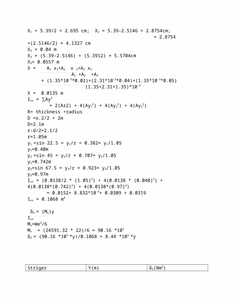
X1 = 5.39/2 = 2.695 cm; X2 = 5.39-2.5146 = 2.8754cm; = 2.8754 +(2.5146/2) = 4.1327 cmX2 = 0.04 mX3 = (5.39-2.5146) + (5.3912) = 5.5704cmX3= 0.0557 mX = A1 x1+A2 x 2+A3 x3

A1 +A2 +A3

= (1.35*10-3*0.02)+(2.31*10-3*0.04)+(1.35*10-3*0.05) (1.35+2.31+1.35)*10-3

X = 0.0135 mIxx = ∑Ay2

= 2(Ar2) + 4(Ay12) + 4(Ay2

2) + 4(Ay32)

R= thickness +radiusD =o.2/2 + 2mD=2.1mr-d/2=2.1/2r=1.05my1 =sin 22.5 = y1/r = 0.382= y1/1.05y1=0.40my2 =sin 45 = y2/r = 0.707= y2/1.05y2=0.742my3=sin 67.5 = y3/r = 0.923= y3/1.05y3=0.97mIxx = (0.0138/2 * (1.05)2) + 4(0.0138 * (0.040)2) + 4(0.0138*(0.742)2) + 4(0.0138*(0.97)2) = 0.0152+ 8.832*10-3+ 0.0309 + 0.0319Ixx = 0.1068 m4

δ2 = (Mx)yIxx

Mx=We2/6Mx = (24591.32 * 22)/6 = 90.16 *103

δ2 = (90.16 *103 *y)/0.1068 = 8.44 *103 *y

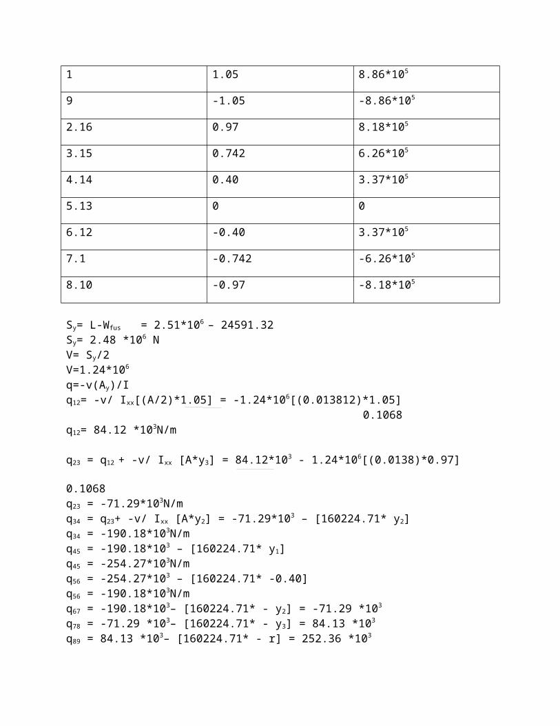
Striger Y(m) δ2(Nm2)

1 1.05 8.86*105

9 -1.05 -8.86*105

2.16 0.97 8.18*105

3.15 0.742 6.26*105

4.14 0.40 3.37*105

5.13 0 0

6.12 -0.40 3.37*105

7.1 -0.742 -6.26*105

8.10 -0.97 -8.18*105

Sy= L-Wfus = 2.51*106 – 24591.32Sy= 2.48 *106 N V= Sy/2V=1.24*106

q=-v(Ay)/Iq12= -v/ Ixx[(A/2)*1.05] = -1.24*106[(0.013812)*1.05] 0.1068q12= 84.12 *103N/m

q23 = q12 + -v/ Ixx [A*y3] = 84.12*103 - 1.24*106[(0.0138)*0.97] 0.1068q23 = -71.29*103N/mq34 = q23+ -v/ Ixx [A*y2] = -71.29*103 – [160224.71* y2]q34 = -190.18*103N/mq45 = -190.18*103 – [160224.71* y1]q45 = -254.27*103N/mq56 = -254.27*103 – [160224.71* -0.40]q56 = -190.18*103N/mq67 = -190.18*103– [160224.71* - y2] = -71.29 *103

q78 = -71.29 *103– [160224.71* - y3] = 84.13 *103

q89 = 84.13 *103– [160224.71* - r] = 252.36 *103

Index = w2/δ CLmax STT= T11+T12

Index = (52323.58)2

12.01*3*512000*39.506 = 3.752 engine TOFL = 857.4 +28.43 Index +0.0185(Index)2

= 857.4+(28.43*3.75)+[0.0185*(3.75)2] = 964.27 m

6. STRUCTURAL DESIGN AND ANALYSIS

6a Internal Structure Design:

The conceptual design is mainly concerned with the gross aspects of the structural design. The complete structural design is primarily completed later in the preliminary and detailed steps of the aircraft design. At this stage, the concern is on general structural aspects, which includes the selection of materials to best withstand the maximum loads, while also seeking a low structure weight.

The type structure used on aircraft since the 1930s is called “semi-monocoque.” The word “monocoque” is French for “shell only.” The semi-monocoque design uses a thin sheet-metal skin (shell) to resist it tensile loading and an internal frame of light-weight stiffeners to resist compressive loading.

In the fuselage, the frame elements that run along its length are called”longerons.” Those elements that run around the internal perimeter of the fuselage are called “bulk-heads”. The structural criterion for the cross-section size of longerons and the spacing of bulkheads is to resist compressive buckling. An example of the internal structural components in the fuselage can be seen in the photograph of a Boeing 767 fuselage section in the figure.

In the wing, the prevalent design consists of having a central internal beam that runs along its span. The beam I refer to a wing “spar” and is designed to withstand the shear and tensile stresses caused by the shear forces and bending moment. The beam cross-section can range from a hollow square or rectangular (“box”) shape to an I-shape.

The wing profile is formed by “ribs”, which are cut into the shape of the airfoil cross-section and attach to the central wing spar .A thin sheet-metal skin is attached to the ribs in order to build up the complete wing shape. As a structural element, the skin primarily adds torsional stiffness to the wing.

The horizontal and vertical tail surfaces can be constructed in the same way as the main wing. Alternately, because of their smaller size and because there is no use for their internal volume, they can be fabricated of full depth stabilizing material such as foam-plastic or honeycomb material. Honeycomb material is made by bonding very thin corrugated sheets together to form internal hexagonal cells (similar to a bee honeycomb), which run through the material. When the honeycomb material is sandwiched between two thin metal sheets, it forms an extremely rigid a light-weight structural element. This form of construction is excellent for other nonstructural elements such as flaps, fillets and landing gear doors in order to reduce weight.

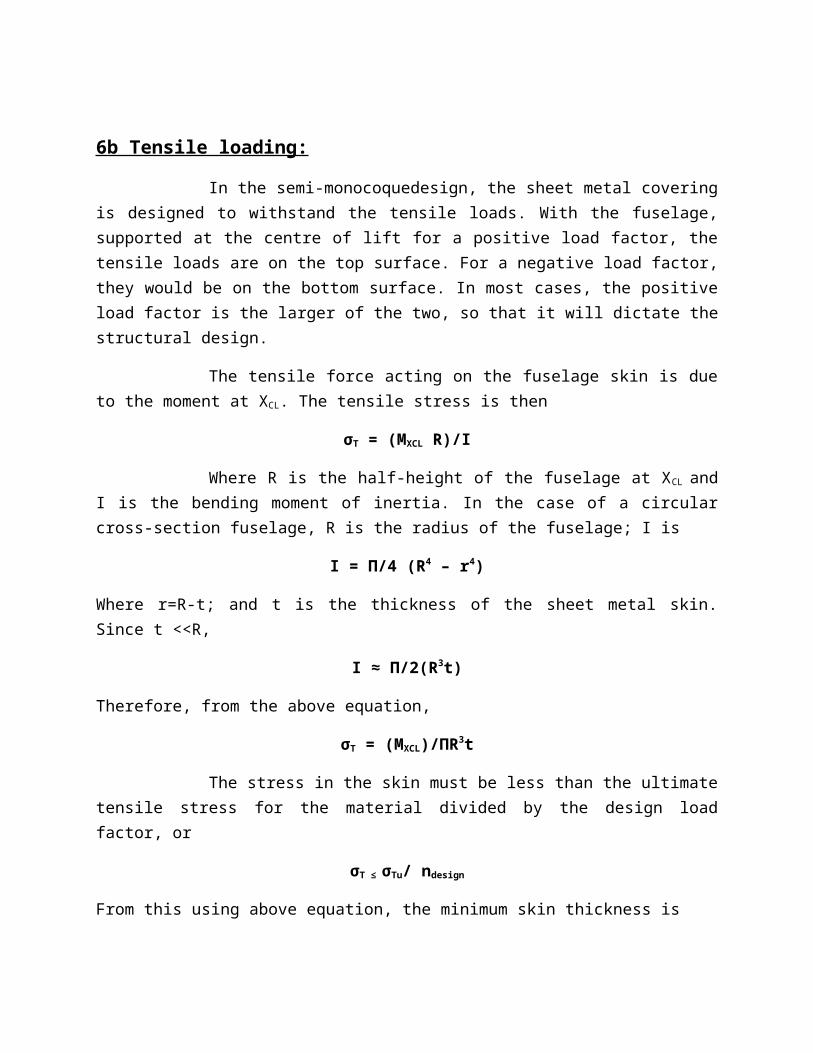
6b Tensile loading:

In the semi-monocoquedesign, the sheet metal covering is designed to withstand the tensile loads. With the fuselage, supported at the centre of lift for a positive load factor, the tensile loads are on the top surface. For a negative load factor, they would be on the bottom surface. In most cases, the positive load factor is the larger of the two, so that it will dictate the structural design.

The tensile force acting on the fuselage skin is due to the moment at XCL. The tensile stress is then

σT = (MXCL R)/I

Where R is the half-height of the fuselage at XCL and I is the bending moment of inertia. In the case of a circular cross-section fuselage, R is the radius of the fuselage; I is

I = П/4 (R4 – r4)

Where r=R-t; and t is the thickness of the sheet metal skin. Since t <<R,

I ≈ П/2(R3t)

Therefore, from the above equation,

σT = (MXCL)/ПR3t

The stress in the skin must be less than the ultimate tensile stress for the material divided by the design load factor, or

σT ≤ σTu/ ndesign

From this using above equation, the minimum skin thickness is

t min = (2 MXCL ndesign)/ПσTuR2

In many cases, a more desirable cross-section shape for the fuselage is elliptic in order to give a higher ceiling height. For an elliptic cross-section fuselage, where the major axis is the vertical height of the fuselage, the bending moment of inertia about the minor axis (due to MXCL) is

I = П/4 (A3B – C3D)

Where A is the major axis radius, B is the minor axis radius, and C=A-t and D=B-t, where again t is the fuselage skin thickness.

For t <<R,

I = П/4 (A3B + A3) t

In this case, the minimum skin thickness is

tmin = (MXCL ndesign) / (ПσTu (A3B + A3))

In either case of a circular or elliptic cross-section fuselage, the above equations provides values for the minimum skin thickness needed to withstand the tensile load produced by the maximum bending moment. The required thickness depends on the material property, σTu. Values for materials typically used are presented in the next section.

6cCompressive Loading:

In the semi-monocoque design, the longerons are designed to withstand the compressive loads. With the fuselage, supported at the centre of lift for a positive load factor, the compressive loads are on the lower side. For a negative load factor, they are on the upper side. Again in most cases, the positive load factor is the larger of the two and dictates the structural design.

Structural failure under compression for the longerons usually occurs due to buckling. Therefore, this will set the structural design limit. The criterion for buckling comes from the Euler column formula, given as

FE = CП2EI/ (L) 2

Where F is the critical column load to produce buckling, L is the unsupported length and C is a factor that depends on how the column is fixed at its ends. For pinned ends, C=1, whereas C=4 for fixed ends. The longerons are often supported by comparatively flexible ribs or bulkheads, which are free to twist or bend. Thus, a value of C=1 is appropriate. If the bulkheads are rigid enough to provide restraint to the longerons, a value of C=1.5 can be used.

Using equation the critical stress is

σE= CП2E/(L/𝝆)2

Where the radius of gyration is given as

𝝆 = √(IA

)

With I being the bending moment of inertia and A being the cross-section area of the column. In order to prevent a structural failure in the longerons, the actual compressive stress must be less than the buckling stress divided by the design load factor namelyσ<σE/ndesign. The next step is then to determine the actual compressive stress in the longerons. This requires setting the configurations of longerons around the fuselage.

7. SHEAR AND BENDING MOMENT ANALYSIS FOR WINGS

The wing structure can be considered to be a cantilever beam, which is rigidly supported at the wing root. The critical loads that need to be determined are the shear forces and bending moments along the span of the wing. These taken into account the loads on the wing produced by the aerodynamic forces and component weights, which were discussed in the previous section. A generic load arrangement is listed in the table and illustrated in figure.

To determine the shear force and bending moments along the span, it is useful to divide the wing into span wise segments of width Δy. A schematic of such element is shown in figure.

SCHEMATIC REPRESENTATION OF SHEAR LOADS AND BENDING MOMENTS ON A SPANWISE ELEMENT OF THE WING

As an example, the element shows a distributed load, W(y). The resultant load acting on the element is then W(y)Δy. In the limit as Δy goes to zero, Δy approaches the differential length, dy, and the resultant load is W(y)dy.

The element shear force, V, is related to the resultant load as

W = dV/dy

The bending moment, M, acting on the element is related to the shear force by

V = dM/dy

Integrals can be approximated by sums, namely

V =∑i

n

Wi Δy

And

M =∑i

n

Vi Δy ,

Where N is the number of elements over which the wing span is divided. Of course, the sums approximate the integrals better as the number of elements becomes large; however, a reasonably good estimate for the conceptual design can be obtained with approximately twenty elements over the half-span of the wing.

In order to make these definite integrals, the integration (summation) needs to be started where the shear and moment are known. With the wing, this location is at the wing tip(y=b/2), where V (b/2)=M (b/2)=0. Note that in this case, the resultant load on an element is Wi=W(y). Δy y which is the quantity inside the sum in equation. If the index, I, in the above equation indicates the elements along the wing span, with i=1 signifying the one at the wing tip, then

V1 =0;

V2 = W1 + W2;

V3 = W1 + W2+W3 = V2 + W3;

V4 = V3 + V4;

.

.

.

VN =VN-1 + WN.

Note that the shear on element N must equal the sum of the resultant loads on the wing. In reality, there might be a small discrepancy due to the finite number elements in

which the wing span is subdivided. However, with a large enough number of elements the difference should be small.

The bending moment on the wing is given by eqn. For the moments along the wing span, one should also start at the wing tip where the moment on the element is zero. Then the following format in the above eqn.

M1 =0;

M2 = V1 +ΔyV2;

M3 = = V1 +ΔyV2 +ΔyV3 = M2 + ΔyV3;

M4 = M3 Δy V4;

.

.

.

MN =MN-1 + ΔyVN.

These formulae provide a good approximation of the distribution of the shear and moment along the span of the wing. An example of the use is given in the spreadsheet that accompanies this chapter.

SPANWISE DISTRIBUTIONS OF LIFT FORCE, L; WEIGHT, W; SHEAR LOADS, V AND BENDING MOMENT, M

An example of the application of these equations is shown in fig. The loads correspond to those listed in the table and illustrated in fig.

The top plot in fig. illustrates Schrenk’s approximation of the span wise lift distribution for the finite span wing. The solid curve corresponds to the lift distribution for the trapezoidal wing. This is constant along the span because the taper ratio (λ) in this example is 1.

The total span wise load distribution, W, shown in fig. for generic wing includes all of the weight and lift components. For this, the wing was divided into 20 span wise elements. The sharp negative spike in the load distribution marks the location of the engine. The more gradual dip in the loads near Y/(b/2) = 0.4 corresponds to the outboard edge of the flaps.

The span wise distribution of the shear load, V, comes from eqn. This shows that the largest shear is at the wing root, with the second largest shear being at the location of the engine.

The moment distribution, M, in fig. is based on eqn. It reflects the wing cantilever structure, whereby the largest moment is at the wing root. The small peak in the moment distribution near Y/(b/2) is due to the engine.

8.SHEAR AND BENDING MOMENT ANALYSIS FOR F USELAGE

The fuselage structure can be considered to be a beam that is simply supported and balancing at XCL. As with the wing, we wish to determine the resulting shear forces and bending moments along the length of the fuselage. The procedure for this is the same as for the wing, namely, to divide the fuselage into discrete elements along its length. It is useful if one of the elements is at the X- location of XCL.

The elemental shear forces and bending moments follow the formulae given in equations, with the exception that Δy in the case of wing is replaced by Δx for the fuselage. The equations for determining shear force and bending moment for the fuselage are given in eqns.

V1 =W1;

V2 = W1 + W2;

V3 = W1 + W2+W3 = V2 + W3;

V4 = V3 + V4

.

.

.

VN =VN-1 + WN.

And

M1 =V1;

M2 = V1 +ΔyV2 ;

M3 = = V1 +ΔyV2 +ΔyV3 = M2 + ΔyV3

M4 = M3 Δy V4;

.

.

.

MN =MN-1 + ΔyVN.

The summation starts at one end of the fuselage (x=0 or x=1). In contrast to the wing, the shear force in the first element is considered to be the load in that element (W1), and the moment is considered to be the shear on that element to the other end, as with the wing.

In this process, the shear force and the moment can be found for the summation of all the loads, or separately for the individual loads, with the total shear and the moment being the sum of the individual shear and moment distributions. In either approach, it is important to include the concentrated reaction load that occurs at the point of support, x=xCL.

The inclusion of the resultant force was not necessary for the wing, because only half of the wing span was considered and the point of support was at the one end. For the fuselage, if the resultant load is properly included, the force on that element minus the shear at xCL, Should equal the sum of the total load across all of the elements.

An example of the application of these equations is shown in fig. The load corresponds to those listed in table and illustrated in fig. The shear V shows a reversal of sign at the eqn x=xCLas a result of the resultant force that acts at the point of support at the wing lift center. As a result, the shear is zero at the leading and trailing point of the fuselage.

LENGTHWISE DISTRIBUTIONS OF THE WEIGHT, W; SHEAR LOADS, V AND BENDING MOMENT,M

The moment, M, in fig. is also a maximum at the point of support of the fuselage, which corresponds to the wing lift center. These values as set the maximum stress condition for the structural design and dictate the internal structural layout of the fuselage.

RESULTANT LOAD

Sy = L - wfus

= 59377.73 – 3578.95

= 55798.78Kg

On Half Portion

V = L - Wfus

= 55798.78/2 = 27899.39Kg

Thickness of fuselage, t = 10mm

Radius = 5m = 5000mm

17.2mm

100mm

38.1mm

Ixx = 2(A*r2)+4(A*y12)+4(A*y2

2)+4(A*y32)

Sinnn67.5 = y1/r = y1/5

Therefore, y1 = 4.62m = 4620mm

Sin45 = y2/r

Therefore, y2 = 5*Sin45

= 3.54m = 3540mm

Sin22.5 = y3/r

Therefore, y3 = 1.91m = 1910mm

A = 1+2+3

= (38.1*17.2)+(65.6*17.2)+(38.1*17.2)

Area, A = 2438.96mm2

Ixx= 2(2438.96*50002)+4(2438.96*46202)+4(2438.96*35402)+4(2438.96*19102)

Ixx= 4.88*1011mm4

Shearflow

q12 = - V/I(A*y1)

= -27899.39/4.88*1011(2438.96*500011)

= - 0.644

q23 = q12 + (- V/I(A*y2))

= - 0.644 - 27899.39/4.88*1011(2438.96*4620)

= - 1.137

q34 = q23 + (- V/I(A*y3))

= - 1.137 - 27899.39/4.88*1011(2438.96*3540)

= - 1.403

q45 = q34 + (- V/I(A*y4))

= -1.403 - 27899.39/4.88*1011(2438.96*0)

= - 1.403

q56 = q45 + (- V/I(A*y5))

= - 1.403 - 27899.39/4.88*1011(2438.96*(-1910))

= - 1.136

q67 = q56 + (- V/I(A*y6))

= -1.136 - 27899.39/4.88*1011(2438.96*(-3540))

= - 0.642

q78 = q67 + (- V/I(A*y7))

= - 0.642 - 27899.39/4.88*1011(2438.96*4620)

= -

Thrust = 0.8*94650.91

= 75720.728Kg

= 742820.34N

Index = wg2/SCLmaxST

= (94650.91*9.81)2/1.225*9.81*3*104.706*742820.34

= 31.34

Take Of Field Length

2 engine, TOFL = 857.4+(28.43*31.34)+(0.0185*31.342)

= 1766.64m

= 1.76Km

9.BIBLIOGRAPHY

1. Aircraft structures for engineering students – T.M.G.MEGSON.2. Analysis and design of flight vehicle structures – E.Bruhn.3. Aircraft design – Thomas Corke.4. Airplane design – Daniel Raymer.