Adjustment for missing plants in cassava evaluation trialsciat-library.ciat.cgiar.org/Articulos_Ciat/Article Missing Feb 2009... · Adjustment for missing plants in cassava evaluation

Adjustment for missing plants in cassava evaluation trials

Pérez Juan C1, Ceballos Hernan1,2, Ramirez Isabel C3, Lenis Jorge I.1, Calle Fernando1,

Morante Nelson1.

1 International Center for Tropical Agriculture (CIAT). Cassava Breeding Proyect.

Palmira, Colombia.

2 Universidad Nacional de Colombia – Palmira Campus, Colombia

3 Universidad Nacional de Colombia. Medellín Campus, Colombia.

(*autor for correpondence: e-mail:j.c.pé[email protected])

Missing plants in cassava. Perez et al. 1

Abstract

Selection in cassava (Manihot esculenta Crantz) breeding offers many

complications. A mayor problem is the impact that storing stems has on their

sprouting capacity. Evaluations with a uniform plant stand are fundamental for

the reliability of their results. However, it is very difficult to correct data of missing

plant within an experimental plot. Linear covariance analysis of crop yield date

using plot-stand as the covariate is not a satisfactory approach especially when

the plants are missed soon after sprouting or early in the growing season. The

overall objective of this study was to analyze yield losses for different number of

missing plants in agronomic trials and to develop a function that satisfactorily

adjust plot yields at different number of missing plants. Seven clones were

evaluated in different locations and for up to five years. For every variety mean

plot yields decreased as the number of missing plant increased. Average losses

ranged from 10.6% to 78.8% by removing one up to eight plants, respectively.

Yields per plant increased significantly when more than four plants were

removed; due to a compensatory growth effect. Graphic analyses showed that

the power function better explained the relationship between fresh root yield and

number of harvested plant. A model properly adjusted yield for all varieties but

one, indicating a good fit of the proposed model. Hopefully, this formula to adjust

yields can help to improve the quality of cassava trials.


Introduction

Uniform competition in cassava (Manihot esculenta Crantz), as for most crops, is

fundamental for an acceptable magnitude of experimental errors in evaluation

trials. However, it is not always feasible to achieve a perfect plant stand in

cassava trials, seriously affecting their precision.

Cassava can be propagated from either stems or botanical seed, but the former

is the commonest practice. The root is not a reproductive organ. Propagation

from botanical seed occurs under natural conditions and is widely used in

breeding programs. The morphological characteristics of cassava are highly

variable. Plant height can vary from 1 to 4 m and plant type ranges from highly

branching to non-branching erect types. Plant architecture influences the amount

of planting material that a mother plant can produce. Erect, non-branching types

generally produce larger amount of planting material and the harvest, storage

and transport of stems is greatly facilitated (Ceballos and de la Cruz, 2002). The

mature stem is woody, cylindrical and formed by alternating nodes and

internodes. A plant grown from stem cuttings can produce as many primary

stems, as there are viable buds on the cutting. However in some cultivars with

strong apical dominance only one stem develops (Alves, 2001). The number of

commercial stakes obtained from a single mother plant in a year ranges from

three to 30, depending upon growth habit, climate, management, and soil

conditions. This is considerably less than the propagation rate that can be


achieved with other commercial crops that are propagated through true seed or

vegetative cuttings (Leihner, 2001).

When roots are harvested the previous season, the stems are also collected and

stored, typically under the shade of a tree (Ceballos et al., 2007; Morante et al.,

2005). Stems can only be stored for one or two months, depending on the

environmental conditions. Several factors affect sprouting capacity such as

degree of lignification and thickness of the stem cutting (this means that cuttings

from different parts of the stem will show differential sprouting capacity), number

of nodes per cutting, varietal differences, mechanical damage of the stems

(particularly of the buds), sanitary conditions of the stem regarding pest and

diseases (particularly damages by stem borers) and physiological status (for

example the gradual dehydration during storage affects negatively the sprouting

capacity). All these factors combined with the low multiplication rate of planting

material (which prevents the overplanting of evaluation plots to thin after

sprouting to reduce plant densities to the adequate ones) result in frequent and

chronic problems of variation in plant densities.

The effect of missing plants on plot yield may not be noticeable when there are

one or two missing plants. The compensatory growth of neighboring plants

usually helps to reduce differences in total plot yield. However, as the proportion

of missing plants increases, the compensatory growth of the remaining plants is

not enough to correct total plot yield. The effects of missing plants in total plot


yields, yields per plant, and other agronomic characteristics have been

investigated for different crops (Gomez and Datta,1972; James et al., 1973;

Ramidi, 1995).

The covariate analysis can some times adjust cassava experimental plot yields

when the plans are missing only for a short time before harvest time. However,

when plants are missed throughout the growing season, competition effects and

compensatory growth invalidate the linear covariance adjustment. The

relationship between plot yield and plot stand is no longer linear, and an analysis

of linear covariance may result in unacceptable yield estimates and failure to

reduce experimental errors. The relationship between plant density and crop

yield has received considerable attention (Willey & Heath, 1969; Kamidi, 1995).

Most crop/yield density curves are essentially of two forms: the asymptotic

response that gradually tends to an asymptote and the parabolic response that

rises to a peak and then declines. In contrast, the quadratic response is

symmetrical about a peak but only has flexibility in the degree of curvature so

that it provides a good fit to symmetrical data but is unrealistic at low and high

densities, where a gradual rise and fall would be more appropriate; it also

postulates an unrealistic non-zero yield at zero density.

Different alternatives have been used to bring the yield to a comparable basis

when there are one o more missing plants in an experimental plot, specially for

maize (Vencovsky et al., 1991; Verones et al., 1995; Schimidt et al., 2001; Zuber,


1942). Vencovsky et al. (1991) proposed a correction based on a compensation

coefficient estimated from of the experimental data, improved the adequacy of

adjustments. Kamidi (1995) proposed an exponential model to correct plot stand

in maize reinforcing the concept that the linear covariance analysis of crop yield

data using plot stand as the covariate is no satisfactory especially when the

plants are missing long before maturity.

The objectives of this work were to estimate yield losses due to missing plants in

experimental agronomy cassava trials and propose a model that can be used to

correct yields based on ideal plant stands.

Materials and methods

Field evaluation trials

A set of agronomic cassava experiments, with seven different varieties, were

conducted during five years at four contrasting environments in Colombia

(Departments of Atlántico, Cauca, Meta and Valle del Cauca). For each variety,

eight different treatments were applied by removing from one, two, up to eight

‘central’ plants of each plot, as well as a control treatment (no missing plant). The

plants inside experimental plots were numbered as illustrated in Figure 1, and

were removed from the treatment plot to achieve the specific treatment target two

month after planting (before plant competition between neighboring plants starts).


Plots consisted of five rows of five plants, spaced 1 m apart within rows and 1 m

between rows (standard plant density for cassava).

The number of experiments per variety was variable (Table 1). Some varieties

were evaluated only one year, while others were evaluated for the five years this

study lasted and at more than one environment. Cassava varieties used were:

CM 4919-9 and MTAI 8 adapted to sub-humid environment; CM 4574-7 and CM

6740-7 adapted to acid-soil savannas; CM 523-7, MCOL 1505 and SM 1058-13

adapted to the mid-altitude valleys environment. These varieties differ in

branching type and, therefore, competitive ability.

The design used was a randomized complete block design with three replications

per experiment. Individual analyses of variances were performed for each

experiment and combined for each variety within each environment and years.

Graphic analysis has been used to identify the best model to explain the

relationship between fresh root yield and number of plants harvested. The

information produced from these evaluation trials and analyses was used to

analyze different models and select the best one based on its capacity to correct

measured yields based on the ideal plants stand.

Estimation of yield losses due to missing plants

Graphic analysis was initially performed to analyze the relationship between

fresh plot yields of perfect plant stands (no missing plant) versus fresh plot yield

for each treatment (different number of missing plants). This graphic analysis


showed that the trend explaining the relationship between fresh root yield and

number of harvested plants is the power function. This function, in all cases,

presented an R-square value above those of the others functions analyzed as

exponential, logarithmic and lineal. The proposed model considers a power

decline of yield associated with decreasing plant stand. The adjusted plot yield

was, therefore, a function of both observed plot yield and plot stand, as follows:

⎥⎥⎦

⎤

⎢⎢⎣

⎡⎟⎟⎠

⎞⎜⎜⎝

⎛⎟⎟⎠

⎞⎜⎜⎝

⎛−+=

−β

αaa

a NN

NN

yy 000 11

where ya is the adjusted plot yield, yo the observed plot yield, Na the adjusted or

planned plot stand, No the observed stand, and α and β are unknown parameters.

This model imposes the requirement that the adjusted yield should coincide with

the observed yield when planned plot stand and observed plot stand are equal.

Additionally, a linear model was also fitted to the data, as follows:

a

a

NN

yy 0

0

βα +=

where ya, yo, Na, and No as the same mean according power model.

The α and β values were estimated by a non-liner least squares iterative

procedure. The SAS non-linear regression procedure based on the modified

Gauss-Newton methods was used to fit the proposed model. The models fit were


assessed from the coefficients of determination (R2) and magnitude of the

residual values. Additionally, the invariances of the best models were tested. In

other words this was a test to define whether or not to fit a common α and β for

all cassava varieties and all environments could be found (Boche and Lavalle,

2004) statistical tests of these hypotheses were performed on the basis of the

“extra sums of squares” or the conditional error principle (Milliken and Debruin,

1978).

Results

Analysis of variance for each experiment showed, as expected, significant

differences among treatments for fresh root yield per plot (Table 1). The

coefficient of variations (CV) ranged from 10.5% (Experiment 3) to 47.9%

(Experiment 10). Experiments with CV above 30% (Exp. 10, 11 and 22) and two

experiments with high root-rot incidence (Exp. 8 and 9) were eliminated from

further analyses. The combined analyses of variance for each variety across

years within environments showed highly significant differences among years

and treatments (Table 2). The treatment-by-environment interactions were no

significant, except for clone MTAI 8 that presented highly significant differences.

It is important to note that varieties CM 4574-7 and CM 6740-7, adapted to the

acid-soil savannas (Meta), were also evaluated in the mid-altitude valleys

environment (Valle del Cauca Department).


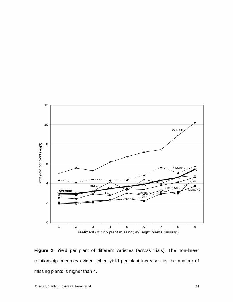
Figure 2 illustrates the non-linear relationship between yield per plant and

number of missing plants. As expected, fresh root yield on a per plant basis

remains relatively stable when few plants are missing. However, as the number

of missing plants is higher than 4, the yield per plant tends to increase

considerably. For all varieties the mean plot yield deceased as the number of

missing plant increased (Table 3). Average yield plot losses ranged from 10.6%

to 78.8% by removing one up to eight plants, respectively.

The R2 values were computed from the analysis of variance routine provided on

the SAS listing. The power model was associated with a largest value of R2

(0.9438) making it the preferred model with respect to regression model (0.5973).

Convergence of power model was achieved in fewer than four interactions. Plots

of the predicted yield ratio against the corresponding observed values indicated

that the suggested power model was appropriate. The fitted curve and the actual

values are shown in Figure 3. It can be observed that variability increases as the

number of missing plants increases. In other words as number of plants

increases the reliability of the adjustment is reduced.

Analysis of residuals for all analyses indicated little evidence to disprove the

hypothesis that residuals were normally distributed with a mean equal to zero.

The approximate F-statistics developed by Milliken and DeBruin (1978) was used

to test the significance of the extra sums of squares due to common fits.

Significant differences were detected between parameters for varieties and


environment (p< 0.05). Table 4 shows the estimated parameter values

individually for each variety, environment and combined data.

The fitted curves for all varieties are depicted en Figure 4. Invariance analysis for

some varieties (MCOL 1505, MTAI 8 and SM 1058-13) did not show significant

differences between their models indicating similar responses. Variety CM 4919-

1, on the other hand, showed highly significant differences with the other

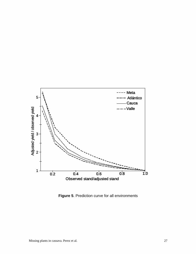
varieties. Figure 5 provides the fitted curves for all environments. Valle and

Cauca present a similar behavior, with smaller values, whereas Meta shows the

largest predicted values. According to the information generated, therefore as

expected, there was a variation in the response to missing plants for different

varieties or the different environments where the trials were conducted.

Nonetheless, a general model across varieties and environments was evaluated

resulting in estimates for α=0.73 and β=0.81.

The general model was used to estimates adjusted yield to uniform full plot

stands for each variety (Table 3). The analysis of variance (data not shown)

indicated no significant difference after adjusted yield for all varieties, except for

CM 4919-1, indicating a good fit of the proposed general model to adjust yield

plot when there are missing plant in experimental plots, regardless of the

environment were the trials are conducted or the varieties used.


Discussion The results obtained in this work clearly indicate the expected effects of missing

plant in agronomic cassava experiments. The yield per plant increases along with

the number of missing plants, mainly because the remaining plants around the

missing one are favored by less competition for limiting environmental factors as

light, water and fertilizer (Figure 2). The average yield when only one plant was

harvested varied from 3.7 kg (CM 6740-7) to 10.2 kg (SM 1058-13), indicating

large variation between varieties (Table 3).

Graphic analyses of the field data showed that the best model to explain the

relationship between fresh root yield and number of harvested plant was the

power function (results from different analyses not shown). For each and every

analysis performed, this function presented the greatest R-square values

compared with the other functions analyzed (logarithmic, exponential and linear).

This model considers a power decline of plot yield as the number of missing plant

increases. Additionally, the model considers that the adjusted yield should be a

function of both observed plot yield and plot plant stand. The ultimate objective

was to develop a model capable of adjusting total plot yields (for treatments

where one or more plants were missing) as close as possible to the values

observed in the perfect plant stand of the same variety. The analysis of

invariance, taking into account varieties and environments, showed similar

responses to different groups. However, some models showed significant


differences indicting that for specific varieties and environment their parameters

were different.

The general model across environments and varieties (based on α=0.73 and

β=0.81) was used to adjust total plot yields as presented in Table 3. It is

recognized that, ideally, the correction for missing plants should be done

individually for each variety and/or location. However, the information required to

make such adjustment is usually missing beforehand and, consequently, such

adjustment is seldom possible. The application of a more general model that can

be applied by default in the analysis of different trials would be highly desirable

(Gomez and De Datta, 1972), even if the precision in the adjustment is not

perfect. The interest to develop a general model applicable to different cassava

varieties and environmental conditions defined the nature of this study. Different

set of environments with varying average yield potential and the use of varieties

with contrasting plant architectures was purposely chosen, therefore, for this

study.

There are few available options to reduce the experimental errors derived from

missing plants. The most obvious one would be to maximize the possibility of

obtaining perfect plant stands. In many crops it is feasible to overplant and then

reduce the number of surviving plants down to the desired plant density.

However, in the case of cassava, availability of planting material is a chronic

limitation because of the low multiplication rate (Ceballos et al., 2007). This is


particularly the case in recurrent selection schemes (Morante et al. 2005).

Therefore, the occurrence of missing plants is unavoidable and approaches to

adjust yields a necessity. The simplest correction would be a linear approach

based on the yield per plant estimate: (total plot yield/number of harvested

plants)*ideal plant stand. As demonstrated (Figure 2), however, this approach

would tend to overestimate corrected yields when the number of missing plants is

high. Another linear correction could be based on the co-variance analysis. At the

bottom of Table 3 the standard deviation of the corrected plot means for these

two approaches is presented. In every case the application of the general model

proposed in this study resulted in considerably smaller standard deviation values,

indicating that the general model is better than other available methods.

The particular performance of cultivar CM 4919-1, a widely grown variety in the

sub-humid environment of Colombia’s northern coast, was interesting because it

failed to fit the general model proposed in this study. Table 5 presents

information related to plant architecture of the different varieties used in this

study. Plant height of CM 4919-1 was relatively low. More important, however,

was that it was the only clone that did not branch at all, showing a very distinctive,

completely erect plant type.

Because of the lack of a reliable method for adjusting yields in the presence of

missing plants, breeders have frequently opted for two approaches, which are

not satisfactory. One alternative is re-planting a cutting in the missing plant. The


plant that develops from this late planted cutting is typically overcome by the

plants that sprouted earlier and its yield is frequently severely reduced. The other

alternative is to harvest plants in the border row (typically of the same variety)

which is not satisfactory either because the plants harvested around the missing

plant would have higher compensatory yields, and therefore, this approach would

tend to overestimate yield potential of these plots with missing plants. The

general model proposed in this study should be used in trials where no such

unsatisfactory corrective measures have been used. Comparisons of coefficient

of variation before and after adjusting the means would provide a fair estimate of

the relative values of the method.


Literature cited

Alves, A.A.C., 2001. Cassava botany and physiology. In R.J. Hillocks, J.M.

Thresh, & A.C. Bellotti (Eds.), Cassava: biology, production and utilization, pp.

67-89. CABI Publishing, Wallingford UK;.

Boché, S. & A. Lavalle, 2004. Comparación de modelos no lineales, una

aplicación al crecimiento de frutos de carozo. Rev. Soc. Arg. Gen. 8(1):

http://www.s-a-e.org.ar/revista-vol8.htlm.

Ceballos, H. & G.A. De la Cruz, 2002. Taxonomía y Morfología de la Planta. In: B.

Ospina & H. Ceballos (Eds.), La Yuca en el Tercer Milenio, pp. 17-33. CIAT,

Cali, Colombia.

Ceballos, H., M. Fregene, J. C. Pérez, N. Morante & F. Calle, 2007. Cassava

Genetic Improvement. In: M.S. Kang & P.M. Priyadarshan (Eds.) Breeding

Major Food Staples, pp. 365-391, Blackwell Publishing. Ames, IA. USA.

Gomez, K. A.; & S. K. De Datta, 1972. Missing Hill in Rice Experimental Plots.

Agron. Journal. 64: 163-164.

James, W. C., C. H. Lawrence, C. S. Smith. 1973. Yield losses due to missing

plants in potato crops. Amer. Potato J. 50(10):345-352.

Kamid, R. E., 1995. Statistical adjustment of maize grain yield for sub-optimal

plots stands. Expl. Agric. 31: 299-306.

Leihner, D., 2001. Agronomy and cropping systems. In: R.J. Hillocks, J.M.

Thresh, & A.C. Bellotti (Eds.), Cassava: biology, production and utilization, pp.

91-113. CABI Publishing, Wallingford UK;.


Mead, R., 1968. Measurement of Competition Between Individuals Plants In a

Population. J. of Ecol. 56(1):35-45.

Milliken, G. A., & R. L. Debruin, 1978. A procedure to test hypotheses for

nonlinear models. Commun. Stat. Theory and Methods. 7:65-69.

Morante, N., X. Moreno, J. C. Pérez, F. Calle, J. I. Lenis, E. Ortega, G. Jaramillo

& H. Ceballos, 2005. Precision of selection in early stages of cassava genetic

improvement. Journal of Root Crops 31: 81-92.

Schimildt, E. R., C. D. Cruz, J. C. Zanuncio, P. R. Gomes F., & R. G. Ferrão,

2001. Avaliação de métodos de correção do estande para estimar a

produtividade em milho. Pesq. Agrop. Bras, Brasilia. 36(8):1011-1018.

Vencovsky, R., & C. D. Cruz, 1991. Comparação de métodos de correção do

rendimeinto de parcelas com estandes variados, I. Dados Simulados. Pesq.

Agropec. Bras., Brasilia. 26(5):647-657.

Verones, J. A., C. D. Cruz, L. A. Correa, & C. A. Scapim, 1995. Comparação de

métodos da ajuste do rendimiento de parcelas con estandes variados. Pesq.


Verones, J. A., C. D. Cruz, L. A. Correa, & C. A. Scapim, 1995. Comparação de

métodos da ajuste do rendimiento de parcelas con estandes variados. Pesq.


Willey.R.W. & S. B. Heath, 1969. The quantitative relationship between corn

populations and yield. Advances in Agronomy. 21:281-321.


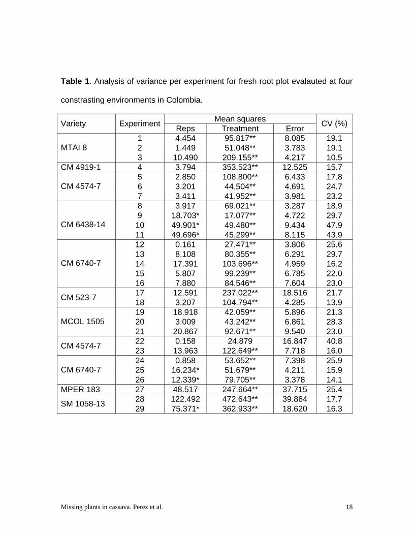
Table 1. Analysis of variance per experiment for fresh root plot evalauted at four

constrasting environments in Colombia.

Mean squares

Variety

Experiment Reps Treatment Error

CV (%)

1 4.454 95.817** 8.085 19.1 2 1.449 51.048** 3.783 19.1

MTAI 8

3 10.490 209.155** 4.217 10.5 CM 4919-1 4 3.794 353.523** 12.525 15.7

5 2.850 108.800** 6.433 17.8 6 3.201 44.504** 4.691 24.7

CM 4574-7

7 3.411 41.952** 3.981 23.2 8 3.917 69.021** 3.287 18.9 9 18.703* 17.077** 4.722 29.7 10 49.901* 49.480** 9.434 47.9

CM 6438-14

11 49.696* 45.299** 8.115 43.9 12 0.161 27.471** 3.806 25.6 13 8.108 80.355** 6.291 29.7 14 17.391 103.696** 4.959 16.2 15 5.807 99.239** 6.785 22.0

CM 6740-7

16 7.880 84.546** 7.604 23.0 17 12.591 237.022** 18.516 21.7

CM 523-7 18 3.207 104.794** 4.285 13.9 19 18.918 42.059** 5.896 21.3 20 3.009 43.242** 6.861 28.3

MCOL 1505

21 20.867 92.671** 9.540 23.0 22 0.158 24.879 16.847 40.8

CM 4574-7 23 13.963 122.649** 7.718 16.0 24 0.858 53.652** 7.398 25.9 25 16.234* 51.679** 4.211 15.9

CM 6740-7

26 12.339* 79.705** 3.378 14.1 MPER 183 27 48.517 247.664** 37.715 25.4

28 122.492 472.643** 39.864 17.7

SM 1058-13 29 75.371* 362.933** 18.620 16.3


Table 2. Mean squares form the ANOVA for each variety cambined across years

within environment.

Source of Variation

Year/

Exp Reps Trmnt

T x Y/

Exp Error

CV

(%)

St

Error

MTAI 8 (3) (Atlántico) 600.7** 4.2 319.8** 18.1** 5.4 15.6 1.10

CM 4574-7(Meta) 274.5** 5.7 182.9** 6.2 4.8 20.8 1.03

CM 4574-7(Valle) 14.0 122.7** 7.7 16.0 2.27

CM 4574-7(All) 495.3** 4.5 287.9** 10.0 5.8 19.6 0.98

CM6740-7(Meta) 181.0** 1.2 360.3** 8.8 6.2 23.3 0.91

CM6740-7(Valle) 56.1** 3.1 161.1** 12.5 5.4 19.2 1.01

CM6740-7(All) 133.9** 1.2 505.8** 10.8 5.9 21.6 0.71

MCOL1505(Valle) 138.9** 14.0 152.7** 7.3 6.7 22.5 1.22

CM523-7(Valle) 335.0** 2.0 322.7** 19.1 11.5 19.6 1.96

SM1058-13(Cauca) 837.8** 19.4 861.0** 59.1 31.8 18.4 3.26

CM4919-1(Atlántico) 3.8 353.5** 12.5 15.7 2.89


Table 3. Varieties mean of observed plot yield and adjusted plot yield.

Harvested MTAI 8 CM 4919-1 CM 4574-7 CM 6740-7 CM 523-7 MCOL 1505 SM 1058-13

plants yo ya yo ya yo ya yo ya yo ya yo ya yo ya

9 22.7 22.7 39.1 39.1 18.9 18.9 17.3 17.3 25.5 25.5 16.8 16.8 45.2 45.2

8 19.5 21.2 32.8 35.7 16.4 17.8 15.9 17.3 22.8 24.8 15.3 16.6 44.4 48.4

7 20.3 24.4 31.1 37.3 15.4 18.5 14.4 17.3 22.4 26.9 14.7 17.7 37.1 44.4

6 16.7 22.3 26.0 34.7 13.6 18.1 13.7 18.3 24.9 33.3 13.6 18.1 37.0 49.5

5 17.2 26.2 21.9 33.3 15.2 23.1 12.2 18.5 16.6 25.1 12.0 18.3 33.6 51.0

4 13.5 24.0 19.5 34.6 11.1 19.8 8.9 15.8 17.6 31.3 10.3 18.3 28.8 51.5

3 11.4 24.8 16.9 36.7 9.9 21.4 8.8 19.2 12.0 26.0 9.4 20.3 22.4 48.6

2 8.2 23.8 10.2 29.4 5.8 16.8 6.3 18.1 9.3 26.8 7.0 20.2 17.8 51.5

1 4.7 22.2 5.7 27.3 4.7 22.5 3.7 17.7 4.8 22.9 4.3 20.4 10.2 48.5

St. Dv.1 5.96 1.54 10.86 3.78 4.83 2.20 4.59 0.96 7.33 3.30 4.12 1.46 11.98 2.50

St.Dev.2 6.79 9.69 5.39 13.45 7.58 8.13 5.49 6.48 6.88 12.93 7.29 5.40 15.48 18.77

yo= observed plot yield, ya= adjusted plot yield.

1 For each variety, standard deviations for observed plot yields (left) and using

the general model correction (right).

2 For each variety, standard deviations for observed plot yields corrected by the

yield per plant approach (left) or the linear approach (right)


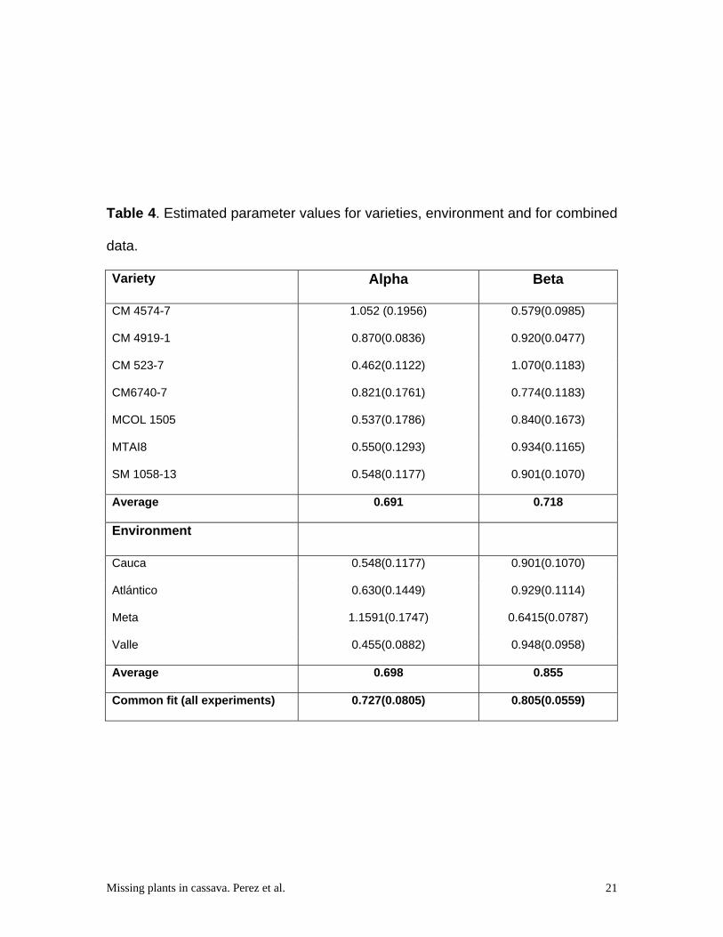
Table 4. Estimated parameter values for varieties, environment and for combined

data.

Variety Alpha Beta

CM 4574-7 1.052 (0.1956) 0.579(0.0985)

CM 4919-1 0.870(0.0836) 0.920(0.0477)

CM 523-7 0.462(0.1122) 1.070(0.1183)

CM6740-7 0.821(0.1761) 0.774(0.1183)

MCOL 1505 0.537(0.1786) 0.840(0.1673)

MTAI8 0.550(0.1293) 0.934(0.1165)

SM 1058-13 0.548(0.1177) 0.901(0.1070)

Average 0.691 0.718

Environment

Cauca 0.548(0.1177) 0.901(0.1070)

Atlántico 0.630(0.1449) 0.929(0.1114)

Meta 1.1591(0.1747) 0.6415(0.0787)

Valle 0.455(0.0882) 0.948(0.0958)

Average 0.698 0.855

Common fit (all experiments) 0.727(0.0805) 0.805(0.0559)


Table 5. Averages of relevant plant type characteristics of the varieties used in

this study.

Height (cm) Number of Genotype Plant 1st branching branching events MTAI 8 200 120 3 CM 4919-1 205 -.- -.- CM 4574-7 245 175 2 CM 6740-7 297 167 2 CM 523-7 220 115 3 MCOL 1505 215 100 3 SM 1058-13 200 56 5


0 0 0 0 0

0 1 2 3 0

0 4 5 6 0

0 7 8 9 0

0 0 0 0 0

Figure 1. Scheme illustrating the identification of each ‘central’ plant inside

experimental plots for measuring the effect the missing plant in cassava

evaluation trials.


0

2

4

6

8

10

12

1 2 3 4 5 6 7 8 9

Treatment (#1: no plant missing; #9: eight plants missing)

Roo

t yie

ld p

er p

lant

(kg/

pl)

SM1508

CM4919

CM523

Tai CM4574COL1505 CM6740Average

Figure 2. Yield per plant of different varieties (across trials). The non-linear

relationship becomes evident when yield per plant increases as the number of

missing plants is higher than 4.


Figure 3. Prediction curve for general values


Figure 4. Prediction curve for all varieties


0.2 0.4 0.6 0.8 1.0Observed stand/adjusted stand

5

4

3

2

1

MetaAtlánticoCaucaValle

0.2 0.4 0.6 0.8 1.0Observed stand/adjusted stand

0.2 0.4 0.6 0.8 1.00.2 0.4 0.6 0.8 1.0Observed stand/adjusted stand

5

4

3

2

1



eld

eld

yi

yi

eded

erv

erv

bsbs

o o

d /

d /

yie

l y

iel

eded

stst

Ad

juAd

ju

Figure 5. Prediction curve for all environments


Documents

Adjustment for missing plants in cassava evaluation trialsciat-library.ciat.cgiar.org/Articulos_Ciat/Article Missing Feb 2009... · Adjustment for missing plants in cassava evaluation