Embed Size (px)
Citation preview

University of Birmingham
Adjustment Behavior and Value of Corporate CashHoldings: the China ExperienceGuariglia, Alessandra; Yang, Junhong
DOI:10.1080/1351847X.2015.1071716
License:None: All rights reserved
Document VersionPeer reviewed version
Citation for published version (Harvard):Guariglia, A & Yang, J 2016, 'Adjustment Behavior and Value of Corporate Cash Holdings: the ChinaExperience', European Journal of Finance. https://doi.org/10.1080/1351847X.2015.1071716
Link to publication on Research at Birmingham portal
Publisher Rights Statement:This is an Accepted Manuscript of an article published by Taylor & Francis in The European Journal of Finance on 16 February 2016,available online: http://dx.doi.org/10.1080/1351847X.2015.1071716
Checked Feb 2016
General rightsUnless a licence is specified above, all rights (including copyright and moral rights) in this document are retained by the authors and/or thecopyright holders. The express permission of the copyright holder must be obtained for any use of this material other than for purposespermitted by law.
•Users may freely distribute the URL that is used to identify this publication.•Users may download and/or print one copy of the publication from the University of Birmingham research portal for the purpose of privatestudy or non-commercial research.•User may use extracts from the document in line with the concept of ‘fair dealing’ under the Copyright, Designs and Patents Act 1988 (?)•Users may not further distribute the material nor use it for the purposes of commercial gain.
Where a licence is displayed above, please note the terms and conditions of the licence govern your use of this document.
When citing, please reference the published version.
Take down policyWhile the University of Birmingham exercises care and attention in making items available there are rare occasions when an item has beenuploaded in error or has been deemed to be commercially or otherwise sensitive.
If you believe that this is the case for this document, please contact [email protected] providing details and we will remove access tothe work immediately and investigate.
Download date: 04. Aug. 2020

1
Adjustment behavior of corporate cash holdings: The China experience
Alessandra Guarigliaa and Junhong Yangb
aDepartment of Economics; University of Birmingham; Birmingham B15 2TT, United
Kingdom; bManagement School; University of Sheffield; Conduit Road; Sheffield S10 1FL,
United Kingdom
Using a panel of 1,478 Chinese listed firms over the period 1998-2010, we examine the behavior of corporate cash holdings. Consistent with the trade-off theory, we document that Chinese firms tend to actively manage their cash balances towards a target level. We also observe a considerable heterogeneity in adjustment speeds of cash holdings across firms, due to the presence of different adjustment costs. Specifically, firms with a high level of excess cash, and firms that actively manage their cash balances through investment, dividend payments, and debt issuance, all display higher adjustment speeds. Finally, the institutional setting does not significantly affect adjustment speeds.
Keywords: Cash holdings; trade-off theory; speed of adjustment; China
JEL classification: G30; G32
2
1. Introduction
Cash and cash equivalents are an important source of finance for firms, especially in the
presence of imperfect capital markets. A huge literature has investigated possible reasons
why companies hold a considerable portion of their assets in the form of cash reserves. Most
of this literature focuses on US and European corporations. Yet, Chinese firms hold higher
levels of cash reserves than firms in most countries, including developed ones, and the cash
holdings of Chinese firms have been growing over the last decade at rates similar to those of
US and European companies. 1 Understanding Chinese firms’ cash holding behavior
represents therefore an interesting research question.
Allen et al. (2007) point out that the malfunctioning financial system in China, which
is mainly bank-based, hinders economic growth. According to Elliott and Yan (2013), the
ratio of total bank credit to GDP reached 128% in 2012. This ratio is much larger than the
corresponding ratio in the US in the same year (48%). The very large banking system, which
is characterized by a significant amount of NPLs (non-performing loans) and an outstanding
government debt, dwarfs all other forms of finance in China. Yet, only a small fraction of
bank credit is directed towards the non-state sector, which suggests that non state-owned
firms may find it difficult to obtain external finance. There is also abundant evidence
showing that the role of China’s stock markets in financing and allocating resources is limited,
and size requirements generally prevent private enterprises from accessing equity markets
(Allen et al. 2012).
Given the difficulties they face in accessing external finance, Chinese firms, and
particularly the non-state ones, rely on self-financing, which comprises retained earnings,
cash reserves, and loans from family, friends and other investors. The average annual growth
rate of self-funding in China was approximately 17.8% between 1994 and 2006, and self-
funding reached $666.5 billion in 2006, which is almost twice the size as domestic bank loans

3
($364.8 billion) in the same year. Moreover, roughly 90% of total financing for individually
owned companies depends on self-funding. Even for state-owned enterprises (SOEs) or
quasi-state-owned companies, 45%-65% of total financing comes from self-funding (Allen,
Qian, and Qian 2007).
A number of studies have found positive effects of internal funds on the investment
and assets growth of Chinese firms (Guariglia, Liu, and Song 2011, Lin and Bo 2012, Firth et
al. 2012, Ding, Guariglia, and Knight 2013). Due to its relatively low cost, a sufficient level
of internal finance (intended as cash reserves or cash flow) provides Chinese firms with the
ability to invest, despite the difficulties they face in accessing external finance. Consequently,
unlike the US or European countries, where the financial system functions efficiently, cash
holdings are likely to play a more crucial role in explaining firm behavior and, ultimately,
economic growth in China. Yet, to the best of our knowledge, only a handful of studies have
analyzed corporate cash holding decisions in China (Feng and Johansson 2014, Chen et al.
2012, Megginson and Wei 2014, Alles, Lian, and Xu 2012, Lian, Xu, and Zhou 2010).
The aim of this study is to fill this gap in the literature by investigating Chinese firms’
cash holding decisions. Specifically, we address the following questions: Do Chinese firms
have cash targets, and if so, how quickly do they adjust towards the targets? What factors
affect their speeds of adjustment (SOAs) towards these targets? Is there heterogeneity in
adjustment speeds across firms?
To this end, making use of a panel of 1,478 listed companies over the period 1998-
2010, we first test the time series properties of Chinese firms’ cash holdings. We find that
they display mean reverting properties, which suggests a tendency towards convergence.
Second, following Opler et al. (1999) (hereafter OPSW), we examine different models of
corporate cash holdings, and find substantial empirical support for the trade-off model,

4
according to which firms assess the costs and benefits of holding cash and adjust their cash
reserves to a target level.
Third, we estimate the rate at which firms adjust their cash reserves towards the target
(i.e. their speed of adjustment, SOA). We find imperfect adjustments of cash holdings: It
takes the typical Chinese firm between 1.2 and 2.1 years to complete half of its required cash
adjustment. This is slightly longer than what is observed for firms from the West, and can be
explained by the higher adjustment costs faced by Chinese firms. Financing frictions may
also prevent firms from keeping their cash holdings in line with the optimal level, and thus
cause a dynamic adjustment of cash holdings.
Fourth, we find that the SOAs of cash holdings are different for firms facing different
adjustment costs. Particularly, firms with excess cash display higher adjustment speeds than
their counterparts with a cash deficit. In other words, it is more costly for a firm to build up
cash stocks than to deplete excess cash reserves. Additionally, higher adjustment speeds are
observed for firms who actively manage their cash balances through higher investment,
dividend payments, and debt issuance. Finally, the institutional setting does not significantly
affect adjustment speeds.
The remainder of this paper proceeds as follows. In Section 2, we briefly review the
theories of cash holdings and their empirical predictions. Section 3 provides a survey of the
literature on corporate cash holdings in China. Section 4 illustrates the main features of our
data and presents summary statistics. Section 5 describes our baseline specifications and
empirical results. Section 6 concludes.

5
2. Theories of cash holdings
In the sub-sections that follow, we illustrate in turn the three main theories on the motives of
corporate cash holdings, namely the trade-off theory, the financial hierarchy theory, and the
free cash flow theory.
2.1. The trade-off theory of cash holdings
The trade-off theory, which has attracted significant empirical support (Opler et al. 1999, Lee
and Powell 2011, Venkiteshwaran 2011, Keynes 2006), suggests that given the costs and
benefits of holding liquid assets, firms tend to rebalance their cash holdings towards a target
level which maximizes shareholder wealth.
The cost of holding cash is the opportunity cost of the capital invested in liquid assets, i.e.
the lower return compared to other investments associated with a similar level of risk (Opler
et al. 1999, Dittmar, Mahrt-Smith, and Servaes 2003). As for the benefit of holding cash, it
stems from two motives: the transaction cost motive and the precautionary motive. According
to the former, firms benefit from holding cash to meet business transactions needs or
unsynchronized expenses. Using cash enables them to make payments without liquidating
assets. Consistent with this perspective, Mulligan (1997) argues that there exist economies of
scale in cash holdings since it is more costly for small firms to access capital markets and
raise external financing and it is more difficult for these firms to sell non-core assets to raise
cash in periods of financial distress. Similarly, one would also expect firms with more
volatile cash flow to hold cash to mitigate the consequences of unexpected earnings shortfalls.
According to the precautionary motive, liquid assets can be used as a buffer to meet
unexpected shocks, enabling firms to avoid the cost premium they would have to pay if they
had to access capital markets. The precautionary motive also suggests that in the presence of
asymmetric information problems, firms hold cash to avoid the costs of forgoing positive net
6
present value (NPV) projects when other sources of finance become either too expensive or
not available. This motive is likely to be more relevant for firms with better investment
opportunities.
The trade-off view suggests that firms have incentives to actively offset deviations from
their optimal cash levels. However, adjustment costs may prevent them from immediately
rebalancing towards their target level, since they need to trade-off the adjustment costs
against the costs of operating with suboptimal cash levels. The speed with which firms adjust
their cash holdings depends on the adjustment costs they face. With zero adjustment costs,
firms should always stick to their optimal cash ratios. If adjustment costs are infinite, one
would expect that there is no reversion of cash changes.
Empirical support for the trade-off theory has been found, among others, by Kim et al.
(1998), Opler et al. (1999), Ozkan and Ozkan (2004), Han and Qiu (2007), and
Venkiteshwaran (2011), who focused on the US and the UK. Yet, the static cash holding
model used by Kim et al. (1998) and Opler et al. (1999) assumes that cash holdings are
determined by a single period trade-off between the costs and benefits of holding liquid assets.
However, the performance of the static trade-off model is weakened by not fully accounting
for firms’ adjustment costs and expectations. By contrast, the dynamic models of cash
holdings developed by Ozkan and Ozkan (2004), Han and Qiu (2007), and Venkiteshwaran
(2011) recognize a sluggish adjustment process of cash holdings due to adjustment frictions2.
2.2 The financial hierarchy (pecking order) theory of cash holdings
Myers and Majluf (1984) propose a pecking order model, according to which, in a world
characterized by imperfect capital markets, firms use first of all retained earnings to finance
themselves, then debt, and then equity as a last resort. This theory suggests that when a firm
has a low level of cash flow relative to investment, it will use stockpiled cash holdings before

7
seeking for costly external financing. Hence, holding a considerable amount of cash can
reduce the costs of raising funds externally, and serve stockholders’ interests. According to
this theory, one would expect that faced with a rise in internal funds, the firm would
accumulate cash and repay its debt when it is due; while if a firm faces a deficit of internal
funds, it is more likely to deplete cash reserves and further raise debt. Generally, cash can be
seen as negative debt. In brief, a firm’s level of cash holdings would rise and fall with its
profitability (Opler et al. 1999). In contrast with the trade-off theory, this theory does not give
rise to an optimal cash holding level.
Empirical support for the pecking order theory has been found, among others, by de
Haan and Hinloopen (2003), for the Netherlands; by Ferreira and Vilela (2004), for EMU
countries; by D’Mello et al. (2008), for the US; and by Bigelli and Sánchez-Vidal (2012), for
Italy.
2.3 The free cash flow theory of cash holdings
The free cash flow theory suggests that managers might not always have the same interests as
shareholders due to empire-building or entrenchment motives. Specifically, managers might
have incentives to stockpile cash as reserves to pursue their own objectives. Holding excess
cash gives them in fact more flexibility to operate their companies, even at the expense of
shareholders. As for the financial hierarchy theory, the free cash flow theory does not predict
an optimal level of corporate liquidity.
By examining a small sample of firms with a cash windfall, Blanchard et al. (1994)
find that in order to secure their positions and firms’ long-run survival, managers often invest
the cash windfall in value-destroying projects rather than returning it to shareholders. Dittmar
et al. (2003) show that there are significantly higher cash reserves in countries with poor
shareholder protection. Similarly, Dittmar and Mahrt-Smith (2007) find that poorly governed

8
firms have lower marginal value of cash holdings and have a worse operating performance
associated with excess cash. These findings are consistent with the predictions of the free
cash flow theory. Additionally, accumulating excess cash may decrease market discipline.
For example, Harford (1999) documents that firms which are holding excess cash are likely
to make value-decreasing acquisitions, while they are less likely to be a takeover target. In
short, without valuable investment opportunities, the agency costs of managerial discretion
may lead firms to use their excess cash to finance unprofitable projects rather than to pay
dividends to shareholders, which decreases the additional value of cash holdings.
Based on the discussion on these motives of cash holdings, we will assess the extent
to which the cash holdings of Chinese firms can be explained by these theories. Initially, we
will test for the presence of a cash target. Should we find evidence for the existence of such a
target, we will investigate what is the adjustment speed with which firms rebalance their cash
ratio towards the optimal level in the presence of adjustment costs.
3. Review of the literature on cash holdings in China
Only a few papers have focused on cash holdings in China. Among these, Megginson and
Wei (2014) analyze the links between state ownership and the level and value of cash
holdings. Using data on share-issue privatized companies over the period 1993-2007, they
find that the level of cash holdings declines as state ownership increases. This can be
explained considering that the higher the level of state ownership in a firm, the better the
firm’s access to credit from state-owned banks. This reduces the need to accumulate high
levels of cash for precautionary reasons. The authors also find that the marginal value of cash
declines as state ownership rises. They explain this considering that managers in firms
characterized by high state ownership are more likely to invest any extra cash in politically

9
motivated projects or projects aimed at building their empires rather than profit-maximizing
projects.
Chen et al. (2012) focus on the effects of the 2005-2006 split share structure reform on
firms’ cash holdings. Using data on 1,293 listed companies over the period 2000-2008, they
observe a decline in both corporate cash holdings and the sensitivity of cash holdings to cash
flow after the reform. This decline was larger for firms with weaker governance arrangements
and firms characterized by a higher degree of financing constraints prior to the reform. These
findings suggest that, in line with the free cash flow theory, prior to the reform, firms held
excessive levels of cash to pursue their own objectives. The reform alleviated these agency
problems, and hence, also indirectly mitigated those financing constraints associated with
poor governance. Furthermore, the authors observe that the decline in corporate cash holdings
was larger for privately controlled firms than for state-owned enterprises (SOEs). They
explain this finding in the light of the fact that the ability of managers to make personal use of
corporate assets was more constrained in SOEs.
Feng and Johansson (2014) concentrate on the effects of political participation on liquid
asset holdings for 2,115 Chinese privately controlled listed firms over the period 1999-2009.
They find that corporate cash holdings are higher for firms whose entrepreneurs are involved
in politics, and that the positive effect of political participation on cash holdings is higher in
those regions with weak institutions. They explain these findings in the light of the fact that
being politically connected reduces the risk of entrepreneurs suffering from political
extraction.
The three papers surveyed above all focus on the level of cash holdings and/or the cash to
cash flow sensitivities, but none of them investigates the existence of a target level of cash
holdings. To the best of our knowledge, only two papers focus on this issue in the Chinese
context, finding support for the trade-off theory. The first one, Alles et al. (2012), makes use

10
of a panel of 780 listed companies over the period 1998 to 2009 to analyze the determinants
of target cash reserves on the one hand, and of firms’ speed of adjustment (SOA) towards the
target, on the other. Their findings suggest that Chinese companies tend to adjust their cash
holdings quite rapidly towards the target level, which is a function of a series of firm-specific
financial and ownership variables. Yet, their paper does not take into account how different
firms may adjust differently towards the target. Lian et al. (2012) go one step further in this
direction. Making use of a panel of 1,026 listed companies over the period 1998-2006, they
investigate possible determinants of the adjustment speeds of cash reserves towards a target.
They find that adjustments from above the target are much faster than adjustments from
below. Furthermore, they show that SOAs are faster for firms with access to bank lines of
credit. This is explained considering that credit lines enable firms to adjust their cash levels at
moderate adjustment cost. The authors also find that younger firms exhibit higher SOAs,
which they explain considering that because these firms are more likely to face financing
constraints, holding the right amount of cash for precautionary reasons is particularly
important for them. Finally, the authors show that SOAs are also affected by the firm’s size,
the volatility of cash flow, growth opportunities, and agency costs, and that the adjustment to
target is mainly undertaken through internal finance, rather than through dividend payments
or leverage.
Our work builds on Lian et al.’s (2012) along the following four dimensions. First, it is
based on a more recent sample period, covering the post-split share structure reform years up
to 2010. Second, unlike Lian et al. (2012), we propose a direct horse-race test of the target
adjustment model against the financial hierarchy model. Third, we investigate the extent to
which SOAs vary for different types of firms using a broader range of criteria to differentiate
firms. Finally, we assess whether the institutional setting affects SOAs, by investigating the

11
extent to which SOAs are affected by ownership, location in more financially developed
regions, and location in proximity of a stock market.
4. Data and descriptive statistics
4.1. The dataset
We use the universe of listed Chinese firms that issue A-shares on either the Shanghai Stock
Exchange (SHSE) or the Shenzhen Stock Exchange (SZSE) during the period 1998-2010,
obtained from the China Stock Market Trading Database (CSMAR) and China Economic
Research Service Centre (CCER). Following the literature, we exclude firms in the financial
sector. Furthermore, to minimize the potential influence of outliers, we winsorize
observations in the one percent tails for the regression variables. Finally, we drop all firms
with less than three years of consecutive observations. All variables are deflated using the
gross domestic product (GDP) deflator (National Bureau of Statistics of China).
We consider the information on acquisition deals announced between January 1, 1999
and December 31, 2011 for our listed Chinese companies on the Thomson Financial SDC
Mergers and Acquisitions Database. Both successful and unsuccessful deals are taken into
consideration.3
Our final unbalanced panel consists of 15,349 firm-year observations representing
1,478 listed firms. The number of firm-year observations of each firm varies between three
and thirteen, with number of observations varying from a minimum of 708 in 1998 to a
maximum of 1,478 in 2008.4
4.2. Descriptive statistics
Table 3 presents descriptive statistics for the main variables used in the study. We observe
that the average cash flow to assets ratio is 4.7%; the average capital expenditure to assets

12
ratio, 5.8%; the average leverage ratio, 23.2%; and average cash flow volatility, 8.7%. These
figures are largely consistent with those reported for US firms by Opler et al. (1999) and
Venkiteshwaran (2011); for EMU and UK firms, by Ferreira and Vilela (2004) and Ozkan
and Ozkan (2004); and for Chinese firms, by Alles et al. (2012). Additionally, Table 3 shows
that on average, the return on assets (ROA) is 2.3% and Tobin’s Q is greater than one (1.75).5
[Insert Table 3]
Furthermore, we observe that the mean level of cash holdings to total assets in our
sample is approximately 14.7%. This is comparable to the ratios observed for US and UK
firms6. However, the median cash-to-assets ratio is 12.1%, higher than the median ratios
observed in the West, which range between 3% for Canadian firms to 9% for French firms
(Ozkan and Ozkan 2004, Opler et al. 1999, Venkiteshwaran 2011, Harford, Mansi, and
Maxwell 2008, Dittmar and Mahrt-Smith 2007, Riddick and Whited 2009). Chinese firms
also hold a relatively higher median percentage of cash reserves than most of the developed
countries analyzed by Dittmar et al. (2003) and Riddick and Whited (2009), for which the
median cash to assets ratio is 6.3% and 6.2%, respectively7. It is interesting to point out that
Japan has similar mean and median cash to assets ratios as China (16.4% and 13.9%,
respectively). In addition, our descriptive statistics reveal that the average cash level (14.7%)
is higher than the sum of average cash flow (4.7%) and capital expenditures (5.8%). Cash
holdings constitute therefore a non-trivial percentage of total assets of Chinese firms. This
may be due to the higher costs associated with raising external credit in China (Allen, Qian,
and Qian 2005), which may lead Chinese firms to rely more on internal finance than firms in
other countries.
The lower part of Table 3 provides summary statistics for the cash-to-assets ratio by
year. It reveals that average (median) cash holdings range from 9.8% (7.9%) in 1998 to 17.2%
(14.3%) in 2010. This suggests that during the sample period, the level of cash holdings in
13
China almost doubled.8 Additionally, in line with Chen et al. (2012), we observe a trough of
cash holdings in 2005 and 2006.9 Chen et al. (2012) attribute the reduction in cash holdings
to an improvement in Chinese firms’ corporate governance and a relaxing in the financial
constraints following the 2005 split share structure reform.10 The noticeable increasing trend
in cash holdings from 2007 onwards may be due to the financial crisis, which made it more
difficult for firms in China to access credit.
5. Evaluation of the results
5.1. Targeting behavior of cash holdings and adjustment towards the target
5.1.1. Targeting behavior of cash holdings
We begin our analysis by investigating whether firms tend to revert cash holdings to their
target levels. To this end, following Opler et al. (1999), we first test the mean reversion
properties of cash holdings by estimating a first-order autoregressive model of the changes in
the cash ratio for each firm in our sample, as outlined in the following equation:
∆(𝐶𝐶𝐶ℎ)𝑖,𝑡 = 𝛼 + 𝛽∆(𝐶𝐶𝐶ℎ)𝑖,𝑡−1 + 𝜀𝑖,𝑡 (1)
where the subscript i indexes firms; and t, years (t=1998-2010). Δ indicates a first-difference
from one period to the next, and 𝐶𝐶𝐶ℎ is the ratio of cash and cash equivalents to total
assets. 𝜀𝑖,𝑡 is assumed to be an independent and identically distributed disturbance with zero
mean.
Fig. 1 illustrates the distribution of the autoregressive coefficient (β) obtained from Eq.
(1).11 The figure shows that the distribution is bell-shaped with a negative centerline. The
median and mean of the coefficients (β) are -0.179 and -0.165, respectively, suggesting that
cash holdings are mean reverting12. Instead of running separate regressions for each firm, we
next run pooled OLS estimates of Eq. (1) with cluster-robust standard errors for the full
sample of firms. 13 The estimated coefficient (β) is found to be -0.166 (t-stat= -14.50,

14
R2=0.03). Once again, the fact that the absolute value of the coefficients (β) is less than 1
suggests that cash balances display mean reverting properties. This finding is consistent with
Opler et al. (1999) and Venkiteshwaran (2011).14
[Insert Fig. 1]
5.1.2. Adjustment towards target cash holdings
We next investigate the extent to which firms in our sample adjust their cash balances
towards the target level over time. To this end, we first sort firms into quintiles in each year
based on their previous year’s cash positions. In Panel A of Fig. 2, the horizontal axis goes
from cash-poor (𝐶𝐶𝐶ℎ=3.15%) to cash-rich (𝐶𝐶𝐶ℎ=31.86%) firms, from left to right. The
vertical axis describes the subsequent year’s changes in cash holdings. It appears that cash-
poor firms tend to increase the mean (median) cash levels by 2.7% (0.9%) in the following
year, while cash-rich firms are inclined to reduce their mean (median) cash ratios by 4.8%
(4.2%) in the subsequent year. This is consistent with convergence. This evidence confirms
that firms exhibit mean reversion in their cash holdings, and presents indirect evidence of
adjustment behavior towards a cash target: A company in the fifth quintile of the cash
holding distribution is in fact more likely to be above target than a company in the lowest
quintile.
[Insert Fig. 2]
Panel B of Fig. 2 examines the links between the firm’s subsequent year’s changes in
cash holdings and their deviations from their cash target levels. We partition firms into
quintiles in each year on the basis of the difference between their real cash holdings and their
optimal cash level (Cash*) obtained from the estimation of an augmented OPSW model,
which controls for acquisitions and ownership 15. The horizontal axis, from left to right,
indicates that the firms in the first quintile have the highest cash deficit (-8.63%), while firms

15
in the last quintile have the highest excess cash holdings (10.23%). Accordingly, the former
raise their cash ratios by an average (median) of 4.7% (2.5%), and the latter reduce their
balances by an average (median) of 6.2% (5.6%) in the following year. The evidence in Panel
B reflects the firms’ unambiguous tendency to correct their deviations from the optimal levels.
In other words, firms that are either cash-rich or cash-deficient adjust their cash ratios
towards the optimal level to offset the gap.
It should also be noted that the adjustments illustrated in both Panels of Fig. 2 are
asymmetric. Specifically, firms with higher deviations from their target levels, i.e. those in
the first quintile (characterized by a lower level or a deficit of cash holdings) and in the last
quintile (characterized by a higher level or an excess of cash holdings) tend to adjust their
cash holdings more aggressively than firms in the median quintiles. Moreover, the average or
median adjustment is more pronounced for cash-rich firms in comparison with cash-poor
ones, which may be due to asymmetric adjustment costs. This can be explained considering
that it is more costly for firms with lower cash balances to build their cash reserves or deviate
from the target, than it is for cash-rich firms to spend cash or deviate from the targets. Cash-
poor firms are in fact more likely to be financially constrained (Dittmar and Duchin 2010). A
similar asymmetric adjustment is also reported for US manufacturing firms by
Venkiteshwaran (2011), and for Chinese listed companies by Lian et al. (2012) 16.
5.2. Targeting behavior versus financial hierarchy
As discussed in the last section, firms exhibit a tendency of cash convergence towards a
target level, which can be explained by the trade-off theory. However, according to the
financial hierarchy theory, adjustments of firms’ cash holdings are simply a consequence of
changes in internal resources, and firms do not actively manage their cash balances. Thus,
there is no optimal level of cash holdings. To distinguish between these two alternative views,

16
following Opler et al. (1999) and Venkiteshwaran (2011), we construct a “financing deficit”
variable, defined as (dividend payments + investment + changes in net working capital –
operating cash flow) / total assets, to proxy the flow of funds, and examine whether this
variable can be used to explain changes in cash holdings.17 If the financial hierarchy behavior
prevails over the trade-off theory, we would expect the financing deficit to wipe out the
effects of the deviation from optimal cash levels �𝐶𝐶𝐶ℎ𝑖,𝑡+1∗ − 𝐶𝐶𝐶ℎ𝑖,𝑡� in a partial
adjustment model of the following type:
𝐶𝐶𝐶ℎ𝑖,𝑡+1 − 𝐶𝐶𝐶ℎ𝑖,𝑡 = 𝛼 + 𝜑�𝐶𝐶𝐶ℎ𝑖,𝑡+1∗ − 𝐶𝐶𝐶ℎ𝑖,𝑡� + 𝐹𝐹𝐹𝐹𝐹𝐹𝑖,𝑡+
𝑣𝑖 + 𝑣𝑡 + 𝑣𝑗 + 𝑣𝑝 + 𝜀𝑖,𝑡 (2)
where the subscript i indexes firms; j indexes industries; p indexes provinces; and t, years
(t=1998-2010). 𝐶𝐶𝐶ℎ is the ratio of cash and cash equivalents to total assets, Cash* is the
estimated target cash holdings, FINDEF is the firm’s financial deficit, and 𝜑 is the speed of
adjustment (SOA), which measures how fast firms adjust their cash holdings towards the
optimal level18. The SOA is expected to be greater than zero if firms exhibit mean reversion,
and smaller than 1 if their adjustment is imperfect.19
The error term in Eq. (2) consists of five components. vi is a firm-specific effect,
embracing any time-invariant firm characteristic which might influence firms’ cash holdings,
as well as any time-invariant component of the measurement error which may affect any
variable in our regression. vt is a time-specific effect, which we control for by including time
dummies capturing the possible effects of business cycles, as well as the impact of change in
interest rates. vj is an industry-specific effect, which we take into account by including
industry dummies20. vp is a province-specific effect, controlling for uneven developments
across different provinces, which we take into account by including province dummies21.
Finally, εi,t is an idiosyncratic component.

17
Table 4 presents the fixed-effects estimates from the partial adjustment model in Eq.
(2).22 In columns 1 to 6, a variant of Eq. (2) which excludes the financial deficit variable is
estimated. In column 1, the firm’s target cash holdings (Cash*) are measured as the average
cash holdings over the previous three years. In column 2, Cash* is given by the median cash
holdings in the firm’s industry in each year. In column 3, it is calculated as the fitted values
from the OPSW model augmented with acquisitions and ownership controls, estimated using
the OLS pooled estimator. In column 4 and 5, it is obtained likewise, except for the fact that
the augmented OPSW model is estimated using the Fama-MacBeth and the fixed-effects
estimators, respectively. Finally, in column 6, Cash* is given by the fitted values of a
dynamic version of the augmented OPSW model estimated using a fixed-effects estimator. In
all six regressions, the adjustment coefficients are significant at the 1% level, which supports
the target adjustment model. The speeds of adjustment are respectively 0.483, 0.555, 0.574,
0.578, 0.581, and 0.466. To give some economic interpretation, we calculate firms’ half-lives
of cash rebalancing, defined as the time necessary to cover half of the deviation from the
initial cash level to the target level. The values are 1.435, 1.248, 1.208, 1.198, 1.194, and
1.487 years, respectively, which imply an imperfect adjustment of cash. Our finding are
similar to those reported in Opler et al. (1999) and Venkiteshwaran (2011), who also find
support for the target adjustment model.
[Insert Table 4]
In column 7 of Table 4, we examine whether the firm’s financial deficit (𝐹𝐹𝐹𝐹𝐹𝐹) is
able to explain the variation in cash holdings. The results indicate that the coefficient
associated with FINDEF is positive and statistically significant. However, the point estimate
of FINDEF evaluated at sample means is only 0.017, indicating that the elasticity of a change
of cash holdings reacting to a change in FINDEF is only around 1.25% of the elasticity of a
change in the deviation �𝐶𝐶𝐶ℎ𝑖,𝑡+1∗ − 𝐶𝐶𝐶ℎ𝑖,𝑡� observed, for instance, in column 5.23 This

18
suggests that the change in cash holdings that follows a percentage change in the deviation
�𝐶𝐶𝐶ℎ𝑖,𝑡+1∗ − 𝐶𝐶𝐶ℎ𝑖,𝑡� is much larger than the one that follows the same percentage change in
FINDEF. In addition, the R2 of the financial hierarchy model (0.03) in column 7 is smaller
than the ones in the trade-off model (which range from 0.13 to 0.30).
In columns 8 to 13, we include the deviation �𝐶𝐶𝐶ℎ𝑖,𝑡+1∗ − 𝐶𝐶𝐶ℎ𝑖,𝑡� and the financing
deficit (FINDEF) in the same regression. The coefficients on the former are similar to what
we obtained when we only included the deviation variable, whilst, with one exception, the
coefficients on the latter are no longer significant 24 . Moreover, we do not observe any
increases in the R2 in columns 8 to 13, compared with columns 1 to 6. The reason is probably
that the deviation �𝐶𝐶𝐶ℎ𝑖,𝑡+1∗ − 𝐶𝐶𝐶ℎ𝑖,𝑡� has more explanatory power in cash rebalancing
than the flow of funds deficit (FINDEF), destroying therefore the significance of the latter.
Overall, our results in Table 4 provide strong support for the fact that cash holdings in
China can best be explained by a trade-off model rather than by the financial hierarchy
theory25. This is in line with most of the findings from US and European firms (Opler et al.
1999, Lee and Powell 2011, Venkiteshwaran 2011, Kim, Mauer, and Sherman 1998, Ozkan
and Ozkan 2004).
5.3 Dynamic adjustment models of cash holdings
In a frictionless world, firms should never deviate from their optimal cash holdings. However,
adjustment costs hinder the immediate rebalancing of cash towards the desired target level.
Adjustment costs can be seen as costs of building up cash reserves making use of internal or
external finance, and costs of depleting cash reserves by investing or paying dividends to
shareholders. In order to further study the properties of the SOA of cash, following
Venkiteshwaran (2011), we estimate a dynamic model, which allows for systematic changes
19
in the determinants of optimal cash levels, and considers a partial adjustment process for the
firm’s cash holdings within each time period. Our model takes the following form:
𝐶𝐶𝐶ℎ𝑖,𝑡+1 − 𝐶𝐶𝐶ℎ𝑖,𝑡 = 𝛼 + 𝜑�𝐶𝐶𝐶ℎ𝑖,𝑡+1∗ − 𝐶𝐶𝐶ℎ𝑖,𝑡�
+𝑣𝑖 + 𝑣𝑡 + 𝑣𝑗 + 𝑣𝑝 + 𝜀𝑖,𝑡 (3)
where 𝐶𝐶𝐶ℎ is the ratio of cash and cash equivalents to total assets, Cash* is the estimated
target cash holdings, and the error term is similar to that in Eq. (2).
We then allow the target level of cash holdings to be determined by firm
characteristics as follows:
𝐶𝐶𝐶ℎ𝑖,𝑡+1∗ = 𝛼 + �(𝛽𝜑)𝑋𝑘,𝑖𝑡𝑘
+𝑣𝑖 + 𝑣𝑡 + 𝑣𝑗 + 𝑣𝑝 + 𝜀𝑖,𝑡 (4)
where Xk,it is a vector of firm characteristics similar to those included in the augmented
OPSW model described in the Appendix.
Substituting Eq. (4) into Eq. (3) leads to the following equation:
𝐶𝐶𝐶ℎ𝑖,𝑡+1 = 𝛼 + (1 − 𝜑)𝐶𝐶𝐶ℎ𝑖,𝑡 + �(𝛽𝜑)𝑋𝑘,𝑖𝑡𝑘
+𝑣𝑖 + 𝑣𝑡 + 𝑣𝑗 + 𝑣𝑝 + 𝜀𝑖,𝑡 (5)
This dynamic adjustment model in Eq. (5) implies that firms aim at closing the deviation
between actual (𝐶𝐶𝐶ℎ𝑖,𝑡) and desired cash-holding levels (𝛽𝑋𝑘,𝑖𝑡). Eventually, they are able to
make sure their actual cash levels converge to the target (𝛽𝑋𝑘,𝑖𝑡). Furthermore, the speed of
adjustment (SOA) is given by subtracting the estimated coefficient on the lagged dependent
variable 𝐶𝐶𝐶ℎ𝑖,𝑡 from 1.
As it is dynamic, we estimate Eq. (5) using the system Generalized Method of
Moments (GMM) estimator developed by Arellano and Bover (1995) and Blundell and Bond
(1998). The advantage of this approach is to not only enable us to account for the dynamic
nature of cash rebalancing, but also to control for the possible endogeneity of the regressors.
20
Specifically, the system GMM estimates the equation in both first-differences and levels. It
employs lagged values of the regressors as instruments in the first-differenced equation, and
makes use of first-differences of the relevant regressors as additional instruments in the levels
equation. This estimator has been shown to dramatically improve the precision and efficiency
of the estimates compared with the simple first-difference GMM estimator (Blundell, Bond,
and Windmeijer 2001).
We also estimate Eq. (5) using the pooled OLS (OLS) and the fixed-effects (Fe)
estimators for comparison. The coefficient on the lagged dependent variable obtained from
the pooled OLS estimator will be upwards biased in a dynamic panel setting, while the
coefficient on the lagged dependent variable obtained from the fixed-effects (Fe) estimator
will be downwards biased in a dynamic panel model. If our GMM coefficients on the lagged
dependent variable is correctly estimated, the value should lie between the estimates obtained
from the pooled OLS and the fixed-effects (Fe) estimators (Bond et al. 2001).
[Insert Table 5]
Table 5 reports the results of the different estimates of our dynamic model of cash
holdings outlined in Eq. (5). Column 1 presents the results obtained using our preferred
system GMM estimator (Arellano and Bover, 1995; Blundell and Bond, 1998). We treat all
regressors as endogenous. Because the test for second-order serial correlation of the
differenced residuals generally rejects the null hypothesis, we use levels of the endogenous
variables lagged three or more times in the first-differenced equations, and first-differences of
the endogenous variables lagged twice as additional instruments in the levels equations
(Baum 2006, Roodman 2009).
The estimated coefficient on the lagged depended variable is significant and positive
(0.609). It suggests that the speed of adjustment is 0.391 (=1-0.609) and the half-life, 1.773
years (=Ln2/ (1-0.609)). Our estimated adjustment speed is slightly lower than that found for
21
US firms (0.566) (Venkiteshwaran 2011) and for UK firms (0.605) (Ozkan and Ozkan 2004),
which were both obtained using a similar estimation methodology.26 A possible explanation
for the relatively low value of Chinese firms’ adjustment speed may be that the significant
information asymmetries, high liquidity risk, and frictions that characterize the Chinese
economy lead to higher adjustment costs, which prevent firms from quickly rebalancing their
cash reserves towards the target level.27 The results also indicate imperfect adjustment, as
firms only close 39.1% of the gap between current and optimal cash level within one year.
In addition, we find that investment opportunities (Tobin’Q), cash flow, and our
industry-level proxy for risk (Var_CF) have a positive impact on cash holdings, whereas
leverage affects cash holdings negatively. The Hansen (J) test and the m(3) test do not reject
the null hypothesis of instrument validity and/or model specification, suggesting that the
instruments based on the system GMM regression are valid.
We also estimate Eq. (5) using the pooled OLS estimator based on cluster-robust
standard errors (column 2), and the fixed-effects estimator (column 3). We can see that the
estimated coefficients on the lagged depended variable are 0.669 and 0.420, respectively. As
predicted, the system GMM estimate (0.609) lies between the fixed-effects estimate (lower
bound) and the pooled OLS estimate (upper bound). The speeds of adjustment obtained from
the pooled OLS estimator and the fixed-effects estimator are 0.331 and 0.580, respectively.
They indicate that, on average, a Chinese firm completes half of its cash adjustment in a
period ranging between 1.195 and 2.094 years.
In summary, the estimates in Table 5 suggest that whatever the estimator used, given
an optimal level of cash holdings, firms tend to actively rebalance their cash holdings towards
the target. This finding is in line with the trade-off theory. However, there are lags in the
adjustment to the target, which may be due to adjustment costs. We next analyze the extent to
which firms characterized by different adjustment costs exhibit different SOAs.

22
5.4. Firm heterogeneity and speed of adjustment (SOA)
The estimates of the partial adjustment model reported in the previous section suggest that, in
line with the trade-off theory, Chinese listed firms have a target cash ratio towards which they
actively manage their cash. Yet, we also find that the cash rebalancing is imperfect. In order
to understand why this is the case, we investigate whether, as suggested by Dittmar and
Duchin (2010), adjustment costs play a role. Trading off the adjustment costs against the
costs of operating with suboptimal cash levels may lead firms to only rebalance their cash
stocks partially. Furthermore, different firms may face different adjustment costs, and hence,
exhibit different and imperfect SOAs.
To shed more light on the role of adjustment costs, in this section, we first examine
the cross-sectional variation in SOAs, focusing on firms with different levels of excess cash,
which are likely to be associated with different levels of adjustment costs 28 . Next, we
investigate whether firms exhibit different SOAs because they manage their cash reserves
differently, namely through different cash management policies, dividend payout, investment,
and debt, which are all associated with different levels of adjustment costs. According to the
trade-off theory, active management of cash should be associated with lower adjustment costs
and a higher adjustment speed.29 Finally, building on Öztekin and Flannery (2012) who find
that better institutions lower the transaction costs associated with a firm’s leverage, we
investigate whether the institutional setting affects the adjustment costs of cash holding, and
hence the speeds of adjustment.
5.4.1. Deviations from the target cash level and speed of adjustment
In column 1 of Table 6, we examine whether the SOAs vary with the extent to which firms’
cash holdings deviate from their target levels. We would expect SOAs to be lower for firms
23
with a cash deficit, as these firms are likely to face high adjustment costs due to the presence
of financial frictions. To test whether this is the case, we partition firms into groups with
relatively low, medium, and high levels of excess cash. We measure excess cash as (Cash-
Cash*), where Cash* is predicted by the augmented OPSW model estimated with fixed-
effects. We define as firms with low excess cash in a given year (Dum_low=1) those firms
whose excess cash falls in the bottom third of the distribution of the excess cash of all firms
operating in the same industry in that given year. Similarly, we define as firm-years with
medium excess cash (Dum_medium=1) those observations falling in the middle third of the
distribution, and as firm-years with high excess cash (Dum_High=1), those with excess cash
in the top third of the distribution. We then interact the lagged dependent variable in Eq. (5)
with these dummies.
We find that the SOA of cash tends to increase monotonically with the levels of
excess cash. In particular, we observe that firms with high excess cash display much higher
speeds of adjustment (0.354=1-0.646) compared with firms that face low excess cash
(0.172=1-0.828). Both p-values based on the Wald tests and empirical p-values based on a
bootstrap procedure reject the equality of the coefficients on the lagged dependent variable
between high-excess-cash and low-excess-cash firms at the 1% level.30
This finding can be explained considering that it may be more costly for firms to build
up cash reserves to close the cash deficit than to deplete their excess cash reserves. It is
consistent with the pattern observed in Fig. 2, according to which cash-rich firms have faster
adjustment in the following year compared with cash-poor firms. It is also in line with Lian et
al. (2012), who find that the downward SOA of Chinese firms with excess cash is
significantly higher than the upward SOA when firms face a cash deficit. This result is
inconsistent with the agency view of cash holdings, according to which firms with less excess
cash reserves are likely to be well-governed firms, and might be inclined to rebalance their

24
cash levels towards the optimal levels faster, while firms with excess cash should display
lower downward adjustment speeds due to entrenchment motives (Dittmar and Duchin 2010).
In column 2 of Table 6, we use the industry median level of cash in a given year to
measure firms’ target cash levels. We define as firms with low excess cash in a given year
(Dum_low=1) and firms with high excess cash (Dum_High=1), respectively those firms
whose levels of cash are below or above the median value of the distribution of the cash
levels of all firms operating in the same industry in that given year. We then interact the
lagged dependent variable in Eq. (5) with these new dummies. The results reveal that firms
with excess cash above the industry median display much higher SOAs (0.469=1-0.531)
compared with firms below the industry median (0.271=1-0.729). Both the Wald and
bootstrap tests reject the equality of the estimates in the two sub-groups of firms. These
results confirm that the presence of adjustment costs might slow down the speed of cash
adjustment for firms with a cash deficit compared to those with excess cash.
[Insert Table 6]
5.4.2. Active management of cash and speed of adjustment
According to the trade-off theory, if firms face lower adjustment costs of cash, they are more
likely to actively adjust their cash holdings through different activities, such as investment,
dividend payments, and debt issuance (Duchin, 2010). In this section, we further examine the
extent to which Chinese firms who actively adjust their cash holdings both in general, and
specifically through high investment, dividend payments, and debt issuance, also display
different SOAs. To this end, we first estimate the change in unexpected (excess) cash as
follows:
𝑋𝐶𝐶𝐶ℎ𝑖,𝑡 − 𝑋𝐶𝐶𝐶ℎ𝑖,𝑡−1 = (𝐶𝐶𝐶ℎ𝑖,𝑡 − 𝐶𝐶𝐶ℎ𝑖,𝑡∗ ) − (𝐶𝐶𝐶ℎ𝑖,𝑡−1 − 𝐶𝐶𝐶ℎ𝑖,𝑡−1∗ ) (6)

25
where Cash is the ratio of cash and cash equivalents to total assets, Cash* is the target cash
holding, and Xcash is the unexpected (excess) cash holding predicted by the augmented
OPSW model estimated with fixed-effects. Rearranging Eq. (6) yields:
𝑋𝐶𝐶𝐶ℎ𝑖,𝑡 − 𝑋𝐶𝐶𝐶ℎ𝑖,𝑡−1 = (𝐶𝐶𝐶ℎ𝑖,𝑡 − 𝐶𝐶𝐶ℎ𝑖,𝑡−1) − (𝐶𝐶𝐶ℎ𝑖,𝑡∗ − 𝐶𝐶𝐶ℎ𝑖,𝑡−1∗ ) (7a)
We next define the following variables:
𝐴𝐴𝑡𝑖𝑣𝐴𝑖,𝑡 = 𝐶𝑎𝐶 � 𝐶𝐶𝐶ℎ𝑖,𝑡 − 𝐶𝐶𝐶ℎ𝑖,𝑡−1
𝑋𝐶𝐶𝐶ℎ𝑖,𝑡 − 𝑋𝐶𝐶𝐶ℎ𝑖,𝑡−1 � (7b)
𝑃𝐶𝐶𝐶𝑖𝑣𝐴𝑖,𝑡 = 𝐶𝑎𝐶 � 𝐶𝐶𝐶ℎ𝑖,𝑡∗ − 𝐶𝐶𝐶ℎ𝑖,𝑡−1∗
𝑋𝐶𝐶𝐶ℎ𝑖,𝑡 − 𝑋𝐶𝐶𝐶ℎ𝑖,𝑡−1 � (7c)
𝐴𝐴𝑡𝑖𝑣𝐴 measures the percentage of the change in unexpected cash holdings attributable to the
change in the real cash ratio, while 𝑃𝐶𝐶𝐶𝑖𝑣𝐴 measures the percentage of the change in
unexpected cash holdings due to the change in the target cash ratio.
Based on Eq. (7b) and Eq. (7c), we construct a dummy variable which is equal to one
if 𝐴𝐴𝑡𝑖𝑣𝐴𝑖,𝑡 > 𝑃𝐶𝐶𝐶𝑖𝑣𝐴𝑖,𝑡 , and 0 otherwise. This indicates whether a firm actively manages
its cash holdings. Around 72% of the firm-years in our sample belong to the Active group.
This suggests that the majority of our Chinese firms tend to actively adjust their cash reserves.
We then interact the lagged dependent variable in Eq. (5) with dummies indicating whether
or not the firm is actively managing its cash. Column 3 of Table 6 reports the difference in
SOAs of cash for sub-groups of firms sorted on the basis of active cash management. As
expected, firms that actively manage their cash holdings have higher speeds of cash
adjustment (0.423=1-0.577) compared with passive firms (0.266=1-0.734). The p-values
associated with the Wald tests and the bootstrap procedure show the difference in the SOAs
between the two sub-groups is statistically significant. In short, this finding suggests that
changes in real cash ratios contribute more to firms’ cash rebalancing than changes in implied
target ratios. This is in line with Dittmar and Duchin (2010), who argue that firms that
26
actively manage their cash levels have higher speeds of adjustments due to lower adjustment
costs.
Next, we consider three specific ways through which firms might actively adjust their
cash holdings, namely by paying cash dividends, investing, and using debt finance. In column
4 of Table 6, we initially partition firms according to their dividend payout status. We interact
the lagged dependent variable in Eq. (5) with dummies indicating whether or not a firm is
paying cash dividends in a given year. In columns 5 and 6, we split firms respectively on the
basis of their investment, defined as capital expenditures scaled by total assets and their debt
ratios, measured by the ratio of their total (short- and long-term) debt to total assets. We
classify a firm as having relatively low (Dum_low=1), medium (Dum_medium=1), or high
(Dum_high=1) investment or debt ratio in a given year if its investment or debt ratio in that
year falls respectively in the bottom, the medium, or the top third of the corresponding ratios
of all firms operating in the same industry it belongs to. We then interact the lagged
dependent variable in Eq. (5) with these dummies. The results reported in columns 4 to 6 of
Table 6 show that the SOA of firms that pay cash dividends, make substantial investments,
and issue significant debt finance are 0.419, 0.464 and 0.462 respectively, much higher than
the ones of those who do not pay dividends (0.314), make small investment (0.376), and issue
little debt finance (0.304). The p-values associated with both tests for the equality of the
coefficients of the lagged dependent variable between firms that pay or do not pay dividends
(column 4), and display high and low of investment (column 5) and debt (column 6), show
that, with one exception (for the Wald test in column 5, where the significance level is 20%),
these differences are statistically significant at conventional levels. These findings suggest
that if firms actively manage their cash ratios towards the target level through dividend
payments, investment, or debt finance, they display higher SOAs of cash, which are probably
27
associated with lower adjustment costs. Our findings are consistent with the evidence in
Dittmar and Duchin (2010).
5.4.3. Institutional setting and speed of adjustment
Building on Öztekin and Flannery (2012), who find that better institutions lower the
transaction costs associated with a firm’s leverage, we next investigate whether the
institutional setting may affect the adjustment costs of cash holding, and hence the speeds of
adjustment. To this end, we add three columns to Table 6, where we examine whether the
speeds of adjustment (SOAs) for cash holdings vary with ownership structure, regional
development, and proximity to a stock market. The rationale for doing this is the evidence of
wide imbalances between state and non-state firms and between firms located in different
regions in China (Allen et al. 2005; Firth et al. 2011). These imbalances may affect
adjustment costs.
In the column labelled Ownership (column 7), we split firms based on ownership.
Specifically, we interact the lagged dependent variable in Eq. (5) with the dummies
Dum_high (Dum_low), which take the value of 1 if a firm is state-owned (non state-owned)
in a given year, and 0 otherwise. In the column labelled MINDEX (column 8), we classify
firms according to whether they are located in regions with relatively high and low market
development, and interact lagged cash holdings with the dummies Dum_high (Dum_low),
which take the value of 1 in a given year if the NERI index of marketization of the province
where the firm is located is greater (lower) than the median value of the index of all
provinces in that given year, and 0 otherwise. Finally, in the column labelled SHSZ (column 9),
we interact the lagged dependent variable with the dummies Dum_high (Dum_low), which
take the value of 1 in a given year if the firm is (is not) located in either Shanghai or
Shenzhen, which are the two regions with a stock market.

28
We find that the differences in the SOAs between SOEs and non-SOEs, between
firms located in provinces with high and low market development, and between firms located
in Shanghai/Shenzhen and in other provinces are not statistically significant. These findings
can be explained in the light of two contrasting effects that may affect non-SOEs and firms
located in less developed institutional settings. According to the first, because they are likely
to face higher financial frictions, it may take these firms longer to adjust their cash holdings
towards the target, compared to state controlled firms and firms based in a more developed
institutional setting. According to the second, however, these firms may adjust their cash
holdings more actively because holding the right amount of cash for precautionary reasons is
particularly important for them (Lian et al., 2012). Additionally, they may adjust their cash
holdings more actively in order to keep an optimal level of cash reserves, which they may use
to alleviate the effects of the financing constraints (Ding et al., 2013).
In summary, the results in Table 6 are in line with the trade-off theory: there exists an
optimal cash level towards which firms actively adjust their cash holdings. However, due to
adjustment costs, this adjustment is not perfect. This explains the asymmetric SOAs we
observe across different types of firms. Finally, the institutional setting does not significantly
affect adjustment speeds.
6. Conclusions
In this paper, we make use of a panel of 1,478 Chinese listed firms during the period 1998-
2010 to examine the behavior of cash holdings. We find evidence of mean reversion of cash
holdings. Following Opler et al. (1999), we then test different theories of corporate cash
holdings and find that, in line with most of the findings from US and European firms (Opler
et al. 1999, Lee and Powell 2011, Venkiteshwaran 2011, Kim, Mauer, and Sherman 1998,
Ozkan and Ozkan 2004), firms in China behave consistently with the trade-off view. We also

29
find evidence of imperfect and continuous rebalancing of cash holdings towards a target level,
with average annual adjustment speeds ranging from 0.331 to 0.580. The values of the
adjustment speeds also indicate that the typical Chinese listed firm completes half of its
required cash adjustment in a period between 1.2 and 2.1 years, which is longer than the
corresponding period found for US and European firms. This suggests that Chinese firms
rebalance their cash holdings slower than firms from the West, probably due to relatively
higher adjustment costs. In addition, we find cross-sectional variation in the speeds of
adjustment. Particularly, firms with a high level of excess cash have higher adjustment speeds.
This is because these firms are likely to face lower adjustment costs than their cash-poor
counterparts. Our results also show that firms display higher speeds of cash adjustment when
they tend to actively manage their cash balances through investment, dividend payments, and
debt issuance, which are all associated with lower adjustment costs. Finally, the institutional
setting does not significantly affect adjustment speeds.
Our findings suggest that Chinese firms actively manage their cash levels based on
the costs and benefits of holding cash. However, relatively high adjustment costs affect the
overall adjustment process, and could cause an inefficient use of cash and hence a reduction
in firms’ investment and growth. Policies aimed at reducing these costs would benefit the
economy.
Appendix: Determinants of cash holdings
In this Appendix, we examine whether the level of cash holdings (measured by the ratio of
cash and cash equivalents to total assets) can be explained by firms’ characteristics.
Following Opler et al. (1999), the explanatory variables that we use as determinants of cash
holdings are motivated by the transaction and precautionary motives. We also add
acquisitions and ownership dummies, as acquisition expenditures may be seen as a substitute

30
to capital expenditures, and the ownership structure is a unique feature in the Chinese context.
Our model of optimal cash holdings (Cash*) is therefore given by the following equation:
𝐶𝐶𝐶ℎ𝑖,𝑡∗ = 𝐶 + ∑ 𝛽𝑋𝑘,𝑖,𝑡𝑘 = 𝐶 + 𝑎1𝑄𝑖,𝑡 + 𝑎2𝑆𝑖𝑆𝐴𝑖,𝑡 + 𝑎3𝐶𝐹𝑖,𝑡 + 𝑎4𝐹𝑁𝐶𝑖,𝑡 + 𝑎5𝐶𝐴𝑃𝐹𝑋𝑖,𝑡 +
𝑎6𝐿𝐴𝑣𝐴𝐿𝐶𝐿𝐴𝑖,𝑡 + 𝑎7𝐹𝑖𝑣𝐷𝐷𝐷𝑖,𝑡 + 𝑎8𝑉𝐶𝐿𝐶𝐶𝑗,𝑡 + 𝑎9SOEs𝑖,𝑡 + 𝑎9𝐴𝐶1𝑖,𝑡 +
𝑣𝑖 + 𝑣𝑡+𝑣𝑗+𝑣𝑝 + 𝜀𝑖,𝑡 (A1)
where the subscript i indexes firms; j indexes industries; p indexes provinces; and t, years
(t=1998-2010). Xk,i,t is a vector of the explanatory variables that affect the costs and benefits
of holding cash. In particular, Q (Tobin’s Q) is the firm’s market-to-book ratio. Firms with
more profitable investment opportunities are more likely to hold more cash, since the
opportunity cost of cash shortfalls is larger for these firms. Therefore, liquid assets are
expected to increase with Tobin’s Q. Firm size is defined as the natural logarithm of the
firm’s total assets. This variable is expected to have a negative sign due to economies of scale
in cash management (Miller and Orr 1966). Small firms have incentives to maintain higher
cash reserves to avoid substantial fixed costs of raising funds. CF (Cash flow) is the ratio of
the sum of net profit and depreciation to total assets. We expect to observe a positive relation
between cash flow and cash holdings since firms with more funds available have the means
to accumulate more liquid assets. NWC (Net working capital) is defined as the ratio of net
working capital (working capital minus cash holdings) to total assets. It can be seen as a
substitute for cash, thus firms with more NWC should hold less cash. CAPEX (Capital
Expenditure) represents the ratio of capital expenditures to total assets. Capital expenditures
could increase the firm’s net worth as well as debt capacity. Thus, firms with higher capital
expenditures are less risky and likely to have easier access to capital markets. Additionally,
firms can manage their cash balances through investment in response to unexpected shocks.
Therefore, one would expect firms that invest more to accumulate less cash. Leverage is
defined as the ratio of short-term and long-term debt to total assets. We expect to observe a

31
negative relation between cash holdings and leverage: When firms are facing surplus internal
funds, they may in fact save cash and reduce leverage. Similarly, when internal funds drop,
firms may cut their cash holdings and obtain more leverage. Additionally, high leverage may
prove the firm was successful at obtaining loans from banks. Therefore, firms with high
leverage may face a lower need to hold liquid assets. Div_Dum is a dividend payout dummy
equal to one if the firm pays cash dividends and 0 otherwise. We expect this dividend dummy
to have a positive effect on cash holdings due to the fact that dividend-paying firms tend to
hold more cash to manage dividend payments in a situation of shortage of liquid assets. A
positive relation could also be due to the fact that cash-rich firms are more likely to pay
dividends.31 Var_CF is a measure of the volatility of cash flow, measured at the industry
level. For a given industry j in a given year t, it is measured as the mean of the standard
deviations of the cash flow to assets ratios of all firms operating in that industry in year t.
According to the precautionary motive, a firm’s individual cash holdings are expected to
react positively to industry cash flow risk. SOEs is a dummy variable, that takes the value of
1 if a firm is state-owned in a given year, and 0 otherwise.32 Given the soft budget constraints
characterizing them, state-owned enterprises are likely to face a lower degree of financial
constraints, thus we expect them to hold less cash than their non-state owned counterparts.
Finally, AC1 is a dummy variable equal to 1 in a given year if a firm attempts acquisitions in
the next fiscal year, and 0 otherwise. According to Harford (1999), substantial cash holdings
increase the likelihood of attempting acquisitions. Hence, we would expect to observe a
positive relation between cash holdings and the chance of undertaking acquisitions.
The error term in Eq. (A1) consists of five components. vi is a firm-specific effect,
embracing any time-invariant firm characteristic which might influence firms’ cash holdings,
as well as any time-invariant component of the measurement error which may affect any
variable in our regression. vt is a time-specific effect, which we control for by including time

32
dummies capturing the possible effects of business cycles, as well as the impact of change in
interest rates. vj is an industry-specific effect, which we take into account by including
industry dummies33. vp is a province-specific effect, controlling for uneven developments
across different provinces, which we take into account by including province dummies34.
Finally, εi,t is an idiosyncratic component. The fitted values of Eq. (A1) can be interpreted as
a proxy for optimal cash holdings.
Table A1 provides the pooled OLS, Fama-MacBeth, and fixed-effects estimates of Eq.
(A1). Column 1 reports the pooled OLS estimates of cash holdings with cluster-robust
standard errors, which control for arbitrary heteroscedasticity and intra-cluster correlation.
We observe that cash holdings rise significantly with cash flow and industry-level cash flow
volatility, and are positively related to the dummy indicating whether a firm pays dividends.
In addition, cash holdings decrease significantly with net working capital, capital
expenditures, and leverage. According to the adjusted R-square, the model is able to explain
around 24% of the variation in firms’ cash holdings. However, the OLS pooled estimator fails
to account for unobserved firm-specific heterogeneity in a panel data set.
[Insert Table A1]
Column 2 presents the estimates obtained using the two-step Fama-MacBeth
estimator (Fama and MacBeth 1973). In the first step, a cross-sectional regression is
estimated for each time period. In the second step, the cross-sectional estimates are averaged
across time to obtain final estimates. With this approach, a time series of cross-sectional
estimates are effectively able to correct for general serial correlation in the residuals in the
panel. The coefficient estimates are very similar in sign and magnitude to the ones obtained
with OLS. Nonetheless, the Fama-MacBeth estimator also fails to properly account for the
data’s panel characteristics.

33
Columns 3 to 5 reports therefore fixed-effects estimates, which exploit more directly
the panel features of the dataset, by eliminating the effect of time-invariant firm
characteristics. Columns 4 and 5 differ from column 3 as they are based on slightly different
dependent variables, namely the ratio of cash to net assets in column 4, and the log of this
same ratio, in column 5. These additional estimates are presented for robustness. The ρ
coefficients reported in columns 3 to 5 suggest that between 59% and 63% of the total error
variance can be captured by unobserved heterogeneity. In addition, focusing on column 3, we
observe that the market to book ratio, size, cash flow, and the dummies indicating whether a
firm pays dividends or attempts acquisitions all have positive and significant coefficients. Net
working capital, capital expenditures, leverage, and the SOEs dummy, on the other hand,
have negative and significant coefficients. The estimates, obtained in columns 4 and 5, all
based on a fixed-effects estimator, are similar to those in column 335.
Generally, the estimated coefficients reported in Table A1, which suggest that firms
with better investment opportunities, more cash flow, and a higher volatility of cash flow are
more likely to hold more cash, are consistent with the transaction cost and precautionary
motives of the trade-off theory, as well as with the pecking order theory. In line with the
trade-off theory, firms with a lager investment opportunity set or a more volatile cash flow
(which indicates a higher industry-level risk) are in fact more likely to hold more cash for
precautionary reasons. In addition, the pecking order theory predicts that firms with more
cash flow hoard more cash.
Our results also provide evidence that changes in net working capital, capital
expenditures and leverage all have a negative impact on cash holdings. In the case of net
working capital, this can be explained considering that net working capital can be used as a
substitute for cash, which is consistent with the trade-off theory. Additionally, according to
the pecking order theory, firms prefer to use internal finance to fund their investment projects.

34
Hence, firms with more capital expenditures will hoard less cash. Alternative reasons might
be that investment projects can increase firms’ marketable collateral, as well as their net
worth, enlarging debt capacity and inducing a decline in demand for cash. Coming to
leverage, its negative and statistically significant sign is consistent with the trade-off theory,
according to which, on the one hand, firms might use cash reserves to reduce debt overhang
(Bates, Kahle, and Stulz 2009, Riddick and Whited 2009), whilst on the other, high leverage
shows a firm’s ability to obtain loans, which may lead to holding less cash in hand.
We also find a positive relationship between firm size and cash holdings in columns 3
to 5, which contradicts the view that there exist economies of scale in holding cash. One way
to interpret this result is that small Chinese firms hold lower cash balances may be that
according to the financial hierarchy theory, these firms are less profitable.36 However, when
we lag all our independent variables in Eq. (A1) to alleviate the simultaneity issue (Polk and
Sapienza 2009, Duchin, Ozbas, and Sensoy 2010), we find that the coefficient on firm size
become negative and significant and the coefficients on the other variables in the model are
virtually identical37.
Finally, the coefficients on the dummy variables indicating whether a firm pays
dividends, attempts acquisitions, or is state-owned are in line with the hypothesized signs.
Cash-rich firms are in fact more likely to pay dividends. Moreover, if a firm is going to take
over other companies in the near future, it is much more likely to accumulate more cash for
the payment. Furthermore, based on the results from Allen et al. (2007) and Guariglia et al.
(2011), state-controlled enterprises face less financial constraints compared with non-state-
controlled firms. For this reason, it is possibly easier for them to raise funds externally, which
makes it unnecessary to hold costly cash balances.
In summary, the coefficient associated with the variables Tobin’s Q, NWC, Leverage,
and Var_CF are consistent with the trade-off theory, while those associated with CF and
CAPEX can better be explained by the pecking order theory.

35
Acknowledgements
The authors thank two anonymous referees, Hisham Farag, Yuqin Huang, Nancy
Huyghebaert and the participants to the fourth conference on Chinese capital markets
organized by the China Development and Research Center held at the University of
Nottingham Ningbo campus in May 2014 for helpful comments.
References
Allen, F., J. Qian, and M. Qian. 2005. "Law, Finance, and Economic Growth in China." Journal of Financial Economics 77 (1):57-116.
Allen, F., J. Qian, and M. Qian. 2007. "China' s Financial System: Past, Present, and Future." In L. Brandt, and T. Rawski (eds.), China’s Great Economic Transition, Cambridge, UK: Cambridge University Press, pp. 506–68.
Allen, F., J. Qian, C. Zhang, and M. Zhao. 2012. "China’s Financial System: Opportunities and Challenges." National Bureau of Economic Research Working Paper No. 17828.
Alles, L., Y. Lian, and C. Y Xu. 2012. "The Determinants of Target Cash Holdings and Adjustment Speeds: An Empirical Analysis of Chinese Firms." Mimeograph, Curtin University of Technology.
Almeida, H., M. Campello, and M. Weisbach. 2004. "The Cash Flow Sensitivity of Cash." Journal of Finance 59 (4):1777-1804.
Arellano, M., and S. Bond. 1991. "Some Tests of Specification for Panel Data: Monte Carlo Evidence and an Application to Employment Equations." Review of Economic Studies 58 (2):277-297.
Arellano, M., and O. Bover. 1995. "Another Look at the Instrumental Variable Estimation of Error-Components Models." Journal of Econometrics 68 (1):29-51.
Bates, T., K. Kahle, and R. Stulz. 2009. "Why do U.S. Firms Hold so Much More Cash than They Used to?" Journal of Finance 64 (5):1985-2021.
Baum, C. 2006. An Introduction to Modern Econometrics using Stata. College Station, Texas Stata Press.
Bigelli, M., and J. Sánchez-Vidal. 2012. "Cash Holdings in Private Firms." Journal of Banking and Finance 36 (1):26-35.
Blanchard, O., F. Lopez-de-Silanes, and A. Shleifer. 1994. "What do Firms do with Cash Windfalls?" Journal of Financial Economics 36 (3):337-360.
Blundell, R., S. Bond, and F. Windmeijer. 2001. "Estimation in Dynamic Panel Data Models: Improving on the Performance of the Standard GMM Estimator." In B. Baltagi, B. Thomas, R. Fomby, R. Carter Hill (ed.) Nonstationary Panels, Panel Cointegration, and Dynamic Panels (Advances in Econometrics, Volume 15), Emerald Group Publishing Limited, pp.53-91.
Blundell, R., and S. Bond. 1998. "Initial Conditions and Moment Restrictions in Dynamic Panel Data Models." Journal of Econometrics 87 (1):115-143.
Bond, S., A. Hoeffler, and J. Temple. 2001. "GMM Estimation of Empirical Growth Models." Discussion paper No. 3048. CEPR, London.

36
Born, B., and J. Breitung. 2012. "Testing for Serial Correlation in Fixed-Effects Panel Data Models." Mimeograph, University of Mannheim.
Chen, Q., X. Chen, K. Schipper, Y. Xu, and J. Xue. 2012. "The Sensitivity of Corporate Cash Holdings to Corporate Governance." Review of Financial Studies 25 (12):3610-3644.
Chen, S., Z. Sun, S. Tang, and D. Wu. 2011. "Government Intervention and Investment Efficiency: Evidence from China." Journal of Corporate Finance 17 (2):259-271.
Cleary, Sean. 1999. "The Relationship between Firm Investment and Financial Status." Journal of Finance 54 (2):673-692.
D’Mello, R., S. Krishnaswami, and P. Larkin. 2008. "Determinants of Corporate Cash Holdings: Evidence from Spin-offs." Journal of Banking and Finance 32 (7):1209-1220.
de Haan, L., and J. Hinloopen. 2003. "Preference Hierarchies for Internal Finance, Bank Loans, Bond, and Share Issues: Evidence for Dutch Firms." Journal of Empirical Finance 10 (5):661-681.
Ding, S., Guariglia, A., and J. Knight. 2013. "Investment and Financing Constraints in China: Does Working Capital Management Make a Difference?" Journal of Banking and Finance 37 (5): 1490-1507.
Dittmar, A., and R. Duchin. 2010. "The Dynamics of Cash." Ross School of Business Paper No. 1138.
Dittmar, A., and J. Mahrt-Smith. 2007. "Corporate Governance and the Value of Cash Holdings." Journal of Financial Economics 83 (3):599-634.
Dittmar, A., J. Mahrt-Smith, and H. Servaes. 2003. "International Corporate Governance and Corporate Cash Holdings." Journal of Financial and Quantitative Analysis 38 (1):111-134.
Duchin, R., O. Ozbas, and B. Sensoy. 2010. "Costly External Finance, Corporate Investment, and the Subprime Mortgage Credit Crisis." Journal of Financial Economics 97 (3):418-435.
Elliott, D., and K. Yan. 2013. "The Chinese Financial System: An Introduction and Overview. Mimeograph, The Brookings Institution.
Fama, E. 1971. "Risk, Return, and Equilibrium." Journal of Political Economy 79 (1):30-55. Fama, E., and J. MacBeth. 1973. "Risk, Return, and Equilibrium: Empirical Tests." Journal
of Political Economy 81 (3):607-636. Fan, G., X. Wang, and H. Zhu. 2007. NERI Index of Marketisation for China’s Provinces:
2006 report (in Chinese), Economic Science Press, Beijing Faulkender, M., and R. Wang. 2006. "Corporate Financial Policy and the Value of Cash."
The Journal of Finance 61 (4):1957-1990. Feng, X., and A. Johansson. 2014. "Escaping Political Extraction: Political Participation,
Institutions, and Cash Holdings in China." China Economic Review 30: 98-112. Ferreira, M., and A. Vilela. 2004. "Why do Firms Hold Cash? Evidence from EMU
Countries." European Financial Management 10 (2):295-319. Firth, M., Malatesta, P., Xin, Q., Xu, L., 2012. "Corporate Investment, Government Control,
and Financing Channels: Evidence from China's Listed Companies." Journal of Corporate Finance 18 (3): 433-450.
Firth, M., Rui, O. M., and Wu, W. (2011). "Cooking the Books: Recipes and Costs of Falsified Financial Statements in China". Journal of Corporate Finance 17 (2): 371-390.
Flannery, M. and K. Rangan (2006). "Partial Adjustment toward Target Capital Structures". Journal of Financial Economics 79: 469-506.
Guariglia, A., X. Liu, and L. Song. 2011. "Internal Finance and Growth: Microeconometric Evidence on Chinese Firms." Journal of Development Economics 96 (1):79-94.

37
Han, S., and J. Qiu. 2007. "Corporate Precautionary Cash Holdings." Journal of Corporate Finance 13 (1):43-57.
Harford, J. 1999. "Corporate Cash Reserves and Acquisitions." Journal of Finance 54 (6):1969-1997.
Harford, J., S. Mansi, and W. Maxwell. 2008. "Corporate Governance and Firm Cash Holdings in the US." Journal of Financial Economics 87 (3):535-555.
Hou, W., J-M Kuo, and E. Lee. 2012. "The Impact of State Ownership on Share Price Informativeness: The Case of the Split Share Structure Reform in China." British Accounting Review 44 (4): 248-261.
Huang, W., F. Jiang, Z. Liu, and M. Zhang. 2011. "Agency Cost, Top Executives' Overconfidence, and Investment-Cash Flow Sensitivity - Evidence from Listed Companies in China." Pacific-Basin Finance Journal 19 (3):261-277.
Jiang, G., C. Lee, and H. Yue. 2010. "Tunneling through Intercorporate Loans: The China Experience." Journal of Financial Economics 98 (1):1-20.
Keynes, J. 2006. General theory of employment, interest and money: Atlantic Publishers and Dist.
Kim, C-S, D. Mauer, and A. Sherman. 1998. "The Determinants of Corporate Liquidity: Theory and Evidence." Journal of Financial and Quantitative Analysis 33 (3).
Lee, E., and R. Powell. 2011. "Excess Cash Holdings and Shareholder Value." Accounting and Finance 51 (2):549-574.
Li, K., T. Wang, Y-L Cheung, and P. Jiang. 2011. "Privatization and Risk Sharing: Evidence from the Split Share Structure Reform in China." Review of Financial Studies 24 (7):2499-2525.
Lin , H-C. M. and Bo, H. (2012). "State Ownership and Financial Constraints on Investment of Chinese Listed Firms: New Evidence.” European Journal of Finance 18 (6): 497-513.
Lian, Y., Y. Xu, and K. Zhou. 2012. "How and why do Firms Adjust their Cash Holdings toward Targets? Evidence from China." Frontiers of Business Research in China 6 (4): 527-560.
Megginson, W. , and Z. Wei. 2014. "State Ownership, Soft-Budget Constraints and Cash Holdings: Evidence from China’s Privatized Firms." Journal of Banking and Finance 48:276-291.
Miller, M., and D. Orr. 1966. "A Model of the Demand for Money by Firms." The Quarterly Journal of Economics 80 (3):413-435.
Mulligan, C. 1997. "Scale Economies, the Value of Time, and the Demand for Money: Longitudinal Evidence from Firms." Journal of Political Economy 105 (5):1061-1079.
Myers, S., and N. Majluf. 1984. "Corporate Financing and Investment Decisions when Firms have Information that Investors do not have." Journal of Financial Economics 13 (2):187-221.
Opler, T., L. Pinkowitz, R. Stulz, and R. Williamson. 1999. "The Determinants and Implications of Corporate Cash Holdings." Journal of Financial Economics 52 (1):3-46.
Ozkan, A., and N. Ozkan. 2004. "Corporate Cash Holdings: An Empirical Investigation of UK Companies." Journal of Banking and Finance 28 (9):2103-2134.
Öztekin, Ö. And Flannery M. (2012). "Institutional Determinants of Capital Structure Adjustment Speeds." Journal of Financial Economics 103, 88-112.
Polk, C., and P. Sapienza. 2009. "The Stock Market and Corporate Investment: A Test of Catering Theory." Review of Financial Studies 22 (1):187-217.
Riddick, L., and T. Whited. 2009. "The Corporate Propensity to Save." Journal of Finance 64 (4):1729-1766.

38
Roodman, D. 2009. "How to do Xtabond2: An Introduction to" Difference" and "System" GMM in Stata." Stata Journal 9: 86-136.
Venkiteshwaran, V. 2011. "Partial Adjustment Toward Optimal Cash Holding Levels." Review of Financial Economics 20 (3):113-121.

39
Table 1 Structure of the unbalanced panel No. of obs. per firm No. of obs. Percent Cumulative
3 354 2.31% 2.31% 4 284 1.85% 4.16% 5 105 0.68% 4.84% 6 714 4.65% 9.49% 7 574 3.74% 13.23% 8 568 3.7% 16.93% 9 774 5.04% 21.98%
10 1,450 9.45% 31.42% 11 1,243 8.1% 39.52% 12 1,860 12.12% 51.64% 13 7,423 48.36% 100%
Total 15,349 100%
Table2 Distribution of the number of firm-year observations by year
Year No. of obs. Percent Cumulative 1998 708 4.61% 4.61% 1999 812 5.29% 9.9% 2000 912 5.94% 15.84% 2001 1,042 6.79% 22.63% 2002 1,115 7.26% 29.9% 2003 1,177 7.67% 37.57% 2004 1,233 8.03% 45.6% 2005 1,320 8.6% 54.2% 2006 1,325 8.63% 62.83% 2007 1,370 8.93% 71.76% 2008 1,478 9.63% 81.39% 2009 1,471 9.58% 90.97% 2010 1,386 9.03% 100% Total 15,349 100%
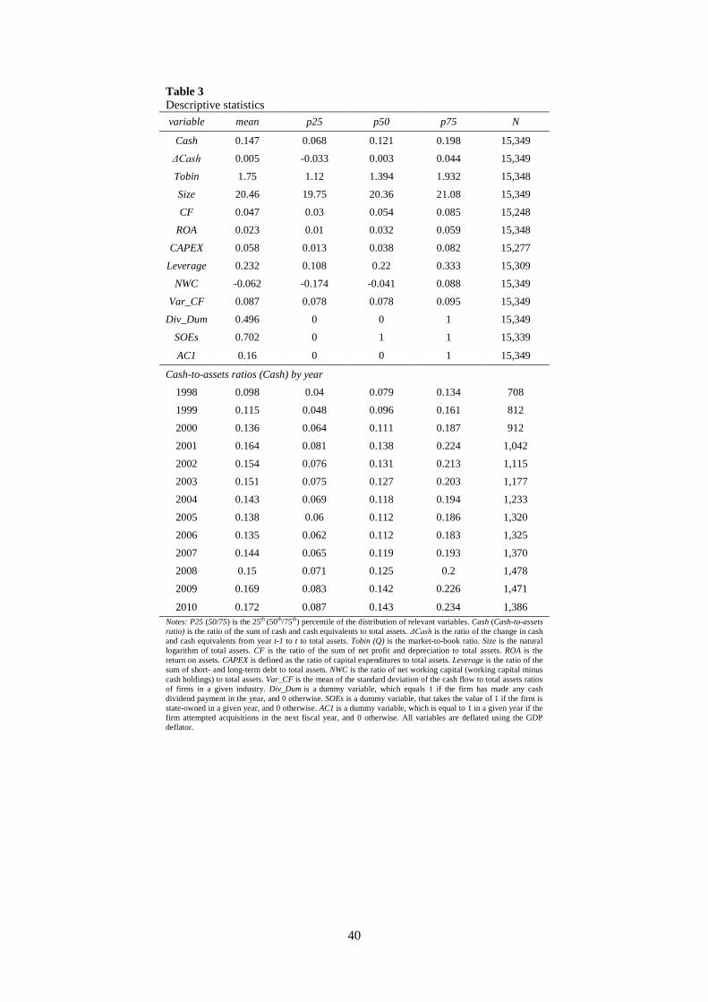
40
Table 3 Descriptive statistics
variable mean p25 p50 p75 N
Cash 0.147 0.068 0.121 0.198 15,349
ΔCash 0.005 -0.033 0.003 0.044 15,349
Tobin 1.75 1.12 1.394 1.932 15,348
Size 20.46 19.75 20.36 21.08 15,349
CF 0.047 0.03 0.054 0.085 15,248
ROA 0.023 0.01 0.032 0.059 15,348
CAPEX 0.058 0.013 0.038 0.082 15,277
Leverage 0.232 0.108 0.22 0.333 15,309
NWC -0.062 -0.174 -0.041 0.088 15,349
Var_CF 0.087 0.078 0.078 0.095 15,349
Div_Dum 0.496 0 0 1 15,349
SOEs 0.702 0 1 1 15,339
AC1 0.16 0 0 1 15,349
Cash-to-assets ratios (Cash) by year
1998 0.098 0.04 0.079 0.134 708
1999 0.115 0.048 0.096 0.161 812
2000 0.136 0.064 0.111 0.187 912
2001 0.164 0.081 0.138 0.224 1,042
2002 0.154 0.076 0.131 0.213 1,115
2003 0.151 0.075 0.127 0.203 1,177
2004 0.143 0.069 0.118 0.194 1,233
2005 0.138 0.06 0.112 0.186 1,320
2006 0.135 0.062 0.112 0.183 1,325
2007 0.144 0.065 0.119 0.193 1,370
2008 0.15 0.071 0.125 0.2 1,478
2009 0.169 0.083 0.142 0.226 1,471
2010 0.172 0.087 0.143 0.234 1,386 Notes: P25 (50/75) is the 25th (50th/75th) percentile of the distribution of relevant variables. Cash (Cash-to-assets ratio) is the ratio of the sum of cash and cash equivalents to total assets. ΔCash is the ratio of the change in cash and cash equivalents from year t-1 to t to total assets. Tobin (Q) is the market-to-book ratio. Size is the natural logarithm of total assets. CF is the ratio of the sum of net profit and depreciation to total assets. ROA is the return on assets. CAPEX is defined as the ratio of capital expenditures to total assets. Leverage is the ratio of the sum of short- and long-term debt to total assets. NWC is the ratio of net working capital (working capital minus cash holdings) to total assets. Var_CF is the mean of the standard deviation of the cash flow to total assets ratios of firms in a given industry. Div_Dum is a dummy variable, which equals 1 if the firm has made any cash dividend payment in the year, and 0 otherwise. SOEs is a dummy variable, that takes the value of 1 if the firm is state-owned in a given year, and 0 otherwise. AC1 is a dummy variable, which is equal to 1 in a given year if the firm attempted acquisitions in the next fiscal year, and 0 otherwise. All variables are deflated using the GDP deflator.

41
Table 4 Testing various cash holding theories
(1) (2) (3) (4) (5) (6) (7) (8) (9) (10) (11) (12) (13)
Mean target adjustment
0.483***
0.481*** (32.71)
(32.32)
Industry target adjustment
0.555***
0.586***
(68.29)
(60.59)
Predicted target adjustment
0.574***
0.588***
(65.19)
(56.59)
Fama-MacBeth target adjustment
0.578***
0.597***
(68.17)
(59.26)
Fixed-effects target adjustment
0.581***
0.604***
(67.02)
(58.59)
Dynamic target adjustment
0.466***
0.467***
(45.35)
(42.95)
FINDEF
0.017*** 0.002 -0.005 0.001 0.001 0.003 0.018***
(3.49) (0.32) (-1.18) (0.29) (0.28) (0.74) (4.03)
Observations 10,632 13,765 13,594 13,594 13,594 12,044 10,589 10,589 10,589 10,475 10,475 10,475 10,511 Half_Life 1.435 1.248 1.208 1.198 1.194 1.487
1.442 1.184 1.178 1.161 1.147 1.484
R2 0.13 0.30 0.28 0.30 0.29 0.19 0.03 0.13 0.30 0.28 0.30 0.29 0.19 Adjusted R2 -0.02 0.20 0.19 0.21 0.20 0.06 -0.13 -0.02 0.19 0.16 0.18 0.18 0.06
ρ 0.29 0.46 0.38 0.38 0.25 0.30 0.27 0.29 0.51 0.45 0.48 0.38 0.30 F-value 37.49 131.17 120.03 130.49 126.37 63.97 6.56 36.12 110.90 97.43 106.23 103.99 58.92
Notes: All specifications were estimated using the fixed-effects estimator. Time and province dummies were included in all specifications. ρ represents the proportion of the total error variance accounted for by unobserved heterogeneity. The dependent variable is given by the difference between the cash to total assets ratio at time t+1 and the corresponding ratio at time t. The target adjustment is the difference between the estimated target cash holdings at t+1 and the realized level of cash holdings at t. We use five different approaches to estimate the levels of target cash holdings. Mean target represents the average cash holdings over the previous three years. Industry target represents the median cash holdings in the firm’s industry in each year. Predicted target is given in each year by the fitted values from the augmented OPSW model estimated using a pooled OLS estimator. Fama-MacBeth target is given in each year by the fitted values from the augmented OPSW model estimated using the two-step Fama-MacBeth estimator. Fixed-effects target adjustment is given by the predicted values from the augmented OPSW model estimated using the fixed-effects estimator. Dynamic target adjustment is given by the predicted values from a dynamic version of the augmented OPSW model estimated using the fixed-effects estimator. FINDEF is the firm’s financial deficit, which is measured as follows: (dividend payments + investment + changes in net working capital – operating cash flow) / total assets. Half-life is the time necessary to cover half of the deviation from the initial cash level to the target level. t-statistics are in parentheses. *, **, *** indicates significance at the 10%, 5%, and 1% level, respectively.

42
Table 5 Dynamic models of cash holdings
Dependent variable (1) (2) (3)
Casht+1 GMM OLS FE
Casht 0.609*** 0.669*** 0.420***
(20.94) (63.94) (49.41)
Tobint 0.007** 0.007*** 0.006***
(2.37) (5.89) (5.73)
Sizet 0.002 -0.001 -0.013***
(0.50) (-0.63) (-7.54)
CFt 0.079** 0.038*** 0.055***
(2.09) (3.48) (5.79)
NWCt 0.001 0.002 0.007*
(0.10) (0.41) (1.66)
CAPEXt 0.003 -0.071*** -0.056***
(0.05) (-6.33) (-4.35)
Leveraget -0.071*** -0.049*** -0.041***
(-2.98) (-8.48) (-5.91)
Div_Dumt -0.009 0.002 0.002
(-1.29) (1.04) (1.22)
Var_CFt 0.755* 0.542**
(1.66) (2.09)
SOEst 0.001 0.002 -0.001
(0.16) (1.02) (-0.45)
AC1t+1 0.006 -0.005*** -0.004**
(0.65) (-2.69) (-2.39)
N 13594 13594 13594
Adjustment Speed 0.391 0.331 0.580
Half_Life 1.773 2.097 1.195
R2 0.56 0.24
Adjusted R2 0.56 0.14
ρ
0.44
F-value 64.91 157.80 78.00
Hansen J test (p-value) 0.15
m3 test (p-value) 0.57
Notes: The specifications were estimated using the system GMM (column 1), the pooled OLS (column 2), and the fixed-effects (column 3) estimators. Time, industry, and province dummies were included in all specifications apart from the fixed-effects estimates in column 3 (which include time and province dummies only). The dependent variable in all regressions is Cash, i.e. the ratio of the sum of cash and cash equivalents to total assets, evaluated at t+1. Tobin (Q) is the market-to-book ratio. Size is the natural logarithm of total assets. CF is the ratio of the sum of net profit and depreciation to total assets. NWC is the ratio of net working capital (working capital minus cash holdings) to total assets. CAPEX is defined as the ratio of capital expenditures to total assets. Leverage is the ratio of the sum of short- and long-term debt to total assets. Div_Dum is a dummy variable, which equals 1 if the firm has made any cash dividend payment in the year, and 0 otherwise. Var_CF is the mean of the standard deviations of the cash flow over total assets ratios of all firms in a given industry. SOEs is a dummy variable that takes the value of 1 if the firm is state-owned in a given year, and 0 otherwise. AC1 is a dummy variable, which is equal to 1 in a given year if the firm attempted acquisitions in the next fiscal year, and 0 otherwise. For the system GMM regression, m3 is a test for third-order serial correlation of the differenced residuals, asymptotically distributed as N(0,1) under the null of no serial correlation. The Hansen J test of over-identifying restrictions is distributed as Chi-square under the null of instrument validity. We treat Cash, Tobin, Size, CF, NWC, CAPEX, Leverage, Div_Dum, SOEs and AC1 as potentially endogenous variables. Levels of these variables dated t-3 and further are used as instruments in the first-differenced equations, and the first-differences of these same variables lagged twice are used as additional instruments in the levels equations. For the pooled regression, t-statistics (in parentheses) are asymptotically cluster-robust to heteroscedasticity and intra-cluster correlation is accounted for at the firm level. For the fixed-effects regression, ρ represents the proportion of the total error variance accounted for by unobserved heterogeneity. Half-life is the time necessary to cover half of the deviation from the initial cash level to the target level. *, **, *** indicates significance at the 10%, 5%, and 1% level, respectively.
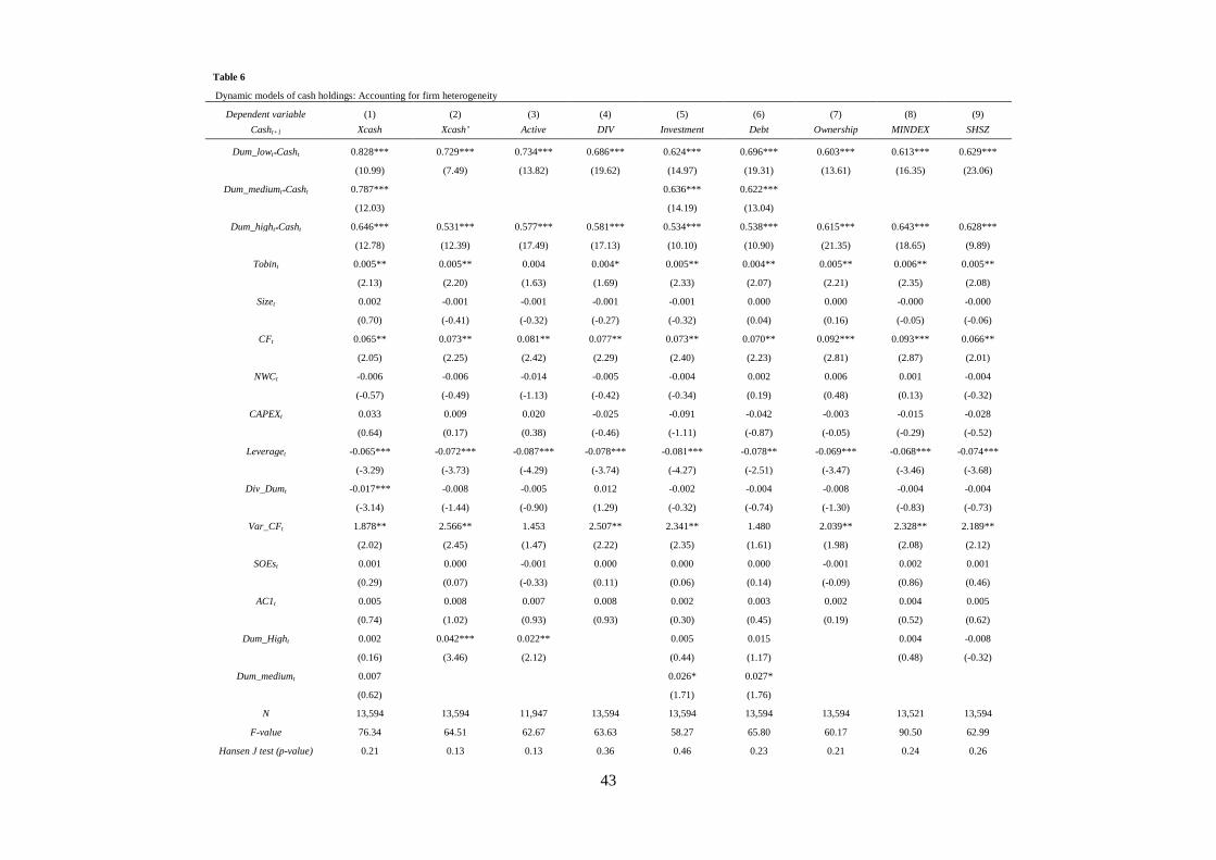
43
Table 6
Dynamic models of cash holdings: Accounting for firm heterogeneity
Dependent variable (1) (2) (3) (4) (5) (6) (7) (8) (9) Casht+1 Xcash Xcash’ Active DIV Investment Debt Ownership MINDEX SHSZ
Dum_lowt*Casht 0.828*** 0.729*** 0.734*** 0.686*** 0.624*** 0.696*** 0.603*** 0.613*** 0.629***
(10.99) (7.49) (13.82) (19.62) (14.97) (19.31) (13.61) (16.35) (23.06)
Dum_mediumt*Casht 0.787***
0.636*** 0.622***
(12.03)
(14.19) (13.04)
Dum_hight*Casht 0.646*** 0.531*** 0.577*** 0.581*** 0.534*** 0.538*** 0.615*** 0.643*** 0.628***
(12.78) (12.39) (17.49) (17.13) (10.10) (10.90) (21.35) (18.65) (9.89)
Tobint 0.005** 0.005** 0.004 0.004* 0.005** 0.004** 0.005** 0.006** 0.005**
(2.13) (2.20) (1.63) (1.69) (2.33) (2.07) (2.21) (2.35) (2.08)
Sizet 0.002 -0.001 -0.001 -0.001 -0.001 0.000 0.000 -0.000 -0.000
(0.70) (-0.41) (-0.32) (-0.27) (-0.32) (0.04) (0.16) (-0.05) (-0.06)
CFt 0.065** 0.073** 0.081** 0.077** 0.073** 0.070** 0.092*** 0.093*** 0.066**
(2.05) (2.25) (2.42) (2.29) (2.40) (2.23) (2.81) (2.87) (2.01)
NWCt -0.006 -0.006 -0.014 -0.005 -0.004 0.002 0.006 0.001 -0.004
(-0.57) (-0.49) (-1.13) (-0.42) (-0.34) (0.19) (0.48) (0.13) (-0.32)
CAPEXt 0.033 0.009 0.020 -0.025 -0.091 -0.042 -0.003 -0.015 -0.028
(0.64) (0.17) (0.38) (-0.46) (-1.11) (-0.87) (-0.05) (-0.29) (-0.52)
Leveraget -0.065*** -0.072*** -0.087*** -0.078*** -0.081*** -0.078** -0.069*** -0.068*** -0.074***
(-3.29) (-3.73) (-4.29) (-3.74) (-4.27) (-2.51) (-3.47) (-3.46) (-3.68)
Div_Dumt -0.017*** -0.008 -0.005 0.012 -0.002 -0.004 -0.008 -0.004 -0.004
(-3.14) (-1.44) (-0.90) (1.29) (-0.32) (-0.74) (-1.30) (-0.83) (-0.73)
Var_CFt 1.878** 2.566** 1.453 2.507** 2.341** 1.480 2.039** 2.328** 2.189**
(2.02) (2.45) (1.47) (2.22) (2.35) (1.61) (1.98) (2.08) (2.12)
SOEst 0.001 0.000 -0.001 0.000 0.000 0.000 -0.001 0.002 0.001
(0.29) (0.07) (-0.33) (0.11) (0.06) (0.14) (-0.09) (0.86) (0.46)
AC1t 0.005 0.008 0.007 0.008 0.002 0.003 0.002 0.004 0.005
(0.74) (1.02) (0.93) (0.93) (0.30) (0.45) (0.19) (0.52) (0.62)
Dum_Hight 0.002 0.042*** 0.022**
0.005 0.015 0.004 -0.008
(0.16) (3.46) (2.12)
(0.44) (1.17) (0.48) (-0.32)
Dum_mediumt 0.007
0.026* 0.027*
(0.62)
(1.71) (1.76)
N 13,594 13,594 11,947 13,594 13,594 13,594 13,594 13,521 13,594
F-value 76.34 64.51 62.67 63.63 58.27 65.80 60.17 90.50 62.99
Hansen J test (p-value) 0.21 0.13 0.13 0.36 0.46 0.23 0.21 0.24 0.26
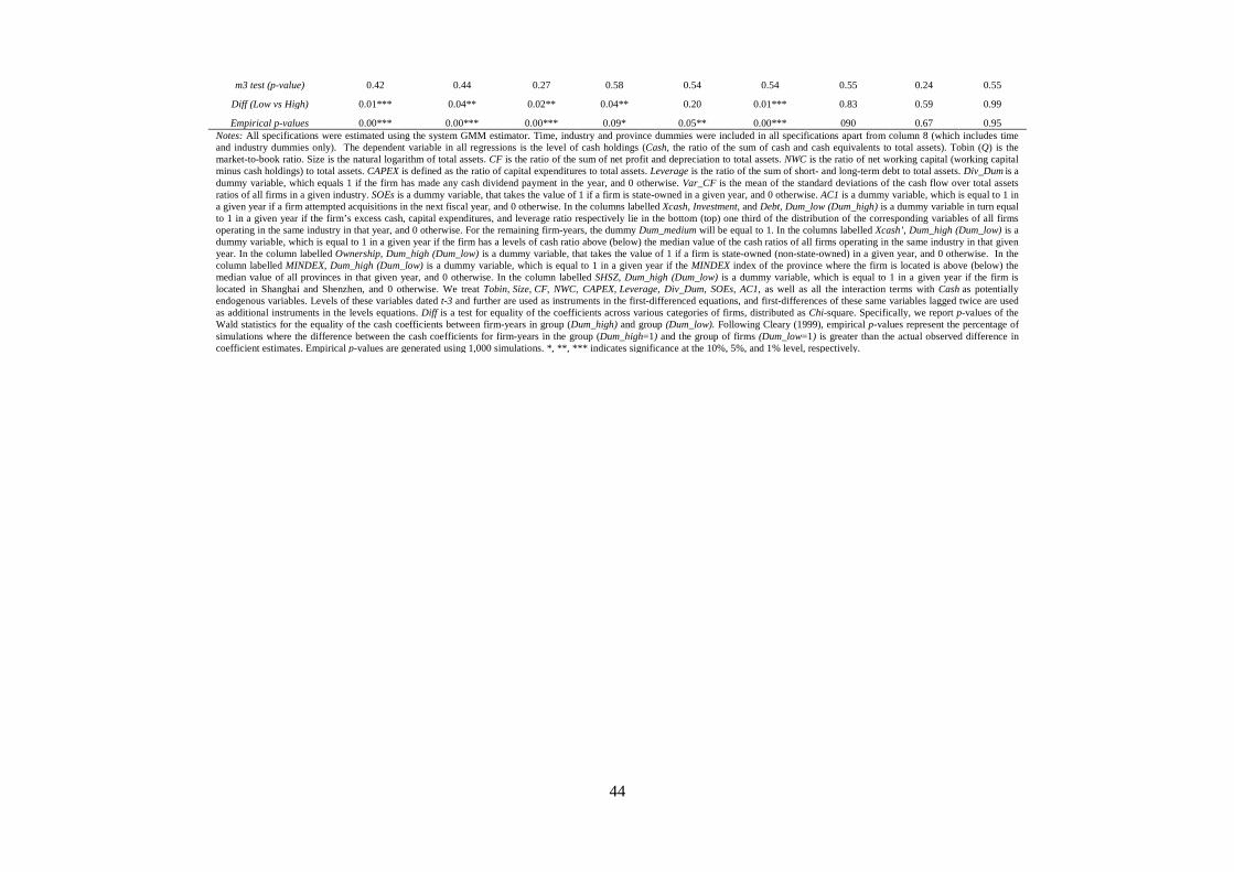
44
m3 test (p-value) 0.42 0.44 0.27 0.58 0.54 0.54 0.55 0.24 0.55
Diff (Low vs High) 0.01*** 0.04** 0.02** 0.04** 0.20 0.01*** 0.83 0.59 0.99
Empirical p-values 0.00*** 0.00*** 0.00*** 0.09* 0.05** 0.00*** 090 0.67 0.95 Notes: All specifications were estimated using the system GMM estimator. Time, industry and province dummies were included in all specifications apart from column 8 (which includes time and industry dummies only). The dependent variable in all regressions is the level of cash holdings (Cash, the ratio of the sum of cash and cash equivalents to total assets). Tobin (Q) is the market-to-book ratio. Size is the natural logarithm of total assets. CF is the ratio of the sum of net profit and depreciation to total assets. NWC is the ratio of net working capital (working capital minus cash holdings) to total assets. CAPEX is defined as the ratio of capital expenditures to total assets. Leverage is the ratio of the sum of short- and long-term debt to total assets. Div_Dum is a dummy variable, which equals 1 if the firm has made any cash dividend payment in the year, and 0 otherwise. Var_CF is the mean of the standard deviations of the cash flow over total assets ratios of all firms in a given industry. SOEs is a dummy variable, that takes the value of 1 if a firm is state-owned in a given year, and 0 otherwise. AC1 is a dummy variable, which is equal to 1 in a given year if a firm attempted acquisitions in the next fiscal year, and 0 otherwise. In the columns labelled Xcash, Investment, and Debt, Dum_low (Dum_high) is a dummy variable in turn equal to 1 in a given year if the firm’s excess cash, capital expenditures, and leverage ratio respectively lie in the bottom (top) one third of the distribution of the corresponding variables of all firms operating in the same industry in that year, and 0 otherwise. For the remaining firm-years, the dummy Dum_medium will be equal to 1. In the columns labelled Xcash’, Dum_high (Dum_low) is a dummy variable, which is equal to 1 in a given year if the firm has a levels of cash ratio above (below) the median value of the cash ratios of all firms operating in the same industry in that given year. In the column labelled Ownership, Dum_high (Dum_low) is a dummy variable, that takes the value of 1 if a firm is state-owned (non-state-owned) in a given year, and 0 otherwise. In the column labelled MINDEX, Dum_high (Dum_low) is a dummy variable, which is equal to 1 in a given year if the MINDEX index of the province where the firm is located is above (below) the median value of all provinces in that given year, and 0 otherwise. In the column labelled SHSZ, Dum_high (Dum_low) is a dummy variable, which is equal to 1 in a given year if the firm is located in Shanghai and Shenzhen, and 0 otherwise. We treat Tobin, Size, CF, NWC, CAPEX, Leverage, Div_Dum, SOEs, AC1, as well as all the interaction terms with Cash as potentially endogenous variables. Levels of these variables dated t-3 and further are used as instruments in the first-differenced equations, and first-differences of these same variables lagged twice are used as additional instruments in the levels equations. Diff is a test for equality of the coefficients across various categories of firms, distributed as Chi-square. Specifically, we report p-values of the Wald statistics for the equality of the cash coefficients between firm-years in group (Dum_high) and group (Dum_low). Following Cleary (1999), empirical p-values represent the percentage of simulations where the difference between the cash coefficients for firm-years in the group (Dum_high=1) and the group of firms (Dum_low=1) is greater than the actual observed difference in coefficient estimates. Empirical p-values are generated using 1,000 simulations. *, **, *** indicates significance at the 10%, 5%, and 1% level, respectively.

45
Table A1 Cash holdings regressions
(1) (2) (3) (4) (5)
Dependent variable OLS Fama-MacBeth FE FE FE
Cash/
Total Assetst Cash/
Total Assetst Cash/
Total Assetst Cash/
Net Assetst Ln (Cash/
Net Assets)t
Tobint 0.002 0.005 0.002*** 0.005*** 0.021**
(1.00) (1.49) (2.60) (2.84) (2.29)
Sizet -0.003 -0.003 0.018*** 0.029*** 0.198***
(-1.57) (-1.32) (10.84) (9.34) (12.07)
CFt 0.171*** 0.186*** 0.162*** 0.257*** 2.190***
(11.45) (11.53) (17.04) (14.71) (23.42)
NWCt -0.059*** -0.067*** -0.097*** -0.188*** -0.490***
(-7.54) (-11.11) (-22.19) (-23.40) (-11.41)
CAPEXt -0.113*** -0.122*** -0.055*** -0.137*** 0.172
(-5.72) (-6.67) (-4.10) (-5.58) (1.31)
Leveraget -0.209*** -0.200*** -0.183*** -0.322*** -1.431***
(-17.14) (-21.99) (-26.72) (-25.68) (-21.36)
Div_Dumt 0.029*** 0.028*** 0.013*** 0.020*** 0.129***
(11.55) (8.81) (7.72) (6.45) (7.69)
Var_CFt 1.135** 1.143***
(2.16) (3.61)
SOEst -0.007** -0.004 -0.009*** -0.016*** -0.056**
(-2.00) (-1.24) (-3.30) (-3.21) (-2.17)
AC1t+1 0.002 0.001 0.005*** 0.008** 0.058***
(0.99) (0.27) (2.94) (2.41) (3.17)
Observations 15,132 15,132 15,132 15,132 15,131
R2 0.24 0.25 0.14 0.12 0.15
Adjusted R2 0.24
0.04 0.02 0.05
ρ
0.62 0.63 0.59
F-value 25.77 535.69 45.60 38.65 50.49
Notes: The specifications were estimated using the pooled OLS (column 1), the Fama-MacBeth (column 2), and the fixed-effects (column 3, 4 and 5) estimators. Time, industry, and province dummies were included in columns 1 and 2. For the fixed-effects estimates (column 3, 4 and 5), only time and province dummies were included. The dependent variable is: Cash/Total Assets (column 1, 2 and 3), Cash/ Net Assets, (column 4), and Ln (Cash/Net Assets) (column 5). Tobin (Q) is the market-to-book ratio. Size is the natural logarithm of total assets. CF is the ratio of the sum of net profit and depreciation to total assets. NWC is the ratio of net working capital (working capital minus cash holdings) to total assets. CAPEX is defined as the ratio of capital expenditures to total assets. Leverage is the ratio of the sum of short- and long-term debt to total assets. Div_Dum is a dummy variable, which equals 1 if the firm has made any cash dividend payment in the year, and 0 otherwise. Var_CF is the mean of the standard deviations of the cash flow to total assets ratios of all firms in a given industry. SOEs is a dummy variable, that takes the value of 1 if the firm is state-owned in a given year, and 0 otherwise. AC1 is a dummy variable, which is equal to 1 in a given year if the firm attempts acquisitions in the next fiscal year, and 0 otherwise. For the pooled regression, t-statistics (in parentheses) are asymptotically cluster-robust to heteroscedasticity, and intra-cluster correlation is accounted for at the firm level. For the Fama-MacBeth specifications, the estimated coefficients are given by the average of the ones obtained from annual cross-sectional regressions. For the fixed-effects regression, ρ represents the proportion of the total error variance accounted for by unobserved heterogeneity. *, **, *** indicates significance at the 10%, 5%, and 1% level, respectively.

46
Fig. 1 Distribution of estimated coefficients on lagged change in the cash-to-assets ratio in Eq. (2)
0.00
0.02
0.04
0.06
0.08
0.10Pr
opor
tion
-1.5 -1.0 -0.5 0.0 0.5 1.0 1.5Regression Model Coeffiecients (β)
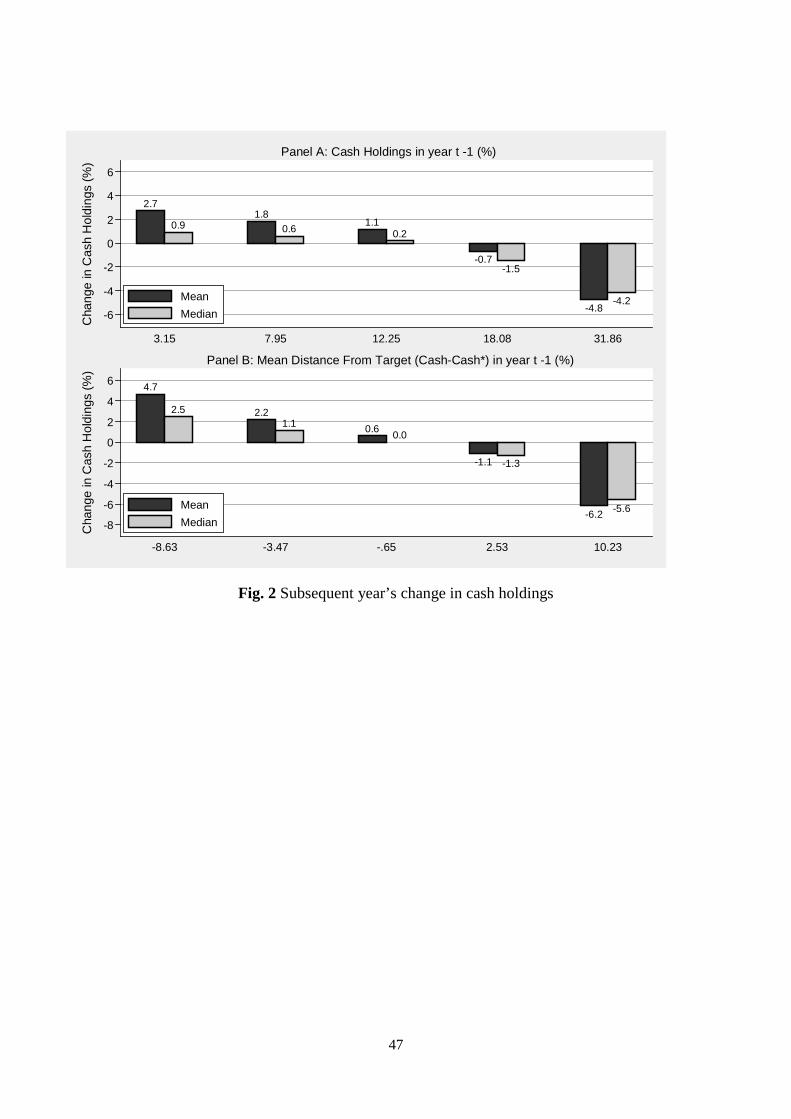
47
Fig. 2 Subsequent year’s change in cash holdings
2.7
0.91.8
0.6 1.10.2
-0.7-1.5
-4.8-4.2
-6
-4
-2
0
2
4
6
3.15 7.95 12.25 18.08 31.86
Cha
nge
in C
ash
Hol
ding
s (%
)
Panel A: Cash Holdings in year t -1 (%)
MeanMedian
4.7
2.5 2.21.1 0.6 0.0
-1.1 -1.3
-6.2 -5.6
-8
-6
-4
-2
0
2
4
6
-8.63 -3.47 -.65 2.53 10.23
Cha
nge
in C
ash
Hol
ding
s (%
)
Panel B: Mean Distance From Target (Cash-Cash*) in year t -1 (%)
MeanMedian

48
Notes
1 Firms in emerging countries are found to hold more cash than those in developed countries, due to poor shareholder protection (Dittmar et al., 2003). In our sample of Chinese listed firms, which covers the period 1998-2010, the median level of cash holdings to total assets is 12.2%, much higher than the overall median (6.2%) of the 45 countries analyzed by Dittmar et al. (2003). In addition, the average level of cash holdings in China almost doubled over our sample period (1998-2010). 2 In our empirical analysis, we therefore estimate firms’ speeds of adjustment using a dynamic cash holdings model. 3 Similar results were obtained when we excluded companies involved in mergers and acquisitions. For brevity, these results are not reported, but are available upon request. 4 See Tables 1 and 2 for details about the structure of our sample. Fewer than 50 percent of firms have the full 13-year observations. Our panel is unbalanced, allowing for both entry and exit. This can be seen as evidence of dynamism and may reduce potential selection and survivor bias. 5 The shares of listed firms in China can be either tradable or non-tradable. Following the literature (Chen et al. 2011, Huang et al. 2011), we calculate Tobin’s Q as the sum of the market value of tradable stocks, the book value of non-tradable stocks, and the market value of net debt, divided by the book value of total assets. The results were similar when tradable stock prices were used to calculate the market value of non-tradable stocks. For brevity, these results are not reported, but are available upon request. 6 Corresponding ratios for US firms are in fact 18.0% according to Dittmar and Mahrt-Smith (2007), 14.8% according to Harford et al. (2008), 8.1% according to Kim et al. (1998), 14.5% according to Opler et al. (1999), 19% according to Venkiteshwaran (2011), and 17.17% (for public firms) and 9.39% (for private firms) according to Gao et al. (2013). The corresponding ratio for UK firms is 9.9% (Ozkan and Ozkan, 2004). 7 It is interesting to note that median cash holdings in our sample are also much higher than the median cash holdings recorded by Gao et al. (2013) both for public (8.68%) and private (3.79%) US firms. 8 To better understand this trend, we regressed firms’ cash holdings on a constant and a firm-specific time trend using the fixed-effects estimator. The estimated coefficient on the time trend was found to be positive and significant (slope = 0.1%; t-statistic= 4.90). This suggests the existence of a 0.1 percentage point per year increase in the tendency of firms to accumulate cash. 9 It should be noted, however, that contrary to us, Chen et al. (2012) report the value of cash and cash equivalents divided by non-cash assets. 10 The split share structure reform was launched in May 2005 by the Chinese Securities Regulatory Commission’s (CSRC) in order to float the non-tradable shares through the open market. Prior to the reform, the majority of shares of listed firms in China was not tradable and typically held by the government itself or government entities. The reform substantially released market frictions and had a positive impact on firms’ governance (Allen et al. 2007; Li et al. 2011; Jiang et al. 2010; Hou et al. 2012). 11 To ensure we have a sufficient number of observations in each cross-sectional regression, following Opler et al. (1999), we drop all firms with less than five years of observations during the period 1998-2010. The chart is based on 1,363 firms, which corresponds to 14,711 firm-year observations. 12 The mean reversion of cash holdings is not in line with the financial hierarchy theory, according to which the time-series properties of changes in cash should be determined by the availability of firms’ internal resources. 13 The cluster-robust standard errors allow for valid inference under heteroskedasticity and autocorrelation in linear panel-data models, especially in large data sets (Born and Breitung 2012). 14 Note that based on the Arellano-Bond (1991) test, we found evidence of serial correlation in the idiosyncratic errors of Eq. (1), which might bias the standard errors and cause inefficient estimates. To correct for autocorrelation, considering that the estimated value of firms’ half-life of cash rebalancing in this study is found to be between 1.2 and 2.1 years, we included 4 lags of the change in cash in the right-hand side of Eq. (1). We found that the estimated coefficient (β) remained significant and negative (between -1 and 0) and that the Arellano-Bond (1991) test no longer rejected the null hypothesis of no autocorrelation. 15 We control for acquisitions and ownership, as acquisition expenditures may be seen as a substitute to capital expenditures, and the ownership structure is a unique feature in the Chinese context. See the Appendix for details about this model and its estimates. 16 Flannery and Rangan (2006) present similar evidence relative to capital structure. They sort firms by quartiles relative to their deviations from a target level of debt and show that the overleveraged firms in quartile 1 significantly reduce their leverage in the following year, whilst the underleveraged firms in quartile 4 raise their leverage in the subsequent year. The firms in the middle two quartiles also move towards their target debt ratios, but with much smaller adjustments. 17 As a robustness test, following Guariglia et al. (2011), we used net income plus depreciation as an alternative proxy for the flow of funds and found similar results. 18 Literally, the SOA refers to the percentage change between the initial cash level and the target.
49
19 If φ = 0, there is no adjustment of the firm’s cash holdings towards its target during each time period. If φ = 1, the adjustment towards the target is perfect. 20 According to the industry classification taken from the China Securities Regulatory Commission (CSRC), firms in China’s listed sector are assigned to one of the following twelve industrial sectors: Farming, forestry, animal husbandry & fishing; Mining; Manufacturing; Utilities; Construction; Transportation & warehouse; Information technology; Wholesale & retailing; Real estate; Social services; Communications & cultural; Conglomerates; Finance & insurance. Following previous literature, we exclude the Finance & insurance sector from our study. 21 There are 31 provinces in China: Coastal provinces (Beijing, Fujian, Guangdong, Hainan, Hebei, Jiangsu, Liaoning, Shandong, Shanghai, Tianjin, and Zhejiang); Central provinces (Chongqing, Anhui, Heilongjiang, Henan, Hubei, Hunan, Jiangxi, Jilin, and Shanxi); and Western provinces (Gansu, Guangxi, Guizhou, Neimenggu, Ningxia, Qinghai, Shaanxi, Sichuan, Xinjiang, and Yunnan ). 22 The results were similar using the pooled OLS estimator with cluster-robust standard errors. For brevity, these results are not reported, but are available upon request. 23 Note that the mean of FINDEF is 0.000769 and the mean of �𝐶𝐶𝐶ℎ𝑖 ,𝑡+1∗ − 𝐶𝐶𝐶ℎ𝑖,𝑡� is -0.00179. Thus, the ratio between the elasticity of ΔCash to FINDEF and the elasticity of ΔCash to �𝐶𝐶𝐶ℎ𝑖 ,𝑡+1∗ − 𝐶𝐶𝐶ℎ𝑖,𝑡� is given by (0.017*0.000769)/(0.581*0.00179)=0.01257. 24 In column 13, both the coefficients on the deviation term and the financial deficit are significant. Yet, the former is much larger than the latter. 25 In unreported results, we estimate an augmented version of Eq. (2), which includes an interaction term between the financing deficit (FINDEF) and a dummy variable (Above target), which equals to 1 if the firm’s cash is above its target level (reflecting excess cash holdings), and 0 otherwise. The motivation for including this interaction term comes from agency considerations, according to which excess cash may lead to free cash flow problems due to the entrenchment of management. As suggested by the agency theory of cash holdings, managers tend to accumulate cash if the firm is making profit. However, even if the firm faces a cash flow deficit, entrenched managers might make efforts to keep a certain level of cash holdings in order to protect their own interests. Therefore, if the free cash flow theory holds, we should observe that the financing deficit (FINDEF) better explains cash rebalancing for firms with excess cash, i.e. we should observe a positive and significant coefficient on the interaction term. Yet, our results show that the coefficient is in fact not statistically significant. This can be seen as evidence against the free cash flow theory. 26 The value of the half-life (1.77 year) is greater than that found for US firms (1.22 year) by Venkiteshwaran (2011). It is also greater than that observed for UK firms (1.15 year), as reported in Ozkan and Ozkan (2004). 27 Our speeds of adjustment are slightly lower than those reported in Alles et al. (2012), also for Chinese listed companies. The differences could be due to the fact that our sample is larger and slightly more recent than theirs, and to the fact that our specifications are not identical. 28 Firms with high excess cash are likely to face lower adjustment costs than firms with low excess cash, as it is more costly for firms to build up cash reserves to close the cash deficit than to deplete their excess cash reserves. 29 In the spirit of Chen et al. (2012), we also checked whether the 2005-2006 split share structure reform had an impact on the speed of adjustment by estimating an augmented version of Equation (5), which includes Cashi,t interacted with a dummy equal to 1 in the year of and the years following the firm’s announcement of the split share reform, and 0 otherwise. We found that the coefficient associated with the interaction term was not statistically significant, which suggests that there were no significant differences in the speed of adjustment before and after the reform. 30 Following Cleary (1999), in order to test for the equality of the cash coeffients between firm-years in the group with high excess cash (whereby Dum_high = 1) and the group with low excess cash (whereby Dum_low = 1), we firstly pool observations across the two groups for each industry and year, ending up with a total of of n1+n2 obsevations in each year and industry, where n1 and n2 denote the number of annual observations available in each group. Secondly, we obtain a bootstrap sample by randomly selecting n1 and n2 observations each year within each industry from the pooled distrubtion, and assigning them to group (Dum_high) and group (Dum_low), respectively. Coefficients estimates are then determined for each group using these observations, and the procedure is repeated 1,000 times. The empirical p-values represent the percentage of simulations where the difference between the coefficient estimates exceeds the observed difference in coefficients estimates. Hence, a p-value of 0.05 suggests that only 50 out of 1000 simulated differences between the coefficients for the two groups of firms exceed the observed difference in coefficient estimates. This implies that the sample difference is significant at the 5% level. These empirical p-values are reported in Table 6. 31 However, the relationship between cash holdings and dividend payment could also be negative since paying dividends signals to the markets that the firm is less risky, which provides it with better access to external financing, and with a lower need to hold cash. 32 We differentiate firms into SOEs and non-SOEs according to their ultimate controlling shareholder. The SOE sector is made up of state-controlled entities. The non-state sector, in which non-state entities are the controlling shareholders, comprises six types of ownership categories: domestic private, foreign, collective, employees’ union, non-profit organizations or institutes, and others. The majority of firm-years in our sample (70.2%) belong to the state sector. Moreover, 83% of the firm-years in the non-state sector are domestic private firms.

50
33 It should be noted that because of collinearity, industry dummies cannot be included in the equations when the fixed-effects estimator is used. The same argument applies to the industry-level measure of cash flow volatility (VAR_CF). 34 Our results were robust to replacing the provincial dummies with the National Economic Research Institute index of marketization (NERI, Fan et al. 2007; Firth et al. 2011), and to including the provincial dummies and the index at the same time. The coefficients associated with the NERI index were positive and statistically significant only in the former case, suggesting that firms located in those provinces with higher market development tend to hold more cash. This can be explained considering that, having more resources at hand and facing less financing constraints, these firms are able to hold more cash. 35 These results were robust to including internal governance variables such as board size, board independence, ownership concentration, CEO duality, and external governance variables such as institutional ownership in the regression. The latter variables were, however, generally not statistically significant. 36 In unreported results, we find that the profitability of large firms is significantly greater than that of small firms, regardless of whether we focus on sample means (t-test) or sample medians (Wilcoxon rank-sum test). Specifically, we split our sample into small/large firms if a firm’s size (measured by total assets) falls below/above the median value of all firms operating in the same industry. We find that large firms have higher return on assets (ROA, 0.036) and cash flow (CF, 0.061) than small firms (ROA, 0.009; CF, 0.033). 37 This exercise is motivated by the fact that some variables in Eq. (A1) may be endogenous and the model may thus suffer from reverse causality problems. The results are not reported for brevity, but available upon request.