Adjoint model of the GYRE configuration of NEMO by using the YAO software

M. Berrada , C. Talandier, M. Crépon, F. Badran, S. ThiriaWork supported by the SHOM (Hydrographic and Oceanographic Department of the French Navy)

under SINOBAD project

LOCEAN-UPMC

NEMO user meeting Paris, 2-3, July 2009

Goal : feasibility of the implementation of the adjoint model of NEMO under YAO

Work in progress

Idealized configuration of the physical part of NEMO

The domain is a limited area in the North of the Atlantic ocean (Gulf stream region)

The horizontal dimension 32x22 and 31 vertical levels

GYRE area localisation

GYRE configuration

The forecasting of the ocean state depends on the initial environment Accurate initial ocean environment

V=(u,v,w) velocity ssh the sea surface height T Temperature S salinity

Data assimilation by the variational approach Control parameters

)S,T,ssh,(V 0000

Initial ocean environment

)S,T,ssh,(Vx 0000

Variational assimilation

Conceptual of an adjoint-based iterative scheme

YAO

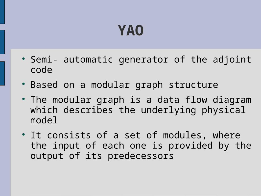
Semi- automatic generator of the adjoint code Based on a modular graph structure The modular graph is a data flow diagram which

describes the underlying physical model It consists of a set of modules, where the input of

each one is provided by the output of its predecessors

YAO: Modular Graph

M1

x11y12

y11

x31

x32

x33y32

y31

x21

x22y21

Forward model

dd

d

d

dd

d

d

d

d

d

1i

1j1 x

yF

)(xfy 111

)(xfy qqq

)(xfy 333

)(xfy 222

3i

3j3 x

yF

2i

2j2 x

yF

M3

M2

Backward model qTqq dydx F

M’2

1. Define the modular graph structure of the model

2. Coding of the local functions fq

3. Coding of the Jacobean

Modular graph in a point of the grid

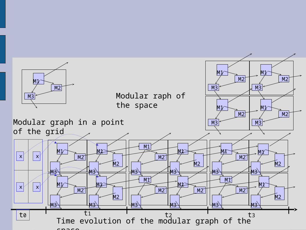
Modular graph in a point of the grid

Modular raph of the space

M1

M2

M3 M1

M2

M3

M1

M2

M3

M1

M2

M3

M1

M2

M3

Time evolution of the modular graph of the space

M1

M2

M3

M1

M2

M3

M1

M2

M3

M1

M2

M3

M1

M2

M3

M1

M2

M3

M1

M2

M3

M1

M2

M3

M1

M2

M3

M1

M2

M3

M1

M2

M3

M1

M2

M3

t2t1 t3

x x

xx

t0

Accomplished work

M1

x11

1i

1j1 x

yF

)(xfy 111 y11

y12

Defined the modular graph structure of the GYRE model under YAO

Coded the forward model

It remains the implementation of the Jacobean of each module which is needed for the backpropagation (This will be done at the end of September)

d

d

d

I shall be ready to cooperate with people wishing to solve assimilation problems

Accomplished work

Comparison: GYRE-YAO vs GYRE-Fortran (accuracy )

Comparison of the intensity of the horizontal velocity in the sea surface at

t=100

Comparison of the ssh at t=100

1110

Comparison of the temperature in the sea surface at t=100

Comparison of the salinity in the sea surface at t=100

Accomplished work

Conclusion

Flexibility: Modifying the model and its adjoint is straightforward due to modular graph structure

One can consider a more complex function as a module for the YAO graph and uses Tapenade (or other) to get the local adjoint

Very useful for sensitivity experiments

Thank you!