Adiabatic expansion of 3He in superfluid 4He

Voncken, A.P.J.

DOI:10.6100/IR426907

Published: 01/01/1994

Document VersionPublisher’s PDF, also known as Version of Record (includes final page, issue and volume numbers)

Please check the document version of this publication:

• A submitted manuscript is the author's version of the article upon submission and before peer-review. There can be important differencesbetween the submitted version and the official published version of record. People interested in the research are advised to contact theauthor for the final version of the publication, or visit the DOI to the publisher's website.• The final author version and the galley proof are versions of the publication after peer review.• The final published version features the final layout of the paper including the volume, issue and page numbers.

Link to publication

Citation for published version (APA):Voncken, A. P. J. (1994). Adiabatic expansion of 3He in superfluid 4He Eindhoven: Technische UniversiteitEindhoven DOI: 10.6100/IR426907

General rightsCopyright and moral rights for the publications made accessible in the public portal are retained by the authors and/or other copyright ownersand it is a condition of accessing publications that users recognise and abide by the legal requirements associated with these rights.

• Users may download and print one copy of any publication from the public portal for the purpose of private study or research. • You may not further distribute the material or use it for any profit-making activity or commercial gain • You may freely distribute the URL identifying the publication in the public portal ?

Take down policyIf you believe that this document breaches copyright please contact us providing details, and we will remove access to the work immediatelyand investigate your claim.

Download date: 23. May. 2018

Adiabatic Expansion of 3He in Soperfluid 4He

A.P.J. Vooeken

Adiabatic Expansion of 3He in Soperfluid 4He

PROEFSCHRIFT

ter verkrijging van de graad van doctor aan de Technische Universiteit Eindhoven,

op gezag van de Rector Magnificus, prof. dr. 1 .H. van Lint, voor een commissie aangewezen door het College van

Dekanen in het openbaar te verdedigen op woensdag 7 december 1994 om 14.00 uur

door

Antonius Petrus Johannes Voncken

geboren te Heerlen

Druk Boek· en OffsetdrvkkenJ Letru. Helmond. 04920·37797

Dit proefschrift is goedgekeurd door de promotoren:

prof. dr. A.T.A.M. de Waele

en

prof. dr. H.M. Gijsman

The work described in this thesis was performed at the Low Temperature Physics group of the Physics department of the Eindhoven University of Technology, and was partly supported by the Dutch Foundation for the Fundamental Research on Matter (FOM), which is financially supported by the Dutch organization for Actvancement of Research, (NWO).

Contents

1 Introduetion 1 1.1 Cooling with helium 1 1.2 Adiabatic expansion 2 1.3 Contents 5

2 Thermodynamic description 7 2.1 Thermodynamics of pure 3He and 3He-4He mixtures 7 2.2 Energy balance of the system 11

2.2.1 Equilibrium over the superteak 12 2.2.2 The 4He reservoir 14 2.2.3 The expansion cell 15

2.3 Temperature evolution of nonadiabatic expansions 16 2.3.1 The low-temperature limit 16 2.3.2 Temperature evolution for constant heat leak and 3He-dilution rate 17 2.3.3 The parasitic heat capacity 19

3 Irreversibilities 21 3.1 Irreversibilities due to viscosity 22

3.1.1 Damping of surface waves 22 3.1.2 Viseaus heating 23 3.1.3 The smoothed 3He layer at the wall 25 3.1.4 Superfluid 3He 26

3.2 Irreversibilities due tothermal conductivity 27 3.2.1 Introduetion 27 3.2.2 Modelling the dilution process with fini te thermal conductiVity 28 3.2.3 Results ofthe numerical calculations 29

3.3 Other types of irreversibilities 34 2.3.1 Exceeding the critical velocity 34 2.3.2 Influence of the sinter layer in the expansion cell 35

4 Experimental setup 38 4.1 Low temperature part of the experimental setup 38

4.1 .1 The mixing chamber 40 4.1.2 The expansion een 41 4.1.3 The •He reservoir 43 4.1.4 The superleaks 44 4.1.5 The heat switch 45

4.2 Experimental procedure 48

5 Measuring techniques 5.1 The vibrating wire thermometer

5 .1.1 Theoretica! description 5 .1.2 Cal i bration of the vibrating wire 5.1.3 The vibrating wire scan

5.2 Speer-resistance thermometers 5.3 The Pd(Fe)-susceptibility thermometer

5.3.1 Calibration ofthe susceptibility thermometèrs 5.4 Liquid-helium level gauges

6 Experimental results 6.1 Viscosity oeHe

6.1.1 The Q-factor in 3He near the liquid-vacuum interrace 6.1.2 Variation of the Q-factor near the phase boundary

6.2 Adiabatic expansions 6.2.1 The expansion process 6.2.2 Temperature gradients during an expansion 6.2.3 The heat teak 6.2.4 Energy balance of the 4He reservoir 6.2.5 Chemica! equilibrium over the superleak 6.2.6 Diffusion of 3He through the superteak to the 4He reservoir 6.2.7 Exceeding the critica! velocity in the superleak 6.2.8 The cooling factor 6.2.9 Conclusions

6.3 Anomalies in the vibrating wire signa!

Appendix

Summary

6.3.1 Examples of anomalous vibrating wire signals 6.3.2 Reproducibilty of the anomalous VW signals 6.3.3 The second resonance mode 6.3.4 Discussion

Samenvatting

Nawoord

Curriculum Vitae

50 50 50 54 55 56 57 58 59

61 61 63 65 66 66 7l 73 74 75 77 79 82 84 85 85 86 86 91

93

1. Introduetion

1.1 . Cooling with helium

Dilution refrigerators are nowadays standard machines in many laboratorles for cooling to tem­peratures down to 2 mK. The dilution refrigerator was developed around 1965, and bas been improved in the following decades. The cooling agent for these. machines is liquid helium. Helium bas two stabie isotopes, 'He and 'He. Their boiling temperatures at atmospheric pressure are 4.2 K and 3.2 K respectively. By reducing the pressure, these temperatures can be lowered to typically 1.2 K for 4He and 0.3 K for 'He.

The cooling principle of the Dilution Refrigerator (DR) is based on the fact that heat is absorbed by the reversible mixing of 3He and 'He. In a DR 3He circulates in a continuous way. In the so-called mixing chamber 3He dilutes at a constant rate, while at another part in the system (the still) the 3He is extracted at the same rate. The cooling power at 10 mK is of the order of ten microwatts at a 1 mmolis 3He circulation rate. The most powerfut dilution refrigerator nowadays can cool to 1.9 mK [Ver87]. It is also possible to circulate 4He insteadof 3He [Pen76]. With this metbod a temperature of 3.4 mK has been reached by Satoh et al. [Sat87].

Another cooling metbod in the millikelvin regime is Pomeranchuk refrigeration. Here the cooling is achieved by isentropic soliditication of liquid 3He by compression. This is, contrary to the two previous techniques, a one-shot cooling technique which can cool to about 2 mK. In the early seventies it was an important way for cooling to temperatures near 2.5 mK, especially since the superfluid phase transitions in liquid 3He was detected with this technique.

The cooling technique, called adiabatic expansion oj3 He in superfluid 4He, [Lon5l], is based on the reversible dilution of 'He in 4He. An important difference with the continuous cooling in the DR, however, is that this is a one-shot technique. A reversible adiabatic dilution of 1 cm' pure 3He initially at 20 mK toa 6.6% 3He-4He mixture results in a volume of 11.6 cm

3 at 4.4 mK.

Further dilution to 76 cm3

to a 1 % mixture would give a final temperature of 1.3 mK. The liquid 3He expands to a larger volume during the dilution process, which explains the name for this cooling technique. In the early seventies, the Leiden group investigated this method in the temperature range from 250 mK down to 30 mK [Pen71 ]. This technique has lost its interest due to the improvements of the dilution refrigerator in those days.

For a detailed treatement on the subject of refrigeration technology at low temperatures, we refer to the hooks of Lounasmaa [Lou7 4] and Pobell [Pob92].

With present nuclear stage cooling technology, matter can be cooled to around 1 2 t.tK [Bra84], [Glo88]. It is, however, very difficult to cool helium mixtures via a nuclear stage to temperatures below 100 t.tK [Oh94]. The reason is the poorthermal coupling of the helium and the metal of the stage. Creating mixtures with temperatures in the microkeivin regime is of significant interest for the onderstanding of the 3He-3He interactions in the 4He background. The superftuid background behaves in many respects as a "mechanica) vacuum" since below 500 mK it bas zero viscosity, and practically zero entropy. At 3He concentrations less than 2% and low temperatures, the 3He-3He interaction can become attractive (singlets-wave pairing). The temperature at which the BCS-type s-wave pairing sets in is the superftuid transition temperature. This temperature is strongly concentration dependent Several estimates of the transition temperature have been reported in the literature, see for instanee [Bar66], [Bar67], and [Iva86], ranging from 1 t.tK to 60 t.tK at concentrations near 2 %. At higher 3He concentrations p-wave pairing becomes favourable, which would correspond to an even lower soperfluid phase transition temperature [Kag88].

1.2 Adiabatic expansion

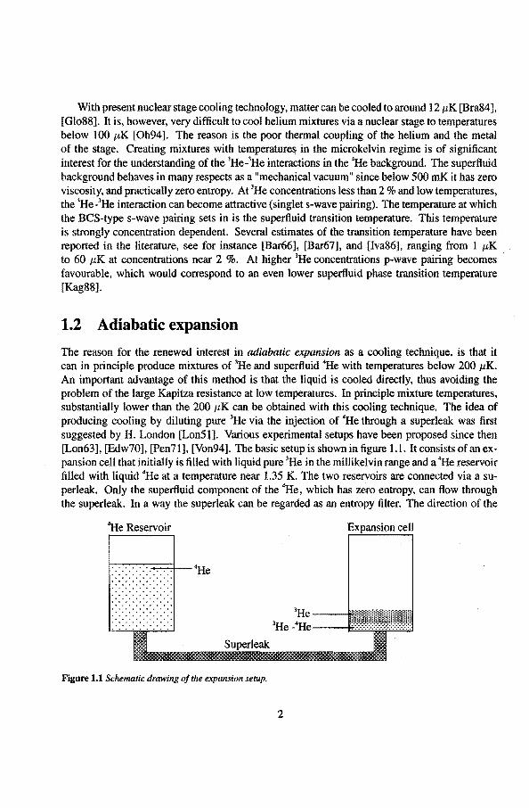
The reason for the renewed interest in adiabatic expansion as a cooling technique, is that it can in principle produce mixtures of 3He and soperfluid 4He with temperatures below 200 t.tK. An important advantage of this method is that the liquid is cooled directly, thus avoiding the problem of the large Kapitza resistance at low temperatures. In principle mixture temperatures, substantially lower than the 200 t.tK can be obtained with this cooling technique. The idea of producing cooling by diluting pure 3He via the injection of 4He through a superleak was first suggested by H. London [Lon5t]. Various experimental setups have been proposed since then [Lon63], [Edw70], [Pen71], [Von94]. The basic setup is shown in tigure 1.1. It consistsof an ex­pansion cell that initially is tilled with liquid pure 3He in the millikelvin range and a 4He reservoir tilled with liquid 4He at a temperature near 1.35 K. The two reservoirs are connected via a su­perleak. Only the superftuid component of the 4He, which bas zero entropy, can flow through the superleak. In a way the superleak can be regarded as an entropy filter. The direction of the

4He Reservoir

F .. :-:: .. :-:: .. -:-: .. -:-: .. :-:: .. ;:::: ... ::: .. :;t. - 4He ......... . . . . . . . . . . . . . . . . . . . . . . . . . . . . . . . . . . . . . . . . . . . . .

Superteak

Figure 1.1 Schematic drawing of the expansion setup.

cell

3He ---l!~~mïmmm 3He 4He---4;;;:;;:;:;:;:;;;:;:;:;;;~::ll

2

4He flow is controlled by variation of the temperature in the 4He reservoir. A similar metbod is used for studying the kinetics of the phase separation curve in soperfluid 3He-4He solutions by Mikheev et al. [Mik91] and for the London thermometer [Lan73]. Fora controlled 4He flow it is essential that the 4He chemical potential is constant over the superleak. Otherwise a highly irreversible expansion occurs. For example mixing of'He at 0 K with pure 3He at 0 K toa 6.6% mixture would result in a temperature of 147 mK, which follows from the energyy balance. If on the otherhand the 4He is injected reversible via a superleak, an adiabatic expansion would be isentropic, that is, the entropy of the helium in the expansion cell after the expansion is the same as before the process. This dilution leads to a temperature decrease. A reversible expan­sion can be accomplished by tuning the chemical potential in the 4He reservoir to that in the expansion cell. In practice this means that the temperature of the 4He reservoir must be close to 1.35 K. The temperature (and thus the chemical potential) of the 4He reservoir can be varied easily by changing the net amount of heat supplied to the 4He reservoir. The 'He can be injected or extracted from the expansion cellat a rate proportional to the net heating power to the reservoir.

100 ~~~-r~~--~~~~~--~~~~Tr-/~/~~~~

10

1 ' ' ' ' H .. -E---.;....E:------, ,'"7"--i F

0.1

0.01 0.1 1 T (mK)

/" /

/

(c) // . ~~)_/ _,.r""" ~ ~·

'

10 100

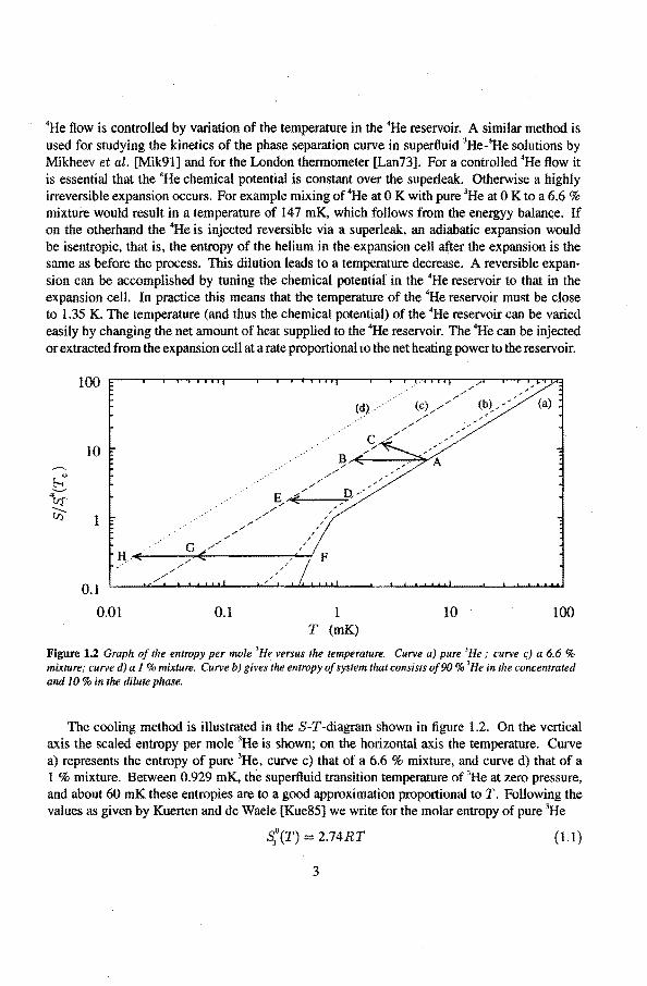
Figure 1.2 Graphof the entropy per mole 'He versus the temperature. Curve a) pure 'He; curve c) a 6.6% mixture; curve d) a 1 %mixture. Curve b) gives the entropy of system that consists of90% 'He in the concentraled and 10 % in the dilute phase.

The cooling metbod is illustrated in the S-T-diagram shown in tigure 1.2. On the vertical axis the scaled entropy per mole 3He is shown; on the horizontal axis the temperature. Curve a) represents the entropy of pure 3He, curve c) that of a 6.6% mixture, and curve d) that of a 1 % mixture. Between 0.929 mK, the superHuid transition temperature of 3He at zero pressure, and about 60 mK these entropies aretoa good approximation proportional toT. Following the values as given by Kuerten and de Waele [Kue85] we write for the molar entropy of pure 3He

q0(T) = 2.14RT (U)

3

and for the entropy per mole 3He of the 6.6 % and 1 % mixtures

S3 (0.066, T) = 12.55RT

S3 (0.01, T) = 42.5RT

(1.2)

(1.3)

respectively, where R is the gas constànt. The mol ar entropy of pure 3He below the superHuid transition temperature, Tc , is calculated from the specitic heat as given by Serene and Rainer [Ser84] giving for 0.6 < T /Tc < l

S:(T) 2.14RTc [1.857 (~r -0.785 (~r -0.072]. (1.4)

An isentropic expansion corresponds to a horizontal transition (for instanee from A toB) in the graph. When the entropy remains constant during the expansion, the relation between the initia! temperature ofthe pure 3He Ti and the final temperature Tr ofthe 6.6% mixture becomes with equations (1.1) and (1.2)

(1.5)

The cooling fator, rJc , defined as (1.6)

then is 4.56. For isentropic expansions starting above 0.929 mK the cooling factor thus is temperature independent. Due to heat leak:s and irreversible effects during the expansion the entropy of the final state will be higher than in the initia! state. An example of such an expansion is shown as the transition from A to C. The final temperature ofthis expansion is higher than the isentropic (horizontal) expansion from A to B. It is of importance, in order to obtain low final temperatures, that the entropy increase is as smal! as possible. Heat leaks and irreversible effects must be reduced as much as possible.

Curve b) in tigure 1.2 represents an initial state of the system consisting of 90 % of the 3He in the concentrated phase and 10 % in the dilute phase. The cooling efficiency for an isentropic expansion toa 6.6 % mixture as shown by the transition from D toE is 3.36. This is smaller than the factor 4.56, because the initially present dilute phase now becomes a parasitic heat capacity.

Below 0.929 mK the entropy of 3He has a steeper slope in the S-T-diagram. This is an particularly interesting temperature regimetostart the expansion process, since now an isentropic expansion corresponds a larger temperature rednetion as the factor 4.56 obtained for isentropic expansions starting above 0.929 mK. For example an isentropic expansion from 600 JLK bas a final temperature of 55 JLK when all the 3He is dlluted to a 6.6 % mixture ( transition F to G), and 8 JLK when further diluted to a 1 % mixture (transition F to H). As noticed before these temperatures are significantly lower than the lowest mixture temperature realized so far when cooling the mixture with a nuclear stage.

4

1.3 Contents

In this thesis we investigate the adiabatic expansion of3He in superjfuid4He as a one-shot cooling technique between 5 and 150 mK. Eventually this technique can be extended to lower temperature regions and can serve as a tooi for producing mixtures at ultralow temperatures. In the following five chapters the theoretica} as well as the experimental concept of the cooling technique will be presented. Chapter two starts with the basic concepts of the dilution process, and investigates the effects of heat leaks and parasitic heat capacities on the performance. In chapter three a closer look is taken at the irreversible effects that can occur during the dilution. Where possible an estimate of each of these irreversibilities is given. The fourth chapter gives a detailed presentation of the ex perimental setup and ex perimental procedure. In chapter five the techniques used for monitoring the dilution process in time are presented. Special attention is paid to the vibrating wire thermometer which is a fast thermometer that can follow the rapid temperature changes dur­ing the expansions below 30 mK. Finally, in chapter six, the experimental results are presented.

References

Bar66 Bar67 Bra84

Edw70

Glo88

Gue83

Iva86 Kag88 Kue85

Lan73 Lon51

Lon63 Lou74

Mik91

Oh94

J. Bardeen, G. Baym, and D. Pines, Phys. Rev. Lett. 17,372 (1966). J. Bardeen, G. Baym, and D. Pines, Phys. Rev. 156, 207 (1967). DJ. Bradley, A.M. Guénault, V. Kieth, C.J. Kennedy, J.E. Miller, S.G. Musset, G.R. Pickett, and W.P. Pratt Jr., J. Low Temp. Phys. 57, 359 (1984). D.O. Edwards, Proceedings of the 1970 Ultralow Temperature Symposium (NRL report 7133, 27 1970). K. Gloos, P. Smeibidl, C. Kennedy, A. Singsaas, P. Sekovski, R.M. Mueller, and F. Pobell, J. Low Temp. Phys. 73, 101 (1988). A.M. Guénault, V. Keith, C.J. Kennedy,I.E. Miller, and G.R. Pickett, Nature 302, 695 (1983). K.D. Ivanova and A.E. Meyerovich, Sov. Phys. JETP64, 964 (1986). M.Y. Kagan and A.V. Chubukov, Zh. Eksp. Teor. Fiz. Pisma 47,525 (1988). J.G.M. Kuerten, C.A.M. Castelijns, A.T.A.M. de Waele, and H.M. Gijsman, Cryogenics 25, 419 (1985). J. Landau and R. L. Rosenbaum, J. Low Temp. Phys. 11,483 (1973). H. London, Proceedings of the 1nternational Conference on Low-Temperature Physics, Oxford Ciarendon Laboratory, 157 (1951). H. London, G.R. Clarke, and E. Mendoza, Phys. Rev. 132, 2373 (1963). O.V. Lounasmaa, Experimental Principles and Methods Below 1 K. (Academie Press Inc., London 1974). V.A. Mikheev, E. Y. Rudavskii, V.K. Chagovets, and G.A. Sheshin, Sov. 1. Low Temp. Phys. 17,233 (1991). G.-H. Oh, Y. Ishimoto, T. Kawae, M. Nakagawa, 0. Ishikawa, T. Hata, and T. Kodama, Physica B 194-196,855 (1994).

5

Osh72 Pen7l Pen76 Pob92 Sat87 Sta69 Ser83 Ver87 Vol90

D.D. Osheroff, R.C. Richerdson, and D.M. Lee, Phys. Rev. Lett. 28, 885 (1972). N.H. Pennings, K.W. Taconis, and R. de Bruyn Ouboter, Physica 56, 171 (1971). N.H. Pennings, R. de Bruyn Ouboter, and K.W. Taconis, Physica B84, lOl (1976). F. Pobell, Matter arld Methods at Low Temperatures (Springer-Verlag, Berlin 1992). N. Satoh, T. Satoh, N. Fukuzawa, and N. Satoh, J. Low Temp. Phys. 67, 195 (1987). F.A. Staas and A.P. Severijns, Cryogenics 9, 422 (1969). J.W. Serene and. D. Rainer, Phys. Reports 101,221 (1983). G.A. Vermeuten and.G. Frossati, Cryogenics 17, 139 (1987). D. Vollhardt and P. Wöltle, The Superfluid Phases of Helium 3 (Taylor & Francis,

. Londo.n 1990). Von94 A.P.J. Voncken and A.T.A.M. de Waele, Physica B194-196, 51 (1994).

6

2. Thermodynamic description

In this chapter a theoretical description of the dilution process is presented. A short review of several important thermadynamie quantities of 3He-4He mixtures and pure 3He for tempera­tures below 200 mK, and of pure 4He around 1.3 K, is given in the first section. In the second section an idealized version of our system is investigated from the thermadynamie point of view. The system consists of a reservoir with pure 4He at approximately 1.3 K, an expansion cell which contains 3He in the concentrated and dilute phases, and a superleak: that connects both cells. From the energy conservation law, relations between the temperatures in the two cells, the 4He flow through the superteak and the amount of heat supplied to either cell, are derived. From these energy balance equations the temperature evolution in the expansion cell can be calculated for nonadiabatic situations. This is done in the third section for the low-temperature limit (T < 50 mK).

2.1 Thermodynamics of pure 3He and 3He-4He mixtures

A thorough treatment of the thermadynamie proprerties. of 3He -4He mixtures for temperatures below 250 mK is given by Kuerten and de Waele [Kue85], [Wae89]. Here a summary of the relevant thermadynamie quantities like the specific heat, the molar entropy, and the 4He chemical potential will be given.

An important quantity of these mixtures is the molar specific heat, Cm. ·In the temperature regime of interest and for mol ar 3He concentrations x less than 30 %, a mixture of 3He and 4He can be regarded as a mixture of pure 4He and a nearly ideal Fermi gas of quasipartiel es with an effective mass m * of 2.46 times the bare mass of a 3He atom, and a quasipartiele density equal to the 3He partiele density. This implies that the molar specific heat ofthe mixture can be written as

Cm xCF +(1-x)q0

(2.1)

where qo is the molar specific heat of pure 4He at constant volume and CF the specific heat of an ideal Fermi gas. The molar 3He concentration is defined as

x = _1\- (2.2) 1\ +~

where n, , ~ the number of moles of 3He and 4He in the mixture. The specific heat of an ideal Fermi gas is a function of the reduced temperature t = T fT F only, i.e. CF (T, x) = CF (t) where

7

T Fis given by

!i? ( N x) 2/3

T F = 2m* ka 371"2 VAm (2.3)

with ka Boltzmann's constant and NA Avogadeo's number. The rnalar volume of the mixture • ( ) 0( ) 0 -6 3 cao be wntten as V m x = Va 1 + ax [Gho79] where a = 0.286 and Va = 27.58 10 m /mol,

the rnalar volume of pure 4He. This gives for the Fermi temperature for x < 0.08

(2.4)

with eF = 2.437 K and y = x/(1 + ax). (2.5)

The mol ar entropy Sm follows from

T I

S (T ) = J Cm(T ,x)dT' m ,X T' (2.6)

0

where we put Sm (0, x) = 0, independent of the concentration x, in accordance with the Third Law. From equation (2.1) it then follows for the entropy of the mixture

(2.7)

with SF the entropy of the quasipartiele gas and S.o the mol ar entropy of pure 4He. lt is convenient to define the specific heat and the entropyin the diluted phase per mole 3He, i.e.

C (T ) =Cm(T,x)=C 1-xCo, d ,X - F + 4 x x

(2.8)

S (T ) = Sm (T, x) = S 1- x 5o d ,X - F + 4 • x x

(2.9)

The contribution to the specific heat and entropy of the pure 4He component cao be neglected in the temperature regime of interest. The specific heat of the quasipartiele gas as fitted by Radebaugh [Rad67] cao be expressed as a function of the reduced temperature t giving

4

CF(t) = R LA,,li+' fort::; 0.15 (2.10) j=O

6

CF(t) = R LAz,/ for0.15::; t::; 0.7 (2.11) j=O

with R the gas constant. The careesponding entropies cao be calculated easily by integniting the above polynomials.

8

The specific heat of pure 3He at zero pressure was measured by Greywall [Gre82]. These measurements can be fitted with

4

C0(T) = R "A . T2H

1

3 L...J 3,) forT~ 0.1 K (2.12) j=O

6

qo(T) = R L A •. iTi forO.l K~ T ~ 0.45 K. (2.13) j=O

The values of the coefficients A,,i are tabulated in Table 2.1. The molar specific heat and entropy in the concentrated phase can be approximated by the values of pure 3He. This is correct as long as the 4He concentration in this phase is negligible, i.e. T < 100 mK.

An important thermodynamic quantity is the 4He chemica! potential J..L4

• The chemica! poten­ti al at a certain pressure, temperature and concentration can be written as

T P x ( ) 0 I I 0 I I a I ~(P,T,x)=~(O,O,O)- jS.(O,T)dT + jV.(P,T)dP +] a~ dx 0 0 0 T,P

(2.14)

where ~ (0, 0, 0) is the zero-point of the chemica! potential. The molar volume of pure 4He is constant in our temperature and pressure range. The above expression can be rewritten to

J1a (P, T, x) = J1a (0, 0, 0) + V.o ( -Pt(T) + P- IT(P, T, x)) (2.15)

where P f is the fountain pressure, defined as

T 1 J 0 I I Pt(T) = o S. (0, T) dT

V. 0

(2.16)

and Il the osmotic pressure, defined as

_ 1 fx (a~) I IT(P, T,x) = - 0 -a I dx . V' x TP 4 0 ,

(2.17)

The pressure dependenee of Il can be written to first order in P as

IT(P, T, x)~ Il(O, T, x)+ P (~~) = Il(O, T, x)- o:xP. (2.18) T,x

For pressures below 103

Pa and concentrations around 7 %, the pressure contribution can be neglected, so

IT(P, T, x)~ Il(O, T, x)=: IT(T, x). (2.19)

9

For T < 200 mK and concentrations less than 8 % the osmotic pressure can be calculated from

2 t

x dTF I ' ' IT(T,x) = IT(O,x) + 0 -d CF(t )dt V x

4 0

where IT(O, x), is the osmotic pressure at T = 0, given by

with y given by equation (2.5).

The concentration of a saturated mixture x. is given by

x. (T) = Xo + 0.5066 T2

- 0.2488 T3 + 18.22 T

4- 74.22 T

5

(2.20)

(2.21)

(2.22)

with x0 = 0.066, the saturated 3He concentration at T = 0. When equation (2.20) and (2.22) are combined the osmotic pressure along the phase separation curve, rr. (T) becomes to first order in T

2

5 2 rr. = 2209 + 1.044 10 T Pa. (2.23)

Finally we present several thermadynamie parameters of pure 4He at saturated vapour pressure around 1.3 K. In this temperature region the chemical poten ti al equals that of the saturated mixture at ultra-low temperatures. The fact that the chemical potential can be tuned to the same value on both sides of the superleak is crucial for the controlled flow of 4He between the cells. The data collected by Conte [Con77] was expanded for temperatures between 1.1 and 1.5 keivin with a third order polynomial around 1.3 K. The 4He chemical potential, in J/mol, at saturated vapour pressure P v , satisfies

3

~(Pv, T, 0)- ~ (0,0,0) = V.o (Pv- Pc)= L B 1,i(T- 1.3/, (2.24) j=O

0 the rnalar entropy S.

3

S.o = L B 2,i (T- 1.3/ (2.25) j=O

and the rnalar specific heat C.o 3

C.o = L B3,j(T- 1.3)j (2.26) j=O

with T is in ketvin and S.o and C.o in J/mol K. Note that the term with j = 0 in equations (2.24), (2.25), and (2.26) give the value of the quantity involved at 1.3 K. In subsection 2.2.2 the quantity

10

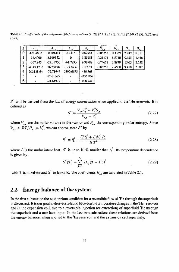
Table 2.1 Coefficients of the polynomial fits from equations (2.10 ), (2.11 ), (2. 12 ), (2.13 ). (2.24 ). (2.25 ), (2.26) and (2.29).

j A!. A," A,,; A •. ; B B,. B,.; B,.; 0 4.934802 -0.201414 2.7415 0.02454 -0.05755 0.3389 2.049 0.311

1 -14.4006 8.919152 0 1.85688 -0.31171 1.5740 9.025 1.446

2 -167.845 -27.14756 -61.7893 9.39988 -0.74673 2.8879 15.05 2.658

3 -4313.1735 56.25498 -177.8937 -117.91 -0.88256 2.4500 9.458 2.097

4 203138.64 -77.71945 2890.0675 440.368

5 - 62.61363 - -735.836

6 - -21.64979 - 468.741

s· will be derived from the law of energy conservation when applied to the 'He reservoir. It is defined as

• V.v.S:- V.0

~v s = ' ' v •. v- V: (2.27)

where V..v are the molar volume in the vapour and ~.v the corresponding molar entropy. Since

v. V ~ RT I p V » V.0 ' we can approximate s· by

(2.28)

where L is the molar latent heat. s• is up to 10 % smaller than ~o. lts temperature dependenee is given by

3

s· (T) 2: B4,j (T- 1.3)j (2.29) j=O

with T is in keivin and s· in J/mol K. The coefficients B,,j are tabulated in Table 2.1.

2.2 Energy balance of tbe system

In the first subsection the equilibrium condition fora reversible flow of 4He through the superleak is discussed. It is our goal to derive arelation between the temperature changes in the 4He reservoir and in the expansion cell, due toa reversible injection (or extraction) ofsuperftuid 4He through the superleak and a nett heat input. In the last two subsections these relations are derived from the energy balance, when applied to the 4He reservoir and the expansion cell separately.

11

2.2.1 Equilibrium over the superteak

The condition that there is chemica! equilibrium over the superleak, links the temperature and 3He concentration of the expansion cell to the temperature of the 'He reservoir. For known 3He concentrations in the expansion cell, and known hydrastatic pressure difference over the superleak, the temperature of the 4He reservoir is a direct measure for the temperature in the expansion cell. A device that measures the temperature of a mixture via a value of the fountain pressure is called the London thermometer [Lon56], [Lan70] and [Lan73]. In the following part the equilibrium condition for the superfluid component over a superleak that joins the 'He reservoir and the expansion cell will be derived.

We assume that the 4He reservoir contains pure 'He and that the expansion cell contains 3He in the concentrated and dilute phase in equilibrium. The equation of motion for the superfluid component is

M dvs -'V~~ 4 dt ""'

(2.30)

with ~ the molar mass of pure 'He, and 'ÏÏ8

the superfluid velocity. In this expression, I1Jt

Expansion cell

contains an implicit contribution due to potential energy. However, in this thesis, J.lJt• as introduced insection 2.1, is a function of P, T, and x only and does not contain a potential energy term. So equation (2.30) should in our case be written as

dv ~ ~ dts = -V(J.lJt +~gz) (2.31)

where g is the gravitational constant, and z the vertical coordinate. In the steady state we have

(2.32)

In terms ofthe osmotic pressure and fountain pressure this = o is equivalent to

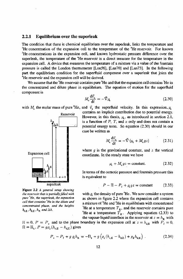
Figure 2.2 A general setup showing the reservoir that is partially filled with pure 'He, the superleak, the expansion eelt that contains 'He in the dilute and concentrared phase, and the heights

\,E ' %.E ' hR and f::.h.

p I1 pf + fJ.9Z =COnStant (2.33)

with P. the density of pure 'He. We now consider a system as shown in tigure 2.2 where the expansion cell contains a mixture of 3He and 'He in equilibrium with concentrated 3He at a temperature TE, and the reservoir contains. pure 4He at a temperature T R. Applying equation (2.33) to

rr = o, P n = ns, p

the vapour-Iiquid interface in the reservoir at z = hR with Pv and to the phase boundary in the expansion cellat z hd,E with Pr 0, 9Pc(hc,E hd,E)gives

(2.34)

12

In this equation Pc and pd are the densities of the concentrated and dilute phase. The heights hc.E, hd,E , hR , and !:lh are visualized in tigure 2.2. With the introduetion of the hydrastatic pressure difference, Ph , as

ph = g (ll hR - Pc ( hc,E - hd,E) - Pd hd,E) (2.35)

we tinally obtain arelation between TE, T R and Ph in the steady state, i.e.

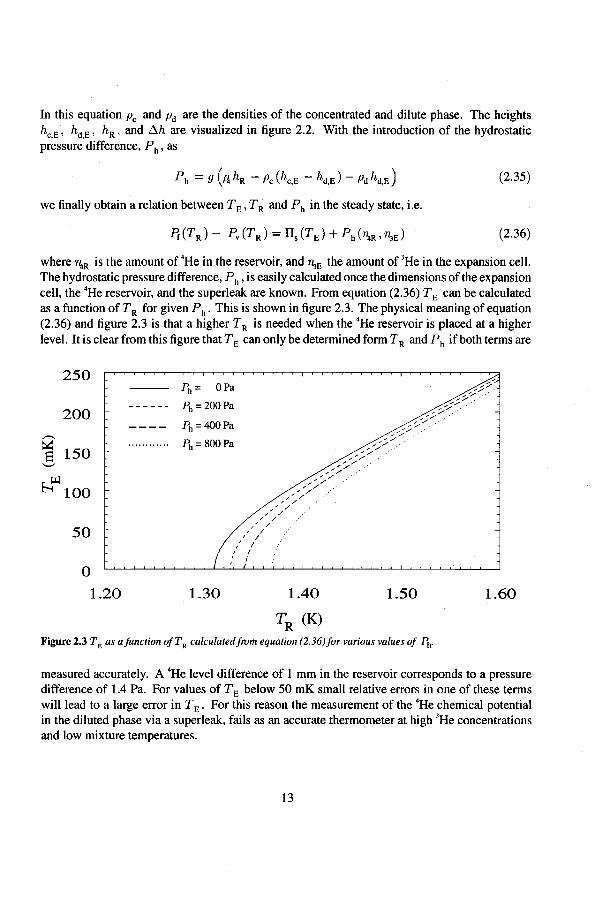
(2.36)

where rlaR is the amount of 4He in the reservoir, and 'TI:!E the amount of 3He in the expansion cell. The hydrastatic pressure difference, Ph , is easily calculated once the dimensions of the expansion cell, the 4He reservoir, and the superleak are known. From equation (2.36) TE can be calculated as a tunetion of T R for given Ph. This is shown in tigure 2.3. The physical meaning of equation (2.36) and tigure 2.3 is that a higher T R is needed when the 4He reservoir is placed at a higher level. lt is clear from this tigure that TE can only be determined form T R and Ph if both terms are

250

200

~

h 100

50

0

1.20

OPa

Ph= 200Pa

Ph=400Pa

Ph= 800Pa

1.30 1.40

TR (K)

1.50

Figure 2.3 TE as ajunetion ofT R calculatedfrom equation (2.36)for various values of Ph.

1.60

measured accurately. A 4He level ditterenee of I mm in the reservoir corresponds to a pressure difference of 1.4 Pa. For values of TE below 50 mK small relative errors in one of these terms will lead to a large error in TE. For this reason the measurement of the 4He chemical potential in the diluted phase via a superleak, fails as an accurate thermometer at high 3He concentrations and low mixture temperatures.

13

2.2.2 The 4He reservoir

The 4He reservoir is a cell with fixed volume V, that contains pure 4He at a temperature T around 1.3 K. The pressure P in the cell at the liquid-vapour interface is equal to the saturated vapour pressure Pv (T). In the reservoir the vapour and liquid phase are in equilibrium. We assume that at a eertaio temperature T there are nv moles in the vapour and n1 moles in the liquid phase. When dn moles 4He are added to the cell, the total volume remains constant so

(2.37)

With (2.38)

and equation (2.37) one obtains

(2.39)

The variation in the molar volume ctv •. i of phase i (note that V.o = V..1) must be taken along phase equilibrium curve, so changes in temperature and pressure are related according to the Clausius-Clapeyron equation which then gives

(av ) (av . ) s - so (av . ) dV . = ~ dT + ~ •.v 4 dT = ~ (I - Ç ) dT

•·• aT ap V - V 0 aT ' p T 4,V 4 p (2.40)

with

Çi = ( 'o) (ap) v •. v- V. FT . v •.•

(2.41)

The entropy change in phase i reacts

n.c . (ap) dS; = ' T m.• dT + n; aT . dV •. i + s •. ; dn; v4,,

(2.42)

where C m,i is the molar specific heat at constant volume. Substituting equation (2.38), (2.39), and (2.40) in (2.42) gives the entropy change of the total system as a function of the temperature change and the actdition of dn moles of 4He

(nê +nê) dS = dS + cts, = V m,v I m,l dT + s· dn

V T (2.43)

where s· is given by equation (2.27), and

(2.44)

14

Por 4He near 1.3 keivin the ratio between the second and the first terms on the right of equation (2.44) is approximately 30 and 10-

3 for the vapour and liquid phase respectively.

In the case the processes in the 4He reservoir are reversible and only the superfluid component passes through the superleak the relation

äQ =TdS (2.45)

holds. With ê ( nv ê m,v + n1 ê m,I) and equations (2.45) and (2.43) we finally find for the heat

balance of the 4He reservoir (2.46)

2.2.3 The expansion cell

If in the previous section the 4He reservoir is replaced by the expansion cell which contains 3He in a concentraled and diluted phase in equilibrium at a temperature T and zero pressure, then equation (2.45) is also valid, i.e.

äQ TdS (2.47)

where äQ is the heat supplied to, and dS the entropy increase of the expansion cell. Equation (2.47) implies that when the processis adiabatic, the entropy of the cell remains constant when 4He is injected reversible. The expansion cell contains two phases in equilibrium at a temperature T and zero pressure, with ~.d moles 3He and '1\ moles 'He in the diluted phase, and ~E - ~.d in the concentraled phase, where ~E is the total amount of 3He in the cell. The entropy increase of this system, due to the injection of d'r\ moles of 4He and a temperature increase dT can be written as

(2.48)

where S:. and S3

are the molar partial entropies in the diluted phase of 4He and 3He respectively. Si nee

(2.49)

with x8

the molar 3He concentration along the phase separation curve, we have

d = ~d - ~.d (ax.) dT. '1\ x ~.d x 2 oT

s s (2.50)

Combining equation (2.47), (2.48) and (2.50) finally gives

äQ (

~.d (ax.) ( -T5;. xs 2 oT + ~E ~.d )(J,0

+ ~.d Cd) dT + T ( S d - s;") dn:J,d. (2.51)

When the time derivative of (2.51) is integrated from an initial state, the temperature evolution can be calculated as a function of the heat leak, QE, and the molar 3He dilution rate it,,d.

15

2.3 Temperature evolution of nonadiabatic expansions

2.3.1 The low-temperature limit

Equation (2.51) relates the temperature change in the expansion cell to the heat leak and the molar 3He ftow crossing the phase boundary. In the reversible limit the energy balance equation can be written as

(cPlf+(~E -~.d)qo+~.dcd)T=~.d T(~o Sd)+QE (2.52)

where Cpa is a parasitic heat capacity. The (ox8 /oT)-term from equation (2.51) has been

neglected, since it is proportional to T 3 while the camparabie terms are linear inT. Possible

contributions to the parasitic heat capacity are the copper expansion cell, the superleak, the thermometers, the sinter sponge, if present, and finally an amount of diluted phase already present in the cell (possibly in the sinter layer) at the beginning of an expansion.

In general QE and ~.d are functions of the timetand G;0, Cd, ~0, S d, and C pa are complicated functions of the temperature. The above equation canthen only be solved numerically. However, in the low-temperature limit, i.e. T < 50 mK, the molar entropies and specHic heats can be written as

S:(T) = G;0(T) := A3,0R T 22.8 T

Sd (T) =Cd (T) := A1,0R T 104 T.

(2.53)

(2.54)

Furthermore the molar 3He concentration in the mixture, x8 can be treated as a constant x0 since T ax.foT « Xo.

We now introduce the dimensionless timeasT = tfte where te is time necessary to dilute all the 3He, and the dimensionless progress parameter N as

N(r) = ~E

(2.55)

Clearly 0::; N(r) ::; 1 with N(O) 0 and N ( 1) = I. In the low-temperature limit equation (2.52) reduces to

((1 + 3.56N)e +~pa) è = 3.56 (4- i..re2

)

with 8 = T/T0

{pa Cpa (T)/(22.8 ~E T0 )

(2.56)

(2.57)

(2.58)

(2.59)

where Çpa is the scaled parasitic heat capacity, ij the dimensionless heat leak, and Ta the starting temperature. The cooling factor, 17c, defined in equation ( 1.6) as the ratio of the initial and final temperature of an expansion now becomes

(2.60)

16

For an i sentropie expansion this is equal to 4.56 for T0 < 50 mK. In the next subsection we will solve equation (2.56) for constant q and constant injection rate, so that N(r) == r. Inthelast subsection finally, a parasitic heat capacity proportional toT is incorporated and the efficiency is calculated as a function of q and ÇP•.

2.3.2 Temperature evolution for constant heat leak and 3He-dilution rate

For constant heat leak and constant dilution rate, the temperature evolution can be calculated analytically. We shall neglect for now the parasitic heat capacity. This situation is described by N(7) 7, q(r) ==ij and Çpa = 0. Equation (2.56) then reduces to

(I + 3.56r )6 è = 3.56 ( q 62

)

with 6(0) 1. The solution is

1.0

0.8

0.6

0.4

0.2 0.0

_ Jt + ((I+ 3.56r)2- 1) q

6 (7)- (I+ 3.56r) for r :5 1.

-- / ____ ___,

4=0.8 q= 0.4

0.5 1.0 1.5 2.0

T

(2.6I)

(2.62)

2.5 3.0

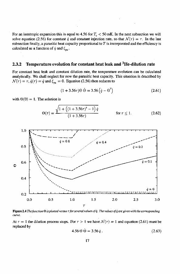
Figure 2.4 The function E> is plotred versus r for several va lues of q. The va lues of q are given with the corresponding curve.

At r I the dil u ti on process stops. For 7 > l we haveN ( 7) = l and equation (2.6I) must be replaced by

4.566 è 3.56 ij. (2.63)

17

5

4

3 " ,:::-

2

1

0

0.01 0.1 1 q

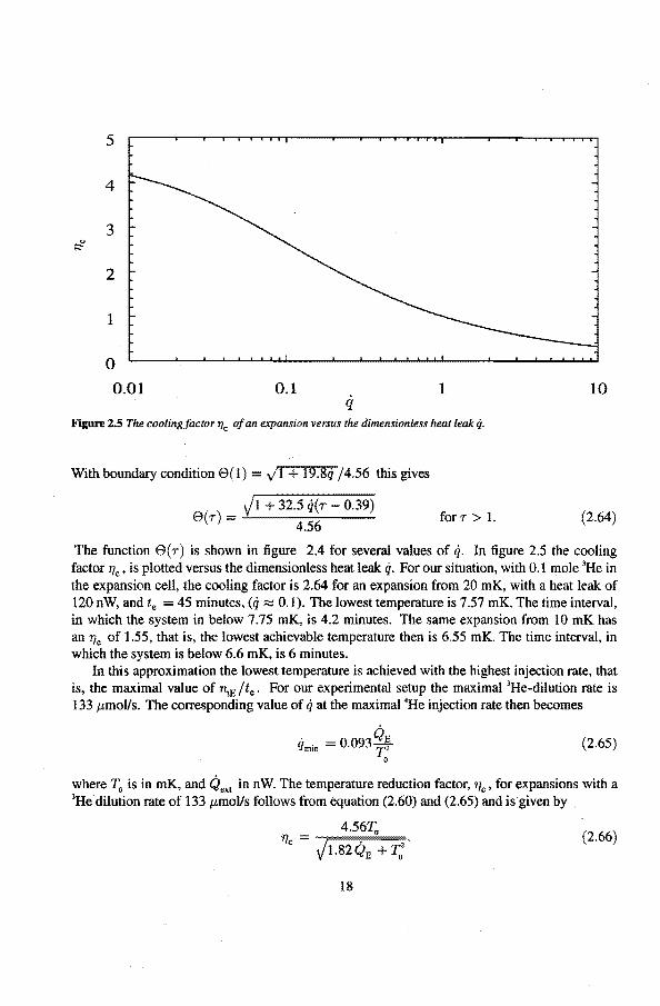
Figure 2.5 The coolingfactor 1Jc of an expansion versus the dimensionless heat leak q.

With boundary condition 8(1) = /1 + t9.8q /4.56 this gives

Jt + 32.5 q(r- 0.39) e(r) = 4.56 forT> I.

10

(2.64)

The function e(r) is shown in figure 2.4 for several values of q. In figure 2.5 the cooling factor 'l7c, is plotted versus the dimensionless heat teak q. For our situation, with 0.1 mole 3He in the expansion cell, the cooling factor is 2.64 for an expansion from 20 mK, with a heat leak of 120 nW, and te = 45 minutes, (q :=:::: 0.1). The lowest temperature is 7.57 mK. The time interval, in which the system in below 7.75 mK, is 4.2 minutes. The same expansion from 10 mK has an 'flc of 1.55, that is, the lowest achievable temperature then is 6.55 mK. The time interval, in which the system is below 6.6 mK, is 6 minutes.

In this approximation the lowest temperature is achieved with the highest injection rate, that is, the maximal value of ~E /te. For our experimental setup the maximal 3He·dilution rateis 133 J.tmoVs. The corresponding value of q at the maximal 4He injection rate then becomes

qmin = 0.093 ~'; 0

(2.65)

where T0 is in mK, and Qext in n W. The temperature reduction factor, 'Tic, for expansions with a 3He dilution rate of 133 J.tmoVs follows from equation (2.60) and (2.65) and is given by .

(2.66)

18

The cooling factor is significantly reduced for heat leaks around 100 n W and temperatures below 20 mK. At 1 mK 'f/c reduces from 4.56 to 2.7 fora 1 nW heat leak. Reducing the heat leak to below 1 n W is crucial for reaching temperatures below 1 mK.

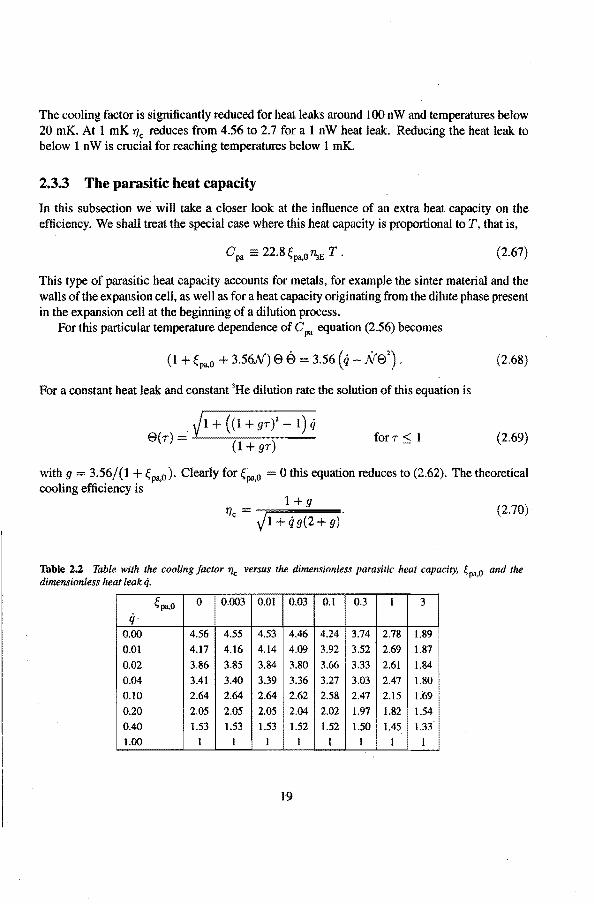
2.3.3 The parasitic heat capacity

In this subsection we will take a closer look at the influence of an extra heat capacity on the efficiency. We shall treat the special case where this heat capacity is proportional toT, that is,

opa= 22.s~p •. o~E T. (2.67)

This type of parasitic heat capacity accounts for metals, for example the sinter material and the walls of the expansion cell, as wellas fora heat capacity originating from the dilute phase present in the expansion cell at the beginning of a dilution process.

For this particular temperature dependenee of C P• equation (2.56) becomes

(t + ~pa.o + 3.56N) e é = 3.56 ( 4- Ne2) • (2.68)

For a constant heat leak and constant 'He dilution rate the solution of this equation is

for r:::; I (2.69)

with g = 3.56/(1 + ~pa.o ). Clearly for Çpa.o 0 this equation reduces to (2.62). The theoretica] cooling efficiency is

1+g 'fj = .

c ~1 + q g(2 + g) (2.70)

Table 2.2 Tab!e with the cooling factor TJc versus the dimensionless parasitic heat capacity. {pa.o and the dimension!ess heat !eak q.

~pa.O 0 0.1 0.3 3

q 0.00 4.56 4.55 4.53 4.46 4.24 3.74 2.78 1.89

O.ot 4.17 4.16 4.14 4.09 3.92 3.52 2.69 1.87

0.02 3.86 3.85 3.84 3.80 3.66 3.33 2.61 1.84

0.04 3.41 3.40 3.39 3.36 3.27 3.03 2.47 1.80

0.10 2.64 2.64 2.64 2.62 2.58 2.47 2.15 1.69

0.20 2.05 2.05 2.05 2.04 2.02 1.97 1.82 1.54

0.40 1.53 1.53 1.53 1.52 1.52 1.50 1.45 1.33

1.00 1

19

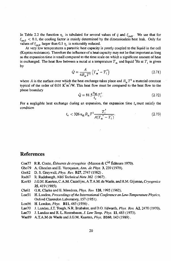
In Table 2.2 the function 'Tic is tabulated for several values of q and Çpa.o. We see that for Çpa,o < 0.1, the cooling factor is mainly determined by the dimensionless heat teak. Only for values of Çpa,o larger than 0.1 r1c is noticeably reduced.

At very low temperatures a parasitic heat capacity is poorly coupled to the liquid in the cell (Kapitza resistance ). Therefore the influence of a heat capacity may not he that important as long as the expansion time is small compared to the time scale on which a significant amount of heat is exchanged. The heat flow between a metal at a temperature Tm and liquid 3He at T1 is given by

(2.71)

where A is the surface over which the heat exchange takes place and RK T3 a material constant typical of the order of 0.01 K

4 m

2 tw. This heat flow must be compared to the heat flow to the phase boundary

(2.72)

For a negligible heat exchange during an expansion, the expansion time te must satisfy the condition

References

Con77 R.R. Conte, Éléments de cryogénie (Masson & cie Éditeurs 1970). Gho79 A. Ghozlan and E. Varoquaux, Ann. de Phys. 3, 239 (1979). Gre82 D. S. Greywall, Phys. Rev. B27, 2747 (1982). Rad67 R. Radebaugh, NBS Technica/ Note 362 (1967).

(2.73)

Kue85 J .G .M. Kuerten, C.A.M. Castelijns, A.T.A.M. de Waele, and H.M. Gijsman, Cryogenics 25,419 (1985).

Cla62 G.R. Clarke and E. Mendoza, Phys. Rev. 128, 1992 (1962). Lon51 H. London, Proceedings of the International Conference on Low-Temperature Physics,

Oxford Ciarendon Laboratory, 157 (1951). Lon56 H. London, Phys. Bll, 483 (1956). Lan70 J. Landau, J.T. Tough, N.R. Brubaker, and D.O. Edwards, Phys. Rev. A2, 2470 (1970). Lan73 J. Landau and R. L. Rosenbaum, J. Low Temp. Phys. 11,483 (1973). Wae89 A.T.A.M de Waele and J.G.M. Kuerten, Phys. B160, 143 (1989).

20

3. Irreversibilities

There are three reasons for a rednetion of the efficiency of the dilution process: heat leaks, "parasitic" heat capacities, and irreversibilities. The influences of a heat leak and of an extra heat capacity have been calculated in the previous chapter. In this chapter we shall focus on the irreversible entropy production during the expansion process. The actual value of the entropy increase due to irreversible effects, however, is difficult to calculate, since it depends on liquid properties like the thermal conductivity and the viscosity which are strongly temperature depen­dent. Following Landau and Lifshitz [Lan59], we can write for the entropy production rate, &i, per unit volume, due to the irreversible processes of thermal conduction and intemal friction

2 2

K (grad T) 'Tl "' ( av, avk 2 ( . ) ( ( . )2 &i :;:::: T2 + 2T f,; lJxk + ax, - 36ik dtv v) + T dtv V . (3.1)

Here v is the velocity, K the coefficient of thermal conductivity, 'Tl the shear viscosity, and ( the volume viscosity. The first term on the right is the rate of entropy increase due to thermal conduction, the other two terms are due to intemal friction. For an incompressible fluid with

div v 0 (3.2)

equation (3.1) reduces to 2 2

&i :;:::: K (grad T) + .!L L ( av, + avk) T

2 2T i,k 8xk lJx,

(3.3)

The intemal friction term multiplied by the temperature is called the viscous heat, <ivi. It is given by

(3.4)

We shall use this expression in the next section, to estimate the order of magnitude of viscous effects in our experiments. In the second section the model for the mixing process is extended by taking the finite thermal conductivity in the liquid phases into account. With this model we canthen calculate the entropy produced by temperature gradients which inevitably occur due to the heat absorption at the phase boundary. From the energy conservalion law a simplified one-dimensional heat-diffusion equation is derived whiçh is solved numerically. The results of the numerical calculations show that in the presence of a heat leak, an optima! injection time top is found. Finally, iri section three, irreversibilities due to the injection of 4He as wellas the effect of the sinter layer are analyzed.

21

3.1 Irreversibilities due to viscosity

In this section we will estimate the order of magnitude of visrous effects. The influence viscosity has on our experiment is threefold. First it can give rise to velocity gradients that contribute to the viscosity term in equation (3.3). Secondly it can produce entropy by a layer of pure 3He that is smoothed to the wall during the expansion. The 3He in the film is irreversibly pushed upward by the hydrastatic pressure difference. The third possible irreversible contribution is due to the viscous damping of gravity waves generated by the mechanical vibration outside the system.

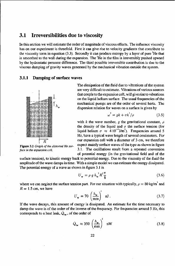
3.1.1 Damping of surface waves

The dissipation of the fluid due to vibrations of the system are very difficult to estimate. Vibrations of various sourees that couple to the expansion cell, will give rise to vibrations on the liquid helium surface. The usual frequencies of the mechanica! pumps are of the order of several hertz. The dispersion relation for waves on a surface is given by

w2=gk+uk'jp (3.5)

with k the wave number, g the gravitational constant, p the density of the liquid and u the surface tension (for liquid helium u ~ 410-4

J/m2). Frequencies around 5

Hz, have a typical wave length of several centimeters. For our expansion cell with a diameter of 3 cm, we therefore

Figure 3.1 Graph ofthe distorted He sur- expect mainly surface waves ofthe type as shown in tigure face in the expansion cell. 3.1. The oscillations result from a repeated conversion

of potential energy (in the gravitational field and of the surface tension), to k:inetic energy back to potential energy. Due to the viscosity of the fluid the amplitude of the wave damps in time. With a simpte model we can estimate the energy dissi pated. The potential energy of a wave as shown in tigure 3 .l is

2 211" Uw = P g hw R S (3.6)

where we can neglect the surface tension part. For our situation with typically, p 80 kg/m3

and R = 1.5 cm, we have

2

Uw =70 (~~) nJ. (3.7)

If the wave decays, this amount of energy is dissipated. An estimate for the time necessary to damp the wave is of the order of the inverse of the frequency. For frequencies around 5 Hz, this corresponds to a heat leak, Q,w' of the order of

2

Q1w ~ 350 (~~) nW (3.8)

22

that is, for hw = 0.5 mm, Q1w ::::::: 90 nW. This heat load is equal to the cooling power of a 24 minutes lasting expansion of 100 mmol 3He at 4 mK. lt is obvious that in order to reach ultra-low temperatures with the expansion process, it is of importance to proteet the system as much as possible from vibrations.

3.1.2 Viscous heating

Viscous heating is an important souree of heat production in the exit tube of the mixing chamber of a dilution refrigerator. The velocity profile of the 3He flowing though a background of 4He to the still gives rise toa viscous heating as given by equation (3.4). At relative high 3He circulation rates the viscous heating term dominates the heat input to the mixing chamber. Viscous heating is probably the main reason why dilution refrigerators can notcool to below 1.9 mK.

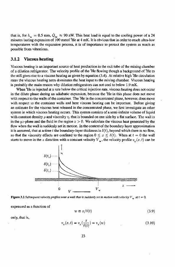
When 4He is injected at a rate below the critica[ injection rate, viscous hearing does not occur in the dilute phase during an adiabatic expansion, because the 3He in this phase does not move with respect to the walls of the container. The 3He in the concentraled phase, however, does move with respect to the container walls and bere viscous heating can be important. Before giving an estimate for the viscous heat released in the concentraled phase, we first investigate an other system in which viscous heating occurs. This system consists of a semi-infini te volume of liquid with constant density pand viscosity 'f/, that is bounded on one side by a flat surface. The wallis in the yz-plane and the fluid in the region x > 0. We calculate the viscous heat generated by the flow when the wall is suddenly set in motion. In the context of the boundary layer approximation it is assumed, that at a timet the boundary-layerthickness is 8(t), beyond which there is no flow, so that the viscosity effects are confined to the region 0 :$ x :$ 8(t). When at t 0 the wall starts to move in the z direction with a constant velocity V w, the velocity profile vz (x, t) can be

l

z-0

V----

Figure 3.2 Subsequent velocity profiles near a wall that is suddenly set in motion with velocity V w at t = 0.

expressed as a function of w = xjó(t) (3.9)

only, that is,

(3.10)

23

where the function vz ( w) is well approximated by [Bir60]

vz (w) = V w ( 1 - fw + !w3) 0 :::; w :::; 1. (3.11)

The flow is described by the Navier-Stokes equation

Ovz iJ2v i)t V ()2; (3.12)

where v 11/P is the kinematic viscosity. When equation (3.11) is inserted in (3.12), and integrated over w from 0 to 1 we get

(3.13)

The boundary thickness thus becomes

ó 2vïzi;t. (3.14)

For this particular velocity distribution, the viscous energy dissipated per secend in a volume dV = dxdydz becomes

1/v;dV

2

; ( ':;'~) dxdydz. (3.15)

Inlegration over the boundary layer and over time from 0 to t gives for the viscous heat produced 2

Qvi = 3p~ w vïzï;i;A (3.16)

where A is the surface area. This expression can be used to estimate the viscous heat released in the expansion cell during an experiment. When we apply equation (3.16) to the concentrated phase in the expansion cell of height l, that is suddenly pusbed upward by the dilute phase with a velocity vph, we find

2 3 pv ph ;;::;-;

Qvi = -5

-v2vt21r Rl. (3.17)

This quantity must be compared with the enthalpy H (T) of the 3He layer

H(T) = 11.41rR:lT2•

v; (3.18)

Viscous heating has a negligible effect if

Qv; « H (T). (3.19)

For our situation the velocity vph is typically 0.06/te rnls, and v = 2.5 10-• /T2

equation (3.19) becomes

-l/1

T » 2 C;) mK. (3.20)

This inequality is always satisfied even for T 1 mK. In our experiment we henceforth can neglect viscous heating effects.

24

3.1.3 The smoothed 3He layer at the wall

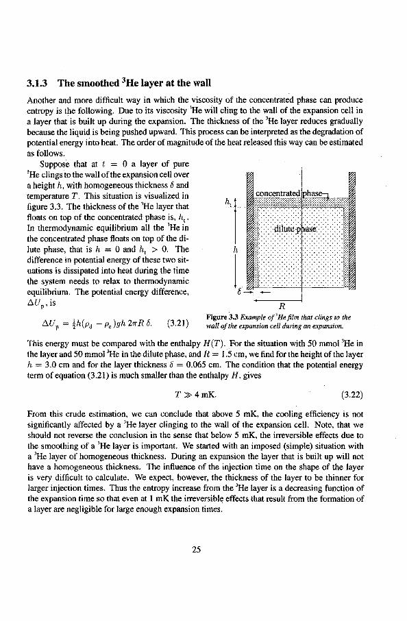
Another and more difficult way in which the viscosity of the concentrated phase can produce entropy is the following. Due to its viscosity 3He will cling to the wall of the expansion cell in a layer that is built up during the expansion. The thickness of the 3He layer reduces gradually because the liquid is being pusbed upward. This process can be interpreled as the degradation of potentlal energy into heat. The order of magnitude of the heat released this way can be estimated as follows.

Soppose that at t = 0 a layer of pure 3He clings to the wall of the expansion cell over a height h, with homogeneous thickness 8 and temperature T. This situation is visualized in tigure 3.3. The thickness of the 3He layer that tloats on top of the concentraled phase is, h1 •

In thermodynamic equilibrium all the 3He in the concentrated phase floats on top of the di­lute phase, that is h = 0 and h1 > 0. The difference in potential energy of these two sit­uations is dissipated into heat during the time the system needs to relax to thermodynamic equilibrium. The potential energy difference,

~UP' is

(3.21)

concentraled nh<>"A.

. ' .. ' .... '. ' ... ' . . :::<:itilt. . . . . ·::::::::::: ·>:::· .. ·.<·~ ... ::·:-:-:-: '.' ............. .

h

t ~/.!~!/~· ····...:....:····...:.....:...:.\~ 8-

R Figure 3.3 Example of'Hefilm that clings to the wall of the expansion cel/ during an expansion.

This energy must be compared with the enthalpy H(T). For the situation with 50 mmol 3He in the layer and 50 mmol 3He in the dilute phase, and R = 1.5 cm, we find for the height of the layer h = 3.0 cm and for the layer thickness 6 = 0.065 cm. The condition that the potentlal energy term of equation (3.21) is much smaller than the enthalpy H, gives

T » 4 mK. (3.22)

From this crude estimation, we can conclude that above 5 mK, the cooling efficiency is not significantly affected by a 1He layer dinging to the wal! of the expansion cell. Note, that we should not reverse the condusion in the sense that below 5 mK, the irreversible effects due to the smoothing of a 1He layer is important. We started with an imposed (simple) situation with a 1He layer of homogeneous thickness. During an expansion the layer that is built up will not have a homogeneous thickness. The intluence of the injection time on the shape of the layer is very difficult to calculate. We expect, however, the thickness of the layer to be thinner for larger injection times. Thus the entropy increase from the 3He layer is a decreasing function of the expansion time so that even at 1 mK the irreversible effects that result from the formation of a layer are negligible for large enough expansion times.

25

3.1.4 Superfluid 3He

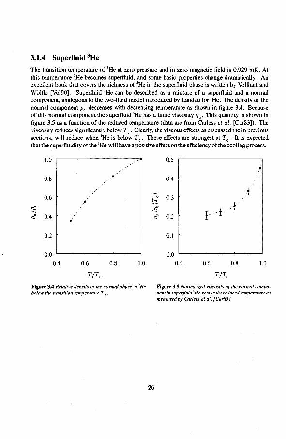
The transition temperature of 3He at zero pressure and in zero magnetic field is 0.929 mK. At this temperature 3He becomes superfluid, and somebasic properties change dramatically. An excellent book that covers the richness of 3He in the superfluid phase is written by Vollhart and Wölfle [Vol90]. Superfluid 3He can be described as a mixture of a superfluid and a normal component, analogous to the two-fluid model introduced by Landau for 4He. The density of the normal component Pn decreases with decreasing temperature as shown in tigure 3.4. Because of this normal component the soperfluid 3He has a fini te viscosity 'Tin • This quantity is shown in ligure 3.5 as a function of the reduced temperature (data are from Carless et al. [Car83]). The viscosity reduces significantly below Tc. Clearly, the viseaus effects as discussed the in previous sections, will reduce when 3He is below Tc. These effects are strongest at Tc. It is expected that the superfluidity of the 3He will have a positive effect on the efficiency of the cooling process.

1.0

0.8

0.6

er --= 0.4 ~

0.2

0.0

0.4 0.6 0.8 1.0

Figure 3.4 Relative density of the normal phase in 'He below the transition temperafure Tc .

0.5

0.4

..-....._

t-." 0.3 ........ ~ --= 0.2 >::'"

0.1

0.0

0.4

~·· •.. /·1.

1······· .l .l

0.6 0.8

T • . 1

1.0

Figure 3.5 Normalized viscosity of the normal compo­nent in superjluid 'He versus the reduced temperature as measured by Carless et al. [ Car83].

26

3.2 Irreversibilities due to thermal conductivity

3.2.1 Introduetion

At low temperatures one can apply the Fermi gas theory to describe the transport properties of 'He in the dilute phase. For concentrations between 3 and 7% the thermal conductivity is almast independent of x as argued by Wei-han Hsu and Pines [Wei85]. The temperature dependenee of the thermal conductivity of a 5% mixture was measured by Abel et al. [Abe67]. We used, as an estimated for the thermal conductivity of a mixture along the phase separation curve, a fit to Abel's 5% mixture over a temperature region from 10 to 100 mK

(3.23)

with Kdo = 3.0 10-4W Km-1 and /id1 = 0.556 W m- 1 K- 1• The thermal conductivity of pure

'He was measured by Greywall [Gre84] .. We fitted his data with

(3.24)

where Kco = 3.610-4W Km- 1 and Kc 1 = 8.0410-3W m-l K- 1/ 2 • The thermal relaxation time

r; in phase i (i= c,d) is

(3.25)

where l, is the length scale in phase i in the direction of the temperature gradient, V; the 3He rnalar volume, and C; the 3He molar specific heat in phase i. For the concentraled phase, with ( = 5 mm, we have

re ~ 0.04 c:K) 2

s (3.26)

while in the dilute phase, with ed = 57 mm, we have

rd ~ 3 (:K) 2 s. (3.27)

The typical time interval over which considerable temperature changes in the system occur, is the injection time te . If te is much larger than the thermal diffusion time, no significant temperature differences can evolve during the expansion/extraction process. Their ratio,

(3.28)

is the Péclet-number, Pe, which gives an estimate for the ratio between the conveelive and conductive heat flow in a medium. If Pe « 1 we can ignore irreversibilities due to temperature gradients in the liquid phases. The value of Pe in the dilute phase is estimated by

( T )z (t )-1

Ped ~ 3 mK ; (3.29)

27

This gives Ped = 3, fora typical injection time of 1000 s and a temperature of 30 mK. Clearly, for values of Ped of the order of unity, a model that takes into account the finite thermal conductivity in the concentrated and the dilute phase has to be used. This is especially important at higher temperatures. In the next subsection this model wiU be derived.

3.2.2 Modelling the dilution process with a finite thermal conductivity

z=O

z

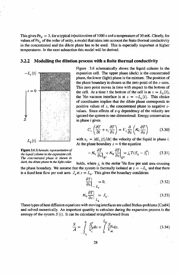
Figure 3.6 Scherrmtic representation of the liquid column in the expansion cell. The concentrared phase is shown in

Figure 3.6 schematically shows the tiquid column in the expansion cell. The upper phase (dark) is the concentrated phase, the Iower (light) phase is the mixture. The position of the phase boundary is chosen as the zero point of the z-axes. This zero point moves in time with respect to the bottorn of the cell. At a timet the bottorn of the cellis at z = Ld (t), the 3He-vacuum interface is at z = -Lc (t). This choice of coordinates implies that the dilute phase corresponds to positive values of z, the concentrated phase to negative z­values. Since effects of x-y dependency of the velocity are ignored the system is one-dimensional. Energy conservalion in phase i gives

C; ( ': + v, ~) = V,! ( K; ~) (3.30)

with v, = I dL, (t)fdtl the velocity of the liquid in phase i. At the phase boundary z = 0 the equation

Kc ara j + Kd ara I = j>T(Sd- S:) zo- zo+

(3.31)

dark, the dilute phase in the light color. holds, where j3

is the molar 3He flow per unit area crossing

the phase boundary. We assume that the system is thermally isolated at z = - Lc and that there is a fixed heat flow per unit area Je at z =Ld. This gives the boundary conditions

arj =o, az L

c

ar I Kd az L; J •.

(3.32)

(3.33)

These types of heat diffusion equations with moving interfaces are called Stefan-problems [Cra84] and solved numerically. An important quantity to calculate during the expansion process is the entropy of the system S ( t). It can be calculated straightforward from

s 0 o Ld

I .s;odz + I s3d dz. (3.34) A

-Lc \S 0 v3d

28

Another manner to calculate the entropy is to add to the initial entropy S (0) the amount of irreversible entropy produced, i.e.

t

S(t) =S(O)+ I Bidt (3.35) 0

where si is the entropy production rate as given by equation (3.3) when integrated over the system's volume

Si o fl,c ({)]') 2 Ld fl,d ({)]') 2

A = I T' {)z dz + I T 2 {)z dz. -Lc 0

(3.36)

Equations (3.34) and (3.35) are equivalent and can be transformed into one another via the partial differential equations (3.30). The numerical method used for solving the equations (3.30) and (3.31) is presented in the appendix. Note that in this analysis only the temperature gradients are assumed to contribute to the irreversible entropy increase. Possible irreversibilities due to concentration gradients have been neglected. Purthermare the volume changes and the motion of the liquids are treated as being reversible.

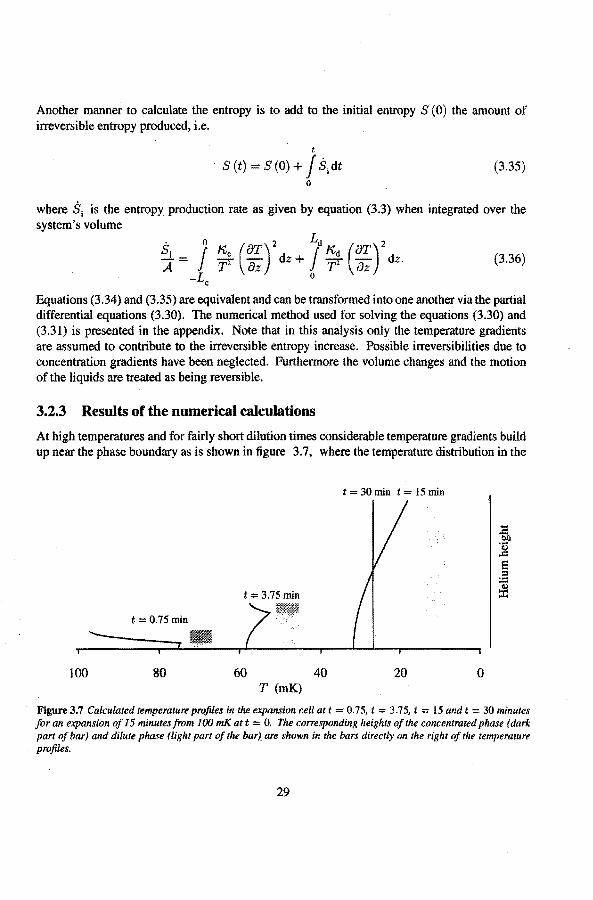
3.2.3 Results of the numerical calculations

At high temperatures and for fairly short dilution times considerable temperature gradients build up near the phase boundary as is shown in figure 3.7, where the temperature distribution in the

t = 30 min t = IS min

100 80 60 40 20 0 T (mK)

Figure 3.7 Calculated temperafure profiles in the expansion cellat t 0.75, t = 3.75, t = 15 and t = 30 minutes for an expansion of 15 minutesfrom 100 mK at t = 0. The corresponding heights ofthe concentraled phase (dark pan of bar) and dilute phase (light part of the bar) are shown in the bars directly on the right of the temperature pro .files.

29

expansion cell is shown at several stages of the expansion. The bars in this graph show the positions and heights of the two phases (dark area concentrated phase, light area dilute phase). This example results from a system with an initia! temperature of 100 mK, an expansion time t. of 15 minutes and with an initia! layer pure 3He thickness Lc (0) of 5 mm. The numerical results that will be presented next, all correspond to an initia! situation with Lc (0) = 5 mm. This corresponds to approximately 100 mmo! of 3He in the expansion cell when scaled to our experimental setup.

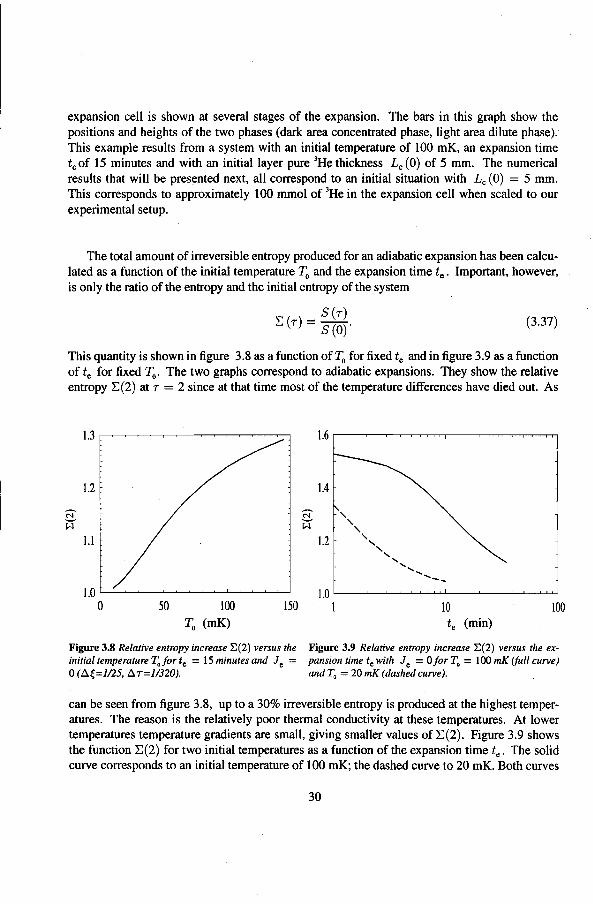
The total amount of irreversible entropy produced for an adiabatic expansion has been calcu­lated as a function of the initia! temperature T0 and the expansion time t.. Important, however, is only the ratio of the entropy and the initia! entropy of the system

S (r) 2: (r) = S (0)" (3.37)

This quantity is shown in ligure 3.8 as a function of T0 for lixed t. and in figure 3.9 as a function of t. for lixed ~- The two graphs correspond to adiabatic expansions. They show the relative entropy 2:(2) at r = 2 since at that time most of the temperature ditierences have died out. As

1.2

' ' ' 1.1 ' ' 1.2 ' ',,

'-.. .... __ 1.0 '------'-~~-'----'-~~~--'-~~~_J 1.0 '-----'-----'--~-'-'-............ ---'-~--'--'-~-'-.J

0 50 100 150 I 10 100 T

0 (mK)

Figure 3.8 Relative entropy increase E(2) versus the initia[ temperafure T0 for t0 = 15 minutes and J

0 =

0 (.Ó.{=J/25, .Ó.T=l/320).

t. (min)

Figure 3.9 Relative entropy increase E(2) versus the ex­pansion time t0 with Je = 0 for T0 = I 00 mK (Juli curve) and T0 = 20 mK (dashed curve).

can beseen from ligure 3.8, up toa 30% irreversible entropy is produced at the highest temper­atures. The reason is the relatively poor thermal conductivity at these temperatures. At Iower temperatures temperature gradients are small, giving smallervalues of 2:(2). Figure 3.9 shows the function 2:(2) for two initia! temperatures as a function of the expansion time t •. The solid curve corresponds to an initia! temperature of 100 mK; the dasbed curve to 20 mK. Both curves

30

show the tendency that the entropy increase is smaller for slower expansions. This is obvious because an infinitely slow expansion is reversible and should have E(2) = I independent ofthe initial temperature.

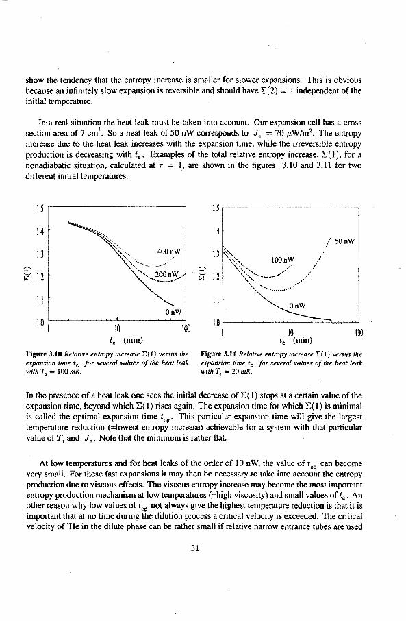
In a real situation the heat Jeak must be taken into account. Our expansion cell bas a cross sectiori area of 7 cm

2• So a heat leak of 50 n W corresponds to J • = 70 p, W /m2• The entropy

increase due to the heat Jeak increases with the expansion time, while the irreversible entropy production is decreasing with t.. Examples of the total relative entropy increase, E( 1), for a nonadiabatic situation, calculated at r = l, are shown in the figures 3.10 and 3.11 for two different initia! temperatures.

1.5 ,--------------

1.4

1.3

1.2

1.1 OnW

10 100 t. (min)

Flgure 3.10 Re/ative entropy increase 2:(1) versus the expansion time te for several values of the heat leak with T0 = l 00 mK.

1.5.--------------,

1.4

1.1

1.0 _ ___.___._..........,._._,_w..J__~..c.:::::l....J....L~

I 10 100 te (min)

Flgure 3.11 Relative entropy increase E( l) versus the expansion time te for several values of the heat leak with T. = 20 mK.

In the presence of a heat leak one sees the initial decrease of E (I ) stops at a certain value of the expansion time, beyond which E( 1) rises again. The expansion time for which E( I) is minimal is called the optimal expansion time top. This particular expansion time will give the largest temperature reduction (=lowest entropy increase) achievable fora system with that particular value of 1'u and Je . Note that the minimum is rather flat.

At low temperatures and for heat Jeaks of the order of 10 nW, the value of top can become very small. For these fast expansions it may then be necessary to take into account the entropy production due to viseaus effects. The viseaus entropy increase may become the most important entropy production mechanism at low temperatures (=high viscosity) and small values of te . An other reason why Jow values of top not always give the highest temperature reduction is that it is important that at no time during the dilution process a critica! velocity is exceeded. The critica! velocity of 4He in the dilute phase can be rather small if relative narrow entrance tubes are used

31

(see subsection 3.3.1). In thin superleaks or smalt entrance tubes, a critica! velocity may easily be exceeded and a large irreversible entropy input results.

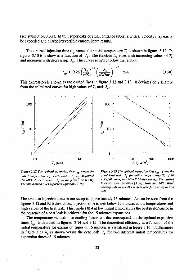
The optima! injection time top versus the initia! temperature T0 is shown in tigure 3.12. In tigure 3.13 it is show as a function of Je. The function top rises with increasing values of T0

and increases with decreasing Je. Thè curves roughly follow the relation

1 8 ( ) -1/2

top ~ 0.26 (:~). /-L.:;m2 min. (3.38)

This expression is shown as the dasbed lines in figure 3.12 and 3.13. lt deviates only slightly from the calculated curves for high values of 'Fo and Je .

100

1

10 100 T. (mK)

Flgure 3.12 The optima/ expansion time top versus the

initia/ temperature T •. Full curve: Je l40ttWim2

(50 nW); dashed curve: Je = 420ttWim2 (ZOO nW). The thin dashed lines represent equation (3.38).

100

10 100 1000 Je (ttWim')

Figure 3.13 The optima/ expansion time top versus the area/ heat teak Je for initia/ temperatures r. of zo mK (full curve) and 60 mK ( dotred curve). The dashed lines represent equation (3.38). Note that 140 I'Wim2

corresponds toa 100 nW heat leakfor our expansion cell.

The smallest injection time in our setup is approximately 15 minutes. As can be seen from the figures 3.12 and 3.13 the optimal injection time is well below 15 minutes at low temperatures and high values of the heat leak. This implies that at lów initia! temperatures the best performance in the presence of a heat leak is achievedfor the 15 minutes expansions.

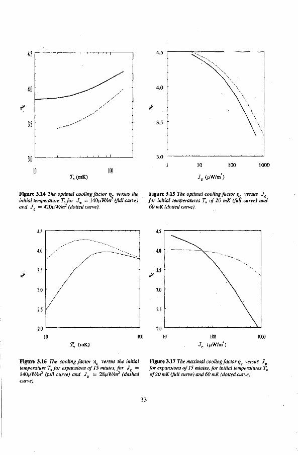
The temperature reduction or cooling factor, "'e , that corresponds to the optima! expansion times top, is depicted in tigures 3.14 and 3; 15. The theoretica! efficiency as a function of the initia! temperature for expansion times of 15 minutesis visualized in figure 3.16. Furthermore in figure 3.17 "'e is shown versus the heat leak Je for two different initial temperatures for expansion times of 15 minutes.

32

10 100 T0 (mK)

Figure 3.14 The optimal coating factor q versus the initial temperafure T"jor Je = 140p;W/mf (fullcurve) and Je = 420J,t W!m2 ( dotted curve).

4.5

4.0

3.5 u

!':"

3.0

2.5

2.0 10 100

T0 (mK)

Figure 3.16 The cooling factor 'flc versus the initia/ temperafure T.for expansions of 15 miutes, for Je = l40J,tW!m2 (/uil curve) and Je = 28p:W!m2 (dashed curve).

33

4.5

4.0

3.5

3.0

Figure 3.15 The optima/ cooling jactor 'flc versus Je for initial temperatures T0 of20 mK (full curve) and 60 mK (dotted curve).

4.5

4.0

3.5 .ft

3.0

2.5

2.0

10 100 1000

Je (p;W/m2

)

Figure 3.17 The maximal coolingjactorqc versus Je jor expansions of 15 miutes,jor initia/ temperatures T0

of 20 mK (full curve) and 60 mK ( dotted curve).

As can be seen from tigure 3.16 the cooling efficiency dramatically reduces at lower temper­atures, mainly as a result of the heat leak. The entropy increase due to temperature gradients is negligible for initia! temperatures below 20 mK in the presence of a heat leak above 20 nW {Je = 28j.JW!m\

We can conclude that the heat leak is the main reason for the reduction of the cooling factor at low temperatures, that is, below 20 mK; irreversibilities due to temperature gradients are of minor importance. The best results (=lowest entropy increase) is obtained for the fastest expansions, as long as the viscous effects can be ignored.

3.3 Other types of irreversibilities

3.3.1 Exceeding the critical velocity

The superfluid component of 4He can flow without friction up to a certain velocity. When in a certain flow channel this so called critica! velocity is exceeded, a nonzero 4He chemica! potential difference develops in the direction ofthe flow and energy is dissipated into heat [Alp69a]. The value of the critica! velocity is strongly system dependent

Measurements of the critica! velocity of 3He in 3He-4He mixtures through tubes were per­formed by Zeegers [Zee90], [Zee91]. He found that in tubes with diameter d the product of the critica! velocity, ver, and the tube diameter follows a logarithmic dependence. For saturated mixtures below 50 mK the empirica! relation becomes

d 2 ver d = 5 ln(

15J.Lm) mm /s. (3.39)

In termsof a critica! volume flow rate, which is *ver d2

, we find that ford > 15 J.Lm, the critica! velocity is first exceeded in the most narrow part of the flow channel. In our ex perimental setup, a 6 mm diameter entrance tube connects the expansion cell with the superleak. The highest injection rate for this setup is f1a = 2 mmolls. This injection rate is critica! for 3 mm diameter tubes. Hence in this setup we do not expect that the critica! velocity in the dilute phase is exceeded at any time.

The other possible place where the superfluid flow can exceed a critica! velocity is in the superleak. The critica! velocity in a superleak is approximately 20 cm/s [Alp69b]. For a 2 mmolis injection rate, this means that for superleaks with a diameter smaller than 1 mm, and a filling factor of 0.5, the critica! velocity can be exceeded. As soon as the critica! velocity is exceeded, dissipation sets in and the 4He chemica! potential difference over the superleak, f:lJ.las becomes nonzero. The created thermal excitations in a pore where the critica! velocity is

34

exceeded can not escape easily, and the temperature of the helium in the pore will rise quickly. Due to this temperature increase, the flow rate in the pore will decrease. This may lead to an increase of the flow rate in the neighbouring pores which in turn may lead to the surpassing of the critica) velocity at another pore. Eventually the superteak wiJl be blocked completely. The amount of energy dissipated into heat by an irreversible 4He flow through the superteak is

(3.40)

This amount of heat can be dissipated at any point in the superteak. If this point is sufficiently far from the expansion cell the thermal ancboring points of the superteak may be able to cool the dissipated heat. If on the other hand the critical velocity is exceeded at a point close to the expansion cell most of the dissipated heat flows directly to the cell. This type of heat input can be avoided by injecting the 4He at a rate below its critica! value.

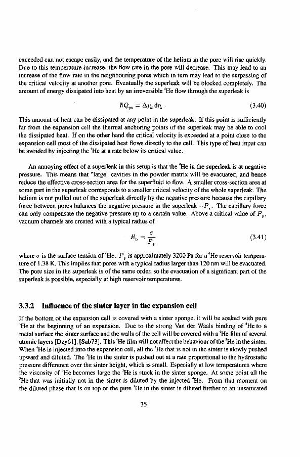
An annoying effect of a superteak in this setup is that the 4He in the superteak is at negative pressure. This means that "large" cavities in the powder matrix will be evacuated, and hence reduce the effective cross-section area for the superHuid to flow. A smaller cross-section area at some part in the superteak corresponds to a smaller critical velocity of the whole superleak. The helium is not pulled out of the superteak directly by the negative pressure because the capillary force between pores balances the negative pressure in the superteak - P • . The capillary force can only compensate the negative pressure up toa certain value. Above a critica! value of P., vacuum channels are created with a typical radius of

(j

ps (3.41)

where a is the surface tension of 4He. P5

is approximately 3200 Pa fora 4He reservoir tempera­ture of 1.38 K. This implies that pores with a typical radius larger than 120 nm will be evacuated. The pore size in the superleak is of the same order, so the evacoation of a significant part of the superteak is possible, especially at high reservoir temperatures.

3.3.2 lnfluence of the sinter layer in the expausion cell

If the bottorn of the expansion cell is covered with a sinter sponge, it will be soaked with pure 3He at the beginning of an expansion. Due to the strong Van der Waals binding of 4He to a metal surface the sinter surface and the walls of the cell will be covered with a 4He film of several atomie layers [Dzy61], [Sab73]. This 4He film will not affectthe behaviourofthe 3He in the sinter. When 4He is injected into the expansion cell, all the 3He that is not in the sinter is slowly pusbed upward and diluted. The 3He inthesinter is pusbed out at a rate proportionaf to the hydrastatic pressure difference over the sinter height, which is small. Especially at low temperatures where the viscosity of 3He becomes large the 3He is stuck in the sinter sponge. At some point all the 3He that was initially not in the sinter is diluted by the injected 4He. From that moment on the diluted phase that is on top of the pure 3He in the sinter is diluted further to an unsaturated

35

concentration with x < 6.6 %. Now a pressure difference equal to Il8 (T)- IT(x, T) builds up,

which pushes the 3He out of the sinter. This is a highly irreversible process that corresponds to a heat release given by

(3.42)

where i!.,. is the amount ofmoles 3He diluting from the sinter per second. On average the value of i!.,, wilt not be constant and can become very smalt at low temperatures due to the high viscosity .. This heat teak depends .on the volume and the geometry of the sinter sponge and on the powder grain size.

To avoid these difficulties it is best to start the expansion when the phase boundary is just above the sinter sponge. Then the maximal amount of 3He is available for the dilution process, and no irreversible flow of 3He through the sinter occurs. The part of the dil u te phase in the sinter then acts as a parasitic heat capacity. The effect of such a heat capacity has been discussed in section 2.3. Optimizing the cooling efficiency means minimizing this heat capacity (or sinter volume), but a large sinter volume is inevitable to ensure a reasonably theemal contact between the liquid and the cell surface.

When the expansion is continued after all the 3He from the concentrated phase has been dis­solved, the 6.6 % mixture in the sinter will give rise to similar irreversible 3He flow through the sinter as discussed befare when the sinter was filled with pure 3He. Again this process of pushing the 3He out of the sinter layer is highly irreversible and will manifest itself as a heat load during the experiment as mentioned by Ishimoto et al. [Ish89]. Clearly for this type of experiment one must carefully calculate the optimal sinter volume in the expansion cell to eosure maximal performance.

References

Abe67 W.R. Abel, R.T. Johnson, J.C. Wheatley, and W. Zimmermann, Phys. Rev. Lett. 18, 737 (1967).

Alp69a W.M. van Alphen, R. de Bruyn Ouboter, K.W. Taconis, and W. de Haas, Phys. 40, 469 (1969).

A\p69b W.M. van Alphen, R. de Bruyn Ouboter, J. Olijhoek, and K.W. Taconis, Phys. 40, 490 (1969).

Amb74 V. Ambogaokar, P.G. de Gennes, and D. Rainer, Phys. Rev. A9, 2676 (1974). Bir60 R.B. Bird, W.E. Stewart, and E.N. Lightfoot, Transport Phenomena (John Wiley &

Sons, Singapore 1960). Car83 D.C. Carless, H.E. Hall, and J.H. Hook, 1 Low Temp. Phys. 50,605 (1983). Cra84 J. Crank, Free and moving boundary problems ( Ciarendon Press Oxford 1984 ). Dzy61 I.E. Dzyaloshinskii, E.M. Lifshitz, and LP. Pitaevskii,Advan. Phys. 10, 165 (1961). Gre84 D. S. Greywall, Phys. Rev. B29, 4933 (1984). Ish89 H. lshimoto, H. Fukuyama, N. Nishida, Y. Miura, Y. Takano, T. Fukuda, T. Tazaki, and

S. Ogawa, J. Low Temp. Phys. 77, 133 ( 1989).

36

Lan59 L.D. Landau and E.M. Lifshitz, Course of Theoretica[ Physics Vol6. (Pergamon Press, Oxford 1959).

Sab73 E.S. Sabisky and C.H. Anderson, Phys. Rev. A7, 790 (1973). Vol90 D. Vollhardt and P. Wölfte, The Superftuid Phases of Helium 3 (Taylor & Francis,

London 1990) . Wei85 Wei-ban Hsu and D.J. Pines, J. Stat. Phys. 38, 283 (1985) . Zee90 J.C.H. Zeegers, Ph.D. Thesis Eindhoven University of Technology Eindhoven The

Netherlands (1990). Zee91 J.C.H. Zeegers, R.G.K.M. Aarts, A.T.A.M. de Waele, and H.M. Gijsman, Phys. Rev.

B45, 12442 (1992).

37

4. Experimental setup

In this chapter the experimental setup is described. First an overview of the low temperature part is presented. In the following subsections a more detailed description of several important components will be given, in particular, the mixing chamber, the expansion cell, the 4He reservoir, the heat switch, and several of the superleaks used in this experiment. Finally in section two a detailed description of the experimental procedure is presented.

4.1 Low temperature part of the experimental setup

In figure 4.1 a schematic cross section of the low temperature part of the system is shown. A detailed description of the dilution refrigerator is given by Coops [Coo79], [Coo81] and Castelijus [Cas85], [Cas86]. The dilution refrigerator has a 3He circulation rate adjustable be­tween 0.080 mmoVs and 2.5 mmoVs.

From the still (S) 3He is pumped via a mechanica! pump (Balzers UNO 250A) 1 and is retumed to the system via a gas-handling system at room temperature. The reentered 3He condenses at the 1 K plate ( 1 K) and is further cooled via a heat exchanger at the still, and ten step heat exchangers (HE) of the Niikoski type [Nii71 ], before it reaches the mixing chamber (M). In the mixing chamber the incoming 3He crosses the phase boundary and flows back to the still through a background of 4He via the dilute side of the step heat exchangers (HE). The 3He circulation rate is controlled by the heat supplied to the still. In normal operation 0.25 mmoVs was circulated, with a typical temperature in the mixing chamber of 8 to 9 mK.

The expansion setup is integrated in the dilution refrigerator. It consists of an expansion cell (E), a superteak (S), and a 4He reservoir (R). The expansion cell is connected to the mixing chamber via a heat switch (H) and to the 4He reservoir via a 91 cm long superleak. The super­Ieale is thermally grounded at the still, the heat exchanger flange (HF) of 50 mK, and finally at the mixing chamber flange (MF) which bas a temperature of 20 mK. In the present setup the heat leak to expansion cellis approximately 150 nW. This corresponds toa lowest precooling temperature of 20 mK. The relatively large heat leak can be reduced if the quality of the theemal ancboring points is significantly improved. The filling capillaries of the expansion cell (not shown

1 A Booster pump which was also part of the pumping system was not used, because the circulation system blocked after several days of operation. Without the use of the Booster pump we were allle to circulate for more than one month (still without any sign of possible blockage of the condenser line) and obtained temperatures in the mixing chamber below 10 mK.

38

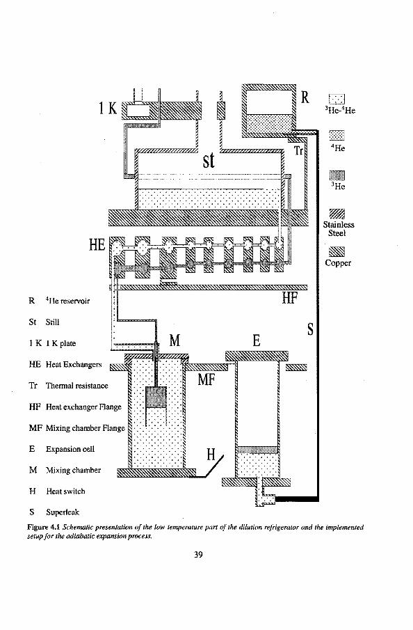
HE

R 4He reservoir

St Still

1 K 1 K plate

HE Heat Exchangers

Tr Thennal resistance

HF Heat exchanger Flange

MF Mixing chamber Flange

E Expansion cell

M Mixing chamber

H Heat switch

S Superleak

st ......................... . . . . . . . . . . . . . . . . . . . . . . . .

M

. ~ . . . . . . . . . . . . . . .

E

MF

R

Tr

s

~ ~

~ Stainless

Steel

~ Copper

Figure 4.1 Schematic presentation of the low temperafure part of the dilution refrigerator and the implemenled setup for the adiabatic expansion process.

39

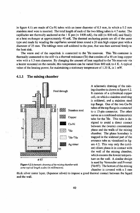
in figure 4.1) are made of Cu-Ni tubes with an inner diameter of 0.3 mm, in which a 0.2 mm stainless steel wireis inserted. The totallength of each of the two filling tubes is 4.7 meter. The capillaries are thermally anchored at the 1 K pot(~ 1400 mK), the still(~ 800 mK) and finally at a heat exchanger at approximately 40 mK. The thermal ancboring points are all of the same type and made by winding the capillaries several times round a 20 mm high capper post with a diameter of 25 mm. The tubings were soft soldered to the post, that was then screwed firmly to the heat sink.

The warm end of the superteak is conneeled to the 4He reservoir. This 4He container is thermally connected to the still via a therm al resistance (Tr) that consists of a I 0 cm long copper wire with a 1.3 mm diameter. By changing the amount of heat supplied to the 4He reservoir via a heater mounted on the outside, this temperature can be varled from 800 mK to 4 K. A typical value of the heating power, for maintaining a stationary temperature of 1.35 K, is 1 mW.

4.1.1 The mixing chamber

Feed through

Stainless steel

1

Copper

Cu-Ni 56

l Ag sinter

l1S85

Figure 4.2 Schematic drawing of the mixing chamberwith some typicallength scales (in millimeters).

A schematic drawing of the mix­ing chamber is shown in figure 4.2. It consistsof a cylindrical copper cell, on which a stainless steel ring is soldered, and a stainless steel top ftange. One of the two Cu-Ni tubes of the top ftange is connected toa 15-pin connector. The other serves as a combinedentrance/exit tube for the 3He. This tube is de­signed to avoid a direct contact between the (warm) concentraled phase and the walls of the mixing chamber. The phase boundary is trapped in the widened part of the entrance tube as visualized in tig­ure 4.2. This way only the (cold­est) dilute phase is in contact with the wall of the mixing chamber, which ensures the lowest tempera­ture on the wall. A similar design is used by Vermeuler and Frossati [Ver87]. The bottorn ofthe mixing chamber is qovered with a 5 mm

thick silver sinter layer, (Japanese silver) to impose a good thermal contact between the liquid and the wall.

40

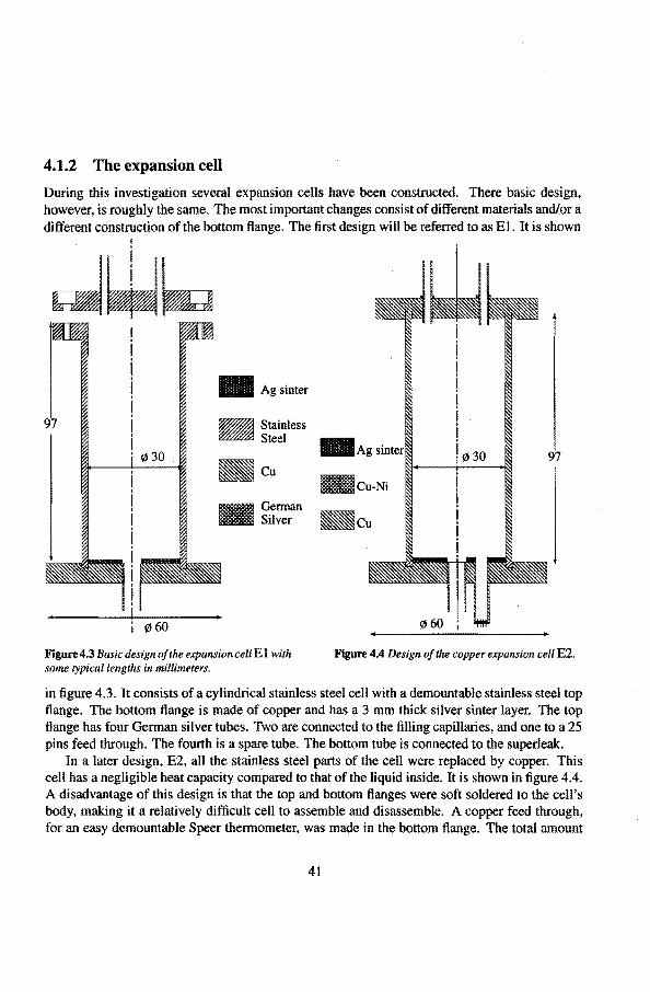
4.1.2 The expansion cell

During this investigation several expansion cells have been constructeet There basic design, however, is roughly the same. The most important changes consist of different materials andlor a different construction of the bottorn ftange. The first design will be referred to as El. It is shown

I

~~ • Agsinter

• Stainless Steel

~30 .Cu Gennan Silver

Figure 4.3 Basic design of the expansion cel/ E 1 with some typicallengths in millimeters.

.. Ag ~30 97

l!llcu-Ni

~Cu

Flgure 4.4 Design of the copper expansion eelt E2.

in tigure 4.3. It consistsof a cylindrical stainless steel cell with a demountable stainless steel top ftange. The bottorn ftange is made of copper and bas a 3 mm thick silver sinter layer. The top flange has four Oerman silver tubes. Two are connected to the filling capillaries, and one toa 25 pins feed through. The fourth is a spare tube. The bottorn tube is connected to the superleak.

In a later design, E2, all the stainless steel parts of the een· were replaced by copper. This cell has a negligible heat capacity compared to that of the Iiquid inside. It is shown in tigure 4.4. A disadvantage of this design is that the top and bottorn flanges were soft soldered to the cell's body, making it a relatively difficult cell to assembie and disassemble. A copper feed through, for an easy demountable Speer thermometer, was made in the bottorn ftange. The total amount

41

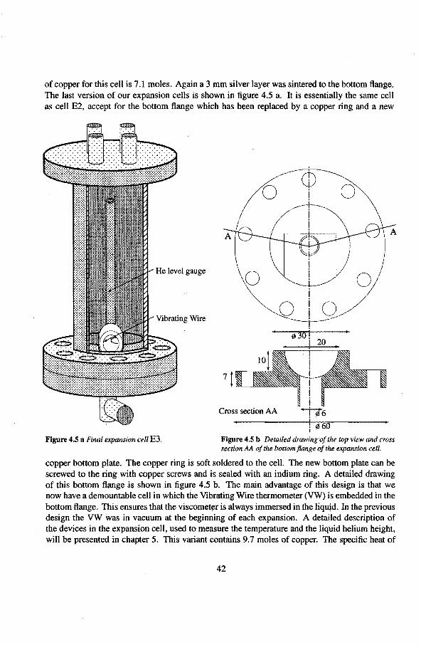
of copper for this cell is 7.1 moles. Again a 3 mm silver layer was sintered to the bottorn ftange. The last version of our expansion cells is shown in ligure 4.5 a. It is essentially the same cell as cell E2, accept for the bottorn ftange which bas been replaced by a copper ring and a new

Vibrating Wire

Figure 4.5 a Final expansion cell E3.

Cross section AA

I

Figure 4.5 b Detailed drawing'of the top view and cross section AA of the bottom jlange of the expansion eetl.

copper bottorn plate. The copper ring is soft soldered to the cell. The new bottorn plate can be screwed to the ring with copper screws and is sealed with an indium ring. A detailed drawing of this bottorn ftange is shown in ligure 4.5 b. The main advantage of this design is that we now have a demountable cell in which the Vibrating Wire thermometer (VW) is embedded in the bottorn flange. This ensures that the viscometer is always immersed in the liquid. In the previous design the VW was in vacuum at the beginning of each expansion. A detailed description of the devices in the expansion cell, used to measure the temperature and the Iiquid helium height, will be presented in chapter 5. This variant contains 9.7 moles of copper. The specHic heat of

42

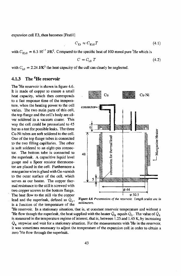
expansion cell E3, then becomes [Fra61]

CE3 RJ CE3,0T

with CE3.0 = 6.3 10-3

J/K?. Compared to the specific heat of 100 mmol pure 3He which is

c =q,O T

with C3,0 = 2.24 J/K2 the heat capacity of the cell can clearly be neglected.

4.1.3 The 4He reservoir

The 4He reservoir is shown in figure 4.6. It is made of copper to ensure a small heat capacity, which then corresponds to a fast response time of the tempera­ture, when the heating power to the cell varies. The two main parts of this cell, the top flange and the cell's body are sil­ver soldered in a vacuum coater. This way the cel! could be pressurized to 45 bar as a test for possîble leak:s. The three Cu-Ni tubes are soft soldered to the cell. One of the top flange tubes is connected to the two filling capillaries. The other is soft soldered to an eight-pin connec­tor. The bottorn tube is conneeled to the superleak:. A capacitive liquid level gauge and a Speer resistor thermome­ter are placed in the cell. Forthermore a manganine wireis glued with Ge-varnish to the outer surface of the cell, which serves as our heater. The copper ther­mal resistance to the still is screwed with two copper screws to the bottorn flange. The heat flow to the still via the copper

Cu

48

Cu-Ni

(4.1)

(4.2)

lead and the superleak:, defined as Qs, Figure 4.6 Presentation ofthe reservoir. Length scales are in millimeters. is a function of the temperature of the

4He reservoir. In a stationary situation, that is, at constant reservoir temperature and without a 4He flow though the superleak:, the heat supplied with the heater QR equals Q8 • The value of Qs

is measured in the temperature regime of interest, that is, between 1.25 and 1.45 K, by increasing QR stepwise and wait for a stationary situation. For the measurements with 4He in the reservoir, it was sometimes necessary to adjust the temperature of the expansion cell in order to obtain a zero 4He flow through the superleak:.

43

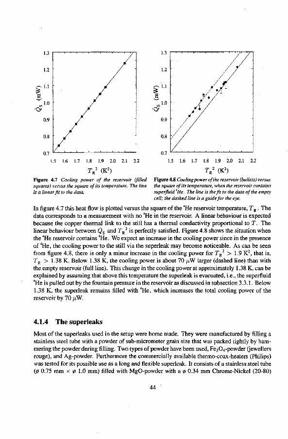
1.3

1.2

~1.1 s '-'

U'l 1.0 ·Q>

0.9

0.8

1.5 1.6 1.7 1.8 1.9 2.0 2.1 2.2

T/ (K2)

Figure 4.7 Coolirtg power of the reservoir (filled squares) versus the square of its temperature. The line is a linear fit to the data.

1.3 / I

/ /

/ /

I

1.2 / /

I /

/ /

/ /

~1.1 I ,

/ .l 8

., 7i '-' •

U'l 1.0 I

~/r ·Q> .. . 0.9 /

IÎ

/ I

/ I

/ I

0.8 /

IJ 1~ 1~ 1B 19 2n 11 12

T R2 (K2)

Figure 4.8 Cooling power of the reservoir (bullets) versus the square of its temperature, when the reservoir contains superjluid 4He. The line is thefit to the data ofthe empty cell; the dashed line is a guidefor the eye.

In figure 4.7 this heat flow is plotted versus the square of the 4He reservoir temperature, T R. The data corresponds to a measurement with no 4He in the reservoir. A linear behaviour is expected because the copper thermal link to the still has a thermal conductivity proportional to T. The linear behaviour between Q8 and T R

2 is perfectly satisfied. Figure 4.8 shows the situation when the 4He reservoir contains 4He. We expect an increase in the cooling power since in the presence of 4He, the cooling power to the still via the superleak may become noticeable. As can be seen from figure 4.8, there is only a minor increase in the cooling power for T R

2 > 1. 9 K2, that is, T R > 1.38 K. Below 1.38 K, the cooling power is about 70 J.tW larger ( dasbed line) than wîth the empty reservoir (fullline). This change in the cooling power at approximately 1.38 K, can be explained by assuming that above this temperature the superleak is evacuated, i.e., the superHuid 4He is pulled out by the fountain pressure in the reservoir as discussed in subsection 3.3 .1. Below 1.38 K, the superleak remains filled with 4He, which increases the total cooling power of the reservoir by 70 J.tW.

4.1.4 The superleaks

Most of the superleaks used in the setup were home made. They were manufactured by filling a stainless steel tube with a powder of sub-micrometer grain size that was packed tightly by ham­mering the powder during filling. Two types of powder have been used, Fe304-powder Uewellers rouge), and Ag-powder. Furthermore the commercially available thermo-coax-heaters (Philips) was tested for its possible use as a long and ftexible superleak. It consists of a stainless steel tube (0 0.75 mm x 0 1.0 mm) tilled with MgO-powder with a 0 0.34 mm Chrome-Nickel (20-80)

44

wire in the center. An important reason for testing this type of thin and flexible superteak was to prove that bending a superteak need not dramatically reduce the critica! flow rate. This type of "of the role" superteak work:ed well, but the critica! flow rate of approximately 0.6 mmolis was rather small. In Table 4.1 the characteristic dimensions of the superteales tested are given, as well as the type of powder.

'Thble 4.1 Various dimensions of tested superleaks.

Name Filling Powder Tube material Length (mm) Diameters (mm) !

SLO Fe3Û4 Stainless steel 105 (b6.0 x 04.0 SLI MgO Stainless steel 930 01.0 x 00.75 SL2 Fe304 &Ag Stainless steel & Cu 805 03.0 x 02.5 SL3 Fe304 Stainless steel 915 03.0 x !1)2.5

For superteak SLO two thermal anchors were used to rednee the heat flow to the expansion cell. One thermal anchor was cooled at the still, the other at the mixing chamber. The critica! flow rate of this superteak was above 2 mmol/s.

Superteak SL2 is made of three stainless steel tubes that are soft soldered to two 40 mm long 11 mm wide and 24 mm broad copper blocks in which a 02.5 mm hole was drilled. The copper blocks served asthermal ancboring points. After the first of the three tubes was filled with jewellers rouge, it was soldered with the second (still empty) tube to the copper block. The block was then filled with a mixture of jewellers rouge and silver powder. The silver powder is added to imprave the theemal conductivity at that part of the superleak. We did not substitute all the powder in the copper blocks by silver powder, because the thermal expansion of the mixture is closer to that of pure jewellers rouge. Next the stainless steel tube was filled with jewellers rouge only. The second ancboring point was assembied in a simHar manner. After the the superteak was filled, the soft solder joints were soldered once more to eliminate smalt cracks in the joints, possibly created by hammering the powder.

Superteak SL3 was made of a single stainless steel tube. It was filled with jewellers rouge only. The thermal ancboring points were made by soft soldering a !il 2 mm copper wire to the tube over a 40 mm distance. This superteak had a critica! 4He flow rate above 2 mmolls.

The thermal conductivity of a 4He filled superteak is comparable to the thermal conductivity of stainless steel [Alp69]. We used the thermal conductivity of stainless steel [Haa71] to estimate the heat leak through the superleak, and to calculate the optima! positions of the thermal ancboring points.

4.1.5 The heat switch

The heat switch is shown in figure 4.9. It is made of a 6 mm broad 0.3 mm thick alnminurn strip that is sandwiched by two 1.0 mm thick copper plates. The contact between the copper and the

45

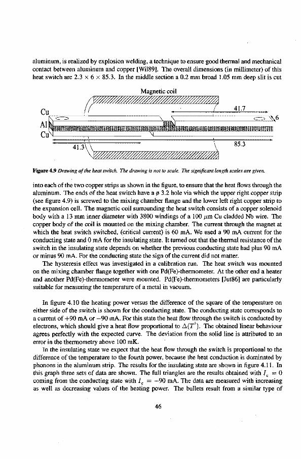
aluminum, is realized by explosion welding, a technique to ensure good theemal and mecbanical contact between aJuminurn and copper [Wil89]. The overall dimensions (in millimeter) of this beat switch are 2.3 x 6 x 85.3. In the middle section a 0.2 mm broad 1.05 mm deep slit is cut

41.7

85.3

Figure 4.9 Drawing of the heat switch. The drawing is not to scale. The significant length scales are given.

into each of the two copper strips as shown in the tigure, to ensure that the heat ftows througb the aluminum. The ends of the heat switch have a 0 3.2 hole via which the upper right copper strip (see tigure 4.9) is screwed to the mixing chamber ftange and the lower left right copper strip to the expansion cell. The magnetic coil suerounding the heat switch consists of a copper solenoid body with a 13 mm inner diameter with 3800 windingsof a 100 ttm Cu cladded Nb wire. The copper body of the coil is mounted on the mixing chamber. The cuerent through the magnet at which the heat switch switched, (critical cuerent) is 60 mA. We used a 90 mA cuerent for the conducting state and 0 mA for the insulating state. It tumed out that the theemal resistance of the switch in the insulating state depends on whetber the previous conducting state had plus 90 mA or minus 90 mA. Por the conducting state the sign of the cuerent did not matter.

The hysteresis effect was investigated in a calibration run. The heat switch was mounted on the mixing chamber ftange together with one Pd(Fe)-thermometer. At the other end a heater and another Pd(Fe)-thermometer were mounted. Pd(Fe)-thermometers [Jut86] are particularly suitable for measuring the temperature of a metal in vacuum.

In tigure 4.10 the heating power versus the difference of the square of the temperature on either side of the switch is shown for the conducting state. The conducting state coeresponds to a cuerent of +90 mA or -90 mA. Por this state the heat flow through tbe switch is conducted by electrons, which should give a heat flow proportional to il(T

2). The obtained linear behaviour

agrees perfectly with the expected curve. The deviation from the solid Iine is attributed to an error in the thermometry above 100 mK.

In the insulating state we expect that the heat flow through the switch is proportional to the difference of the temperature to the fourth power, because the heat conduction is dominated by phonons in the aluminum strip. The results for the insulating state are shown in tigure 4.11. In this grapb three sets of data are shown. Tbe full triangles are tbe results obtained with I c = 0 coming from the conducting state with Je -90 mA. The data are measured with increasing as well as decreasing values of the heating power. The bullets result from a similar type of

46

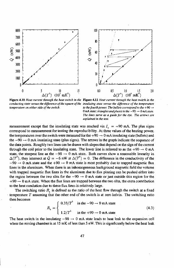
8llXl 100

7001

6lXX) 80 '

~5000 ,....,.

~ 60 '-'

·0' 4000 ·0' 3001 40

2001 20

1001

0 0

0 5 10 15 0.0 0.5 1.0 1.5 2.0 t.(T2) (10

3 mK

2) t.(T') (10

8 mK

4)

Figure 4.10 Heat current through the heat switch in the Figure 4.11 Heat current through the heat switch in the conducting state versus the dijference of the square of the insulating state versus the dijference of the temperafure temperafure on either side of the switch to the fourth power. The bullets correspond to the +90 ->

OmA state; trianglesandplusestothe -90-> OmA state. The lines serve as a gulde for the eye. The arrows are explained in the text.

measurement except that the insulating state was reached via I c = +90 mA. The plus signs correspond to measurement for testing the reproducibility. At three values of the heating power, the temperatures over the switch were measured for the +90 -+ 0 mA insulating state (bullets) and the -90-+ 0 mA insulating state (plus signs). The arrows in the graph indicate the sequence of the data points. Roughly two lines can be drawn with slopes that depend on the sign of the cuerent through the coil prior to the insulating state. The Iower line is referred to as the +90 -+ 0 mA state, the steepest line as the -90 -+ 0 mA state. Both curves show a reasonable lineacity in t.(T'), they interseet at Q = -6 nW at t.(T

4) = 0. The difference in the conductivity of the

-90 -+ 0 mA state and the +90-+ 0 mA state is most probably due to trapped magnetic flux lines in the aluminum. When there is an inhomogeneons background magnetic field the volume with trapped magnetic flux lines in the aluminum due to flux pinning can be pusbed either into the region between the two slits for the -90 -+ 0 mA state or just outside this region for the +90 -+ 0 mA state .. When the flux lines are trapped between the two slits, the extra contribution to the heat condution doe to these flux lines is relatively large.

The switching ratio Rs is defined as the ratio of the heat flow through the switch at a fixed temperature T assuming that the other end of the switch is at zero kei vin. The switching ratio then becomes

{

0.33/T2

R = s 1.2/T

2

in the -90 -+ 0 mA state (4.3)

in the +90 -+ 0 mA state

The heat switch in the insulating -90 -+ 0 mA state leads to heat leak to the expansion cell when the mixing ebaroberis at 15 mK ofless than 5 nW. This is significantly below the heat leak

47

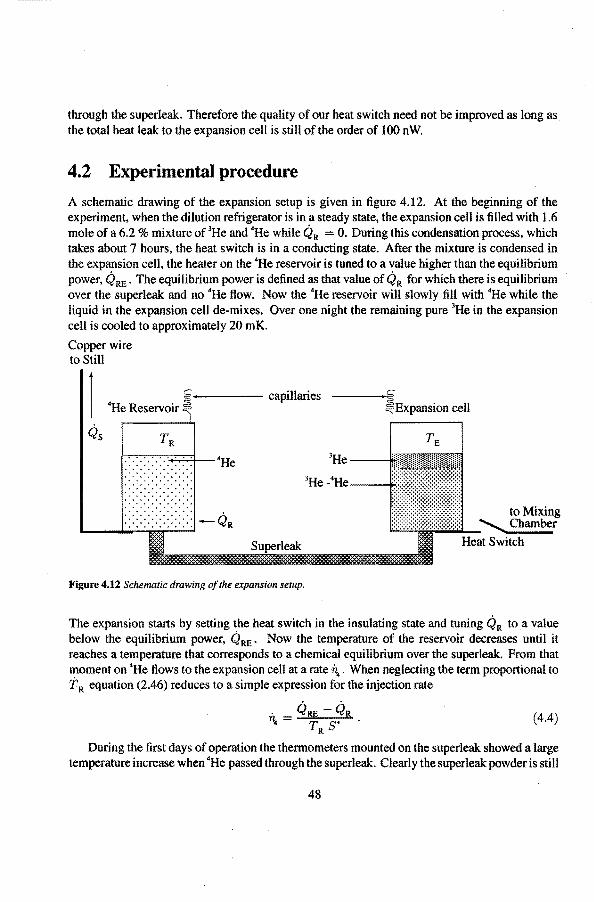
through the superleak. Therefore the quality of our heat switch need not be improved as long as the total heat leak to the expansion cell is still of the order of 100 n W.

4.2 Experimental procedure

A schematic drawing of the expansion setup is given in ligure 4.12. At the beginning of the experiment, when the dilution refrigerator is in a steady state, the expansion cell is lilled with 1.6 mole of a 6.2 % mixture of 3He and "He while QR = 0. During this condensation process, which takes about 7 hours, the heat switch is in a conducting state. After the mixture is condensed in the expansion cell, the heater on the 4He reservoir is tuned to a value higher than the equilibrium power, QRE. The equilibrium power is defined as that value of QR for which there is equilibrium over the superteak and no 4He flow. Now the 4He reservoir will slowly lill with 4He while the liquid in the expansion cell de-mixes. Over one night the remaining pure 3He in the expansion cell is cooled to approximately 20 mK.

Copperwire toStill

1 <=: .... ---- capillaries

4He Reservoir

......... . . . . . . . . . ·.·.·.·.·.·.·.·: -QR .___...._.._

Figure 4.12 Schematic drawing of the expansion setup.

3He ---li!mmm 3He -4He

toMixing ~r

Heat Switch

The expansion starts by setting the heat switch in the insulating state and tuning QR to a value below the equilibrium power, QRE. Now the temperature of the reservoir decreases until it reaches a temperature that corresponds to a chemical equilibrium over the superleak. From that moment on 4He flows to the expansion cell at a rate n.. When neglecting the term proportional to t R equation (2.46) reduces toa simple expression for the injection rate

· QRE QR 1\ = T s·

R

(4.4)

During the first days of operation the thermometers mounted on the superleak showed a large temperature increase when 4He passed through the superleak. Clearly the superleak powder is still

48

at a high temperature. The heat released in the superleak: is conducted to the thermal ancboring points. However, when the temperature of the superteak rises due toa flow of 4He, the injection wiJl be irreversible, that is, there is no equilibrium over the superleak: at that time. The psuedo heat load to the expansion cell due to the irreversible injection is usually much Iarger than the heat conduted via the hot superleak:. This extra heat leak to the expansion cell due to the irreversible flow of "He gradually vanishes within approximately one week.

The •He can be extracted from the expansion cell by tuning QR toa value above QRE. Equation (4.5) then gives the molar 4He extraction rate. The injection-extraction cycle can be repeated many times for various starting tempemtures, and injection(extraction) mtes.

A complete run usually lasted about 3 weeks. In that time all our resistor thermometers as well as the two liquid-helium level gauges were monitored via a computer every 2 to 3 min­utes. Forthermore an extra computer was used for the vibrating wire thermometer controL This thermometer was only implemented during the last two runs. These measuring devices will be presented in the next chapter.

References

Alp69

Cas85

Cas86

Coo79 Coo81

Fra61

Haa71 Jut86 Nii71 Ver87 Wil89

W.M. van Alphen, R. de Bruyn Ouboter, J.F. Olijhoek, and K.W. Taconis, Physica 40, 490 (1969). C.A.M. Castelijns, J.G.M. Kuerten, A.T.A.M de Waele, and H.M Gijsman, Phys. Rev. B32, 2870 (1985). C.A.M. Castelijns, Ph.D. Thesis, Eindhoven University ofTechnology Eindhoven The Netherlands (1986). G.M. Coops, A.T.A.M de Waele, and H.M Gijsman, Cryogenics 19, 659 (1979). G.M. Coops, Ph.D. Thesis, Eindhoven University of Technology, Eindhoven The Netherlands (1981). J.P. Franck, F.D. Manchester, and D.L. Martin, Proc. Roy. Soc. London A263, 494 (1961). J.N. Haasbroek, Ph.D. Thesis, University of Leiden, Leiden The Netherlands (1971). M. Jutzler, B. Schröder, K. Gloos, and F. Pobell, Z. Phys. B64, 115 (1986). T.O. Niinikoski, Nucl. lnstr. Meth. 97,95 (1971). F. Verroeuier and G. Frossati, Cryogenics 27, 139 (1987). R.W. Willekers, W.A. Bosch, F. Mathu, H.C. Meijer, and H. Postma, Cryogenics 29, 904 (1989).

49

5. Measuring techniques

The thennometer, used for monitoring the relatively fast temperature drop during the process, is described in this chapter. First an introduetion to the vibrating wire thennometer is given. This type of thermometer is particularly useful in the temperature range below 30 mK. Temperatures above 30 mK are measured with a calibrated (220 n) Speer resistor. As a fast and reliable thennometer on roetal surfaces in vacuum down to 7 mK we have used Pd(Fe )-susceptibility thennometers [Jut86]. Their design will be presenled in section three. In the last section the Iiquid-level capacity gauges, used to monitor the level of liquid helium in the 4He reservoir and the expansion cell, are presented.

5.1 The vibrating wire thermometer

Nowadays the vibrating wire (VW) is a standard device at many laboratorles for measuring the viscosity of quanturn fluids. The viscosity of quanturn fluids is highly temperature dependent, which makes these devices very useful as thermometers. The VW was first introduced by Tough [Tou63], [Tou64] in the mid sixties and later developed by the Lancaster group [Pic94]. The basis for the measurement of the viscosity via the VW is the damping of an oscillating wire that is bent in a half circular loop. The wireis placed in a magnetic field, B. When an a.c. current

(5.1)

with amplitude î is passed through the wire, the resulting Lorentz force, F L will drive the wire from its equilibrium position at an angular frequency w. The motion ofthe wire in the magnetic field produces an induced voltage V i in the loop that is measured as a function of w.

5.1.1 Theoretical description

Fora detailed presentation of the theory of the VW we refer to the workof Retsina et al. [Ret83], [Ret87]. In this section a short treatment of this theory will be presented, along with the method used to calculate the temperature and viscosity from the induced voltage.

The equation of motion for a VW of diameter dw, immersed in a viscous medium reads ·

(5.2)

50

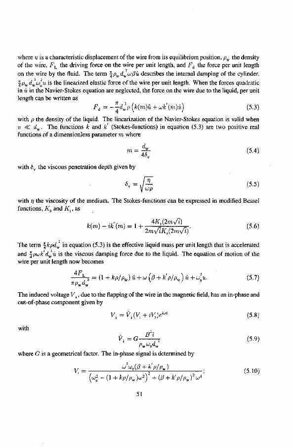
where u is a characteristic displacement of the wire from its equilibrium position, Pw the density of the wire, F L the driving force on the wireperunit length, and Fd the force per unit length

on the wire by the fluid. The term "iPwd:wj3û describes the intemal damping ofthe cylinder,

i Pw d; w ~ 11 is the Iinearized elastic force of the wire per unit length. Wh en the forces quadratic in u in the Navier-Stokes equation are neglected, the force on the wire due to the liquid, per unit length can be wntten as

(5.3)

with p the density of the liquid. The linearization of the Navier-Stokes equation is valid when 11 « dw. The functions k and k' (Stokes-functions) in equation (5.3) are two positive real functions of a dimensionless parameter m where

(5.4)

with óv the viscous penetration depth given by

8 = [!i V V wi> (5.5)

with 11 the viscosity of the medium. The Stokes-functions can be expressed in modified Bessel functions, K 0 and K 1 , as

k( ) .k'( ) 1 4K1(2mv1) m -z m = + . 2mv1I<0 (2mv1)

(5.6)

The term *kpd: in equation (5.3) is the effective liquid mass per unit length that is accelerated

and *pwk' d; û is the viscous damping force due to the liquid. The equation of motion of the wire per unit length now becomes

4FL 2 = (1 + kpfpw) ü +w (!3 + k'pfpw) u+ w;u.

1rpwdw (5.7)

The induced voltage V i, due to the flapping ofthe wire in the magnetic field, has an in-phase and out-of-phasecomponent given by

(5.8)

with

(5.9)

where G is a geometrical factor. The in-phase signa! is determined by

V _ W3

Wo(/3 + k' P/ Pw) . 1

- (w;-(t+kpfpw)w2)2

+(/3+k'pfpw)2 w4 '

(5.10)

51

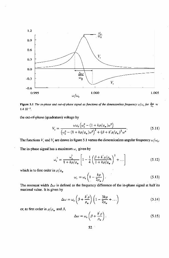
1.2

0.9

0.6

0.3

0.0

-0.3

-0.6

0.995 1.000 1.005

Figure 5.1 The in-phase and out-of-phase signa[ as functions of the dimensionless frequency w fw0 for Aw ~ "'o

1.4 w-3•

the out-of-phase (quadrature) voltage by

WW0 ( w;- (1 + kpj Pw )w2)

v; = 2 . (w;- (1 + kpfpw)w2) + ((3 + k'pfpw) 2 w4

(5.11)

The functions v; and v; are drawn in figure 5.1 versus the dimensionless angular frequency wjw0 •

The in-phase signal has a maximum w, given by

W 2 = w: [1 1 ((3 + k' pj Pw) 2

] r 1 + kpj Pw - 4 1 + kpj Pw + ... (5.12)

which is to first order in pj Pw

(5.13)

The resonant width ~w is defined as the frequency difference of the in-phase signal at half its maximal value. It is given by

~w = W 0 ((3 + ~:) ( 1 - ~;: + ... ) (5.14)

or, to first order in pf Pw and (3,

( k'p)

~W = Wo (3 + Pw . (5.15)

52

The quality factor of the VW is defined as

Q= (5.16)

With equation (5.15) this can be written as

Q (5.17) {3 + k' f!.n • ."

Pw

Por viscosity measurements in 3He -4He mixtures, the contributions of the two fluid components must be added, i.e., the term kp must be replaced by Ps + kp

0 and k' p by k' Pn. The quasipartiele

density p0

and the superHuid density p, are given by

2.46 x M3

V:,0(l + 0.286x) (5.18)

xM3 +(1-x)M4

Ps = V:,0 (l + 0.286x) - Pn (5.19)

with M3

and M. the molar mass of pure 3He and 4He. Once the value of m is determined by fitting equations (5.1 0) and (5.11) to the measured signals, the viscosity 17 follows from equations (5.4) and (5.5), i.e.,

(5.20)

and the Q-factor from equation (5.17). A more elaborate treatment of the flow field near the wire also accounts for phase-slîp effects

[Hjilj80]. When these slip effects are incorporated, the Stokes-functions modify to

k -1 k 1• = 1 + .,----"---,-,.:-:----:---::---;.,---:-:-:-

sip [l+m2'ï'k'J2+[m2Î(k 1)]2 (5.21)

k' _ k' + m2'ï'[(k- 1)2 + k'2

]

slip - [1 + m2Îk'j2 + [m2'ï'(k- 1)]2 (5.22)

where Î is related to the phase-slip length ( via

(5.23)

Por a Fermi-Iiquid ( is equal to 0.579 times the mean free path fm . Clearly when fm ~ dw, the slip-corrected Stokes-functions reduce to the old Stokes-functions. The mean free pathem for quasiparticle-quasiparticle scattering varies as T-

2• In the dilute phase at zero pressure it is given

by [Gué83]

( T )-2

fm = 500 mK pm. (5.24)

53

Below 4 mK the mean free path becomes of the size of the wire diameter and the hydrodynamic approximation of a local viscosity breaks down. The interaction of the wire and the helium at these low temperatures must then be regarded as a bombardment of the wire by individual quasipartkies of the Fermi gas. The above introduced hydrodynamic description is no Jonger applicable in this ballistic regime. It is; however, possible to interpret the damping of the wire in terms ofthe phase-slip model, when equation (5.23) is replaced with [Gué83]

1 + 5.3 · 2lmfdw

1 + 2fm/dw

For our wire, with dw =101 JLm, the function 1 is wel! approximated by

5.79 T 2 +53 1 = T 2 T 2 + 10

(5.25)

(5.26)

with T in millikelvin. In this work the ballistic regime is not reached. The hydrodynamic de­scription is used to interpret the measured resonance peaks. Phase-slip corrections are included only for temperatures below 10 mK to give the correct value of the viscosity.

At low temperatures, the viscosity f1 is proportional to I /T2

, so with (5 .20) m is proportional to T. For values of m larger than 0.1, m can be approximated by [Goo68]

1 + v'f+1! m~

k'..fi (5.27)

When {3 is neglected, the latter equation can be rewritten, via equation (5.17), to

TcxQ(t+Jl+~;J (5.28)

that is, the temperature is proportional to the quality factor times a slowly varying function of Q. We will use the relation between the temperature and Q, obtained in a calibration run, to extract the temperature from the measured Q-factor.

5.1.2 Calibration of the vibrating wire

The VW was calibrated in the mixing chamber, from 8 to 110 mK with a calibrated Speer thermometer and a CMN-thermometer. The Q-factor in vacuum was measured first. The inverse of the Q-factor in vacuum equals {3. With Q = 2 10

4 in vacuum we have

{3~510-5 • (5.29)

In tigure 5.2 the Q-factor is plotted versus the temperature. The data corresponds to our calibration run in the diluted phase in the mixing chamber. The curve shows a perfectly linear behaviour. The fitted line is given by

(I_)= Q+ 17.6. mK 34.2

(5.30)

54

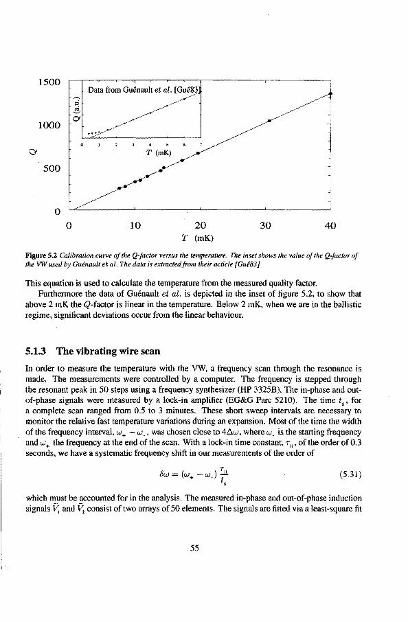
1500

1000

0

500

0

0

Data from Guénault et al. [Gué83

....

10

T (mK)

20 T (mK)

30 40

Figure 5.2 Calibration curve of the Q·factor versus the temperature. The inset shows the value of the Q-factor of the VW used IJy Guénault et al. The data is extracted from their actiele [ Gué83]

This equation is used to calculate the temperature from the measured quality factor. Forthermore the data of Guénault et al. is depicted intheinset of tigure 5.2, to show that

above 2 mK the Q-factor is linear in the temperature. Below 2 mK, when we are in the ballistic regime, significant deviations occur from the linear behaviour.

5.1.3 The vibrating wire scan

In order to measure the tempemture with the VW, a frequency scan through the resonance is made. The measurements were controlled by a computer. The frequency is stepped through the resonant peak: in 50 stepsusinga frequency synthesizer (HP 3325B). The in-phase and out­of-phase signals were measured by a lock-in amplifier (EG&G Pare 5210). The time t,, for a complete scan ranged from 0.5 to 3 minutes. These short sweep intervals are necessary to monitor the relative fast temperature variations during an expansion. Most of the time the width ofthe frequency interval, w+ - w_, was chosen close to 4D.w, where w_ is the starting frequency and w + the frequency at the end of the scan. With a lock-in time constant, r", of the order of 0.3 seconds, we have a systematic frequency shift in our measurements of the order of

7 ów = (w - w).....!!..

+ " t, (5.31)

which must be accounted for in the analysis. The measured in-phase and out-of-phase induction signals V; and V; consist of two arrays of 50 elements. The signals are fitted via a least-square fit

55

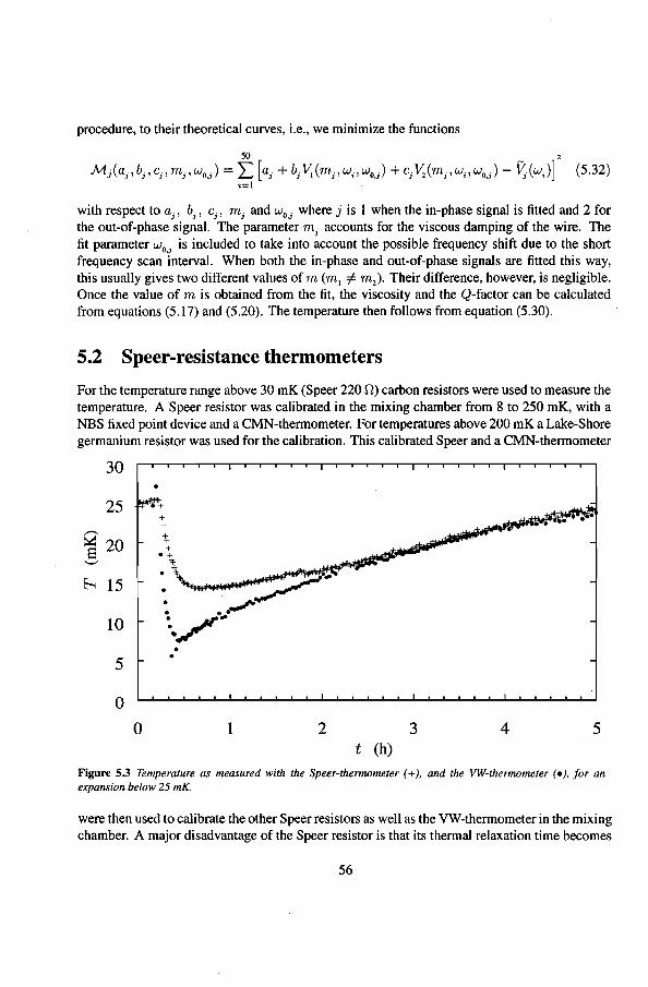
procedure, totheir theoretica! curves, i.e., we minimize the functions

~ 2

Mi(a1 , b1 , c1 , m1 , w0.,) = L h + b1 V, (m1 , w,, w0) + c1 ~(m1 , w,, w0.,)- ~(wJ] (5.32) i=l

with respect to a1

, b1

, c1

, m1

and w0,1

where j is 1 when the in-phase signa! is fitted and 2 for the out-of-phase signa!. The parameter m1 accounts for the viscous damping of the wire. The fit parameter w0,

1 is included to take into account the possible frequency shift due to the short

frequency scan interval. When both the in-phase and out-of-phase signals are fitted this way, this usually gives two different values of m (m, =I m 2). Their difference, however, is negligible. Once the value of m is obtained from the fit, the viscosity and the Q-factor can be calculated from equations (5.17) and (5.20). The temperature then follows from equation (5.30).

5.2 Speer-resistance thermometers

For the temperature range above 30 mK (Speer 220 0) carbon resistors were used to measure the temperature. A Speer resistor was calibrated in the mixing chamber from 8 to 250 mK, with a NBS fixed point device and a CMN-thermometer. For temperatures above 200 mK a Lake-Shore germanium resistor was used for the calibration. This calibrated Speer and a CMN-thermometer

30

25 +

h 15

10

5

0

0

• •

1 2 3 4 5 t (h)

Figure 5.3 Temperafure as measured with the Speer-thermometer(+), and the VW-thermometer (•), for an expansion below 25 mK.

were then used to calibrate the other Speer resistors as well as the VW-thermometer in the mixing chamber. A major disadvantage of the Speer resistor is that its theemal relaxation time becomes

56

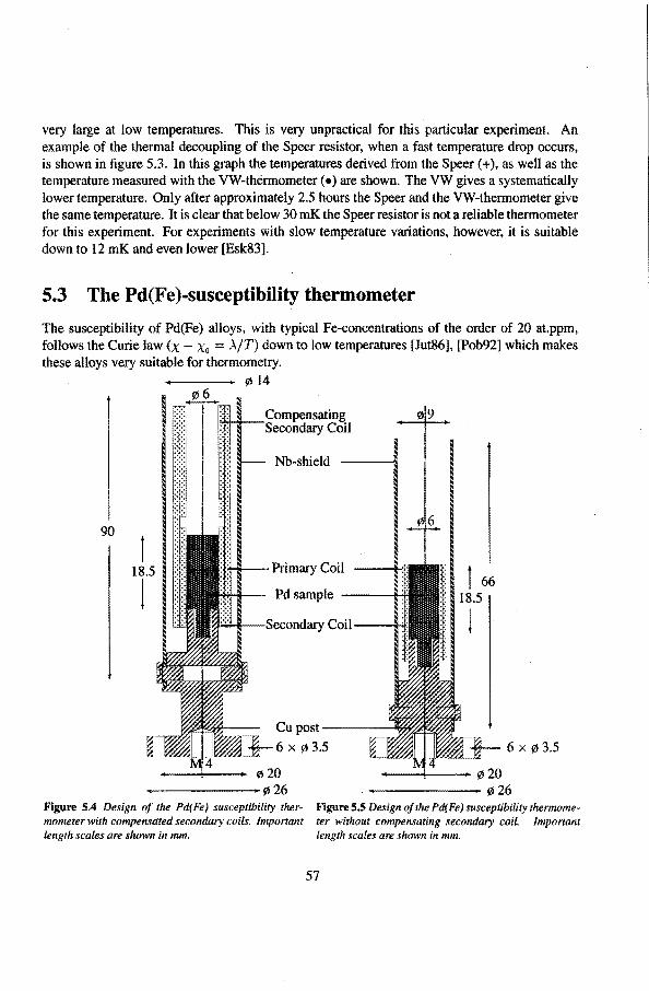
very large at low temperatures. This is very unpractical for this partienlar experiment. An example of the thermal decoupling of the Speer resistor, when a fast temperature drop occurs, is shown in tigure 5.3. In this graph the temperatures derived from the Speer(+), as wellas the temperature measured with the VW-thërmometer ( •) are shown. The VW gives a systematically lower temperature. Only after approximately 2.5 hours the Speer and the VW-thermometer give the same temperature. lt is clear that below 30 mK the Speer resistor is nota reliable thermometer for this experiment. For experiments with slow temperature variations, however, it is suitable down to 12 mK and even lower [Esk83].

5.3 The Pd(Fe )-susceptibility thermometer

The susceptibility of Pd(Fe) alloys, with typical Fe-concentrations of the order of 20 at.ppm, follows the Curie law (x - Xo = >..fT) down to low temperatures [Jut86], [Pob92] which makes these alloys very suitable for thermometry.

90

1 18.5

1

Y' 14

l~r--Compensating Secondary Coil

Nb-shield

Pri mary Coil

Pd sample

Coil

Cu post-----llil'l

6 x~ 3.5

t 66 18.5

!

6 x~ 3.5

Figure 5.4 Design of the Pd(Fe) susceptibility ther- Figure S.S Design ofthe Pd(Fe) susceptibility thermome­mometer with compensated secondary coils. Important ter without compensating secondary coil. Important length scales are shown in mm. length scales are shown in mm.

57

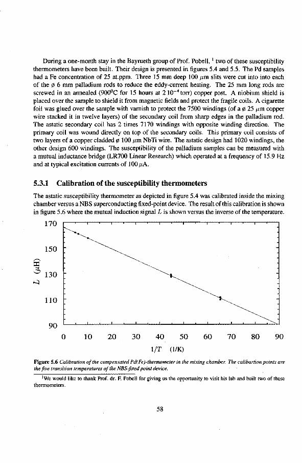
During a one-month stay in the Bayrueth group of Prof. Pobell, 1 two of these susceptibility thermometers have been built. Their design is presented in figures 5.4 and 5.5. The Pd samples had a Fe concentration of 25 at.ppm. Three 15 mm deep 100 J..lm slits were cut into into each of the ~ 6 mm palladium rods to reduce the eddy-current heating. The 25 mm long rods are screwed in an annealed (C)()()ÜC for 15 hours at 2 1 o-4 torr) copper post. A niobium shield is placed over the sample to shield it from magnetic fields and proteet the fragile coils. A cigarette foil was glued over the sample with varnish toproteet the 7500 windings (of a~ 25 J..lm copper wire stacked it in twelve layers) of the secondary coil from sharp edges in the palladium rod. The astatic secondary coil has 2 times 7170 windings with opposite winding direction. The primary coil was wound directly on top of the secondary coils. This primary coil consists of two layers of a copper cladded 9J 100 J..lm Nb Ti wire. The astatic design had 1020 windings, the other design 600 windings. The susceptibility of the palladium samples can be measured with a mutual inductance bridge (LR700 Linear Research) which operated at a frequency of 15.9 Hz and at typical excitation currents of 100 J..lA.

5.3.1 Calibration of the susceptibility thermometers

The astatic susceptibility thermometer as depicted in tigure 5.4 was calibrated inside the mixing chamber versus a NBS superconducting fixed-point device. The result of this calibration is shown in ligure 5.6 where the mutual induction signal L is shown versus the inverse of the temperature.

170

150

""' :I:: :::t

"-" 130 ~

110

90

0 10 20 30 40 50 60 70 80 90

l/T (1/K)

Figure 5.6 Calibration of the compensated Pd( Fe)·thermometer in the mixing chamber. The eaUbartion points are the jive transition temperatures of the NBS-jixed point device.

1 We would like to thank Prof. dr. F. Pobell for giving us the opportunity to visit his lab and built two of these thermometers.

58

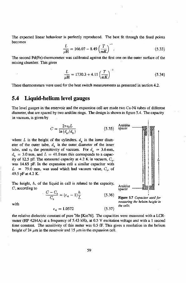
The expected linear behaviour is perfectly reproduced. The best fit through the fixed points becomes

L T -• f.J,H = 166.07- 8.49 (mK) (5.33)

The second Pd(Fe )-thermometer was calibrated against the first one on the outer surface of the mixing chamber. This gives

L T -• f.J,H = 1730.3+4.11 (mK) (5.34)

These thermometers were used for the heat switch measurements as presented in section 4.2.

5.4 Liquid-helium level gauges

The level gauges in the reservoir and the expansion cell are made two Cu-Ni tubes of different diameter, that are spaeed by two araldite rings. The design is shown in tigure 5.4. 1'he capacity in vacuum, is given by

(5.35)

where L is the height of the cylinders, da is the inner diam­eter of the outer tube, db is the outer diameter of the inner tube, and éo the permittivity of vacuum. For da = 3.6 mm, db = 3.0mm, and L = 41.0mm this corresponds toa capac­ity of 12.5 pF. The measured capacity at 4.2 K in vacuum, C0 ,

was 14.65 pF. In the expansion cell a similar capacitor with L = 79.0 mm, was used which had vacuum value, C0 , of 49.5 pF at 4.2 K.

i Araldite --H i spaeer i

1.

i' i i i i i i i i i i i

The height, h, of the liquid in cell is related to the capacity, i C, according to t;:~~~te --lllil~JiiY i !~!im

L

h I = (o:4 -l)L (5.36) Figure 5.7 Capacitoriusedfor

measuring the heluim height in the cells. with

(5.37)

the relative dielectric constant of pure 4He [Kie76]. The capacities were measured with a LCR­meter (HP 4284A) at a frequency of 5.43 kHz, at 0.5 V excitation voltage and with a 1 second time constant. The sensitivity of this meter was 0.5 fF. This gives a resolution in the helium height of 24 f.J,m in the reservoir and 15 f.J,m in the expansion cell.

59

References

Esk83 G. Eska and K. Neumaier, Cryogenics 23, 84 (1983). Gué83 A.M. Guénault, V. Keith, C.J. Kennedy, and G.R. Pickett, Phys. Rev. Lett. 50, 522

(1983). Goo68 J.M. Goodwin, Ph.D. Thesis, Washington University, Washington USA (1968). H!llj80 H. H!lljgaard lensen, H. Smith, P. Wölfle, K. Nagai, and T. M. Bisgaard, J. Low Temp.

Phys. 41, 473 (1980). Jut86 M. Jutzler, B. Schröder, K. Gloos, and F. Pobell, Z. Phys. B64, 115 (1986). Kie76 H.A. Kierstead, J. Low Temp. Phys. 24,497 (1976). Pic94 G.R. Picket, M.P. Enrico, S.N. Fisher, A.M. Guénault, and K. Torizuka, Phys. B197,

390 (1994). Pob92 F. Pobell, Matterand Methods at Low Temperatures (Springer-Verlag, Berlin 1992). Ret86 T. Retsina, S.M. Richardson, and W.A. Wakeham, Appl. Sci. Res. 43, 127 (1986). Ret87 T. Retsina, S.M. Richardson, and W.A. Wakeham, Appl. Sci. Res. 43, 325 (1987). Tou63 J.T. Tough, W.O. McCornick, and J.G. Oash, Phys. Rev. 132, 2373 (1963). Tou64 J.T. Tough, W.O. McComick, andJ.G. Oash, Rev. ofSci. lnstr. 35, 1345 (1964).

60

6. Experimental results

In this chapter the experimentat resutts will be presented. In the first section the resutts of the measurements of the viscosity of the concentrated phase are presented. Furthermore the influence of the tiquid-vacuum interface and the phase boundary on the interpretation of the mea­sured data is discussed. In the second section the results of expansions with initia! temperatures between 20 mK and 190 mK are given. The experiments were performed in severat expansion cells and with different superleaks. First the temperature evolution in the expansion cell and the 4He reservoir during and after the expansion will be examined. From the temperature increase after an expansion the value of the heat leak can be determined. With this heat leak a compar­ison between the theoretica! and the experimental temperature evotution during the expansion is possibte. Next the retation between the heating power to the 4He reservoir and the 4He flow through the superleak, as well as, the equilibrium condition for a reversible 4He flow through the superteak will be verified. For a small diameter superteak or a superteak that is locally still at a high temperature the 4He flow can become dissipative. An exampte of an irreversible 4He injection is given. At the end of section two, several typical values of the cooling factor over the 20 to 190 mK temperature range will be presented. In the third section, finalty, the anomalies in the resonance curves as measured with the VW are anatyzed. The analysis indicate that the anomalous behaviour in the VW signa! is due to a second resonance mode that couples to the "normat" VW resonance mode. This second resonance mode depends on the position of the phase boundary in the expansion cell.

6.1 Viscosity of 3He

The viscosity "1, of pure 3He bas been measured by many groups throughout the years [Atv73], [Alv74], [Arc81], [Car83], [Rit87] using vibrating wire viscorneters and/or torsional oscillators. An empiricat curve fitting best to the measured data is given by Wilks and Betts [Wil90]

0.183 JLPas (6.1)

17_, = T 2 (1 - 2.9T)

with Tin kelvin. The empirica! curve is valid for temperatures below 125 mK.

61

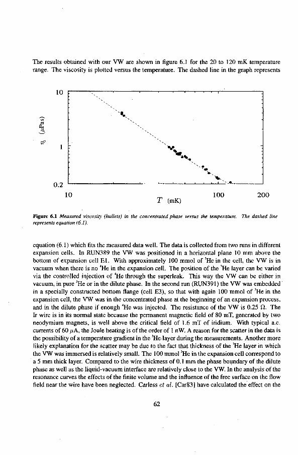
The results obtained with our VW are shown in figure 6.1 for the 20 to 120 mK temperature range. The viscosity is plotted versus the temperature. The dasbed line in the graph represents

10

0.2

10 T (mK)

100 200

Figure 6.1 Measured viscosity (bullets) in the concentraled phase versus the tempera/Ure. The dashed line represents equation (6.1).

equation (6.1) which fits the measured data well. The data is collected from two runs in different expansion cells. In RUN389 the VW was positioned in a horizontal plane I 0 mm above the bottorn of expansion cell El. With approximately 100 mmolof 3He in the cell, the VW is in vacuum when there is no 'He in the expansion cell. The position of the 3He layer can be varied via the controlled injection of 'He through the superleak. This way the VW can be either in vacuum, in pure 3He or in the dilute phase. In the second run (RUN391) the VW was embedded · in a specially constructed bottorn flange (cell E3), so that with again 100 mmolof 3He in the expansion cell, the VW was in the concentraled phase at the beginning of an expansion process, and in the dilute phase if enough 'He was injected. The resistance of the VW is 0.25 n. The Ir wire is in its normal state because the permanent magnetic field of 80 mT, generated by two neodymium magnets, is well above the critical field of 1.6 mT of iridium. With typical a.c. currents of 60 J,LA, the Joule heating is of the order of 1 n W. A reason for the scatter in the data is the possibility of a temperature gradient in the 3He layer during the measurements. Another more Iikely explanation for the sc1,1,tter may be due to the fact that thickness of the 3He layer in which the VW was immersed is relatively smal!. The 100 mmo! 3He in the expansion cell correspond to a 5 mm thick layer. Compared to the wire thickness of 0.1 mm the phase boundary of the dilute phase as wel! as the liquid-vacuum interface are relatively close to the VW. In the analysis of the resonance curves the effects of the finite volume and the influence of the free surface on the flow field near the wire have been neglected. Carless et al. [Car83] have calculated the effect on the

62

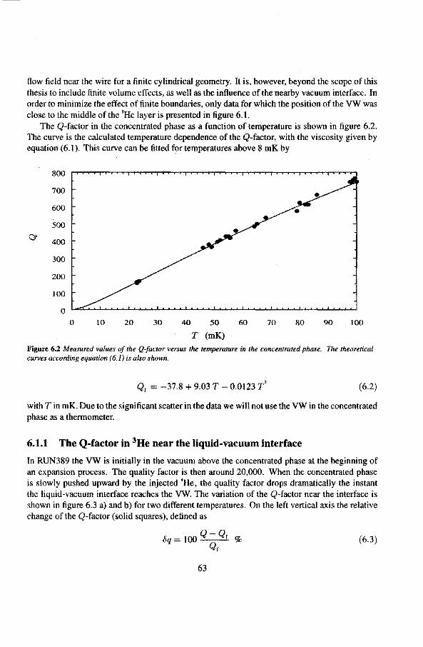
flow field near the wire fora finite cylindrical geometry. It is, however, beyond the scope of this thesis to include finite volume effects, as well as the influence of the nearby vacuum interface. In order to minimize the effect of finite boundaries, only data for which the position of the VW was close to the middle of the 3He layer is presented in tigure 6.1.

The Q-factor in the concentrated phase as a function of temperature is shown in tigure 6.2. The curve is the calculated temperature dependenee of the Q-factor, with the viscosity given by equation (6.1 ). This curve can be titted for temperatures above 8 mK by

800

700

600

500

0' 400

300

200

100

0 0 10 20 30 40 50 60 70 80 90 100

T (mK)

Flgure 6.2 Measured values of the Q-factor versus the temperature in the concentrared phase. The theoretical curves according equation ( 6.1) is a lso shown.

Qc = -37.8 + 9.03 T 0.o123 r' (6.2)

with T in mK. Due to the significant scatter in the data we wiJl not use the VW in the concentrated phase as a thermometer.

6.1.1 The Q-factor in 3He near the liquid-vacuum interface

In RUN389 the VW is initially in the vacuum above the concentrated phase at the beginning of an expansion process. The quality factor is then around 20,000. When the concentraled phase is slowly pusbed upward by the injected 4He, the quality factor drops dramatically the instant the liquid-vacuum interface reaches the VW. The varlation of the Q-factor near the interface is shown in tigure 6.3 a) and b) for two different temperatures. On the left vertical axis the relative change of the Q-factor (solid squares), defined as

{jq = 100 Q Qf % Qf

63

(6.3)

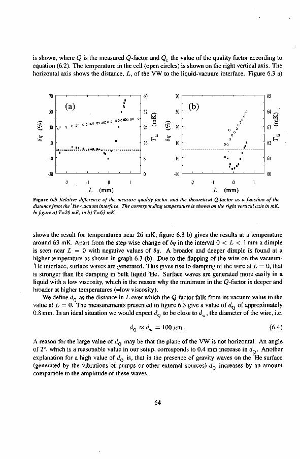
is shown, where Q is the measured Q-factor and Qr the value of the quality factor according to equation (6.2). The temperature in the cell (open circles) is shownon the right vertical axis. The horizontal axis shows the distance, L, of the VW to the liquid-vacuum interface. Figure 6.3 a)

70 40 70 65 •

(a) .

(b) ' 50 32 ,..-._ 50 cP 64,.-._ 0 ~ 0 ~

,..-._ a o ocrJDO oo g ,..-._ 0 8 o ao o aooo oooooo o • 0 ~ 30 cP 0 24 ~ 30

0 63 ......., ......., ......., 0 0

0 ~ Ul ~

0 Ul co h co 0

62 h 10 16 10 oo • ... _--1'--~-!!_,!1_ •• ...._ ........ ___ ..-_____________ I ---------------------------------------. ..

-10 -10 .. 61 • • • • ••

-30 0 -30 60

-2 -I 0 -2 -I 0

L (mm) L (mm)

Figure 6.3 Relative difference of the measure quality jactor and the theoretica{ Q-factor as a function of the disrance from the 'He -vacuum interface. The corresponding temperature is shownon the right vertical axis in mK. In ft gure a) T=26 mK, in b) T=63 mK.

shows the result for temperatures near 26 mK; tigure 6.3 b) gives the results at a temperature around 63 mK. Apart from the step wise change of 8q in the interval 0 < L < 1 mm a dimple is seen near L = 0 with negative values of 8q. A broader and deeper dimple is found at a higher temperature as shown in graph 6.3 (b). Due to the Happing of the wireon the vacuum-3He interface, surface waves are generated. This gives rise to damping of the wire at L = 0, that is stronger than the damping in bulk liquid 3He. Surface waves are genel'ated more easily in a liquid with a low viscosity, which is the reason why the minimum in the Q-factor is deeper and broader at higher temperatures (=low viscosity).

We detine dQ as the distance in L over which the Q-factor falls from its vacuum value to the value at L = 0. The measurements presented in tigure 6.3 give a value of dQ of approximately 0.8 mm. In an ideal situation we would expect dQ to be close to dw, the diameter of the wire, i.e.

(6.4)

A reason for the large value of dQ may be that the plane of the VW is not horizontal. An angle of 2o, which is a reasonable value in our setup, corresponds to 0.4 mm increase in dQ. Another explanation for a high value of dQ is, that in the presence of gravity waves on the 3He surface (generated by the vibrations of pumps or other extemal sources) dQ increases by an amount comparable to the amplitude of these waves.

64

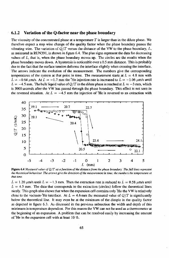
6.1.2 Variation of the Q-factor near the phase boundary

The viscosity of the concentraled phase at a temperature T is larger than in the dilute phase. We therefore expect a step wise change of the quality factor when the phase boundary passes the vibrating wire. The variation of Q fT versus the distance of the VW to the phase boundary, L, as measured in RUN391, is shown in tigure 6.4. The plus signs represent the data for decreasing values of L, that is, when the phase boundary moves up. The circles are the results when the phase boundary moves down. A hysteresis is noticeable over a 0.5 mm distance. This is probably due to the fact that the surface tension deforms the interface slightly when crossing the interface. The arrows indicate the evolution of the measurement. The numbers give the corresponding temperatures of the system at that point in time. The measurement starts at L = 4.8 mm with i = -0.64 f.Lmls. At L -I. 7 mm the 4He injection rateis increased to L = -1.06 Jlmls until L = -4.5 mm. The bulk liquid value of Q fT in the dilute phase is reached at L ~ -3 mm, which is 3000 seconds after the VW has passed through the phase boundary. This effect is not seen in the reversed situation. At L = -4.5 mm the injection of 4He is reversed to an extraction with

40

35 19.1

+-20.7 22.7

,-._ 30 19.1 ::.à

5 25 '-'

20

\ 20.4 \

15

10 \ 0

24.1

5 0 22.1 0

-5 -4 -3 -2 -1 0 l 2 3 4 5 L (mm)

Figure 6.4 Measured value of Q fT as a function of the distance from the phase boundary: The fulllines represent the theoretica/ behaviour. The armws give the direction ofthe measurement in time; the numbers the temperature at that time.

L 1.20 11mls until L = 1.3 mm. Then the extraction rate is reduced to L 0.58 f.LmiS until L 4.5 mm. The data that corresponds to the extraction (circles) follow the theoreticallines nicely. This graph also shows that when the expansion cell contains only 1He the VW is relatively close to the vacuum-3He interface. At L = 4.6 mm the measured value of Q fT is significantly below the theoretica} line. lt may even be at the minimum of the dimple in the quality factor as depicted in tigure 6.3. As discussed in the previous subsection the width and depth of this minimum is temperature dependent For this reason the VW can not be used as a thermometer at the beginning of an expansion. A problem that can be resolved easily by increasing the amount of'He in the expansion cell with at least 10%.

65

6.2 Adiabatic expansions

6.2.1 The expansion process

In this section several expansions will be presented. Typical temperature evolutions during the di Jution process are depicted in figures 6.5 to 6.9. At the beginning of an expansion process the expansion cell contains approximately I 00 mmo! pure JHe at an initial temperature. The heat supplied to the 4He reservoir, QR is above the equilibrium (critical) power QRE; a quantity that was defined in section 4.2. This assures that all the 'He is in the 4He reservoir. The experiment starts by reducing QR to a value below the critical power. The temperature of the 4He reservoir, T R, then starts to decrease until it corresponds to chemical-potential equilibrium over the super­teak. From that moment on 4He ftows through the superteak to the expansion cell at a rate given by equation (4.5). The moment 'He starts to flow, the heat switch is set to the insulating state. The expansion begins. Once all the 4He bas passed through the superleak, the temperature of the 4He reservoir falls toa value where Q8 = QR, where Q8 is the temperature dependent cooling power of the 4He reservoir as introduced in section 4.1.3. The •He can be extracted from the expansion cell by increasing the heating power to the 4He reservoirtoa value above QRE. After an initia! sharp rise in the 4He reservoir temperature til! its equilibrium temperature is reached (a smal! temperature oversboot is possible), the extraction starts. The temperature in the expansion cell rises until ali 4He is extracted. If desired the heat switch can be used to precool the expansion cell before another expansion/extraction cycle starts.

The temperature was measured with a Speer resistor and a VW in the dilute phase. Figures 6.5 and 6.6 show an expansion foliowed by an extraction in expansion cell E2 with superteak SL3. The total amount of 3He in the expansion cell was 102 and I 06 mmo! respectively. In both these graphs the temperature in the expansion cell as a function of time is shown on the left vertical axis (plus signs ). The temperature in the 4He reservoir during the expansion is shown on the right vertical axis (triangles). Furthermore the relative amount of 4He injected in the expansion cellis shown (circles). It is scaled to 100% on the vertical axis scale. This quantity is calculated from the variation of the capacitive liquid level gauge in the 4He reservoir. Since this capacitor is a few mm above the bottorn of the 4He reservoir, the last amount of 4He teaving the 4He reservoir (about 7 %) can not be monitored.

Figure 6.5 shows the temperature evolution ofthe expansion cell (plus signs) for an expansion with an initia! temperature of 130 mK. After seven minutes the helium level starts to increase (circles), and the expansion begins. The temperature in the •He reservoir (triangles) is then 1470 mK. At t = 90 min the level gauge reaches its maximum value. However, 4He is still ftowing through the superleak, as can be seen from the temperature of the 4He reservoir which is still high. At t = 95 min this temperature decreases sharply which indicates that the 4He reservoir is empty. The final temperature ofthis expansion is 37 mK, which gives a cooling factor of 3.5. At t 129 min the heating power QR is increased above QRE. The 4He reservoir temperature rises quickly and is for a few minutes even above the equilibrium temperature. As soon as the 4He ftows back to the 4He reservoir TE increases.

66

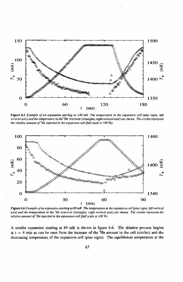
150

100

Ul

&.... 50

0

0 60 120 t (min)

1500

1450 Q' g

..: 1400 &....

1350 180

Figure 6.5 Example of an expansion starring at 130 mK. The temperafure in the expansion eelt (plus signs, left vertical axis) and the temperafure in the 'He reservoir (triangles, right vertical axis) are slwwn. The cirr:les represem the relative amount of'H~ injected in the expansion eelt (full scale is 100 %).

100

80

Q' 60 g

tll 40

&....

20

0 0 30 60

(min)

1460

Q' 1400 s

1340 90

'-'

Figure 6.6 Example of an expansion startingat 89 mK. The temperafure in the expansion cell (plus signs, left vertical axis) and the temperature in the 'He reservoir (triangles, right vertical axis) are shown. The cirr:les represem the relative amount of'He injected in the expansitm cell (full se ale is 100 % ).

A similar expansion starring at 89 mK is shown in tigure 6.6. The dilution process begins at t 8 min as can be seen from the increase of the 4He amount in the cell (circles) and the decreasing temperature of the expansion cell (plus signs). The equilibrium temperature at the

67

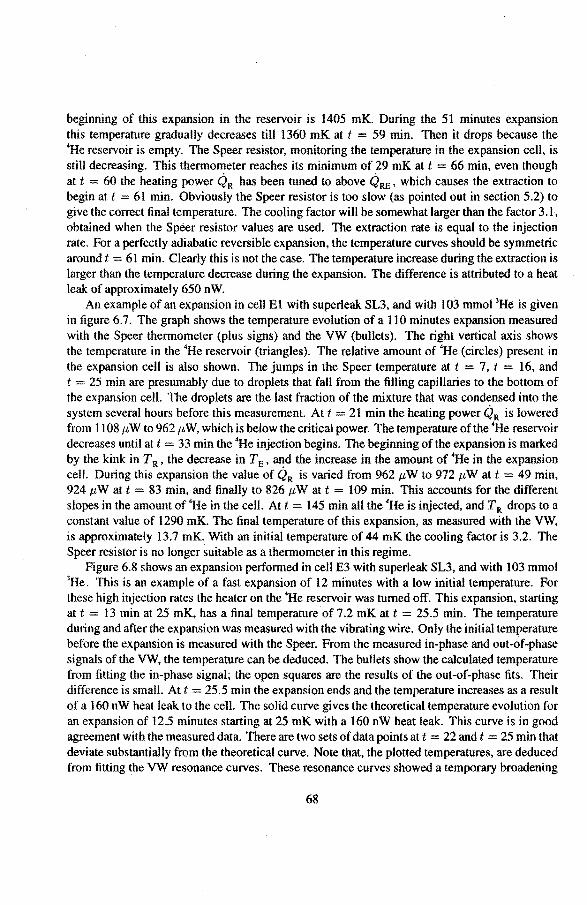
beginning of this expansion in the reservoir is 1405 mK. During the 51 minutes expansion this temperature gradually decreases till 1360 mK at t = 59 min. Then it drops because the 4He reservoir is empty. The Speer resistor, monitoring the temperature in the expansion cell, is still decreasing. This thermometer reaches its minimum of 29 mK at t = 66 min, even though at t = 60 the heating power QR has been tuned to above QRE, which causes the extraction to begin at t 61 min. Obviously the Speer resistor is too slow (as pointed outinsection 5.2) to give the correct final temperature. The cooling factor wiJl be somewhat Jarger than the factor 3.1, obtained when the Spèer resistor values are used. The extraction rate is equal to the injection rate. For a perfectly adiabatic reversible expansion, the temperature curves should be symmetrie around t = 61 min. Clearly this is not the case. The temperature increase during the extraction is larger than the temperature decrease during the expansion. The difference is attributed to a heat leak of approximately 650 nW.

An example of an expansion in cellEl with superteak SL3, and with 103 mmoi 3He is given in tigure 6.7. The graph shows the temperature evolution of a 110 minutes expansion measured with the Speer thermometer (plus signs) and the VW (bullets). The right vertical axis shows the temperature in the 4He reservoir (triangles). The relative amount of •He (circles) present in the expansion cell is also shown. The jumps in the Speer temperature at t = 7, t = 16, and t 25 min are presumably due to dropiets that fall from the filling capillaries to the bottorn of the expansion cell. The dropiets are the last fraction of the mixture that was condensed into the system several hours before this measurement. At t 21 min the heating power QR is lowered from 1108 IJ. W to 962 IJ. W, which is below the critica! power. The temperature of the 4He reservoir decreases until at t = 33 min the 4He injection begins. The beginning ofthe expansion is marked by the kink in T R, the decrease in TE, and the increase in the amount of 'He in the expansion cell. During this expansion the value of QR is varled from 962 ttW to 972 ttW at t = 49 min, 924 JL W at t 83 min, and finally to 826 JL W at t = 109 min. This accounts for the different slopes in the amount of 4He in the cell. At t 145 min all the 'He is injected, and T R dropstoa constant value of 1290 mK. The final temperature ofthis expansion, as measured with the VW, is approximately 13.7 mK. With an initia! temperature of 44 mK the cooling factor is 3.2. The Speer resistor is no Jonger suitable as a thermometer in this regime.

Figure 6.8 shows an expansion performed in cell E3 with superleak SL3, and with 103 mmo I 3He. This is an example of a fast expansion of 12 minutes with a low initia! temperature. For these high injection rates the heater on the 4He reservoir was tumed off. This expansion, starting at t = 13 min at 25 mK, has a final temperature of 7.2 mK at t = 25.5 min. The temperature during and after the expansion was measured with the vibrating wire. Only the initia! temperature before the expansion is measured with the Speer. From the measured in-phase and out-of-phase signals of the VW, the temperature can be deduced. The bullets show the calculated temperature from fitting the in-phase signa!; the open squares are the results of the out-of-phase fits. Their difference is small. At t 25.5 min the expansion ends and the temperature increases as aresult of a 160 nW heat leak to the cell. The solid curve gives the theoretica! temperature evolution for an expansion of 12.5 minutes startingat 25 mK with a 160 nW heat leak. This curve is in good agreement with the measured data. There are two sets of data points at t = 22 and t 25 min that deviate substantially from the theoretica} curve. Note that, the plotted temperatures, are deduced from fitting the VW resonance curves. These resonance curves showed a temporary broadening

68

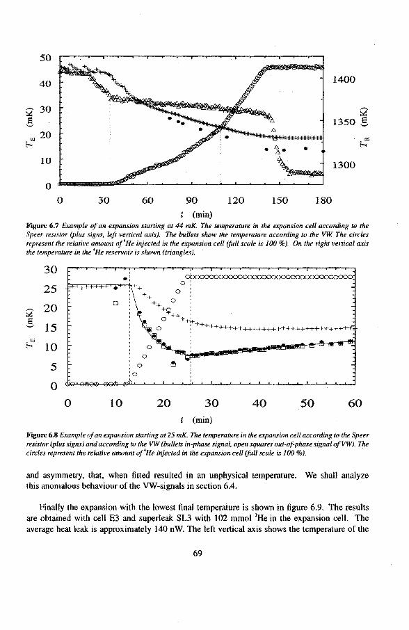
50

40

g 30 El .._,

~ 20

10

0 0 30 60 90 120

t (min)

150 180

1400

g 1350 s

1300

Figure 6.7 Example of an expansion starling at 44 mK. The temperature in the expansion cell according to the Speer resistor (plus signs, left vertical axis). The bullets show the temperature according to the VW The circles represent the relative amount of'He injected in the expansion cel/ (full scale is 100 %). On the right vertical axis the temperafure in the 'He reservoir is shown (triangles).

30

25

""' 20 ::.á

0

El 15 .._,

r i.t.l (:'-; 10

5

0

0 10

' .: 0

++ 0

++ 0 ++

+~ 0 +++'

+'l-++ : +++++++++++++++++++++++++-!·+++ '

0

0 ~ :o

20 30 40 50 (min)

60

Figure 6.8 Example of an expansion startingat 25 mK. The temperature in the expansion cell according to the Speer resistor (plus signs) and according 10 the VW ( bullets in-phase signal, open squares out-of·phase signa[ ofVW). The circles represent the relative amount of4He injected in the expansion cell (full scale is 100 %).

and asymmetry, that, when fitted resulted in an unphysical temperature. We shall analyze this anomalous behaviour of the VW-signals in section 6.4.

Finally the expansion with the lowest final temperature is shown in figure 6.9. The results are obtained with cell E3 and superteak SL3 with 102 mmo! 'He in the expansion cell. The average heat leak is approximately 140 nW. The left vertical axis shows the temperature of the

69

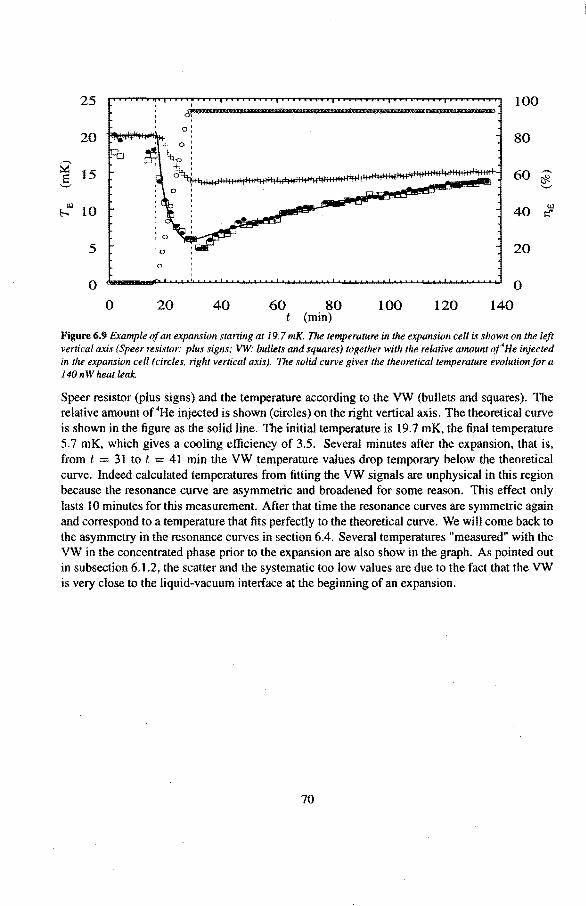
25 100 ~-RBRIQW@ !8 Rhk!ISBMJMMQ!B~

20 o:

' I+ 0: ~ \.o '

' +.

80

g § 15

40 ,;

5 20 :o

0 0

0 20 40 60 80 100 120 140 t (min)

Figure 6.9 Example of an expansion startingat 19.7 mK. The temperature in the expansion cel/ is shownon the leji vertical axis (Speer resistor: plus signs; VW· bullets and squares) logether with the relative amount of'He injected in the expansion cel/ (circles, right vertical axis). The solid curve gives the theoreticaltemperature evolutionfor a 140 n W heat teak.

Speer resistor (plus signs) and the temperature according to the VW (bullets and squares). The relative amount of 4He injected is shown ( circles) on the right vertical axis. The theoretica! curve is shown in the figure as the solid Iine. The initia) temperature is 19.7 mK, the final temperature 5.7 mK, which gives a cooling efficiency of 3.5. Several minutes after the expansion, that is, from t = 31 to t = 41 min the VW temperature values drop temporary below the theoretica} curve. Indeed calculated temperatures from fitting the VW signals are unphysical in this region because the resonance curve are asymmetrie and broadened for some reason. This effect only lasts 10 minutes for this measurement. After that time the resonance curves are symmetrie again and correspond to a temperature that fits perfectty to the theoretica! curve. We will come back to the asymmetry in the resonance curves in section 6.4. Several temperatures "measured" with the VW in the concentraled phase prior to the expansion are also show in the graph. As pointed out in subsection 6.1.2, the scatter and the systematic too low values are due to the fact that the VW is very close to the liquid-vacuum interface at the beginning of an expansion.

70

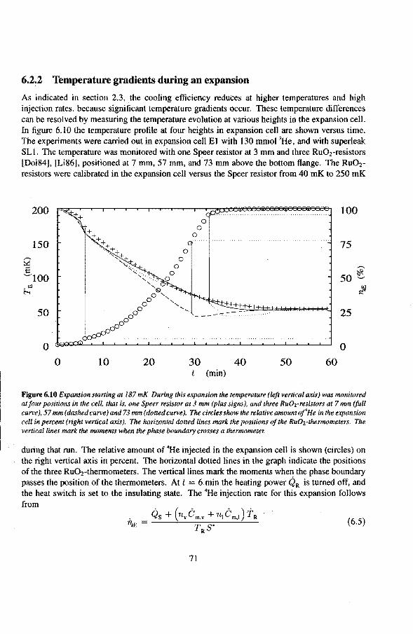
6.2.2 Temperature gradients during an expansion

As indicated in section 2.3, the cooling efficiency reduces at higher temperatures and high injection rates, because significant temperature gradients occur. These temperature differences can be resolved by measuring the temperature evolution at various heights in the expansion cel!. In tigure 6.10 the temperature profile at four heights in expansion cell are shown versus time. The experiments were carried out in expansion cellEl with 130 mmol 3He, and with superteak SLI. The temperature was monitored with one Speer resistor at 3 mm and three RuOrresistors [Doi84], [Li86], positioned at 7 mm, 57 mm, and 73 mm above the bottorn ftange. The Ru02-

resistors were calibrated in the expansion cell versus the Speer resistor from 40 mK to 250 mK

200 100

150 75

---~ s '-'100 50 ~

50 25

0 0

0 10 20 30 40 50 60 t (min)

Figure 6.10 Expansion startingat 187 mK. During this expansion the temperafure (left vertical axis) was monitored at Jour positions in the celL that is, one Speer resistor at 3 mm (plus signs), and three RuOrresistors at 7 mm ({uil curve), 57 mm ( dashed curve} and 73 mm ( dotted curve}. The circies show the rellltive amount of' He in the expansion cell in percent (right vertical axis). The horizontal dotted lines mark the positions ofthe RuOz-thermometers. The verticallines mark the moments when the phase /)(}undary crosses a thermometer.

during that run. The relative amount of 'He injected in the expansion cell is shown (circles) on the right vertical axis in percent. The horizontal dotted lines in the graph indicate the positions of the three Ru02-thermometers. The verticallines mark the moments when the phase boundary passes the position of the thermometers. At t = 6 min the heating power QR is tumed off, and the heat switch is set to the insulating state. The 4He injection rate for this expansion follows from

QS + (nvêm,v +nlêm,l)TR rRs·

71

(6.5)

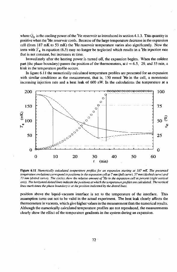
where Qs is the cooling power ofthe 4He reservoir as introduced insection 4.1.3. This quantity is positive when the •He reservoir cools. Because ofthe large temperature decreasein the expansion cell (from 187 mK to 53 mK) the 4He reservoir temperature varies also significantly. Now the term with T R in equation (6.5) may no longer be neglected which results in a 4He injection rate that is not constant, but increases in time.

Immediately after the heating power is tumed off, the expansion begins. When the coldest part (the phase boundary) passes the position of the thermometers, at t = 6.5, 29, and 33 min, a kink in the temperature profile occurs.

In tigure 6.11 the numerically calculated temperature profiles are presented for an expansion with similar conditions as the measurement, that is, 130 mmo! 3He in the eelt, a monotonic increasing injection rate and a heat leak of 600 nW. In the calculations the temperature at a

200 100 -- ..... ' 0

' ' 0

150 ', 75 ' ' ' Q ' "' ' ,......., E ' ._., 100 ' 50 ~ '\ lll ' ~ h 0~

0 ' 0 ',"

50 0 ' 25 0 ', 00

00 "00

0 0

0 10 20 30 40 50 60 t (min)

Figure 6.11" Numerically calculated temperature profiles for an expansion starring at 187 mK. The presented temperature evolutions correspond to positions in the expansüm cellat 7 mm (full curve), 57 mm ( dashed curve) and 73 mm (dotted curve). The circles show the relative amount of'He in the expansion cell in percent (right vertical axis ). The horizontal dotted lines indicate the positions at which the temptrature profiles are calculated. The vertical lines mark times the phase lmundary is at the position indicated by the dotted lines.

position above the liquid-vacuum interface is set to the temperature of the interface. This assumption tums out not to be valid in the actual experiment. The heat leak clearly affects the thermometers in vacuum, which give highervalues in the measurement than the numerical results. Although the numerically calculated temperature profiles are nol reproduced, the measurements clearly show the effect of the temperature gradients in the system during an expansion.

72

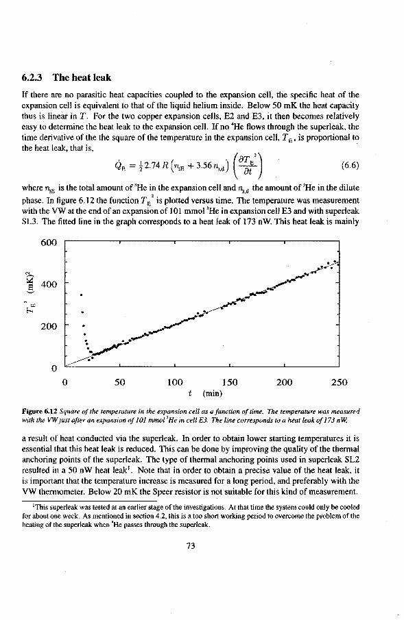
6.2.3 The heat leak

If there are no parasitic heat capacities coupled to the expansion ceH, the specific heat of the expansion cell is equivalent to that of the liquid helium inside. Below 50 mK the heat capacity thus is linear in T. For the two copper expansion cells, E2 and E3, it then becomes relatively easy to determine the heat leak to the expansion cell. If no •He flows through the superleak, the time derivative of the the square of the temperature in the expansion cell, TE, is proportional to the heat teak, that is,

• 1 ( ) (()TE2

) QE = 22.74R '1\E +3.56rt...,d at (6.6)

where Ti:.E is the total amount of 3He in the expansion cell and rl:.,d the amount of 3He in the dilute

phase. In tigure 6.12 the function TE 2

is plotted versus time. The temperature was measurement with the VW at the end of an expansion of 101 mmo! 3He in expansion cell E3 and with superleak SL3. The fitted line in the graph corresponds toa heat teak of 173 nW. This heat leak is mainly

600

. . g

400 E '-'

t.l.l

h

200

0

0 50 100 150 200 250 t (min)

Figure 6.12 Square of the temperature in the expansion cel! as a function of time. The temperafure was measured wilh the VW just afteran expansion of lOl tmrwl 'He in eelt E3. The line corresponds toa heat teakof 173 nW.

a result of heat conducted via the superleak. In order to obtain lower starting temperatures it is essential that this heat leak is reduced. This can be done by improving the quality of the thermal ancboring points of the superleak. The type of thermal ancboring points used in superleak SL2 resulted in a 50 nW heat teak1• Note that in order to obtain a precise vatue of the heat teak, it is important that the temperature incre.ase is measured fora long period, and preferably with the VW thermometer. Below 20 mK the Speer resistor is not suitable for this kind of measurement.

superlealc was tested at an earlierstage of the investigations. At that time the system could only be cooled forabout one week. As mentioned in section 4.2, this is a too short working period to overcome the problem of the healing of the superleak when 'He passes through the superleak.

73

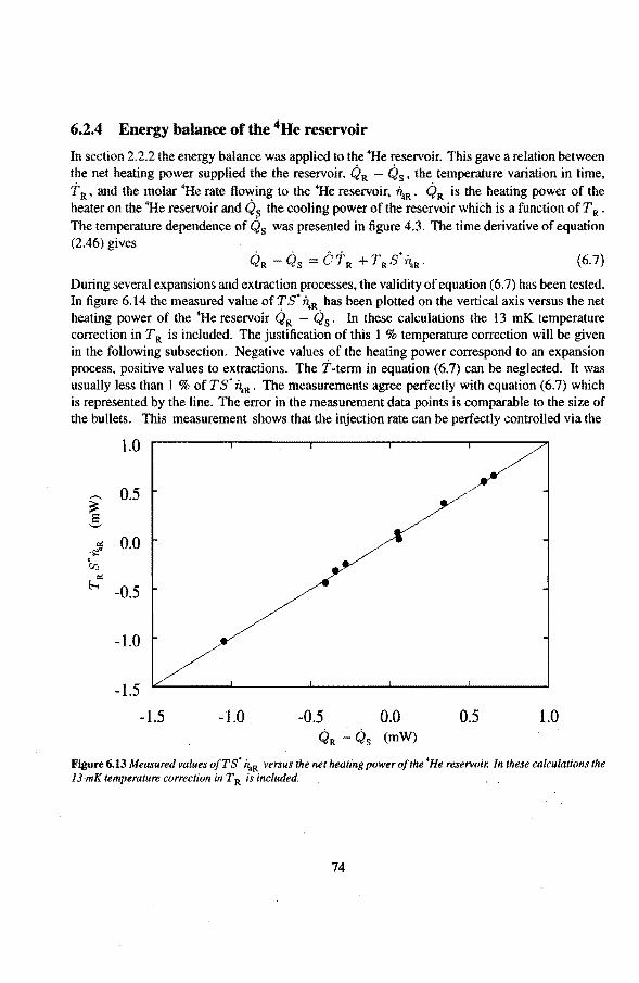
6.2.4 Energy balance of the 4He reservoir

In section 2.2.2 the energy balance was applied to the •He reservoir. This gave arelation between the net heating power supplied the the reservoir, ciR -cis, the temperature variation in time, t R, and the molar 'He rate flowing to the 4He reservoir, 7\R. ciR is the · heating power of the heater on the 4He reservoir and cis the cooling power of the reservoir which is a function of T R.

The temperature dependenee of cis was presented in figure 4.3. The time derivative of equation (2.46) gives

(6.7)

During several expansions and extraction processes, the validity of equation (6. 7) has been tested. In tigure 6.14 the measured value of T s· n

4R bas been plotted on the vertical axis versus the net

heating power of the 4He reservoir ciR cis. In these calculations the 13 mK temperature correction in T R is included. The justilkation of this 1 % temperature correction will be given in the following subsection. Negative values of the heating power correspond to an expansion process, positive values to extractions. The f-term in equation (6.7) can be neglected. It was usually less than 1 % of T s· n4R • The measurements agree perfectly with equation ( 6. 7) which is represented by the line. The error in the measurement data points is comparable to the si ze of the bullets. This measurement shows that the injection rate can be perfectly controlled via the

1.0

,-...

~ 0.5

'-'

..: 0.0 ·.:' .(IJ

..: h -0.5

-1.0

-1.5 -1.5 -1.0 -0.5 0.0 0.5 1.0

ciR cis (mW)

Figure 6.13 Measured va lues ofT s' it4R versus the net heating power ofthe 'He reservoir. In these calculations the 13 mK temperature correction inT R is included.

74

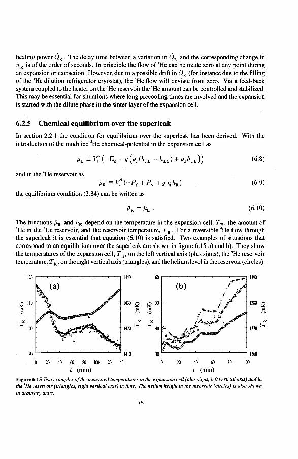
heating power QR. The delay time between a variation in QR and the corresponding change in ·n.R is of the order of seconds. In principle the flow of 4He can be made zero at any point during an expansion or extraction. However, due to a possible drift in Qs (for instanee due to the filling of the 4He dilution refrigerator cryostat), the 4He flow wiJl deviate from zero. Via a feed-back system coupled to the heater on the 4He reservoir the 4He amount can be controlled and stabilized. This may be essential for situations where long precooling times are involved and the expansion is started with the dilute phase in the sinter layer of the expansion cell.

6.2.5 Chemica) equilibrium over the superleak

In section 2.2.1 the condition for equilibrium over the superleak has been derived. With the introduetion of the modified 4He chemical-potential in the expansion cell as

and in the 4He reservoir as jlR :=V." (-Pr + pv + 9 fJ.hR)

the equilibrium condition (2.34) can be written as

(6.8)

(6.9)

(6.10)

The functions jlR and jlE depend on the temperature in the expansion cell, TE, the amount of 4He in the 4He reservoir, and the reservoir temperature, T R • For a reversible 4He flow through the superleak it is essential that equation (6.10) is satisfied. Two examples of situations that correspond to an equilibrium over the superleak are shown in tigure 6.15 a) and b). They show the temperatures of the expansion cell, TE, on the left vertical axis (plus signs ), the 4He reservoir temperature, T R, on the right vertical axis (triangles), and the helium level in thereservoir(circles).

Q' 110 §

tll

h 100

0 W 40 W W 100 lW ~

t (min)

1430 ,-.,

~ ~

1420 h

Q' 50 §

tll

h 40

0 20 40 w t (min)

80 100

1380 ,-.,

~ ~

1370h

Figure 6.15 Two examples o.fthe measured temperaiures in the expansion cel/ (plus signs, le.ft vertical axis) and in the 'He reservoir (triangles, right vertical axis) in time. The helium height in the reservoir (circles) is also shown in arbitrary units.

75

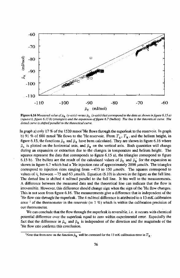
-60

-70

~

ö -80 E

0

..._ g

-90 "' •:::t

-100

-110

-110 -100 -90 -80 -70 -60 jlE (mJ/mol)

Figure 6.16 Measured value of flR (y-axis) versus% (x-axis) that correspond to the data as shown in ft gure 6.15 a) (squares),jigure 6.15 b) (triangles) and the expansion ofjigure 6.7 (bullets). The line is the theoretica/ curve. The dotted curve is shifted parallel to the theoretica{ curve.

In graph a) only 17 % of the 1520 mmol'He tlows tbrough tbe superteak to tbe reservoir. In grapb b) 91 % of 600 mmol 4He tlows to the 4He reservoir. From TE, T R, and the helium height, in tigure 6.15, the functions jlE and ilR have been calculated. They are sbown in tigure 6.16 where i1E is plotted on the horizontal axis, and j1R on the vertical axis. Both quantities will change during an expansion or extraction due to the changes in temperature and helium height. The squares represent the data that corresponds to tigure 6.15 a), tbe triangles correspond to tigure 6.l5 b). The bullets are the result of tbe calculated values of j1E and j1R for the expansion as shown in tigure 6.7 whicb bad a 4He injection rate of approximately 2000 ttmoVs. The triangles correspond to injection rates ranging from -473 to 150 ttmoVs. The squares correspond to values of i!,. between -75 and 63 ttmol/s. Equation (6.10) is shown in tbe tigure as the fullline. The dotted Iine is sbifted 4 mJ/mol parallel to tbe full line. lt fits well to the measurements. A difference between the measured data and the theoretica! line can indicate that the flow is irreversible. However, tbis difference should change sign when tbe sign of the 4He flow changes. This is not seen from tigure 6.16. The measurements give a difference that is independent of the 4He flow rate tbrough the superleak. The 4 mJ/mol difference is attributed toa 13 mK calibration error 1 of the thermometer in the reservoir ( ç::; I %) which is within the calibration precision of our thermometer.

We can coneinde that the flow through the superleak is reversible, i.e. it occurs with chemica) potential difference over tbe superleak equal to zero within experimental error. Especially the fact that the difference in jl,E and jl,R is independent of tbe direction and the magnitude of the 4He flow rate confirms this conclusion.

that from now on the function ji.R will be corrected for the 13 mK calibration error in T R .

76

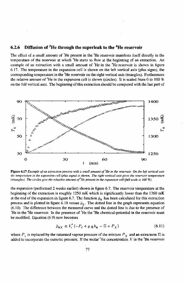
6.2.6 Dilfusion of 3He through the superleak to the 4He reservoir

The effect of a small amount of 3He present in the 4He reservoir manifests itself directly in the temperature of the reservoir at which 4He starts to flow at the beginning of an extraction. An example of an extraction with a small amount of 3He in the 4He reservoir is shown in figure 6.17. The temperature in the expansion cell is shown on the left vertical axis (plus signs), the corresponding temperature in the 4He reservoir on the right vertical axis (triangles). Forthermore the relative amount of 4He in the expansion cell is shown (ei rel es). It is scaled from 0 to l 00 % on the full vertical axis. The beginning of this extraction should be compared with the last part of

90

50

30 0 30

(min) 60

1400

1350 ~

1300

1250 90

Figure 6.17 Example of an extraction pmcess with a small amount of'He in the reservoir. On the left vertical axis the temperature in the expansion cell (plus signs) is siUJwn. The right vertical axis gives the reservoir temperature (triangles). The circles give the releative amount of

4He present in the expansion cel/ (Juli scale is 100 %).

the expansion (performed 2 weeks earlier) shown in figure 6.7. The reservoir temperature at the beginning of the extraction is roughly 1250 mK which is significantly lower than the 1360 mK at the end of the expansion in tigure 6. 7. The function pR has been calculated for this extraction process and is plotted in figure 6.18 versus ilE. The dotted line in the graph represents equation (6.10). The difference between the measured curve and the dotted line is due to the presence of 3He in the 4He reservoir. In the presence of 3He the 4He chemical-potential in the reservoir must be modified. Equation (6.9) now becomes

(6.11)

where P v is replaced by the saturated vapour pressure of the mixture P x and an extra term II is added to incorporate the osmotic pressure. If the molar 3He concentration X in the 4He reservoir

77

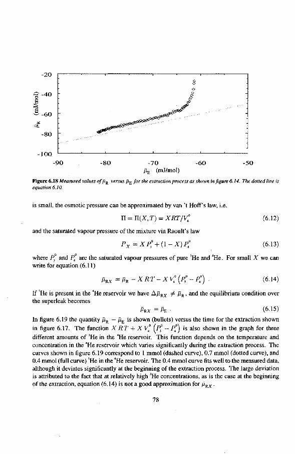
-20

r40 '-' -60

"' I ::I.

-80

-100

-90

g <>

I ~/

~·····

-80 -70 -60 -50 ilE (mJ/mol)

Figure 6.18 Measured va lues of jlR versus for the extraction process as shown in figure 6.14. The dotted line is equation 6.10.

is small, the osmotic pressure can be approximated by van 't Hoff's law, i.e.

TI II(X, T) = x RT IV."

and the saturated vapour pressure of the mixture via Raoult's law

P X =X~·+ (1 -X) ?"0

(6.12)

(6.13)

where ~· and P"" are the saturated vapour pressures of pure 3He and 4He. For small X we can write for equation ( 6.11)

(6.14)

If 3He is present in the •He reservoir we have t::.ilRx =f. ilR , and the equilibrium condition over the superleak becomes

jlRX = jlE · (6.15)

In tigure 6.19 the quantity jlR - ilE is shown (bullets) versus the time for the extraction shown

in tigure 6.17. The function X R T + X V." ( ~" - P"") is also shown in the graph for three

different amounts of 3He in the •He reservoir. This function depends on the temperature and concentration in the 'He reservoir which varies significantly during the extraction process. The curves shown in tigure 6.19 correspond to 1 mmol ( dasbed curve), 0.7 mmol (dotted curve), and 0.4 mmol (full curve) 3He in the 4He reservoir. The 0.4 mmo! curve fits well to the measured data, although it deviates significantly at the beginning of the extraction process. The large deviation is attributed to the fact that at relatively high 3He concentrations, as is the case at the beginning ofthe extraction, equation (6.14) is nota good approximation for ilRx.

78

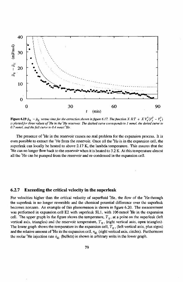
40 ' ' • ;:;;.;- '

0 ' 8 •

;::::; 30 g •

tll I ::'i..

20 .. 10

0 0 30 60 90

t (min)

Figure6.19 P,R P,E versus timejor the extraction shown injigure 6.17. Thefunction X RT + X v: (P; - P:) is plottedfor three values of'He in the 'He reservoir. The do.shed curve corresponds to 1 mmol, the dotted curve to 0.7 mmo[, and the full curve to 0.4 mmo! 'He.

The presence of 3He in the reservoir causes no real problem for the expansion process. lt is even possible to extract the 3He from the reservoir. Once all the 4He is in the expansion cell, the superteak can locally be heated to above 2.17 K, the lambda temperature. This assures that the •He can no longer flow back to the reservoir when it is heated to 3.2 K. Atthis temperature almost all the 3He can be pumped from the reservoir and re-condensed in the expansion cell.

6.2. 7 Exceeding the critical velocity in the superleak

For veloeities higher than the critica! velocity of superfluid 'He, the flow of the •He through the superteak is no Jonger reversible and the chemica! potential difference over the superleak becomes nonzero. An example of this phenomenon is shown in figure 6.20. The measurement was performed in expansion cell E2 with superleak SLI, with 106 mmo! 3He in the expansion cell. The upper graph in the figure shows the temperature, T s, at a point on the superteak (left vertical axis, triangles) and the reservoir temperature, T R, (right vertical axis, open triangles). The lower graph shows the temperature in the expansion cell, TE, (left vertical axis, plus signs) and the relative amount of'He in the expansion cell, rlaE (right vertical axis, circles). Furthermore the mol ar 'He injection rate il;.E (bullets) is shown in arbitrary units in the Iower graph.

79

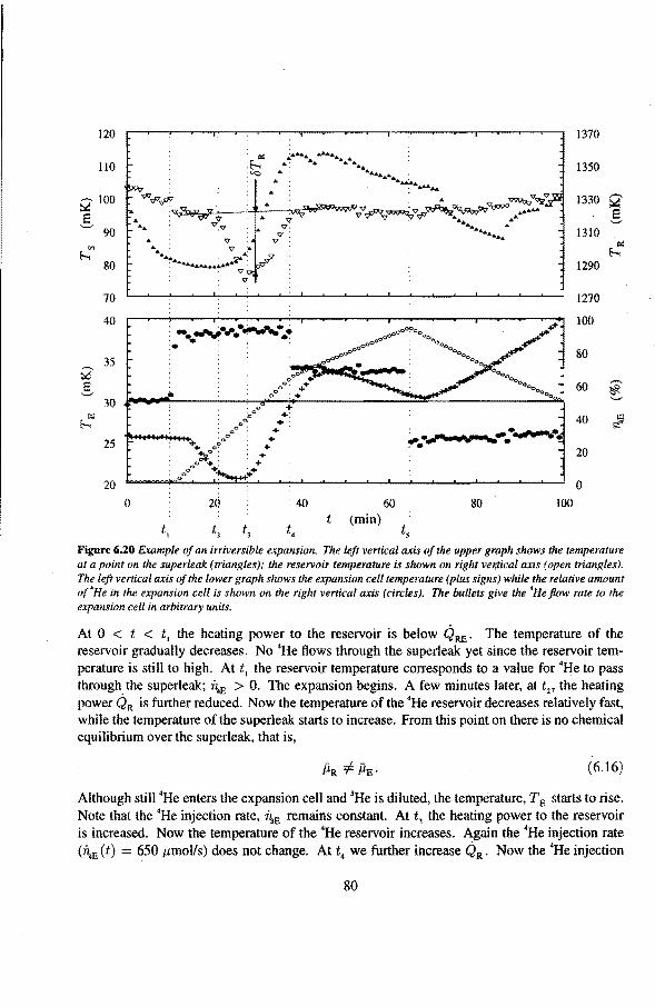
120

IlO

Q 100 e .._.,

90

"' t--. 80

70

40

35 g 5

30 t--. LQ

25

20 0

•

2Ó

t,

+ +:

+· + . +

+ +

+ ;..+

: 40 60 (min)

80 100

1370

1350

1330

1310

1290

1270

100

80

60

40

20

0

_........ :..::: e '-'

~

h

_........

~ .._.,

~

Figure (i.20 Example of an irriversible expansion. The left vertic al axis of the upper graph shows the temperature at a point on the superteak (triangles): the reservoir temperature is shownon right veT;tical axis (open triangles). The left vertical axis of the lower graph shows the expansion eelt temperature (plus signs) while the relative amount t~('He in the expansion cel! is shownon the right vertical axis (circles). The bullets give the 'He flow rate to the expansion cell in arbitrary units.

At 0 < t < t, the heating power to the reservoir is below QRE. The temperature of the reservoir gradually decreases. No 'He flows through the superleak yet since the reservoir tem­pcrature is still to high. At t, the reservoir temperature corresponds to a value for 4He to pass through the superleak; il:,E > 0. The expansion begins. A few minutes later, at t2' the healing power QR is further reduced. Now the temperature of the 'He reservoir deercases relatively fast, while the temperature of the superteak starts to increase. From this point on there is no chemica! equilibrium over the superleak, that is,

(6.16)

Although still 'He enters the expansion cell and 3He is diluted, the temperature, TE starts to rise. Note that the 'He injection rate, 'i~E remains constant. At t 1 the heating power to the reservoir is increased. Now the temperature of the 4He reservoir increases. Again the 'He injection rate (n4E (t) 650 ttmolls) does not change. At t, we further increase QR. Now the 'He injection

80

rate reduces to 300 ttmoVs, and the reservoir temperature corresponds to equilibrium over the superleak. The rest of the injection is reversible. The temperature of the expansion cell soon decreases again. At t, the hearing power is tuned to a value above the critical power, and an extraction begins. The temperature in the expansion cell increases due to the extraction of 4He.

This is a clear example of a highly irreversible expansion, caused by an irreversible injection of 4He. The final temperature is higher than the initia! temperature. This is caused by the exceeding of the critical velocity at some point in the superleak. Then a significant amount of the irreversible entropy produced at that point enters the expansion cel!. The precise spot where the critica! velocity is exceeded can not be determined from this measurement. With an effective cross-section area of approximately2 0.82 mm

2 the critical velocity of the superfluid 4He in the

superleak is 22 crnls, a value that is consistent with literature [Alp69]. We can model the temperature evolution of the expansion cell by assuming a pseudo-heat

load, Q ps, during the interval t 2 < t < t4 that to first order is given by

(6.17)

The function liT R (t) is shown intheupper graphof tigure 6.22, and can be approximated by

{

40 ( ~-:_t:J mK for t2 < t < t3

liTR(t)~

40 C?~:J mK for· t3 < t < t4

(6.18)

With iJ,. ( t) = 650 ttmoVs, equations (6.17) and (6.18) give an average pseudo heat leak of 4 ttW over the interval t2 < t < t •. The total heat input is 39()0 ttl. The enthalpy difference of the system at t = t. and t = t2 is approximately 3800 tt1. The enthalpy difference is very close to the total heat input of the 4 Jt W pseudo heat leak. Th is means that almost all of the irreversible entropy produced in the superleak enters the expansion cell. Only a smal! part causes the increase in temperature of the superleak. It is therefore of vita! importance that the critica! velocity is oot exceeded during the experiment.

Note that a superleak heats considerably when it is tilled with helium. The heat release is due to the strong binding energy of the soperfluid to the powder. The critica! velocity of 4He in a "hot" superteak can be much lower than the critica! velocity in the same superleak at zero kelvin. The injection of 4He through a "hot" superleak, can easily result in an irreversible flow similar to the one presented before. It is indeed found, that during the first week of operation, expansions at moderate injection rates already result in an irreversible 4He flow through the superleak. This effect decreases gradually in time and yanishes after approximately seven days.

better estimate can be given if the filling factor of the MgO-powder in the superleak is known. We used a volume filling factor of 0.7.

81

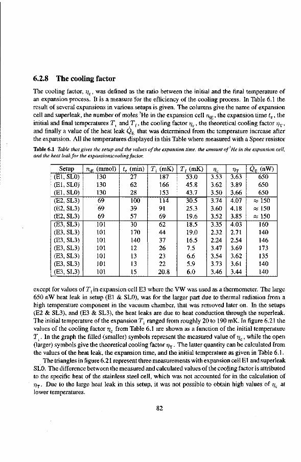
6.2.8 The cooling factor

The cooling factor, Tic, was defined as the ratio between the initia! and the final temperature of an expansion process. It is a measure for the efficiency of the cooling process. In Table 6.1 the result of several expansions in various setups is given. The columns give the name of expansion cell and superleak, the number of moles 3He in the expansion cell ·~E, the expansion time te, the initia! and final temperatures and T r, the cooling factor Tic, the theoretica! cooling factor riT, and finally a value of the heat teak QE that was determined from the temperature increase after the expansion. All the temperatures displayed in this Table where measured with a Speer resistor

Table 6.1 Table that gives the setup and the values of the expansicm time, the amount of' He in the expan.~ion eelt, and the heat leakfor the expansionscoolingfactor.

Setup n,R (mmo!) te (min) Ti (mK) Tr (mK) r1T I QR (nW) (El, SLO) 130 27 187 53.0 3.63 650 (El, SLO) 130 62 166 45.8 3.89 650 (El, SLO) 130 28 153 43.7 3.50 3.66 650 (E2, SL3) 69 100 114 30.5 3.74 4.07 ~ 150 (E2, SL3) 69 39 91 25.3 3.60 4.18 ~ 150 (E2, SL3) 69 57 69 19.6 3.52 3.85 ~ 150 (E3, SL3) 101 30 62 18.5 3.35 4.03 160 (E3, SL3) 101 170 44 19.0 2.32 2.71 140 (E3, SL3) 101 140 37 16.5 2.24 2.54 146 (E3, SL3) 101 12 26 7.5 3.47 3.69 173 (E3, SL3) 101 13 23 6.6 3.54 3.62 135 (E3, SL3) JOl 13 22 5.9 3.73 3.61 140 (E3, SL3) 101 15 20.8 6.0 3.46 3.44 140

except for values ofTrin expansion cell E3 where the VW was used as a thermometer. The large 650 nW heat leak in setup (El & SLO), was for the larger part due tothermal radiation from a high temperature component in the vacuum chamber, that was removed later on. In the setups (E2 & SL3), and (E3 & SL3), the heat leaks are due to heat conduction through the superleak. The initia! temperature ofthe expansion Ti ranged from roughly 20 to 190 mK. In figure 6.21 the values of the cooling factor 1/c from Table 6.1 are shown as a function of the initia! temperature Ti. In the graph the lilled (smaller) symbols represent the measured value of 'f/c, while the open (Iarger) symbols give the theoretica! cooling factor riT. The latter quantity can be calculated from the values of the heat Leak, the expansion time, and the initia! temperature as given in Table 6.1.

The triangles in ligure 6.21 represent three measurements with expansion cel! El and superteak SLO. The difference between the measured and calculated val u es of the cooling factor is attributed to the specific heat of the stainless steel cell, which was not accounted for in the calculation of r1T. Due to the large heat teak in this setup, it was not possible to obtain high values of 'f/c at lower temperatures.

82

-----~-~-- -

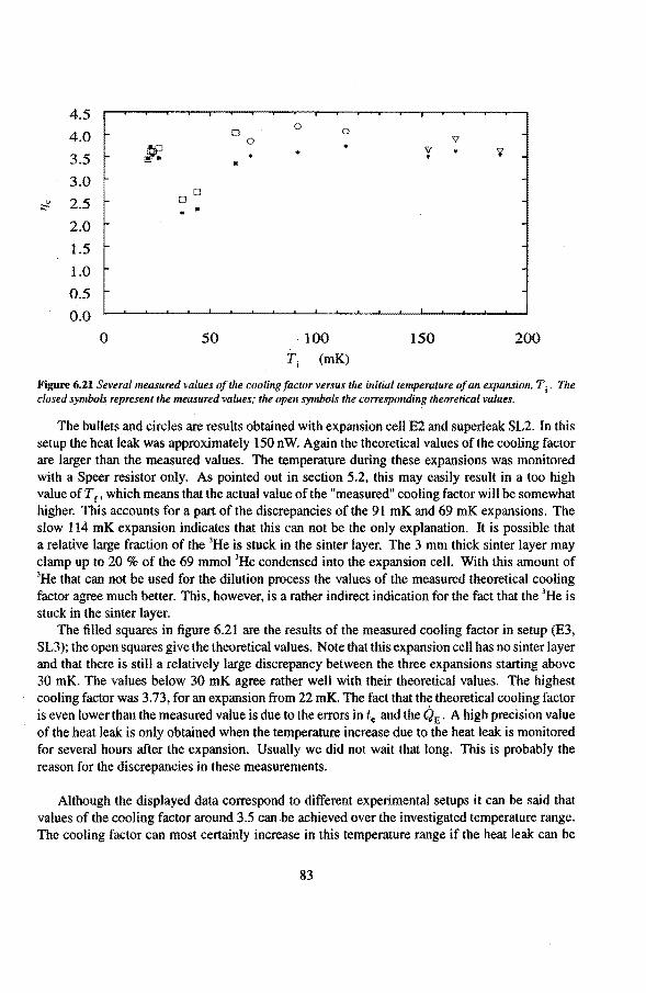
4.5

4.0 0 0

0 0

3.5 lf. • 3.0

0 u 2.5 0 ~

2.0

1.5

1.0

0.5

0.0 0 50 100 150 200

Ti (mK)

Figure 6.21 Several measured values of the cooling factor versus the initialtemperature lJf an expan.çion, Ti. The cllJsed symbols represent the measured values; the open symhl1ls the corresponding thelJretical values.

The bullets and circles are results obtained with expansion cell E2 and superleak SL2. 1n this setup the heat leak was approximately 150 n W. Again the theoretica! values of the cooling factor are larger than the measured values. The temperature during these expansions was monitored with a Speer resistor only. As pointed out in section 5.2, this may easily result in a too high value ofTe, which means that the actual value ofthe "measured" cooling factor will be somewhat higher. This accounts for a part of the discrepancies of the 91 mK and 69 mK expansions. The slow 114 mK expansion indicates that this can not be the only explanation. It is possible that a relative large fraction of the 3He is stuck in the sinter layer. The 3 mm thick sinter layer may damp up to 20 % of the 69 mmol 3He condensed into the expansion cell. With this amount of 3He that can not be used for the dilution process the values of the measured theoretica! cooling factor agree much better. This, however, is a rather indirect indication for the fact that the 3He is stuck in the sinter layer.

The tilled squares in tigure 6.21 are the results of the measured cooling factor in setup (E3, SL3); the open squares give the theoretica! values. Note that this expansion cell basnosinter layer and that there is still a relatively large discrepancy between the three expansions starting above 30 mK. The values below 30 mK agree rather well with their theoretical values. The highest cooling factor was 3.73, for an expansion from 22 mK. The fact that the theoretica! cooling factor is even lower than the measured value is due to the errors in te and the QE. A high precision value of the heat leak is only obtained when the temperature increase due to the heat teak is monitored for several hours after the expansion. Usually we did not wait that long. This is probably the reason for the discrepancies in these measurements.

Although the displayed data correspond to different experimental setups it can be said that values of the cooling factor around 3.5 can be achieved over the investigated temperature range. The cooling factor can most certainly increase in this temperature range if the heat teak can be

83

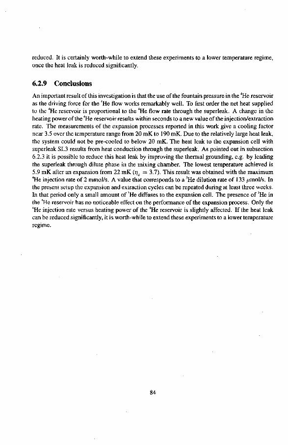
reduced. lt is certainly worth-while to extend these experiments to a lower temperature regime, once the heat leak is reduced significantly.

6.2.9 Conclusions

An important result of this investigation is that the use of the fountain pressure in the 4He reservoir as the driving force for the 'He flow works remarkably well. To first order the net heat supplied to the •He reservoir is proportional to the 'He flow rate through the superleak. A change in the heating power of the 4He reservoir results within seconds toa new value of the injectionlextraction rate. The measurements of the expansion processes reported in this work give a cooling factor near 3.5 over the temperature range from 20 mK to 190 mK. Due to the relatively large heat leak, the system could not be pre-cooled to below 20 mK. The heat leak to the expansion cell with superleak SL3 results from heat conduction through the superleak. As pointed out in subsection 6.2.3 it is possible to reduce this heat leak by improving the thermal grounding, e.g. by leading the superleak through dilute phase in the mixing chamber. The lowest temperature achieved is 5.9 mK after an expansion from 22 mK ('f/c = 3.7). This result was obtained with the maximum 4He injection rate of 2 mmol/s. A value that corresponds to a 1He dilution rate of 133 J.tmol/s. In the present setup the expansion and extraction cycles can be repeated during at least three weeks. In that period only a small amount of 3He diffuses to the expansion cell. The presence of 1He in the 4He reservoir has no noticeable effect on the performance of the expansion process. Only the 4He injection rate versus heating power of the 'He reservoir is slightly affected. If the heat leak can be reduced significantly, it is worth-while to extend these experiments to a lower temperature regime.

84

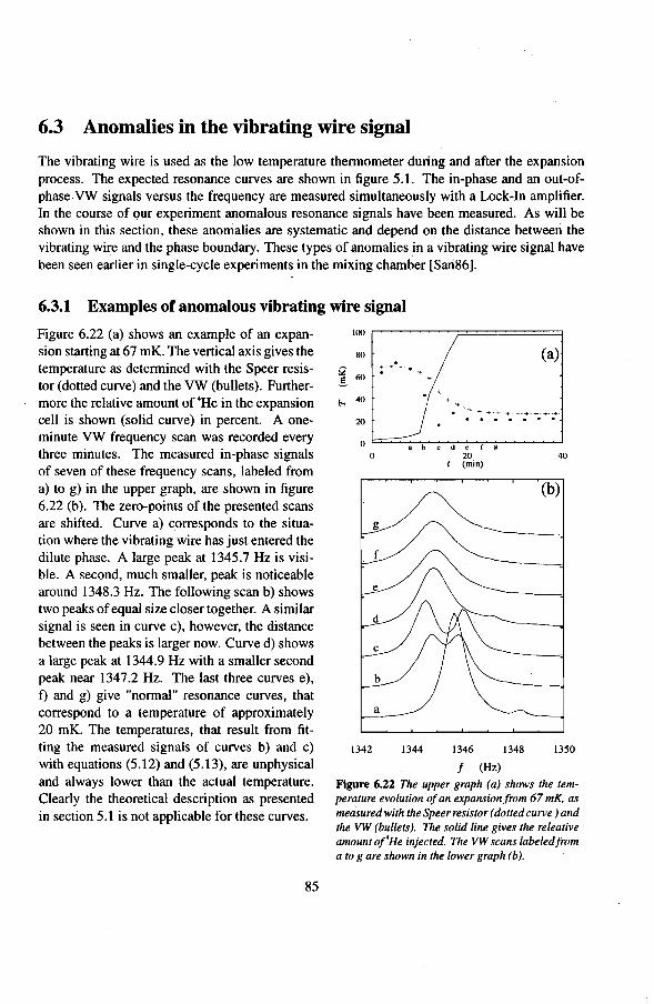
6.3 Anomalies in the vibrating wire signa)

The vibrating wire is used as the low temperature thermometer during and after the expansion process. The expected resonance curves are shown in figure 5.1. The in-phase and an out-of­phase VW signals versus the frequency are measured simultaneously with a Lock-In amplifier. In the course of our experiment anomalous resonance signals have been measured. As will be shown in this section, these anomalies are systematic and depend on the distance between the vibrating wire and the phase boundary. These types of anomalies in a vibrating wire signa! have been seen earlier in single-cycle experimentsin the mixing chamber [San86].

6.3.1 Examples of anomalous vibrating wire signal

Figure 6.22 (a) shows an example of an expan­sion startingat 67 mK. The vertical axis gives the temperature as determined with the Speer resis­tor (dotted curve) and the VW (bullets). Further­more the relative amount of 4He in the expansion cell is shown (solid curve) in percent. A one­minute VW frequency scan was recorded every three minutes. The measured in-phase signals of seven of these frequency scans, labelect from a) to g) in the upper graph, are shown in figure 6.22 (b). The zero-points of the presented scans are shifted. Curve a) corresponds to the situa­tion where the vibrating wire has just entered the dilute phase. A large peak at 1345.7 Hz is visi­ble. A second, much smaller, peak is noticeable around 1348.3 Hz. The following scan b) shows two peaks of equal size closer together. A similar signa! is seen in curve c), however, the distance between the peaks is larger now. Curve d) shows a large peak at 1344.9 Hz with a smaller second peak near 1347.2 Hz. The last three curves e), t) and g) give "normal" resonance curves, that correspond to a temperature of approximately 20 mK. The temperatures, that result from fit-ting the measured signals of curves b) and c) with equations (5.12) and (5.13), are unphysical and always lower than the actual temperature. Clearly the theoretica! description as presented in section 5.1 is not applicable for these curves.

85

l!Xl

80 (a) Q' ·: ·+ + .•

g 60

f.., 40

• + ......... + +·+··+·+· +

20 . . . . . . . 0 c d e f g

0 20 40 t (min)

(b)

a

1342 1344 1346 1348 1350

f (Hz)

Figure 6.22 The upper graph (a) shows the tem· perature evolution of an expansion from 67 mK, as measured with the Speer resistor ( dotted curve) and the VW (bullets). The solid line gives the releative amount of'He injected. The VW scans labeledfrom a to gare shown in the lower graph (b).

1342 1344 1346 1348 1350

f (Hz)

Figure 6.23 The in- and out-of-phasesigna is b), c), and d) as measured with the vibrating wire during the expansion shown in figure 6.22. The juli curves are the in-phase signal, the dotted curves the out-of-phase signals.

The in-phase and out-of-phase signals of curves b), c), and d) are shown in figure 6.23. The full curves are the in-phase signal, the dotted curves the corresponding out-of­phase signals. As can be seen, the anomalies in the in-phase signals also show up in the out-of-phase signals, which rules out the ar­gument that an "exotic" drift in the in-phase­signal is the cause of the anomaly. For a system like the vibrating wire, where an os­cillating driving force produces a linear re­sponse at the same frequency, the Kramers­Kronig-relations are applicable. These rela­tions link the in-phase response V, and out­of-phaseresponse v2 via

2 Pj""V2 (w1

)W1

d 1

12 2 w 1r w -w

(6.19) 0

2 !OO V( (w1) I

V 2 (w)=--wP 12 2 dw. (6.20) 1r . w -w

0

The "P" in front of the integrals denotes the principle part ofthe integral. The best way totest the validity of equations (6.19) and (6.20) is to calculate the integrals by using the measured in- and out-of-phase signals. However, a simpter way to test the validity of the Kramers-Kronig-relations on the measured VW signals, is to check whether an extremum in one signa! corresponds to an extremum in the derivative of the other signa!. This is clearly the case for the three pairs of curves presented in the figure. The fact that the in-phase and out-of-phase signal follow the Kramers-Kronig-relations indicates that the measured signal is indeed aresult of physics near the wire, and not aresult of drift or a ftuctuation in the in-phase signal.

6.3.2 Reproducibility of the anomalous VW signals

The anomalous behaviour in the VW signals is reproducible as can be seen from figures 6.24 and 6.25. The two figures show two expansions startingat the same temperature, but with different expansion times. In figure 6.24 the expansion time is 25 minutes while the expansion shown in figure 6.25 lasts approximately 120 minutes. On the vertical axes the temperature according to the Speer resistor (plus signs) and the VW (bullets) is shown. The relative amountof 4He in the expansion cell is presented by the circles. The full vertical scale corresponds to 1.55 mole 4He.

86

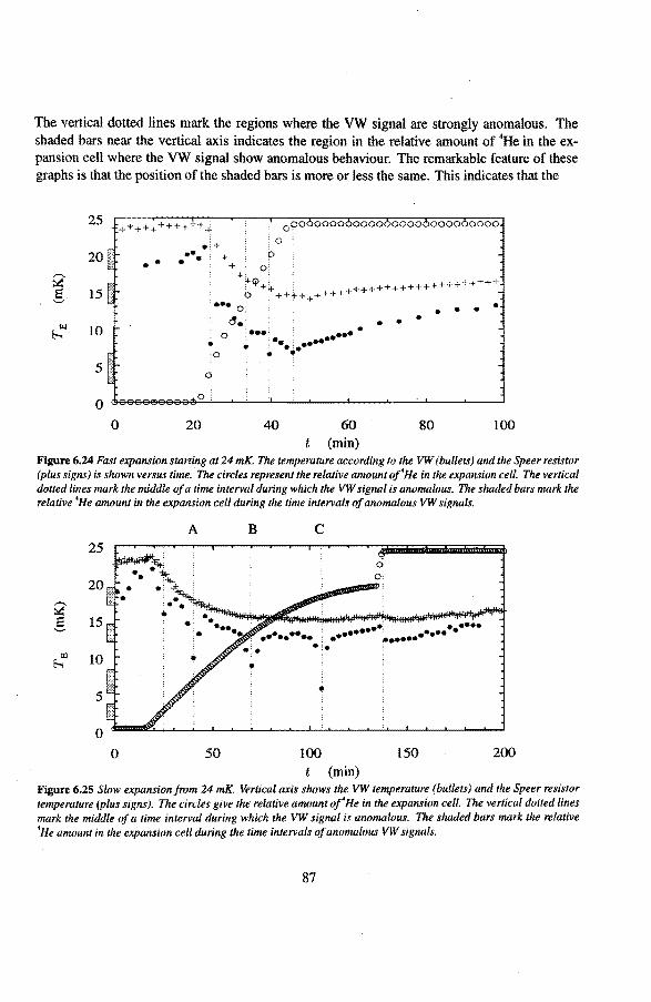
The vertical dotted lines mark the regions where the VW signal are strongly anomalous. The shaded bars near the vertical axis indicates the region in the relative amount of 'He in the ex­pansion cell where the VW signal show anomalous behaviour. The remarkable feature of these graphs is that the posîtion of the shaded bars is more or less the same. This indicates that the

25

20 •• ,...._ ::.á g 15

!ll 10 E--i

5

0 0

0 20

••• O;

~. 0 j••• ' •••••

• • ••• i ••••• '0 • ••

0

40 60 t (min)

• • • • • • •

80 100

Figure 6.24 Fast expansion starring at 24 mK The temperature according to the VW (bullets) and the Speer resistor (plus signs) is shown versus time. The circles represent the relative amount of' He in the expansion cel!. The vertic al dotted lines mark the middle of a time interval during which the VW signa/ is am1malous. The shaded bars mark the relative 'He amount in the expansion cel/ during the time intervals tJf anomalous VW signals.

A B c 25

20 ,...., ::.á e 15 '-'

!ll 10 E--i

5

0

0 50 100 150 200 t (min)

Figure 6.25 Slow expansionfrom 24 mK. Vertical axis shows the VW temperature (bul/ets) and the Speer resistor temperature (plus signs). The circles give the relative amount of' He in the expansion cel/. The vertical dotted lines mark the middle of a time interval during which the VW signa/ is anomalous. The shaded bars mark the relative 'He amount in the expansion cel/ during the time intervals of anomalous VW signals.

87

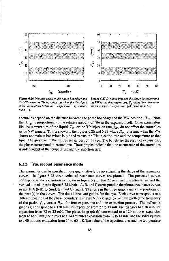
60 60

50 50

Ê ,...-.,

40 e 40 e e ..._, ......., 30 30

lll lll .,.. .,.. ::x:: 20 ::x:: 20

10 10

0 0

100 1000 0 10 20 30 40 50 60

Î\E (p,moUs) TE (mK)

Figure 6.26 Distance between the phase boundary and Figure 6.27 Distance between the phase boundary and the VW versus the 'He injection rate when the VW signa/ the VW versus the tem.perature, TE at the time of anoma­slwws anomalous behaviour. Expansions ( • ); extrac- lous VW signols. Expansions ( • ); extraelions ( + ). tions (+).

anomalies depend on the distance between the phase boundary and the VW position, H PB. Note that H PB is proportional to the relative amount of 4He in the expansion cell. Other parameters like the temperature of the liquid, TE, or the 4He injection rate, Î\E, do not affect the anomalies in the VW signals. This is shown in the figures 6.26 and 6.27 where H PB at a time when the VW shows anomalous behaviour is plotted versus the 4He injection rate and the temperature at that time. The grey bars in the figures are guides for the eye. The bullets are the result of expansions, the pluses correspond to extractions. These graphs indicate that the occurrence of the anomalies is independent of the temperature and the injection rate.

6.3.3 Tbe second resonance mode

The anomalies can be specified more quantitatively by investigating the shape of the resonance curves. In figure 6.28 three series of resonàtlce curves are plotted. The presented curves correspond to the expansion as shown in figure 6.25. The 22 minutes time interval around the vertical dotted lines in figure 6.25 labeled A, B, and C coccespond to the plotted resonance curves in graph A (left), B (middle), and C (right). The stars in the three graphs mark the positions of the peak(s) in the curves. The dotted lines are guides for the eye. Each curve corresponds toa different position of the phase boundary. In tigure 6.29 (a) and (b) we havè plotted the frequency of the peaks, f R, versus H PB for four expansions and one extraction proeess. The bullets in graph (a) correspond toa 120 minutes expansion from 27 to l3 mK, the triangles toa 70 minutes expansion from 72 to 22 mK. The pluses in graph (b) correspond toa 120 minutes expansion from 45 to 19 mK, the circles to a 140 minutes expansion from 38 to 18 mK, and the solid squares to a 40 minutes extraction from 14 to 65 mK.The value of the injection rates and the temperature

88

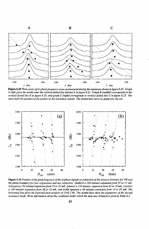
A B c

1340 1350 1340 1350 1340 1350

f (Hz) f (Hz) f (Hz)

Figure 6.28 Three series of in-phase frequency scans as measured during the expansion shown in figure 6.25. Graph A (left) gives the results near the vertical dotted line labeled A infigure 6.25. Graph B (middle) corresponds to the vertical dotted line B injigure 6.25, and graph C (right) corresponds to vertical dotted line C injigure 6.25. The stars mark the position ofthe peak(s) in the resonance signals. The dotted lines serve as guldesJor the eye.

(a) 1348 . 1346 .... 1344

1342

•. I~ ~----~~~~~--~----~

0 15 45

(mm)

60

1350

1348

1346

1344

1342

0

0

a.

+

.+

15

..

.o :q..

+ .i:!"

•

0 +!

• • :~

45

(mm)

(b)

• •

60

Figure 6.29 Position of the peakfrequency of the in phase signa Is as a function of the distance between the VW and the phase boundary for jour expansions and one extraction. (bul/ets) a 120 minutes expansion from 27 to 13 mK, (triangles) a 70 minutes expansionfmm 72 to 22 mK, (pluses) a 120 minutes expansionfmm 45 to 19 mK, (circles) a 140 minutes expansionfmm 38 to 18 mK, and (solid squares) a 40 minutes extractionjrom 14 to 65 mK. The horizontalline gives the expected peak position of 1345.2 Hz. The dotted lines show the asymptotes of the second resonance mode. More information about the conditlans under which the data was obtained is given in Table 6.2.

89

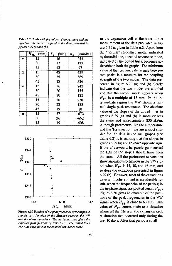
Table 6.2 Table with the values oftemperature and the injection rate that correspond to the data presenled in figures 6.29 (a) and (b).

HI>R (mm) T" (mK) il.p {ttmoVs)

I . 15 16 254 30 13 173 45 13 97

!:::, 15 48 439 30 35 369 45 28 326

0 15 26 242 30 20 155 45 20 122

+ 15 30 220 30 22 183 45 19 88

• 15 37 -672 30 26 -662 45 19 -408

1350

1348 • .-.. • N :• t; 1346 •

• • .:.:: .. ....., 1344

• 1342 •

: 1340

62.5 63.0 63.5

Hpa (mm)

Figure 6.30 Position of the peakfrequenq of the in phase signals as a function of the distance between the VW and the phase boundary. The horizontal line gives the expected peak position of J 345.2 Hz. The dotled lines show the asymptote of the coupled resonance mode.

90

in the expansion cell at the time of the measurement of the data presented in lig­ure 6.29 is given in Table 6.2. Apart from the "normal" resonance mode, indicated by the solid line, a second resonance mode, indicated by the dotted lines, becomes no­ticeable in both the graphs. The minimum value of the frequency difference between two peaks is a measure for the coupling strength of the two modes. The data pre­sented in figure 6.29 (a) and (b) clearly indicate that the two modes are coupled and that the second mode appears when H PB is a multiple of 15 mm. In the in­termediate region the VW shows a nor­mal single peak resonance. The absolute value of the slopes of the dotted lines in graphs 6.29 (a) and (h) is more or less the same and approximately 830 Hz/m. Although parameters like the temperature and the 4He injection rate are almost sirn­ilar for the data in the two graphs (see Table 6.2) it is striking that the slopes in graphs 6.29 (a) and (b) have opposite sign. If the effectwould be purely geometrical the sign of the slopes should have been the same. ·All the performed expansions show anomalous behaviour in the VW sig­na! when H PB is 15, 30, and 45 mm, and so does the extraction presented in figure 6.29 (b ). However, most of the extraelions gave an incoherent and irreproducible re­sult, when the frequencies of the peak(s) in the in-phase signa) are plotted versus H PB •

Figure 6.30 gives an example of the posi­tions of the peak fr~quencies in the VW signal when H PB is close to 63 mm. This value of H PB corresponds to a situation where all the 'He is in the expansion cell. A situation that occurred only during the first 10 days. After that period a smal!

fraction of 3He had diffused to the 'He reservoir as pointed out in section 6.2.6. This 3He fraction prevented the last amount of 4He to flow back to the expansion cell after an expansion, even when the heating power of the reservoir was zero. The major difference between tigure 6.30 and the graphs in tigure 6.29 is that the slope of the dotted line in this graph is much Jaeger. Practically this means that the region in H PB where the second mode occurs is only several hundeed micrometers wide. An annoying effect of the second resonance mode is that the tinal temperature of the expansion may he difficult todetermine when the expansion endsin the regime of the two resonance modes. The deviation of the calculated VW temperatures and the theoretica! curve at the end of the expansions presented in tigures 6.9, 6.24, and 6.25 are a direct result of this effect.

6.3.4 Discussion

The analysis of the in-phase VW signals show that there is, apart from the normal resonance near 1345 Hz, a second coupled resonance mode that depends on the position of the phase boundary. When the phase boundary is a multiple of 15 mm from the bottorn ofthe expansion cell the second resonance mode shows up. lt is interesting to note that this value is equal to the radius of the cell. At the moment it is unclear what physical phenomenon is responsible for the second resonance mode. We expect, however, that some sort of (sound) wave is emitted be the oscillating VW. Once reflected at the phase boundary and the walls of the expansion cell these waves can interfere in a way that they affect the motion of the VW. Within this context the dilute phase can be regarded as a sort of resonance cavity for waves with a typ i cal (sound)velocity of 20 mis ( = 1345 Hz·0.015 m). The waves can not be regular tirst sound waves because the velocity tirst sound in a mixture is approximately 200 mis. Van der Boog [Boo79] measured the second sound velocity in dilute 3He-4He mixtures for temperatures down to 100 mK. He found a value of 16.6 m/s fora 1 % 3He concentration at 130 mK. A value that should decrease at lower temperatures. A third typical velocity for a 3He-'He mixture is the Fermi-velocity of the 3He quasi particles, which is 29 mis for a saturated mixture. Non of the introduced velocities, however, is close to the 20 mis of the second resonance.

The VW is an important instrument for measuring properties of 3He-4He mixtures at low tempertures. For a correct interpretation it is important to understand its properties in detail. Therefore the effects reported bere should he further investigated.

91

References

Alp69

Alv73

Alv74

Arc81

Bet89

Boo79

Car83 Doi84 Li86

Ret87 Rit87 San86

Tou63 Tou64 Wil87

W.M. van Alphen, R. de Bruyn Ouboter, J.F. Olijhoek, and K.W. Taconis, Physica 40, 490 (1969). T.A. Alvesalo, Y.D. Anufriyev, H.K. Collan, O.V. Lounasmaa, and P. Wennerström, Phys. Rev. Lett. 30, 962 (1973). T.A. Alvesalo, H.K. Collan, M.T. Loponen, and M.C. Veuro, Phys. Rev. Lett. 32,981 (1974). C.N. Archie, T.A. Alvesalo, J.D. Reppy, and R.C. Richardson, J. Low Temp. Phys. 42, 295 (1981). D.S. Betts, An Introduetion to Millikelvin Technology (Cambridge University Press, Cambridge 1989). A.G.M. van der Boog, Ph.D. Thesis, Rijkuniversiteit Leiden, Leiden The Netherlands (1979). D.C. Carless, H.E. Hall, andJ.H. Hook, J. Low Temp. Phys. 50, 605 (1983). H. Doi, Y. Narahara, Y. Oda, and H. Nagano, Proc LT-17 Karlsruhe, 405 (1984). Q. Li, C.H. Watson, R.G. Goodrich, D.G. Haase, and H. Lukefahr, Cryogenics 26,467 (1986). T. Retsina, S.M. Richardson, and W.A. Wakeham, Appl. Sci. Res. 43, 325 (1987). D.A. Ritchie, J. Saunders, and D.F. Brewer, Phys. Rev. Lett. 59,465 (1987). R.H.M. Sanders and J.H.H. Thijssen, Trainee report Eindhoven University of Tech­nology, The Netherlands (1986). J.T. Tough, W.D. McComick, and J.G. Dash, Phys. Rev. 132,2373 (1963). J.T. Tough, W.D. McComick, and l.G. Dash, Rev. ofSci. lnstr. 35, 1345 (1964). J. Wilks and D.S. Betts, An Introduetion to Liquid Helium (OXford Science Publica­tions, Oxford 1987).

92

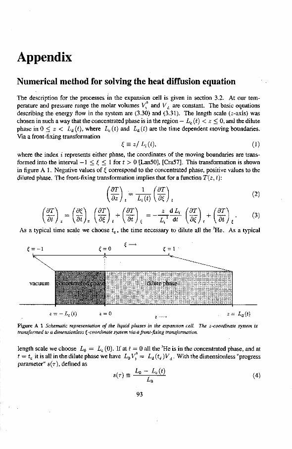
Appendix

Numerical metbod for solving the heat dirfusion equation

The description for the processes in the expansion cell is given in section 3.2. At our tem­perature and pressure range the molar volumes v;o and V d are constant. The basic equations descrihing the energy flow in the system are (3.30) and (3.31). The length scale (z-axis) was chosen in such a way that the concentraled phase is in the region- Lc (t) < z ~ 0, and the dilute phase in 0 ~ z < Ld (t), where Lc (t) and Ld (t) are the time dependent moving boundaries. Via a front-fixing transformation

Ç z/ Li (t), (1)

where tbe index i represents either phase, the coordinates of the moving boundaries are trans­formed into the interval -1 ~ Ç ~ 1 fort > 0 [Lan50], [Cra57]. This transformation is shown in tigure A 1. Negative values of Ç correspond to the concentraled phase, positive valnes to the diluted phase. The front-fixing transformation implies that fora function T(z, t):

(2)

(~~) z = (~;)z (~~) t + (C:) ~ Li (3)

As a typical time scale we choose te , the time necessary to dilute all the 3He. As a typical

ç = -1

Figure A 1 Schematic representation of the liquid phases in the expansion eelt. The z-coordinate system is transformed toa dimensionless Ç-coordinate system via afront-fixing transformation.

length scale we choose L0 Lc (0). If at t 0 all the 3He is in the concentraled phase, and at t = te it is all in the dilute phase we have L0 y;o Ld (te ) V d. With the dimensionless "progress parameter" s(r), defined as

s(r) = Lo Lc(t) Lo

(4)

93

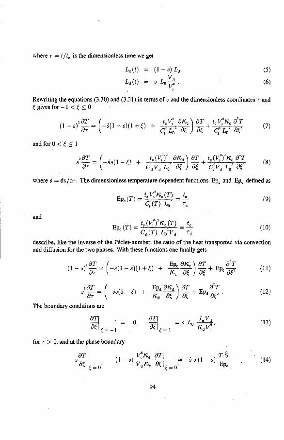
where 1 = tfte is the dimensionless time we get

(I - s) L0

vd s Lo-o. v;

(5)

(6)

Rewriting the equations (3.30) and (3.31) in terros of s and the dimensionless coordinates 1 and Ç gives for - 1 < Ç :::; 0

(1 s)z7_ = (-s(1- s)(l + .c) te y;o a~c) ar te y;o~c azT VI "' + qo Lo 2 aç aç + qo Lo 2 ae (7)

and for 0 < Ç :::; 1

ar ( te (y;0

)

2 a~d) aT te (y;0

)

2 ~d a2T s

2- = -ss(1 - ç) + 2 a -a + o 2 z a, Cd V d L0 Ç Ç q V d L0 aç (8)

where s = dsjd1. The dimensionless temperature dependent functions Epe and Epd defined as

(9)

and

E (T) _ te (y;

0)

2 ~d (T) _ ~ Pd - 2 -

Cd (T) L0 V d 'd (10)

describe, like the inverse of the Péclet-number, the ratio of the heat transported via convection and diffusion for the two phases. With these functions one finally gets

(1 )zaT_ ( .(1 )(1 .c) Epe a~c) ar E a2

T s a, - -s - s +"' + ~c 7Jf aç + Pc (11)

zaT ( Epd a~d) aT a2T sa,= -ss(1-Ç) + ~d 7if aç + Epd af}. (12)

The boundary conditions are

0, (13)

for 1 > 0, and at the phase boundary

(14)

94

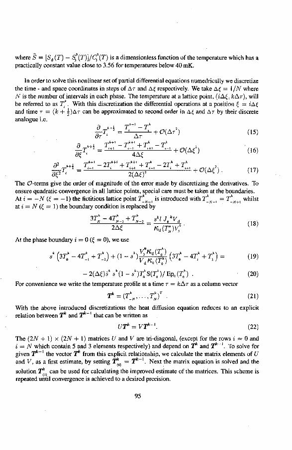
where S = [Sd (T)- ~0(T)]/q0

(T) is a dimensionless function ofthe temperature which bas a practically constant value close to 3.56 for temperatures below 40mK.

In order to solve this nonlinear set of partial differential equations numedrically we discretize the time- and space coordinates in steps of tl7 and tl~ respectively. We take tl~ = 1/ N where Nis the number of intervals in each phase. The temperature at a Iattice point, (i~{, k~7), will be referred to as T.". With this discretization the differential operations at a position Ç itlç

and time 7 = (k + t)tl7 can be approximated to second order in tlÇ and tl7 by their discrete analogue i.e.

(15)

(16)

(17)

The 0-terms give the order of magnitude of the error made by discretizing the derivatives. To ensure quadratic convergence in alllattice points, special care must be taken at the boundaries. At i= -N (Ç = -1) the fictitious lattice point T~N-! is introduced with T~N+l whilst at i= N (Ç = 1) the boundary condition is replaced by

3T;- 4T;_, + r;_2 skl Je kV ct

2~Ç = K,d(T~)~o. (18)

At the phase boundary i 0 (Ç = 0), we use

• ( • • • ) • ~0

1\,d er:) ( • • • ) s 3T0 - 4T_, + T_ 2 + (1 - s ) V K (Tk) 3T0 - 4J; + T2

d c 0

(19)

2(~Ç)s" / (1 - s")T:S(J;,")j Epe (T0") • (20)

For convenience we write the temperature profile at a time 7 = k~7 as a column vector rrk k kT :t. = (T_N, ... ,TN) . (21)

With the above introduced discretizations the heat diffusion equation reduces to an explicit relation between 7* and r-l that can be written as

uT'= v'J"<- 1• (22)

The (2N + 1) x (2N + 1) matrices U and V are tri-diagonal, (except for the rows i = 0 and i = N which contain 5 and 3 elements respectively) and depend on Tand 'J*- 1

• To solve for given r-l the vector 7* from this explicit relationship, we calculate the matrixelementsof u and V, as a first estimate, by setting ~oJ = 7*- 1

• Next the matrix equation is solved and the

solution ~~l can be used for calculating the improved estimate of the matrices. This scheme is repeated until convergence is achieved to a desired precision.

95

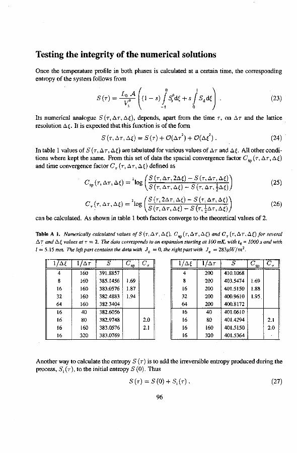
Testing the integrity of the numerical solutions

Once the temperature profile in both phases is calculated at a certain time, the corresponding entropy of the system follows from

(23)

lts numerical analogue S(r,ar,a~). depends, apart from the time 7, on ÀT and the lattice resolution À~. It is expected that this function is of the form

S (r, ar, ÀÇ) = S (7) + O(À/) + O(À~2 ). (24)

In table 1 values of S ( r, .6. r, .6.~) are tabulated for various values of À 7 and aç. All other condi­tions where kept the same. From this set of data the spacial convergence factor esp (7, À7, À~) and time convergence factor c.,. ( 7' .6. 7' À e) defined as

C ( ) 21 (S(r,Àr,2ÀÇ)-S(r,Àr,ÀÇ)) spT,ÀT,ÀÇ = Og ( ) ( I ) S 7, À7, M; S 7, Àr, 2.6.~

(25)

(26)

can be calculated. As shown in table 1 both factors converge to the theoretica! values of 2.

Table A 1. Numerically calculated values of S (r,ÀT, À~). C,P (r, ÀT, ÀÇ} and C.,. (r,.6.r, ÀÇ) for several

ÀT and ae values at T = 2. The data corresponds to an expansion startingat 100 mK, with te= 1000 s and with

l ";, 5.15 mm. The left part contains the data with Je = 0, the right part with Je = 283p,W/m2•

11 1/Àe I l/À7 I s 4 160 391.8857 4 200 410.1068

8 160 385.1456 1.69 8 200 403.5474 1.69

16 160 383.0576 1.87 16 200 401.5150 1.88

32 160 382.4883 1.94 32 200 400.9610 1.95

64 160 382.3404 64 200 400.8172

16 40 382.6056 16 40 401.0610

16 80 382.9748 2.0 16 80 401.4294 2.1

16 160 383.0576 2.1 16 160 401.5150 2.0

16 320 383.0769 16 320 401.5364

Another way to calculate the entropy S ( r) is to add the irreversible entropy produced during the process, si (r), to the initia! entropy s (0). Thus

S(r)=S(O)+S;(r). (27)

96

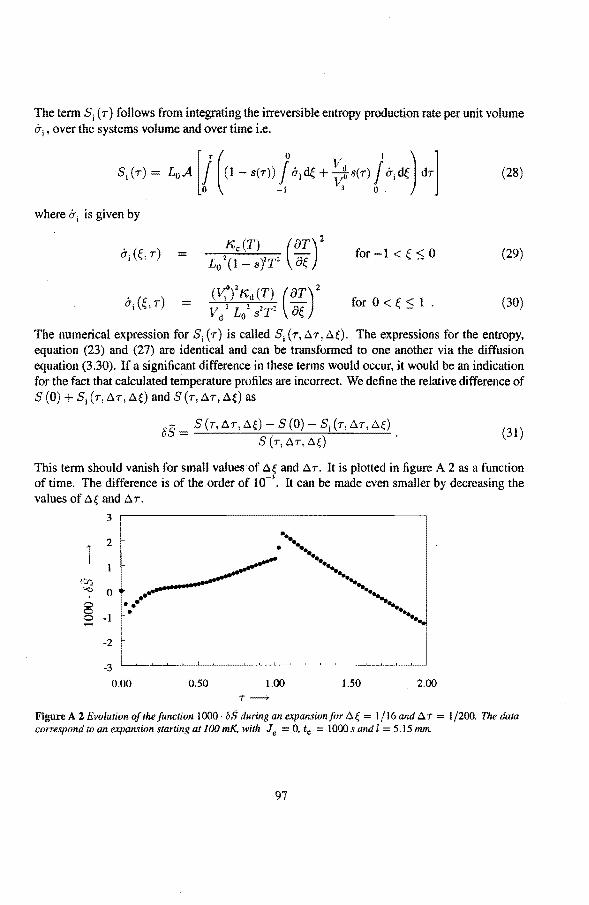
The tenn Si ( T) foliOWS from Întegrating the irreversibJe entropy production rateperunit volume &i, over the systems volume and over time i.e.

(28)

where &i is given by

à;(Ç,r) = K,c(T) c)Tr L0 \1- slT2 8Ç

for -1 < Ç :5 0 (29)

&;(Ç,r) = ("Y;o)z K,d (T) ( 8T) 2

Vd l Lo2 s2T2 8Ç for 0 < Ç :5 1 . (30)

The numerical expression forS; (r) is called S; (r, ~T, ~{). The expressions for the entropy, equation (23) and (27) are identical and can be transfonned to one another via the diffusion equation (3.30). If a significant difference in these tenns would occur, it would be an indication for the fact that calculated temperature profiles are incorrect. We define the relative difference of S (0) + S; (r, t::.r, ~e) and S (r, ~r, ~e) as

os S (T, ~T, ~Ç)- S (0)- Si (7, ~7 1 ~Ç) S (r, t::.r, ~ç)

(31)

This term should vanish for smal! values of ~ç and ~T. It is plotted in tigure A 2 as a function of time. The difference is of the order of 10-3

• It can be made even smaller by decreasing the values of ~ç and ~T.

3

2 .... T . ... ........

..... ~~08 0 ..... ............ .... ~ ..... -1 - .....

-2

-3

0.00 0.50 T

1.00 1.50 2.00

Figure A 2 Evolution ofthefunction 1000 ·oS duringan expansionfor ~Ç = l/16and f:::.T = 1/200. The data correspond to an expansion starring at 100 mK, with Je = 0, t0 = lOOOs and l = 5.15 mm.

97

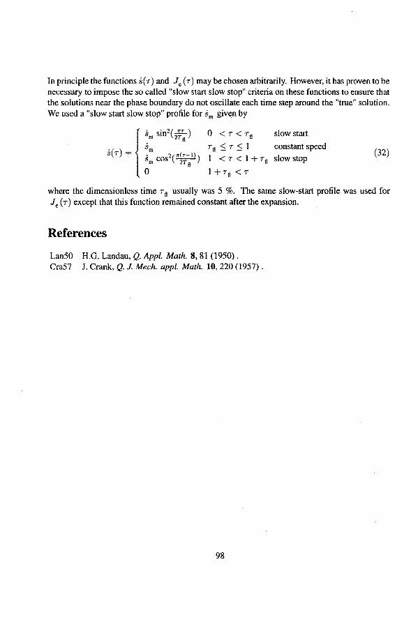
In principle the functions s( r) and Je ( T) may be chosen arbitrarily. However, it has proven to be necessary to impose the so called "slow start slow stop" criteria on these functions to ensure that the solutions near the phase boundary do not oscillate each time step around the "true" solution. We used a "slow start slow stop" profile for sm given by

{

s sin2(..2!:!....) m 278

s(r) = ~m 2("(-r-1)) Sm cos 2To

0

slow start

T 8 :5 T :5 1 constant speed

1 < r < 1 + T 8 slow stop

l+r8 <r

(32)

where the dimensionless time T 8 usually was 5 %. The same slow-start profile was used for Je ( T) except that this function remained constant after the expansion.

References

Lan50 H.G. Landau, Q. Appl. Math. 8, 81 (1950). Cra57 J. Crank, Q. J. Mech. appl. Math. 10,220 (1957).

98

Summary

In this thesis we present the results of a one-shot cooling principle called adiabatic expan­sion of 3 He in superfiuid 4He, in the temperature range from 6 to 200 mK. The experiments were carried out in a setup that was implemented in a dilution refrigerator. The setup consists of an expansion cell, a 4He reservoir, and a superleak that connects the expansion cell with the 4He reservoir. In the expansion cell typically 100 mmol 3He is condensed and pre-cooled to a temperature between 20 and 200 mK. The 4He reservoir contains normally 1.55 mol pure 4He at a temperature around 1.35 K. Via a heater mounted on the 4He reservoir, the flow of superfluid 4He through the superleak can be controlled in such a way that 4He can be injected intoor extracted from the expansion cell. The maximum 4He injection rate for this setup is 2 mmol/s. When the superfluid 4He is injected, the pure 3He in the expansion cell will dilute to a saturated 6.6 % 3He-4He mixture. Duringa reversible dilution of 3He, heat is absorbed from the liquid, which results in a temperature reduction of the liquid in the expansion cell. The most efficient way of cooling is when the expansion is isentropic, that is, the entropy of the initial state is equal to that of the final state. In the initial state the expansion cell contains liquid pure 3He at a temperature Ti . The final state consistsof a 6.6 % mixture of 3He in superfluid 4He at a temperature T f. At the end of the di\ution process the 3He has expanded in a background of superfluid 4He to a volume that is 11.7 times the initial volume. This explains the name of this cooling technique. For i sentropie expansions with initial temperatures above the superfluid transition temperature oeHe (0.929 mK), the ratio ofthe initialand the final temperature (cooling factor) is constant and equal to 4.56. Below 0.929 mK, isentropic expansions should give even larger values of the cooling factor, which makes this a particularly interesting temperature regime to enter. However, befare going to ultra-low temperatures, it is important to test this technique at a higher temperature, because this gives direct information about effects that may limit the performance. The two effects that can limit this cooling methode are irreversibilities and heat leaks. Both these effects lead to a higher final temperature.

In this thesis several sourees of irreversibilities have been analyzed theoretically. The entropy increase due the finite thermal conductivity of the helium in the expansion cell was calculated numerically. lt was found that for adiabatic expansions at a 4He injection rate around 2 mmolis the relative entropy increase is 5 % at 30 mK and only 1 % at 10 mK. This effect becomes smaller at lower injection rates. Viscous effects in the pure 3He layer do not lead to a serious entropy increase above 4 mK. Whether the smoothing of a 3He layer to the walls of the expansion cell, at relatively high injection rates, may become an important souree of entropy production around 1 mK is uncertain at the moment. The effect of an irreversible 4He injection can result in a large entropy increase. Special care must be taken to avoid this, especially since this effect is more serious at lower temperatures. Finally the effect of 3He in a sinter layer in the expansion cell is discussed. To avoid the irreversible effects in the sinter, it is suggested that a marginal sinter volume is used, and that the phase boundary at the beginning of an expansion is positioned just above the sinter layer.

An important result of this investigation is that the use of the fountain pressure in the

4He reservoir as the driving force for the 4He flow works remarkably well. To first order the net heat supplied to the 4He reservoir is linear with the 4He flow rate through the superleak. A change in the heating power of the 4He reservoir results in a new value of the injectionlextraction rate within seconds. The measured chemica! potential difference over the superleak is zero to within experimental error. This implies that the 4He is injected in a reversible manner, which is an essential condition in order to do this experiment at even lower initia! temperatures. The measurements of the expansion processes reported in this work give a cooling factor near 3.5 over the temperature range from 20 mK to 190 mK. The relatively large heat leak is the main reason forthefact that these values are lower than the optima! factor of 4.56. The expansion and extraction cycles can be repeated during at least three weeks. In that period only a small amount of 3He diffuses to the 4He reservoir. The presence of 3He in the 4He reservoir has no noticeable effect on the performance of the expansion process. Only the 4He injection rateversus heating power of the •He reservoir is slightly affected. The lowest temperature obtained in this investi­gation was 5.9 mK at the end an expansion from 22 mK with an 4He injection rate of 2 mmoVs. This corresponds toa cooling factor (efficiency of the cooling process) of 3.7.

For temperatures below 30 mK, a vibrating wire viscometer was used as a fast thermometer in the liquid. The analysis of the VW signals show that there is, apart from the normal resonance, a second coupled resonance mode that depends on the position of the phase boundary in the expansion eetl. When the phase boundary is a multiple of 15 mm from the bottorn of the expansion cell the second resonance mode shows up. At the moment it is unclear what physical phenomenon is responsible for the second resonance mode. The effects reported bere should be further investigated.

These investigations in the 20 to 200 mK regime have shown that 4He can be injected and extracted reversible from the expansion cell. The low-temperature limit is determined by the heat leak. The analyses in this report show that this is not a fundamentallimitation and that it is worth-while to extend these experiments to a lower temperature regime.

Samenvatting

In dit proefschrift worden de resultaten gepresenteerd van een één-staps koelproces genaamd adiabatische expansie van We in superfluïde 4He, in het temperatuurgebied van 6 tot 200 mK. De experimenten zijn uitgevoerd in een aparte koeleenheid die in een mengkoeler is ingebouwd. De eenheid bestaat uit een expansiecel, een •He-reservoir en een superlek dat de expansiecel methet 4He-reservoir verbindt. In de expansiecel bevindt zich typisch 100 mmol 3He die wordt voorgekoeld tot een temperatuur tussen 20 en 200 mK. Het 4He-reservoir bevat gewoonlijk 1,55 mol zuiver 'He op een temperatuur rond de 1,35 K. Door middel van een verwarmingsele­ment op het 4He -reservoir kan de superfluïde 4He stroom door het superlek zodanig worden gecon­troleerd dat 4He toegevoegd of onttrokken kan worden aan de expansieceL De maximale 4He­injectiesnelheid in deze opstelling bedraagt 2 mmol/s. Zodra superfluïde 4He wordt geïnjecteerd in de expansiecel zal het zuivere 3He oplossen tot een verzadigd 6,6 % 3He-4He mengsel. Tijdens het reversibel oplossen van 3He wordt warmte onttrokken aan de vloeistof, hetgeen resulteert in een temperatuurdaling van de vloeistof in de expansieceL De meest rendabele manier van koelen is de isentrope expansie, dat wil zeggen, de entropie van de begintoestand is gelijk aan die van de eindtoestand. In de begintoestand bevat de expansiecel vloeibaar zuiver 3He op een temperatuur Ti . De eindtoestand bestaat uit een 6,6% mengsel van 3He in superfluïde 4He met een temperatuur T r. Aan het eind van een verdunningsproces is het 3He in een achtergrond van superfluïde 4He geëxpandeerd tot een volume dat 11,7 maal groter is dan het beginvolume. Dit verklaart de naam van deze koelmethode. Voor isentrope expansies met begintemperaturen boven de superfluïde­overgangstemperatuur van ~e (0,929 mK) is de verhouding tussen de begin- en eindtemperatuur (koelfactor) constant en gelijk aan 4,56. Beneden 0,929 mK zouden isentrope expansies grotere waarden voor de koelfactor moeten geven, hetgeen een uiterst interessant temperatuurgebied is om te betreden. Alvorens echter naar ultra-lage temperaturen te gaan, is. het belangrijk deze koelmethode te testen bij hogere temperaturen. Dit geeft namelijk directe informatie over de effecten die deze koelmethode kunnen beperken. De twee effecten die een beperking kunnen vormen voor deze koelmethode zijn irreversibiliteiten en warmtelekken. Beide effecten leiden tot een hogere eindtemperatuur.

In dit proefschrift zijn diverse bronnen van irreversibiliteiten theoretisch geanalyseerd. De entropietoename als gevolg van de eindige warmtegeleiding van het helium in de expansiecel is numeriek berekend. Het bleek dat voor een 4He-injectiesnelheid rond 2 mmolis de relatieve entropietoename 5 % bedraagt bij 30 mK en slechts 1 % bij 10 mK. Dit effect neemt af voor lagere injectiesnelheden. Boven 4 mK leiden viskeuze effecten in de laag zuiver 3He niet tot een belangrijke entropietoename. Het is echter nog onduidelijk of het uitsmeren van een laag 3He aan de wand van de expansiecel rond 1 mK wel aanleiding geeft tot een significante entropietoename. Een irreversibele 4He-injectie kan resulteren in een grote entropietoename. Hierop dient speciaal gelet te worden, te meer daar dit effect zwaarder weegt bij lagere temperaturen. Tot slot wordt het effect van 3He in een sinterlaag in de expansiecel besproken. Om de irreversibele effecten in de sinterlaag te beperken, wordt voorgesteld een klein sintervolume te gebruiken en de fasegrens aan het begin van een expansie net boven de sinterlaag te positioneren.

Een belangrijk resultaat van dit onderzoek is dat het gebruik van de fonteindruk in het 4He­reservoir als de drijvende kracht voor de 4He-stroom uitstekend werkt. In eerste orde is de netto toegevoegde warmte aan het 4He-reservoir lineair met de 4He-stroom. Een verandering in de toegevoegde warmte aan het 4He-reservoir resulteert binnen enkele seconden in een andere waarde van de injectie/extractie-snelheid. Het gemeten chemisch-potentiaalverschil over het superlek is nul binnen de experimentele nauwkeurigheid. Hieruit volgt dat het 4He reversibel geïnjecteerd wordt. Dit is een essentiële voorwaarde voor het slagen van deze experimenten bij lagere temperaturen.

De in dit werk vermelde metingen van expansieprocessen geven een koelfactor van ongeveer 3,5 voor het temperatuurgebied van 20 mK tot 190 mK. Het relatief grote warmtelek is de hoofdoorzaak voor het feit dat deze waarden onder de optimale factor van 4,56 blijven. De expansie/extractie-cyclus kan voor een periode van minstens drie weken herhaald worden. In die tijd diffundeert slechts een kleine fractie 3He naar het 4He-reservoir. De aanwezigheid van 3He in het 4He-reservoir heeft geen merkbaar effect op het expansie-proces. Alleen de 4He­injectiesnelheid als functie van de toegevoegde warmte aan het 4He-reservoir verandert enigszins. De laagst behaalde temperatuur in dit onderzoek bedroeg 5,9 mK. Deze werd behaald aan het eind van een expansie van 22 mK met een 4He-injectiesnelheid van 2 mmolls. De bijbehorende koelfactor (rendement van het koelproces) bedroeg 3,7.

Voor temperaturen onder de 30 mK is een trildraad-viscositeitsmeter gebruikt als snelle thermometer in de vloeistof. De analyse van de trildraadsignalen toont aan dat er, naast de gebruikelijke resonantie, een tweede gekoppelde resonantie is, die afhangt van de positie van de fasegrens in de expansieceL Zodra de fasegrens een veelvoud van 15 mm van de bodem van de expansioncel is, wordt de tweede resonantie zichtbaar. Het is momenteel nog onduidelijk welk fenomeen hiervoor verantwoordelijk is. Dit effect dient nader onderzocht te worden.

Dit onderzoek toont aan dat in het temperatuurgebied van 20 tot 200 mK vloeibaar 4He rever­sibel toegevoegd en onttrokken kan worden aan de expansieceL De lage-temperaturen limiet wordt bepaald door het warmtelek. Nadere analyse in dit proefschrift laat zien dat dit geen fundamentele beperking hoeft te zijn en dat de methode naar een lager temperatuurgebied kan worden uitgebreid.

Nawoord

Het in dit proefschrift beschreven onderzoek is verricht in de groep Lage Temperaturen van de faculteit Technische Natuurkunde van de Technische Universiteit Eindhoven, onder leiding van prof. dr. A.T.A.M. de Waele. Een woord van dank gaat uit naar al degenen die een bijdrage hebben. geleverd aan dit onderzoek. Met name wil ik noemen

• Mijn directe begeleider Pons de Waele, voor zijn adviezen en pep-talks op die momenten dat het onderzoek stroef verliep. Onze wekelijkse pool-confrontatie met het uit-etentje vooraf zal ik zeker missen.

• De studenten H. Dankers, J. Nijs, M. Jacobs, H. Jenniskens, G. Verhaegh, M. Breuls, M. Nagtegaal, M. Kemerink, R. de Nijs, P. Frederix, P. Krutzen, H. Schoormans, V. Lam­mers, A. Hammen, H. Gerritsen, R. Luijten en E. Ruigrok, voor hun bijdrage aan dit onderzoek.

• De technici Loek Penders en Leo van Hout, bij wie ik altijd terecht kon indien er weer eens "even snel'' iets gemaakt moest worden.

• De mensen die garant stonden voor de helium voorziening, Jos van Amelsvoort en Wil Delissen.

Curriculum Vitae

12-02-1966

06-1984

15-12-1989

01-01-1990-30-09-1994

09-1992-11-1992

04-07-1993-01-08-1993

15-10-1994

Geboren te Heerlen

Eindexamen VWO aan de Scholengemeenschap St. Miehiel te Geleen

Doctoraal examen Technische Natuurkunde aan de Technische Universiteit Eindhoven. Het afstudeerwerk is verricht in de groep Halfgeleider fysica onder leiding van dr. P. Koenraad.

Promotie-onderzoek in de groep Lage Temperaturen aan de Technische Universiteit Eindhoven, onder leiding van prof. dr. A.T.A.M. de Waele.

Docent van het keuze-college: Thermodynamica van irreversibele processen

Verblijf aan de Technische Universität Bayreuth in de groep van prof. dr. F. Pobell.

Aanstelling aan de Technische Universität Bayreuth als Post-doc

STELLINGEN

behorende bij het proefschrift

Adiabatic Expansion of 3He in SuperHuid 4He

Ton Vooeken

Eindhoven, 7 december 1994

1. De fonteindtuk is zeer geschikt als drijfveer voor de reversibele injectie/extractie van )ie bij adiabatische expansie van 1fe in super­fluïde )ie. A.P.J. Voncken and A.T.A.M. de Waele, Physica 8194-196,51 (1994)

2. Voor een con·ecte interpretatie van de viscositeitsmetingen met een zogenaamde trild.I·aadviscometer, is het belanglijk dat de verschijn­selen die samenhangen met het ontstaan van twee resonantiepieken nader onderzocht worden. Dit proefschrift, hoofdstuk 6

3. In het temperatuurgebied van 6 mK tot 200 mK treden geen funda­mentele beperkingen op die adiabatische expansie van 1fe in super­fluïde 'Re als koeltechniek belemmeren. Het is zinvol deze techniek in een lager temperatuurgebied nader te onderzoeken. Dit proefschrift, hoofdstuk 6

4. Door twee pulsbuizen in tegenfase te laten werken kunnen de rege­neratoren worden vervangen door een warmtewisselaar.

5. Met behulp van een twee-dimensionaal elektronengas met getrapt dichtheidsprofiel kan de Wigoerkristallisatie worden onderzocht. D.C. Glattli, E.Y. Andrei, and F.I.B. Williamson, Phys. Rev. Lett. 60, 420 (1988)

6. Als gevoelige thetmometer in het temperatuurgebied van 0.16 mK tot 0.7 mK kan voor verzadigde ~e-4He mengsels een trildraadvis­cometer gebruikt worden in de geconcentreerde3He fase. R. König, A. Betat, and F. Pobell, J. Low Temp. Phys. 97,311 (1994)

7. Het verdient aanbeveling om nader te onderzoeken of het gebruik van heliumgas in plaats van COrgas bij laparoscopisch onderzoek een gunstige invloed heeft op de herstelperiode.

8. Numerieke simulaties kunnen worden toegepast om de experimen­ten t.a.v. het zogenaamde vrij uitsterven van wervelkluwen nader te onderzoeken. T. Olszok, W. Fizdom, G. Stamm, H.Vogel, and F. Bienert, Proc. lst Int. Workshop on Quan­turn Vorticily and Turbulence in He-Il Flows, Göttingen, November 1993

9. Science-fictionfilms weerspiegelen veeleer de visie over de techniek ten tijde van de filmopnames dan die van de tijd waarin het verhaal gesitueerd is.

IO.Analoog aan het Amelican football, dient bij grote (interna­tionale) voetbaltoernooien een grensrechtersteam uitgerust met video de buitenspelpositie aan te geven.