Supply Chain Coordination and Influenza Vaccination

Stephen E. Chick∗ Hamed Mamani† David Simchi-Levi‡

March 13, 2006

Abstract

Billions of dollars are being allocated for influenza pandemic preparedness, and vaccination is aprimary weapon for fighting influenza outbreaks. The influenza vaccine supply chain has characteristicsthat resemble the news vendor problem, but possesses several characteristics that distinguish it from typicalsupply chains. Differences include a nonlinear value of sales (caused by the nonlinear health benefits ofvaccination due to infection dynamics) and vaccine production yield issues. We show that productionrisks, taken currently by the vaccine manufacturer, lead to insufficient supply of vaccine. Unfortunately,several supply contracts that coordinate buyer (governmental public health service) and supplier (vaccinemanufacturer) incentives in industrial supply chains can not fully coordinate the influenza vaccine supplychain. We design a variant of the cost sharing contract and show that it provides incentives to both partiesso that the supply chain achieves global optimization and hence gurantees sufficient supply of vaccine.

∗INSEAD; Technology and Operations Management Area; Boulevard de Constance; 77300 Fontainebleau France.stephen.chick@insead.edu

†MIT Operations Research Center; 77 Massachusetts Ave. Bldg E40-130; Cambridge, MA 02139, USA.hamed@mit.edu‡MIT Department of Civil and Environmental Engineering, and The Engineering System Division; 77 Mass. Ave. Rm. 1-171;

Cambridge, MA 02139, USA.dslevi@mit.edu

1 Influenza: Overview, Control and Operational Challenges

Influenza is an acute respiratory illness that spreads rapidly in seasonal epidemics. Globally, annual influenza

outbreaks result in 250,000 to 500,000 deaths. The World Health Organization reports that costs in terms of

health care, lost days of work and education, and social disruption have been estimated to vary between $1

million and $6 million per 100,000 inhabitants yearly in industrialized countries. A moderate, new influenza

pandemic could increase those losses by an order of magnitude (WHO, 2005).

This paper provides background about influenza and vaccination, a key tool for controlling influenza

outbreaks, then highlights some operational challenges for delivering those vaccines. One challenge is the

design of contracts to coordinate the incentives of actors in a supply chain that crosses the boundary between

the public sector (health care service systems) and private sector (vaccine manufacturers).

Some experts suggest the U.S. government should promise to purchase a fixed amount of fluvaccine—despite the cost and the likelihood that some of the money would end up being wasted.Canada, for instance, has contracts with vaccine makers to cover most of its population. …Thattakes much of the risk out of the company’s business, but still lets it manufacture additionaldoses for the private market…(WSJ,Wysocki and Lueck, 2006)

I recently met with leaders of the vaccine industry. They assured me that they will work withthe federal government to expand the vaccine industry, so that our country is better prepared forany pandemic. … I’m requesting a total of $7.1 billion in emergency funding from the UnitedStates Congress…(George W.Bush, 2005)

We then present a model of a government’s decision of purchase quantities of vaccines, which balances

the public health benefits of vaccination and the cost of procuring and administering those vaccines, and a

manufacturer’s choice of production volume. We characterize the optimal decisions of each in both selfish

and system-oriented play, then assess whether several contracts can align their incentives. Due to special

features of the influenza value chain, wholesale price and pay back contracts are shown to be unable to fully

coordinate decisions. We conclude by demonstrating a variation of a cost sharing contract that can coordinate

concerns for both public health outcomes and production economics.

p. 1

1.1 Influenza and Influenza Transmission

Influenza is characterized by fever, chills, cough, sore throat, headache, muscle aches and loss of appetite.

It is most often a mild viral infection transmitted by respiratory secretions through sneezing or coughing.

Complications of influenza include pneumonia due to secondary bacterial infection, which is more common

in children and the elderly (e.g., seehttp://www.cdc.gov/flu , or Janeway et al.2001).

The various strains of influenza experience slight mutations in their genome through time (antigenic

drift). This allows for annual outbreaks, as previously acquired adaptive immunity may not cover emerging

strains. Every few decades, a highly virulent strain may emerge that causes a global pandemic with high

mortality rates. This may be caused by a larger genomic mutation (antigenic shift).

The three pandemics that occurred in the twentieth century came from strains of avian flu. The “Spanish

flu” (H1N1) of 1918 killed 20–40 million people worldwide (WHO, 2005), far more than died in World War

I. Milder pandemics occurred in 1957 (H2N2) and 1968 (H3N2). The H5N1 virus is the most likely potential

culprit for a future pandemic (http://www.who.int/csr/disease/influenza/ ).

1.2 Vaccination as a Control Tool

Vaccines can reduce the risk of infection to exposed individuals that are susceptible to infection, and can

reduce the probability of transmission from a vaccinated individual that is infected with influenza (Longini

et al., 1978; Smith et al., 1984; Longini et al., 2000; Chick et al., 2001). Vaccines therefore act on the

basic reproduction number,R0, the mean number of new infections from a single infected in an otherwise

susceptible population (Dietz, 1993). If R0 can be reduced below 1, then the dynamics of a large outbreak

can be averted. Letf0 be the so-called critical vaccination fraction, the minimum fraction of the population

to vaccinate to reduce the reproduction number to 1 (Hill and Longini, 2003).

Vaccination is seen as a principal means of preventing influenza. Although vaccination policies may vary

from country to country, particular attention is typically those those aged 65 or more, health care workers, and

p. 2

those that may have certain risk factors (Bridges et al., 2002; WHO, 2005). Vaccination can be complemented

with antiviral therapy.

Vaccination is cost effective.Nichol et al.(1994) found that immunization in the elderly saved $117 per

person in medical costs.Weycker et al.(2005) argue for the systematic vaccination of children, not only the

elderly, as a means to obtain a significant population-wide benefit for vaccination.

1.3 Operational Challenges in the Influenza Vaccine Supply Chain

Gerdil(2003) overviews the highly challenging and time-constrained vaccine production and delivery process.

We focus on the predominant method, inactivated virus vaccine production. For the northern hemisphere,

the WHO analyzes global surveillance data and in February announces the selection of three virus strains for

the fall vaccination program. Samples of the strains are provided to manufacturers. High-volume production

of vaccine for each of the three strains then proceeds separately. Production takes place in eleven day old

embryonated eggs, so the number of eggs needed must be anticipated well in advance of the production

cycle. Blending and clinical trials begin in May-June. Filling and packaging occur in July and August.

Governmental certification may be required at various steps for different countries. Shipping occurs in

September for vaccination in October-November. Immunity is conferred two weeks after vaccination. The

southern hemisphere uses a separate 6-month cycle. Within two 6-month production cycles, almost 250

million doses are delivered to over 100 countries per year. Figure1 provides a graphic summary.Saluzzo

and Lacroix-Gerdil(2006) provide additional information, particularly with respect to avian flu preparedness.

There are several key operational challenges that are presented by the influenza vaccine value chain.

A challenge at the start of the value chain is antigenic drift, which requires that influenza vaccines be

reformulated each year. Influenza vaccines are one-time news-vendor products, as opposed to all other

vaccines, which closely resemble (perishable) EOQ-type products. Not only are production volumes hard to

predict, but the selection of the target strains is a challenge.Wu et al.(2005) develop an optimization model

p. 3

Figure 1:Influenza vaccine time line.

of antigenic changes. Their results suggest that the current selection policy is reasonably effective. They

also identify heuristic policies that may improve the selection process.

Another challenge occurs toward the end of the value chain, after vaccines are produced. That involves

the allocation of vaccines to various subpopulations, and the logistics of transhipment to insure appropriate

delivery. Hill and Longini (2003) describe a mathematical model to optimally allocate vaccines to several

supbopulations with potentially heterogeneously mixing individuals.Weycker et al.(2005) use a different,

stochastic simulation model to illustrate the benefits of vaccinating certain subpopulations (children). Those

articles do not discuss the logistics of delivery.Yadav and Williams(2005) propose an information clearing-

house for vaccine supply and demand to provide a market overview and help to eliminate order gaming and

price gouging, as well as demand forecasting tools, and regional vaccine redistribution pools to shift supplies

from areas with surpluses to areas experiencing shortages.

This paper is concerned with a challenge in the middle of the value chain: the design of contracts that

align manufacturer choices for production volume and the need for profitability, and governmental choices

that balance the costs and public health benefits of vaccination programs. Special characteristics of the

influenza vaccine supply chain that differentiate it from many other supply chains include a nonlinear value

of a sale (the value of averting an infection by vaccination depends upon nonlinear infection dynamics), and

p. 4

a dependence of production yields on the virus strains selected for the vaccine.

Current production technology for inactivated virus vaccines, market forces, and business practices also

combine to limit the ability to stockpile vaccines, limit production capacity, and slow the ability to respond to

outbreaks. Governmental and industry partnerships may help to improve responsiveness (Pien, 2004; Bush,

2005; Wysocki and Lueck, 2006). The ideal way to structure those partnerships is an open question. This

paper addresses one dimension of that multi-faceted question.

Section2 presents a model to assess contractual mechanisms that align manufacturer risks and incentives

with governmental health care policy objectives for influenza vaccination. Section3 and Section4 analyze

the model. A variant of the cost sharing contract, which we show can align incentives for public health

benefits and production costs, also increases production volumes. Increased production volumes for annual

vaccination are consistent with the recommendations of the Pandemic Influenza Plan of theU.S. Dept. of

Health and Human Services(2005). Section5 discusses implications and limitations of the analysis.

2 Joint Epidemic and Supply Chain Model

The work here unites two previously separate streams of literature. The epidemic literature provides epi-

demic models and cost benefit analysis for interventions such as vaccination (Jacquez, 1996; Diekmann and

Heesterbeek, 2000; Hill and Longini, 2003), but does not address logistical and manufacturing concerns.

The supply chain literature addresses logistical and manufacturing concerns in general, but does not address

the special characteristics of the influenza vaccine supply chain highlighted above.

We use simplified epidemic and supply chain models to focus on contractual issues between a single

government and a single manufacturer. The single government is intended to represent centralized aggregate

planning decisions for vaccination policy. The government initially announces a fractionf of a population of

N individuals to vaccinate. Given the demand by the government, the manufacturer then decides how much

to produce. Production volume decisions are indexed by the number of eggs,nE , a critical factor in influenza

p. 5

vaccine production. Production costs arec per egg. The actual amount produced,nEU , is a random variable

that is indexed by a yield,U . We assume that the yieldU has a continuous probability density function

fU (u) with meanµ and varianceσ2. This assumption means that the yield is affected by the specific strain

of the virus, and may vary from year to year, more so than from one statistically independent batch to the

next within a given production campaign.

The manufacturer then sells whatever vaccine is produced, up to the amount initially requested by the

government (a maximum ofNfd doses, whereN is the population size, andd is the number of doses per

individual). Unmet demand is lost, and excess vaccines are discarded (due to antigenic shift).

When acting separately, the government seeks to minimize the variable cost of procuring,pr, and ad-

ministering,pa, each dose, plus the total social cost of the outbreak,bT (f), whereT (f) is the total number

of infected individuals by the end of the outbreak, andb is the average direct and indirect cost of influenza

infection per outbreak (Weycker et al., 2005, provides estimates of such costs). Definef to be the maximum

fraction of the population for which the net benefit of administering more vaccine is positive, and define¯f

similarly with respect to both vaccine procurement and administration costs,

f = sup{f : bT ′(f) + paNd < 0, for f such thatT ′(f) exists} (1)

¯f = sup{f : bT ′(f) + (pa + pr)Nd < 0, for f such thatT ′(f) exists}. (2)

The epidemic model determines the number of individuals,T (f), that are infected by the end of the

outbreak. While vaccine effects and health outcomes may vary by subpopulation, and vaccination programs

can take advantage of that fact (Weycker et al., 2005), we simplify the model in order to focus on contract

issues for production volume, rather than including details about optimal allocation of a given volume. We use

a deterministic compartmental model ofN homogeneous and randomly mixing individuals (Diekmann and

Heesterbeek, 2000), of which a fractionS0 of the population is initially Susceptible. A fractionI0 is Infected

and infectious (an initial seeding due to exposure from exogenous sources). After recovery, individuals are

p. 6

Table 1:Summary of Notation.Supply ChainnE Number of eggs input into vaccine production by the manufacturerU Random variable for the yield per egg, with pdf offU (u), meanµ, and varianceσ2

d Doses of vaccine needed per personc Unit cost of production for manufacturer, per egg inputpr Revenue to the manufacturer from government, per dose of vaccinepa Cost per dose for government to administer vaccineb Average total social cost per infected individual (direct + indirect costs)Z Number of doses sold from manufacturer to governmentW Number of doses administered by government to susceptible population

OutbreakN Total number of people in the populationR0 Basic reproduction number, or expected number of secondary infections caused by one

infected in an otherwise susceptible, unvaccinated populationf fraction of the population to vaccinate announced by government to manufacturer

T (f) Total number infected during the infection season, a function of the fraction vaccinatedI0 The initial fraction of infected people introduced to the populationS0 The initial fraction of susceptible people in the populationφ Vaccine effects on transmission, including susceptibility and infectiousness effectsψ Linear approximation to number of direct and indirect infections averted by a vaccinationf0 The critical vaccination fraction (fraction of population to vaccinate to halt outbreak)f The maximum fraction for which (free) vaccine can be cost-effectively administered¯f The maximum fraction for which vaccine can be cost-effectively procured and administeredk Relates vaccination fractions and vaccine production inputs,k = fNd

nE

Removed and no longer infectious. This so-called SIR epidemic model is consistent with the natural history

of infection of influenza. Table1 summarizes the notation.

We assume that vaccination removes some fractionφ of individuals from the pool of susceptibles, where

φ is interpreted as a combination of vaccine effects. IfS0 = 1 − I0 − φf , thenT (f) = Np, where the

so-called attack ratep (Longini et al., 1978) satisfies

p = S0(1 +I0

S0− e−R0p). (3)

The critical vaccination fraction isf0 = (R0 − 1)/(R0φ) whenR0 > 1 (Hill and Longini, 2003).

Rather than deriving results via such an implicit characterization from the epidemic model, we derive

results for a nonincreasingT (f) ≥ 0 with specific general characteristics. AppendixB describes why it is

reasonable to consider two functional forms: a piecewise linearT (f), or a strictly convexT (f). This removes

p. 7

the details of an implicit solution for an epidemic model from the supply chain analysis. Section3 handles

the piecewise linear case. Section4 handles the convex case. Any further characteristics of the epidemic

model that are needed below are compatible withLongini et al.(1978), specialized to one subpopulation.

2.1 Game setting

The epidemic and supply chain models above define a sequential game. The government announces a fraction

f of the population for which it will purchase vaccines. The manufacturer then decides on a production

quantity, indexed bynE , in order to maximize expected profits (minimize expected costs), subject to potential

yield losses and market capacity constraints. Themanufacturer problem is:

minnE

MF = E [cnE − prZ] (net manufacturer costs)

s.t. Z = min{nEU, fNd} (doses sold≤ yield and demand)

nE ≥ 0 (nonnegative production volume)

(4)

So that the optimal production level is not zero,n∗E > 0, we assume:

Assumption 1 The expected revenue exceeds the cost per egg,prµ > c, so vaccines can be profitable.

Given that assumption, we characterize the optimal production quantity.

Proposition 1 For any random egg yield,U , with pdffU (u), and given the order quantityD = fNd by

government, the optimal production level for the manufacturer is

∫ fNdn∗

E

0ufU (u)du =

c

pr. (5)

Claims that are not justified in the main text are proven in AppendixA.

A useful corollary follows directly.

Corollary 1 If c, pr, fU (u), N andd are held constant, then the relationship between the fraction of people

to be vaccinated,f , and optimum production level,nE , is linear. That is, there is a fixed constant,kG, such

thatkGnE = fNd.

p. 8

Thegovernment problem is to select a fractionf that indexes demand, knowing that the manufacturer

will behave optimally, as in (5), and may deliver less, in expectation, than what is ordered due to yield losses.

The government may order some excess (evenf > f), in order to account for potential yield losses. In this

base model, we assume that the government purchases up to the amount it announced, but will administer

only those doses that have a nonnegative cost-health benefit.

minf

GF = E[

bT ( WNd) + paW + prZ

](net government costs)

s.t. Z = min{nEU, fNd} (doses bought≤ yield and demand)

W = min{nEU, fNd, fNd} (doses given≤ doses bought, cost effective level)∫ fNd

nE

0ufU (u)du =

c

pr(manufacturer acts optimally)

0 ≤ f ≤ 1 (fraction of population)

nE ≥ 0 (nonnegative production volume)

(6)

Such a two-actor game has a Nash equilibrium (Nash, 1951), which we identify below.

2.2 System setting

The system setting assesses whether the manufacturer and government can collaborate via procurement

contracts to reduce the sum of their expected financial and health costs, to a level that is below the sum of

those costs if each player acts individually as in Section2.1. System costs do not include monetary transfers

from government to manufacturer. Formally, thesystem problemis

minf,nE

SF = E[bT ( W

Nd) + paW + cnE

](total system costs)

s.t. W = min{nEU, fNd, fNd} (doses given≤ yield, demand, cost effective level)

0 ≤ f ≤ 1 (fraction of population)

nE ≥ 0 (nonnegative production volume).

(7)

This formulation does not explicitly linkf andnE together, since we seek system optimal behavior rather

than local profit-maximizing behavior.

p. 9

3 Piecewise Linear Number of Infected

Figure2plots the attack rate,p, which is directly proportional to the total number infected,T (f), as a function

of the fraction of initially exposed individuals,I0 and reasonable values ofR0 for influenza transmission

(Gani et al., 2005). If there are few that are initially infected due to exogenous exposure (smallI0/S0), then

AppendixB justifies the following piecewise linear approximation forT (f).

T (f) =

M −Nψf, 0 ≤ f ≤ f0

0, f0 ≤ f ≤ 1,

(8)

whereψ is interpreted here as the marginal number of infections averted per additional vaccination.

0 0.1 0.2 0.3 0.4 0.5 0.6 0.7 0.8 0.9 10

0.1

0.2

0.3

0.4

0.5

0.6

0.7

0.8

fraction vaccinated

atta

ck r

ate

Io = 0Io = 0.005Io = 0.01Io = 0.05Io = 0.1

(a) R0 = 1.67

0 0.1 0.2 0.3 0.4 0.5 0.6 0.7 0.8 0.9 10

0.1

0.2

0.3

0.4

0.5

0.6

0.7

0.8

0.9

fraction vaccinated

atta

ck r

ate

Io = 0Io = 0.005Io = 0.01Io = 0.05Io = 0.1

(b) R0 = 2.0

Figure 2:Attack rate versusf for different values ofI0 andR0

We seek structural results to compare the values of the game equilibrium and system optimum. With this

approximation forT (f), the maximum cost-effective number of individuals to vaccinate equals the critical

vaccination fraction,f = f0. The government’s objective function from Problem (6) is

GF = E[bmax{M − ψ

W

d, 0}+ paW + prZ

]. (9)

The manufacturer problem is the same.

p. 10

The system’s objective function from Problem (7) is

SF = E[b max{M − ψ

W

d, 0}+ paW + cnE

]. (10)

3.1 Optimal solutions for game and system settings

This section describes the equilibria of the game setting and the optimal system solution for the manufacturer

and government. It assumes that the parameters of the model in Section2 are given. A series of assumptions

and results are developed to show that the optional system solution requires a higher vaccine production level

than in the game setting. Section3.2 uses those results to design contracts that create a new game, to get

individual actors to behave in a system optimal way.

If the following assumption were not valid, then even free vaccines would not be cost effective.

Assumption 2 The expected health benefit of vaccination exceeds the administration cost,ψb− pad > 0.

Proposition 2 Let fS , nSE be optima for the system setting with objective function in (10). If Assumption2

holds, then (1)fS could be any value betweenf0 and1; and (2)nSE satisfies

∫ f0Nd

nSE

0ufU (u)du =

cψbd − pa

. (11)

The next assumption implies that vaccination is cost effective from the government’s point of view.

Assumption 3 The expected health benefit of vaccination exceeds the cost of administering and procuring

the doses,ψb− (pa + pr)d > 0.

Observe that if Assumption3 does not hold, then vaccines at market costs are not cost effective. To see

this, setf = min{f, f0}. Then for all0 ≤ f ≤ 1,

GF (f, nE) ≥ b

∫ fNdnE

0(M − ψ

nEu

d)fU (u)du + b(M −Nψf)

∫ ∞

fNdnE

fU (u)du

+(pa + pr)nE

∫ fNdnE

0ufU (u)du + (pa + pr)(fNd)

∫ ∞

fNdnE

fU (u)du

= bM + nE1d

((pa + pr)d− ψb

) ∫ fNdnE

0ufU (u)du + fN

((pa + pr)d− ψb

) ∫ ∞

fNdnE

fU (u)du.

p. 11

If ψb− (pa + pr)d < 0, thenGF (f, nE) > bM for all f, nE > 0, andfG = nGE = 0 would be optimal.

Given Assumption3 and Proposition2, we can compare the values of (5) and (11) to obtain Corollary2.

Corollary 2 LetfS , nSE be optimal values of the system problem and definekS = f0Nd

nSE

. LetfG, nGE denote

optimal values of the game setting and definekG = fGNdnG

E

. If Assumption3 holds, thenkS < kG.

The conceptk = fNdnE

that relates vaccination fractions to vaccine production volumes is useful below.

Proposition2 characterized the optimal vaccine fraction and production level for the system setting. We

now assess optimal behavior in the game setting. (5) indicates that it suffices to characterize the optimal

vaccine fraction, which then determines the optimal production level in the game setting.

Proposition 3 Let fG, nGE be optimal solutions for the game setting, and setkG = fGNd

nGE

. If Assumption3

holds, thenfG ≥ f0. Furthermore,fG = f0 if and only if

(−ψb

d+ pa + pr)

∫ kG

0ufU (u)du + prk

G

∫ ∞

kG

fU (u)du ≥ 0. (12)

Although it may seem, at first glance, that Condition (12) depends onfG throughkG, this is not true. Given

the problem data, the value ofkG is determined by (5), independently of the values offG andnGE . The

condition in this claim is therefore verifiable by having the initial data of the problem.

Intuitively, the inequality in the second part of Proposition3, Condition (12), shows that ifb is sufficiently

higher than the other costs, then the game pushes the government to order a higher amount of vaccine than

the amount specified by the critical vaccine fraction,f0.

Theorem1 uses our results on the optimal production level in the system setting, Proposition2, and the

game setting, Proposition3, to prove the main result of this section: optimal production volumes are higher

in the system setting than in the game setting.

Theorem 1 Given Assumption3 and the setup above,nSE > nG

E .

The intuition behind Theorem1 is that the manufacturer bears all the risk of uncertain production yields

in the game setting and hence is not willing to produce enough.

p. 12

3.2 Coordinating Contracts

The objective of this section is to design contracts that will align governmental and manufacturer incentives.

We show that wholesale or pay back contracts can not coordinate this supply chain. We then demonstrate a

cost sharing contract that is able to do so.

3.2.1 Wholesale price contracts

In wholesale price contract, the supplier and government negotiate a pricepr. Unfortunately, the system

optimum can not be fully achieved just by adjusting the value ofpr.

Proposition 4 There does not exist a wholesale price contract which satisfies the condition in Assumption3

and coordinates the supply chain.

3.2.2 Pay back contracts

In a pay back contract, the government agrees to buy any excess production, beyond the desired volume, for

a discounted pricepc (with 0 < pc < pr) from the manufacturer. This shifts some risk of excess production

from the manufacturer to the government, and would typically increase production.

We show that the pay back contract does not provide sufficient incentive to coordinate the influenza supply

chain, unlike typical supply chains, for any reasonable value ofpc. Assumption4 defines a reasonablepc as

one that precludes the manufacturer from producing an infinite volume for an infinite profit.

Assumption 4 The average revenue per egg at the discounted price is less than its cost,pcµ < c.

The pay back contract increases the manufacturer’s profit by adding the revenue associated withnEU −

min{nEU, fNd} doses of excess production. This changes the manufacturer problem from Problem (4) to

minnE

MF = E[cnE − prZ − pc(nEU − Z)

]

s.t. Z = min{nEU, fNd}

nE ≥ 0.

p. 13

By adapting the argument of Proposition1, the optimal production leveln∗E can be shown to satisfy

∫ fNdn∗

E

0ufU (u)du =

c− pcµ

pr − pc. (13)

The effect of this contract on the government problem in Problem (6) is to change the objective to

GF = E[b max{M − ψ

W′

d, 0}+ paW

′+ prZ + pc(nEU − Z)

],

and to change the “manufacturer acts optimally” constraint, which determines the optimal production input

quantitynE as a function off , from (5) to (13).

Denote the optimal values of this pay back contract problem byfN , nNE . SetkN = fNNd

nNE

.

Proposition 5 If Assumptions1, 2 and 4 hold, then there does not exist a pay back contract which could

coordinate this supply chain. In fact, under any pay back contract, the resulting production level is less than

the optimal system production level,nNE < nS

E .

Proposition5 suggests that compensating the manufacturer for having excess inventory is not enough to

achieve global optimization. Indeed, a pay back contract does not compensate the manufacturer when the

production volume,nE , is high while the yield,nEU is low. The cost sharing agreement described below is

designed to address this issue.

3.2.3 Cost sharing contracts

In a cost sharing contract, the government pays proportional to the production volumenE at a rate ofpe

per each egg. Such an agreement decreases the manufacturer’s risk of excess production, and provides

an incentive to increase production. Here, we describe a contract that increases production to the system

optimum,f0, nSE .

p. 14

With the cost sharing contract, the manufacturer problem is:

minnE

MF = E[(c− pe)nE − prZ

]

s.t. Z = min{nEU, fNd}

nE ≥ 0

The optimality condition fornE givenf follows immediately, as for the original problem,

∫ fNdn∗

E

0ufU (u)du =

c− pe

pr. (14)

Cost sharing increases the governments costs, changing its objective function to:

GF = E[bmax{M − ψ

W

d, 0}+ paW + prZ + penE

], (15)

and resulting in the following optimization problem.

minf

GF = E[bmax{M − ψ W

d , 0}+ paW + prZ + penE

]

s.t. Z = min{nEU, fNd}

W = min{nEU, fNd, f0Nd}∫ fNd

nE

0ufU (u)du =

c− pe

pr

0 ≤ f ≤ 1

nE ≥ 0

Denote the optimal solutions of this problem byfe, neE , and setke = feNd

neE

.

For any givenpr, choosepe > 0 so thatc−pe

pr= c

ψbd−pa

. Such ape exists sincepr < ψbd − pa. If pe is

chosen this way, thenke = kS . Further, ifpr satisfies Assumption3, such ape not only moveske to kS , but

it aligns the vaccination fractions and production volumes, as in Theorem2.

Theorem 2 If Assumption3 holds andpe is chosen so thatc−pe

pr= c

ψbd−pa

, then the optimal values(fe, neE)

for Problem (15) equal(f0, nSE), so this cost sharing contract will coordinate the supply chain.

p. 15

The cost sharing contract can coordinate incentives, unlike the pay back contract, because the manufac-

turer’s risk of both excess and insufficient yield can be handled by the contract’s balance between paying for

outputs (viapr) and for effort (viape).

4 Strictly Convex Number of Infected

This section presumes thatT (f) is strictly convex. WhileT (f) may not be convex for all choices of the

parameters of the infection model, it is strictly convex for sufficiently largeI0 and values ofR0 that are

representative of influenza (see AppendixB). This corresponds to a larger initial exposure to members of the

population, such as may occur in an initial pandemic wave.

Below we explore the game equilibrium and the optimal system solution; we then show that a variation

of the cost sharing contract can coordinate the supply chain.

4.1 Optimal solutions for game and system settings

The solution to the manufacturer problem in Problem (4) with convexT (f) remains the same as above, as

the manufacturer’s objective function does not depend uponT (f). The analysis of the government problem

in Problem (6) and the system problem in Problem (7) is somewhat more complicated whenT (f) is strictly

convex, but the general ideas are similar to those in the linear model.

For the system setting, the following analog of Proposition2 holds.

Proposition 6 If T (f) is strictly convex,f is the solution of (1), and the optimum values of the system

problem in Problem (7) are denoted byfS , nSE , then (a)fS could be any value betweenf and1; and (b)nS

E

is the solution of the following equation:∫ fNd

nSE

0

[ b

NdT ′(

nSEu

Nd) + pa

]ufU (u)du + c = 0.

The following analog of Proposition3 for convexT (f) characterizes the set of the game equilibria.

p. 16

Proposition 7 LetfG, nGE denote the game solution, letkG = fGNd

nGE

and setnE = fNdkG . If T (f) is strictly

convex, then (a)∫ kG

0ufU (u)du =

c

pr; and (b)fG ≤ f if and only if

∫ kG

0

[ b

NdT ′(

nEu

Nd) + pa

]ufU (u)du + c + prk

G

∫ ∞

kG

fU (u)du ≥ 0. (16)

Theorem3, the main result of this section, shows that, as in the linear case, the system optimal production

level exceeds that of the game equilibrium. The proof requires the following three lemmas.

Lemma 1 If nGE ≥ nS

E , thenfG ≤ f .

Lemma 2 Let ¯f be the solution ofbT ′( ¯f) + (pa + pr)Nd = 0. ThenfG > ¯f .

Lemma 3 LetkS = fNdnS

E

. Then for allk > 0,

∫ kS

0

[ b

NdT ′(

nSEu

Nd) + pa

]ufU (u)du ≤

∫ k

0

[ b

NdT ′(

nSEu

Nd) + pa

]ufU (u)du.

Theorem 3 Let nSE andnG

E denote the production level under the system optimum and game equilibrium,

respectively. For all nonincreasing strictly convexT (f), we havenSE > nG

E .

Thus, the theorem suggests that the production level set by the manufacturer,nE , is below the amount

required by the system. Hence, the need for effective contracts.

4.2 Coordinating Contracts

This section constructs a contract which can coordinate this supply chain. Unfortunately, the cost sharing

contract of Section3.2.3, defined by the pairpr, pe, does not coordinate the supply chain. Observe that in the

piecewise linear case, the government orders enough, i.e.,fG ≥ f0, even without the contract. This is not

the case for the convex case, where without the contract,fG maybe smaller thanf ≤ fS , see Proposition6

and Proposition7.

Thus, the contract should provide incentive for the government to vaccinate a higher fraction of the

population, and provide a manufacturer incentive to produce enough. Section4.2.1shows that this goal

p. 17

can be achieved using a whole-unit discount for the vaccine purchased by the government. In return, the

government will pay the manufacturer a portion of the production cost. The relation between the whole-unit

discount and the cost sharing portion is such that the more people the government plans to vaccinate, the

greater the discount they get and the higher its participation in the production cost.

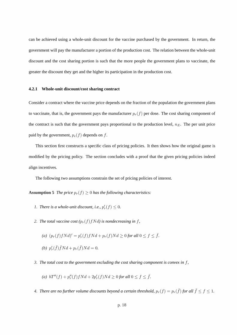
4.2.1 Whole-unit discount/cost sharing contract

Consider a contract where the vaccine price depends on the fraction of the population the government plans

to vaccinate, that is, the government pays the manufacturerpr(f) per dose. The cost sharing component of

the contract is such that the government pays proportional to the production level,nE . The per unit price

paid by the government,pe(f) depends onf .

This section first constructs a specific class of pricing policies. It then shows how the original game is

modified by the pricing policy. The section concludes with a proof that the given pricing policies indeed

align incentives.

The following two assumptions constrain the set of pricing policies of interest.

Assumption 5 The pricepr(f) ≥ 0 has the following characteristics:

1. There is a whole-unit discount, i.e.,p′r(f) ≤ 0.

2. The total vaccine cost (pr(f)fNd) is nondecreasing inf ,

(a) (pr(f)fNd)′ = p′r(f)fNd + pr(f)Nd ≥ 0 for all 0 ≤ f ≤ f .

(b) p′r(f)fNd + pr(f)Nd = 0.

3. The total cost to the government excluding the cost sharing component is convex inf ,

(a) bT ′′(f) + p′′r(f)fNd + 2p′r(f)Nd ≥ 0 for all 0 ≤ f ≤ f .

4. There are no further volume discounts beyond a certain threshold,pr(f) = pr(f) for all f ≤ f ≤ 1.

p. 18

If the derivativep′r(f) does not exist atf = f , then use the left derivative in Assumption5.

Assumption 6 Givenpr(f), let pe(f) ≥ 0 satisfyc− pe(f)

pr(f)=

∫ kS

0ufU (u)du for all f ∈ [0, 1].

In Assumption6, kS = fNdnS

E

is the same as before, wheref, nSE are the solutions for the system setting.

Before proceeding, we show first that the set of the conditions in Assumptions5and6 results in a feasible

set. We give an example that satisfies the conditions in Assumption5, then modify it to obtain functions that

satisfy all of the conditions in both assumptions. Consider the following pricing strategy,

pr(f) =

κb

fNd

[− T (f) + T ′(f)f + T (0)], 0 ≤ f ≤ f

pr(f), f < f ≤ 1.

(17)

Claim 1 If 0 < κ < 1, then the pricing strategy introduced in (17) gives a nonnegative price for anyf and

satisfies all the conditions in Assumption5.

Now we show that for someκ, (17) satisfies Assumption6. It suffices to show thatpe(f) ≥ 0 for all f ,

so the goal is to choose a pricing strategy such thatpr(f)∫ kS

0 ufU (u)du ≤ c. Sincepr(f) is nonincreasing

in f , it suffices to show thatpr(0)∫ kS

0 ufU (u)du ≤ c. For anypr(f) that satisfies (17),

pr(0) = limf→0

pr(f) = limf→0

κb

fNd

[− T (f) + T ′(f)f + T (0)]

= κb

Nd

[T ′(f)− lim

f→0

(T (f)− T (0)f

)]

= κb

Nd

[T ′(f)− T ′(0)

]

Observe that∫ kS

0 ufU (u)du ≤ µ. It suffices to haveκ bNd

[T ′(f) − T ′(0)

]µ ≤ c in order to insure that

Assumption6 holds. This justifies Claim2: pricing strategies exist that satisfy both assumptions.

Claim 2 If 0 < κ < min{1, c[T ′(f)−T ′(0)]µ

}, then the pricing strategypr(f) in (17) satisfies Assumptions5

and6.

p. 19

All the ingredients are in place to build a coordinating contract. The key idea is to keep the relationship

between the optimal production level and order quantity linear. Assumption6 accomplishes this. To see this,

observe that this contract changes the manufacturer objective, for a givenf , to:

MF (nE) = (c− pe(f))nE − pr(f)nE

∫ fNdnE

0ufU (u)du− pr(f)fNd

∫ ∞

fNdnE

fU (u)du

By taking the derivatives, we have:

∂MF (nE)∂nE

= (c− pe(f))− pr(f)∫ fNd

nE

0ufU (u)du

∂2MF (nE)∂n2

E

= pr(f)fNd

n2E

(fNd

nE)fU (

fNd

nE) ≥ 0

Therefore, thisMF is convex innE , and the optimalnE satisfies∫ fNd

n∗E

0 ufU (u)du = c−pe(f)pr(f) . Together

with Assumption6, this implies that∫ fNd

n∗E

0 ufU (u)du =∫ kS

0 ufU (u)du. So for any givenf , the optimal

production level for the manufacturer is linear inf , with

n∗E =fNd

kS. (18)

Therefore this contract changes the government objective to

minf

GF = E[

bT ( WNd) + paW + pr(f)Z + pe(f)nE

], (19)

and changes the manufacturing constraint tofNdnE

= kS . This restatement of the game setting for the

whole-unit discout/cost sharing contract permits the statement of the main result of this section.

Theorem 4 For any pe(f), pr(f) that satisfy Assumptions5 and 6, the optimal values of Problem (19),

denoted by(f c, ncE), are equal to(f , nS

E). That is, this cost sharing contract coordinates the supply chain.

Proof: In order to analyze Problem (19), we again split it into two separate subproblems.

p. 20

Case 1 (0 ≤ f ≤ f ): In this case the optimization problem would be:

minf

GF1 =[

b

∫ fNdnE

0T (

nEu

Nd)fU (u)du + bT (f)

∫ ∞

fNdnE

fU (u)du + panE

∫ fNdnE

0ufU (u)du

+pafNd

∫ ∞

fNdnE

fU (u)du + pe(f)nE + pr(f)nE

∫ fNdnE

0ufU (u)du

︸ ︷︷ ︸= cnE(by Assumption6)

+pr(f)(fNd)∫ ∞

fNdnE

fU (u)du]

subject to the constraintsfNd = kSnE ; 0 ≤ f ≤ f ; andnE ≥ 0. Substituting the constraintnE = fNdkS

into the objective function gives

minf

GF1 =[

b∫ kS

0 T ( fkS u)fU (u)du + bT (f)

∫∞kS fU (u)du + pa

fNdkS

∫ kS

0 ufU (u)du

+pafNd

∫ ∞

kS

fU (u)du + cfNd

kS+ pr(f)fNd

∫ ∞

kS

fU (u)du]

s.t. 0 ≤ f ≤ f

We show that in this case the optimum value is atf . For this purpose, it is enough to analyze the first

derivative ofGF1.

∂GF1

∂f=

[ b

kS

∫ kS

0T ′(

f

kSu)ufU (u)du + bT ′(f)

∫ ∞

kS

fU (u)du + paNd

kS

∫ kS

0ufU (u)du

+paNd

∫ ∞

kS

fU (u)du + cNd

kS+ pr(f)Nd

∫ ∞

kS

fU (u)du + p′r(f)fNd

∫ ∞

kS

fU (u)du]

=Nd

kS

( ∫ kS

0[

b

NdT ′(

f

kSu) + pa]ufU (u)du + c

)(20)

+[

bT ′(f) + paNd + pr(f)Nd + p′r(f)fNd] ∫ ∞

kS

fU (u)du

We show that each of the two components in (20) is negative, making the derivative ofGF1 negative for all

0 ≤ f ≤ f . To see this, first note that the functionJ(f) =∫ kS

0 [ bNdT ′( f

kS u)+ pa]ufU (u)du is an increasing

function of f , asJ ′(f) =∫ kS

0 [ bNdkS T ′′( f

kS u)]u2fU (u) ≥ 0. HenceJ(f) ≤ J(f), ∀f ≤ f . However,

usingfNd = nSEkS , we getJ(f) =

∫ kS

0 [ bNdT ′(nS

EuNd ) + pa]ufU (u) = −c (by Proposition6). As a result

J(f) + c ≤ 0, so

∫ kS

0[

b

NdT ′(

f

kSu) + pa]ufU (u)du + c ≤ 0; ∀ 0 ≤ f ≤ f

p. 21

This shows that the first parenthesis in (20) is negative. To show that the second term of the derivative of

GF1 is also negative, we consider the termbT ′(f) + paNd + pr(f)Nd + p′r(f)fNd. The derivative of this

expression isbT ′′(f)+p′′r(f)fNd+2p′r(f)Nd, which is positive using the third part of Assumption5. This

means thatbT ′(f) + paNd + pr(f)Nd + p′r(f)fNd ≤ bT ′(f) + paNd + pr(f)Nd + p′r(f)fNd for all

0 ≤ f ≤ f . Note thatbT ′(f) + paNd = 0 by the definition off , and thatpr(f)Nd + p′r(f)fNd = 0 by

the second part of Assumption5. This suggests

bT ′(f) + paNd + pr(f)Nd + p′r(f)fNd ≤ 0, ∀ 0 ≤ f ≤ f

which shows the second term of the derivative ofGF1 is also negative. By the strict convexity ofT (f),

equality occurs only atf . Hence (20) implies thatGF1(f) ≤ 0 for all 0 ≤ f ≤ f meaning that the minimum

of GF1 is attained atf . The corresponding production value tof is nSE (using18). So in this case, the only

candidate for optimality is the system optimal solution.

Case 2 (f ≤ f ≤ 1): In this case, using the definition ofpr(f), pr(f) = pr(f), and hencepe(f) = pe(f)

for all f ≥ f . As a result, the government objective becomes:

GF2 =[

b

∫ fNdnE

0T (

nEu

Nd)fU (u)du + bT (f)

∫ ∞

fNdnE

fU (u)du + panE

∫ fNdnE

0ufU (u)du

+pafNd

∫ ∞

fNdnE

fU (u)du + pe(f)nE + pr(f)nE

∫ fNdnE

0ufU (u)du

︸ ︷︷ ︸= cnE(by Assumption5)

+pr(f)fNd

∫ ∞

fNdnE

fU (u)du]

subject to the constraintsfNd = kSnE ; f ≤ f ≤ 1; andnE ≥ 0. Substituting the constraintfNd = kSnE

to removef from the objective gives:

GF2 =[

b

∫ fNdnE

0T (

nEu

Nd)fU (u)du + bT (f)

∫ ∞

fNdnE

fU (u)du + panE

∫ fNdnE

0ufU (u)du

+pafNd

∫ ∞

fNdnE

fU (u)du + cnE + pr(f)nEkS

∫ ∞

kS

fU (u)du]

with the constraintf ≤ f replaced by the constraintnE ≥ nSE .

p. 22

We show the derivative of the objective function in this case is positive and henceGF2 is minimized

when that constraint is tight, i.e.,nE = nSE . Consider,

∂GF2

∂nE=

∫ fNdnE

0[

b

NdT ′(

nEu

Nd) + pa]ufU (u)du + c + pr(f)kS

∫ ∞

kS

fU (u)du (21)

The first term above is exactly the functionH(nE) introduced in the proof of Proposition7, and by using

its nondecreasing property, we getH(nE) ≥ H(nSE) for all nE ≥ nS

E . However, Proposition6 suggests

H(nSE) =

∫ fNd

nSE

0 [ bNdT ′(nS

EuNd ) + pa]ufU (u)du = −c. This implies that

∫ fNdnE

0[

b

NdT ′(

nEu

Nd) + pa]ufU (u)du + c ≥ 0; ∀ nE ≥ nS

E .

By using this result with (21), we obtain the desired result,

∂GF2

∂nE=

∫ fNdnE

0[

b

NdT ′(

nEu

Nd) + pa]ufU (u)du + c + pr(f)kS

∫ ∞

kS

fU (u)du

≥ pr(f)kS

∫ ∞

kS

fU (u)du ≥ 0

In both case 1 and case 2, the optimum values for the game setting aref , nSE . ¤

4.2.2 Coordinating Contract: Numerical Application

This section uses the idea behind Theorem4together with estimates of parameters from the influenza literature

in order to develop a contract that can coordinate the supply chain empirically, even though the actualT (f)

may make a slight deviation from strict convexity.

Hill and Longini(2003) suggestR0 = 1.87 andWeycker et al.(2005) argue thatφ = 0.90 is a reasonable

value for vaccine effects. We use the data fromWeycker et al.(2005) to estimate the direct costs (not indirect)

of each infected individual, with tob = $95 on average over the different groups. The vaccine price is set to

pr = $12 (CDC, 2005). For vaccine administration costs, there are no explicit data, so we usedpa = $40

as a base case, as didWeniger et al.(1998) for pediatric vaccines, being roughly the cost of doctor visit.

We usedd = 1 dose of vaccine, the usual value, per adult vaccinated. We are not aware of literature to

define the variance of vaccine production yields, so we assumed thatU has a gamma distribution with mean

p. 23

µ = 1 (Palese, 2006) and standard deviationσ = 1/5 = 0.2, so thatU ∼ Gamma(25, 1/25). We assumed

a population ofN = 107 individuals and a production cost ofc = $6 (not necessarily the actual number).

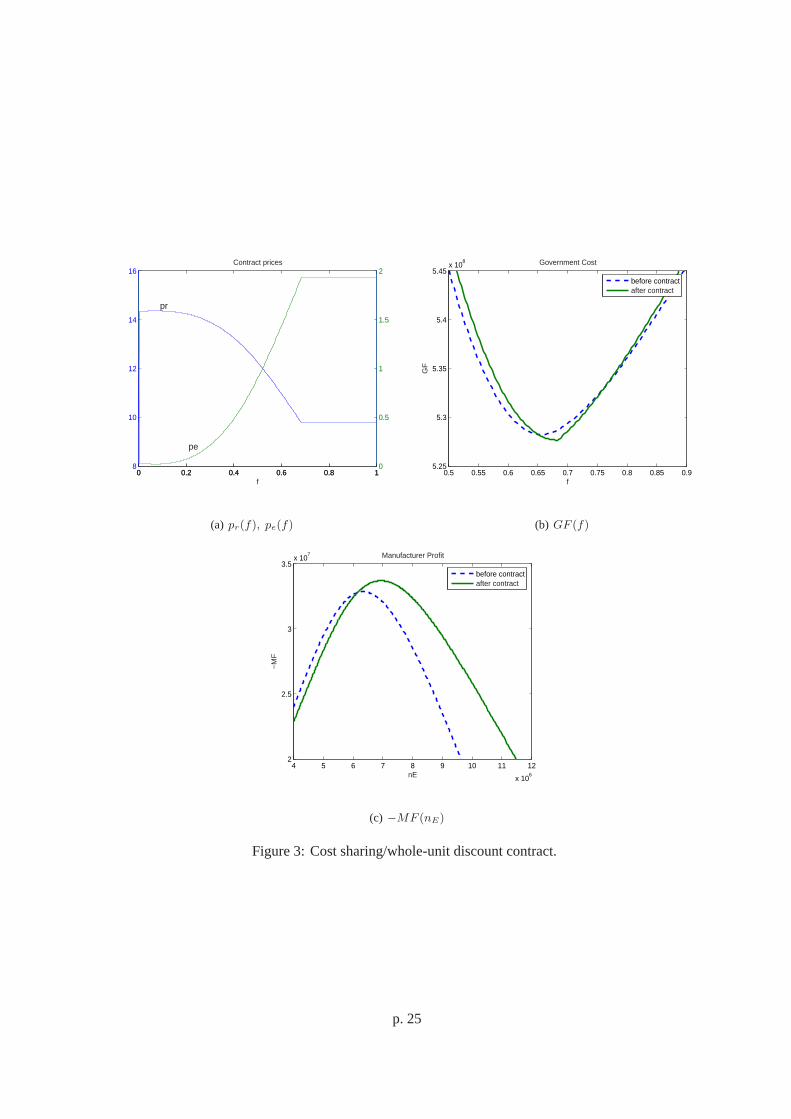
Figure3 depicts the optimal contract, governmental costs and manufacturer profits, for the special case

of T (f) that is based upon the above parameters and a large initial epidemic wave (usingI0 = 0.1). While

T (f) in this case is not precisely convex (slight nonconvexity nearf = 0.08), a strict application of the prices

implied by (17) and Assumption6 leads to a whole-unit discount price,pr(f) (scale on left-hand ofy-axis of

3(a)), and cost sharing pricepe(f) (scale on right-hand side ofy-axis), that empirically coordinates incentives.

The particular choice ofκ = 0.215 for Figure3 insures that the government overall vaccine procurement and

health benefit costs are reduced by the contract from$528M to$527M ; that the government orders more (up

from fG = 0.65 to f = 0.68); that the manufacturer is willing to produce more (n∗E increases from6.3M

to 7M ); and that the manufacturer’s profits increase (from$32.8M to $33.7M ).

For sensitivity analysis, we ran the contract under different administration costs [pa = $20, approximately

the value inPisano2006for Medicare reimbursement, andpa = $60]; and different values for health benefits

[b = $275, a value fromGessner2000converted into 2000 dollars, andb = $450, the combined direct and

indirect costs calculated using data fromWeycker et al.2005]. For values ofb ≥ $250, we foundf = 1

due to the high benefit of vaccination compared with the cost of administraction. In general, a smallerpa or

higherb will increasef , and increasingpa or decreasingb will decreasef .

5 Discussion and Model Limitations

This work derived the equilibrium state of an interaction between a government and a manufacturer, with the

realistic feature of a manufacturer that bears the risk of uncertain production yields. The model shows thata

rational manufacturer will always underproduce influenza vaccinesin that setting, relative to the levels that

provide an optimal system-wide cost-benefit tradeoff.

When the levels of exogenous introduction of influenza into a population are small, leading to the

p. 24

0 0.2 0.4 0.6 0.8 18

10

12

14

16

0 0.2 0.4 0.6 0.8 10

0.5

1

1.5

2

f

Contract prices

pr

pe

(a) pr(f), pe(f)

0.5 0.55 0.6 0.65 0.7 0.75 0.8 0.85 0.95.25

5.3

5.35

5.4

5.45x 10

8 Government Cost

f

GF

before contractafter contract

(b) GF (f)

4 5 6 7 8 9 10 11 12

x 106

2

2.5

3

3.5x 10

7 Manufacturer Profit

nE

−M

F

before contractafter contract

(c) −MF (nE)

Figure 3:Cost sharing/whole-unit discount contract.

p. 25

piecewise linear approximation forT (f) in Section3, a relatively simple cost sharing contract can coordinate

the incentives of the actors to obtain a system optimal solution.

When the levels of exogenous introduction of influenza into a population are somewhat large, as in

a large-wave pandemic situation, the analysis of Section4 may be appropriate. The simple cost sharing

contract must be modified to account for the nonlinear population-level health benefits that are provided

by influenza vaccination programs. It is therefore not surprising that the whole-unit discount/cost sharing

contracts that can align incentives depend on the expected number of infections averted by a given magnitude

of the vaccination program effort.

There are several limitations of this model. Some of the limitations can be handled with existing methods.

Other limitations could lead to interesting future work, but do not limit the value of insights above regarding

contract design for governmental/industry collaboration for influenza outbreak preparedness.

One, an epidemic model with homogeneous and homogeneously mixing populations ignores the potential

to target specific critical subpopulations, such as children or the elderly. In the short run, the contractual

designs here that determine production volumes could be accompanied in a second stage analysis with

other work (e.g.,Hill and Longini, 2003) that can optimally allocate vaccines to different subpopulations.

The generality of the analysis for piecewise linear or convexT (f) allows some flexibility in adapting the

incentive alignment results here to more complex epidemic models that account for the prioritization of

certain subgroups.

Two, the analysis above assumes that the per person benefitb and the cost to administerpa are constant.

The results may generalize nicely to the case of variable marginal benefits of vaccination,b(f), as long

as b(f)T (f) is convex. Terms likebT ′(f) in the definition off , for example, would be replaced with

(b(f)T (f))′ = b′(f)T (f) + b(f)T ′(f). Similarly, a convex increasing administration cost,pa(f), might be

appropriate too. The net effect of these two changes is expected to decrease the optimal vaccination fraction.

Three, the model assumes that health consequences can be quantified by direct and indirect monetary

p. 26

costs, but a multi-attribute approach might be desired to more fully examine issues like the number of deaths

or hospitalizations. These features can be modeled indirectly with the present work by assessing the number

infected and applying the relevant morbidity and mortality rates.

Four, the model assumes that the government can precisely specify the number of individuals to vaccinate.

This is potential drawback of the other epidemic models mentioned in this paper, too. The inclusion of

individual’s choice to become vaccinated would also require much additional complexity.

Five, the model currently examines a single manufacturer and a single government, and assumes that

all parameters are known to all parties. The cost per dose and yield distributions are not likely to be public

information, and there are several providers and many purchasers. Nevertheless the equilibrium still might

still be modeled as an outcome of interactions between two rational actors of the model. Multiple buyers

and suppliers would be an interesting extension. Contracts in the presence of multiple manufacturers and/or

suppliers could be complicated, to avoid collusion on the part of a subset of the players.

6 Conclusion

This work developed the first integrated supply-chain/health economics model of two key players in the

influenza vaccine supply chain: a government that purchase and administer vaccines in order to achieve

an efficient cost-benefit tradeoff, and a manufacturer that optimizes production input levels to achieve cost-

effective delivery of vaccines in the presence of yield uncertainty. The model indicates a lack of coordination

for contracts that leave the manufacturer with the production yield risks. That lack of coordination results in

vaccine production shortfalls.

We show that a global social optimum cannot be fully attained by changing the vaccine price alone, or by

reducing the risk of production yields by having the government contractually pay a reduced rate for doses

that are produced in excess of the original demand. A variation of the cost sharing contract is one option that

can align incentives to achieve a social optimum.

p. 27

Acknowledgments: We are grateful for discussions with Philippe Laurent, Industrial Product Leader for

Influenza, and Catherine Chevat, Health Economics Deputy Director, of Sanofi-Pasteur; and Michel Galy,

former director of the Institut Merieux vaccine facility near Lyon, France (now part of Sanofi-Pasteur). The

content of this paper is ours, and does not necessarily represent the positions of those individuals or of

Sanofi-Pasteur.

REFERENCES

BRIDGES, C. B., K. FUKUDA ., T. M. UYEKI ., N. J. COX., AND J. A. SINGLETON. 2002. Prevention

and control of influenza: Recommendations of the Advisory Comittee on Immunization Practices (ACIP).

MMWR Recommendations and Reports 51(RR03), 1–31.

BUSH, G. W.2005. President outlines pandemic influenza preparations and response. Accessed 22 January

2006 at http://www.whitehouse.gov/news/releases/2005/11/20051101-1.html.

CDC 2005. Vaccine price list. Available from http://www.cdc.gov/nip/vfc/cdc_vac_price_list.htm.

CHICK , S. E., D. C. BARTH-JONES., AND J. S. KOOPMAN. 2001. Bias reduction for risk ratio and vaccine

effect estimators.Statistics in Medicine 20(11), 1609–1624.

DIEKMANN , O. AND J. HEESTERBEEK. 2000.Mathematical Epidemiology of Infectious Diseases. Chich-

ester: Wiley.

DIETZ, K. 1993. The estimation of the basic reproduction number for infectious diseases.Statistical Methods

in Medical Research 2, 23–41.

GANI , R., H. HUGHES., D. FLEMING ., T. GRIFFIN., J. MEDLOCK., AND S. LEACH. 2005. Potential

impact of antiviral drug use during influenza pandemic.Emerging Infectious Diseases 11(9), 1355–1362.

GERDIL, C. 2003. The annual production cycle for influenza vaccine.Vaccine 21, 1776–1779.

p. 28

GESSNER, B. D. 2000. The cost-effectiveness of a hypothetical respiratory syncytial virus vaccine in the

elderly. Vaccine 18, 1485–1494.

HILL , A. N. AND I. M. L ONGINI. 2003. The critical fraction for heterogeneous epidemic models.Mathe-

matical Biosciences 181, 85–106.

JACQUEZ, J. A.1996.Compartmental Analysis in Biology and Medicine(3rd ed.). Ann Arbor: BioMedware.

JANEWAY, C. A., P. TRAVERS., M. WALPORT., AND M. SHLOMCHIK . 2001. Immunobiology(5th ed.).

New York: Garland Publishing.

LONGINI, I. M., E. ACKERMAN., AND L. R. ELVEBACK . 1978. An optimization model for influenza A

epidemics.Mathematical Biosciences 38, 141–157.

LONGINI, I. M., M. E. HALLORAN ., A. NIZAM ., M. WOLFF., P. M. MENDELMAN ., P. E. FAST., AND

R. B. BELSHE. 2000. Estimation of the efficacy of live, attenuated influenza vaccine from a two-year,

multi-center vaccine trial: implications for influenza epidemic control.Vaccine 18, 1902–1909.

NASH, J. F.1951. Non-cooperative games.Annals of Mathematics 54, 286–295.

NICHOL, K. L., K. L. M ARGOLIS., J. WUORENMA., AND T. V. STERNBERG. 1994. The efficacy and

cost effectiveness of vaccination against influenza among elderly persons living in the community.The

New England Journal of Medicine 331(12), 778–784.

PALESE, P.2006. Making better influenza virus vaccines.Emerging Infectious Diseases 12(1), 61–65.

PIEN, H. 2004. Statement presented to Committee on Aging, United States Senate, by President and CEO,

Chiron Corporation. Accessed 22 January 2006 at http://aging.senate.gov/_files/hr133hp.pdf.

PISANO, W.2006. Keys to strengthening the supply of routinely recommended vaccines: View from industry.

Clinical Infectious Diseases 42, S111–S117.

p. 29

SALUZZO , J.-F.AND C. LACROIX-GERDIL. 2006.Grippe aviaire: Sommes-nous prêts?Paris: Belin-Pour

la Science.

SMITH , P. G., L. C. RODRIGUES., AND P. E. FINE. 1984. Assessment of the protective efficacy of

vaccines against common diseases using case-control and cohort studies.International Journal of Epi-

demiology 13(1), 87–93.

U.S. DEPT. OF HEALTH AND HUMAN SERVICES 2005. HHS Pandemic influenza plan: Supplement 6–

Vaccine distribution and use. Accessed 26 January 2006 at http://www.dhhs.gov/pandemicflu/plan/.

WENIGER, B. G., R. T. CHEN., S. H. JACOBSON., E. C. SEWELL., R. DEMON., J. R. LIVENGOOD.,

AND W. A. ORENSTEIN. 1998. Addressing the challenges to immunization practice with an economic

algorithm for vaccine selection.Vaccine 16(9), 1885–1897.

WEYCKER, D., J. EDELSBERG., M. E. HALLORAN ., I. M. LONGINI., A. NIZAM ., V. CIURYLA ., AND

G. OSTER. 2005. Population-wide benefits of routine vaccination of children against influenza.Vaccine 23,

1284–1293.

WHO 2005. Influenza vaccines.Weekly Epidemiological Record 80(33), 277–287, Accessed 21 Jan 2006

at http://www.who.int/wer/2005/wer8033.pdf.

WU, J. T., L. M. WEIN., AND A. S. PERELSON. 2005. Optimization of influenza vaccine selection.

Operations Research 53(3), 456–476.

WYSOCKI, B. AND S. LUECK. 2006. Margin of safety: Just-in-time inventories make U.S. vulnerable in a

pandemic. Wall Street Journal. 12 January 2006.

YADAV, P. AND D. WILLIAMS . 2005. Value of creating a redistribution network for influenza vaccine in

the U.S. Presentation at INFORMS 2006 Annual Conference, San Francisco.

p. 30

Online Appendix

A Appendix: Proofs of mathematical results

Proposition 1. Proof: The expected cost function for the manufacturer is

MF (nE) = cnE − prE[min{nEU, fNd}]

= cnE − prnEE[min{U,

fNd

nE}]

= cnE − prnE(∫ fNd

nE

0ufU (u)du +

∫ ∞

fNdnE

fNd

nEfU (u)du)

= cnE − prnE

∫ fNdnE

0ufU (u)du− prfNd

∫ ∞

fNdnE

fU (u)du

So to get the minimum ofMF we need to see the behavior of its derivative:

∂MF

∂nE= c− pr

∫ fNdnE

0ufU (u)du− prnE

[(fNd

nE)fU (

fNd

nE)(−fNd

n2E

)]− prfNd

[− fU (

fNd

nE)(−fNd

n2E

)]

= c− pr

∫ fNdnE

0ufU (u)du + pr

(fNd)2

n2E

fU (fNd

nE)− pr

(fNd)2

n2E

fU (fNd

nE)

= c− pr

∫ fNdnE

0ufU (u)du

Note that∂2MF∂n2

E= pr[(

(fNd)2

n3E

)fU (fNdnE

)] ≥ 0 so the first order optimality condition is sufficient. Hence the

optimum production quantityn∗E is solution of the following equation:

∫ fNdn∗

E

0ufU (u)du =

c

pr

¤

Corollary 1. Proof: Immediate upon inspection of the values of the parameters.¤

Proposition 2. Proof: To show these results, we analyzeSF in two different regions,f ≤ f0 andf ≥ f0.

Let SF1(f, nE) denotes the value ofSF whenf ≤ f0, and likewiseSF2(f, nE) is the value ofSF where

f ≥ f0. Note that iff ≤ f0 thenW = Z = min{nEU, fNd}, and the value ofSF1 is

SF1(f, nE) =b

∫ fNdnE

0(M − ψ

nEu

d)fU (u)du + b(M −Nψf)

∫ ∞

fNdnE

fU (u)du

+ panE

∫ fNdnE

0ufU (u)du + pa(fNd)

∫ ∞

fNdnE

fU (u)du + cnE (f ≤ f0).

(22)

p. 31

Online Appendix

Forf > f0, given thatM −Nψf = M −Nψf0 = 0, the value ofSF is

SF2(f, nE) =b

∫ f0NdnE

0(M − ψ

nEu

d)fU (u)du + panE

∫ f0NdnE

0ufU (u)du

+ pa(f0Nd)∫ ∞

f0NdnE

fU (u)du + cnE (f ≥ f0).

(23)

The limits of integration in the right hand side of (23) usef0, notf . In order to get the overall optimal values

for fS , nSE , we solve the following two subproblems.

SF1 = min SF1 SF2 = min SF2

s.t. 0 ≤ f ≤ f0 s.t. f0 ≤ f ≤ 1

nE ≥ 0 nE ≥ 0

Optimality conditions for subproblem SF1: The KKT conditions, iff ≤ f0, are,

−Nψb

∫ ∞

fNdnE

fU (u)du + paNd

∫ ∞

fNdnE

fU (u)du + ξ − θ0 = 0

−ψb

d

∫ fNdnE

0ufU (u)du + pa

∫ fNdnE

0ufU (u)du + c− ϕ = 0

ξ(f − f0) = θ0f = ϕnE = 0 ; ξ, θ0, ϕ ≥ 0,

where the first equation is obtained by taking the derivative with respect tof and the second equation is

obtained by taking the derivative with respect to thenE . Moreoverξ, θ0, ϕ are KKT multipliers of constraints

f ≤ f0, f ≥ 0, nE ≥ 0, respectively. Note that if Assumption2 were not valid, then the second equation

of KKT conditions would requireϕ > 0, and the third equation would imply thatn∗E = 0.

We are interested in the case wherenE > 0, f > 0 which is a conclusion of Assumption2. This implies

thatθ0 = ϕ = 0, and the KKT conditions simplify:

[−Nψb + paNd] ∫ ∞

fNdnE

fU (u)du + ξ = 0

[− ψb

d+ pa

] ∫ fNdnE

0ufU (u)du + c = 0

ξ(f − f0) = 0 ; ξ ≥ 0

p. 32

Online Appendix

In the first equation above, Assumption2 suggests thatξ > 0. If ξ > 0, the last of the KKT conditions would

give rise tof∗ = f0. SoSF1 will always get its minimum at the extremef0. The optimalnE in this case

can be obtained from the second equation of the KKT conditions and using the fact thatf∗ = f0, and

∫ f0Ndn∗

E

0ufU (u)du =

cψbd − pa

. (24)

Optimality conditions for the problem SF2: If f ≥ f0, thenSF2 does not depend onf (the vaccine

fraction declared by the government does not change the value of objective function). It follows that all

valuesf0 ≤ f ≤ 1 are optimum and so the first part of the claim is proved.

Now SF2 is a function ofnE only and the derivative ofGF with respect tonE is

∂SF2

∂nE= (−ψb

d+ pa)

∫ f0NdnE

0ufU (u)du + c.

Note that ∂2SF2

∂n2E

= (ψbd − pa)(f0Nd

n2E

)(f0NdnE

)fU (f0NdnE

), which is nonnegative by Assumption2, hence

SF2(nE) is a convex function onnE and the first order optimality condition is sufficient. By getting

the root of the derivative ofSF2 above, we can see that the optimumnE for SF2 is the same as the solution

of (24). So the optimum value fornSE satisfies the same equation in both cases.¤

Proposition 3. Proof: If we defineGF1, GF1 like SF1, SF1 for the case wheref ≤ f0, thenGF1 is:

GF1(f, nE) = b

∫ kG

0(M − ψ

nEu

d)fU (u)du + b(M −Nψf)

∫ ∞

kG

fU (u)du

+(pa + pr)nE

∫ kG

0ufU (u)du + (pa + pr)(fNd)

∫ ∞

kG

fU (u)du

= bM − ψb

dnE

∫ kG

0ufU (u)du−Nψbf

∫ ∞

kG

fU (u)du

+(pa + pr)nE

∫ kG

0ufU (u)du + (pa + pr)fNd

∫ ∞

kG

fU (u)du (∫∞0 fU (u)du = 1)

= bM − ψb

dnE

∫ kG

0ufU (u)du− ψb

nEkG

d

∫ ∞

kG

fU (u)du

+(pa + pr)nE

∫ kG

0ufU (u)du + (pa + pr)nEkG

∫ ∞

kG

fU (u)du (fNd = nEkG)

= bM + nE(−ψb

d+ pa + pr)

[ ∫ kG

0ufU (u)du + kG

∫ ∞

kG

fU (u)du]

p. 33

Online Appendix

By Assumption3, the coefficient ofnE in the last equality is negative, so the optimum value fornE in GF1

lies on the upper boundary, wheref = f0. This proves the first part of the claim.

For the second part, similarly defineGF2, GF2 to represent the government objective functions for the

casesf ≤ f0 andf ≥ f0, respectively. Using the fact thatT (f) = 0 for all f ≥ f0, and the constraint In

the second equation above,f = nEkG

Nd , to obtain

GF2(f, nE) = b

∫ f0NdnE

0(M − ψ

nEu

d)fU (u)du + panE

∫ f0NdnE

0ufU (u)du + prnE

∫ kG

0ufU (u)du

+pa(f0Nd)∫ ∞

f0NdnE

fU (u)du + pr(fNd)∫ ∞

kG

fU (u)du

= b

∫ f0NdnE

0(M − ψ

nEu

d)fU (u)du + panE

∫ f0NdnE

0ufU (u)du + pa(f0Nd)

∫ ∞

f0NdnE

fU (u)du

+prnE

[ ∫ kG

0ufU (u)du + kG

∫ ∞

kG

fU (u)du]

∂GF2

∂nE= (−ψb

d+ pa)

∫ f0NdnE

0ufU (u)du + pr

∫ kG

0ufU (u)du + prk

G

∫ ∞

kG

fU (u)du

∂2GF2

∂n2E

= (ψb

d− pa)

f0Nd

n2E

fU (f0Nd

nE)

for f ≥ f0. Note thatf0NdnE

≤ kG. By Assumption2, ∂2GF2

∂n2E≥ 0, soGF2 is a convex function ofnE . To find

the minimum it suffices to look at the sign of its first derivative. If Condition (12) holds, then Assumption2

implies that∂GF2∂nE

≥ 0 on f ≥ f0, so that the minimum ofGF2 for f ∈ [f0, 1] is obtained atf0. The

optimum for bothGF1 andGF2 lead to the claimed optimum, namelyfG = f0.

If Condition (12) does not hold (i.e.(−ψbd + pa + pr)

∫ kG

0 ufU (u)du + prkG

∫∞kG fU (u)du < 0); then

because of the convexity of functionGF2 onnE (non-decreasing derivative), there are two cases:

Case 1:∃nE ; ∂GF2

∂nGE

= 0. In this case clearly the optimum values for thef, nE are the following:nGE = nE ,

fG = kGnGE/Nd.

Case 2:If nE(1) denotes the maximumnE corresponding tof = 1 (i.e. nE(1) = 1NdkG ) and still ∂GF2

∂nGE

< 0

thenfG = 1, nGE = nE(1).

Combined, the two cases complete the proof.¤

p. 34

Online Appendix

Theorem1. Proof: Proposition2 shows thatfG ≥ f0. We consider the two casesfG = f0 andfG > f0

separately, and prove that both cases lead to the relationnSE > nG

E .

Case 1:fG = f0. Using the inequality in Corollary2 (i.e. kS < kG) and using the definitions ofkG, kS

it immediately follows thatnSE > nG

E , as desired.

Case 2:fG > f0. (proof by contradiction) Assume to the contrary thatnSE ≤ nG

E . First of all we obtain

the sign of[

∂GF2∂nE

]nG

E

. As in the proof of Proposition3, there are two cases fornGE . If the condition in case

1 of Proposition3 holds, then[

∂GF2∂nE

]nG

E

= 0. If case 2 holds, then[

∂GF2∂nE

]nG

E

≤ 0. In either case, the

following relation is true:[∂GF2

∂nE

]nG

E

≤ 0 (25)

On the other hand,

[∂GF2

∂nE

]nG

E

= (−ψb

d+ pa)

∫ f0Nd

nGE

0ufU (u)du + pr

∫ kG

0ufU (u)du + prk

G

∫ ∞

kG

fU (u)du

≥ (−ψb

d+ pa)

∫ f0Nd

nSE

0ufU (u)du + pr

∫ kG

0ufU (u)du + prk

G

∫ ∞

kG

fU (u)du

= (−ψb

d+ pa)(

cψbd − pa

) + c + prkG

∫ ∞

kG

fU (u)du

= prkG

∫ ∞

kG

fU (u)du > 0

The inequality in the second line comes from the assumptionnSE ≤ nG

E , and with Assumption2. The third

line is valid by (5) and Proposition2. But the last inequality contradicts (25), sonGE ≥ nS

E is false. ¤

Proposition 4. Proof: The proof of Theorem1 shows that there does not exist a wholesale contract which

coordinate this supply chain. That proof proceeded in two cases. The first case requiresnSE > nG

E . For full

coordination, we requirenSE = nG

E for somepr. In case 2,nSE = nG

E for somepr implies that∂GF∂nE

∣∣nG

E> 0,

which would not be true for the optimizer ofGF . ¤

p. 35

Online Appendix

Theorem2. Proof: First we show thatfe ≥ f0 by showing that optimum value forGF1 for f ∈ [0, f0] is

always obtained atf0. By replacingf = kenENd we getGF1 to be only a function ofnE :

GF1(nE) = b

∫ ke

0(M − ψ

nEu

d)fU (u)du + b(M −Nψ

nEke

Nd)∫ ∞

ke

fU (u)du

+(pa + pr)nE

∫ ke

0ufU (u)du + (pa + pr)(kenE)

∫ ∞

ke

fU (u)du + penE

Now by taking the derivative ofGF1 with respect tonE we obtain that:

∂GF1

∂nE= −ψb

d

∫ ke

0ufU (u)du− ψb

dke

∫ ∞

ke

fU (u)du

+(pa + pr)∫ ke

0ufU (u)du + (pa + pr)ke

∫ ∞

ke

fU (u)du + pe

= (−ψb

d+ pa)

∫ kS

0ufU (u)du + pr

∫ ke

0ufU (u)du (26)

+ (−ψb

d+ pa + pr)ke

∫ ∞

ke

fU (u)du + pe

= −c + (c− pe) + (−ψb

d+ pa + pr)ke

∫ ∞

ke

fU (u)du + pe (27)

= (−ψb

d+ pa + pr)ke

∫ ∞

ke

fU (u)du, (28)

in which (26) is obtained becauseke = kS , and (27) is obtained using Proposition2 and (14). On the other

hand (28) is negative by Assumption3, so thatGF1 is decreasing for all eligiblenE . Hencef0 and the

correspondingnE (i.e. nE = f0Ndke = f0Nd

kS ) are optimal in this case. Sofe ≥ f0. Becauseke = kS , it

immediately follows thatneE ≥ nS

E .

Now we show that the optimum ofGF2, for f ∈ [f0, 1], also occurs atf0, completing the proof. Note

thatf ≥ f0 andke = kS imply thatnE ≥ nSE . ConsiderGF2.

GF2(nE) = b

∫ f0NdnE

0(M − ψ

nEu

d)fU (u)du + panE

∫ f0NdnE

0ufU (u)du + paf

0Nd

∫ ∞

f0NdnE

fU (u)du

+prnE

∫ ke

0ufU (u)du + pr(kenE)

∫ ∞

ke

fU (u)du + penE

p. 36

Online Appendix

The derivative is nonnegative,

∂GF2

∂nE= (−ψb

d+ pa)

∫ f0NdnE

0ufU (u)du + pr

∫ ke

0ufU (u)du + prk

e

∫ ∞

ke

fU (u)du + pe

= (−ψb

d+ pa)

∫ f0NdnE

0ufU (u)du + c + prk

e

∫ ∞

ke

fU (u)du (29)

≥ (−ψb

d+ pa)

∫ f0Nd

nSE

0ufU (u)du + c + prk

e

∫ ∞

ke

fU (u)du (30)

= prke

∫ ∞

ke

fU (u)du ≥ 0 (31)

(29) comes from (14). As before, (30) comes from Assumption2 and the fact thatnE ≥ nSE . Finally, (31) is

true by Proposition2. The last inequality shows that the optimum value forGF2 occurs atf0 hencefe = f0

and because of the fact thatke = kS , we obtainneE = nS

E . ¤

Proposition 6. Proof: The proof resembles the proof of Proposition2, except for the change in role off0

to f , and the definitions ofSF1, SF1 andSF2, SF2. We first show that the optimum value ofSF1 always

occurs at the border, i.e.f∗ = f , by examining the KKT condition forSF1:

bT ′(f)∫ ∞

fNdnE

fU (u)du + paNd

∫ ∞

fNdnE

fU (u)du + ξ = 0

− b

Nd

∫ fNdnE

0T ′(

nEu

Nd)ufU (u)du + pa

∫ fNdnE

0ufU (u)du + c = 0

ξ(f − f) = 0 ; ξ ≥ 0

If f < f , then by the convexity ofT (f) and the definition in (1), we conclude thatbT ′(f) + paNd < 0.

So the first equation forcesξ > 0, then by the third equation we obtainf∗ = f . So the optimum value for

SF1 occurs at the border which isf . SinceSF does not change asf varies in[f , 1], we have shown the

first part of the claim. The optimum value forn∗E in this case can be obtained using the second equation

of the KKT conditions and the fact thatf∗ = f . Namely, the optimumnE solves the following equation:∫ fNd

n∗E

0

[ b

NdT ′(

n∗Eu

Nd) + pa

]ufU (u)du + c = 0, as claimed.

It is now enough to show that in the second case wheref ≥ f , the same relation holds for the optimum

production level. To show this, note that first of all,SF2 is a function ofnE only, hence to get the optimum

p. 37

Online Appendix

it suffices to find the root of its derivative:

∂SF2

∂nE=

∫ fNdnE

0

[ b

NdT ′(

nEu

Nd) + pa

]ufU (u)du + c

By setting this equation to zero we will end up by the same type of relation forn∗E which we obtained before

from SF1, hence always∫ fNd

nSE

0

[b

NdT ′(nSEu

Nd ) + pa

]ufU (u)du + c = 0. ¤

Proposition 5. Proof: Note that∫ kN

0 ufU (u)du = c−pcµpr−pc

. By rewriting theGF in terms of values off, nE

and by replacingf = kNnENd we have:

GF (nE) = b

∫ f0NdnE

0(M − ψ

nEu

d)fU (u)du + panE

∫ f0NdnE

0ufU (u)du + pa(f0Nd)

∫ ∞

f0NdnE

fU (u)du

+(pr − pc)nE

∫ kN

0ufU (u)du + (pr − pc)(kNnE)

∫ ∞

kN

fU (u)du + pcµnE

By Assumption2, ∂2GF2

∂n2E

= (ψbd − pa)f0Nd

n2E

fU (f0NdnE

) ≥ 0, soGF is a convex function onnE . The optimal

value ofGF can therefore be found by setting its derivative to zero:

∂GF

∂nE= (−ab

d+ pa)

∫ f0NdnE

0ufU (u)du + pcµ

+(pr − pc)[ ∫ kN

0ufU (u)du + kN

∫ ∞

kN

fU (u)du]

= (−ab

d+ pa)

∫ f0NdnE

0ufU (u)du + c + (pr − pc)kN

∫ ∞

kN

fU (u)du

The last inequality comes from (13). The last term indicates implicitly thatnNE < nS

E . To see this, plug

nSE into the last terms, use Proposition2 and using the fact thatpr > pc, to obtain ∂GF

∂nE

∣∣∣nS

E

= (pr −

pc)kN∫∞kN fU (u)du > 0. That implies thatnN

E < nSE . ¤

Proposition 7. Proof: The first part of this claim is just the optimality condition for the manufacturer. As

above, this does not depend on the shape ofT (f) so this relation remains the same. The fractionkG is

therefore determined by the values ofc, pr and the egg yield variability, and are assumed to be known.

p. 38

Online Appendix

To prove the second part, note that if∫ kG

0

[ b

NdT ′(

nEu

Nd)+pa

]ufU (u)du+c+prk

G

∫ ∞

kG

fU (u)du < 0,

then by replacingf = nEkG

Nd , we can rewriteGF1 just as a function ofnE as follows:

GF1(nE) = b

∫ kG

0T (

nEu

Nd)fU (u)du + bT (

nEkG

Nd)∫ ∞

kG

fU (u)du

+(pa + pr)nE

∫ kG

0ufU (u)du + (pa + pr)(nEkG)

∫ ∞

kG

fU (u)du

GF1(nE) is a convex function ofnE so the first derivative shows the behavior of this function completely:

∂GF1

∂nE=

∫ kG

0

[ b

NdT ′(

nEu

Nd) + pa

]ufU (u)du + pr

∫ kG

0ufU (u)du

+kG

Nd

[bT ′(

nEkG

Nd) + paNd

] ∫ ∞

kG

fU (u)du + prkG

∫ ∞

kG

fU (u)du

=∫ kG

0

[ b

NdT ′(

nEu

Nd) + pa

]ufU (u)du + c + prk

G

∫ ∞

kG

fU (u)du

+kG

Nd

[bT ′(

nEkG

Nd) + paNd

] ∫ ∞

kG

fU (u)du

(32)

However, note that the functionGF1 is a convex function so clearly for everyf ≤ f or equivalentlynE ≤ nE

we have:∂GF1

∂nE≤

[∂GF1

∂nE

]nE=nE

. On the other hand if we plugnE into (32) we have:

[∂GF1

∂nE

]nE=nE

=∫ kG

0

[ b

NdT ′(

nEu

Nd) + pa

]ufU (u)du + c + prk

G

∫ ∞

kG

fU (u)du

+kG

Nd

[bT ′(

nEkG

Nd) + paNd

] ∫ ∞

kG

fU (u)du

=∫ kG

0

[ b

NdT ′(

nEu

Nd) + pa

]ufU (u)du + c + prk

G

∫ ∞

kG

fU (u)du

in which the last equality comes from the fact thatnE = fNdkG , and recalling (1). Note that the last expression

is less than zero by assumption, so the optimum ofGF1 occurs at its border,f∗ = f . Because the inequality

is strict, optimum ofGF2 also is greater thanf , sofG > f .

To show the reverse direction, we first show that the function

H(nE) =∫ fNd

nE

0

[ b

NdT ′(

nEu

Nd) + pa

]ufU (u)du

is a nondecreasing function onnE .

∂H

∂nE=

∫ fNdnE

0

[ b

(Nd)2T ′′(

nEu

Nd)]u2fU (u)du +

[ b

NdT ′(f) + pa

] fNd

nEfU (

fNd

nE)× (− fNd

n2E

)

=∫ fNd

nE

0

[ b

(Nd)2T ′′(

nEu

Nd)]u2fU (u)du ≥ 0

p. 39

Online Appendix

The second equation follows from the definition off , and the last inequality is due to the convexity ofT (f)

in f . Hence we haveH(nE) ≥ H(nE) for all nE ≥ nE . By replacingH(nE) with its definition,

∫ fNdnE

0

[ b

NdT ′(

nEu

Nd) + pa

]ufU (u)du ≥

∫ fNdnE

0

[ b

NdT ′(

nEu

Nd) + pa

]ufU (u)du ; ∀nE ≥ nE (33)

If we assume∫ kG

0

[ b

NdT ′(

nEu

Nd) + pa

]ufU (u)du + c + prk

G

∫ ∞

kG

fU (u)du ≥ 0 we will show that

fG ≤ f , which is the reverse direction of part 2 of the claim.

Because this is the game setting,f can be replaced bynEkG

Nd , and

GF2(nE) = b

∫ fNdnE

0T (

nEu

Nd)fU (u)du + bT (

nEkG

Nd)∫ ∞

fNdnE

fU (u)du + prnE

∫ kG

0ufU (u)du (34)

+pr(nEkG)∫ ∞

kG

fU (u)du + panE

∫ fNdnE

0ufU (u)du + pa(fNd)

∫ ∞

fNdnE

fU (u)du

∂GF2

∂nE=

∫ fNdnE

0

[ b

NdT ′(

nEu

Nd) + pa

]ufU (u)du + pr

∫ kG

0ufU (u)du + prk

G

∫ ∞

kG

fU (u)du

=∫ fNd

nE

0

[ b

NdT ′(

nEu

Nd) + pa

]ufU (u)du + c + prk

G

∫ ∞

kG

fU (u)du (35)

≥∫ fNd

nE

0

[ b

NdT ′(

nEu

Nd) + pa

]ufU (u)du + c + prk

G

∫ ∞

kG

fU (u)du ≥ 0

The second equality for∂GF2∂nE

comes from (5). If f ≥ f thennE ≥ nE , so the inequality in the third line

is justified by (33). Finally the last inequality comes by assumption, and implies that for everyf ≥ f the

functionGF2 is nondecreasing under the stated assumptions, so the optimumf∗ for GF2 can be obtained at

f∗ = f . HencefG ≤ f , completing the proof. ¤

Lemma 1. Proof: To proof this lemma we show that the functionGF2 obtains its minimum at its border

(f ). We use the functionH(nE) that was defined in the proof of Proposition7, which was shown to be

nondecreasing, andnGE ≥ nS

E to conclude that

∫ fNd

nGE

0

[ b

NdT ′(

nGEu

Nd) + pa

]ufU (u)du ≥

∫ fNd

nSE

0

[ b

NdT ′(

nSEu

Nd) + pa

]ufU (u)du.

p. 40

Online Appendix

By pluggingnGE into the derivative function ofGF2 in (35), and using the above relation,

[∂GF2

∂nE

]nE=nG

E

=∫ fNd

nGE

0

[ b

NdT ′(

nGEu

Nd) + pa

]ufU (u)du + c + prk

G

∫ ∞

kG

fU (u)du

≥∫ fNd

nSE

0

[ b

NdT ′(

nSEu

Nd) + pa

]ufU (u)du + c + prk

G

∫ ∞

kG

fU (u)du

= prkG

∫ ∞

kG

fU (u)du > 0

The equality in the third line comes from (6). The last inequality shows that the derivative of the function

GF2 at the optimum pointnGE is strictly positive, which is not possible unlessnG

E is at its lower extreme,

nGE = nE , wherenE introduced earlier. ¤

Lemma 2. Proof: By the definitions off and ¯f , and strict convexity ofT (f), we have ¯f < f . Let

¯nE =¯fNdkG . Becausef < f , we examine the government subproblemGF1 to analyze the pair( ¯f, ¯nE).

[∂GF1

∂nE

]nE=¯nE

=∫ kG

0

[ b

NdT ′(

¯nEu

Nd) + pa + pr

]ufU (u)du

+kG

Nd

[bT ′(

¯nEkG

Nd) + paNd + prNd

] ∫ ∞

kG

fU (u)dus

=∫ kG

0

[ b

NdT ′(

¯nEu

Nd) + pa + pr

]ufU (u)du < 0

The second equality is true because the second term in the derivative is zero, by the definition of¯f, ¯nE . The

last inequality comes from the strict convexity ofT (f), soT ′(f) < T ′( ¯f); for all f < ¯f . The derivative of

GF1 is negative atf . By the convexity ofT (f), it follows that the optimum ofGF1 is attained for a point

bigger than¯f (since ¯f < f ), and sofG > ¯f . ¤

Lemma 3. Proof: To prove the lemma, we show thatI(k) =∫ k

0

[ b

NdT ′(

nSEu

Nd) + pa

]ufU (u)du attains

its minimum atk∗ = kS . The derivative ofI(k) is ∂I∂k =

[b

NdT ′(nSEk

Nd ) + pa

]kfU (k). Note that fork < kS ,

we haveknS

ENd <

kSnSE

Nd = f , and so by the definition off , the derivative ofI(k) is negative. SoI(k) is

decreasing fork < kS . If k > kS , thenknS

ENd > f so ∂I

∂k > 0, andI(k) is increasing. ThereforeI(k) attains

its minimum atkS . ¤

p. 41

Online Appendix

Theorem 3. Proof: The proof is by contradiction, namely let’s assume thatnGE ≥ nS

E . First of all by

Lemma1, we havefG ≤ f . We consider two cases:

Case 1: fG < f, nGE ≥ nS

E . In this case, the optimum solution(fG, nGE) would occur in the middle of

the region forGF1, so that[∂GF1

∂nE

]nE=nG

E

= 0. By pluggingnGE into (32), we have

0 =∫ kG

0

[ b

NdT ′(

nGEu

Nd) + pa

]ufU (u)du + c

+kG

Nd

[bT ′(

nGEkG

Nd) + paNd + prNd

] ∫ ∞

kG

fU (u)du

=∫ kG

0

[ b

NdT ′(

nGEu

Nd) + pa

]ufU (u)du + c

+kG

Nd

[bT ′(fG) + paNd + prNd

] ∫ ∞

kG

fU (u)du ; (because ofnGEkG = fGNd)

>

∫ kG

0

[ b

NdT ′(

nGEu

Nd) + pa

]ufU (u)du + c ; (Lemma2 and convexity ofT (f)) (36)

On the other hand note that the functionJ(nE) =∫ k0

[b

NdT ′(nEuNd )+pa

]ufU (u)du is an increasing function

of nE . This is because∂J∂nE

=∫ k0

[b

(Nd)2T ′′(nEu

Nd )]u2fU (u)du ≥ 0, asT (f) is a convex function. So

nGE ≥ nS

E , means thatJ(nGE) ≥ J(nS

E). By the definition ofJ(nE), and fork = kG,

∫ kG

0

[ b

NdT ′(

nGEu

Nd) + pa

]ufU (u)du ≥

∫ kG

0

[ b

NdT ′(

nSEu

Nd) + pa

]ufU (u)du (37)

If∫ kG

0

[ b

NdT ′(

nSEu

Nd) + pa

]ufU (u)du ≥

∫ kS

0

[ b

NdT ′(

nSEu

Nd) + pa

]ufU (u)du, then (37) implies

∫ kG

0

[ b

NdT ′(

nGEu

Nd) + pa

]ufU (u)du + c ≥

∫ kS

0

[ b

NdT ′(

nSEu

Nd) + pa

]ufU (u)du + c

= 0 ; (by Proposition6),

which contradicts (36). So we should have:

∫ kG

0

[ b

NdT ′(

nSEu

Nd) + pa

]ufU (u)du <

∫ kS

0

[ b

NdT ′(

nSEu

Nd) + pa

]ufU (u)du

but this inequality also contradicts Lemma3. So case 1 results in a contradiction.

p. 42

Online Appendix

Case 2:fG = f , nGE ≥ nS

E . In this case, the production level would benGE = nE = fNd

kG . As (f , nE) is

the optimum pair forGF1, we should have:[

∂GF1∂nE

]nE≤ 0 or equivalently:

0 ≥∫ kG

0

[ b

NdT ′(

nEu

Nd) + pa

]ufU (u)du + c + prk

G

∫ ∞

kG

fU (u)du

+kG

Nd

[bT ′(

nEkG

Nd) + paNd

] ∫ ∞

kG

fU (u)du

=∫ kG

0

[ b

NdT ′(

nEu

Nd) + pa

]ufU (u)du + c + prk

G

∫ ∞

kG

fU (u)du

>

∫ kG

0

[ b

NdT ′(

nEu

Nd) + pa

]ufU (u)du + c

On the other hand, the last expression can be written as:

∫ fNdnE

0

[ b

NdT ′(

nEu

Nd) + pa

]ufU (u)du + c < 0 (38)

Note however thatnE = nGE ≥ nS

E . By the monotonicity of the functionH(nE) from Proposition7,

∫ fNdnE

0

[ b

NdT ′(

nEu

Nd) + pa

]ufU (u)du + c ≥

∫ fNd

nSE

0

[ b

NdT ′(

nSEu

Nd) + pa

]ufU (u)du + c = 0,

which contradicts (38). Since both cases lead to a contradiction, the claim is proven.¤

Claim 1. Proof: First we show thatpr(f) ≥ 0. Note that the function−T (f) + T ′(f)f + T (0) is an

increasing function off on [0, f ], as its derivative−T ′(f) + T ′(f) exceeds0 for all f < f becauseT (f)

is strictly convex. Further, its value is zero atf = 0, so−T (f) + T ′(f)f + T (0) is a nonnegative function

over[0, f ]. Thereforepr(f) ≥ 0 for f ∈ [0, f ]. Forf ∈ (f < f ], it is clear thatpr(f) = pr(f) ≥ 0.

We show that thispr(f) satisfies all the conditions in assumption in the reverse order. Multiplyingpr(f)

byfNd and taking the second derivative implies(pr(f)fNd

)′′ = −κbT ′′(f). SobT ′′(f)+(pr(f)fNd

)′′ =

(1 − κ)bT ′′(f). But bT ′′(f) +(pr(f)fNd

)′′is the left hand side of the third condition in Assumption5.

By the strict convexity ofT (f),

bT ′′(f) + p′′r(f)fNd + 2p′r(f)Nd =b

2T ′′(f) ≥ 0; ∀ 0 ≤ f ≤ f

p. 43

Online Appendix

For all f < f ≤ 1 we havebT ′′(f) + p′′r(f)fNd + 2p′r(f) = bT ′′(f) ≥ 0.

To prove validity of the second part of assumption, by taking the derivative of(pr(f)fNd

)we have:

(pr(f)fNd

)′ = κb[− T ′(f) + T ′(f)

]which is nonnegative for0 ≤ f ≤ f (by convexity ofT (f)) and is

zero forf = f . For f < f ≤ 1;(pr(f)fNd

)′ = pr(f)Nd ≥ 0.

Finally to show the first part we take the derivative ofpr(f) for 0 ≤ f ≤ f :

∂pr

∂f= −κb

[T ′(f)f − T (f) + T (0)f2

]

The numerator in the bracket is positive due to convexity ofT (f) indicating the desired result for0 ≤ f ≤ f .

Finally, for f < f ≤ 1 we havep′r(f) = 0. ¤

B Appendix: Justification why linear and convexT (f) are of interest

Figures2 and4 show the shape ofT (f) with respect to different values ofI0 andR0. The four graphs

correspond toR0 = 1.67, 2.0, 2.5, 3.0, which are the range forR0 for the different flu pandemics (Gani et al.,

2005). In each graph,T (f) is drawn forI0 = 0, 0.005, 0.01, 0.05, 0.1. The graphs look like a piecewise

linear function asI0 moves towards smaller values (thick blue curve). IfI0 is sufficiently large, thenT (f)

looks strictly convex. This section formalizes those statements.

Piecewise linear. If the initial fraction of the population that is infected due to exogenous exposure (I0

close to 0), then we can replaceI0/S0 by zero in (3) and conclude:

p

1− e−R0p= S0 = 1− φf (39)

Note that the function p1−e−R0p looks like a linear function ifR0 is not very large, which is the case for

influenza. So the relationship betweenf andp is almost linear.

By replacing p1−e−R0p with its Taylor series expansion around zero we have

p

1− e−R0p≈ lim

p0→0

[ p0

1− e−R0p0

]+ lim

p0→0

[1− (1 + R0p0)e−R0p0

(1− e−R0p0)2](p− 0).

p. 44

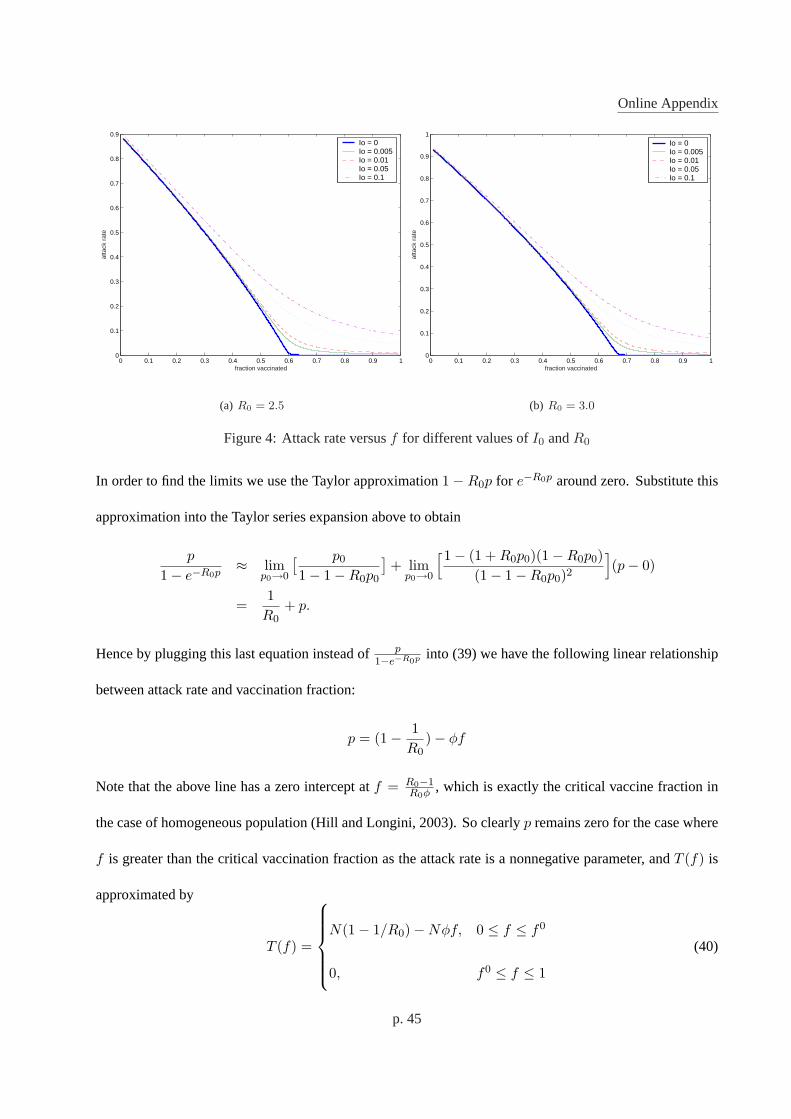
Online Appendix

0 0.1 0.2 0.3 0.4 0.5 0.6 0.7 0.8 0.9 10

0.1

0.2

0.3

0.4

0.5

0.6

0.7

0.8

0.9

fraction vaccinated

atta

ck r

ate

Io = 0Io = 0.005Io = 0.01Io = 0.05Io = 0.1

(a) R0 = 2.5

0 0.1 0.2 0.3 0.4 0.5 0.6 0.7 0.8 0.9 10

0.1

0.2

0.3

0.4

0.5

0.6

0.7

0.8

0.9

1

fraction vaccinated

atta

ck r

ate

Io = 0Io = 0.005Io = 0.01Io = 0.05Io = 0.1

(b) R0 = 3.0

Figure 4:Attack rate versusf for different values ofI0 andR0

In order to find the limits we use the Taylor approximation1 − R0p for e−R0p around zero. Substitute this

approximation into the Taylor series expansion above to obtain

p

1− e−R0p≈ lim

p0→0

[ p0

1− 1−R0p0

]+ lim

p0→0

[1− (1 + R0p0)(1−R0p0)(1− 1−R0p0)2

](p− 0)

=1

R0+ p.

Hence by plugging this last equation instead ofp1−e−R0p into (39) we have the following linear relationship

between attack rate and vaccination fraction:

p = (1− 1R0

)− φf

Note that the above line has a zero intercept atf = R0−1R0φ , which is exactly the critical vaccine fraction in

the case of homogeneous population (Hill and Longini, 2003). So clearlyp remains zero for the case where

f is greater than the critical vaccination fraction as the attack rate is a nonnegative parameter, andT (f) is

approximated by

T (f) =

N(1− 1/R0)−Nφf, 0 ≤ f ≤ f0

0, f0 ≤ f ≤ 1

(40)

p. 45

Online Appendix

While this equation has an epidemiologically attractive interpretation, it estimates the actualT (0) poorly

due to the Taylor series approximations. However, thef - andp-axis intercepts of the roughly linear plot

whenI0 ≈ 0 can be more accurately modeled by replacingN(1− 1/R0) with M = Np0, wherep0 solves

(39) whenf = 0; and by replacing the usual individual-level vaccine effect parameter,φ, with the marginal

population-level benefit of infections averted,ψ, by additional vaccinations. (The two are not necessarily

the same, due to nonlinear infection dynamics.)

Convex case. We now derive some of the properties ofT (f) to argue that it is convex whenI0 is sufficiently

large. Recall (3) for the attack rate, and setS0 = 1− I0 − φf to obtain

p− I0

1− e−R0p+ I0 = 1− φf. (41)

(41) gives rise to the relationp ≥ I0, as1 − I0 − φf = S0 ≥ 0. This is expected. If the initial infected

population isI0 then the fraction that is ultimately infected should be at leastI0.

Our goal is to show thatp is a convex function off . Notice that in (41) p is an implicit function off and

to find its second derivative we will use the following lemma from calculus.

Lemma 4 If y = f(x) then

∂2f−1(y)∂y2

= − 1(∂f(x)

∂x

)3

∂2f(x)∂x2

We rearrange (41) in terms off to obtain

f =1φ

[1− I0 − p− I0

1− e−R0p

].

Using the above lemma fory = f andx = p it turns out:f(p) = 1φ

[1− I0 − p−I0

1−e−R0p

]. So

f ′(p) = − 1φ

[1− e−R0p − e−R0p(p− I0)(1− e−R0p)2

]

p. 46

Online Appendix

First of all we show thatf ′(p) ≤ 0. To prove this notice that (41) suggests we can replacep − I0 by

(1− e−R0p)(1− I0 − φf) in the above relation. So by extending the numerator inf ′(p):

1− e−R0p − e−R0p(p− I0) = 1− e−R0p − e−R0p(1− e−R0p)(1− I0 − φf)

≥ 1− e−R0p − e−R0p(1− e−R0p)(1− I0)

= (1− e−R0p)(1− (1− I0)e−R0p

)

≥ (1− e−R0p)(1− e−R0p) ≥ 0

The last inequality together with the definition off ′(p) suggests thatf ′(p) ≤ 0.

The second piece of the puzzle is to find the relationship forf ′′(p) or the sign of it.

f ′′(p) = − 1φ

[−(R0 + 1)e−R0p(1− e−R0p)2 + R0(p− I0)e−R0p(1− eR0p)(1 + eR0p)

(1− e−R0p)4

]

Note that if the second derivative off(p) were nonnegative, then by the nonpositivity off ′(p) and using the

lemma, we would have∂2p

∂f2 ≥ 0, which is the desired result in this part.

We will show thatf ′′(p) is not always positive, but thatf ′′(p) ≥ 0 for values ofI0 far enough from

zero. To show this, we evaluate the sign of thef ′′(p)’s numerator,−(R0 + 1)e−R0p(1− e−R0p)2 + R0(p−

I0)e−R0p(1− eR0p)(1+ eR0p) = e−R0p(1− eR0p)[− (R0 +1)(1− eR0p)+R0(p− I0)(1+ e−R0p)

]. So it

is enough to find the sign of−(R0 + 1)(1− eR0p) + R0(p− I0)(1 + e−R0p) which is hoped to be negative.

−(R0 + 1)(1− eR0p) + R0(p− I0)(1 + e−R0p) ≤ −(R0 + 1)(1− eR0p) + R0(1− I0)(1 + e−R0p)

≤ −(R0 + 1)(1− eR0p) + R0(p− I0)(1 + e−R0I0)

The first inequality is obtained becausep ≤ 1. The second inequality is obtained because the right hand side

of the first inequality is a decreasing function ofp and obtains its maximum atI0 (asp ≥ I0).

The last statement in the above relation is a decreasing function ofI0, and forI0 = 0 it is positive,

however it is negative for allI0 ≥ 0.1, for the range ofR0 that we are considering (1.5 ≤ R0 ≤ 3). For

p. 47

Online Appendix

those values ofI0, R0, this shows that−(R0 +1)(1− eR0p)+R0(p− I0)(1+ e−R0p) is negative. Therefore

f ′′(p) is positive in this range, showing the desired convexity result forI0 À 0.

p. 48