Embed Size (px)
Citation preview
ADHESIVE BONDED TOWERS FOR
WIND TURBINES
Design, Optimization and Cost Analysis
Ankit Verma
Author:
Ankit Verma
Graduation Supervisors:
ir. M.B. Zaaijer
dr. J.A. Poulis
Prof. dr. G.J.W. van Bussel
Date:
November 2011

Master Thesis
ADHESIVE BONDED TOWERS FOR WIND TURBINES
Design, Optimization and Cost Analysis
Submitted in Partial Fulfillment of the Requirements
for the Degree of Master of Science
in
Sustainable Energy Technology
Track: Wind Energy
Author:
Ankit Verma
November 2011
Department of Aerospace Engineering Department of Mechanical Engineering
Delft University of Technology Eindhoven University of Technology
Adhesive Bonded Towers for Wind Turbines
Copyright © 2011 by Ankit Verma
All rights reserved
Supervised by:
ir. M.B. Zaaijer (Michiel)
dr. J.A. Poulis (Hans)
Prof. dr. G.J.W. van Bussel (Gerard)
Wind Energy Research Group
Delft University of Technology
Kluyverweg 1
2629 HS Delft
The Netherlands

i
Abstract
In an increasingly competitive energy market, the cost of a wind power plant has become more
important. A tubular steel tower supporting a wind turbine can amount to up to 20% of the overall
turbine costs and its optimization may lead to substantial savings with regard to the costs and the use of
materials.
One important aspect of the design is connections between the tower’s sections and between the cans.
The towers usually consist of steel segments, made of several welded cans (conical subsections), which
are further connected by welded flanges. The welded connections have high risk of fatigue failure
leading to the thick tower wall. Also, the flanges are very expensive. This research is focused on
improving wind turbine towers by using adhesive bonded joints instead of welded joints and flanges.
This idea is investigated and the principles of bonded connection are presented. Fatigue resistance is
treated as the main discerning factor between the existing design and the proposed solution in this
study.
The first part of the project focuses on providing a design solution for replacing the bottom-most flange
with the bonded joints. A comparative cost study of the proposed solution is also provided in this
project. In the second part, optimization of the thickness has been investigated for the entire tower
when the cans are bonded circumferentially using adhesives instead of welds.
For the cost analysis of the proposed solution, an 80m reference tower was designed based on the
stability and the fatigue assessment of the welds. The approach is use a reference 3MW wind turbine
model in GH Bladed. The proposed bonded joint is a tubular-single lap joint based on implementation of
simple analytical Volkersen Model. A design guideline for the adhesive bonded joint is presented.
Furthermore, particular focus was given to the factors affecting a joint strength and their behavior in a
bonded joint. Finally, the benefits in terms of fatigue strength, design simplicity, and cost savings are
addressed in detail.
According to this study, the replacement of the bottom-most flanges with an adhesive bonded joint
provides a maximum cost reduction of 17%. This seems to be an economically feasible assembly
solution. For the bonding of entire cans in the tower, only the top two cans can be bonded
economically, keeping the remaining cans to be welded to each other. The replacement of welds in the
entire tower by bonded joints is possible, however, in comparison to the existing solution it is not a
feasible solution in terms of material and cost saving.

ii
iii
Acknowledgement
The work reported is the final research project towards obtaining my masters degree (MSc.) in the Wind
Energy Section of Delft University of Technology. This project work was done under the supervision of
Michiel Zaaijer. First, I would like to express my gratitude to him for his constant guidance and valuable
advices during the last 12 months at TU Delft. He helped me to visualize this project from scratch and
has provided valuable assistance during the entire project. The numerous discussions we had have
contributed greatly in shaping my thesis and thoughts.
Part of the work was done under the guidance of dr. J.A. Poulis, Director of the Adhesion Institute,
TUDelft. I thank him for initiating this project as well as for giving valuable inputs and guidance during
this project. Besides, invaluable suggestions from members of the adhesive department are much
appreciated.
I also thank the master students at Section Wind Energy whose contributions, via informative
discussions, were invaluable and also to the entire team at Section Wind Energy for making my
experience here most memorable.
I would like to take this opportunity to thank all my friends from TUDelft and TU/e. Their company made
this a truly eventful two years. Finally, I would like to thank my dear parents for their continuous support
and motivation. Without them, none of this would have been possible.

iv
v
Table of Contents
Abstract .......................................................................................................................................................... i
Acknowledgement ....................................................................................................................................... iii
List of figures ................................................................................................................................................ ix
List of tables ................................................................................................................................................. xi
List of symbols .............................................................................................................................................xiii
Acronyms ................................................................................................................................................... xvii
1. Introduction .......................................................................................................................................... 1
1.1. Preliminary research ..................................................................................................................... 1
1.2. Objective ....................................................................................................................................... 2
1.3. Approach ....................................................................................................................................... 2
1.4. Report layout ................................................................................................................................ 2
2. Tubular steel tower ............................................................................................................................... 3
2.1. Introduction .................................................................................................................................. 3
2.2. Welded tubular steel tower .......................................................................................................... 3
2.3. Bolted ring flange connections ..................................................................................................... 4
3. Design of a reference tower with flanges and welds ............................................................................ 7
3.1. Introduction .................................................................................................................................. 7
3.2. Tower design procedure ............................................................................................................... 7
3.3. Turbine configuration ................................................................................................................... 8
3.3.1. Turbine model in GH Bladed ................................................................................................. 8
3.3.2. Tower properties................................................................................................................... 9
3.3.3. Foundation geometry ......................................................................................................... 11
3.3.4. Flange geometry at the tower base .................................................................................... 11
3.3.5. Tower input in GH Bladed ................................................................................................... 12
3.4. IEC class and Wind conditions..................................................................................................... 13
3.5. Design loads ................................................................................................................................ 18
3.5.1. Static loads .......................................................................................................................... 18
3.5.2. Fatigue loads ....................................................................................................................... 21
3.6. Redesign of tubular tower .......................................................................................................... 22
3.6.1. Stability check ..................................................................................................................... 22

vi
3.6.2. Fatigue check ...................................................................................................................... 23
3.6.2.1. Welding details in a tubular tower.............................................................................. 23
3.6.2.2. Detail categories of welded joints............................................................................... 23
3.6.2.3. S-N curve ..................................................................................................................... 24
3.6.2.4. Palmgren-miner’s rule................................................................................................. 26
3.6.2.5. Fatigue damage calculation ........................................................................................ 26
3.6.2.6. Approach for dimensioning the wall thickness ........................................................... 27
3.6.3. Natural frequency check ..................................................................................................... 29
3.7. Conclusion ................................................................................................................................... 31
4. Adhesive bonding ................................................................................................................................ 33
4.1. Introduction ................................................................................................................................ 33
4.1.1. Introduction to adhesive ..................................................................................................... 33
4.1.2. Definitions ........................................................................................................................... 33
4.1.3. Adhesive bonded joint ........................................................................................................ 34
4.1.4. Advantages and disadvantages of adhesive bonding ......................................................... 35
4.2. Factors affecting the joint strength ............................................................................................ 36
4.2.1. Adhesive properties ............................................................................................................ 37
4.2.2. Adherend properties ........................................................................................................... 37
4.2.3. Overlap lengths ................................................................................................................... 37
4.2.4. Adhesive thicknesses .......................................................................................................... 38
4.2.5. Environmental effects ......................................................................................................... 39
4.3. Method to improve the joint strength ........................................................................................ 40
4.4. Conclusion ................................................................................................................................... 41
5. Design of adhesive bonded joints ....................................................................................................... 43
5.1. Adhesive bonding design procedure .......................................................................................... 43
5.2. Selection of a joint type .............................................................................................................. 44
5.2.1. Various types of joints......................................................................................................... 44
5.2.2. Considerations for selecting a suitable type of joint .......................................................... 45
5.3. Joint geometry and loading ........................................................................................................ 46
5.4. Material properties ..................................................................................................................... 46
5.5. Closed-form models .................................................................................................................... 47
5.5.1. Types of models .................................................................................................................. 47
vii
5.5.2. Volkersen model ................................................................................................................. 48
5.5.3. Selection of failure criterion ............................................................................................... 50
5.5.4. Linear elastic analysis .......................................................................................................... 50
5.6. Design checks .............................................................................................................................. 52
5.6.1. Resistance at ULS ................................................................................................................ 52
5.6.2. Fatigue check of the bonded joint ...................................................................................... 54
5.6.2.1. S-N curve of adhesive .................................................................................................. 54
5.6.2.2. Safety factor for bonded joints ................................................................................... 55
5.6.2.3. S-N curve for structural steel ...................................................................................... 56
5.7. Modification in the can geometry .............................................................................................. 56
6. Bonding of tower base to the foundation instead of flange and cost comparison ........................... 59
6.1. Results of bonding tower base to the foundation ...................................................................... 59
6.2. Final geometry ............................................................................................................................ 61
6.3. Cost analysis ................................................................................................................................ 62
6.3.1. Flange fabrication cost ........................................................................................................ 62
6.3.2. Flange welding cost ............................................................................................................. 62
6.3.3. Adhesive bonding cost ........................................................................................................ 63
6.4. Cost comparison ......................................................................................................................... 64
7. Bonding of the cans instead of welds and cost comparison ............................................................... 67
7.1. Results of bonding the cans ........................................................................................................ 67
7.2. Cost comparison ......................................................................................................................... 68
8. Conclusion and recommendations ..................................................................................................... 69
8.1. Conclusion ................................................................................................................................... 69
8.2. Recommendations for future work ............................................................................................ 70
9. Bibliography ........................................................................................................................................ 71
Appendix A. Load case descriptions ........................................................................................................... 75
Appendix B. Definition of adhesive related terms ..................................................................................... 78
Appendix C. Adhesive and material properties ......................................................................................... 79
Appendix D. Matlab code for Volkersen Model ......................................................................................... 80
Appendix E. Table showing the failure loads for fillet ............................................................................... 82

viii
ix
List of figures
Figure 2-1: Construction of a tubular steel tower from welded cans ........................................................... 4
Figure 2-2: Bolted ring flange connection [14] ............................................................................................. 5
Figure 3-1: Overview of the design procedure for a wind turbine tower..................................................... 8
Figure 3-2: Blade configuration in GH Bladed ............................................................................................... 8
Figure 3-3: Turbine configurations and components mass details ............................................................... 9
Figure 3-4: Tower design, Vestas 3MW, Onshore [19] ............................................................................... 10
Figure 3-5: (a) Cylindrical structural element [20] and (b) its geometry details ......................................... 11
Figure 3-6: Design of a flange which is welded to the foundation and tower base ................................... 11
Figure 3-7: The Bladed input of initial tower properties along with the flanges as point masses ............. 12
Figure 3-8: Wind speed distribution from GH Bladed ................................................................................ 15
Figure 3-9: Extreme operating gust at Vhub = 25m/s ................................................................................... 17
Figure 3-10: Coordinate system for the design loads on a tower [7] ......................................................... 19
Figure 3-11: Typical weld details in a tubular tower a) weld at flange b) weld between two cans ........... 23
Figure 3-12: The stress cycle [21] ................................................................................................................ 24
Figure 3-13: S-N curve for welds category 80 and 71 ................................................................................. 25
Figure 3-14: Approach for dimensioning the wall thickness ...................................................................... 27
Figure 3-15: Dimensioning of cans adjacent to bottom flange .................................................................. 29
Figure 3-16: Campbell diagram for the final designed tower ..................................................................... 30
Figure 3-17: Dimensioning of the tower wall thickness according to stability and fatigue check ............. 31
Figure 4-1: Different types of loads in an adhesive bonded joint [27] ....................................................... 33
Figure 4-2: Components of a typical adhesive joint [30] ............................................................................ 35
Figure 4-3: Comparison of load transfer in various types of joints [4]. ...................................................... 35
Figure 4-4: S–N curves of lap joints [4] ....................................................................................................... 36
Figure 4-5: Overlap effect on Linear analysis: brittle adhesive (Redux326) and high-strength steel [34] . 38
Figure 4-6: Adhesive thickness effect on linear analysis: adhesive(Hysol9321) and high-strength steel . 38
Figure 4-7: Fatigue of 1.5 mm AISI 304L stainless steel adhesive joints. .................................................... 40
Figure 4-8: Load transfer and shear stress distribution in SLJs (1) with fillet and (2) without fillet [29] .... 41
Figure 5-1: Steps for the design of a adhesive bonded joint ...................................................................... 43
x
Figure 5-2: Joint configurations for (a) Lap joints [30] (b) strap joints (c) tubular joint with a taper [29] . 44
Figure 5-3: Tubular single lap joint [29] ...................................................................................................... 45
Figure 5-4: Rotation of joints in (a) Single lap plate joint (b) Single lap tubular joint [42] ......................... 45
Figure 5-5: Deformations in loaded single-lap joints with elastic adherends [8]. ...................................... 48
Figure 5-6: Single-lap joint analyzed by Volkersen [8]: (a) Geometry and (b) Elemental diagram............. 49
Figure 5-7: Principle of the proposed adhesive bonded connection .......................................................... 51
Figure 5-8: Shear stress variation along the overlap length l=400mm,ta=10mm,tt=36.5mm, tb=55mm . 52
Figure 5-9: Shear stress variation against overlap length at thickness 10mm,tt=36.5mm and tb=55mm 53
Figure 5-10: Effect of varying thicknesses of adherend in a joint on the peak stress ................................ 53
Figure 5-11: S-N curve for simple lap joint bonded with toughened epoxy system, DP 490. .................... 54
Figure 5-12: Dynamic fatigue of steel double-box hat structures [47]. ...................................................... 54
Figure 5-13: S-N curve for simple lap joint bonded with a toughened epoxy system (DP 490) ................. 55
Figure 5-14: S-N curve for the structural steel............................................................................................ 56
Figure 5-15: Transition in butt welds of unequal thicknesses .................................................................... 57
Figure 6-1: Shear stress variation along the overlap length for (a) both wall thickness 55mm, l = 770mm
and (b) both wall thickness 60mm and l = 660mm ..................................................................................... 60
Figure 6-2: Campbell diagram for the turbine with bonded tower base to foundation. ........................... 61
xi
List of tables
Table 3-1: Basic parameters for wind turbine classes [7] ........................................................................... 13
Table 3-2: Design load case parameters ..................................................................................................... 13
Table 3-3: Extreme load cases descriptions ................................................................................................ 18
Table 3-4: Partial safety factors for the load cases ..................................................................................... 18
Table 3-5: Design loads at tower base for different load cases .................................................................. 19
Table 3-6: Extreme design loads at each welded sections ......................................................................... 20
Table 3-7: Fatigue load case description .................................................................................................... 21
Table 3-8: Partial safety factors for fatigue analysis ................................................................................... 21
Table 3-9: Wall thicknesses dimensioned according to stability check ...................................................... 22
Table 3-10: Detail categories for common welds in a tubular tower [22] .................................................. 23
Table 3-11: Redesign of tower thicknesses according to fatigue damage ................................................. 28
Table 3-12: Tower natural frequencies from modal analysis in the Bladed ............................................... 30
Table 5-1: Material properties of adherend and adhesive ......................................................................... 47
Table 5-2: Comparison between different analytical models [32] ............................................................. 48
Table 5-3: Partial safety factors for fatigue analysis of adhesively bonded connections ........................... 55
Table 5-4: Detail Categories and tapering slope for welded parts of a component [48] ........................... 57
Table 6-1: Effect on overlap length and material volume with increase in adherend wall thicknesses .... 59
Table 6-2: Cost of foundation flange connection ....................................................................................... 63
Table 6-3: Dimension of bottommost can before and after bonding......................................................... 63
Table 6-4: Cost of adhesive connection ...................................................................................................... 64
Table 7-1: Detailed analysis of bonding cans with adhesive ...................................................................... 68
Table 7-2: Cost saving from the circumferential bonding .......................................................................... 68

xii
xiii
List of symbols
Latin symbols
I15 characteristic turbulence intensity at 15 m/s [%]
IRef expected value of the turbulence intensity at 15 m/s [%] t tower shell thickness [m] e equivalent geometrical imperfection [m] m inverse slope of S-N curve [-] m° inverse slope in the range N ≤ 5 ∙ 10; 3 for welded joints [-] n� number of stress cycles of the ith stress range [-] t� wall thickness of the tower [m] b joint width [m] l overlap length [m] t� top adherend thickness [m] t� bottom adherend thickness [m] t� adhesive thickness [m] f�,�� limiting shear strength value of adhesive [Pa] k� labour cost factor = 1$/min [$/min] t�� wall thickness at height H set according to stability check [m] t�� wall thickness at height H set according to fatigue check [m] z height above ground [m]
Iturb turbulence intensity [%]
k shape parameter of the Weibull function [-]
Vref reference wind speed average over 10 min [m/s]
A category for higher turbulence characteristics [-]
B category for medium turbulence characteristic [-]
C category for lower turbulence characteristics [-]
Vave annual average wind speed at hub height [m/s]
Vr Rated hub-height wind speed [m/s]
Prated Rated power [MW] P�(V#$�) weibull probability function [-] P&(V#$�) rayleigh probability function [-]
xiv
V#$� 10-min mean of the wind speed at hub height [m/s] V��' annual mean wind speed [m/s]
C scale parameter of the Weibull function [m/s] V(z) wind speed at the height z [m/s] V((z) the expected extreme wind speed with a recurrence period of N years [m/s]
Vgust hub height gust magnitude [m/s]
D rotor diameter [m] V�) cut in wind speed [m/s] V*$� cut out wind speed [m/s] V+ rated wind speed [m/s]
Fx rotor thrust [N]
My tilting moment [Nm]
Mz torsional moment [Nm] N� design axial force [N] M� design bending moment [Nm] N'- euler force for a cantilever beam [Nm] R tower radius [m] S stability check value [-] N� number of cycles to failure [-] D* outer diameter of the tower section [m] D� inner diameter of the tower section [m] I�*�'+ �'2��*) moment of inertia of the tower section [kg·m²] P applied load [N] E adherend modulus [Pa] G� adhesive shear modulus [Pa] L�� circumference of the can [m] V�*��- total volume of two sections getting welded [m3] K2�+ longitudinal weld cost [$]
xv
Greek symbols
Г gamma function [-]
σ1 fixed turbulence standard deviation [-] Λ8 turbulence scale parameter, according to the equation 3-1 [-] γ� partial safety factor for load [-] γ: partial safety factor for material [-] γ) partial safety factor for consequences of failure [-] σ:�< maximum upper stress of a stress cycle [N/mm2] σ:�) maximum lower stress of a stress cycle [N/mm2] ∆σ& fatigue strength reference value of S-N curve at 2 ∙ 10 cycles of stress range [N/mm2] ∆σ stress range [N/mm2] γ?,��# material factor for adhesive bonded joints [-] σ�#''� stress in the sheet due to axial loads and bending moments [N/mm2] κ number of element to be assembled [-] Θ� difficulty factor expressing the complexity of the assembly [-] ρ density of the material [kg/m3] τ��D average shear stress [Pa]

xvi

xvii
Acronyms
DLC Design Load Case
DOWEC Dutch Offshore Wind Energy Converter
ETM Extreme Turbulence Model
EOG Extreme Operating Gust
EWM Extreme Wind Speed Model
FEA Finite Element Analysis
FEM Finite Element Model
FOS Factor of Safety
GH Garrad Hassan
GL Germanischer Lloyd
IEC International Electrotechnical Commission
MCA Multi Criteria Analysis
NREL National Renewable Energy Laboratory
NWP Normal Wind Profile
NTM Normal Turbulence Model
PPI Producer Price Index
SLJ Simple Lap Joint
ULS Ultimate Limit State

xviii
1
1. Introduction
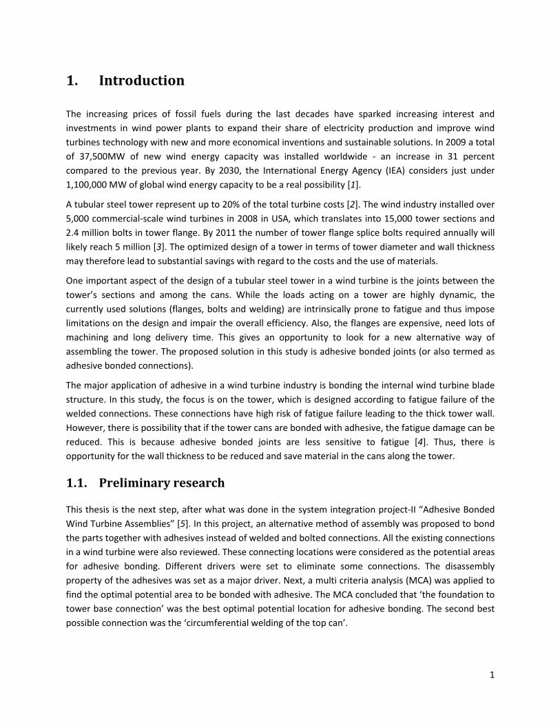
The increasing prices of fossil fuels during the last decades have sparked increasing interest and
investments in wind power plants to expand their share of electricity production and improve wind
turbines technology with new and more economical inventions and sustainable solutions. In 2009 a total
of 37,500MW of new wind energy capacity was installed worldwide - an increase in 31 percent
compared to the previous year. By 2030, the International Energy Agency (IEA) considers just under
1,100,000 MW of global wind energy capacity to be a real possibility [1].
A tubular steel tower represent up to 20% of the total turbine costs [2]. The wind industry installed over
5,000 commercial-scale wind turbines in 2008 in USA, which translates into 15,000 tower sections and
2.4 million bolts in tower flange. By 2011 the number of tower flange splice bolts required annually will
likely reach 5 million [3]. The optimized design of a tower in terms of tower diameter and wall thickness
may therefore lead to substantial savings with regard to the costs and the use of materials.
One important aspect of the design of a tubular steel tower in a wind turbine is the joints between the
tower’s sections and among the cans. While the loads acting on a tower are highly dynamic, the
currently used solutions (flanges, bolts and welding) are intrinsically prone to fatigue and thus impose
limitations on the design and impair the overall efficiency. Also, the flanges are expensive, need lots of
machining and long delivery time. This gives an opportunity to look for a new alternative way of
assembling the tower. The proposed solution in this study is adhesive bonded joints (or also termed as
adhesive bonded connections).
The major application of adhesive in a wind turbine industry is bonding the internal wind turbine blade
structure. In this study, the focus is on the tower, which is designed according to fatigue failure of the
welded connections. These connections have high risk of fatigue failure leading to the thick tower wall.
However, there is possibility that if the tower cans are bonded with adhesive, the fatigue damage can be
reduced. This is because adhesive bonded joints are less sensitive to fatigue [4]. Thus, there is
opportunity for the wall thickness to be reduced and save material in the cans along the tower.
1.1. Preliminary research
This thesis is the next step, after what was done in the system integration project-II “Adhesive Bonded
Wind Turbine Assemblies” [5]. In this project, an alternative method of assembly was proposed to bond
the parts together with adhesives instead of welded and bolted connections. All the existing connections
in a wind turbine were also reviewed. These connecting locations were considered as the potential areas
for adhesive bonding. Different drivers were set to eliminate some connections. The disassembly
property of the adhesives was set as a major driver. Next, a multi criteria analysis (MCA) was applied to
find the optimal potential area to be bonded with adhesive. The MCA concluded that ‘the foundation to
tower base connection’ was the best optimal potential location for adhesive bonding. The second best
possible connection was the ‘circumferential welding of the top can’.
2
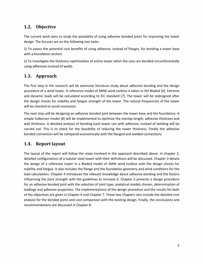
1.2. Objective
The current work aims to study the possibility of using adhesive bonded joints for improving the tower
design. The focuses are on the following two tasks:
1) To assess the potential cost benefits of using adhesive, instead of flanges, for bonding a tower base
with a foundation section.
2) To investigate the thickness optimization of entire tower when the cans are bonded circumferentially
using adhesives instead of welds.
1.3. Approach
The first step in the research will be extensive literature study about adhesive bonding and the design
procedure of a wind tower. A reference model of 3MW wind turbine is taken in GH Bladed [6]. Extreme
and dynamic loads will be calculated according to IEC standard [7]. The tower will be redesigned after
the design checks for stability and fatigue strength of the tower. The natural frequencies of the tower
will be checked to avoid resonance
The next step will be designing an adhesive bonded joint between the tower base and the foundation. A
simple Volkersen model [8] will be implemented to optimize the overlap length, adhesive thickness and
wall thickness. A detailed analysis of bonding each tower can with adhesive, instead of welding will be
carried out. This is to check for the feasibility of reducing the tower thickness. Finally the adhesive
bonded connection will be compared economically with the flanged and welded connections.
1.4. Report layout
The layout of the report will follow the steps involved in the approach described above. In chapter 2,
detailed configurations of a tubular steel tower with their definitions will be discussed. Chapter 3 details
the design of a reference tower in a Bladed model of 3MW wind turbine with the design checks for
stability and fatigue. It also includes the flange and the foundation geometry and wind conditions for the
load calculations. Chapter 4 introduces the relevant knowledge about adhesive bonding and the factors
influencing the joint strength with the guidelines to increase it. Chapter 5 presents a design procedure
for an adhesive bonded joint with the selection of joint type, analytical models chosen, determination of
loadings and adhesive properties. The implementations of the design procedure and the results for both
of the objectives are given in Chapter 6 and Chapter 7. These two chapters also include the detailed cost
analysis for the bonded joints and cost comparison with the existing design. Finally, the conclusions and
recommendations are discussed in Chapter 8.
3
2. Tubular steel tower
2.1. Introduction
A wind turbine tower supports the nacelle and the rotor at the top of a wind turbine. It provides rotor a
necessary elevation up to a level where higher and more uniform speeds are found. Most modern
turbines installed onshore are multi-megawatt machines with nominal outputs between 1.5MW and
3MW. Their rotor diameters range between 70m and 100m. Nowadays, tubular towers dominate the
wind turbine market as they are a prominent compromise between economical, aesthetical and safety
considerations.
This section will deal primarily with the detailed configurations of a tubular steel tower. Different parts
of the tower will be defined. These definitions will be used throughout the report.
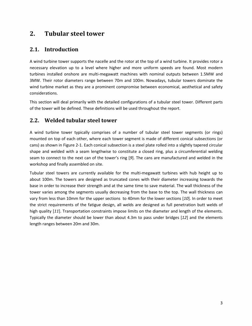
2.2. Welded tubular steel tower
A wind turbine tower typically comprises of a number of tubular steel tower segments (or rings)
mounted on top of each other, where each tower segment is made of different conical subsections (or
cans) as shown in Figure 2-1. Each conical subsection is a steel plate rolled into a slightly tapered circular
shape and welded with a seam lengthwise to constitute a closed ring, plus a circumferential welding
seam to connect to the next can of the tower’s ring [9]. The cans are manufactured and welded in the
workshop and finally assembled on site.
Tubular steel towers are currently available for the multi-megawatt turbines with hub height up to
about 100m. The towers are designed as truncated cones with their diameter increasing towards the
base in order to increase their strength and at the same time to save material. The wall thickness of the
tower varies among the segments usually decreasing from the base to the top. The wall thickness can
vary from less than 10mm for the upper sections to 40mm for the lower sections [10]. In order to meet
the strict requirements of the fatigue design, all welds are designed as full penetration butt welds of
high quality [11]. Transportation constraints impose limits on the diameter and length of the elements.
Typically the diameter should be lower than about 4.3m to pass under bridges [12] and the elements
length ranges between 20m and 30m.
4
Figure 2-1: Construction of a tubular steel tower from welded cans [13] → flanged tower segment →complete tower
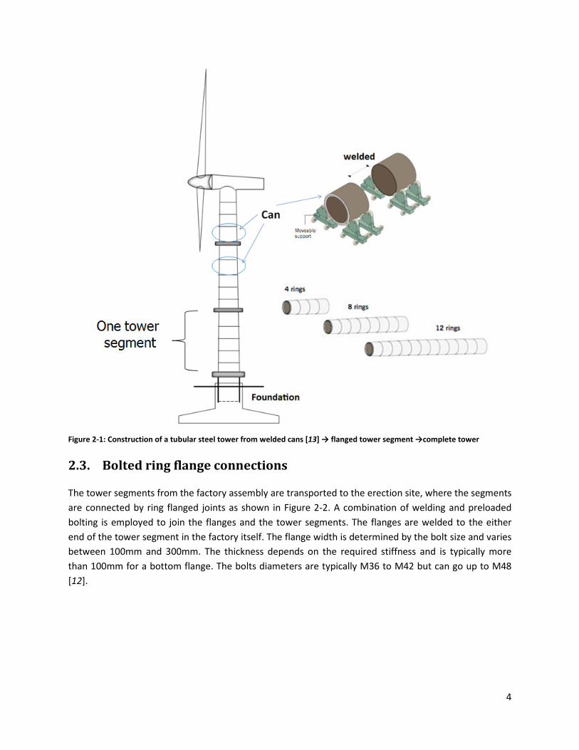
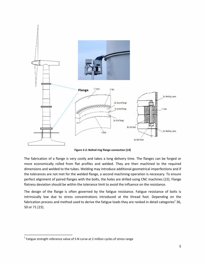
2.3. Bolted ring flange connections
The tower segments from the factory assembly are transported to the erection site, where the segments
are connected by ring flanged joints as shown in Figure 2-2. A combination of welding and preloaded
bolting is employed to join the flanges and the tower segments. The flanges are welded to the either
end of the tower segment in the factory itself. The flange width is determined by the bolt size and varies
between 100mm and 300mm. The thickness depends on the required stiffness and is typically more
than 100mm for a bottom flange. The bolts diameters are typically M36 to M42 but can go up to M48
[12].
5
Figure 2-2: Bolted ring flange connection [14]
The fabrication of a flange is very costly and takes a long delivery time. The flanges can be forged or
more economically rolled from flat profiles and welded. They are then machined to the required
dimensions and welded to the tubes. Welding may introduce additional geometrical imperfections and if
the tolerances are not met for the welded flange, a second machining operation is necessary. To ensure
perfect alignment of paired flanges with the bolts, the holes are drilled using CNC machines [15]. Flange
flatness deviation should be within the tolerance limit to avoid the influence on the resistance.
The design of the flange is often governed by the fatigue resistance. Fatigue resistance of bolts is
intrinsically low due to stress concentrations introduced at the thread foot. Depending on the
fabrication process and method used to derive the fatigue loads they are ranked in detail categories1 36,
50 or 71 [15].
1 Fatigue strength reference value of S-N curve at 2 million cycles of stress range

6
7
3. Design of a reference tower with flanges and welds
This chapter starts with the explanation for the purpose of designing a reference tower. The factors
governing its design are also discussed. It also includes the tower preliminary design procedures,
reference wind turbine model in GH bladed, the flange and foundation geometry, wind conditions and
the design loads. The design checks to be performed are discussed briefly along with the S-N curve for
the typical welds in a tower. The chapter concludes with the designed wall thicknesses along the tower
height.
3.1. Introduction
The current assembly solutions for a wind turbine tower are the flanged and the welded connections.
The new assembly solution proposed in this research work is the adhesive bonded joint. A reference
tower is needed for the cost analysis of the existing and the proposed solution. In this chapter, a
preliminary design of the reference tower is presented with a focus on the flanged and welded
connections. The design of tower connections is often governed by the fatigue resistance. The design of
the flange and the tower wall thickness is both independent. The flange design is dependent on the bolt,
whose low fatigue resistance leads to oversized flange. Whereas, dimensioning of the wall thickness is
based on the fatigue resistance of the ‘welds between the cans’ and ‘flange welding to the cans’. This
leads to conclusion that the tower wall is to be designed with the focus only on the welded connections.
Therefore, the flange has not been designed in this report but for comparison, a reference flange has
been taken from the Vestas V90 turbine [16].
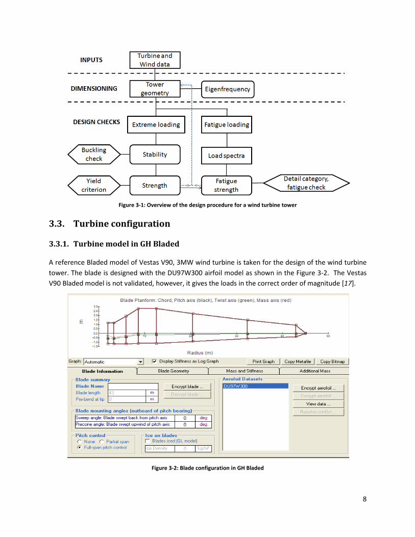
3.2. Tower design procedure
An overview of the design procedure with the main design checks is given on Figure 3-1. The first step is
to input the turbine and wind data for determining the extreme and fatigue loads on the turbine. The
tower geometry is then defined from an existing tower2. To make the design procedure simple, the
tower will be assigned a linearly varying diameter throughout the entire design, with the base and top
diameter from an existing tower. Only the thickness will be optimized according to all design checks. The
natural frequencies of turbine and tower must be adjusted to avoid resonance. Accordingly the wall
thicknesses are increased or decreased.
Using the extreme loads, it is checked whether the tower will resist failure due to buckling or yielding.
Subsequently, a fatigue check is performed for 20 years of turbine operation. If the extreme load checks
and the fatigue check indicate that the wall thickness is insufficient, the wall thickness must be
increased. If both of the checks show that the wall thickness is significantly larger than required, the wall
thickness should be reduced and the buckling and fatigue damage should be re-assessed. After
optimizing the wall thickness, the natural frequency of the support structure should be re-assessed.
2 The existing tower gives the details for tower sections, base and top diameter, bolts specifications and flanges to
be directly taken for the final design of tower (also shown in Figure 3-4).
8
Figure 3-1: Overview of the design procedure for a wind turbine tower
3.3. Turbine configuration
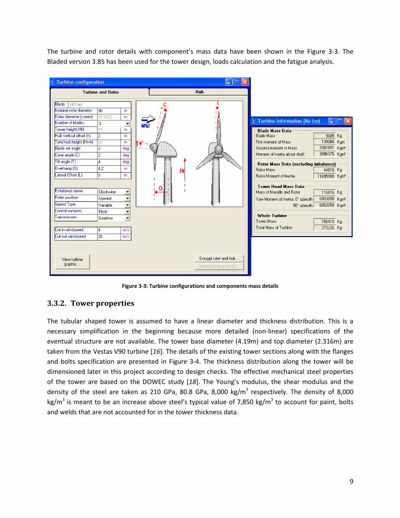
3.3.1. Turbine model in GH Bladed
A reference Bladed model of Vestas V90, 3MW wind turbine is taken for the design of the wind turbine
tower. The blade is designed with the DU97W300 airfoil model as shown in the Figure 3-2. The Vestas
V90 Bladed model is not validated, however, it gives the loads in the correct order of magnitude [17].
Figure 3-2: Blade configuration in GH Bladed
9
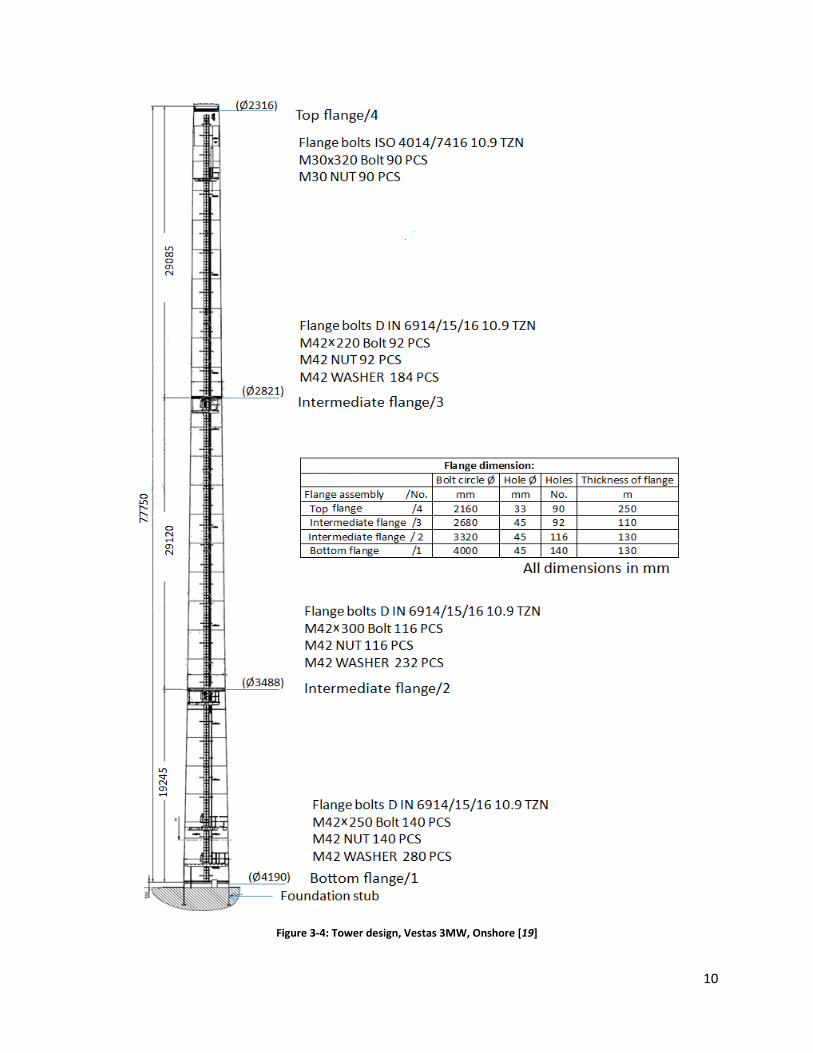
The turbine and rotor details with component’s mass data have been shown in the Figure 3-3. The
Bladed version 3.85 has been used for the tower design, loads calculation and the fatigue analysis.
Figure 3-3: Turbine configurations and components mass details
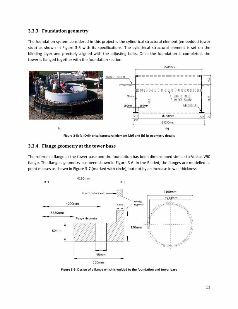
3.3.2. Tower properties
The tubular shaped tower is assumed to have a linear diameter and thickness distribution. This is a
necessary simplification in the beginning because more detailed (non-linear) specifications of the
eventual structure are not available. The tower base diameter (4.19m) and top diameter (2.316m) are
taken from the Vestas V90 turbine [16]. The details of the existing tower sections along with the flanges
and bolts specification are presented in Figure 3-4. The thickness distribution along the tower will be
dimensioned later in this project according to design checks. The effective mechanical steel properties
of the tower are based on the DOWEC study [18]. The Young’s modulus, the shear modulus and the
density of the steel are taken as 210 GPa, 80.8 GPa, 8,000 kg/m3 respectively. The density of 8,000
kg/m3 is meant to be an increase above steel’s typical value of 7,850 kg/m3 to account for paint, bolts
and welds that are not accounted for in the tower thickness data.
10
Figure 3-4: Tower design, Vestas 3MW, Onshore [19]
11
3.3.3. Foundation geometry
The foundation system considered in this project is the cylindrical structural element (embedded tower
stub) as shown in Figure 3-5 with its specifications. The cylindrical structural element is set on the
blinding layer and precisely aligned with the adjusting bolts. Once the foundation is completed, the
tower is flanged together with the foundation section.
Figure 3-5: (a) Cylindrical structural element [20] and (b) its geometry details
3.3.4. Flange geometry at the tower base
The reference flange at the tower base and the foundation has been dimensioned similar to Vestas V90
flange. The flange’s geometry has been shown in Figure 3-6. In the Bladed, the flanges are modelled as
point masses as shown in Figure 3-7 (marked with circle), but not by an increase in wall thickness.
Figure 3-6: Design of a flange which is welded to the foundation and tower base

12
3.3.5. Tower input in GH Bladed
The tower diameter is assumed to be linearly tapered from tower base (4.19m) to tower top (2.316m) as
shown in the table of Figure 3-7. The diameter will not be optimized throughout the design procedure.
To begin with the wall thickness optimization, the thickness has been varied linearly from 30mm at the
base to 14mm at the top. At the top, a flange with 250mm thickness has been welded to raise the tower
height up to 78m. The addition of hub vertical offset (2m) brings the hub height to 80m. The input
specification for the structural properties of tower is shown in the Figure 3-7.
The structural damping3 of the tower is assumed to have a damping of 1% of critical damping4 in all
modes of the tower (without the top mass present), which corresponds to the values used in the
DOWEC study [18].
Figure 3-7: The Bladed input of initial tower properties along with the flanges as point masses
3 The structural damping of a system is usually defined as the percentage decrease of two peaks of an oscillation
and this value is called as the logarithmic damping decrement δ. 4 Critical damping (ζ) is the amount of damping at which system returns to equilibrium as quickly as possible
without oscillating. (ζ = δ/(2π))
Top Flange
Intermediate
Flange 2
Intermediate
Flange 1
Bottom
Flange
13
3.4. IEC class and Wind conditions
IEC Class
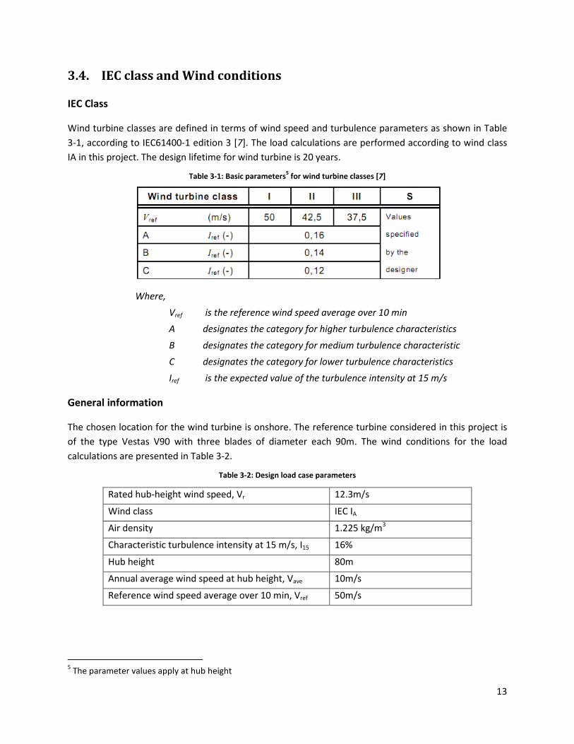
Wind turbine classes are defined in terms of wind speed and turbulence parameters as shown in Table
3-1, according to IEC61400-1 edition 3 [7]. The load calculations are performed according to wind class
IA in this project. The design lifetime for wind turbine is 20 years.
Table 3-1: Basic parameters5 for wind turbine classes [7]
Where,
Vref is the reference wind speed average over 10 min
A designates the category for higher turbulence characteristics
B designates the category for medium turbulence characteristic
C designates the category for lower turbulence characteristics
Iref is the expected value of the turbulence intensity at 15 m/s
General information
The chosen location for the wind turbine is onshore. The reference turbine considered in this project is
of the type Vestas V90 with three blades of diameter each 90m. The wind conditions for the load
calculations are presented in Table 3-2.
Table 3-2: Design load case parameters
Rated hub-height wind speed, Vr 12.3m/s
Wind class IEC IA
Air density 1.225 kg/m3
Characteristic turbulence intensity at 15 m/s, I15 16%
Hub height 80m
Annual average wind speed at hub height, Vave 10m/s
Reference wind speed average over 10 min, Vref 50m/s
5 The parameter values apply at hub height
14
Wind conditions are the primary external conditions affecting the structural integrity. The wind regime
for load and safety considerations is divided into the normal wind conditions, which will occur
frequently during normal operation of a wind turbine, and the extreme wind conditions that are defined
as having a 1-year or 50-year recurrence period.
The wind conditions include a constant mean flow combined, in many cases, with either a varying
deterministic gust profile or with turbulence. In all cases, the influence of an inclination of the mean
flow with respect to a horizontal plane of up to 8° is considered. The expression turbulence denotes
variability in the wind speed from 10 min. averages.
The longitudinal turbulence scale parameter, Λ1, at hub height E is given by
F8 = H0.7E E ≤ 60L42L E ≥ 60LO 3-1
Based on the normal and extreme wind conditions, the following models are defined:
• Normal wind models
− Wind speed distribution
− Normal Wind Profile (NWP)
− Normal Turbulence Model (NTM)
• Extreme wind models
− Extreme Wind speed Model (EWM)
− Extreme Operating Gust (EOG)
− Extreme Turbulence Model (ETM)
The turbulent variation in wind speed has been modeled using a one component Von Karman model
with a characteristic turbulence intensity set according to the Normal Turbulence Model (as defined in
IEC 61400-1 edition 3).
In the following paragraphs, the wind models are described for the chosen wind class IA according to IEC
standard.
Wind speed distribution
The wind speed distribution at the site is significant for the wind turbine design, because it determines
the frequency of occurrence of the individual load components. The wind speed distribution is given by
the probability density function, which is used to describe the distribution of wind speeds over an
extended period of time. The distribution function for most sites is expressed by Weibull distribution as:
PQ(RSTU) = 1 − exp [−(RSTU/[)\] 3-2
^ℎ`a`: Rcde = f [Г(1 + 1i)[√k/2, lm i = 2O
15
For design in the standard wind turbine classes, the Rayleigh distribution shall be taken for the load
calculations. The Rayleigh function is identical to the Weibull function if k = 2 is selected and is given by
Pn(RSTU) = 1 − exp [−k(RSTU/2Rcde)o] 3-3
Where
PQ(RSTU) is Weibull probability function
Pn(RSTU) is Rayleigh probability function
RSTU is 10-min mean of the wind speed at hub height [m/s]
Rcde is the annual mean wind speed [m/s] = 0.2Rpeq
C is the scale parameter of the Weibull function [m/s]
k is the shape parameter of the Weibull function
Г is the gamma function
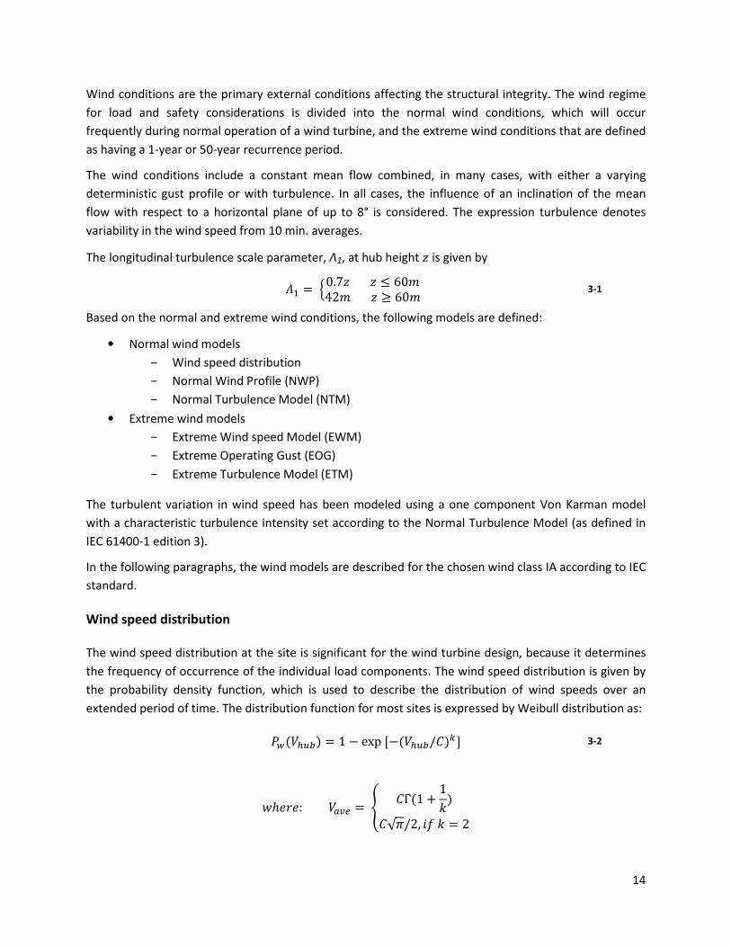
The Weibull wind speed distribution at hub height for annual mean wind speed of 10m/s and Weibull
shape factor 2 is shown in Figure 3-8.
Figure 3-8: Wind speed distribution from GH Bladed
Normal Wind Profile Model (NWM)
The wind profile, R(E) denotes the average wind speed as a function of height E, above the ground. The
assumed wind profile is used to define the average vertical wind shear across the rotor swept area.

16
R(E) = RSTU r EESTUst.o 3-4
Where
R(E) is wind speed at the height z [m/s]
E is height above ground [m]
Normal Turbulence Model (NTM)
For the normal turbulence model, the representative value of the turbulence standard deviation, σ1,
shall be given by the 90 % quantile for the given hub height wind speed. This value for the standard wind
turbine classes shall be given by
u8 = 0.16 ∙ (0.75 ∗ RSTU + 5.6) 3-5
The turbulence intensity is given by
wxTpU = u8RSTU 3-6
Extreme Wind Speed Model (EWM)
The EWM can be either a steady or a turbulent wind model. The wind models are based on the
reference wind speed, Vref, and a fixed turbulence standard deviation, σ1. For the turbulent extreme
wind speed model, the 10 min average wind speeds as functions of z with recurrence periods of 50 years
and 1 year, respectively, are given by
Ryt(E) = Rpeq ∙ r EESTUst.88 3-7
R8(E) = 0.8 ∗ Reyt(E) 3-8
Where
R{(E) The expected extreme wind speed (averaged over 10 minutes), with
a recurrence period of N years. V1 and V50 represent 1 and 50 years.
The longitudinal turbulence standard deviation6 is defined as
u8 = 0.11 ∙ RSTU 3-9
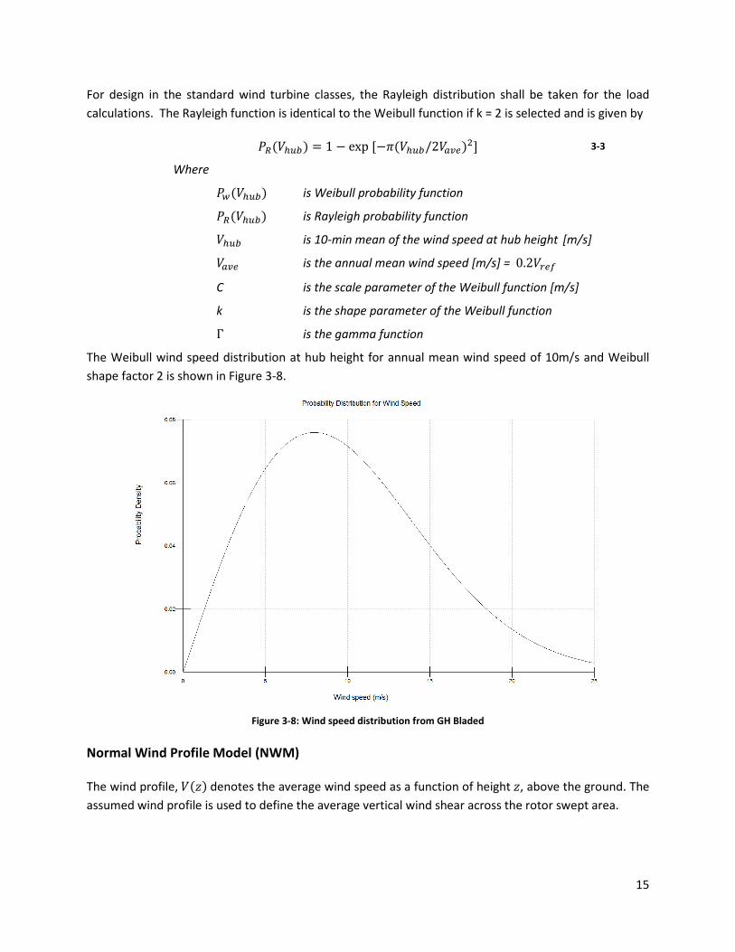
Extreme Operating Gust (EOG)
The extreme operating gust EOG50 is also known as the ‘Mexican hat’. It is the ‘worst gust’ to be
expected during operation with a recurrence period of 50 years. The hub height gust magnitude Vgust for
the wind turbine class A is given by the following relationship:
6 The turbulence standard deviation for the turbulent extreme wind model is not related to the NTM or ETM
17
R|T}x = ~l� �1.35(Re8 − RSTU); 3.3 � u81 + 0.1 ∙ � �F8��� 3-10
Where
u8 is given in equation 3-5
F8 is the turbulence scale parameter, according to the equation 3-1
D is the rotor diameter
The wind speed as a function of height and time is defined as following:
R(E, �) = �R(E) − 0.37 ∙ R|T}x ∙ �l� r3k�� s r1 − ��� �2k�� �s m�a 0 ≤ � ≤ �R(E) ��ℎ`a^l�` O 3-11
Where
R(E) is defined in equation 3-4
T is 10.5s
As an example, for our case at Vhub = 25m/s, the extreme operating gust is shown in Figure 3-9
Figure 3-9: Extreme operating gust at Vhub = 25m/s
Extreme Turbulence Model (ETM)
The extreme turbulence model uses the normal wind profile model given by equation 3-4 and
turbulence with longitudinal component standard deviation given by
u8 = � ∙ wpeq r0.072 ∙ rRcde� + 3s ∙ rRSTU� − 4s + 10s ; � = 2L/� 3-12
18
3.5. Design loads
3.5.1. Static loads
The main loads acting on a wind turbine tower are:
� the self weight of the different elements, including the rotor, the nacelle and all the machinery,
� the actions of the wind (thrust and drag) on the blades, and,
� the wind pressure on the tower.
The static design loads usually are derived from information of the wind speed and its direction; with
help of simplified models including the geometrical properties of the tower. The static loads are
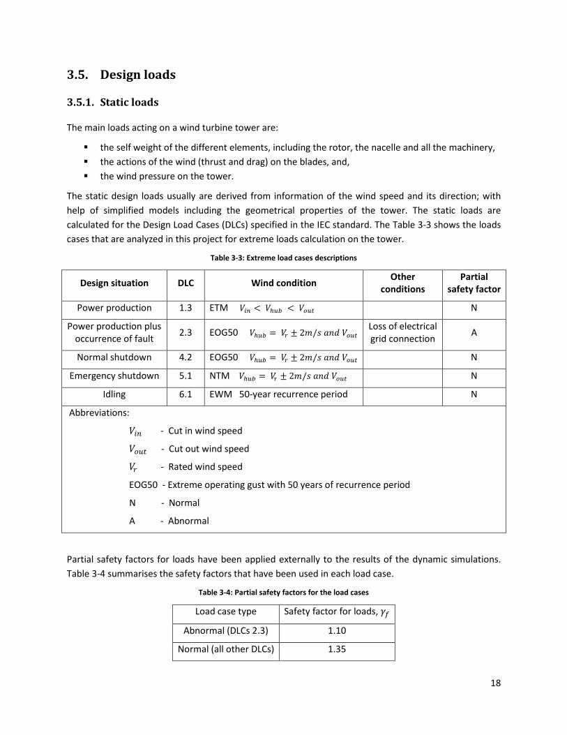
calculated for the Design Load Cases (DLCs) specified in the IEC standard. The Table 3-3 shows the loads
cases that are analyzed in this project for extreme loads calculation on the tower.
Table 3-3: Extreme load cases descriptions
Design situation DLC Wind condition Other
conditions
Partial
safety factor
Power production 1.3 ETM R�� < RSTU < R�Tx N
Power production plus
occurrence of fault 2.3 EOG50 RSTU = Rp ± 2L/� ��� R�Tx
Loss of electrical
grid connection A
Normal shutdown 4.2 EOG50 RSTU = Rp ± 2L/� ��� R�Tx N
Emergency shutdown 5.1 NTM RSTU = Rp ± 2L/� ��� R�Tx N
Idling 6.1 EWM 50-year recurrence period N
Abbreviations:
R�� - Cut in wind speed
R�Tx - Cut out wind speed
Rp - Rated wind speed
EOG50 - Extreme operating gust with 50 years of recurrence period
N - Normal
A - Abnormal
Partial safety factors for loads have been applied externally to the results of the dynamic simulations.
Table 3-4 summarises the safety factors that have been used in each load case.
Table 3-4: Partial safety factors for the load cases
Load case type Safety factor for loads, �q
Abnormal (DLCs 2.3) 1.10
Normal (all other DLCs) 1.35
19
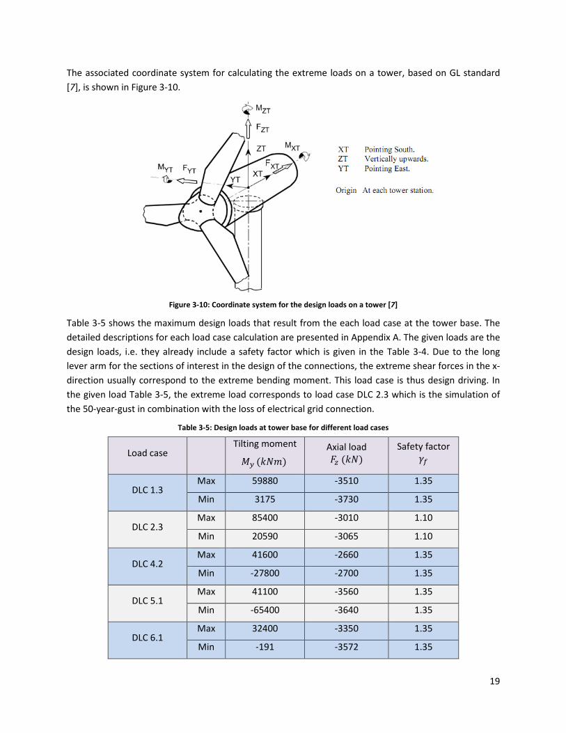
The associated coordinate system for calculating the extreme loads on a tower, based on GL standard
[7], is shown in Figure 3-10.
Figure 3-10: Coordinate system for the design loads on a tower [7]
Table 3-5 shows the maximum design loads that result from the each load case at the tower base. The
detailed descriptions for each load case calculation are presented in Appendix A. The given loads are the
design loads, i.e. they already include a safety factor which is given in the Table 3-4. Due to the long
lever arm for the sections of interest in the design of the connections, the extreme shear forces in the x-
direction usually correspond to the extreme bending moment. This load case is thus design driving. In
the given load Table 3-5, the extreme load corresponds to load case DLC 2.3 which is the simulation of
the 50-year-gust in combination with the loss of electrical grid connection.
Table 3-5: Design loads at tower base for different load cases
Load case Tilting moment ~� (i�L) Axial load �� (i�)
Safety factor �q
DLC 1.3 Max 59880 -3510 1.35
Min 3175 -3730 1.35
DLC 2.3 Max 85400 -3010 1.10
Min 20590 -3065 1.10
DLC 4.2 Max 41600 -2660 1.35
Min -27800 -2700 1.35
DLC 5.1 Max 41100 -3560 1.35
Min -65400 -3640 1.35
DLC 6.1 Max 32400 -3350 1.35
Min -191 -3572 1.35
20
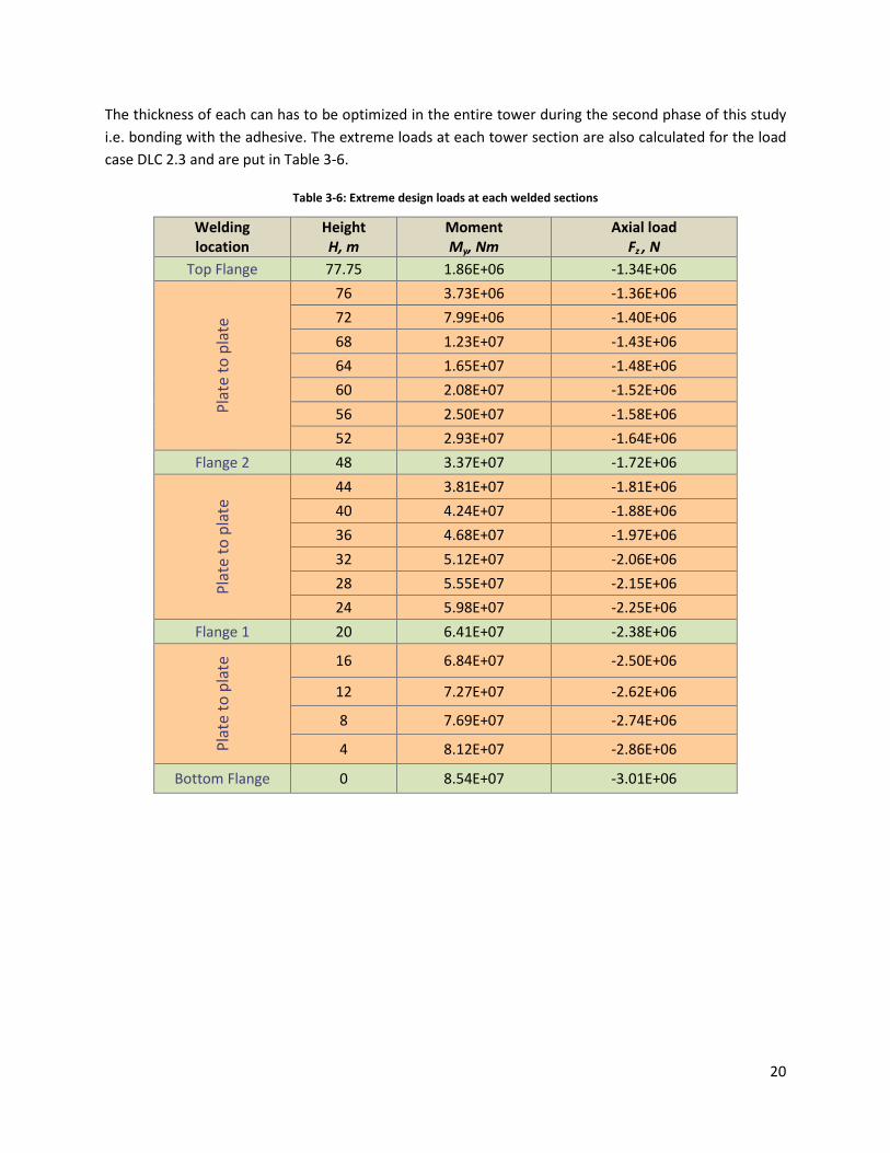
The thickness of each can has to be optimized in the entire tower during the second phase of this study
i.e. bonding with the adhesive. The extreme loads at each tower section are also calculated for the load
case DLC 2.3 and are put in Table 3-6.
Table 3-6: Extreme design loads at each welded sections
Welding
location
Height
H, m
Moment
My, Nm
Axial load
Fz , N
Top Flange 77.75 1.86E+06 -1.34E+06
Pla
te t
o p
late
76 3.73E+06 -1.36E+06
72 7.99E+06 -1.40E+06
68 1.23E+07 -1.43E+06
64 1.65E+07 -1.48E+06
60 2.08E+07 -1.52E+06
56 2.50E+07 -1.58E+06
52 2.93E+07 -1.64E+06
Flange 2 48 3.37E+07 -1.72E+06
Pla
te t
o p
late
44 3.81E+07 -1.81E+06
40 4.24E+07 -1.88E+06
36 4.68E+07 -1.97E+06
32 5.12E+07 -2.06E+06
28 5.55E+07 -2.15E+06
24 5.98E+07 -2.25E+06
Flange 1 20 6.41E+07 -2.38E+06
Pla
te t
o p
late
16 6.84E+07 -2.50E+06
12 7.27E+07 -2.62E+06
8 7.69E+07 -2.74E+06
4 8.12E+07 -2.86E+06
Bottom Flange 0 8.54E+07 -3.01E+06
21
3.5.2. Fatigue loads
Fatigue loads are cyclic loads or repetitive loads, which cause cumulative damage in the materials of the
structural components, and which eventually lead to structural failure. Fatigue loads are usually loads
well below the load level that will cause static failure, and many load cycles are required before a fatigue
failure will take place. This is commonly referred to as high-cycle fatigue. However, if the applied loads
are high enough to cause plastic deformation, the fatigue life is considerably shorter and this is termed
low cycle fatigue. Fatigue failure takes place by the initiation and propagation of a crack until the crack
becomes unstable and propagates fast, if not suddenly, to failure. In some materials a limit is seen,
below which fatigue failure does not occur, or fatigue damage progresses at a low enough rate to be
considered negligible. This is known as the endurance limit or fatigue threshold.
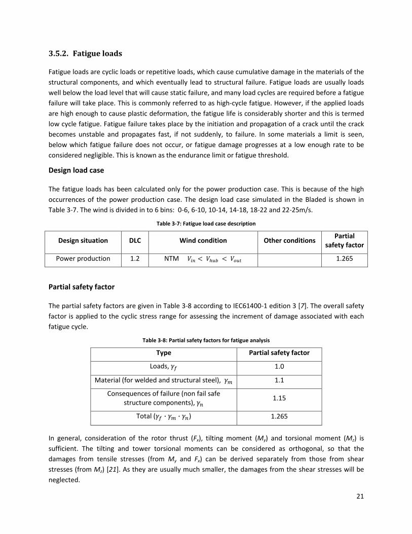
Design load case
The fatigue loads has been calculated only for the power production case. This is because of the high
occurrences of the power production case. The design load case simulated in the Bladed is shown in
Table 3-7. The wind is divided in to 6 bins: 0-6, 6-10, 10-14, 14-18, 18-22 and 22-25m/s.
Table 3-7: Fatigue load case description
Design situation DLC Wind condition Other conditions Partial
safety factor
Power production 1.2 NTM R�� < RSTU < R�Tx 1.265
Partial safety factor
The partial safety factors are given in Table 3-8 according to IEC61400-1 edition 3 [7]. The overall safety
factor is applied to the cyclic stress range for assessing the increment of damage associated with each
fatigue cycle.
Table 3-8: Partial safety factors for fatigue analysis
Type Partial safety factor
Loads, �q 1.0
Material (for welded and structural steel), �� 1.1
Consequences of failure (non fail safe
structure components), �� 1.15
Total (�q ∙ �� ∙ ��) 1.265
In general, consideration of the rotor thrust (Fx), tilting moment (My) and torsional moment (Mz) is
sufficient. The tilting and tower torsional moments can be considered as orthogonal, so that the
damages from tensile stresses (from My and Fx) can be derived separately from those from shear
stresses (from Mz) [21]. As they are usually much smaller, the damages from the shear stresses will be
neglected.
22
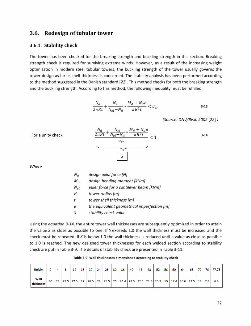
3.6. Redesign of tubular tower
3.6.1. Stability check
The tower has been checked for the breaking strength and buckling strength in this section. Breaking
strength check is required for surviving extreme winds. However, as a result of the increasing weight
optimisation in modern steel tubular towers, the buckling strength of the tower usually governs the
tower design as far as shell thickness is concerned. The stability analysis has been performed according
to the method suggested in the Danish standard [22]. This method checks for both the breaking strength
and the buckling strength. According to this method, the following inequality must be fulfilled
��2k�� + �e��e�−�� ∗ ~� + ��`k�o� < u p 3-13
(Source: DNV/Risø, 2002 [22] )
For a unity check
��2k�� + �e��e�−�� ∗ ~� + ��`k�o�u p < 1 3-14
Where
�� design axial force [N]
~� design bending moment [kNm]
�e� euler force for a cantilever beam [kNm]
� tower radius [m]
� tower shell thickness [m]
` the equivalent geometrical imperfection [m]
¡ stability check value
Using the equation 3-14, the entire tower wall thicknesses are subsequently optimized in order to attain
the value ¡ as close as possible to one. If ¡ exceeds 1.0 the wall thickness must be increased and the
check must be repeated. If ¡ is below 1.0 the wall thickness is reduced until a value as close as possible
to 1.0 is reached. The new designed tower thicknesses for each welded section according to stability
check are put in Table 3-9. The details of stability check are presented in Table 3-11.
Table 3-9: Wall thicknesses dimensioned according to stability check
¡
23
3.6.2. Fatigue check
To ensure that a structure will fulfill its intended function, fatigue assessment should be carried out for
each type of structural detail, which is subjected to extensive dynamic loading. The extent of the
analysis is influenced by the local stress range and/or the number of cycles due to fluctuating loads on
the structure. Wind loading on the turbine is the main source of potential fatigue cracking. Fatigue
design can be carried out by methods based on S-N curves from fatigue tests in the laboratory and/or
methods based on fracture mechanics. In this project, the former method has been used for fatigue
assessment according to Palmgren-Miner’s rule. The fatigue check has been performed for each welded
section of the entire tower in the Bladed.
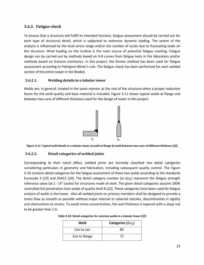
3.6.2.1. Welding details in a tubular tower
Welds are, in general, treated in the same manner as the rest of the structure when a proper reduction
factor for the weld quality and base material is included. Figure 3-11 shows typical welds at flange and
between two cans of different thickness used for the design of tower in this project.
Figure 3-11: Typical weld details in a tubular tower a) weld at flange b) weld between two cans of different thickness [22]
3.6.2.2. Detail categories of welded joints
Corresponding to their notch effect, welded joints are normally classified into detail categories
considering particulars in geometry and fabrication, including subsequent quality control. The Figure
3-10 contains detail categories for the fatigue assessment of these two welds according to the standards
Eurocode 3 [23] and DS412 [24]. The detail category number (or ∆un) represent the fatigue strength
reference value (at 2 ∙ 106 cycles) for structures made of steel. The given detail categories assume 100%
controlled full penetration butt welds of quality level B [22]. These categories have been used for fatigue
analysis of welds in the tower. Also all welded joints on primary members shall be designed to provide a
stress flow as smooth as possible without major internal or external notches, discontinuities in rigidity
and obstructions to strains. To avoid stress concentration, the wall thickness is tapered with a slope not
to be greater than 1:4.
Table 3-10: Detail categories for common welds in a tubular tower [22]
Weld Categories (∆un)
Can to can 80
Can to flange 71
24
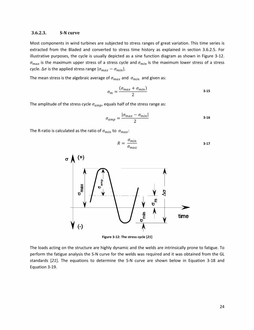
3.6.2.3. S-N curve
Most components in wind turbines are subjected to stress ranges of great variation. This time series is
extracted from the Bladed and converted to stress time history as explained in section 3.6.2.5. For
illustrative purposes, the cycle is usually depicted as a sine function diagram as shown in Figure 3-12. u�c¢ is the maximum upper stress of a stress cycle and u��� is the maximum lower stress of a stress
cycle. ∆u is the applied stress range |u�c¢ − u���|. The mean stress is the algebraic average of u�c¢ and u��� and given as:
u� = (u�c¢ + u���)2 3-15
The amplitude of the stress cycle uc�¤, equals half of the stress range as:
uc�¤ = |u�c¢ − u���|2 3-16
The R-ratio is calculated as the ratio of u��� to u�c¢:
� = u���u�c¢ 3-17
Figure 3-12: The stress cycle [21]
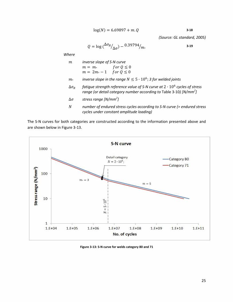
The loads acting on the structure are highly dynamic and the welds are intrinsically prone to fatigue. To
perform the fatigue analysis the S-N curve for the welds was required and it was obtained from the GL
standards [21]. The equations to determine the S-N curve are shown below in Equation 3-18 and
Equation 3-19.
25
log(�) = 6.69897 + L. ¨ 3-18
(Source: GL standard, 2005)
¨ = log (∆un ∆u© ) − 0.39794 L°© 3-19
Where
L inverse slope of S-N curve
L = L° m�a ¨ ≤ 0
L = 2L° − 1 m�a ¨ ≤ 0
L° inverse slope in the range � ≤ 5 ∙ 10; 3 for welded joints
∆un fatigue strength reference value of S-N curve at 2 ∙ 10 cycles of stress
range (or detail category number according to Table 3-10) [N/mm2]
∆u stress range [N/mm2]
� number of endured stress cycles according to S-N curve (= endured stress
cycles under constant amplitude loading)
The S-N curves for both categories are constructed according to the information presented above and
are shown below in Figure 3-13.
Figure 3-13: S-N curve for welds category 80 and 71
26
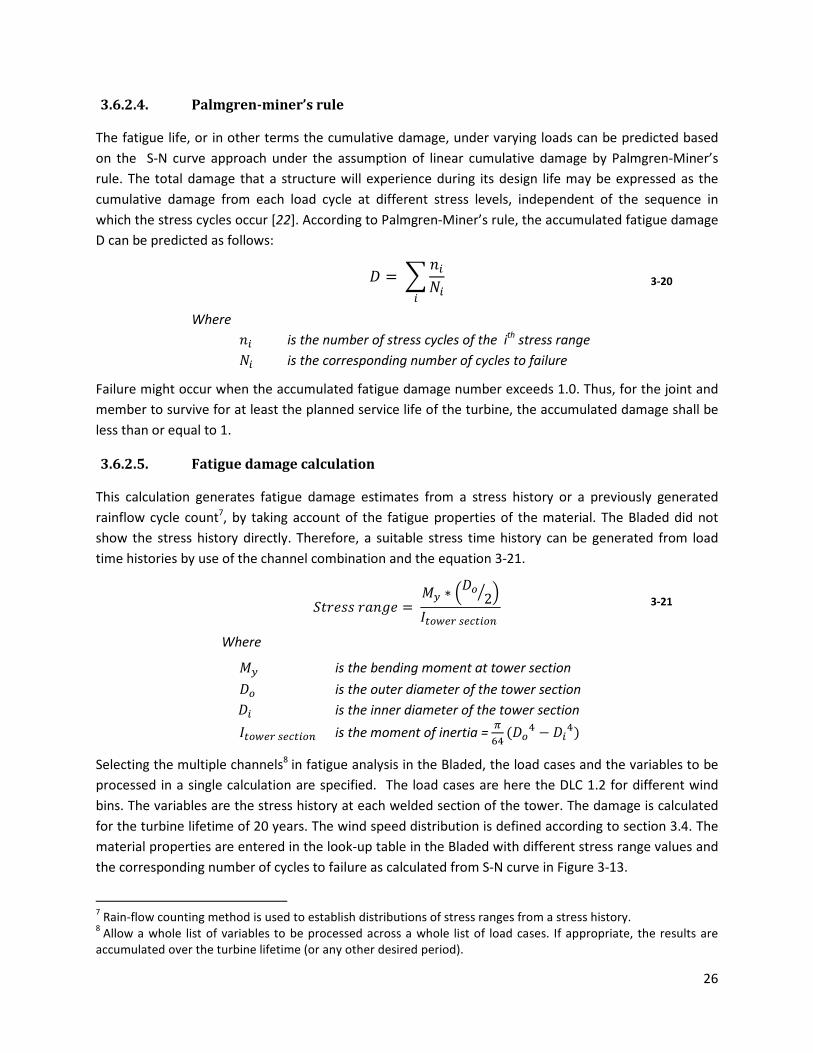
3.6.2.4. Palmgren-miner’s rule
The fatigue life, or in other terms the cumulative damage, under varying loads can be predicted based
on the S-N curve approach under the assumption of linear cumulative damage by Palmgren-Miner’s
rule. The total damage that a structure will experience during its design life may be expressed as the
cumulative damage from each load cycle at different stress levels, independent of the sequence in
which the stress cycles occur [22]. According to Palmgren-Miner’s rule, the accumulated fatigue damage
D can be predicted as follows:
� = « ����� 3-20
Where
�� is the number of stress cycles of the ith stress range
�� is the corresponding number of cycles to failure
Failure might occur when the accumulated fatigue damage number exceeds 1.0. Thus, for the joint and
member to survive for at least the planned service life of the turbine, the accumulated damage shall be
less than or equal to 1.
3.6.2.5. Fatigue damage calculation
This calculation generates fatigue damage estimates from a stress history or a previously generated
rainflow cycle count7, by taking account of the fatigue properties of the material. The Bladed did not
show the stress history directly. Therefore, a suitable stress time history can be generated from load
time histories by use of the channel combination and the equation 3-21.
¡�a`�� a��¬` = ~� ∗ ��� 2© �wx�Qep }e x��� 3-21
Where
~� is the bending moment at tower section
�� is the outer diameter of the tower section
�� is the inner diameter of the tower section
wx�Qep }e x��� is the moment of inertia = ® (��® − ��®)
Selecting the multiple channels8 in fatigue analysis in the Bladed, the load cases and the variables to be
processed in a single calculation are specified. The load cases are here the DLC 1.2 for different wind
bins. The variables are the stress history at each welded section of the tower. The damage is calculated
for the turbine lifetime of 20 years. The wind speed distribution is defined according to section 3.4. The
material properties are entered in the look-up table in the Bladed with different stress range values and
the corresponding number of cycles to failure as calculated from S-N curve in Figure 3-13.
7 Rain-flow counting method is used to establish distributions of stress ranges from a stress history.
8 Allow a whole list of variables to be processed across a whole list of load cases. If appropriate, the results are
accumulated over the turbine lifetime (or any other desired period).
27
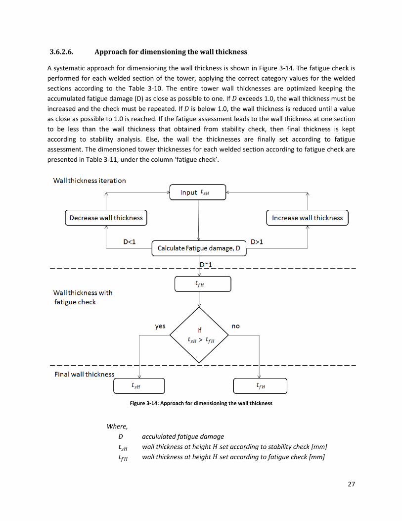
3.6.2.6. Approach for dimensioning the wall thickness
A systematic approach for dimensioning the wall thickness is shown in Figure 3-14. The fatigue check is
performed for each welded section of the tower, applying the correct category values for the welded
sections according to the Table 3-10. The entire tower wall thicknesses are optimized keeping the
accumulated fatigue damage (D) as close as possible to one. If � exceeds 1.0, the wall thickness must be
increased and the check must be repeated. If � is below 1.0, the wall thickness is reduced until a value
as close as possible to 1.0 is reached. If the fatigue assessment leads to the wall thickness at one section
to be less than the wall thickness that obtained from stability check, then final thickness is kept
according to stability analysis. Else, the wall the thicknesses are finally set according to fatigue
assessment. The dimensioned tower thicknesses for each welded section according to fatigue check are
presented in Table 3-11, under the column ‘fatigue check’.
Figure 3-14: Approach for dimensioning the wall thickness
Where,
D accululated fatigue damage
�}¯ wall thickness at height ° set according to stability check [mm]
�q¯ wall thickness at height ° set according to fatigue check [mm]
28
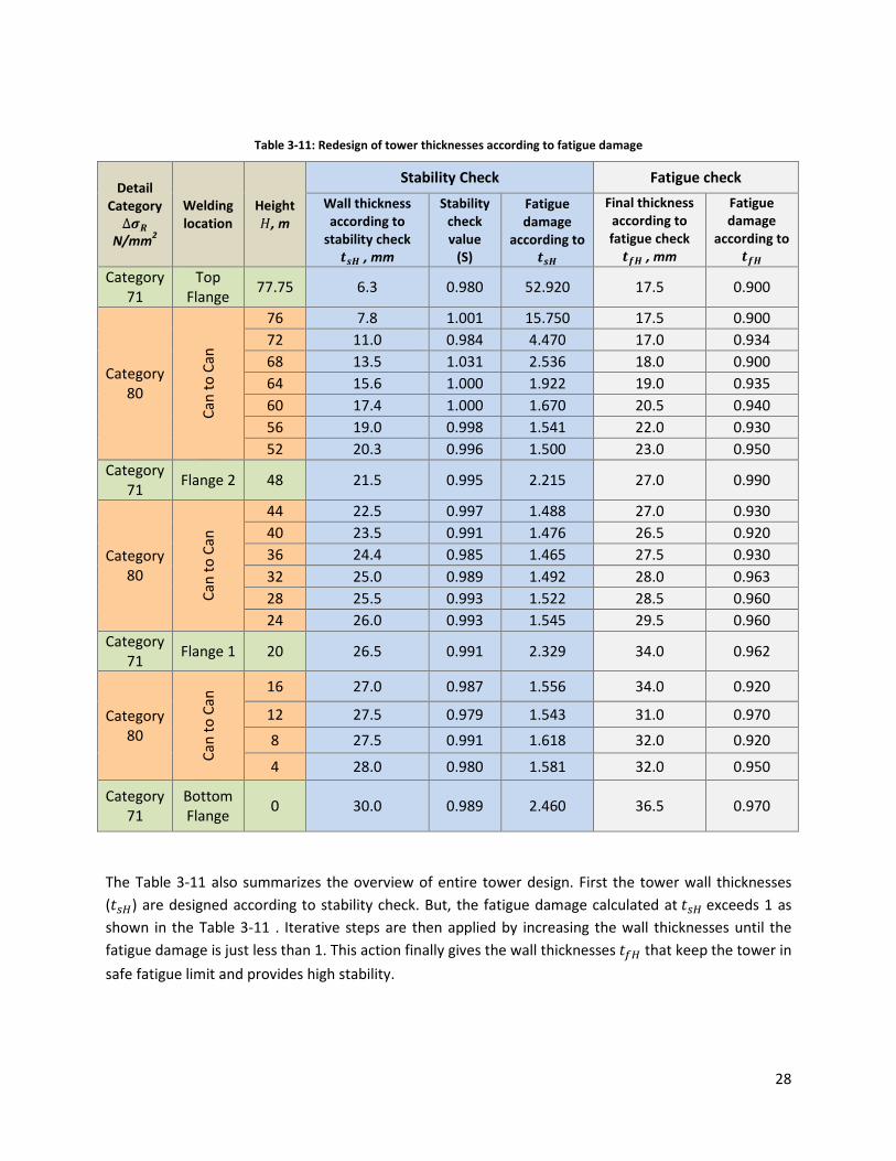
Table 3-11: Redesign of tower thicknesses according to fatigue damage
Detail
Category ∆±²
N/mm2
Welding
location
Height °, m
Stability Check Fatigue check
Wall thickness
according to
stability check ³´µ , mm
Stability
check
value
(S)
Fatigue
damage
according to ³´µ
Final thickness
according to
fatigue check ³¶µ , mm
Fatigue
damage
according to ³¶µ
Category
71
Top
Flange 77.75 6.3 0.980 52.920 17.5 0.900
Category
80
Ca
n t
o C
an
76 7.8 1.001 15.750 17.5 0.900
72 11.0 0.984 4.470 17.0 0.934
68 13.5 1.031 2.536 18.0 0.900
64 15.6 1.000 1.922 19.0 0.935
60 17.4 1.000 1.670 20.5 0.940
56 19.0 0.998 1.541 22.0 0.930
52 20.3 0.996 1.500 23.0 0.950
Category
71 Flange 2 48 21.5 0.995 2.215 27.0 0.990
Category
80
Ca
n t
o C
an
44 22.5 0.997 1.488 27.0 0.930
40 23.5 0.991 1.476 26.5 0.920
36 24.4 0.985 1.465 27.5 0.930
32 25.0 0.989 1.492 28.0 0.963
28 25.5 0.993 1.522 28.5 0.960
24 26.0 0.993 1.545 29.5 0.960
Category
71 Flange 1 20 26.5 0.991 2.329 34.0 0.962
Category
80
Ca
n t
o C
an
16 27.0 0.987 1.556 34.0 0.920
12 27.5 0.979 1.543 31.0 0.970
8 27.5 0.991 1.618 32.0 0.920
4 28.0 0.980 1.581 32.0 0.950
Category
71
Bottom
Flange 0 30.0 0.989 2.460 36.5 0.970
The Table 3-11 also summarizes the overview of entire tower design. First the tower wall thicknesses
(�}¯) are designed according to stability check. But, the fatigue damage calculated at �}¯ exceeds 1 as
shown in the Table 3-11 . Iterative steps are then applied by increasing the wall thicknesses until the
fatigue damage is just less than 1. This action finally gives the wall thicknesses �q¯ that keep the tower in
safe fatigue limit and provides high stability.
29
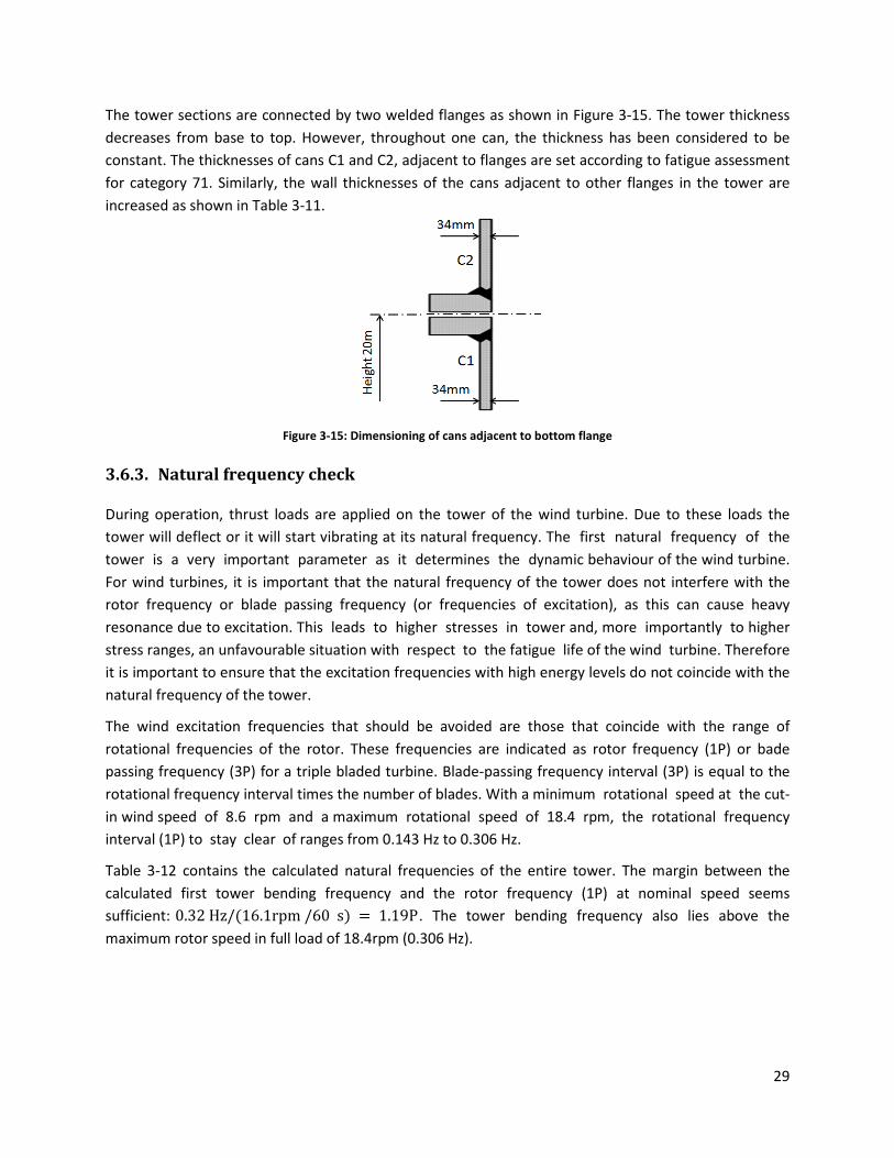
The tower sections are connected by two welded flanges as shown in Figure 3-15. The tower thickness
decreases from base to top. However, throughout one can, the thickness has been considered to be
constant. The thicknesses of cans C1 and C2, adjacent to flanges are set according to fatigue assessment
for category 71. Similarly, the wall thicknesses of the cans adjacent to other flanges in the tower are
increased as shown in Table 3-11.
Figure 3-15: Dimensioning of cans adjacent to bottom flange
3.6.3. Natural frequency check
During operation, thrust loads are applied on the tower of the wind turbine. Due to these loads the
tower will deflect or it will start vibrating at its natural frequency. The first natural frequency of the
tower is a very important parameter as it determines the dynamic behaviour of the wind turbine.
For wind turbines, it is important that the natural frequency of the tower does not interfere with the
rotor frequency or blade passing frequency (or frequencies of excitation), as this can cause heavy
resonance due to excitation. This leads to higher stresses in tower and, more importantly to higher
stress ranges, an unfavourable situation with respect to the fatigue life of the wind turbine. Therefore
it is important to ensure that the excitation frequencies with high energy levels do not coincide with the
natural frequency of the tower.
The wind excitation frequencies that should be avoided are those that coincide with the range of
rotational frequencies of the rotor. These frequencies are indicated as rotor frequency (1P) or bade
passing frequency (3P) for a triple bladed turbine. Blade-passing frequency interval (3P) is equal to the
rotational frequency interval times the number of blades. With a minimum rotational speed at the cut-
in wind speed of 8.6 rpm and a maximum rotational speed of 18.4 rpm, the rotational frequency
interval (1P) to stay clear of ranges from 0.143 Hz to 0.306 Hz.
Table 3-12 contains the calculated natural frequencies of the entire tower. The margin between the
calculated first tower bending frequency and the rotor frequency (1P) at nominal speed seems
sufficient: 0.32 Hz/(16.1rpm /60 s) = 1.19P. The tower bending frequency also lies above the
maximum rotor speed in full load of 18.4rpm (0.306 Hz).
30
Table 3-12: Tower natural frequencies from modal analysis in the Bladed
Description 1st mode, m [°E] 2nd mode, m [°E] 3rd mode, m [°E]
Fore-aft, �qc 0.32 1.83 4.10
Side-to-side, �}x} 0.32 1.54 3.80
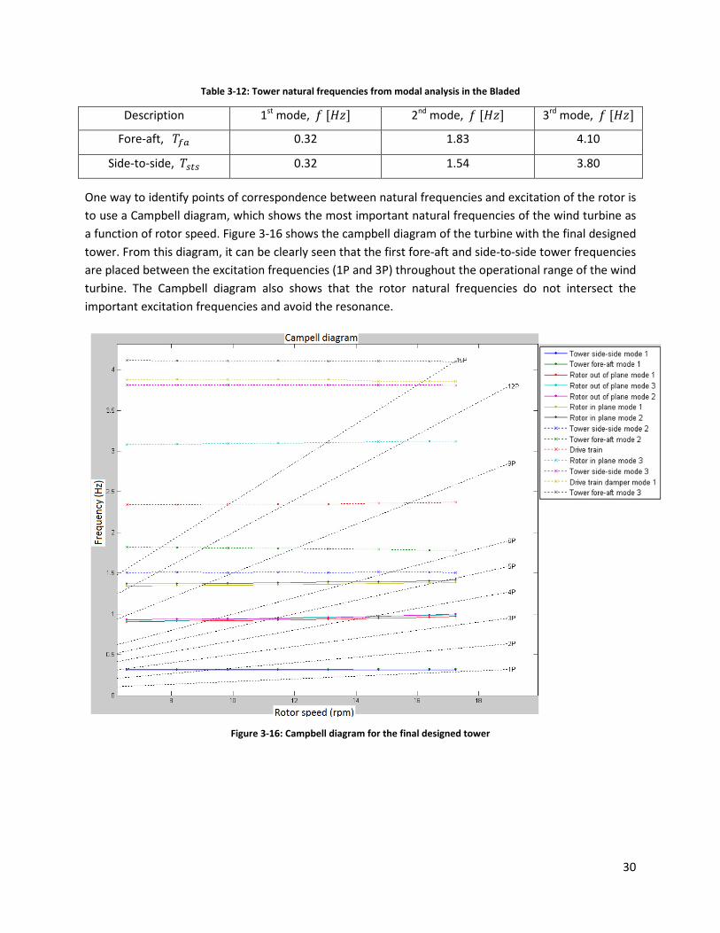
One way to identify points of correspondence between natural frequencies and excitation of the rotor is
to use a Campbell diagram, which shows the most important natural frequencies of the wind turbine as
a function of rotor speed. Figure 3-16 shows the campbell diagram of the turbine with the final designed
tower. From this diagram, it can be clearly seen that the first fore-aft and side-to-side tower frequencies
are placed between the excitation frequencies (1P and 3P) throughout the operational range of the wind
turbine. The Campbell diagram also shows that the rotor natural frequencies do not intersect the
important excitation frequencies and avoid the resonance.
Figure 3-16: Campbell diagram for the final designed tower
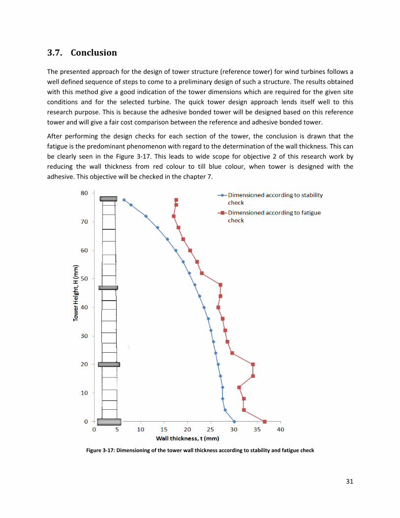
31
3.7. Conclusion
The presented approach for the design of tower structure (reference tower) for wind turbines follows a
well defined sequence of steps to come to a preliminary design of such a structure. The results obtained
with this method give a good indication of the tower dimensions which are required for the given site
conditions and for the selected turbine. The quick tower design approach lends itself well to this
research purpose. This is because the adhesive bonded tower will be designed based on this reference
tower and will give a fair cost comparison between the reference and adhesive bonded tower.
After performing the design checks for each section of the tower, the conclusion is drawn that the
fatigue is the predominant phenomenon with regard to the determination of the wall thickness. This can
be clearly seen in the Figure 3-17. This leads to wide scope for objective 2 of this research work by
reducing the wall thickness from red colour to till blue colour, when tower is designed with the
adhesive. This objective will be checked in the chapter 7.
Figure 3-17: Dimensioning of the tower wall thickness according to stability and fatigue check

32
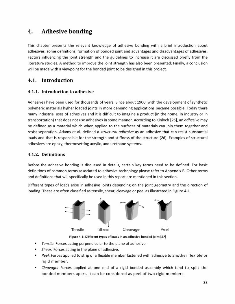
33
4. Adhesive bonding
This chapter presents the relevant knowledge of adhesive bonding with a brief introduction about
adhesives, some definitions, formation of bonded joint and advantages and disadvantages of adhesives.
Factors influencing the joint strength and the guidelines to increase it are discussed briefly from the
literature studies. A method to improve the joint strength has also been presented. Finally, a conclusion
will be made with a viewpoint for the bonded joint to be designed in this project.
4.1. Introduction
4.1.1. Introduction to adhesive
Adhesives have been used for thousands of years. Since about 1900, with the development of synthetic
polymeric materials higher loaded joints in more demanding applications became possible. Today there
many industrial uses of adhesives and it is difficult to imagine a product (in the home, in industry or in
transportation) that does not use adhesives in some manner. According to Kinloch [25], an adhesive may
be defined as a material which when applied to the surfaces of materials can join them together and
resist separation. Adams et al. defined a structural adhesive as an adhesive that can resist substantial
loads and that is responsible for the strength and stiffness of the structure [26]. Examples of structural
adhesives are epoxy, thermosetting acrylic, and urethane systems.
4.1.2. Definitions
Before the adhesive bonding is discussed in details, certain key terms need to be defined. For basic
definitions of common terms associated to adhesive technology please refer to Appendix B. Other terms
and definitions that will specifically be used in this report are mentioned in this section.
Different types of loads arise in adhesive joints depending on the joint geometry and the direction of
loading. These are often classified as tensile, shear, cleavage or peel as illustrated in Figure 4-1.
Figure 4-1: Different types of loads in an adhesive bonded joint [27]
� Tensile: Forces acting perpendicular to the plane of adhesive.
� Shear: Forces acting in the plane of adhesive.
� Peel: Forces applied to strip of a flexible member fastened with adhesive to another flexible or
rigid member.
� Cleavage: Forces applied at one end of a rigid bonded assembly which tend to split the
bonded members apart. It can be considered as peel of two rigid members.
34
Adherend: Body that is or intended to be held to another body by an adhesive.
Adhesion: Adhesion is the attraction between two substances resulting from intermolecular forces that
establish between them.
Post-cure: Further treatment by time and/or temperature of an adhesive to obtain the required
properties by curing.
Cure time: Time required to induce curing at a given temperature.
Fillet: Portion of an adhesive that bridges the adherends outside the bond-line.
Moisture: High humidity or wet conditions affecting the adhesive or adherend.
4.1.3. Adhesive bonded joint
Adhesive bonding is a joining technique similar to other joining techniques like welding, soldering,
riveting, bolting etc. What is considered as adhesive bonded joint is explained by the following
definition.
An adhesive bonded joint can be defined as a joint between two substrates of equal or different
materials by means of a non-metallic third material that has good adhesion and has also sufficient
cohesive strength to maintain the substrates fixed against each other during the operational life of the
product, despite the forces acting on the joint [28].
The formation of bonded joint can be distinguished in three stages as [29]:
� Initially, the adhesive must behave as a liquid to be spread easily on the surface. It should also
wet properly the adherends to be bonded for an intimate molecular contact between adhesive
and the surface.
� Secondly, the liquid adhesive must harden in order to support sometimes continuous and
sometimes variable load throughout their lives.
� Finally, they must transfer and distribute the load among the components in an assembly.
By preference, the load is transferred by shear stresses in the adhesive layer, whereas tensile, peel or
cleavage loads should be avoided or minimized as much as possible. The strength of the joint not only
depends on the shear strength of the adhesive itself, but also on the shear and peel stress distribution
along the length of the overlap.
Sometimes a primer is used with adhesives. A primer is a substance which is applied to a surface prior to
the application of an adhesive. This usually helps in improving the performance of the bond or
protecting the surface until the adhesive or sealant can be applied. The bonded joint is the whole part
formed by the adherends, the adhesive, the primer (if present), and the interphases and interfaces
associated to it, as shown in Figure 4-2.
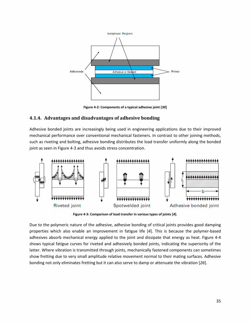
35
Figure 4-2: Components of a typical adhesive joint [30]
4.1.4. Advantages and disadvantages of adhesive bonding
Adhesive bonded joints are increasingly being used in engineering applications due to their improved
mechanical performance over conventional mechanical fasteners. In contrast to other joining methods,
such as riveting and bolting, adhesive bonding distributes the load transfer uniformly along the bonded
joint as seen in Figure 4-3 and thus avoids stress concentration.
Figure 4-3: Comparison of load transfer in various types of joints [4].
Due to the polymeric nature of the adhesive, adhesive bonding of critical joints provides good damping
properties which also enable an improvement in fatigue life [4]. This is because the polymer-based
adhesives absorb mechanical energy applied to the joint and dissipate that energy as heat. Figure 4-4
shows typical fatigue curves for riveted and adhesively bonded joints, indicating the superiority of the
latter. Where vibration is transmitted through joints, mechanically fastened components can sometimes
show fretting due to very small amplitude relative movement normal to their mating surfaces. Adhesive
bonding not only eliminates fretting but it can also serve to damp or attenuate the vibration [26].
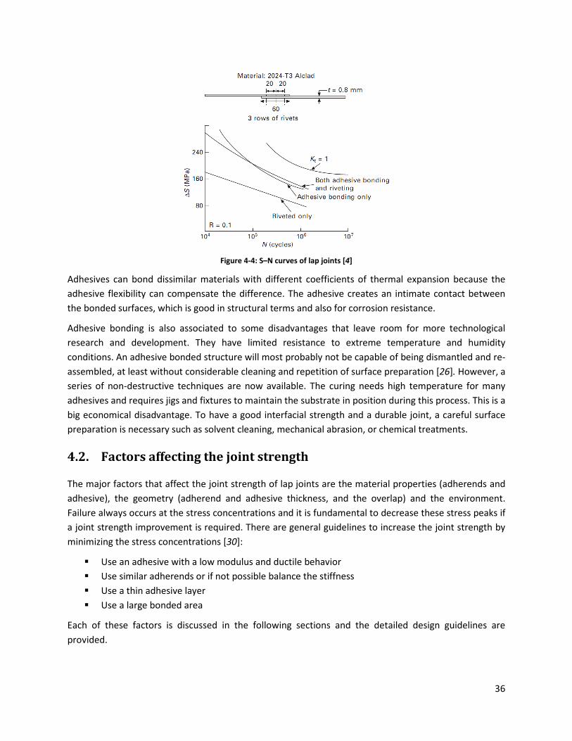
36
Figure 4-4: S–N curves of lap joints [4]
Adhesives can bond dissimilar materials with different coefficients of thermal expansion because the
adhesive flexibility can compensate the difference. The adhesive creates an intimate contact between
the bonded surfaces, which is good in structural terms and also for corrosion resistance.
Adhesive bonding is also associated to some disadvantages that leave room for more technological
research and development. They have limited resistance to extreme temperature and humidity
conditions. An adhesive bonded structure will most probably not be capable of being dismantled and re-
assembled, at least without considerable cleaning and repetition of surface preparation [26]. However, a
series of non-destructive techniques are now available. The curing needs high temperature for many
adhesives and requires jigs and fixtures to maintain the substrate in position during this process. This is a
big economical disadvantage. To have a good interfacial strength and a durable joint, a careful surface
preparation is necessary such as solvent cleaning, mechanical abrasion, or chemical treatments.
4.2. Factors affecting the joint strength
The major factors that affect the joint strength of lap joints are the material properties (adherends and
adhesive), the geometry (adherend and adhesive thickness, and the overlap) and the environment.
Failure always occurs at the stress concentrations and it is fundamental to decrease these stress peaks if
a joint strength improvement is required. There are general guidelines to increase the joint strength by
minimizing the stress concentrations [30]:
� Use an adhesive with a low modulus and ductile behavior
� Use similar adherends or if not possible balance the stiffness
� Use a thin adhesive layer
� Use a large bonded area
Each of these factors is discussed in the following sections and the detailed design guidelines are
provided.
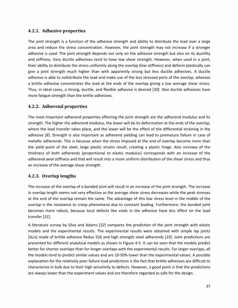
37
4.2.1. Adhesive properties
The joint strength is a function of the adhesive strength and ability to distribute the load over a large
area and reduce the stress concentration. However, the joint strength may not increase if a stronger
adhesive is used. The joint strength depends not only on the adhesive strength but also on its ductility
and stiffness. Very ductile adhesives tend to have low shear strength. However, when used in a joint,
their ability to distribute the stress uniformly along the overlap (low stiffness) and deform plastically can
give a joint strength much higher than with apparently strong but less ductile adhesives. A ductile
adhesive is able to redistribute the load and make use of the less stressed parts of the overlap, whereas
a brittle adhesive concentrates the load at the ends of the overlap giving a low average shear stress.
Thus, in ideal cases, a strong, ductile, and flexible adhesive is desired [30]. Also ductile adhesives have
more fatigue strength than the brittle adhesives.
4.2.2. Adherend properties
The most important adherend properties affecting the joint strength are the adherend modulus and its
strength. The higher the adherend modulus, the lower will be its deformation at the ends of the overlap,
where the load transfer takes place, and the lower will be the effect of the differential straining in the
adhesive [8]. Strength is also important as adherend yielding can lead to premature failure in case of
metallic adherends. This is because when the stress imposed at the end of overlap become more than
the yield point of the steel, large plastic strains result, creating a plastic hinge. Also increase of the
thickness of both adherends (proportional to elastic modulus) corresponds with an increase of the
adherend axial stiffness and that will result into a more uniform distribution of the shear stress and thus
an increase of the average shear strength.
4.2.3. Overlap lengths
The increase of the overlap of a bonded joint will result in an increase of the joint strength. The increase
in overlap length seems not very effective as the average shear stress decreases while the peak stresses
at the end of the overlap remain the same. The advantage of this low stress level in the middle of the
overlap is the resistance to creep phenomena due to constant loading. Furthermore, the bonded joint
becomes more robust, because local defects like voids in the adhesive have less effect on the load
transfer [31].
A literature survey by Silva and Adams [32] compares the prediction of the joint strength with elastic
models and the experimental results. The experimental results were obtained with simple lap joints
(SLJs) made of brittle adhesive Redux 326 and high strength steel adherends [33]. Joint predictions are
presented for different analytical models as shown in Figure 4-5. It can be seen that the models predict
better for shorter overlaps than for longer overlaps with the experimental results. For larger overlaps, all
the models tend to predict similar values and are 10-50% lower than the experimental values. A possible
explanation for the relatively poor failure load predictions is the fact that brittle adhesives are difficult to
characterize in bulk due to their high sensitivity to defects. However, a good point is that the predictions
are always lower than the experiment values and are therefore regarded as safe for the design.

38
Figure 4-5: Overlap effect on Linear analysis: brittle adhesive (Redux326) and high-strength steel [34]
4.2.4. Adhesive thicknesses
The effect of the adhesive thickness on the bond strength of single-lap adhesive joints is still not
perfectly understood. The classical elastic analyses such as those of Volkersen [8] or Goland and
Reissner [35] predict that the strength increases with the adhesive thickness, whereas experimental
results show the opposite. Practice shows that the lap-joint strength increases as the bond line gets
thinner [36]. This can be seen in literature survey by Silva and Adams [32] in which the adhesive
thickness effects for different models have been compared as shown in Figure 4-6. The experimental
joint strength decrease as the adhesive thickness increases while the linear elastic analyses shows the
opposite trend as shown in Figure 4-6.
Figure 4-6: Adhesive thickness effect on linear analysis: adhesive (Hysol 9321) and high-strength steel [32]
39
According to Crocombe [37] thicker single-lap joints have a lower strength considering the plasticity of
the adhesive. An elastic analysis shows that the stress distribution of a thin bondline is more
concentrated at the ends of the overlap than a thicker bondline, which has a more uniform stress
distribution. Therefore, a thin bondline will reach the yielding stress at a lower load than a thick
bondline. However, when yielding does occur in a thicker joint, there is a less ‘‘elastic reserve’’ to sustain
further loading, and thus, yielding spreads more quickly. Also other theories to explain the adhesive
thickness on the strength of SLJs were introduced by Gleich et al. in 2001 [38] and Grant et al (2009).
There are many theories that attempt to explain this fact and this subject is still controversial. However,
Adams and Peppiatt (1974) explained that an increase in the bondline thickness increases the
probability of having internal imperfection in the joint (voids and microcracks), which will lead to
premature failure of the joints [39].
In another investigation, Hans Nordberg [40] has shown that with the increase in the adhesive thickness
the fatigue strength also increases at the same number of cycles. For longer lives the increased bondline
thickness does not seem to affect the strength.
4.2.5. Environmental effects
Water and humidity are two of the most damaging environmental factors for adhesive. The possible
mechanisms by which water can degrade adhesive joints include [27]:
� plasticization
� swelling
� hydrolysis or crazing of the adhesive
� degradation or change of the interface resulting in loss of adhesion
� corrosion of the substrate
The fatigue life of lap joints is progressively reduced after pre-exposure to water. However, control in
water absorption does not seem to affect the fatigue properties with more than 15% as shown in Figure
4-7 [40]. The control in water absorption can be done by:
� coating (encapsulating) the exposed edges of the joint with a water resistant sealant
� using a suitable primer/coupling agent will improve interfacial durability – a fluid primer that
wets the surface will tend to fill discontinuities on the adherend surface
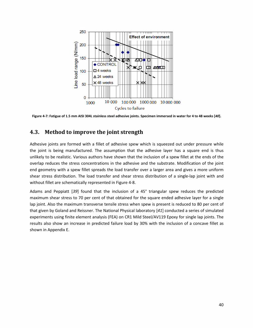
40
Figure 4-7: Fatigue of 1.5 mm AISI 304L stainless steel adhesive joints. Specimen immersed in water for 4 to 48 weeks [40].
4.3. Method to improve the joint strength
Adhesive joints are formed with a fillet of adhesive spew which is squeezed out under pressure while
the joint is being manufactured. The assumption that the adhesive layer has a square end is thus
unlikely to be realistic. Various authors have shown that the inclusion of a spew fillet at the ends of the
overlap reduces the stress concentrations in the adhesive and the substrate. Modification of the joint
end geometry with a spew fillet spreads the load transfer over a larger area and gives a more uniform
shear stress distribution. The load transfer and shear stress distribution of a single-lap joint with and
without fillet are schematically represented in Figure 4-8.
Adams and Peppiatt [39] found that the inclusion of a 45° triangular spew reduces the predicted
maximum shear stress to 70 per cent of that obtained for the square ended adhesive layer for a single
lap joint. Also the maximum transverse tensile stress when spew is present is reduced to 80 per cent of
that given by Goland and Reissner. The National Physical laboratory [41] conducted a series of simulated
experiments using finite element analysis (FEA) on CR1 Mild Steel/AV119 Epoxy for single lap joints. The
results also show an increase in predicted failure load by 30% with the inclusion of a concave fillet as
shown in Appendix E.
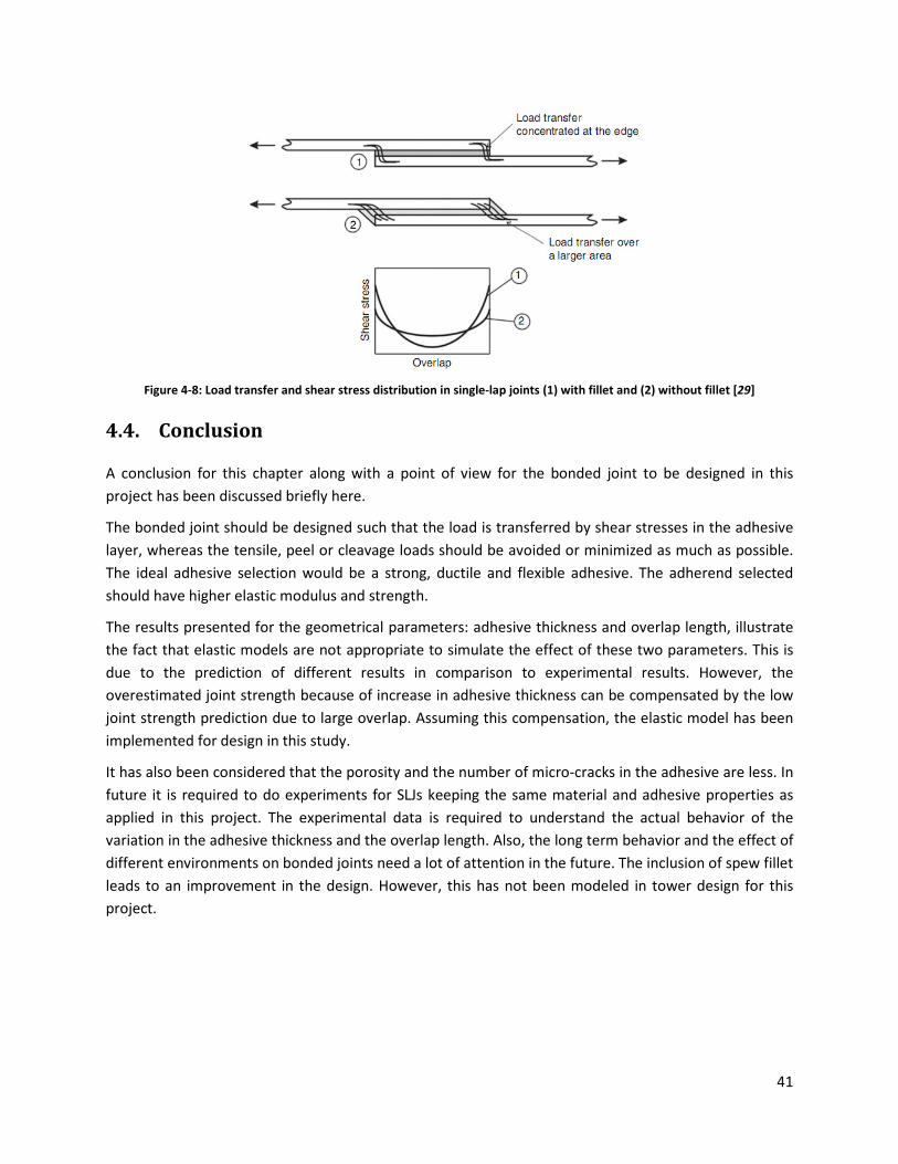
41
Figure 4-8: Load transfer and shear stress distribution in single-lap joints (1) with fillet and (2) without fillet [29]
4.4. Conclusion
A conclusion for this chapter along with a point of view for the bonded joint to be designed in this
project has been discussed briefly here.
The bonded joint should be designed such that the load is transferred by shear stresses in the adhesive
layer, whereas the tensile, peel or cleavage loads should be avoided or minimized as much as possible.
The ideal adhesive selection would be a strong, ductile and flexible adhesive. The adherend selected
should have higher elastic modulus and strength.
The results presented for the geometrical parameters: adhesive thickness and overlap length, illustrate
the fact that elastic models are not appropriate to simulate the effect of these two parameters. This is
due to the prediction of different results in comparison to experimental results. However, the
overestimated joint strength because of increase in adhesive thickness can be compensated by the low
joint strength prediction due to large overlap. Assuming this compensation, the elastic model has been
implemented for design in this study.
It has also been considered that the porosity and the number of micro-cracks in the adhesive are less. In
future it is required to do experiments for SLJs keeping the same material and adhesive properties as
applied in this project. The experimental data is required to understand the actual behavior of the
variation in the adhesive thickness and the overlap length. Also, the long term behavior and the effect of
different environments on bonded joints need a lot of attention in the future. The inclusion of spew fillet
leads to an improvement in the design. However, this has not been modeled in tower design for this
project.

42
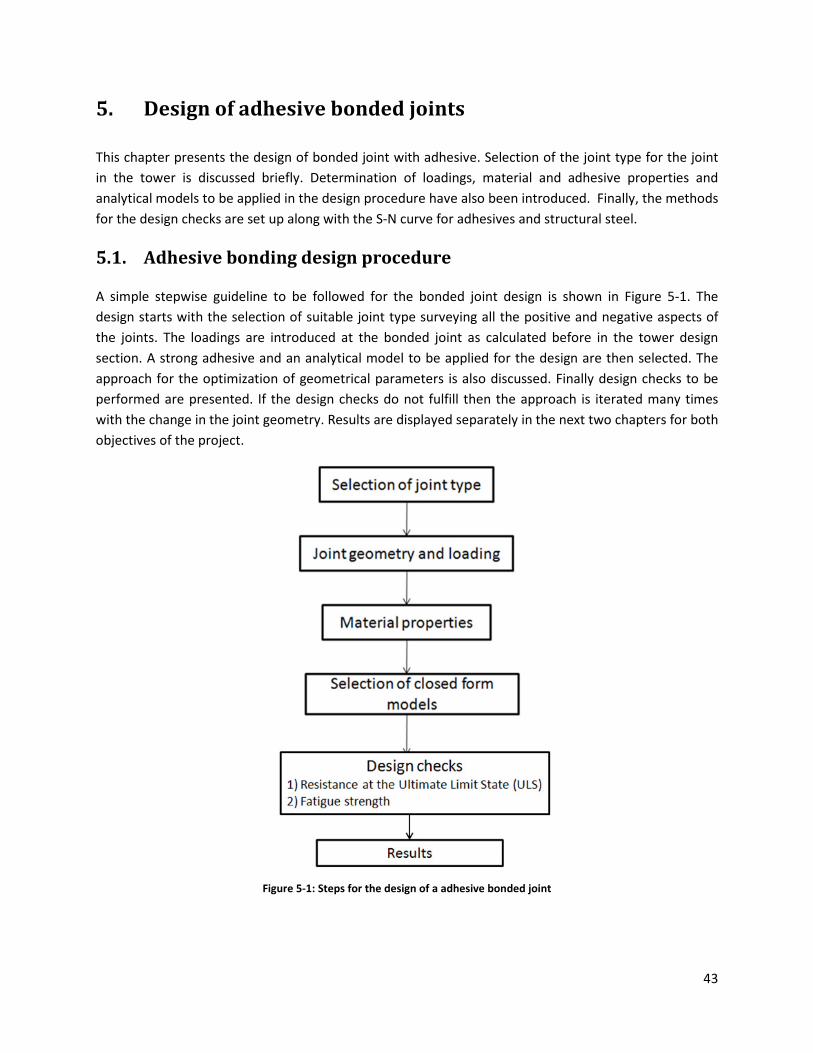
43
5. Design of adhesive bonded joints
This chapter presents the design of bonded joint with adhesive. Selection of the joint type for the joint
in the tower is discussed briefly. Determination of loadings, material and adhesive properties and
analytical models to be applied in the design procedure have also been introduced. Finally, the methods
for the design checks are set up along with the S-N curve for adhesives and structural steel.
5.1. Adhesive bonding design procedure
A simple stepwise guideline to be followed for the bonded joint design is shown in Figure 5-1. The
design starts with the selection of suitable joint type surveying all the positive and negative aspects of
the joints. The loadings are introduced at the bonded joint as calculated before in the tower design
section. A strong adhesive and an analytical model to be applied for the design are then selected. The
approach for the optimization of geometrical parameters is also discussed. Finally design checks to be
performed are presented. If the design checks do not fulfill then the approach is iterated many times
with the change in the joint geometry. Results are displayed separately in the next two chapters for both
objectives of the project.
Figure 5-1: Steps for the design of a adhesive bonded joint
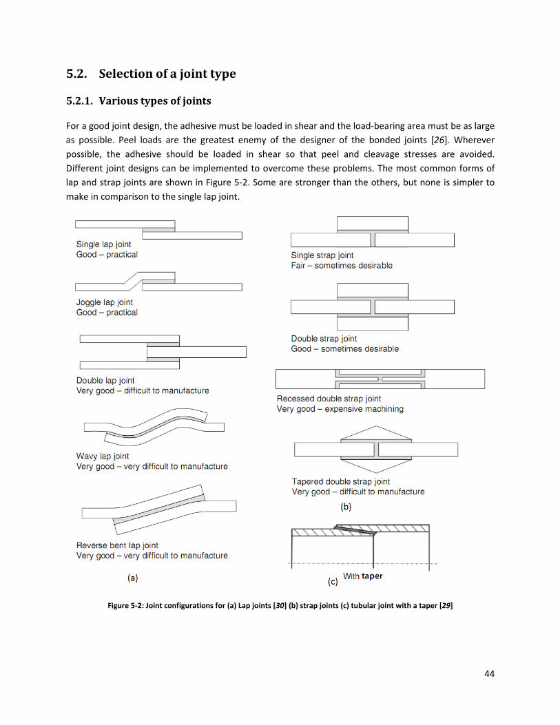
44
5.2. Selection of a joint type
5.2.1. Various types of joints
For a good joint design, the adhesive must be loaded in shear and the load-bearing area must be as large
as possible. Peel loads are the greatest enemy of the designer of the bonded joints [26]. Wherever
possible, the adhesive should be loaded in shear so that peel and cleavage stresses are avoided.
Different joint designs can be implemented to overcome these problems. The most common forms of
lap and strap joints are shown in Figure 5-2. Some are stronger than the others, but none is simpler to
make in comparison to the single lap joint.
Figure 5-2: Joint configurations for (a) Lap joints [30] (b) strap joints (c) tubular joint with a taper [29]
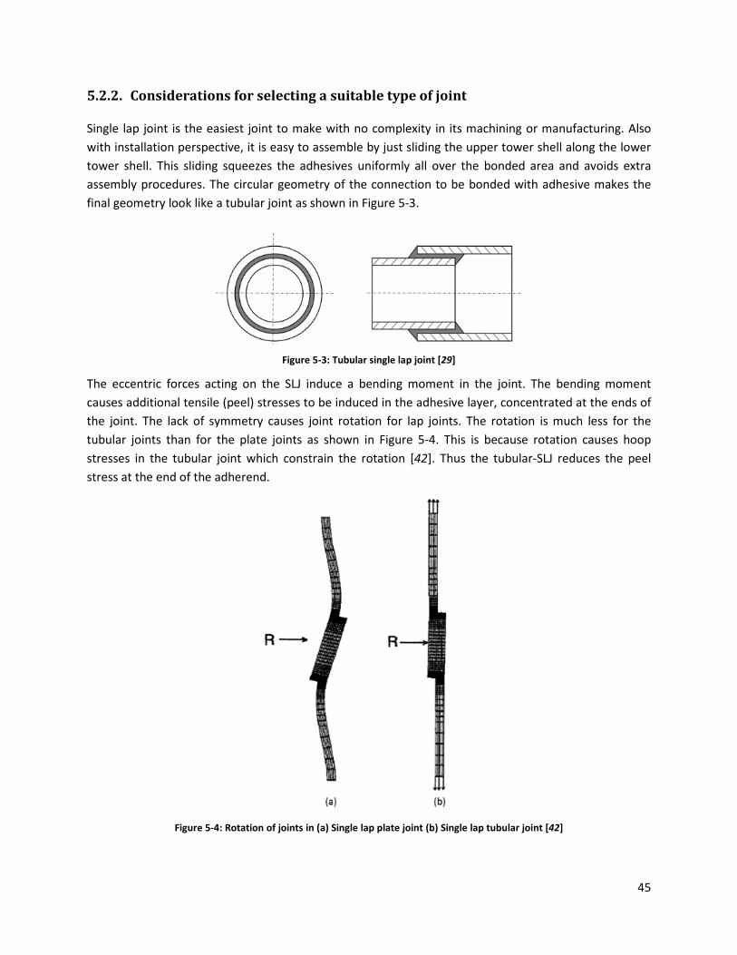
45
5.2.2. Considerations for selecting a suitable type of joint
Single lap joint is the easiest joint to make with no complexity in its machining or manufacturing. Also
with installation perspective, it is easy to assemble by just sliding the upper tower shell along the lower
tower shell. This sliding squeezes the adhesives uniformly all over the bonded area and avoids extra
assembly procedures. The circular geometry of the connection to be bonded with adhesive makes the
final geometry look like a tubular joint as shown in Figure 5-3.
Figure 5-3: Tubular single lap joint [29]
The eccentric forces acting on the SLJ induce a bending moment in the joint. The bending moment
causes additional tensile (peel) stresses to be induced in the adhesive layer, concentrated at the ends of
the joint. The lack of symmetry causes joint rotation for lap joints. The rotation is much less for the
tubular joints than for the plate joints as shown in Figure 5-4. This is because rotation causes hoop
stresses in the tubular joint which constrain the rotation [42]. Thus the tubular-SLJ reduces the peel
stress at the end of the adherend.
Figure 5-4: Rotation of joints in (a) Single lap plate joint (b) Single lap tubular joint [42]
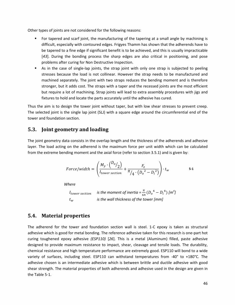
46
Other types of joints are not considered for the following reasons:
� For tapered and scarf joint, the manufacturing of the tapering at a small angle by machining is
difficult, especially with contoured edges. Frigyes Thamm has shown that the adherends have to
be tapered to a fine edge if significant benefit is to be achieved, and this is usually impracticable
[43]. During the bonding process the sharp edges are also critical in positioning, and pose
problems after curing for Non Destructive Inspection.
� As in the case of single-lap joints, the strap joint with only one strap is subjected to peeling
stresses because the load is not collinear. However the strap needs to be manufactured and
machined separately. The joint with two straps reduces the bending moment and is therefore
stronger, but it adds cost. The straps with a taper and the recessed joints are the most efficient
but require a lot of machining. Strap joints will lead to extra assembly procedures with jigs and
fixtures to hold and locate the parts accurately until the adhesive has cured.
Thus the aim is to design the tower joint without taper, but with low shear stresses to prevent creep.
The selected joint is the single lap joint (SLJ) with a square edge around the circumferential end of the
tower and foundation section.
5.3. Joint geometry and loading
The joint geometry data consists in the overlap length and the thickness of the adherends and adhesive
layer. The load acting on the adherend is the maximum force per unit width which can be calculated
from the extreme bending moment and the axial force (refer to section 3.5.1) and is given by:
��a�`/^l��ℎ = ¹ ~� ∙ ��� 2© �wx�Qep }e x��� + ��k 4© ∙ º��o − ��o»¼ ∙ �Q 5-1
Where
wx�Qep }e x��� is the moment of inertia = ® (��® − ��®) [m4]
�Q is the wall thickness of the tower [mm]
5.4. Material properties
The adherend for the tower and foundation section wall is steel. 1-C epoxy is taken as structural
adhesive which is good for metal bonding. The reference adhesive taken for this research is one-part hot
curing toughened epoxy adhesive (ESP110) [26]. This is a metal (Aluminum) filled, paste adhesive
designed to provide maximum resistance to impact, shear, cleavage and tensile loads. The durability,
chemical resistance and high temperature performance are extremely good. ESP110 will bond to a wide
variety of surfaces, including steel. ESP110 can withstand temperatures from -40° to +180°C. The
adhesive chosen is an intermediate adhesive which is between brittle and ductile adhesive with good
shear strength. The material properties of both adherends and adhesive used in the design are given in
the Table 5-1.
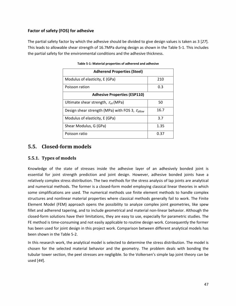
47
Factor of safety (FOS) for adhesive
The partial safety factor by which the adhesive should be divided to give design values is taken as 3 [27].
This leads to allowable shear strength of 16.7MPa during design as shown in the Table 5-1. This includes
the partial safety for the environmental conditions and the adhesive thickness.
Table 5-1: Material properties of adherend and adhesive
Adherend Properties (Steel)
Modulus of elasticity, E (GPa) 210
Poisson ration 0.3
Adhesive Properties (ESP110)
Ultimate shear strength, ½ult (MPa) 50
Design shear strength (MPa) with FOS 3, ½allow 16.7
Modulus of elasticity, E (GPa) 3.7
Shear Modulus, G (GPa) 1.35
Poisson ratio 0.37
5.5. Closed-form models
5.5.1. Types of models
Knowledge of the state of stresses inside the adhesive layer of an adhesively bonded joint is
essential for joint strength prediction and joint design. However, adhesive bonded joints have a
relatively complex stress distribution. The two methods for the stress analysis of lap joints are analytical
and numerical methods. The former is a closed-form model employing classical linear theories in which
some simplifications are used. The numerical methods use finite element methods to handle complex
structures and nonlinear material properties where classical methods generally fail to work. The Finite
Element Model (FEM) approach opens the possibility to analyze complex joint geometries, like spew
fillet and adherend tapering, and to include geometrical and material non-linear behavior. Although the
closed-form solutions have their limitations, they are easy to use, especially for parametric studies. The
FE method is time-consuming and not easily applicable to routine design work. Consequently the former
has been used for joint design in this project work. Comparison between different analytical models has
been shown in the Table 5-2.
In this research work, the analytical model is selected to determine the stress distribution. The model is
chosen for the selected material behavior and the geometry. The problem deals with bonding the
tubular tower section, the peel stresses are negligible. So the Volkersen’s simple lap joint theory can be
used [44].
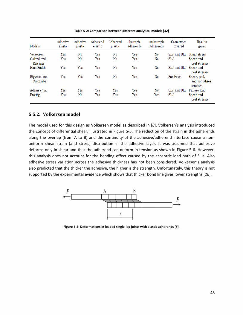
48
Table 5-2: Comparison between different analytical models [32]
5.5.2. Volkersen model
The model used for this design as Volkersen model as described in [8]. Volkersen’s analysis introduced
the concept of differential shear, illustrated in Figure 5-5. The reduction of the strain in the adherends
along the overlap (from A to B) and the continuity of the adhesive/adherend interface cause a non-
uniform shear strain (and stress) distribution in the adhesive layer. It was assumed that adhesive
deforms only in shear and that the adherend can deform in tension as shown in Figure 5-6. However,
this analysis does not account for the bending effect caused by the eccentric load path of SLJs. Also
adhesive stress variation across the adhesive thickness has not been considered. Volkersen’s analysis
also predicted that the thicker the adhesive, the higher is the strength. Unfortunately, this theory is not
supported by the experimental evidence which shows that thicker bond line gives lower strengths [26].
Figure 5-5: Deformations in loaded single-lap joints with elastic adherends [8].
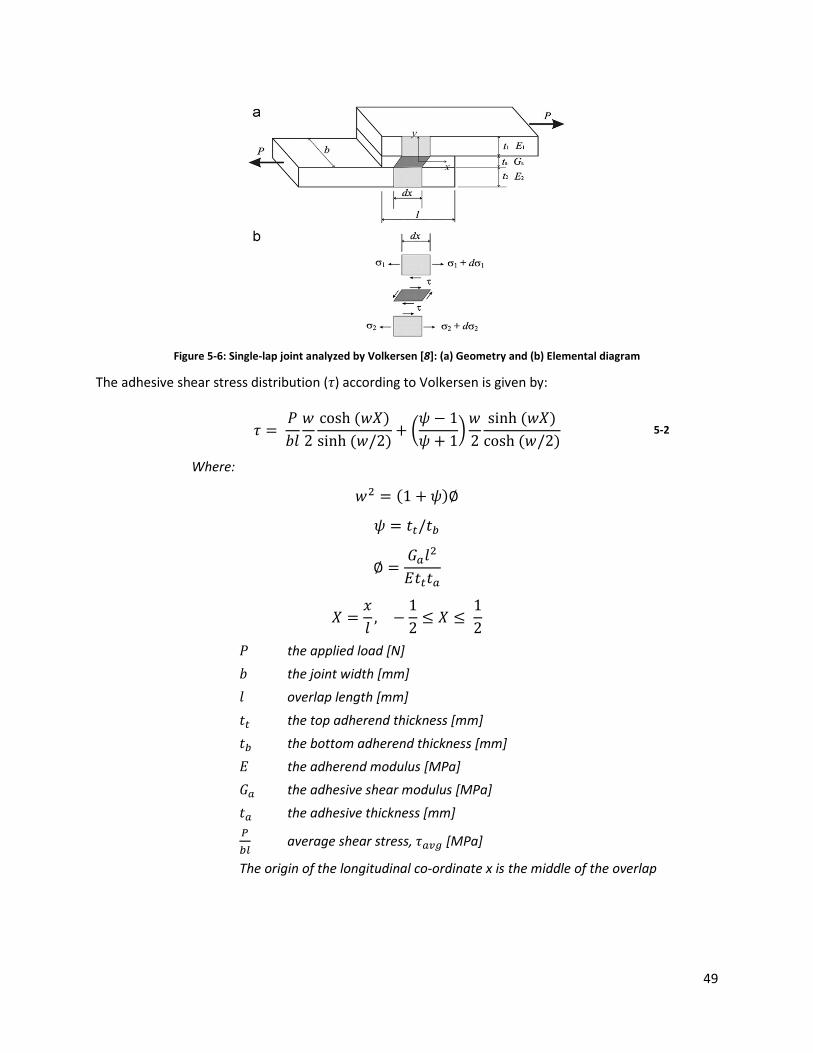
49
Figure 5-6: Single-lap joint analyzed by Volkersen [8]: (a) Geometry and (b) Elemental diagram
The adhesive shear stress distribution (½) according to Volkersen is given by:
½ = P¾¿ 2̂ cosh (^Â)sinh (^/2) + rÄ − 1Ä + 1s 2̂ sinh (^Â)cosh (^/2) 5-2
Where: ^o = (1 + Ä)∅ Ä = �x/�U
∅ = Æc¿oÇ�x�c
 = È¿ , − 12 ≤  ≤ 12
P the applied load [N]
¾ the joint width [mm]
¿ overlap length [mm]
�x the top adherend thickness [mm]
�U the bottom adherend thickness [mm]
Ç the adherend modulus [MPa]
Æc the adhesive shear modulus [MPa]
�c the adhesive thickness [mm]
ÉU� average shear stress, ½cd| [MPa]
The origin of the longitudinal co-ordinate x is the middle of the overlap
50
5.5.3. Selection of failure criterion
The failure criterion chosen for linear elastic analysis in the design is maximum shear stress in the
adhesive according to Volkersen’s model. That is, the maximum adhesive shear stress is to be less than
or equal to the maximum allowable adhesive shear stress as given by:
Ê ≤ ÊËÌÌÍÎ ÍÏ Ð ¶Ñ,ËÒÓÔÕ,ËÒÓÖ 5-3
Where
Ê is the shear stress in the adhesive layer (equation 5-2) [MPa]
¶Ñ,ËÒ is the limiting shear strength value of adhesive [MPa]
ÔÕ,ËÒÓ 3.0 is the material factor for adhesive bonded joints
5.5.4. Linear elastic analysis
The simplest analysis considers the adherends to be rigid and the adhesive to deform only in shear. The
adhesive shear stress is constant over the overlap length. This value for the shear stress can be
interpreted as the average shear stress acting on the adhesive layer [45] and is given by:
½cd| = P¾ ∙ ¿ 5-4
The stress in the sheet material is given by:
u}Seex = P¾ ∙ � 5-5
Where:
� metal thickness (thickness of thinner sheet in joints made of
different thickness) [mm]
u}Seex stress in the sheet due to axial loads and bending moments [N/mm2]
For design purposes it is assumed that the resistance of the bonded joint can be described by the
resistance of a unit width segment of tubular-single lap joint as shown in Figure 5-7. The relationship
between stress level in sheet material and average shear stress in the adhesive can be found by
equating the force per unit width in the sheet and in the adhesive and is given by combining equation
5-4 and 5-5 as:
u}Seex = ½cd| ∙ ¿� 5-6
Combining equations 5-2 and 5-6 give the shear stress distribution in the adhesive along the overlap
which does not include the width term. This equation has been used in the design calculations and is
given by:
½ = (u}Seex ∙ t)¿ 2̂ cosh (^Â)sinh (^/2) + rÄ − 1Ä + 1s 2̂ sinh (^Â)cosh (^/2) 5-7
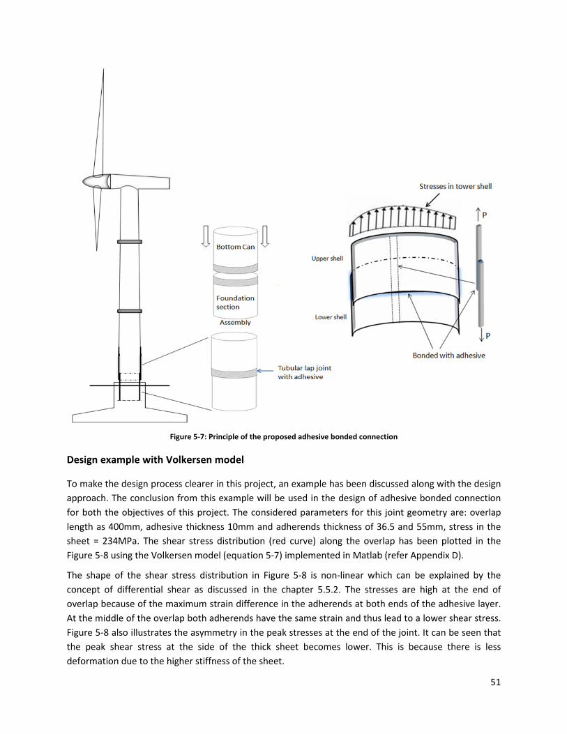
51
Figure 5-7: Principle of the proposed adhesive bonded connection
Design example with Volkersen model
To make the design process clearer in this project, an example has been discussed along with the design
approach. The conclusion from this example will be used in the design of adhesive bonded connection
for both the objectives of this project. The considered parameters for this joint geometry are: overlap
length as 400mm, adhesive thickness 10mm and adherends thickness of 36.5 and 55mm, stress in the
sheet = 234MPa. The shear stress distribution (red curve) along the overlap has been plotted in the
Figure 5-8 using the Volkersen model (equation 5-7) implemented in Matlab (refer Appendix D).
The shape of the shear stress distribution in Figure 5-8 is non-linear which can be explained by the
concept of differential shear as discussed in the chapter 5.5.2. The stresses are high at the end of
overlap because of the maximum strain difference in the adherends at both ends of the adhesive layer.
At the middle of the overlap both adherends have the same strain and thus lead to a lower shear stress.
Figure 5-8 also illustrates the asymmetry in the peak stresses at the end of the joint. It can be seen that
the peak shear stress at the side of the thick sheet becomes lower. This is because there is less
deformation due to the higher stiffness of the sheet.
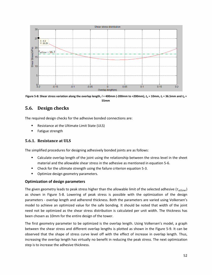
52
Figure 5-8: Shear stress variation along the overlap length, l = 400mm (-200mm to +200mm), ta = 10mm, tt = 36.5mm and tb =
55mm 5.6. Design checks
The required design checks for the adhesive bonded connections are:
� Resistance at the Ultimate Limit State (ULS)
� Fatigue strength
5.6.1. Resistance at ULS
The simplified procedures for designing adhesively bonded joints are as follows:
� Calculate overlap length of the joint using the relationship between the stress level in the sheet
material and the allowable shear stress in the adhesive as mentioned in equation 5-6.
� Check for the ultimate strength using the failure criterion equation 5-3.
� Optimize design geometry parameters.
Optimization of design parameters
The given geometry leads to peak stress higher than the allowable limit of the selected adhesive (½c���Q)
as shown in Figure 5-8. Lowering of peak stress is possible with the optimization of the design
parameters - overlap length and adherend thickness. Both the parameters are varied using Volkersen’s
model to achieve an optimized value for the safe bonding. It should be noted that width of the joint
need not be optimized as the shear stress distribution is calculated per unit width. The thickness has
been chosen as 10mm for the entire design of the tower.
The first geometry parameter to be optimized is the overlap length. Using Volkersen’s model, a graph
between the shear stress and different overlap lengths is plotted as shown in the Figure 5-9. It can be
observed that the shape of stress curve level off with the effect of increase in overlap length. Thus,
increasing the overlap length has virtually no benefit in reducing the peak stress. The next optimization
step is to increase the adhesive thickness.
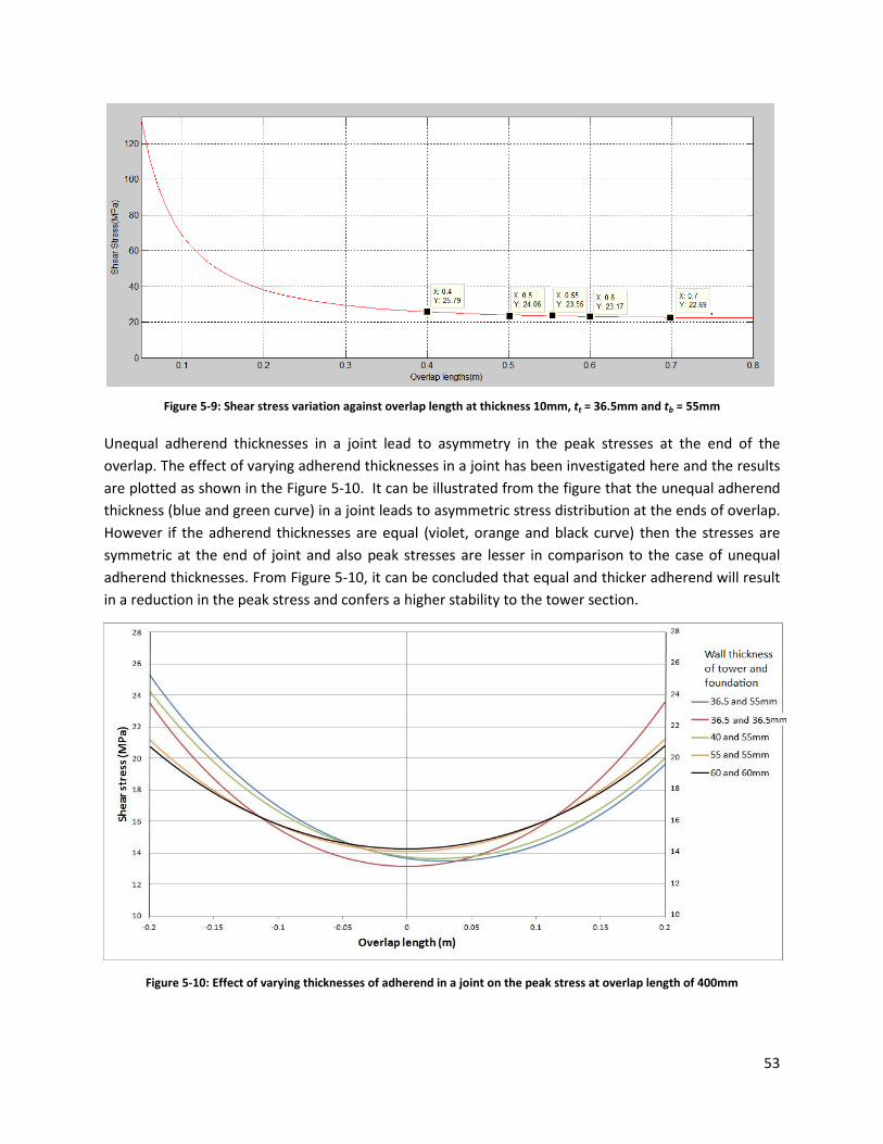
53
Figure 5-9: Shear stress variation against overlap length at thickness 10mm, tt = 36.5mm and tb = 55mm
Unequal adherend thicknesses in a joint lead to asymmetry in the peak stresses at the end of the
overlap. The effect of varying adherend thicknesses in a joint has been investigated here and the results
are plotted as shown in the Figure 5-10. It can be illustrated from the figure that the unequal adherend
thickness (blue and green curve) in a joint leads to asymmetric stress distribution at the ends of overlap.
However if the adherend thicknesses are equal (violet, orange and black curve) then the stresses are
symmetric at the end of joint and also peak stresses are lesser in comparison to the case of unequal
adherend thicknesses. From Figure 5-10, it can be concluded that equal and thicker adherend will result
in a reduction in the peak stress and confers a higher stability to the tower section.
Figure 5-10: Effect of varying thicknesses of adherend in a joint on the peak stress at overlap length of 400mm
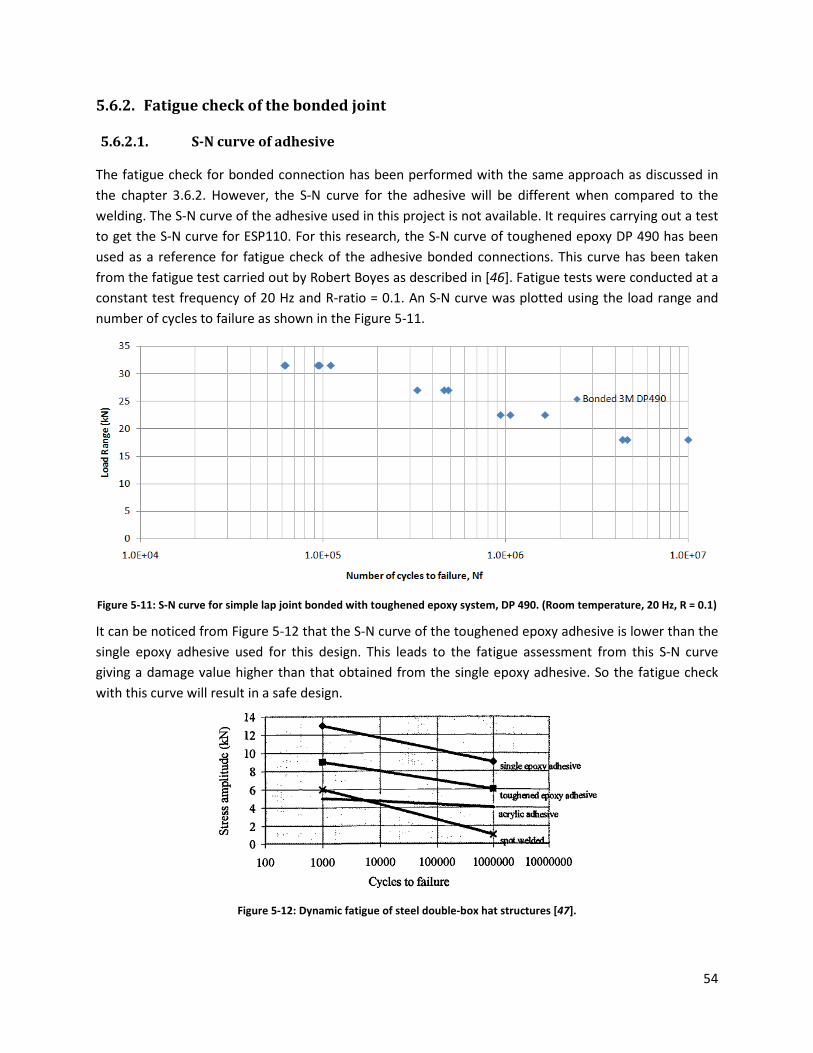
54
5.6.2. Fatigue check of the bonded joint
5.6.2.1. S-N curve of adhesive
The fatigue check for bonded connection has been performed with the same approach as discussed in
the chapter 3.6.2. However, the S-N curve for the adhesive will be different when compared to the
welding. The S-N curve of the adhesive used in this project is not available. It requires carrying out a test
to get the S-N curve for ESP110. For this research, the S-N curve of toughened epoxy DP 490 has been
used as a reference for fatigue check of the adhesive bonded connections. This curve has been taken
from the fatigue test carried out by Robert Boyes as described in [46]. Fatigue tests were conducted at a
constant test frequency of 20 Hz and R-ratio = 0.1. An S-N curve was plotted using the load range and
number of cycles to failure as shown in the Figure 5-11.
Figure 5-11: S-N curve for simple lap joint bonded with toughened epoxy system, DP 490. (Room temperature, 20 Hz, R = 0.1)
It can be noticed from Figure 5-12 that the S-N curve of the toughened epoxy adhesive is lower than the
single epoxy adhesive used for this design. This leads to the fatigue assessment from this S-N curve
giving a damage value higher than that obtained from the single epoxy adhesive. So the fatigue check
with this curve will result in a safe design.
Figure 5-12: Dynamic fatigue of steel double-box hat structures [47].

55
However for the fatigue analysis in the Bladed, it is convenient to input stress ranges along with number
of cycles. The load ranges of S-N curve plot in Figure 5-11 is converted to stress range by using the
geometry of a test specimen as described in the [46]. In the Bladed, it is required to input the stress
range in the descending order. However in the S-N curve plot in Figure 5-11, different numbers of cycles
are marked for the same stress group. The means of the number of cycles for the same stress group
were taken to plot the stress range versus number of cycles as shown in the Figure 5-13. The fatigue
damage calculation will be performed in the Bladed after converting the stress ranges in to shear stress
ranges (from equation 5-2) by using channel combination.
Figure 5-13: S-N curve for simple lap joint bonded with a toughened epoxy system (DP 490) to be used for the fatigue
damage calculation of the designed joint. f = 20Hz and R = 0.1
5.6.2.2. Safety factor for bonded joints
The partial safety factors are given in Table 5-3 according to IEC61400-1 edition 3 [7]. The partial safety
factor for adhesive material is taken from ‘adhesivestoolkit’ [27]. The total safety factor is applied to the
cyclic stress range for assessing the increment of damage associated with each fatigue cycle.
Table 5-3: Partial safety factors for fatigue analysis of adhesively bonded connections
Type Partial safety factor
Loads, �q 1.0
Material (for welded and structural steel), �� 2
Consequences of failure (non fail safe
structure components), �� 1.15
Total (�q ∙ �� ∙ ��) 2.3
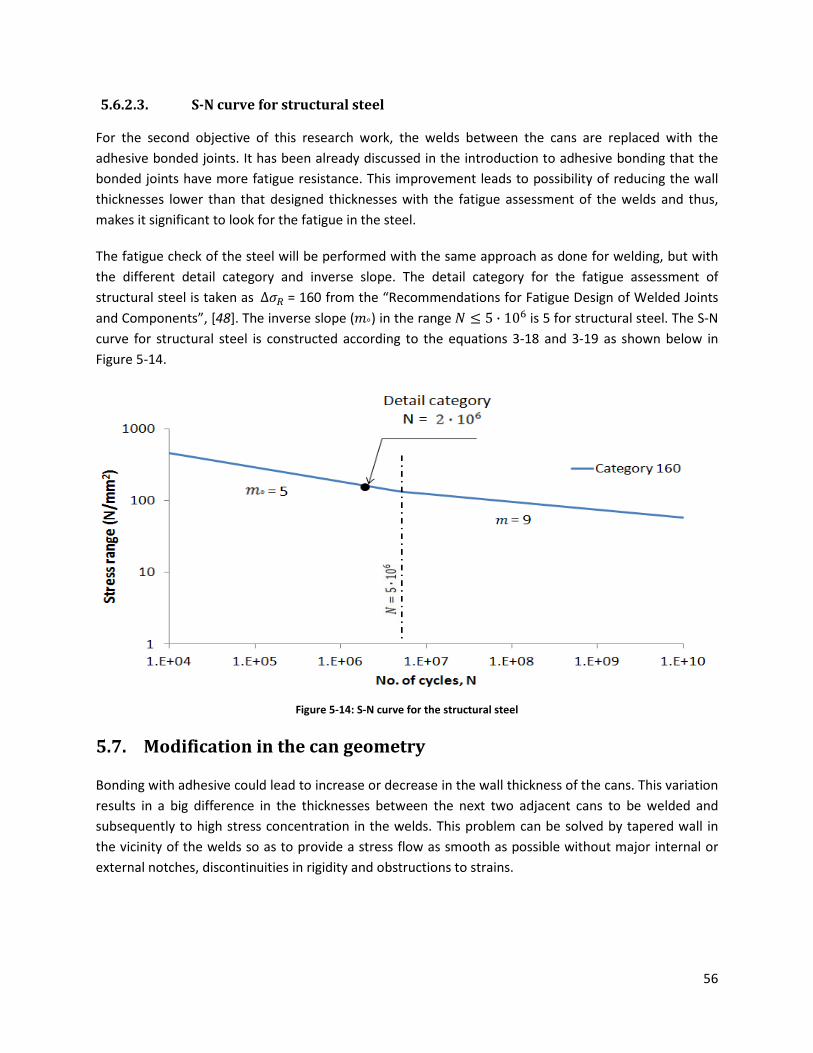
56
5.6.2.3. S-N curve for structural steel
For the second objective of this research work, the welds between the cans are replaced with the
adhesive bonded joints. It has been already discussed in the introduction to adhesive bonding that the
bonded joints have more fatigue resistance. This improvement leads to possibility of reducing the wall
thicknesses lower than that designed thicknesses with the fatigue assessment of the welds and thus,
makes it significant to look for the fatigue in the steel.
The fatigue check of the steel will be performed with the same approach as done for welding, but with
the different detail category and inverse slope. The detail category for the fatigue assessment of
structural steel is taken as ∆un = 160 from the “Recommendations for Fatigue Design of Welded Joints
and Components”, [48]. The inverse slope (L°) in the range � ≤ 5 ∙ 10 is 5 for structural steel. The S-N
curve for structural steel is constructed according to the equations 3-18 and 3-19 as shown below in
Figure 5-14.
Figure 5-14: S-N curve for the structural steel
5.7. Modification in the can geometry
Bonding with adhesive could lead to increase or decrease in the wall thickness of the cans. This variation
results in a big difference in the thicknesses between the next two adjacent cans to be welded and
subsequently to high stress concentration in the welds. This problem can be solved by tapered wall in
the vicinity of the welds so as to provide a stress flow as smooth as possible without major internal or
external notches, discontinuities in rigidity and obstructions to strains.
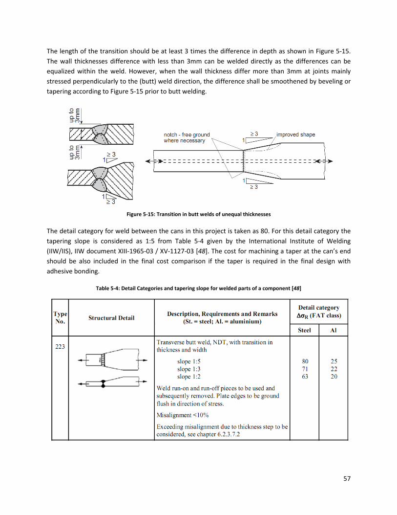
57
The length of the transition should be at least 3 times the difference in depth as shown in Figure 5-15.
The wall thicknesses difference with less than 3mm can be welded directly as the differences can be
equalized within the weld. However, when the wall thickness differ more than 3mm at joints mainly
stressed perpendicularly to the (butt) weld direction, the difference shall be smoothened by beveling or
tapering according to Figure 5-15 prior to butt welding.
Figure 5-15: Transition in butt welds of unequal thicknesses
The detail category for weld between the cans in this project is taken as 80. For this detail category the
tapering slope is considered as 1:5 from Table 5-4 given by the International Institute of Welding
(IIW/IIS), IIW document XIII-1965-03 / XV-1127-03 [48]. The cost for machining a taper at the can’s end
should be also included in the final cost comparison if the taper is required in the final design with
adhesive bonding.
Table 5-4: Detail Categories and tapering slope for welded parts of a component [48]

58

59
6. Bonding of tower base to the foundation instead of flange
and cost comparison
This chapter presents the results of the first objective in the project. The chapter includes the required
design parameters used for adhesive bonding. The results of the optimization steps, fatigue damage
check and the natural frequency check are discussed briefly. Finally, the incurred costs for both the
solutions are compared in detail.
6.1. Results of bonding tower base to the foundation
The section geometries of the tower base and the foundation are shown in Figure 3-5 and Figure 3-6.
The tubular lap-joint is dimensioned after replacing the flanges from both the respective sections. The
thickness of the adhesive is taken as 10mm [49]. This value is high to give enough manufacturing
tolerance for the tower and foundation section.
As discussed in the section 3.5.1, the extreme loadings are calculated for the 50years Extreme Operating
Gust as presented in Table 3-5. The types of loadings considered at the tower foundation are axial and
bending moments. The loading at the adherend is calculated as the maximum force per unit width using
the equation 5-1.
The overlap length is calculated using the relationship between the stress level in the sheet and the
allowable shear stress in the adhesive using equation 5-6. This gives the overlap length approximately
400mm. From the optimization conclusion discussed in section 5.6.1, the adherend thickness and the
overlap length are optimized to have less material usage. The adherend thicknesses are varied from
55mm to 70mm to determine the overlap length until the peak adhesive shear stress is less than the
maximum allowable adhesive shear stress. The material volume for the increase in tower section
thickness, foundation stab thickness and overlap length is also calculated as shown in Table 6-1.
Table 6-1: Effect on overlap length and material volume with increase in tower and foundation wall thicknesses
Tower
base
thickness
(mm)
Foundation
wall
thickness
(mm)
Peak
shear
stress
(MPa)
Overlap
length
(mm)
Increase in material volume (mm3)
Can Foundation Overlap Total increase
in volume
55 55 16.62 770 0.6425 0.0 0.5552 1.198
57 57 16.60 720 0.707 0.0586 0.5383 1.3039
60 60 16.64 660 0.8040 0.1464 0.52 1.4704
63 63 16.59 630 0.9012 0.2341 0.521 1.6563
67 67 16.64 590 1.0310 0.3508 0.52 1.902
70 70 16.65 570 1.1283 0.4382 0.525 2.0915
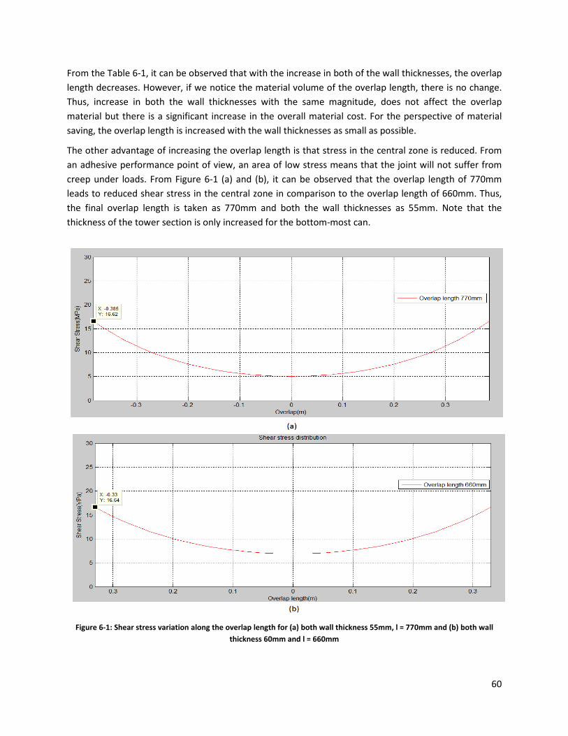
60
From the Table 6-1, it can be observed that with the increase in both of the wall thicknesses, the overlap
length decreases. However, if we notice the material volume of the overlap length, there is no change.
Thus, increase in both the wall thicknesses with the same magnitude, does not affect the overlap
material but there is a significant increase in the overall material cost. For the perspective of material
saving, the overlap length is increased with the wall thicknesses as small as possible.
The other advantage of increasing the overlap length is that stress in the central zone is reduced. From
an adhesive performance point of view, an area of low stress means that the joint will not suffer from
creep under loads. From Figure 6-1 (a) and (b), it can be observed that the overlap length of 770mm
leads to reduced shear stress in the central zone in comparison to the overlap length of 660mm. Thus,
the final overlap length is taken as 770mm and both the wall thicknesses as 55mm. Note that the
thickness of the tower section is only increased for the bottom-most can.
Figure 6-1: Shear stress variation along the overlap length for (a) both wall thickness 55mm, l = 770mm and (b) both wall
thickness 60mm and l = 660mm

61
The fatigue damage is calculated in the Bladed as discussed in the section 5.6.2. Applying the Goodman
correction [22], the accumulated damage value is 0.4 which is less than 1. Thus, the bonded joint may
survive for at least the planned service life of the turbine.
Figure 6-2 shows the campbell diagram of the turbine with the bonded tower base and foundation. It
can be clearly seen that the first fore-aft and side-to-side tower frequencies are placed between the
excitation frequencies (1P and 3P) throughout the operational range of the wind turbine.
Figure 6-2: Campbell diagram for the turbine with bonded tower base to foundation.
6.2. Final geometry
The final optimized geometry parameters of bonding the tower base with the foundation
instead of flanges are:
� Overlap length = 770mm
� Tower wall section thickness = 55mm
� Foundation wall thickness = 55mm
� Adhesive thickness = 10mm

62
6.3. Cost analysis
The material and the fabrication costs for the existing and the proposed solutions have been compared
and other construction aspects are discussed qualitatively in this section.
6.3.1. Flange fabrication cost
The material costs for the bottom-most flange and bolts have been taken from the reference [15]. The
cost details in the reference [15] are provided by Repower Energy Systems in December 2007. The
flange cost in this study is approximated same as cost per unit volume of the flanges given by Repower
and are put in Table 6-2.
Machining and drilling operations in the flanges are tedious and expensive. The fabrication costs for
flanges are also included in this estimation. In an American study [50] this operation was estimated to
cost about 3000$ (2411€) per piece. The bolting assembly cost is also included in the Table 6-2. The
values are taken from the reference [5]. The total rough estimation of the flange cost at the base is given
in the Table 6-2.
6.3.2. Flange welding cost
Two conical cans or the flanges (at towers end) of the tower segments are joined with the
circumferential welds. Submerged arc welding technique is recently used to weld different sections in
the tower. The cost for the circumferential weld is calculated as [51]:
× �p = iØ(ÙQÚκρV�*��- + (1.3 ∙ 0.1559 ∙ 10ÛÜ ∙ �o ∙ (Ý − 1) ∙ ÞQ�)) 6-1
Where:
Ý number of element to be assembled which in our case is 2.
ÙQ difficulty factor expressing the complexity of the assembly = 2
ß density of the material = 7,850kg/m3
ÞQ� circumference of the can [m]
� wall thickness[m]
R radius of the conical tower [m]
Rx�xc� total volume of two sections getting welded [m3]= 2k��ÞQ�
× �p longitudinal weld cost [$]
iØ labour cost factor [$/min]= 1$/min [51]
The calculated costs of flange welding at the tower base and the foundation are put in the Table 6-2.
The flange material accounts for most of the costs in the reference tower.
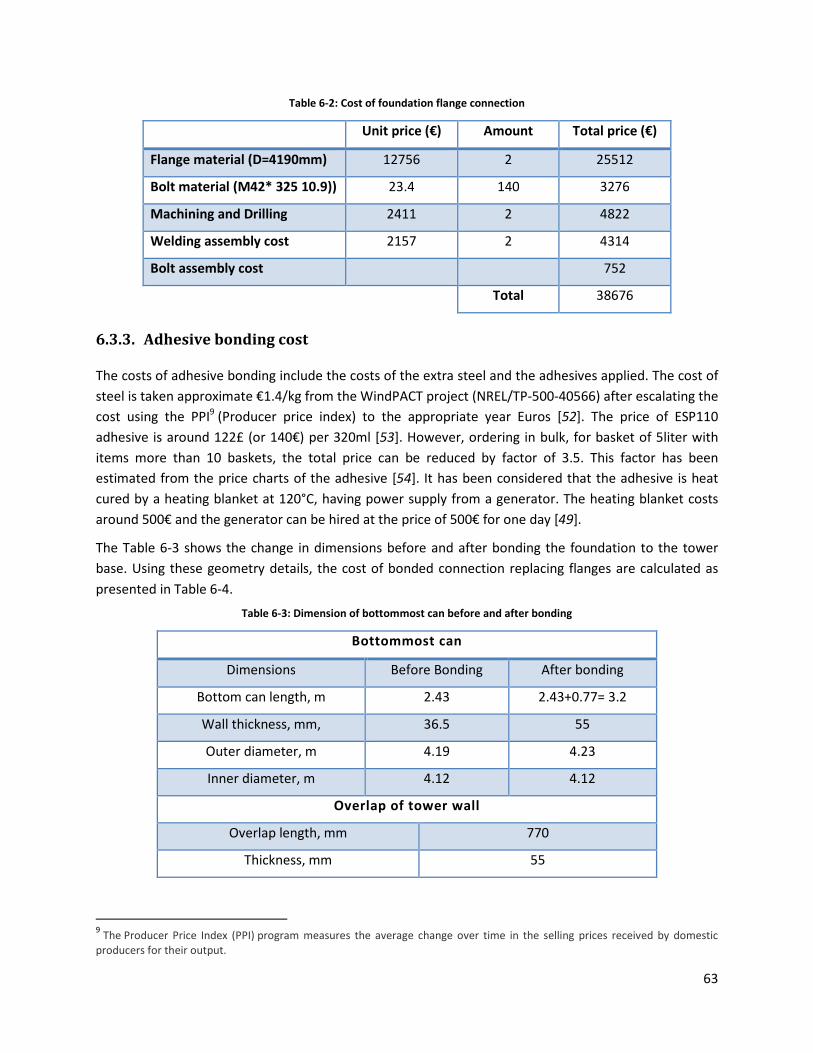
63
Table 6-2: Cost of foundation flange connection
Unit price (€) Amount Total price (€)
Flange material (D=4190mm) 12756 2 25512
Bolt material (M42* 325 10.9)) 23.4 140 3276
Machining and Drilling 2411 2 4822
Welding assembly cost 2157 2 4314
Bolt assembly cost 752
Total 38676
6.3.3. Adhesive bonding cost
The costs of adhesive bonding include the costs of the extra steel and the adhesives applied. The cost of
steel is taken approximate €1.4/kg from the WindPACT project (NREL/TP-500-40566) after escalating the
cost using the PPI9 (Producer price index) to the appropriate year Euros [52]. The price of ESP110
adhesive is around 122£ (or 140€) per 320ml [53]. However, ordering in bulk, for basket of 5liter with
items more than 10 baskets, the total price can be reduced by factor of 3.5. This factor has been
estimated from the price charts of the adhesive [54]. It has been considered that the adhesive is heat
cured by a heating blanket at 120°C, having power supply from a generator. The heating blanket costs
around 500€ and the generator can be hired at the price of 500€ for one day [49].
The Table 6-3 shows the change in dimensions before and after bonding the foundation to the tower
base. Using these geometry details, the cost of bonded connection replacing flanges are calculated as
presented in Table 6-4.
Table 6-3: Dimension of bottommost can before and after bonding
Bottommost can
Dimensions Before Bonding After bonding
Bottom can length, m 2.43 2.43+0.77= 3.2
Wall thickness, mm, 36.5 55
Outer diameter, m 4.19 4.23
Inner diameter, m 4.12 4.12
Overlap of tower wall
Overlap length, mm 770
Thickness, mm 55
9 The Producer Price Index (PPI) program measures the average change over time in the selling prices received by domestic
producers for their output.
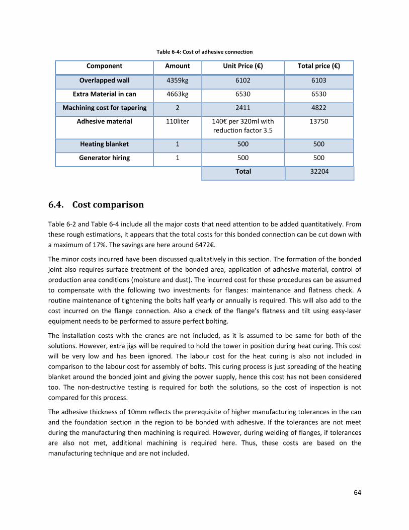
64
Table 6-4: Cost of adhesive connection
Component Amount Unit Price (€) Total price (€)
Overlapped wall 4359kg 6102 6103
Extra Material in can 4663kg 6530 6530
Machining cost for tapering 2 2411 4822
Adhesive material 110liter 140€ per 320ml with
reduction factor 3.5
13750
Heating blanket 1 500 500
Generator hiring 1 500 500
Total 32204
6.4. Cost comparison
Table 6-2 and Table 6-4 include all the major costs that need attention to be added quantitatively. From
these rough estimations, it appears that the total costs for this bonded connection can be cut down with
a maximum of 17%. The savings are here around 6472€.
The minor costs incurred have been discussed qualitatively in this section. The formation of the bonded
joint also requires surface treatment of the bonded area, application of adhesive material, control of
production area conditions (moisture and dust). The incurred cost for these procedures can be assumed
to compensate with the following two investments for flanges: maintenance and flatness check. A
routine maintenance of tightening the bolts half yearly or annually is required. This will also add to the
cost incurred on the flange connection. Also a check of the flange’s flatness and tilt using easy-laser
equipment needs to be performed to assure perfect bolting.
The installation costs with the cranes are not included, as it is assumed to be same for both of the
solutions. However, extra jigs will be required to hold the tower in position during heat curing. This cost
will be very low and has been ignored. The labour cost for the heat curing is also not included in
comparison to the labour cost for assembly of bolts. This curing process is just spreading of the heating
blanket around the bonded joint and giving the power supply, hence this cost has not been considered
too. The non-destructive testing is required for both the solutions, so the cost of inspection is not
compared for this process.
The adhesive thickness of 10mm reflects the prerequisite of higher manufacturing tolerances in the can
and the foundation section in the region to be bonded with adhesive. If the tolerances are not meet
during the manufacturing then machining is required. However, during welding of flanges, if tolerances
are also not met, additional machining is required here. Thus, these costs are based on the
manufacturing technique and are not included.
65
The design of bonded connection has not been modeled with the influence of environmental conditions
(moisture and water), creep and temperature effect. The inclusion of these factors could estimate the
bigger dimensions than what designed now. However a reliable safety of factor is taken in the design to
counterbalance effects of these factors.
Another drawback of the flange connections which may be taken into account is the long delivery time,
typically between three and four months. If 45° triangular spew fillet is also modeled perfectly in the
design, the cost can be possibly further reduced by 15%. This leads to the possibility of achieving the
overall cost reduction by 25% (or approximately 10,000€) for the flange at the tower base.

66
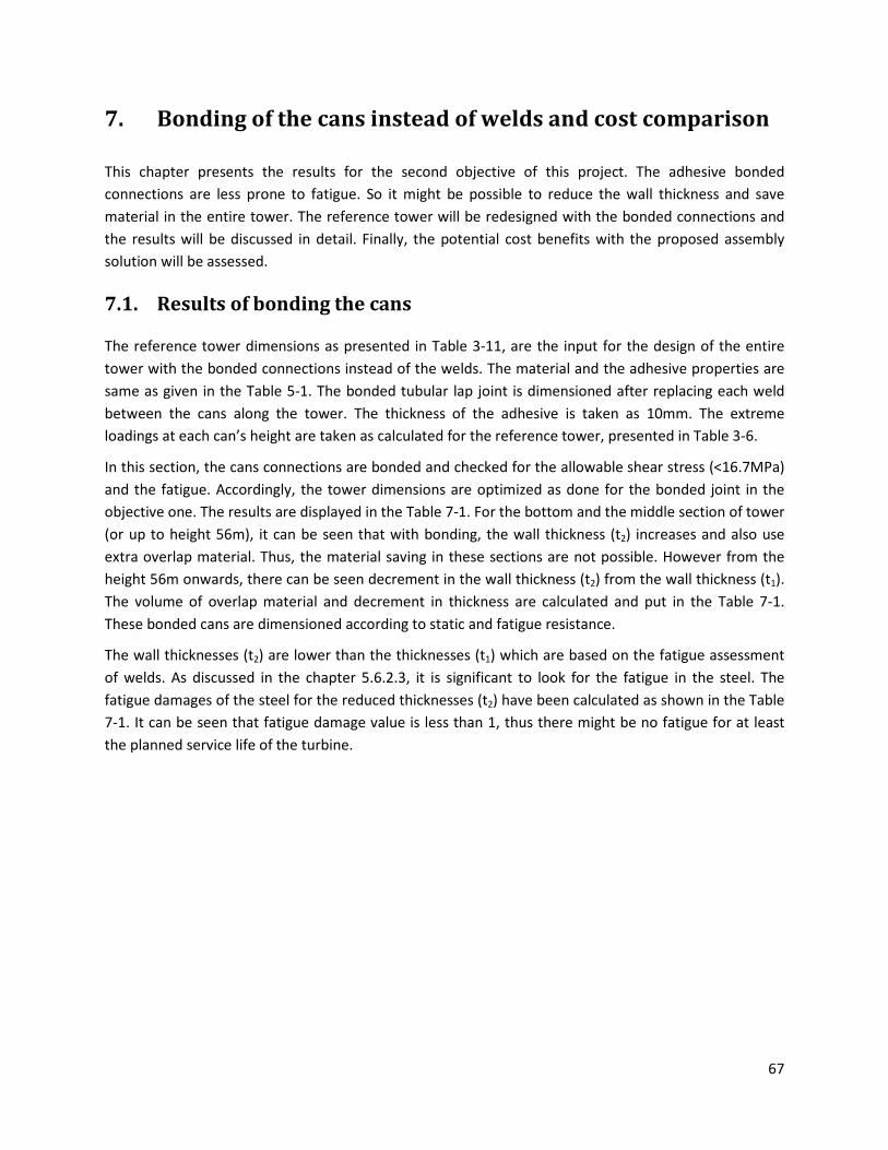
67
7. Bonding of the cans instead of welds and cost comparison
This chapter presents the results for the second objective of this project. The adhesive bonded
connections are less prone to fatigue. So it might be possible to reduce the wall thickness and save
material in the entire tower. The reference tower will be redesigned with the bonded connections and
the results will be discussed in detail. Finally, the potential cost benefits with the proposed assembly
solution will be assessed.
7.1. Results of bonding the cans
The reference tower dimensions as presented in Table 3-11, are the input for the design of the entire
tower with the bonded connections instead of the welds. The material and the adhesive properties are
same as given in the Table 5-1. The bonded tubular lap joint is dimensioned after replacing each weld
between the cans along the tower. The thickness of the adhesive is taken as 10mm. The extreme
loadings at each can’s height are taken as calculated for the reference tower, presented in Table 3-6.
In this section, the cans connections are bonded and checked for the allowable shear stress (<16.7MPa)
and the fatigue. Accordingly, the tower dimensions are optimized as done for the bonded joint in the
objective one. The results are displayed in the Table 7-1. For the bottom and the middle section of tower
(or up to height 56m), it can be seen that with bonding, the wall thickness (t2) increases and also use
extra overlap material. Thus, the material saving in these sections are not possible. However from the
height 56m onwards, there can be seen decrement in the wall thickness (t2) from the wall thickness (t1).
The volume of overlap material and decrement in thickness are calculated and put in the Table 7-1.
These bonded cans are dimensioned according to static and fatigue resistance.
The wall thicknesses (t2) are lower than the thicknesses (t1) which are based on the fatigue assessment
of welds. As discussed in the chapter 5.6.2.3, it is significant to look for the fatigue in the steel. The
fatigue damages of the steel for the reduced thicknesses (t2) have been calculated as shown in the Table
7-1. It can be seen that fatigue damage value is less than 1, thus there might be no fatigue for at least
the planned service life of the turbine.
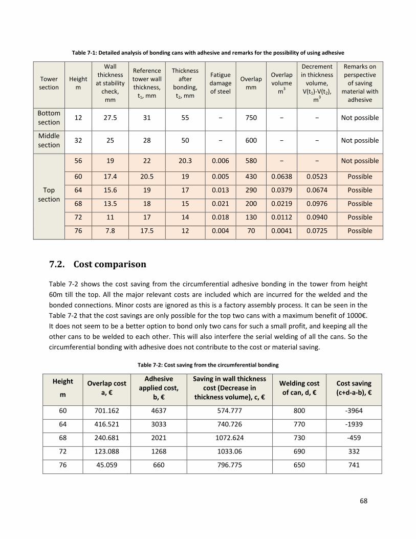
68
Table 7-1: Detailed analysis of bonding cans with adhesive and remarks for the possibility of using adhesive
Tower
section
Height
m
Wall
thickness
at stability
check,
mm
Reference
tower wall
thickness,
t1, mm
Thickness
after
bonding,
t2, mm
Fatigue
damage
of steel
Overlap
mm
Overlap
volume
m3
Decrement
in thickness
volume,
V(t1)-V(t2),
m3
Remarks on
perspective
of saving
material with
adhesive
Bottom
section 12 27.5 31 55 − 750 − − Not possible
Middle
section 32 25 28 50 − 600 − − Not possible
Top
section
56 19 22 20.3 0.006 580 − − Not possible
60 17.4 20.5 19 0.005 430 0.0638 0.0523 Possible
64 15.6 19 17 0.013 290 0.0379 0.0674 Possible
68 13.5 18 15 0.021 200 0.0219 0.0976 Possible
72 11 17 14 0.018 130 0.0112 0.0940 Possible
76 7.8 17.5 12 0.004 70 0.0041 0.0725 Possible
7.2. Cost comparison
Table 7-2 shows the cost saving from the circumferential adhesive bonding in the tower from height
60m till the top. All the major relevant costs are included which are incurred for the welded and the
bonded connections. Minor costs are ignored as this is a factory assembly process. It can be seen in the
Table 7-2 that the cost savings are only possible for the top two cans with a maximum benefit of 1000€.
It does not seem to be a better option to bond only two cans for such a small profit, and keeping all the
other cans to be welded to each other. This will also interfere the serial welding of all the cans. So the
circumferential bonding with adhesive does not contribute to the cost or material saving.
Table 7-2: Cost saving from the circumferential bonding
Height
m
Overlap cost
a, €
Adhesive
applied cost,
b, €
Saving in wall thickness
cost (Decrease in
thickness volume), c, €
Welding cost
of can, d, €
Cost saving
(c+d-a-b), €
60 701.162 4637 574.777 800 -3964
64 416.521 3033 740.726 770 -1939
68 240.681 2021 1072.624 730 -459
72 123.088 1268 1033.06 690 332
76 45.059 660 796.775 650 741
69
8. Conclusion and recommendations
The current work proposes a new assembly solution with adhesive for replacing the bottom-most flange
and the welds in a tower sections. The conclusions reached are presented below after investigating the
feasibility of implementing the bonded connections. After this some recommendations are presented.
8.1. Conclusion
For the welds in the entire tower, fatigue was the predominant phenomenon for determining the wall
thicknesses. The Volkersen model has been implemented to design the adhesive bonded joints. The
proposed bonded joint is a tubular-single lap joint. The design is prepared for the following two cases:
1) Connection between the tower base and the foundation section (replacing the flange), and
2) Connection between the cans for the entire tower (replacing all the welds).
With adhesive bonding, it was observed that static resistance of the bonded connections at Ultimate
Limit State has a dominating effect on the wall thickness. Using Volkersen’s model, it was observed that
the shape of stress curve levels off with the increase in overlap length. Thus, increasing the overlap
length had virtually no benefit in reducing the peak stress, which only left the possibility of increasing
the adherend thickness.
A study of shear stress distribution showed that the unequal adherend thickness in a joint caused
asymmetry in the peak stresses at the end of the overlap. For equal adherend thicknesses, the peak
stresses were found symmetric and also of lesser magnitude in comparison to the case of unequal
adherend thickness.
After comparing the cost for both the proposed cases with already existing design in the reference
tower, the following conclusions can be drawn:
� For the first case, it appears that the bottom-most flange costs can be cut down by a maximum
of 17% if the environmental conditions, creep, and temperature effect are not modeled in the
design. The maximum potential savings in this case has been estimated as 6,500€. The adhesive
bonded joint seems to be a feasible assembly solution for replacing the flange. However, it is
observed that bonded connection adds extra material to the bottommost can. The inclusion of
45° triangular spew fillet can further reduce the dimensions leading to reduced cost of adhesive
bonded connection.
� From the second case, the cost saving can be achieved only for the top two cans in the entire
tower with a maximum saving of 1,000€. The remaining cans get thicker with bonded joints in
comparison to the welded joints, leading to the use of more material. Thus, it is not feasible to
bond only two cans for such a marginal cost saving, keeping all the remaining cans to be welded
to each other.
As a final word, the adhesive bonded joint is an economically feasible assembly solution for the
replacement of the flanges. The replacement of welds in the entire tower is also possible by bonded
joints; however, in comparison to the existing solution it is not a feasible solution in terms of material
and cost saving.
70
8.2. Recommendations for future work
The cost analysis performed on the current tower geometry and material highlighted a potential for
savings of about 17%, i.e. around 6,500€. Hence, it is strongly recommended to further investigate the
feasibility of implementing this solution.
Analytical models used for the design always behave differently from the experimental solutions. The
design models used for bonded connections are simple and are based on limiting assumptions which do
not explicitly account for all the parameters involved. Experimental results are neither available in the
literatures for the geometry considered in this project. Therefore, it is required in the future to test
experimentally for the perfect stress distribution result.
The modeling of spew fillet in the design can lead to a further saving in the material. This has not been
modeled during the tower design in this project. Hence, the modeling of the spew fillet for further
improvement in the design needs to be investigated.
The S-N curve to be applied for certain geometry in the design process requires the S-N curve of the
same geometry. This is because the S-N curve for adhesive bonded connections depends on the
geometry of the connections [55]. Hence, there is a need for experimentation to obtain reliable S-N
curves for designing each connection in this project.
To propose comprehensive design recommendations other aspects must be addressed, from the
designer point of view:
� Improving adhesive joint design using fracture mechanics
� Behaviour of a cylindrical connection, including the effects of peel forces.
� Effects of different environmental conditions (moisture and water), creep and temperature on
the bonded connections
Finally, the surface preparation, interface properties, adhesive application and installation processes
should be also analyzed.
71
9. Bibliography
[1] Wind Energy Market 2010/2011.: German Wind Energy Association (BWE).
[2] E. Hau, Wind Turbines fundamentals, technologies, application, economics, 2nd ed.: Springer, 2006.
[3] W. Wallace. Applied Bolting Technology Products. [Online].
http://www.appliedbolting.com/pdf/ABTP_and_GL_Wind_Turbine_Flange_Bolt_Squirters.pdf
[4] D.A. Dillard, Advances in structural adhesive bonding.: Woodhead publishing limited, 2010.
[5] A. Verma, "Overview of current connection methods and selection of optimal potential area to be
bonded with adhesives," Delft University of Technology, System Integration Project-II 2011.
[6] GL-Garrad Hassan. [Online]. http://www.gl-garradhassan.com/en/software/GHBladed.php
[7] "IEC 61400-1 Ed.3: Wind turbines - Part 1: Design requirements," International Electrotechnical
Commission, IEC, 2005.
[8] O. Volkersen, Luftfahrtforschung , vol. 15, pp. 41–47, 1938.
[9] Danish Wind Industry Association. [Online].
http://guidedtour.windpower.org/en/tour/manu/towerm.htm
[10] I. Lavassas, G. Nikolaidis, P. Zervas, E. Efthimiou, I.N. Doudoumis and C.C. Baniotopoulos, "Analysis
and design of the prototype of a steel 1-MW wind turbine tower," Engineering Structures, vol. 25,
pp. 1097-1106, 2003.
[11] C.C. Baniotopoulos, "Design of Wind-Sensitive Structures," in Wind Effects on Buildings and Design
of Wind-Sensitive, T. Stathopoulos and C.C. Baniotopoulos, Ed. Thessaloniki, Greece: Springer.
[12] M. Seidel, "Entwicklung der Turmbauwerke für die Multi-MW-Klasse," in Tagungsband Deutsche
Windenergie-Konferenz (DEWEK), Wilhelmshaven, 2002.
[13] GAMESA. [Online]. http://www.gamesa.es/en/products-and-services/wind-turbines/design-and-
manufacture/manufacturing-and-assembly-process.html
[14] Cooper & Turner. [Online].
http://www.cooperandturner.co.uk/documents/brochures/Wind_brochure3_08_web.pdf
[15] W. Husson, "Friction Connections with Slotted Holes for Wind Towers," Luleå University of
Technology, PhD Thesis ISSN: 1402-1757, 2008.
[16] "Appendix 8.3: Vestas V90 transport guidelines," Vestas wind systems A/S, 2005.
[17] N. Diepeveen and M. Segeren, Personal communication for 3MW Bladed file, 2011.
72
[18] H.J.T. Kooijman, C. Lindenburg, D. Winkelaar, and E.L. van der Hooft, "DOWEC 6 MW PRE-DESIGN:
Aero-elastic modelling of the DOWEC 6 MW pre-design in PHATAS," DOWEC and ECN, public report:
Re-print of a confidential report ECN-CX--01-135 DOWEC-F1W2-HJK-01-046/9, September 2003.
[19] "General specification V90-3MW VCRS 60Hz," Vestas Wind Systems A/S, class 1: Document no.:
0000-4797 V02, 2009.
[20] Enercon Wind Turbines Technology and Service. [Online].
http://www.ledsjovind.se/entorp/Technologie&Service_Eng.pdf
[21] "Guidelines for Certification of Offshore Wind Turbines," Germanischer Lloyd, WindEnergie, Edition
2005.
[22] Guidelines for Design of Wind Turbines, 2nd ed. Denmark: DNV/Risø, 2002.
[23] "Eurocode 3. Design of steel structures-Part 1-1: General rules and rules for buildings,"
DS/ENV1993-1-1,.
[24] Dansk Ingeniørforening, 1998.
[25] A.J. Kinloch, Adhesion and adhesives: science and technology.: Chapman & Hall, 1987.
[26] J. Comyn and W.C. Wake R.D. Adams, Structural adhesive joints in engineering , 2nd ed.: Chapman
& Hall, London, 1997.
[27] The adhesives design toolkit. [Online]. www.adhesivestoolkit.com
[28] A. Kwakernaak, "AE4740 Lecture notes: Adhesive bonding," Adhesion Institute, Delft University of
Technology, 2011.
[29] E.M. Petrie, Handbook of adhesives and sealants.: McGraw-Hill, New York, 2000.
[30] L.F.M. da Silva, A. Ochsner and R.D. Adams, Handbook of adhesion technology, 1st ed.: Springer,
2011.
[31] L.J. Hart-Smith, "Effects of flaws and porosity on strength of adhesive bonded joints," Proceedings
of 29th Annual SAMPE Symposium and Exhibition, April 3-5, 1984.
[32] L.F.M. da Silva, R.F.T.Lima and R.M.S. Teixeira, "Development of a Computer Program for the Design
of Adhesive Joints," The Journal of Adhesion, vol. 85, no. 12, pp. 889–918, 2009.
[33] L.F.M. da Silva, R.D. Adams and M. Gibbs., "Manufacture of adhesive joints and bulk specimens with
high-temperature adhesives," International Journal of Adhesion & Adhesives, vol. 24, pp. 69-83.
[34] L.F.M. da Silva, P. J.C. das Neves, R.D. Adams, A. Wang and J.K. Spelt, "Analytical models of
adhesively bonded joints—Part II: Comparative study," International Journal of Adhesion &
Adhesives, vol. 29, pp. 331–341, 2009.
73
[35] M. Goland and E. Reissner, "The Stresses in cemented joints," Journal of Applied Mechanics, vol. 66,
pp. A17–A27, 1944.
[36] L.F.M. da Silva, T.N.S.S. Rodrigues, M.A.V. Figueiredo, M.F.S.F. de Moura and J.A.G. Chousal, "Effect
of Adhesive Type and Thickness on the lap shear strength," The Journal of Adhesion, vol. 82, no. 11,
pp. 1091–1115, 2006.
[37] A.D. Crocombe, "Global yielding as a failure criterion for bonded joints," International Journal of
Adhesion and Adhesives, vol. 9, pp. 145–153, 1989.
[38] D.M. Gleich, M. J. L. van Tooren, and A. Beukers, "Analysis and evaluation of bondline thickness
effects on failure load in adhesively bonded structures," Journal of Adhesion Science and
Technology , vol. 15, no. 9, pp. 1091–1101, 2001.
[39] R.D. Adams and N. A. Peppiatt, "Stress analysis of adhesive-bonded lap joints ," The Journal of Strain
Analysis, vol. 9, pp. 185–196, 1974.
[40] H. Nordberg, "Fatigue Properties of Stainless Steel Lap Joints," SAE International, 2005.
[41] W R Broughton, L E Crocker and J M Urquhart, "Strength of Adhesive Joints: A Parametric Study,"
NPL Materials Centre, National Physical Laboratory, ISSN 1473-2734, July 2001.
[42] J.D. Whitcomb and K. Woo, "Analysis of debond growth in tubular joints subjected to tension and
flexural loads," Computers and structures, vol. 46, no. 2, pp. 323-329, 1993.
[43] F. Thamm, "Stress Distribution in Lap Joints With Partially Thinned Adherends," The Journal of
Adhesion Volume , vol. 7, no. 4, pp. 301-309, 1976.
[44] Z.C. Roza and M.J.L. van Tooren, Finite Difference Methods for stress analysis of adhesive bonded
joints - The design of a MATLAB adhesive toolbox, Aerospace materials, Ed.: Delft University Press,
1998.
[45] L.F.M. da Silva, P.J.C. das Neves, R.D. Adams and J.K. Spelt, "Analytical models of adhesively bonded
joints—Part I: Literature survey," International Journal of Adhesion & Adhesives, vol. 29, pp. 319–
330, 2008.
[46] R. Boyes, "Adhesive bonding of stainless steel: strength and durability," Sheffield Hallam University,
PhD Thesis 1998.
[47] T.B. Jones and N.T. Williams, SAE International Congress and Exposition, 1986.
[48] A. Hobbacher, International Institute of Welding (IIW/IIS), IIW document XIII-1965-03 / XV-1127-03,
Update July 2004.
[49] H. Poulis, Personal communcation, 2011.
[50] N.W. Lanier, "LWST Phase I Project Conceptual Design Study: Evaluation of Design and Construction
Approaches for Economical Hybrid Steel/Concrete Wind Turbine Towers," National Renewable
74
Energy Laboratory, NREL/SR-500-36777, January 2005.
[51] P.E. Uys, J. Farkas, K. Jarmai and F. van Tonder, "Optimisation of a steel tower for a wind turbine
structure," Engineering Structures, vol. 29, pp. 1337–1342, 2007.
[52] L. Fingersh, M. Hand and A. Laxson, "Wind Turbine Design Cost and scaling model," National
Renewable Energy Laboratory, Technical report NREL/TP-500-40566, December 2006.
[53] Glue Online. [Online]. http://www.glueonline.co.uk/shop/Cyanoacrylate_Adhesives.html
[54] krayden Inc. [Online].
http://krayden.distone.com/itBrowse.asp?act=search&pgf=grid&pg=8&pl=PBAD&sb=-rel&pgl=12
[55] Rene Alderliesten, Personal communication, 2011.
[56] L.F.M. da Silva, T.N.S.S. Rodrigues, M.A.V. Figueiredo, M.F.S.F. de Moura and J.A.G. Chousal, "Effect
of Adhesive Type and Thickness on the lap shear strength," The journal of adhesion, vol. 82, no. 11,
pp. 1091–1115, 2006.
[57] L.F.M. da Silva, R.D. Adams and M. Gibbs, "Manufacture of adhesive joints and bulk specimens with
high-temperature adhesives," International Journal of Adhesion & Adhesives, vol. 24, pp. 69-83,
2004.
[58] R.D. Adams and V. Mallick, The Journal of Adhesion, vol. 43, no. 1-2, 1993.
[59] W.E. de Vries and V.D. Krolis , "Effects of deep water on monopile support structures for offshore
wind turbines".
[60] Dansk Ingeniørforening, 1983.
[61] R. Alderliesten, Personal communication, 2011.
[62] SeeBA Energiesysteme GmbH. [Online]. www.seeba-online.de
[63] M. Seidel, "Experiences with two of the world's largest wind turbine towers," in European Wind
Energy Conference, Madrid, 2003.
[64] M. Kühn, "Dynamic and Design Optimisation of Offshore Wind Energy Conversion Systems,"
DUWIND, Delft University of technology, PhD thesis 2001.
[65] Cooper and Turner and McLean Buchanan and Wilson. [Online].
http://www.cooperandturner.co.uk/documents/brochures/Wind_brochure3_08_web.pdf
[66] A. Bromage and A. Tricklebank, "Concrete Towers for Onshore and Offshore Wind Farms," The
Concrete Center, 2007.

75
Appendix A. Load case descriptions
Extreme load case descriptions
Design load case: DLC 1.3
Operating conditions: Power production
Wind conditions: Extreme turbulence model (ETM)
Type of analysis: Extreme
Partial safety factors: Normal
Description of simulations:
Load case identifier Mean wind speed (m/s) (mid bin) Longitudinal turbulence intensity (%)
DLC_1.3_bin1 4 70.8
DLC_1.3_bin2 8 40
DLC_1.3_bin3 12 30
DLC_1.3_bin4 16 24.6
DLC_1.3_bin5 20 21.5
DLC_1.3_bin6 23.5 19.7
Comments:
10 minute simulations
Rayleigh wind distribution
Turbulence scaling parameter, c=2
Design load case: DLC 2.3
Operating conditions: Power production plus loss of electrical grid connection
Wind conditions: Extreme operating gust (EOG)
Type of analysis: Ultimate
Partial safety factors: Abormal
Description of simulations:
Load case identifier Vhub (m/s) EOG gust (m/s) Grid loss phasing
DLC_2.3_a 10.3 5.795 tstart gust + 0
tstart gust + 2.45
tstart gust + 4
tstart gust + 5.25
DLC_2.3_b 12.3 6.448
DLC_2.3_c 14.3 7.100
DLC_2.3_d 20 8.960
DLC_2.3_e 25 10.590
Comments:
Steady wind with transient gust (gust period = 10.5s)
One minute simulations
Gust occurs 10s into simulation
Wind gradient exponent (exponential model), α = 0.2
Grid loss phasing indexed x=1 (t=10s), x=2 (t=12.45s), x=3 (t=14s), x =4 (t=15.25s)
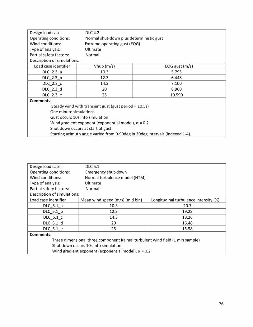
76
Design load case: DLC 4.2
Operating conditions: Normal shut-down plus deterministic gust
Wind conditions: Extreme operating gust (EOG)
Type of analysis: Ultimate
Partial safety factors: Normal
Description of simulations:
Load case identifier Vhub (m/s) EOG gust (m/s)
DLC_2.3_a 10.3 5.795
DLC_2.3_b 12.3 6.448
DLC_2.3_c 14.3 7.100
DLC_2.3_d 20 8.960
DLC_2.3_e 25 10.590
Comments:
Steady wind with transient gust (gust period = 10.5s)
One minute simulations
Gust occurs 10s into simulation
Wind gradient exponent (exponential model), α = 0.2
Shut down occurs at start of gust
Starting azimuth angle varied from 0-90deg in 30deg intervals (indexed 1-4).
Design load case: DLC 5.1
Operating conditions: Emergency shut-down
Wind conditions: Normal turbulence model (NTM)
Type of analysis: Ultimate
Partial safety factors: Normal
Description of simulations:
Load case identifier Mean wind speed (m/s) (mid bin) Longitudinal turbulence intensity (%)
DLC_5.1_a 10.3 20.7
DLC_5.1_b 12.3 19.28
DLC_5.1_c 14.3 18.26
DLC_5.1_d 20 16.48
DLC_5.1_e 25 15.58
Comments:
Three dimensional three component Kaimal turbulent wind field (1 min sample)
Shut down occurs 10s into simulation
Wind gradient exponent (exponential model), α = 0.2
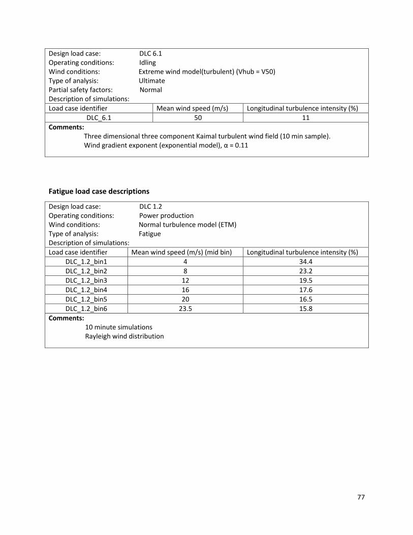
77
Design load case: DLC 6.1
Operating conditions: Idling
Wind conditions: Extreme wind model(turbulent) (Vhub = V50)
Type of analysis: Ultimate
Partial safety factors: Normal
Description of simulations:
Load case identifier Mean wind speed (m/s) Longitudinal turbulence intensity (%)
DLC_6.1 50 11
Comments:
Three dimensional three component Kaimal turbulent wind field (10 min sample).
Wind gradient exponent (exponential model), α = 0.11
Fatigue load case descriptions
Design load case: DLC 1.2
Operating conditions: Power production
Wind conditions: Normal turbulence model (ETM)
Type of analysis: Fatigue
Description of simulations:
Load case identifier Mean wind speed (m/s) (mid bin) Longitudinal turbulence intensity (%)
DLC_1.2_bin1 4 34.4
DLC_1.2_bin2 8 23.2
DLC_1.2_bin3 12 19.5
DLC_1.2_bin4 16 17.6
DLC_1.2_bin5 20 16.5
DLC_1.2_bin6 23.5 15.8
Comments:
10 minute simulations
Rayleigh wind distribution
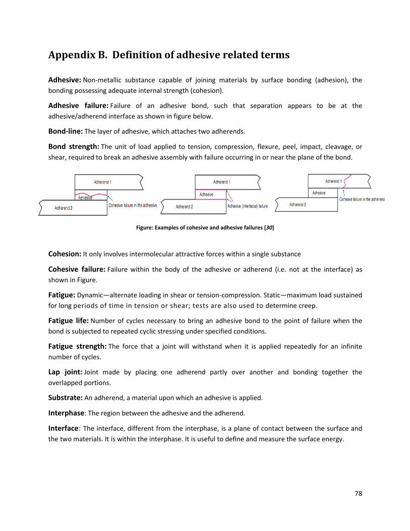
78
Appendix B. Definition of adhesive related terms
Adhesive: Non-metallic substance capable of joining materials by surface bonding (adhesion), the
bonding possessing adequate internal strength (cohesion).
Adhesive failure: Failure of an adhesive bond, such that separation appears to be at the
adhesive/adherend interface as shown in figure below.
Bond-line: The layer of adhesive, which attaches two adherends.
Bond strength: The unit of load applied to tension, compression, flexure, peel, impact, cleavage, or
shear, required to break an adhesive assembly with failure occurring in or near the plane of the bond.
Figure: Examples of cohesive and adhesive failures [30]
Cohesion: It only involves intermolecular attractive forces within a single substance
Cohesive failure: Failure within the body of the adhesive or adherend (i.e. not at the interface) as
shown in Figure.
Fatigue: Dynamic—alternate loading in shear or tension-compression. Static—maximum load sustained
for long periods of time in tension or shear; tests are also used to determine creep.
Fatigue life: Number of cycles necessary to bring an adhesive bond to the point of failure when the
bond is subjected to repeated cyclic stressing under specified conditions.
Fatigue strength: The force that a joint will withstand when it is applied repeatedly for an infinite
number of cycles.
Lap joint: Joint made by placing one adherend partly over another and bonding together the
overlapped portions.
Substrate: An adherend, a material upon which an adhesive is applied.
Interphase: The region between the adhesive and the adherend.
Interface: The interface, different from the interphase, is a plane of contact between the surface and
the two materials. It is within the interphase. It is useful to define and measure the surface energy.
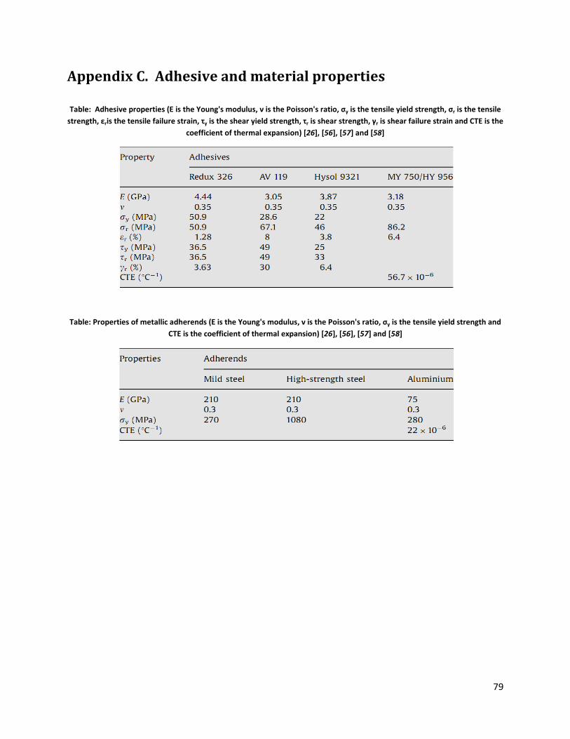
79
Appendix C. Adhesive and material properties
Table: Adhesive properties (E is the Young's modulus, ν is the Poisson's ratio, σy is the tensile yield strength, σr is the tensile
strength, εris the tensile failure strain, τy is the shear yield strength, τr is shear strength, γr is shear failure strain and CTE is the
coefficient of thermal expansion) [26], [56], [57] and [58]
Table: Properties of metallic adherends (E is the Young's modulus, ν is the Poisson's ratio, σy is the tensile yield strength and
CTE is the coefficient of thermal expansion) [26], [56], [57] and [58]

80
Appendix D. Matlab code for Volkersen Model
Variation of peak shear stress against different overlap length
% variation of shear stress when bonding length is changed from 50mm to % 2m keeping the adhesive thickness 10mm clear all clc
tw = 55*10^-3; % Tower section wall thickness (m) tf = 55*10^-3; % Tower foundation wall thickness (m) v = 0.35; % Poisson ratio E = 210*10^9; % Young's modulus for both tower and foundation
section(Pa) ta = 10*10^-3; % Adhesive thickness (m) Ea = 3.7*10^9; % Modulus of elasticity (Pa) Ga = 1.35*10^9; % Shear Modulus (Pa)
% Bending and Axial stress calculation on joint section
di = 4.19-2*0.035; % Inner diameter (m) do = di + 2*tw; % Outer diameter (m) M = 85.404*10^6; % Bending moment (Nm) Sb = M*do*0.5*64/3.14/(do^4-(di)^4); % Bending stress Sa = 3*10^6 * 4/3.14/(do^2-di^2); % Axial stress Stotal = Sb+Sa; % Total stress l = 0.05;
for i=1:196 x = -l/2; phi = Ga*l^2/E/tw/ta; Si = tw/tf; w = sqrt((1+Si)*phi); X = x/l; % Adhesive shear stress Taumax(i) = (Stotal*tw/l/1000000)*((0.5*w*cosh(w*X)/sinh(w/2))+(((Si-
1)/(Si+1))*w*0.5*sinh(w*X)/cosh(w/2))); l = l + 0.01; end
plot(0.05:0.01:2, Taumax,'r') axis([0.05 2 0.0 135]), grid xlabel('Overlap lengths(m)'),ylabel('Shear Stress(MPa)')
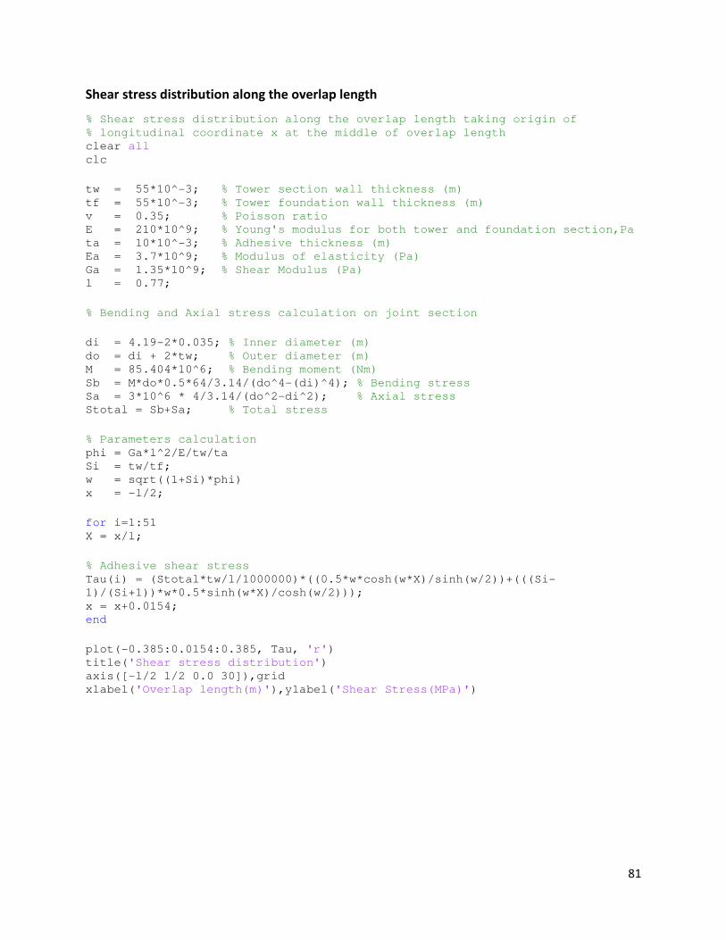
81
Shear stress distribution along the overlap length
% Shear stress distribution along the overlap length taking origin of
% longitudinal coordinate x at the middle of overlap length clear all clc
tw = 55*10^-3; % Tower section wall thickness (m) tf = 55*10^-3; % Tower foundation wall thickness (m) v = 0.35; % Poisson ratio E = 210*10^9; % Young's modulus for both tower and foundation section,Pa ta = 10*10^-3; % Adhesive thickness (m) Ea = 3.7*10^9; % Modulus of elasticity (Pa) Ga = 1.35*10^9; % Shear Modulus (Pa) l = 0.77;
% Bending and Axial stress calculation on joint section
di = 4.19-2*0.035; % Inner diameter (m) do = di + 2*tw; % Outer diameter (m) M = 85.404*10^6; % Bending moment (Nm) Sb = M*do*0.5*64/3.14/(do^4-(di)^4); % Bending stress Sa = 3*10^6 * 4/3.14/(do^2-di^2); % Axial stress Stotal = Sb+Sa; % Total stress
% Parameters calculation phi = Ga*l^2/E/tw/ta Si = tw/tf; w = sqrt((1+Si)*phi) x = -l/2;
for i=1:51 X = x/l;
% Adhesive shear stress Tau(i) = (Stotal*tw/l/1000000)*((0.5*w*cosh(w*X)/sinh(w/2))+(((Si-
1)/(Si+1))*w*0.5*sinh(w*X)/cosh(w/2))); x = x+0.0154; end
plot(-0.385:0.0154:0.385, Tau, 'r') title('Shear stress distribution') axis([-l/2 l/2 0.0 30]),grid xlabel('Overlap length(m)'),ylabel('Shear Stress(MPa)')
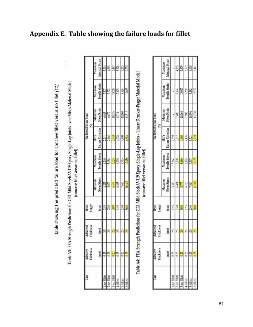
82
Appendix E. Table showing the failure loads for fillet

83