Embed Size (px)
Citation preview

Perceptual fidelity for digital image display
Adela Katharine Devlin
A thesis submitted to the University of Bristol, UK in accordance with the requirements for thedegree of Doctor of Philosophy in the Faculty of Engineering, Department of Computer Science.
2004
c. 32 000 words


Abstract
Many applications require that the original version of an image will appear the same regardlessof where or how it is displayed. However, the conditions in which an image is displayed canadversely affect its appearance. Computer monitor screens not only emit light, but can also reflectextraneous light present in the viewing environment. This can cause images displayed on a monitorto appear faded by reducing their perceived contrast. Current approaches to this problem involvemeasuring this ambient illumination with specialised hardware, then altering the display device orchanging the viewing conditions. This is not only impractical, but also costly and time consuming.For a user who does not have the equipment, expertise or budget to control these facets of imagedisplay, a practical alternative is sought. This thesis presents a method whereby the display deviceitself can be used to determine the effect of ambient light on perceived contrast, thus enabling theviewers themselves to perform visually-based calibration. This method is grounded in establishedpsychophysical experimentation, and we present both an extensive procedure and an equivalentrapid procedure. Our work is extended by providing a novel method of contrast correction sothat the contrast of an image viewed in bright conditions can be corrected to appear the same asan image viewed in a darkened room. This is verified through formal psychophysical validationstudies. These methods and algorithms are easy to apply in practical settings, while accurateenough to be useful.


Declaration
The work in this thesis is original and no portion of the work referred to here has been submittedin support of an application for another degree or qualification of this or any other university orinstitution of learning.
Signed: Date:
Adela Katharine Devlin


Acknowledgements
This work was funded for the most part by EPSRC Student CASE Award 00314469 in conjunctionwith the Defence Evaluation and Research Agency.
First, thanks to Alan Chalmers for seeing this PhD through from start to finish, and for takingme to so many fantastic places along the way. There’ve been some ups and downs, but I hopewe’ve ended on an up! The whole of the infinite number of Ph.D. students in the Graphics Groupalso deserve thanks, especially Patrick, Pete and Ki without whom I would never have survivedthe final night in Saarbrucken. To those I’ve met over conference beers, cheers! (That’s got toinclude the Acknowledgement Tart, Greg Ward.) Much appreciation to those who have sharedadvice, especially Tom Troscianko. Many, many thanks indeed to Erik Reinhard who has kept upthe encouragement and advice and made conferences even more fun than usual. His knowledgeand enthusiasm has proved invaluable, and I thank him for his contributions and his friendship.
Big shout out to the lunchtime posse — the highly insecure (what was that password again?) cryptogroup and the downwardly-mobile wearable team. Alphabetically, sort of: Amoss and his luckycharms, Dan ‘cyberdolphin’ Page, Fre Vercauteren, Martijn and his antimatter flapjacks, Matt‘she’s-not-that-young’ Baldwin, Mike ‘aboot’ McCarthy, Paul ‘oooh-yeah’ Duff, Rich ‘I’m not anaggressive person’ Noad, and, in his bid for world domination, Nigel Smart. For coffee-drinkingsupport and general bitchin’, I thank you. To the cinema-goers, music-lovers, pub drinkers andindecisive diners (that’d be Barry, Eric, and Tim, ably co-ordinated by Peter ‘babe’ Flach), cheers!Indeed, much appreciation to everyone who has made my time in the department so damn enjoy-able (including Chris, Mike and Nige who had to put up with me in their office).
Sarah, Stef, Dave and Angus — there were moments when climbing (and alcohol) was all thatkept me going, and you guys were there, wielding wine bottles and holding the rope (except forAngus who was having difficulty with the 6a sitting start off of the sofa, but who more than madeup for it with the alcohol).
Special thanks to the House of Dysfunction and all who play in her: Antti, Mary, Carl, and the-best-flatmate-ever, Genevieve. Much gratitude to the Mudcatters for online and real-life music,and for putting up with my repertoire of badly-fiddled polkas. Not forgetting the gurls: Chrisand Helen — yay! Love yez babes. Also, my Northbrook buddies deserve (platonic) lurve forpacking me off to Bristol with fond memories of awful hangovers and an unsurpassable roadtripto Memphis: Whoremonger, Needledick and Nicegirlsorcha — now I’ve got time to write thatnovel.
To those who’ve been with me all the way and supported my bid to be an Eternal Student — memammy, me da, and our Louise — yous are the best family I’ve ever had.
These acknowledgements are in no order of preference, except for this: Henk Muller, my bestmate, thank you for so much, including saving my life literally and metaphorically on severaloccasions. vfw.


To Fintan, who’s always asking “what did I send you to university for?”.


Contents
List of Figures vi
List of Tables x
1 Introduction 1
1.1 Contributions of this thesis . .. . . . . . . . . . . . . . . . . . . . . . . . . . . 4
1.2 Thesis outline . . .. . . . . . . . . . . . . . . . . . . . . . . . . . . . . . . . . 5
1.3 Application: virtual heritage .. . . . . . . . . . . . . . . . . . . . . . . . . . . 6
1.3.1 Captured images . . . . . . . . . . . . . . . . . . . . . . . . . . . . . . 7
1.3.2 Rendered representations. . . . . . . . . . . . . . . . . . . . . . . . . . 7
1.3.3 Consistency in delivery . . . . . . . . . . . . . . . . . . . . . . . . . . . 16
2 Background 19
2.1 Light . . . . . . . . . . . . . . . . . . . . . . . . . . . . . . . . . . . . . . . . . 19
2.1.1 Radiometry and photometry . . .. . . . . . . . . . . . . . . . . . . . . 20
2.1.2 Light propagation . . . . . . . . . . . . . . . . . . . . . . . . . . . . . . 22
2.2 Visual perception . . . . . . . . . . . . . . . . . . . . . . . . . . . . . . . . . . 24
2.2.1 The human eye . . . . . . . . . . . . . . . . . . . . . . . . . . . . . . . 24
2.2.2 Visual sensitivity . . . . . . . . . . . . . . . . . . . . . . . . . . . . . . 25
i
2.2.3 Contrast . . . . . . . . . . . . . . . . . . . . . . . . . . . . . . . . . . . 26
2.2.4 Thresholds . . . . . . . . . . . . . . . . . . . . . . . . . . . . . . . . . 26
2.2.5 The Contrast Sensitivity Function . . . . . . . . . . . . . . . . . . . . . 28
2.2.6 Adaptation . . . . . . . . . . . . . . . . . . . . . . . . . . . . . . . . . 28
2.2.7 Brightness perception . . . . . . . . . . . . . . . . . . . . . . . . . . . . 29
2.2.8 Lightness and colour constancy . . . . . . . . . . . . . . . . . . . . . . 31
2.3 Digital image creation . . . . . . . . . . . . . . . . . . . . . . . . . . . . . . . . 31
2.3.1 Capturing digital images . . . . . . . . . . . . . . . . . . . . . . . . . . 32
2.3.2 Generating digital images . . . . . . . . . . . . . . . . . . . . . . . . . 32
2.4 Display technology. . . . . . . . . . . . . . . . . . . . . . . . . . . . . . . . . 32
2.4.1 Cathode Ray Tubes. . . . . . . . . . . . . . . . . . . . . . . . . . . . . 34
2.4.2 Liquid Crystal Displays . . . . . . . . . . . . . . . . . . . . . . . . . . 35
2.4.3 Plasma Display Panels . . . . . . . . . . . . . . . . . . . . . . . . . . . 35
2.5 Controlling the display . .. . . . . . . . . . . . . . . . . . . . . . . . . . . . . 36
2.5.1 Gamma . . . . . . . . . . . . . . . . . . . . . . . . . . . . . . . . . . . 36
2.5.2 Tone reproduction. . . . . . . . . . . . . . . . . . . . . . . . . . . . . 40
2.5.3 Gamut mapping . . . . . . . . . . . . . . . . . . . . . . . . . . . . . . . 54
2.6 Summary . . . . . . . . . . . . . . . . . . . . . . . . . . . . . . . . . . . . . . 55
3 The viewing environment 57
3.1 The influences of ambient illumination. . . . . . . . . . . . . . . . . . . . . . . 57
3.2 Accounting for viewing conditions . . . . . . . . . . . . . . . . . . . . . . . . . 59
3.2.1 Physical alterations to the hardware . . . . . . . . . . . . . . . . . . . . 59
3.2.2 Viewing environment standards . . . . . . . . . . . . . . . . . . . . . . 60
ii

3.2.3 Measurement and image correction. . . . . . . . . . . . . . . . . . . . 61
3.3 Related work . . . . . . . . . . . . . . . . . . . . . . . . . . . . . . . . . . . . 65
3.3.1 Ergonomics. . . . . . . . . . . . . . . . . . . . . . . . . . . . . . . . . 65
3.3.2 Medical imaging . . . . . . . . . . . . . . . . . . . . . . . . . . . . . . 66
3.4 Summary . . . . . . . . . . . . . . . . . . . . . . . . . . . . . . . . . . . . . . 68
4 Measuring reflected ambient light 69
4.1 Conducting experiments . . .. . . . . . . . . . . . . . . . . . . . . . . . . . . 69
4.1.1 Hypotheses. . . . . . . . . . . . . . . . . . . . . . . . . . . . . . . . . 70
4.1.2 Ethics . . . . . . . . . . . . . . . . . . . . . . . . . . . . . . . . . . . . 71
4.1.3 Sample design . . . . . . . . . . . . . . . . . . . . . . . . . . . . . . . 71
4.1.4 Pilot studies . . . . . . . . . . . . . . . . . . . . . . . . . . . . . . . . . 72
4.1.5 Problems with psychophysics and statistical significance. . . . . . . . . 73
4.2 Experiment 1: contrast discrimination thresholds . . . . . . . . . . . . . . . . . 74
4.2.1 Hypotheses. . . . . . . . . . . . . . . . . . . . . . . . . . . . . . . . . 75
4.2.2 Participants. . . . . . . . . . . . . . . . . . . . . . . . . . . . . . . . . 75
4.2.3 Conditions . . . . . . . . . . . . . . . . . . . . . . . . . . . . . . . . . 75
4.2.4 Stimuli . . . . . . . . . . . . . . . . . . . . . . . . . . . . . . . . . . . 76
4.2.5 Procedure . . . . . . . . . . . . . . . . . . . . . . . . . . . . . . . . . . 78
4.2.6 Results and discussion . . . . . . . . . . . . . . . . . . . . . . . . . . . 80
4.3 Experiment 2: rapid characterisation . . . . . . . . . . . . . . . . . . . . . . . . 84
4.3.1 Alternative and pilot experiments . . . . . . . . . . . . . . . . . . . . . 84
4.3.2 Main experiment . . . . . . . . . . . . . . . . . . . . . . . . . . . . . . 87
4.3.3 Participants. . . . . . . . . . . . . . . . . . . . . . . . . . . . . . . . . 88
iii
4.3.4 Conditions . . . . . . . . . . . . . . . . . . . . . . . . . . . . . . . . . 88
4.3.5 Procedure . . . . . . . . . . . . . . . . . . . . . . . . . . . . . . . . . . 89
4.3.6 Results and discussion . . . . . . . . . . . . . . . . . . . . . . . . . . . 89
4.4 Summary . . . . . . . . . . . . . . . . . . . . . . . . . . . . . . . . . . . . . . 92
5 Correcting for Ambient Light 95
5.1 Contrast adjustment . . . . . . . . . . . . . . . . . . . . . . . . . . . . . . . . . 96
5.2 Luminance remapping requirements . . . . . . . . . . . . . . . . . . . . . . . . 96
5.3 Existing remapping methods. . . . . . . . . . . . . . . . . . . . . . . . . . . . 97
5.3.1 Gamma manipulation . . . . . . . . . . . . . . . . . . . . . . . . . . . . 98
5.3.2 Hyperbolic functions . . . . . . . . . . . . . . . . . . . . . . . . . . . . 98
5.3.3 Histogram equalisation . . . . . . . . . . . . . . . . . . . . . . . . . . . 98
5.3.4 Spatially varying techniques . . . . . . . . . . . . . . . . . . . . . . . . 99
5.4 Schlick’s rational function as a basis for remapping . . . . . . . . . . . . . . . . 99
5.5 A new luminance remapping algorithm. . . . . . . . . . . . . . . . . . . . . . . 101
5.5.1 The range[0;L] . . . . . . . . . . . . . . . . . . . . . . . . . . . . . . . 102
5.5.2 The range[L;M] . . . . . . . . . . . . . . . . . . . . . . . . . . . . . . 102
5.5.3 Complete remapping function . . . . . . . . . . . . . . . . . . . . . . . 103
5.5.4 Function inversion . . . . . . . . . . . . . . . . . . . . . . . . . . . . . 103
5.5.5 Colour space . . . . . . . . . . . . . . . . . . . . . . . . . . . . . . . . 105
5.6 Results and discussion . . . . . . . . . . . . . . . . . . . . . . . . . . . . . . . 106
5.7 Summary . . . . . . . . . . . . . . . . . . . . . . . . . . . . . . . . . . . . . . 109
6 Validation of luminance remapping 111
iv

6.1 Validation experiment . . . . . . . . . . . . . . . . . . . . . . . . . . . . . . . . 111
6.1.1 Hypotheses. . . . . . . . . . . . . . . . . . . . . . . . . . . . . . . . . 112
6.1.2 Participants. . . . . . . . . . . . . . . . . . . . . . . . . . . . . . . . . 112
6.1.3 Conditions . . . . . . . . . . . . . . . . . . . . . . . . . . . . . . . . . 113
6.1.4 Procedure . . . . . . . . . . . . . . . . . . . . . . . . . . . . . . . . . . 113
6.1.5 Results . . . . . . . . . . . . . . . . . . . . . . . . . . . . . . . . . . . 113
6.2 Summary . . . . . . . . . . . . . . . . . . . . . . . . . . . . . . . . . . . . . . 115
7 Conclusions 117
7.1 Advantages . . . . . . . . . . . . . . . . . . . . . . . . . . . . . . . . . . . . . 119
7.2 Disadvantages . . . . . . . . . . . . . . . . . . . . . . . . . . . . . . . . . . . . 119
7.3 Further research . .. . . . . . . . . . . . . . . . . . . . . . . . . . . . . . . . . 120
7.4 Closing remarks . . . . . . . . . . . . . . . . . . . . . . . . . . . . . . . . . . . 121
Bibliography 122
A Materials 137
A.1 Experimental Informed Consent Form . . . . . . . . . . . . . . . . . . . . . . . 138
A.2 Instructions for Experiment 1 . . . . . . . . . . . . . . . . . . . . . . . . . . . . 140
A.3 Instructions for Experiment 2 . . . . . . . . . . . . . . . . . . . . . . . . . . . . 141
B Results 143
v

vi
List of Figures
1.1 Example of a ‘washed out’ image . . . . . . . . . . . . . . . . . . . . . . . . . 4
1.2 Virtual heritage: system diagram. . . . . . . . . . . . . . . . . . . . . . . . . . 7
1.3 Experimental archaeology: physical reconstruction of fuel types.. . . . . . . . . 9
1.4 Simulations: differences in lighting . . . . . . . . . . . . . . . . . . . . . . . . . 11
1.5 Examples of medieval pottery. . . . . . . . . . . . . . . . . . . . . . . . . . . . 12
1.6 Medieval house simulations . .. . . . . . . . . . . . . . . . . . . . . . . . . . . 12
1.7 The House of the Vettii today .. . . . . . . . . . . . . . . . . . . . . . . . . . . 13
1.8 Simulation of the House of the Vettii . . .. . . . . . . . . . . . . . . . . . . . . 14
1.9 Simulation with the inclusion of furniture . . . . . . . . . . . . . . . . . . . . . 15
1.10 Cap Blanc . . . . . . . . . . . . . . . . . . . . . . . . . . . . . . . . . . . . . . 16
2.1 The electromagnetic spectrum . . . . . . . . . . . . . . . . . . . . . . . . . . . 20
2.2 The Luminous Efficiency Curve. . . . . . . . . . . . . . . . . . . . . . . . . . 21
2.3 Specular and diffuse reflections . . . . . . . . . . . . . . . . . . . . . . . . . . . 23
2.4 A schematic section through the human eye. . . . . . . . . . . . . . . . . . . . 25
2.5 Weber’s law: JND measurement. . . . . . . . . . . . . . . . . . . . . . . . . . 27
2.6 Threshold versus intensity function . . . . . . . . . . . . . . . . . . . . . . . . . 28
2.7 The Campbell-Robson sensitivity chart and the contrast sensitivity function . . . 29
vii
2.8 Plot of the Stevens’ Power Law . . . . . . . . . . . . . . . . . . . . . . . . . . . 30
2.9 Simplified schematic diagram of a CRT . . . . . . . . . . . . . . . . . . . . . . 34
2.10 Gamma values for a CRT monitor . . . . . . . . . . . . . . . . . . . . . . . . . 37
2.11 Example of test patterns for gamma measurement. . . . . . . . . . . . . . . . . 39
2.12 Image used for simple gamma correction . . . . . . . . . . . . . . . . . . . . . . 40
2.13 A comparative view of dynamic range.. . . . . . . . . . . . . . . . . . . . . . . 41
2.14 Ideal tone reproduction process. . . . . . . . . . . . . . . . . . . . . . . . . . . 41
2.15 Linear scaling versus tone reproduction.. . . . . . . . . . . . . . . . . . . . . . 42
2.16 Example of dynamic range extent using varying exposures.. . . . . . . . . . . . 43
2.17 Chromaticity diagram . . . . . . . . . . . . . . . . . . . . . . . . . . . . . . . . 55
3.1 ICC colour management architecture . . . . . . . . . . . . . . . . . . . . . . . . 63
4.1 Example of the set up for thelight condition . . . . . . . . . . . . . . . . . . . . 76
4.2 Example stimulus . . . . . . . . . . . . . . . . . . . . . . . . . . . . . . . . . . 77
4.3 The staircase method . . .. . . . . . . . . . . . . . . . . . . . . . . . . . . . . 80
4.4 Flowchart showing procedure for Experiment 1. . . . . . . . . . . . . . . . . . . 81
4.5 Simplified measurement using a Campbell-Robson chart .. . . . . . . . . . . . 85
4.6 A type of gamma chart used to measure contrast discrimination . . .. . . . . . . 86
4.7 Grid of squares used for simplified characterisation. . . . . . . . . . . . . . . . . 88
4.8 Flowchart showing procedure for Experiment 2. . . . . . . . . . . . . . . . . . . 90
4.9 Experiment 2: average JND values . . . . . . . . . . . . . . . . . . . . . . . . . 91
5.1 Problems with remapping by subtraction . . . . . . . . . . . . . . . . . . . . . . 96
5.2 Splitting the remapping function into two ranges. . . . . . . . . . . . . . . . . . 101
viii

5.3 Remapping functions forLR . . . . . . . . . . . . . . . . . . . . . . . . . . . . 104
5.4 Remapping results . . . . . . . . . . . . . . . . . . . . . . . . . . . . . . . . . 107
5.5 Comparison with other techniques . . . . . . . . . . . . . . . . . . . . . . . . . 108
6.1 Validation experiment: average JND values . . . . . . . . . . . . . . . . . . . . 114
ix

x
List of Tables
2.1 Radiometric and photometric measurements. . . . . . . . . . . . . . . . . . . . 22
2.2 Display technology comparison. . . . . . . . . . . . . . . . . . . . . . . . . . 33
3.1 Typical lighting recommendation for offices . . . . . . . . . . . . . . . . . . . . 59
4.1 Example of RGB values used in bit-stealing. . . . . . . . . . . . . . . . . . . . 78
4.2 Experiment 1: average JND results, pedestal value = 5% grey . . . . . . . . . . . 81
4.3 Experiment 1: average JND results, pedestal value = 10% grey . . . . . . . . . . 82
4.4 Experiment 1: average JND results, pedestal value = 20% grey . . . . . . . . . . 82
5.1 Requirements for a luminance remapping function . . . . . . . . . . . . . . . . . 97
B.1 Experiment 1: average JND results, pedestal value = 5% grey . . . . . . . . . . . 144
B.2 Experiment 1: average JND results, pedestal value = 10% grey . . . . . . . . . . 144
B.3 Experiment 1: average JND results, pedestal value = 20% grey . . . . . . . . . . 144
B.4 Experiment 2: average JND results, pedestal value = 5% grey . . . . . . . . . . . 145
B.5 Experiment 2: average JND results, pedestal value = 10% grey . . . . . . . . . . 146
B.6 Experiment 2: average JND results, pedestal value = 20% grey . . . . . . . . . . 147
B.7 Validation experiment: average JND results . . . . . . . . . . . . . . . . . . . . 148
xi

xii
Chapter 1
Introduction
Many applications that use electronic display devices require images to appear a certain way. In ar-
eas as diverse as medical imaging [AKK+82, BRN82, RJP87, Nat03], aviation [Fed00], visualisa-
tion [War00], photography [Hun96], and predictive lighting and realistic image synthesis [AF95],
similarity is desirable between the image as it was created and the resultant image that is viewed
by the end-user. The user must be confident that the image they are viewing is faithful to the orig-
inal — they requireperceptual fidelity. However, a given image will not always be perceived in
the same way. Problems may arise because the sequence of events from image creation to percep-
tion is open to adverse influence, which can result in an image that deviates from the way it was
intended to look. As images are often displayed on different monitors and in different locations
from where they were created (such as images displayed over a network, or on the Internet), it is
necessary to ensure that steps have been taken to ensure perceptual consistency, where any point
in an image will look the same regardless of changes in viewing location and display device. To
ensure that the scene as it was created closely resembles the scene as it is displayed, it is necessary
to be aware of any factors that might adversely influence the display medium.
A digital image goes through a sequence of processing before it is ultimately displayed on the
screen of a visual display unit (VDU). Fidelity in modelling or capturing a scene, the use of pre-
dictive lighting software (in the case of computer-generated images), the use of tone reproduction
methods and gamma correction, all go towards achieving perceptual accuracy. However, further
1
2
to the adjustments to the actual image, the processes that occurafter the luminances are displayed
on screen andbeforethey reach the retina must also be considered. This is a physical problem
with a direct perceptual impact.
For certain applications, such as trade or industry where a direct match between a displayed design
and the resulting product is essential, it is likely that a specific viewing environment exists, and full
calibration of all equipment has occurred. However, there are other fields where it is not possible
to guarantee the fidelity of a displayed image. This may be due to lack of equipment, facilities or
cost. Nonetheless, in these circumstances the user may wish to ensure that they have taken any
possible steps within their measure towards perceptual fidelity.
One example of an area where perceptual consistency between images is important is in cultural
heritage applications. In terms of cultural heritage, computer graphics has enabled the capturing
and creation of images that can be used as perceptually equivalent representations of an orig-
inal [DC01, CD02, DCB02]. Virtual reality and visualisation techniques can provide a highly
detailed model of a site or artefact. Improvements in scanning and digital photography have led
to the widespread use of this technology to preserve original text and art. For digital archiving
to be used as a technique for representation or preservation, the integrity of an image must be
vouchsafed [DCR04].
The need to exert control over image presentation has given rise to standards and guidelines con-
cerning digital display and ergonomics, such as the guidelines of the UK’s Arts and Humanities
Data Service (AHDS) [Art] and the International Organization for Standardization (ISO) [Int].
In addition, museums, libraries and archives using digital images are aware of the problems of
inconsistencies in image display. Reilly and Frey’s report to the American Library of Congress
highlighted the differences between images when viewed on different systems or monitors, with
Library staff finding it problematic ‘when discussing the quality of scans with vendors over the
telephone, because the two parties did not see the same image’ [RF96].
Some institutions do address these factors. The Bodleian Library’s online image catalogue at the
University of Oxford states:

3
Note that the apparent quality of the images as viewed on-screen is in part dependent
upon the quality of the monitor used to view them, and the apparent colour-values
are likewise dependent on whether the monitor has been correctly calibrated, and the
ambient lighting conditions of the room. [Bod].
This thesis investigates a potential influence on perceptual fidelity: the lighting in the viewing
environment, and in particular, reflections caused by the average amount of light present in a
room — theambient illumination. It argues that the presence of ambient light in the viewing
environment has an adverse effect on the user’s perception of an image, and that this effect must
be characterised and corrected in order to adhere to perceptual fidelity. It has been suggested
that ambient light can cause a reduction in the perceived contrast of an image displayed on a
CRT screen, causing an image viewed under a high level of ambient light to appear ‘washed
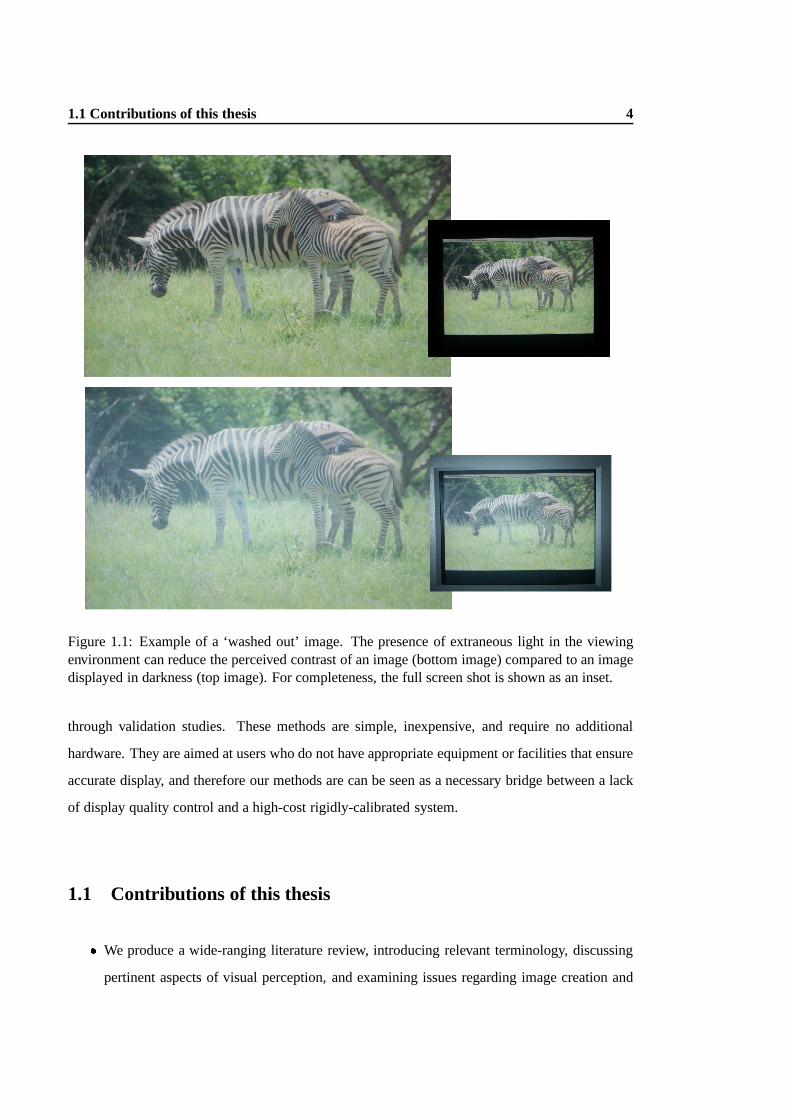
out’ [Gla95, Tra91, War00]. An example of this is given in Figure 1.1 where the same image
is shown as it appears when displayed in a room with no ambient light present (top), and when
displayed under illumination by a D65 light bulb (bottom).
While the presence of such illumination may have a detrimental effect on image appearance, many
working conditions require a certain level of illumination in a room, to enable note-taking, for
example. Therefore, the extraneous illumination cannot simply be removed, but rather should be
accounted for in some way. Current approaches to this problem involve measuring the ambient
illumination with specialised hardware, and altering the display device or changing the viewing
conditions. Measuring the amount of ambient illumination in an environment is possible through
the use of specialised equipment, such as a photometer, spectroradiometer or illuminance meter.
However, this method requires additional hardware — an extra expense and impractical to acquire
— and the knowledge to use this hardware. Moreover, this equipment measures the physical value
of the light present in the viewing environment rather than its perceptual impact.
In this thesis we present a method, based on an experimental framework, whereby the display
device itself can be used to determine the level of ambient illumination affecting an image. We
provide a method of contrast correction to alter the perceived contrast, so that an image viewed in
bright conditions appears the same as an image viewed in a darkened room. This work is tested
1.1 Contributions of this thesis 4
Figure 1.1: Example of a ‘washed out’ image. The presence of extraneous light in the viewingenvironment can reduce the perceived contrast of an image (bottom image) compared to an imagedisplayed in darkness (top image). For completeness, the full screen shot is shown as an inset.
through validation studies. These methods are simple, inexpensive, and require no additional
hardware. They are aimed at users who do not have appropriate equipment or facilities that ensure
accurate display, and therefore our methods are can be seen as a necessary bridge between a lack
of display quality control and a high-cost rigidly-calibrated system.
1.1 Contributions of this thesis
� We produce a wide-ranging literature review, introducing relevant terminology, discussing
pertinent aspects of visual perception, and examining issues regarding image creation and
1.2 Thesis outline 5
display.
� We present an experimental framework that assesses the effect of ambient light on image
perception, using validated psychophysical approaches.
� We hypothesise that reflected ambient illumination affects perceived contrast, and obtain
statistical evidence through our experiments to support this theory.
� We develop a form of rapid visual self-calibration to enable the measurement of ambient
light without the need for specialised equipment or external hardware.
� We present one possible algorithmic form of correction to compensate for ambient reflec-
tions. Its success is validated through a formal psychophysical user study.
1.2 Thesis outline
The remainder of this chapter gives an example application where perceptual fidelity in image dis-
play is desirable and outlines the process of image creation and viewing. The subsequent chapters
are divided as follows:
Chapter 2: Background Chapter 2 provides fundamental information on digital image display,
beginning with the terminology of light and its properties. Aspects of the human visual
system pertaining to the perception of displayed images are examined. In addition, it focuses
on the display of digital images, from their creation or capture and the technology used to
display them, through to techniques used to control the appearance of the displayed image.
Chapter 3: The viewing environment This chapter assesses lighting in workplace viewing en-
vironments. The effect of reflected ambient light on the perception of contrast is discussed.
Methods of dealing with ambient lighting are examined and approaches towards perceptual
fidelity are detailed. Finally, previous related work is described.
Chapter 4: Measuring reflected ambient light Formally-designed psychophysical studies to mea-
sure the perceptual impact of reflected ambient light are presented. A detailed first experi-
ment establishes this impact, and a quick and effective experiment is developed to measure

1.3 Application: virtual heritage 6
changes in contrast perception through visual calibration by the users themselves, without
the need for specialised equipment.
Chapter 5: Correcting for ambient light This chapter details a novel algorithm that can be used
to correct for the effect of ambient light. This is a straightforward rational function, and is
invertible, so that images created under given ambient lighting can be displayed as they
would have originally appeared. Visual examples of the algorithm’s implementation are
given.
Chapter 6: Validation The experimental validation of the algorithm described in Chapter 5 is
described and discussed. This validation follows the procedure of our shortcut experiment,
thus measuring perceived contrast in light and dark conditions, and for corrected and uncor-
rected stimuli.
Chapter 7: Conclusions This final chapter summarises the results and contributions of this the-
sis, and future work revealed during the process is suggested.
1.3 Application: virtual heritage
This section highlights an application where consistency in image perception is desirable: cultural
(and more specifically, virtual) heritage. There are two aspects of virtual heritage that require
perceptual fidelity between images as they were created and images as they are viewed. Either an
image is a captured duplicate of an original artefact or site (such as a photograph of a manuscript,
intended to record or preserve that manuscript), or it is created as a three-dimensional representa-
tion (such as a computer model of a site). It is therefore desirable that the resulting image should
be perceived in the same way by all users, regardless of where they view it, or on which system it
is displayed. Figure 1.2 provides an outline of the process from the archaeological data in its raw
form through to display of the subsequent image.

1.3 Application: virtual heritage 7
Archaeological data
3D model
rendering
original lightingstorage:
e.g. database,web server
display
ambient light
End user
image capture
Figure 1.2: Virtual heritage: system diagram showing an overview of the process from raw scenedata to final image display.
1.3.1 Captured images
Digital image archives are growing in use, and are seen as a way of not only preserving friable or
fragile material in digital form, but also of disseminating this material to a much greater audience.
This has remarkable implications for research into archives once limited in terms of physical
location and number of users. A virtual equivalent of an artefact can be examined without any
harm to the original, and can reach a global audience through a medium such as the Internet.
It is tempting to think that preserving information through image capture is as simple as taking
a photograph, but a wide range of factors need to be addressed: how the artefact will be pho-
tographed, the conditions in which this takes place, the file format that is used to store it, or what
information will be used to describe it, to name just a few examples. Underlying all this difficulty
in determining how best to capture an image is a general assumption that this image is in some
way definitive. However, not only is this image a single form of representation, but it is by no
means guaranteed that it will be displayed in a consistent manner.
1.3.2 Rendered representations
Computer graphics have been used to model archaeological sites and artefacts since the 1980s,
whereby a three dimensional representation of a site is created, then lighting and textures are
added, resulting in an image or animation that represents an original scene. Current use of com-
puter graphics in archaeology provides the public with a glimpse of the past that might otherwise
be difficult to visualise. However, these images are often chosen due to their artistic impact, and
have been manipulated to provide the most aesthetically pleasing representation of a site. To date,
1.3 Application: virtual heritage 8
the emphasis has been on using such images for presentation purposes only, with interpretative
and research purposes taking second place to the demand for visually stunning presentation. The
pervasive media of television and the Internet, and the public fascination for the past, have seen the
adoption of computer-generated representations for entertainment and education of the interested
layman, rather than as a research tool for archaeologists. For computer graphics to benefit the
archaeological community, they must offer the archaeologist the chance to extend or enhance their
analysis of a site or artefact. The accuracy of the images produced must therefore be quantifiable
— the archaeologist must be confident that what they see in the generated image is comparable to
what they would have seen in the original example [CD02].
One area of realistic simulations that is often neglected is that of the original lighting of a site or
artefact. Light cannot be captured in the archaeological record and consequently its importance is
rarely considered in interpretations of past environments. The ways in which we view, perceive
and understand objects is governed by our current lighting methods of steady, bright electric light
or large windows, but in order to understand how an environment and its contents were viewed in
the past we must consider how they were illuminated.
Standard three-dimensional modelling software tends to base the lighting conditions on daylight,
fluorescent light or filament bulbs and not the lamp and candlelight used in past. In some cases,
scenes are illuminated with lighting values that would be impossible in the real world. Realistic
lighting simulation must address both the physical interaction of light in a scene and the spectral
profile of the light source. With control over this, an accurately-lit representation of an environ-
ment can be achieved and the virtual version of an original site or artefact can be manipulated
without having to physically touch or harm the real version.
Accurate illumination
Once an archaeological site or artefact has been modelled in a three-dimensional modelling pack-
age it must berendered; that is, the colours, textures, light and shading are computed, thus pro-
ducing the final two-dimensional image from the three-dimensional geometry. In order to obtain
an approximation of the original lighting in an archaeological representation, two factors must be

1.3 Application: virtual heritage 9
Figure 1.3: Experimental archaeology: physical reconstruction of fuel types.
addressed in the rendering process. First, the spectral composition of the light — the colour of the
light given off by the burning fuel — must match that of the fuel type that would have been used in
a specific archaeological instance. Second, the distribution of this light — the path it takes around
a scene and the reflections and inter-reflections that occur — must mimic the behaviour of light in
the real world.
The only trace of light in the archaeological record are the methods used to provide it, be they
hearths, candles, lamps or windows. In pre-industrial societies, daylight was the regulating factor
of the working hours. Compared to conditions today, sunlight is now far less relevant to how we
work [MCB97]. The evidence from architecture tells us the most about lighting — a lack of glass
and a need for security often meant smaller windows, therefore dimmer interiors. Going further
back in time, the unyielding darkness of a deep cave would require some form of artificial light
for navigation purposes alone. It seems plausible that objects and environments were affected by
the limitations of lighting, and this influence may have extended into their design. By recreating
the means of illumination for a given environment and simulating it accurately, the archaeologist
may (literally) find new ways of viewing things.
The type of flames that were generally used were diffusion wick flames. A typical flame of this na-
ture consists of three parts: the inner core, the blue intermediate zone, and the outer core [GW79].
These different zones produce different emissions depending on the fuel type and environmental
conditions. Various examples of possible light sources have been physically recreated in consulta-
tion with the Department of Archaeology at the University of Bristol, (Figure 1.3). These include
tallow candles (of vegetable origin) and reeds coated in vegetable tallow, a rendered animal fat
lamp, beeswax candles (processed and unrefined) and olive oil lamps (one with olive oil only, one

1.3 Application: virtual heritage 10
with olive oil and salt, and one with olive oil and water).
Each of the above fuels produces a different colour when burnt. To obtain this unique spectral pro-
file for each fuel, detailed data was gathered using a spectroradiometer, a device that measures the
absolute value of the spectral characteristics without making physical contact with the flame. The
spectroradiometer measures the emission spectrum of the light source in the visible bandwidths
in 5nm increments, thus providing an accurate breakdown of the flame-light composition of each
fuel type. The measurements were all taken in a completely dark room, and were taken against a
diffuse white powder (Eastman Kodak Standard, 99% optically pure). An average of ten readings
was calculated for each fuel type.
The resulting spectrographic data was converted into red, green and blue (RGB) values to enable
display on a computer monitor. These RGB values provide us with the data required during the
rendering process to simulate the fuel type of the original light source. Conversion of the spectral
profile of the illuminants to RGB values for use in a computer simulation does lead to an approx-
imation of the colours present. However, at present this is the most effective method in terms of
computational time and efficiency.
The advent of ray-tracing and radiosity in computer graphics has enabled the simulation of light
interaction, providing rendering techniques that mimic the physical behaviour of light in a scene.
Despite the availability of physically-based rendering software many users prefer to produce im-
ages that are aesthetically pleasing rather than perceptually accurate [War94b]. Also, where the
use of predictive lighting software may require some specialist knowledge, access to standard
modelling software is often available in a more user-friendly form. In many cases this can lead to
problems with the validity of computer simulations where the user may — due to time or varying
areas of expertise — lack the skills desired to create a meaningful model, though be fully able to
produce an attractive picture.
The rendering package used to create the images for the case studies below is Greg Ward’sRa-
diance[War94b]. Radianceis a lighting visualisation tool kit that accurately captures luminance
and radiances, models a variety of illumination types, supports a variety of reflectance models and
supports complicated geometry [WLS97]. The values that have been measured from the original
1.3 Application: virtual heritage 11
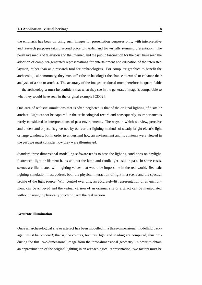
Figure 1.4: Simulation with modern 55w lighting (left) and under tallow lighting (right).
light sources can be used inRadianceas lighting values for a computer-generated model, meaning
that a scene can be rendered under its appropriate lighting conditions.
Changes in perception
Even with the RGB approximation, significant perceptual differences related to variations in fuel
type are apparent. Figure 1.4 shows a test scene containing a MacBeth colour chart illuminated
with modern lighting and light from a tallow candle. The difference in fuel type has a discernible
effect on the appearance of the MacBeth chart. Psychophysical tests can be used to validate sim-
ulations and compare them with real scenes [MCTR98, MCTG00, CMD+01]. Given the type of
lighting that would have been used in past environments, this demonstrates the need to investi-
gate sites and artefacts under their original lighting conditions to ensure we see them as they were
intended to look.
Case studies
The following case studies demonstrate how predictive lighting can be used to benefit the ar-
chaeologist through the development and testing of new hypotheses. All three examples use the
techniques described above, with the archaeological dataset taken from, respectively, measure-
ments made by a tape measure, a scale plan, and a laser scanner. All textures were created from
photographs, with the inclusion of a colour chart for calibration.
Medieval HouseThe initial impetus for work on validated illumination was the question as to how
1.3 Application: virtual heritage 12
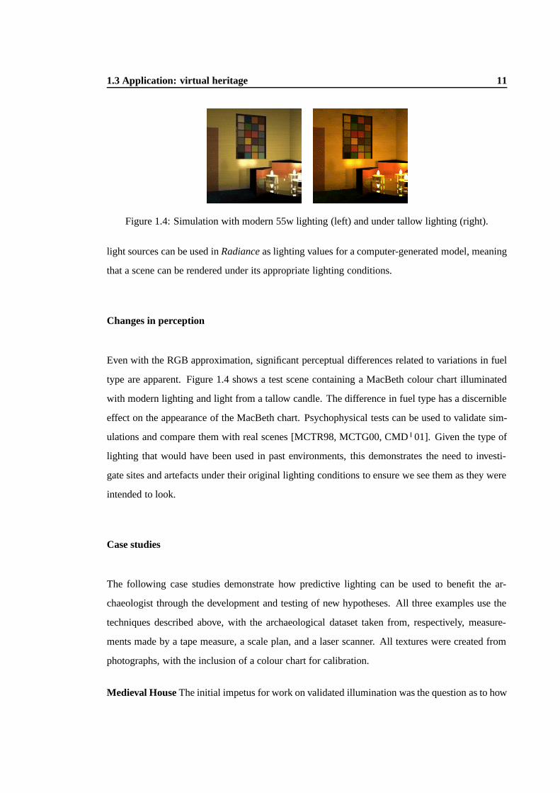
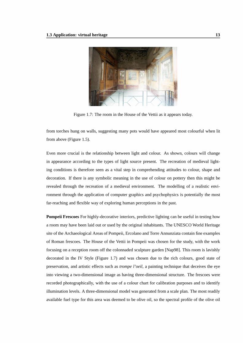
Figure 1.5: Examples of medieval pottery.
Figure 1.6: Medieval house simulations. Images courtesy of Patrick Ledda,c 2002.
medieval pots would have looked in their original setting [MCB97]. This case study considers the
ways in which medieval interiors were illuminated and how lighting conditions might affect the
ways in which objects were perceived and designed.
A computer-generated model of the hall of a medieval town house was created. The model is
based on the Medieval Merchant’s House museum in Southampton, a half-timbered structure ren-
ovated by English Heritage as accurately as possible to represent a 13th century dwelling of some
economic status. This model allows the examination of medieval pottery in a close approxima-
tion to its original setting (Figure 1.6). This reveals details that may bring insight into medieval
ways of living. For example, only the top half of some jugs are glazed and decorated, and this is
perhaps indicative of how they were illuminated in use, perhaps by daylight through windows or
1.3 Application: virtual heritage 13
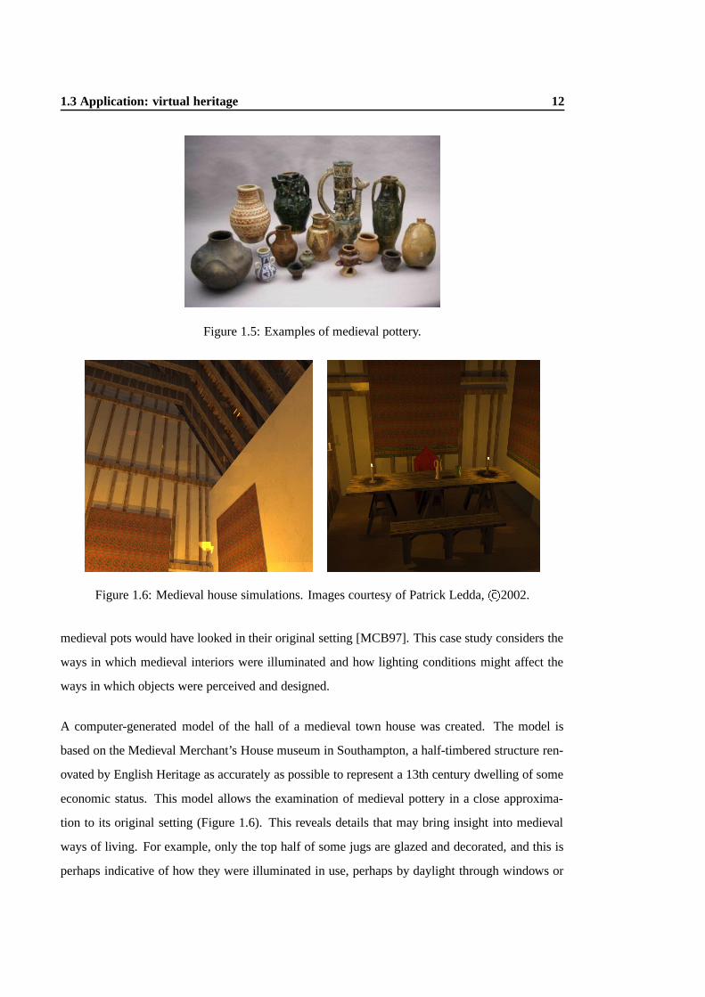
Figure 1.7: The room in the House of the Vettii as it appears today.
from torches hung on walls, suggesting many pots would have appeared most colourful when lit
from above (Figure 1.5).
Even more crucial is the relationship between light and colour. As shown, colours will change
in appearance according to the types of light source present. The recreation of medieval light-
ing conditions is therefore seen as a vital step in comprehending attitudes to colour, shape and
decoration. If there is any symbolic meaning in the use of colour on pottery then this might be
revealed through the recreation of a medieval environment. The modelling of a realistic envi-
ronment through the application of computer graphics and psychophysics is potentially the most
far-reaching and flexible way of exploring human perceptions in the past.
Pompeii FrescoesFor highly-decorative interiors, predictive lighting can be useful in testing how
a room may have been laid out or used by the original inhabitants. The UNESCO World Heritage
site of the Archaeological Areas of Pompeii, Ercolano and Torre Annunziata contain fine examples
of Roman frescoes. The House of the Vettii in Pompeii was chosen for the study, with the work
focusing on a reception room off the colonnaded sculpture garden [Nap98]. This room is lavishly
decorated in the IV Style (Figure 1.7) and was chosen due to the rich colours, good state of
preservation, and artistic effects such astrompe l’oeil, a painting technique that deceives the eye
into viewing a two-dimensional image as having three-dimensional structure. The frescoes were
recorded photographically, with the use of a colour chart for calibration purposes and to identify
illumination levels. A three-dimensional model was generated from a scale plan. The most readily
available fuel type for this area was deemed to be olive oil, so the spectral profile of the olive oil

1.3 Application: virtual heritage 14
Figure 1.8: Simulation viewed under modern lighting (left) and under olive oil lamp (right).
lamps was used to illuminate the scene. Also, a technique for including real flame captured from
video footage and inserted in the virtual scene gave a realistic appearance to the lamps without
having to model the actual flame. Therefore, the virtual scene contained the correct illumination
levels for a scene lit by olive oil lamps, with a real flame incorporated (Figure 1.9). Full details of
this work appear in Devlin and Chalmers [DC01].
In the resulting images it is plainly demonstrable how the scenes vary depending on how they are
illuminated. Under modern lighting conditions such as we might see today, the colours are not as
vibrant as they appear under lamp light (Figure 1.8). When viewed under olive oil lamp, the red
and yellow paint of the frescoes is particularly well-emphasised. Also, thetrompe l’oeil artwork
resembling mock windows and external architecture actually takes on the appearance of a real
view to the exterior as the three-dimensional depth cues are increased.
By changing the number and the positions of the light sources in the room, various effects can
be achieved. It is possible to test how lighting may have been distributed in order to highlight
the artwork in the most effective manner. Such positioning of lighting may have determined the
arrangement of furniture in a room. Again, such manipulations are possible when working with a
virtual version of the scene.
Cave Art The prehistoric site of Cap Blanc illustrates the potential computer graphics has to offer
archaeological interpretation. The rock shelter site of Cap Blanc, overlooking the Beaune valley
in the Dordogne, contains impressive examples of Upper Palaeolithic haut-relief carving. A frieze
of horses, bison and deer — some overlaid on other images — was carved some 15 000 years ago
into the limestone as deeply as 45cms, covering 13m of the wall of the shelter. Since its discovery
in 1909 by Raymond Peyrille, several descriptions, sketches, and surveys of the frieze have been

1.3 Application: virtual heritage 15
Figure 1.9: Simulation viewed under olive oil lamp, with furniture to show shadow effects.
published, but these are variable in their detail and accuracy .
In 1999, a laser scan of was taken of part of the frieze at 20mm precision [RBCS+01], using
a low power laser to ensure there was no possibility of damage to the site. Figure 1.10 (top)
shows part of the frieze from Cap Blanc. Some 55,000 points were obtained and converted into a
triangular mesh. Using detailed photographs as textures (each with a rock art chart to enable colour
calibration) and appropriate lighting values, the model was then rendered inRadiance. Figure 1.10
(bottom left) shows the horse carving illuminated by a simulated 55W incandescent bulb (as in a
low-power floodlight), which is how visitors view the actual site today. The bottom right image
in Figure 1.10 shows the horse under the simulation of an animal fat tallow candle as it may have
been viewed 15 000 years ago. The difference between the two images is significant, with the
candle illumination giving a warmer glow to the scene, as well as increasing the shadows. The
dynamic flame, and its position in the environment may also contribute to changes in perception.
It is conceivable that the dynamic nature of flame, coupled with the careful use of three-dimensional
structure, may have been used by the prehistoric artists to create the appearance of motion, as the
carvings can seem animated under the moving shadows of a flickering flame. The legs of the
horse are not present in any detail, and this has long been believed to be due to erosion, although

1.3 Application: virtual heritage 16
Figure 1.10: Cap Blanc: part of the frieze (top); the simulation lit by 55w incandescent bulb(bottom left), and lit by animal fat lamplight (bottom right).
this does not explain why the rest of the horse is not equally eroded. The possibility exists that
the legs were deliberately not carved in any detail, thereby accentuating any motion by creating
some form of motion blur. Furthermore traces of red ochre have been found on the carvings, and
it is interesting to speculate whether the application of this at key points on the horse’s anatomy
may also have been used to enhance any motion effects. Again, lighting simulation provides an
opportunity to explore such scenarios [CGH00].
1.3.3 Consistency in delivery
A definitive explanation should never be expected in archaeology. Archaeology by its very na-
ture is dynamic, with new ideas surfacing daily. Representing an artefact or a past environment is
fraught with difficulties from the outset, so a means of validating computer-generated representa-
tions or examining virtual copies of artefacts provides an exciting opportunity to explore and test
new ideas, with computer graphics becoming as beneficial to the archaeologist as they are to the
public.
For the above applications, display factors need to be taken into consideration so that colours and

1.3 Application: virtual heritage 17
light levels are portrayed effectively, whether the final image is shown on a computer monitor, on
an audio-visual display system, or as a printed page. With such images, the interpretation of the
information hinges on the appearance of the displayed result.

1.3 Application: virtual heritage 18

Chapter 2
Background
Assessing the impact of ambient illumination in the viewing environment requires an understand-
ing of several diverse areas. This chapter provides an overview of some of the fundamental con-
cepts appropriate to the study. The first section describes the necessary concepts and terminology
concerning the physical behaviour of light. The second section examines relevant information on
visual perception. An account of the process of digital image creation is described in the third
section, and is followed by a section providing an overview of current display technologies. Tech-
niques for controlling the display of digital images are provided in the fifth section.
2.1 Light
The light that humans can see can be defined as electromagnetic radiation falling on the retina
of the eye [Pri99]. The visible range of light is only a narrow span of the entire spectrum, and
this visual band consists of electromagnetic energy with wavelengths in the range of 400 to 700
nanometres. This radiation is perceived as colour, ranging from red in the longer wavelengths, to
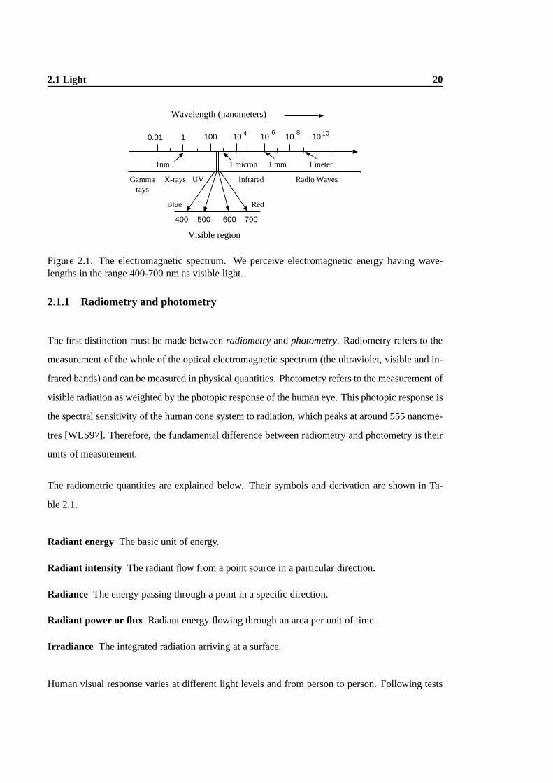
violet in the shorter wavelengths. Figure 2.1 illustrates the comparatively small range of visible
light in the electromagnetic spectrum.
19
2.1 Light 20
Wavelength (nanometers)
0.01 1 100 10 10 10 104 6 8 10
400 500 600 700
Visible region
Gammarays
X-rays UV
Blue Red
Infrared Radio Waves
1nm 1 micron 1 mm 1 meter
Figure 2.1: The electromagnetic spectrum. We perceive electromagnetic energy having wave-lengths in the range 400-700 nm as visible light.
2.1.1 Radiometry and photometry
The first distinction must be made betweenradiometryandphotometry. Radiometry refers to the
measurement of the whole of the optical electromagnetic spectrum (the ultraviolet, visible and in-
frared bands) and can be measured in physical quantities. Photometry refers to the measurement of
visible radiation as weighted by the photopic response of the human eye. This photopic response is
the spectral sensitivity of the human cone system to radiation, which peaks at around 555 nanome-
tres [WLS97]. Therefore, the fundamental difference between radiometry and photometry is their
units of measurement.
The radiometric quantities are explained below. Their symbols and derivation are shown in Ta-
ble 2.1.
Radiant energy The basic unit of energy.
Radiant intensity The radiant flow from a point source in a particular direction.
Radiance The energy passing through a point in a specific direction.
Radiant power or flux Radiant energy flowing through an area per unit of time.
Irradiance The integrated radiation arriving at a surface.
Human visual response varies at different light levels and from person to person. Following tests
2.1 Light 21
400nm 555nm 700nm
1.0
Lum
inou
s ef
fici
ency
Wavelength
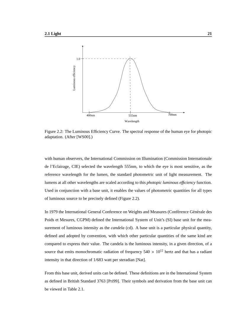
Figure 2.2: The Luminous Efficiency Curve. The spectral response of the human eye for photopicadaptation. (After [WS00].)
with human observers, the International Commission on Illumination (Commission Internationale
de l’Eclairage, CIE) selected the wavelength 555nm, to which the eye is most sensitive, as the
reference wavelength for the lumen, the standard photometric unit of light measurement. The
lumens at all other wavelengths are scaled according to thisphotopic luminous efficiencyfunction.
Used in conjunction with a base unit, it enables the values of photometric quantities for all types
of luminous source to be precisely defined (Figure 2.2).
In 1979 the International General Conference on Weights and Measures (Conf´erence G´enerale des
Poids et Mesures, CGPM) defined the International System of Unit’s (SI) base unit for the mea-
surement of luminous intensity as thecandela(cd). A base unit is a particular physical quantity,
defined and adopted by convention, with which other particular quantities of the same kind are
compared to express their value. The candela is the luminous intensity, in a given direction, of a
source that emits monochromatic radiation of frequency 540� 1012 hertz and that has a radiant
intensity in that direction of 1/683 watt per steradian [Nat].
From this base unit, derived units can be defined. These definitions are in the International System
as defined in British Standard 3763 [Pri99]. Their symbols and derivation from the base unit can
be viewed in Table 2.1.

2.1 Light 22
SYMBOL RADIOMETRIC PHOTOMETRIC IN SI BASE UNITS
Value Unit Value Unit
Q Radiant Energy Joule Luminous Energy Talbot
I Radiant Intensity Watt/sr Luminous Intensity candela (cd)
L Radiance Watt/m2sr Luminance nit cd/m2
Φ Radiant Power Watt Luminous Flux lumen (lm) m2� m�2
� cd = cd
E Irradiance Watt/m2 Illuminance lux (lx) m2� m�4
� cd = m�2� cd
Table 2.1: Radiometric and photometric measurements and how they are calculated in base units.
Luminous energy Radiant energy that produces a visual sensation.
Luminous intensity The quantity which describes the power of a source or surface to emit light
in a given direction.
Luminance The intensity of light emitted in a given direction per projected area of a luminous or
reflecting surface.
Luminous flux The light emitted by a source, or received by a surface.
Illuminance The luminous flux density at a point on a surface.
In this thesis, photometric measurements will be employed, as the work concerns the response of
the human visual system in relation to image perception.
2.1.2 Light propagation
When light of a single frequency strikes a surface, three types of interaction occur:absorption,
where the energy provides no further illumination;reflection, where incident light is mirrored
back into the environment; andtransmission, where incident light travels through the material
of the surface and returns to the environment. If the total energy that is received by the surface
2.1 Light 23
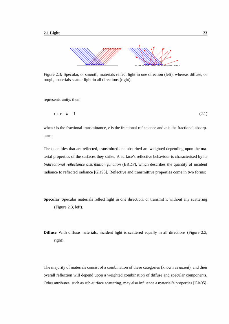
Figure 2.3: Specular, or smooth, materials reflect light in one direction (left), whereas diffuse, orrough, materials scatter light in all directions (right).
represents unity, then:
t + r +a= 1 (2.1)
whent is the fractional transmittance,r is the fractional reflectance anda is the fractional absorp-
tance.
The quantities that are reflected, transmitted and absorbed are weighted depending upon the ma-
terial properties of the surfaces they strike. A surface’s reflective behaviour is characterised by its
bidirectional reflectance distribution function(BRDF), which describes the quantity of incident
radiance to reflected radiance [Gla95]. Reflective and transmittive properties come in two forms:
Specular Specular materials reflect light in one direction, or transmit it without any scattering
(Figure 2.3, left).
Diffuse With diffuse materials, incident light is scattered equally in all directions (Figure 2.3,
right).
The majority of materials consist of a combination of these categories (known asmixed), and their
overall reflection will depend upon a weighted combination of diffuse and specular components.
Other attributes, such as sub-surface scattering, may also influence a material’s properties [Gla95].

2.2 Visual perception 24
2.2 Visual perception
Perception is the process that enables humans to make sense of the stimulus that surrounds them.
Visual perception deals with the information that reaches the brain through the eyes. It links the
physical environment with the physiological and psychological properties of the brain, transform-
ing sensory input into meaningful information.
In recent years visual perception has increased in importance in computer graphics, predominantly
due to the demand for realistic computer generated images [MRC+86, RWP+95, Fer03]. The
goal of perceptually-based rendering is to produce imagery that evokes the same responses as an
observer would have when viewing a real-world equivalent. To this end, work has been carried out
on exploiting the behaviour of the human visual system (HVS). For this information to measured
quantitatively, a branch of perception known aspsychophysicsis employed, where quantitative
relations between physical stimuli and psychological events can be established [SB94].
Psychophysical experiments are a way of measuring psychological responses in a quantitative way
so that they correspond to actual physical values. It is a branch of experimental psychology that
examines the relationship between the physical world and peoples’ reactions and experience of
that world. Psychophysical experiments can be used to determine responses such as sensitivity to
a stimulus. In the field of computer graphics, this information can then be used to design systems
that are finely attuned to the perceptual attributes of the visual system.
To make an assessment of the effects of reflected ambient light on the perception of electronically
displayed images, it is necessary to understand several perceptual phenomena that may play a part
in the process. The attributes of the HVS relevant to this thesis are detailed below.
2.2.1 The human eye
The human visual system receives and processes electromagnetic energy in the form of light
waves. This starts with the path of light through thepupil (Figure 2.4), which changes in size to
control the amount of light reaching the back of the eye. Light then passes through thelens, which

2.2 Visual perception 25
iris
lensretina
optic nerve
cornea
pupil
Figure 2.4: A schematic section through the human eye.
provides focusing adjustments, before reaching the photoreceptors in theretina at the back of the
eye. These receptors in the retina consist of about 120 millionrodsand 8 millioncones[SB94].
Rods are highly sensitive to light and provide low intensity vision in low light levels, but they
cannot detect colour. They are located primarily in the periphery of the visual field. In contrast
to this, high-acuity colour vision is provided through three types of cones:L, which are sensi-
tive to long wavelengths;M, which are sensitive to medium wavelengths; andS, which are short
wavelength sensitive. Finally, thephotopigmentsin the rods and cones transform this light into
electrical impulses that are passed to neuronal cells and transmitted to the brain via theoptic nerve.
2.2.2 Visual sensitivity
The way in which we perceive images depends on the amount of light available. In dark scenes our
visual acuity — the ability to resolve spatial detail — is low and colours cannot be distinguished.
This is due to photoreceptor performance, as mentioned above. It is the rods that provide us with
achromatic vision at thesescotopiclevels, functioning within a range of 10�6 to 10cd=m2, such
as starlight. The cones are active atphotopic levels of illumination, covering a range of 0.01
to 108cd=m2, such as sunlight. The overlap (themesopiclevels), when both rods and cones are
functioning, lies between 0.01 to 10cd=m2 [Fer01].

2.2 Visual perception 26
2.2.3 Contrast
The termcontrastgenerally refers to the intensity difference between given light and dark values.
If the difference is great then the contrast is said to be high; if small, then the contrast is low.
Contrast can be computed in several ways [Pel90], but one of the most common ways is the
Michelson formula. The Michelson formula is used to compute the contrast of a periodic pattern,
and is defined as
C =Lmax�Lmin
Lmax+Lmin(2.2)
whereLmax andLmin refer respectively to the maximum and minimum luminance values in the
pattern.
2.2.4 Thresholds
It is easily demonstrated that in a brightly-lit room the addition of a single candle is not obvious,
but when the room is dark, lighting a candle makes an immediate impression. Similarly, a whisper
is sufficient to be heard in a quiet environment, whereas a shout is necessary in noisy conditions.
In 1834 the German physiologist E.H. Weber observed this principle1, defining Weber’s Law:
the ratio of the increment threshold to the background intensity is a constant, denoted theWeber
fraction.
A threshold is a psychological limit to perception. Theabsolute thresholddefines the transition
between something that is undetectable and something that is detectable. Thedifference threshold
is the minimum amount by which the intensity of a stimulus must be changed before it is de-
tectable [SB94]. Weber’s Law therefore refers to the difference threshold — the minimum amount
by which the stimulus intensity must be changed before aJust Noticeable Difference(JND) is
observed. The size of this JND (∆I ) is a constant proportion of the original stimulus value.
The Weber fraction is used to determine the contrast of a target against a background through the
1Gustav Fechner, a German physicist and a contemporary of Weber, independently observed this principle andformalised Weber’s Law.
2.2 Visual perception 27
JND
Background luminance
(∆I+I)
(I)
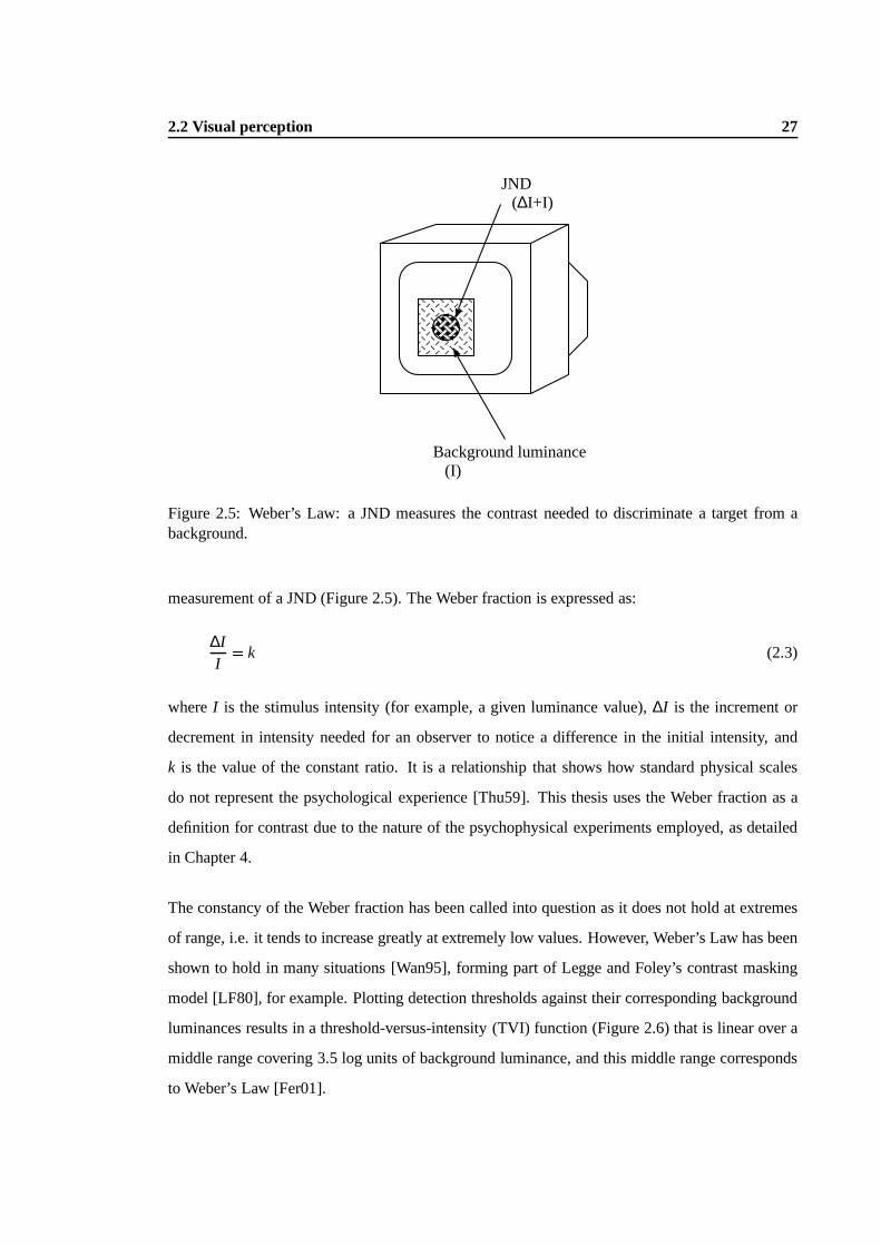
Figure 2.5: Weber’s Law: a JND measures the contrast needed to discriminate a target from abackground.
measurement of a JND (Figure 2.5). The Weber fraction is expressed as:
∆II
= k (2.3)
whereI is the stimulus intensity (for example, a given luminance value),∆I is the increment or
decrement in intensity needed for an observer to notice a difference in the initial intensity, and
k is the value of the constant ratio. It is a relationship that shows how standard physical scales
do not represent the psychological experience [Thu59]. This thesis uses the Weber fraction as a
definition for contrast due to the nature of the psychophysical experiments employed, as detailed
in Chapter 4.
The constancy of the Weber fraction has been called into question as it does not hold at extremes
of range, i.e. it tends to increase greatly at extremely low values. However, Weber’s Law has been
shown to hold in many situations [Wan95], forming part of Legge and Foley’s contrast masking
model [LF80], for example. Plotting detection thresholds against their corresponding background
luminances results in a threshold-versus-intensity (TVI) function (Figure 2.6) that is linear over a
middle range covering 3.5 log units of background luminance, and this middle range corresponds
to Weber’s Law [Fer01].

2.2 Visual perception 28
-3
-2
-1
0
1
2
3
4
5
-6 -4 -2 0 2 4 6
cones
rods
Log
thre
shol
d lu
min
ance
(cd
/m2 )
Log background luminance (cd/m2 )
Figure 2.6: Threshold versus intensity function for the rod and cone systems. (After [Fer01].)
2.2.5 The Contrast Sensitivity Function
The ability to perceive a JND is known ascontrast sensitivity. In 1968 Campbell and Robson
presented a theory of perception showing that contrast sensitivity varies according to spatial fre-
quency [CR68].Spatial frequencyindicates the number ofgratings(pairs of bars, one black and
one white, also known as acycle) which form a retinal image at a given distance [SB94]. They
measured this variation through the use of a compound sinusoidal grating stimulus, as shown in
Figure 2.7. The use of gratings of different spatial frequencies (i.e. with different numbers of cy-
cles per degree of angle of vision) means that contrast sensitivity can be measured at each spatial
frequency. This provides a curve that describes the threshold contrast needed to detect a given
spatial frequency, and this curve is known as thecontrast sensitivity function(CSF), which is also
shown in Figure 2.7.
2.2.6 Adaptation
The visual system adjusts to the stimuli that are presented to it, resulting in changes in sensitivity
known asadaptation. This process enables the visual system to respond to large variations in
luminance, allowing it to adjust to the prevailing light level. The rods in the eye are around

2.2 Visual perception 29
Invisible
Visible
Spatial frequency (cycles/degree)
Thr
esho
ld c
ontr
ast
Sensitivity (1/threshold contrast)
Spatial frequency (cycles/mm on retina)
1.0
01
0.01
0.001
0.1 1 10 100
1 000
100
10
1
0.1 1 10 100
Figure 2.7: The Campbell-Robson sensitivity chart (left, from [CR68]). The spatial frequencyincreases logarithmically from left to right; the contrast varies logarithmically from bottom to top.The resulting curve of the threshold determines an individual’s contrast sensitivity function (right,from [SB94]).
ten times as sensitive as cones, and so provide maximum sensitivity at low light levels [Gla95].
Visual adaptation from light to dark is known asdark adaptation, and can last for tens of minutes;
for example, the length of time it takes the eye to adapt at night when the light is switched off.
Conversely,light adaptation, from dark to light, can take only seconds, such as leaving a dimly
lit room and stepping into bright sunlight. This change in sensitivity is brought about through
physiological processes. In high luminance levels the photopigment in the eye is bleached, causing
a loss of sensitivity in the photoreceptors. The photoreceptors regain their sensitivity gradually,
accounting for the temporal aspects of adaptation. Additionally, though less significantly, the
amount of light entering the pupil changes [War00].
Adaptation also influences contrast sensitivity. When the visual system has adapted to a certain
frequency, sensitivity to that, and nearby frequencies, is decreased [Gla95].
2.2.7 Brightness perception
While luminance intensity can be measured on a physical scale (Section 2.1.1), the termbrightness
actually denotes a perceptual variable, which refers to a perceived level of illumination, such as
the amount of light an area appears to emit [SB94]. In addition, the termlightnessusually refers
2.2 Visual perception 30
0
0.2
0.4
0.6
0.8
1
0 0.2 0.4 0.6 0.8 1
Sensation magnitude
Stimulus intensity
Brightness = 0.33
0.1
1
10
0.01 0.1 1 10 100
Log sensation magnitude
Log stimulus intensity
Simple fields under dark conditionsComplex fields under dark conditions
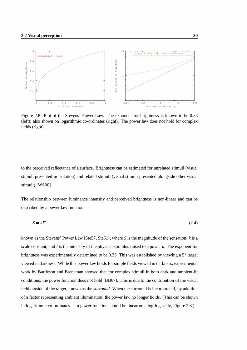
Figure 2.8: Plot of the Stevens’ Power Law. The exponent for brightness is known to be 0.33(left); also shown on logarithmic co-ordinates (right). The power law does not hold for complexfields (right).
to the perceived reflectance of a surface. Brightness can be estimated for unrelated stimuli (visual
stimuli presented in isolation) and related stimuli (visual stimuli presented alongside other visual
stimuli) [WS00].
The relationship between luminance intensity and perceived brightness is non-linear and can be
described by a power law function
S= kIa (2.4)
known as the Stevens’ Power Law [Ste57, Ste61], whereS is the magnitude of the sensation,k is a
scale constant, andI is the intensity of the physical stimulus raised to a powera. The exponent for
brightness was experimentally determined to be 0.33. This was established by viewing a 5Æ target
viewed in darkness. While this power law holds for simple fields viewed in darkness, experimental
work by Bartleson and Breneman showed that for complex stimuli in both dark and ambient-lit
conditions, the power function does not hold [BB67]. This is due to the contribution of the visual
field outside of the target, known as thesurround. When the surround is incorporated, by addition
of a factor representing ambient illumination, the power law no longer holds. (This can be shown
in logarithmic co-ordinates — a power function should be linear on a log-log scale, Figure 2.8.)
2.3 Digital image creation 31
2.2.8 Lightness and colour constancy
The ability to judge a surface’s reflectance properties despite any changes in illumination is known
ascolour constancy. Lightness constancyis the term used to describe the phenomena whereby a
surface appears to look the same regardless of any differences in the illumination [Pal99]. For
example, white paper with black text maintains its appearance when viewed indoors in a dark en-
vironment or outdoors in bright sunlight, even if the black ink on a page viewed outdoors actually
reflects more light than the white paper viewed indoors.Chromatic colour constancyextends this
to colour: a plant seems as green when it’s outside in the sun as it does if it’s taken indoors under
artificial light.
A number of theories have been put forward regarding constancy [Wan95, Pal99, SB94]. Early
explanations involved adaptational theories, suggesting that the visual system adjusts in sensitivity
to accommodate changes. However, this would require a longer time than is needed for lightness
constancy to occur, and adaptational mechanisms cannot account for shadow effects. Other pro-
posed theories include unconscious inference (where the visual system ‘knows’ the relationship
between reflectance and illumination and discounts it); relational theories (where perceived light-
ness depends upon the relative luminance — the contrast — between neighbouring regions); and
anchoring (where the region with the highest luminance is regarded as being white and all other
regions are scaled relative to it).
2.3 Digital image creation
Digital images can becapturedor generated. Capturing a digital image generally involves the
use of a digital camera or scanning device, whereas generating a digital image means modelling
and rendering a scene on a computer. In either case, the image is subsequently stored in some
digital format (usually 24-bit RGB). Other colour models are feasible, and more bits can be used
to increment the dynamic range, as discussed below.
2.4 Display technology 32
2.3.1 Capturing digital images
Scanners are used to sample analogue images and convert them into digital image files, and are
available in a variety of types (flatbed, film, drum and others). A digital camera samples a real-
world scene, processes it internally and then stores it in a digital form.
The majority of digital cameras and the most commonly-used flatbed and transparency scanners
usecharge-coupled device(CCD) technology. The CCD is an array of light-sensitive diodes that
convert photons (light) into electrons (electrical charge) — the brighter the light, the greater the
accumulated electrical charge. The value of the accumulated charge undergoes analogue-to-digital
conversion, storing the information in digital form.
2.3.2 Generating digital images
Computer graphics can also be used to create digital images. This is generally carried out through
the process of three-dimensional modelling, with a subsequent rendering stage where the colours,
textures, light and shading are computed, thus producing the final images. At all stages in this
process the information is in digital form.
2.4 Display technology
The two most commonly encountered visual display units (VDUs) are cathode ray tubes (CRTs)
and liquid crystal displays (LCDs), although the use of plasma display panels (PDPs) for large-
scale, multi-viewer applications, such as art galleries or museums, is becoming more popular.
This section provides an overview of the three devices. A comparative table of current VDU
specifications is given in Table??.

2.4 Display technology 33
ATTRIBUTE CRT LCD PLASMA
Contrast Ratio* 4000+:1** 1300:1*** 3000:1****
Max Brightness 1000cd=m2 450cd=m2 700cd=m2y
Viewing Angle 180Æ 160Æ 180Æ
Fully Digital Display no yes yes
Refresh Rate n/a 10-12ms*** 8ms
Max Resolution 720p 1080i+ 1280 x 1024 1366 x 768
Weight (lbs) 60-300 20-100 50-150+
Set Depth 16” - 30” 2” 3-6”
Screen Size 20” - 40” 1” - 57”*** 30” - 80”
Power consumption High Low Medium
Table 2.2: Display technology comparison. (After [DeB04].)*Higher-end known value given.**Calculated. CRTs not generally shown with contrast ratios.***New high-definition HD2+ development****Real world tests drop this number considerably (400:1).yPlasma “real-world” measure about 100cd=m2
2.4 Display technology 34
Colour signals
Picture tube
Electron guns
Electron beams
Screen
Glass envelope
Phosphor
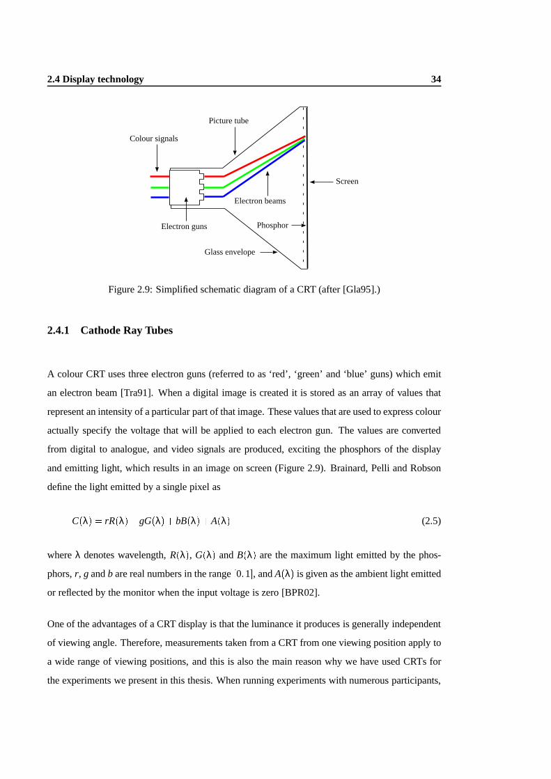
Figure 2.9: Simplified schematic diagram of a CRT (after [Gla95].)
2.4.1 Cathode Ray Tubes
A colour CRT uses three electron guns (referred to as ‘red’, ‘green’ and ‘blue’ guns) which emit
an electron beam [Tra91]. When a digital image is created it is stored as an array of values that
represent an intensity of a particular part of that image. These values that are used to express colour
actually specify the voltage that will be applied to each electron gun. The values are converted
from digital to analogue, and video signals are produced, exciting the phosphors of the display
and emitting light, which results in an image on screen (Figure 2.9). Brainard, Pelli and Robson
define the light emitted by a single pixel as
C(λ) = rR(λ)+gG(λ)+bB(λ)+A(λ) (2.5)
whereλ denotes wavelength,R(λ), G(λ) andB(λ) are the maximum light emitted by the phos-
phors,r, g andb are real numbers in the range[0;1], andA(λ) is given as the ambient light emitted
or reflected by the monitor when the input voltage is zero [BPR02].
One of the advantages of a CRT display is that the luminance it produces is generally independent
of viewing angle. Therefore, measurements taken from a CRT from one viewing position apply to
a wide range of viewing positions, and this is also the main reason why we have used CRTs for
the experiments we present in this thesis. When running experiments with numerous participants,

2.4 Display technology 35
in various locations, it is imperative to ensure that each participant has the equivalent viewpoint to
all the others. For this reason, many perceptual graphics applications use CRT technology, rather
than the now popular LCD technology described below.
2.4.2 Liquid Crystal Displays
An LCD consists of two layers of polarising material trapping a solution which has both liquid
and crystal properties; that is, the liquid crystals may be fluid, but can also retain an ordered
molecular structure. When an electrical field is applied to this solution, the crystals align so that
light cannot pass through. Therefore, two states are possible: either light passes through a cell,
or light is blocked, with each cell representing a pixel [Tra91]. Most LCD screens are backlit
with a fluorescent light which is evenly diffused to give a uniform display. LCDs have grown in
popularity in recent years due to the lower volume, weight and power consumption when compared
with the CRTs [MNK99].
2.4.3 Plasma Display Panels
Like CRTs, plasma displays are emissive and use phosphor, and like LCDs they use a grid of
electrodes as pixels. They work on the same principle as a neon sign, which emits light when
an electrical current is passed through gas. Plasma is a gas which is electrically conductive, and
as the electrons move through it they ionise the individual gas molecules. The energy gained
from ionisation is emitted as light during the decay process. Although the process is simple,
the implementation for mass production is, at present, costly and complex. Currently, a plasma
display is several times as expensive as an LCD, which is again more expensive than a CRT.
Prices of LCD and plasma screens are dropping rapidly, but unless the viewing angle dependence
of LCDs is addressed, computer graphics use will tend towards CRTs.

2.5 Controlling the display 36
2.5 Controlling the display
CRTs, LCDs and plasma screens all have different limitations in terms of how, and with what
quality, images are displayed. These limitations are not benign — display devices alter images
in various perceptually significant ways. This section details some of the corrections that may be
applied to images before they are displayed, so that their visual quality is minimally affected by the
chosen display device. In particular, in the following sections, we show the importance of gamma
correction, tone reproduction, and gamut mapping, all of which are specific image treatments that
make an image suitable for display.
2.5.1 Gamma
The mapping between input voltage values and the actual light emitted by each of the phosphors
would ideally be linear so that the input matches the output. If the intensityL is the value be-
tween 0–1 sent to the digital-to-analogue converter, and the output intensity isLd, then the ideal
relationship would be
Ld = LmaxL (2.6)
whereLmax is the maximum luminance of the display. However, for CRTs the mapping is normally
not linear as the electron gun has a non-linear response to its input voltage. This non-linearity can
be well-approximated with a power law
Ld = LmaxLγ (2.7)
whereLd is the displayed intensity,Lmax is the maximum displayable intensity,L is the input
value between 0 and 1 andγ is an approximation of the display’s non-linearity. The constant
γ, which is usually close to 2.5, also depends upon factors such as luminance and contrast set-
tings of the screen. Monitor adjustment controls labelled ‘Contrast’ and ‘Brightness’ respectively
control the luminance level and the black point of the monitor, which in turn influence what is
displayed [Poy98].
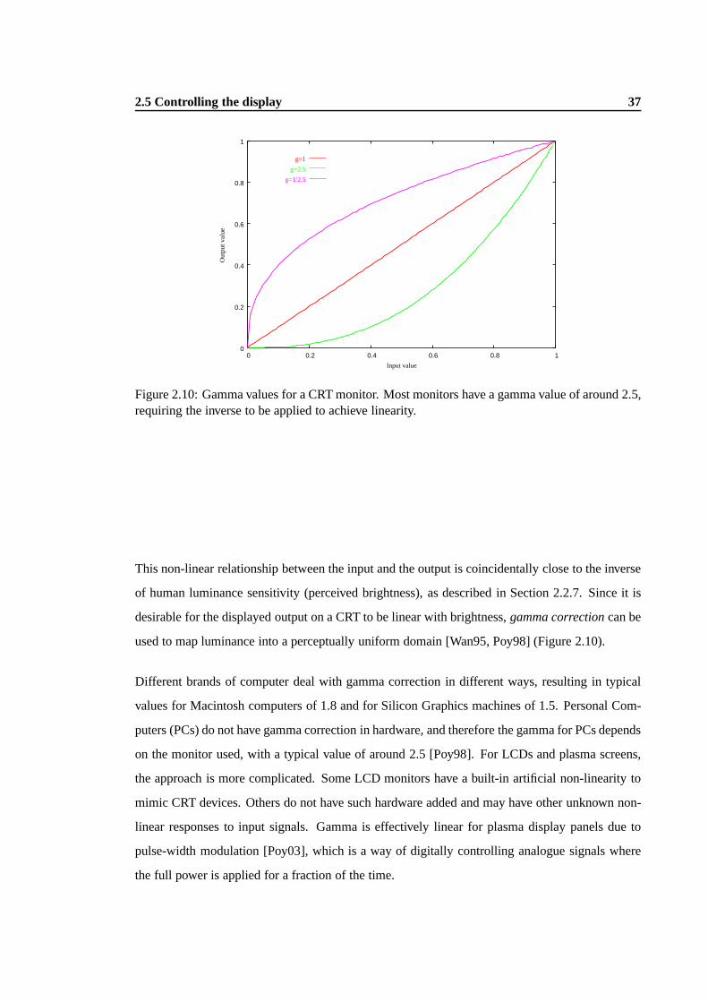
2.5 Controlling the display 37
0
0.2
0.4
0.6
0.8
1
0 0.2 0.4 0.6 0.8 1
Out
put v
alue
Input value
g=1
g=2.5
g=1/2.5
Figure 2.10: Gamma values for a CRT monitor. Most monitors have a gamma value of around 2.5,requiring the inverse to be applied to achieve linearity.
This non-linear relationship between the input and the output is coincidentally close to the inverse
of human luminance sensitivity (perceived brightness), as described in Section 2.2.7. Since it is
desirable for the displayed output on a CRT to be linear with brightness,gamma correctioncan be
used to map luminance into a perceptually uniform domain [Wan95, Poy98] (Figure 2.10).
Different brands of computer deal with gamma correction in different ways, resulting in typical
values for Macintosh computers of 1.8 and for Silicon Graphics machines of 1.5. Personal Com-
puters (PCs) do not have gamma correction in hardware, and therefore the gamma for PCs depends
on the monitor used, with a typical value of around 2.5 [Poy98]. For LCDs and plasma screens,
the approach is more complicated. Some LCD monitors have a built-in artificial non-linearity to
mimic CRT devices. Others do not have such hardware added and may have other unknown non-
linear responses to input signals. Gamma is effectively linear for plasma display panels due to
pulse-width modulation [Poy03], which is a way of digitally controlling analogue signals where
the full power is applied for a fraction of the time.

2.5 Controlling the display 38
Gamma calibration
Calibration of a system refers to attaining a predefined set-up; for example, a specified gamma,
offset and peak white luminance [Ber96]. This is achieved by characterising the properties of
the system and then making adjustments based on the desired set-up. In the case of gamma, this
can be achieved by measuring the output displayed on the screen and comparing it to the input
values. This is best accomplished by displaying a pattern on screen consisting of horizontal or
vertical stripes that step through from 0 to 255, as shown in Figure 2.11. For maximum accuracy
this should be carried out for each of the voltage guns. Stripes should be arranged to equalise the
power drain on the screen, so that a pair of adjacent stripes always totals the maximum voltage
of 255. Also, the stripes should be wide enough that they are not affected by flare from adjacent
stripes [Tra91].
The stripes of fixed voltage should be measured with a chromameter, preferably in a totally dark
environment. The resulting values should be normalised (and, if the value for a voltage of zero is
not actually zero due to a non-dark environment, this value can be subtracted from the other mea-
sured data before normalisation). A function of the formy= mx is fitted to the natural logarithm
of the data to give the value of the best gamma fit.
Shortcut gamma calibration
It is also possible to estimate the gamma of a computer system by displaying an image such as
that in Figure 2.12, which consists of a set of grey values next to an area of alternating black and
white pixels [CD01]. Seen from a distance, the black-and-white pattern fuses to appear grey and
the grey patch which matches the fused pattern best is selected. The intensityLm of this patch is
used to find the gamma response of the CRT:
0:5= Lγm (2.8)

2.5 Controlling the display 39
Figure 2.11: Example of test patterns for gamma measurement.

2.5 Controlling the display 40
3.0 2.8 2.6 2.4 2.2 2.0 1.8 1.6 1.4 1.2 1.0 0.8 0.6
Figure 2.12: Image used for simple gamma correction. (For printing purposes the spacing betweenthe lines has been exaggerated. An actual gamma chart would have stripes the width of one pixel.)
such that
γ =log0:5logLm
(2.9)
Gamma correction
Once the gamma for a particular set-up is known, images to be displayed may be corrected with
the following transformation which is generally known as gamma correction:
L0 = L1=γ (2.10)
2.5.2 Tone reproduction
Ideally, if a scene in the real world and an image representing that scene (be it computer generated
or photographed) are viewed under the same conditions, it is expected that the real-world scene
and the image should have the same tones, i.e. the luminance levels of both scenes match.
Physical accuracy alone of an image does not ensure that the scene in question will have a realistic
visual appearance when it is displayed. This is due to the shortcomings of standard display devices,
many of which can only reproduce a range of luminance of about 100:1 candelas per square metre
(cd=m2), as opposed to real-world luminance, which ranges from 100 000 000:1, from bright
sunlight down to starlight. The human eye can accommodate a luminance range of approximately
10 000:1 in a single view, and an observer’s adaptation to their surroundings, where their response
to a scene changes over time, also needs to be taken into account. The ratio between the maximum

2.5 Controlling the display 41
100 000 000: 1
10 000: 1
100: 1
Range of luminances:
in the real-world
that the eye can accommodate in single view
displayable on a standard CRT monitor
Figure 2.13: A comparative view of dynamic range.
Real-World
Display
Scene
Tone ReproductionOperator
Display withLimited Capabilities
��
��
��
��
Observer
Perceptual Match
Observer
- - -
-
?
6
Figure 2.14: Ideal tone reproduction process
and the minimum tonal values in an image is known as thedynamic range. It is this high dynamic
range (HDR) that exists in the real world that needs to be scaled in some way to fit a display device
that is only capable of outputting a low dynamic range.
Tone reproduction (also known as tone mapping) provides a method of mapping luminance values
in the real world to a displayable range. Tone reproduction is necessary to ensure that the wide
range of light in a real-world scene is conveyed on a display with limited capabilities. In addition
to compressing the range of luminance, it can be used to mimic perceptual qualities, resulting in
an image which provokes the same responses as someone would have when viewing the scene in
the real world. For example, a tone reproduction operator may try to preserve aspects of an image
such as contrast, brightness or fine detail — aspects that might be lost through compression. In
situations where predictive imaging is required, tone reproduction is of great importance to ensure
that the conclusions drawn from a simulation are correct (Figure 2.14).
A straightforward linear scaling between the original high dynamic range data and the display is
not the best solution (see Figure 2.15) as many — if not all — details can be lost. The mapping
must be tailored in some non-linear way. Current state-of-the-art image capturing techniques
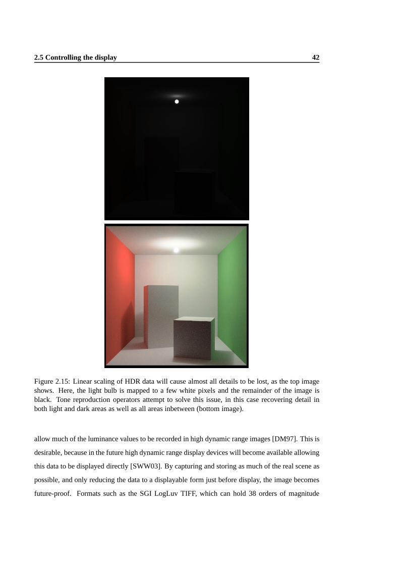
2.5 Controlling the display 42
Figure 2.15: Linear scaling of HDR data will cause almost all details to be lost, as the top imageshows. Here, the light bulb is mapped to a few white pixels and the remainder of the image isblack. Tone reproduction operators attempt to solve this issue, in this case recovering detail inboth light and dark areas as well as all areas inbetween (bottom image).
allow much of the luminance values to be recorded in high dynamic range images [DM97]. This is
desirable, because in the future high dynamic range display devices will become available allowing
this data to be displayed directly [SWW03]. By capturing and storing as much of the real scene as
possible, and only reducing the data to a displayable form just before display, the image becomes
future-proof. Formats such as the SGI LogLuv TIFF, which can hold 38 orders of magnitude
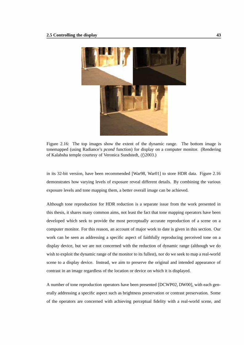
2.5 Controlling the display 43
Figure 2.16: The top images show the extent of the dynamic range. The bottom image istonemapped (using Radiance’spcond function) for display on a computer monitor. (Renderingof Kalabsha temple courtesy of Veronica Sundstedt,c 2003.)
in its 32-bit version, have been recommended [War98, War01] to store HDR data. Figure 2.16
demonstrates how varying levels of exposure reveal different details. By combining the various
exposure levels and tone mapping them, a better overall image can be achieved.
Although tone reproduction for HDR reduction is a separate issue from the work presented in
this thesis, it shares many common aims, not least the fact that tone mapping operators have been
developed which seek to provide the most perceptually accurate reproduction of a scene on a
computer monitor. For this reason, an account of major work to date is given in this section. Our
work can be seen as addressing a specific aspect of faithfully reproducing perceived tone on a
display device, but we are not concerned with the reduction of dynamic range (although we do
wish to exploit the dynamic range of the monitor to its fullest), nor do we seek to map a real-world
scene to a display device. Instead, we aim to preserve the original and intended appearance of
contrast in an image regardless of the location or device on which it is displayed.
A number of tone reproduction operators have been presented [DCWP02, DW00], with each gen-
erally addressing a specific aspect such as brightness preservation or contrast preservation. Some
of the operators are concerned with achieving perceptual fidelity with a real-world scene, and

2.5 Controlling the display 44
mimic aspects of the human visual system. Others concentrate on producing a subjective best
image that is pleasing to the eye. Two types of tone reproduction operators can be used:spatially
uniform (also known assingle-scaleor global) andspatially varying(also known asmulti-scale
or local). Spatially uniform operators apply the same transformation to every pixel. A spatially
uniform operator may depend upon the contents of the image as a whole, but the same transfor-
mation is applied to every pixel. Conversely, spatially varying operators apply a different scale to
different parts of an image.
Spatially uniform operators
In 1984 Miller, Ngai and Miller [MNM84] were the first to use experimental data to try to match
brightness in a real scene to brightness of a displayed image of that scene, for the purpose of
determining pixel luminance for their architectural rendering system [AF95]. They used psy-
chophysical data on brightness perception from work by Stevens and Stevens [SS60]. Upstill’s
1985 PhD thesis reinforced the need for perceptual tone reproduction through the use of an ex-
plicit perceptual model [Ups85].
Tumblin and Rushmeier [TR93], also focused on preserving the viewer’s overall impression of
brightness, providing a theoretical basis for perceptual tone reproduction, again by using Stevens
and Stevens data. This model of brightness perception does not hold for complex scenes, but
was chosen by Tumblin and Rushmeier due to its low computational costs. Their aim was to
create a ‘hands-off’ method of tone reproduction in order to avoid subjective judgements. They
created observer models — mathematical models of the HVS that include light-dependent visual
effects while converting real-world luminance values to perceived brightness images. The real-
world observer corresponds to someone immersed in the environment, and the display observer
to someone viewing the display device. Their tone reproduction operator converts the real-world
luminances to the display values, which are chosen to match closely the brightness of the real-
world image and the display image. If the display luminance falls outside the range of the frame-
buffer then the frame-buffer value is clamped to fit this range.
Ward’s model [War94a] dealt with the preservation of perceived contrast rather than brightness.

2.5 Controlling the display 45
Ward aimed to keep computational costs to a minimum by transforming real-world luminance
values to display values through a scaling factor, concentrating on small alterations in luminance
that are discernible to the eye. Based on a psychophysical contrast sensitivity model by Black-
well [Bla81] he exploited the fact that the consequence of adaptation can be regarded as a shift
in the absolute difference in luminance required for the viewer to notice the variation. Blackwell
produced a comprehensive model of changes in visual performance due to adaptation level. This
approach is useful for displaying scenes where visibility analysis is crucial, such as emergency
lighting, as it preserves the impression of contrast. It is also less computationally expensive than
Tumblin and Rushmeier’s operator but the use of a linear scaling factor causes very high and very
low values to be clamped and correct visibility is not maintained throughout the image [WRP97].
Ferwerda, Pattanaik, Shirley and Greenberg [FPSG96] developed a model which accounts for
changes in colour appearance, visual acuity and temporal sensitivity while preserving global vis-
ibility. This model is based on the concept of matching JNDs for a variety of adaptation levels.
It accounts for both rod and cone response and takes into consideration the aspect of adaptation
over time. Ferwerda et al. exploited the detectability of changes in background luminance in order
to remove those frequencies imperceptible when adapted to real-world illumination. Detection
threshold experiments were used as the basis of the work. By plotting the detection threshold
against the corresponding background luminance, a TVI function is produced for both the display
and the viewer. The implementation of this model is based on Ward’s 1994 operator [War94a].
Ward’s model is used without change for cone TVI data and is extended for rod TVI data. If the
level of adaptation for the real-world viewer falls in the photopic range (i.e.. above 10cd=m2) then
a photopic tone-reproduction operator is applied (making use of the cone data), and if it falls in
the scotopic range (i.e.. below 0.01cd=m2) then a scotopic tone reproduction operator is applied
(making use of the rod data). For mesopic conditions, a photopic display luminance and a scotopic
display luminance are combined appropriately.
To reproduce the loss in visual acuity, Ferwerda et al. used data from psychophysical experiments
that related the detectability of square wave gratings of different spatial frequencies to changes
in background luminance. Using this data it is possible to determine what spatial frequencies are
visible, and thereby eradicate any extraneous data in the image. Light and dark adaptation were

2.5 Controlling the display 46
also considered by adding a parameter to the display luminance, the value of which changes over
time. This model is of particular importance due to the psychophysical model of adaptation that
it adopts, and proves useful for immersive display systems that cover the entire visual field so that
the viewer’s visual state is determined by the whole display [McN01].
Further work by Ward Larson, Rushmeier and Piatko [WRP97] presented a histogram adjustment
technique for reproducing perceptually accurate tone, extending earlier work by Ward [War94a]
and Ferwerda et al. [FPSG96]. The main focus of this work was object visibility and image con-
trast, with a secondary goal of recreating the viewer’s subjective response so that their impression
of the real and virtual scenes were consistent [WRP97]. This technique makes use of the fact that
the eye is sensitive to relative rather than absolute changes to luminance, so bright areas should
be displayed as bright and dim areas as dim, irrespective of the actual absolute luminance inten-
sity values. Luminance levels are not constant across an image, but appear in clusters that vary
in intensity. Also, the eye adapts rapidly to a 1Æ visual field around the fixation point. For these
reasons, the function makes adjustments on the basis of luminance adaptation levels in an image
rather than on spatial location.
The field of image processing has developed methods to adjust image contrast and visibility. One
such method is the histogram equalisation technique whereby the grey levels in an image are re-
distributed to make better use of the display device range and maximise visibility and contrast.
Ward Larson et al. exploited this idea of altering histograms and using perceptual models to guide
alteration, with their aim being to simulate, rather than maximise, visibility in an image. A log of
luminances averaged over 1Æ areas (which correspond with foveal adaptation levels for possible
points in an image) is obtained, and a histogram and cumulative distribution function is built from
this information. Cumulative distribution of the luminance histogram is used to identify clusters
of luminance levels and initially map them to the display values using a histogram adjustment
technique that is based on human contrast sensitivity. Ferwerda et al. ’s [FPSG96] threshold sensi-
tivity data is used to compress the original dynamic range to that of the display device, subject to
the contrast sensitivity limitations of the eye. Although this method is described here as spatially
uniform, spatial variation is introduced through the use of models for glare, acuity and chromatic
sensitivity to increase perceptual fidelity.
2.5 Controlling the display 47
In 1999 Tumblin, Hodgkins and Guenter [THG99] produced two new tone reproduction operators
by imitating some of the HVS’s visual adaptation processes, and also revised Tumblin and Rush-
meier’s [TR93] earlier work. The first, a layering method, builds a display image from several
layers of lighting and surface properties. This is done by dividing the scene into layers and com-
pressing only the lighting layers while preserving the scene reflectances and transparencies, thus
reducing contrast while preserving image detail. Their compression function follows the work
of Schlick [Sch94b]. This method only works for synthetic images where layering information
from the rendering process can be retained. The second, a foveal method, interactively adjusts to
preserve the fine details in the region around the viewer’s gaze (which the viewer directs with a
mouse) and compresses the remainder. In this instance their final tone reproduction operator is
a revised version of the original Tumblin and Rushmeier [TR93] operator, also building on the
work of Ferwerda [FPSG96] and Ward [War94a]. Both of these operators are straightforward in
implementation and are not computationally expensive. The layering method is suited to static,
synthetic scenes (displayed or printed) and the foveal method to interactive scenes (requiring a
computer display).
Scheel, Stamminger and Seidel [SSS00] developed a method of tone reproduction for interactive
applications by representing luminances as a texture. The luminance of each vertex is coded into
texture co-ordinates, and prior to rendering these luminance co-ordinates are mapped into display
luminance values. This allows walkthroughs of large scenes where the tone reproduction can be
adjusted frame-by-frame to the current view of the user, and focuses on tone reproduction for
global illumination solutions obtained by radiosity methods. Due to interactivity, updates in tone
mapping are required to account for changes in view point and viewing direction, and new factors
need to be incorporated into the tone reproduction operator, such as computational speed and
adaptation determination. (In comparison, foveal method presented by Tumblin et al. [THG99]
was interactive to an extent, but relied on pre-computed still images where the fixation point of
the viewer could change, but an interactive walkthrough was not possible.) Spatially uniform
operators were chosen due to computational efficiency, and Scheel et al. based their work on
operators developed by Ward [War94a] and Ward Larson et al. [WRP97]. A centre-weighted
average is used to determine the probability of the user’s focus. The adaptation levels are computed
using samples obtained through ray-tracing, and the luminance of every vertex is held in texture co-
2.5 Controlling the display 48
ordinates. This can then be updated frame-by-frame. This method of tone reproduction provided
a new level of interactivity, but it does not take into consideration adaptation over time.
Pattanaik, Tumblin, Yee and Greenberg [PTYG00] produced a new time-dependent tone repro-
duction operator to automatically create colour image sequences from any input scene. It followed
the perceptual models framework proposed by Tumblin and Rushmeier with the addition of an
adaptation model and appearance model to express retinal response and lightness and colour. The
adaptation model computes retina-like response signals (for rod and cone luminance and colour in-
formation) for each pixel in the scene. Using Hunt’s static model of colour vision, time-dependent
adaptation components are added to describe neural effects, pigment bleaching, regeneration and
saturation effects. The visual appearance model assumes that the real-world viewer determines a
‘reference white’ and a ‘reference black’ and judges the appearance of any visual response against
these standards. Assembling these models reproduces the appearance of scenes that evoke changes
to visual adaptation. This operator is suitable for use in real-time applications as, due to its spa-
tially uniform model of adaptation, it does not require extensive processing.
Durand and Dorsey [DD00] presented an interactive tone mapping model which made use of
visual adaptation knowledge. They also proposed extensions to the tone mapping operator by Fer-
werda et al. and incorporated it into a model for the display of global illumination solutions and
interactive walkthroughs. This model involves time-dependent tone mapping and light adaptation,
and extends the work by Ferwerda et al. by including a blue-shift for viewing night scenes and by
adding chromatic adaptation. For the interactive implementation, work by Tumblin et al. [THG99]
and Scheel et al. [SSS00] was used to take advantage of the observer’s gaze, allowing a weighted
average to be used. Photographic exposure metering used in photography is employed to better
calculate the adaptation level. Loss of visual acuity is simulated in the same manner of Ferw-
erda et al. by use of a 2D Gaussian blur filter. The scene is rendered as normal, with interactivity
introduced by tone mapping computed on the fly, accelerated by caching the function in look-up
tables.
Work by Cohen, Tchou, Hawkins and Debevec [CTHD02] addressed the problem of HDR image
display by storing and rendering high dynamic range texture maps in real time using hardware
texturing architectures. With their method, HDR texture maps are stored as two separate 8-bit
2.5 Controlling the display 49
texture maps, one representing the high intensities and the other the low intensities. During display,
these two texture maps are recombined with the aid of a dynamically adjustable exposure level to
guide the overall intensity of the result.
Drago, Myszkowski, Annen and Chiba [DMAC03] presented a method for displaying high con-
trast scenes. It is based on logarithmic compression of luminance values in imitation of the visual
response to light, through the use of Perlin and Hoffert’s bias power function [PH89] and through
the manipulation of the gamma power function. The dynamic range is compressed using a linear
scaling factor after the logarithm has been applied, with this scaling factor depending on scene
content, interpolated by the bias function. The result is a perceptually-motivated function that can
be used at interactive rates.
Spatially varying operators
Work by Oppenheim, Schafer and Stockham [OSS68] on non-linear filtering in 1968 appears to
be the earliest attempt at tone reproduction in computer graphics. They describe the problem of
excessive dynamic range and suggest a method for simultaneously reducing dynamic range and
enhancing contrast using homorphic filtering. An image can be divided into two parts: the illu-
mination component (the available light) and the reflection component (the ability of objects to
reflect light). The illumination component, which contains large variations in luminance intensi-
ties, primarily consists of low frequencies, and the reflection component primarily consists of high
frequencies. Therefore, low frequency content in an image tends to be high dynamic range, and
high frequency content tends to be low dynamic range. By attenuating the low frequencies in the
Fourier domain, HDR data may be compressed while the high frequencies (the low dynamic range
detail) are preserved. Further work by Stockham [Sto72] in 1972 tied the concept of homorphic
filtering to properties of early portions of the HVS. He developed a visual model based on these
properties and used it to define a measure of image quality.
Chiu, Herf, Shirley, Swamy, Wang and Zimmerman’s [CHS+93] investigation into global opera-
tors led them to believe that the solution should be local instead, as applying the same mapping to
each pixel could produce incorrect results. With an HDR image there is no perfect compression

2.5 Controlling the display 50
curve that fits every pixel in an image, so a method of incorporating local variation is desired.
They deliberately did not incorporate adaptation issues or psychophysical models into their oper-
ator; rather they experimented with a method of spatially varying image mapping. As the HVS is
more sensitive to relative as opposed to absolute changes in luminance they developed a spatially
non-uniform scaling function for high contrast images. Their basis was the argument that the eye
is more sensitive to reflectance than luminance, so that slow spatial variation in luminance may
not be greatly perceptible. The implication is that images with a wider dynamic range than the
display device can be displayed without much noticeable difference if the scaling function has a
low magnitude gradient. By blurring the image to remove high frequencies, and inverting the re-
sult, the original details can be reproduced, but reverse intensity gradients appear when very bright
and very dark areas are in close proximity [McN01]. Due to the fact that it is a local operator, this
model is also computationally demanding. It is also a ‘hands-on’ approach, based purely on ad
hoc results and therefore does not have the advantages of the more robust, theoretical basis of
other tone reproduction operators.
Schlick [Sch94b] presented practical methods of tone reproduction, concentrating on improving
computational efficiency and simplifying parameters. He used a first degree rational polynomial
function to map real-world luminances to display values, a function which worked well when ap-
plied uniformly to all pixels in an image. It is this function that forms the basis for our correction
algorithm in Chapter 5. He produced three methods of mimicking local adaptation. The first of
these, low pass filtering, was susceptible to halo artifacts, as was the method by Chiu et al. —
a problem common among spatially varying operators. The remaining two methods did not pro-
duce as satisfactory results as the uniform approach. Nonetheless, his work produced a valuable
optimisation of spatially varying techniques.
Jobson, Rahman and Woodell [JRW97] based their method on the retinex theory [LM71] of
colour vision, producing a multi-scale version to achieve simultaneous dynamic range compres-
sion, colour consistency and lightness rendition, testing it extensively on (real-world) test scenes
and over 100 images. The retinex is a computational model of lightness and colour perception
of human vision which estimates scene reflectances, and Jobson et al. modified it to perform in a
functionally similar manner to human visual perception. However, in their validation they used
2.5 Controlling the display 51
24-bit RGB test images where dynamic range reduction is not an issue as it can be displayed in
a straightforward manner on a standard CRT. They expressed the need for refinement of their ap-
proach for images with greater maximum contrasts. Also, problems arose with scenes dominated
by one colour as these violated the retinex ‘grey-world’ assumption that the average reflectances
are equal in the three spectral colour bands.
Pattanaik, Ferwerda, Fairchild and Greenberg [PFFG98] developed a technique based on a multi-
scale representation of pattern, luminance, and colour processing in the HVS and addressed the
problems of high dynamic range and perception of scenes at threshold and supra-threshold levels.
They provided a computational model of adaptation and spatial vision for realistic tone reproduc-
tion. There are two main parts to this model: thevisual model, which processes an input image
to encode the perceived contrasts for the chromatic and achromatic channels in their band-pass
mechanism; and thedisplay model, which takes the encoded information and outputs a recon-
structed image. Although it is computationally demanding, the model takes chromatic adaptation
into account. However, as seen in other spatially varying operators, this method is susceptible to
strong halo effects [Tum99]. Although it was designed as a solution towards the tone reproduction
problems of wide absolute range and high dynamic range scenes, it is a general model that can be
applied across a number of areas such as image quality metrics, image compression methods and
perceptually-based image synthesis algorithms [PFFG98].
In 1999 Tumblin and Turk [TT99] produced the Low Curvature Image Simplifier (LCIS) method,
a versatile technique that can accept input from synthetic sources or real-world image maps, and
produces an output suitable for any display. Similar to Tumblin et al. ’s [THG99] layering and
foveal approaches, the LCIS separates the input scene into large features and fine details, com-
pressing the former and preserving the latter. The idea stems from art where an initial sketch
outlines the main structure of a picture, with details and shadings filled in later. The LCIS uses a
form of anisotropic diffusion to define the fine details by scene boundaries and smooth shading.
This provides a high amount of subtle detail, avoids halo artifacts, and claims moderate computa-
tional efficiency [Tum99].
Durand and Dorsey’s [DD02] 2002 method used an edge-preserving filter known as the bilateral
filter to decompose the image into two layers — an approach which builds on Tumblin and Turk’s

2.5 Controlling the display 52
LCIS method [TT99], and Tumblin et al. ’s layering method [THG99] which it extends to pho-
tographs. A base layer (which consists of large-scale variations) is derived using bilateral filtering
and contrast is reduced in this layer while visibility is preserved in the detail layer. Their final
method is a faster, more robust operator that also addresses problems mentioned by Tumblin and
Turk in their LCIS method [TT99], namely halo artifacts and diffusion at discontinuities. Again,
perceptual accuracy is not the aim and their operator does not attempt to model human vision.
Fattal, Lischinski and Wermann [FLW02] presented a new computationally efficient and concep-
tually simple method based on attenuating the magnitudes of the large luminance gradients that
exist in HDR scenes, compressing large gradients and preserving fine details. The changes in
intensity are identified and the larger gradients are reduced and a low dynamic range image is
produced. They did not make an attempt at perceptual accuracy, but instead offered an effective,
fast and easy-to-use form of tone reproduction.
Reinhard, Stark, Shirley and Ferwerda’s function [RSSF02] is analogous to photographic practise,
resulting in a technique designed to suit a wide variety of images. In photography, an approach
known as the Zone System is widely used. This photographic technique divides a scene into print
zones ranging from pure black to white. A luminance reading is taken for a subjectively-defined
middle-grey tone. Readings are taken for light and dark regions and a dynamic range can be
determined, and an appropriate choice for middle-grey ensures that the maximum possible detail
is retained. Reinhard et al. take a user-specified value for middle grey. The log average luminance
of the input image is then mapped to this value by linear scaling. A spatially uniform operator
is then used to compress the high intensities in the image. Spatially varying tone reproduction
is introduced in a manner akin to “dodging and burning” in photography. This allows contrast
to be controlled locally in the image over regions bounded by large contrasts. This was based
on a centre-surround function derived from a model of brightness perception by Blommaert and
Martens [BM90]. They tested their method against existing tone reproduction operators with a
broad range of HDR images.
This operator uses a slightly different definition for dynamic range. In computer graphics, dy-
namic range is held to be the ratio of the highest to the lowest scene luminance, whereas Rein-
hard et al. adopt the photographic definition that dynamic range is the ratio of the highest and

2.5 Controlling the display 53
lowest luminance regionswhere detail is visible. This results in images with ranges lower than
they would be if the computer graphics definition was used. With the standard computer graphics
definition of dynamic range it is difficult to know how successful compression of an HDR image
will be. Using the photographic definition, Reinhard et al. correlate dynamic range with difficulty
of compression, using this to predict how challenging tone reproduction for a given image will be.
This method is simple, fast and computationally efficient. As with other recent tone reproduction
operators, perceptual accuracy is not attempted. Instead they aim to produce credible results and
an image that is pleasing in appearance.
Ashikhmin [Ash02] has produced a tone mapping operator which preserves image details and also
conveys the compression of absolute brightness in a low dynamic range image using a multipass
approach. First, local adaptation luminance is estimated by determining the largest sufficiently
uniform neighbourhood for each pixel. Next, the tone mapping (using a TVI function) is applied,
using the local adaptation information to produce a locally linear mapping. Finally, local contrast
is estimated, thus preserving detail throughout the image. This approach is simple in implementa-
tion and moderate in computational expense.
Related effects
Replication of visual effects that are related to the area of tone reproduction include the modelling
of glare. Spencer, Shirley, Zimmerman and Greenberg [SSZG95] developed a method for repli-
cating glare effects. The idea of adding glare effects was previously recognised by Nakamae et
al [NKON90], although their algorithm did not account for the visual masking effects of glare.
Spencer et al. produced psychophysically-based algorithms for adding glare to digital images,
simulating the flare and bloom seen around very bright objects, and carried out a psychophysical
test to demonstrate that these effects increased the apparent brightness of a light source in an
image. While highly effective, glare simulation is computationally expensive.
2.5 Controlling the display 54
Tone reproduction choices
With a large number of operators available, and validation of tone reproduction operators in its
infancy, the choice of tone reproduction operator is currently a matter of deciding on the best
tool for the job. Currently, there are no defined criteria for selecting the best tone reproduction
operator for a specific task. Initial validation studies have been undertaken [DMMS02, LWC02]
which have led to the development of new operators based on this assessment [DMMC03], but as
yet no formal framework for comparison has been established.
2.5.3 Gamut mapping
While the previous section deals with the range of image intensities that can be displayed, display
devices are also limited in the range of colours that may be displayed. The termgamutis used to
indicate the range of colours that the human visual system can detect, or that display devices can
display. Our work does not deal with issues regarding colour appearance (a well-established field
in its own right), but this section is included to give an overview of factors peripheral to those that
we address in this thesis.
Even with 24-bit colour, sometimes indicated as ‘millions of colours’ or ‘true colour’, there are
many colours within the visible spectrum that monitors cannot reproduce. To show the extent
of this limitation for particular display devices, chromaticity diagrams are often used. Here, the
Yxy colour space is used, where Y is a luminance channel (which ranges from black to white via
all greys), and x and y are two chromatic channels representing all colours. Figure 2.17 shows a
chromaticity diagram indicating the gamut of colours visible to humans, and two restricted gamuts,
one for a typical monitor and one for a printing device. Given that the triangle indicating monitor
capability is completely contained with the shape of all visible colours, there are many visible
colours that cannot be reproduced on a monitor.
Assuming that the some of the colours to be displayed in an image are outside a monitor’s gamut,
the image’s colours may be remapped to bring all its colours within displayable range. This
process is referred to as gamut mapping [BF99, GWA90]. A simple mapping would only map out-

2.6 Summary 55
1
2
3
Green
Yellow
White
Blue-green
Cyan
Blue
Violet
ReddishPurple
Red
y
x
Figure 2.17: Chromaticity diagram showing the range of colours that humans can detect (1), aswell as the ranges of colours displayable on a monitor (2) and printable on a printer (3). The x andy axes show values for the x and y chromaticity coordinates respectively. (After [War00].)
of-range colours directly inward towards the monitor’s triangular gamut. Such a ‘colorimetric’
correction produces visible artefacts. A better solution is to re-map the whole gamut of an image
to the monitor’s gamut, thus remapping all colours in an image. This ‘perceptual’ or ‘photometric’
correction may avoid the above artefacts, but conversely there are many different ways in which
such remapping may be accomplished. As such, there is no standard way to map one gamut into
another more constrained gamut.
2.6 Summary
This chapter has reviewed the background information pertaining to the work presented in this
thesis. The information on light helps to provide an understanding of the following chapter. The
information on visual psychophysics is employed in the design of all of the experiments that we
present. The information on displays forms the basis for our work described in Chapter 5.

2.6 Summary 56
Chapter 3
The viewing environment
This chapter examines ambient lighting in the viewing environment, and details current measures
which could be used to strive for perceptual fidelity. Related work in the fields of ergonomics and
medical imaging display is described.
3.1 The influences of ambient illumination
VDUs are open to influences from the environment in which they are located. A major factor
is that the screen of a display device may reflect any light present in the viewing environment.
The average amount of light present in a room is known as theambient illuminationand it is the
reflection of this off the screen of a monitor that affects the perceived contrast of displayed images.
A computer monitor does not fill the whole of the visual field, and as a result, visual adaptation
is partly determined by the ambient illumination present. It is estimated that under normal office
conditions, between 15% and 40% of illumination reaching the eye via the monitor will indirectly
come from the reflection of ambient light [War00].
Ambient light may be assumed to be uniformly distributed over a screen. This is true in many
working conditions with overhead lighting, but not for an environment where a spotlight (such as
a table or desk lamp) is aimed towards the screen. As with light propagation, described in Sec-
57
3.1 The influences of ambient illumination 58
tion 2.1.2, reflections may be specular or diffuse. Specular reflections occur when light emitted or
reflected by objects is reflected in one direction. Diffuse reflections cause an increase in luminance
in all directions [RJP87]. CRT technology is particularly prone to specular reflection on the screen.
These can often be overcome by adjusting the angle of the screen relative to the light source and
the viewer. LCDs also suffer, but as they are more mobile they can often be easily moved, whereas
a CRT’s bulk means it cannot [SFP99]. Unfortunately, adjusting the viewing angle of an LCD
screen may corrupt the appearance of colours due to the viewing angle dependency.
Reflected ambient illumination may produce a form of glare. This is caused when vision suffers
due to too much brightness. Either the user suffers visual discomfort (discomfort glare), or cannot
see well enough to perform a task (disability glare). A formula for disability glare (defined by a
reduction in contrast) was produced through a series of experiments by Holladay [Hol26], deter-
mined by the position of the source with respect to the user and by the amount of light entering
the user’s eye. Thus:
Contrast reduction=kEθ2 (3.1)
whereE is the illuminance from the glare source reaching the eye,θ is the angle between the line
of sight and the direction of the view gaze, andk is a constant depending on the age of the observer
(given that age causes changes in the consistency of fluids in the eyeball) [Obo95].
For discomfort glare, the international formula for measurement is the CIE’sglare index, also
called aUnified Glare Rating(UGR). This is calculated by:
Discomfort glare=L1:6
s ω0:8
LBP1:6 (3.2)
whereLs is the luminance of the source,LB is the average luminance of the background,ω is the
angular size of the source andP is the position index (indicating the effect of the source’s position
on glare) [Pri99]. As a rough guide, a UGR of less than 10 is rated as ‘barely perceptible’, while
a value of 28 or more is considered ‘intolerable’ [Obo95].
In office environments where computers are widely used, lighting design must consider the effect

3.2 Accounting for viewing conditions 59
LOCATION ILLUMINANCE (LX ) LIMITING UGR
General offices 500 19
Computer workstations 300–500 19
Drawing boards 750 16
Table 3.1: Typical lighting recommendation for offices. The Limiting UGR refers to the CIE’sUnified Glare Rating classification of discomfort glare, calculated through knowledge of thesource luminance, background luminance, and position. (After [Cha].)
of reflected light. Table 3.1 gives the recommended lighting values and glare rating for offices.
Two conflicting areas exist: the aforementioned reduction in contrast (a form of disability glare)
caused by ambient light, and the requirement of an appropriate level of ambient lighting to carry
out other visual tasks [Pri99].
3.2 Accounting for viewing conditions
Correcting for reflections off computer monitors typically follows one of three approaches: the
display device can be physically altered to reduce reflections; the environment can be adjusted,
thereby controlling the ambient light, or the environment can be characterised and the effects of
the ambient light can be taken into account when an image is displayed by applying some form of
algorithmic correction.
3.2.1 Physical alterations to the hardware
To physically alter the display device, anti-glare screens may be fitted to reduce reflections. While
this changes the amount of light reflected off a screen, it does not eliminate the problem — it
merely changes it in an uncalibrated manner as the amount of light reflected still depends on the
amount of light present in the environment. As this ambient quantity is typically unknown, anti-
glare screens may be viewed as a quick fix rather than a principled approach. Also, although

3.2 Accounting for viewing conditions 60
screen reflections may be reduced, this can be at the expense of reduced screen brightness and
resolution [Obo95].
Although monitors have controls labelled ‘Contrast’ and ‘Brightness’, these specify the luminance
level and the black point of the monitor, respectively. The black point should be set to true black,
while the contrast level setting depends on preference. However, setting this excessively high can
produce problems such as sensitivity to flicker, reduced contrast due to light scatter and defocus-
ing of the electron beam [Poy03]. It is therefore recommended that these controls are not used
to reduce the effect of ambient light, and should instead be set only once, and left unchanged
thereafter.
3.2.2 Viewing environment standards
The viewing environment may be controlled to conform to known standards. The International
Standards Organization (ISO) has specified a controlled viewing environment [ISO00], listing a
wide range of prerequisites that should be fulfilled to achieve the best possible viewing conditions
when working with images displayed on screen, thus reducing inconsistencies in image percep-
tion. For many applications, adhering to this standard is impractical as it includes designing the
environment to minimise interference with the visual task, baffling extraneous light, ensuring no
strongly coloured surfaces (including the observer’s clothing) are present within the immediate
environment, and ensuring that walls, ceiling, floors, clothes and other surfaces in the field of view
are coloured a neutral matt grey with a reflectance of 60% or less.
While such guidelines are a step towards a controlled viewing environment, such specific condi-
tions are not always available, or indeed feasible. Much work is carried out in non-specialised
office space, and this must conform to a different set of standards: legislation on workspace con-
ditions. The UK’s Health and Safety at Work Act 1974 [Her74] states that employers should
provide lighting appropriate to the work space and its activities. Further to this, specifications of
the European Commission directive 89/654/EEC [Eur89] regarding minimum safety and health
requirements for the workplace, are met with a level of illumination not less than 200 lx in all con-
tinuously occupied work areas. A further directive, 90/270/EEC [Eur90], specifies requirements
3.2 Accounting for viewing conditions 61
for work with display screen equipment. The minimum requirements state that ‘the screen shall
be free of reflective glare and reflections liable to cause discomfort to the user’. In terms of the
viewing environment, the directive is more specific:
(b) Lighting
Room lighting and/or spot lighting (work lamps) shall ensure satisfactory lighting
conditions and an appropriate contrast between the screen and the background envi-
ronment, taking into account the type of work and the user’s vision requirements.
Possible disturbing glare and reflections on the screen or other equipment shall be
prevented by coordinating workplace and workstation layout with the positioning and
technical characteristics of the artificial light sources.
(c) Reflections and glare
Workstations shall be so designed that sources of light, such as windows and other
openings, transparent or translucid walls, and brightly coloured fixtures or walls cause
no direct glare and, as far as possible, no reflections on the screen.
Windows shall be fitted with a suitable system of adjustable covering to attenuate the
daylight that falls on the workstation. [Eur90]
These directives are established to ensure optimum conditions for office workers, but adherence to
these, including additional requirements, such as the provision of natural light, mean that the ISO’s
controlled viewing environment, described above, is far more difficult to achieve. For this reason,
control of the viewing environment is not a practical or easy approach to controlling ambient light,
and is therefore not widely adopted.
3.2.3 Measurement and image correction
To characterise and correct for the reflective properties of display devices, the amount of reflected
light needs to be measured. Currently, this requires expensive and specialised equipment such as
photometers, illuminance meters or spectroradiometer. Although no changes to the physical envi-
ronment need to be made for this approach, the cost of characterising display reflections is simply
3.2 Accounting for viewing conditions 62
too high to be practical for many applications. This appears to be a major reason why it is not
standard practice to routinely correct for reflections off display devices. Additionally, the ability
of hardware devices to measure the effect of ambient lighting is still lacking, as accurate measures
can require more luminance data than is practical to collect [TV95], or cannot be incorporated in
physical measurements [BS98].
The following sections describe existing approaches that can be used to correct images subject to
ambient illumination.
Gamma adjustment
Ware [War00] has identified the effect of light reflections on the appearance of images. He ex-
presses the presence of ambient illumination by adding a constant after gamma correction
Ld = LmaxLγ +A (3.3)
whereLd is the luminance output,L is the luminance input to the monitor andA is the ambient
illumination reflected from the screen. He suggests that a possible solution would be to apply
gamma correction with a lower value of gamma than the display device itself would dictate. A
value of aroundγ = 1:5 is proposed.
ICC profiles
As shown in Section 2.5.3, an image’s colours may be gamut mapped to bring all its colours
within displayable range. In addition to this procedure, it is desirable to ensure that colours appear
consistent regardless of the display medium. A colour management system can be employed
to ensure colour fidelity across various platforms. In 1983 the International Color Consortium
(ICC) was established to create a specification for cross-platform fidelity through the use of a
standard, reference colour space, independent of viewing environment. ICC profiles are normally
used to convert images for reproduction on different display devices such that the perception of

3.2 Accounting for viewing conditions 63
Application
GraphicsLibrary
Imaging Library
Default Colour
ManagementModule
3rd PartyColour
ManagementModule
3rd PartyColour
ManagementModule
ProfilesColour management Framework
Interface
Figure 3.1: ICC colour management architecture. (After [ICC03].)
the displayed material is minimally affected [ICC03]. Each piece of hardware has anICC profile
which conforms to ICC specification and may be correctly interpreted by other users as they refer
to a standard colour space (Figure 3.1). Thus, a profile for a camera, monitor display and printer
allows these devices to produce consistent colour.
Colour appearance models
Ambient illumination may cause displayed colours to appear desaturated, which adds to the ‘washed
out’ appearance of images [LV82]. To counter this, colour appearance models attempt to predict
how colours are perceived in particular environments, taking into account the ambient light re-
flected off the screen, and any changes in the state of adaptation of the viewer [Fai98]. They are
useful and important tools because they aid in the preservation of colour appearance across display
environments where the monitor does not fill the whole of the field of view.
Many colour appearance models are related to each other [Hun96, Fai97, HL97, ZW97, Fai98,
FJ02, LLH+02, MFH+02] and are logical revisions and extensions of previous versions, and all
aim to predict the appearance of a coloured patch under specific viewing conditions. This is

3.2 Accounting for viewing conditions 64
achieved by computing appearance correlates such as brightness, lightness, colourfulness, chroma,
saturation and hue from relative tristimulus valuesXYZ, the adapting field luminanceLA, the
relative tristimulus values of the white pointXWYWZW, the relative luminance of the background
Yb and the degree of adaptationD [MFH+02]. Their use is therefore advocated alongside this
work. However, colour appearance models do not address the specific issue of monitor reflections.
Contrast manipulation
Images are made up of contrast variations (i.e. differing levels of luminance), so the ability to alter
what is seen by manipulating these variations is useful.Linear contrast stretchingis a method of
manipulation that linearly scales the pixel values in an image, thereby ‘stretching’ the range of
intensity values to span a larger range. In its simplest form, the desired range of the luminance
values is determined (for example,[0;255]) and the actual range of luminance values present in
the image (the input range) is found. This input range is then mapped to the display range. While
this is a simple procedure, a drawback is that the presence of an outlying high or low-value pixel
may produce an unrepresentative scaling [SHB99].
A form of contrast manipulation that does not suffer from outliers ishistogram equalisation. A
histogram of an image describes the frequency of occurrence of each pixel luminance value in that
image. An image with high contrast has a histogram with a broad spread of values. Histogram
equalisation employs a non-linear function to remap the luminance values so that the range of grey
levels is expanded, and the output image therefore contains a uniform distribution of intensities.
While histogram equalisation produces a uniform intensity distribution,histogram specification
can be used to enhance certain luminance values in an image. This is achieved by mapping a
luminance range into a desired distribution range using histogram equalisation as an intermediate
step.
Contrast manipulation can be viewed as a form of tonemapping, but does not claim any perceptual
attributes, and so the perceptual fidelity of the resulting image cannot be guaranteed.

3.3 Related work 65
3.3 Related work
Previous work into the effect of reflected ambient light on perception has tended to be related to
colour appearance, as described above, or in the area of medical imaging. Additionally, work has
been carried out in the field of office ergonomics. This section provides an overview of research
in these areas of ergonomics and medical imaging.
3.3.1 Ergonomics
In addition to the standards described in Section 3.2.2, guidelines also exist pertaining to how
an environment affects the user. This is an area known asergonomics(sometimes referred to
as human factors) and concerns human interaction of technological and work situations. The
objective is to enhance efficiency (by increasing productivity and reducing errors, for example)
and to improve working conditions [SE87]. Vision is of particular interest in this discipline. The
Ergonomics Society reports that:
Vision is usually the primary channel for information, yet systems are often so poorly
designed that the user is unable to see the work area clearly. Many workers using
computers cannot see their screens because of glare or reflections. Others have insuf-
ficient lighting and suffer eyestrain and reduced output as a result. [Soc]
Computer use can be problematic in terms of office ergonomics. The monitor itself is a source
of light, yet often office work requires viewing on-screen and paper documents at the same time.
Poor or inadequate lighting can lead to eye strain, causing headaches, and users may adopt poor
posture when trying to read something in low light levels. By contrast, too much illumination can
cause glare, leading to eye irritation, and poor posture due to the user moving to avoid glare. Eye
discomfort may even be caused by a lack of colour in the surroundings. The legislation on working
conditions described previously make use of ergonomic principles to ensure the wellbeing of office
workers.

3.3 Related work 66
Work by Schenkman, Fukuda and Persson [SFP99] evaluated the visual effect of monitor glare
through the measurement of subjective scales and eye movements. They presented participants
with an image and a piece of text under four conditions: non-glare, specular, diffuse and com-
bined specular/diffuse reflections. Eye tracking was used to record participants’ eye movements,
measuring percent viewing time, average velocity of eye movements, average viewing duration,
maximum eye movement direction and secondary eye movement direction. In addition to this,
participants were asked to provide their subjective responses on scales by assigning a value of 1
(lowest) to 7 (highest) to a number of categories. These included picture quality, irritation, total
impression and legibility. Analysis of the eye movement responses showed no significant effect on
participant responses due to reflection conditions. However, the subjective scaling was significant
for all scales, and showed that participants rated the combined specular/diffuse glare as being the
most disturbing, followed by the specular reflections, then the diffuse reflections. This led them
to conclude that lighting designers should avoid creating brightness fields that lead to specular
reflections. This lends support to the European Directives described above.
3.3.2 Medical imaging
Medical imaging, and in particular, radiology, requires the interpretation of images on either film
or soft-copy. In both cases (film displayed on a lightbox, or on-screen soft-copy) contrast dis-
crimination is important to ensure that the radiologist detects any relevant information on the
radiograph. For this reason, ambient light needs to be kept low, but cannot be completely absent
as enough illumination for paperwork may still be required.
In 1982, Alter, Kargas, Kargas, Cameron and McDermott investigated the influence of ambient
light on visual detection of low-contrast targets in a radiograph [AKK+82]. They carried out their
experiments under two different ambient lighting conditions — fluorescent room lights on, and
room lights off. In addition to this, they varied the lightboxes from a single illuminated viewing
area through to all viewing areas illuminated, resulting in total of 14 conditions. In general, they
found that the visual detection rate was higher when the ambient lighting was lower, and this was
particularly due to extraneous light from surrounding lightboxes.
3.3 Related work 67
In the same year, Baxter, Ravindra and Normann examined changes in lesion detectability in film
radiographs [BRN82]. This work specifically focused on physiological mechanisms in the retina
that can affect contrast perception. Their psychophysical experiments showed that light adaptation
effects can influence the detectability of low-contrast patches, and that extraneous peripheral light
affects visual sensitivity.
Work by Rogers, Johnston and Pizer in 1987 used luminance-discrimination threshold measure-
ment to determine the effect of ambient light on electronically displayed medical images [RJP87].
They were motivated by the fact that images are viewed on multiple displays, and are discussed
with colleagues in different locations, so the information needs to remain constant, without alter-
ation by display device or viewing environment. They investigated this effect using three ambient
light levels typical to radiology reading rooms — 4, 40 and 148 lx (the first two values correspond
to electronic display reading rooms, and the latter represents a typical low-end value for a lightbox
reading room). We have adopted their type of experimental procedure (a two-alternative forced
choice procedure) for our first experiment, so a detailed description of this is given in Section 4.2.
Rogers et al. measured JND detection under different ambient light levels for 4 stimuli. Their
first experiment held the stimuli constant, so that the same stimuli were viewed under each light
condition. Therefore, any changes in discrimination would be attributable to either the ambient
light, or adaptation in the participant. A second experiment varied the stimuli in accordance with
the ambient light, so that it appeared constant regardless of viewing conditions, so that any chances
in discrimination would therefore be due to changes in the visual sensitivity (i.e. the adaptation
level) of the user. Their results for the two experiments indicated that there was no significant
change in adaptation levels for each ambient light condition, but that the ambient light did produce
a significant change in the appearance of the displayed image.
Further to the above work, recent years have seen a move to digital radiology in the USA, where
it has almost entirely replaced hardcopy film. This has resulted in the establishment of the Digital
Imaging and Communications in Medicine (DICOM) standard in 1993. The DICOM Standards
Committee aims to achieve compatibility between imaging systems, and is widely supported by
medical professionals and vendors. Among its current activities, DICOM provides standards on
diagnostic displays, with the goal of visual constancy of images delivered across a network. Their

3.4 Summary 68
‘Greyscale Standard Display Function’ [Nat03] proposes that every sensor quantisation level maps
to at least one JND on the display device. Their function is derived from Barten’s model of
human contrast sensitivity [Bar92] to meet the objective of a perceptual linearisation of the display
device. This perceptual linearisation ensures efficient utilisation of the input luminance levels; if
luminance levels are indistinguishable, they are wasted, and if they are too far apart, the observer
may see contours.
Annex E of the DICOM greyscale standards [Nat03] is entitled ‘Realizable JND range of a dis-
play under ambient light’, and it describes how the dynamic range of an image may be affected
by veiling glare, by noise or by quantisation, in that the theoretically achievable JNDs may not
match the realised JNDs that are ultimately perceived. These standards assume that the emissive
luminance from the monitor and the ambient light are both measured using a photometer.
3.4 Summary
The factors described above that contribute to viewing conditions are pervasive in all decisions
taken in the work that we present. While specialised fields may cater for perceptual fidelity through
the provision of a purpose-built environment in which to work, many users will not have this
facility and must pursue a pragmatic alternative. They will have to seek a practical approach that
involves a trade off between ease-of-use and perceptual loss. In the following chapters we offer
a realistic and serviceable way of measuring and correcting for reduced contrast due to ambient
reflections.

Chapter 4
Measuring reflected ambient light
This chapter constitutes the main contribution of this thesis — a method of measuring the effect of
ambient light without the need for specialised equipment, using the viewer’s perceptual response
to the environment in which they are located. We use this method in the next chapter to enable us
to correct for the effect of ambient light. In this chapter, we discuss the theory behind the experi-
mental framework and detail the decision-making process used in designing the experiments. Our
two measurement experiments are then described. The first experiment was designed to measure
contrast discrimination under various levels of reflected ambient light, indicating that there is a re-
duction in perceived contrast due to extraneous illumination. The second experiment was designed
to be a concise, rapid version of the first that can be undertaken in a more practical manner. Also
included are accounts of pilot studies and our alternative experimental ideas, which were carried
out to decide upon the optimal experimental process.
4.1 Conducting experiments
This section provides an outline of the considerations required when conducting psychophysical
experiments. In this, we detail the planning behind all the experiments undertaken for this thesis.
69
4.1 Conducting experiments 70
4.1.1 Hypotheses
Our experimental framework pursues a certain course — one that is commonly undertaken in
psychological research. Psychophysical experiments follow a set process from their inception to
their conclusion. An initial observation or idea is developed through background research into
a testable hypothesis. This testable, orresearch hypothesis(H1), puts forward a relationship be-
tween data. The research hypothesis may benon-directional, where a difference between groups
is expected but the direction of this difference is not specified (for example, in this thesis, the
hypothesis could be that reflected ambient light affects the perception of perceived contrast); or it
may bedirectional, where the direction of the difference is specified (for example, an increase of
reflected ambient light causes a decrease in perceived contrast). A common practice is to test this
experimental hypothesis against anull hypothesis(H0), which maintains that there is no difference
between conditions. The null hypothesis is an implied hypothesis and is accepted as true in the
absence of any other information. It provides a benchmark, defining a range within which chance
may be a factor [EKR99, Sal00].
A hypothesis suggests an effect on thevariablesin a condition. A condition has adependent vari-
able that may be influenced by changes in one or moreindependent variables. For the hypotheses
proposed in this thesis, the dependent variable is contrast discrimination, while the independent
variable is ambient light. Thus, manipulation of the independent variable may lead to changes in
the dependent variable [Fie00].
The purpose of determining hypotheses for an experiment is to permitsignificance testingthrough
the use of statistical analysis. Any results obtained from experimentation may feasibly have been
caused by chance alone. A level of statistical significance is therefore given to show that this
is not the case. An estimate of the probability,p, represents how much of the result is down to
chance. Thus, a largep value indicates that chance played a large part in the results, and a small
p value suggests that the results are due to an effect, rather than statistical accident. A:05 level
of significance is conventionally used when reporting experimental results. Ifp is less than this
value, the null hypotheses can be rejected, as an observed effect has a low probability of being
caused merely by chance.

4.1 Conducting experiments 71
4.1.2 Ethics
Our experiments were carried out using human observers: participants from the University of Bris-
tol. A number of ethical issues need to be considered when conducting experiments with human
participants. The British Psychological Society has a published Code of Conduct to promote good
practice [Bri02]. The importance of obtaining consent from the participants is emphasised, ensur-
ing that the participants are aware of the nature of the experiment and any consequences it might
have. Where disclosure of the experimental procedure might introducebias in the responses, it
is sufficient to provide full information about the aims and outcomes retrospectively in adebrief-
ing. For the following experiments, all participants received a full debriefing, including results, by
e-mail.
Participants should be made aware that they are free to withdraw from the experiment at any time.
This is particularly important where the participant sample is drawn from a population who are
required to take part in an experiment, such as students receiving credit for participating as part of
a course [EKR99]. Of the three main experiments in this thesis, Experiment 2 used participants
who were receiving course credit for their participation.
When a participant gives their informed consent, they should also be assured that confidentiality
is upheld, and none of their information will be revealed without their permission. For the experi-
ments detailed in this thesis, participants were provided with information about the experiment on
a consent form (Appendix A.1). Their information pertaining to the experiment was then stored
under a randomly allocated identifier.
4.1.3 Sample design
In the following experiments, the participants are either student, research or staff members of
the Department of Computer Science at the University of Bristol. The main purpose of running
experiments is to be able to generalise from a smaller subset of a population. This population
may be a specific group, such as computer users, or people under a certain age; or it may refer to
human behaviour as a whole. In any case, since the population of a given group may be numerous,

4.1 Conducting experiments 72
experiments should be conducted on a subset orsample(denoted byX) that is representative of
that whole population. Approaches must be taken to avoidsampling biaswhere the subset chosen
differs from the norm [Coo99].
The selection of the type and quantity of participants depends upon the purpose of the study.
The experiments developed in this thesis measure low-level visual phenomena, meaning that there
should be little variation in participants reactions. As cognitive processes are not involved, the
background of the participant is also not an issue [KHI+03].
This thesis uses arepeated measuresdesign for all experiments contained herein. In a repeated
measures design the same participants carry out the same task for each condition, providing a
consistent set of results across all conditions. Ideally, if the participants are identical in each
condition, and all other variables are controlled, then any effects that arise should be due to changes
in the independent variable [Coo99].
4.1.4 Pilot studies
Much of the work involved in running psychophysical experiments takes place in the preparation
phase, where the experimental framework is designed and a pre-study, orpilot study, is carried
out to check feasibility and highlight any problems before the actual collection of experimental
data begins [Coo99]. A pilot study tends to be a scaled-down version of the intended experimental
process, with any feedback gained during the pilot version being used to prepare a more robust
and refined full version of the experiment.
Both Experiments 1 and 2 had initial pilot studies to allow the set up to be checked and to determine
the anticipated responses of the participants. The pilot version also enabled the testing of the
written instructions, ensuring that the participants fully understood the process of the experiment
and their required actions, without any additional input. Additionally, the pilot versions allowed
the experiments to be timed, thus determining an optimal experimental process.
Separate pilot studies were also required for each experiment due to the fact that the same equip-
ment, locations and participants were not always available at the same time. These changes in

4.1 Conducting experiments 73
set-up restricted direct comparisons between experimental results, but the experimental design
was such that direct comparisons were not essential, or indeed desirable, and the statistical analy-
sis of each experiment could therefore stand alone and be compared on that basis.
4.1.5 Problems with psychophysics and statistical significance
As mentioned above, psychophysical experiments may not require a large sample size, and low-
level visual studies of the type carried out for this thesis may involve single-figure numbers of
participants [BRN82, RJP87, SFP99]. However, although this is acceptable and adequate, prob-
lems arise with statistical analysis. When comparing means of results for significance testing, it
is important the data is normally distributed. With small sample sizes, this is difficult (or indeed
impossible) to prove. There is no simple solution to this problem. Large-scale projects may have
the time and resources to use enough participants — or enough repeated measures — to ensure
a normal distribution of results. In the case of this thesis, however, this option was not possible.
Participants were volunteers, and there was no means of financing their participation or offering
renumeration, so the time available was limited to what they gave freely. Further constraints were
imposed due to pressure on resources. Decisions had to be made as to the best use of time and
people, and the experiments were designed with this in mind. These restrictions do not affect
the validity of the results, but they do make it harder to analyse those results. This problem is
by no means limited to our work in this thesis — it is common to many psychophysical experi-
ments [WH01].
One approach that can be used to counter the effect of small sample size is to use a non-parametric
test in addition to means analysis. When these two types of tests are used in conjunction, and both
give a statistically significant result, it can remove the doubt cast on the validity of small sample
means testing.

4.2 Experiment 1: contrast discrimination thresholds 74
4.2 Experiment 1: contrast discrimination thresholds
In order to establish the quantity of light reflected off a computer monitor in commonly-encountered
viewing environments, and to establish how this influences the perception of contrast, a psy-
chophysical user study was undertaken, with images displayed on cathode ray tube (CRT) mon-
itors. As described in Section 2.4, Liquid Crystal Display (LCD) monitors are growing in pop-
ularity, but the image quality is affected by the viewing angle. This is particularly important if
the user is outside the optimal viewing position, or if there are multiple users. Also, where the
non-linearity of a CRT can be described by a power law, this does not hold well for describing
LCDs [BPR02]. Hence, we assume that for applications where perceptual fidelity is of crucial im-
portance, current LCD technology will not be used. However, had there been a way of ensuring a
consistent viewing experience for LCDs throughout our experiments, we would have incorporated
the use of these screens.
The image that reaches the eye of the observer is a combination of emitted light and reflected light.
The surface of a CRT screen is typically made of glass, and so the reflections on the glass are
specular. A full characterisation of these reflections would accordingly be viewpoint dependent.
However, since glass is predominantly translucent, most light passes through the glass and lights
the layer below, resulting in diffuse reflections. In addition, for most viewing conditions direct
specular reflections may be minimised with appropriate lighting design [Rea00]. For this thesis,
it is therefore assumed that the environment causes a uniform increase of luminance across the
CRT screen. Further, it is assumed that the environment is lit by white light, i.e. colour appearance
issues are not addressed. (However, the work does not preclude the application of a suitable colour
appearance model.)
The initial experiment followed that of Rogers et al. [RJP87] who measured contrast discrimi-
nation thresholds for computer generated images under three ambient light levels (Section 3.3.2).
Their work was concerned with the effect of ambient light on radiographic images, and this is re-
flected in the low ambient light levels they chose to examine. This experiment uses ambient light
values that reflect common workplace conditions.
4.2 Experiment 1: contrast discrimination thresholds 75
4.2.1 Hypotheses
Based on the work of Rogers et al. , and on existing psychophysical knowledge (that of Weber’s
Law, Section 2.2.4), we predicted that the presence of reflected ambient light in the viewing en-
vironment would affect the perceived contrast of an image displayed on a CRT monitor. The
research hypothesis was that there exists a significant difference between JND perception in the
dark condition, JND perception in themediumcondition, and JND perception in thelight condi-
tion, H1 : Xdark 6= Xmedium 6= Xlight .
4.2.2 Participants
Six individuals (three male, three female) participated in this experiment. All had normal or
corrected-to-normal vision. All participants were fully adapted to the prevailing illumination con-
ditions before beginning their task. All participants took part in all conditions and the order of
their participation was randomised.
4.2.3 Conditions
Three light conditions were chosen for this study. In order to act as a ground truth for the ex-
periments, one condition had no ambient light present. The two other conditions were based on
common viewing environments observed in the workplace. The first condition (dark, 0 lux) —
the ground truth — contained no ambient light and consisted of a room painted entirely with matt
black paint. The tabletop was draped with black fabric. The only light came from the monitor
on which the experimental targets were displayed. The second condition (medium, 45 lux ) was
an office with white walls. No natural light was present. The sole illuminant was an angle-poise
desk lamp with a 60 watt incandescent tungsten bulb with tracing paper used to diffuse the light.
The third condition (light, 506 lux) was the same white-walled office as before, but with overhead
fluorescent reflector lights used instead of the desk lamp (Figure 4.1).
The ambient illumination values for each condition were verified using a Minolta CL-200 180Æ
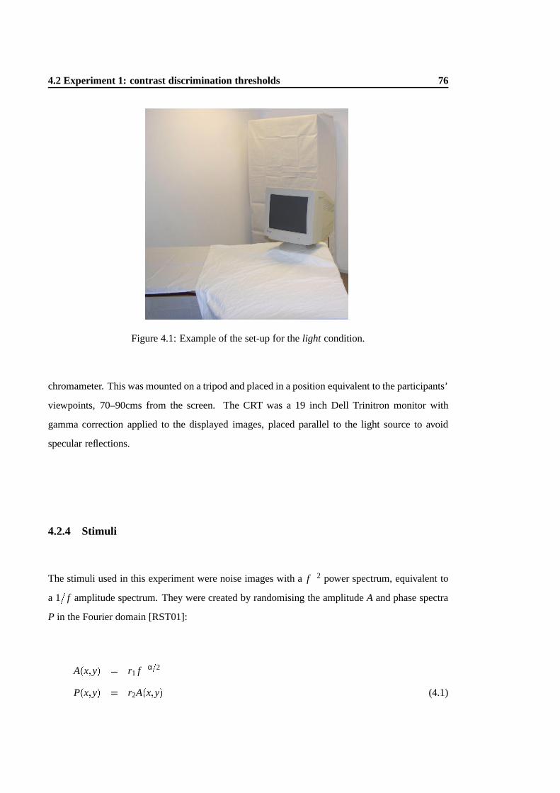
4.2 Experiment 1: contrast discrimination thresholds 76
Figure 4.1: Example of the set-up for thelight condition.
chromameter. This was mounted on a tripod and placed in a position equivalent to the participants’
viewpoints, 70–90cms from the screen. The CRT was a 19 inch Dell Trinitron monitor with
gamma correction applied to the displayed images, placed parallel to the light source to avoid
specular reflections.
4.2.4 Stimuli
The stimuli used in this experiment were noise images with af�2 power spectrum, equivalent to
a 1= f amplitude spectrum. They were created by randomising the amplitudeA and phase spectra
P in the Fourier domain [RST01]:
A(x;y) = r1 f�α=2
P(x;y) = r2A(x;y) (4.1)
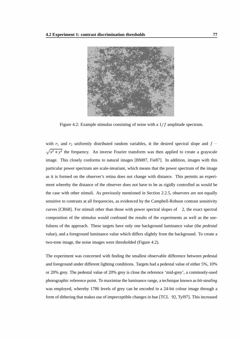
4.2 Experiment 1: contrast discrimination thresholds 77
Figure 4.2: Example stimulus consisting of noise with a 1= f amplitude spectrum.
with r1 and r2 uniformly distributed random variables,α the desired spectral slope andf =px2+y2 the frequency. An inverse Fourier transform was then applied to create a grayscale
image. This closely conforms to natural images [BM87, Fie87]. In addition, images with this
particular power spectrum are scale-invariant, which means that the power spectrum of the image
as it is formed on the observer’s retina does not change with distance. This permits an experi-
ment whereby the distance of the observer does not have to be as rigidly controlled as would be
the case with other stimuli. As previously mentioned in Section 2.2.5, observers are not equally
sensitive to contrasts at all frequencies, as evidenced by the Campbell-Robson contrast sensitivity
curves [CR68]. For stimuli other than those with power spectral slopes of�2, the exact spectral
composition of the stimulus would confound the results of the experiments as well as the use-
fulness of the approach. These targets have only one background luminance value (thepedestal
value), and a foreground luminance value which differs slightly from the background. To create a
two-tone image, the noise images were thresholded (Figure 4.2).
The experiment was concerned with finding the smallest observable difference between pedestal
and foreground under different lighting conditions. Targets had a pedestal value of either 5%, 10%
or 20% grey. The pedestal value of 20% grey is close the reference ‘mid-grey’, a commonly-used
photographic reference point. To maximise the luminance range, a technique known asbit-stealing
was employed, whereby 1786 levels of grey can be encoded in a 24-bit colour image through a
form of dithering that makes use of imperceptible changes in hue [TCL+92, Tyl97]. This increased

4.2 Experiment 1: contrast discrimination thresholds 78
R G B99 99 9999 99 100100 99 99100 99 10099 100 9999 100 100100 100 100100 100 100
Table 4.1: Example of RGB values used in bit-stealing. Instead of two RGB values for grey(99,99,99 and 100,100,100), six intermediate values are created, thus increasing the luminanceresolution.
the luminance resolution, providing more accuracy for JND measurement. The resulting superfine
greyscale is achieved by exploiting the fact that RGB values consist of different luminances. Thus,
instead of stepping between the two grey levels (for example, RGB values of 99, 99, 99 and 100,
100, 100), six intermediate grey levels can be created, as shown in Table 4.1.
While bit-stealing provides the opportunity for higher accuracy in threshold detection, it can be
problematic as the saturation is greater at low levels, so bit-stealing to provide a pseudo-grey may
result in the undesirable appearance of colour. However, a pilot study showed that this effect was
not noticeable at the grey-levels used in the experiment.
4.2.5 Procedure
The main experiment took the form of a signal-detection task consisting of 120 trials. Atwo-
alternative forced choice(2afc) procedure, using two random interleaving staircases, was em-
ployed. This is a process whereby the participant’s answer can be verified, and the magnitude of
the stimulus is then modified dependent on that answer. The 2afc procedure presents the partici-
pant with a stimulus in one of two randomly selected intervals, and the participant must identify
in which interval the stimulus was present. The drawback of this technique is that, with only two
choices, even if the participant guesses the answer they will still make the correct choice half of
the time. Because of this, a large number of trials should be used (Farell and Pelli recommend
at least 60 trials [FP98]) to obtain a good threshold estimate. However, combining this procedure

4.2 Experiment 1: contrast discrimination thresholds 79
with another method, as described next, can limit the probability of error.
The use of thestaircase method, in conjunction with the 2afc mentioned above, provides a more
efficient method of threshold detection, concentrating trials in a range close to threshold. The
staircase method is a variant on themethod of limits. The method of limits is one of three methods
proposed by Fechner to measure thresholds (the other two being themethod of constant stimuliand
themethod of adjustment) [SB94]. Using the method of limits, the stimulus is changed gradually
on each trial until the participant’s response changes. The intensity of the stimulus when this
response change occurs signifies the threshold.
Cornsweet adapted this method through the use of two random interleaving staircases [Cor72].
With this, an experiment begins with an intensity that a participant can definitely see, and de-
creases it until it can no longer be seen. As soon as the participant can no longer identify the
stimulus, its intensity is increased. This point of change is known as acontrast reversal. The
intensity of the stimulus continues to increase until the participant can once again see the it, fol-
lowing which the intensity begins to decrease again. The trials continue until a specific number
of contrast reversals have occurred, and the stimulus intensities at these contrast reversals are then
averaged to estimate the threshold. Figure 4.3 shows how most of the stimulus values are therefore
concentrated close to the threshold, making the procedure more efficient [SB94]. By interleaving
two or more concurrent staircases arbitrarily, randomness is introduced to ensure the participant
does not become aware of the process.
A pilot study, following the main procedure outlined below, was undertaken to observe the re-
quirements of the experiment and decide on the number of trials necessary to provide sufficient
data. The optimal length of the experiment was found to be around 120 trials per pedestal value,
which allowed for at least 4 contrast reversals to occur.
The main trial of Experiment 1 took the form of two 0.5 second intervals, separated by 0.5 seconds
of the pedestal grey value and followed by 4 seconds of grey before the beginning of the next trial.
The first interval was marked by a beep, and the second by a double beep. During one of the
intervals, a target was shown. Participants had to choose whether this target appeared in the first
or the second interval. The instructions shown to the participants are given in Appendix A.2.

4.2 Experiment 1: contrast discrimination thresholds 80
y
y
n
y
n
y
n
n
n
n
y
n
y
n
y = correct repsonse
n = incorrect response
Trial
Stim
ulus
inte
nsity
1 2 3 4 5 6 7 8 9 10 11 12 13
Threshold value
Figure 4.3: Example of results using two interleaving staircases. Use of the staircase methodmeans that stimulus values are concentrated in the threshold region.
Following five correct selections, the contrast of the target was decreased towards the value of
the pedestal grey. Following an incorrect selection, the contrast of the target was set further from
the pedestal grey. With these increases and decreases, the stimulus level approaches the point
where the probability of a correct result is 87%, i.e. 0:50:2, where 0.5 is the 50% chance of
the participant giving the correct answer. This resulted in the collection of threshold values for
each participant, for each given pedestal value, under each of the ambient light conditions. The
experimental program flow is shown in Figure 4.4.
4.2.6 Results and discussion
The research hypothesis stated that JND detection would differ depending on the amount of re-
flected ambient light. Participants’ JND responses were measured to determine their sensitivity
to contrast perception under the three conditions (dark, mediumand light). The average JND
measurements are given in Tables 4.2–4.4 and in Appendix B.
Taking Participant D as an example, the JND value observed by this participant in thedark condi-
tion was 0.004962 for a pedestal of 5% grey. In themediumcondition, when some ambient light
was present in the viewing environment, this JND value increased to 0.005472 — more contrast
was required to discriminate the target from the background. When the ambient lighting was in-
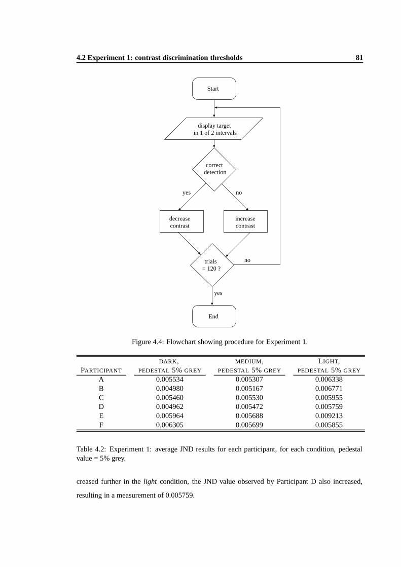
4.2 Experiment 1: contrast discrimination thresholds 81
display target in 1 of 2 intervals
decreasecontrast
increasecontrast
End
Start
correct detection
trials = 120 ?
yes no
yes
no
Figure 4.4: Flowchart showing procedure for Experiment 1.
DARK, MEDIUM , LIGHT,PARTICIPANT PEDESTAL 5% GREY PEDESTAL5% GREY PEDESTAL5% GREY
A 0.005534 0.005307 0.006338B 0.004980 0.005167 0.006771C 0.005460 0.005530 0.005955D 0.004962 0.005472 0.005759E 0.005964 0.005688 0.009213F 0.006305 0.005699 0.005855
Table 4.2: Experiment 1: average JND results for each participant, for each condition, pedestalvalue = 5% grey.
creased further in thelight condition, the JND value observed by Participant D also increased,
resulting in a measurement of 0.005759.

4.2 Experiment 1: contrast discrimination thresholds 82
DARK, MEDIUM , LIGHT,PARTICIPANT PEDESTAL 10% GREY PEDESTAL10% GREY PEDESTAL10% GREY
A 0.009335 0.009250 0.009415B 0.008307 0.007464 0.010490C 0.008153 0.008384 0.008597D 0.009786 0.008213 0.010583E 0.007852 0.009602 0.012601F 0.006976 0.008490 0.009529
Table 4.3: Experiment 1: average JND results for each participant, for each condition, pedestalvalue = 10% grey.
DARK, MEDIUM , LIGHT,PARTICIPANT PEDESTAL 20% GREY PEDESTAL20% GREY PEDESTAL20% GREY
A 0.007740 0.009428 0.008280B 0.007586 0.007854 0.008774C 0.007002 0.007874 0.010476D 0.006343 0.009005 0.009404E 0.007272 0.009241 0.010531F 0.008031 0.008764 0.010011
Table 4.4: Experiment 1: average JND results for each participant, for each condition, pedestalvalue = 20% grey.
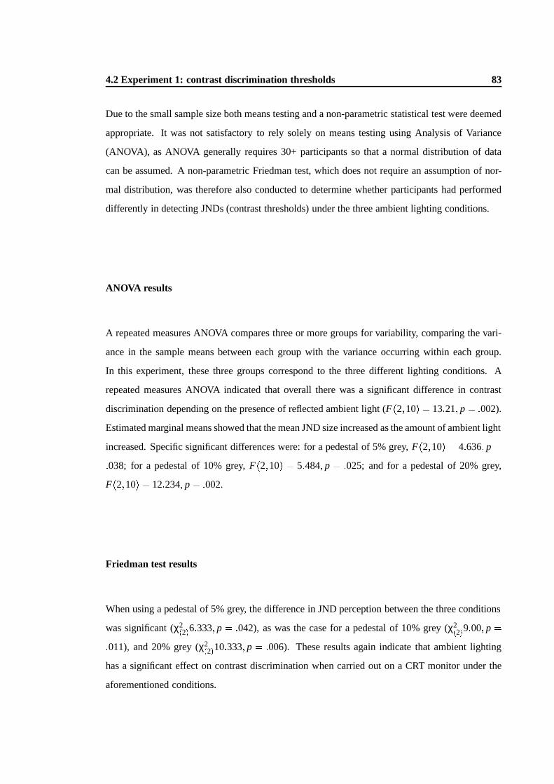
4.2 Experiment 1: contrast discrimination thresholds 83
Due to the small sample size both means testing and a non-parametric statistical test were deemed
appropriate. It was not satisfactory to rely solely on means testing using Analysis of Variance
(ANOVA), as ANOVA generally requires 30+ participants so that a normal distribution of data
can be assumed. A non-parametric Friedman test, which does not require an assumption of nor-
mal distribution, was therefore also conducted to determine whether participants had performed
differently in detecting JNDs (contrast thresholds) under the three ambient lighting conditions.
ANOVA results
A repeated measures ANOVA compares three or more groups for variability, comparing the vari-
ance in the sample means between each group with the variance occurring within each group.
In this experiment, these three groups correspond to the three different lighting conditions. A
repeated measures ANOVA indicated that overall there was a significant difference in contrast
discrimination depending on the presence of reflected ambient light (F(2;10) = 13:21; p = :002).
Estimated marginal means showed that the mean JND size increased as the amount of ambient light
increased. Specific significant differences were: for a pedestal of 5% grey,F(2;10) = 4:636; p =
:038; for a pedestal of 10% grey,F(2;10) = 5:484; p = :025; and for a pedestal of 20% grey,
F(2;10) = 12:234; p = :002.
Friedman test results
When using a pedestal of 5% grey, the difference in JND perception between the three conditions
was significant (χ2(2)6:333; p = :042), as was the case for a pedestal of 10% grey (χ2
(2)9:00; p =
:011), and 20% grey (χ2(2)10:333; p = :006). These results again indicate that ambient lighting
has a significant effect on contrast discrimination when carried out on a CRT monitor under the
aforementioned conditions.
4.3 Experiment 2: rapid characterisation 84
Comparison with Rogers et al.
Our experiment followed the two-alternative forced choice procedure that was used by Rogers et al. .
However, we used different stimuli, and also incorporated a random interleaving staircases method
to improve on efficiency and accuracy. The results of our experiment support the findings by
Rogers et al. that the appearance of an image on-screen is altered by the presence of reflected am-
bient illumination. Further, the results indicate that the apparent reduction in perceived contrast is
increased as the ambient lighting is increased.
4.3 Experiment 2: rapid characterisation
The experiment described above highlights the significance of the contribution of reflected light
to the perception of contrast in complex images, and provides a JND measurement of contrast
perception for the tested level of illumination and display intensity. However, the method is of
little use in a practical setting due to the lengthy procedure (over one-and-a-half hours per person,
excluding periods of rest). Compromise was therefore sought between accurate measurement of
screen reflections, and practical use, with the aim of developing a rapid technique that did not
require any specialised equipment, using only the display device itself to gather information about
the viewing environment. The research hypothesis remained the same as that in Experiment 1:
that the presence of reflected ambient light in the viewing environment would affect the perceived
contrast of an image displayed on a CRT monitor.
4.3.1 Alternative and pilot experiments
In a manner analogous to simplified determination of the gamma value for a display device, as
described in Section 2.5.1, we sought a simple method for measuring contrast perception. We
considered a number of ideas in deciding on a concise method of Experiment 1. Pilot studies
were carried out for each of these in order to determine the most promising method of measuring
contrast discrimination in a quick and effective manner. In all cases, the core idea involved the
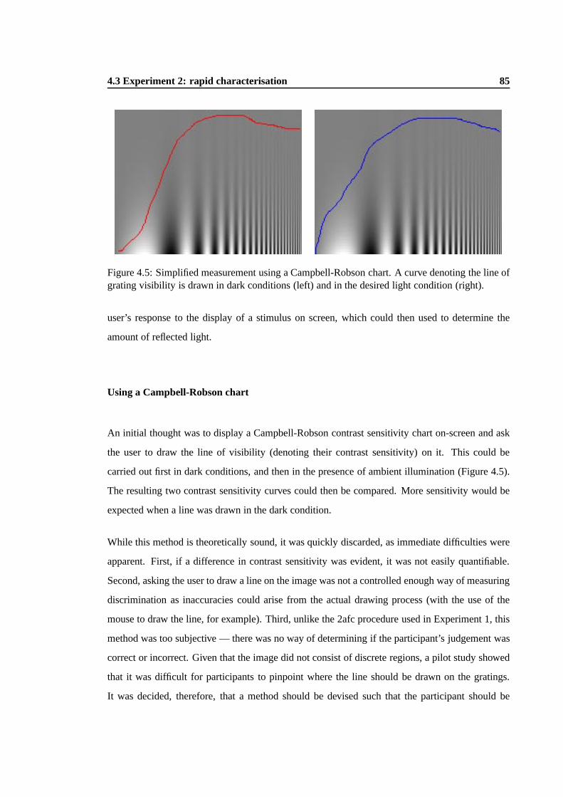
4.3 Experiment 2: rapid characterisation 85
Figure 4.5: Simplified measurement using a Campbell-Robson chart. A curve denoting the line ofgrating visibility is drawn in dark conditions (left) and in the desired light condition (right).
user’s response to the display of a stimulus on screen, which could then used to determine the
amount of reflected light.
Using a Campbell-Robson chart
An initial thought was to display a Campbell-Robson contrast sensitivity chart on-screen and ask
the user to draw the line of visibility (denoting their contrast sensitivity) on it. This could be
carried out first in dark conditions, and then in the presence of ambient illumination (Figure 4.5).
The resulting two contrast sensitivity curves could then be compared. More sensitivity would be
expected when a line was drawn in the dark condition.
While this method is theoretically sound, it was quickly discarded, as immediate difficulties were
apparent. First, if a difference in contrast sensitivity was evident, it was not easily quantifiable.
Second, asking the user to draw a line on the image was not a controlled enough way of measuring
discrimination as inaccuracies could arise from the actual drawing process (with the use of the
mouse to draw the line, for example). Third, unlike the 2afc procedure used in Experiment 1, this
method was too subjective — there was no way of determining if the participant’s judgement was
correct or incorrect. Given that the image did not consist of discrete regions, a pilot study showed
that it was difficult for participants to pinpoint where the line should be drawn on the gratings.
It was decided, therefore, that a method should be devised such that the participant should be

4.3 Experiment 2: rapid characterisation 86
Figure 4.6: A type of gamma chart used to measure contrast discrimination. (It should be notedthat scaling and printing of the image remove the appearance of fusing between the stripes and thelined area.)
presented with a distinct choice of options when determining what they could or could not see.
Using a form of a gamma chart
Given that the desired concise method was inspired by the simplified form of short-cut gamma
calibration, we devised an experiment using a type of gamma chart similar to that described in
Section 2.5.1. Gamma charts of the type shown in Figure 4.6 were created with different levels
of black (either 25%, 50% or 75%) in the lower half of the image. The participants viewed these
charts under the different lighting conditions, selecting the stripe which appeared to fuse best with
the black and white pixels. This resulted in a measurement of the display luminance in the dark
condition, and a corresponding measurement of display luminance plus an ambient term in the
illuminated conditions.
Problems were immediately evident with the user interaction. The concept of simplified gamma

4.3 Experiment 2: rapid characterisation 87
charts had to be explained to participants unfamiliar with the process, and the appearance of fusing
between the top and bottom halves of the chart had to be described in great detail. Participants
also complained that blurring their vision by squinting their eyes (an action that facilitates the
appearance of fusing) began to hurt them after several trials. Also, the pilot study of this procedure
did not suggest a significant difference between conditions. As we were aware that significant
differences should exist, due to the findings of Experiment 1, we decided not to continue with a
full experiment of this type. Instead, a more sensitive method of measurement was sought.
Using a tableau of stimuli
Our third idea for the experimental method was to present the participant with a tableaux consisting
of stimuli similar to those used in Experiment 1. These could be presented in a two dimensional
matrix of stimuli with varying levels of contrast.
Two pilot studies were undertaken using this method. The first used randomly distributed stimuli,
and the second used ordered stimuli that increased in contrast from the top left to the bottom right
of the screen. Participants found the second of these to be more intuitive, as it was explained to
them that they should pick the square on the grid where they could just see the stimulus appear,
and that anything prior to this square should appear blank, and anything following it should be
more easy to distinguish.
Preliminary results from this second method suggested that a significant difference could be mea-
sured by this means. The use of discrete stimuli seemed to indicate that users had more confidence
in their responses (unlike the method which used the Campbell-Robson chart). It was therefore
decided that this was the most suitable method for Experiment 2.
4.3.2 Main experiment
The results from the aforementioned pilot studies led us to adopt the following procedure. It is
almost as straightforward as reading a value off a chart, and constitutes a sensible compromise
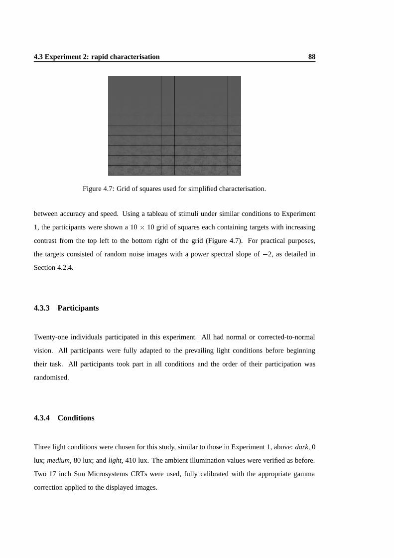
4.3 Experiment 2: rapid characterisation 88
Figure 4.7: Grid of squares used for simplified characterisation.
between accuracy and speed. Using a tableau of stimuli under similar conditions to Experiment
1, the participants were shown a 10� 10 grid of squares each containing targets with increasing
contrast from the top left to the bottom right of the grid (Figure 4.7). For practical purposes,
the targets consisted of random noise images with a power spectral slope of�2, as detailed in
Section 4.2.4.
4.3.3 Participants
Twenty-one individuals participated in this experiment. All had normal or corrected-to-normal
vision. All participants were fully adapted to the prevailing light conditions before beginning
their task. All participants took part in all conditions and the order of their participation was
randomised.
4.3.4 Conditions
Three light conditions were chosen for this study, similar to those in Experiment 1, above:dark, 0
lux; medium, 80 lux; andlight, 410 lux. The ambient illumination values were verified as before.
Two 17 inch Sun Microsystems CRTs were used, fully calibrated with the appropriate gamma
correction applied to the displayed images.

4.3 Experiment 2: rapid characterisation 89
4.3.5 Procedure
Again, the experiment constituted a signal-detection task. A tableau of images displayed in a 10
� 10 grid was shown. The pedestal value was set to either 5%, 10% or 20% grey. A target of
randomly generated 1= f noise was displayed in each square of the grid, with the contrast increas-
ing linearly in each square from the top left to the bottom right of the grid. The minimal contrast
value (0) increased to a pedestal-dependent maximum contrast value (0.004–0.006, determined
through the results of the Experiment 1, described above). The participants were given instruc-
tions which asked them to click once on the square where they couldjust noticesome noise on
the grey background, and it was explained that ‘Just noticeablemeans that it is the square closest
to appearing blank: the other squares contain either no noise or more noise’ (full instructions are
given in Appendix A.3).
By clicking on their chosen square, another tableau was displayed, this time with the contrast
increasing by a power of 2, effectively showing more squares closer to the threshold region. With
each choice made by the participant, the power increased, until the participant could only see
contrast in the high part of the curve, whereupon the power was decreased. For each pedestal
value, under each ambient light condition, the participant made 5 choices indicating in which part
of the tableau they perceived the minimal contrast. These values were then averaged to give an
average JND value for each individual, for each pedestal value, under each condition. This process
is outlined in Figure 4.8
4.3.6 Results and discussion
The research hypothesis stated that JND detection would differ depending on the amount of re-
flected ambient light, as with Experiment 1, above. Participants’ JND responses were measured
to determine their sensitivity to contrast perception under the three conditions (dark, medium and
light). An average threshold (JND value) was calculated for each participant under each condition.
These values are shown in Figure 4.9. Tables of results are given in Appendix B.
As with Experiment 1, Experiment 2 consisted of a repeated measures design with three or more
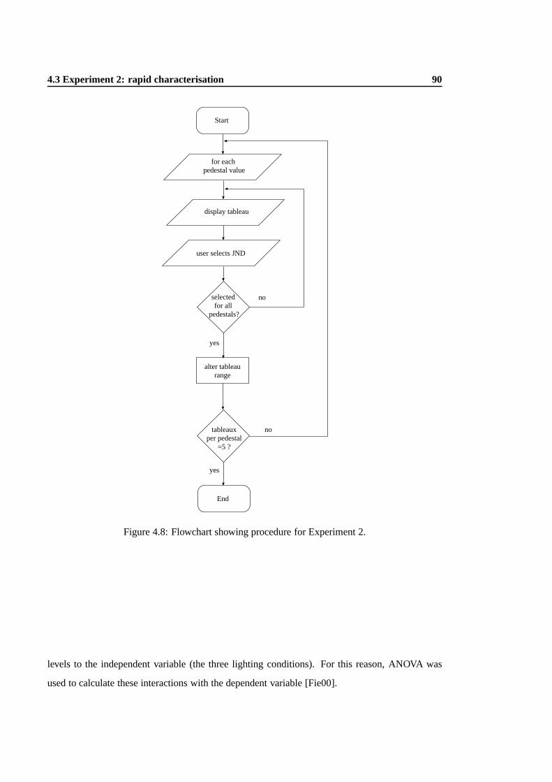
4.3 Experiment 2: rapid characterisation 90
for each pedestal value
alter tableaurange
End
Start
tableauxper pedestal
=5 ?
yes
yes
no
display tableau
user selects JND
selected for all
pedestals?
no
Figure 4.8: Flowchart showing procedure for Experiment 2.
levels to the independent variable (the three lighting conditions). For this reason, ANOVA was
used to calculate these interactions with the dependent variable [Fie00].

4.3 Experiment 2: rapid characterisation 91
0
0.002
0.004
0.006
0.008
0.01
0.012
0.014
5 10 15 20
Avg JND value
Participant
Average JND values, dark condition, pedestal = 5% grey
Average JND values, medium condition, pedestal = 5% grey
Average JND values, light condition, pedestal = 5% grey
0
0.002
0.004
0.006
0.008
0.01
0.012
0.014
5 10 15 20
Avg JND value
Participant
Average JND values, dark condition, pedestal = 10% grey
Average JND values, medium condition, pedestal = 10% grey
Average JND values, light condition, pedestal = 10% grey
0
0.002
0.004
0.006
0.008
0.01
0.012
0.014
5 10 15 20
Avg JND value
Participant
Average JND values, dark condition, pedestal = 20% grey
Average JND values, medium condition, pedestal = 20% grey
Average JND values, light condition, pedestal = 20% grey
Figure 4.9: Graphs to show the average JND values measured in Experiment 2 for pedestal valuesof 5% grey (top), 10% grey (middle) and 20% grey (bottom).
ANOVA results
A repeated measures ANOVA revealed an overall significant difference in threshold detection be-
tween the three lighting conditions,F(2;40) = 58:9; p < :001. These results indicate that when
measured by this rapid method, it can be shown that ambient lighting has a significant effect

4.4 Summary 92
on contrast discrimination. Specific significant differences were: for a pedestal of 5% grey,
F(2;40) = 65:770; p < :001; for a pedestal of 10% grey,F(2;40) = 37:414; p < :001; and for
a pedestal of 20% grey,F(2;40) = 35:761; p< :001.
Friedman test results
The difference in JND perception between the three conditions for a pedestal of 5% grey was
significant (χ2(2)34:048; p < :001), as was the case for a pedestal of 10% grey (χ2
(2)24:795; p <
:001), and 20% grey (χ2(2)25:810; p < :001). These results correspond to the ANOVA results,
confirming the rejection of the null hypothesis.
Comparison with Experiment 1
Although direct comparison cannot be made between the results of Experiment 1 and Experiment
2, both experiments have shown a significant difference between contrast perception under three
different levels of reflected ambient light. Both the ANOVA and the Friedman test results for
Experiment 2 produce a smallerp value than the results of Experiment 1. However, this cannot
be taken to mean that Experiment 2 is somehow more accurate in measuring contrast perception.
This smallerp value may indeed be a result of the larger sample size used in Experiment 2.
Nonetheless, it has been revealed that Experiment 2 is as valid a method of measuring changes in
contrast perception as Experiment 1, yet takes only a fraction of the time (generally no more than
2 minutes in total per person).
4.4 Summary
This chapter has described a method of measuring the effect of reflected ambient light on contrast
perception. A direct correlation was revealed between the amount of reflected ambient light and
the reduction in perceived contrast. Significant differences were revealed between JND discrim-
ination in three different lighting conditions. This relationship was also evident in our second

4.4 Summary 93
experiment, which was designed to perform the same task in much less time. For this second
experiment, we designed and implemented a rapid form of visual calibration, which takes only
minutes to complete, making it around 50 times quicker to carry out than Experiment 1. Thus,
Experiment 2 constitutes the main contribution to this thesis — a method of determining the effect
of ambient light in a quick and effective manner, with the user needing no equipment other than
the computer monitor itself.
In the following chapter, we extend our work to include a novel form of contrast manipulation that
can use the results from Experiment 2 to produce a method of luminance remapping, resulting in
an image displayed under ambient light appearing as it would look when displayed in darkness.
In a subsequent chapter, the success of this algorithm will then be validated through a similar
psychophysical method to Experiment 2.

4.4 Summary 94

Chapter 5
Correcting for Ambient Light
The amount of light reflected by a computer monitor may be indirectly measured with one of the
experiments described in the previous chapter. It is envisaged that the viewer establishes a JND
(∆Ld) in darkness, and a second JND (∆Lb) with normal office lights switched on. In both cases
some desired pedestal valueL will be used (such as 20% of the maximum display intensity, for
example).
The light that travels from the monitor to the eye is thenL in the dark condition, andL+LR in the
light condition. The termLR represents the amount of light diffusely reflected by the monitor and
constitutes the unknown value required for adjustment purposes. Using Weber’s Law,LR can be
computed with the following equations:
∆Ld
L=
∆Lb
L+LR
LR = L
�∆Lb
∆Ld�1
�(5.1)
95

5.1 Contrast adjustment 96
0
m
0 m
Out
put v
alue
Input value
L
L - LR
loss of dynamic range
negative voltage
Figure 5.1: Problems with remapping by subtraction. Dark pixels would produce a negative volt-age, and the dynamic range would be reduced.
5.1 Contrast adjustment
Under the assumption thatLd < Lb, and hence thatLR > 0, we should ideally subtractLR from
each pixel to undo the effect of reflected light. The reflections off the monitor would then add
on this same amount, thus producing the desired percept. Remapping luminance by subtraction
would also yield a function with a derivative of 1 over its range. Any other slope would result
in changes in contrast that may affect image perception. However, there are two problems with
this approach. First, dark pixels will become negative and are therefore impossible to display.
Negative pixels could be clamped to zero, but that would reduce the dynamic range, which for
typical display devices is already limited (Section 2.5.2). The second problem is that subtraction
of LR leads to under-use of the available dynamic range at the upper end of the scale. These
problems are illustrated in Figure 5.1.
5.2 Luminance remapping requirements
With the ability to measureLR through the measurement of JNDs, we seek a function that remaps
intensities such that the amount of contrast perceived around the pedestal valueL is the initial∆Ld,
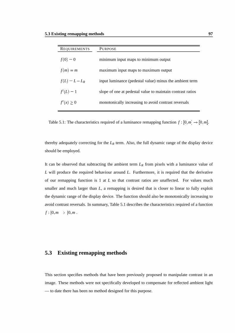
5.3 Existing remapping methods 97
REQUIREMENTS PURPOSE
f (0) = 0 minimum input maps to minimum output
f (m) = m maximum input maps to maximum output
f (L) = L�LR input luminance (pedestal value) minus the ambient term
f 0(L) = 1 slope of one at pedestal value to maintain contrast ratios
f 0(x)� 0 monotonically increasing to avoid contrast reversals
Table 5.1: The characteristics required of a luminance remapping functionf : [0;m]! [0;m].
thereby adequately correcting for theLR term. Also, the full dynamic range of the display device
should be employed.
It can be observed that subtracting the ambient termLR from pixels with a luminance value of
L will produce the required behaviour aroundL. Furthermore, it is required that the derivative
of our remapping function is 1 atL so that contrast ratios are unaffected. For values much
smaller and much larger thanL, a remapping is desired that is closer to linear to fully exploit
the dynamic range of the display device. The function should also be monotonically increasing to
avoid contrast reversals. In summary, Table 5.1 describes the characteristics required of a function
f : [0;m]! [0;m].
5.3 Existing remapping methods
This section specifies methods that have been previously proposed to manipulate contrast in an
image. These methods were not specifically developed to compensate for reflected ambient light
— to date there has been no method designed for this purpose.
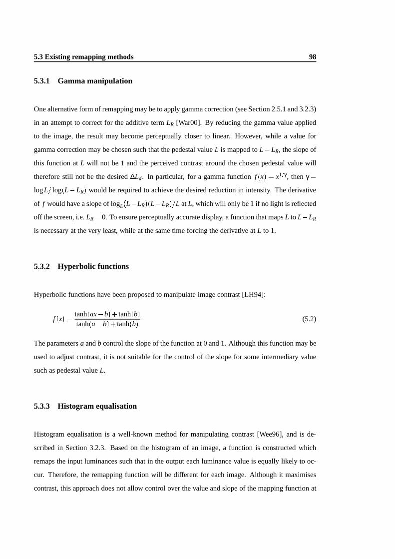
5.3 Existing remapping methods 98
5.3.1 Gamma manipulation
One alternative form of remapping may be to apply gamma correction (see Section 2.5.1 and 3.2.3)
in an attempt to correct for the additive termLR [War00]. By reducing the gamma value applied
to the image, the result may become perceptually closer to linear. However, while a value for
gamma correction may be chosen such that the pedestal valueL is mapped toL�LR, the slope of
this function atL will not be 1 and the perceived contrast around the chosen pedestal value will
therefore still not be the desired∆Ld. In particular, for a gamma functionf (x) = x1=γ, thenγ =
logL= log(L�LR) would be required to achieve the desired reduction in intensity. The derivative
of f would have a slope of logL(L�LR)(L�LR)=L atL, which will only be 1 if no light is reflected
off the screen, i.e.LR= 0. To ensure perceptually accurate display, a function that mapsL to L�LR
is necessary at the very least, while at the same time forcing the derivative atL to 1.
5.3.2 Hyperbolic functions
Hyperbolic functions have been proposed to manipulate image contrast [LH94]:
f (x) =tanh(ax�b)+ tanh(b)tanh(a�b)+ tanh(b)
(5.2)
The parametersa andb control the slope of the function at 0 and 1. Although this function may be
used to adjust contrast, it is not suitable for the control of the slope for some intermediary value
such as pedestal valueL.
5.3.3 Histogram equalisation
Histogram equalisation is a well-known method for manipulating contrast [Wee96], and is de-
scribed in Section 3.2.3. Based on the histogram of an image, a function is constructed which
remaps the input luminances such that in the output each luminance value is equally likely to oc-
cur. Therefore, the remapping function will be different for each image. Although it maximises
contrast, this approach does not allow control over the value and slope of the mapping function at
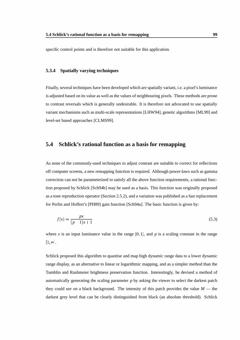
5.4 Schlick’s rational function as a basis for remapping 99
specific control points and is therefore not suitable for this application.
5.3.4 Spatially varying techniques
Finally, several techniques have been developed which are spatially variant, i.e. a pixel’s luminance
is adjusted based on its value as well as the values of neighbouring pixels. These methods are prone
to contrast reversals which is generally undesirable. It is therefore not advocated to use spatially
variant mechanisms such as multi-scale representations [LHW94], genetic algorithms [ML99] and
level-set based approaches [CLMS99].
5.4 Schlick’s rational function as a basis for remapping
As none of the commonly-used techniques to adjust contrast are suitable to correct for reflections
off computer screens, a new remapping function is required. Although power-laws such as gamma
correction can not be parameterized to satisfy all the above function requirements, a rational func-
tion proposed by Schlick [Sch94b] may be used as a basis. This function was originally proposed
as a tone reproduction operator (Section 2.5.2), and a variation was published as a fast replacement
for Perlin and Hoffert’s [PH89] gain function [Sch94a]. The basic function is given by:
f (x) =px
(p�1)x+1(5.3)
wherex is an input luminance value in the range[0;1], and p is a scaling constant in the range
[1;∞].
Schlick proposed this algorithm to quantise and map high dynamic range data to a lower dynamic
range display, as an alternative to linear or logarithmic mapping, and as a simpler method than the
Tumblin and Rushmeier brightness preservation function. Interestingly, he devised a method of
automatically generating the scaling parameterp by asking the viewer to select the darkest patch
they could see on a black background. The intensity of this patch provides the valueM — the
darkest grey level that can be clearly distinguished from black (an absolute threshold). Schlick
5.4 Schlick’s rational function as a basis for remapping 100
reasoned that since the parameters controlling a tone reproduction function (contrast, brightness,
viewing conditions, observation distance, etc.) are difficult to define or measure , thenM can be
used in place of these measurements, on the basis that it is this value that noticeably changes when
the aforementioned parameters change. Schlick’s premise was that rendering programs contain
an ‘epsilon’ value that generates the smallest non-zero value (ε) of the image, beneath which
computed intensities are considered to be negligible. This value can be mapped toM thus:
p=Mm�MεNε�Mε
'MmNε
(becausem� ε andN�M) (5.4)
wherem is the maximum display value andN is any value in the display range[0;N�1]. For our
algorithm, we do not need to setp as we can solve for it given that we will know the values ofL
andLR.
While Schlick reports that this automatic parameter generation method provides satisfactory re-
sults without the need for guesswork, he also acknowledges that this method does not work with
logarithmic or power law tone reproduction. Schlick’s use of measuring a threshold to determine
a value forM shares a common idea with the work we present in this thesis, whereby the display
device itself is used to infer something about the viewing conditions. However, the aim of this
method differs, with Schlick using this information to set a general parameter for the purpose of
dynamic range reduction, whereas we wish to specifically measure JNDs in order to remap lumi-
nance to maintain the appearance of contrast, regardless of dynamic range. Schlick did not provide
any quantitative evidence supporting the success of this parameter generation, whereas our method
for determining JNDs is supported by statistical analysis of psychophysical experimentation. Also,
we provide a form of JND measurement to determine difference thresholds, rather than absolute
thresholds. Nonetheless, our work can be used alongside existing tone reproduction operators, and
would be particularly useful in conjunction with those that aim to mimic perceptual qualities.

5.5 A new luminance remapping algorithm 101
0 m0
m
[0,L]
[L,m]
L
L-LR
0 m
0 m
0
m
0
m
Figure 5.2: An example of how the remapping function is split into two ranges,[0;L] and[L;m]
5.5 A new luminance remapping algorithm
The list of requirements given in Table 5.1 may be satisfied by splitting the function into two
ranges, namely[0;L] and[L;m]. An example of this split is shown in Figure 5.2.
The algorithm presented below maintains the original contrast for a selected input luminance
value, L, and approximately correct perceived contrast for all other input values. As ambient
light reduces the perceived dynamic range, the problem is similar to that of tonemapping for the
purpose of dynamic range reduction, so a tailored mapping based around a specific input value is
feasible.
Using Equation 5.3, the appropriate substitutions are made forx. As we already know the values
for L andLR, we can solve for the free parameterp. In particular, the inputx and the outputf (x)
is scaled before solving forp.

5.5 A new luminance remapping algorithm 102
5.5.1 The range[0;L]
For the range[0;L] we substitutex! x=L in Equation 5.3, thereby normalising it to that range,
and the output is then scaled byL�LR:
f[0;L](x) = (L�LR)px
L
(p�1) xL +1
=(L�LR)pxx(p�1)+L
(5.5)
This equation satisfies the requirements thatf[0;L](0) = 0 and f[0;L](L) = L�LR. As the slope of
f[0;L] is known to be 1 atL, the following equation can be solved forp:
f 0[0;L](x) =p(L�LR)
L((p�1)x=L+1)�
(p�1)px(L�LR)
L2((p�1)x=L+1)2
=p(L�LR)L(xp�x+L)2
= 1 (5.6)
By substitutingx= L then
p=(L�LR)
L(5.7)
5.5.2 The range[L;M]
For the range[L;m] we substitutex! (x�L)=(m�L) in Equation 5.3, and scale the output by
m�L+LR andL�LR is added to the result:
f[L;m](x) =p
x�Lm�L
(m�L+LR)
(p�1)x�Lm�L
+1+L�LR (5.8)
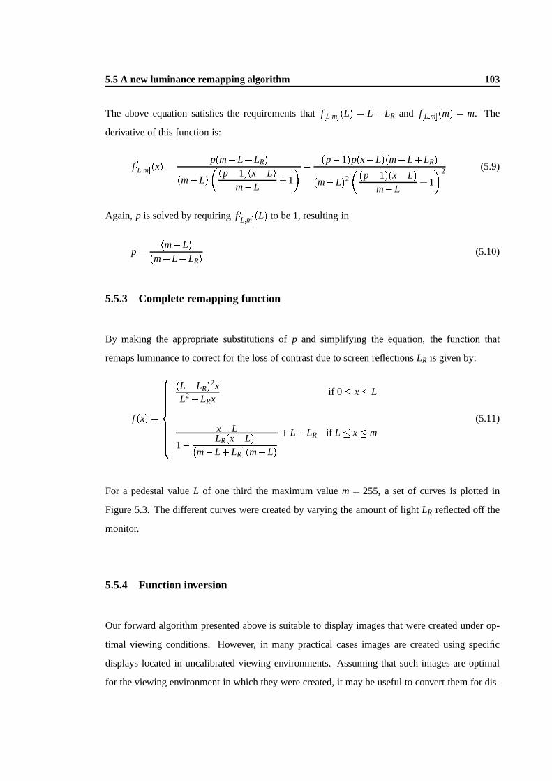
5.5 A new luminance remapping algorithm 103
The above equation satisfies the requirements thatf[L;m](L) = L� LR and f[L;m](m) = m. The
derivative of this function is:
f 0[L;m](x) =p(m�L+LR)
(m�L)
�(p�1)(x�L)
m�L+1
� � (p�1)p(x�L)(m�L+LR)
(m�L)2�(p�1)(x�L)
m�L+1
�2 (5.9)
Again, p is solved by requiringf 0[L;m](L) to be 1, resulting in
p=(m�L)
(m�L+LR)(5.10)
5.5.3 Complete remapping function
By making the appropriate substitutions ofp and simplifying the equation, the function that
remaps luminance to correct for the loss of contrast due to screen reflectionsLR is given by:
f (x) =
8>>>>>>><>>>>>>>:
(L�LR)2x
L2�LRxif 0 � x� L
x�L
1�LR(x�L)
(m�L+LR)(m�L)
+L�LR if L� x�m
(5.11)
For a pedestal valueL of one third the maximum valuem= 255, a set of curves is plotted in
Figure 5.3. The different curves were created by varying the amount of lightLR reflected off the
monitor.
5.5.4 Function inversion
Our forward algorithm presented above is suitable to display images that were created under op-
timal viewing conditions. However, in many practical cases images are created using specific
displays located in uncalibrated viewing environments. Assuming that such images are optimal
for the viewing environment in which they were created, it may be useful to convert them for dis-

5.5 A new luminance remapping algorithm 104
0 50 100 150 200 2500
50
100
150
200
250Contrast correction
L = 12.75L = 25.50L = 38.25L = 51.00
f(x)
x
L = 76.5m = 255
R
R
R
R
Figure 5.3: Remapping functions forLR set to 5%, 10%, 15% and 20% of the maximum displayvaluem. The pedestal value was set toL = 0:3m for demonstration purposes. In practise, a baseluminance value ofL = 0:2m is appropriate.
play in a different viewing environment. An effective way to accomplish this is by transforming
the image into a standard space that is independent of the viewing environment. This is analogous
to the Profile Connection Space used in ICC profiles [ICC03]. ICC profiles are normally used to
convert images for reproduction on different display devices such that the perception of the dis-
played material is least affected. It can be envisaged that the methodology and algorithm described
in this thesis could become part of the ICC file format since it would address device dependent
issues not covered by ICC profiles to date.
A simple method of inverse correction would be to addLR to every pixel value, but this requires
a file format with a pixel range of[LR: : :m+LR]. This is impractical given that many file format
standards only support a specific number of bits (e.g. 8). Therefore, we can instead invert the
function described above to create an inverse correction which does not alter the dynamic range.
The first step in converting between the viewing environment that was used to create an image (the
source environment) and some other display environment would be to undo the effect of the source
environment. Hence, it is desirable to convert such images to a hypothetical viewing environment
in which the screen does not reflect light. This may be achieved by measuring∆Ld and∆Lb for

5.5 A new luminance remapping algorithm 105
the source environment, computingLR and then applying the inverse transformation to the image:
finv(x) =
8>>>>><>>>>>:
xL2
(L�LR)2+xLR0� x� L�LR
x(m�L)2+mLR(x+m+Lr�2L)(m�L)2+LR(x+m+Lr�2L)
L�LR� x�m
(5.12)
For the destination environmentf (x) may then be applied prior to display. One limitation of this
approach is that for both forward and inverse transformations the same pedestal valueL needs
to be used. However, it would not be unreasonable to standardise by fixingL to 0:2m such that
middle grey is always displayed correctly.
5.5.5 Colour space
Most images are given in a device-dependent colour space. While it is possible to apply the
remapping function to the individual colour channels, this is not recommended. Non-linear scaling
functions such as the one described above will alter the colour ratios for individual pixels, leading
to changes in chromatic appearance. This would be an undesirable side-effect of the algorithm,
which is easily avoided by applying the equation to the luminance channel only.
It is therefore necessary to convert to a different colour space which has a separate luminance
channel such as XYZ or Lab. These conversions require knowledge of the image’s white point,
which more often than not is unknown. If the white point is known, an appropriate conversion
matrix may be constructed [Poy03]. In many cases it may be reasonable to make the grey-world
assumption, i.e. the average reflective colour of a scene is grey. If the average pixel value of
the image deviates from grey, this may be attributed to the illuminant. Under the grey-world
assumption the average pixel value is a good estimate of the scene’s white point. Otherwise, one
can resort to white-point estimation techniques [CFB99], or simply estimate that the white point
is always D65. This will be true to a first approximation for outdoor photographs.
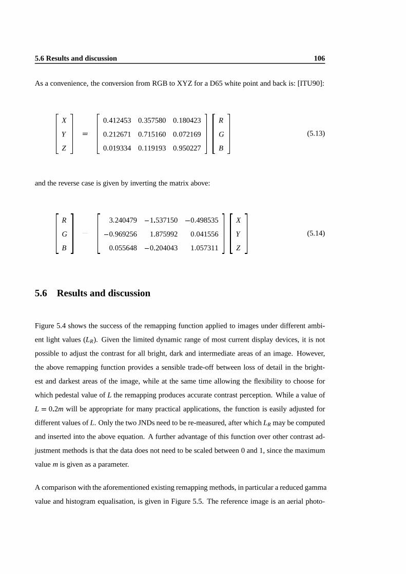
5.6 Results and discussion 106
As a convenience, the conversion from RGB to XYZ for a D65 white point and back is: [ITU90]:
26664
X
Y
Z
37775 =
26664
0:412453 0:357580 0:180423
0:212671 0:715160 0:072169
0:019334 0:119193 0:950227
37775
26664
R
G
B
37775 (5.13)
and the reverse case is given by inverting the matrix above:
26664
R
G
B
37775 =
26664
3:240479 �1:537150 �0:498535
�0:969256 1:875992 0:041556
0:055648 �0:204043 1:057311
37775
26664
X
Y
Z
37775 (5.14)
5.6 Results and discussion
Figure 5.4 shows the success of the remapping function applied to images under different ambi-
ent light values (LR). Given the limited dynamic range of most current display devices, it is not
possible to adjust the contrast for all bright, dark and intermediate areas of an image. However,
the above remapping function provides a sensible trade-off between loss of detail in the bright-
est and darkest areas of the image, while at the same time allowing the flexibility to choose for
which pedestal value ofL the remapping produces accurate contrast perception. While a value of
L = 0:2m will be appropriate for many practical applications, the function is easily adjusted for
different values ofL. Only the two JNDs need to be re-measured, after whichLR may be computed
and inserted into the above equation. A further advantage of this function over other contrast ad-
justment methods is that the data does not need to be scaled between 0 and 1, since the maximum
valuem is given as a parameter.
A comparison with the aforementioned existing remapping methods, in particular a reduced gamma
value and histogram equalisation, is given in Figure 5.5. The reference image is an aerial photo-
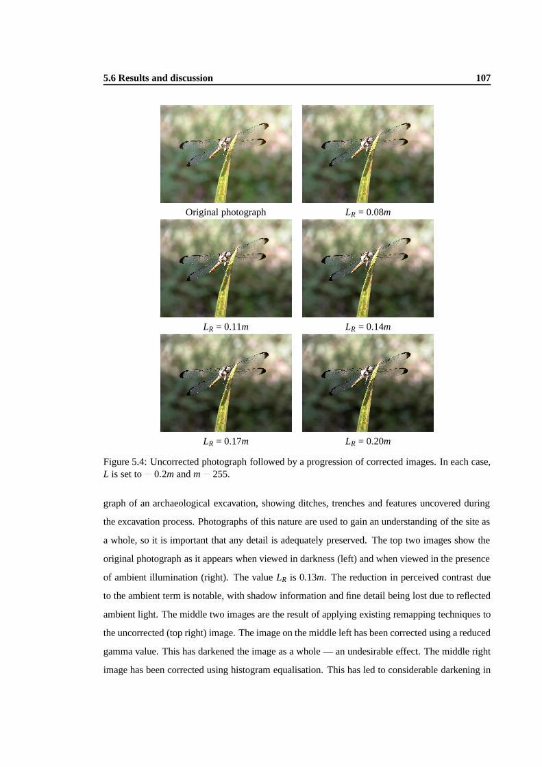
5.6 Results and discussion 107
Original photograph LR = 0.08m
LR = 0.11m LR = 0.14m
LR = 0.17m LR = 0.20m
Figure 5.4: Uncorrected photograph followed by a progression of corrected images. In each case,L is set to= 0:2m andm= 255.
graph of an archaeological excavation, showing ditches, trenches and features uncovered during
the excavation process. Photographs of this nature are used to gain an understanding of the site as
a whole, so it is important that any detail is adequately preserved. The top two images show the
original photograph as it appears when viewed in darkness (left) and when viewed in the presence
of ambient illumination (right). The valueLR is 0.13m. The reduction in perceived contrast due
to the ambient term is notable, with shadow information and fine detail being lost due to reflected
ambient light. The middle two images are the result of applying existing remapping techniques to
the uncorrected (top right) image. The image on the middle left has been corrected using a reduced
gamma value. This has darkened the image as a whole — an undesirable effect. The middle right
image has been corrected using histogram equalisation. This has led to considerable darkening in
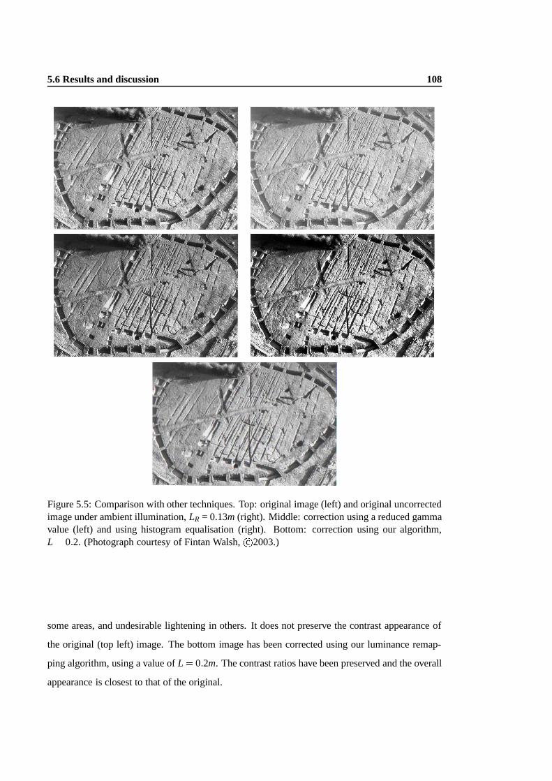
5.6 Results and discussion 108
Figure 5.5: Comparison with other techniques. Top: original image (left) and original uncorrectedimage under ambient illumination,LR = 0.13m (right). Middle: correction using a reduced gammavalue (left) and using histogram equalisation (right). Bottom: correction using our algorithm,L = 0:2. (Photograph courtesy of Fintan Walsh,c 2003.)
some areas, and undesirable lightening in others. It does not preserve the contrast appearance of
the original (top left) image. The bottom image has been corrected using our luminance remap-
ping algorithm, using a value ofL = 0:2m. The contrast ratios have been preserved and the overall
appearance is closest to that of the original.

5.7 Summary 109
5.7 Summary
This chapter has described our method for correcting images where the contrast appears reduced
due to the presence of ambient light. We based our algorithm on Schlick’s rational function,
splitting it into two ranges to meet the requirements for our luminance remapping. We show how
this function can be inverted for images created in an uncalibrated environment. Photographic
results of this algorithm are given. In the following chapter, this algorithm is validated using a
specifically-designed formal psychophysical user study.

5.7 Summary 110

Chapter 6
Validation of luminance remapping
This chapter describes a psychophysical experiment that was developed to validate the success of
the algorithm detailed in the previous chapter. The validation experiment needed to show that an
image displayed in the presence of ambient illumination could be corrected so that its appearance
matched that of the same image viewed when no ambient light was present.
6.1 Validation experiment
The validation of the algorithm follows the form of Experiment 2 — the rapid measurement pro-
cedure described in Section 4.3. This method of validation was chosen because the success of
Experiment 2 had already been established, and it was logical to adapt such an experiment to
allow for validation. Whereas Experiment 2 measured JND discrimination under three different
lighting conditions, the validation experiment required JND measurement under two conditions:
light and dark. This could then establish the effect of the light condition on contrast perception. A
third iteration of the validation experiment could then be carried out under the same light condi-
tions, but with our luminance remapping algorithm applied to the stimuli.
111

6.1 Validation experiment 112
6.1.1 Hypotheses
The research hypotheses were as follows:
� there exists a significant difference between JND perception in thedark condition and JND
perception in thelight condition,H1 : Xdark 6= Xlight ;
� that there exists a significant difference between JND perception for the uncorrected stimuli
shown in thelight condition and for corrected stimuli shown in thelight condition, H2 :
Xlight (uncorrected)6= Xlight (corrected).
A third expectation was that there exists no significant difference between JND perception for the
uncorrected stimuli in thedark condition and JND perception for the corrected stimuli in thelight
condition. This is a form of null hypotheses, and as such cannot be used to indicate a similarity
between two variables [Abe02]. Significance testing is used to determine if it is unlikely that the
null hypothesis is true. It does not allow for the likelihood that a null hypothesis is true. It is a
misconception that failing to reject the null hypothesis means that it must be true. Failure to reject
the null hypothesis actually implies that there is insufficient evidence for its rejection [Nic00].
6.1.2 Participants
As in Experiment 2 (Section 4.3), twenty-one individuals participated in this experiment. How-
ever, due to differences and restrictions in time and location, these were not the same participants
from Experiment 2, nor were the conditions identical, so no direct comparison of results with
those of previous experiments was anticipated. All had normal or corrected-to-normal vision. All
participants were fully adapted to the prevailing lighting conditions before beginning their task.
All participants took part in all conditions and the order of their participation was randomised.

6.1 Validation experiment 113
6.1.3 Conditions
Participants carried out this procedure under two conditions — dark (0 lux) and light (255 lux).
The ambient illumination values were verified as before. A 17 inch Sun Microsystems CRT was
used, fully calibrated with the appropriate gamma correction applied to the displayed images.
6.1.4 Procedure
The procedure was initially identical to that in Experiment 2, using a pedestal value of 20% grey,
as this was the default pedestal value for the algorithm, described in Section 5.2. Participants
proceeded with the experiment under the dark and the light conditions, choosing the squares where
they could just notice the target.
The results from these dark and light conditions, corresponding with the values∆Ld and ∆Lb
(Section 5.1), were then used to determineLR. With these values, our contrast correction algorithm
was applied to the experiment stimulus, and participants repeated the JND selection procedure
once more in the light condition, using this corrected version of the stimulus. Thus, JNDs were
measured under three conditions:dark, uncorrected stimulus (our ground truth);light, uncorrected
stimulus; andlight, corrected stimulus.
6.1.5 Results
A significant difference was expected between the JND values for the two lighting conditions.
Further, a significant difference was anticipated between the JND values detected in thelight con-
dition and the JND values detected using corrected stimuli in thelight condition. The independent
variables had two levels for each hypotheses:dark andlight; and original stimulus and corrected
stimulus. At-test was used to compare the two sets of means for each hypothesis. This statistical
test is used to compare mean values of the same type of measurement made under two different
conditions.

6.1 Validation experiment 114
0
0.002
0.004
0.006
0.008
0.01
0.012
0.014
5 10 15 20
JND value
Participant
Average JND values for the validation experiment
Average JND values, dark condition
Average JND values, light condition (uncorrected)
Average JND values, light condition (corrected)
Figure 6.1: Graph to show the average JND values measured in the validation experiment for apedestal value of 20% grey.
t-Test results
A dependent meanst-test is used when an experiment follows a repeated measures design. Each
participant carried out the same task under each condition, and each hypothesis compared two
sets of means: mean JND values indark andlight (uncorrected)conditions for Hypothesis 1, and
mean JND values inlight (uncorrected)andlight (corrected)conditions for Hypothesis 2.
A dependent meanst-test indicated a significant difference between JND values measured in the
dark condition and uncorrected stimulus JND values measured in thelight condition, t(20) =
�5:034; p < :001. In addition, there was a significant difference between JND values measured
using corrected and uncorrected stimuli in thelight condition,t(20) = 2:69; p = :014. Figure 6.1
shows the average JND measurements of each participant for an image shown in thedarkandlight
conditions, and a corrected version of that image shown inlight conditions. Tables of these results
are also given in Appendix B. Additionally, as might be anticipated, no significant difference was
found between JND values measured in thedark condition and JND values measured using the
corrected stimulus in thelight condition. However, as mentioned above, this represents a null
hypothesis and therefore cannot be directly tested, nor (technically) be accepted [Abe02].

6.2 Summary 115
Wilcoxon Signed Ranks Test results
A Wilcoxon Signed Ranks test (the non-parametric equivalent of a pairedt-test) revealed that JND
values were significantly higher in thelight (uncorrected)condition than in thedark condition,
z= �3:736; p < :001. As predicted, the JND values were also significantly higher in thelight
(uncorrected)condition than in thelight (corrected)condition,z=�2:450; p= :014. These values
match those of the abovet-test).
6.2 Summary
In this chapter we presented a formal method of psychophysical validation for our luminance
remapping algorithm. This validation experiment followed the procedure of Experiment 2, altering
it to permit comparison of uncorrected and corrected stimuli in thelight condition. The statistical
results indicate that when applied to an image that is perceived differently under different levels
of illumination, the algorithm described in Chapter 5 can restore the original contrast appearance,
producing an image that appears unaltered by reflected ambient light. The reuse of the procedure
from Experiment 2 again confirms the ability of that experiment to measure changes in contrast
perception under reflected ambient light.

6.2 Summary 116
Chapter 7
Conclusions
From the outset, this thesis assumes that an image displayed on a computer monitor should appear
the same no matter where, or on which system, it is displayed. This is particularly true for certain
areas of work where the creator of the image must be certain that others who view it see a percep-
tual equivalent of the original. This research focused on a particular aspect, namely the effect that
ambient light has on on-screen images. Working environments tend to require a level of ambient
light sufficient to allow for paperwork alongside computer use. However, when this ambient light
is reflected off the monitor screen, it causes a reduction in perceived contrast, altering the appear-
ance of the image. While this is known in theory, it is seldom corrected due to the expense, skill
and/or knowledge involved. Additionally, while equipment such as photometers or illuminance
meters can physically measure the quantity of ambient light present, the perceptual impact lies
in a human response to that light. Thus, our goal was to devise a rapid method of measuring the
effect of the reflected ambient light, without the use of any extra equipment, instead relying on
the user’s perception of the image. In doing so, we hoped to provide a more amenable approach
to correcting for the effect of reflected ambient light, in the hope that this would aid the quest for
perceptual fidelity in image display.
We have presented a quick and effective way to determine the reduction in perceived contrast
caused by reflected ambient light. The framework is based on established psychophysical knowl-
edge, and is derived from attested psychophysical experimentation. The feasibility of the method
117
118
is evidenced by its comparison with a prior full-length and detailed experiment. Our rapid method
(Experiment 2) produces significant results, but takes only a fraction of the time needed for the
full-length experiment (Experiment 1).
Experiments 1 and 2 output average JND values, i.e. difference threshold values that correspond to
the change in contrast needed for a difference between a target and a background to be perceived.
Since the contrast of an image is reduced when ambient light is reflected off the screen, this
difference threshold value is greater when there is more ambient light present. As expected, this
corresponds with Weber’s Law.
While our method of assessing the effect of reflected ambient light has been shown to be suc-
cessful, it can also be used in a practical way. The values obtained from the experiments provide
information about changes in contrast, and can therefore be employed to manipulate the contrast
in an image to undo the perceived contrast reduction caused by the ambient term. We therefore
extended our work to incorporate a method of contrast correction, producing an algorithm that
permits luminance remapping in order to restore the original perceived contrast of an image, while
maintaining the overall appearance. This produces correct perception of contrast for one input
luminance value, and approximately correct perception of contrast for all other input values. This
algorithm not only works for an image created where no ambient light was present, but is also
invertible, so that an image created in certain ambient-lit conditions can be displayed as it would
have looked in the environment in which it was created.
Visual results of our algorithm were provided, including comparison with other existing remap-
ping methods. However, a better indication of the success of our algorithm is the psychophysical
validation study. This employed the procedure of Experiment 2, thereby measuring JNDs for orig-
inal stimuli under dark and light conditions, and measuring JNDs for stimuli corrected with our
algorithm under the same light conditions. This validation experiment confirmed the ability of our
algorithm to restore the original perceived contrast.
In summary, we have confirmed that light reflected off a monitor significantly alters contrast per-
ception. We have devised a rapid calibration technique to estimate by how much the appearance of
contrast is altered. By specifying a simple task that every viewer can carry out in a short amount of

7.1 Advantages 119
time, we avoid using expensive equipment such as photometers or spectroradiometers. A straight-
forward rational function is then used to adjust the contrast of images based on these measurements
made by each viewer. The effectiveness of this algorithm is shown through a formal user study.
7.1 Advantages
For applications such as visualisation, photography and our intended application of virtual her-
itage, our procedure and algorithm provides a significantly simplified alternative to gain control
over the perception of displayed material. It fits alongside existing correction steps such as gamma
correction and colour appearance models and addresses and solves a significant problem in im-
age display. The visual self-calibration procedure lends itself well to use on the Internet where
perceptual consistency may be desirable amongst online images that are viewed worldwide on a
variety of display devices. This approach may also see use in ICC colour profiles where it not only
allows images to be exchanged between different devices, but between devices located in specific
viewing environments.
With current improvements in rendering and display algorithms, especially those that mimic per-
ceptual traits, it is no longer immediately obvious that one algorithm performs better than another
just by looking at the images they produce. Currently, we must rely more and more on user studies
to decide which algorithm is best for a specific task. Providing easy-to-use, quick and effective
psychophysical methods will enable the progression of perceptual realism in computer graphics.
Our method has shown that this is a feasible and worthwhile approach to graphics research.
7.2 Disadvantages
The methods that we present are not intended to provide full and accurate calibration and correc-
tion for ambient lighting. We realise that for some specific applications, there is no substitute for
extensive and methodical calibration of equipment and provision of a specialised viewing environ-
ment. This includes areas such as fabric dyeing, or pre-press advertising, where perceptual fidelity
7.3 Further research 120
is imperativeand the means to obtain this are achievable; that is, the time, money and expertise are
available to eliminate ambient lighting, thereby making our methods redundant. However, despite
this, we feel that there is still an audience for our work. Gamma correction, in its shortcut form, is
widely used by digital photographers, especially by amateur photographers who do not have the
specialised equipment needed to calibrate their monitors1. In the same way that gamma correction
via a chart is an estimate, and not a full monitor calibration, we have presented a shortcut method
that is similarly an estimate, and not a full calibration. Our work can be seen as an intermediate
step, between a complete lack of calibration and fully-compliant specification. There is a neces-
sary trade-off between accuracy and cost. Therefore, our work, like shortcut gamma correction, is
a usable approach for people concerned about the effect of ambient lighting, yet unable to meet
rigid specifications.
Our methods necessarily assume several factors: that the reflected light is uniform, that the display
device meets certain standards (for example, uniform luminance output, monitor brightness and
contrast controls have been set), and that a new measurement is made if the ambient lighting
changes. While these are reasonable assumptions, it would be interesting to investigate how much
variation is tolerable without invalidating the method.
7.3 Further research
Several interesting areas of research have been revealed during the course of this work. One line
of enquiry is to further increase the accuracy of the rapid calibration procedure by introducing
random grey patches in the tableaux. This would have the effect of making the procedure closer
to that of Experiment 1 by providing a form of 2afc procedure, whereby the participant’s response
can be validated — choosing one of these grey squares would indicate that they were guessing
where the just-noticeable noise appeared.
A second line of enquiry would be to make the ambient light component part of tone mapping
algorithms. Unless tone mapping operators are designed specifically for darkness only, ambient
1A recent Internet search on “gamma chart” using Google produced some 141 000 results:http://www.google.com/search?hl=en&lr=&ie=UTF-8&oe=UTF-8&q=gamma+chart&btnG=Google+Search
7.4 Closing remarks 121
light will play a factor in their delivery and should therefore be accounted for in the operator.
Third, colour appearance should be taken into account. The experiment could be redesigned in
order to calibrate for both colour and luminance. Existing colour appearance models require ex-
tensive testing and our method could provide a fast and efficient alternative.
Finally, a question that should be investigated is that of the role of visual constancy, to examine
how much the human visual system compensates for inadequacies in displays. This is already a
major field of research in its own right (such as the way in which colour constancy affects colour
appearance models), and the work in this thesis could be considered alongside it.
7.4 Closing remarks
The study of human perception is inseparable from the presentation of images in computer graph-
ics. Both at low-level visual responses and higher cognitive processing, the attributes of the human
visual system play an important role in how we perceive all that we are presented with on-screen.
Research into this is still at an exploratory stage — there is a wealth of information still to be
investigated, and much to learn from related fields, such as vision, psychology and neuroscience.
With every advance in computer graphics techniques, new challenges are thrown open, and we find
ourselves looking beyond the traditional boundaries of the field. This thesis demonstrates how we
can learn from other disciplines and use established knowledge to further our studies. Rather than
reinventing research, perhaps without the necessary skill sets of other disciplines, we can glean
information from existing proven sources and employ it to further computer graphics as a whole.

7.4 Closing remarks 122

Bibliography
[Abe02] C. Aberson. Interpreting null results.Journal of Articles in Support of the Null
Hypothesis, 1(3):36–42, 2002.
[AF95] I. Ashdown and P. Franck. Luminance gradients: Photometric analysis and per-
ceptual reproduction. InIESNA Annual Conference Technical Papers. Illuminating
Engineering Society of North America, 1995.
[AKK +82] A.J. Alter, G.A. Kargas, S.A. Kargas, J.R. Cameron, and J.C. McDermott. The
influence of ambient and viewbox light upon visual detection of low-contrast targets
in a radiograph.Investigative Radiology, 17:402–406, 1982.
[Art] Arts and Humanities Data Service.http://ahds.ac.uk/ .
[Ash02] M. Ashikhmin. A tone mapping algorithm for high contrast images. In13th Euro-
graphics Workshop on Rendering. Eurographics, June 2002.
[Bar92] P.G.J. Barten. Physical model for the contrast sensitivity of the human eye. In
Proceedings of SPIE 1666, pages 57–72, 1992.
[BB67] C.J. Bartleson and E.J. Breneman. Brightness perception in complex fields.Journal
of the Optical Society of America, 57(7), 1967.
[Ber96] R.S. Berns. Methods for characterizing CRT displays.Displays, 16(4):173–182,
1996.
[BF99] G.J. Braun and M.D. Fairchild. General-purpose gamut-mapping algorithms: Eval-
uation of contrast-preserving rescaling functions for color gamut mapping. In
123
BIBLIOGRAPHY 124
IS&T/SID Seventh Color Imaging Conference: Color Science, Systems and Appli-
cations, pages 167–172, 1999.
[Bla81] H.R. Blackwell. An Analytical Model for Describing the Influence of Lighting Pa-
rameters upon Visual Performance, volume 1: Technical Foundations. Commission
Internationale De L’Eclairage, 1981.
[BM87] G.J. Burton and I.R. Moorhead. Color and spatial structure in natural scenes.Applied
Optics, 26(1):157–170, January 1987.
[BM90] F.J.J. Blommaert and J.B. Martens. An object-oriented model for brightness percep-
tion. Spatial Vision, 5(1):15–41, 1990.
[Bod] Bodleian Library, University of Oxford. http://www.bodley.ox.ac.uk/
dept/scwmss/wmss/medieval/mss/misc/towards.htm .
[BPR02] D.H. Brainard, D.G. Pelli, and T. Robson. Display characterization. In J. Hornak,
editor, Encyclopedia of Imaging Science and Technology, pages 172–188. Wiley,
2002.
[Bri02] British Psychological Society.Code of Conduct, Ethical Principles and Guidelines,
2002.
[BRN82] B. Baxter, H. Ravindra, and R.A. Normann. Changes in lesion detectability caused
by light adaptation in retinal photoreceptors.Investigative Radiology, 17:394–401,
1982.
[BS98] K. Besuijen and G.P.J. Spenkelink. Standardizing visual display quality.Displays,
19:67–76, 1998.
[CD01] E. Colombo and A. Derrington. Visual calibration of CRT monitors.Displays,
22:87–95, 2001.
[CD02] A. Chalmers and K. Devlin.Recreating the Past. ACM SIGGRAPH, July 2002.
[CFB99] V. Cardei, B. Funt, and K. Barnard. White point estimation for uncalibrated images
(color constancy). InProceedings of the IS&T/SID Seventh Color Imaging Confer-
ence: Color Science, Systems and Applications, pages 97–100, 1999.

BIBLIOGRAPHY 125
[CGH00] A. Chalmers, C. Green, and M. Hall. Firelight, graphics and archaeology. SIG-
GRAPH Electronic Theater, 2000.
[Cha] Chartered Institution of Building Services Engineers.CIBSE 1994 Interior Lighting
Code.
[CHS+93] K. Chiu, M. Herf, P. Shirley, S. Swamy, C. Wang, and K. Zimmerman. Spatially
nonuniform scaling functions for high contrast images. InGraphics Interface ’93,
pages 245–253, Toronto, Ontario, Canada, May 1993. Canadian Information Pro-
cessing Society.
[CLMS99] V. Caselles, J-L. Lisani, J-M. Morel, and G. Sapiro. Shape preserving local histogram
modification.IEEE Transactions on Image Processing, 8(2), February 1999.
[CMD+01] A. G. Chalmers, A. McNamara, S. Daly, K. Myszkowski, and T. Troscianko.See-
ing is Believing: Reality Perception in Modeling, Rendering and Animation. ACM
SIGGRAPH, August 2001.
[Coo99] H. Coolican.Research methods and statistics in psychology. Hodder and Stoughton,
1999.
[Cor72] T.N. Cornsweet. The staircase-method in psychophysics.American Journal of Psy-
chology, pages 485–491, 1972.
[CR68] F. Campbell and J. Robson. Application of Fourier analysis to the visibility of grat-
ings. Journal of Physiology, 197:551–566, 1968.
[CTHD02] J. Cohen, C. Tchou, T. Hawkins, and P. Debevec. Real-Time high dynamic range
texture mapping. In12th Eurographics Workshop on Rendering, pages 313–320.
Eurographics, June 2002.
[DC01] K. Devlin and A. Chalmers. Realistic visualisation of the Pompeii frescoes. In
Alan Chalmers and Vali Lalioti, editors,AFRIGRAPH 2001, pages 43–47. ACM
SIGGRAPH, November 2001.
BIBLIOGRAPHY 126
[DCB02] K. Devlin, A. Chalmers, and D. Brown. Predictive lighting and perception in ar-
chaeological representations. InUNESCO ”World Heritage in the Digital Age” 30th
Anniversary Digital Congress. UNESCO World Heritage Centre, October 2002.
[DCR04] K. Devlin, A. Chalmers, and E. Reinhard. Displaying digitally archived images. In
Proceedings of IS&T Archiving Conference. Society for Imaging Science and Tech-
nology, 2004.
[DCWP02] K. Devlin, A. Chalmers, A. Wilkie, and W. Purgathofer. STAR: Tone reproduction
and physically based spectral rendering. In Dieter Fellner and Roberto Scopignio, ed-
itors,State of the Art Reports, Eurographics 2002, pages 101–123. The Eurographics
Association, September 2002.
[DD00] F. Durand and J. Dorsey. Interactive tone mapping. InRendering Techniques 2000:
11th Eurographics Workshop on Rendering, pages 219–230. Eurographics, June
2000. ISBN 3-211-83535-0.
[DD02] F. Durand and J. Dorsey. Fast bilateral filtering for the display of high dynamic range
image. In John Hughes, editor,SIGGRAPH 2002 Conference Graphics Proceedings,
Annual Conference Series, pages 257–265. ACM Press/ACM SIGGRAPH, 2002.
[DeB04] C. DeBoer. Display technologies guide: Comparisons.http://www.
audioholics.com/techtips/specsformats/displays_LCD_DLP_
plasma8.html , Feb 2004.
[DM97] P.E. Debevec and J. Malik. Recovering high dynamic range radiance maps from
photographs. InSIGGRAPH 97 Conference Proceedings, Annual Conference Series,
pages 369–378, August 1997.
[DMAC03] F. Drago, K. Myszkowski, T. Annen, and N. Chiba. Adaptive logarithmic map-
ping for displaying high contrast scenes. InProceedings of Eurographics 2003, vol-
ume 22, 2003.
[DMMC03] F. Drago, W.L. Martens, K. Myszkowski, and N. Chiba. Design of a tone mapping
operator for high dynamic range images based upon psychophysical evaluation and
BIBLIOGRAPHY 127
preference mapping. InSPIE Electronic Imaging 2003. The Human Vision and Elec-
tronic Imaging VIII Conference., 2003.
[DMMS02] F. Drago, W. Martens, K. Myszkowski, and H-P. Seidel. Perceptual evaluation of
tone mapping operators with regard to similarity and preference. Technical report,
Max-Planck-Institut f¨ur Informatik, 2002.
[DW00] J. DiCarlo and B. Wandell. Rendering high dynamic range images. InProceedings of
the SPIE Electronic Imaging 2000 conference, volume 3965, pages 392–401, 2000.
[EKR99] D.G. Elmes, B.H. Kantowitz, and R.L. Roediger III.Research methods in psychol-
ogy. Brooks/Cole Publishing Company, sixth edition, 1999.
[Eur89] European Commission.Council Directive 89/654/EEC of 30 November 1989 con-
cerning the minimum safety and health requirements for the workplace, 1989.
[Eur90] European Commission.Council Directive 90/270/EEC of 29 May 1990 on the mini-
mum safety and health requirements for work with display screen equipment, 1990.
[Fai97] M.D. Fairchild. The ZLAB color appearance model for practical image reproduction
applications. InCIE Expert Symposium ’97, Colour Standards for Imaging Technol-
ogy, CIE Pub. x014, pages 89–94, Scottsdale, 1997.
[Fai98] M.D. Fairchild.Color appearance models. Addison-Wesley, Reading, MA, 1998.
[Fed00] Federal Aviation Administration.DOT/FAA/CT-96/1 HUMAN FACTORS DESIGN
GUIDE FAA Technical Center For Acquisition, 2000.
[Fer01] J.A. Ferwerda. Elements of early vision for computer graphics.IEEE Computer
Graphics and Applications, 21(5):22–33, 2001.
[Fer03] J.A. Ferwerda. Three varieties of realism in computer graphics. InProceedings SPIE
Human Vision and Electronic Imaging ’03, pages 290–297, 2003.
[Fie87] D.J. Field. Relations between the statistics of natural images and the response proper-
ties of cortical cells.Journal of the Optical Society of America A, 4(12):2379–2394,
December 1987.

BIBLIOGRAPHY 128
[Fie00] A. Field.Discovering Statistics using SPSS for Windows. SAGE Publications, 2000.
[FJ02] M.D. Fairchild and G.M. Johnson. Meet iCAM: an image color appearance model.
In IS&T/SID10th Color Imaging Conference, pages 33–38, Scottsdale, 2002.
[FLW02] R. Fattal, D. Lischinski, and M. Werman. Gradient domain high dynamic range
compression. InProceedings of ACM SIGGRAPH 2002, Computer Graphics Pro-
ceedings, Annual Conference Series. ACM Press / ACM SIGGRAPH, July 2002.
[FP98] B. Farell and D.G. Pelli. Psychophysical methods, or how to measure a threshold and
why. In R.H.S. Carpenter and J.G. Robson, editors,Vision Research: A Practical
Guide to Laboratory Methods, chapter 5. Oxford University Press, 1998.
[FPSG96] J.A. Ferwerda, S. Pattanaik, P.S. Shirley, and D.P. Greenberg. A model of visual
adaptation for realistic image synthesis. InProceedings of SIGGRAPH 96, pages
249–258. ACM SIGGRAPH, 1996.
[Gla95] A.S. Glassner.Principles of Digital Image Synthesis. Morgan Kauffman, San Fran-
cisco, CA, 1995.
[GW79] A.G. Gaydon and H.G. Wolfard.Flames: Their Structure, Radiation and Tempera-
ture. Chapman and Hall, 1979.
[GWA90] R.S. Gentile, E. Walowit, and J.P. Allebach. A comparison of techniques for color
gamut mismatch compensation.Journal of Imaging Technology, 16:176–181, 1990.
[Her74] Her Majesty’s Stationery Office (HMSO).The Health and Safety at Work etc. Act
1974, 1974.
[HL97] R.W.G Hunt and M.R. Luo. The structure of the CIECAM97 colour appearance
model (CIECAM97s). InCIE Expert Symposium ’97, Scottsdale, 1997.
[Hol26] L.L. Holladay. The fundamentals of glare and visibility.Journal of the Optical
Society of America, 12:217–231, 1926.
[Hun96] R.W.G. Hunt. The reproduction of color. Fountain Press, England, 1996. Fifth
edition.

BIBLIOGRAPHY 129
[ICC03] ICC (International Color Consortium).Specification ICC.1:2003-09, File Format for
Color Profiles, Version 4.1.0, 2003.
[Int] International Organization for Standardization.http://www.iso.ch/iso/
en/ISOOnline.frontpage .
[ISO00] ISO (International Standards Organisation).ISO3664 Viewing conditions – Graphic
technology and photography, second edition, 2000.
[ITU90] ITU (International Telecommunication Union), Geneva.ITU-R Recommendation
BT.709, Basic Parameter Values for the HDTV Standard for the Studio and for Inter-
national Programme Exchange, 1990. Formerly CCIR Rec. 709.
[JRW97] D. J. Jobson, Z. Rahman, and G. A. Woodell. A multiscale retinex for bridging the
gap between color images and the human observation of scenes.IEEE Transactions
on Image Processing, 6(7):965–976, July 1997.
[KHI +03] R. Kosara, C.G. Healy, V. Interrante, D.H. Laidlaw, and C. Ware. User studies: why,
how and when?IEEE Computer Graphics and Applications, July/August 2003.
[LF80] G.E. Legge and J.M. Foley. Contrast masking in human vision.Journal of the Optical
Society of America, 70(12):1458–1471, 1980.
[LH94] J. Lu and D.M. Healy. Contrast enhancement via multiscale gradient transformation.
In Proceedings of the16th IEEE International Conference on Image Processing, vol-
ume II, pages 482–486, 1994.
[LHW94] J. Lu, D.M. Healy, and J.B. Weaver. Contrast enhancement of medical images using
multiscale edge representations.Optical Engineering, 33(7):2151–2161, 1994.
[LLH +02] C. Li, M.R. Luo, R.W.G. Hunt, N. Moroney, M.D. Fairchild, and T. Newman. The
performance of CIECAM02. InIS&T/SID 10th Color Imaging Conference, pages
28–32, Scottsdale, November 2002.
[LM71] E.H. Land and J.J. McCann. Lightness and the retinex theory.Journal of the Optical
Society of America, 61(1):1–11, 1971.
BIBLIOGRAPHY 130
[LV82] J. Laycock and J.P. Viveash. Calculating the perceptibility of monochrome and
colour displays viewed under various illumination conditions.Displays, April 1982.
[LWC02] Patrick Ledda, Greg Ward, and Alan Chalmers. Perceptual tone mapping operators
for high dynamic range scenes. InSIGGRAPH 2002 - Conference Abstracts and
Applications, pages 229–229. ACM SIGGRAPH, August 2002.
[MCB97] A. McNamara, A. Chalmers, and D. Brown. Light and the culture of medieval pot-
tery. InProceedings of the International Conference on Medieval Archaeology, pages
207–219, October 1997.
[McN01] A. McNamara. Visual perception in realistic image synthesis.Computer Graphics
Forum, 20(4):211–224, 2001. ISSN 1067-7055.
[MCTG00] A. McNamara, A. Chalmers, T. Troscianko, and I. Gilchrist. Comparing real and
synthetic scenes using human judgements of lightness. InProceedings of the 11th
Eurographics Rendering Workshop, pages 207–219. Springer Verlag, June 2000.
[MCTR98] A. McNamara, A. Chalmers, T. Troscianko, and E. Reinhard. Fidelity of graphics
reconstructions: A psychophysical investigation. InProceedings of the 9th Euro-
graphics Rendering Workshop, pages 237–246. Springer Verlag, June 1998.
[MFH+02] N Moroney, M.D. Fairchild, R.W.G. Hunt, C.J. Li, M.R. Luo, and T. Newman. The
CIECAM02 color appearance model. InIS&T 10th Color Imaging Conference, pages
23–27, Scottsdale, 2002.
[ML99] C. Munteanu and V. Lazarescu. Evolutionary contrast stretching and detail enhance-
ment of satellite images. InProceedings of MENDEL’99, pages 94–99, 1999.
[MNK99] M. Menozzi, U. Napflin, and H. Krueger. CRT versus LCD: A pilot study on vi-
sual performance and suitability of two display technologies for use in office work.
Displays, 20:3–10, 1999.
[MNM84] N.J. Miller, P.Y. Ngai, and D.D. Miller. The application of computer graphics in
lighting design.Journal of the IES, 14:6–26, 1984.

BIBLIOGRAPHY 131
[MRC+86] G. W. Meyer, H.E. Rushmeier, M.F. Cohen, D.P. Greenberg, and K.E. Torrance.
An experimental evaluation of computer graphics imagery.ACM Transactions on
Graphics, 5(1):30–50, 1986.
[Nap98] S. Nappo.Pompeii: Guide to the Lost City. Weidenfeld and Nicolson, 1998.
[Nat] National Institute of Standards and Technology,http://physics.nist.gov/
cuu/index.html . The NIST Reference on Constants, Units and Uncertainty.
[Nat03] National Electrical Manufacturers Association.Digital Imaging and Communica-
tions in Medicine (DICOM) Part 14: Greyscale Standard Display Function, 2003.
[Nic00] R. S. Nickerson. Null hypothesis significance testing: A review of an old and con-
tinuing controversy.Psychological Methods, 5:241–301, 2000.
[NKON90] E. Nakamae, K. Kaneda, T. Okamoto, and T. Nishita. A lighting model aiming at
drive simulators. In Forest Baskett, editor,Computer Graphics (SIGGRAPH ’90
Proceedings), volume 24, pages 395–404, August 1990.
[Obo95] D.J. Oborne.Ergonomics at work. John Wiley & Sons, third edition, 1995.
[OSS68] A. Oppenheim, R. Schafer, and T. Stockham. Nonlinear filtering of multiplied and
convolved signals. InProceedings of the IEEE, volume 56, pages 1264–1291, August
1968.
[Pal99] S.E. Palmer.Vision Science. The MIT Press, 1999.
[Pel90] E. Peli. Contrast in complex images.Journal of the Optical Society of America A,
7(10):2032–2040, 1990.
[PFFG98] S.N. Pattanaik, J.A. Ferwerda, M.D. Fairchild, and Donald P. Greenberg. A multi-
scale model of adaptation and spatial vision for realistic image display. InProceed-
ings of SIGGRAPH 98, Computer Graphics Proceedings, Annual Conference Series,
pages 287–298, Orlando, Florida, July 1998. ACM SIGGRAPH / Addison Wesley.
ISBN 0-89791-999-8.

BIBLIOGRAPHY 132
[PH89] K. Perlin and E. M. Hoffert. Hypertexture. InProceedings of the 16th annual confer-
ence on Computer graphics and interactive techniques, pages 253–262. ACM Press,
1989.
[Poy98] C. Poynton. The rehabilitation of gamma. InHuman Vision and Electronic Imaging
III , Proceedings of SPIE/IS&T Conference, 1998.
[Poy03] C. Poynton.Digital Video and HDTV: Algorithms and Interfaces. Morgan Kaufmann
Publishers, 2003.
[Pri99] D.C. Pritchard.Lighting. Longman, sixth edition, 1999.
[PTYG00] S.N. Pattanaik, J.E. Tumblin, H. Yee, and D.P. Greenberg. Time-dependent visual
adaptation for realistic image display. InProceedings of ACM SIGGRAPH 2000,
Computer Graphics Proceedings, Annual Conference Series, pages 47–54. ACM
Press / ACM SIGGRAPH / Addison Wesley Longman, July 2000. ISBN 1-58113-
208-5.
[RBCS+01] K. A. Robson Brown, A. G. Chalmers, T. Saigol, C. Green, and F. d’Errico. An
automated laser scan survey of the upper palaeolithic rock shelter of Cap Blanc.
Journal of Archaeological Science, 28:283–289, 2001.
[Rea00] M.S. Rea, editor.IESNA Lighting Handbook. Illuminating Engineering Society of
North America, 9 edition, 2000.
[RF96] J.S. Reilly and F.S. Frey. Recommendations for the evaluation of digital images
produced from photographic, microphotographic, and various paper formats. Report
to the Library of Congress, May 1996.
[RJP87] D.C. Rogers, R.E. Johnston, and S.M. Pizer. Effect of ambient light on electroni-
cally displayed medical images as measured by luminance-discrimination thresholds.
Journal of the Optical Society of America A, 4(5):976–983, 1987.
[RSSF02] E. Reinhard, M. Stark, P. Shirley, and J. Ferwerda. Photographic tone reproduction
for digital images. InProceedings of ACM SIGGRAPH 2002. ACM SIGGRAPH,
2002.
BIBLIOGRAPHY 133
[RST01] E. Reinhard, P. Shirley, and T. Troscianko. Natural image statistics for computer
graphics. Technical Report UUCS-01-002, University of Utah, 2001.
[RWP+95] H. Rushmeier, G. Ward, C. Piatko, P. Sanders, and B. Rust. Comparing real and
synthetic images: Some ideas about metrics. InProceedings of the Eurographics
Rendering Workshop 1995, 1995.
[Sal00] N.J. Salkind.Statistics for people who (think they) hate statistics. Sage Publications
Inc., 2000.
[SB94] R. Sekuler and R. Blake.Perception. McGraw-Hill, third edition, 1994.
[Sch94a] C. Schlick. Fast alternatives to Perlin’s bias and gain functions. InGraphics Gems
IV, pages 401–403. Academic Press, 1994.
[Sch94b] C. Schlick. Quantization techniques for visualization of high dynamic range pictures.
In 5th Eurographics Workshop on Rendering. Eurographics, June 1994.
[SE87] M.S. Sanders and E.J.McCormac.Human factors in engineering and design.
McGraw-Hill, sixth edition, 1987.
[SFP99] B. Schenkman, T. Fukuda, and B. Persson. Glare from monitors measured with
subjective scales and eye movements.Displays, 20:11–21, 1999.
[SHB99] M. Sonka, V. Hlavac, and R. Boyle.Image Processing, Analysis and Machine Vision.
Chapman and Hall, second edition, 1999.
[Soc] Ergonomics Society.http://www.ergonomics.org.uk/ .
[SS60] S.S. Stevens and J.C. Stevens. Brightness function: Parametric effects of adaptation
and contrast.Journal of the Optical Society of America, 53(1139), 1960.
[SSS00] A. Scheel, M. Stamminger, and Hans-Peter Seidel. Tone reproduction for interac-
tive walkthroughs.Computer Graphics Forum, 19(3):301–312, August 2000. ISSN
1067-7055.
[SSZG95] G. Spencer, P.S. Shirley, K. Zimmerman, and D.P. Greenberg. Physically-based glare
effects for digital images. InProceedings of SIGGRAPH 95, pages 325–334. ACM
SIGGRAPH, 1995.
BIBLIOGRAPHY 134
[Ste57] S.S. Stevens. On the psychophysical law.Psychological Review, 64:153–181, 1957.
[Ste61] S.S. Stevens. To honor Fechner and repeal his law.Science, 133:80–86, 1961.
[Sto72] T. Stockham. Image processing in the context of a visual model. InProceedings of
the IEEE, volume 60, pages 828–842, 1972.
[SWW03] H. Seetzen, L. Whitehead, and G. Ward. High dynamic range display using low and
high resolution modulators. InThe Society for Information Display International
Symposium, 2003.
[TCL+92] C.W. Tyler, H. Chan, L. Liu, B. McBride, and L. Kontsevich. Bit-stealing: How
to get 1786 or more grey levels from an 8-bit color monitor. InSPIE Proceedings
(Human Vision, Visual Processing & Digital Display III), volume 1666, 1992.
[THG99] J. Tumblin, J.K. Hodgins, and B.K. Guenter. Two methods for display of high con-
trast images.ACM Transactions on Graphics, 18(1):56–94, January 1999. ISSN
0730-0301.
[Thu59] L.L. Thurstone.The Measurement of Values. University of Chicago Press, 1959.
[TR93] J. Tumblin and H.E. Rushmeier. Tone reproduction for realistic images.IEEE Com-
puter Graphics & Applications, 13(6):42–48, November 1993.
[Tra91] D. Travis.Effective Color Displays. Academic Press Ltd., 1991.
[TT99] J. Tumblin and G. Turk. Lcis: A boundary hierarchy for detail-preserving contrast
reduction. InProceedings of SIGGRAPH 99, pages 83–90. ACM SIGGRAPH, 1999.
[Tum99] J. Tumblin. Three Methods of Detail-Preserving Contrast Reduction for Displayed
Images. Phd thesis, Georgia Institute of Technology, December 1999.
[TV95] D.K. Tiller and J.A. Veitch. Perceived room brightness: pilot study on the effect of
luminance distribution.Lighting Research and Technology, 27(2):93–103, 1995.
[Tyl97] C.W. Tyler. Colour bit-stealing to enhance the luminance resolution of digital dis-
plays on a single-pixel basis.Spatial Vision, 10(4):369–377, 1997.

[Ups85] S.D. Upstill.The Realistic Presentation of Synthetic Images. PhD thesis, Computer
Science Division, University of California, Berkeley, 1985.
[Wan95] B.A. Wandell.Foundations of Vision. Sinauer Associates, Inc., 1995.
[War94a] G. Ward. A contrast-based scalefactor for luminance display. InGraphics Gems IV,
pages 415–421. Academic Press, Boston, 1994. ISBN 0-12-336155-9.
[War94b] G. J. Ward. The RADIANCE lighting simulation and rendering system. InProceed-
ings of SIGGRAPH ’94, pages 459–472, 1994.
[War98] G. Ward Larson. Logluv encoding for full-gamut, high-dynamic range images.Jour-
nal of Graphics Tools, 3(1):15–31, 1998. ISSN 1086-7651.
[War00] C. Ware. Information Visualization: Perception for Design. Morgan Kauffman,
2000.
[War01] G. Ward. High dynamic range imaging. InProceedings of the Ninth Colour Imaging
Conference, November 2001.
[Wee96] A.R. Weeks.Fundamentals of Electronic Image Processing. SPIE/IEEE Press, 1996.
[WH01] F.A. Wichmann and N.J. Hill. The psychometric function.Perception and Psy-
chophysics, 63(8):1293–1329, 2001.
[WLS97] G. Ward Larson and R. Shakespeare.Rendering with Radiance. Morgan Kaufman,
1997.
[WRP97] G. Ward Larson, H. Rushmeier, and C. Piatko. A visibility matching tone reproduc-
tion operator for high dynamic range scenes.IEEE Transactions on Visualization and
Computer Graphics, 3(4):291–306, October - December 1997. ISSN 1077-2626.
[WS00] G. Wyszecki and W.S. Stiles.Color Science. John Wiley and Sons, Inc., second
edition, 2000.
[ZW97] X. Zhang and B.A. Wandell. A spatial extension of CIELAB for digital color image
reproduction.SID journal, 1997.
135

136

Appendix A
Materials
137
A.1 Experimental Informed Consent Form
Investigators
Kate Devlin, University of Bristol.
Purpose
Specific hypotheses and predictions cannot be divulged until after the experiment because such
knowledge could affect the results. After the experiment is completed, a detailed debriefing will
be provided.
Selection of Participants
Participants are volunteers who have agreed to take part.
Confidentiality
Your data are recorded with no identifier other than the ID number that is assigned randomly.
Procedure
Procedures vary from study to study. You will be given detailed instructions.
Benefits
Participants will receive no direct benefit from this research.
Risks
The procedures used in the experiments are harmless and have been used in prior research.
Compensation
Participants will be entered into a prize draw. When the study is completed all participants will
receive a summary of the results via e-mail.
Withdrawal
Participation in this research is voluntary. Volunteers are under no obligation to complete the study
and can cease participation at any time.
Further Questions
If you have any questions regarding the purpose, procedure, or other aspects of the experiment,
please feel free to send an e-mail message to the investigator at [email protected]
138

=========================================================================
Name: .....................................................................
Address: ...................................................................
...................................................................................
...................................................................................
...................................................................................
Declaration:
I have been informed about the aims and procedures involved in the experiment. I reserve the right
to withdraw at any stage in the proceedings, and information that I provide as part of the study
will be destroyed or my identity removed unless I agree otherwise.
Signed: ....................................................................
Date: ....................................
139
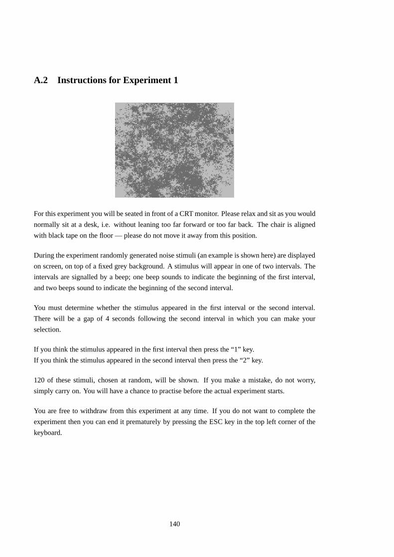
A.2 Instructions for Experiment 1
For this experiment you will be seated in front of a CRT monitor. Please relax and sit as you would
normally sit at a desk, i.e. without leaning too far forward or too far back. The chair is aligned
with black tape on the floor — please do not move it away from this position.
During the experiment randomly generated noise stimuli (an example is shown here) are displayed
on screen, on top of a fixed grey background. A stimulus will appear in one of two intervals. The
intervals are signalled by a beep; one beep sounds to indicate the beginning of the first interval,
and two beeps sound to indicate the beginning of the second interval.
You must determine whether the stimulus appeared in the first interval or the second interval.
There will be a gap of 4 seconds following the second interval in which you can make your
selection.
If you think the stimulus appeared in the first interval then press the “1” key.
If you think the stimulus appeared in the second interval then press the “2” key.
120 of these stimuli, chosen at random, will be shown. If you make a mistake, do not worry,
simply carry on. You will have a chance to practise before the actual experiment starts.
You are free to withdraw from this experiment at any time. If you do not want to complete the
experiment then you can end it prematurely by pressing the ESC key in the top left corner of the
keyboard.
140
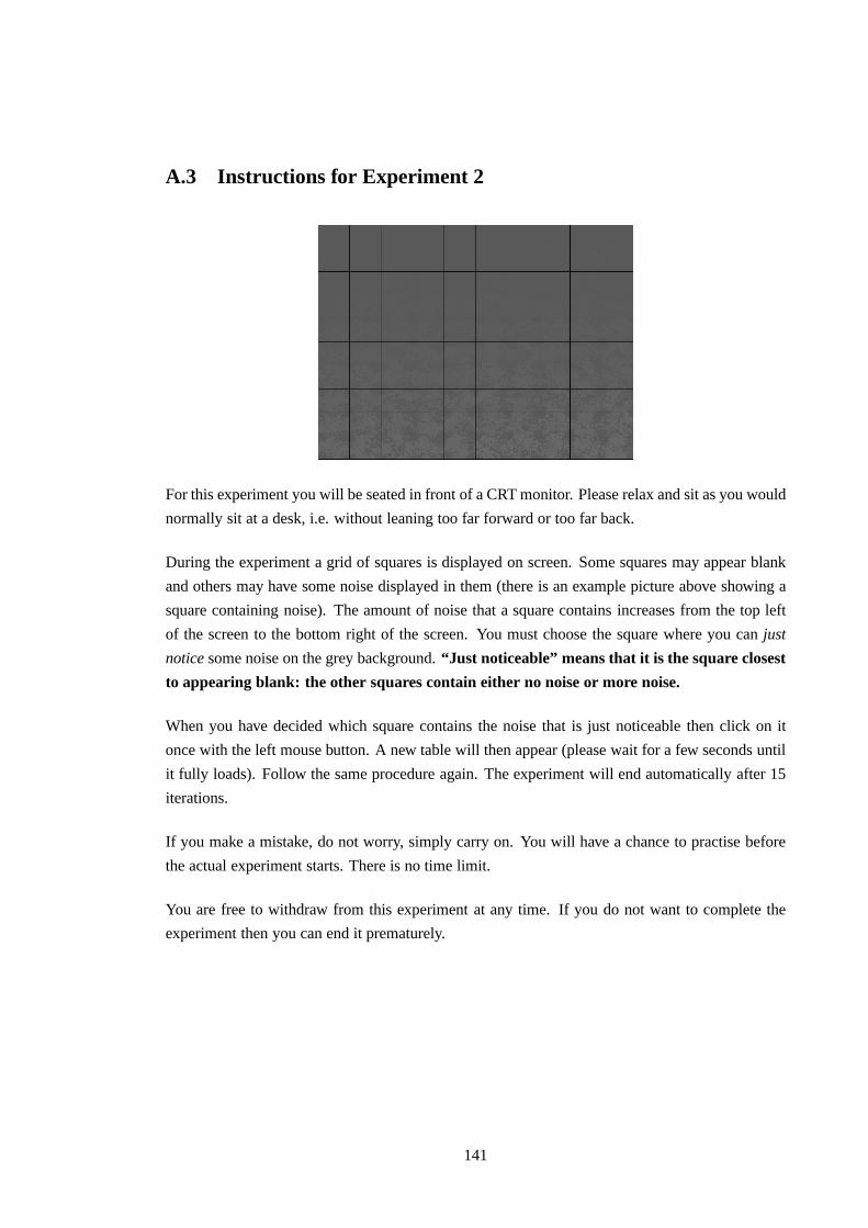
A.3 Instructions for Experiment 2
For this experiment you will be seated in front of a CRT monitor. Please relax and sit as you would
normally sit at a desk, i.e. without leaning too far forward or too far back.
During the experiment a grid of squares is displayed on screen. Some squares may appear blank
and others may have some noise displayed in them (there is an example picture above showing a
square containing noise). The amount of noise that a square contains increases from the top left
of the screen to the bottom right of the screen. You must choose the square where you canjust
noticesome noise on the grey background.“Just noticeable” means that it is the square closest
to appearing blank: the other squares contain either no noise or more noise.
When you have decided which square contains the noise that is just noticeable then click on it
once with the left mouse button. A new table will then appear (please wait for a few seconds until
it fully loads). Follow the same procedure again. The experiment will end automatically after 15
iterations.
If you make a mistake, do not worry, simply carry on. You will have a chance to practise before
the actual experiment starts. There is no time limit.
You are free to withdraw from this experiment at any time. If you do not want to complete the
experiment then you can end it prematurely.
141

142

Appendix B
Results
143

DARK, MEDIUM , LIGHT,PARTICIPANT PEDESTAL 5% GREY PEDESTAL5% GREY PEDESTAL5% GREY
A 0.005534 0.005307 0.006338B 0.004980 0.005167 0.006771C 0.005460 0.005530 0.005955F 0.004962 0.005472 0.005759G 0.005964 0.005688 0.009213H 0.006305 0.005699 0.005855
Table B.1: Experiment 1: average JND results for each participant, for each condition; pedestalvalue = 5% grey.
DARK, MEDIUM , LIGHT,PARTICIPANT PEDESTAL 10% GREY PEDESTAL10% GREY PEDESTAL10% GREY
A 0.009335 0.009250 0.009415B 0.008307 0.007464 0.010490C 0.008153 0.008384 0.008597D 0.009786 0.008213 0.010583E 0.007852 0.009602 0.012601F 0.006976 0.008490 0.009529
Table B.2: Experiment 1: average JND results for each participant, for each condition; pedestalvalue = 10% grey.
DARK, MEDIUM , LIGHT,PARTICIPANT PEDESTAL 20% GREY PEDESTAL20% GREY PEDESTAL20% GREY
A 0.007740 0.009428 0.008280B 0.007586 0.007854 0.008774C 0.007002 0.007874 0.010476D 0.006343 0.009005 0.009404E 0.007272 0.009241 0.010531F 0.008031 0.008764 0.010011
Table B.3: Experiment 1: average JND results for each participant, for each condition; pedestalvalue = 20% grey.
144

DARK, MEDIUM , LIGHT,PARTICIPANT PEDESTAL 5% GREY PEDESTAL5% GREY PEDESTAL5% GREY
A 0.001147 0.002329 0.005741B 0.00294 0.003125 0.00552C 0.002296 0.001081 0.002214D 0.001163 0.001837 0.003882E 0.000997 0.001691 0.003519F 0.00294 0.003064 0.005103G 0.001212 0.0021 0.005535H 0.002192 0.00294 0.003077I 0.00294 0.003036 0.004488J 0.001584 0.003603 0.003603K 0.0021 0.002429 0.00316L 0.000913 0.000936 0.003155M 0.00161 0.00294 0.004824N 0.002814 0.003031 0.004622O 0.002856 0.002854 0.003302P 0.001876 0.00294 0.004205Q 0.002338 0.00296 0.004461R 0.001079 0.001416 0.002958S 0.000937 0.001166 0.002591T 0.001293 0.001583 0.003607U 0.00149 0.002315 0.004438
Table B.4: Experiment 2: average JND results for each participant, for each condition; pedestalvalue = 5% grey.
145

DARK, MEDIUM , LIGHT,PARTICIPANT PEDESTAL 10% GREY PEDESTAL10% GREY PEDESTAL10% GREY
A 0.001934 0.001828 0.003507B 0.004145 0.00447 0.006847C 0.003061 0.001392 0.003267D 0.00229 0.001933 0.003468E 0.000974 0.002255 0.003238F 0.003741 0.003625 0.007257G 0.001233 0.002507 0.004464H 0.003741 0.003804 0.0039I 0.003742 0.003294 0.005527J 0.002887 0.00507 0.00507K 0.003423 0.003181 0.002432L 0.001287 0.00114 0.002318M 0.002825 0.003741 0.005918N 0.003633 0.003681 0.006583O 0.005241 0.004153 0.005529P 0.001735 0.002776 0.004713Q 0.002935 0.003397 0.005928R 0.001053 0.002022 0.002299S 0.001373 0.00091 0.002747T 0.001899 0.001461 0.003741U 0.002896 0.003187 0.006389
Table B.5: Experiment 2: average JND results for each participant, for each condition; pedestalvalue = 10% grey.
146
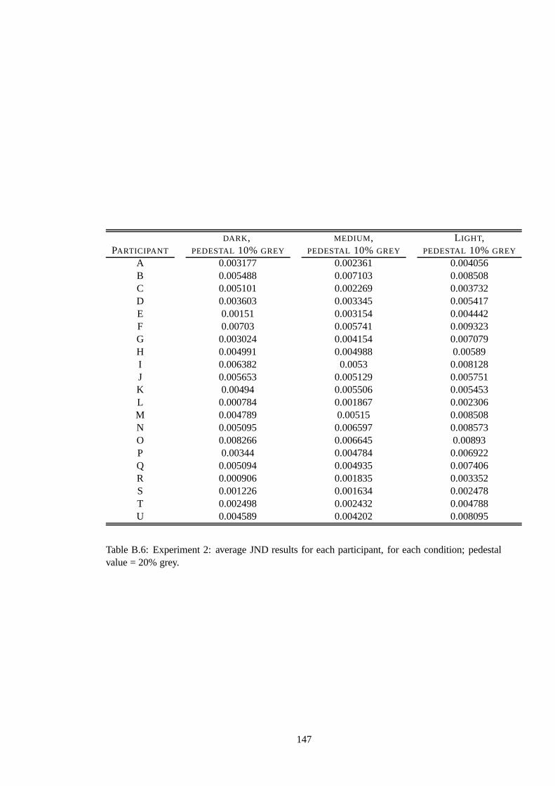
DARK, MEDIUM , LIGHT,PARTICIPANT PEDESTAL 10% GREY PEDESTAL10% GREY PEDESTAL10% GREY
A 0.003177 0.002361 0.004056B 0.005488 0.007103 0.008508C 0.005101 0.002269 0.003732D 0.003603 0.003345 0.005417E 0.00151 0.003154 0.004442F 0.00703 0.005741 0.009323G 0.003024 0.004154 0.007079H 0.004991 0.004988 0.00589I 0.006382 0.0053 0.008128J 0.005653 0.005129 0.005751K 0.00494 0.005506 0.005453L 0.000784 0.001867 0.002306M 0.004789 0.00515 0.008508N 0.005095 0.006597 0.008573O 0.008266 0.006645 0.00893P 0.00344 0.004784 0.006922Q 0.005094 0.004935 0.007406R 0.000906 0.001835 0.003352S 0.001226 0.001634 0.002478T 0.002498 0.002432 0.004788U 0.004589 0.004202 0.008095
Table B.6: Experiment 2: average JND results for each participant, for each condition; pedestalvalue = 20% grey.
147

PARTICIPANT DARK LIGHT, UNCORRECTED LIGHT, CORRECTED
A 0.004068 0.006499 0.004987B 0.004444 0.005474 0.004586C 0.003393 0.005325 0.003075D 0.001267 0.002263 0.001084E 0.003907 0.005016 0.004753F 0.004689 0.005494 0.005647G 0.004507 0.00688 0.00404H 0.003452 0.0049 0.003402I 0.004639 0.004935 0.007347J 0.004269 0.007217 0.004152K 0.003944 0.004099 0.003896L 0.004784 0.00593 0.004805M 0.001968 0.00193 0.000371N 0.004653 0.004742 0.003382O 0.004948 0.004413 0.00564P 0.002944 0.003928 0.001877Q 0.003709 0.00469 0.00397R 0.005041 0.005095 0.007745S 0.004011 0.006708 0.003539T 0.004593 0.004742 0.004266U 0.00355 0.004912 0.003326
Table B.7: Validation experiment: average JND results for each participant, for each condition.
148