Embed Size (px)
Citation preview
Adaptive space and time numerical simulation of
reaction-diffusion models for intracellular calcium
dynamics
Ch. Nagaiah1∗, S. Rudiger2†, G. Warnecke3‡, M. Falcke4§
1 Institute of Mathematics and Scientific Computing, University of Graz, Austria
2 Institute for Physics, Humboldt University, Berlin, Germany
3 Institute of Analysis and Numerics, Otto-von-Guericke University, Magdeburg, Germany
4 Max Delbruck Center for Molecular Medicine, Berlin, Germany
November 16, 2010
Abstract
Adaptivity in space and time for the numerical simulation of stochastic and de-terministic equations for intracellular calcium dynamics is presented. The modelingof diffusion, reaction and membrane transport of calcium ions in cells leads to a sys-tem of reaction-diffusion equations. We describe the modulation of cytosolic and ERcalcium concentrations close to the membrane of the cell organelle.
A conforming piecewise linear finite element method is used for the spatial dis-cretization while linearly implicit methods, Rosenbrock type methods, are used forthe time integration. We adopt a hybrid algorithm to solve the stochastic part.The space grid is adjusted to the strong localization of the calcium release followingstochastic channel transitions. By automatically adapting the spatial meshes andtime steps to the proper scales during the transition of channel states, the methodaccurately resolves the evolution of intracellular calcium concentrations as well asbuffer concentrations. This article emphasizes the adaptive and efficient hybrid nu-merical simulations in two space dimensions. The presented work establishes thebasis for future simulations in a realistic 3D geometry.
∗[email protected], Tel: +43316 3805063, Fax: +43316 3809815†[email protected]‡[email protected]§[email protected]
1
1 Introduction
Calcium signalling is an important part of cellular information processing. The Ca2+ signalemployed by a variety of processes is a transient increase of the concentration in the cytosol[5, 6, 26]. Increase of [Ca2+] is due to entry through the cell membrane or to Ca2+ releasefrom internal storage compartments, specifically the endoplasmic reticulum (ER) and thesarcoplasmatic reticulum. It leads to the formation of spatio-temporal signals in the form ofwaves of high Ca2+ concentration traveling across the cell [28, 20, 13] and global oscillations[4, 29].
The multiplicity of length and time scales poses a specific challenge for any numericaltreatment of the problem. Physiologically, it is now well established that currents ofcalcium through an individual channel lead to very localized calcium spots of nanometerextension. On the other hand, the calcium is rapidly transported over distances of severalmicrometers. Since calcium signals are generated by local feedback as well as coupling todistant channels by transport over a µm scale, we need an efficient and accurate numericalmodeling of processes on both scales. We therefore choose a finite element method withlocal grid adaptivity for the space discretization and linearly implicit Runge-Kutta methodsfor the time discretization. Moreover, to solve the deterministic and stochastic simulationswe used a hybrid algorithm. Here, we will discuss the following important factors in thenumerical solution of the problem: space and time discretization, adapting the spatialmeshes and automatic time steps to the proper scales according to channel transitions, thehybrid algorithm which couples the solving of deterministic and stochastic problems.
We will outline some of the problems which are encountered in the numerical simula-tions. At first, due to the multiple length scales of channels and clusters in the membrane,suitable numerical methods are mandatory. In this work we have chosen the finite elementmethod for solving this problem. To capture the original structure of the cell, adaptivegrid refinement is necessary to provide efficient and fast numerical solutions. Also adaptivespace and time discretization methods are efficient during the intermediate time steps forthis type of complex problems. The release of calcium through channel opening or closingoccurs on the order of microseconds. These small time scales cannot be ignored, thereforean efficient time stepping method to capture these fast changes are needed. For this pur-pose the linearly implicit Runge-Kutta methods, which are very suitable for solving stiffordinary differential equations, are used. The opening of channels occurs in the order ofmicroseconds and when all channels are closed then the time step size is nearly in orderof milliseconds, see [25]. For handling such fast changing step sizes an automatic timestep procedure is suitable. To control the spatial discretization error, a-posteriori errorestimators are computed to steer the mesh improvement by refinement and coarsening ineach time step during the primal and dual solves in optimization algorithm. Various otherforms of adaptive mesh refinement techniques were applied successfully for excitable mediaby varying the spatial or temporal resolution or both [9, 22, 34].
By locally refining the regions in a grid where the solution data have large errors,an adaptive mesh refinement algorithm can greatly reduce the size of grid points andhence the number of unknowns. A both space and time adaptive strategy will further
2
improve the simulation efficiency. The space and time adaptivity for the deterministicsimulation of calcium dynamics is well presented in Nagaiah et.al [24] where the couplingof stochastic channel transition was not considered. The spatial grid adaptivity playsimportant role in the hybrid numerical simulations which shows a good improvement overthe CPU time. The main motivation of the current article is that to present efficientand accurate numerical simulations based on the space and time adaptivity for the hybridstochastic and deterministic simulations of calcium dynamics.
The high and fast concentration changes upon opening and closing of channels have astrong impact on the stochastic dynamics of channel binding and unbinding. The stochasticsolver is based on the Gillespie method, but the usual Gillespie method solves stochasticprocesses where the propensities are constant during the subsequent transitions. However,the concentration and propensities are changes based on the channel opening and closing.For this purpose we have adopted a hybrid algorithm which couples the deterministic andstochastic equations, see Alfonsi et al. [2]. Two different types of time stepping methods areconsidered for solving the deterministic and stochastic processes. One is a linearly implicitRunge-Kutta method to solve the deterministic equations and the other is the Gillespiemethod to solve the stochastic equations. In both parts, deterministic and stochastic, weuse the adaptive time scales to get fast and efficient numerical results.
Briefly, the adaptivity of the spatial grid is controlled by the error estimator by Zien-kiewicz and Zhu [37], which is based on the average of local gradients of the solution. Theclassical embedding technique for ordinary differential equation integrators is employed toestimate the error in time. An automatic step size selection procedure ensures that the stepsize is as large as possible to guarantee the desired precision. We find that the PI-controllerproposed by Gustafsson, Lundh and Soderlind [16] works very well for this problem. Ournumerical realization is based on the public domain software package DUNE [3].
The paper is organized as follows: In the second section we present the model whichcomprises calcium-buffer binding, diffusion and transport through the ER membrane. Wewill then introduce our method and strategies for grid adaptation, finite-element discretiza-tion and time-stepping. Section 5 presents different simulation of test cases. The finalsection gives a short discussion of our work.
2 Deterministic equations
In this section we present the mathematical model equations in 2D which describe theevolution of calcium concentrations during the channel transitions, see for more detailsFalcke [12]. The model consists of equations for the following deterministic quantities:calcium concentration in the cytosol and the ER as well as concentrations of several buffersin the cytosol. As a simplification we do not consider the full three dimensional cytosolicand ER space but instead consider thin sheets below and above an idealized planar ERmembrane. All concentrations are therefore two dimensional in space.
The evolution of concentrations will be determined by diffusion, transport of calcium
3
through the ER membrane, and the binding and unbinding of buffer molecules to calcium
∂c
∂t= Dc∆c+ (Pl + Pc(r, t))(E − c)− Pp
c2
K2d + c2
,
−(k+b,s(Bs − bs)c− k−
b,sbs)− (k+b,m(Bm − bm)c− k−
b,mbm) , (1)
∂E
∂t= DE∆E + γ
[
(Pl + Pc(r, t))(E − c)− Ppc2
K2d + c2
]
, (2)
∂bm∂t
= Db,m∇2bm + k+
b,m(Bm − bm)c− k−b,mbm , (3)
∂bs∂t
= Db,s∇2bs + k+
b,s(Bs − bs)c− k−b,sbs . (4)
Here c is the concentration of Ca2+ in the cytosol, E is the concentration in the ER. Thetransport through the ER membrane comprises three contributions. Calcium is moved fromthe ER into the cytosol through a leak current Pl(E− c) and the channels: Pc(r, t)(E− c).The latter term will be discussed in more detail below. Calcium is resequestered into theER by pumps, the term proportional to Pp. The action of the pumps was found to becooperative in calcium. The parameter Kd is the dissociation constant of the pumps.
The term proportional to Pc in Eqs. (1) and (2) models the current through an openchannel. This current was found to depend on the cross-membrane concentration difference.For differences found in cell-physiological conditions, the current can be approximated by alinear dependence on (E− c). The current is modeled as a source with constant density ina specified channel cluster region. The radius Ri of the cluster i with Nopen,i open channelsis then given by
Ri = Rs
√
Nopen,i .
Clusters are situated at fixed position xi. The flux term is given by
Pc(r, t) =
Pch if ‖r− xi‖ < Ri for a cluster i,0 otherwise.
Note that in a model including the dynamics of channel gating the number of open channelsis time-dependent. The corresponding value of Pch can be found in Table 2. Altogether,the model equations are a system of reaction-diffusion equations. A well established theoryexists for the system of reaction-diffusion equations in the literature [8, 27, 32, 33].
The concentrations of the mobile and stationary buffers bound to calcium in the cytosolare given by bm and bs, respectively. All buffers are assumed to be distributed homoge-neously in the initial state. Total buffer concentrations in the cytosol are denoted by Bm orBs, respectively. Experimentally, the total amounts of some buffers are known quite well,see [21, 36]. However, the amount of other buffers as for example the stationary buffer,comprising contributions from different calcium stores such as mitochondria, are not wellknown.
4
3 Stochastic channel dynamics
One of the principal reasons that modelers and computational scientists have becomemore interested in Ca2+ dynamics is that the concentration of Ca2+ shows highly complexspatio-temporal behavior. Many cell types respond to agonist stimulation with oscillationsin the concentration of Ca2+ . The process causing random behavior in intracellular Ca2+
dynamics is the transition between the different states of the channel subunits and thechannel. Channels open and close randomly. The opening and closing probability dependson the state of the channel subunits.
In this subsection, the stochastic model for the gating of subunits is explained. Thismodel is based on the DeYoung-Keizer (DYK) model for the subunit dynamics, see [11].Details of the modified DYK model which is used in our numerical calculations can befound in [30]. It is known that a subunit has binding sites for Ca2+ and IP3 . Based on theresults of Bezprozvanny et al. [7], DeYoung and Keizer [11] proposed a model for a singlesubunit. The model by DeYoung and Keizer was set up as a deterministic model and usedlater on as a stochastic scheme by Falcke et al. [12, 14]. The subunit has three bindingsites: an activating and an inhibitory Ca2+ as well as an activating IP3 binding sites.
In this work the stochastic solver is based on the Gillespie method [15]. The Gillespiealgorithm uses random pairs (r1, r2) and the equations
a0 · τ = ln(1/r1) ,i∑
j=1
aj ≤ a0 · r2 <i+1∑
j=1
aj . (5)
Using this random pair we can find the next event Ri and that it will occur after time τ .The Gillespie method is based on the assumption that during successive stochastic
events the propensities ai do not change. Indeed, over those successive stochastic events,there must be a significant activity in all reaction channels. However, when linking thestochastic channel dynamics to the calcium dynamics, we expect the propensity ai tochange in time due to its dependence on the local calcium concentration c. This effectwill be particularly strong for openings and closings of channels, since after such eventsthe local calcium concentration c changes dramatically by orders of magnitude. So thepropensities can change too rapidly over small time intervals.
To overcome those problems, a hybrid method is adopted which was introduced byAlfonsi et al. [2]. In their hybrid algorithm, the stochastic reaction equations are partitionedinto deterministic and stochastic equations, to reduce the computational time and increasethe efficiency. To adapt this hybrid algorithm to current problem, we used that the spatial-temporal equations are deterministic and the opening/closing of channels is considered asstochastic part. Here we will give a brief explanation of the hybrid method.
Within their setting the time τ to the next stochastic event is determined by solving
gi(t+ τ |t) =
∫ t+τ
t
ai(c(t), s) ds = ξ , (6)
with ξ = ln(1/r1), where the sum of propensities a0 may explicitly depend both on time andthe local calcium concentration. The function gi(t + τ |t) is non-decreasing for t + τ > t,
5
since the propensities ai are non-negative by definition. Note that the above equationsimplifies to the equation determining τ in Eq. (5) in the case of constant a0. To determinethe time of next reaction τ , condition Eq. (6) is conveniently rewritten in differential formby introducing a variable g(t) and solving
g(s) = a0(c, s) (7)
with initial condition g(0) = 0, along with the deterministic equations for c and buffers.To calculate the propensities we follow the dynamics of the DYK model.
We would like to give the brief outline of the algorithm here. A special feature ofthe calcium system is that not all stochastic events change the open/closed state of achannel. A channel transition has a major impact on the local calcium concentration c,while non-channel transitions do not change the local calcium concentration. During thecomputation of the deterministic part of the calcium dynamics the stochastic events aretraced via Eq. (6) respectively Eq. (7). During the simulation the stochastic system isupdated for every stochastic time step dt. The time step dt is determined using the firstrandom number generation, see Eq. (5), and by fulfilling the requirement a0dt ≤ 1, wherea0 is the sum of the propensities. Using the second random number the reaction event Ri
is determined, see Eq. (5). In this way we can determine the next reaction event Ri andit will occur after the time τ . If a non-channel transition occurs, the stochastic event isperformed. The stochastic channel dynamics is updated correspondingly, while there is noinfluence on the calcium concentration. On the other hand, if a channel transition takesplace, both the channel and the calcium dynamics do change. This typically requires areadjustment of the deterministic time step which will be explained in later sections. Thealgorithmic realization of our hybrid approach is given in [30, 23] and the extension of thealgorithm by using the spatial grid adaptivity is given at the end of section 4. .
4 Numerical method
4.1 Spatial discretization using finite elements
The state variables c(x, t), E(x, t), bm(x, t) and bs(x, t) are functions of space and timeon in Ω × [0, T ] where the domain Ω ⊆ R
2 is a convex polygonal subset. In this sectionwe describe the finite element method for solving the coupled reaction-diffusion system(1-4). We will first consider a so-called semi-discrete analogue of the full system wherewe have discretized in space using the continuous piecewise linear finite elements. Theformulation and subsequent discretization of such an integral form requires the definitionof some function spaces and associated norms. Consider a spatial domain Ω ⊂ R
2 withpiecewise smooth boundary Γ. We shall denote by L2(Ω) the space of functions that aresquare-integrable over the domain Ω, see Adams [1] for other notations.
6
4.2 Semi discretization in space
Consider the parabolic prototype problem
∂u(x,t)∂t
−∇ · (D∇u(x, t)) + s(u,x, t) = 0 in Ω× (0, T ] ,u(x, t) = u0(x) on Ω× t = 0 ,n · ∇u(x, t) = 0 on ∂Ω × [0, T ] ,
(8)
where u(x, t) is unknown, D ∈ R2×2 is assumed to be diagonal with positive coefficients
and s(u,x, t) is the reaction function. The discretization process using the finite elementmethod is based on a reformulation of the given differential equation in the more general,variational formulation. Let V = H1(Ω) and Vh be a finite dimensional subspace of V withbasis w1, . . . , wN. Specifically we take continuous functions that are piecewise linear ona quasi-uniform triangulation of Ω with mesh size h. Replacing the space V by the finitedimensional subspace Vh we get the following semi discretization in space find uh ∈ Vh s.t.
〈∂uh
∂t, vh〉+ 〈D∇uh,∇vh〉+ 〈s(uh,x, t), vh〉 = 0 for all vh ∈ Vh ,
uh(x, t) = u0,h(x) on Ω× t = 0 .(9)
In particular, since Vh is a linear space of dimension N with basis wiNi=1, taking vh = wj,
we get a system of ordinary differential equations in the form
Mu = −Au− S , (10)
where M is the mass matrix, A is the stiffness matrix and S is a vector depending on thereaction term. The matrices are defined as follows
M = 〈wi, wj〉 , A = 〈D∇wi,∇wj〉 ,
S = 〈s(∑N
i=1 ui(t)wi(x)), wj〉 .
In our numerical simulations we considered the free calcium concentration in the cytosol,the free calcium concentration in the ER, and the stationary and mobile buffers in thecytosol. We can apply the analogous spatial discretization to Eqs. (1-4). Then we get theordinary differential equation system as follows
Mu = −Au− S ,
where the block diagonal matrices M = diag(M,M,M,M), A = diag(A,A,A,A) andS is a 4N × 1 vector depending on reaction terms.
4.3 Temporal time-stepping of continuous equations
The discretization in time of Eq. (10) can be accomplished in several possible ways. We havemainly concentrated on implicit methods for solving these equations. For solving problemwe used higher order linearly implicit methods of Rosenbrock type. These methods offerseveral advantages. They completely avoid the solution of nonlinear equations, which
7
means that no Newton iteration has to be controlled. More detailed expositions of thesemethods can be found in [17, 18]. Moreover, for computation of adaptive time step asimple embedding technique can be utilized to estimate the error part arising from thetime discretization. An automatic step size selection procedure ensures that the step sizeis as large as possible while guaranteeing the desired precision.
We considered the ODE problem
M∂u
∂t= F(t,u), u(t0) = u0. (11)
To start with, we partition the time [0, T ] into discrete steps 0 = t0, t1, . . . , tn = T , thatare not necessarily equidistant. The notation for time step is τ i = ti+1 − ti and ui to bethe numerical solution at time ti. For computation an s-stage Rosenbrock method of orderp with embedding of order p 6= p has the form
(1
τ iγM− J)kj = F
(
ti + τ iαj,ui +
j−1∑
l=1
ajlkl
)
−M
j−1∑
l=1
cljτ i
kl , j = 1, . . . , s , (12)
ui+1 = ui +
s∑
l=1
mlkl , (13)
ui+1 = ui +s∑
l=1
mlkl . (14)
Here J = ∂F/∂u is the Jacobian matrix. For the construction of the Jacobian matrix weused exact derivatives of the vector F(t,u). The method coefficients γ, αj , ajl, cjl, ml, andml are chosen such a way that certain order conditions are fulfilled to obtain a sufficientconsistency order and good stability properties. Replacing the coefficients in Eq. (13)by different coefficients ml a second solution ui+1 of lower order p, where p < p, can beconstructed [17, 18] .
Usually, for the complex dynamical behavior problems, for instance the current problemunder consideration, the fixed time steps are not adequate to do longer time horizon whichrequire a huge number of small time steps. Thus, time step adaptation is an importantand should be efficient in order to control the temporal error. After the i-th integrationstep the value ǫi+1 = ‖ui+1 − ui+1‖L2 is taken as an estimator of the local temporal error.A new time step τnew, see Gustafsson et al. [16], is computed by
τ := βτ i
τ i−1
(
TOLt
ǫi+1
)
p2p(
ǫi
ǫi+1
)
p1p
τ i, τnew =
βmaxτi, τ > βmaxτ
i,βminτ
i, τ < βminτi,
τ , otherwise.(15)
The parameter β > 0 is safety factor. The factors βmin and βmax restrict time step jumps.In our computations we have chosen the parameters p1 = 1 and p2 = 1. If ǫ < TOLt,where TOLt is a desired tolerance prescribed by the user, we proceed to the next time
8
step, otherwise the time step has to be shortened according to Eq. (15) and a new try isperformed.
The simulations are performed using the ROS2 method [10] which is a 2nd order methodwith 2(1) internal stages, and ROS3P [19], W-method [31] as well as ROWDA [18] whichare 3(2) order methods with 3 internal stages. Finally, after time discretization, we get asystem of algebraic equations in each internal stage. For solving the algebraic system ineach stage we used the BiCGSTAB method with ILU preconditioning.
4.4 Spatial grid adaptivity
The adaptive mesh refinement(AMR) algorithm try to automatically refine or coarsen themesh to achieve a solution having a specified accuracy in an optimal fashion and it usesa hierarchy of properly nested levels. For this problem we considered the AMR techniquebased on the Z2 error indicator of Zienkiewicz and Zhu [37] which is based on the averaginggradients of the solution. See also [35] for a more detailed description of error estimators.The full spatial and temporal discretization leads to an approximate solution ut
h withuth(·, ti) ∈ Vh at the discrete time points ti, i = 0, . . . ,M where the time integration scheme
is evaluated. Here we will recall the Z2 error indicator.We denote by Wh the space of all piecewise linear vector-fields and set Xh := Wh ∩
C(Ω,R2). Denote u and uh the unique solution of problems (8) and (9), respectively. LetGuh ∈ Xh be the 〈·, ·〉h-projection of ∇uh onto Xh. In this case ‖Guh −∇uh‖L2(T ) can beused as an error estimator, where Guh is an easily computable approximation of ∇uh, see[35] for more details. It can be computed by a local averaging of ∇uh|T (xi) as follows
Guh(xi) =∑
T⊂Dxi
|T |
|Dx|∇uh|T (xi) . (16)
Here, Dxiis the union of the triangles having xi as a vertex and |T | denotes the area of
triangle T . Thus, Guh may be computed by a local averaging of ∇uh. We finally set
ηZ,T := ‖Guh −∇uh‖L2(T ) , (17)
and
ηZ :=
∑
T∈Th
η2Z,T
1/2
. (18)
The Z2 indicator ηZ,T is an estimate for ‖∇uth(·, ti)−∇ut(·, ti)‖L2(T ), see Verfurth [35].
Let λ(T ) ∈ N0 be the refinement level of triangle T ∈ T , λmax ∈ N0 be a given maximumrefinement level, and φ1, . . . , φλmax
be given real numbers satisfying 0 ≤ φ1 . . . ≤ φλmax.
We set φ0 = 0 and φλmax= ∞. With the choice of φ1, . . . , φλmax
one controls the structureof the grid. If we set φ1 = . . . = φλmax
= 0 this leads to a uniform triangulation of levelλmax.
9
In our numerical computations, the fully coupled space-time adaptive algorithm is in-troduced as follows. Suppose that an initial coarse triangular grid is constructed using gridgenerator. To generate the initial coarse adaptive grid, we use a strongly localized functionas initial solution in the vicinity of the cluster area for error estimator. To account for theexponential decay of calcium away from the source we generate a succession of localizedfunctions with decreasing spatial extent. Then we refine the mesh until a minimum of 9grid points lie in the area of each channel. A triangle T is marked for
1. refinement if ηZ,T > φλ(T ) and λ(T ) < i for i = 0, . . . , λmax,
2. coarsening if ηZ,T <φλ(T )
100and λ(T ) > i for i = 0, . . . , λmax,
where ηZ,T is calculated according to Eq. (17). At this level, the constructed mesh isassumed as a coarse mesh when simulation starts, denoted by L0, and it will be the centralpart of the root level of the hierarchical system. It is fixed during the process of adaptivemesh refinement. Finer levels Li for i > 0 are constructed recursively from the coarserlevels Li−1. In our numerical computations, the tolerance for spatial grid refinement isset Tolx = 10−3. The Z2 error estimator is called for every 3 time intervals while solvingthe deterministic part and adapt the grid if the spatial error is greater than the givenprescribed tolerance Tolx. Thus, it adjusts the spatial grid by refining and coarsening,depending on the estimated spatial solution error of the elements. Accordingly, the newsolution is updated based on the new grid construction via linear interpolation. Afteradvancing the solution data to the new grids, the time discretization step has been appliedand the new solution is computed. If the computed time error, based on a simple embeddingtechnique, is less than the prescribed tolerance then step has to be proceeded further. Ifnot, time step has to be shortened based on the time step controller and repeated the timestep procedure again. In this way, both time step control and dynamic mesh refinementbased on a posteriori error estimation can be simultaneously realized in our numericalexperiments.
Here we present algorithmic aspects of hybrid stochastic and deterministic numericalsimulations by utilizing the spatial grid adaptivity as follows where u represent the solutionvector (c, E, bm, bs).
1. Initialization
• Choose uold = u0 X = X0, gold = 0, told = 0, ∆t > 0, and draw a uniformrandom number r1 in [0,1] defining ξ = ln(1/r1).
2. Deterministic step
• Update the new solution unew and gnew by utilizing the AMR technique whichwas explained in section 4.4.
• If the tolerance for the temporal adaptation procedure is not met, reduce thestep size ∆t and go to 2 where the fine (refined) grid is considered for this step.Otherwise update the tnew = told + ∆t and set the new step size ∆t accordingto the time stepping code prediction.
10
3. If gnew < ξ (no stochastic event)
• Set uold = unew, gold = gnew, told = tnew, and go to 2.
4. If gnew ≥ ξ (some stochastic event in the time interval [told, tnew])
• Determine the event time ts ∈ [told, tnew] by (linear) interpolation, and computethe corresponding calcium concentration cs at the event time ts by (linear)interpolation.
• Draw a uniform random number r2 in [0, 1] and determine the stochastic eventRi according to Eq. (5) based on cs.
5. If the next event Ri is non-channel transition
• Perform the stochastic event Ri to determine the new channel state X .
• Set gold = 0 and recompute gnew based on cs, gold and the remaining time(tnew − ts).
• Draw a new uniform random number r1 in [0, 1] defining ξ = ln(1/r1), and goto 3.
6. If the next event Ri is a channel transition
• Perform the channel transition Ri to determine the new state X .
• Set gnew = 0, and draw a new uniform random number r1 in [0, 1] definingξ = ln(1/r1).
• Set tnew = ts, and define new step size ∆t = ∆tchannel (a sufficiently smallnumber).
• Set uold = us, and go to 2.
5 Numerical results
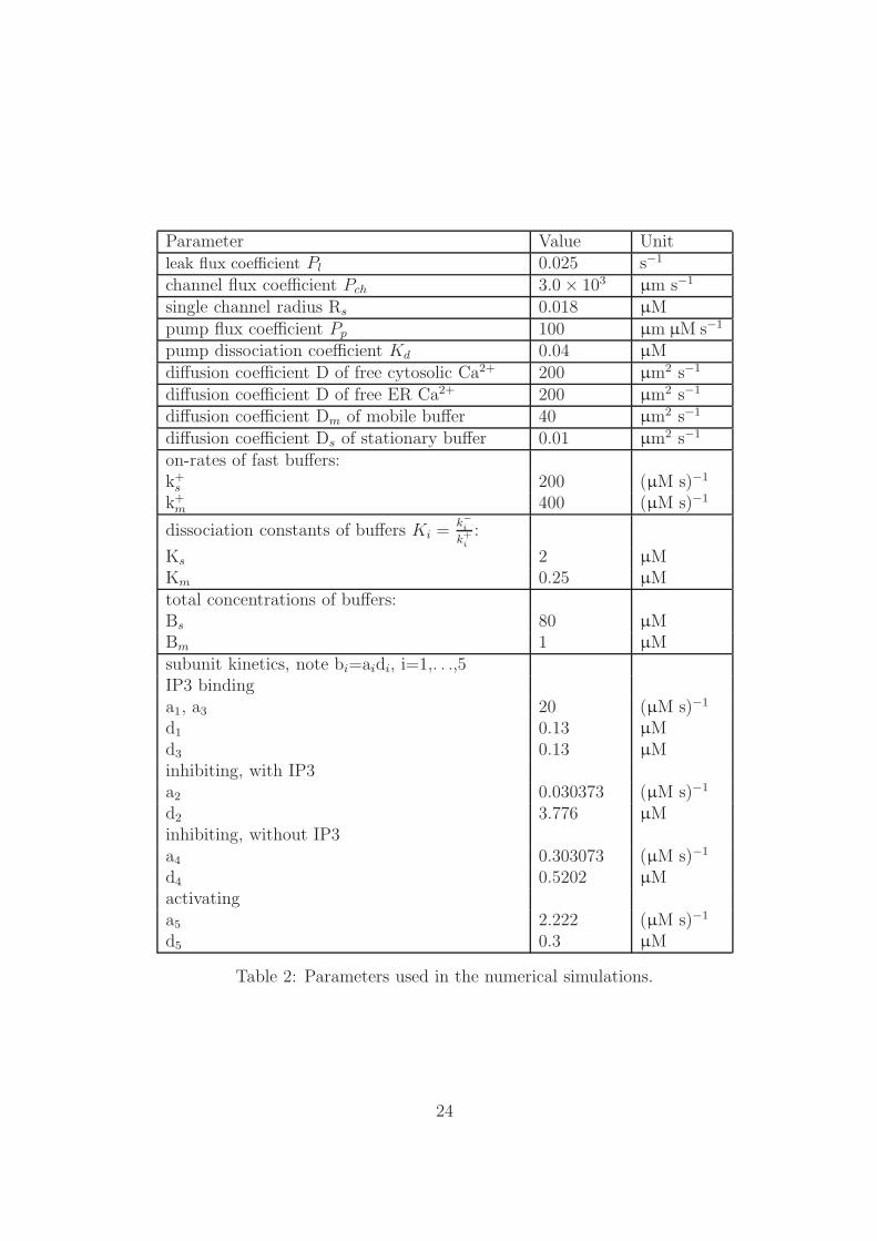
In this section we describe numerical simulations that are performed on a squared geometry,[0 , 33000]× [0 , 33000] nm2, as computational domain with refinement by using triangularelements. This domain represents the ER membrane. In the following subsections weshow the convergence of numerical solutions with different time stepping methods as wellas adaptive grids. The parameters that have been used in the numerical simulation areshown in Table 2. The initial solution for concentrations and buffers is considered asconstants over the computational domain.
All numerical computations were performed by using a Linux machine with 2 GB RAM,2.33 GHz processor, gcc-4.1.0 compiler and the program package DUNE [3] which is a publicdomain and written in C++.
11
5.1 Results for deterministic opening and closing of channels
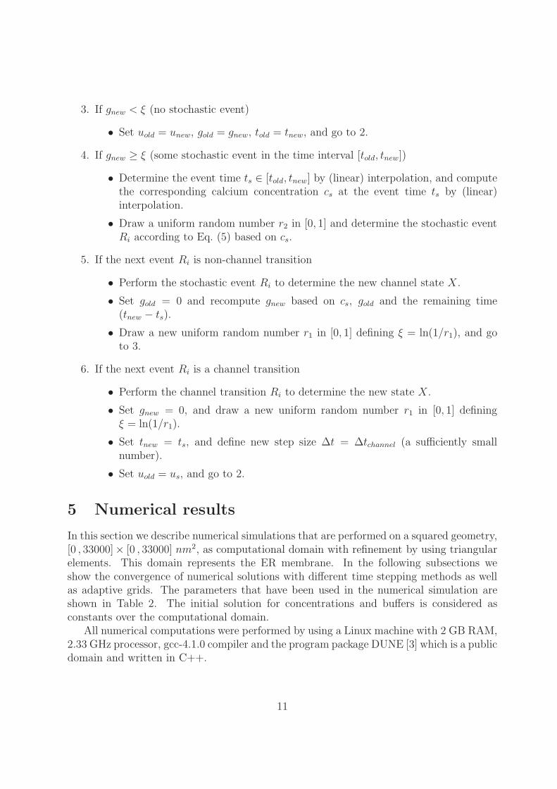
In this subsection we present the numerical tests based on the deterministic opening andclosing of one channel in one cluster arrangement with a static grid and temporal adaptivegrids. The initial coarse grid is shown in Figure 1(a) which is used in the case of adaptivegrid refinement. The static (fine) grid is shown in Figure 1(b).
(a) (b)
Figure 1: Different grids considered for the simulation of arrangement of 1 cluster setup1(a)) coarse grid which is considered as initial grid for adaptive grid refinement simulations,1(b)) fixed grid for other simulations.
methods accepted time steps rejected time steps total CPU time (hours)ROS2 23446 63 38.78
ROS3p 9844 1151 30.83ROWDA 5446 31 27.20
W-method 8794 366 27.37
Table 1: Comparison between different methods.
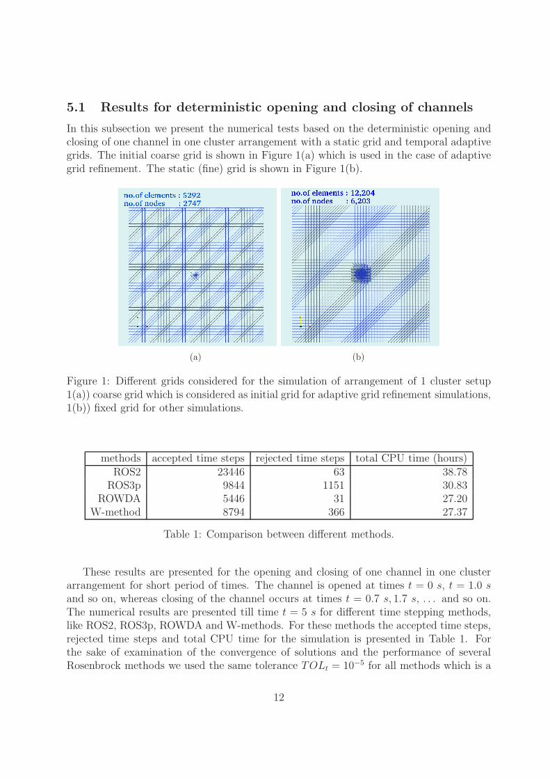
These results are presented for the opening and closing of one channel in one clusterarrangement for short period of times. The channel is opened at times t = 0 s, t = 1.0 sand so on, whereas closing of the channel occurs at times t = 0.7 s, 1.7 s, . . . and so on.The numerical results are presented till time t = 5 s for different time stepping methods,like ROS2, ROS3p, ROWDA and W-methods. For these methods the accepted time steps,rejected time steps and total CPU time for the simulation is presented in Table 1. Forthe sake of examination of the convergence of solutions and the performance of severalRosenbrock methods we used the same tolerance TOLt = 10−5 for all methods which is a
12
small tolerance for the automatic time step selection procedure. Also, it is well known thateach method shows a computational efficiency by properly adjusting the tolerance for timeadaptivity. The maximum and average cytosolic calcium concentrations are presented forthese methods in Figure 2. We can observe that for all integrators the maximum cytosoliccalcium concentration lies on one curve except for the W-method. A closer look in thesolution interval [7.0, 8.8] reveals that the W-method produces a slower propagation ofexcitation of calcium wave front compared to the other Rosenbrock solvers. The reason forthis behavior might be a insufficient resolution in space or time for the W-method. The bestperformance with respect to accuracy and computing time is obtained by ROWDAmethod.Also, in a few other simulations, we experienced that ROWDA method works very well forsmaller tolerances which is used in automatic time step selection, say TOLt = 10−4 to 10−3
, and saves a lot computational time to obtain the accurate solution. From Table 1, wecan observe that ROWDA reaches the final time in 5,446 steps, Ros3p needs 9,844 steps,W-method 8,794 steps, and Ros2 even 23,446 steps. Due to the small tolerance and lowerorder of Ros2 method, it takes more accepted steps compare to other methods. In eachaccepted time step, for this method, the linear solver takes less number of iterations toconverge the solution. We have experienced that if we increase the tolerance for time stepcontrol the Ros2 method also takes less accepted time steps and computational time issaved up to about 6%. Due to the 3 stages of the ROWDA method, it takes less acceptedtime steps and needs more linear solver iterations to converge the solution in comparisonto Ros2 method.
0 1 2 3 4 50
1
2
3
4
5
6
7
8
9
time [s]
max
imum
cyt
osol
ic C
a2+ [µ
M]
Ros2Ros3pRowda3W−method
(a)
0 1 2 3 4 50.06
0.065
0.07
0.075
0.08
0.085
0.09
0.095
0.1
0.105
time [s]
aver
age
valu
e of
cyt
osol
ic C
a2+ [µ
M]
Ros2Ros3pRowda3W−method
(b)
Figure 2: The maximum and average cytosolic calcium concentration in 2(a) and 2(b)respectively for all time integrators.
For further numerical computations, we used the ROWDA method as a time integrator.Next, we examine the performance of different space resolution grids (different fine grid
13
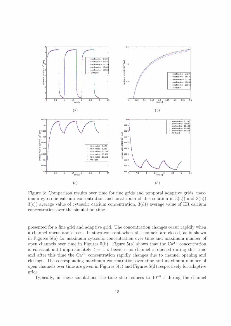
levels) and the AMR grid and the numerical results are presented till time t = 3 s. Thedifference between the solutions of maximum cytosolic calcium concentration for the finegrid levels 17, 18, 19, 20, and 21 which consists of 749, 837, 1,669, 2,061 and 3,225 gridpoints respectively within the area of one channel, and the AMR grid is presented inFigure 3(a). The zoom of this solution is shown in Figure 3(b). From these plots, it can beobserved that the solution converges for finer meshes as well as for temporal adaptive grid.Also the average cytosolic calcium concentration and average ER calcium concentration arepresented in Figure 3(c) and Figure 3(d) respectively. When a channel opens, the maximumcytosolic Ca2+ concentration raises rapidly and stays for a while. When an open channelcloses the Ca2+ concentration falls immediately and recovers the stationary solution. Thesepresented numerical results show that the temporal adaptive grid refinement solution isaccurate as the fine grids during the intermediate time steps.
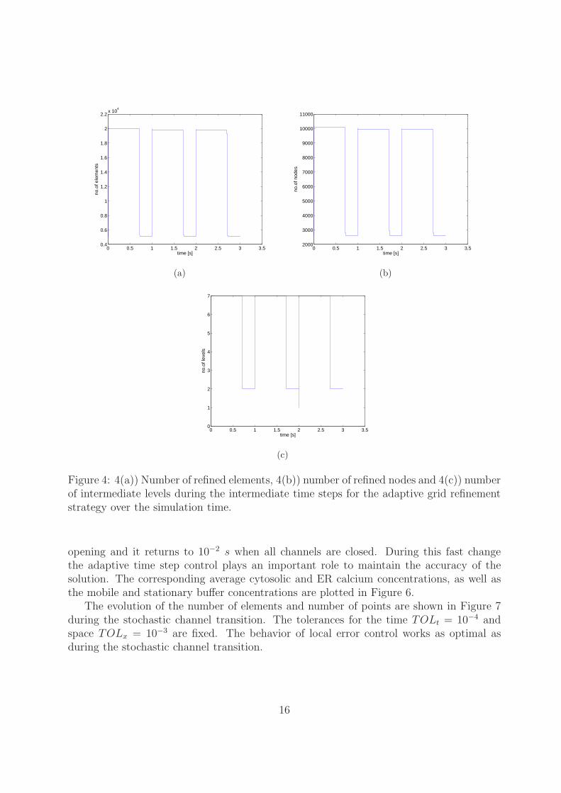
The corresponding number of elements, nodes and intermediate levels are shown inFigure 4. Here we can see that grid refinement strategy refines many elements after openingof a channel and this leads to more accurate solutions for this problem instead of consideringthe fixed grid. Refined elements are coarsened when all channels are closed. Also itproves that it saves more CPU time for the higher cluster set ups which we will presentin later subsections. In our numerical implementation we have a flexibility to restrictthe maximum number of elements and/or maximum number of refinement levels for gridrefinement strategy, which is more useful to perform computations for higher cluster setupswhile considering the stochastic channel transition with moderate CPU time.
To give the comparison of CPU times for static grid and AMR grid, we considered thetime interval for channel transition is 0.02s and total simulation time is 0.16s. Here thefinest level of AMR mesh, during the intermediate time steps, is considered as static grid.In this case, the static grid takes 4300.57 seconds and AMR grid 3157.07 seconds of CPUtime. It shows clearly that for one cluster setup the AMR method is faster. These resultsstrive forward to apply AMR technique for more cluster setup considering the stochasticchannel opening and closings.
5.2 Hybrid numerical results
In this subsection, the adaptive numerical solutions of calcium concentrations with stochas-tic channel transition are presented. To find a suitable time step is a very crucial task inthese stochastic simulations to obtain a moderate overall computational time. In our nu-merical simulations deterministic and stochastic equations are coupled and require twodifferent time steps. One time step for solving the deterministic equations, which is solvedby using the linearly implicit Runge-Kutta method and the other for solving the stochasticpart, where we use the Gillespie algorithm. Both are adaptive with regard to time stepping.
5.2.1 Numerical results with one cluster set up
In this subsection, the hybrid numerical results are shown based on the one cluster set upwhich consists of 20 channels. The simulation time is taken to be t = 30 s and results are
14
0 0.5 1 1.5 2 2.5 3 3.50
1
2
3
4
5
6
7
8
9
time [s]
max
imum
cyt
osol
ic C
a2+ [µ
M]
no.of nodes − 5,129no.of nodes − 6,033no.of nodes − 10,189no.of nodes − 13,685no.of nodes − 18,553AMR grid
(a)
0 0.05 0.1 0.15 0.2 0.25 0.3 0.35 0.47
7.5
8
8.5
time [s]
max
imum
cyt
osol
ic C
a2+ [µ
M]
no.of nodes − 5,129no.of nodes − 6,033no.of nodes − 10,189no.of nodes − 13,685no.of nodes − 18,553AMR grid
(b)
0 0.5 1 1.5 2 2.5 3 3.50.06
0.065
0.07
0.075
0.08
0.085
0.09
0.095
0.1
0.105
time [s]
aver
age
valu
e of
cyt
osol
ic C
a2+ [µ
M]
no.of nodes − 5,129no.of nodes − 6,033no.of nodes − 10,189no.of nodes − 13,685no.of nodes − 18,553AMR grid
(c)
0 0.5 1 1.5 2 2.5 3 3.5699.1
699.2
699.3
699.4
699.5
699.6
699.7
699.8
699.9
700
time [s]
aver
age
valu
e of
ER
Ca2+
[µM
]
no.of nodes − 5,129no.of nodes − 6,033no.of nodes − 10,189no.of nodes − 13,685no.of nodes − 18,553AMR grid
(d)
Figure 3: Comparison results over time for fine grids and temporal adaptive grids, max-imum cytosolic calcium concentration and local zoom of this solution in 3(a)) and 3(b))3(c)) average value of cytosolic calcium concentration, 3(d)) average value of ER calciumconcentration over the simulation time.
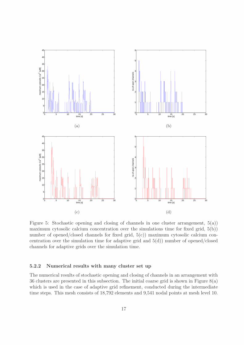
presented for a fine grid and adaptive grid. The concentration changes occur rapidly whena channel opens and closes. It stays constant when all channels are closed, as is shownin Figures 5(a) for maximum cytosolic concentration over time and maximum number ofopen channels over time in Figures 5(b). Figure 5(a) shows that the Ca2+ concentrationis constant until approximately t = 1 s because no channel is opened during this timeand after this time the Ca2+ concentration rapidly changes due to channel opening andclosings. The corresponding maximum concentration over time and maximum number ofopen channels over time are given in Figures 5(c) and Figures 5(d) respectively for adaptivegrids.
Typically, in these simulations the time step reduces to 10−8 s during the channel
15
0 0.5 1 1.5 2 2.5 3 3.50.4
0.6
0.8
1
1.2
1.4
1.6
1.8
2
2.2x 10
4
time [s]
no.o
f ele
men
ts
(a)
0 0.5 1 1.5 2 2.5 3 3.52000
3000
4000
5000
6000
7000
8000
9000
10000
11000
time [s]
no.o
f nod
es
(b)
0 0.5 1 1.5 2 2.5 3 3.50
1
2
3
4
5
6
7
time [s]
no.o
f lev
els
(c)
Figure 4: 4(a)) Number of refined elements, 4(b)) number of refined nodes and 4(c)) numberof intermediate levels during the intermediate time steps for the adaptive grid refinementstrategy over the simulation time.
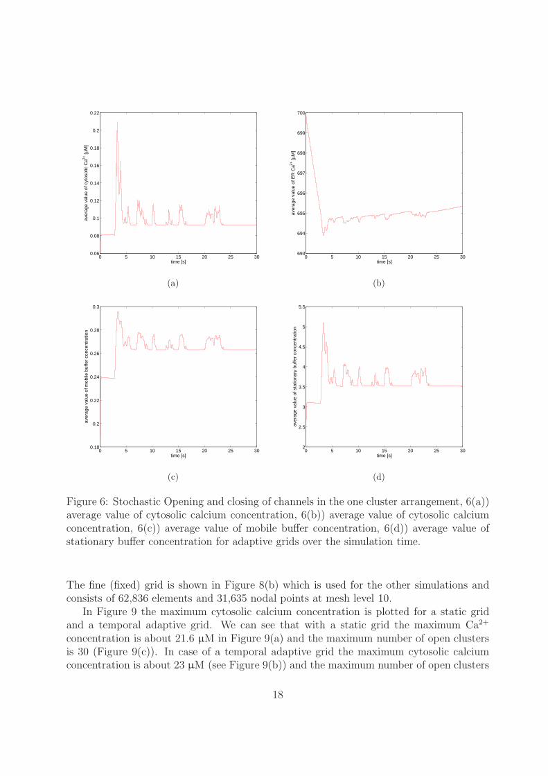
opening and it returns to 10−2 s when all channels are closed. During this fast changethe adaptive time step control plays an important role to maintain the accuracy of thesolution. The corresponding average cytosolic and ER calcium concentrations, as well asthe mobile and stationary buffer concentrations are plotted in Figure 6.
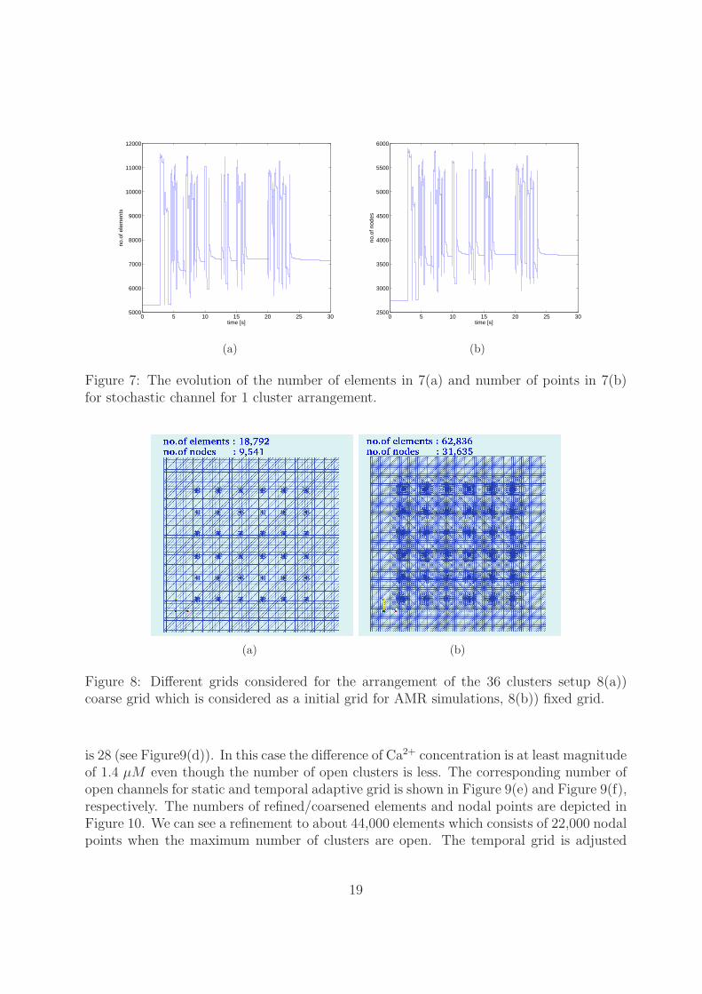
The evolution of the number of elements and number of points are shown in Figure 7during the stochastic channel transition. The tolerances for the time TOLt = 10−4 andspace TOLx = 10−3 are fixed. The behavior of local error control works as optimal asduring the stochastic channel transition.
16
0 5 10 15 20 25 300
5
10
15
20
25
30
35
40
45
time [s]
max
imum
cyt
osol
ic C
a2+ [µ
M]
(a)
0 5 10 15 20 25 300
1
2
3
4
5
6
time [s]
no.o
f ope
n ch
anne
ls
(b)
0 5 10 15 20 25 300
5
10
15
20
25
30
35
40
45
time [s]
max
imum
cyt
osol
ic C
a2+ [µ
M]
(c)
0 5 10 15 20 25 300
1
2
3
4
5
6
time [s]
no.o
f ope
n ch
anne
ls
(d)
Figure 5: Stochastic opening and closing of channels in one cluster arrangement, 5(a))maximum cytosolic calcium concentration over the simulations time for fixed grid, 5(b))number of opened/closed channels for fixed grid, 5(c)) maximum cytosolic calcium con-centration over the simulation time for adaptive grid and 5(d)) number of opened/closedchannels for adaptive grids over the simulation time.
5.2.2 Numerical results with many cluster set up
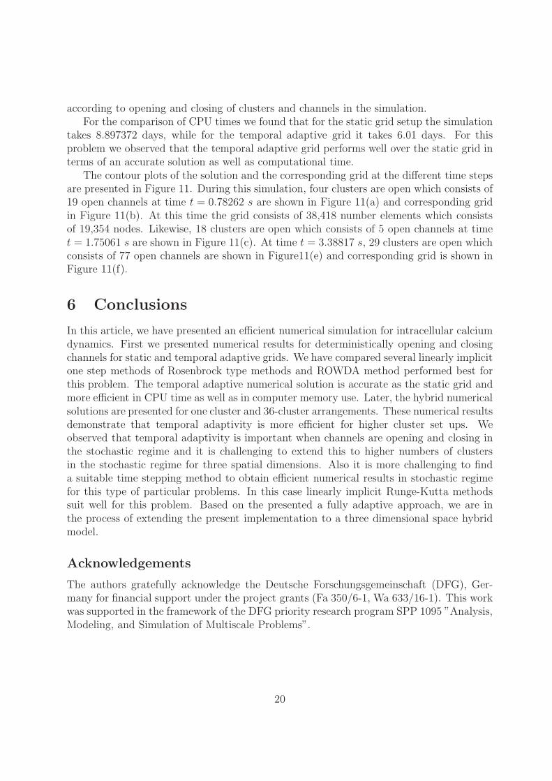
The numerical results of stochastic opening and closing of channels in an arrangement with36 clusters are presented in this subsection. The initial coarse grid is shown in Figure 8(a)which is used in the case of adaptive grid refinement, conducted during the intermediatetime steps. This mesh consists of 18,792 elements and 9,541 nodal points at mesh level 10.
17
0 5 10 15 20 25 300.06
0.08
0.1
0.12
0.14
0.16
0.18
0.2
0.22
time [s]
aver
age
valu
e of
cyt
osol
ic C
a2+ [µ
M]
(a)
0 5 10 15 20 25 30693
694
695
696
697
698
699
700
time [s]
aver
age
valu
e of
ER
Ca2+
[µM
]
(b)
0 5 10 15 20 25 300.18
0.2
0.22
0.24
0.26
0.28
0.3
time [s]
aver
age
valu
e of
mob
ile b
uffe
r co
ncen
trat
ion
(c)
0 5 10 15 20 25 302
2.5
3
3.5
4
4.5
5
5.5
time [s]
aver
age
valu
e of
sta
tiona
ry b
uffe
r co
ncen
trat
ion
(d)
Figure 6: Stochastic Opening and closing of channels in the one cluster arrangement, 6(a))average value of cytosolic calcium concentration, 6(b)) average value of cytosolic calciumconcentration, 6(c)) average value of mobile buffer concentration, 6(d)) average value ofstationary buffer concentration for adaptive grids over the simulation time.
The fine (fixed) grid is shown in Figure 8(b) which is used for the other simulations andconsists of 62,836 elements and 31,635 nodal points at mesh level 10.
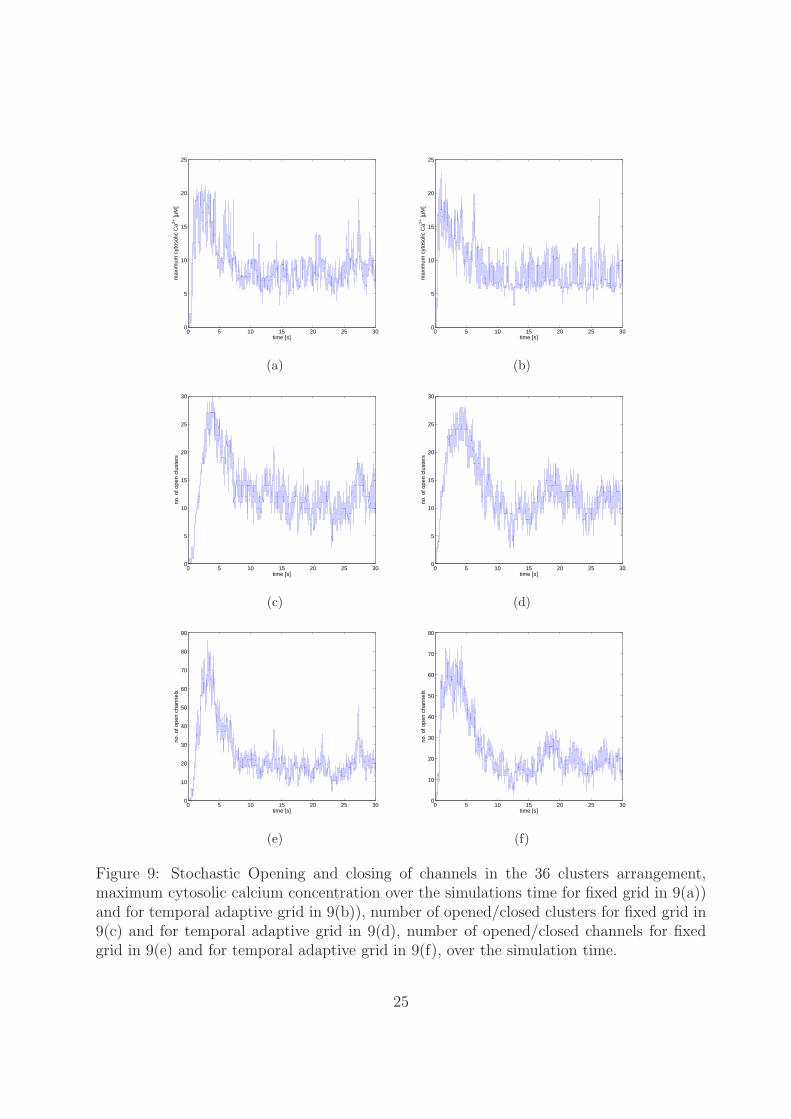
In Figure 9 the maximum cytosolic calcium concentration is plotted for a static gridand a temporal adaptive grid. We can see that with a static grid the maximum Ca2+
concentration is about 21.6 µM in Figure 9(a) and the maximum number of open clustersis 30 (Figure 9(c)). In case of a temporal adaptive grid the maximum cytosolic calciumconcentration is about 23 µM (see Figure 9(b)) and the maximum number of open clusters
18
0 5 10 15 20 25 305000
6000
7000
8000
9000
10000
11000
12000
time [s]
no.o
f ele
men
ts
(a)
0 5 10 15 20 25 302500
3000
3500
4000
4500
5000
5500
6000
time [s]
no.o
f nod
es
(b)
Figure 7: The evolution of the number of elements in 7(a) and number of points in 7(b)for stochastic channel for 1 cluster arrangement.
(a) (b)
Figure 8: Different grids considered for the arrangement of the 36 clusters setup 8(a))coarse grid which is considered as a initial grid for AMR simulations, 8(b)) fixed grid.
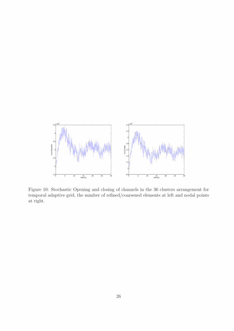
is 28 (see Figure9(d)). In this case the difference of Ca2+ concentration is at least magnitudeof 1.4 µM even though the number of open clusters is less. The corresponding number ofopen channels for static and temporal adaptive grid is shown in Figure 9(e) and Figure 9(f),respectively. The numbers of refined/coarsened elements and nodal points are depicted inFigure 10. We can see a refinement to about 44,000 elements which consists of 22,000 nodalpoints when the maximum number of clusters are open. The temporal grid is adjusted
19
according to opening and closing of clusters and channels in the simulation.For the comparison of CPU times we found that for the static grid setup the simulation
takes 8.897372 days, while for the temporal adaptive grid it takes 6.01 days. For thisproblem we observed that the temporal adaptive grid performs well over the static grid interms of an accurate solution as well as computational time.
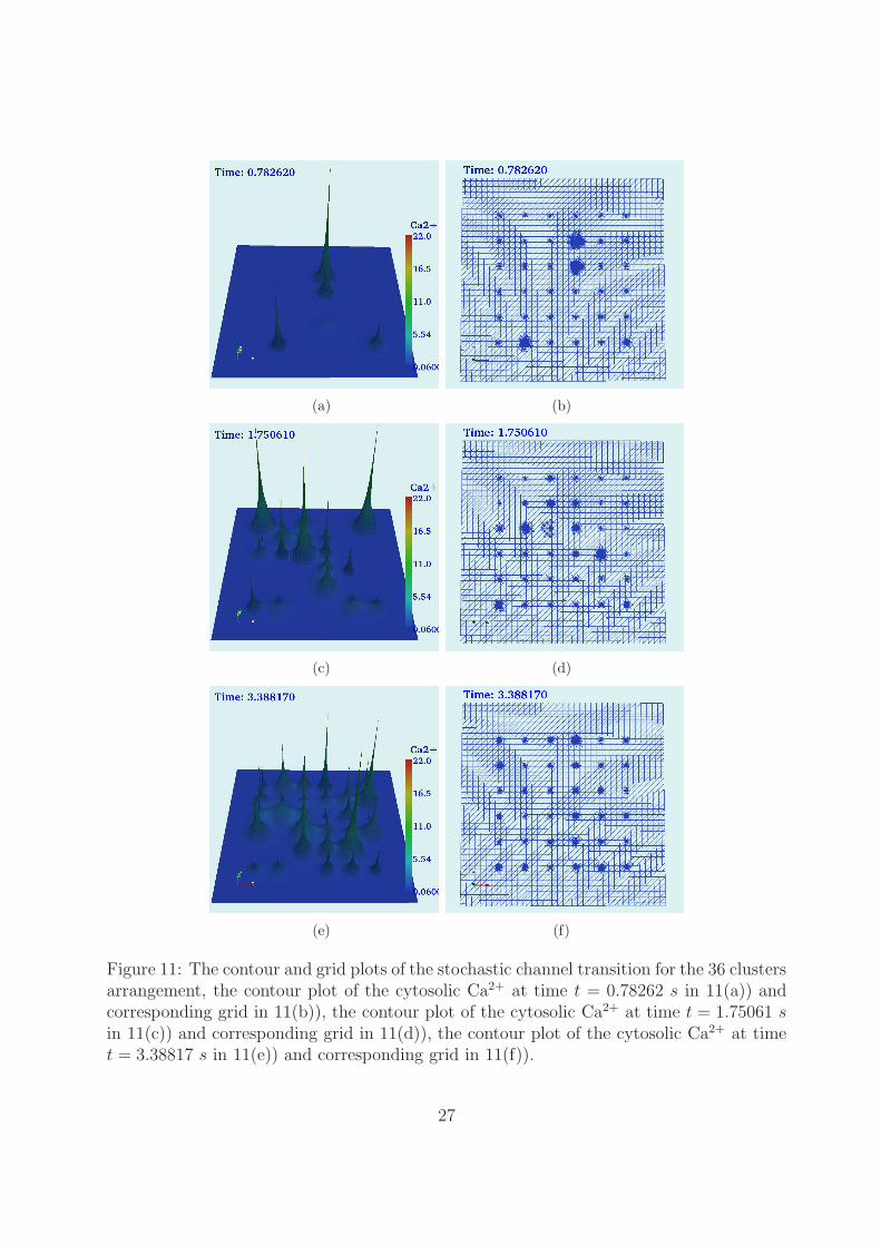
The contour plots of the solution and the corresponding grid at the different time stepsare presented in Figure 11. During this simulation, four clusters are open which consists of19 open channels at time t = 0.78262 s are shown in Figure 11(a) and corresponding gridin Figure 11(b). At this time the grid consists of 38,418 number elements which consistsof 19,354 nodes. Likewise, 18 clusters are open which consists of 5 open channels at timet = 1.75061 s are shown in Figure 11(c). At time t = 3.38817 s, 29 clusters are open whichconsists of 77 open channels are shown in Figure11(e) and corresponding grid is shown inFigure 11(f).
6 Conclusions
In this article, we have presented an efficient numerical simulation for intracellular calciumdynamics. First we presented numerical results for deterministically opening and closingchannels for static and temporal adaptive grids. We have compared several linearly implicitone step methods of Rosenbrock type methods and ROWDA method performed best forthis problem. The temporal adaptive numerical solution is accurate as the static grid andmore efficient in CPU time as well as in computer memory use. Later, the hybrid numericalsolutions are presented for one cluster and 36-cluster arrangements. These numerical resultsdemonstrate that temporal adaptivity is more efficient for higher cluster set ups. Weobserved that temporal adaptivity is important when channels are opening and closing inthe stochastic regime and it is challenging to extend this to higher numbers of clustersin the stochastic regime for three spatial dimensions. Also it is more challenging to finda suitable time stepping method to obtain efficient numerical results in stochastic regimefor this type of particular problems. In this case linearly implicit Runge-Kutta methodssuit well for this problem. Based on the presented a fully adaptive approach, we are inthe process of extending the present implementation to a three dimensional space hybridmodel.
Acknowledgements
The authors gratefully acknowledge the Deutsche Forschungsgemeinschaft (DFG), Ger-many for financial support under the project grants (Fa 350/6-1, Wa 633/16-1). This workwas supported in the framework of the DFG priority research program SPP 1095 ”Analysis,Modeling, and Simulation of Multiscale Problems”.
20
References
[1] R. A. Adams. Sobolev Spaces. Cambridge University Press, 2001.
[2] A. Alfonsi, E. Cancs, G. Turinici, B. Di Ventura, and W. Huisinga. Exact simulationof hybrid stochastic and deterministic models for biochemical systems. INRIA Rapportde Recherche, Themes NUM et BIO, 5435, 2004.
[3] P. Bastian, M. Blatt, A. Dedner, C. Engwer, R. Klofkorn, R. Kornhuber,M. Ohlberger, and O. Sander. A generic grid interface for parallel and adaptive scien-tific computing. Part II: implementation and tests in dune. Computing, 82(2):121–138,July 2008.
[4] M. J. Berridge. Calcium oscillations. J. Biol. Chem., 265(17):9583–9586, 1990.
[5] M. J. Berridge. Inositol trisphosphate and calcium signalling. Nature, 361:315, 1993.
[6] M. J. Berridge, P. Lipp, and M. D. Bootman. The versatility and universality ofcalcium signalling. Nature Rev. Mol. Cell Biol., 1:11–22, 2000.
[7] I. Bezprozvanny, J. Watras, and B. E. Ehrlich. Bell-shaped calcium-response curves ofIns(1,4,5)P3- and calcium-gated channels from endoplasmatic reticulum of cerebellum.Nature, 351:751–754, 1991.
[8] D. Braess. Finite elements: Theory, Fast Solvers, and Applications in Solid Mechanics.Cambridge University Press, 2001.
[9] Elizabeth M. Cherry, Henry S. Greenside, and Craig S. Henriquez. A space-time adap-tive method for simulating complex cardiac dynamics. Phys. Rev. Lett., 84(6):1343–1346, Feb 2000.
[10] K. Dekker and J. G. Verwer. Stability of Runge Kutta methods for stiff nonlineardifferential equations. North Holland Elsevier Science Publishers, 1984.
[11] G. DeYoung and J. Keizer. A single-pool inositol 1,4,5-trisphosphate-receptor-basedmodel for agonist-stimulated oscillations in Ca2+ concentration. Proc. Natl. Acad. Sci.USA, 89:9895–9899, 1992.
[12] M. Falcke. On the role of stochastic channel behavior in intracellular Ca2+ dynamics.Biophys. J., 84(1):42–56, 2003.
[13] M. Falcke. Reading the patterns in living cells - the Physics of Ca2+ signaling. Advancesin Physics, 53(3):255–440, 2004.
[14] M. Falcke, L. Tsimring, and H. Levine. Stochastic spreading of intracellular Ca2+
release. Phys. Rev. E, 62:2636–2643, 2000.
21
[15] D. T. Gillespie. Exact stochastic simulating of coupled chemical reactions.J. Phys. Chem., 81:2340–2361, 1977.
[16] K. Gustafsson, M. Lundh, and G. Soderlind. A PI stepsize control for the numericalsolution of ordinary differential equations. BIT, 28(2):270–287, 1988.
[17] E. Hairer and G. Wanner. Solving Ordinary Differential Equations II. Springer Seriesin Computational Mathematics, 1991.
[18] J. Lang. Adaptive Multilevel Solution of Nonlinear Parabolic PDE Systems, volume 16of Lecture Notes in Computational Science and Engineering. Springer-Verlag, Berlin,2001.
[19] J. Lang and J. Verwer. ROS3P - an accurate third-order Rosenbrock solver designedfor parabolic problems. BIT, 41(4):730–737, 2001.
[20] J. S. Marchant and I. Parker. Role of elementary Ca2+ puffs in generating repetitiveCa2+ oscillations. The EMBO Journal, 20(1 & 2):65–76, 2001.
[21] R. E. Milner, K. S. Famulski, and M. Michalak. Calcium binding proteins in thesarco/endoplasmatic reticulum of muscle and nonmuscle cells. Mol. Cell. Biochem.,112:1–13, 1992.
[22] Peter K. Moore. An adaptive finite element method for parabolic differential systems:Some algorithmic considerations in solving in three space dimensions. SIAM Journalon Scientific Computing, 21(4):1567–1586, 1999.
[23] Ch. Nagaiah. Adaptive numerical simulation of reaction-diffusion systems. PhD thesis,Otto-von-Guericke-University Magdeburg, Germany, 2007.
[24] Ch. Nagaiah, S. Rudiger, G. Warnecke, and M. Falcke. Adaptive numerical solu-tion of intracellular calcium dynamics using domain decomposition methods. AppliedNumerical Mathematics, 58(11):1658–1674, 2008.
[25] Ch. Nagaiah, S. Rudiger, G. Warnecke, and M. Falcke. Parallel numerical solutionof intracellular calcium dynamics. In U. Langer, M. Discacciati, D.E. Keyes, O.B.Widlund, and W. Zulehner, editors, Domain Decomposition Methods in Science andEngineering XVII, volume 60 of Lecture Notes in Computational Science and Engi-neering, pages 155–164, Heidelberg, 2008.
[26] J. W. Putney and G. S. J. Bird. The inositolphosphate-calcium signaling system innonexcitable cells. Endocrine Reviews, 14(5):610–631, 1993.
[27] A. Quarteroni and A. Valli. Numerical Approximation of Partial Differential Equa-tions. Springer Series in Computational Mathematics, 1994.
22
[28] E. B. Ridgway, J. C. Gilkey, and L. F. Jaffe. Free calcium increases explosively inactivating medaka eggs. Proc. Natl. Acad. Sci. USA, 74:623–627, 1977.
[29] T. A. Rooney, E. J. Sass, and A. P. Thomas. Characterization of cytosolic calciumoscillations induced by phenylephrine and vasopressin in single fura-2-loaded hepato-cytes. J. Biol. Chem., 264:17131–17141, 1989.
[30] S. Rudiger, J. W. Shuai, W. Huisinga, Ch. Nagaiah, G. Warnecke, I. Parker, andM. Falcke. Hybrid stochastic and deterministic simulations of calcium blips. Bio-Phys. J., 93:1847–1857, 2007.
[31] B. A. Schmitt and R. Weiner. Matrix-free W-methods using a multiple Arnoldi iter-ation. Appl. Num. Math., 18:307–320, 1995.
[32] J. Smoller. Shock Waves and Reaction-Diffusion Equations. Springer-Verlag, NewYork, 1995.
[33] Vidar Thomee. Galerkin Finite Element Methods for Parabolic Problems (SpringerSeries in Computational Mathematics). Springer-Verlag New York, Inc., Secaucus,NJ, USA, 2006.
[34] John A. Trangenstein and Chisup Kim. Operator splitting and adaptive mesh refine-ment for the Luo-Rudy I model. J. Comput. Phys., 196(2):645–679, 2004.
[35] R. Verfurth. A review of a posteriori error estimation and adaptive mesh-refinementtechniques. Wiley & Teubner, 1996.
[36] Z. Zhou and E. Neher. Mobile and immobile calcium buffers in bovine adrenal chro-maffin cells. J. Physiol., 469:245–273, 1993.
[37] O. C. Zienkiewicz and J. Z. Zhu. A simple error estimator and adaptive procedure forpractical engineering analysis. Int. J. Num. Meth. Eng, 24:337–357, 1987.
23
Parameter Value Unitleak flux coefficient Pl 0.025 s−1
channel flux coefficient Pch 3.0× 103 µm s−1
single channel radius Rs 0.018 µMpump flux coefficient Pp 100 µm µM s−1
pump dissociation coefficient Kd 0.04 µMdiffusion coefficient D of free cytosolic Ca2+ 200 µm2 s−1
diffusion coefficient D of free ER Ca2+ 200 µm2 s−1
diffusion coefficient Dm of mobile buffer 40 µm2 s−1
diffusion coefficient Ds of stationary buffer 0.01 µm2 s−1
on-rates of fast buffers:k+s 200 (µM s)−1
k+m 400 (µM s)−1
dissociation constants of buffers Ki =k−ik+i
:
Ks 2 µMKm 0.25 µMtotal concentrations of buffers:Bs 80 µMBm 1 µMsubunit kinetics, note bi=aidi, i=1,. . .,5IP3 bindinga1, a3 20 (µM s)−1
d1 0.13 µMd3 0.13 µMinhibiting, with IP3a2 0.030373 (µM s)−1
d2 3.776 µMinhibiting, without IP3a4 0.303073 (µM s)−1
d4 0.5202 µMactivatinga5 2.222 (µM s)−1
d5 0.3 µM
Table 2: Parameters used in the numerical simulations.
24
0 5 10 15 20 25 300
5
10
15
20
25
time [s]
max
imum
cyt
osol
ic C
a2+ [µ
M]
(a)
0 5 10 15 20 25 300
5
10
15
20
25
time [s]
max
imum
cyt
osol
ic C
a2+ [µ
M]
(b)
0 5 10 15 20 25 300
5
10
15
20
25
30
time [s]
no. o
f ope
n cl
uste
rs
(c)
0 5 10 15 20 25 300
5
10
15
20
25
30
time [s]
no. o
f ope
n cl
uste
rs
(d)
0 5 10 15 20 25 300
10
20
30
40
50
60
70
80
90
time [s]
no. o
f ope
n ch
anne
ls
(e)
0 5 10 15 20 25 300
10
20
30
40
50
60
70
80
time [s]
no. o
f ope
n ch
anne
ls
(f)
Figure 9: Stochastic Opening and closing of channels in the 36 clusters arrangement,maximum cytosolic calcium concentration over the simulations time for fixed grid in 9(a))and for temporal adaptive grid in 9(b)), number of opened/closed clusters for fixed grid in9(c) and for temporal adaptive grid in 9(d), number of opened/closed channels for fixedgrid in 9(e) and for temporal adaptive grid in 9(f), over the simulation time.
25
0 5 10 15 20 25 301.5
2
2.5
3
3.5
4
4.5x 10
4
time [s]
no.o
f ele
men
ts
0 5 10 15 20 25 300.8
1
1.2
1.4
1.6
1.8
2
2.2
2.4x 10
4
time [s]
no.o
f nod
es
Figure 10: Stochastic Opening and closing of channels in the 36 clusters arrangement fortemporal adaptive grid, the number of refined/coarsened elements at left and nodal pointsat right.
26
(a) (b)
(c) (d)
(e) (f)
Figure 11: The contour and grid plots of the stochastic channel transition for the 36 clustersarrangement, the contour plot of the cytosolic Ca2+ at time t = 0.78262 s in 11(a)) andcorresponding grid in 11(b)), the contour plot of the cytosolic Ca2+ at time t = 1.75061 sin 11(c)) and corresponding grid in 11(d)), the contour plot of the cytosolic Ca2+ at timet = 3.38817 s in 11(e)) and corresponding grid in 11(f)).
27