KUNGLIGA TEKNISKA HOGSKOLAN

AUTOMATIC CONTROL GROUP

Master Thesis in IT

ADAPTIVE SOURCE ANDCHANNEL CODING

ALGORITHMS FOR ENERGYSAVING IN WIRELESSSENSOR NETWORKS

Examiner: Candidate:

Prof. Karl Henrik Johansson Benigno Zurita Ares

Supervisor:

Dr. Carlo Fischione

I hereby encourage the reader to forgive and indicate any possible mistake, omission

or inaccuracy that could find along this work.

AuthorBenigno Zurita Ares

School of Electrical EngineeringDept. Electrical Engineering (EE)

Automatic Control Group

Royal Institute of Technology (KTH),Osquldas vag 10, level 6

SE-100 44 Stockholm, Sweden

Email: benigno.zurita@gmail.comWeb: www.s3.kth.se, www.ee.kth.se

To my parents

Abstract

One of the major challenges to design efficient Wireless Sensors Networks

(WSN) is the scarcity of energy and computational resources. We address

this problem with particular reference to algorithms for efficient source and

channel coding.

Distributed source coding schemes provide closed loop algorithms that ex-

ploit the source redundancy in the WSN to reduce the amount of informa-

tion that each node transmits. A study is herein carried out along with

an implementation of the aforementioned algorithms with the Matlab en-

vironment. The stability of the closed loop algorithms is then tested by

means of simulations.

We also investigate and extend two energy-efficient source plus channel

coding schemes, which can be superimposed on top of the previous dis-

tributed source coding scheme. In this context, we investigate performance

of the WSN in terms of power consumption and bit error probability, where

a detailed wireless channel description is taken into account. We character-

ize the problem of source and channel coding by means of stochastic op-

timization problems. This allows us to propose new solutions to reduce

power consumption while ensuring adequate bit error probabilities.

As a relevant part of our work, a test bed has been set up by using the

Berkeley Telos Motes, along with a Matlab application interface, for the

adaptive source coding algorithm. Experimental results obtained by the

test bed have confirmed those obtained by simulations.

Contents

Acknowledgements 1

Introduction 4

1 Distributed and Adaptive Source Coding 7

1.1 Introduction . . . . . . . . . . . . . . . . . . . . . . . . . . . . 7

1.2 Distributed compression . . . . . . . . . . . . . . . . . . . . . 9

1.3 Correlation tracking . . . . . . . . . . . . . . . . . . . . . . . . 13

1.4 Querying and reporting algorithm . . . . . . . . . . . . . . . 19

1.4.1 Data gathering node algorithm . . . . . . . . . . . . . 20

1.4.2 Sensing nodes algorithm . . . . . . . . . . . . . . . . . 21

2 Minimum Energy Coding 22

2.1 Introduction . . . . . . . . . . . . . . . . . . . . . . . . . . . . 22

2.2 On-Off Keying modulation scheme (OOK) . . . . . . . . . . 23

2.3 Energy consumption in OOK modulation . . . . . . . . . . . 23

2.4 The ME coding . . . . . . . . . . . . . . . . . . . . . . . . . . 24

2.5 MAI reduction by ME source coding . . . . . . . . . . . . . . 28

2.6 Signal model . . . . . . . . . . . . . . . . . . . . . . . . . . . . 30

2.7 Signal to Interference and Noise Ratio (SINR) . . . . . . . . . 32

I

CONTENTS II

2.8 Power consumption . . . . . . . . . . . . . . . . . . . . . . . . 34

2.8.1 Optimal transmission power . . . . . . . . . . . . . . 34

2.8.2 Numerical results . . . . . . . . . . . . . . . . . . . . . 38

2.9 Error probability . . . . . . . . . . . . . . . . . . . . . . . . . 41

3 Modified Minimum Energy Coding 46

3.1 Introduction . . . . . . . . . . . . . . . . . . . . . . . . . . . . 46

3.2 The MME coding . . . . . . . . . . . . . . . . . . . . . . . . . 46

3.3 Signal model . . . . . . . . . . . . . . . . . . . . . . . . . . . . 49

3.4 Signal to Interference and Noise Ratio (SINR) . . . . . . . . . 50

3.5 Error probability . . . . . . . . . . . . . . . . . . . . . . . . . 51

3.6 Power consumption . . . . . . . . . . . . . . . . . . . . . . . . 52

4 Experimental results 54

4.1 Sensor description . . . . . . . . . . . . . . . . . . . . . . . . . 54

4.2 Experimental setup . . . . . . . . . . . . . . . . . . . . . . . . 57

4.3 Analysis of the results . . . . . . . . . . . . . . . . . . . . . . 59

4.4 Results of the simulation . . . . . . . . . . . . . . . . . . . . . 62

4.4.1 Effect of K and the number of sensors . . . . . . . . . 63

4.4.2 Robustness to errors . . . . . . . . . . . . . . . . . . . 64

5 Conclusions and Future Work 71

Appendices 74

CONTENTS III

A Source Coding Basics 74

A.1 Introduction . . . . . . . . . . . . . . . . . . . . . . . . . . . . 74

A.2 Mathematical models for information sources . . . . . . . . . 75

A.3 A logarithmic measure of information . . . . . . . . . . . . . 76

A.4 Average mutual information and entropy . . . . . . . . . . . 77

B Matlab and TinyOS: getting them to work together 79

B.1 Introduction . . . . . . . . . . . . . . . . . . . . . . . . . . . . 79

B.2 Setting up the Matlab environment to use it with TinyOS and

Java . . . . . . . . . . . . . . . . . . . . . . . . . . . . . . . . . 80

B.3 Using the TinyOS java tool chain from Matlab . . . . . . . . 83

B.4 Using Matlab with TinyOS . . . . . . . . . . . . . . . . . . . . 85

B.4.1 Preparing the message . . . . . . . . . . . . . . . . . . 85

B.4.2 Connecting Matlab to the network . . . . . . . . . . . 86

C Acronyms 88

Bibliography 90

List of Figures

1.1 An example of a WSN in which the laptop acts as the sink node

gathering the information requested to the sensors. . . . . . . . . 9

1.2 An example for the tree based codebook. The encoder is asked to

encode X using 2 bits, so it transmits 01 accordingly to the

decoder. The decoder will use the bits 01 in an ascending order

from the least-significative-bit (LSB) to determine the path to the

subcodebook to use to decode Y . . . . . . . . . . . . . . . . . . . 10

2.1 BPSK and OOK modulation schemes. . . . . . . . . . . . . . . . 23

2.2 Principle of Minimum Energy Coding. . . . . . . . . . . . . . . . 26

2.3 Fixed-Length ME Codewords. . . . . . . . . . . . . . . . . . . . 27

2.4 System scenario. . . . . . . . . . . . . . . . . . . . . . . . . . . 28

2.5 DS-CDMA combined with ME source coding. . . . . . . . . . . 29

2.6 Convergence of the power minimization algorithm. . . . . . . . . 40

3.1 DS-CDMA combined with MME source coding. . . . . . . . . . 47

3.2 MME coding. . . . . . . . . . . . . . . . . . . . . . . . . . . . . 48

4.1 Graphic display of the sensors used to run the experiment. . . . . 55

4.2 Physical disposition of the sensors in the lab. . . . . . . . . . . . . 58

4.3 Signals’ reconstruction. . . . . . . . . . . . . . . . . . . . . . . . 59

IV

LIST OF FIGURES V

4.4 Error evolution. . . . . . . . . . . . . . . . . . . . . . . . . . . . 60

4.5 Length of the data packets. . . . . . . . . . . . . . . . . . . . . . 61

4.6 Gilbert-Elliott channel model. . . . . . . . . . . . . . . . . . . . 65

4.7 Effect of the burst noisy channel. . . . . . . . . . . . . . . . . . . 68

4.8 Tolerable versus prediction noise. . . . . . . . . . . . . . . . . . . 69

4.9 Tolerable versus prediction noise with improved number of requested

bits, i. . . . . . . . . . . . . . . . . . . . . . . . . . . . . . . . . 70

List of Tables

2.1 Energy gain of ME coding vs BPSK for two different transmis-

sion powers (Pt = 0 dBm and Pt = −25 dBm). The displayed

gain corresponds to the converged value (the gain increases as the

transmitting time does until it reaches a stable value). . . . . . . . 41

4.1 Analysis of the compression rate achieved. . . . . . . . . . . . . . 62

4.2 Varying the value of K. . . . . . . . . . . . . . . . . . . . . . . . 63

4.3 Optimizing the compression gain. . . . . . . . . . . . . . . . . . 64

4.4 Testing the channel. . . . . . . . . . . . . . . . . . . . . . . . . . 67

4.5 Probability of decoding error for several experimental setups. . . . 67

VI

Acknowledgements

Once more, I find myself in front of the defiant screen of my computer,

who looks at me wondering what kind of discussion I will start typing on

him today. Don’t worry my dear friend, I guess today is a different day,

different from all the days of the past five years; is the day in which my

studies are concluded, the day in which I finally defend my Master Thesis.

And here I am, using the only section where the words ”tradeoff” and ”per-

formance” are completely unnecessary. The only section where engineers

are allowed to write about their feelings and their life.

It all started five years ago, when I faced the question, what should I study

now? The answer was straightforward: you all know it. Durante estos

cinco anos trabaje muy duro, todos lo sabeis. Me dedique en cuerpo y alma

a obtener aquello que tanto anhelaba, y ahora estais conmigo en el ultimo

paso, que no es ultimo sino primero.

En la Escuela me forme, but it was not Fourier who made me wake up

full of illusion every morning. Fuisteis vosotros: Manu (the boss...siempre

estuviste ahı), Bruno (tu solo estabas de vez en cuando), Fani (la alegrıa

del grupo), Natalia (la cordobesa que mas quiero), Inma (por la paz de tu

ser), Oscar (por las Diosas), Sol (que siempres alumbres a mi mejor amigo) y

Pepe (por nuestras discusiones en las que creıamos que podrıamos cambiar

el mundo). Vosotros...y muchos otros que no caben en el papel.

Countless all the things we did together: las clases de Celestino y su bata

en primero (por aquel entonces Manu era rubio), en segundo las de Chavez

(nunca imagine que llegarıa a reirme de chistes donde apareciesse la pal-

abra electron) y las de Justo (y aquel dıa que llegaste tarde, Fani...), el ano

de tercero con ”Los Serrano” y la ”mirada del tigre”, las mananas de cuarto

1

ACKNOWLEDGEMENTS 2

con todas las leyes de Murphy habidas y por haber (¡que pesadilla!) en

Tratamiento Digital de Senales, aquel Matalascanas en el que descubrimos

que los bocadillos de tortilla y arena no estaban tan malos, nuestros paseos

por el rıo. Las noches interminables por Nervion, Plaza Cuba, La Alfalfa y

la Calle Betis. Las cervezas y las risas.

Thanks to you all, I really miss you.

Time went fast, and the last year of my studies arrived, I decided to ”fly out

of the nest”. I left my family, my friends and my comfortable and warm

Sevilla behind me, defying life and weather: I came to Sweden.

It has been an intense year where I have had the luck of meeting incredible

people, find new friends and even love. If I tried to write here the names

of all of you, I would never finish. So I decided to write just four names at

maximum (hard choice here). The first one is you, Isa, because you are my

one. Pablo, you come second, I could say as many things of you as spagetti

we have eaten together. I will limit myself to just one: forever...and you

know you will end up in Spain, don’t you? Fran, it’s a pity you left Sweden

so soon, I always expect to see you again, entering the kitchen with a couple

of beers. And Gabri, because life would be quite boring without you. For

the rest: Rosa, Xavi, Elenassss (en plural y pronunciado en madrisleno),

Jordi, Ana, Marta, Joan...you know how important you are for me. Thanks

for insistingly phoning me even when I disappeared during days, and even

weeks (at the end, they have been more than four names...).

I would like to thank my Master Thesis advisors, Prof. Karl Henrik Johans-

son and Dr. Carlo Fischione. I’m very grateful for the opportunity I had

to work with you at the Kungliga Tekniska Hogskolan (KTH), Stockholm,

Sweden. Thank you for all the things you taught me, and for your contin-

uous support and encouragement. Thanks also for the position you have

offered me, I’m not going to disappoint you.

I would also like to express my gratitude to Dr. F. Javier Payan from Univer-

sidad de Sevilla, Spain, for his endless encouragement and for guiding me

in the complex world of the data transmission theory. Without his teach-

ings I wouldn’t have been able to carry out this work.

To finish with, I would like to thank my family, because they are so few but

ACKNOWLEDGEMENTS 3

so much: papa y mama, tita Isabel, Camino, Ines, Jesus, Carlos y Juanito.

No imagino una vida sin vosotros. Gracias por el apoyo que me habeis

dado durante estos cinco anos, por los mareos a los santos, por las tardes

de aburrimiento comun en Sevilla, por las largas horas de telefono, por

vuestra alegrıa, vuestro carino y vuestro amor...por ser vosotros: gracias

por darme la vida.

Introduction

Recent advancement in the semiconductor industry has enabled the de-

velopment of small, inexpensive, low-powered devices known as sensor

nodes. These sensors are endowed with data sensing, data processing and

communication components that convert them in multi-functional, flexible

platforms.

A wireless sensor network (WSN) is composed of many of these tiny sen-

sor nodes that collaborate to accomplish a common task and are densely

deployed in the area to be monitored. A broad variety of applications rang-

ing from geophysical monitoring (seismic activity) to precision agriculture

(soil management), habitat and environmental monitoring, military sys-

tems and business processes (supply chain management) are supposed to

be implemented on WSN.

Unlike traditional wireless networks and ad hoc networks, WSN feature

dense node deployment, unreliable sensor nodes, frequent topology change,

and severe power, computation and memory constraints. These unique

characteristics pose many new challenges to practical realization of WSNs,

such as energy conservation, self-organization, fault tolerance, etc. In par-

ticular, sensor nodes are usually battery-powered and should operate with-

out attendance for a relatively long period of time. In most scenarios, it is

very difficult and even impossible to change or recharge batteries. For this

reason, energy efficiency is of primary importance for the operational life-

time of a sensor network.

The wireless medium is used for communication in WSN. However, the

wireless nature of the channel forces to deal with undesired phenomena as

path losses, channel fading, interferences, and noise disturbances, which

4

INTRODUCTION 5

cause packets losses, transmission errors and serious delays in the data re-

ception. Therefore, the effect of the wireless channel must be considered

when designing energy efficient WSN.

Previous considerations showed the necessity of suitably addressing the

energy consumption problem. Many efforts have been made in this direc-

tion, and many researchers in the scientific community are currently in-

volved in some specific aspects as:

• Energy-efficient network protocols: most existing network protocols

and algorithms for traditional wireless ad hoc networks cannot effec-

tively address the power constraint and other constraints of sensor

networks. To realize the vision of sensor networks, it is imperative

to develop various energy-efficient network protocols in order to ef-

ficiently use the limited power in each sensor node and prolong the

lifetime of the network.

• Power control: a suitable tuning of the nodes’ transmission power

helps to reduce the overall network consumption by transmitting at

lower power levels when possible.

• Topology control: this technique consists of letting a subset of the

nodes to sleep, while others are active. Topology control reduces the

redundancy present in the network as well as the interferences, as

lesser number of nodes are active in any given neighborhood, which

helps to reduce the Multiple Access Interference (MAI) and conse-

quently, the necessary transmission power.

• Distributed and adaptive source coding: as a result of the high de-

ployment density, nodes sense highly correlated data containing both

spatial and temporal redundancy. Thus, given the high correlation

present in the data, is important to implement suitable protocols and

source coding techniques that exploit this particular characteristic to

reduce the overall transmitted information (i.e. to lower the energy

consumption). Nevertheless, algorithms must remain simple enough

to be able to fit the scarce memory and the low capacity of the sensors’

processing unit.

INTRODUCTION 6

• Energy-efficient source+channel coding: as previously remarked, the

dense deployment of the sensors (few meters is the typical distance

between nodes) causes serious problems in the communication since

nearby nodes can overwhelm the received signal of the desired sensor

node forcing to increase the transmission power. CDMA is a promis-

ing multiple access scheme for sensor and ad hoc networks due to

its interference averaging properties [1]. However, the performance

of CDMA systems is limited by MAI. In the past decade numerous

methods have been developed to reduce MAI, most of which focus on

the design of effective correlation receivers. However, they also intro-

duce an increase in complexity, which is an undesired effect for WSN.

Instead of merely designing receivers to suppress interferences, these

techniques try to smartly represent the output of the source with a

special codebook so that MAI is greatly reduced.

In our work we address the last two issues of the previous list. In Chapter

1 we study a distributed and adaptive source coding algorithm with which

we exploit the existing redundancy in the sensed data in the network to

locally process the measured data so that we reduce the actual information

that needs to be sent over the wireless channel (and so, the power con-

sumed); in Chapter 2 we introduce a source+channel coding scheme, and

we state and solve a constrained power minimization algorithm. We also

carry out a theoretical study of the system performance in terms of power

consumption and bit error probability, considering the presence of the wire-

less channel; in Chapter 3 we step forward and we present a more complex

source+channel coding scheme; novel expressions for the power consump-

tion and bit error probability are derived; in Chapter 4 we report the results

of implementing the distributed source coding algorithm studied in Chap-

ter 1 in a real WSN; Finally, in Chapter 5, we conclude our work with the

presentation of the conclusions and the outline for the future work.

Chapter 1

Distributed and AdaptiveSource Coding

1.1 Introduction

Advances on the electronics and wireless networking have enabled the ap-

pearance of new tiny devices endowed with many different types of sen-

sors and capabilities. They are going to make possible the beginning of new

exciting applications that will open doors previously closed to the human

being. This nodes are usually small in physical dimensions and operated

by battery power. Since in most cases access to the sensors once they have

been deployed is extremely hard or in many cases almost impossible, it is

easy to understand that any technology that make possible energy savings

is welcome. Thus, a big effort has been made by the research and scientific

community in order to reduce energy consumption in such networks. In

this chapter, a method proposed by Petrovic, Ramchandran and Chou [2]

is studied.

An implementation on a real Wireless Sensor Network (WSN) was also car-

ried out. Results are presented in Chapter 4.

The studied algorithm is based on the adaptive signal processing theory

as well as on distributed source coding. The main underlying idea con-

sists of taking advantage of the correlation brought about by the spatio-

temporal characteristics of the physical medium to reduce the amount of

7

CHAPTER 1. DISTRIBUTED AND ADAPTIVE SOURCE CODING 8

information requested to the sensors. Furthermore, this scheme is orthog-

onally different from other studies carried out in the area, allowing a total

integration with other energy-aware technologies like packet/data aggre-

gation (reduces the overhead in the network) [3][4][5], efficient information

processing [6][7].

Two factors of correlation should be highlighted and, consequently, consid-

ered for the correlation tracking algorithm:

• Measures taken by sensors closely located show a similar pattern.

• The signals being sensed (temperature, humidity,...) follow some ba-

sic rules of continuity and/or statistical properties.

Dense networks offer data samples highly correlated, because the sensors

used are physically placed closely, with the consequent redundance ob-

tained in the measures. An example of this can be a WSN deployed to

measure the temperature and humidity in the ecosystem created around a

tree, with the sensors measuring the evolution of these parameters in dif-

ferent parts of the tree. Another example can be the recording of audio data

[2] as the cry of the whales or even a concert. Audio is a very suitable data

source to apply this algorithm, due to the intrinsic presence of redundance

(echoes).

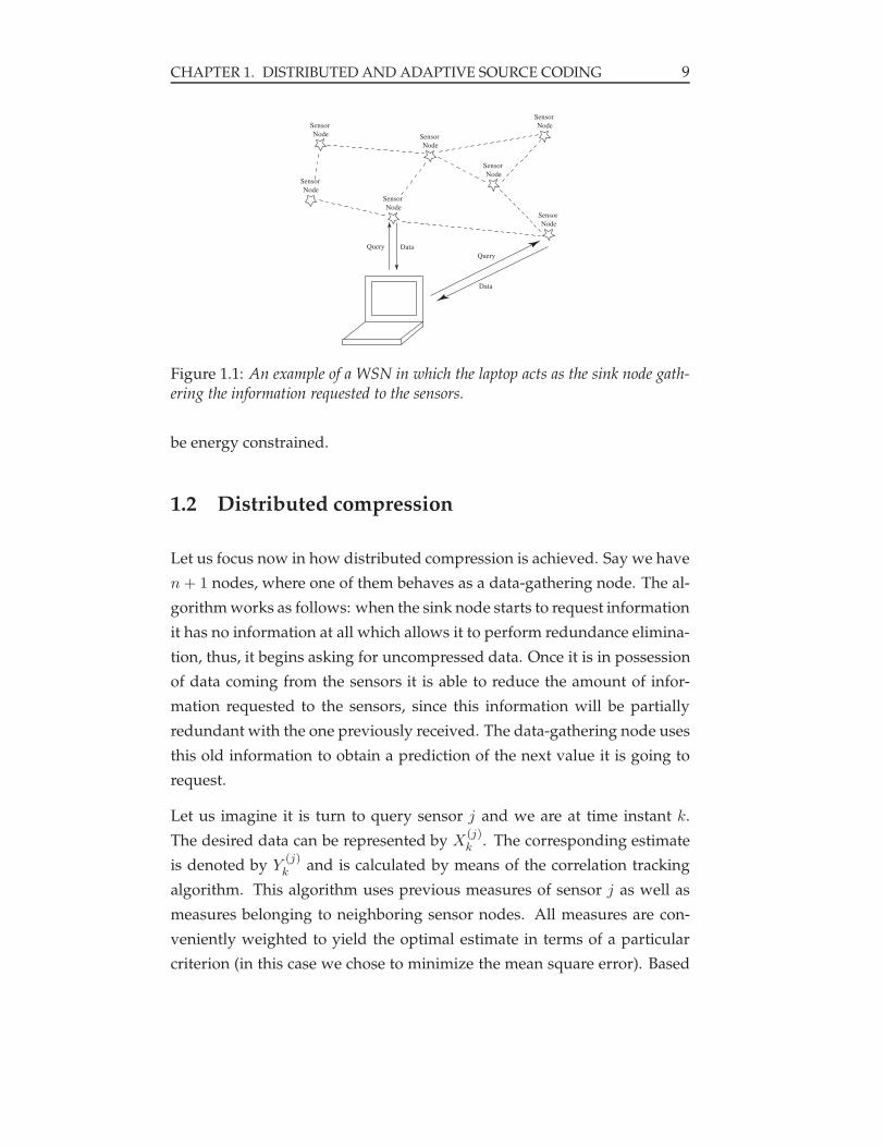
Petrovich’s algorithm is applied in a network consisting on two types of

nodes: many sensing nodes and one or more data-gathering nodes (see

Fig. 1.1). The former ones are supposed to be energy constrained, not so

the latter. One of the most appealing characteristics of this algorithm is that

no data exchange between sensors is needed, the compression takes place

in a fully blind manner, with the subsequent saving of energy. These sav-

ings are achieved by letting the data gathering node track the correlation

structure among nodes and process the information to effect distributed

sensor data compression. The correlation structure is determined by using

an adaptive prediction algorithm. The sensors, in turn, only need to know

the number of bits they are entitled to send to the data-gathering node.

It is obvious the complexity in the decoder is higher than that in the en-

coder, but it resides on the data-gathering node, which is assumed not to

CHAPTER 1. DISTRIBUTED AND ADAPTIVE SOURCE CODING 9

Sensor

Node

Sensor

Node

Sensor

Node

Sensor

Node

Sensor

Node

Sensor

Node

Sensor

Node

Query Data

Query

Data

Figure 1.1: An example of a WSN in which the laptop acts as the sink node gath-ering the information requested to the sensors.

be energy constrained.

1.2 Distributed compression

Let us focus now in how distributed compression is achieved. Say we have

n + 1 nodes, where one of them behaves as a data-gathering node. The al-

gorithm works as follows: when the sink node starts to request information

it has no information at all which allows it to perform redundance elimina-

tion, thus, it begins asking for uncompressed data. Once it is in possession

of data coming from the sensors it is able to reduce the amount of infor-

mation requested to the sensors, since this information will be partially

redundant with the one previously received. The data-gathering node uses

this old information to obtain a prediction of the next value it is going to

request.

Let us imagine it is turn to query sensor j and we are at time instant k.

The desired data can be represented by X(j)k . The corresponding estimate

is denoted by Y(j)k and is calculated by means of the correlation tracking

algorithm. This algorithm uses previous measures of sensor j as well as

measures belonging to neighboring sensor nodes. All measures are con-

veniently weighted to yield the optimal estimate in terms of a particular

criterion (in this case we chose to minimize the mean square error). Based

CHAPTER 1. DISTRIBUTED AND ADAPTIVE SOURCE CODING 10

on the accuracy of this prediction and some other parameters as the desired

probability of error, the sink node will require a specific number of bits (say

m) to sensor j which, in turn, will transmit the data sensed (converted by

the ADC to n bits) compressed to those m bits. The decoder will have to

decode this compressed sequence of bits to the desired data message,X(j)k ,

for what it uses the value Y(j)k previously calculated.

The correlation tracking algorithm must address an important issue: data

statistics might be time-varying and consequently, the amount of correla-

tion can change. This has two consequences, first, the correlation tracking

algorithm can not be static and the coefficients weighting the different data

have to be updated with the sufficient frequency. Second, it is mandatory

to have one unique underlying codebook that it is not changed among the

sensors and can also support multiple compression rates. This concept can

be pictured as having several codebooks forming a tree structure as shown

in Fig. 1.2.

0.0 0.1 0.2 0.3 0.4 0.5 0.6 0.7 0.8 0.9 1.0 1.1 1.2 1.3 1.4 1.5

r0 r1 r2 r3 r4 r5 r6 r7 r8 r9 r10 r11 r12 r13 r14 r15

D=0.1

X=0.9

r0

r2

r4

r6

r8

r10

r12

r14

2D

r1

r3

r5

r7

r9

r11

r13

r15

r4

r8

r12

r r r r2

r6

r10

r14

r1

r5

r9

r13

r3

r7

r11

r15

2D

4D4D 4D 4D

Y=0.8

0 10 1

0 1

0.1 0.5 0.9 1.3

LEVEL

l=0

l=3

r0

l=2

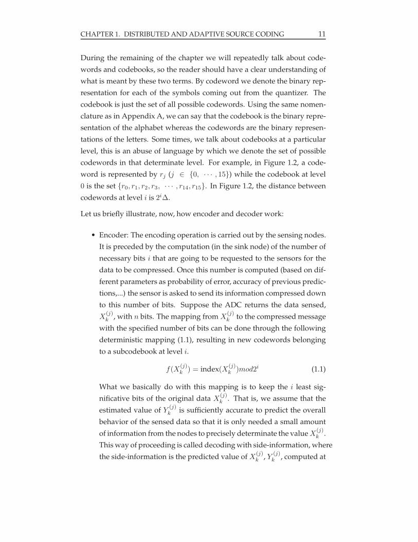
Figure 1.2: An example for the tree based codebook. The encoder is asked to encodeX using 2 bits, so it transmits 01 accordingly to the decoder. The decoder willuse the bits 01 in an ascending order from the least-significative-bit (LSB) todetermine the path to the subcodebook to use to decode Y .

CHAPTER 1. DISTRIBUTED AND ADAPTIVE SOURCE CODING 11

During the remaining of the chapter we will repeatedly talk about code-

words and codebooks, so the reader should have a clear understanding of

what is meant by these two terms. By codeword we denote the binary rep-

resentation for each of the symbols coming out from the quantizer. The

codebook is just the set of all possible codewords. Using the same nomen-

clature as in Appendix A, we can say that the codebook is the binary repre-

sentation of the alphabet whereas the codewords are the binary represen-

tations of the letters. Some times, we talk about codebooks at a particular

level, this is an abuse of language by which we denote the set of possible

codewords in that determinate level. For example, in Figure 1.2, a code-

word is represented by rj (j ∈ 0, · · · , 15) while the codebook at level

0 is the set r0, r1, r2, r3, · · · , r14, r15. In Figure 1.2, the distance between

codewords at level i is 2i∆.

Let us briefly illustrate, now, how encoder and decoder work:

• Encoder: The encoding operation is carried out by the sensing nodes.

It is preceded by the computation (in the sink node) of the number of

necessary bits i that are going to be requested to the sensors for the

data to be compressed. Once this number is computed (based on dif-

ferent parameters as probability of error, accuracy of previous predic-

tions,...) the sensor is asked to send its information compressed down

to this number of bits. Suppose the ADC returns the data sensed,

X(j)k , with n bits. The mapping from X

(j)k to the compressed message

with the specified number of bits can be done through the following

deterministic mapping (1.1), resulting in new codewords belonging

to a subcodebook at level i.

f(X(j)k ) = index(X

(j)k )mod2i (1.1)

What we basically do with this mapping is to keep the i least sig-

nificative bits of the original data X(j)k . That is, we assume that the

estimated value of Y(j)k is sufficiently accurate to predict the overall

behavior of the sensed data so that it is only needed a small amount

of information from the nodes to precisely determinate the valueX(j)k .

This way of proceeding is called decoding with side-information, where

the side-information is the predicted value of X(j)k , Y

(j)k , computed at

CHAPTER 1. DISTRIBUTED AND ADAPTIVE SOURCE CODING 12

the decoder (the interested reader can find more information on this

topic in Appendix A).

• Decoder: The decoding operation is, obviously, performed at the data-

gathering node. When this node receives the requested data it starts

to traverse the tree using the information received to locate the ap-

propriate subcodebook S among all the possible ones at the level i at

which the data has been compressed to. This process starts with the

least-significant-bit (LSB) of f(X(j)k ). Once the suitable subcodebook

has been found, the decoder will use the side-information, Y(j)k , to

decode the closest value in S :

f(X(j)k ) = argminri∈S‖Y

(j)k − ri‖ (1.2)

where ri stands for the ith codeword in S .

If we study more carefully how the tree structure of subcodebooks is con-

structed, we can appreciate that at level i, the different codewords within

the same subcodebook share the last i bits. This can be directly interpreted

as the fact that the estimate Y(j)k is not distinguishable among words of code

belonging to level i+ 1 (or higher) so that it is necessary to have a finer de-

composition. Thus, buy asking for the i least significative bits, we are able

to rule out some codewords so that our subcodebook is small enough to

guarantee a correct decoding from the side-information.

In short, we assure that the prediction Y(j)k differs in less than 2i−1∆ from

X(j)k and we choose a subcodebook S whose codewords are at a distance

2i∆ from each other. In this way, a unique and successful decoding is

achieved.

Let us illustrate the coding/decoding process with a simple example. As-

sume we have the tree structure given by Fig. 1.2, where each codeword

in the codebook at level l = 0 is composed by four bits (the codebook has

sixteen elements). Let us also assume that the data-gathering node has in

some way computed the side-information Y(j)k and the number of bits to

which the data has to be compressed is i = 2. The process starts when

the sink node requests data to sensor j. The sensor node uses its ADC to

CHAPTER 1. DISTRIBUTED AND ADAPTIVE SOURCE CODING 13

obtain a 4-bit value X(j)k = 0.9 corresponding to codeword r9. The follow-

ing thing the sensor node does is to use the rule given by (1.1) to find the

mapping in the compressed domain: f(X(j)k ) = 9mod4 = 1. Thus, the en-

coder will send the two bits, 01, to the k-th sink node. The sink node

will make use of the received message to descend by the tree and find the

suitable subcodebook S where to apply (1.2). It starts using the LSB ’1’

so that it breaks the root codebook (i.e., the codebook at level 0) down to

r1, r3, r5, r7, r9, r11, r13, r15. Afterwards it uses the second bit in the mes-

sage ’0’ to choose codebook r1, r5, r9, r13 as S . It is now when the decoder

uses the side-information Y(j)k conveniently introduced in Eq. (1.2)

f(X(j)k ) = argminri∈S0.7, 0.3, 0.1, 0.5

to derive r9 as the decoded codeword, which is exactly the value sensed in

the node. Thus, we can see how transmission of the information has been

achieved by using only 2 bits instead of 4, as it would have been needed

without encoding.

1.3 Correlation tracking

In the previous section we assumed that some information, Y(j)k , correlated

to the sensors readings, X(j)k , was available at the decoder for sensor j at

time k. The prediction can be done by a linear combination of different

measures available at the decoder and can be expressed as Eq. (1.3):

Y(j)k =

M∑

l=1

αlX(j)k−l +

j−1∑

i=1

βiX(i)k (1.3)

We can think of Y(j)k as a linear prediction based on past values of the sen-

sor whose measure is going to be predicted along with current values of

neighboring sensors. Hence, the main objective of the decoder is to derive

a good estimate of X(j)k for each sensor j.

To find the values αl and βi which minimize the mean square error (MSE), a

mathematical problem must be addressed. Let us start by representing the

prediction error as a random variable, Nj = Y(j)k − X

(j)k . We can expand

CHAPTER 1. DISTRIBUTED AND ADAPTIVE SOURCE CODING 14

the mean square error as:

E[N2

j

]= E

(X

(j)k −

(M∑

l=1

αlX(j)k−l +

j−1∑

i=1

βiX(i)k

))2

= E[X

(j)2

k

]− 2

M∑

l=1

αlE[X

(j)k X

(j)k−l

]

−2N∑

i=1

βiE[X

(j)k X

(i)k

]+ 2

M∑

l=1

j−1∑

i=1

αlβiE[X

(j)k−lX

(i)k

]

+M∑

l,h=1

αlαhE[X

(j)k−lX

(j)k−h

]+

j−1∑

i,h=1

βiβhE[X

(i)k X

(h)k

](1.4)

Now, if we assume that X(j)k and X

(i)k are pairwise jointly wide sense sta-

tionary for i = 1, . . . , j − 1 then we can rewrite the mean square error as:

E[N2j ] = rxjxj (0) − 2PT

j Γj + ΓTj R

jzzΓj (1.5)

where the superscript T stands for the transpose and

Γj =[α1 α2 · · · αM β1 β2 · · · βj−1

]T,

Pj =[rxjxj(1) rxjxj(2) · · · rxjxj(M) rxjx1(0) rxjx2(0) · · · rxjxj−1(0)

]T

and we use the notation rxjxi(l) = E[XjkX

ik+l]. We can express Rj

zz as:

Rjzz =

[Rxjxj Rxjxi

RTxjxi Rxixi

](1.6)

where, in turn, Rxjxj is given as:

Rxjxj =

rxjxj (0) rxjxj (1) · · · rxjxj(M − 1)

rxjxj (1) rxjxj (0) · · · rxjxj(M − 2)...

.... . .

...

rxjxj(M − 1) rxjxj(M − 2) · · · rxjxj(0)

(1.7)

CHAPTER 1. DISTRIBUTED AND ADAPTIVE SOURCE CODING 15

and Rxjxi and Rxixi are given as:

Rxjxj =

rxjx1(1) rxjx2(1) · · · rxjxj−1(1)

rxjx1(2) rxjx2(2) · · · rxjxj−1(2)...

.... . .

...

rxjx1(M) rxjx2(M) · · · rxjxj−1(M)

(1.8)

Rxixi =

rx1x1(0) rx1x2(0) · · · rx1xj−1(0)

rx2x1(0) rx2x2(0) · · · rx2xj−1(0)...

.... . .

...

rxj−1x1(0) rxj−1x2(0) · · · rxj−1xj−1(0)

(1.9)

To find the optimal set of coefficients (represented by Γj) that minimizes the

mean square error, we differentiate Eq. (1.5) with respect to Γj to obtain:

∂E[N2j ]

∂Γj=

∂(rxjxj(0) − 2PT

j Γj + ΓTj R

jzzΓj

)

∂Γj

=∂(−2PT

j Γj

)

∂Γj+∂(Γ

Tj R

jzzΓj

)

∂Γj

= −2Pj +[RjT

zz +Rjzz

]Γj

= −2Pj + 2RjzzΓj (1.10)

Where basic matrix calculus has been employed:

∂(Ax+ b)TC (Dx+ e)

∂x= ATC (Dx+ e) +DTCT (Ax+ b) (1.11)

Please note that in the formula above (1.11) upper case letters denote ma-

trixes while vectors are written in the lower case.

Setting (1.10) equals zero and solving, we obtain the standard Wiener esti-

mate:

Γj,opt = R−1,jzz Pj (1.12)

If the assumption of stationarity held, then the data gathering could request

for uncoded data from all the sensors for the first K rounds of requests and

construct the correlation matrixes for their subsequent use in (1.12). By do-

ing this we would already have tracked the behavior of the system and we

CHAPTER 1. DISTRIBUTED AND ADAPTIVE SOURCE CODING 16

could employ the obtained set of coefficients for computing the side infor-

mation for each future round of requests. Thus, it would be only necessary

to calculate the standard Wiener estimate once, what would be really con-

venient given the extreme computational complexity of this calculus.

In practice, however, the statistics of the data may be (and actually they are)

time varying and as a result, the coefficient vector, Γj , must be continuously

adjusted to minimize the mean square error. One method of doing this is to

move Γj in the opposite direction of the gradient of the objective function

(i.e., the mean squared error) for each new sample received during round

k+1 (this method known in the literature as the ’Steepest Descent Method’):

Γ(k+1)j = Γ

(k)j − µ∇(k)

j (1.13)

where ∇(k)j is given by Eq. (1.10) and µ represents the step size of the Steep-

est Descent Method. The goal of this approach is to descend to the global

minima of the objective function. We are assured that such a minima exists

because the objective function is convex. In fact, it has been shown that if µ

is chosen correctly then (1.13) will converge to the optimal solution.

From (1.10) and (1.13) can be shown that the coefficient vector should be

updated following the rule:

Γ(k+1)j

= Γ(k)j − 1

2µ(−2Pj + 2Rj

zzΓ(k)j

)(1.14)

However, in practice, the data gathering node will not have knowledge of

Pj and Rjzz due to the computational complexity required for obtaining

them. Hence, it will be necessary to provide the algorithm with an efficient

method for estimating Pj and Rjzz. One standard estimate is to use Pj =

CHAPTER 1. DISTRIBUTED AND ADAPTIVE SOURCE CODING 17

X(j)k Zk,j and Rzz = Zk,jZk,j with

Zk,j =

X(j)k−1

X(j)k−2

· · ·X

(j)k−M

X(1)k

X(2)k

· · ·X

(j−1)k

introducing these new terms, Eq. (1.14) remains as

Γ(k+1)j = Γ

(k)j − µZk,j(−X(j)

k + ZTk,jΓ

(k)j )

= Γ(k)j + µZk,jNk,j (1.15)

where the second equality follows from the fact that Y(j)k = Z

Tk,jΓ

(k)j and

Nk,j = X(j)k − Y

(j)k .

In practice the formulas above yield the following practical equations (well

known in the adaptive filtering literature as the Least-Mean-Squares (LMS)

algorithm):

1. Y(j)k = Γ

(k)Tj Zk,j

2. Nk,j = X(j)k − Y

(j)k

3. Γ(k+1)j = Γ

(k)j + µZk,jNk,j

To use this algorithm, the data-gathering node will start asking the sens-

ing nodes for sending their data uncompressed during the first K rounds.

By doing this we ensure that the algorithm converges. Once this phase

has been carried out, we can consider that we have tracked the correlation

structure existing between the different nodes, so we can start to ask for

compressed data. This is done in two steps (as already shown): first, com-

puting the prediction of the data to be requested, for what we know that

Y(j)k = Γ

(k)Tj Zk,j (recall that the statistics of the sources can change with

the time, so the vector of coefficients has to be continuously updated). The

CHAPTER 1. DISTRIBUTED AND ADAPTIVE SOURCE CODING 18

second step mentioned before, consists of obtaining the number of bits for

the data to be compressed to.

The decoder, in turn, will decode Y(j)k to the closest codeword in the sub-

codebook S as has already been seen, yielding X(j)k . From section 1.2 we

know that while 2i−1∆ > |Nk,j| and the encoder encodes X(j)k with i bits,

then, X(j)k = X

(j)k and no decoding errors are made. However, if |Nk,j| >

2i−1∆ then a decoding error will occur. This fact can be used to try to find

a bound for the error committed during the prediction process. The most

straightforward method is to apply Chebyshev’s inequality

P[|Nk,j| > 2i−1∆

]≤

σ2Nj

(2i−1∆)2(1.16)

We adopt the realistic assumption that Nk,j is zero-mean and variance σ2Nj

.

Thus, reading from Eq. (1.16), we deduce that we can take for the proba-

bility of error Pe any value greater or equal thanσ2

Nj

(2i−1∆)2so that we can be

sure that P[|Nk,j| > 2i−1∆

]is fulfilled. We obviously take the equal in the

inequality so that the expression of the probability of error remains as

Pe =σ2

Nj

(2i−1∆)2(1.17)

from where we can work the value of i out

i =1

2log2

(σ2

Nj

∆2Pe

)+ 1 (1.18)

as the number of bits necessaries to ensure a probability of error less or

equal than Pe. Note that it is not necessary to be over-conservative when

choosing Pe because Chebyshev’s inequality is a loose bound.

If we look thoroughly at expression (1.18) we can appreciate the presence

of a new term not taken into account yet: the variance σ2Nj

. This means

that the data gathering node must also maintain an estimate of σ2Nj

. After

the initialization module (K iterations long), the data-gathering node can

initialize σ2Nj

as

σ2Nj

=1

K − 1

K∑

i=1

N2k,j (1.19)

CHAPTER 1. DISTRIBUTED AND ADAPTIVE SOURCE CODING 19

However, in the main module, the variance can be computed and updated

in a weighted way (filtered estimate) as

σ2Nj ,new = (1 − γ)σ2

Nj ,old + γN2k,j (1.20)

The choice of a filtered estimate is consequent with the time varying prop-

erties stated before, so we can adapt to changes in the statistics. γ is known

as the ”forgetting factor” and is a key value for the capacity of adapting to

changes in the statistics.

Beyond our scope stands the correction/detection of errors, even though,

two possible policies are suggested:

a) To detect errors, the use of a cyclic redundancy check (CRC) is proposed.

In this way, each sensor would be entitled to send a CRC formed with

its lastm readings. Afterwards, the data-gathering node will perform

its own CRC, in case both of them do not match, the data-gathering

node will decide between dropping the m last readings or asking for

their retransmission.

b) Another option is to use error-correction codes, as could be the case of

using Reed-Solomon codes [8].

1.4 Querying and reporting algorithm

In this section, the algorithm to be implemented in the encoder and decoder

is reported. Note that, at the beginning of the algorithm, the data-gathering

node must gather enough information to track the correlation structure,

what is achieved by performing K rounds of readings (note that K should

be chosen large enough to allow the LMS algorithm convergence).

The data-gathering node should alternate the requests for ”uncompressed”

data among the nodes to ensure that every single node wastes the same

amount of energy.

CHAPTER 1. DISTRIBUTED AND ADAPTIVE SOURCE CODING 20

1.4.1 Data gathering node algorithm

The provided pseudocode basically expresses in programming language

what has been analyzed along the previous sections. The only novelty in-

troduced here is that, when carrying out the main module, it is necessary to

ask a sensor for its full uncompressed data to keep track of the real data en-

suring that the prediction is not producing erroneous estimates. However,

the request for uncoded data is alternated between the different sensors, so

that we can assure that the waste of energy is shared between sensors.

Once taken into account the previous considerations the pseudocode for

the data-gathering node is reported:

Pseudocode for data gathering node:

Initialization:

for (i = 0; i < K; i+ +)

for (j = 0; j < num sensors; j + +)

Ask sensor j for its uncoded reading

end

for each pair of values i, j

update correlation parameters, using LMS and (1.19) equations.

end

end

Main Loop:

for (k = K; k < N ; k + +)

Request a sensor for uncoded reading

for each remaining sensor

determine number of bits, i, to request for using Eq. (1.18)

request for i bits

end

Decode data for each sensor.

Update correlation parameters for each sensor.

end

CHAPTER 1. DISTRIBUTED AND ADAPTIVE SOURCE CODING 21

1.4.2 Sensing nodes algorithm

Pseudocode for the sensor nodes is given below.

Pseudocode for sensor nodes:

for each request

Extract i from the request

Get X[n] from ADC

Transmit nmod2i

end

Chapter 2

Minimum Energy Coding

2.1 Introduction

Nodes in wireless networks are usually deployed forming a very dense net-

work in which few meters is the typical distance between them. The com-

munication of one with each other can cause serious problems since nearby

nodes can overwhelm (MAI) the received signal of the desired user. CDMA

is a promising multiple access scheme for sensor and ad hoc networks due

to its interference averaging properties [1]. However, the performance of

CDMA systems is limited by MAI.

In the past decade numerous methods have been developed to reduce MAI,

most of which focus on the design of effective correlation receivers. How-

ever, they also introduce an increase in complexity, and often, also in the

demand of computational power, something which is an undesired effect.

In this section a different approach focusing on source coding is studied.

Instead of merely designing receivers to suppress interferences the output

of the source is represented with a special codebook so that MAI is greatly

reduced.

In the remaining sections we start by simply introducing the On-Off Key-

ing modulation scheme and the ME coding to finalize with a further anal-

ysis on the system performance. This is done by first introducing the sig-

nal model of the system to subsequently analyze different relevant perfor-

mance parameters.

22

CHAPTER 2. MINIMUM ENERGY CODING 23

2.2 On-Off Keying modulation scheme (OOK)

On-off keying is a basic type of modulation that represents digital data as

the presence or absence of a carrier wave. In its most basic form, the pres-

ence of a carrier during the bit duration represents a binary one (i.e., 1),

while a binary zero (i.e., 0) results in no signal being transmitted. This

modulation technique yields not a very efficient use of the spectrum due

to the abrupt changes in amplitude of the carrier wave. Having a look at

its power consumption properties, however, it can be appreciated that its

performance is better than that of BPSK, for instance, due to the fact that en-

ergy consumption is larger when high bits are transmitted than when low

ones are. In Figure 2.1 the basic working of BPSK and OOK is depicted.

1 1 1 1 1

1 1 1 1 10 0 0 0 0 0

0 0 0 0 0 0

Eb

Eb

Eb

BPSK

OOK

t

t

Figure 2.1: BPSK and OOK modulation schemes.

2.3 Energy consumption in OOK modulation

During the operation of a sensor node, power is consumed in sensing, data

processing, data storing and communicating [9][10]. Among the four do-

mains we focus in the communications one, since it is the most power con-

suming. The average energy consumption of a pair of nodes, one transmit-

ting and one receiving, in a OOK modulation can be generally modelled as

CHAPTER 2. MINIMUM ENERGY CODING 24

[10]:

Eradio = Etx + Erx

= Ptx,ckt (Ton,tx + Tstartup) + αPtTon,tx + E(e)dsp

+Prx,ckt (Ton,rx + Tstartup) + E(d)dsp

where Etx/rx is the average energy consumption of a sensor node while

transmitting/receiving; Ptx/rx,ckt is the power consumption of the elec-

tronic circuits while transmitting/receiving; Pt is the output transmission

power; Ton,tx/rx is the transmitter/receiver ontime, and Tstartup is the start

up time of the transceiver; E(e/d)dsp is the energy consumed by the circuitry

in encoding/decoding the data. In general, the energy spent in encod-

ing/decoding is negligible compared to that needed to transmit and re-

ceive. Since Ptx/rx,ckt and Tstartup are hardware dependent, these param-

eters cannot be used for the purpose of reducing power consumption by

means of coding the source outputs. In the above expression we have also

modelled the major characteristic brought about by the OOK modulation:

the effective transmitting time is only a fraction of the transmitter ontime

(where α is precisely that fraction of time).

2.4 The ME coding

Minimum Energy (ME) coding [11] attempts to optimize the power con-

sumption in digital RF transmitters, which constitutes one of the most power

consuming sources in portable communication devices. The function of a

digital RF transmitter is to convert the modulated binary codewords into

radio frequency waves able to travel through the air to reach other commu-

nication devices. The power needed to generate these signals is one of the

major sources of power consumption in sensor nodes.

Any attempt to formulate the power optimization problem must be based

on a deep understanding on how these waves are generated, therefore the

type of modulation used is of extreme importance. For the application

of ME coding, On-Off Keying (OOK) modulation is considered. Despite

his limited performance when compared to other modulation schemes like

CHAPTER 2. MINIMUM ENERGY CODING 25

BPSK (it performs nominally 3dB worse due to reduced minimum distance

in the signal constellation), the gain obtained when used along with ME is

more than sufficient to justify its presence.

In Eq. (2.1) the power consumed in a WSN that uses ME coding is shown.

The main characteristic of ME coding is that it reduces the value of the α

coefficient (now termed αME).

Eradio = Etx + Erx

= Ptx,ckt

(TME

on,tx + Tstartup

)+ αMEPtT

MEon,tx + E

(e)dsp

+Prx,ckt

(TME

on,rx + Tstartup

)+ E

(d)dsp (2.1)

Two key aspects should be considered now: with ME coding we are in-

creasing the value of two system parameters, TMEon,tx/rx and the length of the

codeword LME .

• Increasing the transmitter ontime is not a disadvantage, since the ma-

jor power consumption in modern low-power chips is given by Pt

(Pt >> Ptx,ckt) and this term is affected by the design parameter

αME << 1. However, increasing the receiver ontime is extremely

harmful because in the typical distances characteristic of a WSN, the

power spent in receiving is approximately the same than that used

in transmitting, so it could happen that no power savings at all are

achieved. Subsection 2.8.2.2 deals with the evaluation of the ME cod-

ing power consumption properties. In order to reduce the Ton,rx we

will investigate a new coding scheme in Chapter 3.

• On the other hand, an increased codeword length could also be fatal,

since we would increase the codeword error probability. However,

the reduction in the multiaccess interference (provoked by the de-

creased number of high bits achieved by the ME coding) is more than

enough to compensate this drawback.

Equation (2.1) suggests several ways of reducing the power consumption.

Power consumption can be optimized by (i) minimizing Ptx,ckt and Pt,

which is done by improving the transmitter circuitry, (ii) reducing the

CHAPTER 2. MINIMUM ENERGY CODING 26

Ton,tx/rx, that can be done modifying the bit period, tb (this results in an

enlarged frequency spectrum) and, (iii) minimizing the presence of high

bits in the codebook.

The objective of ME coding is to reduce the proportion of high bits in the

codebook, αME . There are two ways of doing this:

• Use a set of codewords with a lesser number of high bits than the one

used previously.

• Exploit the statistics of the source to assign codewords with a smaller

number of high bits to the most probable symbols.

ME coding combines this two methods to provide the energy-optimal cod-

ing algorithm, which, based on the two previous bullets is constructed in

two steps: Codebook Optimality and Coding Optimality. The former is to

determine a set of codewords, termed a codebook, that has the fewest high

bits, and the latter is to assign codewords having less high bits to messages

with higher probability.

ME Coding

L0=Original Codeword Length

Redundant Bits

LME = New Codeword Length (more zeros)

1 0 1 1 0 0 1 0 1 1 0 1 0 0 1 0

0 1 0 0 0 0 0 0 0 0 1 0 0 0 0 0 0 0 1 0 0 0 0 0 0 1 0

Figure 2.2: Principle of Minimum Energy Coding.

Basically, with ME coding we perform a mapping from an original set of

codewords to another one more suitable to the aim of power savings. Each

codeword in the original set has a unique image codeword in the new code-

book. Specifically, the source codewords have length of L0 bits and the ME

codewords have length LME bits, with LME > L0. Thus, what ME coding

CHAPTER 2. MINIMUM ENERGY CODING 27

does is nothing different from endowing the source codebook with new

codewords having less high bits. As a result, the new codebook has larger

codewords, but we do not need to use all the possible new codewords, in

fact, we will just make use of those more suitable for our design goal. Fig-

ure 2.3 illustrates this concept.

Thanks to the increase of the codeword length, we will be able to allocate

new codewords with a smaller number of high bits to the original code-

words, reducing in this way the probability of high bit, αME , and achieving

power savings by means of OOK as previously explained.

Codeword

Number of

codewords

Codeword

pattern

w0w1 w L wL+1

wq w2 -2L w

CL

0CL

1

CL

2

CL

L-1CL

L

2 -1L

Figure 2.3: Fixed-Length ME Codewords.

In one sentence, ME Coding consist of: assigning q codewords of the minimum

codebook in the ascending order of number of high bits to the q-messages in the

descending order of message probabilities.

Of practical importance is ME Coding with fixed length codewords. It is

clear that, for a q-codeword codebook, as the codeword length LME be-

comes longer, the number of high bits decreases. An extreme case is the

unary coding, extensively studied in [12], which presents an interesting be-

havior. Unary coding uses a codeword length, LME , long enough to ex-

press all q messages with at most one high bit per codeword.

CHAPTER 2. MINIMUM ENERGY CODING 28

2.5 MAI reduction by ME source coding

The ME coding described above is useful for the reduction of MAI when

using DS-CDMA. This is attained thanks to the low probability of overlap

between the signals belonging to different users when we have a scenario

consisting of multiple transmitters and receivers (see Figure 2.4).. Since ME

helps to decrease the number of high bits in the codewords it decreases the

probability that two or more users transmit a high bit in the same time,

achieving a reduction in the MAI.

Tx

Rx

Tx

Rx

Tx

Rx

Tx

Rxtransmitter-receiver

pair

12

43

Figure 2.4: System scenario.

In the literature several methods for reducing MAI have been proposed.

When dealing with MAI in the transmitter side, increasing the processing

gain and boosting the signal are the two most common choices, but none

of them are suitable for our purpose. The first one brings an undesired

increase of the complexity of the receiver, while the second one moves in

the opposite direction of the policy of power saving we are adopting.

Trying to reduce MAI in the receiver leads to sophisticated correlation fil-

ters that increase the complexity and cost of the design. The salient char-

acteristic of ME coding is that the more power it saves, the smaller MAI it

reaches, however, at the expense of sacrificing either transmission rate (this

is not a burden in WSN where we are supposed to transmit at a low rate)

or transmission time.

Figure 2.5 shows the configuration of the transmitter in our system when

we use the source coding technique proposed. It is a quasi-typical DS-

CDMA system in which, prior to multiplication by the spreading sequence,

CHAPTER 2. MINIMUM ENERGY CODING 29

we perform a mapping from the source symbols to ME codewords. At the

receiver the structure is similar but inverse. We say it is a quasi-typical DS-

CDMA system because the BPSK modulator has been substituted by an

On-Off Keying.

ME

coding

d1(t)

c1(t) 2P1cos(ωct+θ1)

ME

coding

d2(t)

c2(t) 2P2cos(ωct+θ2)

ME

coding

dM(t)

cM(t) 2PMcos(ωct+θΜ)

Σn(t)

r(t)

Data

Symbols

User 1

Data

Symbols

User 2

Data

Symbols

User M

(a) Transmitter

r(t)dk(t)

ck(t)2Pkcos(ωct+θκ)

^ME

decoder

Decoded

Data

Symbols

User K

(b) Receiver

Figure 2.5: DS-CDMA combined with ME source coding.

The proposed scheme causes a superimposition of the signals originated in

the RF transmitters and, although the DS-CDMA system could send mul-

tiple non-zero signals at the same time (unique PN sequences are assigned

to different users), with the new source coding technique this chance is

reduced, and hence, the performance of the system increased (due to a

lowered MAI). It should be noted that as the number of wireless sensors

increases, so do the interferences. This fact can be overcome by simply

enlarging the codewords (individual users will have sparser non-zero sig-

nals).

CHAPTER 2. MINIMUM ENERGY CODING 30

2.6 Signal model

In this section we introduce the signal model of the system with which

we are working. We are dealing with an asynchronous DS-CDMA system

and a wireless channel where we assume we have K active transmitter-

receivers pairs of nodes carrying a bit rate of Rb = 1Tb

. The same fixed

bandwidth W , and hence the same chip interval Tc, is allocated to each

channel. Let ak (t) and bk (t) denote the spreading signal and the baseband

data signal, respectively, for pair k. Each one of these signals can be ex-

pressed as:

ak (t) =

∞∑

l=−∞a

(k)l pTc (t− lTc) (2.2)

bk (t) =

∞∑

l=−∞bk,lpTb

(t− lTb) (2.3)

Where pTc(t) is a rectangular pulse which takes a constant amplitude of

value one from t = 0 to t = Tc and zero outside this interval. pTb(t) is

similar to pTc(t) but with a time duration of Tb.

a(k)l ∞l=0 and bk,l∞l=0 are the binary sequences corresponding to the spread-

ing sequence and baseband data signal, respectively, for user k.

In this situation, the signal at the transmitter side of the pair k can be for-

mulated as:

sk (t) =√

2Pkbk (t) ak (t) cos (2πfct+ θk) (2.4)

Where Pk denotes the signal power of the transmitter node in link k, fc is

the carrier frequency and θk is the carrier phase.

If we now want to represent the signal at the input of the receiver in pair

i, ri(t), we have to realize that it is composed by several different terms:

the desired signal, the signals transmitted by other users and a noise com-

ponent introduced by the AWGN channel. From now on we will consider

user i what will be denoted with the correspondent subscript:

ri(t) =

K∑

k=1

√2PkΩkibk (t− τk) ak (t− τk) cos (2πfct+ ψk) + n(t) (2.5)

CHAPTER 2. MINIMUM ENERGY CODING 31

Where τk stands for the signal delay for the kth user, ψk = θk − 2πfcτk and

n(t) is the gaussian noise with two sided spectral density N0

2 . We have also

introduced the wireless channel influence by means of the channel coeffi-

cients, Ωki,which are defined in the following way

Ωki = PLkieξki (2.6)

where PLki is the loss present in the path from the transmitter in pair k to

the receiver in pair i, and ξki is the shadow fading parameter. The path loss

can be further written (in dBs) as

PLki|dB= −Pl (dr) |dB−10n log10

(dki

dr

)

with the reference distance dr = constant = 1 meter. dki is the distance be-

tween the transmitter in channel k and the receiver in channel i, Pl (dr) |dB

is a known constant (55 dB for the Telos motes), and n is the path-loss de-

cay constant, which takes the value 2 for the free space and [3.5 − 4] for

urban environments. The shadowing component of Ωki is described by a

log-normal distribution eξki , where ξki is a zero-mean Gaussian distributed

r.v. with variance σ2ξki

.

If the DS-CDMA system were completely synchronized, then one could ig-

nore the time delays τk (k = 1, 2, · · ·,K). Of course, this would require

a perfect common timing reference for the K transmitters being necessary

to introduce mechanisms for compensating the delays in the various trans-

mission paths. However, this is not easy to implement, so that the asyn-

chronous system is the one usually implemented.

Let us consider channel i. Since we are interested in relative phase shifts

modulo 2π, there is no loss of generality in assuming θi = 0 and τi = 0.

Following an approach similar to that found in [13] we can express the

output of the correlation receiver matched to si(t) as:

Zi =

∫ Tb

0r(t)ai(t) cos (2πfct) dt (2.7)

From now on, we assume that fc >> T−1b . This is a realistic assumption

that helps us to ignore the double frequency component of r(t) cos (2πfct)

CHAPTER 2. MINIMUM ENERGY CODING 32

that appears when calculating the output of the correlation receiver. Thus,

it can be shown that Eq. (2.7) can be expressed as:

Zi = Di + Ii +Ng (2.8)

where Di is the desired signal in the channel i, Ii is the interference term

due to the presence of multiple users (MAI) and Ng is a Gaussian random

variable with zero mean and variance N0Tb4 .

Di =

√PiΩii

2Tbbi,0 (2.9)

Ii =

K∑

k=1

k 6=i

√PkΩki

2cos (ψk)B (i, k, τk) (2.10)

Ng =

∫ Tb

0n(t)ai(t) cos (2πfct) dt (2.11)

Without loss of generality we observe the output of the correlation receiver

at the first time instant (l = 0). Also, for convenience, we have introduced

the term B (i, k, τ) adopting a simplified version of that presented in [14]

and used in [15].

B(i, k, τ) =

∫ Tb

0bk (t− τ) ak (t− τ) ai (t) dt (2.12)

2.7 Signal to Interference and Noise Ratio (SINR)

Once we have the signal model perfectly determined, we can undertake

the task of calculating the Signal to Interference and Noise Ratio (SINR)

parameter, which is one of the most important performance measures and

can be obtained within a reasonable computational complexity. The SINR

for transmitter-receiver pair n (denoted as SINRn) is then defined as the

ratio between the average and the standard deviation of Zi (2.13), the ex-

pectation being taken with respect to carrier phases, time delays and data

symbols, but not with respect to the channel coefficients (which are sup-

posed to be slow variant and constant for a period around Tb). However,

we have to make a distinction in the computation of the SINR depending

on what bit is transmitted:

CHAPTER 2. MINIMUM ENERGY CODING 33

1. If bi,0 = 0, since we do not transmit anything (recall we are using

OOK), the power of the desired signal is zero, and hence, the SINR|dB=

−∞.

2. If bi,0 = 1, the calculation of the SINR can be made via Eq. (2.13).

From now on, let us consider the pair n = i:

SINRi =E [Zi]√

V ar[Ng + Ii](2.13)

Since the gaussian noise and the MAI are independent, we can write:

V ar[Ng + Ii] = V ar[Ng] + V ar[Ii]

Thus, the power of the gaussian component of the noise can be calcu-

lated as:

V ar[Ng] = V ar

[∫ Tb

0n(t)ai(t) cos (2πfct) dt

]

=

∫ Tb

0V ar [n(t)] a2

i (t) cos2 (2πfct) dt

=N0Tb

4(2.14)

In all that follows we consider the time delays, phase shifts and data

symbols (ψk, τk, bk,l) as mutually independent random variables. Namely,

we treat ψk and τk as two r.v. uniformly distributed in their respec-

tive range of values, [0, 2π] and [0, Tb]. Also, we assume that the

data symbols bk,l take values 0, 1 with a determinate probability

1 − αME,k, αME,k. Independence among the different transmitting

nodes is a realistic assumption too. All these assumptions are repre-

sentative of real systems [15].

With all these hypotheses in mind, it can be proved thatE [B (i, k, τ)] =

0, V ar [B (i, k, τ)] ∼= 2T 2

b3G and E

[cos2 (ψk)

]= 1

2 where G = WRb

= TbTc

denotes the processing gain.

Therefore, assuming αME,1 = αME,2 = · · · = αME,K = αME and

taking into account all previous considerations and Eq. (2.13), we can

rewrite the SINRi as:

CHAPTER 2. MINIMUM ENERGY CODING 34

SINRi =

√PiΩii

2 Tb

(N0Tb

4 + V ar [Ii]) 1

2

(2.15)

The expression of the variance V ar [Ik] turns out to be:

V ar [Ik] ∼=K∑

j=1

j 6=k

αMEPjΩjkT 2

b

6G(2.16)

Please note the inclusion of the αME coefficient in the formula above

(2.16). This is done because not all the remaining nodes may be trans-

mitting a high bit when the user in channel i does. Taking into ac-

count that αME is the probability of sending a high bit, on average,

only a αME fraction of the codeword time will be carrying ones.

If we introduce Eq. (2.16) into the SINRi we arrive at:

SINRi∼=

√√√√√√√

PiΩii2 T 2

b

N0Tb4 +

K∑j=1

j 6=i

αMEPjΩjiT 2

b6G

(2.17)

2.8 Power consumption

In this section we investigate the power consumption which takes place in

the network when the ME coding is used. To start with, we solve a con-

strained optimization problem to subsequently evaluate the performance

of the ME coding.

2.8.1 Optimal transmission power

Let us imagine a system in which we have K transmitter-receiver pairs. In

this scenario (see figure 2.4), if we want to optimize the overall network

power consumption, we have to consider the transmission power in each

link. However, minimizing the transmission power requires to take into

account the resulting effect on other system parameters as the probability of

CHAPTER 2. MINIMUM ENERGY CODING 35

error and the SINR, because they are all interrelated. Thus, we investigate

the optimization problem:

minP1, P2...PK

K∑i=1

Pi

s.t. EΩi [SINRi] ≥ SINRi , i = 1...K

(2.18)

where Ωi denotes the vector formed by the channel coefficients:

Ωi =[

Ω1i Ω2i · · · Ωii · · · ΩKi

]T(2.19)

The problem consist of the minimization of the sum of the individual trans-

mission powers subject to K constraints, that bound in their lower limit

the EΩi [SINRi] in each pair down to a determinate value SINRi (note

that EΩi [SINRi] is the average SINRi ). The reason for bounding the

EΩi [SINRi] and not simply the SINRi, is that although the channel co-

efficients are slow variant, their change is too fast to track them with an

efficient algorithm for WSN.

The problem (2.18) can be regarded as a power control algorithm, which

should be solved in order to get the powers to assign to the transmitters.

Up to this point, we have stated a constrained optimization problem, but

we have not talked yet about more general characteristics of the power con-

trol algorithm, such as the logical architecture necessary for implementing

it. It should be noted that (2.18), is a centralized problem. Therefore, a sin-

gle super-node should be in charge of computing the transmission power

by solving (2.18) and relying the information to each node. However, (2.18)

can be converted into a distributed problem in which the power control is

carried out by each node in a fully blind manner, meaning that each node

is able to perform the optimization algorithm by its own, without requiring

data from any other node, and without central coordination.

In the remaining of the subsection, we characterize and solve the optimiza-

tion problem.

First, we need to find a suitable expression for the EΩi [SINRi]. To be able

CHAPTER 2. MINIMUM ENERGY CODING 36

to carry out this task let us make some definitions.

Ai , L− 1

2

i , SINRi

L−1i =

PiΩiiT2b

2N0Tb

4+V ar[Ii]

(2.20)

where it can be proved that Li can be approximated with a log-normal

distribution Li = exi and xi ∼ N (µxi , σxi) [15]. The approximation is

useful because allows for computing the expression of the average EΩi .

Let us calculate the mean and variance of Ai [16],

µAi = EΩi [Ai] = e−µxi2

+σ2

xi8 (2.21)

rAi = EΩi

[A2

i

]= e−µxi+

σ2xi2 (2.22)

σ2Ai

= rAi − µ2Ai

(2.23)

It can be shown that

µxi = 2 lnM i1 −

1

2lnM i

2 (2.24)

σ2xi

= lnM i2 − 2 lnM i

1 (2.25)

where

M i1 , EΩi [Li] (2.26)

M i2 , EΩi

[L2

i

](2.27)

If we recall the definition of Li,

Li =2

PiT2b PLii

K∑

j=1

j 6=i

αMEPjPLjieξji−ξii

T 2b

6G+N0Tb

4e−ξii

(2.28)

We can easily calculate the value of M i1 and M i

2 applying the statistical ex-

pectation operator to Li and L2i .

M i1 =

2

PiT2b PLii

βi1 (2.29)

M i2 =

4

P 2i T

4b PL2

ii

βi2 (2.30)

CHAPTER 2. MINIMUM ENERGY CODING 37

where the β coefficients are given by

βi1 =

K∑

j=1

j 6=i

αMEPjPLjieµξji

−µξii+ 1

2

σ2

ξji+σ2

ξii

T 2

b

6G+N0Tb

4e−µξii

+σ2

ξii2 (2.31)

βi2 =

K∑

j=1

j 6=i

α2MEP

2j PL2

jie2µξji

−µξii+σ2

ξji+σ2

ξii

T 4

b

36G2+N2

0T2b

16e2−µξii

+σ2

ξii

+

K∑

j=1

j 6=i

K∑

k=1

k 6=i

k 6=j

α2MEPjPkPLjiPLkie

µξji

+µξki−2µξii

+ 1

2

σ2

ξji+σ2

ξki+4σ2

ξii

T 4

b

36G2

+N0Tb

2

K∑

j=1

j 6=i

αMEPjPLjieµξji

−2µξii+ 1

2

σ2

ξji+4σ2

ξii

T 2

b

6G(2.32)

It should be noticed that neither in βi1 nor in βi

2 there is dependence with

the transmission power in channel i (Pi).

Therefore, we have been able to relate the EΩi [SINRi] to measurable pa-

rameters of the channel and to the transmission powers that should be op-

timized. Furthermore, we can extract Pi from EΩi . This detail is of extreme

importance because it is, actually, the reason why we can implement a dis-

tributed power control algorithm instead a centralized one, as it will be

shown later, also, it should be highlighted that the election of the SINRi

is closely related to the desired value of the bit error probability (Pie), as it

will be shown in Section 2.9

Now that we have the value of EΩi [SINRi] completely determined, we

go further with the constraint of the optimization problem. Recall it was

expressed as:

EΩi [SINRi] ≥ SINRi

Making use of Eqs. (2.20) and (2.21) we can rewrite the constraint as

e−µxi2

+σ2

xi8 ≥ SINRi (2.33)

Introducing the values for µxi and σ2xi

given by Eqs. (2.24) and (2.25) and

after some algebra, it holds true that:

Pi

2T−2b PL−1

ii

(βi

1

)10/4 (βi

2

)−3/4≥(SINRi

)2(2.34)

CHAPTER 2. MINIMUM ENERGY CODING 38

where we have used (2.29) and (2.30).

The optimization problem with the new expressions found for the con-

straints becomes:

minP1, P2...PK

K∑i=1

Pi

s.t. Pi

2T−2

b PL−1

ii (βi1)

10/4

(βi2)

−3/4≥(SINRi

)2, i = 1...K

(2.35)

The solution to this problem is given by the limit

limn→∞

Pni = lim

n→∞

(SINR

)2 (2T−2

b PL−1ii

(βi

1

)10/4 (βi

2

)−3/4)n−1

(2.36)

where the superscript n denotes the time instant n. In fact, it can be

proved that the argument of the limit is a contractive function of Pi.

Implementing this behavior in each receiver node in theK considered links

and applying Eq. (2.36) iteratively, ensures the convergence to the mini-

mum achievable power consumption in the network (subject to the given

constraint). The algorithm (2.36) is decentralized, since each node only

needs to know β1 and β2, which are computed locally.

One important issue should be highlighted now. Obviously, the empirical

implementation will slightly differ from our theoretical approach. Thus,

the nodes will have not to calculate the value of σ2ξji

, µξii, . . ., but simply

compute the expectation and the correlation of the term Li. This is easily

done by tracking the SINR (a facility given in most of the current radio

modules as is the case of the CC2420).

2.8.2 Numerical results

2.8.2.1 Power minimization algorithm

In this section, a numerical implementation is derived and discussed. We

consider the same scenario addressed in [17] and in [18]. We consider the

existence ofK = 50 different pairs, each one with their respective transmit-

ter and receiver. All nodes have been placed randomly within a distance of

3 to 15 meters between each other. Furthermore, we assume that Rb = 250

CHAPTER 2. MINIMUM ENERGY CODING 39

Kbps, the processing gain G = 64 and the path-loss decay constant n = 4;

the power spectral density of the gaussian noise is −115 dBm, αME = 0.1

and the expected value of the signal to interference + noise ratio is set to be

EΩi[SINRi]dB ≥ 7.6 dB (i = 1..K).

To find suitable values for µξjiand σ2

ξji, i, j = 1..K, we established a com-

parison between our model for the path-losses (2.6) and that found in [19][17]:

Ωki|dB= −Pl (dr) |dB−10n log10

(dki

dr

)−Xσ|dB (2.37)

where n = 4 and Xσ|dB has been shown to be a zero-mean Gaussian r.v. (in

dB) with standard deviation σ = 4 representing the shadowing effects1. If

we rewrite our model 2.6 in decibels it appears to be:

Ωki|dB = −Pl (dr) |dB−10n log10

(dki

dr

)+ 10 log10 (e) ξki (2.38)

Comparing both models we directly arrive at:

ξki =−Xσ|dB

10 log10 (e)(2.39)

from where it is easy to derive

µξki= 0 (2.40)

σ2ξki

=σ2

(10 log10 (e))2(2.41)

For our simulation we assume that all links experience the same standard

deviation of the slow fading (shadowing). Initially all nodes transmit at 0

dBm.

In Figure 2.6, the convergence of the limit (2.36) is shown. It can be appreci-

ated how it barely takes 20 iterations to enter the stationary state. If we now

analyze the system we can observe that, effectively, EΩi[SINRi]dB = 7.6

dB in all channels without exception. The mean value of the transmission

power used in the network is −48.76 dBm (i.e, when it transmits it uses a

mean transmission power of −38.76 dBm, but it only transmits during a

fraction αME = 0.1 of the time, what is equivalent to a continuous trans-

mission regimen with power −48.76 dBm ).

1n and σ were obtained through curve fitting of empirical data [17]

CHAPTER 2. MINIMUM ENERGY CODING 40

5 10 15 20 25 30 35 40−80

−70

−60

−50

−40

−30

−20

−10

0

time

Pow

er (

dBm

)

Figure 2.6: Convergence of the power minimization algorithm.

2.8.2.2 Power consumption in ME coding

A comparison, in terms of total power consumption, between a typical

BPSK system and a ME coding system is carried out in this subsection.

If we look thoroughly at the energy model for a system using ME coding

(2.1) we can realize that, if we neglect the coding/decoding energies (as is

usually done), is exactly the same than that of a BPSK system, except for

the αME coefficient. We define the energy gain as the ratio of the energy

used in a BPSK system and the energy used in a ME coding system.

ρdB =

(EBPSK

radio

EMEradio

)

dB

(2.42)

To calculate the energy gain we have considered the CC2420 radio transceiver

module by Chipcon, as is the one incorporated in the Telos motes. The val-

ues considered for the computation of the energy gain have been obtained

from the CC2420 datasheet [20].

Two major conclusions can be drawn from Table 2.1. As we expected, the

smaller the number of high bits in the ME codeword, the higher the gain.

The second main result is that the higher the transmission power, the larger

the gain, what is also logical, since this higher value of the transmission

CHAPTER 2. MINIMUM ENERGY CODING 41

(a) Pt = 0dBm

αME ρdB

0.1 2.46

0.2 2.11

0.3 1.78

0.4 1.48

0.5 1.19

(b) Pt = −25dBm

αME ρdB

0.1 1.43

0.2 1.24

0.3 1.07

0.4 0.90

0.5 0.73

Table 2.1: Energy gain of ME coding vs BPSK for two different transmissionpowers (Pt = 0 dBm and Pt = −25 dBm). The displayed gain corresponds to theconverged value (the gain increases as the transmitting time does until it reaches astable value).

power allow us to further exploit the characteristics of the ME coding. This

last statement is due to the value of Ptx/rx,ckt compared to that of Pt. Thus,

we need that Pt dominates over Ptx/rx,ckt to take advantage of the use of

ME coding. In this sense, ME coding will become more and more important

in the future, as advances in electronics tend to reduce the power consump-

tion of the circuitry.

2.9 Error probability

We can express the error probability for the pair i, P ie , as:

P ie = Pr (Tx 0) Pr (Zi > δi|0 Tx) + Pr (Tx 1) Pr (Zi < δi|1 Tx)

= (1 − αME) pie|0 + αME · pi

e|1 (2.43)

where δi is known as the decision threshold for link i and we have defined,

for convenience, the probabilities given by (2.44) and (2.45). From now

on, we will indicate the dependence of the parameters with the considered

transmitter-receiver pair, i, with the correspondent super/subscript.

pie|0 = Pr (Zi > δi|0 Tx) (2.44)

pie|1 = Pr (Zi < δi|1 Tx) (2.45)

For computing these probabilities let us distinguish, once more, between

the two possible cases:

CHAPTER 2. MINIMUM ENERGY CODING 42

1. If bi,0 = 0 the output of the matched filter at the receiver is formed

exclusively by the noise component:

Zi|0 = Ii +Ng

The decision variable, Zi|0, is given by a MAI term Ii and the thermal

noise Ng.

It can be assumed that Ii can be modelled as a Gaussian random vari-

able with a distribution that is completely specified by its mean and

variance, which is, in turn, a random variable [21] due to the wire-

less channel coefficients. Thus, Zi|0, as the sum of two independent

Gaussian random variables, results in another Gaussian distributed

random variable.

Ng ∼ N(

0,√

N0Tb4

)

Ii ∼ N(0,√V ar[Ii]

) → Zi|0 ∼ N(

0,

√N0Tb

4+ V ar[Ii]

)(2.46)

The previous considerations about the stochastic nature of Zi|0, in-

troduced by the channel coefficients, are of vital importance when

calculating pie|0. In fact, it is necessary to perform an average over the

different realizations of the channel coefficients.

pie|0 = Pr

(Zi|0 > δi

)

= Pr (Ii +Ng > δi)

= EΩi [Pr (Ii +Ng > δi|Ωi)] (2.47)

Let us calculate the probability of error for a single realization:

Pr (Ii +Ng > δi|Ωi) =

∫ ∞

δi

1√2πσZi|0

e− t2

2σ2Zi|0 dt

=1√2π

∫ ∞

δiσZi|0

e−u2

2 du

= Q

(δiσZi|0

)

where

Q (x) = 1√2π

∫∞x e

−u2

2 du and σZi|0=√

N0Tb4 + V ar[Ii]

CHAPTER 2. MINIMUM ENERGY CODING 43

finally,

pie|0 = EΩi

[Q

(δiσZi|0

)](2.48)

2. If bi,0 = 1, there is an additional term in the output of the correla-

tion receiver correspondent to the power emitted when the high bit is

transmitted:

Zi|1 = Di + Ii +Ng

Again, Zi|1 is a random variable due to both the MAI and the desired

signal components of Zi|1. As in the case of bi,0 = 0, Zi|1 can be mod-

elled as a Gaussian distributed random variable.

Zi|1 ∼ N(µZi|1

, σZi|1

)= N

(√PiΩii

2T 2

b ,

√N0Tb

4+ V ar[Ii]

)(2.49)

Once more we can write

pie|1 = Pr

(Zi|1 < δi

)

= Pr (Di + Ii +Ng < δi)

= EΩi [Pr (Di + Ii +Ng < δi|Ωi)] (2.50)

Let us calculate the probability of error given the channel coefficients:

Pr (Di + Ii +Ng < δi|Ωi) = 1 −∫ ∞

δi

1√2πσZi|1

e−

t−µZi|1

2

2σ2Zi|1 dt

= 1 − 1√2π

∫ ∞δi−µZi|1

σZi|1

e−u2

2 du

= Q

(µZi|1

− δi

σZi|1

)

where the variance of Zi|1 is mainly determined by the MAI term

characterized by having fast fluctuations, in contrast with the desired

signal which is slow changing (we can assume Ωii approximately con-

stant during the bit duration). One can see that σZi|1= σZi|0

= σZi , to

finally write

pie|1 = EΩi

[Q

(µZi|1

− δi

σZi

)](2.51)

CHAPTER 2. MINIMUM ENERGY CODING 44

If we recall the average bit error probability in the system (2.43), and make

use of Eqs. (2.48) and (2.51), we can write that

P ie = (1 − αME)EΩi

[Q

(δiσZi

)]+ αMEEΩi

[Q

(µZi|1

− δi

σZi

)](2.52)

= EΩi

[(1 − αME)Q

(δiσZi

)+ αMEQ

(µZi|1

− δi

σZi

)](2.53)

The decision threshold is usually chosen so that it minimizes the probabil-

ity of error. Thus, the optimal value for δi can be calculated as the value

that minimizes the argument of the expected value in Eq. (2.53).

∂

∂δi

[(1 − αME)Q

(δiσZi

)+ αMEQ

(µZi|1

− δi

σZi

)]

= (1 − αME)Q′(δiσZi

)+ αMEQ

′(µZi|1

− δi

σZi

)

= (1 − αME)∂

∂δi

1√

2π

∫ ∞

δiσZi

e−u2

2 du

+ αME

∂

∂δi

1 − 1√

2π

∫ ∞δi−µZi|1

σZi

e−u2

2 du

= − (1 − αME)1√2πe− 1

2

δi

σZi

2

+ αME1√2πe− 1

2

δi−µZi|1

σZi

!2

(2.54)

Setting Eq. (2.54) equals zero and after some algebra, it is easy to show that

δopti =

σ2Zi

µZi|1

ln1 − αME

αME+µZi|1

2(2.55)

Introducing this value into Eq. (2.52) and recalling the definition for the

SINR we obtain

P ie = (1 − αME)EΩi

[Q

(σZi

µZi|1

ln

(1 − αME

αME

)+µZi|1

2σZi

)]

+αMEEΩi

[Q

(− σZi

µZi|1

ln

(1 − αME

αME

)+µZi|1

2σZi

)]

= (1 − αME)EΩi

[Q

(1

SINRiln

(1 − αME

αME

)+SINRi

2

)]

+αMEEΩi

[Q

(− 1

SINRiln

(1 − αME

αME

)+SINRi

2

)](2.56)

To evaluate (2.56) (namely, the expectations of the Q functions) we will

make use of the Stirling Approximation [22], for what we need to calcu-

late the mean and standard deviation of the argument of the Q functions.

CHAPTER 2. MINIMUM ENERGY CODING 45

Let us start writing the Stirling approximation for the expectation of the

function Q with general argument ζi.

EΩi

[Q(ζi)]

≈ 2

3Q(µζi

)+

1

6Q(µζi +

√3σζi

)+

1

6Q(µζi −

√3σζi

)(2.57)

where

µζi = EΩi

[ζi]

rζi = EΩi

[(ζi)2]

σ2ζi = V arΩi

[ζi]

= rζi − µ2ζi

(2.58)

We can use the notation above to rewrite Eq. (2.56) as

P ie = (1 − αME)EΩi

[Q(ζi1

)]+ αMEEΩi

[Q(ζi2

)](2.59)

ζi1 =

1

SINRiln

(1 − αME

αME

)+SINRi

2(2.60)

ζi2 = − 1

SINRiln

(1 − αME

αME

)+SINRi

2(2.61)

Therefore, to compute the P ie we just need to compute the mean and stan-

dard deviation of ζi1 and ζi

2 which is easy to prove that are given by

µζi1

= ln(

1−αMEαME

)e

µxi2

+σ2

xi8 + 1

2e−µxi

2+

σ2xi8

rζi1

= ln2(

1−αMEαME

)eµxi+

σ2xi2 + 1

4e−µxi+

σ2xi2 + ln

(1−αME

αME

)

σ2ζi1

= rζi1

− µ2ζi1

(2.62)

and

µζi2

= − ln(

1−αMEαME

)e

µxi2

+σ2

xi8 + 1

2e−µxi

2+

σ2xi8

rζi2

= ln2(

1−αMEαME

)eµxi+

σ2xi2 + 1

4e−µxi+

σ2xi2 − ln

(1−αME

αME

)

σ2ζi2

= rζi2

− µ2ζi2

(2.63)

Finally, it should be recalled that µxi and σ2xi

are defined in (2.24) and (2.25).

We should finish the section highlighting that we were able to find the op-

timal value for the bit decision threshold (optimal in the sense that makes

the probability of error minimal) in a system model that incorporates the

stochastic nature introduced by the wireless channel, and that in these con-

ditions, we were also able to calculate a very precise approximation to the

aforementioned probability.

Chapter 3

Modified Minimum EnergyCoding

3.1 Introduction

In this chapter, a modification to the ME coding is analyzed. The reason for

using this new coding scheme is that in ME, due to the increased codeword

length, the receiving time is also increased. However, this is an undesir-

able effect because in this short communications range, the power used in

reception is approximately the same as that used in transmission. Thus,

it may happen that the total energy consumption Eradio = Etx + Erx is

only slightly reduced, causing a reduction of the potential energy gain. To

address this drawback MME was proposed [23].

3.2 The MME coding

Modified Minimum Energy coding (MME) basically consists of partition-

ing the ME codeword into several subframes along with the use of indicator

bits. The proposed scheme is shown in Figure 3.1 and is not very different

from that in Fig. 2.5. It keeps its basic structure but introduces some small

changes to exploit the characteristics of MME coding.

The MME codeword is composed of several subframes each one identified

by its own indicator bit. If the indicator bit is a high bit it means that there

46

CHAPTER 3. MODIFIED MINIMUM ENERGY CODING 47

MME

coding

d1(t)

c1(t) 2P1cos(ωct+θ1)

MME

coding

d2(t)

c2(t) 2P2cos(ωct+θ2)

MME

coding

dM(t)

cM(t) 2PMcos(ωct+θΜ)

Σn(t)

r(t)

Data

Symbols

User 1

Data

Symbols

User 2

Data

Symbols

User M

(a) Transmitter

r(t)dk(t)

ck(t)2Pkcos(ωct+θκ)

^MME

decoder

Decoded

Data

Symbols

User K

(b) Receiver

bind(l)=1

Figure 3.1: DS-CDMA combined with MME source coding.

are not non-zero bits in that subframe, so there is no need for decoding

and we can turn off the receiver. Conversely, if the indicator bit is a low

bit, it means that there are some high bits in that subframe, so decoding is

compulsory. Along the chapter we present this technique and perform a

thorough analysis in terms of power consumption and probability of error.

The principle of MME is depicted in Figure 3.2 where the presence of the

indicator bit and the subframes can be observed. As in ME coding, a fixed

length codeword will be used. To be able to turn off the receiver, the system

is equipped with a simple feedback loop as shown in Figure 3.1.

Both the MME coding and ME coding need to know the probability of sym-

bol occurrence (for Coding Optimality), that is not a problem since we can

assume that we are sensing application specific data which follows a de-

terminate distribution. The contrary case in which we cannot assume a

CHAPTER 3. MODIFIED MINIMUM ENERGY CODING 48

MME Coding

L0=Original Codeword Length

Redundant Bits

LMME=New Codeword Length (more zeros)

Ls=Subframe Length Subframe #2 Subframe #3

Indicator bits (1: no high bits in this subframe, 0: there are)Indicator bits (1: no high bits in this subframe, 0: there are)

Ns = number of subframes

1 0 0 0 0 0 0 0 0 1 0 0 0 0 0 0 0 0 0 0 0 0 1 0 0 1 0

1 0 1 1 0 0 1 0 1 1 0 1 0 0 1 0

Figure 3.2: MME coding.

concrete distribution or we do not know the statistics of the data has been

studied in [12].

An initial approach to radio energy consumption was that presented in

(2.1). We will take it here also as reference, but we will introduce the char-

acteristics brought about by the new coding scheme used. Assuming that

the power needed for the startup is the same as in the normal working of

the device, we can model the average consumption of radio communica-

tion as:

Eradio = Etx + Erx

= Ptx,ckt

(TMME

on,tx + Tstartup

)+ αMMEPtT

MMEon,tx + E

(e)dsp

+Prx,ckt

(TMME

on,rx + (N + 1)Tstartup

)+ E

(d)dsp (3.1)

where we have introduced the average number of times, N , the receiver

has to awake from the down (or idle) state. The inclusion of this new term

is of crucial importance when evaluating the energy consumption in the

system. A more careful analysis on how energy is consumed in the receiver

reveals that nowadays Prx,ckt is not negligible at all (actually, is the largest

term between the powers), what justifies the idea that for saving energy

we should reduce the time the receiver is on (on the other hand, due to the

CHAPTER 3. MODIFIED MINIMUM ENERGY CODING 49

small value of Ptx,ckt the application of MME coding at the transmitter side

does not make much sense). Unfortunately, due to the magnitude of the

radio startup time, to turn the radio back on every time is needed can have

a large impact on the average energy per bit. In practice it might introduce

a reduction on the useful bit rates. However, for most of the applications,

like medical monitoring, environment data sensing...this is not a problem,

as large data rates are not required. Also, as technology evolves and smaller

startup times might be reached, higher data rates can be used, allowing the

use of this technique in a new broad range of applications.

In the remaining of the chapter, as it was done for ME coding, the signal

model is firstly presented to subsequently present novel expressions for

the evaluation of the system performance.

3.3 Signal model

Once more, let us consider an asynchronous DS-CDMA system where we

have K = 50 active transmitter-receiver pairs in a local area suffering from

slow fading. This system is exactly the same we already presented in Chap-

ter 2, so all results derived there (referring to the signal model) are still

valid. Thus, we just limit ourselves to present here the main results and we

remit the interested reader to check section 2.6 for a more detailed analysis.

The output of the correlation receiver matched to the transmitted signal in

link i is:

Zi =

∫ Tb

0r(t)ai(t) cos (2πfct) dt (3.2)

It can be shown that Eq. (3.2) can be expressed as:

Zi = Di + Ii +Ng (3.3)

where Di is the desired signal in the link i, Ii is the interference term due

to the presence of multiple transmitters nodes (MAI) and Ng is a Gaussian

CHAPTER 3. MODIFIED MINIMUM ENERGY CODING 50

random variable with zero mean and variance N0Tb4 .

Di =

√PiΩii

2Tbbi,0 (3.4)

Ii =

K∑

k=1

k 6=i

√PkΩki

2cos (ψk)B (i, k, τk) (3.5)

Ng =

∫ Tb

0n(t)ai(t) cos (2πfct) dt (3.6)

Again, without loss of generality we observe the output of the correlation

receiver at the first time instant (l = 0). Also, for convenience, we have in-

troduced the termB (i, k, τ) adopting a simplified version of that presented

in [14] and used in [15].

B(i, k, τ) =

∫ Tb

0bk (t− τ) ak (t− τ) ai (t) dt (3.7)

3.4 Signal to Interference and Noise Ratio (SINR)

It can be demonstrated that the SINR is given, as in section 2.7, by Eq.

(2.17). Considering, once more, transmitter-receiver pair i

SINRi∼=

√√√√√√√

PiΩii2 T 2

b

N0Tb4 +

K∑j=1

j 6=i

αMMEPjΩjiT 2

b6G

(3.8)

The only difference with the SINR of a ME system lies in the α coefficient.

The portion of high bits in the MME codeword (αMME) is larger than that in

the ME codeword due to the inclusion of the indicator bits. Say Pr(b(1)ind

)is

the probability of indicator bit equals 1 in a subframe, then αMME becomes

αMME =H + Pr

(b(1)ind

)Ns

L≈ αME +

Pr(b(1)ind)

Ls(3.9)

where H is the number of high bits in an ME codeword. The subframe

length is usually Ls >> 1, so the increment of αMME , and hence the degra-

dation of SINR is insignificant.

CHAPTER 3. MODIFIED MINIMUM ENERGY CODING 51

3.5 Error probability

An analysis on the system performance regarding its probability of error

demands a careful study which takes into account the special nature of the

MME codeword, i.e. any chosen approach should take into account the

subframe per subframe decoding basis.

We will compute the average equivalent bit error probability as the ratio

between the average number of erroneous bits per codeword and the code-

word length. Let us denote a particular transmitter-receiver pair with the

superscript i.

P ie,MME =

nie,sfNs

LMME(3.10)

whereNs is the number of subframes per codeword and nie,sf is the average

number of erroneous bits in a subframe transmitted in link i.

As a mean value, we can calculate nie,sf as

nie,sf =

Ls−1∑

n=1

npn (3.11)

pn stands for the probability of having n errors in the subframe and can be

computed as follows

pn = Pr(b(1)ind

)Pr(Zi < δi | b(1)ind

)Pri (n decoding errors)

+ Pr(b(0)ind

) [Pr(Zi < δi | b(0)ind

)Pri (n decoding errors)

+ Pr(Zi > δi | b(0)ind

)Pri (n high bits in the codeword)

]

All terms above are already familiar except for

Pri (n decoding errors) =

(Ls − 1

n

)pn

e (1 − pe)Ls−1−n

Pri (n high bits in the codeword) =

(Ls − 1

n

)αn

ME (1 − αME)Ls−1−n

where, pe is given by (2.43) and Q (x) = 1√2π

∫∞x e

−u2

2 du.

It should be noted here that the equivalent bit error probability computed

for the MME coding system is not an exact value but a maximum bound.

CHAPTER 3. MODIFIED MINIMUM ENERGY CODING 52

This is because we did not choose any concrete codebook (for example,

we considered the case in which we transmitted all ones in the codeword

and we failed in receiving all of them, well, this case is simply impossible

because this codeword will never be used in a MME system). Thus, if the

results yielded a performance better or equal than a ME coding system, one

could clearly state that in reality any MME coding system outperforms the

ME coding.

3.6 Power consumption

In this subsection, as in 2.8.2.2, we find the expression for a comparison,

in terms of total power consumed, between two systems, one using ME

coding and the other MME coding.

If one assumes that the required power for CDMA decoding is approxi-

mately the same for both coding schemes (what is completely reasonable),

it is easy to see that the largest power savings would come from a diminu-

tion of the receiver on-time. Let us rewrite here the expression for the en-

ergy wasted in the system (transmitter + receiver):

Eradio = Etx + Erx

= Ptx,ckt

(TMME

on,tx + Tstartup

)+ αMMEPtT

MMEon,tx + E

(e)dsp

+Prx,ckt

(TMME

on,rx + (N + 1)Tstartup

)+ E

(d)dsp

MME coding aims at minimizing the energy used in the receiver so we

should thoroughly analyze the effect of MME coding on the values of TMMEon,rx

and N (which are the ones not hardware-dependent).

Let us start with TMMEon,rx . First, it should be noted that the MME coding

can increase the length of the codeword in Ns bits (where Ns is the number

of subframes per codeword), with respect to that of the ME coding, due

to presence of the indicator bits. Second, MME coding cuts the average

number of necessary information bits to receive (per codeword) ni, (once

more we consider pair i), down to:

ni = Ns

[1 + Pr

(b(0)ind

)Pr(Zi < δi | b(0)ind

)(Ls − 1)

+ Pr(b(1)ind

)Pr(Zi < δi | b(1)ind

)(Ls − 1)

]

CHAPTER 3. MODIFIED MINIMUM ENERGY CODING 53

Hence, the average number of bits received per MME codeword remains

as:

ni = Ns

[1 +

(1 − (1 − αMME)Ls−1

) (1 − pe|0

)(Ls − 1)

+ (1 − αMME)Ls−1 pe|1 (Ls − 1)]

The total receiver ontime for receiver i (Rb is the bit rate):

T i,MMEon,rx =

ni

Rb(3.12)

In second place, we have to calculate the value of N for each pair, what we

will denote as Ni. This can be obtained by realizing that the radio has to

be on to receive each of the indicators bits. We can assume that the radio

is turned on for every subframe except for the case in which the previous

subframe was decoded (the radio is already on). Mathematically, this can

be expressed as:

Ni = Ns

[1 − Pr

(b(0)ind

)Pr(Zi < δi | b(0)ind

)

− Pr(b(1)ind

)Pr(Zi < δi | b(1)ind

)]

= Ns

[1 −

(1 − (1 − αMME)Ls−1

) (1 − pe|0

)

− (1 − αMME)Ls−1 pe|1]

The decoding time for ME coding is TMEon,rx = LME

Rb, which does not take

advantage of the value of αME .

We can, finally, formulate the receive energy gain as:

ρdB =

(EME

radio

EMMEradio

)

dB

(3.13)

Chapter 4

Experimental results

In this section, an implementation of the algorithm previously presented is

carried out. The section is divided in three different subsections. In Section

4.1 a brief introduction to the sensors is given, followed by an explanation

of the experimental setup in 4.2 to finally present the results and conclu-

sions in Section 4.3.

4.1 Sensor description

The experiment was run onto Moteiv’s popular mote: Tmote Sky. Tmote

Sky is an ultra low power wireless module for use in sensor networks, mon-

itoring applications and rapid application prototyping, being a natural re-

placement for Moteiv’s previous product (Telos).

The module was designed to fit the size of two AA batteries from which

is powered. Although 2.1 to 3.6V DC cells are explicitly requested in the

datasheet ([24]) in the experiment 1.5V DC cells were used, as are the ones

provided along the motes. The sensors can also be powered from the USB

port of a computer (as is the case of the data-gathering node). In this case,

it is not necessary to use batteries.

Also, Telos module has been designed to provide a very low power opera-

tion, for what, between many other things, uses an ultra low power Texas

Instruments microcontroller (TI MSP430 F1611) featuring 10kB of RAM and

54

CHAPTER 4. EXPERIMENTAL RESULTS 55

Transceiver unit

CC2420

Radio

Internal

Antenna

Power seatLeds

Temperature

and Humidity

Sensor

Light Sensors

USB connector

Figure 4.1: Graphic display of the sensors used to run the experiment.

48kB of flash. The MSP430 has an internal digitally controlled oscillator

(DCO) that may operate up to 8MHz.

To be able to communicate with a PC through the USB port, Telos uses a

USB controller from FTDI which, of course, requires a previous installation

of FTDI’s drivers on the host. Furthermore, Windows users will need the

Virtual Com Port (VCP) drivers. These drivers are included on the Moteiv

CD shipped with your order or downloaded from FTDI’s website.

On the radio interface, Telos features the Chipcon CC2420 radio for wireless

communications. The CC2420 is an IEEE 802.15.4 compliant radio, being

highly configurable. Two antennas options are provided, an internal an-

tenna built into the module and an external SMA connector for connecting

to external antennas. By default, Telos is shipped with the internal antenna

enabled. Although not a perfect omnidirectional pattern, the antenna may

attain 50-meter range indoors and upwards of 125-meter range outdoors.

There are 4 optional sensors supported onboard:

CHAPTER 4. EXPERIMENTAL RESULTS 56

• The TSR (Total Solar Radiation) and PAR (Photosynthetically Active Ra-

diation) sensors measure using the microcontroller’s 12-bit ADC with

V ref = 1.5V . The photodiodes create a current through a 100kΩ re-

sistor. To calculate this current we can use Ohm’s Law:

I = Vsensor/100kΩ (4.1)

where Vsensor can be obtained as:

Vsensor = valueADC/4096 · V ref (4.2)

The Moteiv datasheet [24] includes curves for converting the photo-

diode’s current into light values (Lux)

• Humidity and Temperature sensors are located in the external Sen-

sirion sensor. Their readings can be converted to IS units as follows:

For temperature, the 14 bits value returned can be converted to Cel-

sius degrees as:

temperature = −39.60 + 0.01SOt (4.3)

where SOt is the raw output of the sensor.

Humidity is a 12-bit value that is not temperature compensated.

humidity = −4 + 0.0405SOrh + (−2.8 · 10−6)(SOrh2) (4.4)

where, same as before, SOrh is the raw output of the relative humid-

ity sensor. Using this calculation and the temperature measurement,

you can correct the humidity measurement with temperature com-

pensation:

humiditytrue = (Tc− 25)(0.01 + 0.00008SOrh) + humidity (4.5)

where Tc is the temperature measured in Celsius from equation (4.3),

SOrh is the raw output of the relative humidity sensor, and humidity

is the uncompensated value calculated in equation (4.4).

CHAPTER 4. EXPERIMENTAL RESULTS 57

4.2 Experimental setup

Several important variables have to be defined before we are able to run

the experiment of distributed source coding.

The first one is to decide how the WSN is deployed. Is straightforward to

choose the network architecture, since it is requested by the algorithm itself

to be as shown in Fig: 1.1. Furthermore, we choose the network to be com-

posed by five sensors to be able to compare results with those presented in

[2].

Since the data-gathering node is represented by a sensor plugged in the

USB port of the PC where the algorithm is run, we have now to decide

which interface are we going to choose for reading and writing to the USB

port and perform the necessary calculations. Here we have several possible

solutions being the most typical ones to write a suitable code in Java or

C. However, we decided to interface the motes with MATLAB. The main

reason being that MATLAB is a well known platform providing a complete

support for matrix processing and where we can reuse code for subsequent

simulations (see section: 4.4). We have provided a description on how to

interface MATLAB with TinyOS in Appendix B.

The experiment took place in the laboratory of the Automatic Control Group

(School of Electrical Engineering) at KTH. In Fig. 4.2 the location of each

sensor is shown. Each star denotes the position of the sensor with net-

work address the displayed number. Our application has been developed

on top of a multihop protocol so that direct line of sight is not required.

The routing protocol will build the routing tree having node with network

address zero as root, what means that all packets will be forwarded to this

node. Hence, the node zero (we will denote the sensors by their network

addresses) will be the one in charge for requesting data to a concrete node

and receiving and processing the correspondent answer. The computer to

which the Base Station (BS) is attached, will be the one responsible for track-

ing the correlation structure and determining when and which sensor must

be enquired.

In the experiment we will test the behavior of the algorithm subject to two

CHAPTER 4. EXPERIMENTAL RESULTS 58

0

1

2

3

4

5

Figure 4.2: Physical disposition of the sensors in the lab.

different environments: indoor and outdoors. The latter one was achieved

by opening the windows.

When computing the prediction for a determinate sensor we use its most

recent four past measures and the current value sensed by one of the re-

maining nodes. Mathematically, this is expressed as

Y(j)k =

4∑

l=1

αlX(j)k−l +X

(m)k (4.6)

where, obviously, m 6= j

To perform the experiment we chose the temperature as the magnitude to

be measured. From Section 4.1 we know that the ADC returns a 14 bit

value, and from Eq. (4.3) we derive that the dynamic range expands over

[−39.60, 124.23] ºC. But we still have to come up with the value of several

important variables as the step size, the value of K (length of the initial-

ization module), the sample time, the maximum waiting time (the time we

wait after a request for concluding whether a packet has been lost or not),...

Let us start by the step size µ and K (see Eqs. (1.13)(1.19)), since they are

closely related to each other. The value of µ and K will be given by the

initial conditions of the coefficients’ vector Γj and the characteristic time

of the signals sensed. Several simulations over real data yielded µ = 2.1 ·10−4 as the quasi-optimal tradeoff value between speed of convergence and

CHAPTER 4. EXPERIMENTAL RESULTS 59

stationary error (following the original theory by Haykin [25] we initialize

Γj as the null vector). For K the value chosen was 30.

As sample time we chose 10 seconds (between measures belonging to one

self-same sensor), in other words, two sensors with consecutive network

addresses are enquired with a time difference of 2 seconds.

Finally, we set the value for the waiting timer to 3 seconds and the proba-

bility of decoding error to 0.01.

4.3 Analysis of the results

With the parameters defined in the previous section, we ran the experiment

during approximately one hour and a half to yield the results shown in

Figs. 4.3, 4.4 and 4.5. Let us give a small insight on each one of the subplots:

• Fig. 4.3 plots the value of the sensed data and its predictions during

the run of the experiment. Note that signals are perfectly tracked,

committing an unnoticeable error, so that we can only appreciate 5

different signals.

0 100 200 300 400 500 6000

5

10

15

20

25

30

tracking the signals

Figure 4.3: Signals’ reconstruction.

• Fig. 4.4 shows the evolution of the error (difference between the de-

coded and the predicted value of the temperature) during the initial-

ization module. It can be appreciated how it barely takes 8 samples to

CHAPTER 4. EXPERIMENTAL RESULTS 60

track the signals with an error smaller than 0.05ºC what validates the

value chosen for the step size µ, and shows that we can decrease the

length of the initialization module (in other words, reduce K), with

the consequent increase of the compression rate.

0 5 10 15 20 25 305

0

5

10

15

20

25

30

Error evolution during the Initialization Module

Figure 4.4: Error evolution.

• Fig. 4.5 is the most illustrative one when trying to show the reduction

achieved in the number of bits requested by means of the algorithm.

In the y-axis it shows the frequency with which a determinate number

of bits (in the x-axis) has been retrieved. We can realize how, without

any compression, this plot would be a single bar at value i = 14 with

frequency 1. However, thanks to the compression algorithm we have

been able to displace it to its right, being the new median of the dis-

tribution around value i = 6 (bits) for most of the sensors.

Now that we have a basic knowledge of what each figure means, it is

mandatory to make a joint analysis of the three figures without which the

potential of the compression algorithm would not be understood.

Initially the sink, where the prediction algorithm is carried out does not

have any information to compute the prediction. This is the reason why

at the beginning the difference between the real and the predicted values

is so large (see Fig. 4.4). As the BS starts to collect measurements from

several nodes, predictions become to be more and more accurate until they

reach an almost perfect estimate. Once the signals have been tracked, the

number of requested bits starts to decrease because the variance of the error

CHAPTER 4. EXPERIMENTAL RESULTS 61

0 1 2 3 4 5 6 7 8 9 10 11 12 13 140

0.05

0.1

0.15

0.2

0.25

0.3

0.35

length of data packet (in bits)

freq

uen

cy

Sensor 1

Sensor 2Sensor 3Sensor 4Sensor 5

Figure 4.5: Length of the data packets.

decreases as a consequence of the smaller prediction error (see Eq. 1.20). In

the experiment two kind of situations can be seen: the first one corresponds

to an indoor environment (for all the sensors from samples K=1:200), in

that moment, the window close to sensor 4 was opened (see Fig: 4.2 for

more information about the location of the sensors) so that the temperature

returned by this sensor (and number 5) reflects a decrease of its value at

the same time that the variance becomes higher, as is typical of an outdoor

environment. This can be easily appreciated in Fig. 4.3. We can see how

one sensor drastically decreases its temperature at the same time the rest

of sensors start to slowly decrease their sensed values of temperatures little

by little(due to the slow cooling of the room). In K = 500 the window

was closed again with the consequent stabilization and slow increase of

the temperature in the room.

In Table 4.1 we show the compression rate achieved during different mod-

ules of the experiment. Note that in the table, IM stands for Initiation Mod-

CHAPTER 4. EXPERIMENTAL RESULTS 62

ule (see Section )

Description Case Compression rate (%)

Whole experiment excluding IM k = K..600 37.8

Whole experiment including IM k = 0..600 36

All windows closed, no IM k = K..200 40.08

One window opened k = 200..500 34.76

Table 4.1: Analysis of the compression rate achieved.

Understanding Table 4.1 is of crucial importance for a deeper comprehen-

sion of the algorithm. Hence, we would like to highlight some aspects:

1. Including the Initialization Module in the computation yields a re-

duction in the compression rate achieved. In this way, a smaller value

of K (it can be set to 10 instead of 30) will perform better.

2. Stationarity of the signals yields more precise estimates. Thus, the

compression rate obtained when the windows are closed is higher

than that got when one window is open. This is easily understand-

able: the colder external temperature provokes a descend of the tem-

perature in the room. This change in the statistics of the temperature

has as a consequence a deviation between the real value and the pre-

dictions (increase of the error), whose ultimate consequence is the

increased number of bits requested.

4.4 Results of the simulation

In this section further studies on several parameters of the algorithm are

presented. The objective of carrying out this simulation work is threefold:

i) Overcome the always cumbersome and time consuming work of setting

up the network, ii) arrive at results comparable to those of the experiment

(which is unique and unrepeatable) by using the data obtained from this

one, iii) perform analysis impossible to carry out in reality.

CHAPTER 4. EXPERIMENTAL RESULTS 63

Simulations are performed in a similar way to that of the real experiment.

The structure of the MATLAB code is basically the same as in the exper-

iment but instead of requesting data to the correspondent node, it reads

the appropriate variable in a log file. Since the data used was recorded in

the experiment and we can assume that it faithfully represents the reality

(the decoding error is null as it will be shown in subsection 4.4.2), we can

consider this data as real.

Prior to going farther we should check the validity of the results given by

the simulator. To do this we just need to introduce the measures recorded

in the experiment into the simulator, which returns a compression ratio of

a 36%, value which fits in that attained in the real implementation.

Once the use of simulations has been motivated and validated, we can pro-

ceed to study the effect of several parameters on the compression rate and

the robustness to errors of the compression algorithm.

4.4.1 Effect of K and the number of sensors

Let us start our analysis with a parameter which obviously affects the over-

all compression rate: the length of the initialization module, K.

During the initialization module (IM) the sensors are asked to send their

data uncompressed. Thus, while IM is taking place, compression is not

being carried out. In Table 4.2 we show the compression rate achieved for

three different runs.

K Compression rate (%)

50 34.5

30 36

10 37.4

Table 4.2: Varying the value of K.

Simulations confirm what we already knew: the higher the value of K, the

smaller the compression rate. It should also be noted that the influence of

K in the final compression gain also depends on the relative value of K

CHAPTER 4. EXPERIMENTAL RESULTS 64

respect to the length of the simulation run (this can be appreciated in Table

4.3 if we consider one individual row).

An analysis of how the number of nodes affects the overall performance

was also carried out. The results have been displayed in Table 4.3, showing

that larger networks attain a better performance than smaller ones. Thus,

if we compare the compression gain for a WSN composed by 5 sensors and

another one having 200 nodes, we can easily see an improvement in the

compression gain of almost the 25%.

number of measures

number of sensors 600 5000 10000 30000 100000

5 37.37 37.93 37.97 37.99 38

20 44.38 45.04 45.09 45.12 45.13

50 45.78 46.47 46.51 46.54 46.55

100 46.25 46.94 46.98 47.02 47.03

200 46.48 47.18 47.22 47.26 47.27

Table 4.3: Optimizing the compression gain.

In Table 4.3, we assumed K = 10, and the IM was included for the cal-

culation of the compression gain. For computing the presented values we

considered the same distribution for the number of requested bits as the

one in the experiment.

4.4.2 Robustness to errors

In this section we check the robustness of the compression algorithm against

the two kinds of errors that can appear. The first type of error is a packet

loss. The second is a decoding error, which means that we decoded the

prediction to the erroneous codeword in the codebook. Each one of these

errors will be considered in the following items:

Packet loss There are two possible ways in which a packet loss can oc-

cur: malfunction of the temperature sensing device or transmission

loss. In principle, a packet loss could enormously affect the decoding

CHAPTER 4. EXPERIMENTAL RESULTS 65

and the correlation tracking processes, because this error propagates

along time (affecting those estimates that depend on this measure-

ment ). There are two possible policies to follow: use the prediction

on behalf of the sensed value or simply use the last correctly decoded

value for that sensor. We chose the latter one. For the simulations we

considered a bursty noise channel: the Gilbert-Elliott Channel model

[26], which is characterized by two states, the Good and the Bad state,

denoted by G and B. Let us express the probabilities of being in each

of these states as πG and πB . The wireless channel is modelled by

choosing the model parameters to match a concrete probability of

packet loss and the average burst length. The Gilbert-Elliott model

has been depicted in Fig. 4.6, where pij (i, j ∈ g, b) is the probabil-

ity of moving from state i to j, and pii the probability of remaining in

state i if the previous state was also i.

G

pgb

pbbpgg

pbg

B

Figure 4.6: Gilbert-Elliott channel model.

From basic probability theory:

pgb + pgg = 1 (4.7)

pbb + pbg = 1 (4.8)

The Gilbert-Elliott Model is a first order, 2-state Hidden Markov Model,

thus we can write the transition matrix, M , as:

M =

[pgg pgb

pbg pbb

](4.9)

CHAPTER 4. EXPERIMENTAL RESULTS 66

which, by using Eqs. (4.7)(4.8), can be rewritten as:

M =

[pgg pgb

pbg pbb

]=

[1 − pgb pgb

pbg 1 − pbg

](4.10)

However, before proceeding, we have to find the relation between

the variables of our channel (average burst length, l, and probability

of packet loss, ppl) and the variables of the Gilbert-Elliott model (pbg

and pgb).

The first relationship is easy to calculate and can be shown to be:

l =1

pbg(4.11)

Calculating the second relationship is a little bit more laborious. Let

us start by writing the local balance equations along with the property

that the sum of all state probabilities has to be one:

pgbπG − pbgπB = 0 (4.12)

πG + πB = 1 (4.13)

It is immediate to verify that:

pgb =pbgπB

1 − πB(4.14)

Finally, by making use of eqs. (4.11) and (4.14) our model remains

totally determined by the parameters of the real channel:

pbg =1

l

pgb =πB

l (1 − πB)

Where we would like to highlight that the probability of packet loss

is the probability of being in the bad state, ppl = πB.

First of all, we should check if the simulated channel effectively cor-

responds to the one described by the design parameters. Thus, we

ran the simulations several times under different channel parameters

and analyzed the resulting systems. The output of these analysis are

shown in Table 4.4.

CHAPTER 4. EXPERIMENTAL RESULTS 67

Desired Channel Simulated Channel

πB l πB l

0.1 11 0.099 10.643

0.2 5 0.199 4.885

0.3 8 0.302 8.089

Table 4.4: Testing the channel.

The main reason for introducing the channel was to check the robust-

ness to packet losses of the compression algorithm. In Fig. 4.7 we can

graphically see the destructive effect of the bursts of errors. There are

two bursts spreading over the time ranges [474 − 493] and [503 − 518]

where the reception of packets is interrupted (it can be deduced that

we are dealing with bursts from the fact that the decoded data remain

constant, not being able to follow the evolution of the real data). As it

was programmed, we stick to the last correctly received temperature

measure, committing decoding errors during these ranges. To study

the performance of the algorithm in terms of probability of decoding

error, a set of simulations were carried out, the results being reported

in Table 4.5.

Average Burst Length

Packet Loss Rate 1 3 5 10 15

0 % 0 0 0 0 0

10 % 7.33 · 10−2 7.5 · 10−2 7.83 · 10−2 8.12 · 10−2 9.45 · 10−2

20 % 1.56 · 10−1 1.58 · 10−1 1.81 · 10−1 1.85 · 10−1 1.95 · 10−1

30 % 2.42 · 10−1 2.71 · 10−1 2.74 · 10−1 2.81 · 10−1 2.87 · 10−1

Table 4.5: Probability of decoding error for several experimental setups.

Prior to drawing any conclusions, it should be noticed that we are

superimposing the probability of packet losses to that of making a

decoding error due to the prediction and decoding algorithm (recall

that this probability was set to 0.01). Having this in mind, there are

three major results to be highlighted from Table 4.5:

a) The first one is to notice that for a probability of having zero packet

CHAPTER 4. EXPERIMENTAL RESULTS 68

470 480 490 500 510 520

22.5

23

23.5

24

24.5

25

time instant

Tem

per

ature

(ºC

)

Real dataDecoded dataPredicted data

Figure 4.7: Effect of the burst noisy channel.

losses, the algorithm is able to perform without doing any errors;

b) The second thing to highlight is that the longer the bursts, the

larger is the probability of decoding errors;

c) The third thing to remark is that for every simulation carried out,

the achieved probability of decoding error was smaller that the

actual packet losses;

From the previous observations we can conclude that the algorithm

is robust to packet loss.

Decoding error Anytime the decoded measure does not match the real

measure we say to have a decoding error. Recall we set the probabil-

ity of decoding error to be Pe = 0.01, and that it was a basic parameter

for choosing the number of bits we wanted to receive from the sensors

(1.18) along with the use of Chebyshev’s bound. It was also stated

that Chebyshev’s inequality was a too loose theoretic bound. The

purpose of this paragraph is to experimentally motivate this state-

ment. In this sense, a comparison between the tolerable noise and

the prediction noise was carried out. By tolerable noise we mean

the amount of noise that can exist between the prediction of a sensor

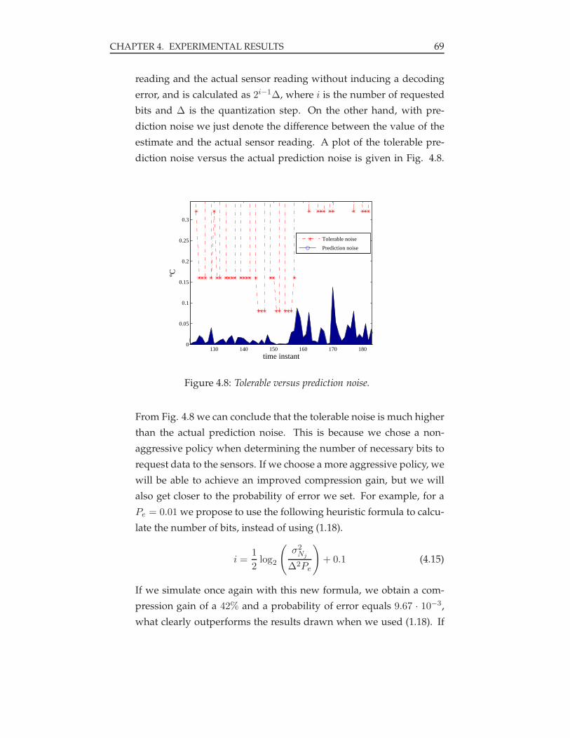
CHAPTER 4. EXPERIMENTAL RESULTS 69

reading and the actual sensor reading without inducing a decoding

error, and is calculated as 2i−1∆, where i is the number of requested

bits and ∆ is the quantization step. On the other hand, with pre-

diction noise we just denote the difference between the value of the

estimate and the actual sensor reading. A plot of the tolerable pre-

diction noise versus the actual prediction noise is given in Fig. 4.8.

130 140 150 160 170 1800

0.05

0.1

0.15

0.2

0.25

0.3

time instant

ºC

Tolerable noise

Prediction noise

Figure 4.8: Tolerable versus prediction noise.

From Fig. 4.8 we can conclude that the tolerable noise is much higher

than the actual prediction noise. This is because we chose a non-

aggressive policy when determining the number of necessary bits to

request data to the sensors. If we choose a more aggressive policy, we

will be able to achieve an improved compression gain, but we will

also get closer to the probability of error we set. For example, for a

Pe = 0.01 we propose to use the following heuristic formula to calcu-

late the number of bits, instead of using (1.18).

i =1

2log2

(σ2

Nj

∆2Pe

)+ 0.1 (4.15)

If we simulate once again with this new formula, we obtain a com-

pression gain of a 42% and a probability of error equals 9.67 · 10−3,

what clearly outperforms the results drawn when we used (1.18). If

CHAPTER 4. EXPERIMENTAL RESULTS 70

we plot again (Fig. 4.9) the tolerable noise versus the prediction noise

we can see how our margin has been reduced below the quantization

step.

130 140 150 160 170 1800

0.05

0.1

0.15

0.2

0.25

0.3

time instant

ºC

Tolerable noisePrediction noise

Figure 4.9: Tolerable versus prediction noise with improved number of requestedbits, i.

Chapter 5

Conclusions and Future Work

Wireless sensor networks are more than just a specific form of ad hoc net-

works. The stringent miniaturization and cost requirements make eco-

nomic usage of energy and computational power a significantly larger issue

than in normal ad hoc networks.

On the distributed and adaptive source coding, we implemented the al-

gorithm analyzed in Chapter 1, yielding an almost perfect tracking of the

environmental magnitudes being sensed. A compression gain of around

50% was shown to be achievable for large WSNs and enough number of

samples. Furthermore, the algorithm was shown to be robust to packet

losses through a simulation of a Gilbert-Elliott channel.

In the chapters of this thesis, different joint source-channel coding schemes

to reducing power consumption have been exposed and analyzed. Firstly,

we have dealt with ME coding and showed how a reduction of the MAI

can be achieved. ME coding allows to save energy when using a DS-CDMA

scheme in which the usual BPSK modulation is substituted by an OOK one,

which takes advantage of the large run of zeros. However, an enlarged

codeword may exhibit two major drawbacks: on the one hand it increases

the bit error probability, on the other it increases the power used on the

receiver.

To address this problem MME coding has been analyzed and compared to

ME coding in terms of relative gain. Novel expressions for the evaluation

of the bit error probability and the power gain have been provided.

71

CHAPTER 5. CONCLUSIONS AND FUTURE WORK 72

We have also proposed and solved a constrained minimization problem to

adapt the optimal transmission powers for the nodes in the WSN, so that

the consumed power in the network is the smallest possible while satisfy-

ing a given expected value of the SINR for each node.

Future lines of investigation should include an evaluation of the bit error

probability and the power gain using the expressions found in the work we

have developed. A modification to the constrained power minimization

algorithm is also thought to be carried out, setting different constraints.

Improved performance of the system is expected to be achieved with this

modification.

Appendix A

Source Coding Basics

A.1 Introduction

Communication systems are designed to transmit information from sources

to destinations. Sources of information can be analog or discrete. An exam-

ple of the former case can be a phone call, where generally, the source is an

audio signal. The output of this source is analog and, hence, they are called

”analog sources”. On the other hand, we have ”discrete sources” which

have discrete values as outputs, as can be the daily stock market index,

computer files. . .

Whether the source is analog or discrete, a digital communication system

is designed to transmit information, consequently, the output of a source

must be conveniently treated to be transmitted digitally. This function is

performed by the source encoder at the transmitter side, whose task is not

only to quantize the signal, but also to make an efficient representation of

the information in digital form (note we haven’t established yet what we

mean by efficient).

Obviously, the smaller number of bits is used to represent the signal (dur-

ing quantization), the less capacity of the channel is used, but the worse

fidelity is achieved. In general, we will permit a given level of distortion

in quantization and we will try to make the most efficient representation of

the levels the signal can take.

74

APPENDIX A. SOURCE CODING BASICS 75

A.2 Mathematical models for information sources

Any information source has an output that can be described statistically. In-

deed, if we knew the output of a source in advance (deterministic output),

there would be no need to transmit it.

Therefore, we need now to model each of the sources described before:

• The output of a discrete source is a sequence of letters belonging to a

finite alphabet of L possible letters: xi ∈ x1, x2...xL.

Each letter has a probability of occurrence:

pk = P (x = xk) (A.1)

L∑

k1

pk = 1 (A.2)

If every letter satisfies statistical independence among all past and

future outputs, we say it is a discrete memoryless source (DMS). On

the other hand, if the discrete output shows statistical dependence,

we should construct a mathematical model which fits this depen-

dence. For instance, a discrete source is said to be stationary if the

joint probabilities of two sequences of length n, say a1, a2, ..., an and

a1+m, a2+m, an+m are identical for n ≥ 1 and all possible shifts of m.

• An analog source can be modelled as one whose output presents a

waveform x(t), which is a sample function of a stochastic process

X(t). We assume that X(t) is stationary with correlation φXX(τ) and

power spectral density ΦXX(f) and bandlimited,ΦXX(f) = 0 ∀ |f | ≥B. The sampling theorem helps us to transmit the samples of the ana-

log signal ( xn = x(n) = x(nTs) = x(n 12B )) for further reconstruction

at the receiver side as:

X(t) =

∞∑

n=−∞X(

n

2B)Sa(2πB(t− n

2B)) (A.3)

Where Sa(x) is given by ...

Our previous analog signal is now a discrete-time signal.

APPENDIX A. SOURCE CODING BASICS 76

Finally, we should observe that the result of sampling an analog source

is usually a discrete-time continuous-amplitude signal, being neces-

sary to perform quantization to obtain a digital signal.

Where X( n2B ) denote the samples of the processX(t) taken at the Nyquist

rate ( fs = 2B samples/s ).

A.3 A logarithmic measure of information

Now we know the information provided by a source can be measured, we

should find an appropriate way to do it.

Suppose we have two random variables which can take values from a finite

alphabet each:

xi ∈ x1, x2, ..., xnyi ∈ y1, y2, ..., yn

If both are statistically independent, the information about X provided by

an event in Y is zero. On the other hand, if the occurrence of Y = yj

determines completely the occurrence of X = xj , then, the information the

event Y provides about X is the same as the information provided by xi.

Any measure of information we devise must fulfil the previous two condi-

tions; the following function appears to be suitable:

I(xi; yj) = logP (xi|yj)

P (xi), known as mutual information (A.4)

If we take log2 the units of the mutual information are called bits.

Let us check if it really satisfies the two conditions previously exposed:

1. If there is independence between both events,

I(xi; yj) = logP (xi|yj)

P (xi)= log

P (xi)

P (xi)= 0

APPENDIX A. SOURCE CODING BASICS 77

2. If occurrence of Y totally determines the occurrence of X, then

I(xi; yj) = logP (xi|yj)

P (xi)= log

1

P (xi)= I(xi), called self-information

(A.5)

We observe that a high-probability event conveys less information than

other with lower probability.

It is also truth that the information about xi provided by yj is identical than

the information provided by xi about the occurrence of yj .

I(xi; yj) = logP (xi|yj)

P (xi)= log

P (xi,yj)P (yj)

P (xi)= log

P (yj|xi)

P (yj)= I(yj;xi)

We can also define the conditional self-information as:

I(xi|yj) = log1

P (xi|yj)(A.6)

Therefore, the following relation holds true:

I(xi; yj) = I(xi) − I(xi|yj)

A.4 Average mutual information and entropy

We can step further and define the average mutual information betweenX

and Y as:

I(X;Y ) =

n∑

i=1

m∑

j=1

P (xi, yj)I(xi; yj) =

n∑

i=1

m∑

j=1

P (xi, yj) logP (xi, yj)

P (xi)P (yj)

(A.7)

It holds that I(X;Y ) ≥ 0 ∀ X,Y .

Identically, we can obtain the average self-information as:

H(X) =n∑

i=1

log1

P (xi)(A.8)

APPENDIX A. SOURCE CODING BASICS 78

Where X represents the alphabet of possible output letters from a source,

H(X) represents the average self-information per output and it is called

the entropy of the source.

H(X) is always less or equal than log(n) , where the equality holds when

symbols are equally probable.

Finally, we can define the average conditional self-information (or condi-

tional entropy) as:

H(X|Y ) =

n∑

i=1

m∑

j=1

P (xi, yj) log1

P (xi|yj)(A.9)

Again it is true: I(X;Y ) = H(X) −H(X|Y ) ≥ 0.

The results previously exposed can be generalized to more than two vari-

ables as:

H(X1X2...Xk) =k∑

i=1

H(Xi|X1X2...Xi−1) (A.10)

That satisfies:

H(X1X2...Xk) ≤k∑

m=1

H(Xm)

This information measures can easily be extended for continuous random

variables by simply applying some little changes.

Appendix B

Matlab and TinyOS: gettingthem to work together

B.1 Introduction

In this chapter we will go through the different aspects which are needed

to be taken into account when interconnecting Matlab and TinyOS, as well

as the way in which they have to be used. We will show why Matlab is a

suitable tool for interacting with WSNs.

Matlab is a scripting language in which large applications can be written

and is interpreted, which means that it is slower than other languages like

C or Java. However, being an interpreted scripting language is also part of

what makes Matlab an appealing way to interact with a sensor network:

the user can interact with the network by calling commands on the Matlab

command line. In contrast, once a java application is started, it can only be

controlled through a GUI.

It is possible to connect Matlab with the motes to receive and inject infor-

mation from and to the network. The system architecture will consist of a

sensor (or several) connected to the computer through the USB port, act-

ing as a data-gathering node, and many others sensing nodes. The sink

node will behave as base station receiving all the packets addressed to its

network address. From Matlab we will be able to connect to this mote, lis-

tening to the desired packets in the network and filtering the rest of them.

79

APPENDIX B. MATLAB AND TINYOS: GETTING THEM TO WORK

TOGETHER 80

We will also have full access to the message structure having the possibility

of accessing/editing the packets'fields in a java-oriented syntax. It will be

also possible to send packets to any sensor in the network, provoking reac-

tions (if programmed beforehand) which will make our network reactive.

Last but not least, Matlab is a complete programming development envi-

ronment having numerous tools for helping the developer in their work.

Thus, Matlab appears as an ideal environment for an easy and fast devel-

opment of a broad range applications.

B.2 Setting up the Matlab environment to use it with

TinyOS and Java

Step 1 The Matlab directory structure provided by TinyOS was meant to

mirror that of the tinyos-1.x directory. Each of the directories is meant

to serve the following purposes:

APPS holds Matlab functions that were built for a certain tinyOS ap-

plications, e.g. oscilloscopeRF.

CONTRIB contains subdirectories to mirror tinyos-x.x/contrib for

matlab applications.

LIB tools that correspond to tinyOS components in tos/lib.

TOOLS Matlab functions or apps that are generally useful but do

not relate specifically to one app (e.g. 'listen.m').

UTIL functions (not apps) that may be shared among several other

Matlab apps, eg. message processing utilities.

Add to your matlab directory in: your path to tinyos-1.x\tools\matlab

those directories above which are not present with the distribution.

Step 2 Create the file startup.m in the folder your path to Matlab\toolbox\local.

Edit the file with the following code:

flag=0;global TOSDIRTOSDIR='your path to UCB\cygwin \opt \tinyos-1.x \tos';

addpath your path to tinyos-1.x \tools \matlab;addpath your path to tinyos-1.x \tools \matlab \comm;

APPENDIX B. MATLAB AND TINYOS: GETTING THEM TO WORK

TOGETHER 81

addpath your path to tinyos-1.x \tools \matlab \apps;addpath your path to tinyos-1.x \tools \matlab \lib;addpath your path to tinyos-1.x \tools \matlab \util;addpath your path to tinyos-1.x \tools \matlab \tools;addpath your path to tinyos-1.x \tools \matlab \contrib;

defineTOSEnvironment;

Basically, what we do in this Matlab script is to set up the Matlab path

and call the script defineTOSEnvironment.m, which in turn, will ini-

tialize the Matlab comm (communications)stack. By giving the script

the name startup.m and placing it in the aforementioned directory,

we ensure the file is executed when Matlab starts up.

Step 3 Edit the file defineTOSEnvironment.m that you can find in your path to tinyos-

1.x\tools\matlab so that it looks like:

global DEBUGDEBUG = 0;

global COMMCOMM.TOSBCASTADDR = 65535;COMM.TOSUARTADDR = 126;COMM.GROUPID = hex2dec('7D');

defineComm;

Step 4 Copy the file comm.jar located in the following directory:

your path to UCB\jdk1.4.1 02\j2sdk1.4.1 02\jre\lib\ext to

your path to tinyos-1.x\tools\java

Step 5 Open the Matlab file classpath.txt and add the following pathes:your path to tinyos-1.x \tools \javayour path to tinyos-1.x \tools \java \comm.jaryour path to tinyos-1.x \tools \java \net \tinyos \message

Step 6 Copy the files win32com.dll and getenv.dll located in

your path to UCB\jdk1.4.1 02\j2sdk1.4.1 02\jre\bin

and the folder your path to tinyos-1.x\tools\java\jni in the Matlab folder

your path to Matlab\sys\java\jre\win32\jre1.4.2\bin

Also copy the file javax.comm.properties located in the folder

your path to UCB\jdk1.4.1 02\lib to the destination folder:

your path to Matlab\sys\java\jre\win32\jre1.4.2\lib

APPENDIX B. MATLAB AND TINYOS: GETTING THEM TO WORK

TOGETHER 82

Step 7 Edit the file cygwin.bat to include in the system classpath the fol-

lowing pathes:

your path to Matlab\java\jar\jmi.jar

your path to UCB\cygwin\opt\tinyos-1.x\tools\java\comm.jar

your path to UCB\cygwin\opt\tinyos-1.x\tools\java

Step 8 The net.tinyos.matlab.MatlabControl class is needed to call

Matlab commands from Java. Previously to compilation is manda-

tory to fix a bug in the MatlabControl.java file, by using the provided

patch file.

Once it has been fixed, proceed to compile the folder

your path to tinyos-1.x\tools\java\net\tinyos\matlab by typing make matlab .

Please, note that you should have already included the jar file jmi.jar

in your CLASSPATH environment variable (otherwise it returns the

error: package comm.mathworks.jmi does not exist )

Step 9 Before you are able to use the Matlab functions (connect, receive,

send and stopReceiving) provided along the TinyOS distribution, you

will have to go through several typographical errors:

1. Edit the file receive.m as below:

• Delete line 52

(moteIFs = [COM.sourceMoteIF TF]; ) to place instead:

if isempty(TF)TF=0;

elseTF=1;

endif TF==0

moteIFs=[];else

moteIFs = [COM.sourceMoteIF TF];end

• In line 63 take the transpose away.

2. Edit the script stopReceiving.m as follows:

• Substitute the code lines:

COMM.globalFunction=COMM.globalFunction ~TF;

APPENDIX B. MATLAB AND TINYOS: GETTING THEM TO WORK

TOGETHER 83

COMM.globalMessageType=COMM.globalMessageType ~TF;

COMM.globalMessageName=COMM.globalMessageName ~TF;

by

COMM.globalFunction= COMM.globalFunction ~TF;

COMM.globalMessageType= COMM.globalMessageType ~TF;

COMM.globalMessageName= COMM.globalMessageName ~TF;

• And the code lines:

for i=1:length(varagin)receive(functionName, message, varargin i )

by

for i=1:length(varargin)stopReceiving(functionName, message, varargin i )

Step 10 To finish with, it should be noticed that there still exist some bugs

in the Java code used by the Matlab scripts that will make necessary

to check the code carefully for every application.

B.3 Using the TinyOS java tool chain from Matlab

It is often easier to use an existing Java tool with TinyOS than to rewrite

it in Matlab. Thus, we can use Matlab to launch the Serial Forwarder, the

Oscilloscope application seen in the TinyOS tutorial [27], etc.

If we want to start the Oscilloscope application from Matlab, we should

enter the following command:

net.tinyos.oscope.oscilloscope.main('125')

You should see the Java GUI open and connect to your serial forwarder.

When using Java from Matlab the syntax remains basically the same, except

that there is no ”new” operator and functions with no arguments do not

terminate with empty parenthesis ”( )”.

Every time a value is returned or passed to a Java method, a conversion of

types takes place automatically (according to the information provided in

APPENDIX B. MATLAB AND TINYOS: GETTING THEM TO WORK

TOGETHER 84

the Matlab help). Most of the arguments are passed by value except for the

Java objects which are passed by reference.

Using Java classes from Matlab reveals two common bugs that should be

fixed before you obtain a successful execution. While both of these bugs do

not appear as such when running the java program from the default Java

environment (i.e. starting a Java application from the command line), they

do it when the program is called from Matlab. Thus, you will find them in

many Java classes, including those in the TinyOS Java toolset.

A. Command Line Arguments In this section you will learn with a very

simple example how to pass arguments from the Matlab command

line to a Java method.

Imagine you want to run the Serial Forwarder to listen to packets

arriving at port COM7. If you are calling the program from your

default shell you should type the following command:

java net.tinyos.sf.SerialForwarder -comm serial@COM7:t elos

To run the same program from the Matlab command line you should

write the command:

net.tinyos.sf.SerialForwarder.main( '-comm','serial@COM7:telos' )

From the previous example we can deduce that the shell automat-

ically packages up the command line arguments into string arrays

before passing them to the main function of the class being called.

In Matlab this has to be explicitly done by directly passing the argu-

ments as string arrays.

In case we do not want to pass any argument, we should send a null

array, which is done as:

net.tinyos.sf.SerialForwarder.main( )

We get a null pointer exception! This is because the static main func-

tion in the main class of the SerialForwarder uses the string before

checking if it is null. Since sending no command-line arguments from

the shell does not result in a null string being passed, this normally

does not cause an error. However, this should be fixed if this class

were to be used from Matlab.

APPENDIX B. MATLAB AND TINYOS: GETTING THEM TO WORK

TOGETHER 85

B. Virtual Machines You will have already realized that when we run a

program in Matlab we do not use the command java. This is due to

the fact that in Matlab we instantiate the objects within the same JVM

(Java Virtual Machine) in which the Matlab session is running. This

is only important for the java.lang.System class, which directly

refers to the JVM you are running in; java.lang.System.exit()

will kill your JVM, and therefore all the classes and your Matlab ses-

sion! You will see this if you close the SerialForwarder window, be-

cause this causes a call to System.exit() . Hence, System.exit()

should never be called.

B.4 Using Matlab with TinyOS

B.4.1 Preparing the message

Prior to connecting the computer to the network we need to build the mes-

sages to which we want to listen to. To illustrate this we will go through a

simple example and we will make use of the available tools we have.

Let us imagine we have a network in which the base station is polling the

nodes one by one and asking them to send back an application-specific

data.

We need to construct two kinds of messages, one carrying the request for

data to the sensors (SimpleCmdMsg) and another one carrying the data sent

back by the sensors (DataMsg).

We can build two header files each one with the message structure we have

devised, for example, if we list the code corresponding to the file Sim-

pleCmdMsg.h:

enum AMSIMPLECMDMSG = 18

;

typedef struct SimpleCmdMsg uint16 t dst;uint16 t source;uint16 t seqno;

APPENDIX B. MATLAB AND TINYOS: GETTING THEM TO WORK

TOGETHER 86

uint8 t type;uint8 t focusaddr;uint8 t newrate;uint8 t hop count;uint8 t bitsT;uint8 t bitsH;uint8 t bitsLtsr;uint8 t bitsLpar;

SimpleCmdMsg;

Once we have the messages in the header files, we can use the MIG tool (see

[27] for further information) to automatically generate Java classes which

take care of the cumbersome details of packing and unpacking fields in

the message's byte format. Using MIG saves you from parsing message

formats in your Java application.

Once we have the output from MIG: SimpleCmdMsg.java and DataMsg.java

we can proceed to compile them, obtaining the respective .class files.

Now we can easily instantiate these objects in Matlab.

B.4.2 Connecting Matlab to the network

This subsection does not intend to be a detailed guide of how to use Mat-

lab with TinyOS because it would be a redundant work over that present

in [27]. We will just try to provide a basic understanding of the overall

working by continuing with the example we started in section B.4.1.

The first step is to connect your Matlab session to your network (namely to

your base station). If you are working with Tmotes this can be done as:

connect('serial@COM7:telos');

Where, same as before, we are assuming that your base station is identified

by the serial port COM7(you can use the command motelist in your cyg-

win environment to check what devices are connected to your computer).

Once you have done this, you can instantiate the MIG message, which is a

Java class that is a subclass of net.tinyos.message.Message . In Mat-

lab you can instantiate Java objects on the command line as follows:

APPENDIX B. MATLAB AND TINYOS: GETTING THEM TO WORK

TOGETHER 87

dataMsg=net.tinyos.report.DataMsg

Now you are prepared to start receiving packets:

receive('handleMsg',dataMsg)

This command specifies the Matlab function handleMsg as the one in charge

for handling the received messages, and the DataMsg messages as the ones

to which the base station is listening to. Any other arriving packet will be

discarded.

If we want to send a packet to a node:

send(3,simpleCmdMsg)

Where simpleCmdMsg is an instance of the class SimpleCmdMsg sent to the

node with network address 3.

At this point, the DataMsg objects should be printed to your screen every

time a message of this type is received. To stop this behaviour you can

use the stopReceiving command to deregister your Matlab function as

a message handler:

stopReceiving('handleMsg',dataMsg)

Finally, you can disconnect yourself from the sensor you are connected to

with the command:

disconnect('serial@COM7:telos')

Appendix C

Acronyms

ADC Analog to Digital Converter

AWGN Additive White Gaussian Noise

BER Bit Error Rate

BPSK Binary Phase Shift Keying

CRC Cyclic Redundancy Check

dB decibel

DCO Digitally Controlled Oscillator

DMS Discrete Memory Source

DS-CDMA Direct Sequence - Coded Division Multiple Access

IM Initialization Module

IR Infrared

IS International System

Kbps Kilobits per second

KTH Kungliga Tekniska Hogskolan

LMS Least-Mean-Squares

LSB Least Significative Bit

MAI Multiple Access Interference

ME Minimum Energy

MME Modified Minimum Energy

MSE Mean Square Error

OOK On-Off Keying

PAR Photosynthetically Active Radiation

PDA Personal Digital Assistant

88

APPENDIX C. ACRONYMS 89

PN Pseudorandom Noise

RF Radio Frequency

SINR Signal to Interference + Noise Ratio

SMA Surface Mount Assembly

TSR Total Solar Radiation

USB Universal Serial Bus

VCP Virtual Com Port

WSN Wireless Sensor Networks

Bibliography

[1] S. Toumpis and A.J. Goldsmith. ”Capacity Regions for Wireless ad

hoc Networks”. In IEEE Trans. on Wireless Communications, volume 24,

pages 3003–3008, May 2003.

[2] Dragan Petrovic, Kannan Ramchandran, and Jim Chou. ”A Dis-

tributed and Adaptive Signal Processing Approach to Reducing En-

ergy Consumption in Sensor Networks”. In IEEE INFOCOM, 2003.

[3] C. Toh. ”Maximum Battery Life Routing to Support Ubiquitous Mo-

bile Computing in Wireless AD-HOC Networks”. In IEEE Communi-

cations Magazine, pages 138–147, June 2001.

[4] R. Shah and J. Rabaey. ”Energy Aware Routing for Low Energy ad-hoc

Sensor Networks”. In Proc. of IEEE WCNC, March 2002.

[5] D.E.C. Intanagonwiwat and R. Govindan. ”Directed Difussion: a Scal-

able and Robust Communication Paradigm for Sensor Networks”. In

Proc. of IEEE MobiCom, August 2002.

[6] G. Pottie and W. Kaiser. ”Wireless Sensor Networks”. In Communica-

tions of the ACM, 2000.

[7] M. Chu, H. Haussecker, and F. Zhao. ”Scalable Information-driven

Sensor Querying and Routing for ad hoc Heterogeneous Sensor Net-

works”. In IEEE Journal of High Performance Computing Applications,

2002.

[8] R. Blahut. Theory and Practice of Data Transmission Codes. 1995.

90

BIBLIOGRAPHY 91

[9] I.F. Akylidiz, W.Y. Sankarasubramaniam, and E. Cayirci. ”A Survey on

Sensor Networks”. In IEEE Communications Magazine, pages 102–114,

August 2002.

[10] E. Shih, H. Calhoun, S. Cho, and A.P. Chandrakasan. ”Energy-Efficient

Link Layer for Wireless Microsensor Networks”. In IEEE Computer

Society Workshop on VLSI, pages 16–21, April 2001.

[11] C. Erin and H.H. Asada. ”Energy Optimal Codes for Wireless Com-

munications”. In Proc. of the 38th IEEE Conference of Decision and Con-

trol, volume 5, pages 4446–4453, December 1999.

[12] Y. Prakash and S.K. Gupta. ”Energy Efficient Source Coding and Mod-

ulation for Wireless Applications”. In Proc. or IEEE WCNC, volume 1,

pages 212–217, March 2003.

[13] M.B. Pursley. ”Performance Evaluation for Phase-Coded Spread-

Spectrum Multiple-Acces Communication - Part I: System Analysis”.

In IEEE Transactions on communications, volume COM. 25, pages 795–

799, August 1977.

[14] S. Yao and E. Geraniotis. ”Optimal Power Control Law for Multimedia

Multirate CDMA Systems”. In IEEE 46th Vehicular Technology Confer-

ence: ’Mobile Technology for the Human Race’, volume 1, pages 392–396,

April 1996.

[15] F. Santucci, G. Durastante, F. Graziosi, and C. Fischione. ”Power Al-

location and Control in Multimedia CDMA Wireless Systems”. In

Telecommunication Systems, volume 23, pages 69–94. Springer Nether-

lands, June 2003.

[16] A. Popoulis. ”Probability, Random Variables, and Stochastic Processes”.

McGraw-Hill, 1984.

[17] M. Zuniga and B. Krishnamachari. ”Analyzing the Transational Re-

gion in Low Power Wireless Links”. In IEEE SECON, 2004.

[18] C. Fischione, A. Bonivento, K.H. Johansson, and A. Sangiovanni-

Vincentelli. ”Cooperative Diversity with Disconnection Constraints

BIBLIOGRAPHY 92

and Sleep Discipline for Power Control in Wireless Sensor Networks”.

In IEEE VTC, 2006.

[19] J.B. Andersen, T.S. Rappaport, and S. Yoshida. ”Propagation Measure-

ments and Models for Wireless Communications Channels”. In IEEE

Communications Magazine, pages 42–49, January 1995.

[20] Chipcon Products by Texas Instruments. 2.4 GHz IEEE 802.15.4 /

ZigBee-ready RF Transceiver, 2006.

[21] John G. Proakis. Digital Communications. Electrical Engineering. Mc-

Graw Hill International Editions, third edition, 1995.

[22] Holtzman. ”A Simple, Accurate Method to Calculate Spread-

Spectrum Multiple-Access Error Probabilities”. In IEEE Trans. Comm.,

volume 40, pages 461–464, 1992.

[23] J. Kim and J.G. Andrews. ”An Energy Efficient Source Coding and

Modulation Scheme for Wireless Sensor Networks”. In IEEE 6th Work-

shop on Signal Processing Advances in Wireless Communications, pages

710–714, June 2005.

[24] Moteiv Corporation. Telos: Ultra low power IEEE 802.15.4 compliant

wireless sensor module. Revision B : Humidity, Light, and Temperature sen-

sors with USB, 2004.

[25] S. Haykin. Adaptive Filter Theory. PrenticeHall, third edition, 1996.

[26] E. N. Gilbert. ”Capacity of a Burst-Noise Channel”. In The Bell System

Technical Journal, volume 39, pages 1253–1265, September 1960.

[27] TinyOS Community Forum. TinyOS tutorial, September 2003.

[28] L. Schwiebert, S.K.S. Gupta, P.S.G. Auner, G. Abrams, R. Lezzi, and

P. McAllister. ”A Biomedical Smart Sensor for Visually Impaired”.

Technical report, IEEE Sensors, June 2002.

[29] B. Yang, S. Rhee, and H.H. Asada. ”A Twenty-four Hour Tele-nursing

System Using a Ring Sensor”. In Proc. of the IEEE International Confer-

ence on Robotics and Automation, volume 1, 1998.

BIBLIOGRAPHY 93

[30] C.H. Liu and H.H. Asada. ”A Source Coding and Modulation Method

for Power Saving and Interference Reduction in DS-CDMA Sensor

Network Systems. In Proc. of American Control Conf., volume 4, pages

3003–3008, May 2002.

[31] B. Hashem and E. Sousa. ”Performance Evaluation of DS-CDMA Sys-

tems Employing Adaptive Transmission Rate under Imperfect Power

Control”. In Proc. of IEEE ICC’98, 1998.

[32] K. Sipila et al. ”Modelling the Impact of the Fast Power Control on

the WCDMA Uplink”. In Proc. of IEEE VTC’99, pages 1266–1270, May

1999.