ii

ii

ii

ii

Adaptive Scalable TextureCompressionStacy Smith, ARM

1.1 Introduction

Adaptative Scalable Texture Compression (ASTC) is a new texture com-pression format which is set to take the world by storm. Having beenaccepted as a new Khronos standard, this compression format is alreadyavailable in some hardware platforms. This article shows how it works, howto use it, and how to get the most out of it. For more in-depth information,there is a full specification provided with the encoder [Eva ].

1.2 Background

ASTC was developed by ARM Limited as the flexible solution to thesparsely populated list of texture compression formats previously avail-able. In the past, texture compression methods were tuned for one or morespecific sweet spot combinations of data channels and related bit rates.Worsening the situation was the proprietary nature of many of these for-mats, limiting availability to specific vendors, and leading to the currentsituation where applications have to fetch an additional asset archive overthe internet after installation, based on the detected available formats.The central foundation of ASTC is that it can compress an input imagein every commonly used format (Table 1.1) and output that image in anyuser selected bit rate, from 8bpp to 0.89bpp, or 0.59bpp for 3D textures(Table 1.2).

Bitrates below 1bpp are achieved by a clever system of variable blocksizes. Whereas most block based texture compression methods have a singlefixed block size, ASTC can store an image with a regular grid of blocks ofany size from 4x4 to 12x12 (including non square block sizes). ASTC canalso store 3D textures, with block sizes ranging from 3x3x3 to 6x6x6.

Regardless of the blocks’ dimensions, they are always stored in 128 bits,hence the sliding scale of bit rates.

1

ii

ii

ii

ii

2 1. Adaptive Scalable Texture Compression

Raw input format Bits per pixelHDR RGB+A 64HDR RGBA 64HDR RGB 48

HDR XY+Z 48HDR X+Y 32

RGB+A 32RGBA 32XY+Z 24RGB 24

HDR L 16X+Y 16LA 16L 8

Table 1.1. Bitrates of raw image for-mats

Output Block Size 1 Bits per pixel4x4 8.0005x5 5.1206x6 3.5568x8 2.000

10x10 1.28012x12 0.8893x3x3 4.7414x4x4 2.0005x5x5 1.0246x6x6 0.5934x6 5.3338x10 1.60012x10 1.067

Table 1.2. Bitrates of ASTC output

1.3 Algorithm

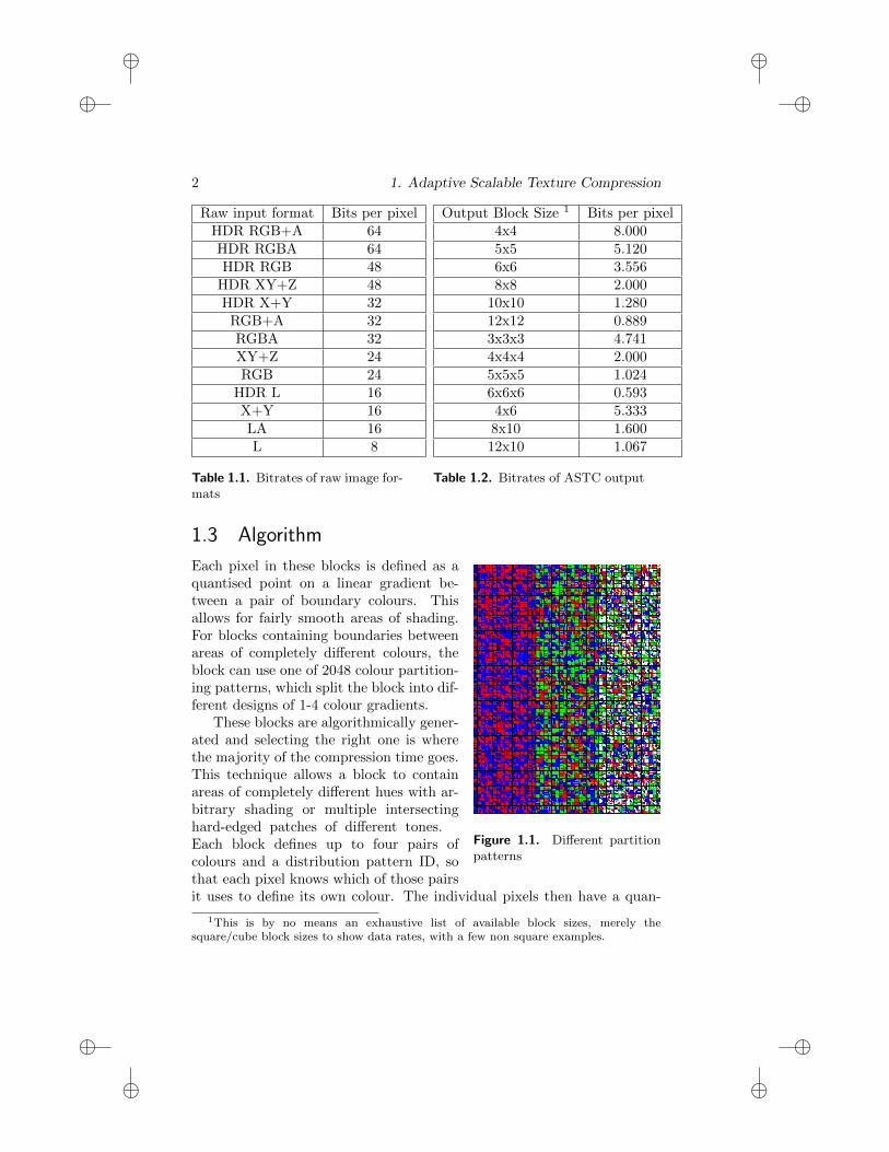
Figure 1.1. Different partitionpatterns

Each pixel in these blocks is defined as aquantised point on a linear gradient be-tween a pair of boundary colours. Thisallows for fairly smooth areas of shading.For blocks containing boundaries betweenareas of completely different colours, theblock can use one of 2048 colour partition-ing patterns, which split the block into dif-ferent designs of 1-4 colour gradients.

These blocks are algorithmically gener-ated and selecting the right one is wherethe majority of the compression time goes.This technique allows a block to containareas of completely different hues with ar-bitrary shading or multiple intersectinghard-edged patches of different tones.Each block defines up to four pairs ofcolours and a distribution pattern ID, sothat each pixel knows which of those pairsit uses to define its own colour. The individual pixels then have a quan-

1This is by no means an exhaustive list of available block sizes, merely thesquare/cube block sizes to show data rates, with a few non square examples.

ii

ii

ii

ii

1.3. Algorithm 3

tised value from 0 to 1 to state where they are on the gradient between thegiven pair of colours.1 Due to the variable number of bounding colours andindividual pixels in each 128 bit block, the precision of each pixel withinthe block is quantised to fit in the available remaining data size.

During compression, the algorithm must select the correct distributionpattern and boundary colour pairs, then generate the quantised value foreach pixel. There is a certain degree of trial and error involved in theselection of patterns and boundary colours, and when compressing, there isa trade off between compression time and final image quality. The higherthe quality, the more alternatives the algorithm will try before decidingwhich is best. However long the compression takes, the decompressiontime is fixed, as the image data can always be re-extrapolated from thepattern and boundary colours in a single pass.

The compression algorithm can also use different metrics to judge thequality of different attempts, from pure value ratios of signal to noise,to a perceptual judgement weighted towards human visual acuity. Thealgorithm can also judge the channels individually rather than as a whole,to preserve detail for textures where the individual channels may be usedas a data source for a shader program, or to reduce angular noise, which isimportant for tangent space normal maps.

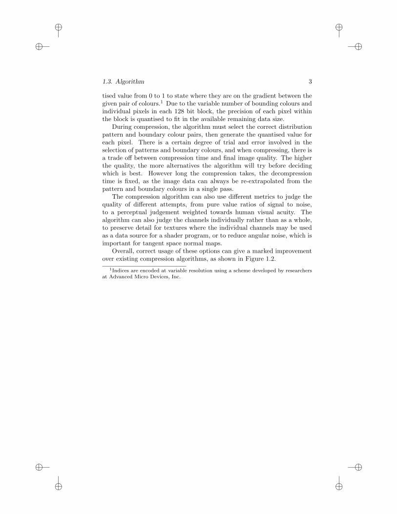
Overall, correct usage of these options can give a marked improvementover existing compression algorithms, as shown in Figure 1.2.

1Indices are encoded at variable resolution using a scheme developed by researchersat Advanced Micro Devices, Inc.

ii

ii

ii

ii

4 1. Adaptive Scalable Texture Compression

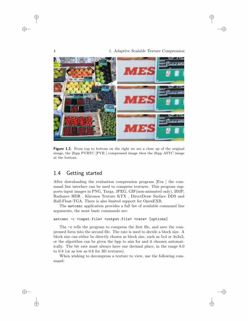
Figure 1.2. From top to bottom on the right we see a close up of the originalimage, the 2bpp PVRTC [PVR ] compressed image then the 2bpp ASTC imageat the bottom.

1.4 Getting started

After downloading the evaluation compression program [Eva ] the com-mand line interface can be used to compress textures. This program sup-ports input images in PNG, Targa, JPEG, GIF(non-animated only), BMP,Radiance HDR , Khronos Texture KTX , DirectDraw Surface DDS andHalf-Float-TGA. There is also limited support for OpenEXR.

The astcenc application provides a full list of available command linearguments, the most basic commands are:

astcenc -c <input.file> <output.file> <rate> [options]

The -c tells the program to compress the first file, and save the com-pressed form into the second file. The rate is used to decide a block size. Ablock size can either be directly chosen as block size, such as 5x4 or 3x3x3,or the algorithm can be given the bpp to aim for and it chooses automat-ically. The bit rate must always have one decimal place, in the range 8.0to 0.8 (or as low as 0.6 for 3D textures).

When wishing to decompress a texture to view, use the following com-mand:

ii

ii

ii

ii

1.4. Getting started 5

astcenc -d <input.file> <output.file> [options]

In this case, the -d denotes a decompression, the input file is a tex-ture which has already been compressed, and the output file is one of theuncompressed formats.

To see what a texture would look like compressed with a given set ofoptions, use the command:

astcenc -t <input.file> <output.file> <rate> [options]

The -t option compresses the file with the given options then immediatelydecompresses it into the output file. The interim compressed image is notsaved, and the input and output files are both in a decompressed file format.

The options can be left blank but to get a good result there are a fewuseful ones to remember.

The most useful arguments are the quality presets:

-veryfast

-fast

-medium

-thorough

-exhaustive

There are many available options to set various compression quality factorsincluding:

• The number and scope of block partition patterns to attempt.

• The various signal to noise cut-off levels to early out of the individualdecision making stages.

• The maximum iterations of different bounding colour tests.

Most users won’t explore all of these to find the best mix for their ownneeds. Therefore, the quality presets can be used to give a high level hintto the compressor, from which individual quality factors are derived.

It should be noted that veryfast, whilst almost instantaneous, gives goodresults only for a small subset of input images. Conversely, the exhaustivequality level (which does exactly what it says and attempts every possiblebounding pattern combination for every block) takes a very much longertime, but will often have very little visible difference to a file compressedin thorough mode.

ii

ii

ii

ii

6 1. Adaptive Scalable Texture Compression

1.5 Using ASTC Textures

ASTC capability is a new hardware feature available from late 2013. Toget started with ASTC right away the ARM R© Mali

TM

OpenGL R© ES 3.0Emulator [Ope ] is available from ARM’s website and this is compatiblewith ASTC texture formats and as such can be used to test ASTC basedprograms on a standard desktop GPU.

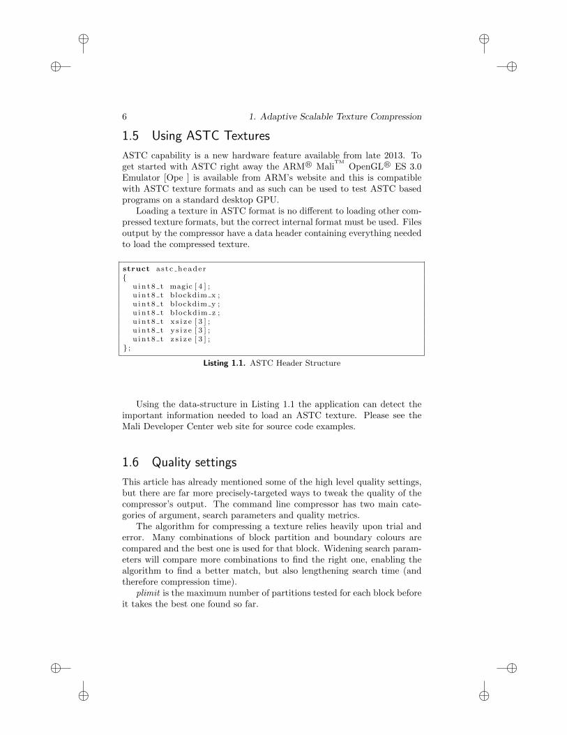
Loading a texture in ASTC format is no different to loading other com-pressed texture formats, but the correct internal format must be used. Filesoutput by the compressor have a data header containing everything neededto load the compressed texture.

struct a s t c heade r{

u i n t 8 t magic [ 4 ] ;u i n t 8 t blockdim x ;u i n t 8 t blockdim y ;u i n t 8 t blockdim z ;u i n t 8 t x s i z e [ 3 ] ;u i n t 8 t y s i z e [ 3 ] ;u i n t 8 t z s i z e [ 3 ] ;

} ;

Listing 1.1. ASTC Header Structure

Using the data-structure in Listing 1.1 the application can detect theimportant information needed to load an ASTC texture. Please see theMali Developer Center web site for source code examples.

1.6 Quality settings

This article has already mentioned some of the high level quality settings,but there are far more precisely-targeted ways to tweak the quality of thecompressor’s output. The command line compressor has two main cate-gories of argument, search parameters and quality metrics.

The algorithm for compressing a texture relies heavily upon trial anderror. Many combinations of block partition and boundary colours arecompared and the best one is used for that block. Widening search param-eters will compare more combinations to find the right one, enabling thealgorithm to find a better match, but also lengthening search time (andtherefore compression time).

plimit is the maximum number of partitions tested for each block beforeit takes the best one found so far.

ii

ii

ii

ii

1.6. Quality settings 7

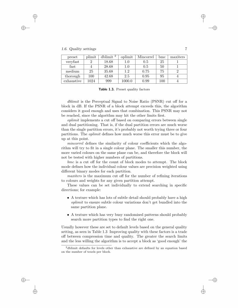
preset plimit dblimit 2 oplimit Mincorrel bmc maxitersveryfast 2 18.68 1.0 0.5 25 1

fast 4 28.68 1.0 0.5 50 1medium 25 35.68 1.2 0.75 75 2thorough 100 42.68 2.5 0.95 95 4

exhaustive 1024 999 1000.0 0.99 100 4

Table 1.3. Preset quality factors

dblimit is the Perceptual Signal to Noise Ratio (PSNR) cut off for ablock in dB. If the PSNR of a block attempt exceeds this, the algorithmconsiders it good enough and uses that combination. This PSNR may notbe reached, since the algorithm may hit the other limits first.

oplimit implements a cut off based on comparing errors between singleand dual partitioning. That is, if the dual partition errors are much worsethan the single partition errors, it’s probably not worth trying three or fourpartitions. The oplimit defines how much worse this error must be to giveup at this point.

mincorrel defines the similarity of colour coefficients which the algo-rithm will try to fit in a single colour plane. The smaller this number, themore varied colours on the same plane can be, and therefore the block willnot be tested with higher numbers of partitions.

bmc is a cut off for the count of block modes to attempt. The blockmode defines how the individual colour values are precision weighted usingdifferent binary modes for each partition.

maxiters is the maximum cut off for the number of refining iterationsto colours and weights for any given partition attempt.

These values can be set individually to extend searching in specificdirections; for example:

• A texture which has lots of subtle detail should probably have a highoplimit to ensure subtle colour variations don’t get bundled into thesame partition plane.

• A texture which has very busy randomised patterns should probablysearch more partition types to find the right one.

Usually however these are set to default levels based on the general qualitysetting, as seen in Table 1.3 Improving quality with these factors is a tradeoff between compression time and quality. The greater the search limitsand the less willing the algorithm is to accept a block as ‘good enough’ the

2dblimit defaults for levels other than exhaustive are defined by an equation basedon the number of texels per block.

ii

ii

ii

ii

8 1. Adaptive Scalable Texture Compression

more time is spent looking for a better match. There is another way to geta better match though, and that is to adjust the quality metrics, alteringthe factors by which the compressor judges the quality of a block.

1.6.1 Channel weighting

The simplest quality factors are channel weighting, using the command lineargument:

-ch <red-weight> <green-weight> <blue-weight> <alpha-weight>

This defines weighting values for the noise calculations. For example theargument -ch 1 4 1 1 makes error on the green channel four times moreimportant than noise on any other given channel. The argument -ch 0.25

1 0.25 0.25 would appear to the same effect but that assumption is onlypartly correct. This would still make errors in the green channel four timesmore prevalent, but the total error would be lower, and therefore morelikely to be accepted by a ‘good enough’ early out.

Channel weighting works well when combined with swizzling, using the-esw argument. For textures without alpha, for example, the swizzle -esw

rgb1 saturates the alpha channel and subsequently doesn’t count it in noisecalculations.

1.6.2 Block weighting

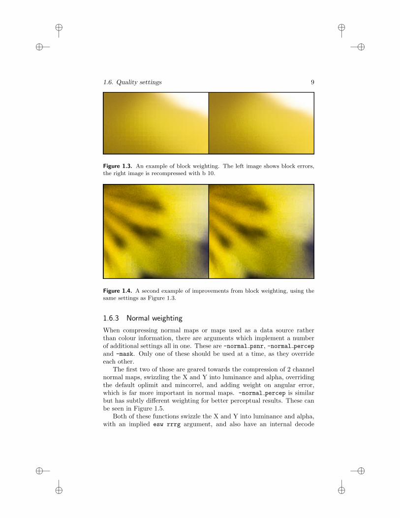
Though human eyesight is more sensitive to variations in green and lesssensitive to variations in red, channel weighting has limited usefulness.Other weights can also improve a compressed texture in a number of usecases. One of these is block error checking, particularly on textures withcompound gradients over large areas. By default there is no error weightbased on inter-block errors. The texels at the boundary of two adjacentblocks may be within error bounds for their own texels, but with noise inopposing directions, meaning that the step between the blocks is noticeablylarge. This can be countered with the command line argument:

b <weight>

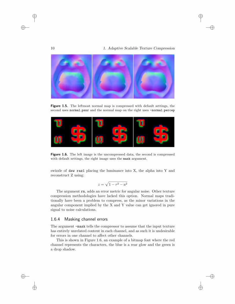
The equation to judge block suitability takes into account the edges of anyadjacent blocks already processed. Figure 1.3 and 1.4 show this in action.However this simply makes the search algorithm accept blocks with bettermatching edges more readily than others, so it may increase noise in otherways. Awareness of adjacent smooth blocks can be particularly helpful fornormal maps.

ii

ii

ii

ii

1.6. Quality settings 9

Figure 1.3. An example of block weighting. The left image shows block errors,the right image is recompressed with b 10.

Figure 1.4. A second example of improvements from block weighting, using thesame settings as Figure 1.3.

1.6.3 Normal weighting

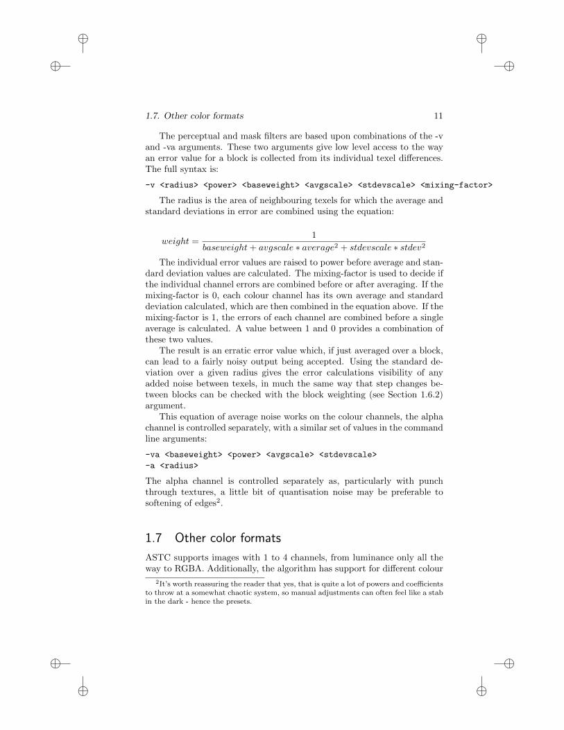
When compressing normal maps or maps used as a data source ratherthan colour information, there are arguments which implement a numberof additional settings all in one. These are -normal psnr, -normal percep

and -mask. Only one of these should be used at a time, as they overrideeach other.

The first two of those are geared towards the compression of 2 channelnormal maps, swizzling the X and Y into luminance and alpha, overridingthe default oplimit and mincorrel, and adding weight on angular error,which is far more important in normal maps. -normal percep is similarbut has subtly different weighting for better perceptual results. These canbe seen in Figure 1.5.

Both of these functions swizzle the X and Y into luminance and alpha,with an implied esw rrrg argument, and also have an internal decode

ii

ii

ii

ii

10 1. Adaptive Scalable Texture Compression

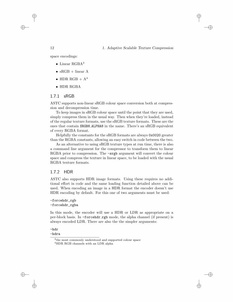
Figure 1.5. The leftmost normal map is compressed with default settings, thesecond uses normal psnr and the normal map on the right uses -normal percep

Figure 1.6. The left image is the uncompressed data, the second is compressedwith default settings, the right image uses the mask argument.

swizzle of dsw raz1 placing the luminance into X, the alpha into Y andreconstruct Z using:

z =√

1 − r2 − a2

The argument rn, adds an error metric for angular noise. Other texturecompression methodologies have lacked this option. Normal maps tradi-tionally have been a problem to compress, as the minor variations in theangular component implied by the X and Y value can get ignored in puresignal to noise calculations.

1.6.4 Masking channel errors

The argument -mask tells the compressor to assume that the input texturehas entirely unrelated content in each channel, and as such it is undesirablefor errors in one channel to affect other channels.

This is shown in Figure 1.6, an example of a bitmap font where the redchannel represents the characters, the blue is a rear glow and the green isa drop shadow.

ii

ii

ii

ii

1.7. Other color formats 11

The perceptual and mask filters are based upon combinations of the -vand -va arguments. These two arguments give low level access to the wayan error value for a block is collected from its individual texel differences.The full syntax is:

-v <radius> <power> <baseweight> <avgscale> <stdevscale> <mixing-factor>

The radius is the area of neighbouring texels for which the average andstandard deviations in error are combined using the equation:

weight =1

baseweight + avgscale ∗ average2 + stdevscale ∗ stdev2

The individual error values are raised to power before average and stan-dard deviation values are calculated. The mixing-factor is used to decide ifthe individual channel errors are combined before or after averaging. If themixing-factor is 0, each colour channel has its own average and standarddeviation calculated, which are then combined in the equation above. If themixing-factor is 1, the errors of each channel are combined before a singleaverage is calculated. A value between 1 and 0 provides a combination ofthese two values.

The result is an erratic error value which, if just averaged over a block,can lead to a fairly noisy output being accepted. Using the standard de-viation over a given radius gives the error calculations visibility of anyadded noise between texels, in much the same way that step changes be-tween blocks can be checked with the block weighting (see Section 1.6.2)argument.

This equation of average noise works on the colour channels, the alphachannel is controlled separately, with a similar set of values in the commandline arguments:

-va <baseweight> <power> <avgscale> <stdevscale>

-a <radius>

The alpha channel is controlled separately as, particularly with punchthrough textures, a little bit of quantisation noise may be preferable tosoftening of edges2.

1.7 Other color formats

ASTC supports images with 1 to 4 channels, from luminance only all theway to RGBA. Additionally, the algorithm has support for different colour

2It’s worth reassuring the reader that yes, that is quite a lot of powers and coefficientsto throw at a somewhat chaotic system, so manual adjustments can often feel like a stabin the dark - hence the presets.

ii

ii

ii

ii

12 1. Adaptive Scalable Texture Compression

space encodings:

• Linear RGBA3

• sRGB + linear A

• HDR RGB + A4

• HDR RGBA

1.7.1 sRGB

ASTC supports non-linear sRGB colour space conversion both at compres-sion and decompression time.

To keep images in sRGB colour space until the point that they are used,simply compress them in the usual way. Then when they’re loaded, insteadof the regular texture formats, use the sRGB texture formats. These are theones that contain SRGB8 ALPHA8 in the name. There’s an sRGB equivalentof every RGBA format.

Helpfully the constants for the sRGB formats are always 0x0020 greaterthan the RGBA constants, allowing an easy switch in code between the two.

As an alternative to using sRGB texture types at run time, there is alsoa command line argument for the compressor to transform them to linearRGBA prior to compression. The -srgb argument will convert the colourspace and compress the texture in linear space, to be loaded with the usualRGBA texture formats.

1.7.2 HDR

ASTC also supports HDR image formats. Using these requires no addi-tional effort in code and the same loading function detailed above can beused. When encoding an image in a HDR format the encoder doesn’t useHDR encoding by default. For this one of two arguments must be used:

-forcehdr_rgb

-forcehdr_rgba

In this mode, the encoder will use a HDR or LDR as appropriate on aper-block basis. In -forcehdr rgb mode, the alpha channel (if present) isalways encoded LDR. There are also the the simpler arguments:

-hdr

-hdra

3the most commonly understood and supported colour space4HDR RGB channels with an LDR alpha

ii

ii

ii

ii

1.8. 3D Textures 13

Which are equivalent to -forcehdr rgb and -forcehdr rgba but withadditional alterations to the evaluation of block suitability (a preset -v and-va) better suited for HDR images. Also available are:

-hdr_log

-hdra_log

These are similar but base their suitability on logarithmic error. Imagesencoded with this setting typically give better results from a mathematicalperspective but don’t hold up as well in terms of perceptual artefacts.

1.8 3D Textures

The compression algorithm can also handle 3D textures at a block level.Although other image compression algorithms can be used to store andaccess 3D textures, they are compressed in 2D space as a series of singletexel layers, whereas ASTC compresses 3 dimensional blocks of texturedata, improving the cache hit rate of serial texture reads along the Z axis.Currently there are no suitably prolific 3D image formats to accept asinputs, as such encoding a 3D texture has a special syntax:

-array <size>

With this command line argument the input file is assumed to be a prefixpattern for the actual inputs, and decorate the file name with 0, 1, and soon all the way up to <size-1>. So for example if the input file was slice.pngwith the argument array 4 the compression algorithm would attempt toload files named slice 0.png, slice 1.png, slice 2.png, and slice 3.png. Thepresence of multiple texture layers would then be taken as a signal to usea 3D block encoding for the requested rate (see Table 1.2).

1.9 Summary

This article shows the advantages of ASTC over other currently availabletexture compression methodologies, and provides code to easily use ASTCtexture files in an arbitrary graphics project, as well as a detailed expla-nation of the command line arguments to get the most out of the theevaluation codec.

ARM provides a free Texture Compression Tool [Tex ] that automatesthe ASTC command line arguments explained in this paper via a GraphicalUser Interface (GUI) which simplifies the compression process and providesvisual feedback on compression quality.

ii

ii

ii

ii

14 BIBLIOGRAPHY

Bibliography

[et. al. 12] Jorn Nystad et. al. “Adaptive Scalable Texture Compression.”pp. 105–114.

[Eva ] “ASTC Codec and Source.” Available online (http://malideveloper.arm.com/develop-for-mali/tools/astc-evaluation-codec/).

[Ope ] “OpenGL ES SDK Emulator.” Available on-line (http://malideveloper.arm.com/develop-for-mali/sdks/opengl-es-sdk-for-linux/).

[PVR ] “Texture Compression using Low-Frequency SignalModulation.”Available online (http://web.onetel.net.uk/∼simonnihal/assorted3d/fenney03texcomp.pdf/).

[Tex ] “Texture Compression Tool.” Available on-line (http://malideveloper.arm.com/develop-for-mali/mali-gpu-texture-compression-tool/).