Adaptive numerical analysis in primal elastoplasticity with hardening

ELSEVIER Comput. Methods Appl. Mech. Engrg. 171 (1999) 175-204

Computer methods in applied

mechanics and engineering

Adaptive numerical analysis in primal elastoplasticity with hardening

J o c h e n A l b e r t y , C a r s t e n C a r s t e n s e n * , D a r i u s Za r r ab i University of Kiel, Mathematisches Seminar II. Ludewig-Meyn-Str, 4, 24098 Kiel, German),

Received 15 February 1998; revised 30 April 1998

Abstract

The quasi-static viscoplastic resp. elastoplastic evolution problem with isotropic or kinematic hardening is considered with emphasis on optimal convergence and adapted mesh-refining in the spatial discretization. Within one time-step of an implicit time-discretization, the finite element method leads to a minimisation problem for non-smooth convex functions on discrete subspaces. For piecewise constant resp. affine ansatz functions, the stress resp. displacement approximations are experimentally and theoretically shown to converge linearly. An a posteriori error estimate then justifies an automatic adaptive mesh-refining algorithm. Numerical examples support the superiority of the adapted mesh. © 1999 Published by Elsevier Science S.A. All rights reserved.

I. Introduction

In the engineering literature, the elastoplastic evolution problem is usually modelled with yield functions and flow rules written in terms of admissible stresses. In the discretization of this, Han and Reddy [1] call dual formulation, displacement and stress approximations are computed simultaneously. The elastoplastic material behaviour can equivalently be modelled by what Han and Reddy [1] call primal formulation where the strains are the primary variables and so a discretization requires the simultaneous approximation of the displacement and plastic strain field.

In this paper, we study the primal formulation and present a refined a priori and a posteriori error analysis for the spatial discretization. For a convenient reading, we outline both, the strain and stress formulation of plasticity, and their duality in Section 2. Within each time-step of the primal formulation in Section 3, we have to minimise a Lipschitz-continuous, but non-smooth convex functional over a linear space (not merely a convex set as in the dual method). The spatial Galerkin discretization in Section 4 is simple: replace the linear space by a conform FE-space.

Notice that the stress related dual model results in a minimisation of a quadratic problem over a convex set and so raises the question of the conform or non-conform approximation of sets. In particular, this is problematic for hp-methods (with higher order polynomial ansatz functions) where the discrete stress field satisfies the yield conditions in a finite set of discrete points rather than almost everywhere.

The error analysis of the time-discretized primal formulation, also called Hencky plasticity, time-independent plasticity, or holonomic plasticity, is the main topic of this paper. In the simplest spatial FE-discretization (piecewise affine displacements) with (largest) mesh-size h, the a priori error estimates in the literature (see e.g. [2] and the survey [1]) predict a convergence as ©(x/h). Since the functional to be minimised is non-smooth, we cannot expect a better convergence rate in general. However, in the dual stress formulation, the convergence

* Corresponding author.

0045-7825/99/$ - see front matter © 1999 Published by Elsevier Science S.A. All rights reserved. PII: S 0 0 4 5 - 7 8 2 5 ( 9 8 ) 0 0 2 1 0 - 2

1 7 6 J. Alberty et al. / Comput. Methods Appl. Mech. Engrg. 171 (1999) 175-204

estimate is O(h) [3,4,23] which seemingly indicates superiority of the latter and more popular model. Since the two models are equivalent on the continuous level, their discrete counterparts are related and so we should expect a higher convergence rate of the discrete primal formulation.

The aim of this paper is to present theoretical and experimental evidence that the convergence rate in the primal formulation is, indeed, O(h). The proof is based on Jensen's inequality in Section 5. This result supports that the primal formulation is equally accurate as the dual formulation but favourable for higher order schemes. In a subsequent mathematical paper [5], we aim to prove this O(h) result also for the case of non-homogeneous data which, according to the subtle argument here, will be a laborious technical task.

Because of the limited regularity of the solution [6-9], adaptive mesh-refining appears to be a necessary tool for the efficient numerical treatment of elastoplastic problems [ 10,11]. In Section 6, we introduce an a posteriori error estimate which yields a computable upper error bound in the discrete primal formulation. The estimate is similar to the standard residual based a posteriori error indicator according to the hardening.

The numerical treatment of the discrete non-smooth problem is discussed in Section 7. We suggest a Newton-Raphson scheme which performs (sometimes) well in practise although we only offer little theoretical support for that. Numerical model examples in Section 8 confirm the improved convergence estimates and provide experimental evidence that the adaptive mesh-refining algorithm proposed leads to a more efficient computation.

The analysis of the fully numerical time-dependent problem with a complete refined error analysis will be the subject of a forthcoming paper [12].

2. Primal model of elastoplasticity

The strong formulation of small strain elastoplasticity with kinematic or isotropic hardening from the engineering literature is outlined and recast to the primal formulation under question here.

The elastoplastic body under consideration occupies a bounded Lipschitz domain g2 in ~J. Local (quasi- static) equilibrium for the stress field 0- E L2(~2; ~d×d) demands

T 0-=0- and d i v e r + f = 0 in ,Q, (2.1)

where f is the vector field of given body forces and we understand the divergence in (2.1) in the sense of distributions. The boundary F is split into a Dirichlet boundary FD, a closed subset of F with positive surface measure, and the remaining (relatively open and possibly empty) Neumann part F N : = / ~ F D. We pose essential and static boundary conditions, namely,

u = 0 on /~D and 0-" n = g on F N , (2.2)

where g is a given applied surface force. With the displacement field u E HD(/2 ) := {u E H~($2) d : u = 0 on FD} we associate the linear Green strain tensor

~(u) := (Vu + (Vu)t)/2 a.e. in O , (2.3)

the symmetric part of the gradient of u. In the context of small strain elastoplasticity, the total strain e'(u) is split additively into two contributions

e'(u) = C-Io" + p a.e. in ~2. (2.4)

The elasticity operator is C : ~J×d___) Rd×d,

Cy = A tr yI d + 21~y (y E ~d×d~ for A, /z > 0 (2.5) - - s y r n z

with the d × d-unit matrix I d and C - ~ 0" is the elastic and p is the plastic part of the total strain o-'(u). Note that the elastic material behaviour is characterised by p = 0 and that we need another material law to determine p. Moreover, there are restrictions on the stress variables prescribed by a dissipation functional ~p which is convex and non-negatiwe but may be +2 . The first restriction is

q~(0", a) < :z a.e. in O . (2.6)

J. Alberty et al. / Comput. Methods Appl. Mech. Engrg. 171 (1999) 175-204 177

In this way, the hardening parameter a ~ R m steers the set of admissible stresses; the couple (o-, a) is named generalised stresses and is called admissible if ~p(o', a ) < oe.

The evolution of p and a is given by the Prandtl-Reug normality law which states, for all other generalised stresses (7, fl), that there holds

fi : (r - ~r) - 5 : (f l - a ) ~< ~p(~-, fl) - ~(o-, a ) a.e. in /2 . (2.7)

Here, the dot denotes time derivatives, e.g. ,6 := OplOt, and colon is a scalar product of matrices such that a AjkBjk if A, B E RJxa; the Euclidean length I1 is defined by Ia[ := , /X: A. A :B = Ej.~=~

R E M A R K 2.1. According to the normality rule (2.7) the problem is time-dependent and so we are seeking variables (u, p, ~r, a ) in a time interval [0, T] that satisfy consistent initial conditions at time t = 0 and (2.1)-(2.7) for almost all times in (0, T). We refer to the mathematical literature [1,6-9] for details, existence and (non-) uniqueness, and for (poor) regularity properties of solutions.

REMARK 2.2. In the examples below, there is a given convex yield function @ such that the admissible generalised stresses are characterised by

45(o; a ) ~< 0 in /2 (2.8)

and q~ is the characteristic functional of the set of admissible generalised stresses, i.e.

(O if *(o-, a ) ~ < 0, (2.9) q~(~ a ) := if 4~(tr, a) > 0 .

In this case, (2.7) means that 4~(tr, a ) ~ 0 and, for all (r, fl) with ~(~, fl) ~ 0, there holds

/ ~ : ( r - o - ) - a : ( f l - a ) ~ 0 a.e. i n / 2 . (2.10)

An equivalent formulation, dual to (2.7), is obtained by using the dual ~0" of ~o, defined by

q~*(b) := sup {a" b - q~(a)}. (2.11) a

In terms of convex analysis, with 0 denoting the subgradient, a ~; O~o(b) is equivalent to b ~ Oq~*(a). Therefore, the dual form to (2.7) reads

o - : ( q - 1 5 ) + a : ( f l + d ~ ) < - ~ * ( q , f l ) - ~ * ( t ~ , - r i ) a.e. in /2 . (2.12)

In the primal formulation under question here, we employ the normal rule (2.12) and require the dual q~* of the dissipation functional.

DEFINITION 2.1 (Problem (P)). Seek (u, p, o~, a ) satisfying consistent initial conditions and, in some time interval (0, T), (2 .1)-(2.4) and (2.12).

EXAMPLE 2.1 (Isotropic harding). Let m = 1, i.e. a is a scalar, and define

qb(o-, a ) : = Idev o-[ - o-v(1 + Ha) (2.13)

d in case a / > 0 (and q~(o-, a ) = ~c if a < 0 which, thereby, is not allowed). With the trace tr A : = Z j= j A~j and the d x d-unit matrix 1 d, the deviatoric part of a matrix is

1 d e v A : = A - - ~ ( t r A ) l d (A ~ IRJx").

The material constant O-y > 0 is the yield stress and the constant 1t > 0 is the modulus of hardening. Then, there exists a unique solution of Problem (P) provided the exterior load f is slightly more regular (and then there holds Johnson's safe-load assumption) [3,4]. The dual functional is known (see e.g. [13] for a proof); for all

d × d A@N~y~ a n d B E I R ,

1 7 8 J. Alberty et al. / Comput. Methods Appl. Mech. Engrg. 171 (1999) 175-204

{~J AI if tr A=O/xB + Ho:vlA[ ~O, ~*(A, B) = if tr A ~ 0 v B +/4GIAI > 0. (2.14)

EXAMPLE 2.2 (Kinematic hardening). Let m = d(d + 1)/2 and identify ~m ~ ~syrndXd"= {A E R Jxd : A = AT}. rc~d×d Like the stress tr we consider a (pointwise) as a eXsy m -matrix and define

,/)(o', a ) : = Idev o" - dev a I - tZ~.. (2.15)

Then, there exists a unique solution of Problem (P) provided the exterior load f is slightly more regular (and then there holds Johnson's safe-load assumption) [1,3,4]. The dual functional equals (see e.g. [13] for a proof). for all A, B E ~dxd

" ~ s y r n

~*(A'B):={~ ~lAI iftrAC0vB~iftrA=0/"B=-A'-a. (2.16)

EXAMPLE 2.3 (Perfect plasticity). In the case m = 0 of no hardening, i.e. the internal variables are absent, the von-Mises yield condition is given by

~(o-) := ]dev o-1- o:~. (2.17)

Although the resulting problem is covered in this section, the missing hardening leads to a different functional analytic frame. There exist solutions of Problem (P) in a much weaker sense (space of bounded deformation BD(g2)) if Johnson's safe-load assumption holds [8,9]. For any A E [~d×a

~ s y m ,

[ ~ ] a l i f t r A = 0 , q~*(A) t ~' i f t r A # 0 . (2.18)

EXAMPLE 2.4 (Viscoplasticity). In Examples 2.1, 2.2 and 2.3 the dissipation functional (2.8) is non-smooth, but may be approximated by a smoother functional. The Yosida-regularisation leads to a viscoplastic material description in the sense of Perzyna where, given a viscosity /~ > 0, for all preceding examples of @ we define

I d×d ~m ~o(~r, a ) : - - ~ - i n f { l ( o ' - r, a - # ) 1 2 : ( r , /3)~R~ym x with q5(7, fl)~<0}. (2.19)

For # > 0 there exists a unique solution of Problem (P) [8]. The dissipation functional (2.19) is, in some sense, converging towards (2.9) as /z ---> 0 [8]. Some calculations verify formulae for the dual functional, e.g. in perfect plasticity of Example 2.3, we obtain

~p*(A)= JAI+~-IAI 2 i f t r A = 0 , (2.20)

, i f t r A ~ 0 .

3. Discretization in time

An implicit time-discretization (such as the implicit Euler method or the Crank-Nicholson scheme) yields in each time-step a spatial problem where we are given the variables (u(t), p(t), ~r(t), a(t)) at time t = t o as initial values, denoted as (u 0, Po, °'o, %), and seek corresponding approximations (u~, p~, o- l, a~) to (U(tl), p(t~ ), o ' ( t j ) , a( t t ) ) at time tj = to + k. Therein, time derivatives such as//(t~) are replaced by backward difference quotients as (p j -po) /k , k : = t ~ - t o > 0 . Rewriting (2.1)-(2.2) with o ' = C [ ~ u ) - p ] in the standard weak form, known as the principle of virtual work in mechanics, we deduce the following time-discretized problem.

2 dXd DEFINITION 3.1 (Variational Problem (P1))" Seek (u l, p,, cq ) E I-IJD(I~) X L (~)~ym X L 2 ( f ~ ) ~ satisfying, for all (v, q, f l ) E H~([2) X L(~)~dy xJ X L(~) '~,

f C[~(u~)-P~[:~v)dx=f f v d x + f r s g v d s , (3.1)

J. Albert)/" et al. / Comput. Methods Appl. Mech. Engrg. 171 (1999) 175-204 179

f a { C [ ~ ( U l ) - P l ] : ( k q - p l +Po) + ch :(kfl cq Olo)}dx +

~ k fa ~o*(q, f l ) d x - k fa ~o*((p, - po)/k, (a o - a , ) / k ) d x . (3.2)

The variational problem (P1) is equivalent to the following minimisation problem.

DEFINITION 3.2 (Minimisation Problem (M 2 )). Seek a minimiser (u I, p j, a I ) ~ H~($2) × L 2(~,~)symd×d × L 2(~2)m of

-~ CIe ' ( u~ ) -p , +po]: (e ' (Ul ) -p , +po) dx + ~- ]Ofll2 dx

, -~ dx - fu, dx - gu t ds - Po : C[e(u,) - p , ] dx. (3.3)

REMARK 3.1. The problem (3.3) is local in aj in the sense that it can be solved separately for each material a ' - n d X d

point [13]. Indeed, for each p := p~ - P o = ~sym, direct calculations show that the condition for c~ in (3.2) resp. (3.3) is equivalent to the minimisation

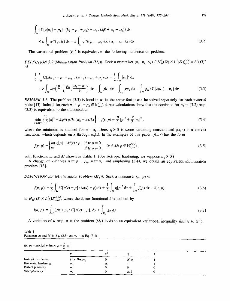
rain { 2 1 a l 2 + k q ~ * ( p / k , ( a o - a ) / k ) } = j ( x , p ) + ~ l p ] 2 - + ' v 2 -~ I•ol , (3 .4) a E ~ m

where the minimum is attained for a = a~. Here, r / ~ O is some hardening constant and j(x, .) is a convex functional which depends on x through So(X ). In the examples of this paper, j (x , . ) has the form

j ( x , p ) = { m ( x ) ] p ] + M ( x ) : p i f t r p = 0 , ,a×d i f t r p ¢ 0 , ( X E O ; p E N , ~ y m ) , (3.5)

with functions m and M shown in Table 1. (For isotropic hardening, we suppose a o i> 0.) A change of variables p : = P l - P o , u := u~, and employing (3.4), we obtain an equivalent minimisation

problem [13].

DEFINITION 3.3 (Minimisation Problem (M2)). Seek a minimiser (u, p) of

if,, f(u, p ) : = -~ C[~u) - p ] " (8(u) - p ) dx + ~ flip] 2 dx + j (p) dx - l(u, p) (3.6)

in H ~ ( / 2 ) 2 d×d × L (O).~rm, where the linear functional l is defined by

l(u, p) := f~, (fu + po : C[e(u) - p]) dx + f t , gu ds . (3.7)

A variation of u resp. p in the problem (M2) leads to an equivalent variational inequality similar to (P~).

Table 1 Parameter m and M in Eq, (3.5) and r/, v in Eq. (3.4)

b' 2 fix, p) = m(x)lp I + M(x) : p + ~lolol

m M r I v

Isotropic hardening (1 + H%)K 0 H:~o'~ 1 Kinematic hardening o-. oz 0 1 1 Perfect plasticity ~. 0 0 0 Viscoplasticity 07, 0 tz/k 0

180 J. Alberty et al. I Comput. Methods Appl. Mech. Engrg. 171 (1999) 175-204

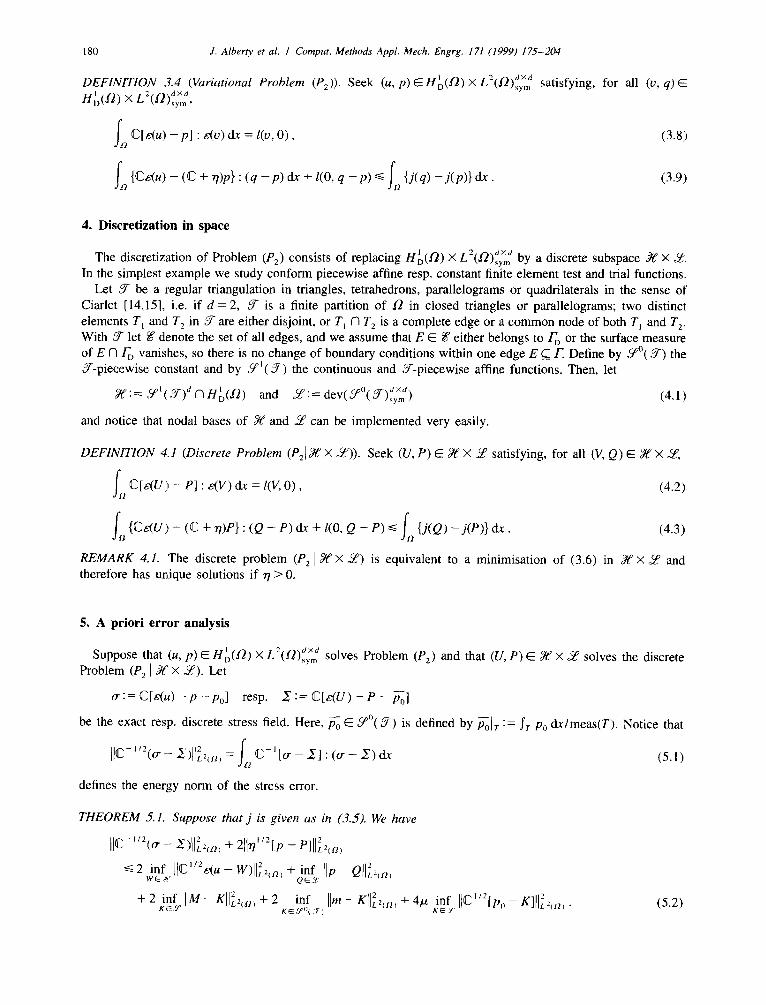
DEFINITION 3.4 (Variational Problem (P2))- Seek (u, p)@HD(a'-2)×L2(O) d×a satisfying, ~--~sym H~,(.O) X 2 a×a L (~(~) sym '

fa c[e'(u) - p] ~(v) dx = l(v, 0) , D

fa {ce'(u) - (C + r/)p} : (q - p ) dx + l(O, q - p ) ~< f {j(q) - j ( p ) } dx. 1

for all (v, q) E

(3.8)

(3.9)

4. Discretization in space

L 2 ( O ) dxa The discretization of Problem (P2) consists of replacing H~(d2) X _ ,__,.~y,~ by a discrete subspace Y( x ~. In the simplest example we study conform piecewise affine resp. constant finite element test and trial functions.

Let 3- be a regular triangulation in triangles, tetrahedrons, parallelograms or quadrilaterals in the sense of Ciarlet [14,15], i.e. if d = 2, 3- is a finite partition of ~ in closed triangles or parallelograms; two distinct elements T~ and T z in 3- are either disjoint, or T~ fq T 2 is a complete edge or a common node of both T~ and T 2. With 3- let g denote the set of all edges, and we assume that E ~ g either belongs to ~ or the surface measure of E 71F D vanishes, so there is no change of boundary conditions within one edge E C/2. Define by 6P°(if) the J-piecewise constant and by 5e~(3-) the continuous and ff-piecewise affine functions. Then, let

69~:=oqal(3-)aAHl(,(2) and ~%f:=dev(;T°( axa ~ ) sym ) (4 , l )

and notice that nodal bases of Y( and ~Lf can be implemented very easily.

DEFINITION 4.1 (Discrete Problem (P21 Y( X ~) ) .

fa C[e(U) - P] : e(V) dr = l(V. 0) ,

fa {Co,'(U) - (C + r/)P} : (Q - P) dx + l(0, Q - P) <~ fa {J(Q) - t iP )} dx. (4.3)

REMARK 4.1. The discrete problem (P21~ x ~) is equivalent to a minimisation of (3.6) in Yg x G~? and therefore has unique solutions if 77 > 0.

Seek (U, P) E Y( X ~ satisfying, for all (V, Q) E Y( X ~,

(4.2)

5. A priori error analysis

2 d×d Suppose that (u, p) E HD(O) × L (~"~)sym solves Problem (P2) and that (U, P) E Yt" × ~cC solves the discrete

Problem (P2 ] Y( x ~5~). Let

o ' : = C [ a ' ( u ) - p - p o ] resp. 2 : = C [ e ( U ) - P - p - 0 0 ]

be the exact resp. discrete stress field. Here, ffoo E ~° (3- ) is defined by Poolr := fr Po dx/meas(T). Notice that

I IC-"2( o" -- ~)llL-,(s~)2 : f , ~ C - ' [o- - 2 ] : (o- - 2 ) dx (5.1)

defines the energy norm of the stress error.

THEOREM 5.1. Suppose that j is given as in (3.5). We have

I } C - " 2 ( o - ~)J),~-,(.~,) + 211 . "~ [p - P i l l % . , ,

~<2 inf [[C'/2e(u 2 0 2 - w)IIL2,,,, + inf [ I p - ILL2.,,

+ 2 inf J IM- gl l ;=. , , + 2 inf IIm " - KIlL,,e,, + 4# inf [[C'/2[po 2 - K i l l , - - , , , , . ( 5 . 2 ) K~Ed¢ K~,~f {h, 3-) KEY'


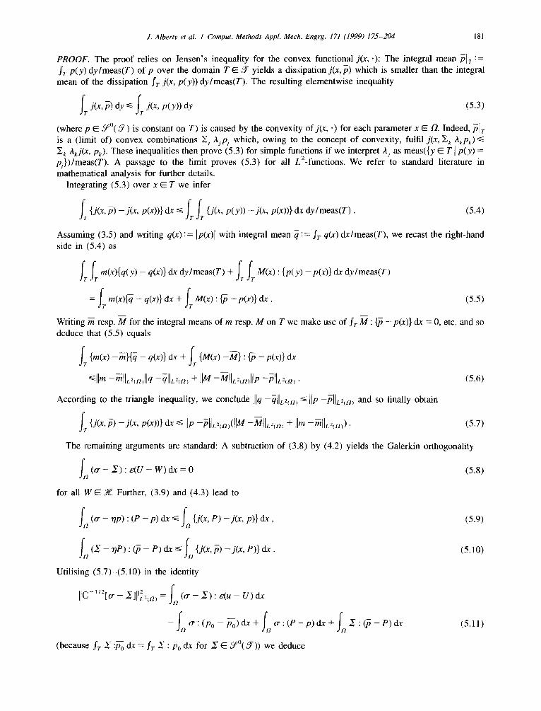
PROOF. The proof relies on Jensen's inequality for the convex functional fix, .): The integral mean pit :---- fr P(Y)dy/meas(T) of p over the domain T E 3-yie lds a dissipation j(x,p) which is smaller than the integral mean of the dissipation f r j(x, p(y)) dy/meas(T). The resulting elementwise inequality

frJ(X,~)dy<~ frJ(x, p(y))dy (5.3)

(where p E 6e°(3-) is constant on T) is caused by the convexity ofj(x, .) for each parameter x E/2 . Indeed, PIT is a (limit of) convex combinations Zj ,~jpj which, owing to the concept of convexity, fulfil j(x, E k akp ,) ~< Ek ;tkj(x, Pk). These inequalities then prove (5.3) for simple functions if we interpret Aj as meas({y E T] p(y) = pfi)/meas(T). A passage to the limit proves (5.3) for all L2-functions. We refer to standard literature in mathematical analysis for further details.

Integrating (5.3) over x ~ T we infer

fr {J(x,~) -j(x, p(x))} dx <- fr fr {j(x, p(y)) -j(x, p(x))} dx dy/meas(T) . (5.4)

Assuming (3.5) and writing q(x) := [p(x)[ with integral mean ~ := fr q(x) dx/meas(T), we recast the right-hand side in (5.4) as

frfrm(x){q(Y)-q(x)}dxdy/meas(T)+frfrM(x):{P(Y)-P(x)}dxdy/meas(T)

= frm(x)f~-q(x)}~+ frM(x):~-p(x)}d~. (5.5)

Writing m resp. M for the integral means of m resp. M on T we make use of f r M : ~ - p(x)} dx = 0, etc. and so deduce that (5.5) equals

f r {m(x)-m}{q - q(x)} dx + f r {M(x)-M} : ~ - p(x)} dx

~<llm -~/IL2(n,llq -~IIL2.~, ÷ IIM --MI[L2,n)I]P --P[]L~m. (5.6)

According to the triangle inequality, we conclude ]]q-~IIL=,~) :<-lip-~11~=.,, and so finally obtain

fT{J(x, fi) -- j(x, p(x))} dx ~< lip -fill~2,.~,(lIM -~11~2.~, + lira -m[l~=.,)) • (5.7)

The remaining arguments are standard: A subtraction of (3.8) by (4.2) yields the Galerkin orthogonality

f (o, - 2:) : e (u - w) dx = 0 (5.8) 2

for all W ~ ~. Further, (3.9) and (4.3) lead to

f , , ( g - "P ) : (P - P) dx ~< f,n {j(x,P)-j(x, p)} dx, (5.9)

f,, ( z - , , ) : , , ax_< f,, {j(x. - ,3) (,.,o3

Utilising (5.7)-(5.10) in the identity

I [ c - " : [ ~ : = f , , - X ] l [ ~ m (o- - .~) : e(u - U ) dx

-f~:(po-po)ax+f~:(P-p)a~+f,~ 2 : (/5 - P ) dx (5.11)

(because fr X :Po dx = fr .S : Po dx for X E 0°°(3-)) we deduce:

182 J. Albert3, et al. / Comput. Methods Appl. Mech. Engrg. 171 (1999) 175-204

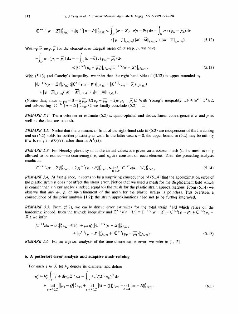
- Z]ll~=.~, + [[r/l/2[p ~< e-'(u w) dx - or : (Po Po) dx - e ] l l L = ( . o ) (o" - 2 ) : -

+lip -~I[~.~,(IIM-M[I~.~) + Jim - ~ 1 1 ~ , ) (5.12)

Writing ~" resp. p for the elementwise integral mean of o- resp. p, we have

- f ~ : tlpo - ~ ) ~ = - f a (~ - ~ ) : (po - ~ ) a~

~< i[cl/2(p ° - - - , ,2

With (5.13) and Cauchy's inequality, we infer that the right-hand side of (5.12) is upper bounded by

lie 1'2( °0 - - z ) l l ~ , ~ , ( l l c ' % ( . - w ) l l ~ . ~ , + IIC"2(p0 - b-;)l[~.~,)

(Notice that, since tr Po = 0 = t r p o, C(po - Po) = 2/Z(Po - P0).) With Young's inequality, ab <- (a 2 + b2)/2, and subtracting [[C- ' /2[o " - s]11~=.~,/2 we finally conclude (5.2). []

REMARK 5.1. The a priori error estimate (5.2) is quasi-optimal and shows linear convergence if u and p as well as the data are smooth.

REMARK 5.2. Notice that the constants in front of the right-hand side in (5.2) are independent of the hardening and so (5.2) holds for perfect plasticity as well. In the latter case 7/= 0, the upper bound in (5.2) may be infinity if u is only in BD(12) rather than in H~(/2).

REMARK 5.3. For Hencky plasticity or if the initial values are given on a coarser mesh (if the mesh is only allowed to be refined--no coarsening), Po and % are constant on each element. Then, the preceding analysis results in

l i e - ]'2(00 - X)[l~2,.~> + 211~"=(p - P)IIL=~o, ~< inf [1C~/24u 2 . 2 - W)I[L2(a , (5.14) g" E 9'~

REMARK 5.4. At first glance, it seems to be a surprising consequence of (5.14) that the approximation error of the plastic strain p does not affect the stress error. Notice that we used a mesh for the displacement field which is coarser than (in our analysis indeed equal to) the mesh for the plastic strain approximations. From (5.14) we observe that any h-, p, or hp-refinement of the mesh for the plastic strains is pointless. This overrules a consequence of the prior analysis [1,2]: the strain approximations need not to be further improved.

REMARK 5.5. From (5.2), we easily derive error estimates for the total strain field which relies on the hardening. Indeed, from the triangle inequality and CJ/2~(u - U) = C lI2(o- - 2 ) + C1/2(p - P) + C1/2(po -

Po) we infer

I I C " 2 ~ . - u)llE2,. . ,-< 2(1 +/~/~)(1lc-"=(00 - ~)11~2.~,

+ [ ] T / I / 2 ( P - - e) l122(~r2, + I l c l / 2 ( p o - Po)l/~.2(~,). (5.15)

REMARK 5.6. For an a priori analysis of the time-discretization error, we refer to [1,12].

6. A posteriori error analysis and adaptive mesh-ref ining

For each T E ~,, let h r denote its diameter and define

71r = hr If + dive-X[ 2 dx + hEIJ(X" r/E)[ 2 ds T

+ inf I[Po - al iEn, r ) + inf IIM 2 2 - Q[lc2(r) + inf [In " - NIIL2,T> ~ dXd dXd N ~ (6.1)


Here, J(~. ne) is the jump of the discrete stress field_~ ~ along an edge E E ~ with normal n e and size h E with the usual modification J ( 2 " hE) := ~ " n E - g if E C F N.

THEOREM 6.1. There exists an ~7-depending constant C(rl) > 0 such that

~ u)IIL2,~, ~ C(r/) "~', r/r (6.2) 110.- 21IZ2.~, + lip - PIIZ2.~, + l i eu - 2 2 . T ~ ,~

PROOF. From (5.12) and (5.13) we have, for all W ~ ~,

- 2 ]11L2 .~ , + I1~' - P]l12~=.,, ~< (o- - 2 ) : ~ u - w ) d x - (o- - ~ - ) - ( P o - P o ) d~

+ lip -pll~=¢a,([ lM - M I I ~ , ~ , + Ilm -ml l~= .~ , ) • (6.3)

Since o" - S is symmetric we have (0. - 2 ) e'(u - W) = (0. -- 2 ) : tT(u - W), and an elementwise integration by parts shows

(0 . - : - W) x = f, R(u- fo ~ J ( u - W ) d s , (6.4)

where U ~ is the skeleton of all edges in J.. The volume residual is

R := f + divv- ~ E L2(~2), (6.5)

where dive denotes the elementwise divergence. Recall that the jump residual J E L2( U ~) is defined by

[!"nL.] if E ~_ F ,

J]E := if E C_ I '~ , (E E ~ ) . (6.6)

- 2 " n i f E C K N ,

For some weak interpolation W to u, the error u - W obeys estimates of the form

]lh~'(u - W)]I2L2(e~) + Hh~l /2(u - W ) H 2 2 ( u ~ ) ~ c~[[V(u - U)[ 22(0 ) . (6.7)

Here, h~ 7 and hu. are piecewise constant, h.rlr = h r and hvl~ = h~. We refer to [16-19] for details. Employing (6.7) in (6.4) shows, with Cauchy's inequality,

(6.8)

Since F D has a positive surface measure, Korn's inequality shows

IIV(u - u)11~21.~1 ~ c2I]CI'2~ u - u)ll~=,~,. (6.9)

Hence, from (6.3), (6.8) and (6.9), we have

i i c - 1 , = ] o . _ 2 1 1 1 2 ÷11 ,,2[p 2 2 1/2 2 ) 1 / 2

~< ~ C l C 2 1 1 c 1 ' 2 ~ u - f)[l~lO,(llh~RIl~=.,, + I[h~.r JIl~=~o ~,

+ 1 1 c - 1 ' 2 ( 0 - - 2 ) 1 1 ~ . , , 1 1 ¢ ' ' 2 ( p o - Yo)l l~2, .~,

+ lip - ~IIL=.~,(IIM - MII~=. ,I + [ Im - m l l ~ , o > ) • (6.10)

With Young's inequality and some r/-depending constants Cl(r/), c207), and c3(r/) we deduce from (5.15)

IIc '/=(0. - S)l l ,~.~, + ]lrf l '2(p - e ) l l , ~ : , s , ) + I [ C l ' : o " ( u - u)ll~=,.,, 1 l /2 2 2 1/2 2

+ ~-IIC -(0. - 2)11,~2,., + c 2 O T ) [ [ c " Z ( p o - pZ)ll2~.,, ÷ ~ I1~ (p - P) I I~ . , t

÷ e ~ ( n ) ( l l M - MIIL~,,~ + lira -m l l L= ,m) ~ • [ ] (6 . l 1)

184 J. Alberty et al. I Comput. Methods Appl. Mech. Engrg. 171 (1999) 175-204

REMARK 6.1. If p0 and a o are constant on T, for instance in time-independent problems (Po = 0 = do) or if the mesh is refined successively (Po, ao E 5e°(3-)), the error indicator fir reduces to

J 2 = h T r T ° ~TT If + div~ ~:l ~ ax + h~lJ(.~ ne)l 2 ds (6.12)

and so is the same as in pure elasticity (utilising the stress field from a discrete elastoplastic problem).

REMARK 6.2. In perfect plasticity, Theorem 6.1 is expected to be false. A closer inspection then shows that it is required to follow the arguments in [11] and derive weaker estimates. Essentially it is because (5.15) is not available and so UV(u - U)llL~m cannot be absorbed.

REMARK 6.3. Employing the arguments of [16,17], we could sharpen the estimate of Theorem 6.1 which shows that, generically, the volume contribution h 2 f r I f + div.~Z[2dx can be neglected (replaced by a higher-order term).

REMARK 6.4. The reliable inequality is sharp in the sense that there holds the reverse inequality up to data approximations, i.e.

2 2 2 " , 7 , - < - c ( , 1 ) ( l l o - + - - ~tlL=¢~) lip + P[IL=(o,) I1,~. u)llz=,~,

+ inf Hp0 2 N 2 , - ollL2¢o, + inf I IM- 2 Ol[L~o,) + inf lira - >¢~o,) (6.13)

for each element T ~ 3- and its neighbourhood w := U {T' E 3- : T N T' # 0} and for some ~7-depending constant C(r / )> 0. The proof is as in [19] and we refer to [5] for details.

ALGORITHM 6.1. (a) Start with a coarse mesh 3- o, k = 0. (b) Solve the discrete problem with respect to the actual mesh ~ . (c) Compute r/r for all T ~ ~ . (d) Compute a given stopping criterion and decide to terminate or to continue and then go to (e). (e) Mark the element T for (red) refinement provided

1 r/r -~-" ~- max r/T,. 2 r'~.%

(f) Mark further elements (within a red-green-blue refinement) to avoid hanging nodes. Define the resulting mesh as the actual mesh T~_ j, update k and go to (b).

Details on the so-called red-green-blue refinement strategies may be found in [19].

REMARK 6.5. In the numerical examples below, the volume contributions to the error indicator ~Tr in (6.12) vanish according to f = 0, Polr is constant and UIT affine. Hence, we may argue as in [19] and obtain equivalence of the edge contributions to the ZZ-estimator. In this way, we justify the popular ZZ-estimator in viscoplasticity and plasticity with hardening (in cases where the influence of l i p - ~o[IL21T) is negligible). According to Remark 6.3, this argument is valid also in case that f is non-zero but smooth. The authors are unaware of any other justification of the reliability of the ZZ-estimator in the context of plasticity. However, the constants are ~7-depending and so the reliability of the ZZ-estimator in perfect plasticity remains as an open question.

7. Numerical solution algorithms

The numerical treatment of (P21 Y( x ~Lf) is simplified by the elimination of the variable P. Indeed, given ~ U ) we can solve (P2 I Yg X ~ ) elementwise.

J. Albert), et al. / Comput. Methods Appl. Mech. Engrg. 171 (1999) 1 7 5 - 2 0 4 185

d x d d x d Given A E ~sym and b > 0 there exists exactly one P E R~y~ with tr P = 0 that satisfies

(7.1)

PROPOSITION 7.1.

{ a - ( C + r/)P} : ( Q - P ) <~ b{ ]QI - IP]}

for all Q E ~a×a with tr Q = 0. This P is characterised as the minimiser o f " -syrn

1 (C + rl)P : P - P : a + blP I (7.2)

(amongst trace-free symmetric d X d-matrices) and equals

( I d e v a l - b ) + devA 21x + ~7 Idev a I ' (7.3)

where (.)+ := max{0, .} denotes the non-negative part. The minimal value o f (7 .2 ) (attained for P as in (Z3)) is

- l ( I d e v A I b 2 - ) + / ( 2 / z + ~ 7 ) . (7 .4)

PROOF. In convex analysis, (7.1) states that

a - (C + 7q)P E bOl.l(P) (7.5)

where 01. I = sign denotes the subgradient of the modulus function, and only trace-free arguments are under consideration. The modulus function is convex and so is (7.2). Identity (7.5) is equivalent to 0 belonging to the subgradient of (7.2), which characterises the minimisers of (7.2). If P = 0, (7.1) states

a : Q <~ blQ I (7.6)

d×d for all Q E R,y m with tr Q = 0. Hence, Idev a I ~< b. I f Idev A I >. b we conclude P ~ 0 and obtain oI'I(P) = {P/ IPI}. Hence, (7.5) yields

dev A - (C + r/)P = bP/]P[. (7.7)

Notice that tr CP = 0 as tr P = 0, and only trace-free arguments are under consideration. Since then CP = 21zP we obtain

devA = (b + (212 + 71)IP[)P/IP I (7.8)

and so Idev A I = b + (2/~ + r/)lP I, whence

[PI = (I dev AI - b)/(Z/x + r/). (7.9)

Using this in (7.8) we deduce

( I d e v a [ - b ) + d e v a P = 2# + r / [dev a[ " (7.10)

The formula (7.10) holds also for P = 0. Taking (7.10) in (7.2) we calculate the minimal value (7.4). []

DEFINITION Z1. For any x ~ $2, K(x) := dev Cpo(x ) + devM(x), M(x), m(x) and rl from Table 1, and d x d

A E ~*ym let

1 1 ~p(x, A) := ~ A : CA - ~ (Idev CA - K(x)l - m(x))Z+/(2/x + *l)-

~ d x d n d X d PROPOSITION 7.2. For any x ~ 1 2 , q~(x,') is ~1 and D~p(x,.): ,ym "-'~/~ym is uniformly convex and Lipschitz, i.e. there exist positive hardening depending constants a and L such that, for all x E ~ and A, B E ~a×d "~syrn ~

a l A - BI 2 + Oq~(x,A) : (B - A) < - ~ (x ,B) - q~(x,A), (7.11)

IDa(x, B ) - O ~ ( x , A)I ~< L I B - A [ . (7.12)

186 J. Alber~ et al. / Comput. Methods Appl. Mech. Engrg. 171 (1999) 175-204

PROOF. A discussion of the two cases Idev CA - K(x) I <~ re(x) or not leads to

( ( ]devCA-K(x) l -m(x))+ d e v C A - K ( x ) ) D~(x, A) = C, a -(2tx~-~) Idev CA K(x)] (7.13)

and, at least for the two cases ]dev CA - K(x)l < m(x) resp. >re(x), we have D2~(x, A) = C resp.

D2~o(x, A) = C 1 - m(x)/]B I C dev ®C dev re(x) 2# + 7/ (2/z + w)IB[ C signB ® C s ignB , (7.14)

d × d where B := dev CA - K(x), sign B = n/Inl, and P : (C dev ® C dev)Q = 4/x 2 dev P : dev Q for all P, Q E I~y m . Since r / > 0, IBI/> m(x) in the second case, and C dev = 2p~ dev,

rt 4p, 2 - - - - <<-D2~(x, A) ~< C (7.15) r / + 2/x C~<qC 2/~ + r/

d × d where ~ ~< [13 means P : ~ ~< P : BP for all P E ~ y m ' Hence, the second derivative D2~o(x, A) is discontinuous but bounded. Then, (7.11) and (7.12) follow from integrations along lines connecting A and B; we refer to [20] for details. [-]

According to Definition 7.1 and Proposition 7.2 we may consider an equivalent variational problem.

DEFINITION 7.2 (Minimisation Problem (M3)). Seek the minimiser u in H~(g2) of

f~ ~ ( x , ~ u ) ) ~ - f , (fu + p , , : C ~ u ) ) ~ - f r guds . (7.16)

THEOREM 7.1. For 7/> 0, there exists a unique minimiser u of (7.16) and u, 0- : = Dq~(x, e-'(u)), and p : = e'(u) - C- lo" solve Problem (P1), (P2) and (M 1 ).

PROOF. Substituting Definition 7.1 for A = dev C~(U) into (7.16) and using (7.2) and (7.3) we eventually obtain (M2). Tile unique solvability of (M 2) follows from standard arguments for uniformly monotone operators (see e.g. [20]). []

On the discrete level, we replace m(x) and K(x) by their elementwise integral means and result in the following discrete problem.

DEFINITION (Minimisation Problem (M 3 ] ~) ) . Seek the minimiser U in Y{ of

f~ ~ ( x , , ~ U ) ) d x - f ~ ( f U + p o : C s ( U ) ) d X - f l gUds

where, for x E T E 3- and A E ff~a×d,

1 1 ~r(x, A ) : = ~ A : CA - ~ (Idev CA - ~'(x)] -~(x))2+/(2/z + 7/)

and K := fT K(x) dx/meas(T) resp. m := ST m(x) dx/meas(T) denote integral means over T.

(7.17)

REMARK 7.1. The discrete problem (P2 ] ~ >(~) is equivalent to the minimisation problem (M 3 ] ~).

REMARK 7.2. The functional ~¢ satisfies (7.1 1) and (7.12) with the same constants. In particular, an a priori and a posteriori effor analysis can also be based on these properties (but includes some implicit perturbation argument on K - K , etc.).

DEFINITION Z4 (Quasi-Newton-Raphson Scheme). Let C,(x), x E ~, be a globally elliptic and bounded fourth-order tensor, i.e. for two positive constants a n and ce,--~ we have


o~]A] 2 <~A : C~(x)A ~ - - 2 ii~d×d a.lAI ( A E x E g 2 ) (7.18) ~sym '

Then, for p, > 0 and U, ~ ~ , define U, + ~ C ~ as the unique solution to

f . - . = { f o ~ x , ~ < ) ) : ~ v ) ~ e(u.+, v,,) C,e(V)dx -p .

- f~ (iv + ~:c~v))dr- frNgVas ) (v~e) (7.19)

We have the following global, but only linear convergence result.

THEOREM Z2. Let oe and L as in Proposition Z2. I f p, = a , / L then, any sequence (Un) generated by the quasi-Newton-Raphson scheme satisfies

O[

<,+,)ILL=.,, + ao , 2(1 + c) 118(U - z + ~< q 8 (7.20)

for q := c/(1 + c) < 1 with 1/2(1 + -'~nnn[Oln)2L2/ol 2 ~ C and

PROOF. The proof follows from standard arguments given, e.g. in [20] for an abstract framework; we give a proof here for the convenience of the reader. According to (7.11) we have, for e, := I I ~ ( e - <)11~=,.,.

z f n ~ £ ae,, + i + D ~ ( x , ~(U, + 1 )) : ~(U - U, + j ) dr <- ~,7(x, e~IU)) dr - ~.~(x, e(U,, 4 , )) dr 2

= - a . , + , + f. ( f (u -u .+ , l+po:C~g-u .+ , ) )dr + ~ g(U-U,,+l)dS. (7.22) . v N

Owing to (7.12), this shows

2 £ ae.+, +6.+, ~ D~(x.e(U.)):e ' (U.+,-U)dr

-- f~ f(Un+ I - U ) + p o ' e ~ ( U n + 1 - U ) ) d x - d l f g ( U n + l - U ) d s

+ t l l ~ u . , + , - U)II~=,.,II~Un+, -- U~)II~,~, - (7.23)

Taking (7.19) for V= U - U,+l, we obtain in (7.23) that

~ e ° + , -< ~ g ° + , - No) : c ° ~ u - S ° + l ) a X + LII~u°+ , - v ) l l ~ , ~ , l l ~ u o + , - uo)l l~2. , ,

<~ (L + 7,/p,)l[e(U,+ ~ - u,)IIL~o~IIe(u,,+, -13')llL2,n ~ . (7.24)

(In the last step we used Cauchy's inequality with respect to C,, and (7.18).) In the same way, we apply (7.11), (7.12) and (7.19), to infer

< l ~ u . , + l - ~ f . U,,)llL2{n ) <~ D~o4x, ~U.+, )) : ~U,, , - U,) dr ) +

ao a,+, + f. (f(U. -- U,+,) + P o ' CaU,, - Un+l) ) dr

188 J. Alberty et al. / Comput. Methods Appl. Mech. Engrg. 171 (1999) 175-204

'L = ~ . - ~ . + , - ~ ~ u . + l - w . ) : c ~ u . + , - u . ) d r

+ f a {Dq~x, e-'(U. +, ) - D~o.(x, e-'(U.)} : e-(U~ +~ - U.) dr

~< 6,, - 6 . + , - ~ . / p . j l e ( u ~ + , - + LIl u.+, - u . ) l l b , . ,

= 6, - ¢5,,+ 1 (7.25)

because of p,, = %/L. Using this in (7.24) with Young's inequality, ab <~a2/2 + bZ/2, we deduce

OZ 2 L2 - - 2

2 + 6,+, ~< ~- e,,+l +-2~a2 (1 + an/ozn)(~,-6,+l) (7.26) O { e n + l - - "

This shows (7.20) and concludes the proof. []

REMARK 7.3. The (non-damped) Newton-Raphson method is defined for p, = 1 and C, := DZ~j(x, o~(U,,)). Then, since ee/L < 1, Theorem 7.2 does not guarantee global convergence. Moreover, q may be very close to ! if hardening is small.

We conclude this section with a discussion of the local convergence properties of the Newton-Raphson scheme to indicate superlinear convergence observed in practice. Suppose U, E ~ is an approximation to U @ ~t ~ and U, +1 E ~ is generated by

fao2~.~X, e'(U,); e '(U,. , - U.), ~V)) dx

= - f~ D~°~(x' ~U'); °"(V)) dx + L,2 ( fV + p° : C~V)) aX + fr~ gV ds (V ~ ~C) . (7.27)

With the (discrete) stress deviator resp. its approximation

o - : = d e v C [ e ' ( U ) - K] resp. o ' , , : = d e v C [ e ( U , ) - K] (7.28)

we define the discrete plastic (and elastic) zone resp. its approximation by

a , : = (x I I (x)l & resp. / 2 p := {x E o I (7.29) le ) (e)

Thus, the prediction of U,, about the plastic or elastic zone is correct on

(I2p n .Onp) U (.O~ N ~(2,, e ) (7.30)

and incorrect on the remaining part of Z2..i:= (Z2p\/2 p) U ( Z 2 \ / 2 ) of the domain. We will work under the hypothesis that~ first, Ije'(U - u,,)llL~m is small and, second, meas (Z2.,~) is very small. Our analysis is based on the fact that

d,(x) := D Z ~ x , e'(U,)(x); e'(U - U,)(x)) + D~.~(x, ~U,)(x)) - Dq~x, e'(U)(x)) (7.31)

and (7.27) lead, for V := U,, + 1 - U, to

fa D 2 ~ x ' e'(U.); e'(U,,+, - U). e'(U.+ 1 - V ) ) d r = - f , , d . : e(U,,+, - U ) d r . (7.32)

This, Cauchy 's inequality and the uniform positive definiteness of D 2 ~ from (7.15) yield, with some r/-depending constant Cl( r / )> 0, that

II~s - s,, +1)11~=,'~/~ cl (n)lld°ll~,,,, (7.33)


and it remains to analyse (7.31). Recalling the proof of Proposition 7.2 we find

Id,(x)[ ~< cz(T1)I~(U - U )(x)[ for almost all x E 12, (7.34)

2 since D ~.~ is bounded, D~oj is Lipschitz. Furthermore, D2~pj( ., ~U,,)) is constant C in 12n.,, and so

d (x ) = 0 for almost all x E 12e 71 12,,,~. (7.35)

, ~d×d I dev C [ C -- Next,_ consider x E 12p (3/2,, p and A = e'(U.)(x) and B = e'(U)(x). We have A, B G {C E --.~r., K(x)] > ~(x)} =: .~ and, although cony{A, B} may leave 9 ~, we can always find a smooth curve 7 : [0. l] ~ with y ( 0 ) = A and 3,(I)= B of length

l <~ c31a - B I . (7.36)

2 Since D ~.~- is smooth in .@ and O3q~ is bounded (cf. the derivative of (7.14)), we obtain (with y parameterised by the arc-length, and so I Ks)] = 1)

d.(x) = D2~j (A; B - A) + D~o~(A) - D~o~,-(B)

fo ° = O 2 ~,AA; B - A) - ~s D ~ y(s)) ds

Jo' = { D ~ . ~ A ; Ks)) - O~q,O,(s); Ks))} ds

I O ~ ( A ) - D ~,~(~,(s))l ds

fo'lfo I fo'[ = ~ D'~o3(y(t)) dt ds <<- ID3¢~y(t))J dt d s . (7.37)

According to the boundedness of O3cfl and (7.36), (7.37) verifies

U '~ ,, . Id,,(~)[ ~ c 4 ( n ) l ~ u - °)(~)[~ for almost all x ~ ~ , n 12,~ (7.38)

To summarise, the above arguments show

-~- 2 C 4 ( ~ ) 1 1 ° ° ( U - - u, , ) l l~, . .~, , , , , l l~(u -uo)ll~.~,.~.~,, ,.,. ( 7 . 3 9 )

Thus, if Ile"(U - U,)[[L~m) ~< S << 1 and meas(~2,.;) ~< 6 z", with 0 < ce ~ 1, then,

II~(v - u . +,)11~=¢~, = 0(~ ' + °) (~ -~ 0 ) . (7.40)

R E M A R K 7.4. Under the present assumptions on e'(U - U,) we can, in general, only expect II~(u - u,,)ll~=,~, = 0(6), and so (7.40) indicates superlinear convergence of Newton-Raphson 's scheme.

R E M A R K 7.5. Although (7.40) may suggest that the local convergence of Newton-Raphson 's method is superlinear, it seems to be a non-obvious task to base a rigorous proof on (7.38). The difficulty arises from the fact that, within a proof by mathematical induction, we have to verify that [ [e(U- U,,+~ )liLy,a)= O(~ '+") and meas(Y2~ + i,, ) = 0(62or( 1 + a ) ) .

R E M A R K 7.6. In our practical experience, the Newton-Raphson scheme often showed quadratic convergence.

R E M A R K 7 ̀7. It is conjectured that damping is necessary in the first steps of the iteration and may be omitted in subsequent iterations.


8. Numerical experiments

Three examples provide numerical evidence of the linear convergence of the lowest order scheme and of the superiority of the adaptive algorithm.

8.1. Plastic ring with known solution

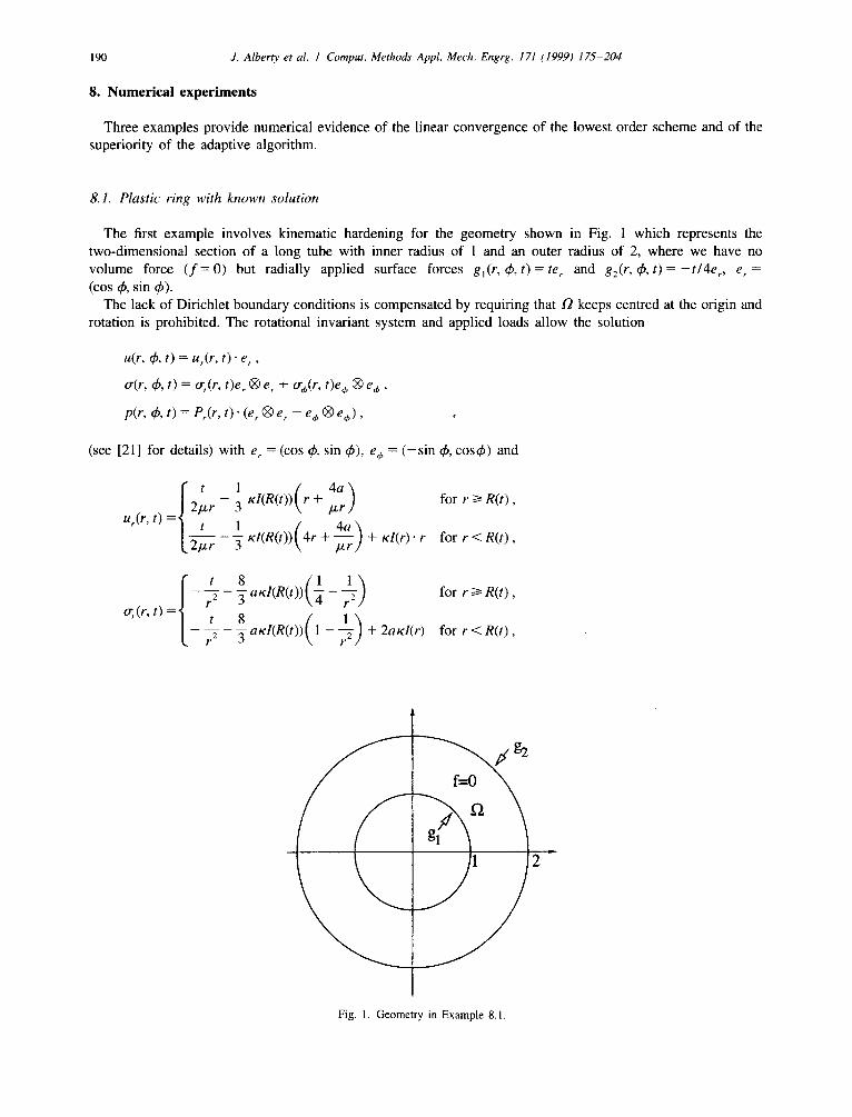
The first example involves kinematic hardening for the geometry shown in Fig. 1 which represents the two-dimensional section of a long tube with inner radius of 1 and an outer radius of 2, where we have no volume force ( f = 0 ) but radially applied surface forces g , ( r , O , t ) = t e ~ and g:(r, ck, t ) = - t / 4 e ~ , e r = (cos ~b, sin 4)).

The lack of Dirichlet boundary conditions is compensated by requiring that $2 keeps centred at the origin and rotation is prohibited. The rotational invariant system and applied loads allow the solution

u(r, ~b, t) -- u,(r, t) " e r ,

tr(r, (h, t) = o'r(r, t)e r ® er + o',t,(r, t)e 6 ® e ~ ,

p(r, dp, t) = P~(r, t)" ( e r i e r - e~ Q e e , ) ,

(see [21] for details) with e r = (cos ~b, sin ~b), e,~ = ( - s i n ~b, cos$ ) and

t 1 4a

3 for r ~ e ( t ) ,

' ( 4--~r) 21zr 3 KI(R(t)) 4r + + Kl(r)" r for r < R(t) ,

t 8 1 1 °'r(r, t) = r 2 3 a K I ( R ( t ) ) ( - ~ - - - ~ ) for r >~ R(t) ,

, 8 ( ÷ ) r 2 3 aKl(R(t)) 1 -- + 2aKl(r) for r < R ( t ) ,

2

Fig. 1. Geometry in Example 8.1.


2 i

1.8

1.6

1.4

r r

1 .2

0 .8

0 . 6

r i i i i

dO I I I i I 1 O0 150 200 250 300 350

t

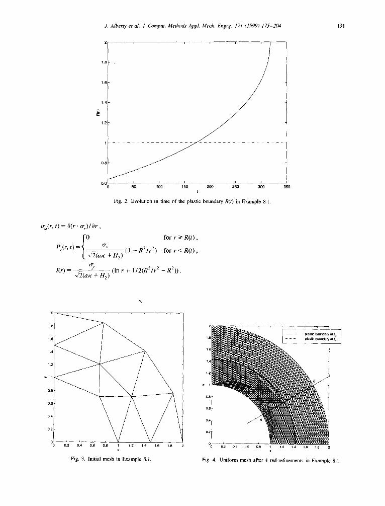
Fig. 2. Evolution in time of the plastic boundary R(t) in Example 8.1.

o%(r, t) = O(r . o" ) / Or ,

I~ for r >~ R(t) ,

P,(r, t) = try /~(a~-+H2) ( l - R 2 / r 2) for r < R ( t ) ,

I(r) - x /2 (ax + He) (In r + 1 /2(R2 / r 2 - R2)).

%

1.8

1.6

1,4

1.2

>" 1

0.8

i! , ,

i 4 i 0 2 0 0 6 0 8 1 1 2 1 4 16 1 8

X

Fig. 3. Initial mesh in Example 8.1.

2

1.1]

1,6

1.4

1.2

>, 1

0,8

0.6

0.4

0.2

plastic bour lda la t t(l plastic boundary at t 1

- - ' 0.2 0.4 0.6 0.8 1 1.2 1.4 1.6 1,8 2 x

Fig. 4. Uniform mesh after 4 red-refinements in Example 8.1.


Here, a =/I, + ,~, K = 2/.t/(2/z + A). The radius of the circular plastic boundary R(t) is determined as the positive root of

f(R)=-2alnR +(a-1)R 2 - a + ~F2

t ,

where ce = 4aK/(3(aK + H2)). Fig. 2 displays R(t) versus t and illustrates for t ~< o:~/x/2 that the body reacts purely elastic (as the inner radius of the domain is 1).

x 10 -3

z.//

- 0 , 5 / 2

-1 ~' 4,

-1.5

-2 / 7 /

~Y-2.5 /

-3

- 3 . 5 /

- 4

- 4 . 5

-5 11.1 11.2 11.3 11.4

(a) 10 -3

7.5

exact Pr at t o

exact Pr at t 1

numerical solution Pr at t 1

i

115 15 117 1:~ ' 1.9 r

i i i i i i i i i

. . . . . . exact u r at t O

7 ~ - - - exact u r at t 1

6.5 \ ' ~ x ~ -- -- - numerical solution U r at 11

6i ~',~. q

4.5

4

3.5 I I I I h I I I I 1.1 1.2 1.3 1.4 1.5 1.6 1.7 1,8 1.9 2

r

(b)

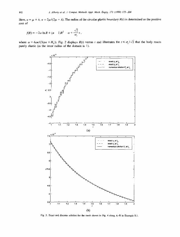
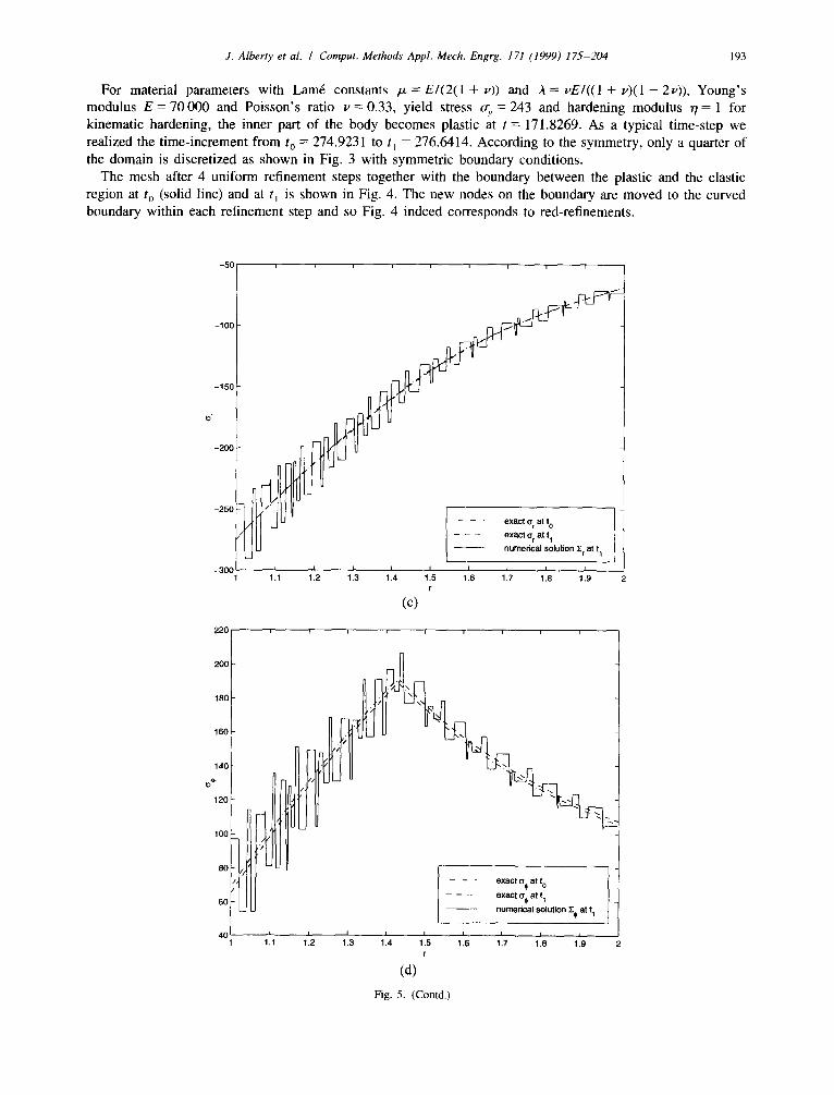
Fig. 5. Exact and discrete solution f o r t h e m e s h shown in Fig. 4 along A - B in Example 8.1.

J. Albert), et al. / Comput. Methods" Appl. Mech. Engrg. 171 (1999) 175-204 193

For material parameters with Lame constants # - - E / ( 2 ( 1 + t,)) and h - - ~E/((1 + ~,)(1 - 2 ; 0 ) , Young's modulus E = 7 0 0 0 0 and Poisson's ratio ~, = 0.33, yield stress ~. = 243 and hardening modulus 7/= 1 for kinematic hardening, the inner part of the body becomes plastic at t = 171.8269. As a typical time-step we realized the time-increment from t o = 274.9231 to t~ = 276.6414. According to the symmetry, only a quarter of the domain is discretized as shown in Fig. 3 with symmetric boundary conditions.

The mesh after 4 uniform refinement steps together with the boundary between the plastic and the elastic region at t o (solid line) and at t~ is shown in Fig. 4. The new nodes on the boundary are moved to the curved boundary within each refinement step and so Fig. 4 indeed corresponds to red-refinements.

- 5 0

-100

-150

-200

-250

-300

220

200

180

160,

140

1201

100

80

6O

40

111 112 113 11, 115 115 117 116 tl, r

(c)

\

)

/.

. . . . exact o~ at t 1

numerical solution Z¢, at t 1

' ' ' ' '6 ' ' '. 1.1 1.2 1 3 1.4 1.5 1 1 7 1,8 1 9 2 r

(d) Fig. 5. (Contd.)


7.5

10 -3

6.5

£ '5 .5

5

4.5

4

3.5

t I I I L "

Z / / /

/Z ZZ/

0

-0.5

-1

-1.5

-2

oY-2.5

- 3

-3.5

- 4

-4.5

-5

. . . . e x a c t Pr a t t o

- - - e x a c t Pr a t t 1 n u m e r i c a l s o l u t i o n Pr a t t 1

111 112 113 11, 115 116 117 118 11, r

(a) 10 -3

i i ~ i i i i i i

. . . . e x a c t u r a t t o

- - - exact u r at t 1

,\

I I I 1.1 1=.2 113 114 1=.5 116 1=.7 1.8 1.9

r

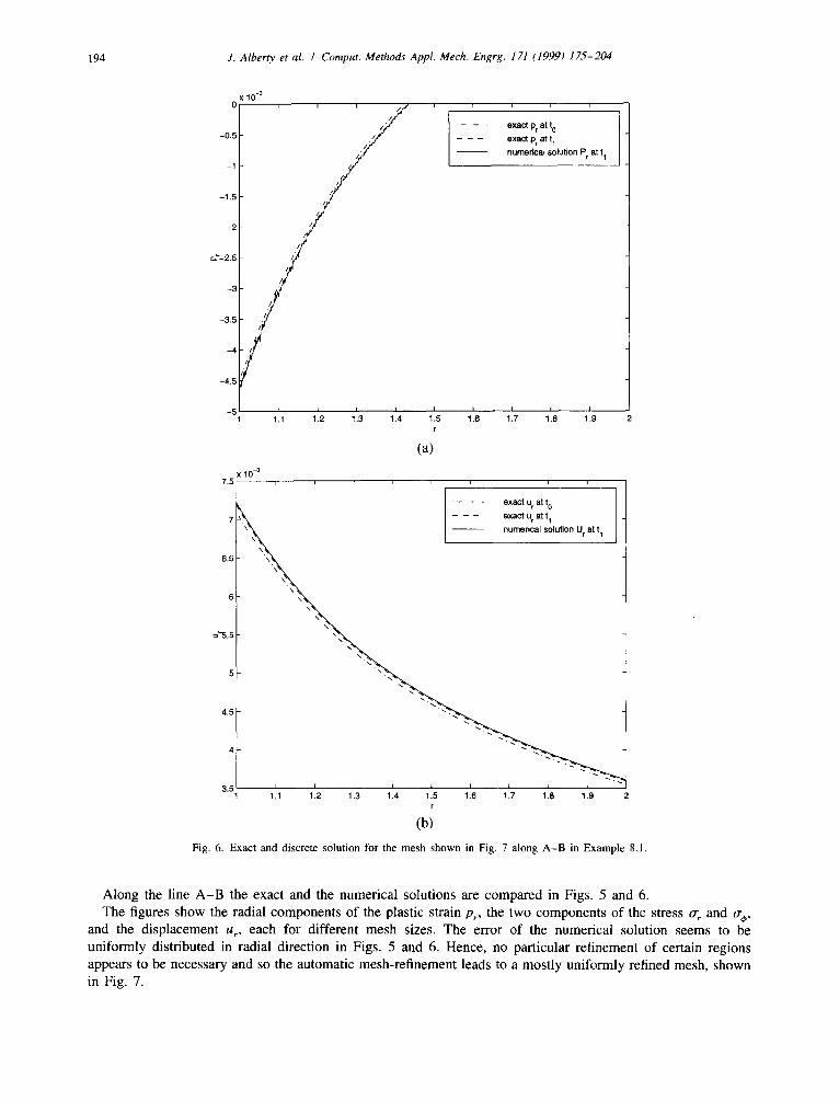
(b) Fig. 6. Exact and discrete solution for the mesh shown in Fig. 7 along A - B in Example 8.1.

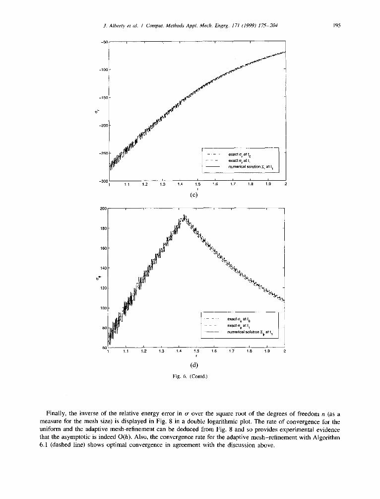
Along the line A - B the exact and the numerical solutions are compared in Figs. 5 and 6. The figures show the radial components of the plastic strain Pr, the two components of the stress o- r and o',b,

and the displacement u r, each for different mesh sizes. The error of the numerical solution seems to be uniformly distributed in radial direction in Figs. 5 and 6. Hence, no particular refinement of certain regions appears to be necessary and so the automatic mesh-refinement leads to a mostly uniformly refined mesh, shown in Fig. 7.

-150

i -200

J. AlherO, et al. / Comput. Methods Appl. Mech. Engrg. 171 (1999) 175-204

- 5 0 i i ~ i t i i ~ t

-100

-250 - - exact o r at t o

exact o r at t 1 numerical solution ]E r at t 1

-300 111 112 113 1=.4 115 '11.6 117 118 119 r

(c)

2 0 0 r

195

180

160

140

120

1 O0

80

\

exact ~ at t o

exact ~¢, at 11 numerical solution ~" al t 1

6 0 L_ 1 1'1 1'.~ 11~ 11, 115 1'5 11~ 11~ 1'~ r

(d) Fig. 6. (Contd.)

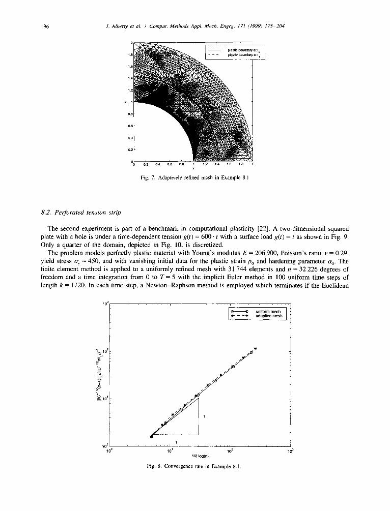
Finally, the inverse of the relative energy error in o- over the square root of the degrees of freedom n (as a measure for the mesh size) is displayed in Fig. 8 in a double logarithmic plot. The rate of convergence for the uniform and the adaptive mesh-refinement can be deduced from Fig. 8 and so provides experimental evidence that the asymptotic is indeed O(h). Also, the convergence rate for the adaptive mesh-refinement with Algorithm 6.1 (dashed line) shows optimal convergence in agreement with the discussion above.

196 J. AlberO, et al. / Comput. Methods Appl. Mech. Engrg. 171 (1999) 175-204

plastic boundary at l 0 1.8 ~ I - - - plastic boundary at t 1

1.6

1.4

1.2

>, 1

0.8

0.6

0.4

0.2

0 0.2 0,4 0.6 0,8 1 1.2 1,4 1.6 1.8 2

X

Fig. 7. Adaptively refined mesh in Example 8.1

8.2. Perforated tension strip

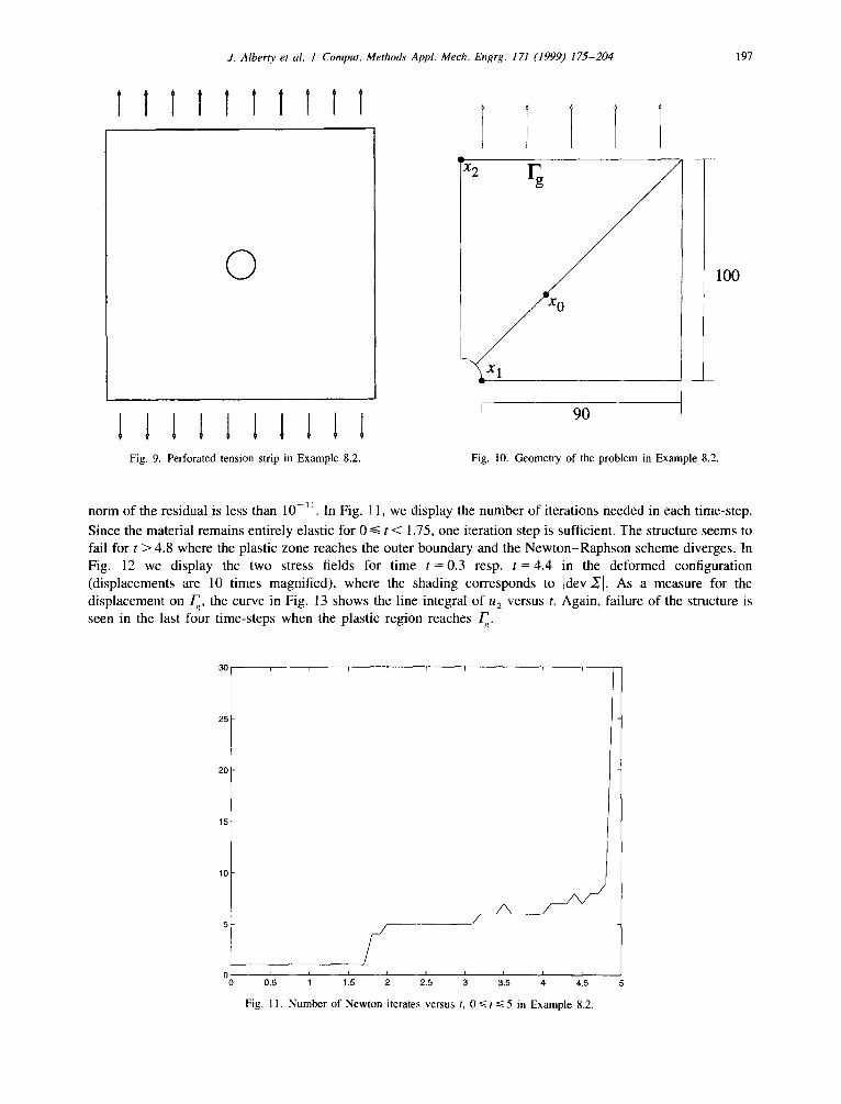
The second experiment is part of a benchmark in computational plasticity [22]. A two-dimensional squared plate with a hole is under a time-dependent tension g( t ) = 6 0 0 . t with a surface load g( t ) = t as shown in Fig. 9. Only a quarter of the domain, depicted in Fig. 10, is discretized.

The problem models perfectly plastic material with Young's modulus E = 206 900, Poisson's ratio p = 0.29, yield stress 4. = 450, and with vanishing initial data for the plastic strain Po and hardening parameter a o. The finite element method is applied to a uniformly refined mesh with 31 744 elements and n = 32 226 degrees of freedom and a time integration from 0 to T = 5 with the implicit Euler method in 100 uniform time steps of length k = 1/20. In each time step, a Newton-Raphson method is employed which terminates if the Euclidean

10 3

10 2

T ~ 10 ~

10 10 °

, i . . . . . . .

Q uni form m e s h - - '¢- adapt ive m e s h

z z z ~

# z z

O"

1 i i i i i I i i i i . . . . [ ,

101 10 2

1/2 log(n) 10 3

Fig. 8. Convergence rate in Example 8.1.

J. Alber~ et al. / Comput. Methods Appl. Mec~,~. Engrg. 171 (1999) 175-204 197

I I I I I T I T I I

©

Fig. 9. Perforated tension strip in Example 8.2.

T ~c 2

~ / Xo

90 I

100

Fig. 10. Geometry of the problem in Example 8.2.

norm of the residual is less than 1 0 - ' 1 In Fig. 11, we display the number of iterations needed in each time-step.

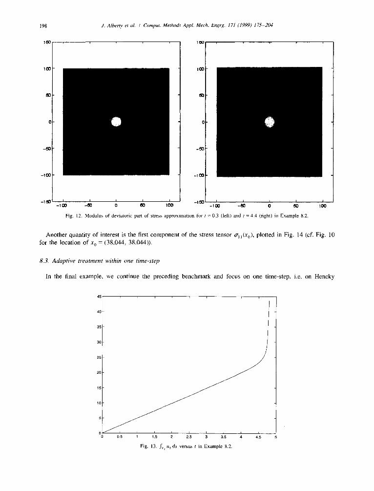
Since the material remains entirely elastic for 0 ~< t < 1.75, one iteration step is sufficient. The structure seems to fail for t > 4.8 where the plastic zone reaches the outer boundary and the Newton-Raphson scheme diverges. In Fig. 12 we display the two stress fields for time t = 0 . 3 resp. t = 4 . 4 in the deformed configuration (displacements are 10 times magnified), where the shading corresponds to ]dev ,SI. As a measure for the displacement on F , the curve in Fig. 13 shows the line integral of u: versus t. Again, failure of the structure is seen in the last four time-steps when the plastic region reaches: F x.

3 0

2 5

2 0

15

1 0

/ 7

I I I I

Fig. 11. Number of Newton iterates versus t, (I ~< t ~< 5 in Example 8.2.

198

100

5 0

- 5 0

-100

- I ~ 0 ! - 1 0 0 - 5 0 0 5 0 ] 0 0

J. Albero, et al. / Comput. Methods Appl. Mech. Engrg. 171 (1999) 175-204

1 ~ o , ,

1 0 0 . . . . . . . . . .

5O

° O

-50

-100 . . . . .

i i i i I - 1 5 0 i i i i - I O0 -~0 o e~O tO0

Fig. 12. Modulus of deviatoric part of stress approximation for t = 0.3 (left) and t = 4.4 (right) in Example 8.2.

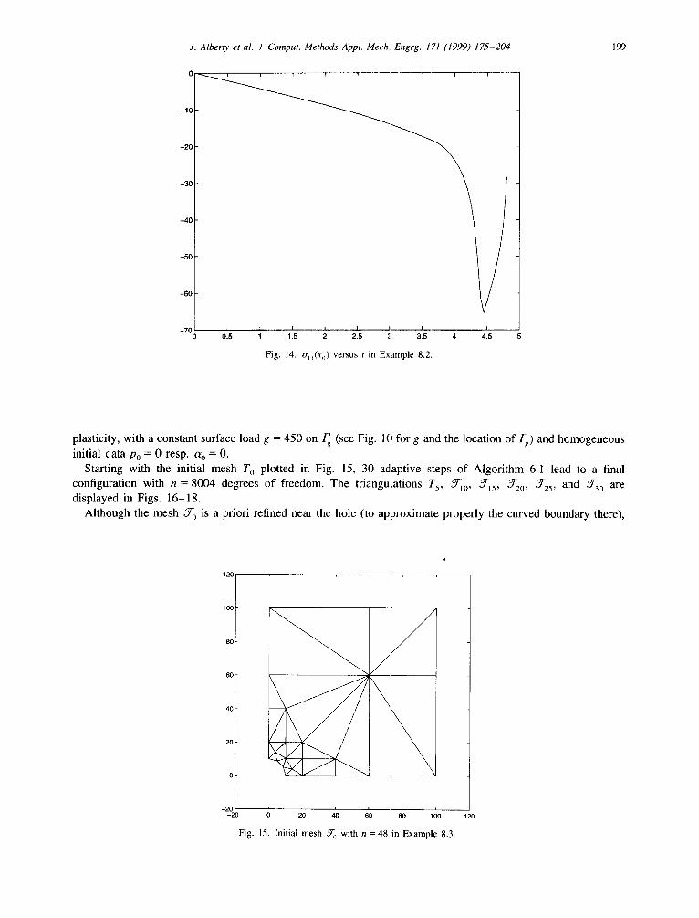
Another quantity of interest is the first component of the stress tensor o-]](Xo), plotted in Fig. 14 (cf. Fig. 10 for the location of x o = (38.044, 38.044)).

8.3. Adaptive treatment within one time-step

In t h e f ina l e x a m p l e , w e c o n t i n u e t h e p r e c e d i n g b e n c h m a r k a n d f o c u s o n o n e t i m e - s t e p , i .e. o n H e n c k y

45

40

35

30

25

20

15

10

5

0 o.s 1 1.5 2 2.5 3 3.5 4 4.5

Fig. 13. J'j; u 2 ds versus t in Example 8.2.

0

- 1 0

- 2 0

- 3 0

- 4 0

- 5 0

-60

1 I I I

J. Alberry et al. / Comput. Methods Appl. Mech. Engrg. 171 (1999) 175-204 199

415 Fig. 14. o-,~(xo) versus t in Example 8.2.

plasticity, with a constant surface load g = 450 on F~ (see Fig. 10 for g and the location of Fg) and homogeneous

initial data Po = 0 resp. a o = 0. Starting with the initial mesh T O plotted in Fig. 15, 30 adaptive steps of Algori thm 6.1 lead to a final

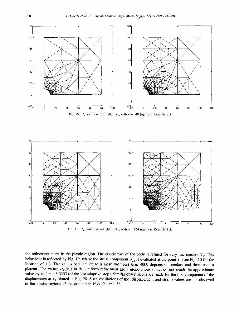
configuration with n = 8004 degrees of freedom. The triangulations Ts, ~r~o, 3-~5, 3-2o, 3-z5 , and J.3o are displayed in Figs. 16-18.

Although the mesh J-o is a priori refined near the hole (to approximate properly the curved boundary there),

120

100

80

60

0

-20 -20

i i i | i

0 20 40 60 80 100 120

Fig. 15. Initial mesh ~ with n =48 in Example 8.3.

2OO

120

10G

80

60

40

20

-2C -20

J. Alberty et al. / Comput. Methods Appl, Mech. Engrg. 171 (1999) 175-204

'2° /

,°° I 8O

40

20

i i i

= ' - 20 ' ~ 40 60 80 1 O0 120 0 20 4'0 6'0 B'O 100 120 -20 0 20

Fig. 16. ~ with n = 150 (left). 3-,, with n = 340 (fight) in Example 8.3.

120 120

100

80

60

40

20

0

- 20 -20

100

80

60

40

20

~~/~,~ /\/\

i i i i i i - 2 0 i I J J r r

0 20 40 60 80 100 120 -20 0 20 40 60 80 100 120

Fig. 17. J-~5 with n = 544 (left), "Y?2o with n = 854 (fight) in Example 8.3.

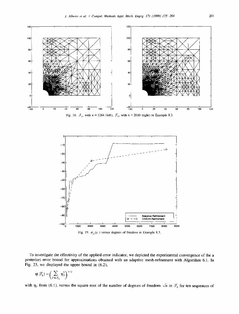
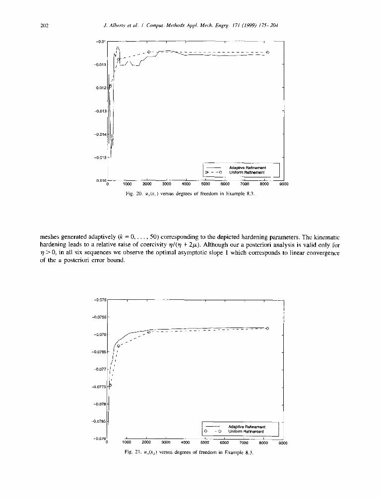
the refinement starts in the plastic region. The elastic part of the body is refined for very fine meshes J-k- This behaviour is reflected by Fig. 19, where the stress component o-2z is evaluated at the point x~ (see Fig. 10 for the location of xj). The values oscillate up to a mesh with less than 4000 degrees of freedom and then reach a plateau. The values 0-22(xj) in the uniform refinement grow monotonously, but do not reach the approximate value 0-z2(x~ ) = -8.6253 (of the last adaptive step). Similar observations are made for the first component of the displacement at xj plotted in Fig. 20. Such oscillations of the (displacement and strain) values are not observed in the elastic regions of the domain in Figs. 21 and 22.

J. AIberty et al. / Comput. Methods Appl. Mech. Engrg. 171 (1999) 175-204 201

120

100

80

60

40

20

0

-20 -20

~ ' \ / /

/ \ J /

120

100

80

60

40

20

0

-20 - - -20

i

/

\ /

i i i i | ~ i i ~ i i i

0 20 40 60 80 100 120 0 20 40 60 80 100

Fig. 18. J-~ with n = 1264 (left), ~ o with n = 2030 (right) in Example 8.3.

120

O | i i i r i I I I

!

~ ~ ~ 0

- 3 0

l /

-°°N/,'

- °Hf -100, ~ - - 0 Uniform R e f i n e m e n t ~

0 1000 2000 3000 4000 5000 6000 7000 8000 9000

Fig. 19. o'22(x~) versus degrees of freedom in Example 8.3.

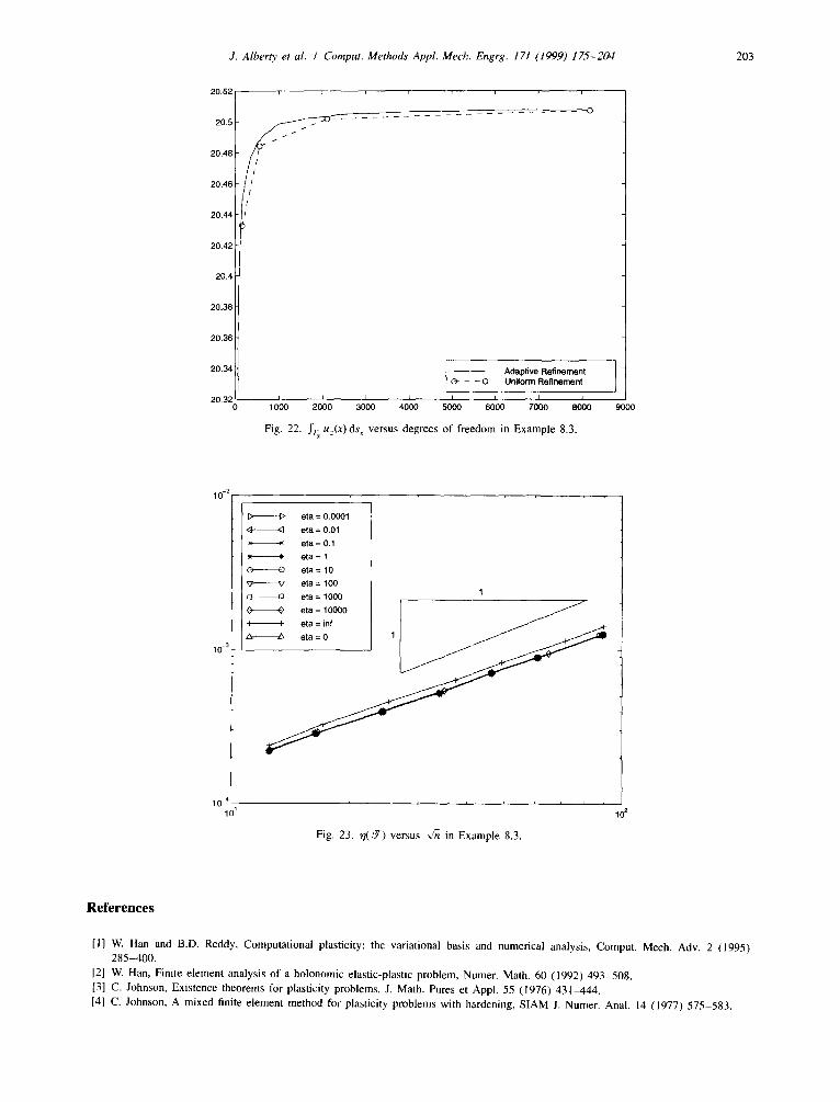
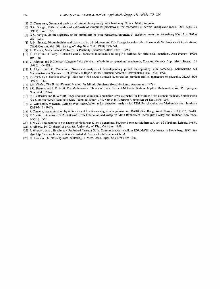
To investigate the effectivity of the applied error indicator, we depicted the experimental convergence of the a posteriori error bound for approximations obtained with an adaptive mesh-refinement with Algorithm 6.1. In Fig. 23, we displayed the upper bound in (6.2),

with 7/r from (6.1), versus the square root of the number of degrees of freedom ~ in ~k for ten sequences of


-0.01

-0.011

-0.012

-0.013

-0.014

-0.015

-0.016

I A d a p t i v e R e f i n e m e n t - - O U n i f o r m R e f i n e m e n t

, . , , , . .

1000 2000 3000 4000 5000 6000 7000 8000

Fig. 20. u~(x~) versus degrees of freedom in Example 8.3.

9000

meshes generated adaptively (k = 0 . . . . . 50) corresponding to the depicted hardening parameters. The kinematic hardening leads to a relative raise of coercivity r//(~? + 2/x). Although our a posteriori analysis is valid only for r / > 0, in all six sequences we observe the optimal asymptotic slope 1 which corresponds to linear convergence of the a posteriori error bound.

-0.075

-0.0755

-0.076

-0.0765

-0.077

-0.0775

-0.078

-0.0785

-0.079 0

111

I 1

.-o

A d a p t i v e R e f i n e m e n t (3- - - O U n i f o r m R e f i n e m e n t

i i i i i i i | 1000 2000 3000 4000 5000 6000 7000 S000 9000

Fig. 21. u,(x~) versus degrees of freedom in Example 8.3.


20.52

20.5

20.48

20.46

20.44

20.42

20.4

20.38

20.36

20.34

20.32

. . . . . . . . . -o

l Adaptive Refinement J (3- - - 0 Uniform Refinement

, , , . . , . ,

1000 2000 3000 40 O0 5000 6000 7000 8000 9000

Fig. 22. J'/~. u~(x)_ ds~ versus degrees of freedom in Example 8.3.

10 -2

10 -3

10 4 10 ~

). o ~2 c~

0 I

L ~

I> eta = 0.0001

(3 e ta = 0.01

K e ta = 0.1

eta = 1

0 eta = 10

~7 eta = 100 eta = 1000 1

0 eta = 10000

, a l . - i ° f I J ~ -

Fig. 23. ~ ,3-) versus -,/n in Example 8.3.

102

References

[1] W. Han and B.D. Reddy, Computational plasticity: the variational basis and numerical analysis, Comput. Mech. Adv. 2 (1995) 285-400.

[2] W. Han, Finite element analysis of a holonomic elastic-plastic problem, Nnmer. Math. 60 (1992) 493-508. [3] C. Johnson, Existence theorems for plasticity problems, J. Math. Pures et Appl. 55 (1976) 431-444. [4] C. Johnson, A mixed finite element method for plasticity problems with hardening, SIAM J. Numer. Anal. 14 (1977) 575-583.

204 J. Albert' et al. / Comput. Methods Appl. Mech. Engrg. 171 (1999) 175-204

[5] C. Carstensen, Numerical analysis of primal elastoplasticy with hardening Numer. Math., in press. [61 G.A. Seregin, Differentiability of extremals of variational problems in the mechanics of perfect viscoplastic media, Diff. Eqns. 23

(1987) 1349-1358. [7] G.A. Seregin, On the regularity of the minimizers of some variational problems of plasticity theory, St. Petersburg Math. J. 4 (1993)

989-1020. [8] R-M. Suquet, Discontinuities and plasticity, in: J.J. Moreau and RD. Panagiotopoulos eds., Nonsmooth Mechanics and Applications,

CISM Courses, Vol. 302 (Springer-Verlag New York, 1988) 279-341. [9] R. Temam, Mathematical Problems in Plasticity (Gauthier-Villars, Paris, 1985).

[10] K. Eriksson, D. Estep, R Hansbo and C. Johnson, Introduction to adaptive methods for differential equations, Acta Numer. (1995) 105-158.

[11] C. Johnson and R Hansbo, Adaptive finite element methods in computational mechanics, Comput. Methods Appl. Mech. Engrg. 101 (1992) 143-181.

[12] J. Alberty and C. Carstensen, Numerical analysis of time-depending primal elastoplasticy with hardening. Berichtsreihe des Mathematischen Seminars Kiel, Technical Report 98-18, Christian-Albrechts-Universitiitzu Kiel, Kiel, 1998.

[13] C. Carstensen, Domain decomposition for a non-smooth convex minimisation problem and its application to plasticity, NLAA 4(3) (1997) 1-13.

[14] RG. Ciarlet, The Finite Element Method for Elliptic Problems (North-Holland, Amsterdam, 1978). [15] S.C. Brenner and L.R. Scott, The Mathematical Theory of Finite Element Methods. Texts in Applied Mathematics, Vol. 15 (Springer,

New York, 1994). [16] C. Carstensen and R. Verf/.irth, Edge residuals dominate a posteriori error estimates for low order finite element methods. Berichtsreihe

des Mathematischen Seminars Kiel, Technical report 97-6, Christian-Albrechts-Universit~it zu Kiel, Kiel, 1997. [17] C. Carstensen, Weighted Clement-type interpolation and a posteriori analysis for FEM Berichtsreihe des Mathematischen Seminars

Kiel 97-19 (1997). [18] R Clement, Approximation by finite element functions using local regularization, RA1RO S6r. Rouge Anal. Num~r. R-2 (1975) 77-84. [19] R. Verftirth, A Review of A Posteriori Error Estimation and Adaptive Mesh-Refinement Techniques (Wiley and Teubner, New York,

Leipzig, 1996). [20] J. Necas, Introduction to the Theory of Nonlinear Elliptic Equations. Teubner-Texte zur Mathematik, Vol. 52 (Teubner, Leipzig, 1983). [21] J. Alberty, Ph.D. thesis in progress, University of Kiel, Germany, 1998. [22] R Wriggers et al., Benchmark Perforated Tension Strip. Communication in talk at ENUMATH Conference in Heidelberg, 1997. See

also http://coulomb.mechanik.tu-darmstadt.de / user / scherf/Benchmark.html. [23] C. Johnson, On plasticity with hardening, J. Math. Anal. Appl. 62 (1978) 325-336.

Documents

Adaptive numerical analysis in primal elastoplasticity with hardening